ECONOMIC LOAD DISPATCH IN THERMAL POWER PLANT ...

16

† Corresponding author © 2015 Conscientia Beam. All Rights Reserved.

ECONOMIC LOAD DISPATCH IN THERMAL POWER PLANT

CONSIDERING ADDITIONAL CONSTRAINTS USING CURVE FITTING AND

ANN

S.K.Gupta1† --- Pankaj Chawala2

1Professor and Research scholar at DCR University of Sc. & Technology, Murthal (Sonepat) Haryana, India

2Research scholar at DCR University of Sc. & Technology, Murthal (Sonepat) Haryana, India

ABSTRACT

This paper presents a new efficient approach to economic load dispatch (ELD) problem with cost functions

using curve fitting, ANN and particle swarm optimization (PSO). Economic load dispatch is one of the

most important problems in power system operation. The practical ELD problems may not have fixed cost

functions rather it changes with the coal quality, that make the problem of finding the global optimum

difficult using any traditional mathematical approach. Therefore, curve fitting technique is used to obtain

the coefficients of the cost curve. The same data is used for the training of the artificial neural network. The

effectiveness of the algorithm is validated by carrying out extensive test on a power system involving 8

thermal generating units. The variation in calorific values of the coal used in different generators cause the

change in coefficients of cost curve. This effect is incorporated using curve fitting, ANN and PSO

approaches. The ELD problem is then optimized. The comparison shows the better results.

Keywords: Economic load dispatch, Gross calorific value, Curve fitting technique, Artificial neural network, Efficiency in

thermal generating units, Particle swarm optimization.

Contribution/ Originality

This study for economic load dispatch is one of very few studies which have investigated for

variation in calorific values of the coal used time to time in thermal power plants. This uses the

comparison of conventional, curve fitting, PSO and ANN.

1. INTRODUCTION

The economic load dispatch (ELD) is one of the most important optimization problems in

power system operation and planning to derive optimal economy. The main objective of economic

load dispatch is to determine the optimal combination of all generating units so as to meet the

required load demand at minimum cost while satisfying the various operating constraints like

energy balance, max-min generation limits, transmission line constraints, running spare capacity

Review of Energy Technologies and Policy Research

2015 Vol. 2, No. 1, pp. 16-28 ISSN(e): 2313-7983 ISSN(p): 2409-2134 DOI: 10.18488/journal.77/2015.2.1/77.1.16.28 © 2015 Conscientia Beam. All Rights Reserved.

http://crossmark.crossref.org/dialog/?doi=10.18488/journal.77/2015.2.1/77.1.16.28

Review of Energy Technologies and Policy Research, 2015, 2(1):16-28

17

© 2015 Conscientia Beam. All Rights Reserved.

and network security. A station has incremental operating costs for fuel, maintenance cost and

fixed cost associated with the station itself that can be quite considerable for a typical thermal and

nuclear power plant for example. Things get even more complicated when utilities try to account

for transmission line losses and the seasonal changes associated with hydraulic power plants.

Conventionally, the cost function for each unit for ELD problem has been approximately

represented by a quadratic equation and is solved by using various mathematical techniques like

Lambda-iteration method, Lagrange method, Curve Fitting and Artificial Neural Network etc [1-

4]. Unfortunately, the cost characteristics of thermal generating units are highly non-linear

because of prohibited operating zones, valve point loading and multi fuel insertion etc. Thus,

Practical ELD problem is represented as a non linear optimization problem with various equality

and inequality constraints, which directly cannot be solved by conventional mathematical

techniques. Hence numerous intelligent techniques like Biogeography-Based Optimization (BBO)

[5], genetic algorithm (GA) [6], Differential Evolutionary (DE) [7], Evolutionary

Programming (EP) [8-10], neural network approaches [11], Tabu Search [12] etc were

introduced to solve complex nonlinear ELD problems over past few years.

Recently, Eberhart and Kennedy suggested particle swarm optimization (PSO) based on the

analogy of swarm of bird and school of fish [13]. In PSO, each individual makes its decision based

on its own experience together with other individual`s experiences. The individual particles are

drawn stochastically towards the position of present velocity of each individual, their own

previous best performance, and the best previous performance of their neighbor. PSO have been

successfully applied to various fields of power system optimization in recent years such as reactive

power and voltage control [14], power system stabilizer design [15] and dynamic security

border identification [16]. Yoshida, et al. [14] presented a modified PSO to control reactive

power and voltage considering voltage security constraint. Since the problem was a mixed-integer

nonlinear optimization problem with inequality constraints, they applied the classical penalty

method to reflect the constraint- violating variables. In order to utilize the PSO algorithm to

solve ELD problem, it is necessary to revise the original PSO to reflect the equality/inequality

constraints of the variables in the process of modifying each individual‟s search. Victoire and

Jeyakumar [17] presented a deterministically guided particle swarm optimization (DGPSO)

algorithm to solve the dynamic ELD of generating units considering the valve-point effects.

Pandian and Thanushkodi [18] presented an Evolutionary Programming (EP) and Efficient

Particle Swarm Optimization (EPSO) techniques to solve ELD problems including transmission

losses in power system. Efficient Particle Swarm Optimization (EPSO) technique is employed so

that optimized results are obtained, and by applying EP, faster convergence is obtained.

In this paper, cost characteristics for different coal quality are obtained by curve fitting

method. The same data is used to train the ANN. The generated power, cost, GCV and these

values as previous operating point are considered input values of ANN to obtain a, b, c coefficients

of cost characteristics for all the generators. The fuel cost curves of generators are represented by

quadratic equation of real power generation.


18


The coefficients a, b, c of each unit are updated automatically depending upon the point of

operation used and GCV of coal. It is therefore, expected better result than conventional method

where a, b, c coefficients are constant throughout all the range of generation irrespective of coal

quality which may actually change time to time. The remaining organization of this paper is as

follows. Section II addresses the formulation of economic load dispatch problem, section III

describes the curve fitting, ANN and PSO approaches, and section IV describes the results and

discussion. Finally, the conclusion is given in section V.

2. FORMULATION OF ELD PROBLEM

The ELD problem is to find the optimal combination of power generations that minimizes

the total generation cost while satisfying an equality constraint and inequality constraints. The

most simplified cost function of each generator can be represented as a quadratic function as given

in (2).

( ) …….(1)

∑ ( ) …….(2)

Where

is the total fuel cost.

is the cost function of generator .

is electrical output of generator .

are the cost coefficients of generator .

While minimizing the total generation cost, the total generation should be equal to the total

system demand plus the transmission network loss. However, the network loss is not considered

in this paper as all the operating units of a power plant are on single bus. This gives the equality

constraint

∑ …….(3)

Where is the total power demand.

The maximum active power generation of a source is limited again by thermal consideration

and also minimum power generation is limited by the flame instability of a boiler. If the power

output of a generator for optimum operation of the system is less than a pre-specified value ,

the unit is not put on the bus bar because it is not possible to generate that low value of power

from the unit. Hence the generator power P cannot be outside the range stated by the inequality

…...(4)

Where ,

is the minimum, maximum output of generator number „ ‟.

3. ELD USING NEW APPROACHES

A. Overview of Curve Fitting Technique

A curve which is most near to given points is called approximating curve which may be linear

or non linear and is called “best fit”. It is obtained by Legendre`s principle of least squares in

which we minimize the sum of the squares of the deviations of the actual values from their


19


estimated as given by the curve of best fit. According to the above description, the performance

steps of this technique are as follows [19]:

1. Data generation, which can be implemented in floating point, since this portion

corresponds to sensors that will be independent of the curve fitting device.

2. Off-line computations which can be implemented in floating points with invariant signals.

3. Run- time computation, which must be implemented in fixed point.

4. Data visualization, which must be implemented in floating point.

5. MATLAB`s extensive, device independent plotting capabilities are one of its most

powerful features.

B. Artificial Neural Networks

Artificial Neural Network, here referred to as ANN, are an attempt at modeling the

processing power of the human brain. Humans are able to adapt to new situations and learn

quickly when given the correct context. Computers are relatively slow at performing simple

human tasks such as recognizing a lizard in a painting of the jungle. ANN work by simulating the

structure of the human brain. At their basic level they consist of a network of neurons connected

by synapse.

Neurons are the basic elements of an ANN. Neurons accept inputs from other connections

and produce an output by firing their synapse. Neurons typically perform a weighted sum on all

of their input connections and then pass it through a transfer function to produce its output. The

traditional ANN is a binary network in which a synapse either fires or doesn`t fire. This type of

transfer function in which the neurons compares its weighted sum to a threshold and then either

emits a 1 or a 0 (fires or doesn`t fire its synapse). While binary networks have their uses, most

engineering applications involve the real number system. ANN has thus been adapted to use real

numbers.

In this model are used to the six inputs ppg1, pg1, GCV1, GCV1, fppg1 and fpg1 i.e. obtain the

output values a1, b1 and c1. In this model, one input layer, one hidden layer and output layer has

been considered. Total epochs values considered are 300. Learning rate considered is 0.05.

Number of neurons in the hidden layer is 1. Back propagation method is used.

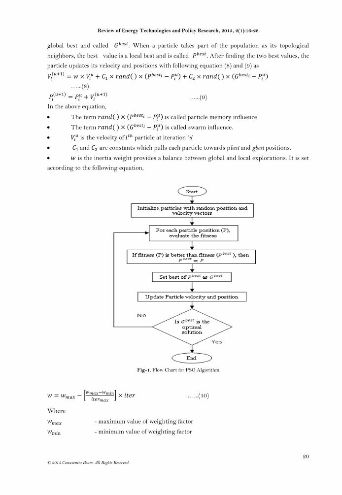
C. PSO as ELD Problem

In PSO, the potential solutions, called particles, fly through the problem space by following

the current optimum particles. The system is initialized with a population of random solutions

and searches for optima by updating generations.

PSO is initialized with a group of random particles (solutions) and then searches for optima

by updating generations. All the particles are updated by following two "best" values in each

iteration. The first one is the best solution (fitness) it has achieved so far. (The fitness value is also

stored.) This value is called . Another "best" value that is tracked by the particle swarm

optimizer is the best value, obtained so far by any particle in the population. This best value is a


20


global best and called . When a particle takes part of the population as its topological

neighbors, the best value is a local best and is called . After finding the two best values, the

particle updates its velocity and positions with following equation (8) and (9) as

( )

( ) (

) ( ) (

)

…...(8)

( )

( )

…...(9)

In the above equation,

The term ( ) ( ) is called particle memory influence

The term ( ) ( ) is called swarm influence.

is the velocity of particle at iteration „u‟

and are constants which pulls each particle towards pbest and gbest positions.

is the inertia weight provides a balance between global and local explorations. It is set

according to the following equation,

Fig-1. Flow Chart for PSO Algorithm

[

] …...(10)

Where

- maximum value of weighting factor

- minimum value of weighting factor


21


- maximum number of iterations

- current number of iteration

When any optimization process is applied to the ELD problem, some constraints are

considered. In this work three different constraints are considered. Among them the equality

constraint is summation of all the generating power must be equal to the load demand and the

inequality constraint is the powers generated must be within the limit of maximum and minimum

active power of each unit. The additional constraint is the real time efficiency. The sequential

steps of the proposed PSO method are given below.

Step 1) the individuals of the population are randomly initialized according to the limit of each

unit including individual dimensions. The velocities of the different particles are also randomly

generated keeping the velocity within the maximum and minimum values.

Step 2) each set of solution in the space should satisfy the equality constraints. So equality

constraints are checked. If any combination doesn‟t satisfy the constraints then they are set

according to the power balance equation.

Step 3) the evaluation function of each individual is calculated in the population using the

evaluation function (2). The present value is set as the value.

Step 4) each values are compared with the other values in the population. The best

evaluation value among the is denoted as .

Step 5) the member velocity v of each individual Pg is modified according to the velocity update

equation (8).

Step 6) the velocity components constraint occurring in the limits from the following conditions

are Checked

Step 7) the position of each individual is modified according to the position update equation (9).

Step 8) If the evaluation value of each individual is better than previous , the current value is

set to be . If the best is better than , the value is set to be .

Step 9) If the number of iterations reaches the maximum, then go to step 10.Otherwise, go to step

2.

Step 10) The individual that generates the latest is the optimal generation power of each

unit with the minimum total generation cost.

4. RESULTS AND DISCUSSION

The proposed methods are used independently to solve case study problem involving 8

generating units. Usually, training of a neural network is a slow intelligence process. So to speed

it up optimization is required at every point, i.e., in deciding the neural network architecture, the

number and type of training or testing patterns, the learning rate, the error goal etc. The training


22


patterns consist of input-output pairs. The proposed approach is tested on a standard test system.

The initial particles are randomly generated within the feasible range. The parameters and

inertia weight are selected for best convergence characteristic. Here = = 2.0 The maximum

value of w is chosen 0.9 and minimum value is chosen 0.4. The velocity limits are selected as

and the minimum velocity is selected as

. There are 10 no of

particles selected in the population.

This test case comprises of 8 generating units with quadratic cost functions given in

appendixes. The outputs of generating units and aggregate fuel cost comparison for 800 MW and

850 MW are shown in Table-1 and 2. Comparison for load dispatch using Curve Fitting and

ANN for different set of data is shown in Fig.2 and Fig.3. The transmission loss is assumed to be

zero.

Table-1. Comparison of Fuel Costs for 8-Generator System with PD = 800MW

Unit1 (MW)

Unit2 (MW)

Unit3 (MW)

Unit4 (MW)

Unit 5 (MW)

Unit6 (MW)

Unit7 (MW)

Unit8 (MW)

Fuel cost (in Rs/Hr)

Efficiency 42.3 51.4 60.0 52.5 61.9 50.8 61.7 58.6 Normal Loading

102 83 80 82 195 210 258 258

ELD Conventional method

60 50 50 50 121.4 138.5 165 165 7651.6

Load Dispatch using Curve fitting GCV3374

60 50 50 50 121.4 138.5 165 165 7651.6

Load Dispatch using Curve fitting GCV 3400

60 50 50 50 121.5 138.5 165 165 7618.8


60 50 50 50 121.5 138.4 165 165 7583.1


60 50 50 50 121.4 138.5 165 165 7547.2


60 50 50 50 121.5 138.4 165 165 7510.1


60 50 50 50 121.4 138.5 165 165 7465.9

ANN with GCV3374

60 50 50 50 126.9 133.0 165 165 7599.8

ANN with GCV 3400

60 50 50 50 127 133 165 165 7585.9

ANN with GCV3450

60 50 50 50 126 133 165 165 7597.08

ANN with GCV3470

60 50 50 50 126 133 165 165 7225.08


23


ANN with GCV3500

60 50 50 50 125 134 165 165 6928.79

ANN with GCV3550

60 50 50 50 126 133 165 165 6911.45

PSO UsingȠ 69.18 50 50 50 115.76 120.83 165 165 7065.25

Table-2. Comparison of Fuel Costs for 8-Generator System with PD = 850MW

Unit1 (MW)

Unit2 (MW)

Unit3 (MW)

Unit4 (MW)

Unit5 (MW)

Unit6 (MW)

Unit7 (MW)

Unit8 (MW)

Fuel cost (in Rs/Hr)

Efficiency 42.3 51.4 60.0 52.5 61.9 50.8 61.7 58.6 Normal Loading 102 83 80 82 195 210 258 258

ELD Conventional 60 50 50 50 144.9 163.4 166.6 165 8715.56 ELD using Curve fitting GCV3526

60 50 50 50 144.9 163.4 166.6 165 8715.56

ELD using Curve fitting GCV3540

60 50 50 50 144.8 163.4 166.6 165 8685.47

ELD using Curve fittingwith GCV 3570

60 50 50 50 144.9 163.1 166.6 165 8648.02


60 50 50 50 144.8 163.2 166.8 165 8612.16


60 50 50 50 144.9 163.2 166.7 165 8576.26


60 50 50 50 145.0 163.2 166.7 165 8531.31

ANN with GCV3526 60 50 50 50 151.2 158.7 165 165 8531.3 ANN with GCV3540 60 50 50 50 150.6 159.3 165 165 8616.9

ANN with GCV3570 60 50 50 50 149.6 160.3 165 165 8623.0 ANN with GCV4100 60 50 50 50 147.3 160.2 167.4 165 8244.0

ANN with GCV4120 60 50 50 50 146.0 161.4 167.4 165 7937.3 ANN with GCV4150 60 50 50 50 147.3 166.2 166.2 165 7892.2

PSO UsingȠ 73.3 53 51.2 52.4 123.5 130.9 165.7 165.7 8235.8

Fig-2. Comparison of Total Fuel Cost (in Thousands) obtained by applying curve fitting and ANN against step wise

increase in different values of GCVs


24


Fig-3. Comparison of Total Fuel Cost (in Thousands) obtained by applying curve fitting and ANN against step wise

increase in different values of GCVs

5. CONCLUSION

This paper presents a new approach of considering efficiency (Turbine, Boiler and

Generator), GCV value of coal as an inequality constraint to solve the economical load dispatch

problem in thermal power plants. A comparison analysis has been made on a test systems

comprises 8 generating units for different load demands. Since quality of coal changes time to

time, the program incorporates the change in GCV of coal. In curve fitting method, we are able to

obtain a, b, c coefficients of cost characteristics from experimental data. This program may not

give it best results for new value of GCV. The program using ANN has been trained to obtain a,

b, c coefficients of cost characteristics from operating point‟s (pg) current value of cost, GCV and

previous operating point. Thus ANN based computer programs developed is most robust and

works dynamically and gives better results in compare to the conventional method as well as

curve fitting approach.

APPENDIX

Table-3. Input Parameters of Various Operating Units

Normal Loading ( MW)

Max limit (MW)

Min limit (MW)

Tripping limit (MW)

a b C

Unit1 102 110 60 35 0.3167 -10.9 102.8

Unit2 83 105 50 35 0.3463 -7.57 100.6 Unit3 80 85 50 60 0.6362 -23.5 104.6 Unit4 82 82 50 60 0.5263 -16.2 109.6 Unit5 195 216 110 30 0.0884 -2.34 63.7 Unit6 210 216 100 45 0.0839 -4.14 77.77 Unit7 258 266 165 80 0.0864 -5.49 98.7 Unit8 258 266 165 75 0.0953 -6.38 58.44


25


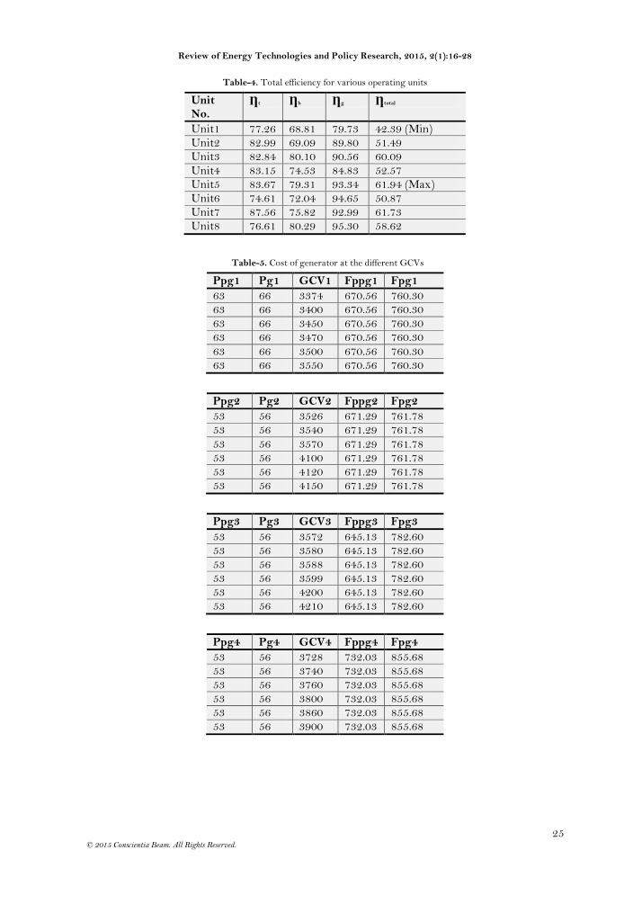
Table-4. Total efficiency for various operating units

Unit No.

Ƞt Ƞb Ƞg Ƞtotal

Unit1 77.26 68.81 79.73 42.39 (Min) Unit2 82.99 69.09 89.80 51.49 Unit3 82.84 80.10 90.56 60.09 Unit4 83.15 74.53 84.83 52.57 Unit5 83.67 79.31 93.34 61.94 (Max) Unit6 74.61 72.04 94.65 50.87 Unit7 87.56 75.82 92.99 61.73 Unit8 76.61 80.29 95.30 58.62

Table-5. Cost of generator at the different GCVs

Ppg1 Pg1 GCV1 Fppg1 Fpg1

63 66 3374 670.56 760.30 63 66 3400 670.56 760.30 63 66 3450 670.56 760.30 63 66 3470 670.56 760.30

63 66 3500 670.56 760.30 63 66 3550 670.56 760.30


53 56 3526 671.29 761.78 53 56 3540 671.29 761.78

53 56 3570 671.29 761.78 53 56 4100 671.29 761.78 53 56 4120 671.29 761.78 53 56 4150 671.29 761.78


53 56 3572 645.13 782.60 53 56 3580 645.13 782.60 53 56 3588 645.13 782.60 53 56 3599 645.13 782.60 53 56 4200 645.13 782.60 53 56 4210 645.13 782.60


53 56 3728 732.03 855.68 53 56 3740 732.03 855.68 53 56 3760 732.03 855.68 53 56 3800 732.03 855.68 53 56 3860 732.03 855.68 53 56 3900 732.03 855.68


26



191 194 3779 2841.6 2936.7 191 194 3790 2841.6 2936.7 191 194 3810 2841.6 2936.7

Continue 191 194 3850 2841.6 2936.7 191 194 3890 2841.6 2936.7 191 194 4050 2841.6 2936.7


181 184 3955 2000.8 2078.8 181 184 4000 2000.8 2078.8 181 184 4050 2000.8 2078.8 181 184 4100 2000.8 2078.8 181 184 4160 2000.8 2078.8 181 184 4200 1996.6 2073.8


168 171 3426 1613.4 1684.7 168 171 3450 1613.4 1684.7 168 171 3490 1613.4 1684.7 168 171 4200 1613.4 1684.7 168 171 4250 1613.4 1684.7 168 171 4280 1575.5 1610.4


168 171 3600 1674.6 1752.3 168 171 3650 1674.6 1752.3

168 171 3700 1674.6 1752.3 168 171 3750 1674.6 1752.3 168 171 3800 1674.6 1752.3 168 171 3850 1645.9 1720.5

NOMENCLATURE

Automatic Generation Control

Quadratic fuel coefficient

Linear fuel coefficient

Minimum fuel used during no load

Computer Integrated Plant Management System

Efficiency of generating units

Acceleration Constants

Differential Evolution

Economic Load Dispatch

Fuel Cost (in Rupees)

Gbest Best of Pbest called as Global best

Total efficiency of generating units

Manimum value of efficiency


27


Incremental Cost

Itermax Maximum number of iteration

Current number of iteration

Gross Penalty Factor for operating unit

LiTurbine Effic Penalty Factor associated with turbine efficiency

LiBoiler Effic Penalty Factor associated with boiler efficiency

LiGenerator Effic Penalty Factor associated with generator efficiency

Li Effic Penalty Factor associated with efficiency

MATLAB Matrix Laboratory

MW Mega-Watt

ANN Artificial Neural Network

PSO Particle Swarm Optimization

Ƞ Efficiency

GCV Gross Calorific Value

Inertia Weighting factor

WMAX Maximum value of weighting factor

WMIN Minimum value of weighting factor

λ Incremental Fuel Cost of the plant

Pgi Power generated by generator no. “i”

GCVi Gross Calorific Value of Coal in generator no”i”

Fpgi Cost offered by generator no. “i” in per hour

Ppgi Previous Power generated by generator no. “i”

Fppgi Previous Cost offered by generator no. “i” in per hour

REFERENCES

[1] P. Aravindhababu and K. R. Nayar, "Economic dispatch based on optimal lambda using radial basis

function network," Elect. Power Energy Syst., vol. 24, pp. 551–556, 2002.

[2] H. H. Happ, "Optimal power dispatch – a comprehensive survey," IEEE Transection on Power

Apparatus and Systems, vol. 96, 1977.

[3] R. Ramanathan, "Fast economic dispatch based on the penalty factors from Newton‟s method,"

IEEE Transection on Power Apparatus and Systems, vol. PAS-104, pp. 1624-1629, 1985.

[4] E. H. Chowdhury and R. Saifur, "A review of recent advances in economic dispatch," IEEE

Transactions on Power System, vol. 5, p. 1248, 1990.

[5] B. Aniruddha, I. Member, and K. C. Pranab, "Biogeography-based optimization for different

economic load dispatch problems," IEEE Transactions on Power Systems, vol. 25, p. 542 548, 2010.

[6] T. Yalcinoz and H. Altun, "Environmentally constrained economic dispatch via a genetic

algorithm with arithmetic crossover," presented at the IEEE 6th Africon Conference in Africa

2002, 2002.


28


[7] S. C. Leandro dos and C. M. Viviana, "Combining of chaotic differential evolution and quadratic

programming for economic dispatch optimization with valve-point effect," IEEE Transactions on

Power Systems, vol. 21, p. 989, 2006.

[8] S. Nidul, R. Chakrabarti, and P. K. Chattopadhyay, "Evolutionary programming techniques for

economic load dispatch," IEEE Transactions on Evolutionary Computation, vol. 7, p. 83, 2003.

[9] Y. M. Park, J. R. Won, and J. B. Park, "A new approach to economic load dispatch based on

improved evolutionary programming," Eng. Intell. Syst. Elect. Eng. Commun., vol. 6, pp. 103–110,

1998.

[10] H. T. Yang, P. C. Yang, and C. L. Huang, "Evolutionary programming based economic dispatch

for units with nonsmooth fuel cost functions," IEEE Trans. Power Syst., vol. 11, pp. 112–118, 1996.

[11] J. H. Park, Y. S. Kim, I. K. Eom, and K. Y. Lee, "Economic load dispatch for piecewise quadratic

cost function using hopfield neural network," IEEE Trans. Power Syst., vol. 8, pp. 1030–1038, 1993.

[12] K. Senthil and K. Manikandan, "Economic thermal power dispatch with emission constraint and

valve point effect loading using improved tabu search algorithm," International Journal of Computer

Applications (0975 – 8887), vol. 3, pp. 0975–8887, 2010.

[13] R. C. Eberhart and J. Kennedy, "A new optimizer using particle swarm theory," in Proceedings of the

6th International Symposium on Micro Machine and Human Science, Nagoya, Japan, 1995, pp. 39-43.

[14] H. Yoshida, K. Kawata, Y. Fukuyama, S. Takayama, and Y. Nakanishi, "A particle swarm

optimization for reactive power and voltage control considering voltage security assessment,"

IEEE Trans. Power Syst., vol. 15, pp. 1232–1239, 2000.

[15] M. Clerc and J. Kennedy, "The particle swarm-explosion, stability, and convergence in a

multidimensional complex space," IEEE Trans. Evol. Comput., vol. 6, pp. 58–73, 2002.

[16] I. N. Kassabalidis, M. A. El-Sharkawi, R. J. Marks, L. S. Moulin, and A. P. A. Da Silva, "Dynamic

security border identification using enhanced particle swarm optimization," IEEE Trans. Power

Syst., vol. 17, pp. 723–729, 2002.

[17] T. A. A. Victoire and A. E. Jeyakumar, "A modified hybrid EP-SQP approach for dynamic dispatch

with valve-point effect," Int. J. Elect. Power Energy Syst., vol. 27, pp. 594–601, 2005.

[18] S. M. V. Pandian and K. Thanushkodi, "Solving economic load dispatch problem considering

transmission losses by a hybrid EP-EPSO algorithm for solving both smooth and non-smooth cost

function," International Journal of Computer and Electrical Engineering, vol. 2, pp. 1793-8163, 2010.

[19] G. D. Pradeep, A text book on computer oriented statistical methods: Jeevansons, Publications, 2010.

Views and opinions expressed in this article are the views and opinions of the author(s), Review of Energy Technologies and Policy Research shall not be responsible or answerable for any loss, damage or liability etc. caused in relation to/arising out of the use of the content.

ECONOMIC LOAD DISPATCH IN THERMAL POWER PLANT ...

Documents

Transcript of ECONOMIC LOAD DISPATCH IN THERMAL POWER PLANT ...