Citation: Sánchez-Mora, M.M.;

Bernal-Romero, D.L.; Montoya, O.D.;

Villa Acevedo, W.M.; López-Lezama,

J.M. Solving the Optimal Reactive

Power Dispatch Problem through a

Python-DIgSILENT Interface.

Computation 2022, 10, 128. https://

doi.org/10.3390/computation

10080128

Academic Editor: Demos T. Tsahalis

Received: 16 June 2022

Accepted: 22 July 2022

Published: 25 July 2022

Publisher’s Note: MDPI stays neutral

with regard to jurisdictional claims in

published maps and institutional affil-

iations.

Copyright: © 2022 by the authors.

Licensee MDPI, Basel, Switzerland.

This article is an open access article

distributed under the terms and

conditions of the Creative Commons

Attribution (CC BY) license (https://

creativecommons.org/licenses/by/

4.0/).

computation

Article

Solving the Optimal Reactive Power Dispatch Problem througha Python-DIgSILENT InterfaceMartin M. Sánchez-Mora 1, David Lionel Bernal-Romero 2, Oscar Danilo Montoya 2,3,* ,Walter M. Villa-Acevedo 1 and Jesús M. López-Lezama 1,*

1 Departamento de Ingeniería Eléctrica, Facultad de Ingeniería, Universidad de Antioquia, Calle 70 No 52-21,Medellín 050010, Colombia; martin.sanchez@udea.edu.co (M.M.S.-M.); walter.villa@udea.edu.co (W.M.V.-A.)

2 Grupo de Compatibilidad e Interferencia Electromágnetica, Facultad de Ingeniería, Universidad DistritalFrancisco José de Caldas, Bogotá 110231, Colombia; dhhernandezr@correo.udistrital.edu.co

3 Laboratorio Inteligente de Energía, Facultad de Ingeniería, Universidad Tecnológica de Bolívar,Cartagena 131001, Colombia

* Correspondence: odmontoyag@udistrital.edu.co (O.D.M.); jmaria.lopez@udea.edu.co (J.M.L.-L.)

Abstract: The Optimal Reactive Power Dispatch (ORPD) problem consists of finding the optimalsettings of reactive power resources within a network, usually with the aim of minimizing activepower losses. The ORPD is a nonlinear and nonconvex optimization problem that involves bothdiscrete and continuous variables; the former include transformer tap positions and settings of reactorbanks, while the latter include voltage magnitude settings in generation buses. In this paper, theORPD problem is modeled as a mixed integer nonlinear programming problem and solved throughtwo different metaheuristic techniques, namely the Mean Variance Mapping Optimization and thegenetic algorithm. As a novelty, the solution of the ORPD problem is implemented through a Python-DIgSILENT interface that combines the strengths of both software. Several tests were performed onthe IEEE 6-, 14-, and 39-bus test systems evidencing the applicability of the proposed approach. Theresults were contrasted with those previously reported in the specialized literature, matching, and insome cases improving, the reported solutions with lower computational times.

Keywords: combinatorial optimization; DIgSILENT software; genetic algorithm; mean variancemapping optimization; optimal reactive power dispatch; power losses minimization; Python pro-gramming language

1. Introduction

Electric power systems play a key role in modern societies, since they allow us totransport energy from generation centers to loads. This is carried out through a complexinfrastructure that involves centrally-dispatched generation, substations and high-voltagetransmission lines. The ORPD is part of the daily operation of power systems; it consistsof finding the right settings of transformer taps, reactor banks and voltage set points ingeneration buses, generally with the aim of minimizing active power losses [1]. The ORPDis usually solved after the unit commitment, which is the process of programming theactive power generation as a function of their biding prices and limits [2,3]. The firstattempts to solve the ORPD problem resorted to classical optimization techniques suchas linear programming [4], quadratic programming [5] and interior point methods [6].Although these techniques are effective for solving convex optimization problems, they donot perform well when solving Mixed Integer Nonlinear Programming (MINLP) problems.These type of problems are better handled by heuristic and metaheuristic techniques asshown in [7–10] when it is not possible to transform these into mixed-integer models.

Owing to its nature, several metaheuristic techniques have been applied to solve theORPD problem. The main advantage of these approaches is that they are able to dealwith nonconvex optimization problems involving discrete and continuous variables [11,12].

Computation 2022, 10, 128. https://doi.org/10.3390/computation10080128 https://www.mdpi.com/journal/computation

Computation 2022, 10, 128 2 of 24

Furthermore, they do not require differentiability of the objective function or constraints,overcoming the disadvantages of classic optimization algorithms. Metaheuristic algorithmsare usually inspired by natural or social phenomena. Some of these methodologies, appliedto the solution of the ORPD problem, are described below.

In [13], the authors propose a gravitational search algorithm (GSA) applied to theORPD problem. In this technique, the solution candidates are represented by masses thatinteract according to the law of gravity and Newton’s laws. The proposed GSA is tested onthe IEEE 30-bus, 57-bus and 118-bus test systems considering minimization of active powerlosses, improvement of voltage profile and enhancement of voltage stability. An opposition-based GSA is developed in [14] to further improve the optimization performance of thebasic GSA.

In [15], the ORPD is approached using a harmony search algorithm with the objectiveof minimizing power losses and improving voltage profile. This method is based on aphenomenon inspired by the improvisation process of musicians. The study is implementedon the IEEE 30-bus and 57-bus test systems, and the results obtained are compared withother techniques that include GA and Particle Swarm Optimization (PSO).

In [16,17], the authors use a particle swarm optimization (PSO) method to solve theORPD problem considering voltage security assessment and voltage stability, respectively.The PSO is a metaheuristic inspired by the behavior of bird flocks and fish schools. Severalvariants of this approach have also been applied to solve the ORPD problem. In [18], threePSO variants are explored to solve the reactive power and voltage control problem. Thefirst two are known as global and local neighborhood variants of PSO, while the thirdone is the coordinated aggregation PSO algorithm. In [19], the turbulent and turbulentcrazy variants of PSO are also implemented. The authors perform several tests on the IEEE57-bus and IEEE 118-bus test systems, comparing their results with other metaheuristictechniques. It was found that the performance of PSO is considerably improved when theturbulent and turbulent crazy variants are implemented, outperforming classic metaheuris-tic approaches. In [20], the authors proposed a hybrid fuzzy-PSO algorithm that featuresimproved exploration and exploitation processes to approach the ORPD in real-size powersystems. Test systems of up to 354 nodes were used to validate the results. This algorithmshowed a better performance than the classical PSO approach.

In [21], a stochastic fractal search method is used to solve the multi-objective ORPDproblem considering the minimization of power losses along with voltage deviation anda voltage stability index. In [22], the authors implemented the mean-variance mappingoptimization (MVMO) algorithm to solve the ORPD problem. The effectiveness of theproposed algorithm was tested in the IEEE 30-bus test system and compared with othermetaheuristic approaches.

A survey of different metaheuristic techniques applied to the ORPD problem is pre-sented in [23]. In this paper, the authors also propose the sine–cosine algorithm to approachthe ORPD problem. A validation of the proposed algorithm is carried out with differentialevolution (DE) and PSO among other techniques. In [24], the authors propose an optimiza-tion algorithm based on the gradient to solve the ORPD, taking into account disperseddistributed generation in distribution networks. In [25], the authors use a hybrid fractionalPSO with GSA (FPSOGSA) to solve the ORPD problem. The proposed model is validatedwith the IEEE 30 and IEEE 57-bus test systems with the minimization of active powertransmission line losses and voltage deviation. The authors in [26] propose an entropyevolution technique implemented into FPSOGSA to further improve its performance.

In [27–30], evolutionary algorithms for addressing ORPD are presented. These al-gorithms are based on the postulates of biological evolution in which an initial set ofindividuals (solution candidates) give rise to other individuals with which they mustcompete in such a way that the fittest (best quality solutions) prevail over time, givingrise to new and better solutions. In [27], an evolutionary algorithm based on quantumcomputing is presented that seeks to jointly solve the optimal dispatch of both activeand reactive power. The authors validate their approach with the IEEE 30 and 118-bus

Computation 2022, 10, 128 3 of 24

test systems comparing their results with those obtained with simulated annealing (SA)and ant colony optimization. In [28], a DE algorithm is proposed bearing in mind sev-eral objectives, including voltage stability enhancement, voltage profile improvement andlosses minimization. In [31], the authors implemented a specialized GA in the DIgSILENTprogramming language (DPL) to solve the ORPD problem. As a main contribution, theproposed approach takes advantage of the modeling capabilities of DIgSILENT [32]. Thissoftware includes a detailed modeling of all sorts of power system elements, includinggenerators, reactors, transmission lines and transformers. Furthermore, it counts with itsown programming language that can be used to run power flow calculations with lowcomputational time.

Other optimization techniques applied to solve the ORPD include moth–flame opti-mization [33], the bat optimization algorithm [34], tabu search [35,36] and the slime moldalgorithm [37] among others. A detailed description of such techniques is not within thescope of this document; nonetheless, a review of metaheuristic techniques used to solve theORPD problem can be consulted in [38].

Following the research line adopted by [31], this paper presents a Python-DIgSILENTinterface to solve the ORPD problem. The proposed approach integrates the advantagesof using a specialized software that allows detailed modeling of network assets and haseffective power flow algorithms (DIgSILENT) with a versatile programming language thatsurpasses the capabilities of DPL (Python). The main contribution of this paper is theintegration of this software to solve the ORPD problem in electric power systems. TheORPD problem is well known in electrical engineering for being nonlinear, nonconvex andpresenting several sub-optimal solutions. The complexity of the ORPD problem largelysurpasses the built-in capabilities and functionalities of the DigSILENT Power Factorysoftware alone. Therefore, an interface with an object-oriented, high-level programminglanguage is implemented. The main advantage of the proposed interface is the fact ofcounting with several optimization libraries that can be used not only to solve the ORPDproblem but other optimization problems in electric power systems. To show the applica-bility of the proposed approach and for comparative purposes with [31], several tests werecarried out with the IEEE 6, IEEE 14 and IEEE 39-bus test system with two metaheuristictechniques developed in Python programming language, namely MVMO and GA.

The rest of the document is organized as follows: Section 2 presents the generalmathematical formulation of the ORPD problem in power systems. Section 3 describes thePython-DIgSILENT interface developed in this research work. Section 4 presents the maincharacteristics of the test systems that feature 6, 14 and 39 buses, respectively. Section 5presents the tests and results where the Python-DIgSILENT interface is used to solve theORPD using MVMO and GA in three benchmark IEEE test systems. Finally, the conclusionsare discussed in Section 6.

2. Mathematical Modeling of the ORPD Problem

Within the ORPD problem the continuous variables are related to generation of activeand reactive power as well as voltage magnitudes. On the other hand, the integer variablesare related to transformer tap positions as well as reactive power compensators. Themathematical modeling of the ORPD problem adopted in this research is described in thenext subsections [39].

2.1. Objective Function

Several objective functions may be envisaged when approaching the ORPD, suchas enhancement of voltage profile, amelioration of voltage stability or minimization ofpower losses, the last one being the most common. Equation (1) presents the objectivefunction considered in this paper which consists on minimizing the total active powerlosses for a given operative scenario. In this case, ploss represents the value of the objectivefunction; vm and vk are the magnitudes of voltages at buses m and k with angles θm andθk, respectively; Ykm(ta) is the admittance magnitude associated with buses k and m. This

Computation 2022, 10, 128 4 of 24

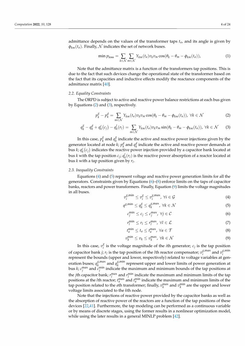
admittance depends on the values of the transformer taps ta, and its angle is given byφkm(ta). Finally, N indicates the set of network buses.

min ploss = ∑k∈N

∑m∈N

Ykm(ta)vkvm cos(θk − θm − φkm(ta)), (1)

Note that the admittance matrix is a function of the transformers tap positions. This isdue to the fact that such devices change the operational state of the transformer based onthe fact that its capacities and inductive effects modify the reactance components of theadmittance matrix [40].

2.2. Equality Constraints

The ORPD is subject to active and reactive power balance restrictions at each bus givenby Equations (2) and (3), respectively.

pgk − pd

k = ∑m∈N

Ykm(ta)vkvm cos(θk − θm − φkm(ta)), ∀k ∈ N (2)

qgk − qd

k + qck(cj)− ql

k(rl) = ∑m∈N

Ykm(ta)vkvm sin(θk − θm − φkm(ta)), ∀k ∈ N (3)

In this case, pgk and qg

k indicate the active and reactive power injections given by thegenerator located at node k; pd

k and qdk indicate the active and reactive power demands at

bus k; qck(cj)

indicates the reactive power injection provided by a capacitor bank located atbus k with the tap position cj; ql

k(rl) is the reactive power absorption of a reactor located atbus k with a tap position given by rl .

2.3. Inequality Constraints

Equations (4) and (5) represent voltage and reactive power generation limits for all thegenerators. Constraints given by Equations (6)–(8) enforce limits on the taps of capacitorbanks, reactors and power transformers. Finally, Equation (9) limits the voltage magnitudesin all buses.

vg,mini ≤ vg

i ≤ vg,maxi , ∀i ∈ G (4)

qg,min ≤ qgk ≤ qg,max

k , ∀k ∈ N (5)

cminj ≤ cj ≤ cmax

j , ∀j ∈ C (6)

rminl ≤ rl ≤ rmax

l , ∀l ∈ L (7)

tmina ≤ ta ≤ tmax

a , ∀a ∈ T (8)

vmink ≤ vk ≤ vmax

k , ∀k ∈ N (9)

In this case, vgi is the voltage magnitude of the ith generator; cj is the tap position

of capacitor bank j; rl is the tap position of the lth reactor compensator; vg,maxi and vg,min

irepresent the bounds (upper and lower, respectively) related to voltage variables at gen-eration buses; qg,max

k and qg,mink represent upper and lower limits of power generation at

bus k; cmaxj and cmin

j indicate the maximum and minimum bounds of the tap positions at

the jth capacitor bank; rmaxl and rmin

l indicate the maximum and minimum limits of the tappositions at the lth reactor; tmax

a and tmina indicate the maximum and minimum limits of the

tap position related to the ath transformer; finally, vmaxk and vmin

k are the upper and lowervoltage limits associated to the kth node.

Note that the injections of reactive power provided by the capacitor banks as well asthe absorption of reactive power of the reactors are a function of the tap positions of thesedevices [22,41]. Furthermore, the tap modeling can be performed as a continuous variableor by means of discrete stages, using the former results in a nonlinear optimization model,while using the later results in a general MINLP problem [42].

Computation 2022, 10, 128 5 of 24

The optimization problem indicated by Equations (1)–(9) is nonlinear and nonconvex.This is evident in Equations (2) and (3) which involve trigonometric functions as well as anonlinear relation of the admittance matrix with the transformer taps [21,43]. Moreover,the presence of integer variables makes the problem even more complex. As evidencedin the literature review, these types of problems are usually solved through metaheuristictechniques instead of classical optimization methods. In this paper we implemented twometaheuristic techniques to approach the ORPD problem through a Python-DIgSILENTinterface, namely MVMO and GA.

3. Python-DIgSILENT Interface

This section presents the main characteristics of the Python-DIgSILENT interfaceto face the ORPD problem through the combination of the Newton–Raphson load flowsolution in DIgSILENT [31], and the metaheuristic optimization techniques, i.e., the MVMOand the GA, implemented in the Python programming environment [44].

3.1. DIgSILENT Power Factory Software

DIgSILENT PowerFactory is one of the most popular power system software availablein the market. It is widely used by electricity companies for analyzing generation, distribu-tion and transmission and is also used by industrial systems. DIgSILENT covers a full rangeof functions, from standard features to advanced and highly sophisticated applications, thatincludes real-time simulation, renewable energy, distributed generation, and performancemonitoring for the supervision and testing of electrical systems. DIgSILENT is easy to use,is Windows compatible and integrates flexible and reliable system modeling capabilitiesalong with sophisticated algorithms and a unique database concept [45]. In addition, withits flexibility for scripting and interfaces, it is suited for highly automated and integratedsolutions in business applications.

To sum up, DIgSILENT PowerFactory was selected in this research work bearing inmind the following criteria: (1) it counts with its own programming language (DPL) thatcan be used to compute several load flows with low computational effort, (2) it allowsdetailed modeling of power system devices that includes transmission lines, transformers,reactors, as well as generators and induction motors, and (3) the integration of powersystem elements is straightforward for load flow analyses [46].

3.2. Python Programming Language

Python is an open-source, cross-platform programming language whose philosophyemphasizes code readability. It is an object-oriented, high-level programming languagethat features fewer steps compared to Java and C [47]. Python was initially founded in 1991by developer Guido Van Rossum. Due to its readability along with dynamic typing andbinding, it has rapidly become popular among programmers, and currently it is among thefastest growing languages in the world. One of the advantages of Python programminglanguage is counting with a very active community. Many organizations such as Google,Yahoo and YouTube have adopted Python.

Python has been integrated with other languages used for solving optimization prob-lems, among which are those related to power systems. Python’s versatility, ease ofadaptation, integration and robustness have given it a place in the formulation of optimiza-tion problems, either as a main language or as a complement. The specialized literaturepresents diverse examples of the use of tools developed in Python that allow modeling,use of specialized analysis methods and easy integration with external methodologies forsolving power system problems [48,49]. In addition, examples of power system problemsolving, such as electrical planning [50], weak node detection using statistical methods [51]and optimal reactive power dispatch [52] have been implemented using this program-ming language.

Computation 2022, 10, 128 6 of 24

3.3. Design of the Python-DIgSILENT Interface

The Python-DIgSILENT interface integrates all the features of Python (libraries, read-able code, documentation and support community) and allows access from Python toall the functionality that DIgSILENT PowerFactory provides as power system modelingsoftware. The interface integrates Python libraries that focus on optimization, data analyticsand machine learning in conjunction with the detailed power system modeling that allowsDIgSILENT PowerFactory. An example of the interface is depicted in Figure 1 where powerlosses of a transmission system are computed.

Figure 1. Example of an AC load flow loss calculation (evaluated using Newton–Raphson) inPython-DIgSILENT script software.

Figure 2 shows how to perform the same calculation using the standard DPL (DIgSI-LENT Programming Language) form of programming, which involves an understandingof the features of writing code, necessitates more time in application development and doesnot have the aforementioned benefits of using a programming language such as Python.

Figure 2. Example of an AC load flow loss calculation (evaluated using Newton–Raphson) inDIgSILENT Programming Language.

Computation 2022, 10, 128 7 of 24

The workflow between DigSILENT and the Python programming language is shownin Figure 3. In this case, the software DigSILENT allows integration with the Pythonexecutable via ComPython objects. Using Python, the integration library is loaded, whichallows the connection with the DigSILENT program and with the optimization libraries.

Figure 3. DIgSILENT Power Factory and Python Programming Language workflow.

3.4. Implementation of Optimization Libraries

The solution of the proposed optimization problem involved the use of open-sourcePython libraries. In this case, the MVMO [53] and PyMoo [54] libraries were used. Theselibraries allow the assignment of constraint functions, the objective function, the controlvariables and the input parameters (initial population, initial control variables, number ofmutations and number of iterations). The PyMoo library contains different optimization al-gorithms. In this paper, the GA was implemented. The use of this library and specificationsfor different algorithms can be consulted in [55].

The power systems under analysis are modeled in the DIgSILENT Power Factory tool,and by means of this tool, the update of the control variables and the validation by meansof load flow of the system constraints are performed. The implementation of the codes, theinitial configurations of the variables and the DIgSILENT Power Factory files are availablein [56].

As already mentioned, since the ORPD is a combinatorial problem, two metaheuristicapproaches were selected for its solution, namely GA and MVMO. These methodologiesare briefly described in the next subsections.

3.4.1. Genetic Algorithm

Genetic algorithms are search heuristics inspired by Charles Darwin’s theory of naturalevolution. They are designed to mimic the process of natural selection in which the fittestindividuals are more likely to transmit their genes to the next generations [57]. There areseveral variants of GAs; nonetheless, the version of GA available in [58] and illustrated inFigure 4 was implemented.

In the first stage of the algorithm, an initial population of randomly or pseudo-randomly candidate solutions is generated. Every candidate solution is represented asa vector (chromosome) that contains the four optimization variables of the system asindicated in Figure 5.

In this case, the initial population is randomly created taking into account the limits ofthe optimization variables. Once the initial population is obtained, the quality or fitness ofevery individual is computed. This corresponds to the power losses given by Equation (1).

Computation 2022, 10, 128 8 of 24

For this, a power flow is executed for every candidate solution using DIgSILENT andtaking as inputs the information provided in their codification.

Start

Read power sistem data

Define initial population

Read and decodeindividuals

Update power sistem data

Use DigSilent to compute Power Flow

Evaluate fitnessfunction

Is the stopping criterion met? Results

End

Selection

Crossover

Mutation

YESNO

Figure 4. Flowchart of the implemented GA.

...... ......

Voltage Setpoints Capacitors Reactors Transformer Taps

Figure 5. Illustration of a candidate solution to the ORPD problem.

The next step of the GA is the process of selection. In this step, two subsets of thepopulation are randomly selected, and the fittest individual from each subset is chosen togenerate new candidate solutions (offspring). The two selected individuals or candidatesolutions are then the parents of new solutions that are obtained through a crossover opera-tion. In this stage, the information of the parents is exchanged at a random position. The laststage of the GA is the mutation in which a randomly selected element of the chromosomeis changed. This steps allows the algorithm to escape from locally-optimal solutions.

Within the GA, the size of the population is kept constant; therefore, new solutions oroffspring replace the worst solutions of the current population. The process is carried outuntil a given number of generations is executed.

3.4.2. MVMO

The MVMO is a population-based stochastic technique which performs a searchprocedure within a normalized range of optimization variables. The MVMO uses thesame structure of candidate solutions as illustrated in Figure 6. MVMO uses the solutionvariables as an adaptive memory to save the n-best solutions that are found, a genericversion available in [59]. Like other evolutionary solution algorithms, MVMO adopts anoptimal value criterion to select the main solution, i.e., the stored optimal solution, fromwhich the next generation (offspring) solution is created.

Computation 2022, 10, 128 9 of 24

Figure 6. Flowchart of the implemented MVMO algorithm.

The search space of the MVMO for all variables is limited to [0, 1]. So then, themaximum and minimum values of the variables must be normalized in this range. Ineach iteration, it is not possible that any solution component surpasses the correspondingconstraints. To achieve this goal, a unique mapping function (h−function) was developed.This function has as inputs the means and variance of the best candidate solutions thatthe optimization algorithm has found so far. The shape and mapping curves are fixed inrelation to the advancement in the search space, and the MVMO updates the good solutionaround the best solutions in each iteration [60]. The MVMO algorithm searches around thebest local candidate solution with a small possibility of being trapped in a local optimalsolution. The feasibility of the solution is examined, and a fitness value is given for thissolution. To handle constraints, the static penalization approach was implemented. In thiscase, all variables are restricted by applying the fitness function due to the fact that controlvariables are self-limited.

The mapping function is in charge of transforming a given variable x∗i varied randomlywith unity distribution to another variable xi, which is concentrated around the mean value.

The solutions file is the knowledge base of the methodology that guides the search.Then, the n best solutions or individuals found so far by the MVMO are stored in thisfile. The fitness value of each solution is also saved. The update is only performed if thenew solution candidate turns out to be better than those currently in the file. The viablesolutions are at the top of the file. These individuals are sorted in accordance to their fitnessvalue. Non-viable solutions are sorted in accordance to their fitness and are placed at the

Computation 2022, 10, 128 10 of 24

bottom of the file. Once the file is complete with n feasible individuals, any non-feasiblecandidate solutions will not have a chance to be saved in the file.

The best solution found so far (the first solution positioned in the file), labeled asxbest, is the parent. In this case, a variable selection is carried out for the generation ofthe offspring. The MVMO algorithm seeks the mean value stored in the solution file forthe best individual only in m selected directions. Therefore, only these dimensions of theoffspring are updated, while the remaining D−m are assigned the corresponding xbestvalues, D being the number of control variables (problem dimension). Next, the mutationstage is carried out for each selected m dimension.

The MVMO also has a swarm variant with np particles. In this case, each particle hasits own solution file and mapping function. In the swarm MVMO algorithm, every particlecarries out m steps to identify an optimal set of independent solutions. Subsequently, thecurrent solutions (particles) exchange information. In some cases, some solution candidatesmight be very close to each other, meaning that there is information redundancy, andtherefore, redundant particles must be discarded. The best local and global solution (gbest)are defined. In addition, the normalized distance between each solution to the best localand global solutions are calculated.

The ith particle is eliminated from the process if its normalized distance is lower than acertain predefined threshold; if the solution is still considered, its search is focused towardsthe global best solution. This is performed by assigning the global best solution as theparent. Finally, the MVMO search process stops after a given number of fitness evaluations.The authors in [61,62] present a detailed description of the swarm MVMO algorithm.

4. Description of the Test Systems

The main features and data of the power systems under study are presented in thissection for future validation of the proposed approach. These systems have 6, 14 and39 buses, respectively. The last two systems can be found directly in the DIgSILENTsoftware [31].

4.1. IEEE 6-Bus Test System

Figure 7 depicts the IEEE 6-bus test system used in this study. The system featurestwo power generators located at buses 2 and 6 (slack bus), 2 capacitive banks, 2 powertransformers and 5 transmission lines. Table 1 presents the data of these devices whichinclude the nominal parameters of capacitor banks, transformers, generators and loads. Inthis case, the capacitor banks were represented as synchronous compensators featuringnominal capabilities from 0 to 5 MVAr.

SG~

SG~

SG~

B_CAPACITOR_B4 LOAD_B1

LOAD_B5

LOAD_B3

GENERATOR_B2B_CAPACITOR_B3

SLACK

BUS_2BUS_5BUS_3

BUS_1BUS_4BUS_6

Figure 7. IEEE 6-bus test system diagram.

Computation 2022, 10, 128 11 of 24

Table 1. Electrical data of the IEEE 6-bus test system.

Transmission Lines

Line From To Line Impedance’s# Bus Bus R (Ω) X (Ω)

1 6 3 4.88187 20.559422 6 4 3.17520 14.685303 4 3 3.84993 16.153834 5 2 11.19258 25.401605 2 1 28.69587 41.67450

Transformer Characteristics

Transformer From To Transformer Tap# Bus Bus Settings

1 4 1 91002 3 5 9100

Bus-Bar Characteristics

Bus Load Power Injections# PL (MW) QL (Mvar) PG (MW) QG (Mvar)

1 55 13 0 02 0 0 50 03 50 5 0 54 0 0 0 55 30 18 0 06 - - Slack node

Table 2 presents the transformer data of this system. In this case, the maximum rangefor a safe operation of these transformers is of ±10%. The data presented in Table 2 areneeded for the parametrization of transformers in DIgSILENT.

Table 2. Characterization of transformers in the IEEE 6-bus test system.

Transformer From To Minimum Maximum Addition Voltage Voltage# Bus Bus Voltage Voltage per Tap (%) Range (%)

1 4 1 9100 11,100 0.001 −0.1 ≤ pT ≤ 0.12 3 5 9100 11,100 0.001 −0.1 ≤ pT ≤ 0.1

Note that the last column in Table 2 defines the parameter pT to define the percentageof variations of the voltage output in the transformers equipped with taps. It is worthmentioning that the minimum and maximum positions for the transformer’s taps (seecolumns 4 and 5 in Table 2 are related with the typical settings in DIgSILENT softwarewhere the nominal input/output voltages for the transformer are defined for a tap valueof 10,000.

Table 3 presents the technical characteristics of the generators present in the IEEE 6-bustest system. In this case, bus 2 is a voltage-controlled node with minimum and maximumvoltages of 0.95 p.u. and 1.15 p.u., respectively. On the other hand, bus 6 is assigned as theslack or reference bus. For comparative purposes with [31], its minimum and maximumvoltages are assigned as 0.95 p.u. and 1.15 p.u., respectively.

Table 3. Technical characteristics of the generators in the IEEE 6-bus test system.

Generator Terminalvg,min

1 =

vg,min6 (p.u.)

vg,max1 (p.u.) vg,max

6 (p.u.)

1 2 0.95 1.1 1.15Slack 6 0.95 1.05 1.1

Computation 2022, 10, 128 12 of 24

4.2. IEEE 14-Bus Test System

The IEEE 14-bus test system is illustrated in Figure 8. This system includes 5 trans-formers, 16 transmission lines, 2 generators and 3 capacitor banks. This power system isalso made of four areas with voltage levels of 132 kV, 33 kV, 11 kV and 1 kV.

SG ~

SG~

SG~

SG~

SG~

Shnt_0009

Load_0009

Load_0006

Load_0005

Load_0004

Load_0003

Load_0002

Load_0014

Load_0013

Load_0012

Load_0011Load_0010

Gen_0008

Gen_0006

Gen_0003

Gen_0002

Gen_0001

Bus_0014

Bus_0013

Bus_0012

Bus_0011Bus_0010

Bus_0009Bus_0008

Bus_0007

Bus_0006

Bus_0005

Bus_0004

Bus_0003

Bus_0002

Bus_0001

Figure 8. IEEE 14-bus test system diagram.

Table 4 presents the electrical parameter of the transmission lines for the IEEE 14-bustest system, while Table 5 shows the transformers information. In this system the slacknode is bus 1, and node 2 is a voltage-controlled bus. Furthermore, three synchronouscompensators are used as capacitor banks operating in the continuous domain. Theseelements are located at buses 3, 6 and 8; buses 3 and 6 feature a nominal power of 20 MVArand bus 8 a nominal power of 30 MVAr.

Table 4. Parameters for the IEEE 14-bus test system.

Transmission Lines

Line From To Line Impedance’s Line From To Line Impedance’s# Bus Bus R Ω) X (Ω) # Bus Bus R (Ω) X (Ω)

1 1 2 6.753542 20.61956 9 6 11 1.034332 2.166022 1 2 6.753542 20.61956 10 6 12 1.33849 2.785773 1 5 9.414187 38.86250 11 6 13 0.72037 1.418644 2 3 8.187537 34.49428 12 9 10 0.34641 0.920205 2 4 10.12509 30.72200 13 9 14 1.38422 2.944436 2 5 9.922968 30.29685 14 10 11 0.89352 2.091647 3 4 11.67582 29.80027 15 12 13 2.40581 2.176698 4 5 2.326104 7.33724 16 13 14 1.86142 3.78993

Transformers Characteristic

Trans. From To Tap Trans. From To Tap# Bus Bus Settings # Bus Bus Settings

1 5 6 11,100 4 8 7 11,1002 4 9 11,100 5 4 7 11,1003 9 7 11,100

Computation 2022, 10, 128 13 of 24

Table 4. Cont.

Bus-Bar Characteristics (All Power Units in MW and MVAr)

Bus Load Injection Bus Load Injection# PL QL PG QG # PL QL PG QG

1 - - Node Slack 8 0.0 0.0 0.0 30.02 21.7 12.7 40.0 42.4 9 29.5 16.6 0.0 0.03 94.2 19.0 0.0 20.0 10 9.0 5.8 0.0 0.04 47.8 −3.9 0.0 0.0 11 3.5 1.8 0.0 0.05 7.6 1.6 0.0 0.0 12 6.1 1.6 0.0 0.06 11.2 7.5 0.0 20.0 13 13.5 5.8 0.0 0.07 0.0 0.0 0.0 20.0 14 14.9 5.0 0.0 0.0

Table 5. Transformers characteristics of the IEEE 14-bus test system.

Transformer From To Minimum Maximum Addition Voltage Voltage# Bus Bus Voltage Voltage per Tap (%) Range (%)

1 4 7 9100 11,100 0.0022 −2.2 ≤ pT ≤ 2.22 4 9 9100 11,100 0.0031 −3.1 ≤ pT ≤ 3.13 5 6 9100 11,100 0.0068 −6.8 ≤ pT ≤ 6.84 8 7 9100 11,100 0.0068 −6.8 ≤ pT ≤ 6.85 9 7 9100 11,100 0.0068 −6.8 ≤ pT ≤ 6.8

4.3. IEEE 39-Bus Test System

The IEEE 39-bus test system, illustrated in Figure 9, features four areas with voltagelevels of 345 kV, 230 kV, 138 kV and 16.5 kV. This system has 10 generators, 34 transmissionlines and 12 transformers.

The electrical parameters of the IEEE 39-bus test system and the characterization ofthe transformers are indicated in Tables 6 and 7, respectively.

Swing Node

SG~

SG~

SG~

SG~

SG~

SG~

SG~

SG~

SG~

SG~

Load 15

Load 24

Load 16

Load 21

Load 20

Load 12

Load 31Load 08

Load 07

Load 39

Load 04Load 03

Load 18

Load 25

Load 26

Load 27

Load 28

Load 29

G 07

G 09

G 06

G 05 G 04

G 03

G 02

G 01

G 08

G 10

Load 23

Bus 09

Bus 39

Bus 01

Bus 02

Bus 30

Bus 38

Bus 29Bus 25 Bus 28Bus 26

Bus 03

Bus 18

Bus 27

Bus 17

Bus 16

Bus 21

Bus 24

Bus 35

Bus 37

Bus 22

Bus 23

Bus 36

Bus 33Bus 34

Bus 19

Bus 20

Bus 15

Bus 14

Bus 13

Bus 32

Bus 10

Bus 12

Bus 11

Bus 31

Bus 06

Bus 04

Bus 05

Bus 07

Bus 08

Figure 9. IEEE 39-bus test system diagram.

Computation 2022, 10, 128 14 of 24

Table 6. Parameters of the IEEE 39-bus test system.

Lines Characteristic

Line From To Line Impedance’s Line From To Line Impedance’s# Bus Bus R (Ω) X (Ω) # Bus Bus R (Ω) X (Ω)

1 1 2 0.025547 0.30 18 13 14 0.026732 0.302 1 39 0.012000 0.30 19 14 15 0.024884 0.303 2 3 0.025827 0.30 20 15 16 0.028723 0.304 2 25 0.244186 0.30 21 16 17 0.023595 0.305 3 4 0.018309 0.30 22 16 19 0.024615 0.306 3 18 0.024812 0.30 23 16 21 0.017777 0.307 4 5 0.018750 0.30 24 16 24 0.015254 0.308 4 14 0.018604 0.30 25 17 18 0.025609 0.309 5 6 0.023076 0.30 26 17 27 0.022543 0.30

10 5 8 0.021428 0.30 27 21 22 0.017142 0.3011 6 7 0.019565 0.30 28 22 23 0.018750 0.3012 6 11 0.025609 0.30 29 23 24 0.018857 0.3013 7 8 0.026086 0.30 30 25 26 0.029721 0.3014 8 9 0.019008 0.30 31 26 27 0.028571 0.3015 9 39 0.012000 0.30 32 26 28 0.027215 0.3016 10 11 0.027906 0.30 33 26 29 0.027360 0.3017 10 13 0.027906 0.30 34 28 29 0.027814 0.30

Transformers Characteristic

Trans. From To Tap Trans. From To Tap# Bus Bus Settings # Bus Bus Settings

1 2 30 9100 7 19 33 91002 6 31 9100 8 20 34 91003 10 32 9100 9 22 35 91004 11 12 9100 10 23 36 91005 13 12 9100 11 25 37 91006 19 20 9100 12 29 38 9100

Bus Characteristics (All Power Units in MW and MVAr)

Bus Load Injection Bus Load Injection# PL QL PG PG # PL QL PG PG

3 322.0 2.4 - - 27 281.0 75.5 - -4 500.0 184.0 - - 28 206.0 27.6 - -7 233.8 84.0 - - 29 283.5 26.9 - -8 522.0 176.0 - - 30 - - 250 0.0

12 7.5 88.0 - - 31 9.2 4.6 Slack bus15 320.0 153.0 - - 32 - - 650 0.016 329.0 32.3 - - 33 - - 632 0.018 158.0 30.0 - - 34 - - 254 0.020 628.0 103.0 - - 35 - - 650 0.021 274.0 115 - - 36 - - 560 0.023 247.5 84.6 - - 37 - - 540 0.024 308.0 −92.2 - - 38 - - 830 0.025 224.0 47.2 - - 39 1104 250 1000 0.026 139.0 17.0 - -

Computation 2022, 10, 128 15 of 24

Table 7. Characterization of the transformers in the IEEE 39-bus test system.

Transformer From To Minimum Maximum Addition Voltage Voltage# Bus Bus Voltage Voltage per Tap (%) Range (%)

1 02 30 9100 11,100 0.0025 −2.5 ≤ pT ≤ 2.52 25 37 9100 11,100 0.0025 −2.5 ≤ pT ≤ 2.53 29 38 9100 11,100 0.0025 −2.5 ≤ pT ≤ 2.54 22 35 9100 11,100 0.0025 −2.5 ≤ pT ≤ 2.55 23 36 9100 11,100 0.0070 −7.0 ≤ pT ≤ 7.06 19 33 9100 11,100 0.0070 −7.0 ≤ pT ≤ 7.07 20 34 9100 11,100 0.0009 −0.9 ≤ pT ≤ 0.98 19 20 9100 11,100 0.0060 −6.0 ≤ pT ≤ 6.09 10 32 9100 11,100 0.0070 −7.0 ≤ pT ≤ 7.0

10 13 12 9100 11,100 0.0006 −0.6 ≤ pT ≤ 0.611 11 12 9100 11,100 0.0006 −0.6 ≤ pT ≤ 0.612 06 31 9100 11,100 0.0070 −7.0 ≤ pT ≤ 7.0

5. Tests and Results

This section presents the results obtained with the power systems described inSection 4. All tests were run on a personal computer Intel(R) Core(TM) i5-8365U pro-cessor 1.60 GHz. RAM 16 Gb, with a Windows 10 operating system, 64 bits, single language.The results of the two implemented methodologies (MVMO and GA) using the Python-DIgSILENT interface described in this paper are compared with those obtained throughthe CBGA proposed in [31] using DPL. For the sake of simplicity, only Case A1 of theaforementioned paper is considered.

5.1. Results with the IEEE 6-Bus Test System

Table 8 presents the results obtained with the developed Python-DIgSILENT inter-face considering MVMO and GA. These results are compared with the CBGA imple-mented in [31].

Table 8. Results for the IEEE 6-bus test system.

Elements Base Case CBGA [31] MVMO GA

Generators Voltage (p.u.) Voltage (p.u.)

G1 Bus06(slack) 1.0000 1.0500 1.0500 1.0500G2 Bus02 1.0000 1.0999 1.0999 1.0999

Transformers Tap Position Tap Position

Trafo Bus 04-01 9100 11,089 11,100 11,099Trafo Bus 03-05 9100 11,099 11,085 11,099

Capacitor Bank Reactive power (Mvar) Reactive power (Mvar)

PQ Bus03 0.0000 4.9992 4.9999 4.9999PQ Bus04 0.0000 4.9995 4.9999 4.9999

Power Losses (MW) 12.910 10.089 10.089 10.089Reduction (%) - 21.85 21.85 21.85

The results presented in Table 8 show that the reduction in power losses obtained withthe three algorithms is identical and corresponds to 21.85% with respect to the originalvalues (base case). Note that the voltage set points of the generators obtained with the threeoptimization approaches is also the same. In this case the voltage set point for the slackbus is 1.05 p.u., and the maximum voltage magnitude for generation buses is 1.1 p.u. Thecapacitor banks installed in the test system operate almost at their maximum limits in thethree approaches explored. Regarding tap positions of transformers, there are some smalldifferences between the results obtained with proposed interface (both MVMO and GA)

Computation 2022, 10, 128 16 of 24

and the DIgSILENT DPL (CBGA); nonetheless, such difference does not alter the amountof power loss reduction.

Table 9 presents the line loading. It can be observed that the three optimizationmethods result in roughly the same loading conditions. In all cases, it is reduced, resultingin lower power losses. Some transmission lines reduce their loading conditions by animportant percentage: for example, line 6-3 that passes from an initial condition of 48.23%to 41.26% or line 6-4 that passes from 55.8% to 47.4% .

Table 9. Line loading for the IEEE 6-bus test system considering different approaches.

Line Base Case CBGA [31] MVMO GA

(Start-End) Loading (%) Loading (%) Loading (%) Loading (%)

Line 6-3 48.2314 41.2668 41.2645 41.2661Line 6-4 55.8039 47.4526 47.4497 47.4517Line 4-3 10.9207 9.5843 9.5841 9.5842Line 5-2 33.5334 30.4007 30.4016 30.4008Line 1-2 17.4563 16.1338 16.1339 16.1337

Figure 10 illustrates the voltage magnitudes for each simulation along with the basecase. Note that for all methodologies, there is an important enhancement of the voltageprofile: nonetheless, without violating the voltage limits of the system. Note that somebuses exhibit important voltage improvements, such as bus 2 that passes from 1.00 p.u. to1.10 p.u. and bus 3 that originally has 0.84 p.u. and passes to 0.94 p.u.

Figure 10. Voltage profile of the IEEE 6-bus test system considering different methodologies.

5.2. Results with the IEEE 14-Bus Test System

Table 10 presents the optimal reactive power outputs in capacitor banks, voltage setpoints of generators, tap positions of transformers and the total power losses for eachmethodology compared to the base case. The active power loss reduction is around 21% forthe three methodologies. The highest reduction is obtained with the CBGA; nonetheless,the differences with the other two methodologies implemented in the proposed Python-DIgSILENT interface are not high. In this case, the solution obtained with the CBGA is0.1% and 0.4% better than those achieved with MVMO and GA, respectively. The voltageset point for the slack bus is kept the same for the three methodologies; nonetheless,there are small differences in the voltage set points obtained for the PV bus. The CBGAproposes 1.037 p.u for generator G2 located at bus 02, while MVMO and GA set this voltageat 1.0353 p.u. and 1.03723 p.u., respectively. Regarding tap position, all methodologiescoincide in the same results. Note that unlike the IEEE 6-bus test system, where transformertaps were set close to their maximum values, in this test system the results of the tapswere different. Such variation in transformer tap positions are principally conditioned byvoltage output in power generators. On the other hand, capacitor banks with nominal rates

Computation 2022, 10, 128 17 of 24

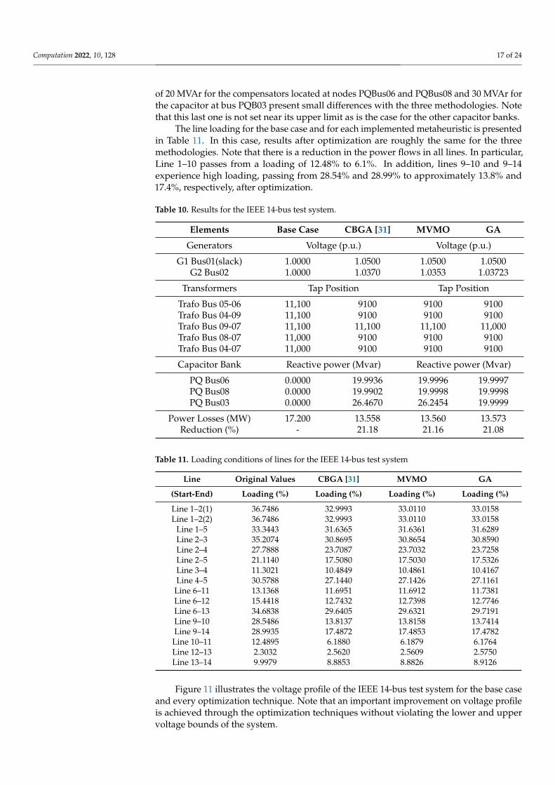
of 20 MVAr for the compensators located at nodes PQBus06 and PQBus08 and 30 MVAr forthe capacitor at bus PQB03 present small differences with the three methodologies. Notethat this last one is not set near its upper limit as is the case for the other capacitor banks.

The line loading for the base case and for each implemented metaheuristic is presentedin Table 11. In this case, results after optimization are roughly the same for the threemethodologies. Note that there is a reduction in the power flows in all lines. In particular,Line 1–10 passes from a loading of 12.48% to 6.1%. In addition, lines 9–10 and 9–14experience high loading, passing from 28.54% and 28.99% to approximately 13.8% and17.4%, respectively, after optimization.

Table 10. Results for the IEEE 14-bus test system.

Elements Base Case CBGA [31] MVMO GA

Generators Voltage (p.u.) Voltage (p.u.)

G1 Bus01(slack) 1.0000 1.0500 1.0500 1.0500G2 Bus02 1.0000 1.0370 1.0353 1.03723

Transformers Tap Position Tap Position

Trafo Bus 05-06 11,100 9100 9100 9100Trafo Bus 04-09 11,100 9100 9100 9100Trafo Bus 09-07 11,100 11,100 11,100 11,000Trafo Bus 08-07 11,000 9100 9100 9100Trafo Bus 04-07 11,000 9100 9100 9100

Capacitor Bank Reactive power (Mvar) Reactive power (Mvar)

PQ Bus06 0.0000 19.9936 19.9996 19.9997PQ Bus08 0.0000 19.9902 19.9998 19.9998PQ Bus03 0.0000 26.4670 26.2454 19.9999

Power Losses (MW) 17.200 13.558 13.560 13.573Reduction (%) - 21.18 21.16 21.08

Table 11. Loading conditions of lines for the IEEE 14-bus test system

Line Original Values CBGA [31] MVMO GA

(Start-End) Loading (%) Loading (%) Loading (%) Loading (%)

Line 1–2(1) 36.7486 32.9993 33.0110 33.0158Line 1–2(2) 36.7486 32.9993 33.0110 33.0158

Line 1–5 33.3443 31.6365 31.6361 31.6289Line 2–3 35.2074 30.8695 30.8654 30.8590Line 2–4 27.7888 23.7087 23.7032 23.7258Line 2–5 21.1140 17.5080 17.5030 17.5326Line 3–4 11.3021 10.4849 10.4861 10.4167Line 4–5 30.5788 27.1440 27.1426 27.1161

Line 6–11 13.1368 11.6951 11.6912 11.7381Line 6–12 15.4418 12.7432 12.7398 12.7746Line 6–13 34.6838 29.6405 29.6321 29.7191Line 9–10 28.5486 13.8137 13.8158 13.7414Line 9–14 28.9935 17.4872 17.4853 17.4782Line 10–11 12.4895 6.1880 6.1879 6.1764Line 12–13 2.3032 2.5620 2.5609 2.5750Line 13–14 9.9979 8.8853 8.8826 8.9126

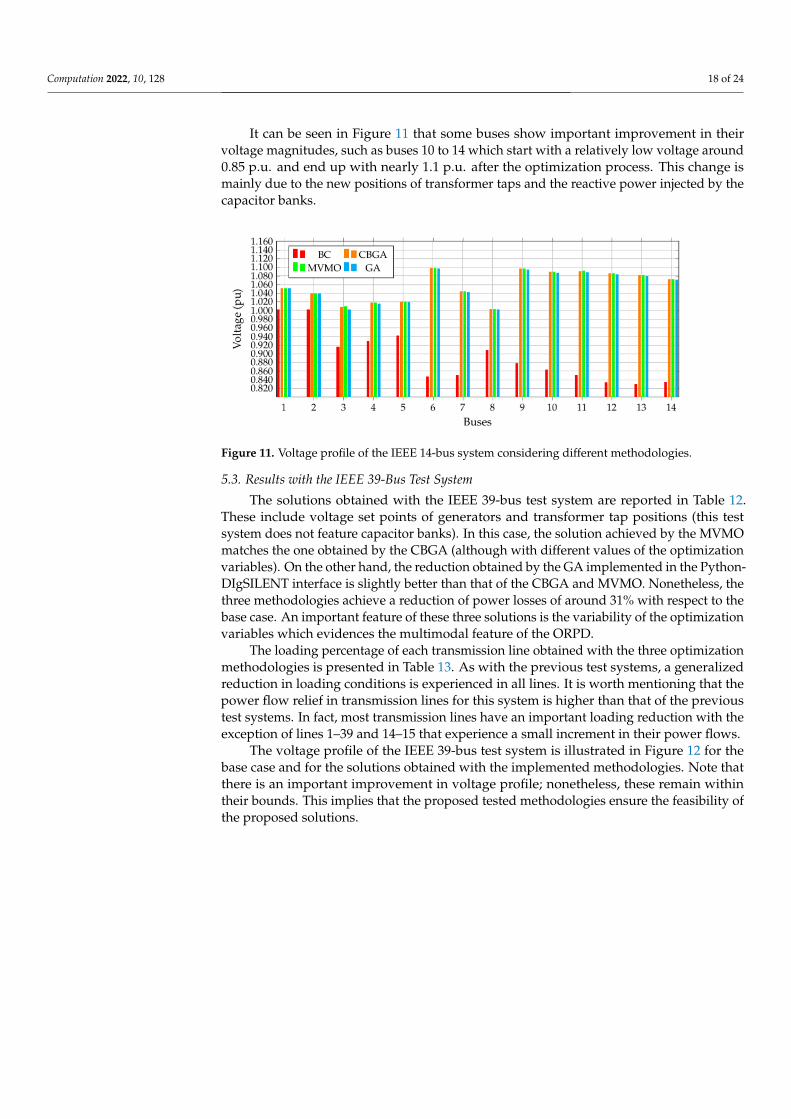
Figure 11 illustrates the voltage profile of the IEEE 14-bus test system for the base caseand every optimization technique. Note that an important improvement on voltage profileis achieved through the optimization techniques without violating the lower and uppervoltage bounds of the system.

Computation 2022, 10, 128 18 of 24

It can be seen in Figure 11 that some buses show important improvement in theirvoltage magnitudes, such as buses 10 to 14 which start with a relatively low voltage around0.85 p.u. and end up with nearly 1.1 p.u. after the optimization process. This change ismainly due to the new positions of transformer taps and the reactive power injected by thecapacitor banks.

Figure 11. Voltage profile of the IEEE 14-bus system considering different methodologies.

5.3. Results with the IEEE 39-Bus Test System

The solutions obtained with the IEEE 39-bus test system are reported in Table 12.These include voltage set points of generators and transformer tap positions (this testsystem does not feature capacitor banks). In this case, the solution achieved by the MVMOmatches the one obtained by the CBGA (although with different values of the optimizationvariables). On the other hand, the reduction obtained by the GA implemented in the Python-DIgSILENT interface is slightly better than that of the CBGA and MVMO. Nonetheless, thethree methodologies achieve a reduction of power losses of around 31% with respect to thebase case. An important feature of these three solutions is the variability of the optimizationvariables which evidences the multimodal feature of the ORPD.

The loading percentage of each transmission line obtained with the three optimizationmethodologies is presented in Table 13. As with the previous test systems, a generalizedreduction in loading conditions is experienced in all lines. It is worth mentioning that thepower flow relief in transmission lines for this system is higher than that of the previoustest systems. In fact, most transmission lines have an important loading reduction with theexception of lines 1–39 and 14–15 that experience a small increment in their power flows.

The voltage profile of the IEEE 39-bus test system is illustrated in Figure 12 for thebase case and for the solutions obtained with the implemented methodologies. Note thatthere is an important improvement in voltage profile; nonetheless, these remain withintheir bounds. This implies that the proposed tested methodologies ensure the feasibility ofthe proposed solutions.

Computation 2022, 10, 128 19 of 24

Figure 12. Voltage profile of the IEEE 39-bus test system considering different methodologies.

Table 12. Results for the IEEE 39-bus system.

Elements Base Case CBGA [31] MVMO GA

Generators Voltage (p.u) Voltage (p.u)

G1 Bus39 1.0000 1.0776 1.0657 1.0753G2 Bus31(slack) 1.0000 1.0500 1.0500 1.0500

G3 Bus32 1.0000 1.0810 1.0728 1.0903G4 Bus33 1.0000 1.0985 1.0733 1.0917G5 Bus34 1.0000 1.0414 1.0764 1.0995G6 Bus35 1.0000 1.0970 1.0879 1.0891G7 Bus36 1.0000 1.0761 1.0574 1.0857G8 Bus37 1.0000 1.0792 1.0703 1.0960G9 Bus38 1.0000 1.0982 1.0841 1.0880G10 Bus30 1.0000 1.0652 1.0565 1.0725

Transformers Tap Position Tap Position

Trafo Bus 02-30 9100 10,440 10,863 10,416Trafo Bus 25-37 9100 10,830 11,100 11,100Trafo Bus 29-38 9100 10,021 11,100 10,844Trafo Bus 22-35 9100 10,214 9455 9480Trafo Bus 23-36 9100 11,065 9397 10,850Trafo Bus 19-33 9100 10,562 10,169 10,892Trafo Bus 20-34 9100 9648 10,966 10,222Trafo Bus 19-20 9100 10,729 9,335 10,041Trafo Bus 10-32 9100 11,037 11,100 10,927Trafo Bus 13-12 9100 10,725 11,100 10,737Trafo Bus 11-12 9100 10,085 10,971 10,373Trafo Bus 06-31 9100 11,058 10,635 10,179

Power Losses (MW) 38.790 26.476 26.479 26.422Reduction(%) - 31.75 31.75 31.88

Computation 2022, 10, 128 20 of 24

Table 13. Loading conditions of the lines for the IEEE 39-bus system.

(Lines(Start-End)

Base CaseLoading CBGA [31] (%) MVMO

Loading GA (%)

L 1–2 31.5919 21.9571 20.7607 21.2570L 1–2 31.5919 21.9571 20.7607 21.2570

L 1–39 24.6876 24.1132 25.7837 25.0039L 2–3 71.5882 56.8398 56.8912 56.7258

L 2–25 44.4287 37.9134 38.0674 37.8657L 3–4 30.8098 16.9084 17.1695 17.4032

L 3–18 13.0756 9.0992 9.6112 8.8264L 4–5 27.6425 22.7757 22.5411 22.5985

L 4–14 50.5295 43.9437 44.0914 43.7494L 5–6 86.2751 72.2391 72.5483 72.1871L 5–8 59.1632 50.8941 51.3915 50.9805L 6–7 79.2231 67.6418 68.1481 67.7006

L 6–11 67.1245 58.4637 58.3799 58.2336L 7–8 35.6682 29.4048 29.7223 29.4501L 8–9 37.8915 12.2439 9.8735 11.5506

L 9–39 32.0210 17.0125 19.1821 17.6749L 10–11 67.6012 59.4466 59.5977 58.8809L 10–13 54.5243 46.9344 46.3916 46.8317L 13–14 52.3392 44.1616 43.9891 43.8117L 13–14 52.3392 44.1616 43.9891 43.8117L 14–15 5.2454 8.0803 7.0235 7.5485L 15–16 62.7392 51.7655 52.1361 51.9074L 16–17 46.8878 35.5673 35.4393 35.5494L 16–19 92.5581 77.7325 77.6822 77.6428L 16–21 60.7955 51.6157 51.2743 51.3467L 16–24 17.5808 17.7158 17.3047 17.2731L 17–18 38.4347 32.6810 32.9077 32.5544L 17–27 13.8078 6.2314 6.1114 5.7034L 21–22 112.7630 93.7010 93.8989 93.7535L 22–23 22.7600 11.7429 7.1108 7.2783L 23–24 64.0312 54.1063 53.9617 53.9557L 25–26 16.4244 12.6808 13.3907 11.8264L 26–27 51.4229 41.5517 41.6268 41.3364L 26–28 25.3862 23.5066 23.3028 23.9918L 26–29 33.9377 31.4868 31.2730 31.9884L 28–29 60.7682 53.7901 53.6518 54.1180

5.4. Processing Times

The average processing times required by the proposed Python-DIgSILENT interfaceand the CBGA implemented in the DPL environment from DIgSILENT [31] are presentedin Table 14. As expected, processing times increase with the number of nodes since moredecision variables must be considered in the optimization processes. Note that an importantimprovement in computation time is achieved through the proposed approach, especiallywhen applying the GA.

Table 14. Average processing times for all the IEEE test systems considering different optimizationapproaches.

Test System CBGA [31] (s) MVMO (s) GA (s)

IEEE 6-bus test system 88.94 24.47 14.45IEEE 14-bus test system 124.74 43.96 29.96IEEE 39-bus test system 193.80 132.59 89.42

Computation 2022, 10, 128 21 of 24

6. Conclusions

This paper presented a Python-DIgSILENT interface to approach the optimal reac-tive power dispatch problem in electric power systems. The proposed interface takesadvantage of all the functionalities provided by DIgSILENT software for system model-ing and power flow calculations along with an object-oriented high-level programminglanguage that allows using optimization libraries. The optimal reactive power dispatchwas solved using two metaheuristic approaches, namely MVMO and GA. Several testswere carried out on three benchmark IEEE power systems. Voltage set points of generators,transformer tap positions and reactive power injection in capacitor banks were used asoptimization variables.

The numerical results reported power loss reductions with respect to the base caseof up to 21.85%, 21.1% and 31.88% for the IEEE-6, 14 and 39 bus test systems, respectively.This evidenced the effectiveness of the proposed approach for reducing active power lossesthrough the optimal management of reactive power resources. All tests were carried outwith a fixed voltage of the slack bus of 1.05 p.u and a maximum voltage in generationbuses of 1.1 p.u. In all cases, it was verified that voltage magnitudes were kept within theirallowable limits. On the other hand, significant reductions on loading conditions wereobserved in all test systems.

A comparison was carried out with previously reported results in the specializedliterature. The proposed approach was able to match the results obtained by a CBGAimplemented in DIgSILENT programming language using the same test systems andinitial conditions. Nonetheless, better computing times were obtained with the proposedapproach.

The proposed Python-DIgSILENT interface opens the possibility to explore othermetaheuristic methodologies available in Python optimization libraries. Future work mayalso include other variants of the optimal reactive power dispatch, such as consideringa multi-period and multi-area approach as well as taking into account voltage stabilityissues.

Author Contributions: Conceptualization, M.M.S.-M., D.L.B.-R., O.D.M., W.M.V.A. and J.M.L.-D.;data curation, M.M.S.-M., O.D.M. and W.M.V.A.; formal analysis, M.M.S.-M., O.D.M., W.M.V.A.and J.M.L.-D.; funding acquisition, O.D.M., W.M.V.A. and J.M.L.-D.; investigation, M.M.S.-M.,D.L.B.-R., O.D.M., W.M.V.A. and J.M.L.-D.; methodology, M.M.S.-M., O.D.M., W.M.V.A. and J.M.L.-D.;project administration, W.M.V.A. and J.M.L.-D.; resources, O.D.M., W.M.V.A. and J.M.L.-D.; software,M.M.S.-M., O.D.M., W.M.V.A. and J.M.L.-D.; supervision, O.D.M., W.M.V.A. and J.M.L.-D.; validation,M.M.S.-M., D.L.B.-R., O.D.M., W.M.V.A. and J.M.L.-D.; visualization, M.M.S.-M., O.D.M., W.M.V.A.and J.M.L.-D.; writing—original draft, M.M.S.-M., D.L.B.-R., O.D.M., W.M.V.A. and J.M.L.-D.; writ-ing—review and editing, M.M.S.-M., D.L.B.-R., O.D.M., W.M.V.A. and J.M.L.-D. All authors haveread and agreed to the published version of the manuscript.

Funding: This research received no external funding.

Institutional Review Board Statement: Not applicable.

Informed Consent Statement: Not applicable.

Data Availability Statement: No new data were created or analyzed in this study. Data sharing isnot applicable to this article.

Conflicts of Interest: The authors declare no conflict of interest.

References1. Villa-Acevedo, W.M.; López-Lezama, J.M.; Valencia-Velásquez, J.A. A Novel Constraint Handling Approach for the Optimal

Reactive Power Dispatch Problem. Energies 2018, 11, 2352. https://doi.org/10.3390/en11092352.2. Marín-Cano, C.C.; Sierra-Aguilar, J.E.; López-Lezama, J.M.; Jaramillo-Duque, Á.; Villegas, J.G. A Novel Strategy to Re-

duce Computational Burden of the Stochastic Security Constrained Unit Commitment Problem. Energies 2020, 13, 3777.https://doi.org/10.3390/en13153777.

Computation 2022, 10, 128 22 of 24

3. Sierra-Aguilar, J.E.; Marín-Cano, C.C.; López-Lezama, J.M.; Jaramillo-Duque, Á.; Villegas, J.G. A New Affinely Ad-justable Robust Model for Security Constrained Unit Commitment under Uncertainty. Appl. Sci. 2021, 11, 3987.https://doi.org/10.3390/app11093987.

4. Mota-Palomino, R.; Quintana, V.H. Sparse Reactive Power Scheduling by a Penalty Function - Linear Programming Technique.IEEE Trans. Power Syst. 1986, 1, 31–39. https://doi.org/10.1109/TPWRS.1986.4334951.

5. Quintana, V.; Santos-Nieto, M. Reactive-power dispatch by successive quadratic programming. IEEE D 1989, 4, 425–435.https://doi.org/10.1109/60.43245.

6. Granville, S. Optimal reactive dispatch through interior point methods. IEEE Trans. Power Syst. 1994, 9, 136–146.https://doi.org/10.1109/59.317548.

7. López-Lezama, J.M.; Cortina-Gómez, J.; Muñoz-Galeano, N. Assessment of the Electric Grid Interdiction Problem using anonlinear modeling approach. Electr. Power Syst. Res. 2017, 144, 243–254. https://doi.org/10.1016/j.epsr.2016.12.017.

8. Gracia-Velásquez, D.G.; Morales-Rodríguez, A.S.; Montoya, O.D. Application of the Crow Search Algorithm to the Prob-lem of the Parametric Estimation in Transformers Considering Voltage and Current Measures. Computers 2022, 11, 9.https://doi.org/10.3390/computers11010009.

9. Arenas-Acuña, C.A.; Rodriguez-Contreras, J.A.; Montoya, O.D.; Rivas-Trujillo, E. Black-Hole Optimization Applied to theParametric Estimation in Distribution Transformers Considering Voltage and Current Measures. Computers 2021, 10, 124.https://doi.org/10.3390/computers10100124.

10. Saldarriaga-Zuluaga, S.D.; López-Lezama, J.M.; Muñoz-Galeano, N. Optimal coordination of over-current relays in microgridsconsidering multiple characteristic curves. Alex. Eng. J. 2021, 60, 2093–2113. https://doi.org/10.1016/j.aej.2020.12.012.

11. Pareja, L.A.G.; Lezama, J.M.L.; Carmona, O.G. Optimal Placement of Capacitors, Voltage Regulators, and Distributed Generatorsin Electric Power Distribution Systems. Ingeniería 2020, 25, 334–354. https://doi.org/10.14483/23448393.16925.

12. Montoya, O.D. Notes on the Dimension of the Solution Space in Typical Electrical Engineering Optimization Problems. Ingeniería2022, 27, e19310. https://doi.org/https://doi.org/10.14483/23448393.19310.

13. Duman, S.; Sonmez, Y.; Guvencc, U.; Yorukeren. Optimal reactive power dispatch using a gravitational search algorithm. IETGener. Transm. Distrib. 2012, 6, 563. https://doi.org/10.1049/iet-gtd.2011.0681.

14. Shaw, B.; Mukherjee, V.; Ghoshal, S. Solution of reactive power dispatch of power systems by an opposition-based gravitationalsearch algorithm. Int. J. Electr. Power Energy Syst. 2014, 55, 29–40. https://doi.org/10.1016/j.ijepes.2013.08.010.

15. Khazali, A.; Kalantar, M. Optimal reactive power dispatch based on harmony search algorithm. Int. J. Electr. Power Energy Syst.2011, 33, 684–692. https://doi.org/https://doi.org/10.1016/j.ijepes.2010.11.018.

16. Yoshida, H.; Kawata, K.; Fukuyama, Y.; Takayama, S.; Nakanishi, Y. A particle swarm optimization for reactive power and voltagecontrol considering voltage security assessment. IEEE Trans. Power Syst. 2000, 15, 1232–1239. https://doi.org/10.1109/59.898095.

17. Cai, G.; Ren, Z.; Yu, T. Optimal Reactive Power Dispatch Based on Modified Particle Swarm Optimization Considering VoltageStability. In Proceedings of the 2007 IEEE Power Engineering Society General Meeting, Tampa, FL, USA, 24–28 June 2007; pp. 1–5.https://doi.org/10.1109/PES.2007.386101.

18. Vlachogiannis, J.; Lee, K. A Comparative Study on Particle Swarm Optimization for Optimal Steady-State Performance of PowerSystems. IEEE Trans. Power Syst. 2006, 21, 1718–1728. https://doi.org/10.1109/TPWRS.2006.883687.

19. Gutiérrez, D.; Villa, W.M.; López-Lezama, J.M. Flujo Óptimo Reactivo mediante Optimización por Enjambre de Partículas. Inform.Tecnol. 2017, 28, 215–224. https://doi.org/10.4067/s0718-07642017000500020.

20. Naderi, E.; Narimani, H.; Fathi, M.; Narimani, M.R. A novel fuzzy adaptive configuration of particle swarm optimization to solvelarge-scale optimal reactive power dispatch. Appl. Soft Comput. 2017, 53, 441–456. https://doi.org/10.1016/j.asoc.2017.01.012.

21. Duong, T.L.; Duong, M.Q.; Phan, V.D.; Nguyen, T.T. Optimal Reactive Power Flow for Large-Scale Power Systems Using anEffective Metaheuristic Algorithm. J. Electr. Comput. Eng. 2020, 2020, 1–11. https://doi.org/10.1155/2020/6382507.

22. Londoño, D.C.; Villa-Acevedo, W.M.; López-Lezama, J.M. Assessment of Metaheuristic Techniques Applied to the OptimalReactive Power Dispatch. In Communications in Computer and Information Science; Springer International Publishing: Cham,Switzerland, 2019; pp. 250–262. https://doi.org/10.1007/978-3-030-31019-6_22.

23. Saddique, M.S.; Bhatti, A.R.; Haroon, S.S.; Sattar, M.K.; Amin, S.; Sajjad, I.A.; ul Haq, S.S.; Awan, A.B.; Rasheed, N. Solution tooptimal reactive power dispatch in transmission system using meta-heuristic techniques—Status and technological review. Electr.Power Syst. Res. 2020, 178, 106031. https://doi.org/10.1016/j.epsr.2019.106031.

24. Zhao, J.; Zhang, Z.; Yao, J.; Yang, S.; Wang, K. A distributed optimal reactive power flow for global transmission and distributionnetwork. Int. J. Electr. Power Energy Syst. 2019, 104, 524–536. https://doi.org/10.1016/j.ijepes.2018.07.019.

25. Khan, N.H.; Wang, Y.; Tian, D.; Raja, M.A.Z.; Jamal, R.; Muhammad, Y. Design of Fractional Particle Swarm Optimiza-tion Gravitational Search Algorithm for Optimal Reactive Power Dispatch Problems. IEEE Access 2020, 8, 146785–146806.https://doi.org/10.1109/ACCESS.2020.3014211.

26. Jamal, R.; Men, B.; Khan, N.H.; Raja, M.A.Z.; Muhammad, Y. Application of Shannon Entropy Implementation Into a NovelFractional Particle Swarm Optimization Gravitational Search Algorithm (FPSOGSA) for Optimal Reactive Power DispatchProblem. IEEE Access 2021, 9, 2715–2733. https://doi.org/10.1109/ACCESS.2020.3046317.

27. Vlachogiannis, J.G.; Lee, K.Y. Quantum-Inspired Evolutionary Algorithm for Real and Reactive Power Dispatch. IEEE Trans.Power Syst. 2008, 23, 1627–1636. https://doi.org/10.1109/TPWRS.2008.2004743.

Computation 2022, 10, 128 23 of 24

28. Ela, A.A.E.; Abido, M.; Spea, S. Differential evolution algorithm for optimal reactive power dispatch. Electr. Power Syst. Res. 2011,81, 458–464. https://doi.org/10.1016/j.epsr.2010.10.005.

29. Bakirtzis, A.; Biskas, P.; Zoumas, C.; Petridis, V. Optimal power flow by enhanced genetic algorithm. IEEE Trans. Power Syst.2002, 17, 229–236. https://doi.org/10.1109/tpwrs.2002.1007886.

30. Ara, A.L.; Kazemi, A.; Gahramani, S.; Behshad, M. Optimal reactive power flow using multi-objective mathematical programming.Sci. Iran. 2012, 19, 1829–1836. https://doi.org/10.1016/j.scient.2012.07.010.

31. Bernal-Romero, D.L.; Montoya, O.D.; Arias-Londoño, A. Solution of the Optimal Reactive Power Flow ProblemUsing a Discrete-Continuous CBGA Implemented in the DigSILENT Programming Language. Computers 2021, 10.https://doi.org/10.3390/computers10110151.

32. Ganesh, S.; Perilla, A.; Torres, J.R.; Palensky, P.; van der Meijden, M. Validation of EMT Digital Twin Models for Dynamic VoltagePerformance Assessment of 66 kV Offshore Transmission Network. Appl. Sci. 2020, 11, 244. https://doi.org/10.3390/app11010244.

33. Mei, R.N.S.; Sulaiman, M.H.; Mustaffa, Z.; Daniyal, H. Optimal reactive power dispatch solution by loss minimization usingmoth-flame optimization technique. Appl. Soft Comput. 2017, 59, 210–222. https://doi.org/10.1016/j.asoc.2017.05.057.

34. Bhongade, S.; Tomar, A.; Goigowal, S.R. Minimization of Optimal Reactive Power Dispatch Problem using BAT Algorithm. InProceedings of the 2020 IEEE First International Conference on Smart Technologies for Power, Energy and Control (STPEC),Nagpur, India, 25–26 September 2020; IEEE: Piscataway, NJ, USA, 2020. https://doi.org/10.1109/stpec49749.2020.9297806.

35. Abido, M.A. Optimal Power Flow Using Tabu Search Algorithm. Electr. Power Compon. Syst. 2002, 30, 469–483.https://doi.org/10.1080/15325000252888425.

36. Lenin, K. Reduction of active power loss by improved tabu search algorithm. Int. J. Res. GRANTHAALAYAH 2018, 6, 1–9.https://doi.org/10.29121/granthaalayah.v6.i7.2018.1277.

37. ElSayed, S.K.; Elattar, E.E. Slime Mold Algorithm for Optimal Reactive Power Dispatch Combining with Renewable EnergySources. Sustainability 2021, 13, 5831. https://doi.org/10.3390/su13115831.

38. Rojas, D.G.; Lezama, J.L.; Villa, W. Metaheuristic Techniques Applied to the Optimal Reactive Power Dispatch: a Review. IEEELat. Am. Trans. 2016, 14, 2253–2263. https://doi.org/10.1109/tla.2016.7530421.

39. Aghbolaghi, A.J.; Tabatabaei, N.M.; Boushehri, N.S.; Parast, F.H. Reactive Power Optimization in AC Power Systems. In PowerSystems; Springer International Publishing: Cham, Switzerland, 2017; pp. 345–409. https://doi.org/10.1007/978-3-319-51118-4_10.

40. Barboza, L.V.; Ziirn, H.H.; Salgado, R. Load Tap Change Transformers: A Modeling Reminder. IEEE Power Eng. Rev. 2001,21, 51–52. https://doi.org/10.1109/mper.2001.4311274.

41. Londoño-Tamayo, D.; Villa-Acevedo, J.L.L..W. Mean-Variance Mapping Optimization Algorithm Applied to the Optimal ReactivePower Dispatch. INGECUC 2021, 17, 239–255. https://doi.org/10.17981/ingecuc.17.1.2021.19.

42. Sharif, S.; Taylor, J. MINLP formulation of optimal reactive power flow. In Proceedings of the IEEE 1997 American ControlConference (Cat. No.97CH36041), Albuquerque, NM, USA, 8–10 May 1997. https://doi.org/10.1109/acc.1997.611033.

43. Morán-Burgos, J.A.; Sierra-Aguilar, J.E.; Villa-Acevedo, W.M.; López-Lezama, J.M. A Multi-Period Optimal Reactive PowerDispatch Approach Considering Multiple Operative Goals. Appl. Sci. 2021, 11, 8535. https://doi.org/10.3390/app11188535.

44. Acosta, M.N.; Adiyabazar, C.; Gonzalez-Longatt, F.; Andrade, M.A.; Torres, J.R.; Vazquez, E.; Santos, J.M.R. OptimalUnder-Frequency Load Shedding Setting at Altai-Uliastai Regional Power System, Mongolia. Energies 2020, 13, 5390.https://doi.org/10.3390/en13205390.

45. Gonzalez-Longatt, F.M.; Rueda, J.L. (Eds.) PowerFactory Applications for Power System Analysis; Springer International Publishing:Cham, Switzerland, 2014. https://doi.org/10.1007/978-3-319-12958-7.

46. Bifaretti, S.; Bonaiuto, V.; Pipolo, S.; Terlizzi, C.; Zanchetta, P.; Gallinelli, F.; Alessandroni, S. Power Flow Management by ActiveNodes: A Case Study in Real Operating Conditions. Energies 2021, 14, 4519. https://doi.org/10.3390/en14154519.

47. Dierbach, C. Python as a First Programming Language. J. Comput. Sci. Coll. 2014, 29, 73.48. Thurner, L.; Scheidler, A.; Schäfer, F.; Menke, J.H.; Dollichon, J.; Meier, F.; Meinecke, S.; Braun, M. Pandapower—An Open-Source

Python Tool for Convenient Modeling, Analysis, and Optimization of Electric Power Systems. IEEE Trans. Power Syst. 2018,33, 6510–6521. https://doi.org/10.1109/TPWRS.2018.2829021.

49. Milano, F. A python-based software tool for power system analysis. In Proceedings of the 2013 IEEE Power Energy SocietyGeneral Meeting, Vancouver, BC, Canada, 21–25 July 2013; pp. 1–5. https://doi.org/10.1109/PESMG.2013.6672387.

50. Condren, J.; An, S. Automation of transmission planning analysis process using Python and GTK+. In Proceedings of the 2006IEEE Power Engineering Society General Meeting, London, UK, 18–22 June 2006, p. 8. https://doi.org/10.1109/PES.2006.1709495.

51. Yusuff, A.; Mosetlhe, T.; Ayodele, T. Statistical method for identification of weak nodes in power system based on voltagemagnitude deviation. Electr. Power Syst. Res. 2021, 200, 107464. https://doi.org/https://doi.org/10.1016/j.epsr.2021.107464.

52. Latif, A.; Ahmad, I.; Palensky, P.; Gawlik, W. Multi-objective reactive power dispatch in distribution networks using modified batalgorithm. In Proceedings of the 2016 IEEE Green Energy and Systems Conference (IGSEC), Long Beach, CA, USA, 6–7 June 2016,pp. 1–7. https://doi.org/10.1109/IGESC.2016.7790069.

53. Mean Variance Mapping Optimization Algorithm. Available online: https://pypi.org/project/MVMO/ (accessed on 30 April2022).

54. Pymoo: Multi-Objective Optimization in Python. Available online: https://pymoo.org/index.html (accessed on 30 April 2022).55. Blank, J.; Deb, K. Pymoo: Multi-Objective Optimization in Python. IEEE Access 2020, 8, 89497–89509.

Computation 2022, 10, 128 24 of 24

56. Implemtación de MVMO y GA en DigSilent Power Factory con Python. Available online: https://github.com/Msanchez1002/MVMO_GA (accessed on 30 April 2022).

57. Agudelo, L.; López-Lezama, J.M.; Muñoz-Galeano, N. Vulnerability assessment of power systems to intentional attacks using aspecialized genetic algorithm. Dyna 2015, 82, 78–84.

58. GA: Genetic Algorithm. Available online: https://pymoo.org/algorithms/soo/ga.html (accessed on 30 April 2022).59. MVMo: Mean Variance Mapping Optimization Algorithm. Available online: https://github.com/dgusain1/MVMO (accessed

on 30 April 2022).60. Erlich, I.; Venayagamoorthy, G.K.; Worawat, N. A Mean-Variance Optimization algorithm. In Proceedings of the IEEE Congress

on Evolutionary Computation, Barcelona, Spain, 18–23 July 2010; pp. 1–6. https://doi.org/10.1109/CEC.2010.5586027.61. Rueda, J.L.; Erlich, I. Optimal dispatch of reactive power sources by using MVMO optimization. In Proceedings of

the 2013 IEEE Computational Intelligence Applications in Smart Grid (CIASG), Singapore, 16–19 April 2013; pp. 29–36.https://doi.org/10.1109/CIASG.2013.6611495.

62. Rueda, J.L.; Erlich, I. Evaluation of the mean-variance mapping optimization for solving multimodal problems. In Proceedings ofthe 2013 IEEE Symposium on Swarm Intelligence (SIS), Singapore, 16–19 April 2013; pp. 7–14. https://doi.org/10.1109/SIS.2013.6615153.