6.12 ECONOmIC DISPATCH
16
376 Chapter 6 | Power Flows controlled, typically these machines are modeled as a constant power factor PQ bus. By themselves these machines have under-excited (consuming reactive power) power factors of between 0.85 and 0.9, but banks of switched capacitors are often used to correct the wind farm power factor. Type 2 WTGs are wound rotor induction machines in which the rotor resistance can be controlled. The advantages of this approach are discussed in Chapter 11; from a power flow perspective, they perform like Type 1 WTGs. Most of the installed wind capacity and almost all new WTGs are either Type 3 or Type 4. Type 3 wind turbines are used to represent doubly-fed asynchronous gen- erators (DFAGs), also sometimes referred to as doubly-fed induction generators (DFIGs). This type models induction machines in which the rotor circuit is also con- nected to the ac network through an ac-dc-ac converter, allowing for much greater control of the WTG. Type 4 wind turbines are fully asynchronous machines in which the full power output of the machine is coupled to the ac network through an ac-dc- ac converter. From a power flow perspective, both types are capable of full voltage control like a traditional bus generator with reactive power control between a power factor of up to 60.9. However, like traditional synchronous generators, how their reactive power is actually controlled depends on commercial considerations, with many generator owners desiring to operate at unity power factor to maximize their real power outputs. 6.12 ECONOMIC DISPATCH This section describes how the real power output of a controlled generating unit is selected to meet a given load and to minimize the total operating costs. This is the economic dispatch problem [16]. In interconnected power systems, economic dispatch is often solved for smaller portions of the system, known as areas, in which the total generation in each area is controlled to match the total area load; further details are provided in Chapter 12. This section begins by considering only fossil-fuel generating units, with no constraints on maximum and minimum generator outputs, and with no transmission losses. The economic dispatch problem is first solved for this idealized case. Then it is 100 80 60 40 20 0 0 5 10 15 20 Wind Speed (m/s) Percent of Rated Output 25 30 FIGURE 6.16 Typical wind speed versus power curve Copyright 2017 Cengage Learning. All Rights Reserved. May not be copied, scanned, or duplicated, in whole or in part. Due to electronic rights, some third party content may be suppressed from the eBook and/or eChapter(s). Editorial review has deemed that any suppressed content does not materially affect the overall learning experience. Cengage Learning reserves the right to remove additional content at any time if subsequent rights restrictions require it.
-
Upload
khangminh22 -
Category
Documents
-
view
5 -
download
0
Transcript of 6.12 ECONOmIC DISPATCH
376 Chapter 6 | Power Flows
controlled, typically these machines are modeled as a constant power factor PQ bus. By themselves these machines have under-excited (consuming reactive power) power factors of between 0.85 and 0.9, but banks of switched capacitors are often used to correct the wind farm power factor. Type 2 WTGs are wound rotor induction machines in which the rotor resistance can be controlled. The advantages of this approach are discussed in Chapter 11; from a power flow perspective, they perform like Type 1 WTGs.
Most of the installed wind capacity and almost all new WTGs are either Type 3 or Type 4. Type 3 wind turbines are used to represent doubly-fed asynchronous gen-erators (DFAGs), also sometimes referred to as doubly-fed induction generators (DFIGs). This type models induction machines in which the rotor circuit is also con-nected to the ac network through an ac-dc-ac converter, allowing for much greater control of the WTG. Type 4 wind turbines are fully asynchronous machines in which the full power output of the machine is coupled to the ac network through an ac-dc-ac converter. From a power flow perspective, both types are capable of full voltage control like a traditional bus generator with reactive power control between a power factor of up to 60.9. However, like traditional synchronous generators, how their reactive power is actually controlled depends on commercial considerations, with many generator owners desiring to operate at unity power factor to maximize their real power outputs.
6.12 ECONOmIC DISPATCHThis section describes how the real power output of a controlled generating unit is selected to meet a given load and to minimize the total operating costs. This is the economic dispatch problem [16]. In interconnected power systems, economic dispatch is often solved for smaller portions of the system, known as areas, in which the total generation in each area is controlled to match the total area load; further details are provided in Chapter 12.
This section begins by considering only fossil-fuel generating units, with no constraints on maximum and minimum generator outputs, and with no transmission losses. The economic dispatch problem is first solved for this idealized case. Then it is
100
80
60
40
20
00 5 10 15 20
Wind Speed (m/s)
Per
cent
of R
ated
Out
put
25 30
FIGURE 6.16
Typical wind speed versus power curve
32134_ch06_ptg01.indd 376 07/12/15 6:21 pm
Copyright 2017 Cengage Learning. All Rights Reserved. May not be copied, scanned, or duplicated, in whole or in part. Due to electronic rights,some third party content may be suppressed from the eBook and/or eChapter(s). Editorial review has deemed that any suppressed content does not materiallyaffect the overall learning experience. Cengage Learning reserves the right to remove additional content at any time if subsequent rights restrictions require it.
Section 6.12 Economic Dispatch 377
expanded to include inequality constraints on generator outputs and to consider the impact of transmission losses. Finally, the dispatch of other types of units including solar and wind, nuclear, pumped-storage hydro, and hydro units is briefly discussed.
FOSSIL-FUEL UNITS, NO INEqUALITY CONSTRAINTS, NO TRANSmISSION LOSSESFigure 6.17 shows the operating cost Ci, of a fossil-fuel generating unit versus its real power output Pi. Fuel cost is the major portion of the variable cost of operation, although other variable costs, such as maintenance, could have been included in the figure. Fixed costs, such as the capital cost of installing the unit, are not included. Only those costs that are a function of unit power output—that is, those costs that can be controlled by operating strategy—enter into the economic dispatch formulation.
In practice, Ci is constructed of piecewise continuous functions valid for ranges of output Pi based on empirical data. The discontinuities in Figure 6.17 may be due to the firing of equipment such as additional boilers or condensers as power output is increased. It is often convenient to express Ci in terms of BTU∙hr, which is relatively constant over the lifetime of the unit, rather than $∙hr, which can change monthly or daily. Ci can be converted to $∙hr by multiplying the fuel input in BTU∙hr by the cost of fuel in $∙BTU.
Figure 6.18 shows the unit incremental operating cost dCi∙dPi versus unit out-put Pi, which is the slope or derivative of the Ci versus Pi curve in Figure 6.17. When Ci consists of only fuel costs, dCi∙dPi is the ratio of the incremental fuel energy input in BTU to incremental energy output in kWh, which is called the incremental heat rate. Note that the reciprocal of the heat rate, which is the ratio of output energy to input energy, gives a measure of fuel efficiency for the unit. For the unit shown in Figure 6.17, maximum efficiency occurs at Pi 5 600 MW, where the heat rate is Ci∙Pi 5 5.4 3 109∙600 3 103 5 9000 BTU∙kWh. The efficiency at this output is
percentage efficency 5 1 19000
kWhBTU2 13413
BTUkWh2 3 100 5 37.92%
FIGURE 6.17
Unit operating cost versus real power output—fossil-fuel generating unit
32134_ch06_ptg01.indd 377 07/12/15 6:21 pm
Copyright 2017 Cengage Learning. All Rights Reserved. May not be copied, scanned, or duplicated, in whole or in part. Due to electronic rights,some third party content may be suppressed from the eBook and/or eChapter(s). Editorial review has deemed that any suppressed content does not materiallyaffect the overall learning experience. Cengage Learning reserves the right to remove additional content at any time if subsequent rights restrictions require it.
378 Chapter 6 | Power Flows
The dCi∙dPi curve in Figure 6.18 is also represented by piecewise continuous functions valid for ranges of output Pi. For analytical work, the actual curves are of-ten approximated by straight lines. The ratio dCi∙dPi can also be converted to $∙kWh by multiplying the incremental heat rate in BTU∙kWh by the cost of fuel in $∙BTU.
For the area of an interconnected power system consisting of N units operating on economic dispatch, the total variable cost CT of operating these units is
CT 5 oN
i5i
Ci
5 C1sP1d 1 C2sP2d 1 Á 1 CNsPNd $yhr (6.12.1)
where Ci, expressed in $∙hr, includes fuel cost as well as any other variable costs of unit i. Let PT equal the total load demand in the area. Neglecting transmission losses.
P1 1 P2 1 Á 1 PN 5 PT (6.12.2)
Due to relatively slow changes in load demand, PT may be considered constant for periods of 2 to 10 minutes. The economic dispatch problem can be stated as follows:
Find the values of unit outputs P1, P2, …, PN that minimize CT given by (6.12.1), subject to the equality constraint given by (6.12.2).
A criterion for the solution to this problem is: All units on economic dispatch should operate at equal incremental operating cost. That is,
dC1
dP1
5dC2
dP2
5 Á 5dCN
dPN
(6.12.3)
An intuitive explanation of this criterion is the following. Suppose one unit is oper-ating at a higher incremental operating cost than the other units. If the output power of that unit is reduced and transferred to units with lower incremental operating costs, then the total operating cost CT decreases. That is, reducing the output of the unit with the higher incremental cost results in a greater cost decrease than the
FIGURE 6.18
Unit incremental operating cost versus real power output—
fossil-fuel generating unit
32134_ch06_ptg01.indd 378 07/12/15 6:21 pm
Copyright 2017 Cengage Learning. All Rights Reserved. May not be copied, scanned, or duplicated, in whole or in part. Due to electronic rights,some third party content may be suppressed from the eBook and/or eChapter(s). Editorial review has deemed that any suppressed content does not materiallyaffect the overall learning experience. Cengage Learning reserves the right to remove additional content at any time if subsequent rights restrictions require it.
Section 6.12 Economic Dispatch 379
cost increase of adding that same output reduction to units with lower incremental costs. Therefore, all units must operate at the same incremental operating cost (the economic dispatch criterion).
A mathematical solution to the economic dispatch problem also can be given. The minimum value of CT occurs when the total differential dCT is zero. That is,
dCT 5≠CT
≠P1
d P1 1≠CT
≠P2
d P2 1 Á 1≠CT
≠PN
d PN 5 0 (6.12.4)
Using (6.12.1), (6.12.4) becomes
dCT 5dC1
d P1
d P1 1dC2
d P2
d P2 1 Á 1dCN
d PN
d PN 5 0 (6.12.5)
Also, assuming PT is constant, the differential of (6.12.2) is
d P1 1 d P2 1 Á 1 d PN 5 0 (6.12.6)
Multiplying (6.12.6) by l and subtracting the resulting equation from (6.12.5),
1dC1
d P1
2 l2 d P1 1 1dC2
d P2
2 l2 d P2 1 Á 1 1dCN
d PN
2 l2 d PN 5 0 (6.12.7)
Equation (6.12.7) is satisfied when each term in parentheses equals zero. That is,
dC1
d P1
5dC2
d P2
5 Á 5dCN
d PN
5 l (6.12.8)
Therefore, all units have the same incremental operating cost, denoted here by l, in order to minimize the total operating cost CT.
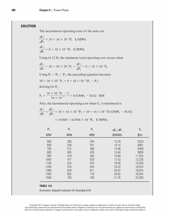
Economic dispatch solution neglecting generator limits and line lossesAn area of an interconnected power system has two fossil-fuel units operating on economic dispatch. The variable operating costs of these units are given by
C1 5 10P1 1 8 3 1023P21 $yhr
C2 5 8P2 1 9 3 1023P22 $yhr
where P1 and P2 are in megawatts. Determine the power output of each unit, the incremental operating cost, and the total operating cost CT that minimizes CT as the total load demand PT varies from 500 to 1500 MW. Generating unit inequality constraints and transmission losses are neglected.
EXAmPLE 6.18
(Continued )
32134_ch06_ptg01.indd 379 07/12/15 6:22 pm
Copyright 2017 Cengage Learning. All Rights Reserved. May not be copied, scanned, or duplicated, in whole or in part. Due to electronic rights,some third party content may be suppressed from the eBook and/or eChapter(s). Editorial review has deemed that any suppressed content does not materiallyaffect the overall learning experience. Cengage Learning reserves the right to remove additional content at any time if subsequent rights restrictions require it.
380 Chapter 6 | Power Flows
SOLUTIONThe incremental operating costs of the units are
dC1
dP1
5 10 1 16 3 1023P1 $yMWh
dC2
dP2
5 8 1 18 3 1023P2 $yMWh
Using (6.12.8), the minimum total operating cost occurs when
dC1
dP1
5 10 1 16 3 1023P1 5dC2
dP2
5 8 1 18 3 1023P2
Using P2 5 PT 2 P1, the preceding equation becomes
10 1 16 3 1023P1 5 8 1 18 3 1023sPT 2 P1d
Solving for P1,
P1 518 3 1023PT 2 2
34 3 1023 5 0.5294PT 2 58.82 MW
Also, the incremental operating cost when CT is minimized is
dC2
d P2
5dC1
d P1
5 10 1 16 3 1023P1 5 10 1 16 3 1023s0.5294PT 2 58.82d
5 9.0589 1 8.4704 3 1023PT $yMWh
PT P1 P2 dCi ∙dP1CT
MW MW MW $/MWh $/hr
500 206 294 13.29 5529600 259 341 14.14 6901700 312 388 14.99 8358800 365 435 15.84 9899900 418 482 16.68 11,525
1000 471 529 17.53 13,2351100 524 576 18.38 15,0301200 576 624 19.22 16,9101300 629 671 20.07 18,8751400 682 718 20.92 20,9241500 735 765 21.76 23,058
TABLE 6.9
Economic dispatch solution for Example 6.18
32134_ch06_ptg01.indd 380 07/12/15 6:22 pm
Copyright 2017 Cengage Learning. All Rights Reserved. May not be copied, scanned, or duplicated, in whole or in part. Due to electronic rights,some third party content may be suppressed from the eBook and/or eChapter(s). Editorial review has deemed that any suppressed content does not materiallyaffect the overall learning experience. Cengage Learning reserves the right to remove additional content at any time if subsequent rights restrictions require it.
Section 6.12 Economic Dispatch 381
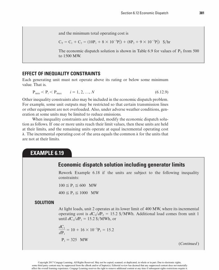
EFFECT OF INEqUALITY CONSTRAINTSEach generating unit must not operate above its rating or below some minimum value. That is.
Pimin , Pi , Pimax i 5 1, 2, …, N (6.12.9)
Other inequality constraints also may be included in the economic dispatch problem. For example, some unit outputs may be restricted so that certain transmission lines or other equipment are not overloaded. Also, under adverse weather conditions, gen-eration at some units may be limited to reduce emissions.
When inequality constraints are included, modify the economic dispatch solu-tion as follows. If one or more units reach their limit values, then these units are held at their limits, and the remaining units operate at equal incremental operating cost l. The incremental operating cost of the area equals the common l for the units that are not at their limits.
and the minimum total operating cost is
CT 5 C1 1 C2 5 s10P1 1 8 3 1023P21d 1 s8P2 1 9 3 1023P2
2d $yhr
The economic dispatch solution is shown in Table 6.9 for values of PT from 500 to 1500 MW.
Economic dispatch solution including generator limitsRework Example 6.18 if the units are subject to the following inequality constraints:
100 % P1 % 600 MW
400 % P2 % 1000 MW
SOLUTIONAt light loads, unit 2 operates at its lower limit of 400 MW, where its incremental operating cost is dC2∙dP2 5 15.2 $∙MWh. Additional load comes from unit 1 until dC1∙dP1 5 15.2 $∙MWh, or
dC1
d P1
5 10 1 16 3 1023P1 5 15.2
P1 5 325 MW
EXAmPLE 6.19
(Continued )
32134_ch06_ptg01.indd 381 07/12/15 6:22 pm
Copyright 2017 Cengage Learning. All Rights Reserved. May not be copied, scanned, or duplicated, in whole or in part. Due to electronic rights,some third party content may be suppressed from the eBook and/or eChapter(s). Editorial review has deemed that any suppressed content does not materiallyaffect the overall learning experience. Cengage Learning reserves the right to remove additional content at any time if subsequent rights restrictions require it.
382 Chapter 6 | Power Flows
For PT less than 725 MW, where P1 is less than 325 MW, the incremental operating cost of the area is determined by unit 1 alone.
At heavy loads, unit 1 operates at its upper limit of 600 MW, where its in-cremental operating cost is dC1yd P1 5 19.60 $yMWh. Additional load comes from unit 2 for all values of dC2yd P2 greater than 19.60 $∙MWh. At dC2∙dP2 5 19.60 $∙MWh,
dC2
d P2
5 8 1 18 3 1023P2 5 19.60
P2 5 644 MW
For PT greater than 1244 MW, where P2 is greater than 644 MW, the incremental operating cost of the area is determined by unit 2 alone.
For 725 , PT , 1244 MW, neither unit has reached a limit value, and the economic dispatch solution is the same as that given in Table 6.9.
The solution to this example is summarized in Table 6.10 for values of PT from 500 to 1500 MW.
PT MW
P1 MW
P2 MW
dC∙dP $/MWh
CT $/hr
500 100 400 11.60 5720600 200 400 13.20 6960700 300 400 14.80 8360725 325 400 15.20 8735800 365 435 15.84 9899900 418 482 16.68 11,525
1000 471 529 17.53 13,2351100 524 576 18.38 15,0301200 576 624 19.22 16,9101244 600 644 19.60 17,7651300 600 700 20.60 18,8901400 600 800 22.40 21,0401500 600 900 24.20 23,370
d C1
d P1 5
TABLE 6.10
Economic dispatch solution for Example 6.19
d C2
d P2 5
PowerWorld Simulator–economic dispatch, including generator limitsPowerWorld Simulator case Example 6_20 uses a five-bus, three-generator loss-less case to show the interaction between economic dispatch and the transmission
EXAmPLE 6.20
32134_ch06_ptg01.indd 382 07/12/15 6:22 pm
Copyright 2017 Cengage Learning. All Rights Reserved. May not be copied, scanned, or duplicated, in whole or in part. Due to electronic rights,some third party content may be suppressed from the eBook and/or eChapter(s). Editorial review has deemed that any suppressed content does not materiallyaffect the overall learning experience. Cengage Learning reserves the right to remove additional content at any time if subsequent rights restrictions require it.
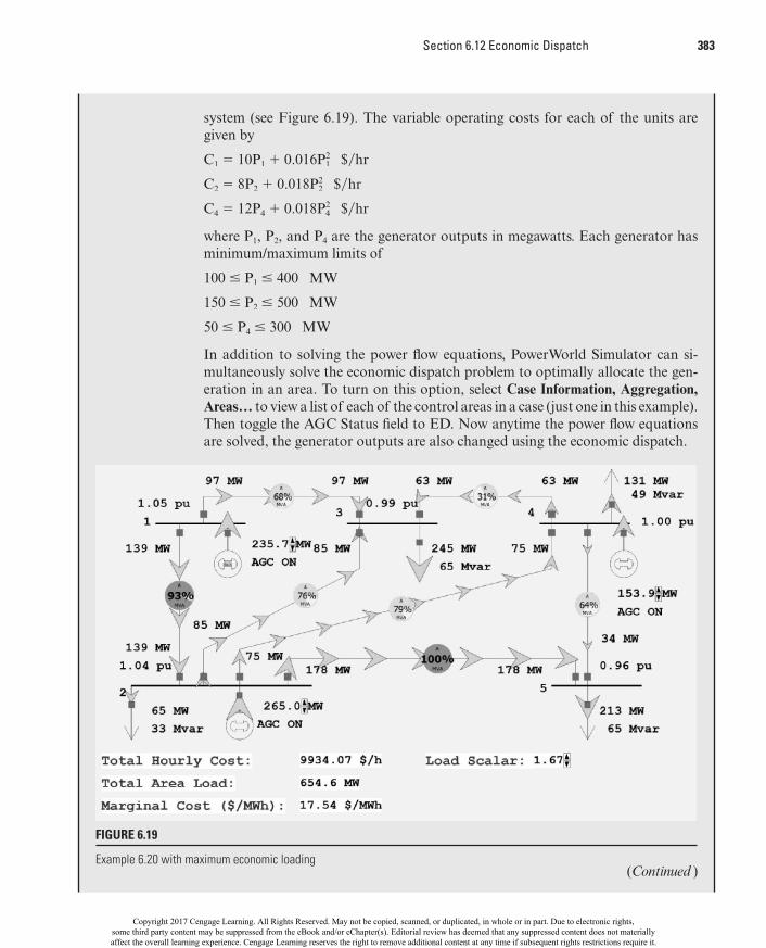
Section 6.12 Economic Dispatch 383
system (see Figure 6.19). The variable operating costs for each of the units are given by
C1 5 10P1 1 0.016P21 $yhr
C2 5 8P2 1 0.018P22 $yhr
C4 5 12P4 1 0.018P24 $yhr
where P1, P2, and P4 are the generator outputs in megawatts. Each generator has minimum/maximum limits of
100 # P1 # 400 MW
150 # P2 # 500 MW
50 # P4 # 300 MW
In addition to solving the power flow equations, PowerWorld Simulator can si-multaneously solve the economic dispatch problem to optimally allocate the gen-eration in an area. To turn on this option, select Case Information, Aggregation, Areas… to view a list of each of the control areas in a case (just one in this example). Then toggle the AGC Status field to ED. Now anytime the power flow equations are solved, the generator outputs are also changed using the economic dispatch.
FIGURE 6.19
Example 6.20 with maximum economic loading(Continued )
32134_ch06_ptg01.indd 383 07/12/15 6:22 pm
Copyright 2017 Cengage Learning. All Rights Reserved. May not be copied, scanned, or duplicated, in whole or in part. Due to electronic rights,some third party content may be suppressed from the eBook and/or eChapter(s). Editorial review has deemed that any suppressed content does not materiallyaffect the overall learning experience. Cengage Learning reserves the right to remove additional content at any time if subsequent rights restrictions require it.

384 Chapter 6 | Power Flows
EFFECT OF TRANSmISSION LOSSESAlthough one unit may be very efficient with a low incremental operating cost, it also may be located far from the load center. The transmission losses associated with this unit may be so high that the economic dispatch solution requires the unit to decrease its output, while other units with higher incremental operating costs but lower trans-mission losses increase their outputs.
When transmission losses are included in the economic dispatch problem, (6.12.2) becomes
P1 1 P2 1 Á 1 PN 2 PL 5 PT (6.12.10)
where PT is the total load demand and PL is the total transmission loss in the area. In general, PL is not constant but depends on the unit outputs P1, P2, …, PN, The total differential of (6.12.10) is
sd P1 1 d P2 1 Á 1 d PNd 2 1≠PL
≠P1
d P1 1≠PL
≠P2
d P2 1 Á 1≠PL
≠PN
d PN2 5 0 (6.12.11)
Multiplying (6.12.11) by l and subtracting the resulting equation from (6.12.5),
1dC1
d P1
1 l≠PL
≠P1
2 l2
d P1 1 1dC2
d P2
1 l≠PL
≠P2
2 l2
d P2
Initially, the case has a total load of 392 MW with an economic dispatch of P1 5 141 MW, P2 5 181, and P4 5 70, and an incremental operating cost, l, of 14.52 $∙MWh. To view a graph showing the incremental cost curves for all of the area generators, right-click on any generator to display the generator’s local menu, and then select All Area Gen IC Curves (right-click on the graph’s axes to change their scaling).
To see how changing the load impacts the economic dispatch and power flow solutions, first select Tools, Play to begin the simulation. Then, on the oneline, click on the up/down arrows next to the Load Scalar field. This field is used to scale the load at each bus in the system. Notice that the change in the To-tal Hourly Cost field is well approximated by the change in the load multiplied by the incremental operating cost.
Determine the maximum amount of load this system can supply without overloading any transmission line with the generators dispatched using economic dispatch.
SOLUTION The maximum system economic loading is determined numerically to be 655 MW (which occurs with a Load Scalar of 1.67) with the line from bus 2 to bus 5 being the critical element.
32134_ch06_ptg01.indd 384 07/12/15 6:22 pm
Copyright 2017 Cengage Learning. All Rights Reserved. May not be copied, scanned, or duplicated, in whole or in part. Due to electronic rights,some third party content may be suppressed from the eBook and/or eChapter(s). Editorial review has deemed that any suppressed content does not materiallyaffect the overall learning experience. Cengage Learning reserves the right to remove additional content at any time if subsequent rights restrictions require it.
Section 6.12 Economic Dispatch 385
1 Á 1 1dCN
d PN
1 l≠PL
≠PN
2 l2
d PN 5 0 (6.12.12)
Equation (6.12.12) is satisfied when each term in parentheses equals zero. That is.
dCi
d Pi
1 l≠PL
≠Pi
2 l 5 0
or
l 5dCi
d Pi
sLid 5dCi
d Pi
1 1
1 2≠PL
≠Pi
2 i 5 1, 2, …, N (6.12.13)
Equation (6.12.13) gives the economic dispatch criteria, including transmission losses. Each unit that is not at a limit value operates such that its incremental operating cost dCi∙dPi multiplied by the penalty factor Li is the same. Note that when transmission losses are negligible ≠PLy≠Pi 5 0, Li 5 1, and (6.12.13) reduces to (6.12.8).
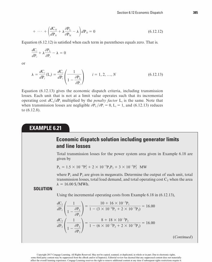
Economic dispatch solution including generator limits and line lossesTotal transmission losses for the power system area given in Example 6.18 are given by
PL 5 1.5 3 1024P12 1 2 3 1025P1P2 1 3 3 1025P2
2 MW
where P1 and P2 are given in megawatts. Determine the output of each unit, total transmission losses, total load demand, and total operating cost CT when the area l 5 16.00 $∙MWh.
SOLUTION Using the incremental operating costs from Example 6.18 in (6.12.13),
dC1
d P1
1 1
1 2≠PL
≠P1
2510 1 16 3 1023P1
1 2 s3 3 1024P1 1 2 3 1025P2)5 16.00
dC2
d P2
1 1
1 2≠PL
≠P2
258 1 18 3 1023P2
1 2 s6 3 1025P2 1 2 3 1025P1)5 16.00
EXAmPLE 6.21
(Continued )
32134_ch06_ptg01.indd 385 07/12/15 6:22 pm
Copyright 2017 Cengage Learning. All Rights Reserved. May not be copied, scanned, or duplicated, in whole or in part. Due to electronic rights,some third party content may be suppressed from the eBook and/or eChapter(s). Editorial review has deemed that any suppressed content does not materiallyaffect the overall learning experience. Cengage Learning reserves the right to remove additional content at any time if subsequent rights restrictions require it.

386 Chapter 6 | Power Flows
Rearranging the two equations,
20.8 3 1023P1 1 32 3 1025P2 5 6.0032 3 1025P1 1 18.96 3 1023P2 5 8.00
Solving,
P1 5 282 MW P2 5 417 MW
Using the equation for total transmission losses,
PL 5 1.5 3 1024(282)2 1 2 3 1025(282)(417) 1 3 3 1025(417)2 5 19.5 MW
From (6.12.10), the total load demand is
PT 5 P1 1 P2 PL 5 282 1 417 2 19.5 5 679.5 MW
Also, using the cost formulas given in Example 6.18, the total operating cost is
CT 5 C1 1 C2 5 10s282d 1 8 3 1023s282d2 1 8s417d 1 9 3 1023s417d2
5 8357 $yh
Note that when transmission losses are included, l given by (6.12.13) is no longer the incremental operating cost of the area. Instead, l is the unit incremental op-erating cost dCi∙dPi multiplied by the unit penalty factor Li.
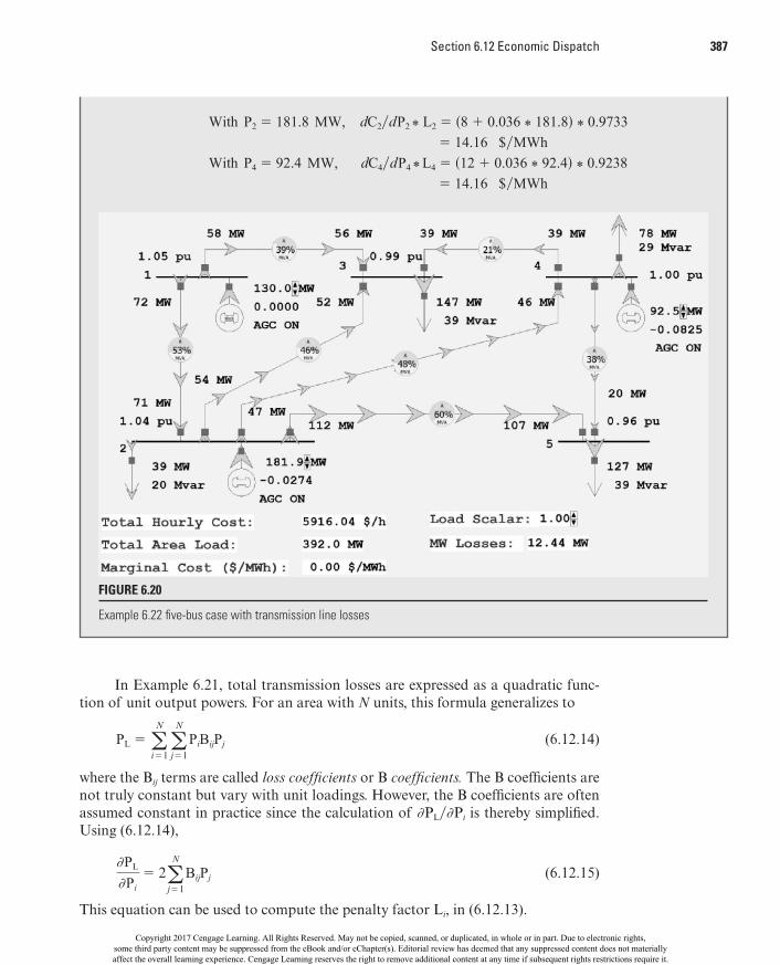
PowerWorld Simulator—economic dispatch, including generator limits and line lossesThis example repeats the Example 6.19 power system, except that now losses are included with each transmission line modeled with an R∙X ratio of 1∙3 (see Figure 6.20). The current value of each generator’s loss sensitivity, −PLy−Pi, is shown immediately below the generator’s MW output field. Calculate the penalty factors Li, and verify that the economic dispatch shown in the figure is optimal. Assume a Load Scalar of 1.0.
SOLUTIONFrom (6.12.13), the condition for optimal dispatch is
l 5 dCiyd Pis1ys1 2 ≠PLy≠Pid 5 dCiyd PiLi i 5 1, 2, Á , Nwith Li 5 1ys1 2 ≠PLy≠PidTherefore, L1 5 1.0, L2 5 0.9733, and L4 5 0.9238. with P1 5 130.1 MW, dC1yd P1 * L1 5 s10 1 0.032 * 130.1d * 1.0 5 14.16 $yMWh
EXAmPLE 6.22
32134_ch06_ptg01.indd 386 07/12/15 6:22 pm
Copyright 2017 Cengage Learning. All Rights Reserved. May not be copied, scanned, or duplicated, in whole or in part. Due to electronic rights,some third party content may be suppressed from the eBook and/or eChapter(s). Editorial review has deemed that any suppressed content does not materiallyaffect the overall learning experience. Cengage Learning reserves the right to remove additional content at any time if subsequent rights restrictions require it.
Section 6.12 Economic Dispatch 387
In Example 6.21, total transmission losses are expressed as a quadratic func-tion of unit output powers. For an area with N units, this formula generalizes to
PL 5 oN
i51oN
j51
PiBijPj (6.12.14)
where the Bij terms are called loss coefficients or B coefficients. The B coefficients are not truly constant but vary with unit loadings. However, the B coefficients are often assumed constant in practice since the calculation of ≠PLy≠Pi is thereby simplified. Using (6.12.14),
≠PL
≠Pi
5 2oN
j51
BijPj (6.12.15)
This equation can be used to compute the penalty factor Li, in (6.12.13).
With P2 5 181.8 MW, dC2yd P2 * L2 5 s8 1 0.036 * 181.8d * 0.9733 5 14.16 $yMWhWith P4 5 92.4 MW, dC4yd P4 * L4 5 s12 1 0.036 * 92.4d * 0.9238 5 14.16 $yMWh
FIGURE 6.20
Example 6.22 five-bus case with transmission line losses
32134_ch06_ptg01.indd 387 07/12/15 6:22 pm
Copyright 2017 Cengage Learning. All Rights Reserved. May not be copied, scanned, or duplicated, in whole or in part. Due to electronic rights,some third party content may be suppressed from the eBook and/or eChapter(s). Editorial review has deemed that any suppressed content does not materiallyaffect the overall learning experience. Cengage Learning reserves the right to remove additional content at any time if subsequent rights restrictions require it.
388 Chapter 6 | Power Flows
Various methods of evaluating B coefficients from power flow studies are avail-able [17]. In practice, more than one set of B coefficients may be used during the daily load cycle.
When the unit incremental cost curves are linear, an analytic solution to the economic dispatch problem is possible, as illustrated by Examples 6.18 through 6.20. However, in practice, the incremental cost curves are nonlinear and contain disconti-nuities. In this case, an iterative solution can be obtained. Given the load demand PT, the unit incremental cost curves, generator limits, and B coefficients, such an iterative solution can be obtained by the following nine steps. Assume that the incremental cost curves are stored in tabular form, such that a unique value of Pi can be read for each dCi∙dPi.
STEP 1 Set iteration index m 5 1.
STEP 2 Estimate mth value of l.
STEP 3 Skip this step for all m . 1. Determine initial unit outputs Pi, (i 5 1, 2, …, N). Use dCi∙dPi 5 l and read Pi from each incremental operating cost table. Transmission losses are neglected here.
STEP 4 Compute ≠PLy≠Pi from (6.12.15) (i 5 1, 2, …, N).
STEP 5 Compute dCi∙dPi from (6.12.13) (i 5 1, 2, …, N).
STEP 6 Determine updated values of unit output Pi (i 5 1, 2, …, N). Read Pi from each incremental operating cost table. If Pi exceeds a limit value, set Pi to the limit value.
STEP 7 Compare Pi determined in Step 6 with the previous value (i 5 1, 2, …, N). If the change in each unit output is less than a specified tolerance «1, go to Step 8. Otherwise, return to Step 4.
STEP 8 Compute PL from (6.12.14).
STEP 9 If *1oN
i51
Pi2 2 PL 2 PT* is less than a specified tolerance «2, stop.
Otherwise, set m 5 m 1 1 and return to Step 2.
Instead of having their values stored in tabular form for this procedure, the incre-mental cost curves instead could be represented by nonlinear functions such as poly-nomials. Then, in Step 3 and Step 5, each unit output Pi would be computed from the nonlinear functions instead of being read from a table. Note that this procedure as-sumes that the total load demand PT is constant. In practice, this economic dispatch program is executed every few minutes with updated values of PT.
OTHER TYPES OF UNITSThe economic dispatch criterion has been derived for a power system area consisting of fossil-fuel generating units. In practice, however, an area has a mix of different types of units including fossil-fuel, nuclear, pumped-storage hydro, hydro, wind, and other types.
Wind and solar generation, which have no fuel costs, are represented with very low or negative cost. As such, they are preferred sources for economic dispatch and
32134_ch06_ptg01.indd 388 07/12/15 6:22 pm
Copyright 2017 Cengage Learning. All Rights Reserved. May not be copied, scanned, or duplicated, in whole or in part. Due to electronic rights,some third party content may be suppressed from the eBook and/or eChapter(s). Editorial review has deemed that any suppressed content does not materiallyaffect the overall learning experience. Cengage Learning reserves the right to remove additional content at any time if subsequent rights restrictions require it.

Section 6.13 Optimal Power Flow 389
are used by system operators whenever possible, unless there are generator operating limits or transmission constraints.
Although the fixed costs of a nuclear unit may be high, their operating costs are low due to inexpensive nuclear fuel. As such, nuclear units are normally base-loaded at their rated outputs. That is, the reference power settings of turbine-governors for nuclear units are held constant at rated output; therefore, these units do not partici-pate in economic dispatch.
Pumped-storage hydro is a form of energy storage. During off-peak hours, these units are operated as synchronous motors to pump water to a higher elevation. Then during peak-load hours the water is released, and the units are operated as syn-chronous generators to supply power. As such, pumped-storage hydro units are used for light-load build-up and peak-load shaving. Economic operation of the area is im-proved by pumping during off-peak hours when the area l is low, and by generating during peak-load hours when l is high. Techniques are available for incorporating pumped-storage hydro units into economic dispatch of fossil-fuel units [18].
In an area consisting of hydro plants located along a river, the objective is to maximize the energy generated over the yearly water cycle rather than to minimize total operating costs. Reservoirs are used to store water during high-water or light-load periods, although some water may have to be released through spillways. Also, there are constraints on water levels due to river transportation, irrigation, or fish-ing requirements. Optimal strategies are available for coordinating outputs of plants along a river [19]. Economic dispatch strategies for mixed fossil-fuel/hydro systems are also available [20, 21, 22].
Techniques are also available for including reactive power flows in the eco-nomic dispatch formulation, whereby both active and reactive powers are selected to minimize total operating costs. In particular, reactive injections from generators, switched capacitor banks, and static var systems, along with transformer tap settings, can be selected to minimize transmission-line losses [22]. However, electric utility companies usually control reactive power locally. That is, the reactive power output of each generator is selected to control the generator terminal voltage, and the re-active power output of each capacitor bank or static var system located at a power system bus is selected to control the voltage magnitude at that bus. In this way, the reactive power flows on transmission lines are low, and the need for central dispatch of reactive power is eliminated.
6.13 OPTImAL POWER FLOWEconomic dispatch has one significant shortcoming—it ignores the limits imposed by the devices in the transmission system. Each transmission line and transformer has a limit on the amount of power that can be transmitted through it, with the limits arising because of thermal, voltage, or stability considerations (Section 5.6). Traditionally, the transmission system was designed so that when the generation was dispatched economically there would be no limit violations. Hence, just solving eco-nomic dispatch was usually sufficient. However, with the worldwide trend toward deregulation of the electric utility industry, the transmission system is becoming
32134_ch06_ptg01.indd 389 07/12/15 6:22 pm
Copyright 2017 Cengage Learning. All Rights Reserved. May not be copied, scanned, or duplicated, in whole or in part. Due to electronic rights,some third party content may be suppressed from the eBook and/or eChapter(s). Editorial review has deemed that any suppressed content does not materiallyaffect the overall learning experience. Cengage Learning reserves the right to remove additional content at any time if subsequent rights restrictions require it.

390 Chapter 6 | Power Flows
increasingly constrained (with these constraints sometimes called congestion). For example, in the PJM power market in the eastern United States, the costs associated with active transmission line and transformer limit violations (congestion) increased from $65 million in 1999 to almost $2.1 billion in 2005 and have averaged about $1 billion per year from 2008 to 2013 [23].
The solution to the problem of optimizing the generation while enforcing the transmission lines is to combine economic dispatch with either the full ac power flow, or a dc power flow. The result is known as the optimal power flow (OPF). There are several methods for solving the OPF with [24] providing a nice summary. One com-mon approach is sequential linear programming (LP); this is the technique used with the PowerWorld Simulator. The LP OPF solution algorithm iterates between solving the power flow to determine the flow of power in the system devices and solving an LP to economically dispatch the generation (and possibility other controls) subject to the transmission system limits. In the absence of system elements loaded to their limits, the OPF generation dispatch is identical to the economic dispatch solution, and the marginal cost of energy at each bus is identical to the system l. However, when one or more elements are loaded to their limits, the economic dispatch becomes constrained, and the bus marginal energy prices are no longer identical. In some electricity markets, these marginal prices are known as the Locational Marginal Prices (LMPs) and are used to determine the wholesale price of electricity at various locations in the system. For example, the real-time LMPs for the Midcontinent ISO (MISO) are available online at www.misoenergy.org/MarketsOperations.
PowerWorld Simulator—optimal power flowPowerWorld Simulator case Example 6_23 duplicates the five-bus case from Ex-ample 6.20, except that the case is solved using PowerWorld Simulator’s LP OPF algorithm (see Figure 6.21). To turn on the OPF option, first select Case Infor-mation, Aggregation, Areas…, and toggle the AGC Status field to OPF. Then, rather than solving the case with the “Single Solution” button, select Add-ons, Primal LP to solve using the LP OPF. Initially the OPF solution matches the ED solution from Example 6.20 since there are no overloaded lines. The green-colored fields on the screen immediately to the right of the buses show the mar-ginal cost of supplying electricity to each bus in the system (i.e., the bus LMPs). With the system initially unconstrained, the bus marginal prices are all identical at $14.5∙MWh, with a Load Scalar of 1.0.
Now increase the Load Scalar field from 1.00 to the maximum economic loading value, determined to be 1.67 in Example 6.20, and again select Add-ons, Primal LP. The bus marginal prices are still all identical, now at a value of $17.5∙MWh, and with the line from bus 2 to 5 just reaching its maximum value. For load scalar values above 1.67, the line from bus 2 to bus 5 becomes con-strained, with a result that the bus marginal prices on the constrained side of the line become higher than those on the unconstrained side.
EXAmPLE 6.23
32134_ch06_ptg01.indd 390 07/12/15 6:22 pm
Copyright 2017 Cengage Learning. All Rights Reserved. May not be copied, scanned, or duplicated, in whole or in part. Due to electronic rights,some third party content may be suppressed from the eBook and/or eChapter(s). Editorial review has deemed that any suppressed content does not materiallyaffect the overall learning experience. Cengage Learning reserves the right to remove additional content at any time if subsequent rights restrictions require it.

With the load scalar equal to 1.80, numerically verify that the price of power at bus 5 is approximately $40.60∙MWh.
SOLUTION The easiest way to numerically verify the bus 5 price is to increase the load at bus 5 by a small amount and compare the change in total system operating cost. With a load scalar of 1.80, the bus 5 MW load is 229.3 MW with a case hourly cost of $11,073.90. Increasing the bus 5 load by 0.9 MW and resolving the LP OPF gives a new cost of $11,110.40, which is a change of about $40.60∙MWh (note that this increase in load also increases the bus 5 price to over $41∙MWh). Because of the constraint, the price of power at bus 5 is actually more than double the incremen-tal cost of the most expensive generator!
FIGURE 6.21
Example 6.23 optimal power flow solution with load multiplier = 1.80
mULTIPLE CHOICE qUESTIONS
SECTION 6.1 6.1 For a set of linear algebraic equations in matrix format, Ax 2 y, for a
unique solution to exist, det(A) should be ________.
6.2 For an N 3 N square matrix A, in (N 2 1) steps, the technique of Gauss elimination can transform into an ________ matrix.
Multiple Choice Questions 391
32134_ch06_ptg01.indd 391 07/12/15 6:22 pm
Copyright 2017 Cengage Learning. All Rights Reserved. May not be copied, scanned, or duplicated, in whole or in part. Due to electronic rights,some third party content may be suppressed from the eBook and/or eChapter(s). Editorial review has deemed that any suppressed content does not materiallyaffect the overall learning experience. Cengage Learning reserves the right to remove additional content at any time if subsequent rights restrictions require it.