Engineering Applications of Artificial Intelligence 26 (2013) 417–429

Contents lists available at SciVerse ScienceDirect

Engineering Applications of Artificial Intelligence

0952-19

doi:10.1

n Corr

E-m

marko.c1 Te

journal homepage: www.elsevier.com/locate/engappai

A multi-objective optimization based solution for the combinedeconomic-environmental power dispatch problem

Blaze Gjorgiev a,n, Marko Cepin b,1

a Reactor Engineering Division, Jozef Stefan Institute, Jamova 39, SI-1000 Ljubljana, Sloveniab Faculty of Electrical Engineering, University of Ljubljana, Trzaska 25, SI-1000 Ljubljana, Slovenia

a r t i c l e i n f o

Article history:

Received 6 June 2011

Received in revised form

15 February 2012

Accepted 1 March 2012Available online 28 March 2012

Keywords:

Multi-objective optimization

Economic-environmental dispatch

Genetic algorithm

Membership function

Penalization

76/$ - see front matter & 2012 Elsevier Ltd. A

016/j.engappai.2012.03.002

esponding author. Tel.: þ386 1 5885 284; fax

ail addresses: blaze.gjorgiev@ijs.si (B. Gjorgie

epin@fe.uni-lj.si (M. Cepin).

l.: þ386 1 4768 243.

a b s t r a c t

The combined economic-environmental dispatch issue is multidimensional, non-linear, non-convex

and highly constrained problem. It involves multiple and often conflicting optimization criteria for

which no unique optimal solution can be determined with respect to all criteria. In this paper a multi-

objective optimization based solution to the combined economic-environmental power dispatch is

proposed. The derivation of the optimal solution is based on the weighted sum method for which

improvements are made in direction of penalty function integration. For that purpose a modified

dynamic normalization is suggested. A penalization method based on membership functions is

introduced in order to calculate the constraint violations. The objective of the proposed method is

gaining an optimal solution for the dynamic combined economic-environmental dispatch problem

associated to real power systems. Therefore, the algorithm is applied on different test power systems.

The obtained results are analyzed and compared with various optimization techniques presented in the

literature. The results demonstrate the efficiency of the proposed method in finding solutions toward

global optimum.

& 2012 Elsevier Ltd. All rights reserved.

1. Introduction

During the last few decades the rapid growth in the use of fossilfuels has led to a significant reduction of this resource worldwide.Another problem that has arisen from this excessive use of fossilfuels is the large amount of atmospheric pollutants that arecontinuously released into the environment. These are the primaryreasons why power production utilities have to focus their atten-tion on more optimal ways to use resources (Kaplan, 2008).

Economic dispatch (ED) is one of the most important pro-blems being dealt with in power system operation and planning(Grainger and Stevenson, 1994; Travers et al., 1954; Wood andWollenberg, 1996). The purpose of ED is to schedule the outputsof all available generation units in the power system in order tominimize fuel costs while also satisfying all units and systemequality and inequality constraints.

The increased public awareness regarding the harmful effectsof atmospheric pollutants on the environment, the more concern-ing greenhouse effect, as well as the environmental regulationshave led to numerous requests that have forced utilities to modifytheir design or operational strategies. Therefore this study is

ll rights reserved.

: þ386 1 5885 377.

v),

concerned with minimizing fuel costs as well as minimizingthe emission of gaseous pollutants. Combined economic-environ-mental power dispatch considers both optimization problemssimultaneously, resulting in what is known as a multi-objectiveoptimization problem (Abido, 2003; Abido, 2009; Basu, 2008;King et al., 1995; Yare and Venayagamoorthy, 2010).

The combined economic-environmental dispatch problem ismultidimensional, non-linear, non-convex and highly constrained.It involves multiple and sometimes conflicting optimization cri-teria for which no unique optimal solution can be determined withrespect to all criteria. These are the main reasons why the use ofvarious heuristic algorithms, which deal with the problem, gain onpopularity in the last two decades. Many methods are developedbased on heuristic algorithms due to the fact that these algorithmsare highly proven tool for function optimization. The main advan-tage of those methods over the conventional methods lies in theirability to deal with the problem using only the objective function.Recent survey of the literature reveals large application of variousheuristic algorithms, showing great success in finding almostglobal optimal solution for the combined economic-environmentaldispatch problem (Basu, 2011; Bhattacharya and Chattopadhyay,2011; Lu et al., 2011; Neyestani et al., 2010; Sivasubramani andSwarup, 2011; Subbaraj et al., 2009; Wang and Singh, 2009).

In (Basu, 2008) the author offers a solution for the dynamiccombined-economic-environmental dispatch of thermal powersystem using elitist non-dominated sorting genetic algorithm

B. Gjorgiev, M. Cepin / Engineering Applications of Artificial Intelligence 26 (2013) 417–429418

(known as NSGA-II). This solution is compared with the solutionobtained as a result of a relatively simple implementation of theweighted sum method using real coded genetic algorithm (RCGA).The latter method is known for its simplicity when one deals withmulti-objective optimization problems. The results show slightlyimproved minimum achieved by NSGA-II over the weightedsum method. Similar application of genetic algorithms (GAs) isproposed by Abido (Abido, 2003) where the author uses novelimplementation of the non-dominate genetic algorithm (NSGA) tosolve static economic-environmental dispatch problem applied ona thermal power system. A fuzzy-based mechanism is employed toextract the best compromise solution over the trade-off curve.

The application of fuzzy set theory is also extended over widerrange in power systems problems. In (Ruey-Hsun and Jian-Hao,2007) authors use various membership functions to take intoaccount the uncertainties due to the prediction of: speed of wind,solar radiation, load prediction, etc. Similar approach was alsoproposed in reference (Attaviriyanupap et al., 2004), whereauthors use fuzzy sets to take into account uncertainties due to:demand and reserves required in each market, prices cleared ineach market, and the probability by which reserves are calledupon in actual operation. The factors that affect the feasibility andoptimality of the solutions to the economic dispatch problem,using fuzzy sets, are examined in (Han et al., 2001).

In this paper a multi-objective optimization method for sol-ving the dynamic combined economic-environmental power dis-patch is proposed. The solution is based on the weighted summethod (Deb, 2001). This method transforms the multi-objectiveoptimization problem into single-objective optimization problemusing weights. In general the method uses external penaltyfunctions to deal with the constraint violations. The penaltyfunctions are responsible to some extent for the distortion onthe objective functions (Deb, 2001), especially during the earlygenerations. In order to achieve better properties for the weightedsum method a modified dynamic normalization is suggested. Theimprovement is made regarding penalty function integration. Inorder to calculate the constraint violations a penalization methodbased on membership functions is introduced. The method isintegrated within a genetic algorithm and applied on variousthermal and hydro-thermal power systems. The results areanalyzed and the achieved optimal solutions are compared withother solutions obtained by different techniques described in thereviewed literature.

2. Combined economic-environmental power dispatch

The economic-environmental power dispatch problem can bestated as finding the thermal unit generation and correspondingwater release from each reservoir throughout all planning timeintervals, so as to minimize the total cost of fuel and pollutantsemission while satisfying load balance, thermal, and hydraulicconstraints. The objectives and constraints considered in theformulation of the combined economic emission power dispatchproblem are addressed in this section.

2.1. Fuel cost function

The fuel cost for each thermal generating unit in the systemis usually determined by a second order function of the activepower generation. During opening of each admission valve in asteam turbine an event known as drawing effect is occurring(Kumar and Naresh, 2007; Walters and Sheble, 1993). Thisrippling effect is modeled as sinusoidal function of the activepower generation. Thus, the fuel cost function is written asnon-linear and non-smooth function (Abido, 2003; Basu, 2005)

as follows:

FCiðPGiÞ ¼ tm½aiþbiPGi

þciP2Giþ9di sinfeiðP

minGi�PGiÞg9� ð1Þ

where ai($/h), bi(US$/MWh), ci($/MW2h), di($/h) and ei(rad/MW)are constants which are unique for each generating unit, PGi

is thepower output of the ith thermal unit, Pmin

Giis the minimum power

output of the ith thermal unit, and tm is the duration of the timeinterval in hours. It is usual practice that the scheduling timeperiod is 24 h divided on 24 time intervals each lasting one hourwith constant load demands. Within this paper two differentscheduling periods were used, depending on the analyzed testpower system.

The thermal unit cost is represented by Eq. (1). The total fuelcost from all thermal units in the system during the scheduledtime period is determined as follows:

FC ¼XT

t ¼ 1

XI

i ¼ 1

FCiðPGi,tÞ ð2Þ

where PGi,tis the power output of the ith thermal unit at time

interval t, T is the number of considered time intervals understudy, and I is the number of thermal units.

2.2. Emission function

The total emission of atmospheric pollutants, such as sulphuroxides (SOX) and nitrogen oxides (NOX), caused by thermal unitscan be modeled together and described by one function (Abido,2003; Basu, 2005, 2008, 2010) as follows:

FEiðPGiÞ ¼ tm½10�2

ðaiþbiPGiþgiP

2GiÞþZi expðliPGi

Þ� ð3Þ

where ai, bi, gi, Zi, and li are constants which are unique for eachthermal unit. The member 10�2 in the equation above is usedonly in the case when metric units are used for the input para-meters (Basu, 2010).

The total emission of atmospheric pollutants from all thermalunits in the system during the scheduled time period is deter-mined as follows:

FE ¼XT

t ¼ 1

XI

i ¼ 1

FEiðPGi,tÞ ð4Þ

2.3. Constraints

2.3.1. Power balance constraint

The power balance equations constraint suggests that the sumof output powers from all generating units must be equal to thetotal load demand plus the power losses in the system at eachtime interval, and it is expressed as follows:

XI

i ¼ 1

PGi,tþXJ

j ¼ 1

PHj,t¼ PLt

þPlosstt¼ 1,2,. . .,T ð5Þ

where J is the number of reservoirs, PHj,tis the power output of the

hydro generating unit connected with reservoir j at time intervalt, and Plosst

are the power losses in the system at time interval t.Beta coefficients (Basu, 2005, 2008) were used to calculate thepower losses for the analyzed test systems. Two different math-ematical models were considered for the hydro generating units.

Model 1: The water discharge from each plant is determined as asecond order function from the generated power output (Basu,2005), therefore the water availability constraint is described

B. Gjorgiev, M. Cepin / Engineering Applications of Artificial Intelligence 26 (2013) 417–429 419

as follows:

XT

t ¼ 1

tmða0hþa1hPHj,tþa2hP2

Hj,t�WHj

¼ 0 ð6Þ

where a0h, a1h, and a2h are coefficients for water discharge ratefunction of hydro generation unit j, and WHj

is pre-specifiedvolume of water available for generation by the jth hydrogeneration unit. This model uses only the water availabilityconstraint, Eq. (6), and the corresponding power generator capa-city constraints when calculating the hydro power output, PHj,t

.

Model 2: This model describes a hydraulic system network (Basu,2010; Yuan et al., 2008), where reservoirs are hydraulicallyconnected with natural or artificial water channels. The hydrogenerator power output is a function of the water dischargethrough the turbine and the volume of stored water in thereservoir (Basu, 2010; Lakshminarasimman and Subramanian,2008; Yuan and Yuan, 2006) as follows:

PHj,t¼ C1,jV j,t

2þC2,jXj,t

2þC3,jV j,tXj,tþC4,jVj,tþC5,jXj,tþC6,i ð7Þ

where Ci,j is the ith hydro power generation coefficient for the jthreservoir, Vj,t is the water storage volume for the jth reservoir attime interval t and Xj,t is the volume of water discharge from thejth reservoir during time interval t.

The water volume in each reservoir j at each time interval t isdetermined (Basu, 2010) as follows:

Vj,tþ1 ¼ Vj,t�Xj,tþ Ij,t�Sj,tþXNUP

l ¼ 1

ðXl, t�tljð ÞþSl,ðt�tljÞÞ ð8Þ

where Ij,t is the natural water inflow volume in the jth reservoirduring time interval t, Sj,t is the water spillage of the jth reservoirat time interval t, NUP is the number of upstream reservoirs, tlj iswater transport delay from reservoir l to j, Xl,ðt�tljÞ

is the waterdischarge from the lth upstream reservoir at time t�tlj and Sl,ðt�tljÞ

is the water spillage of the lth upstream reservoir at time t�tlj.Physical volume limitations of each reservoir in storage are

expressed as follows:

Vminj rVj,t rVmax

j ð9Þ

Xminj rXj,t rXmax

j ð10Þ

where Vminj and Vmax

j are the minimum and maximum watervolumes for the jth reservoir, respectively and Xmin

j and Xmaxj are

the minimum and maximum water discharge volumes from thejth reservoir, respectively.

The initial and final reservoir storage volumes are expressed asfollows:

Vj,t9t ¼ 0¼ Vbegin

j ð11Þ

Vj,t9t ¼ T¼ Vend

j ð12Þ

where Vbeginj and Vend

j are the initial and final water volume in thejth reservoir, respectively.

2.3.2. Generator capacity constraints

The generator capacity constraints are expressed as follows:

PminGi

rPGi,trPmax

Gið13Þ

PminHj

rPHj,trPmax

Hjð14Þ

where PminGi

and PmaxGi

are the minimum and maximum poweroutputs for the ith thermal unit, respectively and Pmin

Hjand Pmax

Hjare

the minimum and maximum power outputs for the jth hydrounit, respectively.

The power produced by each thermal unit is bounded by itsramping response rate limits as follows (Simopoulos et al., 2007):

�MIirPGi,t�PGi,tþ 1

rMDi ð15Þ

where MIi and MDi are the maximum increase and maximumdecrease in the output of the ith thermal unit over one timeinterval respectively.

2.4. Objective functions

Functions FC and FE, represented by Eqs. (2) and (4), are theobjective functions, i.e. the functions to be minimized. Aggregat-ing the objectives and constraints, the economic-environmentalpower dispatch optimization problem can be mathematicallyformulated as a nonlinear, constrained, multi-objective optimiza-tion problem as follows:

Minimize ½FCðxÞ,FEðxÞ� ð16Þ

subject to:

gðxÞ ¼ 0 ð17Þ

hðxÞr0 ð18Þ

where g(x) and h(x) are the equality and inequality problemconstraints, respectively, and x is a decision vector that representspossible solution. The form of the solution is given latter on in thepaper with Eq. (39).

3. Problem solution

3.1. Multi objective optimization-weighted sum method

The weighted sum method, as the name suggests, transforms aset of objectives into a single objective by pre-multiplying eachobjective with user-supplied weight. The weight of an objective isusually chosen in proportion to the objective’s relative importanceto the problem. It is likely that each objective function takesdifferent orders of magnitude as in the combined economic-environmental power dispatch. Therefore, setting up an appropri-ate weight factor depends on the scaling of each objective function(Deb, 2001). It is the usual practice to choose weights such thattheir sum is equal to one. The combined economic-environmentalpower dispatch problem can be formulated as follows:

Minimize f ¼wFCþð1�wÞsFE ð19Þ

where s is the normalization factor which can be essential, simplybecause each objective function may take different range of values,and w is the weighting factor which defines the change of pressureover each objective function. In this paper the normalization factoris determined as the ratio between the maximum fuel cost andmaximum emission as follows:

s¼FCðP

maxGi,tÞ

FEðPmaxGi,tÞ

ð20Þ

The weighting factor, w, can take any number between 0 and1. When w is set to 0.5 equal weight is given to both objectivefunctions, thus giving them equal chances to be minimized. A setof different values for w leads to a set of different solutions whichare known as Pareto optimal solutions.

The definition of the fitness function does not stop with the con-straint objective function shown with Eq. (19). Due to the possibleviolation in constraints, penalty functions are employed. Therefore,the constrained objective function presented with Eq. (19) isupgraded with an external penalty term and transformed into an

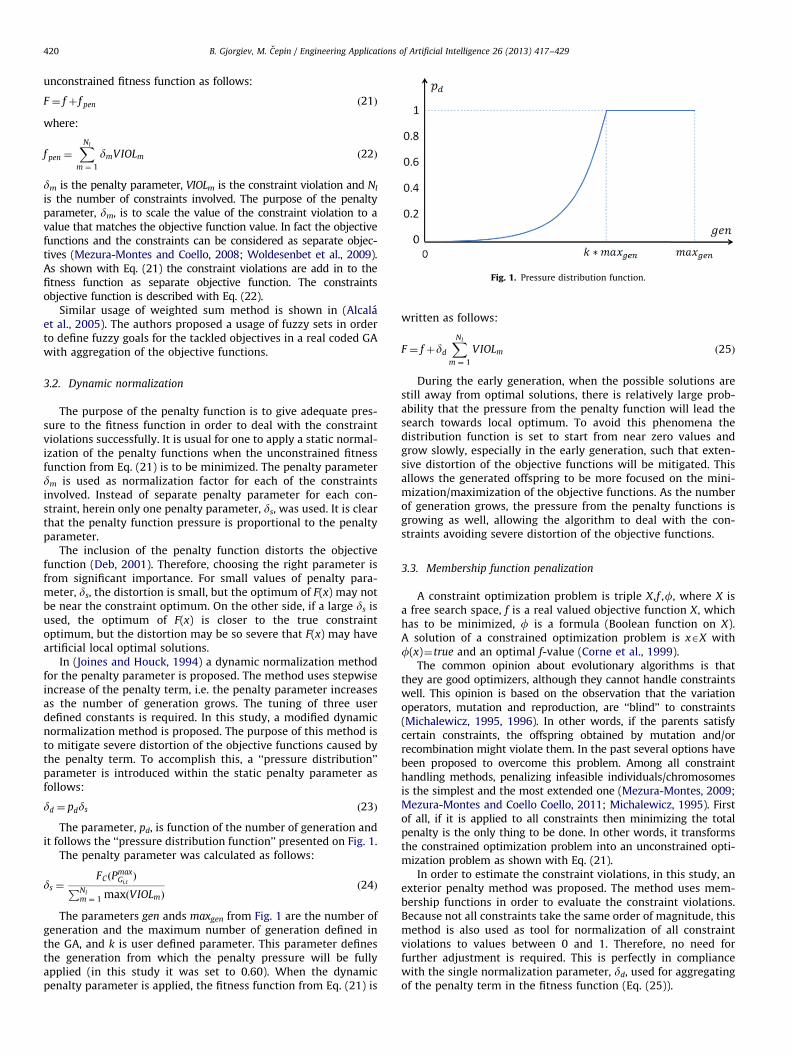
Fig. 1. Pressure distribution function.

B. Gjorgiev, M. Cepin / Engineering Applications of Artificial Intelligence 26 (2013) 417–429420

unconstrained fitness function as follows:

F ¼ f þ f pen ð21Þ

where:

f pen ¼XNl

m ¼ 1

dmVIOLm ð22Þ

dm is the penalty parameter, VIOLm is the constraint violation and Nl

is the number of constraints involved. The purpose of the penaltyparameter, dm, is to scale the value of the constraint violation to avalue that matches the objective function value. In fact the objectivefunctions and the constraints can be considered as separate objec-tives (Mezura-Montes and Coello, 2008; Woldesenbet et al., 2009).As shown with Eq. (21) the constraint violations are add in to thefitness function as separate objective function. The constraintsobjective function is described with Eq. (22).

Similar usage of weighted sum method is shown in (Alcalaet al., 2005). The authors proposed a usage of fuzzy sets in orderto define fuzzy goals for the tackled objectives in a real coded GAwith aggregation of the objective functions.

3.2. Dynamic normalization

The purpose of the penalty function is to give adequate pres-sure to the fitness function in order to deal with the constraintviolations successfully. It is usual for one to apply a static normal-ization of the penalty functions when the unconstrained fitnessfunction from Eq. (21) is to be minimized. The penalty parameterdm is used as normalization factor for each of the constraintsinvolved. Instead of separate penalty parameter for each con-straint, herein only one penalty parameter, ds, was used. It is clearthat the penalty function pressure is proportional to the penaltyparameter.

The inclusion of the penalty function distorts the objectivefunction (Deb, 2001). Therefore, choosing the right parameter isfrom significant importance. For small values of penalty para-meter, ds, the distortion is small, but the optimum of F(x) may notbe near the constraint optimum. On the other side, if a large ds isused, the optimum of F(x) is closer to the true constraintoptimum, but the distortion may be so severe that F(x) may haveartificial local optimal solutions.

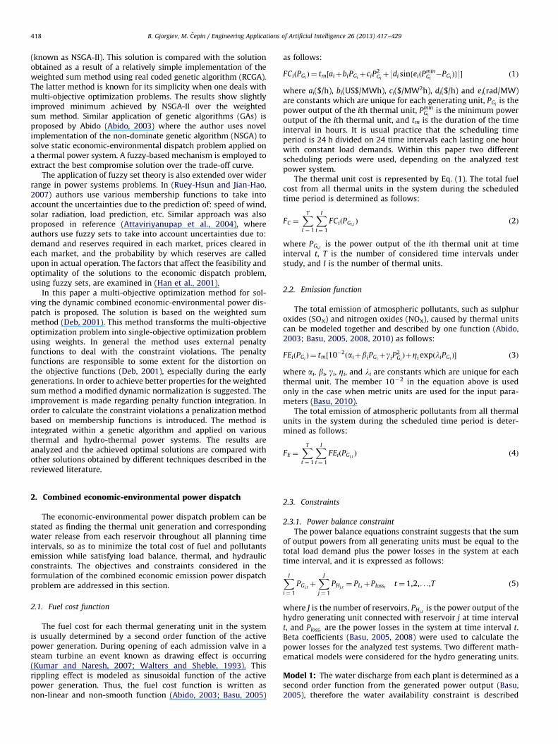
In (Joines and Houck, 1994) a dynamic normalization methodfor the penalty parameter is proposed. The method uses stepwiseincrease of the penalty term, i.e. the penalty parameter increasesas the number of generation grows. The tuning of three userdefined constants is required. In this study, a modified dynamicnormalization method is proposed. The purpose of this method isto mitigate severe distortion of the objective functions caused bythe penalty term. To accomplish this, a ‘‘pressure distribution’’parameter is introduced within the static penalty parameter asfollows:

dd ¼ pdds ð23Þ

The parameter, pd, is function of the number of generation andit follows the ‘‘pressure distribution function’’ presented on Fig. 1.

The penalty parameter was calculated as follows:

ds ¼FCðP

maxGi,tÞPNl

m ¼ 1 maxðVIOLmÞð24Þ

The parameters gen ands maxgen from Fig. 1 are the number ofgeneration and the maximum number of generation defined inthe GA, and k is user defined parameter. This parameter definesthe generation from which the penalty pressure will be fullyapplied (in this study it was set to 0.60). When the dynamicpenalty parameter is applied, the fitness function from Eq. (21) is

written as follows:

F ¼ f þdd

XNl

m ¼ 1

VIOLm ð25Þ

During the early generation, when the possible solutions arestill away from optimal solutions, there is relatively large prob-ability that the pressure from the penalty function will lead thesearch towards local optimum. To avoid this phenomena thedistribution function is set to start from near zero values andgrow slowly, especially in the early generation, such that exten-sive distortion of the objective functions will be mitigated. Thisallows the generated offspring to be more focused on the mini-mization/maximization of the objective functions. As the numberof generation grows, the pressure from the penalty functions isgrowing as well, allowing the algorithm to deal with the con-straints avoiding severe distortion of the objective functions.

3.3. Membership function penalization

A constraint optimization problem is triple X,f ,f, where X isa free search space, f is a real valued objective function X, whichhas to be minimized, f is a formula (Boolean function on X).A solution of a constrained optimization problem is xAX withf(x)¼true and an optimal f-value (Corne et al., 1999).

The common opinion about evolutionary algorithms is thatthey are good optimizers, although they cannot handle constraintswell. This opinion is based on the observation that the variationoperators, mutation and reproduction, are ‘‘blind’’ to constraints(Michalewicz, 1995, 1996). In other words, if the parents satisfycertain constraints, the offspring obtained by mutation and/orrecombination might violate them. In the past several options havebeen proposed to overcome this problem. Among all constrainthandling methods, penalizing infeasible individuals/chromosomesis the simplest and the most extended one (Mezura-Montes, 2009;Mezura-Montes and Coello Coello, 2011; Michalewicz, 1995). Firstof all, if it is applied to all constraints then minimizing the totalpenalty is the only thing to be done. In other words, it transformsthe constrained optimization problem into an unconstrained opti-mization problem as shown with Eq. (21).

In order to estimate the constraint violations, in this study, anexterior penalty method was proposed. The method uses mem-bership functions in order to evaluate the constraint violations.Because not all constraints take the same order of magnitude, thismethod is also used as tool for normalization of all constraintviolations to values between 0 and 1. Therefore, no need forfurther adjustment is required. This is perfectly in compliancewith the single normalization parameter, dd, used for aggregatingof the penalty term in the fitness function (Eq. (25)).

B. Gjorgiev, M. Cepin / Engineering Applications of Artificial Intelligence 26 (2013) 417–429 421

The purpose of this penalization method is to deal with all unitand system equality and inequality constraints in an efficientmanner. For each of the constraints which are not initiallyincluded in the initial population such as power balance (5),water availability constraint (6), water balance at each timeinterval (9), water balance at the end of the time period (12)and ramping response rate (15) a unique membership functionwas employed (Gjorgiev, 2010) as follows:

–

membership function for the power balance constraint, – membership function for the water availability constraint, – membership function for the water balance at each time

interval constraint,

– membership function for the water balance at the end of the

time period constraint,

–

1

0.8

0.6

0.4

0.2

0

40% 20% 0% 0% 20% 40%VV

�

Fig. 3. Membership function for the water balance at each time interval constraint.

membership function for the ramping response rate constraint.

The remaining of the constraints defined in the previoussection are the variable boundaries, referred as internal con-straints. They are included directly in the algorithm procedure,starting from the initial population which is generated randomlywithin these boundaries, continuing through reproduction pro-cess where all other new variables are introduced within theboundaries.

3.3.1. Membership function for the power balance constraint

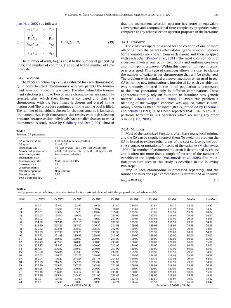
The power balance constraint requires that the sum of thegeneration from all generating units, PS at each time interval t

must be equal to the sum of load demand, PL, and power systemloses, Ploss at the same time interval. Because there is probabilitythat these values will differ from each other, the difference inpercent DPL is calculated. A membership function m ~P as shown onFig. 2 is used. The membership value of 1 is assigned when DPL¼0and smaller than 1 when DPL is greater than 0. The membershipfunction is expressed as follows:

m ~Pt¼

1

1þZPðDPLtÞ2

ð26Þ

where:

DPLt¼

PSt�ðPLt

þPlosstÞ

PLtþPlosst

100% ð27Þ

ZP is the shape parameter, and PStis the sum of all generated

powers at time interval t.

0

0.2

0.4

0.6

0.8

1

1.2

-70.00%

L

�p

-50.00% -30.00% -10.00%

∼

Fig. 2. Membership function for t

The overall violation of the power balance constraint isdetermined as VIOLP ¼

PTi ¼ 1ð1�m ~Pt

Þ.

3.3.2. Membership function for the water balance at each time

interval constraint

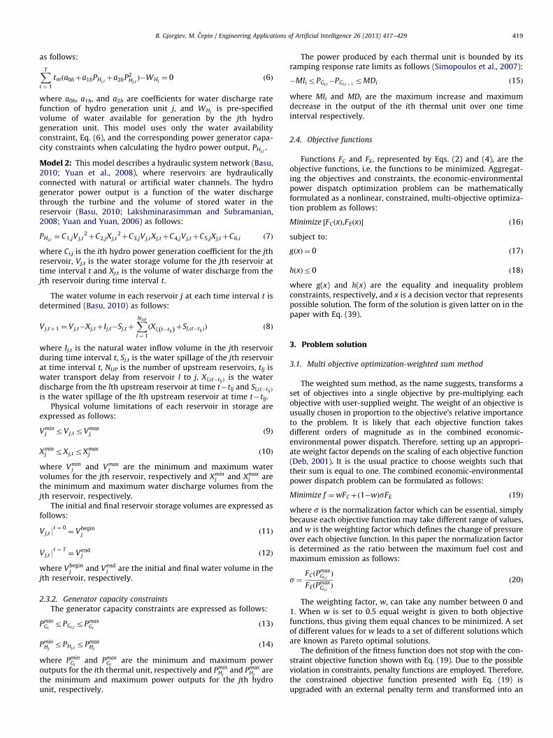
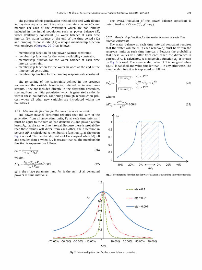
The water balance at each time interval constraint requiresthat the water volume, V, in each reservoir j must be within thereservoir limits at each time interval t. Because the probabilitythat these values will differ from each other, the difference inpercent, DVV, is calculated. A membership function m ~V as shownon Fig. 3 is used. The membership value of 1 is assigned whenEq. (9) is satisfied and value smaller than 1 in any other case. Themembership function is expressed as follows:

m ~Vj,t ¼

11þZV ðDV�Vj,t

Þ2 , Vj,t oVmin

j

1 Vminj rVj,t rVmax

j

11þZV ðDV þVj,t

Þ2 , Vj,t 4Vmax

j

8>>>>><>>>>>:

ð28Þ

where:

DV�Vj,t¼

Vminj �Vj,t

Vminj

100% ð29Þ

eta = 0.1

eta = 0.01

eta = 0.001

10.00% 30.00% 50.00% 70.00%

he power balance constraint.

B. Gjorgiev, M. Cepin / Engineering Applications of Artificial Intelligence 26 (2013) 417–429422

DV þVj,t¼

Vj,t�Vmaxj

Vmaxj

100% ð30Þ

ZV is the shape parameter.The overall violation of the water balance at each time interval

constraint is determined as VIOLV ¼PJ

j ¼ 1

PTt ¼ 1ð1�m ~Vj,t

Þ.

3.3.3. Membership function for the water balance at the end of the

time period constraint

The water balance at the end of the time period constraintrequires that the volume of water, V9T, at each reservoir j at theend of the time period (t¼T) is equal to the predetermined watervolume, Vend, for the reservoir. Because the probability that thesevalues will differ from each other, the difference in percent, DVW,is calculated. A membership function m ~W (similar in shape to theone shown on Fig. 2) is used. The membership value of 1 isassigned when DVW¼0 and smaller than 1 when DVW is greaterthan 0. The membership function is expressed as follows:

m ~Wj¼

1

1þZW ðDVWjÞ2

ð31Þ

where:

DVWj¼

Vj9T�Vend

j

Vendj

100% ð32Þ

ZW is the shape parameter.The overall violation of the water balance at the end of the

time period constraint is determined as VIOLW ¼PJ

j ¼ 1ð1�m ~WjÞ.

3.3.4. Membership function of water availability constraint

The water availability constraint requires that the spent watervolume from each hydro unit, j, at the end of the time period(t¼T) is equal to the predetermined water volume, WH, forthe reservoir. This means that all available water for each hydrounit is spent. Because the probability that these values will differfrom each other, the difference in percent, DWH, is calculated.A membership function m ~R (similar in shape to the one shownon Fig. 2) is used. The membership value of 1 is assigned whenDWH ¼ 0 and smaller than 1 when DWH is greater than 0.The membership function is expressed as follows:

m ~WHj

¼1

1þZW ðDVWjÞ2

ð33Þ

where:

DWHj¼

PTt ¼ 1 tmða0hþa1hPHj,t

þa2hP2Hj,tÞ�WHj

WHj

100% ð34Þ

ZWH is the shape parameter.The overall violation of the water balance at the end of the

time period constraint is determined as VIOLWH ¼PJ

j ¼ 1ð1�m ~WHj

Þ.

3.3.5. Membership function for the ramping response rate constraint

The ramping response rate constraint requires that the changeof the generated power of each thermal unit i during each timeinterval t is within the predetermined limits for the unit. Becausethe probability that these values will differ from each other,the difference in percent, DR, is calculated. A membership func-tion m ~R (similar in shape to the one shown on Fig. 3) is used. Themembership value of 1 is assigned when Eq. (15) is satisfied andvalue smaller than 1 in any other case. The membership function

is expressed as follows:

m ~Ri,t¼

11þZRðDR�i,t Þ

2 , PGi,t�PGi,tþ 1

o�MIi

1 �MIirPGi,t�PGi,tþ 1

rMDi

11þZRðDRþ

i,t Þ2 , PGi,t

�PGi,tþ 14MDi

8>>><>>>:

ð35Þ

where:

DR�i,t ¼9PGi,t�PGi,tþ 1

9�MIi

MIi100% ð36Þ

DRþi,t ¼ðPGi,t�PGi,tþ 1

Þ�MDi

MDi100% ð37Þ

ZR is the shape parameter.The overall violation of the ramping response rate constraint is

determined as VIOLR ¼PI

i ¼ 1

PTt ¼ 1ð1�m ~Ri,t

Þ.As can be observed from Fig. 2, the shape parameter defines

the curve shape. Decrease of the shape parameter results withsmoother shape of the curve. During the tests obtained regard-ing the efficiency of the proposed penalization method, it wasobserved that small values for the shape parameters characterizewith faster and smoother convergence. Therefore, it is recom-mended that the shape parameters for all membership functionsare kept low (e.g. Zs¼0.001). It was also observed that theadditional decrease of the shape parameter will just make theconvergence process slower.

As it can be seen from above, two general shapes of member-ship functions are used, the one from Fig. 2 applies to all equalityconstraint, while the one from Fig. 3 applies to all inequalityconstraints. The set of constraints that defines the penalty termdepends on the hydraulic model of the power system and therequirements regarding thermal units. Therefore, different setof membership function was used for each of the test systemsanalyzed in the paper.

3.4. Genetic algorithm application

The GA is an evolutionary searching technique based on themechanics of natural selection and natural genetics. The GA is anattractive alternative to other optimization approaches because ofits robustness. The GA is searching for better solutions by lettingthe fitter individuals to take over the population using a combi-nation of stochastic process (Chaturvedi et al., 2009; Michalewicz,1996). Like any other optimization algorithm it begins by definingthe optimization variables, the cost function, and the cost, andends by testing for convergence. In between, however, thisalgorithm is quite different, i.e. it uses specific GA operators.The main GA operators are initial population, selection, crossoverand mutation.

3.4.1. Initial population

The GA begins with an initial population of Np chromosomesbeing defined. All variables from each chromosome in the initialpopulation are randomly determined using a uniform probabilitydistribution, covering the entire search space uniformly. The initialpopulation is expressed as follows:

POP¼ ½C1,C2,C3,. . .,Ck,. . .,CNp� ð38Þ

Each chromosome Ck from the initial population is repre-sented by a matrix of (Iþ J)T random values (Ruey-Hsun and

B. Gjorgiev, M. Cepin / Engineering Applications of Artificial Intelligence 26 (2013) 417–429 423

Jian-Hao, 2007) as follows:

Ck ¼

P1,1P1,2 � � � P1,T

^ & ^

PI,1PI,2 � � � PI,T

X1,1X1,2 � � � X1,T

^ & ^

XJ,1XJ,2 � � � XJ,T

266666666664

377777777775

k¼ 1,2,. . .,Np ð39Þ

The number of rows, Iþ J, is equal to the number of generatingunits; the number of columns, T, is equal to the number of timeintervals.

3.4.2. Selection

The fitness function, Eq. (25), is evaluated for each chromosome,Ck. In order to select chromosomes as future parents the tourna-ment selection procedure was used. The idea behind the tourna-ment selection is simple. Two or more chromosomes are randomlyselected, after which their fitness is compared and then thechromosome with the best fitness is chosen and placed in themating pool. The procedure continues until the mating pool is filled.The number of individuals chosen for the tournaments is known astournament size. High tournament size results with high selectionpressure, because wicker individuals have smaller chances to win atournament. A study made by Goldberg and Deb (1991) showed

Table 1Relevant GA parameters.

GA representation Real coded genetic algorithm

GA type Classic GA

Population size 40 (test system-I & II), 60 (test system-III)

Number of generations 2000 (test system-I & II), 3500 (test system-III)

Selection operator Tournament selection

Tournament size 2

Crossover operator Multi-point BLX-0.5

Crossover rate 0.8

Crossover points 0.4

Mutation operator Non-uniform

Mutation rate 0.05

Beta parameter (bm) 2

Table 2Hourly generation scheduling, cost and emission for test system-I obtained with the p

Hour P1 (MW) P2(MW) P3(MW) P4(MW) P5(MW)

1 150.01 135.01 122.00 120.41 123.80

2 150.01 135.01 144.39 109.87 166.88

3 150.03 135.04 185.23 149.62 185.00

4 150.05 138.00 190.33 188.44 235.00

5 150.02 193.63 211.57 180.83 237.90

6 154.38 217.46 287.15 228.36 242.98

7 212.30 222.26 285.25 246.37 242.98

8 226.62 222.98 298.67 296.35 242.99

9 260.89 302.99 339.76 299.98 242.99

10 317.72 351.49 339.99 299.99 243.00

11 371.28 389.07 339.99 299.99 243.00

12 398.79 407.69 340.00 300.00 243.00

13 337.87 385.37 339.99 300.00 242.99

14 257.87 306.07 339.69 299.98 243.00

15 226.60 226.06 302.45 289.53 242.99

16 150.03 180.72 252.75 239.68 228.57

17 150.04 136.27 244.84 237.78 204.88

18 150.59 216.22 277.26 243.02 242.98

19 225.70 229.07 297.21 293.02 242.98

20 305.68 309.09 339.99 299.99 242.99

21 297.48 296.08 324.12 281.09 243.00

22 217.36 215.94 243.96 231.00 228.47

23 150.01 135.83 163.92 180.92 222.55

24 150.01 135.01 168.03 130.90 172.74

Cost¼2.4833Eþ06 ($)

that the tournament selection operator has better or equivalentconvergence and computational time complexity properties whencompared to any other selection operator proposed in the literature.

3.4.3. Crossover

The crossover operator is used for the creation of one or moreoffspring from the parents selected during the selection process.Some variables are chosen from each parent and then swappedwith each other (Kancev et al., 2011). The most common form ofcrossover involves one point, two points and uniform crossoverand multi-point crossover. Within this paper a multi-point cross-over was used. This type of crossover allows the user to choosethe number of variables per chromosome that will be exchanged.The problem with standard crossover methods when used in realGA is that no new information is introduced i.e. each variable thatwas randomly initiated in the initial population is propagatedto the next generation, only in different combinations. Theseapproaches totally rely on mutation to introduce new geneticmaterial (Haupt and Haupt, 2004). To avoid this problem ablending of the swapped variables was applied, which is com-monly known as blend crossover (BLX-a) proposed by Eshelmanand Schaffer (1993). It has been reported that BLX-0.5 (a¼0.5)performs better than BLX operators which are using any othera value (Deb, 2001).

3.4.4. Mutation

Most of the optimized functions often have many local minimaand the GA can be caught in one of them. To avoid this problem theGA is forced to explore other areas of the cost surface by introdu-cing changes, or mutations, for some of the variables (Michalewicz,1996). The number of performed mutation is determined by choiceand is often not more than a couple of percent of the number ofvariables in the population (Volkanovski et al., 2008). The muta-tion procedure used in this study is described in the followingtwo steps:

Step 1: Each chromosome is processed separately, and thenumber of mutations per chromosome is determined as follows:

Nm,c ¼mrðIþ JÞT ð40Þ

roposed method when w¼0.5.

P6(MW) P7(MW) P8(MW) P9(MW) P10(MW)

130.57 87.87 90.10 52.06 43.42

144.88 65.56 119.98 52.06 43.42

159.98 93.85 119.98 59.20 48.02

159.99 123.85 119.99 79.99 54.97

159.98 129.94 119.99 79.98 54.98

159.99 129.97 119.99 79.99 54.98

159.99 129.98 119.99 79.99 54.98

159.99 129.98 119.99 79.99 54.99

159.99 129.99 120.00 80.00 54.99

160.00 129.99 120.00 80.00 55.00

160.00 130.00 120.00 80.00 55.00

160.00 130.00 120.00 80.00 55.00

160.00 130.00 120.00 80.00 55.00

159.99 129.99 119.99 80.00 55.00

159.99 129.99 119.99 79.99 54.99

159.99 129.97 119.99 79.99 54.99

159.97 129.72 119.98 79.99 54.90

159.99 129.98 119.99 79.99 54.98

159.99 129.98 119.99 79.99 54.99

160.00 130.00 120.00 80.00 54.99

160.00 130.00 120.00 80.00 55.00

159.95 129.60 119.99 79.99 49.98

143.45 123.59 119.97 79.97 43.42

158.43 93.58 90.16 66.56 43.42

Emission¼3.0496Eþ05 (lb)

B. Gjorgiev, M. Cepin / Engineering Applications of Artificial Intelligence 26 (2013) 417–429424

where mr is the mutation rate and (Iþ J)T is number of variablesper chromosome. Subsequently, random numbers are chosen toselect the rows and columns of the variables to be mutated.

Step 2 (non-uniform mutation (Michalewicz, 1996)): Thenew value ðvnew

i Þ of the variable vi, after mutation is performed

Table 3Comparison of best compromise solution for test system-I.

Approach Proposed method RCGA

(Basu, 2008)

NSGA-II

(Basu, 2008)

Cost (1Eþ06 $) 2.4833 2.5251 2.5226

Emission (1Eþ05 lb) 3.0496 3.1246 3.0994

CPU (s) 52 1105 1211a

a The time in which NSGA-II obtained all Pareto front solutions (Basu, 2008).

2450000

2500000

2550000

2600000

2650000

2700000

285000

Cos

t ($)

Emission (lb)

RCGA

NSGA-II

Proposed Algorithm

295000 305000 315000 325000 335000

Fig. 4. Pareto fronts obtained with the proposed method, NSGA-II and RCGA for

test system-I.

2481000

2482000

2483000

2484000

2485000

2486000

1

Cos

t ($)

Algorithm2 3 4 5

Fig. 5. Cost and emission obtained in ten r

Table 4Hourly generation scheduling, cost and emission for test system-II obtained with the p

Subinterval Hydro-units Thermal-units

P1(MW) P2ðMWÞ P3ðMWÞ P4ðMWÞ

1 194.69 336.44 98.05 112.67

2 234.84 416.69 98.48 112.67

3 203.44 354.87 96.86 112.67

4 244.99 477.65 98.54 166.75

Cost¼6.7839Eþ04 ($)

during the ith generation, is calculated as:

vnewi ¼ f ðvÞ ¼

viþDðgen,vmaxi �viÞ, if t¼ 0

vi�Dðgen,vi�vmini Þ, if t¼ 1

(ð41Þ

and

Dðgen,yÞ ¼ yð1�rð1�gen=maxgenÞbmÞ ð42Þ

where bm is a positive constant chosen arbitrarily and t is numberrandomly generated with equal probability to be zero or one. Inthis study bm was set to 2.

The function D(gen,y) returns a value in the range [0,y].Therefore the operator gives a value viA ½vmin

i ,vmaxi � such that the

probability of returning a value close to vi increases as the algo-rithm is advancing. This encourages uniform search in the initialstages when the number of generations (gen) is small and localsearch in later stages.

3.4.5. Replacement

An elitist type of replacement strategy is used in this paper.The strategy is based on a comparison among the offspring andtheir parent chromosomes. Each pair of parent chromosomes isresponsible for creation of two offspring chromosomes when thecrossover and the mutation operator are applied. The parents andthe offspring chromosomes are placed in a subgroup containingfour chromosomes. Thereafter, a comparison is made among thechromosomes in the subgroup. Only the best two survive whilethe other two are deleted. The procedure is continuing until allsubgroups are processed. The chromosomes that survive arerepresenting the population of the new generation. These chro-mosomes will later enter the tournaments to compete for place inthe mating pool.

The purpose of the described GA is to solve Eq. (25), whichcomprises the improvements on the weighted sum methoddescribed above.

304100

304300

304500

304700

304900

305100

305300

Run

Cost

Emission

Emis

sion

(lb)

6 7 8 9 10

uns of the algorithm for test system-I.

roposed method when w¼ 0:5.

PPt

ðMWÞ PlosstðMWÞ

P5ðMWÞ P6ðMWÞ

124.91 51.67 918.42 18.75

124.94 139.76 1127.36 27.92

124.93 129.34 1022.04 22.45

209.82 139.76 1337.50 38.94

Emission¼2.4810Eþ04 (lb) – –

B. Gjorgiev, M. Cepin / Engineering Applications of Artificial Intelligence 26 (2013) 417–429 425

4. Analysis and results

The proposed method has been coded in MATLAB 7.7 environ-ment and implemented on Intel Pentium(R) 4 PC. The algorithmproperties were tuned applying the trial and error method usingdifferent objective functions. The relevant GA parameters used inthis study are shown in Table 1.

The algorithm has been applied on a three separate test powersystems, test system-I (Basu, 2008), test system-II (Basu, 2005),and test system-III (Basu, 2010). Each of these power systems hasdifferent properties, which makes them interesting for analysis.

4.1. Test system-I

This power system, presented in (Basu, 2008), is purely thermalpower system, comprising ten thermal generating units and nohydro generating units. This relieves the algorithm from thehydraulic constraints. The only external constraints left are thepower balance constraint and ramping response rate constraint forwhich membership functions described with Eqs. (26) and (35)were used, respectively. The power system losses were consideredusing the Beta matrix given in (Basu, 2008). The scheduling timeperiod is 24 h equally divided on 24 intervals each lasting one hourwith constant load demands within that hour.

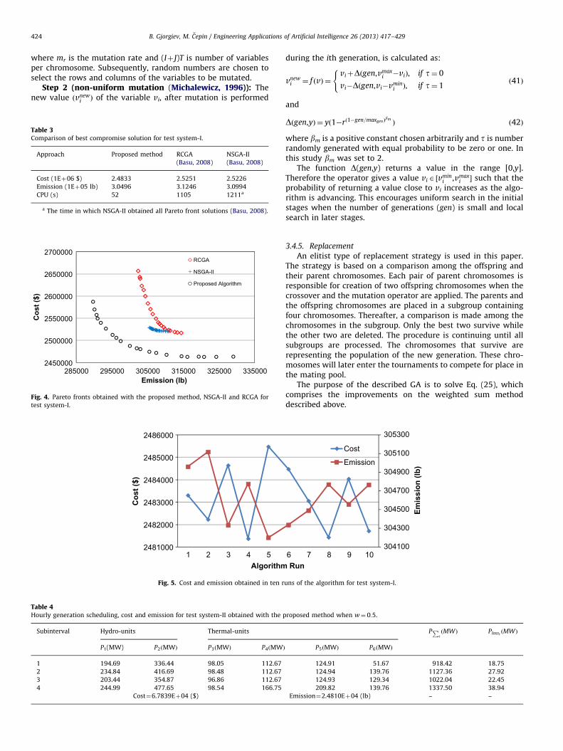
Table 2 shows the hourly generation schedule, cost and emis-sion for test system-I obtained from the combined economic-environmental dispatch using the proposed method. This solutionis known as best compromise solution, obtained when w¼0.5.A comparison was made among the best compromise solutionobtained from the proposed method and the solutions obtainedby the real-coded GA (RCGA) and non-dominate sorting GA-II(NSGA-II) algorithms applied in (Basu, 2008). The results of thiscomparison are shown in Table 3. It can be easily concluded thatthe proposed method has resulted with better best compromisesolution for both cost and emission.

Table 5Comparison of best compromise solution for test system-II.

Approach Proposed method SABGA

(Basu, 2005)

IGAMU

(Chao-Lung, 2007)

Cost (1Eþ04 $) 6.7839 7.3612 6.8493

Emission (1Eþ04 lb) 2.4810 2.6080 2.6081

CPU (s) 33 1492 38.51

65000

70000

75000

80000

85000

90000

22000 2

Cos

t ($)

Emis23000 24000 25000

Fig. 6. Pareto fronts obtained with the propos

Fig. 4 illustrates the Pareto front for a set of 21 optimal solutionsobtained with the proposed algorithm for test system-I. This set ofsolutions was calculated by multiple runs of the algorithm,increasing w from 0 to 1 with step of 0.05. For a comparison, thePareto fronts obtained by RCGA and NSGA-II in (Basu, 2008) arealso shown in Fig. 4. It is evident that the proposed algorithmobtained better solutions compared to the solutions obtained byRCGA and NSGA-II for test system-I.

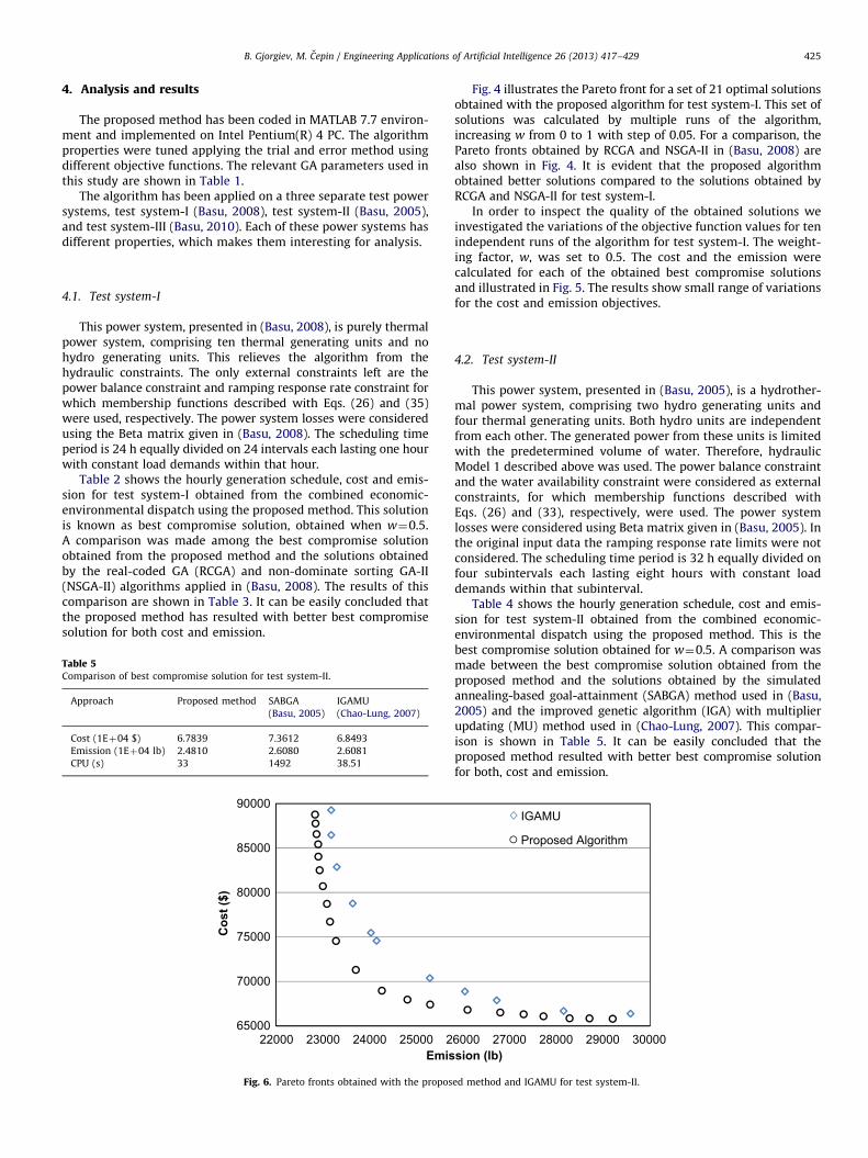
In order to inspect the quality of the obtained solutions weinvestigated the variations of the objective function values for tenindependent runs of the algorithm for test system-I. The weight-ing factor, w, was set to 0.5. The cost and the emission werecalculated for each of the obtained best compromise solutionsand illustrated in Fig. 5. The results show small range of variationsfor the cost and emission objectives.

4.2. Test system-II

This power system, presented in (Basu, 2005), is a hydrother-mal power system, comprising two hydro generating units andfour thermal generating units. Both hydro units are independentfrom each other. The generated power from these units is limitedwith the predetermined volume of water. Therefore, hydraulicModel 1 described above was used. The power balance constraintand the water availability constraint were considered as externalconstraints, for which membership functions described withEqs. (26) and (33), respectively, were used. The power systemlosses were considered using Beta matrix given in (Basu, 2005). Inthe original input data the ramping response rate limits were notconsidered. The scheduling time period is 32 h equally divided onfour subintervals each lasting eight hours with constant loaddemands within that subinterval.

Table 4 shows the hourly generation schedule, cost and emis-sion for test system-II obtained from the combined economic-environmental dispatch using the proposed method. This is thebest compromise solution obtained for w¼0.5. A comparison wasmade between the best compromise solution obtained from theproposed method and the solutions obtained by the simulatedannealing-based goal-attainment (SABGA) method used in (Basu,2005) and the improved genetic algorithm (IGA) with multiplierupdating (MU) method used in (Chao-Lung, 2007). This compar-ison is shown in Table 5. It can be easily concluded that theproposed method resulted with better best compromise solutionfor both, cost and emission.

6000sion (lb)

IGAMU

Proposed Algorithm

27000 28000 29000 30000

ed method and IGAMU for test system-II.

24805

24807

24809

24811

24813

24815

24817

24819

24821

24823

67725

67755

67785

67815

67845

67875

67905

1

Cos

t ($)

Algorithm Run

Cost

Emission

Emis

sion

(lb)

2 3 4 5 6 7 8 9 10

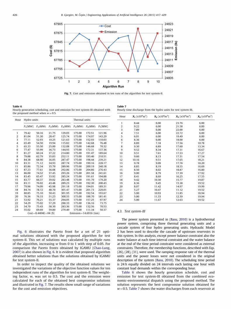
Fig. 7. Cost and emission obtained in ten runs of the algorithm for test system-II.

Table 6Hourly generation scheduling, cost and emission for test system-III obtained with

the proposed method when w¼ 0:5.

Hour Hydro units Thermal units

P1(MW) P2ðMWÞ P3ðMWÞ P4ðMWÞ P5ðMWÞ P6ðMWÞ P7(MW)

1 79.42 50.16 21.75 129.03 175.00 172.51 121.96

2 81.04 51.30 28.47 125.74 175.00 174.97 143.29

3 77.11 52.93 10.25 121.63 175.00 152.93 110.03

4 65.49 54.50 19.94 115.82 175.00 142.68 76.48

5 65.33 55.50 25.00 132.08 175.00 146.68 70.32

6 77.47 55.99 36.73 144.93 175.00 172.31 137.36

7 81.27 60.24 37.22 214.80 175.00 191.47 189.64

8 79.88 62.79 35.83 252.11 175.00 193.46 210.51

9 84.38 68.90 36.05 287.47 175.00 198.44 239.21

10 83.31 71.12 34.93 287.74 175.00 199.16 228.17

11 85.86 72.34 35.79 289.96 175.00 200.19 240.18

12 87.23 77.61 36.08 292.06 175.00 204.86 276.43

13 86.00 74.52 37.45 293.26 175.00 201.58 241.61

14 83.45 65.47 33.92 285.24 175.00 191.61 194.88

15 83.77 66.37 39.02 283.48 175.00 191.79 179.20

16 83.11 76.02 43.48 289.23 175.00 192.30 200.43

17 79.96 74.09 45.98 291.18 175.00 194.01 189.31

18 84.74 78.72 48.70 301.47 175.00 201.73 229.01

19 80.85 75.10 50.43 301.95 175.00 192.54 193.67

20 76.36 76.33 51.23 300.55 175.00 188.70 181.41

21 53.92 76.21 55.37 294.05 175.00 157.25 97.97

22 54.29 75.02 57.29 288.33 175.00 136.16 73.75

23 54.70 75.43 58.30 283.36 175.00 132.56 70.53

24 55.02 69.69 59.00 279.49 175.00 111.34 50.37

Cost¼8.4404Eþ04 ($) Emission¼14.6916 (ton)

Table 7Hourly time discharge from the hydro units for test system-III.

Hour X1 (x104m3) X2 (x104m3) X3 (x104m3) X4 (x104m3)

1 8.44 6.00 23.76 6.00

2 9.22 6.00 21.58 6.00

3 7.89 6.00 22.00 6.00

4 7.51 6.00 22.72 6.00

5 6.01 6.00 19.49 6.00

6 8.36 6.00 18.00 6.00

7 8.89 7.18 17.56 10.78

8 9.30 6.89 17.60 13.34

9 9.52 8.34 17.31 16.67

10 9.51 7.61 17.53 17.27

11 9.60 8.13 17.31 17.54

12 10.16 9.51 17.65 18.21

13 9.78 9.09 17.76 18.20

14 8.85 8.19 18.55 16.69

15 8.50 8.02 18.87 16.80

16 9.00 8.79 17.39 17.92

17 8.41 8.69 16.25 17.55

18 9.42 10.30 15.77 19.87

19 8.36 9.45 15.38 19.52

20 8.07 11.42 14.97 19.99

21 5.27 10.47 11.12 19.52

22 5.00 10.93 11.85 18.94

23 5.00 11.33 12.39 19.94

24 5.00 11.67 12.63 19.52

B. Gjorgiev, M. Cepin / Engineering Applications of Artificial Intelligence 26 (2013) 417–429426

Fig. 6 illustrates the Pareto front for a set of 21 opti-mal solutions obtained with the proposed algorithm for testsystem-II. This set of solutions was calculated by multiple runsof the algorithm, increasing w from 0 to 1 with step of 0.05. Forcomparison the Pareto fronts obtained by IGAMU (Chao-Lung,2007) is also shown in Fig. 6. It is evident that proposed algorithmobtained better solutions than the solutions obtained by IGAMUfor test system-II.

In order to inspect the quality of the obtained solutions weinvestigated the variations of the objective function values for tenindependent runs of the algorithm for test system-II. The weight-ing factor, w, was set to 0.5. The cost and the emission werecalculated for each of the obtained best compromise solutionsand illustrated in Fig. 7. The results show small range of variationsfor the cost and emission objectives.

4.3. Test system-III

The power system presented in (Basu, 2010) is a hydrothermalpower system, comprising three thermal generating units and acascade system of four hydro generating units. Hydraulic Model2 has been used to describe the cascade of upstream reservoirs inthis system. In this analysis, except power balance constraint also thewater balance at each time interval constraint and the water balanceat the end of the time period constraint were considered as externalconstraints. Therefore, the membership functions, described with Eqs.(26), (28), (31), were used. The ramping response rate of the thermalunits and the power losses were not considered in the originaldescription of the system (Basu, 2010). The scheduling time periodis 24 h equally divided on 24 intervals each lasting one hour withconstant load demands within the corresponding hour.

Table 6 shows the hourly generation schedule, cost andemission for test system-III obtained from the combined eco-nomic-environmental dispatch using the proposed method. Thesolution represents the best compromise solution obtained forw¼0.5. Table 7 shows the water discharges from each reservoir at

B. Gjorgiev, M. Cepin / Engineering Applications of Artificial Intelligence 26 (2013) 417–429 427

each hour, for the solution shown in Table 6. A comparison wasmade among the obtained best compromise solution from theproposed method and the algorithms used in (Basu, 2010). Thiscomparison is shown in Table 8. It can be seen that a relativelylarge difference exists among the obtained results. Especially, thedifference is significant when comparing the obtained costs.

To verify our findings we compared the sum of water dischargefrom all reservoirs at each time. The calculation shows that allwater spends by the hydro units obtained by proposed method areequal to 1166.79 (�104 m3) compared to 1,158.04 (�104 m3)obtained by NSGA-II presented in (Basu, 2010). However, thegenerated energy by the hydro units obtained by the proposedmethod is equal to 10,263.50 (MWh) compared to 9,613.56 (MWh)obtained by NSGA-II. If we take a look to the graphical

65000

75000

85000

95000

105000

115000

125000

135000

145000

155000

165000

10

Cos

t ($)

Emis20 30 40

Fig. 8. Pareto fronts obtained with the proposed m

84370

84410

84450

84490

84530

84570

1

Cos

t ($)

Algorithm2 3 4 5

Fig. 9. Cost and emission obtained in ten ru

Table 8Comparison of best compromise solution for test system-III.

Approach Proposed method MODE (Basu, 2010) NSGA-II (Basu, 2010)

Cost (1Eþ04 $) 8.4404 12.6820 12.7200

Emission (ton) 14.6916 17.7019 18.9605

CPU (s) 170 2957a 4301b

a The time in which MODE obtained all Pareto front solutions (Basu, 2010).b The time in which NSGA-II obtained all Pareto front solutions (Basu, 2010).

representation of the water discharges obtained with NSGA-II itcan be observed that the water is randomly discharged. Thesefindings lead us to the conclusion that the water discharge fromthe reservoirs it is not optimized by the NSGA-II. Therefore, it canbe concluded that this is a solutions that belongs to a localminimum. For additional verification, a simple sensitivity analysiswhich was performed, showed that if the number of generations isdecreased significantly, the obtained results are very similar to theone presented in (Basu, 2010). Similar findings can be observed forthe multi-objective differential evolution (MODE).

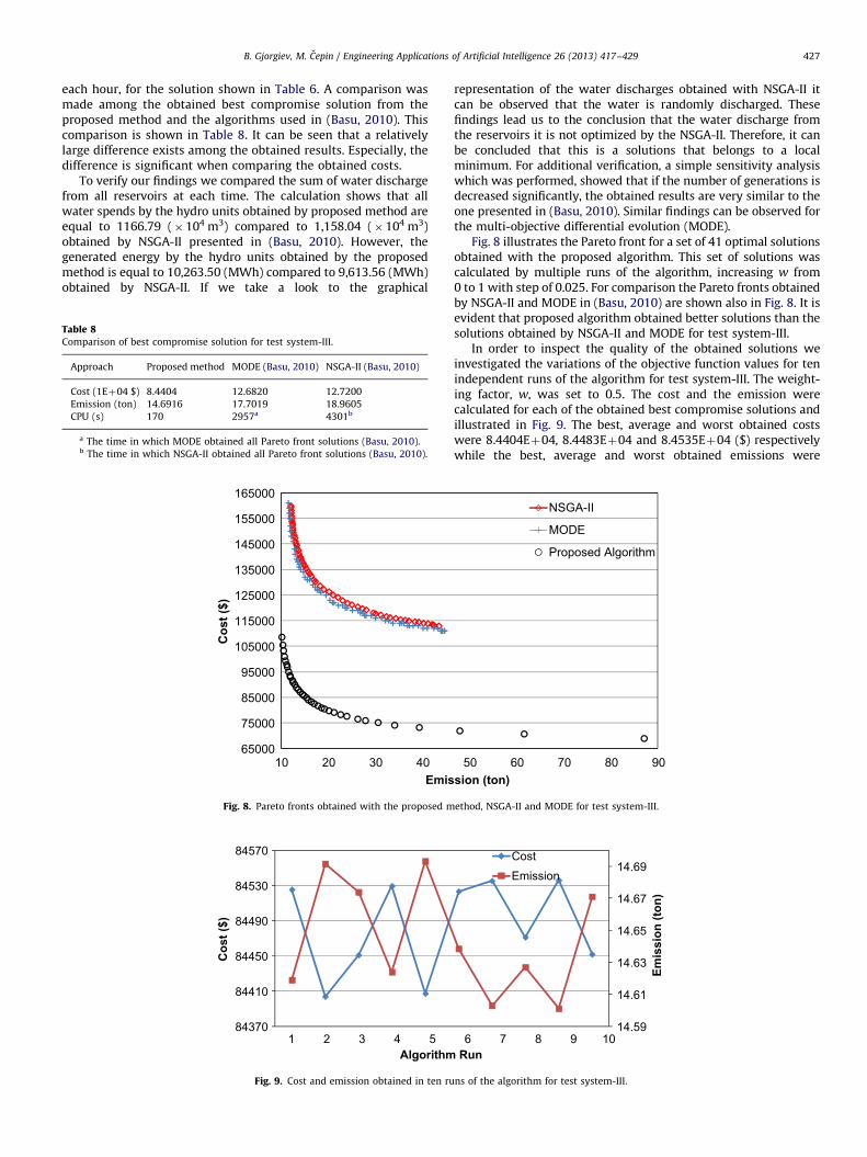
Fig. 8 illustrates the Pareto front for a set of 41 optimal solutionsobtained with the proposed algorithm. This set of solutions wascalculated by multiple runs of the algorithm, increasing w from0 to 1 with step of 0.025. For comparison the Pareto fronts obtainedby NSGA-II and MODE in (Basu, 2010) are shown also in Fig. 8. It isevident that proposed algorithm obtained better solutions than thesolutions obtained by NSGA-II and MODE for test system-III.

In order to inspect the quality of the obtained solutions weinvestigated the variations of the objective function values for tenindependent runs of the algorithm for test system-III. The weight-ing factor, w, was set to 0.5. The cost and the emission werecalculated for each of the obtained best compromise solutions andillustrated in Fig. 9. The best, average and worst obtained costswere 8.4404Eþ04, 8.4483Eþ04 and 8.4535Eþ04 ($) respectivelywhile the best, average and worst obtained emissions were

sion (ton)

NSGA-II

MODE

Proposed Algorithm

50 60 70 80 90

ethod, NSGA-II and MODE for test system-III.

14.59

14.61

14.63

14.65

14.67

14.69

Run

CostEmission

Emis

sion

(ton

)

6 7 8 9 10

ns of the algorithm for test system-III.

0

5

10

15

20

0

20000

40000

60000

80000

100000

120000

115

430

746

061

376

691

910

7212

2513

7815

3116

8418

3719

9021

4322

9624

4926

0227

5529

0830

6132

1433

67

Cos

t ($)

Generation

Cost

Emission

Emis

sion

(ton

)

Fig. 10. Convergence performance of the best solution obtained by the proposed method for test system-III.

B. Gjorgiev, M. Cepin / Engineering Applications of Artificial Intelligence 26 (2013) 417–429428

14.6012, 14.6443 and 14.6932 (ton) respectively. As illustrated inFig. 9, the generated solutions from each trial show small range ofvariations for the cost and emission objectives.

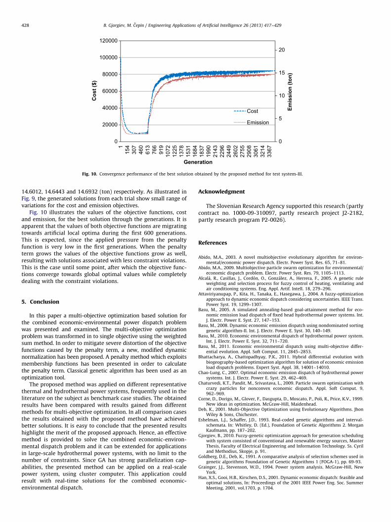
Fig. 10 illustrates the values of the objective functions, costand emission, for the best solution through the generations. It isapparent that the values of both objective functions are migratingtowards artificial local optima during the first 600 generations.This is expected, since the applied pressure from the penaltyfunction is very low in the first generations. When the penaltyterm grows the values of the objective functions grow as well,resulting with solutions associated with less constraint violations.This is the case until some point, after which the objective func-tions converge towards global optimal values while completelydealing with the constraint violations.

5. Conclusion

In this paper a multi-objective optimization based solution forthe combined economic-environmental power dispatch problemwas presented and examined. The multi-objective optimizationproblem was transformed in to single objective using the weightedsum method. In order to mitigate severe distortion of the objectivefunctions caused by the penalty term, a new, modified dynamicnormalization has been proposed. A penalty method which exploitsmembership functions has been presented in order to calculatethe penalty term. Classical genetic algorithm has been used as anoptimization tool.

The proposed method was applied on different representativethermal and hydrothermal power systems, frequently used in theliterature on the subject as benchmark case studies. The obtainedresults have been compared with results gained from differentmethods for multi-objective optimization. In all comparison casesthe results obtained with the proposed method have achievedbetter solutions. It is easy to conclude that the presented resultshighlight the merit of the proposed approach. Hence, an effectivemethod is provided to solve the combined economic-environ-mental dispatch problem and it can be extended for applicationsin large-scale hydrothermal power systems, with no limit to thenumber of constraints. Since GA has strong parallelization cap-abilities, the presented method can be applied on a real-scalepower system, using cluster computer. This application couldresult with real-time solutions for the combined economic-environmental dispatch.

Acknowledgment

The Slovenian Research Agency supported this research (partlycontract no. 1000-09-310097, partly research project J2-2182,partly research program P2-0026).

References

Abido, M.A., 2003. A novel multiobjective evolutionary algorithm for environ-mental/economic power dispatch. Electr. Power Syst. Res. 65, 71–81.

Abido, M.A., 2009. Multiobjective particle swarm optimization for environmental/economic dispatch problem. Electr. Power Syst. Res. 79, 1105–1113.

Alcala, R., Casillas, J., Cordon, O., Gonzalez, A., Herrera, F., 2005. A genetic ruleweighting and selection process for fuzzy control of heating, ventilating andair conditioning systems. Eng. Appl. Artif. Intell. 18, 279–296.

Attaviriyanupap, P., Kita, H., Tanaka, E., Hasegawa, J., 2004. A fuzzy-optimizationapproach to dynamic economic dispatch considering uncertainties. IEEE Trans.Power Syst. 19, 1299–1307.

Basu, M., 2005. A simulated annealing-based goal-attainment method for eco-nomic emission load dispatch of fixed head hydrothermal power systems. Int.J. Electr. Power E. Syst. 27, 147–153.

Basu, M., 2008. Dynamic economic emission dispatch using nondominated sortinggenetic algorithm-II. Int. J. Electr. Power E. Syst. 30, 140–149.

Basu, M., 2010. Economic environmental dispatch of hydrothermal power system.Int. J. Electr. Power E. Syst. 32, 711–720.

Basu, M., 2011. Economic environmental dispatch using multi-objective differ-ential evolution. Appl. Soft Comput. 11, 2845–2853.

Bhattacharya, A., Chattopadhyay, P.K., 2011. Hybrid differential evolution withbiogeography-based optimization algorithm for solution of economic emissionload dispatch problems. Expert Syst. Appl. 38, 14001–14010.

Chao-Lung, C., 2007. Optimal economic emission dispatch of hydrothermal powersystems. Int. J. Electr. Power E. Syst. 29, 462–469.

Chaturvedi, K.T., Pandit, M., Srivastava, L., 2009. Particle swarm optimization withcrazy particles for nonconvex economic dispatch. Appl. Soft Comput. 9,962–969.

Corne, D., Dorigo, M., Glover, F., Dasgupta, D., Moscato, P., Poli, R., Price, K.V., 1999.New ideas in optimization. McGraw-Hill, Maidenhead.

Deb, K., 2001. Multi-Objective Optimization using Evolutionary Algorithms. JhonWiley & Sons, Chichester.

Eshelman, L.J., Schaffer, J.D., 1993. Real-coded genetic algorithms and interval-schemata. In: Whitley, D. (Ed.), Foundation of Genetic Algorithms 2. MorganKaufmann, pp. 187–202.

Gjorgiev, B., 2010. Fuzzy-genetic optimization approach for generation schedulingwith system consisted of conventional and renewable energy sources, MasterThesis, Faculty of Electrical Engineering and Information Technology. Ss. Cyriland Methodius, Skopje, p. 91.

Goldberg, D.E., Deb, K., 1991. A comparative analysis of selection schemes used ingenetic algorithms Foundation of Genetic Algorithms 1 (FOGA-1), pp. 69-93.

Grainger, J.J., Stevenson, W.D., 1994. Power system analysis. McGraw-Hill, NewYork.

Han, X.S., Gooi, H.B., Kirschen, D.S., 2001. Dynamic economic dispatch: feasible andoptimal solutions, In: Proceedings of the 2001 IEEE Power Eng. Soc. SummerMeeting, 2001, vol.1703, p. 1704.

B. Gjorgiev, M. Cepin / Engineering Applications of Artificial Intelligence 26 (2013) 417–429 429

Haupt, R.L., Haupt, S.E., 2004. Practical genetic algorithms, second ed. John Wiley &Sons, New York.

Joines, J.A., Houck, C.R., 1994. On the use of non-stationary penalty functions tosolve nonlinear constrained optimization problems with GA’s, EvolutionaryComputation, 1994. In: Proceedings of the First IEEE Conference on Evolu-tionary Computation, 1994, vol.572, pp. 579–584.

Kancev, D., Gjorgiev, B., Cepin, M., 2011. Optimization of test interval for ageingequipment: a multi-objective genetic algorithm approach. J. Loss Prev. ProcessInd 24, 397–404.

Kaplan, S., 2008. Power Plants: Characteristics and Costs, Washington, p. 102.King, T.D., El-Hawary, M.E., El-Hawary, F., 1995. Optimal environmental dispatch-

ing of electric power systems via an improved Hopfield neural network model.Power Syst., IEEE Trans. 10, 1559–1565.

Kumar, S., Naresh, R., 2007. Efficient real coded genetic algorithm to solve the non-convex hydrothermal scheduling problem. Int. J. Electr. Power E. Syst. 29,738–747.

Lakshminarasimman, L., Subramanian, S., 2008. A modified hybrid differentialevolution for short-term scheduling of hydrothermal power systems withcascaded reservoirs. E. Convers. Manage. 49, 2513–2521.

Lu, Y., Zhou, J., Qin, H., Wang, Y., Zhang, Y., 2011. Chaotic differential evolutionmethods for dynamic economic dispatch with valve-point effects. Eng. Appl.Artif. Intell. 24, 378–387.

Mezura-Montes, E. (Ed.), 2009. Constraint-Handling in Evolutionary Optimization,vol. 198. Springer, Studies in Computational Intelligence Series.

Mezura-Montes, E., Coello, C.A.C., 2008. Constrained Optimization via Multi-objective Evolutionary Algorithms. In: Knowles, J., Corne, D., Deb, K. (Eds.),Multiobjective Problems Solving from Nature: From Concepts to Applications.Springer-Verlag, Berlin, pp. 53–76.

Mezura-Montes, E., Coello Coello, C.A., 2011. Constraint-handling in nature-inspired numerical optimization: past, present and future. Swarm and Evolu-tionary Computation 1, 173–194.

Michalewicz, Z., 1995. A survey of constraint handling techniques in evolutionarycomputation methods, in: Proceedings of the 4th Annual Conference onEvolutionary Programming. MIT Press, pp. 135–155.

Michalewicz, Z., 1996. Genetic Algorithms, Data Structures ¼Evolution Programs,third ed. Springer, New York.

Neyestani, M., Farsangi, M.M., Nezamabadi-pour, H., 2010. A modified particleswarm optimization for economic dispatch with non-smooth cost functions.Eng. Appl. Artif. Intell. 23, 1121–1126.

Ruey-Hsun, L., Jian-Hao, L., 2007. A fuzzy-optimization approach for generationscheduling with wind and solar energy systems. IEEE Trans. Power Syst. 22,1665–1674.

Simopoulos, D.N., Kavatza, S.D., Vournas, C.D., 2007. An enhanced peak shavingmethod for short term hydrothermal scheduling. E. Convers. Manage. 48,3018–3024.

Sivasubramani, S., Swarup, K.S., 2011. Environmental/economic dispatch using multi-objective harmony search algorithm. Electr. Power Syst. Res. 81, 1778–1785.

Subbaraj, P., Rengaraj, R., Salivahanan, S., 2009. Enhancement of combined heatand power economic dispatch using self adaptive real-coded genetic algo-rithm. Appl. E. 86, 915–921.

Travers, R.H., Harker, D.C., Long, R.W., Harder, E.L., 1954. Loss evaluation, Part III.Economic dispatch studies of steam-electric generating systems. Trans. Am.Inst. Electr. Eng. Part III 73, 1091–1104.

Volkanovski, A., Mavko, B., Bosevski, T., Causevski, A., Cepin, M., 2008. Geneticalgorithm optimisation of the maintenance scheduling of generating units in apower system. Reliab. Eng. Syst. Saf. 93, 779–789.

Walters, D.C., Sheble, G.B., 1993. Genetic algorithm solution of economic dispatchwith valve point loading. IEEE Trans. Power Syst. 8, 1325–1332.

Wang, L., Singh, C., 2009. Reserve-constrained multiarea environmental/economicdispatch based on particle swarm optimization with local search. Eng. Appl.Artif. Intell. 22, 298–307.

Woldesenbet, Y.G., Yen, G.G., Tessema, B.G., 2009. Constraint handling in multi-objective evolutionary optimization. IEEE Trans. Evol. Comput. 13, 514–525.

Wood, A.J., Wollenberg, B.F., 1996. Power Generation, Operation, and Control,second ed. John Wiley & Sons, New York.

Yare, Y., Venayagamoorthy, G.K., 2010. Optimal maintenance scheduling ofgenerators using multiple swarms-MDPSO framework. Eng. Appl. Artif. Intell.23, 895–910.

Yuan, X., Cao, B., Yang, B., Yuan, Y., 2008. Hydrothermal scheduling using chaotichybrid differential evolution. E. Convers. Manage. 49, 3627–3633.

Yuan, X., Yuan, Y., 2006. Application of cultural algorithm to generation schedulingof hydrothermal systems. E. Convers. Manage. 47, 2192–2201.