Copyright 1998 by Lynne G. Tudor, Ph.D.; Elena Besedin, Ph.D.; Michael Fisher; and Stuart Smith. Data used is the property ofUSEPA. All rights reserved. Readers may make verbatim copies of this document for non-commercial purposes by any means,provided that this copyright notice appears on all such copies.

ECONOMIC ANALYSIS OF ENVIRONMENTAL REGULATIONS:APPLICATION OF THE RANDOM UTILITY MODEL TO RECREATIONAL BENEFIT ASSESSMENT

FOR THE MP&M EFFLUENT GUIDELINE

AUTHORS

Lynne G. Tudor, Ph.D.Engineering and Analysis Division

Office of WaterUS EPA

401 M Street, SWWashington, DC 20460

Telephone: (202) 260-5834Fax: (202) 260-7185

Tudor.Lynne@EPA.gov

Elena Besedin, Ph.D. Abt Associates, Inc.55 Wheeler Street

Cambridge, MA 02138Telephone: (617) 349-2770

Fax: (617) 349-2660Elena_Besedin@abtasssoc.com

Michael FisherHagler Bailly, Inc.

One Memorial DriveCambridge, MA 02142

Telephone: (617) 252-0405Fax: (617) 252-2275

mfisher@haglerbailly.com

Stuart SmithAbt Associates, Inc.

4800 Montgomery LaneBethesda, MD 20814-5341Telephone: (301) 913-0561

Fax:(301)652-3618Stuart_Smith@abtassoc.com

American Agricultural Economics Association MeetingMay 15, 1999

Abstract

The present study focuses on a state-wide case study to evaluate recreational benefits from forthcoming effluent

limitation guidelines for the Metal Products and Machinery Industry. The study combines water quality modeling

and a random utility model to assess how changes in water quality from the regulation will affect consumer

valuation of water resources. Based on preliminary results, the MP&M regulation has the potential to generate

substantial recreational benefits in Ohio.

1

1. INTRODUCTION

Water pollution controls generally affect a broad range of pollutants, many of which are "toxic" to human and

aquatic life but are not directly observable"(i.e., priority and non-conventional pollutants). These unobservable

"toxic" pollutants degrade aquatic habitats, decrease the size and abundance of fish and other aquatic species,

increase fish deformities, and change watershed species composition. Water quality changes (i.e., changes in

"toxic" pollutant concentrations) may affect consumers’ water resource valuation for recreation, even if they are

unaware of changes in ambient pollutant concentrations.

Although several recreation demand studies value water quality improvement benefits, they have focused

primarily on directly observable water quality effects, e.g., the presence of fish advisories, an oil sheen, or

eutrophication. Our study examines 69 pollutants including the nonconventional nutrient Total Kjeldahl

Nitrogen (TKN) and unobservable ("toxic") pollutants potentially affected by guidelines for the Metal Product

and Machinery (MP&M) industries. Our study uses data from the National Demand Survey for Water-Based

Recreation (NDS), conducted by USEPA and the National Forest Service, to examine effects of in-stream

pollutant concentrations on consumer decisions to visit a particular waterbody. We find that both nutrients and

“toxic” pollutants affect these decisions.

We provide our methodology overview below. Section 3 describes data sources and our approach to

incorporating policy-relevant water quality measures into the model. Sections 4 and 5 describe the empirical

results. Section 6 summarizes benefit estimates for the alternative policy scenarios. Finally, in Section 7, we

summarize our findings and suggest further work to be done on this topic.

2. METHODOLOGY OVERVIEW

With Ohio as a state-level case study, we estimate recreational use benefits associated with water quality

changes due to the MP&M regulation. The study combines direct simulation and inferential analyses to assess

how changes in water quality will affect consumer valuation of water resources. The direct simulation analysis

component is used to estimate baseline and post-compliance water quality at recreation sites actually visited by

2

the surveyed consumers and all other sites within their choice set, visited or not. The inferential analysis

component is based on a random utility model (RUM) analysis of consumer behavior, which estimates the effect

of ambient water quality and other site characteristics on the total number of trips taken for different water-based

recreation activities and the allocation of these trips among particular sites. We modeled two consumer

decisions: (1) How many water-based recreational trips to take during the recreational season (the trip

participation model); and (2) Conditional on the first decision, which recreation site to choose (the site choice

model).

The econometric estimation proceeds in two steps; each corresponding to the above decisions. These

decisions are estimated in reverse order (i.e., the second decision, site choice, is modeled first).

1. Modeling the Site Choice Decision. Assuming a consumer has decided to take a water-based recreation

trip, we estimate the likelihood that the consumer will choose a particular site as a function of site characteristics,

price paid per site visit, and household income. The RUM analysis is a travel cost analytic method in which the

cost to travel to a particular recreational site represents the “price” of a visit. The RUM is estimated by a

multinomial logit (MNL) procedure. We estimate the value to the consumer of being able to choose among J

potential recreation sites on a given day using the site-choice model coefficients. This measure is referred to as

the “inclusive value.”

2. Modeling Trip Frequency. The MNL model, estimated in the previous step, treats the total number of

recreational trips as exogenous to the site selection. The expected number of trips taken during the recreation

season is estimated using a Poisson model (Hausman et al., 1995; Feather et al., 1995; and Creel and Loomis,

1992), which treats trip frequency as a pre-season decision regarding total participation. We estimate the total

number of trips during the recreation season as a function of the expected maximum utility (inclusive value) from

recreational activity participation on a trip, and socioeconomic characteristics affecting demand for recreation

trips (e.g., number of children in the household). The coefficient on the inclusive value (i.e., the individual’s

expected maximum utility of taking a trip) provides a means for estimating the seasonal welfare effect of water

quality improvements, because changes in water quality change the value of available recreation sites.

3

Estimating site choice and total trip participation models jointly is theoretically possible, but computational

requirements make an integrated utility-theoretic model infeasible. We estimate separate site choice and trip

frequency models for four recreational activities: boating, swimming, fishing, and near-water recreation, (e.g.,

viewing wildlife). Additional details on our model are in the attachment.

We combine estimated coefficients of the indirect utility function with estimated changes in water quality to

calculate per-trip changes in consumer welfare from improved water quality at recreation sites within each

consumer choice set. Trip frequency per season will likely increase if site water quality changes are substantial.

Thus, a sample consumer’s expected seasonal welfare gain is a function of both welfare gain per trip and the

estimated change in number of trips per season. Combining the trip frequency model’s prediction of trips under

the baseline and postcompliance scenarios, and the site choice model’s corresponding per-trip welfare measure,

yields the total seasonal welfare measure. We calculate each individual’s seasonal welfare gain for each

recreation activity from post-compliance water quality changes, then use Census data to aggregate the estimated

welfare change to the state level. Finally, we sum estimated welfare changes over the four recreation activities to

yield total welfare gain.

To analyze water quality improvement benefits in the RUM framework, we use available discharge, ambient

concentration, and other relevant data to show baseline and post-compliance water quality at the impact sites.

We assume that consumer trip and site choice decisions, as reflected in the NDS data, are based on respondent’s

perception of expected or typical conditions. Thus, our RUM analysis uses only the typical, or expected, value

of water quality conditions in the baseline and post-compliance cases.

3. DATA

3.1. The Ohio Data - Information on survey respondent socioeconomic characteristics and recreation

behavior is available from NDS. The 1993 survey collected data on demographic characteristics and water-based

recreation behavior using a nationwide stratified random sample of 13,059 individuals aged 16 and over.

Respondents reported on water-based recreation trips taken within the last 12 months, including the primary

purpose of their trips (e.g., fishing, boating, swimming, and viewing), total number of trips, trip length, distance

1 Including only Ohio respondents and only trips within the state of Ohio underestimates the benefits associated with water qualityimprovements, because welfare gains to recreators from neighboring states are ignored.

2 Note that all expenditures are in 1993 dollars because the trip choices and the associated expenditure occurred in 1993.3 The estimate of motor vehicle cost per mile was based on estimates compiled by the Insurance Information Institute.4 For respondents who did not report household income, household income was estimated by using a simple OLS regression that modeled

income as a function of employment status, years of schooling, age, gender, number of adults in the household, and a dummy variable indicatingwhether the respondent participated in water-based recreation activities.

4

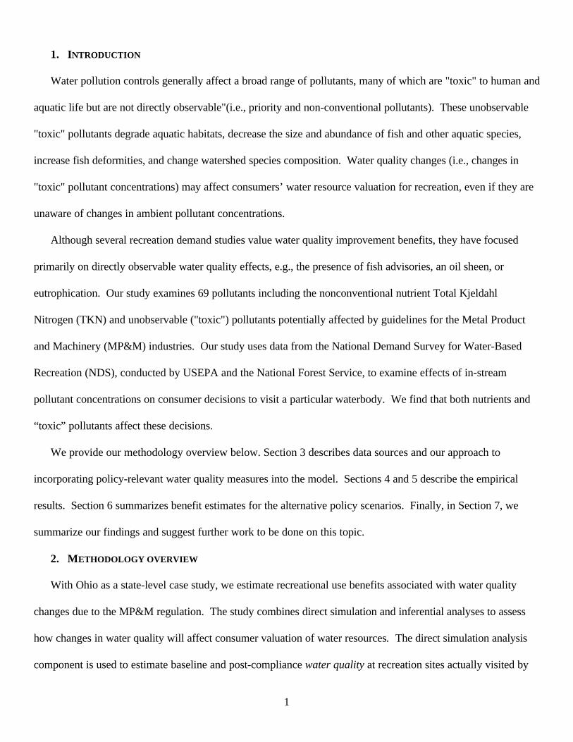
to the recreation site(s), and number of participants. Where fishing was the primary purpose of a trip,

respondents were also asked to state the number of fish caught. Figure 1 shows the number of trips taken per

year by primary recreation activity, as reported in the NDS

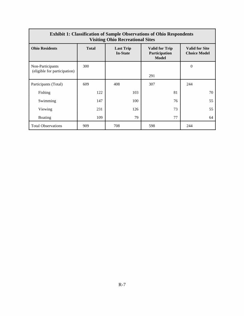
We selected case study observations for Ohio residents who took trips within that state.1 The fishing,

swimming, and viewing models included single-day trips only. We used both single- and multiple-day (i.e.,

weekend) trips to analyze boating trips. We included only activity participants with valid home town zip codes

and whose destination site was uniquely identified. We used data on both participants and non-participants to

estimate total seasonal trips, but only participants were included in the site choice model. Unusable site choice

participant observations with missing location information, were used to analyze the number of trips. Exhibit 1

lists valid observations by activity and model type.

3.2. Estimating the Price of Visits to Sites - Trip “price” is estimated as the sum of travel costs plus the

opportunity cost of time. Based on Parsons and Kealy (1992), we assume time spent “on-site” is constant across

sites and can be ignored in the price calculation. To estimate travel cost we multiplied round-trip distance by

average motor vehicle cost per mile ($0.29, 1993 dollars), and by the respondent family’s share of total

recreation party size, to estimate consumer travel cost.2 3 Trip time and hourly wage were used to compute the

consumer’s opportunity cost of time. We divided round-trip distance by 40 miles per hour to estimate trip time,

and used one-half the average hourly income to yield the opportunity cost of time.4 Visit price was thus

calculated as follows:

Visit Price=Round Trip Distance × $.29 × % Paid + {Round Trip Distance/40mph × 0.5 × Hourly Income}.

3.3. Site Characteristics - We identified 1,954 recreation sites on 1,631 reaches in the universal

opportunity set. Of these, 580 observations are known recreational sites; 1,366 observations are Reach File 1

(RF1) reaches without a known recreational site, and 8 observations are neither located in RF1 nor identified as

5 Substitute sites can be located outside of Ohio as well. Our analysis is based, however, on survey responses corresponding to Ohioresidents who took recreation trips within the State of Ohio. We therefore considered in-state substitute sites only.

6 McFadden (1978) has shown that estimating a model using random draws can give unbiased estimates of the model with the full set ofalternatives.

7We use the logarithm of ACRE because we expect effect of waterbody size on utility to diminish as that size increases.

5

known recreation sites but were visited by an NDS respondent. Each consumer choice set theoretically includes

hundreds of substitutable recreation sites in Ohio.5 To prevent recreation site analysis from becoming

unmanageable and overly costly, we analyze a sample of recreation sites for each consumer observation. We

create randomly chosen reduced choice sets consisting of 20 sites per participant.6 Each participant choice set,

by definition, includes the site actually visited by the respondent. For each consumer, additional sites are drawn

from a geographic area defined by a travel time constraint. We use the greater of (1) 120 miles or (2) the

estimated travel distance to the visited site as the limit. The resulting aggregate choice set of sites for all

individuals is the set of recreation sites used to model consumer decisions regarding trip allocation across

recreation sites.

We estimate site choice using two classes of characteristics: 1) those unaffected by the MP&M regulation,

but likely to determine valuation of water-based recreational resources; and (2) those affected by the regulation

and hypothesized to be significant in explaining recreation behavior and resource valuation. Regulation-

independent site characteristics include waterbody type and size, location characteristics, and the presence of site

amenities (e.g., boat ramps, swimming beaches, picnic areas). Regulation-dependent site characteristics include

regulation-affected water quality variables.

RF1 provided waterbody type (lake, river, or reservoir) and physical dimension (length, width, and depth).

The dummy variable, RIVER, characterizes waterbody type. If a river waterbody, RIVER takes the value of 1;

0 otherwise. We use the logarithm of the waterbody area LN_ACRE to define waterbody size.7 We multiply

reach width by segment length to yield waterbody area. Waterbody size data for sites not located in RF1 came

from the Ohio Department of Natural Resources (ODNR).

ODNR, supplemented by the Ohio Atlas and Gazetteer, provided data on recreational amenities and site

setting (e.g., presence/absence of boat ramps, swimming beaches, or picnic areas; public accessibility; and size of

land available for recreation). Land available for recreation, LN_LNDAC, (i.e., state park acreage, fishing ,

6

hunting, and other recreation areas) is used to approximate site setting and attractiveness. Dummy variables

represent the presence of four recreational amenities: RAMP is a boat ramp; BEACH is a swimming beach;

DOCK is a boating dock; and PARK indicates a park.

Selecting regulation-dependent site characteristic variables that are both policy-relevant and significant in

explaining recreation behavior proves challenging. MP&M facilities discharge many pollutants, most of them

unlikely to have visible indicators of degraded water quality (e.g., odor, reduced turbidity, etc). We hypothesize

that pollutant loadings can, nonetheless, reduce the likelihood of selecting a recreation site. Reduced pollutant

discharges improve water quality and aquatic habitat, thereby increasing fish populations and enhancing

recreational fishing experience. In addition, in-stream nutrient concentrations are good predictors of

eutrophication, which causes aesthetic losses and, thus, may affect the utility of a water resource for all four

recreational uses. The connection between the policy variables (i.e., the change in concentrations of MP&M

pollutants) and the effects perceived by consumers (e.g., increased catch rate, increased size of fish, greater

diversity of species, or improved aesthetic qualities of the waterbody) are not modeled directly, but are captured

implicitly in the differential valuation of water resources as reflected in the RUM analyses.

We consider two types of pollutant effects in defining water quality variables for model inclusion: (1) visible

or otherwise directly observable effects (TKN); and (2) unobservable "toxic" effects likely to impact aquatic

habitat and species adversely. We account for directly observable effects using the ambient concentrations of

nutrients (TKN) as an explanatory variables. Rather than include the concentrations of all “toxic” pollutants

separately, we construct a variable to reflect the adverse impact potential of “toxic” pollutants on aquatic habitat.

We identify recreation sites at which estimated concentrations of one or more MP&M pollutants exceed Ambient

Water Quality Concentration (AWQC) limits for aquatic life protection, to assess the likely adverse impacts on

aquatic organisms. A dummy variable, AWQC_EX, takes the value of 1 if in-stream concentrations of at least

one MP&M pollutant exceed AWQC limits for aquatic life protection, 0 otherwise. This approach accounts for

the fact that adverse effects on aquatic habitat are not likely to occur below a certain threshold level.

8 We considered a nested structure in which individuals first chose a recreation activity, and then made the first choice of which site to visitconditional upon that activity. This model, however, did not perform as well.

7

4. SITE CHOICE MODEL ESTIMATES

We estimate four separate models of recreational demand: fishing, boating, swimming, and viewing.8 Trips

are classified by primary activity listed by the respondent. The fishing, swimming, and viewing models cover

single-day trips. The boating model includes day and weekend trips; the latter comprised 80 percent of sample

boating trips. Mean duration of a single- and multiple-day boating trip is 7.85 hours and 1.59 days, respectively;

mean travel distance is 27.6 miles and 41.59 miles, respectively. Due to their similarities, we modeled single-day

and weekend boating trips together.

We estimate the site choice model using the site actually visited and 19 randomly drawn sites from the choice

set for each recreation activity. Exhibit 2 lists the variables used as arguments in the utility function and

summarizes the estimation results for the four models. Below, we provide a short description of the results of

the site choice models corresponding to each recreation activity.

Fishing Model: Anglers were identified as either cold- or warm-water fishermen, based on information on

targeted species provided in the NDS survey. Of the 70 observations available for estimating the site choice

fishing model, 30 and 40 observations are for cold and warm water fishing, respectively. To account for

heterogeneous choice sets in the model, our angler opportunity set contained only sites with the relevant type of

aquatic life (Haab T. and R. Hicks, 1997).

The most significant variables in determining fishing site choice were price, presence of boating docks,

waterbody size (log of water acres), the index of well being (IWB2), exceedences of AWQC limits, and in-stream

concentrations of TKN. All coefficients have the expected sign and are significantly different from zero at the

95th percentile. The goodness of fit measure, ρ 2, is equal to 0.59.

Other variables, tested as explanatory variables, were found to be insignificant, including the presence of fish

consumption advisories (FCAs). It might be expected, a priori, that the presence of an FCA decreases a site’s

likelihood as a fishing choice. In fact, the existence of FCAs did not affect a site’s probability of being chosen

significantly; 59% of the sites actually chosen by NDS respondents had an FCA in place. Creel surveys provided

8

by the Ohio Department of Natural Resources, indicated that, on average, anglers released 70 percent of their

catch (ODNR, 1997). This finding suggests that recreational anglers are aware of FCAs, and catch but do not

consume fish in the affected areas.

Boating Model. Boaters prefer to visit cheaper, cleaner, and larger water bodies with more abundant

aquatic life. In addition, the significant positive effect of the fish abundance and diversity variable (index of well

being) on boaters’ decisions to visit a particular site suggests that boating trips often have multiple purposes,

including fishing or wildlife viewing. Of the variables representing site amenities and attractiveness, only the

presence of boating docks was significant. On-site amenities, such as swimming beaches or size of the land

available for recreation activities, are not relevant to boating site choice. All coefficients on water quality

variables have the expected signs. The IWB2 and AWQC_EX coefficients are significantly different from zero at

the 95th and 85th percentile, respectively. The TKN is not significant from zero in the original model. The

goodness of fit measure, ρ 2, for the boating model is 0.79.

Swimming Model: Price, waterbody size, and the presence of a park with a beach, increase the probability

of particular site choice for swimming. Swimmers are less likely to visit sites located on a river, sites with

AWQC exceedences, and sites with relatively high in-stream concentrations of TKN.

Again, some variables expected to be significant, such the presence of contact advisories, were not. This

variable’s insignificance probably stems from its scarcity. Of 1,954 sites included in the universal opportunity set,

contact advisories are in place for only 13. (None of the sites actually visited had contact advisories in place.)

The probability that a chosen site has contact advisories in place is very small, because individual choice sets are

randomly selected. The IWB2 variable representing biological characteristics of a waterbody did not have a

significant influence on consumer decisions to visit a particular site. This outcome is not surprising, since

abundant aquatic life may, in fact, interfere with swimming activities. All coefficients have the expected signs

and are significantly different from zero. The goodness of fit measure, ρ 2, for the swimming model is 0.55.

Viewing (near-water activity) model. The probability of choosing a site for near-water activities was most

significantly related to visit price, waterbody and land size, whether the site is on a river, IWB2, the presence of

9 The data on the number of trips in the season from the NDS suffer from ‘overdispersion’. A negative binomial model was used in place ofthe simple Poisson model to correct for this overdispersion, as explained in the reference section.

9

AWQC exceedences, and in-stream concentration of Total Kjeldahl Nitrogen (TKN). The goodness of fit

measure for the viewing model, ρ2, is 0.76.

To test the stability of analytic results, we selected five alternative choice sets by repeating the random draw

procedure used for selecting individuals’ choice sets. We then estimated the fishing, boating, swimming, and

viewing model parameters based on alternative choice sets. We found that our results are relatively stable across

alternative draws.

5. TRIP PARTICIPATION MODEL

We estimated the determinants of individual choice concerning how many trips to take during a recreation

season with a separate model for each of the four activities. These participation models rely on socioeconomic

data, and on estimates of individual utility (the inclusive value) derived from the site choice models. Variables of

importance include age, ethnicity, gender, education, and number of children in the household. Exhibits 3 and 4

present descriptive statistics and define these explanatory variables.9 Results for the participation models of the

four recreation activities are presented in Exhibit 5.

All parameter estimates of the inclusive value index (IVBASE) are within the unit interval [0,1], which

assures us that the model does not violate random utility maximization assumptions. IVBASE coefficients are

positive and differ significantly from zero at the 95th percentile, indicating that water quality improvements have a

positive effect on the number of trips taken during a recreation season.

The AGE variable is negative and significant for all four recreation activities: younger people are likely to

take more recreation trips. Ethnicity and gender (the AFAM and MALE variables) also have a significant impact

on whether an individual participates in water-based recreation. African-Americans living in Ohio are less likely

to participate in any of the four recreation activities than representatives of other ethnic groups. Males are more

likely than females to participate in fishing, boating, and viewing.

Education also influences trip frequency significantly. People who did not complete high school (NOHS = 1)

tend to take fewer recreation trips. Those with a college degree (COLLEGE=1) are more likely to participate in

10

swimming and viewing. Respondents who attended college are less likely, however, to participate in fishing and

boating than those who completed only a high school education. For the boating model, the COLLEGE variable

is significant only at the 80th percentile level.

The presence of older children (KIDS_7UP) in the household is associated with greater participation in

swimming and viewing (near-water recreation) activities, but tends to have a negative impact on participation in

boating trips, and is not a significant determinant in decisions to participate in fishing.

People living in urban areas (URBAN=1) are less likely to participate in boating and viewing than people

who live in suburban and rural areas. Urban location is not a significant influence on the number trips taken for

swimming and fishing purposes.

6. ESTIMATING BENEFITS FROM WATER QUALITY IMPROVEMENTS

We use hypothetical policy scenarios to evaluate potential water quality benefits in our model, because

MP&M facility pollutant loading reduction estimates are not yet available. We calculate from water quality

benefits based on an assumed percentage reduction in pollutant concentrations and on a hypothetical reduction in

the number of streams exceeding AWQC values for MP&M pollutants. Two policy scenarios are considered:

• Scenario 1: Eliminate AWQC exceedences at 10 percent of recreation sites (18 sites) whose base-lines

exceed relevant AWQC values; reduce TKN concentrations at all recreation sites by one percent.

• Scenario 2: Eliminate AWQC exceedences at all 180 recreation sites whose baselines exceed relevant

AWQC values.

To estimate the value of water quality improvements, we first calculated seasonal welfare gain corresponding

to each policy scenario. The expected increase in utility per trip is small for Scenario 1, because AWQC

exceedences are eliminated at only a few MP&M sites. Scenario 2, eliminating all AWQC exceedences in

reaches with MP&M discharges, results in a substantial increase in per trip values for all recreation activities.

Per-trip welfare gain is greatest for boaters under Scenario 2, which proves consistent with prior findings.

Boating is the only activity where multiple-day trips were modeled; previous economic studies found greater per-

trip water quality welfare gains for multiple-day than for single-day trips. Under Scenario 1, however, per-trip

11

welfare gain for boaters is slightly less than for anglers. The site choice set for boating is much smaller than for

fishing (i.e., boating is allowed on only a subset of sites), so fewer relevant sites experience water quality

improvements.

Estimated per-person trip benefits and state-level annual benefits are shown in Exhibit 6. Trip benefits per

person range from $0.05 to $0.08 for Scenario 1, and $0.81 to $3.82 for Scenario 2.

Extrapolating from the sample to the adult population in Ohio yields annual benefit estimates of $1.4, $1.1,

$0.5, and $0.3 million dollars ($1993) for fishing, swimming, viewing and boating, respectively, under Scenario

1; and $36.9, $20.4, $17.6, and $5.7 million dollars ($1993) for fishing, swimming, viewing and boating,

respectively, for Scenario 2.

7. CONCLUDING REMARKS

Preliminary results indicate that consumer decisions to visit a particular recreational site, for any of the four

activities examined, are negatively influenced by MP&M pollutant loadings that adversely affect aquatic habitat

or produce visible water quality effects (e.g., TKN). Reducing ambient concentrations of these pollutants

improves water quality and aquatic habitat, leading to an enhanced recreational experience and an increase in

recreational activities. Water pollution control policies, such as the MP&M regulation, therefore have the

potential to generate substantial recreational benefits.

We considered two hypothetical policy scenarios for this preliminary test. The resulting per-person per-day

benefits from the water quality improvements are consistent with the magnitude of benefit estimates reported in

prior research. For example, Needleman and Montgomery (1995) report the estimated benefits per person per

day from eliminating toxic contamination of freshwater fish in New York of $.20 (1995). Needleman and Kealy

(1995) estimated that eliminating oil and grease in New Hampshire lakes results in an increase in recreational

swimming values of $0.09 per person per day.

The study addresses a wide range of pollutant types and effects, including water quality measures not often

addressed in past recreational benefits studies. In particular, these measures include “toxic” pollutants whose

effects are not directly observable. The estimated model allows policy makers to more fully analyze recreational

12

benefits from reducing nutrients and “toxic” pollutants.

Three of the four recreational choice models understate benefits by excluding both multiple-day and interstate

trips for activities. Future extensions of the model to include a wider set of trips would provide a more complete

estimate of recreational benefits.

R-1

References

Bockstael, N.E., I.E. Strand, and W.M. Hanemann. 1987. Time and the Recreation Demand Model. AmericanJournal of Agricultural Economics 69:213-32.

Creel, M. and J. Loomis. 1992. Recreation Value of Water to Wetlands in the San Joaquin Valley: LinkedMultinomial Logit and Count Data Trip Frequency Models. Water Resource Research. Vol28. No 10pp.2597-2606, October 1992.

Feather, Peter M. ; Hellerstein, Daniel, and Tomasi, Theodore. A Discrete-Count Model of Recreation Demand.Journal of Environmental Economics and Management. 1995; 29:214-227.

Hanemann. M. 1982. An Applied Welfare Analysis with Qualitative Response Models. Working PaperNo.241, Giannini foundation of Agricultural Economics, University of California, October 1982.

Hausman, J., G. Leonard, D. McFadden. 1995. A Utility-Consistent, Combined Discrete Choice and CountData Model: Assessing Recrational Use Losses Due to Natural Resource Damage. J. of PublicEconomics No 56 pp1-30. 1995.

Haab, T. and R. Hicks. 1997. Accounting for Choice Site Endogeneity in Random Utility Models of RecreationDemand. Journal of Environmental Economics and Management 34, 127-147 (1997).

McFadden, D.. 1978. Modeling the Choice of Residential Location. I. A. Karlquist et al. Eds., SpatialInteraction Theory and Planning Models, Amsterdam: North-Holland Publishing, pp. 75-96.

Montgomery, M. And M. Needelman. 1997. The Welfare Effects of Toxic Contamination in FreshwaterFish. Land Economics 72(2): 211-223.

Morey, E.R., R.D. Rowe, and M. Watson. 1993. A Repeated Nested-Logit Models of Participation and SiteChoice. American Journal of Agricultural Economics 75 No.3.

Needleman, M. S. and M. J. Kealy.1995. Recreational Swimming Benefits of New Hampshire Lake WaterQuality Policies: An application of a Repeated Discrete Choice Model. Agricultural and ResourceEconomics Review, April 1995: 78-87.

Ohio Atlas and Gazetteer, The. 1995. Freeport, ME: Delorme.

Ohio Department of Natural Resources, Division of Wildlife. Creel Survey Summaries from 1992 to 1997.

Parsons, G. and M.J. Kealy. 1992. Randomly Drawn Opportunity Sets in a Random Utility Model of LakeRecreation. Land Economics 68 No. 4(1992): 418-33.

ATTACHMENT : COMBINED DISCRETE CHOICE AND COUNT DATA MODEL

In this attachment, we describe in detail the linked discrete choice and count data model used to estimatechanges in welfare presented in the text.

Modeling the Site Choice Decision

We use a RUM framework to estimate the probability of a consumer visiting a recreation site. We

R-2

Bjn'Pr(Vjn%>jn>Vsn%>sn) (1)

Bjn'e

Vjn

jJ

j'1e

Vjn(2)

Vjn'$M(Mjn&Pjn)%$Xjn (3)

assume that a consumer derives utility from the recreational activity at each site. Each decision to make a visitinvolves choosing one site and excluding others. The consumer’s decision involves comparing their utility fromvisiting each site and choosing the site that produces the maximum utility. Because an observer cannot measureall potential determinants of consumer utility, the indirect utility function will have a non-random element (V)and a random error term (ξ), such that the actual determinants of consumer utility VN = V + ξ.

The probability (πjn) that site j will be visited by an individual n is defined as:

where:Vjn +ξjn = utility of visiting site j;Vsn + ξsn = utility of visiting a substitute.

If the random terms ξij, for individual i at site j are independently and identically distributed and have anextreme value Weilbull distribution, π jn takes the form of a multinomial logit model (McFadden, 1978):

where:

= the consumer’s utility from visiting site j.eV jn

= the sum of the consumer’s utility at each site j for all sites in the opportunity set.eV

j

Jjn

=∑

1

Estimation of the model requires specification of the functional form of the indirect utility function, V, inwhich site choice is modeled as a function of site characteristics and the “price” to visit particular sites. Forexample, a set of conditional utility functions (one for each site alternative j in the choice set) can be determinedas follows:

where:Vjn = The utility realized from a conventional budget-constrained, utility maximization model

conditional on choice of site j by consumer n. βΜ = Marginal utility of income.Mjn = The income of individual n available to visit site j. Pjn = A composite measure of travel and time costs for consumer n on site alternative j. β= = A vector of coefficients representing the marginal utility of a specified site characteristic to be

estimated along with βΜ (e.g. size of the waterbody, presence of boating ramps).Xjn = A vector of site characteristics for site alternative j as perceived by consumer n. These

characteristics include the actual monitored and/or modeled water quality parameters that arehypothesized to be determinants of consumer valuation of water-based recreation resourcesand that may also be affected by the MP&M regulation.

The magnitude of the coefficients in equations 2 and 3 reflects the relative importance of sitecharacteristics when consumers decide which site to visit. The coefficients ($) of water quality characteristics

R-3

CVjn'

ln[jJ

j'1

eVjn(W0)

]&ln[jJ

j'1

eVjn(W1)

]

$M

(5)

of recreation sites are expected to be positive, that is, all else being equal, consumers of water-based recreationwould prefer "cleaner" recreation sites. The coefficient on travel cost is expected to be negative, i.e.,consumers prefer lower travel cost. To estimate the model described by equations 2 and 3, we use a standardstatistical software package, LIMDEP.

Once the parameters of the indirect utility function are estimated, they are used to estimate the inclusivevalue. For consumer n, the inclusive value measures the overall quality of recreational opportunities for eachwater-based activity and represents the expected maximum utility of taking a trip. Note that although we use arandom draw from the opportunity set for the purpose of estimating the model parameters, we calculate theinclusive value (i.e., the expected maximum utility) using all recreation sites in the consumer's opportunity set . The inclusive value is calculated as the log of the denominator in equation 2 (Bockstael, Hanemann, and Kling(1987)).

ln(jJ

j'1

eVjn(W)

) (4)

where:

= individual n’s utility from visiting site j;eV jn

W = a vector of baseline water quality characteristics.

The welfare change associated with water quality changes from the baseline to post-complianceconditions can be estimated as a compensating variation (CV), that equates the expected value of realizedutility under the baseline and postcompliance conditions. To calculate the welfare gain from water qualityimprovement for each consumer on a given day, we substitute in the model the estimated post-compliancevalues of water quality variables for the baseline values. We then estimate changes in social welfare as afunction of these variables by using a compensating variation measure (CV) for consumer n:

where:CVjn = the compensating variation for individual n at site j;j = 1,...,J represents a set of alternative sites for a given recreational activity;

is the inclusive value index;ln(jJ

j'1

eVjn(W)

)

W 0 = a vector of information describing baseline water quality;W1 = a vector of information describing post-compliance water quality; and

βΜ = the implicit coefficient on income that influences recreation behavior.

In deriving Equation 5, we assume that the marginal utility of income, β M, is constant across alternatives(as well as across quality changes). If this assumption does not apply, the derivation of Eq. 5 is morecomplicated (Hanemann, 1982).

Modeling Trip Participation

After modeling the site choice decision, the next step is to model the determinants of the number of tripsa consumer of water-based recreation takes during a season. To link the quality of available recreation siteswith consumer demand for recreation trips, we model the number of recreation trips taken during the recreation

R-4

Prob(Yn'yn)'e&8n8

yn

n

yn!(6)

E[yn|xn]'Var[yn|xn]'e$)xn (7)

season as a function of the inclusive value estimated in the previous step and socioeconomic characteristicsaffecting individuals’ demand for recreation activities. The dependent variable, the number of recreation tripstaken by an individual during the recreation season, is an integer value greater than or equal to zero. Toaccount for the non-negative property of the dependent variable, we use count data models based on probabilitydensities that have the non-negative integers as their domain. One of the simplest count data models is aPoisson estimation process, which is commonly used with count data such as number of recreation trips duringthe recreation season. Inherent in the model specification is the assumption that each observation of a numberof trips is drawn from a Poisson distribution. Such a distribution favors a large number of observations withsmall values (e.g., 2 trips, 4 trips) or zeros, resulting in its being skewed toward the lower end. Due to thenature of the observed number of trips, it is quite reasonable to assume that the underlying distribution can becharacterized as a Poisson distribution. Figure 1 shows the number of recreation trips taken per year and thenumber of respondents who reported taking that number of trips.

Estimating the Poisson model is similar to estimating a nonlinear regression. The single parameter ofthe Poisson distribution is λ, which is both the mean and variance of yn. The probability that the actual numberof trips taken is equal to the estimated number of trips is estimated as follows:

where:Yn = the actual number of trips taken by an individual in the sample;yn = the estimated number of trips taken by an individual in the sample;n = 1, 2,..., N, the number of individuals in the sample; andλn = $NX, expected number of trips for an individual in the sample, where X is a vector of variables

affecting the demand for recreational trips (e.g., inclusive value and socioeconomiccharacteristics) and β is the vector of estimated coefficients.

From Equation 6, the expected number of trips per recreation activity season is given by:

where:E[yn|xn] = the expected number of trips, yn, given xn;Var[yn|xn] = the variance of the number of trips, yn, given xn;$ = a vector of coefficients on x; x = a matrix of site characteristic and socioeconomic variables.

An empirical drawback of the Poisson model is that the variance of the number of trips taken must beequal to the mean number of trips and this equality is not always supported by actual data. In particular, theNDS survey data exhibit “overdispersion,” a condition where variance exceeds the mean. The estimatedvariance to mean ratios of the number of trips in the NDS data sample are 31, 27.9, 35.6, and 10.5 for fishing,swimming, viewing and boating trips, respectively. Overdispersion is therefore present in the data set.

To address the problem of overdispersion, we use the negative binomial regression model, an extension

R-5

ln 8n ' $Xn % , (8)

Var[yn]'E[yn](1%"E[yn]) (10)

Var[yn]

E[yn]'1%"E[yn] (11)

of the Poisson regression model, which allows the variance of the number of trips to differ from the mean. Inthe negative binomial model, λ is respecified so that

where the error term (,) has a gamma distribution, E[exp(,i)] is equal to 1.0, and the variance of , is α.

The resulting probability distribution is

Prob[Y'yn|,]'e8nexp(,)8

yn

n

yn!(9)

where:yn = 0,1,2... number of trips taken by an individual in the sample;n = 1,2,..., N number of individuals in the sample;λn = expected number of trips for an individual in the sample.

Integrating , from Equation 9 produces the unconditional distribution of yn. The negative binomialmodel has an additional parameter, α, which is the overdispersion parameter, such that

The overdispersion rate is then given by the following equation:

We use the negative binomial model to predict the seasonal number of recreation trips for eachrecreation activity based on the inclusive value, individual socioeconomic characteristics, and theoverdispersion parameter, α. If the inclusive value has the anticipated positive sign, increases in the inclusivevalue stemming from improved ambient water quality at recreation sites will lead to an increase in the numberof trips. The combined multinominal logit model site choice and count data trip participation models allow usto account both for changes in per trip welfare values and for increased trip participation in response toimproved ambient water quality at recreation sites.

R-6

Figure 1: Number of Trips Per Year By Activity Type

R-7

Exhibit 1: Classification of Sample Observations of Ohio Respondents Visiting Ohio Recreational Sites

Ohio Residents Total Last TripIn-State

Valid for TripParticipation

Model

Valid for SiteChoice Model

Non-Participants (eligible for participation)

300

291

0

Participants (Total) 609 408 307 244

Fishing 122 103 81 70

Swimming 147 100 76 55

Viewing 231 126 73 55

Boating 109 79 77 64

Total Observations 909 708 598 244

R-8

Exhibit 2:Site Choice Model Estimation Results

Variable Fishing Boating Swimming Viewing

PRICE a -0.0833

(-19.47)

-0.0535

(-6.286)

-0.0897

(-12.1)

-0.0934

(-17.07)

Ln_LNDAC b 0.16486

(6.605)N/A N/A

0.2711

(9.093)

Ln_ACRE c 0.3216

(11.75)

0.8062

(8.509)

0.0486

(1.9)

0.3444

(8.472)

River d

N/A N/A-1.6940

(-8.639)

-2.021

(-6.406)

Dock e 1.168

(6.42)

1.647

(3.168)N/A N/A

BEACH

+ PARK f N/A N/A0.9668

(9.435)N/A

AWQC_Ex g -0.8704

(-5.002)

-0.8172

(-1.549)

-0.5338

(-2.475)

-0.911

(-3.644)

IWB2 h 0.2131

(8.89)

0.1988

(2.806)N/A

0.1778

(4.476)

TKN i -0.7426

(-5.221)

-0.5663

(-1.099)

-0.5252

(-2.783)

-0.2467

(-1.716)

Goodness of fit,

D2

0.5879 0.7851 0.549 0.7674

a Price is calculated as 0.5*opportunity cost + travel cost.b Log of the number of land acres.c Log of the number of water acres.d 1 if the site is a river, and 0 otherwise (e.g., lake or reservoir). e 1 if a boating dock is present, and 0 otherwise. f 1 if the site is a park and a swimming beach is present, and 0 otherwise. g 1 for any reach if in-stream concentrations of at least one MP&M pollutant exceed the AWQC limits forprotection of aquatic life, and 0 otherwise. h Index of well being representing biological factors, such as species abundance and diversity.i In-stream concentrations of Total Kejldahl Nitrogen (mg/l).Note: T-statistic for test that coefficient equals 0 is given in parentheses below coefficient estimates. N/A indicates that the variable was not included in the estimation for this activity.

R-9

Exhibit 3: Variable Definitions for Trip Participation Model

Variable Name Description

IVBASE

AGENOHSCOLLEGEMALEKID_7UPURBANAFAMLEISURE HOURSConstant" (alpha)

The inclusive value is estimated using the coefficients obtained from the site choicemodels.Individual’s age. If the individual did not report age, their age is set to the sample mean.Equals 1 if the individual did not complete high school, 0 otherwise.Equals 1 if the individual completed college, 0 otherwise.Equals 1 if the individual is a male, 0 otherwise.Equals 1 if there are children ages 7 years or older in the household, 0 otherwise.Equals 1 if the individual is residing in an urban area.Equals 1 if the individual is African American, 0 otherwise.The individual's number of leisure hours per week as reported in the survey.A constant term representing each individual’s utility associated with not taking a trip.Overdispersion parameter estimated by the Negative Binomial Model.

Exhibit 4: Mean Values for Explanatory Variables used in the Participation Models

Variables(Mean)

Non-Participant

(N=291)

Fishing(N=81)

Boating(N=77)

Swimming(N=76)

Viewing(N=73)

# TRIPS 0.00 10.19 2.35 8.78 9.63

AGE 43.99 38.87 39.14 35.08 36.51

KID_7UP 0.38 0.59 0.51 0.54 0.52

MALE 0.33 0.65 0.49 0.47 0.47

NOHS 0.17 0.15 0.10 0.16 0.15

COLLEGE 0.15 0.20 0.32 0.30 0.33

AFAM 1.07e-01 4.94e-02 2.60e-02 2.63e-02 1.37e-01

LEISURE 18.90 25.74 26.83 20.42 24.77

URBAN 0.26 0.28 0.22 0.33 0.36

R-10

Exhibit 5: Trip Participation Negative Binomial Model Estimates

Variables/Statistics Fishing Boating Swimming Viewing

IVBASE 0.68 0.34 0.92 0.59

(2.99) (3.05) (4.74) (3.26)

NOHS -1.23 -1.82 -1.39 0.19

(-1.692) (-2.462) (-1.882) (.380)

COLLEGE -0.51 0.48 1.00 1.58

(-0.92) (1.30) (2.06) (2.92)

LEISUREN/A

0.20N/A

0.154

(2.06) (1.38)

KID_7UPN/A

-0.76 0.73 0.82

(2.30) (1.48) (1.68)

AFAM -1.76 -2.09 -3.45 -0.69

(-2.02) (-1.88) (-2.72) (-0.86)

AGE -0.446 -0.434 -0.369 -0.479

(-2.37) (-2.94) (-2.40) (-2.54)

URBAN N/A -0.59 N/A -0.55

(-1.40) (-1.10)

MALE 2.10 1.28 N/A 1.01

(2.95) (3.87) (2.47)

Constant -2.90 -4.42 -1.19 -2.97

(-2.32) (-3.00) (-1.17) (-2.05)

Alpha " 10.11 2.70 8.35 7.39

(6.91) (4.85) (6.10) (5.59)

Note: T-statistic for test that coefficient equals 0 is given in parentheses below coefficient estimates. N/A indicates that the variable was not included in the estimation for this activity.

R-11

Exhibit 6:Estimated Fishing Benefits from Water Quality Improvements

Policy Scenario/Activity

Welfare Change(in millions of 1993 dollars)a

Per Person Per Trip State-level BenefitsPer Year

Scenario 1:AWQC exceedences eliminated at 10% of reaches withMP&M discharges and baseline exceedences, and there is a1% reduction in total TKN levels at all MP&M dischargesites

• Fishing• Swimming• Viewing• Boating

$0.08$0.05$0.06$0.07

$1,390,159$1,113,864$461,692$291,950

Scenario 2:AWQC exceedences eliminated at all reaches with MP&Mdischarges and baseline exceedences

• Fishing• Swimming• Viewing• Boating

$2.18$0.81$1.95$3.82

$36,865,532$20,384,756$17,561,349$5,710,310

a. As the year of the NDS survey was 1993, the welfare changes are measured in 1993 dollars.