Ecological significance of core, buffer and transition boundaries in biosphere reserve: A remote...

Computational Ecology and Software, 2013, 3(4): 126-137

IAEES www.iaees.org

Article

Ecological significance of core, buffer and transition boundaries in

biosphere reserve: A remote sensing study in Similipal, Odisha, India

Anima Biswal1, A Jeyaram1, Sumit Mukherjee2, Umesh Kumar2

1Regional remote Sensing Centre, East, NRSC, ISRO, India

2Anthropological Survey of India, Kolkata, India

E-mail: [email protected]

Received 28 June 2013; Accepted 2 August 2013; Published online 1 December 2013

Abstract

Protected areas and national parks need periodic assessment and monitoring for evaluating natural resources,

effectiveness of management and studying the effects of global climate change. The present work has been

undertaken to prepare the multi-date vegetation density maps in terms of Normalised vegetation index (NDVI)

and to monitor the changes in and around the areas close to transition, buffer and core boundaries of Similipal

Biosphere Reserve (SBR) using digital remote sensing and GIS techniques.Time series Landsat images

covering a period of 30 years are used for change detection studies.

Keywords biosphere; reserve; similipal; core; buffer; transition; Remote Sensing; GIS; NDVI; vegetation

density.

1 Introduction

Biosphere Reserve (BR) is an international designation attributed by UNESCO for representative parts of

natural and cultural landscapes that extends over a large area of terrestrial or coastal/marine ecosystems or a

combination thereof. BRs are thus special environments where human beings and nature can co-exist

respecting each others’ needs. In order to carry out complementary activities of biodiversity conservation and

for sustainable management aspects, Biosphere Reserves are demarcated into three inter-related zones. These

are (I) natural or core zone (ii) manipulation or buffer zone and (iii) A transition zone outside the buffer zone.

A core zone secures legal protection and allows management and research activities that do not affect natural

processes and wildlife and this core zone is to be kept free from all human pressures external to the system. In

the Buffer Zone, which adjoins or surrounds core zone where uses and activities such as recreation, tourism,

fishing and grazing are permitted to an limited extent. The Transition Zone is the outermost part of a Biosphere

Reserve that is usually not delimited one and is a zone of cooperation where conservation, knowledge and

Computational Ecology and Software ISSN 2220721X URL: http://www.iaees.org/publications/journals/ces/onlineversion.asp RSS: http://www.iaees.org/publications/journals/ces/rss.xml Email: [email protected] EditorinChief: WenJun Zhang Publisher: International Academy of Ecology and Environmental Sciences


IAEES www.iaees.org

management skills are applied together. This area includes settlements, crop lands, managed forests and area

for intensive recreation, and other economic activities that is prevalent in the region.

Changes in land use/ land cover due to natural and anthropogenic activities can be observed using recent

and archived remotely sensed data. One of the major advantages of remote sensing technique is its capability

for repetitive coverage, which is necessary for change detection studies at global and regional scales. Change

detection of in land use/ land cover involves use of at least two period data sets. Multi date satellite images are

useful for both visual assessments of dynamics of forest ecosystems occurring at a particular time and space as

well as quantitative evaluation of LULC changes overtime (Tekle and Hedlund 2000; Gautam et al. 2003).

Vegetation mapping is very important application of remotely sensed data. Spectral profiles of vegetation

clearly show that the peak reflectance can be found in the near-infrared wavelengths mainly because of the

internal structure of ‘‘green’’ leaves, and the greatest absorption is in the red wavelengths because of the

presence of chlorophyll pigments.The normalized difference vegetation index (NDVI) is one of most

successfully used vegetation indices for land cover classification (Brown et al., 1993; Evans et al., 1993;

Loveland et al., 1991; Townshend et al., 1994). It is also used as an environmental indicator to monitor

temporal and spatial variation in vegetation density as well as the health and viability of plant cover (Fung et

al., 2000; Jiang et al., 2008; Wang et al., 2001; Weng et al., 2004; Ioannis and Meliadis, 2011; Ballestores and

Qiu, 2012), for the derivation of vegetation biophysical properties (Asrar et al., 1992; Goward and Huemmrich,

1992; Sellers et al., 1994) and for estimation of net primary production (Prince, 1991; Running and Nemani,

1988; Tucker and Sellers, 1986). The NDVI is correlated with many biophysical properties of the vegetation

canopy such as leaf area index (LAI), fractional vegetation cover, vegetation condition, and biomass. The

NDVI is used in several studies to estimate vegetation biomass, greenness, primary production, fraction of

absorbed photosynthetically active radiation (fAPAR) (e.g., Gropal et al., 1999; Kawamura et al., 2005; Koide

et al., 1998; Myneni and Williams, 1994; North, 2002; Telesca et al., 2006). The NDVI values increase as

green cover density increases (Lo, 1997); the values are calculated from red and near infrared reflection values

(Fung and Siu, 2000; Jiang et al., 2008; Myeong, Nowak, and Duggin, 2006), that has a wide range used in

vegetation indices (Coops et al., 2008). The NDVI is a potential ecological indicator for successfully

monitoring temporal and spatial variation in vegetation density as well as the health and viability of plant

cover (Fung and Siu, 2000; Jiang et al., 2008; Wang et al., 2001; Weng et al. 2004).

Vegetated landscapes typically have NDVI values ranging from 0.1 in the desert to 0.8 in dense tropical

rain forest (Hassani, Benabadji, and Belbachir, 2006). Sobrino and Raissouni (2000) demonstrated that when

NDVI values are between 0.0 and 0.2, the pixel is considered bare soil; for NDVI values greater than 0.5, the

pixel is considered fully vegetated.

Protected areas and national parks need periodic assessment and monitoring for evaluating natural

resources, effectiveness of management and studying the effects of global climate change. The present work

has been undertaken to prepare the multi-date vegetation density maps in terms of Normalised vegetation

index and to monitor the changes in and around the areas close to transition, buffer and core boundaries of

Similipal Biosphere Reserve (SBR) using digital remote sensing techniques.

2 Study Area

The Similipal is a densely forested hill-range in the heart of Mayurbhanj district of Orissa in the eastern India,

lying close to the eastern-most end of the Easternghats. Located in the Mahanadian Biogeographical Region

and within the Biotic Province of Chhotanagpur Plateau, it is located between 2017' and 22 34' North latitude

and 8540' - 8710' East longitude. The total area of Similipal Biosphere Reserve (SBR) is 5569 Sq Km.

Similipal is unique in many respects, notable among which are its flora, fauna, forests, landscapes,

127


IAEES www.iaees.org

waterfalls and native tribal population. The landscape is beautifully scattered with numerous small and high

hills densely covered with vegetation. The highest mountain is the peak is Khairiburu which is

approximately 1168 mts. above the sea level. Similipal is the richest watershed in the state of Orissa giving

rise to many perennial rivers. Natural colour composite of the SBR along with core, buffer and transition

boundaries are presented in Fig.1. People residing in the Reserve area are largely tribal. Due to low level of

skills, lower educational levels, socio-culture traits, they are mainly dependent on local resources. There are

four villages inside the core namely, Kabatghai, Jenabil, Jamunagarh and Bakua. There are 61 villages in the

buffer. The climate of the area is monsoonal and divisible into three seasons; summer (March-June), rainy

(July- October) and winter (November-February). Pre-monsoon showers are received during May and June.

Post monsoon showers are received during November and December. The natural vegetation is moist

deciduous type (Champion and Seth, 1968) and is dominated by Shorea robusta, Anogeissus latifolia,

Buchnania lanzan, Dillenia pentagyna, Syzygium cumini and Terminalia alata. The area and status of SBR

since 1979 is presented in table 1. Similipal was declared as a biosphere reserve by Government of India on

22nd June 1994 due to its rich biodiversity and natural heritage. There are 1076 plants recorded from the area

including 60 species of ferns, 92 species of orchids and two gymnosperms (Saxena and Brahmam, 1989;

Misra, 2004).

Fig. 1 Natural colour composite of the SBR along with core, buffer and transition boundaries.

3 Data Source and Materials

We used time series Landsat images as the primary data source for derivation of generalized land-cover

information. Landsat images provide multispectral data from the early 1970s to the present. the spatial

resolution of Landsat data was appropriate to provide a general landscape characterization and change analysis

128


IAEES www.iaees.org

instead of detailed vegetation and resource mapping, As the intent of this study was to reveal the general trends

of land-cover change and landscape context, the difference in spatial resolution between MSS and TM/ETM+

images was not a concern as long as we obtained areas of different vegetation density classes. All the landsat

images were obtained from Global Land Cover Facility (GLCF) used to classify vegetation density in terms of

NDVI in the study area. The details of the images used are given in table 2. All the landsat images were

acquired during the dry season, which enables us to ensure that the images are completely cloud free, and also

allow us to differentiate forest from nonforest areas, with a greater degree of accuracy. All image processing

was carried out using the ERDAS Imagine image processing software. The biosphere was delineated in to core,

buffer and transition zones as per the map provided by the state forest department. The ancillary information

was collected by Anthropological Survey of India, Kolkota. Digital topographic maps digitized from hardcopy

Survey of India topographic maps with scale of 1:50,000 were used mainly for geometric correction of the

satellite images and for some ground truth information.

3.1 Geometric correction

After atmospheric correction and elimination of offset value of satellite data, in order to prepare two or more

satellite images for an accurate change detection comparison, it is imperative to geometrically rectify the

imagery.Geo referenced to the UTM map and WGS84 datum using 40–45 ground control points (GCPs) with a

root mean square error not exceed 0.5 pixels (Lunetta and Elvidge, 1998) for accurate registration of the

different time periods images. Accordingly, the 2005 image was used as the bases image to more precisely

geo-reference the other scenes. The correction were made using first order polynomial transformation model

and nearest neighbor method for re-sampling. The geo-referenced images were then clipped with vector masks

for transition, buffer and core boundary to generate the areas of interest.

3.2 Generation of NDVI image

NDVI is based on the spectral properties of green vegetation contrasting with its soil background. This index

has been found to provide a strong vegetation signal and good spectral contrast from most background

materials. NDVI is a measure derived by dividing the difference between near-infrared and red reflectance

measurements by their sum. NDVI provides an effective measure of photosynthetically active biomass (Tucker

and Sellers, 1986). For its measurement scientists use satellite sensors that observe the distinct wavelengths of

visible and near infrared sunlight which is absorbed and reflected by the plants, then the ratio of visible and

near-infrared light reflected back up to the sensor is calculated. The ratio gives a number from minus one (−1)

to plus one (+1). An NDVI value of zero means no green vegetation and close to +1 (0.8–0.9) indicates the

highest possible density of green leaves. The ‘normalized difference vegetation index’ is calculated by the

formula: NDVI = (IR−R)/(IR + R), where IR = infrared light and R = red light (Lellesand and Kiefer, 1994).

The group of pixels having NDVI values from 0 to 0.2 were categories under canopy density class of <10%,

0.2-0.4 as canopy density class of 10-40%, and, the group of pixels having NDVI value > 0.4 were kept under

the canopy density class of 40%.Normalized difference vegetation index NDVI was used to prepare a forest

density map that was categorized into three canopy density classes: <10% (non forest), 10-40% (open), > 40%

(medium/ high/ very high depending on the NDVI value . Image elements like tone, texture, shape, size,

shadow, location and association were also evaluated to aid in the class delineations.

There are many change detection techniques from visual comparison to detailed quantitative approaches

(Howarth and Wickware,1981).The fact that sums and differences of bands are used in the NDVI rather than

absolute values will make the NDVI more appropriate for use in studies where comparisons over time for a

single area are involved, since the NDVI might be expected to be influenced to a lesser extent by variation in

atmospheric conditions. An assessment of vegetation cover change in terms NDVI between 1975,1990 and

2005 was conducted using post classification change detection analysis and the results are as follows.

129


IAEES www.iaees.org

Table 1 Area and status

Zone Area (sq Km) status

Core 845 Sanctuary from 1979

National Park (1980/1986)

Buffer 2129 Sanctuary from 1979

Transition 2595 Reserved Forest

Table 2 Details of the Landsat images used in the study

Satellite/Sensor Path/row Date Spatial resolution

Landsat MSS 150 045 19 November 1975 56

Landsat TM 139 045 21November 1990 30

Landsat TM 139 045 14 November 2005 30

4 Results and Discussion

4.1 Transition zone

It is observed from Table 3 and Fig. 2, the area under < 0.2 class has increased significantly over the years in

the transition zone whereas the area under NDVI class 0.2- 0.4 has not undergone much change. During the

same period, the area under > 0.4 NDVI class has increased by 20,000 hectare. It is observed from Table 4 and

Fig. 3, the area under < 0.2 class has increased significantly over the years in the 5 km buffer area

surrounding the transition boundary whereas the area under NDVI class 0.2- 0.4 has not undergone much

change. During the same period, the area under > 0.4 NDVI class has also increased .This shows that less

dense forest area has undergone deforestation to a greater extent where as marginal reforestation occurred in

the high dense forest area.

Fig. 2 Area (ha) occupied by different NDVI classes in the transition zone in SBR.

4.2 Buffer zone

It is observed from Table 5, Figs 3 and 4, the area under < 0.2 class has increased significantly over the years

130


IAEES www.iaees.org

in the buffer zone whereas the area under NDVI class 0.2- 0.4 has decreased significantly. During the same

period , the area under > 0.4 NDVI class has increased by 15,300 hectare. As shown in Table 6 and Figs 3 and

4 there is an significant increase in < 0.2 NDVI class in the area surrounding 5 km buffer to buffer boundary of

SBR where as in the same area the other two NDVI classes have undergone very less change in area. This

shows that less dense and medium dense forest area has undergone deforestation where as reforestation

process was witnessed in the high dense forest.

Table 3 Area (ha) occupied by different NDVI classes in the transition zone in SBR.

NDVI classes

Transition

Zone 2005

Transition

Zone 1990 Transition Zone 1975

< 0.2 22582.4 21400.1 13579.2

0.2-0.4 182553 184406 193954

> 0.4 349828 347918 328659

Table 4 Area (ha) occupied by different NDVI classes in the 5 km buffer area surrounding

transition boundary in SBR.

NDVI classes

area surrounding

trans boundary

2005

area surrounding

trans boundary

1990

area surrounding

trans boundary

1975

< 0.2 31442 33690.3 19678.7

0.2-0.4 281941 287845 296546

> 0.4 407850 398168 378919

Table 5 Area (ha) occupied by different NDVI classes in the buffer zone in SBR.

NDVI classes

buffer Zone

2005

buffer Zone

1990 buffer Zone 1975

< 0.2 6576.12 3664.98 4365

0.2-0.4 33793.2 24580.2 47567.9

> 0.4 221881 233096 206580

Table 6 Area (ha) occupied by different NDVI classes in the 5 km buffer area surrounding

buffer boundary in SBR

NDVI classes

area

surrounding

buffer boundary

2005

area

surrounding

buffer boundary

1990

area surrounding buffer

boundary 1975

< 0.2 15967.8 13825 10645.9

0.2-0.4 120593 117671 132041

> 0.4 302390 306474 283494

131


IAEES www.iaees.org

4.3 Core zone

It is observed from Table 7 and Fig. 5 the area under < 0.2 and 0.2- 0.4 NDVI classes has decreased

significantly over the years in the core zone whereas the area under NDVI class > 0.4 has increased

significantly. Though the area under 0.2-0.4 NDVI class has decreased to a large extent but the concurrent

increase in other two classes corroborates that reforestation process occurred throughout the core zone that

very much in agreement with the core zone concept of a biosphere reserve.

Table 7 Area (ha) occupied by different NDVI classes in the core zone in SBR.

NDVI classes

core Zone

2005

core Zone

1990 core Zone 1975

< 0.2 21.6 10.98 329.76

0.2-0.4 3821.76 1733.04 14252.8

> 0.4 93539.2 95293.6 81992.5

Table 8 Area (ha) occupied by different NDVI classes in the transition zone excluding

buffer in SBR.

NDVI class

trans minus

buff_05

trans minus

buff_90 trans minus buff_75

< 0.2 16279.9 17850.9 9330.12

0.2-0.4 149676 160335 147316

> 0.4 129923 115747 124064

Table 9 Area (ha) occupied by different NDVI classes in the buffer zone excluding

core in SBR.

NDVI class

buff minus

core_05

buff minus

core_90 buff minus core_75

< 0.2 6499.08 3639.78 4057.56

0.2-0.4 30088.1 22869.7 33540.5

> 0.4 129428 138401 125482

132


IAEES www.iaees.org

Fig. 3 Vegetation density map in the 5 km outer buffer of transition and buffer bounaries in SBR in 1975.

Fig. 4 Area (ha) occupied by different NDVI classes in the buffer zone in SBR.

Fig. 5 Area (ha) occupied by different NDVI classes in the core zone in SBR.

133


IAEES www.iaees.org

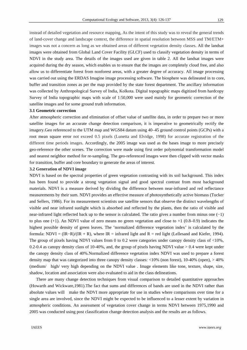
Fig. 6 Area (ha) occupied by different NDVI classes in the transition zone excluding buffer zone in SBR.

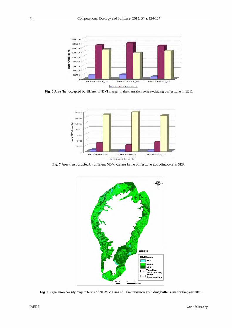
Fig. 7 Area (ha) occupied by different NDVI classes in the buffer zone excluding core in SBR.

Fig. 8 Vegetation density map in terms of NDVI classes of the transition excluding buffer zone for the year 2005.

134


IAEES www.iaees.org

Fig. 9 Vegetation density map in terms of NDVI classes of the buffer excluding core zone of SBR for the year 2005.

4.4 Transition zone excluding buffer zone

It is evident from the Table 8 and Figs 6 and 8 that the transition excluding buffer area in SBR is mostly

occupied by the medium dense forest with NDVI value 0f 0.2 to 04 throughout the time period from 1975 to

2005.There was a mariginal increase in 0.2- 0.4 NDVI class from 1975 to 1990 but again followed by a

decrease to the same extent. The area under the high dense forest cover has changed a little. In this zone

deforestation occurred in less dense forest cover as the area under < 0.2 NDVI class increased significantly.

4.5 Buffer zone excluding core zone

It is observed from Table 9 and Figs 7 and 9 the area under < 0.2 class has increased significantly over the

years in the buffer zone whereas the area under NDVI class 0.2- 0.4 has undergone significant decrease.

During the same period the area under > 0.4 NDVI class has increased by 20,000 hectare. This shows that less

dense vegetation forest area has undergone deforestation to a greater extent than the very dense vegetation area.

5 Conclusion

The results presented above are based on preliminary assessment from time series image analysis. Extensive

field work and survey has to be conducted to verify the results. In general it was observed that the high dense

forest in the core zone is conserved and highest reforestation has also occurred in this zone of SBR. Over the

years, forest density in terms of NDVI as evidenced from the time series Landsat images has increased as the

area under > 0.4 NDVI class has shown a positive trend throughout the zones of analysis.

135


IAEES www.iaees.org

Acknowledgement

This work is collaborately carried out by Regional Remote Sensing Centre, East, NRSC, ISRO, and

Anthropological Survey of India, Kolkata. The Authors are grateful to the Chief General Manager,

RC,NRSC,ISRO and Director ASI for their valuable support and guidance throughout the study.

References

Asrar G, Myneni RB, Choudhury BJ. 1992. Spatial heterogeneity in vegetation canopies and remote sensing of

absorbed photosynthetically active radiation: a modeling study. Remote Sensing of Environment, 41: 85-

101

Ballestores F Jr, Qiu ZY. 2012. An integrated parcel-based land use change model using cellular automata and

decision tree Proceedings of the International Academy of Ecology and Environmental Sciences, 2(2): 53-

69

Brown JF, Loveland TR, Merchant JW, et al. 1993. Using multisource data in global land-cover

characterization:concepts, requirements, and methods. Photogrammetric Engineering and Remote Sensing,

59: 977-987

Champion HG, Seth SK. 1968. A Revised Survey of the Forest Types of India. Govt. of India Press, Delhi,

India

Coops NC, Wulder MA, Iwanicka D. 2008. Demonstration of a satellite-based index to monitor habitat at

continental-scales. Ecological Indicators, 9: 948-958

Evans DL, Zhu Z, Winterberger K. 1993. Mapping forest distributions with AVHRR data. World Resource

Review, 5: 66-71

Fung T, Siu W. 2000. Environmental quality and its changes, ananalysis using NDVI. International Journal of

Remote Sensing, 21(5): 1011-1024

Gautam AP, Webb EL, Shivakoti GP, et al. 2003. Land use dynamics and landscape change pattern in a

mountain watershed in Nepal. Agriculture, Ecosystems and Environment, 99: 83-96

Goward SN, Huemmrich KF. 1992. Vegetation canopy PAR absorbance and the normalized difference

vegetation index: an assessment using the SAIL model. Remote Sensing of Environment, 39: 119-140

Gropal S, Woodcock CE, Strahler AH., 1999. Fuzzy neural network classification of global land cover from a

1u AVHHR data set. Remote Sensing of Environment, 67: 230-243

Hassani A, Benabadji N, Belbachir AH. 2006. AVHRR data sensor processing. Journal of Applied Science,

6(11): 2501-2505

Ioannis M, Meliadis M. 2011. Multi-temporal Landsat image classification and change analysis of land

cover/use in the Prefecture of Thessaloiniki, Greece. Proceedings of the International Academy of Ecology

and Environmental Sciences, 1(1): 15-25

Jiang X,Wan L, Du Q, et al. 2008. Estimation of NDVI images using geostatistical methods. Earth Science

Frontiers, 15(4): 7180

Kawamura K, Akiyama T, Yokota HO, et al. 2005. Quantifying grazing intensities using geographic

information systems and satellite remote sensing in the Xilingol steppe region, Inner Mongolia, China.

Agricultural Ecosystems & Environment, 107: 83-93

Koide M, Purevdorj T, Yokoyama R. 1998. AVHRR data correction for observing NDVI in a Mongolian

highland. In: Space Informatics for Sustainable Development (Sigh RB, Murai S, eds). 107-114, A.A.

Balkema, Netherlands

Lillesand TM, Kiefer RW. 1994. Remote Sensing and Image Interpretation (3rd ed). John Wiley and Sons,

136


IAEES www.iaees.org

Toronto, Canada

Lo CP. 1997. Application of Landsat TM data for quality of life assessment in an urban environment.

computers. Environment and Urban Systems, 21: 259-276

Loveland TR, Merchant JW, Ohlen DO, et al. 1991. Development of a land-cover characteristics database for

the conterminous U.S. Photogrammetric Engineering and Remote Sensing, 57(11): 1453-1463

Lunetta RS, Elvidge CD. 1998. Remote Sensing Change Detection. Ann Arbor Press, MI, USA

Misra S. 2004. Orchids of Orissa. 55-63 Bishen Singh & Mahendra Pal Singh Publication, Dehra Dun, India

Myeong S, Nowak DJ, Duggin MJ. 2006. A temporal analysis of urban forest carbon storage using remote

sensing. Remote Sensing of Environment, 101: 277-282

Prince SD. 1991. A model of regional primary production for use with coarse resolution satellite data.

International Journal of Remote Sensing, 12: 1313-1330

Running SW, Nemani RR. 1988. Relating seasonal patterns of the AVHRR vegetation index to simulated

photosynthesis and transpiration of forest in different climates. Remote Sensing of Environment, 24: 347-

367

Saxena HO, Brahmam M. 1989. The Flora of Similipahar, Orissa. Regional Research Laboratory,

Bhubaneswar, India

Sellers PJ, Tucker CJ, Collatz GJ, et al. 1994. A global 1 by 1 NDVI data set for climate studies: Part 2. The

generation of global fields of terrestrial biophysical 236 parameters from the NDVI. International Journal

of Remote Sensing, 15: 3519

Sobrino JA, Raissouni N. 2000. Toward remote sensing methods for land cover dynamic monitoring:

application to Morocco. International Journal of Remote Sensing, 21(2): 353-366

Tekle K, Hedlund L. 2000. Land cover changes between 1958 and 1986 in Kalu District, Southern Wello,

Ethiopia. Mountain Research and Development, 20(1): 42-51

Townshend JRG, Justice CO, Skole D. 1994. The 1 km resolution global data set: needs of the International

Geosphere Biosphere Programme. International Journal of Remote Sensing,15: 3417-3441

Tucker CJ. 1979. Red and photographic infrared linear combinations for monitoring vegetation. Remote

Sensing of Environment, 8: 127-150

Tucker CJ, Sellers PJ. 1986. Satellite remote sensing of primary productivity. International Journal of Remote

Sensing, 7:1395-1416

Wang J, Price KP, Rich PM., 2001. Spatial patterns of NDVI in response to precipitation and temperature in

the central Great Plains. International Journal of Remote Sensing, 22(18): 3827-3844

Weng Q, Lu D, Schubring J. 2004. Estimation of land surface temperature–vegetation abundance relationship

for urban heat island studies. Remote Sensing of Environment, 89: 467-483

Wickware GM, Howarth PJ. 1981. Change detection in the peace-Athabaska Delta using digital Landsat data.

Remote Sensing of Environment,11: 9-25

137

Ecological significance of core, buffer and transition boundaries in biosphere reserve: A remote...

Documents

Transcript of Ecological significance of core, buffer and transition boundaries in biosphere reserve: A remote...