ÉCOLE DE TECHNOLOGIE SUPÉRIEURE

UNIVERSITÉ DU QUÉBEC

MANUSCRIPT-BASED THESIS PRESENTED TO

ÉCOLE DE TECHNOLOGIE SUPÉRIEURE

IN PARTIAL FULFILLMENT OF THE REQUIREMENTS FOR

THE DEGREE OF DOCTOR OF PHILOSOPHY

Ph.D.

BY

Jean-François PAMBRUN

NOVEL JPEG 2000 COMPRESSION FOR FASTER MEDICAL IMAGE STREAMING

AND DIAGNOSTICALLY LOSSLESS QUALITY

MONTREAL, JUNE 21, 2016

Jean-François Pambrun, 2016

This Creative Commons license allows readers to download this work and share it with others as long as the

author is credited. The content of this work cannot be modified in any way or used commercially.

BOARD OF EXAMINERS

THIS THESIS HAS BEEN EVALUATED

BY THE FOLLOWING BOARD OF EXAMINERS:

Mme Rita Noumeir, Thesis Supervisor

Electrical Engineering, École de technologie supérieure

M. Stéphane Coulombe, President of the Board of Examiners

Software & IT Engineering, École de technologie supérieure

M. Jean-Marc Lina, Member of the Jury

Electrical Engineering, École de technologie supérieure

Mme Farida Cheriet, Independent External Examiner

Computer Engineering, École Polytechnique de Montréal

THIS THESIS WAS PRESENTED AND DEFENDED

IN THE PRESENCE OF A BOARD OF EXAMINERS AND THE PUBLIC

ON JUNE 15, 2016

AT ÉCOLE DE TECHNOLOGIE SUPÉRIEURE

ACKNOWLEDGEMENTS

First and foremost, I would like to thank my advisor, Rita Noumeir, for everything, especially

her patience. Her help and support have been essential to the completion of this thesis.

I would also like to thank my friends and colleagues from the lab, Houssem Eddine Gueziri,

Wassim Bouachir, Jawad Dahmani, Haythem Rehouma and Samuel Deslauriers-Gauthier as

well as Prof. Jean-Marc Lina and Prof. Catherine Laporte for their help and insight. I have

learned so much from them.

My family and friends have also been instrumental the success of this project by supporting me

through everything. Special thanks to my wife Mireille and my closest friends Julien Beaudry,

Jean-François Têtu, Marc-André Levasseur, Louis-Charles Trudeau, Karine Lacourse for their

much-needed support.

Finally, this research would not have been possible without the financial assistance that the

NSERC provided by awarding me the Alexander Graham Bell graduate scholarship.

NOUVELLE MÉTHODE DE COMPRESSION POUR UN TÉLÉVERSEMENT ENCONTINU PLUS RAPIDE ET UNE QUALITÉ DIAGNOSTIQUE SANS PERTE

Jean-François PAMBRUN

RÉSUMÉ

Les dossiers santé électroniques (DSE) peuvent significativement améliorer la productivité des

cliniciens ainsi que la qualité des soins pour les patients. Par contre, implémenter un tel DSE

robuste et universellement accessible peut être très difficile. Ceci est dû en partie à la quantité

phénoménale de données générées chaque jour par les appareils d’imagerie médicaux. Une

fois acquises, ces données doivent être disponibles à distance instantanément et doivent être

archivées pour de longues périodes, au moins jusqu’à la mort du patient. La compression

d’image peut être utilisée pour atténuer ce problème en réduisant à la fois les requis de trans-

mission et de stockage. La compression sans perte peut réduire la taille des fichiers par près

des deux tiers. Par contre, pour réduire davantage, il faut avoir recours à la compression avec

perte où le signal original ne peut plus être récupéré. Dans ce cas, une grande attention doit

être portée afin de ne pas altérer la qualité du diagnostic. En ce moment, la pratique usuelle

implique le recours à des barèmes de compression basés sur les taux de compression. Pourtant,

l’existence de variation du niveau de compressibilité en fonction du contenu de l’image est

bien connu. Conséquemment, pour être sûres dans tous les cas, les recommandations doivent

être conservatrices. Au même moment, les images médicales sont habituellement affichées

après une transformation de niveau de gris qui peut masquer certaines données de l’image et

engendrer des transferts de données inutiles. Notre objectif est d’améliorer la compression et

le transfert en continu d’images médicales pour obtenir une meilleure efficacité tout en conser-

vant la qualité diagnostique. Pour y arriver, nous avons 1- mis en évidence les limitations des

recommandations basées sur les taux de compression, 2- proposé une méthode de transfert en

continu qui tient compte de la transformation des niveaux de gris et 3- proposé une mesure de

qualité alternative spécialement conçue pour l’imagerie médicale qui exploite l’effet bénéfique

du débruitage tout en préservant les structures de l’image. Nos résultats montrent une vari-

abilité significative de la compressibilité, jusqu’à 66%, entre les séries et que 15% des images

compressées à 15:1, le maximum recommandé, étaient de moins bonne qualité que la médiane

des images compressées à 30:1. Lors de la transmission en continu, nous avons montré une

réduction des transferts de l’ordre de 54% pour les images en mode presque sans perte dépen-

damment de la plage des valeurs d’intérêts (VOI) examinée. Notre solution est également

capable de transférer et afficher entre 20 et 36 images par seconde avec la première image

affichée en moins d’une seconde. Enfin, notre nouvelle contrainte de compression a montré

une réduction drastique des dégradations structurelles et les performances de la métrique qui

en découle sont similaires à celle des autres métriques modernes.

Mots clés: JPEG 2000, Compression d’image, Téléversement d’images en continu, Évalu-

ation objective de la qualité d’image, Codage basé sur le VOI, Image médicale.

NOVEL JPEG 2000 COMPRESSION FOR FASTER MEDICAL IMAGESTREAMING AND DIAGNOSTICALLY LOSSLESS QUALITY

Jean-François PAMBRUN

ABSTRACT

Electronic health records can significantly improve productivity for clinicians as well as qual-

ity of care for patients. However, implementing highly available and universally accessible

electric health records can be very challenging. This is in part due to the tremendous amount

of data produced every day by modern diagnostic imaging devices. This data must be instantly

available for remote consultation and must be archived for very long periods, at least until the

patient’s death. Image compression can be used to mitigate this issue by reducing both net-

work and storage requirements. Lossless compression can reduce file sizes by up to two thirds.

Further improvements require the use of lossy compression where the original signal cannot

be perfectly reconstructed. In that case, great care must be taken as to not alter the diagnostic

properties of the acquired image. The current standard practice is to rely on compression ratio

guidelines published by professional associations. However, image compressibility is known

to vary significantly based on image content. Therefore, in order to be consistently safe, rec-

ommendations based on compression ratios have to be very conservative. At the same time,

medical images are usually displayed after a value of interest (VOI) transform that can mask

some of the image content leading to needless data transfers. Our objective is to improve med-

ical image compression and streaming to achieve better efficiency while ensuring adequate

diagnostic quality. To achieve this, 1- we have highlighted the limitations of compression ratio

based guidelines by analyzing the effects of acquisition parameters and image content on the

compressibility of more than 23 thousand computed tomography slices of a thoracic phantom,

2- we have proposed a streaming scheme that leverages the masking effect of the VOI trans-

form and can scale from lossy to near-lossless and lossless levels and 3- we have proposed an

alternative to compression scheme tailored especially for diagnostic imaging by leveraging the

beneficial denoising effect of compression while preserving important structures. Our results

showed significant compression variability, up to 66%, between series. Furthermore, 15% of

the images compressed at 15:1, the maximum recommended ratio, had lower fidelity than the

median of those compressed at 30:1. With our VOI-based streaming, we have shown a reduc-

tion in network transfers of up to 54% for near-lossless levels depending on the targeted VOI.

Our solution is also capable of streaming between 20 and 36 slices per second with the first

slice displayed in less than a second. Finally, our new compression constraint showed drastic

reduction in structure degradations and the performances of the derived metric were on par

with other leading metrics for compression distortions.

Keywords: JPEG 2000, Image compression, Image streaming, Objective image quality as-

sessment, VOI-based coding, Medical imaging.

TABLE OF CONTENTS

Page

INTRODUCTION . . . . . . . . . . . . . . . . . . . . . . . . . . . . . . . . . . . . . . . . . . . . . . . . . . . . . . . . . . . . . . . . . . . . . . . . . . . . . . . . 1

CHAPTER 1 BACKGROUND ON MEDICAL IMAGING INFORMATICS . . . . . . . . . . . . 5

1.1 Compression with JPEG 2000 . . . . . . . . . . . . . . . . . . . . . . . . . . . . . . . . . . . . . . . . . . . . . . . . . . . . . . . . . . . 5

1.1.1 Preprocessing . . . . . . . . . . . . . . . . . . . . . . . . . . . . . . . . . . . . . . . . . . . . . . . . . . . . . . . . . . . . . . . . . . 7

1.1.2 Transform . . . . . . . . . . . . . . . . . . . . . . . . . . . . . . . . . . . . . . . . . . . . . . . . . . . . . . . . . . . . . . . . . . . . . . 7

1.1.3 Quantization . . . . . . . . . . . . . . . . . . . . . . . . . . . . . . . . . . . . . . . . . . . . . . . . . . . . . . . . . . . . . . . . . . . . 9

1.1.4 Entropy coding (Tier-1 coding) . . . . . . . . . . . . . . . . . . . . . . . . . . . . . . . . . . . . . . . . . . . . . . 10

1.1.5 Code-stream organization (Tier-2 coding) . . . . . . . . . . . . . . . . . . . . . . . . . . . . . . . . . . . 10

1.2 Streaming with JPIP . . . . . . . . . . . . . . . . . . . . . . . . . . . . . . . . . . . . . . . . . . . . . . . . . . . . . . . . . . . . . . . . . . . . 13

1.3 Storage and communication with DICOM .. . . . . . . . . . . . . . . . . . . . . . . . . . . . . . . . . . . . . . . . . . . . 15

1.3.1 DICOM with JPEG 2000 . . . . . . . . . . . . . . . . . . . . . . . . . . . . . . . . . . . . . . . . . . . . . . . . . . . . . 16

1.3.2 DICOM with JPIP . . . . . . . . . . . . . . . . . . . . . . . . . . . . . . . . . . . . . . . . . . . . . . . . . . . . . . . . . . . . 17

1.4 Diagnostic imaging characteristics . . . . . . . . . . . . . . . . . . . . . . . . . . . . . . . . . . . . . . . . . . . . . . . . . . . . . 18

CHAPTER 2 LITERATURE REVIEW .. . . . . . . . . . . . . . . . . . . . . . . . . . . . . . . . . . . . . . . . . . . . . . . . . . . 23

2.1 Current state of lossy image compression in the medical domain . . . . . . . . . . . . . . . . . . . . 23

2.2 Image quality assessment techniques . . . . . . . . . . . . . . . . . . . . . . . . . . . . . . . . . . . . . . . . . . . . . . . . . . 25

2.2.1 Mathematical-based quality metrics . . . . . . . . . . . . . . . . . . . . . . . . . . . . . . . . . . . . . . . . . 28

2.2.2 Near-threshold psychophysics quality metrics . . . . . . . . . . . . . . . . . . . . . . . . . . . . . . 29

2.2.2.1 Luminance perception and adaptation . . . . . . . . . . . . . . . . . . . . . . . . . . . 29

2.2.2.2 Contrast sensitivity . . . . . . . . . . . . . . . . . . . . . . . . . . . . . . . . . . . . . . . . . . . . . . . . 30

2.2.2.3 Visual masking . . . . . . . . . . . . . . . . . . . . . . . . . . . . . . . . . . . . . . . . . . . . . . . . . . . . 31

2.2.3 Information extraction and structural similarity quality metrics . . . . . . . . . . . . 31

2.3 Image quality assessment metric evaluation . . . . . . . . . . . . . . . . . . . . . . . . . . . . . . . . . . . . . . . . . . . 32

2.3.1 Evaluation axes . . . . . . . . . . . . . . . . . . . . . . . . . . . . . . . . . . . . . . . . . . . . . . . . . . . . . . . . . . . . . . . 32

2.3.1.1 Prediction accuracy . . . . . . . . . . . . . . . . . . . . . . . . . . . . . . . . . . . . . . . . . . . . . . . 32

2.3.1.2 Prediction monotonicity . . . . . . . . . . . . . . . . . . . . . . . . . . . . . . . . . . . . . . . . . . 33

2.3.1.3 Prediction consistency . . . . . . . . . . . . . . . . . . . . . . . . . . . . . . . . . . . . . . . . . . . . 33

2.3.2 Image quality assessment databases . . . . . . . . . . . . . . . . . . . . . . . . . . . . . . . . . . . . . . . . . 34

2.4 Image quality assessment metric survey . . . . . . . . . . . . . . . . . . . . . . . . . . . . . . . . . . . . . . . . . . . . . . . 34

2.4.1 MSE/PSNR . . . . . . . . . . . . . . . . . . . . . . . . . . . . . . . . . . . . . . . . . . . . . . . . . . . . . . . . . . . . . . . . . . . . 35

2.4.2 SSIM . . . . . . . . . . . . . . . . . . . . . . . . . . . . . . . . . . . . . . . . . . . . . . . . . . . . . . . . . . . . . . . . . . . . . . . . . . . 35

2.4.3 MS-SSIM . . . . . . . . . . . . . . . . . . . . . . . . . . . . . . . . . . . . . . . . . . . . . . . . . . . . . . . . . . . . . . . . . . . . . . 37

2.4.4 VIF . . . . . . . . . . . . . . . . . . . . . . . . . . . . . . . . . . . . . . . . . . . . . . . . . . . . . . . . . . . . . . . . . . . . . . . . . . . . . 38

2.4.5 IW-SSIM . . . . . . . . . . . . . . . . . . . . . . . . . . . . . . . . . . . . . . . . . . . . . . . . . . . . . . . . . . . . . . . . . . . . . . 41

2.4.6 SR-SIM . . . . . . . . . . . . . . . . . . . . . . . . . . . . . . . . . . . . . . . . . . . . . . . . . . . . . . . . . . . . . . . . . . . . . . . . 42

2.4.7 Summary of performance . . . . . . . . . . . . . . . . . . . . . . . . . . . . . . . . . . . . . . . . . . . . . . . . . . . . . 44

2.5 Image quality assessment and compression in the medical domain . . . . . . . . . . . . . . . . . . 44

XII

CHAPTER 3 COMPUTED TOMOGRAPHY IMAGE COMPRESSIBILITY

AND LIMITATIONS OF COMPRESSION RATIO BASED

GUIDELINES . . . . . . . . . . . . . . . . . . . . . . . . . . . . . . . . . . . . . . . . . . . . . . . . . . . . . . . . . . . . . . . . 47

3.1 Introduction . . . . . . . . . . . . . . . . . . . . . . . . . . . . . . . . . . . . . . . . . . . . . . . . . . . . . . . . . . . . . . . . . . . . . . . . . . . . . . 47

3.2 Previous work . . . . . . . . . . . . . . . . . . . . . . . . . . . . . . . . . . . . . . . . . . . . . . . . . . . . . . . . . . . . . . . . . . . . . . . . . . . 49

3.3 Methodology . . . . . . . . . . . . . . . . . . . . . . . . . . . . . . . . . . . . . . . . . . . . . . . . . . . . . . . . . . . . . . . . . . . . . . . . . . . . 53

3.3.1 Data . . . . . . . . . . . . . . . . . . . . . . . . . . . . . . . . . . . . . . . . . . . . . . . . . . . . . . . . . . . . . . . . . . . . . . . . . . . . 53

3.3.2 Compression . . . . . . . . . . . . . . . . . . . . . . . . . . . . . . . . . . . . . . . . . . . . . . . . . . . . . . . . . . . . . . . . . . 56

3.3.3 Fidelity evaluation . . . . . . . . . . . . . . . . . . . . . . . . . . . . . . . . . . . . . . . . . . . . . . . . . . . . . . . . . . . . 56

3.3.4 Compressibility evaluation . . . . . . . . . . . . . . . . . . . . . . . . . . . . . . . . . . . . . . . . . . . . . . . . . . . 57

3.3.5 Statistical analysis . . . . . . . . . . . . . . . . . . . . . . . . . . . . . . . . . . . . . . . . . . . . . . . . . . . . . . . . . . . . 57

3.4 Results . . . . . . . . . . . . . . . . . . . . . . . . . . . . . . . . . . . . . . . . . . . . . . . . . . . . . . . . . . . . . . . . . . . . . . . . . . . . . . . . . . . 58

3.4.1 Impacts of image content . . . . . . . . . . . . . . . . . . . . . . . . . . . . . . . . . . . . . . . . . . . . . . . . . . . . . 58

3.4.2 Impacts of acquisition parameters . . . . . . . . . . . . . . . . . . . . . . . . . . . . . . . . . . . . . . . . . . . . 61

3.4.2.1 Impacts on prediction . . . . . . . . . . . . . . . . . . . . . . . . . . . . . . . . . . . . . . . . . . . . . 61

3.4.2.2 Impacts on fidelity . . . . . . . . . . . . . . . . . . . . . . . . . . . . . . . . . . . . . . . . . . . . . . . . 63

3.4.2.3 Relative importance of each parameter . . . . . . . . . . . . . . . . . . . . . . . . . . 64

3.4.2.4 Impacts of noise . . . . . . . . . . . . . . . . . . . . . . . . . . . . . . . . . . . . . . . . . . . . . . . . . . . 66

3.4.2.5 Impacts of window/level transform on image fidelity . . . . . . . . . . . 67

3.5 Discussion . . . . . . . . . . . . . . . . . . . . . . . . . . . . . . . . . . . . . . . . . . . . . . . . . . . . . . . . . . . . . . . . . . . . . . . . . . . . . . . 69

3.6 Conclusion . . . . . . . . . . . . . . . . . . . . . . . . . . . . . . . . . . . . . . . . . . . . . . . . . . . . . . . . . . . . . . . . . . . . . . . . . . . . . . . 70

CHAPTER 4 MORE EFFICIENT JPEG 2000 COMPRESSION FOR FASTER

PROGRESSIVE MEDICAL IMAGE TRANSFER . . . . . . . . . . . . . . . . . . . . . . . . 73

4.1 Introduction . . . . . . . . . . . . . . . . . . . . . . . . . . . . . . . . . . . . . . . . . . . . . . . . . . . . . . . . . . . . . . . . . . . . . . . . . . . . . . 74

4.2 Previous work . . . . . . . . . . . . . . . . . . . . . . . . . . . . . . . . . . . . . . . . . . . . . . . . . . . . . . . . . . . . . . . . . . . . . . . . . . . 75

4.3 VOI-based JPEG 2000 compression . . . . . . . . . . . . . . . . . . . . . . . . . . . . . . . . . . . . . . . . . . . . . . . . . . . 79

4.4 Proposed coder . . . . . . . . . . . . . . . . . . . . . . . . . . . . . . . . . . . . . . . . . . . . . . . . . . . . . . . . . . . . . . . . . . . . . . . . . . 82

4.4.1 VOI-progressive quality-based compression . . . . . . . . . . . . . . . . . . . . . . . . . . . . . . . . 83

4.4.1.1 Out-of-VOI pruning . . . . . . . . . . . . . . . . . . . . . . . . . . . . . . . . . . . . . . . . . . . . . . . 83

4.4.1.2 Approximation sub-band quantization based on VOI

width . . . . . . . . . . . . . . . . . . . . . . . . . . . . . . . . . . . . . . . . . . . . . . . . . . . . . . . . . . . . . . . 84

4.4.1.3 High frequency sub-band quantization based on

display PV distortions . . . . . . . . . . . . . . . . . . . . . . . . . . . . . . . . . . . . . . . . . . . . 84

4.4.2 VOI-based near-lossless compression . . . . . . . . . . . . . . . . . . . . . . . . . . . . . . . . . . . . . . . 85

4.5 Evaluation methodology . . . . . . . . . . . . . . . . . . . . . . . . . . . . . . . . . . . . . . . . . . . . . . . . . . . . . . . . . . . . . . . . 86

4.5.1 VOI-based near-lossless compression . . . . . . . . . . . . . . . . . . . . . . . . . . . . . . . . . . . . . . . 86

4.5.1.1 Compression schemes . . . . . . . . . . . . . . . . . . . . . . . . . . . . . . . . . . . . . . . . . . . . 86

4.5.1.2 Dataset . . . . . . . . . . . . . . . . . . . . . . . . . . . . . . . . . . . . . . . . . . . . . . . . . . . . . . . . . . . . . 87

4.5.1.3 VOI ordering . . . . . . . . . . . . . . . . . . . . . . . . . . . . . . . . . . . . . . . . . . . . . . . . . . . . . . 88

4.5.2 VOI-progressive quality-based streaming . . . . . . . . . . . . . . . . . . . . . . . . . . . . . . . . . . . 88

4.6 Results . . . . . . . . . . . . . . . . . . . . . . . . . . . . . . . . . . . . . . . . . . . . . . . . . . . . . . . . . . . . . . . . . . . . . . . . . . . . . . . . . . . 90

4.6.1 VOI-based near-lossless compression . . . . . . . . . . . . . . . . . . . . . . . . . . . . . . . . . . . . . . . 90

XIII

4.6.2 VOI-progressive quality-based streaming . . . . . . . . . . . . . . . . . . . . . . . . . . . . . . . . . . . 93

4.7 Conclusion . . . . . . . . . . . . . . . . . . . . . . . . . . . . . . . . . . . . . . . . . . . . . . . . . . . . . . . . . . . . . . . . . . . . . . . . . . . . . . . 97

CHAPTER 5 A NOVEL KURTOSIS-BASED JPEG 2000 COMPRESSION

CONSTRAINT FOR IMPROVED STRUCTURE FIDELITY . . . . . . . . . . . . 99

5.1 Introduction . . . . . . . . . . . . . . . . . . . . . . . . . . . . . . . . . . . . . . . . . . . . . . . . . . . . . . . . . . . . . . . . . . . . . . . . . . . . .100

5.2 Previous work . . . . . . . . . . . . . . . . . . . . . . . . . . . . . . . . . . . . . . . . . . . . . . . . . . . . . . . . . . . . . . . . . . . . . . . . . .101

5.3 WDEK-based JPEG 2000 coder . . . . . . . . . . . . . . . . . . . . . . . . . . . . . . . . . . . . . . . . . . . . . . . . . . . . . . .105

5.4 Evaluation . . . . . . . . . . . . . . . . . . . . . . . . . . . . . . . . . . . . . . . . . . . . . . . . . . . . . . . . . . . . . . . . . . . . . . . . . . . . . .109

5.4.1 Structure distortions . . . . . . . . . . . . . . . . . . . . . . . . . . . . . . . . . . . . . . . . . . . . . . . . . . . . . . . . .110

5.4.1.1 X-Ray computed tomography . . . . . . . . . . . . . . . . . . . . . . . . . . . . . . . . . . .110

5.4.1.2 Breast digital radiography . . . . . . . . . . . . . . . . . . . . . . . . . . . . . . . . . . . . . . .112

5.4.2 Non-medical images . . . . . . . . . . . . . . . . . . . . . . . . . . . . . . . . . . . . . . . . . . . . . . . . . . . . . . . . .112

5.4.3 WDEK as a full reference IQA metric . . . . . . . . . . . . . . . . . . . . . . . . . . . . . . . . . . . . . .113

5.5 Conclusion . . . . . . . . . . . . . . . . . . . . . . . . . . . . . . . . . . . . . . . . . . . . . . . . . . . . . . . . . . . . . . . . . . . . . . . . . . . . . .115

GENERAL CONCLUSION . . . . . . . . . . . . . . . . . . . . . . . . . . . . . . . . . . . . . . . . . . . . . . . . . . . . . . . . . . . . . . . . . . .117

LIST OF REFERENCES . . . . . . . . . . . . . . . . . . . . . . . . . . . . . . . . . . . . . . . . . . . . . . . . . . . . . . . . . . . . . . . . . . . . . . .120

LIST OF TABLES

Page

Table 2.1 Summary of IQA metric performances . . . . . . . . . . . . . . . . . . . . . . . . . . . . . . . . . . . . . . . . . 44

Table 3.1 Acquisition parameters . . . . . . . . . . . . . . . . . . . . . . . . . . . . . . . . . . . . . . . . . . . . . . . . . . . . . . . . . . 55

Table 3.2 Beta coefficient for predicting PSNR when compressed at 8:1 . . . . . . . . . . . . . . . . 65

Table 3.3 Commonality analysis . . . . . . . . . . . . . . . . . . . . . . . . . . . . . . . . . . . . . . . . . . . . . . . . . . . . . . . . . . . 67

Table 4.1 VOI-based near-lossless error distributions for all images . . . . . . . . . . . . . . . . . . . . . 93

Table 4.2 Time (in sec) required to display the 300 first slices . . . . . . . . . . . . . . . . . . . . . . . . . . . 94

Table 5.1 IQA metric performances with the LIVE database . . . . . . . . . . . . . . . . . . . . . . . . . . . .114

LIST OF FIGURES

Page

Figure 1.1 JPEG 2000 coder block diagram . . . . . . . . . . . . . . . . . . . . . . . . . . . . . . . . . . . . . . . . . . . . . . . . 6

Figure 1.2 Three level decomposition. . . . . . . . . . . . . . . . . . . . . . . . . . . . . . . . . . . . . . . . . . . . . . . . . . . . . . . 8

Figure 1.3 Uniform quantizer with a central dead zone . . . . . . . . . . . . . . . . . . . . . . . . . . . . . . . . . . . . 9

Figure 1.4 Bit-plane organization . . . . . . . . . . . . . . . . . . . . . . . . . . . . . . . . . . . . . . . . . . . . . . . . . . . . . . . . . . 10

Figure 1.5 Codeblocks and precinct organization . . . . . . . . . . . . . . . . . . . . . . . . . . . . . . . . . . . . . . . . . 11

Figure 1.6 Code-stream organization optimized for quality layer progression . . . . . . . . . . 13

Figure 1.7 JPIP View-Window . . . . . . . . . . . . . . . . . . . . . . . . . . . . . . . . . . . . . . . . . . . . . . . . . . . . . . . . . . . . . 14

Figure 1.8 DICOM with RAW pixel data . . . . . . . . . . . . . . . . . . . . . . . . . . . . . . . . . . . . . . . . . . . . . . . . . . 16

Figure 1.9 DICOM binary format . . . . . . . . . . . . . . . . . . . . . . . . . . . . . . . . . . . . . . . . . . . . . . . . . . . . . . . . . . 16

Figure 1.10 DICOM with embedded JPEG 2000 image . . . . . . . . . . . . . . . . . . . . . . . . . . . . . . . . . . . 17

Figure 1.11 DICOM with embedded JPIP URL . . . . . . . . . . . . . . . . . . . . . . . . . . . . . . . . . . . . . . . . . . . . 18

Figure 1.12 Window/Level transformation. . . . . . . . . . . . . . . . . . . . . . . . . . . . . . . . . . . . . . . . . . . . . . . . . . 19

Figure 1.13 VOI Examples. . . . . . . . . . . . . . . . . . . . . . . . . . . . . . . . . . . . . . . . . . . . . . . . . . . . . . . . . . . . . . . . . . . 20

Figure 1.14 Effect of VOI transformations on error perception . . . . . . . . . . . . . . . . . . . . . . . . . . . . 21

Figure 1.15 Effect of noise on compressibility . . . . . . . . . . . . . . . . . . . . . . . . . . . . . . . . . . . . . . . . . . . . . 21

Figure 2.1 MSE vs. perceived quality . . . . . . . . . . . . . . . . . . . . . . . . . . . . . . . . . . . . . . . . . . . . . . . . . . . . . 26

Figure 2.2 VIF model diagram (Wang and Bovik, 2006) . . . . . . . . . . . . . . . . . . . . . . . . . . . . . . . . . 39

Figure 3.1 Image content relative to slice location. . . . . . . . . . . . . . . . . . . . . . . . . . . . . . . . . . . . . . . . 54

Figure 3.2 PSNR of lossy compressed image against lossless file size . . . . . . . . . . . . . . . . . . 58

Figure 3.3 Lossless file size shown with respect to slice location . . . . . . . . . . . . . . . . . . . . . . . . 59

Figure 3.4 Maximum absolute difference against lossless file size . . . . . . . . . . . . . . . . . . . . . . . 60

Figure 3.5 Boxplot showing the effect of each acquisition parameter . . . . . . . . . . . . . . . . . . . . 61

XVIII

Figure 3.6 Effect of actquisition parameters on PSNR . . . . . . . . . . . . . . . . . . . . . . . . . . . . . . . . . . . . 62

Figure 3.7 Effect of VOI transform on image fidelity . . . . . . . . . . . . . . . . . . . . . . . . . . . . . . . . . . . . . 68

Figure 4.1 VOI transform used to display medical images on typical monitors . . . . . . . . . 79

Figure 4.2 Simplified JPEG 2000 block diagram. . . . . . . . . . . . . . . . . . . . . . . . . . . . . . . . . . . . . . . . . . 82

Figure 4.3 Block diagram of our proposed VOI-based approach . . . . . . . . . . . . . . . . . . . . . . . . . 87

Figure 4.4 Average size of the different quality layers . . . . . . . . . . . . . . . . . . . . . . . . . . . . . . . . . . . . 91

Figure 4.5 Normalized histograms of the bandwidth improvements . . . . . . . . . . . . . . . . . . . . . 92

Figure 4.6 Sample slice compressed with the proposed method. . . . . . . . . . . . . . . . . . . . . . . . . . 95

Figure 5.1 Histogram of the wavelet domain error of a small region. . . . . . . . . . . . . . . . . . . .102

Figure 5.2 Computed tomography results . . . . . . . . . . . . . . . . . . . . . . . . . . . . . . . . . . . . . . . . . . . . . . . .106

Figure 5.3 Magnified regions of CT scans results . . . . . . . . . . . . . . . . . . . . . . . . . . . . . . . . . . . . . . . .109

Figure 5.4 Digital mammography results . . . . . . . . . . . . . . . . . . . . . . . . . . . . . . . . . . . . . . . . . . . . . . . . .110

Figure 5.5 Non-medical image results . . . . . . . . . . . . . . . . . . . . . . . . . . . . . . . . . . . . . . . . . . . . . . . . . . . .113

LIST OF ABREVIATIONS

2AFC Two-Alternative Forced Choice

ACR American College of Radiology

CAR Canadian Association of Radiologist

CC Correlation Coefficient

CR Compression Ratio

CSF Contrast Sensitivity Function

CT Computed Tomography

DCT Discrete Cosine Transform

DICOM Digital Imaging and Communications in Medicine

DMOS Differential Mean Opinion Score

DPCM Differential Pulse-Code Modulation

DPV Display Pixel Value

DWT Discrete Wavelet Transform

EHR Electronic Health Record

FR Full Reference

GSM Gaussian Scale Mixture

HDR High Dynamic Range

HTTP Hypertext Transfer Protocol

HVS Human Visual System

XX

ICT Irreversible Color Transforms

IFC Information Fidelity Criterion

IQA Image Quality Assessment

IQM Image Quality Metric

ISO International Standardization Organization

IT Information Technologies

ITU International Telecommunication Union

JND Just Noticeable Difference

JP3D JPEG2000 3D

JPEG Joint Photographic Experts Group

JPIP JPEG2000 Interactive Protocol

LSB Least Significant Bits

MAE Maximum Absolute Error

MAX Maximum

MCT Multi-Component Transformation

MIN Minimum

MOS Mean Opinion Score

MPV Modality Pixel Values

MRI Magnetic Resonance Imaging

MSB Most Significant Bits

XXI

MSE Mean Squared Error

NBIA National Biomedical Imaging Archive

NEMA National Electrical Manufacturers Association

NLOCO Near Lossless Coder

NR No Reference

PACS Picture Archiving and Communication System

PCRD Post-Compression Rate-Distortion

PDF Probability Density Function

PE Prediction Error

PLCC Pearson Linear Correlation Coefficient

PMVD Proportional Marginal Variance Decomposition

PSNR Peak Signal-to-Noise Ratio

PV Pixel Value

QA Quality Assessment

QM Quality Metric

RCT Reversible Color Transforms

RGB Red, Green and Blue colour space

RLE Run Length Encoding

RMSE Root Mean Squared Error

ROI Region Of Interest

XXII

SNR Signal-to-Noise Ratio

SPIHT Set Partitioning In Hierarchical Trees

SRCC Spearman Rank order Correlation Coefficient

SSIM Structural SIMilarity

TCGA The Cancer Genome Atlas

URL Uniform Resource Locator

VOI Value of Interest

VQEG Video Quality Expert Group

WADO Web Access to DICOM Persistent Objects

WG4 Working Group 4

LISTE OF SYMBOLS AND UNITS OF MEASUREMENTS

bpp bits per pixel

cm Centimeter

dB Decibel

HU Hounsfield unit

kbps kilobytes per second

kB kilobyte

mAs Milliampere second

mA Milliampere

Mbps megabytes per second

MB Megabyte

mHz Megahertz

mm Millimeter

ms Millisecond

s Second

INTRODUCTION

Modern communication systems have really changed the way we collaborate and exchange

information in the last decade. People from different continents and disciplines can now effort-

lessly collaborate in real-time to achieve common goals. While most of us take this technology

for granted, the medical domain has not completely caught up with this new generation of

technologies. Health records are still often handled manually, patients are often asked to carry

compact disks of their radiology exams between institutions and a lot of communications are

still carried over fax lines. Records are often incomplete, not available in a timely fashion or

simply lost. This leads to repeated exams, treatment delays and reduced clinician productivity

that impedes quality of care and increases costs.

For these reasons, many health-care authorities, including in Canada, started implementing

universally accessible electronic health records (EHR). These records can contain all informa-

tion relevant to patient care: demographics, professional contacts such as referring physicians,

allergies and intolerances, laboratory results, diagnostic imaging results, pharmacological and

immunological profiles, etc. However, deploying a pan-Canadian universally accessible EHR

system is extremely challenging. Implementing high capacity and highly redundant data cen-

ters as well as deploying robust network infrastructures are two factors that make such projects

truly demanding. This is largely due the vast amounts of data produced every day by state-of-

the-art diagnostic imaging devices. Moreover, this imaging data needs to be archived for very

long periods, usually until patient’s death, and must remain instantly available from anywhere

in Canada.

These issues can be mitigated, to some extent, using image compression. Images can be com-

pressed without any information loss in order to reduce those stringent transmission and storage

requirements. These lossless techniques can usually cut file sizes by up to two thirds. However,

lossy compression, where the original signal cannot be reconstructed, is required in order to

further reduce storage requirement and transfer delays. Unfortunately, lossy compression intro-

duces artifacts and distortions that, depending on their levels, can reduce diagnostic accuracy

and may disrupt image processing algorithms. Furthermore, these lossy methods may lead to

2

liability issues if diagnostic errors are the result of unsuitable compression levels. Because of

this, several researchers have invested time and effort in comparative studies aimed at finding

safe lossy compression ratios. In order to foster the use of compression for diagnostic imag-

ing, these studies have been the foundations of compression guidelines adopted by numerous

radiologist associations.

The problem is that image compressibility depends heavily on image content. In the image

processing field, compression ratios are widely known to be poorly correlated with image fi-

delity. Compressing two seemingly similar images with an identical compression ratios can

result in very different distortion levels; one could maintain all diagnostic proprieties while

the other may become completely unusable. This suggests that compression guidelines based

on compression ratios will either have to be very conservative or face the risk of allowing un-

suitable levels of distortions in some cases. On the other hand, displaying diagnostic images

usually requires the use of a value of interest (VOI) transform that allows the rendering high

dynamic range images on low dynamic range displays and improves the contrast of the organ

under investigation. As a result, some of the image content is masked leading to needless data

transfers when streaming.

The main objective of this project is to improve medical image compression and streaming

in order to increase clinician efficiency without impairing diagnostic accuracy. This should

help reduce costs and turnaround times while improving subspecialty availability through

telemedicine. The secondary objectives of this project are: 1- highlight the limitations of

compression ratio based guidelines currently in use, 2- propose a novel streaming scheme that

leverages the masking effect of the VOI transform and 3- propose a novel alternative to com-

pression ratio based schemes tailored specially for diagnostic imaging. In order for this to be

truly useful, our compression scheme needs to integrate easily in the current diagnostic imag-

ing ecosystem and within currently adopted standards. Consequently, the JPEG 2000 codec

was chosen as a basis for our work because it is very expandable and almost ubiquitous in the

medical domain.

3

To achieve our goals, we have first illustrated and quantified the compressibility variations that

exist, even within modality, in order to foster the development and testing more accurate fidelity

metrics for the medical domain. Secondly, we have developed a JPEG 2000 based compression

scheme for streaming that is capable of precisely targeting specific near-lossless or lossy quality

levels after VOI transformation. Finally, we have developed a novel compression constraint

and image quality assessment metric aimed at medical imaging that preserves structures while

allowing acquisition noise to be discarded.

This thesis is separated in five chapters. The first two are introductions to JPEG 2000 com-

pression followed by a survey of the state-of-the-art in image quality metrics and perceptual

compression. The other three are published or submitted journal papers that are the core of our

contributions:

• Pambrun J.F. and Noumeir R. 2015. “Computed Tomography Image Compressibility and

Limitations of Compression Ratio-Based Guidelines”, Journal of Digital Imaging.

• Pambrun J.F. and Noumeir R. 2016. “More Efficient JPEG 2000 Compression for Faster

Progressive Medical Image Transfer”, Transactions on Biomedical Engineering. (sub-

mitted)

• Pambrun J.F. and Noumeir R. 2016. “A Novel Kurtosis-based JPEG 2000 Compression

Constraint for Improved Structure Fidelity”, Transactions on Biomedical Engineer-

ing. (submitted)

Our first main contribution was to show exactly how significant the compressibility variation

can be even with images of similar content. In fact, with 72 X-ray computed tomography

acquisitions containing more than 23 thousand images of the same phantom, but acquired with

different parameters, we have shown that compressibility can vary by up to 66%. With that

dataset, 15% of the images compressed with the maximum recommended 15:1 compression

ratio had lower fidelity than the median of those compressed at 30:1. This work was very well

received at the 2014 society for imaging informatics in medicine (SIIM) annual meeting where

we were awarded the first place scientific award. Our second main contribution is a novel VOI-

based streaming schemes that can target lossy (�2-norm) and near-lossless (�∞-norm) levels

4

and scale up to losslessness. With a browser-based viewer implementation, we have shown

our streaming scheme to be 8 times faster than simply transferring losslessly compressed files.

Even with relatively slow connection, between 20 and 36 slices can be transferred and decoded

in real-time and the first slice can be displayed in under one second. Furthermore near-lossless

scheme can reduce file sizes by up to 54% depending on the targeted VOI while ensuring

predictable diagnostic quality. Our third main contribution is a kurtosis-based compression

constraint and image quality assessment metric that leverage the beneficial denoising effect

of wavelet-based compression. Our method is able to stop compression before any structure is

altered and thus help preserve diagnostic properties. The proposed quality metric performances

are in line with those of other leading metric with JPEG and JPEG 2000 distortions.

CHAPTER 1

BACKGROUND ON MEDICAL IMAGING INFORMATICS

The medical domain, like many others, is seeing an explosion (Kyoung et al., 2005; Rubin,

2000) in the volumes of data produced on a daily basis. This is mainly due to ever-increasing

data generated by digital diagnostic imaging devices. Computerized mammograms, for in-

stance, produce sizable gray-scale images that can reach up to 30 megapixels; with a bit depth

of 12, they can be as large as 50 megabytes. Computed Tomography (CT), on the other hand,

generates image stacks that can contain thousands of slices and grow larger than a gigabyte.

Many public health authorities are in the process of integrating health care systems to provide

instant access to any patient’s EHR from anywhere. These efforts require tremendous amounts

of high-availability redundant storage and very high bandwidth network infrastructure.

Data compression can moderate this issue but brings its own set of challenges. Compatibility,

for instance, is very important and any modification or improvement should have no adverse

impact on existing devices. This chapter presents an overview of the technologies currently

used in distributed medical and diagnostic imaging systems as well as recent advancements

in the fields of image quality assessments, perceptual based compression and medical image

streaming.

1.1 Compression with JPEG 2000

JPEG is probably the most widely used image compression standard. It is used in all digital

cameras and it is currently the preferred image format for transmission over the Internet. How-

ever, JPEG was published in 1992 and modern applications such as digital cinema, medical

imaging and cultural archiving now show some of its shortcomings. These deficiencies in-

clude poor lossless compression performances, inadequate scalability and significant blocking

artifacts at low bit rates.

6

Preprocessing Wavelet transform Quantization

Entropy coding

Code-stream organization

Figure 1.1 JPEG 2000 coder block diagram

In the early 90s, researchers began working on compression schemes based on wavelets trans-

forms pioneered by Daubechies (Daubechies, 1988) and Mallat (Mallat, 1989) with their work

on orthogonal wavelets and multi-resolution analysis. These novel techniques were able to

overcome most weaknesses of the original JPEG codec. Later, in the mid-90s, the Joint Photo-

graphic Experts Group started standardization efforts based on wavelets that culminated with

the publication of the JPEG 2000 image coding system by the International Standardization

Organization (ISO) as ISO/IEC 15444-1:2000 and the International Telecommunication Union

(ITU) as T.800 (Taubman and Marcellin, 2002). Major improvements were achieved by the

use of the Discrete Wavelet Transform (DWT), a departure from the Discrete Cosine Trans-

form (DCT) used in JPEG, that enabled spatial localization, flexible quantization and entropy

coding as well as clever stream organization. It is those enhancements that enabled new fea-

tures for the JPEG 2000 codec, including improved compression efficiency, multi-resolution

scaling, lossy and lossless compression based on a single code-stream, Regions Of Interest

(ROI) coding, random spatial access and progressive quality decoding. Most compression al-

gorithms can be broken up into four fundamental (Fig. 1.1) steps: preprocessing, transform,

quantization, entropy coding. With JPEG 2000, a fifth step, code-stream organization, enables

some of the most advanced features of the codec such as random spatial access and progressive

decoding. The entire coding process is explained in the following subsections.

7

1.1.1 Preprocessing

JPEG 2000’s preprocessing involves three tasks: tiling, DC level shifting and color transform.

Tiling is used to split the image in rectangular tiles of identical size that will be independently

coded and may use different compression parameters. Tiles can be as large as the whole image

(i.e. only one tile) and are usually used to reduce computational and memory requirements of

the compression process. They are not typically used in diagnostic imaging as discontinuities

along adjacent tiles edges tend to produce visible artifacts. Unsigned pixel values are then

shifted by −2(n−1) so their values are evenly distributed around zero thus eliminating possible

overflows and reducing the arithmetic coder’s complexity. This, however, does not affect com-

pression performance. As for color, JPEG 2000 supports as many as 214 components. When

pixels are represented in the RGB (Red, Green and Blue) color space, they can be converted to

luminance and chrominance channels to take advantage of channel decorrelation and increase

compression performance. Two color transforms are included in the base standard: RGB to

YCbCr, called irreversible color transform (ICT) and an integer-to-integer version, RGB to

YDbDr, for reversible color transform (RCT). The former is unsuitable for lossless coding be-

cause of rounding errors caused by floating point arithmetic. Both DC level shift and color

transform are reversed at the decoder.

1.1.2 Transform

As mentioned earlier, the Discrete Wavelet Transform (DWT) is at the core of JPEG 2000’s

implementation. The unidimensional forward DWT involves filtering the input signal by a set

of low and high pass filters that are referred as analysis filter bank. Filtering with the analysis

bank produces two output signals that, once concatenated, are twice as long as the input. They

are then subsampled by dropping every odd coefficient, reducing the number of samples to the

same amount that was present in the original signal (plus one for odd length input signals). The

analysis filter taps were especially selected in order to allow perfect reconstruction regardless

of this sub-sampling operation. The result is a smaller blurred version of the original signal

along with its high frequency information. The process can be reversed by applying the cor-

8

responding synthesis filter bank; coefficients are up-sampled by inserting zeros between every

other coefficient and the results of both low-pass and high-pass synthesis filters are added to

reconstruct the original signal. The forward and backward transformations can be completely

lossless when using the (5,3) integer filter banks provided by LeGall or lossy but more effective

with Daubechies (9,7) floating point filter banks.

HL1

HH1

HH2

HH3

HL3

LH3

LL

HL2

LH2

LH1

Figure 1.2 Three level decomposition

The DWT can easily be expanded to two dimensions by successively applying the analysis

filters on the horizontal and vertical orientations producing four sub-bands: low-pass on both

orientations (LL), horizontal high-pass and vertical low-pass (HL), horizontal low-pass and

vertical high-pass (LH), and high-pass on both orientations (HH). After this decomposition, LL

corresponds to a smaller low-resolution version of the original image that can be decomposed

further by reapplying the same process. For instance, if three levels of decomposition are

required (see Fig. 1.2) the first sub-bands are labeled LL1, HL1, LH1 and HH1. LL1 is further

decomposed producing LL2, HL2, LH2 and HH2. This process is repeated one more time on

LL2. LL3 is referred only as LL because in the end only one LL sub-band persists. Just as

discrete Fourier transforms can be heavily optimized with fast Fourier transform algorithms,

9

DWT computations are not performed by traditional convolutions but with a “lifting scheme”

that significantly reduces computational complexity and provides in place computation thus

reducing memory requirements.

1.1.3 Quantization

JPEG 2000 quantization is simple as it uses a uniform quantizer with a central dead zone. This

means that approximation steps are equally spaced (Δb) except around zero where it is twice

as large (see Fig 1.3). When lossless compression is required, the DWT is performed on an

integer-to-integer basis and the step size is set to one (Δb = 1) otherwise it can be configured

independently for each sub-band of each transformation level explicitly or inferred from the

size specified for the LL sub-band. Usually the step size is kept very small to allow efficient

rate distortion optimization of the code-stream organization stage.

1

2

3

4

5

-5

-4

-3

-2

-1

ΔbΔb 2Δb 3Δb 4Δb 5Δb 6Δb-2Δb-3Δb-5Δb-6Δb -4Δb

Quantized Coef f icients

Coe

f f ic

ient

s

Figure 1.3 Uniform quantizer with a central dead zone

10

1.1.4 Entropy coding (Tier-1 coding)

Entropy coding in JPEG 2000 is performed by a bit-plane binary arithmetic coder called “MQ-

Coder”. Using this algorithm, wavelet coefficients are divided in rectangular areas, called

code-blocks, with power of two (2n) dimensions (32× 32 is common). Code-block dimen-

sions remain constant across all sub-bands and resolution levels. They are then entropy coded

independently to allow random spatial access as well as improved error resilience. Each code-

block is further decomposed into bit-planes that are sequentially coded (Fig. 1.4) from the

most significant to the least significant bits. Bit-planes are encoded in three passes (signifi-

cance propagation, refinement and cleanup). Each coding pass will serve as a valid truncation

point in the post-compression rate-distortion optimization stage. Decoding only a few cod-

ing passes produce a coarser approximation of the original coefficients and, as a result, of the

original image; adding more passes further refines the outcome and thus reduces distortion.

. . . .MSB

LSBWaveletCoef f icient

8×8 Codeblock

Figure 1.4 Bit-plane organization

1.1.5 Code-stream organization (Tier-2 coding)

Coefficients are further organized (Fig. 1.5) in precincts that include neighboring code-blocks

from every sub-bands of a given resolution level needed to decode a spatial region from the

original image. Their dimensions are also power of two (2n) and they must equal or larger than

code-blocks. They represent a space-frequency construct that serves as a building block for

11

random spatial decoding. Bit-plane coding passes are organized into layers that correspond to

quality increments. Each layer can include contributions from all code-blocks from all com-

ponents and all sub-bands. The bit-plane passes included in a given layer are not necessarily

the same for all code-blocks. They are usually selected as part of the post-compression rate-

distortion optimization process.

Level 1P

recinctsLevel 2

Precincts

Codeblocks

Figure 1.5 Codeblocks and precinct organization

Packets are the last organizational elements of the standards. They are the fundamental code-

stream building blocks and contains bit-plane coding passes corresponding to a single quality

layer of a given precinct. They can be arbitrarily accessed and they are the construct that

enables some of the advanced features of JPEG 2000 such as resolution scalability, progressive

quality decoding and random spatial access. Packets can be ordered in the code-stream to allow

progressive decoding along four axes: resolutions, quality layers, components and position.

When progression along the quality axis is required, packets representing the most significant

bits for all components across all resolutions and precincts are to be placed at the beginning

of the code-stream. Consequently, when the image is downloaded, the most significant bit-

12

planes from every code-blocks will arrive first. They can then be decoded to produce a lower

quality preview that is progressively refined as more packets are received. These refinements

can be downloaded and decoded until the image is completely losslessly reconstructed. On

the other hand, if the resolution progression is needed for a three decomposition level image,

packets from all layers, components and precincts from LL3, HL3, LH3 and HH3 sub-bands

are placed at the beginning of the file, followed by HL2, LH2 and HH2, and finally HL1, LH1

and HH1. This technique ensures that packets are already in the desired decoding order when

images are transmitted thus enabling flexible progression schemes.

Rate control can be achieved in two ways in JPEG 2000: quantization steps can be specified

for each sub-band of each resolution level at the encoding stage or the quantization steps can

be kept very small so that bit-planes can be discarded at the post-compression rate-distortion

optimization (PCRD-opt) stage. The first technique is quite similar to what was used in the

original JPEG. Most JPEG 2000 coders offers two operating modes: quality-based and rate-

based compression. For this purpose, both distortion and rate (bytes needed) associated with

each possible truncation point of every code-blocks is computed when encoding In the first

mode, bit-planes are simply truncated until the desired distortion level is reached. In the sec-

ond mode, a Lagrangian optimization is performed to minimize the global distortion while

achieving the targeted bit-rate (or Compression Ratio [CR]). For simplicity, Mean Squared Er-

ror (MSE), the �2-norm of the distortion, is used by most implementations as the distortion

metric in both modes.

As an illustrative example, Figure 1.6 shows the code-stream organization (right) after defining

three quality layers (left). Each bar on the left represents one code-block. In this example, each

code-block is truncated twice to obtain two lossy (dark and medium gray) and one lossless

(light gray) quality layer. These truncation points can be determined by either quality- or rate-

based constraints and are computed independently. Packets associated with the most significant

bits of every code-block (i.e. the first layer) are placed at the beginning of the file. This is

the coarsest approximation that can be transmitted when streaming. Other quality layers can

13

...

...

Figure 1.6 Code-stream organization optimized for quality layer progression

sequentially be transmitted and concatenated on the client to refine the quality of the displayed

image. This allows for very flexible refinement schemes.

1.2 Streaming with JPIP

Traditional image transfer methods, such as HTTP, cannot fully exploit JPEG 2000’s flexible

embedded code-stream. Because files are downloaded sequentially, progressive decoding and

rendering can only be performed in the order that was set at the encoder when packets were

arranged. The JPEG 2000 Interactive Protocol (JPIP) was developed to solve this issue by

defining a standard communication protocol that enables dynamic interactions. Streaming can

be based on tiles (JPT-stream) or precincts (JPP-stream) when finer spatial control is required.

In JPP-stream mode, images are transferred in data-bins that contain all packets of a precinct

for the required quality layer. Requests are performed using a view-window system (Fig. 1.7)

defined by frame size (fsiz), region size (rsiz) and offset (roff). These parameters can be used

to retrieve image sections of a suitable resolution. The request can also include specific com-

ponents (comps) and quality layers (layers). As an example, if the view-port is 1024 pixels

wide by 768 pixels tall and the image size is unknown, the client could issue a JPIP request

with

fsiz=1024,768&rsiz=1024,768&roff=0,0&layer=1

14

to retrieve the first quality layer of the image of a resolution that best fits the display area. On

the other hand, if the upper right corner of the image is required with 3 quality layers, the

request would be:

fsiz=2048,1496&rsiz=1024,768&roff=1024,0&layer=3

Image frame (fsiz)

View-window (rsiz + rof f)

rsizx

fsizx

rsiz

y

fsiz

y

rof fx

rof f y

Figure 1.7 JPIP View-Window

Because clients have no a priori information (number of layers, image size, tile or precinct size,

etc.) about the requested images, servers can slightly adapt incoming requests. For instance,

server implementations can redefine requested regions so their borders correspond to those of

precincts or tiles of the stored image. In the end, a JPIP enabled HTTP server can easily and

effectively enable the same flexibility and interactivity that is available from a locally stored

JPEG 2000 file.

15

1.3 Storage and communication with DICOM

Digital Imaging and Communications in Medicine (DICOM) is the leading standard in med-

ical imaging. Work started almost thirty years ago (NEMA, 2016), in 1983, as a joint effort

between National Electrical Manufacturers Association (NEMA) and the American College of

Radiology (ACR) to provide interoperability across vendors when handling, printing, storing

and transmitting medical images. The first version was published in 1985 and the first rever-

sion, version 2.0, quickly followed in 1988. Both versions only allowed raw pixel storage and

transfer. In 1989, the DICOM working group 4 (WG4) that was tasked with overseeing the

adoption of image compression, published its recommendations in a document titled “Data

compression standard” (NEMA, 1989). They concluded that compression did add value and

defined a custom compression model with many optional prediction models and entropy coding

techniques. Unfortunately, fragmentation caused by many implementation possibilities meant

that while images were compressed internally when stored, transmission over networks was

still performed with uncompressed raw pixels to preserve interoperability. Figure 1.8 shows

an example DICOM file organization with raw pixel data and Figure 1.9 shows the binary file

format.

DICOM 3.0 was released in 1993 and it included new compression schemes: the JPEG stan-

dard that was published the year before, Run Length Encoding and the pack bit algorithm found

in the Tagged Image File Format (TIFF). In this revision, compression capabilities could also

be negotiated before each transmission allowing fully interoperable lossy and lossless com-

pression.

In the mid-90s, significant advancements were made surrounding wavelet-based compression

techniques. At the time, they offered flexible compression scalability and higher quality at low

bit rate but no open standard format was available causing interoperability issues.

16

Tag Tag Meaning VR Data... ... ... ...(0002,0010) Transfer Syntax UID UI 1.2.840.10008.1.2... ... ... ...(0008,0016) SOPClassUID UI 1.2.840.10008.5.1.4.1.1.2(0008,0018) SOPInstanceUID UI x.x.xxxx.xxxxx(0008,0020) StudyDate DA 20110615... ... ... ...(0010,0010) PatientName PN Smith^John(0010,0020) PatientID LO x.x.xxxx.xxxxx(0010,0030) PatientBirthDate DA 19840824(0010,0040) PatientSex CS M... ... ... ...(0020,000D) StudyInstanceUID UI x.x.xxxx.xxxxx(0020,000E) SeriesInstanceUID UI x.x.xxxx.xxxxx... ... ... ...(0028,0010) Rows US 512(0028,0011) Cols US 512(0028,0100) Bits Allocated US 16(0028,0101) Bits Stored US 12... ... ... ...(7FE0,0010) Pixel Data OW

101001011101XXXX 0101010......

Stored Allocated

Figure 1.8 DICOM with RAW pixel data

...10 00 10 00 50 4E 10 00 4A 6F ... 10 00 30 00 44 41 08 00 32 30 30 37 30 38 32 32 ......tag type len data tag type len data

(0010,0010) (0010,0030) 2007-08-22PN DA 816 Jo..

Figure 1.9 DICOM binary format

1.3.1 DICOM with JPEG 2000

The base JPEG 2000 standard was finalized at the end of 2000 and DICOM supplement 61:

JPEG 2000 transfer syntax (NEMA, 2002) was adopted in 2002. The standard did not address

compression parameters or clinical issues related to lossy compression, but defined two new

transfer syntax; one that may be lossy and one for mathematical losslessness. Figure 1.10

17

shows an example DICOM file with J2K transfer syntax and J2K pixel data. The RAW pixel

data tag is simply replaced by the JPEG 2000 code-stream. In most cases, just eliminating the

pixel padding due to storing 12 bits values in 16-bit words saves 25% of the file size.

J2K binary data

Tag Tag Meaning VR Data... ... ... ...(0002,0010) Transfer Syntax UID UI 1.2.840.10008.1.2.4.90... ... ... ...(7FE0,0010) Pixel Data OW

Figure 1.10 DICOM with embedded JPEG 2000 image

Multi-component transformation (MCT), part of JPEG 2000 extensions (part 2), was adopted

in supplement 105 (NEMA, 2005) in 2005. It allows better compression of multi-frame im-

agery, such as 3D image stacks, by leveraging redundancies in the Z axis. Typical color images

only use three, but with volumetric data, such as CT scans, each slice can be represented as

a component. JPEG 2000 allows up to 16,384 (214) components. Two types of decorrelation

techniques can then be applied: an array-based linear combination (e.g. differential pulse-

code modulation [DPCM]) or a wavelet transform using the same analysis filter on the Z axis

that is already used by the encoder on the X and Y axes. Using the later technique lossless

compression efficiency can be improved by 5-25% (Schelkens et al., 2009). However, both

techniques reduce the random spatial access capabilities of the codec since multiple compo-

nents, or frames, are required to reverse this inter-component transform. This effect can be

mitigated with component collections (slice groups) independently encoded and stored as sep-

arate DICOM fragments, but at the cost of reduced coding efficiency.

1.3.2 DICOM with JPIP

Acknowledging the advantages of web services on productivity and quality of care, supplement

85, “Web Access to DICOM Persistent Objects (WADO)”, was adopted in 2004. It enables

18

easy retrieval of DICOM objects through the Hypertext Transfer Protocol (HTTP) using sim-

ple Uniform Resource Locators (URL). Similarly, JPIP was later adopted in 2006 as part of

supplement 106 (NEMA, 2006) to enable interactive streaming of DICOM images. Applica-

tions of JPIP include navigation of large image stacks, navigation of a single large image and

use of thumbnails. Implementation and interoperability can be achieved easily because of the

transfer syntax negotiation process that was introduced in DICOM 3.0. When both devices are

JPIP ready, pixel data from DICOM files are simply replaced by JPIP URLs and the transfer

syntax is changed accordingly.

Unfortunately, JPIP does not know anything about the multi-component transform that can be

used to improve efficiency for large images stacks. In that case, clients must decide, on their

own, which data is required. This issue was addressed with JPEG 2000 part 10 (JP3D) which

has yet to be included in DICOM. Figure 1.11 shows DICOM file with JPIP transfer syntax

and the J2K pixel data replaced by a JPIP retrieve URL.

Tag Tag Meaning VR Data... ... ... ...(0002,0010) Transfer Syntax UID UI 1.2.840.10008.1.2.4.94... ... ... ...(0040,E010) Retrieve URL UT HTTL://serv.er/img.cgi?UID=...

Figure 1.11 DICOM with embedded JPIP URL

1.4 Diagnostic imaging characteristics

Medical images have characteristics that set them apart from natural images taken with nor-

mal cameras or videos taken with camcorders that are usually the subjects of similar research.

These properties, exposed in the following paragraphs, coupled with other requirements, dis-

cussed later, make a direct application of their findings nearly impossible. Diagnostic images

have very wide grayscale ranges (or High Dynamic Range [HDR]) that are not supported by

most conventional, 8 bits, cameras and computer monitors. Specially designed and expensive

19

diagnostic monitors and video adapters are able to display ranges beyond 256 gray levels but

these are impractical for many use cases. A commonly used alternative, that is part of the DI-

COM standard, allows a subset of the total range to be displayed on typical monitor. This subset

can be dynamically changed, in real time, by the clinician by adjusting the window center and

window width parameters of Value of Interest (VOI) transformation shown in Fig. 1.12.

0

256

4096Width

Level Pixel value

Dis

play

val

ue

Figure 1.12 VOI transformation. Defined by the window center and window width.

Using this transformation, gray values from the original image below the lower bound are

all rendered in black while gray values above the upper bound are white. Values in

between are scaled to fit the monitor’s display range losing gray level resolution when

range compression is required.

This process allows physicians to adequately examine specific structures. Fig. 1.13 shows an

example of the same CT slice displayed using four different windows: complete range (1/8 of

the original gray-scale resolution), lung, bone and soft tissues.

This operation can mask compression artifacts since as much as high gray levels from the full

dynamic range image can be compressed into only one display pixel value on the monitor thus

making most distortion with amplitude smaller than four impossible to see. Fig. 1.14 illustrate

this phenomenon.

20

-1000

256

1000

1600

-600

-1000

256

1000

2000

300-1000

256

1000

650

-30-1000

256

1000

Scal

edLu

ngB

one

Soft

tis

sue

Figure 1.13 VOI Examples. Note that the soft tissue VOI discards most details from the

lungs while the lung VOI removes details from the bones.

21

Figure 1.14 Effect of VOI transformation on error perception. Lung VOI is presented on

the left side, soft tissue on the right. The uncompressed image is displayed above the

white line while a JPEG 2000 version compressed to 15:1 is displayed below. Notice that

distortions are imperceptible on the left side, but obvious on the right.

Figure 1.15 Effect of noise on compressibility. Gaussian noise was added on the right

side. The uncompressed image is displayed above the white line while a JPEG 2000

version compressed to 15:1 is displayed below. Again, notice that the differences are

imperceptible on the left side but obvious on the right noisy side.

22

Another particular aspect of medical imaging found with many modalities is the presence of

significant amounts of noise. For instance, CT scans require careful concessions between noise

and radiation levels. With this trade-off, radiologists are expected to minimize the radiation

doses as it can have adverse effects on patients at the expense of image quality. This often

results in noisy images that, when transformed in the wavelet domain, lead to numerous small

uncorrelated coefficients that are very hard to compress without significant losses. Fig. 1.15

illustrate this case.

CHAPTER 2

LITERATURE REVIEW

Medical imaging informatics and image quality assessments are very active fields of research

with plenty of improvement opportunities and challenges. This chapter provides an overview

of the current state of the art.

2.1 Current state of lossy image compression in the medical domain

After a small survey of radiologists’ opinions in 2006, (Seeram, 2006a) reveled that lossy com-

pression was already being used for both primary readings and clinical reviews in the United

States. Canadian institutions, on the other hand, were much more conservative with respect

irreversible compression. In this survey, five radiologists from the United States responded,

two of them reported using lossy compression before primary reading but they all reported us-

ing lossy compression for clinical reviews. The compression ratios used ranged between 2.5:1

and 10:1 for computed tomography (CT) and up to 20:1 for computed radiography. Surpris-

ingly, only three Canadian radiologists out of six reported using lossy compression. And, of

these three, two declared using compression ratio between 2.5:1 and 4:1 which are effectively

lossless or very close to lossless levels. Almost all radiologists who answered claimed they

were concerned by litigation that could emerge from incorrect diagnostic based on lossy com-

pressed images. All radiologists were aware that different image modalities require different

compression ratios; that some types of image are more “tolerant” to compression.

Because of risks involved with lossy diagnostic image compression, a common compression

target is the visually lossless threshold. The assumption is that if a trained radiologist cannot

see any difference between the original and compressed images, compression cannot possibly

impact diagnostic performances and liability issues would be minimal. Finding visually loss-

less threshold usually implies determining the compression ratio at which trained radiologists,

in a two-alternative forced choice (2AFC) experiments where the observer can successively

alternate between both images as many times as required, start to perceive a difference. Images

24

compressed with CR below the visually lossless threshold are then assumed to be diagnosti-

cally lossless. However, some researchers noticed (Erickson, 2002; Persons et al., 1997; Pono-

marenko et al., 2010) that radiologists often preferred the compressed versions. This is likely

because with low CR just above visually lossless levels, acquisition noise is attenuated while

structures remain unaffected. This is supported by the absence of structures in difference im-

ages from image pairs that implies that noise is attenuated before any diagnostically important

information. This suggests that it is possible, even desirable, to compress diagnostic images be-

yond visually lossless levels. Some radiologists are concerned that subtle low intensity findings

may be discarded even at low compression levels. However, evidence (Suryanarayanan et al.,

2004) showed that those low-frequency wavelet coefficients are well preserved by compres-

sion. In that paper, the authors performed a contrast-detail analysis of JPEG 2000 compressed

digital mammography with phantom disks of varying sizes and thicknesses. Their experiments

showed that, even though the contrast disks are inherently hard to perceive, compression had

little effect on perceptibility with CR up to about 30:1. On the other hand, fine uncorrelated

textures, like white matter in brain CT, may be more at risk (Erickson et al., 1998).

Meanwhile, in 2009, David Koff published a pan-Canadian study of irreversible compression

for medical applications (Koff et al., 2009). This was a very large-scale study involving one

hundred staff radiologists and images from multiple modalities. Images were compressed us-

ing different CR that extended beyond the visually lossless threshold and each pair was rated by

trained radiologists using a six-point scale. Diagnostic accuracy was also evaluated by requir-

ing radiologists to perform diagnostics on images of known pathologies. In the end, guidelines

based on CR were proposed for computed radiography, computed tomography, ultrasound and

magnetic resonance. In this study, effects of acquisition parameters were ignored and slice

thickness was restricted to 2.5 mm and higher. This work lead to irreversible compression

recommendations published in 2008 by the Canadian Association of Radiologists (CAR) in an

effort to foster use of image compression (Canadian Association of Radiologists, 2011).

As stated earlier, compressibility differences between different modalities are well known. Dig-

itized chest radiography, for instance, can be compressed up to 30:1 while ultrasound, MRI and

25

CT compression ratios should be kept as low as 8:1 (Canadian Association of Radiologists,

2011). By contrast, many radiologists and researchers are unaware of the significant com-

pression tolerance differences that can be observed within modalities. As an example, chest

wall regions of CT images are far less tolerant to compression than lung regions (Kim et al.,

2009b). Slice thickness can also have adverse effects on compressibility with thinner slices

being less compressible (Kim et al., 2011; Woo et al., 2007). This is why recommendations

from the CAR specify different CRs for different organs or image subtypes. CT scans, for

instance, are divided in six sub-types (angiography, body, chest, muscular skeletal, neuroradi-

ology and pediatric); each one with their own CRs. However, these recommendations disregard

key acquisition parameters that may have substantial impact on compressibility. Furthermore,

different JPEG 2000 libraries use different CR definitions, either based on stored or allocated

bits, resulting in 1.33 fold difference (Kim et al., 2008b). Neither the CAR guidelines, nor the

Pan-Canadian study that served as its basis specify which definition should be used. Even if

they did, radiologists may not know which definition their softwares are actually using.

Most importantly, compression ratios are poorly correlated with image quality (Seeram, 2006b)

because distortion levels depend heavily on image information (or entropy) (Fidler et al.,

2006b) and noise (Janhom et al., 1999). The CAR acknowledged this to some extent by provid-

ing different guidelines for different protocols, but it is still only a very coarse approximation.

Furthermore, variability between implementations of JPEG 2000 encoders may be underesti-

mated thus producing different results with identical target CR (Kim et al., 2009b).

2.2 Image quality assessment techniques

Most JPEG 2000 coders allows compression levels to be configured by specifying either a

target quality or a target rate. With the first case, the code-blocks are simply truncated when the

target quality, usually in terms of MSE, is reached. Similarly, in the latter case, a quality metric,

also usually the MSE, is minimized under the constraint of the targeted rate. Unfortunately,

the MSE (and its derivative the Peak Signal-to-Noise Ratio [PSNR]) is a metric that, like the

CR, is poorly correlated to image fidelity perceived by human observers (Johnson et al., 2011;

26

Figure 2.1 MSE vs. perceived quality. This figure shows six different types of

degradation applied to the same image. The original is shown in the first frame on the left

side of the white line. The degradations from left to right and top to bottom are: DC level

shift, salt & pepper noise, Gaussian noise, blur, 4 bits gray-scale resolution and

superimposition of a gray square. All cases have nearly identical MSE, but have very

different perceived quality.

Kim et al., 2008c; Oh et al., 2007; Ponomarenko et al., 2010; Przelaskowski et al., 2008;

Sheikh and Bovik, 2006; Sheikh et al., 2006; Zhou Wang and Bovik, 2009). This is clearly

illustrated with the example presented in Fig. 2.1 where images with nearly identical measured

distortion have very different perceived quality. Many alternative image quality metrics have

been developed to address this issue. The goal is, of course, to find a quality metric that

would accurately and consistently predict the human perception of image quality. They are

three overarching categories of image quality metrics: full reference (FR), reduced reference

(RR) and no reference (NR). However, since this project is about image compression where

the original images are always available, only full reference techniques are considered. Within

this category, image quality metrics can be further separated into 3 types: mathematical , near-

27

threshold psychophysics, structural similarity / information extraction (Chandler and Hemami,

2007b).

Mathematical based IQA

Mathematical based IQA are simple distance or error measurements. They include MSE, PSNR

and mean absolute difference and they are usually poorly correlated to perceptual quality. Sin-

gular value decomposition IQA metric has recently been proposed (Shnayderman et al., 2006;

Wang et al., 2011) and seemed to offer better results.

Near-threshold psychophysics based IQA metrics

Near-threshold psychophysics based IQA metrics are interested in visual detectability. They

usually take luminance adaptation, contrast sensitivity and visual masking into account. No-

table near-threshold IQA include :

• Visible Difference Predictor (VDP) (Daly, 1992);

• DCTune (Watson, 1993);

• Picture Quality Scale (PQS) (Miyahara et al., 1998);

• Wavelet based Visible Difference Predictor (WVDP) (Bradley, 1999);

• Visible Difference Predictor for HDR image (HDR-VDP) (Mantiuk et al., 2004);

• Visual Signal-to-Noise Ratio (VSNR) (Chandler and Hemami, 2007b);

• Sarnoff JND Matrix (Menendez and Peli, 1995);

• Wavelet Quality Assessment (WQA) (Ninassi et al., 2008);

• Image-Quality Measure based on wavelets (IQM) (Dumic et al., 2010).

28

Structural similarity / information extraction based IQA

Structural similarity / information extraction based IQA work with the assumption that struc-

tural elements of high quality images closely match those of the originals. These include:

• Universal Quality Index (UQI) (Zhou Wang and Bovik, 2002);

• Structural Similarly (SSIM) (Wang et al., 2004);

• Multi-scale SSIM (MSSIM) (Wang et al., 2003);

• Complex Wavelet Structural Similarity (CW-SSIM) (Sampat et al., 2009);

• Discrete Wavelet Structural Similarity (DWT-SSIM) (Chun-Ling Yang et al., 2008);

• Information Weighting SSIM (IW-SSIM) (Wang and Li, 2011);

• Visual Information Fidelity (VIF) (Sheikh and Bovik, 2006);

• Information Fidelity Criterion (IFC) (Sheikh et al., 2005).

2.2.1 Mathematical-based quality metrics

Mathematical-based IQA usually involves computing some norm or distance function between

the original and distorted images. The most obvious and commonly used IQA metric is the

�2-norm of the distortion signal which is equivalent root mean squared errors to a factor. It

is extremely simple to compute and easy to interpret and understand: However, it is based on

some very limiting assumptions (Wang and Bovik, 2006) :

a. perceived quality is independent of spacial relationships;

b. perceived quality is independent of the base signal;

c. perceived quality is independent of the sign of the error signal;

29

d. all samples are equally important.

Another simple, but uncommonly used mathematical IQA metric is the �∞-norm of the dis-

tortion signal. It is also known as the Maximum Absolute Error (MAE) and is usually used

where near-losslessness is required. Using the �∞-norm as a compression constraint ensured

that every pixel is at most degraded by a configurable targeted value.

2.2.2 Near-threshold psychophysics quality metrics

Near-threshold psychophysics IQA metrics are based on perceptual sensitivity. They leverage

our knowledge of the human visual system (HVS) in an attempt to predict the levels of per-

ceived distortion based on its limitations. The detection threshold of our visual system has

been heavily studied with psychophysical experiments. These HVS based IQA metrics usually

involve determining the threshold of detection, the just noticeable difference (JND), and eval-

uating how it is related to the introduced error signal. Several aspects of the HVS have been

applied quality assessment, the most widely used are: luminance perception and adaptation,

contrast sensitivity and visual masking.

2.2.2.1 Luminance perception and adaptation

Ernst Weber observed, at the beginning of the 19th century, a relation between the physical

magnitude of the stimulus and its perceived intensity. The same thing applies to the human

visual system. Later, in 1858, Fechner provided a more elaborate theoretical explanation. Their

observations are now known as the Weber-Fechner law. It states that the amount a variation

needed for detection increases with the level of the background stimulus. This level of just

noticeable difference corresponds Weber’s fraction (Δs/s = K) where the variation (Δs) needed

for JND is proportional to the background stimuli (s).

This law manifests itself in two ways for the purpose of visual quality assessment. First, lo-

cal luminance adaptation is a phenomenon that occurs when an observer looks carefully at

different regions of an image. The observer’s vision becomes adapted to the luminance level

30

of the content surrounding the region being observed and shifts as the viewer explore other

sections of the image. This is very hard to accurately model (Prabhakar and Reddy, 2007),

but most HVS based IQA attempt to approximate luminance adaptation in some ways (Chan-

dler and Hemami, 2007b; Mantiuk et al., 2005; Miyahara et al., 1998; Prabhakar and Reddy,

2007; Wang et al., 2004). Secondly, the perceived variation between gray levels can only

be assumed to be constant if the display device properly accounts for non-linearity (i.e. is

properly gamma corrected). To accurately model these elements, information about viewing

conditions that relate pixels value to gray intensities (in cd/m2) such as black-level offset and

pixel-value-to-voltage ratios are needed. Unfortunately, viewing conditions in the diagnostic

imaging domain are varied and can be dynamically changed.

2.2.2.2 Contrast sensitivity

This aspect of HVS-based IQA leverage our knowledge our sensitivity to the stimulus of dif-

ferent frequencies. Our visual system is most efficient in a narrow band of frequencies (Daly,

1992). Low frequency stimuli are hard to perceive because luminance adaptation and because

of Weber’s law while signals of higher frequencies are blended into a constant color. This

relation can easily be inferred experimentally by presenting a sine wave pattern of difference

frequencies to participants and asking them to adjust the monitor contrast until the pattern

is barely visible (Campbell and Robson, 1968). Repeating this process for multiple frequen-

cies and using the contrast selected by the user as a measure of sensitivity, it is possible to

plot the contrast sensitivity function (CSF). The frequencies are measured in cycles per de-

gree to be independent of distance. The human contrast sensitivity peaks at 1-6 cycles/deg

(Campbell and Robson, 1968; Chandler and Hemami, 2007b; Zhenghma Yu, 2004). This phe-

nomenon is also dependent on viewing conditions, namely screen resolution and viewing dis-

tance. While this is practical in some situation where these parameters remain constant (e.g.

when evaluation the image quality a motion picture), it is not as useful in the medical domain

these conditions can be dynamically adjusted by simply zooming on regions of interest.

31

2.2.2.3 Visual masking

Masking occurs when a stimulus should be visible by itself but is masked by the presence

of underlying signals. The opposite phenomenon can also be observed when a background

signal facilitates the detection of a stimulus (Prabhakar and Reddy, 2007). Stimulus masked by

low-contrast background signals are, of course, much easier to see than those masked by high-

contrast background (Chandler and Hemami, 2007b). Like the CSF, effects of visual masking

can be derived empirically (Daly, 1992) and included in most HVS based IQA. Again, this

technique may not translate well to medical imaging where small faint signals near or inside

high-contrast structure can have high diagnostic values. Furthermore, these normally masked

signals could be highlighted and examined with a carefully chosen VOI transform.

2.2.3 Information extraction and structural similarity quality metrics

Information extraction and structural similarity based metrics work on completely different

principles. Instead of modeling the human visual system, similarity IQA metrics work with the

assumption that the HVS has evolved to extract structural information from the viewing field

(Wang et al., 2004). Based on the principle, measuring structural information changes should

provide a good approximation for perceived image distortions. One of the most popular metrics

in this category, Structural SIMilarity (SSIM), compares luminance, contrast and structures on

a 8 by 8 pixels sliding window using simple statistical tools (i.e. mean and standard deviation).

The result is a structural similarity map showing regions with information loss that can be

pooled to create an objective score of the overall image fidelity. These techniques provide good

correlation, much better than MSE, with human observers at heavy supra-threshold distortion

levels found in video streaming applications for instance. However, they have not been tested

with low near-threshold distortion level and may not be well suited for diagnostic imaging.

32

2.3 Image quality assessment metric evaluation

In order to foster the development of advanced IQA metric, researchers needed standard tools

to compare results and track progress. This task was undertaken by the Video Quality Expert

Group (VQEG) published recommendations on the validation of objective models of video

quality assessments (Rohaly et al., 2000; VQEG, 2003). Based on the proposed performance

evaluation procedure, human subjects are asked to independently rate images that have been

subjected to different distortion levels as well as undistorted reference images. These results

are averaged in mean option scores (MOS) for each image. For each pair of distorted and

reference image, a differential means opinion score (DMOS) is computed. This DMOS is what

IQA metrics try to predict as precisely as possible.

2.3.1 Evaluation axes

Evaluation is performed along three axes: prediction accuracy, prediction monotonicity and

prediction consistency. These axes respectively evaluated with the Pearson Linear Correlation

Coefficient (PLCC), the Spearman Rank order Correlation Coefficient (SRCC) and the Root

Mean Squared Error (RMSE).

2.3.1.1 Prediction accuracy

The output of objective quality metrics should be well correlated with the DMOS of human

subjects. However, the relation between the DMOS and the quality assessment algorithms

doesn’t have to be linear. For this reason, a non-linear regression is performed with a four-

parameter logistic function to map the quality metric output the predicted DMOS. The four-

parameter logistic function is defined as:

g(xi) =β1−β2

1+ e−xi−β3|β4|

+β2 (2.1)

33

In that context, the Person’s linear correlation coefficient is defined by:

PLCC = ρ =

∑i(g(xi)− g)(yi− y)√

∑i(g(xi)− g)2

√∑i(yi− y)2

(2.2)

Where yi is the DMOS and xi is the IQA metric output.

2.3.1.2 Prediction monotonicity

Spearman rank correlation coefficient is defined as the Pearson correlation coefficient between

ranked variables. Raw variables xi and yi are converted to ranks Xi and Yi by assigning ranks

based on their positions in ascending order. No regression is required as Spearman’s Correla-

tion only measures the correlation between ranks. We can compute Spearman Rank Correlation

Coefficient (SRCC) with the following expression:

SRCC = rs =

∑i(Xi− X)(Yi− Y )√

∑i(Xi− X)

2√

∑i(Yi− Y )2

(2.3)

When tied values are not an issue (which is likely the case with this application) SRCC can be

rewritten

SRCC = 1−6

N∑

i=1d2

i

N (N2−1)(2.4)

with di the difference between the ith ranks in subjective and objective evaluation di = Xi−Yi.

2.3.1.3 Prediction consistency

Finally, the Root Mean Squared Error (RMSE) is defined by

34

RMSE =

√√√√∑i(g(xi)− yi)

2

N(2.5)

Outliers ratio (OR) also comes highly recommended assess prediction consistency and is often

issued alongside RMSE.

2.3.2 Image quality assessment databases

If authors can agree on statistical tools like those defined previously and use the same DMOS

image databases, it should be possible to easily compare the performance of different IQA

metrics. This is why publicly available image quality assessment databases are essential. The

LIVE database (Sheikh et al., 2003) from the University of Texas at Austin is probably the

most widely used. It contains 982 subject-rated images of which 779 are distorted from 29

base images. Five types of distortion were used including: JPEG compression, JPEG 2000

compression, white noise, Gaussian blur and JPEG 2000 transmission through noisy channels.

Other databases include the TID2008 database (Ponomarenko et al., 2008) with 17 distortion

types and 1700 distorted images, the Cornell-A57 database (Chandler and Hemami, 2007a), the

IVC database (Le Callet and Autrusseau, 2005) and the Toyama-MICT (Horita et al., 2016).

However, tuning an IQA algorithm with many parameters with the help of these databases will

likely lead to over-fitting. As a result, the metric could perform very well in terms of accuracy

with this dataset, but poorly on other, never seen before, images.

2.4 Image quality assessment metric survey

This section presents a survey of the most common and best performing IQA metrics.

35

2.4.1 MSE/PSNR

Mean Squared Error (MSE) and Peak signal-to-noise ratio (PSNR) are the simplest IQA met-

rics available. They strictly compare two signals by computing the mean of squared differences

of every pixel of the original (I) and the distorted image (I).

The output of MSE in itself isn’t very insightful without knowing the range of the signals being

compared. As an example, an MSE of 16 is much worst on a 3 bpp gray scale image with a

dynamic range of 8 than on an 8 bpp image with a dynamic range of 256. PSNR solves that

issue by taking the signal range into account.

For an image of dimension (m×n), the MSE and PSNR are respectively defined as follows:

MSE =1

mn

m−1

∑i=0

n−1

∑j=0

[I(i, j)− I(i, j)]2 (2.6)

PSNR = 10 · log10

(MAX2

IMSE

)= 20 · log10

(MAXI√

MSE

)(2.7)

Where MAXI is the range assuming that the minimum is zero. If the image is signed or if the

minimum is significantly larger, the zero MAXI−MINI should be used instead.

PSNR results are expressed in decibels (dB) ranging from 10 dB for severely degraded images

up to infinity (MSE = 0) when the two signals are strictly identical. PSNR and MSE require

very few operations per pixel and can be computed at very little computation cost.

2.4.2 SSIM

Structural similarity (SSIM) (Wang and Bovik, 2006; Wang et al., 2004) represented a depar-

ture from bottom-up approaches that try to model individual components of the human visual

system (HVS). Instead, top-down approaches consider the HVS like a black box. In this case,

the working assumption is that it is highly adapted to extract structural information. It follows

36

that measuring structural deterioration should serve as a good proxy for the perceptual quality

of an image. As such, SSIM compares the original and distorted images on three axes: lu-

minance (l) which is consistent with Weber’s law, contrast (c) which in a way is consistent to

contrast masking and finally structure (s).

SSIM is easy to understand and implement and can be computed fairly quickly. It is also

independent of any viewing conditions which is a notable advantage over many HVS-based

approach.

Components l, c and s are computed with these expressions:

l (x,y) = 2μxμy+C1

μ2x +μ2

y +C1c(x,y) = 2σxσy+C2

σ2x +σ2

y +C2s(x,y) = 2σxy+C3

σxσy+C3(2.8)

Where μx, σx and σxy are respectively the mean, variance and covariance computed locally

with a Gaussian weighted sliding window on the original (x) and distorted (y) image. C1, C2

and C3 are small coefficients added for stability.

The three terms from Eq. 2.8 can be combined with:

SSIM(x,y) = [l (x,y)]α · [c(x,y)]β · [s(x,y)]γ (2.9)

Where α , β and γ are used to adjust their relative importance of each term. Setting equal

importance for each term (α = β = γ = 1) yields

SSIM(x,y) =(2μxμy + c1)(2σxy + c2)

(μ2x +μ2

y + c1)(σ2x +σ2

y + c2)(2.10)

Because distortion and statistical features are space-variant, the SSIM index is computed lo-

cally on a sliding window. To avoid blocking artifacts a Gaussian weight is applied to μ , σ and

37

σxy to produce a map of the distortion where each pixel is associated with a local SSIM index.

Pooling these results with

MSSIM =1

mn

m−1

∑x=0

n−1

∑y=0

SSIM(x,y) (2.11)

yields a single mean SSIM index representing the overall structural similarity between both

images.

SSIM equals unity if and only if both images are exactly identical. This value decreases as

more distortions are introduced and it can even become negative because of the s(x,y) term

when image structures are inverted. SSIM also has a low computational cost, though higher

than PSNR, and the number of operations required mostly depends on the size of the sliding

window.

2.4.3 MS-SSIM

Multi-scale SSIM (Wang et al., 2003) is an adaptation of SSIM computed across multiple

scales that are obtained by low-pass filtering and decimation. Contributions from each scale

are weighted differently according to the contrast sensitivity function (CSF) to provide a better

estimation of the perceived distortion.

The multi-scale pyramid is constructed first by successively applying a low-pass filter and

followed by down-sampling. The MS-SSIM is then computed with as:

MS-SSIM = [lM (x,y)]α ·M=5

∏j=1

[c j (x,y)

]β j[s j (x,y)

]γ j (2.12)

The luminance term is only computed at resolution M that corresponds to the smallest scale

while contrast and structure terms are computed at each scale. The luminance, l, is weighted

by α . Contrast (c) and structure (s) terms are respectively weighted at each scale ( j) by β j and

38

γ j. From the original publication, the suggested coefficients are β1 = γ1 = 0.0448, β2 = γ2 =

0.2856, β3 = γ3 = 0.3001, β4 = γ4 = 0.2363, β5 = γ5 = α5 = 0.1333. Interpretation is the same

as SSIM.

Computational complexity remains low when compared to many other objective metric but is

slightly more costly than SSIM. From (Chen and Bovik, 2011) we can see that MS-SSIM is

about 35% slower than SSIM which is consistent with 1+∑∞n=1 1/4n the theoretic cost of an

infinite multi-resolution pyramid (i.e. infinitely adding 1/4 pixels to process).

2.4.4 VIF

Visual information fidelity (VIF) (Sheikh and Bovik, 2006; Wang and Bovik, 2006) is a mem-

ber of a third family of objective quality metrics. Like members of the structural similarity

family, it is a top-down technique and doesn’t try to accurately simulate the human visual sys-

tem. Instead, VIF compares the amount of information available in the reference image with

the amount of information that is still available in the distorted image after they have gone

through the HVS channel (see fig. 2.2). As more distortions are introduced by the distortion

channel, it becomes harder for human observers to extract meaningful information and we can

conclude that the visual quality has decreased. However, because not all information is ex-

tractable by the HVS, the amount of mutual information available before and after the visual

perceptual channel provides a more useful measure.

For this comparison to work, we first need to define models for image information and channel

distortions. In the VIF framework, the image model is based on a wavelet domain Gaussian

Scale Mixture (GSM) that can define as c =√

zu where u is a zero-mean Gaussian vector and√

z is an independent random scalar variable. c is therefore a mixture of Gaussian random

variables sharing the covariance Cu scaled according to the magnitude of√

z. VIF uses a five-

level steerable wavelet decomposition and coefficient from each sub-band k are partitioned in

N non-overlapping block of M coefficients C = {c1,c2, . . . ,cN}. The noise introduced by the

distortion channel is modeled by d = Gc+v where G is a scalar gain field and v is a stationary

39

DistortionChannel

ReferenceSignal VIF

PerceptualChannel

PerceptualChannel

MutualInformation

MutualInformation

d

c

f

e

Figure 2.2 VIF model diagram (Wang and Bovik, 2006)

zero-mean white Gaussian noise with a covariance of Cv = σ2v I. On the other hand, the HVS

channel is modeled only by the white Gaussian noise component (i.e. no attenuation) with

covariance Cn = σ2n I. Overall we have:

c =√

zu

d = Gc+v

e = c+n

f = d+n

(2.13)

The actual VIF measure is defined as the ratio between the amount of information that could be

extracted from the distorted image (I (C;F|z)) and the amount of information that could be ex-

tracted from the reference image (I (C;E|z)) after going, in both cases, through the perceptual

channel. I (A;B|z) represent the mutual information between A and B given z= {z1,z2, . . . ,zN}from the GSM. For instance, if we can extract 2.3 bits of information from the original image

after the HVS channel and 2.2 bits after both distortion and HVS channel, we can conclude that

the image is of relatively high fidelity. On the other hand, if the HVS can extract 4 bits from

40

the distorted image and 6 bits from the reference, we would conclude that the information loss

due to the distortion is significant.

From (Wang and Bovik, 2006) and considering the Cu = QΛQT where Λ is diagonal with

eigenvalues λi we have :

I (C;E|z) = 1

2

N

∑i=1

N

∑j=1

log2

(1+

ziλ j

σ2n

)(2.14)

I (C;F|z) = 1

2

N

∑i=1

N

∑j=1

log2

(1+

g2i ziλ j

σ2v,i +σ2

n

)(2.15)

We can estimate Cu as follows

Cu =1

N

N

∑i=1

cicTi (2.16)

and zi :

zi =1

McT

i C−1u ci (2.17)

gi, σv,i can be obtained by linear regression since we have both images while σn, the noise

from the HVS channel is estimated empirically. The VIF metric across multiple sub-band k is

defined by

VIF =∑K

k=1 I(Ck;Fk|zk)

∑Kk=1 I

(Ck;Ek|zk

) (2.18)

Similar to SSIM, VIF can be computed on entire sub-bands or using a Gaussian weighed sliding

window. The latter case can be used to build VIF maps in order to highlight local distortions.

41

VIF’s lower bound is zero and it occurs when no information can be retrieved from the distorted

image. The upper bound, however, is a bit unusual. As with SSIM, VIF’s output is unity when

the reference and distorted images are strictly identical, but the index is allowed to grow larger

than unity if the information from the distorted channel becomes easier to extract for instance

in the case of contrast stretching. This is a bit controversial and can raise questions about the

pooling process. For instance, what would happen if some parts of the image are “improved”

while others are degraded?

VIF has higher computational complexity than SSIM because of the steerable wavelet decom-

position as well as the estimation of model parameters. In their experiments (Sheikh and Bovik,

2006) noted compute times six times slower for VIF than MSSIM.

2.4.5 IW-SSIM

SSIM can be further improved be leveraging information weighing instead of universal pooling

(Wang and Li, 2011). This approach is based on the VIF model and the weight used is defined

as

w = I (C;E)+ I (D;F)− I (E;F) (2.19)

With I (D;F), the mutual information between the distorted image and the perceived distorted

image and I (E;F) the mutual information between the perceived reference image and the per-

ceived distortion image.

A Laplacian pyramid is used instead of the steerable wavelet decomposition proposed in VIF

so that the weight can be easily applied to existing IQA metrics. VIF is already one of the most

accurate QA metric; it is no surprise that using weights computed in a similar fashion when

pooling other metrics can increase performances. The performances are overall better, but they

are very close to either MS-SSIM or VIF on individual datasets. However, the computation

time is twice as fast as VIF, but almost five times slower than MS-SSIM.

42

2.4.6 SR-SIM

Spectral residual based similarity (SR-SIM) is based on two components: visual saliency and

contrast sensitivity (Zhang and Li, 2012). The first component is used for two purposes: 1- as

a feature map of local quality and 2- as a weighting function that indicates the local importance

of a region to the visual system. This component, the spectral residual visual saliency model,

is computed with:

M(u,v) = abs(F{ f (x,y)}) (2.20)

A(u,v) = angle(F{ f (x,y)}) (2.21)

L(u,v) = log(M(u,v)) (2.22)

R(u,v) = L(u,v)−hn(u,v)�L(u,v) (2.23)

V (x,y) = g(x,y)� (F−1{eR+ jA})2 (2.24)

Where F and F−1 are respectively the forward and inverse Fourier transforms, g(x,y) is a

Gaussian function and hn(u,v) is a n× n mean filter. In the pixel domain, the components

only provide insight on the local distinctiveness with regard to the surroundings. The second

component is simply a gradient modulus in order to take contrast variations into account :

Gx(x,y) =1

16

⎡⎢⎢⎢⎣

3 0 −3

10 0 −10

3 0 −3

⎤⎥⎥⎥⎦� f (x,y) (2.25)

Gy(x,y) =1

16

⎡⎢⎢⎢⎣

3 10 3

0 0 0

−3 −10 −3

⎤⎥⎥⎥⎦� f (x,y) (2.26)

G(x,y) =√

G2x(x,y)+G2

y(x,y) (2.27)

43

We then denote the output of V (x,y), V1(x,y) and V2(x,y) for the original and distorted images

and similarly, G1(x,y) and G2(x,y) for their respective gradient modulus. The visual saliency

similarity is then computed with:

SV =2 ·V1(x,y) ·V2(x,y)+C1

V 21 (x,y)+V 2

2 (x,y)+C1

(2.28)

And the gradient modulus similarity with:

SG =2 ·G1(x,y) ·G2(x,y)+C2

G21(x,y)+G2

2(x,y)+C2

(2.29)

They are then combined with:

S = SV (x,y) · [SG(x,y)]α (2.30)

Where α can be used to determine the relative importance of both terms. The result is pooled

with:

SR-SIM =

m−1

∑x=0

n−1

∑y=0

[S(x,y) ·Vm(x,y)]

m−1

∑x=0

n−1

∑y=0

Vm(x,y)(2.31)

Where Vm(x,y) = max(V1(x,y),V2(x,y)).

This method provides better results in terms of correlation with IQA database than MS-SSIM

and similar to VIF but with much faster computation times. However, the information most im-

portant to the diagnostic task may not be the most initially salient. While the assumptions taken

are reasonable for natural images in entertainment context, they are probably not applicable in

the medical domain.

44

2.4.7 Summary of performance

Table 2.1 shows a summary of the performances of the IQA metrics discussed earlier with

some of the most widely used databases.

Table 2.1 Summary of IQA metric performances (Zhang, 2016)

Database PSNR SSIM MS-SSIM IW-SSIM VIF SR-SIM

LIVE SRCC 0.8756 0.9479 0.9513 0.9567 0.9636 0.9618

PLCC 0.8723 0.9449 0.9489 0.9522 0.9604 0.9553

RMSE 13.3597 8.9455 8.6188 8.3473 7.6137 8.0811

TID2008 SRCC 0.5531 0.7749 0.8542 0.8559 0.7491 0.8913

PLCC 0.5734 0.7732 0.8451 0.8579 0.8084 0.8866

RMSE 1.0994 0.8511 0.7173 0.6895 0.7899 0.6206

CSIQ SRCC 0.8058 0.8756 0.9133 0.9213 0.9195 0.9319

PLCC 0.8000 0.8613 0.8991 0.9144 0.9277 0.9250

RMSE 0.1575 0.1334 0.1149 0.1063 0.0980 0.0997

Toyama-MICT SRCC 0.6132 0.8794 0.8874 0.9202 0.9077 ND

PLCC 0.6429 0.8887 0.8927 0.9248 0.9138 ND

RMSE 0.9585 0.5738 0.5640 0.4761 0.5084 ND

A57 SRCC 0.6189 0.8066 0.8414 0.8709 0.6223 ND

PLCC 0.7073 0.8017 0.8603 0.9034 0.6915 ND

RMSE 0.1737 0.1469 0.1253 0.1054 0.1784 ND

2.5 Image quality assessment and compression in the medical domain

In (Jiang et al., 2007; Miao et al., 2008), the authors developed an HVS-based perceptual IQA

that they used to evaluate MRI reconstruction algorithms. They concluded that their implemen-

tation, case-PDM, performed better than SSIM and MSE at predicting the perceived quality.

However, their assessments were limited to 8-bit low dynamic range images with fixed VOI

presets. Another medical image quality index was proposed in (Lin et al., 2011) but the au-

thors have only shown a correlation with CR that is in line with other metrics such as MSE.

Studies with trained radiologists have shown SSIM to be either on par with (Georgiev et al.,

45

2013; Kim et al., 2010a) or slightly better than PSNR (Kowalik-Urbaniak et al., 2014) at pre-

dicting perceived quality. In other studies (Aydin et al., 2008; Kim et al., 2009a, 2010a,b),

HDR-VDP was found to perform better than MSE and MS-SSIM with JPEG 2000 compressed

CT of the abdomen at predicting visually lossless thresholds. However, classifying visually

identical pairs in a controlled setting may not translate into accurate diagnostically lossless

threshold predictions. Furthermore, HDR-VDP has many parameters and requires careful cal-

ibration for each image modality (Kim et al., 2010b).

There were also some attempts at creating diagnostically lossless compression schemes in the

past. Region of interest based methods, such as (Ashraf et al., 2006), where a region is loss-

lessly coded while other areas are heavily compressed are common. However, these techniques

require prior knowledge of image content and are not the focus of this project. Pre- or post-

filtering methods where a filter is applied either before compression to remove small hard-to-

compress details, such as (Muñoz-Gómez et al., 2011), or after to remove ringging artifacts

introduced by compression, such as (Chen and Tai, 2005), are also common. These techniques

require substantial modifications to the encoders and decoders and introduce new steps that

require further validation. These are also not the focus of the work.

In (Prabhakar and Reddy, 2007), the authors have adapted the set partitioning in hierarchi-

cal trees (SPIHT) algorithm, a wavelet compression scheme similar to JPEG 2000, to weight

coefficients with HVS filters before the quantization process. These filters are designed to en-

able further quantization of wavelet coefficients based contrast sensitivity, contrast adaptation

and visual masking. However, being HVS-based, their method requires prior knowledge of

the viewing conditions and the implementation was only tested with highly compressed low

dynamic range 8-bit images.

Perhaps the most interesting work on this topic was done by Damian Tan and Hong Ren Wu

who published many papers (Tan et al., 2004a, 2010, 2011; Wu et al., 2010, 2002) on perceptual

compression. They have explored many applications ranging from traditional color images

to digital cinema and some of their efforts specifically targeted medical imaging (Tan et al.,

46

2004b; Wu et al., 2003, 2004, 2005a,b, 2006a,b). They have implemented perceptual SPIHT

and JPEG 2000 coder and their implementations were capable of handling 16-bit images. With

JPEG 2000, they have implemented two different solutions. The first method involved pruning

coefficient under the JND threshold while the second replaced the MSE in PCRD-opt stage with

their metric which take contrast sensitivity and visual masking into account. Both techniques

were used to achieve visual losslessness. In their testing, observers were able to change VOI

setting to determine if image pairs displayed side-by-side were indistinguishable. The results

showed that file sizes could be reduced when compared to JPEG NLOCO at visually lossless

levels. However, their implementation is based on assumptions derived from 8-bits natural

images that may not hold for diagnostic imaging. Furthermore, their model has 14 (42 for

color images) parameters that must be adjusted based on viewing conditions (distance, size,

contrast, etc.) and carefully calibrated for each modality (CT, MR, etc.). Those calibration

requirements and prior knowledge of the viewing conditions make their approach impractical

for diagnostic imaging.

CHAPTER 3

COMPUTED TOMOGRAPHY IMAGE COMPRESSIBILITY AND LIMITATIONSOF COMPRESSION RATIO BASED GUIDELINES

Jean-François Pambruna, Rita Noumeirb

a, bDepartment of Electrical Engineering, École de technologie supérieure,

1100 Notre-Dame Ouest, Montréal, Québec, Canada H3C 1K3

Article published in « Journal of Digital Imaging » in 2015.

Abstract

Finding optimal compression levels for diagnostic imaging is not an easy task. Significant

compressibility variations exist between modalities, but little is known about compressibility

variations within modalities. Moreover, compressibility is affected by acquisition parameters.

In this study, we evaluate the compressibility of thousands of CT slices acquired with different

slice thicknesses, exposures, reconstruction filters, slice collimations and pitches. We demon-

strate that exposure, slice thickness and reconstruction filters have a significant impact on image

compressibility due to an increased high frequency content and a lower acquisition signal-to-

noise ratio. We also show that compression ratio is not a good fidelity measure. Therefore,

guidelines based on compression ratio should ideally be replaced with other compression mea-

sures better correlated with image fidelity. Value of interest (VOI) transformations also affect

the perception of quality. We have studied the effect of value of interest transformation and

found significant masking of artifacts when window is widened.

3.1 Introduction

We reasonably expect instant access to a wealth of information. With Internet and cloud com-

puting, we are also used to very efficient collaboration mobile applications. But healthcare

information exchange is very slowly following this trend. Patients’ records are still commonly

handled manually and spread across multiple institutions. As a result, records are not readily

48

available or are incomplete; patients may be required to repeat exams, which causes treatment

delays and reduces productivity.

Being aware of the financial and health implications, many authorities around the world started

laying groundwork for Electronic Health Record (EHR) that will be universally accessible,

readily available and contain information relevant to all aspects of patient care: demographics,

contact information, allergies, intolerances, laboratory results, diagnostic imaging, pharmaco-

logical and immunological profiles, etc. Achieving this will require tremendous resources. In

Canada, for instance, the cost of providing a pan-Canadian Electronic Health Record for each

one of its 35 million citizens is expected to be over 3.5$ billion (Canada Health Infoway, 2008).

The implementation of high capacity redundant data centers and the deployment of robust

network infrastructures are some of the factors that contribute to such high costs. This is

mostly due the vast amount of data produced every day by modern diagnostic imaging devices.

For instance, computed tomography (CT) can generate image stacks containing thousands of

slices that can weigh more than a gigabyte. Moreover, these images need to be archived for a

very long time, usually until the patient’s death, and remain readily available throughout his/her

life.

This issue can be mitigated with the use of data compression. Images can be losslessly com-

pressed by up to two-thirds. Compressing to a greater extend is desirable to further reduce

bandwidth and storage requirements, but lossy compression introduces artifacts and distor-

tions that, depending on their levels, can alter diagnostic accuracy and may interfere with im-

age processing techniques used in computer aided diagnostic applications (The Royal College

Of Radiologists, 2011).

Estimating the impacts of these distortions is very difficult. Images with seemingly similar

characteristics that are compressed using identical compression parameters can result in very

different reconstruction fidelity; some can preserve all their diagnostic qualities while others

may become completely unusable. Because of liability issues raised by possible diagnostic

errors caused by lossy compression, radiologists generally are not inclined to use compression

49

techniques that would produce visually lossy results (Seeram, 2006a). Compression guidelines

were introduced to enable the use of lossy compression, but variations (Kim et al., 2009b; Ringl

et al., 2006) in image compressibility suggest that broad guidelines allow only for conservative

and suboptimal compression.

The term fidelity is used throughout this paper to quantify the accuracy of the reconstruction.

On the other hand, image quality depends on the subjective perception of an observer and

his/her ability to perform a specific task. Image quality can also be improved with image

processing techniques.

Most research on this topic was aimed at finding the maximum safe compression ratios for a

given modality or organ in order to propose guidelines for practitioners. Conversely, our objec-

tive with this paper is to identify and raise awareness on the limitations inherent to the reliance

on compression ratios to characterize image fidelity. To achieve this, we will study the im-

pact of image content and five acquisition parameters on the compressibility of the computed

tomography of a lung phantom and we will show that those factors are more closely related

to fidelity than the compression ratio itself. We will also investigate the relation between CT

acquisition parameters and noise in addition to analyzing how they affect fidelity after compres-

sion. Finally, we will examine the effects of different value of interest (VOI) transformations

commonly used to adapt the high dynamic range of medical images to the limited range of

most displays.

3.2 Previous work

In 2006, a survey of radiologists’ opinions on compression (Seeram, 2006a) revealed that lossy

compression was already used in the United States for both primary readings and clinical re-

views, while Canadian institutions remained much more cautious about irreversible compres-

sion. In the US, two radiologists out of five reported using lossy compression before primary

reading and all reported using lossy compression for clinical reviews. The compression ratios

that they used ranged between 2.5:1 and 10:1 for CT and up to 20:1 for computed radiography.

50

Comparatively, only three Canadian radiologists out of six reported using lossy compression

at all and only one reported using compression before primary reading. Furthermore, two of

them declared using compression ratios between 2.5:1 and 4:1, which are effectively, or very

close to, lossless levels. Almost every radiologist expressed concerns regarding litigations that

could emerge from incorrect diagnostic based on lossy compressed images and all were aware

that images from different modalities require different compression ratios. In view of that,

most radiology departments from the United States had conducted their own tests to establish

visually lossless compression ratios with the assumption that imperceptible distortions cannot

impair diagnostic accuracy in any way.

This task of finding visually lossless compression thresholds is usually done by asking trained

radiologists whether pairs of unaltered and compressed images are identical. These studies

are structured as a two-alternative forced choice (2AFC) experiments where observers can ei-

ther examine both images side-by-side or alternate between both images to determine if the

distortion is perceivable or not. This exercise is repeated with many images compressed at dif-

ferent compression ratios to find a visually lossless threshold for a given modality and/or organ

system. Images compressed with compression ratios below this threshold are then assumed

diagnostically lossless. Interestingly, while performing these experiments some researchers

(Erickson et al., 1997; Persons et al., 1997; Ponomarenko et al., 2010) noticed that when radi-

ologists could perceive differences between both images they often preferred the compressed

version. A possible explanation for this is that when compression ratios are increased beyond

visually lossless thresholds, acquisition noise is significantly attenuated before the signal itself.

This is supported in (Erickson et al., 1997, 1998) by the absence of structures in difference im-

ages from visually lossy image pairs indicating that noise is likely lost before any diagnostically

important information. This suggest that it might be desirable to compress diagnostic images

beyond visually lossless levels.

The impacts of compressibility differences between different modalities on image fidelity are

widely known (Erickson et al., 1998; Seeram, 2006a; The Royal College Of Radiologists,

2011), but as variations within the same modalities are not as widely acknowledged, guidelines

51

are often only defined on a modality basis. However, these variations can be fairly significant.

As an example, tomographic images of the chest walls are far less tolerant to compression than

those of the lung (Kim et al., 2009b) and thinner slice thicknesses are known to have adverse

effects on compressibility (Woo et al., 2007). Because of this, recommendations from the

Canadian Association of Radiologists (CAR) specify different compression ratios for different

anatomical regions and CT scans are divided in six subtypes (angiography, body, chest, mus-

culoskeletal, neuroradiology and pediatric) each with different compression ratios. However,

these recommendations ignore key acquisition parameters that may have substantial impacts on

compression such as reconstruction kernel (Erickson et al., 1998) and slice thickness (Bajpai

et al., 2008) that are known to reduce compressibility. Researchers in (Erickson et al., 1998)

observed a relationship between compressibility and the relative importance of the energy of

the lower subbands in the wavelet domain. Because acquisition parameters are linked to lower

subbands energy levels, they concluded that compression ratio recommendations should not

be developed on a modality or organ system basis. Compressibility variations within images

have also been observed in (Kim et al., 2008c) with regional difference between lungs, chest

wall and mediastinum. Interestingly, they noted that while lung had lower peak signal-to-noise

ratio (PSNR) it had higher perceptual rating. More recently they have tried (Kim et al., 2011)

to predict the perceived image quality using only parameters extracted from DICOM headers

and found that compression ratio and slice thickness are the two best predictors. Unfortunately,

they have limited their model to these two variables even if other parameters are known to be

correlated to compressibility.

In an effort to foster the use of image compression in diagnostic imaging applications, re-

searchers conducted a large scale pan-Canadian study (Koff et al., 2009) on irreversible com-

pression for medical applications. It involved one hundred staff radiologists analyzing images

from several modalities. Images were compressed using multiple compression ratio and each

pair was rated using a six point scale. Diagnostic accuracy was also evaluated by requiring

radiologists to examine images of known pathologies. As a result, guidelines based on com-

pression ratio were proposed for computed radiography, computed tomography, ultrasound and

52

magnetic resonance, but the effects of acquisition parameters were ignored and slice thickness

for CT scans were restricted to 2.5 mm and higher. This work resulted in the recommendations

on irreversible compression (Canadian Association of Radiologists, 2011) that have been pub-

lished by the Canadian Association of Radiologists (CAR) and that are used today in Canada.

Recommendations like those from well established organizations are essential, but compres-

sion ratio, on which these ratios are usually based, is poorly correlated with image fidelity

(Seeram, 2006a) because deterioration levels depend highly on image information (Fidler et al.,

2006b) and noise (Janhom et al., 1999). The CAR acknowledged this by providing different

guidelines for different scenarios, but it is still only a coarse approximation and image fidelity

cannot be guaranteed for a given compression ratio. Therefore, fidelity metrics should be used

instead of compression rate in medical application (Fidler et al., 2006b). Furthermore, differ-

ences in coder implementations (Kim et al., 2009b) can produce different results even when

using identical target compression ratio. Most JPEG2000 coders use the mean squared error to

regulate compression, but this is not a requirement of the standard, which is completely open to

other implementations that could produce completely different outcomes (Andre et al., 2007).

Moreover, different codec vendors use different compression ratio definitions, either based on

stored or allocated bits, resulting in 25% differences (Kim et al., 2008b). The CAR doesn’t

specify which definition should be used with its recommendations and, even if they did, ra-

diologists would probably be unaware of implementation used by their software. Because of

all theses factors, standardization of image quality or fidelity measurement and compression

parameters for clinical applications is desirable (Fidler et al., 2007).

Another issue specific to medical imaging is the high dynamic range. Diagnostic images usu-

ally have more than 255 (8 bits) gray levels. Visualization systems cannot display such a wide

range, but these images can be dynamically adapted using value of interest transforms (VOI)

(Bushberg et al., 2003) that can be manipulated by the clinician in order to explore a different

gray scale window. Papers such as (Bajpai et al., 2008; Flint, 2012; Kalyanpur et al., 2000;

Ringl et al., 2006) on diagnostic image quality have used fixed values of interest for their eval-

uation. However, diagnosis may require unpredictable settings (Seeram, 2006a) and a narrower

53

window make distortions more apparent while a wide widow can mask them. Observers should

be allowed to freely modify (Koff et al., 2009) the value of interest setting as they would in

their practice, otherwise their observation may be skewed. Another options is to allow cus-

tomization within a reasonable range as in (Kim et al., 2008a; Ringl et al., 2008). Imposing a

lower limit on window width eliminates the case where a single and otherwise invisible arti-

fact is amplified and becomes obvious because the window width is narrower than the display

range.

3.3 Methodology

As stated above, the existence of significant compressibility differences between imaging modal-

ities and the variations due to noise levels are well known. However, to our knowledge, the

impact of CT acquisition parameters, analysed individually, has never been thoroughly studied.

This is the gap that this experiment seeks to demonstrate.

3.3.1 Data

Our objective is to study two challenges related to diagnostic image compression: the com-

pressibility variations in computed tomography caused by different acquisition parameters and

the impact of window width on the perception of compression artifacts. We have restricted our

study to computed tomography because it is known to be poorly compressible and generates

an increasing amount of data. To achieve that objective, multiple series of the same region of

the same subject, acquired with different acquisition parameters, are needed.

Acquisition parameters are available from each image DICOM header. However, different

implementations inconsistently report these parameters. Exposure, for instance, is not con-

sistently reported across different devices and reconstruction filters may not have any direct

equivalent for different hardware configurations. Moreover, the field of view and subject size,

when not kept constant, make comparative evaluation very difficult. For example, when the

field of view is increased for a specific subject, the easily compressible black background fills

54

a larger image region resulting in increased compressibility. For these reasons, we used mul-

tiples series of the same subject acquired with the same equipment to ensure that acquisition

parameters are consistently reported.

���

���

���

���

���

���

Figure 3.1 Image content relative to slice location. The number displayed in the upper

left corner of the image indicates the slice location.

55

Table 3.1 Acquisition parameters

Parameter Values

Slice thickness (mm) 0.8, 1.5 , 2, 3, 5

Effective dose (mAs) 25, 100, 200

Filter type detail, medium

Slice collimation (mm) 16x0.75, 16x1.50

Pitch (mm) 0.9, 1.2

Fortunately, the National Cancer Institute made many diagnostic image collections publicly

available to encourage and support cancer research through their Cancer Imaging Archive

project. One of these collection, labeled “Phantom FDA“ (Gavrielides et al., 2010), perfectly

fits the requirements of our experiment. It was developed in an effort to evaluate the effects

of acquisition parameters on the accuracy of automated lung nodule size estimation algorithms

used in computer aided diagnostic solutions. To meet their requirements, the researchers re-

peatedly scanned an anthropomorphic thoracic phantom with synthetic lung nodules using dif-

ferent acquisition parameters. These parameters are presented in Table 3.1. Parameters include

five slice thicknesses varying from 0.8 mm to 5 mm, three effective exposures from 25 mAs to

200 mAs, two slice collimation configurations, two different pitches and two types of recon-

struction filter. Two different nodule layouts were made available through the Cancer Imaging

Archive and we have selected all series, each with a different parameter combination, of the

nodule layout labeled ‘2’. That is 23,767 individual images across 72 series. Slice thickness

depends on slice collimation and only 3 mm thick slices can be acquired with both collimator

configurations. All series were acquired using a Philips 16-row scanner (Mx8000 IDT, Philips

Healthcare, Andover , MA) and precautions were taken to preserve a constant positioning of

the phantom between acquisitions. Figure 3.1 shows six images of the phantom with their slice

locations displayed in the upper left corner. The scanned area spans about 30 cm with the slice

location ranging from 90 mm to 389 mm. Slices were acquired with a slice overlap of 50%;

the thinnest acquisitions (0.8 mm) had a spacing of 0.4 mm and contained 750 images while

the thickest (5 mm) series had a slice spacing of 2.5 mm and contained only 120 slices.

56

3.3.2 Compression

We have compressed each image with JPEG2000 using multiple compression ratios including:

lossless, 4:1, 5:1, 6:1, 8:1, 10:1, 15:1 and 30:1. The wide range of compression ratios covers

ratios that are normally used, except for 30:1 which is twice the CAR recommended ratio for

CT. Our compression ratio is calculated using allocated file size including headers; the codec

used is an open source JPEG2000 implementation (Auli-Llinas, 2013). The software was able

to compress high dynamic range images.

3.3.3 Fidelity evaluation

The fidelity of every compressed image is evaluated : 1) using maximum absolute difference;

2) Mean Squared Error (MSE); 3) peak signal-to-noise ratio (PSNR). Maximum absolute dif-

ferences is the absolute difference of the most altered pixel by the compression process. MSE

is computed with

MSE =1

mn

m−1

∑i=0

n−1

∑j=0

[Io(i, j)− Ic(i, j)]2 (3.1)

where Io is the original image of dimension m× n and Ic is the compressed image. PSNR is

computed with

PSNR = 20 · log10

(IRange√

MSE

)(3.2)

where IRange is the range of the signal, therefore PSNR is the ratio of signal to noise in decibels.

We have calculated the range of the signal in all images and found it to be 1600. Although bit

allocated was 16 and bits stored was 12 suggesting a dynamic range of 4096, we have used

1600 for IRange to compute PSNR values.

57

3.3.4 Compressibility evaluation

Compressibility can be evaluated by:

a. Observing the file size after lossless compression compared to the uncompressed file size;

b. Comparing the relative image fidelity of the two different compressed images with the

same compression ratio.

With the first measure, if one image has a smaller file size, we can conclude that it is more

compressible. With the second measure, if one image has a higher PSNR or conversely a lower

MSE than another one, we can also conclude that it is more compressible.

Most JPEG2000 coder are designed to minimize MSE (maximize PSNR) for a target compres-

sion ratio specified. As a result, both proposed measures are equivalent. This is illustrated in

Figure 3.2: the PSNR of all 23,767 images compressed at 4:1, 5:1, 8:1, 15:1 and 30:1 plotted

against their respective lossless file size. The relation is linear except for images compressed

at 4:1 with lossless file size below 128 kilobytes because these images could have been com-

pressed losslessly using reversible filter banks. Naturally, fidelity decreases for a given ratio

when the lossless file size increases.

3.3.5 Statistical analysis

In order to evaluate the impact of each acquisition parameter on compressibility, we have used

the ’R’ software (R Development Core Team, 2012) to perform statistical analysis and to fit

models. Fitted models are evaluated with the coefficient of determination (R2), root mean

squared prediction error (PE) and Pearson correlation coefficient (CC).

A linear regression was performed between PSNR of images compressed at 8:1 and their corre-

sponding lossless file sizes. The model is extremely well fitted (R2:0.99, PE:0.13dB, CC:0.99)

indicating that both PSNR at fixed Compression ratio and lossless file size can be used inter-

changeably to estimate compressibility.

58

cba

4:1

5:1

6:1

8:1

15:1

30:1PSN

R(d

B)

Lossless file size (kilobyte)100 120 140 160 180 200 220

30

40

50

60

70

80

Figure 3.2 PSNR of lossy compressed image plotted against lossless file size. Each

point represents the PSNR of an image compressed at a specific lossy compression ratio.

This PSNR is plotted against the lossless size of that image. PSNR is directly correlated

to the lossless compression image size.

3.4 Results

3.4.1 Impacts of image content

From Figure 3.2 we note that:

a. for a specific compression ratio, compressibility varies for more than 20dB for different

images, suggesting that this variation is due to image content;

b. for a given image, the fidelity decreases by only about 3dB when compression ratio is

decreased from 6:1 to 8:1 or from 8:1 to 15:1 or from 15:1 to 30:1.

59

Loss

less

com

pres

sed

file

size

(kilo

byte

s)

Slice location (mm)100 150 200 250 300 350

110

120

130

140

150

160

170

180

190

200

210

Figure 3.3 Lossless file size shown with respect to slice location. Each curve represent

one series. Two consecutive images from the same series have very similar

compressibility. For a specific series/curve, compressibility varies with slice location.

Between location 150 and 300 compression is best because noise is less.

This suggests that image content, defined by slice location and acquisition parameters, has a

more significant impact on image fidelity than compression ratios.

Figure 3.2 shows that 15% of images compressed at 15:1 (point b) have a fidelity lower than the

median of those compressed at 30:1 (point a); likewise 4% of those compressed at 8:1 (point c)

have a lower fidelity than the median of those compressed. In other words, some images with

lossless file sizes smaller than 155 kilobytes, compressed at 30:1, are less degraded than some

images with lossless file sizes larger than 190 kilobytes, compressed at 8:1.

Figure 3.3 shows the size of each losslessly compressed image, plotted against slice location,

for all 23,767 images. Each series is displayed using a curve with different gray levels. Series

60

are acquired with different acquisition parameters. Compressibility variations between series

are very important. For the same slice location and subject; the average lossless file size was

116kB in the best case and 193kB in the worst case, a 66% difference.

Compressibility variations along the subject are also apparent. Every series exhibits a similar

behavior with respect to slice location and adjacent images from the same series have similar

compressibility.

ba

4:15:1

6:1

15:1

30:1

Max

imum

abso

lute

diff

eren

ce(H

U)

Lossless file size (kilobytes)100 120 140 160 180 200 220

0

50

100

150

200

Figure 3.4 Maximum absolute difference of lossy compressed image plotted against

lossless file size.

The maximum absolute difference between the original and compressed images for the most

damaged pixel, is displayed in Figure 3.4. With images compressed at 15:1 the maximum

absolute error varies by a factor of ten; 10% (above point b) of the images compressed at 15:1

61

and 4% of the images compressed at 8:1 (not shown) have higher maximum absolute error than

the median of those compressed 30:1 (point a).

3.4.2 Impacts of acquisition parameters

3.4.2.1 Impacts on prediction

20010025

Loss

less

file

size

(Kilo

byte

s)

A) Exposure (mAs)

110120130140150160170180190200210

5.03.02.01.50.8

B) Thickness(mm)

mediumdetails

C) Filter type

16x1.516x0.75

D) Slice collimation(mm)

1.20.9

E) Pitch

Figure 3.5 Boxplots using all 23,676 images. Boxes are located at median, extend from

the 25th to the 75th percentiles, and whiskers extend to the most extreme data points that

were not considered outliers.

We have shown that the image content as well as the acquisition parameters have a significant

impact on compressibility without identifying which one of the acquisition parameters has the

most significant impact. In the dataset that was used, five parameters were varied between each

acquisition; our objective here is to study the impact of each acquisition parameter, such as

exposure. We have grouped the images in subsets of equal exposure. In our case, we have three

groups of images: 1) acquired with 25 mAs, 2) acquired with 100 mAs and 3) acquired with

200 mAs. For each group of images, we have measured the file size. We show in Figure 3.5

where the boxes are centered at the mean and extend between the 25th and 75th percentiles.

62

200 vs. 25 mAs200 vs. 100 mAsPSN

Rdi

ffer

ence

(dB

)0 20 40 60 80 100

-10

-8

-6

-4

-2

0

5 vs. 0.8 mm

5 vs. 1.5 mm

5 vs. 2 mm

5 vs. 3 mmPSN

Rdi

ffer

ence

(dB

)

0 20 40 60 80 100

-10

-8

-6

-4

-2

0

medium vs. detail

PSN

Rdi

ffer

ence

(dB

)

0 20 40 60 80 100

-6

-4

-2

0

Figure 3.6 The reference series was acquired with an exposure of 200 mAs, slice

thickness of 5 mm and medium filter. This series correspond to the best possible

compressibility in our dataset. A) show the impact on compressibility when reducing

exposure from 200 mAs to 100 mAs (dark gray) and from 200 mAs to 25 mAs (light

gray) on compressibility. B) shows the impact on compressibility when reducing

thickness from 5 mm to 3 mm, from 5 mm to 2 mm, from 5 mm to 1 and from 5 mm to 8

mm. C) shows the impact on compressibility when changing from detail to medium filter.

63

When exposure increases from 25 mAs to 100 mAs, the boxes do not overlap. This suggests

that exposure has a definitive impact on compressibility. When exposure increases, the file size

decreases and compressibility increases.

Images have been grouped into subsets of equal thicknesses; boxplots for thicknesses of 0.8

mm 1.5 mm, 2 mm, 3 mm, 5 mm are shown in Figure 3.5b. It is clear than when thickness

increases, so does compressibility.

Images where divided in two groups according to filter type : medium and detail. Images

processed with the “medium” filter contains less noise but has lower spatial resolution. It is

clear from Figure 3.5c that compressibility is increased with the use of the “median” filter.

Images are separated in two subsets according to slice collimation: 16x0.75 mm and 16x1.5

mm. Figure 3.5d suggests that when slice collimation is decreased, compressibility increases.

Finally, images are separated in two groups according to pitch: 0.9 mm and 1.2 mm. Fig-

ure 3.5e suggest that pitch has no effect on compressibility.

Figures 5a to 5e show boxplots on the impact of each one of these five parameters on lossless

file size. These plots clearly indicate that there is a link between exposure, thickness, filter

type, slice collimation and compressibility. Pitch, on the other hand, seems to have little effect.

In fact, z-testing indicates that the means of both groups are statistically identical and that

pitch doesn’t have any statistically significant impact on compressibility. This may appear

counterintuitive and it will be discussed later.

3.4.2.2 Impacts on fidelity

Figure 3.6 shows histograms of PSNR differences between images at the same location taken

from two series acquired while varying one single parameter. The reference series was acquired

with an exposure of 200 mAs, a slice thickness of 5 mm and a medium filter. This series

corresponds to the best possible compressibility in our dataset. Figure 3.6a shows the impact

on compressibility when reducing exposure from 200 mAs to 100 mAs (dark gray), and from

64

200 mAs to 25 mAs (light gray). Figure 3.6b shows the impact on compressibility when

reducing thickness from 5 mm to 3 mm, from 5 mm to 2 mm, from 5 mm to 1, and from 5

mm to 0.8 mm. Figure 3.6c shows the impact on compressibility when changing the filter from

detail to medium.

With this dataset, we observe the following:

a. 7 dB reduction in fidelity when exposure is reduced from 200 mAs to 25 mAs; 2dB

reduction when exposure is reduced from 200 mAs to 100 mAs;

b. 7 dB reduction in fidelity when slice thickness is reduced from 5 mm to 0.8 mm; 3dB

reduction when thickness is reduced from 5 mm to 2 mm; and 5 dB reduction when

thickness is reduced from 5 mm to 1.5 mm;

c. 2.5 dB reduction in fidelity when detail filter is used instead of medium filter.

3.4.2.3 Relative importance of each parameter

To evaluate the relative importance of each acquisition parameter on compressibility, we have

fitted a quadratic model to estimate the PSNR of images compressed at 8:1 using following

equation :

PSNR ∼ Bi +B f ∗Filter+Bc ∗Collimation+Be ∗Exposure

+Bt ∗Thick+Be2 ∗Exposure2 +Bt2 ∗Thick2 (3.3)

Because each acquisition parameter does not have the same distribution in terms of average

and standard deviation, we have normalized each beta variable in eq. 3.3 by subtracting its

mean and dividing by its standard deviation. Using normalized predictor, the quadratic model

can be represented according to the beta coefficients shown in Table 3.2. The model is a well

65

fitted model with a coefficient of determination (R2) of .94, a prediction error of 1.05dB and

a Pearson correlation coefficient of 0.97. Beta values provide an estimation of the relative

importance of each parameter. Moreover, when considering only images located between slice

location 150 mm and 300 mm, the quadratic model is even better, cutting prediction errors

by half. This model was developed solely to estimate the contribution of each acquisition

parameter to the overall compressibility with this particular dataset; it should not be used to

predict compression performances in clinical settings.

Table 3.2 Beta coefficient for predicting

PSNR when compressed at 8:1

Term Beta coefficient values

Intercept (Bi) 0.44

Exposure (Be) 0.73

Slice Thickness (Bt) 0.68

Filter Type (B f ) -0.34

Slice Collimation (Bc) -0.05

Exposure2 (Be2) -0.31

Slice Thickness2 (Bt2) -0.13

Be and Bt , being larger, suggest that exposure and thickness have the most significant impact on

compressibility, followed by filter type and slice collimation. Because of the bias introduced

by the covariance between predictors (Kraha et al., 2012), other methods were developed to

evaluate the contribution of each predictor to R2. By using the proportional marginal variance

decomposition (PMVD) (Grömping, 2007), we have found 53% of the prediction is provided

by exposure, 34% from slice thickness and 13% from filter type. We have also found that slice

collimation has no effect on compressibility by itself. The covariance between collimation and

slice thickness is high because collimation of 16x0.75 mm has been used to acquire series with

slice thicknesses of .8 mm, 1.5 mm and 3 mm; likewise collimation of 16x1.5 mm has been

used only with thicknesses of 2 mm, 3 mm and 5 mm.

We have fitted another model that includes compression ratio as a predictor, in order to compare

the impact of compression ratios with other acquisition parameters. To fit the model, we have

66

considered compression ratios that are usually used with CT images: 6:1, 8:1, 10:1 and 15:1.

We added two terms for compression ratio to eq. 3.3; one linear and one quadratic.

Analyzing each predictors relative importance with PMVD, we found that compression ratio

can only explain 28% of the PSNR variations while exposure explains 38%, slice thickness

25% and filter type 9%. Therefore, with this dataset, acquisition parameters affect the com-

pression fidelity significantly, more so than compression ratio.

3.4.2.4 Impacts of noise

Exposure and slice thickness are directly related to noise in computed tomography. Noise is

a key factor in image compression. Noisy images are hard to compress because they produce

many small uncorrelated coefficients in high frequency wavelet sub-bands.

In our experiment, noise was estimated for each series by calculating the variance within a

uniform region of the first slice. This uniform region of 208 by 94 pixels represents an area of

the phantom molded in urethane with a constant Hounsfield unit value. Noise alone is a fair

predictor (R2:0.85, PE:7.3kB) of image compressibility and it is much more accurate than any

other single predictor. Using exposure, thickness, filter type and slice collimation to predict

noise yields a good fit (R2:0.90, CC:0.95). PMVD reveals that exposure explains 67% of noise

in our highly controlled model, slice thickness 27% and filter type 6%.

Noise was added as a predictor to the quadratic model in eq. 1. The quality of the model

was not significantly improved because noise and the other predictors are highly correlated.

Commonality analysis (Kraha et al., 2012) is used to identify the unique contribution of every

single parameters and the common contribution of every possible combinations of parameters

to R2. It provides separate measures for the explained variances of each individual parameter

as well as measures for the shared variance of all combinations of parameters. It is mostly

useful when the regression contains significant multicollinearity and suppressions as is the

case with this model. Commonality analysis measures always sums to R2 which is .92 in this

case. Table 3.3 shows each contribution in percentage of R2. Exposure, slice thickness, filter

67

Table 3.3 Commonality analysis

Contribution Total

Unique to Exposure 3.36

Unique to Thickness 3.63

Unique to Collimation 0.27

Unique to Filter type 4.81

Unique to Noise 5.37

Thickness and exposure -2.23

Thickness and Collimation 2.26

Exposure and Filter type -2.18

Noise and Exposure 45.46

Noise and Thickness 11.25

Noise and Filter type 8.27

Noise, Thickness and Collimation 15.02

Noise, Exposure and Thickness 1.36

Exposure, Thickness and Filter type 2.27

Exposure, Filter Type and Noise 2.20

Total 100.00

Note: entries with small contribution (<1%) were removed.

type and noise each uniquely accounts for less than 5% of the compressibility variance, while

noise and exposure commonly account for 45%, noise and slice thickness for 26%, and noise

and filter type for 8%. Slice collimation has no effect on compressibility, but is highly co-

dependent on slice thickness. Noise, slice collimation, and slice thickness together account for

15% of the total variance.

3.4.2.5 Impacts of window/level transform on image fidelity

Image visualization requires a “window and level” transformation in order to select parts of

the pixel dynamic range to display. Standard ranges of values of interest (VOI) are defined for

specific tasks and anatomical regions. CT values are shifted and scaled to create presentation

values (p-values) that fit the dynamic range of the display. These different VOI settings affect

the image fidelity by masking coding artifacts. To illustrate this phenomenon, three common

VOI settings were used to transform CT values into p-values : 1) abdomen, centered on 60

Hounsfield Unit (HU) with a window width of 400 HU; 2) lung, centered on -500 HU span-

68

Bone

Abdomen

Lung

PSN

R(d

B)

Lossless file size (kilobytes)100 120 140 160 180 200 220

30

35

40

45

50

55

60

65

Figure 3.7 Each point represents the PSNR computed on presentation values obtained

after applying the grayscale window transform against the lossess file size for a specific

image. Image displayed with abdomen window have shows lower fidelity while those

presented with the bone VOI appears to have higher fidelity.

ning 1500 HU; 3) bone, centered on 750 HU and spanning 3500 HU. Figure 3.7 show the

PSNR computed on the p-values plotted against lossless file size. The display range (IRange )

considered was 256. When abdomen is displayed with 256 gray levels, distortions are atten-

uated by a factor of 1.5. In that case, a CT value difference of 3 would show up as a p-value

difference of 2. On the other hand, distortions that occur outside this range, where HU values

are clamped to either 0 or 255, would become completely invisible. The window width used

to visualize lung is large, more than six times the display range. Only large distortions can

be noticed. The bone window is even larger, 14 times the display range. Consequently, dis-

tortions are significantly masked. Therefore, narrow windows can accentuate distortions while

69

wide windows can significantly underestimate them. This should be carefully considered when

designing metrics or observer-based fidelity studies.

3.5 Discussion

As it has been shown in the past, our results indicate that noise is a key factor in image com-

pressibility. The quantum noise found in computed tomography images is governed by the

Poisson statistic law and the signal-to-noise ratio (SNR) is proportional to the squared root of

N, the number of photons (Kim et al., 2009b). With all other acquisition parameters kept con-

stant, the number of photons generated by the X-Ray source is directly proportional to current

and time product, in milliampere second, called exposure. Increasing this parameter by a factor

of two causes a 41% increase in SNR. This relation holds for slice thickness as well since the

number of photons reaching the X-ray detectors is directly proportional to the detector size.

Because of noise, compressibility is increased with exposure and slice thickness. Moreover,

high frequency details in the image are harder to compress and are attenuated by the averaging

over a larger region along the z axis, which increases with slice thickness.

In multi-slice CT scanners, the pitch is defined as the table feed for each complete revolution

of the X-ray detectors and source. A pitch of one indicates a table feed equivalent to the width

of the detector array. If speed or coverage is needed, images can be reconstructed with less

than a full rotation, resulting in pitches higher than one. Conversely, slices reconstructed with

pitches lower than one are reconstructed with more than one revolution (Bushberg et al., 2003),

resulting in increased exposure. Consequently, with all other parameters kept constant, the

number of photons emitted per slice is inversely proportional to the pitch. Therefore, increasing

the pitch introduces more noise and reduces compressibility. However, multi-slice scanner

manufacturers usually use an alternative definition of exposure that takes pitch into account

: effective exposure. Effective exposure, or mAs per slice, allows radiologists to estimate

acquisition signal-to-noise ratio with fewer parameters. As a result, to keep effective current

constant in our experiment, the X-ray tube current was increased by 30% when the pitch was

increased from 0.9 to 1.2.

70

Reconstruction filters are not standard across manufacturers. However, detail filters usually

accentuate high frequencies while increasing noise. CT images of bones have high contrast

and can benefit from sharper fine details without suffering from significant increase in noise

levels. On the other hand, soft tissues have lower contrast and it is preferable to attenuate noise

using a medium filter in spite of lower spatial resolution (Bushberg et al., 2003). Therefore,

detail and medium filters are commonly called bone and soft tissue filters. Images acquired

using detail filters are less compressible because of increased high frequency details.

3.6 Conclusion

Producing compression guidelines for medical applications is not an easy task. Many factors

affect the overall fidelity of compressed images. Coding algorithms and compression ratios are

obviously important factors but other parameters can also have significant impacts on image

fidelity and, consequently, diagnostic quality. Our study showed that image content as well as

acquisition parameters significantly affect image compressibility of computed tomography.

Exposure appears to be the most significant parameter as it accounted for about half of the

compressibility variations, followed by slice thickness and filter type. Noise is known to be

poorly compressible and all three parameters are directly related to noise levels of the acquired

image. Smaller slice thicknesses and detail filter type are also associated with higher spatial

resolution and higher frequency content; they therefore present additional challenges for image

compression. Slice collimation and pitch did not have any effect on compressibility. Pitch did

not impact noise levels and therefore compressibility because it was taken into account in the

effective exposure parameter.

Visualization transformations such as window and level scaling can significantly alter the per-

ception of quality. Great care is needed while choosing VOI parameters during comparative

study on image quality. Moreover, compression metrics that take into account noise and gray

scale transformations would be more suitable for medical image compression.

71

Finally, in light of on the body of literature, the experiment and the discussion presented in

this paper, we recommend that rate based guidelines be phased out in favor quality based

guidelines. Future work includes proposing fidelity metrics other than global PSNR to control

the quantification step during lossy compression.

CHAPTER 4

MORE EFFICIENT JPEG 2000 COMPRESSION FOR FASTER PROGRESSIVEMEDICAL IMAGE TRANSFER

Jean-François Pambruna, Rita Noumeirb

a, bDepartment of Electrical Engineering, École de technologie supérieure,

1100 Notre-Dame Ouest, Montréal, Québec, Canada H3C 1K3

Article submitted in « Transactions on Biomedical Engineering » in April 2016.

Abstract

Universally accessible Electronic Health Records (EHR) significantly improve accessibility

and accuracy of patient documentation. Modern medical imaging devices produce tremendous

amounts of data that need to be readily available, archived for very long periods and transferred

efficiently. Image compression is needed to reduce storage and network requirements. How-

ever, image fidelity is paramount in the diagnostic imaging domain. Lossless compression can

mitigate these issues, but lossy compression is required to further increase productivity. Mean-

while a value of interest (VOI) transform is usually applied to accommodate the lower dynamic

range of typical computer monitors. This transform effectively masks a significant amount of

the distortion created by lossy compression. In this paper, we present a novel JPEG 2000 byte

allocation scheme that enables VOI-based streaming of medical images at fixed quality and

near-lossless levels. This scheme greatly reduces both storage and transmission requirements

while ensuring constant and predictable image quality. Furthermore, we have implemented and

evaluated a browser-based streaming viewer that enables very fast browsing of large stacks with

up to lossless image fidelity. Our solution could be easily integrated in current infrastructure

since it has been designed within the constraints of the currently adopted standards.

74

4.1 Introduction

Universally accessible Electronic Health Records (EHR) can significantly improve the acces-

sibility and accuracy of patient documentation as well as improve communications between

physicians, staff and patients (Goetz Goldberg et al., 2012). It is estimated that that their adop-

tion could help save hundreds of millions of dollars annually to the Canadian public system

while reducing needless duplicate exams and the length of stay for patients (Canada Health

Infoway, 2008; Georgiou et al., 2015). Furthermore, it can facilitate the use of teleradiology

required to improve radiologists off-hour availability and subspecialty coverage (Silva et al.,

2013). However, implementing diagnostic imaging enabled and universally accessible EHR is

very challenging (Piliouras et al., 2015). Modern medical imaging devices produce tremen-

dous amounts of data that need to be readily available, archived for very long periods and

transferred efficiently (Zhang, 2015). Image compression can be used reduce the storage and

network requirements involved in diagnostic imaging enabled EHR. Nonetheless, losslessly

downloading large computed tomography (CT) datasets that can exceed one gigabyte in size

can take several minutes even on fast networks. While lossy compression can further reduce

transmission delays, great care must be taken in order to preserve diagnostic quality.

Meanwhile, on the viewer side, a value of interest (VOI) transform is usually applied to accom-

modate the lower dynamic range of typical computer monitors (NEMA, 2016). This process

compresses the 12 or 16 bits per pixel high dynamic range modality pixel values (modality

PV) into 8 bits per pixel displayed pixel values (display PV). This dynamic range reduction

can completely mask some of the artifacts caused by the lossy image compression used to

reduce transmission requirements. In this paper, we present a novel VOI-progressive quality-

based JPEG 2000 compression scheme for CT series that leverages the masking effect of the

VOI transform. The resulting streams can scale from lossy to near-lossless display PV for

preconfigured VOI windows up to mathematically lossless modality PV. Multiple VOI can be

targeted without ever needing to re-download redundant information. In addition, we present

a browser-based streaming medical image viewer built using only standard web technologies.

This allows us to evaluate the feasibility and the performance gains of our progressive compres-

75

sion scheme and the resulting performance gains in a context as close to real-world conditions

as possible.

Although JPEG 2000 is not the latest imaging codec, it has been part of the medical land-

scape for a while and is now widely supported. The medical imaging informatics landscape

evolves at a steady but very slow pace and improving productivity for the near term requires

innovation within the boundaries of the currently adopted standards. There have been many

previous works on regions of interest (ROI) coding, but our approach is different because it

does not require any prior knowledge of the geometry of the subject. Our approach can use the

default VOI windows and levels that are included in the Digital Imaging and Communications

in Medicine (DICOM) file header. It ensures constant and predictable fidelity of the medical

image as it is displayed after applying the VOI transformation. With the current implementa-

tion, the scalable fidelity levels can be defined in terms of the �2 norm, near losslessness (low

�∞ norm) or complete losslessness. It allows for faster transfers, improved productivity, and an

image fidelity that can be incrementally refined up to losslessness while remaining completely

standard compliant.

The novelty of our approach is in the reorganization of the code-stream so that the most rel-

evant bytes for a given protocol are at the beginning of the stream. This enables extremely

fast navigation of large image stacks without significant artifacts. An arbitrary number of

lossy or near-lossless VOI layers can be added up towards losslessness. Because the resulting

JPEG 2000 stream is still standard compliant, other medical viewers will simply transfer the

complete lossless files as if nothing had changed.

4.2 Previous work

Most JPEG 2000 coders offers two approaches in order to control the level of compression. The

first is to specify a target compression ratio or equivalently a targeted file size. With this ap-

proach, the coder’s post compression rate-distortion optimization (PCRD-opt) algorithm will

choose optimal truncation points for each code-block (groups of wavelet coefficient corre-

76

sponding to small image regions) under the constraint of the targeted file size. This is mainly

useful when storage or bandwidth requirements are prioritized over predictable image fidelity.

The other approach targets a specific image quality that is usually specified in terms of �2

norm (i.e. mean squared errors (MSE) or peak signal-to-noise ratio (PSNR)). In this second

mode, the coder estimates the reconstruction fidelity associated with each code-block trunca-

tion points and stops the coding process when the target is reached.

Finding a suitable lossy compression level that maximizes efficiency without compromising

diagnostic quality is extremely challenging. For this reason, there are still liability concerns

and radiologists are reluctant to interpret images that have been altered by lossy compression

(The Royal College Of Radiologists, 2011). Furthermore, the effects of compression on post-

processing algorithms have not been thoroughly studied (The Royal College Of Radiologists,

2011).

In 2009, a pan-Canadian study (Koff et al., 2009) involving one hundred trained radiologists

was conducted in order to create national lossy compression guidelines. Using both subjective

and diagnostic accuracy evaluations, they have proposed recommended maximum compression

ratios for several modalities and anatomical regions. However, as early as 2006, a literature

review on lossy compression in dental radiography had noted conflicting recommendations

(Fidler et al., 2006a). For instance, recommended maximum compression ratios for identical

tasks from different publications could vary from 16:1 to 9:1. Based on their findings, they

recommended the use of quality metrics that are independent of the compression method and

image content. Compression ratios fail on both counts. Moreover, compression ratios are

not well-defined when using files in DICOM format. With CT scans for instance, 12-bits

per pixels (bpp) are usually stored in a 16-bits allocated space. Consequently, file sizes are

33% larger than the data they actually contain. When computing the compression ratio, both

comparison points may be valid depending on whether we are interested in data reduction or

file size reduction. Furthermore, it has since been shown (Pambrun and Noumeir, 2013) that

image compressibility can vary widely even within modalities and anatomical regions when

using different acquisition parameters. Similarly, it was suggested in (Signoroni et al., 2011)

77

that PSNR and compression ratio are not stable predictors of quality according to standardized

Quality Acceptance Tests of CT systems. It was also found that the noise component of the

test showed improved quality at low compression levels. This phenomenon had been observed

almost 20 years ago in subjective evaluations (Erickson et al., 1997): when comparing wavelets

compressed images at low levels (<10:1) with their lossless counterparts, radiologists could

sometimes notice slight differences, but often prefered the compressed images because of the

denoising effect. More recently, the European Society of Radiology acknowledged that a side

effect of moderate compression is an improved visual acceptance and diagnostic performance

(in terms of speed) (The Royal College Of Radiologists, 2011). However, because of liability

issues and radiologists reluctance, they suggest that visual losslessness may be the best target.

Near lossless coders, which usually define a maximum allowable difference, such as JPEG-LS,

could provide truly diagnostically lossless compression provided that we know what the max-

imum level of safe distortion is (Pianykh, 2013). JPEG 2000 is a widely supported codec in

diagnostic imaging, but to our knowledge, no implementation allows for the scalable targeting

of a low maximum absolute difference (�∞ norm) in a single embedded stream. Most imple-

mentations are �2-oriented and either minimize file size with an MSE constraint or minimize

MSE with a file size constraint. Developing a �∞-constrained wavelet coder adds significant

complexity because there is no equivalent to Parserval’s theorem that directly links �2 in the

wavelet and pixel domains. The simplest solution is to pre-quantize (Memon, 1998) pixel

data before applying a lossless compression algorithm. The downside of this approach is that

all scalability is lost. Another common method (Carvajal et al., 2008; Lucero et al., 2007;

Yea and Pearlman, 2006) is a two-stage approach that involves a lossy coding pass followed by

a residual coding pass. A typical implementation would be to lossly compress using JPEG 2000

with an arbitrary compression level, then decompress the stream and compute the error resid-

ual. This residual is then quantized to obtain the targeted maximum absolute difference and

is then losslessly encoded at a second stage. This allows some basic scalability at the cost of

added complexity.

78

Ideally, the �∞ norm could replace the �2 typically found in JPEG 2000 coders to produce a

single scalable stream. However, guaranteeing a maximum absolute distortion requires com-

puting numerous interactions between orientation bands and decomposition levels. Such a

scalable embedded wavelet framework was presented in (Alecu et al., 2006) and showed better

�∞ results at the same rate as a �2-constrained JPEG 2000 codec. The authors believed that

their framework could be integrated within the existing JPEG 2000 standard, but it was future

work.

Taking into account the masking effect of VOI transformations could further improve compres-

sion performance while keeping low levels of distortion, even visual losslessness. In (Wen Sun

et al., 2009), acknowledging that JPEG 2000 truncation based the �∞ norm is very arduous, the

authors developed a two-layer pixel domain bit-plane based coder that targets VOI. This quan-

tization step for the first layer is chosen to be lossless in the selected VOI while the second layer

refines the image up to losslessness. The authors compared their solution to a 20-layer modality

PV JPEG 2000 stream and found increased MSE quality at identical bitrate. However, using

20 layers adds a significant overhead and, with the chosen VOI, their implementation could

completely ignore out of body regions that account for about 60% of the sample slice shown

in the paper. It is also possible to apply the VOI transform before transmission and obtain

improved efficiency at the cost of lost scalability (Nagaraj et al., 2003). The efficiency gains

also vanish if more than one VOI is required to complete the task.

In recent proceeding (Shahrukh Athar et al., 2015), it was also discussed whether data com-

pression or VOI transformation should be performed first by using an original approach. It

compares the source modality PV images with both transform-first and compress-first coun-

terparts using identical compression ratios. However, it has several limitations : 1- the metric

is unproven with medical images 2- comparing the modality PV with the display PV when

only the display PV can be seen provides no added value and 3- the compression ratios were

computed with 16 bits per pixel as a reference for the compress-first method compared to 8

bits per pixel for the transform-first method. Not only does it compute the ratios based on the

total allocated space instead of stored bits, but it also means that for identically reported ratios,

79

the compress-first method actually contains twice the amount of data. The authors even noted

that “for a given compression ratio, we found that the [compress-first] scheme results in im-

ages with larger file size as compared to [the transform-first scheme]. However, it still leads to

substantial file size reduction when compared to the [no compression] case” when in fact the

reported file sizes are exactly twice as large. Consequently, their conclusion stipulating that

compression-first provide better quality than transfer-first with identical compression ratio is

not supported. In fact, with identical transfer sizes (i.e. a constant ratio when correctly com-

puted with the 12-bit uncompressed data as a reference) this outcome is very unlikely since

removing invisible data before compression will significantly lower the entropy.

4.3 VOI-based JPEG 2000 compression

Values of interest

-1000 1000

255

Modality PV

Dis

pla

yP

V

Figure 4.1 VOI transform used to display medical images on typical

monitors. It transforms the original modality PV into display PV that

can be displayed on typical computer monitors.

VOI transformations are used in diagnostic imaging because most medical images are acquired

with a higher dynamic range than what most displays can render. Fig. 4.1 shows the linear

transformation usually applied to display computed tomography modality PV, in Hounsfield

units (HU), on monitors that can only render 256 gray levels. This transform maps each modal-

80

ity PV on the horizontal axis to a display PV on the vertical axis. Modality PV between the

upper and lower bounds of the VOI are compressed to fit the dynamic range of the display. This

is very similar to the quantization process of the JPEG 2000 coder, but with a quantization step

proportional the ratio between the VOI width and the display range. Out of bounds modality

PV are clamped to either 0 or 255 thus masking any compression artifacts. For instance, the

lung VOI setting is usually defined with a window center of -600 HU and a window width of

1600 HU. In this case, the ratio between the display range and the VOI range is 6.25. The

quantization process caused by the VOI transform would mask most artifacts below 3 HU and

the maximum display PV for any artifacts below 6.25 HU is one.

As a result, we can improve on current state-of-the-art compression schemes by only transfer-

ring visible information as long as we know what VOI are usually used for a given diagnostic

protocol. Furthermore, taking advantage of JPEG 2000 quality layers allows us to target mul-

tiple VOI windows as well as lossless reconstruction with a single embedded stream.

The JPEG 2000 standard is defined from the decoder’s perspective in order to allow contin-

ued innovation on the encoder side. The rate allocation mechanism of the encoder can be

substantially optimized for specific applications without breaking compatibility with existing

decoders. Compression steps before rate allocation includes multi-channel color transform

(optional), level-shifting (optional), wavelet decomposition/transform and quantization (when

irreversible). At this point, wavelet coefficients are organized into non-overlapping code-blocks

of configurable size. Each block is encoded separately starting from the most significant bit.

To achieve better flexibility, bit-planes are coded sequentially with an arithmetic coder in three

coding passes (significance, refinement and clean-up). Each coding pass adds more bytes to the

code-stream, thus decreasing the compression rate and improving reconstruction quality. The

code-stream associated with code-block can be truncated after each coding-passes allowing

rate and quality control. Code-stream size increments as well as the associated distortions are

computed at the end of each coding-pass. When the encoder is configured to produce a fixed

file size (or compression ratio), the post-compression rate-distortion optimization (PCRD-opt)

algorithm uses Lagrangian optimization along with this information to reach the target rate

81

while minimizing the overall distortion. On the other hand, when the coder is set to produce

fixed quality, the code-stream is simply truncated when the point associated with the targeted

distortion is reached.

MSE and PSNR for a image of dimension m×n are defined as:

MSE =1

mn

m−1

∑i=0

n−1

∑j=0

[I(i, j)− Id(i, j)]2 (4.1)

PSNR = 10 · log10

(r2

MSE

)(4.2)

Where r is the dynamic range. These pixel domain distortion metrics can be estimated from

the wavelet coefficients. The inverse wavelet transform of a single decomposition level can

be expressed by the sum of the convolutions of each up-scaled sub-band (approximation (A),

horizontal (H), vertical (V ) and diagonal (D)) with their associated synthesis filters (Schelkens

et al., 2009):

W l−1φ (m,n) = [W l

φ (m,n) ↑ 2] � φ(m,n) + ∑b=H,V,D

[W l,bψ (m,n) ↑ 2] � ψb(m,n) (4.3)

Where ↑ 2 represents up-scaling by a factor of two. W l−1φ is the approximation sub-band of the

previous decomposition level and W lφ and W l,b

ψ are respectively the approximation and detail

sub-bands of the current level. φ(m,n) and ψi(m,n) are the wavelet convolution filters.

After quantization and truncation, the distorted wavelet coefficient (W ) can be represented as

the sum of lossless coefficients (W ) and error residuals (e):

W l−1φ (m,n) = [W l

φ (m,n) ↑ 2]�φ(m,n)

+ ∑b=H,V,D

[(W l,b

ψ (m,n)+ el,b(m,n)) ↑ 2

]�ψb(m,n) (4.4)

82

Except for the highest level (L) where the first term is [(W Lφ (m,n)+ eL,A(m,n)) ↑ 2] � φ(m,n)

with the approximation band (A). From this point, pixel domain distortions can be computed

with convolutions of the basis functions with the error residual. In practice, this would be

inefficient and look-up tables containing pre-calculated error increments for each bit-planes

are used. Parseval’s theorem cannot be applied because the discrete wavelet transform is not

purely orthogonal, but biorthogonal. However, under certain assumptions, the overall MSE can

be computed as the sum of weighed sub-band MSE (Woods and Naveen, 1992) :

MSE =1

mn ∑l

∑b

(wl,bel,b(m,n)

)2(4.5)

Where the weight wl,i represents the energy contribution of each sub-band.

4.4 Proposed coder

IMPV Wt P|v Q|v W -1t voi IDPV

W W IMPV

Figure 4.2 Simplified JPEG 2000 compression scheme from the original image, IMPV,

to the decompressed and VOI-transformed IDPV. The presented steps are wavelet

transform (Wt), outside of VOI pruning (P|v), quantization (Q|v), inverse wavelet

transform (W -1t ) and the VOI transform (voi).

The proposed coder shown in Figure 4.2 has two modes of operation targeted at specific VOI

windows : quality-based lossy modality PV and near-lossless modality PV. The resulting stan-

dard compliant JPEG 2000 stream can be configured with multiple quality layers of either

mode that can be streamed incrementally. A typical use case could be: 1– lossy in the default

VOI; 2– near-lossless in the default VOI; 3– lossy in a second less requested VOI and 4– math-

83

ematically lossless. Medical images could then be stored losslessly on remote servers, but only

partly transmitted to be diagnostically lossless in specific VOI ranges.

4.4.1 VOI-progressive quality-based compression

The first mode allows us to define quality layers optimized for specific VOI thus allowing

radiologists to inspect images using multiple pre-defined VOI ranges while requiring only in-

cremental data transfers. Because of the flexibility of the JPEG 2000 specification, DICOM

compliant equipment remains completely compatible with the resulting streams. Any viewer

could be easily updated to benefit from lowered bandwidth requirements, faster downloading

speeds and increased overall productivity. The implementation of our proposed scheme is com-

posed of three steps: out-of-VOI pruning, approximation sub-band quantization based on VOI

width and high frequency sub-band quantization based on display PV distortions.

4.4.1.1 Out-of-VOI pruning

Code-blocks containing only modality PV that are outside of the VOI range contribute no in-

formation to the display PV. They are removed from the stream by the following pruning (P|v)

process. The visibility of each code-block is assessed by determining if any of its associ-

ated modality PV (slightly expanded to account for the support of the wavelet kernel) from

the dyadic decomposition pyramid, copied from the wavelet transform (Wt) stage, are in the

targeted VOI range. If fewer than 5% of modality PV are within the VOI bounds, the associ-

ated code-block is deemed insignificant as it most likely does not contribute to the diagnostic

quality.

This process can also be extended to data of interest in order to further improve compression

performance. Some commonly used VOI presets are actually wider than the range of modality

PV in order to increase contrast. For instance, the lower bound of the lung VOI is -1400 HU.

However, by definition, the Hounsfield scale lower limit represents matter with no X-ray at-

tenuation (i.e. vacuum) and is fixed at -1000 HU. Code-blocks containing only modality PV

84

below -980 HU contain only air and acquisition noise does not contribute to the diagnostic

value of the compressed image. In such cases, only the most significant bit plane is included

to avoid distracting artifacts when values are outside of the data of interest, but inside the VOI

window.

4.4.1.2 Approximation sub-band quantization based on VOI width

The approximation sub-band is lossly compressed in the quantization stage (Q|v) by discarding

insignificant bit planes. The number of discarded bit planes is chosen to produce distortions

smaller than the quantization introduced by the VOI transformation itself. For instance, with a

typical 8-bit monitor, the ratio between the lung VOI width and display range is 6.25. In this

case, two bit-planes, which is equivalent to a quantization step of four, can safely be discarded.

This ensures that compression artifacts caused by the quantization of the approximation sub-

band in the displayed image, IDPV, is at most one.

4.4.1.3 High frequency sub-band quantization based on display PV distortions

Lastly, the remaining high frequency wavelet coefficients are quantized (Q|v) until the targeted

distortion is obtained in desired VOI window. The VOI transformation is a piecewise function

defined as

t(x) =

⎧⎪⎪⎪⎪⎪⎨⎪⎪⎪⎪⎪⎩

ymin, if x≤ wc−ww/2

ymax, if x > wc +ww/2

x−(wc−ww/2)ww

(ymax− ymin)+ ymin, otherwise

(4.6)

Where ww and wc are respectively the VOI window width and window center and ymin and

ymax are the display minimum and maximum display PV (typically 0 and 255). Such linear

transforms could be applied directly in the wavelet domain, but doing so would be irreversible

and would allow only one VOI to be embedded in the code-stream. Instead, we will use this

function from the error estimation perspective. The first two cases of eq. 4.6 are already taken

into account of by the previous steps; the third case can be rewritten:

85

x(

rww

)−(

wc− ww

2

)( rww

)+ ymin (4.7)

Where r = ymax− ymin is the dynamic range of display PV. The second and third terms are

constant and do not contribute to the MSE in the VOI window. The wavelet transform being

linear, we can apply the first term to eq. 4.5:

MSE|v = 1

mn ∑l

∑b

( rww

wl,bel,b(m,n))2

(4.8)

With an MSE approximation available in most JPEG 2000 implementations, we can use:

MSE|v =(

rww

)2

MSE (4.9)

And, if the quality of the display PV must be specified in terms of PSNR, we can rearrange

eq. 4.2:

MSE|v = r2

10PSNR|v

10

(4.10)

And finally, the equivalent MSE target:

MSE =w2

wr2

r2

10PSNR|v

10

=w2

w

10PSNR|v

10

(4.11)

4.4.2 VOI-based near-lossless compression

This mode is a variant (Fig. 4.2) of the previously proposed method. The out-of-VOI prun-

ing, P|v, of section 4.4.1.1, is applied without modification. Just as before, coding passes that

contribute no value to the display PV, IDPV, because of the masking effect of the VOI trans-

formation should be discarded. The objective is to obtain only minimal errors, mostly below

|3|, in the displayed image after VOI transformation of the compressed modality PV image.

86

Unfortunately, unlike previously with the MSE, maximum absolute pixel domain errors can-

not be estimated precisely from the wavelet domain distortions. Instead, we use lookup tables

computed for each sub-bands that translate wavelet coefficient distortions, abs(W −W ), to the

maximum pixel distortion amplitudes, (max(abs(IMPV− IMPV)). However, distortion from all

sub-bands are locally additive because coefficients from all sub-bands contribute to each pixel

in the decoded image. For this reason, only the two higher frequency decomposition levels

are quantized. The other lower frequency decomposition levels as well as the approximation

sub-bands are losslessly coded. Those two decomposition levels still account for 93.75% of all

coefficients and thus still allow for good compression performance. This results in six trunca-

tion points used for quantization; one for each compressed wavelet sub-band.

4.5 Evaluation methodology

In order to highlight the benefits of VOI-based coding, we have conducted two experiments.

The first shows the increased efficiency obtained by compressing CT modality PV to near-

lossless levels in a targeted VOI window compared to: 1–multiple lossless display PV images;

2–a single lossless modality PV image. The second experiment illustrates the productivity

gains that can be obtained by implementing an image streaming system with multiple prede-

fined VOI-based truncation points.

4.5.1 VOI-based near-lossless compression

4.5.1.1 Compression schemes

In order to evaluate the improved efficiency when near-losslessness is required, we propose an

exhaustive comparison of our approach with two common schemes presented in Figure 4.3:

lossless modality PV and lossless display PV transmission. Double lines represent 16-bit

modality PV while a single line represents VOI transformed 8-bit display PV. Dashed lines

represent network transfers. Our proposed streaming scheme (Fig. 4.3 top) consists in pro-

ducing a mathematically lossless modality PV stream, sMPV|v , composed of intermediate near-

87

IMPV

j2k|v j2k-1 voi IDPV|v

j2k j2k-1 voi IDPV

voi j2k j2k-1 IDPV

sDPV

sMPV IMPV

sMPV|v IMPV|v

Figure 4.3 Block diagram of our proposed approach and two other common schemes.

Doubled lines represent 16-bit modality PV while singled lines represent 8-bit display PV.

Dashed lines represent networked transmissions.

lossless quality layers in predefined VOI windows and dynamically transfers only the required

data. The second scheme consists in transferring complete mathematically lossless modality

PV streams, s, while delegating the VOI transform to the client (Fig. 4.3 middle). The third

scheme consists in performing the VOI transform on the server followed by the lossless trans-

mission of the 8-bit display PV, sDPV , to the client (Fig. 4.3 bottom). This last scheme has the

advantage of reduced client complexity and increased performance when only one VOI con-

figuration is required. Any subsequent VOI window request will result in a complete and thus

redundant display PV transfer. Only the pixels of code-blocks that are included in the chosen

VOI windows are considered when computing distortion histograms and PSNR values for the

near-lossless scheme.

4.5.1.2 Dataset

A large dataset of computed tomography images was assembled from the cancer genome atlas

collection that was made available for research through the Cancer Imaging Archive (Clark

et al., 2013). It includes images from the lungs, bladder, colon, esophagus and kidneys. Im-

ages corresponding to the following criteria were removed: color images, non-axial slices and

slices with zero-valued pixels accounting for more than 90% of all pixels after VOI transfor-

mation. In effect, this pruning removes secondary captures, slices with incorrectly reported

88

slope/intercept tags and slices with a large field of view with respect to the subject. From a

total of 94,510 images, 81,871 are selected as follows: 14,085 from the bladder, 7,684 from

the colon, 16,659 from the esophagus, 11,747 kidneys and 31,696 from the lung collection.

Because default VOI settings were not always correctly reported in DICOM headers, two VOI

windows were chosen: a wide VOI configuration (from -1400 to 200 HU) usually used when

inspecting lungs and a narrower window (-155 to 295 HU) usually used for soft tissues of the

abdomen.

4.5.1.3 VOI ordering

For each scheme, the selected slices were processed with two progressive VOI window order-

ing: 1– lung followed by abdomen; 2– abdomen followed by lung. For the display PV scheme,

each slice needs to be compressed twice, once for each VOI window. For the near-lossless

modality, each slice is also compressed twice: once for each ordering. However, no additional

files are required for the lossless modality PV scheme since both near-lossless streams are

configured to scale up to mathematically lossless. We end up with four files: 1– display PV

abdomen, 2– display PV lung, 3– modality PV lung-abdomen-lossless ordering, 4– modality

PV abdomen-lung-lossless ordering.

4.5.2 VOI-progressive quality-based streaming

In order to test the performance and usability of the proposed approach, we have developed a

browser-based medical image viewer using only standard web technologies. The JPEG 2000

Interactive Protocol (JPIP) is a very flexible mechanism that enables streaming, but requires

complex stream manipulations on both server and client side. The proposed approach is much

simpler. It requires only a HTTP server with byte-range support and standard compliant

JPEG 2000 DICOM files with added private tags signaling quality layer boundaries. Most

DICOM Web Service (part 18) compliant servers should work without modification. Client

compatibility is preserved since private tags are ignored by other applications that will simply

download the entire lossless stream as usual.

89

The user interface component of the client is based the Cornerstone (Hafey, 2015) medical

imaging platform. A JavaScript JPEG 2000 decoder adapted from Mozilla’s PDF.js (Mozilla

Foundation, 2015) was used to enable the decoding 16 bits signed modality pixel data. The

application supports most features expected for a medical image viewer such as real-time dy-

namic VOI transformation, measurement, zooming, panning, etc. The downloading and de-

coding of every slice of a series is processed in parallel on separate threads using a pool web

worker of configurable size. Two modes of operation are implemented and compared : a

prefetch mode and a manifest mode. In the first mode, each worker starts by downloading the

first few kilobytes of the image, decodes DICOM header and extract the quality layer bound-

ary locations for each layer from the private tags. The worker then downloads and decodes

the remaining data required to display the requested quality layer. With the second mode, the

boundary locations of each layer of every slice are stored in a manifest when the image is

compressed. This manifest is then downloaded by the client when the series is first requested.

This approach eliminates the need for a second HTTP transaction before displaying the first

quality layer. This solution is therefore preferred when latency is high, but is outside of the

scope of DICOM Web Service standard. Alternatively, the prefetching size could be increased

so that the first layer is normally included at the cost of increased bandwidth consumption.

With both methods, the decompressed pixel data and partial JPEG 2000 stream are cached for

future use. While browsing an image stack, if the user stops on a particular slice for more than

200 milliseconds, the first available worker is used to download the next quality layer, con-

catenates it with the cached data and decodes the resulting stream to display the refined pixel

data. This refinement process is repeated until the complete lossless stream is displayed. In our

implementation, a small icon in the top-right corner indicates the quality status of the currently

displayed slice.

The coder was configured with four embedded quality layers using the following configura-

tions : 40 dB in the lung VOI window, 40 dB in the abdomen VOI window, 40 dB or more in

any VOI window wider than 255 and, finally, mathematically lossless. 40 dB was arbitrarily

chosen since no guidelines are defined in terms of PSNR, even less in terms of PSNR after

90

VOI transformation. However, at that level, the compression ratio of the third layer config-

ured for any VOI is much lower than the recommended 15:1 by the Canadian Association of

Radiologists (Canadian Association of Radiologists, 2011). This means that when using the

recommended compression ratio, the display PV PSNR would be much lower than the chosen

40 dB for most VOI configurations.

In order to test a variety of real-life conditions, we built a simple HTTP server that can simulate

network conditions with different bandwidths and latencies. The data used in this test is a

CT series of an anthropomorphic thoracic phantom (Gavrielides et al., 2010) that contains

749 images that were made available via the National Biomedical Imaging Archive (NBIA)

for research purposes. The simulated task was to navigate to the 300th slice as fast as the

image could be displayed. Both the prefetch and manifest methods were tested with different

conditions: using one or more quality layers for the initial transfer, using 1, 4 or 8 workers,

simulating network bandwidths of 5, 25 or 50 Mbps and simulating network latencies of 0, 30

or 100 ms. Each configuration was averaged over 8 attempts for a total of 1,728 trials. The

process was automated with a WebDriver that enables introspection and control of the Chrome

web browser. The time needed to display the first slice, the time needed to display the first 300

slices, average transfer size, average transfer time as well as average decode time are logged

for each attempt for comparison.

4.6 Results

4.6.1 VOI-based near-lossless compression

Our objective is to compare the three compression schemes described in Fig. 4.3: 1– VOI

progressive near-lossless modality PV; 2– lossless modality PV and 3– lossless display PV. We

will conduct our evaluation by assessing: 1– the transfer size required by all schemes; 2– the

error distributions in the near-lossless cases. In order to evaluate transfer sizes, we use the four

files described in section 4.5.1.3. The progressive lossless modality PV files provide streams

that can be truncated to include only a first abdomen or lung layer, or two consecutive layers for

91

abdomen-lung or lung-abdomen. The transfer size of the second scheme, i.e. the transmission

of lossless modality PV, can be obtained by considering any of the two complete progressive

files.

With the proposed VOI-progressive near-lossless modality PV scheme, the coder still produces

small, but barely noticeable, distortions in the targeted VOI. The quality level was empiri-

cally configured to obtain a display PV maximum absolute error of 4 with out-of-VOI pruning

disabled. Out-of-VOI pruning can add small additional distortions near excluded code-blocks

because of the width of the wavelet transform support. This is because the width of the padding

discussed in section 4.4.1.1 was chosen as a trade-off between compression performance and

complete losslessness near discarded blocks. Table 4.1 shows the distribution of the absolute

display PV errors as displayed after VOI transformation (i.e. abs(IDPV− IDPV|v)) with out-of-

VOI pruning enabled. These distortions are very small (almost always equal or smaller than

two) and don’t appear to be spatially correlated suggesting that structures are unaffected.

0 KB 50 KB 100 KB 150 KB

lung layer abdomen layer lossless layer

a)

b) 119 12 57

87 45 57

Figure 4.4 Average size in kilobytes of the lung, abdomen and lossless quality layers

with the a) lung–abdomen and b) abdomen–lung VOI window ordering.

Compared to the lossless modality PV, our near-lossless progressive modality PV with the

lung-abdomen ordering required respectively 54% and 30% fewer bytes on average (188.5

kB down to 86.7 kB and 132.0 kB) for the lung and abdomen windows (Fig. 4.4 top). With

the opposite ordering, gains are much less with respectively 36% and 30% (187.6 kB down

to 119.4 kB and 131.0 kB) for the abdomen and lung VOI windows (Fig. 4.4 bottom). The

normalized histograms of size reduction for both VOI orderings are presented in Figure 4.5a

92

0 20 40 60 800

0.05

0.1

0.15

0.2

0.25

Fewer bytes (%)

Den

sity

sMPV|l vs. sMPV

sMPV|l+avs. sMPV

a) Proposed vs. lossless modality PV scheme –

lung-abdomen ordering

0 20 40 60 800

0.05

0.1

0.15

0.2

0.25

Fewer bytes (%)

Den

sity

sMPV|l vs. sDPV|lsMPV|l+a

vs. sDPV|l + sDPV|a

b) Proposed vs. lossless display PV scheme –

lung-abdomen ordering

0 20 40 60 800

0.05

0.1

0.15

0.2

0.25

Fewer bytes (%)

Den

sity

sMPV|a vs. sMPV

sMPV|a+lvs. sMPV

c) Proposed vs. lossless modality PV scheme –

abdomen-lung ordering

−100 −50 0 500

0.05

0.1

0.15

0.2

0.25

Fewer bytes (%)

Den

sity

sMPV|a vs. sDPV|asMPV|a+l

vs. sDPV|a + sDPV|l

d) Proposed vs. lossless display PV scheme –

abdomen-lung ordering

Figure 4.5 Normalized histograms of the bandwidth improvements

obtained when downloading only one (lung) or two (lung then abdomen)

quality layers a) versus downloading completely lossless modality PV

streams and b) versus respectively downloading one (lung) or two (lung

then abdomen) pre-computed lossless display PV streams. c) and d) same

as a) and b), but with the opposite VOI ordering (abdomen then lung).

and 4.5c. Viewing both VOI windows regardless of the ordering requires the same amount of

data. VOI ordering should be carefully chosen to provide the best scalability.

The last transmission scheme, i.e. transferring pre-transformed display PV losslessly, can be

initially more efficient. However, redundant information must be transferred when multiple

VOI windows are viewed. The average lung lossless display PV file size was 104.5 kB which

is already 17% larger than the lung layer of our proposed progressive modality PV scheme.

Requesting more VOI would further reduce efficiency and real-time VOI manipulation with

93

the mouse is impossible. For instance, if the abdomen VOI window is also required, a second

display PV transfer of 81.1 kB on average must be performed for a total of 185.6 kB, which

is almost equivalent to the average original lossless modality PV file. On the other hand, our

proposed scheme would only require an additional 45.2 kB, for a total of 132.0 kB. For the

opposite VOI ordering (abdomen then lung), the abdomen lossless display PV streams are

usually much smaller than the average modality PV abdomen layer (Fig. 4.5d). In that case,

performance gains can only be observed if a second VOI window is requested.

In all cases, we can observe that ordering layers from the widest to the narrowest VOI is much

more efficient (See Fig. 4.5a vs. 4.5c). This is because the larger VOI-width–to–display-range

ratio masks more distortions and because quality layers must be downloaded in sequential

order. Narrower VOI windows benefit more from out-of-VOI pruning, but file size reduction is

much smaller.

4.6.2 VOI-progressive quality-based streaming

Table 4.1 VOI-based near-lossless error distributions for all images

Lung-abdomen ordering Abdomen-lung ordering

Diff. Lung Lung+abdomen Abdomen Abdomen+lung

0 80.02 % 80.10 % 80.10 % 88.90 %

1 18.61 % 17.71 % 17.71 % 10.79 %

2 1.34 % 2.14 % 2.14 % 0.31 %

3 0.02 % 0.05 % 0.05 % <0.01 %

4+ <0.01 % <0.01 % <0.01 % <0.01 %

In order to illustrate the process before exploring potential productivity gains, Fig. 4.6 shows

the effect of our VOI-progressive quality-based streaming approach on a single slice of the

thoracic phantom collection. Fig. 4.6a and 4.6d show the decoded display PV of the lung

and abdomen layers. Fig. 4.6b and 4.6e show the distortions of the proposed approach on

the left half and the distortions of the traditional rate-based implementation using the same

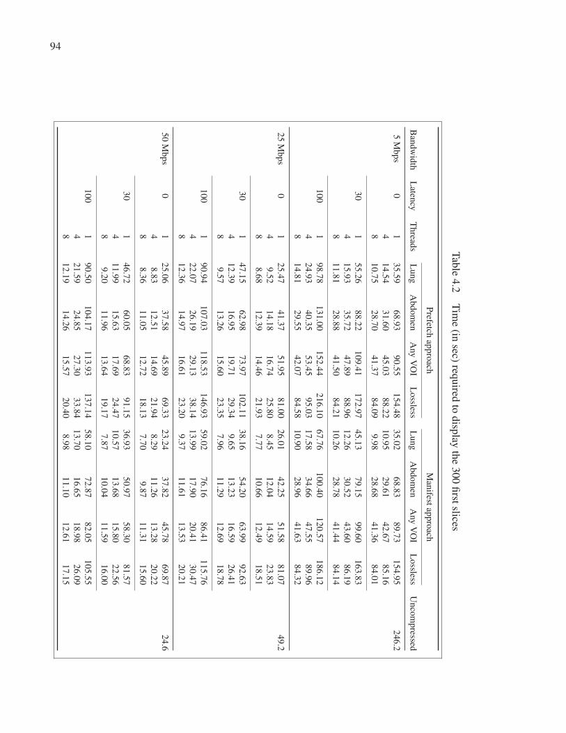
94

Tab

le4.2

Tim

e(in

sec)req

uired

todisp

layth

e300

first

slices

Prefetch

app

roach

Man

ifestap

pro

ach

Ban

dw

idth

Laten

cyT

hread

sL

un

gA

bd

om

enA

ny

VO

IL

ossless

Lu

ng

Ab

do

men

Any

VO

IL

ossless

Un

com

pressed

5M

bp

s0

13

5.5

96

8.9

39

0.5

51

54

.48

35

.02

68

.83

89

.73

15

4.9

52

46

.2

41

4.5

43

1.6

04

5.0

38

8.2

21

0.9

52

9.6

14

2.6

78

5.1

6

81

0.7

52

8.7

04

1.3

78

4.0

99

.98

28

.68

41

.36

84

.01

30

15

5.2

68

8.2

21

09

.41

17

2.9

74

5.1

37

9.1

59

9.6

01

63

.83

41

5.9

33

5.7

24

7.8

98

8.9

61

2.2

63

0.5

24

3.6

08

6.1

9

81

1.8

12

8.8

84

1.5

08

4.2

11

0.2

62

8.7

84

1.4

48

4.1

4

10

01

98

.78

13

1.0

01

52

.44

21

6.1

06

7.7

61

00

.40

12

0.5

71

86

.12

42

4.9

34

0.3

55

3.4

59

5.0

31

7.5

83

4.6

64

7.5

58

9.9

6

81

4.8

12

9.5

54

2.0

78

4.5

81

0.9

02

8.9

64

1.6

38

4.3

2

25

Mb

ps

01

25

.47

41

.37

51

.95

81

.00

26

.01

42

.25

51

.58

81

.07

49

.2

49

.52

14

.18

16

.74

25

.80

8.4

51

2.0

41

4.5

92

3.8

3

88

.68

12

.39

14

.46

21

.93

7.7

71

0.6

61

2.4

91

8.5

1

30

14

7.1

56

2.9

87

3.9

71

02

.11

38

.16

54

.20

63

.99

92

.63

41

2.3

91

6.9

51

9.7

12

9.3

49

.65

13

.23

16

.59

26

.41

89

.57

13

.26

15

.60

23

.35

7.9

61

1.2

91

2.6

91

8.7

8

10

01

90

.94

10

7.0

31

18

.53

14

6.9

35

9.0

27

6.1

68

6.4

11

15

.76

42

2.0

72

6.1

92

9.1

33

8.1

41

3.9

91

7.9

02

0.4

13

0.4

7

81

2.3

61

4.9

71

6.6

12

3.2

09

.37

11

.61

13

.53

20

.21

50

Mb

ps

01

25

.06

37

.58

45

.89

69

.33

23

.24

37

.82

45

.78

69

.87

24

.6

48

.83

12

.51

14

.69

21

.94

8.2

91

1.2

61

3.2

82

0.2

2

88

.36

11

.05

12

.72

18

.13

7.7

09

.87

11

.31

15

.60

30

14

6.7

26

0.0

56

8.8

39

1.1

53

6.9

35

0.9

75

8.3

08

1.5

7

41

1.9

91

5.6

31

7.6

92

4.4

71

0.5

71

3.6

81

5.8

02

2.5

6

89

.20

11

.96

13

.64

19

.17

7.8

71

0.0

41

1.5

91

6.0

0

10

01

90

.50

10

4.1

71

13

.93

13

7.1

45

8.1

07

2.8

78

2.0

51

05

.55

42

1.5

92

4.8

52

7.3

03

3.8

41

3.7

01

6.6

51

8.9

82

6.0

9

81

2.1

91

4.2

61

5.5

72

0.4

08

.98

11

.10

12

.61

17

.15

95

a) Layer 1 - Lung VOI b) Distortions (j2k(( |v | j2k) c) Byte allocation difference

d) Layer 2 - Abdomen VOI e) Distortions (j2k(( |v | j2k) f) Byte allocation difference

Figure 4.6 Sample slice displayed with the a) lung VOI and d) abdomen VOI window.

b, e) associated distortion images with the proposed method (right) and the typical

rate-based approach with identical file sizes (left). c, f) byte displacement maps showing

improved byte allocation.

file size as a target on the right half. Display PV PSNR measurements in regions covered

by the VOI windows were very close to the 40 dB target with 40.0 dB and 40.4 dB for the

lung and abdomen VOI window respectively. Finding a compression ratio that produces a

predictable quality across modality, anatomical regions and acquisition parameters is usually a

challenge in itself. Our approach goes even further by enabling a constant configurable level of

fidelity across all image regions after the VOI transformation. Furthermore, our method ignores

code-blocks that are outside of the VOI window leading to more efficient use of the available

bandwidth. This is illustrated in Fig. 4.6c and 4.6f that show the difference in byte allocation

with the streams used in the previous figures. Each block represents a single code-block. Gray

blocks have identical size while light and dark blocks represent blocks respectively coded with

more or less bytes compared with the traditional rate-based implementation.

96

Because decoding performances depends mostly on the number of coding passes to decode,

discarding useless information has a beneficial impact on both download and transfer times.

With this dataset, decoding only the first layers required on average 55 ms while decoding

all layers required on average 192 ms. Displaying a slice requires both operations and, with

the slow JavaScript decoder, decoding was often the most costly operation. Therefore, perfor-

mance improvements are decreased as network bandwidth is increased.

Table 4.2 shows the time required to browse to the 300th slice for the different combinations

of bandwidth, latency, number of workers and initial layer presented in Section 4.5.2 for both

prefetch and manifest methods. The theoretical minimum time needed to display the first

300 raw uncompressed slices is also reported in the last column. In that case, because no

decoding is required and because downloads can be easily parallelized, the latency and number

of concurrent workers are ignored. These uncompressed results serve as benchmarks. From

this table, we can observe that:

• even with the poor performing JavaScript decoder, displaying lossless JPEG 2000 images

with 4 or more workers is almost always faster than displaying the raw uncompressed data;

• the proposed streaming approach is up to 8 times faster than displaying losslessly com-

pressed JPEG 2000 images;

• using multiple workers significantly reduces the impact of latency;

• the prefetch and manifest method perform almost identically in the absence of latency;

• between 20 and 36 slices per second can be streamed in the lung VOI window using 8 work-

ers with the tested network conditions.

The median time required to load the web application, decode and display the first slice was

about 600 ms. The median of the worst case (8 workers at 5 Mbps with 100 ms of latency)

was 2.5 seconds. In that case, the increased number of concurrent workers means that less of

the already low bandwidth is available to download the very first slice. Using only one worker

97

reduces the median time-to-first-slice to 830 ms. Consequently, waiting until the first slice is

displayed before using multiple workers provide the best possible user experience. This very

low time-to-first-slice means that the radiologist can start browsing the stack almost instantly.

Furthermore, in our testing, refinement up to losslessness could usually be displayed in less

than a second when the user stops on a particular image even while the next few slices are still

being downloaded and decoded in the background.

As mentioned, it is possible to build a completely client side solution with the prefech method

at the cost of added latency. However, our results show that the impact of the added latency is

almost completely mitigated when using 8 concurrent workers.

4.7 Conclusion

In this paper, we have proposed and evaluated a novel JPEG 2000 byte allocation scheme that

enables VOI-based streaming of medical images at fixed quality and near-lossless levels. Our

method allows us to achieve visually lossless diagnostic quality much faster than any lossless

compression method. It greatly reduces both storage and transmission requirements by taking

advantage of the masking effect of the VOI transformation. Most importantly, radiologists can

start their exam almost instantly with very fast browsing capabilities and without any quality

concerns since the embedded code-stream can scale up to losslessness. We have also discussed

how the streaming mechanism could be implemented solely on the client side within the con-

straint of currently adopted standards and infrastructure.

Specifically, we have introduced methods to target specific and constant distortion levels on

medical images as they are displayed on typical computer monitors and that produce near-

lossless JPEG 2000 code-streams for any VOI configuration.

We believe that these contributions enable completely new work-flows. For instance, medical

images could be losslessly archived with multiple embedded quality layers: fixed fidelity in the

default VOI window, fixed fidelity in a second VOI window, near-lossless in the default VOI

window and finally lossless. When the image is moved from the archiving infrastructure to the

98

streaming server, only the first few layers could be transferred. The streaming server would in

turn stream only the required layers to the viewer reducing bandwidth and transfer latency at

every level of the processing pipeline.

In order to support those claims, we have built a browser-based streaming client and evaluated

the productivity gains while browsing a large CT stack. Even with a relatively poor performing

JavaScript JPEG 2000 decoder, our results show increased performance by a factor of up to 24

when compared to transferring uncompressed pixels depending on network conditions.

We have presented performance gains obtained with specific VOI values and compression lev-

els. By changing the VOI values and/or the compression levels, performance gains certainly

change without affecting the conclusion of our work: performance is always better with our

method compared to the other compression schemes. On the other hand, while PSNR is the

most widely used fidelity metric, it is criticized for being poorly correlated with human per-

ception of image quality. Our proposed method can be adapted to use other more sophisticated

quality metrics that can be computed in the wavelet domain.

Future work includes implementing and evaluating other fidelity metrics as well as assessing

the proposed implementation in clinical settings.

CHAPTER 5

A NOVEL KURTOSIS-BASED JPEG 2000 COMPRESSION CONSTRAINT FORIMPROVED STRUCTURE FIDELITY

Jean-François Pambruna, Rita Noumeirb

a, bDepartment of Electrical Engineering, École de technologie supérieure,

1100 Notre-Dame Ouest, Montréal, Québec, Canada H3C 1K3

Article submitted in « Transactions on Biomedical Engineering » in April 2016.

Abstract

Modern diagnostic imaging devices produce enormous amounts of data that needs to be archived

and accessed efficiently. Lossless image compression can be used to mitigate these issues by

reducing file sizes by up to two-thirds without any adverse effect on diagnostic accuracy, but

lossy compression is required to further improve performances. Unfortunately, determining the

compression level needed to ensure diagnostic losslessness is very challenging. Most efforts in

this field have been dedicated to rate-based approaches (i.e. finding suitable compression ra-

tios). However, these approaches have been shown to be very susceptible to image content even

within modalities. Relying on quality–based approaches may be desirable but can remove im-

portant structures on non-noisy images in order to reach the objective quality constraint. This

paper proposes a new technique that improves quality–based approaches by adding a new con-

straint based on the local distribution of errors in the wavelet domain. This new constraint is

then added to a JPEG 2000 coder and evaluated with medical and non-medical images. Fur-

thermore, the new constraint is used as a full reference image quality assessment metric that

performs well when compared with other leading metrics. Our results show a drastic reduction

of structure loss with non-noisy images, while preserving good compression rates with noisy

images.

100

5.1 Introduction

Electronic health records (EHR) and Picture Archiving and Communication System (PACS)

can significantly improve the accuracy and accessibility of patient information as well as im-

prove collaboration between healthcare professionals (Goetz Goldberg et al., 2012). In par-

ticular, PACS can improve productivity, reduce turn around time, eliminate film-related costs,

and reduce the number of needless duplicate exams, as well as length of stays (Georgiou et al.,

2015; Mansoori et al., 2012). In Canada, those benefits are expected to generate hundreds of

millions of dollars in savings each year for the public healthcare system (Canada Health In-

foway, 2008). However, deploying universally accessible imaging enabled EHR can be very

challenging (Piliouras et al., 2015). One of these challenges is caused by the tremendous

amount of data produced by modern medical imaging devices that needs to be archived for

very long terms while remaining readily available. Lossless image compression can help miti-

gate this issue by reducing file sizes by up to two-thirds, but lossy compression is often needed

to further reduce storage and network requirements. Unfortunately, depending on compression

levels, this can introduce visible distortions and great care must be taken not to alter diagnosti-

cally important structures.

Guidelines based on compression ratios (i.e. the ratio of bits before and after compression)

have been introduced to help mitigate this issue. Unfortunately, they fail to take into account

the significant compressibility variations –closely related to entropy– that can be observed be-

tween images of the same modality or even between different slices of the same acquisition

(Pambrun and Noumeir, 2015a). For instance, a computed X-ray tomography acquired with

lower radiation exposure in order to preserve the patient health will have increased noise and

entropy levels and therefore reduced compressibility. This suggests that these recommenda-

tions will either be very conservative or may not fully ensure diagnostic losslessness. Modern

objective image quality assessment (IQA) metrics could be used instead of compression ratios

(CR), but they are generally designed for highly compressed natural images found in entertain-

ment applications and have not been thoroughly tested for medical use.

101

On the other hand, image compression algorithms usually discard small uncorrelated details

such as noise before discarding any structure. Because of this, it has been noted that low level

compression can have a beneficial denoising effect in medical applications (Fritsch and Bren-

necke, 2011; Gupta et al., 2005). In this paper, we present a novel wavelet-domain error kur-

tosis (WDEK) compression threshold that can be used to target the compression level at which

the distortion transitions from acquisition noise to structures. This WDEK method can be used

to leverage the beneficial denoising effect of compression without significant distortion to di-

agnostic features. An existing JPEG 2000 codec is then modified to target the WDEK on a

code-block basis in order to preserve diagnostic fidelity and achieve better efficiency.

JPEG 2000 is not the most cutting-edge image codec available, but it has been part of the Dig-

ital Imaging and Communications in Medicine (DICOM) standard for more than a decade and

is now widely supported in the medical domain (NEMA, 2016). As such, any standard compli-

ant improvements made to the encoder could be immediately beneficial to the community. This

is why JPEG 2000 was chosen as the basis of this contribution. However, the same principles

could be applied to other coders.

The effectiveness of the proposed compression scheme at preserving structures is first illus-

trated with image samples of different types. In a second experiment, our local distortion

metric is universally pooled and compared with established global IQA metrics using a pub-

licly available image database. Our results show that our distortion metric is: 1- effective at

constraining the encoder in the beneficial denoising operation regime regardless of the origi-

nal image compressibility and 2- comparable to leading IQA metrics for a limited subset of

distortion types including JPEG and JPEG 2000 compression.

5.2 Previous work

This link between compression and denoising techniques is well known (Bruni and Vitulano,

2007). Wavelet coders such as JPEG 2000 usually alters noise before altering other structures;

this can have a beneficial denoising effect at relatively low compression levels. In fact, small

102

−40 −20 0 20 400

0.05

0.1

c) WDEK – Noisy image

−40 −20 0 20 400

0.05

0.1

a) PSNR – Noisy image

−40 −20 0 20 400

0.05

0.1

d) WDEK– Clean image

−40 −20 0 20 400

0.05

0.1

b) PSNR – Clean image

Figure 5.1 Histogram of the wavelet domain error of a 4 by 4 code-block region of high

frequency coefficients (4096 total) with a fitted Gaussian distribution (dashed lines). a)

PSNR constrained compression of a noisy image, b) PSNR constrained compression of a

clean image, c) WDEK-based compression of a noisy image, d) WDEK-based

compression of a clean image.

high frequency coefficients, usually associated with acquisition noise, are discarded first as the

quantization step is gradually increased in the post-compression rate-distortion allocation stage

of the image coder. As such, it was observed in (Ponomarenko et al., 2010) that compression

at low levels can improve image quality, albeit not as efficiently as purpose-built denoising

algorithms. Many imaging modalities produce noisy images and the denoising effect of com-

pression has been shown to be beneficial for some medical applications (Gupta et al., 2005;

Persons et al., 1997). It has also been shown that, when presented with moderately compressed

and original images, radiologists often prefer the compressed versions (Erickson et al., 1997;

Koenig et al., 2004). Radiologists may even be more confident (Koenig et al., 2004) in their

diagnostics and the diagnostic accuracy can in fact be improved (Savcenko et al., 1998) by the

use of such moderate compression.

103

Most JPEG 2000 implementations offer two methods of specifying the targeted compression

level : 1- specifying the desired CR and 2- specifying the desired global image quality (usually

in terms of peak signal-to-noise ratio). The first option is a rate-based approach which is mostly

useful when compression requirements are dictated by a fixed time-bandwidth constraint or

when precise storage provisioning is a priority. Conversely, the quality-based approach should

be used when ensuring a minimum image fidelity is paramount.

Surprisingly, the published literature on lossy compression in the medical domain focuses

mostly on the former rate-based approach. Many studies (Koff et al., 2009; Slone et al., 2003;

Sung et al., 2002) were conducted in order to determine safe diagnostically lossless CR for

different modalities. Based on these findings, radiologist associations such as the Canadian

Association of Radiologists (CAR) and the Royal College of Radiologists (RCR) have pro-

duced sets of CR-based guidelines (Canadian Association of Radiologists, 2011; The Royal

College Of Radiologists, 2011) sometimes with conflicting results (The Royal College Of Ra-

diologists, 2011). Compression ratios are known to be inaccurate when used as an IQA metric

(Fidler et al., 2006b, 2007; Pambrun and Noumeir, 2015b) because compressibility can vary

drastically with image content even within modalities. Consequently, these rigid guidelines

will either be very conservative and inefficient or may result in insufficient fidelity with poorly

compressible images.

Quality-based methods may be more desirable, but also suffer from some limitations. In this

mode, the JPEG 2000 coder will in essence increase the local level of compression on small

non-overlapping regions called code-blocks until the targeted distortion is reached. A well-

chosen threshold can leverage the beneficial denoising effect of compression without affecting

diagnostic accuracy. However, when the image has little acquisition noise, the encoder, bound

by the same distortion criteria, has no choice but to degrade potentially diagnostically important

features.

Peak Signal-to-Noise (PSNR), which is essentially equivalent to the Mean Squared Error (MSE),

is the simplest and more commonly used IQA metric. It is used by most JPEG 2000 coders

104

for both quality-based and rate-based compression as either a simple threshold or as a min-

imized constraint when targeting a specific file size. MSE is, however, heavily criticized

(Wang and Bovik, 2009) for being poorly correlated with our perception of quality. Several im-

age fidelity metrics have been designed to better predict the perceived quality with the help of

large distorted image databases. Unfortunately, these databases and IQA metrics were mainly

developed for heavily compressed natural images usually found in entertainment applications.

Medical images have very different characteristics and use cases; they are often very noisy, ex-

amined in great details for very subtle features and are usually dynamically transformed from

high dynamic range modality pixel values to low dynamic range display pixel values.

Structural similarity (SSIM)(Wang et al., 2004) has increasingly gained in popularity in the

image and video compression fields. It is fast to compute and performs well with the LIVE

image quality assessment database (Sheikh et al., 2003). SSIM is one of the few alternative

IQA metrics that was partly integrated in JPEG 2000 coders as a replacement the MSE in

order to improve perceived quality at identical rates. These SSIM-optimal implementations

(Richter and Kim, 2009; Wang et al., 2010) are approximations because, unlike PSNR, pixel

domain SSIM cannot be easily computed in the wavelet domain. Furthermore, this metric was

mostly developed and tested with natural images subjected to heavy distortions, such as the

ones found in the LIVE database, and the results may not translate well to other types of im-

ages such as graphics and diagnostic imaging. Other limitations of SSIM related to the high dy-

namic range of medical images have also been previously highlighted (Pambrun and Noumeir,

2015a). Nonetheless, studies involving diagnostic images and trained radiologists have shown

SSIM to be either on par with (Georgiev et al., 2013; Kim et al., 2010a) or slightly better than

PSNR (Kowalik-Urbaniak et al., 2014) at predicting perceived quality.

Acquisition noise does not only have low diagnostic value, but it is also very difficult to ef-

ficiently compress (Pambrun and Noumeir, 2013) because of the added high frequency co-

efficients. This is especially true for computed tomography where low radiation doses are

preferred over reduced acquisition noise in order to minimize health hazards for patients. For

this reason, some researchers studied the influence of noise filtering as a pre-processing step to

105

compression (Muñoz-Gómez et al., 2011) in order to lower entropy and obtain better compres-

sion ratios. However, a pixel domain denoising solution may not optimally reduce entropy in

the wavelet domain and, most importantly, code-stream scalability (i.e. the ability to construct

an embedded code-stream that can scale up to losslessness) is completely lost.

5.3 WDEK-based JPEG 2000 coder

JPEG 2000 is a bit plane coder that operates in the wavelet domain. Images are decomposed

into a dyadic pyramid with horizontal, vertical and diagonal details sub-bands. Small non-

overlapping blocks of coefficients called code-blocks are then independently coded. Within

each code-block, bit planes are sequentially encoded from the most to the least significant in

three independent coding passes. This stream, associated with a single code-block, can then

be truncated after each coding pass thus providing great scalability. Each discarded bit-plane

increases the wavelet domain quantization by a factor of two. For a given quality target, coding

passes starting from the least significant bits of each code-block are discarded until the desired

distortion level is reached.

Because of the wavelet transform properties (Donoho and Johnstone, 1994), and assuming that

the acquisition noise is approximately Gaussian, coefficients associated with noise will also be

normally distributed in the wavelet domain. These numerous small uncorrelated coefficients

significantly reduce the compressibility of noisy images. However, since those are the coef-

ficients that are discarded first by the quantization process, they can be compressed further

(in terms of measured MSE) before actually altering important structures. On the other hand,

compressing clean images with the same quality target will result in diagnostically relevant

coefficients being further quantized.

The proposed approach estimates the truncation points at which important structures are start-

ing to be altered instead of noise by evaluating when the error residual deviates from the normal

distribution. Specifically, the fourth standardized moment, the kurtosis, is used in conjunction

with the PSNR to determine safe truncation points for high frequency code-blocks. With sym-

106

Lossless: 202 KB CR: 38 KB – 39.1 dB PSNR: 66 KB – 44.3 dB WDEK: 69 KB – 44.6 dB CR(WDEK): 69 KB – 44.7 dB

Lossless: 156 KB CR: 38 KB – 49.0 dB PSNR: 25 KB – 45.5 dB WDEK: 34 KB – 47.3 dB CR(WDEK): 34 KB – 48.2 dB

Lossless: 126 KB CR: 38 KB – 54.2 dB PSNR: 19 KB – 46.1 dB WDEK: 31 KB – 51,1 dB CR(WDEK): 31 KB – 52.5 dB

Lossless: 177 KB CR: 38 KB – 35.8 dB PSNR: 73 KB – 44.9 dB WDEK: 73 KB – 44.9 dB CR(WDEK): 73 KB – 45.0 dB

Lossless: 137 KB CR: 38 KB – 47.0 dB PSNR: 30 KB – 43.8 dB WDEK: 33 KB – 44.3 dB CR(WDEK): 33 KB – 45.2 dB

Lossless: 117 KB CR: 38 KB – 52.1 dB PSNR: 21 KB – 45.6 dB WDEK: 27 KB – 47.5 dB CR(WDEK): 27 KB – 48.7 dB

Figure 5.2 Six sample CT scans with varying noise levels: 3 phantom acquired with

different parameters and 3 simulations with different photon counts. Both sequences are

in decreasing noise levels ordering from top to bottom. The columns respectively contain,

from left to right: the original image, difference image with a CR of 10:1, difference

image with a PSNR constraint of 45 dB, difference image with the added WDEK

constraint, difference image with the traditional CR approach with the CR obtained with

the WDEK method.

107

metric unimodal distributions, kurtosis is an indication of tail weights and peakedness com-

pared to the normal distribution. It is completely independent of the variance. Distributions

with kurtosis higher than 3 have heavier tails, higher peak or both. However, the kurtosis is

mostly affected by the tail weigh (DeCarlo, 1997). In this case, heavier tails means more oc-

currences of large errors than normal and this is unlikely to be the result of denoising. Null

coefficients are very common in high-frequency sub-bands and cannot be distorted by the quan-

tization process. This results in a disproportionate peak at 0 in error residual distribution. These

coefficients are ignored when computing the kurtosis as they would otherwise skew the results

towards the Laplacian distribution that has a kurtosis of 6. To our knowledge, this is the first

time that the kurtosis is used to constrain compression. In this paper, the threshold was empir-

ically set at 3.2 which is just above normal.

We based our codec implementation on the BOI 1.8(Auli-Llinas, 2013) JPEG 2000 codec. It

was modified to enable quality-based compression with a target PSNR. The target PSNR must

be supplied along the useful dynamic range of the image. As with the kurtosis, null coefficients

are ignored when computing the MSE. Otherwise, the targeted distortion in code-block with

large null coefficient patches would be concentrated in few non-null coefficients thus resulting

in very uneven fidelity.

JPEG 2000 coders usually keep track of the quality increments added by each coding pass in

the early stages in order to later compute the PSNR and optimize rate allocation. In addition,

our implementation was modified to track every changed bit. This information will be used in

the rate-distortion stage to precisely compute the wavelet error residual associated with each

coding pass that is needed to compute the kurtosis.

The proposed WDEK-based JPEG 2000 rate-allocation algorithm used to compute optimal

truncation points (t) is presented in Algo. 5.1. For each code-block (cb), the PSNR constraint

(tp) is used to compute (ln. 2) the initial truncation point using the error increments (Δe)

computed in the early stages of the coder. The error residual (E) is then initialized to zero (ln.

3). The loop on line 4 iterates over all coding passes (cp) from the least significant to the most

108

Algorithm 5.1 Algorithm of the WDEK-based JPEG 2000 coder

input : Δe: Error increments after each coding pass

Δb: Bits changed by each coding pass

tp: Target PSNR

tk: Target kurtosis

output: t: Truncation points of each code-block(cb)

1 foreach cb in image do2 t[cb]← calcPsnrBasedTP (Δe[cb], tp);3 E ← 0;

4 foreach coding pass(cp) starting from the LSB do5 if cp is already included by t[cb] then6 break;

7 else8 E ← updateError (E, Δb[cp], cp);9 k← kurtosis (E);

10 if k > tk then11 t[cb]← cp;

12 break;

significant bit. If the current coding pass was already included by the PSNR constraint, there

is nothing else to do as the algorithm uses the most conservative of both metrics. Otherwise,

the error residual (E) is updated (ln. 8) with the list of changed bits (Δb) associated with the

current coding pass (cp). The new kurtosis (k) is then computed (ln. 9). If the kurtosis is

greater than the targeted threshold (tk), the current truncation is used (ln. 11) instead of the

one computed based on PSNR. The added kurtosis constraint can only increase quality and

consequently reduce compression ratios.

The effects of this added constraint are illustrated in Fig. 5.1. Four error residual histograms of

a 4 by 4 code-block region (4096 coefficients) are presented as follows: using only the PSNR

constraint of 45 dB with a a) noisy and b) clean image and using the our WDEK approach

with a c) noisy and d) clean image. The dashed line is a fitted Gaussian distribution function.

The noisy image histograms for both methods are mostly identical. This is because the 45 dB

constraint is already mostly in the beneficial denoising regime. On the other hand, the wide

tails of error distribution of the clean image with the PSNR constraint suggests that not only

109

noise, but structures are affected. Adding the kurtosis constraint almost completely removes

the heavy tails and the error distribution is much closer to the Gaussian distribution expected

when only noise is discarded.

5.4 Evaluation

Lossless: 126 KB

PSNR: 19 KB – 46.1 dB

WDEK: 31 KB – 51.1 dB

Lossless: 202 KB

PSNR: 66 KB – 44.2 dB

WDEK: 69 KB – 44.6 dB

Figure 5.3 Magnified regions of the noisy (left) and clean (right) thoracic phantom

compressed losslessly (top), with the PSNR constraint only (middle) and with the added

WDEK constraint (bottom).

Evaluation was performed by visually assessing the level of structure distortion when com-

pressing images from two diagnostic imaging modalities, computed tomography and breast

digital radiography, as well as with non-medical images. Each image is compressed multiple

times: with the CAR recommended CR when applicable, with the PSNR constraint, with added

WDEK constraint and finally with the same CR obtained with the WDEK method. Difference

images are then inspected for structural distortions. In addition, the local kurtosis-based dis-

110

Lossless: 4,828 KB CR: 511 KB – 37.3 dB PSNR: 541 KB – 37.7 dB WDEK: 737 KB – 38.8 dB CR(WDEK): 737 KB – 39.6 dB

Figure 5.4 Digital mammography compressed losslessly followed by the difference

images with a 25:1 CR, difference image with PSNR constraint of 38 dB, difference

image with the added WDEK constraint and difference image with the traditional CR

approach with the CR obtained with the WDEK method.

tortion metric is pooled and used as an IQA metric and compared with state-of-the-art metrics

using the LIVE image quality assessment database.

5.4.1 Structure distortions

5.4.1.1 X-Ray computed tomography

For this modality, evaluation was performed with two image series: 1-an anatomical thoracic

phantom with synthetic lung nodules and 2-a simulated water phantom with geometric air

vesicles. The thoracic phantom (Gavrielides et al., 2010) was made available for computer-

aided diagnostic research via the National Biomedical Imaging Archive (NBIA). It was scanned

multiple times with different exposures, pitches, slice thicknesses, reconstruction filters and

slice collimation widths. Three images of the same anatomical region, each obtained with

different acquisition parameters resulting in increasing noise levels, were used. The pitch was

0.9 mm, the slice collimation was 16×0.75 mm and the other parameters were:

• exposure of 25 mAs, slice thickness of 0.8 mm and a filter type of “detail”;

• exposure of 100 mAs, slice thickness of 1.5 mm and a filter type of “medium”;

111

• exposure of 200 mAs, slice thickness of 5.0 mm and a filter type of “clean”.

The three images are respectively referred as noisy, fair and clean. The PSNR is computed on

the full dynamic range without any value of interest transformation. Fig. 5.2 shows the three

images in the first column of first three rows starting with the noisy slice at the top, fair slice

in the second row and clean image in the third row. These images are compressed four times:

1- with the recommended CR; 2- with a PSNR constraint of 45 dB; 3- with the added WDEK

constraint and 4- with the same CR obtained with WDEK method.

The pixel domain error residual images associated with each compressed images are presented

in the last four columns of Fig. 5.2. The resulting file sizes and measured PSNR are indicated at

the bottom of each residual image. The PSNR computation excludes the pixels that are outside

of the field of view of the modality. These pixels are represented by null high frequency wavelet

coefficients that cannot be distorted by compression. Including them in the error computation

would significantly overestimate global quality measurements. Fig. 5.3 shows a magnified

region of the clean and noisy thoracic phantom compressed losslessly, compressed with the

PSNR constraint and compressed with the proposed WDEK method.

We repeated the same experiment with a simulated water cylinder phantom computed with mul-

tiple exposure settings using a Monte Carlo photon transport simulation (Badal and Badano,

2009). Each image was created by applying the filtered back projection of 708 individual pro-

jections. Those results are presented in the three lower rows of Fig. 5.2. They respectively

represent noisy, fair and clean images computed by simulating 1E7, 2E8 and 1E9 photons per

projection. As before, the PSNR is computed on the full dynamic range image.

From Fig. 5.2, we can observe that indeed, image content and, most notably, noise levels can

significantly affect compressibility by noting the increased lossless file size with increased

noise. As expected, the distortion level increases with the noise given a constant compression

ratio. This is also reflected in the PSNR measurements. What may not be as obvious is that

conversely, for a given PSNR constraint, the perceived image quality after compression is

reduced when acquisition noise is reduced. The clean image is more compressible (i.e. it has

112

less entropy) and the file size is reduced for a constant PSNR, but most of the distortion is now

affecting important visible structures as presented in the third column. On the other hand, the

WDEK approach can still leverage the added compressibility of cleaner images while keeping

structures unaffected as illustrated in the fourth column. For noisy images, the added kurtosis

constraint has very little effect, lower than 5%. This is also visible in the pixel domain as

depicted in Fig. 5.3.

The last column of Fig. 5.2 shows the result when using the traditional CR approach that

minimizes MSE with the same CR as the proposed WDEK method. The results may appear

similar, but the difference image still shows signs of structure degradation especially in the

cleaner images. Furthermore, obtaining that optimal CR for a given image is the challenge that

we are trying to solve.

5.4.1.2 Breast digital radiography

Digital mammogram images can be much larger, tens of megabytes, but are also very com-

pressible. The same method as before was used with a typical mammogram from The Cancer

Genome Atlas-Breast Cancer (TCGA-BRCA) data collection (Clark et al., 2013) to illustrate

the structure preservation of the WDEK approach. Results are presented in Fig. 5.4. This image

is 2560× 3328 pixels and with 12 stored bits and 16 allocated, it represents 12.18 megabytes

of data stored in a 16.25 megabytes file. Based on the data (allocated size), the lossless CR

for this image was 3.4:1. As in the CT case, the four remaining columns show the difference

image, but with a recommended CR of 35:1 and a PSNR of 38 dB. Again, adding the kurtosis

constraint removes all structure degradation and performs better in terms of error uniformity

than the MSE optimal rate-based approach with identical file size.

5.4.2 Non-medical images

We tested our approach with a natural image (Fig. 5.5 top left) and an illustration(Fig. 5.5 bot-

tom left). The following columns show, from left to right, the difference images with a PSNR

113

Lossless: 124 KB PSNR: 18 KB – 40.0 dB WDEK: 22 KB – 40.8 dB CR(WDEK): 22 KB – 41.0 dB

Lossless: 125 KB PSNR: 67 KB – 39.8 dB WDEK: 71 KB – 40.1 dB CR(WDEK): 71 KB – 38.6 dB

Figure 5.5 Non-medical images compressed losslessly followed by

the difference images with a PSNR of 38 dB, difference image with the

added WDEK constraint and difference image with the traditional CR

approach with the CR obtained with the WDEK method.

of 40 dB, with the added WDEK constraint and with the CR obtained with the WDEK method.

The natural image shows results similar to those presented before with fewer structural distor-

tions, but shows no visible improvement with the illustration. This is because the illustration is

completely noise free and the WDEK approach is designed to target the compression level at

which the distortion transitions from noise to structure. However, it is interesting to note that

the traditional CR-based approach performs significantly worse than both PSNR and WDEK

approaches with similar file sizes.

5.4.3 WDEK as a full reference IQA metric

For evaluation purposes, our WDEK compression constraint was adapted into a full reference

IQA metric by pooling the error kurtosis of 16× 16 non-overlapping blocks of a five-level

LeGall wavelet decomposition. Because the distortions are perceived very differently for dif-

ferent frequencies, results from different decomposition scales are pooled with a weighted

average using the same weights used in MS-SSIM (Wang et al., 2003). The results of our

wavelet domain kurtosis-based image quality assessment metric (WDEK-QM) with the scores

114

Table 5.1 IQA metric performances with the LIVE database

Dataset Metric SRCC PLCC R2 RMSE

J2K VIF 0.9696 0.9788 0.9580 5.2507

MSSIM 0.9651 0.9690 0.9389 6.3286

SSIMd 0.9614 0.9662 0.9336 6.5998

WDEK-QM 0.9547 0.9647 0.9306 6.7460

SSIM 0.9359 0.9431 0.8895 8.5152

CR 0.9154 0.9257 0.8569 9.6888

PSNR 0.8954 0.9001 0.8102 11.1577

JPEG VIF 0.9846 0.9861 0.9723 5.3562

MSSIM 0.9795 0.9813 0.9629 6.2232

SSIMd 0.9764 0.9788 0.9581 6.6133

WDEK-QM 0.9567 0.9610 0.9234 8.9349

SSIM 0.9458 0.9506 0.9037 9.9931

CR 0.9488 0.9487 0.9000 10.2203

PSNR 0.8809 0.8892 0.7906 14.7747

White VIF 0.9858 0.9885 0.9769 4.3237

PSNR 0.9854 0.9843 0.9688 5.0270

MSSIM 0.9729 0.9700 0.9409 6.9201

SSIMd 0.9694 0.9683 0.9376 7.1138

SSIM 0.9614 0.9717 0.9441 6.7310

WDEK-QM 0.9260 0.9203 0.8470 11.1366

Gaussian VIF 0.9728 0.9769 0.9543 4.0195

MSSIM 0.9587 0.9516 0.9056 5.7762

SSIMd 0.9517 0.9438 0.8908 6.2119

SSIM 0.9036 0.8809 0.7760 8.8977

WDEK-QM 0.8097 0.7846 0.6157 11.6539

PSNR 0.7823 0.7837 0.6142 11.6759

Fast fading VIF 0.9650 0.9660 0.9331 7.5002

SSIMd 0.9556 0.9464 0.8956 9.3652

SSIM 0.9421 0.9418 0.8869 9.7500

MSSIM 0.9318 0.9187 0.8439 11.4541

WDEK-QM 0.9202 0.9177 0.8422 11.4739

PSNR 0.8907 0.8901 0.7922 13.2154

from the LIVE database (Sheikh et al., 2003) are presented in table 5.1 and along other leading

metrics: VIF, SSIM, SSIMd , MS-SSIM, PSNR and, in some case, CR. SSIMd uses the rec-

ommended downscaling procedure while SSIM does not. The table shows Spearman’s Rank

115

correlation coefficient (SRCC) as well as Pearson’s linear correlation coefficient (PLCC), coef-

ficient of determination (R2) and root mean squares error (RMSE) after a logistic curve fitting.

For both JPEG and JPEG 2000 distortions, WDEK-QM performed well with results compara-

ble to SSIM and MS-SSIM, and results significantly better than both PSNR and CR. However,

as expected, WDEK-QM performed poorly with both white and Gaussian noise distortions.

This is because our approach was designed to attenuate acquisition noise (i.e. allow distortion

of the noise signal) in order to leverage the denoising effect of compression.

Like most IQA databases, this dataset contains only natural images with some very heavily

distorted samples. These results may hold perfectly for medical images compressed at low

levels, but they suggest that WDEK is better a compression constraint than CR and PSNR.

5.5 Conclusion

In this paper, we have proposed a new wavelet domain error kurtosis compression constraint

that produces better results in the context of diagnostic imaging than commonly used rate-

and quality-based methods. Our approach, unlike fixed-rate methods, takes image content into

account and, unlike other fixed-quality methods, does not impose a fixed level of distortion that

would degrade structures in the absence of acquisition noise. Furthermore, our method does

not rely on human visual system models such as visual masking that may not be desirable in

medical applications. Although one of the limitations of this study was the absence of formal

evaluation by a panel of trained radiologists, our method is supported by the inspection of

difference images from multiple modalities and by the evaluation of our kurtosis-based metric

against leading alternatives with the LIVE database.

This is a completely novel approach that allows some of the information associated with ac-

quisition noise to be discarded as it is with other wavelet domain denoising techniques. The

addition of our proposed compression constraint is completely independent of the decoder and

would remain compatible with existing devices. This could help ensure sufficient diagnostic

116

quality while keeping the embedded code-stream scalability that makes JPEG 2000 so versa-

tile.

GENERAL CONCLUSION

The purpose of our efforts was to improve medical image compression and streaming in order

to increase clinician productivity as well as quality of care for patients. Specifically, our first

objective was to highlight the limitations of the rate-based compression schemes that are cur-

rently in use in order to foster the development of alternative methods. Our second objective

was to develop a streaming scheme that leverage the masking effect of the VOI transform when

browsing remote images. Our last objective was to develop a compression scheme that is safe,

efficient and tailored especially for medical imaging.

First, we have analyzed the effects of image content and acquisition parameters on the com-

pressibility of CT slices of a thoracic phantom. The results showed significant variations, up to

66%, with 15% of the images compressed at 15:1 had lower fidelity than the median of those

compressed at 30:1. Secondly, we have developed a novel VOI-based lossy and near-lossless

streaming scheme that can scale up to losslessness. Our experiments showed a reduction in

transfer sizes by up to 54% for near-lossless levels depending on the targeted VOI. Further-

more, with our browser-based implementation, we were able to stream between 20 and 36

slices per second depending on network conditions with the first slice displayed in less than

a second. Finally, we developed a new compression constraint and image quality assessment

metric that leverage the denoising effect of compression while preserving image structures.

Our results showed a drastic reduction in structure degradation from this constraint. Further-

more, the performance of our metric derived from this constraint were on par with other leading

metrics for this type of distortions. These efforts led to the submission of three journal papers

presented in this thesis:

• Pambrun J.F. and Noumeir R. 2015. “Computed Tomography Image Compressibility and

Limitations of Compression Ratio-Based Guidelines”, Journal of Digital Imaging.

• Pambrun J.F. and Noumeir R. 2016. “More Efficient JPEG 2000 Compression for Faster

Progressive Medical Image Transfer”, Transactions on Biomedical Engineering. (sub-

mitted)

118

• Pambrun J.F. and Noumeir R. 2016. “A Novel Kurtosis-based JPEG 2000 Compression

Constraint for Improved Structure Fidelity”, Transactions on Biomedical Engineer-

ing. (submitted)

An abstract version of the first paper won the scientific award first place at the 2014 society for

imaging informatics in medicine (SIIM) annual meeting. In addition, we have published two

international conference proceedings on these topics:

• Pambrun J.F. and Noumeir R. 2013. “Compressibility variations of JPEG2000 com-

pressed computed tomography”, IEEE International Conference of the Engineering

in Medicine and Biology Society (EMBC)

• Pambrun J.F. and Noumeir R. 2011. “Perceptual quantitative quality assessment of

JPEG2000 compressed ct images with various slice thicknesses”, IEEE International

Conference on Multimedia and Expo (ECME)

SSIM is ubiquitous in the image quality assessment field and is increasingly used in medical

imaging. However, early on, we have found several limitations that we have highlighted in

another conference proceeding:

• Pambrun J.F. and Noumeir R. 2015. “Limitations of the SSIM quality metric in the context

of diagnostic imaging”, IEEE International Conference on Image Processing (ICIP)

We have had many interactions with clinicians and our original plan involved subjective image

quality assessments with trained radiologists. From our discussion, it became clear that they

would feel more conformable with a more mathematical-based method coming from the engi-

neering side instead of psychophysical methods. They wanted a solution that could be easily

understood and that is not based on unproven assumptions or subjective testing. We believe

that this is what we have archived with this thesis. We are eager to see their reception and we

intent to seek qualitative feedback.

Future work includes determining the optimal workflow for PACS-enabled EHR in real clinical

settings where many servers need to work together. In this case, image series usually needs to

be transferred from the imaging archive to dedicated streaming servers before any interactive

navigation can begin on the client. This transfer as well as the sometimes required transcoding

119

can add significant latency. With careful planning, the image could be losslessly compressed

with multiple embedded quality layers for achieving in order to facilitate streaming. In ad-

dition, instead of transferring the complete lossless series from the archive to the streaming

server, only the quality layers required for near-lossless reconstruction in the narrowest likely

VOI window could be transferred. This opens many possibilities that should be explored along

with investigating exactly how many and what quality layers are required for each protocol.

Furthermore, in this project we have chained two metrics, the PSNR and our new kurtosis-

based constraint, so that the image quality must satisfy both requirements for each code-block.

Additional metrics could be used in order to further restrain compression and thus improve

clinicians confidence in lossy compression. For instance, the �∞-norm could be assessed af-

ter both PSNR and kurtosis constraints to ensure that distortions are kept under a maximum

absolute difference threshold.

Finally, we have briefly explored the idea of integrating our work with high-efficiency video

coding (H.265) that is currently being drafted for inclusion in the DICOM standard by the

working group 4. This codec is more modern and considered more efficient than JPEG 2000.

Unfortunately, rate-distortion allocation relies on a quality factor that is only loosely related to

the produced image quality. Furthermore, the complex interactions associated with the intra-

frame prediction mechanism would make any adaptation of our method to this codec extremely

challenging if at all possible.

LIST OF REFERENCES

Alecu, A., A. Munteanu, J. Cornelis, and P. Schelkens. 2006. "Wavelet-based scalable L-

infinity-oriented compression". In IEEE Transactions on Image Processing. p. 2499–

2512.

Andre, T., M. Antonini, M. Barlaud, and R. Gray. 2007. "Entropy-Based Distortion Mea-

sure and Bit Allocation for Wavelet Image Compression". IEEE Transactions on ImageProcessing, vol. 16, n◦ 12, p. 3058–3064.

Ashraf, R., M. Akbar, and N. Jafri. 2006. "Diagnostically Lossless Compression-2 of Medi-

cal Images". In 1st Transdisciplinary Conference on Distributed Diagnosis and HomeHealthcare. p. 28–32. IEEE.

Auli-Llinas, F. 2013. "Boi JPEG2000 Codec". <http://www.deic.uab.cat/~francesc/software/

boi/>.

Aydin, T. O., R. Mantiuk, K. Myszkowski, and H.-P. Seidel. 2008. "Dynamic range indepen-

dent image quality assessment". ACM Transactions on Graphics, vol. 27, n◦ 3, p. 1.

Badal, A. and A. Badano. 2009. "Accelerating Monte Carlo simulations of photon transport in

a voxelized geometry using a massively parallel graphics processing unit". Med. Phys.,vol. 36, n◦ 11, p. 4878–4880.

Bajpai, V., K. H. Lee, B. Kim, J. K. Kil, J. K. Tae, H. K. Young, and S. K. Heung. 2008. "Dif-

ferences in compression artifacts on thin- and thick-section lung CT images". AmericanJournal of Roentgenology, vol. 191, n◦ 2, p. W38—-43.

Bradley, A. 1999. "A wavelet visible difference predictor". IEEE Transactions on ImageProcessing, vol. 8, n◦ 5, p. 717–730.

Bruni, V. and D. Ã. Vitulano. 2007. "Combined image compression and denoising using

wavelets". Signal Processing : Image Communication, vol. 22, p. 86–101.

Bushberg, J. T., J. A. Seibert, E. M. Leidholdt, J. M. Boone, and E. J. Goldschmidt, 2003. TheEssential Physics of Medical Imaging. Lippincott Williams & Wilkins, 1936 p.

Campbell, F. W. and J. G. Robson. 1968. "Application of Fourier analysis to the visibility of

gratings". The Journal of Physiology, vol. 197, n◦ 3, p. 551–566.

Canada Health Infoway, jan 2008. Diagnostic Imaging Benefits Evaluation Final report, vol-

ume 115.

Canadian Association of Radiologists. 2011. "CAR Standards for Irreversible Compression in

Digital Diagnostic Imaging within Radiology.". http://www.car.ca/uploads/standards%

20guidelines/Standard_Lossy_Compression_EN.pdf.

122

Carvajal, G., B. Penna, and E. Magli. 2008. "Unified Lossy and Near-Lossless Hyperspec-

tral Image Compression Based on JPEG 2000". IEEE Geoscience and Remote SensingLetters, vol. 5, n◦ 4, p. 593–597.

Chandler, D. M. and S. S. Hemami. 2007a. "A57 Database". <http://foulard.ece.cornell.edu/

dmc27/vsnr/vsnr.html>.

Chandler, D. and S. Hemami. 2007b. "VSNR: A Wavelet-Based Visual Signal-to-Noise Ratio

for Natural Images". IEEE Transactions on Image Processing, vol. 16, n◦ 9, p. 2284–

2298.

Chen, M.-J. and A. C. Bovik. 2011. "Fast structural similarity index algorithm". Journal ofReal-Time Image Processing, vol. 6, n◦ 4, p. 281–287.

Chen, Y.-Y. and S.-C. Tai. 2005. "Compressing medical images by morphology filter voting

strategy and ringing effect elimination". Journal of Electronic Imaging, vol. 14, n◦ 1, p.

013007.

Chun-Ling Yang, Wen-Rui Gao, and Lai-Man Po. 2008. "Discrete wavelet transform-based

structural similarity for image quality assessment". In 2008 15th IEEE InternationalConference on Image Processing. p. 377–380. IEEE.

Clark, K., B. Vendt, K. Smith, J. Freymann, J. Kirby, P. Koppel, S. Moore, S. Phillips, D. Maf-

fitt, M. Pringle, L. Tarbox, and F. Prior. 2013. "The Cancer Imaging Archive (TCIA):

maintaining and operating a public information repository". J. Digit. Imaging, vol. 26,

n◦ 6, p. 1045–1057.

Daly, S. J. 1992. "Visible differences predictor: an algorithm for the assessment of image

fidelity". Digital Images and Human Vision, vol. 1666, n◦ 1992, p. 2–15.

Daubechies, I. 1988. "Orthonormal bases of compactly supported wavelets". Communicationson Pure and Applied Mathematics, vol. 41, n◦ 7, p. 909–996.

DeCarlo, L. T. 1997. "On the meaning and use of kurtosis". Psychological Methods, vol. 2,

n◦ 3, p. 292–307.

Donoho, D. L. and J. M. Johnstone. 1994. "Ideal spatial adaptation by wavelet shrinkage".

Biometrika, vol. 81, n◦ 3, p. 425–455.

Dumic, E., S. Grgic, and M. Grgic. 2010. "New image-quality measure based on wavelets".

Journal of Electronic Imaging, vol. 19, n◦ 1, p. 011018.

Erickson, B. J., a. Manduca, K. R. Persons, F. Earnest, T. E. Hartman, G. F. Harms, and L. R.

Brown. 1997. "Evaluation of irreversible compression of digitized posterior-anterior

chest radiographs.". Journal of digital imaging, vol. 10, n◦ 3, p. 97–102.

123

Erickson, B. J., a. Manduca, P. Palisson, K. R. Persons, F. Earnest, V. Savcenko, and N. J.

Hangiandreou. 1998. "Wavelet compression of medical images.". Radiology, vol. 206,

n◦ 3, p. 599–607.

Erickson, B. J. 2002. "Irreversible Compression of Medical Images". Journal of DigitalImaging, vol. 15, n◦ 1, p. 5–14.

Fidler, A., B. Likar, and U. Skaleric. 2006a. "Lossy JPEG compression: Easy to compress,

hard to compare". Dentomaxillofacial Radiology, vol. 35, n◦ 2, p. 67–73.

Fidler, A., U. Skaleric, and B. Likar. 2006b. "The impact of image information on compress-

ibility and degradation in medical image compression.". Medical physics, vol. 33, n◦ 8,

p. 2832–2838.

Fidler, A., U. Skaleric, and B. Likar. 2007. "The effect of image content on detail preservation

and file size reduction in lossy compression". Dentomaxillofacial Radiology, vol. 36,

n◦ 7, p. 387–392.

Flint, A. C. 2012. "Determining optimal medical image compression: psychometric and image

distortion analysis". BMC Medical Imaging, vol. 12, n◦ 1, p. 24.

Fritsch, J. P. and R. Brennecke. 2011. "Lossy JPEG compression in quantitative angiography:

the role of X-ray quantum noise". J. Digit. Imaging, vol. 24, n◦ 3, p. 516–527.

Gavrielides, M. A., L. M. Kinnard, K. J. Myers, J. Peregoy, W. F. Pritchard, R. Zeng, J. Esparza,

J. Karanian, and N. Petrick. 2010. "A resource for the assessment of lung nodule size

estimation methods: database of thoracic CT scans of an anthropomorphic phantom".

Opt. Express, vol. 18, n◦ 14, p. 15244–15255.

Georgiev, V. T., A. N. Karahaliou, S. G. Skiadopoulos, N. S. Arikidis, A. D. Kazantzi, G. S.

Panayiotakis, and L. I. Costaridou. 2013. "Quantitative visually lossless compression

ratio determination of JPEG2000 in digitized mammograms". J. Digit. Imaging, vol. 26,

n◦ 3, p. 427–439.

Georgiou, A., M. Prgomet, S. Lymer, A. Hordern, L. Ridley, and J. Westbrook. 2015. "The

Impact of a Health IT Changeover on Medical Imaging Department Work Processes and

Turnaround Times: A mixed method study.". Applied clinical informatics, vol. 6, n◦ 3,

p. 443–53.

Goetz Goldberg, D., A. J. Kuzel, L. B. Feng, J. P. DeShazo, and L. E. Love. 2012. "EHRs

in primary care practices: Benefits, challenges, and successful strategies.". AmericanJournal of Managed Care, vol. 18, n◦ 2, p. e48–e54.

Grömping, U. 2007. "Estimators of Relative Importance in Linear Regression Based on Vari-

ance Decomposition". The American Statistician, vol. 61, n◦ 2, p. 139–147.

124

Gupta, N., M. Swamy, and E. Plotkin. 2005. "Despeckling of medical ultrasound images using

data and rate adaptive lossy compression". IEEE Transactions on Medical Imaging,

vol. 24, n◦ 6, p. 743–754.

Hafey, C. 2015. "Cornerstone JavaScript interactive medical images display platform.". https:

//github.com/chafey/cornerstone.

Horita, Y., K. Shibata, Y. Kawayoke, and Z. M. P. Sazzad. 2016. "MICT image quality

evaluation database". <http://mict.eng.u-toyama.ac.jp/mict/index2.html>.

Janhom, a., P. F. Van der Stelt, F. C. Van Ginkel, and W. G. M. Geraets. 1999. "Effect of noise

on the compressibility and diagnostic accuracy for caries detection of digital bitewing

radiographs". Dentomaxillofacial Radiology, vol. 28, n◦ 1, p. 6–12.

Jiang, Y., D. Huo, and D. L. Wilson. 2007. "Methods for quantitative image quality evaluation

of MRI parallel reconstructions: detection and perceptual difference model". MagneticResonance Imaging, vol. 25, n◦ 5, p. 712–721.

Johnson, J. P., E. a. Krupinski, M. Yan, H. Roehrig, A. R. Graham, and R. S. Weinstein. 2011.

"Using a visual discrimination model for the detection of compression artifacts in virtual

pathology images". IEEE Transactions on Medical Imaging, vol. 30, n◦ 2, p. 306–314.

Kalyanpur, a., V. P. Neklesa, C. R. Taylor, a. R. Daftary, and J. a. Brink. 2000. "Evaluation

of JPEG and wavelet compression of body CT images for direct digital teleradiologic

transmission.". Radiology, vol. 217, n◦ 3, p. 772–779.

Kim, B., K. H. Lee, J. K. Kil, R. Mantiuk, H. R. Kim, and H. K. Young. 2008a. "Artifacts in

slab average-intensity-projection images reformatted from JPEG 2000 compressed thin-

section abdominal CT data sets". American Journal of Roentgenology, vol. 190, n◦ 6, p.

W342—-50.

Kim, K. J., B. Kim, S. W. Choi, Y. H. Kim, S. Hahn, T. J. Kim, S. J. Cha, V. Bajpai, and K. H.

Lee. 2008b. "Definition of compression ratio: difference between two commercial

JPEG2000 program libraries.". Telemedicine journal and e-health, vol. 14, n◦ 4, p.

350–354.

Kim, K. J., B. Kim, K. H. Lee, T. J. Kim, R. Mantiuk, H.-S. Kang, and Y. H. Kim. 2008c.

"Regional Difference in Compression Artifacts in Low-Dose Chest CT Images: Effects

of Mathematical and Perceptual Factors". American Journal of Roentgenology, vol. 191,

n◦ 2, p. W30–W37.

Kim, K. J., K. H. Lee, H.-S. Kang, S. Y. Kim, Y. H. Kim, B. Kim, J. Seo, and R. Mantiuk.

2009a. "Objective index of image fidelity for JPEG2000 compressed body CT images.".

Medical physics, vol. 36, n◦ 7, p. 3218–3226.

Kim, K. J., B. Kim, R. Mantiuk, T. Richter, H. Lee, H. S. Kang, J. Seo, and K. H. Lee. 2010a.

"A comparison of three image fidelity metrics of different computational principles for

125

JPEG2000 compressed abdomen CT images". IEEE Transactions on Medical Imaging,

vol. 29, n◦ 8, p. 1496–1503.

Kim, K. J., R. Mantiuk, K. H. Lee, and W. Heidrich. 2010b. "Calibration of the visual dif-

ference predictor for estimating visibility of JPEG2000 compression artifacts in CT im-

ages". Imaging, vol. 7527, p. 75270G–75270G–9.

Kim, K. J., B. Kim, H. Lee, H. Choi, J.-J. Jeon, J.-H. Ahn, and K. H. Lee. 2011. "Predicting

the fidelity of JPEG2000 compressed CT images using DICOM header information".

Medical Physics, vol. 38, n◦ 12, p. 6449.

Kim, T. J., K. H. Lee, B. Kim, K. J. Kim, E. J. Chun, V. Bajpai, Y. H. Kim, S. Hahn, and K. W.

Lee. 2009b. "Regional variance of visually lossless threshold in compressed chest CT

images: Lung versus mediastinum and chest wall". European Journal of Radiology,

vol. 69, n◦ 3, p. 483–488.

Koenig, L., E. Parks, M. Analoui, and G. Eckert. 2004. "The impact of image compression

on diagnostic quality of digital images for detection of chemically-induced periapical

lesions". Dentomaxillofacial Radiology, vol. 33, n◦ 1, p. 37–43.

Koff, D., P. Bak, P. Brownrigg, D. Hosseinzadeh, A. Khademi, A. Kiss, L. Lepanto, T. Micha-

lak, H. Shulman, and A. Volkening. 2009. "Pan-Canadian evaluation of irreversible com-

pression ratios ("Lossy" Compression) for development of national guidelines". Journalof Digital Imaging, vol. 22, n◦ 6, p. 569–578.

Kowalik-Urbaniak, I., D. Brunet, J. Wang, D. Koff, N. Smolarski-Koff, E. R. Vrscay, B. Wal-

lace, and Z. Wang. 2014. "The quest for ’diagnostically lossless’ medical image com-

pression: a comparative study of objective quality metrics for compressed medical im-

ages". In SPIE Medical Imaging. p. 903717–903717–16. International Society for

Optics and Photonics.

Kraha, A., H. Turner, K. Nimon, L. R. Zientek, and R. K. Henson. 2012. "Tools to Support

Interpreting Multiple Regression in the Face of Multicollinearity". Frontiers in Psychol-ogy, vol. 3, n◦ MAR, p. 44.

Kyoung, H. L., J. L. Hak, H. K. Jae, S. K. Heung, W. L. Kyung, H. Hong, J. C. Ho, and S. H.

Kyoo. 2005. "Managing the CT Data Explosion: Initial Experiences of Archiving

Volumetric Datasets in a Mini-PACS". Journal of Digital Imaging, vol. 18, n◦ 3, p.

188–195.

Le Callet, P. and F. Autrusseau. 2005. "Subjective quality assessment IRCCyN/IVC database".

<http://www2.irccyn.ec-nantes.fr/ivcdb/>.

Lin, S.-C., Y.-C. Lin, W.-S. Feng, J.-M. Wu, and T.-J. Chen. 2011. "A Novel Medical Image

Quality Index". Journal of Digital Imaging, vol. 24, n◦ 5, p. 874–882.

126

Lucero, A., S. D. Cabrera, and E. Vidal. 2007. "On the Use of JPEG 2000 to Achieve Mini-

mum L-Infinity Error when Specifying a Compression Ratio". 2007 IEEE InternationalConference on Image Processing, p. II – 361–II – 364.

Mallat, S. 1989. "A theory for multiresolution signal decomposition: the wavelet representa-

tion". IEEE Transactions on Pattern Analysis and Machine Intelligence, vol. 11, n◦ 7,

p. 674–693.

Mansoori, B., K. K. Erhard, and J. L. Sunshine. 2012. "Picture Archiving and Communication

System (PACS) implementation, integration & benefits in an integrated health system".

Academic radiology, vol. 19, n◦ 2, p. 229–35.

Mantiuk, R., K. Myszkowski, and H.-P. Seidel. 2004. "Visible difference predicator for high

dynamic range images". In 2004 IEEE International Conference on Systems, Man andCybernetics (IEEE Cat. No.04CH37583). p. 2763–2769. IEEE.

Mantiuk, R., S. J. Daly, K. Myszkowski, and H.-P. Seidel. 2005. "Predicting visible differences

in high dynamic range images: model and its calibration". In Proc. SPIE. p. 204–214.

Citeseer.

Memon, N. 1998. "Near-lossless image compression techniques". Journal of ElectronicImaging, vol. 7, n◦ 3, p. 486.

Menendez, A. R. and E. Peli. 1995. Visual Models for Target Detection and Recognition. Serieson Information Display, volume 1, chapter A visual d, p. 245–283. World Scientific Pub

Co Inc. ISBN 978-981-02-2149-2.

Miao, J., D. Huo, and D. L. Wilson. 2008. "Quantitative image quality evaluation of MR

images using perceptual difference models". Medical Physics, vol. 35, n◦ 6, p. 2541.

Miyahara, M., K. Kotani, and V. Algazi. 1998. "Objective picture quality scale (PQS) for

image coding". IEEE Transactions on Communications, vol. 46, n◦ 9, p. 1215–1226.

Mozilla Foundation. 2015. "PDF.js - PDF Reader in JavaScript.". https://github.com/mozilla/

pdf.js.

Muñoz-Gómez, J., J. Bartrina-Rapesta, M. W. Marcellin, and J. Serra-Sagristá. 2011. "Influ-

ence of noise filtering in coding computed tomography with JPEG2000". Data Com-pression Conference, p. 413–422.

Nagaraj, N., S. Mukhopadhyay, F. W. Wheeler, and R. S. Avila. 2003. "Region of interest and

windowing-based progressive medical image delivery using JPEG2000". Proc. SPIE, p.

382–391.

NEMA. 1989. "Data compression Standard". <http://dicom.nema.org>.

NEMA. 2002. "DICOM Supplement 61 : JPEG 2000 Transfer Syntaxes". <http://dicom.nema.

org>.

127

NEMA. 2005. "DICOM Supplement 105 : JPEG 2000 Part 2 Multi-component Transfer

Syntaxes". <http://dicom.nema.org>.

NEMA. 2006. "DICOM Supplement 106 : JPEG 2000 Interactive Protocol". <http://dicom.

nema.org>.

NEMA. 2016. "DICOM: Digital imaging and communications in medicine". <http://dicom.

nema.org>.

Ninassi, a., O. Le Meur, P. Le Callet, and D. Barba. 2008. "Which semi-local visual mask-

ing model forwavelet based image quality metric?". In 2008 15th IEEE InternationalConference on Image Processing. p. 1180–1183. IEEE.

Oh, T., H. Lim, and S. Pang. 2007. "Medical image processing: from lossless to lossy com-

pression". In TENCON 2005 2005 IEEE Region 10. p. 1–6. IEEE.

Pambrun, J.-F. and R. Noumeir. 2013. "Compressibility variations of JPEG2000 compressed

computed tomography". In Engineering in Medicine and Biology Society (EMBC), 201335th Annual International Conference of the IEEE. p. 3375–3378.

Pambrun, J. F. and R. Noumeir. 2015a. "Limitations of the SSIM quality metric in the context

of diagnostic imaging(accepted)". In IEEE International Conference on Image Process-ing (ICIP).

Pambrun, J.-F. and R. Noumeir. 2015b. "Computed Tomography Image Compressibility and

Limitations of Compression Ratio-Based Guidelines". J. Digit. Imaging.

Persons, K., P. Palisson, A. Manduca, B. J. Erickson, and V. Savcenko. 1997. "An analytical

look at the effects of compression on medical images". Journal of Digital Imaging,

vol. 10, n◦ S1, p. 60–66.

Pianykh, O. S., 2013. Digital Image Quality in Medicine. Springer Science & Business Media,

123 p.

Piliouras, T. C., R. J. Suss, and P. L. Yu. 2015. "Digital imaging &amp;amp; electronic

health record systems: Implementation and regulatory challenges faced by healthcare

providers". In 2015 Long Island Systems, Applications and Technology. p. 1–6. IEEE.

Ponomarenko, N., V. Lukin, K. Egiazarian, J. Astola, M. Carli, and F. Battisti. 2008. "Color

image database for evaluation of image quality metrics". In 2008 IEEE 10th Workshopon Multimedia Signal Processing. p. 403–408. IEEE.

Ponomarenko, N., S. Krivenko, V. Lukin, K. Egiazarian, and J. Astola. 2010. "Lossy Com-

pression of Noisy Images Based on Visual Quality: A Comprehensive Study". EURASIPJournal on Advances in Signal Processing, vol. 2010, n◦ 1, p. 976436.

128

Prabhakar, B. and M. R. Reddy. 2007. "HVS scheme for DICOM image compression: Design

and comparative performance evaluation". European Journal of Radiology, vol. 63, n◦ 1,

p. 128–135.

Przelaskowski, a., R. Józwiak, T. Krzyzewski, and A. Wróblewska. 2008. "Ordering of diag-

nostic information in encoded medical images. Accuracy progression". Opto-ElectronicsReview, vol. 16, n◦ 1, p. 49–59.

R Development Core Team. 2012. "R: A Language and Environment for Statistical Comput-

ing". ISSN 16000706. <http://www.r-project.org>.

Richter, T. and K. J. Kim. 2009. "A MS-SSIM Optimal JPEG 2000 Encoder". In IEEE DataCompression Conference, 2009. DCC ’09. p. 401–410.

Ringl, H., R. E. Schernthaner, A. a. Bankier, M. Weber, M. Prokop, C. J.

Herold, and C. Schaefer-Prokop. 2006. "JPEG2000 compression of thin-section CT

images of the lung: effect of compression ratio on image quality.". Radiology, vol. 240,

n◦ 3, p. 869–877.

Ringl, H., R. Schernthaner, E. Sala, K. El-Rabadi, M. Weber, W. Schima, C. J.

Herold, and A. K. Dixon. 2008. "Lossy 3D JPEG2000 compression of abdominal

CT images in patients with acute abdominal complaints: effect of compression ratio on

diagnostic confidence and accuracy.". Radiology, vol. 248, n◦ 2, p. 476–484.

Rohaly, A. M., P. J. Corriveau, J. M. Libert, A. a. Webster, V. Baroncini, J. Beerends, J.-L. Blin,

L. Contin, T. Hamada, D. Harrison, A. P. Hekstra, J. Lubin, Y. Nishida, R. Nishihara,

J. C. Pearson, A. F. Pessoa, N. Pickford, A. Schertz, M. Visca, A. B. Watson, and S. Win-

kler. 2000. "Video Quality Experts Group: current results and future directions". VisualCommunications and Image Processing 2000, p. 742–753.

Rubin, G. D. 2000. "Data explosion: The challenge of multidetector-row CT". EuropeanJournal of Radiology, vol. 36, n◦ 2, p. 74–80.

Sampat, M. P., Z. Wang, S. Gupta, A. C. Bovik, and M. K. Markey. 2009. "Complex wavelet

structural similarity: A new image similarity index". IEEE Transactions on Image Pro-cessing, vol. 18, n◦ 11, p. 2385–2401.

Savcenko, V., B. J. Erickson, P. M. Palisson, K. R. Persons, A. Manduca, T. E. Hartman, G. F.

Harms, and L. R. Brown. 1998. "Detection of subtle abnormalities on chest radiographs

after irreversible compression". Radiology, vol. 206, n◦ 3, p. 609–616.

Schelkens, P., A. Skodras, and T. Ebrahimi, 2009. The JPEG 2000 Suite. John Wiley & Sons,

Ltd, 1–495 p.

Seeram, E. 2006a. "Using irreversible compression in digital radiology: a preliminary study of

the opinions of radiologists". In Medical Imaging 2006: PACS and Imaging Informatics.

p. 614510–614510–22. SPIE.

129

Seeram, E. 2006b. "Irreversible compression in digital radiology. A literature review". Radio-graphy, vol. 12, n◦ 1, p. 45–59.

Shahrukh Athar, H. Y., Z. Wang, and Dept. 2015. "Data rate and dynamic range compression

of medical images : which one goes first ?". In 2015 IEEE International Conference onImage Processing (ICIP).

Sheikh, H. R., Z. Wang, L. Cormack, and A. C. Bovik. 2003. "LIVE image quality assessment

database". <http://live.ece.utexas.edu/research/quality.>.

Sheikh, H. and A. Bovik. 2006. "Image information and visual quality". IEEE Transactionson Image Processing, vol. 15, n◦ 2, p. 430–444.

Sheikh, H., A. Bovik, and G. de Veciana. 2005. "An information fidelity criterion for image

quality assessment using natural scene statistics". IEEE Transactions on Image Process-ing, vol. 14, n◦ 12, p. 2117–2128.

Sheikh, H., M. Sabir, and A. Bovik. 2006. "A Statistical Evaluation of Recent Full Refer-

ence Image Quality Assessment Algorithms". IEEE Transactions on Image Processing,

vol. 15, n◦ 11, p. 3440–3451.

Shnayderman, A., A. Gusev, and A. Eskicioglu. 2006. "An SVD-based grayscale image quality

measure for local and global assessment". IEEE Transactions on Image Processing,

vol. 15, n◦ 2, p. 422–429.

Signoroni, A., C. Tonoli, and I. Castiglioni. 2011. "A study on quality level reproducibility

for the usability of irreversible compression in radiological imaging". In 2011 IEEENuclear Science Symposium Conference Record. p. 3144–3148.

Silva,3rd, E., J. Breslau, R. M. Barr, L. A. Liebscher, M. Bohl, T. Hoffman, G. W. L. Boland,

C. Sherry, W. Kim, S. S. Shah, and M. Tilkin. 2013. "ACR white paper on teleradiology

practice: a report from the Task Force on Teleradiology Practice". J. Am. Coll. Radiol.,vol. 10, n◦ 8, p. 575–585.

Slone, R. M., E. Muka, and T. K. Pilgram. 2003. "Irreversible JPEG compression of digital

chest radiographs for primary interpretation: assessment of visually lossless threshold.".

Radiology, vol. 228, n◦ 2, p. 425–429.

Sung, M.-M., H.-J. Kim, S. K. Yoo, B.-W. Choi, J.-E. Nam, H.-S. Kim, J.-H. Lee, and H.-S.

Yoo. 2002. "Clinical Evaluation of Compression Ratios using JPEG2000 on Computed

Radiography Chest Images". Journal of Digital Imaging, vol. 15, n◦ 2, p. 78–83.

Suryanarayanan, S., A. Karellas, S. Vedantham, S. M. Waldrop, and C. J. D’Orsi. 2004. "A

Perceptual Evaluation of JPEG 2000 Image Compression for Digital Mammography:

Contrast-Detail Characteristics". Journal of Digital Imaging, vol. 17, n◦ 1, p. 64–70.

130

Tan, C., D. Tan, and H. Wu. 2004a. "Perceptual coding of digital colour images based on

a vision model". In 2004 IEEE International Symposium on Circuits and Systems. p.

V–441–V–444. IEEE.

Tan, D. M., C. S. Tan, and H. R. Wu. 2010. "Perceptual color image coding with JPEG2000".

IEEE Transactions on Image Processing, vol. 19, n◦ 2, p. 374–383.

Tan, D. M., H. R. Wu, and Z. H. Yu. 2004b. "Perceptual coding of digital monochrome

images". IEEE Signal Processing Letters, vol. 11, n◦ 2 PART II, p. 239–242.

Tan, D., H. Wu, and Z. Yu. 2011. "Vision model based perceptual coding of digital images".

In Proceedings of 2001 International Symposium on Intelligent Multimedia, Video andSpeech Processing. p. 87–91. IEEE.

Taubman, D. S. and M. W. Marcellin, 2002. JPEG2000: image compression fundamentals,standards, and practice. Springer, 773 p.

The Royal College Of Radiologists. 2011. "Usability of irreversible image compression in

radiological imaging. A position paper by the European Society of Radiology (ESR).".

Insights into imaging, vol. 2, n◦ 2, p. 103–115.

VQEG. 2003. Final report from the video quality experts group on the validation of objectivemodels of video quality assessment, Phase 2. Technical report.

Wang, R., Y.-z. Cui, and Y. Yuan. 2011. "Image quality assessment using full-parameter

singular value decomposition". Optical Engineering, vol. 50, n◦ 5, p. 057005.

Wang, S., S. Ma, and W. Gao. 2010. "SSIM based perceptual distortion rate optimization

coding". Image Processing, vol. 7744, n◦ 1, p. 774407–8.

Wang, Z., E. Simoncelli, and A. Bovik. 2003. "Multiscale structural similarity for image

quality assessment". In The Thrity-Seventh Asilomar Conference on Signals, Systems &Computers, 2003. p. 1398–1402. IEEE.

Wang, Z. and A. C. Bovik, 2006. Modern Image Quality Assessment. 1–156 p.

Wang, Z. and Q. Li. 2011. "Information Content Weighting for Perceptual Image Quality

Assessment". IEEE Transactions on Image Processing, vol. 20, n◦ 5, p. 1185–1198.

Wang, Z., A. C. Bovik, H. R. Sheikh, and E. P. Simoncelli. 2004. "Image quality assessment:

From error visibility to structural similarity". IEEE Transactions on Image Processing,

vol. 13, n◦ 4, p. 600–612.

Wang, Z. W. Z. and A. Bovik. 2009. "Mean squared error: Love it or leave it? A new look at

Signal Fidelity Measures". IEEE Signal Process. Mag., vol. 26, n◦ 1, p. 98–117.

Watson, A. B. 1993. "DCTune: A technique for visual optimization of DCT quantization

matrices for individual images". In Sid International Symposium Digest of TechnicalPapers. p. 946. Citeseer.

131

Wen Sun, Yan Lu, Feng Wu, and Shipeng Li. 2009. "Level embedded medical image compres-

sion based on value of interest". In 2009 16th IEEE International Conference on ImageProcessing (ICIP). p. 1769–1772. IEEE.

Woo, H. S., K. J. Kim, T. J. Kim, S. Hahn, B. Kim, Y. H. Kim, and K. H. Lee. 2007. "JPEG

2000 Compression of Abdominal CT: Difference in Tolerance Between Thin- and Thick-

Section Images". American Journal of Roentgenology, vol. 189, n◦ 3, p. 535–541.

Woods, J. W. and T. Naveen. 1992. "A filter based bit allocation scheme for subband compres-

sion of HDTV". IEEE Trans. Image Process., vol. 1, n◦ 3, p. 436–440.

Wu, D., D. Tan, and H. Wu. 2003. "Visually lossless adaptive compression of medical im-

ages". In Fourth International Conference on Information, Communications and SignalProcessing, 2003 and the Fourth Pacific Rim Conference on Multimedia. Proceedings ofthe 2003 Joint. p. 458–463. IEEE.

Wu, D., D. Tan, and H. R. W. H. R. Wu. 2004. "Visually lossless adaptive compression

for medical images with JPEG 2000". In IEEE International Symposium on ConsumerElectronics, 2004. p. 96–100. IEEE.

Wu, D., D. Tan, and Hong Ren Wu. 2005a. "Perceptually lossless image coding of medical im-

ages with artificial edge segmentation". In 2005 International Symposium on IntelligentSignal Processing and Communication Systems. p. 833–836. IEEE.

Wu, D., D. M. Tan, and H. R. Wu. 2010. "Perceptual coding at the threshold level for the Digital

Cinema System Specification". In 2010 IEEE International Conference on Multimediaand Expo. p. 796–801. IEEE.

Wu, D., D. Tan, and H. Wu. 2005b. "An Improved Visual Pruning Algorithm for Perceptually

Lossless Medical Image Coding". In TENCON 2005 - 2005 IEEE Region 10 Conference.

p. 1–6. IEEE.

Wu, D., D. M. Tan, M. Baird, J. DeCampo, C. White, and H. R. Wu. 2006a. "Perceptually

lossless medical image coding". IEEE Transactions on Medical Imaging, vol. 25, n◦ 3,

p. 335–344.

Wu, D., D. M. Tan, and H. R. Wu. 2006b. "Perceptually Lossless Image Coding of Digital

Medical Mammograms with Arithmetic Visual Pruning". In 2006 International Sympo-sium on Intelligent Signal Processing and Communications. p. 935–938. IEEE.

Wu, H., D. Tan, B. Qui, and Z. Yu. 2002. "Adaptation of vision model based distortion metrics

to perceptual image coding". In 2002 14th International Conference on Digital SignalProcessing Proceedings. p. 181–184. IEEE.

Yea, S. and W. Pearlman. 2006. "A Wavelet-Based Two-Stage Near-Lossless Coder". IEEETransactions on Image Processing, vol. 15, n◦ 11, p. 3488–3500.

Zhang, J. 2015. "Big data issues in medical imaging informatics". In Proc. SPIE. p. 941803.

132

Zhang, L. 2016. "Research on Image Quality Assessment". <http://sse.tongji.edu.cn/linzhang/

IQA/IQA.htm>.

Zhang, L. and H. Li. 2012. "SR-SIM: A fast and high performance IQA index based on spectral

residual". International Conference on Image Processing, ICIP, p. 1473–1476.

Zhenghma Yu. 2004. "Perceptual coding of digital images". In Proceedings 7th InternationalConference on Signal Processing, 2004. p. 1167–1172. IEEE.

Zhou Wang and A. Bovik. 2002. "A universal image quality index". IEEE Signal ProcessingLetters, vol. 9, n◦ 3, p. 81–84.

Zhou Wang and A. Bovik. 2009. "Mean squared error: Love it or leave it? A new look at

Signal Fidelity Measures". IEEE Signal Processing Magazine, vol. 26, n◦ 1, p. 98–117.