Electronic copy available at: http://ssrn.com/abstract=1786483

Early Warning System in ASEAN Countries Using Capital Market Index Return: Modified Markov Regime Switching Model

Imam Wahyudi*, Rizky Luxianto**, Niken Iwani***, and Liyu Adhika Sari Sulung****

Asia’s financial crisis in July 1997 affects currency, capital market, and real market throughout Asian countries. Countries in southeast region (ASEAN), including Indonesia, Malaysia, Philippines, Singapore, and Thailand, are some of the countries where the crisis hit the most. In these countries, where financial sectors are far more developed than real sectors and the money market sectors, most of the economic activities are conducted in capital market. Movement in the capital market could be a proxy to describe the overall economic situation and therefore the prediction of it could be an early warning system of economic crises. This paper tries to investigate movement in ASEAN (Indonesia, Malaysia, Philippines, Singapore, and Thailand) capital market to build an early warning system from financial sectors perspective. This paper will be very beneficial for the government to anticipate the forthcoming crisis. The insight of this paper is from Hamilton (1990) model of regime switching process in which he divide the movement of currency into two regimes, describe the switching transition based on Markov process and creates different model for each regimes. Differ from Hamilton, our research focuses on index return instead of currency to model the regime switching. This research aimed to find the probability of crisis in the future by combining the probability of switching and the probability distribution function of each regime. Probability of switching is estimated by categorizing the movement in index return into two regimes (negative return in regime 1 and positive return in regime 2) then measuring the proportion of switching to regime 1 in t given regime 1 in t-1 (P11) and to regime 2 in t given regime 2 in t-1 (P22). The probability distribution function of each regime is modeled using t-student distribution. This paper is able to give signal of the 1997/8 crisis few periods prior the crisis.

Keywords: Early Warning System, stock market, regime switching, threshold, Markov first order process

*Imam Wahyudi, Department of Management, Faculty of Economics, University of Indonesia, Depok, West Java, Indonesia, Email: i_wahyu@ui.ac.id.**Rizky Luxianto, Department of Management, Faculty of Economics, University of Indonesia, Depok, West Java, Indonesia.***Niken Iwani, Department of Management, Faculty of Economics, University of Indonesia, Depok, West Java, Indonesia.****Liyu Adhika Sari Sulung, Department of Management, Faculty of Economics, University of Indonesia, Depok, West Java, Indonesia.

41

Electronic copy available at: http://ssrn.com/abstract=1786483

Introduction

The event of economic (financial) crisis in various countries, such as Latin America (1994-1995), Russia (1998), Argentina (2002), and South East Asian Countries (hereinafter referred as ASEAN; 1997-1998) has boost many researches to the development of Early Warning System (EWS). The EWS is expected to capture and detect early possibilities of any economic (financial) crisis; therefore necessary action in monetary or fiscal policy could be realized as soon as possible. Kaminsky et al. (1998) and Berg and Pattillo (1999) developed EWS in countries which financial market is categorized as an emerging market. While Schnatz (1998) and Kamin and Babson (2001) developed EWS for central banks.

Prior to implementation of EWS in country policy level, EWS has been developed in banking institutions to detect financially distressed banks, such as Pettway and Sinkey (1980), Persaud (1998), and Roy and Tudela (2001).

Various economic indicators have been used as a variable to define the event of economic (financial) crisis. Kaminsky and Reinhart (1999) and Bussiere and Fratzcher (2006) used currency to define the financial crisis. Further discussion about definition of crisis could be referred to Schnatz (1998).

Many researches were striving to find the perfect model in forming EWS model. Kaminsky and Reinhart (1999), Kaminsky et al. (1998), and Goldstein et al. (2000) used leading indicator approach where each economic indicator were transformed into a binary signal and if any single indicator passes the threshold, the signal then will confirm that the crisis is going to occur, while Pettway and Sinkey (1980), Eichengreen et al. (1995), Frankel and Rose (1996), and Berg and Pattillo (1999) were using discrete dependent variable approach, with discriminant model, logit or probit.

Each research mentioned above inspired by Hamilton’s framework (1989) with fixed transition probabilities (ergodic). Diebold et al. (1999) proposed Markov Switching methodology with time varying transition probabilities where the probability model was based on logit with external inference factor. We noticed that every EWS model was based on the assumption of the property of model‘s data observation, where each country’s specific crisis had a different characteristics, thus, in this research, we will create a fit EWS model for ASEAN countries.

ASEAN countries tend to possess similar social culture and economic structure. By understanding the pattern and characteristics of crisis events in ASEAN countries, academicians as well as policy maker are able to predict the crisis event by utilising signal. The logic of this research was inspired by Hamilton (1989) and Engel and Hamilton (1990) by modifying the probability model and eliminating the process of observed variable.

This paper is organized into five sections. Section 1 is the introduction, consists of research background and research specification. Section 2 is the literature review, while section 3 discusses variables and data as well as model specification, threshold issue and type 1 and 2 error, estimation of probability model, and simple algorithm. Section 4 is results and discussions, includes validity test of EWS model. Section 5 concludes all the content of this paper.

Literature Review

Initiated from Hamilton (1989), probability based EWS was acknowledged and continuously improved, in which the possibilities of events were assumed to follow Markov Chain. Within Hamilton’s framework (1989), unobserved discrete variable (state / regime = 1 or 2) was derived

INDONESIAN CAPITAL MARKET REVIEW • VOL.III • NO.1

42

from observed variable (first difference logarithm of GNP real). Observed variable followed autoregressive model (AR(4)) and the probabilities of state transition followed Markov chain. Initially, Markov Switching model of Hamilton (1989) used to detect business cycle by combining autoregressive model to random observed variable and Markov chain probabilities. Hamilton (1989) used autoregressive model with lag 4 followed by Goodwin (1993). This was done by adding model Markov Switching (MS) 4. In 1990, Engel also used the same methodology to test the presence of long swing in US Dollar with AR(1) model (Engel and Hamilton, 1990). See also AR(1) model by Chauvet (1998).

Markov Switching Model is continuously improved, from the autoregressive model as well as the assumption of probability theory, for example, Dueker (1997) with model Markov-GARCH, Cai (2004) and Hamilton and Susmel (1994) with model Markov-ARCH(2) process and Markov-GARCH(1,1). Haas et al. (2004) used model Markov-Mixed Normal GARCH (MN-GARCH). Every research that has been mention earlier was using MLE for parameter estimation, of course by assuming nonlinearity.

Lux (2004) used GMM method in implementing estimation of parameter multi-fractal model by assuming linearity. Model used by Lux (2004) is Markov Switching Multi Fractal – GARCH model (and FIGARCH).

In developing Markov Switching model, Yao and Attali (2000) proposed several conditions that were required in autoregressive model, which was strictly stationary ergodic, the presence of moment (minimum one level), and the presence of limit theorem which covers string law of large numbers and central limit theorem. Test upon Markov Switching model were continuously developed, for example Hamilton (1989), Engel and Hamilton

(1990), Garcia (1998), Nelson et al. (2001), also Kim and Nelson (2001).

Neftci (1984) applied two states condition in analyzing the economy with US unemployment data, State 1 exists when unemployment rate was rising and in contrary, State 2 exists when unemployment rate was diminishing, while Hamilton (1989) used US GNP to detect US’s business cycle where there were two states; regime 1 when growth state was positive and regime 2 when the growth rate was negative (recession).

Specifically, Peria (2002) utilized currency as a proxy to determine crisis. This method was also used by Eichengreen et al. (1994, 1995, and 1996), Frankel and Rose (1996), Alvarez-Plata and Schrooten (2003), Bruneeti et al. (2003), and Bussiere dan Fratzscher (2006). Utilization of reserve as a proxy, were conducted by Sachs et al. (1996), Kaminsky et al. (1998), Tornell (1998), Radelet and Sachs (1998), Corsetti-Presenti and Roubini (1998), and Berg and Patillo (1999), and Goldstein et al. (2000).

Methodology

Data and variable

We try to utilize stock index as a proxy to detect the ASEAN crisis. Asia’s financial crisis in July 1997 affected currency, capital market and real market throughout Asian countries. Countries in southeast region (ASEAN), including Indonesia, Malaysia, Philippines, Singapore, and Thailand are some of the countries where the crisis hit the most. In these countries, where financial sectors are far more developed than real sectors and the money market sectors, most of the economic activities are conducted in capital market. Movement in the capital market could be a proxy to describe the overall economic situation and therefore the prediction of it could be an early warning system of economic crises.

Wahyudi, Luxianto, Iwani, and Sulung

43

ASEAN countries which included to our research are Indonesia, Malaysia, and Singapore, with observed period from January 1996 to January 2008; Thailand (from January 1996 to September 2007); and Philippines (January 1996 to March 2006). Monthly index data are coming from IMF’s International Financial Statistics.

In this paper, we also employ several other macroeconomic variables such as exchange rate, money supply (M2), inflation (CPI), and interest rates. These variables are supposed to improve the Markov Probability.

Model specification

Following Hamilton (1989) and Engel and Hamilton (1990), we divide the sts(state) into two parts, increasing (st=1) and decreasing (st=2) of index in period t. Engel and Hamilton (1990) assumed that both states were coming from normal distribution (N(μ1,σ1

2)) and (N(μ2,σ22))

along with each trend (μ1 and μ2). When it combined into a single model, Engel and Hamilton (1990) used mixture of normal distribution where St was an unobserved variable whose value were derived from random variable yt that fulfilled the increasing and decreasing specification in period t.

By following the Markov Chain postulate to explain the evolution of variable st , we could conclude that:

p(s1=1|st-1=1)=p11p(s1=2|st-1=1)=1-p11p(s1=1|st-1=2)=1-p22p(s1=1|st-1=2)=p22 (1)

To fulfil the Markov Chain specification, the evolution process of variable st could only be decided prior (st-1) whose reflecting the real values of y and s. Hamilton (1990) used the assumption of autocorrelation on random variable (y1) to lag 4, while Engel

and Hamilton (1990) used only lag 1 in their autoregressive model.

In predicting the events of regimes in period t+1, Hamilton based models (1989) were doing self adjusting on its autoregressive model by entering Markov Chain probability model in estimating model parameter AR and they were also simultaneously estimating the parameter of both probability distribution (assumption: normal distribution, θ=(μ1,μ2,σ1,σ2,p11,p22). These six parameters were sufficient to explain (a) yt distribution conditional on yt, (b) st distribution conditional on st-1, and (c) unconditional distribution of state in initial observation, which was:

(2)

Based on the information of distribution parameter and the value of probability state transition, joint probability of observed variable in period T (y1,...,yT) and variable unobserved (S1,...,ST) could be defined as:

(3)Hamilton (1989) and Hamilton and

Engel (1990) used MLE in estimating the parameter and also Quasi Bayesian Approach (Hamilton, 1991). Further explanation could be found in their paper. When the state of observed variable yt is known, p(St=1;y1,...yT, )=1 or 0, then the estimation of Markov transition probabilities is calculated using frequency approach (Cohort approach). The sum of transition process (St) from regime i to regime j in period t is divided by sum of (St-1) which has been in regime i ( ).

could be estimated by:

INDONESIAN CAPITAL MARKET REVIEW • VOL.III • NO.1

44

( )( )1

1 1 12

11

1 12

ˆ1; ,..., ,ˆ

ˆ; ,..., ,

t

t

T

s t Tt

T

s Tt

n s y yp

n y y

θ

θ−

= −=

==

==∑

∑ (4)

In methodology developed by Hamilton (1989) and later researches, Markov chain inferences were used to detect the regime transition by decomposing non-stationary time series into a stochastic process, which is segmented time series.

The implementation of constant transition probabilities and parameter could only be relevant in stable economic condition such as in G7 countries. In the contrary, developing countries such as ASEAN possess the characteristics of fluctuative economic condition, often with big magnitude and rapid reversion. This difference requires necessary adjustment in model that accommodates the fundamental economic changes (see figure 1). In explaining the behavior of random variable yt, we propose an Equally Weighted Moving Average (EWMA) model superior to AR or ARCH/GARCH model, written as below:

= w1yt-1 + w2 yt-2 + w3yt-3 + w4yt-4 + εt (5)

wi=0.25, , εt ~ t (tst , df) ,

, df = n-1

In this model, we use EWMA(4) as a proxy in obtaining parameter of both t-student distribution from two economic regimes. EWMA (4) different from general Hamilton (1989) based model, where they estimated the parameter of probability distribution and random variable yt simultaneously using numerical method. By using this approach, we are successfully eliminating the issue of local optimum. The standard error parameter is formulated as below:

(6)

Threshold issue and type 1 and 2 error

After defining the inference probability model, the next issue is to set the threshold. Threshold itself is used to detect the origin of random variable. Wecker (1979) used an indicator functions of yt , if yt-1 < yt and yt > yt-1 as an optimum forecast. However, this method tends to be arbitrary. Hamilton (1989) and Engel and Hamilton (1990) set the turning point as an inherent structural event in data generating process. Hamilton (1989) and Hamilton and Engel (1990) utilized the Markov Switching regression approach formulated by Goldfeld and Quandt (1973) to characterize the transition parameter from an autoregressive process.

Wahyudi, Luxianto, Iwani, and Sulung

45

Figure 1. Stock index trends of ASEAN countries

Source: data processing

As in Kalman filter, time path from observed series was used to infer upon the unobserved state variable. But, unlike Kalman filter who used a linear algorithm to estimate the unobserved state variable, Hamilton (1989) used a nonlinear filter developed by Cosslett and Lee (1985) for the discrete variable value of an unobserved state. Further explanation about Hamilton (1989) could be found in Aoki (1967), Tong (1983), and Sclove (1983). Bussiere and Fratzscher (2006) defined crisis when the variable Exchange Market Pressure (EMP) 2 times standard deviation above the average EMP.

In this research, we define threshold of crisis as 60% from maximum index price to period t.

Threshold = 60 % max [Pt=0 : Pt]

This new definition of threshold allows the model to accommodate the continuous fluctuation of fundamental shift. This will lead to a definition of crisis when index price is under the threshold. Every increase on index price is categorized as crisis when the price is still below the threshold line, vice versa.

However, we are not free from the two of errors, which are the Type 1 error and Type 2 error. When the defined threshold relatively too high, the model will tend to alarmed more crisis and the probability will tend to give false signal. In the contrary, when the threshold is too low, the model will tend to produce less crisis signals and the probability of not giving any signal when crisis really occur is tend to be higher (Type 1 error).

It is not possible to reduce both error without adding more sample in time or country (Watson et al., 1993; Wonnacott and Wonnacott, 1984). However, the event of crisis does not occur in every country and if it does, it only happen once for the long period of time. By that condition, we

could only prefer which error we should prioritize. Logically, because the purpose of EWS is to reduce the impact of crisis, every decision maker should prioritize on Type 1 error by consideration that the impact of Type 1 error is more severe to economic condition rather than Type 2 error (Pettway and Sinkey, 1980; Bussiere and Fratzcher, 2006).

Estimation of probability model: the simple algorithm

As common comprehension, the fiscal and monetary policy taken in handling crisis take effect in three months. The EWS model is necessary to anticipate the fore coming crisis for the next three months in order to allow the regulator to implement the policy. To analyze the effect of inference in Markov chain model, we construct the initial model of EWMA(4) without regime transition probabilities. The algorithm for the model written as below:1) Normalizing the monthly index price to

convince no condition of missing value data.

2) Calculating the arithmetic return of index price with formula written as below:

3) Calculating the average and standard error of return three months ahead from return of four months preceding to every regime with formula :

and

4) Setting the threshold period t and calculating the excess (thresh) as below:

INDONESIAN CAPITAL MARKET REVIEW • VOL.III • NO.1

46

5) Calculating the t student test with formula:

6) Calculating the one way probability from the t-student test by assuming t-student distribution. This probability shows the possibilities of being in the crisis regime for the next three months, when the index price going below the threshold line.

To improve the estimation result of EWMA(4) model above, we insert the inference of Markov Chain probability into the model. This inference will improve the random variable yt into a regime along with the transition probabilities in order to obtain the joint probabilities. The algorithm for this Markov-EWMA(4) model is:1) Similar step of (1) and (2) as prior

model. 2) The return is then categorized into two

states, state 1 when negative return occurs and state 2 when positive return occurs. Return classification into these states is not automatically the classification for crisis and non crisis regime, but it is used to obtain

the transition probabilities with Cohort approach.

3) Calculating the average and standard error return one month ahead from previous four month for each regime. This model is different from the preceding model in terms of the assumption of state transition could occur several times in three months (the approach of three times average is incorrect).

4) Calculate the transition probabilities state (Pij) with Cohort approach, using formula as written below:

and

and

N is the amount of return moving from i in period t-1 to state j in period t. When there is no data in the four months preceding, then we assuming the state transition probabilities from any or to any state is 0.5.

5) Calculating the excess threshold as step 4 from the previous model.

6) Calculating the t-student statistic by noticing the combination of state transition as shown in Figure 2

Based on the combination of state transition above, we could conclude t value to calculate the t-student statistic. Table 1 provides the summary of the formula

Wahyudi, Luxianto, Iwani, and Sulung

47

Figure 2. Combination of state transition

Info: States consist of State 1 (prices down) and States 2 (prices up) in condition of crisis not crisis

1) Calculate the one way probabilities from t-statistic of t-student by assuming the distribution follows t-student. This probability portrays the possibility of entering the crisis state, which is when index price goes below the threshold line.

2) Calculate the joint probabilities of state transition and the probabilities of index price passing the threshold; in order to predict the events of crisis for the next three months.

3) Probability of entering the crisis regime is resulted from adding joint probability from every possible state combination.

However, it is very likely that the problem of interstate Markov switching occurred. As explained in the algorithm above, state transition probability for four periods are calculated using a Cohort approach. This will allow the probability value entering state 1 (negative return) close to zero while there is no available data in four preceding periods. When probability entering regime 1 (crisis regime) is 99.99% -probability close to crisis threshold-, the value of group probability becomes very small and cannot catch the crisis itself. Therefore, the next developed EWS model is based on improvement issue of Markov probability of state movement.

To improve the probability of state movement, we will regress the probability of state transition of unobserved dummy

variable which has the value of 1 if the state is 1 and 0 for the others. In addition, we will insert several macroeconomic variables as explanatory variables, which are exchange rates, money supply (M2), inflation (CPI), and interest rates. The last model we built is the model expected to improve the transition probabilities of state event by utilizing information of several macroeconomic variables such as exchange rates, money supply (M2), inflation (CPI), and interest rates. The improvement upon the model uses Logit approach as written below:

and

Zst(t) = α + β1PMarkov(t) + β2dCPI(t) + β3dEX(t) + β4dINT(t) + β5dM2(t) + ε(t)

Result and Discussion

Almost every ASEAN countries experienced similar crisis period, which is begin in the early 1997 (Thailand) to the end of 1999 (Indonesia), and in some countries, there are several indication of repeated crisis

INDONESIAN CAPITAL MARKET REVIEW • VOL.III • NO.1

48

Transition combination Formula statistic t-student test

State Combination : 1-1-1 (return: negative – negative – negative)

1

1

33

t

stst

threstseµ

µ =

=

−=

State Combination: 2-1-1 (return: positive – negative – negative)

( )( )

1 2

2 21 2

2

2t t

st stst

threst

se seµ µ

µ µ= =

= =

− +=

+

State Combination: 2-2-1 (return: positive – positive – negative)

( )( )

1 2

2 21 2

2

2t t

st stst

threst

se seµ µ

µ µ= =

= =

− +=

+

Table 1. Formula statistic t-student test

in the next periods. Even Thailand almost experienced a continuous crisis until 2007, which is caused by its political instability. As its definition, threshold is varying over time. Threshold was changed when there is a fundamental shift in a country’s economic condition which measured by its stock index, where this hardly applicable when using currency as a proxy.

Singapore’s threshold is increasing in 1999 while the stock index were over priced the index price before the ASEAN crisis, and has rising steadily since the end of 2006. The same behavior is shown also in Indonesia, where the index price has gradually increasing since mid 2004.

Malaysia and Philippines also gave the same trend, where it could reach the index price point higher than pre-crisis price of 1997 (mid 2007) even the increasing pattern of index has already begin since 2003. The same behaviors of index price were shown by Thailand stock index. The threshold line remained further, because, until mid 2007, the index price was unable to reach the index price before 1997 crisis (for other countries figure see attachment).

Using EWMA (4) model, the up and down of index prices could be responded properly. This model is very sensitive on capturing the effect of index prices up and prices down. However, this model ignores

Wahyudi, Luxianto, Iwani, and Sulung

49

Figure 3. Singapore Strait Times Index and probability of entering regime 1 in three months ahead

The optimal logit model Zst(t) = -0.47 + 1.11PMarkov(t) + 33.18dEX - 44.74dM2 + e(t)

with

Chi^2 test = 21.53[0.0001]*** (0.32) (0.51)** (12.32)** (19.41)**Source: data processing

INDONESIAN CAPITAL MARKET REVIEW • VOL.III • NO.1

50

the origin of distribution crisis and non crisis regime, where it depicted on its threshold. For example, during 1998 crisis and index prices were gradually rising from its lowest point, the probability on EWMA(4) model has already plummeted even though the index price is far below the threshold (in crisis regime).

For improving EWMA (4) model that could not grasped the increasing (decreasing) of stock index effect within the certain regime threshold, we added Markov probability model to the EWMA (4) model. In Markov-EWMA Model, The increasing-decreasing index probability was grouped with the probability of entering index into the crisis regime threshold. If the rising (declining) index price still below the threshold (within crisis regime), the probability of crisis was still high (above 70%) and then decreasing when index price started to reach the threshold.

Markov-EWMA(4) model was more reliable to capture the crisis probability that started with a progressively decreasing from index price. For example Malaysia’s Index, index decreasing started from the beginning of 2000 and then entered to the crisis regime from the end of 2000 to

the beginning 2002, which can be better captured. Markov-EWMA Model (4) provided response immediately with the crisis probability increasing since the decreasing of the index for the first time. Meanwhile EWMA (4) provided after the second index decreasing. The superiority of predictive power from Markov-EWMA (4) model to the EWMA (4) also could be seen to the other ASEAN’s countries.

As mentioned before, utilizing of stock index has more power to observe the fundamental change to the countries’ economy which has emerging market, such as GDP, compare to currency exchange. With utilizing economic growth proxy, economic crisis threshold became more dynamic and logically fitted. However, the basic problem when using this proxy is the bubble effect. This effect will naturally exist, because the calculation of index used weighted-average approach, equal or not equal. Within the countries’ economy, there will be more than one economic sector that has positive-negative correlation in the performance criteria. Therefore, the possibility of index decreasing effect of economic sector was neutralized by the other economic sectors.

Variable's Logit model Singapore Indonesia Malaysia Thailand Philippines

Constant-0.514 -1.094 *** -0.340 -0.048 -0.095

(0.326) (0.376) (0.342) * (0.332) (0.376)Probability of Markov-EWMA(4) - (P_Mar)

1.147 * 2.094 *** 1.008 0.197 0.324(0.522) 0.548 (0.505) (0.509) (0.551)

First difference of CPI (dCPI)37.861 -25.662 23.711 -5.046 -40.136

(47.380) (15.950) (68.510) (43.470) (39.050)

First difference of interest rate (dInt)-1.376 4.012 2.900 -2.314 -

(1.811) (2.302) (2.154) (3.358) -

First difference of exchange rate (dEx)34.841 ** 2.882 21.038 ** 12.290 * 16.011

(12.500) (3.261) (9.213) (5.798) (8.342)

First difference of money supply (dM2)-45.554 ** -5.714 -41.974 *** -15.234 -3.469

(19.650) (14.430) (15.670) (20.310) (12.730)Log-likelihood -81.346 -79.514 -82.497 -83.741 -74.709Number of observation (n) 135 135 135 126 113Chi^2 test (5) 22.789 [0.0004]*** 23.466 [0.0003]*** 21.258 [0.0007]*** 7.1917 [0.2068] 7.0125 [0.1352]AIC/n 1.294 1.267 1.311 1.424 1.411Mean (Y) 0.444 0.407 0.459 0.500 0.478Var (Y) 0.247 0.241 0.248 0.250 0.250

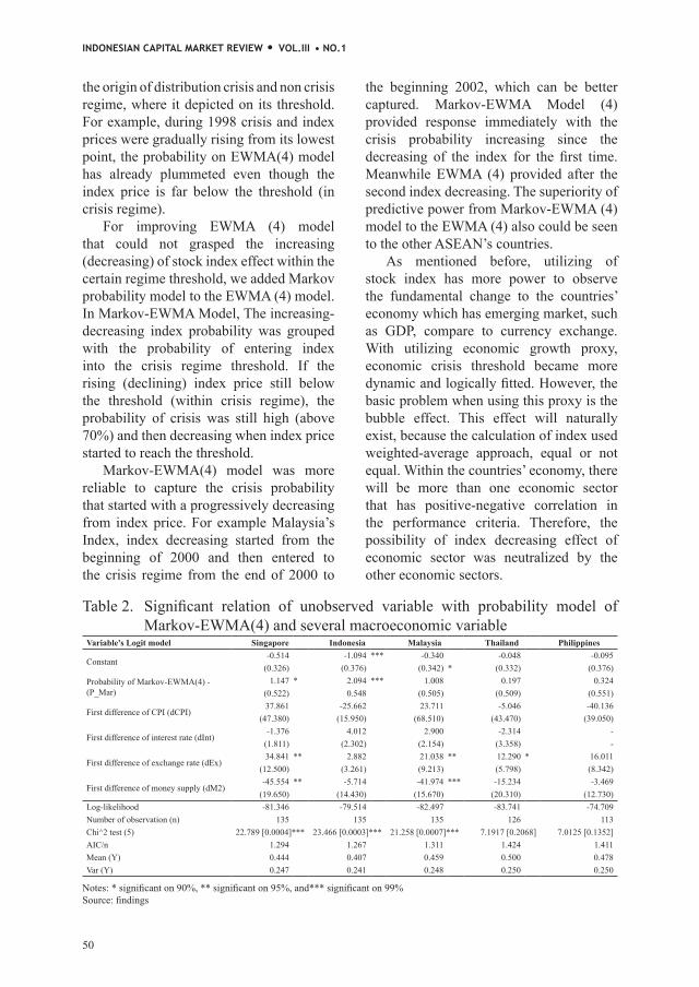
Table 2. Significant relation of unobserved variable with probability model of Markov-EWMA(4) and several macroeconomic variable

Notes: * significant on 90%, ** significant on 95%, and*** significant on 99%Source: findings

Wahyudi, Luxianto, Iwani, and Sulung

51

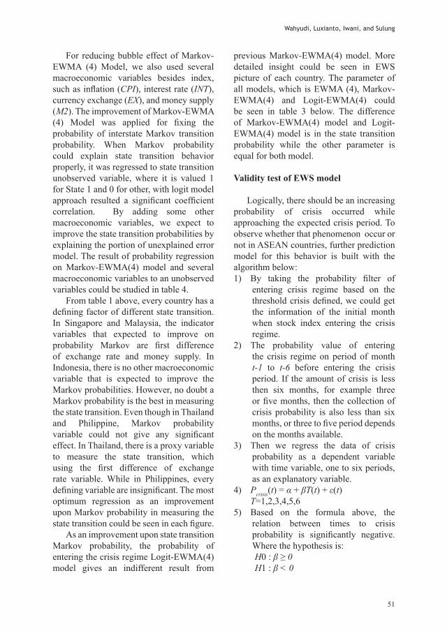
For reducing bubble effect of Markov-EWMA (4) Model, we also used several macroeconomic variables besides index, such as inflation (CPI), interest rate (INT), currency exchange (EX), and money supply (M2). The improvement of Markov-EWMA (4) Model was applied for fixing the probability of interstate Markov transition probability. When Markov probability could explain state transition behavior properly, it was regressed to state transition unobserved variable, where it is valued 1 for State 1 and 0 for other, with logit model approach resulted a significant coefficient correlation. By adding some other macroeconomic variables, we expect to improve the state transition probabilities by explaining the portion of unexplained error model. The result of probability regression on Markov-EWMA(4) model and several macroeconomic variables to an unobserved variables could be studied in table 4.

From table 1 above, every country has a defining factor of different state transition. In Singapore and Malaysia, the indicator variables that expected to improve on probability Markov are first difference of exchange rate and money supply. In Indonesia, there is no other macroeconomic variable that is expected to improve the Markov probabilities. However, no doubt a Markov probability is the best in measuring the state transition. Even though in Thailand and Philippine, Markov probability variable could not give any significant effect. In Thailand, there is a proxy variable to measure the state transition, which using the first difference of exchange rate variable. While in Philippines, every defining variable are insignificant. The most optimum regression as an improvement upon Markov probability in measuring the state transition could be seen in each figure.

As an improvement upon state transition Markov probability, the probability of entering the crisis regime Logit-EWMA(4) model gives an indifferent result from

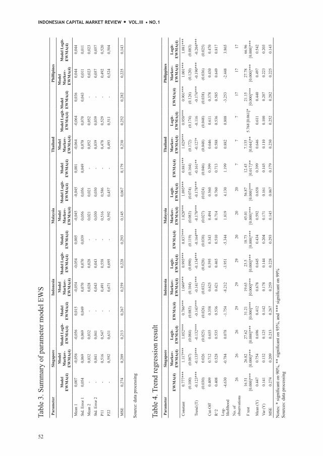
previous Markov-EWMA(4) model. More detailed insight could be seen in EWS picture of each country. The parameter of all models, which is EWMA (4), Markov-EWMA(4) and Logit-EWMA(4) could be seen in table 3 below. The difference of Markov-EWMA(4) model and Logit-EWMA(4) model is in the state transition probability while the other parameter is equal for both model.

Validity test of EWS model

Logically, there should be an increasing probability of crisis occurred while approaching the expected crisis period. To observe whether that phenomenon occur or not in ASEAN countries, further prediction model for this behavior is built with the algorithm below:1) By taking the probability filter of

entering crisis regime based on the threshold crisis defined, we could get the information of the initial month when stock index entering the crisis regime.

2) The probability value of entering the crisis regime on period of month t-1 to t-6 before entering the crisis period. If the amount of crisis is less then six months, for example three or five months, then the collection of crisis probability is also less than six months, or three to five period depends on the months available.

3) Then we regress the data of crisis probability as a dependent variable with time variable, one to six periods, as an explanatory variable.

4) Pcrisis(t) = α + βT(t) + ε(t) T=1,2,3,4,5,65) Based on the formula above, the

relation between times to crisis probability is significantly negative. Where the hypothesis is: H0 : β ≥ 0 H1 : β < 0

INDONESIAN CAPITAL MARKET REVIEW • VOL.III • NO.1

52

Sour

ce: d

ata

proc

essi

ng

Tabl

e 3.

Sum

mar

y of

par

amet

er m

odel

EW

SPa

ram

eter

Sing

apor

eIn

done

sia

Mal

aysi

aT

haila

ndPh

illip

ines

Mod

el

EW

MA

(4)

Mod

el

Mar

kov-

EW

MA

(4)

Mod

el L

ogit-

EW

MA

(4)

Mod

el

EW

MA

(4)

Mod

el

Mar

kov-

EW

MA

(4)

Mod

el L

ogit-

EW

MA

(4)

Mod

el

EW

MA

(4)

Mod

el

Mar

kov-

EW

MA

(4)

Mod

el L

ogit-

EW

MA

(4)

Mod

el

EW

MA

(4)

Mod

el

Mar

kov-

EW

MA

(4)

Mod

el L

ogit-

EW

MA

(4)

Mod

el

EW

MA

(4)

Mod

el

Mar

kov-

EW

MA

(4)

Mod

el L

ogit-

EW

MA

(4)

Mea

n 1

0,00

7-0

,056

-0,0

560,

015

-0,0

54-0

,054

0,00

5-0

,045

-0,0

450,

001

-0,0

64-0

,064

0,03

60,

044

0,04

4St

d. E

rror

10,

054

0,06

90,

069

0,04

90,

070

0,07

00,

039

0,05

60,

056

0,04

90,

070

0,07

00,

043

0,01

10,

011

Mea

n 2

-0,

032

0,03

2-

0,02

80,

028

-0,

021

0,02

1-

0,05

20,

052

-0,

023

0,02

3St

d. E

rror

2-

0,04

10,

041

-0,

043

0,04

3-

0,03

00,

030

-0,

039

0,03

9-

0,05

70,

057

P11

-0,

516

0,54

7-

0,49

10,

558

-0,

516

0,58

6-

0,47

80,

529

-0,

492

0,52

0P2

2-

0,59

20,

631

-0,

671

0,69

5-

0,59

20,

457

-0,

493

0,51

1-

0,52

40,

504

MSE

0,27

40,

209

0,21

30,

267

0,25

90,

228

0,29

30,

145

0,06

70,

179

0,23

00,

252

0,28

20,

225

0,14

3

Not

es: *

sign

ifica

nt o

n 90

%, *

* si

gnifi

cant

on

95%

, and

***

sign

ifica

nt o

n 99

%So

urce

s: d

ata

proc

essi

ng

Tabl

e 4.

Tre

nd re

gres

sion

resu

ltPa

ram

eter

Sing

apor

eIn

done

sia

Mal

aysi

aT

haila

ndPh

ilipp

ines

EW

MA

(4)

Mar

kov-

EW

MA

(4)

Log

it-E

WM

A(4

)E

WM

A(4

)M

arko

v-E

WM

A(4

)L

ogit-

EW

MA

(4)

EW

MA

(4)

Mar

kov-

EW

MA

(4)

Log

it-E

WM

A(4

)E

WM

A(4

)M

arko

v-E

WM

A(4

)L

ogit-

EW

MA

(4)

EW

MA

(4)

Mar

kov-

EW

MA

(4)

Log

it-E

WM

A(4

)C

onst

ant

0.77

7***

1.11

7***

1.05

2***

0.78

6***

1.04

9***

0.99

5***

0.83

7***

1.02

8***

1.09

5***

0.88

1***

1.02

9***

0.95

8***

0.90

1***

1.00

1***

1.08

1***

(0.1

00)

(0.0

87)

(0.0

84)

(0.0

83)

(0.1

04)

(0.0

90)

(0.1

19)

(0.0

83)

(0.0

74)

(0.1

64)

(0.1

72)

(0.1

74)

(0.1

26)

(0.1

20)

(0.0

83)

Tren

d (T

)-0

.123

***

-0.1

35**

*-0

.132

***

-0.1

43**

*-0

.141

***

-0.1

34**

*-0

.164

***

-0.1

78**

*-0

.178

***

-0.1

61**

-0.1

27*

-0.1

16-0

.174

***

-0.1

90**

*-0

.204

***

(0.0

30)

0.02

6 (0

.025

)(0

.026

)(0

.032

)(0

.028

)(0

.038

)(0

.027

)(0

.024

)(0

.046

)(0

.048

)(0

.048

)(0

.038

)(0

.036

)(0

.025

)C

ut-O

ff0.

409

0.71

20.

655

0.35

80.

625

0.59

50.

343

0.49

40.

560

0.39

90.

646

0.61

10.

378

0.43

00.

470

R^2

0.40

80.

528

0.53

50.

536

0.42

10.

465

0.51

00.

714

0.76

00.

713

0.58

80.

536

0.58

50.

649

0.81

7Lo

g-lik

elih

ood

-4.6

30-0

.784

0.07

8-1

.754

-8.2

12-3

.951

-5.3

441.

819

4.13

01.

199

0.88

20.

808

-3.2

53-2

.448

3.86

5

No.

of

obse

rvat

ions

2626

2629

2929

2020

207

77

1717

17

F te

st16

.51

[0.0

00]*

**26

.82

[0.0

00]*

**27

.62

[0.0

00]*

**31

.21

[0.0

00]*

**19

.63

[0.0

00]*

**23

.5

[0.0

00]*

**18

.73

[0.0

00]*

**45

.01

[0.0

00]*

**56

.87

[0.0

00]*

**12

.43

[0.0

17]*

*7.

135

[0.0

44]*

*5.

768

[0.0

61]*

21.1

5 [0

.000

]***

27.7

8 [0

.000

]***

66.9

6 [0

.000

]***

Mea

n (Y

)0.

447

0.75

40.

696

0.41

20.

678

0.64

50.

434

0.59

20.

658

0.39

90.

646

0.61

10.

440

0.49

70.

542

Var (

Y)

0.14

10.

132

0.12

50.

142

0.17

80.

144

0.20

40.

171

0.16

10.

145

0.11

00.

100

0.20

70.

223

0.20

3M

SE0.

274

0.20

90.

213

0.26

70.

259

0.22

80.

293

0.14

50.

067

0.17

90.

230

0.25

20.

282

0.22

50.

143

Using the same logic, we could develop the crisis signal cut off for the next three months. P crisis value is resulted from inserting T=3. This means the regression model above could also be the cut off function for period t-1 to t-6. Nevertheless, the test of predicting power EWS related with cut off issue could not be part of this research.

The validity test to measure the best EWS model is using the Mean Square Error (MSE) approach based on the crisis probability and the occurrence of crisis event based on the crisis threshold (1 when crisis occurred and 0 if other). But to reduce the mistakes of test model related to wrong samples, we could only use the observed data in the model above (the result is shown in table 3).

The result of trend regression and MSE test could be seen in table 4.

Conclusion

Using the stock index from 5 ASEAN countries, which is Singapore, Indonesia, Malaysia, Thailand and Philippines, this paper develops EWS as an anticipatory model of economic crisis event. The preference of stock index proxy could be a debatable issue. Stock index is a combination of every economic sector in one country, where it is possible to have a negative and positive correlation. This will eventually lead to bubble effect as an outcome of counter neutralizing of every up (and down) in stock sectoral price. However, by using this proxy, we were able to capture the fundamental shift of a country.

EWSs were built to predict the event of crisis three months ahead with three models, which is EWMA (4), Markov-EWMA(4), and Logit-EWMA(4). The implementation of EWMA (4) as a basic model of random variable yt was the second debatable issue. Hamilton (1989) use an AR (4) model by

estimating the parameter model of AR(4) simultaneously along with mix normal distribution (two normal distribution with different parameter); by assuming the Markov probability is constant.

Diebold et al. (1999) transforms Hamilton’s (1989) assumption by using logit model on the state transition probabilities, and several other researches uses other random variables yt such as AR(1) model by Chauvet (1998), Dueker (1997) with model Markov-GARCH, Cai (2004) and Hamilton and Susmel (1994) with model Markov-ARCH(2) process, and Haas et al. (2004) who used model Markov-Mixed Normal GARCH (MN-GARCH).

From the plotting of actual data of stock index and crisis probability, we conclude that generally Markov-EWMA(4) model and Logit-EWMA(4) model could present a better result than EWMA(4). This means that the state transition probability are able to improve the probabilities of entering the crisis regime. The last issue was the definition of threshold line to give signal of crisis for three months ahead. The logical foundation in this paper is that the crisis probability was supposed to increase when approaching the crisis period.

By regressing the trend model of crisis probabilities six months prior to crisis event, we could obtained a model that is applicable as a cut off model, where this idea is more academically representable than the cut off threshold definition by Hamilton dan Engel (1990) dan Bussiere dan Fratzcher (2006).

Acknowledgements

The researchers would like to acknowledge Muhammad Halley Yudistira for gathering the data set used for this research. Any constructive suggestions and comments from Bambang Hermanto have inspired the researchers to examine the data more advanced. The researcher would also like to thank Herman

Wahyudi, Luxianto, Iwani, and Sulung

53

Saherudin, Muhammad Budi Prasetyo, Imam Salehudin, and Abdur Rabbi for

any discussion conducted. All errors and opinions are of course our own.

References

Alvarez-Plata, P. and Schrooten, M. (2003), The Argentinean Currency Crisis- A Markov-Switching Model Estimation, Working Paper.

Berg, A. and Pattillo C. (1999), Predicting Currency Crises: The Indicators Approach and an Alternative, Journal of International Money and Finance, 18(4), 561-86.

Bussiere, M. and Fratzscher, M. (2006), Towards a New Early Warning System of Financial Crises, Journal of International Money and Finance, 25, 953-73.

Cai, J. (2004), A Markov Model of Switching-Regime ARCH, Journal of Business & Economic Statistics, 12, 309-16.

Chauvet, M. (1998), An Econometric Characterization of Business Cycle Dynamics with Factor Structure and Regime Switching, International Economic Review, 39, 969-96.

Diebold, F.X., Lee, J.H., and Weinbach, G. (1999), Regime Switching with Time-Varying Transition Probabilities, Nonstationary Time Series Analysis and Cointegration, Oxford University Press, 283-302.

Dueker, M.J. (1997), Markov Switching in GARCH Processes and Mean-Reverting Stock-Market Volatility, The Federal Reserve Bank of St. Louis: Working Paper Series 1994-015B.

Eichengreen, B., Rose, A., and Wyplosz, C. (1995), Exchange Market Mayhem: The Antecedents and Aftermaths of Speculative Attacks, Economic Policy, 21, 249-312.

Engel, R. and Hamilton, J.D. (1990), Long Swings in the Dollar: Are They in the Data and Do Markets Know It?, The American Economic Review, 80, 689-713.

Frankel, J. and Rose, A. (1996), Currency Crashes in Emerging Markets: An Empirical Treatment, Journal of International Economics, 41, 351-66.

Garcia, R. (1998), Asymptotic Null Distribution of the Likelihood Ratio Test in Markov Switching Models, International Economic Review, 39, 763-88.

Giancardo, C., Presenti, P., and Roubini, N. (1998), What Caused the Asian Currency and Financial Crisis? A Macroeconomic Overview, NBER Working Paper Series.

Goldstein, M., Kaminsky, G., and Reinhart, C. (2000), Assessing Financial Vulnerability: An Early Warning System for Emerging Markets, Institute for International Economics, Washington, DC.

Goodwin, T.H. (1993), Business-Cycle Analysis with a Markov-Switching Model, Journal of Business and Economic Statistics, 11, 331-39.

Hamilton, J.D. (1989), A New Approach to the Economic Analysis of Nonstationary Time Series and the Business Cycle, Econometrica, 57, 357-84.

Hamilton, J.D. (1991), A Quasi-Bayesian Approach to Estimating Parameters for Mixtures of Normal Distributions, Journal of Business & Economic Statistics, 9, 27-39.

Haas, M., Mittnik, S., and Paolella, M.S. (2004), A New Approach to Markov-Switching GARCH Models, working paper.

Kamin, S. and Babson, O. (1999), The Contribution of Domestic and External Factors to Latin American Devaluation Crises: An Early Warning Systems Approach, International Finance Discussion Papers Number 645, Board of Governors of the Federal Reserve System.

INDONESIAN CAPITAL MARKET REVIEW • VOL.III • NO.1

54

Wahyudi, Luxianto, Iwani, and Sulung

55

Kaminsky, G., Lizondo, S., and Reinhart, C. (1998), Leading Indicators of Currency Crises, IMF Staff Papers, 45(1), 1-48.

Kaminsky, G. and Reinhart, C. (1999), The Twin Crises: The Causes of Banking and Balance-of-Payments Problems, American Economic Review, 89(3), 473-500.

Kim, C.J. and Nelson C.R. (2001), A Bayesian Approach to Testing for Markov-Switching in Univariate and Dynamic Factor Models, International Economic Review, 42, 989-1013.

Lux, T. (2004), The Markov-Switching Multi-Fractal Model of Asset Returns: GMM Estimation and Linear Forecasting of Volatility, Economics Working Paper, 2004-11.

Peria, M.S.M. (2002), A Regime-switching Approach to the Study of Speculative Attacks: A Focus on EMS Crises, Empirical Economics, 27, 299-334.

Nelson, C.R., Piger, J., and Zivot, E. (2001), Markov Regime Switching and Unit-Root Tests, Journal of Business & Economic Statistics, 19, 404-15.

Persaud, A. (1998), Event Risk Indicator Handbook, J.P. Morgan. Pettway, R.H. And Sinkey, J.F. (1980), Establishing on-site Bank Examination Priorities:

An Early-warning System Using Accounting and Market Information, The Journal of Finance, 35(1), 137-50.

Radelet, S., Sachs, J.D., Cooper, R.N., and Bosworth, B.P. (1998), The East Asian Financial Crisis: Diagnosis, Remedies, Prospects, Brookings Papers on Economic Activity, 1, 1-90.

Roy, A. and Tudela, M. (2001), Emerging Market Risk Indicator (EMRI): Re-estimated Version September 2000, Credit Suisse First Boston (CSFB).

Sachs, J., Tornell, A., Velasco, A., Giavazzi, F., and Szekely, I. (1996a), The Collapse of the Mexican Peso: What Have We Learned?, Economic Policy, 11, 13-63.

Sachs, J., Tornell, A., and Velasco, A. (1996b), Financial Crises in Emerging Markets: The Lessons from 1995. Brookings Papers on Economic Activity, 1, 147-215.

Sachs, J., Tornell, A., and Velasco, A. (1996c), The Mexican Peso Crisis: Sudden Death or Death Foretold?, Journal of International Economics, 41, 265-83.

Schnatz, B. (1998), Macroeconomic Determinants of Currency Turbulences in Emerging Markets, Discussion Paper 3/98, Economic Research Group of the Deutsche Bundesbank.

Watson, C.J., Billingsley, P., Croft, D.J., and Huntsberger, D.V. (1993), Statistics for Management and Economics, USA: Allyn and Bacon.

Wecker, W.E. (1979), Predicting the Turning Points of a Time Series, The Journal of Business, 52, 35-50.

Wonnacott, T.H. and Wonnacott, R.J. (1984), Introductory Statistics for Business and Economics, USA: John Wiley and Sons.

Yao, J.F. and Attali, J.G. (2000), On Stability of Nonlinear AR Processes with Markov Switching, Advances in Applied Probability, 32, 394-407.

INDONESIAN CAPITAL MARKET REVIEW • VOL.III • NO.1

56

Appendix

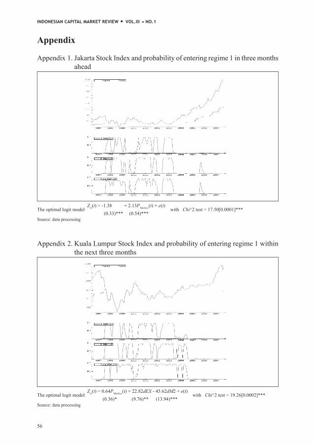
Appendix 2. Kuala Lumpur Stock Index and probability of entering regime 1 within the next three months

The optimal logit model Zst(t) = 0.64PMarkov(t) + 22.82dEX - 45.62dM2 + e(t)

with

Chi^2 test = 19.26[0.0002]*** (0.36)* (9.76)** (13.94)***Source: data processing

Appendix 1. Jakarta Stock Index and probability of entering regime 1 in three months ahead

The optimal logit model Zst(t) = -1.38 + 2.13PMarkov(t) + e(t)

with

Chi^2 test = 17.50[0.0001]*** (0.33)*** (0.54)***Source: data processing

Wahyudi, Luxianto, Iwani, and Sulung

57

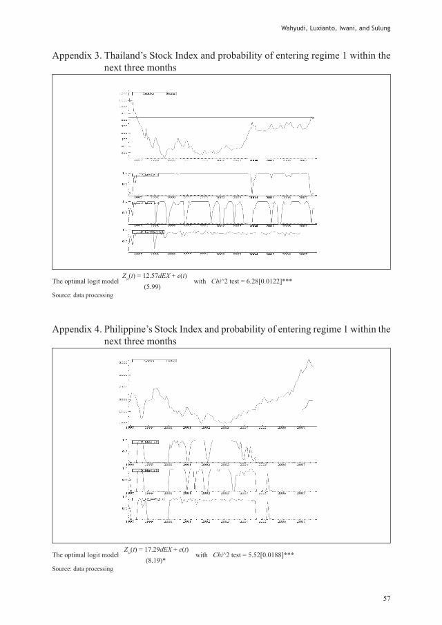
Appendix 3. Thailand’s Stock Index and probability of entering regime 1 within the next three months

The optimal logit model Zst(t) = 12.57dEX + e(t)

with

Chi^2 test = 6.28[0.0122]*** (5.99)Source: data processing

Appendix 4. Philippine’s Stock Index and probability of entering regime 1 within the next three months

The optimal logit model Zst(t) = 17.29dEX + e(t)

with

Chi^2 test = 5.52[0.0188]*** (8.19)*Source: data processing

INDONESIAN CAPITAL MARKET REVIEW • VOL.III • NO.1

58