
university of wollongong copyright warning
284
NOTE This online version of the thesis may have different page formatting and pagination from the paper copy held in the University of Wollongong Library. UNIVERSITY OF WOLLONGONG COPYRIGHT WARNING You may print or download ONE copy of this document for the purpose of your own research or study. The University does not authorise you to copy, communicate or otherwise make available electronically to any other person any copyright material contained on this site. You are reminded of the following: Copyright owners are entitled to take legal action against persons who infringe their copyright. A reproduction of material that is protected by copyright may be a copyright infringement. A court may impose penalties and award damages in relation to offences and infringements relating to copyright material. Higher penalties may apply, and higher damages may be awarded, for offences and infringements involving the conversion of material into digital or electronic form.
-
Upload
khangminh22 -
Category
Documents
-
view
1 -
download
0
Transcript of university of wollongong copyright warning

NOTE
This online version of the thesis may have different page formatting and pagination from the paper copy held in the University of Wollongong Library.
UNIVERSITY OF WOLLONGONG
COPYRIGHT WARNING
You may print or download ONE copy of this document for the purpose of your own research or study. The University does not authorise you to copy, communicate or otherwise make available electronically to any other person any copyright material contained on this site. You are reminded of the following: Copyright owners are entitled to take legal action against persons who infringe their copyright. A reproduction of material that is protected by copyright may be a copyright infringement. A court may impose penalties and award damages in relation to offences and infringements relating to copyright material. Higher penalties may apply, and higher damages may be awarded, for offences and infringements involving the conversion of material into digital or electronic form.


RAPID ADAPTIVE PROGRAMMING USING IMAGE DATA
A thesis submitted in fulfilment of the requirements for the award of the degree
Doctor of Philosophy (PhD)
UNIVERSITY OF WOLLONGONG
Alexander Nicholson
Bachelor of Engineering Honours (Class I)
Bachelor of Mathematics (Distinction)
FACULTY OF ENGINEERING
2005

ii

Acknowledgements
iii
ACKNOWLEDGEMENTS
There are several people I would like to acknowledge for their assistance and support
over the course of this work. Firstly, I would like to sincerely thank Professor John
Norrish for sharing his technical expertise and experience with me – I would be lost
without his support and encouragement. I would like to also express my gratitude to Dr
Paul Di Pietro for his continuing support and invaluable supervision. I acknowledge the
Cooperative Research Centre for Welded Structures (CRC-WS) who initiated this work
and thank the PowerGen sponsor group for their support, in particular, Mr Ivor Wright
for his industrial guidance. Thanks are also extended to Mr Joe Abbott, Dr Gary Dean,
and Dr Dominic Cuiuri who always helped out and offered advice when needed.
Finally, without having wife Katharina by my side I could not have completed this
thesis and I would like to thank her sincerely. To my dad Warren, brothers Josh and
Ben, and friends; thanks for being there when I needed you. To my late mum Pauline, I
hope I have made you proud.

iv

Disclaimer
v
DISCLAIMER
I declare that this thesis, submitted in fulfilment of the requirements for the award of
Doctor of Philosophy in the Faculty of Engineering, University of Wollongong, is my
own work unless otherwise referenced or acknowledged. This thesis has not been
submitted for qualifications at any other academic institution.
____________________________
Alexander Nicholson
17/08/2005

vi

Contents
vii
CONTENTS
List of Figures ................................................................................................................. ix
List of Tables...................................................................................................................xv
Abstract ........................................................................................................................ xvii
Awards .......................................................................................................................... xix
Publications ................................................................................................................... xix
1. Introduction.............................................................................................................1
1.1 Background ........................................................................................................2
1.2 Thesis Objective.................................................................................................2
1.3 Thesis Outline ....................................................................................................3
2. Literature Review ...................................................................................................5
2.1 Introduction ........................................................................................................6
2.2 Hydro Turbine Operation...................................................................................6
2.3 Cavitation .........................................................................................................10
2.3.1 Cavitation Damage ...................................................................................11
2.3.2 Cavitation Erosion in Turbines.................................................................12
2.3.2.1 Cavitation Mechanisms.........................................................................12
2.3.2.2 Cavitation Damage of Turbine Runner Blades.....................................13
2.3.2.3 Cavitation Damage of Other Turbine Equipment.................................15
2.3.2.4 Laboratory Studies of Cavitation ..........................................................16
2.4 Materials...........................................................................................................18
2.4.1 Turbine Runner Parent Materials .............................................................19
2.4.2 Alternative Parent Materials .....................................................................20
2.5 Current Manual Repair Procedures ..................................................................22
2.5.1 Surface Preparation...................................................................................23
2.5.2 Welding Consumables for Runner Repairs ..............................................24
2.5.3 Welding Considerations ...........................................................................24
2.5.4 Post-Weld Heat Treatment and Finishing.................................................25
2.5.5 Quality Assurance and Occupational Safety ............................................26
2.5.6 Welding Process .......................................................................................27
2.6 Robotics ...........................................................................................................30
2.6.1 Advanced Robotics...................................................................................31

Contents
viii
2.6.2 Communications.......................................................................................34
2.6.3 Kinematics................................................................................................35
2.6.4 Welding Robotics .....................................................................................36
2.6.5 Programming ............................................................................................38
2.6.5.1 Online ...................................................................................................38
2.6.5.2 Offline...................................................................................................39
2.6.5.2.1 Trajectory Planning........................................................................41
2.6.5.2.2 Simulation ......................................................................................42
2.7 Adaptive Control and Monitoring....................................................................45
2.7.1 Contact Sensors ........................................................................................46
2.7.1.1 Mechanical Probe .................................................................................46
2.7.1.2 Touch-Sensing ......................................................................................47
2.7.2 Non-Contact Sensors ................................................................................49
2.7.2.1 Arc Parameter Sensing .........................................................................49
2.7.2.2 Electromagnetic Sensors.......................................................................51
2.7.2.3 Ultrasonic Sensors ................................................................................51
2.7.2.4 Thermal Sensors ...................................................................................51
2.7.2.5 Vision Sensors ......................................................................................51
2.7.2.5.1 Laser-Based Systems .....................................................................55
2.7.2.5.2 Non-Laser-Based Systems .............................................................58
2.7.3 Sensor System Summary..........................................................................60
2.8 Profilometry .....................................................................................................60
2.8.1 Surface Scanning Techniques...................................................................60
2.8.1.1 Coordinate Measuring Machine (CMM) ..............................................61
2.8.1.2 CT Scanner ...........................................................................................61
2.8.1.3 Laser Scanners ......................................................................................61
2.8.1.4 Multi-Cameras ......................................................................................62
2.8.1.5 Pre-Weld Grinding for Surface Mapping .............................................62
2.8.1.6 Touch-Sensing ......................................................................................62
2.8.1.7 Ultrasonic Sensors ................................................................................63
2.8.2 Profile Measurement for Hydro Turbines ................................................63
2.9 Robotic Repair Systems ...................................................................................64
2.9.1 Portable Robots ........................................................................................64
2.9.2 Dedicated Welding Machines and Tractors..............................................65

Contents
ix
2.9.3 Robotic Repair of Crawler Shoes .............................................................65
2.9.4 Robotic Repair of Hydro Turbine Runners ..............................................67
2.10 Summary ..........................................................................................................72
3. Experimental Robotic Welding Cell ...................................................................73
3.1 Introduction ......................................................................................................74
3.2 Robot Package..................................................................................................75
3.3 Camera .............................................................................................................76
3.4 Welding System ...............................................................................................77
3.5 Testpiece ..........................................................................................................80
3.6 PC System ........................................................................................................82
3.7 Data Acquisition...............................................................................................83
3.8 Summary ..........................................................................................................84
4. Software Development..........................................................................................87
4.1 Introduction ......................................................................................................88
4.2 Control Module ................................................................................................88
4.2.1 Application Requirements ........................................................................89
4.2.2 System Design ..........................................................................................89
4.2.2.1 Communications ...................................................................................89
4.2.2.2 Development Technologies ..................................................................89
4.2.2.3 Implementation .....................................................................................90
4.3 Image Acquisition and Processing ...................................................................94
4.4 RAPID Weld Path Generator .........................................................................104
4.4.1 TopLeft Search .......................................................................................113
4.4.2 TopRight Search .....................................................................................117
4.4.3 BottomRight Search ...............................................................................121
4.4.4 BottomLeft Search..................................................................................124
4.4.5 Boundary Points .....................................................................................129
4.4.6 Weld Bead Geometry .............................................................................135
4.5 Robot Program Generation ............................................................................149
4.6 Camera Positioning ........................................................................................152
5. Validation ............................................................................................................157
5.1 Introduction ....................................................................................................158
5.2 Touch-Sensing................................................................................................158
5.3 Vision Assisted Programming........................................................................159

Contents
x
5.3.1 Flat Surface.............................................................................................161
5.3.2 Curved Surface .......................................................................................163
5.3.3 Inclined Surface......................................................................................164
6. Discussion ............................................................................................................173
6.1 Surface Mapping ............................................................................................175
6.2 Cell Interfacing ..............................................................................................177
6.3 Programming..................................................................................................177
6.4 Relationship with Existing Automated Repair Techniques ...........................178
7. Conclusions and Recommendations..................................................................181
7.1 Conclusions....................................................................................................182
7.2 Recommendations..........................................................................................182
8. References............................................................................................................185
9. Bibliography........................................................................................................199
10. Appendix..............................................................................................................211
10.1 IRB1400 Specification Details.......................................................................212
10.2 Mini Robots and Portable Welding Machines ...............................................214
10.2.1 FANUC LR Mate 100iB & FANUC LR Mate 200iB............................214
10.2.2 Mitsubishi PA-10 ...................................................................................216
10.2.3 Motoman-SV3X & Motoman-UPJ.........................................................216
10.2.4 Panasonic VR-004..................................................................................217
10.2.5 Portable Welding Machines ...................................................................218
10.2.6 Robot Requirements ...............................................................................219
10.2.7 Suitable Systems.....................................................................................221
10.3 Process Selection for Automated Repair .......................................................221
10.4 Robot Coordinate Representation ..................................................................226
10.5 Robot Simulation Packages ...........................................................................229
ACT-LIB ...............................................................................................................229
GRASP ..................................................................................................................229
MATLAB VR........................................................................................................230
IGRIP.....................................................................................................................230
DELMIA................................................................................................................231
ROBCAD ..............................................................................................................233
Robographics .........................................................................................................233
ROBOSIM.............................................................................................................234

Contents
xi
RobotStudio ...........................................................................................................234
Workspace .............................................................................................................235
10.6 SICK Industrial Sensors.................................................................................236
10.7 Digitisers ........................................................................................................238
10.7.1 Roland 3D Laser Scanners .....................................................................238
10.7.2 ROMER CimCore Scanning Arms.........................................................241
10.7.3 METRICOR............................................................................................245
10.8 Grinding .........................................................................................................246
10.9 Cavitation Mechanisms..................................................................................247
10.10 Welding Consumables for Cavitation Repairs ...........................................249
10.10.1 Stainless Steels....................................................................................249
10.10.2 Advanced Iron-Based Alloys..............................................................250
CaviTec ..............................................................................................................250
Hydroloy 914 .....................................................................................................252
NOREM .............................................................................................................254
D-Cav.................................................................................................................255
10.10.3 Cobalt- and Nickel-Based Alloys .......................................................256
10.10.4 Cavitation Test Results on Various Alloys.........................................256

xii

List of Figures
xiii
LIST OF FIGURES
Figure 2.1 Hydroelectric power plant schematic [3]. ...................................................7
Figure 2.2 Typical operating ranges for various turbines [2]. ......................................7
Figure 2.3 Kaplan turbine: (a) schematic; (b) runner. ..................................................8
Figure 2.4 Francis turbine: (a) schematic;
(b) low head runner – Bendeela Power Station...........................................9
Figure 2.5 Francis turbine: (a) low head runner – Deutsches Museum;
(b) high head runner – Kangaroo Valley Power Station. ............................9
Figure 2.6 Pelton wheel turbine: (a) schematic; (b) runner – Deutsches Museum.....10
Figure 2.7 (a) Schematic representation of cavity growth, collapse and rebound;
(b) graph of cavity diameter as a function of time [9]...............................13
Figure 2.8 Successive stages of non-symmetrical cavity collapse [9]........................13
Figure 2.9 Typical areas of cavitation pitting [10]: (a) Kaplan turbine;
(b) Francis turbine. ....................................................................................14
Figure 2.10 Low pressure cavitation damage: (a) turbine runner; (b) pump impeller..15
Figure 2.11 (a) Draft tube liner cavitation damage; (b) air vent erosion. .....................16
Figure 2.12 Pump casing cavitation corrosion/erosion damage. ..................................16
Figure 2.13 Localised cavitation damage on a Francis turbine runner. ........................17
Figure 2.14 Flow analysis for a Francis turbine runner [11]. .......................................17
Figure 2.15 Alloy groups compared by cavitation erosion resistance [8]. ...................19
Figure 2.16 Manual welding of a turbine runner in restricted space [19]. ...................26
Figure 2.17 ‘Finger’ probe [22]. ...................................................................................46
Figure 2.18 Welding tractor with ‘roller’ sensor [81]. .................................................47
Figure 2.19 Wire touch-sensing algorithms [48]: (a) fillet; (b) edge-butt;
(c) edge detection. .....................................................................................48
Figure 2.20 Touch-sensing used to determine joint location [82]. ...............................48
Figure 2.21 Power spectra can be used for online control [22]. ...................................50
Figure 2.22 Welding trial result [114]. .........................................................................52
Figure 2.23 Coordinate system of the parallel binocular CCD cameras [111].............53
Figure 2.24 Sensors used for collision prevention and measurement tasks [119]. .......55
Figure 2.25 Joint location determination using lasers [120].........................................56
Figure 2.26 Point sensor schematic [22].......................................................................57

List of Figures
xiv
Figure 2.27 Array sensor schematic [22]......................................................................57
Figure 2.28 Seam tracking using lasers: (a) [125]; (b) [29]. ........................................57
Figure 2.29 Area sensor schematic [22]. ......................................................................58
Figure 2.30 NB-2SV portable butt welding machine [81]. ..........................................65
Figure 2.31 Crawler shoe showing excess material at edges (metal flow)...................66
Figure 2.32 Crawler shoe in robotic welding cell prior to welding [133]. ...................66
Figure 2.33 Crawler shoe after robotic welding but prior to grinding/detailing [133].67
Figure 2.34 SCOMPI [19]. ...........................................................................................69
Figure 2.35 SCOMPI grinding operation [19]..............................................................69
Figure 2.36 SCOMPI welding operation [19]. .............................................................70
Figure 2.37 Schematic of polygon contour technique [140]. .......................................71
Figure 2.38 Cavity-fill path planning [141]..................................................................71
Figure 3.1 Robotic welding cell schematic. ...............................................................74
Figure 3.2 ABB IRB1400 [142]. ................................................................................75
Figure 3.3 ABB S4C robot controller and teach pendant...........................................76
Figure 3.4 AVT Marlin F-046C torch-mounted CCD camera. ..................................77
Figure 3.5 Fronius TransPulsSynergic 4000 power supply and Fronius VR 4000
wire feed unit.............................................................................................78
Figure 3.6 Windows Remote Control Unit (WinRCU). .............................................79
Figure 3.7 Robot Visualise. ........................................................................................79
Figure 3.8 LocalNetOPC Server.................................................................................80
Figure 3.9 Low head Francis runner – Bendeela Power Station. ...............................81
Figure 3.10 Mock-up section of turbine runner in laboratory. .....................................81
Figure 3.11 (a) Turbine runner showing cavitation damage;
(b) mock-up runner with simulated damage. ............................................82
Figure 3.12 Robot controller / power supply connections............................................84
Figure 3.13 Welding cell connections. .........................................................................85
Figure 4.1 Login screen. .............................................................................................90
Figure 4.2 Main screen. ..............................................................................................90
Figure 4.3 Status information. ....................................................................................91
Figure 4.4 I/O manipulation. ......................................................................................91
Figure 4.5 File Explorer. ............................................................................................92
Figure 4.6 Text-based offline programming...............................................................93
Figure 4.7 Program details (Excel link)......................................................................93

List of Figures
xv
Figure 4.8 SpotDot GUI. ............................................................................................95
Figure 4.9 Small dots placed to indicate nearby damage. ..........................................96
Figure 4.10 Target identified. .......................................................................................97
Figure 4.11 (a) Unfiltered image; (b) Sobel filtered image. .........................................98
Figure 4.12 QuickSnap GUI. ........................................................................................99
Figure 4.13 Identification sequence............................................................................100
Figure 4.14 Identification sequence............................................................................101
Figure 4.15 SpotDot program flowchart.....................................................................102
Figure 4.16 QuickSnap program flowchart. ...............................................................103
Figure 4.17 WPGenUI GUI........................................................................................104
Figure 4.18 Operation in Point mode. ........................................................................105
Figure 4.19 Operation in Line mode...........................................................................105
Figure 4.20 Save program once weld paths are acceptable. .......................................106
Figure 4.21 Error made when defining region............................................................107
Figure 4.22 Clear erroneous paths. .............................................................................107
Figure 4.23 Text-based program modification. ..........................................................108
Figure 4.24 Viewing window size determination.......................................................109
Figure 4.25 Mouse click locations..............................................................................110
Figure 4.26 Algorithm starts at lowest point. .............................................................112
Figure 4.27 Searching region......................................................................................114
Figure 4.28 Bottom-top search. ..................................................................................115
Figure 4.29 Bottom-top search special case – leftmost point chosen. ........................116
Figure 4.30 Searching region......................................................................................117
Figure 4.31 Searching region......................................................................................118
Figure 4.32 Left-right search. .....................................................................................119
Figure 4.33 Left-right search special case – uppermost point chosen. .......................120
Figure 4.34 Searching region......................................................................................121
Figure 4.35 Top-bottom search...................................................................................122
Figure 4.36 Top-bottom search special case – rightmost point chosen. .....................123
Figure 4.37 Searching region......................................................................................124
Figure 4.38 Right-left search. .....................................................................................125
Figure 4.39 Right-left search special case – lowermost point chosen. .......................126
Figure 4.40 Searching region......................................................................................127
Figure 4.41 Right-left search. .....................................................................................128

List of Figures
xvi
Figure 4.42 Searching region......................................................................................129
Figure 4.43 Intermediate perimeter points. ................................................................130
Figure 4.44 Right hand side test. ................................................................................130
Figure 4.45 Valid points. ............................................................................................131
Figure 4.46 Invalid point. ...........................................................................................132
Figure 4.47 Internal points removed...........................................................................133
Figure 4.48 Final perimeter points. ............................................................................134
Figure 4.49 Weld bead offset. ....................................................................................136
Figure 4.50 Baseline selected based on incline condition. .........................................137
Figure 4.51 Baseline going left...................................................................................138
Figure 4.52 Baseline going right. ...............................................................................139
Figure 4.53 Offset calculations...................................................................................139
Figure 4.54 Projected perimeter point intercepts........................................................143
Figure 4.55 Weld path functions parallel to baseline. ................................................143
Figure 4.56 Determine endpoints. ..............................................................................145
Figure 4.57 Determine endpoints. ..............................................................................146
Figure 4.58 Final weld paths. .....................................................................................147
Figure 4.59 WPGenUI program flowchart. ................................................................148
Figure 4.60 Robot program flowchart. .......................................................................151
Figure 4.61 Normal vector determination. .................................................................152
Figure 4.62 Centre of area determination. ..................................................................154
Figure 4.63 New camera position determination........................................................154
Figure 4.64 Positioning algorithm computer model output........................................156
Figure 5.1 Touch-sensed profile showing limitations of wire touch-sensing...........158
Figure 5.2 WPGenUI output.....................................................................................160
Figure 5.3 Image transferred to PC. .........................................................................160
Figure 5.4 Automatic weld path generation. ............................................................160
Figure 5.5 Deposit weld metal..................................................................................160
Figure 5.6 Flat workpiece algorithm. .......................................................................162
Figure 5.7 Curved workpiece algorithm...................................................................163
Figure 5.8 Inclined workpiece algorithm. ................................................................164
Figure 5.9 Weld paths 1-6. .......................................................................................166
Figure 5.10 Weld paths 7-12. .....................................................................................167
Figure 5.11 Weld paths 13-18. ...................................................................................168

List of Figures
xvii
Figure 5.12 Weld paths 19-24. ...................................................................................169
Figure 5.13 Weld paths 25-30. ...................................................................................170
Figure 5.14 Weld paths 31-36. ...................................................................................171
Figure 10.1 IRB1400 working envelope. ...................................................................214
Figure 10.2 FANUC LR Mate 100iB: (a) robot arm; (b) working envelope..............215
Figure 10.3 FANUC LR Mate 200iB: (a) robot arm; (b) working envelope..............215
Figure 10.4 Mitsubishi PA-10: (a) robot arm; (b) working envelope.........................216
Figure 10.5 Motoman-SV3X: (a) robot arm; (b) working envelope. .........................217
Figure 10.6 Motoman-UPJ: (a) robot arm; (b) working envelope..............................217
Figure 10.7 Panasonic VR-004: (a) robot arm; (b) working envelope. ......................218
Figure 10.8 Noboruder portable welding machines [81]. ...........................................219
Figure 10.9 GRASP 3D modelling and simulation system [147]...............................229
Figure 10.10 MATLAB VR toolbox. ...........................................................................230
Figure 10.11 IGRIP representation of the ABB IRB1400 robot. .................................231
Figure 10.12 DELMIA representation of the ABB IRB1400 robot. ............................232
Figure 10.13 RobotStudio simulation package.............................................................234
Figure 10.14 Workspace simulation package [169]. ....................................................235
Figure 10.15 Roland LPX-1200 3D laser scanner........................................................239
Figure 10.16 Roland LPX-250 3D laser scanner..........................................................239
Figure 10.17 Scanning modes [171]: (a) plane; (b) rotary. ..........................................240
Figure 10.18 (a) ROMER CimCore 3000i scanning arm;
(b) turbine inspection using scanning arm. .............................................241
Figure 10.19 ROMER CimCore INFINITE scanning arm with combination
ball-laser probe........................................................................................242
Figure 10.20 ROMER CimCore LSI system and software. .........................................242
Figure 10.21 3D point-cloud obtained using METRICOR...........................................245
Figure 10.22 3D object surface profiles obtained using METRICOR. ........................245
Figure 10.23 Types of cavitation [1]: (a) profile; (b) slotted; (c) local. .......................248
Figure 10.24 Forms of cavitation in turbines [1]: (a) bubble cavitation;
(b) sheet cavitation; (c) separating cavitation; (d) supercavitation. ........248

xviii

List of Tables
xix
LIST OF TABLES
Table 2.1 Chemical composition of martensitic stainless steels [12]........................20
Table 2.2 Recommended minimum preheat temperature for welding [10]. .............25
Table 2.3 Repair procedures for various damage scenarios [10]. .............................28
Table 2.4 Sensor information [128]. .........................................................................59
Table 4.1 Unsorted coordinates...............................................................................111
Table 4.2 Sorted coordinates. ..................................................................................111
Table 4.3 Extreme points.........................................................................................112
Table 4.4 Searching matrix. ....................................................................................113
Table 4.5 Intermediate perimeter matrix. ................................................................113
Table 4.6 Filtered points matrix. .............................................................................114
Table 4.7 Searching matrix. ....................................................................................115
Table 4.8 Intermediate perimeter matrix. ................................................................115
Table 4.9 Filtered points matrix. .............................................................................116
Table 4.10 Searching matrix. ....................................................................................118
Table 4.11 Intermediate perimeter matrix. ................................................................118
Table 4.12 Filtered points matrix. .............................................................................119
Table 4.13 Searching matrix. ....................................................................................120
Table 4.14 Intermediate perimeter matrix. ................................................................120
Table 4.15 Filtered points matrix. .............................................................................122
Table 4.16 Searching matrix. ....................................................................................123
Table 4.17 Intermediate perimeter matrix. ................................................................123
Table 4.18 Filtered points matrix. .............................................................................125
Table 4.19 Searching matrix. ....................................................................................126
Table 4.20 Intermediate perimeter matrix. ................................................................126
Table 4.21 Filtered points matrix. .............................................................................127
Table 4.22 Searching matrix. ....................................................................................128
Table 4.23 Intermediate perimeter matrix. ................................................................128
Table 4.24 Intermediate perimeter matrix. ................................................................132
Table 4.25 Final perimeter matrix. ............................................................................134
Table 10.1 IRB1400 technical specifications [143,144]. ..........................................212
Table 10.2 IRB1400 arc welding equipment and functionality [144].......................213

List of Tables
xx
Table 10.3 Characteristics for various small robots. .................................................220
Table 10.4 Comparison of different repair techniques [134]. ...................................224
Table 10.5 Roland 3D laser scanner specifications...................................................240
Table 10.6 ROMER CimCore scanning arm specifications......................................244
Table 10.7 Recommended consumables and heat treatment [12]. ............................250
Table 10.8 CaviTec welding parameters [173]. ........................................................251
Table 10.9 Hydroloy 914 welding parameters [174]. ...............................................253
Table 10.10 Chemical compositions of NOREM alloys [175]. ..................................254
Table 10.11 Results of cavitation jet testing of welded alloys [177]. .........................258
Table 10.12 Chemical compositions of various alloys. ..............................................258

Abstract
xxi
ABSTRACT
This work was initiated to address the problem of automated weld repair in a specific
application; namely hydro turbine cavitation damage. An extensive review of the
application requirements was undertaken and this highlighted the need for a new
approach to robot programming. This thesis therefore focused on the development of a
novel rapid programming technique based on a vision system. The implementation
involved the development of algorithms to correlate robot and vision system
coordinates, communication links to the system hardware, and a software environment
to ‘manage’ the process. The complete system was successfully validated by
representative trials on a full-size hydro turbine mock-up.
Several investigations examining different industrial applications such as the weld
repair of hydro turbine runners in the power generation industry and weld repair of
crawler shoes in the mining sector have demonstrated the feasibility of using robot
technology. However, limitations have been identified in these investigations that
continue to impede the widespread acceptance and use of this technology in industry.
An offline programming technique was developed in this thesis that addresses some of
these limitations, and seeks to improve confidence in robotic systems for ‘one-off’ or
small batch run applications.
OH&S regulations were found to be the significant driver in developing systems for in-
situ repair by robot. Small commercial robots are available that partially satisfy the
requirements for in-situ use; however, a fast means of robot programming and the
ability to handle uniquely damaged shapes at arbitrary locations remains unsolved.
These have been appropriately addressed in the current work with the development of
an automatic adaptive system capable of rapid robot programming and online process
control via an intuitive, user-friendly PC-based interface.
Various sensor technologies and profilometry tools and techniques were reviewed.
Based on simplicity, cost, and availability, the most promising approaches identified
were touch-sensing or non-laser-based vision for profilometry, followed by offline robot
programming based on the acquired data. In this thesis, image acquisition was achieved

Abstract
xxii
using a low-cost CCD camera, damaged areas were identified, and weld paths
automatically generated. A combined and integrated profilometry and offline
programming technique was devised in conjunction with a robotic system incorporating
touch-sensing. The speed of the system developed in this thesis enables positional repair
welds of unique shape to commence within minutes, making the prospect of ‘one-off’
repairs commercially viable.
The technique developed is suitable for the target application; hydro turbine cavitation
repair, but can be easily extended to many other wear replacement scenarios commonly
found in industry.

Awards
xxiii
AWARDS
1. Sir William Hudson Memorial Research Grant Award 2003. WTIA.
CITATIONS / EDITORIALS
1. Clayton, B. 2004. “Automated Programming of Welding Robots”. Engineers
Australia. Institution of Engineers Australia. Vol. 76. No. 11. 44.
2. Norrish, J. 2004. “Introduction to Materials Welding and Joining”. Multimedia
CDROM. CEDIR. University of Wollongong.
PUBLICATIONS
1. Nicholson, A., et al. 2005. “Rapid Adaptive Programming using Image Data
(RAPID)”. Submitted for publication.
2. Nicholson, A., et al. 2004. “A PC Based Solution for Integrated Robot Welding
Cell Control”. Proc. IIW Commission XII Arc Welding Processes and
Production Systems. July 12-14. Osaka. Japan. IIW Doc. XII-1828-04.
3. Nicholson, A., et al. 2002. “In-Situ Weld Repair of Hydro Turbine Runners – A
Study of Current Practice and the Feasibility of Automation”. Proc. IIW Asian
Pacific Int. Congress. October 29-31. Singapore. No. 54.
4. Nicholson, A., et al. 2002. “In-Situ Weld Repair of Hydro Turbine Runners – A
Study of Current Practice and the Feasibility of Automation”. Commercial-in-
Confidence. CRC-WS Report. Project No. 2001303.

xxiv

Introduction
1

Introduction
2
1.1 Background
The cavitation damage of hydro turbine runners is a key maintenance issue for the
power generation industry and once initiated can lead to rapid loss of material.
Cavitation can dramatically affect turbine performance and can lead to catastrophic
failure due to runner imbalance. Manual weld reclamation of these eroded areas is often
carried out in-situ using conventional Manual Metal Arc Welding (MMAW), Gas
Tungsten Arc Welding (GTAW) or Gas Metal Arc Welding (GMAW) techniques.
Alternatively, the entire runner requires disassembly and is repaired off-site at greatly
added cost and time and this is often not feasible due to market pressures. When
repaired in-situ, there exists significant safety risks for personnel due to, for example,
the generation of welding fume in a confined space. Difficult access to the cavitated
runner blade can lead to inconsistent weld quality, increased repair time and operator
frustration. In addition, some cavitated areas are physically impossible to reach for
personnel to carry out such repairs.
Automated in-situ weld repair has been recognised for some time to have the potential
to overcome these issues. The advantages of using an automated system include the
removal of the operator from a hazardous area, greater availability to repair zones,
improved control of weld bead deposition, and ultimately reduced repair costs due to
reduced downtime. However, development of such systems has been hampered due to
the inability to successfully deal with highly variable wear patterns, depths, sizes, and
locations typically found in practice. A major obstacle for robotic repair is the excessive
programming time.
1.2 Thesis Objective
The objective of this thesis was to investigate a novel programming methodology for
robotic weld reclamation of worn components. In many industries such as the power
generation and mining industries, components with worn areas are rebuilt by depositing
weld metal on the damaged area and finish-machining or grinding back to restore the
original profile. Prior investigations have indicated that robotic welding is a feasible
option for reclamation of these components; however, the time needed to develop a

Introduction
3
robot program has restricted robotic welding systems to applications with high
production runs; justifying the programming effort with repeat execution of the one
program. Where individual components need to be welded in various locations, each
with unique wear patterns (as is often the case with reclamation work), tailored
programs need to be generated quickly and easily. Traditionally, offline programming
has used Computer Aided Design (CAD) data to assist in generating the weld paths
necessary to perform repair operations, and the robot trajectories are simulated in
software before downloading to the robot controller. Problems arise with this method
when the damaged areas are unknown in size and location (and are undefined in the
CAD model); direct weld path generation is impossible. Also, discrepancies with real
world dimensions and CAD dimensions often lead to misplaced or poorly defined
trajectories. These problems restrict the feasibility of robotic welding for smaller
production runs, and as a result, robotic welding systems have found limited acceptance
in this market.
An offline programming methodology has been developed in this thesis that addresses
certain shortcomings of robotic welding systems as described in the available literature,
industry feedback and site visits, previous work completed at the University of
Wollongong, trade exhibitions, and personal experience. The methodology developed
involves capturing image data from a torch-mounted camera to assist in identifying
damage, calculating the necessary weld path strategy, automating the robot program
generation process, providing inter-cellular equipment communications, and monitoring
and adaptively controlling the welding process.
1.3 Thesis Outline
In this thesis, all aspects of automated weld repair of hydro turbine components were
examined. This included welding metallurgy and welding process selection. Due to the
common use of Francis runners in Australian power generating plants, the work initially
concentrated on the reclamation of these. However, other types of runners were not
precluded from the research program, nor were large valve bodies or pump casings.
Access restrictions, collision points, fume generation, portability, quality, cost
effectiveness, and ease of use were all given due consideration in terms of automation.
Pre- and post-weld grinding was also reviewed but was not pursued in detail.

Introduction
4
This thesis contains an overview of hydro turbine operation and the components subject
to cavitation. Turbine runner materials, welding consumables, and current repair
procedures are discussed, followed by a description of robotic systems for welding.
Limitations of robotic welding systems are identified and a review of options is
outlined. The robotic welding cell and equipment used for this work is described, and
various profilometry techniques are evaluated. The core of this thesis involved the
development of new software packages and this is fully detailed and validated by
experiment. Preliminary work on many other aspects of automated hydro turbine repair
was necessary and details of which are included in the appendix for completeness.

Literature Review
5

Literature Review
6
2.1 Introduction
The core of this thesis was the investigation of rapid robotic programming techniques
for weld reclamation of worn hydro turbine runners but in order to determine the
requirements and assess the solution it was necessary to research a very wide range of
topics. The topics studied varied from cavitation damage and conventional reclamation
techniques to robot programming languages. These topics are discussed in the following
chapter but in view of the large number of references involved, much of the detailed
material has been relegated to the appendix and the bibliography for clarity.
2.2 Hydro Turbine Operation
Hydroelectric power plants use hydro turbines to generate electricity. The energy of the
headwater is converted into useful mechanical energy as it flows through the turbine.
The rotating turbine runner drives the rotor shaft of the electric generator converting the
mechanical energy into electric power, which is then supplied to consumers [1]. The
principle operating characteristics of turbines is determined by the flow passage shape
and arrangement. The delivery of the flow to the turbine, the turbine runner, and the
flow discharge mechanism are the three main elements in hydro turbine operation.
Water is delivered from the headwater to the turbine through pressure conduits and
drawn away from the runner by draft tubes into the tailwater system. A schematic
diagram of a hydroelectric power plant is shown in Figure 2.1.
Hydro turbines can be divided into two main types; reaction turbines and impulse
turbines. Reaction turbines are pressure type turbines that rely on the pressure difference
between both sides of the turbine blades, and impulse turbines use high speed water jets
directed towards buckets located at the perimeter of the runner [2]. Reaction turbine
runners are usually fully submerged in water, while impulse turbine runners rotate in
air. Reaction turbines are able to utilise the pressure energy of the water flowing
through the turbine as well as its kinetic energy, where impulse turbines can only utilise
kinetic energy [1].

Literature Review
7
Figure 2.1 Hydroelectric power plant schematic [3].
Figure 2.2 Typical operating ranges for various turbines [2].

Literature Review
8
It is sometimes convenient to classify hydro turbines in terms of net head. Propeller type
turbines are usually used with low net head (below 30.5 m ), mixed-flow adjustable
blade or propeller type turbines for medium net head (30.5-305 m ), and impulse
turbines for high net head (above 305 m ) [2]. Figure 2.2 shows the typical operating
ranges for various turbine types based on head, flow, and output. Advances in turbine
design technology are expanding actual operating ranges [2]. It can be seen from Figure
2.2 that there are ranges where there may be several suitable turbine types.
Propeller type (axial flow) turbines are designed for low head applications and provide
high specific speed and high capacity [4]. The number of runner blades can vary
between 3 and 10 [2], with higher head applications requiring a greater number of
blades. The blade angles may be fixed or adjustable depending on operating conditions
such as load and head. The adjustable blade propeller type turbine is called the Kaplan
turbine (Figure 2.3).
(a) (b)
Figure 2.3 Kaplan turbine: (a) schematic; (b) runner.
The runner of the Kaplan turbine is located in the throat of the draft tube. Above the
runner is the whirl chamber where the water enters from the spiral scroll case. The water
passes between the stayring vanes and through the wicket gates onto the runner. The
wicket gates regulate the turbine speed and output [4].

Literature Review
9
Francis turbines are classed as radial-axial turbines. Both the Francis turbine and
propeller type turbines have a spiral scroll casing which forms a complete radial water
passage around the runner, allowing the water to contact the runner from all sides.
(a) (b)
Figure 2.4 Francis turbine: (a) schematic; (b) low head runner – Bendeela Power Station.
Figure 2.4a shows schematically a typical Francis turbine. In the Francis turbine, the
water is discharged axially through the outlet in the centre of the runner. Figure 2.4b
shows the water passage for a low head Francis runner. Figure 2.5a shows another low
head Francis runner and Figure 2.5b shows a high head Francis runner.
(a) (b)
Figure 2.5 Francis turbine: (a) low head runner – Deutsches Museum;
(b) high head runner – Kangaroo Valley Power Station.
Impulse type turbines operate at close to atmospheric pressure because the runner is not
immersed in water. Pelton turbines are impulse turbines which use stationary nozzles

Literature Review
10
directing water at runner buckets at the periphery of the wheel disc [4]. The pressure
energy of the water is converted into kinetic energy through the nozzle, producing high
velocity jets of water. The change in momentum of the water produces the propulsive
energy to rotate the runner.
(a) (b)
Figure 2.6 Pelton wheel turbine: (a) schematic; (b) runner – Deutsches Museum.
A typical Pelton turbine arrangement is shown in Figure 2.6a and Pelton wheel in
Figure 2.6b. The size of the jet and the volume of water reaching the buckets are
controlled by a needle in each nozzle. The water jet is divided into two equal parts by a
‘splitter’ in the bucket. The water is turned smoothly through the buckets and is
discharged from the wheel with a relatively low velocity [4]. The energy of the water
leaving the buckets does not contribute to the energy output of the turbine.
2.3 Cavitation
As one would expect, the continuous long-term operation of a hydro turbine in such an
environment leads to surface degradation. The most common damage mechanism
associated with turbine runners is cavitation corrosion/erosion. Romanov [5] reviewed
the cavitation mechanisms which occur in hydro turbines and a summary of this work is
presented below.
Cavitation is the very rapid nucleation, growth, activity and collapse of gas- or vapour-
filled cavities in a flowing liquid that is subjected to rapid and intense pressure changes.
Literature Review
11
In the case of water, cavitation occurs when the local pressure falls below the vapour
pressure of the surrounding water causing the sudden formation of gas bubbles that are
filled mainly with water vapour. These bubbles flow with the fluid, growing in the
region of the low pressure. Once the gas bubbles have formed there is no further drop in
pressure because it is compensated for by the increase in the volume of the bubbles.
When the gas bubbles reach an area of high pressure, collapse takes place and the
vapour condenses instantaneously. When the bubbles collapse severe local forces are
exerted onto any adjacent rigid boundary. These types of situations typically occur
around turbine runners and in other scenarios where surfaces come into contact with
high-velocity liquids subject to changes in pressure. In addition to noise and vibration,
cavitation may reduce the performance of hydro turbines resulting in decreased power
output and efficiency.
2.3.1 Cavitation Damage
Cavitation damage is a form of mechanical degradation resulting from a material’s
exposure to cavitation. Damage may include loss of material, surface deformation,
changes in properties, and changes in appearance. Cavitation erosion is the loss of solid
surface material caused by cavitation. Erosion is a major problem in hydro turbine
equipment which is subjected to continuous exposure to cavitation resulting in the
progressive loss of material from a surface. Cavitation corrosion typically involves
galvanic coupling between a carbon steel runner and a stainless steel overlay, initiated
and promoted in turn, by cavitation or corrosion.
When a hydro turbine is operated under severe cavitation conditions, the surfaces erode
rapidly at places where gas bubbles collapse. The erosion of steel by repeated impulse
loading at microscopically small areas begins by fatigue cracking. The fatigue stresses
generate crack networks that eventually join and knock out small particles resulting in
the appearance of the affected metal surface being sponge-shaped and pitted. On
symmetrical components such as turbine runners, the pattern of damage may repeat
itself at identical locations. The affected surfaces may be localised or extensive
depending on the area affected by cavitation. The amount of damage can range from a
minor amount after many years of service to major failure in a relatively short period of
time.

Literature Review
12
Turbine runners often require welding at regular intervals to repair erosion damage
caused by cavitation. A brief summary of the damage caused by cavitation in turbines is
now given.
2.3.2 Cavitation Erosion in Turbines
2.3.2.1 Cavitation Mechanisms
Cavitation bubbles or cavities are produced when the tensile forces acting on water are
greater than the water’s cohesive strength. Forces capable of doing this can be found in
regions of low pressure near turbine runner blades. When the bubbles pass from the low
pressure region into a region of higher pressure their growth is reversed and they will
implode and disappear as the vapour condenses. It is the collapse of the bubbles which
produce the surface damage. An extreme energy release in the form of a high transient
pressure and a thermal shockwave is created when the walls of the bubble collapse. The
collapse pressure is estimated to be greater than 1,500 atm [6]. Shockwaves and noise
covering a wide frequency band are created from the collapse of the bubbles.
Frequencies up to 1 MHz have been recorded [7]. Acoustic emission may in fact be
used as an indicator to detect the onset of cavitation in a turbine.
Despite a great deal of research the exact nature of the mechanism by which collapsing
bubbles transmit severe localised forces to the surface of a solid material is not fully
understood. At present, experimental observation and computer analysis suggests that
the impulse loading is most likely produced by either the rebound or the non-
symmetrical collapse mechanism, depending on the distance from the surface.
Rebound involves the successive growth, collapse, and rebound of a single travelling
cavity as shown Figure 2.7. The collapse of the cavity emits a shockwave that travels
through the surrounding liquid to a stationary surface. Non-symmetrical collapse causes
damage to the surface of the material by the impingement of a microjet of liquid
through the collapsing cavity shown schematically in Figure 2.8. A cavity tries to
collapse from all sides, but if in contact with (or near to) a rigid boundary, it cannot
collapse from that side so fluid comes in from the other side. Dirt particles reduce the
surface tension of the bubbles and initiate collapse. Since each bubble collapses from a

Literature Review
13
random location, the damage comes from a variety of angles. Water ejected from a
collapsing bubble may have a velocity ranging from 100-500 /m s [8].
(a)
(b)
Figure 2.7 (a) Schematic representation of cavity growth, collapse and rebound;
(b) graph of cavity diameter as a function of time [9].
Figure 2.8 Successive stages of non-symmetrical cavity collapse [9].
Although the shockwaves from individual collapsing cavities are very rapidly attenuated
and the microjet created is too small to produce significant erosion, a large number of
collapsing cavities triggering each other’s collapse enhances the effect of cavities
adjacent to solid surfaces and hence the degree of overall cavitation erosion.
2.3.2.2 Cavitation Damage of Turbine Runner Blades
Kaplan turbines are subjected to more severe cavitation than radial-axial flow turbines.
Cavitation erosion may develop on the suction side of the runner blade in the following
areas: (a) from the centreline to the trailing edge, (b) the leading edge, or (c) the blade
periphery and adjacent area. Cavitation erosion may also develop on the pressure side of
Note
Image not included. See paper copy.

Literature Review
14
the runner blade in the following areas: (a) the leading edge, or (b) the trailing edge.
Additionally, the hub may also be affected by cavitation erosion.
Francis turbines may develop cavitation erosion on the suction side of the runner blade
in the following areas: (a) near the band and trailing edge, or (b) the leading edge near
the band. Cavitation erosion may develop on the pressure side of the runner blade in the
following areas: (a) the leading edge near the band, or (b) the trailing edge.
Figure 2.9 shows schematically where cavitation is likely to occur.
(a)
(b)
Figure 2.9 Typical areas of cavitation pitting [10]: (a) Kaplan turbine; (b) Francis turbine.
Water flow
Note
Image not included. See paper copy.

Literature Review
15
Figure 2.10 shows low pressure cavitation damage on a Francis turbine runner and
pump impeller.
(a) (b)
Figure 2.10 Low pressure cavitation damage: (a) turbine runner; (b) pump impeller.
Cavitation erosion of turbine runner blades reduces the efficiency of the hydroelectric
unit. Shortened trailing edges due to wear and cavitation erosion result in decreased
efficiency that requires increased throughput to maintain power output levels. Extensive
cavitation erosion eventually requires repair. The repairs aim to maximise the service
life of the runner and thereby increase operating periods between overhauls, hence
reducing maintenance costs.
2.3.2.3 Cavitation Damage of Other Turbine Equipment
Kaplan turbines may develop erosion on the discharge ring due to leakage cavitation or
cavitation vortexes shed from the lower trailing edges of the wicket gates. Erosion may
also develop on the draft tube liner due to leakage cavitation or cavitation vortexes shed
from the trailing edges of the runner blades.
Francis turbines may develop erosion on the discharge ring opposite the runner band
due to seal leakage cavitation. Erosion may also develop on the draft tube liner below
the band due to seal leakage cavitation or cavitation vortexes shed from the trailing
edges or leading edges of the blade (see Figure 2.11a). The crown, the leading edge of
the crown, and air vents (Figure 2.11b) may also be affected by cavitation erosion.
Pitting on the side of the wicket gates may be caused by leakage cavitation or galvanic
corrosion between stainless steel overlays and carbon steel substrates. The cavitation

Literature Review
16
and the corrosion mechanisms enhance each other and produce greater metal losses (see
Figure 2.12). Cavitation pitting may result in small holes in stainless steel overlays. This
can lead to large voids in carbon steel substrates beneath overlays caused by galvanic
corrosion [10].
(a) (b)
Figure 2.11 (a) Draft tube liner cavitation damage; (b) air vent erosion.
Figure 2.12 Pump casing cavitation corrosion/erosion damage.
2.3.2.4 Laboratory Studies of Cavitation
Simulating cavitation situations in the laboratory has traditionally proved to be very
difficult due to the turbulent flows involved and the very rapid phase changes that occur
(of the order of microseconds). Modern fluid dynamics laboratories use ultrasonic
agitation, high magnification microscopy, high-speed photography, noise, and pressure
measurements to study the cavitation phenomenon. Simulations of fluid dynamics using
3D flow models may be used to evaluate turbine performance and predict cavitation [5].
An example of localised cavitation erosion damage adjacent to the leading edge of a
Francis turbine runner is shown in Figure 2.13. Figure 2.14 shows a fluid simulation

Literature Review
17
software program applied to unsteady flow separation in an area near the blade and band
on the suction side of a Francis turbine runner. The predicted areas for cavitation
damage and intensities (Figure 2.14) compare well to the observed cavitation damage
shown in Figure 2.13.
Figure 2.13 Localised cavitation damage on a Francis turbine runner.
Figure 2.14 Flow analysis for a Francis turbine runner [11].
A more detailed analysis of cavitation simulation is outside the scope of this thesis but
additional information on this subject may be found in appendix section 10.9.
The performance of hydro turbines is very much dependant on the material properties of
the components used. Therefore, a thorough understanding of these materials is required
in the context of cavitation, and ultimately its repair.

Literature Review
18
2.4 Materials
Romanov [5] reviewed turbine component materials and a summary of his findings is
presented below.
Materials commonly used in turbine components include the following:
● Carbon steel castings may be used for runners, wicket gates, headcovers,
discharge rings and stayrings in areas of low cavitation.
● Martensitic stainless steel castings are commonly used for turbine runners and
wicket gates. This material has relatively high strength and has cavitation
resistance that is comparable to 304 stainless steel.
● Austenitic stainless steel castings are also used for runners and wicket gates.
Castings may be easily welded in-situ and have good corrosion resistance. The
strength of austenitic grades may be lower than that of martensitic grades and
they may cost more due to the higher nickel content.
● Stainless steel overlays using 308 or 309 austenitic stainless steel (usually 3 mm
minimum thickness) over carbon steel components in areas of high cavitation
damage may provide cavitation resistance equal to or better than that of stainless
steel castings.
Materials selected for their resistance to cavitation damage essentially require high
tensile strength, high hardness, adequate ductility, and good fatigue properties. A
reasonable correlation exists between the erosion resistance and hardness of materials as
shown in Figure 2.15.
Stainless steels may be overlayed on carbon steels and have high erosion and corrosion
resistance, with precipitation hardening martensitic steels and work hardening austenitic
steels offering the best combination of properties. Nickel-based alloys such as Monel
and cobalt-based alloys such as Stellite have good chemical and erosion resistance.
Aluminium bronzes with additions have excellent erosion resistance but are expensive
to cast. Titanium has superior erosion and corrosion resistance but is often too
expensive for large applications.

Literature Review
19
Figure 2.15 Alloy groups compared by cavitation erosion resistance [8].
2.4.1 Turbine Runner Parent Materials
Stainless steels commonly used for turbine runners are martensitic types AS2074
Grades H3A, H3B and H3C. The additional nickel content in Grade H3C provides
improved resistance to corrosion and cavitation as well as improved toughness. The
lower carbon content in Grade H3C also provides better resistance to cracking and
better weldability. Grade H3C is also post-weld heat treatable at a lower temperature.
The comparative compositions are shown in Table 2.1.

Literature Review
20
Table 2.1 Chemical composition of martensitic stainless steels [12].
Martensitic stainless steels are prone to the formation of hard and brittle martensite in
the Heat Affected Zone (HAZ) and weld metal making them difficult to weld
successfully without experiencing cold cracking. To ensure minimal internal stresses
remain after welding, it is necessary to carry out preheat and post-weld heat treatments.
Preheat temperatures are in the range of 200-320°C and this temperature should be
maintained during welding. A maximum interpass temperature of 350°C should not be
exceeded due to temper embrittlement that may occur between 370-450°C. Holding
between 150-200°C immediately after welding avoids the formation of high internal
stresses by facilitating the diffusion of hydrogen out of the weld. Post-weld heat
treatment should be carried out immediately after welding by cooling to at least 150°C
and stress-relieving at 650-760°C or full annealing at 840-900°C; in both cases followed
by air cooling from 590°C.
2.4.2 Alternative Parent Materials
Cavitation erosion of turbines is a widely recognised problem. However, a large number
of turbines exhibit no evidence of cavitation damage. In some cases, when additional
demands are placed on turbine performance cavitation damage may occur due to
excessive speed or large variations in head and load. With prudent design and moderate
operation, it is possible to operate turbines without any cavitation damage; however,
many hydroelectric power plants have been in operation for several decades and there is
potential for improvement in performance by upgrading earlier designs.
Replacing the whole runner or upgrading the runner surfaces for longer service life can
be done with a material that will provide the required strength and performance under

Literature Review
21
the specific cavitation and corrosion conditions. The selection of a martensitic stainless
steel, such as AS2074 Grade H3C, for a runner material does have several
disadvantages. Although it can be heat treated to obtain relatively high strengths, it has
significantly less corrosion resistance than austenitic stainless steel. Also, following
major weld reclamation or crack repair involving depths over 30% of through-thickness,
a martensitic stainless steel requires post-weld heat treatment to restore the original
properties [13].
X-Cavalloy is a new metastable austenitic stainless steel cavitation erosion resistant
alloy developed by Ingersoll-Dresser Pumps for use in pump impellers. According to
the company, X-Cavalloy has a tensile strength of 700 MPa and yield strength of 450
MPa and cavitation erosion resistance approximately 500% better than AS2074 Grade
H3C. The addition of manganese improves the ability of the alloy to work harden and
develop a surface layer with high resistance to incipient fatigue cracking associated with
the onset of cavitation damage. Metastable austenitic stainless steels are designed to be
thermodynamically unstable, so that plastic deformation above Ms (martensite start)
induces a transformation to martensite. The hardness of the martensite is ultimately
determined by the carbon and nitrogen contents; however, the level is controlled to
avoid CrC formation and subsequently reduced corrosion resistance. The alloy is readily
weldable and the weldment does not require heat treatment to retain the cavitation
erosion resistance of the parent metal. The nominal composition (weight percent) of X-
Cavalloy is shown below [14].
% C Mn Si Cr Ni Co N Mo W Fe
X-Cavalloy 0.1 15.5 0.5 18 0.5 0.25 bal
Another alternative material which has been suggested for cavitation applications is
NiTiNOL (Nickel Titanium Naval Ordinance Laboratory). This material contains nearly
equal amounts of nickel (55 weight percent) and titanium [15]. The martensitic phase of
NiTi has remarkable fatigue resistance, good mechanical properties and high corrosion
resistance. The martensitic phase transformation has excellent damping characteristics
due to the energy absorption facilitated by the self-accommodating twinned structure.
The scope of applications for this alloy is still under investigation and due to its high
cost; it is thought to be more suitable as a surfacing material.

Literature Review
22
2.5 Current Manual Repair Procedures
In order to evaluate the benefits of automating the repair process, current best-practice
manual procedures were investigated. At the very least, the developed system should
perform as well as existing procedures.
The repair of cavitation erosion damage is “an essential part of a hydro plant
maintenance program” [10]. If inspection and any necessary repairs are not carried out
in a timely manner, the rate of damage accelerates rapidly as the metal surface
deteriorates, resulting in more extensive and costly repairs. All parts of the turbine
should be inspected and a decision must be made as to what depth cavitation erosion is
allowed to progress before repairs are carried out. Benchmark depths are at 3 mm or
deeper because preparation of damaged areas is usually done to a depth of at least 3
mm . Cavitation erosion may even be allowed to progress to a maximum depth of 10
mm because this can generally be repaired with two weld passes. Extensive repairs to
runner blades may however cause distortion and residual stress resulting in cracking at
areas of high stress. If repairs are not carried out properly, further cavitation-induced
damage may occur and possibly lead to a reduction in turbine efficiency. Inspection
may identify the cause of the cavitation damage and appropriate steps should be taken to
mitigate the damage. Each repair should be evaluated on an individual basis taking into
account factors such as the cost of labour, materials, dewatering the unit, obtaining
access to the runner, lost revenue during the outage and the time period between repairs.
If a decision is made to carry out repairs it is necessary to determine the extent of
repairs required.
Depending on the extent of damage, various methods of repair are available and
include:
1. Using weld metal to fill the damaged area. This is the most common and usually
the most successful method of repair; however, repeated repairs that build up
residual stresses in the runner should be avoided. Restoration of the runner
should be carried out using welding consumables with increased cavitation
erosion resistance as discussed in appendix section 10.10.
2. Weld plates over the damaged area. In general, this is only suitable for thick

Literature Review
23
sections in areas of low stress and where there are minimal cyclic loads and
vibration conditions. This method is not recommended for stainless steel runners
unless major profile changes are proposed. Limiting the plate size and providing
holes for plug welding to minimise the effective span of the plate should increase
the strength of the repair.
3. Cut out the damaged area and weld in a new section. This method should only be
used in very severe and advanced stages of cavitation erosion damage, such as in
cases where holes are present in the runner blades. Full penetration welding is
required and if martensitic stainless steel materials are used, post-weld heat
treatment should be carried out. Extensive inspection is mandatory during these
repairs and care must be taken to avoid distortion. This is the most expensive
repair method and may not always be possible to complete in-situ.
Repairs to turbine runners may not be successful unless the cavitation intensity is
reduced. Modification of the runner profile may be a feasible method of solving
cavitation damage problems as an alternative to replacing the turbine runner.
Modifications must be made carefully using templates and verified by dimensional
checks as any changes to the runner profile will alter the operating characteristics of the
turbine. Modifications to the runner may include the following:
● Leading or trailing edge reshaping.
● Profile modification.
● Provision of anti-cavitation fins (for propeller and Kaplan turbines).
2.5.1 Surface Preparation
Adequate grinding of the damaged area prior to welding is required to obtain sound base
material on which welding is to be performed and avoids repeated repairs and further
erosion/corrosion damage. The surface preparation should be uniform and extend up to
13 mm beyond the edge of damage. The prepared area should be visually inspected for
defects and if necessary, by magnetic particle or dye penetrant testing [10].

Literature Review
24
2.5.2 Welding Consumables for Runner Repairs
A wide range of cavitation resistant repair materials have been developed for hydro
turbine applications [5]. These are typically stainless steels or special iron- or nickel-
based alloys. A detailed discussion on the types of alloys used for cavitation repair is
given in appendix section 10.10. Selective deposition of these alloys by welding can
offer improved plant performance and reduce downtime but it is necessary to develop
appropriate welding techniques suitable for in-situ application.
2.5.3 Welding Considerations
Before weld repair can commence, it is necessary to establish the composition of the
base metal, select the welding consumables, select the welding process, and prepare a
weld procedure. Low heat-input welding processes reduce the possibility of runner
blade distortion. Overhead welding such as on the underside of propeller and Kaplan
runner blades is difficult with conventional GMAW, and pulsed arc or controlled dip
transfer operating modes may be used in these situations. The application of braces and
strongbacks on the side of the blade opposite the weld repair will assist in minimising
blade distortion.
It is not always possible to deposit a thickness more than 10 mm of material for the
advanced alloys detailed in appendix section 10.10. Knowledge of the base metal and
application of appropriate buttering layers will decrease the chance of hot cracking.
Effective control of hydrogen cracking in ferritic steels can be achieved by pre- and
post-weld heating of the base material. For carbon steel base materials and mild steel
consumables, the preheat temperature is a function of the carbon equivalent ( Ceq ) and
base material thickness according to Table 2.2, where Ceq is defined by:
Mn Cr Mo V Ni CuC C6 5 15eq
+ + += + + + 2.1
where C is the weight percentage of carbon, Mn is the weight percentage of manganese,

Literature Review
25
Cr is the weight percentage of chromium, Mo is the weight percentage of molybdenum,
V is the weight percentage of vanadium, Ni is the weight percentage of nickel, and Cu is
the weight percentage of copper.
Table 2.2 Recommended minimum preheat temperature for welding [10].
Base material thickness ( mm ) 13 19 25 38 ≥ 51
Ceq
0.35 16 16 16 16 16
0.40 16 16 16 66 93
0.45 16 52 93 121 149
0.50 52 121 149 177 204
0.55 93 149 177 204 204
Units are degrees Celsius (°C) unless stated otherwise
Preheats only applicable to plain carbon steel
2.5.4 Post-Weld Heat Treatment and Finishing
Post-weld heat treatment is often required to relieve residual stresses in the HAZ and
surrounding area. Post-weld grinding is carried out to restore the original profile of the
runner. If a smooth weld is achieved, the need for extensive grinding and profiling is
reduced as well as total repair time. Knowledge of the runner and filler materials used
results in the most suitable grinding wheel being chosen (see appendix section 10.8 for
grinding wheel characteristics) thus the repair time can be further reduced. In all cases it
is important to identify the cause of damage and devise a plan of action, as the grinding
process sometimes takes longer than the welding process itself [16].
Industry experts have indicated [17] that automated grinding is of secondary importance
to the automated welding process; however, if pursued the selection of the grinder
requires consideration of several factors. The grinder should be lightweight so that the
robot arm is able to carry it, be small enough to fit between scanned and identified
obstacles, and the characteristics of the grinding wheel should allow operation at the
required speed to achieve desired surface finish.

Literature Review
26
Once welding is completed the surfaces should be ground to the required contour and a
smooth finish should be obtained on all welded surfaces. Witness holes may be drilled
through stainless steel overlays at regular intervals to check the thickness. After
checking overlay thickness the witness holes must be welded and the surface restored to
the original profile. Prior to and after removal of braces and strongbacks, measurements
should be made to verify that all dimensions are within tolerance. A checklist may be
prepared to verify and document that all necessary repair steps have been satisfactorily
completed [10].
2.5.5 Quality Assurance and Occupational Safety
All repairs should be carried out in accordance with relevant welding, occupational
health and safety, and quality assurance standards (ISO 9000) in addition to contractual
agreements. Personnel involved with the welding repairs should also be suitably
qualified. Safety considerations include access to the turbine interior and the weight of
the equipment needed to carry out the repairs. Welding in-situ may be difficult and
dangerous due to the confined space (see Figure 2.16). Specific regulations must be
observed when welding in confined spaces [18]. Special procedures and equipment are
required during in-situ welding so that sufficient ventilation is provided for the welder
without excessive air movement that could disperse any shielding gases. Adequate low
voltage lighting of the correct intensity should also be provided.
Figure 2.16 Manual welding of a turbine runner in restricted space [19].

Literature Review
27
2.5.6 Welding Process
Selection of the most suitable repair alloy should be made whilst considering the
welding process to be used. Currently, MMAW and manual GMAW give good results
and processes such as GTAW, Plasma Transferred Arc Welding (PTAW) and laser
cladding show promise for automation. However, in the case of laser cladding, out-of-
position issues need to be resolved. Lower deposition rates and higher investment costs
may be offset by higher weld quality, and longer service life of components. Presently,
GMAW appears to be the best option; however, the possible use of multiple wire types
(such as when depositing butter layers) necessitates wire feed changeover and
automation of this process may be difficult.
Table 2.3 summarises some of the above mentioned repair procedures for various
damage scenarios.

Table 2.3 Repair procedures for various damage scenarios [10].
Damaged material Repair Procedure
Damage on carbon steel blade 1. Grind damaged area.
2. Mild steel consumables need preheat according to Table 2.2.
3. If depth after preparation > 10 mm , fill with E4818 (low hydrogen type) mild steel to 10 mm .
4. Use 309 stainless steel buttering layer on carbon steel.
5. Build up area using 300 series austenitic stainless steel material or cavitation resistant alloy.
6. Post-weld heat treat to relieve residual stresses.
7. Post-weld grind/smooth to restore blade profile.
Edge damage on stainless steel overlay on a
carbon steel blade
1. Grind damaged area.
2. Preparation should extend 6-13 mm beyond the edge of damage.
3. Mild steel consumables need preheat according to Table 2.2.
4. If depth after preparation > 10 mm , fill with E4818 (low hydrogen type) mild steel to 10 mm .
5. Use 309 stainless steel buttering layer on carbon steel.
6. Build up area using 300 series austenitic stainless steel material or cavitation resistant alloy.
7. Post-weld heat treat to relieve residual stresses.
8. Post-weld grind/smooth to restore blade profile.

Damage on martensitic stainless steel blade 1. Grind damaged area.
2. For < 102 mm material thickness, preheat to 66°C.
3. For > 102 mm material thickness, preheat to 121°C.
4. If depth after preparation > 10 mm , fill with 308L/309L stainless steel to 10 mm .
5. Build up area using 300 series austenitic stainless steel material or cavitation resistant alloy.
6. Post-weld heat treat to relieve residual stresses.
7. Post-weld grind/smooth to restore blade profile.
Damage on austenitic stainless steel blade 1. Grind damaged area.
2. Preheat to 16°C.
3. If depth after preparation > 10 mm , fill with 308L/309L stainless steel to 10 mm .
4. Build up area using 300 series austenitic stainless steel material or cavitation resistant alloy.
5. Post-weld heat treat to relieve residual stresses.
6. Post-weld grind/smooth to restore blade profile.

Literature Review
30
2.6 Robotics
In addition to a discussion on hydro turbine operation, cavitation, materials, and weld
repair techniques, it is also necessary to review automation systems including robotic
manipulation.
Since the 1960’s robots have been used in industry, with the first simple robots used for
handling and positioning tasks, and to “relieve humans from repetitive or tedious tasks”,
or where hazardous working conditions exist [20]. Robotics can be used for almost
anything that moves in a controlled manner [20] and have been used for a variety of
applications over the years, such as:
● Agriculture – sheep shearing robots [21].
● Automotive – welding robots [22].
● Entertainment – animations and computer games using virtual robots that move
along specified paths according to a specified pattern [23-26].
● Medical – robots assisting surgeons to perform remotely controlled surgery [27].
● Pharmaceuticals – simulating the docking of ligands inside protein cavities [28].
Verhaeghe et al [29] outline the three key drivers for using robotic technology. These
are to improve efficiency (needs of the business), effectiveness (needs of the customer),
and safety (needs of the operator). Efficiency can be improved by reducing set-up time
using rapid programming methods, offline programming techniques, and efficient
communications utilising factory networks [29]. Effectiveness is achieved due to
improved quality and can be accomplished through “improved control and repeatability
of the piece parts and the welding process” [29]. Improved safety for the operator
“requires that standards and legislation be met, hazards be recognised and addressed,
safe access maintained and maintenance planned” [29].
At present, the flexibility of robotic cells may be limited due to outdated robot
controllers and power electronics [30] as older hardware may be incapable of providing
the required efficiency, quality, and/or repeatability. Bright & Potgieter [30] believe
robot performance is directly related to the mechanical characteristics of the robot, but
more-so on the sophistication of the robot controller. Upgrading the robot controller

Literature Review
31
may provide increased performance, efficiency, and flexibility (at significant cost);
however, as technology associated with robotic cells rapidly evolves with advances in
modern electronics and computers, Personal Computer (PC) based integration is likely
to be a more practical and economical solution. Instead of replacing or upgrading
dedicated hardware (such as a robot controller), a similar outcome may be achieved
through interfacing lower cost peripheral equipment with a PC. For example, adding a
low-cost Data AcQuisition (DAQ) card into the PC for process monitoring and control.
Thus, a faster (and cheaper) alternative to upgrading dedicated hardware may be
achieved using PC software and hardware.
Due to safety issues previously raised with respect to in-situ weld repair of hydro
turbines, it is logical to consider automation and robotic welding for such applications.
The feasibility of robotic welding for this application is likely to depend on the
development of more advanced features than those found on conventional robots.
2.6.1 Advanced Robotics
Advanced robots such as those used in Flexible Manufacturing Systems (FMSs) need a
central cell controller to organise and schedule events within the cell and perform other
tasks for the effective and efficient operation of the cell. Commonly in robotic cells the
robot controller is the central element in the information flow; however, this situation is
far from ideal [31]. “Communication with other cell elements is very limited if not
impossible” [31]. Traditionally, robot controllers have been exclusively designed for
controlling the movements of the robot, not for communications or documentation
purposes. When used as the central cell controller, the robot controller’s operating
system, processor speed, and available memory determine to what extent robot
performance is reduced. Many simultaneous instructions may cause the controller to
inadvertently delay an I/O instruction or the robot to overshoot an operation point
(depending on the priorities of the operating system), or data may be lost if the memory
is too small or the processor is not fast enough to move the data to a non-volatile storage
area. It is therefore important to incorporate another element into a Flexible
Manufacturing Cell (FMC) for handling non-robot movement related tasks to reduce the
burden on the robot controller.

Literature Review
32
Industry requirements for a robotic welding cell controller have been detailed by
Schiffers & Drews [31], and the basic required features reported are:
● Communication management.
● Remote control of the robot.
● Supervision of the welding process.
○ Acquisition of the relevant welding parameters for monitoring.
○ Process documentation.
A standard PC with a DAQ card and relevant communications and control software can
fulfil the requirements of a robotic welding cell controller outlined by Schiffers &
Drews [31]. Software can easily be developed for event scheduling, documentation,
communications, and control, with PC processor speeds and memory capacity far
exceeding those of a typical robot controller. Therefore, it is obvious why PC-based
system integration is fast becoming the preferred low-cost alternative for welding
equipment interfacing and control. This approach lends itself to the implementation of
FMSs and FMCs [32] with advanced robots using a PC as the cell controller.
In robotic welding cells, components such as robots, manipulators, Programmable Logic
Controllers (PLCs), Computer Numerically Controlled (CNC) machines, vision
systems, and conveyors may be required to provide flexibility and adaptability [33].
Unfortunately, it is not simply a case of purchasing the equipment and connecting the
power – some programming (either for component operation or calibration) is usually
required to achieve the result being sought. Programming difficulties usually arise from
the unique programming languages and environments of different component vendors.
Barendt et al [34] make particular mention of proprietary software tools and
development environments which “force customers to learn an arcane language or
Application Programming Interface (API)”. Also, certain equipment features or system
capabilities may remain unavailable or difficult to exploit, especially when the task to
be performed is outside the normal range envisaged by the equipment manufacturer.
A common complaint from industry is the inability to integrate components and systems
from different vendors [35]. More specifically, robot controller manufacturers in the
past have designed their controllers such that for customers to interface additional
equipment with their controller, they must purchase add-on equipment from them, or

Literature Review
33
purchase the required equipment with their specific interface. In general, robot
controllers cannot satisfy all the specific requirements of customers straight off the shelf
so some systems integration is required, and this ‘closed structure’ limits the ability of
the system integrator or production engineer to adapt the controller to their specific
needs (without buying the additional interfacing components at extra cost). An analogy
with computers is given by Ågren [36] who describes how computer manufacturers with
closed embedded units that have manufacturer specific interfaces have lost their market
share, while open systems such as PC or UNIX workstations have enjoyed massive
market growth. “By letting more people in – more development is done” [36]. The need
for a flexible interfacing option is obviously desirable. With the introduction of
industrial standards in communication protocols, and the ever increasing power of low-
cost PCs, expensive dedicated interfacing hardware is being replaced with flexible
software solutions. The ‘hard’ (non-flexible) integration approach uses dedicated
interfaces that do not accommodate any additional equipment or vendor substitution,
thus limiting choice and limiting the customer to old technology for the economic life of
the system. ‘Hard’ systems are fortunately continuing to evolve to ‘soft’ (flexible)
systems due to the higher product life cycles of flexible systems. Barendt et al [34]
verify this by explaining how recently the automation market has moved towards these
more flexible “open systems” which allow customers to “integrate products from
different vendors into a control system”. This is in contrast to older “closed systems”
that are not extensible [34].
Previous equipment interfacing attempts have mainly used one ‘new’ core development
environment in which a library of language converters is used to translate instructions
into the different equipment’s native operating language. Object-orientated
programming has been attempted [33,34] whereby each piece of equipment is
programmed in its own native language in a flexible programming environment. Pires &
Costa [33] outlined an object-orientated approach and explain that if a set of complex
functions is defined for a specific class of equipment (e.g. power supply), then in
general, changing the vendor of the equipment will not require major reprogramming.
Many power supplies support various welding operating modes so it is necessary to be
able to set and change modes as required. This instruction subset would need minor
modification if another power supply without the same features were to be used, or the
addition of instructions for modes not yet defined. These functions cannot be directly

Literature Review
34
applied across classes where the equipment set is completely different; however, it is
possible for similar set systems. For example, changing from a robotic welding cell to a
robotic painting cell would require little modification due to the functional similarities
of the equipment set.
2.6.2 Communications
Any attempt to implement advanced robotics in a weld repair situation involves
communication between system components. At the least, communications are required
between the robot controller, the welding power source, and some profile measuring
system. Bard [37] believes this requirement has been recognised in several applications,
for example, inter-cellular communications for training or environment learning [38],
and reprogramming [39,40]. “Without solidly constructed and system-supported
communication (quick and reliable), no intelligent work is possible” [41].
Communication options include Ethernet using Transmission Control Protocol / Internet
Protocol (TCP/IP), serial (e.g. RS232), FieldBus, etc. TCP/IP is the main
communication protocol used within modern Local Area Networks (LANs). While the
IP only deals with packets, TCP enables a set of hosts such as the robot controller and
PC to exchange streams of data with guaranteed delivery and assurance that packets will
be delivered in the same order in which they were sent. These features are essential to
avoid system malfunction in process control applications. In an attempt to provide a
more open structure for interfacing with their robot controllers, ABB developed the
Robot Application Protocol (RAP) which is an Application Specific Protocol (ASP) for
use with Remote Procedure Calls (RPCs), and is the equivalent to the Microsoft Media
Server (MMS) protocol in Manufacturing Automation Protocol (MAP) networks using
TCP/IP [33]. RPCs are typical in client/server environments where the client (caller)
tries to access (call) an external resource. The RPC mechanism is needed to translate the
call into network communications. The server (answerer) receives the request, executes
accordingly, and returns the results (answer) in one of two ways. With a synchronous
RPC the answer is the return value of the call, while for an asynchronous call the
answer is sent when available or after an event (such as StatusChanged).

Literature Review
35
2.6.3 Kinematics
The current work involved real-time interpretation of robot position and automatic
repositioning. A study of robot kinematics was therefore necessary in preparation for
the system development.
Robot kinematics is the study of motions (with respect to a fixed coordinate system) that
a robot must make to achieve a certain configuration, without consideration of the
forces that cause those motions. Robot kinematics can be divided into two categories:
forward and inverse. Common matrix transformations are used in forward kinematics
and are relatively simple to solve, whilst the same cannot be said for inverse kinematics.
Forward kinematics is the mapping from configuration (joint coordinate) space to work
(world coordinate) space. i.e. if the robot’s joint lengths and angles are known, the
location and orientation of the end-effector can be determined. A configuration of a
robot arm with 6 distinct joints can be found mathematically using standard six-by-six
transformation matrices. Due to the relative simplicity of forward kinematics, no further
discussion is warranted. Now, consider the mapping from the work space to the
configuration space. i.e. given the location and orientation of the robot’s end-effector,
determine the joint angles and locations. This is the inverse kinematics problem and is
somewhat troublesome to solve. Computer-controlled robots are usually servo-ed in the
configuration (joint coordinate) space, whereas the desired tasks are normally defined in
a work (world coordinate) space, so world-to-joint space transformations must be
performed to achieve the required position and orientation of the end-effector [42].
Bohlin [20] describes how the end-effector of a robot may reach the same position in a
number of ways. e.g. in an “elbow up” pose or “elbow down” pose. Furthermore, when
joint axes coincide there is an infinite number of ways a position can be reached, so a
unique solution is not always achievable. Due to this redundancy there may be
singularities in the multi-valued mapping from the work space to the configuration
space. As a result, “a smooth path in the configuration space generally gives a smooth
path in the work space, whereas the converse is not always true” [20].
The literature [21,43,44] describes several methods to solve the inverse kinematics
problem. Approaches such as the D-H (Denavit-Hartenberg) parameter approach based

Literature Review
36
on screw theory, dual matrices, Euler angles, and quaternions have been successfully
used [42]. The Euler angle and quaternion approach are most popular and a brief
description is given in appendix section 10.4.
2.6.4 Welding Robotics
According to the literature [22,45], the first industrial welding robot appeared in 1960 in
the form of the hydraulically-driven Unimate. This robot was intended to replace
process workers that performed repetitive tasks or worked in dangerous environments
[22]. Yamazaki & Maeda [46] stated that with the introduction of robots, “workers have
been freed from operations with heavy workloads such as assembling structural steel
and welding”. Human operators were engaged in doing “intelligent work such as
monitoring, maintenance, and quality assurance” [46]. Backes [47] concurs and
suggests a “supervised autonomy” approach which allows task assignment by an
operator.
During the 1960’s, robots were being used in the automotive industry which had quite
low payload capacities and only 5 Degrees of Freedom (DoF), and were limited to
fixed-position welding [37]. More recently, robots have been used in place of humans
for tasks where “extreme precision or high repeatability” is required [20]. Bettonville &
Houben [41] state that robots have the “pretty quality of carrying out their movements
with utter precision”, but require that the workpieces are “presented with the same
precision” [41]. Cast-to-cast variations or component tolerances and fit-up are “the
single biggest problem facing designers and manufacturers alike” [48]. Most welding
applications cannot tolerate deviations greater than half the diameter of the electrode
from the programmed path [22]. Deviations arise from “poor joint fit-up, distortion,
variations in the product dimensions, residual stresses and improper fixturing” [22].
Large components are “seldom dimensionally repeatable” [49], and discrepancies from
the intended weld start position to the actual position on the fabrication can be as much
as 5 mm . Also, angular deviations of 5° are not uncommon [48].
In terms of flexibility, robotic welding falls in between fully automated systems and
manual welding [37]. Robots are not as flexible as manual welders who possess higher
intelligence and high adaptive capability [29], but compared to automated machines,

Literature Review
37
“the ability to respond to a changing environment is what makes a robot superior” [37].
According to Bard [37], “if the economics permit, it (robotics) can take over from
human operators when flexibility is required to accomplish tasks outside the scope of
special-purpose automation”. Further, robot performance in terms of quality and
efficiency should exceed human performance in hostile working environments [37].
Verhaeghe et al [29] and Kargas et al [22] agree, explaining that an operator of a
robotic welding cell should generate a throughput of components at two to four times
the rate of a manual welder.
The literature [22,29] outlines the driving factors for increased investment in robotics
for welding applications. These are:
● Falling robot prices compared to increasing manual labour costs [29].
● Higher demand for more consistent and repeatable quality [29].
● Improved performance “in terms of speed, versatility, accuracy, and
repeatability” [29].
● Increased adoption of integrated robot-dependent manufacturing processes [29].
● More stringent customer delivery requirements [29].
● More stringent environmental regulations [22].
● Shortage of skilled personnel [22].
Smith [48] believes there have been few attempts to construct FMSs in welding
applications due to factors including small batch requirements, cost, and technical
difficulties. Weston [49] believes that robotic welding systems are only cost justified
when there is sufficient repetitive work to be carried out – the repetition offsetting the
inherent programming downtime. i.e. the gains in arc-on time are offset by the loss in
productivity associated with online robot programming [22]. Excessive programming
time is normally thought to prohibit the use of robots in ‘one-off’ applications. Further,
robots are not often used to their full capacity which essentially makes them dedicated
machines [50]. In an attempt to provide a higher “degree of autonomy”, robot
manufacturers are now offering robotic systems with integrated manipulation equipment
and sensing devices [22], and advanced data acquisition tools for adaptive control and
monitoring [51,52].

Literature Review
38
2.6.5 Programming
Weston [49] cites an industrial survey [53] that indicates the major reason for non-
adoption of robot technology was due to excessive programming time. However, other
studies [50] have shown that economically the technology is very attractive (less than 5
years payback periods); but without a fast means of reprogramming, the flexibility of a
robotic system is lost and invested capital may be better used elsewhere.
In robotic applications there are several ways to generate the robot program required to
carry out a task; online (with the robot) using the teach pendant or a stylus, or offline
(without the robot) using software on a PC or workstation. Programming techniques that
require the use of the robot are considered to be online programming techniques, while
techniques utilising CAD without needing the robot are considered to be offline
programming techniques.
The literature relating to online and offline programming techniques is reviewed below.
2.6.5.1 Online
The traditional method for robot programming is to use the teach pendant attached to
the robot controller [54], or a stylus attached to the work head [22]. Robot controllers
without a teach pendant (such as the Unimation Apprentice) require the operator to
physically move the attached stylus around all the paths the robot must travel. This
method is known as lead-through, teach-by-example, or teach-by-doing programming.
Problems arise with this method due to for example, operator tracing errors. Once
taught, program modification is impossible and significant performance loss due to
structural rigidity has been reported when going from teach mode to playback mode
[49].
With teach pendant equipped systems, the robot is moved with the teach pendant to
define points on the robot path and define locations where an operation is to be carried
out. These locations and operations are stored in a robot program. This method is known
as point-to-point programming and has become the standard method for online robot

Literature Review
39
programming [55]. For the specific case of arc welding, the procedure for online
programming with a teach pendant is:
1. Move the robot with the teach pendant to all intermediate positions on-route to
the destination position; at each point storing the robot location and posture with
the teach pendant, and specifying the movement type (linear, curvilinear), speed,
and positional accuracy required to get to that point.
2. At any point requiring a special operation (e.g. start/stop welding), specify the
associated device’s I/O signal state or reference (e.g. arc ‘on’ or a voltage
reference).
3. Set required operating modes of ancillary equipment (e.g. set pulsed-arc welding
mode on power supply).
4. Validate the developed program by performing a ‘dry run’.
Programs generated using the point-to-point technique can be modified and this has
allowed offline programming and simulation packages to be developed [49].
Communications hardware has recently been integrated into robot controllers to enable
an external PC to communicate instructions to control the robot and ancillary equipment
both online and offline. Generated robot programs may be transferred to the PC as
‘files’ (using the communications hardware) which can be modified and then transferred
back to the robot controller to perform a new trajectory or modified operation [50].
2.6.5.2 Offline
Currently the preferred method for robot programming is to use software on a PC to
generate the robot program without using the robot; therefore, reducing the production
system downtime. The methodology for offline programming is essentially the same as
for online programming; following the same logical steps to develop the program except
where the real robot is used to record positions and postures, a simulated (virtual) robot
is used within software on the PC [20]. The PC platform also allows automatic path
planning algorithms to be executed which is considered essential for offline
programming [20]. The time needed to teach the workpiece and environment
geometries, relative locations, and orientations can be reduced if imported from CAD
data. Alternatively, this information can be learned online through sensor integration.

Literature Review
40
Strictly speaking, offline programming can simply be the creation of a robot program
(or modification of an existing program) using a text editor on a PC; however, the
programmer must be completely competent with the robot programming language and
already have all the coordinates and dimensions of the workpiece and surrounding
environment. If these coordinates are not known then they must be taught or learned. A
significant benefit of offline programming is the ability to perform repetitive tasks by
copying previous similar instructions and modifying programs using mathematical
offsets, program translations or master trajectories [50]. Offline programming can also
reduce operator safety risks due to misteaching [56]. Also of importance is the setting of
robot postures and tool angles which can be easily achieved in a simulation package but
not so easily in real life. Often these angles must be ‘set-by-eye’, and without
independent control over each axis, certain robot postures can take a long time to
achieve; basically through trial and error [50].
Early offline programming was difficult as positional data was received as encoder
values which required interpretive software to convert these values into world
coordinates [50]. Any variation in the required welding paths meant more downtime for
reprogramming. Weston [50] describes an early system for offline robotic programming
using 3D CAD data to generate a program, and the interfacing requirements to
communicate the program to the robot controller for execution. Weston [49] identified
the need for rapid automatic program-generation systems. Kitazawa & Izumi [57]
developed an “algorithmic automatic programming system” and claimed a 90%
reduction in programming time compared with conventional manual online teaching.
The authors claimed the incorporation of an automatic interference checking routine in
the simulation process was the key factor for the reduction in overall programming time,
and “essential” for accomplishing teachingless robotic operations in the future. It has
been recognised [57] that to augment offline programming advantages in repair
situations, the time needed to re-teach or reprogram the robot needs to be minimised, or
ideally, to achieve a “teachingless” system. It is the author’s interpretation that a
“teachingless” system is a fully automatic and adaptive system capable of learning all
the required information by itself online. Recent studies in offline programming have
focused on path correction and program generation techniques [49].

Literature Review
41
2.6.5.2.1 Trajectory Planning
In offline programming, some consideration of trajectory and motion planning is
essential. Trajectory planning consists of path planning to determine the locations (fly-
by points) the robot must past through in order to avoid obstacles so that it reaches a
desired position or configuration, and motion planning (based on path planning) that
incorporates such things as joint velocities and forces for the robot along each path.
According to Bohlin [20], the path planning problem is to determine a sequence of
configurations that will take the robot from an initial configuration to a desired final
configuration (avoiding all obstacles on the workpiece and in the surrounding
environment) while considering constraints such as inter-joint relationships. “A robot
may consist of several links that are joined together; if the links are formed in a loop,
the loop must be maintained all along the path” [20]. Path planning can be divided into
three parts: the approach/withdrawal paths, the operation (e.g. welding) paths, and
intermediate paths between successive operations [54]. This path planning often leads to
complex paths with many intermediate (fly-by) points and makes manual programming
“time consuming and sometimes tedious” [20]. The need for an automatic path planning
system is considered essential to achieve a higher level of autonomy for robotic systems
and to “increase the efficiency and applicability of offline programming systems” [20].
The objective of Bohlin’s [20] research was to find any feasible path (for a “known
static environment”), not to optimise over all paths as this is claimed to be “far too
difficult in most cases”. Sometimes the surroundings of the robot are unknown so
obstacle identification has to be performed in real-time, and is usually achievable
through sensor integration. This is discussed further in section 2.7.
Due to the computational complexity of path planning, approximate methods have been
derived. Bohlin [20] describes how randomised techniques have become popular and
gives particular reference to the Probabilistic Roadmap Method (PRM) [58-60].
Once the path planning step has been completed, motion planning begins. This involves
the calculation of a trajectory based on the fly-by points determined in the path planning

Literature Review
42
step, and includes information on the robot dynamics along the path (velocity, forces,
torques, etc). “If limits of joint forces are exceeded, the velocity profile along the path
needs to be reconsidered” [20]. Once the motion plan is established the trajectory plan is
complete, and the last step is the path following step where either the real or virtual
robot executes the trajectory plan and follows the derived path [20].
2.6.5.2.2 Simulation
Many commercial offline simulation packages are currently available. These systems
allow CAD data to be imported or created in a virtual environment on the PC. In this
way, a virtual robotic cell can be created, manipulated, and verified. Simulation
software can provide a very powerful and effective comparison tool, allowing different
configurations and layouts to be tested, and may identify problems earlier in the design
stage [22]. Once verified and satisfactory the simulated robotic cell can be built, or the
simulated program can be sent to the robot controller for online execution. Some of the
more sophisticated (and higher priced) software packages allow direct communications
to the robot controller enabling programs developed offline to be transferred to the robot
controller for execution. For generic (non-proprietary) simulation packages, programs
developed offline are usually post-processed for conversion to the particular robot’s
native operating language before being transferred to the controller. Proprietary
software does not require this step, but obviously the user is limited to the vendor’s
equipment library. Some robot manufacturers have released CAD data for their robots
licensing geometric, kinematic, and dynamic properties of their robots to certain
software vendors, who have incorporated this data into user-accessible robot libraries.
Weston [50] explains how difficult it is to obtain inter-joint relationship information
from the robot controller manufacturers as these are considered to be intellectual
property. Joint motion mathematics is freely available; however, the configuration rules
for a given robot are not [50].
Industry surveys have identified the basic functionality required from offline
programming and simulation systems [22], including:
● A CAD interface with the ability to build geometries or import objects from
other CAD packages.
● A robot library with accurate geometric, kinematic, and dynamic properties.

Literature Review
43
● Application specific modules (e.g. arc and spot welding or painting).
● Automatic reachability and collision detection features.
● Calibration module.
● Cycle timer.
● Offline programming module.
Weston [50] highlights the need for graphical simulation of robotic welding, or more
specifically, a simulation of the robot and the paths it will follow during operation.
Fielding & Illos [61] believe that by incorporating a simulation package, outdated
programming techniques which are downtime associated can be eliminated. Kargas et al
[22] identified the savings in terms of cost and time that can be achieved using
simulation software. Other benefits of offline programming and simulation claimed in
the literature [62,63] are:
● Ease of program change.
● Cycle time optimisation.
● Graphical display of collisions and interference.
● Increased productivity and quality.
● Minimisation of time spent on manual drawings and hand calculations.
● Reduced downtime due to reduced programming time.
● Reduced frequency of accidents.
Kargas et al [22] cited some inadequacies of current simulation programs including “the
inability of models to fully represent the real world in terms of physical properties
(gravity, friction, or inertia), and also the inability of current software to simulate the
operation of robotic sensing” [64,65]. There is a requirement for the user to learn yet
another computer package, and currently there is poor integration with “upstream” and
“downstream” components [66]. Excessive simulation development time is still an issue
as some simulations can take at least as long to develop as manually programming the
real robot [50]. Berg [67] points out that mechanical deficiencies of robots arising from
“inaccuracies in the arm element dimensions, the internal play of joints, non-linearity of
internal gearing, deflection of arm elements and servo positioning errors” all contribute
to the errors obtained when programming robots offline. Weston [50] mentions that the
umbilical cable attached to the welding torch containing power cables, gas lines, wire
conduit, and water cooling lines is rarely included in any offline models, and their effect

Literature Review
44
on dynamics should not be underestimated. Furthermore, layout differences between the
simulation model and real world can cause “significant problems” [50]. Without an
accurate model the results will obviously be poor [50,54]. Often these differences are
“accommodated using sensor systems” when the program executes online [50]. With
further virtual sensor research and development it may be possible to model ‘real world’
discrepancies into the system and view the corrections made by virtual sensors offline in
a simulation package; therefore, creating an ‘adaptive offline system’. Haage et al [68]
verified this and mentioned that further development in sensor-based simulation
techniques would give the user the ability to choose virtual sensor realism (e.g. to vary
lighting conditions to simulate visual disturbances), thus giving a more realistic (and
more accurate) simulation.
Commercial software tools are available for developing custom simulation or
visualisation packages. The Intel Internet 3D Graphics technology is primarily used for
visualisations [68], and although it satisfies some of the industry requirements
mentioned above with seamless integration with other 3D modelling software [69], it
does not include a robot library or CAD interface. When combined with Macromedia
Director Shockwave Studio, it is claimed [70] that the technology “provides developers
with a flexible, extensible, and robust 3D content creation solution”. Haage et al [68]
developed XML/OpenGL-based applications for use in simulations for control of
industrial robots with visual servo-ing. In their experiments they integrated virtual
sensors and virtual actuators to interact with the virtual workpieces. OpenGL was used
for rendering and visualisation and XML (exported from DELMIA) for experiment
descriptions. Virtual viewpoints of virtual cameras were generated and virtual video
streams at video rate were captured. In addition, they developed simulation applications
using Java3D which provided platform independence; however, they reported reduced
graphical performance compared to the OpenGL/C++ applications. Gains were however
realised with Java3D’s web capabilities and low simulation times.
A review of some commercial simulation and offline programming packages is
provided in appendix section 10.5 and some of these are discussed in more detail later in
this thesis.

Literature Review
45
2.7 Adaptive Control and Monitoring
In many applications some compensation is required for variations in workpiece
location. Various attempts have been made to achieve this using online adaptive control.
Sensors have been integrated into robotic systems since the mid 1980’s [55] and there is
a considerable amount of literature [71-73] available. Contact and non-contact sensors
have been used to increase quality and for adaptive control. For example, feedback
control can be achieved using tactile (touch) sensors, ultrasonic sensors, or vision
sensors; all commonly used for seam tracking in robotic arc welding. Numerous sensing
techniques have been developed specifically for robotic arc welding [50,74]. The most
common feedback control is by tactile sensing [37] and is often used to find the start of
the weld joint [50]. During welding, joint tracking can be achieved through arc
parameter monitoring and control, or vision systems can be used for searching, tracking,
and adaptively filling a joint [50].
Adaptive control in welding can be used to alleviate problems associated with joint
misalignment to improve weld quality. Deviations in the joint position from the
programmed trajectory can be caused by programming errors, poor joint fit-up, or
thermal distortion during welding [75]. Poor weld quality or poor base metal fusion can
be caused by an incorrect consumable feed rate or Contact Tip to Workpiece Distance
(CTWD). With real-time control of the power supply, consumable feed rate, or CTWD,
some or all of these problems can be minimised [75].
It has been claimed [76] that skilled human welders are capable of adaptive control
where robotic welding systems are not. “The main problem in robotic welding is the
control of the welding process itself” [76]. Sensors integration is needed to achieve
‘adaptive control’ in robotic welding. Monitoring of welding parameters using data
acquisition equipment can provide a control system with real-time information about a
process, or can be used for quality control purposes. For real-time control, decisions are
made based on rules applied to information the controller receives from the acquisition
system.

Literature Review
46
Previous literature [77-79] indicates that process optimisation in welding can be
achieved through statistical analysis of transient process data [80]. For example,
investigations [77] into dip transfer in GMAW showed that a Fast Fourier Transform
(FFT) of the current waveform can be used to determine process stability [80].
Adaptive control and monitoring could be used to accommodate variations in workpiece
position and geometry by pre-process measurement (e.g. touch-sensing of joint position)
or online correction. However, most of the sensors currently available are fairly
dedicated and the concept of integrated sensor systems with increased flexibility is
relatively new.
2.7.1 Contact Sensors
The following section reviews some of the sensor systems considered for the current
application.
Physical location of a joint may be achieved using the following:
1. Mechanical probe [22].
2. Touch-sensing [29].
2.7.1.1 Mechanical Probe
A simple, low-cost method for joint tracking is to use a mechanical probe attached to
the welding head. There are several varieties of the mechanical probe sensor. Figure
2.17 shows the ‘finger’ probe which “rides the joint ahead of the arc” [22].
Figure 2.17 ‘Finger’ probe [22].

Literature Review
47
The literature [22,29] suggests that due to the inability of mechanical probes to track
irregular seams, or beyond corners, or thin material, and, because of payload and size
restrictions, this type of probe is rarely used for robots.
Figure 2.18 Welding tractor with ‘roller’ sensor [81].
Figure 2.18 shows a welding tractor with a ‘roller’ sensor which sits in a V-groove to
trace the joint ahead of the arc.
2.7.1.2 Touch-Sensing
Touch-sensing is an integrated feature of many modern welding power supplies. Using
GMAW equipment, when the power supply is in touch-sensing mode a nominal voltage
difference is applied between the contact tip (hence the wire) or gas shroud, and the
workpiece [29]. Usually, the ‘current-flow’ signal (digital output) or the voltage signal
(analogue reference) is monitored by the power supply such that when the ‘current-
flow’ signal goes high (logical value 1) or the voltage differential drops to zero, the
circuit is closed; therefore the contact tip, wire, or shroud must be ‘touching’ the
workpiece. After a ‘touch’ has been identified by the power supply, a signal is sent to
the robot controller to stop the robot movement in that direction.
For various reasons, the programmed weld start position may not be the same as the
required start position. To find the correct starting position, touch-sensing is often used
[29]. Figure 2.19 illustrates three different touch-sensing algorithms. Figure 2.20 shows
an example of touch-sensing being used to locate a joint.

Literature Review
48
Figure 2.19 Wire touch-sensing algorithms [48]: (a) fillet; (b) edge-butt; (c) edge detection.
Figure 2.20 Touch-sensing used to determine joint location [82].

Literature Review
49
The literature [22,29] suggests (and the author concurs from personal experience) that
the resolution is a function of the approach speed of the welding torch to the workpiece.
Kargas et al [22] state “speeds of 1.5-2.5 /mm s can provide a sensing resolution of
0.025 mm ”. The sensing resolution depends on the resolution and accuracy of the robot
controller, and how quickly the controller can stop the robot movement after receiving
the stop signal from the power supply. The slow approach speeds make touch-sensing
unsuitable for many applications [22], but with some creative programming, this
technology can turn a welding robot into a distance measuring device or profilometry
device.
Touch-sensing will be discussed further in section 2.8.1.6 where it has been employed
as a profilometry tool.
2.7.2 Non-Contact Sensors
Non-contact sensors which have been considered in the context of this thesis include:
1. Arc parameter sensing [83-85].
2. Electromagnetic sensing (e.g. eddy-current detectors) [86].
3. Ultrasonic sensing [87].
4. Thermal sensing (e.g. infrared thermometers) [88-91].
5. Vision/optical sensing [92-94].
2.7.2.1 Arc Parameter Sensing
Through-the-arc sensing methods are the most commonly used for joint tracking in
welding applications, although some of the GMAW metal transfer modes are poorly
suited [75]. Most methods rely on the principle that varying the arc length changes arc
parameters (such as current, voltage, resistance, etc) which can yield information on the
joint location and profile [29]. “By weaving the torch over a lap, a fillet, or a V-groove
joint, the arc length varies and the coordinates of the joint can be determined” [75].
However, this “necessary weaving motion may, at times, be detrimental to the weld
quality” [75]. Both horizontal and vertical joints with up to 7° difference to
programmed path have been successfully tracked [48], which may accommodate initial
weld line deviations and real-time distortion.

Literature Review
50
Advantages of through-the-arc sensing methods are widely published [22,75] and
include:
● Do not require additional equipment near the torch.
● Relatively low cost.
● Simultaneous track and weld.
● Tolerate spatter, dirt, oil, poor surface finish, and lighting conditions.
● Tolerate thermal distortion effects.
● Work in real time.
New variants of the technique mechanically [95,96] or magnetically [97,98] rotate the
arc (instead of weaving) [29]. Kargas et al [22] describe how newer methods “rely on
stable parameters, such as the frequency power spectrum of the welding current instead
of voltage variations which in the case of GMAW and FCAW produce much more
erratic signals” (see Figure 2.21).
Figure 2.21 Power spectra can be used for online control [22].
Several authors [22,29,75,99] highlight the limitations of through-the-arc sensing
techniques. These are claimed to be:
● Not suitable for materials less than 3 mm thick.
● Problems interpreting signals when welding aluminium or with non-spray
transfer arcs.
● Reduced travel speed due to weaving action.

Literature Review
51
2.7.2.2 Electromagnetic Sensors
Electromagnetic eddy-current detectors are primarily used as proximity sensors and
have not been used extensively in welding applications [75]. Their sensitivity to
electromagnetic interference makes them unsuitable during arc welding [75].
2.7.2.3 Ultrasonic Sensors
White [100] discovered laser-generated ultrasound and this technology has been widely
used [87,101-103] for Non-Destructive Testing (NDT) [104]. Miller et al [104]
developed an automated, non-contact, real-time data acquisition system for robotic
GMAW using a laser to generate ultrasonic waves on one side of the weld, and an
Electro-Magnetic Acoustic Transducer (EMAT) to detect the waves on the opposite
side. Weld bead reinforcement size was measured and used to control weld quality.
2.7.2.4 Thermal Sensors
Doumanidis et al [105] were able to achieve simultaneous closed-loop control of weld
bead geometry using thermal scanning techniques. Holm et al [76] are developing a
thermal feedback system for closed loop control in robotic GTAW welding by using an
offline “planning system” to develop a reference that the online control system can use.
2.7.2.5 Vision Sensors
Vision techniques and sensors have received the most attention for welding applications
over recent years. Bard [37] describes four levels of vision utilisation: detection,
orientation, recognition, and identification. Vision systems can be used for joint
location, seam tracking, profilometry, pre- and post-weld inspection, and adaptive
control. Lower cost and faster processing speed of imaging equipment are gradually
making vision systems more popular. Previously, they have found limited acceptance
due to these factors. “Vision systems are reputed to be expensive, difficult and not
flexible” [41]. Currently, smaller, more reliable, and cheaper devices are replacing
earlier bulky, more expensive vision systems; however, more still needs to be done to

Literature Review
52
further improve user confidence in such systems [29]. Bard [37] believes greater
progress has been made lately in the area of pattern recognition [106,107]. With the
introduction of low-cost, high performance Digital Signal Processors (DSPs), machine
vision systems are becoming increasingly popular [34]. Furthermore, “a large number of
vendors now offer turnkey machine vision systems, greatly simplifying the integration
of vision into manufacturing” [34].
Previous attempts [108-110] at vision integration for improving GMAW/GTAW
processes have been made for weld penetration control [111]. Boillot et al [75] point out
that when using imaging to control the penetration of the weld pool, a sound knowledge
of arc spectrum and radiated energy is required as “applying vision in the severe
environment of arc welding is a major signal-to-noise extraction problem”.
Furthermore, effective modelling of human reactions to weld pool behaviour must be
incorporated into the penetration control software [75].
Several attempts [112,113] have been made to identify objects or edges in camera-space
using visual sensors [114]. Nelson & Khosla [115,116] used Visual Servo-ing (VS) for
path tracking using a camera-in-hand approach; however, transmission delays were
thought to limit the use of VS [114].
Figure 2.22 Welding trial result [114].

Literature Review
53
Galván et al [114] used a “vision-based control methodology” for robotic positioning
and path tracking tasks. They used a laser spot system with 5 spots per square
centimetre of workpiece. Their system included a Graphical User Interface (GUI) with
point-and-click capabilities for robot positioning; however, the weld paths still needed
to be generated manually. A maximum positioning error of 1 mm is claimed and “less
than 1 pixel ” in camera-space. A large source of error in the final 3D position was
primarily from the “designation of the target point within the GUI” [114], and they give
the recommendation for image enlargement. However, this would not increase
positioning accuracy unless there was a corresponding increase in image resolution
(pixels per unit area). A limiting factor in their experiment was the “camera-space
resolution per unit physical space” [114]. One published result is shown in Figure 2.22.
Tung et al [111] developed an image-guided mobile robotic welding system for weld
repair using automated Shielded Metal Arc Welding (SMAW) using two parallel CCD
cameras and a mobile vehicle. Figure 2.23 shows the coordinate system used for the
parallel CCD cameras.
Figure 2.23 Coordinate system of the parallel binocular CCD cameras [111].

Literature Review
54
Claimed features of the system include crack detection, an online algorithm to compare
disparities between images and to obtain welding paths, online adjustment for electrode
consumption, online dynamic control of the robot, and online control of process
parameters (current and voltage). Positioning errors of less than 1 mm are claimed, and
they believe with an average bead width between 5-12 mm , this accuracy is sufficient
for the welding robot. Their approach was to find mathematically the Z distance to the
object, then X and Y distances based on the focal lengths of the lenses and distance
between the CCD chips.
Kargas et al [22] explain how vision equipment is susceptible to damage from the
intense arc heat and light, spatter, and fumes generated during the welding process, and
how equipment protection can be achieved using protective glass, filters, rugged liquid
or air cooled enclosures, and shock sensors.
According to Boillot et al [75], vision systems can be grouped under two categories:
active vision or passive vision. “Active vision makes use of some particular type of
illumination and relies on the interaction of the illumination with the object to be
analysed” [75]. Using a monochromatic light source and appropriate filter reduces
interference from the arc. Structured light (such as a straight stripe or series of parallel
stripes, conical stripe, or spot) from either a halogen lamp or laser generator is most
commonly used for adaptive control in robotic welding using active vision
[75,117,118]. “Passive vision uses scattered light from ambient illumination or emission
from the object” [75]. Due to the relatively high amount of generated/scattered light
from the arc, passive vision systems have found limited use. Silicon-based or more
expensive infrared detectors are necessary; however, it is thought that cheaper CCD
detectors may eventually be used [75]. “Compact cameras that can combine active and
passive vision are now available for easy robot programming; they can control in real
time the quality of robotic welding and thus promote increased productivity” [75].
Vision systems can be further categorised into laser-based and non-laser-based systems;
a description of each follows.

Literature Review
55
2.7.2.5.1 Laser-Based Systems
Figure 2.24 Sensors used for collision prevention and measurement tasks [119].
Some laser-based sensors are able to scan the surrounding environment two-
dimensionally like laser radar [119]. These active scanning sensors require no further
passive components such as reflectors or position markers, and have mainly been used
for collision prevention and measurement tasks in robotic welding cells (Figure 2.24).
Laser-based systems have been widely accepted due to various factors including
reliability, accuracy, and applicability to many joint configurations [22]. The two most
common applications of laser sensors have been in the areas of joint location
determination and seam tracking. Errors in fixturing or product dimensional variance
often mean the robot does not know exactly where the joint or seam is [22]. “These
errors will, obviously, have a detrimental effect on the quality of the weld, perhaps
resulting in scrap or the shipping of bad parts” [120].
Laser sensors (such as the CSS Weld Sensor [120]) have been developed that use
structured light to locate the joint position with accuracies claimed as high as 0.025
mm . It is further claimed that this particular sensor is capable of determining joint
width and depth, which can be used for online control of the welding parameters, and
the seam information can be used for trajectory correction. The circular trace of this
sensor allows the position of all faces to be determined in one measurement [120],
which can overcome some of the problems with edges and corners discussed earlier.

Literature Review
56
Figure 2.25 Joint location determination using lasers [120].
When used for seam tracking, laser-based vision systems use structured light “projected
ahead of the travelling arc, normally at a distance ranging between 20-55 mm ” [22].
These systems are claimed [22] to be capable of detecting and following sheets as thin
as 0.6 mm [121] up to plates 20 mm thick [122,123], with accuracies between 0.3-0.8
mm , and tracking speeds (at this level of accuracy) up to 3 /m min .
According to Kargas et al [22], there are three laser sensor types commonly used for
seam tracking:
1. Point sensor: a phototransistor point sensor is oscillated across the weld line and
the sensor’s position is correlated with reflected light intensity to obtain gap
information and joint position. The intensity of reflection may be reduced by
surface oil and dirt.
2. Array sensor: a single linear array of photodiodes is arranged at a fixed angle to
the structured light source and uses the fact that any change in height ( H∆ ) from
the base will result in the reflected light being received in a different diode in the
array (triangulation principle). The accuracy of the system is dependant on the
quality of the optics used and is directly proportional to the diode spacing which
can be as small as 0.25 mm [124].
3. Area sensor: structured laser light scanned at high frequencies across the weld
line is captured by a CCD camera, and by using the triangulation principle, 3D
profile information can be obtained.

Literature Review
57
Figure 2.26 Point sensor schematic [22].
Figure 2.27 Array sensor schematic [22].
(a) (b)
Figure 2.28 Seam tracking using lasers: (a) [125]; (b) [29].

Literature Review
58
Figure 2.29 Area sensor schematic [22].
2.7.2.5.2 Non-Laser-Based Systems
A few attempts [126,127] have been made to develop vision systems using unstructured
light [22]. Kargas et al [22] detail how these systems have “evolved from 2D pattern
recognition vision systems”, and were “mainly developed for joint location”. Further,
they detail the steps required for 2D correction shifts using unstructured light:
1. Capture initial well-illuminated image prior to welding.
2. Identify target image or pattern (i.e. weld line/seam) prior to welding – during
welding the intense arc light saturates the captured image and no useful data can
be obtained without appropriate filtering.
3. Calibrate the robot position and image coordinate system.
Using this approach, joint search systems were developed that were able to
accommodate shifts of 2.5 mm between the position of the weld line and the
programmed path with 1 mm repeatability [22]. Detection times (including the binary
image processing) of less than 3 seconds were claimed [22].
Some sensor information is detailed in Table 2.4 and their relevance to the current
application is discussed in the following section.

Table 2.4 Sensor information [128].
Sensor Type Range (indicative) Resolution (indicative) Reproducibility (indicative) Accuracy (indicative)
Capacitive Proximity sensors < 25 ±5%
Encoders Linear < 1.7 km 0.1
Rotary (absolute) 32,768 /steps rev
Rotary (incremental) 10,000 /pulses rev
Wire draw < 50 m 0.05/0.025 ±1 step
Inductive Proximity sensors < 60 ±10%
Magnetic Proximity sensors < 70 ±1%
Optoelectronic Colour sensors < 1,000
Contrast scanners < 150 ±10
Distance sensors < 1.1 km 1 ±6 ±10
Luminescence scanners < 300
Position finders 200-2,000 ±0.15
Proximity sensors < 3,500
Reflex sensors < 55 m
Tactile Mechanical sensors
Ultrasonic Distance sensors 60-2,000 0.36 ±0.15% ±2% error
Proximity sensors 30-8,000 0.36-1.0 ±0.15% ±2% error
Units are millimetres ( mm ) unless stated otherwise

Literature Review
60
2.7.3 Sensor System Summary
Boillot et al [75] reviewed many of the issues regarding sensors for automated
applications and provide an informative summary. These authors believe, “offline tasks
such as program optimisation and modelling will [in the future] be vision assisted”,
leading to improved quality and “uniformity of the products while reducing the
programming time and the human resources”. Further, “it appears obvious that vision
systems, particularly those based on triangulation via active vision, will be predominant
in the near future”. Vision systems can increase flexibility with “the ability to yield
information that can be used for more than a single adaptive function”. These authors
state: “this does not rule out other sensors, particularly those relying on the arc signature
but, because of the extensive data that can be provided by vision systems and
considering that their price is constantly being reduced, they are becoming the most
useful intelligent sensors able to perform, when coupled with robots, high-speed, high-
quality, arc or laser welding, etc”.
2.8 Profilometry
In hydro repair situations, surface scanning is necessary to determine the wear pattern
before welding, and to check the profile after welding. Pre-weld scanning is used to
identify damaged areas and determine the robot path. The options for pre-weld scanning
are detailed below.
2.8.1 Surface Scanning Techniques
An alternative approach to programming is possible if positional information can be
obtained from the workpiece using digitisation equipment. The literature on surface
scanning techniques has been reviewed and some relevant options for robotics and
welding are discussed below.

Literature Review
61
2.8.1.1 Coordinate Measuring Machine (CMM)
The CMM is a dedicated touch-based measuring device that can be operated manually
or by CNC control. A touch probe follows the surface and the coordinates ( x , y , z ) are
determined by the angle of the linkages. Manually, accurate profiling can be exhausting
with a large amount of sample points needing to be taken. The CNC controlled CMM is
well established in metrology but is rarely used in-situ. The costs involved in CMM are
relatively low; however, flexible automation is very difficult to implement.
Portable CMMs have been developed that are more appropriate for in-situ applications,
such as the ROMER CimCore scanning arm [129] and the Microscribe Digitizer [130].
A functional description of several specific portable CMMs is given in appendix section
10.7.
2.8.1.2 CT Scanner
The CT scanner uses X-rays to determine the 3D object surface profile. Digitised
information on the attenuation of the X-rays passing through the illuminated plane at
various angles and at various times during rotation is used to mathematically reconstruct
a 2D density map of the sample. A 3D structure can be recorded by sequentially
imaging many 2D ‘slices’ of a specimen. Software is available that generates the 3D
images and allows for digital manipulation and exportation/integration into CAD/CAM
programs. The use of this technique is restricted by the safety hazards associated with
the use of X-ray radiation.
2.8.1.3 Laser Scanners
Laser scanners are non-contact optical devices that use the triangulation principle. Laser
lines are projected on the surface to be scanned and along each line hundreds of points
are measured and recorded. This results in a matrix of data from which a surface can be
interpolated. Large areas can be scanned very accurately by this method. Alternatively,
the distance may be measured by the deflection (scatter) of the laser beam. In this case
only a single measurement point is recorded.

Literature Review
62
3D laser scanners produce scanned data in point-cloud format for manipulation in CAD
software, and more recently, software has been released that converts strings of 3D
coordinate data into a robot program.
Laser scanning is the most commonly used scanning technique in reverse engineering.
A functional description of several specific 3D laser scanners is given in appendix
section 10.7.
2.8.1.4 Multi-Cameras
Surface scanning by multi-cameras is a non-contact scanning technique. Structured light
is projected onto the surface to be scanned from which the 3D object surface profile can
be determined. With this technique, the computational difficulties of handling a large
number of individual 3D points are overcome. The technique requires multiple cameras
and therefore the overall size of the equipment may be relatively large.
2.8.1.5 Pre-Weld Grinding for Surface Mapping
Force feedback data can be obtained during pre-weld grinding and used for surface
mapping. Contour information can be digitally stored and used for the welding process.
2.8.1.6 Touch-Sensing
Various power supply manufacturers produce robotic GMAW equipment that
incorporates touch-sensing capabilities. They utilise through-arc technology to sense
when the wire tip touches the surface to be mapped. Commonly a 20-50 V signal is
used however if mill-scale is particularly heavy, higher voltage levels can be set. Such
systems are claimed [16] to be highly accurate when used in conjunction with a robotic
push-pull torch. This technique avoids the need for pre-scanning with a separate contact
probe.
Industry feedback [131] has indicated that when possible, the wire should not be used as
the searching sensor because the wire is flexible and it cannot be guaranteed that it will
always be in the same position. The cast of the wire will also affect tip position if a long

Literature Review
63
stickout is used. Another problem which arises when using the wire as the touch-sensing
probe is that the wire may retract (even when a push-pull wire feed system is used),
therefore affecting accuracy. This can be avoided by using a solid probe or by using the
contact tip or gas shroud. The gas shroud may be used when touch-sensing by making a
minor wiring modification and is the preferred choice [131]. For limited-access
searching where it is not feasible to use the gas shroud, the wire may be used in
conjunction with an automatic wire cutter to ensure consistent wire stickout. Kargas et
al [22] state “to achieve reliability, the tip of the wire needs to be trimmed to a
consistent length prior to the joint search operation for acceptable accuracy”.
2.8.1.7 Ultrasonic Sensors
Robot mounted non-contact ultrasonic sensors use pulsed or continuous ultrasonic
signals, and are more suitable for distance measurements than surface scanning due to
the large number of measurements involved in the latter. Scanning of complex or
irregular shapes is difficult due to scattering of the waves, although post-weld NDT can
utilise this equipment; therefore, increasing the functionality of the unit. Surface
coupling may also be a problem in automated applications.
2.8.2 Profile Measurement for Hydro Turbines
For mechanised in-situ repair of hydro turbines the equipment must be compact and
robust. The chosen scanning device must be relatively small and portable, accurate, and
faster to implement than manual scanning. Also, the digitised data must be in a suitable
form to import into CAD/CAM software.
CMM is time consuming, hard to automate, and considered unsuitable for this situation.
Dedicated laser scanning equipment is the fastest and most accurate scanning method
available, with the ability of scanning large areas at once. However, their cost at
AUD$80,000 is prohibitive and industrial robustness may be of concern. The large
relative size of multi-camera and CT scanning equipment limit their use in this situation.
Ultrasonic scanning is difficult with potentially irregular surface damage. Recent
commercial touch-sensing systems remove the need for add-on surface scanning
systems and thus eliminate some system complexity. No additional equipment is

Literature Review
64
necessary as the welding torch provides the mapping feedback and thus the payload
constraint is greatly minimised.
If automated grinding is necessary, a quick tool change device will be required. Such a
device is estimated to cost AUD$10,000. Scanning and simulation software would also
need to be developed, which when interfaced with the robot, would be capable of
scanning the cavitated area and exporting the data to a computer. A 3D model of the
workspace may also be needed for import into the program for collision detection.
2.9 Robotic Repair Systems
Bearing in mind the ability of robotic systems to remove welders from the usual
welding hazards (reducing OH&S risks) and provide improved control of quality and
consistency, it is not surprising that several attempts have been made to utilise robots in
repair situations. With the use of offline or adaptive programming techniques, it is
feasible to apply robots in ‘one-off’ repair situations. It has been shown by Siminski
[132] that weld repair of worn components is feasible using conventional robotic
welding systems. Derwort [133] demonstrated the feasibility of robotic repair for worn
crawler shoes in the mining/excavation industry and identified the current limitations
whilst Calkhoven [134] reviewed the feasibility of in-situ repair of hydro turbine
runners.
2.9.1 Portable Robots
Large workpieces such as hydro turbine runners (or immovable objects such as
cemented-in pump casings) generally cannot be easily moved to robotic welding cells so
portable robots have been investigated [49]. Portable robots are now used extensively in
shipbuilding [135]. “A new generation of autonomous portable robots is already
considered as an attractive alternative to field welding as it offers the possibility of
replacing workers whose reluctance is growing towards uncomfortable, unpleasant, and
at times, hazardous environments” [75].

Literature Review
65
2.9.2 Dedicated Welding Machines and Tractors
Arc welding machines are available which although are not as “mechanically flexible as
robots, do utilise similar sensing, programming, and control capabilities” [49]. For
example, the University of Wollongong has developed a simple torch-carrying tractor
for pipe welding which runs on a joint aligned track, and uses CTWD measurement for
adaptive control [136].
Figure 2.30 NB-2SV portable butt welding machine [81].
Several Japanese companies, Noboruder [81] for example, have designed many compact
portable welding machines for fillet, T-joint, and butt weld preparations (see appendix
section 10.2). Figure 2.30 shows the Noboruder NB-2SV which is a portable track-
based welding machine. Some of the smaller machines are 200 mm wide allowing
operation in small and hard-to-reach places which makes these units very attractive for
in-situ applications.
2.9.3 Robotic Repair of Crawler Shoes
Derwort [133] detailed the wear mechanisms and wear locations on crawler shoes used
in the mining industry. Plastic deformation, adhesive friction, and abrasive wear were
identified as the most common wear mechanisms on crawler shoes, occurring on the
roller paths, drive lugs, and guides (see Figure 2.31). Due to the irregular wear patterns

Literature Review
66
on crawler shoes, Derwort [133] machined the damaged surfaces to a “known
dimensional accuracy” prior to welding. Simple metal build-up using pad welds were
used for the crawler shoe repair. The procedure adopted by Derwort [133] included:
1. Pre-weld blasting, NDT, gouging and grinding to remove cracks.
2. Pre-weld workpiece machining to provide uniform height and remove deformed
and damaged material.
3. Robotic welding using gas shielded FCAW.
4. Post-weld grinding/detailing.
Figure 2.31 Crawler shoe showing excess material at edges (metal flow).
Figure 2.32 Crawler shoe in robotic welding cell prior to welding [133].

Literature Review
67
Figure 2.33 Crawler shoe after robotic welding but prior to grinding/detailing [133].
The work by Derwort [133] on crawler shoe reclamation highlighted some of the
problems associated with modern robotic repair, in particular, excessive robot
programming time. As crawler shoes (in general) have irregular wear patterns, they
were machined to a ‘known shape’ prior to welding. A pre-developed robot program for
the ‘known shape’ was used, thus avoiding the need to reprogram the robot for every
different-shaped wear area. It was concluded that robotic welding was the most feasible
method of repairing crawler shoes since the damaged areas are not usually complex and
can be orientated for welding in the down-hand position. The setup used and an
example of a repaired crawler shoe is illustrated in Figure 2.32 and Figure 2.33,
respectively.
2.9.4 Robotic Repair of Hydro Turbine Runners
Another example of the use of a portable robotic device is for the repair of hydro turbine
runners. The runners are similar to those previously discussed in section 2.2. Calkhoven
[134] reviewed the feasibility of robotic in-situ repair of hydro turbine runners, and
noted that restricted work space affects the choice of robot and scanning equipment.
Magnier & Segura [137] explain that dismantling a hydro turbine and removing the
runner is a major overhaul operation due to the location and weight of the runner and
this is confirmed by researchers at two Canadian hydro utilities: Hydro Québec and
Ontario Hydro. Further, Newell [138] explains how repairing components in-situ or on-
site using current robotic welding technology potentially has significant advantages and
cost benefits.

Literature Review
68
Welding of damaged turbine runners followed by profile machining was robotised at
Electricite de France (EdF) in the 1980’s [137]. Initially, the robots were programmed
by manual learning but because of the geometry of the turbine wheels and the type of
paths to be covered, this learning proved tedious. Moreover, the operator had to remain
in the immediate vicinity of the robot in order to monitor its work visually, which was
difficult to reconcile with safety regulations associated with the use of robots. Thus the
need for remote automation was justified [137]. The work of Magnier & Segura [137]
indicates that compared to other applications, repairs to hydro turbine wheels presents
several specific requirements, in particular, sensing of characteristic points. Despite the
repositioning carried out, the calculated weld paths could not be transmitted directly to
the robot because of robot precision problems (already discussed) as well as differences
in relation to the measured profile. A solution given consisted of automatically sensing
the characteristic points which are used to define the orientations of the tool [137]. The
mapping was achieved by the detection of an electric current as the tool touched the
wheel. The corresponding point was then stored.
Due to the limitations of conventional robots for hydro turbine repair applications,
several attempts have been made to design special purpose equipment. One robotic
welding system developed specifically for turbine repair is the SCOMPI. An extensive
research and development project was commenced in 1985 by Hydro-Québec and
Ontario Hydro to develop a compact robotic system for the in-situ weld repair of
cavitation damage in hydro turbine runners. This involved:
1. Air-arc gouging and grinding to remove unsound material.
2. Adaptive welding to fill the gouged-out area.
3. Final grinding to achieve the required profile.
This research program led to the development of a lightweight and portable track-based
robot called SCOMPI (Figure 2.34). The compact 6-axis manipulator (model 345C)
weighs approximately 30 kg . The literature [139] claims SCOMPI is capable of
performing grinding operations and welding on complex shapes with 0.002 mm
resolution and 0.2 mm repeatability. Further, it is claimed that the robot is compact
enough to be able to operate between Francis runner blades 250 mm apart. For each
application, a track is bent to the required contour to suit the particular turbine and may

Literature Review
69
be tack welded to the blade (see Figure 2.34).
Figure 2.34 SCOMPI [19].
Figure 2.35 SCOMPI grinding operation [19].

Literature Review
70
The curvature of the track defines a curved reference surface; however, because the
reference surface may differ slightly in curvature from the true surface, real-time
monitoring and control of voltage and current is used to automatically adjust the robot
head position relative to the work surface.
It is claimed [139] that the SCOMPI welder-friendly programming interface is adapted
for fast on-site programming. The main control computer is located in a ‘clean area’
away from the repair site and is operated via a pendant near the job. Separate tools have
been adapted for gouging, welding, and grinding. An adaptive grinding force control
system is used for grinding and polishing operations.
A water-cooled, lightweight air-arc gouging tool was designed incorporating an auto-
feed electrode magazine. During grinding a force/moment sensor is used to monitor and
maintain a constant applied grinding force. Grinding may be done with a commercially
available electric or air-powered grinder as shown in Figure 2.35. A water-cooled torch
for pulsed GMAW is used for high quality all-positional welding [5]. The SCOMPI
robot is shown in Figure 2.36 performing a welding operation.
Figure 2.36 SCOMPI welding operation [19].

Literature Review
71
Manual online robot programming is used for the SCOMPI system whereby the
operator defines a polygon around the area to be repaired by moving the robot’s head
around the perimeter; storing the vertices of the polygonal contour in a robot program
(see Figure 2.37). This programming method is teach-by-doing programming and has
been discussed previously in section 2.6.5.1. Tracing errors cannot be corrected using
this programming method so an experienced operator must perform this step.
Figure 2.37 Schematic of polygon contour technique [140].
The SCOMPI system requires the development of an extensive knowledge-base of
empirical data for each of the tasks to be performed. To calculate the weld paths, a
cavity-fill path planning technique is used based on a layer-by-layer approach starting
by initially mapping the cavity in relation to the surface (see Figure 2.38) [5].
Figure 2.38 Cavity-fill path planning [141].

Literature Review
72
2.10 Summary
Hydro turbines inevitably suffer from cavitation and regular, periodic repair is necessary
to prolong plant life and maintain optimal efficiency. Manual repair is possible and a
wide range of cavitation resistant alloys have been developed for manual and semi-
automatic (GMAW/FCAW) processes. Automation of repair is highly desirable
primarily for OH&S reasons. The most obvious automation solution for wear
reclamation is the use of programmable systems such as robots. Several attempts have
been made to automate the repair process and although some have been successful, they
have some limitations in turbine repair situations. The available systems have been
evaluated and most of the potential problems relate to the need for adaptive control and
‘one-off’ programming. Sophisticated robotic systems with fast offline programming
techniques, together with the use of digitisers and adaptive control techniques offer new
possibilities. The current work seeks to make use of recent robot developments (such as
enhanced communication and vision equipment) to improve the feasibility of in-situ
repair by robot, and particularly, the ability to adapt to variable workpiece geometry (or
irregular wear patterns) and reduce programming time.

Experimental Robotic Welding Cell
73

Experimental Robotic Welding Cell
74
3.1 Introduction
The following chapter describes the test cell which was assembled to test the feasibility
of direct robot programming using touch-sensing and video profilometry.
The main components of the cell are shown schematically in Figure 3.1.
Figure 3.1 Robotic welding cell schematic.
Note
Image not included. See paper copy.

Experimental Robotic Welding Cell
75
The main components consist of:
● ABB IRB1400 6-axis articulated robotic arm.
● ABB S4C robot controller.
● AVT Marlin F-046C CCD Camera.
● Fronius TransPulsSynergic 4000 multi-process power supply.
● Fronius VR 4000 wire feed unit.
● Fronius Robacta 500 push-pull torch.
● Fronius Rob 5000 I/O interface.
● Mock-up section of turbine runner.
● PC with Pentium processor, Windows, Ethernet adapter, serial port.
● Welding data acquisition and supervisory control system.
Further details of the cell components are given below.
3.2 Robot Package
The ABB IRB1400 robot used in this work is a conventional 6-axis articulated robotic
arm. Figure 3.2 shows the axes of motion of the IRB1400 robot (see appendix section
10.1 for detailed robot specifications).
Figure 3.2 ABB IRB1400 [142].
Note
Image not included. See paper copy.

Experimental Robotic Welding Cell
76
Additional arc welding functions were purchased with the robot system which provided
for process tuning, arc on/off, wire burnback, and weld weaving. Network
communications hardware was purchased for the robot controller, which in conjunction
with proprietary software development tools, allowed applications to be developed for
remote control, online process control, and offline programming of the robot.
Figure 3.3 ABB S4C robot controller and teach pendant.
Figure 3.3 shows the ABB S4C robot controller and teach pendant. The robot may be
programmed online with the teach pendant or offline with a PC. The program is then
loaded or downloaded to the robot controller. Program execution can be initiated via the
teach pendant or the control software (discussed later in section 4.2).
3.3 Camera
A torch-mounted CCD camera was used to capture live video and take photographs for
the damage identification and weld path generation software (discussed later in sections
4.3 and 4.4). Being torch-mounted, the position of the camera can be determined at any
time relative to the TCP (Tool Centre Point) coordinates. This allows calibration of the
captured image data.

Experimental Robotic Welding Cell
77
Figure 3.4 AVT Marlin F-046C torch-mounted CCD camera.
Figure 3.4 shows the camera mounted on the welding torch. The AVT Marlin F-046C
colour CCD camera used has an IEEE-1394 (FireWire) connection to the PC allowing
high data transfer rates (up to 400 Mbps ). Power is supplied to the camera though the
6-pin FireWire cable which is advantageous since additional cables attached to the
welding torch (and/or ancillary equipment) would increase weight and affect joint
dynamics, and reduce positional accuracy. The lens used was a C-mount 12 mm focal
length lens with 16-1.4 aperture and 0.3-∞ m focus range.
3.4 Welding System
The complete welding system used included a Fronius TransPulsSynergic 4000 multi-
process power supply, a top-mounted Fronius VR 4000 wire feed unit, and a Fronius
Robacta 500 water-cooled push-pull torch. The shielding gas used for most of this work
was Argoshield Universal (16% CO2 / 2.8% O2 / 81.2% Ar). Although a series of
cavitation resistant alloys were evaluated, the filler wire used for the programming trials
was a 1.2 mm plain carbon steel 70S6 type. The process used for this work was mainly
pulsed GMAW due to its ability to accommodate out-of-position welding.
The Fronius TransPulsSynergic 4000 multi-process power supply and the Fronius VR
4000 wire feed unit are shown in Figure 3.5. The power supply was retrofitted to the
robot using the Fronius Rob 5000 standard I/O interface, which was supplied with a few
pre-compiled executable programs.
Robot arm Welding torch
Camera

Experimental Robotic Welding Cell
78
Figure 3.5 Fronius TransPulsSynergic 4000 power supply
and Fronius VR 4000 wire feed unit.
Although no Software Development Kit (SDK) was included with the equipment
(emphasising the ‘closed structure’ of vendor-supplied systems discussed earlier) the
software tools supplied were found to be useful on their own. A brief description of the
relevant programs is given below.
The WinRCU (Windows Remote Control Unit) program (a screen from which is shown
in Figure 3.6) allows operation of what is effectively the front panel of the power supply
via the PC. Parameters such as wire feed speed, voltage, inductance, etc, can be set with
this program. The Robot Visualise program (a screen from which is shown in Figure
3.7) displays the power supply status and welding parameters.

Experimental Robotic Welding Cell
79
Figure 3.6 Windows Remote Control Unit (WinRCU).
Figure 3.7 Robot Visualise.

Experimental Robotic Welding Cell
80
Figure 3.8 LocalNetOPC Server.
The LocalNetOPC Server program (as shown in Figure 3.8) is able to monitor and log
average welding parameter values at 10 Hz . Although the LocalNetOPC software can
accommodate certain other equipment types from the same manufacturer, none of the
supplied programs offer any integration possibilities with other vendor equipment or
software. This is a common issue with proprietary software, and although the individual
programs perform their dedicated task well singularly, an integrated customisable ‘all-
in-one’ solution is not available.
3.5 Testpiece
For the experimental work, a mock-up section of a Francis turbine runner was
constructed. The mock-up section was based on the dimensions of a low head turbine
runner from Bendeela Power Station (shown in Figure 3.9). Reduced experimental setup
time was achieved by incorporating a replaceable testpiece (shaded green in Figure
3.10).

Experimental Robotic Welding Cell
81
Figure 3.9 Low head Francis runner – Bendeela Power Station.
Figure 3.10 Mock-up section of turbine runner in laboratory.
Note
Image not included. See paper copy.

Experimental Robotic Welding Cell
82
(a) (b)
Figure 3.11 (a) Turbine runner showing cavitation damage;
(b) mock-up runner with simulated damage.
For the experimental work, random areas of the replaceable testpiece were gouged out
or irregularly milled to simulate typical cavitation damage as shown in Figure 3.11b. In
most (real) repair situations, pre-weld grinding of the damaged areas is performed, so
simulating the damage on the testpiece in this manner provided a realistic scenario for
repair by welding.
3.6 PC System
Two PCs were used over the course of the work. Initially, a low-cost desktop PC with a
Pentium II 600 MHz processor, Windows 98, Ethernet adapter, serial port, 20 GB hard
drive, and 384 MB memory was used. This PC was quite adequate for most of the
experimental work and software development. However, once the camera was
purchased and installed, a FireWire port was needed on the PC to connect with the
camera. At this point, a laptop computer with a FireWire port was obtained and
subsequently used to carry out all tasks of the desktop computer. The medium-cost
laptop computer has a Pentium M 1.7 GHz processor, Windows XP, Ethernet adapter,
serial port, 60 GB hard drive, and 1024 MB memory. The extra storage capacity,
memory, and processing speeds were important for the image capture and analysis
component of the work.
Simulated
cavitation
damage

Experimental Robotic Welding Cell
83
3.7 Data Acquisition
A passive data acquisition system was used for weld process monitoring. Current,
voltage, and wire feed speed reference signals were processed in a signal conditioning
unit, then input to the DAQ card in the PC. When using the desktop PC, a National
Instruments AT-MIO-16E-10 ISA card was used, and when using the laptop computer,
a National Instruments DAQCard-6062E PCMCIA card was used. The software tools
used were LabVIEW 7.0 from National Instruments and MATLAB 7.0 from The
MathWorks. These allowed software to be developed for weld process monitoring and
DAQ card configuration, and interactive GUIs.
With different manufacturers for the power supply and robot system, control limitations
arose because each manufacturer had a different definition for the control parameters in
welding. For example, where the robot controller has an output for ‘welding voltage’
(V ) the power supply has an input for ‘arc-length correction’ (%). Similarly where the
robot controller has an output for ‘welding current’ ( A ) the power supply has an input
for ‘welding power’ (%). Therefore, software needed to be developed to interpret the
requirements of the operator and to control the process accordingly. The software
required was developed during the course of this work for online process control of such
things as arc-length correction and welding power adjustment. If for example, the
operator intends to trim the welding current online, the interpretive software converts
the trim level required to a ‘welding power’ reference value that the power supply can
utilise. There was also a mismatch between the numbers of I/O channels on the robot
controller and the welding power supply which further restricted the system. It became
evident that an independent PC controller could offer a solution to these interfacing and
application difficulties.
A description of the various software components that make up the final solution is
given in chapter 4. Applications were developed for process control, image acquisition,
damage identification, and automatic weld path and robot program generation.

Experimental Robotic Welding Cell
84
3.8 Summary
The test system comprised a series of commercial modules but it was necessary to
develop communication interfaces to allow the various system components to interact.
The robot controller / power supply wiring tables and welding cell physical connection
diagram is shown below.
X1Unit function Signal name Pin Customer conn.
Out ch 1 1 Not connectedOut ch 2 2 JOB/PROGRAM SELECT DI X8.6Out ch 3 3 MODE 0 DI X2.6Out ch 4 4 MODE 1 DI X8.1Out ch 5 5 MODE 2 DI X8.2Out ch 6 6 SOURCE ERROR RESET DI X8.5Out ch 7 7 ARC ON DI X2.4Out ch 8 8 WIRE FEED DI X2.110V for out 1-8 9 0V GND SECONDARY X7.224V for out 1-8 10 24V +24V SECONDARY X7.1
Opto. isol.
X2Signal name PinOut ch 9 1 GAS TEST DI X2.7Out ch 10 2 JOB/PROGRAM BIT 0 DI X11.1Out ch 11 3 JOB/PROGRAM BIT 1 DI X11.2Out ch 12 4 JOB/PROGRAM BIT 2 DI X11.3Out ch 13 5 JOB/PROGRAM BIT 3 DI X11.4Out ch 14 6 JOB/PROGRAM BIT 4 DI X11.5Out ch 15 7 JOB/PROGRAM BIT 5 DI X11.6Out ch 16 8 JOB/PROGRAM BIT 6 DI X11.70V for out 9-16 9 GND SECONDARY24V for out 9-16 10 +24V SECONDARY
X3Unit function Signal name Pin Customer conn.
In ch 1 1 24V POWER SOURCE READY DO X2.14In ch 2 2 Not connectedIn ch 3 3 TOUCH SENSING DI X8.7In ch 4 4 Not connectedIn ch 5 5 MAIN CURRENT SIGNAL DO X8.9In ch 6 6 Not connectedIn ch 7 7 CURRENT FLOW SIGNAL DO X2.12In ch 8 8 Not connected0V for in 1-8 9 0V GND SECONDARYNot used 10 Not connected
Opto. isol.
X6Signal name Pin ExplanationAN_ICH1 1 For test purpose only WELDING CURRENT + AO X2.3AN_ICH2 2 For test purpose only Not connected0V 3 0V for In 1-2 WELDING CURRENT - AO X2.100VA 4 0V for Out 1-2 WELDING POWER - AI X2.8AN_OCH1 5 Out ch 1 ARC LENGTH CORRECTION - AI X2.9AN_OCH2 6 Out ch 2 WELDING POWER + AI X2.1
ARC LENGTH CORRECTION + AI X2.2
Figure 3.12 Robot controller / power supply connections.

Experimental Robotic Welding Cell
85
Figure 3.13 Welding cell connections.
Note
Image not included. See paper copy.

86

Software Development
87

Software Development
88
4.1 Introduction
In the current investigation of robotic weld repair of worn components containing
unpredictable and variable surface profile, the robot programming task was more
complex than conventional weld programming; requiring adaptive offline programming
and/or online adaptive control. Suitable functions for these situations are uncommon in
standard robot or welding packages. The capabilities of the available hardware and
software systems were therefore evaluated and a prototype demonstrator was assembled
and tested.
As a result of this evaluation it was found necessary to develop several different
software modules to handle different events and tasks. The software developed
included:
● Communications and control software for file transfer, I/O manipulation, and
process monitoring.
● Image acquisition supporting live video streaming and still image photography.
● Damage identification using image data.
● Rapid weld path generation using image data.
● Rapid robot programming using generated weld paths.
When used simultaneously or sequentially, these software modules allow an automated
weld repair to begin within minutes. A description of these modules follows.
4.2 Control Module
For this application it was necessary to provide a PC-based control system for the cell in
order to integrate monitoring and control of the robot, profile measurement, and control
of the GMAW package. Although a specific software solution was developed for
interfacing equipment in the robotic welding cell, it is likely that the approach could be
adapted to other welding and non-welding applications involving the networking of
processing equipment.

Software Development
89
4.2.1 Application Requirements
A review of application requirements identified the key features to be incorporated into
the software interface. System security is a priority so password protection is necessary.
The ability to change job or program number is required, and to set the key parameters
for the welding operation (such as current and voltage) as well as real-time adjustment
for tuning purposes. Status information (including fault data) on both robot and
controller is important and positional information on the coordinates of the wire tip is
also required. A key functional requirement of the system is the ability to collect and
manipulate data on the wear profile in order to adjust the robot path and welding
parameters. These requirements formed the basis of a functional specification for the
system design.
4.2.2 System Design
The target system design involved consideration of communications, equipment
interfacing, the functional specification, and the user interface.
4.2.2.1 Communications
Two methods were considered here for data transfer and communications. Microsoft
Dynamic Data Exchange (DDE) technology is commonly used for small amounts of
data and is widely supported. However, along with their ASP (discussed in section
2.6.2), ABB released a library of ActiveX controls (OCXs) in a package called
RobComm which can be incorporated into Microsoft Visual Basic. In the current work,
equipment communications was facilitated by Ethernet adapters using TCP/IP and RAP,
and a serial RS232C connection for the power supply proprietary software (described in
section 3.4).
4.2.2.2 Development Technologies
Various development models and architectures are available including Component
Object Model (COM), Object Linking and Embedding (OLE), ActiveX controls, and

Software Development
90
Common Object Request Broker Architecture (CORBA). With the seamless
interoperability with other types of COM components and services, ActiveX is the
preferred choice. Microsoft Visual Basic supports ActiveX object programming and
was the development environment used.
4.2.2.3 Implementation
The GUI for the control software was developed in Microsoft Visual Basic and provides
the operator with an intuitive user-friendly console. The software incorporates a login
screen (Figure 4.1) which provides password protection for entry to the package.
Figure 4.1 Login screen.
Figure 4.2 Main screen.

Software Development
91
Figure 4.3 Status information.
Job numbers are selected and welding parameters adjusted via the main screen (Figure
4.2). Robot positional information is available on demand. Both status information and
fault conditions are continuously monitored and updated, and for example, on receiving
a StatusChanged event the user is alerted and a description displayed (Figure 4.3).
Figure 4.4 I/O manipulation.

Software Development
92
Figure 4.5 File Explorer.
Analogue and digital I/O channels can be viewed and modified in real-time (Figure 4.4).
A Windows-like ‘File Explorer’ module was designed to allow the user to navigate
through the directories on the robot controller and local hard drives (Figure 4.5). Files
may be created, deleted, or copied to different locations with this module.
Robot programs may be selected and downloaded directly to the robot controller for
execution or opened for editing on the PC. This is particularly useful for text-based
offline programming (Figure 4.6) and system backups. The editing tool has a Multiple
Document Interface (MDI) which allows the user to have several files open at a time.
This enables quick text selection and the copying and pasting of existing code between
programs.

Software Development
93
Figure 4.6 Text-based offline programming.
Figure 4.7 Program details (Excel link).
Data management and collaboration between different applications for different
equipment is also a feature of the software. A Microsoft Excel link is established on
startup giving the software interface access to Excel’s computational power and lookup
functions. The power supply has many preset programs from which the user can choose
so it is necessary to be able to remotely view specific program information. This is

Software Development
94
achieved through a standard Excel or SQL database connection (Figure 4.7). This
generation of robot controllers has quite limited storage capacity (~200 MB ) when
compared to that of a standard low-cost PC (20 GB ), and this is also true for processor
speeds. For these reasons, storing robot programs and welding databases on a central PC
can have significant advantages. This data can then be accessed using the developed
software interface when required.
4.3 Image Acquisition and Processing
To avoid problems with damage characterisation and provide consistent target
identification several programs were developed for live image acquisition and
processing. The SpotDot program can identify a small circular dot in a live video stream
and notify the user. The live video stream is displayed in the GUI of the software and
when the target dot is identified, a red rectangle is used to lock onto (enclose) the target.
An indicator on the front panel changes colour to alert the user that the target has been
found. A brief description of the software is now given followed by the program
flowcharts.
The SpotDot image acquisition module was written in LabVIEW (from National
Instruments) and has been compiled as a standalone executable program for the
Microsoft Windows platform. It can be loaded in the normal manner for Windows-
based programs. The basic GUI is shown in Figure 4.8.
Once the program has started, the user can choose to turn the camera on to acquire a live
image by switching the Camera button (1) to ON, or leave the camera off and use an
image already stored on the PC. After the Run button (2) is clicked, if the camera is
switched on, a live video stream is displayed in the viewing area (3). If the camera is not
switched on, a dialog box is displayed allowing the user to browse the local hard drives
and directories for an image, which is then displayed in the viewing area (3).

Software Development
95
Figure 4.8 SpotDot GUI.
Work initially concentrated on the recognition of the damage itself, but the inherent
problems associated with object recognition (lighting, reflective materials, etc) made
this quite difficult. Rules must be defined in the software for object recognition, but the
problem with evaluating damage in general is that damage is always unique in size and
shape, so to program a set of rules to detect arbitrary areas of damage is almost
impossible. There are different ways to handle this problem however.
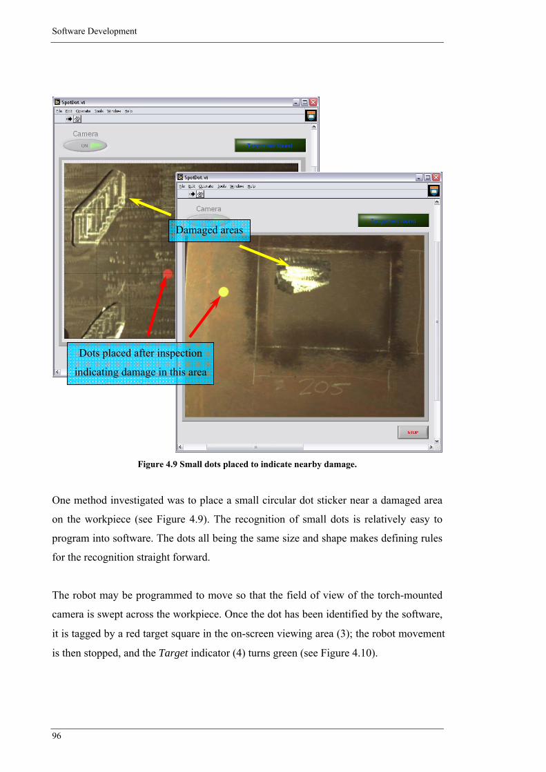
Software Development
96
Figure 4.9 Small dots placed to indicate nearby damage.
One method investigated was to place a small circular dot sticker near a damaged area
on the workpiece (see Figure 4.9). The recognition of small dots is relatively easy to
program into software. The dots all being the same size and shape makes defining rules
for the recognition straight forward.
The robot may be programmed to move so that the field of view of the torch-mounted
camera is swept across the workpiece. Once the dot has been identified by the software,
it is tagged by a red target square in the on-screen viewing area (3); the robot movement
is then stopped, and the Target indicator (4) turns green (see Figure 4.10).
Damaged areas
Dots placed after inspection
indicating damage in this area

Software Development
97
Figure 4.10 Target identified.
Alternatively, there are certain filtering functions that can be performed on the image to
help identify features that cannot be easily found otherwise. Figure 4.11b shows the
result of applying a Sobel filter to an image. Notice the pronounced outline of the
damaged area to the right of the dot. Techniques like this simplify the recognition of
damage, but a higher level of intelligence (i.e. human intervention) is still required for
absolute assurance that what is found is indeed damage. This point is illustrated in
Figure 4.11b, where the chalk lines from Figure 4.11a are still quite obvious; and if left
up to software, may be erroneously identified as damage. Shadows, surface marks, or
slight deviations of surface profile, etc, all may be misconstrued in the same way. These
inherent problems reduce user confidence in object recognition systems to identify
exactly what is required. In this work, the identification of damage is left up to human
intelligence. If the small dot is placed near a damaged area, the recognition algorithm

Software Development
98
can inform the operator that damage is in camera view, and to take a photo. To initiate
the photo capture routine (QuickSnap.vi) the Stop button (5) is clicked.
Figure 4.11 (a) Unfiltered image; (b) Sobel filtered image.
The QuickSnap program can capture a still photograph from a live video stream. The
live video is displayed in a viewing window and a still photograph can be taken by
clicking the mouse button. The image is saved to disk and the weld path generation
program (WPGenUI.m) is loaded.
Figure 4.12 shows the QuickSnap GUI which was developed for taking a single colour
snapshot. The Snap button (6) takes the photo and saves it to disk.
(a)
(b)

Software Development
99
Figure 4.12 QuickSnap GUI.
The identification sequence is illustrated in the examples below followed by the
program flowcharts.

Figure 4.13 Identification sequence.
Note
Image not included. See paper copy.

Figure 4.14 Identification sequence.
Note
Image not included. See paper copy.

Software Development
102
Figure 4.15 SpotDot program flowchart.
Note
Image not included. See paper copy.

Software Development
103
Figure 4.16 QuickSnap program flowchart.
Note
Image not included. See paper copy.

Software Development
104
4.4 RAPID Weld Path Generator
In this section, the acronym RAPID stands for Rapid Adaptive Programming using
Image Data. The RAPID Weld Path Generator program is explained below.
The RAPID Weld Path Generator software was written in MATLAB (from The
MathWorks) and has been compiled as a standalone executable program for the
Microsoft Windows platform. It can be loaded in the normal manner for Windows-
based programs. The basic GUI is shown in Figure 4.17. All figure axes have mm units.
Figure 4.17 WPGenUI GUI.
Once the program has started, the user must click the Load image button (1) to import
the image taken from the torch-mounted camera. The image is displayed in the software
(2) and the input boxes (3) for the weld bead geometry calculations become active. These
input parameters must be set before clicking the Pick Points button (5) as the input
boxes are deactivated afterwards (see Figure 4.18). When the input parameters are
acceptable the user can select between two drawing modes using the drop down list box
(4). The first mode is the Point mode which means after clicking the Pick Points button

Software Development
105
(5), wherever the left mouse button is clicked a circle appears on the display at that
point.
Figure 4.18 Operation in Point mode.
Figure 4.19 Operation in Line mode.
Red circles show where the
mouse has been clicked
Note
Image not included. See paper copy.

Software Development
106
Figure 4.18 shows the software in Point mode. The other mode is the Line mode (see
Figure 4.19) which displays a line between 2 consecutive left mouse button clicks. The
Line mode is particularly useful when defining regions with straight or long edges.
Once the drawing mode has been selected and the Pick Points button (5) is clicked (as in
Figure 4.18 and Figure 4.19), the user defines a region around the damaged area with
the mouse. The left mouse button is used to define peripheral points and the right button
(or Enter key) exits the region definition mode. Note that when the right mouse button
is clicked on the image, this point is valid and becomes the last point in the set, whereas
if clicked outside the image region (invalid point) or when the Enter key is pressed, the
final point will be the last valid point selected with the left mouse button. Once the
region definition is complete the software calculates the weld paths necessary to fill in
the region and displays the paths on the screen.
Figure 4.20 Save program once weld paths are acceptable.
At this point the user is given the option to save the weld paths into a robot program
(see Figure 4.20). If the weld paths are acceptable and the user selects the save option,
the software will generate the robot program necessary to carry out the weld paths and
save it to disk.
Note
Image not included. See paper copy.

Software Development
107
Figure 4.21 Error made when defining region.
Figure 4.22 Clear erroneous paths.
If an error is made when defining the region (usually visibly obvious as in Figure 4.21)
the user can select not to save the program and try again. If the program is not saved, all
Note
Image not included. See paper copy.

Software Development
108
generated weld path data will be lost.
Although not required, it is useful for visual clarity to clear the erroneous paths with the
Clear button (6) before redefining the region. Figure 4.22 illustrates the Clear button
function which results in all generated data being cleared from memory leaving only the
original unaltered image (as in Figure 4.17). Once the region and weld paths are
acceptable and the program has been saved, the user can modify the generated robot
program by clicking the Edit program button (7).
Figure 4.23 Text-based program modification.
The operating system text editor is called to open the program (Figure 4.23) and the user
can modify the program and re-save if desired. However, this is not recommended, as
the generated program is already compiled and ready for execution on the robot
controller. Errors can be made by the user when editing the program rendering it
useless. An extensive knowledge of the native language of the robot controller is
necessary if this feature of the software is used.
Various other features are available under the menus at the top of the screen such as
zoom functions and curve drawing capabilities, but were not extensively used nor

Software Development
109
overly important in the development of the main function of the software – that being
rapid robot programming. Finally, the Exit button (8) shuts down the program.
The basic operation and output of the RAPID Weld Path Generator program has been
described above. The algorithms contained within the RAPID Weld Path Generator
program will now be explained in detail.
Figure 4.24 Viewing window size determination.
After an image file is loaded into the software using the Load image button, a set of
image axes is created according to the robot position relative to the workpiece. The size
of the viewing window (image) is camera and lens specific, and usually requires an
initial manual measurement. Once calibrated, a functional relationship can be
established between the viewing window size and camera offset. The viewing window
size is used as axes limits in the software, effectively calibrating the image. For
example, according to the camera position in Figure 4.24, a viewing window of 315 ×
235 mm would be obtained if the workpiece was 310 mm away, or 360 × 270 mm if

Software Development
110
the workpiece was 360 mm away. It should be noted that with fixed-focal length lenses
it is impractical to move too far away from the surface as image clarity/focus is
compromised.
Most of the menus and buttons on the front panel become active after loading a valid
image, including the input boxes for weld bead geometry calculations. Geometry such
as weld width and weld offsets can be determined from the input data: wire feed speed,
bead overlap, wire diameter, travel speed, and wire efficiency. The software proceeds to
check all input parameters are valid (numeric), and waits for the next command from
the user. With the image now visible in the display area of the software, a transparent
layer including the axes with the calculated limits is overlayed. Being transparent
enables the user to clear any erroneous weld paths and try again, without clearing the
image as well. If this layer was not included, whenever the Clear button is pressed the
image and calibrated axes would also be cleared. When the user clicks the Pick points
button all buttons and menus are deactivated until either the right mouse button is
clicked, or the Enter key is pressed.
Figure 4.25 Mouse click locations.
Note
Image not included. See paper copy.

Software Development
111
Each valid mouse click is plotted on the overlayed axes in the display area (see Figure
4.25) and their coordinates are recorded. When a valid set of points has been defined
and the weld path generation routine is complete, the user can select to save the program
or clear the display and try again.
Within the region definition routine, the coordinates ( x , y ) of the mouse clicks are
stored as rows in a matrix (see Table 4.1). Certain operations are performed on the
matrix of coordinates to pick out valid points and discard invalid points. The matrix is
first sorted in ascending y value order, and this becomes the searching matrix (Table
4.2). At least two points are required for a line weld so if there are less than two points
in the matrix, an error message is displayed to try again.
Table 4.1 Unsorted coordinates.
Point Coordinates
x y
1 209.9344 55.4376
2 67.3523 116.8818
3 94.1357 43.6214
4 254.0481 186.9912
5 111.4661 164.9344
6 238.2932 114.5186
7 142.9759 244.4967
8 187.8775 133.4245
9 27.1772 171.2363
Table 4.2 Sorted coordinates.
Point Coordinates
x y
3 94.1357 43.6214
1 209.9344 55.4376
6 238.2932 114.5186
2 67.3523 116.8818
8 187.8775 133.4245
5 111.4661 164.9344
9 27.1772 171.2363
4 254.0481 186.9912
7 142.9759 244.4967
Starting from the lowest point on the screen (i.e. the point with the smallest y value
which is now the first row in the searching matrix), a search algorithm is performed to
determine the next valid point. Each time a point is found it is removed from the
searching matrix and put into an intermediate perimeter matrix, and the next search
begins from the location of the removed point. This continues until there are no points
left in the searching matrix (i.e. all valid points have been identified and removed). The
idea is to get the next closest peripheral point to form a closed boundary or region.
There are traps in the algorithm to eliminate invalid points such as internal points which

Software Development
112
will obviously not form part of the boundary.
Figure 4.26 Algorithm starts at lowest point.
The following table of extreme points (Table 4.3) are important in the search routine.
Table 4.3 Extreme points.
Point Coordinates
x y
Minimum y value 3 94.1357 43.6214
Minimum x value 9 27.1772 171.2363
Maximum y value 7 142.9759 244.4967
Maximum x value 4 254.0481 186.9912
Start here

Software Development
113
4.4.1 TopLeft Search
As the name implies, the TopLeft search basically searches in the region above and to
the left of the searching point. The TopLeft search is started from the lowest point
(Point 3). Point 3 is immediately removed from the searching matrix (Table 4.4) and put
into the intermediate perimeter matrix (see Table 4.5). Now, the search algorithm
determines if the furthest left point (i.e. point with minimum x value) is in the
searching matrix. When the furthest left point is not in the searching matrix, the
algorithm switches to the TopRight search (explained below). In this example, Point 9
has the minimum x value and is still an element of the searching matrix.
Table 4.4 Searching matrix.
Point Coordinates
x y
1 209.9344 55.4376
6 238.2932 114.5186
2 67.3523 116.8818
8 187.8775 133.4245
5 111.4661 164.9344
9 27.1772 171.2363
4 254.0481 186.9912
7 142.9759 244.4967
Table 4.5 Intermediate perimeter matrix.
Point Coordinates
x y
3 94.1357 43.6214
As the point with minimum x value (Point 9) is in the searching matrix, the algorithm
searches for points higher than (greater y value) and to the left (smaller x value) of the
current point (Point 3). The light-grey region in Figure 4.27 is the searching region.

Software Development
114
Figure 4.27 Searching region.
The following points (shown in Table 4.6) satisfy this condition:
Table 4.6 Filtered points matrix.
Point Coordinates
x y
2 67.3523 116.8818
9 27.1772 171.2363
The point in the filtered matrix with the smallest y value is then found (bottom-top
search). In this example, Point 2 has the smallest y value (see Figure 4.28) so is
removed from the searching matrix and put into the intermediate perimeter matrix (see
Table 4.7 and Table 4.8).

Software Development
115
Figure 4.28 Bottom-top search.
Table 4.7 Searching matrix.
Point Coordinates
x y
1 209.9344 55.4376
6 238.2932 114.5186
8 187.8775 133.4245
5 111.4661 164.9344
9 27.1772 171.2363
4 254.0481 186.9912
7 142.9759 244.4967
Table 4.8 Intermediate perimeter matrix.
Point Coordinates
x y
3 94.1357 43.6214
2 67.3523 116.8818
In the case where 2 points lie on the same horizontal line (same y value), the leftmost
point (point with smallest x value) is chosen (see Figure 4.29). This prevents problems
if the next search were to begin from the rightmost point.

Software Development
116
Figure 4.29 Bottom-top search special case – leftmost point chosen.
The minimum x value point (Point 9) is still in the searching matrix so the algorithm
performs as before. The light-grey region in Figure 4.30 is the new searching region.
The search matrix is filtered again to satisfy the TopLeft search criteria (see Table 4.9):
Table 4.9 Filtered points matrix.
Point Coordinates
x y
9 27.1772 171.2363
Again, the point in the filtered matrix with the smallest y value is then found. In this
example, only one point (Point 9) is in the filtered matrix; therefore, Point 9 is removed
from the searching matrix and put into the intermediate perimeter matrix (see Table 4.10
and Table 4.11). Once the furthest left point (Point 9 in this example) has been removed,
the search algorithm switches to the TopRight search.

Software Development
117
Figure 4.30 Searching region.
4.4.2 TopRight Search
As the name implies, the TopRight search basically searches in the region above and to
the right of the searching point. The TopRight search is started from the leftmost point
(Point 9 in this example). The search algorithm determines if the highest point (i.e. point
with maximum y value) is in the searching matrix. When the highest point is not in the
searching matrix, the algorithm switches to the BottomRight search (explained below).
In this example, Point 7 has the maximum y value and is still an element of the
searching matrix.

Software Development
118
Table 4.10 Searching matrix.
Point Coordinates
x y
1 209.9344 55.4376
6 238.2932 114.5186
8 187.8775 133.4245
5 111.4661 164.9344
4 254.0481 186.9912
7 142.9759 244.4967
Table 4.11 Intermediate perimeter matrix.
Point Coordinates
x y
3 94.1357 43.6214
2 67.3523 116.8818
9 27.1772 171.2363
As the point with maximum y value (Point 7) is in the searching matrix, the algorithm
searches for points to the right of (greater x value) and higher (greater y value) than
the current point (Point 9). The light-grey region in Figure 4.31 is the searching region.
Figure 4.31 Searching region.
Note
Image not included. See paper copy.

Software Development
119
The following points (shown in Table 4.12) satisfy this condition:
Table 4.12 Filtered points matrix.
Point Coordinates
x y
4 254.0481 186.9912
7 142.9759 244.4967
The point in the filtered matrix with the smallest x value is then found (left-right
search). In this example, Point 7 has the smallest x value (see Figure 4.32) so is
removed from the searching matrix and put into the intermediate perimeter matrix (see
Table 4.13 and Table 4.14). Once the highest point (Point 7 in this example) has been
removed, the search algorithm switches to the BottomRight search.
Figure 4.32 Left-right search.
Note
Image not included. See paper copy.

Software Development
120
Table 4.13 Searching matrix.
Point Coordinates
x y
1 209.9344 55.4376
6 238.2932 114.5186
8 187.8775 133.4245
5 111.4661 164.9344
4 254.0481 186.9912
Table 4.14 Intermediate perimeter matrix.
Point Coordinates
x y
3 94.1357 43.6214
2 67.3523 116.8818
9 27.1772 171.2363
7 142.9759 244.4967
In the case where 2 points lie on the same vertical line (same x value), the uppermost
point (point with greatest y value) is chosen (see Figure 4.33). This prevents problems
if the next search were to begin from the lowermost point.
Figure 4.33 Left-right search special case – uppermost point chosen.
Note
Image not included. See paper copy.

Software Development
121
4.4.3 BottomRight Search
As the name implies, the BottomRight search basically searches in the region below and
to the right of the searching point. The BottomRight search is started from the highest
point (Point 7 in this example). The search algorithm determines if the rightmost point
(i.e. point with maximum x value) is in the searching matrix. When the rightmost point
is not in the searching matrix, the algorithm switches to the BottomLeft search
(explained below). In this example, Point 4 has the maximum x value and is still an
element of the searching matrix.
As the point with maximum x value (Point 4) is in the searching matrix, the algorithm
searches for points lower than (smaller y value) and to the right (greater x value) of
the current point (Point 7). The light-grey region in Figure 4.34 is the searching region.
Figure 4.34 Searching region.
Note
Image not included. See paper copy.

Software Development
122
The following points (shown in Table 4.15) satisfy this condition:
Table 4.15 Filtered points matrix.
Point Coordinates
x y
1 209.9344 55.4376
6 238.2932 114.5186
8 187.8775 133.4245
4 254.0481 186.9912
The point in the filtered matrix with the greatest y value is then found (top-bottom
search). In this example, Point 4 has the greatest y value (see Figure 4.35) so is
removed from the searching matrix and put into the intermediate perimeter matrix (see
Table 4.16 and Table 4.17). Once the rightmost point (Point 4 in this example) has been
removed, the search algorithm switches to the BottomLeft search.
Figure 4.35 Top-bottom search.
Note
Image not included. See paper copy.

Software Development
123
Table 4.16 Searching matrix.
Point Coordinates
x y
1 209.9344 55.4376
6 238.2932 114.5186
8 187.8775 133.4245
5 111.4661 164.9344
Table 4.17 Intermediate perimeter matrix.
Point Coordinates
x y
3 94.1357 43.6214
2 67.3523 116.8818
9 27.1772 171.2363
7 142.9759 244.4967
4 254.0481 186.9912
In the case where 2 points lie on the same horizontal line (same y value), the rightmost
point (point with greatest x value) is chosen (see Figure 4.36). This prevents problems
if the next search were to begin from the leftmost point.
Figure 4.36 Top-bottom search special case – rightmost point chosen.
Note
Image not included. See paper copy.

Software Development
124
4.4.4 BottomLeft Search
As the name implies, the BottomLeft search basically searches in the region below and
to the left of the searching point. The BottomLeft search is started from the rightmost
point (Point 4 in this example). The BottomLeft search continues until there are no
points remaining in the search matrix.
The algorithm searches for points to the left of (smaller x value) and lower than
(smaller y value) of the current point (Point 4). The light-grey region in Figure 4.37 is
the searching region.
Figure 4.37 Searching region.
Note
Image not included. See paper copy.

Software Development
125
The following points (shown in Table 4.18) satisfy this condition:
Table 4.18 Filtered points matrix.
Point Coordinates
x y
1 209.9344 55.4376
6 238.2932 114.5186
8 187.8775 133.4245
5 111.4661 164.9344
The point in the filtered matrix with the greatest x value is then found (right-left
search). In this example, Point 6 has the greatest x value (see Figure 4.38) so is
removed from the searching matrix and put into the intermediate perimeter matrix (see
Table 4.19 and Table 4.20).
Figure 4.38 Right-left search.
Note
Image not included. See paper copy.

Software Development
126
Table 4.19 Searching matrix.
Point Coordinates
x y
1 209.9344 55.4376
8 187.8775 133.4245
5 111.4661 164.9344
Table 4.20 Intermediate perimeter matrix.
Point Coordinates
x y
3 94.1357 43.6214
2 67.3523 116.8818
9 27.1772 171.2363
7 142.9759 244.4967
4 254.0481 186.9912
6 238.2932 114.5186
In the case where 2 points lie on the same vertical line (same x value), the lowermost
point (point with smallest y value) is chosen (see Figure 4.39). This prevents problems
if the next search were to begin from the uppermost point.
Figure 4.39 Right-left search special case – lowermost point chosen.
Note
Image not included. See paper copy.

Software Development
127
While there are still points in the searching matrix, the algorithm performs as before.
The light-grey region in Figure 4.40 is the new searching region.
Figure 4.40 Searching region.
The search matrix is filtered again to satisfy the BottomLeft search criteria (see Table
4.21):
Table 4.21 Filtered points matrix.
Point Coordinates
x y
1 209.9344 55.4376
Again, the point in the filtered matrix with the greatest x value is then found. In this
example, only one point (Point 1) is in the filtered matrix; therefore, Point 1 is removed
from the searching matrix and put into the intermediate perimeter matrix (see Table 4.22
and Table 4.23).

Software Development
128
Figure 4.41 Right-left search.
Table 4.22 Searching matrix.
Point Coordinates
x y
Empty matrix: 0-by-2
Table 4.23 Intermediate perimeter matrix.
Point Coordinates
x y
3 94.1357 43.6214
2 67.3523 116.8818
9 27.1772 171.2363
7 142.9759 244.4967
4 254.0481 186.9912
6 238.2932 114.5186
1 209.9344 55.4376
The searching routine finishes when the searching matrix is empty (see Table 4.22).
Figure 4.42 shows the empty searching region.

Software Development
129
Figure 4.42 Searching region.
The four searching routines above are designed to create a perimeter around all points.
Every time a point is removed from the search matrix it is placed into the intermediate
perimeter matrix which will be further processed to determine the final perimeter
coordinates. The resulting set of points for this example is shown in Figure 4.43.
4.4.5 Boundary Points
To form a boundary such that all points either lie on the boundary or are internal to the
boundary, a cross product check is used. This basically checks whether the test point
lies to the left or the right of a line connecting the two adjacent points. Moving
clockwise, if each point around a closed region is tested, any point that lies to the left of
the connecting line is valid and will form part of the final boundary, whereas points that
lie to right are internal points and considered invalid (see Figure 4.44).

Software Development
130
Figure 4.43 Intermediate perimeter points.
Figure 4.44 Right hand side test.
Cycling through all points in the intermediate perimeter matrix, a vector v is formed
between the test point tP and the previous point along the perimeter 1tP− . A second
vector w is created between the next point along the perimeter from the test point 1tP+
and the previous point from the test point 1tP− .
Internal points are
on the right hand
side of these lines

Software Development
131
Figure 4.45 Valid points.
The vectors are calculated from:
[ ] [ ] [ ] [ ]( )1 1 1,t t t t t tx x y yv P P P P P P− − −= − = − − 4.1
[ ] [ ] [ ] [ ]( )1 1 1 1 1 1,t t t t t tx x y yw P P P P P P+ − + − + −= − = − − 4.2
Note: these vectors are 2D (i.e. zv and zw are zero). The cross product is found from:
( )00
x y x y x y
x y
i j kv w v v v w w v k
w w× = = − 4.3
The cross product results in a vector perpendicular to the two input vectors v and w . In
the case where the resulting vector ( )x y x yv w w v k− is zero (i.e. duplicate point) the
redundant point is removed from the perimeter set. If the resulting vector is negative
then the point being tested tP is on the left hand side of the connecting line (Figure
4.45), otherwise, the point is on the right hand side which makes it an internal point and
therefore invalid (Figure 4.46). Invalid points are removed from the perimeter set
leaving only the peripheral points to form a closed boundary around all internal points.
Weld paths are generated to fill this region. The cross product test is performed at every
point. If a point is removed the test automatically runs again to check for further internal
points.
1tP−
tP
1tP+
v
w1tP−
tP
v
1tP+
w

Software Development
132
Figure 4.46 Invalid point.
Table 4.24 Intermediate perimeter matrix.
Point Coordinates
x y
3 94.1357 43.6214
2 67.3523 116.8818
9 27.1772 171.2363
7 142.9759 244.4967
4 254.0481 186.9912
6 238.2932 114.5186
1 209.9344 55.4376
In this example, testing Point 2 in the intermediate perimeter matrix (see Table 4.24) to
see if it lies on the left hand side or right hand side of a line connecting the two adjacent
points (Point 9 and Point 3) would result in the creation of the following two vectors:
( )( )
1 2 3
67.3523 94.1357,116.8818 43.6214
26.7834,73.2604
t tv P P P P−= − = −
= − −
= −
4.4
( )( )
1 1 9 3
27.1772 94.1357,171.2363 43.6214
66.9585,127.6149
t tw P P P P+ −= − = −
= − −
= −
4.5
1tP−
tP
1tP+
vw

Software Development
133
The cross product of the two vectors results in:
( ) ( )( ) ( )( )( )26.7834 127.6149 66.9585 73.2604
1487.44560
x y x yv w v w w v k k
k
× = − = − − −
=>
4.6
The resulting vector is greater than zero which means the test point (Point 2) lies on the
right hand side of the line joining Point 9 and Point 3; therefore, Point 2 is invalid and is
removed (see Figure 4.47).
Figure 4.47 Internal points removed.
Note
Image not included. See paper copy.

Software Development
134
Figure 4.48 Final perimeter points.
Once all points have been checked and internal points removed, the final perimeter
matrix remains. Table 4.25 shows the final perimeter matrix for this example:
Table 4.25 Final perimeter matrix.
Point Coordinates
x y
3 94.1357 43.6214
9 27.1772 171.2363
7 142.9759 244.4967
4 254.0481 186.9912
6 238.2932 114.5186
1 209.9344 55.4376

Software Development
135
4.4.6 Weld Bead Geometry
Now that the final peripheral points have been determined, a routine is called to
generate the weld paths. First of all, the weld bead geometry needs to be calculated from
the input values. With this geometry, a set of weld paths can be constructed to ‘fill in’
the region bounded by the peripheral points.
A semi-circular assumption was made for the weld bead cross sectional area. The
derivation of the geometry calculations is now presented.
For GMAW, the volume of metal deposited per unit time for a wire with diameter wφ ,
and wire feed speed WFS is:
[ ]2
4wVolume WFS
timeπφ
= × 4.7
The cross sectional area of the weld bead is assumed to be semi-circular, so with a
travel speed of TS , the volume of metal in the weld per unit time is:
[ ]21
2 4Volume BeadWidth TS
timeπ⎛ ⎞×
= ×⎜ ⎟⎝ ⎠
4.8
Flux in wires and spatter reduce the volume of metal being transferred to the weldment.
Grouping these into an efficiency factor η , the volume of metal per unit time being
transferred to the weldment with efficiency η is equal to the volume of metal in the
weld per unit time. This leads to:
2 21
4 2 4w BeadWidthWFS TSπφ πη
⎛ ⎞ ⎛ ⎞×× = ×⎜ ⎟ ⎜ ⎟
⎝ ⎠⎝ ⎠ 4.9

Software Development
136
Rearranging for bead width:
2w
WFSBeadWidthTSηφ × ×
= 4.10
The offset between consecutive welds is calculated using the percentage overlap input
value. For an overlap of α %, the offset is:
( )1Offset BeadWidthα= − × 4.11
Figure 4.49 Weld bead offset.
These calculations are necessary for the next step; determining the welding paths. The
information needed to cover a region with parallel weld beads are: (a) the start and
finish points for every weld bead, and (b) the offset between consecutive beads. The
start and finish points will lie on the boundary defined by the peripheral points, and the
offset is determined from Equation 4.11.
During the current work, most welding was performed on a vertical plate. For this type
of positional welding, higher quality weld beads were achieved when welding closer to
horizontal, and welding from the lowest point upwards. Given that the region to be
( )1 BeadWidthα− ×
Offset
BeadWidth
BeadWidthα ×

Software Development
137
filled will consist of a set of parallel weld beads, the bottom bead or baseline weld (from
which all other welds will be offset) can be chosen in a way that favours the deposition
pattern described above.
For this work, the baseline is constructed so that when vectors q and r are made
between the lowest point 1P and the two adjacent points 2P and nP , respectively, the
point that forms the vector with the smallest incline to the horizontal will become the
other endpoint of the baseline. The angle β is measured clockwise from the horizontal
around 1P while angle γ is measured counter clockwise around 1P , with , 90β γ < .
Figure 4.50 Baseline selected based on incline condition.
Vectors q and r are determined by:
[ ] [ ] [ ] [ ]( )2 1 2 1 2 1,x x y y
q P P P P P P= − = − − 4.12
[ ] [ ] [ ] [ ]( )1 1 1,n n nx x y yr P P P P P P= − = − − 4.13
In Figure 4.50, β γ< so the baseline lies along the vector q joining points 1P and 2P .
All weld paths will be made parallel to the baseline (shown as dotted lines in Figure
4.50). This is achieved by creating a line function through the baseline points and
offsetting this function by a portion of the calculated bead offset.
The equation of a line can be described in the form:
( ) ( )tani i i if x m x b x bθ= + = + , 180 180θ− < ≤ , 90θ ≠ ± 4.14
1P
nP
2Pr
qβ γ

Software Development
138
where im (or tanθ ) is the gradient of the line and ib is the f -intercept. As the lowest
point 1P is being used, the angle θ will be between 0 180θ≤ ≤ . If 90θ = the points
are vertically aligned and there would be no baseline function by definition. This is
unimportant in the baseline determination except for single line welds where there are
only two points. In this case, there is no need to determine the baseline function because
the weld path is already known. i.e. between the two points.
Figure 4.51 Baseline going left.
If vector q joining points 1P and 2P has the smallest incline to the horizontal (see
Figure 4.51), the baseline function baselinef will lie along 0f on the interval between
[ ]2 xP and [ ]1 x
P , and can be determined from:
[ ]( ) [ ]0 0 1 1baseline x yf f m x P P= = − + , [ ] [ ]2 1x x
P x P≤ ≤ 4.15
where [ ] [ ][ ] [ ]
2 10
2 1
y y y
x x x
P Pqm
q P P
−= =
−.
If vector r joining points 1P and nP has the smallest incline to the horizontal (see
Figure 4.52), the baseline function baselinef will lie along 0f on the interval between
[ ]1 xP and [ ]n x
P , and can be determined from:
[ ]( ) [ ]0 0 1 1baseline x yf f m x P P= = − + , [ ] [ ]1 nx x
P x P≤ ≤ 4.16
x
( )f x
baselinef
q2P
1P
1f2f
0f
2b1b0b
Offsetθ

Software Development
139
where [ ] [ ][ ] [ ]
10
1
ny y y
x n x x
P Prm
r P P
−= =
−.
Figure 4.52 Baseline going right.
cosOffset f θ= ∆ ×
cosOffsetf
θ∆ = , 0 90θ≤ <
( )cos 180Offset f θ= ∆ × −
( )cos 180Offsetf
θ∆ =
−, 90 180θ< ≤
Figure 4.53 Offset calculations.
For 90 180θ< ≤ and using ( )cos 180 cosθ θ− = − , f∆ can be simplified to:
( )cos 180 cosOffset Offsetf
θ θ∆ = =
− −, 90 180θ< ≤ 4.17
A positive value for f∆ is required giving:
cos cosOffset Offsetf
θ θ∆ = =
−, 90 180θ< ≤ 4.18
Offsetf∆
θ 180 θ−( )f x( )f x
Offset
f∆
θ
nP
x
( )f x
θ
Offset
r
1P
baselinef
1f2f
0f
2b
1b
0b

Software Development
140
which also satisfies f∆ for 0 90θ≤ < , so only one equation is needed for f∆ between
0 180θ≤ ≤ , 90θ ≠ .
cosOffsetf
θ∆ = , 0 180θ≤ ≤ , 90θ ≠ 4.19
where [ ] [ ][ ] [ ]
2 11 10
2 1
tan tan y y
x x
P Pm
P Pθ − −
⎛ ⎞−= = ⎜ ⎟⎜ ⎟−⎝ ⎠
, or [ ] [ ][ ] [ ]
11
1
tan n y y
n x x
P P
P Pθ −
⎛ ⎞−= ⎜ ⎟⎜ ⎟−⎝ ⎠
depending on the
incline condition above.
For subsequent weld paths the new path function is equal to the previous path function
offset by an amount f∆ . i.e. 1 0f f f= + ∆ , 2 1f f f= + ∆ , …, 1i if f f−= + ∆ . The baseline
weld will lie along 0f and is used as a basis for subsequent welds.
[ ]( ) [ ]0 0 1 1x yf m x P P= − + 4.20
[ ]( ) [ ]1 0 0 1 1x yf f f m x P P f= + ∆ = − + + ∆ 4.21
[ ]( ) [ ]( )[ ]( ) [ ]
2 1 0 1 1
0 1 1
0
2
2
x y
x y
f f f m x P P f f
m x P P f
f f
= + ∆ = − + + ∆ + ∆
= − + + ∆
= + ∆
4.22
The thi weld path after the baseline will lie along the thi path function:
[ ]( ) [ ] ( )( )[ ]( ) [ ]
1 0 1 1
0 1 1
0
1i i x y
x y
f f f m x P P i f f
m x P P i f
f i f
−= + ∆ = − + + − ∆ + ∆
= − + + ∆
= + ∆
4.23
Now that the weld path functions have been established, the intersection of these with
the perimeter functions will determine the endpoints of the welds. The perimeter
functions are line segments constructed between consecutive points in the final
perimeter matrix.

Software Development
141
The perimeter functions are derived from Equation 4.14.
( ) ( )tanj j j jg x m x b x bθ= + = + , 180 180θ− < ≤ , 90θ ≠ ± 4.24
( ) 0jg x = , [ ]( ), s xG j P= , 90θ = ± 4.25
where jm (or tanθ ) is the gradient of the line and jb is the g -intercept. There is a
special case when two perimeter points are vertically aligned (i.e. when 90θ = ± –
1j jx xP P+⎡ ⎤ ⎡ ⎤=⎣ ⎦ ⎣ ⎦ ). In this case, the perimeter function is set to zero (i.e. ( ) 0jg x = ) and
handled differently when determining the intersection with the weld path functions. The
array [ ]( ), s xG j P= holds information regarding the perimeter function that caused the
special case ( thj perimeter function), and the x -coordinate of the special perimeter
point sP . When ( ) 0jg x = is detected in the intersection algorithm, the information in
G will be needed to determine the endpoint coordinates.
With n number of points in the perimeter matrix 1 2, ,..., nP P P , there are n lines
segments joining these points, and therefore, n perimeter functions 1 2, ,..., ng g g . The
perimeter functions are:
( )j j j jx yg m x P P⎡ ⎤ ⎡ ⎤= − +⎣ ⎦ ⎣ ⎦ ,
1 j n≤ ≤ , ( ) ( )1 1min , max ,j j j jx x x xP P x P P+ +⎡ ⎤ ⎡ ⎤ ⎡ ⎤ ⎡ ⎤≤ ≤⎣ ⎦ ⎣ ⎦ ⎣ ⎦ ⎣ ⎦
4.26
where 1
1
j jy yj
j jx x
P Pm
P P+
+
⎡ ⎤ ⎡ ⎤−⎣ ⎦ ⎣ ⎦=⎡ ⎤ ⎡ ⎤−⎣ ⎦ ⎣ ⎦
, 1j jx xP P+⎡ ⎤ ⎡ ⎤≠⎣ ⎦ ⎣ ⎦ .
Note: To form a closed perimeter the thn point (last point) in the perimeter matrix must
join with the 1st point in the perimeter matrix. Therefore, the ( )1 thn + point represents
the 1st point (i.e. 1 1nP P+ = ), and the perimeter function ng is the line segment joining
the last point nP with the first point 1P .

Software Development
142
Now that the perimeter has been characterised, the intersection of the weld path
functions ( f ) with the perimeter functions ( g ) will determine the start and finish points
of the welds.
The equations to be solved are in the form:
Left endpoint x -coordinate: 0i leftf g− = 4.27
Right endpoint x -coordinate: 0i rightf g− = 4.28
where leftg is the left boundary perimeter function and rightg is the right boundary
perimeter function. The solution of Equation 4.27 or 4.28 will yield the x -coordinate
( intx ) for an endpoint of a particular weld. The y -coordinate ( inty ) is determined from
evaluating the weld path function f at the x -coordinate of the intersection:
Endpoint y -coordinate: ( )int intiy f x= 4.29
Thus, the endpoint coordinates are ( )int int,x y .
To determine which perimeter functions are used for the left and right boundary
functions leftg and rightg it is necessary to project all the points in the perimeter matrix
(along parallel lines to the baseline) onto the ( )f x (or ( )g x ) axis (see Figure 4.54).
This determines the n intersections with the ( )f x axis denoted by 1 2, ,...,
nP P Pb b b :
[ ]( ) [ ] [ ]0 nn n P nx x yf P m P b P= + = from Equation 4.14
[ ] [ ]0nP n ny xb P m P⇒ = −
4.30
where [ ] [ ][ ] [ ]
2 10
2 1
y y
x x
P Pm
P P
−=
− or
[ ] [ ][ ] [ ]
10
1
n y y
n x x
P Pm
P P
−=
− depending on the incline condition
above.

Software Development
143
Figure 4.54 Projected perimeter point intercepts.
The highest point in the perimeter matrix max yP will also have the highest projected f -
intercept, and is denoted maxb . From Equation 4.30:
maxmax max 0 maxyP y yy xb b P m P⎡ ⎤ ⎡ ⎤= = −⎣ ⎦ ⎣ ⎦ 4.31
The lowest point in the perimeter matrix min yP will also have the lowest projected f -
intercept, and is denoted minb . From Equation 4.30:
[ ] [ ]min 1min min 0 min 1 0 1 0yP y y Py xy x
b b P m P P m P b b⎡ ⎤ ⎡ ⎤= = − = − = =⎣ ⎦ ⎣ ⎦ 4.32
Note: min yP will always be equal to 1P because the lowest point is always put in the first
position of the perimeter matrix.
Figure 4.55 Weld path functions parallel to baseline.
1P( ) θ 2g1g
1 2min P Pb b b= =
2P
max yP
1P
nPb
180 θ−( )f x
maxmax yPb b=
3Pb
( )f x
θ 1P
max yP
nP
maxmax yPb b=
2Pb
1nPb−
1min nP Pb b b= =
Note
Image not included. See paper copy.

Software Development
144
The number of weld paths i after the baseline can be found using:
( ) ( )max min max mincosint int
b b b bi
Offset fθ⎛ − × ⎞ −⎛ ⎞
= =⎜ ⎟ ⎜ ⎟∆⎝ ⎠⎝ ⎠ 4.33
Therefore, including the baseline there will be 1i + weld paths.
Beginning with the baseline weld along 0f , the start and finish points will be the lowest
point 1P and either 2P or nP , respectively. The next weld path will lie along 1f and
intersect with the left boundary function leftg and the right boundary function rightg .
These intersections will become the endpoints of the weld path along 1f . The weld path
function index is incremented after the start and finish points have been determined for
that particular path function. These endpoints are the solutions of Equations 4.27 or 4.28
, and Equation 4.29.
For this work with positional welding, the start point is chosen as the lower of the 2
intersections. This is continued for all 1i + weld path functions. However, the left and
right boundary functions depend on the projected height (onto the ( )f x axis) of the
current weld path function (i.e. f -intercept), so an algorithm to determine the
appropriate left and right boundary functions for each weld path must be used.
Firstly, the f -intercept for each weld path must be calculated:
0 0i i i if m x b m x b f i f= + = + = + ∆ from Equations 4.14 and 4.23
( ) ( )[ ]( ) [ ]
[ ] [ ]
0
0 1 1
1 0 1
0 0
0i i
x y
y x
b f f i f
m P P i f
P m P i f
⇒ = = + ∆
= − + + ∆
= − + ∆
1Pb i f= + ∆ from Equation 4.32
0b i f= + ∆
4.34

Software Development
145
where [ ] [ ][ ] [ ]
2 10
2 1
y y
x x
P Pm
P P
−=
− or
[ ] [ ][ ] [ ]
10
1
n y y
n x x
P Pm
P P
−=
− depending on the incline condition
above.
Figure 4.56 Determine endpoints.
If vector r has the smallest incline to the horizontal (see Figure 4.50), use 1leftg g= as
the initial left boundary function (as shown in Figure 4.56). Equation 4.27 can now be
solved to determine the left hand endpoints for all i weld paths. i.e. solve 1 0kf g− =
where 1 k i≤ ≤ until the f -intercept kb is greater than 2Pb . When
2k Pb b> , use
1 1 2leftg g g+= = as the next left boundary function in Equation 4.27, etc. For example, in
Figure 4.56 when 5k = , 25k Pb b b= > so the new left boundary function will be
2leftg g= . This is used in Equation 4.27 giving 2 0kf g− = , 5 k i≤ ≤ .
The initial right boundary function used is 1right ng g −= . Equation 4.28 can now be
solved to determine the right hand endpoints for all i weld paths. i.e. solve 1 0k nf g −− =
where 1 k i≤ ≤ until the f -intercept kb is greater than 1nPb−
. When 1nk Pb b−
> , use
1 1 2right n ng g g− − −= = as the next right boundary function in Equation 4.28, etc. For
example, in Figure 4.56 when 3k = , 13 nk Pb b b−
= > so the new right boundary function
will be 2right ng g −= . This is used in Equation 4.28 giving 2 0k nf g −− = , 3 k i≤ ≤ .
ng
2ng −
2grightg
leftg
θ1P
max yP
0f
2f1f
5f
nP
( )f x
5b2Pb
max minb b−1nPb−
2b1b
3bkf
kb

Software Development
146
If vector q has the smallest incline to the horizontal (see Figure 4.50), use 2leftg g= as
the initial left boundary function (as shown in Figure 4.57). Using Equation 4.27 to
determine the left hand endpoints; solve 2 0kf g− = where 1 k i≤ ≤ until the f -
intercept kb is greater than 3Pb . When
3k Pb b> , use 2 1 3leftg g g+= = as the next left
boundary function in Equation 4.27, etc. For example, in Figure 4.57 when 5k = ,
35k Pb b b= > so the new left boundary function will be 3leftg g= . This is used in
Equation 4.27 giving 3 0kf g− = , 5 k i≤ ≤ .
Figure 4.57 Determine endpoints.
The initial right boundary function used is right ng g= . Using Equation 4.28 to determine
the right hand endpoints; solve 0k nf g− = where 1 k i≤ ≤ until the f -intercept kb is
greater than nPb . When
nk Pb b> , use 1right ng g −= as the next right boundary function in
Equation 4.28, etc. For example, in Figure 4.57 when 4k = , 4 nk Pb b b= > so the new
right boundary function will be 1right ng g −= . This is used in Equation 4.28 giving
1 0k nf g −− = , 4 k i≤ ≤ . This algorithm is continued until k i= when all endpoints for
the weld paths will have been calculated. If either 0left jg g= = or 0right jg g= =
(special case), the thj perimeter function is found in array G and the corresponding x -
coordinate of the special perimeter point sP stored in G is used in Equation 4.29. In the
special case, Equations 4.27 and 4.28 are not used. The endpoint coordinates are
[ ] [ ]( )( ),s i sx xP f P . Similar to above, the weld path function index i is incremented and
max minb b−nPb3Pb
4bkb
2b1b
5b
180 θ−
max yP
1P
4fkf2f1f
5f
0f rightgleftg
1g
3g
( )f x
1ng −
2P

Software Development
147
the endpoints determined in the special manner until the f -intercept kb is greater than
the special point f -intercept sPb . When
sk Pb b> the algorithm continues as before (or
continues the special case depending on jg ). Two endpoints are determined for every
weld path function. As mentioned earlier, for the positional welding in the current work,
better weld quality is achieved when welding from bottom to top (i.e. lower to higher),
so the endpoint with the lowest y -coordinate is assigned to be the welding start position
and the other; the welding stop position. Once all start- and stop-weld positions have
been determined, the weld paths are superimposed over the area defined by the user in
the GUI (see Figure 4.58). If the weld paths are acceptable, the user can select to save
the weld paths. At this stage the endpoint positions are passed to the robotic program
algorithm which automatically compiles and saves the robot program necessary to weld
along the paths between these points. The program can then be transferred to the robot
controller for execution using the developed communications and control software.
Figure 4.58 Final weld paths.
The weld path generation program flowchart is shown in Figure 4.48.
Note
Image not included. See paper copy.

Software Development
148
Figure 4.59 WPGenUI program flowchart.
Note
Image not included. See paper copy.
Software Development
149
4.5 Robot Program Generation
To alleviate some of the problems associated with conventional programming, the
offline programming system must be able to accommodate the various application-
specific steps required for successful repair. For the target application the robotic
system must carry out certain operations in order to complete the weld repair, including
move and weld instructions, delays, and I/O manipulation. It is possible to apply an
algorithm that incorporates the output of the weld path generation program (i.e. the weld
paths) with general operating instructions such as ‘move to start point of weld’ and
‘switch power supply to touch-sensing mode’. A general structure or shell of a robot
program can be made so that when special operation points are passed to the algorithm,
these points can be inserted into the shell with the end result being a complete compiled
robot program. The weld path generation program calls a routine containing this
algorithm. For advanced manoeuvring techniques or where robot adaptive control is
required, the robotic system should be able to handle comprehensive mathematic
(including goniometric) processing such that mathematic results can be introduced in
the movement instructions. Therefore, by combining the techniques of master template
(shell) modification with mathematical operations and program translations, a more
sophisticated programming methodology is achieved. The general flow and inter-
relationships of the robot programming algorithms is now detailed.
The power supply is put into touch-sensing mode programmatically (within the robot
program) by changing a digital I/O state. Certain touch-sensing routines that depend on
the type of surface to be repaired are available. i.e. if the surface is inclined or curved
the 3-point touch-sensing routine may be used, etc. These routines automatically
calculate the normal to the surface and provide the preferred robot position for taking a
snapshot of the surface. The operator may look directly at the robot or watch the live
video stream (from the torch-mounted camera) on the PC screen to determine the
suitability of the robot position. Position suitability is intuitively determined by the
operator such that the damage is in good view of the camera and that the robot pose is
acceptable. Once satisfied with the robot position, the operator uses the PC GUI to
capture the image from the camera and program the weld paths according to the
identified damage. The robot position is used to calibrate the captured image and the

Software Development
150
weld paths are constructed relative to the calibrated image dimensions. Another touch-
sensing routine can be used to determine the curvature and adjust/transform the 2D
paths developed by the operator using the GUI into the 3rd dimension. The result is that
the weld paths are mathematically moved to the workpiece surface. Touch-sensing
mode is programmatically turned off on the power supply. The robot moves according
to the program to the first weld starting position, welds along the first weld path, moves
to an intermediate point, waits a specified period, moves to the next weld starting
position, and so on until all weld paths have been completed after which the robot
moves to a home position. This sequence is described graphically in the flowchart given
in Figure 4.60.
For this work, using the ABB robot and controller described previously, the robot
language is ABB’s proprietary robot language; also called RAPID. The program shell
and all instructions generated by the algorithm are written in RAPID.

Software Development
151
Figure 4.60 Robot program flowchart.
Note
Image not included. See paper copy.

Software Development
152
4.6 Camera Positioning
To determine the coordinates of the preferred camera position for acquiring an
acceptable image, the following workpiece plane calculations must be made.
Given three points ( 1P , 2P , and 3P ) on the workpiece surface where ( )1 1 1 1, ,P x y z= ,
( )2 2 2 2, ,P x y z= , and ( )3 3 3 3, ,P x y z= , vectors v and w are constructed (see Figure
4.61):
( ) ( ) ( )2 1 2 1 2 1 2 1
21 21 21
v P P x x i y y j z z k
x i y j z k
= − = − + − + −
= + + 4.35
( ) ( ) ( )3 1 3 1 3 1 3 1
31 31 31
w P P x x i y y j z z k
x i y j z k
= − = − + − + −
= + + 4.36
Figure 4.61 Normal vector determination.
Note
Image not included. See paper copy.

Software Development
153
The normal vector ( n ) to vectors v and w is determined by taking the cross product:
( ) ( ) ( )21 21 21 21 31 31 21 21 31 31 21 21 31 31 21
31 31 31
i j kn v w x y z y z y z i x z x z j x y x y k
x y z= × = = − − − + −
4.37
Only the direction information of the normal vector is required for camera positioning;
therefore, the vector is normalised. The unit normal vector n is calculated by:
1n̂ nn
= 4.38
For optimal positioning, the unit normal vector needs to be translated from the
intersection of the two vectors v and w to the geometric centre of the area enclosed by
the three points 1P , 2P , and 3P . Using another three vectors Q , R , and S R Q= − , the
geometric centre can be calculated:
( ) ( ) ( )3 1 3 1 3 12 1 2 1 2 12 2 2
x x y y z zQ x x i y y j z z k− − −⎛ ⎞ ⎛ ⎞ ⎛ ⎞= − − + − − + − −⎜ ⎟ ⎜ ⎟ ⎜ ⎟⎝ ⎠ ⎝ ⎠ ⎝ ⎠
4.39
3 2 3 2 3 21 1 12 2 2
x x y y z zR x i y j z k+ + +⎛ ⎞ ⎛ ⎞ ⎛ ⎞= − + − + −⎜ ⎟ ⎜ ⎟ ⎜ ⎟⎝ ⎠ ⎝ ⎠ ⎝ ⎠
4.40
1 2 1 2 1 21 2 1 2 1 22 2 2
2 2 2x x y y z zS x x i y y j z z k+ + +⎛ ⎞ ⎛ ⎞ ⎛ ⎞= − + + − + + − +⎜ ⎟ ⎜ ⎟ ⎜ ⎟
⎝ ⎠ ⎝ ⎠ ⎝ ⎠ 4.41
The geometric centre (vector r from 1P ) of the triangle will lie along the vector R (see
Figure 4.62). i.e. vector r will be a fraction of vector R according to the ratio between
the magnitudes of vectors v and S . This is simply based on similar triangle theory.

Software Development
154
Figure 4.62 Centre of area determination.
Figure 4.63 New camera position determination.
R
Q
S
3P
1P
2P
Note
Image not included. See paper copy.

Software Development
155
Vector r is calculated by:
v Rr
S= 4.42
A camera offset is required as an input to determine the preferred robot position for
acquiring an acceptable image. An offset distance ( offdist ) of 360 mm was used in this
work. This distance is an input variable depending on camera and lens configuration.
The preferred camera position (see Figure 4.63) is calculated using:
1 ˆcam P r offdist n= + + × 4.43
The robot controller can directly use this information to reposition the robot. This
automated step significantly reduces programming time and effort in preparing the robot
for image acquisition. The algorithms described have been experimentally tested and
verified. A computer model was generated for graphical representation of the
positioning algorithm. Some screenshots of the computer model are shown in Figure
4.64.

Software Development
156
Figure 4.64 Positioning algorithm computer model output.

Validation
157

Validation
158
5.1 Introduction
Some initial feasibility trials were conducted with touch-sensing as a means of assessing
the wear profile. In addition, two sets of experiments designed to validate the vision
based system and evaluate its performance were carried out.
5.2 Touch-Sensing
Using the touch-sensing facility in the welding power source the robot was used to scan
a grid of points on a simulated profile. The profile is shown in Figure 5.1 together with
the resultant digitised image. Although the general representation of the profile is good,
it is obvious that certain features have not been accurately reproduced.
Figure 5.1 Touch-sensed profile showing limitations of wire touch-sensing.
Note
Image not included. See paper copy.

Validation
159
These problems are believed to be due to wire retraction as discussed in the literature
survey. To overcome this, a solid probe constructed from an old welding contact tip was
used and accuracy in the order of 0.05 mm was achieved. However, the scanning time
required to achieve the required resolution was of the order of one hour. For this reason,
further trials on touch-sensing as a profilometry tool were abandoned in favour of a
vision-based system. Touch-sensing was however integrated into the final rapid
programming system as a means of locating the workpiece surface.
5.3 Vision Assisted Programming
The initial demonstration was designed to simulate the steps which would need to be
taken for in-situ repair. These steps included:
● Place robot in-situ, connect power leads, shielding gas, and wire feed unit.
● Run positioning routines to determine where the workpiece is and position
camera.
● On the PC, identify damage (or damage marker) on live video and take photo.
● Outline damage manually and generate the weld paths and robot program
automatically.
● Download program to robot and execute the repair.
● Post-weld heat treatment and/or grinding.
In the laboratory with the robot already positioned, the system was successfully
demonstrated. From initial steps of powering up the system, weld metal was deposited
in a matter of minutes. The weld path generation routine for 22 non-homogenous weld
paths was complete in 6.32 seconds. The complete repair operation finished in 3-4
minutes, with most time lost due to inter-pass delays (for thermal stability).
The summary from the weld path generation program for the initial demonstration is
shown in Figure 5.2, and the results are shown below.

Validation
160
------------------------ Inputs ------------------------
Wire feed speed = 4.0 m/min
Overlap = 30 %
Wire diameter = 1.2 mm
Travel speed = 20.0 cm/min
Wire efficiency = 100 %
--------------------- Calculations ---------------------
Bead width = 7.589 mm
Bead height = 3.795 mm
Weld run offset = 5.313 mm
Required number of weld runs = 22
Elapsed time is 6.320000 seconds
________________________________________________________
Figure 5.2 WPGenUI output.
Figure 5.3 Image transferred to PC.
Figure 5.4 Automatic weld path generation.
Figure 5.5 Deposit weld metal.

Validation
161
Figure 5.3 shows the image taken by the torch-mounted camera which was then
transferred to the PC. Figure 5.4 shows the weld paths which were generated using the
software developed to fill in the damaged region. Once the weld paths have been
defined, the robot program is automatically compiled and transferred to the robot
controller for execution using the control software. Figure 5.5 shows weld metal being
deposited according to the weld paths in Figure 5.4. As mentioned previously, online
welding parameter tuning can then be made using the control software. See section 4.2
for more information on how these steps were performed.
Several observations regarding the performance of the system can be made. Firstly,
there tended to be overfilling on the edges of the cut-out region. In practice this would
be acceptable as post-weld grinding would remove excess material. Industry sponsors
have indicated it preferable to overfill the region and grind back rather than underfill the
region and re-weld.
This trial demonstrated the effectiveness of the technique on flat vertical surfaces. The
ability to repair curved surfaces with unknown orientation was investigated later.
5.3.1 Flat Surface
Flat surfaces are generally the easiest to deal with (see Figure 5.6). A 1-point touch-
sensing routine is used to determine the workpiece distance from the camera. The field
of view of the camera can then be determined, thus completing calibration of the
photograph. The 2D photo is captured and the weld paths are generated in relation to the
calibrated image axes (1st and 2nd dimension), and the touch-sensed profile (3rd
dimension).

Validation
162
Figure 5.6 Flat workpiece algorithm.
Flat surface
Camera viewing
direction
Camera
2D image
Result
Distance determined
using touch-sensing

Validation
163
5.3.2 Curved Surface
For curved surfaces (see Figure 5.7), a 3-point line touch-sensing routine is used to
determine the workpiece profile along the 3rd dimension and represents a more complex
scenario. A spline or curve may be fitted to this data and the weld paths made to follow
the workpiece curvature.
Figure 5.7 Curved workpiece algorithm.
Weld paths follow
curved surface
3-point line touch-
sensing routine to
determine profile
Curved surface

Validation
164
5.3.3 Inclined Surface
For inclined surfaces (see Figure 5.8), a 3-point plane touch-sensing routine is used to
determine an effective plane in which the workpiece lies. The camera is positioned
perpendicular to this plane at some pre-defined offset distance. As in the flat or curved
surface approaches, this distance is used to determine what size the camera’s field of
view is. With fixed-focal length camera lenses it is most practical to set the camera
offset distance to be one where the object in the field of view is in focus. Once the
camera has been positioned with the 3-point plane routine, the flat or curved surface
approach is then applied. In most cases the curvature routine should start with the
inclined surface algorithm as it can handle all 3 cases with minimal extra cost in terms
of time and/or programming effort.
Figure 5.8 Inclined workpiece algorithm.
Note
Image not included. See paper copy.

Validation
165
A second experiment was then undertaken. For this demonstration, instead of milling
out 12 arbitrary regions to simulate damage, white chalk was used to mark areas at
random locations. After each chalk outline had been drawn, the vision system detected
the region, the weld path program generated the weld paths and robot program, and the
control software transmitted the program to the controller for execution. Once the area
defined by the chalk had been filled, the next chalk outline was sketched, and so on.
Examples of the patterns completed are shown in Figures 5.9-5.14. It can be seen that
satisfactory weld deposits were obtained in a wide variety of shapes, orientations, and
locations. As one area is welded up, another chalk outline is drawn arbitrarily on the
testpiece and the system then welds it up, and so on. The average time for programming
each of these patterns was around 7 seconds and the whole panel was completed within
one hour. Note: Figure 5.11 (picture 18) shows an incomplete weld area compared to
the programmed path (picture 17). This was due to inadequate surface preparation – the
testpiece possessed a ‘mill scale’ which prevented arc establishment on the 5th weld
bead. Arc re-establishment was not instructed by the operator at the time which halted
the robotic program; hence the reduced number of actual beads compared with
programmed beads. Usually to avoid this, the surface would be prepared by grinding to
remove the mill scale. For the purpose of this demonstration however, this was thought
unnecessary.

1 2 3
4 5 6
Figure 5.9 Weld paths 1-6.

7 8 9
10 11 12
Figure 5.10 Weld paths 7-12.

13 14 15
16 17 18
Figure 5.11 Weld paths 13-18.

19 20 21
22 23 24
Figure 5.12 Weld paths 19-24.

25 26 27
28 29 30
Figure 5.13 Weld paths 25-30.

31 32 33
34 35 36
Figure 5.14 Weld paths 31-36.

172

Discussion
173

Discussion
174
This research was concerned with the possibility of improving the feasibility of in-
situ/on-site robotic weld repair and resulted in a unique ‘one-off’ programming
technique. The literature was reviewed and the current feasibility of robotic welding for
wear replacement has been established subject to certain limitations; the most serious
being excessive programming time which was effectively resolved. The requirements
were further evaluated during site visits to a hydro facility during maintenance
shutdowns. The overall requirements for a suitable automated repair system were
identified as:
● Adaptive capability to accommodate variable wear pattern and surface profile.
● Adequate welding process capability and performance.
● Compact welding equipment and robotic/automated system.
● Fast reprogramming.
● Integrated profilometry system.
● Low cost.
Due to the nature of cavitation damage, every repair situation will be different
depending on the location, size, depth, orientation, and extent of the damage. Therefore,
in-situ robotic repair of hydro turbine runners requires a robotic system capable of fast
reprogramming and adaptive control. In the current work it was decided that the most
critical aspect was the ability to develop a programming technique which made ‘one-
off’ tasks feasible or cost effective. While the feasibility has been greatly improved with
the techniques presented in this thesis, certain limitations have been identified, such as
the curved/inclined plane problem as discussed in section 5.3 (although suggested
solutions are also presented). There also appears to be an inherent problem with image
acquisition when structured light is not used. Great care is needed to achieve consistent
and uniform illumination and even then, automatic feature recognition is still extremely
unreliable with contrast variations likely to be experienced in this application. For these
reasons it was decided to incorporate manual selection of the damage area. Manual
selection is simple and quick; taking only a few seconds as illustrated in the validation
trials. It also avoids problems in damage characterisation and hence erroneous auto-
identification. While this involves an extra step it is far more robust. In addition, the
ease of defining the damage area has been enhanced by the image processing routine
developed in this work.

Discussion
175
The basic steps of the developed solution are now discussed. An image is captured from
the torch-mounted camera (in view of the damage) and transferred to the PC. The
operator defines some points around the damaged area in the GUI and the software
automatically calculates the weld paths necessary to fill in the region. The output of the
weld path generation software is a compiled robot program which can be directly loaded
into the robot controller for online execution with the control/communications software.
This whole process is generally complete in the order of minutes. Complex
programming was used in order to greatly simplify operation for the user. It was
demonstrated that user competency with the software can be achieved easily after a
brief introduction.
The current system was developed on a 6-axis robot which would be suitable for many
applications such as refurbishment of large industrial components in the heavy
engineering and mining industries. However, a full size 6-axis robot would be too large
to fit in most hydro turbine runner casings. Some investigation of mini robots was
undertaken and although not used in this research, details have been included in the
appendix. It is argued that the ultimate design of a compact repair system was not a
significant issue and simulation using a full size industrial robot was justified.
Performance of vision systems is continually improving with increased investment by
industry. With better manufacturing technologies and increased demand for vision
systems, the cost is expected to continue to drop. Based on performance and price, the
viability of vision systems is obvious. Developments in this area would enhance the
approach described in this thesis.
6.1 Surface Mapping
Various options were investigated in an attempt to automatically map the profile of the
worn area and convert this directly into a robot program. Although techniques such as
laser profilometry were considered, the initial study identified tactile scanning and video
imaging as the most cost effective and practical options. Touch-sensing using an
impressed voltage probe was found to be effective but scan rates were low and would be
impractical for large complex wear-damaged areas. Instead, a vision system which
incorporated some touch-sensing functionality in the robot program was used. A CCD
Discussion
176
camera provides a very fast means of acquiring 2D information. Several touch-sensing
routines were developed and used to obtain information on the 3rd dimension.
Furthermore, program translations were possible since information about the TCP
coordinates could be obtained from the robot controller. In this way, touch-sensing can
be used to calibrate programs written offline. Routines developed in this work
automatically acquire the TCP coordinates and translate the program as necessary.
Excellent accuracy is achieved due to this automatic self-calibration using touch-
sensing. A rapid 3-point touch-sensing technique was developed to enable the plane of
the work surface to be determined. This technique was further developed to determine
the perpendicular to the surface and the centre of area for camera positioning and 2D
calibration. The camera position is particularly important since the captured image is
used to determine the world geometry coordinates for the robot program. Depth
calibration of the image was achieved using touch-sensing; storing the TCP coordinates
at these points. The distance to the object is determined by the difference of the robot’s
TCP position at the time of image capture and TCP position determined using a touch-
sensing operation (± camera position calibration data). The 2D coordinates of an object
are automatically calculated on-screen relative to the image size obtained at this
calculated distance away from the target. An alternate approach was detailed by Tung et
al [111] who used two CCD cameras in their work and mathematically calculated the
workpiece position based on the focal lengths of the lenses and the distance between the
two CCD chips. The 2D coordinates of an object were mathematically determined based
on the calculated workpiece distance. However, an important benefit of the system
presented in this thesis is that it can accommodate a curved/inclined surface which
increases the application scope considerably.
With regard to surface and wear profile digitisation, the alternative options included
using touch-sensing alone, portable CMMs, or more expensive laser-based profilometry
systems. While the price of laser stripe or projected grid systems are relatively high
compared to CCD cameras, they do offer extra functionality with the possibility of
extracting 3D data.
In contrast to Galván et al [114] who considered “all available information about the
geometry of the workpiece” resulting in a large amount of unnecessary image data
being processed (at added computational cost), only the area of interest is considered in

Discussion
177
this thesis. This is believed to produce a leaner, faster, more efficient system.
Furthermore, expensive laser equipment and at least two cameras were used in the
Galván et al [114] system while only one low-cost CCD camera was used in the present
work. Savings in both capital costs and computational costs are expected using the
techniques presented in this thesis.
6.2 Cell Interfacing
A low-cost PC-based software interface for robot cell equipment has been outlined in
this thesis. This interface avoided the need for high capital outlay for dedicated software
that can only control certain cell components from the same vendor. The software was
developed as part of a project for robotic weld repair and as such, is application specific
for welding. It provides all the facilities required to control and monitor the welding
operation. The transition to other applications is however possible at a relatively low
cost of programming effort. The developed software works without modification for all
ABB S4C robot controllers because of the common library used.
6.3 Programming
A new visual programming technique was developed in this work that allows an
operator to visually program the robot on a PC using a mouse and associated software.
Facilities for surface profile acquisition and manipulation of the welding path based on
the wear pattern and profile are features of the software.
The software development packages (outlined in chapter 4) are professional packages
with proven industrial robustness. The choice of one development environment over
another was made based on capability and personal proficiency. The components of the
final system are modular which makes them adaptable to other applications. This is
advantageous over one single program where, for example, isolation and usage of the
image acquisition component would be impossible. In terms of robot programming
language, the offline programming system can be used for any ABB robot and
controller using the proprietary language RAPID. Converters/translators may be applied
to the generated robot program for use with non-ABB robots and controllers, or
alternatively, the incorporated RAPID library may be replaced with another vendor’s

Discussion
178
library with relatively minor program modification. This is another advantage of the
modular programming methodology adopted.
6.4 Relationship with Existing Automated Repair Techniques
As discussed in section 2.9.3, Derwort [133] has developed a robotic repair system that
requires pre-weld machining to a known profile using a single (master) program to
execute the repair. Dimensional variances or improper workpiece fit-up cannot be
tolerated with this system. In contrast, in the present work each repair will have a
unique robot program that is generated based on the extent of damage. The adaptive
function of the touch-sensing routines can accommodate any variances in workpiece
location and profile. Furthermore, the present work can accommodate irregular shaped
wear areas negating the need for pre-weld workpiece machining to a ‘known profile’.
Pre-weld grinding would probably still be undertaken in hydro turbine repair situations
to remove specific areas of damage to obtain sound base material on which to weld but
would not result in a ‘known profile’. Both the present work and the work of Derwort
[133] use pad welds to fill area damage and build-up surfaces. However, the present
work also allows for positional welding which is a requirement in the application
studied.
The SCOMPI robot is part of an existing system for automated repair (discussed in
section 2.9.4). In comparison with the SCOMPI online programming technique, the
programming technique developed here is an offline technique which allows the robot
program to be modified if necessary; with SCOMPI this is not possible. The present
work uses a vision assisted offline programming technique which has characteristics
similar to the polygonal contour technique of the SCOMPI system; however, the weld
paths are calculated automatically on the PC based on geometric data input into the
software. Further, program modifications can easily be made using mathematical offsets
and/or linear extensions (of weld paths) with the present technique. For example, if an
error was made when programming the SCOMPI system whereby the generated weld
paths did not extend a nominal 13 mm beyond the edge of the damage, the robot would
need to be reprogrammed at greatly added programming time and effort.
Mathematically applying a 13 mm extension on the generated weld paths is simple for
the current system which can take advantage of the computational power of a modern

Discussion
179
PC and software. When reprogramming large damaged areas, the SCOMPI system
operator would need to manually redefine the characteristic points online at added
programming time and effort, where conversely, with the present technique a
completely new robot program can be generated for the large area in seconds.
Therefore, it is argued by the author that by using the current technique, the limitation
of excessive programming time for ‘one-off’ or small batch applications has been
eliminated; thus, further improving commercial feasibility.
In summary, the current work demonstrates the feasibility of rapid robot programming
without the need for uniform workpiece preparation or extensive online programming.

180

Conclusions and Recommendations
181

Conclusions and Recommendations
182
7.1 Conclusions
A novel programming methodology for robotic weld reclamation of worn components
has been developed in this research. The literature available indicates the current
feasibility and limitations of the technology, and in an attempt to alleviate some of the
associated problems in ‘one-off’ applications, a new adaptive technique was developed.
This novel programming technique can generate complex robot programs in seconds
rather than hours. Good quality GMAW positional welds have been produced using this
rapid programming technique. The methodology and system have been successfully
demonstrated in the laboratory with the following features and outcomes:
● Automatic 3D profiling and robot program calibration using touch-sensing.
● Automated reprogramming in seconds.
● Associated OH&S problems with in-situ repair have been alleviated.
● Increased setup costs associated with robotic system implementation.
● Improved quality of repair.
● Potential cost savings through reduced maintenance costs (including reduced
maintenance frequency) and reduced downtime.
The technique developed is suitable for the target application; hydro turbine cavitation
repair, and can be extended to many other wear replacement scenarios commonly found
in industry. The technique has potential for direct application to generic weld
programming as well as wear replacement.
7.2 Recommendations
Several options for improvement and further research were identified throughout the
current investigation. Improvements of the current system can be made in the areas of
automatic depth sensing, curved surface and image calibration, optimising robot
positioning, and weld path and control software improvements. Depth sensing can be
improved using alternative measurement techniques and equipment such as structured
light from lasers. A better understanding of robot posture may improve the performance
of the curved surface solution by re-orienting the camera’s roll, pitch, and yaw (via TCP
adjustment) in order to acquire a more perpendicular image. Although the current

Conclusions and Recommendations
183
system can readily handle this situation using various touch-sensing routines, problems
will arise when trying to adapt the system to more complex workpieces such as pipes
because of the increased curvature. Image calibration improvements can be made by
performing a more comprehensive initial calibration of the camera with respect to the
TCP. General operations included in the robot program shell can be improved and
optimised such as robot positioning. Further, with a better understanding of the welding
process used, of thermal stability, and of positional welding, quality improvements of
the final repair can be made. This reduces the effort required when finish machining.
Improvements can also be made in general software operation. The inclusion of more
features into the software such as integrating a weld monitoring and control package to
add online quality assurance may enhance the end-user appeal.
Areas where further research could be directed may include automated pre- and post-
weld surface grinding/profiling, damage identification and characterisation, and weld
process monitoring and adaptive control utilising image data captured online from the
torch-mounted camera. Whilst this study included a review of mini-robots, the
commercial viability of a dedicated programmable automated system should also be
examined.

184

References
185

References
186
[1]. Krivchenko, G. 1994. “Hydraulic Machines: Turbines and Pumps”. Second Ed.
Lewis Publishers. 3-30 & 125-132.
[2]. Elliot, T. C., et al. 1989. “Standard Handbook of Powerplant Engineering”.
Second Ed. McGraw-Hill. 3.92-3.103.
[3]. Anonymous. “Engineering Features of the Snowy Mountains Scheme”. Snowy
Mountains Hydro-Electric Authority. 47 & 49.
[4]. Anonymous. “Module 1-13 Power Station Equipment Mechanical”. Operator
Training School. Hydro Electric Commission. 23-38.
[5]. Romanov, A. 2002. “Review of Cavitation Resistant Wear Materials for Hydro
Turbine Repair”. Dissertation. University of Wollongong.
[6]. Johnson, R. W. 1998. “The Handbook of Fluid Dynamics”. CRC Press. Chapter
20.
[7]. Pearsall, I. S. 1972. “Cavitation”. M & B Monograph ME/10. Mills & Boon Ltd.
22-33 & 53-56.
[8]. Davis, J. R. 2000. “Corrosion Understanding the Basics”. ASM Int. 146-148.
[9]. ASM Handbook Committee. “Failure Analysis and Prevention”. ASM Int. Vol.
11. 163-164.
[10]. U.S. Department of the Interior Bureau of Reclamation. 1989. “Turbine Repair”.
FIST Manual. www.usbr.gov/power/data/fist_pub.htm. Accessed 06/09/2001.
Vol. 2-5.
[11]. Power & Industrial Systems R & D Laboratory. 2001. “Cavitation”.
future.pis.hitachi.co.jp/eng/c_forum/c-2-2g.html. Accessed 05/01/2002. Hitachi
Ltd.
[12]. Australian Welding Research Association. 1987. “Welding of Castings”. AWRA
Technical Note 18. 22-27.
[13]. Spicher, T., Crahan, M. 1997. “Considerations for a Major Overhaul /
Modernization”. Waterpower ’97. ASCE. Vol. 3. 1710-1714.
[14]. Ingersoll-Dresser Pumps. “Ingersoll-Dresser Pumps Develops a State-of-the-Art
New Cavitation Resistant Alloy: X-Cavalloy™”. www.idpump.com/products-
services/brochure/x-cavinfo.html. Accessed 11/12/2001.
[15]. Nitinol Devices & Components. “Nitinol Technology”.
www.nitinol.com/3tech.htm. Accessed 13/02/2002.
[16]. Nicholson, A., et al. 2002. “In-Situ Weld Repair of Hydro Turbine Runners – A
Study of Current Practice and the Feasibility of Automation”. Commercial-in-

References
187
Confidence. CRC-WS Report. Project No. 2001303.
[17]. Wright, I. 2002. Personal communication.
[18]. Australian Welding Research Association. “Health and Safety in Welding”.
AWRA Technical Note 7.
[19]. Brooks, M. “Online Talks and Papers”.
www.iit.nrc.ca/~martin/pages/canada.html. Accessed 01/01/2002. National
Research Council Canada. Slides 14-19.
[20]. Bohlin, R. 2002. “Robot Path Planning”. PhD Thesis. Chalmers University of
Technology.
[21]. McKerrow, P. J. 1991. “Introduction to Robotics”. Addison-Wesley.
[22]. Kargas, A., et al. 1995. “Literature Review: Robotic Arc Welding”. Australian
Welding Research. CRC-MWJ & WTIA. No. 5.
[23]. Canny, J. F. 1988. “The Complexity of Robot Motion Planning”. MIT Press.
[24]. Kalisiak, M., van de Panne, M. 2001. ”A Grasp-Based Motion Planning
Algorithm for Character Animation”. Journal of Visualization and Computer
Animation. Vol. 12. No. 3. 117-129.
[25]. Koga, Y., et al. 1994. “Planning Motions with Intentions”. Proc. SIGGRAPH 94.
July 24-29. Orlando. USA. 395-408.
[26]. Kuffner, J. J. 1999. “Autonomous Agents for Real-Time Animation”. PhD
Thesis. Stanford University.
[27]. Joskowicz, L., Taylor, R. H. 2001. “Computers in Imaging and Guided Surgery”.
Computing in Science & Engineering. IEEE Computer Society & American
Institute of Physics.
[28]. Finn, P., Kavraki, L. 1999. “Computational Approaches to Drug Design”.
Algorithmica. Springer-Verlag New York LLC. Vol. 25. 347-371.
[29]. Verhaeghe, G., et al. 2001. “Considerations for a Robot Welding Cell – A Guide
Document”. TWI. Ref: 12523.01/1074.03.
[30]. Bright, G., Potgieter, J. 1998. “Adaptive PC-Based Modular Robotic System for
Part Assembly Operations”. Proc. 6th IASTED Int. Conf. Robotics and
Manufacturing. July 26-29. Banff. Canada. ISSN: 1027-264X. 86-88.
[31]. Schiffers, C., Drews, P. 1994. “Low Cost Cell Controller for a Robot Welding
Manufacturing System”. Proc. IIW Int. Conf. Advanced Techniques and Low
Cost Automation. September 5-6. Beijing. China. Int. Academic Publishers.
ISBN: 7-80003-318-X. 253-260.

References
188
[32]. Nicholson, A., et al. 2004. “A PC Based Solution for Integrated Robot Welding
Cell Control”. Proc. IIW Commission XII Arc Welding Processes and
Production Systems. July 12-14. Osaka. Japan. IIW Doc. XII-1828-04.
[33]. Pires, J. N., Sá da Costa, J. M. G. 2000. “Object-Oriented and Distributed
Approach for Programming Robotic Manufacturing Cells”. IFAC Journal of
Robotics and Computer Integrated Manufacturing. Pergamon. Vol. 16. No. 1.
29-42.
[34]. Barendt, N. A., et al. 1998. “A Distributed, Object-Oriented Architecture for
Platform-Independent Machine Vision”. Proc. 6th IASTED Int. Conf. Robotics
and Manufacturing. July 26-29. Banff. Canada. ISSN: 1027-264X. 50-55.
[35]. Soboll, H. 1993. “Information Technology – A Critical Success Factor for
European Manufacturing Industry?”. Proc. 2nd Conf. Mechatronics and Robotics.
September 27-29. Duisburg/Moers. Germany. 3-4.
[36]. Ågren, B. G. 1995. “Sensor Integration for Robotic Arc Welding”. PhD Thesis.
Lund University. 25-27.
[37]. Bard, J. F. 1986. “An Assessment of Industrial Robots – Capabilities,
Economics, and Impacts”. Journal of Operations Management. APICS. Vol. 6.
No. 2. 99-124.
[38]. Carrico, L. 1982. “Robotics Training: A Comprehensive Plan”. Robotics Today.
ProQuest. 38-39.
[39]. Park, W. T., Burnett, D. J. 1979. “An Interactive Incremental Compiler for More
Productive Programming of Computer-Controlled Robots and Flexible
Automation Systems”. Proc. 9th SME Int. Symposium Industrial Robots. March
13-15. Washington, DC.
[40]. Taylor, R. N., et al. 1982. “AML: A Manufacturing Language”. Int. Journal of
Robotics Research. Vol. 1. No. 3. 19-41.
[41]. Bettonville, L., Houben, J. 1994. “Vision Integrated in the Robot Controller
Replaces Mechanical Positioning”. Proc. Int. Conf. Mechatronics and Robotics.
April 13-15. Aachen. Germany. 283-292.
[42]. Pashkevich, A. 1997. “Real-Time Inverse Kinematics for Robots with Offset and
Reduced Wrist”. Control Eng. Practice. Pergamon. Vol. 5. No. 10. 1443-1450.
[43]. Craig, J. J. 1989. “Introduction to Robotics: Mechanics and Control”. Addison-
Wesley. 453.
[44]. Paul, R. P., et al. 1981. “Kinematic Control Equations for Simple Manipulators”.

References
189
IEEE Transactions on Systems, Man, and Cybernetics. Vol. 11. No. 6. 449-455.
[45]. Rooks, B. 1991. “Welding Robots – The State of the Art”. Welding & Metal
Fabrication. 238-242.
[46]. Yamazaki, Y., Maeda, J. 1998. “The SMART System – An Integrated
Application of Automation and Information Technology in Production Process”.
Computers in Industry. Elsevier. Vol. 35. 87-99.
[47]. Backes, P. G. 1994. “Supervised Autonomy for Space Telerobotics”. Skaar, S.
B., Ruoff, C. F. 1994. “Teleoperation and Robotics in Space”. Progress in
Astronautics and Aeronautics. AIAA. Vol. 161.
[48]. Smith, P. A. 1989. “An Example of FMS Robot Arc Welding”. Weston, J. 1989.
“Exploiting Robots in Arc Welded Fabrication”. TWI. ISBN: 0-85300-188-X.
Chapter 16. 124-131.
[49]. Weston, J. 1997. “Portable Welding Robots – An Industrial Survey”. TWI. Refs:
595/1997 & 7246.01/96/903.03.
[50]. Weston, J. 1989. “A System for Integrated Off-Line Programming of Welding
Robots”. TWI. Refs: 393/1989 & 7963.01/88/608.3.
[51]. Irving, B. 1993. “How Those Million-Dollar Research Projects are Improving
the State of the Art of Welding”. Welding Journal. AWS. 61-65.
[52]. Reilly, R. 1991. “Real-Time Weld Quality Control Monitor Controls GMA
Welding”. Welding Journal. AWS. 36-41.
[53]. Acton, J. B. 1983. “Flexible Automation in the Shipbuilding Industry”.
Metals/Materials Technology Series. Proc. ASM Conf. Automation in Welding.
November. Texas. USA. 1-9.
[54]. Breat, J.-L., et al. 1994. “ACT Weld – A Unique Off-Line Programming
Software Tailored for Robotic Welding Applications”. Proc. IIW Int. Conf.
Advanced Techniques and Low Cost Automation. September 5-6. Beijing.
China. Int. Academic Publishers. ISBN: 7-80003-318-X. 261.
[55]. Kennedy, N. A. 1985. “Robotics for the Welding Engineer”. TWI Reserve
Bulletin. TWI. Vol. 26. No. 9. 302-307. Vol. 26. No. 10. 334-339. Vol. 26. No.
12. 412-417. Vol. 27. No. 1. 15-19.
[56]. Kimura, N. 1996. “Off-Line Teaching”. Technical Commission on Welding
Processes. “Automation Technology of Arc Welding”. Welding Guide Book III.
JWS. IIW Doc. XII-1471-96. I-62.
[57]. Kitazawa, Y., Izumi, T. 1996. “Automatic Robot Programming System for the

References
190
Arc Welding of Steel-Tube Transmission Tower”. Technical Commission on
Welding Processes. “Automation Technology of Arc Welding”. Welding Guide
Book III. JWS. IIW Doc. XII-1471-96. II-172.
[58]. Kavraki, L. E., Latombe, J. C. 1994. “Randomized Preprocessing of
Configuration Space for Fast Path Planning”. Proc. IEEE Int. Conf. Robotics and
Automation. San Diego. USA.
[59]. Kavraki, L. E., et al. 1996. “Probabilistic Roadmaps for Fast Path Planning in
High Dimensional Configuration Spaces”. IEEE Transactions on Robotics and
Automation. Vol. 12. 566-580.
[60]. Overmars, M., Svestka, P. 1995. “A Probabilistic Learning Approach to Motion
Planning”. Goldberg, K. Y., et al. 1995. “Algorithmic Foundations of Robotics”.
A K Peters Ltd. ISBN: 1-56881-045-8. 1937.
[61]. Fielding, E. R., Illos, E. D. 1995. “PC Based Robotic Control System”.
University of Witwatersrand.
[62]. Hemberg. 1992. “Simulation Software Shows How a Weld System Will Work
Before It’s Built”. Welding Journal. AWS.
[63]. Christensen, N. L. 1987. “Applications of Computer Simulations and Off-Line
Programming in the Danish Welding Industry”. Proc. 2nd Int. Conf.
Developments in Automated and Robotic Welding. November 17-19. London.
UK. No. 17.
[64]. Hoffmann, C. M., Hoperoft, J. E. 1987. “Simulation of Physical Systems from
Geometric Models”. IEEE Journal of Robotics and Automation. 194-206.
[65]. Gini, M. 1987. “The Future of Robot Programming”. Robotica. Vol. 5. No. 3.
235-246.
[66]. Walton, A. D., Whittingham, N. A. 1991. “Computer Simulation: A User’s
View”. Industrial Robot. Vol. 18. No. 4. 3-4.
[67]. Berg, J. O. 1991. “Robot Calibration for Off-Line Programming”. Industrial
Robot. Vol. 18. No. 2. 29-31.
[68]. Haage, M., et al. 2002. “Virtual Experiments”. www.lucas.lth.se. Accessed
11/08/2003. Lund University.
[69]. Intel. 2000. “Intel and Macromedia Team Up to Popularize 3D Technology on
the Web”. www.intel.com/pressroom/archive/releases/in072500.htm. Proc.
SIGGRAPH 2000. July 25. New Orleans. USA.
[70]. Intel. “3D Software”. www.intel.com/labs/media/3dsoftware/index.htm.

References
191
[71]. Grannan, D. 1986. “The New Weld Joint Trackers – Their History and
Technology”. Welding Journal. AWS. 49-51.
[72]. Richardson, R. W. 1986. “Robotic Weld Joint Tracking Systems – Theory and
Implementation Methods”. Welding Journal. AWS. 43-51.
[73]. Hanright, J. 1986. “Robotic Arc Welding Control – A Survey of Current
Technology”. Welding Journal. AWS. 19-24.
[74]. Brown, K. W. 1975. “A Technical Survey of Seam Tracking Methods in
Welding”. TWI. 124.
[75]. Boillot, J. P., et al. 1994. “Automatic Welding Using Laser-Based 3D Vision
Systems”. Proc. IIW Int. Conf. Advanced Techniques and Low Cost
Automation. September 5-6. Beijing. China. Int. Academic Publishers. ISBN: 7-
80003-318-X. 172-181.
[76]. Holm, H., et al. 2003. “A Reference Architecture for the Design of an Industrial
Temperature Feedback Welding Control System”. Journal of Materials
Processing Technology. Elsevier. Vol. 139. 499-504.
[77]. Lucas, W. 1994. “Instrumentation for Arc Welding – Process Monitoring and
Power Source Validation”. Welding & Metal Fabrication. Vol. 62. No. 11.
[78]. Chawla, K. S. 1993. “Objective On-Line Assessment of the Performance of Flux
Cored Wire by Real Time Computer Based Monitoring”. PhD Thesis. Cranfield
University.
[79]. Tapp, J. 1996. “Stability Assessment of Duplex Stainless Steel Wire for Pulse
GMAW Operation”. MSc Thesis. Cranfield University.
[80]. Lucas, W., Tapp, J. 1998. “Development of a PC Based System for Monitoring
Arc Welding Parameters”. TWI. Refs: 652/1998 & 88264.01/97/966.03.
[81]. Kokuho Co. Ltd. “NOBORUDER High-Performance Automatic Welders”.
www.kokuho21.co.jp/products/noboruder.htm. Accessed 13/11/2004. Product
literature.
[82]. HMSO. 1987. “Evaluation of Automation and Robotics for Arc Welding”. Weld-
Link Open Learning Video. HMSO. UK.
[83]. Cook, G. E. 1983. “Through-the-Arc Sensing for Arc Welding”. Proc. 10th NSF
Conf. Production Research and Technology. March. Detroit. USA. 141-151.
[84]. Cook, G. E., et al. 1987. “Electric Arc Sensing for Robot Positioning Control”.
Int. Trends in Manufacturing Technology – Robotic Welding. 181-216.
[85]. Munezane, Y., et al. 1987. “A Sensing System for Arc Welding Robots”. Int.
References
192
Trends in Manufacturing Technology – Robotic Welding. 265-274.
[86]. Von Treuenfels, A. 1985 “Automation of Welding with Contactless Guide
Sensors: Few Moves to Install Despite Availability”. Welding and Cutting. Vol.
3. E34-E35.
[87]. Carlson, N. M., Johnson, J. A. 1988. “Ultrasonic Sensing of Weld Pool
Penetration”. Welding Journal. AWS. Vol. 7. No. 11. 239s-246s.
[88]. Chin, B. A., et al. 1983. “Infrared Thermography for Sensing the Arc Welding
Process”. Welding Journal. AWS. 227-234.
[89]. Begin, G., Boillot, J. P. 1987. “Welding Adaptive Functions Using Infrared
Vision Schemes”. Int. Trends in Manufacturing Technology – Robotic Welding.
231-242.
[90]. Boillot, J. P., et al. 1985 “Adaptive Welding by Fibre-Optic Thermographic
Sensing: An Analysis of Thermal and Instrumental Considerations”. Welding
Journal. AWS. 209s-217s.
[91]. Groom, K. N., et al. 1990 “Automatic Single V-Groove Welding Utilizing
Infrared Images for Error Detection and Correction”. Welding Journal. AWS.
441s-445s.
[92]. Nishada, T. 1978. “Application of Visual Sensor to Welding Robots”. Robot.
Vol. 12. 1-6.
[93]. Cohen, C. 1980. “Robots to Gain Eyes for Seam Welding”. Electronics. Vol. 11.
56-58.
[94]. Oomen, G. L., Verbeek, W. 1987. “A Real-Time Optical Profile Sensor for
Robot Arc Welding”. Int. Trends in Manufacturing Technology – Robotic
Welding. 117-128.
[95]. Nomura, H., Sugitani, Y. 1991. “Control System of High Speed Rotating Arc
Welding Process and its Applications”. Advances in Design and Manufacture.
Mechatronics and Robotics. Vol. 1. 331-342.
[96]. Nomura, H., Sugitani, Y. 1990. “Intelligent Robot Controls Penetration and Bead
Height”. Welding Journal. AWS. 31-38.
[97]. Hughes, R. V. 1985. “Arc Guided Robot Plasma Welding”. Advanced Welding
Systems. No. 17. 171-179.
[98]. Hughes, R. V., Walduck, R. P. 1987. “Electromagnetic Arc Path Control in
Robot Plasma Welding”. Int. Trends in Manufacturing Technology – Robotic
Welding. 243-263.

References
193
[99]. Jones, S. B. 1989. “Trends in Robotic Arc Welding”. Weston, J. 1989.
“Exploiting Robots in Arc Welded Fabrication”. TWI. ISBN: 0-85300-188-X.
Chapter 21. 171-180.
[100]. White, R. M. 1963. “Generation of Elastic Waves by Transient Surface Heating”.
Journal of Applied Physics. Vol. 34. 3559-3567.
[101]. Scruby, C. B., Drain, L. E. 1990. “Laser Ultrasonics: Techniques and
Applications”. Adam Hilger Ltd.
[102]. Scruby, C. B., Moss, B. C. 1993. “Non-Contact Ultrasonic Measurements on
Steel at Elevated Temperatures”. NDT&E Int. Vol. 26. No. 4. 177-188.
[103]. Aussel, J. D., et al. 1988. “Generating Acoustic Waves by Laser: Theoretical and
Experimental Study of the Emission Source”. Ultrasonics. Vol. 26. 245-255.
[104]. Miller, M., et al. 2002. “Development of Automated Real-Time Data Acquisition
System for Robotic Weld Quality Monitoring”. Mechatronics. Pergamon. Vol.
12. 1259-1269.
[105]. Doumanidis, C., Kwak, Y.-M. 2002. “Multivariable Adaptive Control of the
Bead Profile Geometry in Gas Metal Arc Welding with Thermal Scanning”. Int.
Journal of Pressure Vessels and Piping. Elsevier. Vol. 79. 251-262.
[106]. Kelly, R. B., et al. 1981. “A Robot System Which Acquires Cylindrical
Workpieces from Bins”. IEEE Transactions on Systems, Man, and Cybernetics.
Vol. 12. 204-213.
[107]. Lozano-Perez, T. 1981. “Automated Planning of Manipulator Transfer
Movements”. IEEE Transactions on Systems, Man, and Cybernetics. Vol. 11.
681-689.
[108]. Suga, Y., et al. 1997. “Estimation and Adaptive Control of Penetration in GTAW
by Monitoring Dimension of Molten Pool”. Proc. 16th Int. Conf. Offshore
Mechanics and Arctic Engineering. April 13-17. Yokohama. Japan. Vol. 3. Part
3.
[109]. Ohshima, K., et al. 1992. “Digital Control of Torch Position and Weld Pool in
MIG Welding Using Image Processing Device”. IEEE Transactions on Industry
Applications. Vol. 28. No. 3. 607-612.
[110]. Kim, J. S., et al. 1996. “A Robust Visual Tracking System for Robotic Arc
Welding Systems”. Mechatronics. Pergamon. Vol. 6. No. 2. 141-163.
[111]. Tung, P.-C., et al. 2004. “An Image-Guided Mobile Robotic Welding System for
SMAW Repair Processes”. Int. Journal of Machine Tools & Manufacture.

References
194
Elsevier. Article in Press.
[112]. Hager, G. D. 1997. “A Modular System for Robust Hand-Eye Coordination
Using Feedback from Stereo Vision”. IEEE Transactions on Robotics and
Automation. Vol. 13. No. 4. 582-595.
[113]. Cretual, A., Chaumette, F. 2001. “Visual Servoing Based on Image Motion”. Int.
Journal on Robot Research. Vol. 20. No. 11. 857-877.
[114]. González-Galván, E. J., et al. 2003. “An Efficient Multi-Camera, Multi-Target
Scheme for the Three-Dimensional Control of Robots Using Uncalibrated
Vision”. Robotics and Computer Integrated Manufacturing. Pergamon. Vol. 19.
387-400.
[115]. Nelson, B., Khosla, P. K. 1993. “Increasing the Tracking Region of an Eye-in-
Hand System by Singularity and Joint Limit Avoidance”. Proc. IEEE Int. Conf.
Robotics and Automation. Atlanta. USA. 418-423.
[116]. Nelson, B., Khosla, P. K. 1994. “Integrating Sensor Placement and Visual
Tracking Strategies”. Proc. IEEE Int. Conf. Robotics and Automation. San
Diego. USA. 1351-1356.
[117]. Niepold, R., Brummer, F. 1987. “PASS – A Visual Sensor for Seam Tracking
and On-Line Process Parameter Control in Arc Welding Applications”. Int.
Trends in Manufacturing Technology – Robotic Welding. 129-140.
[118]. Agapakis, J. E., et al. 1986. “Joint Tracking and Adaptive Robotic Welding
Using Vision Sensing of the Weld Joint Geometry”. Welding Journal. AWS. 33-
41.
[119]. SICK. SICK Laser Measurement System LMS 200. www.sick.com.au. Accessed
12/11/2004. Product literature.
[120]. Oxford Sensor Technology Ltd. “CSS Weld Sensor – Seam Location”.
www.oxfordsensor.com/css2.htm. Accessed 10/11/2004. Product literature.
[121]. Hollingum, J. “ESAB Sees the Seams”. Industrial Robot. Vol. 18. No. 3. 14-15.
[122]. Davey, P. G., et al. 1987. “New Horizons for Laser Stripe Sensors”. Metal
Construction. 688-691.
[123]. Beattie, R. J., et al. 1987. “The Use of Vision Sensors in Multipass Welding
Applications”. Welding Journal. AWS. 28-33.
[124]. Kuhne, A. H., et al. 1987. “Components for the Automated GMAW Process”.
Welding Journal. AWS. 31-34.
[125]. Oxford Sensor Technology Ltd. “CSS Weld Sensor – Seam Tracking”.

References
195
www.oxfordsensor.com/css3.htm. Accessed 10/11/2004.
[126]. Yaskawa Electric Mfg. Co. Ltd. 1989. “Moto-Eye – Function Manual”. Product
literature.
[127]. Yaskawa Electric Mfg. Co. Ltd. 1989. “VIS-ARC – Visual Arc Sensor for
Industrial Robot”. Product literature.
[128]. SICK. “SENSICK Industrial Sensors”.
www.sick.com.au/de/products/categories/en.toolboxpar.0007.file.tmp/productov
erview_industrialsensors.pdf. Accessed 04/11/2004. Product literature.
[129]. ROMER CimCore. “Portable CMMs”. www.romer.com. Accessed 10/11/2004.
Product literature.
[130]. Immersion Corp. “Microscribe® Digitizer”. www.immersion.com/digitizer.
Accessed 10/11/2004. Product literature.
[131]. ABB. 2002. Personal communication.
[132]. Siminski, M., De Boer, F. G. “Build Strategies for Rapid Prototyping and Wear
Replacement by Gas Metal Arc Welding”. WTIA 49th Annual Conf. Adelaide.
Australia.
[133]. Derwort, E. 2004. “The Refurbishment of Crawler Shoes Using Robotic
Technology”. Dissertation. University of Wollongong.
[134]. Calkhoven, P. 2001. “Feasibility Study of Automated Wear Replacement for
Hydro-Electric Turbine Blades”. Internship. University of Wollongong.
[135]. Skjølstrup, C. E. 1989. “Welding Robots in Shipbuilding”. Proc. Int. Conf.
Joining of Materials. JOM-4. March 19-22. Helsingør. Denmark.
[136]. Norrish, J. Di Pietro, P. 2002. “Mechanised Girth Welding Options for High
Strength Thin Wall Pipe”. Int. Conf. Pipeline Construction Technology. March
4-5. Wollongong. Australia.
[137]. Magnier, P., Segura, J.-Y. 1999. “Repair of Hydraulic Turbine Wheels by
Robotised Welding”. Welding & Metal Fabrication. 20-22.
[138]. Newell, W. 1997. “New Welding Alloys and Approaches for Insitu Repair of
Cavitation Damage”. Waterpower ’97. ASCE. Vol. 2. 1073-1077.
[139]. Hydro-Québec. “The SCOMPI™ Technology for Hydraulic Turbine
Maintenance”. www.ireq.ca/an/expertise/generation/index_scompi.html.
[140]. Tinkler, M. J., et al. 1991. “Development and Field Testing of a Portable Robotic
System for Power Plant Component Repair”. IIW Doc. XII-1231-91. 371-380.
[141]. Tinkler, M. J., et al. 1987. “Development of Self-Programming and Adaptive
References
196
Control for Welding, Gouging and Grinding with a Compact Robotic System”.
Proc. 2nd Int. Conf. Developments in Automated and Robotic Welding.
November 17-19. London. UK. No. 26.
[142]. ABB Flexible Automation. IRB1400 Product Manual. Ref: 3HAC 7617-1. Issue:
M2000. Product literature.
[143]. IPA CIFATT Craiova. “Working Laboratory”.
www.ipacv.ro/proiecte/robotstudio/index/index.html. Accessed 11/08/2003.
[144]. Lakewood Process Machinery Inc. “Lakewood System Integration: IRB1400”.
www.lakewoodpm.com/si/1400.html. Accessed 29/08/2004.
[145]. Banks, C. 2000. “Quaternions”.
www.aerojockey.com/papers/meng/node17.html. Accessed 28/08/2004.
[146]. American National Standard. 1992. “Recommended Practice: Atmospheric and
Space Flight Vehicle Coordinate Systems”. ANSI/AIAA R-004-1992.
[147]. Sivayoganathan, K., Al-Dabass, D. 1999. “Simulation and Robot Calibration”.
ducati.doc.ntu.ac.uk/uksim/papers/zobel/Siva.doc.
[148]. Young, Y., Bonner, M. 1983. “Simulation: Preventing Some Nasty Snarl-Ups”.
Decade of Robotics. 30-33.
[149]. Bonney, M. C., Marshall, R. J. 1989. “The GRASP Robot Simulator”. Weston, J.
1989. “Exploiting Robots in Arc Welded Fabrication”. TWI. ISBN: 0-85300-
188-X. Chapter 18. 136-142.
[150]. The MathWorks. Virtual Reality Toolbox 4.0.1.
www.mathworks.com/products/virtualreality. Product literature.
[151]. Deneb Robotics Inc. “IGRIP”. Product literature.
[152]. Dassault Systèmes. “DELMIA”. www.delmia.com. Product literature.
[153]. Harrison, J. P., Mahajan, R. 1986. “The IGRIP Approach to Off-Line
Programming and Workcell Design”. Robotics Today. ProQuest. 25-26.
[154]. Dassault Systèmes. “CATIA”. www.catia.com. Product literature.
[155]. Dassault Systèmes. 2004. “Microsoft and Dassault Systèmes Form Strategic
Alliance”. www.3ds.com/news-events/press-room/release/350/1.
[156]. BMW. 1991. “Simulation Software Provides High Accuracy in Robotics: BMW
Uses ROBCAD for Spot Welding Applications”. Robotics World. 30-31.
[157]. Tecnomatix Technologies. “ROBCAD”.
[158]. Page, M. 2002. “Robotics Design and Simulation Added to MPM”.
www.manufacturingtalk.com/news/tec/tec137.html. Manufacturingtalk.

References
197
[159]. Kempfer, L. 1992. “Simulating Success”. Computer-Aided Engineering. Vol. 24.
20.
[160]. Beit-On, H. 1991. “Software Slashes Time Required for Robotic Line Design”.
Welding Journal. AWS. 63-65.
[161]. Van Gorp, L. 1991. “The Realisation of a Flexible Welding Cell for
Constructional Steelwork”. Proc. TWI Conf. Automated Welding Systems in
Manufacturing. November 17-19. Gateshead. UK. No. 39.
[162]. Hollingum, J. 1991. “Robots and Software at WeldEX ’91”. Industrial Robot.
Vol. 18. No. 4. 15-17.
[163]. West, D. S., et al. 1991. “Revolutionary Improvements in Robot Welding”. Proc.
TWI Conf. Automated Welding Systems in Manufacturing. November 17-19.
Gateshead. UK. No. 35.
[164]. Boron, R. R. 1985. “Graphics Simulation and Programming for Robotic
Workcell Design”. Robotics Age. 30-33.
[165]. Bräunl, T. “RoboSim – A Simple 6-DOF Robot Manipulator Simulation
System”. robotics.ee.uwa.edu.au/robosim.
[166]. Cook, G. E., et al. “Robot Simulation”. Weston, J. 1989. “Exploiting Robots in
Arc Welded Fabrication”. TWI. ISBN: 0-85300-188-X. Chapter 17. 132-135.
[167]. ABB Flexible Automation. “RobotStudio”. www.abb.com/robots. Product
literature.
[168]. Sallsten, U. 2001. “IndustrialIT for Robotic Applications”. ABB Review. ABB
Robotics AB. 28-30.
[169]. Flow Software Technologies. “Workspace”. www.workspace5.com. Product
literature.
[170]. Owens, J. 1991. “Robot Simulation – Seeing the Whole Picture”. Industrial
Robot. Vol. 18. No. 4. 10-12.
[171]. Roland DG Corp. 3D Laser Scanners. www.rolanddg.com. Accessed
04/11/2004. Product literature.
[172]. Wizwerx Pty. Ltd. METRICOR. Product literature.
[173]. Eutectic Australia. 1996 “CaviTec™”. Castolin S. A. Ref: CAVIPDG. Product
literature.
[174]. Menon, R. 1997. “Cavitation Resistant Alloy for Hydroturbine Repair”.
Waterpower ’97. ASCE. Vol. 2. 1087-1093.
[175]. Ocken, H., et al. 1997. “NOREM: A Welder-Friendly Cavitation-Erosion

References
198
Resistant Hardfacing Alloy”. Waterpower ’97. ASCE. Vol. 2. 1079-1086.
[176]. Demand Arc Inc. “D-Cav Weld Wire – Information Newsletter”. www.d-
cav.com. Accessed 11/12/2001. Product literature.
[177]. Kumar, A. 1998. “Exotic Alloys for Cavitation Resistance: Passing the Tests”.
Hydro Review. 16-21.
[178]. Croker, A. 1989. “Hume Power Station Unit 2 – Turbine Runner and Draft Tube
Specification for Repair”. Ref: MBT 890252.

Bibliography
199

Bibliography
200
1. ABB Flexible Automation. 1998. RobComm User’s Guide. Product literature.
2. Abidi, M. A., Gonzalez, R. C. 1990. “The Use of Multisensor Data for Robotic
Applications”. IEEE Transactions on Robotics and Automation. Vol. 6. No. 2.
159-177.
3. ActewAGL Education Site. “Hydro Electric”.
www.actewagl.com.au/education/electricity/generation/hydroelectric.cfm.
Accessed 05/12/2001.
4. Adams, M. 1999. “Sensor Modelling, Design and Data Processing or
Autonomous Navigation”. World Scientific Publishing Co. Pty. Ltd.
5. Ali, M. K., et al. 2001. ”Fatigue Properties of the Refurbished INCO-617 Alloy”.
Journal of Materials Processing Technology. Elsevier. Vol. 217. 56-61.
6. Allen, D. J. 1996. “Developments in Materials and Welding Technology for
Power Generation”. Welding & Metal Fabrication. 70-75.
7. Allied Vision Technologies. AVT Marlin F-046C. Product literature.
8. Anonymous. 1987. “Research Institute and WIC Unveil New Pipe-on-Positioner
Welding System”. Canadian Welder and Fabricator. Vol. 78. No. 3. 12-13.
9. Australian Dept. of Employment, Education and Training. 1993. “Training
Manual Metal and Engineering Industry, Tool Sharpening Using Off-Hand
Grinding”. Australian Government Publishing Service.
10. Bahr, B., Huang, J. T. 1993. “Microcomputer-Based Optical Sensor for Seam
Tracking Robot”. Computers & Industrial Engineering. Pergamon. Vol. 24. No.
3. 413-420.
11. Banerjee, P., et al. 1993. “Infrared Sensing for On-Line Weld Process
Monitoring and Control”. ASME PED Publication. Vol. 64. 907-918.
12. Będkowski, W., et al. 1999. “Relations Between Cavitation Erosion Resistance
of Materials and Their Fatigue Strength Under Random Loading”. Wear.
Elsevier. Vol. 230. 201-209.
13. Bendeela Power Station. “Welding Process and Procedure for Repair of Stainless
Steel Runner and Wearing Rings”. Refs: S.O. 5644/10317-19 & MB 9-040.9870
E. Part B. 66-67.
14. Bentley, A. E., Marburger, S. J. 1992. “Arc Welding Control Using Quantitative
Feedback Theory”. Welding Journal. AWS. 197s-405s.
15. Bjorkelund, M. A. 1987. “A True Seam-Tracker for Arc Welding”. Int. Trends in
Manufacturing Technology – Robotic Welding. 167-177.

Bibliography
201
16. Bolton, W. 1995. “Mechatronics”. Electronic Control Systems in Mechanical
Engineering. Longman Group Ltd.
17. Borenstein, J., et al. 1996. “Where am I? Sensors and Methods for Mobile Robot
Positioning”. University of Michigan.
18. Boving & Co. Ltd. 1977. “Welding Procedure Summary”. Section 13. 92.
19. Boy, J. H., et al. 1997. “Cavitation- and Erosion-Resistant Thermal Spray
Coatings”. www.cecer.army.mil/techreports/boycavit/index.html. Accessed
22/05/2002. USACERL Technical Report 97. US Army Corps of Engineers. Ref:
SF298.
20. Boyle, N., et al. 1999. “Laser Cladding Development for the Gas Turbine
Industry”. www.irishscientist.ie/p91.htm. Accessed 14/02/2002. The Irish
Scientist.
21. Brandão, F., et al. “Programming Robotic & Automation Applications from
MATLAB”. University of Coimbra.
22. Busboom, A., Schalkoff, R. J. 1996. “Active Stereo Vision and Direct Surface
Parameter Estimation: Curve-to-Curve Image Plane Mappings”. Vision, Image
and Signal Processing. Vol. 143. No. 2. 109-117.
23. Canny, J. 1986. “A Computational Approach of Edge Detection”. IEEE
Transaction on Pattern Analysis and Machine Intelligence. Vol. 8. No. 6. 679-
698.
24. Carvalho, G. C. 1997. “An Adaptive Control System for Off-Line Programming
in Robotic Gas Metal Arc Welding”. PhD Thesis. Cranfield University.
25. Cary, H. B. 1995. “Arc Welding Automation”. Marcel Dekker Inc.
26. Causey, G. C., et al. 1997. “Design of a Flexible Parts Feeding System”. Proc.
IEEE Int. Conf. Robotics and Automation. April. Albuquerque. USA.
27. Central Electricity Generating Board. 1971. “Modern Power Station Practice”.
Second Ed. Vol. 3. Pergamon. 53-57.
28. Cham, S. 1998. “Off-Line Programming for Rapid Prototyping of Solid Object
Using GMAW”. BE Thesis. University of Wollongong.
29. Chun, H. Y. 1997. “Off-Line Programming of a Robotic Welding Cell for Rapid
Prototyping”. BE Thesis. University of Wollongong.
30. Clayton, B. 2004. “Automated Programming of Welding Robots”. Engineers
Australia. Institution of Engineers Australia. Vol. 76. No. 11. 44.
31. COGNEX. “In-Sight Vision Sensor”. Product literature.

Bibliography
202
32. Cook, G. E. 1990. “Feedback and Adaptive Control in Automated Arc Welding
System”. Metal Construction. Vol. 13. No. 9. 551-556.
33. Cullen, C. P. 1988. “An Adaptive Robotic Welding System Using Weld Wire
Touch Sensing”. Welding Journal. AWS. 17-21.
34. Cullison, A., Irving, B. 1992. “Where in the World is the Weld?”. Welding
Journal. AWS. 45-49.
35. Date, R. J. 2000. “Hydro-Electric Power Large Scale Hydro Power”. Crowe
Engineering Works Pty. Ltd.
36. Davis, J. R. 1994. “Stainless Steels”. ASM Int. ISBN: 0-87170-503-6. 13-14 &
113-115.
37. Deam, R., Bicknell, A. 1990. “Transputers and Sensors for Automated
Welding”. Measurement and Control. Vol. 23. 37-42.
38. Delft Instruments Imaging Group. “SEAMPILOT – The Robot’s Eye”.
39. Demand Arc Inc. “With D-Cav Welding Wire”. Product literature.
40. Dinesh, K. P., Leu, M. C. 1986. “Ineffabelle – An Environment for Interactive
Computer Graphics Simulation of Robotic Applications”. Proc. IEEE Int. Conf.
Robotics and Automation. April 7-10. San Francisco. USA. Vol. 3. 897-903.
41. Drews, P. 1992. Proc. IIW Commission XII Computer Aided Welding CAW.
September 8. Madrid. Spain.
42. Earl, C. 1984. “Robot Manipulation, Sensing and Control”. The Open University
Press. ISBN: 0-33515-011-X.
43. Earl, C. 1984. “Robotics and Robot Tasks”. The Open University Press. ISBN:
0-33515-010-1.
44. Escaler, X., et al. 1999. “Experimental Investigation on Forces Due to Vortex
Cavitation Collapse for Different Materials”. Wear. Elsevier. Vol. 233. 65-74.
45. Eutectic Australia. “AbraCor™”. Refs: PDG/ABGR.DOC & PDG/ABK5.DOC
& PDG/ABEX.DOC. Product literature.
46. Ferne, W. D. 1993. “CIM in Australia: Ten Years On”. Proc. Australian Conf.
Manufacturing Engineering. November 22-24. Adelaide. Australia. 115-125.
47. Fihey, J.-L., et al. 1987. “A Prototype Track Based Compact Robotic System for
In Situ Weld Repair of Hydraulic Turbine Runners”. Proc. Conf. Developments
in Automated and Robotic Welding. TWI. No. 25.
48. Fujimu, H., et al. 1987. “Joint Tracking Control Sensor for GMAW:
Development of Method and Equipment for Position Sensing in Welding with

Bibliography
203
Electric Arc Signals – Report 1”. JWS. Vol. 18. No. 1. 32-40.
49. Fukuoka, H. 1991. “Application of Touch Sensor to Arc Welding Robot”.
Technical Commission on Welding Processes. 1991. “Sensors and Control
Systems in Arc Welding”. JWS. 129-138.
50. Gorbachev, V., et al. 1991. “Perestroika and Off-Line Welding”. Industrial
Robot. Vol. 18. No. 1. 24-27.
51. Grekula, M., Bark, G. 2001. “Experimental Study of Cavitation in a Kaplan
Model Turbine”. Chalmers University of Technology. Ref: CAV2001: Session
B9.004.
52. Grigson, A. 1993. “Dedicated Maker of Welding”. Manufacturing Engineer. 32-
33.
53. Gupta, K. C. 1997. “Mechanics and Control of Robots”. Springer-Verlag New
York Inc.
54. Gustafsson, J., Heinakavi, M. 1991. “Experiences with CIM in Shipbuilding”.
Welding Journal. AWS. Vol. 70. No. 3. 27-32.
55. Hanley, T. E. 1986. “Putting Robotic Welding into Practice – The Land Rover
Chassis Line”. Metal Construction. Vol. 18. No. 4. 212-215.
56. Heat Systems Inc. “SONICATOR® Ultrasonic Liquid Processors”.
57. Hollingum, J. 1991. “Triumph Rides Again – With Robots”. Industrial Robot.
Vol. 18. No. 3. 32-35.
58. Hollingum, J. 1993. “IGM – New Directions for Welding Robot Company”.
Industrial Robot. Vol. 20. No. 1. 18-20.
59. Hollingum, J. 1993. “Robot Welds Massive Bridge Girders”. Industrial Robot.
Vol. 20. No. 1. 13-15.
60. Horikawa, K., et al. 1992. “The Present Position in the Practical Application of
Arc Welding Robots and Proposals on Joint Design for Robot Welding of Steel
Structures”. Welding in the World. Vol. 30. No. 9. 256-274.
61. Ikonomopoulos, A. “Robot Grinding Cell for Turbine Blades Repair”. 63-71.
62. Jan, P., Girard, C. 1994. “Robotic Repair of Rotors of Water Turbines at EDF”.
Souder. Electricite de France.
63. Jeffus, L. 1993. “Welding, Principles and Applications”. Delmar Publishers Inc.
64. Jones, J. L., Flynn, A. M. 1993. “Mobile Robots”. A K Peters Ltd.
65. Juang, S. C., et al. 1998. “A Comparison Between the Back-Propagation and
Counter-Propagation Networks in the Modelling of the TIG Welding Process”.

Bibliography
204
Journal of Materials Processing Technology. Elsevier. Vol. 75. 54-62.
66. Kangsanant, T., Lin, F. S. 1992. “CAD/CAM Techniques for Robotic Welding”.
Proc. 5th ASEE Int. Conf. Melbourne. Australia. 341-346.
67. Kim, I., Park, C. E. 2000. “Use of a Neural Network to Control Top-Bead Width
in GMA Welding”. Australasian Welding Journal. Welding Research
Supplement. Vol. 45. No. 3. 33-37.
68. Kim, I.-S., et al. 2003. “A Study on the Quality Improvement of Robotic GMA
Welding Process”. Robotics and Computer Integrated Manufacturing. Elsevier.
Vol. 19. 567-572.
69. Kim, I.-S., et al. 2003. “Optimal Design of Neural Networks for Control in
Robotic Arc Welding”. Robotics and Computer Integrated Manufacturing.
Elsevier. Vol. 20. 57-63.
70. Kim, J. W., Na, S. J. 1991. “A Study on an Arc Sensor for Gas Metal Arc
Welding of Horizontal Fillets”. Welding Journal. AWS. 216s-221s.
71. Kim, P., et al. 1999. “Automatic Teaching of Welding Robot for Free-Formed
Seam Using Laser Vision Sensor”. Optics and Lasers in Engineering. Elsevier.
Vol. 31. 173-182.
72. Kitazawa, Y., et al. 1987. “Through-the-Arc Sensing System for GMA One-
Sided Welding”. Kobelco Technology Review No. 2.
73. Koch, O. 1997. “Surface Profile Digitisation Techniques for Wear Replacement
by Gas Metal Arc Welding”. BE Thesis. University of Wollongong.
74. Koivula, T. 2000. “On Cavitation in Fluid Power”. Proc. 1st FPNI-PhD
Symposium. Hamburg. Germany. 371-382.
75. Kumar, A., Boy, J. H. “Cavitation Resistance of Thermal Spray Coatings”.
Tennessee Valley Authority.
76. Kunz, R. F., et al. 2000. “A Preconditioned Navier-Stokes Method for Two-
Phase Flows with Application to Cavitation Prediction”. Computers & Fluids.
Pergamon. Vol. 29. 849-875.
77. Kwok, C. T., et al. 2001. “Laser-Fabricated Fe-Ni-Co-Cr-B Austenitic Alloy on
Steels – Part I: Microstructures and Cavitation Erosion Behaviour”. Surface and
Coatings Technology. Elsevier. Vol. 145. 194-205.
78. Lallemand, J. P. 1990. “Joint Tracking with Self-Teaching System”. Welding
Journal. AWS. 41-45.
79. Lant, T., et al. 2001. “Review of Weld Repair Procedures for Low Alloy Steels

Bibliography
205
Designed to Minimise the Risk of Future Cracking”. Int. Journal of Pressure
Vessels and Piping. Elsevier. Vol. 78. 813-818.
80. Lappeenranta University of Technology. “Laser Material Processing”.
www.lut.fi/kote/hitstek/laseri/lasmatpr.htm. Accessed 14/02/2002.
81. Lau, T. W., et al. 1996. “Development of Controlled Deposition Repair Welding
Procedures at Ontario Hydro”. Welding Research Council Bulletin. Vol. 412. 35-
42.
82. Lehmann, R. 1991. “Robots and Boiler Production”. Industrial Robot. Vol. 18.
No. 3. 26-27.
83. Li, P., et al. 1997. “Modelling of Submerged Arc Welding Bead Using Self-
Adaptive Offset Neural Network”. Journal of Materials Processing Technology.
Elsevier. Vol. 71. 228-298.
84. Lin, Y., Webster, M. 1992. “Inconel 625 Weld Cladding by Pulse GMAW
Process for Submarine Components”. Proc. PACRIM WELDCON ’92. June.
Darwin. Australia.
85. Lincoln Electric Automation Division. “Robotic Solutions”.
86. Loughlin, C. 1991. “IGM Give Ayrshire Metal Products a Smooth Profile”.
Industrial Robot. Vol. 18. No. 1. 14-16.
87. Lozano-Perez, T. 1983. “Spatial Planning: A Configuration Space Approach”.
IEEE Transactions on Computers. Vol. 32. 108-120.
88. Malin, V. 1985. “Designer’s Guide to Effective Welding Automation – Part 1:
Analysis of Welding Operations as Objects for Automation”. Welding Journal.
AWS. Vol. 64. No. 11. 17-27.
89. Malin, V. 1986. “Designer’s Guide to Effective Welding Automation – Part 2:
Flexibility and Economics”. Welding Journal. AWS. 43-52.
90. Mann, B. S. 1998. “Erosion Visualisation and Characteristics of a Two
Dimensional Diffusion Treated Martensitic Stainless Steel Hydrofoil”. Wear.
Elsevier. Vol. 217. 56-61.
91. Mann, B. S. 1999. “High-Energy Particle Impact Wear Resistance of Hard
Coatings and Their Application in Hydroturbines”. Wear. Elsevier. Vol. 237.
140-146.
92. Mann, B. S., Arya, V. 2001. “Abrasive & Erosive Wear Characteristics of
Plasma Nitriding and HVOF Coatings: Their Application in Hydro Turbines”.
Wear. Elsevier. Vol. 249. 354-360.

Bibliography
206
93. Marr, D. C., Hildreth, E. C. “Theory of Edge Detection”. Proc. Royal Society of
London. Series B. Biological Sciences. Vol. 207. 187-217.
94. McEwan, W. 1995. “Investigation into Cavitation Resistance of Weld Overlays”.
SGS Australia Pty. Ltd. Ref: 12621.
95. Microsoft Corporation. ActiveX Controls.
www.microsoft.com/com/tech/activex.asp.
96. Mintek. “New Stainless-Steel Alloys”.
www.mintek.ac.za/Physmet/stainlss/newalloy.htm. Accessed 04/01/2002.
97. Mouritz, A. P., et al. 2001. “Review of Advanced Composite Structures for
Naval Ships and Submarines”. Composite Structures. Elsevier. Vol. 53. 21-41.
98. Murphy, R. 1998. “Introduction to AI Robotics”. Massachusetts Institute of
Technology Press.
99. Nagarajan, S., et al. 1990. “Thermal Imaging for Weld Quality Control in Arc
Welding Processes”. ASME HTD Publication. Vol. 146. 171-178.
100. Nagesh, D. S., Datta, G. L. 2002. “Prediction of Weld Bead Geometry and
Prediction in Shielded Metal-Arc Welding Using Artificial Neural Networks”.
Journal of Materials Processing Technology. Elsevier. Vol. 79. 1-10.
101. Nakata, S., et al. 1988. “Visual Sensing for In-Process Control of Arc Welding
Process”. Welding Int. No. 12. 1086-1090.
102. Nakata, S., Jie, H. “Construction of a Visual Sensing System for In-Process
Control of Arc Welding and its Application in Automatic Weld Line Tracking –
Study on Visual Sensing Systems for In-Process Control of Arc Welding”.
Welding Int. Vol. 4. No. 11. 845-850.
103. Neary, C. M. 1996. “Utility Guidelines for Controlled Deposition Repair
Welding”. Welding Research Council Bulletin. Vol. 412. 60-62.
104. Nicholson, A., et al. 2002. “In-Situ Weld Repair of Hydro Turbine Runners – A
Study of Current Practice and the Feasibility of Automation”. Proc. IIW Asian
Pacific Int. Congress. October 29-31. Singapore. No. 54.
105. Nicholson, A., et al. 2005. “Rapid Adaptive Programming using Image Data
(RAPID)”. Submitted for publication.
106. Nomura, H., et al. 1987. “Automatic Real-Time Bead Height Control with Arc
Sensor: Development of Multi-Pass MAG Arc Welding System – Report 2”.
JWS. Vol. 18. No. 2. 43-50.
107. Nomura, H., et al. 1991. “Development and Application of Arc Sensor Control

Bibliography
207
with High Speed Rotating Arc Process”. Technical Commission on Welding
Processes. 1991. “Sensors and Control Systems in Arc Welding”. JWS. 103-108.
108. Norrish, J. 1992. “Advanced Welding Processes”. Institute of Physics. ISBN: 0-
85274-326-2.
109. Norrish, J. 2004. “Introduction to Materials Welding and Joining”. Multimedia
CDROM. CEDIR. University of Wollongong.
110. Ohshima, K. “Observation and Control of Weld Pool Phenomena in Arc
Welding”. Welding Int. Vol. 4. No. 12. 934-938.
111. Pacific Power Int. 2001. Metallurgy Inspection Report. Job Number 376.
Technical Services. Figure 68.
112. Patella, R. F., et al. 2000. “Cavitation Damage Measured by 3D Laser
Profilometry”. Wear. Elsevier. Vol. 246. 59-67.
113. Quinn, R. D., et al. 1996. “Design of an Agile Manufacturing Workcell for Light
Mechanical Applications”. Proc. IEEE Int. Conf. Robotics and Automation.
April 22-28. Minneapolis. USA. 858-863.
114. Ragavan, M., Roth, B. 1990. “A General Solution for the Inverse Kinematics of
Manipulators”. Proc. 8th CISM-IFToMM Int. Symposium Theory and Practice of
Robots and Manipulators. July 2-6. Cracow. Poland. 24-31.
115. Rathwell, I. M. 2001. “Tips for Better Gas Metal Arc Welding”. Welding
Journal. AWS. 100-101.
116. Ribeiro, A. F. M. 1995. “Automated Off-Line Programming for Rapid
Prototyping Using Gas Metal Arc Welding”. PhD Thesis. Cranfield University.
117. Richardson, R. W., et al. 1984. “Coaxial Arc Weld Pool Viewing for Process
Monitoring and Control”. Welding Journal. AWS. 43-50.
118. Rodrigue, P. R. 1986. “Cavitation Pitting Mitigation in Hydraulic Turbines;
Volume 1: Guidelines and Recommendations”. Acres Int. Corp. EPRI. Vol. 1.
Refs: AP-4719 & Research Project 1745-10.
119. Rodrigue, P. R. 1986. “Cavitation Pitting Mitigation in Hydraulic Turbines;
Volume 2: Cavitation Review and Assessment”. Acres Int. Corp. EPRI. Vol. 2.
Refs: AP-4719 & Research Project 1745-10.
120. Rokhlin, S. I., et al. 1989. “Closed-Loop Process Control of Weld Penetration
Using Real-Time Radiography”. Materials Evaluation. Vol. 47. No. 3. 363-369.
121. ROMER CimCore. “HighRES for ROMER CimCore Portable CMMs”.
www.highres4romercimcore.com. Accessed 10/11/2004. Product literature.

Bibliography
208
122. Royle, N., Barnett, D. 1996. “Reclamation of Hydro Turbine Cavitation
Damage”. Proc. IIW Asian Pacific Welding Congress. February 4-9. Auckland.
New Zealand. 475-494.
123. Salter, G. R., Weston, J. 1989. “Principles and Terminology of Robotic Arc
Welding”. Weston, J. 1989. “Exploiting Robots in Arc Welded Fabrication”.
TWI. ISBN: 0-85300-188-X. Chapter 2. 16-21.
124. Sexton, C. L. 2003. “Applications for Repair and Remanufacture of Engineering
Components Using Laser Cladding”. Proc. 20th Int. Manufacturing Conf.
Knowledge Driven Manufacturing. September 3-5. 532-540.
125. Shape Memory Applications Inc. 1999. “Application Examples of Shape
Memory and Superelastic Alloys”. www.sma-inc.com/Applications.html.
Accessed 14/02/2002.
126. Shape Memory Applications Inc. 1999. “Specifying NiTi Materials”. www.sma-
inc.com/SpecifyingNiTi.html. Accessed 14/02/2002.
127. Shen, H. 2003. “Seam Position Detection in Pulsed Gas Metal Arc Welding”.
MComSc Thesis. University of Wollongong.
128. Shiyan, Y., et al. 2001. “Development of a Welding System for 3D Steel Rapid
Prototyping Process”. China Welding. Vol. 10. No. 1. 50-56.
129. Siminski, M. “Weld Path Optimisation for Rapid Prototyping and Wear
Replacement by Robotic Gas Metal Arc Welding”. PhD Thesis. University of
Wollongong.
130. SINTEF. “Hydropower Laboratory”. www.energy.sintef.no/avd/Lab/uk_5.asp.
Accessed 03/01/2002. SINTEF Group.
131. Skaar, S. B., et al. 1990. “Three Dimensional Camera Space Manipulation”. Int.
Journal of Robotic Research. Vol. 9. No. 4. 22-39.
132. Skidmore, K. 1993. “Hume Power Station Present and Future Maintenance
Strategy”. Hydro Power Engineering Exchange. Topic 22.
133. Srikanthan, L. T., Chandel, R. S. 1988. “Neural Network Based Modelling of
GMA Welding Process Using Small Data Sets”. Proc. 5th Int. Conf. Control,
Automation, Robotics and Vision. Singapore. 474-478.
134. Stoody Deloro Stellite Inc. “Hydroloy 914®”. Ref: PDS-SP-010. Product
literature.
135. Stroud, R. 1989. “Problems and Observations Whilst Dynamically Monitoring
Molten Weld Pools Using Ultrasound”. British Journal of Non-Destructive

Bibliography
209
Testing. Vol. 31. No. 1. 29-32.
136. Sugitani, Y., et al. “Simultaneous Control of Penetration Depth and Bead Height
by Controlling Multiple Weld Parameters”. Welding Int. Vol. 4. No. 3. 194-199.
137. Sugitani, Y., Nishi, Y. “Investigation of a Method for Optimum Penetration
Control”. Welding Int. Vol. 4. No. 2. 116-122.
138. Sun Microsystems. “Java3D”. www.java3d.org.
139. Szkodo, M., et al. 1999. “Cavitation Resistance of New Chromium-Manganese
and Chromium-Cobalt Electrodes and Their Metallographic Structures”. Wear.
Elsevier. Vol. 233. 111-119.
140. Tecnomatix Technologies. “ROBCAD/ARC – The ROBCAD Arc-Welding
Product”. Version 2.5 Reference Manual.
141. Thalberg, N., et al. 2002. “High Deposition Welding of Francis Turbine Runners
for the Three Gorges Dam Project”. Svetsaren. ESAB. No. 2. 3-8.
142. Uemura, Y., et al. 2001. “Application of YAG Laser Welding for Gas Turbine
Blade”. Proc. 7th JWS Int. Symposium. Kobe. Japan. 421-424.
143. US Army Corps of Engineers. “Introduction to Test Results & D-Cav Weld
Wire”.
144. Wantang, F., et al. 2001. “Resistance of a High Nitrogen Austenitic Steel to
Cavitation Erosion”. Wear. Elsevier. Vol. 249. 788-791.
145. Weartech Inc. “Hardfacing & Wear Resistant Alloys”.
www.weartech.net/alloys.php3. Accessed 23/12/2001.
146. Webster, J. 1990. “Simulating the Factory Floor”. Computer Graphics World.
93-96.
147. Weston, J. 1983. “Arc Welding: A Difficult Path for Robots to Tread”. Decade
of Robotics. 40-43.
148. Weston, J. 1988. “Robotics for the Welding Engineer”. TWI Research Bulletin.
TWI.
149. Whitman. “Cavitation”. wilkes.edu/~whitman/ENV352/LEC/pump4.html.
Accessed 16/12/2001.
150. Wloka, D. W. 1986. “Robsim – A Robot Simulation System”. Proc. IEEE Int.
Conf. Robotics and Automation. April 7-10. San Francisco. USA. Vol. 3. 1859-
1864.
151. Wolke, R. C. 1982. “Integration of a Robotic Welding System with Existing
Manufacturing Processes”. Welding Journal. AWS. Vol. 61. No. 9. 23-28.

Bibliography
210
152. Woodman, C. L. 1992. “Purchasing Your First Robotic Welding System”.
Welding Journal. AWS. Vol. 71. No. 12. 59-61.
153. Yocum, M. G. 1991. “Simulation Slashes Weld Line Design Time”. Industrial
Robot. Vol. 18. No. 4. 33-34.
154. Yushchenko, K. A., Savchenko, V. S. 2000. “Repair of Turbine Blades”. Proc.
IIW Asian Pacific Int. Congress. October 29. Melbourne. Australia. No. 13.

Appendix
211

Appendix
212
10.1 IRB1400 Specification Details
Table 10.1 IRB1400 technical specifications [143,144].
Axes 6
Payload ( kg ) 5.0
Dimensions H × W 1195 × 975
Weight ( kg ) 225.0
Rated speed ( /m s ) * 1.0
Maximum TCP velocity ( /m s ) 2.1
Maximum TCP acceleration ( 2/m s ) 15.0
Repetitive positioning accuracy 0.050
Linear path accuracy AT 1.016
Linear path repeatability RT 0.152
Circular path repeatability RT 0.330
Average power consumed on ISO test paths (W ) 130
I/O up to 512
Digital I/O 24 V DC, 120 V AC, or relay outputs
Analogue I/O ±10 V and ±20 mA
Serial channels 2 × RS232
1 × RS485
Network Ethernet
FieldBus CAN
Allen Bradley PLC
Interbus-S
Profibus
Diskette drive 3.5" MS-DOS
Units are millimetres ( mm ) unless stated otherwise
* designates test speed according to ISO standards

Appendix
213
Table 10.2 IRB1400 arc welding equipment and functionality [144].
Process equipment ● Weld power sources.
● Wire feed systems.
● Welding torches.
● Workpiece manipulators.
Process signal interface ● Status information (digital input): arc, voltage, current,
water, gas, wire feed.
● Turn on/off (digital output): power, gas, wire feed,
error information.
● Signal value (analogue output): wire feed speed,
voltage, current.
Equipment functions ● General power source interface.
● Process tuning of welding parameters during program
execution (hot edit).
● Weld-retry including “go-to-service” routine.
● Weld error report and logging.
● Arc start/end.
● Material preheating/cooling.
● Scrape start.
● Crater filling.
● Wire burnback.
● Weaving pattern definition.
● Monitoring of arc data, seam coordinates, wire, water,
voltage, current, gas.

Appendix
214
Figure 10.1 IRB1400 working envelope.
10.2 Mini Robots and Portable Welding Machines
A brief description of six small robots investigated for in-situ repair of hydro turbine
runners is given below. A characteristic comparison of these robots is given in Table
10.3.
10.2.1 FANUC LR Mate 100iB & FANUC LR Mate 200iB
The FANUC LR Mate 100iB (Figure 10.2) and FANUC LR Mate 200iB (Figure 10.3)
are small commercial robots with a 5 kg payload capacity. The robot controllers for
these robots are quite advanced compared to the other systems. Features include: force
sensing capabilities including advanced collision detection functionality, a dedicated
communications processor, I/O manipulation capabilities, and file transfer possibilities.
The FANUC LR Mate controllers also come with an offline programming package.
Automatic payload determination is a feature, with the absolute accuracy of the robot
enhanced by automatic arm length and arm deflection compensation. This is claimed to
allow the robot program generated offline to be used with little modification.
Furthermore, the relatively good positional accuracy of these systems (compared to the
excellent accuracy of the portable CMMs discussed earlier) allows them to be used with
some confidence as a measuring device.

Appendix
215
(a) (b)
Figure 10.2 FANUC LR Mate 100iB: (a) robot arm; (b) working envelope.
(a) (b)
Figure 10.3 FANUC LR Mate 200iB: (a) robot arm; (b) working envelope.
The LR Mate 100iB weighs 38 kg , has five degrees of freedom, and is suitable for high
speed handling, small parts packaging, and diecast spraying. The LR Mate 200iB
weighs 45 kg , has six degrees of freedom, and is more suited to flexible operations
such as assembly, deburring and arc welding.

Appendix
216
10.2.2 Mitsubishi PA-10
The Mitsubishi PA-10 (Figure 10.4) weighs 35 kg with a 10 kg payload. The payload
is much higher than most other small robots on the market which gives it an advantage
as heavier equipment can be supported. The PA-10 has seven degrees of freedom; one
more than most other small robots, allowing advanced manoeuvrability.
(a) (b)
Figure 10.4 Mitsubishi PA-10: (a) robot arm; (b) working envelope.
The Mitsubishi PA-10 system claims to be “highly suitable for use in research” with an
open data system. Incorporating a built in processor, memory, and IO board (standard),
it is claimed that the whole system can be controlled from the computer, thus avoiding
interfacing and timing problems. The computer simulation software with offline
teaching allows 3D modelling, collision checking, and process cycle time calculation.
10.2.3 Motoman-SV3X & Motoman-UPJ
The Motoman-SV3X (Figure 10.5) and Motoman-UPJ (Figure 10.6) are small robots
that are not dedicated welding robots. These two systems have the best positional
accuracy of all the mini robots considered for in-situ repair, but the relatively low
payload of 3 kg may limit them in some operations/applications.

Appendix
217
(a) (b)
Figure 10.5 Motoman-SV3X: (a) robot arm; (b) working envelope.
(a) (b)
Figure 10.6 Motoman-UPJ: (a) robot arm; (b) working envelope.
The UPJ model weighs less and is smaller than the SV3X model but the UPJ controller
does not support welding. The SV3X controller (using optional Ethernet adapter)
supports communications with a PC. Both robots have a teach pendant which enables
easy control and programming; however, no information regarding simulation or offline
programming software is given.
10.2.4 Panasonic VR-004
The Panasonic VR-004 (Figure 10.7) is the smallest robot from the Panasonic range, but
still weighs 70 kg . This is considered to be too heavy for in-situ applications. No

Appendix
218
reference is made to the interface between controller and computer, although simulation
and teaching software is available. The software is claimed to be capable of 3D
graphical programming, editing and simulation, but no information is given about
importing peripherals into the program.
(a) (b)
Figure 10.7 Panasonic VR-004: (a) robot arm; (b) working envelope.
10.2.5 Portable Welding Machines
Various arc welding machines were investigated for in-situ repair of hydro turbine
runners. Several examples are shown in Figure 10.8.
Fillet
NB-5. NB-5J (200 mm wide).

Appendix
219
Butt
NB-2SV. NB-8SW.
T-joint
NB-4TW. NB-TWK.
Figure 10.8 Noboruder portable welding machines [81].
10.2.6 Robot Requirements
For the target application, the complete mechanical system needs to be positioned
within the turbine pit and remote robotic control may be required. The system must be
small enough to fit through manholes and negotiate all bends. Further, the robot may
need to be placed on a temporary repair platform. The system would require manual
handling and therefore its weight needs to be kept relatively low (a limit of around 50
kg ). In addition, the robot has to have certain capabilities that enable it to do tasks such
as scanning, welding and possibly grinding. This results in the following requirements
and restrictions for the robotic system:
● Enough degrees of freedom and reach to access damaged areas.
● High enough payload to carry required equipment.
● Portability of the robotic system – robot, power supply, wire feed unit, gas, and
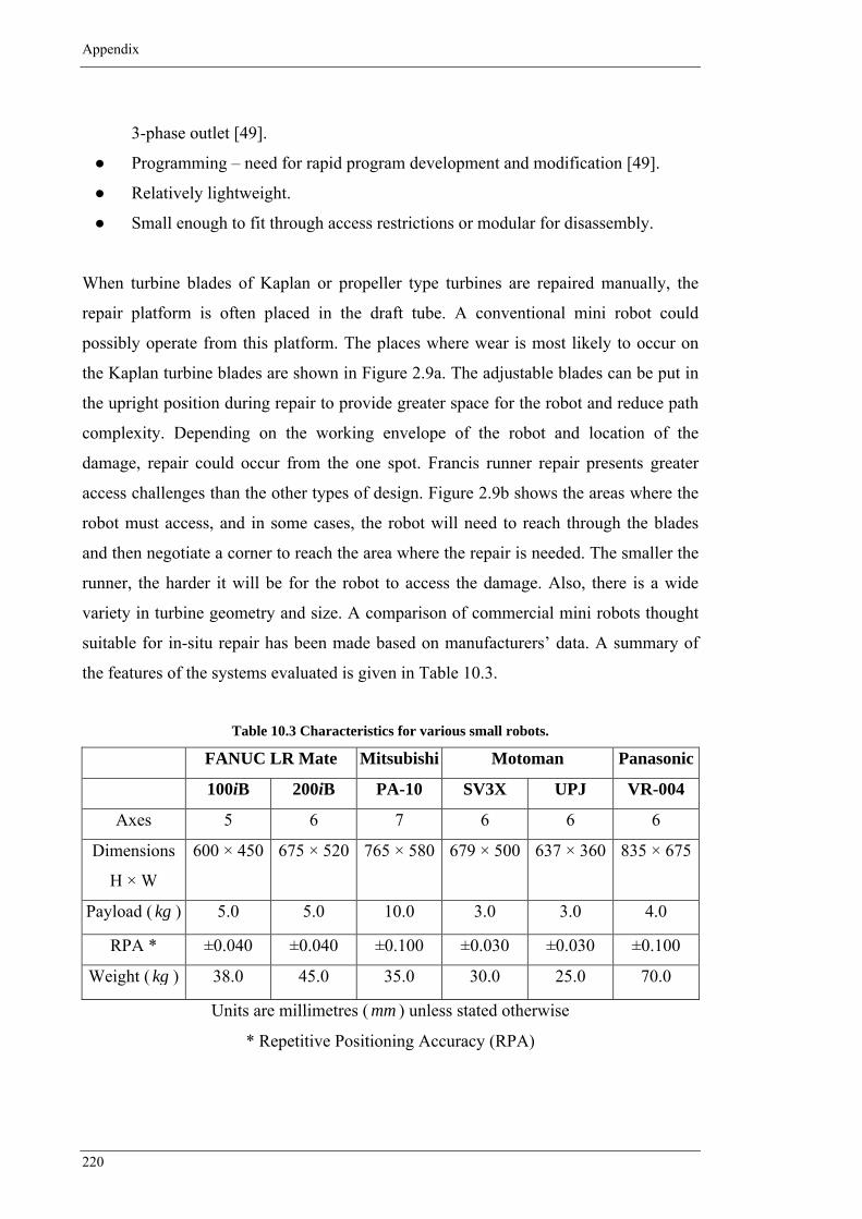
Appendix
220
3-phase outlet [49].
● Programming – need for rapid program development and modification [49].
● Relatively lightweight.
● Small enough to fit through access restrictions or modular for disassembly.
When turbine blades of Kaplan or propeller type turbines are repaired manually, the
repair platform is often placed in the draft tube. A conventional mini robot could
possibly operate from this platform. The places where wear is most likely to occur on
the Kaplan turbine blades are shown in Figure 2.9a. The adjustable blades can be put in
the upright position during repair to provide greater space for the robot and reduce path
complexity. Depending on the working envelope of the robot and location of the
damage, repair could occur from the one spot. Francis runner repair presents greater
access challenges than the other types of design. Figure 2.9b shows the areas where the
robot must access, and in some cases, the robot will need to reach through the blades
and then negotiate a corner to reach the area where the repair is needed. The smaller the
runner, the harder it will be for the robot to access the damage. Also, there is a wide
variety in turbine geometry and size. A comparison of commercial mini robots thought
suitable for in-situ repair has been made based on manufacturers’ data. A summary of
the features of the systems evaluated is given in Table 10.3.
Table 10.3 Characteristics for various small robots.
FANUC LR Mate Mitsubishi Motoman Panasonic
100iB 200iB PA-10 SV3X UPJ VR-004
Axes 5 6 7 6 6 6
Dimensions
H × W
600 × 450 675 × 520 765 × 580 679 × 500 637 × 360 835 × 675
Payload ( kg ) 5.0 5.0 10.0 3.0 3.0 4.0
RPA * ±0.040 ±0.040 ±0.100 ±0.030 ±0.030 ±0.100
Weight ( kg ) 38.0 45.0 35.0 30.0 25.0 70.0
Units are millimetres ( mm ) unless stated otherwise
* Repetitive Positioning Accuracy (RPA)

Appendix
221
10.2.7 Suitable Systems
The most common turbine type used in the Australian power generation industry is the
Francis turbine [134]. This type is also the hardest to repair because of the placement of
the blades between two rings (the crown and band) and the repairs need to be carried out
between these rings. Kaplan turbines are also used in Australia. This type of turbine has
blades more accessible for repair and access can be increased by adjusting the angle of
the blades. Pelton (impulse type) turbines are not affected by cavitation but erode from
foreign abrasive particles in the water. Wheel access is straightforward and the turbine
pit has large open spaces to accommodate a robot. To cover most turbine types and
sizes, at least a 6-axis robot is envisaged to be necessary. The Panasonic VR-004 is not
very suitable for in-situ turbine runner repair due to its weight. The Motoman-SV3X
supports welding and is preferred over the Motoman-UPJ which does not. The FANUC
LR Mate 100iB is lightweight and has good repetitive positioning accuracy but is
limited with only 5 degrees of freedom. Based on the requirements mentioned earlier,
the FANUC LR Mate 200iB and the Mitsubishi PA-10 seem to be appropriate for in-
situ repair. The PA-10 has a higher allowable payload than the LR Mate 200iB and has
an extra axis of motion making it more manoeuvrable; the trade-off being a reduction in
repetitive positioning accuracy. The weight of the PA-10 allows for easier transport to
the turbine pit and placement on the repair platform. The full featured simulation
software available with the PA-10 robot is advantageous. Although this robot has a
smaller repetitive positioning accuracy compared to the LR Mate 200iB, this is not
problematic. A price indication of the FANUC LR Mate 200iB and Mitsubishi PA-10
was obtained. The FANUC LR Mate 200iB was priced at approximately US$29,900.
The Mitsubishi PA-10 costs approximately US$64,000, and a further US$10,000 is
charged for simulation software and operation support program.
10.3 Process Selection for Automated Repair
Automated weld repair differs substantially from manual processes in that operator
adaptive and corrective responses cannot occur, and thus the selected process must be
robust and tolerant to changes in welding conditions. For example, positional welding
must be possible by the chosen process. Also, processes that produce minimal slag are

Appendix
222
preferable as automated slag removal is difficult. Further, high heat input processes may
require the application of strongbacks which add to repair complexity through the
requirement for distortion control.
The repair processes that have been investigated for hydro turbine applications include
adhesive coating, arc welding, boriding, hard chrome plating, laser cladding, plasma
nitriding, and thermal spraying [5]. Some details of various processes are given below.
Adhesive coatings. Various non-fused materials have been used for cavitation repair.
These include paint, epoxies, ceramics, neoprene, and urethane. Metallic polymers
commonly used are marketed as Belzona and Devcon. A major difficulty with these
coatings is that they are subject to disbondment at the metal to coating interface which
makes them unsuitable for use in areas subject to severe cavitation. Adhesive coatings
may be used to carry out temporary repairs between major overhauls. Epoxy type
coatings may be used as a protective barrier at the carbon steel and stainless steel
interface against galvanic corrosion. For adhesive coatings to be successful they require
surface cleaning and roughening usually by blasting, and product application within the
recommended temperature, humidity, and time limit guidelines.
Laser cladding involves fusing cobalt, nickel or iron-base alloys to a substrate to
produce a high quality metallurgically bonded surface. Entire surfaces or specific
regions may be treated in a single step to produce a clad surface very close to the
required profile. The advantages of this low energy input process include low distortion,
minimal dilution, improved production, excellent reproducibility, and cost savings.
Thermal spraying processes such as HVOF (High Velocity Oxygen Fuel) and plasma
arc sprayed coatings are effective methods of protecting turbine runners from damage
due to erosion, cavitation erosion, and dissimilar metal corrosion. Tungsten carbide with
or without nickel and chromium powders are widely used to provide coatings with high
density and bond strength. They have excellent erosion resistance in high-energy
particle impingement wear; however, voids and defects may be present in the coating.
Although the thermal spray method for surface repair is less than half the cost of
welding, these processes are less suited to local cavity repair.

Appendix
223
Calkhoven [134] gives an overview of available repair techniques as listed in Table
10.4. For robotic applications, process attributes should include [134]:
● Ease of automation.
● Low heat input positional welding capability.
● Slag free.
● High quality surface finish.
Four processes that meet these criteria are GMAW, GTAW, PTAW and laser cladding.

Table 10.4 Comparison of different repair techniques [134].
Process Application Mode Advantages Disadvantages
FCAW Manual
Semi-automatic
Automatic
1. Adapts well to field use.
2. High deposition rate.
3. Flexible.
1. Fume.
2. Spatter.
Friction Surfacing Automatic 1. Layer refined by hot working.
2. Metal matrix composites can be deposited.
3. Sound bonding.
4. No/low dilution.
1. Availability of process limited.
2. Complex shapes difficult.
3. Substrate must withstand extensive mechanical
force.
Gas Welding Manual
Semi-automatic
1. Universally available. 1. High heat input.
2. Very slow.
GMAW Manual
Semi-automatic
Automatic
1. High deposition rate.
2. High productivity.
3. High surface quality and appearance.
4. Positional welding.
1. Equipment more complex.
2. High dilution.
3. Must maintain gas shield, especially during field
use.
GTAW Manual
Automatic
1. Low dilution.
2. No flux residue.
1. Low deposition rate.
2. Small areas only.

Laser Cladding Automatic 1. Composite and dissimilar layers.
2. Control of position and heat input.
3. Localised heating, low distortion.
4. Rapid heating and cooling.
5. Low dilution.
1. High equipment cost.
2. Low deposition rates.
3. Use of powder feeder.
MMAW Manual 1. Easy to use.
2. Highly portable.
3. Low capital cost.
4. Positional welding.
1. Cannot easily automate.
2. Slow.
3. Spatter.
4. Quality highly dependent upon operator skill.
PTAW and HVOF Semi-automatic
Automatic
1. Good surface finish.
2. Low dilution.
3. Metallurgical bond and sound coating.
4. Versatile powder feed.
1. Availability of equipment.
2. High initial expense.
3. High powder cost.
4. Noise.
SAW Automatic 1. Consistent high quality.
2. Good for heavy build-up.
3. Good surface finish.
4. High productivity.
5. Readily automated.
6. Requires minimum of operator skill once set-up.
1. Continuous need to handle flux.
2. High dilution.
3. High heat input.
4. No positional welding.

Appendix
226
10.4 Robot Coordinate Representation
Robot orientations can be specified (relative to local axes) by three sequential rotations
around the body axes [145]. These are also known as the Euler angles. Banks [145]
describes the Euler angles in this way: “starting with the body axes aligned with the
local axes, the first rotation is about the z -axis through an angle ψ , followed by a
rotation about the y -axis through an angle θ , followed by a rotation about the x -axis
through an angle φ ”. From the Euler angles, the robot’s direction cosine matrix is
constructed as [145]:
cos cos sin sin cos cos sin cos sin cos sin sincos sin sin sin sin cos cos cos sin sin sin cos
sin sin cos cos cosC
θ ψ φ θ ψ φ ψ φ θ ψ φ ψθ ψ φ θ ψ φ ψ φ θ ψ φ ψ
θ φ θ φ θ
− +⎡ ⎤⎢ ⎥= + −⎢ ⎥⎢ ⎥−⎣ ⎦
10.1
and the kinematic equations for the Euler angles relating the Euler angle time
derivatives to the angular velocity are:
sin tan cos tanp q rφ φ θ φ θ= + + 10.2
cos sinq rθ φ φ= − 10.3
sin sec cos secq rψ φ θ φ θ= + 10.4
where p , q , and r are the components of angular velocity in body axes.
According to Banks [145], there are two disadvantages with Euler angle representation.
Firstly, the Euler angle equations contain many trigonometric functions which are
computationally inefficient compared to basic arithmetic operations. Secondly,
numerical singularities exists in Equations 10.2 and 10.4 when 90θ = ± . i.e. when the
robot’s end effector is vertically aligned.
Quaternion representation is a way to avoid such problems. Four quaternions ( 0e , 1e ,
2e , and 3e ) replace the three Euler angles (ψ , θ , and φ ). Banks [145] explains that

Appendix
227
because only three parameters (ψ , θ , and φ ) define any possible rotation, the four
quaternions need a constraint so that there are only three independent variables. This
constraint is [146]:
2 2 2 20 1 2 3 1e e e e+ + + = 10.5
The quaternions (in terms of Euler angles) are given by [146]:
0 cos cos cos sin sin sin2 2 2 2 2 2
e ψ θ φ ψ θ φ= + 10.6
1 cos cos sin sin sin cos2 2 2 2 2 2
e ψ θ φ ψ θ φ= − 10.7
2 sin cos sin cos sin cos2 2 2 2 2 2
e ψ θ φ ψ θ φ= + 10.8
3 sin cos cos cos sin sin2 2 2 2 2 2
e ψ θ φ ψ θ φ= − 10.9
Banks [145] explains that numerical integration of the quaternion time derivatives tends
not to destroy the constraint given in Equation 10.5, and with high enough numerical
precision normalising Equations 10.6-10.9 may never be necessary.
The reverse process of obtaining the Euler angles from quaternions is done indirectly
after calculating the cosine matrix. By inspection of Equation 10.1, the following
relations yield the Euler angles:
( )132 33tan /C Cφ −= 10.10
( )131sin Cθ −= − 10.11
( )121 11tan /C Cψ −= 10.12

Appendix
228
The quaternion representation of the direction cosine matrix given in Equation 10.1 is
[146]:
( ) ( )( ) ( )( ) ( )
2 2 2 20 1 2 3 1 2 0 3 1 3 0 2
2 2 2 21 2 0 3 0 1 2 3 2 3 0 1
2 2 2 21 3 0 2 2 3 0 1 0 1 2 3
2 22 22 2
e e e e e e e e e e e eC e e e e e e e e e e e e
e e e e e e e e e e e e
⎡ ⎤+ − − + −⎢ ⎥= − − + − +⎢ ⎥⎢ ⎥+ − − − +⎣ ⎦
10.13
and the kinematic equations for the quaternions are:
( )0 1 2 312
e e p e q e r= − + + 10.14
( )1 0 3 212
e e p e q e r= − + 10.15
( )2 3 0 112
e e p e q e r= + − 10.16
( )3 2 1 012
e e p e q e r= − + + 10.17
where p , q , and r are the components of angular velocity in body axes.
Quaternions are “more computationally efficient than Euler angles, and do not exhibit
singularities” [145]. Banks [145] suggests that “the kinematic equations using
quaternions are hardly more complex than the corresponding equations using Euler
angles; some might say that the quaternion equations are simpler”. Furthermore, the
only drawback to using quaternions is “that they have no useful physical meaning”. In
practice, this is not a major problem. “Only a human can benefit from the direct
physical meaningfulness of the Euler angles” [145]. Humans can use Euler angles to
visualise robot orientation, but computers determine the orientation by mathematical
computation. Therefore, “it is only important to use Euler angles when transferring
information to and from a human, i.e. for input and output” [145]. It is not important at
all to use Euler angles internally.

Appendix
229
10.5 Robot Simulation Packages
ACT-LIB
ACT-Weld [54] and ACT-Turbines [137] are two specific applications from the ACT-
LIB CAD development library. In both applications the software is used offline to
prepare and simulate the robotic operations to be performed. The ACT-Turbines
package was specifically developed for Pelton turbine runner repair.
GRASP
GRASP is a 3D modelling and robotic simulation system with textual programming and
offline program generation capability [147]. GRASP requires a post-processor to
generate a robot program from a simulation.
Figure 10.9 GRASP 3D modelling and simulation system [147].
Many users [148,149] have reported a lack of application specific tools, such as arc
welding or spray painting modules [22]. GRASP does not come with a built-in robot
library, which is considered essential for comparative evaluation of different robots
[22]. Some literature [22] highlights the calibration limitations of GRASP. Others
suggest effective calibration can be achieved by “supplying ‘real world’ data” to the
GRASP model which can then adjust the simulation accordingly [147].

Appendix
230
MATLAB VR
The MATLAB Virtual Reality (VR) toolbox [150] from The MathWorks provides a 3D
virtual reality environment in which dynamic system simulations can be viewed and
interactively modified. Object locations and rotations can be controlled by MATLAB or
Simulink, and animations based on dynamic systems defined in Simulink can be
generated. Autodesk Inventor or Dassault SolidWorks files can be used as well as
models in XML or VRML format. MATLAB is platform independent; however; to use
the VR toolbox the host computer needs a VRML enabled browser [68].
Figure 10.10 MATLAB VR toolbox.
IGRIP
IGRIP [151] from Deneb Robotics is a robotic simulation package for modelling and
offline programming complex robotic workcells. A wide range of options are available,
including arc and spot welding, painting, virtual reality, and process documentation.
IGRIP also includes an automatic path planner for creating collision-free robot
trajectories [152]. IGRIP includes a Graphical Development Environment (GDE) and
Graphical Simulation Language (GSL). Harrison & Mahajan [153] describe the GSL as
a device independent language for simulation purposes [22]. Further, developed
simulations can be post-processed to generate device specific robot programs. Again

Appendix
231
there is a need to learn another programming language and environment. Also, some
robot controllers have advanced functions that cannot be programmed in the GSL or
sometimes the GSL cannot translate its own code into the native robot language [22].
From experience, it is the author’s opinion that IGRIP is a very capable and user-
friendly package. However, as mentioned above, some of the advanced functions of the
particular robot controller were not able to be used which limits its potential as a tool for
research in adaptive control.
Figure 10.11 IGRIP representation of the ABB IRB1400 robot.
DELMIA
In 1998 Dassault Systèmes of France acquired Deneb Robotics. Deneb are the makers
of IGRIP and ENVISION. Soon after the acquisition Dassault released CATIA Robotics
[154]. Since then Dassault have released a range of standalone virtual manufacturing
products including CATIA, DELMIA, and ENOVIA, including the SolidWorks product
line. DELMIA [152] was designed as a successor to IGRIP to allow companies to
“digitally define, control, and monitor the automated systems that control the factory
floor” [155]. Dassault has focused on providing an integrated simulation package

Appendix
232
incorporating a robotics module which was available as a menu within a familiar CAD
interface. DELMIA includes application specific modules such as arc and spot welding.
Figure 10.12 DELMIA representation of the ABB IRB1400 robot.
Haage et al [68] effectively used DELMIA for virtual reality simulation and offline
programming, and noted its extended dynamics database. Questions regarding the
sophistication and effectiveness of the calibration methods used in CATIA Robotics
have been raised [156], and some early users [63] suggest inferiority to ROBCAD for
robotic simulations but considerable improvements have been implemented since these
claims were made.
In 2004, Dassault Systèmes and Microsoft formed a strategic alliance hoping together
they can develop fully integrated products in the field of automation [155].

Appendix
233
ROBCAD
ROBCAD [157] from Tecnomatix Technologies was developed in the 1980’s to help
process engineers quickly and easily perform design, simulation, and offline
programming of automated workcells [158]. ROBCAD has modules for arc and spot
welding, painting, and drilling [159,160].
There is a lot of literature [62,156-163] on ROBCAD that say similar things about the
software. ROBCAD has an extensive robot library with good kinematic and dynamic
definitions, and in conjunction with a calibration module, can provide very accurate
simulations [156]. West et al [163] used ROBCAD to optimise a particular welding
process and achieved increases in deposition rates of 120-150% [22]. Kempher [159]
quotes a user of ROBCAD who claims for a particular weld, programming is 8 to 16
times faster with ROBCAD compared to the time needed to manually program the robot
[22]. Conversely, Van Gorp [161] used ROBCAD for short welding runs but found it
took longer to develop the offline program with ROBCAD than to manually program
the robot online with the teach pendant [22]. However, many of the weld runs were
similar but offset, so through weld-instruction translations much of the program could
be easily modified [22].
ROBCAD has recently been re-branded as eM-Workplace [158].
Robographics
Robographics from Unimation is another robotic simulations package. Unimation is the
same company that made one of the first industrial robots – the Apprentice. Similar to
GRASP, there are no application specific modules which limit its usefulness when
compared to competitor products [22]. The quick design-change capability is a key
feature of the package eliminating the need for costly prototyping [164].

Appendix
234
ROBOSIM
ROBOSIM was developed by the National Aeronautics and Space Administration
(NASA). An online Java version of ROBOSIM has also been developed [165].
ROBOSIM uses wire frames to represent objects giving the system speed compared to
some packages which use fully rendered graphics, and it incorporates a collision
detection feature to help reduce costly mistakes [166]. ROBOSIM comes with libraries
for robots and positioners, but has no calibration module [22].
RobotStudio
RobotStudio [167] from ABB is an object-based offline programming system specific to
ABB equipment. RobotStudio allows users to build an exact virtual copy of their real
ABB robotics system. It has a familiar CAD interface where virtual cells can be
constructed or imported, and includes support for Microsoft Visual Basic scripting [68].
Because ABB RobotStudio is proprietary software there is no need for post-processing
programs before transferring the program to the robot controller (as long as the robot
and controller are made by ABB).
Figure 10.13 RobotStudio simulation package.

Appendix
235
There are several application specific modules such as the ArcWeld module which is a
dedicated geometry-based offline programming tool for generating arc welding
programs. Tool orientations and positions, and weld locations are defined in relation to
the geometry. Automatic weld path generation is a feature of the package as well as a
“semi-automatic optimisation tool” that defines robot arm configurations along the weld
path [167]. This helps avoid joint-limit and singularity errors. Reachability and collision
checks are also automatically performed during a simulation [167]. Cycle times can also
be displayed and optimised. RobotStudio includes a library of virtual robot controllers
which use the exact source code as the real controllers. This way, every function of the
controller can be accessed and the user can be assured that what is seen in the
RobotStudio simulation will be what is seen in real life [168].
Workspace
Figure 10.14 Workspace simulation package [169].
Workspace [169] by Flow Software Technologies is as a low-cost simulation package
[170]. The software has a TCP trace to aid “reverse engineering” CAD drawings. No
information was obtained regarding application specific modules or ease of use.

Appendix
236
10.6 SICK Industrial Sensors
This section details some commercial industrial sensors applicable to the current
investigation. Explanations and illustrations are from the manufacturer SICK [128].
Capacitive sensors detect changes caused by objects in the electrical field
of their detection area. The evaluation of the changes gives exact
information on the presence of objects in this area. Capacitive sensors
have a high level of temperature stability, and are immune to EM
interference.
In industrial automation, encoders are used for precise position, displacement, angle,
speed, and acceleration determination. Linear displacement measurement using
encoders can achieve a resolution of micrometers, and a resolution of a few thousandths
of a degree for rotational measurement using rotary encoders.
Incremental encoders generate information relating to position and angle
in the form of electrical impulses. The number of pulses per revolution
determines the resolving capability. The individual position is determined
by counting these pulses from a point of reference.
Absolute encoders generate information relating to position, angle or
number of revolutions in the form of unique codes. A unique code is
assigned to each angular step. The number of unique code patterns per
revolution determines the resolving capability.
Linear position measuring systems have particularly high requirements.
The current position is continuously evaluated by the sensor unit and is
transmitted as an encoded signal. Since the sensor unit and the reference
scale are separate components, extremely long distances can be
measured.

Appendix
237
Wire draw encoders consist of wire draw mechanism and encoder. The
rotation of the drum is proportional to the length being measured. This
movement is counted by an encoder and converted to a measuring signal.
This provides high-resolution position or distance information for linear
measurement paths, even under difficult ambient conditions. Precise
linear guidance, as required for other length measurement systems, is not
necessary.
Inductive sensors detect metallic objects in typically very small scanning
areas. The sensor diameter is the decisive parameter for the switching
interval, which can range from a few millimetres to several centimetres.
Conversely, inductive sensors are fast, accurate and extremely rugged.
Magnetic proximity sensors are commonly used for triggering AGVs in
high-bay warehouses. They actuate the safety sensor systems when the
vehicle enters the aisle between the high-bay racks. Very high switching
distances and detection of permanent magnets through material are
possible using accurate and reliable magnetic sensors.
Modern optoelectronic sensors operate on the basis of different light sources.
Depending on the application, visible red light, invisible infrared light, blue, green or
laser light may be used. Every change in the light beam is detected, evaluated in the
receiver and converted into a digital or analogue signal. Different functional principles
open up a wide field of applications for optoelectronic sensors in all areas of
automation.
Photoelectric proximity sensors make use of the light reflected from the
object being detected. Photoelectric reflex (passive) sensors require an
additional reflector which is mounted opposite the sender-receiver unit.
Every break in the light beam is detected and evaluated.
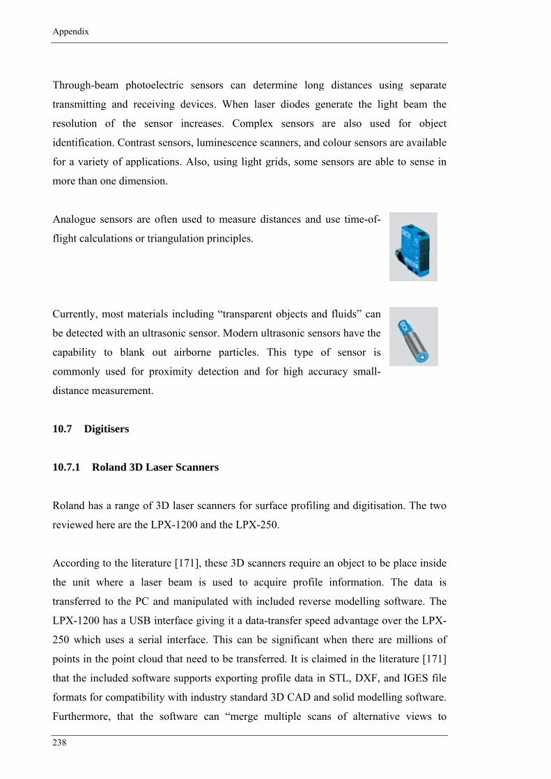
Appendix
238
Through-beam photoelectric sensors can determine long distances using separate
transmitting and receiving devices. When laser diodes generate the light beam the
resolution of the sensor increases. Complex sensors are also used for object
identification. Contrast sensors, luminescence scanners, and colour sensors are available
for a variety of applications. Also, using light grids, some sensors are able to sense in
more than one dimension.
Analogue sensors are often used to measure distances and use time-of-
flight calculations or triangulation principles.
Currently, most materials including “transparent objects and fluids” can
be detected with an ultrasonic sensor. Modern ultrasonic sensors have the
capability to blank out airborne particles. This type of sensor is
commonly used for proximity detection and for high accuracy small-
distance measurement.
10.7 Digitisers
10.7.1 Roland 3D Laser Scanners
Roland has a range of 3D laser scanners for surface profiling and digitisation. The two
reviewed here are the LPX-1200 and the LPX-250.
According to the literature [171], these 3D scanners require an object to be place inside
the unit where a laser beam is used to acquire profile information. The data is
transferred to the PC and manipulated with included reverse modelling software. The
LPX-1200 has a USB interface giving it a data-transfer speed advantage over the LPX-
250 which uses a serial interface. This can be significant when there are millions of
points in the point cloud that need to be transferred. It is claimed in the literature [171]
that the included software supports exporting profile data in STL, DXF, and IGES file
formats for compatibility with industry standard 3D CAD and solid modelling software.
Furthermore, that the software can “merge multiple scans of alternative views to

Appendix
239
achieve more accurate results” [171].
Figure 10.15 Roland LPX-1200 3D laser scanner.
Figure 10.16 Roland LPX-250 3D laser scanner.
The literature [171] suggests both 3D scanners support plane and rotary scanning modes
(shown in Figure 10.17). “Plane Scanning Mode is especially suited for capturing flat
areas, hollow objects, oblique angles and fine details” [171]. “Rotary Scanning Mode is
ideal for quickly scanning spherical and smooth-surfaced objects” [171].

Appendix
240
(a) (b)
Figure 10.17 Scanning modes [171]: (a) plane; (b) rotary.
Table 10.5 lists the specifications of the two Roland 3D scanners.
Table 10.5 Roland 3D laser scanner specifications.
Model LPX-1200 LPX-250
Dimensions H × W × D 609 × 443 × 396 742 × 528 × 431
Plane scanning area H × W 203.2 × 130 406.4 × 230
Rotary scanning area H × diameter 203.2 × 130 406.4 × 254
Maximum table load weight ( kg ) 5.0 5.0
Resolution 0.100 0.200
Plane scanning pitch:
Width direction 0.1-130 0.2-230
Height direction 0.1-203.2 0.2-406.4
Rotary scanning pitch:
Circumference (°) 0.18-3.6 0.2-60
Height direction 0.1-203.2 0.2-406.4
Sensor Non-contact laser sensor Non-contact laser sensor
Table diameter 130 254
Weight ( kg ) 35.0 32.0
Units are millimetres ( mm ) unless stated otherwise

Appendix
241
The literature [171] highlights some limitations of laser scanners in general, such as:
1. Scan quality may vary depending on the materials or colours of the objects.
2. It is not possible to scan around the top of an object where the laser beam either
hits at too shallow an angle or cannot hit the object at all.
3. Objects that are transparent, translucent, or have surfaces which are fuzzy,
glossy, or highly reflective, made of fabric, or of dark colours such as black, blue
or green, may not produce good results. In these instances, using a matte-finish
white overcoat or other temporary surfacing agent is required.
Neither of these 3D scanners from Roland is suitable for large components or for in-situ
use (although they do possess the required functionality). A more appropriate tool for
large components either in the workshop or in-situ is a portable CMM.
10.7.2 ROMER CimCore Scanning Arms
ROMER CimCore manufacture carbon fibre scanning arms that have up to 7 degrees of
freedom. These scanning arms are portable CMMs with the largest model weighing less
than 9 kg . These scanning arms are similar to older teach-by-doing robotic arms;
however, these arms possess infinite rotation of the principle axes and are much lighter
and easier to manoeuvre. Most modern robots must be guided to a location or pose
using the teach pendant whereas the scanning arms are moved by hand which can be
less time consuming.
(a) (b)
Figure 10.18 (a) ROMER CimCore 3000i scanning arm; (b) turbine inspection using scanning arm.

Appendix
242
Figure 10.19 ROMER CimCore INFINITE scanning arm with combination ball-laser probe.
Figure 10.20 ROMER CimCore LSI system and software.

Appendix
243
ABB Robotics released some software called TeachSaver that can automatically
generate robot programs from 3D coordinates gathered from these scanning arms [129].
When a scanning arm is used for robot programming, it is required to be “a little bit
more accurate than the robot’s repeatability, which is between 0.1-0.2 mm ” [129].
Accuracies of the scanning arms are claimed in the literature [129] to be as high as
0.005 mm .
ROMER CimCore also sell a Laser Scanning Inspection (LSI) system for use with their
portable scanning arms. The LSI system comes with software that has point-cloud and
colour gradient functionality. Real-time inspection of parts and comparison against
CAD data is possible, with the acquisition and analysis of 23,000 points per second.
A comparison of three different scanning arms from ROMER CimCore is given in
Table 10.6.

Table 10.6 ROMER CimCore scanning arm specifications.
Measuring Envelope ( m ) 1.2 1.8 2.4 3.0 3.6
Measuring Volume ( 3m ) 0.9 3 7 14 24
3000 i iSC i iSC i iSC i iSC i iSC
STINGER II II II II
Axes 6 7 6 7 6 6 7 6 6 7 6 6 7 6
Single Point Sphere Test ±0.005 ±0.010 ±0.015 ±0.015 ±0.030 ±0.036 ±0.075 ±0.050 ±0.100
Point Repeatability Test ±0.011 ±0.016 ±0.018 ±0.024 ±0.040 ±0.022 ±0.028 ±0.040 ±0.038 ±0.050 ±0.080 ±0.055 ±0.070 ±0.110
Volumetric Length Accuracy * ±0.016 ±0.023 ±0.025 ±0.035 ±0.055 ±0.032 ±0.040 ±0.070 ±0.055 ±0.070 ±0.055 ±0.110 ±0.100 ±0.155
Weight ( kg ) ** 5.4 5.4 5.8 5.8 3.6 7.0 7.0 4.1 8.3 8.2 4.3 8.5 8.6 4.5
Units are millimetres ( mm ) unless stated otherwise
* add 0.050 for Laser Scanning Inspection system – LSI system accuracy is ±0.050 mm
** add 0.3 kg for laser probe

Appendix
245
10.7.3 METRICOR
In contrast to the laser scanning systems described above, the METRICOR Shape
Measurement System is a non-contact optical surface scanner.
Figure 10.21 3D point-cloud obtained using METRICOR.
Figure 10.22 3D object surface profiles obtained using METRICOR.
Note
Image not included. See paper copy.

Appendix
246
According to the literature [172], a purpose-built projector is used to illuminate lines
sequentially on the target. “The height of a projection on the target is then represented
by the displacement of the line segment on the raster of the TV camera” [172]. Digitised
profile data can be saved on the PC for later use. It is claimed in the literature [172] that
the included software can provide full 3D surface measurement by merging up to 8
views of the target. Furthermore, the system does not use lasers like many competitor
products (satisfying OH&S requirements) [172]. A resolution of 1 part in 7,500 of the
field of view is claimed in the literature [172], with data acquisition times of less than 2
seconds. The system costs approximately AUD$49,000.
10.8 Grinding
The two most common abrasives used for grinding wheels are aluminium oxide and
silicon carbide [134]. Aluminium oxide abrasives are softer than silicon carbide
abrasives and are suitable for most applications. Silicon carbide abrasives should be
used for cast iron, bronze, and for very hard materials. Silicon carbide should never be
used on stainless steel. Stainless steel is susceptible to rapid corrosion if its surface has
been damaged or contaminated by grinding or weld spatter. Aluminium oxide abrasives
should be used for grinding stainless steel and cast steel.
The type of bond to be used depends on the final surface finish required, the amount of
material to be removed, and the type of grinding wheel. For vitrified bonds, abrasive
particles are mixed with clay and then baked together. Vitrified bonds produce strong
rigid wheels that are not affected by water, acid, or normal temperature changes. The
vitrified bond wheels are the most common type and are used for most general grinding.
Silicate bonds use silicate of soda for the bonding. It produces a wheel that has a milder
cutting action than the wheels using vitrified bonds. The organic bonds listed above are
often used for wheels on portable grinders and for rough foundry work because they are
more robust. Resinoid bonded wheels are best suited for the removal of small amounts
of material and for obtaining very fine finishes.
The grade (hardness) of a grinding wheel depends on the strength of the bond and the
amount of bond. The stronger the bond, the harder the wheel. The bond supports the
grains; the amount of bond determines whether the abrasive grains are held loosely or

Appendix
247
tightly. The more bond material between the different abrasive particles the harder it is
for the particle to break out, and therefore, the harder the wheel. The grade needed
depends on the material. Normally, hard wheels are used for soft work materials and
soft wheels are used for hard work materials. This is because the grinding of soft
materials does not blunt the grains as quick. A hard wheel holds the grains in place for a
longer time and allows them to do more work. The grain size selection depends on the
finish required and the desired material removal rate. A larger grain size provides a
faster material removal rate but a rougher finish. If a fine finish is required, a smaller
grain size should be used. Usually a fine-grained wheel has a dense structure, and a
coarse-grained wheel has an open structure.
The grinding wheel speed is important for the safety of the operator, but less important
if handled by a robot. Wheel speeds vary from 1,400-5,000 /m min (surface),
depending on the strength of the bond used. Most surface grinding is done in the speed
range from 1,700-2,000 /m min (surface). Grinding wheels should never be used at
speeds higher than that recommended by the manufacturer. New wheels should be run
for one minute before use, and cold grinding wheels should be loaded gradually to
reduce the chance of breakage.
Availability of electricity or compressed air to drive the grinder should also be
considered for in-situ application, as well as force feedback controllers to keep the
process forces constant during grinding. The grinding equipment and force sensors are
estimated to cost AUD$7,000 [134].
10.9 Cavitation Mechanisms
Cavitation occurs in different areas of a turbine compared to other hydraulic equipment
(such as pumps) because the cascade is accelerating. Therefore, the low pressure areas
are further back along the blade. The three characteristic types of cavitation (depicted in
Figure 10.23) that apply to turbines are:
1. Profile cavitation occurs in an area exposed to the region of lower pressure.
2. Slotted cavitation occurs in areas where a large decrease in water pressure results
from its flow through clearances such as the space between the turbine case and
the runner blade.

Appendix
248
3. Local cavitation is caused by liquid flowing past irregularities.
Figure 10.23 Types of cavitation [1]: (a) profile; (b) slotted; (c) local.
These three cavitation types may have the following forms:
● Bubble cavitation is where individual bubbles move through water from an area
of low pressure (origination area); follow the flow until they collapse at an area
of high pressure.
● Sheet cavitation is where a continuous bubble is filled with oscillating vortexes
of water.
● Separating cavitation is when no water vortexes fill the bubble cavity.
● Supercavitation is where the spaces of the cavity are so large they engulf the
blade boundaries.
These four forms of cavitation are illustrated in Figure 10.24.
Figure 10.24 Forms of cavitation in turbines [1]: (a) bubble cavitation;
(b) sheet cavitation; (c) separating cavitation; (d) supercavitation.
Separating cavitation and supercavitation affect the flow of water altering the efficiency
of the turbine. Bubble and sheet cavitation are associated with damaging erosion. A
particularly insidious form of sheet cavitation is known as cloud cavitation. During

Appendix
249
cloud cavitation the leading edge of sheet cavitation casts off bubble clouds. When the
individual bubbles in this collective cloud collapse, they produce strong shockwaves.
Cavitation is accelerated in high fluid velocity situations because local hydrodynamic
pressures vary more widely and rapidly. Some plants inject air into the turbine to reduce
the capacity and consequently lower the possibility of cavitation.
10.10 Welding Consumables for Cavitation Repairs
Stainless steels have traditionally been the most commonly used materials to repair
cavitation damage in hydro turbine runners. More recently however, several materials
such as cobalt- and nickel-based alloys and advanced iron-based alloys have been
developed, all of which have superior cavitation resistance compared to stainless steel.
10.10.1 Stainless Steels
Weld repairs that require the weld metal and the parent metal to have similar properties
must be made using consumables that closely match the parent metal. In the case of
martensitic stainless steels, weld repairs require heat treatment if parent property
matching is necessary. For this purpose, E410 electrodes or ER410 filler metal may be
used for welding both AS2074 Grade H3A and Grade H3B. E410NiMo electrodes or
ER410NiMo filler wire may be used for welding AS2074 Grade H3C.
Austenitic electrodes E309 and E312 or filler metal ER309 and ER312 may be used for
minor repairs where post-weld heat treatment is not possible. Consumables and heat
treatments recommended by AWRA [12] are shown in Table 10.7.
312 stainless steel electrodes or filler wire are normally recommended when welding a
base metal with high carbon content to avoid a reduction in ferrite. Ferrite dissolves
impurities that could otherwise form low melting point segregates and interdendritic
cracks. Austenitic stainless steel electrodes are designed to produce a small amount of
ferrite in the deposit. If the carbon is too high it will reduce the amount of ferrite in the
weld deposit and render it fully austenitic and very crack sensitive. A capping layer,
such as a cobalt-containing stainless steel, may be welded over the layer of 309 stainless
steel. A 309 stainless steel is used when the first pass is on mild steel to reduce the

Appendix
250
possibility of hot-short cracking, but if the substrate to be repaired is stainless steel, a
308 stainless steel may be used. Overlays require careful buttering and filling to ensure
that the correct dilution and penetration is achieved. Low carbon ‘L’ grades may also be
used to reduce the risk of carbide precipitation.
Table 10.7 Recommended consumables and heat treatment [12].
Steel Type Specifications
No. and Grade
AS2074
MMAW
AWS A.5.4
GTAW and
GMAW
AWS A.5.9
Preheat
Temp.
Range (°C)
Post-weld Heat
Treatment (°C)
9CR-1Mo H2A E505 ER505 250 min. 650-720
13Cr H3A E410
E309
E312
ER410
ER309
ER312
200-300 650-760
840-900
13Cr H3B as above as above 200-320 as above
13Cr-4Ni H3C E410NiMo
E309
E312
ER410NiMo
ER309
ER312
100-150 590-620 or
790-815
10.10.2 Advanced Iron-Based Alloys
The use of stainless steel to repair turbine runners does not always provide adequate
protection against severe cavitation and this prompted the industry to develop alloys
with superior cavitation resistance. These advanced alloys are used instead of 309
stainless steel for weld repairs and do not require heat treatment after welding. Four
products currently on the market are CaviTec™ from Castolin Eutectic Corp, Hydroloy
914™ from Stoody Co., NOREM™ marketed under license from the Electric Power
Research Institute (EPRI) and D-Cav™ from Demand Arc Inc.
CaviTec
Hydro-Québec initially developed an alloy named Ireca steel that was highly resistant to
cavitation erosion.

Appendix
251
Ireca steel was marketed under the trade name Hydroloy 913™ by Stoody Co. The
nominal compositions (weight percent) of Ireca and Hydroloy 913 are shown below:
% C Mn Si Cr Ni Co N Mo W Fe
Ireca 0.3 10 3 17 10 0.1 bal
Hydroloy 913 0.2 10 3 17 10 0.2 bal
In the early 1990’s Hydroloy 913 was widely used with success but it was difficult to
weld and grind. It contained 10% cobalt that provided the hardness but also made it very
expensive. Further research and alterations led to the development of CaviTec which is
marketed by the Castolin Eutectic Corp. CaviTec-SMA contains cobalt, chromium,
silicon and manganese, and CaviTec-GMA does not contain chromium. CaviTec is a
high strain and work hardening austenitic stainless steel; however, the precise formula is
proprietary information. According to company information [173], CaviTec offers easy
welding and profiling and lasts up to 4-10 times longer than stainless steel. Table 10.8
shows the suppliers recommended welding parameters for CaviTec.
Table 10.8 CaviTec welding parameters [173].
Wire: CaviTec 1.2 mm CaviTec 1.6 mm
Transfer Mode Short Circuit Spray Short Circuit Spray
Amperage ( A ) 75 125 110 200
Voltage (V ) 17 20 18 25
Polarity DC +ve
Shielding Gas 100% CO2 or Ar / 16% CO2 / 2.5% O2
Electrode: CaviTec 3.2 mm CaviTec 4.0 mm
Amperage ( A ) 90-140 (AC/DC +ve) 120-180 (AC/DC +ve)
309 butter layer recommended when welding on carbon steel
The features of this alloy are claimed to include all positional weldability, excellent
corrosion resistance, very good ductility, hardness, toughness, and fatigue strength.
CaviTec may be applied using both pulsed and conventional GMAW transfer modes.
For optimum cavitation resistance, weld deposits should be a minimum of 3 mm thick.
Cavities deeper than 9.5 mm should be first filled with a 309L stainless steel deposit.
Maximum deposit thickness for CaviTec is 9.5 mm .

Appendix
252
Under cavitation stress, the as-welded austenitic (γ ) phase transforms to the martensitic
(α ) phase. The mechanism by which this deformation takes place is twinning. The
phase transformation absorbs the energy of the shockwaves generated by the collapsing
vapour bubbles in the water and the metal effectively undergoes ‘surface hardening’.
Compared to other stainless steels, the incubation period for CaviTec is much longer,
metal loss is generally minimal and the surface is smooth and hardened. Further
exposure to cavitation causes surface fatigue cracking that subsequently leads to the
detachment of metal particles at the intersection of the deformed twins. The cavitation
damage is slow and uniform because the twins are relatively small, and therefore, only
small metal particles are able to be detached.
Hydroloy 914
This alloy was a development of an alloy called Tristelle TS-2™ that was hard, but also
brittle and crack sensitive which made it difficult to contour by grinding.
Subsequent testing of Tristelle TS-2 was carried out at lower levels of carbon so that the
microstructure of the weld deposit would be austenitic or lean-austenite. This led to the
development of Hydroloy 914 which is a relatively low cost austenitic stainless steel
that possesses good cavitation erosion resistance and ductility. The nominal
compositions (weight percent) of Tristelle TS-2 and Hydroloy 914 are shown below:
% C Mn Si Cr Ni Co N Mo W Fe
Tristelle TS-2 2 5 35 10 12 bal
Hydroloy 914 0.22 10 4.6 17 2 10 0.3 bal
According to the company, the level of cavitation erosion resistance depends on the
ratio of silicon to nickel. High silicon to nickel ratios result in low ductility, whilst low
silicon to nickel ratios result in high ductility but poor cavitation erosion resistance. For
optimum cavitation erosion resistance and good ductility, a silicon level of up to 5% and
a nickel level of up to 2% are preferred. Compared to Hydroloy 913, Hydroloy 914
contains higher silicon (4.6%) and higher nickel (2%). The composition of Hydroloy
914 is maintained within strict limits to achieve the maximum cavitation erosion

Appendix
253
resistance combined with good ductility. The silicon level increases the hardness and
cavitation erosion resistance, whilst the nickel level protects the alloy from becoming
too brittle. High levels of nickel (up to 5%) result in a decrease in the ferrite number and
a reduction in cavitation erosion resistance. Silicon compensates for the detrimental
effect of nickel; however, high levels of silicon (up to 7%) result in poor ductility.
Cobalt and chromium are beneficial for cavitation erosion resistance but are less
effective when compared to silicon. Molybdenum is beneficial for cavitation erosion
resistance, and lower manganese is beneficial when nickel is present. It is claimed that
due to the judicious balancing of elements, Hydroloy 914 has better cavitation erosion
resistance than Hydroloy 913, Tristelle TS-2 and Stellite 21™.
Hydroloy 914 is produced as welding wire in 1.2 mm and 1.6 mm diameters as well as
Shielded Metal Arc (SMAW) welding electrodes in 3.2 mm and 4 mm diameters. The
wire can be applied using a simple constant potential power source using 100% CO2 as
a shielding gas. Out of position weldability is enhanced when a helium-based mix is
used as the shielding gas. Table 10.9 shows the recommended welding parameters for
Hydroloy 914 consumables.
Table 10.9 Hydroloy 914 welding parameters [174].
Wire: Hydroloy 914 1.2 mm Hydroloy 914 1.6 mm
Amperage ( A ) 100-140 110-145
Wire Feed Speed ( ipm ) 160-200 110-130
Voltage (V ) 15-17
Position Out of Position
Polarity DCEN
Stick out 9.5-12.7 mm
Shielding Gas Helium Tri-Mix or 100% CO2
Power Source Constant Voltage
Electrode: Hydroloy 914 3.2 mm Hydroloy 914 4.0 mm
Amperage ( A ) 90-120 120-150
Polarity DCEN
309 butter layer recommended when welding on carbon steel

Appendix
254
NOREM
EPRI originally developed this highly wear resistant alloy that did not contain cobalt for
use in nuclear power plant valves because rogue cobalt atoms released by wear and
corrosion would pass through the reactor’s core and transform to the highly radioactive
cobalt-60 isotope. This posed a threat to the occupational health and safety of the plant
workers. The name NOREM means no REM (Roentgen-Equivalent-Man) which is a
unit of measurement of ionising radiation. Subsequent testing revealed that NOREM
was also resistant to cavitation erosion. The use of iron as the base metal and the
elimination of cobalt which is an expensive additive give a significant cost advantage.
Table 10.10 shows the compositions of the various types of NOREM alloys. The
various welding consumables were developed for various welding processes to ensure
that the weld chemistry provided desired cavitation erosion and wear resistance
properties.
Table 10.10 Chemical compositions of NOREM alloys [175].
% C Mn Si Cr Ni Co N Mo W Fe
NOREM 02A 1.1 4 3.1 23 3.7 < 0.06 1.8 bal
1.35 5 3.5 26 5 2.2 bal
NOREM 03B 0.7 3 2.2 20 4 < 0.1 1.7 bal
1.1 4 3 24 5.5 2.2 bal
NOREM 04B 0.7 3 2.2 20 3.5 < 0.1 1.7 bal
1.1 4.5 3 24 5.5 2.2 bal
NOREM 05B 0.8 3.5 2.2 20 3.2 < 0.1 1.7 bal
1.2 4.5 3 24 5.5 2.2 bal
The requirement for significant levels of preheat is an undesirable condition for repair
welding in-situ. According to the manufacturer, NOREM can be deposited with the
GTAW, GMAW and SMAW processes without the need for preheat; however, a 90°C
preheat is recommended to remove residual moisture and help maintain consistent
cooling rates [175]. Manual GTAW can be accomplished by using commercially
available constant current DC welding power sources with high frequency starting

Appendix
255
capability and standard GTAW torches with 100% Ar as the shielding gas. Semi-
automatic GMAW can be performed using standard or pulsed machines with a 75% Ar /
25% CO2 mixture as the shielding gas. SMAW electrodes are produced in 3.2 mm , 4
mm , 5 mm , and 6.4 mm diameters and welding can be performed using a conventional
constant current DC power source.
NOREM is able to produce porosity-free and crack-free deposits on carbon steel and
stainless steel substrates with machining and grinding characteristics similar to those of
300 series stainless steels. When welding on carbon steel it is recommended that
preheating and a 309 stainless steel buttering layer is used. To ensure that the correct
deposit chemistry is achieved, two layers of NOREM are specified to minimise dilution.
It is claimed that NOREM 04 has better cavitation erosion resistance than Hydroloy
913, and Stellite 21. The development of the NOREM chemistry concentrated on
controlling the level of incidental impurities in the welding consumables which was
found to be the means by which to avoid solidification cracking and hot tearing. In all
the product forms, phosphorous and oxygen levels are limited to less than 0.02 ppm
and sulphur is limited to 100 ppm . Boron is limited to 0.006% except for the GTAW
alloy where it is limited to 0.002%.
D-Cav
D-Cav does not contain cobalt which gives it a cost advantage; however, the precise
formula is proprietary information. According to the manufacturer [176], the D-Cav
alloy was exclusively formulated for cavitation wear resistance with good weldability
and grindability. The overall weldability performance is enhanced by its ability to be
welded in all positions on par with flux cored stainless steel wire with the use of Ar / O2
/ CO2 or straight CO2 as the shielding gas.
D-Cav is only available in 1.2 mm and 1.6 mm diameter wires. The operating
parameters for the 1.2 mm diameter wire are 175-180 A and 26-28 V . Using the 1.6
mm diameter wire at a travel speed of 889 /mm min it is possible to build up a 9.25
mm thick layer with a single pass. Welding time is greatly reduced because the need for
a second pass is eliminated; representing a 40% reduction in repair costs [176].

Appendix
256
10.10.3 Cobalt- and Nickel-Based Alloys
Various Monel™, Incoloy™, Inconel™, Stellite™, Stoodite™, and Tribaloy™ alloys
are widely used in industry due to their excellent wear and corrosion resistance. These
alloys have traditionally been used for runner repairs in situations of severe cavitation
damage where stainless steel alone proved to be inadequate; however, the cobalt and
nickel used to manufacture these alloys makes them relatively expensive.
Nickel-based alloys are resistant to wear and corrosion. Monel Alloy 400 is the basic
nickel (66.5%) and copper (31.5%) alloy that is used in highly corrosive environments.
It is tough and can be easily welded in all positions. Cobalt-based alloys are resistant to
corrosion, erosion, abrasion, and galling.
Two cobalt-based alloys that have high wear and cavitation erosion resistance are
Stellite 6 and Stellite 21 (nominal compositions in weight percent):
% C Mn Si Cr Ni Co N Mo W Fe
Stellite 6 1.1 1 0.8 28 3 bal 4 4
Stellite 21 0.25 0.7 0.5 28 2.5 bal 5.5 4
Although cobalt- and nickel-based alloys possess superior cavitation erosion resistance
compared to austenitic stainless steels such as 308 and 309 types, the advanced iron-
based cavitation erosion resistant alloys available today have comparable weldability
and improved cavitation resistance over these alloys, and are much cheaper.
10.10.4 Cavitation Test Results on Various Alloys
Table 10.11 shows the published results [177] of cavitation jet testing of various alloys
compared to 308 stainless steel (used as the reference point). These tests show that for
severe cavitation, repair welding using advanced iron-based alloys is preferable due to
their superior cavitation resistance [5]. It can be seen that cavitation resistance is 300-
400% better for some of the new alloys compared to 308 stainless steel. The results are
for wire consumables. In these tests it was reported that the two best performing cobalt

Appendix
257
free alloys were NOREM and D-Cav. Throughout the development of these cavitation
resistant alloys, the weldability of the alloys was an important consideration. The
manufacturer of D-Cav claims to have overcome all weldability problems, and welding
tests at Hume Power Station have been carried out [178]. Superior results were achieved
with GMAW using D-Cav compared to MMAW with 308 stainless steel [178]. No
information was available on the weldability of NOREM in this instance.
Table 10.12 summarises the chemical compositions of some alloys suitable for use in
hydro turbine equipment subjected to cavitation erosion [5]. Austenitic stainless steels
types 308, 309, and 312 have good cavitation erosion resistance and are relatively
cheap. They are widely used for weld repair of hydraulic components. For martensitic
turbine runners, martensitic stainless steels with appropriate heat treatment should be
used. The austenitic stainless steels have cavitation resistance far superior to carbon
steel and have good weldability. Cobalt-based alloys are again superior (in terms of
cavitation resistance) to austenitic stainless steels, but the higher cost of these alloys
may not justify their use in certain applications. Iron alloyed with cobalt results in alloys
with high hardness and good cavitation erosion resistance but reduced grindability.
Through further research, advanced alloys such as CaviTec, Hydroloy 913/914,
NOREM, and D-Cav have been developed which possess good weldability and
grindability.

Appendix
258
Table 10.11 Results of cavitation jet testing of welded alloys [177].
Alloy Test Pressure
( psi )
Weight Loss
( mg/hr )
Cavitation Rate
vs 308
308 Stainless Steel 4,000 3.2 1.0
NOREM 4,000 1.0 0.3
D-Cav 4,000 1.3 0.4
Hydroloy 914 Sample A 4,000 1.7 0.5
Hydroloy 914 Sample B 4,000 2.0 0.6
CaviTec Sample A 4,000 2.3 0.7
CaviTec Sample B 4,000 2.6 0.8
308 Stainless Steel 6,000 11.3-15.5 1.0
NOREM 6,000 4.3 0.3
D-Cav 6,000 3.4 0.3
Hydroloy 914 6,000 3.5 0.3
CaviTec Sample A 6,000 3.1 0.2
CaviTec Sample B 6,000 3.4 0.3
Table 10.12 Chemical compositions of various alloys.
% C Mn Si Cr Ni Co N Mo W Fe
308 Stainless 0.08 2 1 21 12 bal
309 Stainless 0.20 2 1 24 15 bal
Ireca Steel 0.3 10 3 17 10 0.1 bal
Hydroloy 913 0.2 10 3 17 10 0.2 bal
Hydroloy 914 0.22 10 4.6 17 2 10 0.3 bal
Tristelle TS-2 2.0 5 35 10 12 bal
NOREM 03B 1.1 4 3 24 5.5 < 0.1 2.2 bal
Stellite 6 1.1 1 0.8 28 3 bal 4 4
Stellite 21 0.25 0.7 0.5 28 2.5 bal 5.5 4
CaviTec Proprietary composition austenitic stainless steel
D-Cav Proprietary composition austenitic stainless steel – cobalt free