Dynomation6™ and DynoSim6™ Engine Simulations
314
Dynomation6™ and DynoSim6™ Engine Simulations
-
Upload
khangminh22 -
Category
Documents
-
view
0 -
download
0
Transcript of Dynomation6™ and DynoSim6™ Engine Simulations

Dynomation6™ and DynoSim6™ Engine Simulations

MOTION SOFTWARE, INC. SOFTWARE LICENSE
PLEASE READ THIS LICENSE CAREFULLY BEFORE BREAKING THE SEAL ON THE DISKETTE ENVELOPE AND USING THE SOFTWARE. BY BREAKING THE SEAL ON THE DISKETTE ENVELOPE, YOU ARE AGREEING TO BE BOUND BY THE TERMS OF THIS LICENSE. IF YOU DO NOT AGREE TO THE TERMS OF THIS LICENSE, PROMPTLY RETURN THE SOFTWARE PACKAGE, COMPLETE, WITH THE SEAL ON THE DISKETTE ENVELOPE UNBROKEN, TO THE PLACE WHERE YOU OBTAINED IT AND YOUR MONEY WILL BE REFUNDED. IF THE PLACE OF PUR-CHASE WILL NOT REFUND YOUR MONEY, RETURN THE ENTIRE UNUSED SOFTWARE PACKAGE, ALONG WITH YOUR PURCHASE RECEIPT, TO MOTION SOFTWARE, INC., AT THE ADDRESS AT THE END OF THIS AGREEMENT. MOTION SOFTWARE WILL REFUND YOUR PURCHASE PRICE WITHIN 60 DAYS. NO REFUNDS WILL BE GIVEN IF THE PACKAGING HAS BEEN OPENED.
Use of this package is governed by the following terms:1. License. The application, demonstration, and other software accom-panying this License, whether on disk or on any other media (the “Motion Software, Inc. Software”), and the related documentation are licensed to you by Motion Software, Inc. You own the disk on which the Motion Software, Inc. Software are recorded but Motion Software, Inc. and/or Motion Software, Inc.’s Licensor(s) retain title to the Motion Software, Inc. Software, and related documentation. This License allows you to use the Motion Software, Inc. Software on a single computer and make one copy of the Motion Software, Inc. Software in machine-readable form for backup purposes only. You must reproduce on such copy the Motion Software, Inc. Copyright notice and any other proprietary legends that were on the original copy of the Motion Software, Inc. Software. You may also transfer all your license rights in the Motion Software, Inc. Software, the backup copy of the Motion Software, Inc. Software, the related documentation and a copy of this License to another party, provided the other party reads and agrees to accept the terms and conditions of this License.2. Restrictions. The Motion Software, Inc. Software contains copyrighted material, trade secrets, and other proprietary material, and in order to protect them you may not decompile, reverse engineer, disassemble or otherwise reduce the Motion Software, Inc. Software to a human-perceivable form. You may not modify, network, rent, lease, loan, distribute, or create derivative works based upon the Motion Software, Inc. Software in whole or in part. You may not electronically transmit the Motion Software, Inc. Software from one computer to another or over a network.3. Termination. This License is effective until terminated. You may terminate this License at any time by destroying the Motion Software, Inc. Software, related documentation, and all copies thereof. This License will terminate immediately without notice from Motion Software, Inc. If you fail to comply with any provision of this License. Upon termination you must destroy the Mo-tion Software, Inc. Software, related documentation, and all copies thereof.4. Export Law Assurances. You agree and certify that neither the Motion Software, Inc. Software nor any other technical data received from Motion Software, Inc., nor the direct product thereof, will be exported outside the United States except as authorized and permitted by United States Export Administration Act and any other laws and regulations of the United States.5. Limited Warranty on Media. Motion Software, Inc. warrants the disks on which the Motion Software, Inc. Software are recorded to be free from defects in materials and workmanship under normal use for a period of ninety (90) days from the date of purchase as evidenced by a copy of the purchase receipt. Motion Software, Inc.’s entire liability and your exclusive remedy will be replacement of the disk not meeting Motion Software, Inc.’s limited warranty and which is returned to Motion Software, Inc. or a Motion Software, Inc. authorized representative with a copy of the purchase receipt. Motion Software, Inc. will have no responsibility to replace a disk damaged by accident, abuse or misapplication. If after this period, the disk fails to function or becomes damaged, you may obtain a replacement by returning the original disk, a copy of the purchase receipt, and a check or money order for $10.00 postage and handling charge to Motion Software, Inc. (address is at the bottom of this agreement).6. Disclaimer of Warranty on Motion Software, Inc. Software. You expressly acknowledge and agree that use of the Motion Software, Inc. Software is at
your sole risk. The Motion Software, Inc. Software and related documenta-tion are provided “AS IS” and without warranty of any kind, and Motion Software, Inc. and Motion Software, Inc.’s Licensor(s) (for the purposes of provisions 6 and 7, Motion Software, Inc. and Motion Software, Inc.’s Licensor(s) shall be collectively referred to as “Motion Software, Inc.”) EXPRESSLY DISCLAIM ALL WARRANTIES, EXPRESS OR IMPLIED, INCLUDING, BUT NOT LIMITED TO, THE IMPLIED WARRANTIES OF MERCHANTABILITY AND FITNESS FOR A PARTICULAR PURPOSE. Motion Software, Inc. DOES NOT WARRANT THAT THE FUNCTIONS CONTAINED IN THE Motion Software, Inc. SOFTWARE WILL MEET YOUR REQUIREMENTS, OR THAT THE OPERATION OF THE Motion Software, Inc. SOFTWARE WILL BE UNINTERRUPTED OR ERROR-FREE, OR THAT DEFECTS IN THE Motion Software, Inc. SOFTWARE WILL BE CORRECTED. FURTHERMORE, Motion Software, Inc. DOES NOT WARRANT OR MAKE ANY PRESENTATIONS REGARDING THE USE OR THE RESULTS OF THE USE OF THE Motion Software, Inc. SOFTWARE OR RELATED DOCUMENTATION IN TERMS OF THEIR CORRECTNESS, ACCURACY, RELIABILITY, OR OTHERWISE. NO ORAL OR WRITTEN INFORMATION OR ADVICE GIVEN BY Motion Software, Inc. OR A Motion Software, Inc. AUTHORIZED REPRESENTATIVE SHALL CREATE A WARRANTY OR IN ANY WAY INCREASE THE SCOPE OF THIS WARRANTY. SHOULD THE Motion Software, Inc. SOFTWARE PROVE DEFECTIVE, YOU (AND NOT Motion Software, Inc. OR A Motion Software, Inc. AUTHORIZED REPRESENTATIVE) ASSUME THE ENTIRE COST OF ALL NECESSARY SERVICING, REPAIR, OR CORRECTION. SOME JURISDICTIONS DO NOT ALLOW THE EXCLUSION OF IMPLIED WARRANTIES, SO THE ABOVE EXCLUSION MAY NOT APPLY TO YOU.7. Limitation of Liability. UNDER NO CIRCUMSTANCES INCLUDING NEG-LIGENCE, SHALL Motion Software, Inc. BE LIABLE FOR ANY INCIDENT, SPECIAL, OR CONSEQUENTIAL DAMAGES THAT RESULT FROM THE USE, OR INABILITY TO USE, THE Motion Software, Inc. SOFTWARE OR RELATED DOCUMENTATION, EVEN IF Motion Software, Inc. OR A Motion Software, Inc. AUTHORIZED REPRESENTATIVE HAS BEEN ADVISED OF THE POSSIBILITY OF SUCH DAMAGES. SOME JURISDICTIONS DO NOT ALLOW THE LIMITATION OR EXCLUSION OF LIABILITY FOR INCIDENTAL OR CONSEQUENTIAL DAMAGES SO THE ABOVE LIMITA-TION OR EXCLUSION MAY NOT APPLY TO YOU.In no event shall Motion Software, Inc.’s total liability to you for all dam-ages, losses, and causes of action (whether in contract, tort (including negligence) or otherwise) exceed the amount paid by you for the Motion Software, Inc. Software.8. Controlling Law and Severability. This License shall be governed by and construed in accordance with the laws of the United States and the State of California. If for any reason a court of competent jurisdiction finds any provi-sion of this License, or portion thereof, to be unenforceable, that provision of the License shall be enforced to the maximum extent permissible so as to effect the intent of the parties, and the remainder of this License shall continue in full force and effect.9. Complete Agreement. This License constitutes the entire agreement between the parties with respect to the use of the Motion Software, Inc. Software and related documentation, and supersedes all prior or contem-poraneous understandings or agreements, written or oral. No amendment to or modification of this License will be binding unless in writing and signed by a duly authorized representative of Motion Software, Inc.
Motion Software, Inc.222 South Raspberry LaneAnaheim, CA 92808 © 1995, 2018 to present By Motion Software, Inc. All rights reserved by Mo-tion Software, Inc. MS-DOS, Windows, and Windows95/98/Me/NT/2000/XP/Vista and Windows 7, 8 and 10 are trademarks of Microsoft Corporation. IBM is a trademark of the International Business Machines Corp.Dynomation™, Dynomation6™, DynoSim6™, and Motion Software™ are trademarks of Motion Software, Inc.All other trademarks, logos, or graphics are the property of their respec-tive owners.
2—Dynomation6 & DynoSim6 Engine Simulations v6.02.08, 061518

The text, photographs, drawings, and other artwork (hereafter referred to as information) contained in this publication is provided with out any warranty as to its usability or perfor mance. Specific system configurations and the applicability of described pro cedures both in software and in real-world conditions—and the qualifica tions of individu al readers—are beyond the control of the publish er, there fore the publisher dis claims all liability, either expressed or implied, for use of the information in this publication. All risk for its use is entire ly assumed by the purchaser/user. In no event shall Motion Software, Inc., be liable for any indirect, special, or conse quential damages, including but not limited to personal injury or any other dam ages, arising out of the use or misuse of any in formation in this publication or out of the software that it describes. This manual is an independent publication of Motion Software, Inc. All trademarks are the registered property of the trademark holders.The publisher (Motion Software, Inc.) reserves the right to revise this pub lication or change its content from time to time without obli ga tion to notify any persons of such revisions or changes.
ACKNOWLEDGMENTS: Larry Atherton of Motion Software wishes to thank the many individuals who contributed to the develop-ment of this program:
Brent Erickson, Programmer—Simulation Designer, Windows, C, C++, Assembler Programmer, and avid automotive enthu-siast! Brent’s positive “can-do” attitude is backed up by his ability to accomplish what many dismiss as impossible. Thanks so much, Brent!
Our Beta Testers And Dedicated Dynomation Enthusiasts—There are many individuals that regularly use Dynomation that have graciously given their time to provide suggestions, test new features, and help our development team. Many of these individuals have treated Dynomation6 as if it was their own, truly caring about making it the best simulation possible. To these dedicated enthusiasts, many of which run their own companies and have limited time to give, we offer our sincerest thanks. We could not have done it without you!
Here is just a few of the talented people that helped us with this software project:
ACKNOWLEDGMENTS, ETC.
Chuck Palmgren & Dan GurneyJohn AllerRod & Ronnel BadertscherRick HannemanTed JamesSteve JenningsDoug MacmillanMichael MarriottBob MullenMike NormanDave PropstTrinity SimpsonAudie Thomas
Many additional individuals have assisted us in beta testing and have helped us im-prove and extend our simulation software.
Larry Atherton, Pres., CEOMotion Software, Inc.
This publication is the copyright property of Motion Software, Inc., Copyright © 1995, 2018 to present by Motion Software, Inc. All rights reserved. All text and photographs in this publication are the copyright property of Motion Software, Inc. It is unlawful to reproduce—or copy in any way—resell, or redistribute this information without the expressed written permission of Motion Software, Inc. This PDF document may be downloaded by anyone for informational and educational use only. No other uses are permitted.
Dynomation6 & DynoSim6 Engine Simulations, v6.02.08, 061518—3

CONTENTSMOTION SOFTWARE LICENSE........................ 2
ACKNOWLEDGMENTS ..................................... 3
INTRODUCTION .............................................. 10 What Are DynoSim6 and Dynomation6? ...... 11 How Dynomation6 and DynoSim6 Work ...... 12 What’s New In Version6 ............................... 13 Program Requirements ................................ 14 Additional Requirements .............................. 15
INSTALLATION ................................................ 18 Program Installation Steps ........................... 18 Post Program Installation Setup ................... 20 Installing The USB Security Device ......... 20 Solving USB Key Issues .......................... 20 Installing The CamDisk 10-Point Library ...... 21 Installing A Lobe-Profile Library .................... 21 Starting The Simulation For The First Time .. 21 Registering Your Software ............................ 22 Automatic Program Updates ........................ 22 Un-installing This Simulation ........................ 22 Solving Installation Related Problems .......... 23 Tech Support Contact Info ............................ 23
PROGRAM OVERVIEW ................................... 24 Main Program Screen ................................... 24 Title Bar ..................................................... 24 Program Menu Bar ....................................... 24 File Menu ................................................. 25 Edit Menu ................................................ 25 View Menu ............................................... 25 Simulation Menu ...................................... 25 Units Menu .............................................. 26
Tools Menu .............................................. 26 Window Menu .......................................... 26 Help Menu ............................................... 26 Tool Bar ..................................................... 26 Simulation Category ..................................... 26 Engine Component Categories .................... 27 Short Block .............................................. 27 Cylinder Heads ........................................ 27 Induction .................................................. 27 Camshaft ................................................. 27 Combustion ............................................. 27 Exhaust ................................................... 27 Notes ..................................................... 27 Program Screen Panes & Display Tabs ....... 28 Engine Selection Tabs .................................. 28 Range Limit Line ........................................... 29 QuickAccess™ Buttons ................................ 29 Vertical Screen Divider ................................. 29 Simulation Progress Indicator ....................... 29 Crank-Angle SimData™ Window ................. 29 Port Velocity Graph ....................................... 30 Port Pressures Graph ................................... 30 Graph Options & Properties ......................... 30 Horsepower/Torque Graph ........................... 31 Graph Reticule Line ...................................... 31 Window Size Buttons .................................... 32 Pop-Up DirectClick™ Menus ........................ 32 Direct-Input vs Menu Input ........................... 33 Keyboard Selection And Shortcuts ............... 33 Cursor Keys Move Reticule Lines ........... 33 Menu-Bar Menus ..................................... 33 Moving Through Component Fields ........ 34 Entering Data In Component Fields ........ 34 The Meaning Of Screen Colors .................... 34
4—Dynomation6 & DynoSim6 Engine Simulations v6.02.08, 061518

CONTENTS White ..................................................... 35 Light Blue (Cyan) ..................................... 35 Light Gray ................................................ 35
FIVE-MINUTE TUTORIAL ................................ 36 Building An Engine With FE & WA ................ 36 Getting Started/Building From Scratch ......... 36 Simulation Setup ..................................... 36 Selecting A Shortblock ............................. 37 Selecting Cylinder Heads ........................ 38 Induction Selections ................................ 39 Camshaft, Combustion, Exhaust ............. 39 Creating A QuickCompare™ Baseline .... 40 Changing Cams & Exhaust ..................... 41 Trying Manifolds, Cylinderheads, etc. ..... 42 Switching To Wave-Action Model ................. 43 Completing Component Selections ......... 43 Tuning Intake Port Area ........................... 45 Tuning Intake Runner Length .................. 46 Tuning Exhaust System Specs ............... 46 Building Tri-Y Headers ............................ 47 Comparison Testing ................................. 48 Creating A ProPrint™ Report .................. 48
THE ENGINE COMPONENT MENUS ............. 50Simulation Component Category ...................... 50 Overview Of FE And WA Sim Models...... 50 Which Simulation Model To Choose ............. 51 Simulation Convergence & “Cycles” ............. 52 Wave-Action Simulation “Meshing” ............... 53 RPM Ranges and Atmospherics. .................. 54 Shortblock Component Category ..................... 56 Rod Ratio, Length, Pin Offset .................. 57 Cylinder Head Component Category ................ 60
Valve Diameters & Basic Flow Theory .... 60 Domestic Head Selections ...................... 62 2-Valve, Low-Performance ................. 62 2-Valve , Wedge ................................. 64 2-Valve, Hemi/Canted ........................ 65 4-Valve Hemi/Canted ......................... 65 Sport-Compact Head Selections ............. 67 4-Valve, Pentroof ................................ 68 2-Valve, Pentroof, Stock ..................... 69 Custom Port Flow .................................... 70 Valve-Per-Port And Diameter Menus ...... 71 Test Valve Diameters ............................... 73 Running Diameters And Auto Calc. ......... 73 Alternate Valve-Flow Calc Methods. ....... 74 When To Apply Alternate Methods. .... 76 Induction Category ........................................... 78 Intake Manifold Design ............................ 78 Baseline Manifold Models ....................... 80 Domestic Plenum Manifolds .................... 80 Dual-Plane Manifolds ......................... 80 Dual-Plane Theory ............................. 80 Single-Plane Manifolds ...................... 83 Single-Plane Theory ........................... 83 Tunnel-Ram Manifolds ....................... 85 LS1/LS6 Composite Manifolds ........... 86 Direct Port Injection HP Manifolds ..... 88 Sport-Compact Plenum Manifolds ........... 88 Non-Tuned Manifolds ......................... 89 Long-Tubing Runner Manifolds .......... 90 Tuned-Runner Manifolds .................... 90 Honda Type Manifolds ....................... 93 Individual-Runner Manifolds .................... 95 Individual Runner For Carbs ................... 97 Runner Wall Temperature .................. 98
Dynomation6 & DynoSim6 Engine Simulations, v6.02.08, 061518—5

CONTENTS Airflow And Pressure Drop Selection ............ 98 Airflow-Rate Assumptions ....................... 99 Wave-Action Intake Runner Specs ............. 100 Runner Length....................................... 100 Port Entry Area ...................................... 100 Minimum Port Area ................................ 101 Plenum Volume ..................................... 102 Taper Angle ........................................... 102 Elliptical Bellmouth Runners .................. 103Forced-Induction Specifications ..................... 104 Flow Restriction Location ...................... 105 Turbine Size .......................................... 105 Turbine Housing A/R Ratio .................... 106 Number Of Turbos ................................. 107 Boost Limit ............................................. 108 Belt Ratio ............................................... 108 Internal Gear Ratio ................................ 108 Operational Indicators ........................... 108 Surge ............................................... 109 Choke ............................................... 109 Overspeed ....................................... 110 Selecting The Best Supercharger ......... 110 Selecting Turbochargers .................. 110 Selecting Centrifugals ...................... 112 Belt-Ratio Calculations ............... 112 Selecting Roots/Screw ..................... 113 Intercoolers ............................................ 115CamShaft Category ........................................ 118 Introduction............................................ 121 Quick Overview ..................................... 105 Cam Basics ........................................... 108 Valve Events .......................................... 122 Seat-To-Seat Valve Timing ............... 123 0.050-Inch Lobe Timing ................... 125
10-Point And Profile Cam Data ................... 126 Best Of Both Worlds .............................. 128 10-Point Camshaft Menu Choices .............. 129 2- & 4-Valve Non-V-V-T Cams ............... 129 2- & 4-Valve V-V-T Cams ...................... 134 V-V-T Activation & Modeling ....................... 139 Lobe Lift, Rocker Ratio, Lash ..................... 139 Using The Net (Sim) Valve-Lift Menu ......... 141 Rocker-Math Calculator (Introduction) ........ 142 Lifter/Valve Acceleration ............................. 142 Using The 10-Point CamManager™ .......... 146 Variable Valve Timing Group ................. 148 Cam Description Group ......................... 148 Extended Application Info ...................... 149 Camshaft Timing Diagram ..................... 149 Estimated Lifter Acceleration. ................ 150 Tabbed Data Pages ............................... 151 Camshaft Specs Tabbed Page ......... 151 Event Timing Tabbed Page .............. 152 Search For CamFiles Tabbed Page . 152 CamManager Buttons ........................... 153 Loading 10-Point Camfiles .................... 153 Opening .DCM, .SCM, .CAM ........... 153 Saving CamFiles .............................. 154 Importing And Using Lobe-Profile Files ...... 156 CamPro and CamProPlus (CPP) .......... 156 CamDoctor ............................................ 157 S96 ASCII Files ..................................... 157 .ECP COMP Lobe Profile Files ............. 158 Importing Lobe Profiles ......................... 158 Lobe Source-Data List ..................... 159 Description ....................................... 159 Lobe Lift And Duration ..................... 159 Lobe-Profile Rendering/Base Circle . 160
6—Dynomation6 & DynoSim6 Engine Simulations v6.02.08, 061518
CONTENTS Lobe-Data Destination ..................... 160 Convert To 10-Point ......................... 161 Lobe Centerline ................................ 161 Lobe Lift And Acceleration Graph .... 161 Tuning And Modifying Profile Data ........ 162 Advance/Retard Cam Timing ................ 164 Adv/Ret For Single-Cam Engine ...... 164 Adv/Ret For Dual-Cam Engine......... 166
Combustion Category ..................................... 168 About Compression Ratio ..................... 169 Bore, Stroke, And Compression ....... 171 Compression Ratio Calculator ......... 173 Piston/Chamber Thermal Coatings ....... 173 Fuel Selection ........................................ 173 Nitrous-Oxide Injection .......................... 175 Combustion Chamber Selection ............ 178 Ignition Timing ....................................... 180
Exhaust Category ........................................... 184 Filling-And-Emptying Selections ............ 184 Stock Manifolds/Mufflers .................. 185 HP Manifolds/Mufflers ...................... 186 Small Headers W/Mufflers ............... 187 Small Headers Open Exhaust .......... 187 Small Flow Optimized Headers ........ 188 Small Tri-Y Headers Open Exhaust . 188 Large Header Selections ................. 188 Large Stepped Headers ................... 188 Filling-And-Emptying Tune RPM ...... 189 Wave-Action Exhaust Selections .......... 190 Header Design ........................... 191 Minimum Port Area ..................... 192 Pipes Per Cylinder ...................... 192
Primary, Secondary, Tertiary ....... 192 Primary, Secondary Collector ..... 193 Megaphone And Exit Diameter ... 193 Real-World Examples/WA Designs .. 194 4-to-1 Header ........................ 194 Add A Primary Step ............... 196 Tri-Y Header Buildup ............. 196
SIMULATION RESULTS DISPLAYS .............. 198 Main Results Graphs .................................. 198 Graph Reticule Lines ............................. 199 Graph Underlying Component ............... 200 DataSim™ Window .................................... 200 Vertical And Horizontal Dividers ................. 202 Graph Options Menu .................................. 202 Axis Data ............................................... 202 Axis Scaling ........................................... 202 Optimize Y1/Y2 Scaling ......................... 203 QuickCompare™ ................................... 204 Graph Properties Dialog ............................. 205 Graph Data Tab ..................................... 205 Axis Properties Tab ............................... 206 DataZones ™ Tab .................................. 206 Reset All Button ..................................... 207 Exact Value Tables ..................................... 208 3D Engine Pressure/Flow Display .............. 208 Intake Port Color Intensity ..................... 209 Exhaust Port Color Intensity .................. 209 Intake Port Flow Arrow .......................... 209 Exhaust Port Flow Arrow ....................... 210 Gray Arrows ........................................... 210 Mass Flow Arrows ................................. 210 Crank Position Indicator ........................ 211 Display Only Wireframe ......................... 211
Dynomation6 & DynoSim6 Engine Simulations, v6.02.08, 061518—7

CONTENTS Display Exterior Engine Outline ............. 211 Display Color Engine Cycle ................... 211
THE Quick-Iterator™ ...................................... 212 Using The Quick Iterator™ ......................... 213
THE Pro-Iterator™ .......................................... 216 Using The ProIterator™ .............................. 216 Iterator Status Group ............................. 217 Current Test Group ................................ 217 QuickStart™ Presets Group .................. 218 Cam-Timing Tabbed Page ..................... 219 Induction Tabbed Page .......................... 219 Bore/Stroke Tabbed Page ..................... 220 Optimize For Tabbed Page .................... 221 Run/Results Tabbed Page ..................... 222 Close/Save State Button ....................... 224 Close/Quit Button .................................. 224 Reset All Button ..................................... 224 ProIterator™ Testing Walkthrough .............. 224 Tips For Effective Iterative Testing .............. 227
VERSION-6 BUILT-IN CALCULATORS ......... 230 Induction-Flow Calculator ........................... 230 Airflow Pressure-Drop Converter ................ 232 Mode 1, Any Flow To 1.5-In/Hg ............. 232 Mode 2, Any Flow To 3.0-In/Hg ............. 233 Mode 3, Any Flow To Any Pres Drop ..... 233 Rocker-Math Calculator .............................. 234 CamMath QuickCalculator™ ...................... 236 Compression Ratio Calculator .................... 238 Using Known Volumes .......................... 239 Known Volumes Mode ..................... 239 Using Measured Volumes ..................... 241
Burette-Measured Mode .................. 241
PRINTING ................................................... 244 ProPrinting™ Dyno Data/Power Curves ..... 244 ProPrint™ Function & Setup ................. 223 ProPrint™ Menu Choice .................. 245 ProPrint™ Preview ........................... 246 ProPrint™ Setup .............................. 246 Printout Customizing .................................. 247 Printout Page Descriptions .................... 247 Report Modification (Advanced) ............ 249 SIMULATION ASSUMPTIONS ....................... 250 General Simulation Assumptions ................ 250 Fuel ................................................... 250 Environment .......................................... 251 Methodology .......................................... 251 Camshaft Modeling ............................... 251 Air/Fuel Ratio Modeling ......................... 251 Forced-Induction Modeling .................... 253 Roots & Screw Superchargers ......... 253 Centrifugal Superchargers ............... 254 Turbo Superchargers ....................... 255 Intercoolers ...................................... 256 Simulation Engine File Compatibility .......... 257 Dynomation6 & DynoSim6 Features .......... 258
WAVE-DYNAMICS ANALYSIS ....................... 263 The IC Engine: Unsteady Flow Machine .... 263 Acoustic Waves Vs. Finite Waves ......... 264 Compression & Expansion Waves ........ 265 Pressure Waves & Engine Tuning ......... 268 Pressure-Time Histories ............................. 269 Gas Flow Vs. Engine Pressures ............ 272
8—Dynomation6 & DynoSim6 Engine Simulations v6.02.08, 061518

CONTENTS Intake Tuning .............................................. 273 Induction Runner Taper Angles ............. 276 Port Flow Velocities ............................... 277 Exhaust Tuning ........................................... 280 Exhaust Flow Velocities ......................... 283 Exhaust Tubing Lengths ........................ 283 Valve-Events And Tuning Strategies .......... 286 IVO (Intake Valve Opening) ................... 286 EVC (Exhaust Valve Closing) ................ 287 EVO (Exhaust Valve Opening) .............. 288 IVC (Intake Valve Closing) .................... 289 Using Pressure Diagrams ........................... 289 The Pressure-Crank-Angle Diagram ..... 289 The Pressure-Volume Diagram ............. 291 Optimizing Valve Events ............................. 293
FREQUENTLY ASKED QUESTIONS............. 296 General Troubleshooting ............................ 296 Installation /Basic Operation ....................... 297 Screen Display ........................................... 298 Bore, Stroke, Shortblock ............................. 299 Induction, Manifolds, Fuel ........................... 299 Camshaft/Valvetrain ................................... 299 Compression Ratio ..................................... 301 Running A Simulation ................................. 301
MINI GLOSSARY ........................................... 304
DYNO TEST NOTES ...................................... 311
Dynomation6 & DynoSim6 Engine Simulations, v6.02.08, 061518—9
INTRODUCTIONINTRODUCTIONNote: If you can’t wait to start using this engine simulation, feel free to jump ahead to INSTALLATION (or review the 16-page QuickStart Guide supplied with your software), but don’t forget to review this manual when you have time. Also, please complete the Registration Form that appears when you first start your software. It entitles you to receive tech support, obtain free automatic releases and more. Also, if you change your mailing address or email anytime in the future, please update your registration information by re-selecting Registration from the HELP menu.
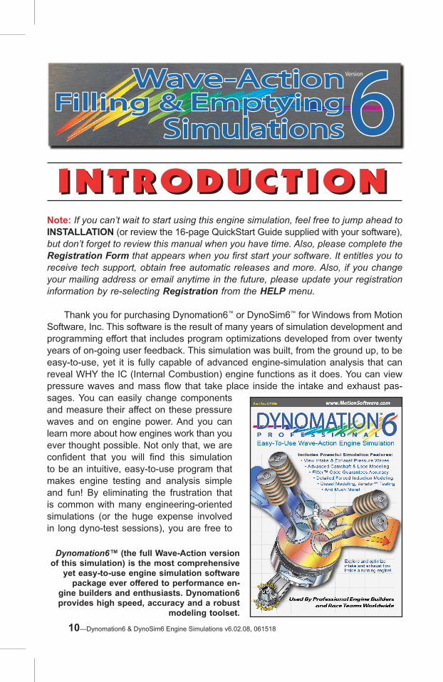
Thank you for purchasing Dynomation6™ or DynoSim6™ for Windows from Motion Software, Inc. This software is the result of many years of simulation development and programming effort that includes program optimizations developed from over twenty years of on-going user feedback. This simulation was built, from the ground up, to be easy-to-use, yet it is fully capable of advanced engine-simulation analysis that can reveal WHY the IC (Internal Combustion) engine functions as it does. You can view pressure waves and mass flow that take place inside the intake and exhaust pas-
Dynomation6™ (the full Wave-Action version of this simulation) is the most comprehensive
yet easy-to-use engine simulation software package ever offered to performance en-
gine builders and enthusiasts. Dynomation6 provides high speed, accuracy and a robust
modeling toolset.
sages. You can easily change components and measure their affect on these pressure waves and on engine power. And you can learn more about how engines work than you ever thought possible. Not only that, we are confident that you will find this simulation to be an intuitive, easy-to-use program that makes engine testing and analysis simple and fun! By eliminating the frustration that is common with many engineering-oriented simulations (or the huge expense involved in long dyno-test sessions), you are free to
VersionWave-ActionFilling & Emptying
Simulations
Wave-ActionFilling & Emptying
Simulations66
10—Dynomation6 & DynoSim6 Engine Simulations v6.02.08, 061518

“play,” using your imagination to uncover power secrets for single or multiple-cylinder, four-stroke engines for automotive, racing, or a myriad of other applications.
What Are DynoSim6 and Dynomation6?
At the core of Dynomation6 and DynoSim6 is are mathematical models that simu-lations four-stroke, internal combustion (IC) engines. These simulations incorporate
Introduction To Version6 SimulationsThe simulation incorporates a completely unique, intuitive user interface (shown us-ing one of several program color schemes). If you wish to change an engine com-ponent, simply click on any component field on the left side of the screen and select a new specification from the drop-down list or enter custom values. Engine com-ponents are shared between both the Filling-And-Emp-tying (FE) and Wave-Action (WA) simulation models. Results can be displayed in a wide variety of tables and graphs.
Main Program Screen
two distinct simulation methods: 1) A Filling-And-Emptying (FE) method, used in both DynoSim6 and Dynomation6 simulations, that provides fast mathematical solutions to engine physics, including flow analysis through intake- and exhaust systems, making this technique a powerful and efficient way to optimize engine designs, and 2) A full Wave-Action (WA) method used in Dynomation6 that calculates and predicts the complex pressure-wave dynamics and particle flows in intake and exhaust passages. The Wave-
DynoSim6™ uses the FE (Filling-and-Emp-tying) simulation method and incorporates many features of Dynomation6, including ease of use, fast calculation times and exceptional accuracy. Plus the full toolset provided with Dynomation6 is included in this powerful simulation package.
Dynomation6 & DynoSim6 Engine Simulations, v6.02.08, 061518—11
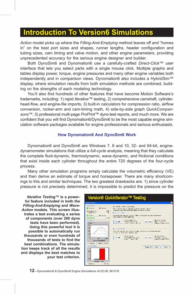
Introduction To Version6 SimulationsAction model picks up where the Filling-And-Emptying method leaves off and “homes in” on the best port sizes and shapes, runner lengths, header configuration and tubing sizes, cam timing and valve motion, and other engine parameters, providing unprecedented accuracy for the serious engine designer and builder. Both DynoSim6 and Dynomation6 use a carefully-crafted Direct-Click™ user interface that lets you select parts with a single mouse click. Multiple graphs and tables display power, torque, engine pressures and many other engine variables both independently and in comparison views. Dynomation6 also includes a HybridSim™ display, where simulation results from both simulation methods are combined, build-ing on the strengths of each modeling technology. You’ll also find hundreds of other features that have become Motion Software’s trademarks, including: 1) rapid Iterative™ testing, 2) comprehensive camshaft, cylinder-head-flow, and engine-file imports, 3) built-in calculators for compression ratio, airflow conversion, rocker-arm and cam-timing math, 4) side-by-side graph QuickCompari-sons™, 5) professional multi-page ProPrint™ dyno-test reports, and much more. We are confident that you will find Dynomation6/DynoSim6 to be the most capable engine sim-ulation software packages available for engine professionals and serious enthusiasts.
How Dynomation6 And DynoSim6 Work
Dynomation6 and DynoSim6 are Windows 7, 8 and 10, 32- and 64-bit, engine-dynamometer simulations that utilize a full-cycle analysis, meaning that they calculate the complete fluid-dynamic, thermodynamic, wave-dynamic, and frictional conditions that exist inside each cylinder throughout the entire 720 degrees of the four-cycle process. Many other simulation programs simply calculate the volumetric efficiency (VE) and then derive an estimate of torque and horsepower. There are many shortcom-ings to this and similar techniques. The two greatest drawbacks are: 1) since cylinder pressure is not precisely determined, it is impossible to predict the pressure on the
Version6 QuickIterator™ TestingIterative Testing™ is a power-ful feature included in both the
Filling-And-Emptying and Wave-Action models. This screen illus-
trates a test evaluating a series of components (over 200 dyno
tests have been performed). Using this powerful tool it is
possible to automatically run thousands or even hundreds of
thousands of tests to find the best combinations. The simula-
tion keeps track of all the results and displays the best matches to
your test criterion.
12—Dynomation6 & DynoSim6 Engine Simulations v6.02.08, 061518
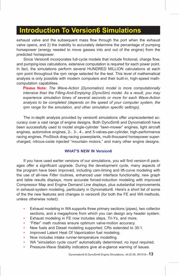
Introduction To Version6 Simulationsexhaust valve and the subsequent mass flow through the port when the exhaust valve opens, and 2) the inability to accurately determine the percentage of pumping horsepower (energy needed to move gasses into and out of the engine) from the predicted horsepower. Since Version6 incorporates full-cycle models that include frictional, charge flow, and pumping-loss calculations, extensive computation is required for each power point. In fact, the simulations perform several HUNDRED MILLION calculations at each rpm point throughout the rpm range selected for the test. This level of mathematical analysis is only possible with modern computers and their built-in, high-speed math-computation capabilities.
Please Note: The Wave-Action (Dynomation) model is more computationally intensive than the Filling-And-Emptying (DynoSim) model. As a result, you may experience simulation times of several seconds or more for each Wave-Action analysis to be completed (depends on the speed of your computer system, the rpm range for the simulation, and other simulation specific settings).
The in-depth analysis provided by version6 simulations offer unprecedented ac-curacy over a vast range of engine designs. Both DynoSim6 and Dynomation6 have been successfully used to model single-cylinder “lawn-mower” engines, light aircraft engines, automotive engines, 2-, 3-, 4-, and 5-valves-per-cylinder, high-performance racing engines, ProStock drag-racing powerplants, multi-thousand horsepower super-charged, nitrous-oxide injected “mountain motors,” and many other engine designs.
WHAT'S NEW IN Version6
If you have used earlier versions of our simulations, you will find version-6 pack-ages offer a significant upgrade. During the development cycle, many aspects of the program have been improved, including cam-timing and lift-curve modeling with the use of all-new Fitter routines, enhanced user interface functionality, new graph and table results displays, more accurate forced-induction modeling with improved Compressor Map and Engine Demand Line displays, plus substantial improvements in exhaust-system modeling, particularly in Dynomation6. Here's a short list of some of the the new features and changes in version6 (for both the FE and WA methods, unless otherwise noted):
• Exhaust modeling in WA supports three primary sections (pipes), two collector sections, and a megaphone from which you can design any header system.
• Exhaust modeling in FE now includes steps, Tri-Ys, and more. • “Fitter” math routines ensure optimum valve-motion accuracy. • New fuels and Diesel modeling supported; CRs extended to 30:1. • Improved Latent Heat Of Vaporization fuel modeling. • Now includes intake runner-temperature modelling. • WA "simulation cycle count" automatically determined; no input required. • Pressure-Wave Stability indicators give at-a-glance warning of issues.
Dynomation6 & DynoSim6 Engine Simulations, v6.02.08, 061518—13

Introduction To Version6 Simulations • WA Manifold-Plenum and Runner-Bellmouth modeling. • FE displays pressure waves and particle flow velocities, just like WA! • FE includes several additional exhaust models and tubing-size prediction. • Iterator finds optimum Runner-Length and Runner-Areas. • Improved Forced-Induction modeling and Turbo Map displays. • Added feedback in the Simulation Log, helps diagnose simulation issues. • Graph Coefficient of Discharge (CD) and Curtain Areas for all valves. • Table displays Mass Flow, in Lb/min and Kg/sec, at each RPM step. • Enter your own conversion factor for Brake-to-Wheel Horsepower. • Improved Units handling for US and Metric, and a new Hybrid Units Mode! • And a lot more!
The display and analysis of pressure waves in the intake and exhaust ports also has been improved. Click on the power/torque graph to select any rpm point; you will instantly see the status of pressure waves and mass flow for that engine speed for both the WA and FE simulations. Drag the reticule line on the power/torque graph; the pressures and flow dynamics will be instantly updated as you scan through the rpm range. This capability provides an unprecedented view of pressure and particle flow within a “running” engine for both WA and FE simulations. Enhancements were added to Iterative Testing™, an exclusive feature of Motion Software simulations. Iterative Testing allows you to automatically perform thousands of dyno tests, keep track of all the results, and locate the best component combina-tion that matches your search criterion. In addition to cam timing, intake manifolds, bore, and stroke, you can now Iterate intake runner lengths, and minimum and entry areas in the intake ports (for the WA simulation only). Version6 also offers many additional improvements. Diesel modeling is now sup-ported with compression ratios as high as 30.0:1. Latent Heat of Vaporization modelling has been enhanced to better simulate intake-charge temperatures, particularly with supercharges and racing fuels, like methanol. Manifold runner wall temperature can be modeled to directly support "air-gap" manifolds and other unique manifold/runner ambient conditions. Cam Dynamic Stability Indicators have been included to alert the user if the current cam timing values generates stability issues. Additional indicators in Dynomation6 located in the Induction and Exhaust categories show calculation issues in intake or exhaust pressure-wave analysis. But most important is what hasn't changed: our top-tier tech support. The Motion Software, Inc., development staff will be available to help you if you run into issues that you can't solve on your own. We are very interested in helping you succeed with Version6 simulations. Let us know how we can help!
Program Requirements
Here are the basic hardware and software requirements: • A Windows-compatible PC with a CD-ROM drive or access to an external
CD drive.
14—Dynomation6 & DynoSim6 Engine Simulations v6.02.08, 061518
• A USB Port for the Security Key for Dynomation6 only (see INSTALLATION for more information on program security). The USB Security Key supplied with your software is required to run Dynomation6 (not required for DynoSim6).
• A minimum of 2GB of RAM (random access memory) for Windows 7, 8 and 10. More memory than this will improve program performance.
• Windows 7, 8 or 10 (32- or 64-bit). Note: Version6 software may run on earlier versions of Windows (such as XP and Vista), but these installations are not supported.
• An Internet connection to obtain Free program updates (you will receive periodic updates, all free for registered users of version 6).
Note: Automatic updates over the Internet are not supported in Windows 2000.
• A video system capable of 1280 x 1024 or higher to optimize screen display of engine components and graphics.
• A fast system processor (2GHz or faster) will improve processing speeds; especially helpful for Wave-Action and Iterative testing. However, Version6 simulations will operate on any Windows qualified system, regardless of processor speed.
• A mouse/mousepad/trackball is required for cursor movement and component selection.
• Any Windows compatible printer (to obtain dyno-test printouts). • You can export simulation data in a format that is readable by Microsoft Excel
(spreadsheet). Excel (or a compatible product) is needed to utilize this feature.
Additional System RequirementsAnd Considerations
Windows 7, 8 and 10: This software is fully compatible with Windows 7, 8 and 10 (either 32- or 64-bit versions). Make sure to install all the latest service packs and updates (use the Microsoft Windows Update feature available in the Start Menu, All Programs Menu, or visit www.microsoft.com to locate or activate automatic updatesfor your operating system; this is an automatic feature in Windows 10.
Windows 2000/XP/Vista: Our testing shows that Version6 simulations will usually operate on WindowsXP, Windows 2000, and Windows Vista. Make sure to install all the latest service packs and updates (use the Microsoft Windows Update feature available in the Start Menu, All Programs Menu, or visit www.microsoft.com to locate updates and service packs for your operating system).
Note-1: Windows95 is not supported.Note-2: We recommend that you run this simulation on a Windows 7, 8 or 10 ma-chine. These operating-system versions are the most sophisticated and reliable.
Video Graphics Card And Monitor: An 800 x 600 resolution monitor/video card is required to use version6 simulations. Systems with 1280 x 1024 (HD) resolution will
Introduction To Version6 Simulations
Dynomation6 & DynoSim6 Engine Simulations, v6.02.08, 061518—15

provide more screen “real estate,” and this additional display space is very helpful in component selection and power/pressure-curve analysis. Screens of 19-inches or larger with 1280 x 1024 resolution or higher are optimum for simulation testing.System Processor: Version6 engine simulations, especially Dynomation6, are ex-tremely calculation-intensive. Over 2 billion mathematical operations are performed for each complete power-curve simulation. While the program has been written to optimize speed, a faster processor will improve data analysis capabilities. Furthermore, our simulations incorporate powerful Iterative Testing that can perform an analysis of hundreds or thousands of simulation runs. To reduce calculation times and extend the modeling capabilities of the program, use the fastest processor possible.
Mouse: A mouse (trackball, or other cursor control device) is required to use this software. While many component selections can be performed with the keyboard, several operations within this simulation require the use of a mouse.
Printer: Dynomation6 and DynoSim6 can print a comprehensive ProPrint™ “Dyno-Test Report” of the simulated dyno engine on any Windows-compatible printer. If you use a color printer, the data curves and component information will print in color.
Introduction To Version6 Simulations
16—Dynomation6 & DynoSim6 Engine Simulations v6.02.08, 061518

Dynomation6 & DynoSim6 Engine Simulations, v6.02.08, 061518—17

INSTALLATIONINSTALLATION Note: In most cases, you can install Motion Software products simply by
following on-screen prompts. As additional help, the following steps 1 through 8 provide information that will ensure a trouble-free installation. If you skip this part, we recommend all users review post-installation instruc-tions later in this section:
• Installation Overview: Dynomation6—As the purchaser/owner of Dynomation6, you are granted a
license to install the simulation on as many computers as you wish, however, Dynomation will only startup and run on a computer that has the USB Security Key plugged into a USB port on your system (the USB Key is supplied in your software package).
DynoSim6—As the purchaser/owner of this DynoSim6, you are granted a license to install this simulation on two computers for your personal use. Installation on more systems, or “loaning” this software to friends, is a violation of the Motion Software License agreement.
• Make sure all other applications are closed before you begin this installation. The best way to do that is to restart your system, then begin this installation be-fore you start any other programs. If other programs are using system resources during Dynomation installation, your computer may appear to “lock-up” when in fact, another application (“hiding” in the background) has taken focus away from the Dynomation installer.
• Make sure that you have sufficient memory to install/run this simulation (review system requirements in the previous chapter). Note: You must have Administrator Rights to properly install Dynomation
under Windows 7, 8 and 10. Administrator Rights are also required to receive automatic updates over the Internet.
Program Installation Steps
1) Close all other applications before you begin this installation.
VersionWave-ActionFilling & Emptying
Simulations
Wave-ActionFilling & Emptying
Simulations66
18—Dynomation6 & DynoSim6 Engine Simulations v6.02.08, 061518

Installing & Starting Version6 SimulationsDynomation6 Install Menu
From the op-tions provided in the Instal-lation Menu, select Install Dynomation6 or DynoSim6. If the Menu does not ap-pear, see the Note in Step 3.
2) Insert the simulation CD-ROM into your CD drive.
3) A Software Installa-tion Menu will open on your Desktop with-in 5 to 30 seconds. Click the Install op-tion.
Note: If the Software Instal lat ion Menu does not automati-cally appear on your desktop within 30 to 60 seconds, view the contents of the install CD using Windows Explorer (not Internet Explorer) and double-click on Dynomation6_In-stallMenu.exe or DynoSim6_InstallMenu.exe to begin program installation.
4) After you select an Install, allow up to two minutes for the program installer to read files from the CD and display an opening window. Click Next to view the Motion Software License Agreement. Read the Agreement and if you agree with the terms, click I Accept...., then click Next to continue the installation.
5) A Readme file is now displayed that includes information about installation and program updates. After you have reviewed the Readme, click Next to proceed with the installation.
6) Important Note: This software will be installed on its default path (on your boot drive, C:\, in the root). This location is essential to ensure that future updates install properly.
7) The installer Start Installation display gives you a chance to review the license agreement or readme info. Press Install to begin installation.
8) When the basic installation is complete, a Setup Complete dialog will be displayed. Click Finish to close the main installation window and start the installation of ad-
ditional helper-software:a) Dynomation6 only: The latest Sentinel-HASP USB Security Key driver will install next. This driver is required for Dynomation6 to communicate with the USB Security Key provided in your software package.
b) Next, a dialog box may appear and ask for permission to install Microsoft DirectX on your system (DirectX is required for 3D animations within the soft-ware). If you have the same or a newer version of DirectX already installed, the
Dynomation6 & DynoSim6 Engine Simulations, v6.02.08, 061518—19

Installing & Starting Version6 Simulationsinstaller will detect its presence and will not overwrite newer files.
c) After the DirectX installation, program installation is complete.
POST-INSTALLATION SETUP
Dynomation6 Only:Installing The USB Security Key
9) Plug the USB Security Key (the small USB device supplied with Dynomation6) into any available USB port on your computer. This key is licensed to you, the purchaser of this software, and will allow you to run Dynomation6 on any of your computer systems. You are licensed to install Dynomation6 on as many comput-ers as you wish, however, Dynomation6 will only run on one system at a time; the computer with the Security Key installed.
Note: If you do not have an available USB port (your computer must have at least one free USB port to run Dynomation6), you can install a USB Card or Hub to extend the number of available USB ports. The Dynomation6 Security Key functions properly with most external USB Hubs.
Dynomation6 Only:
Solving USB Security Key Issues
If Dynomation6 displays an error message that the Security Key (or HASP) is missing, here are some quick steps you can follow to isolate and correct this prob-lem:
a) Restart Windows after you install Dynomation6 to make sure the USB Key driv-ers are loaded and running.
b) Make sure the Security Key is, in fact, properly connected to a functioning USB port on your computer or has been plugged in a USB hub that is connected to your computer. If you plugged the Key into a hub (rather than into a USB port on the computer), try connecting it directly to a port on your computer system.
Note: The Security Key contains a small red LED that illuminates when it is properly connected and communicating with its software drivers.
c) Disconnect all other USB devices from your system, then reconnect the Dynomation6 Security Key (try a different port if possible).
d) Try reinstalling the Security Key drivers by reinstalling Dynomation6 from the program CD (you do not need to un-install first), or install the latest driver posted on our Support page (www.motionsoftware.com/support.htm).
e) If your computer is experiencing technical difficulties, such as non-functional
20—Dynomation6 & DynoSim6 Engine Simulations v6.02.08, 061518

Installing & Starting Version6 Simulationsdevices, spontaneous rebooting, numerous system messages, etc., the device drivers for the Security Key may not function properly on your system. You must have a stable computer system and a clean, virus-free Windows installation to properly use this simulation.
f) As a “last resort,” try installing the simulation (and the Security Key) on a second computer system to determine if your original computer is at fault.
Installing A 10-PointCamDisk Library (Any Version)
10) CamDisks are additional libraries of 10-Point camfiles (much more information on 10-Point camfiles is provided later in this User Guide). If you wish to install a 10-point library (from a separate install CD or it can be included on the program installation CD), click the Install option on the Program Installation Menu.
Note-1: CamDisk camfiles can only be installed after the simulation has been successfully installed on your system.
Note-2: 10-Point camfiles are NOT the same as Lobe-Profile files; refer to the Camshaft Category later in this User Guide for more information on the differ-ences between 10-Point valve timing and lobe-profile specifications.
Installing A Lobe-Profile Library
11) Motion Software offers libraries of cam-lobe profiles that allow version6 simula-tions to model exact valve motion and predict engine power with the highest accuracy. Lobe-Profile files consist of data that “maps” the entire shape of the lobe, not simply the valve opening, closing, and maximum lift points used in 10-Point Camfiles. If you wish to install a Lobe-Profile library, click on the Install option on the Program Installation Menu that will appear on your desktop after you insert the Profile CD into your CDROM drive.
Note: Profile Libraries can only be installed after a version6 simulation has been successfully installed on your system.
Starting The SimulationFor The First Time
12) To start the simulation, double-click the Dynomation6 or DynoSim6 program icon that was installed on your Desktop. Alternatively, you can open the Windows START menu, select All Programs or Apps, then choose Motion-Dynomation6 Engine Sim, or Motion-DynoSim6 Engine Sim and click on the software icon displayed in that folder.
Dynomation6 Only: If Dynomation6 displays an error message indicating that the Security Key (HASP) is missing or cannot be found, refer to the information on the previous page (Solving USB Security Key Issues).
Dynomation6 & DynoSim6 Engine Simulations, v6.02.08, 061518—21

Installing & Starting Version6 Simulations
RegisteringYour Software
13) When you first start the simulation, a Registration dialog will be displayed. Please fill in the requested information, including your Serial Number found on the Quick-Start Guide provided in your software package. Then press the Register Now! button. If you have an Internet connection, your registration will be submitted to Motion Software, Inc. If you do not have an Internet connection, you will be presented with other registration options. If you do not register this simulation, you may not qualify for tech support or free updates.
If you move or change your email address, you can update your registration information at any time simply by selecting Registration from the HELP menu. Keep up to date with the latest program advances by keeping your registration information current.
AutomaticProgram Updates
14) This simulation incorporates an automatic program updater that will keep your software current with the latest simulation developments. Before you put the simulation to work, make sure you allow the Motion Updater to check our servers and install the latest program updates (requires Internet connection). The Motion Updater will run automatically after program installation and then approximately every 30 days thereafter. You can check for a new update at any time by se-lecting Check For Newer Version... from the HELP menu within the simulation. If an automatic update was not installed properly, you can manually download the latest program update from our support page at: www.motionsoftware.com/support.htm.
Important: Don’t assume you are running the latest software version if you just installed the software from the installation CD. CD’s are NOT updated each time new releases are issued. The ONLY way to make sure you are running the lat-est version is to use the Check For Latest Version feature (in the HELP menu) or to download the latest installer from our web site. If you cannot obtain/install program updates using either of these means, contact technical support at: [email protected].
Un-Installing This Simulation
You can un-install this simulation by either: 1) Use the program removal fea-ture in Windows (Start menu, select Control Panel, then choose Programs and Features, or 2) Use the Uninstaller placed in the Program folder (Start menu, select All Programs or Apps, then choose Motion-Dynomation6 Engine Sim or Motion-DynoSim6 Engine Sim, and finally click on the UNInstall).
22—Dynomation6 & DynoSim6 Engine Simulations v6.02.08, 061518

Installing & Starting Version6 Simulations
Solving Installation And Operational Problems
Important Note: You can obtain technical support and program updates by visiting (www.MotionSoftware.com). Open the Start menu, select Programs or (Apps), Motion-Dynomation6 Engine Sim or Motion-DynoSim6 Engine Sim, then click on the Tech Support Website icon. Contact our Tech Support staff by sending an email to [email protected].
If you experience problems installing or using this simulation, please review the information presented in this Users Manual, including the information earlier in this chapter, the FAQs later in this manual, and check online for program updates (www.MotionSoftware.com/support.htm).
Send any mail correspondence to:
Motion Software, Inc. 222 South Raspberry Lane Anaheim, CA 92808-2268
Other contact information:
Voice Line: 714-231-3801 Web: www.MotionSoftware.com
Tech Support (Preferred Contact Method) Email: [email protected] Tech Support Fax: 714-283-3130
Tech Support Email: [email protected] This is the best way to reach Dynomation tech support quickly. Always include your email address and attach any .DXML engine files that may help diagnose problems. Include a thorough explanation of the steps that lead up to the fault. Note1: Tech support will only be provided to registered users. Please complete the Registration Form that appears when you first start your software to qualify for technical support from the Motion Software staff (or select Registration from the HELP menu in the program).Note2: If you need to update your address or any other personal information, simply select Registration from the Help menu, make any necessary address changes, then press Register Now! to transmit your updated info.
Dynomation6 & DynoSim6 Engine Simulations, v6.02.08, 061518—23

OVERVIEWOVERVIEW
THE MAIN PROGRAM SCREEN
The left side of the Main Program Screen includes component categories that you can use to select simulation models and enter engine components, dimensions, and specifications. The right side of the screen displays simulation results consisting of graphs, charts and tables. The Main Program Screen is composed of the following elements:
1) The Title Bar displays the program name followed by the name of the currently-selected engine.
2) The Program Menu Bar contains pull-down menus that control overall program
(1) Title Bar
(3) Tool Bar
(7) Engine Selection
Tabs
(6b) Right Pane Display Tabs
(12) Crank Angle SimData Window
(6a) Left PaneDisplay Tabs
(18) Windows Size Buttons
(16) Power & Torque Curves
(17) Graph Reticule
(14) Port PressureCurves And
(15) Right-Click Graph Options
(13) Port VelocityCurves
(11) Simulation Calc Progress
(8) Range Limits And Status Bar
(2) ProgramMenu
Bar
(19) Pop-Up DirectClick™ Menu
(10) Vertical Screen Divider Resizes Left/Right Panes
(9) Quick-Access Buttons™
(5) EngineComponentCategories
WithRoll-Up Menus
(4) Simulation Selection/Setup
VersionWave-ActionFilling & Emptying
Simulations
Wave-ActionFilling & Emptying
Simulations66
24—Dynomation6 & DynoSim6 Engine Simulations v6.02.08, 061518

Program Overview
function. Here is an overview of these control menus, from left to right:
File—Opens and Saves version6 (.DXML) files; Imports other Motion simulation files, including previous version Dynomation4 and 5 engine files, DynoSim4 and 5 and even various DOS-based engine files; Exports crank-angle and rpm-based engine test data in an Excel-importable format; ProPrint™ generates a comprehensive report of engine components and simulation results, finally, the bottom of the File menu displays the most recently used simulation files, and contains a program-exit function.
Edit—Clears all component choices from the currently-selected engine (the current engine is highlighted on the Engine Selection Tabs at the bottom of the screen; see Engine Selection Tabs, later in this section).
View—Allows you to display the Toolbar(3), Status Bar(8) and Workbook (see the Workbook note, below) layout features. The View menu also includes a choice to reset all graphs to program defaults.
Note: The Workbook features activate the Engine Selection Tabs(7) at the bottom of the screen, allowing rapid switching between simulated engines. If you have limited screen space (or you only simulate one engine at a time), you can turn off the Workbook features and access multiple simulated engines from the Windows menu.
Simulation—Run forces an update (recalculation) of the current simulation. Auto Run enables or disables (toggles) automatic simulation update every time a component is changed. You can also display a Simulation Log that contains diagnostic information about the simulation just completed. The Graph...On Baseline selection will re-scale pressure graphs to position the
Program Menu Bar Program Menu Bar contains nine pull-down menus that control overall program function.
Program Menus—Simulation Menu Each Program Menu pro-vides access to overall program features. Here the Simulation Menu lets you to choose when the simulation is performed and whether the SimLog and Blower-Map dia-logs are displayed. You can also open a Program Default dialog where startup charac-teristics for the software can be modified.
Dynomation6 & DynoSim6 Engine Simulations, v6.02.08, 061518—25
Program Overview
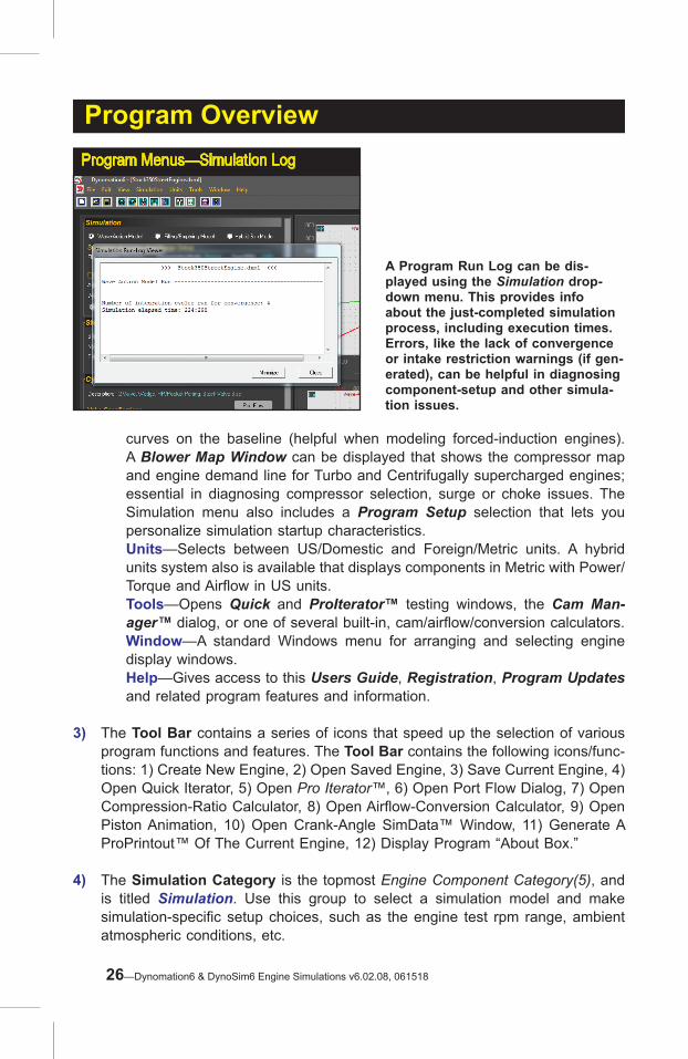
curves on the baseline (helpful when modeling forced-induction engines). A Blower Map Window can be displayed that shows the compressor map and engine demand line for Turbo and Centrifugally supercharged engines; essential in diagnosing compressor selection, surge or choke issues. The Simulation menu also includes a Program Setup selection that lets you personalize simulation startup characteristics.
Units—Selects between US/Domestic and Foreign/Metric units. A hybrid units system also is available that displays components in Metric with Power/Torque and Airflow in US units.
Tools—Opens Quick and ProIterator™ testing windows, the Cam Man-ager™ dialog, or one of several built-in, cam/airflow/conversion calculators.
Window—A standard Windows menu for arranging and selecting engine display windows.
Help—Gives access to this Users Guide, Registration, Program Updates and related program features and information.
3) The Tool Bar contains a series of icons that speed up the selection of various program functions and features. The Tool Bar contains the following icons/func-tions: 1) Create New Engine, 2) Open Saved Engine, 3) Save Current Engine, 4) Open Quick Iterator, 5) Open Pro Iterator™, 6) Open Port Flow Dialog, 7) Open Compression-Ratio Calculator, 8) Open Airflow-Conversion Calculator, 9) Open Piston Animation, 10) Open Crank-Angle SimData™ Window, 11) Generate A ProPrintout™ Of The Current Engine, 12) Display Program “About Box.”
4) The Simulation Category is the topmost Engine Component Category(5), and is titled Simulation. Use this group to select a simulation model and make simulation-specific setup choices, such as the engine test rpm range, ambient atmospheric conditions, etc.
Program Menus—Simulation Log
A Program Run Log can be dis-played using the Simulation drop-down menu. This provides info about the just-completed simulation process, including execution times. Errors, like the lack of convergence or intake restriction warnings (if gen-erated), can be helpful in diagnosing component-setup and other simula-tion issues.
26—Dynomation6 & DynoSim6 Engine Simulations v6.02.08, 061518

Component Category Status The status of the Component Categories are indicated by the color of the Cat-egory Title Bars. The Title Bars are either red tone, indicating that required data has not been entered (inhibiting a simu-lation run), or dark tone indicating that all required data in that category has been entered. The simulation determines whether a category is “complete” based on the simulation method selected. For example, the Filling-And-Emptying model requires fewer data values than the Wave-Action model. As a result, cat-egories may indicate dark when Filling-And-Emptying is active, but may switch to red when the Wave-Action model is activated, indicating that additional data in those categories is required.
Program Overview
5) The remaining Engine Component Categories are made up of the following groups:
ShortBlock—Select the bore, stroke, number of cylinders, pin-offset, and rod length and/or rod ratio in this category.
Cylinder Head—Select the cylinder head type from generic choices in the menu or enter custom data using the Port-Flow dialog (click the Port-Flow button).
Induction—Select intake manifold designs, airflow rates, pressure drop and runner temperatures for the induction system. Also select intake runner and plenum dimensions for the Wave-Action simulation. At the bottom of the In-duction category you can activate and configure a forced-induction system for any engine. Roots and Screw blowers, Centrifugal superchargers, and Turbochargers are supported.
Camshaft—Select the camshaft type, activate V-V-T (variable valve timing similar to Honda’s VTEC), set various cam timing/specifications, and displays the True Timing used by the simulation. Buttons open the CamManager™, Rocker-Math™ dialog, and the Lobe-Profile Import dialog.
Combustion—Selects the compression ratio, the type of fuel, air/fuel ratio, nitrous flow rate, combustion chamber design, and ignition timing.
Exhaust—Selects the exhaust-system configuration, runner and tubing di-mensions and interconnection specifications.
Notes—Enter any comments about the current simulation. Notes are saved with the engine .DXML file.
Note: Each component category indicates its status by the color of the Category
All RequiredData Entered
CategoryIncomplete
Dynomation6 & DynoSim6 Engine Simulations, v6.02.08, 061518—27

Program Overview
Title Bar. The Title Bars have either a red tone, indicating that the category is not complete (inhibiting a simulation run), or a dark-tone indicating that all com-ponents in that category have been selected. When all component categories indicate complete, a simulation can be performed (calculation will begin automati-cally if the Auto Run feature is selected in the Simulation Menu).
6a & 6b) The Main Program Screen window is divided into two panes. The left and right panes each provide a set of Screen Display Tabs at the bottom Use these tabs to switch the left and right pane displays to tables, graphs, or other simulation displays.
7) This software can simulate several engines at once (supports multiple open documents). Switch between “active” engines (documents) by selecting any open engine from the Engine Selection Tabs, located just above the Status Bar at the bottom of the main program screen (engine selection can also be made from the Windows Menu). The current engine is highlighted on the foreground Tab. The name of the currently-selected engine is also displayed in the program Title
Program Screen Display TabsThe Main Program Screen win-dow is divided into two panes.
The left and right portions of each contain a set of Screen
Display Tabs located at the bottom of the panes. Use these
tabs to switch the displays to Engine component lists,
Tables, Graphs, or other data displays.
Empty Component Fields
Incomplete Component Fields
Component fields that do not yet contain valid entries are marked with a series of asterisks. This indicates that the field is empty and can accept data input. Most
numeric fields accept direct keyboard entry and/or selections from the pro-
vided drop-down menus. Some selec-tion fields (like the Cylinder Heads Type
menu) only accept selections from the associated drop-down menu. When a valid selection has been made, it will
replace the asterisks.
28—Dynomation6 & DynoSim6 Engine Simulations v6.02.08, 061518

Program Overview
Bar.
8) All Component Category menus allow either direct numeric entry or menu-selec-tion choices, and some accept both. During data entry, the range of acceptable values and other helpful information will be displayed in a Range Limit Line within the Status Bar at the bottom-left corner of the main program window.
9) Several component categories contain QuickAccess Buttons™ that give “one-click” access to important data-entry functions and calculators. The CYLINDER HEAD category contains a PortFlow button that opens the Port-Airflow dialog box, allowing direct entry of flowbench data; the COMPRESSION category con-tains a CR Calc button that opens the Compression-Ratio Calculator, a tool that can save time and improve accuracy in determining engine compression ratio; the INDUCTION category contains a FlowCalc button that allows quick airflow calculations from throttle diameter, etc.; and the CAMSHAFT category contains the CamManager™, Rocker Math™, and Import Profile buttons that give ready access to important tools that help you with cam simulation and valve-timing modifications.
10) The widths of all program panes are adjustable. Simply drag the Vertical or Horizontal Screen Divider to re-size the Component-Selection and Graphics-Display panes. Horizontal Dividers are located between the right-hand graphs. By adjusting the position of these dividers, you can increase the display size of the power-curve and pressure/flow displays for optimum resolution.
11) The Simulation Progress Indicator (appears in the Status Bar when a simula-tion calculation is underway) shows the progress of calculations for the selected simulation model. Each “step” of the progress bar indicates the completion of a simulation at one rpm point.
12) The Crank-Angle SimData™ Window (see photo, next page) displays the exact values of port pressures, flow rates, horsepower, and more at various rpm and crank-angle points. Click on the rpm graph to set the rpm reticule line, then click
Engine Selection TabsThe simulation can work with several engines at once. Switch between en-
gines by selecting any available engine from the Engine Selection Tabs, located just above the Status Bar at the bottom-
left of the main program screen. The currently-selected engine is highlighted
in the foreground (colored) Tab. Note: the Status Bar displays “Ready” in this
photo.
Dynomation6 & DynoSim6 Engine Simulations, v6.02.08, 061518—29

Program Overview
on any crank-angle graph to display a crankangle reticule (see 17, below). As you drag the reticule left and right across the graph, exact data values under the reticule intersection will be displayed in the SimData™ Window (open the SimData Window from the Tools drop-down menu).
13) The Port Velocity lower graph displays port flow rates at various rpm and crank-angle values (velocity is default display; can be customized with the right-click menu). The displayed velocity values are calculated at the location of minimum cross-sectional area in the port. Click the top horsepower/torque graph to display a reticule line and establish the rpm for viewing flow and pressure data. Drag the reticule left and right on the RPM graph to establish the port flow data (in the lower graph) at each of the selected engine speeds. Click on the Port Velocity (lower) graph to display a crank-angle reticule line; the exact data at the reticule intersection are displayed in the SimData™ Window (see 12, above).
14) The Port Pressures are displayed in the middle graph (pressure is the default display; can be customized with the right-click menu). The displayed pressures are calculated at the location of minimum cross-sectional area in the port. Click on the top RPM-based horsepower/torque graph to display a reticule line and establish the rpm for viewing pressure and velocity data. Drag the reticule left and right on the RPM graph to establish the port pressure data (in the center graph) at each of the selected engine speeds. Click on the Port Pressures graph to display a crank-angle reticule line; the exact values at the reticule intersection are displayed in the SimData™ Window (see 12, above).
15) The various graphs display horsepower, torque, port pressures, flow rates, valve lift, and more for the currently-selected engine. These graphic displays
SimData™ Window
The Crank-Angle SimData™ Window displays the exact values of port pres-sures, flow rates and other simulation
data at various rpm and crank-angle values. Click on the rpm graph to set
the rpm reticule line, then click on any crank-angle graph to display a crank-
angle reticule. As you drag the reticule left and right, exact data values at the reticule intersections will be displayed
in the SimData™ Window (open the SimData Window from the Tools drop-
down menu).
30—Dynomation6 & DynoSim6 Engine Simulations v6.02.08, 061518

Program Overview
can be customized to display additional data in many formats using the Graph Options Box. To display the Options Box, right-click on any graph; reassign the X, Y1 (left axis) and Y2 (right axis) curves to any of the data sets provided in the submenu. Optimize functions quickly setup curves for best visual resolu-tion. QuickCompare™ will setup sim "baselines" to help evaluate changes or establish comparisons with other engine files (discussed in detail later in this manual). Finally, use the Properties choice at the bottom of the menu to open the Graph Properties box where you can assign custom axis values and setup multiple engine-to-engine comparisons.
16) The Horsepower And Torque top graph displays engine output throughout the simulation rpm range (HP and Torque are the default displays; the graphs can be customized using the right-click menu). Click on the graph to display a reticule line. The exact data at the reticule intersection can be viewed in the SimData™ Window (see 12, and photo on previous page). In addition, horsepower and torque results (and much more) are displayed in the data tables; click the Table, ProData, or Crank Data Screen Display Tabs near the bottom left and right of the Main Program Screen (see 6a & 6b, earlier in this section).
17) Each of the four graphs (the fourth is located “under” the Component Categories; to view this graph, click on a Graph Tab at the bottom of the left main-program window) incorporate a Reticule Line that appears when you left-click on the graph. You can “drag” the Reticule Line left and right across the graph between the lowest and the highest test rpm (for the horsepower and torque graphs), or between 0- and 720-degrees of crankshaft rotation (for the middle and lower port pressure/velocity graphs). The exact values of the underlying data at the reticule intersections is displayed are the SimData™ Window (see 12, earlier
Graph Options Box
The Graph Options Box allow you to customize any graph. Right-Click to
Reassign the X, Y1 and Y2 curves to different data sets, to set Optimize func-
tions, to setup Quick Comparsions, to assign custom axis Properties and setup
multiple engine-to-engine comparisons.
Dynomation6 & DynoSim6 Engine Simulations, v6.02.08, 061518—31
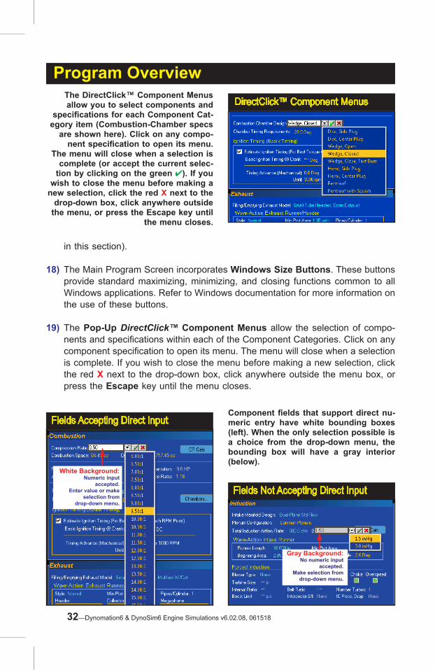
White Background:Numeric input
accepted.Enter value or make
selection fromdrop-down menu.
in this section).
18) The Main Program Screen incorporates Windows Size Buttons. These buttons provide standard maximizing, minimizing, and closing functions common to all Windows applications. Refer to Windows documentation for more information on the use of these buttons.
19) The Pop-Up DirectClick™ Component Menus allow the selection of compo-nents and specifications within each of the Component Categories. Click on any component specification to open its menu. The menu will close when a selection is complete. If you wish to close the menu before making a new selection, click the red X next to the drop-down box, click anywhere outside the menu box, or press the Escape key until the menu closes.
Program OverviewDirectClick™ Component Menus
The DirectClick™ Component Menus allow you to select components and
specifications for each Component Cat-egory item (Combustion-Chamber specs
are shown here). Click on any compo-nent specification to open its menu.
The menu will close when a selection is complete (or accept the current selec-
tion by clicking on the green ✔). If you wish to close the menu before making a
new selection, click the red X next to the drop-down box, click anywhere outside
the menu, or press the Escape key until the menu closes.
Fields Accepting Direct Input
Fields Not Accepting Direct Input
Component fields that support direct nu-meric entry have white bounding boxes (left). When the only selection possible is a choice from the drop-down menu, the bounding box will have a gray interior (below).
Gray Background:No numeric input
accepted.Make selection from
drop-down menu.
32—Dynomation6 & DynoSim6 Engine Simulations v6.02.08, 061518

Program Overview
Direct-Input vs. Menu-Input Component Categories
Component menus fall into three categories: 1) Those that accept direct user input (custom values), 2) those that only accept a selection from their attached drop-down menu, and 3) those that accept input from either direct input or menu selections. For example, the Number Of Cylinders menu in the ShortBlock cat-egory will accept direct input (any integer value from 1 to 16), and you can also select common cylinder combinations from the drop-down menu. When a menu supports direct-data entry, the component-entry bounding box will have a white interior (see photos). On the other hand, the Pressure Drop menu associated with the Total Induction Flow Rate, will only accept one of the two selections from its attached menu (1.5- or 3.0-inHg). The data entry box for these input fields have a light-gray interior (rather than white).
Note1: Almost all custom-input categories include an attached menu from which common data inputs are also provided.
Note2: Data entry into any component field is limited to values over which this software can accurately predict power. The range limits are displayed in the Range Limit Line within the Status Bar at the bottom-left of the Main Program Screen. If you enter an invalid number, the simulation will sound the Windows error tone and wait for new input.
Keyboard Selections And Shortcuts The following keyboard “speed tips” will help you make the process of data entry and “what-if” testing more efficient. None of these operations are essential, and if you prefer to only use a mouse, you can skip this section.
Cursor Arrow Keys Move Reticule Lines—You can move the reticule lines on any of the graphs in small increments by using the Cursor Arrow keys. First, click on a graph to “select” it, then use the Right-Arrow key to the move the reticule line to the right; use the Left-Arrow key to move it to the left. If you hold the SHIFT key, the increment of movement on the crank-angle graphs increases to 10-degrees.
Opening Menu-Bar Menus—Press and hold the Alt key, then press the F key to highlight and open the File menu (in the Menu-Bar at the top of the program screen). Use the cursor-arrow keys to move through menu selec-tions; press the Right-Arrow key to open submenus and the Left-Arrow key to close submenus. With any menu open, you can also use the right-and-left arrow keys to activate other menu-bar menus—e.g., Edit, View, Simulation, etc. When you have highlighted the menu selection you wish, press Enter to accept the selection. Press ESC (the escape key) repeatedly to close the menus without making a selection.
Dynomation6 & DynoSim6 Engine Simulations, v6.02.08, 061518—33

Program OverviewNote: You can also use the Alt key combination with the E, V, S, U, T, W, and H keys to directly open the other program drop-down menus.
Moving Through Component Fields—After you have selected any field within a component category, you can press the TAB key to move the highlight from field to field within that category. Tab key-presses will not open fields for data entry, but rather will move the focus highlight from field to field. Tabbing always keeps field selection within the current category.
Note: The Shift Tab key combination will move the highlight box backwards to the previous component field.
Entering Data In Component Fields—When you've highlighted a component field, press the Enter key once to convert the highlight to a data-entry bounding box. Then key in your data (or open the drop-down menu and make a selec-tion), finally press the Enter key again to close the bounding box and accept the data. To move to the next field, you can press the Tab key, or you can again press Enter. Using Enter instead of the Tab key not only moves the highlight to the next field, but also opens the data-entry bounding box in one step. So by pressing keys in the sequence “Enter, Enter, (data entry), Enter Enter,” you can quickly enter (or jump past) data in all component fields within a specific component category.
THE MEANING OF SCREEN COLORS
The colors used on the component-selection screen provide information about various engine components and specifications. Here is a quick reference to screen color functionality; these descriptions apply to the default color scheme:
Screen Colors
The colors used on the component-selection screen provide informa-
tion about what fields are currently being used and whether you can
modify these components. This is the Dynomation6 (default) color
scheme; White/Cyan indicates components that can be entered
and modified, while white/light-gray are fields that indicate “display-
only” (like Runner Connections and Average Taper Angle, shown in the
Induction category.).
34—Dynomation6 & DynoSim6 Engine Simulations v6.02.08, 061518

Program Overview
White: Most engine component field names (not the component values) are displayed in white. This indicates that their associated data fields are required for a simulation to be performed.
Light Blue (Cyan): Engine component values displayed in light blue can be entered into the program and/or modified. For example, the value of Total Induction Airflow in the Induction Category is Cyan and can be changed to any value within the limits of the simulation.
Light Gray: These “display only” values have been automatically calculated by program and cannot be directly modified. For example, the Average Taper Angle value in the Induction Category is a display-only value that is determined by the minimum and maximum port areas (values that you can enter in the pro-gram).
Note: The basic color functionality described here applies to the Dynomation6
default color scheme. While other color schemes may use some of these colors, not every color scheme uses the same default colors for data inputs. However, the differences in display colors within each color scheme will always reflect the same functionality described here.
Dynomation6 & DynoSim6 Engine Simulations, v6.02.08, 061518—35

Building And Testing An Engine Using DynoSim6And Dynomation6 Simulations
This tutorial is primarily intended for first-time version 6 users. However, anyone wishing to get a quick overview of basic data entry, simulation setup and results analysis can benefit from following along with this step-by-step example.
The most common method of starting an engine-simulation project in this simula-tion is to “assemble” a test engine from component parts. In this tutorial, we'll quickly build a basic engine using the Filling-and-Emptying simulation model. Then, after we have obtained initial results, we'll modify a few components to determine how they affect engine output. Finally, we'll switch to the Wave-Action (Dynomation6 only) simulation and continue to fine-tuning engine components. Follow along with these steps for a quick overview of how to perform a simulations and analyze the results. While this may take you more than five-minutes to complete, once you are familiar with this simulation, you'll be able to do similar engine buildups and basic testing in less than five minutes. One more thing before we begin: Make sure that current simulation Units have been set to US for this tutorial in the Units Menu at the top of the program screen.
Note: Engine power values and other simulation results shown in this tutorial may vary as the software is updated and/or new features are incorporated over time. The results shown here reflect the current version of the simulation at the time this chapter was last updated (the software version at publication is pro-vided at the bottom of page, next to the page number).
Getting Started:Building An Engine From Scratch
1) If necessary, start the simulation. Select New from the File menu. Component categories on the left side of the program screen begin empty, indicated by a string of asterisks ( **** ) next to each incomplete field.
FIVE-MINUTE TUTORIALFIVE-MINUTE TUTORIAL
VersionWave-ActionFilling & Emptying
Simulations
Wave-ActionFilling & Emptying
Simulations66
36—Dynomation6 & DynoSim6 Engine Simulations v6.02.08, 061518

Five-Minute, Engine-Buildup Tutorial
2) Data fields in the Component Categories accept your inputs within a “bounding box” that appears after you click on a data value. Click on the ▼ symbol inside the bounding box to open a drop-down menu.
3) Begin the engine build by moving your mouse into the Simulation category and (left) clicking the Filling-And-Emptying Model radio button, activating the FE simulation method (not necessary for DynoSim6 users). Then select the RPM Range values for the simulation as shown here:
The Simulation Category Choices:• Simulation Selection Radio Button: Click on the Filling-And-Emptying Model.• Start RPM: Select 1000-rpm from the drop-down menu.• Finish RPM: Select 6500-rpm from the drop-down menu.
The DirectClick™ Component Menus are how you enter component values and specifications in the simulation.
Click on any component specifica-tion to open its menu. Click on the ▼
symbol inside the bounding box to open a drop-down menu of possible
choices. The menu will close when a selection is complete (or manually
accept the current selection by click-ing on the green ✔). If you wish to
close the menu before making a new selection, click the red X next to the drop-down box, or press the Escape
key until the menu closes.
4) Leave the remaining fields in the Simulation Category with their default selections.
The simulation will use the J1394 Atmoshperic Standard widely used as a baseline in dyno testing. And the Single-Pass Converge selection for FE Integration will allow the simulation to run as fast as possible. (The number of integration cycles required to reach convergence is displayed in the Simulation Log, available from the Simulation Menu.)
5) Now move to the Shortblock category (see photo, next page). Click on the asterisks in the Short Block field. Move through the menu choices and select American. When the submenu opens, select Chevy, 8 Cylinder SB, and finally click the left mouse button on 350 V8.
Shortblock Category Choice:• Short Block: Choose the Chevy 350 V8 shortblock.
Selecting The Start RPM
Dynomation6 & DynoSim6 Engine Simulations, v6.02.08, 061518—37

7) Now, move to the Cylinder Head component category and click on the asterisks ( **** ) next to the Description field. Select Domestic Cylinder Heads, then
from the submenu, right click on 2-Valve Wedge, HP-Stock Ports And Valves. Notice that after you have made your selection, the category Title Bar remains red. This is because not all of the components fields in this category have been completed. Intake and exhaust valve diameters still need to be entered. To simplify this selection (and illustrate another program feature), let the simulation make a calculated “guess” of the valve diameters for you. Open either the Intake Valve Diameter or Exhaust Valve Diameter menu and select Auto Calculate Valve Sizes. This selection will calculate appropriate valve sizes based on bore size, cylinder-head flow, etc. This completes the Cylinder Head category; the Title Bar is now a dark-tone.
Cylinder Head Category Choices:
Five-Minute, Engine-Buildup Tutorial
6) The engine name, bore, stroke, num-ber of cylinders, rod length, and pin offset are loaded into the Shortblock category. Each component category has colored Title Bars located at the top. They are either a red-tone, indicating that the category is not complete (inhibiting a simulation run), or a dark-tone indicating that all components in that category have been selected. When you make a selection from the Short Block menu, all the fields in that category is filled-in and the red Title Bar switches to dark-tone.
Navigating The Short Block Menu
Pause over each selection to open a se-ries of submenus. When you reach 350 V8, click on it to load the selection into the simulation.
Selecting Intake and Exhaust Port Flow• Description: Domes-tic Cylinder Heads / 2-Valve Wedge, HP-Stock Ports And Valves.
• Intake Valve Dia: Auto Calculate Valve Siz-es.
You'll notice that the simu-lation has assigned 1.94-inch intake and 1.50-inch
38—Dynomation6 & DynoSim6 Engine Simulations v6.02.08, 061518

Five-Minute, Engine-Buildup Tutorialexhaust valves to the cylinder heads. These sizes were calculated based on the cylinder head flow, engine bore diameter, and other engine specifications.
8) Continue moving down through the component categories and make the following selections:
Induction Category Choices:• Intake Manifold Design: Baseline Common Plenum.
The Main Graph Displays• Average Runner Temperature: 180-degrees F.
• Total Induction Airflow: 650 CFM (for a 4/8barrel carb/injection).
• Pressure Drop (indicated by the “@” symbol): 1.5-InHg.
Camshaft Category Choices:• Cam Type: Generic Cams For
2-Valve Engines / Stock Street/Economy.
• Rocker Ratio: Set both Intake and Exhaust Rocker Ratios to 1.5:1.
• Valve Lash: Set both Intake and Exhaust Valve Lash to 0.000.
Combustion Category Choice:• Compression-Ratio: Select
9.5:1.
Exhaust Category Choice:• Filling/Emptying Exhaust Model
Menu: HP Manifolds, Muffler Without Catalytic Converter.
Dynomation6 User Note: Since you are performing a Filling-And-Emptying (FE) simulation, the com-ponent fields that are directly related to the Wave-Action (WA) simulation are dimmed and do not require data entry.
Rpm-based results are shown on the top graph (horsepower, torque, etc.); crank-angle based data on the center and lower graphs (pressures, velocities). Use the Selection Tabs to display data tables.
Dynomation6 & DynoSim6 Engine Simulations, v6.02.08, 061518—39

Five-Minute, Engine-Buildup Tutorial
Simulation Results: At this point, all the Category Title Bars should be dark-tone, and the simulation will display power and torque curves (in the RPM graph located at the top-right of the main program screen). The engine produces about 240-hp at 4500-rpm; typical of “old-school” 1960's, V8 street engines with mufflers and restrictive catalytic converters.
Problems?: If the simulation did not run, first check that all the Category Title Bars, in fact, have switched to dark-tone. Next, make sure that Auto Run is checked in the Simulation Menu (located at the top of the screen). Finally, check each data-entry field to make sure you entered the correct values.
Helpful Engine Files: Engine files that duplicate the status of your engine at several points during this tutorial are included with the simulation in the default engine files directory C\:Dynomation6\Engine Files\Engine-Files (.DXML Dynomation-6) or C\:DynoSim6\Engine Files\EngineFiles (.DXML DynoSim-6). For example, the file FiveMinuteTutorial_Step8.dxml should be identical to your engine at this point in the tutorial (providing the software versions are identical). You can load the tutorial engine files to compare component selections and check your progress.
9) Now let's make a few component changes, but before we do, it's helpful to es-tablish baseline curves on the graph so that we can easily compare changes in power and torque. Called QuickCompare™, activate this function by right-clicking anywhere in the Power/Torque graph, then from the pop-up Options Menu, select QuickCompare™. Finally, select Make From Current Test.
RPM-Based Graph Option (right-click menu):• QuickCompare™: Make From Current Test.
Table Display Of Simulation Results
Click the Table Tab at the bottom of the graph pane (see photo on previous page) to switch to a table view of exact power values and other simulation results.
40—Dynomation6 & DynoSim6 Engine Simulations v6.02.08, 061518

Five-Minute, Engine-Buildup Tutorial This creates a new, identical engine in the simulation called CompareRun1 (a
new Engine Tab will be shown at the bottom-left of the screen). At the same time, a “side-by-side” comparison is established on the current graph with data from the newly created baseline engine (the comparison curves lie directly un-derneath the existing power and torque curves on the graph...the curves exactly match because the new baseline engine, CompareRun1, is identical).
10) Now, change the cam to the next choice from the Cam Type menu: A High-Performance Street grind:
Camshaft Category Choice:• Cam Type: Generic Cams For 2-Valve Engines / High-Performance Street
Profile
The new cam creates more power; the engine now produces about 260-hp at 4500-rpm. But there has been a significant sacrifice in torque below 4000-rpm.
Click on the Power/Torque graph to activate a reticule line that marks the rpm point at which data is obtained for the center and lower graph displays of intake and exhaust pressure waves and flow velocities. Drag the reticule line back and forth across the rpm graph. The changing pressure and velocity curves were recorded at each rpm point during the simulation.
Notice that exhaust pressure (the red curve on the center, crank-angle graph) is averaging about 1.7-bar (that's about 10-psi backpressure in the exhaust system at 5000-rpm). To get a better feel for the capabilities of this engine, let's
Side-by-Side Results Comparisonsee how it responds to a more free-flowing exhaust system. Install a set of small-tube headers with open collectors (a typical dyno setup):
Exhaust Category Choice:
• Filling/Emptying Exhaust Mod-el: Small-Tube Headers, Open Collector
• Filling/Emptying Exhaust Tune RPM: 5000.
11) The comparison curves now show the improvements in power and torque across all engine speeds! The engine now produces almost 330-hp at 5000-rpm. Low-speed torque was either maintained or boosted throughout the rpm range. The results show that high exhaust
Here is the Side-By-Side comparison of the 350 engine after the HP Street Pro-file cam and small-tube headers were installed. The significant boost in higher rpm power was obtained with little loss in low-speed torque.
Dynomation6 & DynoSim6 Engine Simulations, v6.02.08, 061518—41

Five-Minute, Engine-Buildup Tutorialbackpressure and a lack of cylinder scavenging (caused primarily from muffler restriction) significantly limited the potential of this engine.
We've also learned that the cylinder heads are able to supply substantial ad-ditional flow; if this were not true, the power increase from open headers would have been much less.
This is starting to get interesting! Before we proceed, let’s perform another QuickCompare™ to set current results as a new baseline
RPM-Based Graph Option (right-click menu):
• QuickCompare™: Make From Current Test
Note: The engine configuration at this point in the tutorial was saved as FiveMinu-teTutorial_Step11.dxml.
12) To determine if this engine has more airflow potential with the current cam tim-ing and cylinder heads, let’s improve the induction system by testing a tuned intake manifold. Since this is still a street engine, we’ll select a manifold suit-able for this application.
Induction Category Choices:• Intake Manifold Design: Dual-Plane Std-Flow (from the Plenum, Domestic
sub menus)
This Dual-Plane manifold is designed to boost torque within the rpm range of a typical street engine. The power now stands at about 350hp at 5000-rpm, and we also see an accompanying boost in torque across the rpm range.
13) Let’s try another improvement in the induction system. This time we’ll install high-performance OEM cylinder heads that offer improved flow (primarily from pocket porting techniques, performance valves, seats, etc.).
Cylinder Head Category Choices:• Description: 2-Valve, Wedge, HP/Pocket Porting, Stock Valve Size.
The additional port flow generated virtually no negative affects on torque (thanks, in part, to the Dual-Plane manifold), however, the horsepower jumped up to nearly 410hp at 5500-rpm. But that’s with open headers. Let’s see how much power we can expect if mufflers are installed after the headers.
Exhaust Category Choice:• Filling/Emptying Exhaust Model: Small-Tube Headers, Mufflers, W/O Cat
Based on the exhaust pressure estimates within the simulation, the power dropped about 40 hp. The engine now produces about 370hp; not bad for a
42—Dynomation6 & DynoSim6 Engine Simulations v6.02.08, 061518

Five-Minute, Engine-Buildup Tutorial
relatively inexpensive street hot-rod buildup. The engine in this configuration was saved as FiveMinuteTutorial_Step13.dxml.
Note: Mufflers vary widely and some engine builders are confident that well-designed high-flow exhaust systems would reduce power by less than 20hp over open headers on this engine.
14) USING Dynomation6 Wave-Action Simulation: The remaining portion of
this tutorial covers intake and exhaust port and tubing modifications; features available only in Dynomation6, Motion Software’s professional Wave-Action simulation.
Before we proceed, switch the FE model back to Small Open Headers. This will provided a more appropriate back-to-back comparison with the Wave-Ac-tion simulation we perform in the next steps.
Exhaust Category Choice:• Filling/Emptying Exhaust Model: Small-Tube Headers, Open Collector
Now we’ll look into some of the capabilities of the Wave-Action simulation to delve deeper into the power potential of this engine. Switch to the Wave-Ac-tion Model in the Simulation Category.
Simulation Category Choice:• Sim Model Radio Button: Wave-Action Model
15) You may have noticed that the Title Bars of the Induction and Exhaust Com-
Side-by-Side Results For Step 13
After the installation of a Dual-Plane manifold and cylinder heads with improved port flow, the engine per-formance is obviously much better, despite the restriction from mufflers added to the collectors of the small-tube headers.
Dynomation6 & DynoSim6 Engine Simulations, v6.02.08, 061518—43

Five-Minute, Engine-Buildup Tutorial
ponent categories have now switched from a dark-tone to red, indicating that the Wave-Action model lacks sufficient data in these categories to complete the simulation. Fill in the missing component data with the following values:
Induction Category Choices:• Runner Length: 10.5 inches• Minimum Port Area: 1.25 sq-inches• Port Entry Area: 3.0 sq-inches• Plenum Volume: 100 cubic-inches (when you enter plenum volume, the pro-
gram will display default plenum dimensions; these are for reference, the simulation only uses volume in its calculations).
Exhaust Category Choices:• WA Exhaust Type: Basic Header--(Pipes Merge At Collector) • Min Port Area (for each exhaust port): 1.0-sq-inches • Primary Pipes Per Cylinder: 1 pipe-per-cylinder • Primary Length: 36-inches• Primary Inlet Diameter: 1.5-inches• Primary Exit Diameter: 1.5-inches• Collector Length: 18-inches• Collector Inlet Diameter: 3-inches• Collector Exit Diameter: 3-inches
16) The Wave-Action power and torque curves are similar to the FE at peak values, but the torque curve has a slightly different shape. This is due to the more ex-tensive pressure-wave modeling used in the wave-action sim.
Note: The results would not have matched while the FE if the exhaust system
Intake Runner DimensionsIntake Runner Length is defined as the distance from the intake-valve seat to the point in the port where the area substantially increases. Port Entry Area is measured at the port entrance junc-tion with the plenum or just inside the runner bellmouth. And Mini-mum Port Area usually occurs just above the valve seat, near the valve guide.
Runne
r Len
gth
Runne
r Len
gth
Minimum Area
Port EntryArea
44—Dynomation6 & DynoSim6 Engine Simulations v6.02.08, 061518

Five-Minute, Engine-Buildup Tutorialwas no switched back to the open-header model, since the WA does not model the backpressure created by mufflers or catalytic converters.
17) Now we’ll dig a little deeper into pressure waves in the intake runners by testing the effects of Intake Port Areas. The Minimum Port Area is the smallest cross-section in the intake port, and is typically located just after the valve seat, near the valve guide. Currently we are using a value of 1.25-in2 for this restriction. Try changing this value to 2.0-in2.
Induction Category Choice:• Minimum Port Area (per valve): 2.0-in2; then find the area that makes peak
power.
You will see power decrease with the larger minimum intake area of 2.0-in2. Now decrease the area in 0.1-in2 steps until you locate a size that produces optimum power (you can switch to the table display to view the exact power values; click Table in the Selection Tabs at the bottom of the graphs).
You should find that optimum power occurs at about 1.60-in2. The power should be about 430-hp at 5500-rpm. Notice how the power drops on either side of the optimum value. This indicates that a port that is either too small or too large for the current port flow and cam timing will reduce engine power.
18) Let's modify the Port Entry Area from its current value of 3.0-in2. This area is the maximum port cross-sectional area, located where the port begins inside the intake manifold plenum or where it opens to the atmosphere with individual-runner (or injector) stacks.
Induction Category Selection:• Port Entry Area: 5.0-, 4.0-, 2.0-, and 1.75-in2; then find the area that gener-
ates what you consider to be the most usable power curve.
As the Port Entry Area decreases (lower numerical values), the port taper angle also decreases, tuning the runner/manifold to a lower rpm. A reduced taper angle (port expands less from valve to manifold) tends to boost peak torque and reduce peak power. Larger Port Entry Areas typically tune the engine for higher rpm, boosting horsepower at the expense of mid-range torque.
Did you locate a port area that produces a good compromise between torque and horsepower? Taper angles of about 3.0- to 5.0-degrees often provide a good compromise (the optimum taper angle will vary depending on the usable rpm range of the engine).
Overview: Cylinder heads with intake ports that are too big or too small do not allow the engine to reach peak performance. In a few minutes of testing, you
Dynomation6 & DynoSim6 Engine Simulations, v6.02.08, 061518—45

Five-Minute, Engine-Buildup Tutorialhave discovered this fact and explored optimum port shapes that can, otherwise, take weeks of work and thousands of dollars to discover!
19) Next, let’s explore how Runner Length further tunes the engine power band. Increase the current runner length from 10.5-inches to 18-inches and, then, shorten it to 6-inches. Watch the power and torque shift up and down the rpm range.
Induction Category Selection:• Runner Length: Increase to 18-inches, shorten to 6-inches, then return to
10.5-inches.
As runner length increases, pressure-wave tuning is altered so that the re-turning positive pressure intake wave (the GREEN pressure wave on the center graph) arrives at the intake valve just before valve closing, when the piston is moving up in the cylinder). This helps prevent intake back-flow (reversion) into the intake manifold, boosting low-speed power. This phenomenon is visible on both the center (pressure) and lower (velocity) graphs. On the other hand, with runner lengths shorter than about 10-inches, intake pressure-pulse tuning moves to engine speeds too high to be of much use on this basic street engine. For this test engine, 10.5-inch intake runners have a practical length and are close to optimum. Reset to the following values and we’ll try some exhaust tuning:
Induction Category Selection:• Runner Length: Return to 10.5-inches.• Minimum Port Area (per valve): 1.60-in2.• Port Entry Area: 3.0-in2.
Then set the current engine design as the new baseline.
RPM-Based Graph Option (right-click menu):• QuickCompare™: Make From Current Test
20) There is a lot more we could explore in intake tuning (such as valve sizes, port flow, modifications to valve timing, and more), but for this introductory tutorial, let’s have a look at the exhaust system. Currently, header primary plumbing is constructed from 36-inch long, 1.5-inch diameter tubing and the collectors are 18-inches long and 3-inches in diameter.
First try increasing the Primary Inlet Diameter and Exit Diameter to 2-inches.
Exhaust Category Selections:• Primary Inlet Diameter: 2.0-inches (Note: Dynomation will not allow the pri-
46—Dynomation6 & DynoSim6 Engine Simulations v6.02.08, 061518

Five-Minute, Engine-Buildup Tutorialmary pipe inlet to be larger than the outlet. So, after you enter 2.0-inches for the Inlet, the program will display a message box and, when you click OK, the Exit Diameter will be set to the same larger size).
• Primary Exit Diameter: 2.0-inches
This boost in peak power (primarily from a reduction in exhaust restriction), comes at the expense of a drop in torque below 4000rpm. Torque is lower due to reduced exhaust scavenging from lower wave pressures within the tubing. The weakened returning negative pressure wave provides less assistance to exhaust flow just before EVC. This increases cylinder pressure near EVC, and higher cylinder pressure presents an increased restriction to intake flow.
21) Seems like that was one small step forward and one step backward! How can we regain low-end torque while maintaining higher-rpm power output? The secret lies in harnessing the same phenomenon that is responsible the loss: Exhaust Pressure Waves. By installing an exhaust system that returns stronger negative pressure pulses, we can reduce cylinder pressure, and regain lost intake flow.
Let's try installing a header configuration with a reputation for helping low rpm torque and higher rpm horsepower at the same time: a Tri-Y design. Before we do, reset the baseline one more time to make it easier to see the resulting changes:
RPM-Based Graph Option (right-click menu):• QuickCompare™: Make From Current Test
Exhaust Category Selections:• WA Exhaust Type: Tri-Y With 2 Collectors and 1-Step Primary • Primary Length: 15-inches• Primary Inlet Diameter: 1.5-inches• Primary Exit Diameter: 1.5-inches• Secondary Length: 20-inches• Secondary Inlet Diameter: 1.875-inches• Secondary Exit Diameter: 1.875-inches• Collector One Length: 6-inches• Collector One Inlet Diameter: 2.50-inches• Collector OneExit Diameter: 2.50-inches• Collector Two Length: 10-inches• Collector Two Inlet Diameter: 3.50-inches• Collector Two Exit Diameter: 3.50-inches
The Tri-Y design of multiple, size-step collectors (and the primary pipe size-step) sends a series of scavenging pulses back to cylinders that reduce cylin-der pressures and improve intake flow. Because of this, we were able to use a
Dynomation6 & DynoSim6 Engine Simulations, v6.02.08, 061518—47

Five-Minute, Engine-Buildup Tutoriallarger secondary pipe (that reduces exhaust restriction), while maintain cylinder scavenging at lower engine speeds. The result: nearly the same hp we obtained with the larger 2-inch primary pipes and the same torque we achieved with the original 1.5-inch headers.
Note: The pipe dimensions used for this Tri-Y header were obtained by experi-mentation. You can probably find an even better combination than we did. Give it a try!
The engine configuration at this point was saved as FiveMinuteTutorial_Step21.dxml).
22) We have only just scratched the surface of engine development using this simu-lation. There are literally thousands of additional possibilities you can explore in Dynomation6. The information presented in this User Manual, starting with the next Chapter on Component Menus, will help you get the most from your software investment.
23) Before this tutorial ends, generate a ProPrint™ report for this simulation: Select ProPrint Preview from the FILE menu. This will generate a comprehensive ProPrint™ report and load it into your default Internet browser. Use the scroll bar or page down keys in your browser to move through the report.
You can also send the document to your printer by selecting Print from your browser's File menu.
Before And After Tri-Y Headers
The left screen shows engine output after Step 20, before adding Tri-Y headers. Note the dip in mid-range torque with conventional headers. With a Tri-Y design, the engine regained the lost torque and maintained nearly all peak power.
48—Dynomation6 & DynoSim6 Engine Simulations v6.02.08, 061518

Five-Minute, Engine-Buildup Tutorial
ProPrint™ Report
This is just one of 17 pages included in the simulation ProPrint™ report. Keep this com-prehensive analysis for your records or present to your customers with your engine buildups.
Additional information about ProPrinting™ is provided later in this manual.
22) Finally, Motion Software, Inc., our version 6 software developers would like to thank you for following along with this tutorial. Any comments are welcome; contact us a [email protected].
Dynomation6 & DynoSim6 Engine Simulations, v6.02.08, 061518—49
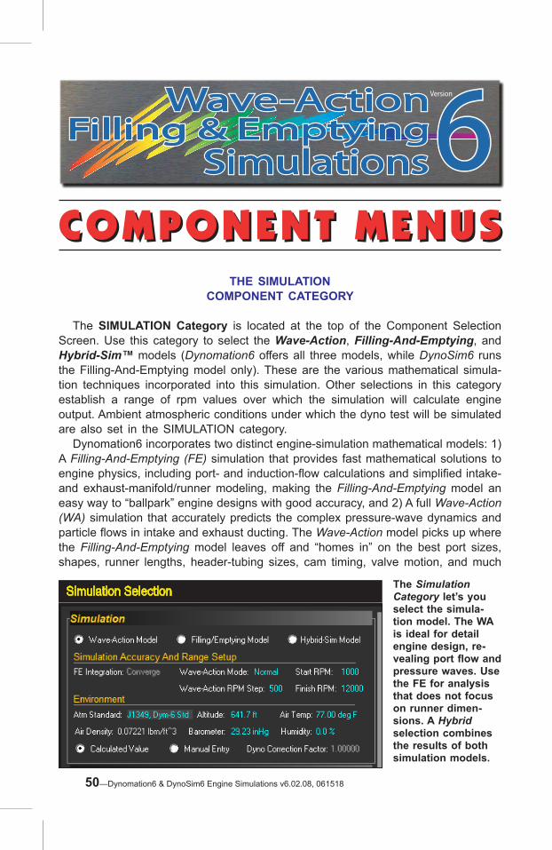
COMPONENT MENUSCOMPONENT MENUSTHE SIMULATION
COMPONENT CATEGORY
The SIMULATION Category is located at the top of the Component Selection Screen. Use this category to select the Wave-Action, Filling-And-Emptying, and Hybrid-Sim™ models (Dynomation6 offers all three models, while DynoSim6 runs the Filling-And-Emptying model only). These are the various mathematical simula-tion techniques incorporated into this simulation. Other selections in this category establish a range of rpm values over which the simulation will calculate engine output. Ambient atmospheric conditions under which the dyno test will be simulated are also set in the SIMULATION category. Dynomation6 incorporates two distinct engine-simulation mathematical models: 1) A Filling-And-Emptying (FE) simulation that provides fast mathematical solutions to engine physics, including port- and induction-flow calculations and simplified intake- and exhaust-manifold/runner modeling, making the Filling-And-Emptying model an easy way to “ballpark” engine designs with good accuracy, and 2) A full Wave-Action (WA) simulation that accurately predicts the complex pressure-wave dynamics and particle flows in intake and exhaust ducting. The Wave-Action model picks up where the Filling-And-Emptying model leaves off and “homes in” on the best port sizes, shapes, runner lengths, header-tubing sizes, cam timing, valve motion, and much
Simulation Selection The Simulation Category let’s you select the simula-tion model. The WA is ideal for detail engine design, re-vealing port flow and pressure waves. Use the FE for analysis that does not focus on runner dimen-sions. A Hybrid selection combines the results of both simulation models.
VersionWave-ActionFilling & Emptying
Simulations
Wave-ActionFilling & Emptying
Simulations66
50—Dynomation6 & DynoSim6 Engine Simulations v6.02.08, 061518
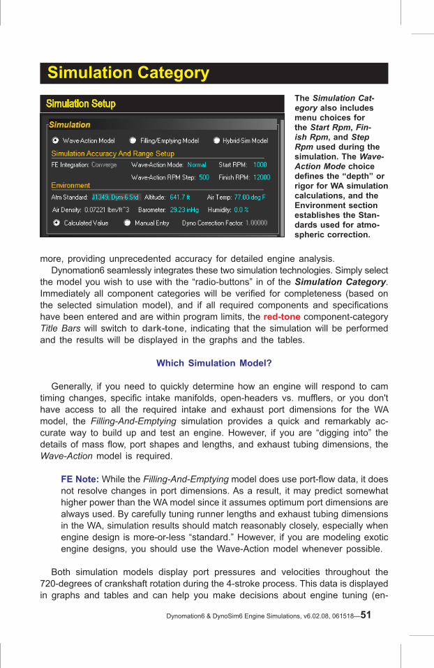
more, providing unprecedented accuracy for detailed engine analysis. Dynomation6 seamlessly integrates these two simulation technologies. Simply select the model you wish to use with the “radio-buttons” in of the Simulation Category. Immediately all component categories will be verified for completeness (based on the selected simulation model), and if all required components and specifications have been entered and are within program limits, the red-tone component-category Title Bars will switch to dark-tone, indicating that the simulation will be performed and the results will be displayed in the graphs and the tables.
Which Simulation Model?
Generally, if you need to quickly determine how an engine will respond to cam timing changes, specific intake manifolds, open-headers vs. mufflers, or you don't have access to all the required intake and exhaust port dimensions for the WA model, the Filling-And-Emptying simulation provides a quick and remarkably ac-curate way to build up and test an engine. However, if you are “digging into” the details of mass flow, port shapes and lengths, and exhaust tubing dimensions, the Wave-Action model is required.
FE Note: While the Filling-And-Emptying model does use port-flow data, it does not resolve changes in port dimensions. As a result, it may predict somewhat higher power than the WA model since it assumes optimum port dimensions are always used. By carefully tuning runner lengths and exhaust tubing dimensions in the WA, simulation results should match reasonably closely, especially when engine design is more-or-less “standard.” However, if you are modeling exotic engine designs, you should use the Wave-Action model whenever possible.
Both simulation models display port pressures and velocities throughout the 720-degrees of crankshaft rotation during the 4-stroke process. This data is displayed in graphs and tables and can help you make decisions about engine tuning (en-
Simulation CategorySimulation Setup The Simulation Cat-
egory also includes menu choices for the Start Rpm, Fin-ish Rpm, and Step Rpm used during the simulation. The Wave-Action Mode choice defines the “depth” or rigor for WA simulation calculations, and the Environment section establishes the Stan-dards used for atmo-spheric correction.
Dynomation6 & DynoSim6 Engine Simulations, v6.02.08, 061518—51

Pressure and Particle Velocity Displays The simulation displays port pressure and velocity curves for the entire 720-de-grees of crank rotation of the 4-stroke process (shown in the middle and lower graphs). This data can help you make critical decisions about valve-event timing and intake/exhaust tuning. The WA sim performs a much more rigorous analy-sis of engine flows, and its displayed pressure waves should be considered a more accurate representa-tion of engine pressure-wave dynamics.
gine tuning is discussed in-depth later in this manual). However, keep in mind that pressure/velocity data calculated by the Wave-Action simulation is derived through a much more rigorous mathematical approach and should be considered the most accurate representation of actual engine pressure-wave dynamics.
WA Note: In cases where you have sufficient test data for the Wave-Action model, but you would like to test a restrictive exhaust system, you can reduce the Minimum Exhaust Port Area (by about 30% for typical mufflers) to simulate backpressure in the exhaust system. For detailed information about wave-dynamics and pressure-wave tuning, refer to the Wave-Dynamics Analysis chapter later in this User Guide.
FE and WA Simulations:“Cycles” And Convergence
Both the WA and FE simulation models perform an analysis of the gas-exchange process within engine passages. These processes are dependent on valve position, piston position, engine speed, and much more. To ensure that these mathematical processes have reached a “steady-state” condition, several cycles may be neces-sary. These “cycles” should not be confused with engine cycles; rather they repre-sent the number of times the simulation model must work through a gas-dynamics analysis to reach the same results, or stability. In some ways, this phenomenon is similar to the instability often seen in real-world dyno tests just before the engine “smooths out” at the measurement rpm. Some of this instability is due to the same gas-dynamic effects calculated within the simulation. In previous versions of this software, you were required to select the number of
Simulation Category
52—Dynomation6 & DynoSim6 Engine Simulations v6.02.08, 061518

Simulation Categorycalculation “cycles.” Often this required entering a number that would ensure stability (also called convergence) but could allow the simulation to run more cycles than necessary, extending calculation times. In Dynomation6, the number of simulation cycles is determined automatically during the calculation process. In most cases, a steady-state condition will be reached in 4 to 6 cycles. However, in some drag-racing or very-high-rpm race engines, it may require as many as 10 or more cycles to stabilize gas dynamics. In the FE simulation (and in DynoSim6), you can chose to run the simulation in the single-pass mode (without convergence), which was the default in previous program versions. Alternatively, you can select Converge (the default mode), al-lowing the FE to run until it finds gas-dynamic stability. An Extended Converge mode is also available specifically for high-output racing engines. If you enable either Converge modes in the FE, the calculation times will usually double or triple. The FE Converge mode almost always improves accuracy (in the WA model, as mentioned in the previous paragraph) the simulation always runs to convergence. The number of calculation cycles for both simulations is displayed in the Simulation Log (open the Log using the Simulation Menu, located at the top of the program screen).
Wave-Action Only:Simulation “Meshing”
The Wave-Action simulation calculates gas-dynamics within engine passages by dividing the intake and exhaust passages into small, equal-size volumes, called meshes (this is not performed in the FE simulation). The smaller the mesh size, the greater number of mesh volumes into which the passage volumes will be divided. This can improve simulation accuracy, but at the expense of calculation times, since a larger number of mesh volumes require a more complex mathematical analysis.
Wave-Action “Mesh¨ Mode
The Wave-Action simulation calculates gas-dynamics by dividing the intake and exhaust passages into small volumes, called meshes. Smaller mesh sizes can improve simu-lation accuracy, but at the expense of calculation times. The Normal mesh is usually sufficient to accurately analyze gas dynamics and provide good simulation accuracy.
Dynomation6 & DynoSim6 Engine Simulations, v6.02.08, 061518—53

Simulation Category The Wave-Action simulation incorporates three mesh sizes selected from the Wave-Action Mode field: Normal, Fine and Optimized. In most cases, the Normal mesh size is sufficient to accurately analyze gas dynamics within intake and exhaust passages. But, in some cases, a more rigorous analysis is required to overcome instabilities, shock waves in the exhaust runners, or odd pressure-wave interactions. For example, if you notice a pressure spike or oscillation in the intake or exhaust pressure curve close to TDC, it may be an anomaly that will “disappear” with the more rigorous analysis offered in the Fine and Optimized modes. However, lacking pressure-trace anomalies or other unusual displays, the Normal level of mesh will provide good simulation accuracy.
Note: The Fine mode takes about three times longer than Normal to complete the simulation. And the Optimized selection directs the sim to not only use the smallest mesh size possible, but also to use the most detailed calcula-tions for engine physics. For Optimized, processing time is not a factor, and it usually takes about 20 times longer to complete simulation calculations. In almost all cases, this option is not required to produce accurate results, and in fact, the differences between Fine and Optimized are often barely visible on the results graphs.
FE and WA Simulations: RPM Ranges And Atmospheric Standards
The Simulation Category also includes fields to specify the rpm range for the simulation (Start & Finish RPMs). The narrower the range, the faster the simulation is performed. If you are using a supercharging system, and it's developing errors at higher engine speeds (like overspeed or choke), you can reduce the upper rpm limit to help prevent these errors. In addition, if you are running an Iterative Test (see the Quick and Pro Iterator chapters later in this User Guide), keeping the RPM range as narrow as possible will substantially reduce testing time. Set ambient conditions (or Standards) for the simulation by selecting one of the built-in models in the Atmospheric Standard menu. You can apply SAE, ISO, and other world standards commonly used for dynamometer testing. The default used in Dynomation6 and DynoSim6 is different from Dynomation5/DynoSim5, and is based on the SAE J1394 v3 standard widely used in modern dyno test facilities. The available Standards are:
• Standard Atmosphere: Temp (F): 59.0 Humidity: 0% Barometer(in): 29.921 • AE J606/7: Temp (F): 60.0 Humidity: 0% Barometer(in): 29.921 • ISO 1585: Temp (F): 60.0 Humidity: 0% Barometer(in): 29.530 • JIS D 1001: Temp (F): 68.0 Humidity: 0% Barometer(in): 29.234 • Dynomation-5 Standard: Temp (F): 68.0 Humidity: 0% Barometer(in): 29.919 • SAE J1349 v3, Ver-6 Std: Temp (F): 77.0 Humidity: 0% Barometer(in): 29.234 • SAE J1394 v1: Temp (F): 77.0 Humidity: 0% Barometer(in): 29.318 • SAE J1394 v2: Temp (F): 77.0 Humidity: 0% Barometer(in): 29.380
54—Dynomation6 & DynoSim6 Engine Simulations v6.02.08, 061518

Simulation Category • SAE J1394 v3: Temp (F): 77.0 Humidity: 0% Barometer(in): 29.234 • SAE J1995: Temp (F): 77.0 Humidity: 0% Barometer(in): 29.530
In addition to the standards available in the menu, you may enter any Altitude, Air Temperature, Barometer, and Humidity value you wish. The changes in environmental variables are applied to the simulation through a “correction factor.” This value is normally calculated by Dynomation after you make a menu selection or enter specific atmospheric values. However, you can click Manual Entry and directly enter any correction factor you wish.
Dynomation6 & DynoSim6 Engine Simulations, v6.02.08, 061518—55

ShortBlock CategoryShort Block Component Menu
The Short Block component menu contains over 500 bore and stroke combinations of popular domestic and import engines that you can instantly use in any engine simula-tion. In addition, you can directly enter a custom description of any engine into the Short Block component field.
THE SHORTBLOCK COMPONENT CATEGORYApplies To Both the FE and WA Simulations
The ShortBlock menu is located in the Shortblock Component Category. By open-ing this menu, you are presented with a variety of domestic and import “predefined” shortblock configurations. If any one of these choices is selected, the appropriate bore, stroke, number of cylinders, rod ratio, and pin offset (see entering Rod Ra-tio, Rod Length And Pin Offset, next) will be loaded into the ShortBlock category. In addition to the predefined shortblocks in the menu, you can directly enter any shortblock name (description) into the ShortBlock field, then enter custom values for Stroke, Bore, Number Of Cylinders (also Rod Ratio and Piston Pin Offset) within the acceptable range limits of the program (as indicated at the range limit line at the bottom of the screen).
Note: The Short Block menu can be considered a “handy” list of common engine bores, strokes, rod-length and offset values. When you select a shortblock, you are not selecting any “hidden” characteristics, like material composition (alumi-
56—Dynomation6 & DynoSim6 Engine Simulations v6.02.08, 061518
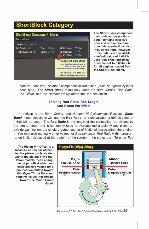
ShortBlock CategoryShortBlock Component Menu The Short Block component
menu (shown on previous page) contains over 500 bore and stroke combina-tions. Many selections also include rod-ratio, however if this data is not available, a default value of 1.636 is used. Pin offset specifica-tions are set to 0.000-inch for all engines loaded from the Short Block menu.
Rod Length & PinOffset:Note: Rod Ratio will default to
1.636 if actual value is notavailable in the Short Block menu.
Pin Offset is set to 0.000-inchfor all engines loaded from menu.
Ro
MinorThrust Face
MajorThrust Face
EnterPositive Values
EnterNegative Values
Piston-Pin Offset ValuesThe Piston-Pin Offset is a measure of how far off-cen-ter the piston pin is located within the piston. The simu-lation models these chang-
es in pin offset when you enter positive values for a
pin location shifted toward the Major Thrust Face and
negative values (for offsets toward the Minor Thrust
Face).
num vs. cast iron) or other component assumptions (such as typical cylinder head type). The Short Block menu only loads the Bore, Stroke, Rod Ratio, Pin Offset, and the Number Of Cylinders into the simulation.
Entering Rod Ratio, Rod LengthAnd Piston-Pin Offset
In addition to the Bore, Stroke, and Number Of Cylinder specifications, Short Block menu selections will load the Rod Ratio (or if unavailable, a default value of 1.636 will be used). The Rod Ratio is the length of the connecting rod divided by the stroke length and is commonly used to evaluate rod angularity and piston-to-cylinderwall friction, the single greatest source of frictional losses within the engine. You may also manually enter values for Rod Length or Rod Ratio within program range limits (displayed at the bottom of the screen in the status bar). To enter Rod
Dynomation6 & DynoSim6 Engine Simulations, v6.02.08, 061518—57

ShortBlock CategoryRatio, select the “radio” button next to the Rod Ratio field, then enter the desired value. the simulation will display the calculated value for Rod Length. Or, by se-lecting the Rod Length radio button, you can directly enter a length value; Rod Ratio will then be calculated and displayed in the Rod Ratio field. The SHORTBLOCK category also includes a field for Piston-Pin Offset. This is a measure of how far off-center (from the rod-to-crank centerline) the piston pin is located within the piston. Enter positive values to indicate a shift toward the Major Thrust Face and negative values to shift the pin toward the Minor Thrust Face.
Note: Piston-Pin Offset is set to 0.000-inch for all engines loaded from Short-Block menu.
58—Dynomation6 & DynoSim6 Engine Simulations v6.02.08, 061518

ShortBlock Category
Dynomation6 & DynoSim6 Engine Simulations, v6.02.08, 061518—59

Cylinder-Head Type Menu
The Cylinder Head Type (Description) menu contains a wide range of head/port choices. The main menu is divided into two groups: Domestic Cylinder Heads model typical 4-cylinder through V8 passenger car engines. The Sport-Compact Cylinder Heads selec-tions primarily model newer, multiple-valve-per-port head designs.
Cylinder-Head Category
THE CYLINDER-HEAD COMPONENT CATEGORYApplies To Both the FE and WA Simulations
The Cylinder-Head Type pull-down menu is located in the CYLINDER HEAD category. Selections from this menu allow the simulation to model various intake and exhaust port airflow characteristics for both Domestic and Sport-Compact ap-plications. Built-in selections range from restrictive low-performance ports to high-performance four-valve cylinder heads. Each grouping of head/port designs includes several stages of modifications. In addition to the provided choices, the Custom Port Flow selection at the bottom of the Cylinder Head Type menu lets you directly enter flowbench data, allowing the simulation to model any cylinder head for which airflow test data is available (for convenience, a Port Flow button in the Cylinder Head category provides fast access to the same custom-airflow, data-entry dialog). Custom port flow data entry will be detailed after the following brief descriptions of the “generic” menu choices.
Valve Diameters And Basic Flow Theory
A selection from the Cylinder Head menu is the first part of the process that
60—Dynomation6 & DynoSim6 Engine Simulations v6.02.08, 061518

Cylinder-Head CategorySelecting Valve Sizes
Selecting a specific valve size fixes the theoretical peak flow of each port. Cyl-inder heads flow from about 50% to as
high as 90% of this value. This percent-age, called the discharge coefficient, has
proven to be an effective link between flow-bench data and the calculation of mass flow moving into and out of the
cylinders. In other words, the valve size and the derived discharge coefficient
help establish a practical framework to accurately simulate mass flow within a
running engine.
establishes a baseline for the simulation of cylinder-head airflow. A Cylinder-Head Description selection (or entering Custom Port Flow values) dictates the airflow restriction generated by the valves and ports. That is, flow data determines how much airflow, below the theoretical maximum peak flow for a straight pipe of the same area, will pass through the valve orifice at all valve lift heights. The percent-age of ideal flow is called the Coefficient of Discharge (CD) and is always less than 100% (less than 1.0). The CD values are calculated and displayed in the Port-Flow Dialog as you enter flow-bench data (described later).
Dynomation6 Only: The Port-Flow Dialog also contains a dropdown menu that lets you select alternate methods of calculating CDs and valve flow areas. We recommend that you use the default Dynomation Method for most engine analysis, as this algorithm has demonstrated proven accuracy for more than 20 years of engine simulations (for more information on this feature and when to consider using alternate methods refer to Selecting Alternate Methods To Calculate CDs at the end of this chapter).
Dynomation6 Only: In Wave-Action simulations, the Intake MinPortArea (located in the Induction Category) establishes the restriction in the ports and the dimensional characteristics of the intake runners needed for pressure-wave analysis (in Filling-And-Emptying simulations, the optimum minimum area is determined automatically during the simulation process). These restriction values help determine mass flow into and out of the cylinders.
The additional data point needed to characterize overall engine airflow is the
Dynomation6 & DynoSim6 Engine Simulations, v6.02.08, 061518—61

Cylinder-Head CategoryTypical Low-Performance Cylinder Heads
The Low Performance cylinder head choices are intended to model cylinder heads that have restrictive ports, valves, and combus-tion chambers. Heads of this type were often designed for low-speed, economy applications, with little concern for high-speed perfor-mance.
Total Induction Airflow Rate (also located in the Induction Category). This can be considered the rated flow of the carburetor or throttle plates/valves measured at a specific pressure drop. This establishes an overall flow-rate restriction for entire engine. When this essential data has been entered, the program is a step closer to deter-mining mass flow within the ports. Unfortunately, the flow in the ports of a running engine is vastly different than the steady-state flow measured on a flow bench. A running engine will generate rapidly and widely varying pressures that directly affect—in fact, they directly cause—the flow of air and exhaust gasses within the engine. To determine the instantaneous flow in all ports at any point during engine operation, the simulation must calculate all internal port and cylinder pressures at closely-spaced, small increments of time throughout the four-cycle process. Overall mass flow into and out of the cylinders is found from the sum of these instantaneous pressures, calculated gas densities, and flow restrictions throughout the runners. After a series of integration operations using this data, engine output and related “dyno” results can be determined. (Not magic, but close!)
Domestic Cylinder-Head Selections
Here is some basic information that will help you determine the appropriate cylinder-head selections (and port flow data) from the built-in menu selections for domestic engine applications. Note: Each of the generic choices in the Cylinder Head menu has flowbench
data associated with it. To view this test data simply select the cylinder head from the menu then click the Port Flow button.
Wedge-Chamber, 2-Valve Cylinder Heads
Domestic—2-Valve, Low Performance Cylinder Heads (Three variations: Stock, Ported, and Ported With Large Valves)
There are three Low Performance cylinder head selections listed at the top
62—Dynomation6 & DynoSim6 Engine Simulations v6.02.08, 061518

Cylinder-Head Category2-Valve, HP Wedge Cylinder Heads
The 2-Valve, HP Wedge Cylinder Head selec-tions model cylinder heads that have ports and valves sized with performance in mind, like this Edelbrock smallblock Chevy head.
of the Domestic Cylinder Head menu. Each of these choices is intended to model cylinder heads that have small ports and valves relative to engine displacement. Heads of this type were often designed for low-speed, economy applications, with little concern for high-speed performance. Early 260 and 289 smallblock Ford and to a lessor degree early smallblock Chevy castings fall into this category. These choices have the lowest discharge coefficient of all the head configurations listed in this menu. Minimum port cross-sectional areas are approximately 60% of the valve areas, and if Auto Calculate Valve Size has been selected, relatively small (compared to the bore diameter) intake and exhaust valve diameters will be selected.Note: These low-performance cylinder-head choices are a good option if you wish to model flathead (L-head & H-head) and hybrid (F-head) engines for which you do not have actual flow data. While the port flow in these engines is quite restrictive, by selecting Low-Performance and manually entering the actual valve sizes, the simulation will provide a good approximation of power output from these early engine designs.
Domestic—2-Valve, Wedge Cylinder Heads (Three Variations: Stock, Ported, Large Valves)
The first three wedge cylinder-head selections model castings that have ports and valves sized with performance in mind. Ports are only somewhat restric-tive for high-speed operation, and overall port and valve-pocket design offers a good compromise between low restriction and excessive flow velocity at higher engine speeds. The stock and pocket-ported choices are applicable to high-performance street to modest racing applications.
Domestic—2-Valve, Wedge/Fully Ported, Large ValvesThe fourth wedge head moves away from street applications. This casting has improved discharge coefficients, greater port cross-sectional areas, and increased valve sizes. Consider this head to be an modified, high-performance, factory-
Dynomation6 & DynoSim6 Engine Simulations, v6.02.08, 061518—63
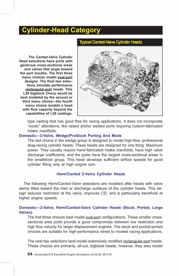
Cylinder-Head CategoryTypical Canted-Valve Cylinder Heads
The Canted-Valve Cylinder Head selections have ports with generous cross-sectional areas
and valves that angle toward the port mouths. The first three menu choices model oval-port
designs. The final two selec-tions simulate performance
rectangular-port heads. This L29 bigblock Chevy would be
best modeled by the second or third menu choice—the fourth
menu choice models a head with flow capacity beyond the
capabilities of L29 castings.
type casting that has good flow for racing applications. It does not incorporate “exotic” alterations, like raised and/or welded ports requiring custom-fabricated intake manifolds.
Domestic—2-Valve, Wedge/ProStock Porting And ModsThe last choice in the wedge group is designed to model high-flow, professional drag-racing cylinder heads. These heads are designed for one thing: Maximum power. They usually require hand-fabricated intake manifolds, have high valve discharge coefficients, and the ports have the largest cross-sectional areas in the smallblock group. This head develops sufficient airflow speeds for good cylinder filling only at high engine rpm.
Hemi/Canted 2-Valve Cylinder Heads
The following Hemi/Canted-Valve selections are modeled after heads with valve stems tilted toward the inlet or discharge surfaces of the cylinder heads. This de-sign reduces restriction at the valve, improves CD, and is particularly beneficial at higher engine speeds.
Domestic—2-Valve, Hemi/Canted-Valve Cylinder Heads (Stock, Ported, Large Valves)
The first three choices best model oval-port configurations. These smaller cross-sectional area ports provide a good compromise between low restriction and high flow velocity for larger displacement engines. The stock and pocket-ported choices are suitable for high-performance street to modest racing applications.
The next two selections best model extensively modified rectangular-port heads. These choices are primarily, all-out, bigblock heads, however, they also model
64—Dynomation6 & DynoSim6 Engine Simulations v6.02.08, 061518
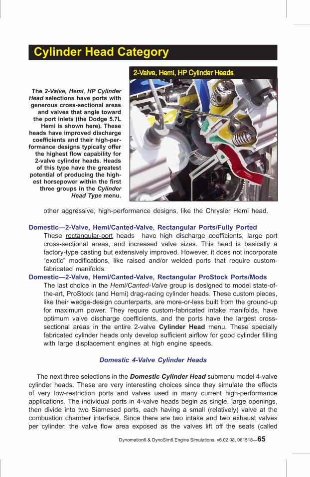
Cylinder Head Category2-Valve, Hemi, HP Cylinder Heads
The 2-Valve, Hemi, HP Cylinder Head selections have ports with generous cross-sectional areas
and valves that angle toward the port inlets (the Dodge 5.7L
Hemi is shown here). These heads have improved discharge
coefficients and their high-per-formance designs typically offer
the highest flow capability for 2-valve cylinder heads. Heads of this type have the greatest
potential of producing the high-est horsepower within the first
three groups in the Cylinder Head Type menu.
other aggressive, high-performance designs, like the Chrysler Hemi head.
Domestic—2-Valve, Hemi/Canted-Valve, Rectangular Ports/Fully PortedThese rectangular-port heads have high discharge coefficients, large port cross-sectional areas, and increased valve sizes. This head is basically a factory-type casting but extensively improved. However, it does not incorporate “exotic” modifications, like raised and/or welded ports that require custom-fabricated manifolds.
Domestic—2-Valve, Hemi/Canted-Valve, Rectangular ProStock Ports/ModsThe last choice in the Hemi/Canted-Valve group is designed to model state-of-the-art, ProStock (and Hemi) drag-racing cylinder heads. These custom pieces, like their wedge-design counterparts, are more-or-less built from the ground-up for maximum power. They require custom-fabricated intake manifolds, have optimum valve discharge coefficients, and the ports have the largest cross-sectional areas in the entire 2-valve Cylinder Head menu. These specially fabricated cylinder heads only develop sufficient airflow for good cylinder filling with large displacement engines at high engine speeds.
Domestic 4-Valve Cylinder Heads
The next three selections in the Domestic Cylinder Head submenu model 4-valve cylinder heads. These are very interesting choices since they simulate the effects of very low-restriction ports and valves used in many current high-performance applications. The individual ports in 4-valve heads begin as single, large openings, then divide into two Siamesed ports, each having a small (relatively) valve at the combustion chamber interface. Since there are two intake and two exhaust valves per cylinder, the valve flow area exposed as the valves lift off the seats (called
Dynomation6 & DynoSim6 Engine Simulations, v6.02.08, 061518—65

Cylinder Head CategoryTwo-Valves-Per-Port Cylinder Head
The 4-Valve Cylinder Head selections model cylinder heads with two intake and two exhaust valves per cylinder. These heads can offer more than 1.5 times the curtain area of the largest 2-valve heads. This large valve flow area, combined with high-flow, low-restriction ports greatly improves air and fuel flow at higher engine speeds.
curtain area) is considerably greater than in the largest single-valve-per-port designs. In fact, 4-valve heads can offer more than 1.5 times the curtain area of the largest 2-valve heads. This large flow area, combined with high-flow, low-restriction ports, improves air and fuel flow at low valve lifts and at high engine speeds. Unfortunately, the ports offer an equally low restriction to reverse flow (reversion of charge from the cylinder back into the intake port) that commonly occurs at low engine speeds when the piston moves up the cylinder from BDC to Intake Valve Closing (IVC) on the early portion of the compression stroke. For this reason, 4-valve heads, even when fitted with more conservative ports and valves, can be a poor choice for small-displacement, low-speed engines, unless camshaft timing is carefully de-signed to complement the low-lift flow capabilities of these cylinder heads (using, for example, variable-valve timing...V-V-T). On the other hand, the outstanding flow characteristics of 4-valve heads puts them in another “league” when it comes to horsepower potential at high engine speeds.
Domestic—4-Valve, Hemi/Canted-Valve, Stock Ports And ValvesThe first choice in the 4-valve group simulates a 4-valve cylinder head that would be “standard equipment” on factory high-performance engines. These heads offer power comparable to high-performance 2-valve castings equipped with large valves and porting work. However, because they still have relatively small ports, reasonably high port velocities, and good low-lift flow characteristics, they can show a boost in low-speed power over comparable 2-valve heads.
Domestic—4-Valve, Hemi/Canted-Valve, Ported With Large ValvesThe next choice incorporates mild performance modifications. Larger valves have been installed and both intake and exhaust flow has been increased
66—Dynomation6 & DynoSim6 Engine Simulations v6.02.08, 061518
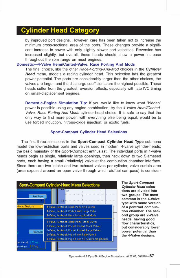
Cylinder Head Category
Sport-Compact Cylinder-Head Menu Selections The Sport-Compact Cylinder Head selec-tions are divided into two groups. The most common is the 4-Valve type with some version of a pentroof combus-tion chamber. The sec-ond group are 2-Valve heads, having good flow characteristics, but considerably lower power potential than the 4-Valve designs.
by improved port designs. However, care has been taken not to increase the minimum cross-sectional area of the ports. These changes provide a signifi-cant increase in power with only slightly slower port velocities. Reversion has increased slightly, but overall, these heads should show a power increase throughout the rpm range on most engines.
Domestic—4-Valve Hemi/Canted-Valve, Race Porting And ModsThe final choice, like the other Race-Porting-And-Mod choices in the Cylinder Head menu, models a racing cylinder head. This selection has the greatest power potential. The ports are considerably larger than the other choices, the valves are larger, and the discharge coefficients are the highest possible. These heads suffer from the greatest reversion effects, especially with late IVC timing on small-displacement engines.
Domestic-Engine Simulation Tip: If you would like to know what “hidden” power is possible using any engine combination, try the 4-Valve Hemi/Canted-Valve, Race Porting And Mods cylinder-head choice. It is safe to say that the only way to find more power, with everything else being equal, would be to use forced induction, nitrous-oxide injection, or exotic fuels.
Sport-Compact Cylinder Head Selections
The first three selections in the Sport-Compact Cylinder Head Type submenu model the low-restriction ports and valves used in modern, 4-valve cylinder-heads; the basic mainstay of the Sport-Compact enthusiast. The individual ports in 4-valve heads begin as single, relatively large openings, then neck down to two Siamesed ports, each having a small (relatively) valve at the combustion chamber interface. Since there are two intake and two exhaust valves per cylinder, valve curtain area (area exposed around an open valve through which air/fuel can pass) is consider-
Dynomation6 & DynoSim6 Engine Simulations, v6.02.08, 061518—67

Cylinder Head Category4-Valve, Pentroof, HP Cylinder Heads
The 4-Valve Cylinder Head selections model cylinder heads with two intake and two exhaust valves. These heads can offer more than 1.5 times the curtain area of the largest 2-valve heads. This large valve flow area, combined with high-flow, low-restriction ports greatly improves air and fuel flow into the cylinders at high engine speeds.
Honda VTEC, 4-Valve, Pentroof Engine4-Valve Cylinder Heads are commonly used on Import high-performance
street engines, like the Variable Valve Timing powerplants installed in many
Honda vehicles. These engines offer a level of performance and driveability
that is impossible with 2-valve cylinder heads.
ably larger than the largest single-valve-per-port designs. In fact, 4-valve heads can offer more than 1.5 times the curtain area of the largest 2-valve heads. This large flow area, combined with the high-flow, low-restriction ports greatly improves air and fuel flow into the cylinders at low valve lifts and high engine speeds. How-ever, the ports offer an equally low restriction to reverse flow (reversion) that can occur at low engine speeds when the piston moves up the cylinder from BDC to Intake Valve Closing (IVC). For this reason, 4-valve heads, even when fitted with more conservative ports and valves, can be a poor choice for small-displacement, low-speed engines, unless camshaft timing and valve lift is carefully designed to complement the flow capabilities of these cylinder heads.
Sport-Compact 4-Valve Cylinder Heads
Sport-Compact—4-Valve, Pentroof, Stock Ports And Valves Note: Each of the generic choices described below in the Cylinder Head menu
68—Dynomation6 & DynoSim6 Engine Simulations v6.02.08, 061518

Cylinder Head Categoryhas flowbench data associated with it. To view this test data simply select the cylinder head from the menu, then click the Port Flow button.
The first choice in the 4-valve group simulates a 4-valve cylinder head that would be “standard equipment” on factory high-performance, sport-compact engines. Although excellent for street performance, since they have relatively small ports, reasonably high port velocities, and good low-lift flow characteristics, with proper cam timing they often show a boost in low-speed power over comparable 2-valve heads (and at higher engine speeds, they will outperform all but the most highly modified 2-valve heads).
Sport-Compact—4-Valve, Pentroof, Ported With Large ValvesThe next choice incorporates mild performance modifications. Larger valves have been installed and both intake and exhaust flow has increased from improved port designs. However, care has been taken not to increase the minimum cross-sectional area of the ports. These changes provide a significant increase in power with only slightly slower port velocities. Reversion has increased, but overall, these heads will show a power increase throughout most of the rpm range on many engines.
Sport-Compact—4-Valve, Pentroof, Race Porting And ModsThe final choice, like other Racing options in the Cylinder Head menu, models a very efficient, high-flowing cylinder head. This selection has the greatest power potential of all sport-compact menu choices. The ports are considerably larger, the valves are larger, and the discharge coefficients are the highest possible. These heads suffer from the greatest reversion effects at lower engine speeds, especially with late IVC timing on small-displacement engines.
Sport-Compact Simulation Tip: If you would like to know what “hidden” power is possible using any particular engine combination, try this cylinder head choice. It is safe to say that the only way to find more power, with everything else being equal, would be to add forced induction, nitrous-oxide injection, or use exotic fuels.
Sport-Compact-Design, 2-Valve Cylinder Heads
The next five choices in the Sport-Compact/Import Cylinder Head menu model pentroof-chamber, “canted-valve” heads with one valve per port, each tilted or canted toward the port inlet/discharge surface. This positioning improves discharge coefficients and overall airflow. All ports in this menu group have cross-sectional areas sized for performance.
Sport Compact/Import—2-Valve, Pentroof, HP Cylinder Heads (Stock, Ported, Large Valves)
The first three choices can be considered suitable for street/performance appli-
Dynomation6 & DynoSim6 Engine Simulations, v6.02.08, 061518—69

Cylinder Head Category
Port-Flow Dialog Data Import
You can enter flowbench data from a variety of sources. Open the Port-Flow Dialog by clicking the Port Flow button in the Cylinder Head component category. Basic flow-test data can be directly entered using any valve size at any pressure drop.
cations. These selections model smaller cross-sectional area ports (sometimes oval or round) that provide a good compromise between low restriction and high flow velocity for production engines.
Sport-Compact/Import—2-Valve, Pentroof, High-Flow, Fully PortedThe final two Pentroof, 2-valve selections simulate extensively modified, high-performance cylinder heads. These castings have high discharge coefficients, large port cross-sectional areas, and increased valve sizes. These heads are basically factory-type castings but incorporate improved porting and valve work. However, they do not use “exotic” modifications, like raised and/or welded ports that require custom-fabricated manifolds.
Sport-Compact/Import—2-Valve, Pentroof, High-Flow, All-Out Porting/ModsThe last choice in this group is designed to model state-of-the-art, 2-valve, drag-racing cylinder heads. These custom pieces are extensively modified for maximum power. They require hand-fabricated or custom intake manifolds, have optimum valve discharge coefficients, and the ports have the largest cross-sectional areas of the 2-valve head designs. These cylinder heads only develop sufficient airflow for good cylinder filling at high engine speeds.
Custom Port Flow And The Port-Flow Dialog
The simulation will accept flowbench data from a variety of sources. Basic flow-test data can be directly entered into the Port Flow dialog using any valve size, at any
70—Dynomation6 & DynoSim6 Engine Simulations v6.02.08, 061518

Cylinder Head CategoryPort-Flow Dialog Data Import
Basic flow data can be entered manually or you can load flowbench data
from external sources: Load Dynomation Airflow files
(.DFW, version 5 and 6), or use the Import buttons to load
Flow Pro files produced on a flowbench equipped with
Audie Technology software.
Extend Valve LiftValues In RemainingData Entry BoxesBy Constant Value
Import IndividualFlowPro Files FromFlowbenches UsingAudie Software
Open .DFW, .FLW, and.SFW Flow Files. SaveDynomation .DFWFlow Files
The simulation will accept flow data from cylinder heads us-ing 1, 2, or 3 valves-per-port. Multiple valves-per-port cylinder heads are flow tested by open-ing all valves in each port to the same lift while recording the flow rate. The number of valves is used to calculate the overall flow area and the Coefficient of Discharge. Since the flow data is always linked to the number of valves, this value can only be selected/changed from within the Port Flow dialog.
Select Number Of Valves Per Port
pressure drop. In addition, you can load version 5 and 6 airflow files (.DFW files). You can also Import FlowPro files containing individual-port-flow data obtained from flow-bench testing using Audie Technology FlowPro software. Open the Port Flow dialog by clicking the Port Flow button in the Cylinder Head component category or clicking the Port AirFlow icon in the Toolbar.
To manually enter custom flowbench data, first select a suitable name for the flow data and enter it in the Description field. This description will also be displayed in the Cylinder Head category Description field. Next, select the number of data points in your flowbench test data using the Data Points field (a minimum of 4 points are required; click the up icon to increase, down to decrease). Also, enter the Test Valve Diameters (valve sizes used on the flow bench), and the Pressure Drop (in inches, or mm, of H20) used during testing. Enter the number of Valves Per Port for individual intake and exhaust ports. Finally, enter Flow and Valve-Lift
Dynomation6 & DynoSim6 Engine Simulations, v6.02.08, 061518—71
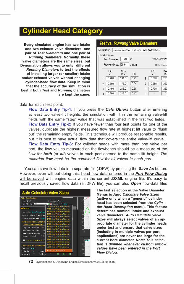
Cylinder Head CategoryTest vs. Running Valve DiametersEvery simulated engine has two intake
and two exhaust valve diameters: one pair of Test Diameters and one pair of
Running Diameters. Normally, these valve diameters are the same sizes, but
Dynomation allows you to enter different Running Diameters to test the effects of installing larger (or smaller) intake
and/or exhaust valves without changing cylinder-head flow data. Keep in mind that the accuracy of the simulation is
best if both Test and Running diameters are kept the same.
Auto Calculate Valve Sizes The last selection in the Valve Diameter Menus is Auto Calculate Valve Sizes (active only when a “generic” cylinder head has been selected from the Cylin-der Head Description menu). This feature determines nominal intake and exhaust valve diameters. Auto Calculate Valve Sizes will always select valves of an ap-propriate diameter for the cylinder heads under test and ensure that valve sizes (including in multiple valves-per-port applications) are never too large for the current bore diameter. Note: This selec-tion is dimmed whenever custom airflow values have been entered in the Port Flow Dialog.
data for each test point.Flow Data Entry Tip-1: If you press the Calc Others button after entering at least two valve-lift heights, the simulation will fill in the remaining valve-lift fields with the same “step” value that was established in the first two fields.Flow Data Entry Tip-2: If you have fewer than four test points for one of the valves, duplicate the highest measured flow rate at highest lift value to “flush out” the remaining empty fields. This technique will produce reasonable results, but it is best to have actual flow data that covers the entire valve-lift curve.Flow Data Entry Tip-3: For cylinder heads with more than one valve per port, the flow values measured on the flowbench should be a measure of the flow for both (or all) valves in each port opened to the same lift height. The recorded flow must be the combined flow for all valves in each port.
You can save flow data in a separate file (.DFW) by pressing the Save As button. However, even without doing this, head flow data entered in the Port Flow Dialog will be saved with engine data within the current .DXML engine file. It’s easy to recall previously saved flow data (a .DFW file), you can also Open flow-data files
72—Dynomation6 & DynoSim6 Engine Simulations v6.02.08, 061518

Cylinder Head Category
Entering Running Valve SizesSelecting a specific valve size will disable the Auto Calculate Valve Size feature. Select from the provided siz-
es (displayed in both Metric and US measurements), or you can directly
enter any valve dimension within the range limits of the simulation (range
limits are shown in the Status and Range Limit Line, at the bottom of
the main program screen).
created in other Motion Software engine simulations, including DynoSim4 and 5 (load .FLW files). Pressing the OK button in the Port Flow dialog will transfer flow-test data into the engine simulation and display the flow-test data Description in the CYLINDER HEAD category.
TEST Valve Diameters
The intake and exhaust Test Diameters are entered in the Port-Flow Dialog. These are the diameters of the valves used in the cylinder head during flow-bench testing. Normally, these are the same diameters as the valves used in the simulated engine (the Running Diameters), but Dynomation allows you to enter a different Running Diameter to test the effects of installing larger (or even smaller) intake or exhaust valves without retesting the cylinder heads (flow data is “scaled” up or down with the valve diameters). The accuracy of the simulation is best if both Test and Running diameters are the same, but small differences between these diameters (no more than 5% of the Test valve size) will be modeled accurately by the simulation. The results will be as if the larger/smaller valves were installed in the cylinder heads, the heads were retested, and the new flow data was used in Dynomation.
Engine RUNNING Valve Diameters
The Running Valve Diameter menus are located in the Cylinder Head category. This selection is the diameter of the valves that you wish to use in the simulated engine. As stated previously, the accuracy of the simulation is best if Test Diameters (entered in the Port-Flow dialog and used during flow-bench testing) are the same
Dynomation6 & DynoSim6 Engine Simulations, v6.02.08, 061518—73

Cylinder Head Categoryas the Running diameters. However, small differences between these diameters (no more than 5% of the Test valve diameter) can be modeled accurately by the simulation. If you use this feature, make sure the CD values (can be displayed on any crank-angle graph) have not exceeded 0.95.
The last selection in each menu is Auto Calculate Valve Sizes. This feature is functional only when a “generic” cylinder head was selected from the Cylinder Head Description menu. Auto Calculate instructs the simulation to determine the nominal intake and exhaust valve diameters for use with the current engine based on an assessment of the bore diameter and cylinder-head selection. When the Auto Calculate function is activated, Auto will be displayed next to the calculated sizes, and it will remain active on the current engine until turned off (by choosing Auto Calculate a second time or by selecting a new diameter for either the intake or exhaust valve). Auto Calculate will always select valves of an appropriate diameter for the engine under test (including multiple valves-per-port applications) and ensure that valve sizes are never too large for the current bore diameter.
Note-1: Auto Calculation of valve size will only function with the generic cylinderhead choices provided in the Cylinder Head Type menu. If any modification is made to these heads, or other Port Flow files are loaded, The simulation assumes that the sizes of the valves are known by the user and Auto Calculation is turned off.Note-2: Auto Calculation is turned OFF by default when the simulation is started and whenever Clear Components is chosen from the Edit menu.Note-3: While Auto Calculate Valve Sizes can be helpful during quick back-to-back testing, it probably will not “guess” the precise valve sizes typically used by the engine/cylinder-head manufacturer.
Wave-Action Only:Selecting Alternate Valve-Flow Area
Calculation Methods
The Port-Flow Dialog allows you to select alternate methods of calculating port flow areas and, subsequently, valve CDs. To understand how these different algorithms function and when to use them in Dynomation6, a bit of background is helpful. As we have discussed in this chapter, the method used to determine the restric-tion in the ports and the mass flow rates within an engine simulation are derived from cylinder-head flowbench test data. Many engine developers have concerns that this steady-state flow may not accurately represent the flow that occurs within the running engine, particularly in high-output, high-speed engines. The cyclical, highly pulsed flow that occurs in the ports as charge moves toward and away from the valves may produce flow regimes across the valve openings that cannot be accurately modeled using steady-state flow measurements. In addition, the changing shape and geometry of the openings created when the
74—Dynomation6 & DynoSim6 Engine Simulations v6.02.08, 061518

Cylinder Head Category
valves move off their seats may have also affect overall mass flow. And because most engines respond dramatically to changes in low-lift flow, alternate methods of calculating the “exposed areas” of partially-open valves have been developed. The flow areas, also known as the Curtain Areas, are the entire open area through which mass can move through each valve at every point in the lift curve. However, analysis has shown that changing flow geometries as the valve moves through low-lift into higher lift regimes can alter the effective Curtain Areas. Since the Curtain Area is compared to the calculated flow within in a straight pipe of equal area (to determine the CD or Coefficient of Discharge), using precise Curtain Area values is fundamental in determining accurate flow rates within an engine simulation. To address these modeling complexities, we have added two additional math-ematical algorithms in Dynomation6 that determine Curtain Areas and CD values using alternate methodologies. An explanation of each of these methods follows. Finally, this section concludes with additional tips and suggestions that can help you model unique powerplants that don't seem to fit the “mold."
Standard Dynomation Method (Default): This is the default method used in Dynomation 4, 5, and 6. It has been successful in modeling with excellent ac-curacy over a wide range of engines since it’s introduction in 1995. We strongly suggest that you, at least, begin any engine design using this method of flow
Alternate CD Calculation Methods
To simulate engines with unique cylinder heads or that have other unique modeling complexities, we have added two new methods of determining Curtain Areas and CD Values. These alternate algorithms may be more appropriate for very high-speed or large displacement racing engines, particularly where pulsed flow may affect engine output. See text for more details.
Dynomation6 & DynoSim6 Engine Simulations, v6.02.08, 061518—75

area determination. It does not emphasize low-lift flow through the valves, rather it maintains a consistent analysis of valve flow during low- and high-lift regimes (although Dynomation6 includes additional analysis of mass flow within the Wave-Action simulation and can apply a “compression” coefficient to CD values during low-lift flow to improve accuracy).
2-Step Gordon Blair Method: This algorithm was developed by the well-known engine expert Dr. Gordon P. Blair in the mid to late 1990’s. It is based on two separate methods to determine flow areas depending on valve lift (the switch between methods is based primarily on valve dimensions). The overall effect is to decrease calculated flow areas (more on this later) and increase CD values within low-lift values and, to a lessor extent, increase flow throughout the entire lift range. You’ll likely see an increase in power at mid to high rpm, with some loss in torque at lower speeds on high-output engines.
3-Step Trenity Simpson Method: This algorithm was developed within a PhD thesis by Dr. Trenity Simpson at Iowa State University. It is based on a three-step method to isolate and individually analyze three flow regimes that occur during low- to mid-lift regions of valve lift. The overall effect is very similar to Blair’s method, but with slightly more boost in CD values. This method often produces an increase in high-speed power and slight losses in torque at low engine speeds, although with lessor effect in low-performance engines.
When to ApplyAlternate Methods
Since it is virtually impossible to know if alternate CD calculations are helping or hurting the accuracy of the simulation, in most cases these algorithms are best used to help match Dynomation output to actual dyno results. If the engine you are simulating seems to have insufficient top end power, and you have tried modifying other options, like induction airflow, port areas, induction temperatures, etc., the application of one of the alternate CD calculation methods may help you develop a better simulation model. But there are other options that you might want to consider before you switch to an alternate CD model. For example, by increasing or decreasing the flowbench pressure-drop values entered in the simulation, you can make subtle or dramatic adjustments to the slope of the power curve. You might be thinking that is this somehow “cheating.” In reality, with the uniqueness of each engine design and the way pressure waves and mass flow moves in the engine, if you are able to adjust how static flowbench data is used to better match true dyno output, you are simply extending the concept of refining the simulation model. The more accurately the simulation is able to model your engine, the more useful it will be in predicting the outcome of other engine changes, such as valve timing, exhaust tuning, etc.
Cylinder Head Category
76—Dynomation6 & DynoSim6 Engine Simulations v6.02.08, 061518

One Final Note: The alternate valve curtain-area algorithms discussed in this section effectively INCREASE the CDs of the intake and exhaust valves over the default Dynomation method. This may seem counter intuitive, since Blair's and Trenity's methods calculate SMALLER effective valve areas at low- to mid-lift heights. How can smaller flow areas generate higher CDs and more calculated horsepower? The answer lies in the fact that, once again, the measured flow through the valve openings at each lift point is obtained from flowbench testing. And since the two new methods also use this same measured airflow rate (the flowbench values don't change) but through a smaller calculated orifice size, the CD must be higher. Or in other words, the flow through the calculated (smaller) curtain area (again, the same flowbench data) is now closer to the flow in a straight pipe of the smaller cross-sectional area, therefore CD values must in-crease. (Like many things in engine design, this only makes sense when you think about it a while.)
Cylinder Head Category
Dynomation6 & DynoSim6 Engine Simulations, v6.02.08, 061518—77
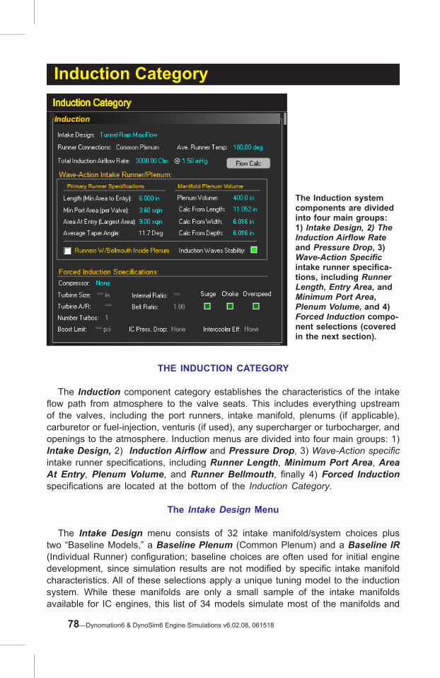
Induction CategoryInduction Category
The Induction system components are divided into four main groups: 1) Intake Design, 2) The Induction Airflow Rate and Pressure Drop, 3) Wave-Action Specific intake runner specifica-tions, including Runner Length, Entry Area, and Minimum Port Area, Plenum Volume, and 4) Forced Induction compo-nent selections (covered in the next section).
THE INDUCTION CATEGORY
The Induction component category establishes the characteristics of the intake flow path from atmosphere to the valve seats. This includes everything upstream of the valves, including the port runners, intake manifold, plenums (if applicable), carburetor or fuel-injection, venturis (if used), any supercharger or turbocharger, and openings to the atmosphere. Induction menus are divided into four main groups: 1) Intake Design, 2) Induction Airflow and Pressure Drop, 3) Wave-Action specific intake runner specifications, including Runner Length, Minimum Port Area, Area At Entry, Plenum Volume, and Runner Bellmouth, finally 4) Forced Induction specifications are located at the bottom of the Induction Category.
The Intake Design Menu
The Intake Design menu consists of 32 intake manifold/system choices plus two “Baseline Models,” a Baseline Plenum (Common Plenum) and a Baseline IR (Individual Runner) configuration; baseline choices are often used for initial engine development, since simulation results are not modified by specific intake manifold characteristics. All of these selections apply a unique tuning model to the induction system. While these manifolds are only a small sample of the intake manifolds available for IC engines, this list of 34 models simulate most of the manifolds and
78—Dynomation6 & DynoSim6 Engine Simulations v6.02.08, 061518

The “Baseline” Induc-tion choices remove
any specific manifold modeling characteristics from simulation results. Engine developers use
these choices (one for Common-Plenum
manifolds and one for IR induction) when
beginning initial engine development.
"Baseline" Induction Models
Induction Category
Domestic Manifold SelectionsThe Domestic Plenum Mani-fold menu consists of 13
intake manifold choices. Each of these selections applies
a unique tuning model to the induction system. While these manifolds are only a small sample of the intake
manifolds available for typical IC engines, these simulation models reproduce the char-
acteristics of many manifolds and induction systems used
today for both street and professional/amateur racing
applications.
induction systems for both street and racing applications. The manifold models are divided into four main groups: 1) "Baseline" Intake Models (2 choices), 2) Plenum—Domestic Intake Manifolds (14 choices), 3) Plenum—Sport-Compact Manifolds(14 choices), and 4) Individual-Runner In-ductions(5 choices). These categories are only general classifications. In some cases, certain “domestic” engines (utilizing modern tuned-runner induction) are best modeled with selections from the Sport-Compact submenu. Finally, if you are interested in a manifold that falls “in between” two menu selections, you can use the trend method to estimate power for a hybrid design. For example, run a test simulation using manifold Type A, then set up a Quick Comparison™ (right click on the rpm graph) and view the differences in power attributed to manifold Type B. The power differences will give you insight into how a hybrid manifold Type A/B should perform.
Dynomation6 & DynoSim6 Engine Simulations, v6.02.08, 061518—79

Induction Category
BaselineManifold Models
The Baseline Induction models provided in the Intake Design menu apply either no manifold algorithm or use the simplest model available for both the Filling-And-Emptying and Wave-Action simulations. These baseline models leave simulation results as “untouched” as possible by manifold influences, and this may improve the accuracy of “back-to-back” cam-timing and exhaust-system tuning efforts. In addition, consider using the Baseline Induction models if you are unsure of which specific manifold model to apply. The Baseline Common Plenum or Baseline Individual-Runner choices provide an excellent starting point on which to build further engine testing and development.
DomesticCommon-Plenum Manifolds
The following sections provide an overview of each Domestic Common-Plenum manifold models provided in the Intake Design menu. Here you’ll find a brief de-scription of the assumptions used in each model, and recommendations associated with that individual design.
Domestic—Dual-Plane, (Four versions: Maximum-Torque, Standard-Flow, High-Flow, and Max-Flow Manifolds)
The Dual-Plane, Max-Torque Manifold models dual-plane manifolds with smaller runners, such as those designed for heavy vehicles, economy and other high-torque, applications. The Dual-Plane Max-Torque model will tune for a lower peak engine speed, due mainly to runner and plenum restrictions. The Standard-Flow, Dual-Plane Manifold selection represents the majority of street-oriented dual-plane manifolds available to performance enthusiasts (including many OEM manifolds). The Standard-Flow model will accurately simulate street and performance engines with “as-cast” dual-plane manifolds. The Dual-Plane, High-Flow and Max-Flow Manifold selections model modi-fied, large-port, (and even custom-fabricated) dual-plane manifolds, as used on high-performance and all-out racing engines.
Dual-Plane Manifold Theory
Remarkably, the well-known and apparently straightforward design of the dual-plane manifold is, arguably, one of the more functionally-complex manifolds to model. An intake manifold is considered to have an effective dual-plane configura-tion when 1) the intake runners can be divided into two groups, so that 2) each group alternately receives induction pulses, and 3) the pulses are spaced at even intervals. If all of these criteria are met, the manifold is said to have a 2nd degree
80—Dynomation6 & DynoSim6 Engine Simulations v6.02.08, 061518

Dual-Plane Manifold
The Edelbrock Performer Q-Jet rep-resents a typical dual-plane manifold
design (of “Standard-Flow” capability). This manifold is said to have a 2nd de-
gree of freedom. A powerful resonance multiplies the force of the pressures waves, simulating the effects of long
runners, boosting low- and mid-range power.
Hybrid Dual-Plane Design Many dual-plane manifolds are hy-brids. This Edelbrock dual-plane manifold is designed for the 440 Chrysler engine and has a partially open plenum. In manifold such as this, the opening adds mid-range and high-speed performance with, typically, a slight sacrifice in low-speed torque. Not all hybrid designs are as success-ful as this one. In situations where you are not familiar with specific engine or manifold characteristics, it may be worthwhile to stick with “plane-vanilla” designs.
Induction Category
of freedom, allowing it to reach a unique resonance producing oscillations within the entire manifold. During this resonance, pressure readings taken throughout the manifold will be in “sync” with one another. Full-manifold resonance multiplies the force of the pressures waves, simulating the effects of long runners. Since longer runners tune at lower engine speeds, the dual-plane manifold is most known for its ability to boost lower-to-midrange rpm performance. The divided plenum is another common feature of dual-plane manifolds that boosts low-end power with carbureted engines. Since each side of the plenum is connected to only one-half of the cylinders (4-cylinders in a V8), each cylinder is “exposed” to only one-half of the carburetor. This maximizes wave strength and improves low-speed fuel metering (these effects are less pronounced with throttle-body fuel-injection systems). However, the restriction inherent in a divided plenum can reduce peak power at higher speeds. The main benefits of the dual-plane design are its low-speed torque-boosting capability, compact design, wide availability, and ease of use with both carburetors and injection systems. However, not all engines are capable of utilizing a dual-plane configuration. Typically, engines that do not have an even firing order or have too
Dynomation6 & DynoSim6 Engine Simulations, v6.02.08, 061518—81

Induction Category
Dual-Plane vs. Single-Plane Design
The basic differences between single- and dual-plane manifolds are clearly illustrated here. The dual-plane (left) divides the plenum in half, with the runners grouped by firing order. Each cylinder “sees” only one-half of the carburetor, transferring a strong signal to the venturis. This manifold design is said to have a 2nd degree of freedom, allowing it to reach a unique resonance that makes its short runners act as if they were longer and boosts low-speed power. The single-plane manifold (right) has short, nearly equal-length runners with a large open plenum, much like a tunnel ram laid flat across the top of the engine. The manifold has excellent high-speed performance, but its design prevents full-manifold resonance. That reduces low-speed torque, which can impair driveability and fuel economy.
many cylinders to generate a resonance effect will not benefit from a dual-plane manifold. While there are exceptions, engines having 2 or 4 cylinders work best with this manifold. Since most V8 engines are basically two 4-cylinder engines on a common crankshaft, even-firing V8s benefit from the resonance effects of the dual-plane manifold. The simulation does not prevent the selection of a dual-plane manifold on engines that will not develop a full resonance effect. For example, you can install a dual-plane manifold on a 5-cylinder engine, but the results—a low-end power boost—may not reproducible in the real world, since an effective dual-plane manifold cannot be built for this engine. The Filling-And-Emptying simulation is best utilized by modeling dual-plane manifolds combinations that already exist rather than testing theoretical fabrications. Many dual-plane manifolds are hybrids, incorporating facets of other manifold designs. Especially common is the use of an undivided or open plenum typically associated with single-plane manifolds. These “mixed” designs are attempts at harnessing the best features of both manifolds while eliminating the drawbacks of each. Sometimes the combinations are successful, adding more performance without much sacrifice in low-speed driveability. With these designs, you can successfully use the “trend” method described earlier to estimate engine torque and power. Un-fortunately, there is no shortage of manifolds that can reduce power without giving anything back in driveability or fuel economy. In fact, some of the worst designs
82—Dynomation6 & DynoSim6 Engine Simulations v6.02.08, 061518

Induction Category
Single-Plane ManifoldA single-plane manifold is simply a low-profile tunnel ram. The design combines short, nearly equal-length runners with an open ple-num, but “lays” the entire
configuration flat across the top of the engine.
The single-plane manifold combines improved flow
capacity, higher charge density, and short runners to build substantial horse-
power at higher engine speeds.
are remarkably bad. It is impossible to determine which of these combo designs is better than others using Dynomation6 (a future multi-junction version of Dynomation, that models every segment of all intake passages, including the complex effects of multi-cylinder interference, will be able to perform this analysis). Unless you can perform actual dyno testing on these manifolds to determine what works and what doesn’t, it may be worthwhile to stick with more “plain-vanilla” designs that produce predictable results.
Domestic—Single-Plane (Three Versions: Standard-Flow, High-Flow, and Max-Flow Manifolds)
The Single-Plane, Standard-Flow Manifold selection represents the majority of single-plane manifolds sold to performance enthusiasts. The Standard-Flow selection accurately simulates street and performance engines with “as-cast,” single-plane manifolds.The Single-Plane IMCA Track manifold is a high flow design with specific modifications to help boost torque in midrange engine speeds. This manifold was designed for IMCA dirt track racing but can be useful for any application needing near-max power with a improved midrange (available from Weiand, as model 7547).The Single-Plane High-Flow and Max-Flow manifolds simulate modified, large-port, air-gap, and/or custom-fabricated single-plane manifolds, as used on high-performance and racing engines.
Single-Plane Manifold Theory
In a very real sense, a single-plane manifold is simply a low-profile tunnel ram. The tunnel-ram manifold (discussed next) is a short-runner system combined with a large common plenum; a design that optimizes power on all-out racing engines
Dynomation6 & DynoSim6 Engine Simulations, v6.02.08, 061518—83
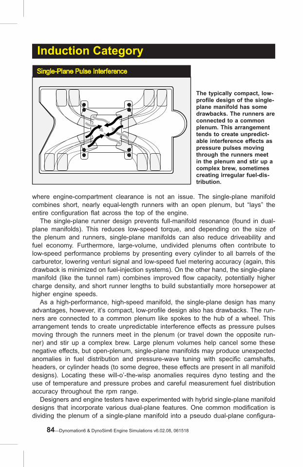
Induction CategorySingle-Plane Pulse Interference
The typically compact, low-profile design of the single-plane manifold has some drawbacks. The runners are connected to a common plenum. This arrangement tends to create unpredict-able interference effects as pressure pulses moving through the runners meet in the plenum and stir up a complex brew, sometimes creating irregular fuel-dis-tribution.
where engine-compartment clearance is not an issue. The single-plane manifold combines short, nearly equal-length runners with an open plenum, but “lays” the entire configuration flat across the top of the engine. The single-plane runner design prevents full-manifold resonance (found in dual-plane manifolds). This reduces low-speed torque, and depending on the size of the plenum and runners, single-plane manifolds can also reduce driveability and fuel economy. Furthermore, large-volume, undivided plenums often contribute to low-speed performance problems by presenting every cylinder to all barrels of the carburetor, lowering venturi signal and low-speed fuel metering accuracy (again, this drawback is minimized on fuel-injection systems). On the other hand, the single-plane manifold (like the tunnel ram) combines improved flow capacity, potentially higher charge density, and short runner lengths to build substantially more horsepower at higher engine speeds. As a high-performance, high-speed manifold, the single-plane design has many advantages, however, it’s compact, low-profile design also has drawbacks. The run-ners are connected to a common plenum like spokes to the hub of a wheel. This arrangement tends to create unpredictable interference effects as pressure pulses moving through the runners meet in the plenum (or travel down the opposite run-ner) and stir up a complex brew. Large plenum volumes help cancel some these negative effects, but open-plenum, single-plane manifolds may produce unexpected anomalies in fuel distribution and pressure-wave tuning with specific camshafts, headers, or cylinder heads (to some degree, these effects are present in all manifold designs). Locating these will-o’-the-wisp anomalies requires dyno testing and the use of temperature and pressure probes and careful measurement fuel distribution accuracy throughout the rpm range. Designers and engine testers have experimented with hybrid single-plane manifold designs that incorporate various dual-plane features. One common modification is dividing the plenum of a single-plane manifold into a pseudo dual-plane configura-
84—Dynomation6 & DynoSim6 Engine Simulations v6.02.08, 061518
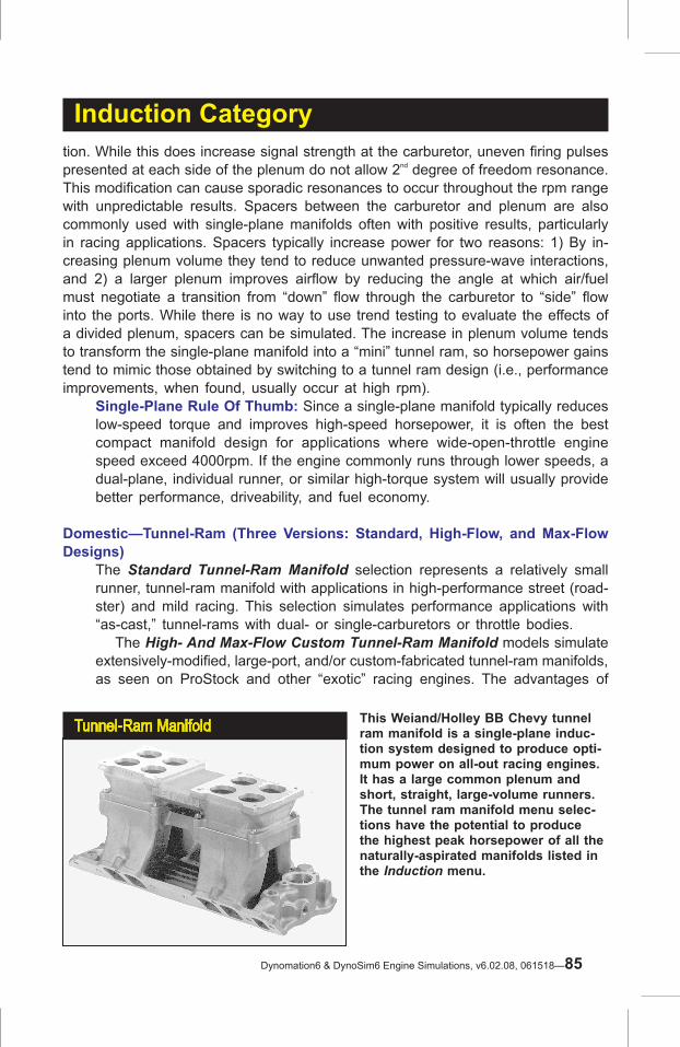
Tunnel-Ram Manifold This Weiand/Holley BB Chevy tunnel ram manifold is a single-plane induc-tion system designed to produce opti-mum power on all-out racing engines. It has a large common plenum and short, straight, large-volume runners. The tunnel ram manifold menu selec-tions have the potential to produce the highest peak horsepower of all the naturally-aspirated manifolds listed in the Induction menu.
Induction Categorytion. While this does increase signal strength at the carburetor, uneven firing pulses presented at each side of the plenum do not allow 2nd degree of freedom resonance. This modification can cause sporadic resonances to occur throughout the rpm range with unpredictable results. Spacers between the carburetor and plenum are also commonly used with single-plane manifolds often with positive results, particularly in racing applications. Spacers typically increase power for two reasons: 1) By in-creasing plenum volume they tend to reduce unwanted pressure-wave interactions, and 2) a larger plenum improves airflow by reducing the angle at which air/fuel must negotiate a transition from “down” flow through the carburetor to “side” flow into the ports. While there is no way to use trend testing to evaluate the effects of a divided plenum, spacers can be simulated. The increase in plenum volume tends to transform the single-plane manifold into a “mini” tunnel ram, so horsepower gains tend to mimic those obtained by switching to a tunnel ram design (i.e., performance improvements, when found, usually occur at high rpm).
Single-Plane Rule Of Thumb: Since a single-plane manifold typically reduces low-speed torque and improves high-speed horsepower, it is often the best compact manifold design for applications where wide-open-throttle engine speed exceed 4000rpm. If the engine commonly runs through lower speeds, a dual-plane, individual runner, or similar high-torque system will usually provide better performance, driveability, and fuel economy.
Domestic—Tunnel-Ram (Three Versions: Standard, High-Flow, and Max-Flow Designs)
The Standard Tunnel-Ram Manifold selection represents a relatively small runner, tunnel-ram manifold with applications in high-performance street (road-ster) and mild racing. This selection simulates performance applications with “as-cast,” tunnel-rams with dual- or single-carburetors or throttle bodies. The High- And Max-Flow Custom Tunnel-Ram Manifold models simulate extensively-modified, large-port, and/or custom-fabricated tunnel-ram manifolds, as seen on ProStock and other “exotic” racing engines. The advantages of
Dynomation6 & DynoSim6 Engine Simulations, v6.02.08, 061518—85

Induction CategoryCustom Fabricated Tunnel-Ram Manifold
This custom-fabricated tunnel-ram manifold (by
Jon Kaase Racing En-gines) has the potential to produce the highest peak
horsepower of all plenum-based, naturally-aspirated induction systems. Com-
bined with the proper cam timing, compression, and
other components, the large cross-sectional ar-
eas, straight runners, and short tuned lengths make
this custom manifold a “no compromise” high-
rpm racing design.
these tunnel rams derive from their combination of a large common plenum and short, straight, large-volume runners. The large plenum can accommodate one or two carburetors, potentially flowing up to 2200cfm or more. The large plenum also minimizes pressure-wave interaction and fuel distribution issues (especially with dual carburetors or fuel-injection throttle bodies). The short runners can be kept cooler than their lay-flat, single- and dual-plane counter-parts, and they offer a straight path into the ports, optimizing ram-tuning and minimizing flow restriction. Tunnel-ram applications are limited because of their large physical size; vehicles using tunnel-ram manifolds usually require a hole in the hood and/or a hood scoop to provide manifold and carburetor clearance. While a protruding induction system may be a “sexy” addition to a street rod, in single-carburetor configurations, the tunnel ram offers very little potential power over a well-designed, single-plane manifold. Only at very high engine speeds, with multiple carburetors, will the advantages in the tunnel ram contribute substantially to power. The Standard and Max-Flow Tunnel Ram manifold selections have the potential to produce the highest peak horsepower of all naturally-aspirated induction systems listed in the Manifold Type menu. The large cross-sectional areas, straight runners, and short tuned lengths make this manifold a “no compromise” racing design.
Domestic—LS1/LS6 Stock Composite and LS1/LS6 HP Runner/Mods ManifoldsSince the mid 1980’s, engine simulation programs have been regularly used by engine designers and manufacturers to optimize wave dynamics developed inside the intake passages of the IC engine. These pressure waves can have a marked effect on engine performance. When unharnessed, they can pro-
86—Dynomation6 & DynoSim6 Engine Simulations v6.02.08, 061518

LS1/LS6 Composite Manifolds
Composite intake manifolds have become standard equipment on many
modern IC engines. They allow de-signs that could not be easily replicat-
ed in aluminum, and some offer unique performance technologies. The stock
GM LS1/LS6/Z06 induction, shown on the right, and the FAST version il-
lustrates the changes in runner length and volumes that can improve power
in HP applications.
Induction Category
Edelbrock Port Injection Manifold The final selection in the Domestic Plenum manifold menu is a Direct Port Injection manifold with high-flow run-ners. The Edelbrock Pro-Flo XT is a good example of this design. Because of its tunnel-ram-like features, this manifold offers excellent performance for street and racing applications, yet fits under the hood of most street iron.
duce non-uniform fuel distribution, prevent cylinder filling, and adversely affect driveability. On the other hand, when an induction system has been carefully designed to harness pressure-wave dynamics, the engine can benefit from improved airflow and cylinder filling at the desired engine speeds. Using this technology, manifolds can produce “designer” power and torque curves to op-timize overall engine performance within specific rpm ranges and within fuel economy and emissions requirements. The fully composite manifold developed by GM for their “new” smallblock engine is a good example of this design. It is biased toward producing power at higher rpms, while maintaining good torque throughout the rpm range. In-stalled in many performance vehicles, like the Z06, 405hp Corvette, the new composite design allows high power while maintaining good driveability and low emissions. This manifold can be modeled in the simulation by selecting the LS1/LS6 Composite Stock from the Domestic selections provided in the Manifold Type menu. Despite the fact that this manifold packs its runners in a small package designed to fit under the low-profile hoods of modern vehicles, generous flow capacities produces good peak power. Aftermarket companies have taken this concept a bit further to provide
Dynomation6 & DynoSim6 Engine Simulations, v6.02.08, 061518—87

Induction Category
Sport-Compact Manifold SelectionsThe Sport-Compact mani-fold submenu consists of 14
choices. Each selection ap-plies a unique tuning model
to the induction system. While this is far from a com-plete list of intake manifolds available for Sport-Compact
engines, these generic mod-els can simulate many of
the manifolds and induction systems available for racing
and street applications.
more performance for the automotive enthusiast. High-performance versions of this manifold have been shown to add from 3% to 12% more power with very little sacrifice in bottom-end torque. You can test a performance design with the LS1/LS6 HP Runner/Mod induction selection. This induction model was based on the FAST™ manifold for the same engine.
Domestic—Direct Port Injection W/HP Runners & PlenumThis manifold category models modern designs that use direct port injection and incorporate free-flowing runners. This manifold is typically construction like a low-profile tunnel ram, designed for under-the-hood installations. The Edelbrock Pro-Flo XT pictured on the previous page is an example of this type of manifold.
Sport-CompactCommon-Plenum Manifolds
The following sections provide an overview of each of the 14 Sport-Compact manifold models in the INDUCTION category. Here you’ll find a brief description of the assumptions used in each model, and recommendations associated with that individual design.
Sport-Compact—Non-Tuned Runner Manifolds (Three Versions: Stock, Ported, Race Ported)
The Non-Tuned, Small Runner, Stock selection models an intake manifold with
88—Dynomation6 & DynoSim6 Engine Simulations v6.02.08, 061518

Non-Tuned Manifold
The Non-Tuned Manifold selections model intake manifolds with small-di-ameter runners that connect to a cen-
tral plenum with little consideration for equal length or tuning characteristics.
Induction Category
Short, Non-Tuned RunnersPorting the runners, modify-ing the plenum, and even
modifying and welding the runner passages can improve
performance on non-tuned manifolds. However, despite
extensive modifications to non-tuned manifolds, a more modern OEM-type induction
systems will generally produce more torque and horsepower.
small-diameter runners that connect to a central plenum with little consideration for equal length or tuning characteristics. This restrictive manifold was designed for low-performance economy vehicles or other “basic” engine configurations. In naturally-aspirated applications, this manifold produces the least power and offers the least boost in torque since there is very little runner tuning effects.The Non-Tuned, Small Runner, Ported Manifold selection provides a slight improvement in airflow that improves power at higher engine speeds. But the same non-tuned runners provide little pressure-wave tuning and low-speed torque boost. The Non-Tuned, Larger Runner, Race Ported model represents an attempt to improve this simple manifold design as much as possible. By porting the runners, modifying the plenum, and even modifying and welding the runner passages, this is about as much as you can expect to improve this non-tuned intake manifold design. Even with this extensive work, however, this design simply cannot match the torque potential of a stock, OEM, tuned induction system. Primarily, this induction model has been included for comparison pur-poses, since such basic manifolds are rarely modified to this degree.
Dynomation6 & DynoSim6 Engine Simulations, v6.02.08, 061518—89
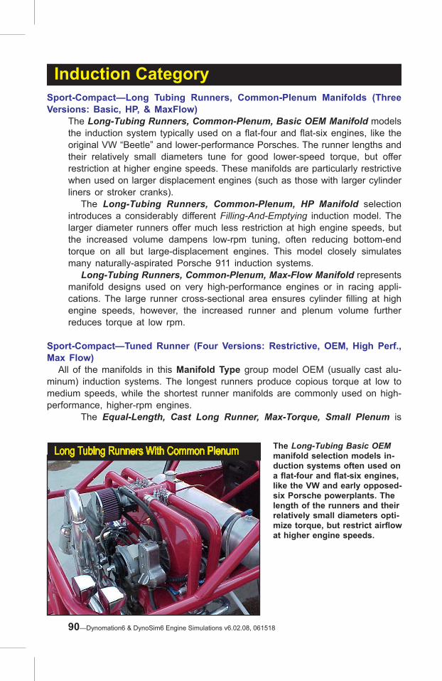
Induction Category
Long Tubing Runners With Common Plenum The Long-Tubing Basic OEM manifold selection models in-duction systems often used on a flat-four and flat-six engines, like the VW and early opposed-six Porsche powerplants. The length of the runners and their relatively small diameters opti-mize torque, but restrict airflow at higher engine speeds.
Sport-Compact—Long Tubing Runners, Common-Plenum Manifolds (Three Versions: Basic, HP, & MaxFlow)
The Long-Tubing Runners, Common-Plenum, Basic OEM Manifold models the induction system typically used on a flat-four and flat-six engines, like the original VW “Beetle” and lower-performance Porsches. The runner lengths and their relatively small diameters tune for good lower-speed torque, but offer restriction at higher engine speeds. These manifolds are particularly restrictive when used on larger displacement engines (such as those with larger cylinder liners or stroker cranks). The Long-Tubing Runners, Common-Plenum, HP Manifold selection introduces a considerably different Filling-And-Emptying induction model. The larger diameter runners offer much less restriction at high engine speeds, but the increased volume dampens low-rpm tuning, often reducing bottom-end torque on all but large-displacement engines. This model closely simulates many naturally-aspirated Porsche 911 induction systems. Long-Tubing Runners, Common-Plenum, Max-Flow Manifold represents manifold designs used on very high-performance engines or in racing appli-cations. The large runner cross-sectional area ensures cylinder filling at high engine speeds, however, the increased runner and plenum volume further reduces torque at low rpm.
Sport-Compact—Tuned Runner (Four Versions: Restrictive, OEM, High Perf., Max Flow) All of the manifolds in this Manifold Type group model OEM (usually cast alu-minum) induction systems. The longest runners produce copious torque at low to medium speeds, while the shortest runner manifolds are commonly used on high-performance, higher-rpm engines.
The Equal-Length, Cast Long Runner, Max-Torque, Small Plenum is
90—Dynomation6 & DynoSim6 Engine Simulations v6.02.08, 061518

Modern “Tubing” Long-Runner Manifold
This Porsche 993 uses a cast-alu-minum equivalent of the steel-tub-ing manifolds of the past. While the length of these runners have positioned this induction into the Tubing, Long-Runner manifold category, HP or Max-Flow selec-tions can be used with this free-flowing design.
Induction Category
“Tubing,” Max-Flow ManifoldThe Long-Tubing Runners, Com-mon-Plenum, Max-Flow selection
models manifold designs used on high-performance engines or
in racing applications, like this Porsche 928 V8. The large runner cross-sectional areas ensure cyl-
inder filling at high engine speeds, however, the additional runner and plenum volume can reduce torque
at low rpm, offset somewhat, in this case, by the length of the run-
ners.
the first selection in this group, and it models a manifold ideal for engines in heaver vehicles, like trucks and vans. The low-rpm tuning boosts efficiency, economy, and driveability in stock engines. However, while the runners are somewhat long, they are not overly restrictive and stock engines using this manifold will produce good power. The next selections (downwards in the menu within this 3rd group) is the OEM, High-Perf., and Max Flow versions of equal-runner length runner mani-folds. The Equal-Length, Cast Long Runner, OEM, Small Plenum version has slightly shorter runners are capable of producing more horsepower, but torque below 3500rpm can suffer somewhat. This is still excellent manifolds for heavier performance vehicles. The Equal-Length, Cast Medium Length Runner, HP Design, Medium Size Plenum manifold is the first manifold in this group to offer a bias toward performance and higher engine speed. Manifolds of this type are commonly
Dynomation6 & DynoSim6 Engine Simulations, v6.02.08, 061518—91

Induction CategoryTuned-Runner Induction SystemsThe Tuned-Runner Manifold group
(3rd group in Sport Compact menu) models induction systems
that have slightly smaller ple-nums and runners than the more
aggressive manifolds in the 4th group of Flat or Horizontal Tun-
nel Ram designs. This 3.0L V6 Honda is typical of engines that
can be modeled by Tuned-Runner Manifold selections. The torque curves are broad and flat, while peak power occurs about 500 to
1000rpm lower than manifolds with shorter runners and larger
cross-sectional areas.
Medium-Length, Tuned-Runner InductionThe Tuned Runner, Me-dium Length, Larger Ple-num manifold provides a bias toward performance and higher engine speed. Manifolds of this type are
commonly found on 4, V6, V8, and V12 engines in
performance sedans and sports cars.
found on 4, V6, V8, and V12 engines in performance sedans and sports cars. The most performance oriented manifold, the Tuned, Short-Runner, Max-Flow, Large Plenum is an excellent choice on lightweight, performance ve-hicles. The tuned runners offer good pressure-wave tuning, while low restriction and large plenum volume give excellent horsepower potential. This manifold design is used on many performance-oriented sports cars, like Aston Martin, Maseratti, and Ferrari. The only manifolds that are superior in performance to this selection are the “Honda Type” listed in the next group that have the largest runner and plenum volumes. However, even “Honda” manifolds may not provide as broad a range of torque and power as the manifolds in this group.
Sport-Compact—Honda Type (Four Versions: Standard And Short Runner,
92—Dynomation6 & DynoSim6 Engine Simulations v6.02.08, 061518

Induction Category
Large Plenum, Long And Short Runners (Honda-Type, Flat Tunnel Ram)
The Honda-Type manifold selections (referred to as Flat Tunnel Rams) in the simulation model Honda induction systems used on 4-cylinder, high-performance engines, like the B16, B18, S2000 and others. This manifold model can be applied to any engine that uses direct, high-volume runners and a large plenum. The stock-length runner designs (like the Edelbrock Performer X, shown on the left) generate a characteristic broad and flat torque curve, and its large runners and plenum volume will supply all but the largest engines with adequate airflow to well beyond 7500rpm. Manifolds with shorter runners will often lower torque below 4000- 5000-rpm and offer slight-to-significant power gains above 7000- to 8000rpm.
Small And Large Plenum Designs) While the manifolds in this group are designed to model the Honda induction systems used on their 4-cylinder, high-performance engines, like the B16, B18, S2000 and others. This manifold model can be applied to any engine that uses straight, high-volume runners and a large-volume plenum. The power potential from this manifold model is similar to “all-out” induction systems, such as tunnel-ram manifolds. In fact, we refer to this manifold as a “Flat Tunnel Ram,” since it is basically a tunnel ram turned 90-degrees from vertical to horizontal.
The Flat Tunnel Ram, Standard-Length Runner, Factory Plenum Volume selection models the stock Honda manifold supplied on many of its B16A high-performance engines, like the Del Sol, Civic Si, the Integra GSR, and others. This induction system generates a characteristic broad and flat torque curve (with 4-valve heads), and its large runners and plenum volume will supply all but the largest engines with adequate airflow to well beyond 7500rpm. For many high-performance street vehicles, this is an excellent manifold with the only weak point being somewhat lower torque, usually below 3500- to 4000rpm, compared to the longer-runner manifolds in the previous group. But above these engine speeds, the OEM Honda-Type induction system with medium-length runners is virtually unbeatable. The next “stage” in Flat-Tunnel Ram manifold designs is the shorter-runner
Dynomation6 & DynoSim6 Engine Simulations, v6.02.08, 061518—93

Custom Racing Manifolds
The Honda-Type, Standard Or Short Runner, Large Volume manifolds simulate induc-tions that have increased cross-sectional area runners combined with large plenum vol-umes. These manifolds will usually reduce low-speed torque below 5000rpm. However expect substantial gains on modified, high-speed engines, especially above 8000rpm. Notice the tapered runners on the manifold on the right.
Induction Categoryversion of the stock B16A intake, the Flat Tunnel Ram, Short Runner, Fac-tory Plenum Volume. Manifolds of this type are supplied on the Type R (originally on the 1.8L, B18C5 Honda engines) and are available in many forms from aftermarket manufacturers. They will often generate a slight reduction in torque below 4000- to 5000-rpm and offer a slight-to-significant gain in power above 7000- to 8000rpm. This is not necessarily the best manifold for a small-displacement street engine, but for a modified or “stroker” engine it can offer more power with little or no loss in torque.\ The third selection (working towards the bottom of the menu within this group), is the Flat Tunnel Ram, Standard-Length Runner, Large Plenum Volume manifold model. This choice simulates a manifold (only available from the aftermarket, such as the Edelbrock Performer X manifold) that has increased cross-sectional area runners of about factory length combined with a large-volume plenum. This manifold will show power gains above max-torque engine speeds, while the standard-length runners will usually maintain good torque at lower speeds. This may be the best manifold for a modified engine that will be operated on the street. Finally, the Flat Tunnel Ram, Short Runner, Large Plenum Volume mani-fold model simulates many of the exotic induction systems used on racing all-motor and forced induction applications. This induction has the largest volume runners and plenum, and will reduce low-speed torque below about 5000rpm. However expect substantial gains on highly-modified engines, especially above 8000rpm.
94—Dynomation6 & DynoSim6 Engine Simulations v6.02.08, 061518

Induction CategoryIndividual-Runner Menu Selections
Individual- (or isolated) runner, I.R., induction systems, use separate tubes for each runner with their own individu-al throttle plates. These induction systems offer the potential for op-timum power at high engine speeds.
Manifold Plenum-ConfigurationWhen you select any mani-fold model from the Intake Manifold Design menu, the
appropriate plenum model is displayed in the Plenum Con-figuration field. For example,
if you select a Single-Plane manifold, the Common Ple-
num model is used to analyze total induction airflow. On
the other hand, if you select an I.R. system, an IR Runner model is used to divide total induction airflow between all
cylinders.
Manifold Plenum ConfigurationManifold Plenum Configuration
Individual-Runner Induction Choices
Individual Runner, No Plenum (Large And Small Diameter, Long And Short Stacks) For naturally-aspirated, professional racing applications, individual- (or isolated) runner (I.R.) induction systems, with separate tubes containing their own throttle plates for each cylinder, can offer the ultimate in power potential at high engine speeds. The single element that sets the I.R. system apart from any other induc-tion models is that each “barrel” or individual “stack” does not share flow with other stacks through interconnecting passages (like a plenum). This characteristic means that the overall induction flow is divided between all barrels (or cylinders). All of the manifolds in the Manifold Type submenus that we have discussed up to this point have shared-flow between cylinders, typically through a plenum.
Dynomation6 & DynoSim6 Engine Simulations, v6.02.08, 061518—95

Induction Category
Individual Runner (Injector Stack) Induction System
I.R. systems offer the lowest potential restriction of any induction system. The bell-mouth entrance can help tune the horsepower peak to the desired rpm range. Careful selection of stack size, length, bellmouth size, and flow rate are essential to building a winning I.R. induction. All of these elements can be tuned and optimized, including elliptical bellmouth runners.
And the induction flow (Total Induction Flow Rate) in the INDUCTION category specifies the maximum airflow that passes through the restriction common to all cylinders: typically, the throttle body. Similarly, in an I.R. system the Flow Rate is the total airflow through all of the individual stacks. So, for example, if each I.R. stack has a rated flow of 100cfm, the correct induction Flow Rate you should enter in the Induction Category is 400cfm (100cfm x 4-cylinders).
Note: The Total Induction Flow Rate is divided equally between all of the individual runners/stacks.
The Small Diameter, Longer Stacks model produces a power curve similar to the Flat Tunnel Ram, Standard Runner, Factory Volume manifold discussed in the previous section. However, the improved flow potential over the factory manifold at higher engine speeds offers improved power that will peak at a slightly higher rpm. The Small Diameter, Short Stacks is the shorter-runner version of the previous I.R. selection. It produces a power curve similar to the Honda Type, Short Runner, Factory Volume manifold discussed earlier. The improved flow potential at higher engine speeds offers improved power that will peak at a slightly higher rpm. Expect this I.R. induction to produce good power levels beyond 8000rpm on a properly modified race engine. The Large Diameter, Long Stacks selection produces a horsepower curve similar to the Flat Tunnel Ram, Standard Runner, Large Volume manifold. The improved flow potential at higher engine speeds offers improved power that will peak at a higher rpm. Expect this I.R. induction to produce good power
96—Dynomation6 & DynoSim6 Engine Simulations v6.02.08, 061518

Induction CategoryHonda IR Induction
For naturally-aspirated, profes-sional racing applications, in-dividual- (or isolated) runner
(I.R.) induction systems offer the ultimate in flow potential and peak
power at high engine speeds. Each runner/tube contains its own
throttle plate or slide valve.
Racing/Street IR Carburetion While IR systems with carburetors are now rare, they still look awesome. The flow
potential of these four Webers is quite a bit less than injector stacks, however in
street-rod applications, they produce good low- and mid-range power. The air screens on this setup are available from Carbs Un-
limited (they offer a range of accessories for Webers and Dellortos carburetors).
beyond 8000rpm on a properly modified race engine.
Finally, the Large Diameter, Short Stacks produces a horsepower curve similar to the Flat Tunnel Ram, Short Runner, Large Volume manifold. The improved flow potential at higher engine speeds offers improved power that will peak at a higher rpm. Expect this I.R. induction to produce excellent power beyond 9000rpm on a properly modified race engine.
Individual Runner Manifold For Carburetors Similar to the previous I.R. induction systems, individual- (or isolated) runners connect each cylinder to one “barrel” of a (in this case) carburetor and they do not share flow with other cylinders/barrels through interconnecting passages. These systems, once commonplace in drag racing, are now mostly limited to specific classes or vintage street vehicles.
Dynomation6 & DynoSim6 Engine Simulations, v6.02.08, 061518—97

Induction Category
Runner Wall TemperatureAverage Runner Temperature menu sets the temperature of the intake manifold and/
or runners leading from the atmosphere or plenum to the junction at the cylinder head.
This temperature lets you model intake systems that are cooler (or hotter) than
the overall engine tempera-ture (e.g., “air-gap” manifold
designs).
Runner Wall Temperature
The Average Runner Temperature menu sets the temperature of the intake manifold and/or the runner passages leading from the plenum/atmosphere to the junction at the cylinder head. The default selections are 180-degrees(F) for plenum inductions and 120-degrees(F) for individual runner systems. This temperature setting models manifolds or runners that are cooler (or hotter) than the overall engine temperature (e.g., “air-gap” and other raised-runner designs). Keep in mind that average runner wall temperature only indirectly changes air/fuel charge temperatures. At lower engine speeds, slower runner flow interacts with the walls for a longer time, increasing the exchange of heat. At higher engine speeds, this interaction time decreases, reducing the effects of wall temperature on charge density.
Note: When you select an intake manifold from the Intake Design menu, the Average Runner Temperature will automatically revert to the default values. Make sure to review (and change, if necessary) runner wall temperatures after selecting an induction system (manifold or IR).
Airflow Selection And Pressure Drop
The Total Induction Airflow Rate menus establish the rated airflow for the induction system and the pressure drop at which it’s measured. The consists of 2-barrel-carburetor and 4-barrel-carburetor/fuel-injection choices. In addition, you can directly specify any rated airflow from 100 to 7000cfm.
Note-1: The flow ratings for 2-barrel carburetors are measured at a pressure drop twice as high (3.0-in/HG) as the pressure used to rate 4-barrel carbure-tors and most fuel-injection systems (1.5-in/HG). The higher pressure drop
98—Dynomation6 & DynoSim6 Engine Simulations v6.02.08, 061518

Induction Category
Induction Airflow Rate MenuThe Total Induction Airflow Rate menu establishes the flow rate and pressure drop through the induction system. It also establishes an overall airflow restriction for induction modeling. The menu consists of 2-barrel-carburetors (at 3.0-in/Hg) and 4-barrel-carburetor/fuel-in-jection choices (at 1.5-in/Hg). In addition, you can directly enter any airflow from 100 to 7000cfm at either pressure drop.
increases the measurement resolution for smaller carburetors and “shifts” the flow numbers toward the range commonly found in automotive applica-tions (roughly, 100 to 700cfm). The pressure drop is the pressure differential maintained across the system (e.g., carburetor or throttle body) during airflow measurement at wide-open throttle.Note-2: You can use the built-in Airflow Pressure-Drop Conversion Calcula-tor (available in the Tools Menu) for quick conversions between airflow and pressure-drop values.
Airflow Rate Assumptions
The Total Induction AirFlow menu selections “install” 2-bbl carburetors from 300- to 600cfm or 4/8-Bbl Carb Or Inj. systems from 300- to 7000cfm. The 4/8-BBL label indicates that the induction system can consist of single or multiple carburetors (or fuel injection throttles.) that combine to produce of the rated airflow. An induc-tion system equipped with twin 1100cfm carburetors would have a rated airflow of 2200cfm. If an air cleaner is used, total airflow (at the same pressure drop) should be adjusted to compensate for the increase in restriction at the atmospheric bound-ary.
Note: The simulation makes no assumption about the type of restriction used in the induction system (any throttle configuration, any runner shapes or inter-connections, etc.). The airflow rating is simply a means to model the greatest overall restriction of the entire induction system. As higher airflow levels are
Dynomation6 & DynoSim6 Engine Simulations, v6.02.08, 061518—99

Induction CategoryInduction Pressure-Drop Menu
Use the Induction Airflow Pressure Drop menu to select either 1.5-inches of mercury (1.5-in/Hg), a measure-ment standard for 4-barrel carburetors and injection systems, and the two-barrel carburetor standard of 3.0-inches of mercury (3.0-in/Hg).
selected, the simulation lowers the restriction within the induction system.
Wave-Action OnlyIntake-Runner Specifications
The power of the Wave-Action simulation lies in its ability to predict and analyze the interaction of pressure waves and their influence on mass flow in the engine. By design, this simulation is sensitive to runner lengths, passage taper angles and volumes. The Induction category includes a group of data-input fields specifically for the Wave-Action simulation. These fields are Runner Length, Port Entry Area, Minimum Port Area, and Plenum Volume, plus a checkbox to activate an Ellipti-cal Bellmouth model applied to the runner atmospheric boundary. The following sections provide an overview of each of these Wave-Action intake-runner data-entry fields:
Runner Length (WA Only)
This is the distance from the point of minimum cross-sectional area to the location in the port where the area substantially increases. In a common-plenum manifold, like a single-plane or tunnel-ram, this point is usually located at the plenum junction. In the case of an individual-runner system, this transition occurs at the bellmouth of the velocity stack.
Port Entry Area (WA Only)
This is the area at the entrance to the port runner (in in2 or mm2, depending on the Units currently selected). This value is the starting point for the port, and is used, along with the Minimum Port Area, to determine the included Port Taper Angle, a critical dimension analyzed in the Wave-Action simulation.
Minimum Port Area (WA Only)
100—Dynomation6 & DynoSim6 Engine Simulations v6.02.08, 061518

Induction Category
Wave-Action-Only Induction Fields The Induction category includes data-input fields specifically for the Wave-Action simu-lation. These are Run-ner Length, Port Entry Area, Minimum Port Area, and Plenum Vol-ume, plus a checkbox to activate an Elliptical Bellmouth model.
This is the area at the point of greatest restriction in the port and is also the point at which runner length is measured. It is usually located just above the valve seat near the valve guide, however, it may also occur at other locations within the port. The Minimum Port Area is a very critical engine dimension; carefully measure and/or calculate this value to optimize simulation accuracy in Dynomation6. If you in-accurately measure this value, horsepower predictions and your tuning efforts will also be inaccurate. As you test various engine configurations using the Wave-Action model, you will find that Minimum Port Area has a "resonant" value at the point of optimum power. For any particular engine, areas larger or smaller than this will produce less power. If your cylinder heads provide optimum port areas and Taper Angles, your engine can produce peak power. When the Minimum Port Area is tuned to an optimum size, it generates a "sweet spot" between restriction that produces high port velocities, allowing pressure waves to impart sufficient energy to the intake charge and "ram tune" the cylinders, ver-sus an oversize area that, although offering less restriction, depletes the strength of pressure-waves and consequently diminishes cylinder filling. Rapidly pinpointing the Minimum Port Area that produces peak performance is a terrific strength of the wave-action simulation. Determining optimum Minimum Port Area is entirely dependent on engine dis-placement, cam timing, port flow, valve sizes, engine speed range, and many other variables that make this job extremely difficult without using a mathematical simula-tion. Dynomation6 analyzes all of these variables in every Wave-Action run. After just a few simulations, you can easily home-in on an optimum Minimum Port Area for any engine application!
Important-1: This may seem obvious (but it's easy to forget), the Port Entry Area and Minimum Port Area are areas, not diameters of the ports/runners.
Important-2: The Minimum Port Area can range from below 50% of the area of the intake valve, to as large a 75-to-80% or larger of the valve area in racing cylinder heads.
Dynomation6 & DynoSim6 Engine Simulations, v6.02.08, 061518—101

Runne
r Len
gth
Runne
r Len
gth
Minimum Area
Port EntryArea
Induction CategoryMeasuring Runner Dimensions
Intake Runner Length in the wave-action simulation is defined as the distance from the point of minimum area to the point where the port area substantially increases. Port Entry Area is measured at the port entrance junction with the plenum or just inside the runner bellmouth. And the Minimum Port Area usu-ally occurs just above the valve seat, although it can occur at other locations in the port.
Minimum Area
Port EntryArea
Port
Tape
r Ang
le
Intake Port Taper Angle
Intake runner Minimum Port Area and Taper Angle are critical dimensions in the induction system. If in-correct values are entered, power predictions will also be incorrect.NOTE: The Minimum Port Area value used in Dynomation6 is the area Per Port. If you are mod-eling multiple-valve-per-port cylinder heads (2 or 3 valves per port), do not add these port areas together to determine Mini-mum Port Area!
Important-3: The Minimum Port Area is a dimension in in2 or mm2 (depending on the current Units selection) within the port of Each Valve of multiple-valve-per-port cylinder heads. Do Not Add minimum port areas together when you enter a Minimum Port Area for 2- or 3-valves-per-port applications.
Plenum Volume (WA Only)
The Plenum Volume models the volume (in3 or mm3) not the shape, of a plenum used in Common-Plenum induction systems. You can directly enter the volume of the plenum, or enter the approximate physical dimensions and Dynomation6 will calculate the volume. The minimum plenum volume is dependent on the Port Entry Area (Maximum Area of the port). The simulation checks to ensure a transition of sufficiently large volume occurs at the port/plenum boundary. If a larger plenum
102—Dynomation6 & DynoSim6 Engine Simulations v6.02.08, 061518

An Elliptical Bellmouth may be added to the
end of intake runners using the Wave-Action
simulation. Here are the typical dimensional relationships modeled
by the sim. An El-liptical profile typi-
cally outperforms a simple radius or airfoil
shapes.
Induction Category
Elliptical Bellmouth Specifications
volume is required, a message box will indicate the issue and it will be corrected automatically when you click on OK.
Note: Only the volume of the plenum is used in the simulation; height, width and depth are only used to calculate a volume and hold no further significance within the simulation.
Elliptical Bellmouth (WA Only)
A checkbox is provided in the Induction category to activate an Elliptical Bell-mouth model that can be applied to the runners, either at their connection to a plenum or at the atmospheric interface. Principal bellmouth characteristics include a wide radius with an elliptical profile and a short overall height (equal to the diameter of the main stack tube). The effects on performance generally occur at higher rpm but depend on runner dimensions and overall engine design.
Pipe Begin Diameter = 2.13 x Tube Diameter
Elliptical Pro�le Stack
Tube Diameter
Same HeightAs Tube Diameter
Dynomation6 & DynoSim6 Engine Simulations, v6.02.08, 061518—103
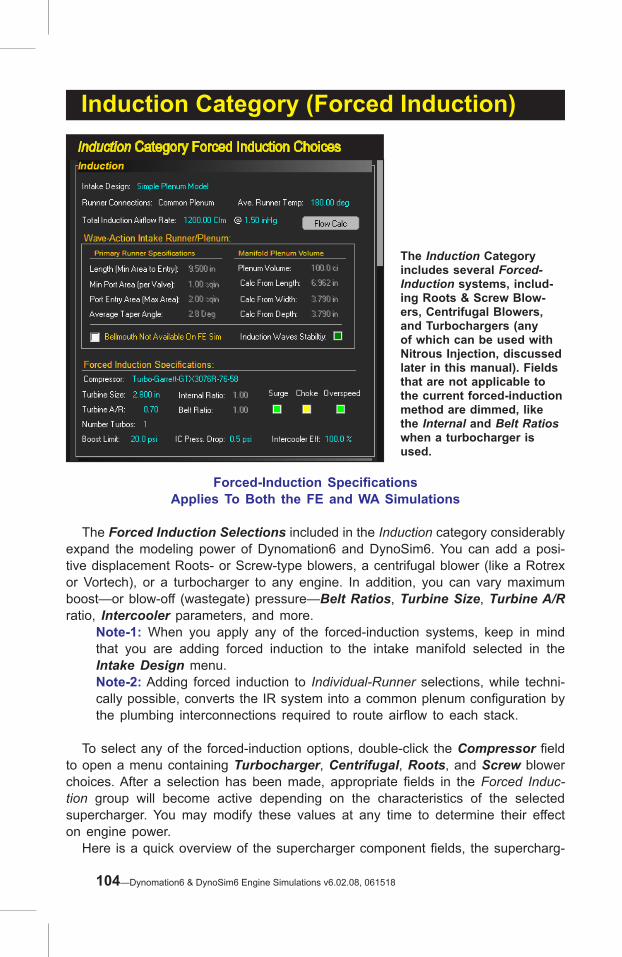
Induction Category (Forced Induction)
Forced-Induction SpecificationsApplies To Both the FE and WA Simulations
The Forced Induction Selections included in the Induction category considerably expand the modeling power of Dynomation6 and DynoSim6. You can add a posi-tive displacement Roots- or Screw-type blowers, a centrifugal blower (like a Rotrex or Vortech), or a turbocharger to any engine. In addition, you can vary maximum boost—or blow-off (wastegate) pressure—Belt Ratios, Turbine Size, Turbine A/R ratio, Intercooler parameters, and more.
Note-1: When you apply any of the forced-induction systems, keep in mind that you are adding forced induction to the intake manifold selected in the Intake Design menu.Note-2: Adding forced induction to Individual-Runner selections, while techni-cally possible, converts the IR system into a common plenum configuration by the plumbing interconnections required to route airflow to each stack.
To select any of the forced-induction options, double-click the Compressor field to open a menu containing Turbocharger, Centrifugal, Roots, and Screw blower choices. After a selection has been made, appropriate fields in the Forced Induc-tion group will become active depending on the characteristics of the selected supercharger. You may modify these values at any time to determine their effect on engine power. Here is a quick overview of the supercharger component fields, the supercharg-
Induction Category Forced Induction Choices
The Induction Category includes several Forced-Induction systems, includ-ing Roots & Screw Blow-ers, Centrifugal Blowers, and Turbochargers (any of which can be used with Nitrous Injection, discussed later in this manual). Fields that are not applicable to the current forced-induction method are dimmed, like the Internal and Belt Ratios when a turbocharger is used.
104—Dynomation6 & DynoSim6 Engine Simulations v6.02.08, 061518

Turbine & Compressor Impellers The turbine (impeller shown on the right end of the shaft) is placed in the exhaust stream of an engine and is driven by a combination of exhaust flow and exhaust pressure waves. Two parameters in the simulation adjust the performance of the turbine: the Turbine Wheel Size and the Turbine Housing A/R Ratio. Modify-ing the turbine wheel size will make large changes in the turbine speed; the smaller the wheel, the faster the turbine will rotate. The higher the turbine speed, the more airflow will be driven through the compressor (until the compressor blade tips reach supersonic speed).
Forced Induction Menus
The simulation includes over 100 forced induction choices. Select-ing a supercharg-er from any of the submenus will load that device into the Induc-tion Category and transfer super-charger-map data into the simula-tion.
Induction Category (Forced Induction)
ers to which they apply, and how they affect forced-induction performance:
Flow Restriction (throttle) Location—The location of the primary intake restric-tion (commonly the throttle) can have a significant affect on forced induction engines. If the restriction is located Before the compressor, inducted air is drawn-through the restriction and (like all naturally aspirated engines) the maxi-mum pressure drop (and resulting mass flow) through the restriction is limited to one atmosphere. However, if the restriction is positioned After the compressor, the pressure drop across the same restriction is limited by manifold pressure (as opposed to atmospheric pressure), potentially generating greater mass flow for the same size restriction. Many turbo systems position the throttle after the compressor, while Roots and Centrifugal compressors typically place the throttles before the compressor.
Turbine Size—(Turbos only) This is the diameter of the exhaust-driven impeller (in inches or millimeters). The turbine is placed in the exhaust stream of an engine
Dynomation6 & DynoSim6 Engine Simulations, v6.02.08, 061518—105

and is driven by a combination of exhaust flow and exhaust pressure pulses. Two parameters adjust the performance of the turbine: in general, the Turbine Wheel Size and the Turbine Housing A/R Ratio (discussed next). Modifying the turbine wheel size will make relatively large changes in the turbine speed; the smaller the wheel, the faster the turbine (and the compressor) will rotate. The higher the turbine speed, the more airflow will be driven through the compressor. Smaller turbines generate boost earlier in the rpm range, however, if the turbine is too small for the application, the turbocharger shaft speed can exceed the manufacturer’s recommendations (turning the Overspeed indicator from green to yellow, and if overspeed is sufficiently high, it will turn red).
Turbine Housing A/R Ratio—(Turbos only) This is a ratio of the cross-sectional area of the turbine housing inlet to the inlet passage distance (radius) from
Induction Category (Forced Induction)
Boost Limiter (Wastegate)
Boost Limit is an arbitrary maximum induction pressure established by the wastegate setting. It is not a measure of the capability of the super-charger, i.e., the blower may or may not be able to de-velop sufficient pressure to activate the wastegate. The simulation incorporates a wa-stegate model that modulates the size of its bypass pas-sages when the Boost Limit is reached.
A1
R1R2R3
R4
R5 R6
A2
A3
A4
A5 A6
A/R Turbine-Housing Ratio
The Turbine (the exhaust-driven element) Housing A/R ratio is a comparison of the cross-sectional area of the housing inlet (the “A’s” in the photo) to the distance the inlet passage is positioned from the center of the turbine (the radius, or “R’s” in the photo). Unlike the Turbine Size (that has a dramatic affect on turbine speed), the Tur-bine Housing A/R Ratio fine-tunes turbine speed and helps establish where—in the engine rpm range—the turbo begins to pro-duce boost pressure.
106—Dynomation6 & DynoSim6 Engine Simulations v6.02.08, 061518

Induction Category (Forced Induction)
the center of the turbine wheel (see photo). As the A/R Ratio is increased, the overall size of the turbine housing and its internal passage become larger. Unlike Turbine Size that has a dramatic affect on turbine speed, the Turbine A/R Ratio fine-tunes turbine speed. Changing A/R has many effects. By using a larger A/R Ratio, the turbo produces less boost at lower engine speeds but develops more boost at a higher engine speeds, primarily due to the reduction in exhaust backpressure in larger turbine housings. Lower engine backpressure improves engine volumetric efficiency (VE), and that can result in an power increase throughout the usable rpm range. So, finding the optimum values for both the A/R Ratio and Turbine Size are important steps in building the most efficient and responsive turbocharger system.
Number Of Turbos—(Turbos only) This selection divides the exhaust flow and in-
Both centrifugal and roots blowers are mechanically driven by the engine. The
Belt Gear Ratio (external drive) is the mechanical connection between the engine crankshaft and blower input
shaft. This Jackson Supercharger pul-ley setup provides an overdrive (an
overall Belt Ratio of 1.20:1).
Belt Ratio
Centrifugal superchargers are driven through an external Belt Ratio, but this speed increase is insufficient for most centrifugal supercharg-
ers to reach their optimum operating speeds (35,000rpm and higher). An internal gear train
is commonly used to further increase rota-tional speed.
Internal Gear Ratio
Dynomation6 & DynoSim6 Engine Simulations, v6.02.08, 061518—107

take flow restrictions equally between all turbos (up to four turbos in parallel can be modeled). Compressed outflow from all turbos is directed into the induction system of the engine (through an intercooler, if selected) and is divided equally between all cylinders. Multiple turbo applications are most successful when the engine produces sufficient exhaust-gas volume to spin up all turbos; using small turbine sizes and housings usually improves multiple-turbo applications.
Boost Limit—(Turbos, Centrifugals, Roots, Screw) This is the pressure at which the wastegate or blow-off valve is activated, maintaining maximum induction pressure at or below this value.
Note: Boost Limit is an arbitrary pressure, chosen by you, for the simulation. It is not a measure of the capability of the supercharger. In other words, be-cause of component mismatch and other factors, the blower may not be able to develop sufficient airflow and boost to reach the wastegate relief pressure.
Belt Ratio—(Centrifugals, Roots, Screw) Centrifugal, roots, and screw supercharg-ers are mechanically driven by the engine. The Belt Ratio (the external drive ratio) is the ratio of the mechanical connection between the engine crankshaft and blower input shaft. This value is multiplied by the Internal Ratio (internal gear ratios are commonly used on centrifugal superchargers) to determine final compressor/rotor speed.
Internal Ratio—(Centrifugal) Centrifugal superchargers are driven by a mechanical connection to the engine crankshaft (the external Belt Ratio). Input shaft speed, however, it usually insufficient for most centrifugal superchargers to reach their optimum operating speeds (35,000rpm and higher), so an internal gear train is commonly used to further increase rotational speed. The ratio of this internal gearing determines how much faster the turbine rotates. To determine the final speed of a centrifugal turbine, multiply crankshaft rpm by the Belt Ratio, then multiply that by the Internal Ratio.
Operational Indicators—(Turbos, Centrifugals) The forced-induction portion of the
Induction Category (Forced Induction)
Operational Indicators The Forced Induction Specifi-cations group includes three “indicators” that will alert you if Surge, Choke, or Overspeed are present during any por-tion of the test rpm range. See the text for a definition of each indicator and tips on how to correct problems. Also, refer to the Simulation Log for more information about the indicated problem.
108—Dynomation6 & DynoSim6 Engine Simulations v6.02.08, 061518

Induction category includes three “indicators” that will help you select the correct turbocharger, turbine wheel size, and A/R ratio. Each indicator shows a potential operational problem by turning from green to yellow (minimal problem), or to red (should be corrected). Additional information about the cause and extent of the problem will be included in the Simulation Log (displayed using the Simulation Menu).
Surge: (Turbo Only) This condition occurs when mismatched components cause unstable airflow through the compressor. If a turbo is operated consistently within surge, additional loads can damage the turbines, shafts, and bearings. If surge is detected during a simulation run, the Surge indicator will display either yellow or red. A yellow Surge indicator means that the turbo has entered surge only a limited time during the full engine rpm range. This limited-surge operation is not considered unusual and is not normally associated with shortened turbocharger life. If the indicator turns red, the turbo has entered into surge often during the engine “dyno test.” The turbocharger, Turbine Size, or A/R ratio should be changed to eliminate this condition.
Choke: (Centrifugals, Turbos) While Choke can apply to both the Compressor and Turbine impellers (in turbocharger applications), Choke most often refers to the point at which compressor wheel tips reach sonic velocity, preventing further flow. The choke line on a compressor map can be recognized by the steeply descending speed lines at the right side of the map. If choke is detected at any point during the engine rpm range, the Choke Indicator will turn from green to yellow, indicating a condition that should be corrected. However, choke problems are relatively easy to correct, often disappearing with a slight reduction in shaft speed (use a larger Turbo or Turbine Size, and/or increase the A/R ratio).
Induction Category (Forced Induction)
Turbocharger Compressor MapThis turbo compressor map, produced by the manufacturer, shows how the
compressor turbine performs at various flow rates, pressure ratios, and rpms. If insufficient engine demand causes the
turbo to operate “off the map” to the left, Surge can occur. If engine demand line
pushes off the right side of the map, the turbo is said to be in a Choke condition.
And if the turbocharger speed exceeds its maximum rpm, as shown on the map (in this case slightly above 200,000rpm), an Overspeed condition exists. Each of
these abnormal operating conditions will turn a forced-induction indicators from
green to yellow, and if the condition occurs at multiple rpm points or is well beyond the limit, the indicator will turn
red.
Dynomation6 & DynoSim6 Engine Simulations, v6.02.08, 061518—109

The Version6 Compressor Map Window The compressor map display window in the simulation can be viewed by choosing Show Turbo/Centrifugal Compressor Map from the Simulation Menu. The left vertical axis shows the output pressure ratio (2.0 equals 2 atmo-spheres of pressure; about 15 psi of boost). The bottom horizontal axis is the mass flow through the compressor in pounds per minute (Lb/Min). The small numbers po-sitioned along the left edge of the map are the rpm values for the red speed lines. The black line on the graph is the calculated engine demand line; the dots indicate the mass flow at each rpm test point (also displayed in the ProTools table). You can move the map window to any position on your desktop. Use the Minimize button to temporarily “park” the window to a tab that appears at the bot-tom of the program screen; to re-display the window, click the parking-tab.
Induction Category (Forced Induction)
Overspeed: (Centrifugals, Turbos) If the shaft speed exceeds the manufac-ture’s recommendations (the engine demand line travels off of the top of the compressor map), the Overspeed Indicator will change from green to yellow. If the overspeed condition exceeds the manufacturer’s recommended speed by over 10%, the indicator will switch from yellow to red, indicating a potentially harmful condition to the turbocharger bearings and seals. If you are simulating a turbocharger system and you have a red Overspeed condition, increase the Turbine Size and/or the Turbine Housing A/R ratio.Important Note: If overspeed occurs in a real supercharging system, you risk destroying the compressor and spraying metal particles into your engine.
Selecting The Best Supercharger For Your Application
Selecting a Turbocharger—A turbocharger consists of a compressor and a turbine. The “compressor side” characteristics are established when you choose the turbo from the main Blower Type menu. The compressor acts as pump that forces air into the induction system. The output of the compressor is determined by the speed of the impeller (inside the compressor housing), the shape of the
When an Overspeed condition occurs, the simulation will apply a severe restriction to charge flow and engine horsepower will drop substantially. This is done to show you when, in the rpm range, Overspeed occurs, and to ensure you recognize that overspeed has occurred.
110—Dynomation6 & DynoSim6 Engine Simulations v6.02.08, 061518

When an Overspeed condition occurs, the simulation will apply a severe restriction to charge flow and engine horsepower will drop substantially. This is done to show you when, in the rpm range, Overspeed occurs, and to ensure you recognize that overspeed has occurred.
Induction Category (Forced Induction)housing, and the swallowing capacity of the engine. These variables are visually illustrated on a compressor map. The simulation incorporates more than 100 turbo maps within its library that cover a wide range of capacities. The turbine side of the turbocharger is composed of a turbine wheel and the surrounding housing. The turbine is placed in the exhaust stream of the engine and is driven by a combination of exhaust flow and exhaust pressure waves. The turbine is connected to the compressor impeller through an interconnecting shaft. Two principal parameters modify the performance of the turbine: 1) the Turbine Size and, 2) the Turbine A/R ratio. As described earlier, the Turbine Size has a major effect on turbine and compressor speed. In general, the smaller the wheel, the faster the turbine will rotate. The Turbine A/R ratio acts to fine-tune the turbine speed. The smaller the Turbine A/R, the more quickly the turbo will “spool up.” To find the optimum turbocharger for your engine, first select a basic turbo/compressor (turbocharger) from the Blower Type menu. For help in making an initial selection, consult with the turbo manufacturer or visit the many performance websites that offer turbo kits and performance modifications. You will often find turbo recommendations and even suggestions for turbine-wheel diameters and A/R ratios. After you have selected the basic turbo, set the Boost Limit (wastegate pressure) to the desired level (use 10psi if you’re not sure). Next, you’ll need to analyze how much airflow the turbo is delivering to the engine by viewing the manifold pressure curve (right-click the rpm-based graph, located on the top-right of the main screen, and assign Boost Pressure to either the Y1 or Y2 axis). Inspect the manifold pressure curve for the rpm point at which the pressure rises to a maximum. Make sure that the turbo you have selected, in fact, reaches the wastegate relief pressure chosen in the Boost Limit field.
Note-1: The simulation can display either Boost Pressure and/or Absolute Pressure. If the graph pressure curve is an absolute pressure plot, remember to subtract ambient pressure to determine boost pressure (for example, an absolute pressure of 25psi would indicate a boost pressure of about 10psi—25psi absolute, minus 14.7psi ambient, equals 10.3psi boost).Note-2: The mass flow rate of the engine is displayed in the ProTools graph. This value is helpful in selecting a supercharger or a turbocharger, since the mass flow rate is also shown on the blower map and plotted as dots on the demand line. Pick a turbo that has a maximum flow somewhat greater than the highest value of engine demand, otherwise the turbo may enter a restric-tive “choked flow” state at full load.
If the maximum-boost rpm point occurs considerably late in the rpm range, the boost pressure may never reach the Boost Limit, or if the Choke indicator is il-luminated, installing a larger compressor may solve the restriction problem. On the other hand, if the boost pressure curve begins too early in the rpm range, or the Surge or Overspeed indicators are red, installing a larger turbine wheel or increas-ing the A/R ratio may solve the problem.
Dynomation6 & DynoSim6 Engine Simulations, v6.02.08, 061518—111

Induction Category (Forced Induction)
Selecting a Centrifugal Supercharger—Like a turbocharger, a centrifugal super-charger consists of a compressor wheel and housing, but the driving force comes from the engine crankshaft through a drive belt or direct coupling and an internal gear box. Also like the turbocharger, the centrifugal compressor has performance characteristics defined in a “map” provided by the manufacturer. Because the cen-trifugal compressor turbine also must rotate at high speed, an internal “step-up” gear typically increases input pulley speed by several times. And input speed is often 1.5- to 3-times engine speed, determined by the appropriately sized pulleys. Final impeller speed is found by multiplying the Internal Ratio by the Belt Ratio and multiplying the result by engine RPM.
Note: While the internal gear ratio is not usually changeable, the simulation gives you the freedom to experiment with this ratio in addition to all the other tunable elements in the Forced Induction category.
Belt Ratio can be calculated using the following formulas:
For Serpentine and V-Belts: Belt Ratio = Crank pulley diameter Supercharger pulley diameter For Cog Pulleys: Belt Ratio = Crank pulley teeth count Supercharger pulley teeth count
To find the optimum centrifugal supercharger for your engine, first select a cen-trifugal supercharger from the menu. For help in making an initial selection, consult with the manufacturer’s website or visit the numerous performance sites that offer kits and performance modifications. You will often find supercharger recommenda-tions and suggestions for belt ratios. After you have selected the basic blower, set
Centrifugal Supercharger
Like a turbocharger, a centrifu-gal supercharger uses a com-pressor wheel, but the driving force comes from an internal gear box connected to the engine crankshaft. Because the centrifugal compressor also must rotate at high speed, the internal “step-up” gear increases input pulley speed by up to four times.
112—Dynomation6 & DynoSim6 Engine Simulations v6.02.08, 061518

Induction Category (Forced Induction)the Boost Limit (wastegate pressure) to the desired level (use 10psi if you’re not sure). Next select the Belt Ratio and set the Internal Gear Ratio to the values used by the manufacturer (many centrifugal blower run with approximately 2.5:1 external Belt Ratios and 3.5:1 Internal Gear Ratios). Finally, you’ll need to analyze how much airflow the blower is delivering to the engine by viewing the manifold pres-sure curve (right-click the rpm-based graph on the top, right of the main program screen and assign Boost Pressure to either the Y1 or Y2 axis). Inspect the manifold pressure curve for the rpm point at which the pressure reaches the maximum boost pressure. Check that the supercharger you have se-lected, in fact, reaches the wastegate relief pressure chosen in the Boost Limit field.
Note: The simulation can display either Boost Pressure and/or Absolute Pres-sure. If the graph pressure curve is an absolute pressure plot, remember to subtract ambient pressure to determine the boost level (for example, an absolute pressure of 25 psi would indicate a boost pressure of about 10psi; 25psi absolute minus 14.7psi ambient equals 10.3psi boost).
If the maximum-boost rpm point occurs considerably late in the rpm range, or if the boost pressure never reaches the Boost Limit, increasing the Belt Ratio or installing a larger supercharger may solve the problem. On the other hand, if the pressure curve rises early in the rpm range, or the Surge or Overspeed indicators are lit, try decreasing the Belt Ratio or installing a smaller supercharger.
Selecting a Roots or Screw Supercharger—Roots or Screw-type supercharger selection involves only two parameters: the flow volume and the Belt Ratio (these superchargers usually do not have internal overdrive gear boxes). The compressor-flow volume is fixed in the design of the supercharger and is indicated in the blower menu as a volume-per-revolution value.
Manifold Pressure GraphInspect the manifold pressure curve (use the Graph Op-
tions Menu to assign boost pressure to either the Y1 or
Y2 axis) for the rpm point at which the pressure rises to
the maximum boost pressure. This display will show you
if, in fact, the selected turbo reaches the wastegate relief
pressure set in the Boost Limit field. Here, the green
curve indicates that a boost pressure of about 19psi is reached at about 5000rpm.
Dynomation6 & DynoSim6 Engine Simulations, v6.02.08, 061518—113
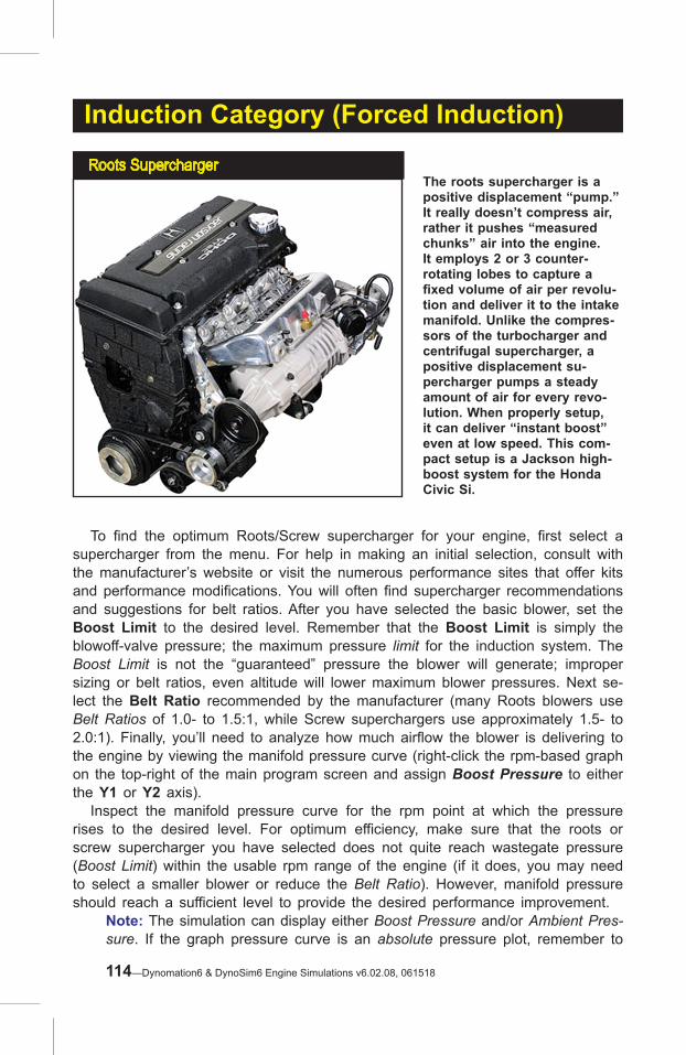
Induction Category (Forced Induction)
To find the optimum Roots/Screw supercharger for your engine, first select a supercharger from the menu. For help in making an initial selection, consult with the manufacturer’s website or visit the numerous performance sites that offer kits and performance modifications. You will often find supercharger recommendations and suggestions for belt ratios. After you have selected the basic blower, set the Boost Limit to the desired level. Remember that the Boost Limit is simply the blowoff-valve pressure; the maximum pressure limit for the induction system. The Boost Limit is not the “guaranteed” pressure the blower will generate; improper sizing or belt ratios, even altitude will lower maximum blower pressures. Next se-lect the Belt Ratio recommended by the manufacturer (many Roots blowers use Belt Ratios of 1.0- to 1.5:1, while Screw superchargers use approximately 1.5- to 2.0:1). Finally, you’ll need to analyze how much airflow the blower is delivering to the engine by viewing the manifold pressure curve (right-click the rpm-based graph on the top-right of the main program screen and assign Boost Pressure to either the Y1 or Y2 axis). Inspect the manifold pressure curve for the rpm point at which the pressure rises to the desired level. For optimum efficiency, make sure that the roots or screw supercharger you have selected does not quite reach wastegate pressure (Boost Limit) within the usable rpm range of the engine (if it does, you may need to select a smaller blower or reduce the Belt Ratio). However, manifold pressure should reach a sufficient level to provide the desired performance improvement.
Note: The simulation can display either Boost Pressure and/or Ambient Pres-sure. If the graph pressure curve is an absolute pressure plot, remember to
Roots SuperchargerThe roots supercharger is a positive displacement “pump.” It really doesn’t compress air, rather it pushes “measured chunks” air into the engine. It employs 2 or 3 counter-rotating lobes to capture a fixed volume of air per revolu-tion and deliver it to the intake manifold. Unlike the compres-sors of the turbocharger and centrifugal supercharger, a positive displacement su-percharger pumps a steady amount of air for every revo-lution. When properly setup, it can deliver “instant boost” even at low speed. This com-pact setup is a Jackson high-boost system for the Honda Civic Si.
114—Dynomation6 & DynoSim6 Engine Simulations v6.02.08, 061518
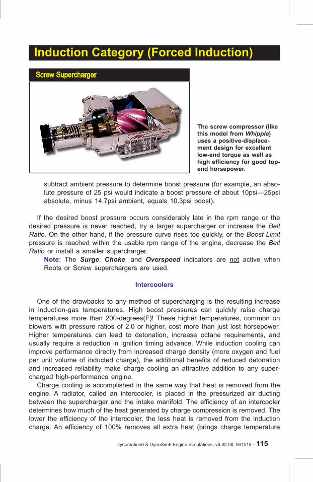
Screw Supercharger
The screw compressor (like this model from Whipple) uses a positive-displace-ment design for excellent low-end torque as well as high efficiency for good top-end horsepower.
Induction Category (Forced Induction)
subtract ambient pressure to determine boost pressure (for example, an abso-lute pressure of 25 psi would indicate a boost pressure of about 10psi—25psi absolute, minus 14.7psi ambient, equals 10.3psi boost).
If the desired boost pressure occurs considerably late in the rpm range or the desired pressure is never reached, try a larger supercharger or increase the Belt Ratio. On the other hand, if the pressure curve rises too quickly, or the Boost Limit pressure is reached within the usable rpm range of the engine, decrease the Belt Ratio or install a smaller supercharger.
Note: The Surge, Choke, and Overspeed indicators are not active when Roots or Screw superchargers are used.
Intercoolers
One of the drawbacks to any method of supercharging is the resulting increase in induction-gas temperatures. High boost pressures can quickly raise charge temperatures more than 200-degrees(F)! These higher temperatures, common on blowers with pressure ratios of 2.0 or higher, cost more than just lost horsepower. Higher temperatures can lead to detonation, increase octane requirements, and usually require a reduction in ignition timing advance. While induction cooling can improve performance directly from increased charge density (more oxygen and fuel per unit volume of inducted charge), the additional benefits of reduced detonation and increased reliability make charge cooling an attractive addition to any super-charged high-performance engine. Charge cooling is accomplished in the same way that heat is removed from the engine. A radiator, called an intercooler, is placed in the pressurized air ducting between the supercharger and the intake manifold. The efficiency of an intercooler determines how much of the heat generated by charge compression is removed. The lower the efficiency of the intercooler, the less heat is removed from the induction charge. An efficiency of 100% removes all extra heat (brings charge temperature
Dynomation6 & DynoSim6 Engine Simulations, v6.02.08, 061518—115

Induction Category (Forced Induction)
down to ambient). An efficiency of over 100% (reduces charge temperatures below ambient) is possible with water or ice. Everything from outside air to ice water and even evaporating pressurized liquefied gas (like Freon or nitrous oxide) have been used to remove heat from an intercooler. The ballpark efficiencies for these devices are:
Air-To-Air 40% Air-To-Cooler Ducted Air 50%Air-To-Water 75% Air-To-Cooled Water 100%Air-To-Ice Water 120% Air-To-Evaporating Liquid 120+%
Intercoolers: The “Secret” To Supercharging Power Higher induction tem-peratures, common on blowers with pressure ratios of 2.0 or higher, can cost horsepower and reliability. An Intercooler cools the inducted air the same way that heat is re-moved from the engine itself: with a radiator. Intercooling is the key to power and reliability in high-boost systems.
Intercooler And Pressure-Drop Menu
The simulation includes an Inter-cooler model that can be activated with any forced-induction system. An intercooler reduces high induc-tion temperatures that can sub-stantially reduce performance. The Intercooler is selected from a menu that indicates efficiency; 100% ef-ficiency reduces induction tempera-ture to ambient. An IC PressureDrop menu shows an estimated pressure drop value based on the Intercooler efficiency (due to increased charge density from charge cooling).
116—Dynomation6 & DynoSim6 Engine Simulations v6.02.08, 061518
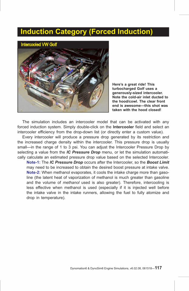
The simulation includes an intercooler model that can be activated with any forced induction system. Simply double-click on the Intercooler field and select an intercooler efficiency from the drop-down list (or directly enter a custom value). Every intercooler will produce a pressure drop generated by its restriction and the increased charge density within the intercooler. This pressure drop is usually small—in the range of 1 to 3 psi. You can adjust the Intercooler Pressure Drop by selecting a value from the IC Pressure Drop menu, or let the simulation automati-cally calculate an estimated pressure drop value based on the selected Intercooler.
Note-1: The IC Pressure Drop occurs after the Intercooler, so the Boost Limit may need to be increased to obtain the desired boost pressure at intake valve.Note-2: When methanol evaporates, it cools the intake charge more than gaso-line (the latent heat of vaporization of methanol is much greater than gasoline and the volume of methanol used is also greater). Therefore, intercooling is less effective when methanol is used (especially if it is injected well before the intake valve in the intake runners, allowing the fuel to fully atomize and drop in temperature).
Induction Category (Forced Induction)Intercooled VW Golf
Here’s a great ride! This turbocharged Golf uses a generously-sized intercooler. Note the cold-air inlet ducted to the hood/cowl. The clear front end is awesome—this shot was taken with the hood closed!
Dynomation6 & DynoSim6 Engine Simulations, v6.02.08, 061518—117

Camshaft CategoryCamshaft Category
The Camshaft Category establishes one of the most important specifica-tions in the engine: Intake And Ex-haust Valve-Event Timing that dictates the beginning and ending of all four engine cycles. The Camshaft Category organizes and labels the numerous timing specifications that define cam design and helps you visualize their effect on engine performance. In ad-dition, the simulation includes many features and tools that will help you find optimum cam-timing for just about any engine application.
THE CAMSHAFT CATEGORYApplies To FE and WA Simulations, Except as Indicated
The Camshaft component category lets you select and modify one of the single most important components of the engine. For many enthusiasts and even profes-sional engine builders, the subtleties of cam timing defy explanation. And, consid-ering the various “standards” of measurement and pervasive advertising hype, the reason for the confusion is understandable. The camshaft is often called the “brains” of the engine, directing the beginning and ending of all four engine cycles. Even with a good understanding of engine systems, the interrelatedness of the dynamic processes within the IC engine can make the results of cam timing changes read like a mystery. In many cases there are only two ways to determine the outcome of a modification: 1) run a real dyno test, or 2) run a simulation of the flow dynamics of the engine. Since the camshaft directly affects several functions at once, e.g., the flow of the exhaust and intake gases, the reverse (or reversion) flow in intake and exhaust passages, cylinder
118—Dynomation6 & DynoSim6 Engine Simulations v6.02.08, 061518

Camshaft Categorypressures, etc., using a computer engine simulation is the only practical way to keep track of all these variables and accurately predict the outcome.
The Camshaft Category: A Quick Overview
The Camshaft Category in this Version-6 simulation has several enhancements over previous program versions. The most important changes are: 1) The use of new algorithms (collectively called the “Fitter”) that mathematically generate very precise valve lift data used by simulation, and 2) 0.050-inch valve timing (second-ary timing points) are used, along with primary (seat-to-seat) timing values, as the “controller” of lifer and valve acceleration rates. If you wish to change the cam/lifter acceleration, you use the same methods as all cam manufacturer's: by changing the primary and secondary valve timing. As a result, valve acceleration rate fields are now measured values (will only change when cam timing is changed). The overall result of these changes is that entering and testing camshaft specs better represents real-world camshaft design and testing practices. We will explore all the features available the Camshaft Category in this chapter, however, let’s begin by looking at basic cam data input and the analysis provided
Data Input, True Data From SimThe Camshaft Category is divided into two functional groups: 1) Cam Modeling
Data In, From User Input, and 2) Cam Modeling Results, Measured During Sim
Calculations. The Data In group contains the input fields you use to specify the
desired timing, lift and other values for the current camshaft (or multiple cam-
shafts in VVT...variable valve timing...applications). These data-input fields are displayed in Cyan (in the default color scheme). In the Results group,
the simulation displays the outcome of a mathematical analysis of input data
and gives you precise feedback about possible problems or inconsistencies.
If the Data In matches the Data Out, the camshaft was precisely modeled (to
within 0.5 crank degrees) and this data was used to actuate valve motion within
the simulation run. Details on how to get the most from the new Camshaft Cat-
egory are provided in this section of the User Manual.
Cam Modeling Input
Cam Modeling Results
Dynomation6 & DynoSim6 Engine Simulations, v6.02.08, 061518—119
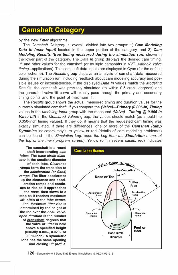
Camshaft Category
Cam Lobe BasicsThe camshaft is a round shaft incorporating cam
lobes. The base circle diam-eter is the smallest diameter
of each lobe. Clearance ramps form the transition to
the acceleration (or flank) ramps. The lifter accelerates up the clearance and accel-
eration ramps and contin-ues to rise as it approaches
the nose, then slows to a stop as it reaches maximum lift, often at the lobe center-
line. Maximum lifter rise is determined by the height of the toe over the heal. Valve-open duration is the number
of crankshaft degrees that the valve or lifter is held above a specified height (usually 0.006-, 0.020-, or 0.050-inch). A symmetric
lobe has the same opening and closing lift profile.
Base CircleDiameter
Rotation
ClearanceRamp
AccelerationRamp
AccelerationRamp
Lobe Centerline
ClearanceRamp
Opening
AecelerationC
losi
ng
Acc
eler
atio
n
Nose or Toe
Foot orHeel
LifterRise
Valve-Open Duration
by the new Fitter algorithms. The Camshaft Category is, overall, divided into two groups: 1) Cam Modeling Data In (user input) located in the upper portion of the category, and 2) Cam Modeling Results (true timing measured during the simulation run) shown in the lower part of the category. The Data In group displays the desired cam timing, lift and other values for the camshaft (or multiple camshafts in VVT...variable valve timing...applications). This camshaft data-inputs are displayed in Cyan (for the default color scheme). The Results group displays an analysis of camshaft data measured during the simulation run, including feedback about cam modeling accuracy and pos-sible issues or inconsistencies. If the displayed Data In values match the Modeling Results, the camshaft was precisely simulated (to within 0.5 crank degrees) and the generated valve-lift curve will exactly pass through the primary and secondary timing points and the point of maximum lift. The Results group shows the actual, measured timing and duration values for the currently simulated camshaft. If you compare the (Valve)—Primary (0.006-in) Timing values in the Modeling Input group with the measured (Valve)—Timing @ 0.006-in Valve Lift in the Measured Values group, the values should match (as should the 0.050-inch timing values). If they do, it means that the requested cam timing was exactly simulated. If there are differences, one or more of the Camshaft Ramp Dynamics indicators may turn yellow or red (details of cam modeling problem(s) can be found in the Simulation Log; open the Log from the Simulation menu; at the top of the main program screen). Yellow (or in severe cases, red) indicates
120—Dynomation6 & DynoSim6 Engine Simulations v6.02.08, 061518

Camshaft Category
The best way to visualize camshaft timing in a running engine is to picture this “twin-hump” Valve-Motion diagram (drawn “on the fly” in the CamManager™). You can see valve motion for the exhaust lobe on the left and the intake lobe on the right. Also illustrated are the valve-timing points, duration, valve overlap, valve lift, centerlines, lobe center angle, and “ideal” engine-cycle timing, all relative to TDC at the center of the drawing. Study this picture and the text in this section to help you visualize the intricacies of cam-timing specifications.
Valve-Motion Diagram Shown In The CamManager™
that it was not possible for the simulation to produce a lift curve with precisely the valve-event timing that was requested. Before we delve more deeply into the Camshaft Category and cam modeling in the simulation, it’s essential that we cover 10-point cam timing vs. lobe-profile timing.
Cam Basics
Most camshafts are steel or iron shafts with eccentric lobes. They are mechani-cally driven by the crankshaft, typically by a chain or gear train and are usually rotated at one-half crank speed. Lifters (or cam followers)—and for in-block cam locations, pushrods, and rockerarms—translate the rotary motion of the cam into an up-and-down motion that opens and closes the intake and exhaust valves. This entire assembly must function with high precision and high reliability. Street engines driven hundreds-of-thousands of miles operate their valvetrain components multiple billions of cycles. And after all that use, if the overall camshaft and valvetrain em-body a solid design, a precision measurement will detect only negligible wear! The camshaft controls valve opening and closing points by the shape and rota-tional “index” of the lobes (position relative to each other and the crankshaft). Most cams are ground to a precision well within one crankshaft degree, ensuring that valves actuate exactly when intended. However, timing variations of several degrees
Dynomation6 & DynoSim6 Engine Simulations, v6.02.08, 061518—121

Published Cam Timing SpecsLong before engine simulations were widely used, cam manufacturers estab-lished a methodology for identifying and classifying camshafts. Unfortunately, some of these “catalog” specs can be misleading. But the trend is toward pub-lishing exact valve-event timing for both seat-to-seat and 0.050-inch timing meth-ods (and even at additional lift points, like 0.100 or 0.200). Many cam manufactur-ers publish timing data for their entire camshaft line on the web. In fact, since printed catalogs are typically updated yearly, web postings tend to be more timely, including their latest cam develop-ments.
Camshaft Category
often develop in the cam drive, especially in chain-drive systems (racing gear drives typically reduce variations to within two crank degrees or less of indicated timing). Camshaft lobe height (heal-to-toe) and the multiplying ratio of rockerarms (if used) less any valve lash determines how far valves will lift off of the valve seats. The rates at which the valves are accelerated open and then returned to their seats are also “ground into” cam lobe profiles. Only a very specific range of contours will maintain stable valve motion, particularly with high-lift, racing profiles. Unstable profiles or excessive engine speed can force the valvetrain into “valve float” or other instabilities, resulting in component and/or engine failure.
Valve EventsAnd Event-Timing Standards
There are six “basic” cam timing events ground into cam lobes. These points control the following events:
1—Intake-Valve Opening (IVO) 2—Intake-Valve Closing (IVC)3—Exhaust-Valve Opening (EVO) 4—Exhaust-Valve Closing (EVC)5—Intake-Valve Maximum Lift 6—Exhaust-Valve Maximum Lift
The first four basic timing points (IVO, IVC, EVO, EVC) pinpoint the “true” begin-ning and end of the four engine cycles and dictate when the phase of the piston/cylinder mechanism changes from intake to compression, compression to power, power to exhaust, and exhaust back to intake. These six points can be “adjusted” somewhat (we’ll discuss which and how events can be altered in the next section), but for the most part they are fixed by the design of the cam. Several other timing points are often used, but they are always derived from the above, six events. Common derivative events are (discussed more later):
122—Dynomation6 & DynoSim6 Engine Simulations v6.02.08, 061518
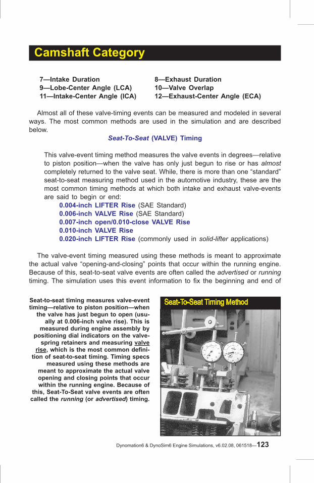
7—Intake Duration 8—Exhaust Duration 9—Lobe-Center Angle (LCA) 10—Valve Overlap 11—Intake-Center Angle (ICA) 12—Exhaust-Center Angle (ECA)
Almost all of these valve-timing events can be measured and modeled in several ways. The most common methods are used in the simulation and are described below.
Seat-To-Seat (VALVE) Timing
This valve-event timing method measures the valve events in degrees—relative to piston position—when the valve has only just begun to rise or has almost completely returned to the valve seat. While, there is more than one “standard” seat-to-seat measuring method used in the automotive industry, these are the most common timing methods at which both intake and exhaust valve-events are said to begin or end:
0.004-inch LIFTER Rise (SAE Standard)0.006-inch VALVE Rise (SAE Standard)0.007-inch open/0.010-close VALVE Rise0.010-inch VALVE Rise0.020-inch LIFTER Rise (commonly used in solid-lifter applications)
The valve-event timing measured using these methods is meant to approximate the actual valve “opening-and-closing” points that occur within the running engine. Because of this, seat-to-seat valve events are often called the advertised or running timing. The simulation uses this event information to fix the beginning and end of
Camshaft Category
Seat-To-Seat Timing MethodSeat-to-seat timing measures valve-event timing—relative to piston position—when
the valve has just begun to open (usu-ally at 0.006-inch valve rise). This is
measured during engine assembly by positioning dial indicators on the valve-
spring retainers and measuring valve rise, which is the most common defini-
tion of seat-to-seat timing. Timing specs measured using these methods are
meant to approximate the actual valve opening and closing points that occur within the running engine. Because of
this, Seat-To-Seat valve events are often called the running (or advertised) timing.
Dynomation6 & DynoSim6 Engine Simulations, v6.02.08, 061518—123
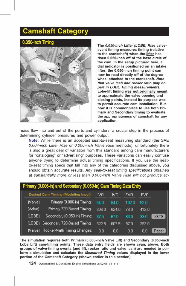
mass flow into and out of the ports and cylinders, a crucial step in the process of determining cylinder pressures and power output.
Note: While there is an accepted seat-to-seat measuring standard (the SAE 0.004-inch Lifter Rise or 0.006-inch Valve Rise methods), unfortunately there is also a great deal of variation from this standard among cam manufacturers for “cataloging” or “advertising” purposes. These variations can easily confuse anyone trying to determine actual timing specifications. If you use the seat-to-seat timing specs that fall into any of the categories discussed above, you should obtain accurate results. Any seat-to-seat timing specifications obtained at substantially more or less than 0.006-inch Valve Rise will not produce ac-
Camshaft Category0.050-Inch Timing
The 0.050-inch Lifter (LOBE) Rise valve-event timing measures timing (relative to the crankshaft) when the lifter has risen 0.050-inch off of the base circle of the cam. In the setup pictured here, a dial indicator is positioned on an intake lifter; the 0.050-inch timing point can now be read directly off of the degree wheel attached to the crankshaft. Note that valve lash and rocker ratio play no part in LOBE Timing measurements. Lobe-lift timing was not originally meant to approximate the valve opening and closing points, instead its purpose was to permit accurate cam installation. But now it is commonplace to use both Pri-mary and Secondary timing to evaluate the appropriateness of camshaft for any application.
The simulation requires both Primary (0.006-inch Valve Lift) and Secondary (0.050-inch Lobe Lift) cam-timing points. These data entry fields are shown cyan, above. Both groups of valve-timing events (and lift, rocker ratio and valve lash) are needed to per-form a simulation and calculate the Measured Timing values displayed in the lower portion of the Camshaft Category (shown earlier in this section).
Primary (0.006-in) and Secondary (0.050-in) Cam Timing Data Entry
124—Dynomation6 & DynoSim6 Engine Simulations v6.02.08, 061518

Camshaft Category
curate results when using 10-Point cam timing values (discussed below).
0.050-Inch (LOBE) Timing
This timing method is widely used and has been standardized by cam manu-facturers. 0.050-inch cam timing points are always measured at: 0.050-inch LIFTER Rise for both the intake and exhaust valves.
This measurement technique was not originally introduced to help evaluate valve opening-and-closing events, valvetrain acceleration, or cam suitability for a particular application. Rather it was intended to be used as an accurate index of cam-to-crank position during cam installation. Because of this, it is based on the movement of the cam follower (lifter) rather than the valve, eliminating valve lash and rocker ratio when measuring cam-to-crank timing. Since the follower will be positioned within the cam acceleration ramp at 0.050-inch lobe lift, and will have begun rapid movement up the lobe flank, using this point provides good way to verify the precise rotational index of the camshaft relative to the crankshaft. Although 0.050-inch valve timing events do not pinpoint when the intake and exhaust valves open or close, they provide valuable data for the simulation to mathematically model acceleration rates and to generate an accurate valve lift curve.
Important Note: Keep in mind that 0.050 Lobe Lift points (also called Secondary Timing) do NOT change when the rocker ratio or valve lash are altered. These timing points are measured on the cam follower, and only the lobe shape, lifter design, and the rotational-index between the cam and the crankshaft (ICA or ECA) will change Secondary Timing.
If you only have access to 0.050-inch timing data for a particular camshaft, you can still model the valve timing (albeit with somewhat reduced accuracy). Use the Convert To STS Timing (->STS) button to have the simulation extrapolate a “best guess” of seat-to-seat timing from the current 0.050-in Secondary values.
Note-1: To optimize accuracy, whenever possible, use the cam manufacturer’s
Extrapolating Seat-To-Seat Event Timing
Pressing the ->STS button in the Camshaft category will extrapolate new/updated Seat-To-Seat valve-event timing from the current 0.050-in Secondary values. Use this feature if you only have access to 0.050-in lobe-lift timing data for a particular camshaft.
Dynomation6 & DynoSim6 Engine Simulations, v6.02.08, 061518—125

Camshaft Category
published Seat-To-Seat and 0.050-in Timing values as the basis for 10-Point cam simulations.Note-2: Using the ->STS feature is never needed if you are importing Lobe Profile files, since both Seat-To-Seat and 0.050-in Lift points are obtained by direct measurement of the imported profile data. More information about 10-Point cam modeling and how it differs from Lobe-Profile modeling is presented next.
Cam Modeling With10-Point And Lobe-Profile Data
The simulation can use two distinct methods of modeling cam events and gen-erating a valve-motion curve. They are based on: 1) 10-Point Cam Data, or 2) Lobe-Profile Data. Here is a quick overview of these methods and how they are used to complete a simulation:
10-Point Cam-Data (CamFiles) consists of Valve-Event and Lobe-Event Timing for both the intake and exhaust lobes. These eight values, plus the maximum lift of each lobe, produce 10-data-points for each camshaft. The simulation uses this 10-Point data to accurately extrapolate the entire valve-motion curve. Profile Lobe Data (Profile Files) contain a virtual “blueprint” of cam lobes. While Profile Files may differ in their content depending on what measuring apparatus was used to analyze cam lobe shapes, they all contain lobe-lift data recorded at discrete rotational increments, typically at each degree of cam rotation (360 points). This profile data can be used as the basis for a valve-motion curve (only interpolation is needed to determine the exact valve lift for any crank positions “between” recorded values in the profile file). Ad-ditional information on using and importing Lobe Profile Files is presented later in this chapter.
10-Point Cam Timing Data
Rotation
Maximum Lift AtCalculatedLobeCenterline(assumingsymmetricprofile) Lifter
Rise
0.006-inchClosingPoint
0.006-inchOpeningPoint
0.050-inchTimingPoint
0.050-inchTiming
Point
10-Point Lifter Acceleration IsDerived From Seat-To-Seat and 0.050-Inch
Opening and Closing Points, And The Maximum Lift Of Each Lobe
“10-Point” Cam Data consists of valve-event timing for both the intake and
exhaust lobes at both seat-to-seat and 0.050-inch timing points. These eight
values, plus the maximum lift of each lobe, produce 10-data points for each
camshaft. The simulation uses 10-Point data to generate a valve-motion curve.
126—Dynomation6 & DynoSim6 Engine Simulations v6.02.08, 061518

Camshaft Category
You may be asking, “Since the simulation can read Lobe Profile files, why use any other “less precise” cam-data in a simulation”? The answer is: While cam profiles do contain the most accurate valve-motion data for a specific camshaft, using them in an engine simulation has some limitations. When a profile data set is used, modifying individual valve-opening or closing points is next to impossible. For example—just as in the real world—you can advance and retard profile data (for each lobe), change lash, rocker ratio, and that’s about the end of your tuning options. If you would like to test different intake timing (IVO, or IVC independently), your only option is to import a completely different profile using new timing values. Since individual valve-event timing is “baked into” profile data, it can’t be easily
Profile Data Conversion To 10-Point When Cam-Profile data is being used on the intake and/or exhaust valve, it is indicated in the Modeled From field. If you would like to use modified valve-event timing, profile data must be converted to 10-Point timing using the Convert To 10-Point (->10-pnt) but-ton. When the conversion is complete (engine power should be very similar if the conversion process was suc-cessful), you can modify any timing point and test its effect on engine output.
Lobe-ProFile Data
Profile data is made up of lobe-lift data recorded at, usually, each degree of camshaft rotation (by in-stalling the cam in a special fixture designed for this recording pro-cess). The simulation can use this data to determine valve positions at any point during the simulation.
Rotation
Maximum Lift Point Is DefinedTo Be Cam LobeCenterline
Lifter RiseDeterminesValve DurationOpening Point(0.020-inchis commonon manysolid-liftercams)
Lobe Lift Is MeasuredAt Each DegreeOf Cam Rotation
Lifter FallDetermines
Valve DurationClosing Point
(0.020-inchis common
on manysolid-lifter
cams)
Lobe Profiles Are Directly MeasuredAt Each Degree Of Camshaft Rotation
Measured Duration
Convert to 10-Point Timing
Pro�le Data Used
Dynomation6 & DynoSim6 Engine Simulations, v6.02.08, 061518—127

Camshaft Categorychanged without “corrupting” the original profile shape. When it comes to profile files, testing various cam-timing combinations requires loading completely different profiles, much the same way you would install a different cam in a real-world dyno test.
The Best Of Both Worlds
10-Point cam data can make cam simulation testing a lot more versatile, espe-cially when you are searching for optimum cam timing for a new application; one for which you may not have done extensive testing or research. 10-Point data sets are just that, 10 data points that the simulation uses to extrapolate a full valve-motion curve (in effect, a new “profile” data set) that establishes valve lift at each crank degree during the simulation process. The 10 points used are: IVO, IVC, EVO, and EVC, at both 0.006-in valve lift and 0.050-in lobe lift points...that’s 8 data points...plus the maximum lift for each lobe; that's 10 data points. This data, readily available on manufacturer's “cam cards,” cam catalogs and websites, is analyzed by the Fitter routines in the simulation to derive lobe and valve lift curves using a sinusoidal dynamics model that exactly passes through all 10 timing points. Since both Dynomation6 and DynoSim6 use the Fitter algorithm “on-the-fly” to derive valve-lift curves from event timing, you are free to alter any timing point and instantly see how it affects engine performance. You can quickly change any valve event, lift, or advance/retard timing and test the effects on engine performance. When you have completed your testing, you can: 1) Use the CamManager™ to automatically search through a 10-Point camfile library to locate “real” camshafts with published data that closely matches your test timing, or you can 2) Find cam-profile data sets that have event timing close to the discovered optimum. In both cases, using 10-Point cam timing facilitated finding best cam for your application. The following several sections discuss how 10-Point cam files are loaded, tested, and manipulated in the Camshaft Category and in the CamManager™. Importing Lobe Profile Files is also discussed in detail. Even if you were planning on using Lobe Profile data almost exclusively, we suggest that you read the following sec-
CamDisk™ For Dynomation6CamDisk™ for Dynomation6, included on the Dynomation CD, includes over
6000, 10-Point CamFiles. Using the CamManager™ and the Quick and
ProIterator™, Dynomation6 can automati-cally locate optimum profiles for virtu-
ally any application. Install the CamDisk library AFTER Dynomation6 has been
installed on your computer.
128—Dynomation6 & DynoSim6 Engine Simulations v6.02.08, 061518

Camshaft Category
tions on 10-Point timing. The information may help you improve your ability to test and locate optimum cam combinations for your test engine.
10-Point Generic Camshaft Menu Selections
The Cam Type menu in the Camshaft category contains 18 “generic,” camshafts (modeled using 10-Point timing data; see the previous section for an introduction to 10-Point cam timing) separated into two groups: Cams for 2-valve engines and cams for 4-valve engines. Since 2- and 4-valve applications can differ significantly in valve lift, and to some extent duration, the menu arrangement will help you quickly select a starting-point cam on which to base further testing. When using any of these camshafts, the lift and timing data is loaded into the appropriate fields in the Camshaft category. In addition, the Intake and Exhaust Centerlines, the Lobe Center Angle, the Intake and Exhaust Valve Duration, Valve Overlap and other cam-related data is measured by the Fitter (after the simulation is has been completed) and displayed in the lower portion of the Cam-shaft category. A general description of each cam in the Cam Type menu is provided in the next section.
2- And 4-Valve (Non-VVT) Cam Selections
2- And 4-Valve, Stock Street/Economy Cams These first cam selections are OEM-replacement street cams for 2- and 4-valve engines. The lifter acceleration rate falls between 2.51 and 2.83 (on a 1.00-to-7.00 scale), which indicates that valve motion for these cams fall in the range of stock OEM to mild street performance applications. Rated valve lift is 0.510/0.510-inch for 2-valve engines and 0.305/0.305-inch for 4-valve engines (intake/exhaust).
Several “generic” 10-Point cam data-sets are included in the Cam Type drop-down menu. They are separated into two groups, cams for 2-valve engines and cams for 4-valve engines. In addition, you can easily input any custom tim-ing and valve-lift specifications.
Camshaft Type Menu
Dynomation6 & DynoSim6 Engine Simulations, v6.02.08, 061518—129

Camshaft Category The EVO timing maintains combustion pressure late into the power stroke and early IVC minimizes intake flow reversion. Late IVO and early EVC produce 38 degrees of overlap for 2-valve engines and 11-degress for 4-valve engines, enough to harness some scavenging effects but limited enough to prevent severe exhaust gas reversion into the induction system. The characteristics of these cams are smooth idle, good power from 600- to 5000-rpm for 2-valve engines and typically between 1500- and 6500-rpm for 4-valve engines. These generic cams produce good fuel economy and work well in high-torque-demand applications.
2-Valve And 4-Valve High-Performance Street Cams These profiles are designed to simulate high-performance “street” camshafts for 2- and 4-valve engines. These cams produce lifter acceleration rates between 3.10 and 3.32, indicating that valve motion falls in the range of a typical, mild, street-performance camshaft. Rated valve lift is 0.552 / 0.552-inch for 2-valve engines and 0.432 / 0.435-inch for 4-valve engines (intake/exhaust). This camshaft uses relatively-late EVO to fully utilize combustion pressure and early IVC minimizes intake flow reversion (can be a serious problem on 4-valve engines, since low-lift flow can be substantial when both valves are open and expose large curtain areas). IVO and EVC produces between 54- and 60-degrees of overlap; profiles clearly intended to harness exhaust scavenging effects. The modestly-aggressive overlap allows some exhaust gas reversion into the induction system at lower engine speeds, affecting idle quality and low-speed torque. The characteristics of these cams are fair idle, good power from 1800- to 6000-rpm in 2-valve engines and between 2200- and 7500-
Non-V V T Cam Modeling Cam timing events, lift, and more are displayed in the Camshaft Category on the Main Program Screen. Cam specifications shown in Light Blue can be changed with a mouse click. Since the engine being modeled in this photo uses a 10-Point cam model, all remaining cam specifications can be modified both in the Cam-Shaft Category and in the CamManager™. Note this cam uses non-variable timing as shown by an unchecked V-V-T Enable box.
130—Dynomation6 & DynoSim6 Engine Simulations v6.02.08, 061518

Drag-Racing, High-Speed Cam Modeling All-out drag-racing cams for 2- and 4-valve engines are designed to optimize power on larger displacement engines at very high engine speeds with large-tube, open headers, and high com-pression ratios. These camshafts are often not effective in small dis-placement engines.
Camshaft Categoryrpm in typical 4-valve engines. Good fuel economy is still a by-product of the relatively “mild” cam timing. Both High Performance Street cams can be used with higher acceleration rates (typically up to about 4.00) to model more ag-gressive profiles.
2-Valve And 4-Valve Dual Purpose Street/Track Cams These profiles simulates high-performance aftermarket camshafts designed for street and mild track applications in 2- and 4-valve valve engines. These cams produce lifter acceleration rates of approximately 3.90, indicating that valve motion falls in the range of a high-performance street and mild racing. Rated valve lift is 0.608 / 0.614-inch for 2-valve engines and 0.472 / 0.457-inch for 4-valve engines (intake/exhaust). EVO timing on this camshaft is beginning to move away from specs that would be expected for optimum combustion pressure utilization, with more of an emphasis on blowdown and minimizing exhaust-pumping losses. The later IVC attempts to strike a balance between harnessing the ram effects of the induction system while minimizing intake flow reversion. IVO and EVC produce 63- to 65-degrees of overlap, profiles designed to harness exhaust scavenging. The modestly aggressive overlap allows some exhaust gas reversion into the induction system at lower engine speeds, affecting idle quality and low-speed torque (can be a more substantial issue on 4-valve engines, since low-lift flow can be substantial when both valves are off their seats and expose large cur-tain areas). The characteristics of this cam are lopey idle, good power from 2500- to 6500-rpm in 2-valve engines and between 2500- and 7800-rpm in typical 4-valve engines. These cams develop considerable power at higher engine speeds and are especially effective in lightweight vehicles.
Dynomation6 & DynoSim6 Engine Simulations, v6.02.08, 061518—131
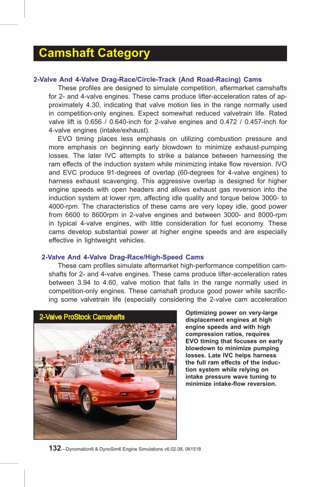
Camshaft Category
2-Valve And 4-Valve Drag-Race/Circle-Track (And Road-Racing) Cams These profiles are designed to simulate competition, aftermarket camshafts for 2- and 4-valve engines. These cams produce lifter-acceleration rates of ap-proximately 4.30, indicating that valve motion lies in the range normally used in competition-only engines. Expect somewhat reduced valvetrain life. Rated valve lift is 0.656 / 0.640-inch for 2-valve engines and 0.472 / 0.457-inch for 4-valve engines (intake/exhaust). EVO timing places less emphasis on utilizing combustion pressure and more emphasis on beginning early blowdown to minimize exhaust-pumping losses. The later IVC attempts to strike a balance between harnessing the ram effects of the induction system while minimizing intake flow reversion. IVO and EVC produce 91-degrees of overlap (60-degrees for 4-valve engines) to harness exhaust scavenging. This aggressive overlap is designed for higher engine speeds with open headers and allows exhaust gas reversion into the induction system at lower rpm, affecting idle quality and torque below 3000- to 4000-rpm. The characteristics of these cams are very lopey idle, good power from 6600 to 8600rpm in 2-valve engines and between 3000- and 8000-rpm in typical 4-valve engines, with little consideration for fuel economy. These cams develop substantial power at higher engine speeds and are especially effective in lightweight vehicles.
2-Valve And 4-Valve Drag-Race/High-Speed Cams These cam profiles simulate aftermarket high-performance competition cam-shafts for 2- and 4-valve engines. These cams produce lifter-acceleration rates between 3.94 to 4.60, valve motion that falls in the range normally used in competition-only engines. These camshaft produce good power while sacrific-ing some valvetrain life (especially considering the 2-valve cam acceleration
2-Valve ProStock Camshafts Optimizing power on very-large displacement engines at high engine speeds and with high compression ratios, requires EVO timing that focuses on early blowdown to minimize pumping losses. Late IVC helps harness the full ram effects of the induc-tion system while relying on intake pressure wave tuning to minimize intake-flow reversion.
132—Dynomation6 & DynoSim6 Engine Simulations v6.02.08, 061518

Camshaft Categoryrates of 4.60). Rated valve lift is 0.692 / 0.692-inch for 2-valve engines and 0.488 / 0.472-inch for 4-valve engines (intake/exhaust). All timing events on this camshaft are designed to optimize power on larger displacement engines at very high engine speeds with large-tube, open head-ers, and high compression ratios. This camshaft may not be effective in small displacement engines. EVO timing places the utilization of combustion pressure on the “back burner” and focuses emphasis on beginning early blowdown to minimize pumping losses during the exhaust stroke. This technique will help power at very high engine speeds, especially on 2-valve, large-displacement engines that do not easily discharge the high volume of exhaust gasses they produce. The late IVC attempts to harness the full ram effects of the induction system while relying on intake pressure wave tuning to minimize intake-flow reversion. IVO and EVC produce 104-degrees of overlap (71-degrees for 4-valve engines), a profile that is clearly intended to utilize exhaust scavenging effects. This very aggressive overlap seriously affects idle quality and torque below 4500rpm. A 5000rpm stall torque converter is recommended for auto-matic transmission applications. The characteristics of this cam are extremely lopey idle, good power from 4500 to 7200rpm in 2-valve engines and between 5000- and 9500-rpm in typical 4-valve engines, with no consideration for fuel consumption.
2-Valve ProStock/Max-Power Cam (modeled after CompCams 11-728-9) This profile is designed to simulate an all-out, maximum-power competition camshaft for 2-valve engines (because of the inherent better breathing in a 4-valve design, a cam of this design—an all-out attempt to generate maximum blowdown at the very highest speeds—is not necessary). This cam uses roller-solid lifters and produces an acceleration rate of 5.40, indicating that valve motion falls in the high range normally used in competition-only engines. Valvetrain loads will be substantial, and frequent replacement of valvesprings and other components may be required. Rated valve lift is 0.867-inch for the intake and 0.816-inch for the exhaust. This ProStock cam is designed for one thing: maximum power at all costs. It is designed to optimize power on very-large displacement engines at very high engine speeds with large-tube, open headers, and very-high compression ratios. EVO timing focuses on beginning early blowdown to minimize pumping losses, a technique that helps large-displacement engines discharge the high volume of exhaust gasses they produce. Late IVC attempts to harness the full ram effects of the induction system while relying on intake pressure wave tuning to minimize intake-flow reversion. IVO and EVC produce 110 degrees of overlap. This very aggressive overlap basically has no idle quality or torque below 6000rpm. The characteristics of this cam are extremely lopey idle, and awesome power potential from 7000 to 9000rpm.
2- And 4-Valve Variable-Valve-Timing (V-V-T)
Dynomation6 & DynoSim6 Engine Simulations, v6.02.08, 061518—133

Camshaft Category
Cam Modeling
There have been two major engineering “enhancements” incorporated in modern automobile engines that have contributed to new levels of performance and the potential for even more. Getting more air and fuel in the engine has always been the bottom-line for performance, and 4-valve cylinderheads accomplish that goal with
V-V-T Best Of Both WorldsVariable Valve Timing, like the VTEC
system used on this B16 (1600cc) Honda engine, lets the engine build optimum
power yet obtain good driveability and fuel economy (and much lower emis-
sions) at lower engine speeds.
V-V-T (VTEC) Camshaft Modeling
You can model variable valve tim-ing (V-V-T) as used by Honda (in their VTEC system) and engines with similar valvetrain designs. This mechanism uses a discrete low-speed profile, and then at a particular engine speed switches to a high-speed cam profile. Honda uses a simple pin (shown in green) driven with oil pres-sure (timed with an electronic control-ler) that locks the outer two low-speed rockers (actuating the valves) to the center rocker that rides on the high-speed lobe. This allows the engine to maintain excellent driveability and fuel economy at low speeds, yet produce power similar to a “race” engine at higher speeds.
134—Dynomation6 & DynoSim6 Engine Simulations v6.02.08, 061518

Porsche Boxter VarioCam™
The Porsche Boxter uses variable valve timing technology called Va-rioCam™. It alters the timing on the intake valves based on engine speed and load. As well as enhancing power and torque, the system offers smoother performance, improved fuel economy and lower emissions.
Camshaft Category
aplomb. While certainly not a “new” invention, 4-valve cylinder heads have become commonplace in showroom floors. But that’s not the whole picture, for it’s the com-bination of better breathing cylinder heads and Variable-Valve-Timing schemes that have brought power levels to such heights. These technologies have allowed the auto manufacturers to build a “one-two punch” into modern engines: 1) High flow potential with “aggressive,” high-speed cam profiles combined with low-restriction ports and valves, and 2) Maintain low emissions and excellent low-rpm power with mild, low-speed cam timing. Variable valve timing lets car manufacturers have what they need—a “mild” engine that meets emissions and driveability requirements—while giving performance enthusiasts what they want—no-compromise valve timing and optimum power. The Variable-Valve-Timing (V-V-T) model in the simulation functions like the basic cam-control system used on many Honda automobile engines (called VTEC™, for Variable Timing Electronic Control). At low speeds, the engine operates on Low-Speed Lobe profiles designed to minimize emissions and optimize driveability. Then, at some higher engine speed (usually between 4000 to 6000rpm), the valvetrain “switches over” to High-Speed Lobe profiles that, primarily, are designed for per-formance. Without the V-V-T system, Honda and other car manufacturers wouldn’t even consider using a cam with the timing specs of the high-speed lobes, since the engine would barely idle, have poor low-speed throttle response and torque, and generate plenty of unwanted emissions. But when that same cam is limited to high-rpm, wide-open-throttle use, power and driveability coexist.
Note-1: With more sophisticated electronic valvetrain systems, the timing of individual intake valves is staggered at low rpm and their lift is asymmetric, which creates charge swirl within the combustion chambers, reducing emis-
Dynomation6 & DynoSim6 Engine Simulations, v6.02.08, 061518—135

Camshaft Categorysions and improving fuel economy. At higher rpm, when more performance is desired—but before the valvetrain transitions to the High-Speed Lobes—both valves open in unison. Finally, at still higher speeds, the variable-valve-timing computer switches, as described previously, into high-lift, long-duration cam profile program.Note-2: There are many variations of variable cam timing technologies. The most advanced of these designs can provide virtually “ideal” timing for every driving situation, from idle through full-throttle performance and every step in between.
Whenever you select any of the V-V-T cams from the Cam Type menu, V-V-T modeling will be activated, as indicated by a checkmark in the box next to V-V-T Enable in the CAMSHAFT category. Also, when V-V-T is activated, the box next to the Variable Valve Timing field in the 10-Point CamManager™ (discussed later in this chapter) will display a checkmark.
4-Valve V-V-T Mild Street Cam This profile is designed to simulate conservative OEM camshafts that are used in some 4-valve, V-V-T engines. This cam uses direct-rocker valve actuation (Overhead Cam) and produces an acceleration rate of 2.55 for the Low-Speed Lobe and 2.85 for the High-Speed Lobe, indicating that valve acceleration for these profiles fall well within the range of stock to mild-performance rates. Rated valve lift is 0.325-inch (8.25mm) on the Low-Speed Lobes and 0.420 / 0.416-inch (10.67 / 10.57mm) for the intake and exhaust on the High-Speed Lobes. This camshaft uses very mild cam timing on the low-speed lobes, with only 15-degrees overlap. This profile is designed, primarily, to minimize emissions and maximize fuel economy up to the activation rpm of the high-speed lobes (typically 5000-to-5500rpm). The high speed lobe is of moderate performance design, with 30% more lift and a 6% increase in valve durations. Valve overlap is increased to 25-degrees, so exhaust scavenging effects will be minimal. The overall characteristics of this cam are smooth idle, good power from 1000 to 7500rpm, and good part-throttle fuel economy.
2- And 4-Valve V-V-T Performance Street Cams These profiles are designed to simulate mild-performance street camshafts commonly for 2- and 4-valve, V-V-T (VTEC) engines. These cams produce an acceleration rate of 2.83 to 2.41 for the Low-Speed Lobes about 3.15 for the High-Speed Lobes, indicating that valve acceleration for these profiles fall in the range of mild to performance rates. Rated valve lift is 0.510 (2-valve) / 0.335-inch (4-valve) on the Low-Speed Lobes and 0.552 (2-valve) / 0.459 & 0.416-inch (4-valve, intake/exhaust) for the High-Speed Lobes. This camshaft uses mild cam timing on the low-speed lobes, with only 38-de-grees overlap (2-valve cams) and 11-degrees (4-valve cams). These profiles
136—Dynomation6 & DynoSim6 Engine Simulations v6.02.08, 061518

VANOS™ BMW TechnologyVariable Valve Timing has be-come a “standard” on most engines. This Double-VANOS system, used on the BMW M3, changes the relationship between cams (alters the cam-centerline angle) to mod-ify valve overlap as engine rpm and engine load change.
Camshaft Categoryare designed, primarily, to reduce emissions and optimize fuel economy up to the activation rpm of the high-speed lobes (typically 5000-to-5500rpm). The high speed lobe is of moderate performance design. Valve overlap is increased to 60-degrees (2-valve) and 46-degrees (4-valve), a sufficient amount to begin harnessing some exhaust scavenging effects. If the high-speed lobe was used below about 4000rpm, the modestly-aggressive overlap would allow exhaust-gas reversion into the induction system at lower engine speeds, affecting idle quality and low-speed torque. The overall characteristics of this cam are smooth idle, good power from 1000 to 7500rpm, and good part-throttle fuel economy.
2- And 4-Valve V-V-T High-Performance Street Cams These profiles are designed to simulate high-performance street camshafts for 2- and 4-valve, V-V-T (VTEC) engines. These cams produce accelera-tion rates of 2.93 to 3.12 for the Low-Speed Lobes and 3.84 to 3.93 for the High-Speed Lobes, indicating that valve acceleration for this profile falls in the range commonly used for high-performance applications. Rated valve lift is 0.552 (2-valve) / 0.354-inch (4-valve) on the Low-Speed Lobes and 0.608 & 0.614-inch (2-valve, intake/exhaust) / 0.472 & 0.457-inch (4-valve, intake/exhaust) for the High-Speed Lobes. These camshafts use somewhat more aggressive cam timing on the low-speed lobes, with 60-degrees of overlap (2-valve cams) and 29-degrees (4-valve cams). These profiles will begin to harness exhaust scavenging effects even while running the low-speed cam timing. The increased overlap allows some exhaust gas reversion into the induction system at lower engine speeds, slightly affecting idle quality and low-speed torque. The high speed lobes are designed for performance, with 20% to 33% more lift and a 10% to 18% increase in valve durations. Valve overlap is increased to 63-degrees (2-valve cams) and 65-degrees (4-valve cams), modestly-aggressive values that take advantage
Dynomation6 & DynoSim6 Engine Simulations, v6.02.08, 061518—137

Camshaft Category
of free-flowing headers and mufflers (recommended for this cam). The narrow lobe centerline angle of 102-degrees on the 4-valve cam applications should be widened (with adjustable cam sprockets on dual-overhead cam engines) for turbocharged applications and even on some naturally-aspirated engines with low exhaust restriction. The overall characteristics of this cam are a slightly rough idle, good power from 2500 to 8500rpm, and moderate -to-good part-throttle fuel economy.
2- And 4-Valve Max Street/Race Cams These profiles are designed to simulate maximum performance street camshafts for 2- and 4-valve, V-V-T (VTEC) engines. These cams produce acceleration rates of 2.69 to 3.12 for the Low-Speed Lobes and 4.09 to 4.27 for the High-Speed Lobes, indicating that valve acceleration for this profile falls in the range for high-performance applications. Rated valve lift is 0.552 (2-valve) / 0.380 & 0.370-inch (4-valve, intake/exhaust) on the Low-Speed Lobes and 0.656 & 0.640-inch (2-valve, intake/exhaust) / 0.500 & 0.480-inch (4-valve, intake/exhaust) for the High-Speed Lobes. These low-speed lobe profiles for 2-valve engines are the same as the previous High-Performance Street Cam. The 4-valve camshaft uses relatively mild cam timing on the low-speed lobes, with only 16-degrees overlap. This profile is designed to maintain a good idle and torque at low engine speeds. The high speed lobes are a high-performance design, with an 18% to 31% more lift and 9% to 20% increase in valve durations. Valve overlap is increased to an aggressive 91-degrees (2-valve cams) and 76-degrees (4-valve cams) that takes advantage of free-flowing headers and mufflers (headers, while not required, will significantly improve performance with this cam). The lobe cen-
When any of the V-V-T cams have been select-ed or a V-V-T CamFile has been loaded in the CamManager™, V-V-T modeling will be activated, indicated by a checkmark in the V-V-T Enable box in the CAMSHAFT category and in the Variable Valve Timing box in the CamManager™. To display High-Speed lobe timing, click the Display High-Speed Lobe radio button.
Activating V-V-T And Displaying High-Speed Lobe
138—Dynomation6 & DynoSim6 Engine Simulations v6.02.08, 061518

Camshaft Categoryterline angle (106- to 109-degrees) of the high-speed lobes can be widened somewhat (with adjustable cam sprockets) for turbocharged applications and even on naturally-aspirated engines with very low exhaust restriction. The overall characteristics of this cam are good to slightly-rough idle and excellent power from 1500 to 9000rpm, with good to moderate part-throttle fuel economy.Note: Each of the previous application-specific cams can be modified by directly entering custom valve-event timing or other cam specifications.
Variable Valve Timing (V-V-T) ActivationAnd Custom V-V-T Modeling
When you select a V-V-T cam from the Cam Type menu in the CAMSHAFT category, or you import/load a V-V-T cam, Variable Valve Timing modeling will be activated, however, you can activate or deactivate Variable Valve Timing at any time. When activated, Low-Speed Lobe timing will be used in the simulation until the engine reaches the HS Lobe Activation rpm, after which High-Speed Lobe tim-ing will be used.
Note: When V-V-T is deactivated, by un-checking the V-V-T Enable checkbox, only “Low-Speed Lobe” timing will be used in the simulation.
You can also create a V-V-T cam from “scratch” to meet any requirement. For example, if you have found a non-V-V-T camshaft that produces good low-speed performance and another cam that produces good high-speed power, you can “com-bine” the two cams in the simulation. Here’s how: First, import or directly enter the cam timing for the low-speed lobe. When low-speed data has been entered (and all other engine component specs have been entered), a simulation will be performed. Next, activate V-V-T camshaft modeling (by clicking the V-V-T Enable checkbox). The Camshaft Category indicator may switch to RED, indicating that the category is no longer complete. Now, click on the Display High-Speed Lobe radio button and enter the cam timing for the High-Speed Lobe. When complete, the simulation will model the original Low-Speed camshaft up to the HS Lobe Activation speed, after which High-Speed timing will be used.
Lobe-Lift, Rocker-Ratio, Valve-LashAnd Net Valve Lift
The Intake and Exhaust True Lift @ Valve fields display the maximum lift (at the valves) for the currently-selected camshaft, regardless of whether the cam was chosen from the Cam Type menu, loaded as a Cam Profile, manually entered as valve-event specs, or loaded from a CamFile using the 10-Point CamManager™. The values displayed in the True Lift @ Valve fields are mathematically linked with the current Lash values and the Rocker Ratios. Normally, the True Lift @ Valve values are computed from data in the fields directly above: Gross Lobe Lift, Rocker Ratio, and Valve Lash. The calculation begins at Gross Lobe Lift. This
Dynomation6 & DynoSim6 Engine Simulations, v6.02.08, 061518—139

Camshaft Category
value is multiplied by the Rocker Ratio and the result is displayed in the Gross Valve Lift field. This value is then reduced by the Valve Lash to yield the final True Lift @ Valve for both the intake and exhaust valves. The simulation main-tains this mathematical relationship. If you change the Lash, the True Lift will be recalculated. In fact, if you change the True Lift directly, the program will assume that the Gross Lobe Lift must have changed, and it will recalculate that value to keep the mathematical relationship “in sync.”
Rocker-Ratio, Lash, And The Rocker-Math Calculator: DO NOT use the Rocker-Math Calculator (discussed in more detail later in this chapter) to enter the cam manufacturer’s specifications for Rocker Ratio and Valve Lash. Always
Valve Lift, Lash, And Rocker RatioThe simulation maintains the mathematical relationship
between all the Lift fields in the Camshaft Category. If you change the Lash, the True Lift
will be recalculated. If you change the final True Lift, the program will assume that the Gross Lobe Lift was changed
and it will recalculate that value to keep the mathematical
relationships “in sync.”
Gross Lobe LiftGross Lobe Liftx Rocker Ratiox Rocker Ratio
= Gross Valve Lift
= Net Valve Lift
Gross Valve Lift
= Net Valve Lift— Valve Lash
True Valve Lift Menu
Use the True Lift data field to quickly enter after-lash and after-rocker-ratio maximum valve lift values for the intake and/or exhaust valves. Note: If you perform an entry in this field, the Gross Lash will be re-calculated to maintain the mathematical relationships between the lift, lash, and ratio fields. Use Auto Calculate Valve Lift to have the simulation automatically calculate BOTH intake and exhaust valve-lift values when valve lift data is unknown (see the text for more information on using “auto calc” features in the simulation).
140—Dynomation6 & DynoSim6 Engine Simulations v6.02.08, 061518

Auto Calculate Valve Lift Indicator When Auto Calculate Valve Lift is en-abled, the simulation will automatically calculate BOTH intake and exhaust valve-lift values. The Auto-Calculation feature displays an “A” next to the calculated valve lift values when it is activated. Selecting Auto Calculate from the menu, instructs the simulation to automatically calculate appropriate valve lifts values for both the intake and exhaust valves. This is useful to quickly estimate typical cam manufac-turer's valve lift for the selected cam timing and application.
Camshaft Categoryenter these specs in the Camshaft Category directly. Then, after the recom-mended specifications have been entered, use the Rocker Math Calculator to determine how CHANGES to these stock specifications will affect cam timing, valve lift, and simulation results. For more information on using the Rocker-Math Calculator, see the chapter Version-6 Built-In Calculators).
Using the Net (Sim) True Valve-Lift Menu
As mentioned previously, the Direct-Click™ menus for the True Lift @ Valve fields allow you to quickly change the maximum valve lift, useful in those cases where you wish to perform “free-form” testing of lift vs. engine output. If you have imported a specific cam, be aware that the original Gross Lift values from your CamFile will be overwritten to maintain the mathematical relationship between the newly entered Net Lift and the existing Rocker Ratio and valve Lash. The True Lift @ Valve menus are intended for those times when you aren’t concerned about maintaining existing cam specs; you simply wish to enter a specific lift without concern for rocker ratio, lash, or other considerations. This also applies to the Auto Calculate Valve Lift option at the bottom of the True Lift @ Valve menu. This function (see photo, below) is useful when you want to use an appropriate valve-lift based on the current valve diameters. When Auto Calculate is enabled, the simulation will automatically calculate the lift for BOTH intake and exhaust valves (Gross Lobe Lift may be recalculated to maintain the mathematical relationships with the Rocker Ratio, and Valve Lash. The Auto-Calculation feature can be turned off by re-selecting Auto Calculate Valve Lifts (“A” indicator and the checkmark in the menu will be removed).
Note 1: Auto Calculate Valve Lifts is turned off by default when any CamFile is loaded, since each CamFile represents a “real-world” cam that has specific valve-lift values associated with it. However, you can reactivate Auto-Calculation at any time by selecting it from the menus.Note 2: If Valve Diameters are also being automatically calculated in the Cyl-
AutoCalc Lift Indicator
Dynomation6 & DynoSim6 Engine Simulations, v6.02.08, 061518—141

Camshaft Category
inder Head component category—cylinder-bore diameter and a cylinder-head selection must be made before the program can complete the calculation of valve diameters and, consequently, valve lifts.
An Introduction ToThe Rocker-Math Calculator
The Camshaft Category includes a Rocker-Math Calculator that will help you analyze how and why changes in rocker ratio affect engine output. To use the Calculator appropriately, follow this simple rule: Enter original cam manufacturer’s specifications for Rocker Ratio in the Camshaft Category FIRST! Then use the Rocker Math Calculator to determine how CHANGES to these specifications will affect cam timing, valve lift, and engine power. For more information on using the Rocker-Math Calculator, see the chapter Version-6 Built-In Calculators later in this manual.
Lifter/Valve Acceleration Rates
The simulation performs an analysis of the valve motion generated by cam lobe profiles and displays an overall valvetrain acceleration rate. The acceleration values are calculated from an analysis of intake and exhaust opening and closing ramps, flank and nose radii, all timing specifications, and maximum lift data. The values (from 1.0 to 9.0+), displayed in the Additional Cam Specs group in the Camshaft Categtory. Individual intake and exhaust valve acceleration rates are displayed in the Measured Values group. The range of acceleration values form a relative scale that offers 900-steps of granularity. The values include acceleration rates used in modern production/street cams (with values ranging from 1 to 3) to racing-only applications (with values
Rocker-Math Calculator
Follow a simple rule when using Rocker Math: Enter the original
cam manufacturer’s specifica-tions for Rocker Ratio in the
Camshaft Category FIRST! Then use the Rocker Math Calculator to determine how CHANGES to
these stock specifications affect cam timing, valve lift, and engine
power.
142—Dynomation6 & DynoSim6 Engine Simulations v6.02.08, 061518

Rotation
Maximum Lift AtCalculatedLobeCenterline(assumingsymmetricprofile) Lifter
Rise
0.006-inchClosingPoint
0.006-inchOpeningPoint
0.050-inchTimingPoint
0.050-inchTiming
Point
10-Point Lifter Acceleration IsDerived From Seat-To-Seat and 0.050-Inch
Opening and Closing Points, And The Maximum Lift Of Each Lobe
Valve Motion Curves & Acceleration
The simulation calculates valve accelera-tion rates based on current valve timing
specifications. Valvetrain acceleration values range from 1.00 (very-low acceler-ation) to 9.00+ (extremely-high accelera-tion). This data is provided for any Lobe
Profile or any 10-Point cam model.
Camshaft Category
from 4 or 5 to as high as 6 to 8+). Using this simple designation, you can quickly determine the general operating characteristics of any camshaft. Use the following guidelines to evaluate Acceleration Rates: 1.00 Very Low Acceleration 2.00 Stock Production, OEM Camshafts, Long Valvetrain Life 3.00 Performance OEM and Aftermarket Performance, Good Life 4.00 Mild Racing & Performance, Limited Street Application
Lifter/Valve Acceleration Display The simulation automatically calcu-lates values that represent the Over-all Cam Acceleration and individual Valve Acceleration Rates by perform-ing an analysis of valve timing and lobe dimensional specifications. The Intake and Exhaust Valve Accelera-tion values are displayed in the Mea-sured Values group. The overall Cam Acceleration Rate is shown in the Additional Cam Specifications fields. The acceleration rates vary from 1.0 to as high as 9.0+ (see the text for more information on these values).
Cam & Valve Acceleration Rates
Dynomation6 & DynoSim6 Engine Simulations, v6.02.08, 061518—143

Camshaft Category 5.00 Racing, Valvetrain Loads Require Use Of Optimum Components 6.00 Racing, Reduced Valvetrain Life With Best Components 7.00 High Valvetrain Loads, Requires Regular Valvetrain Maintenance 8.00+ Extreme Acceleration And Loads, Very Limited Valvetrain Life
If you wish to evaluate changes in valve acceleration, you must alter the shape of the lobes; defined, in part, by the location of Seat-to-Seat and 0.050-inch tim-ing points and the maximum lift of the lobes. Moving 0.050-timing closer to Seat-To-Seat (and/or increasing lift) will mathematically reshape the lobe and increase the acceleration (this requires 10-point cam timing as described earlier). Moving 0.050-timing farther from Seat-To-Seat values will decrease acceleration. All modified timing values are analyzed for stability by the Fitter algorithms in the simulation. Values that generate lobe shapes that cannot be properly modeled will trigger one of the Valvetrain Dynamics Indicators in the Camshaft Category to switch from green to yellow or red.
Note-1: Select Show Simulation Log from the Simulation Menu at the top of the program screen to obtain additional information about any displayed yellow or red valvetrain indicators.Note-2: In Dynomation-5 & DynoSim5, the acceleration rate could be directly modified. Now, cam/valve timing points directly control the acceleration values for both the intake and exhaust valves. You can still modify the acceleration rates, however, it requires changing valve timing, rocker ratios, and/or maxi-mum lift values.
Ramp Dynamics IndicatorsThe simulaton analyzes valvetrain dynamics for
any 10-point cam used in the simulation. If the Fitter
algorithms cannot gener-ate a stable sinusoidal
curve that passes through the opening, closing and
max-lift points, one or more of the Dynamics
Indicators in the Camshaft Category will switch from
green to yellow or red (de-pending on the severity of
the mismatch).
Valvetrain Indicators
144—Dynomation6 & DynoSim6 Engine Simulations v6.02.08, 061518

Camshaft CategoryNote-3: The valvetrain acceleration rates for 4-valve engines often are not as high as those for 2-valve engines designed for similar applications. 4-valve engines benefit from higher low-lift flow (due to the increased curtain area exposed as both valves open), and consequently, cams for these engines do not normally accelerate the valves as rapidly off of the seats.
Dynomation6 & DynoSim6 Engine Simulations, v6.02.08, 061518—145

Camshaft Category—The CamManager™
The 10-Point CamManager™ is a cam manipulation tool for 10-Point cam specs built into the simulation. It offers complete control and visualization of all 10-Point timing and lift values. Use it to enter and modify any cam-related information and search for “real-world” camshafts from your cam libraries that matches any desired range of tim-ing values.
The 10-Point Cam Manager™
Using The 10-Point CamManager™Applies To FE and WA Simulations, Except as Indicated
The CamManager™ is a comprehensive tool built into the simulation that will help you display, test, modify, and even search your cam libraries for optimum 10-Point cam modeling data for any engine application.
Note About Lobe Profile Files: When a Lobe Profile file is loaded into the simulation, the CamManager is no longer directly accessible. If you attempt to open the CamManager, a dialog will let you know that if you proceed, all Profile data used by the current simulation will be converted to 10-Point timing data. The reason for this is that the CamManager is specifically designed as a 10-Point valve-event manipulation tool. Since individual valve-events cannot be changed when Lobe Profile files are used (only centerlines, cam advance and retard, rocker ratio, and lash can be altered; these specifications can all be modified directly from within the Camshaft Component category) the CamManager features are not available when Lobe Profile data is used in
146—Dynomation6 & DynoSim6 Engine Simulations v6.02.08, 061518

Camshaft Category—The CamManager™
The CamManager™ incorporates a wide range of functionality and tools that are intui-tive and easy-to-use. To this end, the CamManager is divided into functional groups that separate basic functionality into several “boxes” (see text for more information).
The CamManager™ Features And Functional Groups
Lifter Acceleration Display
Variable ValveTiming Lobe
Selection/Activation OK/Apply/
Cancel
Cam-TimingDiagram
Open/SaveCamFiles
Tabbed Data-Entry Pages
FunctionalGroupBoxes
the simulation.
The CamManager has many features and capabilities. To make this comprehen-sive tool as easy-to-use as possible, the interface is divided into functional “groups.” Each group of controls is positioned within a “titled box” or on a “tabbed data page.” For example, when the CamManager is first opened (click the CamManager but-
When a Cam Profile file is used, the CamManager™
is no longer available (works only with 10-point
cam files data). If you attempt to open the
CamManager, a dialog will let you know that if you proceed, all current Lobe-Profile data will be
converted to 10-Point data. If you click OK, the
simulation will convert all Lobe Profiles to 10-point
data that closely matches the original Lobe Profiles.
Lobe Profile Data And The CamManager
Dynomation6 & DynoSim6 Engine Simulations, v6.02.08, 061518—147
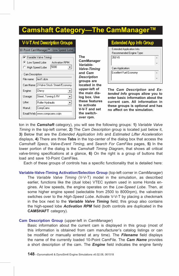
Camshaft Category—The CamManager™
ton in the Camshaft category), you will see the following groups: 1) Variable Valve Timing in the top-left corner, 2) The Cam Description group is located just below it, 3) Below that are the Extended Application Info and Estimated Lifter Acceleration displays, 4) There are three Tabs in the top-center of the dialog box that access the Camshaft Specs, Valve-Event Timing, and Search For CamFiles pages, 5) In the lower portion of the dialog is the Camshaft Timing Diagram, that shows all critical valve-timing specifications at a glance, 6) On the right is a group of buttons that load and save 10-Point CamFiles. Each of these groups of controls has a specific functionality that is detailed here:
Variable-Valve-Timing Activation/Selection Group (top-left corner in CamManager) The Variable Valve Timing (V-V-T) model in the simulation, as described earlier, functions like the (dual lobe) VTEC system used in some Honda en-gines. At low speeds, the engine operates on the Low-Speed Lobe. Then, at some higher engine speed (selectable from 2500 to 8000rpm), the valvetrain switches over to the High-Speed Lobe. Activate V-V-T by placing a checkmark in the box next to the Variable Valve Timing field; this group also contains the high-speed lobe Activation RPM field (both controls are duplicated in the CAMSHAFT category).
Cam Description Group (upper-left in CamManager) Basic information about the current cam is displayed in this group (most of this information is obtained from cam manufacturer’s catalog listings or can be modified or manually entered at any time). The Filename field displays the name of the currently loaded 10-Point CamFile. The Cam Name provides a short description of the cam. The Engine field indicates the engine family
V-V-T And Description Groups
The CamManager Variable-Valve-Timing and Cam Description groups are located in the upper-left of the main dia-log box. Use these features to activate V-V-T and set the switch-over rpm.
Extended App Info Group
The Cam Description and Ex-tended Info groups allow you to enter basic information about the current cam. All information in these groups is optional and has no affect on the simulation.
148—Dynomation6 & DynoSim6 Engine Simulations v6.02.08, 061518

Camshaft Category—The CamManager™for which the camshaft was designed. The Usage field indicates the intended application. The Lifter field displays the lifter technology used with this cam. The Manufacturer field displays the manufacturer/designer of the cam. And the Email/Web field provides contact info. The Engine, Usage, and Lifter fields have suggested entries available in drop-down menus. And although you can skip entering any information into these fields, we recommend that you complete them since this data can help locate the camshaft when performing CamFile searches, described later.About Entered Text And Special Characters: If you paste data into any of the data fields in the Cam Manager (e.g., using the Ctrl-C and Ctrl-V cut-and-paste functions), the simulation will examine the text for special (non-standard-text) characters. If any are found, they will be replaced with spaces. If this is not done, Camfiles or Engine files may not open properly and can cause program crashes.
Extended Application Info (left-center in CamManager dialog)Additional operational characteristics of the cam and engine can be included in this group. The Recommended Engine Type field typically displays the engines for which the cam was designed. The Cam Application field can be used to describe cam specs, operation, related requirements, and performance characteristics. The information in this group was usually obtained from cam manufacturer’s catalogs and other published data sources. You can edit, modify, or add information to either of these fields.Note: All data in the Cam Description and Extended Application Info groups is optional and has no affect simulation output; it is provided for information and documentation only.
Camshaft Timing Diagram (lower-center in CamManager dialog)This graph, sometimes called a “twin-hump” diagram, shows the motion curves for the intake and exhaust valves (Note: The portion of crank rotation during which the intake and exhaust valves are closed, 120-degrees on this diagram,
Dynamic “Twin-Hump” Camshaft Timing DiagramThe “Twin-Hump” valve motion
diagram in the CamManager is
dynamically updat-ed anytime timing specifications are
changed (see text).
Dynomation6 & DynoSim6 Engine Simulations, v6.02.08, 061518—149
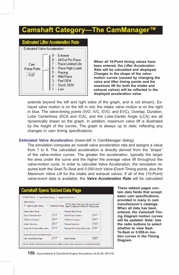
Camshaft Category—The CamManager™
extends beyond the left and right sides of the graph, and is not shown). Ex-haust valve motion is on the left in red; the intake valve motion is on the right in blue. The valve-timing points (IVO, IVC, EVO, and EVC), Overlap, Duration, Lobe Centerlines (ECA and ICA), and the Lobe-Center Angle (LCA) are all dynamically drawn on the graph. In addition, maximum valve lift is illustrated by the height of the curves. The graph is always up to date; reflecting any changes in cam timing specifications.
Estimated Valve Acceleration (lower-left in CamManager dialog)The simulation computes an overall valve acceleration rate and assigns a value from 1 to 9. The calculated acceleration is directly derived from the “shape” of the valve-motion curves. The greater the acceleration, typically the larger the area under the curve and the higher the average valve lift throughout the valve-motion cycle. In order to calculate Valve Acceleration, the simulation re-quires both the Seat-To-Seat and 0.050-inch Valve-Event Timing points, plus the Maximum Valve Lift for the intake and exhaust valves. If all of this (10-Point) valve-event data is available, the Valve Acceleration Rate will be calculated
Estimated Lifter Acceleration Rate
When all 10-Point timing values have been entered, the Lifter Acceleration Rate will be calculated and displayed. Changes in the shape of the valve-motion curves (caused by changing the valve and lifter timing points and the maximum lift for both the intake and exhaust valves) will be reflected in the displayed acceleration value.
Camshaft Specs Tabbed Data Page These tabbed pages con-tain data fields that accept basic cam specifications, provided in many in cam manufacturer’s catalogs. When all data has been entered, the Camshaft Tim-ing Diagram motion curves will be updated. Note: Use the radio buttons to select whether to view Seat-To-Seat or 0.050-in mo-tion curves in the Timing Diagram.
150—Dynomation6 & DynoSim6 Engine Simulations v6.02.08, 061518
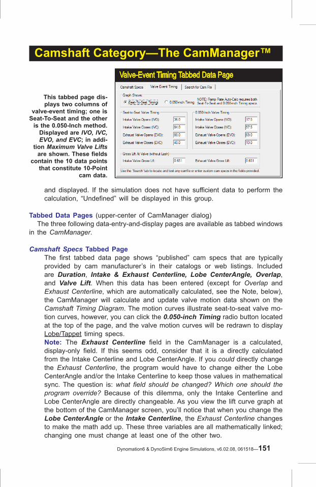
Camshaft Category—The CamManager™
and displayed. If the simulation does not have sufficient data to perform the calculation, “Undefined” will be displayed in this group.
Tabbed Data Pages (upper-center of CamManager dialog) The three following data-entry-and-display pages are available as tabbed windows in the CamManager.
Camshaft Specs Tabbed PageThe first tabbed data page shows “published” cam specs that are typically provided by cam manufacturer’s in their catalogs or web listings. Included are Duration, Intake & Exhaust Centerline, Lobe CenterAngle, Overlap, and Valve Lift. When this data has been entered (except for Overlap and Exhaust Centerline, which are automatically calculated, see the Note, below), the CamManager will calculate and update valve motion data shown on the Camshaft Timing Diagram. The motion curves illustrate seat-to-seat valve mo-tion curves, however, you can click the 0.050-inch Timing radio button located at the top of the page, and the valve motion curves will be redrawn to display Lobe/Tappet timing specs.Note: The Exhaust Centerline field in the CamManager is a calculated, display-only field. If this seems odd, consider that it is a directly calculated from the Intake Centerline and Lobe CenterAngle. If you could directly change the Exhaust Centerline, the program would have to change either the Lobe CenterAngle and/or the Intake Centerline to keep those values in mathematical sync. The question is: what field should be changed? Which one should the program override? Because of this dilemma, only the Intake Centerline and Lobe CenterAngle are directly changeable. As you view the lift curve graph at the bottom of the CamManager screen, you’ll notice that when you change the Lobe CenterAngle or the Intake Centerline, the Exhaust Centerline changes to make the math add up. These three variables are all mathematically linked; changing one must change at least one of the other two.
Valve-Event Timing Tabbed Data Page
This tabbed page dis-plays two columns of
valve-event timing; one is Seat-To-Seat and the other
is the 0.050-Inch method. Displayed are IVO, IVC, EVO, and EVC; in addi-
tion Maximum Valve Lifts are shown. These fields
contain the 10 data points that constitute 10-Point
cam data.
Dynomation6 & DynoSim6 Engine Simulations, v6.02.08, 061518—151

Camshaft Category—The CamManager™
Valve-Event Timing Tabbed PageThe second tabbed data-entry page displays valve-event timing for both seat-to-seat and 0.050-inch timing specs. Included are IVO, IVC, EVO, EVC and Maximum Valve Lifts. When this data is complete, the simulation will (re)calculate the Camshaft Specs and use the new data in the simulation. Both seat-to-seat and 0.050-inch valve-event values must be entered (completing all data fields on this tabbed page), before a simulation can be performed.Note: The fields shown in the Valve-Event Tabbed Page constitute the 10 data values defined in 10-Point cam data.
Search For CamFiles Tabbed PageThe third tabbed page provides considerable versatility in locating 10-Point CamFiles for your test engine. Search through thousands of CamFiles and locate only those that meet your criterion. For example, you can find all the cams designed for a Honda, or locate all cams that closely match the speci-fications discovered in an Iterator™ test series (more on the Iterators later). If you would like to search for specific filenames or cam descriptions, first enter any search terms into the Criteria fields. If you would like to locate CamFiles that fall within a range of timing values centered around the current camshaft timing (the current cam is the cam currently used in the simulated engine), check the box labeled Find The Following Specs. Finally, click the Search button to perform a search of all CamFiles found in the folder listed in the Look In field and in any folders that are nested below that folder (a full recursive search for all .DCM, .CAM, and .SCM files is performed). When a list of matching CamFiles is presented, simply click on any file to view its characteristics (use the up-and-down arrow keys to quickly move through the results list). Transfer any CamFile into the CAMSHAFT component category and into the simulated engine by clicking Apply (“installs” the cam and leaves the CamManager open) or OK (“installs” the cam and closes the CamManager).
Search For CamFiles Tabbed Data Page
The Search For CamFiles “tabbed” page provides a way to rapidly locate 10-Point CamFiles. You can search through thousands of CamFiles and locate only those that meet your criterion.
152—Dynomation6 & DynoSim6 Engine Simulations v6.02.08, 061518

Camshaft Category—The CamManager™Note: To extend the search capabilities of the CamManager, a 10-Point Cam Data Library is included with Dynomation6 and is available for DynoSim6. You can install these addi-tional library files into the normal directory structure of the simulation (the installer is provided on the Dynomation6 CD or on the optional CamDisk for DynoSim6), adding more than 6000 CamFiles to those already available to the CamManager.
CamManager Button FunctionsThe standard OK, Cancel, and Apply buttons transfer (or Cancel) any changes made in the CamManager. The Clear button erases all data in the CamManager in preparation for entering all specs from “scratch.” Finally, the Open and Save buttons are used to load and save cam files (using Apply updates the simulation with the current cam specs and leaves the CamManager open).
Important Note: Keep in mind that if you enter or change cam specifications within the CamManager after saving or retrieving a CamFile, the changed cam data WILL be saved in the engine (.DXML) file but NOT in a separate CamFile unless you specifically Save the modified cam data to a CamFile on your computer.
Loading 10-Point CamFiles
The CamManager is the “central clearing house” through which you can load, import, save, and search for 10-Point CamFiles. Here is a quick overview of how to load and save various CamFiles:
Opening .DCM, SCM, and .CAM Camfiles (Motion Software CamFiles)The CamManager will Open camfiles that were either saved by Dynomation6 or DynoSim6 (.DCM file) or other Motion Software engine simulations. To open any of these files, simply click the Open button in the CamManager and se-lect the desired file type from the File Open dialog box. Here are the 10-point camfiles compatible with this simulation:
10-Point Cam-Timing Files File ExtensionDynomation-5 & -6 CamFiles .DCMDynoSim6 CamFiles .DCMDynoSim-4 & -5 CamFiles .CAMSC-DynoSim CamFiles .SCM
The CamManager uses the stan-dard OK, Cancel, & Clear buttons. Open and Save loads and saves 10-Point Cam-files.
Dynomation6 & DynoSim6 Engine Simulations, v6.02.08, 061518—153

Camshaft Category—The CamManager™
To import any of these camfiles, open the CamManager, click the Open button, select the desired file extension from the Files Of Type drop-down list, then locate the file you wish to import and click OK. When the dialog box closes, press the Apply or OK button in the CamManager to transfer the cam data into the simulation.
Saving CamFilesOpen the CamManager, click the Save button, locate the CamFile (.DCM) folder (or one of its subfolders), then save the current CamFile to your hard drive.
Important Note: Keep in mind that if you enter or change any cam specifica-tions either inside or outside the CamManager, the changed cam data WILL be saved with the engine (.DXML) file but WILL NOT be saved in a separate CamFile unless you specifically Save the modified cam data from within the CamManager.
154—Dynomation6 & DynoSim6 Engine Simulations v6.02.08, 061518

Camshaft Category—The CamManager™
Dynomation6 & DynoSim6 Engine Simulations, v6.02.08, 061518—155

Camshaft Category—Using Lobe Profiles
Lobe-ProFile Data Lobe-Profile data is made up of lobe-lift data recorded for the intake and exhaust lobes (by installing the cam in a special fixture designed to measure and record this data). The simulation can individu-ally import intake and exhaust data from several common lobe-profile formats.
Rotation
Maximum Lift Point Is DefinedTo Be Cam LobeCenterline
Lifter RiseDeterminesValve DurationOpening Point(0.020-inchis commonon manysolid-liftercams)
Lobe Lift Is MeasuredAt Each DegreeOf Cam Rotation
Lifter FallDetermines
Valve DurationClosing Point
(0.020-inchis common
on manysolid-lifter
cams)
Lobe Profiles Are Directly MeasuredAt Each Degree Of Camshaft Rotation
Measured Duration
Importing And Using Lobe-Profile Files
Dynomation6 and DynoSim6 can Open/Import a variety of cam-data files. These files are divided into two main groups: 1) 10-Point CamFiles, and 2) Lobe-Profile Data Files. 10-Point cam data is primarily handled through the CamManager (see previous section). This portion of the Camshaft Category chapter discusses import-ing and using Lobe-Profile data files in your engine testing.
Note: For more information on the differences between 10-Point and Profile data, refer to 10-Point And Lobe-Profile Cam Data earlier in this chapter.
Lobe-Profile data is virtual “snapshot” of a cam lobe (separate data-sets are used for intake and exhaust lobes). Lobe-lift data is recorded at, usually, each degree of camshaft rotation. This is accomplished by installing the cam in a special, lathe-type fixture designed to measure lifter rise as the cam is rotated on centers. Audie Technology, and several other companies, manufacture these devices. Profile files vary in format, but most contain 360 data points. Some profile files also contain data-sets for more than one lobe, centerline data, application info, etc. The simulation can Import several common Lobe-Profile file formats.
Supported Cam-Profile Files Common File Extension CamPro .P1 and .P CamProPlus .CPP Cam Doctor .CXX (XX = lobe ID numbers)
S96 .S96
CamPro and CamProPlus (CPP) Profile FilesCamPro files were developed by Audie Technology, Inc. The file extensions for CamPro files are .Px or .Pxx, where x or xx is usually the cylinder num-ber of the cam lobes. CamProPlus files have a .CPP extension. These files
156—Dynomation6 & DynoSim6 Engine Simulations v6.02.08, 061518
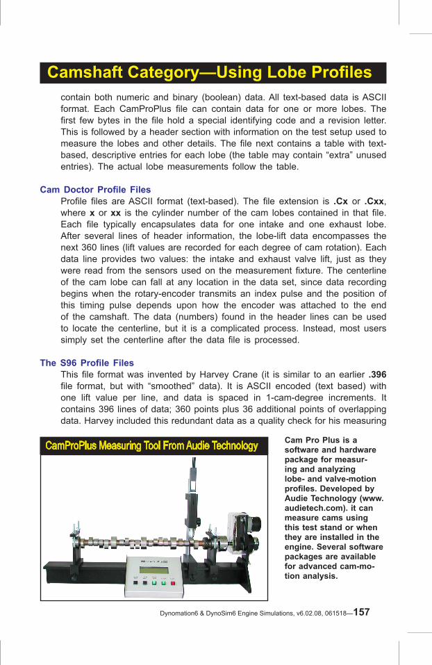
Camshaft Category—Using Lobe Profiles
CamProPlus Measuring Tool From Audie Technology Cam Pro Plus is a software and hardware package for measur-ing and analyzing lobe- and valve-motion profiles. Developed by Audie Technology (www.audietech.com). it can measure cams using this test stand or when they are installed in the engine. Several software packages are available for advanced cam-mo-tion analysis.
contain both numeric and binary (boolean) data. All text-based data is ASCII format. Each CamProPlus file can contain data for one or more lobes. The first few bytes in the file hold a special identifying code and a revision letter. This is followed by a header section with information on the test setup used to measure the lobes and other details. The file next contains a table with text-based, descriptive entries for each lobe (the table may contain “extra” unused entries). The actual lobe measurements follow the table.
Cam Doctor Profile FilesProfile files are ASCII format (text-based). The file extension is .Cx or .Cxx, where x or xx is the cylinder number of the cam lobes contained in that file. Each file typically encapsulates data for one intake and one exhaust lobe. After several lines of header information, the lobe-lift data encompasses the next 360 lines (lift values are recorded for each degree of cam rotation). Each data line provides two values: the intake and exhaust valve lift, just as they were read from the sensors used on the measurement fixture. The centerline of the cam lobe can fall at any location in the data set, since data recording begins when the rotary-encoder transmits an index pulse and the position of this timing pulse depends upon how the encoder was attached to the end of the camshaft. The data (numbers) found in the header lines can be used to locate the centerline, but it is a complicated process. Instead, most users simply set the centerline after the data file is processed.
The S96 Profile FilesThis file format was invented by Harvey Crane (it is similar to an earlier .396 file format, but with “smoothed” data). It is ASCII encoded (text based) with one lift value per line, and data is spaced in 1-cam-degree increments. It contains 396 lines of data; 360 points plus 36 additional points of overlapping data. Harvey included this redundant data as a quality check for his measuring
Dynomation6 & DynoSim6 Engine Simulations, v6.02.08, 061518—157

Camshaft Category—Using Lobe Profiles
process. Peak lift is always located in the middle of the data set. Two common variations of S96 exist: 1) With peak lift on line 180 (the overlapping points are located at the end of the file), and 2) With peak lift on line 198 (with the overlap data split between the start and the end of the file).
The .ECP Profile FilesCompCams lobe-profile format was developed by Motion Software, Inc. The lobe-profile data in these files was provided by CompCams, Inc, and (as of 2018) includes a large portion of the CompCams catalog. The raw profile data was processed and saved in .ECP files (Encrypted Comp Profile) in a protected format that prevents direct lobe copying and duplication. ECP files are only readable by Dynomation. The format protection does not affect file loading or accuracy when using these files in the simulation.
Note: The simulation automatically handles the subtitles of reading and in-terpreting Lobe-Profile file formats; refer to the following sections for help in using profile data in your simulations.
How To ImportLobe-Profile Data
Press the Import Lobe Profile button in the Camshaft Category to begin the import process. When the file-open dialog appears, select the desired sub-folder and file (review Lobe Profile Formats described in the previous section), then click OK. A Lobe Profile Import dialog will open to help you assign lobe data to a specific valve, set centerlines, and make other determinations about the data obtained from the file. Here are the key features and data-entry groups in the Cam Profile Import dialog:
Import Lobe Profile Data The simulation can Import many of common Profile file formats, including CamPro, CamProPlus, Cam Doctor, CompCams ECP, and S96. Press the Import Lobe Profile button in the Camshaft category to open the file-selection dialog shown here. This dialog lists several lobe profile groups that are supplied with Dynomation6 (included for testing and familiarization with profile-file usage).
158—Dynomation6 & DynoSim6 Engine Simulations v6.02.08, 061518

Camshaft Category—Using Lobe Profiles
Lobe Source-Data ListA list of the lobes in the selected file are displayed in the top-left Source Data list. Some file types (like .S96) will have one or two lobes, while other files (like CamProPlus files) may have several profiles included in the file. Click on any lobe described in the Source List to apply its data to the other fields in the import dialog.
DescriptionWhen any lobe is selected from the Source List, information about the profile data may be displayed in the Description box. Many profile files will only have simple lobe identifications, like “Intake,” “Exhaust,” or other brief descriptions of the selected lobe, while other files may offer more detailed information.
Lobe Lift and DurationSince lobe-profile data only consists of lobe-lift values recorded at each cam degree, lobe duration must be calculated from lift data (keep in mind that we are referring to Lobe Duration not Valve Duration; to determine valve dura-tion, multiply the lobe lift values by the rocker ratio and then subtract any valve lash). Lobe duration is determined by the lobe lift height selected for the beginning and ending points. Since the SAE standard starting-lift value is 0.006-inch, and since the most common rocker ratio is 1.5:1, the lobe lift for the same duration would be .006 / 1.5, or 0.004-inch. However, many cam manufacturer's use their own values to rate lobe duration. Common values are 0.006-inch, .0068-inch, 0.020-inch, 0.050-inch, 0.058-inch, and even 0.100
Import Lobe Profile Dialog
After you have selected a lobe profile file, this dialog will open and help you verify the data and assign the lobe to any of four possible destinations: 1-Intake, 2-Exhaust, 3-In-take of the VVT High-Speed Cam and 4-Exhaust of the VVT High-Speed Cam.
Dynomation6 & DynoSim6 Engine Simulations, v6.02.08, 061518—159

Camshaft Category—Using Lobe Profilesand 0.200-inch are used. The simulation displays the lobe duration for many of these lobe lift points. In addition, you can enter any lift value in the Enter Custom Lift field and the corresponding duration will be calculated.
Note: Once lobe-lift data is imported, the valve seat-to-seat duration displayed in the Camshaft Component category is determined using 0.006-inch valve lift points (includes rocker ratio and lash), On the other hand, 0.050-lift lobe duration is determined from the 0.050-inch lobe/tappet lift points and does not include rocker ratio or lash.
Lobe-Profile Rendering And Base-Circle DiameterThe Lobe Profile Import dialog also includes an illustration of the lobe selected in the Source List that is rendered from actual lobe-lift data. Use this illustra-tion to make sure there are no missing points or interruptions in the lift curve; if you see any discontinuities, the profile data in the file is invalid.
Note-1: Since profile data only indicates how far the lifter rises above the base circle of the cam (not the actual base-circle diameter), the simulation has to make a calculated “guess” of the base-circle size to render the profile. If the lobe-to-base-circle size relationship looks odd, you can enter a different base-circle diameter that may improve the “look.” This display is only provided as a check for lift-data completeness; base-circle size does not affect the data used in the engine simulation.Note-2: The arrow shown in the cam rendering indicates a normal clockwise rotation (cam rotation is always assumed to be clockwise); the opening flank is on the right side of the illustration and the closing ramp is on the left.
Lobe-Data DestinationThe profile data associated with lobes selected in the Lobe Source-Data List are assigned to either an intake or exhaust valve (and in the case of V-V-T cam modeling, to the high-speed Intake or Exhaust valve) using the Lobe-Data Destination group. This data-entry area contains either two or four radio but-
Invalid Lobe-Profile Data The cam-lobe image (rendered from lift data in the profile file) can confirm the validity of the data file and help you get a general “feel” for the shape of the lobe. The lift curve shown on the left is missing the opening ramp and is invalid.
160—Dynomation6 & DynoSim6 Engine Simulations v6.02.08, 061518

Camshaft Category—Using Lobe Profiles
tons, depending on whether Variable Valve Timing is currently active. Notice that the radio buttons allow the selection of only one destination.The procedure here is to select a lobe profile, assign it to a specific intake or exhaust valve, then close the Import Dialog to complete the import for one lobe. Reopen the Import dialog to import additional lobe profiles.
Convert Wave-Action Profile Data To 10-Point TimingLobe-profile data can be “handed over” to the simulation in two ways: 1) You can directly import the “raw” valve-lift data into the Wave-Action simulation (this is the default method). When this is done, Profile data will be used “as-is” to determine valve motion, or 2) By checking the Convert Profile Data To 10-Point Timing, you can force the conversion of Profile lobe-lift data into 10-Point timing values.Note: You can still convert the lobe-profile lift data to 10-Point modeling at any time buy simply clicking the “->10-pnt” (Convert To 10-Point) buttons in the Camshaft category. Remember that profiles files are “fixed,” while 10-Point timing can be edited or modified in any way (you can modify valve-event tim-ing, lift, etc.).
Lobe Centerline (in crank degrees)Lobe-lift profile data must be “synchronized” with crankshaft and piston move-ment to be useful. Lobe Centerline is the data point that fixes the rotational index, in crank degrees, from the center of the lobe-profile data (point of maxi-mum lift) to Top-Dead-Center piston position. You can enter Lobe Centerline data in the Import Dialog or you can enter (or modify) this value within the Camshaft Category.
Lobe-Lift And Acceleration GraphTo help you visualize the profile data selected from the Source List, lift and
Assign Lobe Data To A Simulation ValveThe lobe profile selected in the Lobe Source-Data List can be assigned to either an intake or exhaust valve (and in the case of V-V-T cam model-ing, to either of the high-speed cam lobes) using the Lobe-Data Destination group. The Centerline for the lobe data can also entered in this group. With a known centerline, the simulation is able to calculate Seat-To-Seat Valve- and 0.050 Lobe-Event timing (the simulation will set a default centerline value of 110.0 degrees whenever the Lobe Profile Dialog is opened).
Dynomation6 & DynoSim6 Engine Simulations, v6.02.08, 061518—161

Camshaft Category—Using Lobe Profiles
acceleration curves are displayed in the Lobe Lift and Acceleration Graph. Keep an eye out for rough or bumpy curves that can indicate poor recorded data quality during cam lobe measurements.
Press the OK button in the Import Dialog to transfer the cam file data into the CAMSHAFT Category and update the simulation with the new cam specs..
Tuning And Modifying Profile Cam Data
Profile files, as mentioned, consist of hundreds of data points that define the position of the cam follower throughout its lift range. Because these points are
Lobe Lift And Acceleration GraphThe Lobe-Lift and Acceleration Graph displays data for the profile selected in the
Lobe Source-Data List. Use the graph to get an overall visualization of the lift curve
and acceleration rates of the profile. A roughly shaped curve can signal erroneous
data in the profile.
Choosing Lobe Centerline
A lobe-lift profile must be “synchronized” with crankshaft and piston movement to be use-ful. The Lobe Center-line Angle (shown here as an LCA of 106 de-grees) is the distance, in crank degrees, from the center of the lobe-profile data (in this case, the point of maximum intake-valve lift) to the Top-Dead-Center piston position.
Intake Centerline (106)Crank Degrees BetweenTop Dead Center AndLobe Centerline
Lobe Profile And Centerline Measurement
162—Dynomation6 & DynoSim6 Engine Simulations v6.02.08, 061518

Camshaft Category—Using Lobe Profiles
fixed, they can not be individually changed without corrupting the lift curve. Basi-cally, profile valve-event timing (IVO, IVC, etc.) is “built into” the data and cannot be altered without re-defining the entire profile. However, there are a few tuning “knobs” that you can turn when using Profile data without converting into 10-point data. Modifying the following cam specifications offer some options when Profile data is being used:
Timing Point/Specification Comment Cam Advance and Retard Shifts entire lobe profile (see following text for details) Intake Centerline Shifts entire intake lobe timing Exhaust Centerline Shifts entire exhaust lobe timing Rocker Ratio Changes lobe-lift-to-valve-lift ratio and has some affect on duration Valve Lash Affects opening/closing timing and has some affect on duration When Profile modeling is being used, you will notice that many of the valve-event specifications within the Camshaft category are dimmed and cannot be directly modified. To "unlock" all timing data fields, you must use the “->10-pnt” (Convert To 10-Point) buttons to convert profile data into 10-point timing; this allows you to modify all cam timing data, but keep in mind that converting to 10-point data will create...usually small...valve motion differences from the original cam Profile curve.
After a Lobe Profile has been imported into the simulation, the Modeled From field(s) in the Camshaft category will display “Profile.” You convert to 10-Point modeling at any time by clicking a “->10-pnt” (Convert To 10-Point) button. Profile data for that lobe will be discarded and 10-Point valve-event timing will be used that matches the profile data as closely as possible.
Convert Profile Data To 10-Point Modeling
“Profile” Indicates LobeProfile Data Is Being Used.
“->10-pnt” Buttons will convertProfile data to 10-Point Modeling
Dynomation6 & DynoSim6 Engine Simulations, v6.02.08, 061518—163

Camshaft Category—Cam Adv/RetAdvance/Retard Cam Timing
The simulation allows direct entry of Intake and/or Exhaust camshaft lobe ad-vance or retard values for both Profile and 10-Point cam modeling. Changing these specifications from zero (the default) to a positive value advances the cam lobe (in crank degrees) while negative values retard the lobe. Why advance or retard the cam? It’s just about the only valve-timing change that can be made after the camshaft has been installed. While it is sometimes possible to improve performance using this technique, let’s investigate what happens when valve events are advanced or retarded in unison.
Tuning A Single-Cam Engine
It is generally accepted that advancing the cam improves low-speed power while retarding the cam can improve high-speed power. When the cam is advanced, IVC and EVC occur earlier and that can improve low-speed performance; however, EVO and IVO also occur earlier, and these changes tend to improve power at higher engine speeds, but to a lessor extent. The net result of these “conflicting” changes typically is a slight boost in low-speed power. The same goes for retarding the cam. Two events (later IVC and EVC) boost high-speed power and two (later EVO and IVO) boost low-speed performance, but again, to a lessor extent. The net result is often a slight boost in high-speed power. Advancing or retarding a camshaft under these conditions has the overall affect of reducing valve-timing efficiency in exchange for slight gains in low- or high-speed power. Consequently, many cam manufacturers recommend avoiding this tuning
To ensure the most accurate cam timing and to facilitate tuning, a gear drive is
often used in high-performance applica-tions. This a CompCams drive was de-
signed for GM LS engines (with three-bolt cams on all 24x and 58x LS engines).
DOHC Cam Sprockets
164—Dynomation6 & DynoSim6 Engine Simulations v6.02.08, 061518

Camshaft Category—Cam Adv/Ret
technique. If advancing or retarding allows the engine to perform better in a specific rpm range, the cam profile was probably not optimum for the engine in the first place. More power can be found at both ends of the rpm range by installing an optimized cam rather than advancing or retarding the wrong cam. However, if you already own a specific camshaft, advancing or retarding overall timing may offer
Advance/Retard Menu
The simulation allows direct entry of camshaft advance or retard for each lobe (permits DOHC modeling). Changing this specification from zero (the default) to a positive value advances the cam lobes; negative values retard the lobes. See text for more information on how these changes can affect engine output.
DOHC Cam Sprockets In DOHC engines, like the Honda VTEC and many other engines, where separate cams are used for the intake and exhaust lobes, the cam advance/retard can be set independently for the intake and exhaust cams. In the real world, this tuning is easily accomplished with adjustable cam sprockets, like these from ZEX. Adjustable timing sprockets can also compensate for milled deck and head surfac-es that can alter cam timing.
Dynomation6 & DynoSim6 Engine Simulations, v6.02.08, 061518—165

Camshaft Category—Cam Adv/Retsome “fine tuning” capabilities.
Tuning DOHC Engines
Tuning DOHC engines with individual intake and exhaust cams is a straightforward process. While changing cam timing on an engine with a single cam forces you to change ALL lobes the same amount and in the same direction—often reducing any benefits you may have gained—on DOHC engines cam tuning takes on a much greater significance. When you install an optimum cam for a specific application, you can expect it to produce peak power (or torque) when installed “heads-up,” or without any advance or retard. However, engine builders often find improvements by advancing one cam and retarding the other. This is especially true in turbocharged applications, where advancing the intake cam and retarding the exhaust cam in-creases the Lobe-Separation Angle (also called the Lobe-Centerline Angle, or LCA), reducing valve overlap, which sometimes improves forced-induction efficiency. Dyno testing has shown that it is sometimes impossible to predict how the engine will respond to intake- or exhaust-cam advance and retard. This is may be due to subtleties within, and interactions between, the induction and exhaust systems. While this simulation will give you valuable feedback, this fine-tuning process should be confirmed on a real-world dynamometer.
Note: Make sure you keep in mind that changing cam advance or retard on
DOHC Gear Train
166—Dynomation6 & DynoSim6 Engine Simulations v6.02.08, 061518

Camshaft Category—Cam Adv/Reta real-world engine will alter valve-to-piston clearance. Changing cam timing by 4-degrees or less will rarely cause interference problems, however, it is always the engine builder/tuner’s responsibility to ensure mechanical contact between the pistons and values does not take place at any engine speed. Just starting and idling an engine with piston-to-valve interference can damage valves, break cams, and bend valvetrain components.
Dynomation6 & DynoSim6 Engine Simulations, v6.02.08, 061518—167

THE COMBUSTION CATEGORYApplies To FE and WA Simulations, Except as Indicated
The Combustion Category contains combustion-related components and speci-fications. Included are Compression Ratio, Thermal Coatings Modeling, Fuel Type (includes spark- and combustion-ignition fuels), Air/Fuel Ratio (one value or a “map” of values), Fuel Vaporization Percentage within the intake tract before IVC, Com-bustion-Chamber geometry, and Ignition Timing (for spark-ignition fuels only). Each of these specifications directly affect how fuel is burned and the overall combustion efficiency. This category also includes a Compression Ratio Calculator (see text),
Combustion Category
The Combustion Category includes Compression Ratio, Thermal Coatings, Fuel Type, Air/Fuel Ratio (fixed or adjustable for each rpm point), Fuel Vaporization within the intake tract (before IVC), Combustion-Chamber geometry, and Ignition Timing. Each of these specifications directly affect how fuel is burned in the engine. This category also includes a Compression Ratio Calculator, and a Combustion-Chamber-Selection dialog. Clicking the Estimate Ignition Timing checkbox, will direct the simulation to determine the MBT for the engine at each rpm point (see text).
Combustion Category
168—Dynomation6 & DynoSim6 Engine Simulations v6.02.08, 061518

Combustion Category
Compression Ratio =
Swept Cylinder Volume + Combustion Space Volume––––––––––––––––––––––––––––––––––––––––––
Combustion Space Volume
Compression ratio is calculated by dividing the total volume with-
in the cylinder when the piston is located at Bottom Dead Center
(BDC) by the volume that exists when the piston is positioned at
Top Dead Center (TDC).
Basic Compression Ratio Equation
and a Chamber-Selection dialog. Clicking the Estimate Ignition Timing checkbox will instruct the simulation to determine the MBT (Minimum Ignition Advance For Best Torque) for the engine at each rpm point.
Note: When you select Diesel fuel, the following fields are dimmed, since they cannot be changed in compression-ignition applications:
Combustion Chamber Design: An analysis of chamber shape is not included in this version of the simulation. Ignition Timing: Ignition point determined by the simulation
Compression Ratioand How It Is Calculated
The Compression Ratio menu, located in the Combustion Component category, establishes the compression ratio for the simulated engine (within the range of 3:1 to 30:1) for gasoline and other spark-ignition fuels or for Diesel fuel using compres-
Compression Ratio MenuThe Compression Ratio field is located at the top of the Combustion Category. Compres-
sion Ratio is a comparison of the geometric volumes that exist in the cylinder (including the cylinderhead and gasket volumes) when
the piston is located at BDC (bottom dead center) to the “compressed volume” when the
piston reaches TDC (top dead center). The simulation will model any compression ratio
from 3.00:1 to 30.00:1.
Dynomation6 & DynoSim6 Engine Simulations, v6.02.08, 061518—169

Combustion Categorysion ignition. Compression-ratio is the comparison of two volumes in the engine, as illustrated by the “standard equation” shown nearby. The variables are: 1) Swept-Cylinder Volume, and 2) Combustion-Space Volume. While these are the only two volumes that affect compression ratio, each of these volumes is made up of multiple other volumes, so the first step in understanding compression ratio is to become familiar with these volumes. Swept Cylinder Volume is the most straightforward: It is simply the three-dimensional space displaced by the piston as it “sweeps” from BDC to TDC, and is determined solely by the bore diameter and stroke length. The swept cylinder volume is calcu-lated by the simulation—and displayed in the Combustion category—as soon as the bore and stroke have been selected for the test engine. The other main variable in the compression-ratio equation is Combustion-Space Volume. This is the total volume that exists above the piston when it is positioned at TDC. This space includes the combustion-chamber volume, the volume taken up by the thickness of the head gasket, any volume added by the piston not ris-ing fully to the top of the bore, plus any valve-pocket volume, less any volume displaced by the piston or piston dome protruding above the top of the cylinder bore (block deck). The complexity of these volumes is often a stumbling block in becoming comfortable with all aspects of compression ratio. However, the following explanation and illustrations should clarify these important concepts. Imagine yourself as a “lilliputian,” wandering around inside the engine. Take a stroll inside the combustion space. Picture in your mind what you would see in the cylinder with the piston at TDC. The combustion chamber would look like a ceiling above you. The floor would be the top of the piston. If the piston (at TDC) didn’t rise completely to the top of the cylinder, you would see a bit of the cylinderwall around the edges of the floor, with the head gasket sandwiched between the head and block like trim molding around the room. There may be “steps” (valve pockets) in the top of the piston just under your feet (don’t trip!). If the piston had a dome, it
Picturing Compression Ratio And Swept Volume
PISTONAT
TDC
PISTONAT
BDC
A good way to visualize com-pression ratio volumes is to
imagine yourself as a “lillipu-tian” wandering around inside the engine. You would see the
combustion chamber above you like a ceiling. Your floor would be the top of the piston. Swept
Cylinder Volume is the three-dimensional space displaced as the piston “sweeps” from
BDC to TDC, and is determined solely by the bore diameter and
stroke length.
170—Dynomation6 & DynoSim6 Engine Simulations v6.02.08, 061518

Combustion Categorymight act as a small room divider rising from the floor, to, perhaps, knee high. The space in this room (combustion space) would be larger if the piston was positioned lower down the bore or if the “steps” under your feet were deeper, and it would be tighter squeeze if the room divider (dome) volume was larger. This entire space is “home” for the compressed charge when the piston reaches TDC. This is the volume that makes up the combustion space, the denominator of the compression-ratio calculation equation. Now let’s continue our tour of compression spaces, but this time we’ll explore what we see inside the cylinder when the piston is located at BDC. The very same volumes that we just described (chamber, dome, notches, gasket, etc.) are still there, but are now located well above our head. It looks like the room has been stretched, like the elevator ride in the Haunted House at Dis-neyland. This “stretched” volume is described in the numerator of the compression-ratio equation. It’s simply the original combustion volume plus the volume added by the “sweep” of the piston as it traveled from TDC to BDC. The ratio between these two volumes is the compression ratio.
Bore, Stroke, And Compression Ratio
Another quick look at the compression-ratio equation reveals that if engine dis-placement (swept volume) is increased, either by increasing the bore or stroke, the compression ratio will rise. In fact, with everything else being equal, a longer stroke will increase compression ratio much more quickly than increasing bore diameter. This is due to the fact that a longer stroke (without changing other engine dimen-sions) not only increases displacement, but it tends to decrease combustion space volume, since the piston moves higher the bore if the rod length and pin position are not changed (in our “lilliputian” example, raising the floor closer to the ceiling). This “double positive” results in rapid increases in compression ratio for small increases in stroke length. On the other hand, increasing cylinder-bore diameter also increases compression ratio but less significantly. This is due, in part, to the increase in Combustion-Space Volume that often accompanies a larger bore.
CombustionChamberVolume
CombustionSpace
Volume
PISTONATTDC
While Combustion-Chamber Volume is sim-ply the volume of the chamber in the cylin-der head, the Combustion-Space Volume is the total enclosed volume when the piston is located at TDC. This space includes the
volume in the combustion chamber, plus any volume added by the piston not rising
to the top of the bore, the volume within any valve pockets, and the head-gasket thick-
ness, less any volume contained within the piston dome or displaced by the piston
protruding above the top of the bore.
Top-Dead-Center Volumes
Dynomation6 & DynoSim6 Engine Simulations, v6.02.08, 061518—171
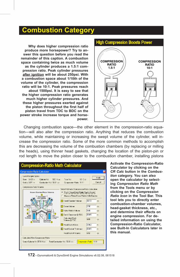
Combustion Category
Changing combustion space—the other element in the compression-ratio equa-tion—will also alter the compression ratio. Anything that reduces the combustion volume, while maintaining or increasing the swept volume of the cylinder, will in-crease the compression ratio. Some of the more common methods to accomplish this are decreasing the volume of the combustion chambers (by replacing or milling the heads), using thinner head gaskets, changing the location of the piston-pin or rod length to move the piston closer to the combustion chamber, installing pistons
Compression-Ratio Math Calculator Activate the Compression-Ratio Calculator by clicking on the CR Calc button in the Combus-tion category. You can also open the calculator by select-ing Compression Ratio Math from the Tools menu or by clicking on the Compression Ratio Icon in the Tool Bar. This tool lets you to directly enter combustion-chamber volumes, head-gasket thickness, etc., and determine their effects on engine compression. For de-tailed information on using the Compression-Ratio Calculator, see Built-In Calculators later in this manual.
COMPRESSIONRATIO1.5:1
COMPRESSIONRATIO10:1
High Compression Boosts PowerWhy does higher compression ratio
produce more horsepower? Try to an-swer this question before you read the
remainder of this caption. A combustion space containing twice as much volume
as the cylinder produces a 1.5:1 com-pression ratio. Peak cylinder pressures after ignition will be about 250psi. With
a combustion space about 1/10th of the volume of the cylinder, the compression ratio will be 10:1. Peak pressures reach
about 1500psi. It is easy to see that the higher compression ratio generates
much higher cylinder pressures. And these higher pressures exerted against
the piston throughout the first half of piston travel from TDC to BDC on the
power stroke increase torque and horse-power.
172—Dynomation6 & DynoSim6 Engine Simulations v6.02.08, 061518
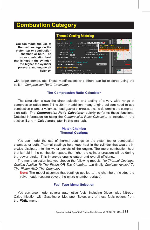
Combustion Category
with larger domes, etc. These modifications and others can be explored using the built-in Compression-Ratio Calculator.
The Compression-Ratio Calculator
The simulation allows the direct selection and testing of a very wide range of compression ratios from 3:1 to 30:1. In addition, many engine builders need to use combustion-chamber volumes, head-gasket thickness, etc., to determine the compres-sion ratio. The Compression-Ratio Calculator, quickly performs these functions. Detailed information on using the Compression-Ratio Calculator is included in the section Built-In Calculators later in this manual).
Piston/ChamberThermal Coatings
You can model the use of thermal coatings on the piston top or combustion chamber, or both. Thermal coatings help keep heat in the cylinder that would oth-erwise dissipate into the water jackets of the engine. The more combustion heat that is held in the combustion space, the higher the cylinder pressure will be during the power stroke. This improves engine output and overall efficiency. The menu selection lets you choose the following models: No Thermal Coatings, Coating Applied To The Piston OR The Chamber, and finally Coatings Applied To The Piston AND The Chamber. Note: The model assumes that coatings applied to the chambers includes the
valve heads (coating covers the entire chamber surface).
Fuel Type Menu Selection
You can also model several automotive fuels, including Diesel, plus Nitrous-Oxide injection with Gasoline or Methanol. Select any of these fuels options from the FUEL menu:
You can model the use of thermal coatings on the
piston top or combustion chamber, or both. The more combustion heat
that is kept in the cylinder, the higher the cylinder
pressure and engine ef-ficiency.
Thermal Coating Modeling
Dynomation6 & DynoSim6 Engine Simulations, v6.02.08, 061518—173
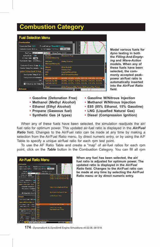
Combustion Category
• Gasoline (Detonation Free) • Gasoline W/Nitrous Injection• Methanol (Methyl Alcohol) • Methanol W/Nitrous Injection• Ethanol (Ethyl Alcohol) • E85 (85% Ethanol, 15% Gasoline)• Propane (Gaseous fuel) • LNG (Liquefied Natural Gas) • Synthetic Gas (4 types) • Diesel (Compression Ignition)
When any of these fuels have been selected, the simulation readjusts the air/fuel ratio for optimum power. This updated air-fuel ratio is displayed in the Air/Fuel Ratio field. Changes to the Air/Fuel ratio can be made at any time by making a selection from the Air/Fuel Ratio menu, by direct numeric entry, or by using the A/F Table to specify a unique air/fuel ratio for each rpm test point. To use the AF Ratio Table and create a “map” of air-fuel ratios for each rpm point, click on the Table button in the Combustion Category. You can fill all rpm
Fuel Selection Menu
Model various fuels for dyno testing in both the Filling-And-Empty-ing and Wave-Action models. When any of these fuels have been selected, the com-monly accepted peak-power air/fuel ratio is automatically inserted into the Air/Fuel Ratio field.
When any fuel has been selected, the air/fuel ratio is adjusted for optimum power. The updated ratio is displayed in the Air/Fuel Ratio field. Changes to the Air/Fuel ratio can be made at any time by selecting the Air/Fuel Ratio menu or by direct numeric entry.
Air-Fuel Ratio Menu
174—Dynomation6 & DynoSim6 Engine Simulations v6.02.08, 061518
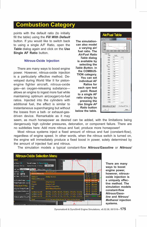
Combustion Category
seem, as much horsepower as desired can be added, with the limitations being dangerously high cylinder pressures, detonation, or component failure. There are no subtleties here: Add more nitrous and fuel; produce more horsepower! Most nitrous systems inject a fixed amount of nitrous and fuel (constant-flow), regardless of engine speed. In other words, when the nitrous switch is turned on, the engine will immediately produce a fixed boost in power, solely determined by the amount of injected fuel and nitrous. The simulation models a typical constant-flow Nitrous/Gasoline or Nitrous/
Air/Fuel Table
The simulation-can also model
a varying air/fuel ratio. The Air/Fuel Ratio
Table dialog is available by
selecting the Table Button. in
the COMBUS-TION category.
You can set individual AF
Ratios for each rpm test
point. Reset to a single AF
ratio simply by pressing the
Use Single AF Ratio button
below the table.
Nitrous-Oxide Selection Menu
There are many ways to boost engine power, however, nitrous-oxide injection is a uniquely effec-tive method. The simulation models constant-flow Nitrous/Gaso-line and Nitrous/Methanol injection systems.
points with the default ratio (to initially fill the table) using the Fill With Default button. If you would like to switch back to using a single A/F Ratio, open the Table dialog again and click on the Use Single AF Ratio button.
Nitrous-Oxide Injection There are many ways to boost engine power. However, nitrous-oxide injection is a particularly effective method. De-veloped during World War II for piston-engine fighter aircraft, nitrous-oxide gas—an oxygen-releasing substance—allows an engine to ingest more fuel while maintaining optimum air(oxygen)-to-fuel ratios. Injected into the cylinders with additional fuel, the effect is similar to instantaneous supercharging but without the losses from a belt- or exhaust-gas-driven device. Remarkable as it may
Dynomation6 & DynoSim6 Engine Simulations, v6.02.08, 061518—175

Combustion CategoryMethanol injection system. Nitrous is “injected” by the simulation in precise amounts throughout specific increments of crank degrees, similarly to an actual nitrous sys-tem. You select the desired HP boost, and the simulation will calculate the Nitrous Mass Flow required to produce that power (calculation of nitrous flow is performed before the actual simulation is run, so engine design and other factors...just like in the real world...can affect the actual power output reported by the simulation). The simulation will tell you how much of the injected nitrous mass actually entered the cylinder and how much was rejected back into the intake manifold (or lost to exhaust flow). The enhanced nitrous modeling included in this version-6 simulation includes these elements in a nitrous-augmented engine:
1) Nitrous Inflow restriction at the intake valves 2) Cylinder filling (capacity vs. overfill backpressure) and gas reversion 3) Nitrous (and added fuel) effects on charge cooling (LHV) 4) Nitrous details are included in the Simulation Log and ProTools Printout 5) Enhanced Nitrous Injection is included in both the WA and FE simulations
A nitrous injection system designed to add 100 horsepower (flowing about 4 pounds per minute of nitrous oxide and additional fuel to maintain the correct air/fuel ratio), will produce a 100 horsepower boost instantly upon triggering the system. Remarkably, the engine will continue to produce an this additional 100 horsepower across the entire rpm range. That means a 100hp nitrous system activated at 2000rpm (when the engine may have been producing only about 70hp) can double or even triple power output! These huge power boosts at low engine speeds (when each cylinder ingests
Nitrous-Oxide Injection And BMEP This graphic shows how cylinder pressures (in this case the BMEP shown by the green line) increase af-ter a 200-horsepower nitrous system is activated (this pressure compari-son includes colored DataZones™, discussed later in this manual). Since the simulation models a fixed-flow ni-trous system, cylinder loads increase as engine speed decreases (the lon-ger time the intake valve is open, the greater nitrous load is inducted into the cylinder). Below 3000rpm, BMEP exceeds 300psi (shown by the top, light green band). In this situation, nitrous-system activation should be delayed until 3000rpm to help main-tain engine reliability.
176—Dynomation6 & DynoSim6 Engine Simulations v6.02.08, 061518

a large “dose” per power cycle) can generate excessive cylinder pressures. As a result, fixed-flow-rate systems often include a delayed trigger to allow the engine to reach sufficient speed to maintain safe cylinder pressures. Maintaining cylinder pressures below critical levels is essential to prevent detonation and mechanical failure. During engine simulations with nitrous augmentation, you can keep track of cyl-inder pressures (for example, a BMEP greater than 300psi is usually considered borderline dangerous). For example, the nearby test graph illustrates a 350 smallblock equipped with a 200hp nitrous system. Note that BMEP pressures below 3000rpm exceed 300psi.
Note-1: BMEP (Brake Mean Effective Pressure) is an “average” cylinder pres-sure; when it exceeds 300psi, peak pressures often reach detonation levels and can quickly lead to mechanical failure—for a description of BMEP, refer to the Glossary later in this manual.Note-2: There are other ways to help reduce low-speed cylinder pressure in a Nitrous engine including modified cam timing. It has long been known that increasing valve duration and overlap will lower cylinder pressures at lower engine speeds. This typically-unwanted phenomenon is a low-speed power killer, but combined with a nitrous-oxide injection system, it can permit earlier nitrous flow while optimizing power at higher engine speeds. Other ways to decrease low-speed cylinder pressures include reduced compression ratios, increased exhaust-system back pressure, reduced induction airflow, larger engine displacement, and of course, reducing the nitrous flow rate.
You can activate the nitrous-injection model by selecting Gasoline/Nitrous Injec-
Combustion Category
To activate any Nitrous Boost Horse-power from zero to 800hp, first select one of the Nitrous-Injec-tion selections from the Fuel Type menu (which activates the Nitrous Power Menu), then open the Power Menu to enter any power value.
Nitrous Power Menu
Dynomation6 & DynoSim6 Engine Simulations, v6.02.08, 061518—177

tion or Methanol/Nitrous Injection from the Fuel Type menu (see previous page). You will see the following choices:
• 25 HP (~1 lb/min N2O flow) • 50 HP (~2 lb/min N2O flow)• 100 HP (~4 lb/min N2O flow) • 200 HP (~8 lb/min N2O flow)• 300 HP (~12 lb/min N2O flow) • 400 HP (~16 lb/min N2O flow)• 500 HP (~20 lb/min N2O flow) • 600 HP (~24 lb/min N2O flow)• 700 HP (~28 lb/min N2O flow) • 800 HP (~32 lb/min N2O flow)
In addition to these 10 menu options, you can use the Nitrous Power Menu to manually enter any nitrous power value from zero to 800hp.
Combustion-Chamber Design
The Combustion-Chamber Design field in the Combustion category sets the fuel burn rate and adjusts the combustion efficiency based on the physical geometry of the combustion space. In general, a “disc-shaped” chamber with a side-mounted sparkplug generates the lowest turbulence and flame speed. The burn-rate differences between this oldd technology chamber and a modern pentroof designs with squish-assisted turbulence can be as much as 30-degrees of reduced ignition timing “lead” to accommodate the faster-burn rates. A mathematical analysis of the burn process (can be thought of as simply a rapid pressure rise) reveals that peak power would be obtained if the fuel burned instantly at a crank angle slightly after TDC. This would produce the greatest push on the piston at the point at which this pressure is most efficiently
Nine combustion-chamber geometries from the slowest-burning disc shape to
the fast-burn pentroof designs model most high-performance and racing
engines. Clicking the Chambers Quick-Access™ button in the Combustion
Category provides an overview of these chamber shapes, including the basic
Chamber Timing Requirements of these designs (timing values in the dialog as-
sume gasoline as the fuel). Note: This dialog does not open when using Diesel
as a fuel.
Combustion-Chamber Selection
Combustion Category
178—Dynomation6 & DynoSim6 Engine Simulations v6.02.08, 061518

Combustion Categoryconverted into the highest force on the crankpin. While an instant fuel burn (and pressure rise) is not possible for several practical reasons, including knock preven-tion and maintaining mechanical integrity, typically a fast pressure rise in the cylin-der will produce more power (reaching peak pressure at about 20- to 30-degrees ATC is typical for many high-output engines). To facilitate this, modern chamber designs are optimized for high turbulence and fame speeds while minimizing pre-ignition and detonation.
Note: As always, there are exceptions. In a nitromethane-fueled engine, the slower burn-rate hemispherical chamber is often used. In this case, there are benefits to slowing down the burn rate and giving the flame front a symmet-ric volume in which to propagate. With nitromethane this results in a more uniform application of the huge cylinder pressures produced by this powerful racing fuel. The overriding consideration here is reliability not peak pressures!
The simulation provides nine combustion-chamber geometries from the slowest-burning disc shape, provided primarily for comparison purposes, to the fast-burn pentroof designs used in many modern high-performance and racing engines. Clicking on the Chambers Quick-Access™ button (not active for Diesel fuel) provides an overview of these chamber shapes, including the basic Chamber Timing Require-ment (assumes gasoline as the baseline fuel). The Chamber Timing Requirement is based on the time lag between the sparkplug discharge, referred to as the SparkPoint, and the beginning of cylinder pressure rise. This delay can be considered as the innate rate at which fuel burns in that chamber geometry. This is the least possible timing advance that the engine will need to produce optimum power with that chamber at low engine speeds. As speed
From upper left, a 2-valve hemi chamber with center plug, a pen-troof 4-valve motorcycle, then a pair of 2-valve wedge chambers, one as machined and the other polished and detailed.
Dynomation6 & DynoSim6 Engine Simulations, v6.02.08, 061518—179

Combustion Categoryincreases, or if non-optimum air/fuel ratios are used, greater ignition lead (more time) will be required to efficiently burn the fuel and produce optimum power. This minimum timing requirement for optimum power at a specific operating condition is often called MBT (or Minimum ignition advance for Best Torque). An engine does not have single MBT, but rather many MBTs as engine speed, temperature, AF Ratio, fuel chemistry and other real-world factors change.
Ignition Timing
Optimum power production depends on the precise timing of the “ignition point,” an event that, as described above, can vary substantially. There is a significant delay in the initiation of measurable combustion after the SparkPoint, and even beyond that, many factors affect lag and the rate of combustion. So, what shall we call the actual point of ignition? Should it be: 1) when the spark occurs, or 2) when the fuel starts burning, or 3) when pressure begins to rise in the cylinder? Rather than debating this, we will use other terms that have more precise meanings. To begin, let’s establish the beginning of the Combustion Cycle at the SparkPoint, commonly know as the Ignition Timing Point of the engine. This will be the pre-cise point, in crank degrees before top-dead center (BTDC), when the initiation of spark occurs. After the SparkPoint there is a delay before the pressure within the cylinder actually increases. This delay can be exaggerated when the piston begins to move down the bore after TDC, increasing combustion-space volume. At some point, however, the increasing volume is overcome by the rapid rise in temperature from expanding combustion. The first indication of a pressure increase is usually defined as the Start Of Combustion, even though it’s obvious that the combustion process was already underway, but remained in a low-burn-rate initiation phase. We mentioned that the Ignition-Timing requirement for optimum power is com-
While an instantaneous fuel burn that produce peak pres-sures at the optimum crank angle is not possible, in general, the faster the pres-sure rises in the cylinder the more power the engine will produce. Modern combus-tion chamber designs are optimized for high turbulence and fame speeds within the constraints of preventing pre-ignition and detonation.
Optimum Ignition Point
800
1000
600
400
14.7
360 740 0 & 720TDCTDC
Degrees of Crankshaft Rotation
BDC
Ignition
BDC360180
Cyl
inde
r P
ress
ure
(psi
)
Figure 20
180—Dynomation6 & DynoSim6 Engine Simulations v6.02.08, 061518

Combustion Category
monly called the MBT (Minimum advance for Best Torque). But this timing require-ment changes as turbulence in the combustion chamber changes, since the burn rate is substantially linked to, among other things, the turbulence of the gasses in the combustion chamber. Furthermore, turbulence also changes when: 1) Engine speed changes, 2) Air/Fuel ratio changes, and 3) When engine load (throttle posi-tion) changes. And, as mentioned, there are additional subtle changes to burn rate from charge temperature changes, differences in compression ratio, and even bore size and stroke length. How can we take all these factors into consideration and determine the MBT for all engine speeds? The simulation performs these complex calculations and derives an estimate of an Optimum Ignition advance curve. To activate this feature, simply check the Estimate Ignition Timing checkbox in the Combustion Category (selected by default). You can view the calculated ignition timing values in the ProData Table, and on the top-right RPM graph. If you would like to enter a specific ignition timing value and/or an advance curve based on engine speed, that option is also available. Un-check the Estimate Ignition Timing box, and enter values for Basic Ignition Timing (BTDC). This is the SparkPoint relative to TDC measured in crank degrees. In addition, you can direct the simulation to calculate an advance curve by specifying the number of degrees of advance for each 1000-rpm increase in engine speed. You can “flatten”
Manual and MBT Advance CurvesThe advance curve (set in the Manual Advance Curve dialog shown above and illustrated in this graph by the light red line) started at 24-degrees advance, increased 2.2 degrees up to a limit at 6500rpm. The dark-red curve is the MBT advance curve calculated by the simula-tion.
Manual Advance Curve With Speed Limit Activate a manual, rpm-based advance curve by un-checking “Estimate Timing...” and speci-fying the initial-timing advance and the number of degrees for each 1000-rpm increase in engine speed. You can cap the advance curve by specifying a limit rpm.
Dynomation6 & DynoSim6 Engine Simulations, v6.02.08, 061518—181

Combustion Categorythe advance curve by specifying a limit rpm, after which no further advance is ap-plied. After defining your own ignition values, you can quickly compare your curve with the MBT determined by the simulation; simply re-check the Estimate Ignition Timing box and note the changes in the advance curve and engine power. Note: Overall engine design, including chamber geometry, fuel type and quality,
and other factors, can produce variations in optimum ignition timing and advance curve requirements. In addition, a 3D model of the combustion space and a full analysis of flame travel (beyond the capabilities of this simulation) are required to fully simulate the ignition timing requirements, especially a high-performance or race engine. Use the ignition timing features available in Dynomation to help you establish baseline timing requirements. Actual dyno testing under real-world conditions is the only way to precisely determine an optimum ignition timing curve.
182—Dynomation6 & DynoSim6 Engine Simulations v6.02.08, 061518

Combustion Category
Dynomation6 & DynoSim6 Engine Simulations, v6.02.08, 061518—183

Exhaust CategoryTHE EXHAUST SYSTEM CATEGORY
Unique Models Are Used In The FE and WA Simulations,Both Are Detailed In This Chapter
The EXHAUST category establishes a mathematical model for the exhaust system of the simulated engine. Dynomation6 incorporates two distinct simulation methods, and each of these methods uses its own exhaust modeling technique. The Filling-And-Emptying simulation (used in DynoSim6) uses a simplified exhaust model, on the other hand, the Wave-Action method performs a much more rigorous mathematical analysis of exhaust pressure waves and, as a result, requires more detailed data inputs to complete a simulation. An overview of Filling-And-Emptying menu selections is provided below. Wave-Action exhaust data entry is covered in the next section.
IMPORTANT NOTE ABOUT ALL HEADER CHOICES: Some engines can de-rive scavenging benefits from suction waves created in the collector by adjacent cylinders (although studies have revealed that the benefits, when they exist, are relatively small). The “one-cylinder-scavenges-another” is not modeled in this simulation. Instead, the headers are assumed to deliver a scavenging wave only to the cylinder that generated the initial and any subsequent pressure pulses.
Filling-And-Emptying (FE) Exhaust Selections
While the simplified Filling-And-Emptying exhaust method cannot not resolve exact header dimensions (approximations of lengths and sizes are calculated and
The WA and FE Exhaust Category The Exhaust System Category estab-lishes the exhaust modeling for the FE Simulation (on the top, within the red box) while the Wave-Action Simulation choices take up the lower part of the Exhaust category. The FE selections are made from a two menus, consisting of 15 Model choices and one Tun-ing Speed selection. The WA exhaust selections are more detailed and allow hundreds of pipe, junction, and taper possibilities. When the WA simulation is used, the FE Exhaust choices are dimmed and vice-versa. However, when the Hybrid Simulation Mode is used, the exhaust systems of both simula-tions are available for input.
184—Dynomation6 & DynoSim6 Engine Simulations v6.02.08, 061518

Exhaust Category—FE (DynoSim) Model
shown in the FE exhaust group), it can predict engine power changes from vari-ous discrete selections of exhaust manifolds and headers provided in the Filling/Emptying Exhaust Model menu. Each of the exhaust system selections apply a unique tuning model to the simulation. The menu includes fifteen selections, seven of which include mufflers, four include mufflers and catalytic converters, the remaining selections use “open collector” systems. When any of these exhaust configurations are used, the simula-tion will calculate and display an estimate of tubing diameters and lengths:
Stock Manifolds And Mufflers W/CatThe first choice in the Exhaust Model menu simulates the most restrictive exhaust system; a “log-type” design, where all ports connect at nearly right angles to a common passage. This exhaust-modeling selection assumes that
“Log-Type ” Exhaust ManifoldThe first choice in the Filling-And-Emptying Exhaust Model
menu simulates typical, pro-duction, cast-iron, “log-type” exhaust manifolds, where all ports connect at nearly right
angles to a common “log” passage. These manifolds are designed to provide clearance
for various chassis and engine components and provide less
than optimum exhaust flow.
Filling-And-Emptying Exhaust System Menu
The simulation contains different exhaust-system models for the Filling-And-Emptying and Wave-Action simulations. The Filling-And-Emptying selections (shown here) are “generic” models of various exhaust manifolds and headers, both with and without mufflers and cata-lytic converters.
Dynomation6 & DynoSim6 Engine Simulations, v6.02.08, 061518—185

Exhaust Category—FE (DynoSim) Model
the manifolds are connected to typical OEM mufflers and catalytic converters with short sections of pipe. The exhaust manifolds and mufflers cancel all scavenging effects, and back pressure levels in the exhaust system effectively cancel blowdown effects of early EVO timing and increase pumping work losses during the exhaust cycle.
H.P. Manifolds And Mufflers W/Cat and WO/CatThese choices offers significant improvements over the stock exhaust system discussed previously. The high-performance exhaust manifolds modeled are designed to improve exhaust gas flow and reduce system restriction. They are usually a “ram-horn” or other low-restrictive designs. While this system is considered a “high-performance” design, it offers little tuning effects and virtu-ally all suction waves are fully damped. This exhaust system may allow some benefits from early-EVO timing blowdown effects.
HP Manifolds And Mufflers
The HP Manifolds And Mufflers exhaust-system choices offer a measurable improvement over the stock-exhaust selection. High-performance exhaust manifolds are designed to improve exhaust gas flow and reduce system re-striction. They are usually a “ram-horn” or other “sweeping” design with fewer sharp turns and larger internal passages, like this manifold for the Eclipse/Laser. The connecting pipes to the mufflers are large diameter and the mufflers generate less back pressure.
Here is an excellent ex-ample of a high-performance “manifold” replacement from Edelbrock for the Ford Focus. When used with mufflers, model this system using the Filling-And-Emptying H.P. Manifolds And Mufflers Model selection. When used without mufflers, select Small Headers Open Exhaust.
Custom HP “Manifolds”
186—Dynomation6 & DynoSim6 Engine Simulations v6.02.08, 061518

Small Tube Headers, Mufflers W/Cat and WO/CatThis is the first exhaust-system model that begins to harness the tuning po-tential of wave dynamics in the exhaust system. Suction waves are created in the collector, but are somewhat damped by the attached muffler and catalytic converter, if used.
Small-Tube Headers, Open ExhaustThis choice simulates headers with primary tubes individually connecting each exhaust port to a common collector or tube. No mufflers are used. Strong suction waves provide a substantial boost to cylinder filling and exhaust gas outflow. These headers show the greatest benefits on smaller displacement engines.
Exhaust Category—FE (DynoSim) Model
Here is another example of factory high-perfor-mance cast-iron exhaust manifolds. These were developed by Chrysler in the 1960’s for their Max-Wedge Program. You would not believe how heavy these manifolds were! It's also hard to believe that today they sell to collectors for more than $2000 a set!
Original Max-Wedge Exhaust
Small-Tube Headers
This is the first exhaust-system selection that begins to harness the tuning po-tential of wave dynamics in the exhaust system. This tubular exhaust system from S&S for Honda engines offers wave-dynamic scavenging.
Large-Tube Headers
Large-tube headers mirror the capabilities of their small-tube counterparts, but their
reduced restriction boosts performance on larger displacement engines.
Dynomation6 & DynoSim6 Engine Simulations, v6.02.08, 061518—187

Exhaust Category—FE (DynoSim) Model
Small-Tube Headers, Flow Optimized, Race DesignThis choice simulates headers with large, sweeping curves, top-quality welding and construction. This professional design produces strong suction waves provide a substantial boost to cylinder filling and exhaust gas outflow. Backpressure is minimized. These headers show the greatest benefits on higher-rpm, smaller displacement engines.
Small Tri-Y Headers, Open ExhaustThis choice simulates open headers with separate primary and secondary tubes that converge to a common collector. This design creates strong suction waves over a wide rpm range that aids cylinder filling and exhaust gas outflow. These headers show the greatest benefits on smaller displacement engines.
Large-Tube FE SelectionsThese choices are functionally the same as the Small-Tube equivalents, but are constructed of larger, lower-restriction tubing. Primary tubes individually connect each exhaust port to a common collector. Suction waves are created in the collector, and if the collectors open to the atmosphere, these headers can show significant benefits on high-rpm or on supercharged engines. These headers may not increase power as much on small-displacement engines or when operating in lower-rpm ranges.
Large-Tube “Stepped” SelectionsThe “stepped” design of the primary tubes reduces pumping work on some engines. As high-pressure compression waves leave the port and encounter a step in the tube diameter, they return short-duration rarefaction waves. These low-pressure “pulses” assist the outflow of exhaust gasses by returning to the open exhaust valve(s) and assisting cylinder depressurization and reducing
Large, Stepped-Tube Racing Headers Large-tube Stepped headers have large-diameter primary tubes with one or more transitions to larger tubing diameters. These “steps” can reduce pumping work and improve horsepower on high-rpm engines.
188—Dynomation6 & DynoSim6 Engine Simulations v6.02.08, 061518

Exhaust Category—FE (DynoSim) Model
pumping work. This can generate a measurable increase in horsepower on large displacement and/or high-rpm engines.
Filling-And-Emptying Tune RPM
The FE Exhaust Category includes an input for Tune RPM that applies to all (FE only) header-based exhaust systems (excludes the first three manifold choices in the Exhaust menu, since these are not sensitive to length and do not generate reflec-tion waves that can be tuned). The rpm value you enter into this field establishes the engine speed at which the exhaust system reaches peak tune; this is speed at which the exhaust pressure waves return the strongest reflection (suction) wave back to the cylinder to assist exhaust scavenging. This scavenging process assists exhaust gas outflow and improves intake inflow by lowering cylinder pressures. Since the characteristics of exhaust pressure waves are pre-calculated in the FE simulation (making the FE model much faster and reduces the number of user inputs), the values entered in the Tune RPM on high-performance engines may have a more pronounced effect on power than the same pipe length changes in the Wave-Action simulation. Despite this, the FE can accurately predict engine power when the Tune RPM is set at an appropriate value for the current engine configu-ration (not tuned too far outside the “natural” peak-power point of the engine).
Wave-Action Simulation Note: The WA simulation used in Dynomation6 does not pre-calculate exhaust (or any other) pressures. Instead, the model continu-ously determines the effects of current exhaust pipe lengths, sizes, etc., by analyzing the evolving pressure waves as they progress through all the intake and exhaust passages of the engine.
Here are a few things to keep in mind when using Tune RPM in your simula-
FE Exhaust Tune RPM & Pipe Lengths
The FE Exhaust Category includes an input for Tune RPM that establishes the engine speed at which the ex-haust system reaches peak tune (the rpm value is also used to estimate pipe lengths and diameters). You can also select AUTO Estimate... at the bottom of the menu that will automati-cally run a series of simulations and pick a (near) optimum selection for Tune RPM.
Dynomation6 & DynoSim6 Engine Simulations, v6.02.08, 061518—189

Exhaust Category—Wave-Action Modeltions:
On engines with peak speeds of less than 6500rpm, no special considerations are required when selecting exhaust Tune RPM.On engines built with an intended power peak of 6500rpm or greater, setting the Tune RPM to a low value (like 4500rpm) may over-predict low-speed torque.Avoid Tune RPM values that produce unusually shaped horsepower peaks on high output (and high-rpm) racing engines (like ProStock, motorcycles, etc.). Setting the Tune RPM value to generate a more typically-shaped power peak will produce the most accurate results.Use the Auto Estimate FE Exhaust Tune RPM feature included in the Tune RPM menu. In many cases, it will find the best pipe length and tuning point within about +/-1000rpm.Note: To run the FE Auto Estimate feature, the engine must be complete and have successfully run at least one simulation.
Wave-Action (WA) Exhaust Menu Selections
The following section covers the extended exhaust tuning used in the Dynomation6 Wave-Action simulation (does not apply to the FE simulation used in DynoSim6).
The exhaust system—perhaps more than any other single part of the IC engine—is a virtual “playground” for high-pressure wave dynamics. The interactions of these complex waveforms require a sophisticated simulation techniques to fully describe the physics of these high energy waves (called finite pressure waves). While the Filling-And-Emptying simulation determines pressure wave characteristics and then applies these pressure signatures to the simulation, the Wave-Action method performs a much more rigorous mathematical analysis. The WA sim constructs mathematical representations of the pressure waves as they are created and continues to “follow” their progress (updating the wave shapes, intensities and interactions) through all exhaust passages and junctions as the simulation runs through the 720 crank degrees
Wave-Action Header Design Menu The Wave-Action Header Design menu provides 18 “basic” system configura-tions of pipes and junctions. Each menu choice activates the specific elements used to build that header configuration. From these basic types, you can construct almost about any possible exhaust header.
190—Dynomation6 & DynoSim6 Engine Simulations v6.02.08, 061518

of the four-cycle process. This analysis is repeated at each rpm point throughout the engine test (requiring billions of calculations!). The Wave-Action model, and its ability to precisely recreate and display port pressures and velocities, can help you pinpoint optimum exhaust-system designs and dimensions.
Note: The Wave-Action model is designed to simulate open-exhaust systems without mufflers; however, you can introduce a restriction into the exhaust sys-tem by reducing the size of the Minimum Exhaust Port Area that can simulate a known exhaust system backpressure. Also, consider using the Filling-And-Emptying model to simulate the effects of mufflers, catalytic converters, etc.
Header DesignThe Wave-Action Header Design menu established the basic pipe-junction model for the exhaust system. Eighteen model selections are available in from the menu:
Basic Exhaust/Header Configuration Active Elements UsedIndividual--Primary Pipes Only PRIIndividual--With Megaphone PRI, MEGIndividual--W/One Step PRI, SEC
Exhaust Category—Wave-Action Model
Valve SeatDiameter
Primary PipeLength
Dynomation6 Exhaust Elements
Secondary PipeCollector One
MegaphoneMegaphone
End Diameter
Collector TwoTertiary PipePrimary Pipe
Exhaust PortRunner
Typical PointOf Minimim Area
Wave-Action Exhaust Elements
The Dynomation6 Header Design menu offers a “palette” of components that you can use to build virtually any header design. This drawing shows all elements arranged in order. Dynomation will only activate the elements necessary to build the header configuration you select. Choose from single pipe (Zoomies—as used on funny-cars and top-fuel dragsters) to complex headers with multiple collectors that merge pipe segments of increasing diameters (Tri-Y designs). Each element is actually modeled as an individual pipe segment, so except for name and dimensions, Pipe, Collector, and Megaphone are handled in a very similar ways by the WA simulation.
Dynomation6 & DynoSim6 Engine Simulations, v6.02.08, 061518—191

Exhaust Category—Wave-Action ModelIndividual--W/One Step And Megaphone PRI, SEC, MEGIndividual--W/Two Steps PRI, SEC, TERIndividual--W/Two Steps And Megaphone PRI, SEC, TER, MEGBasic Header--(Pipes Merge At Collector) PRI, COL1Basic Header--With Megaphone PRI, COL1, MEGBasic Header--W/One Step PRI, SEC, COL1Basic Header--W/One Step And Megaphone PRI, SEC, COL1, MEGBasic Header--W/Two Steps PRI, SEC, TER, COL1Basic Header--W/Two Steps And Megaphone PRI, SEC, TER, COL1, MEGTri-Y--(Two Collectors) PRI, COL1, COL2Tri-Y--(Two Collectors) With Megaphone PRI, COL1, COL2, MEGTri-Y--(Two Collectors) W/One Step Primary PRI, SEC, COL1, COL2Tri-Y--(Two Collectors) W/One Step Primary & Megaphone PRI, SEC, COL1, COL2, MEGTri-Y--(Two Collectors) W/Two Step Primary PRI, SEC, TER, COL1, COL2Tri-Y--(Two Collectors) W/Two Step Primary & Megaphone PRI, SEC, TER, COL1, COL2, MEG
PRI: Primary Pipe always begins at exhaust port at the cylinderheadSEC: Secondary Pipe always begins at end of the PRI pipeTER: Tertiary Pipe always begins at end of the SEC pipeCOL1: First Collector always begins at end of the PRI, SEC, or TER pipe and
can join/merge multiple pipesCOL2: Second Collector always begins at end of COL1 and can join/merge
multiple collectorsMEG: Megaphone is always last element in the header system
Minimum Exhaust Port AreaThis is the exhaust port area at the point of greatest restriction. It is usually located just above the valve seat near the valve guide (similar to the Intake Port Minimum Area). If the engine being modeled has multiple-valves per port, enter the area for a single (each valve) port branch; don’t add the minimum areas of multiple port branches.
Pipes Per CylinderThe Wave-Action model can simulate exhaust systems that use two exhaust pipes per cylinder, a design sometimes used on high-output engines also equipped with two exhaust valves per cylinder (Rotax, Honda, and other specialized high-output engines). In all other cases where one exhaust pipe is attached to the port outlet of each cylinder, this data field should be set to 1 (one).
Primary, Secondary, and Tertiary Pipe Lengths, Inlet Diameters, And Exit Di-ameters
The Primary Pipe Length is the distance from the exhaust port minimum-area location to the end of that pipe segment. The Secondary and Tertiary pipe lengths begin at the end of the previous pipe and terminate at the next junction or at the atmosphere. The Pipe Inlet Diameters are the inside diam-eter of the pipe at the point of connection to the cylinder head or a previous
192—Dynomation6 & DynoSim6 Engine Simulations v6.02.08, 061518

Exhaust Category—Wave-Action Model
pipe. When the inlet diameter is larger than the previous pipe exit diameter, a Step is created that will generate a rarefaction wave. Pipe Exit Diameters are either the same size as the Inlet Diameter (for a simple tube) or is larger when modeling a tapered pipe segment. If the inlet and exit diameters are different, the simulation models the pipe segment using a perfect taper and displays the Taper Angle used in the calculation.
Primary and Secondary Collector Lengths, Inlet Diameters, And Exit DiametersThe Collector Length begins at the end of the previous pipe or collector and terminates at the next junction or at the atmosphere. The Collector Inlet Di-ameters are the inside diameter of the pipe at the point of connection to the previous pipe(s). When the inlet diameter is larger than each of the previous pipe(s) exit diameter, a Step is created that will generate a rarefaction wave. Collector Exit Diameters are either the same size as the Inlet Diameter (for a straight collector) or is larger or smaller when modeling a tapered collector. If the inlet and exit diameters are different, the simulation models the pipe segment using a perfect taper and displays the Taper Angle used in the calculation.
Megaphone Length And Exit DiameterThis is the Length and Exit Diameter of the Megaphone. Note that the inlet of the Megaphone is always set to the exit diameter of the previous pipe seg-ment (you cannot create a Step at the entrance of a megaphone). By entering an Exit Diameter larger than the Inlet Diameter, the simulation will model the megaphone using a perfect taper and display the Taper Angle used in the calculation.
Note: Only the Wave-Action exhaust elements currently in use (not dimmed) are active, based on the current selection from the Header Design menu. When you switch to a different Header Design, Dynomation will remember cur-
Wave-Action 4-to-1 Header Model
The Dynomation6 Wave-Action model can simulate typical 4-to-1 automotive headers with the default Header Design selection: Basic Header—(Pipes Merge At Collector). This will activate the Primary Pipe and Collector One elements. The model will “join” the exit of the primary pipe(s) to the inlet of the collector.
Dynomation6 & DynoSim6 Engine Simulations, v6.02.08, 061518—193

Exhaust Category—Wave-Action Model
rent pipe specifications (even those not used in the new model just selected), so if you switch back to a previous model, the values you entered are still available in most cases.
Real-World Examples OfWA Exhaust Header Modeling
Dynomation6 Wave-Action exhaust modeling offers a “palette” of components that you can use to build virtually any header design in just minutes. Start by selecting the basic configuration that matches your overall design from the Header Design menu in the Exhaust Category. Next, enter the dimensions for the elements that are active in your design (not dimmed). When complete, the simulation will run and use the system model you have defined. Let's build a couple of real-world exhaust models to illustrate this process.
A “Standard” 4-into-1 HeaderWe'll start out with a typical 4-to-1 header, where four cylinders (or four of eight cylinders in a V8 engine) are merged together using a collector.Note: The term “collector” and “collector extension” are sometimes confused or have unique meanings in different parts of the world. To be consistent in Dynomation, the term collector will refer to the pipe that “collects” the outflow of other pipes and merges them into a single flow stream (usually of larger cross-sectional area). The length of the collector is the length of this merge area PLUS the length of remainder of the collector pipe that, at its end, opens to the atmosphere. The term “extension,” if used in this context, will mean any slip-on/removable pipe used to extend the overall length of the collector (modeled by adding a 2nd collector with the same entrance and exit diameter).
Collector OneLengthCollector Two
Length
Point of GreatestArea Change
Point of GreatestArea Change
Point of GreatestArea Change
Measuring Exhaust Tubing LengthsThe key to determin-
ing where the Primary Pipe ends and the
Collector(s) begin is to locate the point of greatest area change
within the header. This is where the stron-
gest rarefaction waves are generated. On
this header, the area change is the greatest
at approximately the middle of the merge
sections of the collec-tors.
194—Dynomation6 & DynoSim6 Engine Simulations v6.02.08, 061518

These custom Tri-Y headers have stepped Primary pipes that increase in diameter about 8-inches from the port flange. The larger tubes them mearge into two first collectors (Collec-tor One) which then merge into a second collector (Collector Two) which finally terminates at the atmosphere.
Wave-Action Stepped-Header Modeling
To activate the elements needed for the “standard” header, first make sure that the WA Simulation is active by clicking the Wave Action Model radio button in the Simulation Category. Then select Basic Header—(Pipes Merge At Collector) from the WA Header Design menu in the Exhaust Category. The exhaust component menus will activate the PRI (Primary Pipe) and the COL1 (Collector One) groups. Enter the primary tube length by clicking on the “***” or the current value displayed in the Primary Tube Length: field. You can select a value from the menu or you can directly enter any value within the limits of the program (shown in the Status Bar at the bottom of the program screen). Move to the Inlet Dia: field by either clicking on the field or (without using the mouse) press Enter to accept the Length: and automatically jump to Inlet Dia:. Press Enter again to open that field, enter a value, then continue pressing Enter to move through the remaining fields. When all data for the Primary Pipe and Collector One groups has been entered, the Exhaust Category will be complete (providing you have also entered a value in the Minimum Exhaust Port Area and Pipes Per Cylinder fields, as described earlier in this section).
NOTE ABOUT EXHAUST TUBING LENGTHS: As far as simulation is concerned, the lengths of the various elements of the exhaust system are determined by the location of the greatest area transition between one element and the next. This is where the strongest rarefaction wave is returned to the exhaust valve to assist exhaust-gas outflow. When measuring the ending point between a primary and secondary pipe, the point of transition is easy to see; it’s the junction of the two elements. However, the functional transition between merging pipes and a collector is not as clear. When a pressure pulse reaches a collector junction, the simulation “sees” the strongest evidence of the junction when the outgoing pressure pulse reaches the area of greatest change between the pipe and collector. However, depending on the interior shape of the collector (where the primary pipes end within the collector, whether the pipes have transition “cones,” etc.), it may oc-
Exhaust Category—Wave-Action Model
Dynomation6 & DynoSim6 Engine Simulations, v6.02.08, 061518—195

cur closer to the multiple-pipe merge entrance or closer to the straight portion of the collector. If you are in doubt about the exact location of a transition, use the center of the merge span of the pipes into the collector.
Add A “Step” To The Primary PipeIf you would like to model a step in the Primary Pipe before the Collector, select Basic Header—W/One Step from the WA Header Design menu. This will activate the Secondary Pipe group. Since the Step is a transition from one pipe size to a larger diameter, the Step acts as the beginning of a Secondary element in the exhaust system. Enter the Length:, Inlet Dia: and Exit Dia: values for the Secondary Pipe. Note that you may have adjust the Primary Pipe length if you wish to keep the overall length of tubing at an optimum length for the application (the Pre-Collector Pipe Length: is displayed at the bottom of the Exhaust Category).
A Tri-Y Header With Two StepsFinally, let's consider a more complex model: a Tri-Y header (with two collec-tors) and a primary section incorporating two steps (modeling Primary, Second-ary, and Tertiary pipe sections). Select Tri-Y—(Two Collectors) W/Two Step Primary from the WA Header Design menu. This menu choice will activate the PRI, SEC, TER pipes (Primary, Second-ary and Tertiary Pipes) and the COL1, COL2 (Collector One and Two) groups. Enter in the Primary, Secondary, and Tertiary pipe data as before. Keep in mind that all of these lengths combine to make up the total pipe length before the first collector. Then enter Collector One and Collector Two data, with the first Collector Length: based on the information in the note ABOUT EXHAUST TUBING LENGTHS presented earlier in this section. Typically, these distances are measured from the middle of the first merge section to the middle of the second merge section and the Second Collector length measured from the middle of the second merge section to the end of the open pipe at the atmo-sphere.
Exhaust Category
Determining Transition Points In Pipes When you measure pipe lengths for simula-tion, the start and end points from one pipe to the next occur half-way through a transition, such as these tapered collectors from Cone Engineering (manufac-tures header pipes and accessories).
196—Dynomation6 & DynoSim6 Engine Simulations v6.02.08, 061518

Exhaust Category
Dynomation6 & DynoSim6 Engine Simulations, v6.02.08, 061518—197
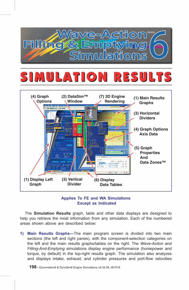
SIMULATION RESULTSSIMULATION RESULTS
Applies To FE and WA Simulations Except as Indicated
The Simulation Results graph, table and other data displays are designed to help you retrieve the most information from any simulation. Each of the numbered areas shown above are described below:
1) Main Results Graphs—The main program screen is divided into two main sections (the left and right panes), with the component-selection categories on the left and the main results graphs/tables on the right. The Wave-Action and Filling-And-Emptying simulations display engine performance (horsepower and torque, by default) in the top-right results graph. The simulation also analyzes and displays intake, exhaust, and cylinder pressures and port-flow velocities
(6) Display Data Tables
(3) Vertical Divider
(1) Display Left Graph
(5) Graph Properties And Data Zones™
(1) Main Results Graphs
(4) Graph Options Axis Data
(4) Graph Options
(2) DataSim™ Window
(7) 3D Engine Rendering
(3) Horizontal Dividers
VersionWave-ActionFilling & Emptying
Simulations
Wave-ActionFilling & Emptying
Simulations66
198—Dynomation6 & DynoSim6 Engine Simulations v6.02.08, 061518

which are presented in the in the center and lower crank-angle-based graphs (and in the graph located under the Component Categories activated using the Display Data Tabs [#6] in the photo on the left). For more information on how to interpret port pressure and flow graphs, refer to Wave-Dynamics Analysis (later in this manual).
Graph Reticule Lines All results graphs can display a red-dotted reticule line to indicate specific points
in the data being displayed. For example, the top horsepower graph reticule line indicates a specific engine speed, while the center and lower graphs point to a crank-angle (for Wave-Action simulations only). To “activate” any of these reticule lines, simply click on the graph. To use the reticule lines, first drag the reticule on the top horsepower graph to set an rpm point. Next, click on either
Simulation Results Displays
GraphReticuleLines
Graph Reticule Lines
All results graphs can display a red-dotted reticule line to
indicate specific points within the data being displayed. For example, the top horsepower
graph reticule line indicates a specific engine speed, while the center and lower graphs
point to a crank-angle (for Wave-Action simulations
only). To “activate” any of these reticule lines, simply
click on the graph.
Left Underlying Graph In addition to the three graphs dis-played on the right side of the main program screen, a fourth graph is available by clicking on the Graph tab located at the bottom of the Component Category pane (left Pane). This graph shows Cylinder-Pressure vs. Cylinder-Volume by default (commonly known as a P-V diagram), however, you can re-assign any crank-angle based data to either the Y1 or Y2 graph axis and either crank-angle or cylinder-volume to the X axis.
Dynomation6 & DynoSim6 Engine Simulations, v6.02.08, 061518—199
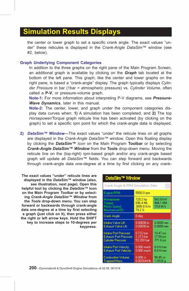
Simulation Results Displaysthe center or lower graph to set a specific crank angle. The exact values “un-der” these reticules is displayed in the Crank-Angle DataSim™ window (see #2, below).
Graph Underlying Component CategoriesIn addition to the three graphs on the right pane of the Main Program Screen, an additional graph is available by clicking on the Graph tab located at the bottom of the left pane. This graph, like the center and lower graphs on the right pane, is based a “crank-angle” display. The graph typically displays Cylin-der Pressure in bar (1bar = atmospheric pressure) vs. Cylinder Volume, often called a P-V, or pressure-volume graph.Note-1: For more information about interpreting P-V diagrams, see Pressure-Wave Dynamics, later in this manual.Note-2: The center, lower, and graph under the component categories dis-play data curves when: 1) A simulation has been completed, and 2) The top Horsepower/Torque graph reticule line has been activated (by clicking on the graph) to set a specific rpm point for which the crank-angle data is displayed.
2) DataSim™ Window—The exact values “under” the reticule lines on all graphs are displayed in the Crank-Angle DataSim™ window. Open this floating display by clicking the DataSim™ Icon on the Main Program Toolbar or by selecting Crank-Angle DataSim™ Window from the Tools drop-down menu. Moving the reticule line on the (top-right) rpm-based graph and/or any crank-angle based graph will update all DataSim™ fields. You can step forward and backwards through crank-angle data one-degree at a time by first clicking on any crank-
DataSim™ WindowThe exact values “under” reticule lines are displayed in the DataSim™ window (also,
see illustration, next page). Open this helpful tool by clicking the DataSim™ Icon on the Main Program Toolbar or by select-
ing Crank-Angle DataSim™ Window from the Tools drop-down menu. You can step
forward or backwards through crank-angle data one-degree at a time by first selecting a graph (just click on it), then press either
the right or left arrow keys. Hold the SHIFT key to increase steps to 10-degrees per
keypress.
200—Dynomation6 & DynoSim6 Engine Simulations v6.02.08, 061518

Simulation Results Displays
Moveable Screen Pane DividersAny of the four screen-pane dividers can be moved to
allow specific data displays more screen “real estate.”
You can drag the vertical divider to the left or right and
move any horizontal graph dividers to the top and bottom
to show graphs at any size you wish.
(2) Crank-Angle Data-Sim™ Window
Data Values “Under”Dotted Reticule Lines
(1) Crank-Angle Data Displays
Wave-Action Simulation Port Pressures And Velocities
(3) Port PressuresCenter Graph
Lower Graph
(5) Port Velocities
(6) Valve-Event Timing Indicator Lines
(4) TDC/BDC Piston Position Indicators
Simulation Crank-Angle Data Displays
The simulation Crank-Angle Data Displays (1) reveal an entire spectrum of pressures and flow velocities for the simulated engine. The crank-angle Port Pressures graph (3) displays intake, exhaust, and (optionally) cylinder pressures and other data. Port Gas Velocities for intake and exhaust flow are shown by default in the lower graph (5). Exact values of displayed data are shown in the Crank-Angle DataSim™ window (2). Simply position the Dotted Reticule Line over the data you wish to examine. The Crank-Angle graphs also have indicator lines for valve-event timing (6) and piston position (4). Study-ing these pressure curves can help locate inefficiencies and diagnose tuning problems (for more information about how to interpret the port pressure and flow graphs, refer to Wave-Dynamics Analysis later in this manual).
Dynomation6 & DynoSim6 Engine Simulations, v6.02.08, 061518—201

Simulation Results Displaysangle graph (to select it), then pressing either the right or left arrow keys. Holding SHIFT key will increase the cursor key steps to 10-degrees.
3) Vertical And Horizontal Screen Dividers—The center divider between the left and right panes and the horizontal dividers between the right-pane graphs can be moved (click and drag) to re-size any results display to suit your require-ments. When any screen area has been adjusted, the graphs will redraw and re-scale to take advantage of changes in display area. Divider positions are not “remembered” from session to session (however, all other graph and display defaults are stored in the .dxml engine simulation file and will be reapplied the next time the engine file is opened).
4) Graph Options Menu—Right click on any graph to open the Graph Options Menu. This menu provides fast access to custom graph settings, including data displayed, axis scaling, establishing side-by-side comparisons, and more:
Axis Data The first three choices from the Graph Options Menu allow you to customise the
data displayed on each of the three graph axis (Horizontal X Axis, Left Vertical Y1, and Right Vertical Y2; see photo on next page). Each of these axis can be assigned a variety of simulation results (the exact selection varies depending on whether the X Axis is rpm, crank-angle or cylinder-volume). Some the data-set choices are: Indicated, Frictional, Pumping, and Brake Horsepower, Wheel Horsepower, Torque, Volumetric Efficiency, a variety of Pressures (Imep, Fmep, Pmep, Bmep, Manifold, Boost), velocities (Intake and Exhaust Port Flow), Intake and Exhaust Valve Lifts, CD’s and Curtain Areas, Cylinder Volume, Mechanical Efficiency, Induction Airflow, Gas Force On The Piston and more.
Axis Scaling
The second group in the Graph Options Menu allows you to select several methods of axis scaling. You will notice that each axis can be scaled to a
Graph Options MenuRight-click any graph to show the Graph Options menu. Use the Data choices to
assign any simulation data set to any axis you desire (within the graph family of either rpm-based, or crank-angle based data). The
Range choices provide a variety of fixed and auto-scaling options for each axis. Use the
Optimize Yx Range selections to quickly set optimum (fixed) scaling for any currently
displayed data. For even more options, choose Properties to open the Graph Prop-
erties Dialog box.
202—Dynomation6 & DynoSim6 Engine Simulations v6.02.08, 061518

Simulation Results Displays
fixed low, medium, and high value. In addition, an auto-scaling feature can be enabled for any axis (turned off, by default). Use any fixed-axis scaling to maintain constant axis values. This establishes a “fixed visual baseline,” making it easy to see changes in power or torque as engine specifications are modi-fied (graph won’t rescale). However, when component changes dramatically alter data, use the auto-scaling feature will ensure that the entire data set is always visible and shown at 80 to 90% of full graph height for good resolution.
Optimize Y1(Left) / Y2(Right) RangesThe Graph Options Menu includes two Optimize Y1/Y2 Range selections that quickly establish optimum viewing using Fixed Axis Values (axis will not re-scale automatically after it has been set). To reset the graph back to normal range scaling, select one of the Range options described in the previous paragraph, or select Properties from the bottom of the Options menu and click Reset All to restore the display (only on the selected graph) to default values.
QuickCompare™ Graphic DisplayThe Graph Options Menu also contains a QuickCompare™
feature that instantly establishes any engine as a “baseline,” al-lowing easy-to-see changes in engine performance from that
point onward.
Optimize Y1/Y2 With Fixed ScalingResults graph consists of two verti-
cal axis, a left and right. Either of these axis can be quickly set for
optimum viewing using the Optimize Y1 (left axis) or Optimize Y2 (right
axis) choices (lower graph on right is Optimized display of exactly the
same data). Optimize choices ap-ply Fixed-Axis scaling (axis will not re-scale automatically). To reset the
graph back to normal scaling, select one of the Range options, or select
Properties from the bottom of the Options Menu and click Reset All.
Dynomation6 & DynoSim6 Engine Simulations, v6.02.08, 061518—203
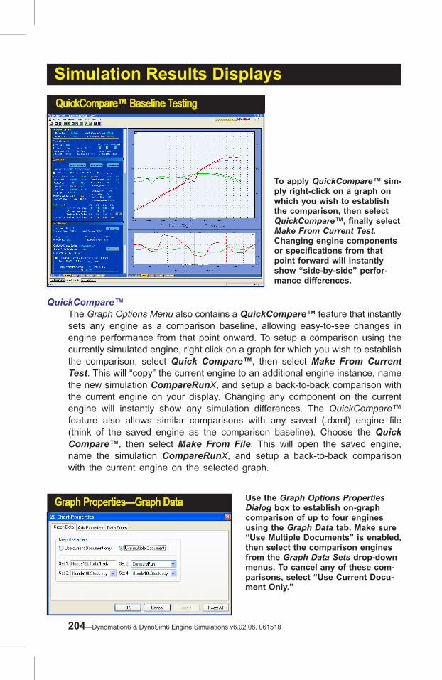
Graph Properties—Graph Data Use the Graph Options Properties Dialog box to establish on-graph comparison of up to four engines using the Graph Data tab. Make sure “Use Multiple Documents” is enabled, then select the comparison engines from the Graph Data Sets drop-down menus. To cancel any of these com-parisons, select “Use Current Docu-ment Only.”
Simulation Results Displays
QuickCompare™The Graph Options Menu also contains a QuickCompare™ feature that instantly sets any engine as a comparison baseline, allowing easy-to-see changes in engine performance from that point onward. To setup a comparison using the currently simulated engine, right click on a graph for which you wish to establish the comparison, select Quick Compare™, then select Make From Current Test. This will “copy” the current engine to an additional engine instance, name the new simulation CompareRunX, and setup a back-to-back comparison with the current engine on your display. Changing any component on the current engine will instantly show any simulation differences. The QuickCompare™ feature also allows similar comparisons with any saved (.dxml) engine file (think of the saved engine as the comparison baseline). Choose the Quick Compare™, then select Make From File. This will open the saved engine, name the simulation CompareRunX, and setup a back-to-back comparison with the current engine on the selected graph.
QuickCompare™ Baseline Testing
To apply QuickCompare™ sim-ply right-click on a graph on which you wish to establish the comparison, then select QuickCompare™, finally select Make From Current Test. Changing engine components or specifications from that point forward will instantly show “side-by-side” perfor-mance differences.
204—Dynomation6 & DynoSim6 Engine Simulations v6.02.08, 061518

Compare Up To Four “Open” Engines
This comparison of three engines was setup using the
Graph Options Properties Dialog. Up to four “open” engines can be compared on any graph. This graph
shows how horsepower and torque varied on all three test
engines.
Simulation Results Displays
5) Graph Properties Dialog—This dialog contains three tabbed pages that provide detailed control of the current graph. Here is an overview of each tab:
Graph Data: Using the drop-down lists on this page you can quickly es-tablish on-graph comparisons with up to three additional different engines. The engines you wish to include on the current graph must be “open,” with active Selection Tabs at the bottom of the Main Program Screen. First, make sure the Use Multiple Documents radio button is selected (allows multiple data sets). Next, select the specific engine you wish to add using the Graph Data Sets drop-down menus. Up to three additional engines can be selected using Set 2, Set 3 and Set 4 menus. When you click Apply or OK, the current graph will redraw and include the desired engine-data comparisons. Legends at the bottom of the graphs will provide keys to all graphic curves.
Graph Properties—Axis PropertiesChange the data and display characteristics of the current graph by modifying the Data Type, Graph Range, and Nu-merical Range using the Axis Properties tabbed page
Dynomation6 & DynoSim6 Engine Simulations, v6.02.08, 061518—205

Graph Properties—Data Zones™
DataZones™ extend the graphic-dis-play and data-analysis capabilities of the simulation. Using this feature, you can display additional engine data, show ranges, or clearly label danger-ously high pressures, engine speeds, and more.
Piston-Speed DataZone™
This DataZone display shows Piston-Speed bands drawn on the standard HP/Torque graph. The range values are indicated at the top of the graph.
Multiple DataZones™ Defined
DataZones™ can be defined for any of the four graphs available in the simulation. DataZone setups are saved with .dxml engine files.
Simulation Results Displays
Axis Properties shows the current Data Types and Ranges for the cur-rent graph. Modify any characteristic by changing properties. Create custom numeric ranges by selecting Custom-Range from the bottom of any of the drop-down Range menus).
DataZones™ Displays: DataZones™ extend the graphic-display and
data-analysis capabilities of the simulation. Using this feature, you can display additional engine data and/or show ranges for target power values or label dangerously high pressures, engine speeds, and more. To setup a DataZone, first select the data that you would like to display from the Type drop-down menu. Next, select the number of DataZones you would like to display by clicking on the “up” or “down” arrows next to the Zones field. You can modify the Range values and Colors for each zone (to have the simulation build a uniform transition between these colors for intermediate zones, set a starting and ending colors then press Blend Colors). Click
206—Dynomation6 & DynoSim6 Engine Simulations v6.02.08, 061518
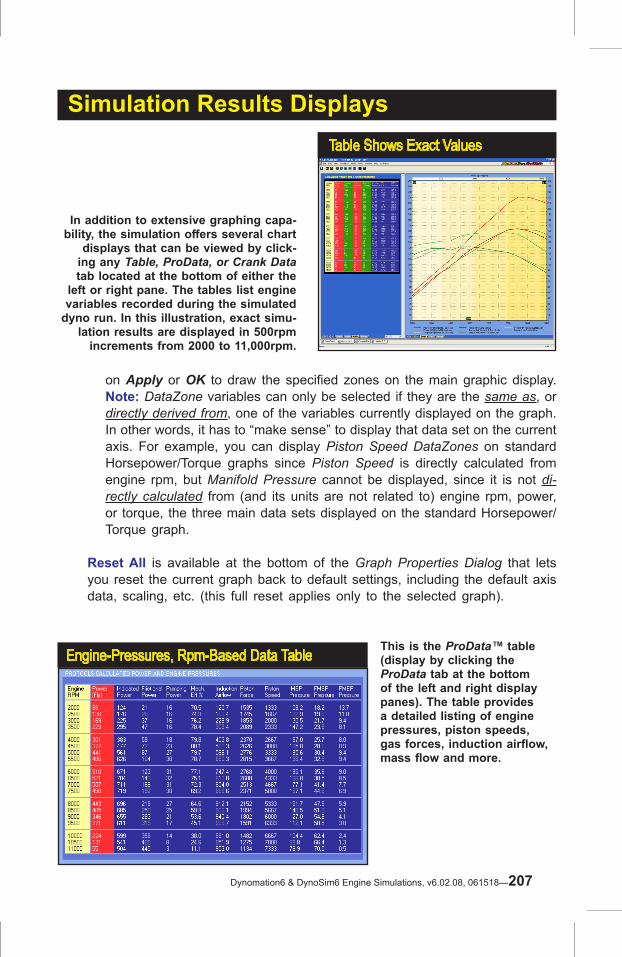
Simulation Results Displays
on Apply or OK to draw the specified zones on the main graphic display. Note: DataZone variables can only be selected if they are the same as, or
directly derived from, one of the variables currently displayed on the graph. In other words, it has to “make sense” to display that data set on the current axis. For example, you can display Piston Speed DataZones on standard Horsepower/Torque graphs since Piston Speed is directly calculated from engine rpm, but Manifold Pressure cannot be displayed, since it is not di-rectly calculated from (and its units are not related to) engine rpm, power, or torque, the three main data sets displayed on the standard Horsepower/Torque graph.
Reset All is available at the bottom of the Graph Properties Dialog that lets you reset the current graph back to default settings, including the default axis data, scaling, etc. (this full reset applies only to the selected graph).
Engine-Pressures, Rpm-Based Data Table This is the ProData™ table (display by clicking the ProData tab at the bottom of the left and right display panes). The table provides a detailed listing of engine pressures, piston speeds, gas forces, induction airflow, mass flow and more.
Table Shows Exact Values
In addition to extensive graphing capa-bility, the simulation offers several chart
displays that can be viewed by click-ing any Table, ProData, or Crank Data tab located at the bottom of either the
left or right pane. The tables list engine variables recorded during the simulated
dyno run. In this illustration, exact simu-lation results are displayed in 500rpm
increments from 2000 to 11,000rpm.
Dynomation6 & DynoSim6 Engine Simulations, v6.02.08, 061518—207
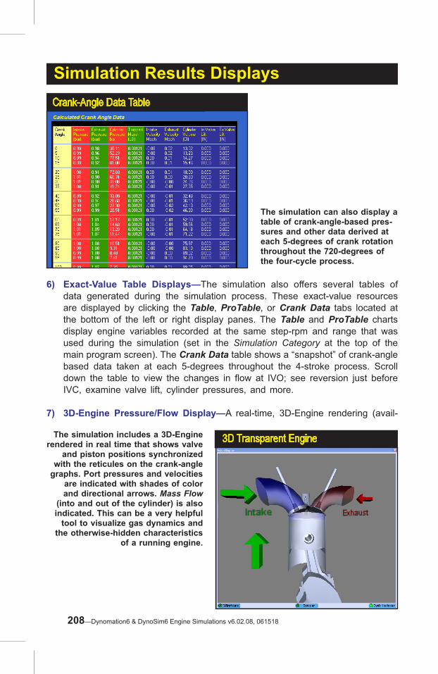
3D Transparent EngineThe simulation includes a 3D-Engine rendered in real time that shows valve
and piston positions synchronized with the reticules on the crank-angle
graphs. Port pressures and velocities are indicated with shades of color and directional arrows. Mass Flow
(into and out of the cylinder) is also indicated. This can be a very helpful
tool to visualize gas dynamics and the otherwise-hidden characteristics
of a running engine.
Simulation Results Displays
6) Exact-Value Table Displays—The simulation also offers several tables of data generated during the simulation process. These exact-value resources are displayed by clicking the Table, ProTable, or Crank Data tabs located at the bottom of the left or right display panes. The Table and ProTable charts display engine variables recorded at the same step-rpm and range that was used during the simulation (set in the Simulation Category at the top of the main program screen). The Crank Data table shows a “snapshot” of crank-angle based data taken at each 5-degrees throughout the 4-stroke process. Scroll down the table to view the changes in flow at IVO; see reversion just before IVC, examine valve lift, cylinder pressures, and more.
7) 3D-Engine Pressure/Flow Display—A real-time, 3D-Engine rendering (avail-
Crank-Angle Data Table
The simulation can also display a table of crank-angle-based pres-sures and other data derived at each 5-degrees of crank rotation throughout the 720-degrees of the four-cycle process.
208—Dynomation6 & DynoSim6 Engine Simulations v6.02.08, 061518
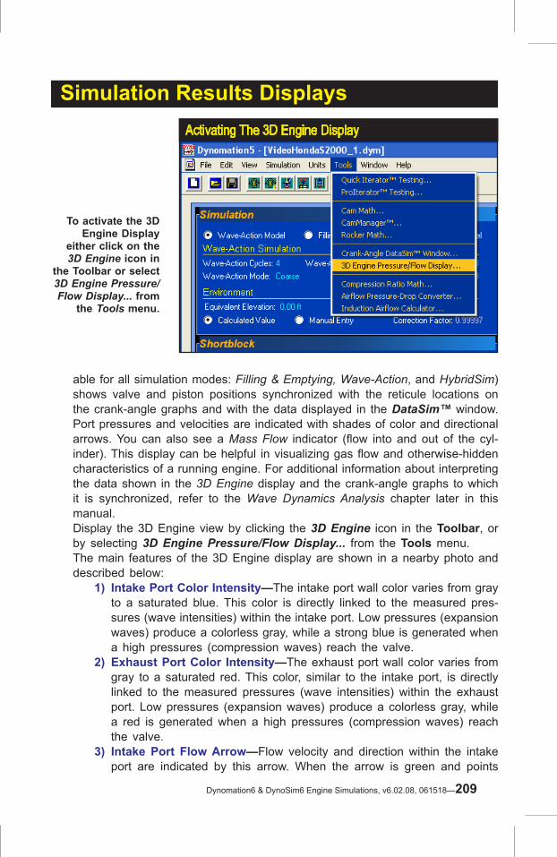
Simulation Results Displays
able for all simulation modes: Filling & Emptying, Wave-Action, and HybridSim) shows valve and piston positions synchronized with the reticule locations on the crank-angle graphs and with the data displayed in the DataSim™ window. Port pressures and velocities are indicated with shades of color and directional arrows. You can also see a Mass Flow indicator (flow into and out of the cyl-inder). This display can be helpful in visualizing gas flow and otherwise-hidden characteristics of a running engine. For additional information about interpreting the data shown in the 3D Engine display and the crank-angle graphs to which it is synchronized, refer to the Wave Dynamics Analysis chapter later in this manual.
Display the 3D Engine view by clicking the 3D Engine icon in the Toolbar, or by selecting 3D Engine Pressure/Flow Display... from the Tools menu.
The main features of the 3D Engine display are shown in a nearby photo and described below:
1) Intake Port Color Intensity—The intake port wall color varies from gray to a saturated blue. This color is directly linked to the measured pres-sures (wave intensities) within the intake port. Low pressures (expansion waves) produce a colorless gray, while a strong blue is generated when a high pressures (compression waves) reach the valve.
2) Exhaust Port Color Intensity—The exhaust port wall color varies from gray to a saturated red. This color, similar to the intake port, is directly linked to the measured pressures (wave intensities) within the exhaust port. Low pressures (expansion waves) produce a colorless gray, while a red is generated when a high pressures (compression waves) reach the valve.
3) Intake Port Flow Arrow—Flow velocity and direction within the intake port are indicated by this arrow. When the arrow is green and points
Activating The 3D Engine Display
To activate the 3D Engine Display
either click on the 3D Engine icon in
the Toolbar or select 3D Engine Pressure/Flow Display... from
the Tools menu.
Dynomation6 & DynoSim6 Engine Simulations, v6.02.08, 061518—209
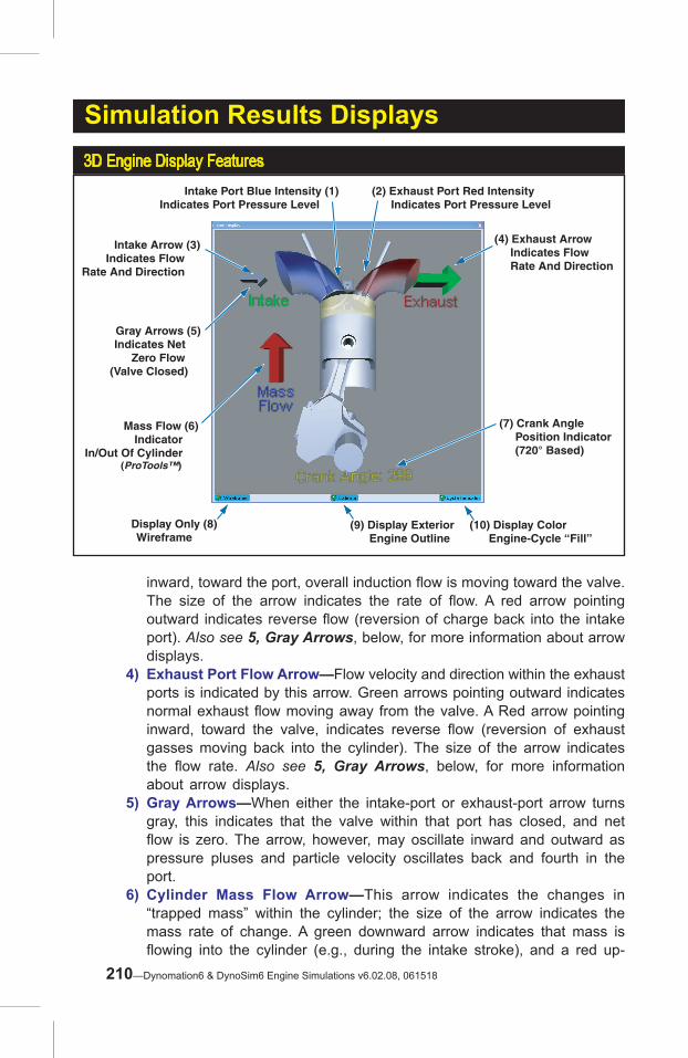
3D Engine Display Features(2) Exhaust Port Red Intensity Indicates Port Pressure Level
Intake Port Blue Intensity (1) Indicates Port Pressure Level
(10) Display Color Engine-Cycle “Fill”
(9) Display Exterior Engine Outline
Display Only (8)Wireframe
(4) Exhaust Arrow Indicates Flow Rate And Direction
Mass Flow (6)Indicator
In/Out Of Cylinder (ProTools™)
(7) Crank Angle Position Indicator (720° Based)
Intake Arrow (3)Indicates Flow
Rate And Direction
Gray Arrows (5) Indicates Net
Zero Flow (Valve Closed)
Simulation Results Displays
inward, toward the port, overall induction flow is moving toward the valve. The size of the arrow indicates the rate of flow. A red arrow pointing outward indicates reverse flow (reversion of charge back into the intake port). Also see 5, Gray Arrows, below, for more information about arrow displays.
4) Exhaust Port Flow Arrow—Flow velocity and direction within the exhaust ports is indicated by this arrow. Green arrows pointing outward indicates normal exhaust flow moving away from the valve. A Red arrow pointing inward, toward the valve, indicates reverse flow (reversion of exhaust gasses moving back into the cylinder). The size of the arrow indicates the flow rate. Also see 5, Gray Arrows, below, for more information about arrow displays.
5) Gray Arrows—When either the intake-port or exhaust-port arrow turns gray, this indicates that the valve within that port has closed, and net flow is zero. The arrow, however, may oscillate inward and outward as pressure pluses and particle velocity oscillates back and fourth in the port.
6) Cylinder Mass Flow Arrow—This arrow indicates the changes in “trapped mass” within the cylinder; the size of the arrow indicates the mass rate of change. A green downward arrow indicates that mass is flowing into the cylinder (e.g., during the intake stroke), and a red up-
210—Dynomation6 & DynoSim6 Engine Simulations v6.02.08, 061518

Simulation Results Displaysward arrow indicates that cylinder mass is decreasing (e.g., during the exhaust stroke). The Mass Flow Arrow also can also identify induction reversion during overlap and just before IVC. When there is no change in cylinder mass (when both valves are closed), the Mass Flow Arrow is no longer displayed.
7) Crank Position Indicator—The rotational position of the crank is dis-played using 720-degree notation. The zero position starts at TDC on the beginning of the power stroke. This corresponds to the crank-angle graphs on the right of the Main Program Screen.
8) Display Only Wireframe—If you wish to display the 3D Engine using only the underlying wireframe model, click this control (faster screen draw).
9) Display Exterior Engine Outline—This control toggles on and off a transparent image of the exterior dimensions of the engine.
10) Display Color Engine Cycle—This control toggles on and off the color fill for the cylinder that indicates the current engine cycle: Red indicates the power stroke; Yellow for the exhaust stroke; Green for the intake stroke; and Blue for the compression stroke.
Note-1: You can control the size, view, and position of the 3D Engine. To “grab” the engine, rotate it, and position it within the window, hold down the left mouse and drag. To enlarge and reduce the size of the 3D Engine, hold down the right mouse button and drag inward and outward.
Note-2: You can step forward and backwards through crank-angle data one-degree at a time by first clicking on any crank-angle graph (to select it), then either the right or left arrow keys. Holding SHIFT key will increase the cursor key steps to 10-degrees. The 3D Engine display will remain synchronized to the current crank-angle reticule line as it moves with each keypress.
Dynomation6 & DynoSim6 Engine Simulations, v6.02.08, 061518—211

With the power and speed of simulation makes is possible to fill file cabinets with simulated dyno-test data. In fact, it’s easy to become “bogged down” in an overabundance of data. Sorting through simulation results, analyzing the best power curves, and selecting promising component combinations can turn into a job nearly as difficult as the old trial-and-error dyno testing method! One solution to this problem was introduced by Motion Software’s as Iterative Testing™ (pronounced “it-er-ah-tive” and “it-ter-a-tor”), a powerful feature available in both the FE and WA simulations. Iterative testing performs series of simulation calculations automatically until the final, optimum answer is obtained. The simulation incorporates two versions of Iterative testing, The Quick Iterator™ is extremely simple to use (refer to the next chapter for information on the ad-vanced ProTools™ ProIterator™). By clicking a single button, the Quick Iterator will perform a test series to find optimum horsepower or torque. The Quick Iterator
Quick Iterator™Dual-Phase Status
WindowsCloseButton
SaveIteratorResult
Best Power/Torque Increase
Iterator RunningStatus
Find OptimumCam Timing Group
Find OptimumBore/Stroke Group
SimulationTests
In CurrentPhase
CurrentResults
BestResults
QUICK-ITERATORTMQUICK-ITERATORTM
VersionWave-ActionFilling & Emptying
Simulations
Wave-ActionFilling & Emptying
Simulations66
212—Dynomation6 & DynoSim6 Engine Simulations v6.02.08, 061518

Quick Iterator™ Generated Engines When the Quick Iterator has completed its analysis, you can save the results (by clicking the Save button). The program will generate a new simulated engine with the component combina-tion that produced optimum power or torque. The new engine will be added to the “open” engines included in the Engine Selection Tabs at the bottom of the Main Pro-gram Screen. Quick-Iterator engines can be analyzed, compared with other open engines, and modified in any way, just like any other engine in the simulation.
Using The Quick Iterator™
applies an optimization process called Dual-Phase™ Testing to find the best com-bination in short period of time. The first test phase uses a wide range of testing values. After the best result has been found from this wide-range search, a second phase is performed using a much narrower range of test values. The Dual-Phase approach allows the Quick Iterator to perform, for example, a search for optimum cam timing in less than 2500 simulation runs; typically, less than two minutes of processing time for the Filling-And-Emptying simulation and about 10 minutes for a Wave-Action simulation (on 4.0 Ghz or faster computer systems).
Using The Quick Iterator™
To perform a Quick Iterator analysis, select all the components for the baseline engine. Make sure all Title Bars in each Component Category are dark-tone, indi-cating that all engine components have been selected. There are two main testing groups in the Quick Iterator and two buttons in each group. The upper group searches for optimum cam timing for either peak horsepower or peak torque. The lower group determines the best bore and stroke combination (maintaining current engine displacement) for either optimum horsepower or peak torque. Press either the Best HP or Best Torque button in the Optimize Cam Timing group to begin an analysis of valve-event timing that will optimize horsepower or torque within ±500rpm of the current power or torque peak. The Quick Iterator assumes that the current cam used the simulated engine is a “roughly” appropri-ate for the intended application and uses current cam timing as a starting point. You can follow the progress of the Quick Iterator by viewing the indicators in the Iterator Status group. To perform an analysis of cylinder-bore and crankshaft-stroke dimensions, press
Dynomation6 & DynoSim6 Engine Simulations, v6.02.08, 061518—213
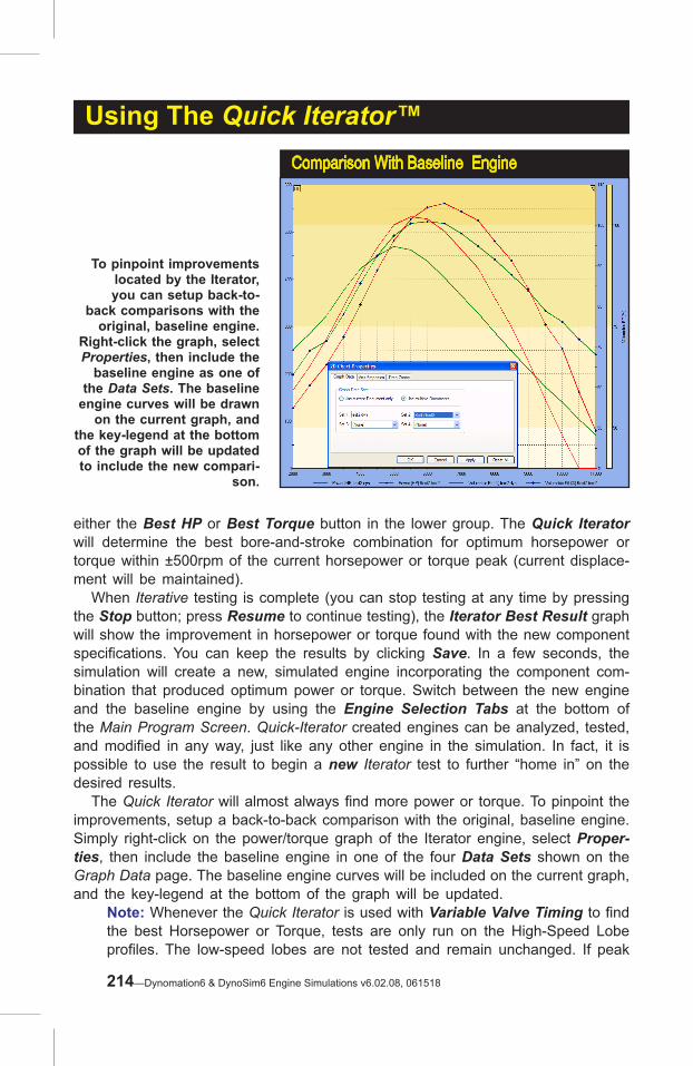
Using The Quick Iterator™
either the Best HP or Best Torque button in the lower group. The Quick Iterator will determine the best bore-and-stroke combination for optimum horsepower or torque within ±500rpm of the current horsepower or torque peak (current displace-ment will be maintained). When Iterative testing is complete (you can stop testing at any time by pressing the Stop button; press Resume to continue testing), the Iterator Best Result graph will show the improvement in horsepower or torque found with the new component specifications. You can keep the results by clicking Save. In a few seconds, the simulation will create a new, simulated engine incorporating the component com-bination that produced optimum power or torque. Switch between the new engine and the baseline engine by using the Engine Selection Tabs at the bottom of the Main Program Screen. Quick-Iterator created engines can be analyzed, tested, and modified in any way, just like any other engine in the simulation. In fact, it is possible to use the result to begin a new Iterator test to further “home in” on the desired results. The Quick Iterator will almost always find more power or torque. To pinpoint the improvements, setup a back-to-back comparison with the original, baseline engine. Simply right-click on the power/torque graph of the Iterator engine, select Proper-ties, then include the baseline engine in one of the four Data Sets shown on the Graph Data page. The baseline engine curves will be included on the current graph, and the key-legend at the bottom of the graph will be updated.
Note: Whenever the Quick Iterator is used with Variable Valve Timing to find the best Horsepower or Torque, tests are only run on the High-Speed Lobe profiles. The low-speed lobes are not tested and remain unchanged. If peak
Comparison With Baseline Engine
To pinpoint improvements located by the Iterator, you can setup back-to-
back comparisons with the original, baseline engine.
Right-click the graph, select Properties, then include the
baseline engine as one of the Data Sets. The baseline
engine curves will be drawn on the current graph, and
the key-legend at the bottom of the graph will be updated to include the new compari-
son.
214—Dynomation6 & DynoSim6 Engine Simulations v6.02.08, 061518

Using The Quick Iterator™torque is generated by the low-speed cam and you wish to optimize torque using the low-speed profile, build a separate engine—without V-V-T—using the low-speed cam data. Then run a Quick Iterator on that engine model to find the best-torque, valve-event timing.
Dynomation6 & DynoSim6 Engine Simulations, v6.02.08, 061518—215

The ProIterator™ (pronounced “it-ter-a-tor” and “it-er-ah-tive testing”) provides a powerful and easy-to-use tool for optimizing engine components. The serious engine designer needs the ability to perform Iterative testing on multiple engine systems, such as Induction, in the testing criterion. This, combined with greater flexibility in setting testing parameters, area-under-the-curve results analysis, variable power-band ranges, and more, is offered in the ProIterator™.
Using The ProIterator™
Open the ProIterator™ by choosing ProIterator™ Testing... from the Tools menu or by clicking the ProIterator™ Icon in the Toolbar. Tips on setting up the ProIterator are provided in the Walkthrough later in this section. The ProIterator main screen consists of the following Groups:
PRO-ITERATOR TMPRO-ITERATOR TM
Close QuitPower/Torque
Found By Iterator CloseSave State
WindowsCloseButton
ProIterator™Title Bar
QuickStart Presets Tabbed Data Pages
FunctionalGroupBoxes
SaveRest All
VersionWave-ActionFilling & Emptying
Simulations
Wave-ActionFilling & Emptying
Simulations66
216—Dynomation6 & DynoSim6 Engine Simulations v6.02.08, 061518
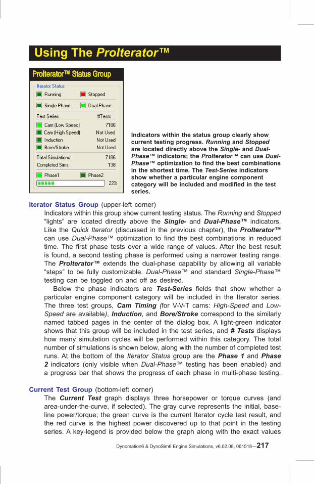
Using The ProIterator™
Iterator Status Group (upper-left corner) Indicators within this group show current testing status. The Running and Stopped “lights” are located directly above the Single- and Dual-Phase™ indicators. Like the Quick Iterator (discussed in the previous chapter), the ProIterator™ can use Dual-Phase™ optimization to find the best combinations in reduced time. The first phase tests over a wide range of values. After the best result is found, a second testing phase is performed using a narrower testing range. The ProIterator™ extends the dual-phase capability by allowing all variable “steps” to be fully customizable. Dual-Phase™ and standard Single-Phase™ testing can be toggled on and off as desired. Below the phase indicators are Test-Series fields that show whether a particular engine component category will be included in the Iterator series. The three test groups, Cam Timing (for V-V-T cams: High-Speed and Low-Speed are available), Induction, and Bore/Stroke correspond to the similarly named tabbed pages in the center of the dialog box. A light-green indicator shows that this group will be included in the test series, and # Tests displays how many simulation cycles will be performed within this category. The total number of simulations is shown below, along with the number of completed test runs. At the bottom of the Iterator Status group are the Phase 1 and Phase 2 indicators (only visible when Dual-Phase™ testing has been enabled) and a progress bar that shows the progress of each phase in multi-phase testing.
Current Test Group (bottom-left corner)The Current Test graph displays three horsepower or torque curves (and area-under-the-curve, if selected). The gray curve represents the initial, base-line power/torque; the green curve is the current Iterator cycle test result, and the red curve is the highest power discovered up to that point in the testing series. A key-legend is provided below the graph along with the exact values
ProIterator™ Status Group
Indicators within the status group clearly show current testing progress. Running and Stopped are located directly above the Single- and Dual-Phase™ indicators; the ProIterator™ can use Dual-Phase™ optimization to find the best combinations in the shortest time. The Test-Series indicators show whether a particular engine component category will be included and modified in the test series.
Dynomation6 & DynoSim6 Engine Simulations, v6.02.08, 061518—217
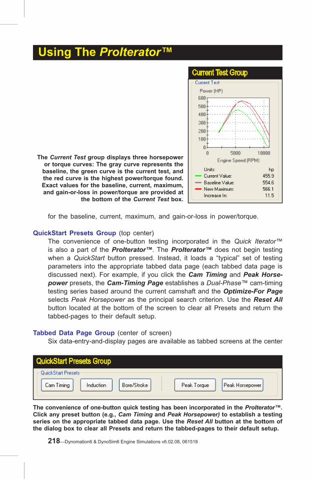
for the baseline, current, maximum, and gain-or-loss in power/torque.
QuickStart Presets Group (top center)The convenience of one-button testing incorporated in the Quick Iterator™ is also a part of the ProIterator™. The ProIterator™ does not begin testing when a QuickStart button pressed. Instead, it loads a “typical” set of testing parameters into the appropriate tabbed data page (each tabbed data page is discussed next). For example, if you click the Cam Timing and Peak Horse-power presets, the Cam-Timing Page establishes a Dual-Phase™ cam-timing testing series based around the current camshaft and the Optimize-For Page selects Peak Horsepower as the principal search criterion. Use the Reset All button located at the bottom of the screen to clear all Presets and return the tabbed-pages to their default setup.
Tabbed Data Page Group (center of screen)Six data-entry-and-display pages are available as tabbed screens at the center
Current Test Group
Using The ProIterator™
The Current Test group displays three horsepower or torque curves: The gray curve represents the
baseline, the green curve is the current test, and the red curve is the highest power/torque found. Exact values for the baseline, current, maximum, and gain-or-loss in power/torque are provided at
the bottom of the Current Test box.
QuickStart Presets Group
The convenience of one-button quick testing has been incorporated in the ProIterator™. Click any preset button (e.g., Cam Timing and Peak Horsepower) to establish a testing series on the appropriate tabbed data page. Use the Reset All button at the bottom of the dialog box to clear all Presets and return the tabbed-pages to their default setup.
218—Dynomation6 & DynoSim6 Engine Simulations v6.02.08, 061518

Using The ProIterator™
of the ProIterator™.
Cam-Timing Tabbed Pages (Standard and Variable-Valve Timing)The first two tabbed pages establish a Single- or Dual-Phase™ test of cam-timing changes on power or torque output. The Low Speed lobe is also used for standard, non-VVT (Variable Valve Timing) cams, while the High-Speed tab is only used for the high-speed lobe on VVT applications.You can quickly setup tests by clicking on the Cam Timing button in the QuickStart Preset group (described previously). This will perform a Dual-Phase test of 8,962 simulations that will take about 5 minutes for the FE model on 4Ghz and faster computers.If you did not press one of the Preset Buttons, the Cam-Timing Tabbed Pages default to Exclude (perform no cam-timing tests) as shown by radio-button controls at the top-left of the pages. To setup cam-timing Iteration, select either the Single- or Dual-Phase radio button and enter the testing criterion in the Single- and/or Dual-Phase Test boxes, located below the radio buttons. The number of degrees through which valve-timing events will be evaluated are shown just below the twin-hump cam-timing diagram.
Note: When performing Iterative testing on Variable Valve Timing cams of the dual-lobe type), it is more efficient to test each lobe (low and high-speed) separately and select the best of each test for the final camshaft specifications. While the ProIterator can run “combined” tests of both lobe profiles at once, this often results in a test series requiring a long time to complete.
Induction Tabbed PageThe third tabbed page sets up a standard, Single-or Dual-Phase test of the
Camshaft-Timing “Tabbed” Data Pages
The Cam Timing tabbed pages establish a Single- or Dual-Phase™ test of cam-timing changes on power or torque output. Select either the Single- or Dual-Phase radio button and enter the testing cri-terion in the Single- and/or Dual-Phase Test boxes. The ranges of individual cam-timing values evalu-ated during ProIterator™ testing are displayed just below the “twin-hump” cam-timing diagram.
Dynomation6 & DynoSim6 Engine Simulations, v6.02.08, 061518—219

Using The ProIterator™Induction “Tabbed” Data Page
The Induction tabbed page sets up a Single- or Dual-Phase test of the ef-fects of various induction system components and
dimensions. To perform an Iterative test of Induction
components, select the Single or Dual radio but-ton and select the mani-folds/induction-systems
that you would like to add to the test series. Note:
Runner dimensions only apply to WA simulations.
effects of various Induction Manifolds and (if the WA Simulation is selected) Runner Lengths and Dimensions on power or torque output. By default, the Induction Tabbed Page is set to Exclude (perform no induction tests) as shown in the radio buttons at the top-left of the page. To perform an Iterative test of induction systems, select Include and check the manifolds/induction-systems that you would like to include in the test series. You can also quickly setup an Induction system test of Intake Runner Lengths and Areas by clicking on the Induction button in the QuickStart Preset group (top of dialog box, described earlier).
Note: When selecting any of the Individual Runner induction systems, take note of the two additional radio-buttons: Use Existing Runner Temp and Use Temp Compensation During IR Testing that com-pensates for the lower temperatures of typical IR systems.In most cases, you should enable Use Temp Comp.. since this allow the simulation to alter runner temperatures, providing a more realistic environment when modeling a variety of manifolds that include both plenum and IR systems.
Bore/Stroke Tabbed PageThis tabbed page establishes a Single- or Dual-Phase™ test of bore-and-stroke dimensional changes on power or torque output. By default, the Bore/Stroke Tabbed Page is set to Exclude (perform no bore-and-stroke modifications) as shown in radio buttons at the top-left of the page. To in-clude a Bore/Stroke Iteration, select either the Single- or Dual-Phase radio button and enter the testing criterion in the Single- and/or Dual-Phase Test boxes, located just below the radio buttons. You can quickly setup an comprehensive test by clicking the Bore/Stroke button in the QuickStart
220—Dynomation6 & DynoSim6 Engine Simulations v6.02.08, 061518

Using The ProIterator™Bore/Stroke “Tabbed” Data Page
The Bore/Stroke tabbed page establishes an Iterative test of bore-and-stroke dimensional changes. Perform a Bore/Stroke Iteration by select-ing either the Single- or Dual-Phase radio button and entering the testing criterion. You can chose to Maintain Current Displace-ment or let engine dis-placement vary throughout Bore/Stroke testing (see text for details).
Preset group (described earlier). Note About Bore/Stroke Iteration: You can chose to Maintain Current Dis-placement or let engine displacement vary throughout Bore/Stroke Iterative testing. By checking the Maintain Current Displacement box, the Stroke within both Phase-Test boxes will switch to (Auto), indicating that Stroke will be allowed to vary as much as required to keep displacement constant while the Bore varies from its current value throughout the indicated (±) Range. Alternately, you can choose to allow Bore (rather than Stroke) to vary as much as required to keep displacement constant while Stroke changes from its current value throughout its (±) Range.Follow these steps to change the (Auto) variable: 1) With Maintain Current Displacement checked, 2) set the Bore (±) Range value to zero, 3) then set the Stroke (±) Range to any desired value (except zero). The (Auto) function will switch to Bore.
Optimize For Tabbed PageThis tabbed page establishes the desired results from Iterative testing. By default, the ProIterator™ will search for the combination of components that produces Peak Horsepower. Alternately, you can select Optimize For Peak Torque. In addition to these two options, two additional Optimize choices are available: Maximum Area Under The Horsepower Curve or Torque Curve. While the peak torque and horsepower choices focus on absolute maximum values, the areas-under-the-curves selections will find parts combinations that produce the greatest “volume” of horsepower or torque within the selected rpm range.In general, peak horsepower searches may find optimum components for narrow-rpm-band racing (like drag-racing), and maximum area under the curve
Dynomation6 & DynoSim6 Engine Simulations, v6.02.08, 061518—221

Using The ProIterator™
may find the best components for wide-rpm band racing (like road racing). Below the Optimize settings box, the RPM Range choices let you set the lower and upper limits through which the Iterator will search for optimum power or torque combinations. When the Iterator is searching for peak values, the RPM Range will be illustrated as dotted vertical lines on the Criterion graph. When either Area Under The Curve choice is selected, the RPM Range values will be displayed as a “bounded area” under the horsepower or torque curves.
Note: Optimizing engine components for maximum area under the curve is a unique way to look at engine power output. There is little published data on this method of evaluating engine power or torque, nor is there much research available on which racing applications may benefit from this analysis. Rumor has it, though, that racing teams have used this method to find a winning edge. Now you can use this powerful analysis method in the ProIterator™ to your advantage!
Run/Results Tabbed Page—Use this final tabbed page to begin an Itera-tive test series, to view testing progress, and to display the top ten results. Once you have selected testing parameters (on the Cam Timing, Induction, and Bore/Stroke tabbed pages) and set the optimization criterion, click the Run button to begin the Iterative test series. As the ProIterator™ locates promising results, they are displayed in the Best Results graph as vertical bars. A horizontal “baseline” within the graph indicates the power level of the current engine (established from components selected in the Component Categories on the Main Program Screen). As the Iterator finds better and better component combinations, the bars continue to increase in height (the graph axis will rescale as needed). If the Iterator finds combinations
Optimize For “Tabbed” Data PageThe Optimize For tabbed
page establishes the goals for the Iterator. By de-
fault, the ProIterator™ will search for Peak Horsepow-er. While Peak Torque and Peak Horsepower choices
focus on absolute maxi-mum values, the Areas Under The Curve selec-
tions locate engine setups that produce the greatest “volume” of horsepower
or torque. Think of this as the maximum horsepower or torque throughout the selected rpm range (over
time).
222—Dynomation6 & DynoSim6 Engine Simulations v6.02.08, 061518

Using The ProIterator™Run/Results “Tabbed” Data Page
The Run/Results tabbed page will begin Iterative testing, display testing progress, and let you save any of the top ten results. When testing is complete, save any (or all) results by clicking specific Save boxes located below the vertical bars in the Best Results graph, then click OK to spawn (create) these engines within the simulation.
that produce more power or torque than the baseline engine, the vertical results bars will exceed the baseline and continue to grow taller. The top ten horsepower or torque curves that match the bar-chart results are dis-played on the Best Results—3D graph. You can view these curves from any prospective using the X+, X-, Y+, Y-, Z+, and Z- buttons (Home returns the 3D graph to its original position). During the calculation of an Iterative test series, you can view the number of completed and remaining simulations in the Iterator Status box (you can stop testing at any time by pressing the Stop button; press Run to continue testing or Restart to clear current results). Save any (or all) of the top ten results by clicking the individual Save boxes located below the vertical bars in the Best Results graph. After selecting which results to save, click the OK button at the bottom of the ProIterator™ dialog box. The Iterator will close and “spawn” (create) new engines based on the components that were used in the selected tests. You can switch to any of these new en-gines by clicking on the Engine Selection Tabs at the bottom of the Main Component Screen (continue modifying and testing as you would with any simulated engine). The ProIterator™ will almost always find more power or torque. To pinpoint these improvements, you can quickly setup back-to-back comparisons with the original, baseline engine: Right-click on the power/torque graph of any Iterator-generated engine, select Properties, then include the baseline engine in one of the four Data Sets shown on the Graph Data page. The baseline engine curves will be included on the current graph, and the key-legend at the bottom of the graph will be updated.
Close/Save State (bottom)Dynomation6 & DynoSim6 Engine Simulations, v6.02.08, 061518—223

Using The ProIterator™Spawned Engines Shown In Engine Selection Tabs
When you close the Iterator screen, new “spawned” engines will be created and displayed in the Engine Selection Tabs at the bot-tom of the Main Program Screen. Each new engine can be brought into the foreground by clicking on its Se-lection Tab. Iterator-spawned engines can be analyzed, tested, and modified in any way, just like any other engine in the simulation.
Closes the Iterator and saves the current testing setup (changing engine com-ponents of this saved engine may force the Iterator to reset to its default). Use the Close/Save State button when you wish to continue Iterative testing on the same engine using similar components and Iterator settings.
Close/Quit (bottom)Closes the Iterator without saving the current state.
Reset All Button (bottom)Resets the current setup to default within the Iterator, but leaves it open so you can begin to enter a new Iteration setup.
ProIterator™ Testing—A Quick Walkthrough
The first step in performing an Iterative test is to design the baseline engine. When the engine has been simulated, you may begin an Iterative test series. Open the ProIterator™ by choosing ProIterator™ Testing... from the Tools menu or by clicking the ProIterator™ Icon in the Toolbar. Use the tabbed data-entry-and-display pages to establish components and/or engine-systems for testing. Alternately, to quickly setup a test series you can use the QuickStart buttons at the top of the dialog box. For this walkthrough, click on the CamTiming QuickStart Preset button. This establishes a Dual-Phase test based around current camshaft timing specifications. Notice that 2,401 tests will be performed during the first phase, and 6,561 tests will be run in Phase-2 using the best result from the Phase-1 as the starting point.
224—Dynomation6 & DynoSim6 Engine Simulations v6.02.08, 061518

Using The ProIterator™During Phase-1 simulations, individual cam timing points (IVO, IVC, EVO, EVC) will be varied through a range of +/- 24 degrees in 8-degree steps. That’s seven tests for each timing point, making the total number of tests performed during Phase-1 equal to 2,401 (7 x 7 x 7 x 7). When this first series is complete, the simulation will select the best result and begin Phase-2 testing. This time, each valve event will be varied through a range of +/- 4 degrees in 1-degree steps. This means that nine tests will be needed for each timing point, resulting in 6,561 tests in this series (9 x 9 x 9 x 9). The total number of tests required to complete the entire Iterative test is the sum of each series, or 8,962. Any of the timing point values, their +/- ranges, or the step sizes can be altered to suit custom requirements.
Note: As you select QuickStart Preset buttons or enter data on individual tabbed pages, the Iterator Status box (upper-left of dialog) shows the com-ponent groups that have been included and the number of tests that must be performed to complete the current series. Since the program will typically perform 1 to 10 simulation tests per second (depending on the speed of your computer, the rpm range of the tests, etc.), keep in mind that it will take about an hour to execute 18,000 tests.Keep the testing criterion limited and the range and step values large to minimize calculation times. Also, set the simulation rpm range as narrow as possible (set this in the Simulation Category).
Before Iterative test can begin, the results criterion you would like to optimize must be specified. For this walkthrough, press the Peak Horsepower button at the top of the Iterator dialog. When you click the button, the Optimize For tabbed page is selected and is setup with Optimize For Peak Horsepower within the RPM
Setting Up A Camshaft Iteration For this walkthrough, click on the CamTim-ing QuickStart Preset button. This sets up a Dual-Phase test around current cam-shaft timing specifica-tions. Notice that 2,401 tests will be performed on the first phase, and 6,561 tests will be run in Phase-2 using the best result from the Phase-1 as the start-ing point. See text for more information on how this Iterative test evaluates cam timing.
Dynomation6 & DynoSim6 Engine Simulations, v6.02.08, 061518—225
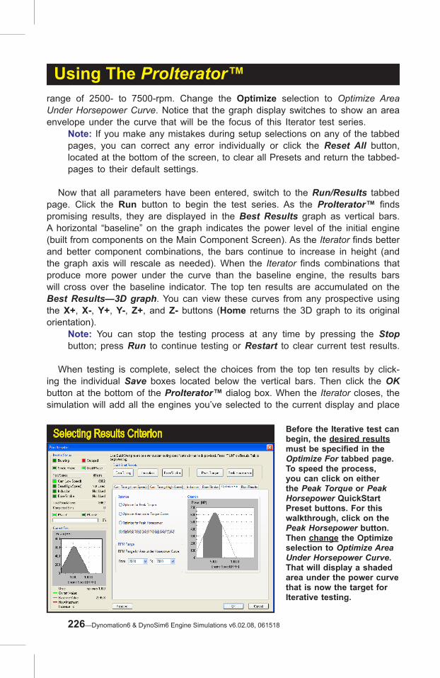
range of 2500- to 7500-rpm. Change the Optimize selection to Optimize Area Under Horsepower Curve. Notice that the graph display switches to show an area envelope under the curve that will be the focus of this Iterator test series.
Note: If you make any mistakes during setup selections on any of the tabbed pages, you can correct any error individually or click the Reset All button, located at the bottom of the screen, to clear all Presets and return the tabbed-pages to their default settings.
Now that all parameters have been entered, switch to the Run/Results tabbed page. Click the Run button to begin the test series. As the ProIterator™ finds promising results, they are displayed in the Best Results graph as vertical bars. A horizontal “baseline” on the graph indicates the power level of the initial engine (built from components on the Main Component Screen). As the Iterator finds better and better component combinations, the bars continue to increase in height (and the graph axis will rescale as needed). When the Iterator finds combinations that produce more power under the curve than the baseline engine, the results bars will cross over the baseline indicator. The top ten results are accumulated on the Best Results—3D graph. You can view these curves from any prospective using the X+, X-, Y+, Y-, Z+, and Z- buttons (Home returns the 3D graph to its original orientation).
Note: You can stop the testing process at any time by pressing the Stop button; press Run to continue testing or Restart to clear current test results.
When testing is complete, select the choices from the top ten results by click-ing the individual Save boxes located below the vertical bars. Then click the OK button at the bottom of the ProIterator™ dialog box. When the Iterator closes, the simulation will add all the engines you’ve selected to the current display and place
Using The ProIterator™
Selecting Results Criterion Before the Iterative test can begin, the desired results must be specified in the Optimize For tabbed page. To speed the process, you can click on either the Peak Torque or Peak Horsepower QuickStart Preset buttons. For this walkthrough, click on the Peak Horsepower button. Then change the Optimize selection to Optimize Area Under Horsepower Curve. That will display a shaded area under the power curve that is now the target for Iterative testing.
226—Dynomation6 & DynoSim6 Engine Simulations v6.02.08, 061518

Using The ProIterator™
them in the Engine Selection Tabs at the bottom of the Main Program Screen (see Engine Selection Tabs described earlier in this manual). Each test engine can be brought into the foreground by clicking on its Tab. Iterator “found” engines can be further analyzed, tested, and modified in any way, just like any other engine in loaded in the simulation. In fact, you can begin a new Iterator test using any of the spawned engines as a new baseline to further “home in” on desired results.
Tips For Running Efficient Iterative Tests
Setting up an Iterative series only takes a few seconds, however, if you include too many test parameters, ranges that are too wide, or step values that are too small, you will create an Iterator series that contains too many tests. If you create
Beginning The Test SeriesWhen all parameters have been entered, switch to the Run/Results tabbed page. Click the Run button to begin the test series. As the ProIterator™ finds promising results, they are displayed in the Best Results graph as vertical bars. A horizontal “baseline” on the graph (shown here near the top of the bar graph) indicates the power level of the baseline en-gine. As the Iterator finds better and better component combi-nations, the bars continue to increase in height.
Iterator Test Series Complete When testing is complete, pick your choices among the top ten results by clicking the Save boxes located below the vertical bars in the Best Results graph. Then click the OK button at the bottom of the ProIterator™ dialog box. When the Iterator closes, the simulation will spawn (create) all the engines you have selected and display them in the Engine Selection Tabs at the bottom of the Main Program Screen
Dynomation6 & DynoSim6 Engine Simulations, v6.02.08, 061518—227

Using The ProIterator™
an excessively long test series even fast computer systems may require days or months to complete. In these cases, the simulation may request that you increase step values for selected parameters. The best way to find optimum components, especially cam timing, is to setup a Dual-Phase™ test that uses large step values (20 degrees or more) to “get in the ballpark” on the first phase, then focus the second Iteration phase with a narrower range of values (perhaps just a 2 to 4 degrees) and a smaller step value (perhaps 1 degree) to precisely locate the best timing. Narrowly-focused tests may still require many thousands of test cycles to com-plete. In these cases, it is possible to continue to use your computer while the
Spawned Engines In Engine Selection Tabs
When the Iterator closes (after you have selected one or more engines from the Best Results list) the program will create the selected engines and display them in the Engine Selection Tabs at the bottom of the Main Program Screen. Each test engine can be brought into the foreground by clicking its Tab. Iterator-generated engines can be analyzed, tested, and modi-fied in any way, just like any other engine in the simulation.
An Extremely Long Iterator Test Series Narrowly-focused or mul-tiple-component tests may require several thousand, or even millions of test cycles to complete. A test series as large as the one shown here, can require several days of calcula-tion time depending on the speed of your computer. The same results can be obtained by a more care-fully designed test that takes a fraction of the time to complete. Use wide first-phase ranges and steps to keep the number of Iteration cycles to a minimum.
228—Dynomation6 & DynoSim6 Engine Simulations v6.02.08, 061518

Using The ProIterator™Iterator is still running. Simply use the Start menu to begin other applications or use Alt-Tab to switch between applications (see your Windows documentation for more information on program switching).
Note: You may also “minimize” the program and regain your desktop during an Iterator test.
Dynomation6 & DynoSim6 Engine Simulations, v6.02.08, 061518—229

The simulation incorporates several built-in calculators that will assist your data entry and analysis. Some are simple, one-step calculators, others are powerful, multi-step “math engines” that make short work of otherwise error-prone calcula-tions. This chapter presents an overview of these calculators.
THE INDUCTION-FLOW CALCULATOR
The Flow Rate field in the INDUCTION category establishes the overall flow for the simulated induction system, typically limited by the throttle size and opening. Determining the flow rate for injectors or carburetors, especially if the flow rating is unknown, can be problematic. In these cases, the built-in Flow Calculator can help determine the appropriate total induction flow for the simulation. Open the Flow Calculator by clicking on the Flow Calc button in the INDUCTION category. The calculator presents two distinct calculation models: 1) the Known Airflow Per Carb/Throttle, and 2) Known Throtte-Bore Diameter.
Induction-Flow Calculator If you are modeling an induction system that uses multiple carburetors or injec-tor “stacks,” you can use the built-in Flow Calculator to help determine total induction flow. Enter the number of throttles, the throttle bore diameter or the flow per throttle. The calculator will estimate the airflow for the entire system (flow for each throt-tle times the number of throttles).
BUILT-IN CALCULATORSBUILT-IN CALCULATORS
VersionWave-ActionFilling & Emptying
Simulations
Wave-ActionFilling & Emptying
Simulations66
230—Dynomation6 & DynoSim6 Engine Simulations v6.02.08, 061518

Built-In Calculators & Tools
To calculate the flow for an induction system when you only know the throttle-bore diameters (not the rated flow), select the right-hand radio button. Enter the number of “stacks” or “barrels,” the diameter of the throttle-bores, and select between But-terfly or Flat-Side throttle configurations (a Flat-Side is a slide-valve throttle that, when opened fully, provides no restriction to flow). The calculator will estimate the appropriate airflow for the entire system (flow for each throttle times the number of throttles). To apply the calculated airflow to the simulated engine, press the Apply button.
THE AIRFLOW PRESSURE-DROP CONVERTER
The simulation will accept induction airflow in CFM measured at a pressure drop of either 1.5- or 3.0-In/Hg (or in metric units). For those instances where an induc-tion system, injector, or carburetor was flow tested at a different pressure drop, or whenever you would like to convert flow values from one pressure-drop rating to another, the Airflow Pressure-Drop Converter easily performs these conversion
Airflow Pressure-Drop ConverterThe Airflow Pressure-Drop Converter is a general-purpose tool that will
convert airflow to/from any pressure-drop standard. Activate the Airflow
Converter by either selecting Airflow Pressure-Drop Converter... from the
Tools menu or by clicking on the Air-flow Converter Icon in the Toolbar.
Flat-Side (Slide-Valve) Throttle
Carburetors and injector stacks use two common throttle mechanisms: 1) The “standard” throttle plate that piv-ots on a shaft through the middle of the throttle bore, and 2) A slide-valve that when in the wide-open throttle position, is retracted entirely from the throttle bore. These carburetors are commonly called “FlatSide” since the chamber to accommodate the slide valve gives the carburetors a “flat,” appearance on the sides.
Opens Airflow Pressure-Drop Converter
Dynomation6 & DynoSim6 Engine Simulations, v6.02.08, 061518—231

CalculatedAirflow At1.5 Inches/Hg
Non-StandardAirflow
Convert To Standard4-Barrel Flow Rating
MODE 1—Convert To 4-bbl StandardMODE 1: When the calculator is first activated, the Airflow Ratings Standard is set to 4-Barrel Rating at 1.5-in/Hg Pressure Drop. To convert from any known airflow to this flow standard, enter the known airflow and pressure drop in the Known Airflow category. The airflow at the 4-barrel rating standard will be displayed in the Calcu-lated Airflow category.
Built-In Calculators & Tools
functions. This tool can also convert flow ratings measured in inches-of-mercury (in/Hg) of depression to and from airflow values rated in inches-of-water (in/H2O).
Note: A pressure drop of 1.5-in/Hg is equivalent to 20.3-in/H2O. The Airflow Pressure-Drop Converter has three basic modes of operation: 1) Convert flow to the 4-Barrel Standard pressure-drop rating, 2) convert to the 2-Barrel Standard pressure-drop rating, and 3) calculate airflow between any two pressure-drop rating levels. Each of these methods are described below. Activate the Airflow Pressure-Drop Converter by either selecting Airflow Pressure-Drop Converter... from the Tools drop-down menu or click on the Airflow Icon located in the Toolbar.
Using The Airflow Pressure-Drop Converter
Mode 1:Convert Any Flow To 1.5-in/Hg—The 4-Barrel Standard.
When the calculator is first activated, the 1.5-in/Hg Airflow Ratings Standard “radio button” is selected. The RESULTS category also defaults to a fixed pressure drop of 1.5-in/Hg or 20.3-in/H2O (these pressure drops are identical). To convert any known airflow measured at any pressure drop to the 1.5-in/Hg, 4-barrel standard, enter the measured airflow and pressure drop in the INPUT category (if needed, you can switch between Inches-of-Mercury[Hg] and Inches-of-Water[H2O] by click-ing on the appropriate radio buttons in the INPUT and RESULTS categories). The converted airflow will be displayed in the Calculated Airflow field. You can change to any of the previous fields (by clicking on them or using the Tab or SHIFT-Tab keys) to explore their effects on calculated airflow. At any time, you can click Ap-ply To Sim to load the new calculated airflow into the Total Induction Airflow
232—Dynomation6 & DynoSim6 Engine Simulations v6.02.08, 061518

Built-In Calculators & Tools
Rate field in the Induction category. Alternately, you can press Cancel to discard all entries and close the Airflow Pressure-Drop Converter.
Mode 2:Convert Any Flow To 3.0-in/Hg, The 2-Barrel Standard.
Switch the RESULTS—Airflow Ratings Standard category selection to the radio button marked 2-Barrel Carb of 3.0-in/Hg Pressure Drop. This changes the RE-SULTS Airflow/Pressure Drop category to a fixed 3.0-in/Hg (40.7-in/H2O) pressure drop. To convert any airflow measured at any pressure drop to the 3.0-in/Hg, 2-barrel standard, enter the known airflow and pressure drop in the INPUT category (you can switch between Inches-of-Hg and Inches-of-H2O by clicking on the appropriate radio buttons in the INPUT and RESULTS categories). The converted airflow will be displayed in the Calculated Airflow field. You can change any of the previous fields (by clicking on them or using the Tab or SHIFT-Tab keys) to explore their effects on calculated airflow. At any time, you can click Apply To Sim to load the new, converted airflow into the Total Induction Airflow Rate field in the Induction category. Alternately, you can press Cancel to discard all entries and close the Airflow Pressure-Drop Converter.
Mode 3:Convert Any Airflow To Equivalent Flow At Any Pressure-Drop.
Switch the RESULTS—Airflow Ratings Standard category to the radio button marked Any Pressure Drop. This allows the INPUT and RESULTS to be set to any pressure drop measured in Inches of Hg or Inches of H2O. Enter the known airflow and pressure drop in the INPUT category. Then enter the desired pressure
Calculated AirflowAt 3.0 Inches/Hg(2-Barrel Std.)
Any Known Airflow
Convert To Standard2-Barrel Flow Rating
MODE 2—Convert To 2-Bbl Standard
MODE 2: Switch the Airflow Ratings Standard to 2-Bar-
rel Rating at 3.0-in/Hg Pressure Drop.
Enter the known airflow and pressure
drop in the Known Airflow category. The airflow at the 2-barrel
rating standard will be displayed in the Calculated Airflow
category.
Dynomation6 & DynoSim6 Engine Simulations, v6.02.08, 061518—233

MODE 3—Convert To/From Any Pressure Drop
MODE 3: Switch the Airflow Ratings
Standard to No Rat-ings Standard. Enter
the Known Airflow at any pressure drop
measured in Inches of Hg or H2O. Then
enter the desired pressure drop in the
Calculated Airflow category. The equiva-
lent airflow will be displayed in the
Airflow Rate field.
Convert AirflowTo AnyPressure Drop
Any Airflow @ AnyPressure Drop
Convert Between AnyTwo Flow Rating Systems
Built-In Calculators & Tools
drop in the RESULTS category. The calculated equivalent airflow will be displayed in the Calculated Airflow field. You can modify any of the fields (by clicking on them or using the Tab or SHIFT-Tab keys) to explore their effects on calculated airflow.
Note: Since the Total Induction Airflow Rate field in the Induction category accepts only airflow values rated at either 1.5- or 3.0-in/Hg (20.3- or 40.7-in/H2O), the Apply To Sim button is not available when No Ratings Standard is selected. If you wish to use the new calculated values in a dyno test, select either the 1.5-in/Hg or 3.0-in/Hg Pressure Drop in the RESULTS—Airflow Ratings Standard group at the top of the calculator dialog.
Rocker-Math Calculator
The Camshaft Category includes an in-depth Rocker-Math Calculator tool that will help you determine how and why changes in Rocker Ratio can have subtle affects on valve timing.
IMPORTANT: Follow this simple rule when using Rocker Math: Enter the baseline Rocker-Ratio specifications (used by the cam manufacturer to determine their published valve-event timing, duration, etc.) in the Camshaft Category FIRST! Then use the Rocker Math Calculator to determine how changes to the initial values affect cam timing, valve lift, and engine power.
The Rocker-Math Calculator analyzes the subtle changes to valve-event timing that can occur when rocker-arm ratios are modified. When the intake or exhaust rocker-arm ratio is changed, overall valve lift is altered directly by the increase or decrease in ratio. It is clear that an increase in rocker ratio will open the valve further and increase valve acceleration. But what is less obvious is that rocker-ratio changes can also affect valve-open duration. When you click the Apply button af-
234—Dynomation6 & DynoSim6 Engine Simulations v6.02.08, 061518

Built-In Calculators & Tools
Rocker Math Calculator Overview
To properly use the Rocker Math Calculator: Enter the original manu-facturer’s cam specification for Rocker Ratio in the Camshaft Cat-egory FIRST! Then use the Rocker Math Calculator to determine how CHANGES to the baseline ratios will affect valve timing, valve lift, and engine power. In this photo, the cam manufacturer’s specified rocker ratio of 1.5 was increased to 1.75 for the intake and 1.6 for the exhaust. The intake timing changed more than one degree and the exhaust duration has increased about 0.6 degrees.
Rocker-Math Calculator Data EntryEnter new rocker ratios in the boxes (1). Changes in valve lift are displayed
in (4). Changes in seat-to-seat valve timing and duration are shown in the
Effects On Valve Timing area. If you click Apply, the new rocker ratios,
and changes in timing and valve lift will be transferred to the Camshaft
Component category and used in the simulation.
Enter CHANGES in RockerRatio and Lash here
View CHANGES inValve Lift here
View CHANGES inValve Timing here
View CHANGES inDuration here
Dynomation6 & DynoSim6 Engine Simulations, v6.02.08, 061518—235
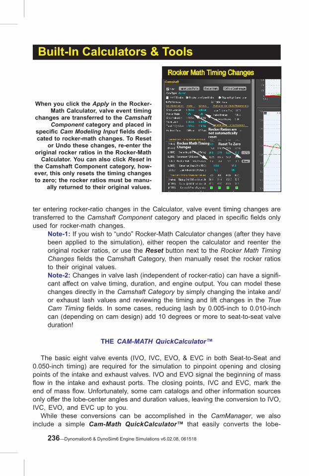
Built-In Calculators & Tools
ter entering rocker-ratio changes in the Calculator, valve event timing changes are transferred to the Camshaft Component category and placed in specific fields only used for rocker-math changes.
Note-1: If you wish to “undo” Rocker-Math Calculator changes (after they have been applied to the simulation), either reopen the calculator and reenter the original rocker ratios, or use the Reset button next to the Rocker Math Timing Changes fields the Camshaft Category, then manually reset the rocker ratios to their original values.Note-2: Changes in valve lash (independent of rocker-ratio) can have a signifi-cant affect on valve timing, duration, and engine output. You can model these changes directly in the Camshaft Category by simply changing the intake and/or exhaust lash values and reviewing the timing and lift changes in the True Cam Timing fields. In some cases, reducing lash by 0.005-inch to 0.010-inch can (depending on cam design) add 10 degrees or more to seat-to-seat valve duration!
THE CAM-MATH QuickCalculator™
The basic eight valve events (IVO, IVC, EVO, & EVC in both Seat-to-Seat and 0.050-inch timing) are required for the simulation to pinpoint opening and closing points of the intake and exhaust valves. IVO and EVO signal the beginning of mass flow in the intake and exhaust ports. The closing points, IVC and EVC, mark the end of mass flow. Unfortunately, some cam catalogs and other information sources only offer the lobe-center angles and duration values, leaving the conversion to IVO, IVC, EVO, and EVC up to you. While these conversions can be accomplished in the CamManager, we also include a simple Cam-Math QuickCalculator™ that easily converts the lobe-
Rocker Math Timing Changes
When you click the Apply in the Rocker-Math Calculator, valve event timing
changes are transferred to the Camshaft Component category and placed in
specific Cam Modeling Input fields dedi-cated to rocker-math changes. To Reset
or Undo these changes, re-enter the original rocker ratios in the Rocker-Math
Calculator. You can also click Reset in the Camshaft Component category, how-ever, this only resets the timing changes to zero; the rocker ratios must be manu-
ally returned to their original values.
236—Dynomation6 & DynoSim6 Engine Simulations v6.02.08, 061518

Built-In Calculators & Tools
center angle, intake centerline, and the duration values into IVO, IVC, EVO, and EVC valve events ready for use in the simulation. One click of the Apply button transfers event-timing values into the CAMSHAFT category for use as Primary (Seat-To-Seat) or Secondary (0.050-inch) timing events. Furthermore, if you are using a VVT cam, you can specify if you would like to transfer the event timing to the low- or high-speed cam.
Note: In order for the Cam-Math QuickCalculator to determine valve opening and closing events, BOTH the Lobe-Center Angle AND the Intake Centerline must be entered. Without the Intake Centerline, there is no way to determine
Cam-Math QuickCalculator™ The Cam-Math QuickCalculator allows direct entry and con-version of cam-manufacturer published data. Since this Cam-Math Calculator opens with the timing events currently used in the simulation, it also simplifies changing the lobe centerline angle and duration values.
Opens Low-Speed or High-SpeedCamMath QuickCalculator
Opening The Cam-Math QuickCalculator
The Cam-Math QuickCalculator is avail-
able from the Tools menu. If a V-V-T cam
is currently simulated, you can select between
two versions of the QuickCalculator: low-
speed and high-speed versions. Use Cam-Math
QuickCalculator to easily modify Lobe Center An-gles or Duration values.
Dynomation6 & DynoSim6 Engine Simulations, v6.02.08, 061518—237

Built-In Calculators & Toolshow the cam is “timed” or “indexed” to the crankshaft. Many (unfortunately not all) cam manufacturer catalogs provide sufficient information to determine valve-event timing. If you have a catalog or have visited a website that does not provide this information, try another cam manufacturer.
If IVO, IVC, EVO and EVC cam-timing values were already entered in the CAMSHAFT Category, the Cam-Math QuickCalculator will display the lobe-center angle, intake centerline, and duration values for the current cam and accept any changes you would like to make. As you modify the data fields, the corresponding IVO, IVC, EVO and EVC points will be calculated and displayed. You may then either accept the calculated values and transfer them to the CAMSHAFT category by clicking one of the Apply buttons or discard the new values and close the Cam-Math QuickCalculator by clicking Cancel.
THE COMPRESSION-RATIO CALCULATOR
You can select and test a wide range of compression directly in the Combus-tion Component category. However, many engine builders need to directly enter combustion-chamber volumes, head-gasket thickness, etc., to calculate or modify the compression ratio. The Compression-Ratio Calculator quickly performs these functions. In addition, this tool is more than a simple calculator, it adjusts itself to the needs of the engine builder; changing the way it functions depending on whether combustion volumes are known values or need to be measured directly from engine components.
Compression-Ratio Calculator Activate the Compression-Ratio Calculator by clicking on the CR Calc button in the Combustion Component cat-egory, by selecting Compres-sion Ratio Math from the Tools menu, or by clicking on the Compression Ratio Icon in the Toolbar.
Opens CompressionRatio Calculator
238—Dynomation6 & DynoSim6 Engine Simulations v6.02.08, 061518
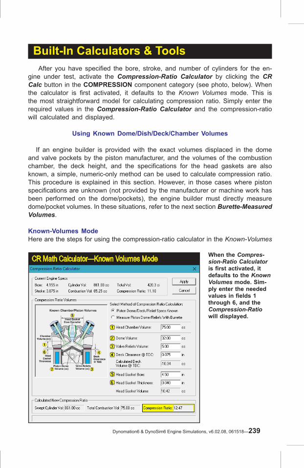
Built-In Calculators & Tools After you have specified the bore, stroke, and number of cylinders for the en-gine under test, activate the Compression-Ratio Calculator by clicking the CR Calc button in the COMPRESSION component category (see photo, below). When the calculator is first activated, it defaults to the Known Volumes mode. This is the most straightforward model for calculating compression ratio. Simply enter the required values in the Compression-Ratio Calculator and the compression-ratio will calculated and displayed.
Using Known Dome/Dish/Deck/Chamber Volumes
If an engine builder is provided with the exact volumes displaced in the dome and valve pockets by the piston manufacturer, and the volumes of the combustion chamber, the deck height, and the specifications for the head gaskets are also known, a simple, numeric-only method can be used to calculate compression ratio. This procedure is explained in this section. However, in those cases where piston specifications are unknown (not provided by the manufacturer or machine work has been performed on the dome/pockets), the engine builder must directly measure dome/pocket volumes. In these situations, refer to the next section Burette-Measured Volumes.
Known-Volumes ModeHere are the steps for using the compression-ratio calculator in the Known-Volumes
CR Math Calculator—Known Volumes Mode When the Compres-sion-Ratio Calculator is first activated, it defaults to the Known Volumes mode. Sim-ply enter the needed values in fields 1 through 6, and the Compression-Ratio will displayed.
Dynomation6 & DynoSim6 Engine Simulations, v6.02.08, 061518—239

Built-In Calculators & Tools
Mode. Start off by verifying that the upper radio button Piston Dome/Deck/Relief Specs Known has been selected. Next, enter the combustion-chamber volume (in cubic centimeters—cc’s) in the (1) Head Chamber Volume data box. Next, enter the volume displaced by the piston dome in (2) Dome Volume and the volume of the valve reliefs in one piston into (3) Valve Reliefs Volume. If your piston manu-facturer provided one value for both of these volumes, enter this combined volume in the (2) Dome Volume field and enter zero in field (3).
Note: If any of these values are unknown, they must be manually measured (with a burette; see the next section for Burette-Measured Volumes).
The next data entry field is (4) Deck Clearance @ TDC. This dimension indi-cates how far down the bore the piston is located when positioned at TDC. Enter a positive number for “down-the-bore” distances and a negative number if the piston protrudes above the deck surface. A typical value might be +0.040-inch, indicat-ing that the piston comes to a rest at TDC positioned 0.040-inch below the deck surface.
Important Note: A positive Deck Clearance @ TDC indicates the piston is positioned below the deck surface and this volume adds to the combustion space at TDC; a negative number indicates the piston protrudes above the deck surface at TDC and reduces the combustion space.
The next two data-entry boxes are used to calculate the volume added to the combustion space by the head gasket that is compressed between the cylinder head and the block-deck surface. The data box marked (5) accepts the Head Gasket Bore diameter (in the appropriate Metric or U.S. units). Most head gaskets have a “bore-circle” or “bore diameter” larger than the cylinder-bore diameter. For gaskets with bore-circles of odd shapes, simply estimate the bore circle by averaging the larger and smaller dimensions. Finally, enter the compressed (6) Head Gasket Thickness. This dimension is often available from the head-gasket manufacturer.
Measuring Deck Height
To measure how far down the bore the piston is positioned at TDC, use
a dial indicator and stand. Enter a positive number for “down-the-bore”
distances and a negative number if the piston protrudes above the
deck surface. A typical value might be +0.040, indicating that the piston
comes to a rest at TDC 0.040-inch below the deck surface.
240—Dynomation6 & DynoSim6 Engine Simulations v6.02.08, 061518

Built-In Calculators & ToolsWhen the compressed thickness is entered, the Head Gasket Volume and the Compression Ratio are calculated. At this point, you can change any data-input values and determine their effects on compression ratio. At any time, you can click Apply to load the calculated compression ratio into the COMPRESSION category and save all entered values for the simulated engine. Alternately, you can press the Cancel button to discard all entries and leave any previously entered compression ratio-value unchanged.
Using Burette-Measured Volumes
If you are using pistons with domes, dishes, or valve-pockets/reliefs of unknown volumes, determining the compression ratio requires a bit more work. Each of these volumes must be accurately measured so that the net effect of all “positive” (domes) and “negative” (pockets, reliefs) can be included in the calculations.
Burette-Measured ModeStart off by verifying that the lower radio button Measured Piston Dome/Reliefs With Burette is selected. Enter the combustion chamber volume (in cubic centi-meters—cc’s) in the first (1) Head Chamber Volume data field. The next entry, (2) Piston Down From TDC For Burette Measurement, is a more-or-less arbitrary distance down the bore (measured from the deck surface) of sufficient depth so that the entire piston dome is located below the deck surface. Typical values may be 0.100-inches or 0.250-inches depending on the height of the piston dome (any distance is acceptable as long as the entire dome is positioned below the deck
CR Math Calculator—Burette Measured ModeWhen the Compression-Ratio Calculator is switched to the Burette Measured Mode, the
data fields are redefined to allow the engine builder to
input individual volumes that sum to determine the Calcu-
lated Deck Volume @ TDC. To measure this volume, the
piston is lowered down the bore until the dome is entirely
below the deck surface (2), and a direct measurement is taken of the cylinder volume using a burette. After enter-
ing this volume and the head gasket specs, the compres-
sion-ratio is displayed.
Dynomation6 & DynoSim6 Engine Simulations, v6.02.08, 061518—241

Built-In Calculators & Tools
surface). At this depth, a direct measurement is made of the Volume Above The Piston in the cylinder (sometimes called Dome/Deck Volume). This measurement is taken by the engine builder using a liquid-filled burette to fill the space above the piston (a flat Plexiglas plate is often used to seal the top of the bore; grease is typically used to seal the piston to the bore). For pistons with positive dome volumes, the volume of liquid dispensed will be less than the volume for a simple cylinder of the same height. The liquid volume dispensed from the burette is entered in the Measured Liquid Volume Above Piston field. The difference between this volume and the volume of a simple cylinder (of a height equal to the value entered in field (2)) is the Calculated Deck Volume At TDC, a volume equivalent to the sum of the dome, dish, relief, and deck volumes of the piston.
Important Note: A negative Calculated Deck Volume At TDC indicates that the total dome/deck/relief volumes reduce the combustion space and will, therefore, increase the compression ratio over a flattop piston. A positive value indicates that the sum of all dome/dish/relief volumes will increase the combustion space volume and decrease the compression ratio over a similar flattop piston (with the same deck height at TDC).
The next two data-entry fields are used to calculate the volume added to the combustion space by the head gasket compressed between the cylinder head and the block deck surface. The data box marked (3) accepts the Head Gasket Bore diameter (in the appropriate Metric or US units). Most head gaskets have a “bore-circle” or “bore diameter” larger than the cylinder-bore diameter. For gaskets with bore-circles of odd shapes, simply estimate the bore circle by averaging the larger
Measuring Dome/Deck VolumeMeasure the volume above the piston while the highest portion of the piston dome is positioned below the deck surface. Enter this value in field (5) Volume Above Piston. The difference between this volume and the volume of a simple cylinder [of a height equal to the value entered in field (4)] is the Deck Volume At TDC. This volume is equivalent to the combined volumes in the dome, dish, and valve reliefs in the piston. A negative Deck Vol-ume At TDC indicates that the dome reduces the combustion space and will increase the compression ratio over a flattop piston. A positive value indicates that the sum of all dome/deck/dish/relief volumes will increase the combustion volume and decrease the compression ratio over a flattop piston.
242—Dynomation6 & DynoSim6 Engine Simulations v6.02.08, 061518

Built-In Calculators & Toolsand smaller dimensions. Next, enter the compressed (4) Head Gasket Thickness. This dimension is often available from the head gasket manufacturer. When the compressed thickness is entered, the Head Gasket Volume and Compression Ratio are calculated and displayed. At this point, you can change any data-input values and determine their effects on compression ratio. At any time, you can click Apply to load the new calculated compression ratio into the COMPRESSION component category and save all entered values with the simulated engine. Alternately, you can press the Cancel button to discard all entries and leave any previously entered compression ratio value intact.
Dynomation6 & DynoSim6 Engine Simulations, v6.02.08, 061518—243

PRINTINGPRINTINGPRO-PRINTING™ ENGINE DATA AND RESULTS CURVES
The simulation can print a complete report of dyno-test results, including engine components, cylinder head airflow data, exact engine-test result values, 2D graphic displays of several engine-test variables and much more. Called ProPrinting™, this professional printout comprises a multi-page, dyno-test document of the currently-selected engine ProPrinting™ features include custom page graphics, a cover page with the name and address of your business (or your personal name and address) and logo, a table of contents, optional text printed at the bottom of each page (can be a disclaimer, copyright notice or any other text you wish), even an optional glossary of common terms can be printed with your engine simulation report. The full-color ProPrinting™ report is “assembled” within the simulation and de-livered to your default Internet browser (e.g., Internet Explorer™, Chrome, FireFox, Opera, etc.). Printing is performed within your Browser either in the foreground (for Print-Preview) or in the background (for non-preview, direct printing; only available with Internet Explorer). You can direct the output to any installed Windows printer.
Note: Some browsers, like the deprecated Internet Explorer, do not print “back-ground graphics” by default. This can prevent the printing of background colors in many of the data tables and other graphics in ProPrinting™ reports. To enable full-function printing, open the Options choices (typically located in the Tools or Setup menus—you may have to choose the Advanced options—and enable Print Backgound Colors and Images).
ProPrinting™ Functions And Setup
The ProPrinting™ capabilities are another exclusive feature of this simulation. The ProPrint™ dyno-test report consists of fully-formatted data pages built from an HTML template. This template is “filled” with data from your current simulation which is sent to your default Internet browser for viewing and subsequent printing. Your Internet Browser is used for print-preview and to perform the complex process of converting the HTML into specific instructions that your printer can understand. By using the graphic capabilities of HTML, the simulation is able to produce a fully-formatted, professional test report.
VersionWave-ActionFilling & Emptying
Simulations
Wave-ActionFilling & Emptying
Simulations66
244—Dynomation6 & DynoSim6 Engine Simulations v6.02.08, 061518

ProPrinting™ Menu Selections
There are three ProPrint™ choices in the File menu that will help you setup re-
port formats and initiate report printing. ProPrint—Opens a dialog box that allows
the selection of a printer; clicking OK from this dialog starts printing (only available in
Internet Explorer). ProPrint Preview—Opens the ProPrint report within your Internet Browser so you can review each page.
ProPrint Setup—Opens a dialog box that allows you to select the information that is included on the pages of the ProPrint
report.
ProPrinting™ Features
ProPrinting™ setup and function are controlled by three choices from the pro-gram File menu:
ProPrint (Requires Internet Explorer to be set as your default browser)Selecting ProPrint from the FILE menu starts the process of building the HTML document and, when completed (takes a few seconds), opens the standard Windows Print dialog box that allows you to Select a printer, provides access to printer Properties, and sets the print Range (by entering X-Y in the Print Range field, with Y the starting page and X the ending page). Printing can be started (or canceled) from this dialog box.
Pro-Printing™ Explorer Setup Some browsers, like the deprecated In-ternet Explorer, do not print “background graphics” by default. This can prevent the printing of data table background colors in ProPrinting™ reports. To enable full-function printing, open the Options choices (typically located in the Tools or Setup menus—you may have to choose the Advanced option—and enable Print background colors and images).
Dynomation6 Engine Simulation, v.5.03.0528—245

ProPrinting™ Features
ProPrint Preview—(Works with IE, Chrome, FireFox, Opera and other browsers)Opens the ProPrint report in your default Internet browser, with page 1 at the top. Uses the scroll bar in your browser to move (down) through all pages in the report. You can print the report by opening the Print or Print Preview choices from the File or Setup menus within your browser.Note: If your browser supports the feature, you may be able to preview mul-tiple side-by-side pages by opening the Print Preview function from within your browser.
ProPrint SetupOpens a dialog that allows you to customize Pro-Printing™ features. You can add your name, address, your company logo, specialized (copyright) text, a table of contents, and even a short or long glossary to your ProPrint report. Use the
ProPrint Preview—Multiple Pages Some browsers support a multiple page Print Preview. Here is a six-up display; you may be able to select any number of pages you wish.
ProPrint Preview
Print Preview displays your ProPrint report in your Internet browser for you to review (works with most browsers). The first page is shown, and you can scroll through the rest of the document with the scroll bar. Select Print from the File or Settings menu to send the report to your printer.
246—Dynomation6 & DynoSim6 Engine Simulations v6.02.08, 061518

ProPrinting™ displays the results of any engine simulation in a professional, multi-page test
report. Use the Pro-Printing™ Setup dialog box, from the File menu, to enable and customize
Pro-Printing™ features. You can add your name, address, your company logo, specialized text, a
table of contents, and even a short or long glos-sary to your ProPrint report. Use the Save button
to save your preferences, which will be applied to all subsequent engine simulations. The files for the Default Logo.bmp and the DefaultCopyright.
txt are located in Dynomation6/Manuals & Videos/ProPrint or the DynoSim6/Manuals & Videos/
ProPrint subdirectory. You can modify these files to suit your requirements.
Pro-Printing™ Setup
ProPrinting™ Features
Save button to save your preferences, which will be applied to all subsequent engine simulation reports. The files for the Default Logo.bmp (should be square with a size near 100 by 100 pixels) and the DefaultCopyright.txt are located in Dynomation6/Manuals & Videos/ProPrint or DynoSim6/Manuals & Videos/ProPrint subdirectory (within your main program directory: C:/Dynomation6 or C:/DynoSim6). You can modify these files to suit your requirements.
Custom ProPrinting™ Options
ProPrinting™ Setup will let you configure ProPrinting™ features. If you activate Include Logo, the logo file DefaultLogo.BMP will be displayed and printed at the top of ProPrint pages. If you activate Include @ Bottom Of Page, the Include file (default is DefaultCopyright.txt) will be printed at the bottom of most pages. The location of the Default Logo.bmp and DefaultCopyright.txt is the Dynomation6/Manuals & Videos/ProPrint or DynoSim6/Manuals & Videos/ProPrint subdirectory. You can modify the Include @ Bottom Of Page text to display any non-formatted text. Use a non-formatting word processor (we recommend Windows Notepad) to modify the text to fit your needs. Keep the length under about 50 words. The De-faultLogo.BMP file can be replaced with your own logo. Keep the file in a square, BMP graphic format, and it should be no larger than approximately 100 by 100 pixels.
ProPrinting™ Page Descriptions
The complete ProPrinting™ report generated by the simulation consists of 22+ pages (you can decide what pages to print using the print dialog and the
Dynomation6 & DynoSim6 Engine Simulations, v6.02.08, 061518—247
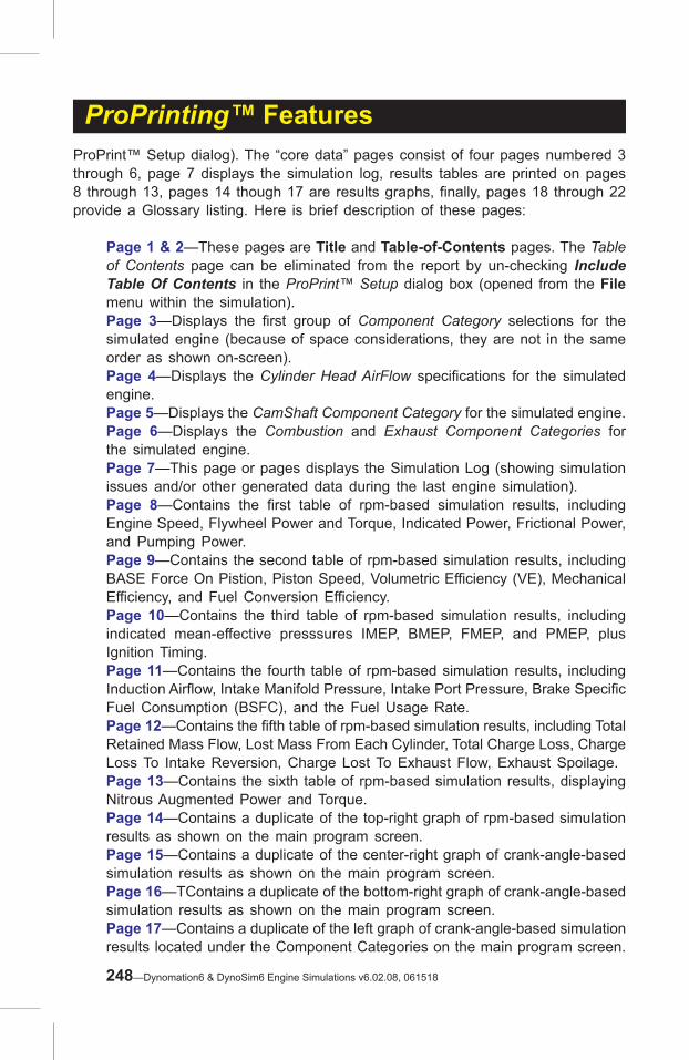
ProPrinting™ FeaturesProPrint™ Setup dialog). The “core data” pages consist of four pages numbered 3 through 6, page 7 displays the simulation log, results tables are printed on pages 8 through 13, pages 14 though 17 are results graphs, finally, pages 18 through 22 provide a Glossary listing. Here is brief description of these pages:
Page 1 & 2—These pages are Title and Table-of-Contents pages. The Table of Contents page can be eliminated from the report by un-checking Include Table Of Contents in the ProPrint™ Setup dialog box (opened from the File menu within the simulation).Page 3—Displays the first group of Component Category selections for the simulated engine (because of space considerations, they are not in the same order as shown on-screen).Page 4—Displays the Cylinder Head AirFlow specifications for the simulated engine.Page 5—Displays the CamShaft Component Category for the simulated engine.Page 6—Displays the Combustion and Exhaust Component Categories for the simulated engine.Page 7—This page or pages displays the Simulation Log (showing simulation issues and/or other generated data during the last engine simulation).Page 8—Contains the first table of rpm-based simulation results, including Engine Speed, Flywheel Power and Torque, Indicated Power, Frictional Power, and Pumping Power.Page 9—Contains the second table of rpm-based simulation results, including BASE Force On Pistion, Piston Speed, Volumetric Efficiency (VE), Mechanical Efficiency, and Fuel Conversion Efficiency.Page 10—Contains the third table of rpm-based simulation results, including indicated mean-effective presssures IMEP, BMEP, FMEP, and PMEP, plus Ignition Timing.Page 11—Contains the fourth table of rpm-based simulation results, including Induction Airflow, Intake Manifold Pressure, Intake Port Pressure, Brake Specific Fuel Consumption (BSFC), and the Fuel Usage Rate.Page 12—Contains the fifth table of rpm-based simulation results, including Total Retained Mass Flow, Lost Mass From Each Cylinder, Total Charge Loss, Charge Loss To Intake Reversion, Charge Lost To Exhaust Flow, Exhaust Spoilage.Page 13—Contains the sixth table of rpm-based simulation results, displaying Nitrous Augmented Power and Torque.Page 14—Contains a duplicate of the top-right graph of rpm-based simulation results as shown on the main program screen.Page 15—Contains a duplicate of the center-right graph of crank-angle-based simulation results as shown on the main program screen.Page 16—TContains a duplicate of the bottom-right graph of crank-angle-based simulation results as shown on the main program screen.Page 17—Contains a duplicate of the left graph of crank-angle-based simulation results located under the Component Categories on the main program screen.
248—Dynomation6 & DynoSim6 Engine Simulations v6.02.08, 061518

Modifying HTML Format Files
You can completely customize ProPrinting™ pages by editing the HTML DefaultFileInput.html. This file is the template that the simulation uses as the basis for ProPrint reports. The simula-tion key fields, such as _DATE, _TIME, etc., are replaced with data from the current engine test. Do not modify these keys or your reports may not include all simulation data!
ProPrinting™ Features
Page 18 to 22—These pages contain a Glossary Of Terms that may help explain the “language” of engine simulations to your customers or others you may provide ProPrint reports.
ProPrinting™ Report Modifications (Optional, Advanced)
You can customize ProPrinting™ pages by editing the HTML DefaultFileInput.html (see Important Note, below). This Input file is the HTML template that the simulation uses as the basis for ProPrint reports. The simulation adds current engine data and sends the result as DefaultFileOutput.html to your default Browser. To make permanent changes to ProPrinting™ report pages, edit the Input file (make sure you make a backup copy of the original file first). You will notice key fields that begin with an underscore, such as _DATE, _TIME, etc. During processing, these data keys are located by the simulation and replaced with data from the current engine test. Do not modify these keys or your reports may not include all simulation data!
Important Note: Many HTML editors have their own methods of generating HTML code and may include characters and formatting that affect how reports are printed. If you are not familiar with HTML, don’t attempt to modify the report Input File. Because of the unique characteristics of HTML, modifying ProPrinting™ HTML files is NOT supported by Motion Software, Inc.Also, your modified DefaultFileInput.html may be overwritten when the simu-lation is updated using the Motion Updater, so keep a backup copy of your modified file to prevent loosing your work.
Dynomation6 & DynoSim6 Engine Simulations, v6.02.08, 061518—249
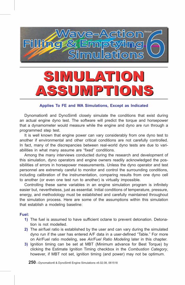
Applies To FE and WA Simulations, Except as Indicated
Dynomation6 and DynoSim6 closely simulate the conditions that exist during an actual engine dyno test. The software will predict the torque and horsepower that a dynamometer would measure while the engine and dyno are run through a programmed step test. It is well known that engine power can vary considerably from one dyno test to another if environmental and other critical conditions are not carefully controlled. In fact, many of the discrepancies between real-world dyno tests are due to vari-abilities in what many assume are “fixed” conditions. Among the many interviews conducted during the research and development of this simulation, dyno operators and engine owners readily acknowledged the pos-sibilities of errors in horsepower measurements. Unless the dyno operator and test personnel are extremely careful to monitor and control the surrounding conditions, including calibration of the instrumentation, comparing results from one dyno cell to another (or even one test run to another) is virtually impossible. Controlling these same variables in an engine simulation program is infinitely easier but, nevertheless, just as essential. Initial conditions of temperature, pressure, energy, and methodology must be established and carefully maintained throughout the simulation process. Here are some of the assumptions within this simulation that establish a modeling baseline:
Fuel: 1) The fuel is assumed to have sufficient octane to prevent detonation. Detona-
tion is not modelled. 2) The air/fuel ratio is established by the user and can vary during the simulated
dyno run if the user has entered A/F data in a user-defined “Table.” For more on Air/Fuel ratio modeling, see Air/Fuel Ratio Modeling later in this chapter.
3) Ignition timing can be set at MBT (Minimum advance for Best Torque) by clicking the Estimate Ignition Timing checkbox in the Combustion Category, however, if MBT not set, ignition timing (and power) may not be optimum.
SIMULATIONASSUMPTIONSSIMULATION
ASSUMPTIONS
VersionWave-ActionFilling & Emptying
Simulations
Wave-ActionFilling & Emptying
Simulations66
250—Dynomation6 & DynoSim6 Engine Simulations v6.02.08, 061518

Simulation Assumptions & Considerations
Environment: 1) Depending on the Atmospheric Standard in use (set in the Environment Group
in the Simulation Category, inducted air is 77-degrees (F), dry (0% humidity), and of 29.23-in/Hg atmospheric pressure unless changed by the user.
2) The simulation assumes that engine, oil, and coolant have been warmed to operating temperature.
Methodology: 1) The simulated engine is put through a series of “step” tests, during which
the load is adjusted to “hold back” engine speed as the throttle is opened wide. The load is adjusted to allow the engine speed to rise to the first test point. The engine is held at this speed at wide-open-throttle (WOT) and a power reading is taken. Then engine speed is allowed to increase to the next step and a second power reading is taken. This process continues until the maximum testing speed is reached.
Note: Since some engines, especially those with cam timing designed for all-out drag racing, are not able to run at full throttle under load at very low engine speeds, the power generated at some of the lower rpm points may register as zero.
2) Since the testing procedure increases engine speed in discrete steps, and engine speed is held steady during the power measurement, measured engine output does not reflect losses from accelerating the rotating assembly (the effects of rotational inertia in the crank, rods, etc.). These processes affect power in most “real-world” applications, such as road racing and drag racing, where engine speed is rapidly changing throughout the race.
Camshaft Modeling: As detailed in the Component Category chapter, the simulation uses two distinct
If cam timing for any of the lobes used in the current simulation are based on an imported Profile data, the W/A Lobe Data field display will switch from 10-Point to Profile in the CAMSHAFT cat-egory. Profile data is the closest match to “real-world” camshaft profiles and offers the highest modeling accuracy. 10-Point data doesn't follow “true” cam profiles as well as Profile data, but has the advantage of being extremely flexible by allowing modifications to any cam-timing events and lift data.
“Profile” Indicates LobeProfile Data Is Being Used.
“->10-pnt” Buttons will convertProfile data to 10-Point modeling
Using Imported Cam Profile Data
Dynomation6 & DynoSim6 Engine Simulations, v6.02.08, 061518—251

Simulation Assumptions & Considerationstypes of cam data for simulation modeling: 1) 10-Point Timing and 2) Lobe-Profile lift data. Profile data is the closest match to a specific “real-world” lobe profile and offers the highest modeling accuracy. 10-Point data, while not as precise in modling a specific lobe, has the advantages of being extremely flexible by allowing modi-fications to any cam-timing events and lift data; very helpful during the process of finding optimum cam timing for specific applications.
Air/Fuel Ratio Modeling: Air/Fuel ratio has a strong influence on engine output. Fuel and oxygen molecules combine during combustion to produce heat, pressure, and residual gases. If all the carbon and oxygen atoms combine within the cylinder during combustion, no carbon monoxide or unburned hydrocarbons will remain. This “complete burning” is called stoichiometric combustion (and is a theoretical optimum condition that is not achieved in the real world). The air/fuel ratio that allows complete combustion is called the stoichiometric air/fuel ratio, and it is approximately 14.6:1 for gasoline. However, for maximum power a richer mixture is required, often around 12.5:1.
Note: The air/fuel ratios for maximum power for all fuels modeled by the simulation are listed in the Air/Fuel Ratio drop-down menu within the Com-bustion category.
Finally, when Nitrous-Oxide augmentation is used with either Gasoline or Metha-nol, additional fuel flow is required to maintain the correct air(oxygen)/fuel ratio. The
The simulation can model a varying air/fuel ratio through-out the simulation rpm test range. The Air/Fuel Ratio Map is available by selecting Table from in the Combustion category.
Air/Fuel “Map”
252—Dynomation6 & DynoSim6 Engine Simulations v6.02.08, 061518
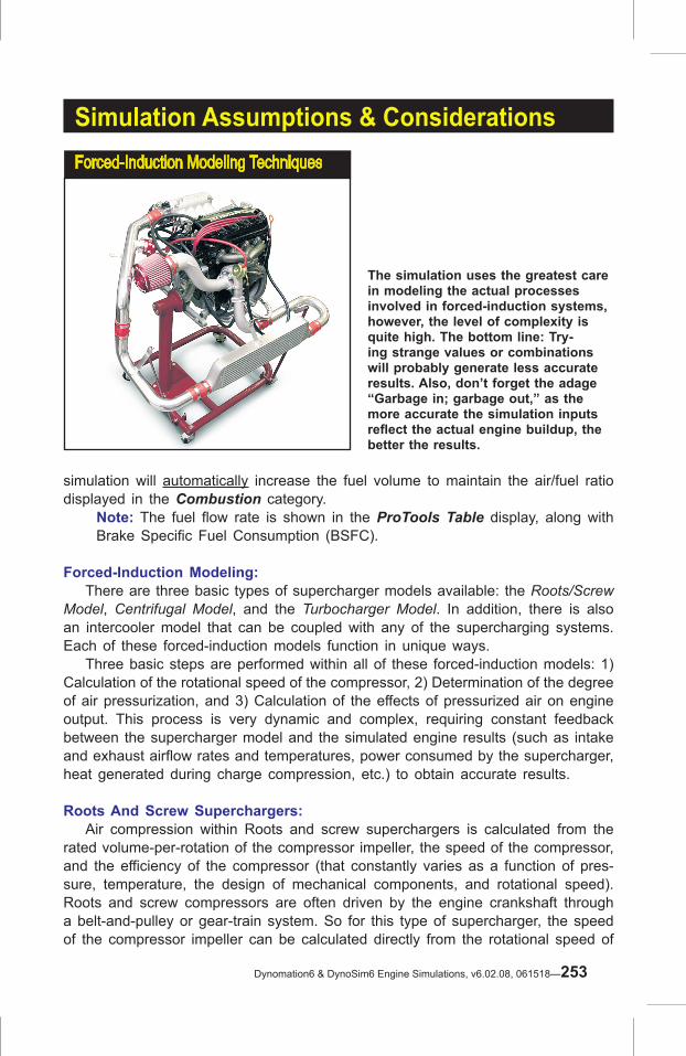
Simulation Assumptions & Considerations
simulation will automatically increase the fuel volume to maintain the air/fuel ratio displayed in the Combustion category.
Note: The fuel flow rate is shown in the ProTools Table display, along with Brake Specific Fuel Consumption (BSFC).
Forced-Induction Modeling: There are three basic types of supercharger models available: the Roots/Screw Model, Centrifugal Model, and the Turbocharger Model. In addition, there is also an intercooler model that can be coupled with any of the supercharging systems. Each of these forced-induction models function in unique ways. Three basic steps are performed within all of these forced-induction models: 1) Calculation of the rotational speed of the compressor, 2) Determination of the degree of air pressurization, and 3) Calculation of the effects of pressurized air on engine output. This process is very dynamic and complex, requiring constant feedback between the supercharger model and the simulated engine results (such as intake and exhaust airflow rates and temperatures, power consumed by the supercharger, heat generated during charge compression, etc.) to obtain accurate results.
Roots And Screw Superchargers: Air compression within Roots and screw superchargers is calculated from the rated volume-per-rotation of the compressor impeller, the speed of the compressor, and the efficiency of the compressor (that constantly varies as a function of pres-sure, temperature, the design of mechanical components, and rotational speed). Roots and screw compressors are often driven by the engine crankshaft through a belt-and-pulley or gear-train system. So for this type of supercharger, the speed of the compressor impeller can be calculated directly from the rotational speed of
The simulation uses the greatest care in modeling the actual processes involved in forced-induction systems, however, the level of complexity is quite high. The bottom line: Try-ing strange values or combinations will probably generate less accurate results. Also, don’t forget the adage “Garbage in; garbage out,” as the more accurate the simulation inputs reflect the actual engine buildup, the better the results.
Forced-Induction Modeling Techniques
Dynomation6 & DynoSim6 Engine Simulations, v6.02.08, 061518—253

Simulation Assumptions & Considerationsthe engine. A Roots compressor does not strictly compress the air, but rather “moves” a fixed volume of air mass into the induction system for each revolution of the impel-ler. It is here the air is compressed: pressure is a result of the difference in the amount of air being pumped into the manifold relative to the amount of air being “swallowed” by the engine. Because this pressure is dependant on engine speed, it is possible for a Roots blower to function under vacuum conditions, or lower than ambient pressure, when the engine is drawing in more air than the compressor can supply. This typically occurs at low engine speeds. Air compression in a screw-compressor system is very similar to that of a Roots, except that a screw compressor produces a small amount of internal compression. Peak pressure regulation in the induction system of Roots or screw superchargers is controlled with a pop-off valve that releases overpressure to the atmosphere. However, the most efficient operation is obtained by carefully selecting the correct blower displacement and belt ratios so that pop-off valve operation is not required. The work required to pump additional air into the induction system comes with a price: The energy required to operate a Roots or screw compressor is substantial. The total power consumed depends on many factors, including ambient pressure, output pressure, temperature, compressor size, compressor friction, engine displace-ment, engine and supercharger rpm and operational efficiency.
Centrifugal Superchargers: Like Roots/screw superchargers, a centrifugal supercharger is driven directly from the engine, usually by the crankshaft through a series of gears or pulleys and belts. The centrifugal supercharger consists of impeller that spins at high speed. The blades on the impeller draw-in and accelerate air into the supercharger hous-ing. The degree of compression is dependant on the speed, the size of the impel-ler wheel, the wheel trim (the shape of the blades), and housing (often called the “scroll”) size. The pressure delivered to the engine is calculated from a “compres-
Roots superchargers do not di-rectly compress the air but rather pump a fixed volume of air into the induction system for each rev-olution of the impeller. Induction pressure is calculated as the dif-ference in the amount of air being delivered to the intake manifold relative to the amount of air being “swallowed” by the engine.
Roots Supercharger Simulation
254—Dynomation6 & DynoSim6 Engine Simulations v6.02.08, 061518

Simulation Assumptions & Considerationssor map” (consisting of measured performance data for that specific supercharger supplied by the manufacturer). The map contains information about the efficiency of the compressor at various pressures and speeds. Numerical data from the map is dynamically extracted during the simulation, and data points are interpolated to ensure the highest accuracy in predictions of induction temperature and pressure. To limit maximum output pressure, typical centrifugal systems will use a pop-off valve that opens to release the additional pressure to the inlet side of the super-charger. The power consumed by a centrifugal compressor is not as great as it is for a roots or screw supercharger, but it is, nevertheless, a significant source of “lost” power.
Turbochargers: Turbocharger are, basically, centrifugal superchargers with the compressor ele-ment connected to a turbine wheel driven by exhaust pressure. And while calculation of compressor speed is straightforward on a centrifugal supercharger, the same cannot be said for a turbocharger. Internal shaft speed (connecting the turbine and compressor wheels) is determined by (among other things) an analysis of exhaust flow, turbine wheel size, turbine housing shape, and the efficiency read from the turbine “map” (in addition to the compressor map!). Internal wheel speeds are based on a balance between the energy used to spin the turbine and the energy needed to compress incoming air. The simulation uses another “iterative” technique to find a shaft speed that balances energy generated with energy consumed. The differences between the energy required to compress the incoming air and the energy available in the exhaust system is also the basis from which “backpres-sure” in the exhaust system is calculated. Backpressure robs the engine of its ability to purge itself of exhaust gasses and prevents efficient cylinder filling with fresh charge. To limit maximum intake manifold pressure and to minimize backpressure in the exhaust system, the turbocharger uses a pressure-limiting technique different from roots, screw, or centrifugal superchargers. When maximum boost pressure has been reached, excess exhaust-gas flow is diverting around the turbine through a
Air pumping in a screw-compres-sor system is very similar to that to
a Roots, except that a screw com-pressor produces a small amount
of internal charge compression and is typically more efficient.
Screw Supercharger Simulation
Dynomation6 & DynoSim6 Engine Simulations, v6.02.08, 061518—255

Simulation Assumptions & Considerations
“wastegate” valve. Since diverted exhaust gasses no longer impinge on the turbine, the speed of the turbine can be effectively reduced and controlled, and the bypassed exhaust gas flow reduces backpressure and improves engine efficiency.
Note: The turbocharging algorithms used in the simulation were designed to model the properties of a “stable-state” turbo system. In other words, transient factors, like turbo “lag” that can occur when the engine is rapidly increasing in rpm, are not modeled. The simulation will provide a “steady-state” analysis of a turbocharged engine, that is, a power prediction when the engine reaches a steady-state condition on the dynamometer at each test rpm.
Intercoolers: The temperature of the air entering the engine from a supercharging system is
Centrifugal superchargers are driven directly from the engine, usually by the crankshaft through a series of gears and/or pulleys and belts. The centrifugal supercharger consists of impeller that spins at high speed. The blades on the impeller draw-in and accelerate air into the surrounding housing. In addition to shaft speed, the pressure delivered to the engine is also determined from data obtained from a “compressor map” (consisting of measured performance data supplied by the manufacturer for that specific compressor).
Centrifugal Simulation
To limit maximum intake manifold pressure and to minimize back-pressure in the exhaust system, turbochargers use a pressure-limiting technique different from roots, screw, or centrifugal superchargers. When maximum boost pressure has been reached, excess exhaust-gas flow is di-verting around the turbine by a “wastegate” valve. Since diverted exhaust gasses no longer im-pinge on the turbine, the speed of the turbine can be effectively controlled, and bypassed exhaust gas flow reduces backpressure and improves pumping efficiency.
Turbocharger Exhaust Wastegates
256—Dynomation6 & DynoSim6 Engine Simulations v6.02.08, 061518

determined by several factors, including: 1) The Gas Law description of how air will always increase in temperature as it is compressed, and 2) The efficiency of the compressing device; the lower the efficiency, the greater the temperature rise. Intercoolers, sometimes referred to as “aftercoolers,” are used to reduce the temperature of the compressed air exiting the supercharger before it enters the engine. Intercoolers are rated by their ability to absorb heat, and the ability to move air through the maze of passages within the intercooler (determines the amount of pressure reduction across the intercooler—some efficient intercoolers have pressure drop of less than 10%). The higher the intercooler efficiency, the more heat the intercooler removes from the compressed charge and the lower the pressure drop loss applied to the induction system.
Simulation File Compatibility
Motion Software users have created a nearly countless number of engine simula-tion files in several different file formats that have “evolved” as the simulation has improved over time. Many of these engine files are available on the Internet on enthusiast sites (with extensions of .DYN, .DYM, and .SDY). The simulation can now can open engine files created in most previous Windows-based versions of Dynomation and DynoSim. If you are a user of the DOS-based Dynomation sold in the mid 1990’s, you can import these files, too. Importing older engine simulation is easy, just use the Import Other Simulation Engine Files selection from the File menu (don't try to “Open” these files directly;
Simulation Assumptions & Considerations
Both centrifugals and turbo-chargers use an efficiency “map” of the compressor, but turbochargers also use a second map for the exhaust turbine. Internal impeller speeds are based on a intricate balance between the energy used to spin the turbine and the energy needed to compress incoming air. The simulation uses an “iterative” process to balance energy generated with energy consumed to determine a stable internal shaft speed.
Centrifugal/Turbocharger Simulation
Dynomation6 & DynoSim6 Engine Simulations, v6.02.08, 061518—257

Simulation Assumptions & Considerations
they must be Imported). Note: You can install engines simulated in in this program into vehicles using DragSim and test 1/8- or 1/4-mile performance. And using FastLapSim you can test any simulated engine on virtually any closed-course track. Find out more about the other Motion Software simulations on www.MotionSoftware.com and on www.ProRacingSim.com.
Dynomation6 and DynoSim6 Simulation Features
The simulation can utilize two distinct simulation models for engine analysis: The Filling-And-Emptying (in DynoSim6) and the Wave-Action (both models are avail-able in Dynomation6). Each of these simulation methods have their strong points, and like using the right tool for a specific job, selecting the best simulation model will help you find optimum component combinations in the shortest time. Refer to the chart on the next page for an overview the features and capabilities of this
Intercooler ModelingHigher induction tem-peratures, common on blowers with pressure ratios of 2.0 or higher, can cost horsepower and reliability. An Intercooler cools the inducted air the same way that heat is re-moved from the engine itself: with a radiator. Intercooling is the key to power and reliability in high-boost systems.
Motion Software have been used successfully for many years. Many of these engine simulation files are available on the Inter-net on enthusiast sites (search for .DYN, .DYM, SDY and .DXML files). The simulation can import engine files created in many earlier program versions, includ-ing older DOS-based Dynomation files.
Importing Engine-Simulation Files
258—Dynomation6 & DynoSim6 Engine Simulations v6.02.08, 061518

Simulation Assumptions & Considerationssoftware.
Here is a brief description of the features in the table that follows:(1) Forced-Induction Modeling: Adds sophisticated turbocharger, roots and centrifugal supercharger modeling. Display manifold pressures, modify belt ra-tios, pressure ratios, A/R ratios, intercooler efficiency, and more! Also includes wastegate modeling.
(2) Extended-Data Displays: Professionals often need additional data beyond power, torque, elapsed time, speeds, and other “basic” measurements to optimize
Dynomation6 Wave-Action And DynoSim6Filling-And-Emptying Functional Differences
Motion Engine SimulationCapabilities
Filling-And-Emptying Simulation
Wave-Action Simulation
DynoSim6 andDynomation6
Dynomation6 Only
Dyno-Testing RPM Range 1000 to 14500 rpm 1000 to 14500 rpm
Bore Range Limits 2.00 to 7.00-in 2.00 to 7.00-in
Stroke Range Limits 1.50 to 7.00-in 1.50 to 7.00-in
Forced-Induction Modeling (1) Yes Yes
Extended-Data Displays (2) Yes Yes
ProPrinting™ Extended Dyno Reports (2) Yes Yes
ProData™ Tables (4) Yes Yes
Graph DataZones™ (5) Yes Yes
ProIterator™ Testing (6) Yes Yes
Analyze Area Under Power And Torque Curves (7) Yes Yes
Full Wave-Action Simulation (8) No Yes
Analyze Induction & Exhaust Pressure Waves (9) Simplified Modelling Full Analysis
Model Intake & Exhaust Runner Lengths & Taper Angles (10) No Yes
Megaphone/Normal Headers (11) No Yes
Transparent 3D-Engine Pressure-Analysis Display (12) Yes Yes
Graph Reticle Synchronized With 3D Engine Analysis (13) Yes Yes
Import Earlier Engines, Port Flow And CamFiles (14) Yes Yes
Import FlowPro Flow-Bench Files (15) Yes Yes
Import CamPro+, S96, CamDoctor Lobe-Profile Files (16) Yes Yes
Supplied With 3500+ Lobe-Profile Library (17) Optional Included
View 3D-Engine Mass-Flow Analysis (18) Yes Yes
Dual-Sim (Hybrid) Simulation (19) No Yes
Dynomation6 and DynoSim6 use two distinct simulation models: The Filling-And-Emptying (used in DynoSim6) and the Wave-Action (both models are included in Dynomation6). Each of these simulation methods have their strong points, and like using the right tool for the job, selecting the best simulation model will help you find optimum component combinations in the shortest time and at the lowest cost. Refer to this chart for comparison of the features of these powerful engine simulations.
Dynomation6 & DynoSim6 Engine Simulations, v6.02.08, 061518—259

engine and vehicle performance. To provide this data, internal physics models are extended, “in-depth” data is calculated and made available for graphic and table-based displays. Extended data types depend on the simulation, but examples include various engine pressures, frictional power consumption, trapped cylinder mass, etc.
(3) ProPrinting™: ProPrinting produces custom, full-color, multi-page test re-ports, including cover pages, tables of contents, your name and/or company name and logo, and even an optional glossary. ProPrinting produces an easy-to-read, comprehensive, professional printed test reports that you will be proud to display, present to customers, or just to keep a testing journal.
(4) ProData™ Graphic Displays And Tables: Includes the calculation and dis-play of even more simulation data often needed by professional racers and/or engine developers.
(5) Graph DataZones™: DataZones allow you to display additional graph data and/or show ranges for target data values. DataZones can clearly illustrate dan-gerously high pressures, engine speeds, or almost anything you wish to highlight. DataZones can be displayed in any color(s), and you can automatically select a gradient range between beginning and ending colors.
(6) ProIterator™: Iterative™ testing, an exclusive feature of Motion Software products, is an automated method of performing multiple tests and locating op-timum combinations. The ProIterator ™ provides maximum flexibility in selecting components and setting up testing criterion. Search for optimum power/torque/acceleration, or locate the component combination that produces maximum “area-under-the-curve” for horsepower, torque, acceleration, or other variables. Once you have established the testing criterion, the ProIterator will begin a series of tests and display the best 10 results, all without user intervention.
(7) Analyze Area Under Data Curves: Part of the ProIterator™. While peak val-ues of torque, horsepower, acceleration, and other simulation data focus on the “absolute maximum,” the areas under these curves represent the greatest “vol-ume” of power or acceleration. Think of this area as the maximum horsepower throughout the rpm range. The ProIterator can search for the 10 best combina-tions that produce the greatest area under any portion of a selected data curve.
(8) Full Wave-Action Simulation: Finite-amplitude, wave-dynamics analy-sis using the Wave-Action, Method-Of-Characteristics mathematical model, Dynomation6 simulates the complex interactions of pressure waves in the intake and exhaust passages. Since these waves significantly affect the flow charac-teristics within engine ducting, a comprehensive analysis of pressure pulses and how they interact with runner length and taper angles is an essential element in accurately determining mass flow within the IC engine.
Simulation Assumptions & Considerations
260—Dynomation6 & DynoSim6 Engine Simulations v6.02.08, 061518

Simulation Assumptions & Considerations(9) Analyze Induction And Exhaust Pressure Waves: Comprehensive graphs and data displayed in tables, synchronized to the graph-reticle position (indicating the instantaneous crank-angle), are provided in the Dynomation6 engine simula-tion. DynoSim6 also offers these same features, however, pressure waves are pre-calculated in DynoSim and so offer lower resolution than the wave presenta-tion in Dynomation6. These pressure-wave data-sets are clearly displayed and can be compared with pressure pulses at different engine speeds or even with different engine designs.
(10) Model Intake/Exhaust Runner Lengths And Taper Angles: The “secrets” to engine performance often lie in the subtle elements of engine design, like the lengths and shapes of induction and exhaust passages. Dynomation6 allows any-one to test a wide variety of runner lengths and taper angles to determine, not only how these critical elements affect engine power throughout the powerband, but also to select optimum shapes for virtually any application.
(11) Megaphone And Normal Header Design Modeling: The Dynomation6 en-gine simulation models single exhaust pipes per cylinder, “standard” headers with collectors, and megaphone exhaust systems. All tubing lengths, diameters, and taper angles can be tuned for a variety of applications. Megaphone exhaust sys-tems are often used in racing motorcycle applications, but are sometimes applied to performance automotive applications.
(12) Transparent 3D-Engine Pressure-Analysis Display: Provides a unique and powerful way to visualize the motion of pressure waves within a running engine. A cutaway view of a engine, rendered in real time using sophisticated 3D graphics, synchronizes valve and piston motions to the pressure-crank angle diagram. As you move the reticule across the diagram—to any crank angle within the 720 degrees of the 4-cycle process—the motion of the pistons, valves, and pressure waves are displayed. This unprecedented technology allows you to “see inside” the engine, providing the ultimate tool for pressure-wave understanding and analysis.
(13) Graph Reticule Synchronized With Engine Data: Moveable reticule lines on graphs that are synchronized with the underlying data. By moving the reticule over the graph, the exact data can be displayed.
(14) Import DynoSim & SC-DynoSim Engine, Cam, & Flow Files: Import and test engine, cam, and flow files from virtually all other Motion Software engine simulations. This makes testing and analysis much easier for those who have developed a library of data files from other Motion simulations.
(15) Imports FlowPro Flow-Bench Test Files: This simulation models intake and exhaust port flow from measurements taken at a wide variety of pressure drops and valve-lift points. To accommodate the professionals that uses Audie Technology software on their flow bench, it also directly reads FlowPro files.
Dynomation6 & DynoSim6 Engine Simulations, v6.02.08, 061518—261

Simulation Assumptions & Considerations
(16) Import CamPro, CamProPlus, S96, and CamDoctor Cam-Profile Files: Supports the direct import of a number of commonly used cam-profile formats, including CamPro, CamPro+, S96, and Cam-Doctor files. A comprehensive Im-port dialog helps you assign centerline values and determine valve-open duration from lifter-rise measurements.Motion Software offers a ProFile Library that contain 3500+ modern lobe profile files specifically designed for these engine simulations.
(17) Supplied With 3500+ Lobe-Profile Library: The Dynomation6 software package includes a separate CD with an extensive Lobe-Profile Library of more than 3500 modern lobe profile files from stock to ProStock applications! The Lobe-Profile Library is also compatible with DynoSim6, but is an optional item (can be purchased at any time).
(18) View 3D Engine Mass-Flow Analysis: Includes a cutaway view of a engine allowing you to view the motion of the pistons, valves, and pressure waves within the engine. In addition, a 3D visualization of mass flow into and out of the cylin-ders is also provided.
(19) Dual-Sim (Hybrid) Engine Modeling: Dynomation6 offers both the Filling-And-Emptying and Wave-Dynamics engine simulation models. These complimen-tary simulation models work together to provide the engine researcher with the greatest flexibly and modeling feedback. The Hybrid model combines the results from both simulations to best utilize the strengths of each modeling technique.
(20) Automatic Software Update—Includes Motion’s Automatic Software Up-date tool that automatically checks for updates (you can initiate a update check at any time by selecting Check For New Version from the HELP menu in the program). Users not only receive the typical bug fixes and minor enhancements, but often Motion Software, Inc., provides new features and modeling capabili-ties. More than 100 software enhancements have been made available FREE OF CHARGE for both Dynomation and DynoSim within the past few of years!
262—Dynomation6 & DynoSim6 Engine Simulations v6.02.08, 061518
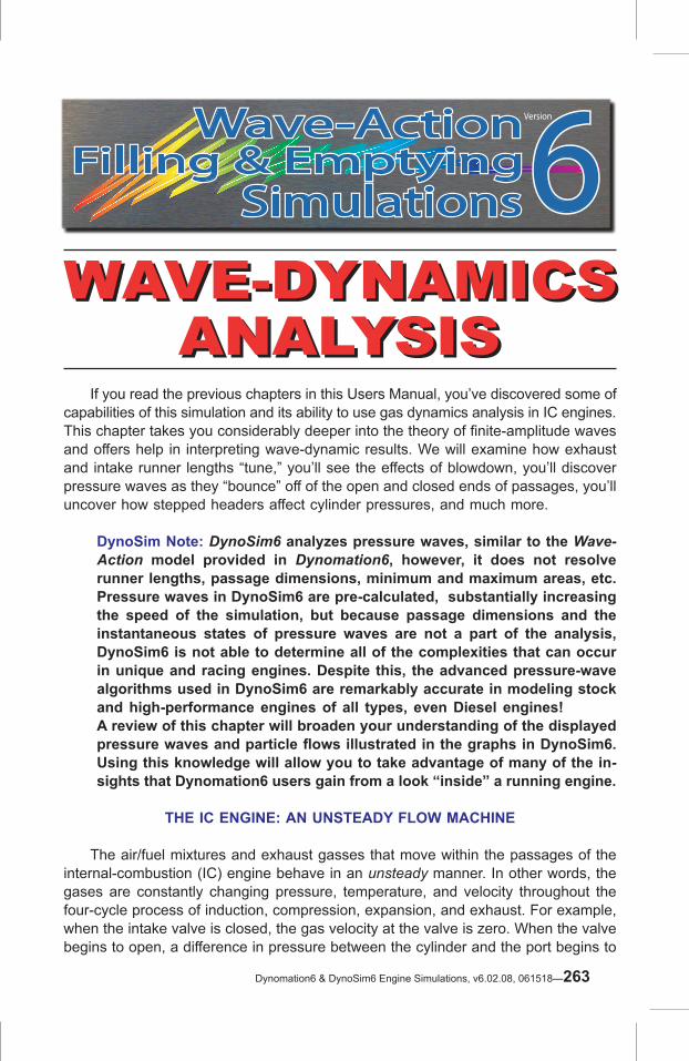
WAVE-DYNAMICSANALYSIS
WAVE-DYNAMICSANALYSIS
If you read the previous chapters in this Users Manual, you’ve discovered some of capabilities of this simulation and its ability to use gas dynamics analysis in IC engines. This chapter takes you considerably deeper into the theory of finite-amplitude waves and offers help in interpreting wave-dynamic results. We will examine how exhaust and intake runner lengths “tune,” you’ll see the effects of blowdown, you’ll discover pressure waves as they “bounce” off of the open and closed ends of passages, you’ll uncover how stepped headers affect cylinder pressures, and much more.
DynoSim Note: DynoSim6 analyzes pressure waves, similar to the Wave-Action model provided in Dynomation6, however, it does not resolve runner lengths, passage dimensions, minimum and maximum areas, etc. Pressure waves in DynoSim6 are pre-calculated, substantially increasing the speed of the simulation, but because passage dimensions and the instantaneous states of pressure waves are not a part of the analysis, DynoSim6 is not able to determine all of the complexities that can occur in unique and racing engines. Despite this, the advanced pressure-wave algorithms used in DynoSim6 are remarkably accurate in modeling stock and high-performance engines of all types, even Diesel engines!A review of this chapter will broaden your understanding of the displayed pressure waves and particle flows illustrated in the graphs in DynoSim6. Using this knowledge will allow you to take advantage of many of the in-sights that Dynomation6 users gain from a look “inside” a running engine.
THE IC ENGINE: AN UNSTEADY FLOW MACHINE
The air/fuel mixtures and exhaust gasses that move within the passages of the internal-combustion (IC) engine behave in an unsteady manner. In other words, the gases are constantly changing pressure, temperature, and velocity throughout the four-cycle process of induction, compression, expansion, and exhaust. For example, when the intake valve is closed, the gas velocity at the valve is zero. When the valve begins to open, a difference in pressure between the cylinder and the port begins to
VersionWave-ActionFilling & Emptying
Simulations
Wave-ActionFilling & Emptying
Simulations66
Dynomation6 & DynoSim6 Engine Simulations, v6.02.08, 061518—263
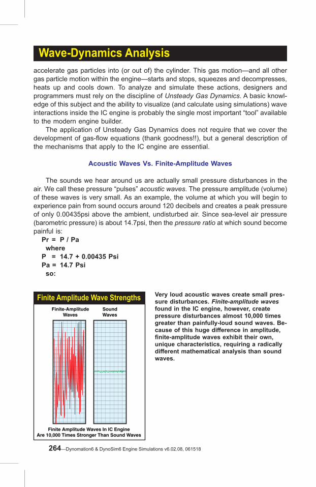
Wave-Dynamics Analysisaccelerate gas particles into (or out of) the cylinder. This gas motion—and all other gas particle motion within the engine—starts and stops, squeezes and decompresses, heats up and cools down. To analyze and simulate these actions, designers and programmers must rely on the discipline of Unsteady Gas Dynamics. A basic knowl-edge of this subject and the ability to visualize (and calculate using simulations) wave interactions inside the IC engine is probably the single most important “tool” available to the modern engine builder. The application of Unsteady Gas Dynamics does not require that we cover the development of gas-flow equations (thank goodness!!), but a general description of the mechanisms that apply to the IC engine are essential.
Acoustic Waves Vs. Finite-Amplitude Waves
The sounds we hear around us are actually small pressure disturbances in the air. We call these pressure “pulses” acoustic waves. The pressure amplitude (volume) of these waves is very small. As an example, the volume at which you will begin to experience pain from sound occurs around 120 decibels and creates a peak pressure of only 0.00435psi above the ambient, undisturbed air. Since sea-level air pressure (barometric pressure) is about 14.7psi, then the pressure ratio at which sound become painful is:
Pr = P / Pa where
P = 14.7 + 0.00435 PsiPa = 14.7 Psi
so:
Very loud acoustic waves create small pres-sure disturbances. Finite-amplitude waves found in the IC engine, however, create pressure disturbances almost 10,000 times greater than painfully-loud sound waves. Be-cause of this huge difference in amplitude, finite-amplitude waves exhibit their own, unique characteristics, requiring a radically different mathematical analysis than sound waves.
Finite Amplitude Wave Strengths Finite-Amplitude
Waves
Finite Amplitude Waves In IC EngineAre 10,000 Times Stronger Than Sound Waves
SoundWaves
264—Dynomation6 & DynoSim6 Engine Simulations v6.02.08, 061518

Wave-Dynamics AnalysisPr = 14.70435 / 14.7Pr = 1.0003 or a 0.03% Increase In Pressure
that’s three one-hundredths of one percent increase over atmospheric pressure! Obviously, very “loud” acoustic waves create very small pressure disturbances. There are waves that produce substantially higher pressure ratios than even loud sound waves. These powerful energy-charged waves are called finite-amplitude waves. Pressure disturbances at these higher intensities can be found in the induction and exhaust passages of the IC engine. Remarkably, pressure ratios of 2.5 can be read-ily measured (that’s a pressure ratio almost 10,000 times greater than painfully loud sound waves—certainly something you would never want to “hear”). This enormous difference in intensity between acoustic and finite-amplitude waves gives some insight into why the misnomer “acoustic theory” (still commonly used) for calculating optimum “tuned lengths” of intake and exhaust passages is misapplied (more on this later).
Compression And Expansion Waves
Finite-amplitude waves take two forms within the IC engine: Compression and Expansion. The Compression wave is a positive pressure disturbance that will always have a pressure ratio greater than one. The Expansion wave is a strong drop below ambient pressure, and therefore will always have a negative pressure ratio (less than one). Expansion waves are known by other names, such as “rarefaction waves” or “suction waves,” however, they all refer to the identical phenomenon. Compression and expansion waves act in similar—but uniquely different—ways as they move through IC engine passages. Understanding how these waves move and how they interact with their surroundings is an important part of understanding how gasses move inside the IC engine. The first piece of the puzzle is illustrated in Figure-1. This drawing depicts a positive compression wave traveling from left to right
As positive compression waves travel from left to right through a pipe (top), they drive gas particles in the same rightward direction. When expansion waves (lower) travel from left to right, they pass through gas particles in the pipe and propel them in the opposite direction, in this case, leftward.
Compression And Expansion Waves
Particle flow direction
Compression Wave Motion
Compression waves drive particlesin same direction as wave
Expansion waves drive particlesin opposite direction of wave
+Pa-
Particle flow direction
Expansion Wave Motion+Pa-
Figure 1
Figure 2
Dynomation6 & DynoSim6 Engine Simulations, v6.02.08, 061518—265

Wave-Dynamics Analysisthrough a pipe. As the pressure waves travel rightward, they drive gas particles in the same rightward direction. However, the velocity of the gas is considerably slower than the speed of the pressure waves. There are many analogs to this in everyday life. For example, consider logs that are pushed ashore by waves on the surface of a lake. The waves wash through floating logs driving them forwards but at a much slower rate than the speed of the waves. An expansion wave is shown in Figure-2. This low-pressure wave is also travel-ing from left to right. However, as it passes through gas particles, its lower pressure gradient draws particles toward the wave, in effect, driving particle flow in the opposite direction, in this case, leftward. In addition, both compression and expansion waves change their character when they encounter sudden transitions in area. Area changes within engine ducting occur at an open end, a closed end, or at transition to smaller or larger diameter passages. Perhaps the most familiar area change occurs at the end of an exhaust header pipe. The primary tube either abruptly ends at the opening to the atmosphere, or it empties into a larger-diameter collector that opens to the atmosphere several inches down-stream. Beyond this very visible (and easily heard) pipe transition, there are many other changes in area within engine ducting. For example, where the intake runner transitions into the manifold plenum or directly into the atmosphere (in the case of injector stacks), a substantial area change is produced. Furthermore, the intake and exhaust valve sits at the end of a pipe that is either closed or partially open, again creating significant changes in areas. What happens when a finite-amplitude wave reaches one of these area transitions? First, let’s examine a case where pressure waves reach the closed end of a pipe. Figure-3 illustrates a positive-pressure compression wave striking the closed end of a passage. It returns with its original profile intact. The only change is that the pressure wave is now moving in the opposite direction. Consider how this affects gas particle motion. When the compression wave travels rightward, it nudges the gas particles toward the right. After reflection, the compression wave nudges the particles
Positive pressure compression waves striking the closed end of a passage return with their original profile intact. Expansion waves behave simi-lar to compression waves. Net particle motion is zero.
Wave Interaction With Closed Pipe End
Compression wavesbefore reaching
closed end of pipe.
Compression waves afterreflecting from closed end.
Note that the reflected wavesare still positive.
+Pa-
+Pa-
Figure 3+Pa-
+Pa-
Expansion wavesbefore reaching
closed end of pipe.
Expansion waves afterreflection from closed end.
Note that the reflected wavesreturn as expansion waves.
Figure 4
266—Dynomation6 & DynoSim6 Engine Simulations v6.02.08, 061518

A leftward-moving compression wave
is reflected as a rightward-moving ex-
pansion wave when it reaches the open
end of a pipe (figure 5). Particle movement
is leftward in both cases. A leftward
moving expansion wave is reflected as a rightward-moving compression wave (figure 6). Particle
movement is right-ward in both cases.
Wave Interaction With Open Pipe End
Compression wavesbefore reaching
open end of pipe.
Compression waves afterreflecting from open end.
Note that the reflected wavesreturn as expansion waves.
+Pa-
+Pa-
Figure 5+Pa-
+Pa-
Expansion wavesbefore reaching
open end of pipe.
Expansion waves afterreflection from open end.
Note that the reflected wavesreturn as compression waves.
Figure 6
Wave-Dynamics Analysis
leftward. The gas particles are returned to their original position; there is no net flow in the pipe. This is exactly what you would expect to find in a pipe that is closed at one end! Figure-4 depicts an expansion wave as it travels rightward within the same closed-end pipe. Behaving similar to a compression wave, the reflected leftward mov-ing wave remains an expansion wave with the same profile. Net particle motion is, again, zero. Now let’s explore the interesting actions of finite-amplitude waves as they move within an open-end pipe. Figure-5 shows the arrival of a compression wave at a transition to a larger area. Notice that leftward-moving compression wave is reflected as a rightward-moving expansion wave. This has fascinating implications for particle movement. Initially, while the compression wave traveled leftward, it helped propel gas particles in the same leftward direction, toward the pipe end. When the expan-sion wave is created and it begins rightward movement, it continues to drive particles in the leftward direction (because expansion waves move particles in the opposite direction of wave travel). Finite-amplitude compression waves moving toward the open end of a pipe provide a “double assist” to particle movement in the same direction.
In an effort to explain gas flow in the exhaust system, it was believed that when the exhaust valve opened, a high pressure “slug” of gas blasted out of the port and down the header pipe. As this slug moved, it created a low-pressure “wave” behind it. This Kadenacy theory was conclusively disproved nearly 60 years ago. Despite this, it is still widely believed by engine “experts” to this day!
Simple Kadenacy TheoryIncorrect “Kadenacy” TheoryFor Exhaust Gas Dynamics
High Pressure “Slug”(similar to compressed spring)
Low Pressure Follows(similar to expanded spring)
Dynomation6 & DynoSim6 Engine Simulations, v6.02.08, 061518—267
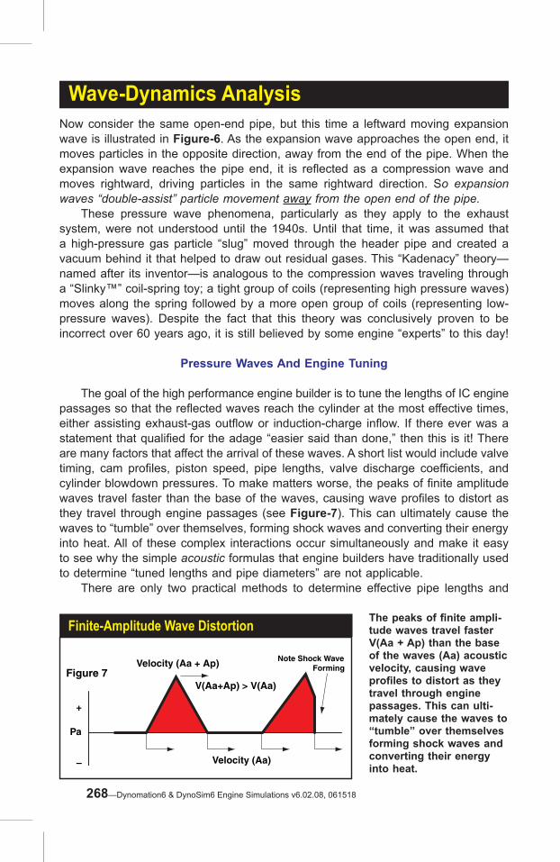
Wave-Dynamics AnalysisNow consider the same open-end pipe, but this time a leftward moving expansion wave is illustrated in Figure-6. As the expansion wave approaches the open end, it moves particles in the opposite direction, away from the end of the pipe. When the expansion wave reaches the pipe end, it is reflected as a compression wave and moves rightward, driving particles in the same rightward direction. So expansion waves “double-assist” particle movement away from the open end of the pipe. These pressure wave phenomena, particularly as they apply to the exhaust system, were not understood until the 1940s. Until that time, it was assumed that a high-pressure gas particle “slug” moved through the header pipe and created a vacuum behind it that helped to draw out residual gases. This “Kadenacy” theory—named after its inventor—is analogous to the compression waves traveling through a “Slinky™” coil-spring toy; a tight group of coils (representing high pressure waves) moves along the spring followed by a more open group of coils (representing low-pressure waves). Despite the fact that this theory was conclusively proven to be incorrect over 60 years ago, it is still believed by some engine “experts” to this day!
Pressure Waves And Engine Tuning
The goal of the high performance engine builder is to tune the lengths of IC engine passages so that the reflected waves reach the cylinder at the most effective times, either assisting exhaust-gas outflow or induction-charge inflow. If there ever was a statement that qualified for the adage “easier said than done,” then this is it! There are many factors that affect the arrival of these waves. A short list would include valve timing, cam profiles, piston speed, pipe lengths, valve discharge coefficients, and cylinder blowdown pressures. To make matters worse, the peaks of finite amplitude waves travel faster than the base of the waves, causing wave profiles to distort as they travel through engine passages (see Figure-7). This can ultimately cause the waves to “tumble” over themselves, forming shock waves and converting their energy into heat. All of these complex interactions occur simultaneously and make it easy to see why the simple acoustic formulas that engine builders have traditionally used to determine “tuned lengths and pipe diameters” are not applicable. There are only two practical methods to determine effective pipe lengths and
The peaks of finite ampli-tude waves travel faster V(Aa + Ap) than the base of the waves (Aa) acoustic velocity, causing wave profiles to distort as they travel through engine passages. This can ulti-mately cause the waves to “tumble” over themselves forming shock waves and converting their energy into heat.
Finite-Amplitude Wave Distortion
Pa
–
+
V(Aa+Ap) > V(Aa)
Velocity (Aa)
Velocity (Aa + Ap) Note Shock WaveFormingFigure 7
268—Dynomation6 & DynoSim6 Engine Simulations v6.02.08, 061518

Wave-Dynamics Analysisdiameters. One is to build the engine, install it on a dyno, connect pressure-reading transducers to the intake and exhaust passages and cylinders and record pressure data. By analyzing these pressure signatures and running a series of tests with vari-ous component combinations, the engine builder can develop an effective engine for the desired purpose. The problem with this method is the associated high costs in time and money. Another method of finding effective pipe lengths and “zeroing in” on optimum component combinations is to simulate the pressure waves and particle flow that occurs within the IC engine. The problem with this method was that, until recently, an affordable four-cycle, pressure-wave simulation program for personal computers simply did not exist. In 1993, V.P. Engineering introduced Dynomation DOS, a PC computer program that applied the Method Of Characteristics mathematical solutions to the analysis of finite-amplitude waves within the 4-stroke racing engine. This early DOS version of Dynomation allowed engine builders to analyze pressure-waves and particle-flow mo-tions (although at a snail’s pace). It displayed intake, exhaust, and cylinder-pressure curves along with intake and exhaust flow velocities and directions. The experienced engine builder used this information to develop better component combinations. Now with introduction of Dynomation6 from Motion Software, this powerful simu-lation method runs under Windows about 10 to 100 times faster, displays simulation results in custom graphics, includes 3D engine renderings, calculates mass flow in ports and passages, includes more sophisticated modeling, forced induction, multiple fuel modeling and much more.
PRESSURE-TIME HISTORIES
The direct measurement of engine pressures can reveal a great deal about en-
Engine pressures can be directly mea-sured with special transducers precisely positioned in the intake and exhaust pas-sages and directly in the cylinders. The intake and the exhaust transducers are often located near the valves. The cylin-der pressure transducer is located in the cylinderhead, protruding into the combus-tion chamber.
Pressure-Wave Measurement
Pressure Transducers
INTAKE EXHAUST
Figure 8
Dynomation6 & DynoSim6 Engine Simulations, v6.02.08, 061518—269

Wave-Dynamics Analysisgine function. An analysis of engine pressures—throughout the complete four-cycle process—reveals the combined effects of all mechanical components, plus the ther-modynamic effects of heat transfer, the results of all finite-wave interactions, and mass flow of induction and exhaust gasses within the engine. The measurement of these pressures requires the precise placement of pressure transducers in the intake and exhaust passages, and directly in the cylinders of the engine. Figure-8 shows typical
These graphs are called pressure crank-angle diagrams. They trace out the pressures measured throughout all four engine cycles, as if recorded by (simulated) transduc-ers located in the ports and cylinders (see photo, previous page). In the upper graph, notice when the exhaust valve opens (EVO). The formation of the primary exhaust pulse occurs. Cylinder pressure (shown in the lower graph) quickly falls and begins to approach exhaust port pressure. The pressure wave created at EVO returns to the cylinder during overlap. It creates subatmospheric pressures that stops reversion and helps induct fresh charge. If the exhaust system was designed correctly, the expansion wave will continue to assist induction flow throughout overlap until the exhaust valve closes (EVC).
Pressure Crank-Angle Diagram
TDC
Figure 9 Pressure Crank-Angle Graphs
Power Exhaust Intake CompressionPre
ssu
re (
Bar
)P
ress
ure
(B
ar) P
ressure (B
ar)P
ressure (B
ar)
CylinderPressure OnLeft Axis Scale
CylinderPressure On
Right Axis Scale
ExhaustPressureSlight
ReversionFlow
IntakePressure
VALVEOVERLAP
270—Dynomation6 & DynoSim6 Engine Simulations v6.02.08, 061518

Wave-Dynamics Analysislocations. The intake and the exhaust transducers are often positioned close to the valves. The cylinder pressure transducer is located in the cylinderhead, protruding into the combustion chamber. The typical pressures recorded by these transducers is illustrated by the graphs shown in Figure-9. This plot is referred to as a pressure crank-angle graph or pressure time-history diagram. The horizontal axis displays the crank position throughout the 4-cycles from 0-720 degrees. The zero point on the left of the graph starts at TDC just be-fore the power stroke. Moving rightward, the first vertical line indicates the exhaust valve opening point (EVO), typically occurring slightly after 100 degrees. Continuing rightward, the next vertical line pinpoints intake valve opening (IVO) around 330 degrees. The exhaust valve closing point (EVC) occurs just under 400 degrees. The distance between the IVO and EVC graphically indicates the valve-overlap period. Around 600 degrees the intake valve closes (IVC). Finally, the diagram ends at 720 degrees with the piston back at TDC, marking the end of the compression stroke. The vertical axis of the diagram indicates pressure in terms of the pressure ratio (or Bar). A value of 1.0 represents standard atmospheric pressure (Pa). A value below this indicates subatmospheric pressure or expansion waves. Values above 1.0 are positive pressures above atmospheric and represent compression waves.
Note: The axis for the left and right vertical axis can be independently set. Notice that the left and right vertical axis on the upper graph both display up to 2.0 Bar, while the lower graph has independently scaled vertical axis set at 2.0 and 50.0 Bar, even though both axis display Cylinder Pressure. This allows a broader view of this widely changing pressure.
Now let’s trace out the pressures measured throughout all four engine cycles (on Figure-9) as recorded by the three simulated transducers. Keep in mind that the pressures illustrated in this diagram reflect an engine that is “in-tune.” (We’ll explore out-of-tune pressures later.) When the exhaust valve opens (EVO), the formation of the primary exhaust pulse occurs. This high-pressure compression wave is created when the exhaust valve releases cylinder pressures (produced by the combustion of fuel and air) into the exhaust port and header pipe system. Cylinder pressure quickly falls and begins to approach exhaust port pressure. Before IVO, an intake pressure wave—created during the previous intake cycle—bounces between the closed inlet valve and the open end of the runner. This is shown by the oscillating wave (green) on the diagram alternately becoming an expansion and compression wave, with pressures centering around 1-Bar, or atmospheric. When the intake valve opens, cylinder pressure is almost always higher than the pressure in the induction system. For the short period of time that this pressure differential exists (intake pressure pulse indicated as Reversion Flow on graph), a reverse flow of exhaust gasses begins to move into the induction tract. Very little reverse flow generally occurs since piston speed is quite slow near TDC. During this time, the pressure wave that was generated when the exhaust valve opened reached the end of the header pipe and has now returned to the cylinder during the valve overlap period (between IVO and EVC) as an expansion wave. This wave creates subatmospheric pressures that stops reversion
Dynomation6 & DynoSim6 Engine Simulations, v6.02.08, 061518—271

Wave-Dynamics Analysisand helps draw in fresh charge from the induction system before the piston begins to move down from TDC on the intake stroke. If the exhaust system (and several other engine parameters) are designed correctly, the expansion wave will continue to assist induction flow until the exhaust valve closes (EVC), as shown in Figure-9. With the ending of the overlap period, the intake stroke begins in earnest. Throughout at least the first half of this period, inlet pressure closely follows cylin-der pressure. Just before IVC a pressure surge or “hump” in the induction pressure begins to increase cylinder pressure. This surge is caused by a strong compression wave arriving from the induction system (created during the previous intake stroke), helping to “ram” fresh charge into the cylinder and minimize back flow. The arrival of this critically important compression wave is determined by runner length and shape, engine speed, and other factors. After IVC, the cylinder pressure continues to rise as the piston heads for TDC on the compression stroke.
Gas Flow Vs. Engine Pressures Up to this point, you may have assumed that there exists a direct relationship between the pressures measured in the ports and the flow of gasses. Furthermore, you may have assumed that when a pressure transducer registers a compression wave within a passage that opens on the right, gas flow would move in a rightward direction. In some instances gas flow does not coincide with pressures. Figure 10 will help shed some light on this confusing issue. As compression Wave-1 moves right-ward it propels gas particles toward the right. A second compression wave, Wave-2, moves leftward in the same passage and propels gas particle toward the left. When Waves 1 and 2 pass through each other they form the superposition Wave-3 (1 + 2). Gas particles that were being propelled towards each other by the separate waves
A direct relationship between measured pressures and the flow of gasses within the ports does not always exist. Consider compression Wave-1 moving rightward and pro-pelling gas particles toward the right. Wave-2 moves leftward in the same passage and propels gas particles toward the left. When Wave-1 and Wave-2 pass through each other they form the superposition Wave-3 (1 + 2). Gas particles come to rest, but a pressure transducer measuring this “new” wave would register a significant pressure increase.
Pressure-Wave Vs. Gas-Particle Flow
Pa
Wave-1 Wave-2
SuperpositionWave-3
+
-
Figure 10
1 21 + 21 21 + 2
272—Dynomation6 & DynoSim6 Engine Simulations v6.02.08, 061518

Wave-Dynamics Analysis
will collide and come to rest within Wave-3. A pressure transducer measuring this “new” wave will register a pressure increase. It would be easy to assume that the higher pressure represented an increase in particle velocity. This phenomenon makes the interpretation of pressure data difficult and eas-ily misleading. Fortunately, Dynomation6 and DynoSim6 also calculate and display particle-flow velocity and direction in addition to pressures for each degree of crank rotation. With the display of port flow velocities, the simulation provides the engine builder a comprehensive picture of port and cylinder pressures, intake and exhaust particle flow velocities, and the direction of that flow.
INTAKE TUNING
The first part of effective intake tuning begins with good exhaust system tuning. As mentioned previously, when the exhaust valve opens it generates a powerful positive pressure wave that travels to the end of the header pipe and returns to the cylinder as a strong expansion wave. When the timing is right, this suction wave will arrive during valve overlap and draw out burnt gases while starting the inflow of fresh charge. This scavenging effect lowers cylinder pressures just before the exhaust valve closes, early in the intake stroke. After EVC, the piston begins to move rapidly down the bore and when it reaches maximum speed, between 73- and 82-degrees after TDC, the rapid increase in cylinder volume will “yank” down the already low pressure in the cylinder. On the pressure-crank angle diagram this will occur between 400- and 440-degrees and is usually the lowest point on the cylinder pressure trace. This sudden drop in pressure generates a strong suction wave that travels toward the open end of the intake runner where it is reflected as a positive compression wave. Depending on the length of the runner and the speed of the engine, this compres-sion wave will return to the cylinder just before the intake valve closes. The arriving
The first part of effective intake tuning begins with good exhaust system tuning. When the exhaust valve opens it generates a power-ful positive pressure wave that travels to the end of the header pipe and returns to the cylinder as a strong expansion wave. When the timing is right, this suction wave will arrive during valve overlap and draw out burnt gases while starting the inflow of fresh charge, optimizing horse-power.
Pressure-Wave Measurement
Dynomation6 & DynoSim6 Engine Simulations, v6.02.08, 061518—273

Wave-Dynamics Analysis
intake compression wave provides two benefits: 1) As the wave moves through the port it pushes particles in the same direction, helping to fill the cylinder. When the compression wave reaches the intake valve just before IVC, 2) the positive pressure overcomes the buildup of pressure in the cylinder created by the piston moving up the bore on the early part of the compression stroke. This forces additional charge into the cylinder while delaying charge reversion until just before intake valve closes (an effect sometimes described as ram tuning). This complex series of tuning events adds the winning edge to many racing engines, but the exhaust system, induction system design, and all cam timing events must be synchronized to produce these effects. When this critical synchronization is lost, intake charge will be driven back into the induction system before IVC. And reversion is a power killer. The simulation can accurately predict when this will occur in the port-flow velocity diagram (we’ll provide specific examples of this later in the chapter). After IVC the strong expansion wave created by the now completed intake stroke oscillates between the pipe end and the closed intake valve. It changes its sign from expansion to compression each time it encounters the open end of the runner. Figure-11 shows the typical intake pressure trace throughout the 720 degrees of crankshaft rotation. Each successive reflection returns with slightly lower peak pres-sure (displayed on the pressure graph from zero to IVO). To gain the greatest benefit from the reflected wave at peak engine speed, it is often best to tune the induction system to utilize the second or third returned pulse, since these retain the highest energy levels (engine timing and the physical length of the passages make it difficult to utilize the first pulse). At lower engine speeds there will be more time for pressure reflections to return from the induction system, so additional waves will appear in the pressure crank-angle diagram. It is also possible to increase the number of pulsations at any given rpm by decreasing the length of the inlet runner. Similarly, a longer runner will decrease the number of pulsations since it takes more time for each pulse to return to the intake
Typical intake pres-sures throughout the full 720 degrees of crankshaft rotation show how each suc-cessive wave reflection returns with slightly lower peak pressure. To gain the greatest ben-efit from the reflected wave at peak engine speed, it is often best to tune the induction system to utilize the second or third re-turned pulse.
Reflected Waves In Intake Port
TDC
Figure 11
Intake Pressure Crank-Angle Graph
Power Exhaust Intake CompressionPre
ssu
re (
Bar
)
IntakePressure
274—Dynomation6 & DynoSim6 Engine Simulations v6.02.08, 061518

Wave-Dynamics Analysisvalve. Optimum runner length to return a second pulse at IVC can be “ballparked” with the following equation:
Second Pulse Length (inches) = 108,000 / RPMNote: This is an approximation of pulse length, as it varies with charge density, pressure, cam timing, runner temperature, and other factors.
This formula works best for engines that operate at relatively high rpm. Unfortunately, at lower engine speeds this equation predicts a tuned length that is too long to be practical. Under these conditions, tuning to the third, fourth, or possibly even the fifth returned pulse requires a much shorter and more-practical length runner. The famous “Long Ram” of the early 1960s was designed by Chrysler to boost lower-speed torque on some of its big-block engines (used in vehicles like the 300G). It was based on second and third pulse tuning, requiring runners so long the carburetors wound up positioned over the exhaust manifolds of the adjacent bank of cylinders. The runner lengths could have been much shorter if the manifold was tuned to the third or fourth induction pulses. Here are good approximations for runner lengths tuned for the third, fourth, and fifth returned induction pulse:
Third Pulse Length (inches) = 97,000 / RPMFourth Pulse Length (inches) = 74,000 / RPMFifth Pulse Length (inches) = 54,000 / RPM
Engine designers and builders can use these equations to obtain good initial estimates for further “fine tuning” in the simulation. Because of the nature of “pulse-tuning,” an intake manifold goes in and out of tune as the engine accelerates through the rpm range. The manifold transitions from
This custom intake manifold was de-signed with the help of Dynomation software. The manifold boosts low- and mid-range power on smallblock Ford engines. Dyno tests confirmed expected performance. Without simulation software, intake manifold design is strictly a trial-and-error process involving considerable time and money without any guarantee of success.
Manifold Designed Using Dynomation
Dynomation6 & DynoSim6 Engine Simulations, v6.02.08, 061518—275

Wave-Dynamics Analysisfifth, to fourth, to third, and then, possibly, to second pulse tuning at maximum engine speed. As the engine passes through each of these tuning points, the runner phases in and out of sync with the expansion wave created when the piston reaches maximum speed on the intake stroke. At lower speeds, when the engine tunes on the fifth or higher pulse, little benefit is derived from the weak returning pulse. However, by the time the engine reaches sufficient speed so that the third or second pulse arrives just before IVC, a substantial pressure differential strongly assists cylinder filling and prevents charge reversion.
Note: Since the second pulse delivers the strongest returning wave, the ques-tion arises: Why not use second-pulse tuning for all manifold designs? The answer is that the un-tuned gap between the second and third pulse is much greater than the gap between the third and fourth pulse. This means that en-gines using manifolds based on second-pulse tuning will have narrow, peaky, power bands, while third-pulse manifolds will tend to produce wider, although potentially lower, power curves.
Intake Runner Taper Angles
The taper angle of the inlet runner has a significant effect on the optimum tuned length. As runner taper angle increases, the returning pressure waves speed up, requiring a higher engine speed to regain the same level of “tune.” For example, a 13-inch runner with a 4-degree taper angle will tune at approximately the same engine speed as a 10-inch straight runner. Straight runners often provide more power at lower engine speeds and work
The taper angle of the inlet run-ner has a significant effect on the optimum tuned length and peak power. As runner taper angle increases, the returning pressure waves speeds up, so a higher engine speed is needed to regain the same level of “tune.” There are several complex reasons why taper angles optimize power, but the most straightforward are: 1) A tapered port has a greater vol-ume to “store” air/fuel charge and feed the cylinder during the main portion of intake stroke, and 2) A taper angle acts somewhat like a stepped-header for the induc-tion system, generating a series of positive pressure waves that return to the valve and assist cyl-inder filling.
Measuring Port/Runner Taper Angle
Minimum Area
Port EntryArea
Port
Tape
r Ang
le
276—Dynomation6 & DynoSim6 Engine Simulations v6.02.08, 061518

Wave-Dynamics Analysis
quite well for stock engines. However, to obtain peak performance from a high-speed racing engine, intake runners must incorporate a taper of 2 to 4 degrees (included). There are several complex reasons why taper angles optimize power, but the most straightforward are: 1) A tapered port has a greater volume to “store” air/fuel charge and feed the cylinder during the main portion of intake stroke, and 2) a taper angle acts somewhat like a stepped-header for the induction system, generating a series of positive pressure waves that return to the valve and assist cylinder filling. Inlet-runner taper angles can be varied in Dynomation6 not only to develop better-functioning induction systems, but also to gain a better understanding of how this important tuning element affects engine power. A particularly revealing test can be done by overlaying port velocities and cylinder pressures for various inlet taper angles.
Port Flow Velocities
Another very important element of intake and exhaust tuning is port flow velocity. The speed at which gasses move through the ports essentially is controlled by port area and piston speed. For example, if intake port velocity is too low, gas particles flowing into the cylinder near IVC will not have sufficient momentum to overcome the rise in cylinder pressure as the piston moves up the bore. Fresh charge will flow back
The taper angle of the inlet runner has a
significant effect on the optimum tuned length.
Inlet-runner taper angles can be varied in
Dynomation6 not only to develop better-func-tioning induction sys-tems, but also to gain
a better understanding of how this important
tuning element affects engine power. Here is
a comparison between straight runners (darker
curves) and 3-degree taper runners. Notice that exhaust velocity
is higher while intake velocity is lower. With
tapered runners the engine produces more
horsepower at peak engine speed.
Effect Of Taper Angles
Dynomation6 & DynoSim6 Engine Simulations, v6.02.08, 061518—277

Wave-Dynamics Analysisout of the cylinder into the inlet tract. Furthermore, when the ports are too large, all pressure waves generated by piston motion and exhaust gas outflow are diminished. This will decrease the effectiveness of returning pressure waves during scavenging and cylinder filling. In fact, port size is so important that we can make this blanket statement: Developing an engine with optimum port sizes will potentially produce more power than the same effort put forth in determining optimum tuned runner lengths! Research has shown that maximum port velocity through the minimum cross-sectional area of the runner should fall between 0.5 to 0.6 Mach, or about 600- to 720-feet-per-second. Port velocities higher than 0.6 Mach produce no further increases in volumetric efficiency. Since it is impossible for any port to generate optimum flow velocities at all engine speeds, it is essential that the engine builder accurately determine the required operating range for the engine and develop ports that flow appropriately at these speed ranges. If a broad power range is required, port areas should be sized so that maximum engine speeds produce port velocities of about 0.75 Mach. This will place optimum velocities (between 0.5 and 0.6 Mach) at lower engine speeds, optimizing volumetric efficiency vs rpm. If high-speed, maximum power is the goal, then port velocity at peak engine speed should be no higher than 0.6 Mach. During your design sessions, here’s some important concepts to keep in mind. It
This is a good example of “in tune” induction pressures. The intake pressure wave is oscillating inside the runner and arrives at the intake valve during maximum piston speed (highest volume change) approximately 60- to 80-degrees after TDC. The “trough” of this wave combines with the suction created by the piston moving down the bore to “yank” the pressure wave to a very low amplitude. This low pressure generates a strong expansion wave that reflects back from the open-end runner as an equally strong compression wave that arrives at IVC. This not only drives additional charge into the cylinder, but reduces or eliminates reversion.
“In-Tune” Induction System
TDC
Intake Pressure Crank-Angle Graph
Pre
ssu
re (
Bar
)
Oscillating wave in runner combineswith Max piston speed to “yank”
inlet pressure low.
Returning compressionwave improves cylinderfilling and prevents reversion.
Figure 12
278—Dynomation6 & DynoSim6 Engine Simulations v6.02.08, 061518

Wave-Dynamics Analysisis often possible to make port areas small enough—and velocities high enough—to completely eliminate intake reversion at IVC. When this is accomplished, it often produces insufficient port volume and constricted flow. A better approach, producing higher peak power, is to allow some reversion to occur. It is also possible to design ports that flow between 0.5 or 0.6 Mach and do not show an increase in power. This situation can occur when intake valve or port restriction becomes too great. In these cases, the engine designer will simply have to experiment with several different port sizes, valve diameters, and valve lifts to find the optimum combination. The following formula can help you ballpark the required minimum port cross-sectional areas:
Minimum Area (Square Inches) = RPM x STROKE x BORE2) / 190,000This formula is an approximation that tends to provide conservative values.(RPM, STROKE, and BORE are in inches)
One reason this formula can only be an approximation of port area is that port velocity is also dependent on the valve-discharge coefficient. This value is the mea-sured volume of flow across the valve divided by the perfect, theoretical (isentropic) flow. The discharge coefficient will always be less than one and is essentially a rating for the efficiency of the valve. Specific discharge coefficient values are unique for
These engine pressures depict an engine with an exhaust system and cam timing that are “in-tune.” The scavenging wave is wide enough to cover the overlap period, assist-ing exhaust gas outflow and preventing charge reversion.
Exhaust And Cam Timing In Sync
TDC
Pressure Crank-Angle Graph
Power Exhaust Intake Compression
Pre
ssu
re (
Bar
)
Figure 13
CylinderPressure
Exhaust Scavenging WaveIs Wide Enough To SpanValve Overlap Period.
ExhaustPressure
VALVEOVERLAP
Dynomation6 & DynoSim6 Engine Simulations, v6.02.08, 061518—279

Wave-Dynamics Analysiseach valve and cylinderhead design. The simulation allows the direct input of flow-bench data and will calculate the discharge coefficients for specific cylinder head combinations. Since about 30% of flow loss through the port occurs at the valve, an improved discharge coefficient can result in substantial performance gains.
EXHAUST TUNING
Incomplete removal of exhaust gases from the cylinder reduces engine perfor-mance in two ways. First, volumetric efficiency is decreased when residual gases occupy space within the cylinder that could have been filled with fresh charge. Second, higher cylinder pressures, resulting from incomplete exhaust blowdown, force residual burnt gasses into the inlet tract upon IVO. This “spoils” the fresh charge pulled back into the cylinder during the intake stroke. When the compression wave produced at exhaust valve opening (EVO) reaches
As rpm increases, the pressure-crank
angle diagram curves “stretch” out to the right, as shown by
these exhaust traces. If the scavenging
wave is wide enough and the overlap is short enough, the
exhaust system will remain in tune throughout a wide
rpm range. Good scavenging is still
taking place at higher rpm in Figure-14a, but relatively little
scavenging remains at even higher rpm in
Figure-14b.
Exhaust System Scavenging Vs. Increasing RPM
TDC
Pressure Crank-Angle Graph
Power Exhaust Intake Compression
Pre
ssu
re (
Bar
)
Figure 14a
CylinderPressure
At Higher Rpm, ExhaustSystem Begins To MoveOut Of Tune.
ExhaustPressure
VALVEOVERLAP
TDC
Pressure Crank-Angle Graph
Power Exhaust Intake Compression
Pre
ssu
re (
Bar
)
Figure 14b
CylinderPressure
At Still Higher Rpm, ExhaustSystem Falls Out Of Tune.
ExhaustPressure
VALVEOVERLAP
280—Dynomation6 & DynoSim6 Engine Simulations v6.02.08, 061518

Wave-Dynamics Analysisthe end of the header pipe (at the transition to the collector), a lower-strength expan-sion wave is reflected back to the cylinder. The positive compression wave, now of lower intensity, continues to move through the collector. When it reaches the atmo-sphere boundary, a second expansion wave is generated that moves back through the collector and into the primary header pipe. If the header system and cam timing are properly coordinated, the first expansion wave will return to the cylinder at, or slightly before, IVO. This will assist exhaust-gas scavenging and improve the flow of fresh charge from the induction system. Then, slightly later, the second expansion wave will arrive and continue the scavenging process until EVC. A well-designed collector can effectively broaden the scavenging wave to “cover” the entire overlap period. When this occurs, the engine and exhaust system “in tune.” If a significant portion of the overlap period is not accompanied by a scavenging wave, the engine and exhaust system fall “out of tune.” Engine pressures illustrating an in-tune condition are pictured in Figure-13. As rpm increases, the pressure crank-angle diagram traces “stretch” to the right. If the scavenging wave is “wide enough” (i.e., of sufficient duration) and the overlap is short enough, the exhaust system will remain in tune even though engine rpm has increased. Notice that good scavenging is still taking place at higher rpm in Figure-14a, however, at an even higher rpm in Figure-14b the engine falls out of tune. A wide scavenging wave is particularly desirable in engines with long overlap periods. A scavenging wave that maintains a low pressure differential at the exhaust valve throughout the entire overlap period will assist exhaust scavenging, prevent reversion,
Exhaust tuning works by using the proper header pipe length to “time” the arrival of the suction wave to occur during the overlap. However, optimum primary pipe and collector lengths are not very critical for low- to medium-performance engines. This graph shows how induction flow changed as header length was varied from 25 inches to 40 inches (engine power changed by only about 2%). How-ever, high-output, high-speed engines with long overlap periods require much more precise tub-ing lengths to optimize power. As power levels increase, the margin for error decreases.
Exhaust Header Lengths Vs. Induction Flow
TDC
Figure 15 Pressure Crank-Angle Graphs
Power Exhaust Intake CompressionPre
ssu
re (
Bar
)P
ress
ure
(B
ar)
Very Little ChangeIn ScavengingInduction Flow
ExhaustPressure Traces
25-Inch PrimaryTube Length
40-Inch PrimaryTube Length
36-Inch PrimaryTube Length
VALVEOVERLAP
Dynomation6 & DynoSim6 Engine Simulations, v6.02.08, 061518—281

Wave-Dynamics Analysisand ensure high power levels over a wider range of engine speeds. This fact brings to light an important point about exhaust-header tuning. Optimum primary pipe and collector lengths are not very critical for low- to medium-performance engines (see Figure-15). In these applications, overlap periods are short and cylinder pressures are often not very high at the end of the exhaust stroke (lower performance engines produce a smaller volume of exhaust gasses and blowdown more effectively in shorter time periods). However, high-output, high-speed engines with long overlap periods require much more precise tubing lengths to optimize power. As power levels increase, the margin for error decreases.
An Interesting Note About Collectors: When exhaust pulses from multiple cylinders enter a collector, primary and reflected waves interfere and interact with one another. The influence of this interaction is sometimes overstated. These “interference” waves are considerably lower in magnitude and have much
Peak Exhaust Flow Velocities Vs. Engine RPM
TDC
EVO EVC
Exhaust
Pressure Crank-Angle Graph
Engine Speed Graph
Power Intake CompressionPre
ssu
re (
Bar
)E
ng
ine
Po
wer
En
gin
e Torq
ue
Figure 16a
Engine Rpm At Peak Power
Blowdown Peak Pumping Peak
Exhaust Velocity Peaks Twice DuringTheExhaust Cycle. Exhaust
Pressure Trace
Blowdown Peak
Pumping Peak
TDC
EVO EVC
Exhaust
Pressure Crank-Angle Graph
Engine Speed Graph
Power Intake CompressionPre
ssu
re (
Bar
)E
ng
ine
Po
wer
En
gin
e Torq
ue
Figure 16b
Engine Rpm Past Peak Power
Exhaust Flow Restriction At EVOIncreases Pumping Losses At MaximumPiston Speed In Exhaust StrokeExhaust
Pressure Trace
Peak exhaust velocity typi-cally occurs twice during the exhaust cycle. The first peak-
flow event, at approximately 60 degrees after EVO, is produced by maximum flow during blow-down (Figure-16a). The second
event occurs at maximum piston speed on the exhaust
stroke, about 73- to 82-de-grees before TDC, and is the
maximum flow during exhaust pumping (Figure-16b). If the
flow at the second peak is the greater of the two, it usually indicates excessive restric-
tion in the exhaust system; in this case, caused by engine
overspeed (reducing the time for exhaust-gas blowdown) in a
very-large displacement V8.
282—Dynomation6 & DynoSim6 Engine Simulations v6.02.08, 061518

Wave-Dynamics Analysisless effect than the primary and first reflection waves from cylinder blowdown. Dr. Jon C. Morrison of the Institute of Mechanical Engineers conducted experi-ments on interference effects in collectors and concluded that multicylinder wave interference had an essentially insignificant affect on performance.
Exhaust Flow Velocities
Another important aspect of exhaust tuning is optimizing gas particle velocity throughout the exhaust system. When the exhaust valve opens (EVO), the piston is still moving downward on the power stroke. However, a large percentage of combusted gasses “blowdown” during the period between EVO and BDC. This occurs despite the fact that exhaust valve lift is relatively low. This phenomenon highlights the importance of low-lift flow characteristics of the exhaust valve and port for optimum performance. If the header system is too restrictive—possibly from insufficient pipe diameter—or if low-lift valve flow provides a restriction—often from improper port and valve seat/face contours—to allow sufficient blowdown, the piston will have to physically “pump” out the remaining gasses during the exhaust stroke. This substantially increases pump-ing work and cylinder pressures at IVO (which, in turn, reduce effective scavenging and create reversion into the induction system). On the other hand, when primary pipe diameters are too large, the returning scavenging wave is weakened and is too defuse to effectively assist exhaust gas outflow and initiate induction inflow during overlap. Optimum exhaust pipe diameters, like intake runner areas, are essential in producing flow velocities that achieve a balance between minimizing restriction and optimizing finite-amplitude-wave actions. Peak exhaust velocity typically occurs twice during the exhaust cycle. The first peak-flow event, at approximately 60 degrees after EVO, is produced by maximum flow during blowdown. The second event occurs at maximum piston speed on the exhaust stroke, about 73- to 82-degrees before TDC, and is the maximum flow during exhaust pumping. In most well-designed engines, the first peak will be the greater of the two (see Figure-16a); if the flow at the second peak is greater, it can indicate excessive restriction in the exhaust system (see Figure-16b). When the exhaust system is designed properly, the level of the first peak should fall between 0.45 to 0.5 Mach. If flow rates over 0.5 Mach are recorded, the exhaust system is too restrictive. If flow values fall below 0.45 Mach (as is the case in the two examples shown in Figures 16a & 16b), blowdown will not generate expansion waves strong enough to effectively scavenge the cylinder during overlap. Similar to intake tuning, it is possible to establish optimum flow velocities yet not measure a performance gain. When this occurs, the problem may be excessive exhaust-valve restriction. Fortunately, this can be easily detected by reviewing the pressure-crank angle diagram or the pressure-volume diagram (discussed later in this chapter).
Exhaust Tubing Lengths
While it is impossible to exactly predict primary lengths and diameters without
Dynomation6 & DynoSim6 Engine Simulations, v6.02.08, 061518—283
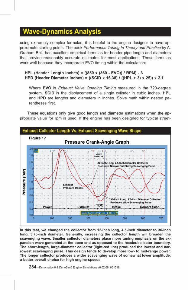
TDCExhaust
VALVEOVERLAP
Pressure Crank-Angle Graph
Power Intake Compression
Pre
ssu
re (
Bar
)
Figure 17
12-Inch Long, 4.5-Inch Diameter CollectorProduces Narrow But Strong Scavenging Pulse
36-Inch Long, 3.5-Inch Diameter CollectorProduces Wide Scavenging Pulse
ExhaustPressure Traces
In this test, we changed the collector from 12-inch long, 4.5-inch diameter to 36-inch long, 3.75-inch diameter. Generally, increasing the collector length will broaden the scavenging wave. Smaller collector diameters place more tuning emphasis on the ex-pansion wave generated at the open end as opposed to the header/collector boundary. The short-length, large-diameter collector (light-red line) produced the lowest and nar-rowest scavenging pulse. This design tends to develop more low- to mid-range power. The longer collector produces a wider scavenging wave of somewhat lower amplitude, a better overall choice for high engine speeds.
Exhaust Collector Length Vs. Exhaust Scavenging Wave Shape
Wave-Dynamics Analysisusing extremely complex formulas, it is helpful to the engine designer to have ap-proximate starting points. The book Performance Tuning In Theory and Practice by A. Graham Bell, has excellent empirical formulas for header pipe length and diameters that provide reasonably accurate estimates for most applications. These formulas work well because they incorporate EVO timing within the calculation:
HPL (Header Length Inches) = ((850 x (360 - EVO)) / RPM) - 3HPD (Header Diameter Inches) = ((SCID x 16.38) / ((HPL + 3) x 25)) x 2.1
Where EVO is Exhaust Valve Opening Timing measured in the 720-degree system. SCID is the displacement of a single cylinder in cubic inches. HPL and HPD are lengths and diameters in inches. Solve math within nested pa-rentheses first.
These equations only give good length and diameter estimations when the ap-propriate value for rpm is used. If the engine has been designed for typical street-
284—Dynomation6 & DynoSim6 Engine Simulations v6.02.08, 061518

Wave-Dynamics Analysisdriving, the selected rpm should correspond with peak-torque speed. Racing engines should use either the engine speed at peak horsepower or some value in between. While Bell’s formulas derive reasonably accurate estimations of primary tubing lengths and diameters, unfortunately, there are no reliable empirical formulas for col-lector length and diameter. However, there are rules-of-thumb to keep in mind when choosing starting values for these dimensions. Longer collectors drive peak torque lower in the engine rpm range. This happens because, at higher engine speeds, ex-pansion waves generated at the end of a long collector take too much time to travel back to the cylinder, failing to assist exhaust scavenging. Longer collectors should be used to widen powerbands at lower engine speeds, whereas, shorter collectors optimize peak power at higher engine speeds. Choosing collector diameters requires further development of a previous theory. Recall that when a compression or expansion wave reached the open end of a pipe, a reflected wave was generated by this sudden change in area. What was not dis-cussed, however, was that the amplitude of the reflected wave is dependent on the extent of area change. If a wave reaches an open-end pipe that discharges into the atmosphere (effectively, has an infinite change in area), then the reflected wave will be of maximum possible amplitude; nearly equal to the originating wave but of the opposite sign. If the area change is small, for instance, a 1.00-inch pipe joining a 1.05-inch pipe, a reflection wave will still be generated, but it will have a very small
These cylinder pressure curves illustrate how stepped headers work. Stepped head-ers return small expansion waves at each step. These scavenging waves help exhaust gases flow out of the cylinder, particularly helpful on large-displacement, high-speed engines. Notice the lower cylinder pressures produced with stepped headers (lighter-red line). The lower pressures reduce pumping work.
Stepped Headers Can Lower Cylinder Pressures
TDCExhaust
VALVEOVERLAP
Pressure Crank-Angle Graph
Power Intake Compression
Pre
ssu
re (
Bar
)
Figure 18
Standard, Fixed-DiameterPrimary Tube Header
Stepped Header LowersCylinder Pressure
CylinderPressure Traces
Dynomation6 & DynoSim6 Engine Simulations, v6.02.08, 061518—285

Wave-Dynamics Analysisamplitude. The lesson to be learned from this for collector design is that smaller collector diameters decrease the area change and reduce the amplitude of the first reflected wave. As collector diameter is decreased, higher amplitude waves are gen-erated at the open-end of the collector and smaller reflected waves are generated at the primary/collector pipe boundary. Since the open end is farther away from the cylinder, smaller collectors often boost low- to mid-rpm power. Larger diameter col-lectors generate stronger waves at the primary/collector boundary, and since this is closer to the cylinder, larger collectors generally boost high-rpm power (see Figures 17 and 18 that illustrate some of these principals). While there are no simple formulas to accurately calculate these variables, the following formula can provide “broad ballpark” figures for high-speed, racing engines:
Collector Diameter = 1.9 x HPD Collector Length = .5 x HPL (HPL and HPD are in inches)
VALVE EVENTS AND TUNING STRATEGIES
The four basic valve-event timing points (IVO, IVC, EVO, EVC) can be grouped into three categories based on their influence on engine performance:
1) EVC and IVO are the least important individually, but the “angular” distance between these two events comprise the overlap period that has a significant effect on power.2) EVO is the next most important timing point since it determines the beginning of the exhaust cycle which initiates cylinder blowdown.3) IVC is the most critical event since it fixes the balance between cylinder filling and intake reversion, each having a potent effect on engine output.
Combining your knowledge of finite-amplitude waves with this information on valve timing will allow you to use the simulation to design or select camshafts (and choose related intake and exhaust components) for virtually any application. Each valve-timing point is described below, including tips about event timing and how incorrect timing can affect wave-dynamic tuning. The reader is encouraged to use the simulation to recreate these phenomena and examine the pressure and velocity data to better understand how valve-event timing affects engine performance.
(IVO) Intake Valve Opening—This valve event marks the beginning of the in-take process and valve overlap. IVO is probably the least sensitive timing point of all four valve events. However, when the exhaust system returns a broad, strong expansion wave, earlier IVO timing can boost performance. If a strong scavenging wave is not present, the same early IVO timing will cause exhaust gasses to flow into the induction system (reversion). This will substantially reduce power from not only fresh-charge “spoiling,” but also charge heating.There are several additional conditions, along with IVO, that influence intake reversion. Low engine speeds usually produce low port velocities. Since induc-tion gasses have less momentum when they are moving at slower speeds,
286—Dynomation6 & DynoSim6 Engine Simulations v6.02.08, 061518

Valve-Timing Events
The four basic valve-event timing points (IVO, IVC, EVO, EVC) can be grouped into three categories based on their influence on engine performance: 1) EVC and IVO are the least important individually, but together comprise the overlap period that has a significant effect on power, 2) EVO is the next most important timing point since is determines the beginning of the exhaust cycle which initiates cylinder blowdown, and 3) IVC is the most critical event since it fixes the balance between cylinder filling and intake rever-sion, each having a potent effect on engine output.
Wave-Dynamics Analysis
it is easier for the piston—moving upward at IVO—to force residual exhaust gasses into the inlet track. Furthermore, low intake manifold pressures that occur during part-throttle operation or with restricted carburetion create large pressure differentials between the intake port and the cylinder, again contrib-uting to reversion. A similar condition can occur at wide-open throttle when IVO is too early, as cylinder pressures are still quite high. Engines with these conditions might benefit from later IVO timing.
(EVC) Exhaust Valve Closing—This event marks not only the end of the exhaust process, but also the ending of the overlap period. At low rpm EVC strongly influences the degree to which exhaust gasses back-flow into the cylinder from the exhaust system. This low-speed back flow happens for two reasons. First, at EVC, the piston is beginning to move down the bore on the intake stroke, and since exhaust gas outflow velocity is low, the piston can begin to draw exhaust back into the cylinder. The second reason is more in-teresting. The negative scavenging wave created at the end of the header is always followed by another, positive compression wave. At low engine speeds both the scavenging and compression waves arrive prematurely. If the com-pression wave arrives during overlap, it forces exhaust gases back into the cylinder. One solution to this problem is the reverse-megaphone “collector” often used on motorcycle exhaust systems. This device dampens the follow-
Dynomation6 & DynoSim6 Engine Simulations, v6.02.08, 061518—287

Wave-Dynamics Analysisup compression wave and reduces exhaust reversion at mid to low rpm. This discovery was made by accident (true for most discoveries!) when motorcycle racers tried using a reverse-megaphone in an effort to strengthen their flimsy exhaust systems. At higher engine speeds, later EVC will shift the power curve towards higher rpm at the expense of low-speed torque. At peak power the exhaust valve should close just slightly before exhaust back-flow occurs. Don’t forget that exhaust system tuning also has a significant influence on reversion. So, final EVC timing should only be determined after the exhaust system has been optimized.
(EVO) Exhaust Valve Opening—This timing point always occurs during the latter part of the power stroke and signals the start of the blowdown process. Optimum EVO timing permits a reduction in cylinder pressure that would oth-
The Pressure Crank-Angle diagram is one of two common ways that cylinder pressures are illustrated. This method plots cylinder pressures against the crank position during the 720-degrees of the four engine cycles. On this graph (adjusted 360-degrees “for-ward” from the graph standard used in the simulation) it is easy to see widely varying cylinder pressures from induction through peak-ignition pressure.
Pressure-Crank-Angle Diagram
800
1000
600
400
14.7
360 740 0 & 720TDCTDC
Degrees of Crankshaft Rotation
BDC
Ignition
BDC360180
Cyl
inde
r P
ress
ure
(psi
)
Figure 20
288—Dynomation6 & DynoSim6 Engine Simulations v6.02.08, 061518

Wave-Dynamics Analysiserwise result in exhaust gas reversion into the induction system at IVO and during overlap. However, at higher engine speeds it is almost impossible for some reversion not to take place. If there is no reversion flow during overlap at high speed, it is likely (but not certain) that EVO is too early, and cylinder pressure that could have been used to push the piston during the power stroke is being prematurely expelled from the engine, reducing thermal efficiency and horsepower. If EVO occurs too late, insufficient blowdown will increase pumping work during the exhaust stroke and, in turn, reduce horsepower. Late EVO will also increase cylinder pressures at IVO contributing to reversion and additional losses in power.
Note: Thermal efficiency research has shown that within the normal range of EVO timing, this event has less affect on low-speed power than either IVC or EVC. Therefore, EVO timing should be early enough to satisfy high-speed performance requirements, but no earlier, or thermal efficiency will suffer.
(IVC) Intake Valve Closing—This is the most important valve event in the 4-cycle, IC engine. IVC occurs well into the compression stroke and intake flow is easily susceptible to reversion if induction velocity and/or pressure-wave tuning do not provide sufficient energy to hold back increasing cylinder pres-sures. This is especially true at low to mid-range engine speeds where port velocity is still sluggish. Late IVC reduces volumetric efficiency at lower rpm and potentially increases volumetric efficiency at higher rpm. Optimum IVC at maximum engine speeds depends on port velocity, pressure wave tuning, and piston speed.
Using Pressure Diagrams
The simulation can display additional graphs that illustrate otherwise “hidden” engine operating conditions. One of these important graphs illustrate cylinder pressure as a function of crank angle throughout the 4-cycle process—called a Pressure-Crank-Angle Diagram shown in Figure-20 (to recreate this graph, use either the center or bottom graph on the right program pane, redefine the X axis to Crank Angle, Y1 to Cylinder Pressure, and Y2 axis to None). Cylinder pressure can also be graphed as a function of cylinder volume—called a Pressure-Volume, or PV Diagram as shown in Figure-21 (using either the center or bottom graph, redefine the X axis to Cylinder Volume, Y1 to Cylinder Pressure, and Y2 axis to None).
The Pressure-Crank-Angle Diagram
The pressure crank-angle diagram plots cylinder pressure against the position of the crankshaft during all four cycles (when this graph is reproduced, the zero point is fixed at TDC just after ignition on the power stroke). Ambient or atmospheric pres-sure forms the baseline for the vertical “Cylinder Pressure” axis, below which vacuum levels are plotted. As the intake stroke begins, cylinder pressure decreases to near
Dynomation6 & DynoSim6 Engine Simulations, v6.02.08, 061518—289

Wave-Dynamics Analysis
The PV diagram compares cylinder pressure to displaced volume and illustrates the same cylinder pressures displayed in the pressure crank-angle diagram. The PV dia-gram has the remarkable feature of isolating the work consumed from the work devel-oped by the engine. The area within the lower loop, drawn in a counterclockwise direc-tion, represents the work consumed by pumping losses (exhaust and intake stroke). The upper loop area, drawn in a clockwise direction, indicates the work produced by expanding gasses after combustion (compression and power stroke). The PV diagram can be a useful tool for optimizing valve-event timing, with the pumping loop providing the most helpful information.
Pressure-Volume Diagram
3
2
7
4
5
6
1
Pre
ssu
re In
Cyl
ind
er
Piston Cylinder
Piston Displacement
(V1 - V2)
V1V2
TDC
TDC
BDC
BDC
ClearanceVolume
Pressure-Volume DiagramFigure 21
1 - 2 Intake Stroke2 - 3 Compression Stroke3 - 4 Ignition4 - 6 Power Stroke6 - 1 Exhaust Stroke
290—Dynomation6 & DynoSim6 Engine Simulations v6.02.08, 061518

Wave-Dynamics Analysisambient as exhaust venting concludes. Pressures then change to a slight vacuum during the intake stroke (or a much stronger vacuum during part-throttle operation) until the cycle ends with the closing of the intake valve. Now the trapped charge is compressed and cylinder pressures rise to a few hundred pounds per square inch (psi). Typically, a few degrees before the piston once again reaches TDC, the spark plug fires, igniting the mixture and sending cylinder pressures up to several hundred or even thousands of psi within about 40 degrees of crank rotation. If the ignition point was timed properly, peak cylinder pressure will occur about 12 to 14 degrees after TDC. This timing allows cylinder pressures to be most efficiently converted to rotational force or torque by the rod/crank assembly. As the piston continues to move down the cylinder and pressures decrease, the exhaust valve opens, beginning a dramatic drop in pressure. Finally, cylinder pressures stabilize at a few psi during the exhaust stroke when remaining burnt gasses are forced out of the cylinder.
The Pressure-Volume Diagram
The pressure crank-angle diagram provides a straightforward view of the widely varying pressures in the cylinder. While it’s easy to see “what’s happening and where it’s happening” with this diagram, another method of plotting the identical cylinder pressures offers a very different “look” and unique insight into the same data. This plot, known as a pressure-volume (PV, called a Pee-Vee or indicator) diagram, is very helpful in understanding the work produced-from and consumed-by the engine. The PV diagram plots pressure against the displaced volume in the cylinder. Notice in the illustration (Figure-21) that the curve tends to wrap around and recon-nect with itself, forming a complete path. This curve represents cylinder pressures throughout the entire Otto-cycle process. It begins at the same point as the previ-ous crank-angle diagram—just after the intake valve opens—marked as a 1 on the graph. The cylinder and piston below the graph illustrate the position of the piston and the volume in the cylinder at each point on the PV. As the intake stroke continues, the piston moves down the bore and the plot indicates pressure below atmospheric continuing to point 2. Here the piston begins to move back up the bore and pressure rises as the compression cycle begins. At point 3, the fuel is ignited, rapidly increasing cylinder pressure. The piston reaches TDC at point 4, and the power stroke begins. Cylinder pressure continues to rise to point 5, ideally about 15 degrees after TDC. The exhaust valve opens at point 6, just before BDC, assisting in cylinder depres-surization. The piston reaches BDC at point 7. The exhaust cycle continues as the piston moves back up the bore maintaining some positive pressure in the cylinder until, at point 1, the piston once again reaches TDC.
Note: The lower “pumping” loops illustrated in the accompanying PV diagrams depict naturally-aspirated engines (it’s called a “pumping” loop because the engine is either pumping in fresh charge or pumping out exhaust gasses; the average pressure of this loop is the pumping mean effective pressure—Pmep). This pressure loop will look completely different for a supercharged engine because positive (forced induction) pressures will act on the piston during the intake stroke.
Dynomation6 & DynoSim6 Engine Simulations, v6.02.08, 061518—291

Wave-Dynamics Analysis
Notice that the “pressure areas” have internal directional arrows that indicate the same sequence of events just described. Trace along the curve, again, from the starting point 1 around part of the “lower loop” marked with a minus sign. Notice that you are moving in a counterclockwise direction. As you move from point 2 through the junction between the upper and lower loops, continuing past points 3, 4, 5, 6 and finally arrive at point 7, this trip has taken you around the “upper loop,” marked with a plus sign, in a clockwise direction. Finally, as you move past point 7 back to 1, you trace out the upper half of the “lower loop,” again in a counterclockwise direction. What does all the “clockwise stuff” have to do with anything? You may be amazed by the relationship. A PV diagram has the remarkable feature of isolating the work consumed from the work developed by the engine. The area within the lower loop, drawn in a counterclockwise direction, represents the work consumed by the engine “pumping” the charge into the cylinder and forcing the exhaust gasses from the cylinder. The upper loop area, drawn in a clockwise direction, indicates the work produced by the engine from pressures generated by expanding gasses after combustion. Look again at the crank-angle diagram, Figure-20. Would you have thought the relatively “simple” curve in that illustration would contain so much more “hidden” information? Let’s test the work-isolating concepts of PV diagram with a cylinder misfire (see
The work-isolating concepts of a PV diagram are evident with
a cylinder misfire. In this case, the air/fuel mixture is drawn
into the cylinder as usual, but it fails to ignite and boost
cylinder pressure. The PV diagram of this event still con-sists of two loops; however, if
we start at point 1 and trace through the sequence of pres-sures, we outline two counter-
clockwise loops. Both loops represent power consumed by
the engine.
PV Diagram Of Cylinder Misfire
Pre
ssur
e In
Cyl
inde
r
Piston Cylinder
Piston Displacement
(V1 - V2)
V1V2
TDC
TDC
BDC
BDC
ClearanceVolume
Pressure-Volume DiagramCylinder Misfire
Figure 21a
1 - 2 Intake Stroke2 - 3 Compression Stroke3 - 4 Misfire4 - 6 “Power” Stroke6 - 1 Exhaust Stroke
3Misfire
2
7
45
16
292—Dynomation6 & DynoSim6 Engine Simulations v6.02.08, 061518

Wave-Dynamics Analysis
This PV diagram illustrates how the pumping loop changes as engine speed increases from 3200rpm to 5200rpm. Notice how the lower portion of the loop (the intake cycle) remains relatively constant, while the upper portion of the loop (the exhaust cycle) dramatically rises as rpm increases. The changes in exhaust pressure are caused by the decreas-ing time available to blowdown the cylinder as engine speed increases. Higher pumping pressures increase pumping work (increasing Pmep) and that consumes horsepower.
Pumping Loop Vs. RPM
-10
Pa
100
200
300
TDC BDC
Figure 22Pressure-Volume Diagram
Cyl
ind
er P
ress
ure
(p
si)
Swept Volume In Cylinder
3200rpm
4400rpm
5200rpm
EVC
IVO
IVC
Figure-21a). In this case, the air/fuel mixture is drawn into the cylinder as usual, but it fails to ignite and boost cylinder pressure. The PV diagram of this event still con-sists of two loops (more or less). However, if we start at point 1 and trace through the sequence of pressures, we outline two counterclockwise loops. So both loops represent power consumed by the engine. The upper loop encloses very little area since most of the power used to compress the charge is returned when the piston is forced back down the bore by the compression pressure on the “power” stroke.
Note: The pressure in the cylinder as the piston moves down the bore on the “power” stroke of a misfire is slightly less than the measured pressure on the compression stroke because the charge has given up some heat, and therefore pressure, to the cylinderwall and other surfaces.
Optimizing Valve Events
The pressure-volume diagram can be a useful tool for locating optimum valve event timing, with the pumping loop providing the most insightful information. Fig-ure-22 shows a close-up view of a typical pumping loop. This period is also called the “valve-open cycle,” since at least one of the valves is open throughout the entire loop. This illustration also shows how the pumping loop changes shape as engine speed increases from 3200rpm to 5200rpm. The lower, pumping loop obviously “balloons.” However, notice that the lower portion of the lower loop (the intake cycle) remains relatively constant, while the upper portion of the loop (the exhaust cycle) dramati-cally rises as rpm increases. The increasing exhaust pressures are the result of the
Dynomation6 & DynoSim6 Engine Simulations, v6.02.08, 061518—293

Wave-Dynamics Analysis
Here are the effects of early and late exhaust valve open-ings. Early EVO (dotted line)
causes the pressure curve to slope strongly from left
to right as cylinder pressure decreases during blowdown.
If EVO is too late the pres-sure curve takes much more
of a vertical “dive” and tends to level out consider-
ably above Pa.
Effects Of Early And Late Valve Timing Events
-10
Pa
100
200
300
TDC BDC
Figure 24Pressure-Volume Diagram
Cyl
ind
er P
ress
ure
(p
si)
Swept Volume In Cylinder
EVC
IVC
Early EVCPressure Curve
Early IVCPressure Curve
This PV plot shows the sharp rise in cylin-der pressure from too early EVC timing (dotted line). The “spike” at the left end of the loop is caused by the upward moving piston begin-ning to re-compress exhaust gasses. Also illustrated is too early IVC timing (solid line). Notice the “pointed tail” at the lower right. This is produced when the intake valve closes near BDC and prevents the inflow of fresh charge normally caused by the ram tuning effects of the induction system.
Early Exhaust And Intake Valve Closing
-10
Pa
100
200
300
TDC BDC
Figure 23Pressure-Volume Diagram
Cyl
ind
er P
ress
ure
(p
si)
Swept Volume In Cylinder
EVC
IVO
IVC
Early EVO Late EVO
294—Dynomation6 & DynoSim6 Engine Simulations v6.02.08, 061518

Wave-Dynamics Analysisdecrease in time available to blowdown the cylinder as engine speed increases. Higher pumping pressures increase pumping work (increasing Pmep) and that consumes horsepower. The 5200rpm curve in Figure-22 also shows the beginning of “bulge” forming around maximum piston speed on the exhaust stroke. This is a sign of exhaust flow restriction, sometimes caused by insufficient exhaust valve size and/or valve lift. This “restriction” bulge also would be visible on the pressure-crank angle diagram where cylinder pressure drops to parallel inlet pressure, at about 80 degrees before TDC. Figure-23 show how early and late exhaust valve openings affect cylinder pres-sure. Notice the slope of the blowdown pressure at the upper right hand corner of the diagrams. If EVO is too early (dotted line), the pressure curve slopes strongly from left to right as cylinder pressure decreases during blowdown. If EVO is late, the pressure curve takes a much more vertical “dive” and tends to level out considerably higher above Pa. Ideal EVO timing will produce a pressure plot that will slope from left to right at a relatively steep angle (similar to the 4400rpm curve in Figure 22). Figure-24 shows the sharp rise in cylinder pressure from very early EVC timing (dotted line). The “spike” at the left end of the loop is caused by the upward moving piston beginning to re-compress exhaust gasses trapped in the cylinder when the exhaust valve closed too early. This figure also illustrates how early IVC timing can change the lower part of the pumping loop (solid line). Notice the “pointed tail” at the lower right. This is produced when the intake valve closes near BDC and prevents the inflow of fresh charge normally developed by the ram tuning effects of the induction system.
One Final Note: IVO is the least sensitive valve event, and its opening point (within the range of typical valve event timing) is often not distinguishable on the PV diagram.
Dynomation6 & DynoSim6 Engine Simulations, v6.02.08, 061518—295
FAQ'sFAQ'sFREQUENTLY ASKED QUESTIONS
The following information may be helpful in answering questions and solving prob-lems that you encounter when installing or using this simulation. If you don’t find an answer to your problem here, send and email to: [email protected]. You can also fax in the Mail/Fax Tech Support Form (Motion Software provides Email and Fax technical service to registered users only). We will review your problem and return an answer to you as soon as possible.
IMPORTANT: The simulation includes Motion’s Software Update tool that auto-matically checks for updates (plus, you can initiate a update check at any time by selecting Check For New Version from the HELP menu in the program). You’ll not only receive the usual bug fixes and minor enhancements, but often updates include entirely new features and modeling capabilities.Many of these new features have been requested by our users (yes, we really do listen to our customers!). If you have ideas for enhancements or you have found issues with our software, please let us know. You'll probably see your requested feature “appear” in the next update!
GENERAL TROUBLESHOOTING
Here are just a few of the things you might think about when trying to solve problems:
a) If the cam data that you are testing or reviewing in one of the graphs appears in-correct, make sure you are viewing the correct lobe (this is particularly important if you are using a Variable-Valve-Timing cam setup).
b) If a turbocharging system is not developing the boost or power you expect, re-member that the Boost Limit is an upper limit. It does not force a too-large turbo to spin up more quickly and generate the desired boost. You need to select the correct size turbo, turbine, and A/R ratio to obtain the desired boost curve.
c) Take a few minutes to carefully review all your component selections. You may find that reviewing your engine component selections directs you to the source of the problem. It’s easy to look at a component specifications a hundred times and see the “right” number, only to look again and find that an error that was in “plain sight.”
VersionWave-ActionFilling & Emptying
Simulations
Wave-ActionFilling & Emptying
Simulations66
296—Dynomation6 & DynoSim6 Engine Simulations v6.02.08, 061518

d) If you are certain that you have found an outright “bug,” we are anxious to hear from you. It is our firm intention to make sure this engine simulation stays one of the most sophisticated, stable, and useful development tools available to the engine builder and enthusiast. Use the email address [email protected] or [email protected] to contact our development team. Al-ways include your main email address and attach any .dxml engine files (or any other related cam or flow files) that may us help diagnose the problem. Include a thorough explanation of the issues. We will make every attempt to review and reply to your problem as soon as possible.
INSTALLATION/BASIC-OPERATION QUESTIONS
Question: Received an “Error Reading Drive D” (or another drive) message when attempting to install the software. What does this mean?
Answer: This means your computer cannot read the disk in your CD-ROM drive. The disk may not be properly seated in your drive, the drive may be defective, or the disk may be damaged. If you can properly read other CDs in your CD-ROM drive, but our software distribution disk produces error messages, try requesting a directory of a known-good disk. If these operations produce an error message only when using the Motion CD, the disk is probably defective. Contact Mo-tion Software, Inc., for a replacement (email address on the back cover of this manual). Replacement CD's or USB Security Keys are free for as long as you own our software (you must be the original purchaser). Just return the defective merchandise to Motion Software, Inc., and we will replace it at no charge. If you have lost the CD or the USB Key, please call for replacement pricing.
Question: “Could not locate HASP USB Security Key” error message was displayed when trying to run Dynomation6.
Answer: If Dynomation6 displays an error message indicating that the HASP Security Key is missing or cannot be found, here are some quick steps you can follow to isolate and correct common problems:a) Make sure the Security Key is, in fact, properly connected to a functioning USB
port on your computer or to a USB hub that is connected to your computer. If you connected the Key to a hub, try connecting it directly to a USB port on your computer system. The Security Key contains a small LED that lights up when it is properly connected and after it has located the correct software drivers on your system (these drivers are normally installed during Dynomation6 installa-tion, see step “c” below).
b) Make sure your USB port is functioning correctly by disconnecting all other USB devices from your system. Then connect the Security Key to another USB port. If that works, try another USB device in the port that did not work to determine if that port is defective.
c) Try re-installing or updating the Security Key drivers. Updates are posted on the Support page of the Motion Software, Inc., website (www.motionsoftware.
Troubleshooting & Common Questions
Dynomation6 & DynoSim6 Engine Simulations, v6.02.08, 061518—297

Troubleshooting & Common Questionscom). Restart your computer after you install the new drivers.
And here’s some additional tips for both Dynomation6 and DynoSim6 users:
d) Is your computer experiencing technical difficulties, such as non-functional devices, spontaneous rebooting, etc? If so, the device drivers for our Security Key may not properly install on your system. You should have a “stable” com-puter system and a “clean,” virus-free Windows installation to properly use this software. You also should have the latest Windows updates installed on your system (available free from www.microsoft.com).
e) Try installing this software (and for Dynomation6, the Security Key) on another computer system to determine if your computer is at fault.
f) Make sure you are using the latest version of this simulation by by opening the Windows Start menu, then choose Motion-Dynomation6 Engine Sim (or Motion-DynoSim6 Sim), and finally click on the MotionUpdater icon in that folder. Your computer must be connected to the Internet to obtain the latest updates.
g) Refer to additional information on the Support page of the www.MotionSoft-ware.com website.
Question: The software won’t start. It displays messges saying something like, “msvcrt.dll linked to missing export...”
Answer: You need to update your version of Windows by using the Windows Up-date service built into Windows, or directly go to www.microsoft.com to obtain Windows updates. Consider updating to Windows7 or Windows10.
Question: The simulation produced an Assertion Failure error. What should I do?Answer: Please note down all of the information presented in the error-message
box, provide a quick synopsis of what lead up to the error, then send this infor-mation, along with the Dynomation7-Run.log or DynoSim6_Run.log data file (located in the C:/Dynomation6 or C:/DynoSim6 director) to Motion Software at [email protected]. Thank you for your assistance in helping us improve this software. If you cannot send this email, contact [email protected] for assistance.
SCREEN DISPLAY QUESTIONS
Question: Even though I have a 21-inch monitor, I can only see a portion of the simulation screen on my monitor. What can I do so that I don’t have to scroll both horizontally and vertically?
Answer: The screen resolution of your monitor (not its size) determines how much of the simulation screen you can see without scrolling left and right. You can change screen resolution by RIGHT CLICKING on your desktop, then select-ing PROPERTIES from the drop-down menu. Choose the SETTINGS tab and
298—Dynomation6 & DynoSim6 Engine Simulations v6.02.08, 061518

Troubleshooting & Common Questionsincrease screen resolution by moving the Screen Area slider to the right. For more information about screen resolution, refer to the documentation that was supplied with your computer, your video graphics card, or with Windows.
BORE/STROKE/SHORTBLOCK QUESTIONS
Question: I cannot find the shortblock I want to model in the Shortblock menus? Answer: The Shortblock menu is simply a list of most of the common engines.
If you cannot find your shortblock in the menus, simply enter the bore, stroke and number of cylinders directly in the Shortblock Component Category. Send us an email and let us know what engines you would like to see in the menu ([email protected]).
INDUCTION/MANIFOLD/FUELS QUESTIONS
Question: When I choose induction flow that is too large for an engine (for example 4000cfm on a Honda 4-cylinder), why does the power increase without showing “bog,” or power drop at low speeds?
Answer: The simulation assumes an optimum air/fuel ratio regardless of the se-lected CFM rating. As a result, the program produces increasingly smaller positive results from larger-and-larger induction flows. However, you won’t go wrong if you use common sense when selecting induction/carburetor flow capacities.
Question: The engine I am building uses two carburetors. How can I simulate the airflow?
Answer: You can simulate induction airflow from less than 100 to 7000cfm, rated at either the standard pressure drop of 1.5-inches or 3.0-inches of mercury (a pressure drop of 1 inch of mercury is equivalent to 13.55 inches of water). To simulate two carburetors, simply add the airflow and enter the total cfm value into the Induction category (or you can use the Flow Calculator if you are unsure about the rated flow of a venturi or throttle).
CAMSHAFT/VALVETRAIN QUESTIONS
Question: I built a relatively stock engine but installed a drag-race camshaft. The engine only produced 9hp @ 2000 rpm. Is this correct?
Answer: Yes. Very low power outputs at low engine speeds occur when racing camshafts are used without complementary components, such as high-flow cylinder heads, high compression ratios, and exhaust system components that match the performance potential of the cam.
Question: The simulation doesn’t predict power unless I enter both seat-to-seat and 0.050-inch valve timing. Why is this necessary?
Answer: The simulation can use either Cam Profile data or 10-Point Timing (specs
Dynomation6 & DynoSim6 Engine Simulations, v6.02.08, 061518—299
Troubleshooting & Common Questionsfound on your cam card and in cam manufacturer’s catalog/website). To opti-mize accuracy with 10-Point timing, it is essential to provide both seat-to-seat and 0.050-inch timing points. With both sets of timing points, the simulation can calculate the lifter acceleration rates accurately generate a full valve-motion curve. If you only enter 0.050-inch timing points, the simulation can extrapolate seat-to-seat timing, however, this introduces potential errors in power prediction.
Question: How does the simulation allow for the different acceleration rate cams used with hydraulic, solid, and roller lifters?
Answer: The simulation calculates a valve acceleration rate and a valve-motion curve using both the seat-to-seat and 0.050-inch cam timing specifications (see previous answer). Note that the acceleration rate of cams is not directly linked to the type of lifters (e.g., mild street cams often used roller lifters), and determin-ing the acceleration rates (intake and exhaust) from seat-to-seat and 0.050-inch timing points produces quite accurate results.
Question: Can I change rockerarm ratios? Answer: Yes. You can directly change the rocker ratios in the Camshaft Component
category. You can also use the Rocker Math calculator to get insight into how rocker-ratio changes affect valve timing and lift.
Question: I found the published factory seat-to-seat valve timing for an engine that I am building. The IVC occurs at 112 degrees (ABDC). Something goes wrong when I enter the valve events into the simulation.
Answer: There are so many ways that cam specs can be described for catalog-ing purposes that it can be quite confusing. The cam specs for your engine are a classic example of this lack of standards. The OEM cam listed in the factory manual is a hydraulic grind with seat-to-seat timing measured at 0.001-inch lifter rise. Because the cam is designed for long life and quite operation, it has ex-tended (quiet) opening ramps. This is the reason for the large number of crank degrees between the specified “opening” and “closing” points. In fact, during the first 35 degrees of crank rotation, the lifter rises less than 0.010-inch. If this wasn’t the case, and the valve truly opened and closed at the factory specified timing points, the cam would have over 350-degrees duration, and it’s unlikely the engine would even start! Simulation seat-to-seat timing should be based on the SAE standard of 0.006-inch valve rise. The 0.001-inch lifter-rise figures published in your factory manual do not indicate when mass flow begins in the ports and are useless for engine simulation purposes.
Question: My cam manufacturer’s catalog does not list seat-to-seat, valve-event tim-ing. But it does list seat-to-seat intake and exhaust duration, lobe-center angle, and intake centerline. Can I calculate the valve-event timing from these figures?
Answer: Yes. Use the CamMath QuickCalculator™ built into the simulation to calculate the intake and exhaust opening and closing points. You’ll need the fol-
300—Dynomation6 & DynoSim6 Engine Simulations v6.02.08, 061518

Troubleshooting & Common Questionslowing information:
1) Intake Duration 2) Exhaust Duration 3) Lobe-Center Angle (sometimes called lobe separation angle). 4) And the Intake Centerline Angle. Question: I have been attempting to test camshafts from data obtained on the
Internet. I can find the duration and lobe center angle. However, I can’t find the seat-to-seat timing (they act like it’s a trade secret!). Can I use the available data to run a simulation?
Answer: No. Our suggestion is to contact another cam manufacturer.
COMPRESSION-RATIO QUESTIONS
Question: The simulation calculated the total Combustion Volume at 92ccs. But I know my cylinder heads have only 75ccs. What’s wrong?
Answer: This confusion comes from assuming that the calculated Total Combus-tion Volume is the same as your measured combustion-chamber volume. The Total Combustion Volume is the entire volume that remains in the cylinder when the piston reaches top dead center.
Question: When using the Compression Ratio Calculator, the “Measured Volumes, Burrette Method” mode, Item-2 should, but does not, allow a zero entry. I have flattop pistons with zero deck clearance and 5cc valve pockets. Wouldn’t this be the correct entry since I am running zero deck clearance?
Answer: The assumption in the “Measured Volumes” option is that there is a vol-ume (the combination of the displacements in the domes/dishes/pockets) that cannot be calculated by the engine builder. The only practical way to measure this volume is to move the piston down the bore an arbitrary amount, say 0.250 (sufficient to ensure that the entire dome is below the deck surface), and measure the volume in the cylinder (with a liquid and a burette). This is then compared to the volume of a cylinder 0.250 inches high with the same bore diameter. The difference in volume is the volume taken up by the dome/dish/pockets.
However, on your engine, you know that the flattop pistons with valve pockets that you have will produce a zero deck height at TDC, and the displacement of the valve pockets is 5cc. Knowing this, you can select the “Known Volumes” model, set the deck clearance to zero, add 5cc for valve-pocket volume, enter the combustion chamber volume, and the compression ratio will be calculated.
GENERAL QUESTIONS ABOUT RUNNING A SIMULATION
Question: The simulation displayed an error message “Program was unable to complete the simulation. A more balanced combination of components...” What
Dynomation6 & DynoSim6 Engine Simulations, v6.02.08, 061518—301

Troubleshooting & Common Questionswent wrong?
Answer: The combination of components you have selected produced a calculation error in the simulation process. This can be caused by using restrictive induction flow on large-displacement engines, using radical cam timing on otherwise mild engines, or large taper angles on intake and exhaust passages. Try increasing induction flow, selecting a cam with less duration, reducing the compression ratio, or try changing the Wave-Action Simulation Mode from Course to Fine or SuperFine (this decreases the Mesh size used to divide engine passages for analysis and provides a more effective damping of shock waves).
Question: When I run a simulation, part of the horsepower and torque graph goes off the end of the graph. What can I do to correct the display?
Answer: Open the Graph Options menu (right-click on the graph) and select Auto Range for the Y1 or Y2 variable.
302—Dynomation6 & DynoSim6 Engine Simulations v6.02.08, 061518

Troubleshooting & Common Questions
Dynomation6 & DynoSim6 Engine Simulations, v6.02.08, 061518—303

MINI GLOSSARYMINI GLOSSARY0.050-Inch Cam Timing Method—See Cam Timing, @ 0.050-inch. ABDC or After Bottom Dead Center—Any position of the piston in the cylinder bore after its lowest point in the stroke (BDC). ABDC is measured in degrees of crankshaft rotation after BDC. For example, the point at which the intake valve closes (IVC) may be indicated as 60-degrees ABDC. In other words, the intake valve would close 60 degrees after the beginning of the compression stroke (the compression stroke begins at BDC).
Air-Fuel Ratio—The proportion of air to fuel: by weight: that is produced by the carburetor or injector.
ATDC or After Top Dead Center—Any position of the piston in the cylinder bore after its highest point in the stroke (TDC). ATDC is measured in degrees of crankshaft rotation after TDC. For example, the point at which the exhaust valve closes (EVC) may be indicated as 30-degrees ATDC. In other words, the exhaust valve would close 30 degrees after the beginning of the intake stroke (the intake stroke begins at TDC).
Atmospheric Pressure—The pressure created by the weight of the gases in the atmosphere. Measured at sea level this pressure is about 14.69psi.Back Pressure: A pressure developed when a moving liquid or gaseous mass passes through a restriction. “Backpressure” often refers to the pressure generated within the exhaust system from internal restrictions from tubing and tubing bends, mufflers, catalytic converters, tailpipes, or even turbochargers.
BBDC or Before Bottom Dead Center—Any position of the piston in the cylinder bore before its lowest point in the stroke (BDC). BBDC is measured in degrees of crankshaft rotation before BDC. For example, the point at which the exhaust valve opens (EVO) may be indicated as 60-degrees BBDC. In other words, the exhaust valve would open 60 degrees before the exhaust stroke begins (the exhaust stroke begins at BDC).
Big-Block—A generic term that usually refers to a V8 engine with a displacement that is large enough to require a physically “bigger” engine block. Typical bigblock
VersionWave-ActionFilling & Emptying
Simulations
Wave-ActionFilling & Emptying
Simulations66
304—Dynomation6 & DynoSim6 Engine Simulations v6.02.08, 061518
Mini Glossaryengines displace over 400 cubic inches.
Blowdown or Cylinder Blowdown—Blowdown occurs during the period between exhaust valve opening and BDC. It is the period (measured in crank degrees) dur-ing which residual exhaust gases are expelled from the engine before the exhaust stroke begins. Residual gasses not discharged during blowdown must be physically “pumped” out of the cylinder during the exhaust stroke, lowering power output from consumed “pumping work.”
Bore or Cylinder Bore—The internal surface of a cylindrical volume used to retain and seal a moving piston and ring assembly. “Bore” is commonly used to refer to the cylinder bore diameter, unusually measured in inches or millimeters. Bore surfaces are machined or ground precisely to afford an optimum ring seal and minimum fric-tion with the moving piston and rings.
Brake Horsepower (bhp)—Brake horsepower (sometimes referred to as shaft horse-power) is always measured at the flywheel or crankshaft by a “brake” or absorbing unit. Gross brake horsepower describes the power output of an engine in stripped-down, “race-ready” trim. Net brake horsepower measures the power at the flywheel when the engine is tested with all standard accessories attached and functioning. Also see Horsepower, Indicated Horsepower, Friction Horsepower, and Torque.
Brake Mean Effective Pressure (bmep)—A theoretical average pressure that would have to be present in each cylinder during the power stroke to reproduce the force on the crankshaft measured by the absorber (brake) on a dynamometer. The bmep present during the power stroke would produce the same power generated by the varying pressures in the cylinder throughout the entire four-cycle process.
BTDC or Before Top Dead Center—Any position of the piston in the cylinder bore before its highest point in the stroke (TDC). BTDC is measured in degrees of crank-shaft rotation before TDC. For example, the point at which the intake valve opens (IVO) may be indicated as 30-degrees BTDC. In other words, the intake valve would open 30 degrees before the intake stroke begins (the intake stroke begins at TDC).
Cam Timing @ 0.050-Lift—This method of determining camshaft valve timing is based on 0.050 inches of tappet rise to pinpoint timing events. The 0.050-inch method was developed to help engine builders accurately install camshafts. Lifter rise is quite rapid at 0.050-inch lift, allowing the cam to be precisely indexed to the crankshaft. Camshaft timing events are always measured in crankshaft degrees, relative to TDC or BDC.
Cam Timing @ Seat-To-Seat—This method of determining camshaft timing uses a specific valve lift (determined by the cam manufacturer) to define the beginning or ending of valve events. There is no universally accepted valve lift used to define seat-to-seat cam timing, however, the Society of Automotive Engineers (SAE) has
Dynomation6 & DynoSim6 Engine Simulations, v6.02.08, 061518—305

accepted 0.006-inch valve lift as its standard definition. Camshaft timing events are always measured in crankshaft degrees, relative to TDC or BDC.
Camshaft Advance/Retard—This refers to the amount of advance or retard from the manufacturers recommended timing that the cam is installed in the engine. Focusing on intake timing, advancing the cam closes the intake valve earlier. This setting typi-cally increases low-end performance. Retarded cam timing closes the intake valve later which tends to help top end performance.
Camshaft Lift—The maximum height of the cam lobe above the base-circle diameter. A higher lobe opens the valves further, often improving engine performance. Lobe lift must be multiplied by the rocker ratio (for engines using rocker arms) to obtain total valve lift. Lifting the valve more than 1/3 the head diameter generally yields little ad-ditional performance. Faster valve opening rates add stress and increase valvetrain wear but can improve performance. High lift rates usually require specially designed, high-strength components.
Centerline—An imaginary line running through the center of a part along its axis, e.g., the centerline of a crankshaft running from front-to-back directly through the center of the main-bearing journals.
Duration or Valve Duration—The number of crankshaft degrees (or much more rarely, camshaft degrees) of rotation through which the valve lifter or cam follower is raised above a specified height; either seat-to-seat valve duration measured at 0.006-, 0.010-inch or other valve lifts (even 0.020-inch lifter rise), or duration measured at 0.050-inch lifter rise, called 0.050-inch duration. Intake duration is a measure of all intake lobes, and exhaust duration indicates the exhaust timing for all exhaust lobes. Longer cam durations hold the valves open longer, often allowing increased cylinder filling or scavenging at higher engine speeds.
Exhaust Center-Angle/Centerline or ECA—The distance in crank degrees from the point of maximum exhaust valve lift (on symmetric cam profiles) to TDC during the valve overlap period.
Exhaust Valve Closing or EVC—The point at which the exhaust valve returns to its seat, or closes. This valve timing point usually occurs early in the intake stroke. Although EVC does not have substantial effects on engine performance, it contributes to valve overlap (the termination point of overlap) that can have a significant effect on engine output.
Exhaust Valve Opening or EVO—The point at which the exhaust valve lifts off of its seat, or opens. This valve timing point usually occurs late in the power stroke. EVO usually precedes BDC on the power stroke to assist exhaust-gas blowdown. The EVO timing point can be considered the second most important cam timing event
Mini Glossary
306—Dynomation6 & DynoSim6 Engine Simulations v6.02.08, 061518

Mini Glossaryfrom a performance standpoint.
Filling & Emptying Simulation—This engine simulation technique includes multiple models (e.g., thermodynamic, kinetic, etc.), and by dividing the intake and exhaust passages into a finite series of sections it describes mass flow into and out of each section at each degree of crank rotation. The Filling And Emptying method can ac-curately predict average pressures within sections of the intake and exhaust system and dynamically determine VE and engine power. However, the basic Filling And Emptying model can not account for variations in pressure within individual sections due to gas dynamic effects.
Four-Cycle Engine—Originally devised by Nikolaus Otto in 1876, the four-cycle engine consists of a piston moving in a closed cylinder with two valves (one for inlet and one for outlet) timed to produce four separate strokes, or functional cycles: Intake, Compression, Power, and Exhaust. Sometimes called the ”suck, squeeze, bang, and blow” process, this technique—combined with a properly atomized air/fuel mixture and a precisely timed spark ignition—produced an engine with high efficiency and power potential. Dynomation6 and DynoSim6 are designed to simulate the functional processes of a four-cycle engine.
Horsepower—Torque measures how much work (an engine) can do; and power is the rate-based measurement of how fast the work is being done. Starting with the static force applied at the end of a torque arm (torque), then multiplying this force by the swept distance through which the same force would rotate the torque arm one full revolution determines the power per revolution: Power Per Revolution = Force or Weight x Swept Distance. James Watt (1736-1819) established the current value for one horsepower: 33,000 pound-feet per minute or 550 pound-feet per second. So horsepower is currently calculated as: Horsepower = Power Per Revolution/33,000, which is the same as Horsepower = (Torque x 2 x Pi x RPM)/33,000, or simply: Horsepower = (Torque x RPM)/5,252. The horsepower being calculated by these equations is just one of several ways to rate engine power output. Various additional methods for calculating or measuring engine horsepower are commonly used (to derive friction horsepower, indicated horsepower, etc.), and each technique provides additional information about the engine under consideration.
Induction Airflow—The airflow rating (a measurement of restriction) of a carburetor or fuel injection system. Standard automotive four-barrel carburetors are rated by the measured airflow when the device is subjected to a pressure drop equal to 1.5-inches of mercury. Two-barrel carburetors are tested at 3.0-inches of mercury.
Intake Centerline Angle—The distance in crank degrees from the point of maximum intake valve lift (on symmetric cam profiles) to TDC during the valve overlap period.
Intake Stroke—One of the four 180-degree full “sweeps” of the piston moving in the
Dynomation6 & DynoSim6 Engine Simulations, v6.02.08, 061518—307

Mini Glossarycylinder of a four-stroke, internal-combustion engine (originally devised by Nikolaus Otto in 1876). During the intake stroke, the piston moves from TDC to BDC and in-ducts (draws in by lowering the pressure in the cylinder) air/fuel mixture through the induction system. Note: The 180-degree duration of the intake stroke is commonly shorter than the period during which the intake valve is open, sometimes referred to as the true “Intake Cycle.” The intake stroke is followed by the compression stroke.
Intake Valve Closing or IVC—Considered the most important cam timing event from a performance standpoint. The point at which the intake valve returns to its seat, or closes. This valve timing point usually occurs early in the compression stroke. Early IVC helps low-end power by retaining air/fuel mixture in the cylinder and reducing charge reversion at lower engine speeds. Late IVC increases high-speed performance (at the expense of low speed power) by allow additional charge to fill the cylinder from the ram-tuning effects of the induction system at higher engine speeds.
Intake Valve Opening or IVO—The point at which the intake valve lifts off of its seat, or opens. This valve timing point usually occurs late in the exhaust stroke. Although IVO does not have a substantial effect on engine performance, it contributes to valve overlap (the beginning point of overlap) that can have a significant effect on engine output.
Lobe-Center Angle or LCA—The angle in cam degrees from maximum intake lift to maximum exhaust lift. Typical LCAs range from 100 to 116 camshaft degrees (or 200 to 232 crank degrees).
Normally Aspirated—When the air-fuel mix is inducted into the engine solely by the lower pressure produced in the cylinder during the intake stroke; aspiration not aided by a supercharger.
Otto-Cycle Engine—See Four-Cycle Engine
Overlap or Valve Overlap—The period, measured in crank degrees, when both the exhaust valve and the intake valve are open. Valve overlap allows the negative pres-sure scavenge wave to return from the exhaust system and begin the inflow of air/fuel mixture into the cylinder even before the intake stroke begins. The effectiveness of the overlap period is dependent on engine speed and exhaust “tuning.”
RPM—Revolutions Per Minute. A unit of measure for angular speed. As applied to the IC engine, rpm indicates the instantaneous rotational speed of the crankshaft described as the number of crank revolutions that would occur every minute if that instantaneous speed was held constant throughout the measurement period. Typi-cal idle speeds are 300 to 800rpm, while peak engine speeds can reach as high as 10,000rpm or higher in some racing engines.
308—Dynomation6 & DynoSim6 Engine Simulations v6.02.08, 061518

Mini GlossarySimulation and Engine Simulation—A engine simulation process or program at-tempts to predict real-world responses from specific component assemblies by apply-ing fundamental physical laws to “duplicate” or simulate the processes taking place within the components.
Smallblock—A generic term that usually refers to a V8 engine with a displacement small enough to be contained within a “small” size engine block. Typical smallblock engines displace under 400 cubic inches.
Stroke—The maximum distance the piston travels from the top of the cylinder (at TDC) to the bottom of the cylinder (at BDC), measured in inches or millimeters. The stroke is determined by the design of the crankshaft (the length of the stroke arm).
Top Dead Center or TDC—The position of the piston in the cylinder bore at its up-permost point in the stroke. Occurs twice within the full cycle of a four-stroke engine; at the start of the intake stroke and 360 degrees later at the end of the compression stroke.
Torque—The static twisting force produced by an engine. Torque varies with the length of the “arm” over which the twisting force is measured. Torque is a force times the length of the measurement arm: Torque = Force x Torque Arm, where Force is the applied or the generated force and Torque Arm is the length through which that force is applied. Typical torque values are ounce-inches, pound-feet, etc.
Valve Head and Valve Diameter—The large end of an intake or exhaust valve that determines the working diameter. Valve head temperature can exceed 1200 degrees(F) during engine operation and a great deal of that heat is transferred to the cylinderhead through the contact surface between the valve face and valve seat.
Valve Lift—The distance the valve head raises off of the valve seat as it is actuated through the valvetrain by the camshaft. Maximum valve lift is the greatest height the valve head moves off of the valve seat; it is the lift of the cam (lobe height minus base-circle diameter) multiplied by the rockerarm ratio (in engines equipped with rockerarms).
Valve Motion Curve or Valve Displacement Curve—The movement (or lift) of the valve relative to the position of the crankshaft. Different cam styles (i.e., flat, mush-room, or roller) typically have different displacement curve acceleration rates. Engine simulation programs calculate a valve motion curve from valve event timing, maximum valve lift, and other cam timing specifications.
Volumetric Efficiency—An engine measurement calculated by dividing the mass of air inducted into the cylinder between IVO and IVC by the mass of air that would fill the cylinder at atmospheric pressure (with the piston at BDC). Typical values range
Dynomation6 & DynoSim6 Engine Simulations, v6.02.08, 061518—309

Mini Glossaryfrom 0.6 to 1.2, or 60% to 120%. Peak torque always occurs at the engine speed that produced the highest volumetric efficiency.
310—Dynomation6 & DynoSim6 Engine Simulations v6.02.08, 061518

Dyno Testing Notes
_______________________________________________________________________
_______________________________________________________________________
_______________________________________________________________________
_______________________________________________________________________
_______________________________________________________________________
_______________________________________________________________________
_______________________________________________________________________
_______________________________________________________________________
_______________________________________________________________________
_______________________________________________________________________
_______________________________________________________________________
_______________________________________________________________________
_______________________________________________________________________
_______________________________________________________________________
_______________________________________________________________________
_______________________________________________________________________
_______________________________________________________________________
_______________________________________________________________________
_______________________________________________________________________
_______________________________________________________________________
_______________________________________________________________________
_______________________________________________________________________
_______________________________________________________________________
_______________________________________________________________________
_______________________________________________________________________
_______________________________________________________________________
Dynomation6 & DynoSim6 Engine Simulations, v6.02.08, 061518—311

Dyno Testing Notes
_______________________________________________________________________
_______________________________________________________________________
_______________________________________________________________________
_______________________________________________________________________
_______________________________________________________________________
_______________________________________________________________________
_______________________________________________________________________
_______________________________________________________________________
_______________________________________________________________________
_______________________________________________________________________
_______________________________________________________________________
_______________________________________________________________________
_______________________________________________________________________
_______________________________________________________________________
_______________________________________________________________________
_______________________________________________________________________
_______________________________________________________________________
_______________________________________________________________________
_______________________________________________________________________
_______________________________________________________________________
_______________________________________________________________________
_______________________________________________________________________
_______________________________________________________________________
_______________________________________________________________________
_______________________________________________________________________
_______________________________________________________________________
312—Dynomation6 & DynoSim6 Engine Simulations v6.02.08, 061518

Dyno Testing Notes
_______________________________________________________________________
_______________________________________________________________________
_______________________________________________________________________
_______________________________________________________________________
_______________________________________________________________________
_______________________________________________________________________
_______________________________________________________________________
_______________________________________________________________________
_______________________________________________________________________
_______________________________________________________________________
_______________________________________________________________________
_______________________________________________________________________
_______________________________________________________________________
_______________________________________________________________________
_______________________________________________________________________
_______________________________________________________________________
_______________________________________________________________________
_______________________________________________________________________
_______________________________________________________________________
_______________________________________________________________________
_______________________________________________________________________
_______________________________________________________________________
_______________________________________________________________________
_______________________________________________________________________
_______________________________________________________________________
_______________________________________________________________________
Dynomation6 & DynoSim6 Engine Simulations, v6.02.08, 061518—313

Motion Software, Inc.222 South Raspberry LaneAnaheim, CA 92808-2268
Support Phone: 714-231-3801Support Fax: 714-947-5389
Web: www.MotionSoftware.comEmail: [email protected]