8834 J. Phys. Chem. 1994,98, 8834-8843

ARTICLES

Dynamics of Very High Molecular Rydberg States: The Intramolecular Processes

Eran Rabani and R. D. Levine. The Fritz Haber Research Center for Molecular Dynamics, The Hebrew University, Jerusalem 91 904, Israel

U. Even School of Chemistry, Sackler Faculty of Exact Sciences, Tel Aviv University, Tel Aviv 69984, Israel

Received: March 16, 1994; In Final Form: May 26, 1994”

Classical trajectory computations are used to document and examine the purely intramolecular decay dynamics of very high Rydberg states of an isolated cold molecule. The Hamiltonian is that of an anisotropic ionic core about which the Rydberg electron revolves. The equations of motion are integrated using action angle variables in order to ensure numerical stability for many orbits of the electron. Examination of individual trajectories verifies that both “up” and “down” intramolecular processes are possible. In these, the electron escapes from the detection window by a gain or loss of enough energy. Either process occurs in a diffusive like fashion of many smaller steps, except for a very small fraction of prompt processes. The results for ensembles of trajectories are examined in terms of power spectra of the different modes of motion and in terms of the decay kinetics. More than one time scale can be discerned in the intramolecular decay kinetics and the faster decay occurs on a nanosecond time scale. The fraction of faster decaying trajectories which exit by an up or a down process does vary with the initial energy.

1 . Introduction

Observations of the time evolution of very high Rydberg states of cold aromatic molecules1.2 reveal a short (submicrosecond) decay followed by a slower long-time tail. The short time decay constant is quite short except near the ionization threshold where it increases but becomes shorter again just below the threshold. This frequency- and time-resolved behavior is quite different from that observed for atoms3 under similar experimental conditions4 and suggests that intramolecular processes play a role. The present paper reports on a computational study undertaken for the purpose of identifying the possible intramolecular decay mechanisms in such systems. We use classical trajectories because it is a method that is practical when a very large number of states are coupled. Furthermore, one can determine the dynamics for a wide variety of initial conditions. A secondary advantage is that the trajectories provide detailed insight as to the time history of the system. In this paper we intentionally center attention on the dynamics of the strictly isolated molecule not because weconsider that external perturbations are unimportant but because one needs to know the nature of the possible purely intramolecular processes and their time scales in order to gauge the role of the different possible external effects. For the understanding of the technique and results of this paper it is very important to keep in mind that unlike the experiments on lower Rydberg states, what is measured in the experiments’ under discussion is not necessarily the lifetime of the initially excited state. Rather, and as will be further discussed below, the time-resolved experiment determines the number of Rydberg states within the “detection window” at a given time after an initial excitation at a given frequency.

Nonradiative processes in low-lying electronically excited states have, of course, been known and understood for some time,5-9 and the extension to higher Rydberg states has also received active What is special about the spectral range of interest in this paper is a very low binding energy of the Rydberg

9 Abstract published in Aduance ACS Abstracts, August 1, 1994.

0022-3654/94/2098-8834%04.50/0

electron which means that its frequency is lower than any other mechanical motion of the isolated system. Thus, while states of low n are also not stationary, in the present energy regime it is not unreasonable to think of the slow electron as undergoing a diffusive-like motion?’ being continuously buffeted by the faster nuclear modes. Such an 7nverse” Born-Oppenheimer limitlJJ2 is of interest in its own right, and the present computational study is an attempt to examine the electron-nuclear coupling in this regime where the orbital period of the electron is exceedingly long. Preliminary experimental evidence that the dynamics of high Rydberg states is possibly qualitatively different has recently been pre~ented.2~.~~ Of special note is that theoriginal experiments were on vibrationally cold molecules and so the sourceof excitation energy for the electron, if any, must be due to coupling with the rotation of the ionic core. The coupling to the vibrations of the core will be discussed in a separate study, where we use a quantal description of the nuclear modes.

A second reason for being interested in the spectral region just below the ionization threshold is its relevance to ZEKE (zero electron kinetic energy) ~pectroscopy.~’~~ It has been recognized for some time that very long living states16v28 can be populated by subthreshold excitation. It is also becoming quite clear that external effects are important in such experiments20.26.2e” when the detection is delayed by several microseconds. We defer a discussion of the extreme long-time stability38 of such ZEKE states to a sequel paper where the role of external fields will be discussed in detail. That high Rydberg states are very susceptible to external perturbations has of course been recognized for a long time.39 It has also been suggested40 that the observed1.2 sub- microsecond decay processes are also primarily due to external effects. The point of the present paper is that even in the absence of such perturbations there is an interesting dynamical evolution of high molecular Rydberg states, an evolution which is absent in atoms and which can be comparable or, often, faster than the rates of transitions induced by external effects. It is the purely intramolecular dynamics which is the subject of the present paper.

0 1994 American Chemical Society

Very High Molecular Rydberg States

We do not argue that external effects are unimportant or irrelevant. We do argue that intramolecular processes are important on the timescales of interest and that they areinteresting in their own right as they provide a probe of intramolecular dynamics on hitherto unexplored time scales. We furthermore argue that due to the rather steep (n-3) dependence of the orbital frequency (or, equivalently, of the mean spacing between states) one cannot safely extrapolate (experimental or computational) results obtained at rather lower n values.

The two intramolecular processes which are of special interest to us1v2 are the quenching of the high Rydberg states by energy and angular momentum exchange with the ionic core which result in the decrease of the principal quantum number n of the electron and the complementary process in which n increases until the electron ionizes. We shall present computational results showing that for realistic molecular parameters, both the “down” and the “up” processes can take place a t significant rates. Indeed, we shall show that these rates are 1 (or more) orders of magnitude faster than the experimentally observed1v2s22 rates. We shall further argue that the rates of these processes do vary (in opposite directions) with the principal quantum number n, in accord with our preliminary interpretation.l.2 That the experimental rate for the disappearance of the Rydberg states from the observation window is significantly slower than the rates determined in the present computational study suggests that one needs to identify a mechanism for extending the lifetime. One such possible mechanism will be discussed in a sequel paper. We reiterate that we are discussing here the observed1J.22 “short time” (sub- microsecond) decay and not the “slow” decay often noted in connection with ZEKE

The important role of the molecular degrees of freedom and, in particular, of the anisotropy of the ionic core around which the electron revolves has been pointed out early on10J2J3 and reiterated in the theories based on the multichannel quantum defect (MQDT) approach~4~~5.18~4~~42 and in connection with ZEKE spectroscopy.20+46 The present approach is also motivated by earlier work47+‘ on subthreshold rotational excitation. There too, an inverse adiabatic picture proved the key to a simplified description of the problem. We reiterate that in the “inverse” picture one determines an effective potential for the radial motion by allowing the internal (both rotational and vibrational) to adjust at the local, instantaneous value of the radial coordinate. In the earlier work,4749 the radial motion was that of a slow atom while here it is the motion of the slow Rydberg electron. It is the exceptionally high orbital period of this very high Rydberg electron which makes the physics of thevery high Rydberg states different and interesting and provides a hitherto unexplored time regime.s0

The important time scales in the present problem are the fast vibrational motion51 and the far slower rotation of the ionic core, the orbital period of the Rydberg electron and the slow precession of the Rydberg orbital due to the deviations of the radial potential from a pure Coulomb field.52 It is the latter deviations which give rise to the quantum defect52 as familiar for non-hydrogenic atoms. If, as in the present case, these deviations include also deviations from spherical symmetry, one needs the multichannel versionl4J5~53 of the theory.

The experimental “observation window” spans a wide range of Rydberg states (say n = 90-400, where the lower limit is determined by the magnitude of the delayed dc field used for detection of Rydberg states by ionization and the upper limit is determined by the magnitude of stray dc fields). What the computation ultimately needs to determine is the rates for exiting from this window, in either the up or the down directions. The large number of states that needs to be taken into account makes an MQDT prohibitive and leads us to the choice of a classical trajectory approach.

In a sequel paper dealing with external field effects we will need to pay particular attention to the time scale of the precessional

The Journal of Physical Chemistry, Vol. 98, No. 36, 1994 8835

motion. Other time scales in the problems are the time resolution of the experiment (here one can expect rapid progresss4~55) and the time scale imposed by the rise time of the delayed electrical field used for ZEKE detection.24,28.31,56 In labile molecules22 in van der Waals clusters57 and in general when the ionic core is highly excited,3’ one also needs to consider the finite time to dissociation. The mass-analyzed (MATI) technique58 is par- ticularly important in this respect.

The computational study as reported in section 2 uses classical dynamics. For a high orbital motion in a Coulomb field this is a realistic first approximation.59 In the model Hamiltonian we use, the motion of the Rydberg electron is perturbed by couplings to the rovibrations of the core. The numerical results show that while the electron loses or gains action which is of the order of Planck‘s constant or more (Le., its quantum numbers change by one or more units per interaction with the core), the actions of the nuclei can change by smaller amounts. (The reason is energetic. The transfer of one quantum of vibration suffices to ionize the weakly bound high Rydberg electron.) We therefore compute not only individual trajectories (and the corresponding ensemble averages over initial conditions) but also the power spectra of the different motions. As is known,6°+51 this provides for a realistic semiclassical representation also for high-frequency strongly coupled vibrational motion. The best route for improving on the present approach appears to be the use of a hybrid, classical electron-uantal nuclei procedure. A stationary quantum scat- tering formulation is made difficult by the large number62 of closed yet coupled channels which need to be included in the description of the observation window. A parametrization of a scattering theoretic formulation as in MQDT1616J8-41 faces the same difficulty. An ab initio stationary quantal approach63.64 will have the advantage that the interaction of the Rydberg electron with the core will be properly handled. A time-dependent wave-packet65 propagation has, so far, been implemented only for the atomic case66.67 or for the molecular problem involving few electronic states.68 It has the advantage of providing a visual as well as a quantitative output. Elsewhere, when we discuss the role of the vibrations, we shall use a hybrid approach where the vibrations are treated quantum mechanically.

The numerical work, discussed in section 2, is carried out using action-angle ~ a r i a b l e s . 6 ~ 9 ~ ~ The results are thereby expressed in a manner that is quantum-like and to take full advantage of this, we express all actions as dimensionless numbers (i.e., in units of Planck’s constant). Of course, the similarity to quantum mechanics is only a semiclassical analogy, and the real reason for our use of action variables is the numerical stability which is gained thereby. This is due to the very long time that the high Rydberg electron spends a t the far end of its orbit where it is uncoupled to the ionic core. During all that time the actions are unchanging and the conjugate angle variables are changing with a constant frequency. This is unlike a description of the electron using Cartesian or polar geometric variables whose dynamic range during a Rydberg orbit spans 5 (or more) orders of magnitude. (Recall that the length of the major axis of the orbit is 2aon2 in atomic units). At the high n’s of interest, we were unable, using geometric variables, to ensure numerical stability for more than several orbital periods even with the use of integrators which take the separation of time scales into consideration, (e.g., ref 71). In contrast, using action-angle variables in conjunction with a variable time step integrator, we can integrate even on the time scales relevant for the discussion of external perturbations.

The results of the computational studies of the intramolecular dynamics are presented in three sections dealing with the mechanism of coupling between the electron and the core, the power spectra of the different motions and the time scales for loss of the Rydberg electron from the ZEKE observation window. The entire range of high-nvalues which is of experimental interest

8836 The Journal of Physical Chemistry, Vol. 98, No. 36, 1994

is explored in order to be able to discuss the n dependence of the different processes. approximation will breakdown.

2. Method

Rabani et al.

Rydberg-valence electronic coupling is importantJ4 the present

In this paper we consider the simple case of a diatomic-like ionic core. There is however no inherent limitations to extending

This section provides the technical details of the classical trajectory computations. The motivation and limitations of using classical mechanics have already been discussed in the introduc- tion. The computational results are presented in sections 3-5.

(A) Hamiltonian. The time propagation is generated by a Hamiltonian which describes an electron orbiting around an anisotropic, diatomic-like, ionic core. The magnitude of the anisotropy of the core can be static or can be made to depend on the vibrational coordinate of the core. Both a dipolar and a quadrupolar anisotropy were used. There are no inherent limitations to extending the procedure to a polyatomic core and we intend to present such a discussion in connection with an analysis of the role of excitation of different vibrational modes.72 There are three contributions to the Hamiltonian:

H = H , + H , + H, (2.1)

We think of this Hamiltonian in terms of an expansion of the electrical field of the ionic core about its center of charge.1°J2J3 He is the Hamiltonian for the motion in a pure Coulomb field:

H, = -'12n2 where n is the principle quantum number. The core is described as a Morse oscillator, rigid linear rotor:

H , = Bj2 + 8 ' ( 2 D / m ) ' / 2 i - (B2f2m)i2 (2 .3)

Here i and j are the corresponding action variables (in units of Planck's constant) so that all the constants in (2.3) have their usual spectroscopic meaning. B is the rotational constant, D and /3 are the dissociation energy and range parameter of the Morse potential, and m is the reduced mass of the ionic core vibration.

Only the leading term of the anisotropy of the field is retained and this term (as would be the case in reality) is allowed to depend on the displacement of the core from its vibrational equilibrium. Both dipolar and quadrupolar leading terms were employed. The quadrupolar anisotropy is of course of shorter range. Otherwise, the qualitative trends appear to be the same, and we report below only the results for a dipolar coupling:

The angle x is between the position vector of the electron and the axis of the core. The angle-independent part of the coupling is a diagonal distortion term necessary as the expression of cos x in action angle variables, which is explicitly given in subsection B, has no term which is independent of the angle variables. This is unlike the quadrupolar, P~(cosx), term which does have a 'diagonal" part. p is the dipole moment:

The dipole derivative is approximated in terms of the internuclear dependence of the anharmonic potential used to describe the vibrational mode.

The Hamiltonian (2.1) neglects the distortion of the electrical field seen by the Rydberg electron when it penetrates the charge cloud of the core.10J3-73 This effect is that which gives rise to the quantumdefect in atoms.52 There are two reasons why we consider such a neglect to be warranted. The first is that due to its nonzero initial angular momentum the Rydberg electron is not in a very penetrating orbital to begin with. Moreover, the spherical part of the anisotropy of the core serves to induce a larger quantum defect which is of molecular origin. For such systems where

the approach to a polyatomic core, and this will be of particular interest to us in a future publication dealing with the role of vibrations in a molecule where dissociation is dynamically facile.7s

(B) Dynamics1 Variables. The electron, the rotation and vibration of the ionic core are described using classical action- angle variables. The only, trivial, nonclassical aspect is that the values of the action variables are given in units of Planck's constant so as to provide a direct correspondence with quantum numbers. We reiterate that this is but a correspondence and that the actual dynamical law is classical. On the other hand, for the Coulomb field the correspondence is quite realisticeSg Moreover, since the radial action (in units of Planck's constant) is the number of nodes of the wave function, it is the number of deBroglie wavelengths per orbit. For our problem, this number is of the order of 100.

We use action-angle variables because most of the time the action variables are conserved while the angles vary linearly with time. The reason, as will be very clear from the computational results, is that during most of the time the electron is very far from thecore and hence, toan excellent approximation, completely decoupled from it.

The electron is described by three action variables and their conjugate angles. n is the principle action, 1 is the angular momentum of the rotational motion of the electron around the ionic core, and ml is its projection on some axis. a,, a!, and am/ are the conjugate angles respectively. a1 fixes the orientation of the ellipse. The position of the electron r is related to the action- angle variables by the introduction of an auxiliary variable u, known as the eccentric anomaly:

u itself is related to a, by the implicit equation:

a, = u + c , sin(u) (2 .7)

where

The zero of a, is taken when the electron is at its outer turning point. The transformation from the usual polar coordinates used in the Coulomb problem to action-angle variables has often been disc~ssed.69~~0

The ionic core is also described by three action variables and their conjugate angles. i is the action of the vibration, j is the angular momentum of the rotation of the ionic core, and mj is its projection on some axis. The corresponding angles are ai, aJ, and amp ai is the phase of the oscillator and is taken to be equal to zero at the inner turning point. aj is connected to the polar angle 8:

cos(e) = 4- cos(a,) (2 .9)

The vibrational coordinate R of a Morse oscillator written in action-angle variables has the form

(1 + &COS((Yi) 1 - ci

R = R e + f ' In

where

ti = /3(2/mD)'l2i - (P2 f 2mD)i2 (2.1 1 )

Very High Molecular Rydberg States The Journal of Physical Chemistry, Vol. 98, No. 36, 1994 8837

The transformation of the ionic core problem is76 based on the Hamilton-Jacobi equation, and is canonical since it is generated by partial differentiation of some generating function,69bv76 in ' our case F2.

(C) Dynamics. Time propagation uses the Hamiltonian equations of motion

lu = a H / d i (2.12)

I = - a H / d a , (2.13)

To gain numerical stability and to be able to integrate for very long time intervals, we used a Gear six-value predictor corrector integrator.77 Since there are several time scales in the system (electronic motion, rotational motion, and vibrational motion) we had to use a variable time step. The procedure was adapted from a similar one described in the literature78 for a Runge- Kutta fourth-order integrator.

Only terms in the Hamiltonian which depend on the angle variables can cause the corresponding actions to vary in time. In the Hamiltonian (2.1) it is the anisotropy of the core that induces the coupling. Written explicitly in terms of the action-angle variables, and the orientation angle + of r with respect to the majoraxisoftheellipse(cf. (2.17)), theangle between theposition vector of the electron and the axis of the diatomic ionic core has the form

cos(x) = sin(aj) sin(amj) sin($ + a,) sin(a,,) + sin(aj) X

cos(amj) sin(+ + a/) cos(a,,) - sin(aj) sin(amj) X

cos($ + a,) cos(aml) cos(@/) + sin(aj) cos(amj) X

cos(+ + a,) sin(a,,) cos(/3,) - cos(aj) cos(amj) sin($ + a,) sin(a,,) cos(pj) + cos(aj) sin(amj) sin($ + a,) X

cos(pj) cos(@,) + cos(aj) sin(amj) cos($ + a,) sin(a,,) X

cos(Oj) cos(@,) + cos(aj) cos($ + a,) sin(pj) sin(@,) (2.14)

cos(a,,) + cos(aj) C0S(cYmj) cos($ + a/) cos(a,,) x

where

COS(@^) = mj/ j (2.15)

cos(@,) = m,/l (2.16)

The position of the electron r is related to + by the standard polar representation of an ellipse with the origin at its focus:

n2(1 - e,)

1 - e, cos($) r = (2.17)

(D) Initial Conditions. Individual trajectories are specified by a full set of initial values of all the action and angle variables. To mimic a quantal initial state one needs to average over the initial classical values in a manner consistent with the uncertainty principle and with any additional averaging (e.g., a thermal distribution) implied by the experiment. The simplest ensemble is when the action variables are assigned sharp values and the angle variables have a random distribution, and this ensemble is used in the present computation. The high density of Rydberg states raises the possibility that the initial, optically prepared, state has a spread in its n values with a localized distribution in the angle variables. In other words, the initial state may be coherent (or partly so). Such coherent Rydberg states have been prepared for a t 0 m s . 6 ~ . ~ ~ We await the discussion of coherence effects to experiments specifically designed to excite such states in molecules.

Most of the results reported below are for a molecule initially in its ground vibrational state as would be the case for cold

molecules in a supersonic jet pumped via a vibrationless intermediate SI state. We have however verified that similar decay channels as discussed below operate also for vibrationally excited molecules.

(E) Detection Window. Those Rydberg states that survived are detected via a delayed dc electrical pulse. There is a finite range of states below the nominal ionization potential that will be so dete~ted.20,24,~*,31,56 We shall assume an imposed field of about 10 V/cm correspondings6 to a detection of Rydberg states down ton = 90. When a trajectory descends to a value of n below 90, the integration is stopped and the trajectory is counted as having escaped from the detection window. From a strictly mechanical point of view this is wrong since such a trajectory can and will eventually increase its value of n to above 90. However, in a real polyatomic molecule such a lower Rydberg orbit will have reached the regime of stronger coupling to the vibrational manifold and hence can be permanently lost from the detection window. In a sequel paper, where we consider the role of an external field, we shall also examine the question2 of the long- term revival of such trajectories that have descended below the lower end of the detection window.

The other extreme end of the detection window is put at n = 400. Trajectories that reach or exceed that value of n are deemed to have ionized. This is to save on integration times as a few trajectories do not strictly ionize but reach extremely high n values where the orbital period is very long. In any real experiment such states will ionize even by very weak stray fields (it requires a stray field of 0.1 V/cm to ionize a state a t n = 300).

3. Up and Down Decay Channels Individual trajectories with the same initial values of the action

variables but different values of the angle variables differ in their dynamics. This is only to be expected since the action variable for, say, the electron determines the orbit, but it is the initial value of the angle variable that determines where along its elliptical orbit the electron is initiated. In this section such individual trajectories are examined. One special reason for doing so is to clearly document that a high Rydberg electron revolving about an ionic core which is not in its ground rovibrational state can gain energy a t the expense of the core and be ionized. Such autoionization processes are well known for low Rydberg states.1C-19 It will be argued below that even the typically very low rotational excitation of cold molecules is sufficient to ionize the weakly bound highermost Rydberg states. The other decay channel is the transfer of energy in the opposite direction. Both processes occur only when the electron is near to the core (Figure 1). Hence the rate of either the up or the down process scales with the orbital period which scales with r3. This is, of course, equally true at lower values of n. What is different about the regime of high-n values is the magnitude of the period which is slower than any other intramolecular motion. It is under such circumstances that it becomes appropriate to think of the notion of the electron as being diffusive like, as seen in Figure 2.

Due only to the need to return to the core, the lifetime of the Rydberg electron should increase as its energy increases due to the longer time intervals between its successive returns to the core. However, what is measured in the time-resolved, ZEKE type detection, experiment's2 is not the rate of exit from the state n but rather the rate of exit from the observation window. As n increases, the increment in energy needed for ionization is smaller while the loss of energy needed to disappear from the detection window increases. For the down process, the two effects are in a similar direction, while for the up process the slowing down of the orbital motion is compensated by the lower energy which is required for ionization. It is this aspect which was proposed in ref 1 as an interpretation of the frequency dependence of the lifetime of the Rydberg states. We discuss this mechanism in two stages. Individual trajectories are examined in this section while ensemble averages are discussed in section 5 .

8838 The Journal of Physical Chemistry, Vol. 98, No. 36, 1994 Rabani et al.

3 io4 I -4 - I I .... I 1

0 0.5 I _ _

1.5 time (ns)

Figure 1. Distance of the electron to the ionic core and the energy below the threshold for ionization plotted vs time for a high Rydberg state. Only a few revolutions around the core are shown. Even so, the orbital period is so much longer than the duration, near the perihelion, where the electron and core are strongly coupled, that on such a plot the energy of the electron appears to be constant except for *instantaneous" changes. Note also the different orbital period for orbits of different energies. On a longer time scale, the electron appears to undergo kicks of both random magnitude and separation in time with the result that its motion appears to be Brownian like, i.e., diffusive.

6 0 0 1 1 l , , ,

450

300

150

n E , 1 1 1 ,

450

300

150

0 " " " '

4

3

2

1

u.

4

3

2 0 5 10 15 20 25 30 35

time (ns)

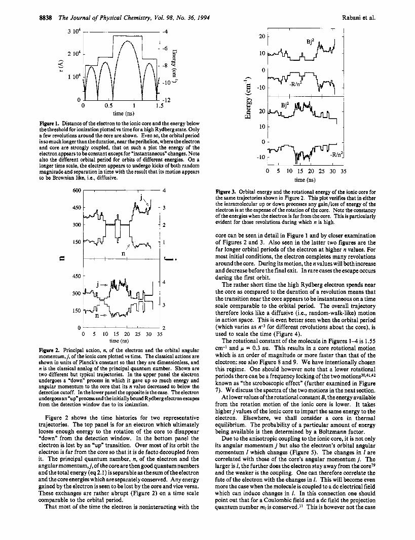
Figure 2. Principal action, n, of the electron and the orbital angular momentum, j , of the ionic core plotted vs time. The classical actions are shown in units of Planck's constant so that they are dimensionless, and n is the classical analog of the principal quantum number. Shown are two different but typical trajectories. In the upper panel the electron undergoes a "down" process in which it gave up so much energy and angular momentum to the core that its n value decreased to below the detection cutoff. In the lower panel the opposite is the case. The electron undergoes an *up" process and the initially bound Rydberg electron escapes from the detection window due to its ionization.

Figure 2 shows the time histories for two representative trajectories. The top panel is for an electron which ultimately looses enough energy to the rotation of the core to disappear "down" from the detection window. In the bottom panel the electron is lost by an "up" transition. Over most of its orbit the electron is far from the core so that it is de facto decoupled from it. The principal quantum number, n, of the electron and the angular momentum,j, of the core are then good quantum numbers and the total energy (eq 2.1) is separable as the sum of the electron and the core energies which are separately conserved. Any energy gained by the electron is seen to be lost by the core and vice versa. These exchanges are rather abrupt (Figure 2) on a time scale comparable to the orbital period.

That most of the time the electron is noninteracting with the

I 20 L

l o i ' 1 0 -

-10 -

0 5 10 15 20 25 30 35 time (ns)

Figure 3. Orbital energy and the rotational energy of the ionic core for the same trajectories shown in Figure 2. This plot verifies that in either the intramolecular up or down processes any gain/loss of energy of the electron is at the expense of the rotation of the core. Note the constancy of the energies when the electron is far from the core. This is particularly evident for those revolutions during which n is high.

core can be seen in detail in Figure 1 and by closer examination of Figures 2 and 3. Also seen in the latter two figures are the far longer orbital periods of the electron a t higher n values. For most initial conditions, the electron completes many revolutions around the core. During its motion, the nvalues will both increase and decrease before the final exit. In rare cases the escape occurs during the first orbit.

The rather short time the high Rydberg electron spends near the core as compared to the duration of a revolution means that the transition near the core appears to be instantaneous on a time scale comparable to the orbital period. The overall trajectory therefore looks like a diffusive (Le., random-walk-like) motion in action space. This is even better seen when the orbital period (which varies as n-3 for different revolutions about the core), is used to scale the time (Figure 4).

The rotational constant of the molecule in Figures 1-4 is 1.55 cm-l and 1.1 = 0.3 au. This results in a core rotational motion which is an order of magnitude or more faster than that of the electron; see also Figure 8 and 9. We have intentionally chosen this regime. One should however note that a lower rotational periods there can be a frequency locking of the two m o t i o n ~ 3 ~ ~ ~ 1 . ~ * known as "the stroboscopic effect" (further examined in Figure 7). We discuss the spectra of the two motions in the next section.

At lower values of the rotational constant B, the energy available from the rotation motion of the ionic core is lower. It takes higherj values of the ionic core to impart the same energy to the electron. Elsewhere, we shall consider a core in thermal equilibrium. The probability of a particular amount of energy being available is then determined by a Boltzmann factor.

Due to the anisotropic coupling to the ionic core, it is not only its angular momentum j but also the electron's orbital angular momentum 1 which changes (Figure 5). The changes in 1 are correlated with those of the core's angular momentum j . The larger is I , the further does the electron stay away from the core79 and the weaker is the coupling. One can therefore correlate the fate of the electron with the changes in 1. This will become even more the case when the molecule is coupled to a dc electrical field which can induce changes in I . In this connection one should point out that for a Coulombic field and a dc field the projection quantum number mI is c~nserved.~' This is however not the case

Very High Molecular Rydberg States

I

:k 100

I L

1 I I I -1 ' 0 5 10 15 20 25

time (ns) Figure 5. Angular momentum of the electron (scale on the right) and its projection, mr (scale on the left) plotted vs time. Note that while m, is not conserved, it does not quite span its entire range of possible values.

when the anisotropy of the core is taken into account. Neither 1 nor mi are conserved, as seen in Figure 5 .

The precession of the orbit is shown in Figure 6. The rate of precession is variable due to the changes in n which are possible during the temporal evolution of the trajectory (Figure 2). Note that, as in Figures 2 and 3, the change in the orientation angle of the elliptical orbit appears to be instantaneous on the time scale of Figure 6. The reason is that, as in atoms, the precession occurs due to the deviation of the potential from a pure Coulomb field, deviations which are only noticeable near the core. The orientation angle changes only once per orbit, during the rapid passage through the aphelion. Most of the orbit it is constant. The higher is the n value during the orbit, the longer is the time between changes in the orientation of the elliptical orbit. The rate of precession will be of importance in a sequel paper where we discuss the role of external field effects.

In general the projection, A, of 1 on the molecular axis is not conserved. This is unlike the usual situation in the ground and low-lying electronic states and is consistent with an inverse Born- Oppenheimer limit. A special situation where A is conserved, known as Hund's coupling case *an, is possible for such special values of n and j that the orbital period of the electron matches that of the c0re.29.30,~~ This requires lower n values as the frequency of rotation of the core is 2Bj and at all but the lowest j values

The Journal of Physical Chemistry, Vol. 98, No. 36, 1994 8839

271 I I I 6 0 0

450

300 1

150

0 I I 1 10 0 4 8 12 16

time (ns)

Figure 6. Precession of the orbit. Plotted is the orientation angle of the orbit with respect to a fixed axis, solid curve, vs time. Shown as a dashed line is the value of n. As expected on the basis of quantum defect theory, the orientation changes when the electron passes through its perihelion.

4 , I I

c I

-2 , 0 0.1 0.2 0.3

time (ns) Figure 7. Projection, A, of the angular momentum vector of the electron on the molecular axis plotted vs. time. Hund's coupling case acorresponds to A being conserved. Computed for n = 30 (orbital frequency of 8.1 cm-I) and for a rotational constant of B = 0.15 cm-I. Upper panel: initial J = 16 (2Bj = 4.8 cm-1). Note how A is a very oscillatory function of time, varying between *I. In the lower panel the initial j is j = 27 (rotation period - orbital period). The stroboscopic-like29.30.42 locking of I to the molecular axis is seen in the value of A becoming nearly constant.

the rotation of the core is faster than the orbital motion, unless B is very low. Figure 7 contrasts the typical situation where A is not conserved with a special trajectory a t a higher value of j where stroboscopi~-like29~30~4* locking of the orbital and rotational motions is possible. Figure 7 is drawn for a lower value of the rotational constant B and for a lower n value, in order to make the rotational period comparable to that of the electron's orbit. The failure of A to be conserved when the motion of the electron is slower than the rotation is a direct signature of the inverse Born-Oppenheimer regime.

All the results shown were computed using a dipolar anisotropic coupling term (eq 2.4). We have also made extensive computa- tions using only a quadrupolar anisotropy. There are quantitative differences between the two coupling terms, related mostly to the realistic value for the coupling of the quadrupole moment of an ion being typically smaller than that of its dipole moment. No qualitatively different features were noticed by us.

8840 The Journal of Physical Chemistry, Vol. 98, No. 36, 1994 Rabani et al.

0.8 c 1 I

1 1

0 0.5 1 1.5 2 w(cm-')

Figure 8. Classical power spectrum of the electron vs frequency (in wave numbers). Average over ten trajectories for an initial value n = 100. Note the peak at the corresponding frequency of 0.2 cm-l and the broadening due to the up and down processes.

'e cd W h

v 3

0.8

0.6

0.4

0.2

0.8

0.6

0.4

0.2

* 0.8 1 1 I i

1

0 2 4 6 8 10 12 14 16 w (cm-')

Figure 9. Classical power spectrum of the rotation of the ionic core, computed without (upper panel) and with (lower panel) coupling to the electron.

I

-50 -40 -30 -20 -10 0 -R / nz (cm-')

Figure 10. Classical power spectrum of the electron, as in Figure 8, plotted vs the binding energy of the electron. 4. Power Spectra

Power spectra of the electron and of the core rotation were computed as Fourier transforms of the respective dipoles taken as functions of time. The results are shown in Figures 8 and 9, respectively. Figure 10 is the same as Figure 8 but plotted vs the energy of the electron below the nominal ionization threshold. These power spectra, while equivalent to the plots vs time, provide a complementary picture of the dynamics. In the frequency domain, the continuous nature of theclassicalvariables is replaced

by spectra which are sharp when the actions are conserved but are broad when the coupling is turned on (cf. Figure 9). While this manner of presentation is not a substitute for a truly quantal computation, it should serve to show that the electron4ore coupling is not so feeble that it will disappear when the core motion is quantized.

The power spectrum of the electron shows the expected main peak corresponding to the initial value of n with secondary peaks due to those values of n where several revolutions were completed. Both Figures 8 and 10 clearly exhibit the manifestations of orbits with values of n well above the initial value. This is, of course, also evident in the time-dependent view (Figures 2 and 3). The only advantage of the otherwise equivalent frequency domain representation is that it is independent of an interpretation of n. The spectra shown are the spectra of the moving charge.

Figure 9 shows the power spectrum of the rotation of the core computed for trajectories generated in the absence and presence of the dipolar anisotropic coupling term in the Hamiltonian (eq 2.1). The broadening due to the coupling is quite evident.

When the core is also vibrationally excited one can also compute a vibrational power spectrum. We have computed the electron power spectrum at much lower values of n for comparison with the observed22 Rydberg series in vibrationally excited molecules.

Resolution of the rotational states of the ionic core following the pulsed field induced ionization*O.24,36,4~,631*0 for excitation through a rotationally selected state of S1 is one route to determination of the rotational spectrum. The use of special pulsed delays, whether a staircase temporal variation of the field strength or others20.28 can provide useful insights on the distribution of n values.

5. Kinetics of High Rydberg States

Running a large number of trajectories with the same initial values of the action variables but with different starting values for the angle variables provides a time history for an ensemble which mimics the initial excitation of a single quantum state. We believe that under realistic laser characteristics, this is a good approximation provided that no dc electrical field, which can cause Stark broadening, is present in the excitation region. The reason is, that under continuous-wave operation, the coherence width of a dye laser is about 1C2 cm-l, which is smaller than the spacings of adjacent Rydberg states. In a time domain language, the coherence time of the laser is longer than the orbital period of the electron. The initial ensemble as introduced above is therefore the one that has been used in this paper. Elsewhere, when we discuss the role of a stray dc field, it will be necessary to reexamine this point.

As already discussed, some trajectories will exit from the observation window at their first passage near the core. Most other trajectories will however live for many revolutions (this is because a uniform sampling over the angle variables generates more initial conditions where the trajectory is initiated with the electron far from the core). Similarly, for some trajectories the electron will exit "up" while for others it will be damped "down",

Figure 11 is a plot of the fraction of initial trajectories which remain within the detection window as a function of time. Beyond the small fraction of very prompt (i.e., suborbital period) decays, several time scales are evident in the decay. It is very suggestive to note that the observed2 decay kinetics can be superposed on such plots provided however that the time scale of the compu- tational results is scaled upward by more than an order of magnitude. The origin of this stretching of the time axis remains a subject for further work. Elsewhere we shall suggest that a stray dc electrical field can account for it.

One can analyze the decays separately as to whether they are due to up or to down processes. When one does this, one can examine the decay kinetics due to either mechanism. It is not quite trivial to assign a rate constant since the decay is not purely

Very High Molecular Rydberg States The Journal of Physical Chemistry, Vol. 98, No. 36, 1994 8841

n = 100

500

300

500 1 n = 190

I .

0 2 4 6 8 1 0 time (ns)

Figure 11. Number of trajectories, all with a given initial value of n which are still in the detection window at the time 1, plotted vs time. There is clearly more than one decay scale. Note that the rate of the fast decay is n-dependent. Not evident on this plot is the contribution of a few trajectories which very promptly exit.

Down

1 1 . I

120 160 200 240 n

Figure 12. The mean (over theensembleof trajectories) branching fraction for the fast down process plotted vs n. The solid line is a fit to a power dependence in n and is included only to guide the eye. Note how there are practically no trajectories which decay by the fast down channel for very high n's.

exponential. We have therefore done three distinct things: (1) an average rate constant (as, e.g., in RRKM theorys1) is determined by including all trajectories in the sample; (2) a rate constant is determined (as in the analysis of the experimental data1J) by fitting the kinetic data to a biexponential form and using the faster decay constant (excluding however the very prompt decays which are also excluded in the experiment); (3) a histogram of lifetimes is generated by recording the time when each trajectory exits from the observation window.

The overall conclusion is independent on how one chooses to treat the data and is summarized in Figures 12 and 13. For initial values of n between 100 and 260 and for a large (several hundreds) number of trajectories run for each n value, we find that for the faster component, the branching ratio for down transitions is a strongly decreasing function of n. The rate constant for up transitions is increasing with n. (The experimental results,lV2 where the internal energy is thermally distributed, suggest an essentially exponential increase of kUp We do not expect a similar effect in the present computation since here the initial energy of the ionic core is sharply defined.)

The two opposite trends in k,, and kdown, result in the branching

A I I I

120 160 200 240 n

Figure 13. Mean (over the ensemble of trajectories) branching fraction for the fast up process plotted vs n. Note that all trajectories in the ensemble have the same sharp initial value of the core rotational energy. The solid line is a fit to a power dependence in n and is included only to guide the eye.

30

20 10 n -

0.3 1.05 1.8 2.55 kup (ns-9

Figure 14. Histogramic representation of the up decay rates for two values of n. We do expect a distribution of rates,*l but we also expect the distribution to have one peak. Two and possibly three sets of rates can be distinguished. Not seen in such a plot are the very high rates which are far to the right on the scale shown. See Figure 16.

fraction for the fast decay which shows a minimum around n = 150. The present results show that the initially proposed mechanism is a viable possible interpretation of the intramolecular dynamics and that (very slow) radiative decay is not the only intramolecular process by which high molecular Rydberg states of cold molecules can exit from the detection window.

When examined in detail, theensemble oftrajectories generates an entire histogram of lifetimes. Typical results are shown in Figures 14 and 15 for up and down processes, respectively. We note that as a general property of such ensembles one expects a distribution of decay rates.81-82 The qualitative shape of the histogram is also as expected from the general considerations, namely, there are many more decay processes with longer lifetimes (i.e., smaller rates). What is unexpected is that a more detailed examination reveals that within each histogram there is typically more than one component; often our statistics suffice to discern a t least two components as is also seen when the decay curves are plotted vs time. Not readily evident on the time scale of the figures shown is the contribution of the very short lifetimes which is due to the prompt processes in which the electron departs in much less than an orbital period. One expects such processest2

8842 The Journal of Physical Chemistry, Vol. 98, No. 36, I994 Rabani et al.

10 m e, (3

$ 5

E u e, .-

0.5 1.75 3 4.25 kdown (ns-9

Figure 15. Same as Figure 14 but for the down process.

100

6.6 15 23 32 b

0.3 0.9 1 .5 2.1 Number of Revolutions

Figure 16. Histogramic representation of the rates of the faster up process, bottom panel, and the slower up processes, top panel, for n = 140. The rate is expressed in units of the orbital period for n = 140 so as to show that the few very prompt exits occur in less than an orbital period. These are the classical analogs of direct ionization and are expected62 to be rare.

and one expects them to be a very minor component, as clearly verified in Figure 16, in which the time scale is expanded to show an interval of up to one orbital period. Next are the processes when an electron departs without having sojourned in a high-n orbit during its previous history. Whether for an up or down process, such trajectories live for several orbital periods. As n varies over the experimentally interesting range (say between 90 and 250) the orbital period varies by a factor of 20 or so. A sojourn at a high-n orbit does however increase the period by a similar or larger factor. Hence the two classes of trajectories are distinguishable throughout the range of n which is of experimental interest. We regard the results shown in Figures 11 and 15, 16 as providing numerical evidence that there are at least two possible time scales in the purely intramolecular decay of high Rydberg states, over and above the very prompt decay.

The very clear numerical evidence is that the slow decay rate is essentially identical for all the initial values of n above 100 and below 250. The trajectories which contribute to the slow decay

are, of course, those which have been integrated longest. One cannot thereforeentirely ruleout the possibility that it is numerical instabilities, inherent in long-time integration,*3 which erases the dependence on the initial value of n. If correct, this suggests that the exit time of the long time trajectories, which sample very many values of n within the observation range prior to their exit, is no longer very sensitive to where these trajectories originated from. The experimentally determined “long” decay time is equally not very dependent on n except that, as already mentioned, the experimental time scale is slower by a factor of about 100.

Not addressed in the present study is the core-size dependence of the rates of the up and down processes. The expectations4 that down processes will become more probable for larger molecules must await future work. We also hope to examine there the subsequent decay channel in which the core dissociates into two neutral, (or, at higher energies, an ionic anda neutral38) fragments.

6. Concluding Remarks Time-resolved experiments1-3.22 reveal both a short (> 100 ns)

and a longer (microsecond range) decay of high Rydberg states of cold molecules. The present study was undertaken to elucidate the possible purely intramolecular dynamical processes with special reference to the short time evolution of such high Rydberg states. Particular attention was therefore focused on the coupling of the Rydberg electron to the rotation of the molecular core. It was verified that the Rydberg electron can effectively exchange energy and angular momentum with the ionic core any time that it passes near to it. These exchanges can result in the electron exiting from the experimental detection window either up or down. The time scale for such processes is determined both by how often the electron gets near the core (i.e., by the period of the orbit) and by the probability of the transition when the electron is near the core. For our diatomic-like core, the time scales for the evolution of the strictly isolated Rydberg state are however shorter than that observed for aromatic molecules by more than an order of magnitude. Because it takes many revolutions for the exit of the electron and because the electron sojourns in a wide range of n values prior to its final exit, there is an initial induction time during which a few electrons escape, followed by a diffusive- like kinetic regime. In that regime, the computed time evolution rather closely mimics the one observed, except for the already mentioned time stretch.

Acknowledgment. We thank Profs. R. Bersohn, J. Jortner, and E. W. Schlag, Drs. K. Muller-Dethlefs and H. Selzle and Mr. L. Ya. Baranov for discussions. E.R. is a Clore foundation scholar. This work was supported by the Volkswagenwerk Stiftung and by the German-Israel foundation for research (GIF). The experimental work at Tel Aviv University is supported by the German-Israel James Franck binational program. The Fritz Haber research center is supported by MINERVA.

References and Notes (1) Bahatt, D.; Even, U.; Levine, R. D. J. Chem. Phys. 1993, 98, 1744. (2) Even, U.; Ben-Nun, M.; Levine, R. D. Chem. Phys. Lett. 1993,210,

(3) Bahatt, D.; Cheshnovsky, 0.; Even, U. Z . Phys. 1993, D40, 1. (4) The temporal evolution reported in refs 1 and 2 has been reproduced

under quitedifferent experimental conditions. U. Even, private communication. ( 5 ) Bixon, M.; Jortner, J. J . Chem. Phys. 1968, 48, 715. (6) Schlag, E. W.; Schneider, S.; Fischer, F. S. Ann. Rev. Phys. Chem.

(7) Freed, K. F. Top. Cur. Chem. 1972,31, 105. ( 8 ) Avouris, Ph.; Gelbart, W. M.; El-Sayed, M. A. Chem. Reu. 1977,27,

(9) Jortner, J.; Levine, R. D. Adu. Chem. Phys. 1981, 47, 1. (10) (a) Berry,R. S. J . Chem. Phys. 1966,45,1228. (b) Berry, R.S.Adu.

Moss. Spectrom. 1974,6, 1. (c) Berry, R. S . Adu. Electron. Electron. Phys. 1980, 51, 137.

(11) Bardsley, J. N. Chem. Phys. Lett. 1967, 1 , 229. (12) Russek, A.; Patterson, M. R.; Becker, R. L. Phys. Rev. 1968, 167,

416.

1971, 22, 465.

393.

17.

Very High Molecular Rydberg States

(13) Ritchie, B. Phys. Rev. 1972, A6, 1761. (14) Fano, U. J . Opt. Soc. Am. 1975,65,979. (15) Greene, C. H.; Jungen, Ch. Adv. Atom. Mol. Phys. 1985, 21, 51. (16) Whetten, R. L.; Ezra, G. S.; Grant, E. R. Annu. Rev. Phys. Chem.

(17) Ito, M.; Ebata, T.; Mikami, N. Annu. Rev. Phys. Chem. 1988, 39,

(18) Child, M. S.; Jungen, Ch. J . Chem. Phys. 1990, 93, 7756. (19) Nakamura, H. Inr. Rev. Phys. Chem. 1991, 10, 123. (20) Merkt, F.; Softley, T. P. Int. Rev. Phys. Chem. 1993, 12, 205. (21) Schlag, E. W.; Levine, R. D. J . Phys. Chem. 1992, 96, 10668. (22) Even, U.; Levine, R. D.; Bersohn, R. J . Phys. Chem. 1994,98,3472. (23) Theevidencein ref 22is basedondetermining thewidthof theRydberg

transitions at lower n values. When these are extrapolated to the highermost n's the resulting widths exceed by several orders of magnitude the values of the directly observed decay rates.

(24) Miiller-Dethlefs, K.; Schlag, E. W. Annu. Rev. Phys. Chem. 1991, 42, 109.

(25) Grant, E. R.; White, M. G. Nature 1991, 354, 249. (26) Reiser, G.; Rieger, D.; Wright, T. G.; Miiller-Dethlefs, K.; Schlag,

E. W. J. Phys. Chem. 1993, 97, 4335. (27) Miiller-Dethlefs, K. J . Chem. Phys. 1991, 95, 4821. (28) Reiser, G.; Dopfer, 0.; Lindner, R.; Henri, G.; Muller-Dethlefs, K.;

Schlag, E. W.; Colson, S. D. Chem. Phys. Lett. 1991, 181, 1. (29) Bordas, C.; Brevet, P. F.; Broyer, M.; Chevaleyre, J.; Labastie, P.;

Petto, J. P. Phys. Rev. Lett. 1988, 60, 917. (30) (a) Chevaleyre, J.; Bordas, C.; Broyer, M.; Labastie, P. Phys. Rev.

Lett. 1986, 57, 3027. (b) Bordas, C.; Broyer, M.; Chevaleyre, J.; Labastie, P. J. Phys. 1987, 48, 647.

(31) Chupka, W. A. J . Chem. Phys. 1993, 98,4520. (32) Pratt, S . T. J . Chem. Phys. 1993, 98, 9241. (33) Merkt, F.; Fielding, H. H.; Softley, T. P. Chem. Phys. Lett. 1993,

(34) Park, H.; Zare, R. N. J . Chem. Phys. 1993, 99, 6537. (35) Zhang, Xu;Smith, J. M.; Knee, J . L.J. Chem.Phys. 1993,99,3133. (36) Nemeth, G. I.; Selzle, H. L.; Schlag, E. W. Chem. Phys. Lett. 1993,

1985, 36, 277.

123.

202, 153.

214. 141. ~~

(37) -Merkt, F.; Zare, R. N., private communication. Merkt, F. J . Chem.

(38) Schemer, W. G.; Selzle, H. L.; Schlag, E. W.; Levine, R. D. Phys. Phys. 1994, 100, 2623.

Rev. Lett. 1994, 72, 1435. (39) Debye, P. Phys. Z . 1919,20, 160. Holtsmark, J. Ibid, 1924,25,73.

Stebbings, R. F., Dunning, F. B., Eds. RydbergStates ofAroms andMolecules; Cambridge University Press: Cambridge, 1983.

(40) Chupka, W. A. J . Chem. Phys. 1993, 99, 5800. (41) Bordas, C.; Labastie, P.; Chevaleyre, J.; Broyer, M. Chem. Phys.

(42) Lombardi, M.; Labastie, P.; Bordas, M. C.; Broyer, M. J . Chem.

(43) Bryant, G. P.; Jiang, Y.; Martin, M.; Grant, E. R. J . Phys. Chem.

(44) Gilbert, R. D.; Child, M. S. Chem. Phys. Lett. 1991, 287, 153. (45) Akulin, V. M.; Reiser, G.; Schlag, E. W. Chem. Phys. Lett. 1992,

(46) Merkt, F.; Softley, T. P. Phys. Rev. 1992, A46, 302. (47) Levine, R. D.; Johnson, B. R.; Muckerman, J. T.; Bernstein, R. B.

(48) Levine, R. D. J. Chem. Phys. 1968, 49, 51. (49) Levine, R. D. Acc. Chem. Res. 1970, 3, 273. (50) For rotational excitation in heavy atom collisions one needs to go to

very low collision velocities to achieve a comparable time scale; see, for example: Tusa, J.; Sulkes, M.; Rice, S. A. J . Chem. Phys. 1979, 70, 3136. Sulkes, M.; Tusa, J.; Rice, S . A. J . Chem. Phys. 1980, 72, 5733.

(51) Itisknown(e.g.,refs 17and22) that Rydbergspectraatintermediate n values often require some vibrational excitation of the molecule to be experimentally discerned.

(52) White, H. E. Introduction to Atomic Spectra; McGraw-Hill: New York, 1934.

1989, 129, 2 1.

Phys. 1988,89, 3479.

1992, 96, 6875.

195, 383.

J . Chem. Phys. 1968,49, 56.

re Journal of Physical Chemistry, Vol. 98, No. 36, 1994 8843

(53) Seaton, M. J. Rep. Prog. Phys. 1983, 46, 167. (54) Wie-senfeld. J. R.: Greene. B. I. Phvs. Rev. Lett. 1983. 51. 1745. (55j Janssen, M: H. M:; Dantus', M.; Gui, H.; Zewail, A. H. Cheh. Phys.

(56) Baranov, L. Ya.; Kris, R.; Levine, R. D.; Even, U. J . Chem. Phvs. Lett. 1993, 214, 281.

1994, loo, 186. (57) Krause, H.; Neusser, H. J. J . Chem. Phys. 1992, 97, 5932. (58) Zhu, L.; Johnson, P. M. J . Chem. Phys. 1991, 94, 5769. (59) Due to the underlying dynamical symmetry, the classical and quantal

dynamics of the Coulomb problem are rather similar. A familiar application is the computation of the Rutherford differential cross section or the exact results provided by WKB quantization. For coherent quantum mechanical states of the Coulomb problem which move along the classical orbits, see: Nauenberg, M. Phys. Rev. 1989, A40,1133. Gay, J.-C.; Delande, D.; Bommier, A. Ibid. 1989, A39.6587. See also: Uzer, T.; Farrelly, D.; Milligan, J. A.; Raines, P. E.; Skelton, J. P. Science 1991, 253, 42.

(60) Noid, D. W.; Koszykowski, M. L.; Marcus, R. A. Annu. Rev. Phys. Chem. 1981, 32, 267.

(61) Gomez Llorente, J. M.; Pollak, E . Annu. Rev. Phys. Chem. 1992,43, 91.

(62) Remade, F.; Levine, R. D. Phys. Lett. 1993, A173, 284. (63) Lee, M.-T.; Wang, K.; McKoy, V. J . Chem. Phys. 1992,96,7848. (64) Lee, M.-T.; Wang, K.; McKoy, V. J . Chem. Phys. 1992,97, 3108. (65) (a) Raithel, G.; Fauth, M.; Walther, H. Phys. Rev. 1991, A44,1898.

(b) Yeazell, J. A.; Raithel, G.; Marmet, L.; Held, H.; Walther, H. Phys. Rev. Lett. 1993, 70, 2884.

(66) (a) Noordam, L. D.; ten Wolde, A.; Muller, H. G.; Lagendijk, A.; van Linden van den Heuvell, H. B. J . Phys. 1988, B21, L533. (b) ten Wolde, A.; Noordam, L. D.; Lagendijk, A.; van Linden van den Heuvell, H. B. Phys. Rev. 1989, A40,485. (c) Noordam, L. D.; ten Wolde, A.; Lagendijk, A.; van Linden van den Heuvell, H. B. Phys. Rev. 1989, A40, 6999.

(67) Kosloff, R. J . Phys. Chem. 1988, 92, 2087. (68) Stock, G.; Domcke, W. J . Phys. Chem. 1993, 97, 12466. (69) (a) Born, M. Mechanics of the Atom; Blackie: London, 1951. (b)

Child, M. S. Semiclassical Mechanics with Molecular Applications; Clar- endon: Oxford, 1991.

(70) (a) Cohen, A. 0.; Marcus, R. A. J . Chem. Phys. 1968,49,4509. (b) Cohen, A. 0.; Marcus, R. A. J . Chem. Phys. 1970,52, 3140. (c) Miller, W. H. J. Chem. Phys. 1971,54, 5386.

(71) Tuckerman, M. E.; Berne, B. J . J . Chem. Phys. 1991, 95, 8362. (72) (a) Bryant, G. P.; Jiang, Y.; Grant, E. R. J . Chem. Phys. 1992,96,

4827. (b) Reiser, G.; Habenicht, W.; Miiller-Dethlefs, K. J. Chem. Phys. 1993, 98, 8462.

(73) Berry, R. S.; Nielsen, S. E. Phys. Rev. 1970, AI , 383. (74) (a) Rottke, H.; Welge, K. H. J . Chem. Phys. 1992, 97, 908. (b)

Lefebvre-Brion, H.; Field, R. W. Perturbations in the Spectra of Diatomic Molecules; Academic: New York, 1986.

(75) Dissociation is energetically possible even in the diatomic case but the energy transfer from the high-n Rydberg electron to the vibration is too inefficient on the time scale of interest. The far higher density of vibrational states favors dissociation in the polyatomic case.

(76) Goldstein, H. Classical Mechanics; Addison-Wesley: Cambridge, 1953.

(77) Allen, M. P.;Tildedey, D. J. Computer Simulation of Liquids; Oxford University Press: Oxford, 1992.

(78) Press, W. H.; Flannery, B. P.; Teukolsky, S. A.; Vetterling, W. T. Numerical Recipes in C; Cambridge University Press: New York, 1988.

(79) At high values of the principle quantum number n the distance of closest approach is well approximated by l ( I + 1)/2 au.

(80) Lindner, R.; Sekiya, H.; Miiller-Dethlefs, K. Angew. Chem., Inr. Ed. Engl. 1993, 32, 1364.

(81) Levine, R. D. Ber. Bunsen-Ges. Phys. Chem. 1988, 92, 222. (82) For a concrete example, see: Engel, Y. M.; Levine, R. D.; Thoman,

J. W. Jr.; Steinfeld, J. I.; McKay, R. J . Phys. Chem. 1988, 92, 5497. (83) Brumer. P. Adu. Chem. Phvs. 1981.47. 201. (84j Schlag,'E. W.; Grotemeyer; H. J.; Levine, R. D. Chem. Phys. Lett.

1992, 190, 521.