Chaos, Solitons and Fractals 41 (2009) 2812–2819

Contents lists available at ScienceDirect

Chaos, Solitons and Fractals

journal homepage: www.elsevier .com/locate /chaos

Dynamics of a three-species food chain model with adaptive traits q

Chengjun Sun *, Michel LoreauDepartment of Biology, McGill University, 1205, rue Docteur Penfield, Montréal, Que., Canada H3A 1B1

a r t i c l e i n f o

Article history:Accepted 17 October 2008

0960-0779/$ - see front matter � 2008 Elsevier Ltddoi:10.1016/j.chaos.2008.10.015

q This work was supported by a National Science FCouncil of Canada to Michel Loreau, McGill Univers

* Corresponding author.E-mail address: cj.sun@mcgill.ca (C. Sun).

a b s t r a c t

A three-species food chain model is proposed with dynamically variable adaptive traits inthe intermediate consumer. We prove that its solutions are non-negative and bounded, andwe analyze the existence and stability of its equilibria. By applying Li and Muldowney’s [LiMY, Muldowney J. On Bendixson’s criterion. J Differ Equ 1993;106:27–39] high-dimen-sional Bendixson criterion, we show that the positive equilibrium is globally stable underspecific conditions. We support our analytical findings with numerical simulations.

� 2008 Elsevier Ltd. All rights reserved.

1. Introduction

Ecologists and mathematicians have often used food chains to describe the feeding relationships between species withinecosystems (see [1–5,21,22,24]). The simplest and most classical food chain model is the two-dimensional predator-preyLotka–Volterra model, which was first introduced by the famous Italian mathematician Vito Volterra [1]. Recently therehas been considerable interest in predator-prey models, especially for systems of three-species (see [3,6,7,21–23]). Amongthem is the resource-prey-predator model with a self-limiting term in the resource:

dxdt¼ x r 1� x

K

� �� ay

h i;

dydt¼ yðc1ax� bz� d1Þ;

dzdt¼ zðc2by� d2Þ;

ð1:1Þ

where xðtÞ; yðtÞ and zðtÞ represent, respectively, the resource population, the prey population, and the predator population asfunctions of time. The positive parameters r;K; a; b; c1; c2; d1 and d2 are interpreted as follows:

� r represents the intrinsic rate of natural increase of the resource in the absence of consumers;� K represents its carrying capacity;� a represents the consumption rate of the prey on the resource;� b represents the predation rate of the predator on the prey;� c1 represents the conversion efficiency of consumed resource into new prey;� c2 represents the conversion efficiency of consumed prey into new predators;� d1 represents the natural death rate of the prey;� d2 represents the natural death rate of the predator.

. All rights reserved.

oundation subcontract and by a Discovery Grant from the Natural Sciences and Engineering Researchity.

C. Sun, M. Loreau / Chaos, Solitons and Fractals 41 (2009) 2812–2819 2813

Model (1.1) is based on the traditional assumption that all species interact with each other simply via changes inpopulation density. Such interactions are called density-mediated interactions. Mathematicians have already given acomprehensive analysis of its local and global properties, including the existence, local stability and global stability ofits critical points, and the boundedness of the system (see [8,24]). But in recent years, biologists have showed theoret-ically and empirically that in natural systems preys often display anti-predator responses, i.e., they alter their foragingbehavior on resources to reduce predation risk (for example, seeking refuge or becoming vigilant at the expense of feed-ing). Altered foraging can result in an increased risk of starvation, and hence in a reduction in prey density (see [9,16,17]and the references therein). These indirect effects of changes in species traits are called trait-mediated indirect effects.Trait-mediated indirect effects have been shown to profoundly alter the dynamics of all trophic levels in food webs (see[18]).

2. The model establishment

Based on the biological information we provided in the introduction, we assume that the two consumption rates aand b are adaptive traits in model (1.1). These two traits are positively related to each other, such that prey increasesresource consumption (greater a) at the expense of a higher predation risk by carnivores (greater b), which impliesthat herbivores can be caught more easily by carnivores when they are actively searching for and consuming food.Here we assume that b ¼ ba2ðb > 0Þ, where the constant b measures the predation risk incurred by an individual preyper unit foraging time per unit density of the predator. This simple relationship arises from the fact that the two pre-dation rates are proportional to the amount of time that herbivores spend foraging, which implies that the herbivorecan only be caught by its predator when it is actively searching for food. Therefore we only need to model the dynam-ics of a since the dynamics of b can be known through a due to the assumption b ¼ ba2. Applying Abrams’ [19] meth-od and differentiating the fitness of species y with respect to the trait a, we obtain the following dynamical equationfor trait a:

dadt¼ nðc1x� 2bazÞ; ð2:1Þ

where the parameter n scales the rate at which the adaptive trait changes. Incorporating Eq. (2.1) into model (1.1), we obtainmodel (2.2), which describes a food chain with a non-instantaneous dynamic trait. Dynamic traits are common in the eco-evolutionary dynamics of community and ecosystems [20].

dxdt¼ x r 1� x

K

� �� ay

h i;

dydt¼ yðc1ax� ba2z� d1Þ;

dzdt¼ zðc2ba2y� d2Þ;

dadt¼ nðc1x� 2bazÞ:

ð2:2Þ

The rest of our paper is organized as follows. In Section 3, we analyze the equilibria and their stability using a linear anal-ysis; we also study the non-negativity and boundedness of model (2.2) with a non-instantaneous dynamic trait. In Section 4,we study the global stability of model (2.2) using the high-dimensional Bendixson criterion.

3. Basic analysis results

Model (2.2) always has a positive equilibrium. The positive a-axis of (2.2) is an invariant singular line (each pointE0ð0;0;0; aÞ on the positive a- axis is an equilibrium of model (2.2)). A variational matrix analysis at the boundary equilib-rium E0 shows that E0, is a saddle, and hence is always unstable. Thus, the singular line of model (2.2) is a repellor, and model(2.2) is a uniformly persistent system.

Lemma 3.1. All solutions ðxðtÞ; yðtÞ; zðtÞ; aðtÞÞ of model (2.2) with initial value ðx0; y0; z0; a0Þ 2 R4;0þ are non-negative.

The non-negativity of xðtÞ; yðtÞ and zðtÞ can be verified by the equations

xðtÞ ¼ x0 expZ t

0r 1� xðsÞ

K

� �� aðsÞyðsÞ

� �ds

� ;

yðtÞ ¼ y0 expZ t

0½c1aðsÞxðsÞ � ba2ðsÞzðsÞ � d1�ds

� ;

zðtÞ ¼ z0 expZ t

0½c2ba2ðtÞyðtÞ � d2�ds

� ;

ð3:1Þ

2814 C. Sun, M. Loreau / Chaos, Solitons and Fractals 41 (2009) 2812–2819

with x0; y0; z0 P 0. The non-negativity of aðtÞ can be easily deduced from the fourth equation of model (2.2). Also, ifxð0Þ ¼ x0 > 0, then xðtÞ > 0 for all t > 0. The same argument is valid for components yðtÞ; zðtÞ and aðtÞ. Hence, R4;0

þ , the interiorof R4

þ, is an invariant set for model (2.2). And the planes x–y, x–z and x–z are also invariant. Our next task is to study theboundedness of the solutions of model (2.2).

To simplify the calculations, we apply the following transformations to model (2.2):

x! xK; y! c1Ky; z! bz; a! a

c1K:

Model (2.2) then becomes

dxdt¼ x½rð1� xÞ � ay�;

dydt¼ yðmax�ma2z� d1Þ;

dzdt¼ zðna2y� d2Þ;

dadt¼ nðx� 2azÞ;

ð3:2Þ

where the number of parameters is reduced from eight to six and the two non-dimensional parameters m and n can be de-fined in terms of the original parameters:

m ¼ c21K2; n ¼ c1c2bK:

Due to the uniform persistence of model (3.2), there exists a time T such that xðtÞ; yðtÞ; zðtÞ; aðtÞ > ~cð0 < ~c < 1Þ fort > T. From the first equation of model (3.2) and considering the non-negativity of components y and a, we havedx=dt 6 rxð1� xÞ. The usual comparison theory [10] tells us that xðtÞ 6 1 as t !1. Denote S1 ¼ mnxþ nyþmz. Assum-ing d1 6 d2,

dS1

dt¼ �mnd1x� d1ny� d2mzþmnrx�mnrx2 þmnd1x 6 �d1S1 þmn½ðr þ d1Þx� rx2� 6 �d1S1 þ b1;

where

b1 ¼mnðrþd1Þ2

4r ; if d1 < r;

mnd1; if d1 P r:

(ð3:3Þ

Note that the values of d1 and d2 do not affect the boundedness of x; y and z. From the inequality above, we have

S1 6 S1ð0Þ expð�d1tÞ þ b1ð1� expð�d1tÞÞd1

:

Moreover, we have lim supt!1S1ðtÞ 6 b1=d1, which is independent of initial values and equivalent tolim supt!1ðmnxðtÞ þ nyðtÞ þmzðtÞÞ 6 b1=d1. The variables x; y and z are thus ultimately bounded regardless of the value ofthe dynamic trait a. Denote S2 ¼ xþ a. Then when t > T ,

dS2

dt¼ rx� rx2 � axyþ nx� 2naz 6 rx� rx2 þ nxþ 2~cnx� 2~cnx� 2naz < �2~cnðxþ aÞ þ ðr þ nþ 2~cnÞx� rx2

6 �2~cnS2 þ b2;

where

b2 ¼ðrþnþ2~cnÞ2

4r ; if nþ 2~cn < r;

nþ 2~cn; if nþ 2~cn P r:

(ð3:4Þ

Define b3 ¼ 2~cn. From the inequality above, we conclude that

xðtÞ þ aðtÞ < ðx0 þ a0Þ expð�b3tÞ þ b2ð1� expð�b3tÞÞb3

:

Therefore, we have lim supt!1ðxðtÞ þ aðtÞÞ < b2=b3, which is also independent of initial values.

Lemma 3.2. All solutions initiating in R4;0þ are bounded, with an ultimate bound.

In order to find the local stability of the positive equilibrium of model (3.2) we have to calculate the Jacobian matrix J atthis equilibrium. The positive equilibrium for model (3.2) is E�ðx�; y�; z�; a�Þ, where

C. Sun, M. Loreau / Chaos, Solitons and Fractals 41 (2009) 2812–2819 2815

x� ¼ 2d1nrd2mþ 2d1nr

; y� ¼ d2m2nr2

ðd2mþ 2d1nrÞ2;

z� ¼ d1mn2r2

ðd2mþ 2d1nrÞ2; a� ¼ d2mþ 2d1nr

mnr:

The Jacobian matrix of (3.2) at E� is

J ¼

�rx� �a�x� 0 �x�y�

ma�y� 0 �ma�2y� y�ðmx� � 2ma�z�Þ0 na�2z� 0 2d2z�

a�

n 0 �2na� �2nz�

0BBB@

1CCCA;

whose characteristic equation is

k4 þ Ak3 þ Bk2 þ Ckþ D ¼ 0; ð3:5Þ

where

A ¼ 2d1nr2

d2mþ 2d1nrþ 2d1mn2r2n

ðd2mþ 2d1nrÞ2;

B ¼ 2d1d2mrd2mþ 2d1nr

þ 2d1mn2r2nð2d2 þ rÞðd2mþ 2d1nrÞ2

;

C ¼ 2d21d2nr2

d2mþ 2d1nrþ 2d1d2mn2r2n

ðd2mþ 2d1nrÞ2þ 4d2

1d2mn2r3nðmþ 2nrÞðd2mþ 2d1nrÞ3

;

D ¼ 2d21d2mn2r3n

ðd2mþ 2d1nrÞ2:

Notice that zero is not the root of (3.5). From the Routh–Hurwitz criteria [11], all the real parts of roots for (3.5) are neg-ative if and only if

ABC � A2D > C2; ð3:6Þ

which is equivalent to

16d41d2n4r4 þ 8d3

1d2mn3r3ð4d2 þ nnÞ þ 4d21d2mn2r2½6md2

2 þ 3mnd2n

þ 2nrnðmþ 2nr þ n2nÞ� þ 2d1mnr½4d42m2 þ 3d3

2m2nnþ 2d2mn4rn3

2n3r3ðmþ 2nrÞn2 þ 4d22mnrðmþ 2nr þ n2nÞn� þm2½d5

2m2 þ d42m2nn

þ 2d22mn4rn3 þ 2n4r3ðmþ 2nrÞn3 þ 2d2n3r2ðmþ 2nrÞðr þ 2nnÞn2

þ 2d32mnrðmþ 2nr þ n2nÞn� > 0:

ð3:7Þ

Inequality (3.6) or (3.7) always holds for any positive parameters in (3.2), and thus the positive equilibrium E� is locallystable.

4. Analysis of global stability

When the positive equilibrium E� is locally asymptotically stable, it is of interest to know its basin of attraction. In par-ticular, we would like to know if its basin of attraction includes all the points in the feasible region, namely, if E� is globallyasymptotically stable. The difficulty associated with this problem is largely due to the lack of practical tools. The method ofLyapunov functions is most commonly applied (see [10]). However, its application is often hindered by the fact that globalLyapunov functions are difficult to construct and there is no general approach to construct them. Another method to proveglobal stability is to use the higher Poincare–Bendixon theory (see [12]). This approach depends crucially on the fact that thesystem studied is competitive. But model (2.2) or (3.2) is not a competitive system. Therefore, to investigate the global sta-bility of the positive equilibrium E�, we now apply the high-dimensional Bendixson criterion of Li and Muldowney [13],which we briefly summarize next.

Let D � Rn be an open set and function F : X#FðXÞ 2 Rn be C1 for X 2 D. Consider the differential equation

dXdt¼ FðXÞ: ð4:1Þ

As shown in [13], to derive a high-dimensional Bendixson criterion, it is sufficient to show that the second compoundequation

2816 C. Sun, M. Loreau / Chaos, Solitons and Fractals 41 (2009) 2812–2819

dZdt¼ @F ½2�

@XðXðt;X0ÞÞZðtÞ ð4:2Þ

with respect to a solution Xðt;X0Þ 2 D of system (4.1) is equi-uniformly asymptotically stable, namely, for each X0 2 D, sys-tem (4.2) is uniformly asymptotically stable, and the exponential decay rate is uniform for X0 in each compact subset of D,where D � Rn is an open connected set. Here @F=@X ½2� is the second additive compound matrix of the Jacobian matrix @F=@X.

It is a n2

� �� n

2

� �matrix, and thus (4.2) is a linear system of dimension n

2

�(see [14,15] for details).

For a general 4� 4 matrix

A ¼

a11 a12 a13 a14

a21 a22 a23 a24

a31 a32 a33 a34

a41 a42 a43 a44

0BBB@

1CCCA;

its second additive compound matrix A½2� is

A½2� ¼

a11 þ a22 a23 a24 �a13 �a14 0a32 a11 þ a33 a34 a12 0 �a14

a42 a43 a11 þ a44 0 a12 a13

�a31 a21 0 a22 þ a33 a34 �a24

�a41 0 a21 a43 a22 þ a44 a23

0 �a41 a31 �a42 a32 a33 þ a44

0BBBBBBBB@

1CCCCCCCCA: ð4:3Þ

The equi-uniform asymptotic stability of (4.2) implies the exponential decay of the surface area of any compact two-dimensional surface in D. If D is simply connected, this excludes the existence of any invariant simple closed rectifiable curvein D, including periodic orbits.

Proposition 4.1 [13]. Let D � Rn be a simply connected region. Assume that the family of linear systems (4.2) is equi-uniformlyasymptotically stable. Then

(a) D contains no simple closed invariant curves, including periodic orbits, homoclinic orbits, heteroclinic cycles;(b) each semi-orbit in D converges to a single equilibrium.

In particular, if D is positively invariant and contains a unique equilibrium X, then X is globally asymptotically stable in D.

The required uniform asymptotic stability of the family of linear systems (4.2) can be proved by constructinga suitable Lyapunov function. For instance, (4.2) is equi-uniformly asymptotically stable if there exists a positivedefinite function VðZÞ, such that dVðZÞ=dtjð4:2Þ is negative definite, and V and dV=dtjð4:2Þ are both independent ofX0.

In order to prove the global stability of the positive equilibrium in model (2.2) or (3.2), we first make the followingassumption.

(H) There exist positive numbers -; h; #;q and r such that

max c11 þc12-

hþ c13-þ

c15-q

;c21h- þ c22 þ c23hþ

c24h#þ c26h

r;

c32

hþ c33 þ

c35

q;

c42#

hþ c44 þ

c45#

qþ c46#

r;

�c51q- þ c53qþ

c54q#þ c55 þ

c56qr

;c62r

hþ c65r

qþ c66

< 0:

For model (3.2), denote X ¼ ðx; y; z; aÞT and

FðXÞ ¼ ðx½rð1� xÞ � ay�; yðmax�ma2z� d1Þ; zðna2y� d2Þ; nðx� 2azÞÞT :

We then have

@F@X¼

r � 2rx� ay �ax 0 �xy

may max�ma2z� d1 �ma2y mxy� 2mayz

0 na2z na2y� d2 2nayz

n 0 �2na �2nz

0BBB@

1CCCA;

C. Sun, M. Loreau / Chaos, Solitons and Fractals 41 (2009) 2812–2819 2817

and we assume that

@F ½2�

@X¼

b11 b12 b13 b14 b15 b16

b21 b22 b23 b24 b25 b26

b31 b32 b33 b34 b35 b36

b41 b42 b43 b44 b45 b46

b51 b52 b53 b54 b55 b56

b61 b62 b63 b64 b65 b66

0BBBBBBBB@

1CCCCCCCCA:

By (4.3), we obtain that

b11 ¼ r � d1 � 2rx� ayþmax�ma2z; b12 ¼ �ma2y; b13 ¼ mxy� 2mayz; b14 ¼ 0;

b15 ¼ xy; b16 ¼ 0; b21 ¼ na2z; b22 ¼ r � d2 � 2rx� ayþ na2y; b23 ¼ 2nayz;b24 ¼ �ax; b25 ¼ 0; b26 ¼ xy; b31 ¼ 0; b32 ¼ �2na; b33 ¼ r � 2rx� ay� 2nz;

b34 ¼ 0; b35 ¼ �ax; b36 ¼ 0; b41 ¼ 0; b42 ¼ may; b43 ¼ 0;

b44 ¼ �d1 � d2 þmax�ma2zþ na2y; b45 ¼ 2nayz; b46 ¼ �mxyþ 2mayz;

b51 ¼ �n; b52 ¼ 0; b53 ¼ may; b54 ¼ �2na; b55 ¼ �d1 þmax�ma2z� 2nz;

b56 ¼ �ma2y; b61 ¼ 0; b62 ¼ �n; b63 ¼ 0; b64 ¼ 0; b65 ¼ na2z; b66 ¼ �d2 þ na2y� 2nz:

The second compound system

_z1

_z2

_z3

_z4

_z5

_z6

0BBBBBBBB@

1CCCCCCCCA¼ @F ½2�

@X

z1

z2

z3

z4

z5

z6

0BBBBBBBB@

1CCCCCCCCA

then becomes

_z1 ¼ ðr � d1 � 2rx� ayþmax�ma2zÞz1 �ma2yz2 þ ðmxy� 2mayzÞz3 þ xyz5;

_z2 ¼ na2zz1 þ ðr � d2 � 2rx� ayþ na2yÞz2 þ 2nayzz3 � axz4 þ xyz6;

_z3 ¼ �2naz2 þ ðr � 2rx� ay� 2nzÞz3 � axz5;

_z4 ¼ mayz2 þ ð�d1 � d2 þmax�ma2zþ na2yÞz4 þ 2nayzz5 þ ð�mxyþ 2mayzÞz6;

_z5 ¼ �nz1 þmayz3 � 2naz4 þ ð�d1 þmax�ma2z� 2nzÞz5 �ma2yz6;

_z6 ¼ �nz2 þ na2zz5 þ ð�d2 þ na2y� 2nzÞz6;

ð4:5Þ

where XðtÞ ¼ ðxðtÞ; yðtÞ; zðtÞ; aðtÞÞT is an arbitrary solution of model (3.2) with X0ðtÞ ¼ ðx0ðtÞ; y0ðtÞ; z0ðtÞ; a0ðtÞÞT 2 R4;0þ . Set

WðZÞ ¼maxf-jz1j; hjz2j; jz3j; #jz4j;qjz5j;rjz6jg:

Direct calculations lead to the following inequalities:

dþ

dt-jz1j 6 c11-jz1j þ

c12-h

hjz2j þ c13-jz3j þc15-q

qjz5j;

dþ

dthjz2j 6

c21h- -jz1j þ c22hjz2j þ c23hjz3j þ

c24h#

#jz4j þc26hr

rjz6j;

dþ

dtjz3j 6

c32

hhjz2j þ c33jz3j þ

c35

qqjz5j;

dþ

dt#jz4j 6

c42#

hhjz2j þ c44#jz4j þ

c45#

qqjz5j þ

c46#

rrjz6j;

dþ

dtqjz5j 6

c51q- -jz1j þ c53qjz3j þ

c54q#

#jz4j þ c55qjz5j þc56qr

rjz6j;

dþ

dtrjz6j 6

c62rh

hjz2j þc65rq

qjz5j þ c66rjz6j;

ð4:6Þ

2818 C. Sun, M. Loreau / Chaos, Solitons and Fractals 41 (2009) 2812–2819

in which dþ=dt denotes the right-hand derivative and

c11 ¼ r � d1 � 2r~c � ~c2 þmð1þ 2~cÞ2

16~c2 ; c12 ¼ �m~c3; c13 ¼m2ðd1 þ rÞ2

4d1r;

c15 ¼mðd1 þ rÞ2

4d1r; c21 ¼

n2ðd1 þ rÞ2ð1þ 2~cÞ4

45~c4d1r; c22 ¼ r � d2 � 2r~c þmnðd1 þ rÞ2ð1þ 2~cÞ4

45~c4d1r;

c23 ¼mn2ðd1 þ rÞ4ð1þ 2~cÞ2

128~c2d21r2

; c24 ¼ �~c2; c26 ¼mðd1 þ rÞ2

4d1r; c32 ¼ �2n~c;

c33 ¼ r � 2r~c � 2n~c; c35 ¼ �~c2; c42 ¼m2ðd1 þ rÞ2ð1þ 2~cÞ2

64~c2d1r;

c44 ¼ �d1 � d2 þmð1þ 2~cÞ2

16~c2 þmnðd1 þ rÞ2ð1þ 2~cÞ4

45~c4d1r; c45 ¼

mn2ðd1 þ rÞ4ð1þ 2~cÞ2

128~c2d21r2

;

c46 ¼ �m~c2 þm2nðd1 þ rÞ4ð1þ 2~cÞ2

128~c2d21r2

; c51 ¼ �n; c53 ¼m2ðd1 þ rÞ2ð1þ 2~cÞ2

64~c2d1r;

c54 ¼ �2n~c; c55 ¼ �d1 þmð1þ 2~cÞ2

16~c2 � 2n~c; c56 ¼ �m~c3; c62 ¼ �n;

c65 ¼n2ðd1 þ rÞ2ð1þ 2~cÞ4

45~c4d1r; c66 ¼ �d2 þ

mnðd1 þ rÞ2ð1þ 2~cÞ4

45~c4d1r� 2n~c:

ð4:7Þ

Therefore,

dþ

dtWðZðtÞÞ 6 wWðZðtÞÞ;

with

w ¼ max c11 þc12-

hþ c13-þ

c15-q

;c21h- þ c22 þ c23hþ

c24h#þ c26h

r;

c32

hþ c33 þ

c35

q;

c42#

hþ c44 þ

c45#

qþ c46#

r;

�c51q- þ c53qþ

c54q#þ c55 þ

c56qr

;c62r

hþ c65r

qþ c66

:

Thus, under hypothesis (H), and by the boundedness of solution of model (3.2), there exists a positive constant s such thatw 6 �s < 0, and thus

WðZðtÞÞ 6WðZðsÞÞ expð�sðt � sÞÞ; t P s > 0:

This establishes the equi-uniform asymptotic stability of the second compound system (4.5), and hence the positive equi-librium E� of model (3.2) is globally stable following from Proposition 4.1. We summarize the above analysis in the followingtheorem.

0 5000 10000

0.2

0.4

0.6

0.8

t x-plane

x(t)

0 5000 100000

0.1

0.2

0.3

t y-plane

y(t)

0 5000 10000 0.05

0

0.05

0.1

0.15

t z-plane

z(t)

00.5

00.1

0.20

0.01

0.02

x(t)y(t)

z(t)

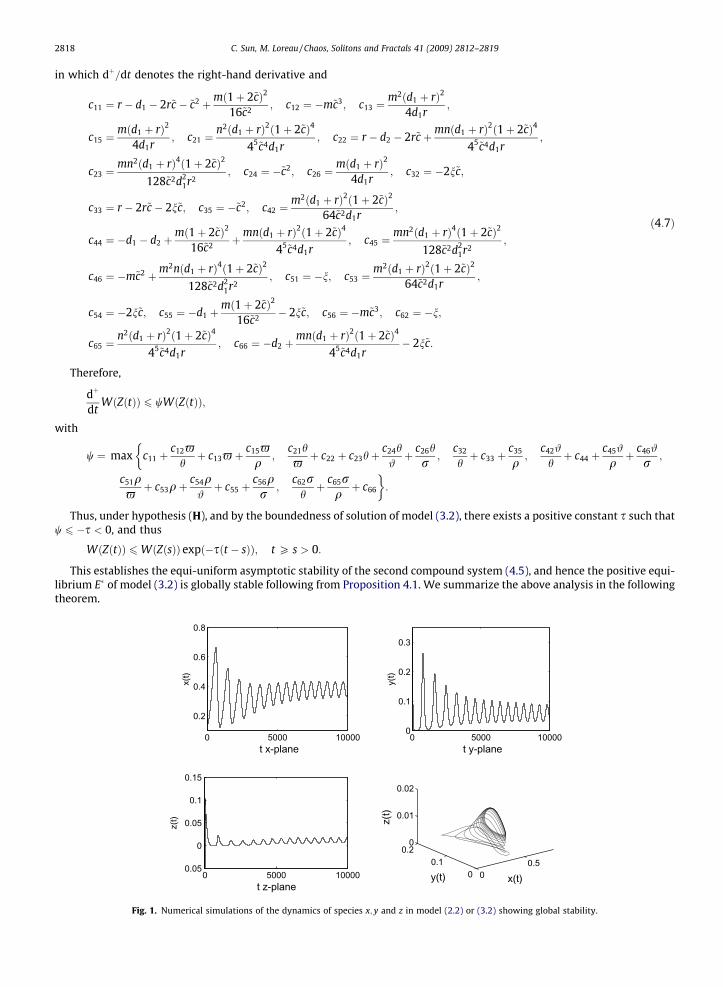
Fig. 1. Numerical simulations of the dynamics of species x; y and z in model (2.2) or (3.2) showing global stability.

C. Sun, M. Loreau / Chaos, Solitons and Fractals 41 (2009) 2812–2819 2819

Theorem 4.2. If hypothesis (H) is satisfied, then model (2.2) or (3.2) has no non-trivial periodic solutions. Furthermore, thepositive equilibrium E� is globally stable in R4;0

þ .

Based on the local stability analysis in Section 3 and Theorem 4.2, we next carry out numerical simulations of the dynam-ics of species x; y and z (see Fig. 1) to illustrate its global stability through an example. We use the following parameter valuesin the original model (2.2): r ¼ 2;K ¼ 4; c1 ¼ c2 ¼ b ¼ 1=2; d1 ¼ 1; d2 ¼ 5; n ¼ 14 (we also take ~c ¼ 1=4). From the non-dimen-sional transformation in Section 3 we know that m ¼ 1; n ¼ 1=2. We also know that the positive equilibrium E� is locally sta-ble from Section 3. We then substitute the above parameter values into (4.7), and obtain

c11 ¼ 2:1875; c12 ¼ �0:0156; c13 ¼ 1:1250; c15 ¼ 1:1250; c21 ¼ 1:4238; c22 ¼ �1:1524;c23 ¼ 1:4238; c24 ¼ �0:0625; c26 ¼ 1:1250; c32 ¼ �8:1667; c33 ¼ �6:2500; c35 ¼ �0:0625;c42 ¼ 2:5312; c44 ¼ �0:9024; c45 ¼ 1:4238; c46 ¼ 2:7851; c51 ¼ �14; c53 ¼ 2:5312;c54 ¼ �7; c55 ¼ �5:75; c56 ¼ �0:0156; c62 ¼ �14; c65 ¼ 1:4238; c66 ¼ �9:1524:

The positive numbers - ¼ 1:0000; h ¼ 0:0030; # ¼ 0:0001;q ¼ 1:0000 and r ¼ 1:0000 are such that

maxf�1:8841;�1:1404;�2728:5458;�0:0583;�74669:9011;�4674:3953g < 0:

Therefore the positive equilibrium E� is globally stable (see Fig. 1).

References

[1] Volterra V. Variazioni e fluttuazioni del numero d’individui in specie animali conviventi. Mem R Accad Naz dei Lincei Ser VI 1926;2.[2] So Joseph WH. A note on the global stability and bifurcation phenomenon of a Lotka–Volterra food chain. J Theoret Biol 1979;80(2):185–7.[3] Freedman HI, Waltman P. Mathematical analysis of some three-species food-chain models. Math Biosci 1977;33(3–4):257–76.[4] Hsu SB, Hwang TW, Kuang Y. A ratio-dependent food chain model and its applications to biological control. Math Biosci 2003;181(1):55–83.[5] Sun CJ, Han MA, Lin YP, Chen YY. Global qualitative analysis for a predator-prey system with delay. Chaos, Solitons and Fractals 2007;32(4):1582–96.[6] Haussman U. Abstract food webs in ecology. Math Biosci 1971;11:291–316.[7] Rescigno A. The struggle for life-IV two predators sharing a prey. Bull Math Biol 1977;39:179–85.[8] Krikorian N. The Volterra model for three species predator-prey systems: boundedness and stability. J Math Biol 1979;7:117–32.[9] Schmitz OJ. Effects of predator hunting mode on grassland ecosystem function. Science 2008;319:952–4.

[10] Hale JK. Ordinary differential equations. New York: John Wiley; 1969.[11] Hurwitz A. On the conditions under which an equation has only roots with negative real parts. Math Ann 1895;46:273–84.[12] Smith RA. Some applications of Hausdorff dimension inequalities for ordinary differential equations. Proc R Soc Edinburgh A 1986;104:235–59.[13] Li MY, Muldowney J. On Bendixson’s criterion. J Differ Equ 1993;106:27–39.[14] Fiedler M. Additive compound matrices and inequality for eigenvalues of stochastic matrices. Czech Math J 1974;99:392–402.[15] Muldowney JS. Compound matrices and ordinary differential equations. Rocky Mount J Math 1990;20:857–72.[16] Celine AM Griffin, Jennifer S Thaler. Insect predators affect plant resistance via density- and trait-mediated indirect interactions. Ecol Lett

2006;9:335–43.[17] Loeuille N, Loreau M, Ferriere R. Consequences of plant-herbivore coevolution on the dynamics and functioning of ecosystems. J Theor Biol

2002;217(3):369–81.[18] Goudard A, Loreau M. Nontrophic interactions, biodiversity, and ecosystem functioning: an interaction web model. Am Nat 2008;171:91–109.[19] Abrams PA. Implications of dynamically variable traits for identifying, classifying, and measuring direct and indirect effects in ecological communities.

Am Nat 1995;146(1):112–34.[20] Fussmann GF, Loreau M, Abrams PA. Eco-evolutionary dynamics of communities and ecosystems. Funct Ecol 2007;21:465–77.[21] Chen YY, Yu J, Sun C. Stability and Hopf bifurcation analysis in a three-level food chain system with delay. Chaos, Solitons and Fractals

2007;31(3):683–94.[22] Gomes AA, Manica E, Varriale MC. Applications of chaos control techniques to a three-species food chain. Chaos, Solitons and Fractals

2008;35(3):432–41.[23] Gakkhar S, Singh B. The dynamics of a food web consisting of two preys and a harvesting predator. Chaos, Solitons and Fractals 2007;34(4):1346–56.[24] Zhang S, Chen LA. Holling II functional response food chain model with impulsive perturbations. Chaos, Solitons and Fractals 2005;24(5):1269–78.