Dynamical Effects on the Habitable Zone for Earth-like Exomoons

arX

iv:1

304.

4377

v1 [

astr

o-ph

.EP

] 16

Apr

201

3

Mon. Not. R. Astron. Soc.000, 1–12 () Printed 17 April 2013 (MN LATEX style file v2.2)

Dynamical Effects on the Habitable Zone for Earth-like Exomoons

Duncan Forgan1⋆ and David Kipping2,31Scottish Universities Physics Alliance (SUPA), Institute for Astronomy, University of Edinburgh, Blackford Hill, Edinburgh, EH9 3HJ, Scotland, UK2Harvard-Smithsonian Centre for Astrophysics, Cambridge, Massachusetts 02138, USA3Carl Sagan Fellow

17 April 2013

ABSTRACT

With the detection of extrasolar moons (exomoons) on the horizon, it is important to considertheir potential for habitability. If we consider the circumstellar Habitable Zone (HZ, oftendescribed in terms of planet semi-major axis and orbital eccentricity), we can ask, “How doesthe HZ for an Earth-like exomoon differ from the HZ for an Earth-like exoplanet?”

For the first time, we use 1D latitudinal energy balance modelling to address this question.The model places an Earth-like exomoon in orbit around a Jupiter mass planet, which in turnorbits a Sun-like star. The exomoon’s surface is decomposedinto latitudinal strips, and thetemperature of each strip is evolved under the action of stellar insolation, atmospheric cooling,heat diffusion, eclipses of the star by the planet, and tidalheating. We use this model to carryout two separate investigations.

In the first, four test cases are run to investigate in detail the dependence of the exomoonclimate on orbital direction, orbital inclination, and on the frequency of stellar eclipse by thehost planet. We find that lunar orbits which are retrograde tothe planetary orbit exhibit greaterclimate variations than prograde orbits, with global mean temperatures around 0.1 K warmerdue to the geometry of eclipses. If eclipses become frequentrelative to the atmospheric ther-mal inertia timescale, climate oscillations become extremely small.

In the second investigation, we carry out an extensive parameter study, running the modelmany times to study the habitability of the exomoon in the 4-dimensional space composed ofthe planet semi-major axis and eccentricity, and the moon semi-major axis and eccentricity.We find that for zero moon eccentricity, frequent eclipses allow the moon to remain habitablein regions of high planet eccentricity, but tidal heating severely constrains habitability in thelimit of high moon eccentricity, making the habitable zone asensitive function of moon semi-major axis.

Key words:astrobiology, methods:numerical, planets and satellites: general

1 INTRODUCTION

The increasing rate of discovery of extrasolar planets (exoplanets)has given astronomers licence to consider their potential as habi-tats for extraterrestrial life. To date, more than 860 exoplanets havebeen confirmed1, with over 2,300 exoplanet candidates identifiedby the Kepler mission (Batalha et al. 2013). Of the confirmed ex-oplanets, several are in the circumstellar Habitable Zone (HZ), anannular region surrounding the star where planets with orbits insideit may be expected to possess liquid water on their surface.

The HZ is derived for planets of terrestrial mass and com-position - the inner edge is determined by water loss (via hy-drogen escape and photolysis), and the outer edge is deter-

⋆ E-mail:[email protected] http://exoplanet.eu

mined by runaway glaciation due to a build up ofCO2 clouds(Kasting, Whitmire & Reynolds 1993). In the case of single stars,the HZ is a circular annulus, and hence terrestrial planets on circu-lar orbits inside the annulus are expected to be habitable. Even ifthe planet’s orbit is not circular, it may still be habitabledepend-ing on the average received flux over its orbit, which can varysig-nificantly if the orbit is highly elliptical (Williams & Pollard 2002;Kane & Gelino 2012a,b). If the star is a multiple system, the geom-etry of the HZ annulus becomes time-dependent, and this can haveimportant consequences for the climates of planets in the system(Forgan 2012; Eggl et al. 2012b,a; Kane & Hinkel 2013).

To date, all exoplanets that reside within their local single-star HZ have radii 1.5 to 2 times larger than that of the Earth,and as such may be mini-Neptunes than super-Earths (see forexample Barnes et al. 2009). Even if such planets were terres-trial in nature, they are likely to have significantly higherman-

c© RAS

http://arxiv.org/abs/1304.4377v1

2 Duncan Forgan and David Kipping

tle viscosity, which suppresses convection and as a result hasimplications for heat transfer and the planet’s ability to degas(Stamenkovic, Spohn & Breuer 2010; Liu & Zhong 2010).

This being the case, the current crop of exoplanets in the HZshould not be ruled out as a source of habitable niches. Extrasolarmoons (exomoons) belonging to these planets may be terrestrial innature, and as a result may be habitable (Williams, Kasting &Wade1997). This is true even in our own Solar System: outside the Earth,the best chances for life in the Solar System are believed to be ontidally heated icy moons which are thought to possess liquidsub-surface oceans, such as Europa (Melosh et al. 2004) and Enceladus(Parkinson et al. 2007). Titan, the largest moon in the SolarSystem,has a thick atmosphere, with evidence of precipitation and lakesconstituting a hydrological cycle (Stofan et al. 2007).

Exomoons are yet to be detected, but Earth-mass ex-omoons are in principle detectable indirectly with Kepler(Kipping, Fossey & Campanella 2009). Studying an exoplanet’stransit timing variations and transit duration variations(TTV andTDV respectively) allows observational constraints on themoon’smass, and its orbital semi-major axis around the host exoplanet. Ad-ditionally, auxiliary transits of the moon and planet-moonmutualevents lead to unique transit features revealing the moon’sradiusand other orbital parameters (Kipping 2011). Such efforts to realisea detection are underway as part of the Hunt for Exomoons withKepler (HEK) project (Kipping et al. 2012).

A large component of habitability studies is the study of theenergy balance associated with the celestial body in question. Thevarious sources and sinks of heat are catalogued and compared, andthe system is evolved over time to understand their interplay, eitherby analytical calculation or numerical simulation. In the case of ex-omoons, the list of sources is longer than that of exoplanets. Along-side direct stellar insolation, exomoons receive starlight reflectedfrom the planet (as well as the planet’s own radiation), and they aretidally heated. Also, the moon is more prone to stellar eclipses as aresult of the host planet, providing an extra (effective) energy sink.

The study of habitable exomoons has grown apace in recentyears: early calculations by Reynolds, McKay & Kasting (1987)demonstrated that Europa is a viable niche for marine life such asthat found under Antartic ice, and proposed a tidally heatedcircum-planetary habitable zone. In the early phase of exoplanet detection,Williams, Kasting & Wade (1997) suggested that two of the then 9known giant exoplanets could host habitable moons. They raisedthe three key obstacles to exomoon habitability, namely:

(i) Tidal locking of the moon with respect to the planet, resultingin extreme weather conditions (Joshi 1997).

(ii) Increased EUV and X-Ray radiation from the hostplanet’s magnetosphere leading to loss of the moon’s atmosphere(Kaltenegger 2000), and

(iii) A poorly proportioned distribution of volatile abundances,due to the differing environments of planet and moon formation.Kaltenegger (2000) notes that Solar System moons may be over-abundant with water to be habitable, if placed in the inner SolarSystem, as they would lack the large areas of land required tosus-tain a carbonate-silicate cycle. Without this, the body would lack acrucial regulatory system to ameliorate the effect of the star’s grow-ing luminosity as it evolves along the Main Sequence.

Scharf (2006) investigated the then-known exoplanet popula-tion for the potential to host habitable exomoons. Estimating thatalmost 30% of the total population could host small moons withicy mantles, he goes on to estimate that tidal heating could increasethe habitable zone’s extent in planet semi-major axis by a factor of

around 2 (although he notes that the tidal heating required can be-come several orders of magnitude larger than that experienced byIo, one of the more extreme cases in our Solar System).

Heller & Barnes (2013) points out that exomoons may insome cases provide better niches than exoplanets, for several rea-sons:

(i) Exoplanets in the HZ of low mass stars (e.g.Dressing & Charbonneau 2013) are likely to be tidally locked,whereas moons of such exoplanets are likely to be tidallylocked to the planet, not the star (Kaltenegger & Selsis 2010;Sasaki, Barnes & O’Brien 2012). This reduces the strong fluctua-tion of surface insolation (and potential atmospheric collapse) thata moon would suffer if it was tidally locked to the star (Joshi1997;Kite, Gaidos & Manga 2011). This may also provide energy todrive the moon’s internal dynamo, and generate a magnetosphereto guard against atmospheric loss.

(ii) Exoplanet obliquity will erode due to tidal evolution,asdemonstrated by the axial orientations of Venus and Mercury. Thiserosion is resisted more easily by more massive planets, if itsorbital semi major axis is not too low and the planet does notpossess relatively massive neighbours (Heller, Leconte & Barnes2011; Sasaki, Barnes & O’Brien 2012). As a result, exomoonstidally locked to their host planet can retain the obliquityof theirhost planet and not suffer such strong erosion.

In their work, Heller & Barnes (2013) calculate the time de-pendent flux upon a moon due to the star’s insolation, reflectedstarlight and thermal emission from the planet’s surface, and addto this the tidal heating received. They use this total effective fluxto calculate a parameter space of habitability in the moon’sorbitabout the host planet, and the host planet’s mass, which theyin-vestigate for Kepler-22b and KOI211.01, both of which reside inthe circumstellar HZ. By averaging over the moon’s orbital period,they produce a corrective term for the circumstellar HZ depend-ing on the planet’s albedo and the moon’s orbital semi-majoraxisrelative to the planet, as well as surface temperature maps for themoons. However, while these calculations are among the mostso-phisticated to date, they do not allow for the transfer of heat due toan atmosphere. This is clearly a crucial component of any climatemodel, particularly in the case of exomoon systems, which presentmany opportunities to set up strong temperature gradients that willgenerate heat transport.

In this paper, we implement a 1D latitudinal energy balancemodel (LEBM) to study the climate of an Earth-like exomoon inorbit around a Jupiter mass planet, which in turn orbits a Sun-likestar. Our use of a LEBM allows us to go beyond analytical calcu-lations of detailed energy balance by allowing the moon to transferheat across its surface (via a simple diffusion approximation) aswell as adding some of the sources and sinks of energy describedabove.

Rather than investigate the circumstellar HZ separately fromthe circumplanetary habitable region, we choose instead toinvesti-gate them together as a combined four dimensional manifold,con-stituted by the planet’s semi-major axis and eccentricity relative tothe star (ap, ep) and the moon’s semi-major axis and eccentricityrelative to the planet (am, em). We wish to investigate how the extradimensions of this manifold produces features unique to exomoonhabitability, and how other factors, such as the moon’s orbital di-rection, affect the resulting climate.

We investigate this problem in two parts: in the first, we sim-ulate four simple test cases to study in detail the effect of orbitaldynamics on the resulting climate. In the second, we carry out a

c© RAS, MNRAS000, 1–12

Dynamical Forcing of Exomoon Climates 3

large parameter study of simulations to investigate the four dimen-sional habitable manifold.

In section 2 we describe the LEBM and its implementation;in section 3 we display results from our investigations; in section 4we discuss the results, and in section 5 we summarise the work.

2 LATITUDINAL ENERGY BALANCE MODELLING

2.1 Simulation Setup

In all simulations, we fix the star mass atM∗ = 1M⊙, themass of the host planet atMp = 1MJup, and the mass of themoon at 1M⊕. This system has been demonstrated to be dynam-ically stable on timescales comparable to the Solar System lifetime(Barnes & OBrien 2002).

The planet’s orbit around the star is specified by its semi-majoraxis ap and its eccentricityep, and the moon’s orbit around theplanet is specified by its semi-major axisam, eccentricityem andinclination relative to the planet’s orbital planeim (see Figure 1).The orbital longitudes of the planet and moon are defined suchthatφp = φm = 0 corresponds to the x-axis. Note that as the moonmass is much less than the planet mass, we assumeam is equal tothe distance of the moon from the planet, as this is approximatelyequal to the distance from the moon to the barycentre of the planet-moon system.

Comparing this to the more traditional setup for exoplanetLEBMs, there are two principal differences:

(i) The epicyclic motion of the moon relative to the star (as de-scribed by the distance between the star and the moon,r∗m), and

(ii) The potential for stellar eclipses by the planet.

A third difference is the potential for an extra energy source in theform of tidal heating, which we approximate using the expressionsin Scharf (2006). While our calculations are of a lower dimensionthan those of Heller & Barnes (2013)By allowing for diffusion ofheat across latitudes, we also differ from Heller & Barnes (2013).We describe the equations that constitute the LEBM in the follow-ing section.

2.2 A One Dimensional Latitudinal Energy Balance Modelwith Tidal Heating

In this paper, we adapt the one dimensional LEBM applied to plan-ets to function for moons with an atmosphere of similar composi-tion to the Earth. LEBMs solve the following diffusion equation:

C∂T

∂t− ∂

∂x

(

D(1− x2)∂T

∂x

)

= S [1− A(T )]− I(T ), (1)

whereT = T (x, t) is the temperature at timet, x = sinλ, andλ isthe latitude (between−90◦ and90◦). This equation is evolved withthe boundary conditiondT

dx= 0 at the poles. The(1− x2) term is

a geometric factor, arising from solving the diffusion equation inspherical geometry.

C is the effective heat capacity of the atmosphere,D is a diffu-sion coefficient that determines the efficiency of heat redistributionacross latitudes,S is the insolation received from the star,I is theatmospheric infrared cooling andA is the moon’s albedo. In theabove equation,C, S, I andA are functions ofx (either explicitly,asS is, or implicitly throughT (x, t)).

D is defined such that an Earth-like planet at 1 AU arounda star of 1M⊙, with diurnal period of 1 day will reproduce

the average temperature profile measured on Earth, see e.g.Spiegel, Menou & Scharf (2008). Planets that rotate rapidlyexpe-rience inhibited latitudinal heat transport, due to Coriolis effects(see Farrell 1990). We follow Spiegel, Menou & Scharf (2008)byscalingD according to:

D = 5.394 × 102(

ωd

ωd,⊕

)−2

, (2)

whereωd is the rotational angular velocity of the planet, andωd,⊕

is the rotational angular velocity of the Earth. This is a simplifiedexpression, which does not describe the full effects of rotation, butallows for rapid computation without severely compromising themodel’s accuracy.

The diffusion equation is solved using a simple explicit for-ward time, centre space finite difference algorithm (as was done inForgan 2012). A global timestep was adopted, with constraint

δt <(∆x)2 C

2D(1− x2). (3)

The parameters are diurnally averaged, i.e. a key assumptionof the model is that the moons rotate sufficiently quickly relative totheir orbital period. This is clearly not applicable for certain orbitalparameters, as tidal locking will play a significant role at low valuesof am (Joshi 1997).

The atmospheric heat capacity depends on what fraction ofthe planet’s surface is ocean,focean, what fraction is landfland =1.0− focean, and what fraction of the ocean is frozenfice:

C = flandCland + focean ((1− fice)Cocean + ficeCice) . (4)

The heat capacities of land, ocean and ice covered areas are

Cland = 5.25 × 109 erg cm−2 K−1, (5)

Cocean = 40.0Cland, (6)

Cice =

9.2Cland 263 K< T < 273 K2Cland T < 263 K0.0 T > 273 K.

(7)

The infrared cooling function is

I(T ) =σSBT

4

1 + 0.75τIR(T ), (8)

where the optical depth of the atmosphere

τIR(T ) = 0.79

(

T

273K

)3

. (9)

The albedo function is

A(T ) = 0.525 − 0.245 tanh

[

T − 268K

5K

]

. (10)

This produces a rapid shift from low albedo to high albedo as thetemperature drops below the freezing point of water, producinghighly reflective ice sheets. It is this transition that makes the outerhabitable zone extremely sensitive to changes to various orbitaland planetary parameters, and makes LEBMs an important toolinstudying short-term temporal evolution of planetary climates.

The insolation fluxS is a function of both season and latitude.At any instant, the bolometric flux received at a given latitude at anorbital distancer is

S = q0 cosZ

(

1AU

r

)2

, (11)



Figure 1. The setup for the latitudinal energy balance model (LEBM), shown in the x-y and x-z planes respectively. We assume the moon’s mass is negligiblecompared to the planet mass, and as such the moon orbits the planet, not the barycentre of the planet-moon system.

whereq0 is the bolometric flux received from the star at a distanceof 1 AU, andZ is the zenith angle:

q0 = 1.36 × 106(

M∗

M⊙

)4

erg s−1 cm−2 (12)

cosZ = µ = sinλ sin δ + cos λ cos δ cos h. (13)

We have assumed a simple main sequence scaling for the luminos-ity. δ is the solar declination, andh is the solar hour angle. Thesolar declination is calculated from the obliquityδ0 as:

sin δ = − sin δ0 cos(φ∗m − φperi,m − φa), (14)

whereφ∗m is the current orbital longitude of the moonrelativeto the star, φperi,m is the longitude of periastron, andφa is thelongitude of winter solstice, relative to the longitude of periastron.We setφperi,m = φa = 0 for simplicity.

We must diurnally average the solar flux:

S = q0µ. (15)

This means we must first integrateµ over the sunlit part of theday, i.e.h = [−H,+H ], whereH is the radian half-day lengthat a given latitude. Multiplying by the factorH/π (asH = π ifa latitude is illuminated for a full rotation) gives the total diurnalinsolation as

S = q0

(

H

π

)

µ =q0π

(H sinλ sin δ + cos λ cos δ sinH) . (16)

The radian half day length is calculated as

cosH = − tanλ tan δ. (17)

In the interest of computational expediency, we make a simple ap-proximation for tidal heating, by firstly assuming the tidalheatingper unit area is (Peale, Cassen & Reynolds 1980; Scharf 2006):

eT =21

38

ρ2mR5/2m e2mΓQ

(

Mp

a3m

)5/2

(18)

whereΓ is the moon’s elastic rigidity (which we assume to be uni-form throughout the body),Rm is the moon’s radius,ρm is themoon’s density,Mp is the planet mass,am andem are the moon’sorbital semi-major axis and eccentricity (relative to the planet), andQ is the moon’s tidal dissipation parameter. We assume terrestrialvalues for these parameters, henceQ = 100,Γ = 1011 dyne cm−2

(appropriate for silicate rock) andρm = 5 g cm−3.To calculate how this heating is distributed latitudinally, we as-

sume the heating rate is at its maximum at the subplanetary point.

We reuse equation (16), substitutingq0 for eT , δ for the appro-priateδ of the moon relative to the planet (which in this case isequal to zero as we assumeδ0, i.e the relative obliquity betweenthe moon and the planet, is zero), and fixingH = π (i.e. tidal heat-ing occurs throughout the diurnal period of the moon). This is verymuch an approximation - indeed, the multi-dimensional nature oftidal heating prohibits latitudinal models from improvingmuch onapproximations such as this - habitability studies typically assumetidal heating is uniformly distributed throughout the body(see e.g.Heller & Barnes 2013).We calculate habitability indices in the same manner asSpiegel, Menou & Scharf (2008). The habitability functionξ is2:

ξ(λ, t) =

{

1 273 K< T (λ, t) < 373 K0 otherwise.

(19)

We then average this over latitude to calculate the fractionof hab-itable surface at any timestep:

ξ(t) =1

2

∫ π/2

−π/2

ξ(λ, t) cos λ dλ. (20)

Each simulation is allowed to evolve until it reaches a steady orquasi-steady state, and the final ten years of climate data are usedto produce a time-averaged value ofξ(t), ξ, and the sample stan-dard deviation,σξ. We use these two parameters to classify eachsimulations as follows:

(i) Habitable Moons - these moons possess a time-averagedξ >0.1, andσξ < 0.1ξ, i.e. the fluctuation in habitable surface is lessthan 10% of the mean.

(ii) Hot Moons - these moons have temperatures above 373 Kacross all seasons, and are therefore conventionally uninhabitable(ξ < 0.1).

(iii) Snowball Moons - these moons have undergone a snowballtransition to a state where the entire moon is frozen, and arethere-fore conventionally uninhabitable (ξ < 0.1).

(iv) Transient Moons - these moons possess a time-averagedξ > 0.1, andσξ > 0.1ξ, i.e. the fluctuation in habitable surfaceis greater than 10% of the mean.

2 This function is often labelledη - we chooseξ to avoid confusion withthe use ofη as the frequency of Earth-like/habitable planets used in theexoplanets/SETI communities



3 RESULTS

Exomoon systems present a parameter space of high dimension. Wetherefore take two approaches to exploring subsets of this space.The first approach fixes the planet’s orbit, and considers four dif-ferent sets of moon orbital parameters as test cases.

The second is a larger survey of parameter space, systemati-cally varyingap, ep, am, em (with the other orbital parameters heldfixed). This allows us to map out a four-dimensional manifoldtorepresent the habitable zone, a subset of the true, higher dimen-sional habitable zone manifold (which will depend on extra param-eters such as the obliquity of the moon and its chemical composi-tion, which we do not vary).

3.1 Four Test Cases

We fix the orbit of the planet withap = 0.9 AU with ep = 0,and consider four simple test cases to probe the effects of epicylicmotion and eclipses on exomoon habitability.

(i) A prograde circular orbit (i.e. where the orbital angular mo-menta of the planet and moon are aligned), witham = 0.023AU =481Rp (approximately 0.3 Hill Radii), withim = 90◦

(ii) As 1., but with a retrograde orbit (where the orbital angularmomenta are anti-aligned, andim = 270◦).

(iii) As 1., but with a semi-major axis reduced by a factor of 5:am = 0.0046AU = 96Rp, (approximately 0.06 Hill Radii).

(iv) As 1., but withim = 0◦ (i.e. a polar orbit).

These parameter choices are not entirely physically motivated - forexample, it is unlikely that the orbit described in case 3 would re-main stable on long time scales (Weidner & Horne 2010), not tomention that synchronous rotation would become important to themoon’s climate. We choose these cases to illustrate more clearly thedynamical effects of changing the orbital parameters of themoon.We selectap = 0.9 AU to guarantee that all four test cases arehabitable (see following section).

All four moons are entirely habitable (ξ = 1). This is easilyestablished by studying the mean, minimum and maximum surfacetemperatures (Figure 2). The minimum temperature does not de-crease beneath 290 K throughout the orbit of the moon and theplanet. The differences between prograde and retrograde moonsare immediately obvious (top left and top right panel respectively).While the mean temperatures appear to be similar, the maximumand minimum temperatures fluctuate much more strongly in theret-rograde case. Case 3 is very similar to case 1, and case 4 also hasa similar mean temperature (with a more pronounced oscillation inthe maximum and minimum temperatures).

Why should we see such a large change by changing some-thing as simple as the direction of orbit, and yet see little change byreducing the moon’s orbital distance by a factor of 5? The answerlies in considering the mean temperature more carefully (Figure 3).The mean temperature fluctuates by< 0.1 K, in all cases, but it isthe nature of the fluctuations that are telling. The retrograde orbitis consistently hotter than the prograde orbit, and the frequency oftemperature fluctuations is also higher. Case 4, where the exomoonorbits perpendicular to the plane, exhibits a superposition of fre-quencies, and case 3, with lowam, exhibits essentially no variationat all.

We can find an explanation for these phenomena if we con-sider the orbital dynamics. Let us consider first the difference be-tween the prograde and retrograde cases.

Figure 4. The precession of the moon’s longitude of periastron. The sun andplanet are marked in yellow and red respectively, with the moon’s longitudeof periastron indicated by the blue dot.

The planet’s orbit is circular, and as such has no apastron orperiastron. The moon’s orbit is also circular relative to the planet,and hence has no apojove or perijove. But, relative to the star itundergoes epicyclic motion, and hence the moon has well-definedperiastron and apastron. Figure 4 shows the location of the moon’speriastron over the course of the planet’s orbit.

The longitude of moon periastron,φper, precesses with a pe-riod equal to the planet’s orbital period,Ppl. We define the x-axis ascorresponding toφ = 0, and therefore initially,φper = π radians.So,

φper(t) = π + φpltmod 2π. (21)

If the planet were static (φpl = 0) then the longitude of periastronwould not precess, and the time taken for the moon to move fromapastron to periastron would be

τ0 =π

φm

, (22)

whereφm = 2π/Pm = nm, andPm is the moon’s orbital period.However,φpl 6= 0, and therefore the longitude of periastron movesduring this interval. If the moon’s orbit is prograde, the angular dis-tance between apastron and periastron increases, and the timescalebecomes

τP =π + φplτP

φm

. (23)

If the orbit is retrograde, the angular distance decreases,and

τR =π − φplτR

φm

. (24)

Rearranging the above equations gives

τP =π

φm − φpl

(25)

and

τR =π

φm + φpl

(26)

respectively. Therefore, the ratio of one to the other is



Figure 2. The temperature evolution of the four test cases, over 2 years, approximately 18 moon orbital periods (560 for case 3), and approximately 2.35planetary orbital periods). The top left panel shows case 1,the top right panel shows case 2, the bottom left panel shows case 3, and the bottom right panelshows case 4. The solid lines indicate the mean temperature,the dashed lines indicate the global minimum temperature, and the dotted lines indicate the globalmaximum temperature.

Figure 3. The mean temperature of the four test cases, over 2 years, approximately 18 moon orbital periods (560 for case 3), and approximately 2.35 planetaryorbital periods). The top left panel shows case 1, the top right panel shows case 2, the bottom left panel shows case 3, and the bottom right panel shows case4.



Figure 5. Arrangement ofLp andLm, the planet and moon orbital angu-lar momentum vectors respectively, in test case 3, a polar orbit. The figureshows the arrangement at timet = 0

τRτP

=φm − φpl

φm + φpl

(27)

The orbital periods of both bodies are related by (Appendix BofKipping 2009a):

Pm = Ppl

√

χ3

3, (28)

whereχ is am normalised by the moon’s Hill Radius. This givesthe more digestible

τRτP

=

√3− χ3/2

√3 + χ3/2

(29)

For the object masses and semi-major axes used here, this corre-sponds to a ratio of 0.758. Therefore, the forcing timescaleof ret-rograde moons is faster than prograde exomoons, and hence wemight expect to see more variations in temperature for theseorbits.Comparing the period of oscillations for cases 1 and 2, we findtheratio is indeed approximately 0.758.

We should also note the amplitude of the oscillations, with theprograde displaying an amplitude of around 0.14 K, comparedtothe retrograde amplitude of 0.1K. This is again sensible consider-ing the orbital dynamics:τP > τR, the prograde moon will spendmore time at larger and smaller distances from the star, allowingthe mean temperature to increase and decrease appropriately. Theretrograde moon will encounter apastron and periastron more fre-quently, but spend less time there. This will not allow the meantemperature to rise as much, but will facilitate some latitudes toincrease and decrease their temperature more readily (which givesan explanation for the high oscillations seen in the maximumandminimum temperatures in Figure 2).

Case 3 has a significantly lower orbital period (approximately3.6 days), compared to the 41 day orbit of the other moons. As thediurnal and orbital periods are extremely close, and the periastronand apastron distances are extremely similar, the effect ofepicyclicmotion is extremely weak, and the climate becomes difficult to dis-tinguish from that of an Earth-like planet orbiting with parameters(ap, ep).

The counter-intuitive behaviour of Case 4 becomes clear whenthe alignment of the two orbital angular momentum vectors,Lp

andLm are considered.Lp is aligned with the z-axis, andLm

is aligned with the x-axis in the negative direction (see Figure 5).At t = 0, the vector productLp × Lm = L

′ is aligned withthe negative y direction. As there are no external torques actingon the system,L′ maintains this alignment throughout the orbit,

and as such the moon’s periastron and apastron distances become afunction of the orbital longitude of the planet.

At t = 0, the periastron and apastron distances are equal, andthe distance between the star and the moonr∗m will not change dur-ing its orbit. After 0.25 planetary orbital periods have elapsed, theperiastron and apastron distances are now equal to that in the other3 cases. Similarly, att = 0.5 planetary orbital periods the perias-tron and apastron distances are the same, and att = 0.75 planetaryorbital periods they reach their maximum values once more. Thisprovides the amplitude modulation seen in the bottom right panelof Figure 3. Note the frequency of the oscillation is the sameas thatof case 1, as they are both prograde orbits.

3.2 Parameter study

The previous section has shown us that while the global propertiesof the exomoon are relatively insensitive to the orbital architecture,the detailed behaviour of the exomoon’s climate depends on theorbital direction and period. We shall now look at how the globalproperties depend on the parameters more easily determinable byexoplanet and exomoon searches: the semi major axes of both ob-jects relative to their host, and their eccentricities. To do this, wecarry out over 3500 separate climate simulations, and classify eachone as hot, cold, habitable or transient according to the classifica-tion system outlined previously.

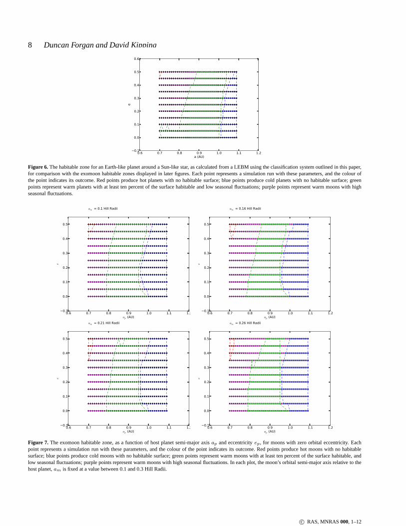
3.2.1 A Control - The Circumstellar Planetary Habitable Zone

To provide grounds for comparison, we ran a separate series of 440simulations with an Earth-like planet orbiting a Sun-like star to mapout the traditional circumstellar HZ according to our classificationsystem. The results of this are displayed in Figure 6. Green pointsrepresent simulations where the planet is classified as habitable;purple points where the planet is classified as a transient; and thered and blue points indicate planets that are too hot and too coldrespectively.

The model does not contain a carbonate-silicate cycle, un-like e.g. Williams & Kasting 1997, which modified the atmo-sphericCO2 pressure in accordance with temperature dependentweathering rates. Lower temperatures produce lower weatheringrates, and as a result the atmosphericCO2 (produced by vol-canic outgassing) cannot be sequestered. Therefore, cooler plan-ets can be expected to have higher atmospheric concentrations ofCO2, boosting the greenhouse effect and moving the outer edgeof the HZ to higher semi-major axes than we see in Figure 6 (cfKasting, Whitmire & Reynolds 1993).

The extension of the HZ at lowep to semi-major axes as lowas 0.7 AU is a reflection of our (fairly lenient) criterion forhabit-ability - namely, that 10% of the planet’s surface remains habitableover a ten year period, with a standard deviation less than 10% ofthe mean habitable area. Asep is increased,σξ increases quickly,producing planets which are habitable on a seasonal basis only. Ifwe are to compare to traditional habitability studies, thenwe shouldinfer that the inner edge of the HZ is at approximately 0.8 AU forep = 0. Equally, many of the transient classifications in this studywould normally have been considered to be uninhabitable (asmanyof these simulations undergo seasonal periods when the habitablesurface fraction is close to zero, but this is not sufficient to labelthem as hot or cold planets). We should bear this in mind as weconsider the habitable zone for exomoons in the following sections.



0.6 0.7 0.8 0.9 1.0 1.1 1.2a (AU)

−0.1

0.0

0.1

0.2

0.3

0.4

0.5

0.6

e

Figure 6. The habitable zone for an Earth-like planet around a Sun-like star, as calculated from a LEBM using the classification system outlined in this paper,for comparison with the exomoon habitable zones displayed in later figures. Each point represents a simulation run with these parameters, and the colour ofthe point indicates its outcome. Red points produce hot planets with no habitable surface; blue points produce cold planets with no habitable surface; greenpoints represent warm planets with at least ten percent of the surface habitable and low seasonal fluctuations; purple points represent warm moons with highseasonal fluctuations.

0.6 0.7 0.8 0.9 1.0 1.1 1.2ap (AU)

−0.1

0.0

0.1

0.2

0.3

0.4

0.5

e

am = 0.1 Hill Radii

0.6 0.7 0.8 0.9 1.0 1.1 1.2ap (AU)

−0.1

0.0

0.1

0.2

0.3

0.4

0.5

e

am = 0.16 Hill Radii

0.6 0.7 0.8 0.9 1.0 1.1 1.2ap (AU)

−0.1

0.0

0.1

0.2

0.3

0.4

0.5

e


0.6 0.7 0.8 0.9 1.0 1.1 1.2ap (AU)

−0.1

0.0

0.1

0.2

0.3

0.4

0.5

e


Figure 7. The exomoon habitable zone, as a function of host planet semi-major axisap and eccentricityep, for moons with zero orbital eccentricity. Eachpoint represents a simulation run with these parameters, and the colour of the point indicates its outcome. Red points produce hot moons with no habitablesurface; blue points produce cold moons with no habitable surface; green points represent warm moons with at least ten percent of the surface habitable, andlow seasonal fluctuations; purple points represent warm moons with high seasonal fluctuations. In each plot, the moon’s orbital semi-major axis relative to thehost planet,am is fixed at a value between 0.1 and 0.3 Hill Radii.



3.3 Zero Moon Orbital Eccentricity

We first consider the habitable zone manifold in the case whereem = 0, (and consequently the tidal heating rate is zero) and weconsider several different values ofam. This allows us to constructap−ep slices of the HZ manifold to compare with the typical planetHZ shown in the previous section. Figure 7 shows fourap − epslices, for four different values ofam. In each simulation, we fixam

relative to the Hill Radius at the given value ofap, so the absolutevalue ofam will increase with increasingap.

Comparing the top left panel of Figure 7 with Figure 6, we canimmediately see that the habitable zone exists in general atlowersemi-major axis. This is especially true at highep: the inner edgeof the HZ ate = 0.5 is now at 0.84 AU, as compared to 0.89 AU inthe planetary case. Asam is increased, the highep component ofthe inner HZ boundary shifts to higher and higherap. We thereforesurmise that the effect of frequent eclipses allows the moonto re-main cooler, and damps the fluctuations in temperature experiencedas the planet eclipses the star.

In all cases, the lowap, low ep habitable tail observed inthe planetary case disappears in the exomoon case. While frequenteclipses can cool the climate and damp oscillations, the habitablesurface fraction of these moons is generally low (typicallycloseto the minimum 0.1). Therefore, a relatively small increasein thevalue ofσξ due to eclipses is large enough to ensureσξ > 0.1ξ,and as a result be classified as transient moons rather than habitablemoons.

Comparing the outer edge of the HZ in the planet and mooncases, we can see it takes on a significantly different shape.Whilethe planet outer HZ moves steadily outward asep is increased, themoon outer HZ changes direction asep is increased. Initially hab-itable at 0.99 AU forep = 0, the outer boundary moves inward asep increases, finding its minimum value of∼ 0.95 AU at ep = 0.2,and then moves outward again. This appears to be due to a combi-nation of planet and moon motion relative to the star. The moon’sepicyclic motion atep = 0 changes its distance from the star byonly a small amount, and hence the climate remains stable enoughto be classified as habitable. Asep is increased, the epicyclic mo-tion of the moon is modulated by the motion of the planet as itmoves between its own periastron and apastron. This extra mod-ulation is sufficient to trigger a positive feedback in albedo, anda subsequent snowball effect. Asep increases to large values, thestrong heating the moon experiences as the planet passes throughits periastron is sufficient to keep it warm throughout the rest ofthe orbit, and the outer HZ boundary remains atap ∼ 0.99 AU.As the eclipse duration increases with increasingam, the outer HZboundary is pushed inwards for largerep asam is increased.

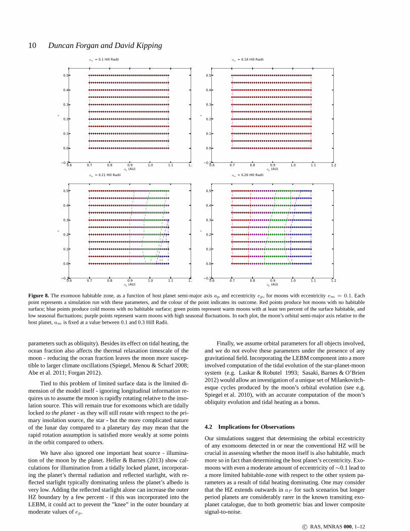
3.4 High Moon Orbital Eccentricity

We now repeat the above analysis, but increase the moon’s ec-centricity toep = 0.1. This is quite a large value to assume formoon eccentricity - without eccentricity pumping, it is unlikely thatmoons will possess eccentricities as large as this after tidal evolu-tion with their host planet - we present these results as an extremecase. Intermediate eccentricities will produce results somewherebetween the results of this section and the results of the previoussection.

Indeed, Figure 8 illustrates how extreme this case is by the ef-fect on the climate of the simulations. As tidal heating increases asam is decreased, it is clear that tidal heating dominates the proper-

ties of highly eccentric moons foram < 0.2 Hill Radii (top panels),and all simulations are classified as hot.

As am is increased, a habitable zone appears. This zone ismuch narrower than seen previously, and is restricted to large val-ues ofap, as tidal heating allows for warmer solutions when inso-lation is weak. In the case wheream = 0.21 Hill Radii (bottom leftpanel of Figure 8), the HZ exists atap > 0.95 AU, and potentiallyextends beyond 1.1 AU at highep. The HZ is typically around 0.1AU in width, although at lowep it is as narrow as 0.03 AU.

Whenam is increased to 0.26 Hill Radii, the HZ begins tomore closely resemble the HZ seen forem = 0 moons. Whilestill around 0.1 AU in width, it now displays the knee in the outerHZ boundary seen previously, and it is centred on similar valuesof ap as before. At this value ofam, the tidal heating has becomesmall compared to the traditional heating from insolation.This be-ing the case, tidal heating still makes its presence felt at low ap,where simulations that would have been habitable forep = 0 arenow seasonally habitable due to the extra forcing from tidalheatingproducing stronger climate oscillations.

4 DISCUSSION

4.1 Limitations of the Model

As with all studies using 1D LEBMs, the nature of the assumptionsmade limit the applicability of the results obtained in thisanaly-sis. The models are insensitive to the longer term climate varia-tions produced by oceanic circulation, as well as the compensatoryeffects of the carbonate-silicate cycle which can halt the albedo-driven snowball effect. These effects, with timescales ranging be-tween a few thousand to a million years (Williams & Kasting 1997)are much longer than the orbital periods of both the moon and thehost planet, and as such are of less consequence (in the shortterm)than the dynamical forcing due to eclipses and tidal heating.

Assuming a value for the diffusion constant,D limits theapplication of LEBMs to exomoons in a different sense.D iscalibrated such that a fiducial Earth-Sun climate model producesthe correct latitudinal temperature distribution as obtained fromreal data (Spiegel, Menou & Scharf 2008). Therefore,D containsa great deal of hidden information about the atmospheric andther-modynamic properties of the Earth. Modifying these properties,e.g. the atmospheric pressure, has significant consequences for thehabitability of the object (Williams & Kasting 1997; Vladilo et al.2013) and it is less clear howD ought to be modified for frozenmoons such as Europa, or moons with fundamentally differentchemistry such as Titan, without more data on their own latitudinaltemperature distributions. Even with this data, a full understandingof how tidal heating affects the temperature balance at any latitudeis essential for the correct calibration ofD. Equally, a more accu-rate implementation of tidal heating in the LEBM is vital forfuturestudies of exomoons.

Tidal forces are expected to affect land and ocean accordingto their elastic rigidities. While we have assumed a fixed oceanfraction of 0.7 throughout this analysis, the LEBM does not con-tain information as to how these oceans are distributed across thesurface. Instead, the ocean and land components are assumedtobe uniformly mixed over all latitudes. Future calculationsof tidalheating will require the LEBM to be more specific about the dis-tribution of landmasses. Ocean fraction may therefore become animportant parameter in future studies of the exomoon HZ mani-fold (which should also investigate the effects of changingother



0.6 0.7 0.8 0.9 1.0 1.1 1.2ap (AU)

−0.1

0.0

0.1

0.2

0.3

0.4

0.5

eam = 0.1 Hill Radii

0.6 0.7 0.8 0.9 1.0 1.1 1.2ap (AU)

−0.1

0.0

0.1

0.2

0.3

0.4

0.5

e


0.6 0.7 0.8 0.9 1.0 1.1 1.2ap (AU)

−0.1

0.0

0.1

0.2

0.3

0.4

0.5

e


0.6 0.7 0.8 0.9 1.0 1.1 1.2ap (AU)

−0.1

0.0

0.1

0.2

0.3

0.4

0.5

e


Figure 8. The exomoon habitable zone, as a function of host planet semi-major axisap and eccentricityep, for moons with eccentricityem = 0.1. Eachpoint represents a simulation run with these parameters, and the colour of the point indicates its outcome. Red points produce hot moons with no habitablesurface; blue points produce cold moons with no habitable surface; green points represent warm moons with at least ten percent of the surface habitable, andlow seasonal fluctuations; purple points represent warm moons with high seasonal fluctuations. In each plot, the moon’s orbital semi-major axis relative to thehost planet,am is fixed at a value between 0.1 and 0.3 Hill Radii.

parameters such as obliquity). Besides its effect on tidal heating, theocean fraction also affects the thermal relaxation timescale of themoon - reducing the ocean fraction leaves the moon more suscep-tible to larger climate oscillations (Spiegel, Menou & Scharf 2008;Abe et al. 2011; Forgan 2012).

Tied to this problem of limited surface data is the limited di-mension of the model itself - ignoring longitudinal information re-quires us to assume the moon is rapidly rotating relative to the inso-lation source. This will remain true for exomoons which are tidallylockedto the planet - as they will still rotate with respect to the pri-mary insolation source, the star - but the more complicated natureof the lunar day compared to a planetary day may mean that therapid rotation assumption is satisfied more weakly at some pointsin the orbit compared to others.

We have also ignored one important heat source - illumina-tion of the moon by the planet. Heller & Barnes (2013) show cal-culations for illumination from a tidally locked planet, incorporat-ing the planet’s thermal radiation and reflected starlight,with re-flected starlight typically dominating unless the planet’salbedo isvery low. Adding the reflected starlight alone can increase the outerHZ boundary by a few percent - if this was incorporated into theLEBM, it could act to prevent the ”knee” in the outer boundaryatmoderate values ofep.

Finally, we assume orbital parameters for all objects involved,and we do not evolve these parameters under the presence of anygravitational field. Incorporating the LEBM component intoa moreinvolved computation of the tidal evolution of the star-planet-moonsystem (e.g. Laskar & Robutel 1993; Sasaki, Barnes & O’Brien2012) would allow an investigation of a unique set of Milankovitch-esque cycles produced by the moon’s orbital evolution (see e.g.Spiegel et al. 2010), with an accurate computation of the moon’sobliquity evolution and tidal heating as a bonus.

4.2 Implications for Observations

Our simulations suggest that determining the orbital eccentricityof any exomoons detected in or near the conventional HZ will becrucial in assessing whether the moon itself is also habitable, muchmore so in fact than determining the host planet’s eccentricity. Exo-moons with even a moderate amount of eccentricity of∼0.1 lead toa more limited habitable-zone with respect to the other system pa-rameters as a result of tidal heating dominating. One may considerthat the HZ extends outwards inaP for such scenarios but longerperiod planets are considerably rarer in the known transiting exo-planet catalogue, due to both geometric bias and lower compositesignal-to-noise.



The orbital eccentricity of a moon will affect the position andduration of moon transits in the light curve (Kipping 2011) andis, in principle, an observable quantity. It is therefore quite reason-able that constraints on exomoon eccentricity could be determinedin the case of a confirmed detection. It is also worth noting thatexomoons are expected to rapidly tidally circularize even if start-ing with a large initial eccentricity due to a capture, for examplePorter & Grundy (2011); Williams (2013).

To maintain a large exomoon eccentricity over Gyr wouldlikely require forcing due to resonant massive satellites,but theoccurence of multiple captures of Earth-mass moons around asin-gle planet is surely less than that of single captures of Earth-massmoons.

We also find that the sense of orbital motion affects the cli-mate of moons and in principle this may also be determined obser-vationally (Kipping 2009b). However, in general such a determina-tion is highly challenging with Kipping et al. (2012) findingevenoptimstic synthetic data is marginal for uniquely determining thisto high-confidence usingKepler. Of course, once a confirmed sig-nal has been found, follow-up with larger instrumentation such asJWST would greatly increase our ability to make this assesment.

Finally, in this work we have established an LEBM capableof modelling hundreds of realizations of exomoon configurations.Due to the likely low signal-to-noise of any future exomoon de-tection one should expect fuzzy and complex parameter posteri-ors, as demonstrated in synthetic tests by Kipping et al. (2012). Wetherefore suggest coupling an LEBM, such as that presented here,directly with representative realizations drawn from the joint pos-terior distribution of the relevant parameters. This wouldenable usto compute a marginalised distribution for the habitability of an ex-omoon (ξ).

5 CONCLUSIONS

In this work, we have used a one dimensional latitudinal energybalance model (LEBM) to investigate the evolution of climate onan Earth-like exomoon. We have incorporated the effects of stellarinsolation, tidal heating, eclipses of the star by the planet, atmo-spheric cooling and heat diffusion, and investigated how the dy-namical circumstances of exomoons affect the resulting climate.

We simulated four test cases to study the exomoon climatesin detail, finding that exomoons in orbits retrograde to their hostplanet’s orbit experience stronger climate oscillations than theirprograde equivalents, and are around 0.1K warmer. In the case ofmoons with sufficiently short orbital periods, we find that the fi-nite thermal relaxation time of the atmosphere allows it to act asa buffer against the otherwise strong rapid temperature oscillationsproduced by frequent eclipses.

We then went on to carry out an extensive parameter study ofthe four dimensional space constituted by the planet’s semi-majoraxis and eccentrictity (ap, ep) and the moon’s semi-major axis andeccentricity relative to the planet (am, em). Comparing to the habit-able zone of an Earth-like planet orbiting the same star, we find thatif the exomoon’s orbit is circular, the exomoon habitable manifoldtends to exist at lowerap thanks to the cooling effect of eclipses,and the inner edge of the habitable zone can exist at lowerap forhigherep, again as eclipses keep the moon sufficiently cool. If theexomoon’s orbit is highly eccentric, the heating budget is domi-nated by tidal effects, and the habitable manifold is much narrowerin ap, and exists at greater distance from the star.

The simplicity of LEBMs, plus their (albeit limited) ability to

be augmented by new heat sources and sinks, makes them a usefultool for studying Earth-like exomoon climates. As they are com-putationally inexpensive, it is straightforward to run them multipletimes, whether it is to map out their behaviour in a set parameterspace as done here, or to assess the habitability of detectedexo-moons, by using realisations of the joint posterior distribution de-rived from observations. We are keen to hone and utilise thismod-elling technique for both of these uses.

ACKNOWLEDGMENTS

DF gratefully acknowledges support from STFC grantST/J001422/1. DMK is supported by the NASA Carl SaganFellowships.

REFERENCES

Abe Y., Abe-Ouchi A., Sleep N. H., Zahnle K. J., 2011, Astrobi-ology, 11, 443

Barnes J. W., OBrien D. P., 2002, ApJ, 575, 1087Barnes R., Jackson B., Raymond S. N., West A. A., Greenberg R.,2009, ApJ, 695, 1006

Batalha N. M. et al., 2013, ApJ, 204, 24Dressing C. D., Charbonneau D., 2013, ApJ, in pressEggl S., Pilat-Lohinger E., Funk B., Georgakarakos N., Haghigh-ipour N., 2012a, MNRAS, 428, 3104

Eggl S., Pilat-Lohinger E., Georgakarakos N., GyergyovitsM.,Funk B., 2012b, ApJ, 752, 74

Farrell B. F., 1990, Journal of Atmospheric Sciences, 47Forgan D., 2012, MNRAS, 422, 1241Heller R., Barnes R., 2013, Astrobiology, 13, 18Heller R., Leconte J., Barnes R., 2011, A&A, 528, A27Joshi M., 1997, Icarus, 129, 450Kaltenegger L., 2000, Exploration and Utilisation of the Moon.Proceedings of the Fourth International Conference on Explo-ration and Utilisation of the Moon: ICEUM 4. Held 10-14 July

Kaltenegger L., Selsis F., 2010, EAS Publications Series, 41, 485Kane S. R., Gelino D. M., 2012a, Astrobiology, 12, 940Kane S. R., Gelino D. M., 2012b, Publications of the Astronomi-cal Society of the Pacific, 124, 323

Kane S. R., Hinkel N. R., 2013, ApJ, 762, 7Kasting J., Whitmire D., Reynolds R., 1993, Icarus, 101, 108Kipping D. M., 2009a, MNRAS, 392, 181Kipping D. M., 2009b, MNRAS, 396, 1797Kipping D. M., 2011, MNRAS, 416, noKipping D. M., Bakos G. A., Buchhave L., Nesvorny D., SchmittA., 2012, ApJ, 750, 115

Kipping D. M., Fossey S. J., Campanella G., 2009, MNRAS, 400,398

Kite E. S., Gaidos E., Manga M., 2011, ApJ, 743, 41Laskar J., Robutel P., 1993, Nature, 361, 608Liu X., Zhong S., 2010, American Geophysical UnionMelosh H., Ekholm A., Showman A., Lorenz R., 2004, Icarus,168, 498

Parkinson C. D., Liang M.-C., Hartman H., Hansen C. J., TinettiG., Meadows V., Kirschvink J. L., Yung Y. L., 2007, A&A, 463,353

Peale S., Cassen P., Reynolds R., 1980, Icarus, 43, 65Porter S. B., Grundy W. M., 2011, ApJ, 736, L14



Reynolds R. T., McKay C. P., Kasting J. F., 1987, Advances inSpace Research, 7, 125

Sasaki T., Barnes J. W., O’Brien D. P., 2012, ApJ, 754, 51Scharf C. A., 2006, ApJ, 648, 1196Spiegel D. S., Menou K., Scharf C. A., 2008, ApJ, 681, 1609Spiegel D. S., Raymond S. N., Dressing C. D., Scharf C. A.,Mitchell J. L., 2010, ApJ, 721, 1308

Stamenkovic V., Spohn T., Breuer D., 2010, American Geophysi-cal Union

Stofan E. R. et al., 2007, Nature, 445, 61Vladilo G., Murante G., Silva L., Provenzale A., Ferri G., Ragazz-ini G., 2013, ApJ, 767, 65

Weidner C., Horne K., 2010, Astronomy and Astrophysics, 521,A76

Williams D., Kasting J. F., 1997, Icarus, 129, 254Williams D. M., 2013, Astrobiology, in pressWilliams D. M., Kasting J. F., Wade R. A., 1997, Nature, 385, 234Williams D. M., Pollard D., 2002, International Journal of Astro-biology, 1


Dynamical Effects on the Habitable Zone for Earth-like Exomoons

Documents

Transcript of Dynamical Effects on the Habitable Zone for Earth-like Exomoons