Dynamic Performance Analysis of a Fighter Jet with Nonlinear ...

IN DEGREE PROJECT VEHICLE ENGINEERING,SECOND CYCLE, 30 CREDITS

, STOCKHOLM SWEDEN 2019

Dynamic Performance Analysis of a Fighter Jet with Nonlinear Dynamic Inversion

Dynamisk prestandaanalys av stridsflygplan med NDI

BOBAN PAVLOVIC

KTH ROYAL INSTITUTE OF TECHNOLOGYSCHOOL OF ENGINEERING SCIENCES

Dynamic PerformanceAnalysis of a Fighter Jet withNonlinear Dynamic Inversion

BOBAN PAVLOVIC

Master in Aerospace EngineeringDate: July 24, 2019Supervisor: Mats Dalenbring, Fredrik BerefeltExaminer: Raffelo MarianiSchool of Engineering SciencesHost company: Totalförsvarets Forskningsinstitut (FOI)Swedish title: Dynamisk prestandaanalys av stridsflygplan medNDI

iii

AbstractA modern view of aircraft performance analysis, is to quantify aircraft ma-noeuvrability with agility metrics. There are several different agility metrics,which can be seen as indexing of the aircraft agility performance. The quan-tified unit is the time it takes for the aircraft to perform a specific manoeuvrerelevant to a given agility metric. In this thesis, estimations are done of twoagility metrics, the CCT (Combat Cycle Time) and the T90 (Time to capture90 bank angle) for the F-18 HARV aircraft.

Estimations of the agilitymetrics were obtained by simulating a six-degree-of-freedom aircraft model of the F-18 HARV aircraft performing the specificmanoeuvres. To control the aircraft model during the simulation a control sys-tem was developed based on the NDI (Nonlinear Dynamic Inversion) methodwith time scale separation assumption. Themethod uses the feedback from thecontrolsystem for linearizing the aircraft system, which results in that simplelinear controllers can be applied to the nonlinear aircraft model.

In this case simple proportional controllers were implemented and in thecase of estimating the T90 agility metric additional gain scheduling as func-tions of altitude and Mach number was required to extract maximum perfor-mance. Although the control system was developed for these two specificagility metrics, results indicates that the NDI method provides an effectiveway to implement controllers for complex systems, especially when consider-ing a high nonlinear flight regime.

iv

SammanfattningEtt modernt synsätt vid utvärdering av prestanda för stridsflygplan är att kvan-tifiera manövreringsprestanda med den tid det tar att genomföra en specifikmanöver (agility metric). Olika manövrar har utvecklats för att kvantifiera ochstudera specifika egenskaper. Genom att indexera data från flera olika manöv-rar kan ett prestandaunderlag framställas som representerar flygplanets ma-növreringsbarhet. I detta arbete görs uppskattningar av tidsåtgången för att ge-nomföra två välkända manövrar, CCT och T90 för flygplanet F-18 HARV.

Estimeringarna av tidsåtgången för att utföra manövreringarna utfördes ge-nom att simulera en modell av flygplanet med sex frihetsgrader. För att styraflygplanet under simuleringen utvecklades ett styrsystem med NDI metodensom är baserad på tillbaka återlinjärisering. Metoden använder återkopplingenav styrsystemet för att linjärisera flygplansmodellen, vilket medför att enklalinjära regulatorer kan tillämpas på den ickelinjära flygplansmodellen.

I detta fall implementerades enkla proportionella regulatorer, samt sche-maläggning av kretsförstärkningen som funktion av höjd och Mach tal vid es-timering av T90 för att uppnå maximal roll prestanda. Även om reglersystemetvar specifikt anpassat för att utföra dessa två manövrar så indikerar resultatenatt NDI metoden är effektiv vid implementering av styrsystem för flyplansmo-deller, speciellt om flygregimen innehåller stora ickelinjäriteter, exempelvishöga anfallsvinklar.

Contents

1 Introduction 11.1 Outline . . . . . . . . . . . . . . . . . . . . . . . . . . . . . 31.2 Acknowledgement . . . . . . . . . . . . . . . . . . . . . . . . 3

2 Notations 4

3 Feedback Linearization 5

4 Aircraft System 94.1 Reference Frames . . . . . . . . . . . . . . . . . . . . . . . . 94.2 Aircraft Equations of Motion . . . . . . . . . . . . . . . . . . 11

4.2.1 Linear Momentum . . . . . . . . . . . . . . . . . . . 114.2.2 Angular Momentum . . . . . . . . . . . . . . . . . . 12

4.3 Aircraft System Dynamics . . . . . . . . . . . . . . . . . . . 124.3.1 Aerodynamics And Propulsion . . . . . . . . . . . . . 13

5 Control System 155.1 Control Variables . . . . . . . . . . . . . . . . . . . . . . . . 165.2 Control System Dynamics . . . . . . . . . . . . . . . . . . . 175.3 Time Scale Separation . . . . . . . . . . . . . . . . . . . . . 185.4 Control Law Design with NDI . . . . . . . . . . . . . . . . . 19

6 Simulation 236.1 The F-18 HARV Model . . . . . . . . . . . . . . . . . . . . . 236.2 Combat Cycle Time . . . . . . . . . . . . . . . . . . . . . . . 246.3 T90 . . . . . . . . . . . . . . . . . . . . . . . . . . . . . . . 28

7 Conclusions 32

Bibliography 34

v

Chapter 1

Introduction

A classical approach to aircraft performance analysis is based on simplifiedequations of motions, where the motion is often reduced to three-degrees-of-freedom (longitudinal motion). The aerodynamic forces are assumed to be ina steady state and the analysis is considered static and time independent.

Most of the time during the analysis, the aircraft is assumed to be in levelflight, in a state defined by the altitude and airspeed. At a given state, trimcondition is calculated and based on this the performance of the aircraft canbe quantified in terms of energy such as specific excess power (SEP), whichspecifies howmuch additional energy is available that can be used for changingthe altitude or velocity at any instant in time during the manoeuvre.

From these methods, flight envelope, trim for steady level flight, powercurve, roll, and turn rates can be analysed. Further, if the equations of mo-tions are linearized, some information regarding the static stability can also beobtained by analysing the rigid body eigen modes.

A more modern view of performance analysis is to quantify the aircraft’sagility in addition to the classical methods. This is done by analysing theresponse of the aircraft due to specific manoeuvres, resulting in a series ofquantities, which are called agility metrics. The quantified unit is time, whichis the time it takes to perform a specific manoeuvre [1].

The reason for this new approach of analysing agility metrics is to obtain abetter estimation of the aircraft’s manoeuvring performance. With new tech-nological advancements of both modern fighter aircraft’s and weapon deliverysystems, the traditional combat arena has been divided in two significant differ-ent parts, the beyond visual range (BVR) and the within visual range (WVR).BVR is considered to be a region in the flight envelope of higher altitudesand Mach numbers, were WVR is at lower altitudes and Mach numbers. The

1

2 CHAPTER 1. INTRODUCTION

agility metrics addresses how well an aircraft can transition between these tworegions [2]. More specifically, the classical type of analysis which are basedon a static assumption do not consider the dynamic transient effects of themanoeuvre, and provide less information about the true manoeuvring perfor-mance, especially when considering a short period of the time frame [3].

Several different agility metrics have been developed with correspondingmanoeuvres to be performed. Obtaining the estimation of the metric could besolved as an optimization problem as is done in the work of Chou [4] and Hoff-man [5]. The objective of this work is to evaluate how agility metrics can beestimated by simulating a six-degrees-of-freedom aircraft model performingthe specific manoeuvre relevant to the agility metric under investigation.

The approach in this work is to use a control system in the simulation, withthe objective of controlling and orienting the aircraft duringmanoeuvring. Themanoeuvres are done by issuing set point commands for the control systemwhich calculates corresponding control surface deflections. Further objec-tives of incorporating handling qualities are not consider, since these are morerelevant when there is a man-in-the-loop simulation.

An aircraft is a highly nonlinear system with multiple inputs and outputs.Therefore, the nonlinear control method Nonlinear Dynamic Inversion (NDI)is used [7, 6]. Using the traditional method of linearizing the equations ofmotion before hand leads to a time consuming approach of gain schedulingand fine tuning of several controllers to cover a large part of the flight envelope.

The NDI method is based on feedback linearization (FBL). A benefit ofFBL is that the system is linearized by cancelling nonlinearities with feedbackthorough the control system. Theoretically this means that the same linearizedmodel is used for control design over the flight envelope. This reduction oflinearized models leads to a decreased developing time for controllers. Oneimportant assumption for applying NDI on an aircraft system is the time scaleseparation assumption. Essentially, with time scale separation the idea is tosplit the aircraft dynamics into subsystems of fast and slow dynamics [9, 8],which simplifies the control system structure.

Since the system is linearized, different linear control methods can be ap-plied. An example is to apply Linear Quadratic (LQ) control, which is donein the work of Fer [10] and Escande[11]. Although, in this work simple pro-portional controllers will be used.

In the end, two agility metrics are estimated: the Combat Cycle Time(CCT), which is the time it takes for the aircraft to perform a 180 headingturn; and Time to capture 90 bank angle (T90), which is the time it takes toperform and capture a 90 bank angle change with a constant angle of attack.

CHAPTER 1. INTRODUCTION 3

1.1 OutlineThe report is structured as follows:

Chapter 2 contains general information about the notation used throughoutthe report.

Chapter 3 describes the general theory of feedback linearization and the moregeneral method Input-Output Linearization.

Chapter 4 and 5 present the chosen system modelling approach. The com-plete system is treated as two separate systems, the aircraft system and thecontrol system. In chapter 4 general modelling of a six-degrees-of-freedomaircraft is presented. Chapter 5, discusses the modelling for the control sys-tem and how the control law design is applied to an aircraft model.

Chapter 6 shows results from simulations of CCT and T90 with the controlsystem applied on the F-18 HARV model.

Chapter 7 summarizes the conclusions of the work.

1.2 AcknowledgementThe work was performed at the Swedish Defence Research Department, FOI,which I would like to thank for providing this opportunity. I would like tothank my supervisors Mats Dalenbring and Fredrik Berefelt for their patienceand support, but also to Lars Forssell and other co-workers at FOI for theirguidance and the joyful experience.

I would also like to thank Assistant Professor Raffaello Mariani at theAeronautical and Vehicle Engineering department at KTH Royal Institute ofTechnology for his feedback.

Chapter 2

Notations

Unit Vector

A unit vector has the notationea

where the subscript denotes the direction of the unit vector.

Vector

A vector v which expresses a relationship between frame a relative to frame bhas the notation

vba

Vector in a coordinate system

The above vector is not expressed in any coordinate system. To express thevector in a coordinate system c the following notation is used,

vcba

where the superscript denotes the coordinate system.

Transformation Matrix

A change of the coordinate system is done with a transformation matrix. Thenotation for a change of coordinates, from coordinate system c to coordinatesystem d is given by

Rbc

As an example,vdba = Rd

cvcba

4

Chapter 3

Feedback Linearization

Control theory of linear systems is, in terms of control design for stability androbustness for linear system, by now very well understood. The methods haveevolved in a mathematical sense, where the controllers (system gains) can beoptimized for a given specification.

The general control problems are often given in the form "input u(t) toget a desired output y(t)". The concept with feedback linearisation is, as thename indicates, that the nonlinear system is linearized through feedback. Thisis achieved by designing the control law for the control input u(t), so that thesystem nonlinearities are cancelled and a linear system is obtained. If this isachieved then any linear control design technique can be applied to the system.In simpler terms, feedback linearization provides a path for applying linearcontrol methods to a nonlinear system and this is the major benefit.

Input - Output LinearizationLet’s assume a model of a real system in control affine form, which means thatthe input u is linearly dependent,

x = f(x) + g(x)u

y = h(x)(3.1)

where x ∈ Rn are the system states, u ∈ Rm is the control input, and y ∈ Rp

is the system output, where f : Rn → Rn, g : Rm → Rn and h : Rn → Rp aresmooth nonlinear functions which model the system dynamics. For simplicity,it is assumed that the system is squarem = p, and that each output is controlledby a corresponding input, otherwise some form of control input allocationwould be needed.

5

6 CHAPTER 3. FEEDBACK LINEARIZATION

In a control tracking problem, where a reference signal for the output yref ∈Rp is given as a function of time, it is desired that the output y(t) tracks thereference signal. Therefore, a tracking error variable e ∈ Rp can be defined as

e(t) = yref (t)− y(t) (3.2)

The tracking error e(t) is kept small by controlling the output y(t). However, asit can be noted in the system (3.1), it is only possible to control the output y(t)

implicitly with the control input u(t), through the system states x. Therfore, inorder to control the output y(t), a control law for the control input u(t), whichis based on the system states x, needs to be defined.

In the Input-Output linearization method, the idea is to form an explicitrelationship between the control input u(t) and the derivative of the outputy(t). This is achieved by taking the derivative of the output until the inputu(t) appears,

y =∂h(x)

∂xx =

∂h(x)

∂x(f(x) + g(x)u) (3.3)

By actually controlling the derivative of the output y(t), the output y(t) iscontrolled. The derivative of the output thus acts as a virtual control of theoutput [12, 13].

Since an tracking formulation has been formed and the error e(t) is depen-dent on the output y(t), it is possible to extend the above concept and expressa relationship between the tracking error derivative e(t) and the control inputu(t). By differentiating the tracking error (3.2) and inserting equation (3.3),the error dynamics is obtained accordingly,

e = yref (t)− y(t) = yref (t)− ∂h(x)

∂x(f(x) + g(x)u) (3.4)

Feedback linearization is achieved by selecting a control law for u(t) sothat the nonlinear terms of the error dynamics in equation (3.4) cancel and alinear relationship is left. If the control law for the input u(t) is chosen as

u = (∂h(x)

∂xg(x))−1(−∂h(x)

∂xf(x) + yref (t) + υ) (3.5)

where υ ∈ Rp is a so called auxiliary input, the nonlinearities are cancelledand a linear relationship between the error dynamics and the auxiliary input isobtained [14], as shown in equation (3.6)

e = −υ(t) (3.6)

CHAPTER 3. FEEDBACK LINEARIZATION 7

The auxiliary input υ(t) is used to drive the tracking error e(t) to zero. Acontrol law for the auxiliary input needs to be constructed, but since the rela-tionship (3.6) is linear any linear control method can be applied. One simplechoice is to use an ordinary proportional control law with the tracking error,

v = Ke(t) (3.7)

whereK = diag(K1, ..., Kp) is a proportional gain matrix. Inserting the con-trol law (3.7) into equation (3.6) gives, after linearization, the error dynamics

e = −Ke(t) (3.8)

For a positive definite K, the error dynamics are stable by definition and theerror e(t) will tend to zero, and tracking of the desired output is achieved. Thesize of the gains inK determines the response and can be fine tuned to obtaina response according to a given specification.

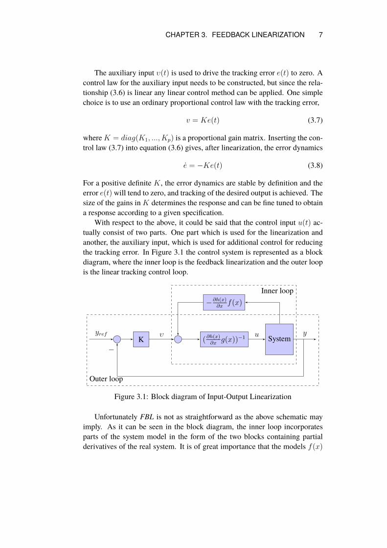
With respect to the above, it could be said that the control input u(t) ac-tually consist of two parts. One part which is used for the linearization andanother, the auxiliary input, which is used for additional control for reducingthe tracking error. In Figure 3.1 the control system is represented as a blockdiagram, where the inner loop is the feedback linearization and the outer loopis the linear tracking control loop.

System(∂h(x)∂x

g(x))−1

−∂h(x)∂x

f(x)

Kuυ y

−

yref

Inner loop

Outer loop

Figure 3.1: Block diagram of Input-Output Linearization

Unfortunately FBL is not as straightforward as the above schematic mayimply. As it can be seen in the block diagram, the inner loop incorporatesparts of the system model in the form of the two blocks containing partialderivatives of the real system. It is of great importance that the models f(x)

8 CHAPTER 3. FEEDBACK LINEARIZATION

and g(x) of the real system are accurate. Otherwise, wrong nonlinearities arefed back which can have a counter productive and destabilizing effect.

Problems can arise for systems that have low control effectiveness. Mathe-matically this means that g(x) is small and that the control input u(t) in equa-tion (3.4) has a small contribution to the change of the state variables. Lowcontrol effectiveness requires larger control signals, since the control inputu(t) is inversely proportional to g(x), which can be seen in the control law(3.5).

Problems appear since in reality the control effort and magnitude of thecontrol input u(t) is often physically limited. For example in an aircraft sys-tem, the control input could be a control surface deflection, which is obviouslylimited to some range of motion. The result is that a conflicting scenario exists,since some of the control input effort must be used for the feedback lineariza-tion and some for the outer loop tracking.

Other problems occur when having a non-square system where there aremore states than there are inputs, n > m. In aeronautical terms this could forexample correspond to a flying wing configuration where the rudder actuationis greatly limited due to the lack of direct rudder input. More emphasis oncontrol allocation is then needed, otherwise some dynamics can be left un-controlled. In literature these type of uncontrolled sub dynamical systems arecalled internal dynamics [12]. Since the internal dynamics are uncontrolledthe global stability of the system greatly depends on the stability of the internaldynamics [15].

Chapter 4

Aircraft System

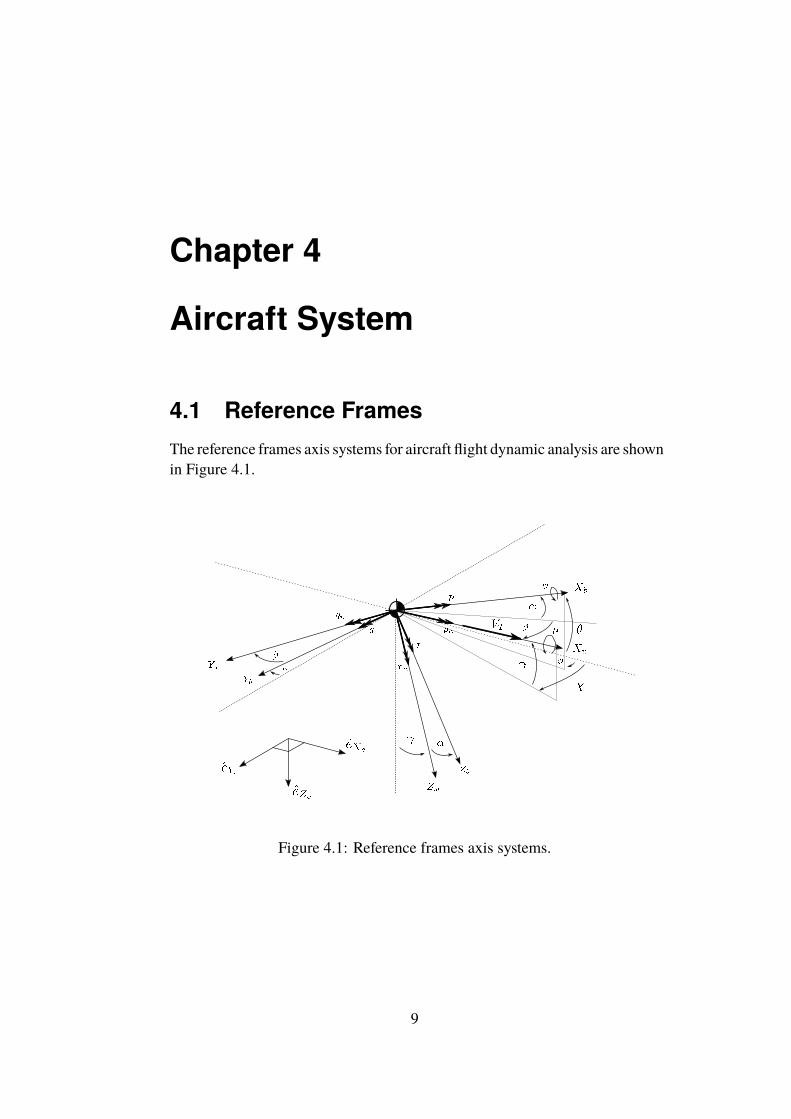
4.1 Reference FramesThe reference frames axis systems for aircraft flight dynamic analysis are shownin Figure 4.1.

Figure 4.1: Reference frames axis systems.

9

10 CHAPTER 4. AIRCRAFT SYSTEM

Earth Axis System

The inertial earth frame is assumed to be a non-rotating flat Earth and it isdenoted with the lower case letter e. The unit vector eXe of the Earth x-axisis pointing in the north direction, the y-axis unit vector eYe is pointing to eastand the z-axis unit vector eZe is pointing downwards.

Body Axis System

To keep track of the aircraft’s orientation in space, it is appropriate to define areference axis system which is fixed to the body. For simplicity, it is assumedthat the reference frame is fixed to the center of mass and it is denoted bylower case letter b. The unit vector of the body x-axis eXb is pointing towardsthe nose of the aircraft, the unit vector of the y-axis eYb is parallel to the rightwing and points to the wing tip, and the unit vector of the z-axis eZb is pointingdownwards.

The orientation of the body frame relative to the earth frame is expressedwith a set of Euler angles for the body frame noted Ωb = [φ θ ψ]. The threeangles φ, θ and ψ, corresponding to the roll, pitch and yaw angles.

The direction-cosine transformation matrix between earth and body frameis given by three individual rotation matrices, each matrix corresponding to arotation around an axis. The matrices are not commutative and the standardsequence in aeronautics when transforming from body to earth axis is φ, θ, ψ,which gives the direction-cosine transformation matrix [16]

Reb =

cosθcosψ sinφsinθcosψ − cosφsinψ cosφsinθcosψ + sinφsinψ

cosθsinψ sinφsinθcosψ + cosφsinψ cosφsinθcosψ − sinφsinψ−sinθ sinφcosθ cosφcosθ

Wind Axis System

The aerodynamic forces are generated by the relative wind experienced by theaircraft, and it is assumed that there are no additional wind gusts in the inertialearth frame. Thus, a wind axis system, denoted by w, can be defined suchthat its x-axis unit vector eXw is pointing in the same direction as the aircraft’svelocity vector, as shown in Figure 4.1.

The orientation of the wind frame relative to the body frame is by definitiononly dependent on the two aerodynamic angles, angle of attack α and sideslipangle β, which can also be seen in Figure 4.1, with the transformation matrixfrom body to wind frame defined as [14],

CHAPTER 4. AIRCRAFT SYSTEM 11

Rwb =

cosα cosβ sinβ sinα cosβ

−cosα sinβ cosβ −sinα sinβ−sinα 0 cosα

In a similar manner as for the body frame, Euler angles for the wind frame

relative to the earth frame can be defined as Ωw = [µ γ χ] . The wind frameEuler angles µ, γ and χ, which in aeronautical terms have the names bankangle, flight path angle and heading angle, are actually the velocity frame Eu-ler angles. Since it is assumed that there is no additional wind gust in themodelling, the wind frame and velocity frame are equivalent.

4.2 Aircraft Equations of Motion

4.2.1 Linear MomentumThe model for the aircraft in this work is assumed to be a moving point mass.The position of the aircraft mass center (body frame) relative to the Earthframe, can be expressed with a vector reb ∈ R3. The change of the position isgiven by the kinematic equation,

reb = veb, (4.1)

where the vector veb ∈ R3 is the velocity vector of the aircraft, relative to theEarth frame. The change of the velocity vector, is given by Newton’s secondlaw

veb =1

mF (4.2)

wherem ∈ R is the mass of the aircraft and F ∈ R3 is the sum of all externalforces. The derivative in the above equation is taken with respect to the inertialframe. Often it is more convenient to take the derivative with respect to thebody frame instead, which gives

veb + ωeb × veb =1

mF (4.3)

where ωeb ∈ R3 are the angular velocities of the body relative to the Earthframe.


4.2.2 Angular MomentumThe change of the body Euler angles are purely kinematic and given by thekinematic equation

Ωb =

1 sinφ tanθ cosφ tanθ

0 cosφ −sinφ0 sinφ/cosθ cosφ/cosθ

ωeb (4.4)

where the matrix is a rotation rate transformation matrix which relates theaircraft’s angular rates to the change of the Euler angles.

The angular rates ωeb are generated by the moment acting on the aircraft.The relation between the moments and angular rates are given by the Eulerequation

M = Jωeb + ωeb × Jωeb (4.5)

whereM ∈ R3 are the moments acting on the body and J ∈ R3×3 is the massmoment of the inertia matrix.

4.3 Aircraft System DynamicsBy solving for the derivatives in the two dynamic equations (4.3) and (4.5),and combining with the two kinematic expression (4.1) and (4.4), the aircraftequations of motion can be written as a system of 12 first order differentialequations of the form

xAC = fAC(xAC , δs, δT ) (4.6)

where xAC ∈ R12 is the aircraft state vector, δs = [δA δE δR]T are the controlsurface deflections, and where δA ∈ R is the aileron deflection, δE ∈ R theelevator deflection, δR ∈ R the rudder deflection, and δT ∈ R is the throttleposition.

The main components of the aircraft state vector are, in common notation,shown in equation (4.7)

xAC =

Xe Ye Ze︸︷︷︸reeb

u v w︸︷︷︸vbeb

φ θ ψ︸︷︷︸Ωb

p q r︸︷︷︸ωbeb

T

(4.7)

where Xe, Ye and Ze are the aircraft’s position in the inertial earth axissystem, u, v and w are the aircraft’s normal acceleration in body axis system,and p, q and r are the roll, pitch and yaw rates.

CHAPTER 4. AIRCRAFT SYSTEM 13

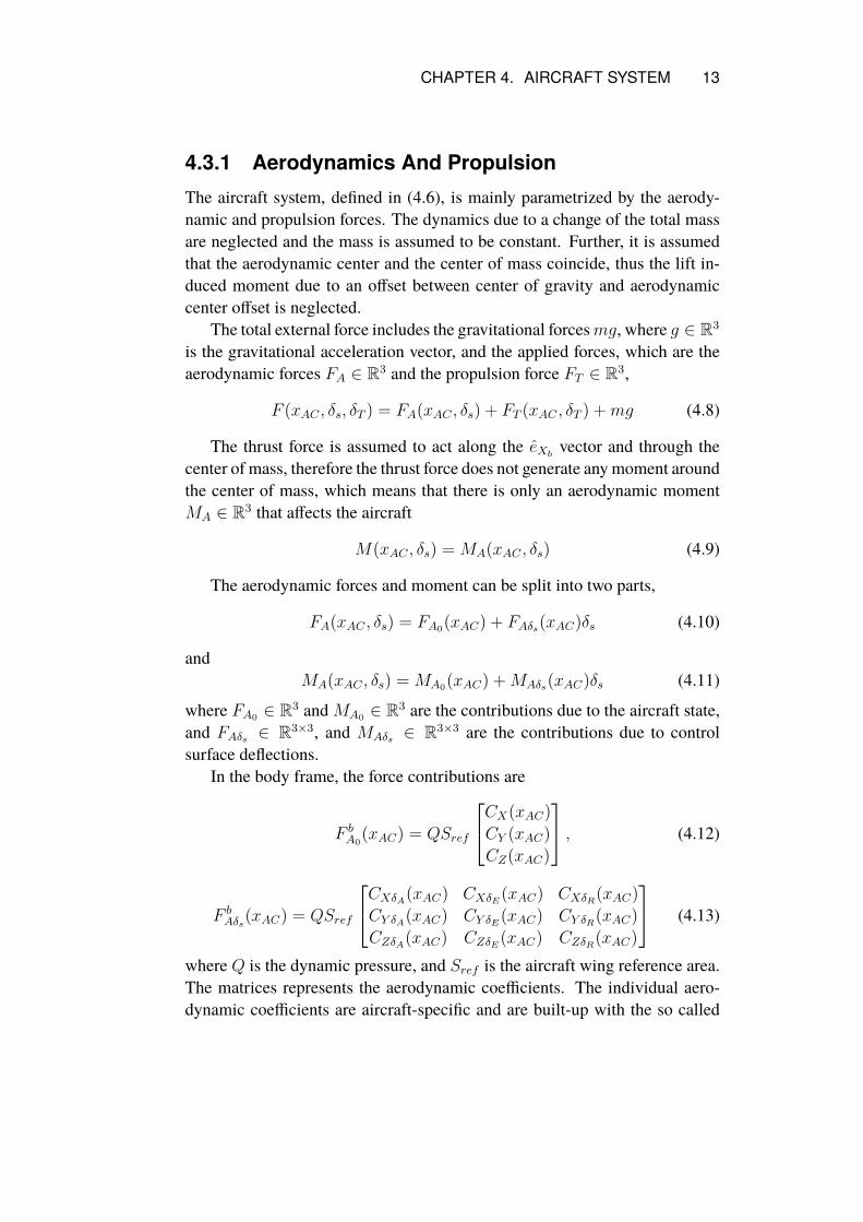
4.3.1 Aerodynamics And PropulsionThe aircraft system, defined in (4.6), is mainly parametrized by the aerody-namic and propulsion forces. The dynamics due to a change of the total massare neglected and the mass is assumed to be constant. Further, it is assumedthat the aerodynamic center and the center of mass coincide, thus the lift in-duced moment due to an offset between center of gravity and aerodynamiccenter offset is neglected.

The total external force includes the gravitational forcesmg, where g ∈ R3

is the gravitational acceleration vector, and the applied forces, which are theaerodynamic forces FA ∈ R3 and the propulsion force FT ∈ R3,

F (xAC , δs, δT ) = FA(xAC , δs) + FT (xAC , δT ) +mg (4.8)

The thrust force is assumed to act along the eXb vector and through thecenter of mass, therefore the thrust force does not generate anymoment aroundthe center of mass, which means that there is only an aerodynamic momentMA ∈ R3 that affects the aircraft

M(xAC , δs) = MA(xAC , δs) (4.9)

The aerodynamic forces and moment can be split into two parts,

FA(xAC , δs) = FA0(xAC) + FAδs(xAC)δs (4.10)

andMA(xAC , δs) = MA0(xAC) +MAδs(xAC)δs (4.11)

where FA0 ∈ R3 andMA0 ∈ R3 are the contributions due to the aircraft state,and FAδs ∈ R3×3, and MAδs ∈ R3×3 are the contributions due to controlsurface deflections.

In the body frame, the force contributions are

F bA0

(xAC) = QSref

CX(xAC)

CY (xAC)

CZ(xAC)

, (4.12)

F bAδs(xAC) = QSref

CXδA(xAC) CXδE(xAC) CXδR(xAC)

CY δA(xAC) CY δE(xAC) CY δR(xAC)

CZδA(xAC) CZδE(xAC) CZδR(xAC)

(4.13)

where Q is the dynamic pressure, and Sref is the aircraft wing reference area.The matrices represents the aerodynamic coefficients. The individual aero-dynamic coefficients are aircraft-specific and are built-up with the so called


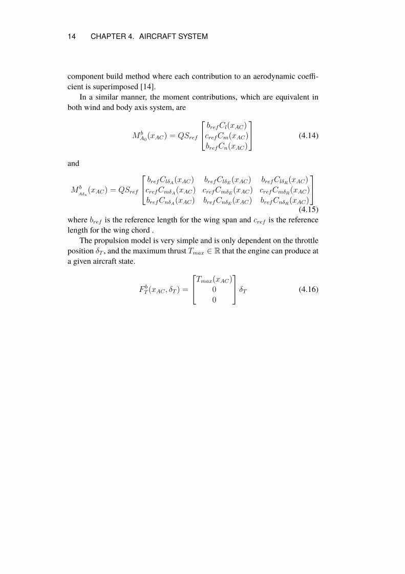
component build method where each contribution to an aerodynamic coeffi-cient is superimposed [14].

In a similar manner, the moment contributions, which are equivalent inboth wind and body axis system, are

M bA0

(xAC) = QSref

brefCl(xAC)

crefCm(xAC)

brefCn(xAC)

(4.14)

and

M bAδs

(xAC) = QSref

brefClδA(xAC) brefClδE(xAC) brefClδR(xAC)

crefCmδA(xAC) crefCmδE(xAC) crefCmδR(xAC)

brefCnδA(xAC) brefCnδE(xAC) brefCnδR(xAC)

(4.15)

where bref is the reference length for the wing span and cref is the referencelength for the wing chord .

The propulsion model is very simple and is only dependent on the throttleposition δT , and the maximum thrust Tmax ∈ R that the engine can produce ata given aircraft state.

F bT (xAC , δT ) =

Tmax(xAC)

0

0

δT (4.16)

Chapter 5

Control System

When designing a control system for a dynamical system it is important todetermine the objectives. For aircraft systems, control laws can be designed forvarious reasons. For example, a stability augmentation system (SAS) is used toprovide control laws which stabilize the system, while a control augmentationsystem (CAS), has the objective of incorporating specific handling qualities inthe control laws [14].

As mentioned in the introduction, the objective for this study is to designa control system which is used to manoeuvre an aircraft model during simu-lation. An aircraft manoeuvres mainly by changing its orientation, and witha change of the orientation the direction and magnitude of the aerodynamicforces are altered, and thus a movement occurs. The orientation of the aircraftcan be controlled in various ways by a pilot or an autopilot, by controllingsome of the aircraft states. These states are called control variables and com-mand signals of the control variables are set by the pilot and are interpretedby the control system, which generates a response according to control laws.

In the case of a pilot controlling the aircraft at low dynamic pressures, thecontrol variables are mainly the angular body rates, such as pitch rate, rollrate, and yaw rate. However, a modern control systems is very adaptive andthe control variables often alter with dynamic pressure. At higher dynamicpressure the controlled variables are instead closely linked to the translationalmotion such as the angle of attack or load factor [17]. Control variables canalso be a linear combination of different aircraft states. A classical exampleis the C∗-star control variable which is a linear combination of the pitch rateand angle of attack [14].

In this case a simpler approach of non-adaptive control variables is usedwhich takes inputs as set point commands during the simulation. The main

15

16 CHAPTER 5. CONTROL SYSTEM

idea is to control the aerodynamic angles and then have a control system thatgenerates the corresponding angular rates and control surface deflections. Thereason for this approach is that it is more intuitive to control the aerodynamicangles in a simulation environment than to directly control the angular rates.

5.1 Control VariablesLongitudinal Control - Angle of attack

For the longitudinal control, the angle of attack α is selected as the controlvariable. The main reason for this choice is that the magnitude of the lift hasa strong dependence on the angle of attack. Hence, the curvature of the flightpath trajectory can be increased or decreased by increasing or decreasing theangle of attack.

Lateral Control - Velocity Vector Bank Angle and Sideslip Angle

For lateral motion there are two-degrees-of-freedom that need to be addressed.The sideslip angle β is selected as one, as during flight it is always preferredto keep the sideslip angle to zero in order to reduce unnecessary drag. Twoexceptions are in skidding turns or crosswind landings.

The other control variable for lateral control is the bank angle µ, aroundthe velocity vector. The reason for this choice is that the direction of the liftforce in the lateral plane can be controlled by the bank angle. The turn rateand the direction of the flight path curve is determined by the size of the liftforce projection onto the horizontal plane. By increasing the bank angle theprojected forces increases leading to a higher turn rate. Another reason for theselection is due to the chosen agility metrics for this work. In both cases abanking with constant angle of attack is performed .

Control System States

Based on the parameters discussed above, the control system states are,

x = [α, β, µ]T . (5.1)

In addition to these control variables, the true airspeed VT is also con-trolled, although it is treated as a separate system since the propulsion dynam-ics is much slower in relation to other dynamics.

CHAPTER 5. CONTROL SYSTEM 17

5.2 Control System DynamicsTo design control laws for the control system, the dynamics of the controlsystem states in (5.1) need to be known. The dynamics for the two controlvariables α and β can be derived by expressing equation (4.2) in the windcoordinate system

vweb + ωwbw × vweb = (1/m)Fw − ωweb × vweb (5.2)

All the elements in equation (5.2) have been defined previously, except ωwbwwhich is the angular rotation of the wind frame with respect to the body frame.

From the definition of the wind frame the angular velocity vector ωbw isgiven by

ωwbw = −βewwz + αewby = −βewwz + αRwb e

bby =

−αsinβ−αcosββ

(5.3)

Inserting equation (5.3) on the left side of equation (5.2) and applying acoordinate transformation for the forces and the angular rates on the right handside, the dynamics of α, β, and the true airspeed VT can be written in matrixform as, VT

βVTαcosβVT

=1

mRwb F

b −Rwb ω

beb × vweb (5.4)

Evaluating the right hand side of the above equation, the dynamics of αand β can be written in scalar form as

α =−Xsinα + Zcosα

mVT cosβ− cosα tanβ p+ q − sinα tanβ r (5.5)

β =−Xcosα sinβ + Y cosβ − Zsinα sinβ

mVT+ sinα p− cosα r (5.6)

where X(xAC , δs, δT ), Y (xAC , δs, δT ) and Z(xAC , δs, δT ) are the componentsof the total force acting on the aircraft in the body coordinate system. Finally,the dynamics for the true airspeed is

VT = Xcosα cosβ + Y sinβ + Zsinα cosβ (5.7)

Since the bank angle µ is an Euler angle, the dynamics can be expressedin the same way as in equation (4.4) for the aircraft body Euler angles, by


expressing the change in the wind frame Euler angles asµγχ

=

1 sinµ tanγ cosµ tanγ

0 cosµ −sinµ0 sinµ/cosγ cosµ/cosγ

pwqwrw

(5.8)

where pw, qw and rw are the angular velocities of the wind frame. Using thefirst and last row of equation (5.8), the dynamics of the bank angle can bewritten in scalar form as,

µ = pw + χsinγ (5.9)

The control system dynamics is built up from the dynamic equations (5.5),(5.6) and (5.9) which can be expressed as a system of the form,

x = f(x, xAC , δs) (5.10)

5.3 Time Scale SeparationAs it was shown in chapter 3, in order to apply FBL the system needs to be ina control affine from. The control system described by equation (5.10) couldbe expressed in the control affine form

x = f(x) + g(x)δs (5.11)

However, due to low effectiveness of the control surface on the control variablestates α, β and µ, a time scale separation assumption is postulated [9, 8].

Essentially, time scale separation means that the system in equation (5.11)is divided into a system of two first order systems,

x = f(x) + g(x)ωebωeb = h(x, ωeb) + k(x)δs

(5.12)

where the aircaft’s angular rates ωeb acts as an input for the control variablesx, and the control surface deflections δs are inputs to the angular rates ωeb.

Another very important property which is implied when applying the timescale separation assumption, is that the dynamics of the angular rates ωeb, de-scribed by the second system in (5.12), is assumed to be much faster than thedynamics for the control variables x, described by the first system in (5.12).The reason is that since the angular rates ωeb are effectively inputs for the con-trolled variables x, it would be very hard to control a fast system with a slowercontrol input, as the faster system would be able to change where the responseof the control input would be constantly out of phase. In fact the stability withthe time scale separation assumption depends on this property [18].


5.4 Control Law Design with NDIFor the control law design, the procedure starts in the same way as for Input-Output Linearization in chapter 3. A tracking problem is introduced, and thecontrol variable error is defined as

x = x− xcmd (5.13)

where x is the error and xcmd is the commanded values for the control vari-ables. Taking the derivative of equation (5.13) and inserting it in the firstsubsystem in equation (5.12) gives the error dynamics

˙x = f(x)− xcmd + g(x)ωeb (5.14)

where the nonlinear functions f(x) and g(x) are obtained from the controlsystem in equation (5.10) by separating the angular rates. For the states α andβ this is a rewriting of the equations (5.5) and (5.6). In the case of the bankangle µ, the wind frame roll rate pw needs to be expressed in the body angularrates ωeb, which is achieved by the following expression,pwqw

rw

= ωwew = ωweb − ωwbw = Rwb ω

beb − ωwbw (5.15)

Inserting equation (5.3) in the above equation gives,

pw = cosα cosβ p+ sinβ q + sinα cosβ r − αsinβ (5.16)

There is a problem with the last term since it contains α, which can be ne-glected for two reasons. The first reason is that β is kept small by the controlsystem itself, and the second reason is due to the time scale separation assump-tion. Since the angular rates are assumed to be much faster then α, it can beseen as a constant in this expression. This gives the nonlinear functions f(x)

and g(x) accordingly,

f(x) =

χsinγ−Xsinα+Zcosα

mVT cosβ−Xcosα sinβ+Y cosβ−Zsinα sinβ

mVT

(5.17)

and

g(x) =

cosα cosβ sinβ sinα cosβ

−cosα tanβ 1 −sinα tanβsinα 0 −cosα

(5.18)


In the NDI method some desired dynamic fxdes(x) is postulated for theerror dynamics in (5.14). To achieve the wanted dynamics the aircraft needsto hold some corresponding angular rates ωebdes , which gives

fxdes(x) = f(x)− xcmd + g(x)ωebdes (5.19)

The control law for the needed angular rates ωebdes are obtained by invertingequation (5.19), in the same way as for Input-Output Linearization in equation(3.5), resulting in

ωebdes = g(x)−1(−f(x) + xcmd + fxdes(x)) (5.20)

Replacing the angular rates in equation (5.14) with the control law given byequation (5.20) gives

˙x = fxdes(x) (5.21)

The desired dynamic fxdes(x) is thus an auxiliary input in the same manneras υ in equation (3.5), and represents the outer loop error dynamics and themanner in which the error x is reduced. However, the desired angular ratesωebdes cannot be realized immediately by the aircraft. Therefore, there existsan error variable for the angular rates,

ωeb = ωeb − ωebdes (5.22)

where ωeb is the error between the actual angular rates and the desired ones.Inserting ωeb into equation (5.19) gives

fxdes(x) = f(x)− xcmd + g(x)ωebdes + g(x)ωeb (5.23)

Comparing equations (5.19) and (5.23), it can be noted that the desireddynamics fxdes(x) is only achieved if ωeb = 0. This can be seen as a secondarytracking control objective and a control law can be formed in a similar mannerby first taking the derivative of equation (5.22), which gives

˙ωeb = ωeb − ωebdes (5.24)

Since the time scale separation was based on the assumption that the dynamicsof the angular rates ωeb are much faster then the dynamics of the control vari-ables x, the time scale separation assumption can be extended and it can beassumed that the dynamics of ωebdes is slow, since it is based on the slower con-trol variables x. Thus the last term in equation (5.24) can be disregarded andthe change of error ˙ωeb can be assumed to be only dependent on the change of


the aircraft angular rates ωeb, were the dynamics is given by the second systemin (5.12),

˙ωeb = ωeb = h(x, ωeb) + k(x)δs (5.25)

Applying the NDI method of postulating some desired dynamics fωdes(ω)

for the angular rates error ˙ωeb, and inverting equation (5.25), gives the controllaw for the control surface deflections δs that is needed to achieve the trackingobjectives

δs = k(x)−1(−h(x, ωeb) + fωdes(ωeb)) (5.26)

The functions h(x, ωeb) and k(x) can be obtainedwith equation (4.5) and equa-tion (4.11), resulting in

h(x, ωeb) = J−1(MA0(x, ωeb)− ωbeb × Jωbeb) (5.27)

k(x) = J−1MAδs(x). (5.28)

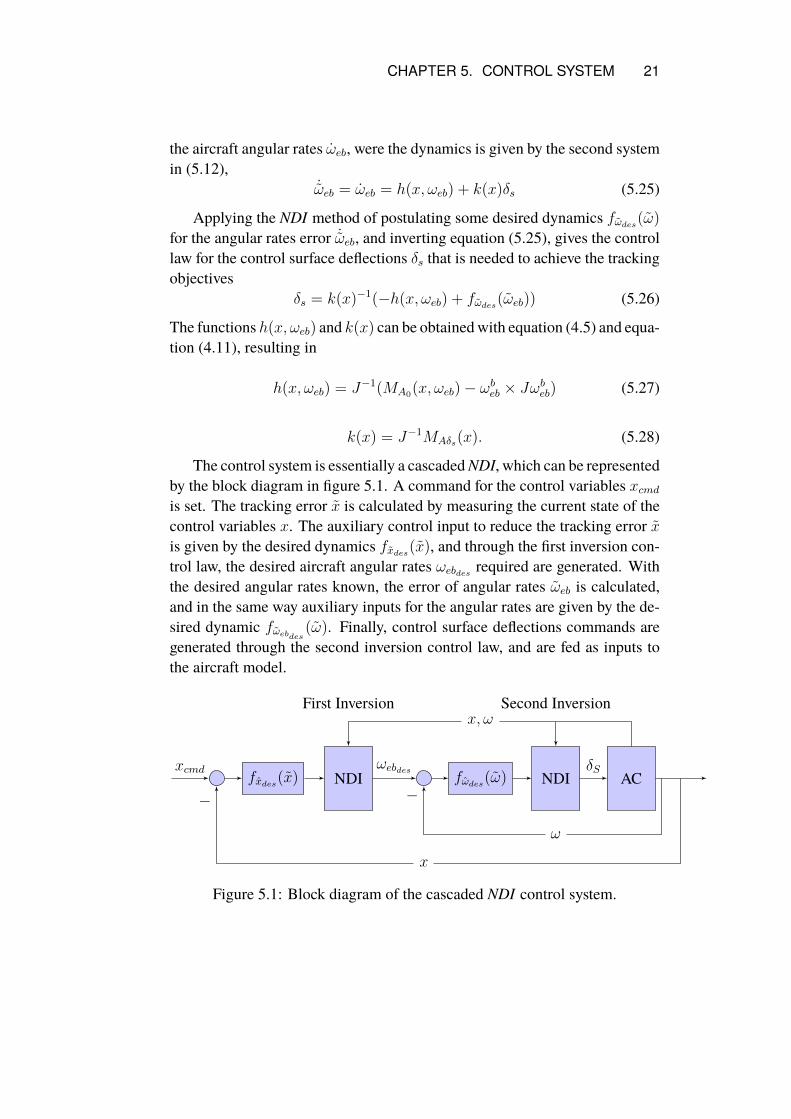
The control system is essentially a cascadedNDI, which can be representedby the block diagram in figure 5.1. A command for the control variables xcmdis set. The tracking error x is calculated by measuring the current state of thecontrol variables x. The auxiliary control input to reduce the tracking error xis given by the desired dynamics fxdes(x), and through the first inversion con-trol law, the desired aircraft angular rates ωebdes required are generated. Withthe desired angular rates known, the error of angular rates ωeb is calculated,and in the same way auxiliary inputs for the angular rates are given by the de-sired dynamic fωebdes (ω). Finally, control surface deflections commands aregenerated through the second inversion control law, and are fed as inputs tothe aircraft model.

ACNDINDI fωdes(ω)

Second InversionFirst Inversion

ω

x, ω

δS

−

ωebdesfxdes(x)

x

−

xcmd

Figure 5.1: Block diagram of the cascaded NDI control system.


For both the control variable error dynamics ˙x and the angular rate errordynamics ˙ωeb, the desired dynamics fxdes(x) and fωebdes (ω) which determinesthe desired responses to a tracking error, have in this case been chosen as firstorder systems for simplicity and are shown in equations (5.29)

fxdes(x) = −

Kµ 0 0

0 Kα 0

0 0 Kβ

(x− xcmd)

fωdes(ω) = −

Kp 0 0

0 Kq 0

0 0 Kr

(ωeb − ωebdes)

(5.29)

The above equations are equivalent to a proportional controller whereKµ, Kα

and Kβ are the proportional gains for the control variables, and Kp, Kq andKr are the gains for the angular rates .

The control of the airspeed VT has not been mentioned, but it is obtainedin the same manner by first writing the dynamics in control affine form

VT = fVT (x, xAC) + gVT (x, xAC)δT (5.30)

where the functions fVT (x, xAC) and gVT (x, xAC) are obtained from rewritingequation (5.7). Following the same procedure as described above a controllaw for the throttle position δT can be defined.

Chapter 6

Simulation

6.1 The F-18 HARV ModelSimulations have been performed on the F-18 HARV Model [19]. The ma-noeuvres were performed without an afterburner, and the control surface de-flections and rate limits are specified in Table 6.1.

Aileron Elevator Rudder

Rate Limit[deg/s] 100 40 82Deflection limit[deg] +45, -25 +25,-10 +30,-30

Table 6.1: Control surface limits.

The F-18 HARV has a split elevator configuration which means that theright and left elevator are able to move independently. In the simulation thishas been neglected and the elevator is assumed to be as one piece. Actuatorsfor the control surfaces and engine were modelled with a first order differentialequation,

δ =1

τ(δcmd − δ) (6.1)

where τ is the time constant. The time constants used in the simulations arelisted in Table 6.2.

Engine Aileron Elevator Rudder

Time Constant 0.02 0.2 0.2 0.2

Table 6.2: Time constants of actuator dynamics for control surface and engine.

23

24 CHAPTER 6. SIMULATION

6.2 Combat Cycle Time

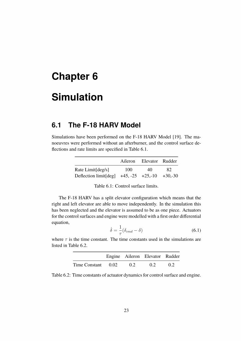
Figure 6.1: Flight trajectory comparison of two CCT turns at 5km altitudeand Mach 0.9. The trajectory with larger radius ( blue aircraft) is at constantairspeed and the other with smaller radius (red aircraft) is a high-angle-of-attack CCT.

A CCT manoeuvre is defined as the time required to perform a 180 headingturn in the horizontal plane. The time is measured from initiating the turn untilthe aircraft has performed the turn and reached the same initial speed.

There are many ways to perform a CCT turn. Comparing a selection ofmanoeuvres, it apparent that the shortest time for a CCT turn is when theleast amount of kinetic energy is depleted. The reason is that it is very timeconsuming to build up the kinetic energy by acceleration at constant altitude.

In Figure 6.1 the flight path trajectories from two different CCT turns areshown, with the same initial state at 5km of altitude and MACH 0.9. The blueaircraft path represents a CCT where constant airspeed is held, and the redaircraft path represents a high angle of attack - short radius CCT.

For the blue aircraft to complete the turn it takes approximately 23 seconds,

CHAPTER 6. SIMULATION 25

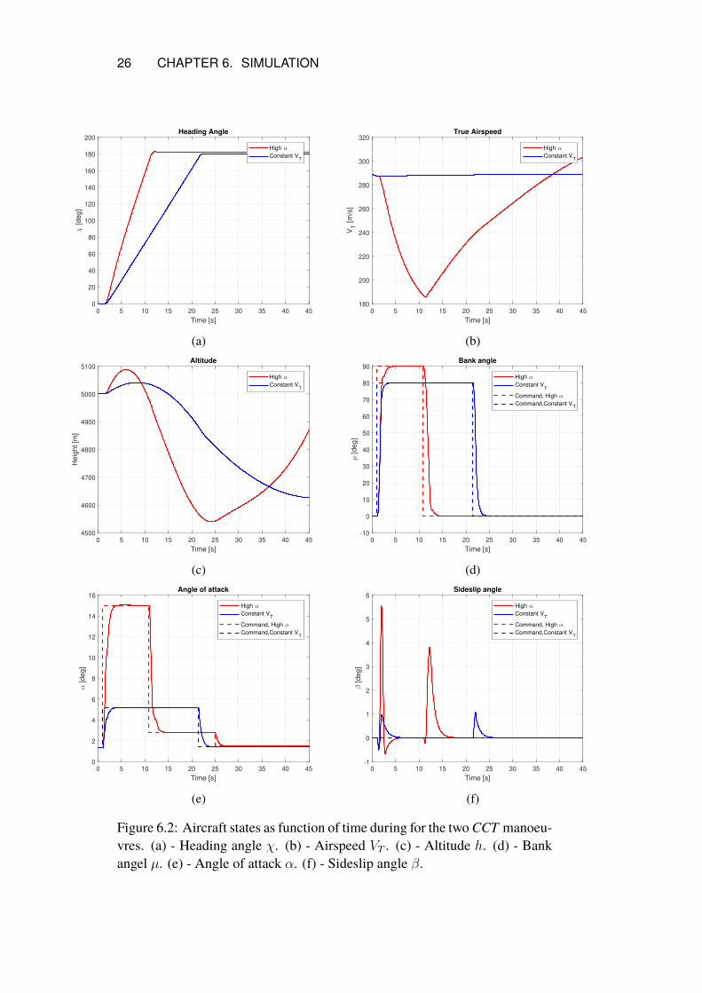
where the red aircraft completes the 180 heading change in 12 seconds, whichis seen in Figure 6.2a. At the same time the airspeed has dropped by 100m/s,which is seen in Figure 6.2b. The time to complete the CCT and reach theinitial airspeed for the red aircraft takes an additional 26 seconds and the totaltime for the CCT is 38 seconds.

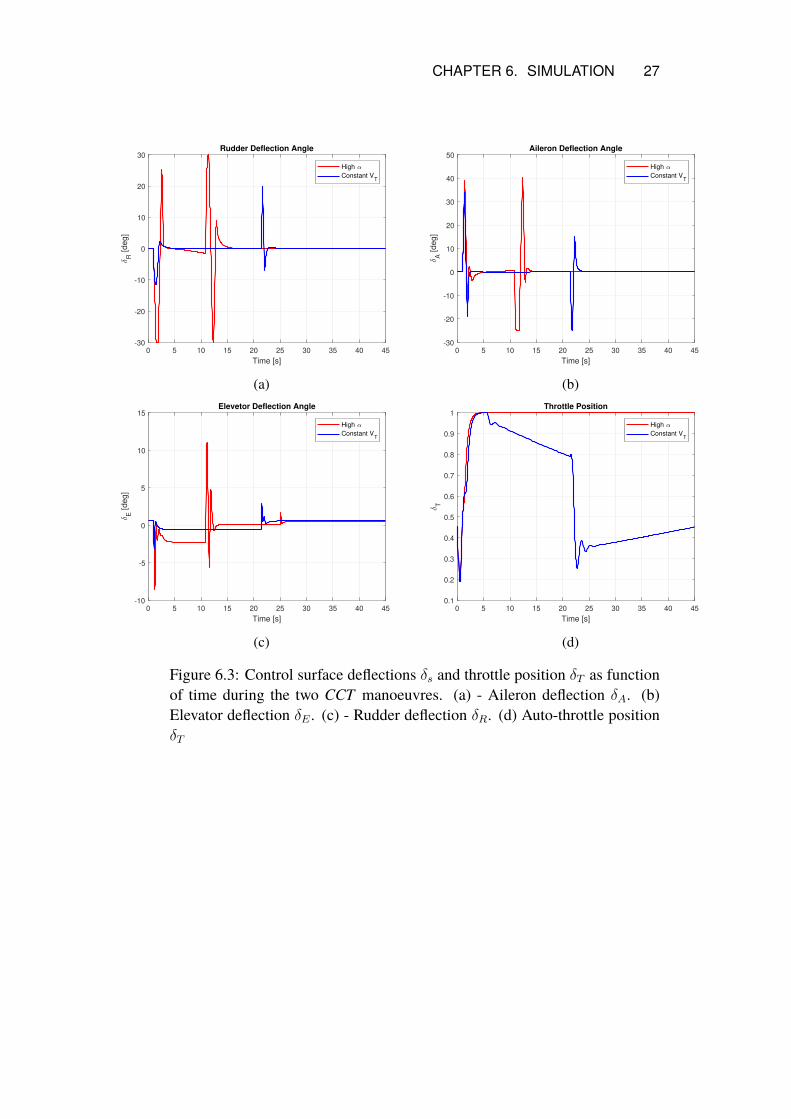
In both cases altitude is lost, which can be seen in Figure 6.2c. This is dueto how precise the angle of attack commands are set during the simulation. Thecommands for the angle of attack and bank angle are issued at the same time,which can be seen in Figures 6.2d and 6.2e. Due to cross coupling this leadsto induced sideslip, which can be seen in Figure 6.2f. For the high angle ofattack CCT this effect is more noticeable. It can also be noted that the sideslipreduces at a slower rate after 12 seconds. With a lower dynamic pressure therudder has to work harder which can be seen Figure 6.3a where the wholerange of rudder deflection is used.

Aileron actuation at initiation of the turn is comparable for both cases,which can be seen in Figure 6.3b. For the high angle of attack case, there isa longer actuation for levelling the aircraft after the turn, where for the con-stant airspeed case the aileron deflection is the same in magnitude as in thebeginning of the turn but reversed in direction. The elevator deflections canbe seen in Figure 6.3c. In the high angle of attack case a significantly largerangle of attack is commanded, which in turn requires a larger elevator actua-tion compared to the constant airspeed case. However, in both cases a smallpart of the total range of motion is required. Since the F-18 HARV has a splitelevator configuration, and the elevator are clearly not used to its maximum, itcould be used to generate additional yaw moment and reduce the work load ofthe rudder which would provide additional reduction of the induced sideslip.Another way to reduce the sideslip could be to separate the angle of attack andbank angle commands, for example by first setting a command for banking andwhen the reference value is reached, setting a command for angle of attack.

In Figure 6.3d the throttle position for the engine is seen. Since altitudeis lost during the turn and kinetic energy is gained, the throttle in the constantairspeedCCT is reduced tomaintain the speed, whichmeans that there is someroom for improving the CCT by just setting the throttle to maximum. In thehigh angle of attack case, airspeed is lost and the control system response is toset the throttle to maximum.


0 5 10 15 20 25 30 35 40 45

Time [s]

0

20

40

60

80

100

120

140

160

180

200

[deg]

Heading Angle

High

Constant VT

(a)

0 5 10 15 20 25 30 35 40 45

Time [s]

180

200

220

240

260

280

300

320

VT [m

/s]

True Airspeed

High

Constant VT

(b)

0 5 10 15 20 25 30 35 40 45

Time [s]

4500

4600

4700

4800

4900

5000

5100

Heig

ht [m

]

Altitude

High

Constant VT

(c)

0 5 10 15 20 25 30 35 40 45

Time [s]

-10

0

10

20

30

40

50

60

70

80

90

[deg]

Bank angle

High

Constant VT

Command, High

Command,Constant VT

(d)

0 5 10 15 20 25 30 35 40 45

Time [s]

0

2

4

6

8

10

12

14

16

[deg]

Angle of attack

High

Constant VT

Command, High

Command,Constant VT

(e)

0 5 10 15 20 25 30 35 40 45

Time [s]

-1

0

1

2

3

4

5

6

[deg]

Sideslip angle

High

Constant VT

Command, High

Command,Constant VT

(f)

Figure 6.2: Aircraft states as function of time during for the twoCCT manoeu-vres. (a) - Heading angle χ. (b) - Airspeed VT . (c) - Altitude h. (d) - Bankangel µ. (e) - Angle of attack α. (f) - Sideslip angle β.


0 5 10 15 20 25 30 35 40 45

Time [s]

-30

-20

-10

0

10

20

30

R [deg]

Rudder Deflection Angle

High

Constant VT

(a)

0 5 10 15 20 25 30 35 40 45

Time [s]

-30

-20

-10

0

10

20

30

40

50

A [deg]

Aileron Deflection Angle

High

Constant VT

(b)

0 5 10 15 20 25 30 35 40 45

Time [s]

-10

-5

0

5

10

15

E [deg]

Elevetor Deflection Angle

High

Constant VT

(c)

0 5 10 15 20 25 30 35 40 45

Time [s]

0.1

0.2

0.3

0.4

0.5

0.6

0.7

0.8

0.9

1

T

Throttle Position

High

Constant VT

(d)

Figure 6.3: Control surface deflections δs and throttle position δT as functionof time during the two CCT manoeuvres. (a) - Aileron deflection δA. (b)Elevator deflection δE . (c) - Rudder deflection δR. (d) Auto-throttle positionδT


6.3 T90

0.45 0.5 0.55 0.6 0.65 0.7 0.75 0.8 0.85 0.9

Mach

1

1.5

2

2.5

T9

0 [

s]

Time To Capture 90° Bank Angle

1 km

3 km

5 km

7 km

10 km

Simulation Point

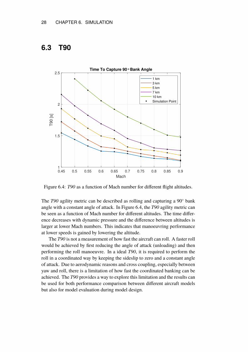
Figure 6.4: T90 as a function of Mach number for different flight altitudes.

The T90 agility metric can be described as rolling and capturing a 90 bankangle with a constant angle of attack. In Figure 6.4, the T90 agility metric canbe seen as a function of Mach number for different altitudes. The time differ-ence decreases with dynamic pressure and the difference between altitudes islarger at lower Mach numbers. This indicates that manoeuvring performanceat lower speeds is gained by lowering the altitude.

The T90 is not a measurement of how fast the aircraft can roll. A faster rollwould be achieved by first reducing the angle of attack (unloading) and thenperforming the roll manoeuvre. In a ideal T90, it is required to perform theroll in a coordinated way by keeping the sideslip to zero and a constant angleof attack. Due to aerodynamic reasons and cross coupling, especially betweenyaw and roll, there is a limitation of how fast the coordinated banking can beachieved. The T90 provides a way to explore this limitation and the results canbe used for both performance comparison between different aircraft modelsbut also for model evaluation during model design.


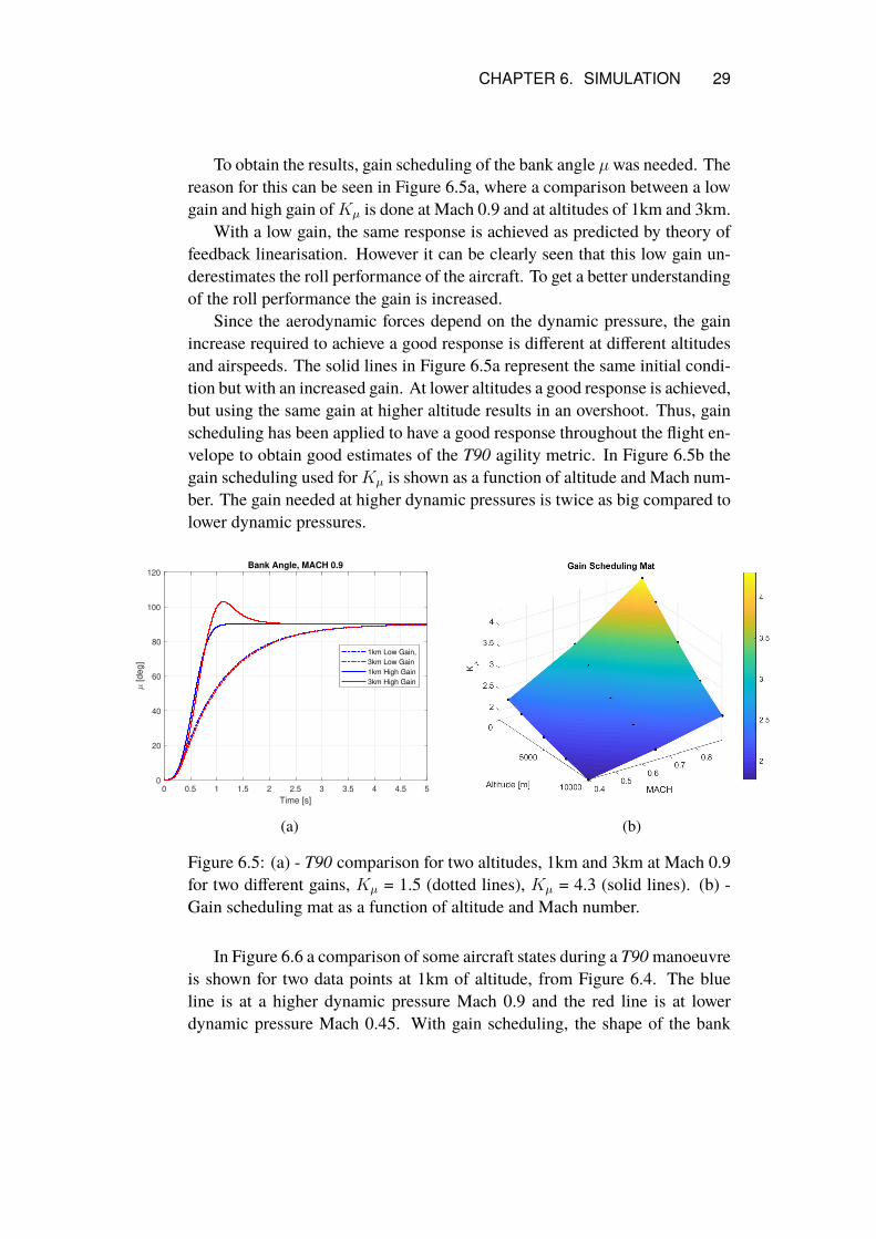
To obtain the results, gain scheduling of the bank angle µwas needed. Thereason for this can be seen in Figure 6.5a, where a comparison between a lowgain and high gain ofKµ is done at Mach 0.9 and at altitudes of 1km and 3km.

With a low gain, the same response is achieved as predicted by theory offeedback linearisation. However it can be clearly seen that this low gain un-derestimates the roll performance of the aircraft. To get a better understandingof the roll performance the gain is increased.

Since the aerodynamic forces depend on the dynamic pressure, the gainincrease required to achieve a good response is different at different altitudesand airspeeds. The solid lines in Figure 6.5a represent the same initial condi-tion but with an increased gain. At lower altitudes a good response is achieved,but using the same gain at higher altitude results in an overshoot. Thus, gainscheduling has been applied to have a good response throughout the flight en-velope to obtain good estimates of the T90 agility metric. In Figure 6.5b thegain scheduling used forKµ is shown as a function of altitude and Mach num-ber. The gain needed at higher dynamic pressures is twice as big compared tolower dynamic pressures.

0 0.5 1 1.5 2 2.5 3 3.5 4 4.5 5

Time [s]

0

20

40

60

80

100

120

[deg]

Bank Angle, MACH 0.9

1km Low Gain,

3km Low Gain

1km High Gain

3km High Gain

(a) (b)

Figure 6.5: (a) - T90 comparison for two altitudes, 1km and 3km at Mach 0.9for two different gains, Kµ = 1.5 (dotted lines), Kµ = 4.3 (solid lines). (b) -Gain scheduling mat as a function of altitude and Mach number.

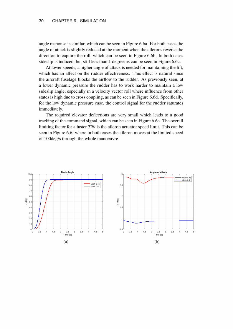
In Figure 6.6 a comparison of some aircraft states during a T90manoeuvreis shown for two data points at 1km of altitude, from Figure 6.4. The blueline is at a higher dynamic pressure Mach 0.9 and the red line is at lowerdynamic pressure Mach 0.45. With gain scheduling, the shape of the bank


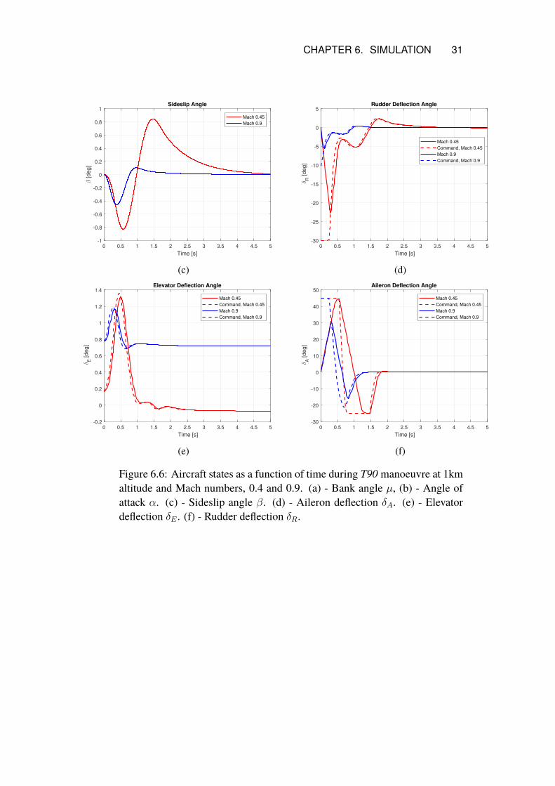
angle response is similar, which can be seen in Figure 6.6a. For both cases theangle of attack is slightly reduced at the moment when the ailerons reverse thedirection to capture the roll, which can be seen in Figure 6.6b. In both casessideslip is induced, but still less than 1 degree as can be seen in Figure 6.6c.

At lower speeds, a higher angle of attack is needed for maintaining the lift,which has an affect on the rudder effectiveness. This effect is natural sincethe aircraft fuselage blocks the airflow to the rudder. As previously seen, ata lower dynamic pressure the rudder has to work harder to maintain a lowsideslip angle, especially in a velocity vector roll where influence from otherstates is high due to cross coupling, as can be seen in Figure 6.6d. Specifically,for the low dynamic pressure case, the control signal for the rudder saturatesimmediately.

The required elevator deflections are very small which leads to a goodtracking of the command signal, which can be seen in Figure 6.6e. The overalllimiting factor for a faster T90 is the aileron actuator speed limit. This can beseen in Figure 6.6f where in both cases the aileron moves at the limited speedof 100deg/s through the whole manoeuvre.

0 0.5 1 1.5 2 2.5 3 3.5 4 4.5 5

Time [s]

0

10

20

30

40

50

60

70

80

90

100

[deg]

Bank Angle

Mach 0.45

Mach 0.9

(a)

0 0.5 1 1.5 2 2.5 3 3.5 4 4.5 5

Time [s]

0.5

1

1.5

2

2.5

3

[deg]

Angle of attack

Mach 0.45

Mach 0.9

(b)


0 0.5 1 1.5 2 2.5 3 3.5 4 4.5 5

Time [s]

-1

-0.8

-0.6

-0.4

-0.2

0

0.2

0.4

0.6

0.8

1

[deg]

Sideslip Angle

Mach 0.45

Mach 0.9

(c)

0 0.5 1 1.5 2 2.5 3 3.5 4 4.5 5

Time [s]

-30

-25

-20

-15

-10

-5

0

5

R

[deg]

Rudder Deflection Angle

Mach 0.45

Command, Mach 0.45

Mach 0.9

Command, Mach 0.9

(d)

0 0.5 1 1.5 2 2.5 3 3.5 4 4.5 5

Time [s]

-0.2

0

0.2

0.4

0.6

0.8

1

1.2

1.4

E [deg]

Elevator Deflection Angle

Mach 0.45

Command, Mach 0.45

Mach 0.9

Command, Mach 0.9

(e)

0 0.5 1 1.5 2 2.5 3 3.5 4 4.5 5

Time [s]

-30

-20

-10

0

10

20

30

40

50

A [deg]

Aileron Deflection Angle

Mach 0.45

Command, Mach 0.45

Mach 0.9

Command, Mach 0.9

(f)

Figure 6.6: Aircraft states as a function of time during T90 manoeuvre at 1kmaltitude and Mach numbers, 0.4 and 0.9. (a) - Bank angle µ, (b) - Angle ofattack α. (c) - Sideslip angle β. (d) - Aileron deflection δA. (e) - Elevatordeflection δE . (f) - Rudder deflection δR.

Chapter 7

Conclusions

In this thesis work a control system was developed based on the NDI methodfor estimating specific agility metrics, namely the Combat Cycle Time (CCT)and Time to capture 90 bank (T90), for the F-18 HARV aircraft model. Esti-mations were performed and in the case of the CCT two scenarios were com-pared. Results show that the fastest CCT is the one where the least amount ofairspeed is lost during the manoeuvre. In the case of the T90, a gain schedulingwas required for extracting the maximum banking performance of the aircraftmodel, and it can be concluded that the overall limiting factor for better per-formance for this aircraft model is the aileron actuator speed.

NDI is an effective method for implementing simple control structures tomore complex nonlinear systems, such as an aircraft. The effectiveness comesfrom the fact that the linearization is based on cancelling the nonlinear ef-fects with the equations of motion itself, and pre-linearizations of the modelis not necessary. This is very useful, especially in high nonlinear regimes. Forexample, considering the high angle of attack CCT, using traditional methodwould have been required to have several different linearized models with cor-responding controllers to cover the same flight path.

However, since the NDI method relies on the assumption that the controlsystem linearizes the system, instead of this being done before hand, there isa general performance loss of the overall manoeuvrability, since some of thecontrol power is used for linearization, as a result there is a limitation of howmuch of the control power can be used for manoeuvring, while maintainingthe linearization. For systems that have low control effectiveness this can bea very significant limitation, which makes the system slow. In the end, onecould say that the method can be regarded as a trade-off between peak per-formance and implementation time of the controller. This can be valuable in

32

CHAPTER 7. CONCLUSIONS 33

an iterative model developing process, where emphasis is put on fast turnovertime between new model designs and controller implementation, where thefinal maximum performance has not been reached.

Building a more general control system for performance evaluation, morefocus needs to be put on the control variables since these greatly affect howmuch effort is needed for the linearization and overall control, since there arevarious levels of how nonlinear variables are. Another point to consider isthat the NDI method requires that some desired dynamic is postulated and it isimportant that proper desired dynamics are used. In this work, only first orderdifferential systems were used for the desired dynamics. Most natural physicalsystems are of second order or higher, including the aircraft. Forcing a secondorder system to behave as a first order system requires control actuation, whichmay be unnecessarily wasted, instead of letting more of the natural behaviourthrough and controlling it as a second order system.

Improvements can be made in various ways, a suggestions is to incorporatea pilot model instead of the first inversion block in figure 5.1. Handling qual-ities could be added in the loop as a second step by implementing a referencemodel. The reference model would be specified with the handling qualities inmind, and controlled by the pilot model, the reference model would then inturn generate the commands to the aircraft model. Another approach could beto implement trajectory tracking, where instead of commanding specific air-craft states the commands are generated from a specified trajectory in space.As a suggestion this could be done with the use of Frenet-Serret formulas.

And to end with a quote regarding feedback linearization in general fromHassan Kahlil, author of the book Nonlinear Systems

"...there are situations where nonlinearities are beneficial and cancellingthem should not be an automatic choice. We should try our best to understandthe effect of the nonlinear terms and decide whether or not cancellation isappropriate. Admittedly, this is not an easy task. "

Bibliography

[1] RANDALL K. LIEFER et al. “Fighter agility metrics, research andtest”. In: Journal of Aircraft 29.3 (1992), pp. 452–457.

[2] A. SKOW,W. HAMILTON, and J. TAYLOR. “Advanced fighter agilitymetrics”. In: 12th Atmospheric Flight Mechanics Conference. 1985.

[3] John Robinson, Fredrik Berefelt, and Anders Lennartsson. Manover-prestanda hos flyplan. Tech. rep. FOI-R–4351–SE. Swedish DefenceReaschers Department, 2017.

[4] Jen - Nai Chou. Optimal turning maneuvers for six-degree-of-freedomhigh angle-of-attack aircraft models. Jan. 1995.

[5] E. G. Hoffman. “On Minimum Time Six-Degree-of-Freedom TurningManeuvers for a High-Alpha Fighter Aircraft.” PhD thesis. George In-stitute of Technology, 1991.

[6] Daniel J. Bugajski and Dale F. Enns. “Nonlinear control law with appli-cation to high angle-of-attack flight”. In: Journal of Guidance Controland Dynamics - J GUID CONTROL DYNAM 15 (May 1992), pp. 761–767.

[7] DALE ENNS et al. “Dynamic inversion: an evolving methodology forflight control design”. In: International Journal of Control 59.1 (1994),pp. 71–91.

[8] Jacob Reiner, Gary J. Balas, and William L. Garrard. “Flight controldesign using Robust dynamic inversion and time-scale separation”. In:Automatica 32 (Nov. 1996), pp. 1493–1504.

[9] Daigoro Ito et al. Reentry Vehicle Flight Controls Design Guidelines:Dynamic Inversion. Tech. rep. NASA Johnson Space Center, 2002.

[10] H Fer and D.F. Enns. “Nonlinear longitudinal axis regulation of F-18HARV using feedback linearization and LQR”. In: vol. 5. Jan. 1998,4173–4178 vol.5.

34

BIBLIOGRAPHY 35

[11] Béatrice Escande. “Nonlinear dynamic inversion and LQ techniques”.In: Robust Flight Control. Ed. by Jean-François Magni, Samir Bennani,and Jan Terlouw. Berlin, Heidelberg: Springer Berlin Heidelberg, 1997,pp. 523–540. isbn: 978-3-540-40941-0.

[12] Jean-Jaques E Slotine.Applied nonlinear control. eng. EnglewoodCliffs,N.J.: Prentice-Hall, 1991. isbn: 0-13-040049-1.

[13] John Robinson. Nonlinear Control Methods for an Agile Missile withThrust Vectoring Control. Tech. rep. FOI-D–0627–SE. Swedish De-fence Reaschers Department, 2015.

[14] Brian Stevens and Frank Lewis. “Aircraft Control and Simulation”. eng.In: Aircraft Engineering 76.5 (2004). issn: 0002-2667.

[15] Hassan K Khalil. Nonlinear systems. eng. 3. ed.. Upper Saddle river:Prentice Hall, 2002. isbn: 0-13-067389-7.

[16] Mark Drela. Flight vehicle aerodynamics. eng. 2014. isbn: 1-62870-920-0.

[17] Application of multivariable control theory to aircaft control laws. Hon-eywell Technology Center, Lockheed Martin Skunkworks. 1996.

[18] Corey Schumacher, Pramod Khargonekar, and N. McClamroch. “Sta-bility analysis of dynamic inversion controllers using time-scale separa-tion”. In: Guidance, Navigation, and Control Conference and Exhibit.1998.

[19] NASA.F-18HARVModel.https://www.nasa.gov/centers/dryden / history / pastprojects / HARV / Work / NASA2 /nasa2.html.

[20] Johan Knöös, John Robinson, and Fredrik Berefelt. “Nonlinear Dy-namic Inversion and Block Backstepping: A Comparison”. In: Aug.2012.

[21] Evgeny Kolesnikov. “NDI-Based Flight Control Law Design”. In: Aug.2005.

[22] S. Sieberling, Q. P. Chu, and J. A. Mulder. “Robust Flight Control Us-ing Incremental Nonlinear Dynamic Inversion and Angular Accelera-tion Prediction”. In: Journal of Guidance, Control, and Dynamics 33.6(2010), pp. 1732–1742.

36 BIBLIOGRAPHY

[23] Johan Thunberg and John Robinson. “Block Backstepping, NDI andRelated Cascade Designs for Efficient Development of Nonlinear FlightControl Laws”. In:AIAAGuidance, Navigation andControl Conferenceand Exhibit.

[24] Wayne C. Durham, Frederick H. Lutze, andWilliamMason. “Kinemat-ics and aerodynamics of velocity-vector roll”. In: Journal of Guidance,Control, and Dynamics 17.6 (1994), pp. 1228–1233.

www.kth.se

Dynamic Performance Analysis of a Fighter Jet with Nonlinear ...

Documents

Transcript of Dynamic Performance Analysis of a Fighter Jet with Nonlinear ...