Dynamic multi-level analysis of households’ living standards and poverty: Evidence from Vietnam

Arnstein Aassve

(ISER, University of Essex)

Bruno Arpino (University of Florence)

ISER Working Paper

2007-10

Acknowledgement: The project is funded under the framework of the European Science Foundation (ESF) – European Research Collaborative Program (ERCPS) in the Social Sciences, by Economic and Social Research Council (award no RES-000-23-0462), the Italian National Research Council (Posiz. 117-14), and the Austrian Science Foundation (contract no P16903-605). We are grateful to Leonardo Grilli, Fabrizia Mealli and Letizia Mencarini for very useful comments on this work.

Readers wishing to cite this document are asked to use the following form of words: Aassve, Arnstein, Bruno Arpino (May 2007) ‘Dynamic multi-level analysis of households’ living standards and poverty: Evidence from Vietnam’, ISER Working Paper 2007-10. Colchester: University of Essex. The on-line version of this working paper can be found at http://www.iser.essex.ac.uk/pubs/workpaps/ The Institute for Social and Economic Research (ISER) specialises in the production and analysis of longitudinal data. ISER incorporates

MISOC (the ESRC Research Centre on Micro-social Change), an international centre for research into the lifecourse, and

ULSC (the ESRC UK Longitudinal Studies Centre), a national resource centre to promote longitudinal surveys

and longitudinal research. The support of both the Economic and Social Research Council (ESRC) and the University of Essex is gratefully acknowledged. The work reported in this paper is part of the scientific programme of the Institute for Social and Economic Research. Institute for Social and Economic Research, University of Essex, Wivenhoe Park, Colchester. Essex CO4 3SQ UK Telephone: +44 (0) 1206 872957 Fax: +44 (0) 1206 873151 E-mail: iser@essex.ac.uk Website: http://www.iser.essex.ac.uk

© May 2007 All rights reserved. No part of this publication may be reproduced, stored in a retrieval system or transmitted, in any form, or by any means, mechanical, photocopying, recording or otherwise, without the prior permission of the Communications Manager, Institute for Social and Economic Research.

ABSTRACT The paper investigates the role of multi-level structures in poverty analysis based on

household level data. We demonstrate how multi-level models can be applied to

standard poverty analysis and highlight its usefulness in terms of assessing the

extent community characteristics matter in determining poverty status and dynamics.

We provide two applications. The first is an example of a growth model that control

for characteristics measured at the initial time period, and considers directly to what

extent the same characteristics contribute to explain changes in economic wellbeing

over time. In the second application we model the determinants of escaping poverty.

Both applications use longitudinal data from Vietnam recorded at two points in time

during the nineties, a period where Vietnam experienced strong economic growth.

We demonstrate that failing to control for multi-level data structures could give

incorrect inference about the effect of covariates of interest. We also demonstrate

how the multi-level models can be used for regional and community level policy

analysis that otherwise is difficult to implement in more standard regression analysis.

NON-TECHNICAL SUMMARY The paper provides an illustration of how multilevel models can be used to

correctly handle hierarchical data structures applied to household wellbeing

and poverty dynamics. From the models we also demonstrate how to provide

recommendations for policy interventions. We present two examples: A

growth model with a continuous dependent variable – the log equivalent

household expenditure, and a probit model for studying the determinants of

poverty exit.

In both cases we find that the multilevel structure is highly relevant as

attested by the intra-class correlation coefficients. Hence, failing to control for

the multilevel structure will influence model predictions in significant ways,

leading to possibly incorrect inference about the effect of the covariates.

Whereas an alternative approach would be to simply use robust standard

errors, this would omit essential information about the multilevel structure

relevant for policy analysis. Multilevel models instead give us insight that is

otherwise unfeasible in the more standard methods.

The growth model separates the initial economic status from the

growth effect of the covariates. The estimates related to the initial condition

demonstrate that Kinh ethnic origin, education, and living in a community with

health facilities, are all associated with higher wealth. In contrast, households

with a high percentage of unemployed members and those working in

agricultural activities were disadvantaged. Also household size and the

number of children are negatively associated with consumption expenditure.

These effects are of course, sensitive to the equivalence scale; we adopt here

the well used WHO scale which is in line with many previous studies.

The growth dimension of the model attests that, on average, household

consumption growth rate between the two waves was 17%, a reflection of the

economic boom experienced in Vietnam during the nineties. However, the

growth trend varied substantially by households and community

characteristics. We find that those who were better off initially were not

necessarily the same benefiting during the economic boom. For example,

households with many children benefited from the economic growth whereas

farm households benefited less.

1

Since the Vietnam economy is dominated by rural activities, in

particular agriculture, and rural areas are the poorest, we focus our attention

on farm households. The model includes therefore random slopes that allow

the effect of agriculture to differ by community. Standard deviations of these

random effects attest that the place where farmers reside matters. Even

though the average growth differential for farmer in respect to non farmer is

negative there were certain communities in which farm households grew

more. This is especially the case if the community is well connected to other

neighbourhoods through road links. The poverty exit model highlighted that

the key factors behind escaping poverty are in part similar to those associated

with higher consumption in the growth model.

An important benefit of the multilevel approach is that predictions can

be used to assess community and regional differences. These predictions

produce groups of communities that benefit from economic growth more than

others, and communities that in fact suffered during the period. Given these

classifications it is straight forward to investigate differences in characteristics,

which is an important tool for policy makers to target policies. Critical

characteristics of a successful community include key infrastructural or socio-

economic variables such as the availability of electricity and daily markets,

and school enrolment. These are clearly important policy variables for

promoting further poverty reduction. On the basis of community level

predictions, we also derive a ranking of regions. This identifies which

communities that performs badly in regions that performed well and vice

versa. Such analysis provides a critical tool for better targeting policy

interventions.

2

1. Introduction

With the emergence of large scale household surveys for Less Developed Countries

(LDC), notably the World Bank Living Standard Measurement Surveys (LSMS),

poverty analysis has become widespread. These surveys contain detailed information

on consumption expenditure behaviour, and are ideal for poverty mapping and

analysis of the determinants underlying variation in poverty across and within

countries. Several of these surveys are longitudinal where households are followed

over several time periods. The longitudinal dimension is extremely useful since it

allows for dynamic analysis of households’ living standards. Why is it for instance the

case that some households are more likely to escape poverty, whereas others are less

likely to do so? Such question cannot be examined in cross-sectional surveys.

Examples of longitudinal LSMS surveys include Vietnam, Albania, Nicaragua, Peru

and recently Bosnia-Herzegovina.

A factor that is often ignored in dynamic analysis of living standards or

poverty is that households are often sampled from the same communities or villages.

In so far there is correlation within communities in terms of their poverty experiences,

parametric regression analysis may become unreliable unless the community effects

are controlled for explicitly. In this paper we explore this issue by using data from the

Vietnam LSMS surveyed in 1993, and followed up as a panel in 1998. As is well

documented, Vietnam experienced a dramatic drop in overall poverty during this

period. However, it is also documented that the poverty reduction was not uniform,

with substantial variation across households, communities and also regions. The

LSMS shows that poverty reduction was much stronger in urban areas than rural ones.

However, the data also shows much stronger heterogeneity in poverty reduction in

rural areas. There is in other words a significant degree of clustering across rural

areas. As a result we focus our analysis on rural areas of Vietnam. Focusing on rural

household has also a practical motivation: only the rural sample of the LSMS contain

community level variables. We present results of the estimation of two set of models,

each focusing on change in living standards or poverty. The first is a growth model

for household’s expenditures, while the second is a model of poverty dynamics where

we focus on the determinants behind households escaping poverty.

3

The paper is organised as follow. Section 2 provides a review of the literature

concerning poverty in Vietnam and also describes the pervasive transformation of the

Vietnam economy and its institutions during the nineties. Section 3 presents the

Vietnamese Living Standard Measurement Survey. Section 4 explains the statistical

models. Section 5 show results, whereas in section 6 we assess the policy implications

of the estimates through an empirical bayes analysis, a technique often applied in

multi-level models. Section 7 concludes.

2 Background: political and socio-economic change in Vietnam

during the nineties.

At the beginning of the 1980s, Vietnam was one of the worlds’ poorest countries.

Since then the country embarked on a remarkable recovery, a fact that is reflected by

strong economic growth and a dramatic reduction in poverty (Glewwe et al., 2002).

The country also experienced a dramatic improvement in others indicators of social

and economic wellbeing. For example, school enrolment rates increased during the

period both for boys and girls. In particular, upper secondary enrolment rates

increased from 6 to 27 percent for girls, and from 8 percent to 30 percent for boys

(World Bank, 2000). Access to public health centres, clean water and other

infrastructure have all increased, as well as the ownership of consumer durables.

Overall these improvements have had a positive effect on households’ own

assessment of their living conditions. As The World Bank Vietnam Development

Report states: “ […] Households report a greater sense of control over their

livelihoods, reduced stress, fewer domestic and community disputes […] ”.

Much of this improvement has been attributed to the “Doi Moi” policy

(translated in English as “renovation”). This was initiated in the late 1980s and

roughly coincided with the collapse of the Soviet Union, on which Vietnam had been

heavily dependent. The Doi Moi had many similarities with the reforms taking place

in China a decade earlier. The main elements of the Doi Moi were to replace

collective farms by allocating land to individual households; new legalisation

encouraging private economic activity; removal of price controls; and legalisation and

encouragement of Foreign Development Investment (FDI). During the nineties,

4

immediately following the Doi Moi, Vietnam experienced dramatically strong

economic growth. The average annual GDP growth was at a staggering 7 percent. In

the period covered by the Vietnam LSMS panel (i.e. from 1993 to 1998), the growth

rate was even higher at 8.9 percent. This was followed by significant changes in the

labour market; during the 1990s the employment grew by 2.5%. Output was increased

through improved productivity and prices rose as a result of expansion in export of

rice. By mid 1990 Vietnam passed to be a net importer to be one of world’s largest

exporters of rice on the international markets. The increase in agriculture

diversification was another remarkable factor of the economic change.

Given such a strong economic performance, it is not unexpected that the

overall poverty rate fell. The official poverty rate, which is derived from the per capita

household consumption expenditure, declined from 58% in 1993 to 37% in 1998.

Though the exact number is contested, as this depends on how poverty is measured

through the equivalence scale, (Justino and Litchfield, 2004; White and Masset, 2003;

World Bank, 2000), there is little doubt that poverty indeed declined during this

period.

The introduction of the Vietnam LSMS has sparked several poverty studies

(examples include Justino and Litchfield, 2004; White and Masset, 2001 and 2003;

Huong et al, 2003; Glewwe et al, 2002; Haughton et al, 2001). These studies suggest

that female headed households, lack of education, large households (large number of

children), rural households (or living in the Northern Uplands), households dependent

upon agriculture, are associated with higher poverty. However the effect of

demographic variables, such as the household size or the number of children3, is less

clear given its sensitivity to any imposed equivalence scale. In general the association

between poverty and number of children is weakened when imposing equivalence

scales that are different from per capita expenditure (White and Masset, 2003;

Balisacan et al, 2003).

Of course, household characteristics are not the only driver behind poverty –

also characteristics of the community where the household resides might matter. A

benefit of the Vietnam LSMS survey is that it includes detailed community

information. Justino and Litchfield (2004), using this information, find that the quality

of community infrastructure is not always associated with a lower probability of being 3Justino and Lithcfield argue that the high cost of education might be a factor explaining higher poverty rates among household with many children (Justino and Litchfield, 2004; page 22).

5

poor. For example, they find that access to electricity is negatively associated with

poverty, while the presence of secondary school has an opposite sign. A problem in

such analysis is of course that the various community characteristics are often highly

correlated, often resulting in non-intuitive parameter estimates when included

together. Moreover, community variables might be endogenous with respect to

poverty. This is particularly the case if government policies are implemented in

response to adverse community circumstances.

Economic growth by itself is not a sufficient condition for poverty reduction

(Huong et al, 2003; Ghura et al, 2002; Glewwe et al, 2002; Bruno et al, 1999) and the

way in which individuals may gain from the growth depends on their individual skills,

education and health, ethnicity, their religion, geographical location, and type of

employment and occupations. Whereas the economic boom in Vietnam affected all

geographical, ethnic, and socio-economic groups, it did so in very different ways, and

the poverty reduction was certainly not uniform across the population (Justino and

Litchfield, 2004; Balisacan et al, 2003; Glewwe et al, 2002). In particular, it is noted

that inequality increased during the nineties (Haughton, 2001), a fact that is robust to

how inequality is measured. Gains from economic growth was stronger in urban

areas, for South East and Red River Delta2, for Kinh3 which is the main ethnic group

in Vietnam, for households headed by a white collar worker and for those with higher

education.

3 Data: The Vietnam LSMS

The panel was first surveyed in 1992/93 with a full follow up in 1997/98. It follows

the LSMS format and includes rich information on education, employment, fertility

and marital histories, together with rich information on household income and

consumption expenditure. The overall quality of the panel is impressive with a very

low attrition rate (Falaris, 2003). The Vietnam LSMS also provides detailed

community information from a separate community questionnaire. It is available for

2 The Red River Delta and the Mekong River Delta were the regions that benefited most from rice market liberalisation (Justino and Litchfield, 2004). 3 In Vietnam there is a significant population of ethnic minorities that tend to be considerably poorer than the Kinh majority. An analysis of the sources of the ethnic inequalities in Vietnam can be found in Van de Walle and Gunewardana, 2001.

6

120 rural communities and includes information on health, schooling and main

economic activities. The communities range in size from 8,000 inhabitants to 30,000.

In the analysis we use as a measure of household’s living standard the

household’s consumption expenditure, which requires detailed information on

consumption behaviour. It is a widely accepted measure in the literature on LDC and

used by the World Bank (Coudouel et al, 2002; Deaton and Zaidi, 2002). We use here

the expenditure variables constructed by the World Bank procedure which is readily

available with the Vietnam LSMS survey. Poverty status is defined as a binary

variable and a household is deemed poor if their consumption expenditure falls below

a certain threshold. We specify the poverty line using the “Cost of Basic Needs”

(CBN) approach following Ravallion and Bidani (1994). In brief this involves

estimating the cost of a certain expenditure level which corresponds to a minimum

calorie requirement. The construction of the poverty level consists of two steps. First,

a food poverty threshold is defined as the expenditure needed to purchase a basket of

goods that will give the required minimum calorie intake (this is also referred to as the

extreme poverty threshold). Following FAO recommendations, for LDC, this

threshold is set to 2100 calories. Secondly, the general poverty line combines the food

poverty threshold with an average non-food consumption expenditure.

It is clear that the distribution of consumption expenditure within the

household is unlikely to be uniform across household members, and it is probable that

children consume less than adults. The standard solution is to impose an assumption

on intra-household resource allocation, and adjustments can be done by applying an

equivalence scale that is consistent with the assumption made – producing a measure

of expenditure per equivalent adult. Here we apply the WHO (World Health

Organisation) equivalence scale taking a weight of 1 for adults and 0.65 for children

as used by other authors (Justino and Litchfield, 2001; White and Masset, 2002). This

means that the mean poverty rate for the two waves will be different from the official

ones, given that the latter is based on per capita expenditure, which in effect implies

an equivalence scale that assigning weights to all household members.

The Vietnam LSMS includes a range of variables that are important

determinants for the household’s standard of living. Our choice of variables is based

mainly on dimensions which are important for the household’s income generating

process, such as employment and human capital. Many of these variables are defined

in terms of household ratios. That is, we are interested in the number of household

7

members that are engaged in gainful employment as a ratio of the total number of

household members. The effect of children is distinguished by their age distribution,

and again expressed as a ratio of the total number of household members. We then

include the average number of months that household members were working away

from their village, the ratio of household members with post-compulsory education,

the ratio of school attendance, the household literacy rate, the ratio of unskilled

workers, and the ratio of members looking for work. We also include characteristics

of the dwelling. These include whether the household has electricity and whether the

household head is a home owner. Both of these measures are expected to be

associated with higher household wealth. The survey also includes rich information

on the characteristics of the community where the household resides. Here we include

indicators for whether there is a lower secondary school, hospital facilities, whether

there is a large enterprise located nearby, whether farming is organised through

agricultural cooperatives, and the amount of large tractors, the latter being a measure

of farming technology in the community. It should be noted that the Vietnam LSMS

contains many more community level variables. However, many of these variables are

highly correlated. For instance, the quality of health care in the community can be

proxied by availability of doctors or pharmacies, in the same way as we here use the

hospital indicator. When such variables are included separately they tend to have

significant effect in most of the regression analysis, but many become insignificant

when combined together, which is driven by the strong correlation. We have therefore

made an effort to include one variable from different dimensions – hospital referring

to health conditions of the community, agricultural cooperatives to the way the

agricultural sector is organised, the number of large tractors being a measure of

advancement in agriculture, and low secondary schools as a measure of the

educational infrastructure.

4 Methods: Multilevel models for living standards and poverty

dynamics.

In this section we present two multilevel models to study poverty in rural Vietnam.

The first model exploits the longitudinal information in form of a growth model of

consumption expenditure, whereas the second model presents an application of

8

poverty dynamics, in particular a model of poverty exit. The multilevel structure is

highly relevant in both models and is driven by the fact that the economic growth, and

consequently changes in the economic structure of the country, varied substantially

across communities and regions (Glewwe et al, 2002). The multilevel structure of the

Vietnam LSMS is illustrated in Figure 1. The time dimension, i.e. the two waves of

the LSMS, represents the lowest level, i.e. level 1. The household is at the second

level, community the third level, and the region, the most aggregate level, is the

fourth4.

The arguments for using multilevel models to analyse hierarchical data are

well known (Skrondal and Rabe-Hesketh, 2004; Snijders and Bosker, 1999;

Goldstein, 1995; Hox, 1995; Di Prete and Forristal, 1994). When units are clustered

classical regression analysis are not appropriate since the underlying hypothesis of

independence of the observations is violated. In our case, households in the same

communities tend to be more similar to each other than households in different

communities. As a result of this dependency, standard errors are estimated with a

downward bias and, hence, inferences about the effects of the covariates might be

spurious (Hox, 1995). A standard solution is to use robust methods for estimating the

standard errors. But, when the multilevel structure is not only a mere nuisance factor

but instead a key dimension of the analysis, multilevel models are more appropriate.

As we will see in the following sections, the multilevel approach exploits the richness

of hierarchical data structures in a way that offer highly interesting policy analysis

that is not possible in more standard regression analysis.

4 In our models we have not included regional because they are too few (there are seven regions all together). This hampers accurate estimation of the standard deviation of the random effect (Maas and Hox, 2004). However, standard errors are corrected for any intra-regional correlation.

9

Figure 1 – The representation of the multilevel structure of the Vietnam LSMS

4.1 A growth multi-level model of household expenditure

The typical growth model consists of regression analysis where controls are made for

variables measured in the initial time period, a time trend, and the interaction between

control variables and the time trend. The benefit of this approach is that it enables a

decomposition of the growth pattern by background characteristics. Moreover, the

effect of the initial status can be compared with the growth effect. For example, large

households being associated with lower expenditure in the initial wave, might be

associated with higher growth over time, as is reflected by the interaction with the

time trend. Similar comparisons can be made for all background characteristics.

However, these models are not normally extended to take into account multilevel

structures.

A multi-stage formulation of the growth model

Based on the multilevel structure in Figure 1 we can easily derive a multi-stage

formulation of our growth model (Bryk and Raudenbush, 1987). First, the dependent

variable is here defined as the logarithm of the equivalent household consumption at

10

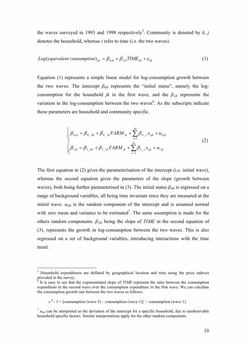
the waves surveyed in 1993 and 1998 respectively5. Community is denoted by k, j

denotes the household, whereas i refer to time (i.e. the two waves).

ijkijkjkjkijk eTIMEnconsumptioequivalentLog ++= 10) ( ββ (1)

Equation (1) represents a simple linear model for log-consumption growth between

the two waves. The intercept β0jk represents the “initial status”, namely the log-

consumption for the household jk in the first wave, and the β1jk represents the

variation in the log-consumption between the two waves6. As the subscripts indicate

these parameters are household and community specific.

⎪⎪⎩

⎪⎪⎨

⎧

+++=

+++=

∑

∑

=

=

jks

sjksjkkkjk

jks

sjksjkkkjk

uxFARM

uxFARM

1

16

2_11_10_11

0

16

2_01_00_00

ββββ

ββββ (2)

The first equation in (2) gives the parameterisation of the intercept (i.e. initial wave),

whereas the second equation gives the parameters of the slope (growth between

waves), both being further parameterised in (3). The initial status β0jk is regressed on a

range of background variables, all being time invariant since they are measured at the

initial wave. u0jk is the random component of the intercept and is assumed normal

with zero mean and variance to be estimated7. The same assumption is made for the

others random components. β1jk, being the slope of TIME in the second equation of

(3), represents the growth in log-consumption between the two waves. This is also

regressed on a set of background variables, introducing interactions with the time

trend.

5 Household expenditures are deflated by geographical location and time using the price indexes provided in the survey. 6 It is easy to see that the exponentiated slope of TIME represent the ratio between the consumption expenditure in the second wave over the consumption expenditure in the first wave. We can calculate the consumption growth rate between the two waves as follows:

e β - 1 = [consumption (wave 2) – consumption (wave 1)] / consumption (wave 1)

7 u0jk can be interpreted as the deviation of the intercept for a specific household, due to unobservable household specific factors. Similar interpretations apply for the other random components.

11

⎪⎪⎪⎪

⎩

⎪⎪⎪⎪

⎨

⎧

++=

++=

+=

++=

∑

∑

=

=

kkkh

mkmkmk

kk

km

mkmk

vROAD

vC

v

vC

31_1_10_1_11_1

22

172_10_0_10_1

10_1_01_0

0

22

17_00_0_00_0

βββ

βββ

ββ

βββ

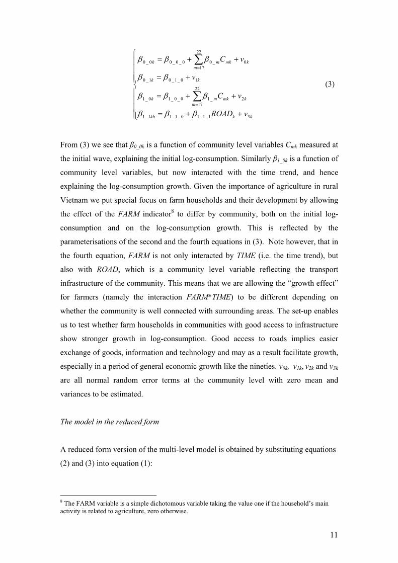
(3)

From (3) we see that β0_0k is a function of community level variables Cmk measured at

the initial wave, explaining the initial log-consumption. Similarly β1_0k is a function of

community level variables, but now interacted with the time trend, and hence

explaining the log-consumption growth. Given the importance of agriculture in rural

Vietnam we put special focus on farm households and their development by allowing

the effect of the FARM indicator8 to differ by community, both on the initial log-

consumption and on the log-consumption growth. This is reflected by the

parameterisations of the second and the fourth equations in (3). Note however, that in

the fourth equation, FARM is not only interacted by TIME (i.e. the time trend), but

also with ROAD, which is a community level variable reflecting the transport

infrastructure of the community. This means that we are allowing the “growth effect”

for farmers (namely the interaction FARM*TIME) to be different depending on

whether the community is well connected with surrounding areas. The set-up enables

us to test whether farm households in communities with good access to infrastructure

show stronger growth in log-consumption. Good access to roads implies easier

exchange of goods, information and technology and may as a result facilitate growth,

especially in a period of general economic growth like the nineties. v0k, v1k, v2k and v3k

are all normal random error terms at the community level with zero mean and

variances to be estimated.

The model in the reduced form

A reduced form version of the multi-level model is obtained by substituting equations

(2) and (3) into equation (1):

8 The FARM variable is a simple dichotomous variable taking the value one if the household’s main activity is related to agriculture, zero otherwise.

12

ijkjkkjkkkijkkjkjkijk

ijkjkk

ijkm

mkmijks

sjksijkjk

mmkm

ssjksjkijk

ijk

TIMEFARMvFARMvvTIMEvuue

TIMEFARMROAD

TIMECTIMEXTIMEFARM

CXFARMTIME

conumptionequivalentLog

*)(

**

* * *

) (

310210

1_1_1

22

17_1

16

2_10_1_1

22

17_0

16

2_00_1_00_0_10_0_0

+++++++

+

+++

++++

=

∑∑

∑∑

==

==

β

βββ

βββββ

(4)

The first three rows of the reduced form model can be thought of as the “fixed part”,

whereas the last one represents the “random part”. eijk is the idiosyncratic error, u0jk

refers to the household random intercept and v0k to the random intercept at the

community level. u1jk and v2k are the random components of the slope of the time

trend, respectively, at household and at community level9, v1k is the random

component of the slope of the FARM variable at community level, whereas v3k is the

random component of the slope of the interaction of FARM and TIME, again at the

community level. Consistent with the literature (see for example Skrondal and Rabe-

Hesketh, 2004), we allow the random effects at the same level to be correlated, while

random effects at different levels are assumed uncorrelated. The results from the

model estimation are presented in section 5.

4.2 A multi-level model for poverty dynamics

In this application we focus on why some households are able to escape poverty. We

limit therefore our sample to include households that were classified as poor in the

first wave. Thus, the analysis focuses on household and community determinants of

poverty exit. We specify a two level random intercept probit model, where the first

level is now the household (j) and the second is the community (k). We define the

following binary variable:

9 The global slope of TIME is β1_0_0+ u1jk +v2k. The fixed component is given by β1_0_0 (that represents the average slope over households and communities) and two random components given by u1jk and v2k (that represents, respectively, the deviation from β1_0_0 for the household jk and for the community k). Similar reasoning applies for the other random slopes.

13

⎪⎩

⎪⎨⎧

=

>==

otherwise poor"remain " 0

0Y if exit"poverty " 1 *jk

jkY

where Y* is an unobservable continuous variable that in our case could be interpreted

as the “ability” to escape out of poverty. We model the latent variable Y* using a two

level random intercept model

kjk

mmkm

ssjksjk

vu

CxY

++

Δ+Δ+= ∑∑==

20

17

16

10

* βββ (5)

Equation (5) is the reduced form specification of our model where the covariates are

constructed by taking the first difference of the original variables which were

measured at the first and second waves (both at household and community level).

As was the case in the growth model, equation (5) consists of a fixed part (the

first row) and a random component (the second row). ujk is the random error at the

household level, whereas vk is the community level random effect. We assume, as in

the classical probit model, ujk to be distributed as a standard normal, while vk is

assumed normal with zero mean and variance to be estimated.

4.3 Intra-class correlation coefficients

A useful way to demonstrate the importance of clustering, here at household and

community levels, is to decompose the total variability into between and within

clusters and to calculate intra-class correlation coefficients (ICC). In a simple two-

level random intercept model ICC gives the correlation between units belonging to the

same second level cluster and reflects therefore the “closeness” of observations in the

same cluster relative to the “closeness” of observations in different clusters. The ICC

for a two level model is defined as:

(6)

θ

ρ+

=ΨΨ

14

where ψ and θ are, respectively, the second and first level variances and ρ

corresponds to the proportion of the between cluster variance out of the total variance.

The higher is ρ the more important is the clustering. For a general l-level model, the

overall error term can be decomposed into l additive components, given the

assumption of independence between random effects belonging to different levels.

Section 5 reports the results together with the ICC calculations.

5 Results

In this section we report the parameter estimates of the growth and the poverty exit

models respectively. The discussion is in both cases preceded by the analysis of the

ICC calculations that makes evident the importance of clustering

Growth model

The decomposition of the total variability and ICC values for the growth model are

reported in Table 1. The calculations refer to two types of models: 1) a two level

model (including time and household levels) and 2) a three level model that also

includes the community level. The latter is represented by equation (4). Both models

are preceded by the null version, meaning that covariates are omitted. It is clear that

the cluster effects are considerable. It is important to note, however, from the first

column, that a large part (more than 50%) of the total variability is explained by the

time level. This is chiefly driven by the dramatic economic growth that took place

between the two waves.

The second column shows that the introducing covariates reduce both

variances at wave and household level10. In the third column we decompose the

variation at household level (shown in the first column) into the two components

reflecting 1) the household and 2) the community level.

10 We refer to the covariates included into the final model (see equation 4). They are covariates defined at time, household and community level. In general, the introduction of a covariate at a given level reduces the variability at that level, has an unpredictable effect on the variability at higher levels and has no effects on variability at lower levels .levels.

15

Table 1 – Variance decomposition and intra-class correlation coefficients for different specifications of the growth model

Level 2-levels null model

2-levels model

3-levels null model

3-levels model

Variance decomposition waves 0.1428 0.0798 0.1428 0.0798 household 0.1067 0.0812 0.0457 0.0471 community 0.0609 0.0394 Intra-class correlations

household 0.4277 *** (0.0142)

0.5043*** (0.0133)

community 0.2442*** (0.0266)

0.2372*** (0 .0271)

household, community 0.4277 *** (0.0233)

0.5211*** (0.0201)

Notes: Standard errors for ICC are calculated using delta method. This is a valid approximation since we have a sufficient number of clusters both at household and at community level. ***: Significant at 1% level.

The fourth column shows again that introducing covariates reduce the variances at

wave and community level, while the variance at household level is almost

unchanged. The calculations tell us that the community level variation is about 23%

of the total, while when we cumulate this with the household level we obtain the 52%

of the total variation. All in all this demonstrates the importance of the clustering,

justifying the use of a three level model.

The results of the growth model are presented in Table 2. The model is run

with and without standard error adjustment, but the difference is very small as

expected. To ease interpretation and help assessing the magnitude of the parameter

estimates we present the exponentiated estimate minus one which can be interpreted

as the effect of a unitary increase in a covariate on the relative variation of

consumption expenditure.

The time trend (i.e. TIME) reflects the average increase in consumption

between the two waves (17%). As expected its parameter estimate is positive and

highly significant. But the remaining estimates show that those who were relatively

better off initially were not necessarily benefiting from the economic boom of the

nineties (and vice versa of course) to the same extent. The estimate of the random part

16

shows a significant and negative correlation between the random intercept and the

random slope at household level. This suggests that households with high

consumption levels in 1993 experienced lower growth, on average, compared to those

starting at lower levels, and explains to a large extent why many of the coefficients

change sign when measured in the growth dimension (as opposed to the initial time

period). Whereas there were no significant differences between male and female

headed households in 1993, the latter fared worse during the nineties. In contrast the

Kinh ethnic origin (the main ethnic population in Vietnam), had higher expenditure

initially and excelled further during the nineties. Large households with many

children were associated with lower expenditure in 1993, but all of these households

benefited clearly from the economic growth.

Farm households clearly lost out during the nineties. Not only were they

associated with a lower expenditure in the initial wave (their consumption was about

14% lower than non farmers), their relative economic situation also worsened during

the nineties (their growth was 7% lower than that of non farmers). In contrast,

unskilled workers and those looking for work, both worse off in 1993, benefited in the

period leading up to 1998. These estimates are manifestations of the structural change

taking place in Vietnam during this period. In particular, these effects reflect a shift

from agriculture towards industrialisation, including the service industry, improving

the conditions for low skilled workers, but worsening the situation for farmers.

Whereas immigrant households were associated with higher levels of expenditure in

1993, our estimates show that during the nineties they lost out. The pattern is difficult

to explain. It is natural to think that migrants choose location according to job

prospects, services and infrastructures. They might also be privileged or have higher

human capital, which explains why they were better off. But it is somewhat difficult

to see why they were less effective in exploiting the opportunities arising during the

period of economic growth. Education also shows some mixed effects. Whereas

educational variables are all positively associated with higher consumption in 1993,

the growth effects are more ambiguous. Finally, there are some characteristics that

are important for the initial wave, but show no effect in the growth dimension. This

includes home ownership, and living in a dwelling with electricity, the latter being a

proxy of the household wealth.

As previously mentioned the Vietnam LSMS contains a wealth of community

variables. The multilevel model enables us to estimate their effects appropriately.

17

However, there is high correlation between these variables. For instance, the survey

includes several measures of the health facilities in the community, but including

several of them in a regression often leads to collinearity. As a result we include

variables capturing different dimensions of critical community characteristics. These

include education, proxied by whether there is a secondary school in the community,

health, here proxied by hospital, industrialisation measured by presence of a “big”

enterprise, the way agriculture is organised, measured by whether it is organised as a

cooperative or not, and, the number of large tractors – a proxy of agricultural

development. As is clear, educational infrastructure and presence of a large enterprise

has very little effect on household expenditure, whereas health facilities are associated

with a higher initial level of expenditure, but in the growth dimension there is no

significant effect. This is in contrast to variables reflecting the agricultural sector. Our

estimates show that communities dominated by cooperatives were less well off in

1993. The parameter is strong and highly significant, indicating that the difference in

household expenditure in these communities compared to those without cooperatives

was substantial. In contrast, households residing in communities with more modern

agriculture had clearly higher expenditure levels. Looking at the time interaction, we

see that the coefficients switch sign, implying that less modern agriculture

communities gained relatively more than those already enjoying more modern forms

of agriculture. So, though cooperative farming arrangements used less modern

technology, they have seemed well adept to exploit the opportunities following the

economic growth. As such, these households are clearly recovering and catching up,

but interestingly this recovery takes place at the community level.

The final interaction between farm households and ROAD, which is here a

proxy for the infrastructure of the community in which the farmer lives, shows an

interesting positive effect, suggesting that though farm households did not gain an

overall benefit, those residing in communities with easy access to roads and other

transport facilities, certainly did. This is an indication that the economic growth had

differential impact on farmers depending upon their community characteristics, in this

case obviously related to the available transport links to surrounding area.

Further differential effects for farmers are evident when we consider the random

effects. Recall that we have allowed for a random slope parameter for farmers in both

dimensions (i.e. the initial period and in growth). Both are significant, suggesting that

the farm initial status and growth differ significantly across communities. Hence, for a

18

correct interpretation of the parameters estimates for farm households we have also to

consider the standard deviation of this random effect. This analysis is elaborated in

Table 3.

We have also allowed for a correlation between the random terms. The

correlation between the random intercept at community level and the random slope

for FARM is very small and insignificant (-0.0043). The correlation between the

random slope of the interaction term between FARM and TIME, and, the random

intercept is also negative, but here more substantial although again not significant.

However, the meaning of this negative sign is that in poorer communities farmer

growth was higher.

The correlation between the random slope of farm variable and the one related

to the interaction of FARM and TIME is highly negative and significant, meaning that

those farm households which were relatively worse off initially in 1993, benefited

more during the nineties, relatively speaking, compared to those farm households that

were better off in the initial wave. In some sense this is an indication that ineffective

farms found it easier to expand and improve than farms that are already well off,

possibly having gained significant growth prior to 1993.

19

Table 2 - Random coefficient growth model.

INITIAL TIME PERIOD

(1993) INTERACTED WITH TIME

TREND

PARAMETER ESTIMATE

(β)

EFFECT ON THE

RELATIVE VARIATION

(eβ-1)

PARAMETER ESTIMATE

(β)

EFFECT ON THE

RELATIVE VARIATION

(eβ-1) HOUSEHOLD LEVEL Gender of Household head 0.0203 2.05 -0.0363** -3.56 (0.0170) (0.0178) Age of Household head 0.0082 0.82 0.0050 0.50 (0.0059) (0.0062) Ethnic origin is Kinh 0.0927*** 9.71 0.0491* 5.03 (0.0286) (0.0280) Household size -0.0477*** -4.66 0.0238*** 2.41 (0.0036) (0.0037) Percentage of children 0 - 4 -0.0016** -0.16 0.0026*** 0.26 (0.0007) (0.0007) Percentage of children 5 - 9 -0.0004 -0.04 0.0030*** 0.30 (0.0006) (0.0006) Percentage of workers -0.0015*** -0.15 0.0006 0.06 (0.0004) (0.0004) Months away for work per capita 0.0019 0.19 -0.0014 -0.14 (0.0051) (0.0053) Percentage of born elsewhere (immigrated) 0.0017*** 0.17 -0.0009*** -0.09 (0.0003) (0.0004) Farm household -0.1387*** -12.95 -0.0736* -7.10 (0.0228) (0.0438) Percentage with post compulsory education 0.0029*** 0.29 0.0009*** 0.09 (0.0003) (0.0003) Percentage unskilled -0.0023*** -0.23 0.0010** 0.10 (0.0004) (0.0005) Percentage ever attended school 0.0031*** 0.31 -0.0011* -0.11 (0.0006) (0.0006) Household literacy rate 0.0011* 0.11 -0.0002 -0.02 (0.0006) (0.0006) Percentage looking for work -0.0095*** -0.95 0.0101*** 1.02 (0.0027) (0.0028) Owner of dwelling 0.1138*** 12.05 -0.0349 -3.43 (0.0403) (0.0420) Dwelling has electricity 0.2156*** 24.06 -0.0235 -2.32 (0.0204) (0.0200) COMMUNITY LEVEL Lower secondary school 0.0048 0.48 0.0186 1.88 (0.0632) (0.0337) Hospital 0.1696* 18.48 -0.0693 -6.70 (0.0934) (0.0605) Big enterprise 0.0036 0.36 -0.0300 -2.96 (0.0427) (0.0254) Agricultural cooperative -0.3175*** -27.20 0.0685*** 7.09 (0.0448) (0.0265) Number of large tractors 0.0129*** 1.30 -0.0057*** -0.57

20

(0.0033) (0.0017) ROAD * FARM 0.1242*** 13.22 (0.0421) TIME 0.1570* 17.00 (0.0812) Constant 6.8708***

RANDOM PART

TIME LEVEL Residual error (sd) 0.1495 HOUSEHOLD LEVEL Random intercept (sd) 0.3232*** Random slope of TIME (sd) 0.3101**

-0.5336** Correlation between random slope of TIME and the random intercept COMMUNITY LEVEL Random intercept (sd) 0.1948*** Random slope of FARM (sd) 0.0979*** Random slope of TIME * FARM (sd) 0.1535***

Correlation between random slope of FARM and random intercept -0.0043

Correlation between random slope of TIME*

FARM and random intercept -0.1602 Correlation between random slope of FARM

and random slope of FARM * TIME -0.6223**

Notes: ***: Significant at 1% level; **: significant at 5% level; *: significant at 10% level. Significance of random effects are based on likelihood ratio tests. sd = standard deviation.

As we have seen, the estimated random effects are significant and should not be

ignored in the modelling. However, it is difficult to assess the magnitude or the

importance of these effects. As a result we calculate predicted levels of consumption

expenditure for a range of hypothetical values of the random intercepts. In Table 3 we

compare these predictions with the case where the random intercept is set to zero. For

random slopes, we compare two households with a unitary difference in the value of

the covariates. We can see that the effects are generally substantial, confirming their

importance for the modelling and also in terms of policy implications. For example,

the predicted consumption expenditure for a household with a value of 0.3232 of the

random intercept (equal to the estimated standard deviation of the random intercept) is

38% higher than those who have a random intercept equal to 0 (and hence a global

intercept equal to the average).

21

Table 3 – Sensitivity analysis of the impact of random effects Interpretation of random intercepts

Hypothetical values of the random intercept

Effect of random intercept in terms of percentage relative difference in household consumption compared to a value of zero.

Random intercept at household level (u0)

–2*sd(uo)= –0.6464 –1*sd(uo)= –0.3232 +1*sd(uo)= +0.3232 +2*sd(uo)= +0.6464

-47.61 -27.62 38.15 90.87

Random intercept at community level (v0)

–2*sd(vo)= –0.3896 –1*sd(vo)= –0.1948 +1*sd(vo)= +0.1948 +2*sd(vo)= +0.3896

-32.27 -17.70 21.51 47.64

Interpretation of random slopes

Some hypothetical values of the slope

Effect of an unitary difference in the covariate in terms of percentual relative difference in household consumption for different values of the slope

Slope of TIME (β1_0 + u1)

β1_0 – 2*sd(u1) = –0.4632 β1_0 – 1*sd(u1) = –0.1531 β1_0 – 1*sd(u1) = +0.1570 β1_0 + 1*sd(u1) = +0.4671 β1_0 + 2*sd(u1) = +0.7772

–37.07 –14.20 17.00 59.54 117.54

Slope of FARM (β0_1_0 + v1)

β0_1_0 – 2*sd(v1) = –0.3345 β0_1_0 – 2*sd(v1) = –0.2366 β0_1_0 – 2*sd(v1)= –0.1387 β0_1_0 + 1*sd(v1) = –0.0408 β0_1_0 + 2*sd(v1) = +0.0571

–28.43 –21.07 –12.95 –4.00 5.88

Slope of FARM*TIME (β1_1_0 + v2)

β1_1_0 – 2*sd(v2) = –0.3806 β1_1_0 – 1*sd(v2) = –0.2271 β1_1_0 – 1*sd(v2)= –0.0736 β1_1_0 + 1*sd(v2) = +0.0799 β1_1_0 + 2*sd(v2) = +0.2334

–31.65 –20.32 –7.10 8.32 26.29

Similarly, the predicted consumption expenditure for a household living in

communities with a random intercept equal to 0.1948 is 22% higher than consumption

for the reference household.

As far as random slopes are concerned, we observe that consumption growth

between the two waves varied considerably by households – the average growth being

17%. If we set the random slope of TIME to -0.4632, which is equivalent to minus

two times its standard deviations, we obtain a predicted growth of -37%. In contrast,

setting its value to plus two times its standard deviations we obtain a growth of 118%.

22

Also farmers’ relative conditions vary considerably by community. On average,

farmers’ expenditure was 13% lower than that of non farmers. However, it is clear

from Table 3 that many experienced even lower expenditure. For instance, by

imposing a negative value of the random effect (equivalent to minus one of the

standard deviation) produce an expenditure level that is 20% lower than non-farmers.

Obviously, the gap between farmers and non-farmers is smaller for lower values of

the random effect. Only for very large positive values of the random effect, do we

find farmers to be less poor than non-farmers. The policy implications are important,

in the sense that policy makers might want to consider the heterogeneity of farming

communities, bearing in mind that some fare considerably worse than others.

Poverty exit model

We start presenting, as above, variance decomposition and ICC calculations. In a

multilevel probit model we assume that the error at the first level is distributed as a

standardised normal random variable. The ICC is calculated as before but this is now

seen as the correlation between the latent responses instead of the correlation of the

outcomes. In the Table 4 we show ICC calculations for the two level model

represented by equation (5). Calculations are also made for the null version.

Introducing covariates reduce the community level variation. As a result, correlation

among households living in the same community (measured by the ICC) is lower but

still not negligible and significant. Hence, as for the growth model we can see that the

clustering effects, here only at community level, are considerable.

Table 4 – Variance decomposition and intra-class correlations for the poverty exit model

Level 2-levels null model 2-levels model

Variance decomposition Household 1.0000 1.0000 Community 0.4581 0.3723

Intra-class correlations

Community 0.3142 *** (0.0403)

0.2713*** (0.0415)

Notes: Standard errors for ICC are calculated using delta method. This is a valid approximation since we have a sufficient number of clusters at community level. ***: Significant at 1% level.

23

The results from the poverty exit model are presented in Table 5. Note that we

present here the specifications with and without the multilevel model. Since the probit

is non-linear, inclusion of the community level may also affect the parameter

estimates and not only the estimated standard errors as is in the linear case (i.e. the

growth model)11.

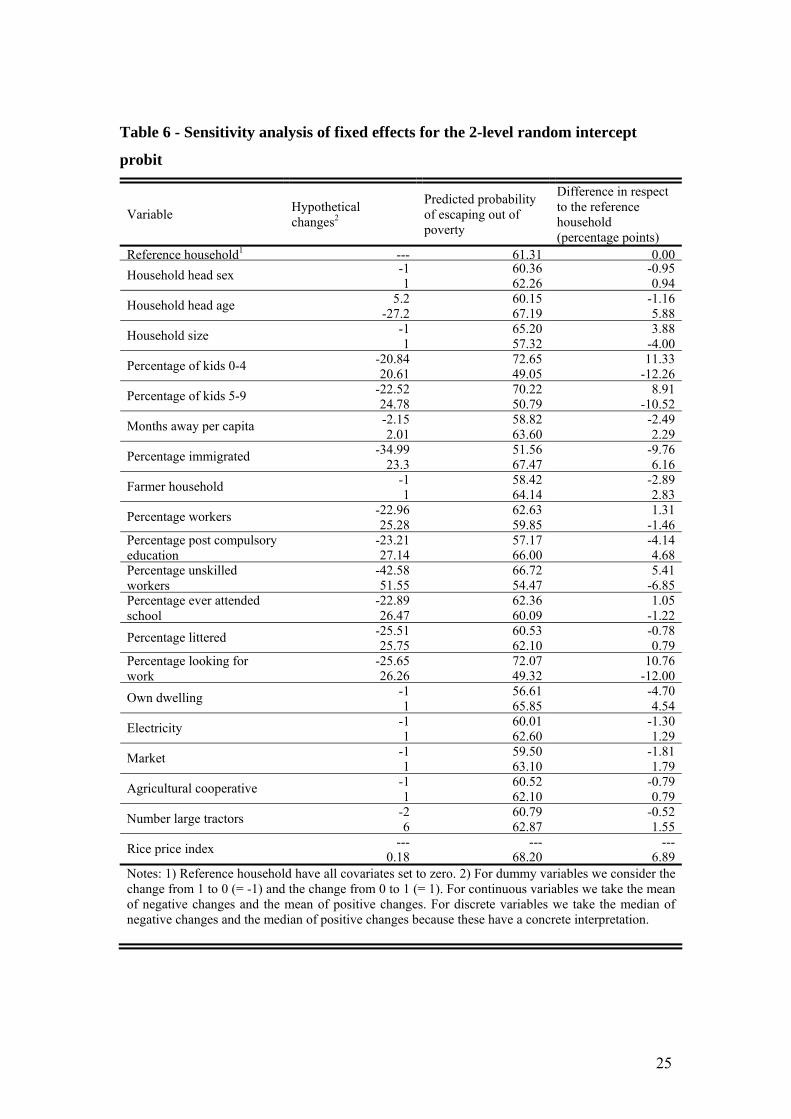
The nonlinearity of the probit model implies that calculated marginal effects

depend on the covariate values. To ease interpretation we compute predicted

probabilities for selected exemplificative households. These are presented in table 6.

We define a reference household where all covariates and the random effect are set to

zero. We then consider the effect on the predicted probabilities by changing the

covariate values. For binary variables we consider changes from 1 to 0 (= −1) and

from 0 to 1 (= +1). For continuous and discrete variables we considered respectively,

the mean and the median of the positive changes and the mean and the median of the

negative changes.

The results confirm many of the patterns found in the growth models, but there

are also interesting differences. Households with an increase in the percentage of

members with post compulsory education and members immigrating from elsewhere

have higher exit probabilities. In contrast, households increasing in size, increasing

percentage of children, and percentage of unskilled workers, generally find it harder

to escape poverty. From Table 6 we can see that the estimated probability of escaping

poverty for a household grown in size by one unit is four percentage points lower than

households having no change. In a similar way, households that experienced an

increase in the proportion of children aged between 0 and 4 years of 21% had an

estimated probability of escaping poverty of 12 percentage points lower than the

reference household As is clear, the model gives a different picture than the growth

model. There we showed that large households and households with many children

benefited during the nineties.

11 We also run these models with standard error adjustment controlling for additional cluster effects of communities and regions for the non multilevel probit model and regions for the 2-levels probit. Results are similar to those of the models presented in the table.

24

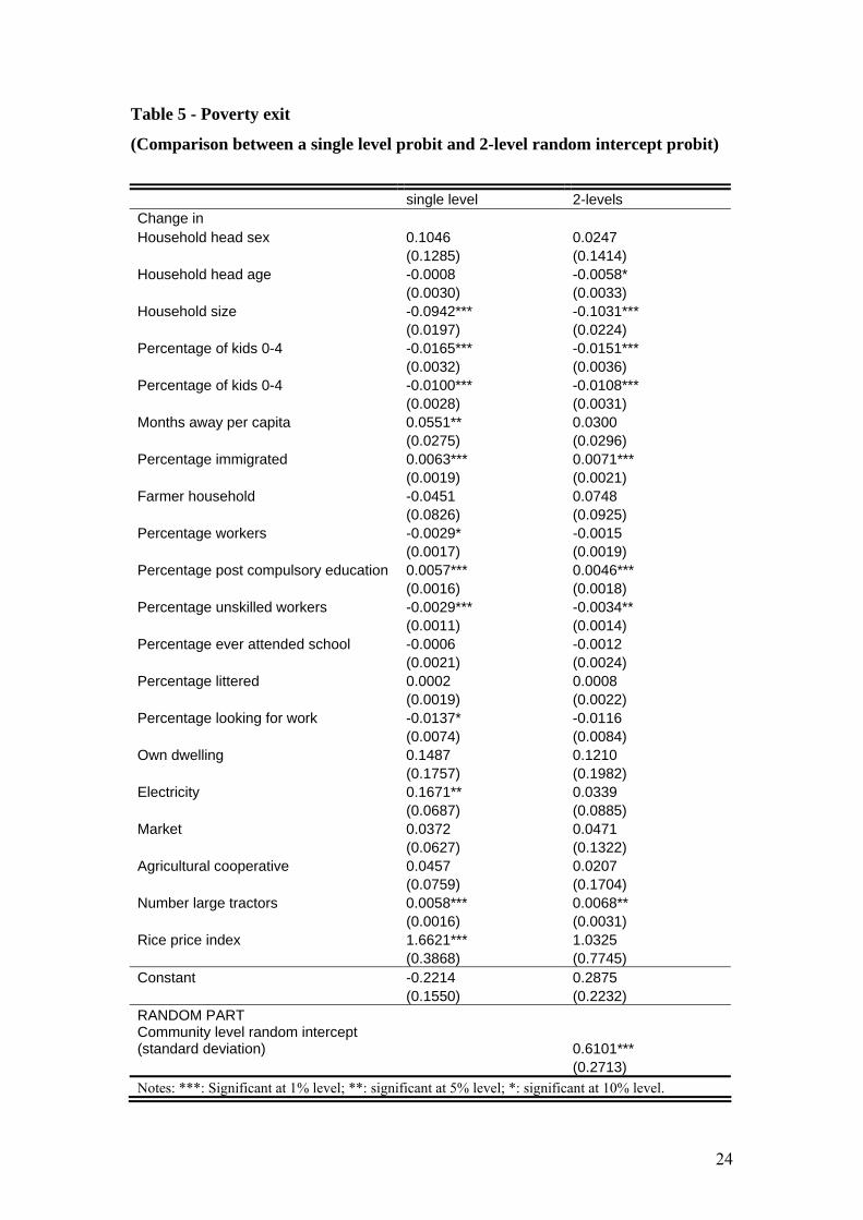
Table 5 - Poverty exit

(Comparison between a single level probit and 2-level random intercept probit)

single level 2-levels Change in Household head sex 0.1046 0.0247 (0.1285) (0.1414) Household head age -0.0008 -0.0058* (0.0030) (0.0033) Household size -0.0942*** -0.1031*** (0.0197) (0.0224) Percentage of kids 0-4 -0.0165*** -0.0151*** (0.0032) (0.0036) Percentage of kids 0-4 -0.0100*** -0.0108*** (0.0028) (0.0031) Months away per capita 0.0551** 0.0300 (0.0275) (0.0296) Percentage immigrated 0.0063*** 0.0071*** (0.0019) (0.0021) Farmer household -0.0451 0.0748 (0.0826) (0.0925) Percentage workers -0.0029* -0.0015 (0.0017) (0.0019) Percentage post compulsory education 0.0057*** 0.0046*** (0.0016) (0.0018) Percentage unskilled workers -0.0029*** -0.0034** (0.0011) (0.0014) Percentage ever attended school -0.0006 -0.0012 (0.0021) (0.0024) Percentage littered 0.0002 0.0008 (0.0019) (0.0022) Percentage looking for work -0.0137* -0.0116 (0.0074) (0.0084) Own dwelling 0.1487 0.1210 (0.1757) (0.1982) Electricity 0.1671** 0.0339 (0.0687) (0.0885) Market 0.0372 0.0471 (0.0627) (0.1322) Agricultural cooperative 0.0457 0.0207 (0.0759) (0.1704) Number large tractors 0.0058*** 0.0068** (0.0016) (0.0031) Rice price index 1.6621*** 1.0325 (0.3868) (0.7745) Constant -0.2214 0.2875 (0.1550) (0.2232) RANDOM PART Community level random intercept (standard deviation) 0.6101*** (0.2713) Notes: ***: Significant at 1% level; **: significant at 5% level; *: significant at 10% level.

25

Table 6 - Sensitivity analysis of fixed effects for the 2-level random intercept

probit

Variable Hypothetical changes2

Predicted probability of escaping out of poverty

Difference in respect to the reference household (percentage points)

Reference household1 --- 61.31 0.00-1 60.36 -0.95Household head sex 1 62.26 0.94

5.2 60.15 -1.16Household head age -27.2 67.19 5.88-1 65.20 3.88Household size 1 57.32 -4.00

-20.84 72.65 11.33Percentage of kids 0-4 20.61 49.05 -12.26-22.52 70.22 8.91Percentage of kids 5-9 24.78 50.79 -10.52-2.15 58.82 -2.49Months away per capita 2.01 63.60 2.29

-34.99 51.56 -9.76Percentage immigrated 23.3 67.47 6.16-1 58.42 -2.89Farmer household

1 64.14 2.83-22.96 62.63 1.31Percentage workers 25.28 59.85 -1.46-23.21 57.17 -4.14Percentage post compulsory

education 27.14 66.00 4.68-42.58 66.72 5.41Percentage unskilled

workers 51.55 54.47 -6.85-22.89 62.36 1.05Percentage ever attended

school 26.47 60.09 -1.22-25.51 60.53 -0.78Percentage littered 25.75 62.10 0.79-25.65 72.07 10.76Percentage looking for

work 26.26 49.32 -12.00-1 56.61 -4.70Own dwelling

1 65.85 4.54-1 60.01 -1.30Electricity

1 62.60 1.29-1 59.50 -1.81Market

1 63.10 1.79-1 60.52 -0.79Agricultural cooperative

1 62.10 0.79-2 60.79 -0.52Number large tractors 6 62.87 1.55--- --- ---Rice price index 0.18 68.20 6.89

Notes: 1) Reference household have all covariates set to zero. 2) For dummy variables we consider the change from 1 to 0 (= -1) and the change from 0 to 1 (= 1). For continuous variables we take the mean of negative changes and the mean of positive changes. For discrete variables we take the median of negative changes and the median of positive changes because these have a concrete interpretation.

26

However, this result should not be confused with the estimates of the poverty exit

model. Here we condition on the change in the covariates, which confirms that having

more children, is still negatively associated with escaping poverty. Consequently the

two models show two different dimensions of dynamics. The first shows that

relatively speaking large families improved their living conditions over the period,

whereas the poverty exit model shows that there is still a positive relationship

between having more children and poverty12. As for the community variables, we

found an increase in large tractors, generally reflecting increased modernity and

technical progress in the agricultural sector, is associated with a significant reduction

in poverty. Again holding these estimates up against those of the growth model,

demonstrate how the poverty exit model provides different and additional

information.

Many of the included variables are found to have little effect on exiting

poverty. We note however, that some of these variables only loose their significance

once the multi-level structure is controlled for. The most noticeable examples are

access to electricity and the rice price index, both losing their significance in the

multilevel model. The rice price index is simply a measure of the change in the rice

price specific to each community. The positive effect in the simple probit suggests

that households residing in communities where the rice price increased, with the

possible consequence of increased revenues among farmers that sell rice (which is a

large proportion of the sample), are able to escape poverty much easier than

households in other communities. In fact, it has been argued that the increase in rice

price has been one of the main contributors to reduce rural poverty in Vietnam during

the nineties (Huong et al, 2003; Niimi et al, 2003; Haughton et al, 2001). However, it

is well known that economic improvements are followed by higher inflation,

including rice price inflation. Controlling for such geographical variations, as we do

with the multilevel model, shows that the rice price itself played less of a role in

explaining poverty reduction. Unobserved factors operating at community level, such

as land quality (and hence rice quality), the accessibility to international markets and

so on, could also be associated with the rice price inflation. Of course, the multi-level

model will capture such unobserved factors, revealing the spurious nature of the

12 Note that while the growth model uses the whole sample, the probit model use only the sub-sample of households that was poor in 1993.

27

relationship found in the non multilevel model13. A similar argument applies for the

variable capturing access to electricity, as this variable also marks differences in

geographic specific growth patterns. It is clear that households gaining access to

electricity live in areas with reduced poverty. Again, the multilevel model suggests

that access to electricity by itself – is not a causal factor behind poverty reduction.

The two-level model includes only a community random intercept. It is highly

significant and important, as reflected by the ICC calculations. In Table 7 we asses the

importance of this random effect. As in the growth model, different values of the

random intercept produce very different predicted probabilities. Considering a

reference household where all covariates and the random effect are set to zero, we see

that subtracting two times the standard deviation from the random intercept give a

probability of escaping poverty of 17.5%, which is 43.7 percentage points lower than

the reference household. In contrast, adding two times its standard deviations gives a

probability of escaping poverty of 93.4%, which is 32.1 percentage points higher than

the reference household. These figures suggest of course, that the community where

the household resides matter considerably for poverty exit. The importance of the

community random effects are analysed further in the next section.

Table 7 - Sensitivity analysis of the random effect two-level probit model

Hypothethical value of the random intercept

Probability of escaping out of poverty

Difference in respect to the reference household (percentage points)

–2*sd(vo)= -1.2202 17.55 -43.76 –1*sd(vo)= -0.6101 37.35 -23.96 +1*sd(vo)= +0.6101 81.53 20.22

Random intercept at community level (v0)

+2*sd(vo)= +1.2202 93.42 32.10

13 Rice inflation is not the only key variable in this context. Glewwe et al (2002) argue that increased productivity in rice production was important, while Van de Walle (1996) argue that improvements in water irrigation were important for reducing poverty among farmers.

28

6 Policy analysis: Empirical Bayes predictions

In this section we develop a tool for better understanding the implications of the

estimated multilevel poverty exit model. As we have seen, the estimated random

effect is highly relevant, meaning that there is substantial variation in how

communities are able to cope in terms of economic progress and poverty reduction.

From the estimated model we are able to make predictions about the random

effect, and therefore compare communities14. There are two main statistical

approaches to assign values a posteriori to the random effects. The first uses a

Maximum Likelihood (ML) procedure where parameter estimates for the fixed part is

assumed known. The obtained estimates for the random effects are treated as

parameters to be estimated through maximising the likelihood function. The second

approach is based on Empirical Bayes (EB) predictions. In contrast to the ML

approach, EB uses information about the prior distribution of the random effects, in

addition to the observed responses. EB predictions are consequently the mean of the

posterior distribution of the random effect. In this case the random effects are treated

as proper random variables hence the term prediction is used in contraposition to ML

estimates. Since the posterior distribution is a compromise between the prior

distribution and the likelihood the EB lies between the ML estimates and the mean of

the prior. For linear models, EB predictions could be obtained from the ML estimates

using the formula:

(7)

where S)

is termed the shrinkage factor whose value is bounded by 0 and 1. S)

can be

thought of as a measure of the reliability of the ML estimator and depends on the

variance components and on the cluster size.

14 This kind of analysis is commonly found in the education literature, where the focus is on school performance (Aitkin et al, 1986; Goldstein and Thomas, 1996). Controlling for characteristics of schools, students, and class attributes, schools can be classified according to their effectiveness. In essence this is based on predictions about the unobserved heterogeneity at school level (random intercept). This allows the identification of the contribution of each school to the individual results of the pupils: a positive value indicates a school performance greater than the mean, vice versa a negative value.

SMLEB)

*∧∧

=

29

In the following analysis we apply the EB approach to the multilevel model of

poverty exit15. With this analysis we investigate the extent communities differed in

promoting poverty exit among its households. The random intercept at community

level represent the combined effect of all omitted covariates at community level that

cause some households to be more inclined to escape poverty than others according to

the place they live only. Consequently we use predictions of the random intercept to

produce a ranking of communities. As explained below, a ranking of regions is

possible taking the means of the predictions at community level by region.

Communities are ordered from the lowest (worst) prediction of the community

level random intercept to the highest (best). It is important to note that these

predictions control for household observed characteristics, which means that the

following analysis allow us to answer one of the key research question that arise in

multilevel research (Subramanian et al, 2003): are there significant contextual

differences among communities, after taking into account the compositional

characteristics of communities16?. Therefore a ranking based on these predictions is

more informative than the ones based on the row poverty exit rates or other similar

measures.

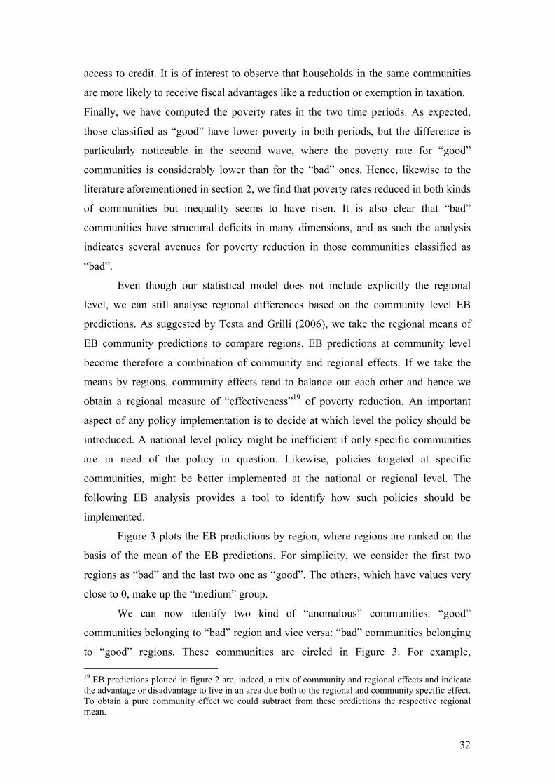
Figure 2 show these predictions with a 95% confidence interval for pair wise

comparisons based on comparative standard errors17. An overlap in terms of the

confidence intervals indicates that communities are not significantly different,

whereas non-overlap reflects that they are. For simplicity we make a classification of

communities into three groups: 1) bad, 2) medium and 3) good.

15 Similar analysis could be made for the growth model (or any other cross sectional model). Obviously the interpretations will change depending on the application and the model. In the growth model, the analysis would inform us whether certain communities were different in encouraging consumption growth for the households over the time period of the nineties. Analysis based on a cross sectional model, say for the 1993 wave, would investigate if communities were different in encouraging high living standard for households in 1993. Analysis of this kind could be based also on a random slope model instead of a simpler random intercept as in our case. But in this case the analysis becomes complex since intercept rankings change for the values of the variables given random coefficients. 16 In multilevel socio-economic research it’s important to distinguish between two sources of variation in the outcome at cluster level: contextual (relating to differences in specific areas’ characteristics) and compositional (relating to characteristics of the households or individuals living in different places). 17 We represent intervals centred on the EB predictions and with lengths equals to 2*1.39 times the comparative standard errors. These are the square root of the variances of the prediction errors (Skrondal and Rabe-Hesketh, 2004). They are referred to as the comparative standard errors because they can be used for inferences regarding differences between predictions of the random effects. They have to be distinguished from the sampling standard deviation that is the square root of sampling variance of the EB predictions distribution. These are referred as diagnostic standard errors since they can be used to find aberrant predictions.

30

Figure 2 – Empirical Bayes predictions at community level

Bad

Medium

Good

-2-1

01

2pr

edic

tion

0 20 40 60 80 100commune rank

Bad Medium Good

Figure shows 95% confidence intervals for pair wise comparisons (interval lengths are equals to 2 *

1.39 times the comparative standard errors and centred on the predictions)

The classification of the groups is of course somewhat arbitrary. We chose to include

into the “bad” and “good” group communities that had significantly different

predictions from each other (with no interval overlap)18. The “Medium” group

collects the remaining communities.

Based on this ranking we can now tabulate, and compare differences in a

range of characteristics of “good” and “bad” communities. Table 8 gives the results

for a range of variables, some of which are measured at the first wave, other at the

18 As we can see from the figure, none of the interval for “bad” communities overlaps with intervals of the “good” group and vice versa. Hence, we concentrate on the comparisons of these two groups whose communities are significantly different. We have to note that intervals completely below or up 0 are not necessarily related to predictions significantly different from 0 because intervals are based on comparative standard errors instead of diagnostic standard errors.

31

second, and some measuring the differences between the two waves. We presented

into the table only variables whose means are significantly different in the two groups.

Table 8 – Comparing characteristics of “bad” and “good” communities

Characteristic Mean “bad”

Mean “good” Difference

Principal ethnic group (Kinh = 1; W1) 0.65 1.00 -0.35***Principal religious group (Buddhists = 1; W1) 0.48 0.84 -0.36***Presence of road (Road is present =1; W1) 0.91 1.00 -0.09*** Road is impassable (W1) 0.39 0.15 0.24***Electricity (W1) 0.35 0.55 -0.20***Radio station (W1) 0.30 0.60 -0.30***Daily market (W1) 0.26 0.60 -0.34***Distance upper secondary school (W1) 9.54 5.80 3.74***Number of large tractors (W1) 0.83 2.65 -1.82***Use of fertiliser (W1) 0.91 1.00 -0.09***Percentage of households with a radio (W1) 38.43 53.10 -14.67***Percentage of households with a television (W1) 7.70 16.20 -8.50***School enrolment rate (age 11-14; W1) 3.65 6.80 -3.15***Manufacturing is present (W2) 0.43 0.70 -0.27***N. of households with subsidised credit (W2) 187.68 280.94 -93.26***N. of households with fiscal advantages (W2) 53.36 176.18 -122.82***Credit availability for non agric. investments (W2) 0.35 0.67 -0.32***Change in the Time to catch up a doctor (ΔW) 283.08 -63.33 364.41***Poverty rates (W1) 87.78 68.30 19.48***Poverty rates (W2) 74.91 25.70 52.02***Note: for quantitative variable we tested the difference between the means in the two groups. For binary variables we tested the difference between the percentages of 1s in the two groups. In both cases, we made one tail tests to verify if “good” communities have, on average, significantly better characteristics than “bad”.W1 = variable measured at first wave. W2 = wave measured at second wave. ΔW = variation between the two waves. Significance at *** 1%; ** 5%; * 10%.

Apart from ethnic and religious differences (here measured at the community level),

there are important structural gaps between “good” and “bad” communities. The

“good” communities are better in almost all dimensions, including infra structure,

education, communication, access to trading markets, and the technological level in

agriculture, the latter being particularly strong. They are also more likely to have

some manufacturing present in the community. The “good” communities

consequently perform better in community characteristics that reflect economic

outcomes. From the ones we included, we see that “good” communities have higher

educational enrolment and have better access to mass-communication, and better

32

access to credit. It is of interest to observe that households in the same communities

are more likely to receive fiscal advantages like a reduction or exemption in taxation.

Finally, we have computed the poverty rates in the two time periods. As expected,

those classified as “good” have lower poverty in both periods, but the difference is

particularly noticeable in the second wave, where the poverty rate for “good”

communities is considerably lower than for the “bad” ones. Hence, likewise to the

literature aforementioned in section 2, we find that poverty rates reduced in both kinds

of communities but inequality seems to have risen. It is also clear that “bad”

communities have structural deficits in many dimensions, and as such the analysis

indicates several avenues for poverty reduction in those communities classified as

“bad”.

Even though our statistical model does not include explicitly the regional

level, we can still analyse regional differences based on the community level EB

predictions. As suggested by Testa and Grilli (2006), we take the regional means of

EB community predictions to compare regions. EB predictions at community level

become therefore a combination of community and regional effects. If we take the

means by regions, community effects tend to balance out each other and hence we

obtain a regional measure of “effectiveness”19 of poverty reduction. An important

aspect of any policy implementation is to decide at which level the policy should be

introduced. A national level policy might be inefficient if only specific communities

are in need of the policy in question. Likewise, policies targeted at specific

communities, might be better implemented at the national or regional level. The

following EB analysis provides a tool to identify how such policies should be

implemented.

Figure 3 plots the EB predictions by region, where regions are ranked on the

basis of the mean of the EB predictions. For simplicity, we consider the first two

regions as “bad” and the last two one as “good”. The others, which have values very

close to 0, make up the “medium” group.

We can now identify two kind of “anomalous” communities: “good”

communities belonging to “bad” region and vice versa: “bad” communities belonging

to “good” regions. These communities are circled in Figure 3. For example, 19 EB predictions plotted in figure 2 are, indeed, a mix of community and regional effects and indicate the advantage or disadvantage to live in an area due both to the regional and community specific effect. To obtain a pure community effect we could subtract from these predictions the respective regional mean.

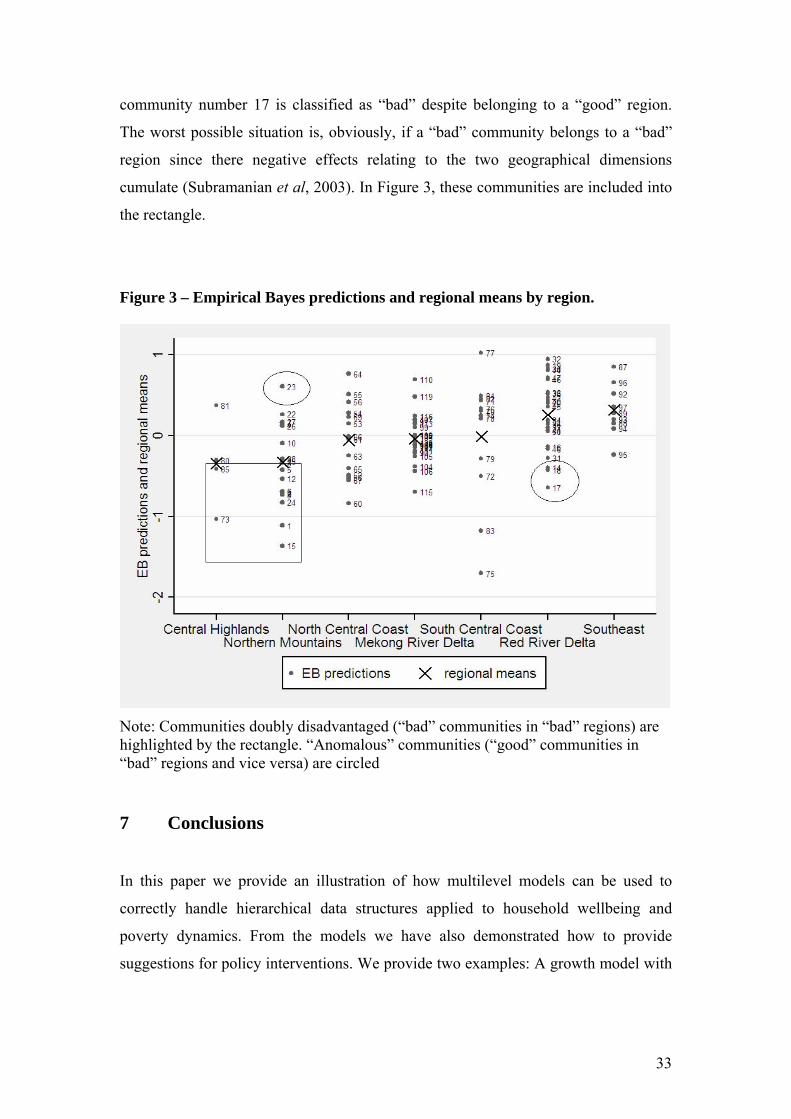
33

community number 17 is classified as “bad” despite belonging to a “good” region.

The worst possible situation is, obviously, if a “bad” community belongs to a “bad”

region since there negative effects relating to the two geographical dimensions

cumulate (Subramanian et al, 2003). In Figure 3, these communities are included into

the rectangle.

Figure 3 – Empirical Bayes predictions and regional means by region.

Note: Communities doubly disadvantaged (“bad” communities in “bad” regions) are highlighted by the rectangle. “Anomalous” communities (“good” communities in “bad” regions and vice versa) are circled 7 Conclusions

In this paper we provide an illustration of how multilevel models can be used to

correctly handle hierarchical data structures applied to household wellbeing and

poverty dynamics. From the models we have also demonstrated how to provide

suggestions for policy interventions. We provide two examples: A growth model with

34

a continuous dependent variable, the log equivalent household expenditure, and a

probit model for studying the determinants of poverty exit.

In both cases we found that the multilevel structure is highly relevant as

attested by the intra-class correlation coefficients. Hence, failing to control for the

multilevel structure will influence model predictions in significant ways, leading to

possibly incorrect inference about the effect of the covariates. Whereas an alternative

approach would be to simply use robust standard errors, this would omit essential

information about the multilevel structure relevant for policy analysis. Multilevel

models instead give us insight that is otherwise unfeasible in the more standard

methods.

The growth model separates the initial effect from the growth effect of the

covariates. The estimates related to the initial condition demonstrate that Kinh ethnic

origin, education, and living in a community with health facilities, are all associated

with higher wealth. In contrast, households with a high percentage of unemployed

members and those working in agricultural activities were disadvantaged. Also

household size and the number of children are negatively associated with

consumption expenditure. These effects are of course, sensitive to the equivalence

scale; we adopted here the well used WHO scale which is in line with many previous

studies.

The growth dimension of the model attests that, on average, household

consumption growth rate between the two waves was 17%, a reflection of the

economic boom experienced in Vietnam during the nineties. However, the growth

trend varied substantially by households and community characteristics. We find that

those who were better off initially were not necessarily the same benefiting during the

economic boom. For example, households with many children benefited from the

economic growth whereas farm households benefited less.

Since the Vietnam economy is dominated by rural activities, in particular

agriculture, and rural areas are the poorest, we focus our attention on farm

households. The model includes therefore random slopes that allow the effect of

agriculture to differ by community. Standard deviations of these random effects attest

that the place where farmers reside matters. Even though the average growth

differential for farmer in respect to non farmer was negative there were certain

communities in which farm households grew more. This is especially the case if the

community is well connected to other neighbourhoods through road links. The

35

poverty exit model highlighted that the key factors behind escaping poverty are in part

similar to those associated with higher consumption in the growth model.

An important benefit of the multilevel approach is that predictions can be used

to assess community and regional differences. These predictions produce groups of

communities that benefited from economic growth more than others, and

communities that in fact suffered during the period. Given these classifications it is

straight forward to investigate differences in characteristics, which is an important

tool for policy makers to target policies. Critical characteristics of a successful

community include key infrastructural or socio-economic variables such as the

availability of electricity and daily markets, school enrolment rates. These are clearly

important policy variables for further promoting poverty reduction. On the basis of

community level predictions, we also derived a ranking of regions. This identifies

which communities that performed badly in regions that performed well and vice

versa. Such analysis provides a critical tool for better targeting policy interventions.

36

References

Aitkin M., Longford N. (1986), Statistical modelling in school effectiveness studies

(with discussion), Journal of Royal Statistical Society A, Vol. 149, pp.1-42.

Balisacan A.M., Pernia E.M. and Estrada G.E.B. (2003), Economic Growth and

Poverty Reduction in Vietnam, in Poverty, Growth and Institutions in Developing

Asia, edited by Pernia E.M. and Deolalikar A.B., Hampshire, England: Palgrave

Macmillan Publishers.

Bryk A.S. and Raudenbush S.W. (1987), Application of hierarchical linear models to

assessing change, Psychological Bulletin, Vol. 101, pp.147-158.

Bruno M., Ravallion M., Squire L. (1999), Equity and Growth in Developing

Countries. Old and New Perspectives on the Policy Issues, World Bank Policy

Research, Working Paper No. 1563.

Coudouel A., Hentschel J., Wodon Q. (2002), Poverty Measurement and Analysis,

Poverty Reduction Strategy Paper Sourcebook, World Bank, Washington D.C.

Deaton A., Zaidi S. (2002), Guidelines for Constructing Consumption Aggregates for

Welfare Analysis, Living Standards Measurement Study Working Paper No. 135, The

World Bank.

Di Prete T.A. and Forristal J. D. (1994), Multilevel Models: Methods and Substance,

Annual Review of Sociology, Vol.20, pp.331-357.

Falaris E.M. (2003), The effect of survey attrition in longitudinal surveys: evidence

from Peru, Cote d’Ivoire, and Vietnam, Journal of Development Economics, Vol. 70,

pp.133-157.

37

Glewwe P., Gragnolati M. and Zaman H. (2002), Who Gained from Vietnam's Boom

in the 1990s? Economic Development and Cultural Change, 50(4), 773-792.

Goldstein H. (1995), Multilevel Statistical Models, Edward Arnold, London.

Goldstein H., Thomas S. (1996), Using examination results as indicators of school

and college performance, Journal of the Royal Statistical Society A, Vol.159, pp.149-

63.

Ghura D., Leite C. A., Tsangarides C. G. (2002), Is growth enough ? Macroeconomic

Policy and Poverty Reduction, IMF (International Monetary Fund) Working paper,

Wp/03/118.

Hox J.J. (1995), Applied Multilevel Analysis. Amsterdam: TT- Publikaties.

Haughton D., Haughton J., Phong N. (edited by) (2001), Living Standards during an

Economic Boom. Vietnam 1993-1998, Statistical Publishing House, Hanoi.

Huong P. L., Tuan B. Q., Minh D. H. (2003), Employment Poverty Linkages and

Policies for Pro-Poor Growth in Viet Nam, ILO Issues in Employment and Poverty,

Discussion Paper 9, Geneva.

Justino P. and Litchfield J. (2004), Welfare in Vietnam During the 1990s: Poverty,

Inequality and Poverty Dynamics, Journal of the Asian Pacific Economy, Vol. 9(2),

pp145-169.

Maas C.J.M. and Hox J.J. (2004), Robustness issues in multilevel regression analysis,

Statistica Neerlandica, Vol.58(2), pp.127–137.

Niimi Y., Vasudeva-Dutta P. and Winters A. (2003), Trade Liberalization and

Poverty Dynamics in Vietnam, PRUS Working Paper, No. 17, Poverty Research Unit

at Sussex, University of Sussex.

Ravallion M. and Bidani B. (1994), How robust is a poverty profile? World Bank

Economic Review, Vol.8(1), pp75-101.

38

Skrondal, A. and Rabe-Hesketh, S. (2004), Generalized Latent Variable Modelling:

Multilevel, Longitudinal and Structural Equation Models, Boca Raton, FL: Chapman

& Hall/CRC.

Snijders T.A.B. e Bosker R. J. (1999), Multilevel Analysis. An Introduction to Basic

and Advanced Multilevel Modelling, London: Sage.

Subramanian S. V., Jones K., Duncan C. (2003), Multilevel methods for public health

research, in Kawachi I, Berkman LF, eds. Neighborhoods and Health, New York:

Oxford University Press: 65-111.

Testa M. R., Grilli, L. (2006), The influence of childbearing regional contexts on ideal

family size in Europe: A multilevel analysis, Population, Vol. 61(1-2), pp107-137.

Van de Walle D. and Gunewardana D. (2001), Sources of ethnic inequality in

Vietnam, Journal of Development Economics, Vol. 65, pp177-207.

Van de Walle D. (1996), Infrastructure and Poverty in Vietnam, Living Standards

Measurement Study Working Paper No. 121, The World Bank Group, Washington

DC.

White H. and Masset E. (2003), Constructing the Poverty Profile: An Illustration of

the Importance of Allowing for Household Size and Composition in the Case of

Vietnam, Young Lives Working Paper No. 3, London: Young Lives and Save the

Children Fund UK.

White H. and Masset E. (2002), Child poverty in Vietnam: using adult equivalence

scales to estimate income-poverty for different age groups, MPRA Paper 777,

University Library of Munich, Germany.

World Bank (2000), Vietnam: Attacking Poverty - Vietnam Development Report 2000,

Joint Report of the Government-Donor-NGO Working Group, Hanoi.

39

Xuan T. D. (2000), Vietnam's Economy, After the Asian Economic Crisis, Asian-

Pacific Economic Literature, Vol. 14(1), pp36-43.