Dynamic Light Scattering of short Au–Rods with low aspect

Ratio

Jessica Rodrıguez-Fernandez, Jorge Perez–Juste, Luis M. Liz–Marzan, Peter R. Lang†

Departamento de Quımica Fısica and Unidad Asociada

CSIC- Universidade de Vigo, 36310, Vigo, Spain

† Forschungszentrum Julich, Institut fur Festkorperforschung;

Weiche Materie, D–52425 Julich, Germany

Abstract

The translational and rotational diffusion of a series of gold nanorods with low aspect ratio

was investigated by dynamic light scattering (DLS). It is shown that the translational and the

rotational diffusion coefficient can be determined because the particle shape causes an anisotropy

of the polarizability. This gives rise to two clearly distinguishable relaxation modes in the time

correlation function of the scattered light. The particle length and aspect ratio were determined

independently by transmission electron microscopy (TEM). Using a hydrodynamic model, these

geometrical parameters were converted to diffusion constants, which agree well with the values

determined by DLS. Additionally it is possible to obtain an estimate of the particles aspect ratio

from the amplitude ratio of the two relaxation modes.

1

Introduction

Metal nanoparticles have received a great deal of attention since the early times of Col-

loid Science, when Michael Faraday first observed the range of different colours that gold

colloids display as a function of size [1]. Since then, a plethora of studies have dealt with

the production and characterization of noble metal colloids in a wide range of sizes [2–4],

and for a variety of applications, including catalysis [5], biolabelling [6], biosensing [7], op-

tical switches [8], among others. Only recently, variations in nanoparticle shape have been

recognized as having a strong impact on their properties, which has motivated the develop-

ment of synthetical methods for the preparation of particles with various geometries, such

as rods [9–13], wires [14–16], prisms [17–21], cubes [22–24] and other polyhedrons [25, 26].

Most of these methods are based on wet chemistry reactions involving the reduction of

metal salts and the adsorption of surfactants or other molecules, generally known as cap-

ping agents. The mechanisms directing the growth of particles with a particular geometry

are still a matter of debate for most systems, but what is general is that they involve the

growth of pre-existing nuclei in solution and this leads to a random process that implies that

all particles are different, even in the most monodisperse samples. The characterization of

the dimensions for such a variety of shapes is usually carried out using electron microscopy

(EM), which implies the measurement of a large number (typically >100) of particles fol-

lowed by averaging. This provides values for average dimensions and polydispersity (usually

as standard deviation), but still is only representative of a limited population within the

sample, and therefore may not provide the real size distribution of the whole sample. Addi-

tionally, EM measurements are carried out on dry samples, under vacuum and irradiating

the specimen with high energy electron beams, which very likely affect the morphology and

dimensions of the particles. We have been working on gold nanorods for several years now,

with the objective to understand the mechanism underlying their formation [13, 27, 28] as

well as to understand and manipulate their extremely interesting, surface plasmon-related

optical properties [29–31].

In this context, we have identified the need to apply alternative characterization tech-

niques which overcome the mentioned drawbacks, i.e. techniques which probe a larger

amount of particles, do not require solvent evaporation, and do not modify the particles

themselves. Such requirements are fulfilled by scattering methods, which have been widely

and successfully used for other colloidal systems. Among the various scattering techniques,

light scattering is the one requiring a simpler setup and therefore it is available at many

laboratories. However, its use to characterize metal colloids in general and gold nanorods in

particular has not been very popular because of heating problems derived from absorption

of the laser beam, limited applicability of the Rayleigh-Gans-Debye approximation, small

particle sizes, and because models to analyze data for non-spherical particles seemed compli-

cated. In the literature dealing with dynamic light scattering of rod like particles, very often

the limiting case of rods with negligible anisotropy of the polarizability is considered, where

different scenarios have to be applied depending on the rod length, L. For systems where

the product of the scattering vector magnitude and rod length QL . 5 a single–exponential

decay of the correlation function of the scattered intensity g2(t) (ITCF) is expected, pro-

vided the rods are fairly monodisperse in length. In the case where QL > 10 additional

relaxation modes are observed in the correlation function. However, these cases are not

relevant for our systems, because (i) the anisotropy of the polarizability of gold nanorods is

not negligible, especially for particles with low aspect ratio [33], and (ii) the length of the

rods in our case lies typically in the 50 nm range, i. e. QL . 1. Nevertheless we clearly

observed two relaxation modes in the ITCF. To our knowledge, two relaxation modes in

the correlation function from rods smaller than 50 nm in length have been reported only

once [34], in a fluorescence correlation spectroscopy (FCS) experiment. However, in that

case the relaxation times of the relaxation mode which is ascribed to the translational dif-

fusion is larger by two orders of magnitude than in our case, even though the particles are

of comparable size. We therefore conjecture that long time diffusion has been observed in

that case, while we are investigating short time Brownian dynamics. Thus, the unexpected

appearance of two relaxation modes requires a thorough analysis.

An expression for the time auto correlation function for the scattered field can be ex-

tracted from the seminal work by Pecora [35], who showed that the spectral density of the

scattered light can be expressed as the sum of an isotropic and an anisotropic contribution.

Fourier transforming the spectral density gives the time dependence of the field auto corre-

lation function, from which g2(t) can be calculated using the Siegert relation. By non–linear

least squares fitting of this expression to our experimental data we determined the averaged

translational, D, and the rotational, Dr, diffusion coefficient of the Au–rods. Further we

could obtain an estimate of the particle aspect ratio from the relative amplitudes of the

ITCF. The paper is structured as follows. We describe the Au–rod synthesis, as well as the

data acquisition and analysis procedures in the experimental section, while the results from

dynamic light scattering are discussed and compared to transmission electron microscopy

(TEM) data in the results and discussion section. Finally we append a brief derivation of

the expression for the ITCF for the non-expert reader.

Experimental

Synthesis and characterization of Au–rods. A series of Au–nanorod samples (labelled as

Au-1 to Au-5) with different aspect ratios were prepared through a seeding growth method

first reported by Nikoobakht and El-Sayed [12] growing CTAB stabilized Au nanoparticle

seeds (<3 nm) by reduction of HAuCl4 with ascorbic acid in the presence of a BDAC/CTAB

mixture (in a 2.7 ratio) and a small amount of AgNO3. The aspect ratio was varied through

the amount of seed solution added (increasing from Au-1 to Au-5). Sample Au-6 was

synthesized according to the modification of the seeding growth method reported by Liu

and Guyot-Sionnest [32], where the reduction of HAuCl4 with ascorbic acid on the pre-

formed Au seeds in CTAB is carried out in the presence of HCl, to adjust the pH between 2

and 3. Tetrachloroauric acid (HAuCl4·3H2O), cetyltrimethylammonium bromide (CTAB),

benzyldimethylammonium chloride (BDAC), ascorbic acid, sodium borohydride (NaBH4),

AgNO3 and hydrochloric acid (HCl) were purchased from Aldrich and used as received.

Milli-Q water with a resistivity higher than 18.2 MΩ×cm was used in all of the preparations.

Optical characterization was carried out by UV-visible-NIR spectroscopy with a Cary

5000 UV-Vis-NIR spectrophotometer, using 10 mm path length quartz cuvettes. Transmis-

sion electron microscopy (TEM) images from all samples were obtained with a JEOL JEM

1010 transmission electron microscope operating at an acceleration voltage of 100 kV. In

the series from Au–1 through Au–5, the average aspect ratio of the particles was found to

increase from 4.2 to 5.5, as expected from the synthesis conditions. For the sample Au–6

the aspect ratio is 4.2 (see Table I).

Dynamic Light Scattering. Sample solutions for light scattering were prepared from the

original solution by repeated dilution steps with water, until the transmission of the solution

and that of water could not be distinguished any more at a wavelength of λ0 = 647nm. We

further checked that additional dilution by a factor of two did not change the relaxation

times of the time auto–correlation functions. In this case we may consider the solutions as

infinitely dilute.

Time–autocorrelation functions of the scattered intensity g2(Q, t) were recorded with a

standard DLS apparatus equipped with a Kr–ion laser (λ0 = 647nm) as a light source. The

scattering angle, θ, was varied from 40o to 130o in steps of 10o, accordingly the scattering

vector Q = 4πns sin(θ/2)/λ0 covered a range of 8.835 × 10−3nm < Q < 2.43 × 10−2nm.

The polarization state of incident and scattered light was controlled with a λ/2-plate and

a polarizer in the primary beam and an analyzer (all polarzing optics from Bernhard Halle

Nachfl, Berlin Germany) in the scattered beam. The scattered light was collected with

a monomode optical fiber (OZ-Optics, Ottawa, Canada) and detected with a SOSIP dual

photomultiplier unit by ALV Laservertriebsgesellschft mbH, Langen, Germany. The TTL

output of the avalanche diode was processed in the cross-correlation mode of a multiple

tau correlator, ALV-5000. The shortest delay time which is reliably accessible with this

detector–correlator combination is ≈ 100ns. For each sample, a complete angular set of

correlation functions was recorded in both vertical–vertical (V V ) and vertical–horizontal

(V H) geometry.

Data analysis. For the particular case of small particles with cylindrical shape and non–

negligible anisotropy of the polaraizability, expressions for the normalized intensity auto–

correlation functions measured in the V H– and V V –geometry are given by

gV V2 (Q, t) − 1 = β

[A2 exp −Γt+ 2AB exp −(Γ + ∆/2)t+ B2 exp −(Γ + ∆)t] (1)

gV H2 (Q, t) − 1 = β′ exp −(Γ + ∆)t (2)

respectively. Here Γ = 2DQ2 and ∆ = 12Dr, while A + B = 1 (see apendix for details).

The parameters β and β′ describe the non—ideal dynamical contrast of the light scattering

set up, and are slightly less than unity. According to eqs. 1 and 2 the standard procedure

to determine D and Dr is to plot the relaxation rate of gV H2 (t) − 1 vs. Q2. The intercept

of the resulting linear relation is 12Dr and the slope is 2D. Furthermore, a plot of the

relaxation rate of gV H2 (t À 1/6Dr) − 1 gives a linear relation with a slope of 2D and zero

intercept. We decided not to use this procedure for three reasons. First, the choice of

the threshold t À 1/6Dr could not be determined unambiguously from our data. Second,

as will turn out, the relaxation rate of gV H2 (t) − 1 does not depend significantly on the

scattering vector. This implies that 6Dr À D and that D cannot be determined with high

reliabilty from either of the two mentioned possibilities. Third, the determination of the

relaxation rates requires some kind of least squares fitting in any case. We therefore chose

to non–linear least squares fit the entire ITCFs by eqs. 2 and 1 to determine Dr and D.

This has the further advantage that also the amplitudes of the two relaxation modes can

be determined, which carry information on the aspect ratio of the particles. To achieve

the highest possible reliability of the best fitting parameters, we applied a global fitting

algorithm, in which we analyzed the complete set of of correlation functions obtained from

one sample simultaneously. In his procedure A, D and Dr were treated as global parameters,

while β and β′ were allowed to vary between different correlation functions.

Results and Discussion

The choice of samples for the measurements was based on a compromise among various

parameters. First, we intended to achieve a reasonably wide range of aspect ratios, and

whenever possible of particle size. However, in order to avoid excessive absorption of the

incident laser beam (647 nm), which would lead to significant local heating, the correspond-

ing transverse and longitudinal surface plasmon absorption bands should be located below

and above this wavelength, respectively. Another constraint was the need for the highest

monodispersity achievable in practice, which is mainly restricted to aspect ratios below 6.

Since low aspect ratios would involve high absorption at the wavelength of interest and high

aspect ratios lead to high polydispersity, we decided to concentrate on a relatively narrow

10-5 10-4 10-3 10-2 10-1 100 101

0.0

0.2

0.4

0.6

0.8

1.0

gVV

2(Q

,t)-1

t / ms

FIG. 1: ITCF from the sample Au–1 recorded in the V V -geometry. Different symbols refer to

different scattering angles. For the sake of clarity only three out of ten curves are displayed, i. e.

40o (¤), 90o () and 130o (M). Full lines are non linear least squares fits according to eq. 1

range of aspect ratios between 4.2 and 5.5. As described in Table 1, for aspect ratios be-

tween 4.4 and 5.5, the nanorod average length was maintained approximately constant, with

a systematic variation of the width, while for aspect ratio 4.2, two relatively different dimen-

sions were selected. The UV-vis-NIR spectra for all samples are shown in the Supporting

Information, together with representative TEM images.

Intensity auto–correlation functions (ITCF) obtained from the sample Au–1 recorded in

V V –geometry are displayed in Fig. 1. For clarity we have plotted only the curves from

three different scattering angles, namely 40o, 90o and 130o. It can be clearly seen that at all

different angles there are two relaxation modes, one of which becomes faster with increasing

θ, and one which is virtually independent of the scattering angle. Similarly the relaxation

times of the ITCF recorded in V H–geometry do not change with scattering angle. This is

10-5 10-4 10-3 10-2 10-1 100 101

0.0

0.2

0.4

0.6

0.8

1.0

gVH

2(t

)-1

t / ms

FIG. 2: ITCF from the sample Au–1 recorded in the V H-geometry. Different symbols refer to

different scattering angles. For the sake of clarity only three out of ten curves are displayed, i. e.

40o (¤), 90o () and 130o (M). Full lines are non linear least squares fits according to eq. 2

shown for the sample Au–1 in Fig. 2. This behavior is not expected at first glance from

eqs. 1 and 2, since all exponentials in these equations have relaxation rates which are linearly

proportional to Q2. On the other hand, if DQ2 ¿ Dr only the first term of eq. 1 depends

significantly on the scattering angle. This means that the slow relaxation mode in the V V

correlation functions is related to the translational diffusion of the rods alone while the fast

mode and the relaxation rates of the V H correlation functions are dominated by rotational

diffusion. Global fitting of the experimental ITCF as described in the experimental section

yielded the parameters listed in Table I. In this table we also list the geometrical particle

parameters, L and L/Dcs obtained from the analysis of TEM micrographs. The deviations

listed together with the data are reliability intervals from the fitting routine in case of the

diffusion coefficients. In the case of the parameters from TEM they represent standard

TABLE I: Mean translational, D, and rotational, Dr, diffusion coefficients measured by DLS of

gold rods in suspension, and rod lengths L as well as aspect ratios, L/dcs from TEM.

sample D Dr L L/dcs

nm2/ms ms−1 nm

Au–1 12200± 200 23.2± 0.6 45.9±6.3 4.2±1.1

Au–2 14100± 400 29.7± 0.3 38.2±5.9 4.4±0.9

Au–3 15200± 600 36.5± 1.2 38.4±5.0 4.6±1.0

Au–4 16300± 600 47.3± 0.9 37.5±5.4 5.2±1.1

Au–5 19000± 500 52.6± 0.3 37.3±5.7 5.5±1.2

Au–6 7100± 400 8.3± 0.7 60.6±10.4 4.2±0.8

100 nm

FIG. 3: TEM micrograph of sample Au–4.

deviation of the distribution of the corresponding parameter. As a representative example

we show a TEM-picture in Fig. 3

This micrograph shows that the rods have relatively narrow distribution both in length

and aspect ratio, which is confirmed by the standard deviations of the corresponding dis-

tributions, which are in the range of 15 % for the length and about 10% for the aspect

ratio. We also observe a small number of cubes, which is a general finding in these samples.

However, their relative amount is very low and thus they are not expected to contribute

significantly to the global scattering of the sample. Therefore we will consider the rods

to be monodisperse in the following discussion. A first approximation for the relation be-

tween geometrical parameters and diffusion constants of colloidal rods has been given by

Brørsma [36, 37], which however is sufficiently accurate only for rods with ln(L/dcs) > 2.

Since this requirement is not fulfilled for our Au–rods, we chose to apply the expression by

Ortega and de la Torre [38]

D =kBT (ln (L/dcs) + C)

3πηL

Dr =3kBT (ln (L/dcs) + Cr)

πηL3. (3)

Here C and Cr are second order polynomials in dcs/L, the coefficients of which have been

determined by fitting of numerical data.

C = 0.312 + 0.565dcs

L− 0.100

(dcs

L

)2

Cr = 0.662 + 0.917dcs

L− 0.05

(dcs

L

)2

. (4)

These equations apply to our particles, because they were derived for the ranges of 2 <

L/dcs < 20. In Table II we compare the diffusion coefficients measured by DLS with those

calculated with eqs. 3 and 4. Reasonable agreement between the experimental and the

calculated values could only be achieved by considering a double-layer of CTAB around the

rods, which stabilizes the particles by exposing the charged ammonium groups to the polar

solvent [39, 40] The thickness of this bilayer was estimated to be ca. 4 nm according to the

standard rule of thumb for the contour length of an alkane chain, i. e. lc = n × 0.126 +

0.154 nm [41], where n is the number of carbon atoms in the chain. A similar effect was

observed by van der Zande et al [42] for long gold rods (typically L > 200 nm and L/dcs >

10) which were sterically stabilized by an adsorbed polymer layer. These authors found

TABLE II: Mean translational, D, and rotational, Dr, diffusion coefficients measured by DLS,

and corresponding values, D∗ and D∗

r , calculated by using eqs. 3 through 4 and the geometrical

parameter listed in Table I. In addition, a stabilizing surfactant layer of 4 nm thickness was

accounted for.

sample D Dr D∗

D∗r

nm2/ms ms−1 nm2/ms ms−1

Au–1 12200 23.2 13900 19.4

Au–2 14100 29.7 16000 30.1

Au–3 15200 36.5 16200 30.4

Au–4 16300 47.3 17000 34.2

Au–5 19000 52.6 17300 35.4

Au–6 7100 8.3 11400 10.1

that the translational diffusion coefficients were up to a factor of four smaller than those

expected from the particles geometrical parameters. For the rotational diffusion coefficient

the discrepancy could even amount to almost an order of magnitude. This discrepancy was

assigned to the stabilizing polymer layer, which in this case had a thickness comparable to

the particles cross sectional diameter.

In the present study we find agreement between the calculated and the experimental

values within less than 20% for the rotational diffusion coefficient of the particles with an

aspect ratio smaller than 5. Only for the two samples with the largest aspect ratios the

discrepancy is ca. 30%. In the case of D the agreement is better than 15 % in most cases

with a slight tendency to decrease with increasing aspect ratio of the rods. This is probably

due to the fact that the theory by Ortega and Garcia de la Torre was devised for cylinders

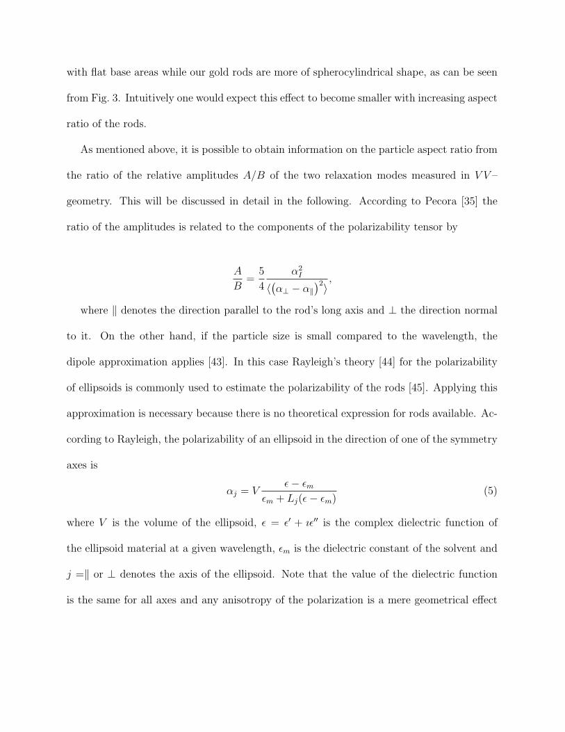
with flat base areas while our gold rods are more of spherocylindrical shape, as can be seen

from Fig. 3. Intuitively one would expect this effect to become smaller with increasing aspect

ratio of the rods.

As mentioned above, it is possible to obtain information on the particle aspect ratio from

the ratio of the relative amplitudes A/B of the two relaxation modes measured in V V –

geometry. This will be discussed in detail in the following. According to Pecora [35] the

ratio of the amplitudes is related to the components of the polarizability tensor by

A

B=

5

4

α2I

〈(α⊥ − α‖)2〉

,

where ‖ denotes the direction parallel to the rod’s long axis and ⊥ the direction normal

to it. On the other hand, if the particle size is small compared to the wavelength, the

dipole approximation applies [43]. In this case Rayleigh’s theory [44] for the polarizability

of ellipsoids is commonly used to estimate the polarizability of the rods [45]. Applying this

approximation is necessary because there is no theoretical expression for rods available. Ac-

cording to Rayleigh, the polarizability of an ellipsoid in the direction of one of the symmetry

axes is

αj = Vε− εm

εm + Lj(ε− εm)(5)

where V is the volume of the ellipsoid, ε = ε′ + ıε′′ is the complex dielectric function of

the ellipsoid material at a given wavelength, εm is the dielectric constant of the solvent and

j =‖ or ⊥ denotes the axis of the ellipsoid. Note that the value of the dielectric function

is the same for all axes and any anisotropy of the polarization is a mere geometrical effect

2 4 6 8 100

1

2

A/B

L/dcs

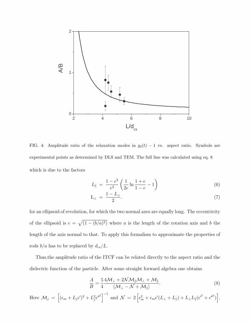
FIG. 4: Amplitude ratio of the relaxation modes in g2(t) − 1 vs. aspect ratio. Symbols are

experimental points as determined by DLS and TEM. The full line was calculated using eq. 8

which is due to the factors

L‖ =1− e2

e2

(1

2eln

1 + e

1− e− 1

)(6)

ÃL⊥ =1− L⊥

2. (7)

for an ellipsoid of revolution, for which the two normal axes are equally long. The eccentricity

of the ellipsoid is e =√

(1− (b/a)2) where a is the length of the rotation axis and b the

length of the axis normal to that. To apply this formalism to approximate the properties of

rods b/a has to be replaced by dcs/L.

Thus,the amplitude ratio of the ITCF can be related directly to the aspect ratio and the

dielectric function of the particle. After some straight forward algebra one obtains

A

B=

5

4

4M⊥ + 2NM‖M⊥ +M‖〈M⊥ −N +M‖〉 . (8)

Here Mj =[(εm + Ljε

′)2 + L2jε′′2

]−1

and N = 2[ε2m + εmε′(L⊥ + L‖) + L⊥L‖(ε′

2+ ε′′

2)].

With this expression we calculated the dependence of A/B on the particle aspect ratio,

which is shown in Fig. 4, together with the experimental data for A/B. For the values for

the dielectric function of gold at λ0 = 647 nm we used ε′ = −12.789 and ε′′ = 1.116 [46]and

for the solvent we took the value of water εm = n2 = 1.772. We find good qualitative

agreement between the calculated curve and the experimental data points. Generally the

theoretical curve is lying below the data points with an increasing deviation towards smaller

aspect ratios. This is probably due to the approximation of the rods’ polarizabilty, by that

of an ellipsoid. As the anisotropy of the polarizabilty is only due to the particle shape, this

approximation is expected to hold better for larger aspect ratios. Further, the single data

point which is lying below the theoretical curve corresponds to the sample Au–6, which is

significantly longer than the others. This might lead to reduction of A due to the influence

of the particle form factor P (Q).

Generally the above calculations show that the amplitude of the relaxation mode which

depends on the translational and the rotational diffusion coefficient, i. e. B become increas-

ingly dominating with respect to A, if the particle aspect ratio exceeds a value of 10. This

is obviously the reason why in the pioneering work by van der Zande et al [42] on dynamic

light scattering of gold rods, a single relaxation process of the ITCF was observed. These

authors had investigated only samples with L/dcs > 12 with dynamic light scattering. They

refrained from DLS measurements of the rods with smaller aspect ratios because of the high

polydispersity of their samples[47].

Conclusions

The auto–correlation function of the scattered intensity recorded in V V –geometry from

gold rods with small aspect ratio shows two distinct relaxation processes. Applying Pecora’s

expression for the correlation function we determined the translational and rotational diffu-

sion coefficients as well as the amplitudes of the individual relaxation modes. The diffusion

coefficients are in good agreement with the values calculated from the geometrical parame-

ters of the rods, if the thickness of the stabilizing surfactant bilayer is taken into account.

Further, we presented a path to estimate the aspect ratio of the particles from the ratio of

the relative amplitudes of the correlation function.

Acknowledgements

Part of this work was supported by the European Network of Excellence SoftComp which

is gratefully acknowledged. J.R.-F. acknowledges the Spanish Ministerio de Educacion y

Ciencia for granting an F.P.U. fellowship, and L.M.L.M. for funding through grant No.

MAT2004-02991. We thank Jan Dhont for helpful discussions.

Appendix: Time auto–correlation function, g1(t), of the scattered field.

In reference [35] Pecora showed that the spectral density of scattered light can be written

as the sum of an isotropic and an anisotropic contribution

I(Q,ω) = Iiso(Q,ω) + Ianiso(Q,ω). (9)

With

Iiso(Q,ω) =ρ

2πK2 cos2(φ) sin2(θ)α2

IP (Q)Siso(Q,ω) (10)

and

Ianiso(Q,ω) =ρ

30πK2

(3 + cos2(φ) sin2(θ)

)Saniso(Q,ω) (11)

where ρ is the particle number density, K is an optical contrast factor and αI = (2α⊥+α‖)/3.

The angle between the wave vector of the scattered light and the polarization vector of

the incident light is denoted θ, while φ is the angle between the polarizatoion vector of

the scattered light and the plane span by the wave vector of the scattered light and the

polarization vector of the incident light. Thus in V V –geometry cos2(φ) sin2(θ) = 1 and

cos2(φ) sin2(θ) = 0 in V H–geometry. The isotropic contribution to the dynamic structure

factor is given by the Lorentzian

Siso(Q,ω) =2Q2D

ω2 + (Q2D)2, (12)

while the anisotropic contribution consists of a sum of five Lorentzians. For the particularly

simple case of particles with cylindrical symmetry the latter reduces to

Saniso(Q,ω) =〈(α⊥ − α‖

)2〉3

2(Q2D + 6Dr)

ω2 + (Q2D + 6Dr)2, (13)

According to the Wiener–Khinchin theorem, the time auto–correlation function of the scat-

tered light is related by a Fourier transformation to the spectral density, thus

g1(t) = Siso(Q, t) + Saniso(Q, t). (14)

Consequently, we get for the normalized field auto-correlation function in V V –geometry

gV V1 (t) = A exp

−DQ2t

+ B exp−(DQ2 + 6Dr)

, (15)

with A = α2I/(α

2I + 〈(α⊥ − α‖

)2〉) and B = 415〈(α⊥ − α‖

)2〉/(α2I + 〈(α⊥ − α‖

)2〉). The

corresponding expression for V H–geometry is

gV H1 (t) = exp

−(DQ2 + 6Dr)

. (16)

Applying the Siegert–relation gives the final expressions of eqs. 1 and 2 which we used as

model functions for the analysis of our experimental data.

[1] Faraday, M. Philos. Trans. Royal Soc. London 1857, 147, 145.

[2] Frens, G. Nature 1973, 241, 20.

[3] Rodrıguez-Fernandez, J.; Perez-Juste, J.; Garcıa de Abajo, F. J.; Liz-Marzan, L. M. Langmuir

2006, 22, 7007.

[4] Evanoff, D. D. Jr.; Chumanov, G. J. Phys. Chem. B 2004, 108, 13948.

[5] Toshima, N., Metal nanoparticles for catalysis in Nanoscale Materials; Kluwer Academic

Publishers: Boston, 2003.

[6] Gittins, D. I.; Caruso, F. Chem. Phys. Chem. 2002, 3, 110.

[7] Lee, K.-S.; El-Sayed, M.A. J. Phys. Chem. B 2006, 110, 19220.

[8] Hu, M.-S.; Chen, H.-L.; Shen, C.-H.; Hong, L.-S.; Huang, B.-R.; Chen, K.-H.; Chen, L.-

C.Nature Mater. 2006, 5, 102.

[9] van der Zande, B. M. I.; Boehmer, M. R.; Fokkink, L. G. J.; Schoenenberger, C. J. Phys.

Chem. B 1997, 101, 852.

[10] Chang, S.-S.; Shih, C.-W.; Chen, C.-D.; Lai, W.-C.; Wang, C. R. C. Langmuir 1999, 15, 701.

[11] Busbee, B. D.; Obare, S. O.; Murphy, C. J. Adv. Mater. 2003, 15, 414.

[12] Nikoobakht, B.; El-Sayed, M. A. Chem. Mater. 2003, 15, 1957.

[13] Perez-Juste, J.; Liz-Marzan, L. M.; Carnie, S.; Chan, D. Y. C.; Mulvaney, P. Adv. Funct.

Mater. 2004, 14, 571.

[14] Sun, Y.; Gates, B.; Mayers, B.; Xia, Y. Nano Lett. 2002, 2, 165.

[15] Sun, Y.; Yin, Y.; Mayers, B. T.; Herricks, T.; Xia, Y. Chem. Mater. 2002, 714, 4736.

[16] Vasilev, K.; Zhu, T.; Wilms, M.; Gillies, G.; Lieberwirth, I.; Mittler, S.; Knoll, W; Kreiter,

M. Langmuir 2005 21 12399

[17] Jin, R.; Cao, Y.; Mirkin, C. A.; Kelly, K. L.; Schatz, G. C.; Zheng, J. G. Science 2001, 294,

1901.

[18] Pastoriza-Santos, I.; Liz-Marzan, L. M. Nano Lett. 2002, 2, 903.

[19] Sun, Y.; Xia, Y. Adv. Mater. 2003, 15, 695.

[20] Millstone, J. E.; Park, S.; Shuford, K. L.; Qin, L.; Schatz, G. C.; Mirkin, C. A. J. Am. Chem.

Soc. 2005, 127, 5312.

[21] Bastys, V.; Pastoriza-Santos, I.; Rodrıguez-Gonzalez, B.; Vaisnoras, R; Liz-Marzan, L. M.

Adv. Funct. Mater. 2006, 16, 766.

[22] Sun, Y.; Xia, Y. Science 2002, 298, 2176.

[23] Kim, F.; Connor, S.; Song, H.; Kuykendall, T.; Yang, P. Angew. Chem. Int. Ed. 2004, 43,

3673.

[24] Im, S. H.; Lee, Y. T.; Wiley, B.; Xia, Y. Angew. Chem. Int. Ed. 2005, 44, 2154.

[25] Wiley, B. J.; Xiong, Y.; Li, Z.-Y.; Yin, Y.; Xia, Y. Nano Lett. 2006, 6, 765.

[26] Sanchez-Iglesias, A.; Pastoriza-Santos, I.; Perez-Juste, J.; Rodrıguez-Gonzalez, B.; Garcıa de

Abajo, F. J.; Liz-Marzan, L. M. Adv. Mater. 2006, 18, 2529.

[27] Rodrıguez-Fernandez, J.; Perez-Juste, J.; Mulvaney, P.; Liz-Marzan, L. M. J. Phys. Chem. B

2005, 109, 14257.

[28] Grzelczak, M.; Perez-Juste, J.; Rodrıguez-Gonzalez, B.; Liz-Marzan, L. M. J. Mater. Chem.

2006, 16, 3946.

[29] Perez-Juste, J.; Rodrıguez-Gonzalez, B.; Mulvaney, P.; Liz-Marzan, L. M. Adv. Funct. Mater.

2005, 15, 1065.

[30] Correa-Duarte, M. A.; Perez-Juste, J.; Sanchez-Iglesias, A.; Giersig, M.; Liz-Marzan, L. M.

Angew. Chem. Int. Ed. 2005, 44, 4375.

[31] Pastoriza-Santos, I.; Perez-Juste, J.; Liz-Marzan, L. M. Chem. Mater. 2006, 18, 2465.

[32] Liu, M.; Guyot-Sionnest, P. J. Phys. Chem. B 2005, 109, 22192.

[33] Khlebtsov, N. G.; Melnikov, A. G.; Bogatyrev, V. A.; Dykman, L. A.; Alekseeva, A. V.;

Trachuk, L. A.; Khlebtsov, B. N. J. Phys. Chem. B 2005, 109, 13578.

[34] Pelton, M.; Liu, M; Kim, H. Y.; Smith, G.; Guyot–Sionnest, P.; Scherer, N. F. Optics Letters

2006, 31, 2075.

[35] Pecora, R. J. Chem. Phys. 1968, 49, 1036.

[36] Broersma, S. J. Chem. Phys. 1960, 32, 1626. 1960!. 12 S.

[37] Broersma, S. J. Chem. Phys. 1960, 32, 1632.

[38] Ortega, A.; Garcia de la Torre, J. J. Chem. Phys. 2003, 119, 9914.

[39] Gao, J.; Bender, C. M.; Murphy, C. J. Langmuir 2003, 19, 9065.

[40] Nikoobakht, B.; El-Sayed, M. A., Langmuir 2001, 17, 6368.

[41] Tanford, C. The Hydrophobic Effect ; Wiley: New York, 1973.

[42] van der Zande, B. M. I.; Dhont, J. K. G.; Bohmer, M. R.; Philipse, A. P.Langmuir 2000, 16,

459.

[43] Mie, G. Ann. d. Phys. 1908, 25, 377.

[44] Lord Rayleigh Phil. Mag. 1897, 44, 28.

[45] Perez-Juste, J.; Pastoriza-Santos, I.; Liz-Marzan, L. M.; Mulvany, P. Coord. Chem. Rev. 2005,

249, 1870.

[46] Johnson, P. B.; Christy, R. W. Phys. Rev. B 1972, 8, 4370.

[47] Dhont, J. K. G. personal communication.