Dynamic Human Resource Predictive Model for Complex ...

University of Tennessee, Knoxville University of Tennessee, Knoxville

TRACE: Tennessee Research and Creative TRACE: Tennessee Research and Creative

Exchange Exchange

Masters Theses Graduate School

8-2011

Dynamic Human Resource Predictive Model for Complex Dynamic Human Resource Predictive Model for Complex

Organizations Organizations

Tachapon Saengsureepornchai [email protected]

Follow this and additional works at: https://trace.tennessee.edu/utk_gradthes

Part of the Industrial Engineering Commons

Recommended Citation Recommended Citation Saengsureepornchai, Tachapon, "Dynamic Human Resource Predictive Model for Complex Organizations. " Master's Thesis, University of Tennessee, 2011. https://trace.tennessee.edu/utk_gradthes/1019

This Thesis is brought to you for free and open access by the Graduate School at TRACE: Tennessee Research and Creative Exchange. It has been accepted for inclusion in Masters Theses by an authorized administrator of TRACE: Tennessee Research and Creative Exchange. For more information, please contact [email protected].

https://trace.tennessee.edu/

https://trace.tennessee.edu/

https://trace.tennessee.edu/utk_gradthes

https://trace.tennessee.edu/utk-grad

https://trace.tennessee.edu/utk_gradthes?utm_source=trace.tennessee.edu%2Futk_gradthes%2F1019&utm_medium=PDF&utm_campaign=PDFCoverPages

http://network.bepress.com/hgg/discipline/307?utm_source=trace.tennessee.edu%2Futk_gradthes%2F1019&utm_medium=PDF&utm_campaign=PDFCoverPages

mailto:[email protected]

To the Graduate Council:

I am submitting herewith a thesis written by Tachapon Saengsureepornchai entitled "Dynamic

Human Resource Predictive Model for Complex Organizations." I have examined the final

electronic copy of this thesis for form and content and recommend that it be accepted in partial

fulfillment of the requirements for the degree of Master of Science, with a major in Industrial

Engineering.

Rupy Sawhney, Major Professor

We have read this thesis and recommend its acceptance:

Joseph Wilck, Gregory A. Sedrick

Accepted for the Council:

Carolyn R. Hodges

Vice Provost and Dean of the Graduate School

(Original signatures are on file with official student records.)

Dynamic Human Resource Predictive Model for Complex Organizations

A Thesis Presented for The Master of Science Degree

The University of Tennessee, Knoxville

Tachapon Saengsureepornchai August 2011

ii

Copyright © 2011 by Tachapon Saengsureepornchai

All rights reserved.

iii

ACKNOWLEDGEMENTS

I would like to thank my advisor, Dr.Rupy Sawhney, for all his tremendous

assistance and guidance. His high expectations and continuous support are

greatly appreciated. I am also grateful to my other committee members, Dr.

Joe Wilck and Dr. Greg Sedrick for their constructive criticism. Finally, I would

like to thank Mr. William Dan Davis and Mr. Steve Abercrombie for working

closely with me during my model test on the sample data to test the model.

I would like to thank all my friends, Sasima, Narapat, Bharadwaj, Gagan,

Amoldeep, Sashi, Ernest, Anna and Prasanna who were supportive and

helped enthusiastically in completion of my thesis.

Finally, I am very grateful to my parents and my family for their support and

constant encouragement throughout my time at University of Tennessee.

iv

ABSTRACT

Every organization has to deal with planning of the appropriate level of human

resources over time. The workforce is not always aligned with the

requirements of the organization and it increases an organization‟s budget. A

literature review reveals that there is no model that can systematically predict

accurate human resource required within a complex organization. To address

this gap, a human resource predictive model was developed based on

material requirements planning (MRP). This approach accounts for

complexity in workforce planning and generalized it with a logistic regression

model. The model estimates the employee turnover number and forecasts the

expected remaining headcount for the next time period based on employee

information such as; age, working year, salary, etc. Moreover, external

variables and economic data can be utilized to adjust the estimated turnover

probability. This model also suggests the possible internal workforce

movement in case of in-house manpower imbalance.

v

TABLE OF CONTENTS

Chapter Page

CHAPTER I .................................................................................................................. 1

Introduction and General Information .......................................................................... 1

1.1 Introduction ......................................................................................................... 1

1.1.1 Overstaffing ................................................................................................. 1

1.1.2 Insufficient Workforce ................................................................................. 2

1.2 Problem Statement .............................................................................................. 3

1.3 Conceptual Framework ....................................................................................... 4

1.4 General Approach ............................................................................................... 6

1.5 Organization of Thesis ........................................................................................ 9

CHAPTER II ............................................................................................................... 10

Literature Review........................................................................................................ 10

2.1 Human Resource Planning ................................................................................ 10

2.2 Employee Withdrawal and Variables ............................................................... 14

CHAPTER III ............................................................................................................. 19

Materials and Methods ................................................................................................ 19

3.1 General Approach of Human-Resource Planning ............................................. 20

3.2 Prediction of Voluntary Workforce Withdrawal .............................................. 23

CHAPTER IV ............................................................................................................. 36

Results and Discussion ............................................................................................... 36

vi

CHAPTER V .............................................................................................................. 50

Conclusions and Recommendations ........................................................................... 50

5.1 Summary of Research ....................................................................................... 50

5.2 Future Work ...................................................................................................... 51

LIST OF REFERENCES ............................................................................................ 53

APPENDICES ............................................................................................................ 60

Appendix 1 .............................................................................................................. 61

Withdrawal Prediction Coefficients for Manager ............................................... 61

Withdrawal Prediction Coefficients for Manager (con’t) ................................... 61

Withdrawal Prediction Coefficients for Craftsman ............................................ 62

Withdrawal Prediction Coefficients for Craftsman (con’t) ................................ 62

Appendix 2 .............................................................................................................. 63

Program Source Code in Microsoft Excel Marco ............................................... 63

Appendix 3 .............................................................................................................. 73

Comparison Table between Predicted HC’ and Actual HC’ .............................. 73

VITA ....................................................................................................................... 74

vii

LIST OF TABLES

Table Page

Table 1: Summary of Literature Review on Human Resource Planning ......... 11

Table 2: Sample of the data-gathering worksheet ............................................. 24

Table 3: Critical Predictor Identification Worksheet ............................................ 28

Table 4: Regression Coefficients Worksheet ...................................................... 32

Table 5: Sample of the Final Results and Recommendations .......................... 32

Table 6: Example of Time Period Indication ........................................................ 40

Table 7: Result Verification ..................................................................................... 44

Table 8: Final Combinations of Predictors ........................................................... 45

Table 9: Logistic Regression Predictive Model ................................................... 46

Table 10: HR Approach for Manager Group ........................................................ 47

Table 11: HR Approach for Craftsman Group ..................................................... 48

Table 12: HR Approach for 14 Job Titles ............................................................. 49

viii

LIST OF FIGURES

Figure Page

Figure 1: Components and Relationships of the HR planning model ................ 6

Figure 2: General Approach ..................................................................................... 8

Figure 3: Human resource Planning General Approach .................................... 22

Figure 4: Incompatibility of Predicted Data from Linear Regression and Actual

Data in Retirement Eligible Employee .......................................................... 29

Figure 5: Incompatibility of Predicted Data from Linear Regression and Actual

Data in Retirement Ineligible Employee ....................................................... 29

Figure 6: Screen Shot of Start Page ..................................................................... 34

Figure 7: Screen Shot of RAW.xlsx ....................................................................... 34

Figure 8: Screen Shot of Result Worksheet ........................................................ 35

Figure 9: Interaction between YCS and Age ....................................................... 41

Figure 10: Demographic Decomposition by Employee's Age ........................... 43

1

CHAPTER I

INTRODUCTION AND GENERAL INFORMATION

1.1 Introduction

In today‟s dynamic business environment, organizations often experience

great stress when determining an appropriate level of their workforce.

An adequate workforce is critical to the smooth functioning of any

organization. Thus, a systematic approach to monitor, manage and accurately

estimate the correct number of employees is essential for the healthy

functioning of the organization. The two most basic problems arising out of a

misaligned workforce are overstaffing and its opposite, an insufficient

workforce. The following sections discuss the relevance of these issues in

detail.

1.1.1 Overstaffing

This section describes and illustrates the issue of overstaffing. The recent

economic downturn has resulted in U.S. unemployment rates that increased

dramatically from 4.5 percent in 2000 to 9.6 percent in 2010 (Statistics, 2010).

Many organizations have opted to cut their nonessential workers in order to

produce a quick, budget-saving response to the financial crisis. However,

cutting nonessential workers presupposes that these organizations already

2

had a chronic overstaffing problem, or they would not have been able to make

the cuts; during favorable economic times, more and more employees had

been hired, perhaps without management‟s explicit consciousness of the

actual workforce demand. In fact, many authors have reported on overstaffing

both in public and private organizations (Borcherding, Pommerehne, &

Schneider, 1982; Clarke & Pitelis, 1993; Hart, Shleifer, & Vishny, 1997;

Haskel & Szymanski, 1993).

Overstaffing in companies usually entails excessive human-capital costs

along with the expense of providing the extra staff with facilities such as office

spaces, parking space, and IT resources. Downsizing does indeed provide

organizations with a quick way to reduce costs. However, a sudden reduction

in workforce can cause indelible trauma to the morale of the workforce (Noer,

1993). It can also damage an organization‟s core ability to compete. (Trevor &

Nyberg, 2008). For example, if an organization reduces headcount from an

oversized workforce to a certain level without monitoring the turnover rate and

workforce competence, the company‟s workforce may eventually prove

inadequate (Cascio, 1993; Sturman, Trevor, Boudreau, & Gerhart, 2003).

1.1.2 Insufficient Workforce

This section describes the situation when organizations have an insufficient

workforce. One problem with an inadequate workforce in some types of

3

companies is late delivery. The costs associated with delivery delays are

enormous and may, over time result in a loss of market share. Another

example can be found in the U.S. health-care system, where there are

continual risks of workforce shortage across the entire spectrum of the

system, from nurses to primary physicians to highly trained surgeons. The

number of general surgeons (who play a crucial role in the country‟s health-

care system) has begun to drop in recent years, while the U.S. population as

a whole has kept increasing (Kwakwa & Jonasson, 2001). As a result, more

patients have to wait outside emergency rooms in the hospitals. This problem

is apparent in such subspecialties as dermatological services. Multiple

surveys have documented a stable undersupply of dermatological services

since 1999 (Kimball & Resneck Jr, 2008) resulting in new patients having to

wait an average of 33 days for an appointment.

The ability to systematically detect an oversized or undersized workforce

based on dynamic workforce management system would make contemporary

organizations more competitive.

1.2 Problem Statement

A 1993 Society for Human Resources Management (SHRM) survey found

that six out of ten companies had no strategy for planning their workforce

(Lavelle, 2007). In fact, organizations generally treat recruitment as a reactive

4

event, responding to the need to fill either a new position or one that has been

left open. This reactive approach will, over time, create a misalignment

between the number of employees and the workforce requirement, especially

when the process of hiring and training new employees requires large lead

times. It is probable that a predictive model would alleviate this concern to

some extent. Mobley et al. (1979) reviewed the studies of variables or factors

that impact workforce withdrawal, but to date, no predictive model has been

developed to help organizations manage their workforces. This leads to a

precarious imbalance between organizational goals, budgets, employee

morale, and overheads over the long term.

1.3 Conceptual Framework

The conceptual framework of this study, as shown in Figure 1, aims to provide

a general approach to developing a Human Resource Predictive Model

(HRPM). This framework is based on the logic used in Material Requirement

Planning (MRP) systems for controlling physical inventory. This HRPM

consists of two modules: Gross Workforce Demand (D) and Workforce

Availability (HC‟)

This study anticipates that a given organization has the ability to forecast the

value of D (Gross Workforce Demand), based on the techniques shown

below. This thesis will utilize the available data and apply it to the workforce-

planning model to generate the predictions.

5

Gross Workforce Demand (D): The techniques for determining “D” can

be classified into six major categories (Ward, 1996):

o Direct managerial input,

o Best guess

o Historical ratios

o Process analysis

o Statistical methods

o Scenario analysis.

Workforce Availability (HC‟): The functioning of HC‟ requires

knowledge about the existing workforce (known information) and about

workforce leaving (predicted information). It is important to enter

accurate information about each component in order to enhance

planning reliability. A literature review reveals that there is no strong

evidence to recommend a predictive model of employee voluntary

withdrawal. Therefore how can an organization predict employee

turnover so as to balance organizational goals, budgets, employee

morale, and overheads over the long term? This study focuses on the

determination of an optimal approach to predicting voluntary

withdrawal of workforce and hence to developing a systematic

workforce planning model.

6

Figure 1: Components and Relationships of the HR planning model

In Figure 1, the highlighted portions are of active interest in this study. As

mentioned earlier, the “D” data is given. This approach, when applied to an

organization‟s human resource planning, is expected to encourage

awareness of the workforce dynamic, allowing a human resource team to

understand their workforce‟s current and future status and situation.

1.4 General Approach

This HRPM was developed in two major phases, as shown in Figure 2. The

first phase consisted of three activities:

A literature search on human resource planning models;

The development of an HRPM;

Existing

Workforce

Workforce

Leaving

Available

Workforce

Gross Workforce

Requirement

Human Resource

Planning Model

Component Module Model

7

The identification of the critical information, required to form a

systematical planning approach.

In the second phase, a mathematical prediction model was developed. This

phase consisted of four steps:

In the first step, the data was received from the organization and

organized to be fed into the model;

In the second step, the significant predictors were identified based on

the least MPAE (Mean Percentage Absolute Error);

In the third step, regression was performed to develop a staffing

equation;

As the final step, the results were justified and validated by testing the

model on holdout data.1

1 The last few data points, removed from a given data series, are called “holdout” data. The remaining

historical data series is called “in-sample” data; the holdout data is also called “out-of-sample” data.

8

Figure 2: General Approach

9

1.5 Organization of Thesis

This thesis is presented in five chapters. A brief description of each chapter is

presented below;

Chapter I consists of the introduction, the problem statement, the

conceptual framework, the general approach, and the organization of

the thesis;

Chapter II includes a literature review of existing human resource

planning and the elements of prediction. It also includes a study of

predictors for employee withdrawal;

Chapter III describes the methodology used to identify significant

predictors and to perform the regression analysis;

Chapter IV presents the implementation of the planning model; and

Chapter V contains the conclusions and indications for future work.

10

CHAPTER II

LITERATURE REVIEW

This chapter provides the results of a literature search focusing on two groups

of workforce studies. The first group of studies concentrates on approaches

related to workforce alignments and workforce planning strategies. The

second group of studies focuses on studies related to techniques for the

prediction of personnel withdrawal behavior and variables associated with it;

these techniques are used to enhance the reliability of planning.

2.1 Human Resource Planning

Workforce planning is designed to ensure that an organization prepares for its

present and future workforce needs by having “the right people in the right

places at the right time” (Jacobson, 2010). Human Resources (HR) refers to

individuals who make up the workforce of an organization (Kelly, 2001). The

human resource department in an organization is generally charged with

implementing strategies and policies relating to workforce management.

Successful human resource planning plays a crucial role in the reinforcement

of business strategy performance (F. H. Lee, Lee, & Wu, 2010). The

competitiveness of organizations relies on having the appropriate number of

employees in order to enhance the organization‟s capabilities and efficiency

11

(Lopez-Cabrales, Valle, & Herrero, 2006). Although the human resource team

is a critical player in developing and supporting the human resource planning

structure in organizations, the ownership of the plan belongs to top

administrators and managers (Keel, 2006). Over the years, many techniques,

models and methods have been used to identify appropriate workforce

requirements. Table 1 shows a brief summary of the literature review and

describes the main human resource planning methodologies, followed by the

details of each work reviewed.

Table 1: Summary of Literature Review on Human Resource Planning

Author(s) Methods Year

Kwak and Lee

Linear goal programming 1997

Hendriks et al.

Rough-cut project and portfolio planning 1999

Kwak Fuzzy set approach 2003

Jacobson Comparison of several different structures of important workforce planning models in the past.

2010

Größler and Zock

System dynamic model 2010

Barber and Lopez-Valcarcel

Simulation 2010

Kwak and Lee (1997) introduced the technique of linear goal

programming in a micro-management program (S. M. Lee & Shim,

1986) for workforce scheduling in health care, with the goal of

assigning personnel to proper shift hours. The constraints of the model

12

were constructed based on working procedure regulations such as

physician-nurse ratios in order to minimize total payroll costs and

maximize manpower utilization.

Hendriks et al. (1999) proposed five elements to set up an adequate

resource-allocation process by using a rough-cut project and portfolio

planning method (Platje, Seidel, & Wadman, 1994). They divided the

planning into three stages or elements: “long term” (5-year planning),

“medium term” (±1-year planning) and “short term” (±5-week planning).

Each stage served different purposes and was connected by two

elements: the “link” and the “response.” The output of one stage

served as the input of the other stages. The “response” stage monitors

and evaluates the “link” between two stages. This feedback improved

overall planning by adjusting the result over time.

Kwak (2003) found that goal programming could not handle the

organizational differentiation problems generated by a single resource

serving multiple requirements. He proposed a fuzzy set approach to

generate a simultaneous solution of the complex system in order to

deal with uncertain situations.

Jacobson (2010) evaluated several different structures for workforce

planning models. He found similar basic aspects in the models and

identified the steps needed to develop a workforce plan. The following

are the four fundamental steps proposed:

o Review organizational objectives

13

o Analyze present and future workforce needs to identify gaps or

surpluses

In the analysis, the current workforce needs are

determined based on demographics, retirement eligibility

statistics, employee skills/competencies, salary data, the

correlation between employee turnover and skill set

availability, etc.

The most significant factors affecting the future workforce

needs are the factors affecting demand for services,

critical positions, required skill sets, predicted change in

the workforce, impact of legislative changes, and socio-

economic changes, among others.

Finally, the gap analysis was done based on the

difference between projected need and projected supply.

o Develop and implement human-resource strategies and plan

o Evaluate, monitor and adjust the plan.

Größler and Zock (2010) introduced the system dynamic model, which

utilizes a modeling and simulation method to reduce lead time in the

overall recruiting process. This approach was originally utilized to

enhance supply-chain performance, but it was applied in this case to

personnel-supply problems. In this case, it helped the researchers gain

insight into the problem and to reduce the variations in the recruitment

and training processes

14

Barber and Lopez-Valcarcel (2010) used a simulation technique to

analyze the results of diverse human-resource policies of the health-

care system in Spain. Because the people involved in health require

many years to gain professional experience, the model also

considered demographic, education and labor-market variables as

dynamic factors.

2.2 Employee Withdrawal and Variables

Employee attrition and methods for predicting voluntary withdrawal have been

examined by several researchers. The prediction of employees‟ withdrawal

gives HRPM the critical information to produce practical results. The following

presents some research efforts on workforce prediction:

Markov Analysis (MA) is one of the prediction tools utilized to study

internal workforce movement throughout an organization, as well as

exit occurrences (Heneman & Sandver, 1977). Fundamentally, MA

translates the organizational structure into mutual states based upon

function and hierarchy. These states are then arranged into a matrix,

with the current state occupying rows and the immediate successor

states, as well as the exit option, occupying the columns. Assuming the

conditions of constancy in the organization and the external

environment, this transition matrix, developed from historical data,

demonstrates the probability of a worker‟s transition from one job level

15

to another. MA has been used to describe the internal labor markets by

organizations, to audit labor practices, to do career planning and

development, to forecast internal labor supply for the future and to

engage in affirmative-action programs.

Mobley et al. (1979) reviewed several studies attempting to find a

relationship between potential variables and turnover behavior. This

study was generic in nature, not industry-specific. The following list

summarizes the crucial independent variables at the individual level:

o Personal factors

Age: The age of an employee is the most significant

independent variable of turnover rate. It has negative

response to turnover rate. That is, older workers are less

likely to leave their jobs, so turnover decreases with age

(Federico, Federico, & Lundquist, 1976; Marsh &

Mannari, 1977; Mobley, et al., 1979).

Education: The role of the education level of an employee

is still unclear. Independent studies disagree on how

education affects turnover rate (Federico, et al., 1976;

Hellriegel & White, 1973).

o Job satisfaction: At least two studies indicate a negative

relationship between overall job fulfillment and turnover. That is,

an employee who feels unfulfilled at a job is more likely to leave

it (Marsh & Mannari, 1977; Mobley, et al., 1979).

16

o Salary expectation: Federico (1976) found that higher pay was

connected to longer tenure. However, even those who were

paid more were likely to leave if they were not satisfied with their

pay.

o Economic conditions

Unemployment: Woodward (1975) found a negative

relationship between the unemployment rate and

turnover. People are less likely to leave their jobs when

unemployment is higher.

Unfilled Vacancies: Woodward (1975) also found a

positive correlation between available job vacancies and

turnover rate. That is, when other jobs are more

available, employees are more likely to leave.

Michaels and Spector (1982) performed a test on Mobley, Griffeth,

Hand, and Meglino‟s turnover model in four different case studies,

raising a question about the direct effect of labor-market conditions on

turnover. They found that organizational commitment was excluded

from the model. This result was confirmed by Marsh and Mannari‟s

research (1977). The latter found that Japanese companies‟ turnover is

lower than US companies‟ turnover precisely because of the

organizational commitment.

Muchinsky and Tuttle (1979) reviewed several studies on the basis of

common variables for turnover prediction. The job profiles taken into

17

consideration had a wide variety. It included telephone operators,

service representative, foremen, sales managers, engineers,

psychiatric aides, life insurance salesmen among many other

categories. The predicting variables were separated into the following

five groups:

o Job Attitude

o Biological Data

o Work-Related Data

o Personal Data

o Test Scores

They concluded that the results of the many empirical turnover studies

were controversial.

Taylor and Shore (1995) conducted a survey distributed to 264

respondents of an unnamed multinational corporation in order to

research the significant factors and predictors of planned retirement.

The result indicated that employees with low retirement benefit levels

delayed retirement. Retirement-eligible employees extended their

years of service if they were not satisfied with their retirement benefits.

This survey also revealed that self-rated health was the strongest

predictor of planned retirement.

Somers (1999) found a nonlinear relationship between employees‟

withdrawal behavior and employee attrition with respect to the correct

18

classification of employees who left employment (“leavers”). This study

was conducted on a sample group of 577 hospital employees.

The conventional methods did not provide a comprehensive prediction

model considering real world variables of market conditions as well as

personality traits. They simply pointed out certain relevant indicators that

effect turnover. Somers is closest to a prediction model using statistical

tools. He however considered only personality traits, which completely

ignored the business environment and as such will not be effective in

prediction.

This Thesis attempts to build a comprehensive employee turnover

prediction model using a logistic regression model and involving

personality as well as economic data. The marriages of these aspects

have never been experimented before. The use of the „interaction

variable‟ further fine tunes accuracy.

19

CHAPTER III

MATERIALS AND METHODS

The review of relevant literature in Chapter II highlighted some deficits in the

methods and techniques used for human-resource planning. This brought

about the conclusion that the conventional methods did not provide a

comprehensive prediction model considering real world variables of market

conditions as well as personality traits. Therefore how can an organization

predict employee turnover so as to balance organizational goals, budgets,

employee morale, and overheads over the long term? This chapter focuses

on the methodology for addressing those drawbacks and presents a

forecasting model for voluntary employee withdrawal in an organization. The

method requires an in-depth understanding of the specific relationship

between employees‟ withdrawal behavior and the factors that affect the

behavior. The model utilized in the human resource-planning process is

expected to adequately predict workforce needs to allow employers to

maintain the required staffing levels. The coefficients for the model are

developed based on the original set of data. However this model assumes

environmental variables in the analysis and hence the model is flexible in

incorporating the environmental factors in addition to personnel data. The

next section demonstrates the conceptual framework of human-resource

20

planning and is adapted from the approach used for materials requirements

planning.

3.1 General Approach of Human-Resource Planning

In dynamic business environments, organizations have to plan to achieve the

optimal staffing levels that will be required over predetermined time periods.

Since the workforce is not always aligned with the requirements of the

organization at a given time, adjusting the workforce in turn increases an

organization‟s budgetary expenditures. The main objective of this model is to

align the workforce with the organization‟s requirements, not only helping the

human-resource team minimize overall operating cost, but also making sure

that the organization always has ample staffing to serve its needs.

Materials Requirements Planning (MRP) has been known for a very long time

as a tool for managing and minimizing the physical flow of inventory. MRP

generally consists of two major modules, demand and supply; these are

linked to each other by a master schedule, which helps manage demand and

supply to serve sales (Hopp & Spearman, 2007). The ideal of MRP is to have

the right amount of inventory to produce or purchase exactly what the

customer wants (van der Laan & Salomon, 1997). In order to minimize the

21

total cost, several of factors have to be considered such as shelf life, holding

cost and/or ordering cost etc (Whitin, 1955).

MRP activity is similar in concept to workforce management in aligning

workforce level and workforce demand. In fact, the fundamental principle of

HRPM (Human-Resource Predictive Model) is based on MRP (Material

Requirement Planning). As a result, the general human resource planning

approach has been formed. As mentioned in Section1.3, this study

anticipates that a given organization has the ability to forecast the value of D,

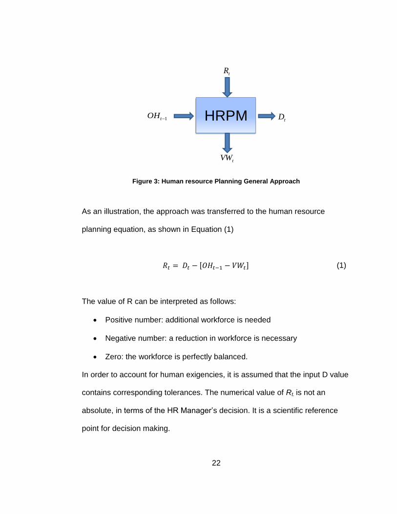
the future workforce demand.2 Figure 3 demonstrates the relationship

between current available workforce and future workforce demand (D) which

can be illustrated by clearly understanding the relationship between:

T (time horizon of prediction)

D (number of employees needed).

OH (on-hand workforce),

VW (voluntary withdrawal)

R (changing required in workforce level).

2 In this study we do not anticipate any changes in process. However if a change in process and the

organization can anticipate and predict the corresponding D, the model still holds true and w ill remain

valid.

22

Figure 3: Human resource Planning General Approach

As an illustration, the approach was transferred to the human resource

planning equation, as shown in Equation (1)

(1)

The value of R can be interpreted as follows:

Positive number: additional workforce is needed

Negative number: a reduction in workforce is necessary

Zero: the workforce is perfectly balanced.

In order to account for human exigencies, it is assumed that the input D value

contains corresponding tolerances. The numerical value of Rt. is not an

absolute, in terms of the HR Manager‟s decision. It is a scientific reference

point for decision making.

HRPM1tOHtD

tR

tVW

23

The process of evaluating employee withdrawal will be demonstrated in detail

in the following section.

3.2 Prediction of Voluntary Workforce Withdrawal

This prediction considers only voluntary withdrawal. Other types of withdrawal

such as discharges, lay-offs, and deaths will not be considered in this

particular model. Discharges and lay-offs are organizational decisions. Death

is an event which is beyond control. This goal of this model is to predict

voluntary withdrawal of employees and the above mentioned reasons are not

within the employee‟s voluntary decision making. Hence the model holds true

even without consideration of these factors. The procedure for determining

the workforce voluntary withdrawal prediction by means of regression

analysis consists of six stages. The first stage involves data gathering,

followed by stage two, decomposition of the data characteristics based on a

self-selection model. In stage three, critical predictors are identified, and in

stage four, regression analysis is performed on all relevant predictors. The

fifth stage includes model validation, and the final stage is the

implementation.

Stage 1: Data Gathering

The time horizon of the prediction is identified (i.e., over what period of

time is the prediction desired?)

24

Data is gathered from authorized personnel with detailed information

about the workforce of the organization, as shown in Table 2. These

data includes basic information such as employee names, ages, job

titles, and salaries. The response „y‟ is a measure of predictive data for

the future which is shown in the third column; „0‟ indicates that the

employee was in the service at a given time as shown in the second

column, and „1‟ indicates that the employee was not in service at the

given time also shown in the second column.

Table 2: Sample of the data-gathering worksheet

Employee‟s ID Time

Horizon y

(in service) Info 1 Info 2 Info 3 Info n

1001 1

1001 2

1001 3

1001 t

1002 1

1002 2

1002 3

1002 t

1000+u 1

1000+u 2

1000+u 3

1000+u t

25

Reserve some sample data from the original database to use for

validation in the later steps.

Modify and refine the data to a user-friendly form as the original data

may not necessarily be user-friendly. In such cases, the data need to

be modified and refined to yield a “cleaner,” form as shown in Table 2.

Stage 2: Decomposition of Workforce Characteristics

The master dataset is analyzed for the levers that have the most impact on

turnover. It could be location, retirement benefits, workplace culture etc. On

such basis, the dataset is separated. The process of separation of the

workforce dataset follows a „self-selection‟ or „sample selection‟ model by

adding a decision equation, as shown in Equation (2). The decision equation

decomposes observations on individuals who were self-selected into the

sample on the basis of a criterion that is correlated with the dependent

variable of the outcome equation (Heckman, 1979).

(2)

In workforce withdrawal prediction, there are several factors that can be used

in the decision equation as explained in the preceding paragraph. One of the

most possible decision equations is based on retirement eligibility because of

retirement benefits. Retirement eligibilities are highly organization-specific.

26

People who have left an organization to retire when they were eligible have a

full right to get a pension provided by the organization, insurance company,

and/or government. Consequently, being retirement-eligible could be used as

a decision equation indicating the motivational factors for an employee‟s

withdrawal.

Stage 3: Critical Predictor Identification

The prediction model‟s accuracy relies on a set of combinations of

independent variables consisting of the following groups:

Direct factors

Indirect factors

Interaction factors

The time period indicator matrix.

The time horizon matrix variables are additional variables eliminating the

seasonal characteristics of the data. In this study dataset, employees tended

to quit the job during some particular period of the year. This variable allows

the model to control the change of withdrawal related to recurring events. For

example, if the period of three months (quarterly) is set to be the time horizon,

the matrix will be determined as follows:

[0 0 1] refers to Q1



27


A number of studies have been conducted seeking the relevant factors or

significant predictors of employee withdrawal, as mentioned in Chapter II.

However, the combinations of significant variables in different datasets vary

depending on an organization‟s culture. An initial set of predictors can be

gathered from a group of people who know the nature of the organization,

and then irrelevant factors can be eliminated to refine the group of significant

variables by using Akaike Information Criterion (AIC) (Bozdogan, 1987), as

shown in Equation (3). „AIC‟ is a measure of the relative goodness of fit of a

statistical model. It offers a relative measure of the information lost when a

given model is used to describe reality and as such is describes the tradeoff

between „bias‟ and „variance‟ in the model construction. AIC is a relative

selection tool with no standard optimal AIC value and it selects the best

model among all alternatives. The combination of predictors that gives the

minimal value of AIC is selected.

(3)

where

k is the number of parameters in the model

L is the likelihood function for the model.

28

Table 3 shows a sample of the critical predictor identification worksheet. The

highlighted sections are examples of predictors indicating statistically

insignificant to decision equations. In the sample worksheet, predictor 1, for

example, is relevant to exclusively I * = 1.

Table 3: Critical Predictor Identification Worksheet

Decision

Equation Predictor 1 Predictor 2 Predictor 3 Predictor 4 Predictor n

I * = 1

I * = 0

Stage 4: Regression Analysis

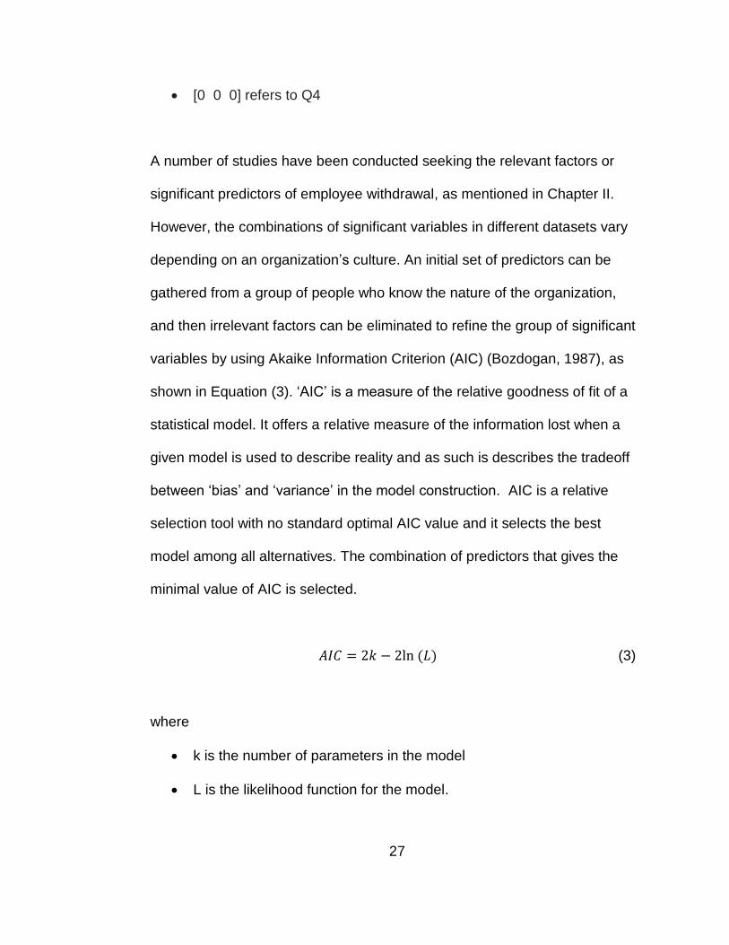
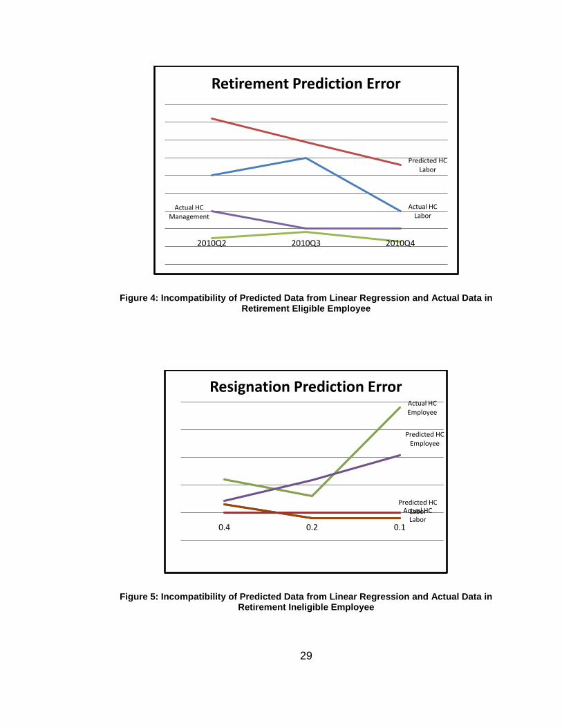
Initially Linear Regression was employed to predict the workforce withdrawal

number. However this method was not successful as the actual data was far

from linear as shown in Figure 4 and Figure 5.

29

Figure 4: Incompatibility of Predicted Data from Linear Regression and Actual Data in Retirement Eligible Employee

Figure 5: Incompatibility of Predicted Data from Linear Regression and Actual Data in Retirement Ineligible Employee

Actual HC Labor

Predicted HC Labor

Actual HC Management

2010Q2 2010Q3 2010Q4

Retirement Prediction Error

Actual HC Labor

Predicted HC Labor

Actual HC Employee

Predicted HC Employee

0.4 0.2 0.1

Resignation Prediction Error

30

Workforce withdrawal was analyzed to have binary outcomes and this leads

us to binary regression modeling. This paper will introduce logistic binary

regression modeling to find the probability of individual volunteer withdrawals

(dependent variables, shown by Y) given by a set of relevant predictors

(independent variables, shown by X) consisting of direct factors, indirect

factors, the time period indicator matrix, and interaction factors

In binary regression theory, the dependent variable is equal to 1 when the

event occurs and 0 when the event does not occur (Durlauf & Blume, 2010).

This is known as a dummy output variable. In workforce planning, the

occurring event (Y = 1) refers to the individual‟s leaving and the non-occurring

event (Y = 0) refers to the individual continuing working in service. Therefore,

logistic regression is utilized to seek the probability of the event occurring

given by independent variables.

The logistic regression model determines an equation that calculates the

probability of event Y occurring to maximize the likelihood function. The

model is formed by parameterizing the probability p depending on repressor

vector X and parameter vector β. The model is an identical conditional

probability given by Equation (4):

(4)

31

Equation (5) presents the most common form of logistic binary regression

model:

(5)

The logistic maximum likelihood (MLE) first-order conditions is simplified into

the following, Equation (6)

(6)

This simple form is similar to the ordinary-least-squares (OLS) regression and

it arises because it demonstrates the canonical link function for the Bernoulli

density.

The regression coefficients that have been calculated by using logistic

regression analysis are shown in Table 4

32

Table 4: Regression Coefficients Worksheet

Decision

Equation Predictor 1 Predictor 2 Predictor 3 Predictor 4 Predictor n

I * = 1 γ1 γ2 0 γ3 γn

I * = 0 0 β2 β3 β4 β2

Stage 5: Final Workforce Requirements and Recommendations

In this phase, The probability of employee withdrawal (p) is calculated from

Equation (5) using the regression coefficients as shown in Table 4 and

employee‟s information as shown in Table 2. Then HC‟ is estimated from

equation below.

(7)

Table 5 shows the recommendations that should be done to serve the

demand number.

Table 5: Sample of the Final Results and Recommendations

Time Horizon

Demand Total HC'

Requirement Cumulative

Requirement

t+1

t+2

t+n

Where

Demand = workforce gross requirement

33

Total HC‟ = the grand summation of the predicted HC‟ in every

decision equations

Requirement is calculated based on Equation (8).

(8)

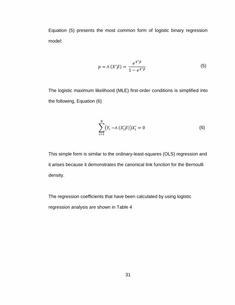
Stage 6: Implementation

The last stage of the model involves developing a user-friendly interface of

the human-resource planning model in Microsoft Excel Macro. The user

simply has to upload the input data into an inbuilt excel file. The software will

process the data to give the output. This eliminates any need for manual

computations and gives a definitive output.

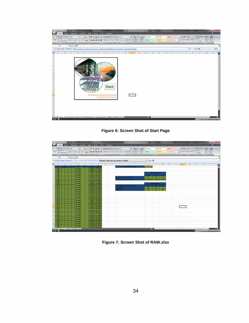
The program performs human-resource planning based on determined

predictor coefficients with a dynamic dataset. It will transfer and utilize the

initial information from “RAW.xlsx” to arrive at a suggestion for workforce

alterations. Sample source code for the program is shown in Appendix 2.

34

Figure 6: Screen Shot of Start Page

Figure 7: Screen Shot of RAW.xlsx

35

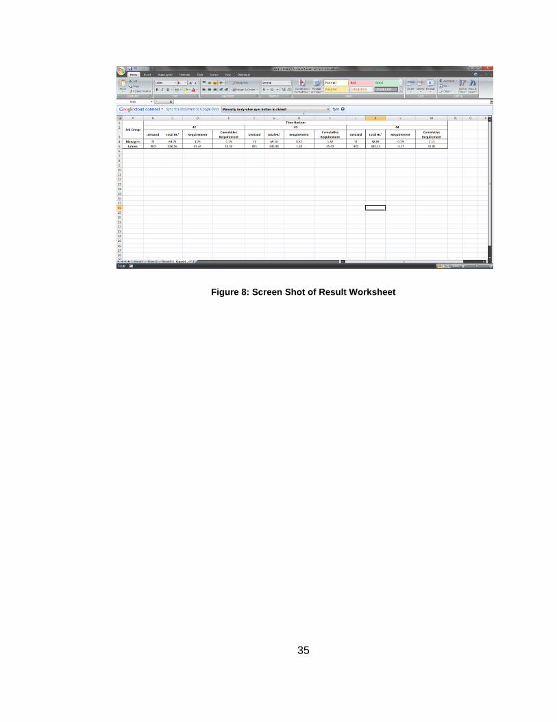
Figure 8: Screen Shot of Result Worksheet

36

CHAPTER IV

RESULTS AND DISCUSSION

Chapter IV illustrates a workforce withdrawal prediction for a human-resource

planning model using historical data obtained from a government agency. The

case study was drawn from 11 years‟ worth of records of the organization‟s

employment data. This organization had datasets for two groups:

Managers

o In this study, the working definition of a manager is that of a

person who occupies one of the four manager level grades as

classified by the HR policy of the organization. The four grades

are namely M1, M2, M3 and M4, M4 in the ascending order of

grade. A total of 71 managers in a certain division were

considered here.

Craftsmen

o For the purposes of this study, the working definition of a

Craftsman is that of a person who occupies one of the ten „L‟

level positions as classified by the HR policy of the organization.

The ten grades are L1 through L10 in the ascending order of the

base salary. At the time of the study there were 894 personnel

who belonged to this category and participated in the study.

37

Step 1: Data Gathering

The horizontal time of the model was defined as the quarter. There were

datasets on two groups (managers and Craftsmen). In the organization, each

dataset covered 41 consecutive quarters. Quarters „1–38‟ were used for the

prediction and quarters „39–41‟ were used as „holdout data‟ for the validation

process. The initial dataset contained information on

Employee ID

Job Title

Date of Hire

Date of Termination

Division of organization

Race

Gender

Number of Employee Points

Years of service (YCS)

Age

Base Salary

Step 2: Decomposition of Workforce Characteristics

In this case study, the data were decomposed into two groups: retirement and

resignation. Retirement is defined as voluntary withdrawal from a job in a

manner that satisfies the organization‟s retirement criteria. Voluntary retirees

38

get associated benefits or pensions depending on their individual retirement

plan. The pension plan will be established by the organization. Retirement-

eligible employees tend to consider the pension benefit as one of the

withdraw decision factors. Resignation is also a form of voluntary withdrawal

but does not fully satisfy the organization‟s retirement criteria. Resignation is

a withdrawal that does not accord pension rights, whereas, retirement entails

a continuing relationship with the organization with pension benefits.

Consequently, the withdrawal behavior may be different. Therefore, the

decision equation was followed by the proposition as shown in Equation (9).

In this case study, there were two criteria for receiving retirement benefits, of

which an employee had to meet at least one to be considered as retirement

eligible. An employee meeting retirement eligibility has the choice to continue

working or to opt for voluntary retirement. The following are the criteria for

voluntary retirement;

Age: employee is 65 years old or over

Point: employee has more than 85 points (point is the sum of the

employee‟s age and the total working year of the employee in this

organization)

(9)

39

Step 3: Critical Predictors Identification

After analysis on withdrawal variables, the initial set of predicting variables

have been iterated down to the following.

Employee information

o Gender

o Number of Employee Points

o Years of service (YCS)

o Age

o Base Salary

Economy condition

o Percentage change from NYSE: NYA3t-1 to NYSE: NYAt

The readings of the NYSE: NYA is taken for 2 two

timestamps. The primary reading is the average index

value of a given quarter and the secondary reading is the

same, from the previous quarter. The percentage change

between these readings is calculated and this number is

taken as one of the input variables.

o Unemployment Rate (UR)

The unemployment rate is a measure of the prevalence

of unemployment and it is calculated as a percentage by

dividing the number of unemployed individuals by all

individuals currently in the labor force.

3 New York Stock Exchange Composite Index

40

Time period indicator: Analysis showed that attrition rates varied

according to the quarter of a given fiscal year. In order to accurately

capture these seasonal variations, four independent variables were

generated, namely q1, q2, q3 and q4, where q1 denotes quarter1 of

the fiscal year, q2 the second quarter of the fiscal year and so forth.

All the quarters of the master dataset are mapped to these variables in

a matrix. This is illustrated in Table 6.

Table 6: Example of Time Period Indication

Time Horizon

q1 q2 q3 q4

1 1 0 0 0

2 0 1 0 0

3 0 0 1 0

4 0 0 0 1

5 1 0 0 0

However, after a preliminary analysis of the historical data, it was determined

that the initial variables were not adequate to predict the likelihood of an

employee‟s voluntary withdrawal. Therefore, an analysis of the interactions

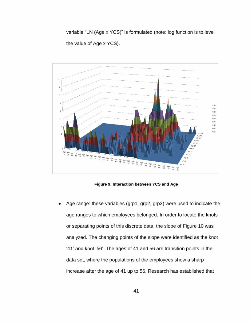
between variables was required. Figure 9 populates the employee withdrawal

according to age and YCS. As a result, the following variable was developed:

Interaction between variables: the shape of Figure 9 is exponential

function from low age low YCS to high age high YCS. Therefore the

41

variable “LN (Age x YCS)” is formulated (note: log function is to level

the value of Age x YCS).

Figure 9: Interaction between YCS and Age

Age range: these variables (grp1, grp2, grp3) were used to indicate the

age ranges to which employees belonged. In order to locate the knots

or separating points of this discrete data, the slope of Figure 10 was

analyzed. The changing points of the slope were identified as the knot

„41‟ and knot „56‟. The ages of 41 and 56 are transition points in the

data set, where the populations of the employees show a sharp

increase after the age of 41 up to 56. Research has established that

YCS 0

YCS 4

YCS 8

YCS 12

YCS 16

YCS 20

YCS 24

YCS 28

YCS 32

YCS 36

YCS 40

YCS 50

0

1

2

3

4

5

6

7

8

9

Age 18

Age 20

Age 22

Age 24

Age 26

Age 29

Age 31

Age 33

Age 36

Age 38

Age 40

Age 42

Age 44

Age 46

Age 48

Age 50

Age 52

Age 54

Age 56

Age 58

Age 60

Age 62

Age 64

Age 66

Age 68

Age 70

Age 72

Age 84

8-9

7-8

6-7

5-6

4-5

3-4

2-3

1-2

0-1

42

this is primarily because at around the age of 40, people think of a job

shift considering long term career advancement. After 56 there is a

sharp decline in the employee population. Again, research shows that

during the mid-fifties people tend to stay on in their current

organization as they near retirement.

o Further the values of each group were represented numerically

as „0‟ or „1‟. The three ranges were the following:

“grp1” = 1 if the individual employee was less than 41

years old.

“grp2” = 1 if the individual employee was between 41 and

56 years old.

“grp3” = 1 if the individual employee was more than 56

years old.

43

Figure 10: Demographic Decomposition by Employee's Age

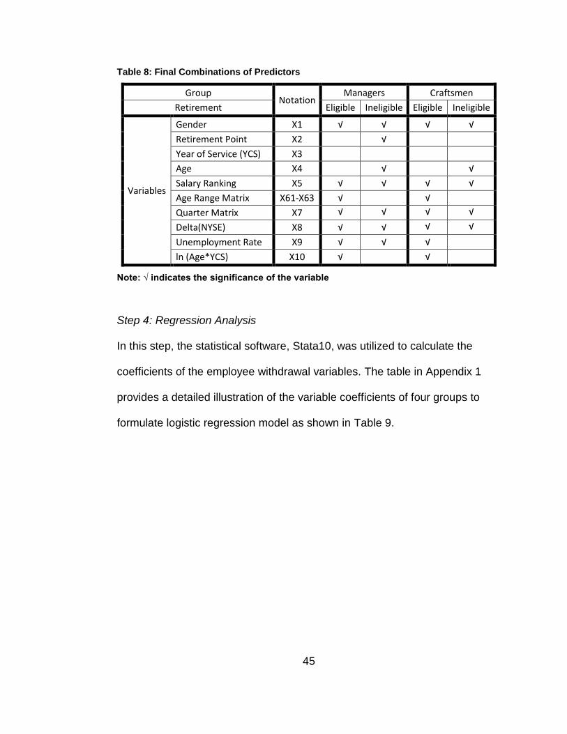
There are 511 possible combinations of the nine variables. The combination

for which the AIC value is least is chosen. Table 8 shows the final result of the

variable combination selection. The final combination was also tested by

comparing predicted employee withdrawal and actual employee withdrawal

during the holdout quarters 38-41 by computing the MAPE (Mean Absolute

Percentage Error) values as shown in Table 7.

Where

A is the actual value

0

5

10

15

20

25

30

35

40

45

50

18 23 28 33 38 43 48 53 58 63 68 73

Head

co

un

t o

f th

e T

erm

inati

on

s

Age

grp1

41

grp2 grp3

56

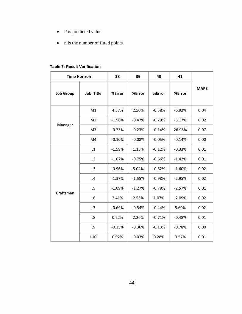
44

P is predicted value

n is the number of fitted points

Table 7: Result Verification

Time Horizon 38 39 40 41

MAPE Job Group Job Title %Error %Error %Error %Error

Manager

M1 4.57% 2.50% -0.58% -6.92% 0.04

M2 -1.56% -0.47% -0.29% -5.17% 0.02

M3 -0.73% -0.23% -0.14% 26.98% 0.07

M4 -0.10% -0.08% -0.05% -0.14% 0.00

Craftsman

L1 -1.59% 1.15% -0.12% -0.33% 0.01

L2 -1.07% -0.75% -0.66% -1.42% 0.01

L3 -0.96% 5.04% -0.62% -1.60% 0.02

L4 -1.37% -1.55% -0.98% -2.95% 0.02

L5 -1.09% -1.27% -0.78% -2.57% 0.01

L6 2.41% 2.55% 1.07% -2.09% 0.02

L7 -0.69% -0.54% -0.44% 5.60% 0.02

L8 0.22% 2.26% -0.71% -0.48% 0.01

L9 -0.35% -0.36% -0.13% -0.78% 0.00

L10 0.92% -0.03% 0.28% 3.57% 0.01

45

Table 8: Final Combinations of Predictors

Group Notation

Managers Craftsmen

Retirement Eligible Ineligible Eligible Ineligible

Variables

Gender X1 √ √ √ √

Retirement Point X2 √

Year of Service (YCS) X3

Age X4 √ √

Salary Ranking X5 √ √ √ √

Age Range Matrix X61-X63 √ √

Quarter Matrix X7 √ √ √ √

Delta(NYSE) X8 √ √ √ √

Unemployment Rate X9 √ √ √

ln (Age*YCS) X10 √ √

Note: √ indicates the significance of the variable

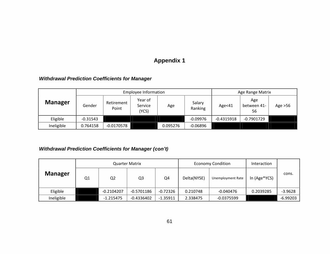
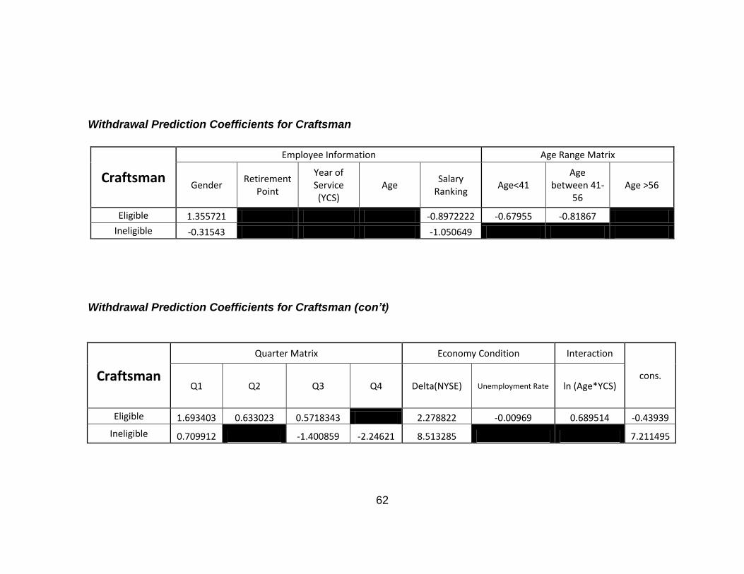
Step 4: Regression Analysis

In this step, the statistical software, Stata10, was utilized to calculate the

coefficients of the employee withdrawal variables. The table in Appendix 1

provides a detailed illustration of the variable coefficients of four groups to

formulate logistic regression model as shown in Table 9.

46

Table 9: Logistic Regression Predictive Model

Group Logistic Regression Equations

Manager (Retirement Eligibility)

Manager (Retirement Ineligibility)

Craftsman (Retirement Eligibility)

Craftsman (Retirement Ineligibility)

)9628.3)92039285.0()8040476.0()7210748.0()627901729.0()614315918.0()509976.0()1((-0.31543

)9628.3)92039285.0()8040476.0()7210748.0()627901729.0()614315918.0()509976.0()1((-0.31543

1ˆ

XXXXXXX

XXXXXXX

e

ey

)9628.3)92039285.0()8040476.0()7210748.0()627901729.0()614315918.0()509976.0()1((-0.31543

)9628.3)92039285.0()8040476.0()7210748.0()627901729.0()614315918.0()506896.0()4(0.095276)28(-0.017057)1((0.764158

1ˆ

XXXXXXX

XXXXXXXXX

e

ey

)211495.7)7709912.0()62400589.1()61513285.8()5050649.1()1((-0.31543

)211495.7)7709912.0()62400589.1()61513285.8()5050649.1()1((-0.31543

1ˆ

XXXXX

XXXXX

e

ey

)43939.0)9689514.0()800696.0()7278822.2()6281867.0()6167955.0()58972222.0()1((1.355721

)43939.0)9689514.0()800696.0()7278822.2()6281867.0()6167955.0()58972222.0()1((1.355721

1ˆ

XXXXXXX

XXXXXXX

e

ey

47

Stage 5: Recommendations

in Equation (7) was the average of provided in Table 9 depended on job

group. HC‟ of each employee group were calculated by using Equation (7).

Then, Rt or „Requirement‟ were calculated by using Equation (8) and recorded

In Table 10 and Table 11. These recommendations will guide the human

resource team as they plan the organization‟s workforce recruitments. In

Table 10 and Table 11, the demand column shows the demand for the given

quarter. The Total HC‟ illustrates the predicted headcount for that quarter.

The requirement displays the required manpower to reach the demand for

that quarter. The cumulative requirement at any given row depicts the overall

headcount needed through that quarter from the initial quarter of the

forecasted dataset.

Table 10: HR Approach for Manager Group

Time Horizon

Demand Total HC'


Requirement

42 71 69.75 1.25 1.25

43 71 69.18 0.57 1.82

44 71 68.89 0.29 2.11

48

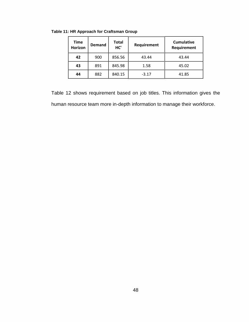
Table 11: HR Approach for Craftsman Group

Time Horizon

Demand Total HC'


Requirement

42 900 856.56 43.44 43.44

43 891 845.98 1.58 45.02

44 882 840.15 -3.17 41.85

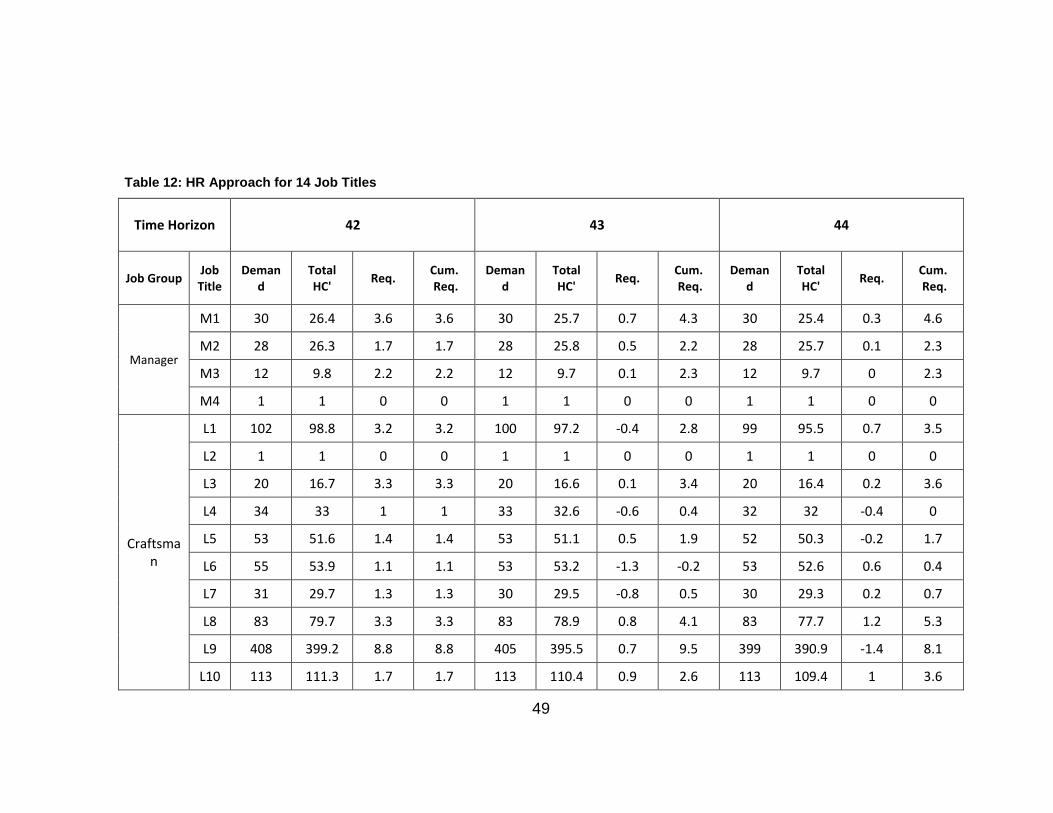
Table 12 shows requirement based on job titles. This information gives the

human resource team more in-depth information to manage their workforce.

49

Table 12: HR Approach for 14 Job Titles

Time Horizon 42 43 44

Job Group Job Title

Demand

Total HC'

Req. Cum. Req.

Demand

Total HC'

Req. Cum. Req.

Demand

Total HC'

Req. Cum. Req.

Manager

M1 30 26.4 3.6 3.6 30 25.7 0.7 4.3 30 25.4 0.3 4.6

M2 28 26.3 1.7 1.7 28 25.8 0.5 2.2 28 25.7 0.1 2.3

M3 12 9.8 2.2 2.2 12 9.7 0.1 2.3 12 9.7 0 2.3

M4 1 1 0 0 1 1 0 0 1 1 0 0

Craftsman

L1 102 98.8 3.2 3.2 100 97.2 -0.4 2.8 99 95.5 0.7 3.5

L2 1 1 0 0 1 1 0 0 1 1 0 0

L3 20 16.7 3.3 3.3 20 16.6 0.1 3.4 20 16.4 0.2 3.6

L4 34 33 1 1 33 32.6 -0.6 0.4 32 32 -0.4 0

L5 53 51.6 1.4 1.4 53 51.1 0.5 1.9 52 50.3 -0.2 1.7

L6 55 53.9 1.1 1.1 53 53.2 -1.3 -0.2 53 52.6 0.6 0.4

L7 31 29.7 1.3 1.3 30 29.5 -0.8 0.5 30 29.3 0.2 0.7

L8 83 79.7 3.3 3.3 83 78.9 0.8 4.1 83 77.7 1.2 5.3

L9 408 399.2 8.8 8.8 405 395.5 0.7 9.5 399 390.9 -1.4 8.1

L10 113 111.3 1.7 1.7 113 110.4 0.9 2.6 113 109.4 1 3.6

50

CHAPTER V

CONCLUSIONS AND RECOMMENDATIONS

5.1 Summary of Research

The main purpose of this research was to develop predictive ability of the

human resource requirements for a large complex organization. The initial

methodology of linear regression used to predict the expected number of

workforce withdrawal showed inaccurate results as the actual data was not

linear but binary in nature.

To get effective predictions of binary data, the „logistic regression model‟, a

non-linear regression model, was chosen. The new prediction results arrived

at, using this model showed very good accuracy with minimal deviation from

the actual data. On testing the model on the holdout data, the results showed

high accuracy levels with MAPE measurements well below 5%. ( As a

standard, readings below 10% MAPE are considered good predictions with

high acceptability).

The Demand „D‟ for a particular period is given by the organization which is

input into the model. The model computes the Requirement, „R‟ by means of

the HRPM, Human Resource Predictive Model. This „Requirement‟ number

will indicate whether there is a balanced workforce (zero), whether additional

employees are needed (positive number), or whether there is an excess

51

manpower situation (negative number); any of these numbers will give the

organization necessary information for crafting a strategic human resources

master plan. HR analysis and decisions on recruitments, dismissals, skillset-

role matching, etc. can be significantly impacted by means of this model, as it

gives a scientific reference point for all decision making.

5.2 Future Work

Successful human resource planning involves a deep understanding of

human nature and human resource allocation. This thesis has focused on the

prediction of human behavior regarding resignation and retirement, employee

withdrawal forecasting, demand estimation, and workforce allocation.

Although the allocation part is calculated based on a human resource

predictive model, it does not consider the cost of human transactions, training

for new hires, or layoff compensation. Workforce manipulation is not always

easily done. Eliminating workers sometimes costs an organization more than

money. For example, Division A of an organization has too few employees

and Division B has too many. The question is “Is it economically viable to

transfer five employees of compatible skill-sets from Division B to Division A

instead of getting rid of five people in Division B and hiring five new people for

Division A?”

52

To answer the question, operational research should be performed based on

cost and working skill constraints. This will give the management team an

idea about their workforce situation and financial position. Besides, this

prospective model could come up with a workforce transaction strategy,

giving users planning data to be able to maintain an appropriate number of

employees at a minimum total operational cost.

53

LIST OF REFERENCES

54

LIST OF REFERENCES

Barber, P., & Lopez-Valcarcel, B. G. (2010). Forecasting the need for medical

specialists in Spain: application of a system dynamics model. Human

Resources for Health, 8.

Borcherding, T. E., Pommerehne, W. W., & Schneider, F. (1982). Comparing the

efficiency of private and public production: The evidence from five

countries. Zeitschrift fiir Nationalilkonomie/Journal of Economics

Supplemen(2), 127-156.

Bozdogan, H. (1987). Model selection and Akaike's Information Criterion (AIC): The

general theory and its analytical extensions. Psychometrika, 52(3), 345-370.

Cascio, W. F. (1993). Downsizing: What Do We Know? What Have We Learned?

The Executive, 7(1), 95-104.

Clarke, T., & Pitelis, C. (Eds.). (1993) The political economy of privatization.

London: Routledge.

Durlauf, S. N., & Blume, L. (2010). Macroeconometrics and time series analysis.

Basingstoke: Palgrave Macmillan.

Federico, S. M., Federico, P. A., & Lundquist, G. W. (1976). Predicting Women's

Turnover as a Fucntion of Extent of Met Salary Expectations and

Biodemographic Data. Personnel Psychology, 29(4), 559-566.

55

Größler, A., & Zock, A. (2010). Supporting long-term workforce planning with a

dynamic aging chain model: A case study from the service industry. Human

Resource Management, 49(5), 829-848.

Hart, O., Shleifer, A., & Vishny, R. W. (1997). The Proper Scope of Government:

Theory and an Application to Prisons*. Quarterly Journal of Economics,

112(4), 1127-1161.

Haskel, J., & Szymanski, S. (1993). Privatization, Liberalization, Wages and

Employment: Theory and Evidence for the UK. Economica, 60(238), 161-

181.

Heckman, J. J. (1979). Sample Selection Bias as a Specification Error. Econometrica,

47(1), 153-161.

Hellriegel, D., & White, G. E. (1973). TURNOVER OF PROFESSIONALS IN

PUBLIC ACCOUNTING: A COMPARATIVE ANALYSIS1. Personnel

Psychology, 26(2), 239-249.

Hendriks, M. H. A., Voeten, B., & Kroep, L. (1999). Human resource allocation in a

multi-project R&D environment: Resource capacity allocation and project

portfolio planning in practice. [doi: DOI: 10.1016/S0263-7863(98)00026-X].

International Journal of Project Management, 17(3), 181-188.

Heneman, H. G., III, & Sandver, M. G. (1977). Markov Analysis in Human Resource

Administration: Applications and Limitations. The Academy of Management

Review, 2(4), 535-542.

Hopp, W., & Spearman, M. (2007). Factory Physics Third Edition: McGraw-

Hill/Irwin.

56

Jacobson, W. S. (2010). Preparing for Tomorrow: A Case Study of Workforce

Planning in North Carolina Municipal Governments. Public Personnel

Management, 39(4), 353-377.

Keel, J. (2006). Workforce Planning Guide. Retrieved January 15, 2011, from

http://sao.hr.state.tx.us/Workforce/06-704.pdf

Kelly, D. J. (2001). Dual Perceptions of HRD: Issues for Policy: SME's, Other

Constituencies, and the Contested Definitions of Human Resource

Development. Retrieved January 27, 2011, from

http://ro.uow.edu.au/artspapers/26/

Kimball, A. B., & Resneck Jr, J. S. (2008). The US dermatology workforce: A

specialty remains in shortage. [doi: DOI: 10.1016/j.jaad.2008.06.037]. Journal

of the American Academy of Dermatology, 59(5), 741-745.

Kwak, N. K., & Lee, C. (1997). A linear goal programming model for human

resource allocation in a health-care organization. J Med Syst, 21(3), 129-140.

Kwak, W., Shi, Y., & Jung, K. (2003). Human Resource Allocation in a CPA Firm: A

Fuzzy Set Approach. [10.1023/A:1023676529552]. Review of Quantitative

Finance and Accounting, 20(3), 277-290.

Kwakwa, F., MA, & Jonasson, O., MD, FACS. (2001, June 11, 2001). The General

Surgery Workforce. from

http://www.facs.org/about/councils/advgen/gstitlpg.html

Lavelle, J. (2007). On workforce architecture, employment relationships and

lifecycles: Expanding the purview of workforce planning & management.

Public Personnel Management, 36(4), 371-385.

http://sao.hr.state.tx.us/Workforce/06-704.pdf

http://ro.uow.edu.au/artspapers/26/

http://www.facs.org/about/councils/advgen/gstitlpg.html

57

Lee, F. H., Lee, T. Z., & Wu, W. Y. (2010). The relationship between human

resource management practices, business strategy and firm performance:

evidence from steel industry in Taiwan. [Article]. International Journal of

Human Resource Management, 21(9), 1351-1372.

Lee, S. M., & Shim, J. P. (1986). Interactive Goal Programming on the

Microcomputer to Establish Priorities for Small Business. The Journal of the

Operational Research Society, 37(6), 571-577.

Lopez-Cabrales, A., Valle, R., & Herrero, I. (2006). The contribution of core

employees to organizational capabilities and efficiency. Human Resource

Management, 45(1), 81-109.

Marsh, R. M., & Mannari, H. (1977). Organizational Commitment and Turnover: A

Prediction Study. Administrative Science Quarterly, 22(1), 57-75.

Michaels, C. E., & Spector, P. E. (1982). Causes of employee turnover: A test of the

Mobley, Griffeth, Hand, and Meglino model. [doi: DOI: 10.1037/0021-

9010.67.1.53]. Journal of Applied Psychology, 67(1), 53-59.

Mobley, W. H., Griffeth, R. W., Hand, H. H., & Meglino, B. M. (1979). Review and

conceptual analysis of the employee turnover process. [doi: DOI:

10.1037/0033-2909.86.3.493]. Psychological Bulletin, 86(3), 493-522.

Muchinsky, P. M., & Tuttle, M. L. (1979). Employee turnover: An empirical and

methodological assessment. [doi: DOI: 10.1016/0001-8791(79)90049-6].

Journal of Vocational Behavior, 14(1), 43-77.

58

Noer, D. M. (1993). Healing the wounds: Overcoming the trauma of layoffs and

revitalizing downsized organizations (1st edition ed.). San Francisco: Jossey-

Bass.

Platje, A., Seidel, H., & Wadman, S. (1994). Project and portfolio planning cycle :

Project-based management for the multiproject challenge. [doi: DOI:

10.1016/0263-7863(94)90016-7]. International Journal of Project

Management, 12(2), 100-106.

Somers, M.-J. (1999). Application of two neural network paradigms to the study of

voluntary employee turnover. Journal of Applied Psychology, 84(1), 177-185.

Statistics, U. S. B. o. L. (2010). Unemployment Rate. Retrieved 12/2, 2010, from

http://data.bls.gov/PDQ/servlet/SurveyOutputServlet?data_tool=latest_numbe

rs&series_id=LNS14000000

Sturman, M. C., Trevor, C. O., Boudreau, J. W., & Gerhart, B. (2003). IS IT WORTH

IT TO WIN THE TALENT WAR? EVALUATING THE UTILITY OF

PERFORMANCE-BASED PAY. Personnel Psychology, 56(4), 997-1035.

Taylor, M. A., & Shore, L. M. (1995). Predictors of planned retirement age: An

application of Beehr's model. [doi:10.1037/0882-7974.10.1.76]. Psychology

and Aging, 10(1), 76-83.

Trevor, C. O., & Nyberg, A. J. (2008). Keeping your headcount when all about are

losing theirs: Downsizing, voluntary turnover rates, and the moderating role of

HR practices. [Article]. Academy of Management Journal, 51(2), 259-276.

van der Laan, E., & Salomon, M. (1997). Production planning and inventory control

with remanufacturing and disposal. [doi: DOI: 10.1016/S0377-

http://data.bls.gov/PDQ/servlet/SurveyOutputServlet?data_tool=latest_numbers&series_id=LNS14000000

http://data.bls.gov/PDQ/servlet/SurveyOutputServlet?data_tool=latest_numbers&series_id=LNS14000000

59

2217(97)00108-2]. European Journal of Operational Research, 102(2), 264-

278.

Ward, D. (1996). Workforce demand forecasting techniques. Human Resource

Planning (19), 54-55.

Whitin, T. M. (1955). Inventory Control and Price Theory. Management Science,

2(1), 61-68.

Woodward, N. (1975). The economic causes of labour turnover: a case study*.

Industrial Relations Journal, 6(4), 19-32.

60

APPENDICES

61

Appendix 1

Withdrawal Prediction Coefficients for Manager

Manager

Employee Information Age Range Matrix

Gender Retirement

Point

Year of Service (YCS)

Age Salary

Ranking Age<41

Age between 41-

56 Age >56

Eligible -0.31543 0 0 0 -0.09976 -0.4315918 -0.7901729 0

Ineligible 0.764158 -0.0170578 0 0.095276 -0.06896 0 0 0

Withdrawal Prediction Coefficients for Manager (con’t)

Manager

Quarter Matrix Economy Condition Interaction

cons. Q1 Q2 Q3 Q4 Delta(NYSE) Unemployment Rate ln (Age*YCS)

Eligible 0 -0.2104207 -0.5701186 -0.72326 0.210748 -0.040476 0.2039285 -3.9628

Ineligible 0 -1.215475 -0.4336402 -1.35911 2.338475 -0.0375599 0 -6.99203

62

Withdrawal Prediction Coefficients for Craftsman

Craftsman

Employee Information Age Range Matrix

Gender Retirement

Point

Year of Service (YCS)

Age Salary

Ranking Age<41

Age between 41-

56 Age >56

Eligible 1.355721 0 0 0 -0.8972222 -0.67955 -0.81867 0

Ineligible -0.31543 0 0 0 -1.050649 0 0 0

Withdrawal Prediction Coefficients for Craftsman (con’t)

Craftsman

Quarter Matrix Economy Condition Interaction

cons. Q1 Q2 Q3 Q4 Delta(NYSE) Unemployment Rate ln (Age*YCS)

Eligible 1.693403 0.633023 0.5718343 0 2.278822 -0.00969 0.689514 -0.43939

Ineligible 0.709912 0 -1.400859 -2.24621 8.513285 0 0 7.211495

63

Appendix 2

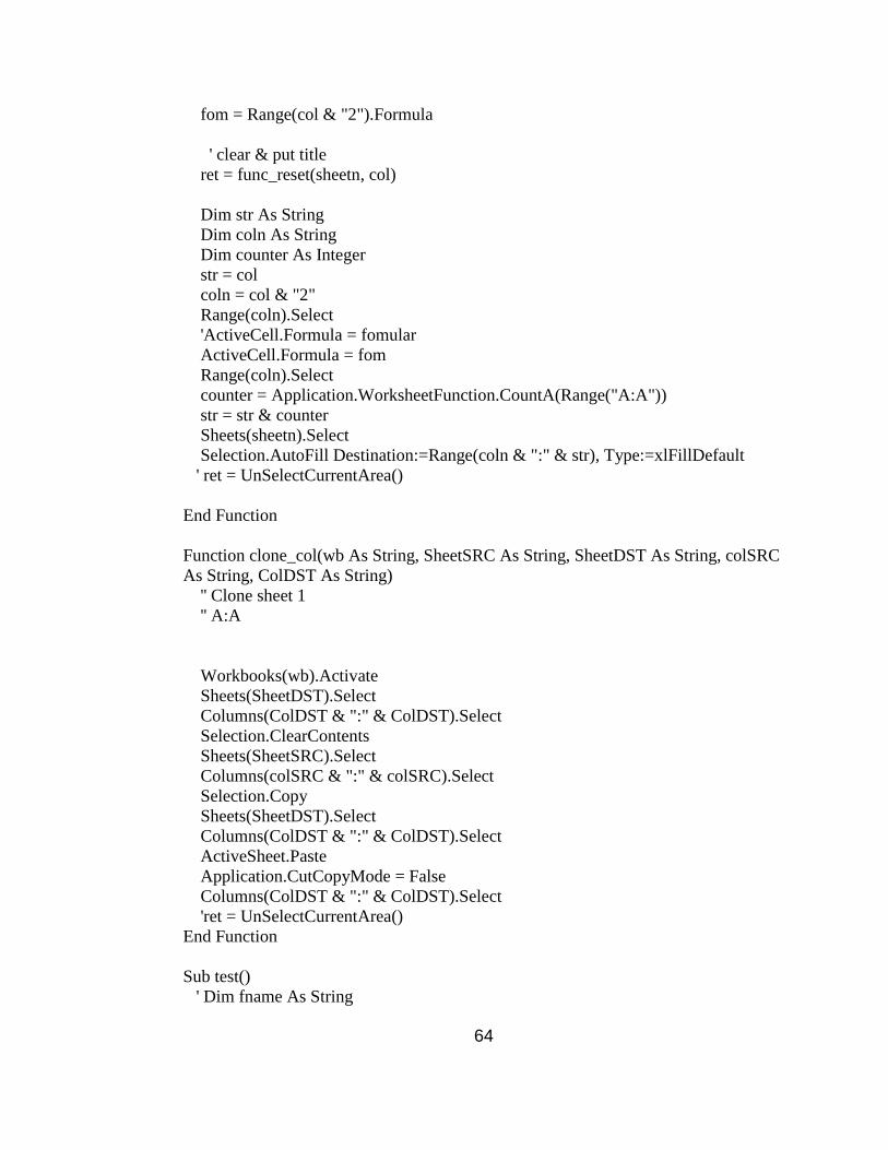
Program Source Code in Microsoft Excel Marco

Dim ret As Integer

Sub UnSelectCurrentArea()

Dim Area As Range

Dim RR As Range

For Each Area In Selection.Areas

If Application.Intersect(Area, ActiveCell) Is Nothing Then

If RR Is Nothing Then

Set RR = Area

Else

Set RR = Application.Union(RR, Area)

End If

End If

Next Area

If Not RR Is Nothing Then

RR.Select

End If

End Sub

Function func_reset(sheetn As String, col As String)

' MsgBox (Range("P1").Value)

Dim tmp_title As String

Sheets(sheetn).Select

tmp_title = Range(col & "1").Value

Columns(col & ":" & col).Select

Selection.ClearContents

Range(col & "1").Select

ActiveCell.FormulaR1C1 = tmp_title

'ret = UnSelectCurrentArea()

End Function

Function func_col_reset(sheetn As String, col As String, fomular As String)

' keep Formula


Dim fom As String

64

fom = Range(col & "2").Formula

' clear & put title

ret = func_reset(sheetn, col)

Dim str As String

Dim coln As String

Dim counter As Integer

str = col

coln = col & "2"

Range(coln).Select

'ActiveCell.Formula = fomular

ActiveCell.Formula = fom

Range(coln).Select

counter = Application.WorksheetFunction.CountA(Range("A:A"))

str = str & counter


Selection.AutoFill Destination:=Range(coln & ":" & str), Type:=xlFillDefault

' ret = UnSelectCurrentArea()

End Function

Function clone_col(wb As String, SheetSRC As String, SheetDST As String, colSRC

As String, ColDST As String)

'' Clone sheet 1

'' A:A

Workbooks(wb).Activate

Sheets(SheetDST).Select

Columns(ColDST & ":" & ColDST).Select


Sheets(SheetSRC).Select

Columns(colSRC & ":" & colSRC).Select

Selection.Copy

Sheets(SheetDST).Select


ActiveSheet.Paste

Application.CutCopyMode = False


'ret = UnSelectCurrentArea()

End Function

Sub test()

' Dim fname As String

65

' fname = ThisWorkbook.Name

End Sub

Sub Generate()

'

' Generate Macro

Dim fname As String

fname = ThisWorkbook.Name

Dim str As String

Dim RAW As String

Dim RAWfname As String

RAWfname = "RAW.xlsx"

' Full path and name of file.

RAW = (ActiveWorkbook.Path) & "\" & RAWfname

Application.Workbooks.Open (RAW)

'' Clone sheet 1

'' A:A

Windows(fname).Activate

Sheets("data").Select

Columns("A:A").Select


Windows(RAWfname).Activate

ActiveWindow.WindowState = xlNormal



Selection.Copy




ActiveSheet.Paste

'' Clone sheet 1

'' B:B


Columns("B:B").Select






Selection.Copy

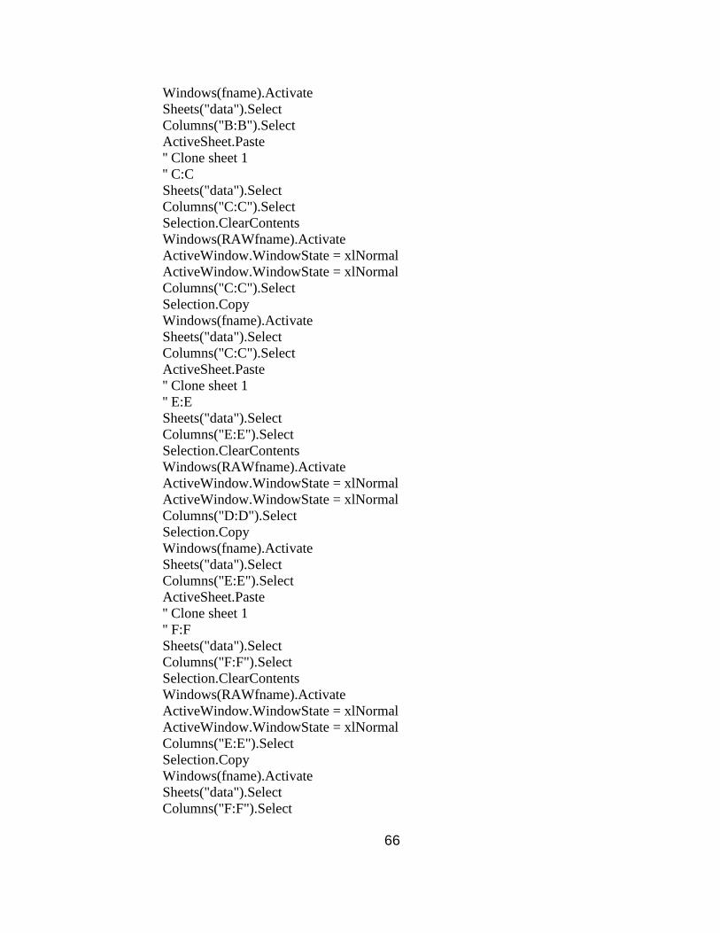
66




ActiveSheet.Paste

'' Clone sheet 1

'' C:C


Columns("C:C").Select






Selection.Copy




ActiveSheet.Paste

'' Clone sheet 1

'' E:E


Columns("E:E").Select





Columns("D:D").Select

Selection.Copy




ActiveSheet.Paste

'' Clone sheet 1

'' F:F


Columns("F:F").Select






Selection.Copy



Columns("F:F").Select

67

ActiveSheet.Paste

' E+F


ret = func_col_reset("data", "D", "=E2+F2")

' diff and ur

' diff_nyse


ret = func_reset("DATA", "O")

Range("O2").Select


Range("I7").Select

Selection.Copy


Range("O2").Select

ActiveSheet.Paste


str = "O"

count = Application.WorksheetFunction.CountA(Range("A:A"))

str = str & count


Selection.AutoFill Destination:=Range("O2:" & str), Type:=xlFillDefault

' ur

ret = func_reset("DATA", "P")

Range("P2").Select


Range("I8").Select

Selection.Copy


Range("P2").Select

ActiveSheet.Paste


str = "P"


str = str & count


Selection.AutoFill Destination:=Range("P2:" & str), Type:=xlFillDefault

68


Dim quarter As Integer


quarter = Range("I1").Value



Columns("G:G").Select


Range("G1").Select

ActiveCell.FormulaR1C1 = "qone"

Columns("H:H").Select


Range("H1").Select

ActiveCell.FormulaR1C1 = "qtwo"

Columns("I:I").Select


Range("I1").Select

ActiveCell.FormulaR1C1 = "qthr"

Columns("J:J").Select


Range("J1").Select

ActiveCell.FormulaR1C1 = "qfor"


Range("G2").Select

If quarter = 1 Then

ActiveCell.FormulaR1C1 = 1

Else


End If

Range("H2").Select

If quarter = 2 Then


Else


69

End If

Range("I2").Select

If quarter = 3 Then


Else


End If

Range("J2").Select

If quarter = 4 Then


Else


End If

If quarter > 4 Then

MsgBox ("ERROR")

End If


str = "G"


str = str & count


Range("G2").Select

Selection.AutoFill Destination:=Range("G2:" & str), Type:=xlFillDefault

str = "H"


str = str & count


Range("H2").Select

Selection.AutoFill Destination:=Range("H2:" & str), Type:=xlFillDefault

str = "I"


str = str & count


Range("I2").Select

Selection.AutoFill Destination:=Range("I2:" & str), Type:=xlFillDefault

str = "J"


str = str & count

70


Range("J2").Select

Selection.AutoFill Destination:=Range("J2:" & str), Type:=xlFillDefault

'K

' ret = func_reset("DATA", "K")

ret = func_col_reset("DATA", "K", "=IF((F2+E2)>=85,1,0)")

'Q Jobrank

' ret = func_reset("DATA", "Q")

ret = func_col_reset("DATA", "Q", "=VLOOKUP(B2,'Job Title

Convertion'!$A$1:$B$35,2,FALSE)")

'R lagexysc

' ret = func_reset("DATA", "R")

ret = func_col_reset("DATA", "R", "=LN(E2*F2)")

'S Eli =IF(OR(F2>=65,D2>=85),1,0)

' ret = func_reset("DATA", "S")

ret = func_col_reset("DATA", "S", "=IF(OR(F2>=65,D2>=85),1,0)")

'T Group

=IF(S2=0,IF(Q2>=1,IF(Q2<=10,"Res_Lo",IF(Q2>=11,IF(Q2<=14,"Res_Up")))),IF(

Q2>=1,IF(Q2<=10,"Ret_Lo",IF(Q2>=11,IF(Q2<=14,"Ret_Up")))))

' ret = func_reset("DATA", "T")

ret = func_col_reset("DATA", "T",

"=IF(S2=0,IF(Q2>=1,IF(Q2<=10,""Res_Lo"",IF(Q2>=11,IF(Q2<=14,""Res_Up"")))

),IF(Q2>=1,IF(Q2<=10,""Ret_Lo"",IF(Q2>=11,IF(Q2<=14,""Ret_Up"")))))")

'U SEX

' ret = func_reset("DATA", "U")

ret = func_col_reset("DATA", "U",

"=VLOOKUP($T2,Logit_Parameter!$A$2:$R$5,CELL(""col"",U2)-

CELL(""col"",$T2)+1,FALSE)*C2")

'V point

' ret = func_reset("DATA", "V")

ret = func_col_reset("DATA", "V",

"=VLOOKUP($T2,Logit_Parameter!$A$2:$R$5,CELL(""col"",V2)-

CELL(""col"",$T2)+1,FALSE)*D2")

'W ysc

' ret = func_reset("DATA", "W")

ret = func_col_reset("DATA", "W",

"=VLOOKUP($T2,Logit_Parameter!$A$2:$R$5,CELL(""col"",W2)-

CELL(""col"",$T2)+1,FALSE)*E2")

'X age

' ret = func_reset("DATA", "X")

ret = func_col_reset("DATA", "X",

"=VLOOKUP($T2,Logit_Parameter!$A$2:$R$5,CELL(""col"",X2)-

CELL(""col"",$T2)+1,FALSE)*F2")

'Y qone

71

' ret = func_reset("DATA", "Y")

ret = func_col_reset("DATA", "Y",

"=VLOOKUP($T2,Logit_Parameter!$A$2:$R$5,CELL(""col"",Y2)-

CELL(""col"",$T2)+1,FALSE)*G2")

'Z qtwo

' ret = func_reset("DATA", "Z")

ret = func_col_reset("DATA", "Z",

"=VLOOKUP($T2,Logit_Parameter!$A$2:$R$5,CELL(""col"",Z2)-

CELL(""col"",$T2)+1,FALSE)*H2")

'AA qthr

' ret = func_reset("DATA", "AA")

ret = func_col_reset("DATA", "AA",

"=VLOOKUP($T2,Logit_Parameter!$A$2:$R$5,CELL(""col"",AA2)-

CELL(""col"",$T2)+1,FALSE)*I2")

'AB qfor

' ret = func_reset("DATA", "AB")

ret = func_col_reset("DATA", "AB",

"=VLOOKUP($T2,Logit_Parameter!$A$2:$R$5,CELL(""col"",AB2)-

CELL(""col"",$T2)+1,FALSE)*J2")

'AC p85

' ret = func_reset("DATA", "AC")

ret = func_col_reset("DATA", "AC",

"=VLOOKUP($T2,Logit_Parameter!$A$2:$R$5,CELL(""col"",AC2)-

CELL(""col"",$T2)+1,FALSE)*K2")

'AD grp1_age

' ret = func_reset("DATA", "AD")

ret = func_col_reset("DATA", "AD",

"=VLOOKUP($T2,Logit_Parameter!$A$2:$R$5,CELL(""col"",AD2)-

CELL(""col"",$T2)+1,FALSE)*L2")

'AE grp2_age

' ret = func_reset("DATA", "AE")

ret = func_col_reset("DATA", "AE",


CELL(""col"",$T2)+1,FALSE)*M2")

'AF grp3_age

' ret = func_reset("DATA", "AF")

ret = func_col_reset("DATA", "AF",


CELL(""col"",$T2)+1,FALSE)*N2")

'AG diff_nyse

' ret = func_reset("DATA", "AG")

ret = func_col_reset("DATA", "AG",


CELL(""col"",$T2)+1,FALSE)*O2")

'AH ur

72

' ret = func_reset("DATA", "AH")

ret = func_col_reset("DATA", "AH",


CELL(""col"",$T2)+1,FALSE)*P2")

'AI jobrank

' ret = func_reset("DATA", "AI")

ret = func_col_reset("DATA", "AI",


CELL(""col"",$T2)+1,FALSE)*Q2")

'AJ lagexyse

' ret = func_reset("DATA", "AJ")

ret = func_col_reset("DATA", "AJ",


CELL(""col"",$T2)+1,FALSE)*R2")

'AK cons.

' ret = func_reset("DATA", "AK")

ret = func_col_reset("DATA", "AK",


CELL(""col"",$T2)+1,FALSE)")

'AL L

' ret = func_reset("DATA", "AL")

ret = func_col_reset("DATA", "AL", "=SUM(U2:AK2)")

'AM e^L

' ret = func_reset("DATA", "AM")

ret = func_col_reset("DATA", "AM", "=2.71828183^AL2")

'AN p(x)

' ret = func_reset("DATA", "AN")

ret = func_col_reset("DATA", "AN", "=AM2/(1+AM2)")

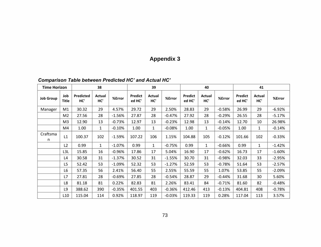
73

Appendix 3

Comparison Table between Predicted HC’ and Actual HC’

Time Horizon 38 39 40 41

Job Group Job Title

Predicted HC'

Actual HC'

%Error Predicted HC'

Actual HC'


Actual HC'


Actual HC'

%Error

Manager M1 30.32 29 4.57% 29.72 29 2.50% 28.83 29 -0.58% 26.99 29 -6.92%

M2 27.56 28 -1.56% 27.87 28 -0.47% 27.92 28 -0.29% 26.55 28 -5.17%

M3 12.90 13 -0.73% 12.97 13 -0.23% 12.98 13 -0.14% 12.70 10 26.98%

M4 1.00 1 -0.10% 1.00 1 -0.08% 1.00 1 -0.05% 1.00 1 -0.14%

Craftsman

L1 100.37 102 -1.59% 107.22 106 1.15% 104.88 105 -0.12% 101.66 102 -0.33%

L2 0.99 1 -1.07% 0.99 1 -0.75% 0.99 1 -0.66% 0.99 1 -1.42%

L3L 15.85 16 -0.96% 17.86 17 5.04% 16.90 17 -0.62% 16.73 17 -1.60%

L4 30.58 31 -1.37% 30.52 31 -1.55% 30.70 31 -0.98% 32.03 33 -2.95%

L5 52.42 53 -1.09% 52.32 53 -1.27% 52.59 53 -0.78% 51.64 53 -2.57%

L6 57.35 56 2.41% 56.40 55 2.55% 55.59 55 1.07% 53.85 55 -2.09%

L7 27.81 28 -0.69% 27.85 28 -0.54% 28.87 29 -0.44% 31.68 30 5.60%

L8 81.18 81 0.22% 82.83 81 2.26% 83.41 84 -0.71% 81.60 82 -0.48%

L9 388.62 390 -0.35% 401.55 403 -0.36% 412.46 413 -0.13% 404.81 408 -0.78%

L10 115.04 114 0.92% 118.97 119 -0.03% 119.33 119 0.28% 117.04 113 3.57%

74

VITA

Tachapon Saengsureepornchai was born January 9th 1983, in Chanthaburi,

Thailand and attended Benjamarachutis School. He later moved to Bangkok,

Thailand and attended Kasetsart University, where he obtained a Bachelor‟s

of Engineering in Industrial Engineering in May 2004. He then worked as an

Industrial Engineer at Fabrinet Co., Ltd. for two years. He joined the

University of Tennessee – Knoxville in the fall of 2008 and began working

towards his Master of Science in Industrial Engineering under the tutelage of

Dr. Rupy Sawhney. During his master‟s program, he has worked as a

Graduate Research Assistant under Dr. Sawhney on many interesting

industrial projects.

Dynamic Human Resource Predictive Model for Complex ...

Documents

Transcript of Dynamic Human Resource Predictive Model for Complex ...