A comparison of Monte Carlo tree search andmathematical optimization for large scale dynamic

resource allocation I

Dimitris Bertsimasa, J. Daniel Griffithb, Vishal Guptac, Mykel J.Kochenderferd, Velibor V. Misicc, Robert Mossb

aSloan School of Management and Operations Research Center, Massachusetts Institute ofTechnology; 77 Massachusetts Avenue, Cambridge MA 02139

bLincoln Laboratory, Massachusetts Institute of Technology; 244 Wood Street, LexingtonMA 02420

cOperations Research Center, Massachusetts Institute of Technology; 77 MassachusettsAvenue, Cambridge MA 02139

dDepartment of Aeronautics and Astronautics, Stanford University; 496 Lomita Mall,Stanford CA 94305

Abstract

Dynamic resource allocation (DRA) problems are an important class of dynamicstochastic optimization problems that arise in a variety of important real-worldapplications. DRA problems are notoriously difficult to solve to optimalitysince they frequently combine stochastic elements with intractably large stateand action spaces. Although the artificial intelligence and operations researchcommunities have independently proposed two successful frameworks for solvingdynamic stochastic optimization problems—Monte Carlo tree search (MCTS)and mathematical optimization (MO), respectively—the relative merits of thesetwo approaches are not well understood. In this paper, we adapt both MCTSand MO to a problem inspired by tactical wildfire and management and un-dertake an extensive computational study comparing the two methods on largescale instances in terms of both the state and the action spaces. We show thatboth methods are able to greatly improve on a baseline, problem-specific heuris-tic. On smaller instances, the MCTS and MO approaches perform comparably,but the MO approach outperforms MCTS as the size of the problem increasesfor a fixed computational budget.

Keywords: Dynamic resource allocation; Markov decision process; Monte

IThis work is sponsored by the Assistant Secretary of Defense for Research and Engineer-ing, ASD(R&E), under Air Force Contract #FA8721-05-C-0002. Opinions, interpretations,conclusions, and recommendations are those of the authors and are not necessarily endorsedby the United States Government.

Email addresses: dbertsim@mit.edu (Dimitris Bertsimas), dan.griffith@ll.mit.edu (J.Daniel Griffith), vgupta1@mit.edu (Vishal Gupta), mykel@stanford.edu (Mykel J.Kochenderfer), vvmisic@mit.edu (Velibor V. Misic), robert.moss@ll.mit.edu (RobertMoss)

Preprint submitted to Elsevier May 22, 2014

arX

iv:1

405.

5498

v1 [

mat

h.O

C]

21

May

201

4

Carlo tree search; mathematical programming; tactical wildfire management

1. Introduction

Dynamic resource allocation (DRA) problems are problems where one mustassign resources to tasks or requests over some finite time horizon. Many impor-tant real-world problems can be cast as DRA problems, including applicationsin air traffic control [6, 13], network revenue management (see, e.g., [54] for anoverview), scheduling [12, 26] and logistics, transportation and fulfillment [1, 47].DRA problems are notoriously difficult to solve for two reasons. First, manyreal-world DRA problems exhibit stochasticity, i.e., the requests to be processedmay arrive randomly according to some stochastic process that, itself, dependson where resources are allocated. Second, many real-world DRA problems ex-hibit extremely large state and action spaces, making solution by traditionaldynamic programming methods infeasible [7, 46]. A number of scientific com-munities, particularly within artificial intelligence and operations research, havesought more sophisticated techniques for addressing DRA and other dynamicstochastic optimization problems.

Within the AI community, one approach for dynamic stochastic optimizationproblems that has received increasing attention in the last 15 years is a methodknown as Monte Carlo tree search (MCTS) [24, 16]. In any dynamic stochasticoptimization problem, one can represent the possible trajectories of the system—the state at each decision epoch and the actions taken at those epochs—asa tree, where the root represents the initial state. In MCTS, one iterativelybuilds an approximation to this tree and uses it to inform the choice of action.In our opinion, MCTS’s effectiveness stems from two key features: 1) “banditupper confidence bounds” (see [4, 39]) can be used to balance exploration andexploitation in learning, 2) application-specific heuristics and knowledge can beused to customize the base algorithm [16]. Moreover, the MCTS algorithm isvery flexible and can easily be tailored to a variety of problems. Indeed, theonly technical requirement for implementing MCTS is a generative model that,given a state and an action at a given decision epoch, generates a new statefor the next epoch and an immediate reward received. This flexibility makesMCTS particularly attractive as a general purpose methodology.

Most importantly, MCTS has been extremely successful in a number of ap-plications, particularly in designing expert computer players for difficult gamessuch as Go [31, 40, 25], Hex [2, 3], Kriegspiel [19], and Poker [51]. Although,we think it is fair to say that MCTS is the one of the top performing, generalpurpose algorithms for this class of games, we observe that games like Go andHex are qualitatively very different from DRAs. Namely, unlike typical DRAproblems, the state of these games does not evolve stochastically, and, further-more, the size of the feasible action space is often much smaller than for typicalDRA problems. For example, in the instances of Go studied in [31], the actionbranching factor is at most 81, whereas in the DRA instance we consider, atypical branching factor is approximately 230 million (cf. Eq. (6)). This raises

2

a question about the performance of MCTS for this new class of real-worldproblems.

On the other hand, within the operations research community, the study ofDRAs has proceeded along different lines. A prominent stream of research isbased upon mathematical optimization (MO). In contrast to MCTS which onlyrequires access to a generative model of the stochastic system, MO approachesmodel the dynamics of the system explicitly via a constrained optimizationproblem. The solution to this optimization problem then yields a control policyfor the system. This paradigm has a long history within the dynamic controlliterature (see, e.g., [10] for an overview).

In the special case of stochastic, dynamic resource allocation problems, therea number of competing proposals to incorporate the stochastic evolution includ-ing robust optimization / control [11, 9, 43, 33] and chance constrained opti-mization [17]. In what follows, however, we focus on a third proposal, sometimescalled model predictive control [8]. Specifically, we replace uncertain parame-ters in a MO formulation with their expected values and periodically re-solvethe optimization problem for an updated policy as the true system evolves.Variants of this paradigm are known by many names in the literature includ-ing fluid approximation [30, 5], certainty equivalent control ([10, Chapt. 6]).These (re-)optimization frameworks are well-known to have excellent practicalperformance in application domains like queueing [18, 52] and network revenuemanagement [20], and in some special cases, additionally enjoy strong theoreti-cal guarantees on performance (e.g., [20, 30, 38, 41, 48, 53]).

In any case, regardless of the particular proposal for incorporating stochas-ticity, the widespread use and success of MO approaches for DRAs contrastsstrongly with a lack of computational experience with MCTS for DRAs.

In this paper, we aim to understand the relative merits of both the aboveMCTS and MO approaches by applying them to a challenging DRA problem in-spired by tactical wildfire management. Our interest in tactical wildfire manage-ment as a benchmark problem stems simultaneously from practical importanceof this application area and the computational difficulty of the underlying DRA.Indeed, the severity of wildland fires has been steadily increasing in recent years,particularly in the southwestern US [32], and as a result, US federal governmentspending on wildfire management has also been increasing, amounting to $3.5billion in 2013 [15]. Suppression costs are only part of the total cost of wildfire;combined costs of loss of property, damage to the environment and loss of humanlife are estimated to be many times larger [56]. Consequently, there has beenrenewed interest in models for realtime decision support tools to assist in tacti-cal wildfire management, namely how best to utilize fire suppression resourcesto contain and extinguish a fire. Unfortunately, this is an extremely challengingproblem both from the complexity of the system dynamics and uncertainty inthe underlying data.

Although there have been a number of empirically validated, deterministicmodels for wildfire spread proposed (e.g., [27, 55]), there have been fewer worksthat incorporate the stochastic elements of fire spread [14, 44, 29]. Most worksfocus on developing models for the rate and simulation of the spread of wildfire.

3

Fewer consider the associated problem of managing suppression resources. Anotable exception is the research stream [36, 45], which proposes 1) an optimiza-tion formulation of the initial attack problem, i.e., the problem of determininghow many and what kind of suppression resources to allocate to an ongoingfire and 2) a simulation engine to study how specific, user-specified heuristicsuppression rules affect the growth of a fire. To the best of our knowledge, theauthors do not address the tactical problem of optimally controlling suppressionresources as the fire evolves. In other words, the authors do not consider theunderlying DRA.

By contrast, we develop a model for the underlying DRA as a particularMarkov decision problem (MDP) which incorporates several of the most promi-nent features of existing wildfire spread models. We then compare the perfor-mance of MCTS and MO inspired algorithms for this problem. We stress thatthis is a particularly challenging MDP, having many possible states and manypossible actions for even small instances of the problem. Our computationalexperience with this benchmark both elucidates some of the features of thesealgorithms and illustrates how they might be incorporated into a larger decisionsupport system like [37].

We summarize our contributions as follows:

1. We propose a flexible MDP to model tactical wildfire management thatcaptures the most important deterministic and stochastic features of wild-fire spread. We also propose a simple, high-quality, and customized heuris-tic for this problem that may be of independent interest to practitioners.

2. We develop an MCTS-based approach for the above MDP. To the best ofour knowledge, this represents the first application of MCTS to a DRAproblem motivated by a real-world application. Towards this end, wecombine a number of classical features of MCTS, such as bandit upperconfidence bounds, with new features such as double progressive widening[23]. We also propose a novel action generation approach to cope with thesize of the state and action spaces of the DRA.

3. We propose a mathematical optimization formulation that approximatesthe original discrete and stochastic elements of the MDP by suitable con-tinuous and deterministic counterparts. Although this approximation isin the same spirit as other fluid approximation literature in operationsresearch ([5, 30]), our particular formulation incorporates elements of alinear dynamical system which we believe may be of independent interestin other DRA problems.

4. Through extensive computational experiments, we show the following:

(a) The MCTS and MO approaches both produce high-quality solutions,generally performing as well or better than our customized heuris-tic for this problem. MCTS and MO perform comparably when theproblem instance is small. With a fixed computational budget, how-ever, the MO approach begins to outperform the MCTS approachas the size of the problem instance grows, either in state space oraction space. Indeed, for very large action spaces, MCTS can begin

4

to perform worse than our baseline heuristic. The MO approach, bycomparison, still performs quite well.

(b) The choice of hyperparameters in the MCTS algorithm—such as theexploration bonus and the progressive widening parameters—can sig-nificantly affect overall performance of the algorithm. The interde-pendence between these parameters is complex, and they cannot,in general, be selected independently. Some care must be taken toappropriately tuning the algorithm to a specific DRA problem.

The rest of this paper is organized as follows. In Section 2, we introduce ourMDP formulation of the tactical wildfire management problem that we use tocompare the MCTS and MO approaches. In Sections 3 and 4, we describe theMCTS and MO approaches, respectively. In Section 5, we describe our com-putational experiments and report on the results of these experiments. Finally,in Section 6, we summarize the main contributions of the work and highlightpromising directions for future research.

2. Tactical Wildfire Dynamics as Dynamic Resource Allocation

In what follows, we consider a simplified model in order to more clearly high-light the difference between the MCTS and MO approaches in our experimentswhile still capturing the key features of wildfire propagation, e.g., stochastic evo-lution, wind and topography effects and dependence on fuel. Although we donot explore the ideas here, it would be (at least conceptually) straightforward toextend our approach to a higher fidelity model incorporating moisture contentand surface fuel-type as in [50] by using techniques similar to those developedin [37].

Specifically inspired by the stochastic model of [14] for wildland fire simula-tion, we model tactical wildland fire management as a Markov decision process.We partition the landscape into a grid of cells X . There are two attributes foreach cell x ∈ X :

• B(x), a Boolean variable indicating whether the cell is currently burning,and

• F (x), an integer variable indicating how much fuel is remaining in the cell.

The collection of these two attributes over all cells in the grid represents thestate of the Markov decision process.

We further assume a set of suppression resources I fighting the wildland fire.To simplify the model, we will treat all suppression resources as identical, butit is straightforward to extend to the case heterogenous resources with differentcapabilities as in [42, 37]. The decisions of our MDP correspond to assigningresources to cells. For each i ∈ I, let a(i) ∈ X denote the cell to which we assignsuppression resource i. We assume that any resource can be assigned to anycell at any time step, i.e., that the travel time between cells is negligibly smallcompared to the decision interval of the MDP.

5

Once ignited, a cell consumes fuel at a constant rate. Once the fuel isexhausted, the cell extinguishes. Since fuel consumption occurs a a constantrate, without loss of generality, we can rescale the units of time to make thisrate equal to unity. Thus, we model the evolution of fuel in the model by

Ft+1(x) =

{Ft(x) if ¬Bt(x) ∨ Ft(x) = 0

Ft(x)− 1 otherwise.(1)

Notice this evolution is deterministic given Bt(x).The evolution of Bt(x), however, is stochastic. Figure 1 shows the proba-

bilistic transition model for Bt(x) where

ρ1 =

{1−

∏y(1− P (x, y)Bt(y)) if Ft(x) > 0

0 otherwise(2)

and

ρ2 =

{1 if Ft(x) = 0

1−∏i(1−Q(x)δx(a(i))) otherwise.

(3)

Here, P (x, y) is the probability that a fire in cell y ignites a fire in cell x.Generally, only the neighbors of x can ignite x, and so we expect P (x, y) tobe sparse. The specification of P (x, y) can capture the tendency of a fire topropagate primarily in one direction due to wind or sloping terrain. Q(x) is theprobability that a suppression effort on cell x successfully extinguishes the cell.We assume that the probability of success for multiple attempts on the samecell are independent.

false true

ρ1

1 − ρ1

ρ2

1 − ρ2

Figure 1: B(x) transition model.

We stress that under these dynamics, cells that have been previously extin-guished by a suppression team may later reignite.

The reward for a cell burning is R(x) (always negative) and the total rewardreceived every step is

∑t,xBt(x)R(x). We can vary the reward across the grid

to represent a higher cost of a fire in particular areas. For example, we maypenalize a fire in a populated area more heavily.

3. Monte Carlo Tree Search

Our review of MCTS is necessarily brief. Please see [16] for a more thoroughsurvey. In particular, we will focus on a variation of MCTS that employs double

6

progressive widening, a technique that explicitly controls the branching factorof the search tree [23]. This variation is specifically necessary when the actionspace is continuous or so large that all actions cannot possibly be explored.This is frequently the case in most DRA problems. We note that there existother strategies for managing the branching factor, such as the pruning strategyemployed in the “bandit algorithm for smooth trees” (BAST) method of [21];we do not consider these here.

We first describe MCTS with double progressive widening in general, andthen discuss two particular modifications we have made to the algorithm totailor it to DRAs.

3.1. MCTS with double progressive widening

Algorithm 1 involves running many simulations from the current state whileupdating an estimate of the state-action value function Q(s, a). We use a gen-erative model G to produce samples of the next state s′ and reward r giventhe current state s and action a. We draw samples (s′, r) ∼ G(s, a). All of theinformation about the state transitions and rewards is represented by G; thestate transition probabilities and expected reward function are not used directly.There are three stages in each simulation: search, expansion, and rollout.

3.1.1. Search

If the current state in the simulation is in the set T (initially empty), weenter the search stage. Otherwise, we proceed to the expansion stage. Duringthe search stage, we update Q(s, a) for the states and actions visited and triedin our search. We also keep track of the number of times we have visited a stateN(s) and the number of times we have taken an action from a state N(s, a).

During the search, the first progressive widening controls the number ofactions considered from a state. To do this, we generate a new action if ‖A(s)‖ <kN(s)α, where k and α are parameters that control the number of actionsconsidered from the current state and A(s) is the set of actions tried froms. When generating a new action, we add it to the set A(s), and initializeN(s, a) and Q(s, a) with N0(s, a) and Q0(s, a), respectively. The functionsN0 and Q0 can be based on prior expert knowledge of the problem; if none isavailable, then they can both be initialized to 0. We also initialize the empty setV (s, a), which contains the set of states s′ transitioned to from s when selectingaction a. A default strategy for generating new actions is to randomly samplefrom candidate actions. If ‖A(s)‖ ≥ kN(s)α, then we execute the action thatmaximizes

Q(s, a) + c

√logN(s)

N(s, a),

where c is a parameter that controls the amount of exploration in the search.The second term is an exploration bonus that encourages selecting actions thathave not been tried as frequently.

Next, we draw a sample (s′, r) ∼ G(s, a), if ‖V (s, a)‖ < k′N(s, a)α′. In

this second progressive widening step, the parameters k′ and α′ control the

7

Algorithm 1 Monte Carlo tree search with double progressive widening

function MonteCarloTreeSearch(s, d)loop

Simulate(s, d)

return arg maxaQ(s, a)

function Simulate(s, d)if d = 0 then

return 0if s 6∈ T then

T = T ∪ {s}N(s)← N0(s)return Rollout(s, d)

N(s)← N(s) + 1if ‖A(s)‖ < kN(s)α then

a← Getnext(s,Q)(N(s, a), Q(s, a), V (s, a))← (N0(s, a), Q0(s, a), V (s, a))A(s) = A(s) ∪ {a}

a← arg maxaQ(s, a) + c√

logN(s)N(s,a)

if ‖V (s, a)‖ < k′N(s, a)α′

then(s′, r) ∼ G(s, a)if s′ 6∈ V (s, a) then

V (s, a) = V (s, a) ∪ {s′}R(s, a, s′)← rN(s, a, s′)← N0(s, a, s′)

elseN(s, a, s′)← N(s, a, s′) + 1

elses′ ← Sample(N(s, a, ·))r ← R(s, a, s′)N(s, a, s′)← N(s, a, s′) + 1

q ← r + γSimulate(s′, d− 1)N(s, a)← N(s, a) + 1

Q(s, a)← Q(s, a) + q−Q(s,a)N(s,a)

return q

function Rollout(s, d)if d = 0 then

return 0a ∼ π0(s)(s′, r) ∼ G(s, a)return r + γRollout(s′, a, d− 1)

8

number of states transitioned to from s. If s′ is not a member of V (s, a),we add it to the set V (s, a), initialize R(s, a, s′) to r, and initialize N(s, a, s′)with N0(s, a, s′). If s′ is a member of V (s, a), then we increment N(s, a, s′).However, if ‖V (s, a)‖ ≥ k′N(s, a)α

′, then we select s′ from V (s, a) proportional

to N(s, a, s′).

3.1.2. Expansion

Once we have reached a state that is not in the set T , we generate a newaction a available from the state, add it to the set A(s), and initialize N(s, a)and Q(s, a) with N0(s, a) and Q0(s, a), respectively. We then add the currentstate to the set T .

3.1.3. Rollout

After the expansion stage, we simply select actions according to some rollout(or default) policy π0 until the desired depth is reached. Typically, rolloutpolicies are stochastic, and so the action to execute is sampled a ∼ π0(s). Therollout policy does not have to be close to optimal, but it is a way for an expertto bias the search into areas that are promising. The expected value is returnedand is used in the search to update the value for Q(s, a) used by the searchphase.

Simulations are run until some stopping criteria is met, often simply a fixednumber of iterations. We then execute the action that maximizes Q(s, a). Oncethat action has been executed, we can rerun Monte Carlo tree search to selectthe next action. It is common to carry over the values of N(s, a), N(s), andQ(s, a) computed in the previous step.

3.2. Tailoring MCTS to DRAs

We next discuss two modifications we have found to be critical when applyingMCTS to DRAs.

3.3. Action Generation

As previously mentioned, the default strategy for generating new actionsduring the search stage of MCTS involves randomly sampling an action fromall candidate actions. In DRAs where the action space may be very large, thisstrategy is inefficient; we may need to search many actions before identifying ahigh-quality choice. Rather, we would like to bias the sampling towards poten-tial actions that we believe may perform well. One way to identify such actionsis via some application specific heuristic.

We follow a slightly different approach. Specifically, consider MCTS afterseveral iterations. The current values of Q(s, a) provide a (noisy) estimate ofthe value function, and, hence, can be used to approximately identify promisingactions. Consequently, we use these estimates to bias our sampling procedurethrough a sampling scheme inspired by genetic algorithm search heuristics [57].Our strategy, described in Algorithm 2, involves generating actions using oneof three approaches: with probability u′ an existing action in the search tree is

9

mutated, with probability u′′ two existing actions in the search tree are recom-bined, or a new action is generated from the default strategy. Mutating involvesrandomly changing the allocation of one or resources. Recombining involves se-lecting a subset of allocations from two actions and combining the two subsets.When mutating or recombining, we select the existing action (or actions) fromA(s) using tournament select where the fitness for each action is proportionalto Q(s, a). Note that it is permissible to use other methods such as softmax,too.

Algorithm 2 Action Generation

function Getnext(s,Q)u ∼ U(0, 1)if u < u′ then

a′ ← Sample(Q(s, ·))a←Mutate(a′)

else if u < u′ + u′′ thena′ ← Sample(Q(s, ·))a′′ ← Sample(Q(s, ·))a← Recombine(a′, a′′)

elsea ∼ π0(s)

return a

Our numerical experiments confirm that our proposed action generation ap-proach significantly outperform the default strategies in our benchmark prob-lem.

3.4. Rollout Policy

In many papers treating MCTS, it is argued that even if the heuristic usedfor the rollout policy is highly suboptimal, given enough time the algorithmwill converge to the correct state-action value function Q(s, a). In DRAs withcombinatorial structure (and, hence, huge state and action spaces), it may takean extremely long time for this convergence. (Similar behavior was observed in[22]). Indeed, we have observed that for DRAs that having a good initial rolloutpolicy makes a material difference in the performance of MCTS. Unfortunately,designing a good heuristic seems to be an application specific task.

For our benchmark, we use a heuristic that involves assigning a weight toeach cell x

W (x) =∑y

R(y)

D(x, y), (4)

where D(x, y) is the shortest path between x and y assuming that the distancebetween adjacent cells is P (x, y). We compute the values D(x, y) offline using agraph analysis algorithm, such as the Floyd-Warshall algorithm [28], and conse-quently term this heuristic the FW heuristic. Figure 2 shows example weights

10

assigned to different cells on an eight by eight grid with two different rewardprofiles. The heuristic performs generally well because it prioritizes allocatingresources to cells that are near large negative reward cells (i.e., populated areas).

(a) Uniform reward. (b) Large negative reward in lower left.

Figure 2: Example heuristic weights. Lighter cells correspond to higher weights.

The rollout policy involves selecting the cells that are burning and assigningresources to the highest weighted cells. We are also able to randomly samplefrom the weights to generate candidate actions.

In our experiments, we have observed that the heuristic performs fairly well,and, consequently, may be of independent interest to the wildfire suppressioncommunity.

4. A Mathematical Optimization Approach

In this section, we present an optimization-based solution approach for thetactical wildland fire management problem. In this approach, we formulate adeterministic optimization problem approximating the original MDP. At eachdecision step, we re-solve this approximation based on the current state of theprocess and select the first prescribed allocation.

The key feature of the formulation is the use of a deterministic, “smoothed”version of the dynamics presented in Section 2. Rather than modeling the statewith a discrete level of fuel and binary state of burning, we model fuel as acontinuous quantity and model a new (continuous) intensity level of each cellrepresenting the rate at which fuel is consumed. Other authors have used similarideas when motivating various fluid approximations in the operations researchliterature. For example, continuous fluid approximations have been used tostudy the control of queuing networks [5], where the size of each queue in thenetwork can be modeled continuously through systems of differential equations,and the decision at each time for each server in the network is the “rate” at whicheach queue is being served/emptied. Another example comes from revenuemanagement (RM). In a typical RM problem, the decision maker needs to sell

11

some fixed inventory of a product, and must at each point in time set a pricefor this product. The price determines the rate of a stochastic demand process,with the goal of maximizing the total revenue at the end of the selling period.The optimal solution of the exact problem is, with few exceptions, extremelydifficult to obtain. However, if the dynamics of the problem are relaxed so thatthe demand is continuous and arrives at a deterministic rate that varies withthe price, one can obtain useful bounds and near-optimal pricing policies for theexact, stochastic problem [30].

Most importantly, smoothing the dynamics allows for two important sim-plifications. First, we can replace the probabilistic dynamics in Section 2 withsimpler, deterministic dynamics governing the evolution of the intensity. Second,and most importantly, we no longer have to consider the entire exponentiallylarge state space of the MDP, but rather only its evolution along the one pathdetermined by the deterministic dynamics.

4.1. Optimization Model

Let At(x, i) be a binary variable that is 1 if suppression resource i ∈ I isassigned to cell x at time t and 0 otherwise; this is the main decision variableof the problem. Recall that Ft(x) denotes the amount of fuel available at thestart of period t in cell x. Furthermore, let It(x) represent the intensity of thefire in cell x ∈ X at time t. Intensity is a continuous decision variable thatwill be determined by the optimization algorithm. Unlike the original MDPformulation, it is no longer possible to rescale the parameters so that exactlyone unit of fuel is consumed per period. (We discuss how to calibrate the fuelappropriately next.)

Some additional notation is required to describe the evolution of It(x). De-fine N (x) as the set of cells that are neighbors of x in the sense of fire transmis-sion, i.e. N (x) = {y : P (x, y) > 0}. Let ζt(y, x) ∈ [0, 1] be the rate at which theintensity It−1(y) of cell y at time t−1 contributes to the intensity It(x) of cell xat time t. Furthermore, let ζt(x, i) ∈ [0, 1] be the relative reduction in intensitywhen suppression team i is assigned to cell x at time t. Finally, let I0(x) = 1 ifcell x is burning at time 0, and I0(x) = 0 if cell x is not burning.

12

With this notation, our formulation is

minimize∑x∈X

T∑t=0

R(x)It(x) (5a)

subject to It(x) ≥ It−1(x) +∑

y∈N (x)

It−1(y) · ζt(y, x)

−∑i∈I

At−1(x, i) · It(x) · ζt(x, i)−

F0(x) +∑

y∈N (x)

F0(y)

· zt−1(x),

∀x ∈ X , t ∈ {1, . . . , T}, (5b)

Ft(x) = F0(x)−t−1∑t′=0

It′(x), ∀x ∈ X , t ∈ {0, . . . , T}, (5c)

Ft(x) ≥ δ · (1− zt(x)), ∀x ∈ X , t ∈ {0, . . . , T}, (5d)

Ft(x) ≤ δ · zt(x) + F0(x) · (1− zt(x)), ∀x ∈ X , t ∈ {0, . . . , T},(5e)

It+1(x) ≤ F0(x) · (1− zt(x)), ∀x ∈ X , t ∈ {0, . . . , T}, (5f)∑x∈X

At(x, i) ≤ 1, ∀t ∈ {0, . . . , T}, i ∈ I, (5g)

It(x), Ft(x) ≥ 0, ∀x ∈ X , t ∈ {0, . . . , T}, (5h)

zt(x) ∈ {0, 1}, ∀x ∈ X , t ∈ {0, . . . , T}, (5i)

At(x, i) ∈ {0, 1}, ∀x ∈ X , i ∈ I, t ∈ {0, . . . , T}. (5j)

Here, δ > 0 is a small threshold chosen so that a cell with less than δ unitsof fuel cannot burn. Consequently, the binary decision variable zt(x) representsthe indicator that the fuel at time t in cell x is below δ. Finally in the spirit of“big-M” constraints, It(x) is an upperbound on the maximal value attainableby It(x). We will discuss how to compute this value shortly.

The constraints have the following meaning:

• Constraint (5b) expresses the one-step dynamics of the fire intensity inregion x at time t. Although we have written the constraint in inequalityform, it is not difficult to see that in an optimal solution, the constraint willalways be satisfied at equality since the objective is a sum of the intensitiesover all periods and regions weighted by the (positive) importance factors.

The first two terms of the right-hand side represent that—without inter-vention and without regard for fuel—the intensity of a cell one step into thefuture is the current intensity (It−1(x)) plus the sum of the intensities ofthe neighboring cells weighted by the transmission rates (

∑y∈N (x) It−1(y)·

ζt(y, x)). If suppression team i is assigned to cell x at t−1, then At(x, i) =1 and the intensity is reduced by ζt(x, i) · It(x). If the cell’s fuel is be-low δ at time t − 1, then zt(x) = 1, and the intensity is reduced by

13

F0(x) +∑y∈N (x) F0(y); since the intensity of a cell is upper bounded by

the initial fuel of that cell, the term −(F0(x) +

∑y∈N (x) F0(y)

)· zt−1(x)

ensures that whenever the fuel Ft(x) drops below δ, this constraint be-comes vacuous.

• Constraint (5c) is the equation for the remaining fuel at a particular timepoint as a function of the intensities (intensity is assumed to be the fuelburned in a particular time period).

• Constraint (5d) and (5e) are forcing constraints that force Ft(x) to bebetween δ and F0(x) if z(t) = 0, and between 0 and δ if z(t) = 1.

• Constraint (5f) ensures that if there is insufficient fuel in cell x at periodt, then the intensity at that cell in the next time point is zero. If thereis sufficient fuel, then the constraint is vacuous (the intensity is at mostF0(x), which is already implied in the formulation).

• Constraint (5g) ensures that each team in each period is assigned to atmost one cell.

• The remaining constraints ensure that the fuel and intensity are continu-ous nonnegative variables, and that the sufficient fuel and team assignmentvariables are binary.

The objective (5a) is the sum of the intensities over all of the time periods andover all cells, weighted by the importance factor of each cell in each time period.

Problem (5) is a mixed integer linear optimization model with two sets ofbinary variables: the At(x, i) variables, which model the assignment of suppres-sion teams to cells over time, and the zt(x) variables, which model the loss offuel over time. Although mixed linear optimization is not solvable in polyno-mial time, there exist high-quality open-source and commercial solvers whichare able to solve such problems extremely efficiently in practice, even for verylarge instances.

In highly resource constrained environments when it is not possible to solvethe above model to optimality, we can still obtain extremely good approximatesolutions by relaxing the At(x, i) variables to be continuous within the unitinterval [0, 1]. Then, given an optimal solution with fractional values for theAt(x, i) variables at t = 0, we can compute a score v(x) for each cell x asv(x) =

∑i∈I A0(x, i). We then assign suppression teams to the |I| cells with

the highest values of the index v. Indeed, we will follow this strategy in Section 5.

4.2. Calibrating the Model

Given parameters for the original MDP formulation of the tactical wildlandfire management problem, parameters for our nominal optimization formulationare obtained as follows:

14

• It(x) is computed by iterating a modified version of the one-step recursion,assuming that there is no intervention and infinite fuel:

It(x) = It−1(x) +∑

y∈N (x)

It−1(y),

where I0(x) = I0(x). In this modified one-step recursion, each transmis-sion rate ζt(y, x) is essentially assumed to be 1, which is the highest valueit can be.

• F0(x) is obtained by summing the fuel threshold δ and the It(x) valuesover the horizon t = 0, 1, . . . ,min{T, F (x)}, where F (x) is the number ofperiods that cell x can burn into the future according to the original MDPdynamics:

F0(x) = δ +

min{T,F (x)}∑t=0

It(x).

Intuitively, since the intensity It(x) can be thought of as how much fuel wasconsumed by the fire in cell x at time t, the initial fuel value F0(x) can bethought of as a limit on the cumulative intensity in a cell over the entire

horizon. Once the cumulative intensity has reached∑min{T,F (x)}t=0 It(x),

the fuel in the cell enters the interval [0, δ], at which point the variablezt(x) is forced to 1 and the intensity is forced to zero for all remainingtime periods.

• ζt(y, x) is set to P (x, y) (the transmission probability from y to x) for eacht.

• ζt(x, i) is set to Q(x) (the probability of successful extinguishing a fire incell x) for each period t and each suppression team i.

• δ is set to 0.1.

5. Numerical Comparisons

This section presents experiments comparing Monte Carlo tree search (MCTS)and the mathematical optimization formulation (MO). We seek to understandtheir relative strengths and weaknesses as well as how the user-defined param-eters of each approach, such as the exploration bonus c for MCTS, affect theperformance of the algorithm. Before proceeding to the details of our experi-ments, we summarize our main insights here:

• Overall, MO performs as well as or better than MCTS. For even moderatecomputational budgets, MO generates high quality solutions.

• Although the MCTS approach works well for certain smaller examples, itsperformance can degrade for larger examples (with a fixed, computationalbudget). Moreover, the dependence on the algorithm on its underlying

15

hyperparameters is complex. The optimal choice of the exploration bonusand progressive widening factors depends both on the underlying heuristicused in the rollout as well as available computational budget.

5.1. Algorithmic Parameters and Basic Experimental Setup

In what follows, we use a custom implementation of MCTS written in C++and use the mixed-integer optimization software Gurobi 5.0 [34] to solve the MOformulation. All experiments were conducted on a computational grid with 2.2GHz cores with 4GB of RAM in a single-threaded environment. Although it ispossible to parallelize many of the computations for each of the four methods,we do not explore this possibility in these experiments.

Many of our experiments will study the effect of varying various hyperparam-eters (like the time limit per iteration) on the solution quality. Unless otherwisespecified in the specific experiment, all hyperparameters are set to their baselinevalues in Table 1.

Table 1: Default parameters for algorithms

Method Parameter Value

MCTS Time Limit per Iteration 60 sExploration Bonus c 50Rollout Policy FW HeuristicRollout Length 10Progressive Widening, Action Space α 0.5Progressive Widening, State Space α′ 0.2Progressive Widening, Action Space k 40Progressive Widening, State Space k′ 40Algorithm 2 (u′, u′′) (0.3, 0.3)

MO Time Limit per Iteration 60 sHorizon Length 10

To ease comparison in what follows, we generally present the performanceof each our algorithms relative to the performance of a randomized suppres-sion heuristic. At each time step, the randomized suppression heuristic chooses|I| cells without replacement from those cells which are currently burning andassigns suppression teams to them. This heuristic should be seen as a naive“straw man” for comparisons only. We will also often include the performanceof our more tailored heuristic, the Floyd-Warshall (FW) heuristic, as a moresophisticated straw man.

There are two experimental setups that we will return to throughout thissection.

16

5.1.1. Grid 1

In this setup, we consider a k × k grid with a varying reward function.There is a negative one reward received when the lower left cell is burning andthe reward for a cell burning increases by one when traversing up or to the rightacross the grid. Also, the reward in the upper right hand corner is always −10.Figure 3 shows the rewards for a k = 8 grid.

−1 −2 −3 −4 −5 −6 −7 −8

−2 −3 −4 −5 −6 −7 −8 −9

−3 −4 −5 −6 −7 −8 −9 −10

−4 −5 −6 −7 −8 −9 −10−11

−5 −6 −7 −8 −9 −10−11−12

−6 −7 −8 −9 −10−11−12−13

−7 −8 −9 −10−11−12−13−14

−8 −9 −10−11−12−13−14−10

Figure 3: Rewards for Grid 1 with k = 8.

The fire in this experiment propagates as described in Section 2 with

P (x, y) =

{0.06 if y ∈ N (x)

0 otherwise.

We also assume for this experiment that suppression efforts are successful withan 80% probability—that is, Q(x) = 0.8 for all x ∈ X .

For a single simulation we randomly generate an initial fire configuration—that is, whether or not each cell is burning and the fuel level in each cell. Aftergenerating an initial fire, suppression then begins according to one of our fourapproaches with |I| teams. The simulation and suppression efforts continue untilthe fire is extinguished or the entire area is burned out. A typical experimentwill repeat this simulation many times with different randomly generate initialfire configurations and aggregate the results.

The specific process for initializing the fire configuration in a simulation isas follows:

1. Initialize all of the cells with a fuel level of b k2P (x,y)c and seed a fire in the

lower left hand cell.2. Allow the fire to randomly propagate for b k

2P (x,y)c steps. Note that the

lower left hand cell will naturally extinguish at the point.3. Next, scale the fuel levels by a factor of k−0.25. We scale the fuel levels to

reduce the length of experiments where the number of suppression teamsis insufficient to successfully fight the fire.

17

Table 2: Grid 1 initial fire statistics

k = 8 k = 12 k = 16 k = 20 k = 30

Mean cells burning 37.6 91.4 168.7 275.5 664.2Maximum cells burning 62 142 244 372 845Mean fuel level for burning cells 15.8 19.9 22.8 25.7 31.4Fuel level for non-burnt cells 24 29 34 38 46

Table 2 shows summary statistics for the initial fire configurations that arisefrom this process for this experiment. We stress that the primary goal of thisexperiment is to explore the scalability of the various approaches.

5.1.2. Grid 2

This setup mirrors the setup in the previous experiment with two exceptions.First, we initialize fires in the middle of the grid. Second, the reward functionfor cells is exponential across the grid.

Specifically, at time t = 0 we ignite the cell in the middle of the grid, i.e., thecell at location (dk/2e, dk/2e). The reward for cell x = (i, j) is −C · exp(−λi)where C−1 ≡

∑ki=1 e

−λi. Notice that the reward only depends on the horizontallocation of the cell in the grid. In other words, cells located to the left are morevaluable. The value of λ controls the rate at which the reward grows. Sometypical reward curves are shown in Figure 4 for a k = 20 grid. Observe that forlarge values of λ, the local reward structure at the site of the fire may seem quiteflat. Good policies need to account for the fact that despite this local structure,suppression of cells on the righthand side of the fire is ultimately more valuablethan suppression to the left.

In this experiment, suppression efforts are still 80% successful. The spreadprobabilities are given by

P (x, y) =

{0.02 if y ∈ N (x)

0 otherwise.

As in the previous experiment, we begin with a random initial fire configu-ration. The specific process for initializing fire situations in this experiment isas follows:

1. Initialize the cells with fuel levels of b k4P (x,y)c and seed the fire in the cell

in the middle of the grid—that is, the cell at location (dk/2e, dk/2e).2. Allow the fire to randomly spread for b k

4P (x,y)c steps. Note that we selected

smaller fuel levels and initial times for the fire to build because the firenow starts in the middle of the grid.

3. Next, scale the fuel levels by a factor of k−0.25.

18

−0.2

−0.1

0.0

−10 −5 0 5 10X−coordinate of cell

Rew

ard

for

cell

Lambda0.10.20.3

Figure 4: Grid 2 reward structure for various values of λ.

Table 3 shows summary statistics for the initial fire configurations randomlygenerated in this experiment. This experiment was designed to explore theability of the various approaches to consider how the allocation of suppressionteams now will impact future reward received. Because the reward functionmay be very different outside the local region of the fire, the approaches mayneed to plan many steps into the future.

Table 3: Grid 2 initial fire statistics

k = 9 k = 17 k = 25

Mean cells burning 37.8 154.9 363.7Maximum cells burning 69 224 487Mean fuel level for burning cells 5.3 7.5 8.9Fuel level for non-burnt cells 8 11 13

5.2. Tuning Hyperparameters for the MCTS Methodology

The MCTS approach includes a number of hyperparameters to control theperformance of the algorithm. In this section, we explore the effects of someof these parameters using Grid 1, with k = 20 and 4 assets, and a time limitof 10 s per iteration. We vary the exploration bonus c ∈ {0, 10, 50, 100}, theprogressive widening factors α = α′ ∈ {1, 0.5, 0.2}, the depth of the rollouttree d ∈ {1, 5, 10}, whether or not we use Algorithm 2 (based on genetic algo-rithm search heuristics) in action generation, and whether we use the random

19

suppression heuristic or the FW heuristic in the rollout. For each combinationof hyperparameters, we run 256 simulations and aggregate the results.Figure 5presents box plots of the cumulative reward. The top panel groups these boxplots by the exploration bonus c, while the bottom one groups the same plotsby the heuristic used. Several features are noticeable:

1. The effect of the exploration bonus c is small and depends on the heuristicused. For the FW heuristic, the effect is negligible. One explanation forthis features is that the FW heuristic is fairly strong on it own. Hence,the benefits from local changes to this policy are somewhat limited. Forthe random suppression heuristic, there may be some effect, but it seemsto vary with α. When α = 0.2, increased exploration benefits the randomsuppression heuristic, but when α = 0.5, less exploration is preferred.

2. From the second panel, in all cases it seems that MCTS with the FWheuristic outperforms MCTS with the random suppression heuristic. Thebenefit of Algorithm 2 in action generation, however, is less clear. UsingAlgorithm 2 does seem to improve the performance of the random sup-pression heuristic in some cases. For the FW heuristic, there seems tobe little benefit. Again, one explanation of this phenomenon is that theFW heuristic already generates fairly good actions on its own. With only10 s of computational time, it is difficult for the MCTS algorithm to findsuperior alternatives.

To assess the statistical significance of these differences, we fit an additiveeffects model [49]. To simplify the analysis, we fit two separate models, one forthe random suppression heuristic and one for the FW heuristic. Moreover, tosimplify the models we use backward stepwise variable deletion beginning withthe a full model with interactions of order two [35]. See Table 4 for the results.

One can check that the features we observed graphically from the box plotsare indeed significant. Moreover, the random suppression heuristic demonstratesinteresting second order effects between the depth and α. The performanceimproves substantially when the depth is greater than one and we restrict thesize of the searched actions. One explanation is that both parameter serve toincrease the quality of the search tree, i.e., its depth, and the accuracy of theestimate at each of the searched nodes.

5.3. State Space Size

We first study the performance of our algorithms as the size of the statespace grows. We simulate the performance of each of our methods on Grid 1 witheither 4 or 8 suppression teams, using our default values of the hyperparametersand varying k ∈ {8, 12, 16, 20, 30}. For each algorithm and combination ofparameters, we simulate 256 runs and amalgamate the results.

Figures 6a and 6b show the average and maximum solution time per iterationof the MO methodology when requesting at most 120 s of computation time.Notice that for most grids, the average time is well below the threshold – inthese instances the underlying integer program is solved to optimality. Forsome grids, though, there are a few iterations which require much longer to find

20

1 0.5 0.2

● ● ● ● ●

●●

● ●● ●

●

● ●● ●

●●

●

●

● ● ●

● ●

●

●●

●

●

● ● ●

●

●●●●

● ● ●●

●

●●

● ●

● ●● ●

● ● ● ● ● ● ● ●

● ● ● ●

●● ●

●● ●

●●

●●

●●

● ● ● ●

● ● ● ● ● ● ● ●

● ● ● ● ● ● ● ●

−6e+05−5e+05−4e+05−3e+05−2e+05−1e+05

−6e+05−5e+05−4e+05−3e+05−2e+05−1e+05

−6e+05−5e+05−4e+05−3e+05−2e+05−1e+05

15

10

Ran

dom

Ran

dom

A2

FW

FW

A2

Ran

dom

Ran

dom

A2

FW

FW

A2

Ran

dom

Ran

dom

A2

FW

FW

A2

Horizon Length

Impr

ov. o

ver

Ran

dom

(%

)

0 10 50 100

(a)

1 0.5 0.2

●●

●

●●

●

●

●

● ●

●

●

●● ●

● ●

●●

●

●●

●

●

●

●

●

●

●

●●

●

●

●●

●

●

●●●●

●

●

●●

●

● ● ●●

●

● ● ● ● ● ● ● ●

● ● ● ●

●

●

●

● ●●

●

●●

●●

●

● ●●

●

● ● ● ● ● ● ● ●

● ● ● ● ● ● ● ●

−6e+05−5e+05−4e+05−3e+05−2e+05−1e+05

−6e+05−5e+05−4e+05−3e+05−2e+05−1e+05

−6e+05−5e+05−4e+05−3e+05−2e+05−1e+05

15

10

0 10 50 100 0 10 50 100 0 10 50 100Horizon Length

Impr

ov. o

ver

Ran

dom

(%

)

Random RandomA2 FW FWA2

(b)

Figure 5: The cumulative reward of the MCTS algorithm for various valuesorganized by the exploration parameter c and the rollout heuristic. “Random”and “FW” refer to the random burn and Floyd-Warshall heuristics. “A2” in-dicates that we additionally use our Algorithm 2 (based on genetic algorithmsearch heuristics) in the action generation phase.

21

Table 4: Estimated effects for the MCTS hyperparameters

FW Heuristic Random Suppression

(Intercept) −353903.78∗∗∗ (0.00) −408969.13∗∗∗ (0.00)α = 0.5 −3073.68 (0.37) 5335.56 (0.16)α = 0.2 7292.33∗ (0.03) 4616.83 (0.23)Depth = 5 34551.16∗∗∗ (0.00) 4211.96 (0.14)Depth = 10 35375.98∗∗∗ (0.00) 3952.83 (0.17)A2 −40434.84∗∗∗ (0.00) −976.72 (0.71)c = 10 2857.04 (0.32)c = 50 6900.73∗ (0.02)c = 100 9366.90∗∗ (0.00)α = 0.5 : Depth = 5 4412.72 (0.29) 58653.80∗∗∗ (0.00)α = 0.2 : Depth = 5 −11279.75∗∗ (0.01) 41290.86∗∗∗ (0.00)α = 0.5 : Depth = 10 2989.4 (0.48) 65456.71∗∗∗ (0.00)α = 0.2 : Depth = 10 −11282.11∗∗ (0.01) 47508.01∗∗∗ (0.00)α = 0.5 : A2 8467.03∗ (0.01) 6960.33∗ (0.02)α = 0.2 : A2 20363.68∗∗∗ (0.00) −1457.66 (0.61)depth = 5 : A2 23627.58∗∗∗ (0.00)depth = 10 : A2 24100.29∗∗∗ (0.00)α = 0.5 : c = 10 −2543.39 (0.53)α = 0.2 : c = 10 −983.12 (0.81)α = 0.5 : c = 50 −10139.50∗ (0.01)α = 0.2 : c = 50 −1250.75 (0.76)α = 0.5 : c = 100 −16684.02∗∗∗ (0.00)α = 0.2 : c = 100 −674.51 (0.87)depth = 5 : A2 12733.89∗∗∗ (0.00)depth = 10 : A2 12608.70∗∗∗ (0.00)R2 0.06 0.14adj. R2 0.06 0.14

† significant at p < 0.10; ∗p < 0.05; ∗∗p < 0.01; ∗∗∗p < 0.001

See Section 5.2 for details. Baseline should be interpreted as the valueof α = 1, Depth of 1, c = 0, without Algorithm 2 (based on geneticalgorithm search heuristics).

22

●

●

●●●●●

●

●

●

●●●●

●●●

●

0

50

100

8 12 16 20 30k

Avg

. Sol

Tim

e pe

r Ite

ratio

n (s

) Math. Opt. Approach

(a) Average

●●●●●●●●●●●●●●●●

●

●●●●● ●●●●●●●●●●●●●●●●●

●

●●

●

●●●●

●

●

●

●

●●

●

●

0

100

200

300

400

8 12 16 20 30k

Max

. Sol

Tim

e pe

r Ite

ratio

n (s

) Math. Opt. Approach

(b) Maximum

Figure 6: Average and maximum iteration solution time with 8 teams and adesired time limit of 120 s (dotted line). Instances which exceed their allottedtime are typically not solved to optimality.

a feasible integer solution (cf. the long upper-tail in Figure 6b). Consequently,we compare our MO method to the MCTS method with both 60 s and 120 s ofcomputation time.

A summary of the results is seen in Figures 7a and 7b. We stress that the runswith 4 suppression teams are more difficult than with 8 teams; these instancesare more resource constrained. Several features are evident in the plot. First,all three methods seem to outperform the FW heuristic, but there seems to onlybe a small difference between the two MCTS runs. The MO method does seemto outperform MCTS method, especially for tail-hard instances. Namely, thelower whisker on the MO plot is often shorter than the corresponding whiskeron the MCTS plots.

To assess some of the statistical significance of these differences, we again fittwo additive effects model; one for 8 suppression teams and one for 4. In bothcases, there are no significant second order interactions. The coefficients of thefirst order interactions and corresponding p-values are shown in Table 5. Thevalues suggest that the two MCTS methods are very similar, with a slight edgefor the 120 s variant, and that the MO method with a time limit of 60 s doesoutperform both.

To further understand the effect on performance of varying the time limit periteration of the MCTS method, we re-ran the above experiment with 60 s, 90 sand 120 s of time for the MCTS method. Results are summarized in Figure 8.As can be seen, the difference in performance is small.

In summary then, these results suggest that MCTS and MO perform com-parably for small state spaces, but as the size of the state space grows, MObegins to outperform MCTS, with the magnitude of the edge growing with thestate space size.

23

●

●

●

●

●

●

●

●

●

●●

●

●●

●●

●

●

●

●

●

●●

●

●

●●●

●

●

●

●

●

●●

●

●●●●●

●●

●

●

●●

●●

0

20

40

60

8 12 16 20 30k

(%)

FWMOMCTSMCTS_120

Improv. over Random

(a) 8 suppression teams.

●

●●●

●

●

●

●

●

●

●

●

●

●●●

●

●

●

●●

●●●

●

●

●●

●●●

0

20

40

60

80

8 12 16 20 30k

(%)

FWMOMCTSMCTS_120

Improv. over Random

(b) 4 suppression teams.

Figure 7: Performance as a function of state space size.

24

Table 5: Estimated effects for the percentage improvement relative to therandom heuristic

8 Teams 4 TeamsCoefficient p-value Coefficient p-value

(Intercept) 7.77∗∗∗ (0.00) 16.92∗∗∗ (0.00)k = 12 14.46∗∗∗ (0.00) 11.98∗∗∗ (0.00)k = 16 21.89∗∗∗ (0.00) 9.75∗∗∗ (0.00)k = 20 19.53∗∗∗ (0.00) 6.09∗∗∗ (0.00)k = 30 10.99∗∗∗ (0.00) −2.12∗∗∗ (0.00)MCTS (120 s) 0.87∗ (0.03) 3.03∗∗∗ (0.00)MCTS (60 s) 0.83∗ (0.04) 2.74∗∗∗ (0.00)MO 2.22∗∗∗ (0.00) 3.80∗∗∗ (0.00)R2 0.47 0.21adj. R2 0.47 0.20

† significant at p < 0.10; ∗p < 0.05; ∗∗p < 0.01; ∗∗∗p < 0.001

For details, see Section 5.3. The intercept should be interpreted asbaseline of k = 8 with the FW heuristic.

4 8

●●

●

● ●●

●

●

●

●

●

●

●

●●●

●

●

●●

●

●●●

●●● ●

●● ●●

●●●

●

●

●

●

●

●

●

●

● ●

●

●●●

●

●●●

●

●

●

●●

●●

0

20

40

60

80

8 12 16 20 30 8 12 16 20 30k

Impr

ov. o

ver

Ran

dom

(%

)

6090120

Figure 8: MCTS performance as a function of time allotted. See also Sec-tion 5.3.

25

●

●

●

●

●

●

●● ● ●

●●

●

●

●●●

●

● ●●

●

●●

●

●●●●

●

●●●

●●●●●●0

25

50

75

2 4 8 16 32No. of Teams

Impr

ov. o

ver R

ando

m (%

) FWMCTSMO

Figure 9: Performance as function of number of suppression teams, k = 10.

5.4. Action Branching Factor

Intuition suggests that the performance of the MCTS algorithm is highlydependent on the magnitude of the action branching factor, i.e., the number ofactions available from any given state. As mentioned in the main text, withoutprogressive widening, when the action branching factor is larger than the numberof iterations, the MCTS algorithm will only expand the search tree to depthone. Even with progressive widening, choosing good candidate actions is criticalto growing the search tree in relevant directions. A simple calculation usingStirling’s approximation confirms that for the MDP outlined in Section 2, theaction branching factor at time t is given by

NB(t)|I|

|I|!≈

(e · NB(t)

|I|

)|I|√

2π|I|, (6)

where NB(t) is the number of cells that are burning at time t. For even mediumsized-instances, this number is extremely large. Consequently, in this section westudy the performance of our algorithms with respect to the action branchingfactor.

We have already seen initial results in Section 5.2 suggesting that both ourprogressive widening and Algorithm 2 for action generation improve upon thebase MCTS algorithm. It remains to see how MCTS with these refinements com-pares to our mathematical optimization formulation. We compute the relativeimprovement of the MCTS and MO approaches over the randomized suppres-sion heuristic on Grid 1 over 256 simulations and k = 10. Figure 9 summarizesthe average relative improvement for each our methods.

Recall that it is not possible to control for the exact time used by the MOalgorithm. Figure 10a shows a box-plot of the average time per iteration for

26

●●●

●

●

●●

●

●●●●

●

●

●

●●

●●

●

●

●

●

●

●

●●

●

●

●●

●

●

●●

●●

●●

●●●●

●

●

●

●

●

●

●

●●●●

●●

●

●

●●●

●

●

●●

●

●●

●

●

●

●●●

●

●

●

●

●●●●

●

●●●

●

●●

●

●

●●

●

●●

●

●

●●●●

●

●

●

●

●

●

●

●●●●

●

●●●

●

●

●

●

●●●●

●

●●

●

●●

●●

●

●

●●●

●

●●

●●●

●●

●

●

●

0

50

100

150

200

2 4 8 16 32No. of Teams

Avg.

Sol

. Tim

e (s

)

Math. Opt. Sol. Times

(a) k = 10

●●

●●

●

●●●

●●●

●●

●●

●

●●

●

●●

●●●

●●

●

●

●

●

●●●

●●

●●

●●

●

●

●

●●

●

●●●●

●●●●

●

●●●

●

●

●

●●●●

●

●●

●●

●

●

●●

●●●●

●

●

●●

●

●

●

●

●●

●●

●

●●

●●

●

●

●

●

●

●●●●

●

●

●●

●●●●

●●

●●●●●●

●

●●

●●

●

●

●

●

●●

●

●

●

●

●

●

●

●

●

●

●●

●

●

●

●

●

●●

●

●●

●●

●

●

●

●

●

●

●

●

●

●

●

●

●

0

50

100

150

2 4 8 16 32No. of Teams

Avg

. Sol

. Tim

e (s

)

Math. Opt. Sol. Times

(b) k = 20

Figure 10: MO average solution times.

the MO approach. Based on this plot, we feel that comparing the results to theMCTS algorithm with 60 s of computational time is a fair comparison.

The relative performance of all our methods degrades as the number of teamsbecome large. This is principally because the randomized suppression heuristicimproves with more teams. Although the FW heuristic is clearly inferior, theremaining approaches appear to perform similarly. Indeed, ANOVA testingsuggests the differences between these to MO and MCTS, the difference betweenMO and MCTS is not statistically significant (p-values are well above 0.4). Totry and isolate more significant differences between the methodologies, we re-run the above experiment with k = 20. The results can be seen in Figure 11and the average solution times in Figure 10b.

In contrast with the previous experiment, MO appears to outperform MCTS.Interestingly, although MCTS seems to outperform the FW heuristic for a smallnumber of suppression teams, it performs worse for more teams. To test thesignificance of these differences, we fit a linear regression model for the improve-ment over the randomized suppression heuristic as a function of the number ofteams, the algorithm used, and potential interactions between the number ofteams and the algorithm used. The results are in Table 6. The intercept value isthe baseline, fitted value of the FW heuristic policy for 4 teams. Several obser-vations can be drawn from Table 6. First, MO outperforms FW for all choicesof team size with statistical significance. MCTS, however, is statistically worsethan FW with 16 or 32 teams.

In summary, differences between the MO and MCTS methods become vis-ible only when the grid size k is large, i.e., when the instances are sufficiently“difficult” to solve. It appears that although progressive widening and Algo-rithm 2 for action selection partially address the challenges of a large actionstate branching factor, the mathematical optimization approach is better suitedto these instances.

27

●

●

●

●●

●

●

●

●

●

●●●

●●●●●●

●

0

20

40

60

80

4 8 16 32No. of Teams

Impr

ov. o

ver

Ran

dom

(%

) FWMCTSMO

Figure 11: Performance as a function of number of suppression teams, k = 20.

Table 6: Estimated effects for MCTS and MO with varying team size

Coefficients p-value

(Intercept) 23.40∗∗∗ (0.00)8 Teams 3.92∗∗∗ (0.00)16 Teams 4.79∗∗∗ (0.00)32 Teams −10.84∗∗∗ (0.00)MCTS 3.01∗∗∗ (0.00)MO 4.55∗∗∗ (0.00)8 Teams : MCTS −1.93† (0.10)16 Teams : MCTS −4.36∗∗∗ (0.00)32 Teams : MCTS −5.86∗∗∗ (0.00)8 Teams : MO −1.49 (0.20)16 Teams : MO −3.19∗∗ (0.01)32 Teams : MO −4.02∗∗∗ (0.00)R2 0.36adj. R2 0.36

† significant at p < 0.10; ∗p < 0.05; ∗∗p < 0.01; ∗∗∗p < 0.001

See also Section 5.4. The intercept should be interpreted as the per-formance of four teams under the FW algorithm.

28

0.1 0.2 0.4

●

●

●

●

●●

●●

●

●

●●

●

●●●●●

●●●●

●

●

●●

●

●

●

●

●●

●●

●

●

●

●●

●

●

●●●● ●●

●●●●

●

●

●

●

●●

●●

●

●

●

●●●●

●

●●●●●●●

●●●

●●●●

●

●●

●●

●

●

●

●

●

●

●●

●

●●●

●

●

●

●

●

●

●●

●

●●

●●

●

●

●

●

●

●

●●

●

●

●

●● ●

●

●

●

●

●

●

●

●

●●

●●

●

●

●

●

●

●

●

●

●

●

●●●

●

●

●

●

●●●

●

●

●

●

●

●

●●●●●

●●●●●● ●

●●●●●●

●●●●●● ●●●

●●●●●●●●

●●●●●●

●●●●

●●●●●●●

●

●●

●●●

●

●●

●●

●

●●●●●●

●●

●●●

●

●●●● ●

●●●

●●

●●●

●

●●●●●●

●●

●●

●●●●●●

●●●●●●

●

●●●●

●●

●●●●●●

●●●●●●

●●●

●

●

●

●

●●

●●●●●●

●

●●●●● ●●●●●●

●●● ●● ●● ● ●●●

● ●● ●● ● ●●● ●● ● ● ●●

●

−30

0

30

60

90

−30

0

30

60

90

−30

0

30

60

90

917

25

2 5 10 2 5 10 2 5 10Horizon Length

Impr

ov. o

ver

Ran

dom

(%

)

FWMCTSMO

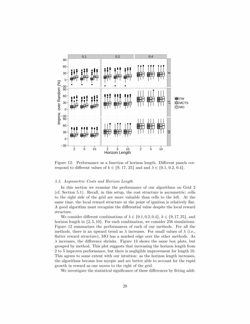
Figure 12: Performance as a function of horizon length. Different panels cor-respond to different values of k ∈ {9, 17, 25} and and λ ∈ {0.1, 0.2, 0.4}.

5.5. Asymmetric Costs and Horizon Length

In this section we examine the performance of our algorithms on Grid 2(cf. Section 5.1). Recall, in this setup, the cost structure is asymmetric; cellsto the right side of the grid are more valuable than cells to the left. At thesame time, the local reward structure at the point of ignition is relatively flat.A good algorithm must recognize the differential value despite the local rewardstructure.

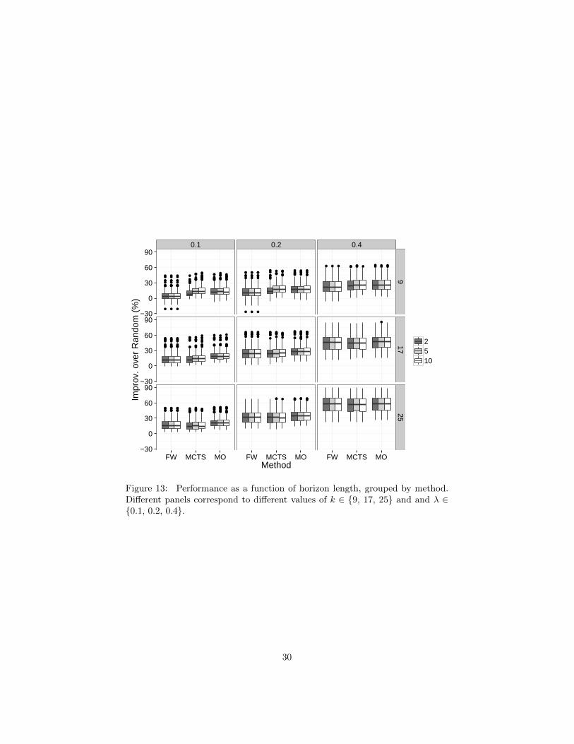
We consider different combinations of λ ∈ {0.1, 0.2, 0.4}, k ∈ {9, 17, 25}, andhorizon length in {2, 5, 10}. For each combination, we consider 256 simulations.Figure 12 summarizes the performances of each of our methods. For all themethods, there is an upward trend as λ increases. For small values of λ (i.e.,flatter reward structure), MO has a marked edge over the other methods. Asλ increases, the difference shrinks. Figure 13 shows the same box plots, butgrouped by method. This plot suggests that increasing the horizon length from2 to 5 improves performance, but there is negligible improvement for length 10.This agrees to some extent with our intuition: as the horizon length increases,the algorithms become less myopic and are better able to account for the rapidgrowth in reward as one moves to the right of the grid.

We investigate the statistical significance of these differences by fitting addi-

29

0.1 0.2 0.4

●

●

●

●

●●

●●

●

●

● ●

●

●

●

●●

●●

●

●

● ●

●

●

●

●●

●●

●

●

●●

●

●●●●●

●●

●

●

●●●● ●●

●●

●

●●●●●●● ●●●

●

●

●

●● ●●

●●●●

●●●

●●●●

●

●●

●●

●

●

●

●

●

●

●●

●●

●

●

●

●

●

●

●●

●●

●

●

●

●

●

●

●●

●

●●●

●

●●

●

●

●

●●

●

●

●

●

●

●●●

●

●

●

●

●

●

●

●● ●

●

●

●

●

●

●

●

●

●

●

●●●

●

●

●

●

●

●

●●●●●

●●●●●

●●●●●

●●●●●● ●●●

●●●●● ●

●●●●●●

●●●●●●●●

●●●●●●●●

●

●●

●●●

●

●●

●●●

●

●●

●●●

●

●●

●●

●

●

●●●●

●●●●●●

●●●●● ●

●●●

●●

●●

●●●●●●

●●●●●●

●●●●●●

●●●●●●

●●●●●●

●

●●●●●●

●●●●

●●

●●●

●

●

●

●

●●

●●●●●●

●● ● ●●● ●● ●●●

● ● ● ●● ●●● ● ●● ●● ●●

●

−30

0

30

60

90

−30

0

30

60

90

−30

0

30

60

90

917

25

FW MCTS MO FW MCTS MO FW MCTS MOMethod

Impr

ov. o

ver

Ran

dom

(%

)

2510

Figure 13: Performance as a function of horizon length, grouped by method.Different panels correspond to different values of k ∈ {9, 17, 25} and and λ ∈{0.1, 0.2, 0.4}.

30

tive effects models. The full model contains many insignificant interactions. Wedrop insignificant variables using backwards stepwise deletion. The resulting fitcan be seen in Table 7. The fitted model suggests that differences observed inthe previous plot are statistically significant.

6. Conclusion

In this study, we consider a dynamic resource allocation problem motivatedby tactical wildfire management, in which fire spreads stochastically on a finitegrid and the decision maker must allocate resources at discrete epochs to sup-press it. We propose two different solution approaches: one based on MonteCarlo tree search, and one based on mathematical optimization.

Our study makes three broad methodological contributions. The first ofthese contributions is to the understanding of MCTS: to the best of our knowl-edge, this study is the first application of Monte Carlo tree search to high-dimensional dynamic resource allocation motivated by a real-world application,and our results suggest that MCTS holds promise in other large scale stochas-tic control applications. Our numerical results uncover some interesting insightsinto how MCTS behaves in relation to parameters such as the exploration bonus,the progressive widening parameters and others, as well as larger componentssuch as the method of action generation and the rollout heuristic. Our resultsshow that these components are highly interdependent and cannot be calibratedseparately of each other—for example, our results show that the choices of ac-tion generation method and progressive widening factor become very importantwhen the rollout heuristic is not strong on its own (e.g., the random suppres-sion heuristic) but are less valuable when the rollout heuristic is strong to beginwith (e.g., the Floyd-Warshall heuristic). These insights will be valuable forpractitioners interested in applying MCTS to other problems.

The second broad methodological contribution of our study is to the un-derstanding of mathematical optimization in dynamic resource allocation. Theformulation that we consider is a continuous, deterministic one that avoids thecombinatorial nature of the true fire dynamics, which are discrete and stochas-tic. Our results indicate that such approximations, in spite of how much theydepart from the true dynamics, can lead to effective heuristics for large scalestochastic control problems. This insight is both important and not obvious.

The third broad methodological contribution is towards the understandingof the relative merits of MCTS and mathematical optimization. Our resultsshow that while both methodologies exhibit comparable performance for smallerinstances, for larger instances, the mathematical optimization approach exhibitsa significant edge. Initial evidence suggests this edge may be related more closelyto action branching factor than the state space branching factor.

Acknowledgements

This paper is the result of research and development sponsored by the Assis-tant Secretary of Defense for Research and Engineering, ASD(R&E). The work

31

Table 7: Estimated effects for Section 5.5

Effect Coefficient p-value

(Intercept) 5.45∗∗∗ (0.00)λ = 0.2 6.66∗∗∗ (0.00)λ = 0.4 17.70∗∗∗ (0.00)k = 17 7.84∗∗∗ (0.00)k = 25 10.87∗∗∗ (0.00)Depth 5 0.00 (1.00)Depth 10 0.00 (1.00)MCTS 6.25∗∗∗ (0.00)MO 8.76∗∗∗ (0.00)λ = 0.2 : k = 17 5.22∗∗∗ (0.00)λ = 0.4 : k = 17 14.38∗∗∗ (0.00)λ = 0.2 : k = 25 9.33∗∗∗ (0.00)λ = 0.4 : k = 25 23.56∗∗∗ (0.00)λ = 0.2: MCTS −1.47∗∗ (0.00)λ = 0.4 : MCTS −2.94∗∗∗ (0.00)λ = 0.2 : MO −2.81∗∗∗ (0.00)λ = 0.4 : MO −4.98∗∗∗ (0.00)k = 17 : MCTS −5.14∗∗∗ (0.00)k = 25 : MCTS −6.51∗∗∗ (0.00)k = 17 : MO −2.33∗∗∗ (0.00)k = 25 : MO −3.48∗∗∗ (0.00)Depth 5 : MCTS 1.50∗∗ (0.00)Depth 10 : MCTS 1.47∗∗ (0.00)Depth 5 : MO 0.18 (0.72)Depth 10 : MO 0.14 (0.78)

† significant at p < 0.10; ∗p < 0.05; ∗∗p < 0.01; ∗∗∗p < 0.001

The intercept should be interpreted as the value of the FW heuristicwhen λ = .1, k = 9 and the horizon length is 2.

32

of the fifth author was supported by a PGS-D award from the Natural Sciencesand Engineering Research Council (NSERC) of Canada.

References

[1] Acimovic, J., Graves, S., 2012. Making better fulfillment decisions on the flyin an online retail environment. Tech. rep., Working Paper, MassachusettsInstitute of Technology, Boston, MA.

[2] Arneson, B., Hayward, R., Henderson, P., 2009. MoHex wins Hex tourna-ment. International Computer Games Association Journal 32 (2), 114–116.

[3] Arneson, B., Hayward, R. B., Henderson, P., 2010. Monte Carlo tree searchin hex. IEEE Transactions on Computational Intelligence and AI in Games2 (4), 251–258.

[4] Auer, P., Cesa-Bianchi, N., Fischer, P., 2002. Finite-time analysis of themultiarmed bandit problem. Machine Learning 47 (2-3), 235–256.

[5] Avram, F., Bertsimas, D., Ricard, M., 1995. Fluid models of sequencingproblems in open queueing networks: An optimal control approach. Insti-tute for Mathematics and its Applications, 199–234.

[6] Barnhart, C., Belobaba, P., Odoni, A. R., 2003. Applications of operationsresearch in the air transport industry. Transportation science 37 (4), 368–391.

[7] Bellman, R. E., 1957. Dynamic Programming. Princeton University Press.

[8] Bemporad, A., 2006. Model predictive control design: New trends andtools. In: Decision and Control, 2006 45th IEEE Conference on. IEEE, pp.6678–6683.

[9] Ben-Tal, A., El Ghaoui, L., Nemirovski, A., 2009. Robust optimization.Princeton University Press.

[10] Bertsekas, D. P., 1995. Dynamic programming and optimal control. Vol. 1.Athena Scientific Belmont.

[11] Bertsimas, D., Brown, D. B., Caramanis, C., 2011. Theory and applicationsof robust optimization. SIAM review 53 (3), 464–501.

[12] Bertsimas, D., Gupta, S., Lulli, G., 2013. Dynamic resource allocation: Aflexible and tractable modeling framework. European Journal of Opera-tional Research.URL http://www.sciencedirect.com/science/article/pii/

S0377221713008928

[13] Bertsimas, D., Stock Patterson, S., 1998. The air traffic flow managementproblem with enroute capacities. Operations Research 46 (3), 406–422.

33

[14] Boychuck, D., Braun, W. J., Kulperger, R. J., Krougly, Z. L., Stanford,D. A., 2008. A stochastic forest fire growth model. Environmental andEcological Statistics 1 (1), 1–19.

[15] Bracmort, K., August 2013. Wildfire management: Federal funding andrelated statistics. Tech. rep., Congressional Research Service.URL https://www.fas.org/sgp/crs/misc/R43077.pdf

[16] Browne, C. B., Powley, E., Whitehouse, D., Lucas, S. M., Cowling, P. I.,Rohlfshagen, P., Tavener, S., Perez, D., Samothrakis, S., Colton, S., 2012.A survey of Monte Carlo tree search methods. IEEE Transactions on Com-putational Intelligence and AI in Games 4 (1), 1–43.

[17] Charnes, A., Cooper, W. W., 1959. Chance-constrained programming.Management science 6 (1), 73–79.

[18] Chen, H., Yao, D. D., 1993. Dynamic scheduling of a multiclass fluid net-work. Operations Research 41 (6), 1104–1115.

[19] Ciancarini, P., Favini, G. P., 2010. Monte Carlo tree search in Kriegspiel.Artificial Intelligence 174 (11), 670 – 684.URL http://www.sciencedirect.com/science/article/pii/

S0004370210000536

[20] Ciocan, D. F., Farias, V., 2012. Model predictive control for dynamic re-source allocation. Mathematics of Operations Research 37 (3), 501–525.

[21] Coquelin, P.-A., Munos, R., 2007. Bandit algorithms for tree search. In:Proceedings of the Twenty-Third Conference Annual Conference on Uncer-tainty in Artificial Intelligence (UAI-07). AUAI Press, Corvallis, Oregon,pp. 67–74.

[22] Coquelin, P.-A., Munos, R., 2007. Bandit algorithms for tree search. arXivpreprint cs/0703062.

[23] Couetoux, A., Hoock, J.-B., Sokolovska, N., Teytaud, O., Bonnard, N.,2011. Continuous upper confidence trees. In: International Conference onLearning and Intelligent Optimization. pp. 433–445.

[24] Coulom, R., 2007. Efficient selectivity and backup operators in monte-carlotree search. In: Computers and Games. Springer, pp. 72–83.

[25] Enzenberger, M., Muller, M., Arneson, B., Segal, R., 2010. Fuego—anopen-source framework for board games and Go engine based on MonteCarlo tree search. IEEE Transactions on Computational Intelligence andAI in Games 2 (4), 259–270.

[26] Erdelyi, A., Topaloglu, H., 2010. Approximate dynamic programming fordynamic capacity allocation with multiple priority levels. IIE Transactions43 (2), 129–142.

34

URL http://www.tandfonline.com/doi/abs/10.1080/0740817X.2010.

504690

[27] Finney, M. A., 2004. FARSITE: Fire area simulator–model developmentand evaluation. Research Paper RMRS-RP-4, USDA Forest Service.

[28] Floyd, R. W., Jun. 1962. Algorithm 97: Shortest path. Communications ofthe ACM 5 (6), 345.

[29] Fried, J. S., Gilless, J. K., Spero, J., 2006. Analysing initial attack on wild-land fires using stochastic simulation. International Journal of WildlandFire 15, 137–146.

[30] Gallego, G., Van Ryzin, G., 1994. Optimal dynamic pricing of inventorieswith stochastic demand over finite horizons. Management Science 40 (8),999–1020.

[31] Gelly, S., Silver, D., 2011. Monte-Carlo tree search and rapid action valueestimation in computer go. Artificial Intelligence 175 (11), 1856 – 1875.

[32] Gorte, R., June 2013. The rising cost of wildfire protection. Tech. rep.,Headwater Economics.URL http://headwaterseconomics.org/wphw/wp-content/uploads/

fire-costs-background-report.pdf

[33] Grieder, P., Parrilo, P. A., Morari, M., 2003. Robust receding horizoncontrol-analysis & synthesis. In: Decision and Control, 2003. Proceedings.42nd IEEE Conference on. Vol. 1. IEEE, pp. 941–946.

[34] Gurobi Optimization, Inc., 2013. Gurobi optimizer reference manual.URL http://www.gurobi.com

[35] Hastie, T., Tibshirani, R., Friedman, J., 2009. The Elements of StatisticalLearning: Data Mining, Inference, and Prediction, 2nd Edition. Springer.

[36] Hu, X., Ntaimo, L., Nov. 2009. Integrated simulation and optimization forwildfire containment. ACM Trans. Model. Comput. Simul. 19 (4), 19:1–19:29.URL http://doi.acm.org/10.1145/1596519.1596524

[37] Hu, X., Sun, Y., Ntaimo, L., 2012. Devs-fire: design and application of for-mal discrete event wildfire spread and suppression models. SIMULATION88 (3), 259–279.URL http://sim.sagepub.com/content/88/3/259.abstract

[38] Jasin, S., Kumar, S., 2012. A re-solving heuristic with bounded revenueloss for network revenue management with customer choice. Mathematicsof Operations Research 37 (2), 313–345.

35

[39] Kocsis, L., Szepesvari, C., 2006. Bandit based Monte-Carlo planning. In:Proceedings of the European Conference on Machine Learning. Springer,pp. 282–293.

[40] Lee, C.-S., Wang, M.-H., Chaslot, G., Hoock, J.-B., Rimmel, A., Teytaud,O., Tsai, S.-R., Hsu, S.-C., Hong, T.-P., 2009. The computational intel-ligence of MoGo revealed in Taiwan’s computer Go tournaments. IEEETransactions on Computational Intelligence and AI in Games 1 (1), 73–89.

[41] Maglaras, C., Meissner, J., 2006. Dynamic pricing strategies for multiprod-uct revenue management problems. Manufacturing & Service OperationsManagement 8 (2), 136–148.

[42] Martin-Fernndez, S., Martnez-falero, E., Prez-Gonzlez, J. M., 2002. Opti-mization of the resources management in fighting wildfires. EnvironmentalManagement 30, 352–364.

[43] Nilim, A., El Ghaoui, L., 2005. Robust control of markov decision processeswith uncertain transition matrices. Operations Research 53 (5), 780–798.

[44] Ntaimo, L., Arrubla, J. A. G., Stripling, C., Young, J., Spencer, T., 2012. Astochastic programming standard response model for wildfire initial attackplanning. Canadian Journal of Forest Research 42 (6), 987–1001.

[45] Ntaimo, L., Gallego-Arrubla, J. A., Jianbang, G., Stripling, C., Young,J., Spencer, T., 2013. A simulation and stochastic integer programmingapproach to wildfire initial attack planning. Forest Science 59 (1), 105 –117.URL http://search.ebscohost.com/login.aspx?direct=true&db=

egh&AN=85825800&site=ehost-live

[46] Powell, W. B., 2011. Approximate Dynamic Programming: Solving theCurses of Dimensionality, 2nd Edition. Wiley.

[47] Powell, W. B., Shapiro, J. A., Simao, H. P., 2002. An adaptive dynamicprogramming algorithm for the heterogeneous resource allocation problem.Transportation Science 36 (2), 231–249.

[48] Reiman, M. I., Wang, Q., 2008. An asymptotically optimal policy for aquantity-based network revenue management problem. Mathematics of Op-erations Research 33 (2), 257–282.

[49] Rice, J. A., 2007. Mathematical Statistics and Data Analysis. CengageLearning.

[50] Rothermel, R. C., 1972. A mathematical model for predicting fire spreadin wildland fuels. Tech. Rep. INT-115, USDA Forest Service.

[51] Rubin, J., Watson, I., 2011. Computer poker: A review. Artificial Intelli-gence 175 (56), 958 – 987.

36

[52] Shah, D., Wischik, D., 2012. Switched networks with maximum weightpolicies: Fluid approximation and multiplicative state space collapse. TheAnnals of Applied Probability 22 (1), 70–127.

[53] Talluri, K., Van Ryzin, G., 1998. An analysis of bid-price controls fornetwork revenue management. Management Science 44 (11-Part-1), 1577–1593.

[54] Talluri, K. T., van Ryzin, G. J., 2004. The Theory and Practice of RevenueManagement. International Series in Operations Research and ManagementScience, vol. 68. Springer.

[55] Tymstra, C., Bryce, R., Wotton, B., Taylor, S., Armitage, O., 2010. Devel-opment and structure of prometheus: The Canadian wildland fire growthsimulation model. Information Report NOR-X-417, Canadian Forest Ser-vice.

[56] Western Forestry Leadership Coalition, Apr. 2010. The true cost of wildfirein the Western U.S.URL http://www.wflccenter.org/news_pdf/324_pdf.pdf

[57] Whitley, D., 1994. A genetic algorithm tutorial. Statistics and Computing4 (2), 65–85.

37