Characterizing, Modeling and Predicting Dynamic Resource Availability in aLarge Scale Multi-Purpose Grid

Farrukh Nadeem, Radu Prodan, Thomas FahringerInstitute of Computer Science, University of Innsbruck

Technikerstraße 21a, A-6020 Innsbruck, Austriafarrukh@dps.uibk.ac.at

Abstract

The functional heterogeneity of computational Grids hashighly increased due to inclusion of resources other thandedicated to Grid, like from non-dedicated desktop Grids,on-demand systems and even from P2P systems and mo-bile Grids. At such a diversified scale, resources exhibit dif-ferent availability properties mainly due to administrators’policies for resource availability in the Grid, and their fail-ure/unavailability properties. These make resources’ avail-ability predictions for optimized resource selection, a chal-lenging problem. Addressing this problem, we character-ize resource availability properties against their availabil-ity policies to understand their availability behavior andquantify it through availability models. We further exploitthe availability/failure properties to make predictions abouttheir availability through pattern recognition and classifi-cation. We have achieved, on average, accuracy of morethan 90% and 75% in our predictions for resource instanceavailability and lifetime respectively.

1 IntroductionAs the Grid technology is getting mature day by day,

the composition, functionality, utilization and scale of com-putational Grids continue to evolve. The large scale com-putational Grid environments and testbeds under central-ized administrative controls, such as, Cern LCG [1], TeraGrid [4], Grid’5000 [2], Austrian Grid [3] etc. amass hun-dreds/thousands of resources, which vary considerably interms of number of sites, resources at each site and theiravailability patterns. At such a diversified scale, a largernumber of these resources may be unavailable at any time,mainly due to wide range of policies for contributing theseresources to the Grid. Some of the Grid-sites might even betemporarily removed partially or completely from the Gridto accommodate other tasks or projects. In this scenarioonline predictions about resources’ availability are requiredfor effective resource capacity planing.

The resource’s components, Grid middleware maturity,varying resource maintenance and failure properties makeresource availability characterization and prediction a hardproblem. In addition, necessity of inclusion of informationfrom a wide range of policies for resource availability in theGrid makes the problem even more challenging. To addressthis problem, we present in this paper our Grid resourcecharacterization, modeling and prediction system. Avail-ability trace of resources in Austrian Grid is undertaken forour present study.

We begin by considering resource availability policies,exposing availability characteristics and finding differentpatterns over time from a long-term availability trace, (Sec-tion 2.2). Several other studies characterize or model avail-ability in different environments like cluster of comput-ers [6], multi-computers [16], meta-computers (also calleddesktop Grids) [7], Grid [14], [5], super-computers [16],and peer-to-peer systems [12], we are the first to identify thedifferent resource classes based on their high level policiesfor availability in the Grid and characterize their availabilitybehavior to find availability patterns at class level. To under-stand and quantify resource long term availability behavior,we model resource lifetimes (availability durations) at classlevel to find mathematical models of their availability andmake their survival analysis (Section 3). We further makeresource instance and lifetime availability predictions usingmethods from pattern recognition and classifications, in-corporating their availability patterns (Section 4). We haveimplemented a prototype of our system in ASKALON [17]and results are presented to show effectiveness of our ap-proach.

2 Characterizing Resource Availability in aMulti-Purpose Grid Environment

In this section, we describe an analysis of availabil-ity of resources in a large-scale, multi-cluster and multi-purpose Austrian Grid. Austrian Grid is the nation-wide,multi-institutional, -administrative and -VO Grid platform,

consisting of 28 Grid-sites geographically distributed inAustria. Every Grid-site comprises of multiple CPUs,shared (SMP, ccNUMA) or distributed memory architec-ture(COW(cluster of working nodes) or NOW(network ofworking nodes)), and collectively there are over 1.5 thou-sand processors. Resources in Austrian Grid include re-sources dedicated to Austrian Grid users, resources fromlabs of universities and resources available only on demand,and collectively it contains a variety of availability patternsand behavior. Please note that in this paper we use the termsmachine and resource interchangeably.

2.1 Resource Classification

The resources in Austrian Grid possess different(un)availability properties . These properties can be bet-ter exposed, analyzed and lead to optimized resource se-lection decisions if we classify them based on the policiesfor their availability in the Grid. Based on this criteria, weidentify three main classes of resources in Austrian Grid:dedicated resources, temporal resources and on-demand re-sources. The dedicated resources are meant to be alwaysavailable to the Grid users for production and experimentalwork. Resources from university labs, referred as temporalresources are available in the Grid as long as they are turnedon, but students very often turned them off while leaving thelabs. Some resources are made available to the Grid only ondemand from the Grid users for large scale jobs. These arereferred as on-demand resources.

2.2 Austrian Grid Trace Analysis

We accessed, organized and analyzed Austrian Grid re-source availability trace of approx. one year from mid-June2006 to mid-April 2007, recorded after the intervals of 5minutes. Altogether this trace is comprised of more than23 million of events that occurred on the whole AustrianGrid. Each trace event represents availability or unavailabil-ity of a Grid resource with the time stamp at which the sta-tus (available or unavailable) of the resource was recorded.Next in this section, we describe availability characteristicsof resource classes as a whole, to further enable us to makeconclusive inferences about their aggregate behavior. In thepresented work, we consider a resource available if it isturned on and accessible remotely (e.g. through GRAM),otherwise it is considered unavailable.

2.2.1 Pool Availability over Time

Figure 1 shows the daily availability of Austrian Grid re-sources at Grid and resource class levels. On average, theresource availability in Austrian Grid is 33%, with a mini-mum of 4% and maximum of 71% per day (Figure 1(A)).At resource classes level, the pool of dedicated resourcesshows the highest availability of 92% with a minimum of

48% and a maximum of 100% per day (Figure 1(B)); thetemporal resources collectively show a relatively lower av-erage daily availability of 47% ranging between 0%-92%(Figure 1(C)); on-demand resources are observed to be theleast available, on average 9% daily ranging between 0%-88% (Figure 1(D)). The standard deviation (SD) of 19.19was observed at Grid level, and that of 6.54, 9.24, 8.17 inthe three classes respectively.

2.2.2 Pool Hourly and Week-day AvailabilityIn addition to availability analysis over time, we also per-formed an analysis for potential patterns of (un)availabilityduring different hours of a day and over different days ofweek. Here, we report average availability of three resourceclasses as a function of both hour of the day andday of the week. Figure 2 depicts diurnal resourceavailability patterns; availability peaks during 8a.m. to8p.m. and recesses during the remaining hours. Availabilitytoggles between 37% and 55% at Grid level, with maximumat 3p.m. and minimum at 9a.m. (Figure 2(A)). For classof dedicated resources this toggles between 95% and 99%(Figure 2(B)), for temporal resources between 43% and64% (Figure 2(C)), and for on-demand resources between3% and 17% (Figure 2(D)). The maximum availabilitywas found at 4p.m., 2p.m., 3p.m. and the minimum at4a.m., 8a.m., 4a.m. respectively for the three classes. Weobserved interesting patterns at resource class level as wellat Grid level. The availability remains comparatively in asmall range during the night hours with the minimum valuebetween 4a.m. and 8a.m. This is the time when most ofthe resources are turned off or given a restart. After theminimum value it starts increasing towards the peak value(except one decrease in dedicated resources), and fromthe maximum it decreases towards a certain level to be

0 50 100 150 200 250 300 35040

50

60

70

80

90

100

Days

Per d

ay a

vaila

bility

(%ag

e)

Daily Resource Availability of Dedicated Cluste

0 50 100 150 200 250 300 3500

20

40

60

80

100

Days

Per d

ay a

vaila

bility

(%ag

e)

Daily Resource Availability of on Demand Clusters

0 50 100 150 200 250 300 3500

20

40

60

80

100

Days

Per d

ay a

vaila

bility

(%ag

e)

Daily Resource Availability of Temporal Clusters

0 50 100 150 200 250 300 3500

20

40

60

80

Days

Per d

ay a

vaila

bility

(%ag

e)

Daily Resource Availability in Austrian Grid

A B

C D

Figure 1. Resource daily availability at re-source class and Grid level.

0 5 10 15 20 2536

40

45

50

55

Hour of the day

Per d

ay a

vaila

bility

(%ag

e)

Hourly Availability of Austrian Grid Resources

0 5 10 15 20 2594

95

96

97

98

99

Hours of the day

Per d

ay a

vaila

bility

(%ag

e)

Hourly Availability of Dedicated Resources

0 5 10 15 20 2540

45

50

55

60

65

Hour of the day

Per d

ay a

vaila

bility

(%ag

e)

Hourly Availability of Temporal Resources

0 5 10 15 20 251

5

10

15

20

Hour of the day

Per d

ay a

vaila

bility

(%ag

e)

Hourly Availability of on Demand Resources

A B

C D

Figure 2. Resource hour-of-the-day availabil-ity at resource class and Grid level.

maintained till the minimum occurs. The average SD overdifferent hours of the day was 4.16 as compared with thatof 1.37 on a specific hour of the day. Moreover, at Gridlevel, an average SD of 6.6 was observed in availabilitieson specific week days. This remarkable lower SD inavailabilities on a specific day of the week than that onall week days, indicates similar availability pattern onspecific week days. In sequel, lower SD in availabilitieson specific hour of the day than that on all hours, showssimilar availability patterns over specific hours of the day.

Sun Mon Tue Wed Thu Fri Sat35

40

45

50

55

60

65

70

75

Day of the week

Perd

ay av

ailab

ility(

%ag

e)

Figure 3. Week days avail-ability patterns in AustrianGrid.

The availabil-ity patterns on28 machines(machinenames areirrelevant)over differentweek daysare shownin Figure 3.Two classesof patterns canbe visualizedfrom this figure; first, with lower availability at week ends,and higher during the working week days. This class has anincreasing availability till Tuesday or Wednesday and thendecreasing till weekend. Second, with higher availabilityon weekends and lower during the working weekdays. Thisclass has a decreasing availability till Wednesday and thenincreasing availability till Saturday.

Aggregate resource availability over hour of theday and day of the week indicates the work day us-age and availability patterns in the Grid. Furthermore,it manifests the policy of shutting down most the non-

dedicated resources during the night as opposed to leav-ing them on over night. Changes in availability of dedi-cated resources reflect their failure or turning off for main-tenance/repairs in the non-working hours.

2.2.3 Pool LifetimeWe define machine lifetime as the consistent time durationfor which it is available. A probabilistic resource lifetimescomparison for three resource classes as sum of probabili-ties of the different lifetimes(t) and their greater lifetimes, isshown in Figure 4. On average, classes of dedicated, tem-poral and on-demand resources have a maximum lifetimeof 93495 min. (approx. 65 days), 5275 min. (approx. 4days) and 1000 min. respectively. It is interesting to notethat dedicated resources on average have 35% probability ofa continuous availability lasting more than a day, temporalresources have 50% probability that resource will fail after6 hours, and on-demand resources have 50% probability offailing after 90 min.

The resource availability time distribution in differentlife times and their life times distribution over the wholemonitoring period (referred as Time and Duration (T&D)distribution) of three resource classes is presented in Fig-ure 5. In dedicated resources (Figure 5(a)), more than halfof availability time lies in availability durations greater than7000 min., that covers 53% of total available time and com-prise 17% of all durations. This shows that dedicated re-sources exhibit good consistent availability and intuitivelythe highest one also. Figure 5(b) shows T&D distributionof temporal resources. The highest portion of the availabil-ity time, 17%, lies in durations 3001-4000 min., which cor-responds to only 3% of all available durations. This distri-bution indicates that some of the temporal resources havelonger availability durations, while the others have quitesmall. The T&D distribution for on-demand resources inFigure 5(c) shows that most of their availability time lies indurations ranging between 1001-2000 min. and these en-compass only 3% of all durations, with the second highestpart of availability time in 2001-3000 min., which corre-sponds to only 1% of all available durations. Furthermore,the maximum availability duration is 3001-4000 min. This

0

0.2

0.4

0.6

0.8

1

518

046

091

011

8514

2027

2541

5570

2510

485

1847

046

765

Lifetime (min)

P(X

>=t)

dedicated res.temporal res.on-demandres.

Figure 4. Lifetime comparison of three re-source classes.

53%

15%

5%

4%

10%

3%2%

<6060-100101-200201-300301-400401-500501-600601-700701-800801-900901-10001001-20002001-30003001-40004001-50005001-60006001-7000>7000

Time Distribution of Availability Durations inDedicated Resources

7%

2% 2% 1%1%1%1%4%

20%

6%17%

7%

15%

3%

1%1%

5%

5%

<6060-100101-200201-300301-400401-500501-600601-700701-800801-900901-10001001-20002001-30003001-40004001-50005001-60006001-7000>7000

Availability Durations Distribution in DedicatedResources

< 1%

(a) Time and duration distribution in dedicated resources

22%

9%

10%7%6%

6%

16%

5%

7%1%1%

1% 3%1%0%0%<1%3%

<6060-100101-200201-300301-400401-500501-600601-700701-800801-900901-10001001-20002001-30003001-40004001-50005001-60006001-7000>7000

Availability Durations Distribution in TemporalResources

1%

14%

10%5%

17%

3%4%

11%2%

1%

5%

3%3%

4%

9%

2%2%

5%

<6060-100101-200201-300301-400401-500501-600601-700701-800801-900901-10001001-20002001-30003001-40004001-50005001-60006001-7000>7000

Time Distribution of Availability Durations inTemporal Resources

(b) Time and duration distribution in temporal resources

7%4%

12%

20%

<1% 3%2% 7% 7%

11%

6%

6%

10%

5%<6060-100101-200201-300301-400401-500501-600601-700701-800801-900901-10001001-20002001-30003001-4000

Time Distribution of Availability Durations in on-Demand Resources

17%15%

6%

5%

7%

4%3%

<1%

1%1%

3% <1%

1%

37%

<6060-100101-200201-300301-400401-500501-600601-700701-800801-900901-10001001-20002001-30003001-4000

Availability Durations Distribution of on-DemandResources

(c) Time and duration distribution in on-demand resources

Figure 5. Time and duration distribution inthree resource classes.

distribution indicates that on-demand resources were avail-able for a few times and used only for short periods of time.Their almost symmetrical distribution of durations (even forvery short periods) indicates that there are some unstable re-sources among them also.

3 Resource Availability ModelsIn this section we model resource availability in a multi-

cluster and multi-policy Grids. The main purpose of mod-eling is to find parametric models for mathematical analysisof resource (un)availability, which are presented at the endof this section.We begin by considering basic statistical properties of(un)availability of resources in Austrian Grid at class level.Table 1 summarizes them as minimum, first quartile, me-dian, third quartile, mean, maximum and SD. The results foravailability durations show that the ratios between mean andmedian are largely different across the three classes. More-over, the distribution of (un)availability durations is sub-stantially different in each class, as shown in Section 2.2.3.These measures indicate that single parameter distributionsmay not be used for a good fit for these classes. In addition,these indicate that either individual distributions for the re-

Table 1. Summery of the basic statisticalproperties of (un)availability of three re-source classes in Austrian Grid.

Resource ClassesDedicated Temporal on-Demand

Avail. Unavail. Avail. Unavail. Avail. Unavail.Min. 5 5 5 5 5 51st Qrt. 70 5 35 10 27.5 25Median 80 15 230 105 105 6803rd Qrt. 230 40 575 685 362.5 1458.75Mean 2212.37 166.36 721.52 969.78 265.48 2916.7Max 150500 131685 150405 145750 3245 95200SD 6.54 9.18 10.24 33.19 8.17 9.71

source classes or distributions with higher degree of free-dom (e.g. hyper-gamma or hyper-exponential) are neededto model availability durations of these resource classes.Due to better accuracy we opt for the first choice.At first, we perform a graphical analysis of the fitted dis-

tribution. This allows us to exterminate some of the distri-butions from the process of modeling which clearly do notfit the availability data. Figures 6, 7 and 8 show the graph-ical analysis of CDF (Cumulative Distribution Function) ofdifferent lifetimes of dedicated, temporal and on-demandresource classes respectively, for Lognormal, Weibull, Ex-ponential, Gamma, Normal, Pareto distributions along withreal values. For details regarding these distributions andtheir properties, e.g. probability density functions (PDFs),CDFs we refer the reader to [11]. Clearly, extreme valuefit and normal fit are far away from the actual data, andother distributions appear reasonably close to the actualdata, with the Lognormal, Weibull and Pareto looking es-pecially promising in all the cases.

To further accentuate the best fit, we make detailedmodel fitting and analysis. We now attempt for statisti-cal analysis for remaining fitted distributions. The Weibulldistribution has been often used to model the lifetimesof objects including physical system components [7, 12],whereas the others have been previously used to model ma-chine availability [10, 5]. We perform the following anal-ysis for each distribution in each resource class. First, wefit each of the above mentioned distributions by estimatingtheir parameters through the method of Maximum Likeli-hood Estimation (MLE) [11]. Next, we assess quality offitting of these distributions to establish the best fit for eachresource class, by performing goodness-of-fit test for eachof the fitted distributions. Kolmogorov-Smirnov test (KS-test) is used to test our hypothesis (the null hypothesis) forgoodness-of-fit of a distribution di, where di represents adistribution model we want to test. We phrase our null hy-pothesis as: ”resource class availability data comes fromthe distribution di”, whose parameters were estimated inthe last step. The KS-test compares the empirical distribu-tion function of availability data with that of the distributionspecified in null hypothesis. Contrary to other traditionalgoodness-of-fit tests like t-test or chi-square test, the mainadvantage of this test is that it is non-parametric and dis-tribution free i.e. we do not need to make any assumptionabout the underlying cumulative distribution function being

100 102 1040.00010.0010.01

0.10.250.5

0.750.9

0.990.999

0.9999

Data

Pro

babi

lity

Probability plot for Lognormal distribution

0 2 4 6 8 10x 104

0

0.2

0.4

0.6

0.8

1

Life time

Cum

ulat

ive

prob

abilit

y

Modeling Life Time of Dedicated Resources

Original DataLognormal FitExponential FitGamma FitNormal FitWeibull FitExtreme values FitPareto Fit

103 104 1050.9996

0.9997

0.9998

0.9999

1Survivor Fcn

0 5 10x 104

0

2

4

6

x 10-4 Hazard Rate Fcn

0 2 4 6 8 10x 104

10-6

10-4

Prob. Density Fcn

Figure 6. Availability modeling, fit check, andsurvival analysis of dedicated resource.

100 102 104 1060.00050.001

0.0050.01

0.050.1

0.250.5

0.750.95

0.999

Data

Prob

abilit

y

Probability plot for Exponential distribution

0 0.5 1 1.5 2 2.5 3 3.5 4x 104

0

0.2

0.4

0.6

0.8

1

Life time

Cum

ulat

ive

prob

abilit

y

Modeling Life Time of Temporal Resources

Original DataWeibull FitExponential FitGamma FitNormal FitLognormal FitExtreme values FitPareto Fit

0 5 10 15x 104

10-10

10-5

100Prob. Density Fcn

102 103 104 1050

0.1

0.2

Survivor Fcn

0 1 2 3 4 5x 104

10-10

10-5

100 Hazard Rate Fcn

Probability plot for Pareto distribution

Figure 7. Availability modeling, fit check, andsurvival analysis of temporal resource.

100 101 102 103 104

0.0050.01

0.050.1

0.250.5

0.750.95

0.999

Data

Prob

abilit

y

Probability plot for Weibull distribution

0 500 1000 1500 2000 2500 30000

0.2

0.4

0.6

0.8

1

Life time

Cum

ulat

ive

prob

abilit

y

Modeling Life Time of on Demand Resources

Original DataWeibull FitExponential FitGamma FitNormal FitLognormal FitExtreme values FitPareto Fit

0 1000 2000 3000 4000

10-5

Hazard Rate Fcn

0 1000 2000 3000 400010-8

10-6

10-4

10-2

Prob. Density Fcn

101 102 103 1040

0.2

0.4

0.6

0.8

1Survivor Fcn

Figure 8. Availability modeling, fit check, andsurvival analysis of on-demand resources.

tested. Kolmogorov-Smirnov statistic D, for a given test,estimates the maximum distance at any point between thetwo distributions. The null hypothesis is rejected if the teststatistic D is greater than the critical value obtained from aKS-table. The higher the value of D, the higher the degreeof dissimilarity between the availability data and the datafrom the tested distribution. We use this property to selectthe best fit, and find that the best fit for availability durationsare Lognormal, Pareto and Weibull for dedicated, temporaland on-demand classes of resources respectively, whereasbest fit model for overall Austrian Grid is found to be Log-normal.In contrast to traditional resource availability models [16]and [7], we have found that the overall probability dis-tribution of Grid model of (un)availability is shaped fromthe probability distribution models of underlying differentclasses of resources, which are based on their different poli-cies of availability to the Grid. Hence, lognormal dominatesfor the three resource classes in our case, which is due todominating size of dedicated resources class in the AustrianGrid. We found that these resources can be more accuratelymodeled on their individual class level instead of the wholeGrid level. We find the class level models conforming theactual data with an accuracy of more than 90%, as com-pared with that of 77% for Grid level models. The accuracyof fit of the best model for the three classes is also shownas the probability plot of the best model and the originaldata in Figures 6, 7 and 8 respectively. The straight linein these figures represent the probabilities through modeledparameters and the dotted line represent the original data.

Table 2 shows the parameter values of the best fit modelof availability durations for each of the resource classes inAustrian Grid. The higher scale parameters for Pareto andWeibull are a bit alarming, which indicate the increasinghazard rate functions for these distributions. The hazard rategives the instantaneous probability of failure/unavailabilitygiven the survival to a given time. It is the PDF dividedby survival function. The survival function gives the proba-bility of survival as a function of time. It is simply 1 minuscumulative distribution function (1−CDF ). In the selectedbest fit models the hazard rate turns out to be increasing intemporal and on-demand resources, which means that theresources are more susceptible to failure/unavailability astime passes (aging). The hazard rate in dedicated resourcesis decreasing which means that resources get more stable asthe time increases. The survival function of dedicated re-sources is increasing, indicating that resources have higherprobability of availability for the longer durations. Con-trarily, decreasing survival functions in temporal and on-demand resources show a lower probability of availabil-ity for longer durations. The PDF, survival function andthe hazard rate function of the best fit models for the threeclasses are shown in Figures 6, 7 and 8 respectively.

0 1000 2000 3000 40000.3

0.4

0.5

0.6

0.7

0.8

0.9

1

Time

Cumu

lative

prob

abilit

y

Modeling Time to Reboot of Dedicated Resources

Original DataWeibull FitExponential FitGamma FitNormal FitLognormal FitExtreme values FitPareto Fit

0 1 2 3 4x 104

0

0.2

0.4

0.6

0.8

1

Time

Cumu

lative

prob

abilit

y

Modeling Time to Reboot of Temporal Resources

Original DataWeibull FitExponential FitGamma FitNormal FitLognormal FitExtreme values FitPareto Fit

0 1 2 3 4 5 6x 104

0

0.2

0.4

0.6

0.8

1

Time

Cumu

lative

prob

abilit

y

Modeling Time to Reboot of on-Demand Resources

Original DataWeibull FitExponential FitGamma FitNormal FitLognormal FitExtreme values FitPareto Fit

A B C

Figure 9. Resource unavailability (MTR) models at resource class level.

3.1 Resource Unavailability Models

Resource unavailability behavior gives an insight of howlong and when a resource is unavailable. This implicitlyincludes resource maintenance and failure properties, andtheir policies for unavailability in the Grid. To understandand quantify resource unavailability behavior, in this sec-tion we model resource (un)availability properties as MeanTime to Reboot(MTR). In the same sequence of steps as inmodeling resource availability behavior, we model resourceunavailability behavior. Different models fit for resourceunavailability for dedicated, temporal and on-demand re-sources are shown in Figure 9(A,B,C) respectively. Fromthe graphically analysis, clearly extreme values fit and thenormal distribution do not fit any class of the resources.For dedicated resources, Weibull, Lognormal an Pareto lookpromissing; for temporal and on-demand resources Weibulland Lognormal seem closely modeling the real trace data.In the detailed statistical analysis, like that in Section 3,we found Lognormal as best fit for dedicated resources,while Weibull fitted trace data the best for temporal andon-demand resources. The best fit model parameters of re-source unavailability behavior and their 95% confidence in-tervals are presented in Table 3. It is interesting to note thatdedicated and on-demand classes of resources exhibit samedistributions as best fit in availability behavior as well as inunavailability behavior. This shows that these resources ex-hibit their (un)availability behavior in a consistent fashion,and make these resources more predictable. The opposite istrue for temporal resources.

Table 2. Best fit model parameters of avail-ability data for three resource classes.Resource Classes Best Fit Distribution Parameter Values

Dedicated Resources Lognormal Mean SD6.8138 1.9612

95% conf. inter. (6.6741,6.9534) (1.8673,2.0651)

Temporal Resources Pareto Shape param. Scale param.0.8383 181.8480

95% conf. inter. (0.7403,0.9364) (164.4317,201.1089)

On Demand Resources Weibull 0.5609 351.195295% conf. inter. (324.5505,380.0273) (0.5445,0.5777)

Table 3. Best fit model params. of resourceclasses’ unavailability (MTR) behavior.

Resource Class Best Fit Dist. Parameter Values

Dedicated Lognormal MU Sigma2.8283 1.1205

95% conf. inter. (2.7763,2.8714) (1.0878,1.1552)

Temporal Weibull Shape param. Scale param.0.4527 278.3892

95% conf. inter. (0.4390,0.4667) (252.4212,307.0286)

on-Demand Weibull 0.4266 960.089395% conf. inter. (735.755,1253.038) (0.4545,0.5777)

4 Resource Availability PredictionThe static availability models of resource availability (as

in Section 3) give a probabilistic estimate of resource avail-ability, which is most of the time insufficient to decide aboutresource state and lifetime. The major drawback of usingthese models is that they use static information about re-source availability and ignore resource dynamic behaviorover time as well as its current behavior. Moreover, these ig-nore different patterns of availability over time. In this sec-tion we describe our prediction methodology consideringresource dynamic availability properties and patterns overtime and its current availability behavior.

We employ two methods from pattern recognition andclassification to serve resource instance or point availabil-ity and duration availability predictions: the Bayes’ Ruleand Nearest Neighbor Rule. Instance or point availabilitydescribes resource availability at a certain point of time; inour presented work it refers to the next monitoring instance.Where as, the duration availability describes resource avail-ability over a certain time duration, in our presented workit refers to the immediate next duration of a certain timespan. These methods utilize knowledge of resource past andcurrent availability behavior, gained in the characterizationphase, to serve its future availability predictions. In the nextsections we describe these methods and explain how theyare used to make predictions.

4.1 Bayes’ Rule

Bayes’ rule estimates (future) chances of an event fromits likelihood and priori, as its probability conditional toits characteristics. Thus, for resource availability predic-

tion, Bayes’ rule by nature will exploit resource availabilitycharacteristics from past traces and current behavior. Toincorporate availability patterns over time we exploit dif-ferent availability features specific to time as described inSection 2. Here, we define Bayes’ rule for our two-class re-source state (in our present work, we only consider the twostates of a resource, available and unavailable).

Let ω1 and ω2 represent the two classes to which ourresource state may belong. In the sequel, we assume thattheir priori probabilities P (ω1) and P (ω2) are knownfrom the characterization phase. These can be calculatedas follows: if N is the total number of events and N1, N2

belong to ω1 and ω2 respectively, then P (ω1) = N1/Nand P (ω2) = N2/N . Let p(x|ωi) for i = 1, 2 representthe class-conditional PDFs, describing the distribution offeature vector x in each class. Here, the feature vectorconsists of our availability features found in Section 2.2:x=[day of week,hour of day,hour of day:day of week].The feature day of week represents any day of the weekand its feature space consists of {Mon,...,Sun.}, the fea-ture hour of day represents any hour of the day and itsfeature space consists of {0, 1, 2, ..., 23}, and the featurehour of day:day of week represents an hour of the dayon a given day of the week and its feature space consistsof cross product of the earlier two feature spaces. Theclass-conditional PDFs are also calculated from the tracedata during the characterization phase. Then, according toBayes rule, the probability of class ωi when a feature x isselected is:

P (ωi|x) =p(x|ωi)P (ωi)

p(x)(1)

where p(x) is the PDF of x and for our case of two classesp(x) =

∑

2

i=1p(x|ωi)P (ωi). At a time, we consider one

feature from the feature vector x, which can have any valuefrom the respective feature space. In our case, since the fea-ture spaces can take only discrete values, the density func-tions p(x|ωi) becomes probabilities and will be calculatedas P (x|ωi).

Resource state is decided using equation 1 as:Decide ω1 if p(x|ω1)P (ω1) > p(x|ω2)P (ω2); otherwisedecide ω2.

4.2 Nearest Neighbor Rule (NN-Rule)

Nearest Neighbor rule is a well known pattern classifi-cation technique, which gives the nearest neighbor value asa prediction. In our work it takes the last monitored statusas the nearest neighbor. This method typically suits the ma-chines with high MTBF and MTR, and has a theoretical perday error rate of:

E =

{

fd/Md if resource status is unavailable(fd + 1)/Md if resource status is available

where fd denotes number of transition from available tounavailable state per day, and Md represent number of re-source states monitored per day.

5 Empirical EvaluationThis section describes the evaluation results for the pre-

diction methods presented in Section 4. We evaluatedthese methods for their prediction accuracy, calculated asAccuracy =(No. of true predictions)/(Total number of pre-diction queries) represented as percentage. The whole eval-uation phase was conducted over Austrian Grid availabilitytrace. In case of instance availability prediction, a predic-tion is treated true if the resource immediate next status isthe same as predicted, otherwise it is considered false. Incase of duration availability prediction, prediction is treatedas true if a resource is predicted to be available for a certainimmediate duration and resource is available for that dura-tion or longer, otherwise it is considered false. In case whenresource is available for a duration lesser than the predicted,the accuracy of prediction is calculated as the ratio of actualavailable duration to the predicted. Furthermore, the accu-racy is recorded for different predictors which use differentfeatures from the feature vector described in Section 4.1.These predictors are described in Table 4.

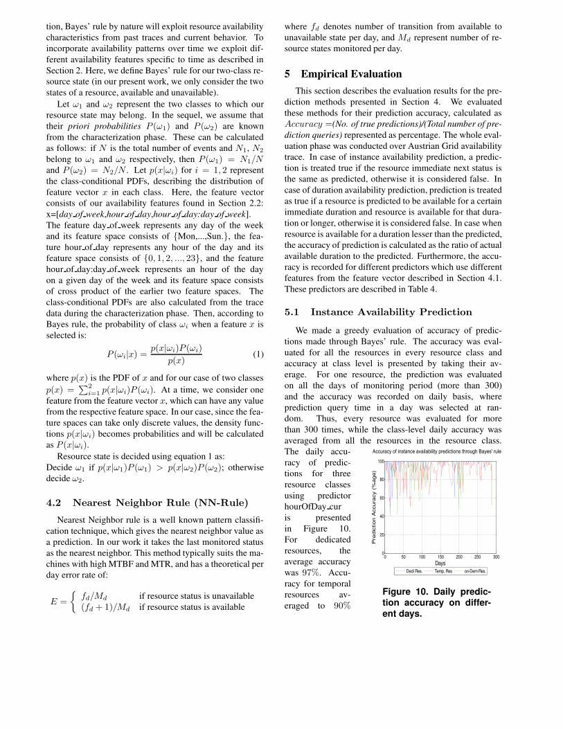
5.1 Instance Availability Prediction

We made a greedy evaluation of accuracy of predic-tions made through Bayes’ rule. The accuracy was eval-uated for all the resources in every resource class andaccuracy at class level is presented by taking their av-erage. For one resource, the prediction was evaluatedon all the days of monitoring period (more than 300)and the accuracy was recorded on daily basis, whereprediction query time in a day was selected at ran-dom. Thus, every resource was evaluated for morethan 300 times, while the class-level daily accuracy wasaveraged from all the resources in the resource class.

0 50 100 150 200 250 3000

20

40

60

80

100

Days

Pre

dict

ion

Acc

urac

y(%

age)

Dedi Res. Temp. Res on-Dem Res.

Figure 10. Daily predic-tion accuracy on differ-ent days.

The daily accu-racy of predic-tions for threeresource classesusing predictorhourOfDay curis presentedin Figure 10.For dedicatedresources, theaverage accuracywas 97%. Accu-racy for temporalresources av-eraged to 90%

Table 4. Details and description of different predictors used in predictions.Predictor Name Feature(s) used Hist. data employed Hist. units Description

dayOfWeek day of week 7, 14, 21, 30, 40, 50 weeks uses hist. data from the specified day of theweek only

hourOfDay all hour of day 1, 7, 14, 21, 30, 60, 120 days uses hist. data only from specified hour of theday on all days of the week

hourOfDay cur day of week andhour of day

7, 14, 21, 30, 40, 50 weeks uses hist. data from specified hour of the dayon specified day of the week only

96.296.496.696.8

9797.297.497.697.8

98

7 14 21 30 40 50No. of weeks

Pred

ictio

n A

ccur

acy

(%ag

e)

1 7 14 30 60 120No. of days

dayOfWeekhourOfDay_allhourOfDay_cur

(a) Instance avail. predictions by Bayes’ rule:accuracy comparison of different predictors fordedicated resources

0102030405060708090

100

7 14 21 30 40 50

1 7 14 30 60 120No. of days

dayOfWeekhourOfday_allhourOfDay_cur

(b) Instance avail. predictions by Bayes’ rule:accuracy comparison of different predictors fortemporal resources

0

20

40

60

80

100

120

7 14 21 30 40 50

No. of weeks

1 7 14 30 60 120No. of days

dayOfWeekhourOfDay_curhourOfDay_all

(c) Instance avail. predictions by Bayes’ rule:accuracy comparison of different predictors foron-demand resources

Figure 11. Accuracy comparisons of predictions through Bayes’ rule using different predictors forthree resource classes.

and on-demand resources exhibited that of 94%. Fig-ures 11(a), 11(b) and 11(c) show the prediction accuracycomparisons of different predictors for dedicated, temporaland on-demand resources respectively. In these figures, thepredictors dayOfWeek and hourOfDay cur are plotted onprimary x-axis, while the predictor hourOfday all is plottedon secondary x-axis.We found for the all three classes that prediction accuracydecreases as more historical data distant from the predictionquery time is included in calculating the priories. The threepredictors performed differently for the three resourceclasses. The hourOfDay cur gave the best accuracy resultsfor dedicated resources and the predictor dayOfWeeksuperseded in other two classes. It is interesting to notethat in temporal resources hourOfDay cur gave the highestprediction accuracy when data from only one historicalinstance (hour or day) was used. Almost equal accuraciesof three predictors for dedicated resources show theirconsistent availability over different hours of the day anddays of week. Whereas higher accuracy for the predictordayOfWeek in other two classes depicts that these resourceshave a better consistent-availability behavior over longertime (the feature day of week) than over shorter time (thefeature hour of day).

A similar greedy setup was made for evaluation of in-stance availability predictions through NN-rule, as the samefor Bayes’ rule. Prediction accuracy results for the three re-source classes and for the whole Austrian Grid using NN-

rule are depicted in Figure 12(a). The average accuracieswere recorded as 99.98%, 82.4% and 98.4% respectivelyfor dedicated, temporal and on-demand resources at classlevel, while it remained 90.1% at Grid level. The very highprediction accuracy for dedicated and on-demand resourcesis due to their high MTBF and high MTR, respectively .NN-rule gives higher accuracies for instance availabilitypredictions for all three resource classes as compared withthose through Bayes’ rule.

5.2 Duration availability prediction

We also set up experiments for an extensive evaluationof the both prediction methods for duration availability pre-diction. For every resource, predictions were evaluated forevery time duration starting from 10 min. to 24 hrs. withthe increments of 5 min. Prediction for every duration wasrepeated 100 times, where date and time were randomly se-lected from the resource monitoring duration. These 100repetitions were later averaged to record accuracy for thatduration for the selected resource. Average accuracy foreach time duration on all resources in a resource class,was recorded as accuracy of the class for that duration.The average accuracy of prediction of different durationsthrough Bayes’ rule, with dayOfWeek predictor, using dif-ferent amount of trace data, for the three resource classes isshown in Figure 12(b). We have noted that the predictionaccuracy decreases as amount of historical data more dis-

0

20

40

60

80

100

1 26 51 76 101 126 151 176 201 226 251

Days

Dedicated Res.Temporal Res.on-Demand Res.All Austrian Grid

(a) Resource instance avail. prediction throughNN-rule: Prediction accuracy comparisons ondifferent days for the three resource classes

0

10

20

30

40

50

60

70

80

90

7 4 21 30 40 50

No. of weeks

dedicated res.temporal res.on demand res.

(b) Resource duration availability predictionthrough Bayes’ rule: Average prediction ac-curacy of different durations, against differenttrace lengths, for the three resource classes

0

20

40

60

80

100

10 135 260 385 510 635 760 885 1010 1135 1260 1385

Resource Lifetimes (min.)

dedicated. res.on demand res.temporal res.

(c) Resource duration availability predictionthrough NN-rule: Accuracy comparisons of pre-dictions of different durations, for the three re-source classes

Figure 12. Prediction accuracies using different predictors for the three resource classes.

tant from the prediction query time is included while cal-culating priories. This was later conformed by ACF (auto-correlation function) of availability durations(not shown inhere). The highest accuracy of duration availability predic-tions was observed in class of dedicated resources. Bayes’rule exhibited a better accuracy of duration availability pre-dictions for temporal resources than on-demand resources,which shows that on-demand resources were made availablefor quite different time durations. This random distributionof their durations is also conformed from the results shownin Figure 5(c).

We demonstrate here the accuracy of predictions for du-ration availability, through NN-rule for the time durations of10min-24hrs. The Figure 12(c) presents the prediction ac-curacy results for different durations at resource class level.Dedicated resources, as in all other evaluations showed thehighest accuracy, within the range of 79% − 99%. NN-rule prediction accuracy increases from a minimum of 64%to a maximum of 93% for temporal resources, whereas,in case of on-demand resources, it increases from a mini-mum of 36% to a maximum of 100%. The increase in pre-diction accuracy by NN-rule, for temporal and on-demandresources is as expected- because resources in these twoclasses were available for relatively shorter time durationsand NN-rule made availability predictions with higher ac-curacy for longer durations than for smaller durations.

6 Related WorkThere have been a large number of studies that have

investigated the properties of machine (un)availability,like [8], [15], [12] and [9], to mention a few. Most of thesestudies are about early systems considering only short termavailability data, and ignoring machine availability poli-cies. The two most closely related studies to ours are [5]and [14]. These works consider the availability characteris-tics at Grid level only, whereas we identify different classesof resources based on their policies of availability in theGrid, and analyze their properties on the class level, and

achieve better representative aggregates. Another closelyrelated study to ours is [19] that analyzes resource avail-ability through CPU failures, and finds its implications onlarge-scale clusters. We compare different resources basedon their availability properties like daily availability, hourlyavailability, MTBF, MTR etc. as done in the above citedworks. However, we are the first to compute the resourcestability for execution of jobs of different durations anduse this to compare different resources. Moreover, we alsocompare resources based on their availability distribution indifferent durations and distribution of these durations overtime.

Among many others, [7], and [9] used statistical mod-eling to predict resource availability at Grid level, and atindividual resource level [5]. Contrary to these works, inour study, we have found that the overall availability modelat Grid level is composed of availability models of policy-based resource classes. Hence, we model availability at re-source class level and achieve different models than in pre-vious studies. Our models give a better accuracy than Gridlevels models and yield better efficiency for serving the pre-dictions on the fly (due to less modeling cost) still with acomparable accuracy.

Predictions from availability models give probability ofresource in available state and are most of the times insuffi-cient to decide whether the resource will be available or not.Works in [13], [18] and [14] have made predictions basedon previous weekday or weekend only, and have got mod-erate accuracy in their predictions. In contrast we employmethods from pattern recognition and classification, whichexploit knowledge from our resource availability character-ization phase, and takes into account patterns from resourcepast behavior as well as its current behavior, and yield verypromising results.

7 ConclusionAs Grid technology is getting matured, currently de-

ployed Grids are increasing their computational and stor-

age resources day by day. However, different policies ofresource owners/administrators regarding their availabilityin the Grid, and resources’ working stability raise seriousissues about consistent availability. In this work we identifydifferent classes based on the policies of resource availabil-ity in the Grid and find different availability properties andpatterns to describe their aggregate behavior.

We analyze a long term resource (un)availability traceof multi-cluster Austrian Grid. We identify three differentclasses or resources for which resource availability variesgreatly due to their different policies of availability in theGrid. Among the week days, the highest availability wasobserved on Thursday or Wednesday, and with in one day,the highest availability was observed at 15 or 16 hrs. Theseavailability features are later exploited while making pre-dictions.

We model resource (un)availability at individual classeslevel to find mathematical model of their (un)availabilityover time. Different models are found best for differentresource classes, which collectively model the availabilityof the whole Grid. Lognormal, Pareto and Weibull werefound the distributions most closely satisfying the availabil-ity duration distributions in dedicated, temporal and on-demand resources respectively. Resource survival analy-sis with PDF, survival function, and hazard function helpsone step further to analyze these availability models anddraw meaningful inferences. Similary, Lognormal distribu-tion for dedicated Resources, and Weibull distribution fortemporal and on-demand resources were found to be mostclosely satisfying the unavailability duration distributions.These analyses show that resources belonging to dedicatedclass exhibit more behavior constancy as time passes andthe opposite is true for resources belonging to other twoclasses.

Finally, we make resource instance and duration avail-ability predictions by using two methods from patternrecognition and classification; Bayes’ Rule, and NearestNeighbor Rule. We extensively evaluated the accuracyfor these methods using different predictors and differentamount of historical data. On average more than 90% and70% accuracy is found for instance and duration predictionsrespectively, when minimum of historical data was used.

As future work, first we would like to validate our re-source availability prediction methods using availabilitytraces from other Grids. We also plan to evaluate improve-ments in job execution performance through availabilityaware resource selection, and availability aware data stor-age.

Acknowledgments

This work is partially supported by the European Unionthrough IST-2002-004265 CoreGRID, IST-034601

edutain@grid projects, and by Higher EducationCommission of Pakistan.

References

[1] EGEE Team LCG 2004. http://lcg.web.cern.ch/.[2] Grid’5000 project, 2007. https://www.grid5000.fr/.[3] The Austrian Grid Consortium. http://www.austriangrid.at.[4] The TeraGrid Project, March 2006.

http://www.teragrid.org/.[5] Alexandru Iosup et al. On the dynamic resources availabil-

ity in grids. In IEEE International Symposium on ClusterComputing and the Grid, Rio de Janeiro, Brazil, May 14-17,2007.

[6] Anurag Acharya et al. The utility of exploiting idle worksta-tions for parallel computation. In international conferenceon measurement and modeling of computer systems, Seattle,Washington, USA, 1997.

[7] J. Brevik, D. Nurmi, and R. Wolski. Automatic methods forpredicting machine availability in desktop grid and peer-to-peer systems. In IEEE International Symposium on ClusterComputing and the Grid, Washington, DC, USA, 2004.

[8] D. Darrell et al. . A longitudinal survey of internet host relia-bility. In Symposium on Reliable Distributed Systems, 1995.

[9] D. Kondo et al. Characterizing and evaluating desktop grids:An empirical study, 2004.

[10] M. Mutka and M. Livny. Profiling workstations’ avail-able capacity for remote execution. In International Sym-posium on Computer Performance Modeling, Measurementand Evaluation, Brussels, Belgium, 1987.

[11] J. K. Patel, C. H. Kapadia, and D. B. Owen. The Handbookof Statistical Distributions. Marcel Dekkar, Inc., 1976.

[12] R. Bhagwan et al. Understanding availability. In Proceed-ings of the 2nd International Workshop on Peer-to-Peer Sys-tems, Feb 2003.

[13] X. Ren and R. Eigenmann. Empirical studies on the behav-ior of resource availability in fine-grained cycle sharing sys-tems. In International Conference on Parallel Processing,Washington, DC, USA, 2006.

[14] B. Rood and M. J. Lewis. Multi-state grid resource availabil-ity characterization. In International Conference on GridComputing, Austin, TX, September 17-19, 2007.

[15] B. Schroeder and G. A. Gibson. A large-scale study of fail-ures in high-performance computing systems. In Interna-tional Conference on Dependable Systems and Networks,Washington, DC, USA, 2006.

[16] D. Tang and R. K. Iyer. Dependability measurement andmodeling of a multicomputer system. IEEE Trans. Comput.,42(1), 1993.

[17] Thomas Fahringer et al. Askalon: a grid application devel-opment and computing environment. In GRID, 2005.

[18] Xiaojuan Ren et al. Resource availability prediction in fine-grained cycle sharing systems. In International Performanceand Distributed Computation, 2006.

[19] Yanyong Zhang et al. Performance implications of failuresin large-scale cluster scheduling. 2004.