DYNAMIC EVENT TREE ANALYSIS METHOD (DETAM)FOR ACCIDENT SEQUENCE ANALYSIS

by

C. G. Acosta and N. 0. Siu

Massachusetts Institute of TechnologyNuclear Engineering Department

MITNE-295October 1991

Final ReportGrant Number NRC-04-88-143

"Physical Dependencies in Accident Sequence Analysis"

Project Officer: Thomas G. Ryan

Office of Nuclear Regulatory ResearchUnited States Nuclear Regulatory Commission

Washington, D.C. 20555

DYNAMIC EVENT TREE ANALYSIS METHOD (DETAM)FOR ACCIDENT SEQUENCE ANALYSIS

by

C. G. Acosta and N. 0. Siu

Massachusetts Institute of TechnologyNuclear Engineering Department

MITNE-295October 1991

FinalGrant Number

"Physical Dependencies in

ReportNRC-04-88-143

Accident Sequence Analysis"

Project Officer: Thomas G. Ryan .

Office of Nuclear Regulatory ResearchUnited States Nuclear Regulatory Commission

Washington, D.C. 20555

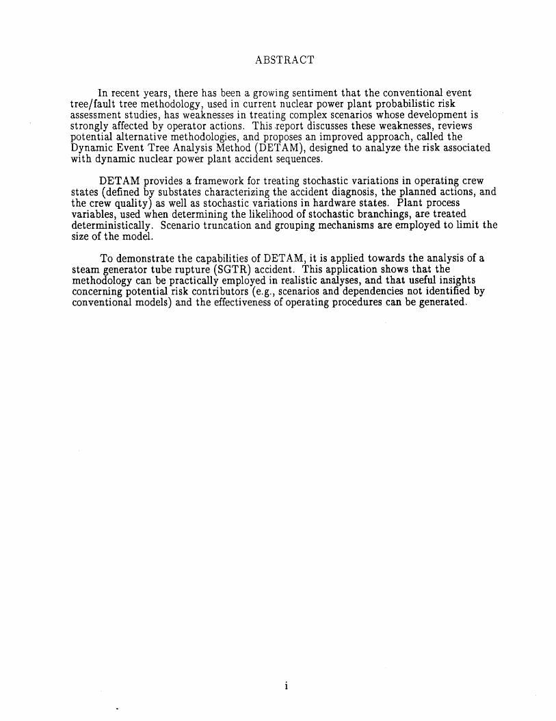
ABSTRACT

In recent years, there has been a growing sentiment that the conventional eventtree/fault tree methodology, used in current nuclear power plant probabilistic riskassessment studies, has weaknesses in treating complex scenarios whose development isstrongly affected by operator actions. This .report discusses these weaknesses, reviewspotential alternative methodologies, and proposes an improved approach, called theDynamic Event Tree Analysis Method (DETAM), designed to analyze the risk associatedwith dynamic nuclear power plant accident sequences.

DETAM provides a framework for treating stochastic variations in operating crewstates (defined by substates characterizing the accident diagnosis, the planned actions, andthe crew quality) as well as stochastic variations in hardware states. Plant processvariables, used when determining the likelihood of stochastic branchings, are treateddeterministically. Scenario truncation and grouping mechanisms are employed to limit thesize of the model.

To demonstrate the capabilities of DETAM, it is applied towards the analysis of asteam generator tube rupture (SGTR) accident. This application shows that themethodology can be practically employed in realistic analyses, and that useful insightsconcerning potential risk contributors (e.g., scenarios and dependencies not identified byconventional models) and the effectiveness of operating procedures can be generated.

i

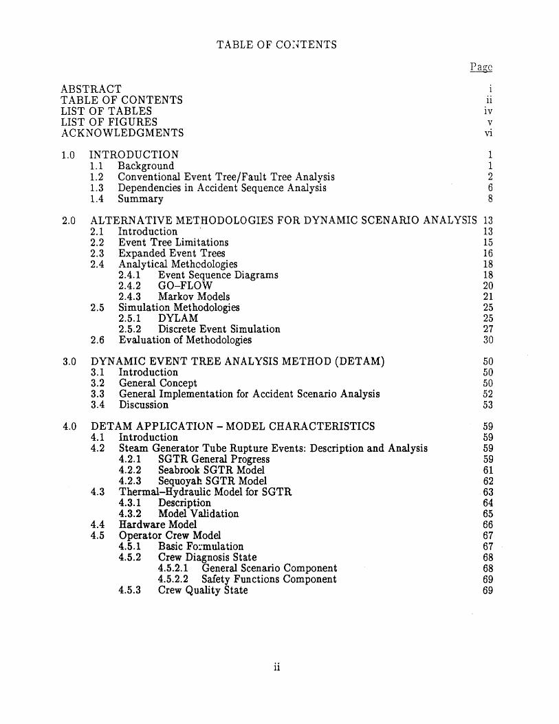
TABLE OF CONTENTS

Page

ABSTRACTTABLE OF CONTENTS iiLIST OF TABLES ivLIST OF FIGURES vACKNOWLEDGMENTS vi

1.0 INTRODUCTION 11.1 Background 11.2 Conventional Event Tree/Fault Tree Analysis 21.3 Dependencies in Accident Sequence Analysis 61.4 Summary 8

2.0 ALTERNATIVE METHODOLOGIES FOR DYNAMIC SCENARIO ANALYSIS 132.1 Introduction 132.2 Event Tree Limitations 152.3 Expanded Event Trees 162.4 Analytical Methodologies 18

2.4.1 Event Sequence Diagrams 182.4.2 GO-FLOW 202.4.3 Markov Models 21

2.5 Simulation Methodologies 252.5.1 DYLAM 252.5.2 Discrete Event Simulation 27

2.6 Evaluation of Methodologies 30

3.0 DYNAMIC EVENT TREE ANALYSIS METHOD (DETAM) 503.1 Introduction 503.2 General Concept 503.3 General Implementation for Accident Scenario Analysis 523.4 Discussion 53

4.0 DETAM APPLICATION - MODEL CHARACTERISTICS 594.1 Introduction 594.2 Steam Generator Tube Rupture Events: Description and Analysis 59

4.2.1 SGTR General Progress 594.2.2 Seabrook SGTR Model 614.2.3 Sequoyah SGTR Model 62

4.3 Thermal-Hydraulic Model for SGTR 634.3.1 Description 644.3.2 Model Validation 65

4.4 Hardware Model 664.5 Operator Crew Model 67

4.5.1 Basic Fo-mulation 674.5.2 Crew Diagnosis State 68

4.5.2.1 General Scenario Component 684.5.2.2 Safety Functions Component 69

4.5.3 Crew Quality State 69

ii

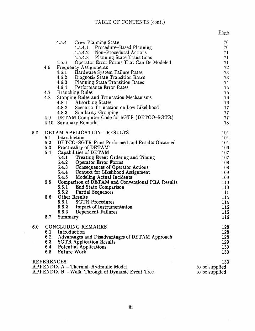
TABLE OF CONTENTS (cont.)

Page

4.5.4 Crew Planning State4.5.4.1 Procedure-Based Planning4.5.4.2 Non-Procedural Actions4.5.4.3 Planning State Transitions

4.5.6 Operator Error Forms That Can Be Modeled4.6 Frequency Assignments

4.6.1 Hardware System Failure Rates4.6.2 Diagnosis State Transition Rates4.6.3 Planning State Transition Rates4.6.4 Performance Error Rates

4.7 Branching Rules4.8 Stopping Rules and Truncation Mechanisms

4.8.1 Absorbing States4.8.2 Scenario Truncation on Low Likelihood4.8.3 Similarity Grouping

4.9 DETAM Computer Code for SGTR (DETCO-SGTR)4.10 Summary Remarks

5.0 DETAM APPLICATION - RESULTS5.1 Introduction5.2 DETCO-SGTR Runs Performed and Results Obtained5.3 Practicality of DETAM5.4 Capabilities of DETAM

5.4.1 Treating Event Ordering and Timing5.4.2 Operator Error Forms5.4.3 Consequences of Operator Actions5.4.4 Context for Likelihood Assignment5.4.5 Modeling Actual Incidents

5.5 Comparison of DETAM and Conventional PRA Results5.5.1 End State Comparison5.5.2 Partial Sequences

5.6 Other Results5.6.1 SGTR Procedures5.6.2 Impact of Instrumentation5.6.3 Dependent Failures

5.7 Summary

6.0 CONCLUDING REMARKS6.1 Introduction6.2 Advantages and Disadvantages of DETAM Approach6.3 SGTR Application Results6.4 Potential Applications6.5 Future Work

REFERENCESAPPENDIX A - Thermal-Hydraulic ModelAPPENDIX B - Walk-Through of Dynamic Event Tree

7070717171727373747575767677777778

104104104106107107108108109109110110111114114115115116

128128128129130130

133to be suppliedto be supplied

iii

LIST OF TABLES

No. Title P age

2.1 Control Laws for Holdup Tank Problem [9] 332.2 Characteristic Parameters for Tank Problem [9] 332.3 GO-FLOW Signals for Holdup Tank Problem 342.4 GO-FLOW Time Points for Holdup Tank Problem 342.5 GO-FLOW Computation Chart for Holdup Tank Problem 352.6 DYMCAM Rules for an Active Component {47] 37

3.1 Dynamic Event Tree Characterization of DYLAM 563.2 Characteristics of Dynamic Event Trees for Accident Scenario 56

Analysis

4.1 Seabrook PRA SGTR Top Events [61 804.2 Sequoyah PRA SGTR Top Events [5] 804.3 Process Variables Carried in Dynamic Event Tree Model for SGTR 814.4 Systems Included in DETAM SGTR Analysis 824.5 Scenario Transition Parameters 834.6 Scenario Transition Criteria 834.7 Diagnosis State Parameters . 844.8 Response to Reactor Trip or Safety Injection Procedure Steps (E-0) 854.9 Loss of Secondary Heat Sink Procedure Steps (FR-H.1) 864.10 Loss of Reactor or Secondary Coolant Procedure Steps (E-1) 864.11 Steam Generator Tube Rupture Procedure Steps (E-3) 874.12 Nominal Transitions from Reactor Trip or Safety Injection 88

Procedure (E-0)4.13 Nominal Transitions from Loss of Secondary Heat Sink Procedure 89

(FR-H.1)4.14 Nominal Transitions from Loss of Reactor or Secondary Coolant 91

Procedure (E-1)4.15 Nominal Transitions from Steam Generator Tube Rupture Procedure 92

(E-3)4.16 Hardware Failure Frequencies 934.17 Qualitative Likelihoods 934.18 Likelihood of Incorrect Scenario Diagnosis During An SGTR Event 944.19 Meta-Rules for Prccedure Transitions 944.20 Transition Likelihood from Procedure E-0 to E-3 954.21 Likelihood that the Operator Crew Skips a Step While in E-0 95

Procedure4.22 Likelihood that the Operator Crew Turns Off HPIS 964.23 Likelihood that the Operator Crew Starts Bleed and Feed Cooling 96

5.1 DETAM Runs Performed 1175.2 Most Frequent End States (Runs 2-7) 1185.3 Distribution of the Time to Initiate Cooldown and 119

Depressurization (Run 2)5.4 North Anna 1 SGTR Chronology of Events [63] 1205.5 Ginna SGTR Chronology of Events [60,61] 1205.6 Comparison of Conventional and Dynamic Event Tree End State 121

Conditional Frequencies5.7 Conditional Split Fractions [5,6] 122

iv

LIST OF FIGURES

No. Title P age

1.1 Portion of Sequoyah Event Tree for SGTR [5] 91.2 Portion of Seabrook Frontline Systems Early Response Tree 10

for SGTR [6]1.3 Simplified Event Tree Representation of TMI-2 Accident [11] 111.4 Event Tree for Seabrook Top Event SL [6] 12

2.1 Holdup Tank Problem [9] 382.2 Simple Hardware-Oriented Event Tree for Holdup Tank Problem 392.3 Event Sequence Diagram for Holdup Tank Problem 402.4 Expanded Event Tree for Davis Besse Event (6/9/85) [28] 412.5 Initial Portion of Expanded Event Tree for Holdup Tank Problem 422.6 Event Sequence Transition Representation of an SLOCA Accident [12] 432.7 Possible Sequences of Transitions for the SLOCA Event Tree [12] 432.8 GO-FLOW Chart for Holdup Tank Problem (First Two Phases) 442.9 GO-FLOW Operators [20,36] 452.10 Example Application of DYLAM to Holdup Tank Problem 462.11 Example Dynamic Evolution of Master Schedule 472.12 Tank Level History (One Discrete Event Simulation Trial) 482.13 Generic Component Model for DYMCAM 49

3.1 Example Dynamic Event Tree for Two Binary Systems 573.2 Tasks Performed During A Single DETAM Time Step 58

4.1 Portion of Seabrook Frontline Systems Early Response Tree 97for SGTR [6]

4.2 Event Tree for Seabrook Top Event SL [6] 984.3 Portion of Sequoyah Event Tree for SGTR [5] 994.4 Simple 4-Node Physical Model 1004.5 Comparison of Primary Pressure Predictions 1014.6 Comparison of Ruptured Steam Generator Pressure Predictions 1014.7 Heat Sink Critical Safety Function Status Tree [70] 1024.8 DETCO-SGTR Flow Chart 103

5.1 SGTR Dynamic Event Tree with Failed EFWS 1235.2 A Dynamic Event Tree with Simple Crew Response 1245.3 Portion of Dynamic Event Tree Illustrating Different Error Forms 1255.4 SGTR Dynamic Event Tree with Failed EFWS (Reduced) 1265.5 Comparison of DETAM SGTR Predictions and North Anna 1 and Ginna 127

Incidents

v

ACKNOWLEDGMENTS

The authors would like to thank N. Rasmussen, Y. Huang, V. Dang and T. Ryan fortheir useful comments and discussion. Special thanks are given to S. Kao and M. Boyle ofNew Hampshire Yankee for their generous technical support. This paper was preparedwith the support of the U.S. Nuclear Regulatory Commission (NRC) under grantNRC-04-88-143. The opinions, findings, conclusions and recommendations expressedherein are those of the author and do not necessarily reflect the view of the NRC.

vi

1.0 INTRODUCTION

1.1 Background

In current probabilistic risk assessment (PRA) studies for nuclear power plants, thepropagation of an accident scenario from an initiating event to some final plant damagestate is analyzed in two steps, largely as described in WASH-1400 [1]. In the first step,event trees are used to model the scenario as a sequence of successes and failures ofmitigating safety systems and operator actions, i.e., as a sequence of "top events." In thesecond step, the likelihood of the scenario, the probability of the joint occurrence of the topevents defining the scenario, is determined. This step often uses fault trees to analyze theindividual top events.

In recent years, the event tree/fault tree approach has gained widespread acceptanceas being a mature methodology for analyzing accident scenarios. This viewpoint stemsfrom a number of factors, including: the demonstrated usefulness of the approach (e.g., forstructuring information on plant response to abnormal conditions, and for assessingproposed plant improvements using that information [2]), the nuclear industry'saccumulated experience with PRA since WASH-1400, and the favorable results of criticalreviews. In particular, the Lewis Commission's review of WASH-1400 [3] states that

"...it is incorrect to say that the event-tree/fault-tree analysis is fundamentallyflawed, since it is just an implementation of logic."

Ref. 3 concludes that event tree/fault tree methodology, when coupled to an adequate database, is the best available tool to quantify the probabilities of nuclear reactor accidents.

Of course, it is widely recognized that many of the detailed models currently used inrisk studies, as well as the data base, need improvement. Recently, much attention hasbeen focused on the issues of human errors and common cause failures. However, theseefforts focus on improving the implementation of the event tree/fault tree methodology,rather than revising the methodology itself. Not only is the methodology currently seen asan important tool that can be used to solve real design and operations problems, it iswidely viewed as being synonymous with PRA.

Is this confidence in the event tree/fault tree methodology completely warranted?With the hindsight provided by the accident at Three Mile Island, by the occurrence ofother significant precursors, and by over 15 years of PRA applications since WASH-1400,are there reasons to believe that improvements in this basic structure may be needed?

Given the rarity of severe accidents, these questions cannot be answered by a simplecomparison of PRA results with observed data. For example, it is a simple matter to showthat if we hypothesize the existence of a class of "TMI-like" accidents leading to coredamage with mean frequency of 10-3 per reactor-year (an order of magnitude higher thanthe total core melt frequencies predicted by many PRAs), the probability of not observingsuch an accident in any U.S. plant in the 12 years following Three Mile Island isroughly 0.4. It follows that PRA models which do not identify any accidents in thishypothesized class cannot be proven right or wrong solely on the basis of statistics for coredamage accidents.

The purpose of this report is to provide a partial answer to the above questions. Thereport shows that there are a number of potentially significant issues that are notwell-treated by the event tree/fault tree methodology, and that there is an alternativemethodology, called the Dynamic Event Tree Analysis Method (DETAM) that can be used

1

INITIATING STEAM OPERATOR MSIV AND OE OPERATOR MAINARR5OSEMN ONERTR STAMIN ARV ARV ARV SV NOT SV OPENS&EVENT DUMP DECIDES TO BYPASS STEAM BRO TACTN OPENS CLOSES ISOLATED DEMANED CLOSES SL

AVAILABLE ISOLATE SG ISOLATED GENERATORS BREAK FLOW INTACT STATE

SGO so Osv SG OR MS AO AC Al SN SO

NN NN NN NN NN NN I U ES

NN NN NN 2 SUC ESS

- NN 3 SUCCESS

4 SUCC E SSNN - - 5 LEAK

N LEAK

7 SUCC E SSNN _ NNGF a LEAK

NN _ NN - NN NNNN- EA

NN - NN NN - NN NN NN 1 JCE3

N N NN NN 11 EUCC E3

NN 12 SUCCESS

13 SUCCESS

14 LEAK

-16 SUCCES3- - NNI- LEAK

Nod- NN -- N N NH NN - Is LEAK

N RNNN NN NN NN NN NN NN 19 LEAK

NN - NN - NN - NN - NN - NN- NN NN NN- 20 LEAK- NN NN NN - 21 SUCCLI $

NN -2 BUCCE 5

23 SUC~C E 53

24 LEAK

NN 25 LEAK

26 SUCCESSNo- NN - GF

46 LEAK

N NN- 29 skUCCESs

30 succ C is1

39 LEAK

NmN NN 3 2 LEAK

3.3 U CC t -E

34 LEAK

NN NNHN NN NN NN 36 LEAK

N N N N - NN ---. 38 SUCC E s$

NN N 3 7 $UCC E S3

34 sUCC E 53

r,- - _ " LEAK

NN - NN- 40 LEAK

41 SUCC E 3

42 LEAK

NN NN - NN - 43 SUCCE S$

NN - 4-4 SUCC ES3

4 5 SUCC E S3

46 LEAK

NN N N 47 LEAK

48 SIUCC E 3

N N NNH N N N N N N 50 LEAK

N N N N N N N N N N N'N N N 51 LEAK

-NN NNH NN N N N4N N N N N N N N N 52 LEAK

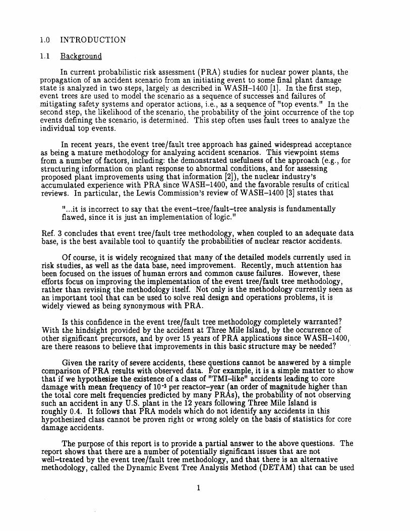
Figure 1.4 - Event Tree for Seabrook Top Event SL [6]

to treat these issues. An application of DETAM to a specific accident initiator (apressurized water reactor steam generator tube rupture) demonstrates the potential of themethod, and also provides useful insights regarding the accident.

In the remainder of this section, the structural and quantitative characteristics of theevent tree/fault tree approach are examined. It is shown that the static nature of theevent tree/fault tree approach can, in certain cases, lead to an incorrect characterization ofscenario frequencies. In Section 2, alternative methodologies for dynamic accidentsequence analysis are reviewed. This review includes extensions of the event tree/fault treemethodology, as well as more dynamic analysis methods. The dynamic event tree analysisapproach is identified as being particularly promising; the implementation of this approachfor accident sequence analysis, called the Dynamic Event Tree Analysis Method (DETAM)is described in Section 3. In Section 4, a demonstration DETAM model is constructed forthe analysis of a PWR steam generator tube rupture accident. The results of thedemonstration analysis are discussed in Section 5; the discussion includes a comparison ofresults with the results from two representative conventional event tree/fault tree analyses.Section 6 provides some concluding remarks, including a discussion of areas for furtherwork.

1.2 Conventional Event Tree/Fault Tree Analysis

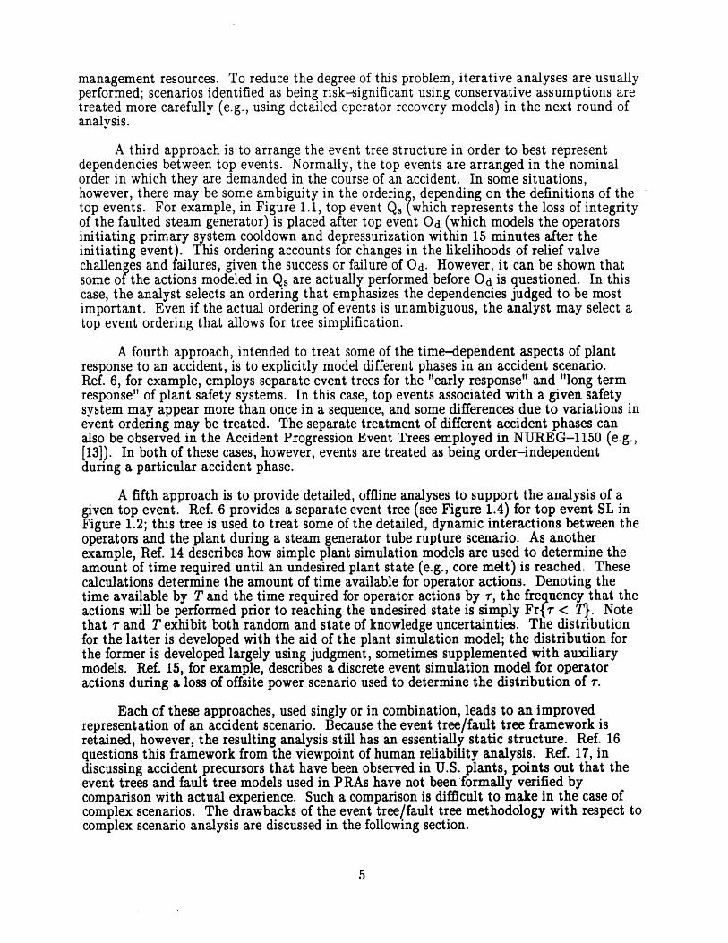
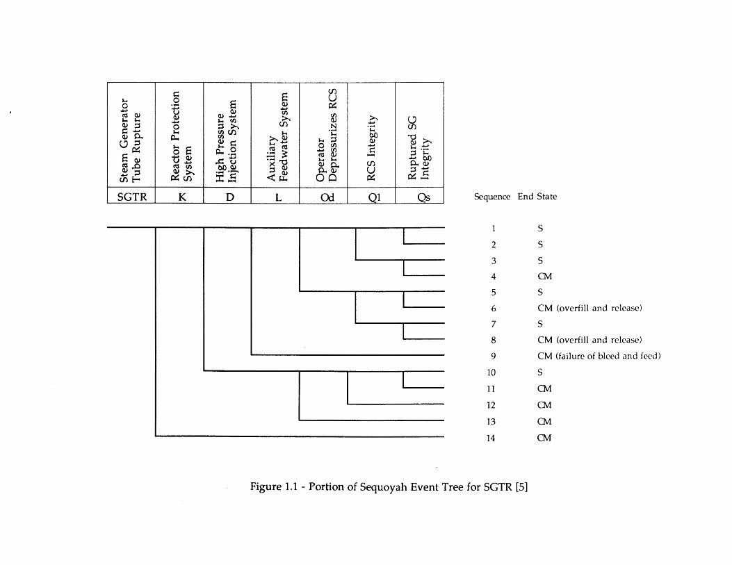
Two principal styles for applying event trees and fault trees to accident sequenceanalysis are used in current PRA studies: the "fault tree linkinI" approach, and the "eventtree with boundary conditions" approach (more popularly the 'large fault tree/small eventtree" and "large event tree/small fault tree" approaches) (4]. Briefly, the fault tree linkingapproach usually employs event trees whose top events represent failures of plant frontlinesystems (e.g., auxiliary feedwater, high pressure injection). Component-level orsupercomponent-level cut sets are developed for each tree sequence and for each plantdamage state by analyzing the logic trees created by linking the fault trees (and successtrees, if needed) for the different top events. Note that operator actions and supportsystem (e.g., electric power, service water) failures are generally included in the fault trees,rather than in the event trees. The accident sequence and plant damage state frequenciesare determined by quantifying the frequency of each cut set. Figure 1.1 shows a reducedversion of the event tree used for the NUREG-1150 analysis of postulated steam generatortube rupture (SGTR) accidents in the Sequoyah plant [5].

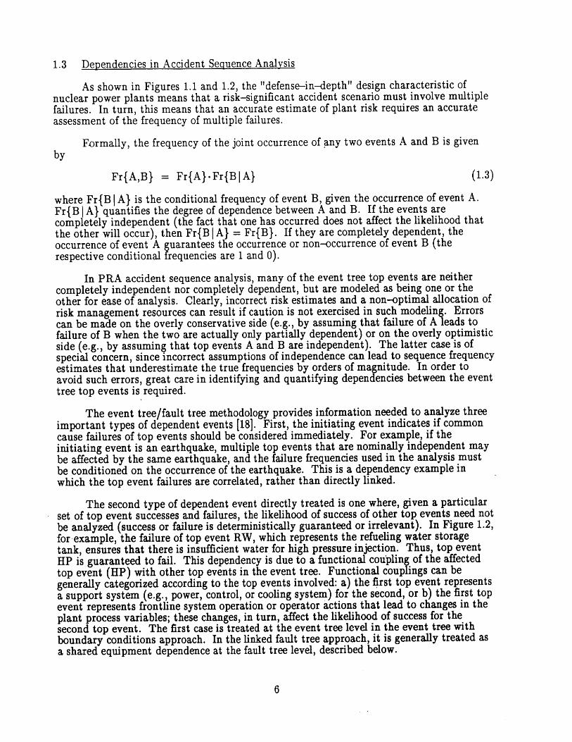
Whereas the fault tree linking approach defines accident sequences in terms ofcomponent-level cut sets, the event tree with boundary conditions approach definessequences in terms of top event successes and failures. The frequency of each accidentsequence is computed as the product of the initiating event frequency and the conditionalfrequencies of succeeding top event failures (and successes). For example, considerSequence 14 in Figure 1.2, a reduced version of the early response SGTR tree used inRef. 6. The conditional frequency of this sequence', given the SGTR initiating event (SG),is written as:

'This report adopts the "probability of frequency" formalism discussed in Ref. 7. The term"frequency" is used to quantify the stochastic uncertainty associated with random events(e.g., event tree top event failures). The term "probability" is used to quantify state ofknowledge uncertainties (e.g., the uncertainty in the value of a conditional frequency.

2

Fr{Sequence 14|SG} = Fr{TT|SG}*Fr{EF|SGTT}*Fr{NL|SG,TT,EY}

*Fr{RW SG,TT,EFNL}*Fr{HP I SG,TT,LT,NL,RW}

*Fr{OR I SG,TT,EF,NL,RW,HP}*Fr{SL I SG,TT,EF,NL,RW,HP,OR}

*Fr{DUji SG,TT,EP,NL,RW,HPOR,SL}

Eq. (1.1) shows that the conditional frequency of failure for a given top event (often termed"conditional split fraction") depends on the successes and failures of preceding top events.Thus, the structure of the event tree provides the boundary conditions required to quantifya given top event. Recent applications of the event tree with boundary conditionsapproach often define top events in terms of safety system trains (rather than entiresystems). Furthermore, operator actions and support system train successes/failures aretreated using separate top events, rather than as supporting events in a frontline systemfault tree.

Regardless of the particular style of analysis, the event tree/fault tree methodologydoes not, nor is it intended to, lead to models that directly simulate the integrated,dynamic response of the plant/operating crew system during an accident. Instead, asindicated above, an accident scenario is described as a set of successes and failures.Furthermore, each scenario is associated with a single plant damage state. Thus, an eventtree/fault tree model can be replaced by a set of logic statements (i.e., a set of rules)deterministically associating sets of top event or component successes and failures withplant damage states. Assuming for sake of example that Sequence 14 in Figure 1.2 leads tocore damage, the logic statement underlying this sequence can then be written as:

{SG n TT n EF n NL n RW n HP n OR n SL n 0-9} -4 {Core Damage} (1.2)

A number of structural characteristics of this static, logic-based approach formodeling accident scenarios are of interest. First, variations in the ordering of the successand failure events do not affect the final outcome of a scenario or its frequency. (Ifordering does make a difference, the event tree would have to be expanded in order tohandle possible permutations of events.) Second, variations in event timing do not affectscenario outcomes or frequencies (as long as these variations are not large enough to change"failures" to "successes," or vice versa). Third, the effect of process variables and operatorbehavior on scenario development are incorporated through the success criteria defined forthe event tree top events. Fourth, the boundary conditions for the analysis of a given topevent (or basic event, when dealing with cut set representations of accident scenarios) areprovided in terms of top event (basic event) successes and failures; variations in parametersnot explicitly modeled are not treated.

In some risk analysis applications, it appears that some of these characteristics canaffect the scenario identification process. For example, Ref. 8 describes a fault-tolerantcomputer system reliability analysis application in which variations in the ordering ofevents can be significant. Section 2 of this report presents a simple process control systemexample, obtained from Ref. 9, illustrating the potential importance of dynamics whenmultiple system failure modes are possible. Ref. 10 employs order-dependent "scenariotrees" in place of conventional event trees in an analysis of a test reactor.

For commercial nuclear power plant applications, on the other hand, staticrelationships between top events and plant damage states can be reasonably assumed (atleast within a given accident phase) as long as the top event success criteria are defined inbroad terms, e.g., when "system failure" means that the system is unable to perform its

3

(1.1)

function adequately. In such cases, the use of event trees to identify accident sequencesleading to a given plant damage state is, as pointed out in Ref. 3, just an exercise in logic.Thus, the event tree/fault tree methodology appears to be a good approach for identifyinglogically correct, or, at least, conservative relationships between top event successes andfailures and plant damage states. However, it is less clear that the methodology iscompletely adequate for quantifying the risk associated with all potentially significantscenarios.

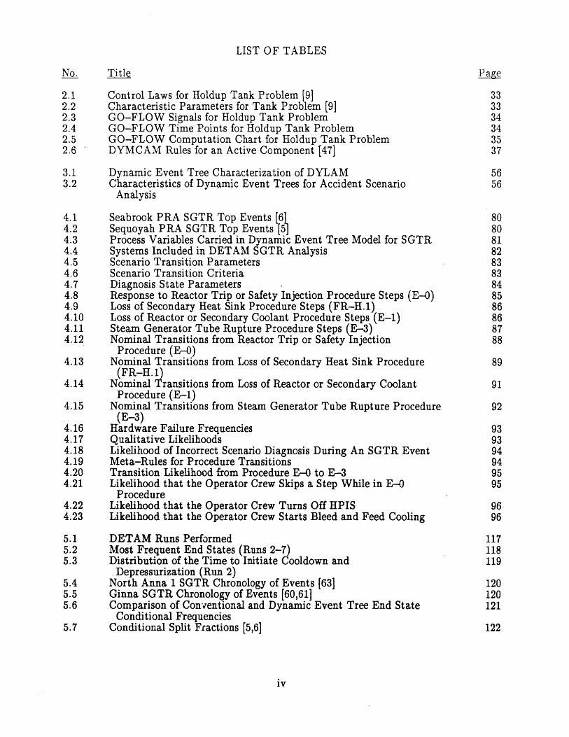
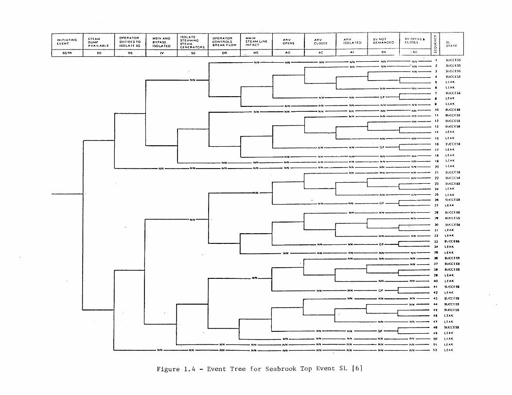
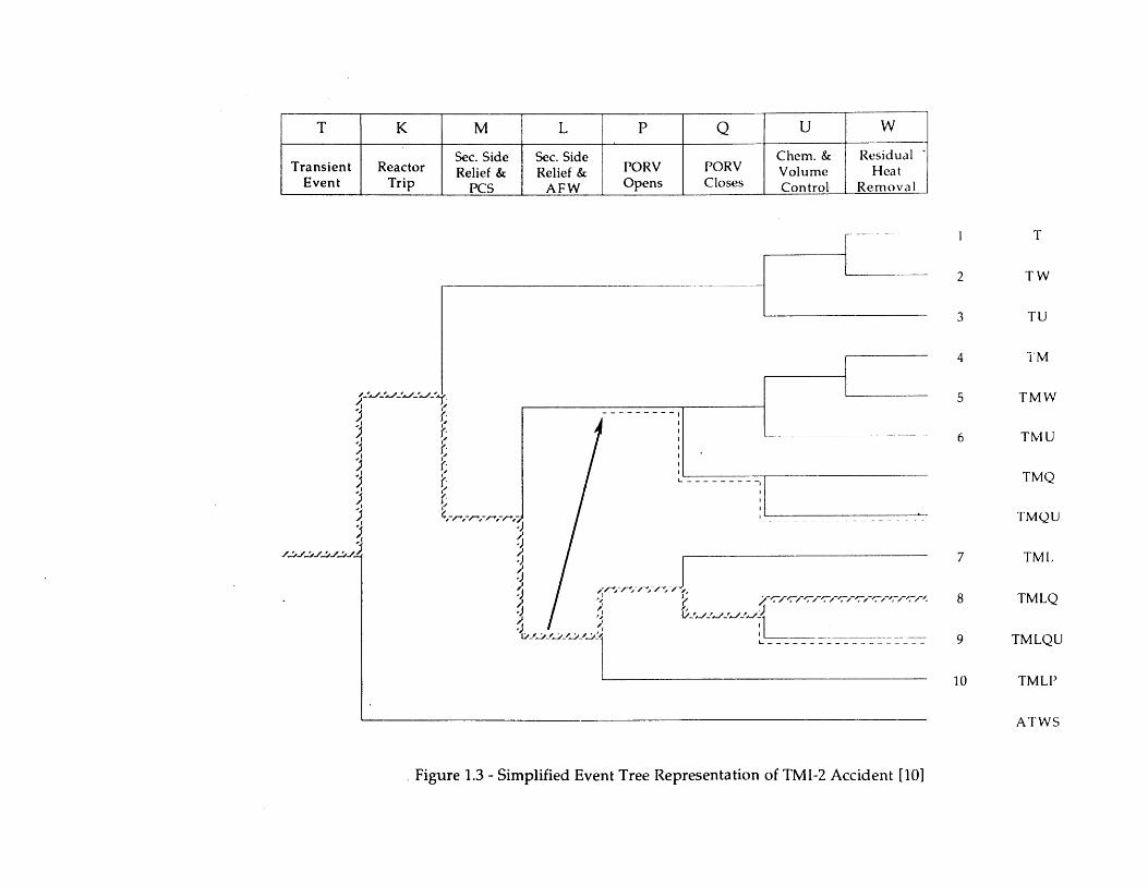
To illustrate this point, consider the well-known Three Mile Island Unit 2 (TMI-2)accident. Figure 1.3 shows a modified WASH-1400 event tree for that accident obtainedfrom Ref. 11. Key elements in the actual course of the scenario are shown in that tree;hence, the early failure of auxiliary feedwater and its recovery 8 minutes later isrepresented as a transition between sequences (Ref. 12 uses a similar representation tomodel more general aspects of the accident). Note that sequences TMQ and TMQU arenot treated in the original WASH-1400 tree due to physical differences between the Surryreactor treated in WASH-1400 and TMI-2. Note also that, although the accident startedwith a loss of main feedwater (represented by top event M), the ordering of events K andM is not judged to have a significant impact on subsequent scenario development.

Figure 1.3 illustrates the gross sequence of events at TMI-2 reasonably well.However, it fares less well as a quantitative tool. The key to correct quantification of thesequence is to determine the likelihood that the operators will throttle high pressuremakeup (represented by top event U), given that the pilot-operated relief valve (PORV)fails to reclose (top event Q). The tree shows that the reactor is tripped, main feedwater isnot available, auxiliary feedwater is operating, the PORV has opened on demand, and thePORV has failed to reclose. It does not show that the pressurizer level rises as an eventualconsequence of the PORV failing to reclose; this information, of course, is necessary tocorrectly quantify the likelihood that the operators would deliberately cause the failure of

top event U. The fact that the event tree does not provide this information does notnecessarily preclude an experienced analyst from correctly analyzing the scenario. It does,however, make the job much more difficult, especially considering that numerous scenariosmay require a similar, detailed analysis.

In general, as discussed further in Section 1.3, the static, logical structure of aconventional event tree/fault tree analysis does not explicitly provide all of the informationneeded to quantitatively analyze dependencies between top events. This point has notgone unnoticed in nuclear power plant PRAs; to improve the analysis with respect to theseissues, a number of strategies are employed. First, as an aid to event tree construction,event sequence diagrams (ESDs) are often used to qualitatively model the progression of anaccident scenario. These diagrams depict not only possible courses of the accident in termsof hardware state changes, they also indicate salient physical variables during the accident.In recent PRAs, ESDs can also indicate the section of the emergency operating proceduresrelevant to a particular point in the sequence. The ESDs, however, do not provide thetiming of events, nor do they provide complete information on the process variables.Therefore, one event sequence, either in the ESD or in the event tree constructed from theESD, may represent many chronological scenarios.

A second approach is to employ conservative assumptions, thereby eliminating theneed to analyze dependencies between multiple events. For example, Figure 1.1 assumesthat scenarios involving a steam generator tube rupture and subsequent failure of auxiliaryfeedwater will lead to core damage; thus, the conditional frequency with which operatorssuccessfully perform bleed and feed cooling need not be quantified. The main problem withthis approach is economic rather than technical since it can lead to an incorrectidentification of significant scenarios and, therefore, a non-optimal allocation of risk

4

management resources. To reduce the degree of this problem, iterative analyses are usuallyperformed; scenarios identified as being risk-significant using conservative assumptions aretreated more carefully (e.g., using detailed operator recovery models) in the next round ofanalysis.

A third approach is to arrange the event tree structure in order to best representdependencies between top events. Normally, the top events are arranged in the nominalorder in which they are demanded in the course of an accident. In some situations,however, there may be some ambiguity in the orderin , depending on the definitions of thetop events. For example, in Figure 1.1, top event Qs which represents the loss of integrityof the faulted steam generator) is placed after top event Od (which models the operatorsinitiating primary system cooldown and depressurization within 15 minutes after theinitiating event). This ordering accounts for changes in the likelihoods of relief valvechallenges and failures, given the success or failure of Od. However, it can be shown thatsome of the actions modeled in Qs are actually performed before Oa is questioned. In thiscase, the analyst selects an ordering that emphasizes the dependencies judged to be mostimportant. Even if the actual ordering of events is unambiguous, the analyst may select atop event ordering that allows for tree simplification.

A fourth approach, intended to treat some of the time-dependent aspects of plantresponse to an accident, is to explicitly model different phases in an accident scenario.Ref. 6, for example, employs separate event trees for the "early response" and "long termresponse" of plant safety systems. In this case, top events associated with a given safetysystem may appear more than once in a sequence, and some differences due to variations inevent ordering may be treated. The separate treatment of different accident phases canalso be observed in the Accident Progression Event Trees employed in NUREG-1150 (e.g.,[13]). In both of these cases, however, events are treated as being order-independentduring a particular accident phase.

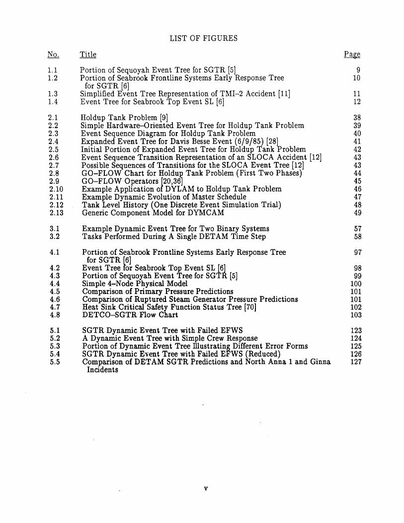
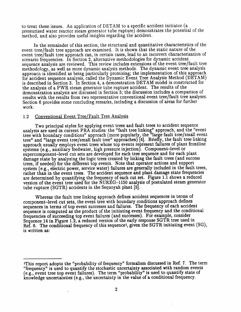
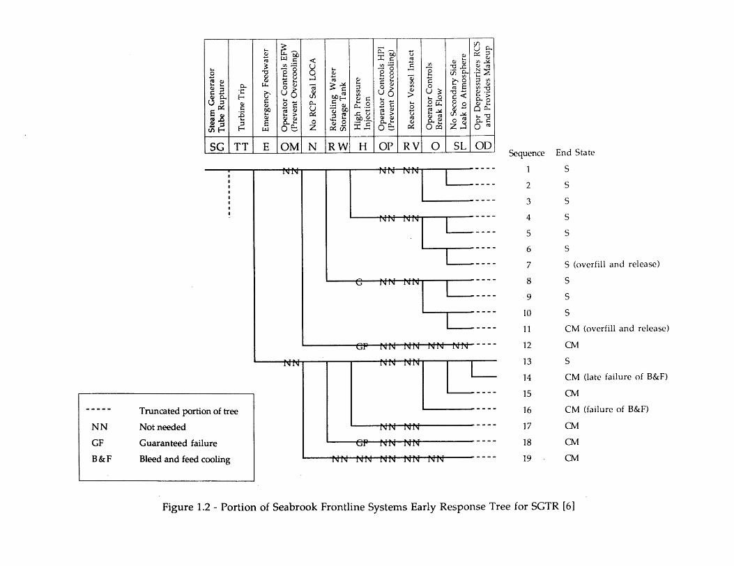
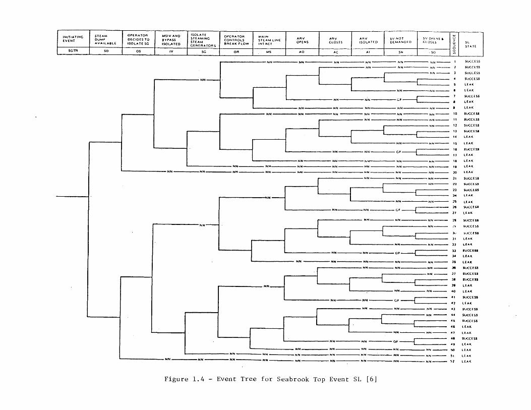
A fifth approach is to provide detailed, offline analyses to support the analysis of agiven top event. Ref. 6 provides a separate event tree (see Figure 1.4) for top event SL inFigure 1.2; this tree is used to treat some of the detailed, dynamic interactions between theoperators and the plant during a steam generator tube rupture scenario. As anotherexample, Ref. 14 describes how simple plant simulation models are used to determine theamount of time required until an undesired plant state (e.g., core melt) is reached. Thesecalculations determine the amount of time available for operator actions. Denoting thetime available by T and the time required for operator actions by r, the frequency that theactions will be performed prior to reaching the undesired state is simply Fr {r < T}. Notethat r and T exhibit both random and state of knowledge uncertainties. The distributionfor the latter is developed with the aid of the plant simulation model; the distribution forthe former is developed largely using judgment, sometimes supplemented with auxiliarymodels. Ref. 15, for example, describes a discrete event simulation model for operatoractions during a loss of offsite power scenario used to determine the distribution of r.

Each of these approaches, used singly or in combination, leads to an improvedrepresentation of an accident scenario. Because the event tree/fault tree framework isretained, however, the resulting analysis still has an essentially static structure. Ref. 16questions this framework from the viewpoint of human reliability analysis. Ref. 17, indiscussing accident precursors that have been observed in U.S. plants, points out that theevent trees and fault tree models used in PRAs have not been formally verified bycomparison with actual experience. Such a comparison is difficult to make in the case ofcomplex scenarios. The drawbacks of the event tree/fault tree methodology with respect tocomplex scenario analysis are discussed in the following section.

5

1.3 Dependencies in Accident Sequence Analysis

As shown in Figures 1.1 and 1.2, the "defense-in-depth" design characteristic ofnuclear power plants means that a risk-significant accident scenario must involve multiplefailures. In turn, this means that an accurate estimate of plant risk requires an accurateassessment of the frequency of multiple failures.

Formally, the frequency of the joint occurrence of any two events A and B is givenby

Fr{A,B} = Fr{A}-Fr{BIA} (1.3)

where Fr{B A} is the conditional frequency of event B, given the occurrence of event A.Fr{B I A} quantifies the degree of dependence between A and B. If the events arecompletely independent (the fact that one has occurred does not affect the likelihood thatthe other will occur), then Fr{B I A} = Fr{B}. If they are completely dependent, theoccurrence of event A guarantees the occurrence or non-occurrence of event B (therespective conditional frequencies are 1 and 0).

In PRA accident sequence analysis, many of the event tree top events are neithercompletely independent nor completely dependent, but are modeled as being one or theother for ease of analysis. Clearly, incorrect risk estimates and a non-optimal allocation ofrisk management resources can result if caution is not exercised in such modeling. Errorscan be made on the overly conservative side (e.g., by assuming that failure of A leads tofailure of B when the two are actually only partially dependent) or on the overly optimisticside (e.g., by assuming that top events A and B are independent). The latter case is ofspecial concern, since incorrect assumptions of independence can lead to sequence frequencyestimates that underestimate the true frequencies by orders of magnitude. In order toavoid such errors, great care in identifying and quantifying dependencies between the eventtree top events is required.

The event tree/fault tree methodology provides information needed to analyze threeimportant types of dependent events [18]. First, the initiating event indicates if commoncause failures of top events should be considered immediately. For example, if theinitiating event is an earthquake, multiple top events that are nominally independent maybe affected by the same earthquake, and the failure frequencies used in the analysis mustbe conditioned on the occurrence of the earthquake. This is a dependency example inwhich the top event failures are correlated, rather than directly linked.

The second type of dependent event directly treated is one where, given a particularset of top event successes and failures, the likelihood of success of other top events need notbe analyzed (success or failure is deterministically guaranteed or irrelevant). In Figure 1.2,for example, the failure of top event RW, which represents the refueling water storagetank, ensures that there is insufficient water for high pressure injection. Thus, top eventHP is guaranteed to fail. This dependency is due to a functional coupling of the affectedtop event (HP) with other top events in the event tree. Functional couplings can begenerally categorized according to the top events involved: a) the first top event representsa support system (e.g., power, control, or cooling system) for the second, or b) the first topevent represents frontline system operation or operator actions that lead to changes in theplant process variables; these changes, in turn, affect the likelihood of success for thesecond top event. The first case is treated at the event tree level in the event tree withboundary conditions approach. In the linked fault tree approach, it is generally treated asa shared equipment dependence at the fault tree level, described below.

6

The third type of dependency that is naturally treated using the event tree/fault treemethodology arises when multiple top events share a set of components (or basic events).In this case, the joint frequency of failure of the affected top events can be easily developedusing normal fault tree analysis techniques; the conditional frequency of failure can then bedeveloped using Eq. (1.3). Note that when dealing with shared equipment dependencies inthe linked fault tree approach, the conditional frequencies need not be evaluated explicitly.Instead, this type of dependency is treated by logic tree reduction when evaluating thelinked fault tree modeling an accident sequence.

Dependencies falling outside of the above three categories (common cause initiators,functional coupling, shared equipment) are not as well treated by the event tree/fault treeapproach. These other dependencies involve situations where the status of the plantcannot be defined solely in terms of top event successes and failures. Of particular interestin this study are complex scenarios whose development is strongly affected by operatoractions.

As discussed in the preceding section, the event tree/fault tree methodologyrepresents each accident scenario as a set of hardware failures and operator errors. Thelatter are treated in much the same fashion as hardware failures, and often treated at avery broad level, e.g., failure to depressurize the reactor coolant system in r minutes.There are two major consequences resulting from this representation.

First, many of the conditions affecting operator errors (e.g., previous decisions by theoperating crew, behavior of plant process variables) are not explicitly included in themodel. For scenarios dominated by hardware failures, this is not an important concern.However, for scenarios involving multiple human errors in nominally separate tasks, thelack of contextual information can lead to erroneous conclusions regarding the level ofdependence between the errors and, therefore, erroneous quantitative results. For example,PRA models rarely treat events in which operators turn off safety systems when thesesystems are needed, although this was a prime contributor to the TMI-2 accident. In theabsence of a context provided by a description of the dynamic progression of the accident,it is difficult for an analyst to develop accurate conditional frequencies for such events.

Second, the treatment of human error in an analogous fashion to the treatment ofhardware failure inhibits accurate modeling of the remainder of the accident sequencefollowing an error. The likelihood that an operating crew fails to perform a required taskcorrectly (within a given amount of time) is treated explicitly. However, the different waysin which the crew may perform the task incorrectly, and the resulting dynamic responses ofthe plant/crew system to these different errors, are not treated. Therefore, the properboundary conditions for establishing the conditional frequencies for top events downstreamof the task performance failure are not provided. Moreover, from the standpoint of riskmanagement, the lack of realistic treatment of the scenario following human error can leadto an incomplete identification of factors important to risk, and of alternatives that can beemployed to reduce risk.

In order to address these weaknesses in the event tree/fault tree representation of anaccident scenario, it must be recognized that: a) plant operators and plant components areinteracting parts of an overall system that responds dynamically to upset conditions, b) theactions of operators are dependent on their beliefs as to the current state of the plant, andc) the operators have memory; their beliefs at any given point in time are influenced (tosome degree) by the past sequence of events and by their earlier trains of thought. Each ofthese observations points to a need for an accident sequence model whose structure differssignificantly from that of current event trees and fault trees. Such a model must carryinformation on the following [19]:

7

0 Current hardware status9 Current levels of process variables0 Current operator "state of mind"0 Scenario historya Time

With this information, dependencies between system failure events can, in principle,be more accurately identified and quantified. Note that the process variable levels areincluded because they affect the actuation of automatic systems and provide cues to theoperators, thereby providing an important link in the interaction between the operatorsand the plant hardware. Time is included not only because the process variablecalculations are time dependent, but also because time can be a key performance shapingfactor for modeling operator behavior.

1.4 Summary

In nuclear power plant risk assessments, accurate estimation of the frequency ofaccident scenarios and the overall plant risk requires an accurate treatment of dependenciesbetween multiple failure events. The event tree/fault tree methodology currently used isfundamentally well suited to treat dependencies that can be expressed in static, logicalterms. It is not as well suited to treat dependencies associated with time-dependentprocesses or continuously varying variables. In particular, the methodology does notexplicitly carry information concerning the evolution of process variables and operatorstate that may couple a number of failure events together.

8

VK

0-

-.4

A

*-

00-

W

r -~

t=

\

V K

Ste

am G

ener

ator

Tub

e R

uptu

re

Rea

ctor

Pro

tect

ion

Sys

tem

Hig

h P

ress

ure

Inje

ctio

n S

yste

m

Aux

ilia

ryF

eedw

ater

Sys

tem

Ope

rato

rD

epre

ssur

izes

RC

S

o

RC

S In

tegr

ity

Rup

ture

d SG

Q In

tegr

ity

M

N

1-4

a\N

p P

W

-

rrL

~1 0 0~ 0~ 0- 0~

(1

QP

Q

P

UC

) V ~1 0~ ~1

V 0~

~1

20 0 (I

)

0 (I) Ci

Hc

-t 0 0 0 h-I 0 0 h-I 0 Cl)

tTl

(I~ 0 '4) H h

-I CD

CD 0 h-I Cr) C)

H ON

I I

* I

* I

I I

C)

C

B

I I

I I I

I I

I0

I I

0I

I I

I I

I I

h4

-A

-A

-.

1,

-Q

a*,

U-i

OP

. W~~ t

-~

C

)\

~t1 zc.n

Ste

am G

ener

ator

C)

Tub

e R

uptu

re

Tur

bine

Tri

p

Em

erge

ncy

Fee

dwat

er

Ope

rato

r C

ontr

ols

EFW

(Pre

vent

Ove

rcoo

ling

)

No

RC

P Se

al L

OC

A

Ref

ueli

ng

Wat

erS

tora

ge T

ank

Hig

h P

ress

ure

Inje

ctio

n

Ope

rato

r C

ontr

ols

HP

I(P

reven

t O

ver

coo

lin

g)

Rea

ctor

V

esse

l In

tact

Ope

rato

r C

ontr

ols

0 B

reak

Flo

w

U

No

Sec

onda

ry S

ide

t L

eak

to A

tmos

pher

e

Opr

Dep

ress

uriz

es

RC

San

d P

rovi

des

Mak

eup

o~

u-i

~ (j,)

~

-~

U )

C

(P)

U-n

(f

i (P

(

(P

U(P

~11

6 -I

-I

0 0I

I*

II

II

I

C

T

-J

-~ r

r-J (-J CSi)Si

-

/

-

'~-'~' ,~i_________________

~1

TW

TU

T M

2

3

4

5

6

TMW

TMU

TMQ

TMQU

7 TML

Figure 1.3 - Simplified Event Tree Representation of TMI-2 Accident [10]

8 TMLQ

9 TMLQU

10 TMLP

ATWS

I

1I

- -- - - --- --

INITIATING STEAM OPERATOR MSIV AND ISOLATE OPERATOR MAIN R AEVENT DUMP DECIDES TO BYPASS STEAMING CONTROLS STEAM LINE ARV ARV ARV SV NOT Sv OPENS &

AVAILABLE ISOLATE SG ISOLATED STEAM BREAK FLOW INTACT OPENS CLOSES ISOLATED DEMANDED CLOSES SLGENERATORS STATE

SGTR so OIS IV SG OR _Ms AO AC Al SN ,s

-NN - NN - NN - NN NN NN I kc E

NN NN - NN 2 SUCC ESS

NN 3 SUCCESS

NN - - SUCCE SS5 LEAK

NN NN 6 LEAK

f7 SUCC E Ss

14a LEAK

N NN NN - NN - NN LEAK

NN NN NN NN NN NN 10 SLCCEf 3

NN NN NN -- SUCCES

NN 12 SUCCESS

L ~ 3 SUCC E5314 LEAK

-NN NN - 1s LEAK

-6 SUCC E SSNNH N N G F IFLA

17 LEAK

NMil NNN. NN NN 18 LEAK

NN - NN - NN - NN - NN NN HNN 19 LEAK

NN NN N N NN" NN NN - NN NN NN - 20 LEAK

NN NN NN 21 SUCCISS

NN - 77 SUCCES3

- 23 SUCC ESS24 LEAK

NN N 2S LEAK

26 SUCC ES3

27 LEAK

NNNNNN 4 21 ( SCCES3

BNN SUCCESS

-j 301 SUC E

31 LEAK

RN NN 32 LEAK

NN NNOP 3.3 U CC I34 LEAK

NMmNM NN - NN - NN - 36 LEAK

-NN NN NN 36 ucc E S3

NN 37 SUCCES3

I --i3s F$UCC E 3

NN - N N 40 L E AK

NN - ~ ~ NNGFA SUCC E SS

4 2 LEAK

NN NN NN4 43 SUICC ES$

N1 N 4-4 SUC~C E "

45 SUCCX E S.3

46 LEAK

NNNN 47 LEAK

-48 SU-CC ( S3

49 LEAK

NN HNN NN NmN NN So LE AKNN NN NNNN NN NN NN S1 LE AK

- NN NN N NN NN- NN - NN - NN - NN - 52 LEAK

Figure 1.4 - Event Tree for Seabrook Top Event SL [6]

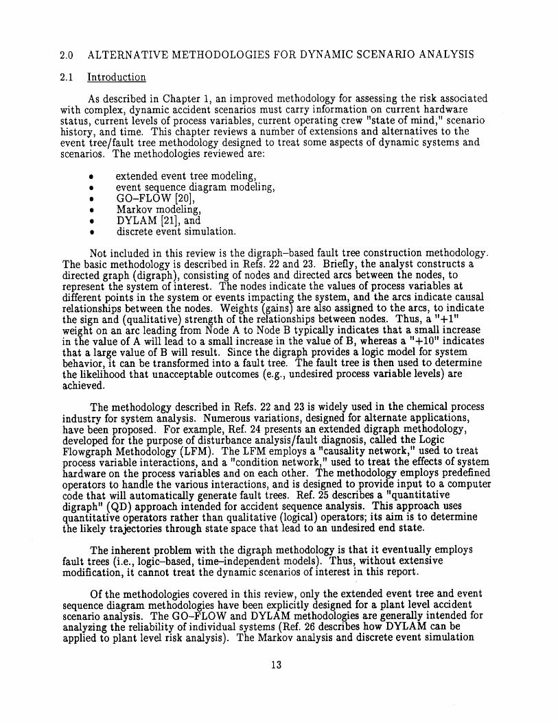
2.0 ALTERNATIVE METHODOLOGIES FOR DYNAMIC SCENARIO ANALYSIS

2.1 Introduction

As described in Chapter 1, an improved methodology for assessing the risk associatedwith complex, dynamic accident scenarios must carry information on current hardwarestatus, current levels of process variables, current operating crew "state of mind," scenariohistory, and time. This chapter reviews a number of extensions and alternatives to theevent tree/fault tree methodology designed to treat some aspects of dynamic systems andscenarios. The methodologies reviewed are:

0 extended event tree modeling,* event sequence diagram modeling,0 GO-FLOW [20],* Markov modeling,* DYLAM [21], and0 discrete event simulation.

Not included in this review is the digraph-based fault tree construction methodology.The basic methodology is described in Refs. 22 and 23. Briefly, the analyst constructs adirected graph (digraph), consisting of nodes and directed arcs between the nodes, torepresent the system of interest. The nodes indicate the values of process variables atdifferent points in the system or events impacting the system, and the arcs indicate causalrelationships between the nodes. Weights (gains) are also assigned to the arcs, to indicatethe sign and (qualitative) strength of the relationships between nodes. Thus, a "+1"weight on an arc leading from Node A to Node B typically indicates that a small increasein the value of A will lead to a small increase in the value of B, whereas a "+10" indicatesthat a large value of B will result. Since the digraph provides a logic model for systembehavior, it can be transformed into a fault tree. The fault tree is then used to determinethe likelihood that unacceptable outcomes (e.g., undesired process variable levels) areachieved.

The methodology described in Refs. 22 and 23 is widely used in the chemical processindustry for system analysis. Numerous variations, designed for alternate applications,have been proposed. For example, Ref. 24 presents an extended digraph methodology,developed for the purpose of disturbance analysis/fault diagnosis, called the LogicFlowgraph Methodology (LFM). The LFM employs a "causality network," used to treatprocess variable interactions, and a "condition network," used to treat the effects of systemhardware on the process variables and on each other. The methodology employs predefinedoperators to handle the various interactions, and is designed to provide input to a computercode that will automatically generate fault trees. Ref. 25 describes a "quantitativedigraph" (QD) approach intended for accident sequence analysis. This approach usesquantitative operators rather than qualitative (logical) operators; its aim is to determinethe likely trajectories through state space that lead to an undesired end state.

The inherent problem with the digraph methodology is that it eventually employsfault trees (i.e., logic-based, time-independent models). Thus, without extensivemodification, it cannot treat the dynamic scenarios of interest in this report.

Of the methodologies covered in this review, only the extended event tree and eventsequence diagram methodologies have been explicitly designed for a plant level accidentscenario analysis. The GO-FLOW and DYLAM methodologies are generally intended foranalyzing the reliability of individual systems (Ref. 26 describes how DYLAM can beapplied to plant level risk analysis). The Markov analysis and discrete event simulation

13

methodologies are general methodologies for treating stochastic systems and can, inprinciple, be applied to plant level analysis. However, to date, most applications are alsoaimed at the system level (Ref. 27 provides an exception to this general rule). Partly forthis reason, none of the methodologies is designed to accommodate a completely integratedmodel for operator cognitive activity; most applications of these methodologies do not treathuman error at all. Three exceptions that treat human error are the extended event treeanalysis reported in Ref. 28 (which uses an approach very similar to that used inconventional event tree/fault tree analysis), the event sequence diagram model described inRef. 12 (which treats errors of commission using a statistical approach), and some recentapplications of DYLAM [29,30]. Only the last-named applications treat to any extent theoperating crew's state of mind. The purpose of this review, then, is to determine whichmethodology is the best candidate for improvement; the chosen methodology is thenextended to allow a broader, integrated treatment of operators, as discussed in thefollowing chapters of this report.

To make the review concrete, a sample problem involving a holdup tank and threediscrete control loops is adopted from Ref. 9. This problem is simple to analyze, yetpossesses a number of characteristics important to the analysis of dynamic scenariosallowing comparison of the different methodologies. (Operator modeling issues, which arenot illustrated by this problem, are discussed for those few analyses which have consideredhuman errors.)

Figure 2.1 shows the holdup tank. The tank level is regulated by the actions of threecontrol loops. Under normal conditions, the tank level is maintained between levels ai anda2 by balancing the flow out of the tank through the valve with the flow into the tank viaPump 1. If the valve fails closed, the running pump stops, or the 50% backup pump(Pump 2) starts, the tank level will change. Level sensors will then attempt to actuateequipment to maintain the tank level between a, and a2. The control laws are given inTable 2.1. Failure occurs when the tank level (L) rises above "b" (Tank Overflow) or whenit falls below "a" (Tank Dryout).

For simplicity, it is assumed that:

0 control loops can be modeled as single entities (components);e possible pump loop states are: {on, off, failed on, failed off}; possible valve loop

states are: (open, closed, failed open, failed closed};e loops can fail on demand or during operation; the latter failures are Poisson

processes;e operation failures not leading to changes of state (e.g., an open valve sticking

open) are included with demand failures;e failed loops cannot be repaired;0 relevant failure modes and flow parameters are as given in Table 2.2; and0 the loops are nominally independent, i.e., the failure of a loop does not directly

influence the likelihood of success or failure of a second loop.

Note that this problem differs from that in Ref. 9 in the definition of possible loop states(Ref. 9 only employs "on" or "off" loop states) and in the modeling of failures on demand.

This problem has two characteristics that apply to more general dynamic problems.First, as discussed in more detail in Section 2.2, the response of the overall system dependson the order and timing of the failure events. For example, an accident sequence initiatedby the closure of the valve will differ from one initiated by the stoppage of Pump 1.Further, the system response following the initiating event will vary according to the valueof the tank level (L) when the next failure occurs. Second, system control depends on a

14

continuous process variable, the tank level (L). (In contrast with a number of othercontrol problems, system control is performed in discrete stages, rather than with acontinuous controller.)

Because the system responds dynamically to an initiating event, an event tree is amore natural tool than a fault tree for modeling the holdup tank. A simplistic,hardware-oriented tree for the system's response to the initiating event "Pump 1 Fails Off"is shown in Figure 2.2. The tree models the different failure modes of the loops explicitly,since these can lead to different system failure modes. Note that since the valve has alarger flow capacity than Pump 2 (see Table 2.2), the valve behavior overrides the behaviorof Pump 2 in the first two sequences.

If the dynamics of the system are ignored, the sequences in Figure 2.2 can bequantified quite simply. For example, the conditional frequency of Sequence 2, given theinitiating event, can be approximated by (see Table 2.2)

Fr{Sequence 21 Initiating Event} '== #v + Ayr (2.1)

where r is time interval since the occurrence of the initiating event. (The last term in theequation represents a scenario in which the valve closes successfully on demand, but latertransfers open.)

Overlooking the system dynamics does not affect the failure logic shown inFigure 2.2. However, it can lead to inaccurate frequency estimates for the two undesiredoutcomes (dryout and overflow). Further, it prevents the accurate assessment of thefrequency distributions for the times to achieve these outcomes. This last piece ofinformation is important, since it indicates the amount of time likely to be available forrecovery from the initiating event. These issues are discussed in the following section.

2.2 Event Tree Limitations

To better illustrate the dynamic response of the holdup tank to the initiating event"Pump 1 Fails Off," some of the different possible system response scenarios are shown inFigure 2.3. The scenarios include changes in loop states, failures (denoted by an asterisk),changes in tank level, and changes in the rate of change of tank level (dL/dt). Forexample, starting with Box 1, three possible state changes may occur. Either the valvemay transfer closed (with rate Ay), Pump 2 may start spuriously (with rate Ap), or thetank level may drop to a, (before either of the two failure events occurs).

Figure 2.3 shows that the behavior of the holdup tank system is fairly complex. Thisis because of the control laws specified in Table 2.1. These govern the sequence of demandson the control loops, which in turn, determines the possible sequences of specific failuremodes. Thus, the sequences 1 -. 10 -411 -417 and 1 -4 10 -418 lead to two different outcomes(dryout and overflow, respectively), even though they both involve the sequential failure ofPump 2 and the valve. In the former scenario, the valve fails to close on demand (i.e., thevalve is failed open) when the tank level reaches a control region boundary (L = a,),whereas in the latter, the valve fails closed before a, is reached.

As a result of this complex dynamic behavior, the simplistic quantification ofEq. (2.1) can lead to erroneous results. As an example, the first term in Eq. (2.1) modelsthe likelihood of demand failure for the valve as the frequency that the valve will fail on asingle demand. However, scenarios can be easily generated where the valve is demandedmore than once. One such sequence of events is: valve closes when L = a,, Pump 2 failson, valve opens when L = a2, valve fails to close when L = a,. This sequence is partially

15

represented in Figure 2.3 as the path 1 -+ 2 -+ 3 - 4 - 13 -+ 14. Although a number of eventsare involved, it is not very unlikely. Assuming that the demand failure frequency does notchange with the number of demands and that the failure time scale is much larger than thetime scale for tank level changes, the likelihood of this single sequence is approximatelygiven by

P{sequence} = (1 - #v). (1 - #y) -v (2.2)

which could easily be of the same order as #y. Similar results can be obtained for all othersequences in which the valve eventually fails to close when L = a,. Thus, Eq. (2.1) couldbe significantly non-conservative.

A second result of neglecting the system dynamics is that the distribution of thetimes to overflow and dryout cannot be accurately obtained. Consider the sequences1 -4 10 -+ 18 and 1 - 19 -4 20 in Figure 2.3. Both involve the premature closing of the valveand the premature stopping of Pump 2, and both lead to overflow, but the order of failuresis reversed. In the first case, the tank level continues to drop after the failure of Pump 2,and there is very little time available for the valve to fail. (If the valve doesn't fail in thismode, dryout is likely to occur.) In the second case, the failure of the valve leads to aquasi-stable tank level. Therefore, much longer times to overflow can be expected.

This application shows that a hardware-oriented application of the event treemethodology does not properly quantify the likelihood of the dynamic event sequences,since it does not treat the physical behavior of the system. Further, the event tree cannotbe used to determine the distribution of the time to an undesired end state for thesesequences.

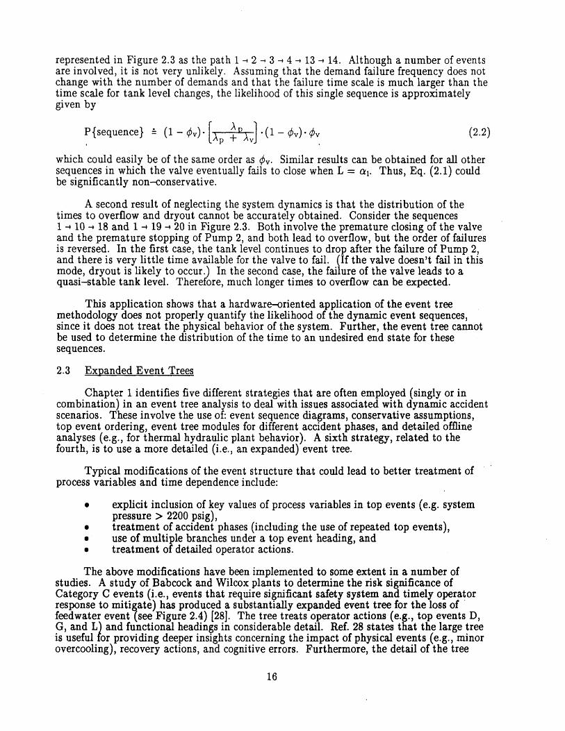
2.3 Expanded Event Trees

Chapter 1 identifies five different strategies that are often employed (singly or incombination) in an event tree analysis to deal with issues associated with dynamic accidentscenarios. These involve the use of: event sequence diagrams, conservative assumptions,top event ordering, event tree modules for different accident phases, and detailed offlineanalyses (e.g., for thermal hydraulic plant behavior). A sixth strategy, related to thefourth, is to use a more detailed (i.e., an expanded) event tree.

Typical modifications of the event structure that could lead to better treatment ofprocess variables and time dependence include:

0 explicit inclusion of key values of process variables in top events (e.g. systempressure > 2200 psig),

0 treatment of accident phases (including the use of repeated top events),e use of multiple branches under a top event heading, and0 treatment of detailed operator actions.

The above modifications have been implemented to some extent in a number ofstudies. A study of Babcock and Wilcox plants to determine the risk significance ofCategory C events (i.e., events that require significant safety system and timely operatorresponse to mitigate) has produced a substantially expanded event tree for the loss offeedwater event (see Figure 2.4) [28]. The tree treats operator actions (e.g., top events D,G, and L) and functional headings in considerable detail. Ref. 28 states that the large treeis useful for providing deeper insights concerning the impact of physical events (e.g., minorovercooling), recovery actions, and cognitive errors. Furthermore, the detail of the tree

16

allows a reasonable mapping of actual loss of feedwater events into the tree (for use in aprecursor analysis).

Other uses of expanded event trees are provided in Ref. 31 (in a human reliabilityanalysis) and in the NUREG-1150 Accident Progression Event Trees (APETs) created forthe analysis of events following core damage (e.g., [13]). In the latter case, over 100 topevents can be used. Further, there can be more than two branches per top event.

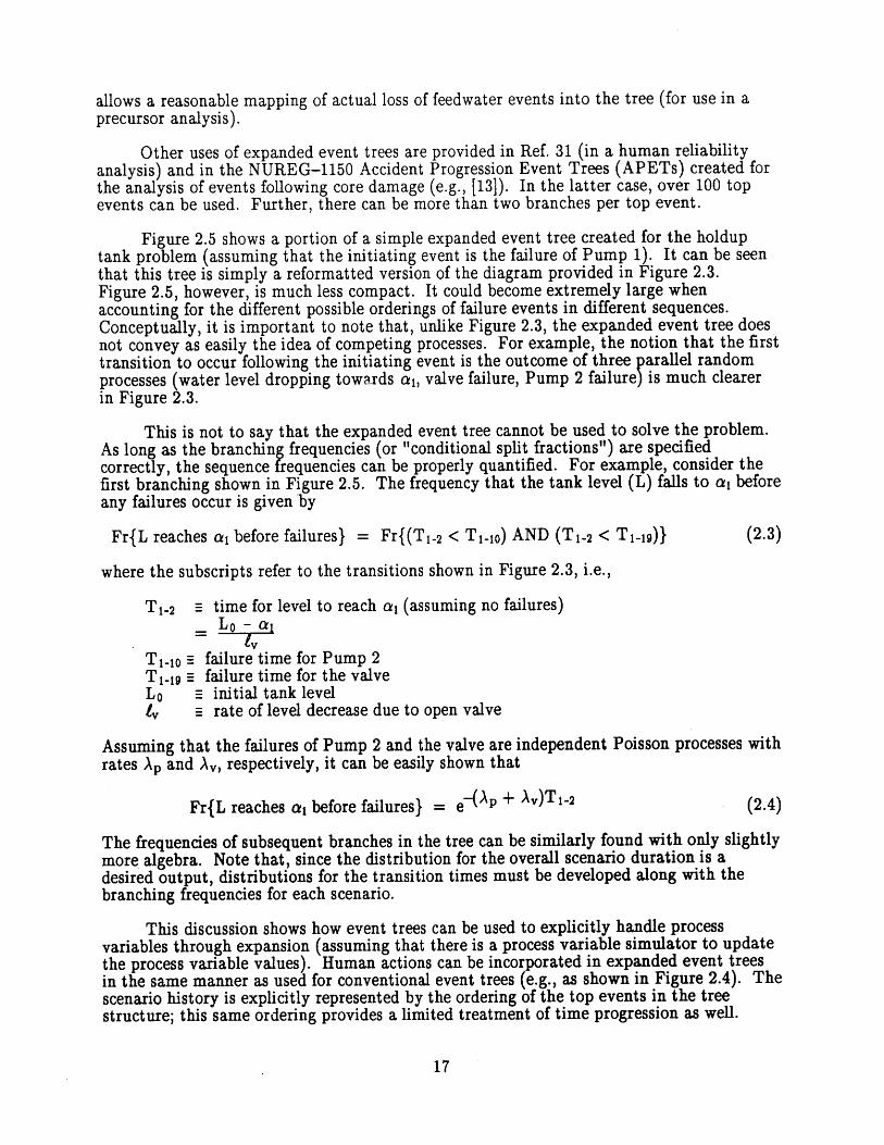
Figure 2.5 shows a portion of a simple expanded event tree created for the holduptank problem (assuming that the initiating event is the failure of Pump 1). It can be seenthat this tree is simply a reformatted version of the diagram provided in Figure 2.3.Figure 2.5, however, is much less compact. It could become extremely large whenaccounting for the different possible orderings of failure events in different sequences.Conceptually, it is important to note that, unlike Figure 2.3, the expanded event tree doesnot convey as easily the idea of competing processes. For example, the notion that the firsttransition to occur following the initiating event is the outcome of three parallel randomprocesses (water level dropping towards a,, valve failure, Pump 2 failure) is much clearerin Figure 2.3.

This is not to say that the expanded event tree cannot be used to solve the problem.As long as the branching frequencies (or "conditional split fractions") are specifiedcorrectly, the sequence frequencies can be properly quantified. For example, consider thefirst branching shown in Figure 2.5. The frequency that the tank level (L) falls to a, beforeany failures occur is given by

Fr{L reaches a, before failures} = Fr{(Ti- 2 < T 1io) AND (Ti-2 < Ti-19)} (2.3)

where the subscripts refer to the transitions shown in Figure 2.3, i.e.,

T1-2 mtime for level to reach a, (assuming no failures)_L o - a,

TI.10 afailure time for Pump 2Tj.1g 3failure time for the valveL o initial tank level4v rate of level decrease due to open valve

Assuming that the failures of Pump 2 and the valve are independent Poisson processes withrates Ap and Ay, respectively, it can be easily shown that

Fr{L reaches a, before failures} = e-(Ap + Ay)Ti- 2 (2.4)

The frequencies of subsequent branches in the tree can be similarly found with only slightlymore algebra. Note that, since the distribution for the overall scenario duration is adesired output, distributions for the transition times must be developed along with thebranching frequencies for each scenario.

This discussion shows how event trees can be used to explicitly handle processvariables through expansion (assuming that there is a process variable simulator to updatethe process variable values). Human actions can be incorporated in expanded event treesin the same manner as used for conventional event trees (e.g., as shown in Figure 2.4). Thescenario history is explicitly represented by the ordering of the top events in the treestructure; this same ordering provides a limited treatment of time progression as well.

17

On the other hand, it can be seen that the event tree representation will becomeextremely complicated when several process variables, several components, and multiplecomponent states must be treated. In addition to the extremely (if not excessively) largetrees required, the analysis will require an assessment of the branching frequencies andtransition times, and can become quite burdensome when dealing with multiple parallelprocesses. The methodology does not treat the cognitive activity of the operating crew,and does not treat time dependence explicitly. Regarding the latter point, loops or evensimple events at multiple points in time (e.g., multiple relief valve challenges) cannot betreated without some arbitrary truncation rules (to limit a priori the number of repetitionsallowed for a given top event). These limitations can be overcome. To do this, however,requires a time-dependent extension of the event tree concept, as described in Chapter 3.

2.4 Analytical Methodologies

As shown in the preceding section, the expanded event tree methodology has only alimited capability for treating systems whose time-dependent behavior is important. Thissection reviews three analytical methodologies capable of treating time dependence to agreater extent: event sequence diagrams, the GO-FLOW methodology, and Markovmodeling. The difference between these methodologies and the simulation-basedmethodologies discussed in Section 2.5 is that the former require the analyst to explicitlydefine system states and transitions between states. The latter require the analyst todefine rules of behavior for the system. The system states, and the likelihood of a givenaccident scenario trajectory through state space, are defined implicitly as the outcome ofthe modeling rules.

2.4.1 Event Sequence Diagrams

Event sequence diagrams (ESDs) can be viewed as generalized event trees. Likeevent trees, they show possible scenarios stemming from an initiating event. Unlike eventtrees, they are not necessarily restricted in their presentation of event sequences. Forexample, Figure 2.3, which is actually an ESD, includes failure event ordering in itsdefinition of accident scenarios. More generally, ESDs can provide a more literalrepresentation of the plant state, indicating the behavior of key process variables and evenoperators, as well as hardware state changes. ESDs have been used for some time inconventional risk assessment studies as qualitative aids for event tree construction; morerecently, they have been used as quantitative tools in a study of a simple chemical processsystem [32], in a phased mission study [33], and in a risk assessment for a research reactor[10].

It should be noted that the terminology "event sequence diagram" is not universallyused for these quantitative analyses, perhaps to reduce the possibility of confusion with thequalitative diagrams used as event tree precursors. For example, Ref. 10 refers to itsscenario models as "scenario trees." However, "ESD" is a useful label for the class ofmodels lying in between the extended event trees described earlier and the dynamic eventtrees described in Chapter 3.

One particular ESD analysis, described in Ref. 121, provides a useful illustration ofthe potential advantages and disadvantages of ESDs for quantitative accident scenarioanalysis. Ref. 12 proposes a simple state-transition model for treating time-dependentaccident scenarios. For a given initiating event, the different states of the plant arerepresented using the sequences in the conventional event tree for that initiating event.

'Again, the authors of Ref. 12 do not refer to their model as an ESD.

18

Thus, a dynamic scenario can be treated as a sequence of transitions between eventsequences, as illustrated in Figure 2.6. ESDs showing possible transitions are thendeveloped (see Figure 2.7).

The objectives of the analysis are: to determine the frequency that the plant arrivesat a particular state (event tree sequences) at time ti, and to determine the likelihood thatthe plant stays in that state until an undesired event (e.g., core uncovery) occurs.Achievement of the first objective requires the modeling of operator error, including errorsof commission; achievement of the second requires knowledge of the time remaining untilthe undesired event occurs. This requires a model for the ongoing physical processes in theplant.

It is worth noting that, unlike conventional event tree analyses, Ref. 12 uses theevent tree sequences to represent the instantaneous plant state, rather than thecombinations of overall success or failure of the different accident mitigating systems.Thus, the restoration of the auxiliary feedwater system (AFWS) 8 minutes into the TMIaccident is represented as a transition from Sequence 4 to Sequence 2 in Figure 2.6. In aconventional event tree analysis, on the other hand, it would be recognized that thecriterion for AFWS success was met (the system was restored in sufficient time), and,therefore, the scenario does not ever follow the lower branch for AFWS.

To implement the general concept, Ref. 12 presents a limited analysis of TMI-likeaccidents. It is presumed that a loss of feedwater event occurs at a pressurized waterreactor, and that an auxiliary feedwater system and a high pressure injection system(HPIS) are potentially available to mitigate the initiating event. The initial statefrequencies are determined using the frequency of the sequence and the (hardware)unavailabilities of the mitigating systems (AFWS and HPIS). Recognizing that runtimefailures are extremely unlikely, the analysis focuses on state transitions due to operatormisdiagnosis; the likelihood of misdiagnosis is treated statistically using a Bayesian model,where the evidence used is obtained from four stuck-open pilot-operated relief valve(PORV) events. The likelihood of remaining in a given state until core uncovery occurs iscomputed assuming that the three transition times respectively associated with: turning offthe HPIS, recovering from misdiagnosis, and closing the PORV block valve, areexponentially distributed. The time to core uncovery is calculated using a response surfacebased on the predictions of a simple thermal hydraulic model; uncertainties in the modelpredictions are treated explicitly.

In the limited implementation covered in Ref. 12, the transition frequencies do notdepend on the scenario history (i.e., the analysis is Markovian, as discussed in the followingsection). The ESD framework can, in principle, accommodate scenario history if thenumber and order of transitions between states are tracked (as in Figure 2.3). Thedifference between this approach and the DYLAM and dynamic event tree approachesdescribed later is that time is not used as an explicit parameter for branching. Allbranches in the ESD are determined by changes in system state; time enters only as animplicit parameter quantifying the length of stay in a state (which can affect the branchingfrequencies).

Figure 2.3 shows how ESDs can better represent a dynamic accident scenario than acomparable event tree. Thus, although this ESD is quantified in the same manner as theextended event tree [e.g., see Eqs. (2.3) and (2.4)], the analyst is provided with a clearerpicture of the multiple competing processes, aiding the formulation of the properprobabilistic model for the branching frequencies. Ref. 12 shows how ESDs can be used toquantify scenarios involving more complicated process physics and operator actions.

19

The primary drawback of the approach is its requirement that all system states andstate transitions be explicitly defined at the beginning of the analysis. For complexsystems, this can lead to the development of an extremely large ESD. Even moreimportantly, it is not clear how the states (and transitions) should be defined to treat thecognitive activity of the operators. Although Ref. 12 treats the difficult error ofcommission problem, it does so on a behavioral basis. When data for errors are availableand judged to be relevant (Ref. 12 analyzes such a case), the analysis can be performed in astraightforward manner. When data are not available, as is often the case wheninvestigating rare events, the modeling framework needs to be extended to treat theprocesses underlying the operator actions.

2.4.2 GO-FLOW

One of the key requirements of an improved accident scenario analysis methodologyis that it be able to treat time dependence. One area where time dependence is of interestinvolves phased mission scenarios. These are scenarios in which the progression of anaccident can be divided into a predetermined number of phases of specified duration, and inwhich the model boundary conditions can be different in each of the phases [34,35]. Forexample, early in an accident, a certain cooling system may be called upon to perform at100% capacity, whereas later in the accident, only 50% output may be needed. A phasedmission analysis will account for the different success criteria for each phase. It can alsoaccount for variations in failure frequency parameters for the phases.

A conventional approach towards phased mission analysis (using the event tree/faulttree methodology) is to distinguish the accident phases in the event tree, and to developseparate system fault trees for each phase. As pointed out in Ref. 36, this can lead to acomplex representation, especially since basic failure events must be distinguishedaccording to accident phase. Ref. 36 shows how the GO-FLOW methodology, introducedin Ref. 20 as a time-dependent availability methodology, can be used to treat the phasedmission problem in a more compact manner. The name "GO-FLOW" indicates that thismethodology is derived from the earlier GO methodology [37], but concentrates onmodeling the flow of physical signals in a system.

GO-FLOW can be viewed as an upgraded reliability block diagram methodology.Similar to the reliability block diagram approach (see, for example, [38]), the analystcreates a diagram showing how a signal propagates through the system of interest. Theprobability of output at any pcint in time is determined algebraically, using the standardlaws of probability. Unlike rehability block diagrams analyses (but similar to a GOanalysis), a number of predefined operators are used to assist the analyst to create aGO-FLOW chart. The operators represent different failure modes, logic operators, andsignal generators. The last are used to send signals into the model at predefined times, andcan therefore be used as triggers that signal the beginning and end of each accident phase.

A second difference between GO-FLOW and conventional reliability block diagramsis due to the former's emphasis on physical signals. Unlike reliability block diagrams, theoutput of a GO-FLOW analysis is the probability that a signal (e.g., flow, electric current)exists at a given point in time. Whether signal existence represents "success" or "failure"must be specified by the user.

To briefly illustrate the GO-FLOW approach in the context of the holdup tankexample, Figure 2.8 and Tables 2.3-2.5 show a GO-FLOW model for the first two phasesof a holdup tank accident scenario which follow an initial failure of Pump 1. These twophases represent the period where the tank level drops, and the (instantaneous) period

20

where the control laws for the tank change when the level reaches a,. The figure shows theGO-FLOW operators used to model component failure modes, and the linkages betweenthe operators; these operators are defined in Figure 2.9. Of particular interest in thephased mission analysis is the Type 40 operator; this is used to link the outputs of thedifferent model parts used to model the different phases. The tables define the signalsentering the system, the time points for which results are to be generated, and the stepwisecomputation procedure used to compute the probability of an output signal at the differenttime points. This probability is developed using the probability of input signals,information concerning the existence of subinput signals, and the operator definitions ofFigure 2.9.

The holdup tank problem is not a typical problem for GO-FLOW, since themethodology is designed to handle binary systems in phased mission situations. Anadditional modeling assumption, required to develop the model shown, is that the analystis only interested in the time-dependent probability of success. Any deviation fromnominal behavior defined by Table 2.1 is treated as failure and is not further modeled.With this assumption, the duration of the first phase in the accident is known (it isspecified by the initial tank level and the valve flow rate) and the problem is also a binaryone.

In the case of more prototypical applications, the primary advantage of GO-FLOWidentified by Refs. 20 and 36, as compared with -the event tree /fault tree approach, lieswith is compactness of representation of the phased mission problem. Ref. 36 provides anexample, involving a number of multicomponent systems, which shows that a complexphased mission analysis can be performed with a single GO-FLOW model. It is also shownthat the system's time-dependent availability function can be developed in a single run.

However, the methodology has some drawbacks. GO-FLOW is not designed toeasily provide structural information regarding the system (i.e., the minimal cut sets), norare importance measures computations provided. This information, routinely provided byfault tree and event tree analyses, is quite important when trying to decide how to reducethe system risk/unavailability. Further, GO-FLOW does not directly treat common causefailures, which frequently dominate the unavailability of redundant systems. An analystcan work around some of these problems (for example, an extra operator can be introducedto deal with common cause failure), but this can lead to model elements that don't directlycorrespond to actual objects in the system, and diminishes the easy interpretation of theGO-FLOW model.

With regard to the issues emphasized in this report, it is important to recognize that,as mentioned earlier, phased mission analysis deals with situations where the changes insystem performance requirements (and other boundary conditions) are predetermined.Thus, GO-FLOW can be used to analyze more dynamic problems, such as the holdup tankproblem, only after some simplifications in the problem statement.

2.4.3 Markov Models

Markov modeling is a well-known technique that can be used for assessing thetime-dependent availability of many dynamic systems (e.g., see [39-41]). To apply thistechnique, the analyst constructs a state-transition diagram indicating the possible(discrete) system states and the possible transitions between states.

In a "Markov chain" process (to use the terminology of Ref. 41), transitions betweenstates are assumed to occur only at discrete points in time. In the case of uniform timeintervals, therefore, transitions can occur at t=O, t=At, t=2At, etc. The weight on an arc

21

going from State j to State i, pij, is then defined as the conditional probability of transitionfrom state j to i, given that the system is currently in state j. Notationally,

pij a P{transition from j to i in next At I currently in state j} (2.5)

In a "discrete Markov process", on the other hand, transitions between states are allowedto occur at any point in time. The transition time from state j to state i, Tij, is assumedto be exponentially distributed with rate Aij, and Aij (instead of pij) is the weight assignedto the arc connecting State j and State i.

Eq. (2.5) shows that the essential feature of a Markov model for a system is that thesystem is assumed to be memoryless. Transition probabilities therefore depend only on thecurrent state, and not on how the system arrived in the current state (i.e., what path wasfollowed in the state-transition diagram), or how long it took to arrive in the current state.This assumption places some restrictions on the applicability of Markov analysis to generaldynamic systems.

Once the weights are assigned to the arcs, the probability that the system is in agiven state at a given point in time can be found quite easily. In the case of a discreteMarkov chain, the column vector of time-dependent state probabilities, P(t), is developedusing:

P(t) = Mp*P(t - At) (2.6)where

P(t) E column vector of state probabilities Pj(t)P (t) P{in state j at time t}MP Ematrix of state-transition probabilities pij

In the case of a continuous Markov system analysis, P(t) is found by solving a coupled setof first order, constant coefficient, ordinary differential equations:

= My*P(t) (2.7)

where M, is the matrix of coefficients whose off-diagonal elements are the transition rates

Aij and whose diagonal elements are such that the matrix columns sum to zero. Thesimple forms of Eqs. (2.6) and (2.7) are due to the assumption that the system ismemoryless. Both equations can be easily solved, given the initial probability vector P(O).

It can be seen that Markov models are simple in concept. The challenge is to definea set of states useful for the problem of interest, and to quantify the likelihood of thetransitions between states.

Refs. 9 and 42 present an application of Markov chain modeling to the problem ofprocess system reliability analysis. In this application, the discrete system states aredefined in terms of ranges of process variables as well as component status. Ref. 43formulates a more general representation allowing for the continuous variation of processvariables.

To illustrate the approach adopted by Refs. 9 and 42, consider the holdup tankproblem described in Section 2.1. (As noted earlier, this is a slightly generalized version ofa sample problem presented in Ref. 9.) In this problem, the system state at any point intime is defined by the current statuses of the pumps and valve, and by the current level of

22

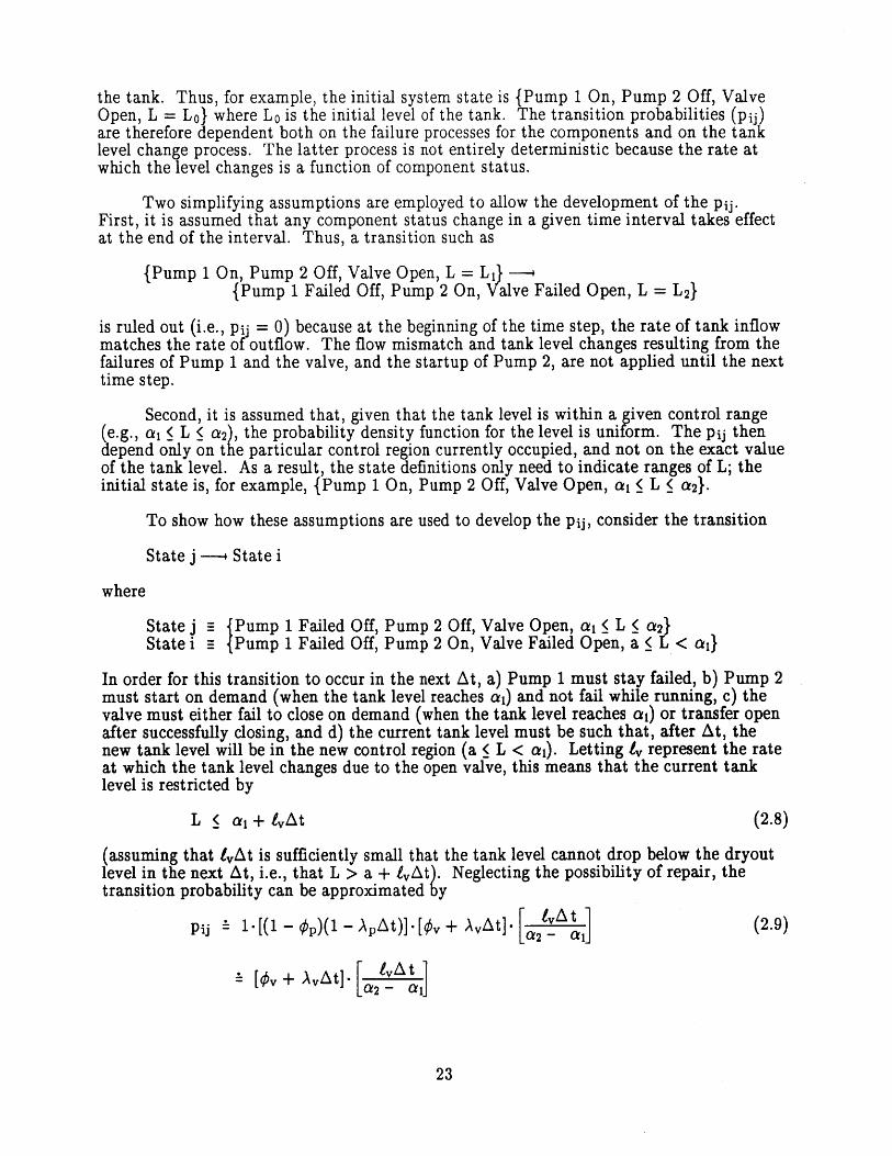
the tank. Thus, for example, the initial system state is {Pump 1 On, Pump 2 Off, ValveOpen, L = Lo} where Lo is the initial level of the tank. The transition probabilities (pij)are therefore dependent both on the failure processes for the components and on the tanklevel change process. The latter process is not entirely deterministic because the rate atwhich the level changes is a function of component status.

Two simplifying assumptions are employed to allow the development of the pij.First, it is assumed that any component status change in a given time interval takes effectat the end of the interval. Thus, a transition such as

{Pump 1 On, Pump 2 Off, Valve Open, L = L1}{Pump 1 Failed Off, Pump 2 On, Valve Failed Open, L = L2}

is ruled out (i.e., pij = 0) because at the beginning of the time step, the rate of tank inflowmatches the rate of outflow. The flow mismatch and tank level changes resulting from thefailures of Pump 1 and the valve, and the startup of Pump 2, are not applied until the nexttime step.

Second, it is assumed that, given that the tank level is within a given control range(e.g., at L < a2), the probability density function for the level is uniform. The pij thendepend only on the particular control region currently occupied, and not on the exact valueof the tank level. As a result, the state definitions only need to indicate ranges of L; theinitial state is, for example, {Pump 1 On, Pump 2 Off, Valve Open, a, L < a2}.

To show how these assumptions are used to develop the pij, consider the transition

State j - State i

where

State j {Pump 1 Failed Off, Pump 2 Off, Valve Open, a, L < a2}State i E{Pump 1 Failed Off, Pump 2 On, Valve Failed Open, a < L < a'}

In order for this transition to occur in the next At, a) Pump 1 must stay failed, b) Pump 2must start on demand (when the tank level reaches ai) and not fail while running, c) thevalve must either fail to close on demand (when the tank level reaches ai) or transfer openafter successfully closing, and d) the current tank level must be such that, after At, thenew tank level will be in the new control region (a < L < ai). Letting 4y represent the rateat which the tank level changes due to the open valve, this means that the current tanklevel is restricted by

L < ai+ IyAt (2.8)

(assuming that IyAt is sufficiently small that the tank level cannot drop below the dryoutlevel in the next At, i.e., that L > a + eyAt). Neglecting the possibility of repair, thetransition probability can be approximated by

pij - 1-[(1 - #p)(1 - ApAt)]-[#v + AvAt]- IVA (2.9)

[0v + AvAt]. [ I t1[a2- ail

23

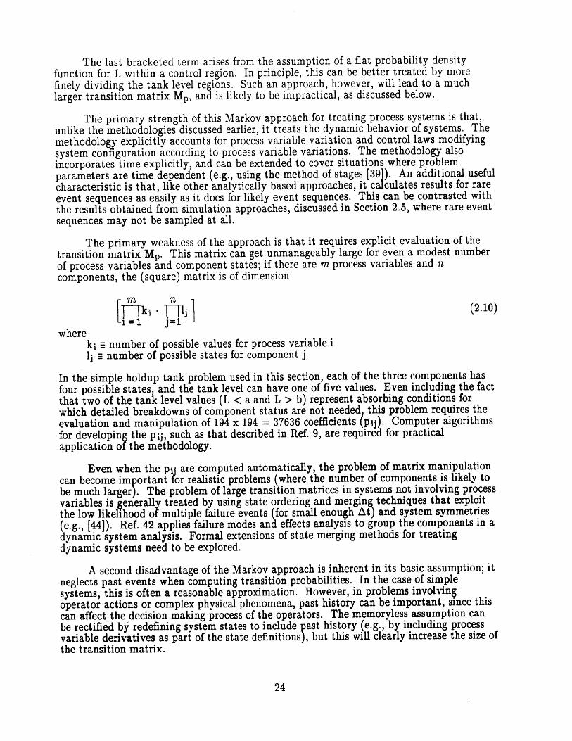
The last bracketed term arises from the assumption of a flat probability densityfunction for L within a control region. In principle, this can be better treated by morefinely dividing the tank level regions. Such an approach, however, will lead to a muchlarger transition matrix Mp, and is likely to be impractical, as discussed below.

The primary strength of this Markov approach for treating process systems is that,unlike the methodologies discussed earlier, it treats the dynamic behavior of systems. Themethodology explicitly accounts for process variable variation and control laws modifyingsystem configuration according to process variable variations. The methodology alsoincorporates time explicitly, and can be extended to cover situations where problemparameters are time dependent (e.g., using the method of stages [39]). An additional usefulcharacteristic is that, like other analytically based approaches, it calculates results for rareevent sequences as easily as it does for likely event sequences. This can be contrasted withthe results obtained from simulation approaches, discussed in Section 2.5, where rare eventsequences may not be sampled at all.

The primary weakness of the approach is that it requires explicit evaluation of thetransition matrix Mp. This matrix can get unmanageably large for even a modest numberof process variables and component states; if there are m process variables and ncomponents, the (square) matrix is of dimension

[m n

i 1 j=1where

ki = number of possible values for process variable ilj = number of possible states for component j

In the simple holdup tank problem used in this section, each of the three components hasfour possible states, and the tank level can have one of five values. Even including the factthat two of the tank level values (L < a and L > b) represent absorbing conditions forwhich detailed breakdowns of component status are not needed this problem requires theevaluation and manipulation of 194 x 194 = 37636 coefficients (pij). Computer algorithmsfor developing the pij, such as that described in Ref. 9, are required for practicalapplication of the methodology.

Even when the pj are computed automatically, the problem of matrix manipulationcan become important for realistic problems (where the number of components is likely tobe much larger). The problem of large transition matrices in systems not involving processvariables is generally treated by using state ordering and merging techniques that exploitthe low likelihood of multiple failure events (for small enough At) and system symmetries(e.g., [44]). Ref. 42 applies failure modes and effects analysis to group the components in adynamic system analysis. Formal extensions of state merging methods for treatingdynamic systems need to be explored.

A second disadvantage of the Markov approach is inherent in its basic assumption; itneglects past events when computing transition probabilities. In the case of simplesystems, this is often a reasonable approximation. However, in problems involvingoperator actions or complex physical phenomena, past history can be important, since thiscan affect the decision making process of the operators. The memoryless assumption canbe rectified by redefining system states to include past history (e.g., by including processvariable derivatives as part of the state definitions), but this will clearly increase the size ofthe transition matrix.

24

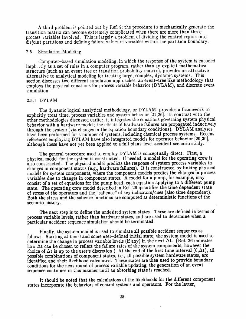
A third problem is pointed out by Ref. 9: the procedure to mechanically generate thetransition matrix can become extremely complicated when there are more than threeprocess variables involved. This is largely a problem of dividing the control region intodisjoint partitions and defining failure values of variables within the partition boundary.

2.5 Simulation Modeling

Computer-based simulation modeling, in which the response of the system is encodedimpli ly as a set of rules in a computer program, rather than an explicit mathematicalstructure (such as an event tree or transition probability matrix), provides an attractivealternative to analytical modeling for treating large, complex, dynamic systems. Thissection discusses two different simulation approaches: an event-tree like methodology thatemploys the physical equations for process variable behavior (DYLAM), and discrete eventsimulation.

2.5.1 DYLAM

The dynamic logical analytical methodology, or DYLAM, provides a framework toexplicitly treat time, process variables and system behavior [21,26]. In contrast with theother methodologies discussed earlier, it integrates the equations governing system physicalbehavior with a hardware model; the effects of hardware failures are propagated inductivelythrough the system (via changes in the equation boundary conditions). DYLAM analyseshave been performed for a number of systems, including chemical process systems. Recentreferences employing DYLAM have also integrated models for operator behavior [29,30],although these have not yet been applied to a full plant-level accident scenario study.

The general procedure used to employ DYLAM is conceptually direct. First, aphysical model for the system is constructed. If needed, a model for the operating crew isalso constructed. The physical model predicts the response of system process variables tochanges in component status (e.g., hardware failures). It is constructed by linking physicalmodels for system components, where the component models predict the changes in processvariables due to changes in component states. A model for a pump, for example, mayconsist of a set of equations for the pump head, each equation applying to a different pumpstate. The operating crew model described in Ref. 29 quantifies the time dependent stateof stress of the operators and the "salience" of key indicators/cues (also time dependent).Both the stress and the salience functions are computed as deterministic functions of thescenario history.

The next step is to define the undesired system states. These are defined in terms ofprocess variable levels, rather than hardware states, and are used to determine when aparticular accident sequence simulation should be terminated.

Finally, the system model is used to simulate all possible accident sequences asfollows. Starting at t = 0 and some user-defined initial state, the system model is used todetermine the change in process variable levels (if any) in the next At. (Ref. 26 indicateshow At can be chosen to reflect the failure rates of the system components; however thechoice of At is up to the user's discretion.) At the end of the first time interval (0,At), allpossible combinations of component states, i.e., all possible system hardware states, areidentified and their likelihood calculated. These states are then used to provide boundaryconditions for the next round of process variable updating; the generation of an eventsequence continues in this manner until an absorbing state is reached.

It should be noted that the calculations of the likelihoods for the different componentstates incorporate the behaviors of control systems and operators. For the latter,

25

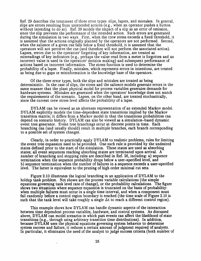
Ref. 29 describes the treatment of three error types: slips, lapses, and mistakes. In general,slips are errors resulting from unintended actions (e.g., when an operator pushes a buttonwithout intending to do so). Ref. 29 models the impact of a slip as an error of omission,since the slip prevents the performance of the intended action. Such errors are generatedduring the simulation in two ways. First, when the crew stress exceeds a fixed threshold, itis assumed that the actions originally planned by the operators are not performed. Second,when the salience of a given cue falls below a fixed threshold, it is assumed that theoperators will not perceive the cue (and therefore will not perform the associated action).Lapses, errors due to the operators' forgetting of key information, are treated asmisreadings of key indicators (e.g., perhaps the value read from a meter is forgotten and anincorrect value is used in the operators' decision making) and subsequent performance ofactions based on incorrect information. The stress function is used to determine theprobability of a lapse. Finally, mistakes, which represents errors in intentions, are treatedas being due to gaps or misinformation in the knowledge base of the operators.

Of the three error types, both the slips and mistakes are treated as beingdeterministic. In the case of slips, the stress and the salience models generate errors in thesame manner that the plant physical model for process variables generates demands forhardware systems. Mistakes are generated when the operators' knowledge does not matchthe requirements of the scenario. Lapses, on the other hand, are treated stochastically,since the current crew stress level affects the probability of a lapse.

DYLAM can be viewed as an alternate representation of an extended Markov model.DYLAM explicitly models the time-dependent state transitions implied by the Markovtransition matrix; it differs from a Markov model in that the transitions probabilities candepend on scenario history. DYLAM can also be viewed as a simulation-based dynamicevent tree generator. Event tree branchings occur at discrete points in time. Eachbranching can (and usually should) result in multiple branches, each branch correspondingto a possible set of system changes.

Clearly, in order to practically apply DYLAM to realistic problems, rules for limitingthe event tree expansion need to be provided. One such rule is provided by the undesiredstates defined prior to the start of the simulation. These states are used as absorbingstates; all event sequences reaching absorbing states are terminated upon arrival. Anumber of branching and stopping rules are described in Ref. 26, including: a) sequencetermination when the sequence probability drops below a user-specified level, andb) sequence termination when the number of failures in a sequence exceeds a user-specifiedlevel. The latter is equivalent to the pruning of high order minimal cut sets.

Figure 2.10 illustrates the logical branching in an application of DYLAM to theholdup tank problem. Not shown are the process variable calculations (the simpleequations governing tank level rate of change), or the probability calculations. The figureshows two situations where sequence expansion is truncated on the basis of probability:when multiple failures must occur in a single time interval, and when a component mustfail randomly before a control region boundary is reached (the time scale of Figure 2.10 issuch that the tank level will take roughly a single At to reach a different control region).

This example shows how DYLAM can handle dynamic aspects of the interactionbetween time dependent process variables, hardware, and control systems. As discussedabove, DYLAM can model scenarios in which past events can affect the likelihood of statetransitions (e.g., through using arbitrary transition time distributions). In addition,because DYLAM uses the physical equations governing system behavior to determinesystem success and failure, it reduces a certain amount of judgment required of analysts.In particular, it eliminates the need of the analyst to judge success criteria (both number of

26

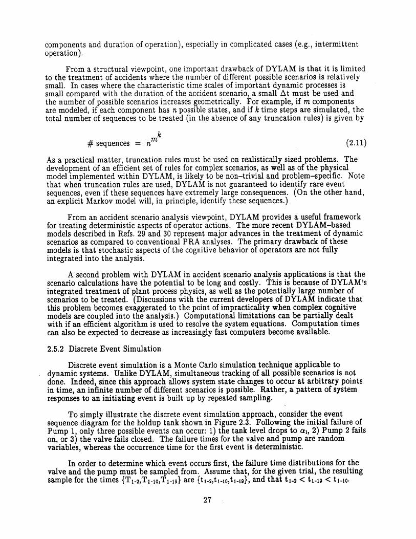
components and duration of operation), especially in complicated cases (e.g., intermittentoperation).

From a structural viewpoint, one important drawback of DYLAM is that it is limitedto the treatment of accidents where the number of different possible scenarios is relativelysmall. In cases where the characteristic time scales of important dynamic processes issmall compared with the duration of the accident scenario, a small At must be used andthe number of possible scenarios increases geometrically. For example, if m componentsare modeled, if each component has n possible states, and if k time steps are simulated, thetotal number of sequences to be treated (in the absence of any truncation rules) is given by

# sequences = nm (2.11)

As a practical matter, truncation rules must be used on realistically sized problems. Thedevelopment of an efficient set of rules for complex scenarios, as well as of the physicalmodel implemented within DYLAM, is likely to be non-trivial and problem-specific. Notethat when truncation rules are used, DYLAM is not guaranteed to identify rare eventsequences, even if these sequences have extremely large consequences. (On the other hand,an explicit Markov model will, in principle, identify these sequences.)

From an accident scenario analysis viewpoint, DYLAM provides a useful frameworkfor treating deterministic aspects of operator actions. The more recent DYLAM-basedmodels described in Refs. 29 and 30 represent major advances in the treatment of dynamicscenarios as compared to conventional PRA analyses. The primary drawback of thesemodels is that stochastic aspects of the cognitive behavior of operators are not fullyintegrated into the analysis.

A second problem with DYLAM in accident scenario analysis applications is that thescenario calculations have the potential to be long and costly. This is because of DYLAM'sintegrated treatment of plant process physics, as well as the potentially large number ofscenarios to be treated. (Discussions with the current developers of DYLAM indicate thatthis problem becomes exaggerated to the point of impracticality when complex cognitivemodels are coupled into the analysis.) Computational limitations can be partially dealtwith if an efficient algorithm is used to resolve the system equations. Computation timescan also be expected to decrease as increasingly fast computers become available.

2.5.2 Discrete Event Simulation

Discrete event simulation is a Monte Carlo simulation technique applicable todynamic systems. Unlike DYLAM, simultaneous tracking of all possible scenarios is notdone. Indeed, since this approach allows system state changes to occur at arbitrary pointsin time, an infinite number of different scenarios is possible. Rather, a pattern of systemresponses to an initiating event is built up by repeated sampling.

To simply illustrate the discrete event simulation approach, consider the eventsequence diagram for the holdup tank shown in Figure 2.3. Following the initial failure ofPump 1, only three possible events can occur: 1) the tank level drops to a,, 2) Pump 2 failson, or 3) the valve fails closed. The failure times for the valve and pump are randomvariables, whereas the occurrence time for the first event is deterministic.

In order to determine which event occurs first, the failure time distributions for thevalve and the pump must be sampled from. Assume that, for the given trial, the resultingsample for the times {T 1-2,T 1 _10 ,T 1-19} are {t 1-2 ,t 1 -1 0 ,t 1 -19 }, and that t 1-2 < t i-i < t 1 -10.

27

To organize the simulation, the event occurrence times are put into the simulation's"master schedule" (also called event calendar or pending list) in the order of theiroccurrence times, as shown in Figure 2.1la. This master schedule is a key entity in adiscrete event simulation. It indicates what events are scheduled to occur and when theyare scheduled to occur. Furthermore, because event occurrence is associated with theexecution of some subroutine in the simulation, the master schedule implicitly defines theset of actions to be performed as a result of event occurrence.

Figure 2.11a shows that there are no other events scheduled before the tank levelreaches ai (i.e., Event 1). Therefore, the simulation clock is advanced to time t = t 1 2 , andthe event "level reaches a," is executed, with two consequences. First, an immediatedemand is placed on the valve to close, as per the control laws in Table 2.1 (as inFigure 2.3 it is assumed that Pump 2 will start if L = ai and the valve fails to close). Thisis the fourth scheduled event in the sequence. Second, the originally scheduled Events 2and 3 (the failure of the valve and Pump 2) are no longer relevant; these events areremoved from the master schedule. The resulting master schedule after these changes isshown in Figure 2.11b. Figures 2.11c and d continue the development of the scenario, andFigure 2.12 illustrates the time-dependent tank level for the scenario.

This example shows how a scenario is treated by dynamically modifying the masterschedule. The execution of a given event can inject additional events into the schedule orcan lead to the removal of events from the schedule. More generally, the execution of anevent can lead to arbitrarily complex changes in the current system state, the masterschedule, or even in the rules used to model system responses to change; the only limitingfactor is the ability of the analyst to encode these changes into the simulation. It can beseen that this simulation approach can be used to model more complicated processes,including operator behavior.

Note that once the event occurrence times are generated, the scenario depicted inFigure 2.12 can be followed deterministically. Variability in system behavior due torandomness (or state-of-knowledge uncertainty) can be represented only after repeatedtrials.

Currently, discrete event simulation is not widely used in risk and reliabilityassessment. Monte Carlo simulation has been used to determine fault tree cut sets and toquantify top event probabilities (e.g., [45]), and is almost universally used to performuncertainty propagation. However, largel because the issue of system dynamic response isa relatively recent one in risk assessment (e.g., see [19,21]), discrete event simulation, withits capability for treating dynamic systems, has only been used in a few analyses.

Refs. 46, 15, and 47 describe discrete event simulation analyses based on thesimulation language SIMSCRIPT 11.5 [48]. Ref. 46 treats delays in the physical response ofa chemical process system to failure events. Ref. 15 models the recovery of electric powerin a nuclear plant risk assessment; the variable task completion times for operatorsresponding to a loss of power are modeled explicitly.

Ref. 47 describes a discrete event simulation computer code (also written usingSIMSCRIPT 11.5) for system availability analysis. In this code, called DYMCAM (fordynamic availability model), components are modeled as separate objects (i.e., the codecreates separate subroutines for each component). Note that this approach allows theconstruction of a system model whose objects correspond directly with objects in the actualsystem. At the cost of some loss of computational efficiency, such a one-to-one model canbe more transparent and, therefore, more easily maintainable than the models associatedwith some of the other methodologies described earlier.

28

Similar to the CAT methodology [49] and GO-FLOW [20], DYMCAM treats linksbetween components using physical signals; a generic component is pictured in Figure 2.13.Changes in component status can be triggered by changes in the input signals, externalevents (e.g., maintenance actions), or simple random failures. The former are governed byrules encoded in the simulation. Table 2.6 provides an example of these rules, used tomodel an active component (e.g., a pump). Ref. 47 also describes an analysis of the holduptank problem. This analysis requires some small extensions of DYMCAM, in order to treatthe continuous process variable L (tank level).

At the accident sequence level, Ref. 27 performs a discrete event simulation of ashutdown heat removal system which accounts for the dynamic response of the system assubsystem failures arise. The method also treats increases in component failure rates asthe scenario progresses (due to increasing temperatures). Ref. 27 states that the simulationmodel compares favorably with a similar Markov approach, not only because of itsincreased level of detail, but also because the problem is such that the Markov modeltransition matrix becomes too large for practical analysis.

More recently, Refs. 50 and 51 describes a simulation model (written in SIMSCRIPT11.5) for control room crews in nuclear power plants intended for eventual use in accidentscenario analysis. The model treats the cognitive activities of each individual operator, andthe communication between the operators. It has been used with quite good success tosimulate the behavior of ten different crews performing training exercises for a steamgenerator tube rupture accident.

It can be seen that discrete event simulation has the ability to treat all of the issuesof interest in dynamic accident scenario analysis: hardware state, process variables,operator state of mind, scenario history, and time. However, there are at least twotechnical issues that need to be better resolved before it can be practically employed.

First, it is well known that, even when dealing with simple simulation models, directMonte Carlo sampling is often an inefficient method for developing estimators of averagesystem performance. The method becomes progressively worse when attempting toestimate higher moments of system performance measures (e.g., when estimating thevariance), since the estimates rely on good sampling from the tails of the distribution forthe performance measures. This problem is greatly exaggerated when simulation is used inrisk assessment, because such an assessment, almost invariably, deals with extremely rareevents. On the other hand, improved sampling schemes are usually very problem specificand expensive to develop. Ref. 15 employs a simplistic conditional Monte Carlo scheme inwhich it the sampling is conditioned on a limited number of predefined system failurestates. Ref. 52, in a simulation analysis of a feedback control system first analyzed inRef. 22, employs various variance reduction techniques (including stratified sampling,importance sampling, and antithetic variates) to obtain improved results. However, notonly is the effectiveness of a given variance reduction technique usually quiteproblem-specific, the integration of these techniques with a model can greatly complicatethe model.

A second problem arises when trying to use the results of the simulation. The outputof the event trees and fault trees conventionally used in risk assessment includes not only a"bottom line" estimate of the system risk, but also structural information indicating theimportant contributors to risk. Armed with the knowledge of the most important eventsequences, in the case of event trees, or minimal cut sets, in the case of fault trees, thesystem designer can take steps to reduce the overall risk.

29

On the other hand, partly because it involves more detail, a discrete event simulationanalysis does not yield such information as easily. Counters can be provided to indicatethe failure events occurring in each trial; these can be used to estimate the frequency ofvarious cut sets. However, because these cut sets will not be minimal, some postprocessing will be needed to filter out non-critical failures from the output. Moreimportantly, this approach is not useful when attempting to determine the importance ofother parameters governing system behavior. For example, it cannot directly identifyimportant continuous parameters (e.g., the value of a control setpoint), nor can it singleout critical operational policies that affect risk (e.g., decision rules for taking equipmentout of service for maintenance). Note that in the event tree/fault tree approach, answersto these questions are also not provided directly, but can be readily obtained by backtracking through the model (the computational path between input and results tends to bemore transparent because system dynamics are not treated in detail).

2.6 Evaluation of Methodologies

The ability to treat dynamic accident scenarios comes at a price; the addition of thetime dimension leads unavoidably to a more complicated analysis. Almost all of themethodologies reviewed in this chapter are significantly more complex and have moreextensive data requirements than the conventional event tree methodology. (GO-FLOWis the lone exception, but it does not appear that the GO-FLOW approach can be easilyextended to treat the issues of process variables and operator behavior central to thisreport.) The question is not if there is a simple methodology to handle dynamic scenarios,but rather which of the available methodologies has the greatest potential for near-termpractical application in PRA studies.

Within the group of analytical methodologies reviewed, event sequence diagrams arecurrently being used to qualitatively model accident scenarios, and can be extended totreat accident scenarios, as demonstrated by Ref. 12. Markov models 2 can treat processvariables with appropriate state definitions [9,431. Scenario history can also be treated tosome extent with careful state definitions. The method of stages [39], for example, can beused to treat non-exponential distributions for transition times.

The primary drawback of these analytical approaches is their requirement that allsystem states and state transitions be explicitly defined at the beginning of the analysis.For complex systems, this can lead to the development of an extremely large model. Evenmore importantly, it is not clear how the states (and transitions between states) should bedefined to represent the operators' state of mind. This problem must be addressed by thesimulation-based methodologies, of course. However, the latter are allowed to developthese definitions implicitly in the form of rules that can be scenario-dependent andemployed only as the scenario is generated.

Both of the simulation methodologies described in this chapter can deal with theissues of time, process variables, and scenario history. DYLAM presents a more structuredrepresentation of an accident sequence, but requires a good deal of computer memory (tostore the accident sequences). Note that this difficulty with problem size is simply adifferent manifestation of the same issue faced by the analytical methodologies. Thisproblem is dealt with in Markov modeling using state-merging techniques; DYLAM

2Most implementations of simulation models can be viewed as being Markovian with theproper definition of "system state." For the sake of classification, this report distinguishesthese implementations from the conventional, analytically-based Markov models in whichthe state transition matrix is defined and manipulated explicitly.

30

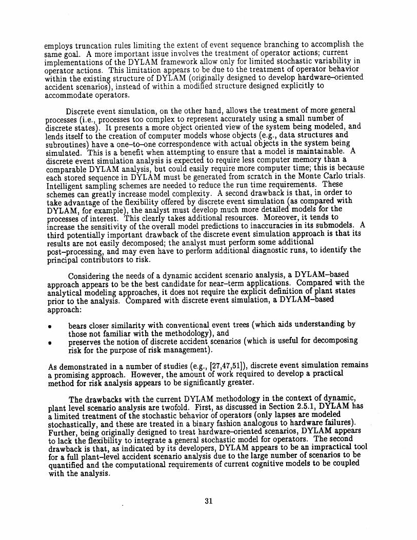
employs truncation rules limiting the extent of event sequence branching to accomplish thesame goal. A more important issue involves the treatment of operator actions; currentimplementations of the DYLAM framework allow only for limited stochastic variability inoperator actions. This limitation appears to be due to the treatment of operator behaviorwithin the existing structure of DYLAM (originally designed to develop hardware-orientedaccident scenarios), instead of within a modified structure designed explicitly toaccommodate operators.

Discrete event simulation, on the other hand, allows the treatment of more generalprocesses (i.e., processes too complex to represent accurately using a small number ofdiscrete states). It presents a more object oriented view of the system being modeled, andlends itself to the creation of computer models whose objects (e.g., data structures andsubroutines) have a one-to-one correspondence with actual objects in the system beingsimulated. This is a benefit when attempting to ensure that a model is maintainable. Adiscrete event simulation analysis is expected to require less computer memory than acomparable DYLAM analysis, but could easily require more computer time; this is becauseeach stored sequence in DYLAM must be generated from scratch in the Monte Carlo trials.Intelligent sampling schemes are needed to reduce the run time requirements. Theseschemes can greatly increase model complexity. A second drawback is that, in order totake advantage of the flexibility offered by discrete event simulation (as compared withDYLAM, for example), the analyst must develop much more detailed models for theprocesses of interest. This clearly takes additional resources. Moreover, it tends toincrease the sensitivity of the overall model predictions to inaccuracies in its submodels. Athird potentially important drawback of the discrete event simulation approach is that itsresults are not easily decomposed; the analyst must perform some additionalpost-processing, and may even have to perform additional diagnostic runs, to identify theprincipal contributors to risk.

Considering the needs of a dynamic accident scenario analysis, a DYLAM-basedapproach appears to be the best candidate for near-term applications. Compared with theanalytical modeling approaches, it does not require the explicit definition of plant statesprior to the analysis. Compared with discrete event simulation, a DYLAM-basedapproach:

* bears closer similarity with conventional event trees (which aids understanding bythose not familiar with the methodology), and

0 preserves the notion of discrete accident scenarios (which is useful for decomposingrisk for the purpose of risk management).

As demonstrated in a number of studies (e.g., [27,47,51]), discrete event simulation remainsa promising approach. However, the amount of work required to develop a practicalmethod for risk analysis appears to be significantly greater.

The drawbacks with the current DYLAM methodology in the context of dynamic,plant level scenario analysis are twofold. First, as discussed in Section 2.5.1, DYLAM hasa limited treatment of the stochastic behavior of operators (only lapses are modeledstochastically, and these are treated in a binary fashion analogous to hardware failures).Further, being originally designed to treat hardware-oriented scenarios, DYLAM appearsto lack the flexibility to integrate a general stochastic model for operators. The seconddrawback is that, as indicated by its developers, DYLAM appears to be an impractical toolfor a full plant-level accident scenario analysis due to the large number of scenarios to bequantified and the computational requirements of current cognitive models to be coupledwith the analysis.

31

These drawbacks do not invalidate the general DYLAM concept. Rather, theyindicate: 1) areas where the DYLAM structure needs to be extended, and 2) the need forsignificant approximations in practical applications. The following chapter describes anextension of the DYLAM concept, the Dynamic Event Tree Analysis Method (DETAM),which deals with these problems and enables the practical analysis of dynamic accidentscenarios.

32

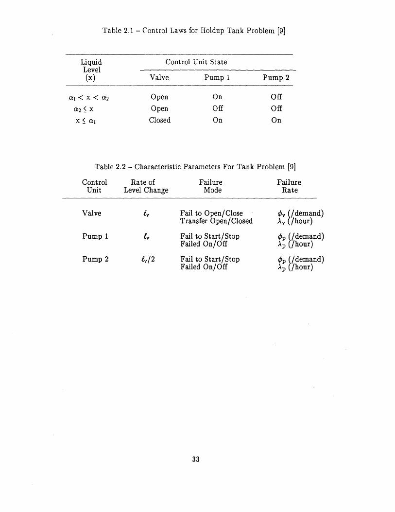
Table 2.1 - Control Laws for Holdup Tank Problem [9]

Liquid Control Unit StateLevel(x) Valve Pump 1 Pump 2

Open

Open

Closed

On

Off

On

Off

Off

On

Table 2.2 - Characteristic Parameters For Tank Problem [9]

ControlUnit

Rate ofLevel Change

FailureMode

FailureRate

Fail to Open/CloseTransfer Open/Closed

Fail to Start/StopFailed On/Off

Fail to Start/StopFailed On/Off

#v (/demand)Ay (/hour)

P (/demand)Ap (/hour)

#p (/demand)Ap (/hour)

33

ai < x < a2

a 2 X

x < a1i

Valve

Pump 1

Pump 2

IV

Iy

4y/2

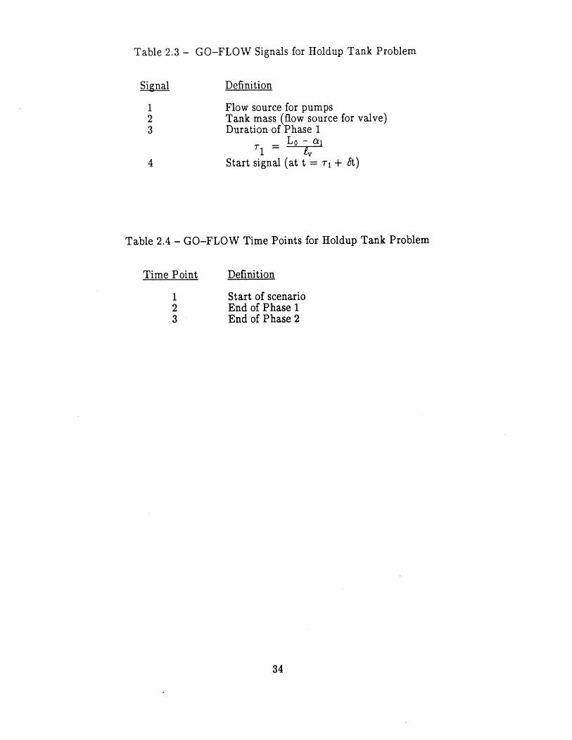
Table 2.3 - GO-FLOW Signals for Holdup Tank Problem

Signal Definition

1 Flow source for pumps2 Tank mass (flow source for valve)3 Duration of Phase 1

- Lo - a,

4 Start signal (at t = T + t)

Table 2.4 - GO-FLOW Time Points for Holdup Tank Problem

Time Point

123

Definition

Start of scenarioEnd of Phase 1End of Phase 2

34

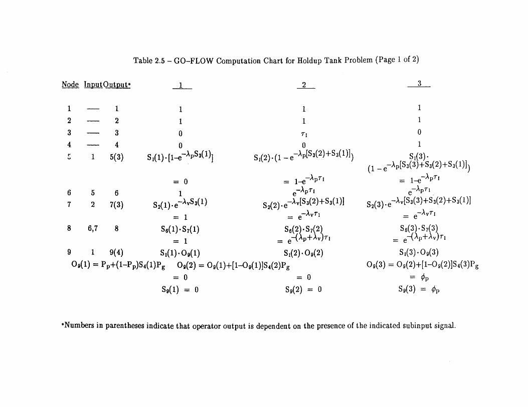
Table 2.5 - GO-FLOW Computation Chart for Holdup Tank Problem (Page 1 of 2)

Node IniputOutput* 1 2

-- 1

2

-- 3-- 41 5(3)

5

26

7(3)

8 6,7 8

1

1

0

0

S Ii1-1-ApS3(1)]

=0

S2(1) e-AvS3(1)= 1

S6(1)-S 7(1)= 1

1

1

TI

0

S1(2) -(1 - e-Ap[S3(2)+S3(1))

=1-e~ AP7-1

e APT1

S2(2)-e--Av[S3(2)+S3(1)I= e~AVTI

S6(2)-Sr(2)= e-(Ap+Ay)rI

9 1 9(4) S (1)-09(1) S1

09(1) = Pp+(l-Pp)S4(1)Pg 09(2) = O9(1)+[1-O9(1)]S4(2)Pg= 0

Sg(1) = 0 S

(2).Og(2)

= 0

9(2) = 0

1

10

1

SI(3)-

(1 - e-AP[S3(3)+S3(2)+S3(1)])= 1-eApTI

e-ApTI

S2(3) -e-Av[S 3(3)+S 3(2)+S 3(1)]

= e

S6(3). S 7(3)e-(Ap+Ay)Ti

S1(3).09(3)

Og(3) = 09(2)+[1-0(2)]S4( 3)Pg

= #pS9(3) = #p

*Numbers in parentheses indicate that operator output is dependent on the presence of the indicated subinput signal.

1

2

3

4r,

3

6

7

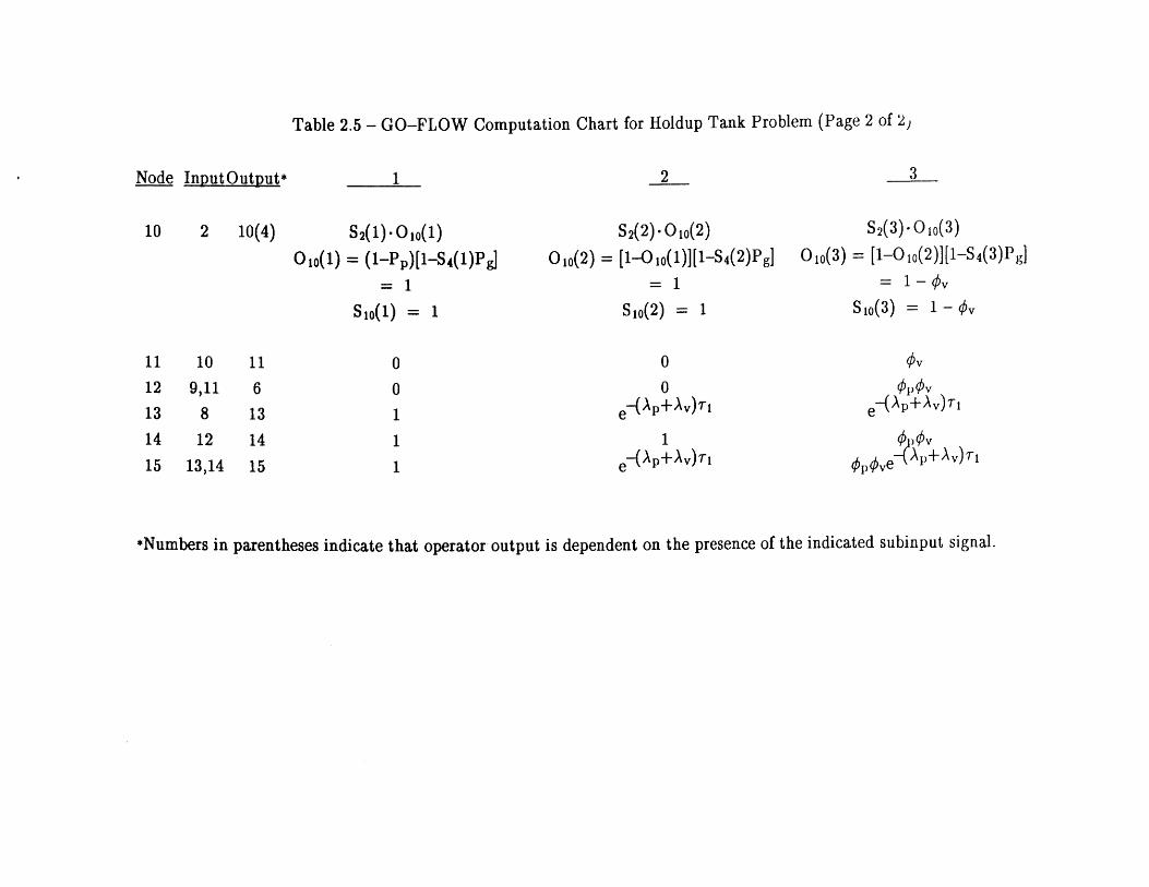
Table 2.5 - GO-FLOW Computation Chart for Holdup Tank Problem (Page 2 of 2)

Node InputOutput*

10 2 10(4)

1

S 2(1). 0 1(1)

O10(1) = (1-Pp)[1-S4(1)Pg]

= 1

Sio(1) = 1

11 10 11

12 9,11 6

13 8 1314 12 14

15 13,14 15

0

0

1

1

1

2

S2(2)0- O o(2)

O10(2) = [1-0 t0(1)][1-S4(2)Pg]

= 1

SIo(2) = 1

0

0

e-(Ap+Av)ri

1

e-(Ap+Av)TI

3

S2(3). O10(3)

O1o(3) = [1-Oo(2)][1-S4(3)P]

= 1-0v

Sijo(3) = 1 - #2

#v

e Ap+Av)Ti

04V5

*Numbers in parentheses indicate that operator output is dependent on the presence of the indicated subinput signal.

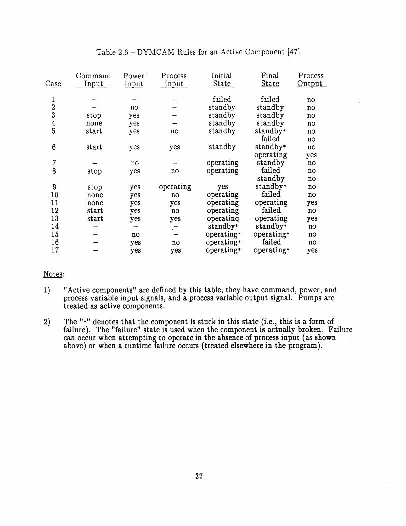
Table 2.6 - DYMCAM Rules for an Active Component [47]

CommandCase Input

12345

6

78

91011121314151617

stopnonestart

start

stop

stopnonenonestartstart

Power ProcessInput Input

noyesyesyes

yes

noyes

yesyesyesyesyes

noyesyes

no

yes

no

operatingnoyesnoyes

noyes

InitialState

failedstandbystandbystandbystandby

standby

operatingoperating

yesoperatingoperatingoperatingoperatinqstandby*

operating*operating*operating*

Final ProcessState Output

failedstandbystandbystandbystandby*

failedstandby*operatingstandbyfailed

standbystandby*

failedoperating

failedoperatingstandby*

operating*failed

operating*

nononononononoyesnononononoyesnoyesnonono

yes

Notes:

1) "Active components" are defined byprocess variable input signals, and atreated as active components.

this table; they have command, power, andprocess variable output signal. Pumps are

2) The "*" denotes that the component is stuck in this state (i.e., this is a form offailure). The "failure" state is used when the component is actually broken. Failurecan occur when attempting to operate in the absence of process input (as shownabove) or when a runtime failure occurs (treated elsewhere in the program).

37

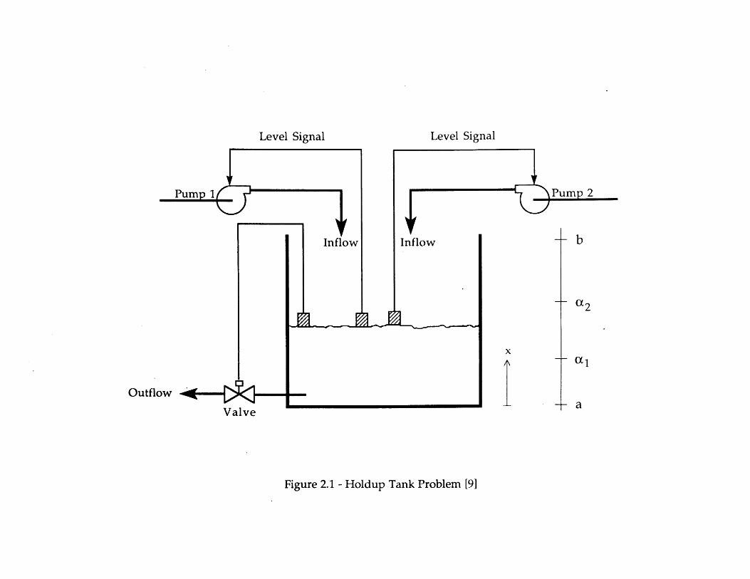
Level Signal

Inflow

Figure 2.1 - Holdup Tank Problem [91

2

Outflow

Valve

b

-a

T

Level Signal

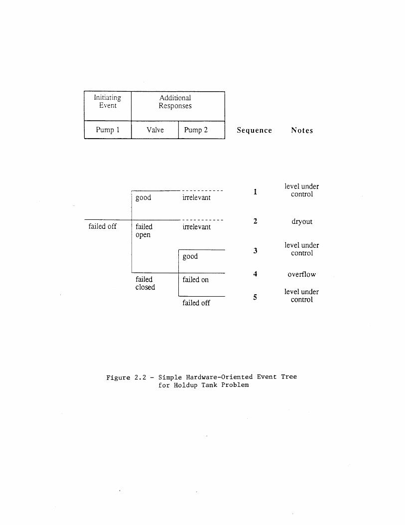
Initiating AdditionalEvent Responses

Pump 1 Valve Pump 2

failed off

-----------good irrelevant

failedopen

failedclosed

irrelevant

good

failed on

failed off

Sequence

1

2

3

4

5

Notes

level undercontrol

dryout

level undercontrol

overflow

level undercontrol

Figure 2.2 - Simple Hardware-Oriented Event Treefor Holdup Tank Problem

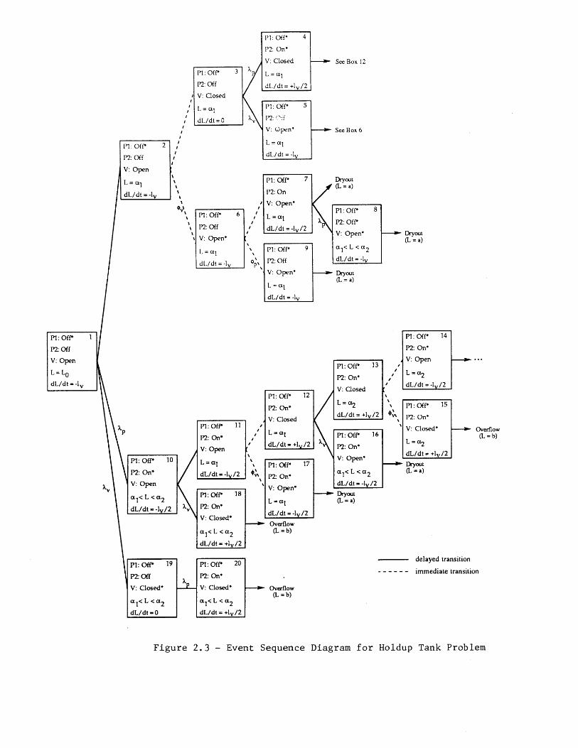
See Box 12

See Box 6

Dryout(L = a)

Overflow(L = b)

Dryout(L = a)

Dryout(L = a)

Overflow(L = b)

delayed transition

- - - - - - immediate transition

Overflow(L = b)

Figure 2.3 - Event Sequence Diagram for Holdup Tank Problem

XP

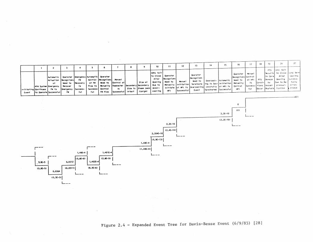
1 2 3 4 5 6 7 8 9 10 11 12 13 14 15 16 11 18 19 2o 2

SRVs fall PTS sav' FaIl

Automatic Operator Emergency Automatic Operator to Close Operator Operator Operator tknual usult s to Close toLn TernActuation Recognizes FW Contr'ol Recognizes fnual After Recognizes Pacognizes tbcognlzes Control In Core At ner Cool Inq

of Need to Recovery of FW Need to Control of Size of Opening Need to Vnual Need to Overcool- Automatic Wed to of HPI PTS Dimage Opening uccess-

f FW System Emergency Recover Is Flow Is nua ly F Isdwater Secondary Secondary ue to anually initiation Terminate Ing Is Suc- initiation Conual Sy Is Conds- y Due to W- fully

nitiating Continues FW Is Emergency Success- Success- Control Is Side Is Steam Leak ecoder- initiate of itI Is Oercooling cessfully of HP Is Control Success- tIons vessel pressur- to isl-Event to Oerate Successful FW ful f FW Flow Successful intact (Large) cooling HIf Successful Event TermInated Successful HP ful Occur Rupture Iztlon IlIsnel

(0)

(2.2E-10)

(2.4E-14)2. 204E-10

(5.9E-13)1.40E-4

1.40E-4

.- 0.0312 I 1.4021E

<S.S-5>) (8.SE-6)

1.401E-4

(2.SE-5)

L---

(1.40E-4)

L---

Figure 2.4 - Expanded Event Tree for Davis-Besse Event (6/9/85) [28]

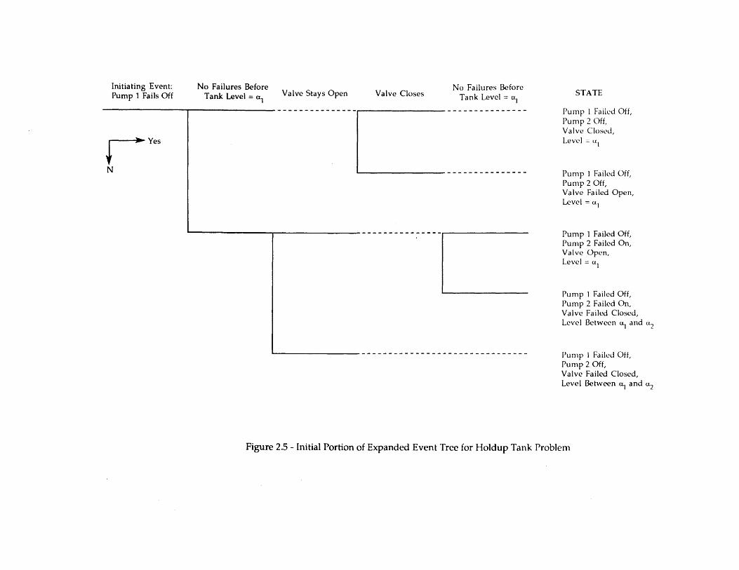
Initiating Event:Pump 1 Fails Off

No Failures BeforeTank Level = al

Valve Stays Open Valve ClosesNo Failures Before

Tank Level = c

Yes

N

Pump I Failed Off,Pump 2 Off,Valve Closed,Level = a,

Pump I Failed Off,Pump 2 Off,Valve Failed Open,Level = al

Pump 1 Failed Off,Pump 2 Failed On,Valve Open,Level = at

Pump I Failed Off,Pump 2 Failed On,Valve Failed Closed,Level Between u and a2

Pump I Failed Off,Pump 2 Off,Valve Failed Closed,Level Between al and "2

Figure 2.5 - Initial Portion of Expanded Event Tree for Holdup Tank Problem

STATE

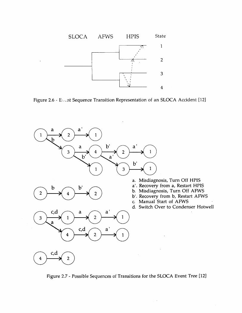
SLOCA AFWS HPIS State

1

2

3

4

Figure 2.6 - Ex -nt Sequence Transition Representation of an SLOCA Accident [12]

a.

b b a.

2 4 2 b.

c.d.

Misdiagnosis, Turn Off HPISRecovery from a, Restart HPISMisdiagnosis, Turn Off AFWSRecovery from b, Restart AFWSManual Start of AFWSSwitch Over to Condenser Hotwell

c,dC4 )- 2

Figure 2.7 - Possible Sequences of Transitions for the SLOCA Event Tree [12]

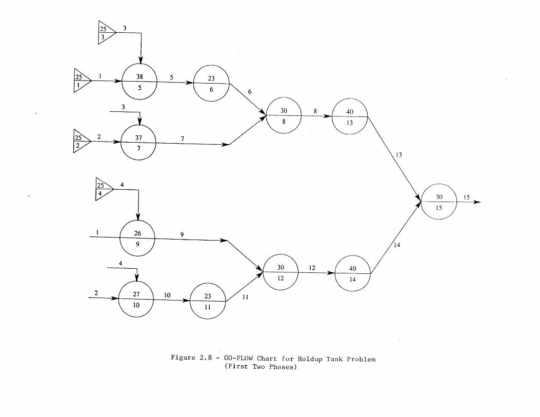
3

6

3

7

13

9

14

4

11

Figure 2.8 - GO-FLOW Chart for Holdup Tank Problem(First Two Phases)

2

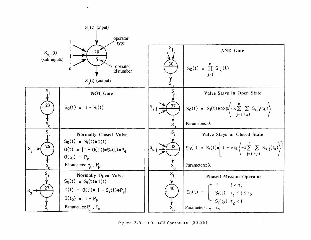
S1 (t) (input)

Ssj(t)

(sub-inputs)

1

n

operatortype

. operatorid number

S 0 (t) (output)

Si NOT Gate

r2 SoMt I - Si(t)

So .

Si Normally Closed Valve

So(t) = Si(t).0(t)

s 26 0(t) = [1 - 0(t')]eS(t).P90 (to) = P,

Sp 0 Parameters: P , PP

Si Normally Open ValveSo(t) = Si(t)eo(t)

Ss 27 0(t) = 0(t')[ 1 - SS(t)ePg]0 (to) = 1- P

S9 0 Parameters: P , PP

Figure 2.9 - GO-FLOW Operators [20,36]

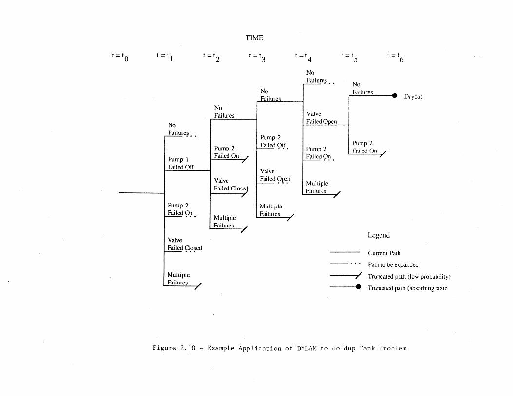
t =t2

TIME

t=t3

NoFailures

Pump 2Failed On

ValveFailed Close4

MultipleFailures

ValveFailed Closed

MultipleFailures

t =t

NoF ilures

Pump 2Failed Off

ValveFailed Open

MultipleFailures

t = t5

No

Failure''

ValveFailed Open

Pump 2Failed On

MultipleFailures -

NoFailures

Dryout

Pump 2Failed On /

Legend

Current Path

*. * Path to be expanded

/ Truncated path (low probability)

Truncated path (absorbing state

Figure 2. ]O - Example Application of DYLAM to Holdup Tank Problem

t=t0 t =t

NoFailures

Pump 1Failed Off

PumpFailed

2On

t -t 6

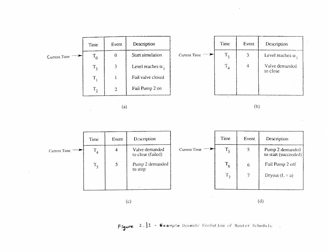
T0 0 Start simulation

T3 3 Level reaches a

TI 1 Fail valve closed

T2 2 Fail Pump 2 on

(a)

Time Event Dscription

T5

Cu rrent Time -

Current Time

(c)

Valve demandedto close (failed)

Pump 2 demandedto stop

Description

(d)

FI ure 2.}1 - &xarnple IyrImic Evoltion of Master ScheduIe

EventTime

4

5

Time Event Description

Current Time - 3 3 Level reaches a

T4 4 Valve demandedto close

(b)

Time Event Description

Current Time - T5 5 Pump 2 demandedto start (succeeded)

T6 6 Fail Pump 2 off

T7 7 Dryout (L = a)

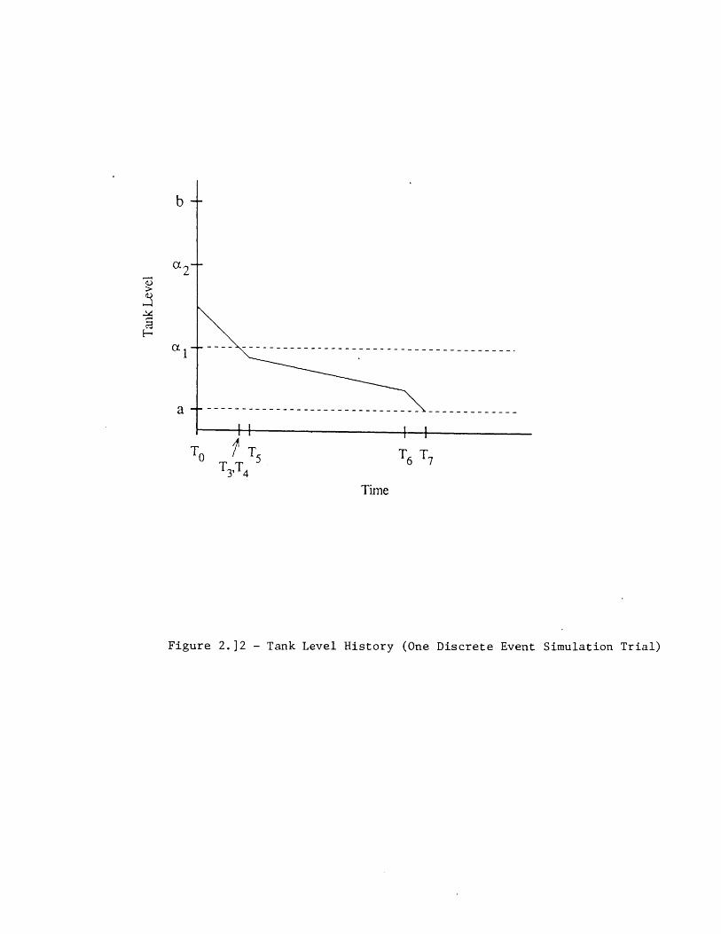
To T T5 T6 T7T,T 4

Time

Figure 2.]2 - Tank Level History (One Discrete Event Simulation Trial)

b

IH

oc 1

a

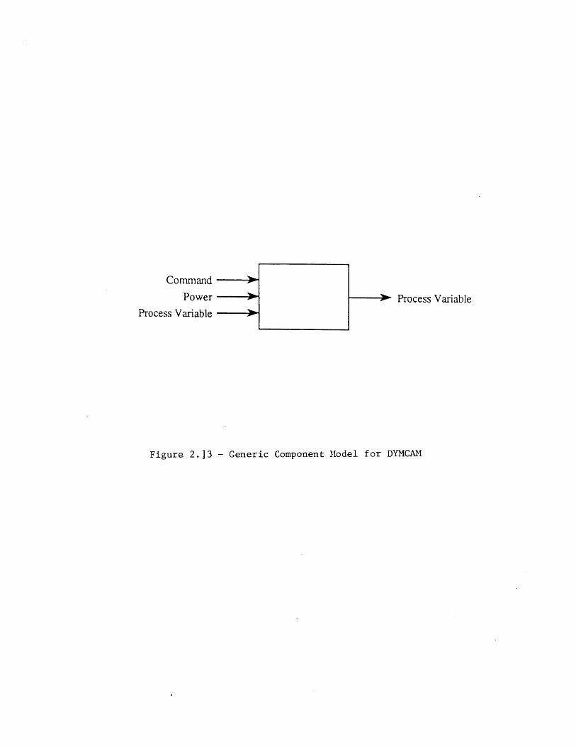
Command

Power

Process VariableProcess Variable

Figure 2.]3 - Generic Component Model for DYMCAM

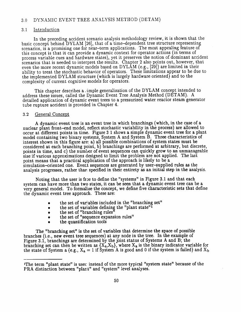
3.0 DYNAMIC EVENT TREE ANALYSIS METHOD (DETAM)

3.1 Introduction

In the preceding accident scenario analysis methodology review, it is shown that thebasic concept behind DYLAM [26], that of a time-dependent tree structure representingscenarios, is a promising one for near-term applications. The most appealing feature ofthis concept is that it can provide a dynamic context for operator actions (in terms ofprocess variable cues and hardware states), yet it preserves the notion of dominant accidentscenarios that is needed to interpret the results. Chapter 2 also points out, however, thateven the more recent dynamic models based on DYLAM (e.g., [29]) are limited in theirability to treat the stochastic behavior of operators. These limitations appear to be due tothe implemented DYLAM structure (which is largely hardware oriented) and to thecomplexity of current cognitive models for operators.

This chapter describes a imple generalization of the DYLAM concept intended toaddress these issues, called the Dynamic Event Tree Analysis Method (DETAM). Adetailed application of dynamic event trees to a pressurized water reactor steam generatortube rupture accident is provided in Chapter 4.

3.2 General Concept

A dynamic event tree is an event tree in which branchings (which, in the case of anuclear plant front-end model, reflect stochastic variability in the process) are allowed tooccur at different points in time. Figure 3 1 shows a simple dynamic event tree for a plantmodel containing two binary systems, System A and System B. Three characteristics ofinterest shown in this figure are: a) all possible combinations of system states must beconsidered at each branching point, b) branchings are performed at arbitrary, but discrete,points in time, and c) the number of event sequences can quickly grow to an unmanageablesize if various approximations designed to limit the problem are not applied. The lastpoint means that a practical application of the approach is likely to be asimulation-oriented one. Event sequences are generated by user-supplied rules as theanalysis progresses, rather thar specified in their entirety as an initial step in the analysis.

Noting that the user is free to define the "systems" in Figure 3.1 and that eachsystem can have more than two states, it can be seen that a dynamic event tree can be avery general model. To formalize the concept, we define five characteristic sets that definethe dynamic event tree approach. These are:

a the set of variables included in the "branching set"* the set of variables defining the "plant state"'e the set of "branching rules0 the set of "sequence expansion rules"0 the quantification tools

The "branching set" is the set of variables that determine the space of possiblebranches (i.e., new event tree sequences) at any node in the tree. In the example ofFigure 3.1, branchings are determined by the joint status of Systems A and B; thebranching set can then be written as {Xa,Xb}, where Xa is the binary indicator variable forthe state of System a (e.g., Xa = 1 if System A is good and 0 if the system is failed) and Xb

'The term "plant state" is usec instead of the more typical "system state" because of thePRA distinction between "plant" and "system" level analyses.

50

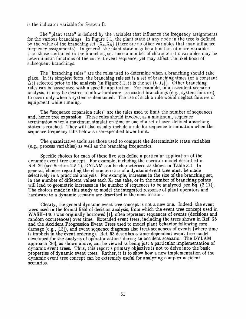
is the indicator variable for System B.

The "plant state" is defined by the variables that influence the frequency assignmentsfor the various branchings. In Figure 3.1, the plant state at any node in the tree is definedby the value of the branching set {Xa,Xb} (there are no other variables that may influencefrequency assignments). In general, the plant state may be a function of more variablesthan those contained in the branching set since a number of characteristic variables may bedeterministic functions of the current event sequence, yet may affect the likelihood ofsubsequent branchings.

The "branching rules" are the rules used to determine when a branching should takeplace. In its simplest form, the branching rule set is a set of branching times (or a constantAt) selected prior to the analysis (in Figure 3.1, it is the set {tit 2}). Other branchingrules can be associated with a specific application. For example, in an accident scenarioanalysis, it may be desired to allow hardware-associated branchings (e.g., system failures)to occur only when a system is demanded. The use of such a rule would neglect failures ofequipment while running.

The "sequence expansion rules" are the rules used to limit the number of sequencesand, hence tree expansion. These rules should involve, as a minimum, sequencetermination when a maximum simulation time or one of a set of user-defined absorbingstates is reached. They will also usually include a rule for sequence termination when thesequence frequency falls below a user-specified lower limit.

The quantitative tools are those used to compute the deterministic state variables(e.g., process variables) as well as the branching frequencies.

Specific choices for each of these five sets define a particular application of thedynamic event tree concept. For example, including the operator model described inRef. 29 (see Section 2.5.1), DYLAM can be characterized as shown in Table 3.1. Ingeneral, choices regarding the characteristics of a dynamic event tree must be madeselectively in a practical analysis. For example, increases in the size of the branching set,in the number of different values each Xi can take, or in the number of branching pointswill lead to geometric increases in the number of sequences to be analyzed [see Eq. (2.11)].The choices made in this study to model the integrated response of plant operators andhardware to a dynamic scenario are described in the next section.

Clearly, the general dynamic event tree concept is not a new one. Indeed, the eventtrees used in the formal field of decision analysis, from which the event tree concept used inWASH-1400 was originally borrowed [1], often represent sequences of events (decisions andrandom occurrences) over time. Extended event trees, including the trees shown in Ref. 28and the Accident Progression Event Trees used to model plant behavior following coredamage (e.g., [13]), and event sequence diagrams also treat sequences of events (where timeis implicit in the event ordering). Ref. 53 describes a time-dependent event tree modeldeveloped for the analysis of operator actions during an accident scenario. The DYLAMapproach [26], as shown above, can be viewed as being just a particular implementation ofdynamic event trees. Thus, this report's primary objective is not to delve into the basicproperties of dynamic event trees. Rather, it is to show how a new implementation of thedynamic event tree concept can be extremely useful for analyzing complex accidentscenarios.

51

3.3 General Implementation for Accident Scenario Analysis

In the context of dynamic accident scenario analysis, it is important that the choicesfor the dynamic event tree characteristics be made in such a manner that thosetime-dependent variables governing the likelihood of various operator actions are treatedexplicitly. Thus, following the discussion in Section 1.3, an application of the dynamicevent tree analysis method to nuclear power plant accident scenarios requires thetreatment of: the plant process variables, the operators' understanding of the currentsituation, the operators' internal conditions, and the actions planned by the operators.

The plant process variables (e.g., steam generator and pressurizer level, reactorcoolant system pressure) are important because they determine the timing of events (e.g.,demands for safety system actuations, occurrence of undesired physical plant states).Requirements for operator actions are often keyed to the process variables; these actionslead to changes in the process variables which, in turn, lead to different required actions.

The operators' understanding of the current accident situation, called the crew's"diagnosis state," clearly can affect the likelihood of future actions. Representations of thediagnosis state are potentially quite complex, but need not be. For example, Ref. 54 showshow experimental observations inferences of an operator's mental model during simulationexercises can be mapped as a trajectory on a fairly simple two-dimensional matrix in whichthe rows and columns of the matrix represent different levels of abstraction along the"whole-part" and "means-ends" dimensions. The first dimension corresponds to thediagnosis state, as it defines where the operator thinks the current problem is (e.g., at plantlevel, at system level, at train level, etc.). The second dimension is more concerned withthe actions the operator is thinking of taking to deal with the problem; this corresponds tothe planning state, discussed shortly.

The internal condition of the crew, called the crew's "quality state," characterizes thecrew's ability to efficiently perform tasks. This condition is defined by such factors as timepressure, workload, and crew group structure, which can affect crew performance and canchange over time. (Note that a variety of organizational factors, e.g., training, can affectcrew performance, but are not explicitly included since they will remain static through thecourse of the scenario. These factors provide initial conditions for the analysis.) Theoperator stress models discussed in Refs. 29 and 51 illustrate potential approaches forquantifying one important aspect of the crew's quality state. Models for the dynamics ofcharacteristics other than stress (e.g., communication effectiveness), need to be developedand integrated into the analysis. Refs. 50 and 51 provide some initial steps in thisdirection.

The actions planned by the operators define the "planning state" for the crew. In thehighly proceduralized environment of current plants, the planning state is strongly affectedby the procedural requirements on the operators. Of course, deviations in procedurefollowing can occur, and have been observed in actual incidents. (Ref. 55 presents ataxonomy of error types associated with procedure following.) Note also that the separatetreatment of diagnosis and planning can lead to situations where the correct steps aretaken, although an incorrect diagnosis has been made (such situations have been observedin simulator exercises).

Following these ideas, the general characteristics of the dynamic event trees used inthis study are given in Table 3.2. Comparing Tables 3.1 and 3.2, it can be seen that thisstudy's inclusion of operator state variables in the branching set allows a more generaltreatment of stochastic variability in operator behavior than that used in DYLAM. Asecond advantage of this discretized state approach to operator modeling is that a complex,

52

high fidelity simulation of operator cognitive activity is not necessarily required. Here, ananalysis can proceed if experts knowledgeable about operator behavior during accidents areavailable. Thus, the approach is similar to that used in a conventional human reliabilityanalysis for current PRAs (the difference being that here, the time-dependent context forthe operator actions is directly available to the experts).

Figure 3.2 shows how the characteristics listed in Table 3.2 are implemented in anaccident scenario analysis. (It is important to observe that this figure applies to a singlescenario within a single time step; the same process is applied repeatedly during thesimulation for all scenarios and all time steps.) As shown by this figure, the first task inthe analysis is the deterministic computation of the plant process variables. The next taskis to stop the branching process if an absorbing state, as defined by the needs of theanalysis, is reached. Absorbing states can represent the successful completion of thescenario, or the achievement of a particular undesired physical state, e.g., primary coolantsaturation. In the next task, the new set of possible hardware states, and their associatedlikelihoods, are generated. Changes in hardware states can occur when process variablesreach their associated setpoints and when operators start/stop equipment (based on theplanning state from the previous time step). Note that errors in executing actions arereflected at this step, rather than when determining the crew planning state. In the fourththrough sixth tasks, branchings associated with the crew diagnosis, quality, and planningstates are generated. Although it might be philosophically argued that, given detailedenough information about the operating crew at the previous time step, the crew states canbe defined deterministically, the dynamic event tree implementation discussed here clearlydoes not provide such detail, and the state transitions must be handled stochastically. Inthe seventh task, a check is made to determine if the scenario has a reasonable potential tobe risk significant. This means that, not only should the scenario be reasonably likely atthis stage of the analysis, it should also have a non-negligible frequency of leading to anundesired state. Scenarios with low risk potential are screened out. In the last task, thescenario is checked to determine if it is similar to other scenarios being modeled, where"similarity" is defined by the analyst. Similar scenarios are grouped together, to reducethe degree of "scenario explosion" [26] inherent in the dynamic event tree approach. If thesole criterion for scenario similarity is based on hardware states, a structure quite similarto conventional event tree structure will be recovered. Note that the seventh and eighthtasks are performed for every scenario developed in the given time step.

3.4 Discussion

Table 3.2 and Figure 3.2 indicate some of the key characteristics of the dynamicevent tree analysis method (DETAM) as applied to accident scenario analysis. Thesecharacteristics supply some of the constraints on the detailed models that can be used in anactual analysis, and also affect the practicality and accuracy of the approach.

As implied by Figure 3.2, a large number of branches can be generated for a givenaccident scenario; the computerized model implementing the dynamic event tree musttherefore be capable of handling the many branches and their links (the latter are necessaryto preserve the scenario history, since this can be a strong factor in determining thelikelihood of various operator actions). Furthermore, for a practical analysis, thecomputerized model must be able to process the many branches and links efficiently. Sincethe computational requirements associated with the simulation of physical plant behaviorfar outweigh those associated with generation and manipulation of the logical treestructure, an efficient analysis requires that the plant physical model satisfy threeconditions.

53

First, the model must be simple enough to perform the required computations foreach time step within a short time (much faster than real time). Second, the model mustbe able to function in a dynamic event tree setting, i.e., it must be able to input somesummary representation of the plant state at a given point in time and update the plantstate over the next time step. To minimize computer storage requirements, this impliesthat the plant physical state should be characterized with as few process variables aspossible (since a different set of values must be stored for each branch or node in thedynamic event tree). Third, the model must be reasonably accurate.

The idea behind the third condition is not necessarily trite. During an analysis, thephysical model is used to determine the time-dependent values of the plant processvariables. These values, in turn, are then used to determine if and when various automaticand operator actions are called for. It can be seen that, if there are inaccuracies in thephysical model, situations can arise where the model predicts that a setpoint is neverreached, whereas it would certainly have been reached in an actual accident. Clearly, insuch situations, the predicted dynamic plant response can differ greatly from the actualresponse, since the automatic/manual actions in response to a setpoint's exceedance cansend the plant along a new trajectory in phase space (temperature, pressure, hardwarestate, operator state, etc.). This can, in turn, lead to a requirement for operator actions (inthe model's simulation) that are completely out of phase with the plant operatingprocedures (which are designed to respond to the correct ordering and timing of key eventsduring the accident). Care should therefore be employed when creating a physical modelthat also satisfies the first two conditions.

A second implication of the large number of branches associated with a DETAManalysis is that an equally large number of rules governing the branchings, and thefrequencies of these branchings, must be generated. For example, rules must be providedto determine the likelihood that operators will properly transfer from one emergencyoperating procedure to another, given the current instrumentation readings, their initialscenario diagnosis, etc. Other rules/models must be employed to determine the length oftime required to perform various actions (e.g., the length of time required to execute eachstep in the operating procedures). It can be seen that the DETAM analysis requires a largeamount of analyst effort to either: supply the detailed context-specific rules for eachscenario, or develop a set of meta-rules that can be used by the simulation to generate thecontext-specific rules.

Table 3.2 shows that a DETAM analysis for accident scenarios contains two implicitassumptions. These assumptions are made to reduce the size of the problem, recognizingthat a dynamic analysis must sacrifice some level of detail (even details normally treatedby conventional PRA analyses) to cover time-dependent scenarios. First, it is assumedthat a reasonable analysis can be made with plant systems as basic entities, rather thancomponents. Second, it is assumed that the process variables can be treateddeterministically. The DETAM application described in Chapters 4 and 5 shows thatalthough the first assumption can be reasonable, the second one can lead to problemsrelated to the issue of physical model accuracy discussed above.

More specifically, if the physical model is inaccurate, and if the state of knowledgeuncertainties in the modeling accuracy are not treated, then the analysis may not coverwith any probability the actual accident progression. An uncertainty analysis will notimprove the basic accuracy of a model, but it can reduce the sensitivity of the analysisresults to modeling inaccuracy.

In general, formal quantification of the uncertainties in the predictions of thermalhydraulic models for accident progression (prior to core damage) is not done routinely in

54

PRA studies. Instead, sensitivity analyses are often used to develop some sense of thepossible output variability associated with variations in input parameter values. Oneexception is provided by Ref. 56, which describes a response-surface based approach toquantify the uncertainties associated with the event sequence diagram analysis discussed inRef. 12. More recently, Ref. 57 presents a methodology to improve the uncertaintyanalysis for thermal-hydraulic codes, although this methodology is not directly aimed atPRA applications. Both Refs. 56 and 57 concentrate on the problem of propagating modelparameter uncertainties through a given model structure; the uncertainty in the modelstructure itself is not quantified. Methods for formal quantification of modelinguncertainties have been developed for other areas of PRA application (e.g., see Ref. 58),but are not generally employed in accident scenario analysis. Future applications of theDETAM approach may need to address this issue, as well as the more basic structural issueof how uncertainties can be efficiently treated in a dynamic event tree framework.

55

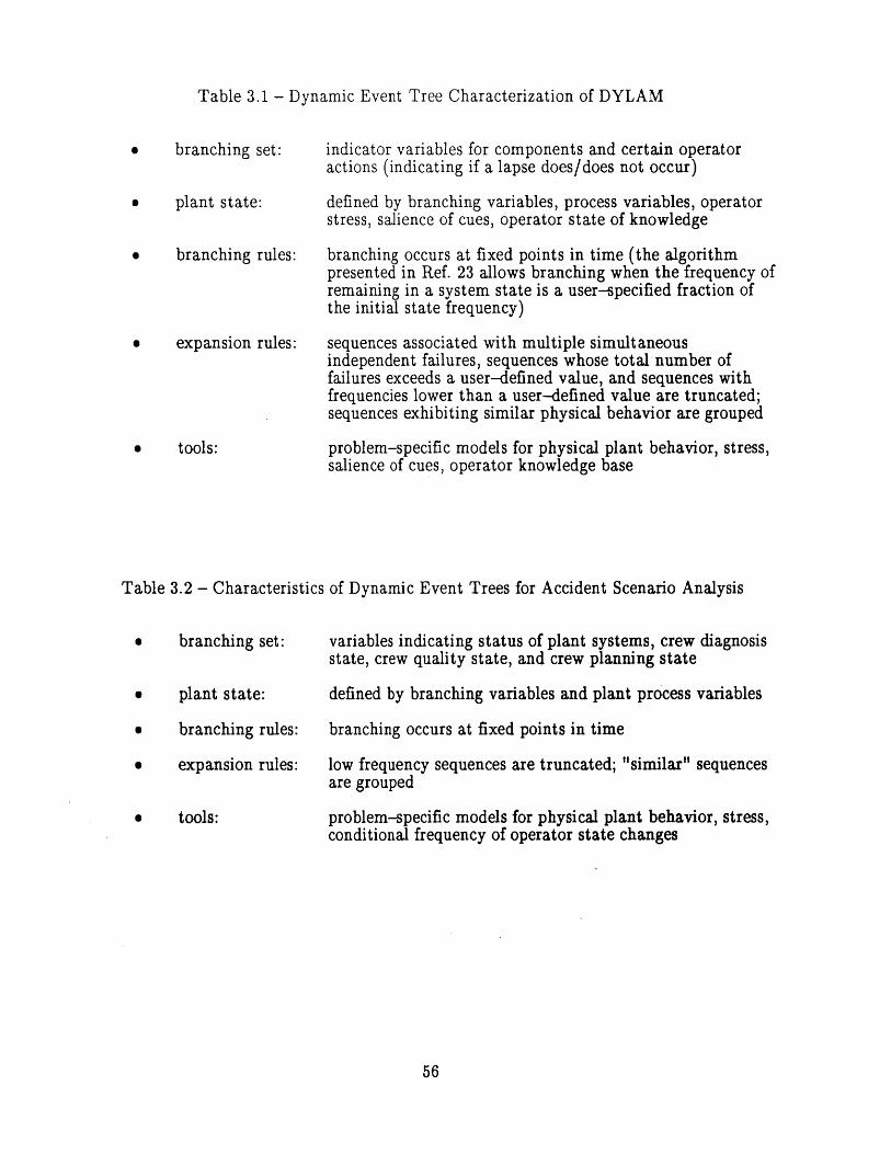
Table 3.1 - Dynamic Event Tree Characterization of DYLAM

* branching set:

* plant state:

* branching rules:

* expansion rules:

* tools:

indicator variables for components and certain operatoractions (indicating if a lapse does/does not occur)

defined by branching variables, process variables, operatorstress, salience of cues, operator state of knowledge

branching occurs at fixed points in time (the algorithmpresented in Ref. 23 allows branching when the frequency ofremaining in a system state is a user-specified fraction ofthe initial state frequency)

sequences associated with multiple simultaneousindependent failures, sequences whose total number offailures exceeds a user-defined value, and sequences withfrequencies lower than a user-defined value are truncated;sequences exhibiting similar physical behavior are grouped

problem-specific models for physical plant behavior, stress,salience of cues, operator knowledge base

Table 3.2 - Characteristics of Dynamic Event Trees for Accident Scenario Analysis

* branching set:

e plant state:

e branching rules:

* expansion rules:

* tools:

variables indicating status of plant systems, crew diagnosisstate, crew quality state, and crew planning state

defined by branching variables and plant process variables

branching occurs at fixed points in time

low frequency sequences are truncated; "similar" sequencesare grouped

problem-specific models for physical plant behavior, stress,conditional frequency of operator state changes

56

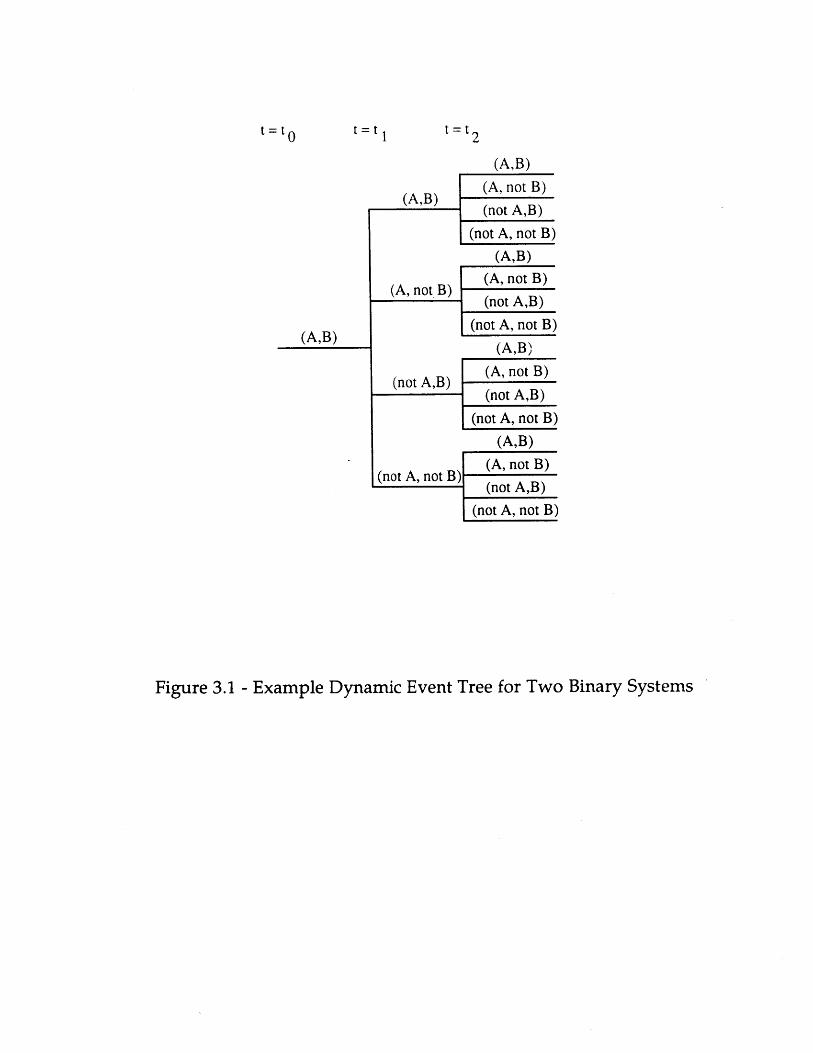
t t 0 t tI t= t 2

(A,B)

(o A, not B)(A,nB) (not A,B)

(not A, not B)

(A, B)

(A, not. B) -(Anot AB)

(not A, ntB)_

(A,B) (o ,ntB

(A,B)J

(not A,B) (A, not B)

(not A,B)

(not A, not B)

(A, B)_

(no AnotB) (A, not B)(no AnotB) (not A,B)_

(not A, not B)

Figure 3.1 - Example Dynamic Event Tree for Two Binary Systems

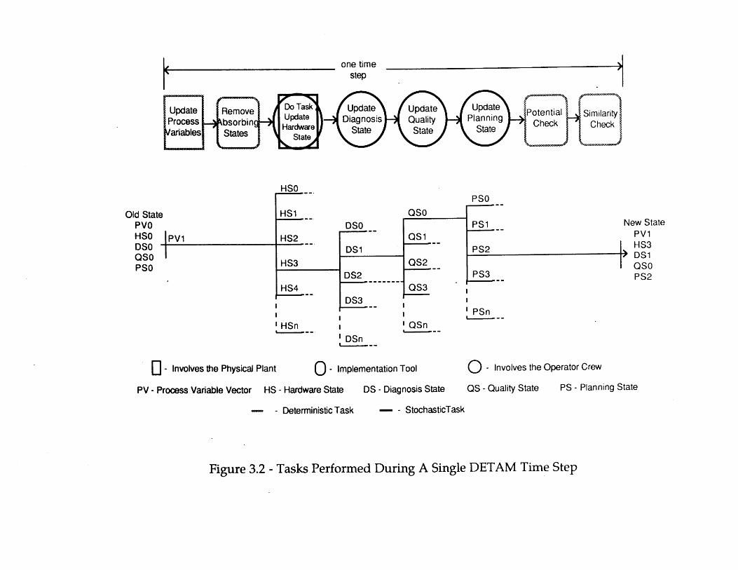
one timestepI'

Old StatePVOHSODSOQSOPSO

HSO

HS1

HS2

HS3

HS4

HSn

U - Involves the Physical Plant

DSO

DS1

DS2

DS3

DSn

080

QS1

QS3

QSn

0 - Implementation Tool

PSO

PS1 -

PS2

O - Involves the Operator Crew

PV - Process Variable Vector HS - Hardware State

- - Deterministic Task

DS - Diagnosis State

- - StochasticTask

QS - Quality State PS - Planning State

Figure 3.2 - Tasks Performed During A Single DETAM Time Step

'I

New StatePV1HS3DS1QS0PS2

|PV1

PSn

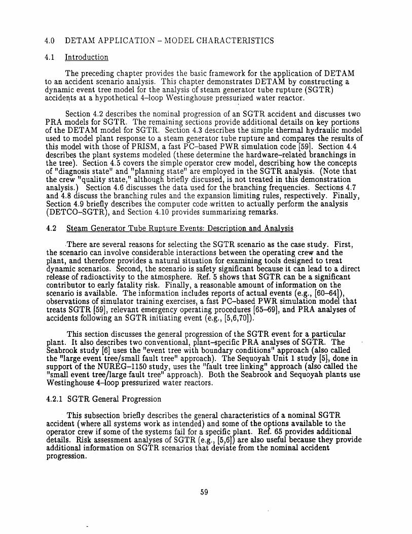
4.0 DETAM APPLICATION - MODEL CHARACTERISTICS

4.1 Introduction

The preceding chapter provides the basic framework for the application of DETAMto an accident scenario analysis. This chapter demonstrates DETAM by constructing adynamic event tree model for the analysis of steam generator tube rupture (SGTR)accidents at a hypothetical 4-loop Westinghouse pressurized water reactor.

Section 4.2 describes the nominal progression of an SGTR accident and discusses twoPRA models for SGTR. The remaining sections provide additional details on key portionsof the DETAM model for SGTR. Section 4.3 describes the simple thermal hydraulic modelused to model plant response to a steam generator tube rupture and compares the results ofthis model with those of PRISM, a fast PC-based PWR simulation code [59]. Section 4.4describes the plant systems modeled (these determine the hardware-related branchings inthe tree). Section 4.5 covers the simple operator crew model, describing how the conceptsof "diagnosis state" and "planning state" are employed in the SGTR analysis. (Note thatthe crew "quality state," although briefly discussed, is not treated in this demonstrationanalysis.) Section 4.6 discusses the data used for the branching frequencies. Sections 4.7and 4.8 discuss the branching rules and the expansion limiting rules, respectively. Finally,Section 4.9 briefly describes the computer code written to actually perform the analysis(DETCO-SGTR), and Section 4.10 provides summarizing remarks.

4.2 Steam Generator Tube Rupture Events: Description and Analysis

There are several reasons for selecting the SGTR scenario as the case study. First,the scenario can involve considerable interactions between the operating crew and theplant, and therefore provides a natural situation for examining tools designed to treatdynamic scenarios. Second, the scenario is safety significant because it can lead to a directrelease of radioactivity to the atmosphere. Ref. 5 shows that SGTR can be a significantcontributor to early fatality risk. Finally, a reasonable amount of information on thescenario is available. The information includes reports of actual events (e.g., [60-64]),observations of simulator training exercises, a fast PC-based PWR simulation model thattreats SGTR [59], relevant emergency operating procedures [65-69], and PRA analyses ofaccidents following an SGTR initiating event (e.g., [5,6,70]).

This section discusses the general progression of the SGTR event for a particularplant. It also describes two conventional, plant-specific PRA analyses of SGTR. TheSeabrook study [6] uses the "event tree with boundary conditions" approach (also calledthe "large event tree/small fault tree" approach). The Sequoyah Unit 1 study [5}, done insupport of the NUREG-1150 study, uses the "fault tree linking" approach (also called the"small event tree/large fault tree" approach). Both the Seabrook and Sequoyah plants useWestinghouse 4-loop pressurized water reactors.

4.2.1 SGTR General Progression

This subsection briefly describes the general characteristics of a nominal SGTRaccident (where all systems work as intended) and some of the options available to theoperator crew if some of the systems fail for a specific plant. Ref. 65 provides additionaldetails. Risk assessment analyses of SGTR (e.g., [5,6]) are also useful because they provideadditional information on SGTR scenarios that deviate from the nominal accidentprogression.

59

A steam generator tube rupture accident breaks the barrier between the reactorcoolant and the secondary side of the steam generator. The difference in pressure betweenthe primary system and the steam generators causes the reactor coolant to flow from theprimary into the secondary side of the faulted steam generator. As a result of this loss ofprimary coolant, the pressurizer pressure and pressurizer level drop (the rate of decreasedepends on the size and the number of ruptures). The decrease in primary pressure willeventually result in a reactor trip.

The leakage of the contaminated primary coolant increases the activity of thesecondary side, causing radiation monitors to actuate. The leakage also increases the leveland pressure of the faulted steam generator; the rate of increase depends on the size of therupture. Moreover, the leakage leads to a reduction in feedwater flow, in order tocompensate for the high steam generator level in the faulted steam generator.

The reactor trip causes the core power to rapidly decrease to decay heat levels, thesteam flow to the turbine to terminate, and the steam dump (i.e., the turbine bypass)system to actuate. Soon afterwards, the continued decrease in primary pressure leads toactuation of the safety injection (SI) signal. The SI signal causes the isolation of the mainfeedwater system (MFWS) and initiates the high pressure injection system (HPIS) and theemergency feedwater system (EFWS).

Following the reactor trip, the operator crew's concerns are to: a) establish asecondary heat sink, b) identify and isolate the faulted steam generator, c) cooldown anddepressurize the primary system, and d) provide for long term cooling. Refs. 65-69describe the specific tasks that must be accomplished to address these concerns. It shouldbe noted that this study assumes that there is an additional system available to help theoperators: the Safety Parameter Display System (SPDS). As the operator crew performsits tasks, it should monitor the states of the critical safety functions through the SPDScolor-coded status trees (more details on the SPDS are provided in Section 4.4). Thecolor-coded status trees serve as a backup system to help the crew diagnose the plantcondition and subsequently lead the crew to the appropriate procedure. The trees areparticularly useful if the crew misdiagnoses the event or if the procedure being followed isinsufficient to handle the event (e.g., during multiple-failure situations).

The emergency feedwater system (EFWS) provides the cooling water to the steamgenerators for heat removal from the primary system under nominal accident conditions. Ifthe EFWS fails, the operators can provide water to the steam generators through thecondensate system; however, this requires depressurization of at least one intact steamgenerator. If water cannot be provided to the steam generators (so that the steamgenerators are not available), "bleed and feed" cooling can be performed. Bleed and feedcooling involves the letdown of primary coolant through the pressurizer power-operatedrelief valve (PORV), and the injection of water into the reactor coolant system using theHPIS. Failure to establish a heat sink through one of these mechanisms will result in coredamage.

The identification and isolation of the faulted steam generator is essential to controlthe release of radioactive coolant outside of the containment building. The faulted steamgenerator can be identified by an unexpected rise in the steam generator level (specifically,a rise in the narrow range level), high radiation measurements for the steam line, or highradiation measurements from steam generator samples. Once identified, isolation of thefaulted steam generator requires closing of the steam generator relief valves, blowdownisolation valves, upstream drain valves, and main steamline isolation and bypass valves.

60

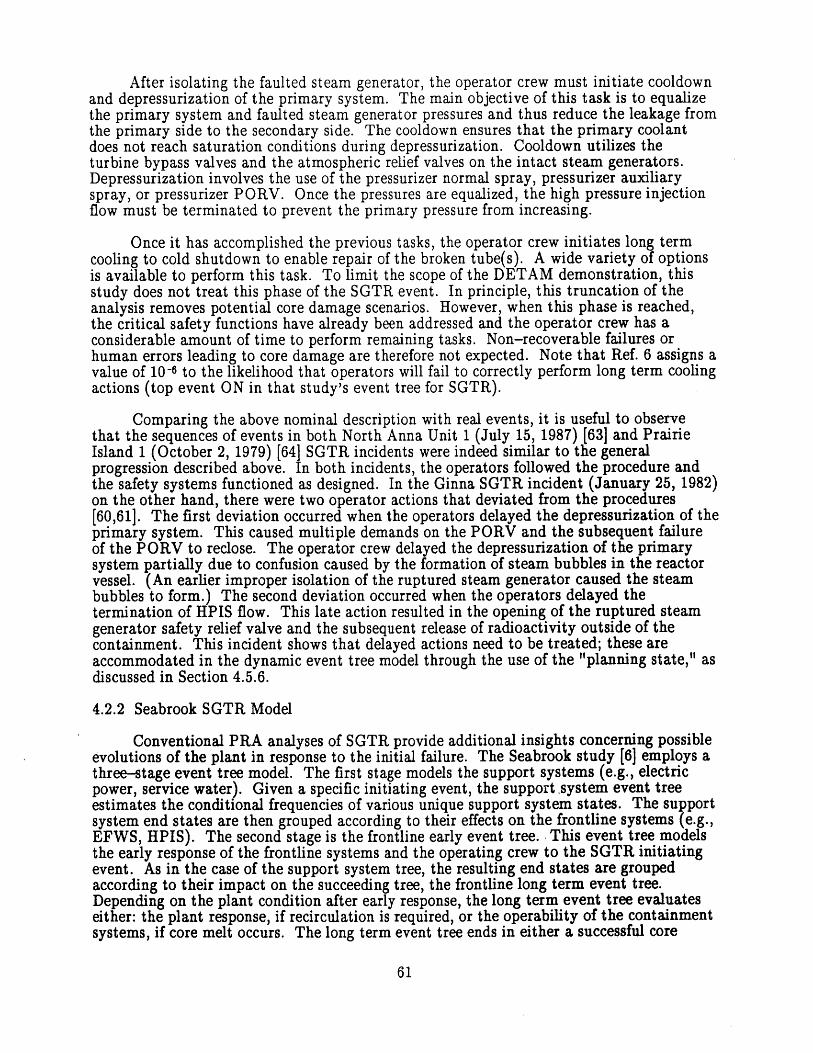
After isolating the faulted steam generator, the operator crew must initiate cooldownand depressurization of the primary system. The main objective of this task is to equalizethe primary system and faulted steam generator pressures and thus reduce the leakage fromthe primary side to the secondary side. The cooldown ensures that the primary coolantdoes not reach saturation conditions during depressurization. Cooldown utilizes theturbine bypass valves and the atmospheric relief valves on the intact steam generators.Depressurization involves the use of the pressurizer normal spray, pressurizer auxiliaryspray, or pressurizer PORV. Once the pressures are equalized, the high pressure injectionflow must be terminated to prevent the primary pressure from increasing.

Once it has accomplished the previous tasks, the operator crew initiates long termcooling to cold shutdown to enable repair of the broken tube(s). A wide variety of optionsis available to perform this task. To limit the scope of the DETAM demonstration, thisstudy does not treat this phase of the SGTR event. In principle, this truncation of theanalysis removes potential core damage scenarios. However, when this phase is reached,the critical safety functions have already been addressed and the operator crew has aconsiderable amount of time to perform remaining tasks. Non-recoverable failures orhuman errors leading to core damage are therefore not expected. Note that Ref. 6 assigns avalue of 10-6 to the likelihood that operators will fail to correctly perform long term coolingactions (top event ON in that study's event tree for SGTR).

Comparing the above nominal description with real events, it is useful to observethat the sequences of events in both North Anna Unit 1 (July 15, 1987) [63] and PrairieIsland 1 (October 2, 1979) [64] SGTR incidents were indeed similar to the generalprogression described above. In both incidents, the operators followed the procedure andthe safety systems functioned as designed. In the Ginna SGTR incident (January 25, 1982)on the other hand, there were two operator actions that deviated from the procedures[60,61]. The first deviation occurred when the operators delayed the depressurization of theprimary system. This caused multiple demands on the PORV and the subsequent failureof the PORV to reclose. The operator crew delayed the depressurization of the primarysystem partially due to confusion caused by the formation of steam bubbles in the reactorvessel. (An earlier improper isolation of the ruptured steam generator caused the steambubbles to form.) The second deviation occurred when the operators delayed thetermination of HPIS flow. This late action resulted in the opening of the ruptured steamgenerator safety relief valve and the subsequent release of radioactivity outside of thecontainment. This incident shows that delayed actions need to be treated; these areaccommodated in the dynamic event tree model through the use of the "planning state," asdiscussed in Section 4.5.6.

4.2.2 Seabrook SGTR Model

Conventional PRA analyses of SGTR provide additional insights concerning possibleevolutions of the plant in response to the initial failure. The Seabrook study [6] employs athree-stage event tree model. The first stage models the support systems (e.g., electricpower, service water). Given a specific initiating event, the support system event treeestimates the conditional frequencies of various unique support system states. The supportsystem end states are then grouped according to their effects on the frontline systems (e.g.,EFWS, HPIS). The second stage is the frontline early event tree. This event tree modelsthe early response of the frontline systems and the operating crew to the SGTR initiatingevent. As in the case of the support system tree, the resulting end states are groupedaccording to their impact on the succeeding tree, the frontline long term event tree.Depending on the plant condition after early response, the long term event tree evaluateseither: the plant response, if recirculation is required, or the operability of the containmentsystems, if core melt occurs. The long term event tree ends in either a successful core

61

cooling state or a specific plant damage state that serves as input to the subsequent coreand containment response analysis.

The support system and the frontline long term event trees are generally applicableto all initiating events (although the conditional branching frequencies/split fractions maydiffer). On the other hand, each initiating event has a unique frontline early event tree. Inthe case of an SGTR event, the frontline early event tree has 16 top events (see Table 4.1).Figure 4.1 shows portions of the Seabrook SGTR early event tree leading up to thecooldown and depressurization of the primary system. Dashed lines indicate portions of thetree not considered in this comparlzun (the corresponding top events are assumedsuccessful). Some of the top events in Figure 4.1 are purely hardware-related; othersinvolve operating crew response. For example top events TT1 (Turbine Trip) and RV(Reactor Vessel Intact) are essentially hardware top events. Top event OR (OperatorControls Break Flow), on the other hand, involves both hardware and operator responses.If all systems respond as designed, OR entails the opening of the intact generators'atmospheric relief valves to cool down the primary coolant, closing of relief valves when theprimary temperature reaches the desired level, and pressurizer spray actuation todepressurize the primary system to the ruptured steam generator pressure. Otherwise, ORinvolves bleed and feed cooling.

It is interesting to note that the Seabrook model incorporates scenario dynamics to alimited extent. For example, order-dependence issues arise in the analysis of top event SL(No Secondary Leak to the Atmosphere). This top event is used to model a number ofevents that: a) are sequentially interrelated, and b) can lead to a variety of failure scenariosif failed. A special event tree (see Figure 4.2) is constructed to determine the SL splitfraction. This tree, which has 11 specific top events, covers the potential of an early leakdue to failure to isolate the ruptured steam generator and a late leak due to operator failureto control the break flow. Thus, top event OR, which comes before SL in the SGTR tree,also appears in the SL tree; however, OR is used as a boundary condition (it only takeseither a successful or an unsuccessful state). Recall from Section 4.2.1 that, nominally, theruptured steam generator is supposed to be isolated before actions to control the break floware performed.

By careful definition and ordering of the top events, the Seabrook SGTR tree alsoreflects, to some extent, the timing of events. For example, top event OR represents thecooldown and depressurization process up until the point where primary and rupturedsteam generator pressures equalize. Top event OD, on the other hand, takes thedepressurization up to the point when long term cooling measures can be initiated.

The two dominant sequences in Figure 4.1 are: a) the sequence involving the failureof both OD (operator depressurizes the reactor coolant system and provides makeup) andEF (emergency feedwater actuation), and b) the sequence involving the failure of NL (noreactor coolant pump seal LOCA). These correspond to Sequences 14 and 12, respectively,in Figure 4.1. Note that Sequence 14 involves the failure of the emergency feedwatersystem and of bleed and feed cooling.

4.2.3 Sequoyah SGTR Model

The Sequoy ah study [6] is a demonstration of the Accident Sequence EvaluationProgram (ASEP). The intent is to use less resources for analysis (as compared withstandard Level 1 risk studies), yet produce results that closely approximate standardLevel 1 results. Thus, simple models are used for parts of the analysis not judged to have asignificant impact on risk.

62

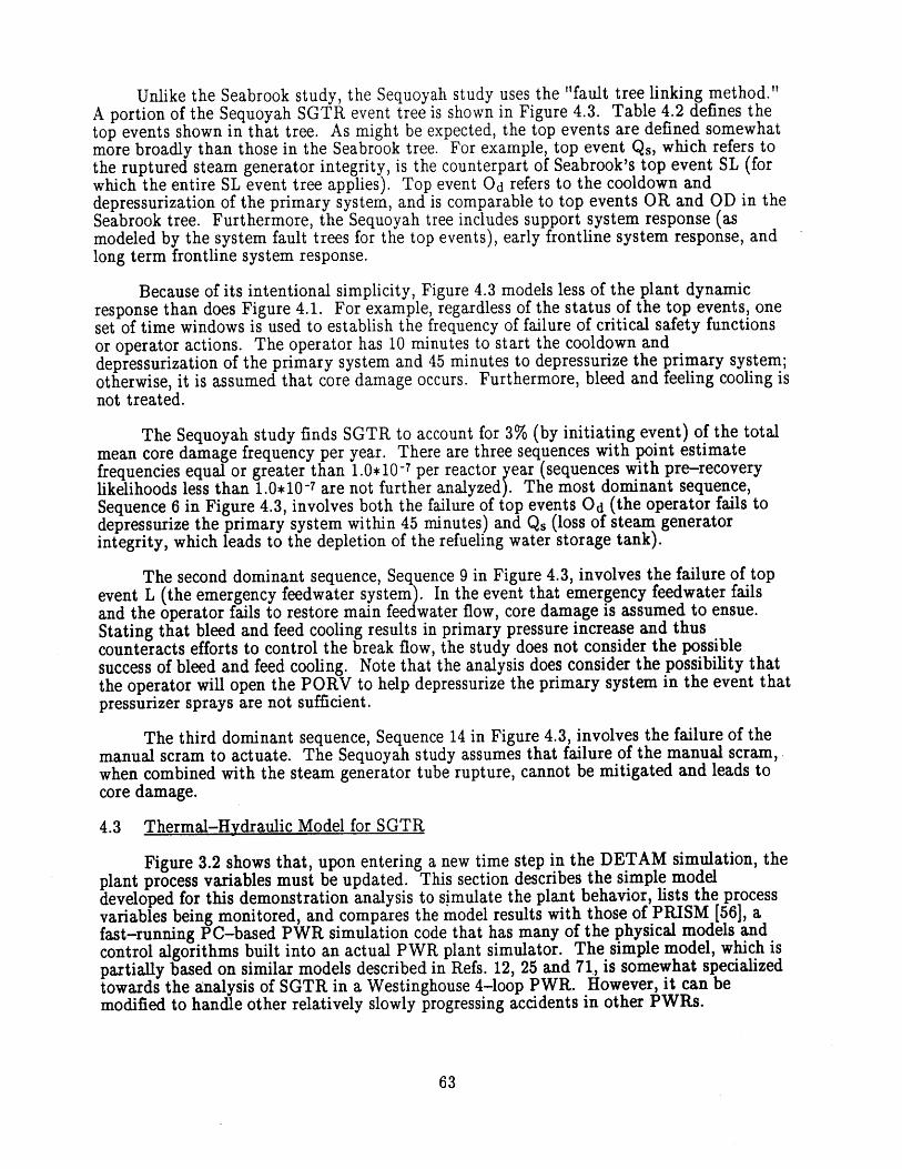
Unlike the Seabrook study, the Sequoyah study uses the "fault tree linking method."A portion of the Sequoyah SGTR event tree is shown in Figure 4.3. Table 4.2 defines thetop events shown in that tree. As might be expected, the top events are defined somewhatmore broadly than those in the Seabrook tree. For example, top event Q, which refers tothe ruptured steam generator integrity, is the counterpart of Seabrook's top event SL (forwhich the entire SL event tree applies). Top event Od refers to the cooldown anddepressurization of the primary system, and is comparable to top events OR and OD in theSeabrook tree. Furthermore, the Sequoyah tree includes support system response (asmodeled by the system fault trees for the top events), early frontline system response, andlong term frontline system response.

Because of its intentional simplicity, Figure 4.3 models less of the plant dynamicresponse than does Figure 4.1. For example, regardless of the status of the top events, oneset of time windows is used to establish the frequency of failure of critical safety functionsor operator actions. The operator has 10 minutes to start the cooldown anddepressurization of the primary system and 45 minutes to depressurize the primary system;otherwise, it is assumed that core damage occurs. Furthermore, bleed and feeling cooling isnot treated.

The Sequoyah study finds SGTR to account for 3% (by initiating event) of the totalmean core damage frequency per year. There are three sequences with point estimatefrequencies equal or greater than 1.0*10-7 per reactor year (sequences with pre-recoverylikelihoods less than 1.0*10-7 are not further analyzed). The most dominant sequence,Sequence 6 in Figure 4.3, involves both the failure of top events Od (the operator fails todepressurize the primary system within 45 minutes) and Qs (loss of steam generatorintegrity, which leads to the depletion of the refueling water storage tank).

The second dominant sequence, Sequence 9 in Figure 4.3, involves the failure of topevent L (the emergency feedwater system). In the event that emergency feedwater failsand the operator fails to restore main feedwater flow, core damage is assumed to ensue.Stating that bleed and feed cooling results in primary pressure increase and thuscounteracts efforts to control the break flow, the study does not consider the possiblesuccess of bleed and feed cooling. Note that the analysis does consider the possibility thatthe operator will open the PORV to help depressurize the primary system in the event thatpressurizer sprays are not sufficient.

The third dominant sequence, Sequence 14 in Figure 4.3, involves the failure of themanual scram to actuate. The Sequoyah study assumes that failure of the manual scram,when combined with the steam generator tube rupture, cannot be mitigated and leads tocore damage.

4.3 Thermal-Hydraulic Model for SGTR

Figure 3.2 shows that, upon entering a new time step in the DETAM simulation, theplant process variables must be updated. This section describes the simple modeldeveloped for this demonstration analysis to simulate the plant behavior, lists the processvariables being monitored, and compares the model results with those of PRISM [56], afast-running PC-based PWR simulation code that has many of the physical models andcontrol algorithms built into an actual PWR plant simulator. The simple model, which ispartially based on similar models described in Refs. 12, 25 and 71, is somewhat specializedtowards the analysis of SGTR in a Westinghouse 4-loop PWR. However, it can bemodified to handle other relatively slowly progressing accidents in other PWRs.

63

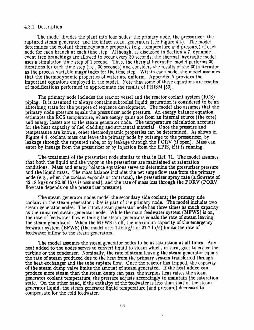
4.3.1 Description

The model divides the plant into four nodes: the primary node, the pressurizer, theruptured steam generator, and the intact steam generators (see Figure 4.4). The modeldetermines the coolant thermodynamic properties (e.g., temperature and pressure) of eachnode for each branch at each time step. Although, as discussed in Section 4.7, dynamicevent tree branchings are allowed to occur every 30 seconds, the thermal-hydraulic modeluses a simulation time step of 1 second. Thus, the thermal hydraulic-model performs 30iterations for each time step (i.e., 30 seconds) and considers the results of the 30th iterationas the process variable magnitudes for the time step. Within each node, the model assumesthat the thermodynamic properties of water are uniform. Appendix A provides theimportant equations employed in the model. Note that some of these equations are resultsof modifications performed to approximate the results of PRISM [59].

The primary node includes the reactor vessel and the reactor coolant system (RCS)piping. It is assumed to always contains subcooled liquid; saturation is considered to be anabsorbing state for the purpose of sequence development. The model also assumes that theprimary node pressure equals the pressurizer node pressure. An energy balance equationestimates the RCS temperature, where energy gains are from an internal source (the core)and energy losses are to the steam generator node. The temperature calculation accountsfor the heat capacity of fuel cladding and structural material. Once the pressure andtemperature are known, other thermodynamic properties can be determined. As shown inFigure 4.4, coolant mass can leave the primary node by outsurge to the pressurizer, byleakage through the ruptured tube, or by leakage through the PORV (if open). Mass canenter by insurge from the pressurizer or by injection from the HPIS, if it is running.

The treatment of the pressurizer node similar to that in Ref. 71. The model assumesthat both the liquid and the vapor in the pressurizer are maintained at saturationconditions. Mass and energy balance equations serve to determine the pressurizer pressureand the liquid mass. The mass balance includes the net surge flow rate from the primarynode (e.g., when the coolant expands or contracts), the pressurizer spray rate (a flowrate of42.18 kg/s or 92.80 lb/s is assumed), and the rate of mass loss through the PORV (PORVflowrate depends on the pressurizer pressure).

The steam generator nodes model the secondary side coolant; the primary sidecoolant in the steam generator tubes is part of the primary node. The model includes twosteam generator nodes. The intact steam generator node has three times as much capacityas the ruptured steam generator node. While the main feedwater system (MFWS) is on,the rate of feedwater flow entering the steam generators equals the rate of steam leavingthe steam generators. When the MFWS is off, the maximum capacity of the emergencyfeewater system (EFWS) (the model uses 12.6 kg/s or 27.7 lb/s) limits the rate offeedwater inflow to the steam generators.

The model assumes the steam generator nodes to be at saturation at all times. Anyheat added to the nodes serves to convert liquid to steam which, in turn, goes to either theturbine or the condenser. Nominally, the rate of steam leaving the steam generator equalsthe rate of steam produced due to the heat from the primary system transferred throughthe heat exchanger and the tube rupture flow. Once the reactor has tripped, the capacityof the steam dump valve limits the amount of steam generated. If the heat added canproduce more steam than the steam dump can pass, the surplus heat raises the steamgenerator coolant temperature; the pressure adjusts accordingly to maintain the saturationstate. On the other hand, if the enthalpy of the feedwater is less than that of the steamgenerator liquid, the steam generator liquid temperature (and pressure) decreases tocompensate for the cold feedwater.

64

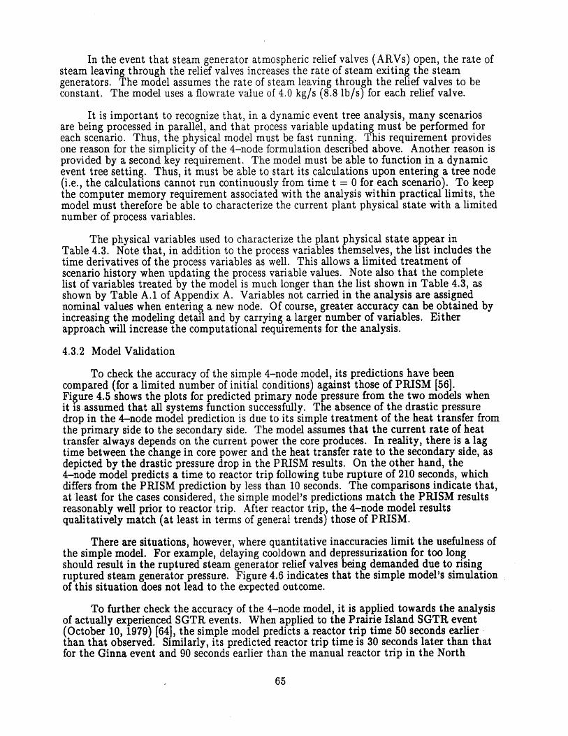
In the event that steam generator atmospheric relief valves (ARVs) open, the rate ofsteam leaving through the relief valves increases the rate of steam exiting the steamgenerators. The model assumes the rate of steam leaving through the relief valves to beconstant. The model uses a flowrate value of 4.0 kg/s (8.8 lb/s) for each relief valve.

It is important to recognize that, in a dynamic event tree analysis, many scenariosare being processed in parallel, and that process variable updating must be performed foreach scenario. Thus, the physical model must be fast running. This requirement providesone reason for the simplicity of the 4-node formulation described above. Another reason isprovided by a second key requirement. The model must be able to function in a dynamicevent tree setting. Thus, it must be able to start its calculations upon entering a tree node(i.e., the calculations cannot run continuously from time t = 0 for each scenario). To keepthe computer memory requirement associated with the analysis within practical limits, themodel must therefore be able to characterize the current plant physical state with a limitednumber of process variables.

The physical variables used to characterize the plant physical state appear inTable 4.3. Note that, in addition to the process variables themselves, the list includes thetime derivatives of the process variables as well. This allows a limited treatment ofscenario history when updating the process variable values. Note also that the completelist of variables treated by the model is much longer than the list shown in Table 4.3, asshown by Table A.1 of Appendix A. Variables not carried in the analysis are assignednominal values when entering a new node. Of course, greater accuracy can be obtained byincreasing the modeling detail and by carrying a larger number of variables. Eitherapproach will increase the computational requirements for the analysis.

4.3.2 Model Validation

To check the accuracy of the simple 4-node model, its predictions have beencompared (for a limited number of initial conditions) against those of PRISM [56].Figure 4.5 shows the plots for predicted primary node pressure from the two models whenit is assumed that all systems function successfully. The absence of the drastic pressuredrop in the 4-node model prediction is due to its simple treatment of the heat transfer fromthe primary side to the secondary side. The model assumes that the current rate of heattransfer always depends on the current power the core produces. In reality, there is a lagtime between the change in core power and the heat transfer rate to the secondary side, asdepicted by the drastic pressure drop in the PRISM results. On the other hand, the4-node model predicts a time to reactor trip following tube rupture of 210 seconds, whichdiffers from the PRISM prediction by less than 10 seconds. The comparisons indicate that,at least for the cases considered, the simple model's predictions match the PRISM resultsreasonably well prior to reactor trip. After reactor trip, the 4-node model resultsqualitatively match (at least in terms of general trends) those of PRISM.

There are situations, however, where quantitative inaccuracies limit the usefulness ofthe simple model. For example, delaying cooldown and depressurization for too longshould result in the ruptured steam generator relief valves being demanded due to risingruptured steam generator pressure. Figure 4.6 indicates that the simple model's simulationof this situation does not lead to the expected outcome.

To further check the accuracy of the 4-node model, it is applied towards the analysisof actually experienced SGTR events. When applied to the Prairie Island SGTR event(October 10, 1979) [64], the simple model predicts a reactor trip time 50 seconds earlier-than that observed. Similarly, its predicted reactor trip time is 30 seconds later than thatfor the Ginna event and 90 seconds earlier than the manual reactor trip in the North

65

Anna 1 SGTR event. The late reactor trip in the North Anna 1 event was partially due toa turbine load reduction performed by the operator crew. The predicted reactor trip timeis also 22 seconds earlier than that given in Ref. 65 for a double ended tube rupture event.

In general, the simple 4-node model appears to be adequate for predicting theprimary side response to SGTR in the early stages of the accident. Once saturation isreached, the model is no longer satisfactory. The model is also not very good at predictingthe secondary side response, due to its use of a homogeneous steam generator sub-model.As a result, the steam generator pressure rise and resulting challenges to the atmosphericrelief valves (which could stick open, leading to a potential containment bypass scenario)are underestimated. As further discussed in Section 4.8, these weaknesses prevent the fullsimulation of accident scenarios leading to core damage, and clearly limit the immediateusefulness of this study's results in managing risk. However, for the purpose ofdemonstrating DETAM, the simple model is sufficiently accurate.

4.4. Hardware Model

The explicit treatment of the time dimension in a dynamic event tree analysis canrequire the processing of much larger amounts of information than treated in a staticanalysis of comparable detail. Given that conventional PRA models are already quite largeand that computing resources are finite, a practical dynamic analysis must sacrifice somelevel of detail in the hardware, process physics, and operating crew models. In thisanalysis, the following hardware-related assumptions are made to limit the amount ofinformation to be processed.

First, the hardware states in the model are defined by the status of a limited numberof frontline systems. Support systems are not treated, nor are individual trains orcomponents within the frontline systems. Event tree branches can be generated for onlythose hardware systems (or groups of systems) which can significantly affect the behaviorof the plant during the early part of the steam generator tube rupture event (starting fromthe initiation of the steam generator tube rupture and culminating when cooldown anddepressurization of the primary system commences). These include the emergencyfeedwater system (EFWS), the high pressure injection system (HPIS), the safety injectionsignal (S-signal or SI), the start-up feed pump (SUFP), the pressurizer power-operatedrelief valves (PORV), the 40% steam dump valves that bypass the turbine and condensatesystem (SDV), and the atmospheric relief valves on the ruptured and intact steamgenerators (ARV1 and ARV2).

The EFWS provides water to the steam generators during abnormal conditions. SIactuation initiates the EFWS (it also turns off the main feedwater system). The SUFPserves as a backup to the EFWS. In the event of EFWS failure, bleed and feed cooling,using the HPIS and PORV, is a possible way of restoring the secondary heat sink. TheHPIS is assumed to include both centrifugal charging pumps and safety injection pumps.The PORV can depressurize the primary system in case the pressurizer spray fails. TheARVs and SDV are used to cool down the primary system prior to depressurization. TheARVs are assumed to include the 10% atmospheric dump valves and the safety reliefvalves. These systems are listed in Table 4.4.

The effect on scenario development of systems not on this list (e.g., reactor trip andturbine trip) are also modeled. However, these systems are assumed to function asdesigned (i.e., their indicator variables are not included in the branching set). Othersystems treated in this manner include the main feedwater system (MFWS), thepressurizer spray (SPRY), and the radiation alarm monitor (RAM). The Safety ParameterDisplay System (SPDS) is also one of the systems assumed to work correctly for the

66

duration of the accident. An example SPDS is described in Ref. 72. Through color-codedstatus trees, the SPDS informs the operator crew of the current status of the critical safetyfunctions. There are four possible color indicators which help the crew recognize abnormalconditions and take appropriate measures. A "red" color indicates that the critical safetyfunction is in danger and that immediate operator action is necessary. This will require theoperator crew to go to the specific procedures designed to restore the safety function. An"orange" color indicates that the safety function is severely challenged and promptoperator action is necessary. A "yellow" color means that the safety function is not fullysatisfied and operator action may be required eventually. A "green" color requires nooperator action. Figure 4.7 shows a sample logic tree for the secondary heat sink criticalsafety function. A red indicator for the heat sink occurs if the EFWS fails.

A second hardware-related modeling assumption is that only failures on demandrequire treatment. The demand can be due to an operator action or to an automatic signalsent when a process variable reaches a setpoint. Failures during operation are generally oflower likelihood and are neglected; equipment unavailability due to testing or maintenancecan be treated as an initial condition for the analysis, and need not be simulateddynamically. As mentioned in Section 3.3, operator errors in executing planned actions areincluded in the hardware state branching frequencies. For example, if the crew is supposedto close the ruptured steam generator relief valve ARV1, the likelihood of proceeding alongthe ARV1 failure branch (at the hardware branching step shown in Figure 3.2) includes thefrequency that the crew errs in closing the valve and the hardware failure rate for ARV1,which is independent of crew performance.

It is useful to observe that hardware-related branchings need not be binary. Thestatus of a system depends on its functional state (e.g., on, off, closed, open) as well as itsoperational state (e.g., good, failed). One feature of the DETCO-SGTR code (described inSection 4.9) is that two types of system failures are distinguised: minor failures and majorfailures. Minor failures are those that are recoverable; major failures are unrecoverable forthe duration of the accident. A minimum repair time for each system is defined by theanalyst. If the time since the discovery of the minor failure is greater than the requiredrepair time of a particular system, that system is assumed repaired; else, the systemremains failed. The minimum repair time and the likelihood of minor failure given systemfailure for each system are user input.

In the following analysis of SGTR, the full capabilities of DETCO-SGTR are notexercised. It is assumed that: a) hardware failures are not recoverable, andb) instrumentation failures do not occur. These assumptions do not result from structurallimitations in the code or in the dynamic event tree methodology; they are simplyemployed to limit the scope of the analysis.

4.5 Operator Crew Model

This section describes the operator crew model incorporated in the SGTR applicationof DETAM. The implementation of the three crew substates mentioned in Chapter 3, i.e.,crew diagnosis state, crew quality state and crew planning state, is discussed. This sectionalso briefly discusses the operator crew's actual implementation of the tasks planned.

4.5.1 Basic Formulation

As discussed in Section 1.3, much of the motivation for the dynamic event treeapproach is provided by three considerations: a) plant operators and plant components areinteracting parts of an overall system that responds dynamically to upset conditions, b) the

67

actions of operators are dependent on their beliefs as to the current state of the plant, andc) the operators have memory; their beliefs at any given point in time are influenced (tosome degree) by the past sequence of events and by their earlier trains of thought. The3-substate model for the operating crew employed in this study is designed to carry theinformation needed to deal with these issues in a dynamic event tree format.

The 3-substate model builds on work performed by other investigators interested inhuman behavior during nuclear power plant accidents.

Ref. 73 points out that, in the course of a scenario, the operator crew performs fourfundamental activities: monitoring, explanation building, action planning, and actionimplementation. Monitoring involves keeping track of the different indicators andinstrumentation. Explanation building refers to crew efforts to understand the ongoingscenario. Planning refers to the crew's building of a strategy or set of actions in responseto the situation. Implementation entails the actual execution of planned tasks or strategy.Note that the actual ordering of these tasks may vary (e.g., operators may start to planactions before they have completely explained the situation).

This representation of crew activities is quite similar to the operator action tree(OAT) notion, originally described in Ref. 74 and applied in a number of PRAs (e.g., [6]).A typical OAT (e.g. [75]) has three top events: diagnosis, action, and rediagnosis. Ref. 76uses an OAT with four top events; the time-dependent event trees in Ref. 53 can be viewedas extensions of the OAT idea. The tasks of monitoring, explanation formulation, andplanning are included in the diagnosis. top event in the OAT. The action implementationactivity, on the other hand, corresponds to the action top event in the OAT.

It can be seen that two of the tree substates used in the DETAM model for theoperating crew cover these concepts. For example, the diagnosis state models the results ofthe monitoring and the explanation building activities described in Ref. 73; the planningstate models the results of the planning activitiy. Of course, the repetitive application ofthese substates in a dynamic simulation render the rediagnosis top event in the OATunnecessary. The third substate, the crew quality state, models the influence of suchperformance shaping factors (PSFs) as stress. These PSFs are treated in conventionalhuman reliability analyses, as well. In a DETAM analysis, however, the dynamicdevelopment of these PSFs in response to the operator/plant interaction can be modeledexplicitly.

4.5.2 Crew Diagnosis State

The crew diagnosis state indicates the crew's understanding of the plant's past andcurrent conditions. As discussed in Ref. 54, this understanding can be represented at avariety of levels (e.g., plant level, system level). This analysis defines the diagnosis state interms of two components: the crew's understanding of the general scenario and the states offive safety functions.

4.5.2.1 General Scenario Component

The model assumes that the crew may diagnose that the plant is undergoing one offour possible general scenarios. These scenarios are: steady state, uncertain, SGTR andsmall loss of coolant accident (SLOCA). The crew thinks that the plant is at steady stateif it observes no change in the parameters being monitored. If the crew observes deviationsfrom the nominal levels of variables being monitored but is not definite on the specificscenario, the scenario diagnosis is uncertain. The SGTR diagnosis indicates that the crewis certain that the plant is experiencing a steam generator tube rupture. A SLOCA

68

diagnosis indicates that the crew is confident that a small loss of coolant accident is inprogress. The SLOCA is included because its indicators closely resemble those of SGTR[75]. In this way, this DETAM demonstration allows the crew to err in diagnosing thegeneral scenario.

Four indicators [secondary radiation alarm monitor (RAM), Reactor Cooling Systempressure, pressurizer level, and steam generator level] provide the basis for diagnosing thegeneral.scenario. Both SGTR and SLOCA lead to decreases in RCS pressure andpressurizer level. The conditions of the RAM and the steam generator (SG) leveldetermine if the accident is an SGTR or a SLOCA. If either the radiation alarm is on orthe SG level is increasing, the general scenario is an SGTR. On the other hand, if thealarm is off and the SG level is decreasing, the scenario is an SLOCA. Table 4.6 shows thepossible values of the scenario indicators. Each indicator may have three values (exceptRAM which has two). These values refer to the conditions of the parameters which theoperator crew monitors. The unobserved value accounts for situations in which the crewhas not yet observed the indicator (the minimum observation times are user input).Table 4.6 shows the nominal criteria that indicate how transitions from one scenario-leveldiagnosis to another can occur. This table is based on plant emergency operatingprocedures, backup documentation, and discussions with training instructors knowledgeableabout the SGTR scenario. Errors in diagnosis are discussed later in Section 4.7.

4.5.2.2 Safety Functions Component

The crew diagnosis state is further defined by the crew's understanding of the statusof five safety functions. These functions, which are also monitored by the SafetyParameter Display System, are: primary pressure control, primary inventory control,secondary heat sink, secondary pressure control, and secondary heat removal. Table 4.7indicates the different possible states, along with their respective transition criteria, ofthese safety functions. For example, the primary inventory control function has threepossible values. The first value is when the pressurizer and the RCS levels are normal orunobserved. The second value is when the pressurizer level is approaching the "solid"level. This value is a concern for the crew because a solid pressurizer reduces the crew'sability to regulate RCS pressure through the pressurizer. The third value is when the RCSlevel approaches the uncovery level. The secondary heat sink function also has threepossible states; the rest of the safety functions have four each.

Although the DETCO-SGTR code allows the safety function portion of the crewdiagnosis state to change stochastically, the demonstration model for SGTR described inthis chapter assumes that the operator crew correctly understands the status of thesefunctions. This assumption is consistent with the earlier assumption (see Section 4.4) thatnearly all instrumentation functions correctly, and limits the number of states to beconsidered. Note that with the general scenario and five safety functions describing thediagnosis state, 2304 diagnosis states are possible.

4.5.3 Crew Quality State

The crew quality state indicates the dynamic portion of the internal state of the crewthat affects its ability to plan and perform required tasks. It includes such factors as thecrew's group structure, emotional condition, and degree of coordination in executing themembers' respective assigned tasks. Thus, the crew quality state is intended toaccommodate performance shaping factors (e.g., stress) that are deemed important inexisting human reliability models [77-79].

69

Both the general structure of DETAM and the computer code implementationDETCO-SGTR allow the crew quality state to change stochastically. Thus, for example,the analysis is capable of treating the dynamic stress models proposed in Refs. 29 and 51.For the sake of simplicity, however, this demonstration does not exercise this capability.

4.5.4 Crew Planning State

The operator crew planning state refers to the set of actions that the crew plans toperform. In keeping with crew training and plant operating policies, the DETAMimplementation crew model treats crew planning as being procedure-oriented, that is, thecrew tends to follow the procedures as closely as possible. The model also accommodatesoperator actions which are not explicitly part of the actual procedure. These actions areincorporated into the procedures, i.e. they are treated like procedure steps.

4.5.4.1 Procedure-Based Planning

In the case of procedure following, the crew planning state at any point in time canbe described in terms of two substates: the procedure substate, which indicates whichemergency procedure is to be followed, and the step substate, indicating the specific step inthe selected procedure to be performed. (Recall that, as shown in Figure 3.2, the actualexecution of planned actions affecting equipment is simulated in the next time step whenthe likelihoods of the new hardware states are determined.)

The procedure substate can be any of the four emergency operating procedures,namely: Reactor Trip or Safety Injection (E-O) [66], Loss of Secondary Heat Sink(FR-H.1) [69], Loss of Reactor or Secondary Coolant (E-1) [67], and Steam GeneratorTube Rupture (E-3) [68]. E-0 covers the verification of safety functions and determinesthe appropriate event-specific procedure to use. FR-H.1 handles the restoration of thesecondary heat sink in case it fails or is unavailable. The secondary heat sink is necessaryfor all abnormal scenarios. E-1 handles the small loss of coolant accident and other eventsinvolving loss of coolant. E-3 mitigates the steam generator tube rupture event. Thesefour. emergency operating procedures are modeled because they are the likely proceduresthat the crew will use for the portion of SGTR event being considered. Becauseinformation on the appropriate procedures for crew response to warnings from the criticalsafety function status trees was not obtained in this study, this demonstration of DETAMtreats the occurrence of a "red" or "orange" branch as a boundary condition, terminatingthe development of the associated scenario.

The step substate refers to the specific step of an emergency procedure that theoperators are planning to execute. Tables 4.8-4.11 show the procedure steps modeled, theassumptions taken, and the time allocated to perform each step. There are 37 E-0 steps,16 FR-H.1 steps, 13 E-1 steps, and 18 E-3 steps modeled. An actual exercise simulatingthe SGTR event (at a PWR training simulator) served as a basis in assigning stepcompletion time. The times allotted for steps not performed during the simulation areassessed judgmentally. The model assumes that the successful performance of tasks insteps which involve systems not explicitly modeled and allocates times to perform theassociated operator actions. For example, since the model does not include the systemneeded to verify containment isolation (E-4 Step 6 in Table 4.8), the model assumes thatcontainment isolation status is normal (this is a reasonable assumption for the SGTR case)and allots 15 seconds for the crew to perform the step.

70

4.5.4.2 Non-Procedural Actions

As previously mentioned, the operators may perform actions which are not explicitlywritten in the procedure. For example, the operator crew may decide to turn off the highpressure injection system (HPIS) when the pressurizer level becomes alarmingly high inorder to prevent the pressurizer from becoming "solid." Non-procedural actions such asthis are integrated into the the analysis as pseudo-procedures or pseudo-steps withinactual procedures. Step 19 of Table 4.11 shows how the action to turn off HPIS is added tothe SGTR procedure (E-3). Thus, the modeling framework easily accommodates inclusionof operator actions that are not included in the formal procedures.

4.5.4.3 Planning State Transitions

In this analysis, the execution of a transition between two planning states is atwo-step process. The first step involves the transition from one procedure to another, e.g.from E-0 to FR-H.1. In implementing this transition, the model assumes that theoperator is very unlikely to transfer to a particular procedure not prescribed by the currentstep and procedure being followed. In other words, transfer to a particular procedure ispossible only if the current procedure step being executed mentions that procedure as anoption. For example Step 10 in Table 4.12 suggests that the next planning states can onlyhave either FR-H.1 or E-0 as the procedure substate. The table does not considertransitions to the E-1 or E-3 procedures because the step explicitly instructs the operatorcrew to either proceed to FR-H.1 if the emergency feedwater system (EFWS) is failed orremain in the current procedure (E-0) if EFWS is operating properly.

The second step involves a transfer from one step to another. The criteria fornominal transitions appear in Tables 4.12-4.15. These tables assume that the crew followsthe procedures to the letter. However, the DETCO-SGTR code does allow the crew tojump from one state (or step) to any other at each time step (with user-providedlikelihoods). More general transition tables are presented in Section 4.6.4.

4.5.6 Operator Error Forms That Can Be Modeled

The flexibility of the operator crew model enables DETAM to account for variousoperator error forms and to evaluate the consequences of such errors1 . In particular, thefollowing error forms can be directly treated:

0 Improper diagnosis0 Overly quick procedure following0 Overly slow procedure following9 Improper procedure following0 Loopinga Errors of commission

These errors can be categorized into two groups: diagnosis-related andplanning-related. Diagnosis-related errors refer to the failure of the crew to diagnose theplant condition correctly. For example, the crew may think that the plant is experiencingan SLOCA when in reality an SGTR is in progress.

'Here, the term "error" is, for the sake of convenience, used to indicate a variance betweenthe operator actions and the desired actions, regardless of the reason for the variance.Thus, for example, an error results if the operators faithfully follow faulty procedures.

71

Most of the planning-related "errors" listed involve non-prescribed procedurefollowing. Overly quick procedure following can involve the skipping of steps in aprocedure (perhaps because the crew is sure that these steps are irrelevant). Overly slowprocedure following can involve delays in performing prescribed actions (e.g., initiatingbleed and feed cooling), perhaps due to operator reluctance to take these actions. Improperprocedure following can involve the performance of the procedures (or procedure steps) inan incorrect order, using steps not in the procedures, or using incorrect procedures. Notethat the occurrence of these errors could be a direct or indirect consequence of adiagnosis-related error. The DETAM model used in this analysis can account for theseerrors because, as mentioned earlier, each procedure-step combinations is considered as apotential next planning state at each time step. For example, if the current planning statehas E-0 as the procedure substate and Step 6 as the step substate, the next planning statecan have E-3 as the procedure substate and Step 4 as the step substate. The user isrequired to supply the likelihood of each possible procedure-step transition. This is furtherdiscussed in Section 4.6.

The "looping" error form refers to certain situations where the operators arefollowing the procedures in the prescribed manner, but the procedures are not completelyappropriate for the situation. For example, cases may arise where the cues needed to allowtransfer to a new procedure are not available (or are not observed by the operators). Insuch cases, this demonstration analysis assumes that the operators remain in the procedure(i.e., the operators are treated as automatons).

The final error form that can be treated in this modeling framework is the so-called"error of commission." This error is closely associated with misdiagnosis errors, althoughthe occurrence of a misdiagnosis does not always result in an error of commission. Itappears that most, if not all, errors of commission can be treated in the same manner asplanning-related errors. For cases involving improper procedure following, an error ofcommission can be viewed as a consequence. Cases not involving improper procedurefollowing can be treated by inserting pseudo-procedure steps into the model, as describedin Section 4.5.4.2, and then using the same modeling framework.

4.6 Frequency Assignments

The emphasis of the previous sections is on the structure of the DETAM applicationto SGTR. This section discussess the assessment of branching likelihoods. Four sets oftransition rates are required: hardware failure rates, diagnosis state transition rates,planning state transition rates, and human error rates in executing planned tasks. Thehardware failure rates and the human error rates are obtained from conventional sourcesand are applied in a relatively straightforward manner. The rates of diagnosis state andplanning state transitions, on the other hand, require a considerable amount of judgment.

The assessment of the rates for operator state transitions can require, for example,development of context-dependent likelihoods of misdiagnosis and inexact procedurefollowing. Well-accepted estimates for these frequencies are not yet available, and willlikely depend upon the development of advanced cognitive models for operators (e.g., [73]),or even models for entire operating crews (e.g., [50,51]). For the purposes of demonstratingthe elements of DETAM, subjectively assessed branching frequencies, based upon thedetailed characteristics of the scenario leading up to the branching scenario, are judged tobe adequate.

It should also be pointed out that the degree of subjectivity of this analysis might, insome cases, actually be less than that employed in conventional human reliability analyses.Consider, for example, the top event OR (discussed in Section 4.2), used in the Seabrook

72

PRA to model operator actions to control the tube break by depressurizing the reactorcoolant system to the ruptured steam generator pressure level. This top event involves aset of operator actions that could take from several minutes to a few hours to complete,depending on the plant condition. It is not clear that all potentially significantsubscenarios associated with this top event are included in the analysis. The DETAMtreatment of this situation, on the other hand, treats the set of actions included in OR byexplicitly modeling the component tasks (e.g. turning on the pressurizer spray) as theyappear in the procedure. This disaggregation of the global top event facilitates the analysisbecause even though expert judgment is still required, the judgments are made for moretightly defined situations.

4.6.1 Hardware System Failure Rates

In this analysis, hardware systems are allowed to fail only when they are demanded.Automatic demands occur when a process variable level reaches the actuation setpoint of asystem. For example, if the reactor coolant system pressure drops below 1875 psia, thesafety injection signal (SI) actuates automatically. The operators may also manuallycreate a demand for a system.

In principle, the hardware failure rates can be dependent on the magnitudes of theprocess variables (such a case is treated by Ref. 27) and on the system's previous history.For example, the failure rate of a relief valve can depend on the number of times it hasalready cycled. In this analysis, a conventional approach is taken; system unavailabilitiestaken from Ref. 6 are conservatively used as demand failure frequencies (recall thatruntime failures are expected to have a small contribution to risk, and that testing andmaintenance unavailabilities are to be treated as initial conditions). Table 4.16 shows theassumed failure rates for the modeled systems.

4.6.2 Diagnosis State Transition Rates

If the crew and the instrumentation are perfect (i.e., the crew does not make anymistakes in diagnosing the plant condition), the transitions between diagnosis statesbecome deterministic (see Tables 4.7 and 4.8). Since the operator crew can err indiagnosis, however, non-nominal transitions and their corresponding likelihoods must beaddressed.

To ensure some degree of consistency in the estimation process, a two-step procedureis followed to develop the diagnosis branching frequencies (recall the assumption that theinstrumentation is perfect). In the first step, possible transitions are assigned qualitativelikelihoods. In the second step, the qualitative likelihoods are quantified. The range ofqualitative likelihoods used in this study, along with the associated numerical values,appear in Table 4.17.

Table 4.18 shows the diagnosis branching frequencies developed for this analysis ofSGTR. Table 4.18 was developed on the basis of a thorough study of the relevantprocedures (to determine: the indicators monitored by the operator crew, and the criteriaused by the crew to identify which scenario is in progress), walk-throughs of somesequences to understand how the crew might treat the indicators during the event,consultations with a training instructor knowledgeable about the SGTR scenario and crewresponses to that scenario, and discussions with an analyst experienced in human reliabilityanalysis. In Table 4.18, the transition likelihoods are affected by variations in the criticalSGTR indicators (radiation alarm status and ASG level), as well as by the initial diagnosisstate. For example, if the crew has a "steady state" or 'uncertain" diagnosis state at thebeginning of a time step, and if the radiation alarm actuates and the difference between the

73

faulted steam generator level and the intact steam generator level rises to a value greaterthan a given (user-defined) threshold during the time step, it is judged that a transition tothe SLOCA diagnosis state is very very unlikely (VVUnLKLY). Note that the physicalmodel employed in the analysis limits the indicators that can be used in developing thetransition frequencies.

The following assumptions are used in developing the diagnosis transition rates:

* If the initial scenario diagnosis state is neither "steady state" nor "uncertain",transitions to either the "steady state" or "uncertain" diagnosis states is allowed.

0 Once the crew has observed a very convincing indicator of a scenario (e.g., apronounced difference in steam generator levels), transitions between diagnoses arenot allowed.

Both of these assumptions allow a simplified treatment of the "confirmation bias"phenomenon. This term is used to describe situations where a person clings to an initialdiagnosis in spite of evidence to the contrary; in fact, the person distorts that evidence toprove the truth of the initial diagnosis [80].

Although the crew's diagnosis state is defined by its knowledge of the status of thefive critical safety functions, as well as its understanding of the general scenario, this is notreflected in Table 4.18. More generally, diagnosis state branchings associated withinstrumentation are not treated; it is assumed that all instrumentation (except theradiation alarm monitor) always functions perfectly and that the operators correctlyobserve the instrumentation readings. These assumptions need to be further examined inmore detailed applications of DETAM.

4.6.3 Planning State Transition Rates

Similar to the case of diagnosis state transition analysis, the nominal planning statetransitions rules in Tables 4.12-4.15 are sufficient if the operator crew acts in textbookfashion. The crew may, however, advertently or inadvertently deviate from the pathprescribed by the procedures. The potential deviations can be categorized as being one ofthe error forms listed in Section 4.5.

The approach used to develop context-dependent transition rates between planningstates is similar to that employed for the diagnosis transition rates. Thus, information isgathered from the relevant procedures and from discussions with persons knowledgeableabout operator behavior and human reliabilty analysis. Transition branches are assignedqualitative likelihoods depending on the values of key time-dependent parameters; thesequalitative likelihoods are translated into quantitative values using Table 4.17.

To help ensure consistency in assigning transition likelihoods, meta rules (or guidingprinciples) are developed. Table 4.19 shows the meta rules used to assign likelihoods ofswitching from one procedure to another. These rules indicate how the transitionlikelihood is affected by the consistency between: a) the crew's diagnosis state and theprocedure being considered, and b) the available indicators and the procedure beingconsidered. Two other factors that are used to affect planning state transitions are therelative importance of the indicators monitored and the potential consequence of theoperator action. Note that the transition likelihoods are also affected by the tendency ofthe operator crew to follow procedures, but this tendency is not treated as a dynamiccharacteristic (i.e., it is treated as an initial condition of the analysis).

74

The second and sixth rows of Table 4.19 provide the meta-rules developed forsituations when the crew has to decide if it should transfer to a procedure consistent withits plant diagnosis, given that the specific transfer criteria are not met. Thus, the tableshows that the crew has a greater tendency to transfer if it is currently in procedure E-0(second row) than if it is already in an event-specific procedure (sixth row) such as E-1.This reflects a reasonable assumption that it is easier to convince a crew that is still unsurethan a crew that has formed a diagnosis state or has committed itself to an event-specificprocedure.

A sample set of actual rules governing the transition from one procedure to another isshown in Table 4.20. The table shows the transition rates from the E-0 procedure to theE-3 (SGTR) procedure along with the parameters used in the estimate.

To provide examples of how the various error forms identified in Section 4.5 aretreated, Tables 4.21-4.23 provide the rules used to estimate context-dependent likelihoodsof procedure step skipping, deliberate actions to turn off safety equipment, and variationsin the timing of actions required by procedures. Table 4.21 treats three possible instancesduring which an operator crew might skip steps while following the E-0 procedure. Theseparticular steps are chosen because of their importance; skipping any of these steps resultsin the operator missing a step that checks if a transfer to another procedure is necessary.Table 4.22 provides the rules used to determine the likelihood that the operator crew turnsoff the HPIS (a non-procedural action as described in the previous chapter). This situationmay occur when the crew is attempting to prevent the pressurizer from overfilling and tomaintain control reactor coolant system pressure with the pressurizer. Table 4.23 dealswith situations where bleed and feed cooling can be performed earlier or later than specifiedin the procedures. Note that although the Loss of Secondary Heat Sink procedure(FR-H.1) [69] states that the intact steam generator wide range liquid level should be lessthan 26% and the primary pressure should be greater than 2385 psig before bleed and feedcooling is initiated, Table 4.23 only considers the steam generator level. Thissimplification is used because it is very unlikely that the SGTR event will result in anabnormal increase in primary pressure.

4.6.4 Performance Error Rates

In this study, performance errors refer to human errors in executing planned tasks.Factors which could affect performance error rates include the crew quality state (whichaccounts for, among other things, the emotional condition of the crew). Since the tasksconsidered in this SGTR analysis are primarily actions that the operators have practicedfor or committed to memory, these tasks are treated as being skill-based. To makeDETAM demonstration results comparable with those of the Sequoyah study [5], thesuggested error rate of 2.7E-3 for each task executed is used [81].

4.7 Branching Rules

As shown in Table 3.2, branchings are allowed to (but need not) occur at fixed pointsin time. In this analysis, uniform time steps of 30 seconds are used. This time step ischosen largely to represent the time scale for the operator actions considered. (Note that,as described in Section 4.3, the physical model employs 1 second time steps to ensureaccuracy.) If an event (e.g., an automatic system demand) occurs during the time step, itis treated as occurring at the end of the time step.

Other rules used to limit branching are discussed in Sections 4.4 and 4.5. Forexample, the neglect of hardware failures during operation (due to their low likelihood)means that hardware branching only occurs when a system is demanded. The numerous

75

tables for operator state transitions also limit the number of transitions that can beconsidered at any one point in time.

The regularly spaced branching intervals used in the current analysis allow a simpletreatment of the branching process, but may not be especially efficient. In future,improved analyses, dynamic time steps (accounting for the time required by processvariables to reach key values, as well as the time required for operators to perform keyactions) might be used to reduce the computational burden. Although such a change is notexpected to significantly affect the number of branches generated (actual branching doesnot occur unless a hardware system is demanded or the operating crew changes state), itwould reduce the number of calls to the branching process. Furthermore, it would reducethe number of computations performed by the physical model for a given scenario.

4.8 Stopping Rules and Truncation Mechanisms

The development of dynamic scenarios can be stopped at three points. First, it canbe stopped when an absorbing state (either desired or undesired) is reached. Second, it canbe stopped if the potential contribution to risk from the scenario is judged to beinsignificant. Third, it can be stopped if it is similar to another scenario; in this case, allsimilar scenarios are grouped and treated as a single scenario.

4.8.1 Absorbing States

The thermal-hydraulic model described in Section 4.4 largely determines theabsorbing states used in this application. This model employs a somewhat oversimplifiedrepresentation of the plant's secondary side, and is unable to deal with saturated conditionsin the reactor coolant system. Clearly, the model cannot treat such issues as the behaviorof the plant following steam generator dryout or the generation of a steam bubble in themain loop (as observed at Ginna). Thus, the model is restricted to the early phase of anSGTR.

The limited number of operating procedures explicitly included in the model placesadditional restrictions on the analysis. For example, procedures dealing with situationswhere the critical safety functions reach and pass warning levels are not incorporated. Thisdemonstration analysis considers the following plant conditions as absorbing states in theanalysis:

0 Successful completion of the reactor coolant system cooldown and depressurization(in Procedure E-3).

0 Successful depressurization through bleed and feed cooling.0 Any of the critical safety functions monitored by the SPDS reaches "orange" or "red"

status. The demonstration does not model appropriate procedures to handle thisconditions.

0 The reactor coolant system node reaches saturation. This condition is undesirablebecause it complicates control of the pressurizer level and core cooling can bedegraded (e.g., due to reduced or even blocked flow). The thermal-hydraulic modelimplemented does not handle saturation conditions well.

* The intact steam generators reach dryout. Once the plant reaches this condition, itloses its ability to transfer heat from the primary side to the secondary.

* The ruptured steam generator overfills. This releases radioactive coolant outside ofthe containment.

0 The pressurizer overfills. The crew loses its ability to control primary pressurethrough the pressurizer.

76

* Bleed and feed cooling cannot be initiated successfully on demand. This indicates thefailure of the crew to restore the secondary heat sink.

By truncating scenarios when these absorbing are reached, severe physical modelinginaccuracies, which will lead to incorrect modeling of hardware demands and operatoractions, are avoided. On the other hand, the full set of accident sequences is not modeled.Although some of the above absorbing states represent undesirable conditions, they are farless severe than core damage. Moreover, the conditional frequency of core damage, giveneach undesired absorbing state, varies from state to state. Thus, the overall results of theanalysis are not directly comparable with those of conventional risk studies (whichcompute the likelihood of core damage). This makes comparison of the dynamic event treeapproach with conventional methods a difficult task. Improved physical models must beincorporated into the DETAM analysis to avoid this problem.

4.8.2 Scenario Truncation on Low Likelihood

In Figure 3.2, the seventh task to be performed in a DETAM analysis checks if thescenario being analyzed has a reasonable potential to be risk significant. This means thatnot only should the scenario have a reasonable likelihood at the current time step, it shouldalso have a non-negligible conditional frequency of leading to core damage.

This demonstration analysis employs the simple approach of truncating scenarioswhose frequency (at the current time step) falls below a user-specified threshold. In moreadvanced applications, where the number of dynamic scenarios may be very large, moresophisticated "risk potential" truncation methods (e.g., methods that estimate theconditional frequency of core damage) may be need to be developed.

4.8.3 Similarity Grouping

As pointed out in Ref. 26, one strategy to reduce the size of a dynamic event tree isto group scenarios that are "similar." Such grouping is often done in conventional PRAevent sequence analysis as well (the concept of "pinch points" between event tree modulesis discussed in Ref. 82).

Grouping can be done at a variety of levels of approximation. For example, in astrict case, two sequences might be grouped only if all they have identical hardware andoperator states and if the values of the plant associated process variable are dose. In aliberal case, sequences might be grouped on the basis of hardware states alone. Thisapproach reduces the dynamic event tree to an event sequence diagram of the formsuggested by Ref. 12. In this demonstration analysis, a relatively strict policy is used; atany given time step (see Figure 3.2), scenarios are grouped only if: i) they have identicalhardware and operator crew states, and ii) their primary pressure and temperature valuesare within 5 psia and 50F, respectively. As in the case of low risk potential scenariotruncation, more powerful methods for grouping scenarios may need to be developed formore detailed applications of DETAM.

4.9 DETAM Computer Code for SGTR (DETCO-SGTR)

The DETAM approach, being simulation oriented, is implemented via a computercode. A computer code, called DETCO-SGTR, has been constructed to perform aDETAM analysis for the SGTR scenario, subject to the boundary conditions discussed inthe previous sections of this chapter. DETCO-SGTR is application-specific; significantchanges in the analysis assumptions (e.g., in the tables for transition rates betweenoperator crew substates) will require some programming modifications.

77

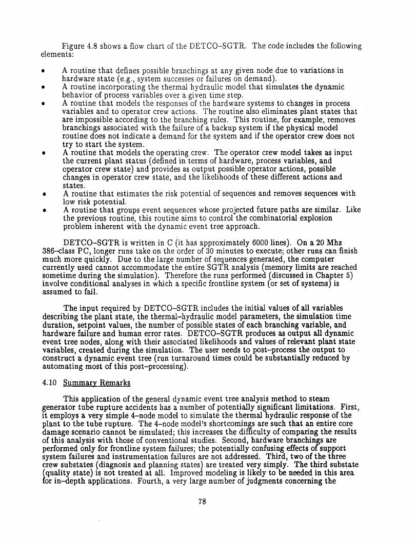
Figure 4.8 shows a flow chart of the DETCO-SGTR. The code includes the followingelements:

* A routine that defines possible branchings at any given node due to variations inhardware state (e.g., system successes or failures on demand).

* A routine incorporating the thermal hydraulic model that simulates the dynamicbehavior of process variables over a given time step.

* A routine that models the responses of the hardware systems to changes in processvariables and to operator crew actions. The routine also eliminates plant states thatare impossible according to the branching rules. This routine, for example, removesbranchings associated with the failure of a backup system if the physical modelroutine does not indicate a demand for the system and if the operator crew does nottry to start the system.

0 A routine that models the operating crew. The operator crew model takes as inputthe current plant status (defined in terms of hardware, process variables, andoperator crew state) and provides as output possible operator actions, possiblechanges in operator crew state, and the likelihoods of these different actions andstates.

* A routine that estimates the risk potential of sequences and removes sequences withlow risk potential.

* A routine that groups event sequences whose projected future paths are similar. Likethe previous routine, this routine aims to control the combinatorial explosionproblem inherent with the dynamic event tree approach.

DETCO-SGTR is written in C (it has approximately 6000 lines). On a 20 Mhz386-class PC, longer runs take on the order of 30 minutes to execute; other runs can finishmuch more quickly. Due to the large number of sequences generated, the computercurrently used cannot accommodate the entire SGTR analysis (memory limits are reachedsometime during the simulation). Therefore the runs performed (discussed in Chapter 5)involve conditional analyses in which a specific frontline system (or set of systems) isassumed to fail.

The input required by DETCO-SGTR includes the initial values of all variablesdescribing the plant state, the thermal-hydraulic model parameters, the simulation timeduration, setpoint values, the number of possible states of each branching variable, andhardware failure and human error rates. DETCO-SGTR produces as output all dynamicevent tree nodes, along with their associated likelihoods and values of relevant plant statevariables, created during the simulation. The user needs to post-process the output toconstruct a dynamic event tree (run turnaround times could be substantially reduced byautomating most of this post-processing).

4.10 Summary Remarks

This application of the general dynamic event tree analysis method to steamgenerator tube rupture accidents has a number of potentially significant limitations. First,it employs a very simple 4-node model to simulate the thermal hydraulic response of theplant to the tube rupture. The 4-node model's shortcomings are such that an entire coredamage scenario cannot be simulated; this increases the difficulty of comparing the resultsof this analysis with those of conventional studies. Second, hardware branchings areperformed only for frontline system failures; the potentially confusing effects of supportsystem failures and instrumentation failures are not addressed. Third, two of the threecrew substates (diagnosis and planning states) are treated very simply. The third substate(quality state) is not treated at all. Improved modeling is likely to be needed in this areafor in-depth applications. Fourth, a very large number of judgments concerning the

78

operator state transition frequencies are required of the analyst. The analysis burden islikely to increase with more complicated cognitive models, unless a wider set of meta-rulesfor assigning frequencies can be developed. Fifth, the transition frequency assignments are,with only a few exceptions, independent of scenario history. This is not necessarily asignificant limitation, but further work is required to determine if the dynamic event treeframework, as shown in Figure 3.2, carries enough information to allow this approximation.

D.espite its limitations, however, this application of DETAM analysis leads to someuseful insights concerning the SGTR accident. These insights are presented in Chapter 5.

79

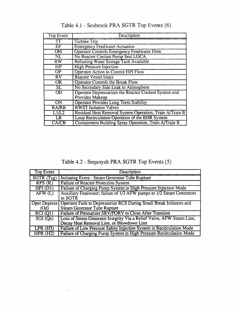
Table 4.1 - Seabrook PRA SGTR Top Events [6]

To Event DescriptionTT Turbine TripEF Emergency Feedwater ActuationOM Operator Controls Emergency Feedwater FlowNL No Reactor Coolant Pump Seal LOCARW Refueling Water Storage Tank AvailableHP High Pressure InjectionOP Operator Action to Control HPI FlowRV Reactor Vessel IntactOR Operator Controls the Break FlowSL No Secondary Side Leak to AtmosphereOD Operator Depressurizes the Reactor Coolant System and

Provides MakeupON Operator Provides Long Term Stability

RA/RB RWST Isolation ValvesL1/L2 Residual Heat Removal System Operation, Train A/Train B

LR Loop Recirculation Operation of the RHR SystemCA/CB Containment Building Spray Operation, Train AFrain B

Table 4.2 - Sequoyah PRA SGTR Top Events [5]

Top Event DescriptionSGTR (Tsg) Initiating Event - Steam Generator Tube Rupture

RPS (K) Failure of Reactor Protection SystemHPI (D1) Failure of Charging Pump System in High Pressure Injection ModeAFW (L) Auxiliary Feedwater; failure of 1/3 AFW pumps to 1/2 Steam Generators

in SGTROper Depress Operator Fails to Depressurize RCS During Small Break Initiators and

(Od) Steam Generator Tube RuptureRCI (Q1) Failure of Pressurizer SRV/PORV to Close After TransientSGI (Qs) Loss of Steam Generator Integrity Via a Relief Valve, AFW Steam Line,

Decay Heat Removal Line, or Blowdown LineLPR (H3) Failure of Low Pressure Safety Injection System in Recirculation ModeHPR (H2) Failure of Charging Pump System in High Pressure Recirculation Mode

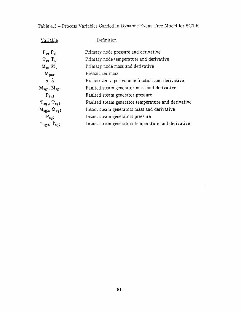
Table 4.3 - Process Variables Carried In Dynamic Event Tree Model for SGTR

Variable

Pp PpTp, Tp

Mpzr

a, a

Msgi, Msgi

Psgi

Tsgi, Tsgi

Msg2, Msg2

Psg2

Tsg2, T sg2

Definition

Primary node pressure and derivative

Primary node temperature and derivative

Primary node mass and derivative

Pressurizer mass

Pressurizer vapor volume fraction and derivative

Faulted steam generator mass and derivative

Faulted steam generator pressure

Faulted steam generator temperature and derivative

Intact steam generators mass and derivative

Intact steam generators pressure

Intact steam generators temperature and derivative

81

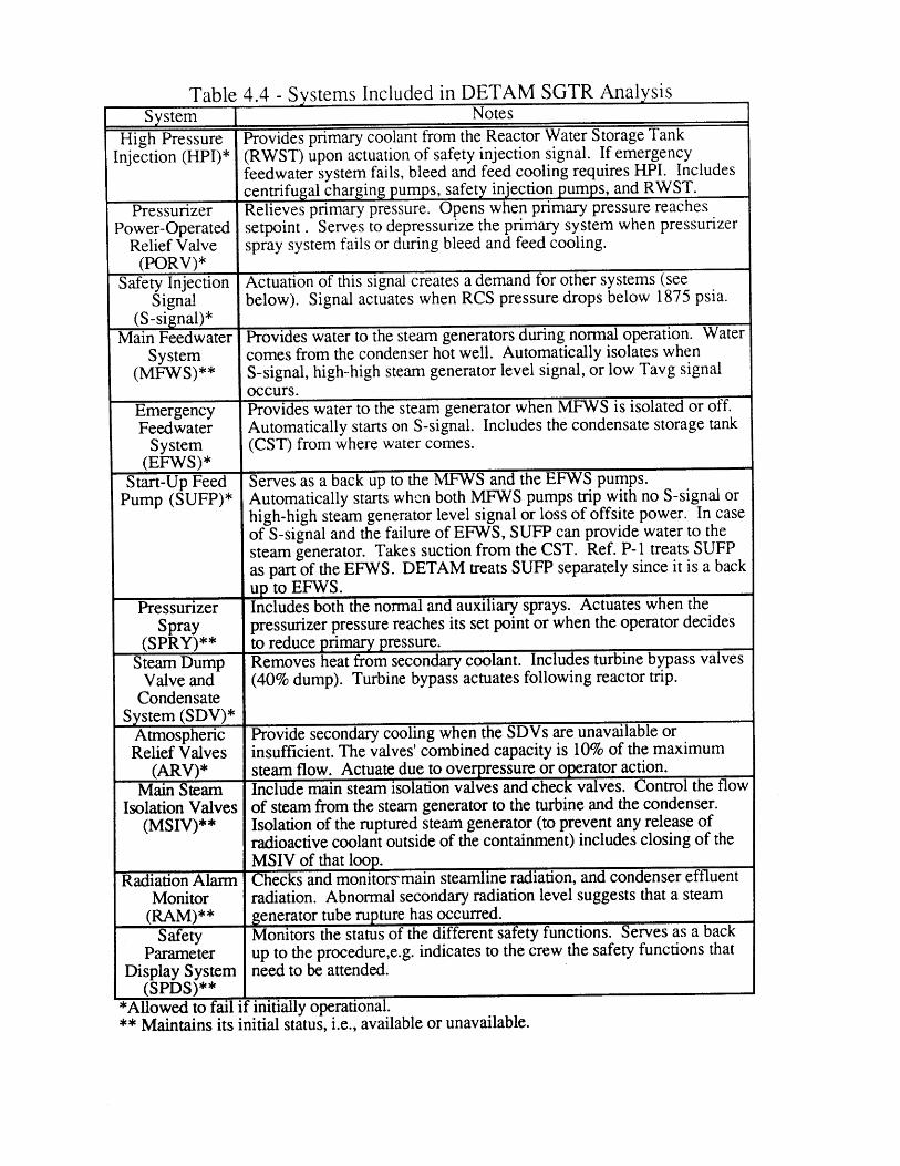
Table 4.4 - Systems Included in DETAM SGTR AnalysisSystem [ Notes

High Pressure Provides primary coolant from the Reactor Water Storage TankInjection (HPI)* (RWST) upon actuation of safety injection signal. If emergency

feedwater system fails, bleed and feed cooling requires HPI. Includescentrifugal charging pumps, safety injection pumps, and RWST.

Pressurizer Relieves primary pressure. Opens when primary pressure reachesPower-Operated setpoint . Serves to depressurize the primary system when pressurizer

Relief Valve spray system fails or during bleed and feed cooling.(PORV)*

Safety Injection Actuation of this signal creates a demand for other systems (seeSignal below). Signal actuates when RCS pressure drops below 1875 psia.

(S-signal)*Main Feedwater Provides water to the steam generators during normal operation. Water

System comes from the condenser hot well. Automatically isolates when(MFWS)** S-signal, high-high steam generator level signal, or low Tavg signal

occurs.Emergency Provides water to the steam generator when MFWS is isolated or off.Feedwater Automatically starts on S-signal. Includes the condensate storage tank

System (CST) from where water comes.(EFWS)*

Start-Up Feed Serves as a back up to the MFWS and the EFWS pumps.Pump (SUFP)* Automatically starts when both MFWS pumps trip with no S-signal or

high-high steam generator level signal or loss of offsite power. In caseof S-signal and the failure of EFWS, SUFP can provide water to thesteam generator. Takes suction from the CST. Ref. P-I treats SUFPas part of the EFWS. DETAM treats SUFP separately since it is a backup to EFWS.

Pressurizer Includes both the normal and auxiliary sprays. Actuates when theSpray pressurizer pressure reaches its set point or when the operator decides

(SPRY)** to reduce primary pressure.Steam Dump Removes heat from secondary coolant. Includes turbine bypass valves

Valve and (40% dump). Turbine bypass actuates following reactor trip.Condensate

System (SDV)*Atmospheric Provide secondary cooling when the SDVs are unavailable orRelief Valves insufficient. The valves' combined capacity is 10% of the maximum

(ARV)* steam flow. Actuate due to overpressure or operator action.Main Steam Include main steam isolation valves and check valves. Control the flow

Isolation Valves of steam from the steam generator to the turbine and the condenser.(MSIV)** Isolation of the ruptured steam generator (to prevent any release of

radioactive coolant outside of the containment) includes closing of theMSIV of that loop.

Radiation Alarm Checks and monitors'main steamline radiation, and condenser effluentMonitor radiation. Abnormal secondary radiation level suggests that a steam

(RAM)** generator tube rupture has occurred.Safety Monitors the status of the different safety functions. Serves as a back

Parameter up to the procedure,e.g. indicates to the crew the safety functions thatDisplay System need to be attended.

(SPDS)***Allowed to fail if initially operational.** Maintains its initial status, i.e., available or unavailable.

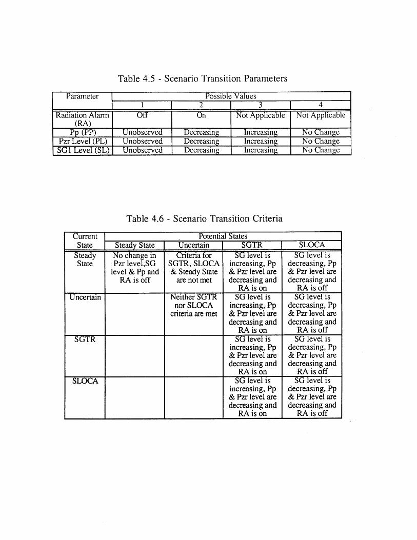
Table 4.5 - Scenario Transition Parameters

Parameter Possible Values__ _[ 1 2 3 4

Radiation Alarm Off On Not Applicable Not Applicable(RA)

Pp (PP) Unobserved Decreasing Increasing No ChangePzr Level (PL) Unobserved Decreasing Increasing No Change

SG1 Level (SL) Unobserved Decreasing Increasing No Change

Table 4.6 - Scenario Transition Criteria

Current Potential StatesState Steady State Uncertain SGTR SLOCA

Steady No change in Criteria for SG level is SG level isState Pzr level,SG SGTR, SLOCA increasing, Pp decreasing, Pp

level & Pp and & Steady State & Pzr level are & Pzr level areRA is off are not met decreasing and decreasing and

RA is on RA is offUncertain Neither SGTR SG level is SG level is

nor SLOCA increasing, Pp decreasing, Ppcriteria are met & Pzr level are & Pzr level are

decreasing and decreasing andRA is on RA is off

SGTR SG level is SG level isincreasing, Pp decreasing, Pp& Pzr level are & Pzr level aredecreasing and decreasing and

RA is on RA is offSLOCA SG level is SG level is

increasing, Pp decreasing, Pp& Pzr level are & Pzr level aredecreasing and decreasing and

RA is on RA isoff

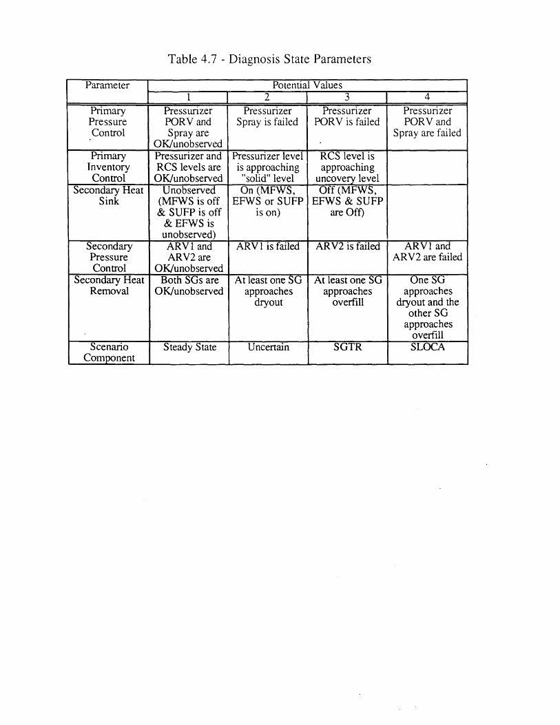
Table 4.7 - Diagnosis State Parameters

Parameter Potential Values 4_ _1 _ _ _23 1 4

Primary Pressurizer Pressurizer Pressurizer PressurizerPressure PORV and Spray is failed PORV is failed PORV andControl Spray are Spray are failed

OK/unobserved_Primary Pressurizer and Pressurizer level RCS level is

Inventory RCS levels are is approaching approachingControl OK/unobserved "solid" level uncovery level

Secondary Heat Unobserved On (MFWS, Off (MFWS,Sink (MFWS is off EFWS or SUFP EFWS & SUFP

& SUFP is off is on) are Off)& EFWS isunobserved)

Secondary ARVI and ARVI is failed ARV2 is failed ARVI andPressure ARV2 are ARV2 are failedControl OK/unobserved

Secondary Heat Both SGs are At least one SG At least one SG One SGRemoval OK/unobserved approaches approaches approaches

dryout overfill dryout and theother SG

approachesoverfill

Scenario Steady State Uncertain SGTR SLOCAComponent I I I

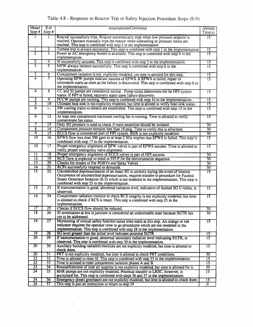
Table 4.8 - Response to Reactor Trip or Safety Injection Procedure Steps (E-0)

Model E-0 Assumptions/Comments AllottedStep # Step # I Time(s)

i 1 Reactor successfully trips. Reactor automatically trips when low pressure setpoint is 15reached. Operator manually trips the reactor when subcooling or pressure limits arereached. This step is combined with step 2 in the implementation

1 2 Turbine trip is always successful. This step is combined with step 1 in the implementation 152 3 Power to AC emergency busses is available. This step is combined with step 4 in the 15

implementation.2 4 SI successfully actuates. This step is combined with step 3 in the implementation. 153 5 MFW always isolates successfully. This step is combined with step 6 in the 15

implementation.3 6 Containment isolation is not explicitly modeled, yet time is allotted for this step. 154 -7 Operating EFW pumps indicate success of EFWS. If EFWS is failed, repair or 15

restoration starts as soon as the failure is discovered. This step is combined with step 8 inthe implementation.

4 8 CC and SI pumps are considered similar. Pump status determines the he HPI system 15status. If HPI is failed, recovery starts upon failure discovery.

5 9 PCCW pumps are running. This step is combined with step 10 in the implementation. 155 10 Ultimate heat sink is not explicitly modeled, but time is alloted to verify heat sink status. 156 1 SW cooling trains to diesels are established. This step is combined with step 12 in the 15

implementation.6 1T At least one containment enclosure cooling fan is running. Time is allotted to verify 1T

containment fan status.7 13 Only SG pressure is used to check if main steamline should be isolated. 308 14 Containment pressure remains less than 18 psig. Time to verify this is allocated. 309 15 ECCS flow is considered part of HPI system. RHR is not explicitly modeled. 3010 16 EFWS flow less than 500 gpm to at least 2 SGs implies that EFWS is failed. This step is 15

combined with step 17 in the implementation.10 17 Proper emergency alignment of EFW valves is part of EFWS success. Time is allotted to 15

verify proper emergency valve alignment.11 18 Proper emergency alignment of ECCS valves is part of HPI success. 3012 19 RCS Tave is expected to trend to 555 F for the demonstration sequence. 3013 20 Checks for modes of Pzr PORVs and Spray Valves 3014 21 RCPs successfully respond to demands. 30T 22 Uncontrolled depressurization of an intact SG is unlikely during the event of interest. 15

Occurrence of uncontrolled depressurization, requires transfer to procedure for FaultedSteam Generator Isolation (E-2) which is not modeled in the implementation. This step iscombined with step 23 in the implementation.

15 23 If instrumentation is good, abnormal radiation level, indicative of faulted SG U-tubes, is 15observed.

16 24 Containment radiation monitor to check RCS integrity is not explicitly modeled, but time 15is allotted to check if RCS is intact. This step is combined with step 25 in theimplementation.

17 25 Checks if ECCS flow should be reduced. 3018 26 SI termination at this is juncture is considered an undesireable state because SGTR has 30

yet to be addressed.19 27 Monitoring of critical safety function status trees starts at this step. An orange or red 15

indicator requires the operator crew to go procedures which are not modeled in theimplementation. This step is combined with step 28 in the implementation.

19 28 SG level greater than the initial level indicates potential SGTR. 1520 29 If instrumentation is good, abnormal secondary radiation level indicating SGTR, is 15

observed. This step is combined with step 30 in the implementation.20 30 Auxiliary building radiation monitors are not explicitly modeled, but time is allotted to 15

check them.20 31 PRT is not explicitly modeled, but time is allotted to check PRT conditions. 3022 32 Time is allotted to reset SI. This step is combined with step 33 in the implementation. 1522 33 Time is allotted to reset containment isolation phases A and B. 1523 34 Reestablishment of instr air supplies is not explicitly modeled, but time is allotted for it. 3024 35 RHR pumps are not explicitly modeled. Potential transfer to LRSC, however, is 15

accounted for. This step is combined with steps 36 and 37 in the implementation.24 36 Emergency diesel generators are not explicitly modeled, but time is allotted to check them. 1524 T1 This step is just an instruction to return to step 19

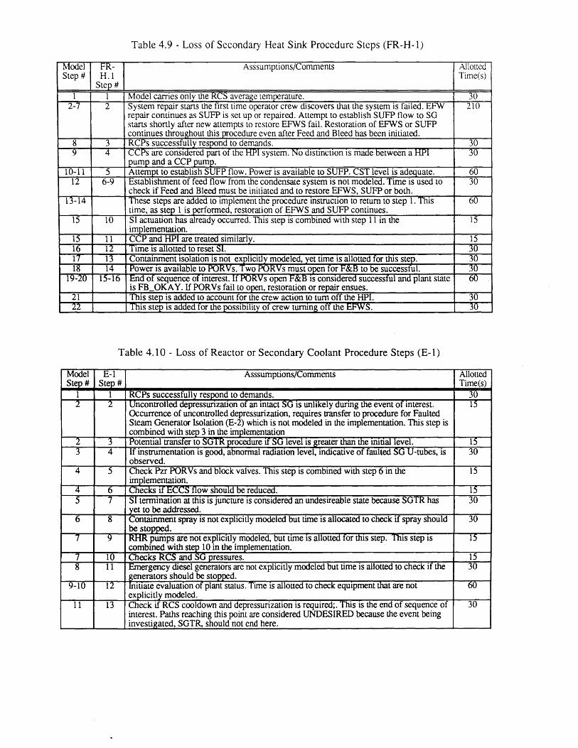
Table 4.9 - Loss of Secondary Heat Sink Procedure Steps (FR-H-1)

Model FR- Asssumptions/Comments AllottedStep # H.1 Time(s)

Step #1 1 Model carries only the RCS average temperature. 30

2-7 2 System repair starts the first time operator crew discovers that the system is failed. EFW 210repair continues as SUFP is set up or repaired. Attempt to establish SUFP flow to SGstarts shortly after new attempts to restore EFWS fail. Restoration of EFWS or SUFPcontinues throughout this procedure even after Feed and Bleed has been initiated.

8 3 RCPs successfully respond to demands. 30T 4 CCPs are considered part of the HPI system. No distinction is made between a HPI 30

pump and a CCP pump.10-11 5 Attempt to establish SUFP flow. Power is available to SUFP. CST level is adequate. 60

12 6-9 Establishment of feed flow from the condensate system is not modeled. Time is used to 30check if Feed and Bleed must be initiated and to restore EFWS, SUFP or both.

13-14 These steps are added to implement the procedure instruction to return to step 1. This 60time, as step 1 is performed, restoration of EFWS and SUFP continues.

15 10 SI actuation has already occurred. This step is combined with step 11 in the 15implementation.

15 11 CCP and HPI are treated similarly. 1516 12 Time is allotted to reset SI. 3017 13 Containment isolation is not explicitly modeled, yet time is allotted for this step. 3018 14 Power is available to PORVs. Two PORVs must open for F&B to be successful. 30

19-2 15-16 End of sequence of interest. If PORVs open F&B is considered successful and plant state 60is FB OKAY. If PORVs fail to open, restoration or repair ensues.

21 This step is added to account for the crew action to turn off the HPI. 3022 This step is added for the possibility of crew turning off the EFWS. 30

Table 4.10 - Loss of Reactor or Secondary Coolant Procedure Steps (E-1)

Model E-1 Asssumptions/Comments Allotted

Step # Step # Time(s)1 1 RCPs successfully respond to demands. 30

2 Uncontrolled depressurization of an intact SG is unlikely during the event of interest. 15Occurrence of uncontrolled depressurization, requires transfer to procedure for FaultedSteam Generator Isolation (E-2) which is not modeled in the implementation. This step iscombined with step 3 in the implementation

1 3 Potential transfer to SGTk procedure if SG level is greater than the initial level. 153 4 If instrumentation is good, abnormal radiation level, indicative of faulted SG U-tubes, is 30

observed.4 5 Check Pzr PORVs and block valves. This step is combined with step 6 in the 15

implementation.4 6 Checks if ECCS flow should be reduced. 155 7 SI termination at this is juncture is considered an undesireable state because SGTR has 30

yet to be addressed.6 8 Containment spray is not explicitly modeled but time is allocated to check if spray should 30

be stopped.7 9 RHR pumps are not explicitly modeled, but time is allotted for this step. This step is 15

combined with step 10 in the implementation.7 10 Checks RCS and SG pressures. 158 11 Emergency diesel generators are not explicitly modeled but time is allotted to check if the 30

generators should be stopped.9-10 12 Initiate evaluation of plant status. Time is allotted to check equipment that are not 60

explicitly modeled.11 13 Check if RCS cooldown and depressurization is required;. This is the end of sequence of 30

interest. Paths reaching this point are considered UNDESIRED because the event beinginvestigated, SGTR, should not end here.

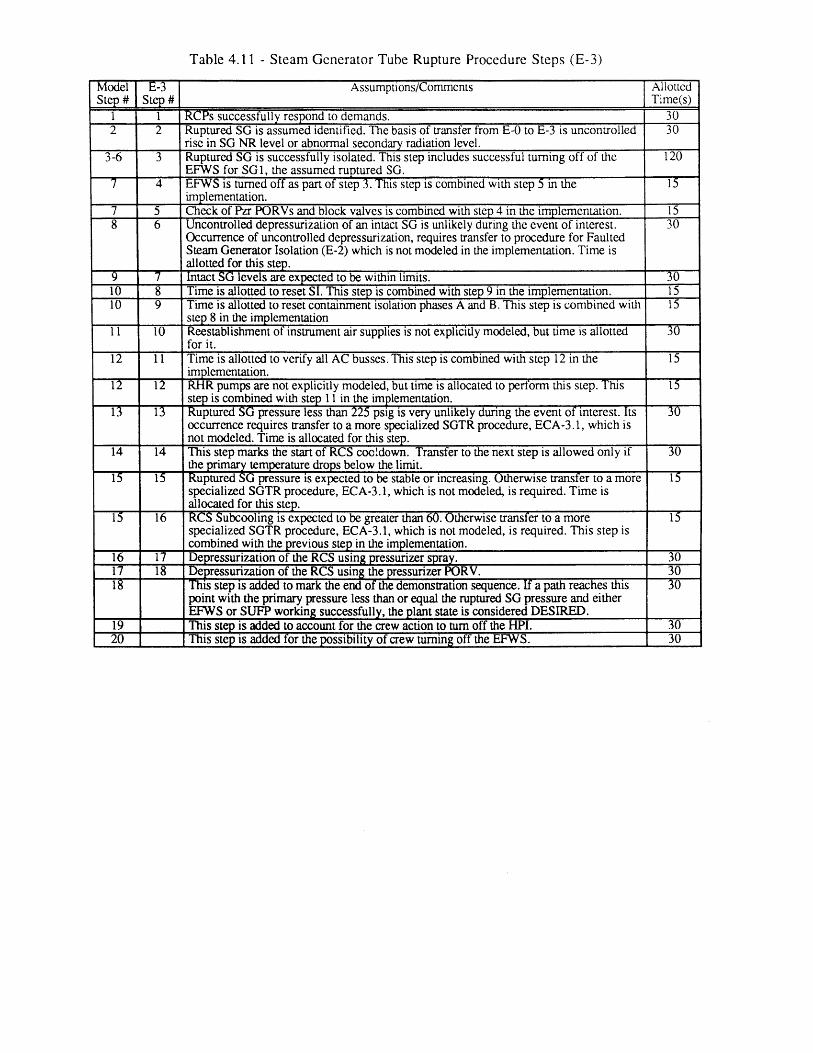
Table 4.11 - Steam Generator Tube Rupture Procedure Steps (E-3)

Model E-3 Assumptions/Comments AllottedStep# Step # Time(s)

1 1 RCPs successfully respond to demands. 302 2 Ruptured SG is assumed identified. The basis of transfer from E-0 to E-3 is uncontrolled 30

rise in SG NR level or abnormal secondary radiation level.3-6 3 Ruptured SG is successfully isolated. This step includes successful turning off of the 120

EFWS for SG1, the assumed ruptured SG.7 4 EFWS is turned off as part of step 3. This step is combined with step 5 in the 1

implementation.7 5 Check of Pzr PORVs and block valves is combined with step 4 in the implementation. 158 6 Uncontrolled depressurization of an intact SG is unlikely during the event of interest. 30

Occurrence of uncontrolled depressurization, requires transfer to procedure for FaultedSteam Generator Isolation (E-2) which is not modeled in the implementation. Time isallotted for this step.

9 7 Intact SG levels are expected to be within limits. 3010 8 Time is allotted to reset SI. This step is combined with step 9 in the implementation. 1510 9 Time is allotted to reset containment isolation phases A and B. This step is combined with 15

step 8 in the implementation11 10 Reestablishment of instrument air supplies is not explicitly modeled, but time is allotted 30

for it.12 11 Time is allotted to verify all AC busses. This step is combined with step 12 in the 15

implementation.11 12 RHR pumps are not explicitly modeled, but time is allocated to perform this step. This 15

step is combined with step 11 in the implementation.1T 13 Ruptured SG pressure less than 225 psig is very unlikely during the event of interest. Its 30

occurrence requires transfer to a more specialized SGTR procedure, ECA-3.1, which isnot modeled. Time is allocated for this step.

14 14 This step marks the start of RCS cocidown. Transfer to the next step is allowed only if 30the primary temperature drops below the limit.

15 15 Ruptured SG pressure is expected to be stable or increasing. Otherwise transfer to a more 15specialized SGTR procedure, ECA-3.1, which is not modeled, is required. Time isallocated for this step.

15 16 RCS Subcooling is expected to be greater than 60. Otherwise transfer to a morespecialized SGTR procedure, ECA-3.1, which is not modeled, is required. This step iscombined with the previous step in the implementation.

16 17 Depressurization of the RCS using pressurizer spray. 3017 18 Depressurization of the RCS using the pressurizer PORV. 3018 This step is added to mark the end of the demonstration sequence. If a path reaches this 30

point with the primary pressure less than or equal the ruptured SG pressure and eitherEFWS or SUFP working successfully, the plant state is considered DESIRED.

19 This step is added to account for the crew action to turn off the HPI. 3020 This step is added for the possibility of crew turning off the EFWS. 30

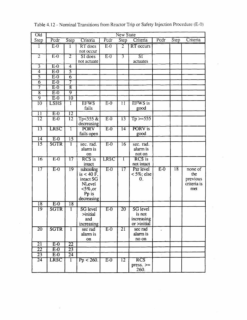
Table 4.12 - Nominal Transitions from Reactor Trip or Safety Injection Procedure (E-0)

Old New StateStep Pcdr Step Criteria Pcdr Step Criteria Pcdr Step Criteria

1 E-0 1 RT does E-0 2 RT occursnot occur

2 E-0 2 SI does E-0 3 S1not actuate actuates

3 E-0 44 E-0 55 E-0 66 E-0 77 E-0 88 E-0 9 ___ _______

9 E-0 1010 LSHS I EFWS E-0 II EFWS is

fails good11 E-0 1212 E-0 12 Tp<555 & E-0 13 Tp >=555

decreasing13 LRSC 1 PORV E-0 14 PORV is

fails open good14 E-0 15 .15 SGTR 1 sec. rad. E-0 16 sec. rad.

alarm is alarm ison noton

16 E-0 17 RCS is LRSC 1 RCS isintact not intact

17 E-0 19 subcoling E-0 17 Pzr level E-0 18 none ofis < 40 F, < 5%; else theintact SG 0. previousNLevel criteria is<5%,or met

Ppisdecreasing

18 E-0 1819 SGTR 1 SG level E-0 20 SG level

>initial is notand increasing

increasing or >initial20 SGTR 1 sec rad E-0 21 sec rad

alarm is alarm is___ ____on no on____

21 E-0 22 on noon22 E-0 2323 E-0 2424 LRSC 1 Pp <260. E-0 12 RCS

press. >=260.

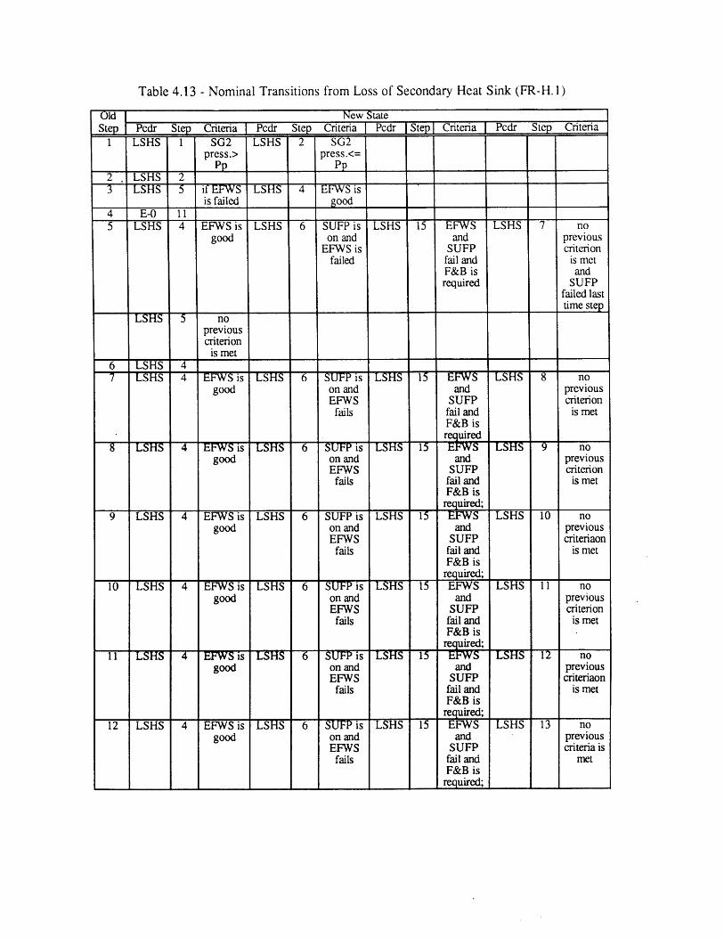
Table 4.13 - Nominal Transitions from Loss of Secondary Heat Sink (FR-H. 1)

Old 1New State

Step Pedr Step Criteria IPcdr Step Criteria I Pcdr IStep Criteriaf Pcdr Step Criteria1 LSHS 1 SG2 LSHS 2 SG2

press.> press.<=Pp Pp

2 , LSHS 2 __T- Fffh T EWST L-SH T4 -EF-W i

is failed good _4 E-0 115 LSHS 4 EFWS is LSHS 6 SUFP is LSHS 15 EFWS LSHS 7 no

good on and and previousEFWS is SUFP criterion

failed fail and is metF&B is andrequired SUFP

failed lasttime step

TL1HS 5 nopreviouscriterion

is met-6 LSHS 4

7T SI T-6 W~ s- _E S* HUP SI 15 'TPW3- T=T T8 nogood on and and previous

EFWS SUFP criterionfails fail and is met

F&B isrequired

good on and and previousEFWS SUFP criterion

fails fail and is metF&B is

. required;9 LSHS 4 EFWS is LSHS 6 SUFP is LSHS 15 EFWS LSHS 10 no

good on and and previousEFWS SUFP criteriaon

fails fail and is metF&B is

grequired10 LSHS 4 ~EFWSis LSHS 6 SUFP is LSHS 13 EFWS LSHS 11 no

good on and and previousEFWS SUFP criterionfails fail and is met

F&B is

II~~LHS~ ~4~EWSis -LSS ~ UPis ~~HT ~13~ ~~ SHS ~T nogood on and and previous

EFWS SUFP criteriaonfails fail and is met

F&B isrequired,

12 LSHS 4 EFWS is LSHS 6 SUFP is LSHS ~3 EFWS LSHS 13 nogood on and and previous

EFWS SUFP criteria isfails fail and met

F&B isrequired;

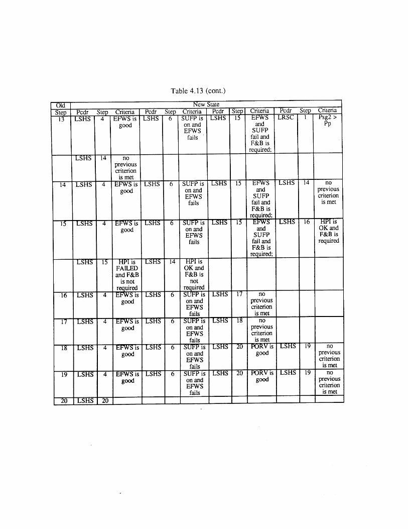
Table 4.13 (cont.)

Old New State

Step Pcdr Step Criteria Pcdr Step Criteria Pcdr Step Criteria Pcdr Step Criteria13 LSHS 4 EFWS is LSHS 6 SUFP is LSHS 15 EFWS LRSC I Psg2 >

good on and and PpEFWS SUFP

fails fail andF&B is

____grequired; ____

EHS~ 14 nopreviouscriterion

is met I14 LSHS 4 EFWS is LSHS 6 SUEP is LSHS 15 EFWS LSHS 14 no

good on and and previousEFWS SUFP criterion

fails fail and is metF&B isrequired;

T I ~ EFWE s~~IS 6 SUFP"is TTSHS ~ IT TSHW 16 HPI Tgood on and and OK and

EFWS SUFP F&B isfails fail and required

F&B is___ required;

TLTIS 15 HPI is LSHS 14 TI~ -is

FAILED OK andand F&B F&B is

is not notrequired required

16 LSHS 4 EFWS is LSHS 6 SUFP is LSHS 17 nogood on and previous

EFWS criterionfails is met

17 TSHS 4 EFW is TT TSS SUFP is rLriS 18 nogood on and previous

EFWS criterionfails is met

-T L~TS- 4 EFWS is ~HS~ 6 SUFP is ~~IHS- P-- RV is -T51TWS- nogood on and good previous

EFWS criterionfails is met

19 LSHS 4 EFWS is LSHS 6 SUFP is LSHS 20 PORV is LSHS 19 nogood on and good previous

EFWS criterionfails is met

20 LSHS 20 1 _ I I

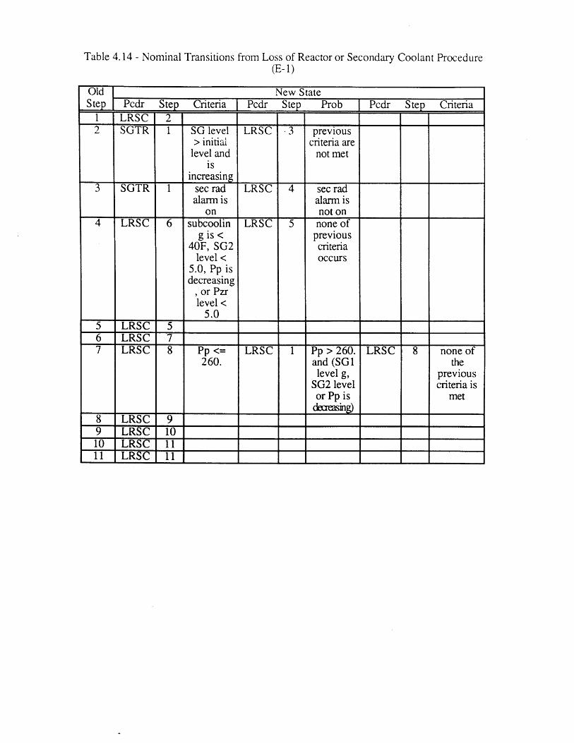
Table 4.14 - Nominal Transitions from Loss of Reactor or Secondary(E-1)

Coolant Procedure

Old New StateStep Pcdr_ Step Criteria_ Pcdr Step Prob | Pcdr Step Criteria

1 LRSC 22 SGTR 1 SG level LRSC -3 previous

> initial criteria arelevel and not met

isincreasing

3 SGTR 1 sec rad LRSC 4 sec radalarm is alarm is

on not on4 LRSC 6 subcoolin LRSC 5 none of

g is < previous40F, SG2 criteria

level < occurs5.0, Pp isdecreasing

or Pzrlevel <

5.05 LRSC 56 LRSC 77 LRSC 8 Pp <= LRSC 1 Pp > 260. LRSC 8 none of

260. and (SG1 thelevel g, previous

SG2 level criteria isor Pp is met

dreasing)8 LRSC 99 LRSC 1010 LRSC 11 111 LRSC 11 M I I II

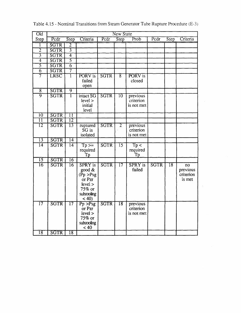
Table 4.15 - Nominal Transitions from Steam Generator Tube Rupture Procedure (E-3)

Old New StateStep Pcdr Step Criteria | Pcdr Step Prob Pcdr Step Criteria1 SGTR 22 SGTR 33 SGTR 44 SGTR 55 SGTR 66 SGTR 77 LRSC I PORV is SGTR 8 PORV is

failed closedopen

8 SGTR 99 SGTR 1 intact SG SGTR 10 previous

level > criterioninitial is not metlevel

10 SGTR 1111 SGTR 1212 SGTR 13 ruptured SGTR 2 previous

SG is criterionisolated is not met

13 SGTR 1414 SGTR 14 Tp>= SGTR 15 Tp<

required requiredT TP

15 SGTR 1616 SGTR 16 SPRY is SGTR 17 SPRY is SGTR 18 no

good & failed previous(Pp >Psg criterion

or Pzr is metlevel >75% or

subooling< 40)

17 SGTR 17 Pp >Psg SGTR 18 previousor Pzr criterionlevel > is not met75% or

subcooling<40

18 SGTR 18

Hardware Systems Failure Frequencies

System Frequency Seabrook PRA [6]_ _ (per demand) Page (Source)

EFWS 1.73E-4 (hardware) D.9-18HPI 1.03E-6 D.8-80

PORV 1.05E-2 D.10-5SUFP 4.46E-3 D.9-16ARV 4.27E-3 (to open) D.10-8

2.50E-2 (to close) D.10-8

Table 4.17 - Qualitative Likelihoods

Likelihood* Description ValueCRTN NO Certain No 0.00

VVUnLKLY Very Very Unlikely 0.01VUnLKLY Very Unlikely 0.10UnLKLY Unlikely 0.30

EVEN Even 0.50LKLY Likely 0.70

VLKLY Very Likely 0.90VVLKLY Very Very Likely 0.99

CRTN YS Certain Yes 1.00

* If a number appears before a qualitative likelihood, the numerical value ismultiplied by that number. Any number appearing after the likelihood is inhundredths and is added to the numerical value of likelihood. For example,EVEN 10 has a numerical value of .60, whereas 2VUnLKLY has a value of0.02.

Table 4.16

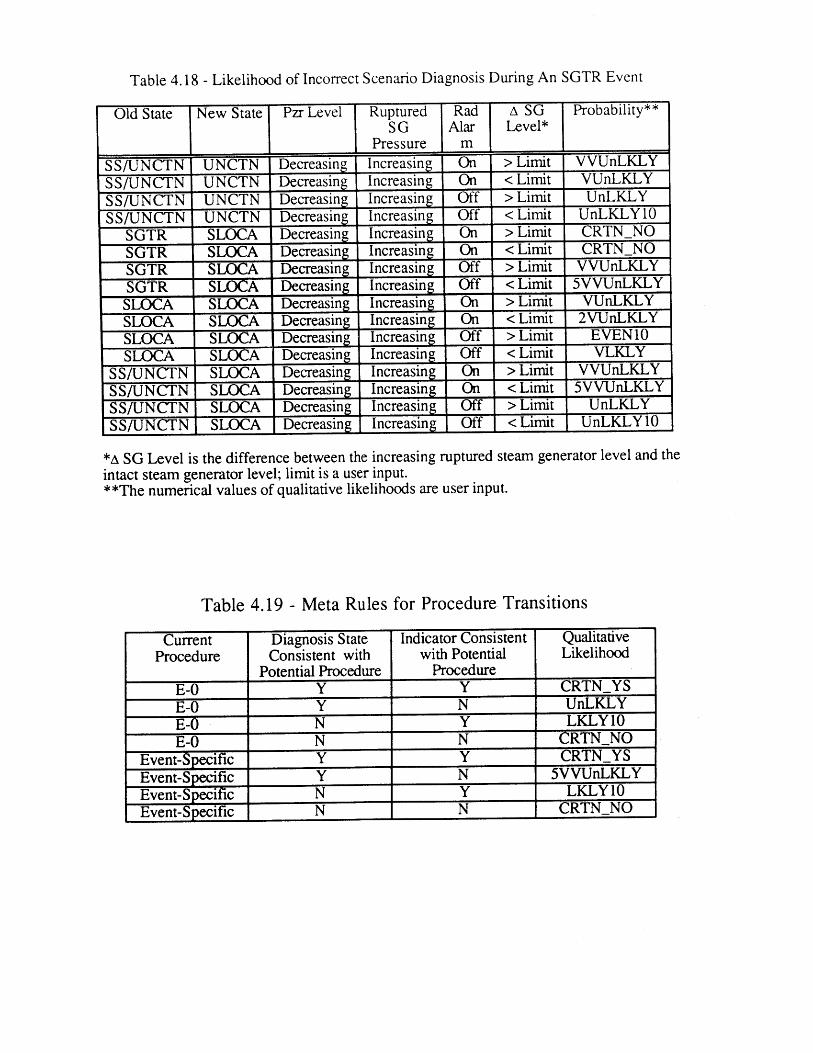
Table 4.18 - Likelihood of Incorrect Scenario Diagnosis During An SGTR Event

Old State New State Pzr Level Ruptured Rad A SG Probability**SG Alar Level*

Pressure m

SS/UNCTN UNCTN Decreasing Increasing On > Limit VVUnLKLYSS/UNCTN UNCTN Decreasing Increasing On < Limit VUnLKLYSS/UNCTN UNCTN Decreasing Increasing Off > Limit UnLKLYSS/UNCTN UNCTN Decreasing Increasing Off < Limit UnLKLY10

SGTR SLOCA Decreasing Increasing On > Limit CRTN NOSGTR SLOCA Decreasing Increasing On <Limit CRTN NOSGTR SLOCA Decreasing Increasing Off > Limit VVUnLKLYSGTR SLOCA Decreasing Increasing Off < Limit 5VVUnLKLYSLOCA SLOCA Decreasing Increasing On > Limit VUnLKLYSLOCA SLOCA Decreasing Increasing On < Limit 2VUnLKLYSLOCA SLOCA Decreasing Increasing Off > Limit EVEN10SLOCA SLOCA Decreasing Increasing Off < Limit VLKLY

SS/UNCTN SLOCA Decreasing Increasing On > Limit VVUnLKLYSS/UNCTN SLOCA Decreasing Increasing On < Limit 5VVUnLKLYSS/UNCTN SLOCA Decreasing Increasing Off > Limit UnLKLYSS/UNCTN SLOCA Decreasing Increasing Off <Limit UnLKLY10

*A SG Level is the difference between the increasing ruptured steam generator level and theintact steam generator level; limit is a user input.**The numerical values of qualitative likelihoods are user input.

Table 4.19 - Meta Rules for Procedure Transitions

Current Diagnosis State Indicator Consistent QualitativeProcedure Consistent with with Potential Likelihood

Potential Procedure ProcedureE-0 Y Y CRTNYSE-0 Y N UnLKLYE-0 N Y LKLY10E-0 N N CRTNNO

Event-Specific Y Y CRTN YSEvent-Specific Y N 5VVUnLKLYEvent-Specific N Y LKLY10Event-Specific N N CRTN NO

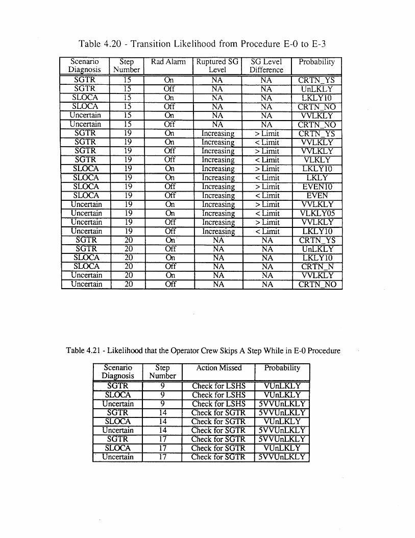
Table 4.20 - Transition Likelihood from Procedure E-0 to E-3

Scenario Step Rad Alarm ' Ruptured SG SG Level ProbabilityDiagnosis Number Level Difference

SGTR 15 On NA NA CRTNYSSGTR 15 Off NA NA UnLKLY

SLOCA 15 On NA NA LKLY10SLOCA 15 Off NA NA CRTN NO

Uncertain 15 On NA NA VVLKLYUncertain 15 Off NA NA CRTN NO

SGTR 19 On Increasing > Limit CRTN YSSGTR 19 On Increasing < Limit VVLKLYSGTR 19 Off Increasing > Limit VVLKLYSGTR 19 Off Increasing < Limit VLKLY

SLOCA 19 On Increasing > Limit LKLY10SLOCA 19 On Increasing < Limit LKLYSLOCA 19 Off Increasing > Limit EVEN10SLOCA 19 Off Increasing < Limit EVEN

Uncertain 19 On Increasing > Limit VVLKLYUncertain 19 On Increasing < Limit VLKLY05Uncertain 19 Off Increasing > Limit VVLKLYUncertain 19 Off Increasing < Limit LKLY10

SGTR 20 On* NA NA CRTN YSSGTR 20 Off NA NA UnLKLY

SLOCA 20 On NA NA LKLY10SLOCA 20 Off NA NA CRTNN

Uncertain 20 On NA NA VVLKLYUncertain 20 Off NA NA CRTN NO

Table 4.21 - Likelihood that the Operator Crew Skips A Step While in E-0 Procedure

Scenario Step Action Missed ProbabilityDiagnosis Number I

SGTR 9 Check for LSHS VUnLKLYSLOCA 9 Check for LSHS VUnLKLY

Uncertain 9 Check for LSHS 5VVUnLKLYSGTR 14 Check for SGTR 5VVUnLKLY

SLOCA 14 Check for SGTR VUnLKLYUncertain 14 Check for SGTR 5VVUnLKLY

SGTR 17 Check for SGTR 5VVUnLKLYSLOCA 17 Check for SGTR VUnLKLY

Uncertain 17 Check for SGTR 5VVUnLKLY

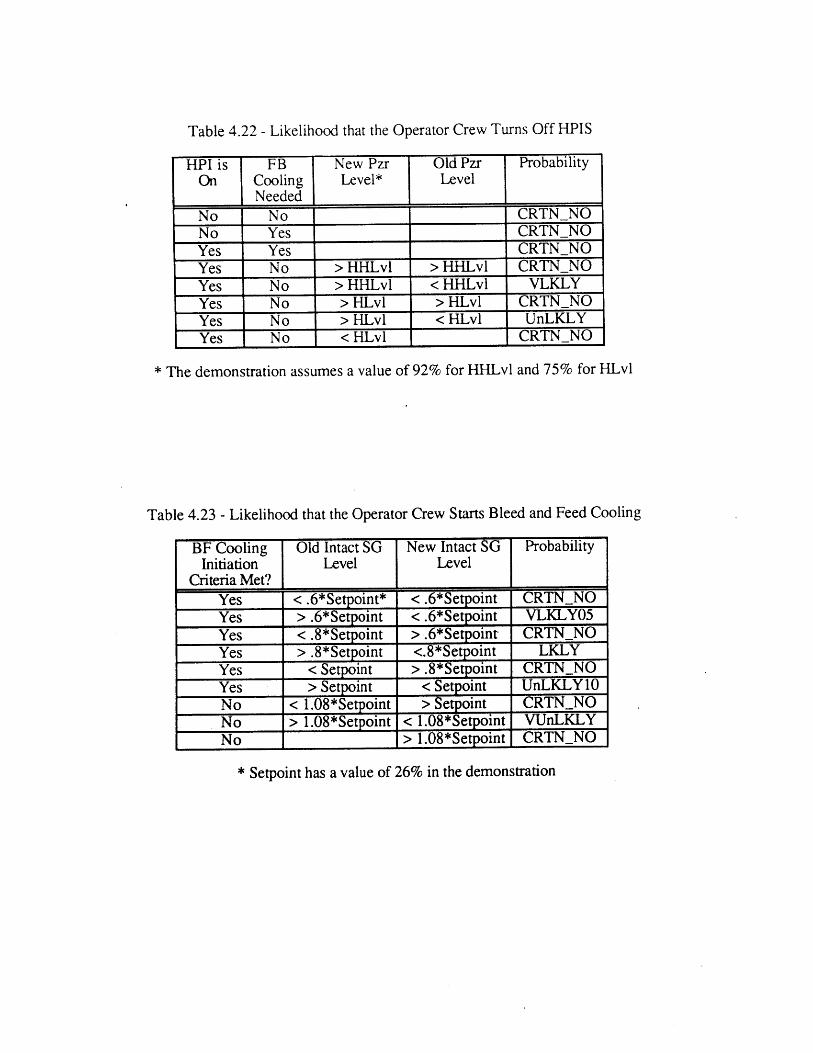
Table 4.22 - Likelihood that the Operator Crew Turns Off HPIS

HPI is FB New Pzr Old Pzr ProbabilityOn Cooling Level* Level

NeededNo No CRTN NONo Yes CRTN NO

Yes Yes CRTN NOYes No > HHLvl > HHLvl CRTN NOYes No > HHLvl < HHLvl VLKLYYes No > HLvl > HLvl CRTNNOYes No > HLvl < HLvl UnLKLYYes No < HLvl I CRTN NO

* The demonstration assumes a value of 92% for HHLvl and 75% for HLvl

Table 4.23 - Likelihood that the Operator Crew Starts Bleed and Feed Cooling

BF Cooling Old Intact SG New Intact SG ProbabilityInitiation Level Level

Criteria Met?Yes <.6*Setpoint* <.6*Setpoint CRTN NOYes > .6*Setpoint <.6*Setpoint VLKLY05Yes <.8*Setpoint > .6*Setpoint CRTN NOYes > .8*Setpoint <.8*Setpoint LKLYYes < Setpoint > .8*Setpoint CRTNNOYes > Setpoint < Setpoint UnLKLY10No < 1.08*Setpoint > Setpoint CRTN NONo > 1.08*Setpoint < 1.08*Setpoint VUnLKLYNo > 1.08*Setpoint CRTN NO

* Setpoint has a value of 26% in the demonstration

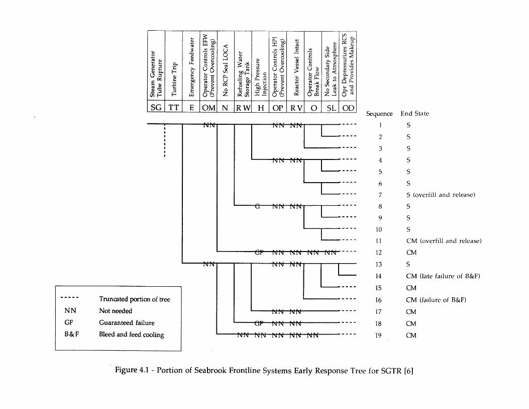
0~

z

0

0

0 0- 0 0 ;07

0~

C

B

II

F

F

-~ ~

a

Qn

-0-

4

W~

r-

j C

D

C) 0

0

C)

~1 0~ C)

C)

Ct

C)

2 F

'7e

I e

I B

I

II

B

I S

* I

I B

I I

0 zm

Ste

am G

ener

ator

C)

Tub

e R

uptu

re

Tur

bine

Tri

p

M

Em

erge

ncy

Fee

dwat

er

Ope

rato

r C

ontr

ols

EFW

(Pre

vent

Ove

rcoo

ling

)

No

RC

P Se

al L

OC

A

Ref

ueli

ng

Wat

erS

tora

ge T

ank

Hig

h P

ress

ure

Inje

ctio

n

Ope

rato

r C

ontr

ols

HPI

(Pre

vent

Ove

rcoo

ling

)

Rea

ctor

V

esse

l In

tact

Ope

rato

r C

ontr

ols

O

Bre

ak F

low

U

No

Sec

ondar

y S

ide

r L

eak t

o A

tmosp

her

e

Opr

Dep

ress

uriz

es

RC

San

d P

rovi

des

Mak

eup

(0

~ ~

O

N

(J1

~

(A

k)

-~

0~ Cr)

C)

0~ -i C)

C)

Ct

C)

0 O0

BIn

B

B

n Z

'71

Z17

1

I

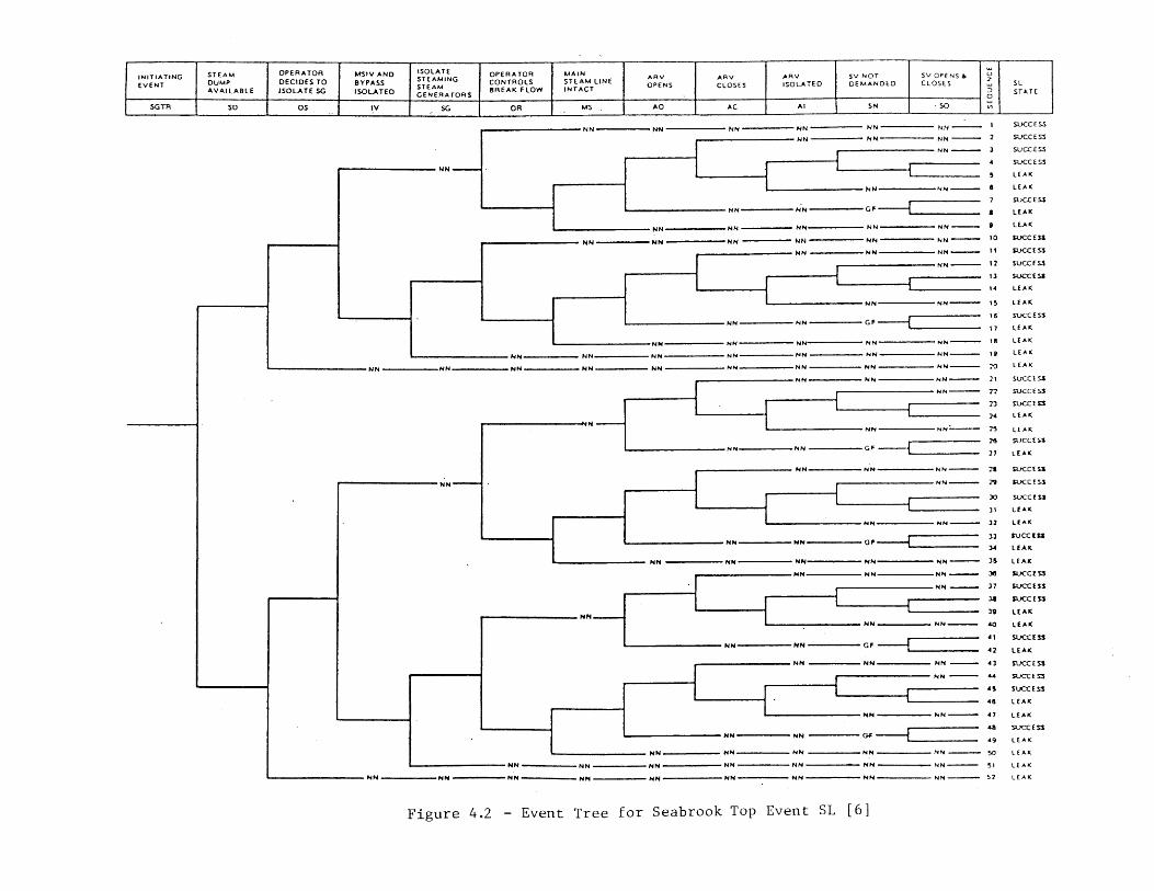
INITIATING STEAM OPERATOR MSIV AND ISOLATE OPERATOR MAIN ARV ARV ARV SV NOT SV OPENS UEVENT DUMP DECIDES TO BYPASS STEAM ONTROLS STEAM LINE OPENS CLOSES ISOLATED DEMANDED CLOSES SL

AVAILABLE JSOLATE SG SSLATD TEEATR BREAK FLOW INTACT D STA TEiSLT CIISOLATED GENERATORS a TT

SGTR SD OS IV SG OR MS AD AC Al SN so

_NN - NN - NN NN NN - NN I SUCS

NN NN - NN 2 SUCCESS

NN 3 SUCCESS

NN- 4 SUjCC E SS

5 LEAK

NN NN 8 LEAK

7 SUCZ E SSNN1NN LEAK

NN _ NN _ NN NN - NN- LEAK_NN - NN - NN - NN - NN - NN 0PJE3

NN - NN NN - 11 SUCC ES3

NN 12 5UCCE SS

13 SUCCESS

14 LEAK

NNNN 1s LEAK

16 SUCC E S3NN7

LEAK

Nk NN _ N INN - NN - 18 LEAK

MNN MNN NN NN _ NN NN - NN- 19 LEAK

L NN - NN - NN NN - NN - NNNN - NN - NN- 20 LEAK

NN NN NN - 21 SUCCESS

NN 2-2 SUCCES$

73 SUCC E S3

24 LEAK

SNN 75s LEAK

ml SUCCESS

427 LEAK

NNNNNN N711 GFC S

N~N NN NN- 29 SUC CEfS3

NN49 STUCCES3

30) SUC C 1! i3

46 LEAK

N04 NN 32 LEAK

33 sUCCEs

34 LEAK

N N RN RN NN 35 LEAK

MNN NN NN 38 $UCC E33

N"N 37 PUCC E S33 SUCC E 33

MN N-19 L E AK

MNN NN 410 LE AK

4 ' SUCC E 33NN _ NN GF 2LA

NN NN - NN - 43 SU1CCE S3

NN N 44 SUCC E 53

4 5 SUCCE SS46 LEAK

NN NN 47 LEAK

-48 SUCC E S$sNN N GF49 L EA K

MNN MN - NN _ NN NN 50 L EAKNN - NN - NN NN NN - NN NN - \1 LEAK

NN NN NN NN NM N - NN NN NN NN - 52 LEAK

Figure 4.2 - Event Tree for Seabrook Top Event SL [6]

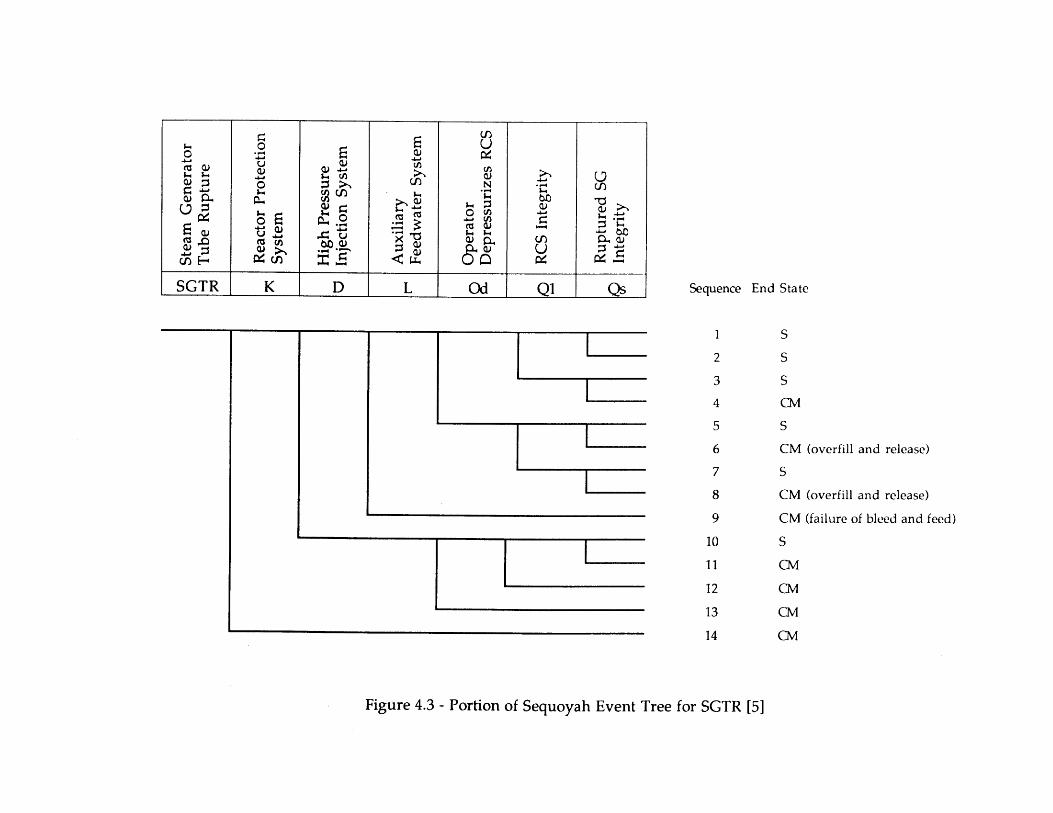
C~)S

team

G

ener

ator

Tub

e R

uptu

re

Rea

ctor

Pro

tect

ion

Sys

tem

Hig

h P

ress

ure

0 In

ject

ion

Sys

tem

Aux

ilia

ryF

eedw

ater

Sys

tem

Ope

rato

rD

epre

ssur

izes

RC

S

RC

S In

tegr

ity

Rup

ture

d SG

Inte

grit

y

1 C M

--]

a,\

Uln

4.-

w

-

0 0 z 0 C)I

2 ni

U-I

K KK K

C)

Un

~ U

n)(i-I

n 0 0~ 0~ 0~

'-1 ~1 (I)

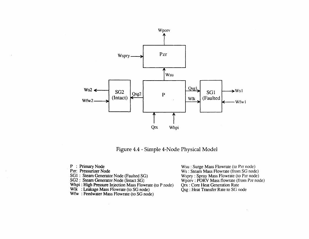
Wporv

Wspry

Ws2

Wfw2 3

SG2(Intact)

Qsg2+--

Pzr

Wsu

p

Qrx

WikSG1

(Faulted:- Wfw 1

Whpi

Figure 4.4 - Simple 4-Node Physical Model

P : Primary NodePzr: Pressurizer NodeSG1 : Steam Generator Node (Faulted SG)SG2: Steam Generator Node (Intact SG)Whpi : High Pressure Injection Mass Flowrate (to P node)Wik : Leakage Mass Flowrate (to SG node)Wfw : Feedwater Mass Flowrate (to SG node)

Wsu : Surge Mass Flowrate (to Pzr node)Ws : Steam Mass Flowrate (from SG node)Wspry : Spray Mass Flowrate (to Pzr node)Wporv : PORV Mass flowrate (from Pzr node)Qrx : Core Heat Generation RateQsg : Heat Transfer Rate to SG node

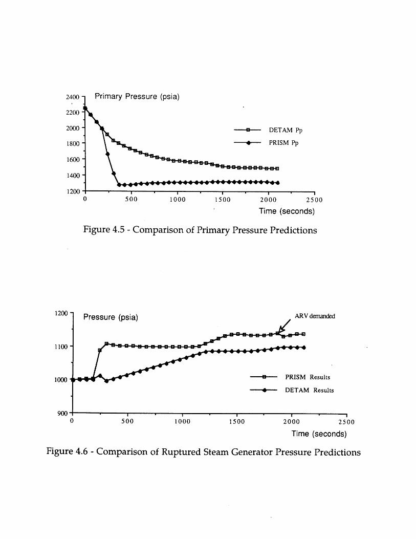
Primary Pressure (psia)

------ DETAM Pp

-- PRISM Pp

0 500 1000 1500 2000 2500

Time (seconds)

Figure 4.5 - Comparison of Primary Pressure Predictions

Pressure (psia) ARV demanded

----- PRISM Results

4- DETAM Results

0 500 1000 1500 2000 2500

Time (seconds)

Figure 4.6 - Comparison of Ruptured Steam Generator Pressure Predictions

2400

2200

2000

1800

1600

1400

1200

1200

1100

1000

900

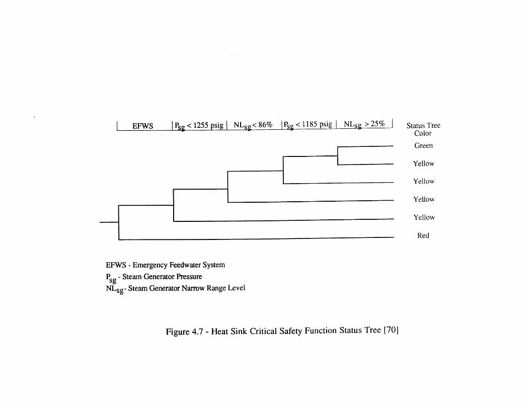
,8 |Ps5g<1185psig | NLsg > 2 5 %.|

EFWS - Emergency Feedwater System

Psg - Steam Generator Pressure

NLsg- Steam Generator Narrow Range Level

Figure 4.7 - Heat Sink Critical Safety Function Status Tree [70]

EFWS Status TreeColor

Green

Yellow

Yellow

Yellow

Yellow

Red

|P ,g < 1255 psig | NSg< 86%

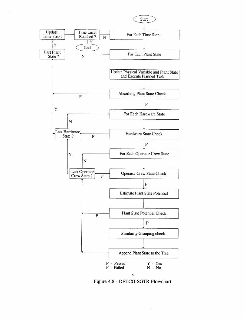
Star

Update Time LimitTime Step t -Reached ? N

YL s PE n d

Last PlantState N

For Each Time Step t

For Each Plant State

P - Passed Y - YesF - Failed N - No

Figure 4.8 - DETCO-SGTR Flowchart

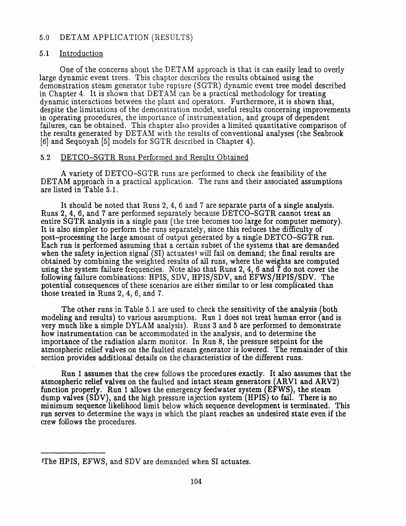
5.0 DETAM APPLICATION (RESULTS)

5.1 Introduction

One of the concerns about the DETAM approach is that is can easily lead to overlylarge dynamic event trees. This chapter describes the results obtained using thedemonstration steam generator tube rupture (SGTR) dynamic event tree model describedin Chapter 4. It is shown that DETAM can be a practical methodology for treatingdynamic interactions between the plant and operators. Furthermore, it is shown that,despite the limitations of the demonstration model, useful results concerning improvementsin operating procedures, the importance of instrumentation, and groups of dependentfailures, can be obtained. This chapter also provides a limited quantitative comparison ofthe results generated by DETAM with the results of conventional analyses (the Seabrook[6] and Sequoyah [5] models for SGTR described in Chapter 4).

5.2 DETCO-SGTR Runs Performed and Results Obtained

A variety of DETCO-SGTR runs are performed to check the feasibility of theDETAM approach in a practical application. The runs and their associated assumptionsare listed in Table 5.1.

It should be noted that Runs 2, 4, 6 and 7 are separate parts of a single analysis.Runs 2, 4, 6, and 7 are performed separately because DETCO-SGTR cannot treat anentire SGTR analysis in a single pass (the tree becomes too large for computer memory).It is also simpler to perform the runs separately, since this reduces the difficulty ofpost-processing the large amount of output generated by a single DETCO-SGTR run.Each run is performed assuming that a certain subset of the systems that are demandedwhen the safety injection signal (SI) actuates' will fail on demand; the final results areobtained by combining the weighted results of all runs, where the weights are computedusing the system failure frequencies. Note also that Runs 2, 4, 6 and 7 do not cover thefollowing failure combinations: HPIS, SDV, HPIS/SDV, and EFWS/HPIS/SDV. Thepotential consequences of these scenarios are either similar to or less complicated thanthose treated in Runs 2, 4, 6, and 7.

The other runs in Table 5.1 are used to check the sensitivity of the analysis (bothmodeling and results) to various assumptions. Run 1 does not treat human error (and isvery much like a simple DYLAM analysis). Runs 3 and 5 are performed to demonstratehow instrumentation can be accommodated in the analysis, and to determine theimportance of the radiation alarm monitor. In Run 8, the pressure setpoint for theatmospheric relief valves on the faulted steam generator is lowered. The remainder of thissection provides additional details on the characteristics of the different runs.

Run 1 assumes that the crew follows the procedures exactly. It also assumes that theatmospheric relief valves on the faulted and intact steam generators (ARV1 and ARV2)function properly. Run 1 allows the emergency feedwater system (EFWS), the steamdump valves (SDV), and the high pressure injection system (HPIS) to fail. There is nominimum sequence likelihood limit below which sequence development is terminated. Thisrun serves to determine the ways in which the plant reaches an undesired state even if thecrew follows the procedures.

'The HPIS, EFWS, and SDV are demanded when SI actuates.

104

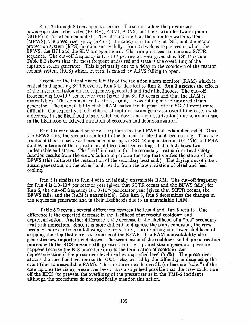
Runs 2 through 8 treat operator errors. These runs allow the pressurizerpower-operated relief valve (PORV), ARV1, ARV2, and the startup feedwater pump(SUFP) to fail when demanded. They also assume that the main feedwater systemMFWS), the pressurizer spray (SPRY), the safety injection signal (SI), and the reactor

protection system (RPS) function successfully. Run 2 develops sequences in which theEFWS, the HPI and the SDV are operational. This run produces the nominal SGTRsequence. The cut-off frequency is 1.0*10-6 per reactor year given that SGTR occurs.Table 5.2 shows that the most frequent undesired end state is the overfilling of theruptured steam generator. This is primarily due to a delay in the cooldown of the reactorcoolant system (RCS) which, in turn, is caused by ARV2 failing to open.

Except for the initial unavailability of the radiation alarm monitor (RAM) which iscritical in diagnosing SGTR events, Run 3 is identical to Run 2. Run 3 assesses the effectsof the instrumentation on the sequences generated and their likelihoods. The cut-offfrequency is 1.0*10-4 per reactor year (given that SGTR occurs and that the RAM isunavailable). The dominant end state is, again, the overfilling of the ruptured steamgenerator. The unavailability of the RAM makes the diagnosis of the SGTR event moredifficult. Consequently, the likelihood of ruptured steam generator overfill increases (witha decrease in the likelihood of successful cooldown and depressurization) due to an increasein the likelihood of delayed initiation of cooldown and depressurization.

Run 4 is conditioned on the assumption that the EFWS fails when demanded. Oncethe EFWS fails, the scenario can lead to the demand for bleed and feed cooling. Thus, theresults of this run serve as bases in comparing the SGTR application of DETAM and PRAstudies in terms of their treatment of bleed and feed cooling. Table 5.2 shows twoundesirable end states. The "red" indication for the secondary heat sink critical safetyfunction results from the crew's failure to perform the step that verifies the status of theEFWS (this initiates the restoration of the secondary heat sink). The drying out of intactsteam generators, on the other hand, results from the late initiation of bleed and feedcooling.

Run 5 is similar to Run 4 with an initially unavailable RAM. The cut-off frequencyfor Run 4 is 1.0*10-5 per reactor year (given that SGTR occurs and the EFWS fails); forRun 5, the cut-off frequency is 1.0*10-4 per reactor year (given that SGTR occurs, theEFWS fails, and the RAM is unavailable). Like Run 3, Run 5 determines the changes inthe sequences generated and in their likelihoods due to an unavailable RAM.

Table 5.2 reveals several differences between the Run 4 and Run 5 results. Onedifference is the expected decrease in the likelihood of successful cooldown anddepressurization. Another difference is the decrease in the likelihood of a "red" secondaryheat sink indication. Since it is more difficult to diagnose the plant condition, the crewbecomes more cautious in following the procedures, thus resulting in a lower likelihood ofskipping the step that checks the status of the EFWS. The RAM unavailability alsogenerates new important end states. The termination of the cooldown and depressurizationprocess with the RCS pressure still greater than the ruptured steam generator pressurehappens because the E-3 procedure directs the termination of cooldown anddepressurization if the pressurizer level reaches a specified level (75%). The pressurizerattains the specified level due to the C&D delay caused by the difficulty in diagnosing theevent (due to unavailable RAM). The pressurizer could overfill (or become "solid") if thecrew ignores the rising pressurizer level. It is also judged possible that the crew could turnoff the HPIS (to prevent the overfilling of the pressurizer as in the TMI-2 incident)although the procedures do not specifically mention this action.

105

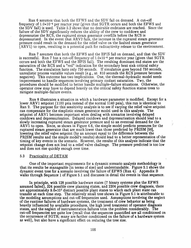
Run 6 assumes that both the EFWS and the SDV fail on demand. A cut-offfrequency of 1.0*10-4 per reactor year (given that SGTR occurs and both the EFWS andthe SDV fail) is used. Table 5.2 shows that no desirable endstates are reached. Since thefailure of the SDV significantly reduces the ability of the crew to cooldown anddepressurize the RCS, the ruptured steam generator overfills before the RCS isdepressurized. In the event that ARV2 fails, the increase in the ruptured steam generatorpressure could result in the demand for the relief valve on the faulted steam generator(ARVI) to open, resulting in a potential path for radioactivity release to the environment.

Run 7 assumes that both the EFWS and the HPIS fail on demand, and that the SDVis successful. Run 7 has a cut-off frequency of 1.0*10-4 per reactor year (given that SGTRoccurs and both the EFWS and the HPIS fail). The resulting dominant end states are thesaturation of the RCS and a "red" indication for the secondary heat sink critical safetyfunction. The simulation lasts only 750 seconds. If simulation goes beyond 750 seconds,unrealistic process variable values result (e.g., at 810 seconds the RCS pressure becomesnegative). This outcome has two implications. One, the thermal-hydraulic model needsimprovement to handle sequences involving primary coolant saturation. Two, theprocedures should be modified to better handle multiple-failure situations. Otherwise, theoperator crew may have to depend heavily on the critical safety function status trees tomitigate multiple-failure events.

Run 8 illustrates a situation in which a hardware parameter is modified. Except for alower ARV1 setpoint (1100 psia instead of the normal 1140 psia), this run is identical toRun 2. The purpose for this sensitivity analysis is to see if varying the relief valve setpointcan compensate for the simplistic steam generator model used in this analysis. Thesetpoint of ARV1 becomes important when dealing with scenarios involving delayedcooldown and depressurization. Delayed cooldown and depressurization should lead to aslowly increasing ruptured steam generator pressure and to an eventual demand for theARV1 to open. Since, as shown in Figure 4.6, the simple model predicts pressures for theruptured steam generator that are much lower than those predicted by PRISM [56],lowering the relief valve setpoint (by an amount equal to the difference between thePRISM results and the simple model's results) should lead to a better representation of thetiming of key events in the scenario. However, the results of this analysis indicate that thesetpoint change does not lead to a relief valve challenge. The pressure predicted is too lowand does not rise quickly enough over time.

5.3 Practicality of DETAM

One of the important requirements for a dynamic scenario analysis methodology isthat its results be manageable (in terms of size) and understandable. Figure 5.1 shows thedynamic event tree for a scenario involving the failure of EFWS (Run 4). Appendix Bwalks through Sequence 1 of Figure 5.1 and discusses in detail the events in that sequence.

In principle, with 128 possible hardware states (7 binary systems plus the EFWSassumed failed), 324 possible crew planning states, and 2304 possible crew diagnosis, thereare approximately 9.6*107 distinct possible plant states to which each plant state cantransfer at each time step. The relatively small tree shown in Figure 5.1 is attributable tothe modeling assumptions and cut-off frequencies used. Assumptions involving the neglectof the runtime failures of hardware systems, the treatment of crew behavior as beingheavily influenced by available procedures, the high level treatment of operator diagnosisstates, and the neglect of instrumentation failures trim the problem considerably. Thecut-off frequencies are quite low (recall that the sequences quantified are all conditioned onthe occurrence of SGTR; many are further conditioned on the failure of a hardware systemas well), but also have a significant effect on reducing the tree size.

106

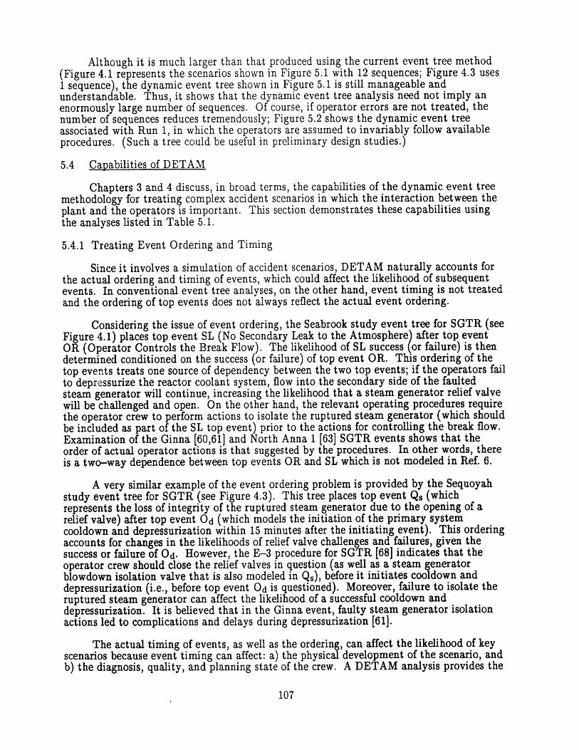
Although it is much larger than that produced using the current event tree method(Figure 4.1 represents the scenarios shown in Figure 5.1 with 12 sequences; Figure 4.3 uses1 sequence), the dynamic event tree shown in Figure 5.1 is still manageable andunderstandable. Thus, it shows that the dynamic event tree analysis need not imply anenormously large number of sequences. Of course, if operator errors are not treated, thenumber of sequences reduces tremendously; Figure 5.2 shows the dynamic event treeassociated with Run 1, in which the operators are assumed to invariably follow availableprocedures. (Such a tree could be useful in preliminary design studies.)

5.4 Capabilities of DETAM

Chapters 3 and 4 discuss, in broad terms, the capabilities of the dynamic event treemethodology for treating complex accident scenarios in which the interaction between theplant and the operators is important. This section demonstrates these capabilities usingthe analyses listed in Table 5.1.

5.4.1 Treating Event Ordering and Timing

Since it involves a simulation of accident scenarios, DETAM naturally accounts forthe actual ordering and timing of events, which could affect the likelihood of subsequentevents. In conventional event tree analyses, on the other hand, event timing is not treatedand the ordering of top events does not always reflect the actual event ordering.

Considering the issue of event ordering, the Seabrook study event tree for SGTR (seeFigure 4.1) places top event SL (No Secondary Leak to the Atmosphere) after top eventOR (Operator Controls the Break Flow). The likelihood of SL success (or failure) is thendetermined conditioned on the success (or failure) of top event OR. This ordering of thetop events treats one source of dependency between the two top events; if the operators failto depressurize the reactor coolant system, flow into the secondary side of the faultedsteam generator will continue, increasing the likelihood that a steam generator relief valvewill be challenged and open. On the other hand, the relevant operating procedures requirethe operator crew to perform actions to isolate the ruptured steam generator (which shouldbe included as part of the SL top event) prior to the actions for controlling the break flow.Examination of the Ginna [60,61] and North Anna 1 [63] SGTR events shows that theorder of actual operator actions is that suggested by the procedures. In other words, thereis a two-way dependence between top events OR and SL which is not modeled in Ref. 6.

A very similar example of the event ordering problem is provided by the Sequoyahstudy event tree for SGTR (see Figure 4.3). This tree places top event Qs (whichrepresents the loss of integrity of the ruptured steam generator due to the opening of arelief valve) after top event Od (which models the initiation of the primary systemcooldown and depressurization within 15 minutes after the initiating event). This orderingaccounts for changes in the likelihoods of relief valve challenges and failures, given thesuccess or failure of Od. However, the E-3 procedure for SGTR [68] indicates that theoperator crew should close the relief valves in question (as well as a steam generatorblowdown isolation valve that is also modeled in Qs), before it initiates cooldown anddepressurization (i.e., before top event Od is questioned). Moreover, failure to isolate theruptured steam generator can affect the likelihood of a successful cooldown anddepressurization. It is believed that in the Ginna event, faulty steam generator isolationactions led to complications and delays during depressurization [61].

The actual timing of events, as well as the ordering, can affect the likelihood of keyscenarios because event timing can affect: a) the physical development of the scenario, andb) the diagnosis, quality, and planning state of the crew. A DETAM analysis provides the

107

timing of events as a natural intermediate output. Moreover, since event timing can varyfrom scenario to scenario, DETAM can provide the distributions for the occurrence timesof key events. Table 5.3, for example, displays the distribution of the time to startcooldown and depressurization (for Run 2 of Table 5.1). This information can be useful forconventional PRA analyses, which compare the time required to perform certain actionsagainst the time available (e.g., [14]), and for risk management.

5.4.2 Operator Error Forms

As discussed in Section 4.5.6, the DETAM approach provides a natural frameworkfor analyzing a variety of diagnosis-related and planning-related error forms:

0 Improper diagnosis0 Overly quick procedure following0 Overly slow procedure following9 Improper procedure following0 Looping0 Errors of commission

The dynamic event tree treatment of the first five forms are demonstrated by theDETAM application model described in Chapter 4. Figure 5.3, a reduced Version ofFigure 5.1, illustrates these various error forms. For example, Sequences 3 through 5 resultfrom late initiation of bleed and feed cooling. Sequence 5 models a situation where theoperator crew fails to start the process before the intact steam generators boil dry. The"looping" error form refers to situations where the cues needed to allow transfer to a newprocedure are not available (or are not observed by the operator crew). In such cases, it isassumed that the operator crew remains in the procedure (i.e., the operators are treated asautomatons). Sequence 7 represents a situation where looping could occur if the secondaryheat sink safety function indicator does not alarm; here, the procedures are written in sucha way that a crew blindly following procedures will remain in the current procedure untilsteam generator dryout occurs. A final error form, not shown in Figure 5.3, is the so-called"error of commission." This error is closely associated with misdiagnosis errors, althoughthe occurrence of a misdiagnosis does not always result in an error of commission. SinceDETAM allows branching based on misdiagnosis, it can account for any erroneous action,e.g. turning off the HPIS when it is actually needed, that occurs after the initialmisdiagnosis. Put another way, DETAM allows the analyst to provide a causal model forerrors of commission. This will aid the quantification of such errors, and will also aid thedevelopment of specific schemes to reduce the impact of the more significant errors.

5.4.3 Consequences of Operator Actions

One of the problems with the current event tree method, as discussed in Chapter 1, isthat dynamic operator actions during an accident scenario are treated in a binary fashion,much the same as hardware performance. Operator action top events (e.g., OR inFigure 4.1), which can include many separate tasks, are either successful or failed. Thisapproach does not treat the fact that top event success (and failure) can usually beachieved in many different ways, and the manner in which success (failure) is achieved canaffect the likelihood of the success (failure) of subsequent top events. DETAM, on theother hand, treats a spectrum of detailed operator behaviors and actions (state changes),some of which may be classified as "successes," and some of which may be classified as"failures." This treatment enables a causal (although not necessarily deterministic)analysis of the consequences of the remainder of the sequence following the action.

108

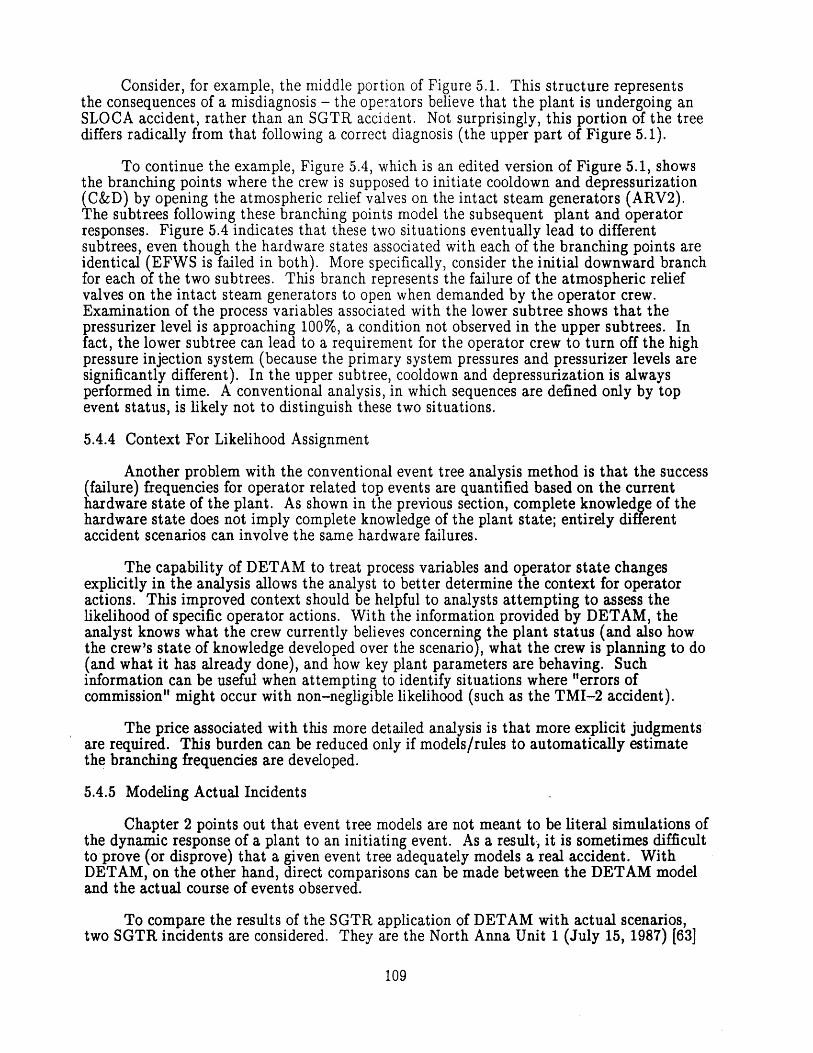
Consider, for example, the middle portion of Figure 5.1. This structure representsthe consequences of a misdiagnosis - the operators believe that the plant is undergoing anSLOCA accident, rather than an SGTR accident. Not surprisingly, this portion of the treediffers radically from that following a correct diagnosis (the upper part of Figure 5.1).

To continue the example, Figure 5.4, which is an edited version of Figure 5.1, showsthe branching points where the crew is supposed to initiate cooldown and depressurization(C&D) by opening the atmospheric relief valves on the intact steam generators (ARV2).The subtrees following these branching points model the subsequent plant and operatorresponses. Figure 5.4 indicates that these two situations eventually lead to differentsubtrees, even though the hardware states associated with each of the branching points areidentical (EFWS is failed in both). More specifically, consider the initial downward branchfor each of the two subtrees. This branch represents the failure of the atmospheric reliefvalves on the intact steam generators to open when demanded by the operator crew.Examination of the process variables associated with the lower subtree shows that thepressurizer level is approaching 100%, a condition not observed in the upper subtrees. Infact, the lower subtree can lead to a requirement for the operator crew to turn off the highpressure injection system (because the primary system pressures and pressurizer levels aresignificantly different). In the upper subtree, cooldown and depressurization is alwaysperformed in time. A conventional analysis, in which sequences are defined only by topevent status, is likely not to distinguish these two situations.

5.4.4 Context For Likelihood Assignment

Another problem with the conventional event tree analysis method is that the success(failure) frequencies for operator related top events are quantified based on the currenthardware state of the plant. As shown in the previous section, complete knowledge of thehardware state does not imply complete knowledge of the plant state; entirely differentaccident scenarios can involve the same hardware failures.

The capability of DETAM to treat process variables and operator state changesexplicitly in the analysis allows the analyst to better determine the context for operatoractions. This improved context should be helpful to analysts attempting to assess thelikelihood of specific operator actions. With the information provided by DETAM, theanalyst knows what the crew currently believes concerning the plant status (and also howthe crew's state of knowledge developed over the scenario), what the crew is planning to do(and what it has already done), and how key plant parameters are behaving. Suchinformation can be useful when attempting to identify situations where "errors ofcommission" might occur with non-negligible likelihood (such as the TMI-2 accident).

The price associated with this more detailed analysis is that more explicit judgmentsare required. This burden can be reduced only if models/rules to automatically estimatethe branching frequencies are developed.

5.4.5 Modeling Actual Incidents

Chapter 2 points out that event tree models are not meant to be literal simulations ofthe dynamic response of a plant to an initiating event. As a result, it is sometimes difficultto prove (or disprove) that a given event tree adequately models a real accident. WithDETAM, on the other hand, direct comparisons can be made between the DETAM modeland the actual course of events observed.

To compare the results of the SGTR application of DETAM with actual scenarios,two SGTR incidents are considered. They are the North Anna Unit 1 (July 15, 1987) [63]

109

and the Ginna (January 25, 1982) [64] SGTR events. Tables 5.4 and 5.5 show thechronologies of important events during the North Anna Unit 1 and the Ginna incidents,respectively. Figure 5.5 shows a dynamic event tree for the nominal condition (i.e., allsystems work as expected and required) and traces the North Anna and the Ginnaincidents.

It can be seen that the North Anna Unit 1 sequence of events matches the DETAMtree better than Ginna sequence. The reason for this is that the North Anna crew followedthe procedures more closely than the Ginna crew. One operator error in the Ginna incidentwas the delayed tripping of the reactor coolant pumps (RCPs), which in effect delayed thedepressurization. Figure 5.5 does not show the delayed tripping of the RCPs because thedemonstration DETAM analysis does not explicitly model the RCPs.

It can also be seen that the DETAM predicted event occurrence times differ fromthose of the actual incidents. For example, the North Anna trace reaches depressurizationearlier than the DETAM nominal scenario. This timing difference is partially due to thedifferences in hardware systems, e.g. the number and volumes of steam generators, and inthe details of the incident. In the North Anna 1 incident, the crew performed a turbineload reduction. The reduction of turbine load slowed down the primary pressure decrease,thus delaying the automatic reactor trip. In fact, the crew manually tripped the reactor.

It is reasonable to expect that as long as a DETAM model includes the systems andoperator actions involved in an actual event, it can capture much (if not all) of theimportant qualitative behavior of the incident. However, the accuracy of the predictedtiming of events will depend heavily on the accuracy of the physical model used. Further,as discussed earlier, inaccuracies in physical model predictions can also lead to scenariopredictions that are qualitatively incorrect.

5.5 Comparison of DETAM and Conventional PRA Results

Because of the differences in scope and sequence modeling assumptions between theDETAM and conventional SGTR analyses, and because there is considerable uncertainty inthe detailed branching frequency assignments made in the DETAM analysis, a directquantitative comparison of results is difficult. This section provides a limited comparisonof the DETAM, Seabrook, and Sequoyah analysis results. Differences in selected end stateand partial sequence frequencies are discussed.

5.5.1 End State Comparison

Table 5.6 shows the likelihoods of two end states and the dominant se uences leadingto those end states predicted by the DETAM, Seabrook [6], and Sequoyah [51 models. Thetwo end states are ruptured steam generator overfill and failure of bleed and feed cooling.The former state is undesirable, since it leads to the release of radioactive coolant to theenvironment. On the other hand, it does not guarantee the occurrence of core damage.The latter state does eventually lead to core damage (unless other sources of heat removalare found).

Comparing the dominant sequences leading to the steam generator overfill end state,the Seabrook analysis identifies the failure to control break flow (OR) and the occurrenceof a secondary side leak (SL), whereas the Sequoyah analysis identifies the failure tocooldown and depressurize (Od) followed by the loss of steam generator integrity (Qs).Both of these sequences are quite similar. Note, however, that although the Seabrookanalysis predicts a higher frequency of occurrence, it does not assume that core damagenecessarily ensues. On the other hand, the Sequoyah analysis assumes (with substantially

110

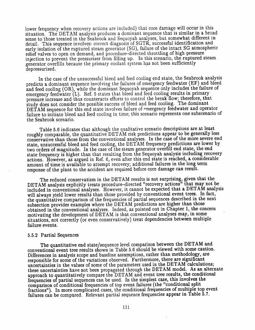
lower frequency when recovery actions are included) that core damage will occur in thissituation. The DETAM analysis produces a dominant sequence that is similar in a broadsense to those treated in the Seabrook and Sequoyah analyses, but somewhat different indetail. This sequence involves: correct diagnosis of SGTR, successful identification andearly isolation of the ruptured steam generator (SG), failure of the intact SG atmosphericrelief valves to open on demand, and procedure-directed throttling of high pressureinjection to prevent the pressurizer from filling up. In this scenario, the ruptured steamgenerator overfills because the primary coolant system has not been sufficientlydepressurized.

In the case of the unsuccessful bleed and feed cooling end state, the Seabrook analysispredicts a dominant sequence involving the failures of emergency feedwater (EF) and bleedand feed cooling (OR), while the dominant Sequoyah sequence only includes the failure ofemergency feedwater (L). Ref. 5 states that bleed and feed cooling results in primarypressure increase and thus counteracts efforts to control the break flow; therefore, thatstudy does not consider the possible success of bleed and feed cooling. The dominantDETAM sequence for this end state involves failure of -mergency feedwater and operatorfailure to initiate bleed and feed cooling in time; this scenario represents one subscenario ofthe Seabrook scenario.

Table 5.6 indicates that although the qualitative scenario descriptions are at leastroughly comparable, the quantitative DETAM risk predictions appear to be generally lessconservative than those from the conventional analyses. In the case of the more severe endstate, unsuccessful bleed and feed cooling, the DETAM frequency predictions are lower bytwo orders of magnitude. In the case of the steam generator overfill end state, the endstate frequency is higher than that resulting from the Sequoyah analysis including recoveryactions. However, as argued in Ref. 6, even after this end state is reached, a considerableamount of time is available to attempt recovery; additional failures in the long termresponse of the plant to the accident are required before core damage can result.

The reduced conservatism in the DETAM results is not surprising, given that theDETAM analysis explicitly treats procedure-directed "recovery actions" that may not beincluded in conventional analyses. However, it cannot be expected that a DETAM analysiswill always yield lower results than those provided by conventional event trees. In fact,the quantitative comparison of the frequencies of partial sequences described in the nextsubsection provides examples where the DETAM predictions are higher than thoseobtained in the conventional analyses. Indeed, as pointed out in Chapter 1, the concernmotivating the development of DETAM is that conventional analyses may, in somesituations, not correctly (or even conservatively) treat dependencies between multiplefailure events.

5.5.2 Partial Sequences

The quantitative end state/sequence level comparison between the DETAM andconventional event tree results shown in Table 5.6 should be viewed with some caution.Differences in analysis scope and baseline assumptions, rather than methodology, areresponsible for some of the variations observed. Furthermore, there are significantuncertainties in the values of some of the parameters used in the DETAM calculations;these uncertainties have not been propagated through the DETAM model. As an alternateapproach to quantitatively compare the DETAM and event tree results, the conditionalfrequencies of partial sequences can be used. In the simplest case, this involves thecomparison of conditional frequencies of top event failures (the "conditional splitfractions"). In more complicated cases, the conditional frequencies of multiple top eventfailures can be compared. Relevant partial sequence frequencies appear in Table 5.7.

111

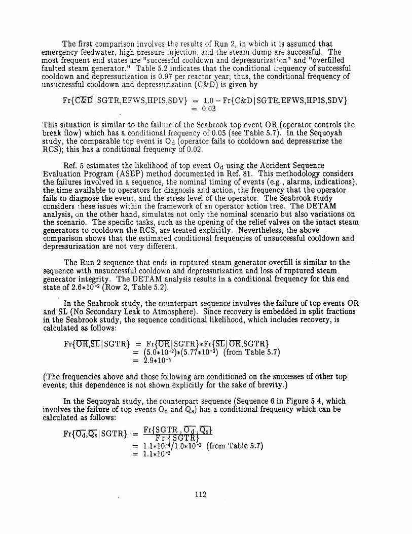
The first comparison involves the results of Run 2, in which it is assumed thatemergency feedwater, high pressure injection, and the steam dump are successful. Themost frequent end states are "successful cooldown and depressurizat'on" and "overfilledfaulted steam generator." Table 5.2 indicates that the conditional I:equency of successfulcooldown and depressurization is 0.97 per reactor year; thus, the conditional frequency ofunsuccessful cooldown and depressurization (C&D) is given by

Fr{CU ISGTR,EFWS,HPIS,SDV} = 1.0 - Fr{C&D I SGTR,EFWS,HPIS,SDV}= 0.03

This situation is similar to the failure of the Seabrook top event OR (operator controls thebreak flow) which has a conditional frequency of 0.05 (see Table 5.7). In the Sequoyahstudy, the comparable top event is Od (operator fails to cooldown and depressurize theRCS); this has a conditional frequency of 0.02.

Ref. 5 estimates the likelihood of top event Od using the Accident SequenceEvaluation Program (ASEP) method documented in Ref. 81. This methodology considersthe failures involved in a sequence, the nominal timing of events (e.g., alarms, indications),the time available to operators for diagnosis and action, the frequency that the operatorfails to diagnose the event, and the stress level of the operator. The Seabrook studyconsiders these issues within the framework of an operator action tree. The DETAManalysis, on the other hand, simulates not only the nominal scenario but also variations onthe scenario. The specific tasks, such as the opening of the relief valves on the intact steamgenerators to cooldown the RCS, are treated explicitly. Nevertheless, the abovecomparison shows that the estimated conditional frequencies of unsuccessful cooldown anddepressurization are not very different.

The Run 2 sequence that ends in ruptured steam generator overfill is similar to thesequence with unsuccessful cooldown and depressurization and loss of ruptured steamgenerator integrity. The DETAM analysis results in a conditional frequency for this endstate of 2.6*10-2 (Row 2, Table 5.2).

In the Seabrook study, the counterpart sequence involves the failure of top events ORand SL (No Secondary Leak to Atmosphere). Since recovery is embedded in split fractionsin the Seabrook study, the sequence conditional likelihood, which includes recovery, iscalculated as follows:

Fr{0U,STSGTR} = Fr{URJSGTR}*Fr{ST |U,SGTR}(5.0*10-2)*(5.77*10-3) (from Table 5.7)

= 2.9*10-4

(The frequencies above and those following are conditioned on the successes of other topevents; this dependence is not shown explicitly for the sake of brevity.)

In the Sequoyah study, the counterpart sequence (Sequence 6 in Figure 5.4, whichinvolves the failure of top events Od and Q,) has a conditional frequency which can becalculated as follows:

Fr{UO7,I SGTR} = Fr{ QsGR)0= 1.1*10 4/1.0*10 2 (from Table 5.7)= 1.1*10-2

112

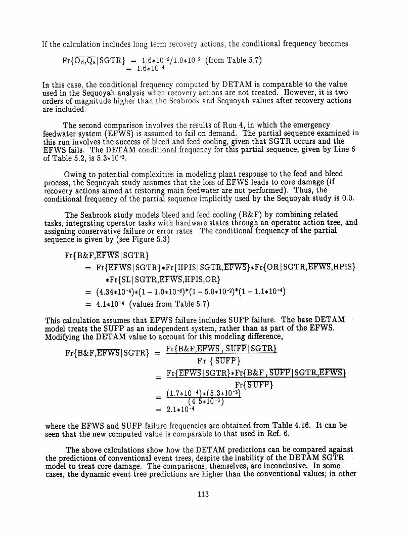
If the calculation includes long term recovery actions, the conditional frequency becomes

Fr{~O7,jSGTR} = 1.6*10-6/1.0*10-2 (from Table 5.7)= 1.6*10-4

In this case, the conditional frequency computed by DETAM is comparable to the valueused in the Sequoyah analysis when recovery actions are not treated. However, it is twoorders of magnitude higher than the Seabrook and Sequoyah values after recovery actionsare included.

The second comparison involves the results of Run 4, in which the emergencyfeedwater system (EFWS) is assumed to fail on demand. The partial sequence examined inthis run involves the success of bleed and feed cooling, given that SGTR occurs and theEFWS fails. The DETAM conditional frequency for this partial sequence, given by Line 6of Table 5.2, is 5.3*10-3.

Owing to potential complexities in modeling plant response to the feed and bleedprocess, the Sequoyah study assumes that the loss of EFWS leads to core damage (ifrecovery actions aimed at restoring main feedwater are not performed). Thus, theconditional frequency of the partial sequence implicitly used by the Sequoyah study is 0.0.

The Seabrook study models bleed and feed cooling (B&F) by combining relatedtasks, integrating operator tasks with hardware states through an operator action tree, andassigning conservative failure or error rates. The conditional frequency of the partialsequence is given by (see Figure 5.3)

Fr{B&F,EFWSISGTR}

= Fr{EFWISGTR}*Fr{HPIS ISGTR,EFW5}*Fr{ORISGTR,EFWS,HPIS}*Fr{SL I SGTR,EFWS,HPIS,OR}

= (4.34*10-4)*(1 - 1.0*10-6)*(1 - 5.0*10-2)*(i - 1.1*10-4)

= 4.1*10-4 (values from Table 5.7)

This calculation assumes that EFWS failure includes SUFP failure. The base DETAMmodel treats the SUFP as an independent system, rather than as part of the EFWS.Modifying the DETAM value to account for this modeling difference,

Fr{B&F,EFWSISGTR} = Fr{B&F,EFW,U1FFISGTR}Fr {SUFF}

Fr{EFW5i SGTR}*Fr{B&F , SUFPSGTR,EFWS}Fr{~SUFF}

(1.7*10 -4)*(5.3*10-3)(4.5*10-3)

= 2.1*10-4

where the EFWS and SUFP failure frequencies are obtained from Table 4.16. It can beseen that the new computed value is comparable to that used in Ref. 6.

The above calculations show how the DETAM predictions can be compared againstthe predictions of conventional event trees, despite the inability of the DETAM SGTRmodel to treat core damage. The comparisons, themselves, are inconclusive. In somecases, the dynamic event tree predictions are higher than the conventional values; in other

113

cases, the dynamic event tree values are lower. Until the weaknesses in the currentDETAM SGTR model are rectified, definitive conclusions concerning the relative accuracyof the two methods cannot be drawn 2.

5.6 Other Results

Although the SGTR analysis documented in this report is constructed to demonstratethe DETAM approach, and although the demonstration model has a number of weaknessesthat affect the accuracy of its predictions, a number of useful results are obtained from thisanalysis. These results cover the current operating procedures pertaining to SGTR, theimportance of instrumentation in this accident, and dependencies between events.

5.6.1 SGTR Procedures

In a DETAM application to accident analysis, it is necessary for the analyst toexplicitly model the written procedures. This modeling provides the primary basis for thedetailed definitions of the possible crew planning states and the transitions between states.As a byproduct of the modeling process, two potential weaknesses in the current SGTRprocedures have been identified.

The first potential weakness is the absence of steps in the E-3 (SGTR) procedurewhich will allow the operator crew to transfer to the FR-H.1 (loss of secondary heat sink,or LSHS) procedure when the emergency feedwater system (EFWS) fails and the crewinitially fails to recognize LSHS (Sequence 7 of Figure 5.6). Without these steps, the crewmust rely on a warning from the Safety Parameter Display System (the failure of EFWS, ifunmitigated, eventually leads to the SPDS secondary heat sink indicator turning "red" or"orange" and alerts the Shift Technical Advisor that the plant is not responding asdesired). Further, if the SPDS does not alarm, the procedures are written in such a waythat a crew blindly following procedures could remain in the current procedure until theintact steam generators dry out. If the time delay associated with the activation of theSPDS alarm is important, or if the likelihood of SPDS failure is significant (neither issue isinvestigated in this analysis), the current procedure may require some modification toensure that the crew transfers to FR-H.1 in a timely manner.

A second potential weakness arises when both the EFWS and the startup feedwaterpump (SUFP) fail during an SGTR. In this condition, the emphasis in the FR-H.1procedure is on the restoration of the secondary side cooling through bleed and feed cooling.The procedure does not mention the need to mitigate the SGTR. Thus, it seems that thecrew will again have to depend on the SPDS critical safety function status trees in order tomitigate the SGTR situation. Although the crew may be trained for this multiple failurescenario, the explicit treatment of these situations in the procedures could help the crewbetter handle actual events.

In general, it appears that the provision of redundancy in a few spots in theprocedure, through the addition of backup checks for key symptoms and of additionalprocedure transfer steps, could improve the effectiveness of procedures. A DETAManalysis can identify: if changes are needed, where the changes should be made, and if theadded redundancy provided by these changes outweighs the associated negative effects

2Differences also arise because a different groups of analysts are developing the branchingprobabilities for the DETAM and conventional analyses. More comparable, andinteresting, results might be obtained using a single group of analysts to use bothapproaches to address a given problem.

114

(e.g., possible increases in crew response times).

5.6.2 Impact of Instrumentation

Instrumentation, being the primary link between the operators and the plant,intuitively is an important factor in the development of an accident scenario. Faulty orfailed instrumentation could lead to an incorrect diagnosis of the plant condition and henceerroneous crew actions. For example, instrumentation readings serve as primary bases notonly in selecting the procedure to follow but also in making decisions within a procedure(e.g., whether to initiate bleed and feed cooling or not). Despite this importance,instrumentation failures are rarely treated in conventional PRA studies.

To show the impact of instrumentation failures, consider Runs 2 and 3, listed inTable 5.1; the only difference between these two is that the RAM is assumed failed in thelatter. The results of these runs are provided in Table 5.2. It can be seen that when theRAM is failed, the conditional frequency of successful cooldown and depressurization (givenSGTR) drops from 0.97 to 0.89. Furthermore, the conditional likelihood of ruptured steamgenerator overfill increases from 0.026, in the case of Run 2, to 0.088 in Run 3.

Runs 4 and 5 provide a similar comparison. In both cases, the EFWS is assumedfailed. In Run 5, the RAM is also assumed to be failed. Here, the conditional frequency ofsuccessful cooldown and depressurization drops from 0.89 (Run 4) to 0.72 (Run 5). Notethat in Run 5, the unavailable RAM also leads to the generation of new sequences, asdiscussed in Section 5.2.

Thus, the DETAM analysis of SGTR not only confirms the importance of aparticular piece of instrumentation (the radiation alarm monitor, or RAM), it also providesa quantitative measure for the risk associated with the failure of the RAM. Furthermore,it can be seen how the analysis can be extended to treat more general sets ofinstrumentation failures. Thus, the dynamic event tree approach provides a usefulframework for evaluating the risk significance of instrumentation.

5.6.3 Dependent Failures

As discussed in Chapter 1, the identification of dependent system failures is key toquantitative risk assessment. The DETAM approach explicitly treats human and processvariable related causal links between failure events. Thus, it can identify groups ofdependent failures that are not necessarily treated by conventional event tree analyses.

One direct example is provided by the discussion on the ordering of failure events inSection 5.4.1. It is shown that there is a two-way dependence between the actionsassociated with depressurizing the reactor coolant system (top events OR and Od in theSeabrook and Sequoyah studies, respectively) and the integrity of the faulted steamgenerator (top events SL and Qs in the Seabrook and Sequoyah studies, respectively). Theconventional event tree analyses treat the dependence of SL/Qs on OR/Od, but not thedependence of OR/Od on SL/Qs. DETAM, by virtue of its simulation-based approach,treats the two-way dependence directly.

A more interesting example of a dependent failure group is provided by the earlierdiscussion on instrumentation failures. As stated in Section 5.6.2, the failure of theradiation alarm monitor (RAM) increases the difficulty of correctly diagnosing the SGTR,and increases the likelihood of faulted steam generator overfill. In other words, there is alink between the failures of the RAM and of the faulted steam generator atmospheric reliefvalves (considered as part of the top event SL in the Seabrook SGTR model, and as part of

115

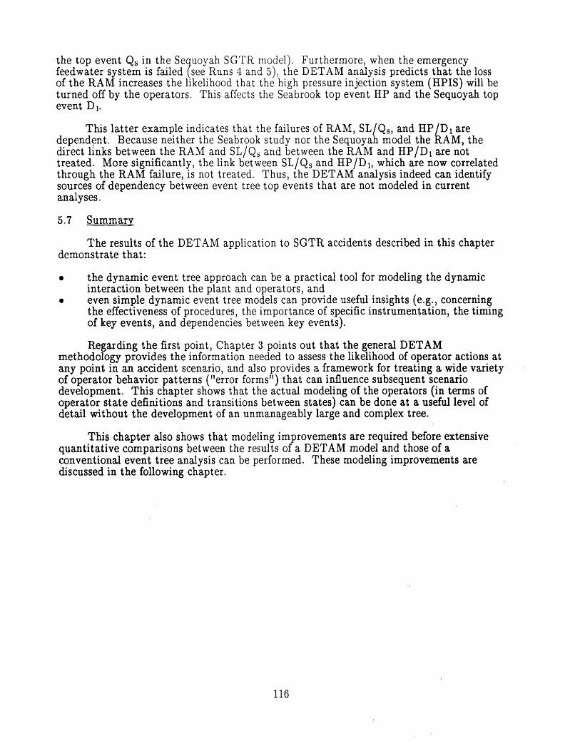
the top event Qs in the Sequoyah SGTR model). Furthermore, when the emergencyfeedwater system is failed (see Runs 4 and 5), the DETAM analysis predicts that the lossof the RAM increases the likelihood that the high pressure injection system (HPIS) will beturned off by the operators. This affects the Seabrook top event HP and the Sequoyah topevent D1.

This latter example indicates that the failures of RAM, SL/Qs, and HP/Di aredependent. Because neither the Seabrook study nor the Sequoyah model the RAM, thedirect links between the RAM and SL/Qs and between the RAM and HP/DI are nottreated. More significantly, the link between SL/Qs and HP/D 1 , which are now correlatedthrough the RAM failure, is not treated. Thus, the DETAM analysis indeed can identifysources of dependency between event tree top events that are not modeled in currentanalyses.

5.7 Summary

The results of the DETAM application to SGTR accidents described in this chapterdemonstrate that:

0 the dynamic event tree approach can be a practical tool for modeling the dynamicinteraction between the plant and operators, and

0 even simple dynamic event tree models can provide useful insights (e.g., concerningthe effectiveness of procedures, the importance of specific instrumentation, the timingof key events, and dependencies between key events).

Regarding the first point, Chapter 3 points out that the general DETAMmethodology provides the information needed to assess the likelihood of operator actions atany point in an accident scenario, and also provides a framework for treating a wide varietyof operator behavior patterns ("error forms") that can influence subsequent scenariodevelopment. This chapter shows that the actual modeling of the operators (in terms ofoperator state definitions and transitions between states) can be done at a useful level ofdetail without the development of an unmanageably large and complex tree.

This chapter also shows that modeling improvements are required before extensivequantitative comparisons between the results of a DETAM model and those of aconventional event tree analysis can be performed. These modeling improvements arediscussed in the following chapter.

116

Table 5.1 - DETAM Runs Performed

Run # Unavailable Systems Allowed to Fail Cut-off Operator ErrorSystem Frequency* 'Treated ?

1 None EFWS, SDV, HPI 0.0 No2 None PORV,ARV1,ARV2,SUFP, 1.E-6 Yes

EFWS, HPI,SDV3 Rad Alarm PORV,ARV1,ARV2,SUFP, 1.E-4 Yes

Monitor EFWS, HPI,SDV4 EFWS PORV,ARV1,ARV2,SUFP, 1.E-5 Yes

HPI,SDV5 EFWS, Rad PORV,ARV1,ARV2,SUFP, 1.E-4 Yes

Alarm Monitor HPI,SDV6 EFWS, SDV PORV,ARV1,ARV2,SUFP,HPI 1.E-4 Yes7 EFWS,HPI PORV,ARV1,ARV2,SUFP,SDV 1.E-4 Yes8 None (lower PORV,ARV1,ARV2,SUFP, 1.E-6 Yes

ARVI setpoint) EFWS, HPI,SDV I

*Cut-off frequencies are conditional on the unavailability of systemscolumn 2 and on the occurrence of SGTR

indicated in

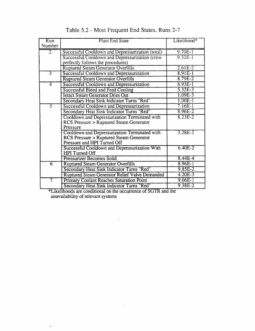
Table 5.2 - Most Frequent End States, Runs 2-7

Run Plant End State Likelihood*Number

2 Successful Cooldown and Depressurization (total) 9.70E-1Successful Cooldown and Depressurization (crew 9.32E-1perfectly follows the procedures)Ruptured Steam Generator Overfills 2.61E-2

3 Successful Cooldown and Depressurization 8.91E-1Ruptured Steam Generator Overfills 8.79E-2

4 Successful Cooldown and Depressurization 8.93E- 1Successful Bleed and Feed Cooling 5.32E-3Intact Steam Generator Dries Out 1.09E-3Secondary Heat Sink Indicator Turns "Red" 1.OOE- 1

5 Successful Cooldown and Depressurization 7.16E- 1Secondary Heat Sink Indicator Turns "Red" 8.96E-2Cooldown and Depressurization Terminated with 8.23E-2RCS Pressure > Ruptured Steam GeneratorPressureCooldown and Depressurization Terminated with 3.28E-2RCS Pressure > Ruptured Steam GeneratorPressure and HPI Turned OffSuccessful Cooldown and Depressurization With 6.40E-2HPI Turned OffPressurizer Becomes Solid 8.44E-4

6 Ruptured Steam Generator Overfills 8.96E- 1Secondary Heat Sink Indicator Turns "Red" 9.85E-2Ruptured Steam Generator Relief Valve Demanded 4.20E-3

7 Primary Coolant Reaches Saturation Point 9.06E- 1Secondary Heat Sink Indicator Turns "Red" 9.38E-2

*Likelihoods are conditional on the occurrence of SGTR and theunavailability of relevant systems

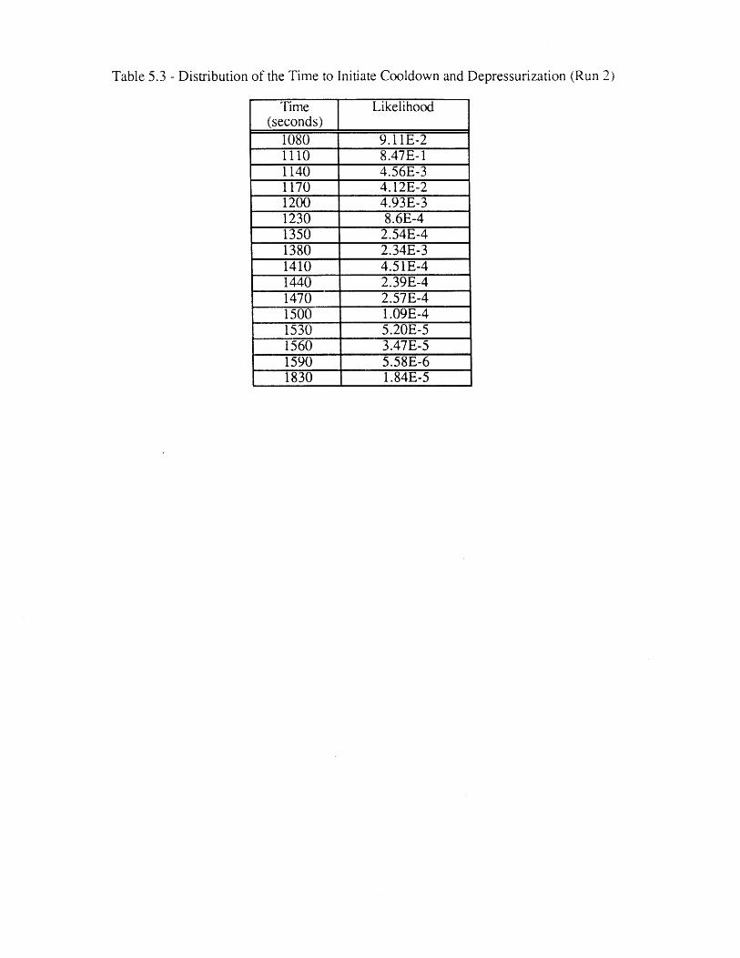
Table 5.3 - Distribution of the Time to Initiate Cooldown and Depressurization (Run 2)

Time Likelihood(seconds)

1080 9.11E-21110 8.47E-11140 4.56E-31170 4.12E-21200 4.93E-31230 8.6E-41350 2.54E-41380 2.34E-31410 4.51E-41440 2.39E-41470 2.57E-41500 1.09E-41530 5.20E-51560 3.47E-51590 5.58E-61830 1.84E-5

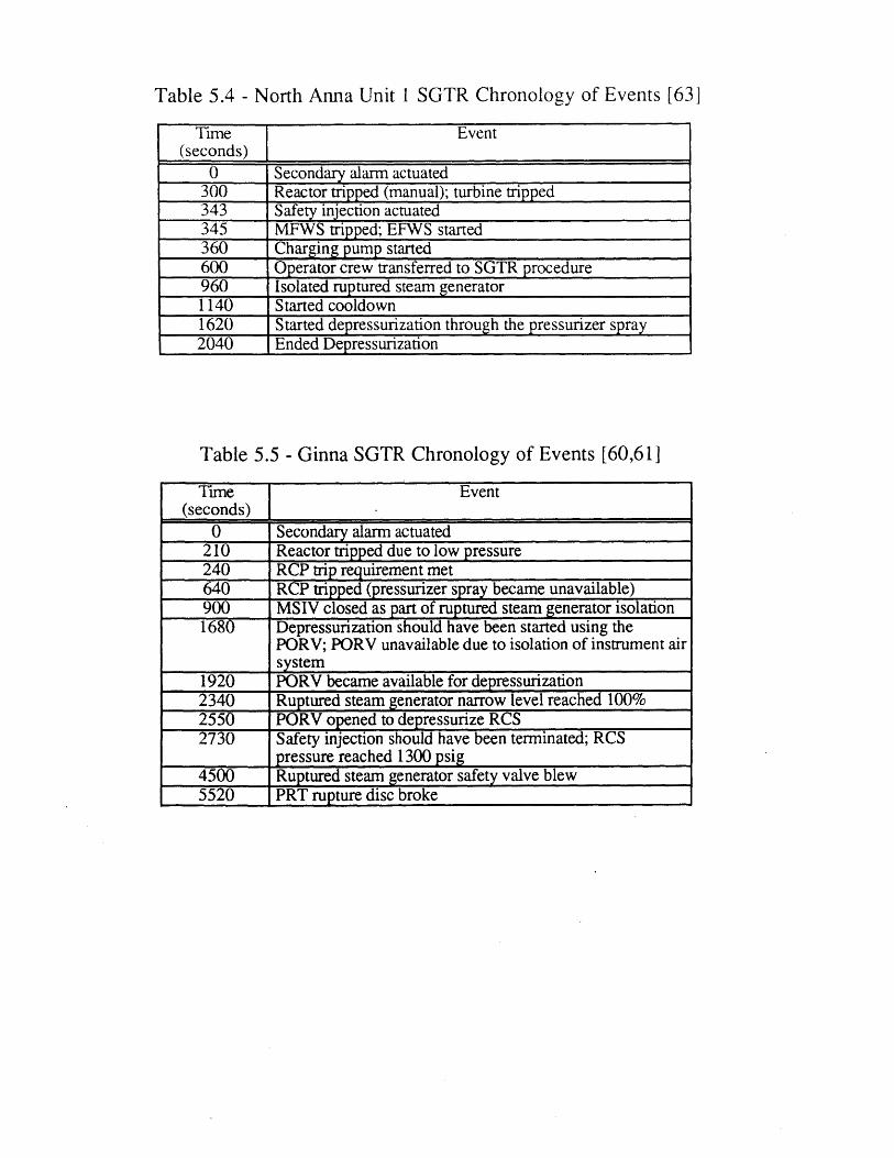
Table 5.4 - North Anna Unit 1 SGTR Chronology of Events [63]

Time Event(seconds)

0 Secondary alarm actuated300 Reactor tripped (manual); turbine tripped343 Safety injection actuated345 MFWS tripped; EFWS started360 Charging pump started600 Operator crew transferred to SGTR procedure960 Isolated ruptured steam generator1140 Started cooldown1620 Started depressurization through the pressurizer spray2040 Ended Depressurization

Table 5.5 - Ginna SGTR Chronology of Events [60,61]

Time Event(seconds)

0 Secondary alarm actuated210 Reactor tripped due to low pressure240 RCP trip requirement met640 RCP tripped (pressurizer spray became unavailable)900 MSIV closed as part of ruptured steam generator isolation1680 Depressurization should have been started using the

PORV; PORV unavailable due to isolation of instrument airsystem

1920 PORV became available for depressurization2340 Ruptured steam generator narrow level reached 100%2550 PORV opened to depressurize RCS2730 Safety injection should have been terminated; RCS

pressure reached 1300 psig4500 Ruptured steam generator safety valve blew5520 PRT rupture disc broke

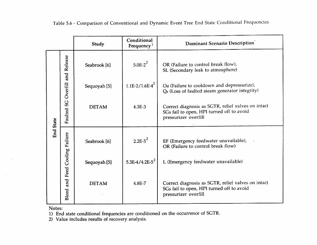
Table 5.6 - Comparison of Conventional and Dynamic Event Tree End State Conditional Frequencies

Study___ 4 4

Seabrook [6]

Sequoyah [5]

DETAM

ConditionalFrequency 1

5.OE-2 2

1.1E-2/1.6E-4 2

4.3E-3

I I I

Seabrook [6]

Sequoyah [5]

DETAM

2.2E-5 2

5.3E-4/4.2E-52

4.8E-7

Dominant Scenario Description

OR (Failure to control break flow),SL (Secondary leak to atmosphere)

Od (Failure to cooldown and depressurize),Qs (Loss of faulted steam generator integrity)

Correct diagnosis as SGTR, relief valves on intactSGs fail to open, HPI turned off to avoidpressurizer overfill

EF (Emergency feedwater unavailable),OR (Failure to control break flow)

L (Emergency feedwater unavailable)

Correct diagnosis as SGTR, relief valves on intactSGs fail to open, HPI turned off to avoidpressurizer overfill

i I

Notes:1) End state conditional frequencies are conditioned2) Value includes results of recovery analysis.

on the occurrence of SGTR.

0

(U

0)(U

w

0

(U

0U

(U

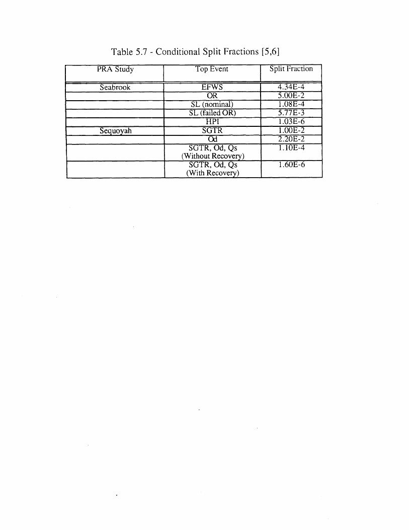
Table 5.7 - Conditional Split Fractions [5,6]

PRA Study Top Event Split Fraction

Seabrook EFWS 4.34E-4OR 5.OOE-2

SL (nominal) 1.08E-4SL (failed OR) 5.77E-3

HPI 1.03E-6Sequoyah SGTR 1.OOE-2

Od 2.20E-2SGTR, Od, Qs 1.1OE-4

(Without Recovery)SGTR, Od, Qs 1.60E-6

(With Recovery)

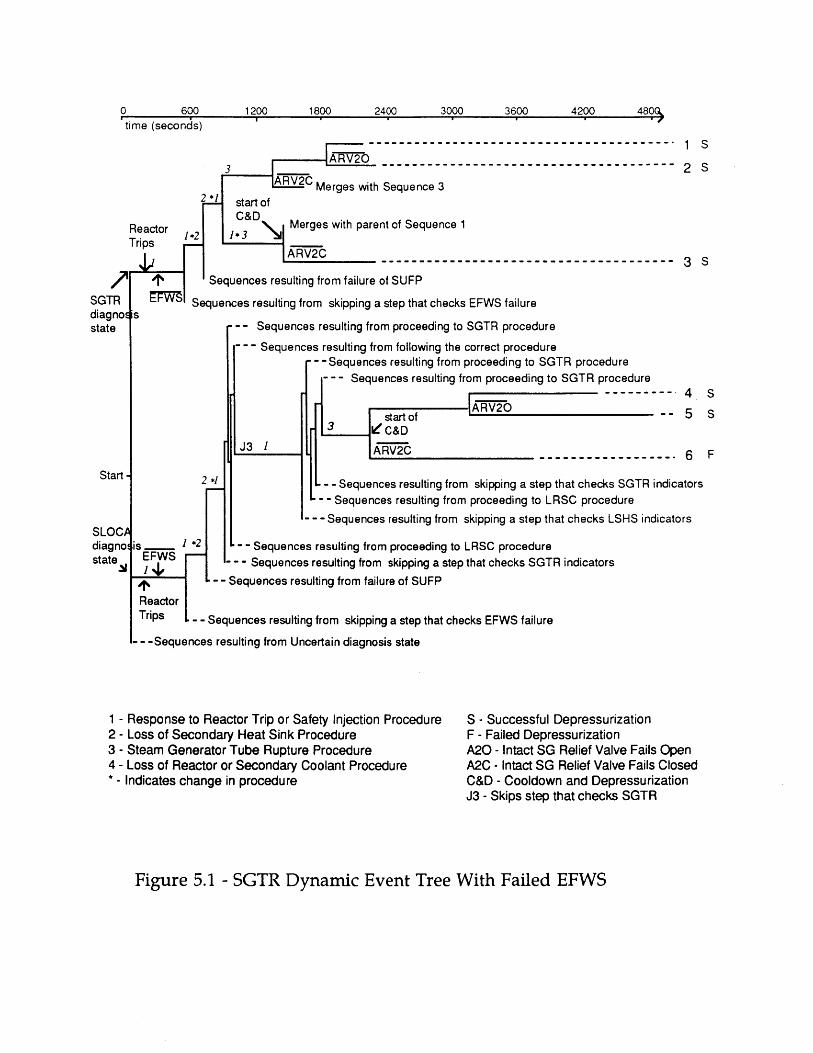
0 600time (seconds)

1200 1800 2400 3000 3600 4200 480Q,

---------------------------------------- 2 SARV2C Merges with Sequence 3

*1start of

Reactor C*2 Merges with parent of Sequence 1

TripsA RV2C

ILI- -- -------------------------------------- 3 S

t Sequences resulting from failure of SUFP

Sequences resulting from skipping a step that checks EFWS failures

2 *1

- - Sequences resulting from proceeding to SGTR procedure

- -- Sequences resulting from following the correct procedure-- Sequences resulting from proceeding to SGTR procedure

--- Sequences resulting from proceeding to SGTR procedure--------------------------------------.4

start of -- 5. 3 -1C&D

J3 I-- A-C 6-----------------6

- - - Sequences resulting from skipping a step that checks SGTR indicators- - - Sequences resulting from proceeding to LRSC procedure

- - - Sequences resulting from skipping a step that checks LSHS indicators

/ISGTRdiagnoEstate

Start

SLOCAdiagnostate

S

S

F

R indicators

1 - Response to Reactor Trip or Safety Injection Procedure2 - Loss of Secondary Heat Sink Procedure3 - Steam Generator Tube Rupture Procedure4 - Loss of Reactor or Secondary Coolant Procedure* - Indicates change in procedure

S - Successful DepressurizationF - Failed DepressurizationA20 - Intact SG Relief Valve Fails OpenA2C - Intact SG Relief Valve Fails ClosedC&D - Cooldown and DepressurizationJ3 - Skips step that checks SGTR

Figure 5.1 - SGTR Dynamic Event Tree With Failed EFWS

is - *2 - - Sequences resulting from proceeding to LRSC procedureEFWS --- Sequences resulting from skipping a step that checks SGT

-- Sequences resulting from failure of SUFP

ReactorTrips - - Sequences resulting from skipping a step that checks EFWS failure

-- -Sequences resulting from Uncertain diagnosis state

2400

-

:

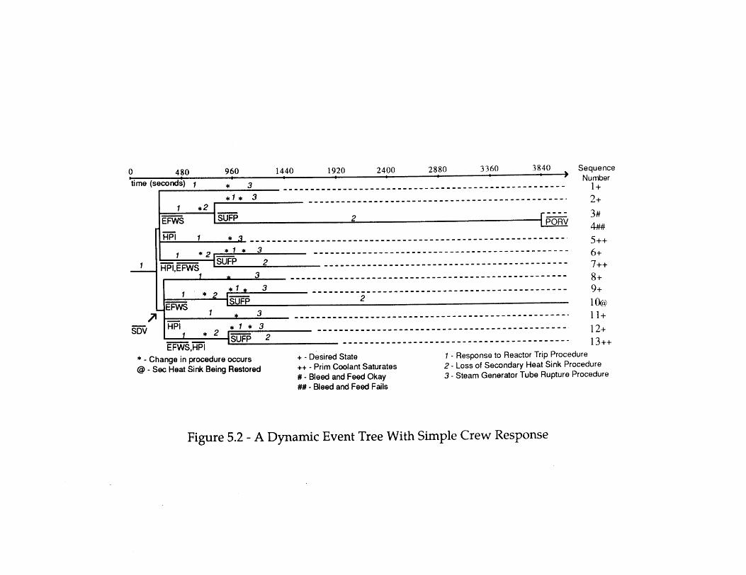
48 A 960 1440 1920 2400 2880 3360 3840

time (seconds) 1#

1

* 2 3 ----------------------------------------------------

*1* 3__ _ _ _ _ _ _ _ _ _ _ _ _ _ _ _ - . . . . - ..

HPI 1 1* 3 ____ ____ ____ ____ ____ ___- ___.--- _-----------------------

*221 * 3 _____________- _____---------------------------

-- ---- |fW S SUFP 2 __..........- _...... ....... .......------------------

1 ,3 _________-----__.__-........---------------------

.-.. ... .--------------------------------

SequenceNumber

1+2+

5++6+7++

8+9+1 o(@I 1 +

SD'/ rp * 2 1*3 - 12+SI277UFp ___________ - -_..__....------------ 13++

SChange in procedure occurs + - Desired State 1 - Response to Reactor Trip Procedure

@ - Sec Heat Sink Being Restored ++ - Prim Coolant Saturates 2 - Loss of Secondary Heat Sink Procedure

# - Bleed and Feed Okay 3 - Steam Generator Tube Rupture Procedure

## - Bleed and Feed Fails

Figure 5.2 - A Dynamic Event Tree With Simple Crew Response

0AQn r% 0 2400

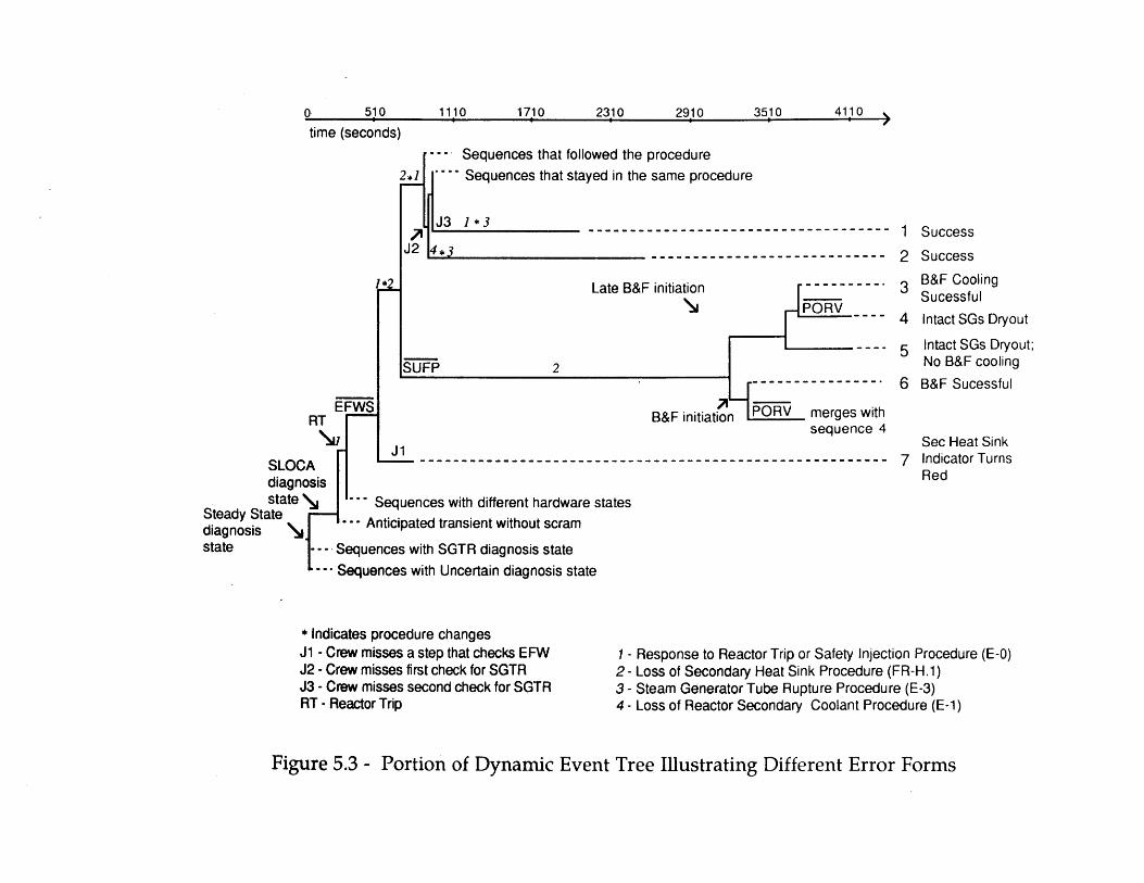
time (seconds)-- - Sequences that followed the procedure

2 .--- Sequences that stayed in the same procedure

J3 1*3

J2 4*3 -----------

1*2 Late B&F initiationPORV

---- ---SUFP 2

EFWSRT

-J1SLOCA --------------------------diagnosisstate --- Sequences with different hardware states

Steady State..diagnosis --- Anticipated transient without scram

state - - - Sequences with SGTR diagnosis stateSequences with Uncertain diagnosis state

PORB&F initiation ORV merges withsequence 4

------------------------------

3

4

5

6

7

Success

Success

B&F CoolingSucessfulIntact SGs Dryout

Intact SGs Dryout;No B&F coolingB&F Sucessful

Sec Heat SinkIndicator TurnsRed

* Indicates procedure changesJ1 -Crew misses a step that checks EFWJ2 -Crew misses first check for SGTRJ3 -Crew misses second check for SGTRRT - Reactor Trip

1 - Response to Reactor Trip or Safety Injection Procedure (E-0)2 - Loss of Secondary Heat Sink Procedure (FR-H.1)3 - Steam Generator Tube Rupture Procedure (E-3)4 - Loss of Reactor Secondary Coolant Procedure (E-1)

Figure 5.3 - Portion of Dynamic Event Tree Illustrating Different Error Forms

I

4110 .,0. 510 1110 1710 2310 2910 3510

-----------------

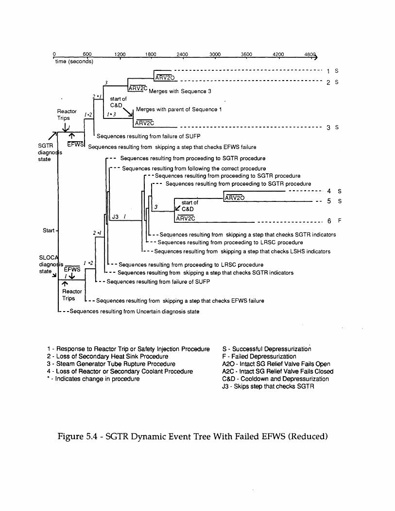
0 600 1200 1800 2400 3000 3600 4200 48time (seconds) IO

---------------------------------------- 1 S

. aRV2C Merges with Sequence 3

Reactor Merges with parent of Sequence 11*2 *3 Mege

Trips 1 ..j;[ ~A RV2C3S ----------------------------------------------------- 3S

T ~ Sequences resulting from failure of SUFP

Sequences resulting from skipping a step that checks EFWS failureo s

-- - Sequences resulting from proceeding to SGTR procedure

2*1

- - - Sequences resulting from following the correct procedure- - Sequences resulting from proceeding to SGTR procedure

--- Sequences resulting from proceeding to SGTR procedure---------- 4

start of --V2 5. 3V'C&D

J3 I A-- - C 6-----------------6

- - Sequences resulting from skipping a step that checks SGTR indicators-- Sequences resulting from proceeding to LRSC procedure

- - - Seuences- resulting from skinning a sten that checks I SHS indie-atnrs

S

S

F

is_ 1 *2 -- Sequences resulting from proceeding to LRSC procedureEFWS --- Sequences resulting from skipping a step that checks SGTR indicators

-- Sequences resulting from failure of SUFP

ReactorTrips - - Sequences resulting from skipping a step that checks EFWS failure

-- -Sequences resulting from Uncertain diagnosis state

1 - Response to Reactor Trip or Safety Injection Procedure2 - Loss of Secondary Heat Sink Procedure3 - Steam Generator Tube Rupture Procedure4 - Loss of Reactor or Secondary Coolant Procedure* - Indicates change in procedure

S - Successful DepressurizationF - Failed DepressurizationA20 - Intact SG Relief Valve Fails OpenA2C - Intact SG Relief Valve Fails ClosedC&D - Cooldown and DepressurizationJ3 - Skips step that checks SGTR

Figure 5.4 - SGTR Dynamic Event Tree With Failed EFWS (Reduced)

SGTFdiagnstate

Start -

SLOCAdiagnostate

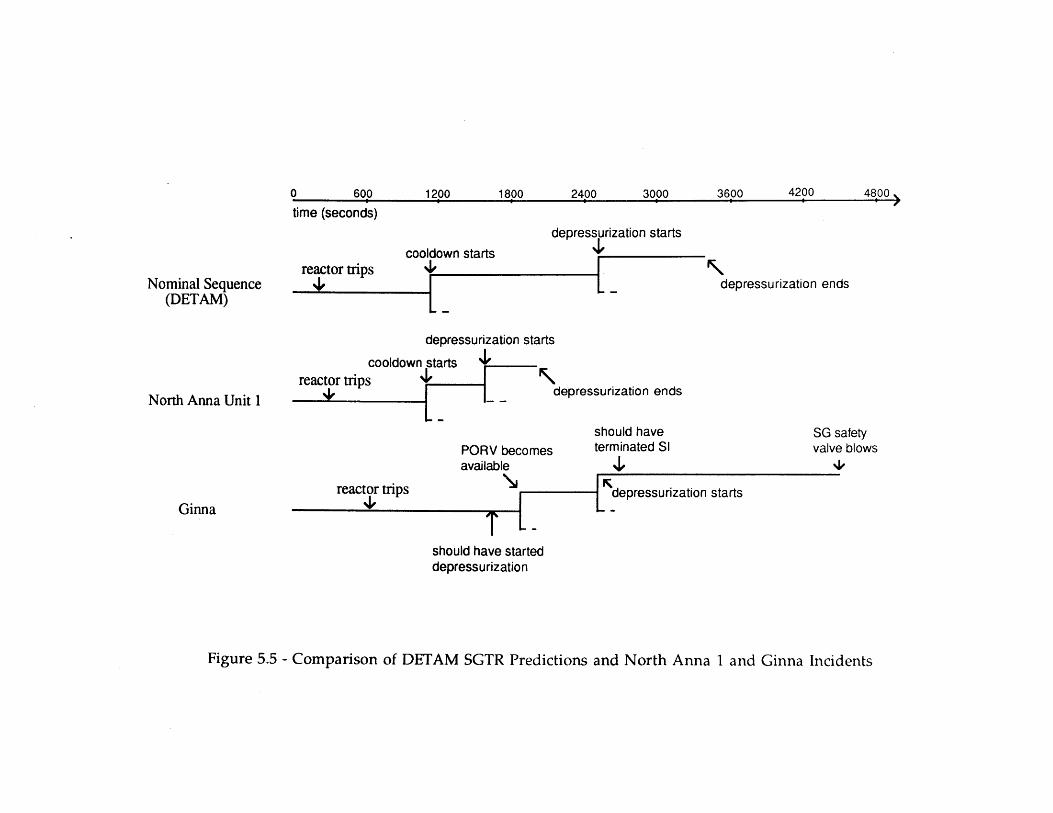
0 600 1290 1800 2400 3000 3600 4200 4800 ~time (seconds)

r

cooldown starts

depressurization starts'19

Nominal Sequence(DETAM)

North Anna Unit 1

Ginna

reactor trips 449

depressurization starts

cooldown startsreactor trips 4

-I

PORV becomesavailable

depressurization ends

depressurization ends

should haveterminated SI

should have starteddepressurization

Figure 5.5 - Comparison of DETAM SGTR Predictions and North Anna I and Ginna Incidents

SG safetyvalve blows

%I-

starts

3600 4200 48000 600

LI_

1200 1800 2400 3000

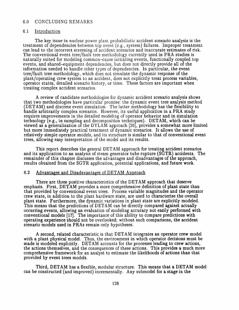
6.0 CONCLUDING REMARKS

6.1 Introduction

The key issue in nuclear power plant probabilistic accident scenario analysis is thetreatment of dependencies between top event (e.g., system) failures. Improper treatmentcan lead to the incorrect screening of accident scenarios and inaccurate estimates of risk.The conventional event tree/fault tree methodology currently used in PRA studies isnaturally suited for modeling common-cause initiating events, functionally coupled topevents, and shared-equipment dependencies, but does not directly provide all of theinformation needed to handle other types of dependencies. In particular, the eventtree/fault tree methodology, which does not simulate the dynamic response of theplant/operating crew system to an accident, does not explicitly treat process variables,operator states, detailed scenario history, or time. These factors are important whentreating complex accident scenarios.

A review of candidate methodologies for dynamic accident scenario analysis showsthat two methodologies have particular promise: the dynamic event tree analysis method(DETAM) and discrete event simulation. The latter methodology has the flexibility tohandle arbitrarily complex scenarios. However, its useful application in a PRA studyrequires improvements in the detailed modeling of operator behavior and in simulationtechnology (e.g., in sampling and decomposition techniques). DETAM, which can beviewed as a generalization of the DYLAM approach [26], provides a somewhat more limitedbut more immediately practical treatment of dynamic scenarios. It allows the use ofrelatively simple operator models, and its structure is similar to that of conventional eventtrees, allowing easy interpretation of the model and its results.

This report describes the general DETAM approach for treating accident scenariosand its application to an analysis of steam generator tube rupture (SGTR) accidents. Theremainder of this chapter discusses the advantages and disadvantages of the approach,results obtained from the SGTR application, potential applications, and future work.

6.2 Advantages and Disadavantages of DETAM Approach

There are three positive characteristics of the DETAM approach that deserveemphasis. First, DETAM provides a more comprehensive definition of plant state thanthat provided by conventional event trees. Process variable magnitudes and the operatorcrew state, in addition to the plant hardware state, are used to characterize the overallplant state. Furthermore, the dynamic variations in plant state are explicitly modeled.This means that the predictions of DETAM can be directly compared against actuallyoccurring events, allowing an evaluation of modeling accuracy not easily performed withconventional models [17]. The importance of this ability to compare predictions withoperating experience should not be overlooked; without such comparisons, the accidentscenario models used in PRAs remain only hypotheses.

A second, related characteristic is that DETAM integrates an operator crew modelwith a plant physical model. Thus, the environment in which operator decisions must bemade is modeled explicitly. DETAM accounts for the processes leading to crew actions,the actions themselves, and the consequences of these actions. This provides a much morecomprehensive framework for an analyst to estimate the likelihoods of actions than thatprovided by event trees models.

Third, DETAM has a flexible, modular structure. This means that a DETAM modelcan be constructed (and improved) incrementally. Any submodel for a stage in the

128

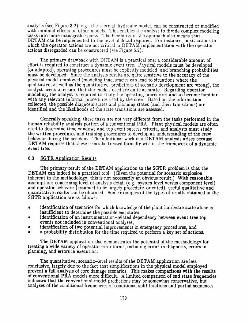
analysis (see Figure 3.2), e.g., the thermal-hydraulic model, can be constructed or modifiedwith minimal effects on other models. This enables the analyst to divide complex modelingtasks into more manageable parts. The flexibility of the approach also means thatDETAM can be implemented to the level of detail required. For instance, in situations inwhich the operator actions are not critical, a DETAM implementation with the operatoractions disregarded can be constructed (see Figure 5.2).

The primary drawback with DETAM is a practical one: a considerable amount ofeffort is required to construct a dynamic event tree. Physical models must be developed(or adapted), operating procedures must be explicitly modeled, and branching probabilitiesmust be developed. Since the analysis results are quite sensitive to the accuracy of thephysical model employed (modeling inaccuracies can lead to situations where thequalitative, as well as the quantitative, predictions of scenario development are wrong), theanalyst needs to ensure that the models used are quite accurate. Regarding operatormodeling, the analyst is required to study the operating procedures and to become familiarwith any relevant informal procedures used by the crew. Based on the informationcollected, the possible diagnosis states and planning states (and their transitions) areidentified and the likelihoods of the state transitions are assessed.

Generally speaking, these tasks are not very different from the tasks performed in thehuman reliability analysis portion of a conventional PRA. Plant physical models are oftenused to determine time windows and top event success criteria, and analysts must studythe written procedures and training procedures to develop an understanding of the crewbehavior during the accident. The additional work in a DETAM analysis arises becauseDETAM requires that these issues be treated formally within the framework of a dynamicevent tree.

6.3 SGTR Application Results

The primary result of the DETAM application to the SGTR problem is that theDETAM can indeed be a practical tool. (Given the potential for scenario explosioninherent in the methodology, this is not necessarily an obvious result.) With reasonableassumptions concerning level of analysis detail (e.g., system level versus component level)and operator behavior (assumed to be largely procedure-oriented), useful qualitative andquantitative results can be obtained. Some examples of the types of results obtained in theSGTR application are as follows:

0 identification of scenarios for which knowledge of the plant hardware state alone isinsufficient to determine the possible end states,

* identification of an instrumentation-related dependency between event tree topevents not included in conventional analyses,

e identification of two potential improvements in emergency procedures, and0 a probability distribution for the time required to perform a key set of actions.

The DETAM application also demonstrates the potential of the methodology fortreating a wide variety of operator error forms, including errors in diagnosis, errors inplanning, and errors in execution.

The quantitative, scenario-level results of the DETAM application are lessconclusive, largely due to the fact that simplifications in the physical model employedprevent a full analysis of core damage scenarios. This makes comparisons with the resultsof conventional PRA models more difficult. A limited comparison of end state frequenciesindicates that the conventional model predictions may be somewhat conservative, butanalyses of the conditional frequencies of conditional split fractions and partial sequences

129

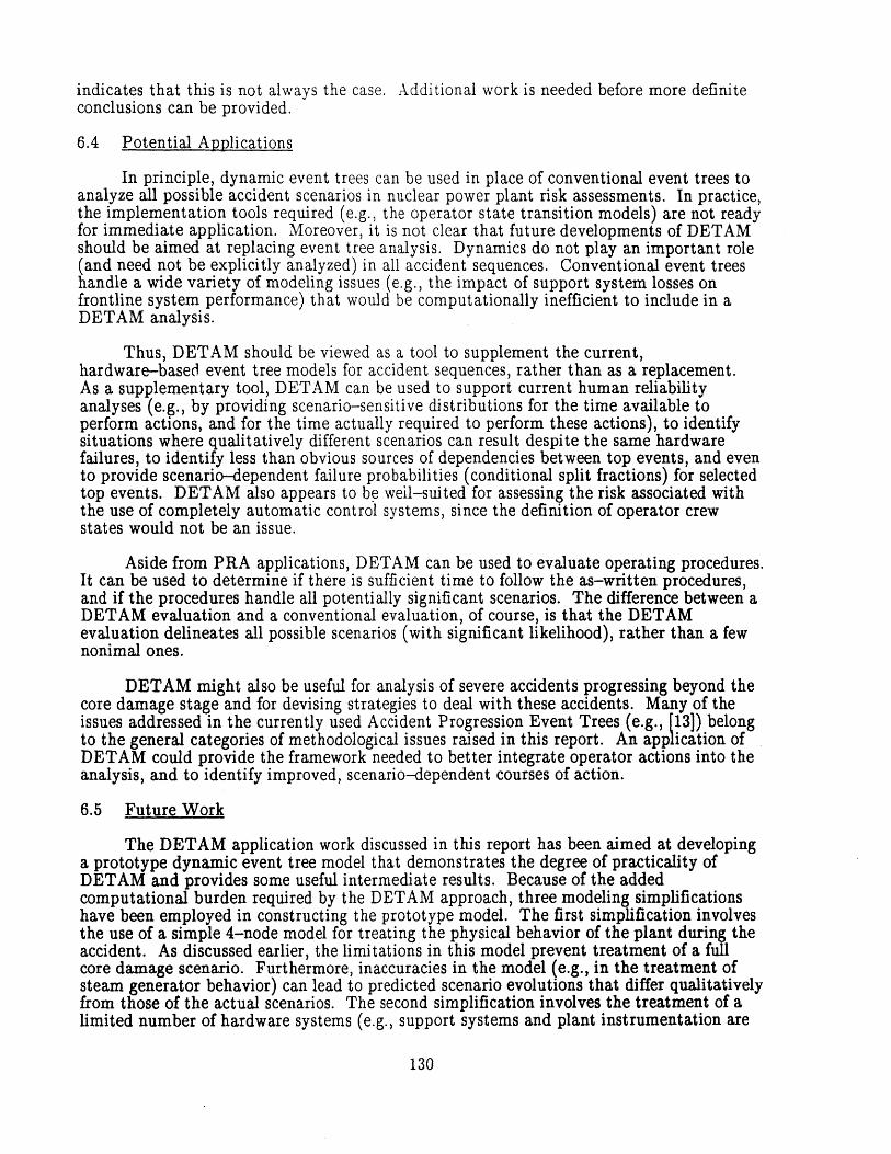
indicates that this is not always the case. Additional work is needed before more definiteconclusions can be provided.

6.4 Potential Applications

In principle, dynamic event trees can be used in place of conventional event trees toanalyze all possible accident scenarios in nuclear power plant risk assessments. In practice,the implementation tools required (e.g., the operator state transition models) are not readyfor immediate application. Moreover, it is not clear that future developments of DETAMshould be aimed at replacing event tree analysis. Dynamics do not play an important role(and need not be explicitly analyzed) in all accident sequences. Conventional event treeshandle a wide variety of modeling issues (e.g., the impact of support system losses onfrontline system performance) that would be computationally inefficient to include in aDETAM analysis.

Thus, DETAM should be viewed as a tool to supplement the current,hardware-based event tree models for accident sequences, rather than as a replacement.As a supplementary tool, DETAM can be used to support current human reliabilityanalyses (e.g., by providing scenario-sensitive distributions for the time available toperform actions, and for the time actually required to perform these actions), to identifysituations where qualitatively different scenarios can result despite the same hardwarefailures, to identify less than obvious sources of dependencies between top events, and evento provide scenario-dependent failure probabilities (conditional split fractions) for selectedtop events. DETAM also appears to be weil-suited for assessing the risk associated withthe use of completely automatic control systems, since the definition of operator crewstates would not be an issue.

Aside from PRA applications, DETAM can be used to evaluate operating procedures.It can be used to determine if there is sufficient time to follow the as-written procedures,and if the procedures handle all potentially significant scenarios. The difference between aDETAM evaluation and a conventional evaluation, of course, is that the DETAMevaluation delineates all possible scenarios (with significant likelihood), rather than a fewnonimal ones.

DETAM might also be useful for analysis of severe accidents progressing beyond thecore damage stage and for devising strategies to deal with these accidents. Many of theissues addressed in the currently used Accident Progression Event Trees (e.g., [13]) belongto the general categories of methodological issues raised in this report. An application ofDETAM could provide the framework needed to better integrate operator actions into theanalysis, and to identify improved, scenario-dependent courses of action.

6.5 Future Work

The DETAM application work discussed in this report has been aimed at developinga prototype dynamic event tree model that demonstrates the degree of practicality ofDETAM and provides some useful intermediate results. Because of the addedcomputational burden required by the DETAM approach, three modeling simplificationshave been employed in constructing the prototype model. The first simplification involvesthe use of a simple 4-node model for treating the physical behavior of the plant during theaccident. As discussed earlier, the limitations in this model prevent treatment of a fullcore damage scenario. Furthermore, inaccuracies in the model (e.g., in the treatment ofsteam generator behavior) can lead to predicted scenario evolutions that differ qualitativelyfrom those of the actual scenarios. The second simplification involves the treatment of alimited number of hardware systems (e.g., support systems and plant instrumentation are

130

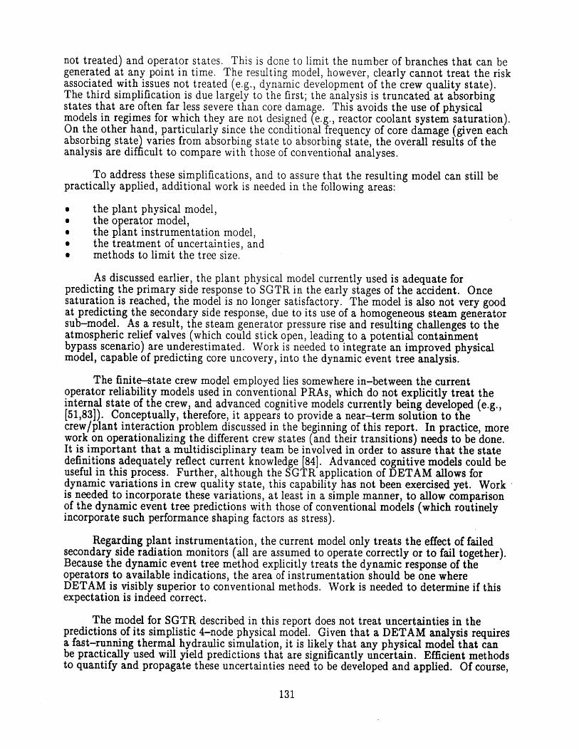
not treated) and operator states. This is done to limit the number of branches that can begenerated at any point in time. The resulting model, however, clearly cannot treat the riskassociated with issues not treated (e.g., dynamic development of the crew quality state).The third simplification is due largely to the first; the analysis is truncated at absorbingstates that are often far less severe than core damage. This avoids the use of physicalmodels in regimes for which they are not designed (e.g., reactor coolant system saturation).On the other hand, particularly since the conditional frequency of core damage (given eachabsorbing state) varies from absorbing state to absorbing state, the overall results of theanalysis are difficult to compare with those of conventiofial analyses.

To address these simplifications, and to assure that the resulting model can still bepractically applied, additional work is needed in the following areas:

9 the plant physical model,e the operator model,e the plant instrumentation model,0 the treatment of uncertainties, and0 methods to limit the tree size.

As discussed earlier, the plant physical model currently used is adequate forpredicting the primary side response to SGTR in the early stages of the accident. Oncesaturation is reached, the model is no longer satisfactory. The model is also not very goodat predicting the secondary side response, due to its use of a homogeneous steam generatorsub-model. As a result, the steam generator pressure rise and resulting challenges to theatmospheric relief valves (which could stick open, leading to a potential containmentbypass scenario) are underestimated. Work is needed to integrate an improved physicalmodel, capable of predicting core uncovery, into the dynamic event tree analysis.

The finite-state crew model employed lies somewhere in-between the currentoperator reliability models used in conventional PRAs, which do not explicitly treat theinternal state of the crew, and advanced cognitive models currently being developed (e.g.,[51,83]). Conceptually, therefore, it appears to provide a near-term solution to thecrew/plant interaction problem discussed in the beginning of this report. In practice, morework on operationalizing the different crew states (and their transitions) needs to be done.It is important that a multidisciplinary team be involved in order to assure that the statedefinitions adequately reflect current knowledge [84]. Advanced cognitive models could beuseful in this process. Further, although the SGTR application of DETAM allows fordynamic variations in crew quality state, this capability has not been exercised yet. Workis needed to incorporate these variations, at least in a simple manner, to allow comparisonof the dynamic event tree predictions with those of conventional models (which routinelyincorporate such performance shaping factors as stress).

Regarding plant instrumentation, the current model only treats the effect of failedsecondary side radiation monitors (all are assumed to operate correctly or to fail together).Because the dynamic event tree method explicitly treats the dynamic response of theoperators to available indications, the area of instrumentation should be one whereDETAM is visibly superior to conventional methods. Work is needed to determine if thisexpectation is indeed correct.

The model for SGTR described in this report does not treat uncertainties in thepredictions of its simplistic 4-node physical model. Given that a DETAM analysis requiresa fast-running thermal hydraulic simulation, it is likely that any physical model that canbe practically used will yield predictions that are significantly uncertain. Efficient methodsto quantify and propagate these uncertainties need to be developed and applied. Of course,

131

state-of-knowledge uncertainties in other parts of the model (e.g., in the operator statetransition rates) need to be addressed as well. (The dynamic event tree branchings treatstochastic uncertainties.)

Finally, when the more detailed models described above are implemented, it is likelythat more powerful methods for grouping and truncating scenarios will be required. Oneidea that may be worth pursuing is the development of a formal methodology forestimating the conditional frequency of an undesired state (e.g., core damage), given thecurrent state of the plant. If dynamic estimates of this conditional frequency can beobtained for each scenario as the simulation progresses, they can be combined with thecurrent likelihoods of the scenarios to estimate their "risk potential," which can then beused to truncate scenarios. (Note that the current scenario truncation methodology, whichonly uses the current frequency of the scenario, can be viewed as an application of a generaltruncation methodology in which the conditional frequency of core damage is set equal tounity.)

132

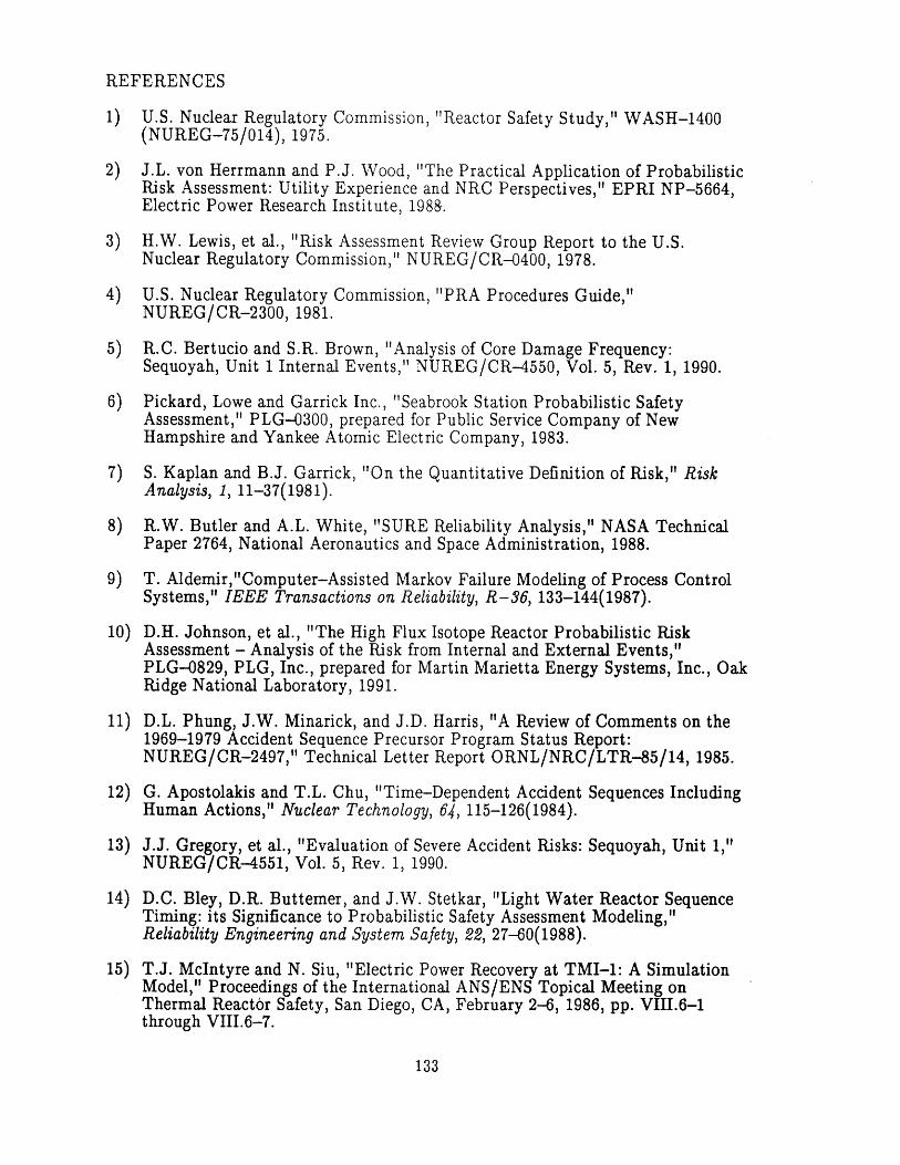
REFERENCES

1) U.S. Nuclear Regulatory Commission, "Reactor Safety Study," WASH-1400(NUREG-75/014), 1975.

2) J.L. von Herrmann and P.J. Wood, "The Practical Application of ProbabilisticRisk Assessment: Utility Experience and NRC Perspectives," EPRI NP-5664,Electric Power Research Institute, 1988.

3) H.W. Lewis, et al., "Risk Assessment Review Group Report to the U.S.Nuclear Regulatory Commission," NUREG/CR-0400, 1978.

4) U.S. Nuclear Regulatory Commission, "PRA Procedures Guide,"NUREG/CR-2300, 1981.

5) R.C. Bertucio and S.R. Brown, "Analysis of Core Damage Frequency:Sequoyah, Unit 1 Internal Events," NUREG/CR-4550, Vol. 5, Rev. 1, 1990.

6) Pickard, Lowe and Garrick Inc., "Seabrook Station Probabilistic SafetyAssessment," PLG-0300, prepared for Public Service Company of NewHampshire and Yankee Atomic Electric Company, 1983.

7) S. Kaplan and B.J. Garrick, "On the Quantitative Definition of Risk," RiskAnalysis, 1, 11-37(1981).

8) R.W. Butler and A.L. White, "SURE Reliability Analysis," NASA TechnicalPaper 2764, National Aeronautics and Space Administration, 1988.

9) T. Aldemir,"Computer-Assisted Markov Failure Modeling of Process ControlSystems," IEEE Transactions on Reliability, R-36, 133-144(1987).

10) D.H. Johnson, et al., "The High Flux Isotope Reactor Probabilistic RiskAssessment - Analysis of the Risk from Internal and External Events,"PLG-0829, PLG, Inc., prepared for Martin Marietta Energy Systems, Inc., OakRidge National Laboratory, 1991.

11) D.L. Phung, J.W. Minarick, and J.D. Harris, "A Review of Comments on the1969-1979 Accident Sequence Precursor Program Status Report:NUREG/CR-2497," Technical Letter Report ORNL/NRC/LTR-85/14, 1985.

12) G. Apostolakis and T.L. Chu, "Time-Dependent Accident Sequences IncludingHuman Actions," Nuclear Technology, 64, 115-126(1984).

13) J.J. Gregory, et al., "Evaluation of Severe Accident Risks: Sequoyah, Unit 1,"NUREG/CR-4551, Vol. 5, Rev. 1, 1990.

14) D.C. Bley, D.R. Buttemer, and J.W. Stetkar, "Light Water Reactor SequenceTiming: its Significance to Probabilistic Safety Assessment Modeling,"Reliability Engineering and System Safety, 22, 27-60(1988).

15) T.J. McIntyre and N. Siu, "Electric Power Recovery at TMI-1: A SimulationModel," Proceedings of the International ANS/ENS Topical Meeting onThermal Reactor Safety, San Diego, CA, February 2-6, 1986, pp. VIII.6-1through VIII.6-7.

133

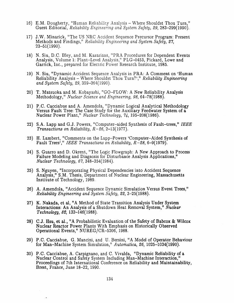
16) E.M. Dougherty, "Human Reliability Analysis - Where Shouldst Thou Turn,"Guest Editorial, Reliability Engineering and System Safety, 29, 283-299(1990).

17) J.W. Minarick, "The US NRC Accident Sequence Precursor Program: PresentMethods and Findings," Reliability Engineering and System Safety, 27,23-51(1990).

18) N. Siu, D.C. Bley, and M. Kazarians, "PRA Procedures for Dependent EventsAnalysis, Volume 1: Plant-Level Analysis," PLG-0453, Pickard, Lowe andGarrick, Inc., prepared for Electric Power Research Institute, 1985.

19) N. Siu, "Dynamic Accident Sequence Analysis in PRA: A Comment on 'HumanReliability Analysis - Where Shouldst Thou Turn?'," Reliability Engineeringand System Safety, 29, 359-364(1990).

20) T. Matsuoka and M. Kobayashi, "GO-FLOW: A New Reliability AnalysisMethodology," Nuclear Science and Engineering, 98, 64-78(1988).

21) P.C. Cacciabue and A. Amendola, "Dynamic Logical Analytical MethodologyVersus Fault Tree: The Case Study for the Auxiliary Feedwater System of aNuclear Power Plant," Nuclear Technology, 74, 195-208(1986).

22) S.A. Lapp and G.J. Powers, "Computer-aided Synthesis of Fault-trees," IEEETransactions on Reliability, R -26, 2-13(1977).

23) H. Lambert, "Comments on the Lapp-Powers 'Computer-Aided Synthesis ofFault Trees'," IEEE Transactions on Reliability, R-28, 6-9(1979).

24) S. Guarro and D. Okrent, "The Logic Flowgraph: A New Approach to ProcessFailure Modeling and Diagnosis for Disturbance Analysis Applications,"Nuclear Technology, 67, 348-354(1984).

25) S. Nguyen, "Incorporating Physical Dependencies into Accident SequenceAnalysis," S.M. Thesis, Department of Nuclear Engineering, MassachusettsInstitute of Technology, 1989.

26) A. Amendola, "Accident Sequence Dynamic Simulation Versus Event Trees,"Reliability Engineering and System Safety, 22, 3-25(1988).

27) K. Nakada, et al, "A Method of State Transition Analysis Under SystemInteractions: An Analysis of a Shutdown Heat Removal System," NuclearTechnology, 82, 132-146(1988).

28) C.J. Hsu, et al., "A Probabilistic Evaluation of the Safety of Babcox & WilcoxNuclear Reactor Power Plants With Emphasis on Historically ObservedOperational Events," NUREG/CR-5206, 1988.

29) P.C. Cacciabue, G. Mancini, and U. Bersini, "A Model of Operator Behaviourfor Man-Machine System Simulation," Automatica, 26, 1025-1034(1990).

30) P.C. Cacciabue, A. Carpignano, and C. Vivalda, "Dynamic Reliability of aNuclear Control and Safety System Including Man-Machine Interaction,"Proceedings of 7th International Conference on Reliability and Maintainability,Brest, France, June 18-22, 1990.

134

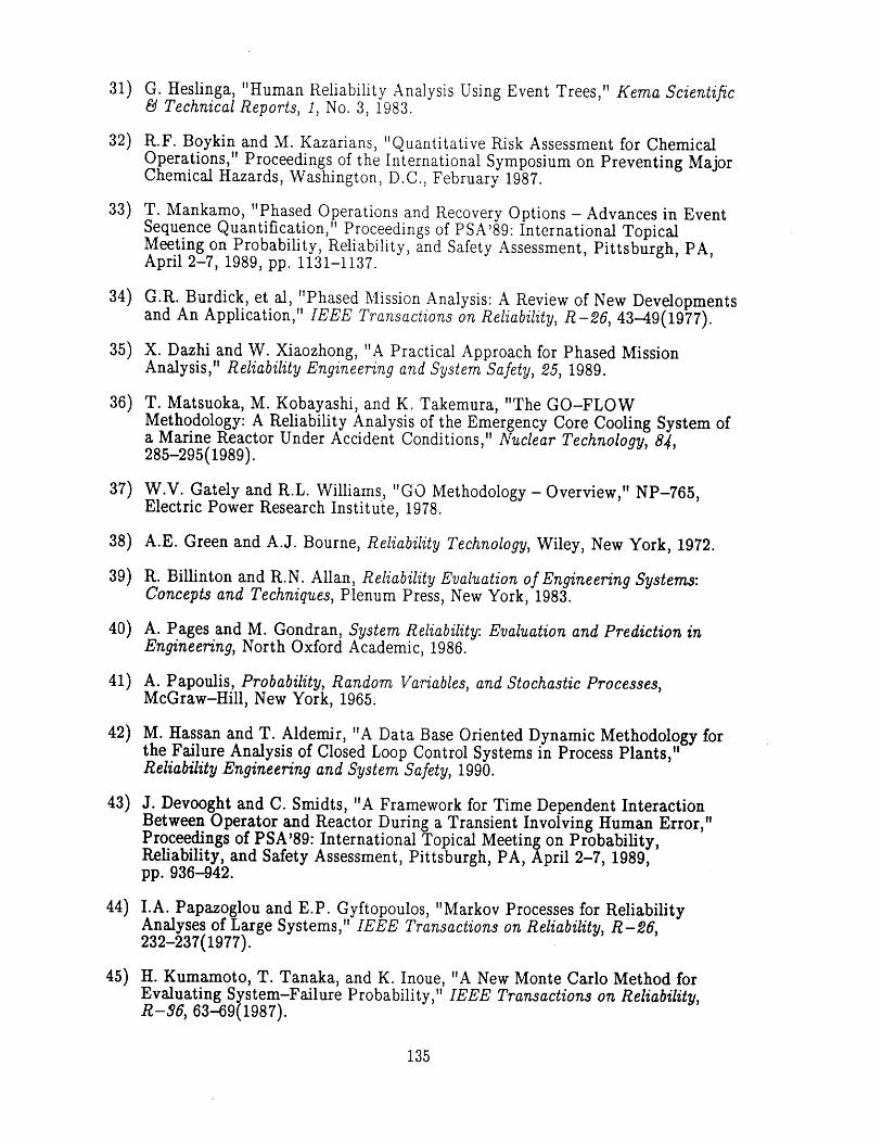
31) G. Heslinga, "Human Reliability Analysis Using Event Trees," Kema Scientific& Technical Reports, 1, No. 3, 1983.

32) R.F. Boykin and M. Kazarians, "Quantitative Risk Assessment for ChemicalOperations," Proceedings of the International Symposium on Preventing MajorChemical Hazards, Washington, D.C., February 1987.

33) T. Mankamo, "Phased Operations and Recovery Options - Advances in EventSequence Quantification," Proceedings of PSA'89: International TopicalMeeting on Probability, Reliability, and Safety Assessment, Pittsburgh, PA,April 2-7, 1989, pp. 1131-1137.

34) G.R. Burdick, et al, "Phased Mission Analysis: A Review of New Developmentsand An Application," IEEE Transactions on Reliability, R -26, 43-49(1977).

35) X. Dazhi and W. Xiaozhong, "A Practical Approach for Phased MissionAnalysis," Reliability Engineering and System Safety, 25, 1989.

36) T. Matsuoka, M. Kobayashi, and K. Takemura, "The GO-FLOWMethodology: A Reliability Analysis of the Emergency Core Cooling System ofa Marine Reactor Under Accident Conditions," Nuclear Technology, 84,285-295(1989).

37) W.V. Gately and R.L. Williams, "GO Methodology - Overview," NP-765,Electric Power Research Institute, 1978.

38) A.E. Green and A.J. Bourne, Reliability Technology, Wiley, New York, 1972.

39) R. Billinton and R.N. Allan, Reliability Evaluation of Engineering Systems:Concepts and Techniques, Plenum Press, New York, 1983.

40) A. Pages and M. Gondran, System Reliability: Evaluation and Prediction inEngineering, North Oxford Academic, 1986.

41) A. Papoulis, Probability, Random Variables, and Stochastic Processes,McGraw-Hill, New York, 1965.

42) M. Hassan and T. Aldemir, "A Data Base Oriented Dynamic Methodology forthe Failure Analysis of Closed Loop Control Systems in Process Plants,"Reliability Engineering and System Safety, 1990.

43) J. Devooght and C. Smidts, "A Framework for Time Dependent InteractionBetween Operator and Reactor During a Transient Involving Human Error,"Proceedings of PSA'89: International Topical Meeting on Probability,Reliability, and Safety Assessment, Pittsburgh, PA, April 2-7, 1989,pp. 936-942.

44) I.A. Papazoglou and E.P. Gyftopoulos, "Markov Processes for ReliabilityAnalyses of Large Systems," IEEE Transactions on Reliability, R-26,232-237(1977).

45) H. Kumamoto, T. Tanaka, and K. Inoue, "A New Monte Carlo Method forEvaluating System-Failure Probability," IEEE Transactions on Reliability,R-36, 63-69(1987).

135

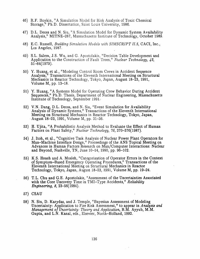
46) R.F. Boykin, "A Simulation Model for Risk Analysis of Toxic ChemicalStorage," Ph.D. Dissertation, Saint Louis University, 1986.

47) D.L. Deoss and N. Siu, "A Simulation Model for Dynamic System AvailabilityAnalysis," MITNE-287, Massachusetts Institute of Technology, October 1989.

48) E.C. Russell, Building Simulation Models with SIMSCRIPT 11.5, CACI, Inc.,Los Angeles, 1987.

49) S.L. Salem, J.S. Wu, and G. Apostolakis, "Decision Table Development andApplication to the Construction of Fault Trees," Nuclear Technology, 42,51-64(1979).

50) Y. Huang, et al., "Modeling Control Room Crews in Accident SequenceAnalysis," Transactions of the Eleventh International Meeting on StructuralMechanics in Reactor Technology, Tokyo, Japan, August 18-23, 1991,Volume M, pp. 13-18.

51) Y. Huang, "A Systems Model for Operating Crew Behavior During AccidentSequences," Ph.D. Thesis, Department of Nuclear Engineering, MassachusettsInstitute of Technology, September 1991..

52) V.N. Dang, D.L. Deoss, and N. Siu, "Event Simulation for AvailabilityAnalysis of Dynamic Systems," Transactions of the Eleventh InternationalMeeting on Structural Mechanics in Reactor Technology, Tokyo, Japan,August 18-23, 1991, Volume M, pp. 31-36.

53) H. Ujita, "A Probabilistic Analysis Method to Evaluate the Effect of HumanFactors on Plant Safety," Nuclear Technology, 76, 370-376(1987).

54) J. Itoh, et al., "Cognitive Task Analysis of Nuclear Power Plant Operators forMan-Machine Interface Design," Proceedings of the ANS Topical Meeting onAdvances in Human Factors Research on Man/Computer Interactions: Nuclearand Beyond, Nashville, TN, June 10-14, 1990, pp. 96-102.

55) K.S. Hsueh and A. Mosleh, "Categorization of Operator Errors in the Contextof Symptom-Based Emergency Operating Procedures," Transactions of theEleventh International Meeting on Structural Mechanics in ReactorTechnology, Tokyo, Japan, August 18-23, 1991, Volume M, pp. 19-24.

56) T.L. Chu and G.E. Apostolakis, "Assessment of the Uncertainties Associatedwith the Core Uncovery Time in TMI-Type Accidents," ReliabilityEngineering, 8, 23-56(1984).

57) CSAU

58) N. Siu, D. Karydas, and J. Temple, "Bayesian Assessment of ModelingUncertainty: Application to Fire Risk Assessment," to appear in Analysis andManagement of Uncertainty: Theory and Application, B.M. Ayyub, M.M.Gupta, and L.N. Kanal, eds., Elsevier, North-Holland, 1992.

136

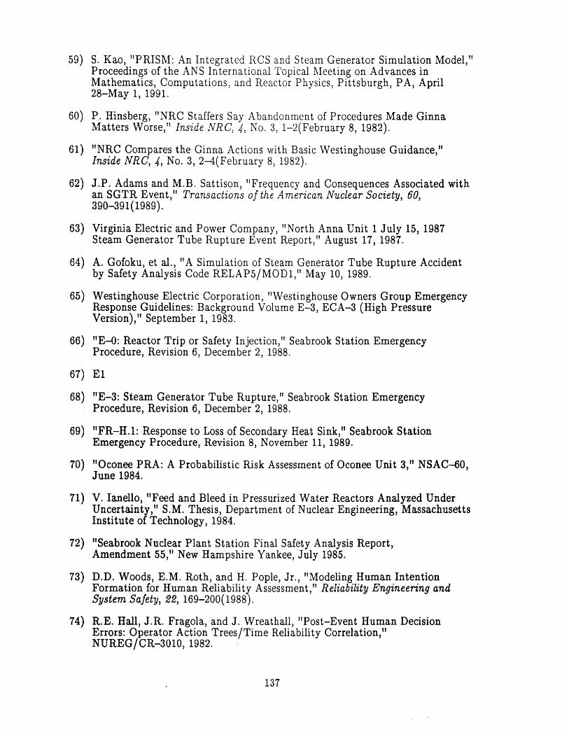
59) S. Kao, "PRISM: An Integrated RCS and Steam Generator Simulation Model,"Proceedings of the ANS International Topical Meeting on Advances inMathematics, Computations, and Reactor Physics, Pittsburgh, PA, April28-May 1, 1991.

60) P. Hinsberg, "NRC Staffers Say Abandonment of Procedures Made GinnaMatters Worse," Inside NRC, 4, No. 3, 1-2(February 8, 1982).

61) "NRC Compares the Ginna Actions with Basic Westinghouse Guidance,"Inside NRC, 4, No. 3, 2-4(February 8, 1982).

62) J.P. Adams and M.B. Sattison, "Frequency and Consequences Associated withan SGTR Event," Transactions of the American Nuclear Society, 60,390-391(1989).

63) Virginia Electric and Power Company, "North Anna Unit 1 July 15, 1987Steam Generator Tube Rupture Event Report," August 17, 1987.

64) A. Gofoku, et al., "A Simulation of Steam Generator Tube Rupture Accidentby Safety Analysis Code RELAP5/MOD1," May 10, 1989.

65) Westinghouse Electric Corporation, "Westinghouse Owners Group EmergencyResponse Guidelines: Background Volume E-3, ECA-3 (High PressureVersion)," September 1, 1983.

66) "E-0: Reactor Trip or Safety Injection," Seabrook Station EmergencyProcedure, Revision 6, December 2, 1988.

67) El

68) "E-3: Steam Generator Tube Rupture," Seabrook Station Emergency. Procedure, Revision 6, December 2, 1988.

69) "FR-H.1: Response to Loss of Secondary Heat Sink," Seabrook StationEmergency Procedure, Revision 8, November 11, 1989.

70) "Oconee PRA: A Probabilistic Risk Assessment of Oconee Unit 3," NSAC-60,June 1984.

71) V. lanello, "Feed and Bleed in Pressurized Water Reactors Analyzed UnderUncertainty," S.M. Thesis, Department of Nuclear Engineering, MassachusettsInstitute of Technology, 1984.

72) "Seabrook Nuclear Plant Station Final Safety Analysis Report,Amendment 55," New Hampshire Yankee, July 1985.

73) D.D. Woods, E.M. Roth, and H. Pople, Jr., "Modeling Human IntentionFormation for Human Reliability Assessment," Reliability Engineering andSystem Safety, 22, 169-200(1988).

74) R.E. Hall, J.R. Fragola, and J. Wreathall, "Post-Event Human DecisionErrors: Operator Action Trees/Time Reliability Correlation,"NUREG/CR-3010, 1982.

137

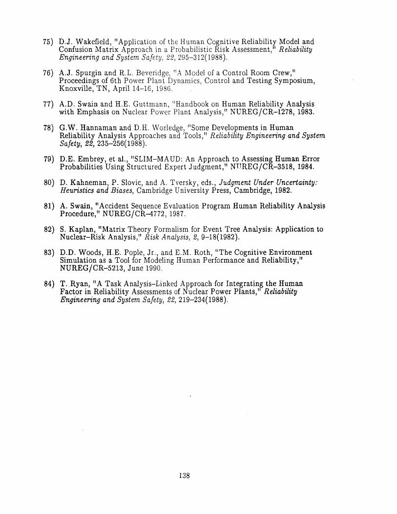
75) D.J. Wakefield, "Application of the Human Cognitive Reliability Model andConfusion Matrix Approach in a Probabilistic Risk Assessment," ReliabilityEngineering and System Safety, 22, 295-312(1988).

76) A.J. Spurgin and R.L. Beveridge, "A Model of a Control Room Crew,"Proceedings of 6th Power Plant Dynamics, Control and Testing Symposium,Knoxville, TN, April 14-16, 1986.

77) A.D. Swain and H.E. Guttmann, "Handbook on Human Reliability Analysiswith Emphasis on Nuclear Power Plant Analysis," NUREG/CR-1278, 1983.

78) G.W. Hannaman and D.H. Worledge, "Some Developments in HumanReliability Analysis Approaches and Tools," Reliability Engineering and SystemSafety, 22, 235-256(1988).

79) D.E. Embrey, et al., "SLIM-MAUD: An Approach to Assessing Human ErrorProbabilities Using Structured Expert Judgment," NTREG/CR-3518, 1984.

80) D. Kahneman, P. Slovic, and A. Tversky, eds., Judgment Under Uncertainty:Heuristics and Biases, Cambridge University Press, Cambridge, 1982.

81) A. Swain, "Accident Sequence Evaluation Program Human Reliability AnalysisProcedure," NUREG/CR-4772, 1987.

82) S. Kaplan, "Matrix Theory Formalism for Event Tree Analysis: Application toNuclear-Risk Analysis," Risk Analysis, 2, 9-18(1982).

83) D.D. Woods, H.E. Pople, Jr., and E.M. Roth, "The Cognitive EnvironmentSimulation as a Tool for Modeling Human Performance and Reliability,"NUREG/CR-5213, June 1990.

84) T. Ryan, "A Task Analysis-Linked Approach for Integrating the HumanFactor in Reliability Assessments of Nuclear Power Plants," ReliabilityEngineering and System Safety, 22, 219-234(1988).

138

APPENDIX A. THERMAL-HYDRAULIC MODEL

This appendix lists the thermal-hydraulic model equations incorporated in

DETCO-SGTR. The model, which is partially based on similar models described in Refs.

25, 26, and 71, is somewhat specialized towards the analysis of SGTR in a Westinghouse

4-loop PWR. However, it can be modified to handle other relatively slowly progressing

accidents in other PWRs. The model divides the plant into four nodes: the primary node,

the pressurizer, the ruptured steam generator, and the intact steam generators (see Figure

A.1). The model determines the coolant thermodynamic properties (e.g., temperature and

pressure) of each node for each branch at each time step. Within each node, the model

assumes that the thermodynamic properties of water are uniform. Note that some of the

equations are results of modifications to approximate the results of PRISM [59].

A-1

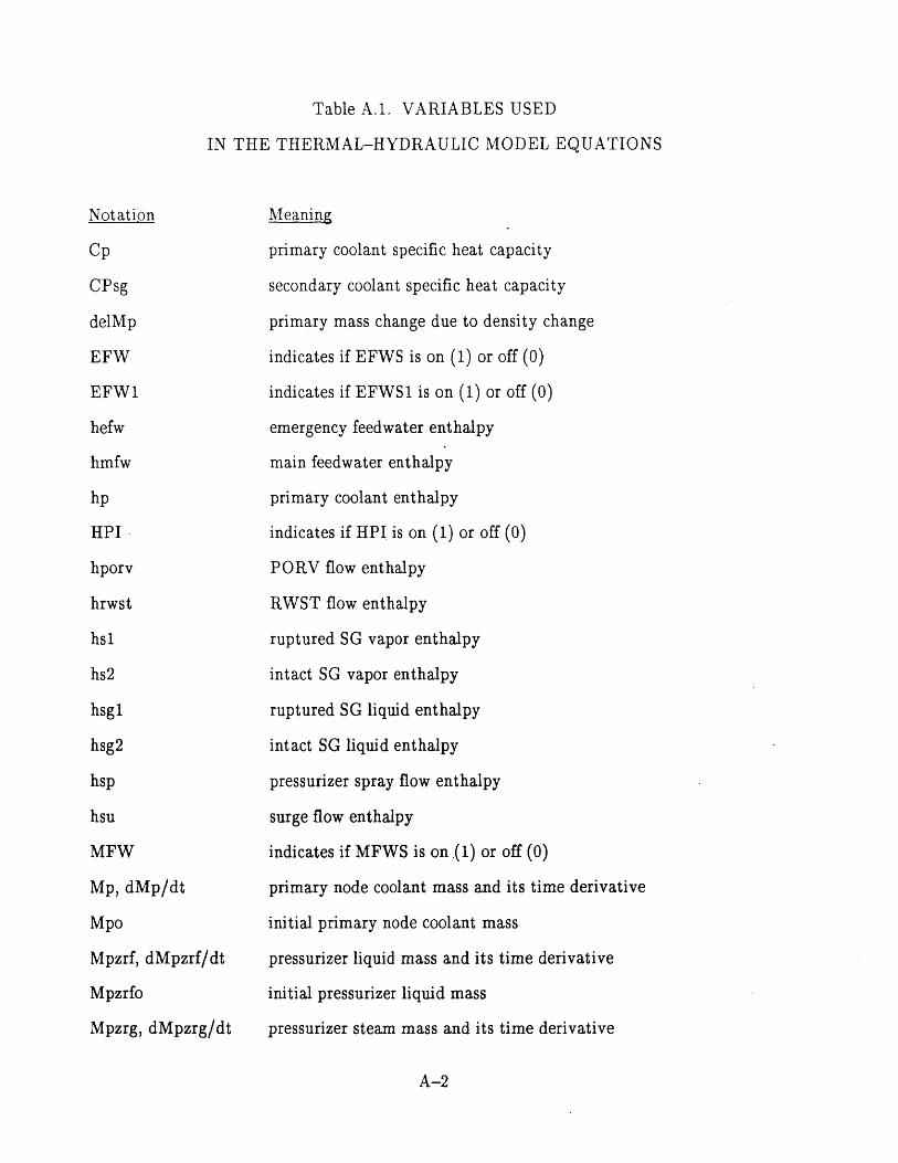
Table A.1. VARIABLES USED

IN THE THERMAL-HYDRAULIC MODEL EQUATIONS

Notation

Cp

CPsg

delMp

EFW

EFW1

hefw

hmfw

hp

HPI

hporv

hrwst

hs1

hs2

hsg 1

hsg2

hsp

hsu

MFW

Mp, dMp/dt

Mpo

Mpzrf, dMpzrf/dt

Mpzrfo

Mpzrg, dMpzrg/dt

Meaning

primary coolant specific heat capacity

secondary coolant specific heat capacity

primary mass change due to density change

indicates if EFWS is on (1) or off (0)

indicates if EFWS1 is on (1) or off (0)

emergency feedwater enthalpy

main feedwater enthalpy

primary coolant enthalpy

indicates if HPI is on (1) or off (0)

PORV flow enthalpy

RWST flow enthalpy

ruptured SG vapor enthalpy

intact SG vapor enthalpy

ruptured SG liquid enthalpy

intact SG liquid enthalpy

pressurizer spray flow enthalpy

surge flow enthalpy

indicates if MFWS is on (1) or off (0)

primary node coolant mass and its time derivative

initial primary node coolant mass

pressurizer liquid mass and its time derivative

initial pressurizer liquid mass

pressurizer steam mass and its time derivative

A-2

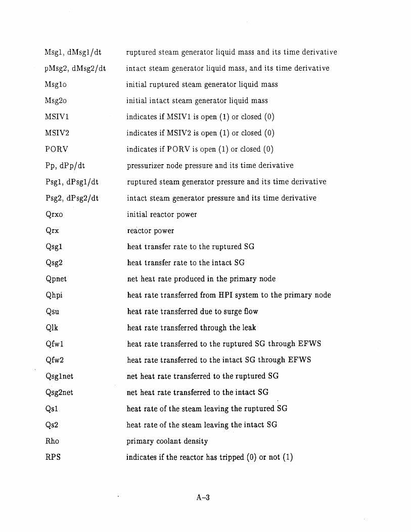
Msg1, dMsgl/dt

pMsg2, dMsg2/dt

Msglo

Msg2o

MSIV1

MSIV2

PORV

Pp, dPp/dt

Psg1, dPsg1/dt

Psg2, dPsg2/dt

Qrxo

Qrx

Qsgl

Qsg2

Qpnet

Qhpi

Qsu

Qlk

Qfwl

Qfw2

Qsglnet

Qsg2net

Qs1

Qs2

Rho

RPS

ruptured steam generator liquid mass and its time derivative

intact steam generator liquid mass, and its time derivative

initial ruptured steam generator liquid mass

initial intact steam generator liquid mass

indicates if MSIV1 is open (1) or closed (0)

indicates if MSIV2 is open (1) or closed (0)

indicates if PORV is open (1) or closed (0)

pressurizer node pressure and its time derivative

ruptured steam generator pressure and its time derivative

intact steam generator pressure and its time derivative

initial reactor power

reactor power

heat transfer rate to the ruptured SG

heat transfer rate to the intact SG

net heat rate produced in the primary node

heat rate transferred from HPI system to the primary node

heat rate transferred due to surge flow

heat rate transferred through the leak

heat rate transferred to the ruptured SG through EFWS

heat rate transferred to the intact SG through EFWS

net heat rate transferred to the ruptured SG

net heat rate transferred to the intact SG

heat rate of the steam leaving the ruptured SG

heat rate of the steam leaving the intact SG

primary coolant density

indicates if the reactor has tripped (0) or not (1)

A-3

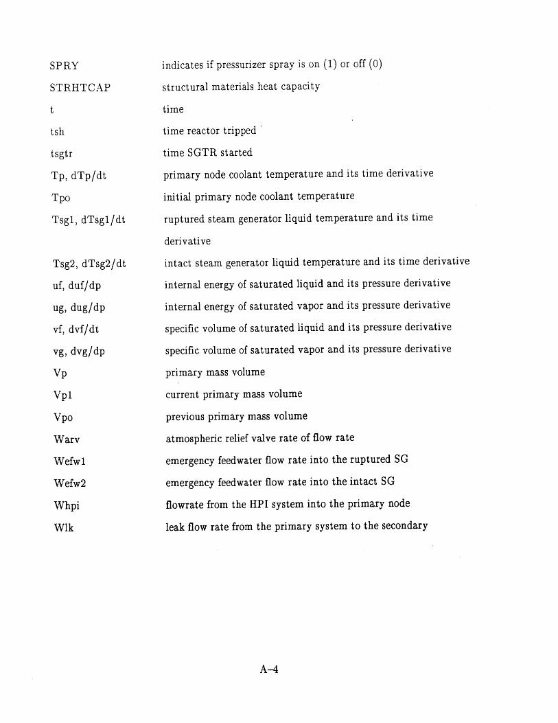
SPRY

STRHTCAP

t

tsh

tsgtr

Tp, dTp/dt

Tpo

Tsg1, dTsg1/dt

Tsg2, dTsg2/dt

uf, duf/dp

ug, dug/dp

vf, dvf/dt

vg, dvg/dp

Vp

Vpl

Vpo

Warv

Wefw1

Wefw2

Whpi

Wlk

indicates if pressurizer spray is on (1) or off (0)

structural materials heat capacity

time

time reactor tripped

time SGTR started

primary node coolant temperature and its time derivative

initial primary node coolant temperature

ruptured steam generator liquid temperature and its time

derivative

intact steam generator liquid temperature and its time derivative

internal energy of saturated liquid and its pressure derivative

internal energy of saturated vapor and its pressure derivative

specific volume of saturated liquid and its pressure derivative

specific volume of saturated vapor and its pressure derivative

primary mass volume

current primary mass volume

previous primary mass volume

atmospheric relief valve rate of flow rate

emergency feedwater flow rate into the ruptured SG

emergency feedwater flow rate into the intact SG

flowrate from the HPI system into the primary node

leak flow rate from the primary system to the secondary

A-4

Wmfwl main feedwater flow rate into the ruptured SG

Wmfw2 main feedwater flow rate into the intact SG

Wporv PORV flow rate

Wsl steam flow rate from the ruptured SG

Ws2 steam flow rate from the intact SG

Wsu surge flow rate

A-5

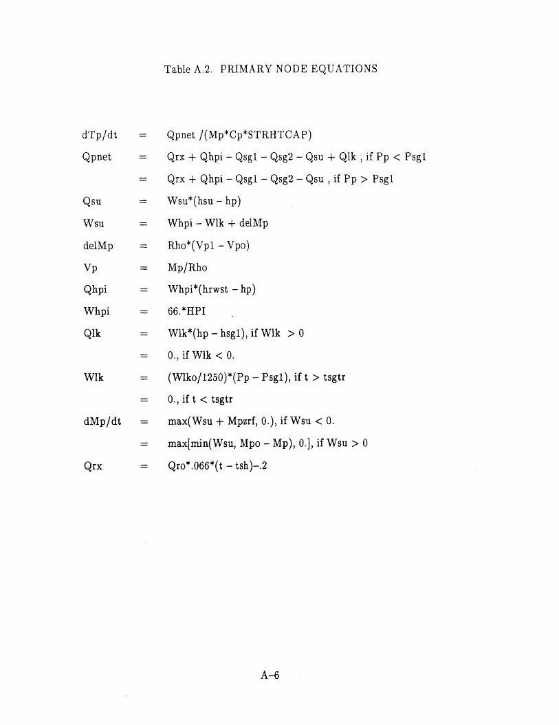
Table A.2. PRIMARY NODE EQUATIONS

dTp/dt Qpnet /(Mp*Cp*STRHTCAP)

Qpnet = Qrx + Qhpi - Qsgl - Qsg2 - Qsu + Qlk , if Pp < Psg1

Qrx + Qhpi - Qsgl - Qsg2 - Qsu , if Pp > Psg1

Qsu = Wsu*(hsu - hp)

Wsu = Whpi - Wlk + delMp

delMp = Rho*(Vpl - Vpo)

Vp = Mp/Rho

Qhpi = Whpi*(hrwst - hp)

Whpi = 66.*HPI

Qik = Wlk*(hp - hsg1), if Wlk > 0

= 0., if Wlk < 0.

Wlk = (Wlko/1250)*(Pp - Psg1), if t > tsgtr

= 0., if t < tsgtr

dMp/dt = max(Wsu + Mpzrf, 0.), if Wsu < 0.

= max[min(Wsu, Mpo - Mp), 0.1, if Wsu > 0

Qrx = Qro*.066*(t - tsh)-.2

A-6

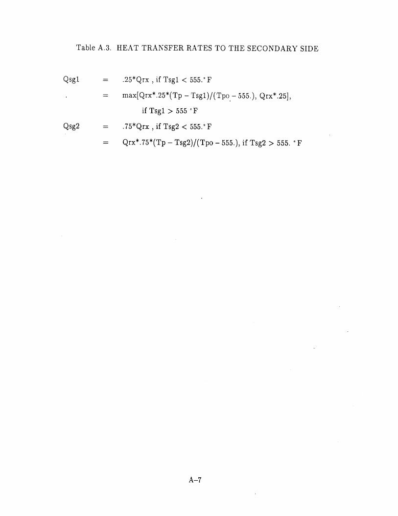
HEAT TRANSFER RATES TO THE SECONDARY SIDE

= .25*Qrx , if Tsgl < 555. F

- max[Qrx*.25*(Tp - Tsgl)/(Tpo - 555.), Qrx*.25],

if Tsgl > 555 "F

S.75*Qrx , if Tsg2 < 555.* F

= Qrx*.75*(Tp - Tsg2)/(Tpo - 555.), if Tsg2 > 555. F

A-7

Qsg1

Qsg2

Table A.3.

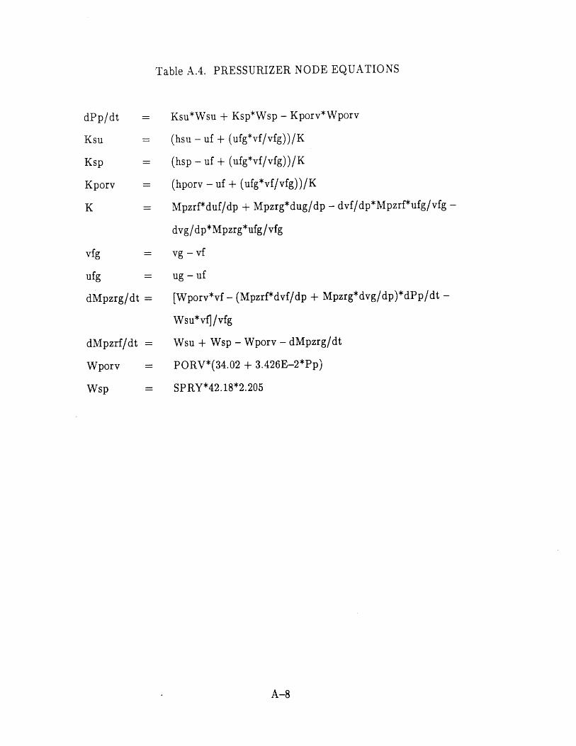
PRESSURIZER NODE EQUATIONS

= Ksu*Wsu + Ksp*Wsp - Kporv*Wporv

(hsu - uf + (ufg*vf/vfg))/K

= (hsp - uf + (ufg*vf/vfg))/K

= (hporv - uf + (ufg*vf/vfg))/K

Mpzrf*duf/dp + Mpzrg*dug/dp - dvf/dp*Mpzrf*ufg/vfg -

dvg/dp*Mpzrg*ufg/vfg

= vg - vf

= ug - uf

dMpzrg/dt = [Wporv*vf - (Mpzrf*dvf/dp + Mpzrg*dvg/dp)*dPp/dt -

Wsu*vf] /vfg

dMpzrf/dt = Wsu + Wsp - Wporv - dMpzrg/dt

Wporv = PORV*(34.02 + 3.426E-2*Pp)

Wsp = SPRY*42.18*2.205

A-8

dPp/dt

Ksu

Ksp

Kporv

K

vfg

ufg

Table A.4.

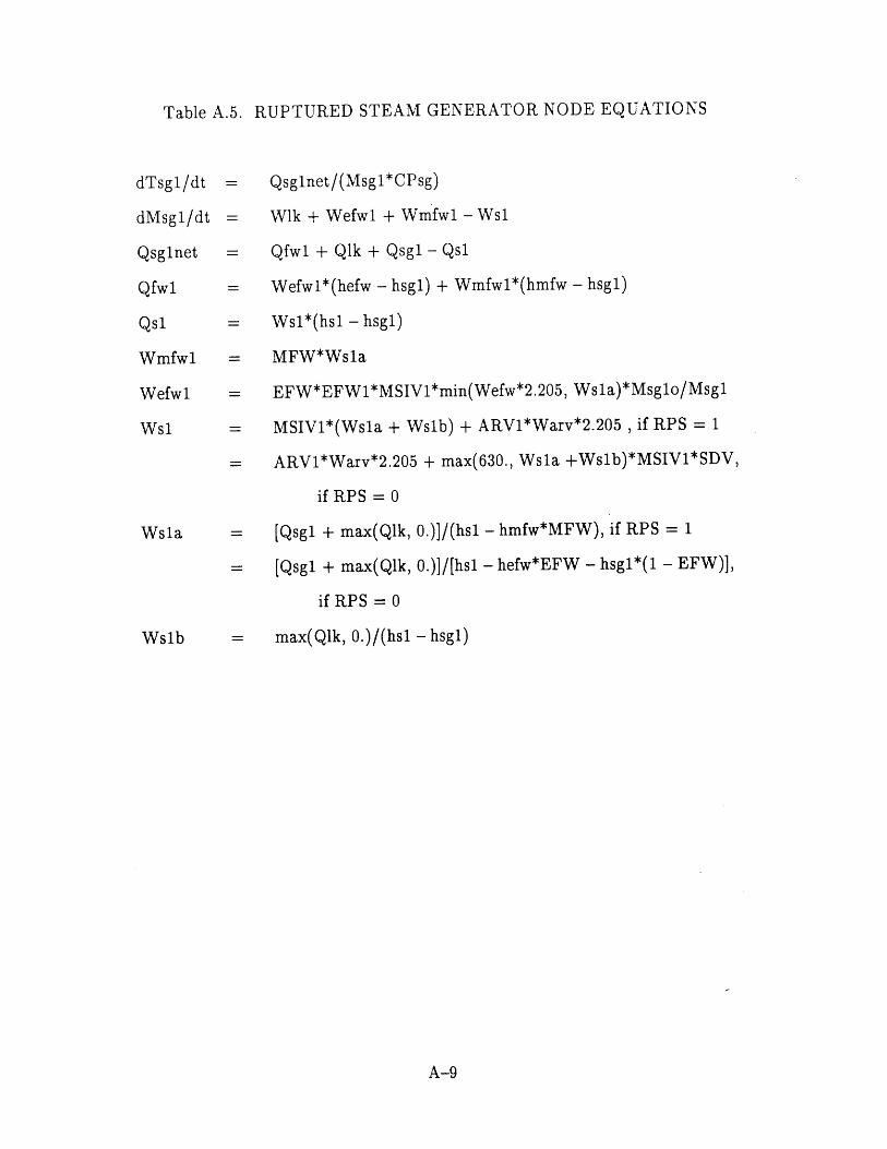
Table A.5. RUPTURED STEAM GENERATOR NODE EQUATIONS

dTsgl/dt

dMsg1/dt

Qsglnet

Qfwl

Qs1

Wmfwl

Wefwl

Ws1

Wsla

= Qsglnet/(Msgl*CPsg)

= Wlk + Wefwl + Wmfwl - Ws1

= Qfwl + Qlk + Qsgl - Qsl

= Wefwl*(hefw - hsg1) + Wmfwl*(hmfw - hsg1)

- Ws1*(hs1 - hsg1)

= MFW*Wsla

= EFW*EFW1*MSIV1*min(Wefw*2.205, Wsla)*Msglo/Msgl

= MSIV1*(Wsla + Wslb) + ARV1*Warv*2.205 , if RPS = 1

= ARV1*Warv*2.205 + max(630., Wsla +Wslb)*MSIV1*SDV,

if RPS = 0

= [Qsgl + max(Qlk, 0.)]/(hsl - hmfw*MFW), if RPS = 1

= [Qsg1 + max(Qlk, 0.)]/[hsl - hefw*EFW - hsgl*(1 - EFW)],

if RPS = 0

= max(Qlk, 0.)/(hsl - hsg1)Ws1b

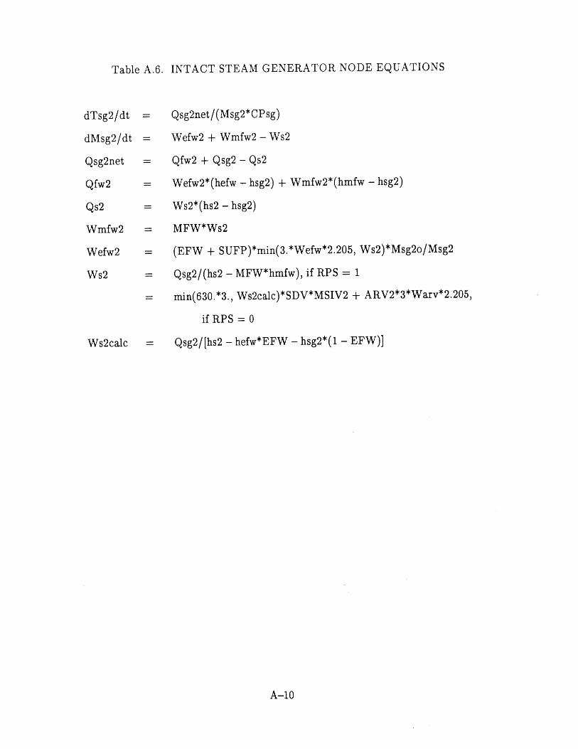
INTACT STEAM GENERATOR NODE EQUATIONS

dTsg2/dt = Qsg2net/(Msg2*CPsg)

dMsg2/dt = Wefw2 + Wmfw2 - Ws2

Qsg2net = Qfw2 + Qsg2 - Qs2

Qfw2 = Wefw2*(hefw - hsg2) + Wmfw2*(hmfw - hsg2)

Qs2 = Ws2*(hs2 - hsg2)

Wmfw2 = MFW*Ws2

Wefw2 = (EFW + SUFP)*min(3.*Wefw*2.205, Ws2)*Msg2o/Msg2

Ws2 = Qsg2/(hs2 - MFW*hmfw), if RPS = 1

= min(630.*3., Ws2calc)*SDV*MSIV2 + ARV2*3*Warv*2.205,

if RPS = 0

Ws2calc = Qsg2/[hs2 - hefw*EFW - hsg2*(1 - EFW)]

A-10

Table A.6.

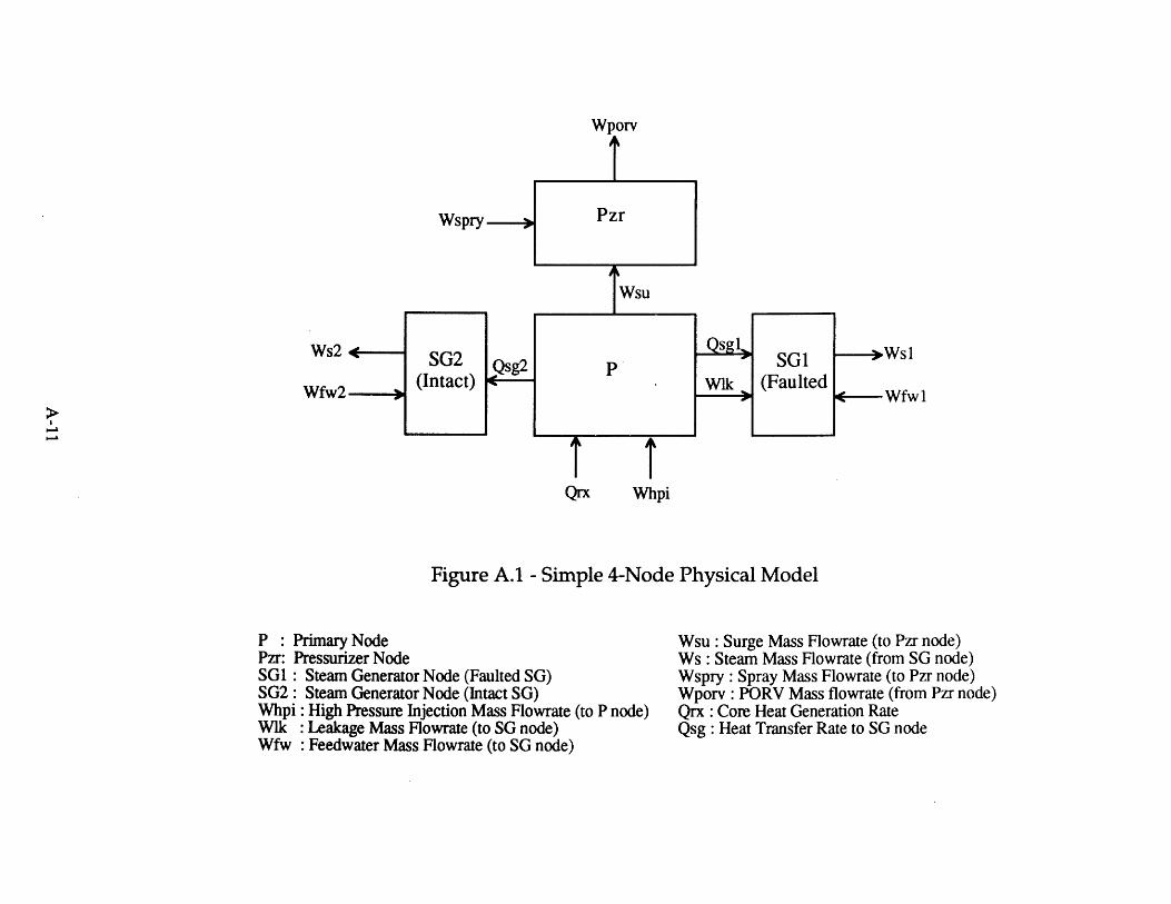
Wporv

Wspry Pzr

Wsu

Ws2 *-

Wfw2 3

SG2(Intact)

Qsg2

1TQrx

iWhpi

Wik--- +

SG1(Faulted

-Ws1

(--Wfw 1

Figure A.1 - Simple 4-Node Physical Model

P : Primary NodePzr: Pressurizer NodeSG1 : Steam Generator Node (Faulted SG)SG2: Steam Generator Node (Intact SG)Whpi: High Pressure Injection Mass Flowrate (to P node)Wik : Leakage Mass Flowrate (to SG node)Wfw : Feedwater Mass Flowrate (to SG node)

Wsu : Surge Mass Flowrate (to Pzr node)Ws : Steam Mass Flowrate (from SG node)Wspry Spray Mass Flowrate (to Pzr node)Wporv PORV Mass flowrate (from Pzr node)Qrx Core Heat Generation RateQsg: Heat Transfer Rate to SG node

P

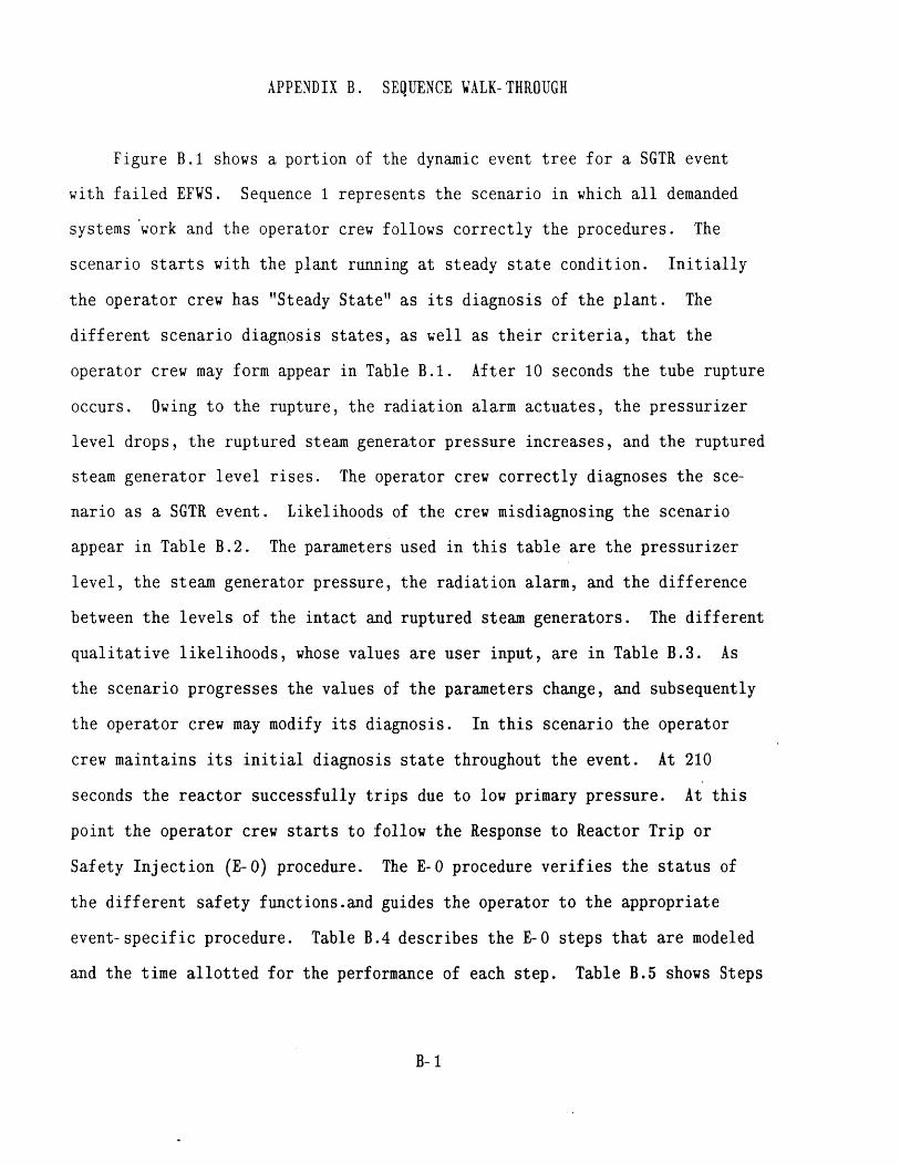
APPENDIX B. SEQUENCE WALK-THROUGH

Figure B.1 shows a portion of the dynamic event tree for a SGTR event

with failed EFWS. Sequence 1 represents the scenario in which all demanded

systems 'work and the operator crew follows correctly the procedures. The

scenario starts with the plant running at steady state condition. Initially

the operator crew has "Steady State" as its diagnosis of the plant. The

different scenario diagnosis states, as well as their criteria, that the

operator crew may form appear in Table B.1. After 10 seconds the tube rupture

occurs. Owing to the rupture, the radiation alarm actuates, the pressurizer

level drops, the ruptured steam generator pressure increases, and the ruptured

steam generator level rises. The operator crew correctly diagnoses the sce-

nario as a SGTR event. Likelihoods of the crew misdiagnosing the scenario

appear in Table B.2. The parameters used in this table are the pressurizer

level, the steam generator pressure, the radiation alarm, and the difference

between the levels of the intact and ruptured steam generators. The different

qualitative likelihoods, whose values are user input, are in Table B.3. As

the scenario progresses the values of the parameters change, and subsequently

the operator crew may modify its diagnosis. In this scenario the operator

crew maintains its initial diagnosis state throughout the event. At 210

seconds the reactor successfully trips due to low primary pressure. At this

point the operator crew starts to follow the Response to Reactor Trip or

Safety Injection (E-0) procedure. The E-0 procedure verifies the status of

the different safety functions.and guides the operator to the appropriate

event-specific procedure. Table B.4 describes the E-0 steps that are modeled

and the time allotted for the performance of each step. Table B.5 shows Steps

B- 1

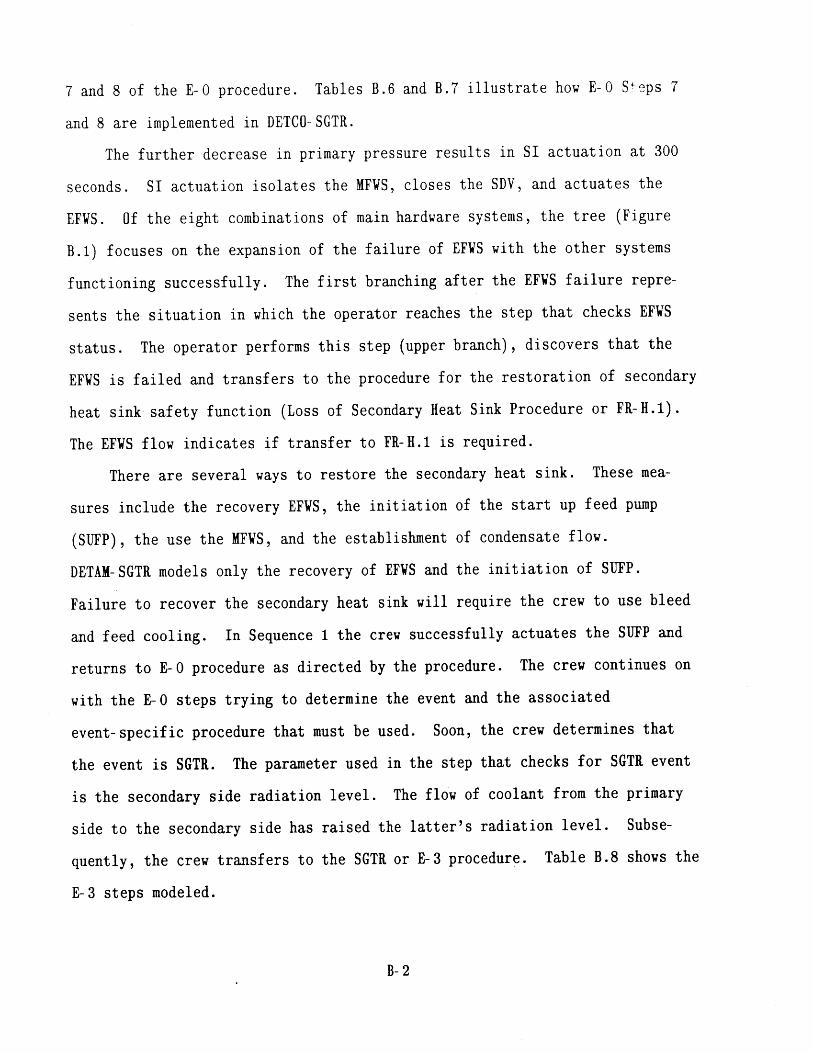
7 and 8 of the E-0 procedure. Tables B.6 and B.7 illustrate how E-0 Steps 7

and 8 are implemented in DETCO-SGTR.

The further decrease in primary pressure results in SI actuation at 300

seconds. SI actuation isolates the MFS, closes the SDV, and actuates the

EFWS. Of the eight combinations of main hardware systems, the tree (Figure

B.1) focuses on the expansion of the failure of EFWS with the other systems

functioning successfully. The first branching after the EFWS failure repre-

sents the situation in which the operator reaches the step that checks EFWS

status. The operator performs this step (upper branch), discovers that the

EFWS is failed and transfers to the procedure for the restoration of secondary

heat sink. safety function (Loss of Secondary Heat Sink Procedure or FR-H.1).

The EFWS flow indicates if transfer to FR-H.1 is required.

There are several ways to restore the secondary heat sink. These mea-

sures include the recovery EFWS, the initiation of the start up feed pump

(SUFP), the use the MFS, and the establishment of condensate flow.

DETAM-SGTR models only the recovery of EFVS and the initiation of SUFP.

Failure to recover the secondary heat sink will require the crew to use bleed

and feed cooling. In Sequence 1 the crew successfully actuates the SUFP and

returns to E-0 procedure as directed by the procedure. The crew continues on

with the E-0 steps trying to determine the event and the associated

event-specific procedure that must be used. Soon, the crew determines that

the event is SGTR. The parameter used in the step that checks for SGTR event

is the secondary side radiation level. The flow of coolant from the primary

side to the secondary side has raised the latter's radiation level. Subse-

quently, the crew transfers to the SGTR or E-3 procedure. Table B.8 shows the

E-3 steps modeled.

B- 2

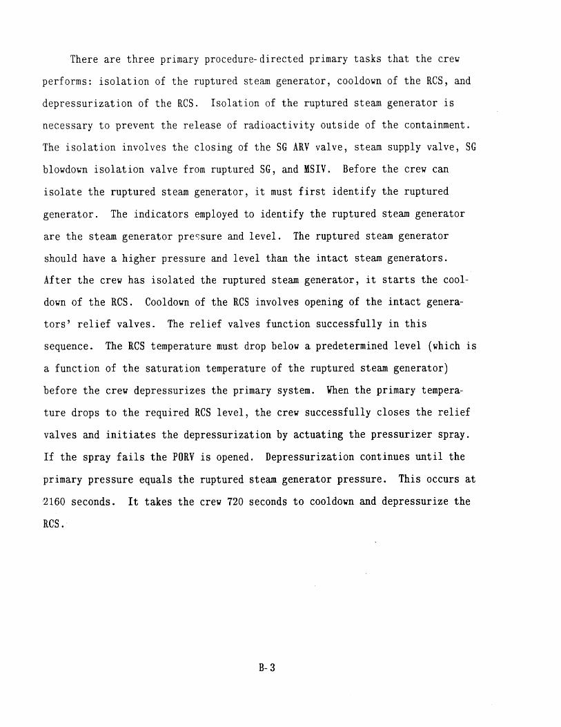
There are three primary procedure-directed primary tasks that the crew

performs: isolation of the ruptured steam generator, cooldown of the RCS, and

depressurization of the RCS. Isolation of the ruptured steam generator is

necessary to prevent the release of radioactivity outside of the containment.

The isolation involves the closing of the SG ARV valve, steam supply valve, SG

blowdown isolation valve from ruptured SG, and MSIV. Before the crew can

isolate the ruptured steam generator, it must first identify the ruptured

generator. The indicators employed to identify the ruptured steam generator

are the steam generator pressure and level. The ruptured steam generator

should have a higher pressure and level than the intact steam generators.

After the crew has isolated the ruptured steam generator, it starts the cool-

down of the RCS. Cooldown of the RCS involves opening of the intact genera-

tors' relief valves. The relief valves function successfully in this

sequence. The RCS temperature must drop below a predetermined level (which is

a function of the saturation temperature of the ruptured steam generator)

before the crew depressurizes the primary system. When the primary tempera-

ture drops to the required RCS level, the crew successfully closes the relief

valves and initiates the depressurization by actuating the pressurizer spray.

If the spray fails the PORV is opened. Depressurization continues until the

primary pressure equals the ruptured steam generator pressure. This occurs at

2160 seconds. It takes the crew 720 seconds to cooldown and depressurize the

RCS.

B- 3

Table B.1. SCENARIO TRANSITION CRITERIA

B- 4

POTENTIAL STATESCURRENTSTATE

STEADY STATE UNCERTAIN SGTR SLOCA

STEADY No change in Criteria for SG level is SG level isSTATE Pzr level, SG SGTR, SLOCA increasing, decreasing, Pp

level & Pp & steady Pp & Pzr and RA is offstate are not are not met level are

met decreasingand RA is on

UNCERTAIN Neither SGTR SG level is SG level isnor SLOCA increasing, decreasing,criteria are Pp & Pzr 1 Pp & Pzr levelmet level are are decreasing

decreasing and RA is offand RA is on

SGTR SG level is SG level isincreasing, decreasing, Pp && Pzr level Pzr level areare decreas- decreasing anding and RA is RA is offon

SLOCA SG level is SG level isincreasing, decreasing, PpPp & Pzr & Pzr level arelevel are decreasing anddecreasing RA is offand RA is on

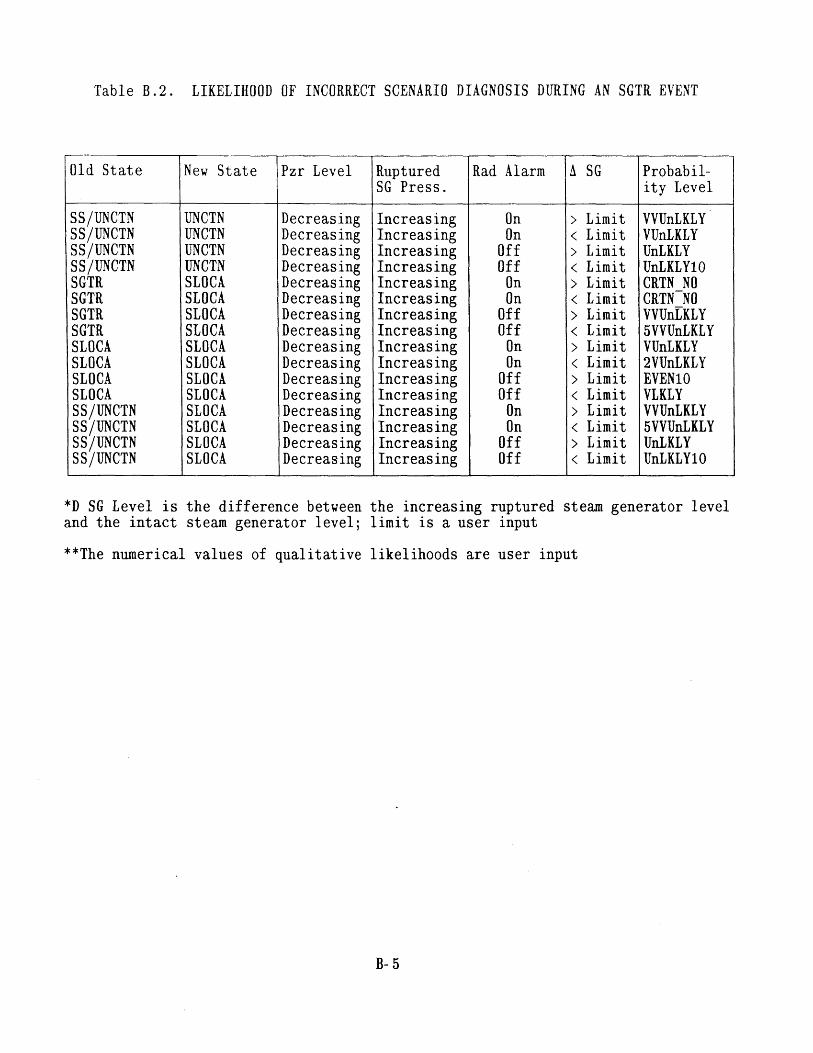
Table B.2. LIKELIHOOD OF INCORRECT SCENARIO DIAGNOSIS DURING AN SGTR EVENT

Old State New State Pzr Level Ruptured Rad Alarm A SG Probabil-SG Press. ity Level

SS/UNCTN UNCTN Decreasing Increasing On > Limit VVUnLKLYSS/UNCTN UNCTN Decreasing Increasing On < Limit VUnLKLYSS/UNCTN UNCTN Decreasing Increasing Off > Limit UnLKLYSS/UNCTN UNCTN Decreasing Increasing Off < Limit UnLKLY10SGTR SLOCA Decreasing Increasing On > Limit CRTN NOSGTR SLOCA Decreasing Increasing On < Limit CRTNNOSGTR SLOCA Decreasing Increasing Off > Limit VVUnLKLYSGTR SLOCA Decreasing Increasing Off < Limit 5VVUnLKLYSLOCA SLOCA Decreasing Increasing On > Limit VUnLKLYSLOCA SLOCA Decreasing Increasing On < Limit 2VUnLKLYSLOCA SLOCA Decreasing Increasing Off > Limit EVEN10SLOCA SLOCA Decreasing Increasing Off < Limit VLKLYSS/UNCTN SLOCA Decreasing Increasing On > Limit VVUnLKLYSS/UNCTN SLOCA Decreasing Increasing On < Limit 5VVUnLKLYSS/UNCTN SLOCA Decreasing Increasing Off > Limit UnLKLYSS/UNCTN SLOCA Decreasing Increasing Off < Limit UnLKLY10

*D SG Level is the difference between the increasing ruptured steam generator leveland the intact steam generator level; limit is a user input

**The numerical values of qualitative likelihoods are user input

B- 5

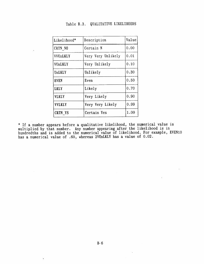
Table B.3. QUALITATIVE LIKELIHOODS

Likelihood* Description Value

CRTNNO Certain N 0.00

VVUnLKLY Very Very Unlikely 0.01

VUnLKLY Very Unlikely 0.10

UnLKLY Unlikely 0.30

EVEN Even 0.50

LKLY Likely 0.70

VLKLY Very Likely 0.90

VVLKLY Very Very Likely 0.99

CRTNYS Certain Yes 1.00

* If a number appears before a qualitative likelihood, the numerical value ismultiplied by that number. Any number appearing after the likelihood is inhundredths and is added to the numerical value of likelihood. For example, EVEN10has a numerical value of .60, whereas 2VUnLKLY has a value of 0.02.

B- 6

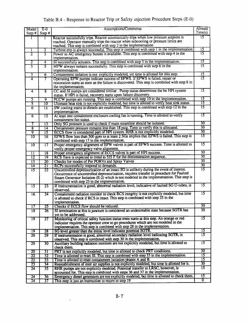
Table B.4 - Response to Reactor Trip or Safety injection Procedure Steps (E-0)

Model Assumptions/Comments AlloTed

Step# Step # Time(s)1 1 Reactor successfully trips. Reactor automatically trips when low pressure setpoint is 15

reached. Operator manually trips the reactor when subcooling or pressure limits arereached. This step is combined with step 2 in the implementation

1 2 Turbine trip is always successful. This step is combined with step 1 in the implementation 152 3 Power to AC emergency busses is available. This step is combined with step 4 in the 15

implementation.2 4 SI successfully actuates. This step is combined with step 3 in the implementation. 153 5 MFW always isolates successfully. This step is combined with step 6 in the 15

implementation.3 6 Containment isolation is not explicitly modeled, yet time is allotted for this step. 154 7 Operating EFW pumps indicate success of EFWS. If EFWS is failed, repair or 15

restoration starts as soon as the failure is discovered. This step is combined with step 8 inthe implementation.

4 8 CC and SI pumps are considered similar. Pump status determines the he HPI system 15status. If HPI is failed, recovery starts upon failure discovery.

9 PCCW pumps are running. This step is combined with step 10 in the implementation. 155 10 Ultimate heat sink is not explicitly modeled, but time is alloted to verify heat sink status. 156 11 SW cooling trains to diesels are established. This step is combined with step 12 in the 15

implementation.6 12 At least one containment enclosure cooling fan is running. Time is allotted to verify 15

containment fan status.7 13 Only SG pressure is used to check if main steamline should be isolated. 308 14 Containment pressure remains less than 18 psig. Time to verify this is allocated. 309 15 ECCS flow is considered part of HPI system. RHR is not explicitly modeled. 3010 1 EFWS flow less than 500 gpm to at least 2 SGs implies that S is failed. This step is 15

combined with step 17 in the implementation.10 17 Proper emergency alignment of EFW valves is part of EFWS success. Time is allotted to 13

verify proper emergency valve alignment.11 18 Proper emergency alig nent of ECCS valves is part of HPI success. 3012 19 RCS Tave is expected to trend to 555 F for the demonstration sequence. 3013 20 Checks for modes of Pzr PORVs and Spray Valves 3014 71 RCPs successfully respond to demands. 3015 2 Uncontrolled depressurization of an intact SG is unlikely during the event of interest. 15

Occurrence of uncontrolled depressurization, requires transfer to procedure for FaultedSteam Generator Isolation (E-2) which is not modeled in the implementation. This step iscombined with step 23 in the implementation.

15 23 If instrumentation is good, abnormal radiation level, indicative of faulted SG U-tubes, is 15observed.

16 24 Containment radiation monitor to check RCS integrity is not explicitly modeled, but time 15is allotted to check if RCS is intact. This step is combined with step 25 in theimplementation.

17 25 Checks if ECCS flow should be reduced. 3018 26 SI termination at this is juneture is considered an undesireable state because SGTR has 30

yet to be addressed.19 27 Monitoring of critical safety function status trees starts at this step. An orange or red 15

indicator requires the operator crew to go procedures which are not modeled in theimplementation. This step is combined with step 28 in the implementation.

19 28 SG level fgreater than the initial level indicates potential SGTR. 1520 29 If instrumentation is good, abnormal secondary radiation level indicating SGTR, is 15

observed. This step is combined with step 30 in the implementation.20 30 Auxiliary building radiation monitors are not explicitly modeled, but time is allotted to 15

check them.20 31 PRT is not explicitly modeled, but time is allotted to check PRT conditions. 3022 32 Time is allotted to reset SI. This step is combined with step 33 in the implementation. 1522 73 Time is allotted to reset containment isolation ases A and B. 1523 Reestablishment of instr air supplies is not explicitly modeled, but time is allotted for it. 324 3 RHR pumps are not explicitly modeled. Potential transfer to LRSC, however, is 15

accounted for. This step is combined with steps 36 and 37 in the implementation.24 36 Emergency diesel generators are not explicitly modeled, but time is allotted to check them. 1524 37 This step is just an instruction to return to step 19 0

B- 7

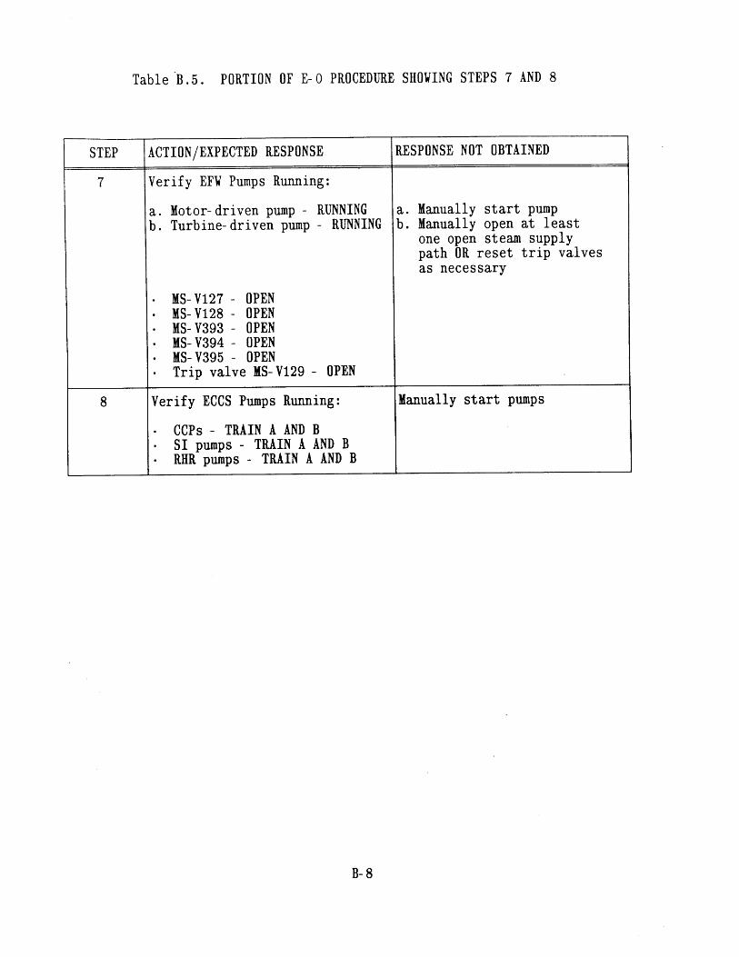
Table B.5. PORTION OF E-0 PROCEDURE SHOWING STEPS 7 AND 8

B- 8

STEP ACTION/EXPECTED RESPONSE RESPONSE NOT OBTAINED

7 Verify EFV Pumps Running:

a. Motor-driven pump - RUNNING a. Manually start pumpb. Turbine-driven pump - RUNNING b. Manually open at least

one open steam supplypath OR reset trip valvesas necessary

- MS-V127 - OPEN- MS-V128 - OPEN- MS-V393 - OPEN- MS-V394 - OPEN- MS-V395 - OPEN- Trip valve MS-V129 - OPEN

8 Verify ECCS Pumps Running: Manually start pumps

- CCPs - TRAIN A AND B- SI pumps- TRAIN A AND B- RHR pumps - TRAIN A AND B

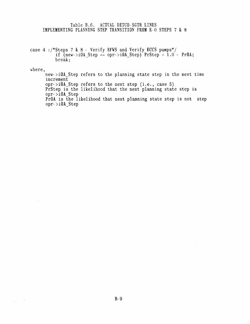
Table B.6. ACTUAL DETCO-SGTR LINESIMPLEMENTING PLANNING STEP TRANSITION FROM E-0 STEPS 7 & 8

case 4 :/*Steps 7 & 8 - Verify EFWS and Verify ECCS pumps*/if (new->iOAStep == opr->iOA_Step) PrStep = 1.0 - PrOA;break;

where,new->iOA Step refers to the planning state step in the next timeincrementopr->iOA Step refers to the next step (i.e., case 5)PrStep is the likelihood that the next planning state step isopr->iOA StepPrOA is the likelihood that next planning state step is not stepopr->iOAStep

B- 9

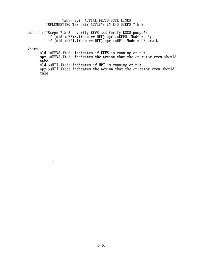
Table B.7 ACTUAL DETCO-SGTR LINESIMPLEMENTING THE CREW ACTIONS IN E-0 STEPS 7 & 8

case 4 :/*Steps 7 & 8 - Verify EFWS and Verify ECCS pumps*/if (old->sEFWS.iMode == OFF) opr->sEFVS.iMode O ON;if (old->sHPI.iMode OFF) opr->sHPI.iMode = ON break;

where,old->sEFWS.iMode indicates if EFWS is running or notopr->sEFWS.iMode indicates the action that the operator crew shouldtakeold->sHPI.iMode indicates if HPI is running or notopr->sHPI.iMode indicates the action that the operator crew shouldtake

B- 10

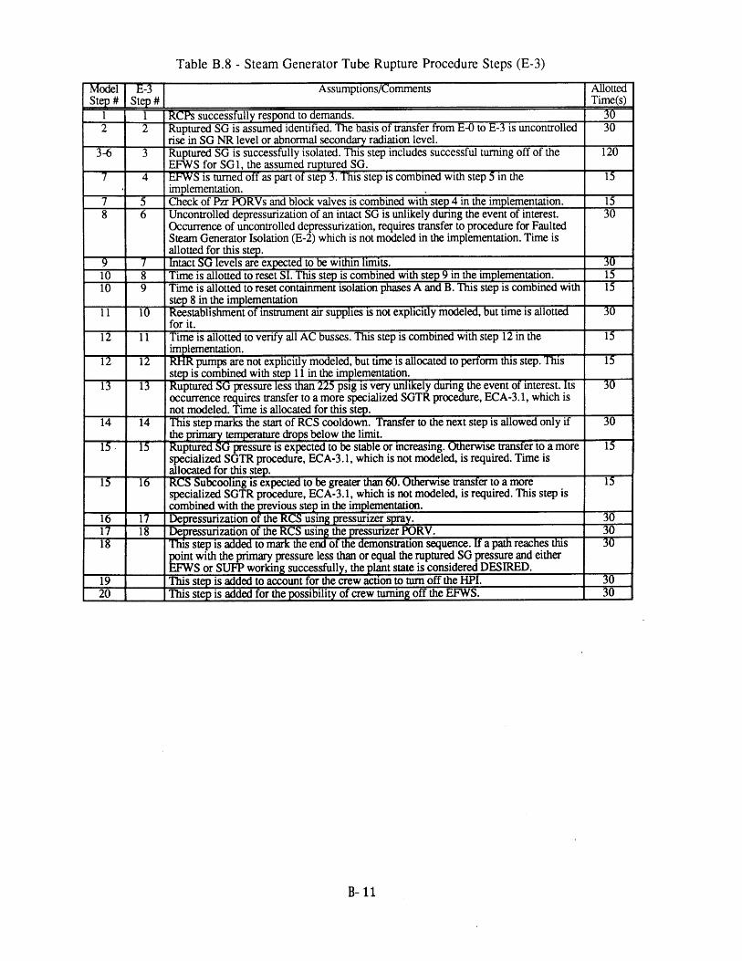
Table B.8 - Steam Generator Tube Rupture Procedure Steps (E-3)

Model E-3 Assumptions/Comments AllottedStep # Step # Time(s)

I I RCPs successfully respond to demands. 302 2 Ruptured SG is assumed identified. The basis of transfer from E-0 to E-3 is uncontrolled 30

rise in SG NR level or abnormal secondary radiation level.3-6 3 Ruptured SG is successfully isolated. This step includes successful turning off of the 120

EFWS for SG1, the assumed ruptured SG.7 4 EFWS is turned off as part of step 3. This step is combined with step 5 in the 15

-_ implementation.7 T Check of Pzr PORVs and block valves is combined with step 4 in the implementation. 158 6 Uncontrolled depressurization of an intact SG is unlikely during the event of interest. 30

Occurrence of uncontrolled depressurization, requires transfer to procedure for FaultedSteam Generator Isolation (E-2) which is not modeled in the implementation. Time isallotted for this step.

9 7 Intact SG levels are expected to be within limits. 3010 8 Time is allotted to reset SI. This step is combined with step 9 in the implementation. 1510 9 Time is allotted to reset containment isolation phases A and B. This step is combined with 15

step 8 in the implementation11 10 Reestablishment of instrument air supplies is not explicitly modeled, but time is allotted 30

for it.12 11 Time is allotted to verify all AC busses. This step is combined with step 12 in the 15

implementation.12 12 RHR pumps are not explicitly modeled, but time is allocated to perform this step. This 15

step is combined with step 11 in the implementation.13 13 Ruptured SG pressure less than 225 psig is very unlikely during the event of interest. Its 30

occurrence requires transfer to a more specialized SGTR procedure, ECA-3.1, which isnot modeled. Time is allocated for this step.

14 14 This step marks the start of RCS cooldown. Transfer to the next step is allowed only if 30the primary temperature drops below the limit.

13 15 Ruptured SG pressure is expected to be stable or increasing. Otherwise transfer to a more 15specialized SGTR procedure, ECA-3. 1, which is not modeled, is required. Time isallocated for this step.

15 16 RCS Subcooling is expected to be greater than 60. Otherwise transfer to a more 15specialized SGTR procedure, ECA-3.1, which is not modeled, is required. This step iscombined with the previous step in the implementation.

16 17 Depressurization of the RCS using pressurizer spray. 3017 18 Depressurization of the RCS usi the pressurizer PORV. 30

This step is added to mark the end of the demonstration sequence. If a path reaches this 30point with the primary pressure less than or equal the ruptured SG pressure and eitherEFWS or SUFP working successfully, the plant state is considered DESIRED.

19 This step is added to account for the crew action to turn off the HPI. 3020 This step is added for the possibility of crew turning off the EFWS. 30

B- 11

-1

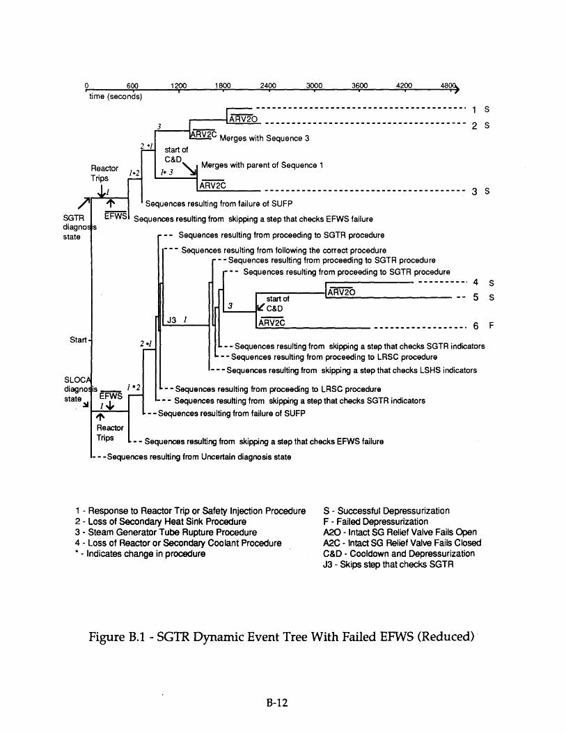
0 600time (seconds)

1200 1800 2400 3000 3600 4

AM/----------------------------------------- 1 S

ARV203 1 - - - -- ~- ~ - - - -- - ------~~~----~~ ~ ~ ~ ~ ~ ~ ~ -~ - 2 SRV2C Merges with Sequence 3

2.*1 start of

Reactor Merges with parent of Sequence 1.eco 1*2 1* 3 N

Tnips - -.---ARC - -------------------------------------- 3 S

t F Sequences resulting from failure of SUFP

S Sequences resulting from skipping a step that checks EFWS failures

-- Sequences resulting from proceeding to SGTR procedure

--- Sequences resulting from following the correct procedure- - Sequences resulting from proceeding to SGTR procedure

--- Sequences resulting from proceeding to SGTR procedure---------- 4

start of -ARV- 5- _3 __l C&D

J3 I L A -C 6------------------6

2 *1 - - Sequences resulting from skipping a step that checks SGTR indicators- - Sequences resulting from proceeding to LRSC procedure

-- uen-es rsiultin fmm skinnin a ete that checks I SHS indicatnrs

SGTRdiagnosstate

Start -

SLOCAdiagnostate

3

S

R indicators

1 - Response to Reactor Trip or Safety Injection Procedure2 - Loss of Secondary Heat Sink Procedure3 - Steam Generator Tube Rupture Procedure4 - Loss of Reactor or Secondary Coolant Procedure* - Indicates change in procedure

S - Successful DepressurizationF - Failed DepressurizationA20 - Intact SG Relief Valve Fails OpenA2C - Intact SG Relief Valve Fails ClosedC&D - Cooldown and DepressurizationJ3 - Skips step that checks SGTR

Figure B.1 - SGTR Dynamic Event Tree With Failed EFWS (Reduced)

B-12

q g p g. p

is _ 1 *2 - - Sequences resulting from proceeding to LRSC procedureEFWS --- Sequences resulting from skipping a step that checks SGT

. - - Sequences resulting from failure of SUFP

Reactor

Trips - - Sequences resulting from skipping a step that checks EFWS failure

--- Sequences resulting from Uncertain diagnosis state

1 2I 1800, 2400 3000 3600 4200 4800L