Dynamic and static asymmetric response of a layesred thick disk

This article appeared in a journal published by Elsevier. The attachedcopy is furnished to the author for internal non-commercial researchand education use, including for instruction at the authors institution

and sharing with colleagues.

Other uses, including reproduction and distribution, or selling orlicensing copies, or posting to personal, institutional or third party

websites are prohibited.

In most cases authors are permitted to post their version of thearticle (e.g. in Word or Tex form) to their personal website orinstitutional repository. Authors requiring further information

regarding Elsevier’s archiving and manuscript policies areencouraged to visit:

http://www.elsevier.com/copyright

http://www.elsevier.com/copyright

Author's personal copy

Dynamic and static asymmetric response of a layered thick disk

Michael El-RahebSatellite Consulting Inc., 1000 Oakforest Lane, Pasadena, CA 91107, United States

a r t i c l e i n f o

Article history:Received 24 July 2011Received in revised form 29 October 2011Available online 13 November 2011

Keywords:Thick layered disksAsymmetric loadingElasto-dynamicsElasto-staticsSurface stresses

a b s t r a c t

Treated is the asymmetric static and dynamic response of a stack of layered thick disks from externalload. Variables of the three-dimensional equations are separated assuming approximate simple supportsalong the cylindrical perimeter, yielding non-orthogonal eigenfunctions. This also couples the truncatedset of radial wave numbers. Applying a radial transform to all variables eliminates radial dependence pro-ducing a diagonal eigenproblem in all coupled axial wave numbers. Comparing 3-D and 2-D asymmetricmodels of industrial glass disks reveals that the 3-D resonances are close to their 2-D counterparts adopt-ing the Mindlin model. A Fourier analysis of a specific asymmetric line-load from pressure or thermalexpansion produces a scale factor to static stress from a limited number of asymmetric solutions eachwith a different circumferential wave number.

� 2011 Elsevier Ltd. All rights reserved.

1. Introduction

Thick disks of brittle material like glass are used as mandrills inthe process of constructing accurate parabolic space antennas.Hardness and low thermal expansion are required properties whenadhering the thin reflective coating to the surface of the reflectorstructure. These properties are met by industrial glass. Applica-tions for space exploration require a light but stiff frame made ofhot-pressed ceramics with integral ribs. Pressing the bare side ofthe antenna frame on the coated glass mandrill transmits asym-metric loads to the glass sometimes producing small superficialcracks near the disk center. Due to the substantial manufacturingcost of these mandrills, care is needed in the loading process toavoid damaging the surface.

Due to the circumferential and radial asymmetry in stiffness ofthe reflector structure, loads transmitted to the mandrill are alsoasymmetric. Analysis of this setup requires the solution of staticand dynamic response of a thick disk forced by an asymmetricexcitation. Discretization by finite elements is applicable to itssolution. Yet, the asymmetry in loading requires elements through-out the mandrill volume. This translates to a large number of de-grees of freedom and in turn to a substantial computationaleffort especially when parametric analysis is needed. Moreover,an analytical method helps comparing results with other purelynumerical methods and the timely evaluation and interpretationof experimental results.

Response of thick disks is mostly treated by finite element orother purely numerical methods. Chen and Doong (1984) analyzed

the vibration of initially stressed isotropic thick disks by eliminat-ing circumferential dependence and solving the radial and axialdependence by finite difference. Chen and Chen (1988, 1989) ana-lyzed the asymmetric buckling, vibration and dynamic stability ofbi-modulus thick annular disks by a Rayleigh–Ritz finite elementmethod. Soamidas and Ganesan (1991) analyzed the vibration ofthick polar orthotropic and variable thickness disks adoptingMindlin’s plate equations and a finite series expansion radially.Vinayak and Singh (1996) analyzed annular disks with holes andinclusions adopting Mindlin’s equations and bi-orthogonal shapefunctions in a Ritz method. In all references above, normal stressis varying linearly across the thickness. Singh and Subramaniam(2003) devised a purely numerical finite element method for thevibration of thick disks and shells of revolution after eliminatingthe circumferential dependence. Dong (2008) analyzed the vibra-tion of functionally graded annular disks using the Chebyshev–Ritzmethod. El-Raheb and Wagner (1996) analyzed the 3-D axisym-metric wave propagation in layered disks from impulsive loading.Since the present work is an extension to this analysis, a summaryof the method serves as an introduction to what will follow.

Displacement vector is expressed in terms of two scalar poten-tials (Miklowitz, 1984) which when substituted in the Navier equa-tions of elasto-dynamics yields two Helmholtz equations, one foreach of the scalar potentials, and with wave lengths related toextensional and shear wave motions respectively. Displacementsand stresses are then expressed in terms of the potentials and theirderivatives. Satisfying boundary conditions on the disk cylindricalsurface produces a dispersion relation in radial wave number. Thisprocess also determines axial wave number since it is related to ra-dial wave number. Natural boundary conditions on the cylindricalsurface are either traction-free where radial and shear stresses

0020-7683/$ - see front matter � 2011 Elsevier Ltd. All rights reserved.doi:10.1016/j.ijsolstr.2011.11.002

E-mail address: [email protected]

International Journal of Solids and Structures 49 (2012) 599–612

Contents lists available at SciVerse ScienceDirect

International Journal of Solids and Structures

journal homepage: www.elsevier .com/locate / i jsols t r


vanish, or restrained where radial and axial displacements vanish.Neither of these conditions can be satisfied exactly. An approxi-mate alternative is to let gradient of radial displacement vanish.Although this condition is not natural to the problem, it approxi-mates simple supports meaning that both axial displacement uand radial stress rrr on the disk perimeter (see Fig. 1) are finitebut relatively small. In fact when adopting this constraint, radialwave number asymptotically approaches that of the exact simplesupports at higher wave numbers. The drawback is that the prob-lem loses its self-adjoint nature and in turn eigenfunctions becomenon-orthogonal.

The state vector formed of two displacements and two tractionson a layer’s face is related to that on the opposite face by a transfermatrix. Continuity of state vectors at each interface of layers pro-duces a global transfer matrix yielding an implicit eigenvalue prob-lem. An iterative solution yields the system eigenset. Forcedresponse follows using the static-dynamic superposition method.

Steps similar to those presented above are followed in the pres-ent analysis although the asymmetric problem is more compli-cated since asymmetry raises the number of independent anddependent variables. Section 2 develops the dynamic asymmetricanalysis.

Section 3 develops the static asymmetric analysis. The staticproblem is that of the thick glass disk with one face lying on a rigidbase and the other subjected to pressure applied by a stiff hexago-nal lattice. A Fourier expansion of the lattice determines which cir-cumferential wave numbers contribute to static response, namelyzero and multiples of 6. Also, the expansion allows superpositionof stress from the different wave number static solutions yieldingan approximate estimate of maximum stress in the disk. Section4 presents dynamic and static results.

2. Dynamic analysis

In cylindrical coordinates, the general linear elasto-dynamicequations in terms of the divergence D defined in (2) and rotationswr, wh, wz are (Love, 1944)

ðkþ 2lÞ@rD� 2l@hwz=r þ 2l@zwh=r � q@ttu ¼ 0

ðkþ 2lÞ@hD=r � 2l@zwr þ 2l@rwz � q@ttt ¼ 0

ðkþ 2lÞ@zD� 2l@rðrwhÞ=r þ 2l@hwr=r � q@ttw ¼ 0

ð1Þ

k, l are Lame’ constants, (r,h,z) are radial, circumferential and axialcoordinates, (u,t,w) are displacements along (r,h,z) (see Fig. 1), t istime, and

D ¼ r � u � 1=r@rðruÞ þ 1=r@htþ @zw

2wr ¼ 1=r@hw� @zt; 2wh ¼ @zu� @rw; 2wz ¼ 1=rð@hðrtÞ � @huÞð2Þ

For harmonic motions in time with radian frequency x, assume theexpansions

uðr; h; z; tÞ ¼X

n

Xk

unkðzÞJ0nðckrÞ cosðnhÞeixt

tðr; h; z; tÞ ¼X

n

Xk

tnkðzÞJnðckrÞ sinðnhÞeixt

wðr; h; z; tÞ ¼X

n

Xk

wnkðzÞJnðckrÞ cosðnhÞeixt

ð3Þ

is a solution to Eq. (1), where n is an integer wave number along thecircumferential coordinate h, Jn(ckr) is the Bessel function satisfyingradial dependence of the governing equations, ( )0 is derivative withrespect to the argument, ck is radial wave number, and i ¼

ffiffiffiffiffiffiffi�1p

.Since the trigonometric functions in h are exact eigenfunction satis-fying circumferential dependence of the separated equations, theyare dropped temporarily in the expressions for shortness. Substitut-ing (3) in (2) then in (1) yieldsX

k

lu00nkðzÞ þ ðkþ lÞn2=r2 � ðkþ 2lÞc2k þ qx2� �

unkðzÞ�þðkþ lÞckntnkðzÞ=rþðkþ lÞckw0nkðzÞ

�J0nðckrÞ

� 2ðkþ 2lÞn2=ðckr3ÞunkðzÞ þ ðkþ 3lÞntnkðzÞ=r2� �JnðckrÞ ¼ 0

ð4aÞXk

lu00nkðzÞ þ ðkþ lÞn2=r2 � ðkþ 2lÞc2k þ qx2� �

unkðzÞ�þðkþ lÞckntnkðzÞ=rþðkþ lÞckw0nkðzÞ

�J0nðckrÞ

� 2ðkþ 2lÞn2=ðckr3ÞunkðzÞ þ ðkþ 3lÞntnkðzÞ=r2� �JnðckrÞ ¼ 0

ð4bÞXk

ðkþ 2lÞw00nkðzÞ � lc2kwnkðzÞ þ ðkþ lÞ=ck n2=r2 � c2

k

� �u0nkðzÞ

�þðkþ lÞnt0nkðzÞ=r þ qx2wnkðzÞ

�JnðckrÞ ¼ 0 ð4cÞ

Define the matrix coefficients

akk0p ¼Z a

0J0nðckrÞJ0nðck0 rÞrð1�pÞdr;

bkk0p ¼Z a

0J0nðckrÞJnðck0rÞrð1�pÞdr;

ckk0p ¼Z a

0JnðckrÞJnðck0rÞrð1�pÞdr ð5Þ

In (5), a is disk radius. Multiplying (4a) by rJ0nðcjrÞ, (4b) and (4c) byrJn(cjr), then integrating from 0 to a utilizing (5) produces a set ofcoupled second order ordinary differential equations in un k, tnk,wn k with constant coefficientsX

k

1�k2dc

2k

� �akj0þ k2

d�k2s

� �n2akj2þ2k2

dn2bjk3=ck�k2s n2akj2

� �unkðzÞ

hþk2

s akj0u00nkðzÞþ k2d�k2

s

� �nckakj1� k2

dþk2s

� �nbkj2

� �tnkðzÞ

þ k2d�k2

s

� �ckakj0w0nkðzÞ

i¼0 ð6aÞ

Xk

n k2d � k2

s

� �c2

k ckj1 � n2ckj3� �

=ck � k2s nbkj2

� �unkðzÞ þ k2

s ckj0t00nkðzÞh� n2 k2

d � k2s

� �cjk2 þ k2

s c2k ckj0 þ ckbkj1 þ ckj2

� �� tnkðzÞ

�n k2d � k2

s

� �ckj1w0nk

i¼ 0 ð6bÞ

u, σrr

v, σθθ

w, σzz

σrz

σrθ

σzθ

σθz

σzr

σθr

r

z

θ

Fig. 1. Cylindrical element.

600 M. El-Raheb / International Journal of Solids and Structures 49 (2012) 599–612


Xk

� k2d � k2

s

� �=ck c2

k ckj0 � n2ckj2� �

u0nkðzÞ þ n k2d � k2

s

� �ckj1t0nkðzÞ

hþk2

dckj0w00nkðzÞ þ ckj0 1� k2s c

2k

� �wnkðzÞ

i¼ 0

k2d ¼ ðkþ 2lÞ=qx2; k2

s ¼ 2l=qx2

ð6cÞ

To convert (6) into a standard eigen-matrix, diagonalize the termsfactoring u00nk; t00nk; w00nk by multiplying (6a) by a�1

kj0 � �akj0, and (6b)and (6c) by c�1

kj0 � �ckj0Xk

djk 1� k2dc

2k

� �þ n2 k2

d � k2s

� �ejk þ 2k2

dn2ojk=ck � k2s n2ejk

� �unkðzÞ

hþk2

s djku00nkðzÞ þ n k2d � k2

s

� �ckdjk � n k2

d þ k2s

� �fjk

� �tnkðzÞ

þ k2d � k2

s

� �ckdjkw0nkðzÞ

i¼ 0 ð7aÞ

Xk

n k2d � k2

s

� �c2

kgjk � n2ljk

� �=ck � k2

s n�njk

� �unkðzÞ þ k2

s djkt00nkðzÞh� n2 k2

d � k2s

� �hjk þ k2

s c2kdjk þ ckmjk þ hjk

� �� tnkðzÞ

�n k2d � k2

s

� �gjkw0nkðzÞ

i¼ 0 ð7bÞ

Xk

� k2d � k2

s

� �c2

kdjk � n2hjk

� �u0nkðzÞ=ck þ n k2

d � k2s

� �gjkt0nkðzÞ

hþk2

ddjkw00nkðzÞ þ djk 1� k2s c

2k

� �wnkðzÞ

i¼ 0 ð7cÞ

dkj ¼XN

q

�akq0aqj1; ekj ¼XN

q

�akq0aqj2; f kj ¼XN

q

�akq0bqj2

gkj ¼XN

p

�ckq0cqj1; hkj ¼XN

q

�ckq0cqj2; lkj ¼XN

q

�ckq0bqj3

mkj ¼XN

q

�ckq0bqj1; �nkj ¼XN

q

�ckq0bqj2; okj ¼XN

q

�akq0bqj3

ð7dÞ

dkj is the Kroneker delta, and in (7d) the number of ck is truncated toN. Since in Eqs. (7a)–(7c) coefficients of the z-dependence are con-stants, these equations admit a solution in the form:

unsðzÞ ¼XN

k¼1

unkseansz; tnsðzÞ ¼XN

k¼1

tnkseansz; wnsðzÞ

¼XN

k¼1

wnkseansz ð8Þ

Substituting (8) in (7) yields a set of matrix equations in the 6N un-knowns {u,t,w,u0,t0,w0}ns

u0ns � ansuns ¼ 0

t0ns � anstns ¼ 0

w0ns � answns ¼ 0

ð9aÞ

Auuuns þ Auttns þ Buww0ns � ansu0ns ¼ 0

Atuuns þ Atttns þ Btww0ns � anst0ns ¼ 0

Awwwns þ Bwuu0ns þ Bwtt0ns � answ0ns ¼ 0

ð9bÞ

uns = {un k s}T, tns = {t nk s}T, wns = {w nks}T, ans is a diagonal matrixand

Auujk ¼� djk�k2

d c2kdjk�n2ejkþ2n2ojk=ck

� ��k2

s n2ejk

h i=k2

s

Autjk ¼�n k2

d�k2s

� �ckdjk� k2

dþk2s

� �fjk

h i=k2

s ; Awwjk ¼�djk 1�k2

s c2k

� �=k2

d

Atujk ¼�n c2

k gjk�n2ljk

� �k2

d�k2s

� �=ck�2k2

s �nkj

h i=k2

s

Attjk ¼� djk�k2

dn2hjkþk2s ðn2�1Þhjk�c2

kdjk� �h i

=k2s

Buwjk ¼� k2

d�k2s

� �ckdjk=k2

s ; Btwjk ¼ k2

d�k2s

� �ngjk=k2

s

Bwujk ¼ k2

d�k2s

� �c2

kdjk�n2hjk

� �=ðckk2

dÞ;Bwtjk ¼� k2

d�k2s

� �ngjk=k2

d

ð9cÞ

A condensed form of (9) follows

Yns � ansXns ¼ 0

AXns þ BYns � ansYns ¼ 0

Xns ¼ fu; t;wgTns; Yns ¼ fu0; t0;w0gT

ns

ð10Þ

A and B in (10) are the ensemble of all matrices in (9b). Eq. (10) is inthe form of a diagonal eigen-matrix with eigenvalues ans, s = 1,6N.To determine ck assume the approximate boundary condition

J00nðckaÞ ¼ 0 ð11Þ

where a is disk radius. This condition satisfies @ru(a) = 0. For eachans corresponds an eigenvector {Xns,Yns}T = {{u,t,w}ns, {u0,t0,w0}ns}T

within a multiplicative constant Cnsk.To determine the transfer matrix relating conjoined segments,

define the state vector

Sns ¼ fu;rgTns; uns ¼ fu; t;wgT

ns; rns ¼ frzz;rrz;rhzgTns ð12Þ

with stresses

rzzns ¼XN

k

�k c2k � n2=r2� �

unsk=ck

þkntnsk=r þ ðkþ 2lÞanswnsk�eanszJnðckrÞ ð13aÞ

rrzns ¼XN

k

lðansunsk þ ckwnskÞeanszJ0nðckrÞ ð13bÞ

rhzns ¼XN

k

lðanstnsk � nwnsk=rÞeanszJnðckrÞ ð13cÞ

Because of the (1/r) and (1/r2) dependences in (13a) and (13c), theseexpressions are not purely a sum of terms each proportional toJn(ckr). To bring them into this form, the following approximationsare used

�rzzns �X

k

Xq

unskfukq þ tnskf

tkq þwnskf

wkq

h ieanszJnðckrÞ

�rhzns �X

k

Xq

tnskntkq þwnskn

wkq

h ieanszJnðckrÞ

ð14aÞ

with the requirementZ a

0

�rzznk

�rhznk

�JnðckrÞr dr ¼

Z a

0

rzznk

rhznk

�JnðckrÞr dr ð14bÞ

Substituting (13a) and (13c) and (14a) in (14b) yield relations forfu;t;w

kq and nt;wkq

fukq ¼ �k c2

kdkq � n2hTkq

� �=ck; ft

kq ¼ kngTkq; fw

kq ¼ ðkþ 2lÞasdkq

ntkq ¼ lasdkq; nw

kq ¼ �lngTkq

ð15aÞ

M. El-Raheb / International Journal of Solids and Structures 49 (2012) 599–612 601


In terms of barred variables, displacements and stresses become

�uns ¼XN

k

XN

q

Cnskunskakq0eansz; �tns ¼XN

k

XN

q

Cnsktnskckq0eansz

�wnk ¼XN

k

XN

q

Cnskwnskckq0eansz ð16aÞ

�rzzns ¼XN

k

XN

q

Cnsk �k c2k ckpq0 � n2ckq2

� �unsk=ck þ knckq1tnsk

þðkþ 2lÞansckq0wnsk

�eansz

�rrzns ¼XN

s

XN

q

Cnsklðansunsk þ ckwnskÞakq0eansz

�rhzns ¼XN

k

XN

q

Cnsklðansckq0tnsk � nckq1wnskÞeansz

ð16bÞ

�rrrns ¼XN

k

XN

q

Cnsk ðkþ 2lÞ �c2kckq0 þ n2ckq2

� �=ck � 2lbkq1

� �unsk

þknckq1tnsk þ kansckq0wnsk

�eansz

�rhhns ¼XN

k

XN

q

Cnsk k �c2k ckq0 þ n2ckq2

� �=ck þ 2lbkq1

� �unsk

þðkþ 2lÞnckq1tnsk þ kansckq0wnsk

�eansz

�rrhns ¼XN

k

XN

q

Cnsklðnakq1unsk þ akq0cktnskÞeansz ð16cÞ

Barred variables in (16) and in what follows are in the transformedspace. To return to physical space, consider a vector V1 resultingfrom the transform

V1 ¼Z a

0V1ðrÞJnðckrÞr dr ð17aÞ

There exists a vector b1 satisfying the expression

V1ðrÞ ¼ JnðrÞb1;

b1 ¼ fb1k; k ¼ 1;Ng; JnðrÞ ¼ diag½JnðckrÞ; k ¼ 1;N�ð17bÞ

Applying the transform to (17b) yields the matrix equation

b1 ¼ c�10 V1 � �c0V1; c0 ¼ ckk00½ � ð17cÞ

Coefficients ckk00 are defined in (5). Similarly, for

V2 ¼Z a

0V2ðrÞJ0nðckrÞr dr () V2ðrÞ ¼ b2J0nðrÞ; J

0nðrÞ

¼ diag J0nðckrÞ; k ¼ 1;N �

b2 ¼ a�10 V2 � �a0V2; a0 ¼ akk00½ �

ð17dÞ

Coefficients akk00 are also defined in (5).Let the transformed variables in (16) be combined into a single

state vector Sn of length 6N including displacements and tractionsat an interface: Sn ¼ fð�u; �t; �w; �rzz; �rrz; �rhzÞnk; k ¼ 1;NgT . (16) thenbecomes

SnðzÞ ¼MneanzCn ) Cn ¼M�1n Snð0Þ ð18Þ

where eanz is a diagonal matrix whose sth element is eansz;Cn is thevector of modal weights Cnsk, and Mn is the matrix of coefficientsin (14a)–(14c). Eq. (18) can be re-written as

SnðzÞ ¼MneanzM�1n MnCn ¼ TnSnð0Þ ) Tn ¼MneanzM�1

n ð19Þ

Continuity of �u and equilibrium of �r at interfaces of layers is ex-pressed in terms of their respective state vectors Snl where l is layernumber. The ensemble of all these conditions at interfaces of layers

in addition to boundary conditions at the 2 exterior faces deter-mines a global transfer matrix TG in tri-diagonal form operatingon the global state vector SGn

TGSG ¼ Fo ð20aÞ

where Fo is the global vector of external excitation. For a 3-layerstack,

0 I 0 0tð1Þ11 tð1Þ12 �I 0

tð1Þ21 tð1Þ22 0 �I 0 0

0 0 tð2Þ11 tð2Þ12 �I 0

tð2Þ21 tð2Þ22 0 �I 0 0

0 0 tð3Þ11 tð3Þ12 �I 0

tð3Þ21 tð3Þ22 0 �I0 0 �ub2 �rb2

26666666666666664

37777777777777775

�u1

�r1

�u2

�r2

�u3

�r3

�u4

�r4

8>>>>>>>>>>>>><>>>>>>>>>>>>>:

9>>>>>>>>>>>>>=>>>>>>>>>>>>>;¼

�fo1

0000000

8>>>>>>>>>>>>>><>>>>>>>>>>>>>>:

9>>>>>>>>>>>>>>=>>>>>>>>>>>>>>;ð20bÞ

tðlÞ11; tðlÞ12; tðlÞ21; tðlÞ22 are transfer sub-matrices of the lth layer,�ub2 ¼ I; �rb2 ¼ 0 when the last face is fixed, �ub2 ¼ 0; �rb2 ¼ I whenthat face is traction-free, and �fo1 is the transformed external tractionover the 1st face. Putting Fo ¼ 0 in (20a) yields an implicit eigen-value problem with eigen-set

fU;xgnm; Unmðr; h; zÞ ¼ f �uðr; zÞ cosðnhÞ; �gðr; zÞ

� sinðnhÞ;�fðr; zÞ cosðnhÞgTnm ð21Þ

Unm is the mth eigenfunction that implicitly includes all the coupledeigenvalues as from eigenproblem (10) and ck from (11).

Transient response proceeds by expressing u as a superpositionof two solutions (Berry and Naghdi (1956))

uðr; h; z; tÞ ¼ uDðr; h; z; tÞ þ uSðr; h; zÞfpðtÞ ð22Þ

uD is the dynamic solution expressed in terms of the eigenfunctions(21) satisfying homogeneous boundary conditions on the exteriorfaces, where

uðr; h; z; tÞ ¼Xm¼1

Xn¼0

anmðtÞunmðr; zÞ cosðnhÞ

tðr; h; z; tÞ ¼Xm¼1

Xn¼0

anmðtÞgnmðr; zÞ sinðnhÞ

wðr; h; z; tÞ ¼Xm¼1

Xn¼0

anmðtÞfnmðr; zÞ cosðnhÞ

ð23Þ

and uS is the static solution satisfying the inhomogeneous boundarycondition at that face when fp(0) = 1 as derived in Section 3. As withuD, uS also decouples for each n as

uS

tS

wS

8><>:9>=>;ðr; h; zÞ ¼

Xn¼0

uSnðr; zÞ cosðnhÞtSnðr; zÞ sinðnhÞwSnðr; zÞ cosðnhÞ

8><>:9>=>; ð24Þ

Note that in (23), {u,g,f}nm in (23) are those in (16a) after trans-forming back to physical space. Substituting (23) and (24) in (22),and the resulting into (4a)–(4c), then eliminating the r dependenceby the integral transforms in (5) yields coupled ordinary differentialequations in the generalized coordinates an(t) = {anm(t)}T

Mgn €anðtÞ þx2nanðtÞ

� �¼ Nan

€f pnðtÞ ð25aÞ

Mgnmi ¼ ð1þ dn0ÞpqZ a

0ðunmuni þ gnmgni þ fnmfniÞr dr

Nanm ¼ ð1þ dn0ÞpqZ a

0ðunmuSn þ gnmtSn þ fnmwSnÞr dr

ð25bÞ

(�) is derivative with respect to time, and dn0 is the Kroneker delta.



Inverting Mgn in (25a) decouples anm(t)

€anðtÞ þx2anðtÞ ¼M�1gn Nan

€f pnðtÞ ð25cÞ

3. Static analysis

With the time dependence eliminated in (1), solution (3)becomes

uSn ¼X

k

UnkðzÞJ0nðckrÞ cosðnhÞ

tSn ¼X

k

VnkðzÞJnðckrÞ sinðnhÞ

wSn ¼X

k

WnkðzÞJnðckrÞ cosðnhÞ

ð26Þ

where ck are identical to those determined by characteristic Eq.(11). Similarly, subscript n is dropped from there on and will bere-instituted at some point in the derivation. Based on the axisym-metric static solution (El-Raheb, 2002), assume a z solution in theform

UkðzÞ ¼ uSk 1þ bukz

� �eakz; VkðzÞ ¼ tSk 1þ bt

kz� �

eakz; WkðzÞ¼ wSk 1þ bw

k z� �

eakz ð27Þ

buk ; bt

k; bwk are undetermined constants. Derivatives of (27) follow

D0kðzÞ ¼ dSk ak þ bdkð1þ akzÞ

� �eakz;

D00kðzÞ ¼ dSk a2k þ akb

dkð2þ akzÞ

� �eakz

Dk � Uk;Vk;Wk;dSk � uSk; tSk;wSk

ð28Þ

where ()0 stands for derivative with respect to z. Substitute (27) and(28) in the static version of Eq. (26), then separate each equationinto two parts: Part 1 proportional to eakz and Part 2 proportionalto zeakz. Part 1 is

Xk

ðkþ2lÞ � c2k �n2=r2� �

uSkþncktSk=rþck akþbwk

� �wSk

� ��l=r ncktSkþn2uSk=r

� �þl a2

k þ2akbuk

� �uSk

��ck akþbw

k

� �wSk

��J0nðckrÞ�

Xk

ðkþ2lÞ 2n2uSk=ðckr3ÞþntSk=r2� �

þlntSk=r2�JnðckrÞ¼0 ð29aÞX

k

ðkþ 2lÞn c2k � n2=r2� �

uSk=ðckrÞ � ntSk=r � ak þ bwk

� �wSk

� �þ l n ak þ bw

k

� �wSk=r þ ak ak þ 2bt

k

� �tSk

� �� ltSk=r2

þl n2=r2 � c2k

� �ðcktSk þ nuSk=rÞ=ck

�JnðckrÞ

�X

k

l cktSk=r þ 2nuSk=r2 �J0nðckrÞ ¼ 0 ð29bÞ

Xk

ðkþ 2lÞ � c2k � n2=r2

� �ak þ bw

k

� �uSk=ck þ nck ak þ bw

k

� �tSk=r

�þak ak þ 2bw

k

� �wSk

�þ l c2

k � n2=r2� �=ck ak þ bu

k

� �uSk � ckwSk

� ��l=r n2wSk=r þ n ak þ bt

k

� �tSk

� ��JnðckrÞ ¼ 0 ð29cÞ

Part 2 isXk

ðkþ 2lÞ � c2k � n2=r2� �

bukuSk þ nckb

tktSk=r þ ckakb

wk wSk

� ��l=r nckb

tktSk þ n2bu

kuSk=r� �

þ l a2kb

ukuSk � ckakb

wk wSk

� ��J0nðckrÞ

�X

k

ðkþ 2lÞ 2n2bukuSk=ðckr3Þ þ nbt

ktSk=r2� �þlnbt

ktSk=r2�JnðckrÞ ¼ 0 ð30aÞ

Xk

ðkþ 2lÞn=r c2k � n2=r2� �

bukuSk=ck � nbt

ktSk=r � akbwk wSk

� �� lbt

ktSk=r2 � l �nakbwk wSk=r � a2

kbtktSk

� �þl �n2=r2 þ c2

k

� �=ck ckb

tktSk þ nbu

kuSk=r� ��

JnðckrÞ�X

k

l ckbtktSk=r þ 2nbu

kuSk=r2 �J0nðckrÞ ¼ 0 ð30bÞ

Xk

ðkþ 2lÞ � c2k � n2=r2� �

akbukuSk=ck þ nakb

tktSk=r þ a2

kbwk wSk

� �� l n2=r2 � c2

k

� �akb

ukuSk � ckb

wk wSk

� �=ck

�l=r n2bwk wSk=r þ nakb

tktSk

� ��JnðckrÞ ¼ 0 ð30cÞ

Multiply (29a) and (30a) by rJ0nðckrÞ, (29b), (29c) and (30b), (30c) byrJn(ckr), and integrate from 0 to a, then divide the integrated (29a)and (30a) by lakk, and the integrated (29b), (29c) and (30b), (30c)by (k + 2l)ckk yields

Ax Ay½ �xy

�þa Bx By½ �

xy

�þa2x¼0; AxyþaBxyþa2y¼0

x¼fuS;tS;wSgTk ; y¼fbuuS;b

ttS;bwwSgT

k

ð31Þ

Since x0 = ax and y0 = a y, then ax0 = a2x and ay0 = a2y recasting (32)as

x0 � ax ¼ 0

Ax Ay½ �xy

�þ Bx By½ �

x0

y0

�þ ax0 ¼ 0 ð32aÞ

y0 � ay ¼ 0

Axy þ ðBx þ aÞy0 ¼ 0

)

0 I 0 0�Ax �Bx �Ay �By

0 0 0 I0 0 �Ax �Bx

2666437775� a

I 0 0 00 I 0 00 0 I 00 0 0 I

2666437775

2666437775

xx0

yy0

8>>><>>>:9>>>=>>>; ¼ 0

ð32bÞ

Expressions for the coefficients of Ax, Ay, Bx, By are listed below

Ax11¼ðkþ2lÞ n2ejk�c2kdkj�2n2ojk=ck

� �=l�n2ejk

Ax12¼ðkþ2lÞðnckdjk�nfjkÞ=l�nckdjk�nfjk

Ax21¼ððkþ2lÞ=l�1Þ c2k gjk�n2ljk

� �n=ck�2n�nkj

Ax22¼�ðkþ2lÞn2hjk=lþðn2�1Þhjk�c2kdjk; Ax33¼�lc2

kdjk=ðkþ2lÞAx13¼Ax23¼Ax31¼Ax32¼0

ð33aÞ

Ay13¼Bx13¼ððkþ2lÞ=l�1Þckdjk;Ay23¼Bx23

¼�ððkþ2lÞ=l�1ÞngjkAy31

¼Bx31�ðl=ðkþ2lÞ�1Þ c2kdjk�n2hjk

� �; Ay32

¼Bx32�ðl=ðkþ2lÞ�1ÞngjkAy11¼Ay12¼Ay21¼Ay22

¼Ay33¼Bx11¼Bx12¼Bx21¼Bx22¼Bx33¼0Bypq

¼0 except for By11¼By22¼By33¼2djk ð33bÞ

djk,ejk, fjk, . . . ,ojk are defined in (7d). Solving the eigenvalue problem(32b) produces each eigenvalue and its corresponding eigenvectorwith a multiplicity of 4 times. To demonstrate this, introduce thedependent variables

X ¼ fx; x0gT; Y ¼ fy; y0gT ð34Þ

This re-casts (32b) as



A1Xþ B1Y � aX ¼ 0

A1Y � aY ¼ 0;A1 ¼0 I�Ax �Bx

� �; B1 ¼

0 0�Ay �By

� � ð35Þ

The form of (35) demonstrates that the 2 eigenvalue-problems arenot independent and imposes to each eigenvalue a multiplicity of2. Let the eigenvector be Ym, i.e. A1Ym � amYm = 0. Then from thefirst in (35)

X�m ¼ �½A1 � amI��1G B1Ym ð36Þ

Inspection reveals that [A1 � amI]G is singular, so its inverse is ageneralized matrix noted by the subscript G, where rows corre-sponding to the zero divisors are also set to zero. The superscript( )⁄ signifies that the solution is not unique. In fact, if �a is any com-plex number then X�m ¼ ½�aI� ½A1 � amI��1

G B1�Ym is also a solution of(35). In fact, all that is required are the vectors {xm,ym}. Vector ym isthe top half of Ym, and xm is found from (32a)

x�m ¼ �½Ax þ aðB x þ amIÞ��1G ½Ay þ aBy�ym ) xm ¼ �aym þ x�m ð37Þ

The first bracketed matrix above is also singular, meaning that itsinverse must be generalized also. The generalized inverse is deter-mined by singular value decomposition.

For each eigenvalue as, the eigenvector dependence on z is

fUsðzÞ;VsðzÞ;WsðzÞgT ¼ x�s þ ð�as þ zÞys

�easz ð38Þ

where each pair x�s ; ys is uniquely determined

x�1x�2x�3

8><>:9>=>;

s

ðr; hÞ ¼XN

k¼1

unskJ0nðckrÞ cosðnhÞtnskJnðckrÞ sinðnhÞwnskJnðckrÞ cosðnhÞ

8><>:9>=>; ð39aÞ

y1

y2

y3

8><>:9>=>;

s

ðr; hÞ ¼XN

k¼1

unskbukJ0nðckrÞ cosðnhÞ

tnskbtkJnðckrÞ sinðnhÞ

wnskbwk JnðckrÞ cosðnhÞ

8><>:9>=>; ð39bÞ

The complete static solution is expressed through the expansions

uSðr; h; zÞ ¼X3N

s

As x�1sðr; hÞ þ ð�as þ zÞy1sðr; hÞ �

easz

¼X3N

s

As x�1sðr; hÞ þ zy1sðr; hÞ� �

þ Bsy1sðr; hÞ �

easz;

Bs ¼ �asAs ð40Þ

with similar expansions for tS and wS where subscript 1s is replacedby 2s and 3s respectively. The total number of unknows As,Bs totals6N. Stress components are also separated in As,Bs similar to Eq. (40)using the notation rijA and rijB for functions factoring As and Bs

respectively. Also the r, h, z functions are excluded from the expres-sions for shortness

rzzA ¼X

k

� c2k � n2=r2� �

usk=ck þ ntsk=r þwskðas þ bwÞ �

þX

k

z �ðc2k � n2=r2Þbuusk=ck þ nbttsk=r þ asb

wwsk

�rrzA ¼

Xk

l½asuskð1þ zbuÞ þ buusk þ ckwskð1þ zbwÞ�

rhzA ¼X

k

l astskð1þ zbtÞ þ bttsk � nwskð1þ zbwÞ=r½ �

ð41Þ

As in the dynamic case, rzzA and rhzA must be approximated becauseof their r dependence. Proceeding along the same steps adopting thefactors f, n defined in Eq. (15a) yields

�rzzA ¼X

k

Xq

uskð1þ zbuÞfukq þ tskð1þ zbtÞft

kq

hþwskð1þ bw=as þ zbwÞfw

kq

iJnðckrÞ

�rhzA ¼X

k

Xq

tskð1þ bt=as þ zbtÞntkq þwskð1þ zbwÞnw

kq

h iJnðckrÞ

ð42Þ

To recover the forms for rzzB, rrzB and rhzB, drop all the bu,t,w termsfrom rzzA, rrzA, rhzA, and include them in the remaining terms

�rzzB ¼X

k

Xq

uskbunu

kq þ tskbtnt

kq þwskbwnw

kq

h iJnðckrÞ

�rhzB ¼X

k

Xq

tskbtnt

kq þwskbwnw

kq

h iJnðckrÞ

ð43Þ

To derive the transfer matrix of a layer, combine all the transformedstate vectors in a single global vector ST

G ¼ ðu; t;w;rzz;frrz;rhzÞsk; k ¼ 1; . . . ;Ng. Then in terms of the 6N unknowns As, Bs

S¼G ½Mþ zcM�eKzAþcMeKzB ð44Þ

where eKz is a diagonal matrix whose sth element is easz;A;B are thevectors of As, Bs, M and cM are each 6N � 3N matrices with an overalllayout given in terms of individual 6 � 1 sub-matrices Mks and bMks

Mks1 ¼X

q

usqaqk; Mks2 ¼X

q

tsqcqk; Mks3 ¼X

q

wsqcqk

Mks4 ¼X

q0

Xq

usq0fuq0q þ tsq0f

tq0q þwsq0 ð1þ bw=asÞfw

q0q

h icqk

Mks5 ¼X

q

l½usqðas þ buÞ þ cqwsq�aqk

Mks6 ¼X

q0

Xq

tsq0 ð1þ bt=asÞntq0q þwsq0n

wq0q

h icqk

bMks1 ¼X

q

usqbuaqk; bMks2 ¼

Xq

tsqbtcqk; bMks3 ¼

Xq

wsqbwcqk

bMks4 ¼X

q0

Xq

usq0bufu

q0q þ tsq0btft

q0q þwsq0bwfw

q0q

h icqk

ð45ÞbMks5 ¼X

q

l½usqasbu þ cqb

wwsq�aqk;

bMks6 ¼X

q0

Xq

tsq0btnt

q0q þwsq0bwnw

q0q

h icqk

Rewriting (44) as

SGðzÞ ¼ Mþ zcM cMh i eKz 00 eKz

� �AB

� �ð46aÞ

0

10

20

30

40

m

Ωn,

mK

Hz

n=02468

101214161820

0 012 4 6 8

Fig. 2. Xn,m spectra of simply supported thick disk.



Evaluating (46a) at z = 0 and z = h yields the transfer matrix of alayer

SGð0Þ ¼ M cMh i AB

� �SGðhÞ

¼ Mþ hcM cMh i eKh 00 eKh

� �AB

� �¼ Mþ hcM cMh i eKh 0

0 eKh

� �M cMh i�1

¼ Tðh;0ÞSGð0Þ ð46bÞ

3.1. Results from dynamic analysis

Consider a glass disk with properties

E ¼ 90 GPa; q ¼ 2500 kg=m3; m ¼ 0:243

ru ¼ 100 MPa; a ¼ 0:6 m; h ¼ 0:12 m

ru is ultimate strength. The disk is traction free on both faces z = 0,h, and satisfies approximate simple supports along the perimeterr = a (see Eq. (11)).

0

20

40

1 2 3 4 5 6 1 2 3 4 5 6

Ωn,

mK

Hz

n=02468101214161820

n=024

681012141618

20

(a) 3-D model (b) 2-D model

mf m

f

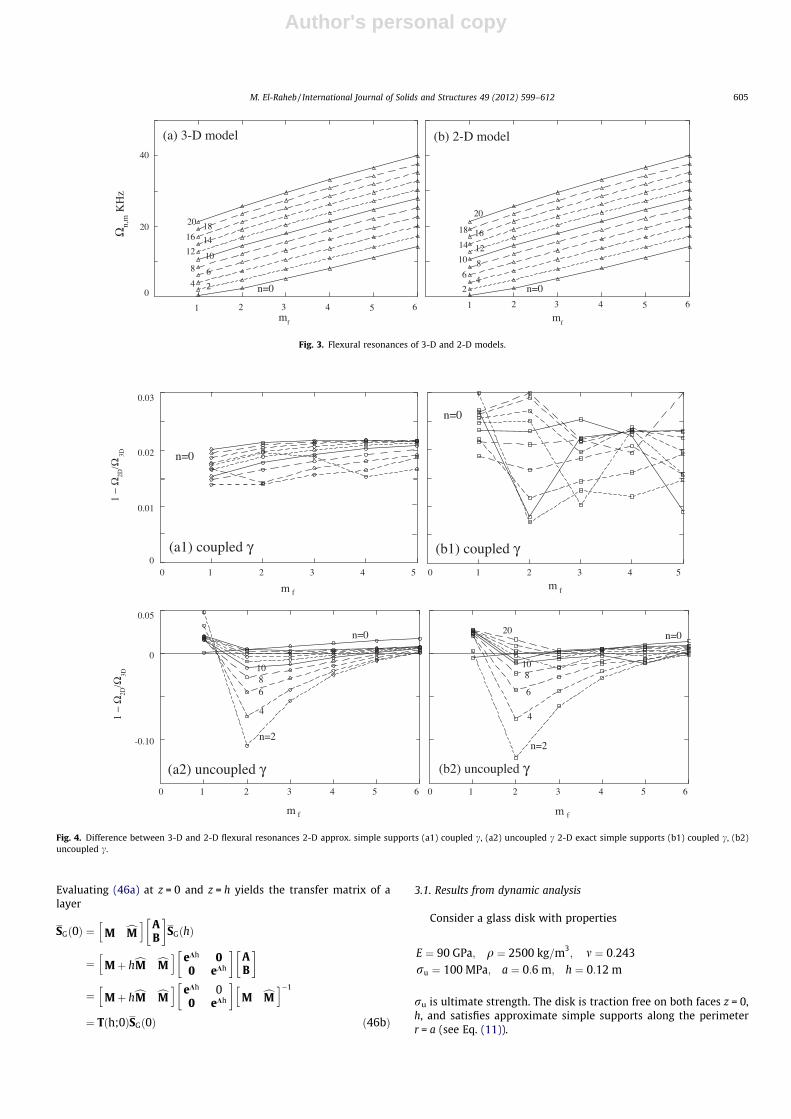
Fig. 3. Flexural resonances of 3-D and 2-D models.

0

0.05

-0.10

n=0

n=2

4

6810

1 −

Ω2D

/Ω3D

m f

(a2) uncoupled γ

m f

(b2) uncoupled γ

n=2

4

6

810

20 n=0

0

0.01

0.02

0.03

(a1) coupled γ (b1) coupled γ

1 2 3 4 5 60 1 2 3 4 5 60

0 1 2 3 4 5 0 1 2 3 4 5

m fm f

1 −

Ω2D

/Ω3D n=0

n=0

Fig. 4. Difference between 3-D and 2-D flexural resonances 2-D approx. simple supports (a1) coupled c, (a2) uncoupled c 2-D exact simple supports (b1) coupled c, (b2)uncoupled c.



Fig. 2 plots resonant Xn,m versus mode number m for1 6m 6 10 with even n as parameter in the range 0 6 n 6 20. Linesof constant n, termed n-lines, rise uniformly with m. Note that n-lines are not smooth but seem discontinuous, and line n = 0 crossesother n-lines. The reason is that the spectrum includes modes ofdifferent types: flexural, extensional along r and z, and shear. Thesetypes appear intermittently making the ordering of mode number

inconsistent with type. In other words, if only flexural modes areplotted versus flexural mode number mf, then n-lines becomesmooth and never cross as evidenced by Fig. 3(a). A mode type isidentified from its w mode shape.

A comparison of the present 3-D analysis with simpler modelslike Mindlin’s (1951) establishes the limitations of 2-D modelsand the error committed when using them. In the literature,

0

0.4

0.8

-0.4

-0.8

0

0.4

0.8

-0.4

-0.8

0

6.e5

-6.e5

0

4.e6

-2.e6

6.e6

0

-6.e6

0

4.e6

-4.e6

υw

σzz σθz

σθθσrr

0 0.2 0.4 0.6 0.8 1. 0 0.2 0.4 0.6 0.8 1.

(a)

8.e6

0

-8.e6

σθθ

0

4.e6

-4.e6

σrr

0 0.2 0.4 0.6 0.8 1.0 0.2 0.4 0.6 0.8 1.

r/a r/a

z/h z/h

(b) (c)

(d) (e)

(f) (g)

(h) (k)

Fig. 5. Modal variables of thick disk for n = 12 and X12,7 = 26.27 kHz (a) flexural mode shape cross-section, (b) t(r), (c) w(r), (d) r(r), (e) rhz(r), (f) rrr(r), (g)rhh(r); z/h-parameter, (h) rrr(r), (g)rhh(z); r/a-parameter.



comparison of 3-D and 2-D models concerned only axisymmetricmotions. An extension to Mindlin’s plate equations to includeasymmetric motions was formulated and solved analytically byEl-Raheb (2002). It is that model that is compared with the present3-D analysis. In the 2-D model, both approximate boundary condi-tion in Eq. (11) termed SSA, and the exact one termed SSE are used.Fig. 3(b) plots X2D versus mf with n as parameter using SSA. Com-paring it with Fig. 3(a) of the 3-D model shows that behavior is thesame.

Fig. 4(a1) and (b1) plots the difference ~d ¼ ðX3D �X2DÞ=X3D ver-sus mf with n as parameter for X2D with SSA and SSE respectively.In both cases, ~d lies between 1 and 2%. To evaluate the effect onresonances of coupling radial wave number ck in Eqs. (4) and (6),~d is determined for X3D with uncoupled ck as shown in Fig. 4(a2)and (b2). For these cases, j~dj is 3 times grater than j~dj inFig. 4(a1) and (b1) revealing that coupling ck improves accuracyof the 3-D solution. This is consistent with results reportedby Singh and Subramaniam (2003) for a disk of aspect ratio

h/a = 0.2, where X3D was close to X2D adopting a Mindlin modelindependent of boundary condition.

As an example of an asymmetric resonant mode, consider theflexural mode with four radial half waves X12,7 (n = 12, m = 7) withan r–z cross-section shown in Fig. 5(a). Fig. 5(b)–(g) plot distribu-tion of displacement and stress along r with z/h as parameter at8 equidistant z stations. Note that all dependent variables becomefinite for r/a P 0.3, consistent with the property of Bessel functionJ12(ckr). Fig. 5(h) and (k) plot rrr and rhh along z with r/a as param-eter at 6 equidistant r stations. Unlike in 2-D where stress it is pro-portional to z, in 3-D it varies non-linearly along z.

3.2. Results from static analysis

Consider the same disk as in Section 3.1 but with the bottomface lying on a rigid base and the top face compressed by a hexagonlattice with cyclic segment shown in Fig. A1(b). Along the thick-ness, the origin of the z-axis is at the center of the loaded face.

0

-0.2

-0.4

0

-0.6

-1.2

0

-1.0

0

1.e-7

2.e-7

σzz

σθθ

σθz

w

0 0.2 0.4 0.6 0.8 1.r/a

0 0.2 0.4 0.6 0.8 1.z/h

(a1) (a2)

(b1) (b2)

(c1) (c2)

(d1) (d2)

z/h=0

z/h=1

z/h=0

z/h=0.12

z/h=1

z/h=0

r/a=0.120.24

0.3

r/a=0.84

0.36

r/a=0.12

0.84

Fig. 6. Static variables from asymmetric pressure with n = 12 (a1)–(d1) w(r), rzz(r), rhz(r), rhh(r) with z-parameter (a2)–(d2) w(z), rzz(z), rhz(z), rhh(z) with r-parameter.



Assume that pressure applied by the lattice on the disk is uniformunder each branch.

Since circumferential dependence cos(nh) is uncoupled, severalstatic solutions each with a different n and with unit pressure areobtained independently. For n = 12, Fig. 4 shows distribution of wand 3 stress components along r with z as parameter and along zwith r as parameter. Fig. 6(a1) plots w along r. It starts at zero forr/a 6 0.05 then rises linearly to a maximum at r/a = 0.8 then shar-ply drops back to zero at r = a. Fig. 6(b1) plots rzz along r. At z = 0,rzz starts from zero at r/a 6 0.05 then rises sharply to �1, attain-ing the prescribed on that face, then continues along that line tillit drops to zero at the boundary of the foot-print r/a = 0.93. rzz

diminishes uniformly with z because pressure distribution onthe forced face varies periodically along h allowing an expansionacross radial node lines that reduces pressure, unlike the axisym-metric case where bulk compression exists throughout the vol-ume. Fig. 6(c1) plots rhz along r. At z = 0, rhz = 0 satisfying theboundary condition. At z/h = 0.12, jrhzj rises sharply reaching amaximum of 0.37 at r/h = 0.27. Such large magnitude of shearstress near the forced face and close to the disk center agreeswith the location of the observed micro-cracks. This behavior ap-pears also in Fig. 6(c2) as a sharp rise in jrhzj along z, and it is re-peated at neighboring stations r/a = 0.24 and 0.26. Fig. 6(d1) plotsrhh along r. At z = 0, rhh is negative resembling rzz there. However,at z/h = 0.12, rhh turns positive attaining a maximum of 0.15 thendrops back to negative. Again, the small but positive rhh in the re-gion where rhz attains its largest magnitude may lead to a com-bined principal tensile stress producing the observed superficialmicro-cracks.

For other values of n, stress distribution resembles that forn = 12 in Fig. 6. A more concise way of presenting results is to plotmaximum stress along r versus parameter z/h as in Fig. 6(c1) and(d1), and maximum stress along z versus parameter r/a as inFig. 6(c2) and (d2). Fig. 7(a1) and (b1) shows that in the vicinityof extrema, distribution of variables from different n solutions fol-low the same trend. When maxima are plotted versus r/a (see

Fig. 7(a2) and (b2)), distribution is comparable to Fig. 7(a1) and(b1) except for a shift in r/a.

The procedure of combining stress from different n solutions toobtain actual stress in the disk starts by expanding in Fourier seriesthe lattice projected line load. This is achieved in Appendix A forthe hexagon geometry in Fig. 1(b) with radius 0.56 m. A scaling fac-tor to stress is determined by plotting maximum amplitude Fmx

from the Fourier series versus number of terms nmx in the expan-sion. For 0 6 nmx 6 300, Fmx rises smoothly but slowly with nmx

approaching a horizontal asymptote, meaning that the series con-verges. To extend Fmx beyond nmx = 300 in order to reach the con-verged value, an accurate non-linear fit is utilized. Thisdetermines an approximate factor scaling stress to its asymptoticvalue from a limited number of static solutions (n 6 30)

sF ¼ ðFas � Fmxð0ÞÞ=ðFmxð30Þ � Fmxð0ÞÞ � 8:4 ð47Þ

Fas is the asymptotic Fmx. Consequently, data from curves in Fig. 5can be combined by

rmx � sF

Xn¼30

n¼6

C1;n;0rðnÞmx ð48Þ

C1;6;0 ¼ 0:02145; C1;12;0 ¼ 0:02351; C1;18;0 ¼ 0:03426

C1;24;0 ¼ 0:03578; C1;30;0 ¼ 0:02615

where C1;n;0 is the Fourier coefficient multiplying solution rðnÞmx fromFig. 5. This yields combined normalized stresses

rhz ¼ �0:43; rhh ¼ 0:16; rzz ¼ �1:0rrr ¼ �0:5; rrz ¼ 0:01; rrh ¼ 0:01

ð49Þ

and principal stressesrtens ¼ 0:31; rshr ¼ 0:72 ð50Þ

Since values in (50) are based on unit applied pressure p, then in ordernot to exceed ultimate stress ru = 100 MPa, p should be limited to

p 6 ru � rtens ¼ 31 MPa ð� 4:5ksiÞ

n=30

6

1218

n=3024

18

126

n=6

1218

2430

n=6

1218

30

σθz

σθθ

0

−0.2

−0.4

0

0.1

0.2

0 0.2 0.4 0.6 0.4 1. 0 0.2 0.4 0.6 0.4 1.

(a1) (a2)

(b1) (b2)

z/h r/a

Fig. 7. Maxima and minima along r and z (a1) jrhzj max along r versus z, (a2) jrhzj max along z versus r (b1) jrhhj max along r versus z, (b2) jrhhj max along z versus r.



4. Conclusion

Asymmetric dynamic and static response of a thick disk is ana-lyzed. Noteworthy results follow:

(1) A finite transform in r eliminates it from the governingequations.

(2) In addition to flexural modes, the 3-D model includes exten-sional and shear dominated modes, and for short wavelengths the difference is not discernable.

(3) Comparing flexural modes from 3-D and 2-D asymmetricmodels reveals that X3D differs by less than 2% from X2D

independent of boundary condition.(4) Magnitude of rhh is greater than all other components by at

least 30%.(5) Unlike 2-D plate theories where flexural stress varies line-

arly along z, in 3-D it is strongly non-linear.(6) Coupling radial wave numbers ck improves the accuracy of

the 3-D model.(7) For a thick disk statically loaded by a unit pressure varying

along h with wave numbers n, jrhzj reaches a maximum inthe vicinity of the loaded face. Also, rhh becomes tensilethere.

(8) For a hexagon lattice applying pressure on the disk face, aFourier decomposition of its projected line-load determinesthe non-vanishing terms in the series; these are zero andmultiples of 6 due to cyclic symmetry of the hexagon.

(9) Also, the Fourier series determine an approximate scalingfactor to combined maximum stress from a limited numberof static solutions within 6 6 n 6 30.

Acknowledgment

The Author thanks Dr. James Zwissler of the Jet Propulsion Lab-oratory for suggesting the problem and for useful discussions onpractical issues.

Appendix A. Stress scaling factor from Fourier series

The static load transmitted to the disk is that from a hexagonallattice with cyclic segment shown in Fig. A1(b). To determinestresses in the disk from this line load requires a 3-D finite element

method coupling disk and lattice with a substantial number of ele-ments throughout the volumes of disk and lattice. An approxima-tion expands the lattice projected area in Fourier series. Thisexpansion determines the non-vanishing terms and yields a scalefactor to stress from a limited number of static solutions each withdifferent n.

The Fourier series expansion of a hexagon segment is evaluatednumerically in a cylindrical coordinate system. Fig. A1(a) shows arectangular branch, lf long and hf wide, in the cyclic segment ofthe hexagon lattice of Fig. A1(b). Let r be a radial line from thehexagon origin to a point in the rectangle, h the angle it sustainswith the reference X-axis, and / the slope of the rectangle center-line. Let F(r,h) = 1 be distribution on the lattice to be expanded inFourier series

Fðr; hÞ ¼Xnmx

n0¼0

Xmmx

j¼0

C1n0 j cosðjpr=af Þ þ C2n0j sinðjpr=af Þh i

cosðn0hÞ

ðA:1Þ

af is hexagon radius and equals nordlf where nord is lattice order de-fined as number of branches on a radial line. Multiplying both sidesof (A.1) independently once by rcos(nh)cos(mpr/af) and once byrcos(nh)sin(mpr/af) then integrating over the domain yields

AC ¼ F; A ¼A11 A12

A21 A22

" #; C ¼

C1

C2

( ); F ¼

F1

F2

( )ðA:2Þ

A11 and A22 are diagonal matrices with coefficients

A11;nmj ¼pa2

f

4dmjð1þ dm0Þð1þ dn0Þ

A22;nmj ¼pa2

f

4dmjð1� dm0Þð1þ dn0Þ

ðA:3Þ

where dm j = 1 when m = j and zero otherwise. A12 and A21 are fullmatrices with coefficients

A12;nmj ¼�ja2

f =ðj2 �m2Þð1þ dn0Þ; m – j

�a2f =ð4jÞð1þ dn0Þ; m ¼ j

8<:A21;nmj ¼ A12;njmð1� dj0Þð1� dm0Þ

ðA:4Þ

For each rectangular segment in the lattice, the integrals in F are

θ1

θ2

θ

r

x

y

r2

r1

...

(x1,y1)

(x2,y2)

(x3,y3)

(x4,y4)

l

h

π−φ

ο

(a) (b)

9876

line 1

line 2

line 3

line 4

line 1.5

hexagon edge

segment interface

P11

10

P12

P21

P22

P32

P42

P31 P41

P2a P3a

P3b

P4a

P4b

P4c

line 2.5

line 3.5

line 0.5

Fig. A1. Branch and cyclic segment of line load from hexagonal frame (a) branch and cylindrical coordinates and (b) cyclic segment.



F1n;m ¼Z h2

h1

Z r2ðhÞ

r1ðhÞcosðmpr=af Þr dr cosðnhÞdh

F2n;m ¼Z h2

h1

Z r2ðhÞ

r1ðhÞsinðmpr=af Þr dr cosðnhÞdh

ðA:5Þ

rkðhÞ ¼ð�yk � �xk tan /Þ

cos hðtan h� tan /Þ

�� ; k ¼ 1;2

ð�xk; �ykÞ are coordinates of intersections of r with sides of the rectan-gle shown in Fig. A1(a). The integrals in (A.5) are then summed overall branches of the lattice. Since A is not diagonal, the series is notorthogonal. For each n, A must then be inverted to determine theindependent Fourier coefficients C

C ¼ A�1F ðA:6Þ

A intermediate result partially validating the analysis is that F1,0,0

when summed over all branches of the lattice yields its projectedarea

Xnb

i¼1

ðF1;0;0Þi ¼ Sf ¼ hf lf nb ðA:7Þ

where nb is total number of branches in the lattice. For h = 0.3 cm,l = 14 cm, and a lattice order nord = 4) nb = 156, Sf = hflfnb =0.065 m2 that agrees with the sum in (A.7).

Consider the truncated series in (A.1) with N = 300 and M = 100.Only terms with n being multiples of 6 and zero are finite becauseof the hexagon cyclic nature. Moreover, only terms with even m areincluded to insure diagonal A11 and A22.

Fig. A2 plots F versus h along lines parallel to the outer edges ofthe hexagon (see Fig. A1(b)). Since nord = 4, there are 4 equidistantparallel branch-lines separated by an interval D r = lf cos(p/6). Linei is di = iDr distant from the center. Also, lines may be located be-tween these branch-lines such as line (i � 1)/2 distant d(i�1)/2 =(i � 1)Dr/2 from the center. These half-lines cross intermediateslant branches as shown in Fig. A1(b). For all lines, sharp peaks

appear along radial interfaces of segments at intervals of h = p/3,i.e. Pi1 and Pi2 on line i, i = 1, 4.

For all lines in Fig. A2, F’s lower bound is unity. In a cyclic seg-ment and along lines 2, 3 and 4, Fig. A2(b)–(d) show 1, 2 and 3additional peaks respectively at branch intersections, i.e. P2a online 2, P3a,b on line 3, and P4a,b,c on line 4.

Fig. A3 plots F along half-lines 0.5, 1.5, 2.5 and 3.5. As expected,along these lines F has a lower bound of zero because they do notcoincide with parallel branches. In a cyclic segment and along lines1.5, 2.5 and 3.5, Fig. A3(b)–(d) shows 2, 4 and 6 additional peaksrespectively at intersections with slant branches, i.e. P1.5a,b on line1.5, P2.5a,b,c,d on line 2.5, and P3.5a,b,c,d,e,f on line 3.5.

Since observed damage from micro-cracks occurs in the vicinityof disk center where radial dependence is negligible, it is appropri-ate to set m = 0. Fig. A4(a) plots the Fourier coefficients C1n0 versusn for n = 0,6,12, . . . ,300. After some oscillation with diminishingamplitude, C1n0 drops slowly indicating that the series converges.Since the goal of the Fourier analysis is to estimate stress producedby the hexagon lattice pressing on the glass disk, determining 50static solutions to reach n = 300 is impractical. A further approxi-mation is then needed to extrapolate stress from a limited numberof n solutions like n 6 30. To this purpose, Fmx is evaluated as afunction of number of terms nmx in the expansion equation (A.1).Fig. A4(b) plots Fmx from the Fourier analysis versus nmx for0 6 nmx 6 300 where points labeled by open circles.

From Fig. A4(b), it appears that the series has not convergedwith nmx = 300. An accurate extrapolation is then needed to extendthe curve to nmx 300. For such large n, the procedure employingEq. (A.2)–(A.6) would lead to erroneous Fmx because of inaccuraciesin numerical integration. Instead, a non-linear fit based on Marqu-ardt’s method is adopted (Marquardt, 1963) for extending Fmx. Acandidate function to fit that approaches a horizontal asymptoteas in Fig. A4(b) is the hyperbolic tangent

Fmx � e1 þ e2 tanhðe3nþ e4Þe1 ¼ �0:772; e2 ¼ 2:055; e3 ¼ 0:0185; e4 ¼ 0:45

ðA:8Þ

0 0.2 0.4 0.6 0.8 1 0 0.2 0.4 0.6 0.8 1

θ / 2π θ / 2π

0

2

4

0

2

4

F

F

(a) line 1 (b) line 2

(c) line 3 (d) line 4

P11 P

12P

21 P22

P2a

P32P

31

P3a

P3b

P41 P

42

P4a

P4b

P4c

cyclic segment cyclic segment


Fig. A2. F(r,q) distribution from Fourier series with n P 300 (a) line 1, (b) line 2, (c) line 3, (d) line 4.



The fit depicted by a solid line in Fig. A4(b) matches the values com-puted from the series in the range 0 6 n 6 300 with an error not

exceeding 0.5%, and extends further with nmx approaching theasymptote.

Scaling of Fmx(nmx) then proceeds as follows. Note fromFig. A4(b) that Fmx(0) = 0.10, Fmx(30) = 0.24, Fmx(300) = 1.04, andFmx(1200) � Fas = 1.28. Since for all nmx the lower bound of F isthe same as Fmx(0), it implies that Fmx(0) depends only on C100 inde-pendent of nmx and must be subtracted from the Fmx(nmx) to prop-erly scale Fmx(30). Consequently, the approximate scaling factormultiplying solutions n = 6,12, . . . ,30 is

sF ¼ ðFas � Fmxð0ÞÞ=ðFmxð30Þ � Fmxð0ÞÞ � 8:4 ðA:9Þ

Given a stress component with a maximum rðnÞmx over a range of n,combined stress rmx for that component is determined by

rmx � sF

Xn¼30

n¼6

�C1;n;0rðnÞmx ðA:10Þ

C1;6;0 ¼ 0:02145; C1;12;0 ¼ 0:02351; C1;18;0 ¼ 0:03426

C1;24;0 ¼ 0:03578; C1;30;0 ¼ 0:02615

In summary, results from Fourier analysis of the hexagon lattice are

(a) The series is not orthogonal due to the necessary choice ofcylindrical coordinates.

(b) Only terms with n equal to zero and multiples of 6 in the ser-ies are finite because of cyclic symmetry.

(c) Along lines parallel to the edges, sharp peaks Fmx appearalong interfaces of cyclic segments and at intersections ofbranches. Fmx is threefold that along intermediate parallellines.

(d) The lower bound of F depends only on �C100 independent ofnmx.

(e) When m = 0, Fmx rises smoothly but slowly with nmx

approaching Fas as asymptote.

0

1

0

1

F

F

0 0.2 0.4 0.6 0.8 1 0 0.2 0.4 0.6 0.8 1θ / 2π θ / 2π



(a) (b)

(c) (d)

P0.5,1

P0.5,2

P1.5,1

P1.5,2

P2.5,2

P2.5,1

a bc d

e fab c

d

a b

P3.5,1

P3.5,2

Fig. A3. F(r,q) distribution from Fourier series with n P 300 (a) line 0.5, (b) line 1.5, (c) line 2.5, (d) line 3.5.

0

0.01

0.02

0.03

0.04

1.0

0.5

1.5

0 100 200 300n

C1 n 0

Fmx

(b)

(a)

n =30

n = 30, Fmx

= 0.24

0 600 1200300 900n

mx

n = 300, Fmx

= 1.04

non-linear fit

Fourier series

Fmx

= 1.28

n = 0, Fmx

= 0.1

0

_

Fig. A4. Fourier series of hexagon lattice (a) Fourier coefficient C1n0 versus n forn = 6, m = 0 and (b) Fmx versus nmx: Fourier series, — nonlinear fit.



(f) Fas and Fmx (30) determine an approximate scaling factor tormx from a limited number of static solutions within6 6 n 6 30.

References

Berry, J., Naghdi, P., 1956. On the vibration of elastic bodies having time dependentboundary conditions. Quarterly of Applied Mathematics 14, 43–50.

Chen, L., Doong, J., 1984. Vibrations of an initially stressed transversely isotropiccircular thick plate. International Journal of Mechanical Sciences 26 (4), 253–263.

Chen, L., Chen, C., 1988. Asymmetric buckling of bi-modulus thick annular plates.Computers & Structures 29 (6), 1063–1074.

Chen, L., Chen, C., 1989. Asymmetric vibration and dynamic stability of bi-modulusthick annular plates. Computers & Structures 31 (6), 1013–1022.

Dong, C., 2008. Three-dimensional free-vibration analysis of functionally gradedannular plates using the Chebyshev–Ritz method. Journal of Materials andDesign (29), 1518–1525.

El-Raheb, M., Wagner, P., 1996. Transient elastic waves in finite layered media: two-dimensional axisymmetric analysis. Journal of the Acoustical Society of America99 (6), 3513–3527.

El-Raheb, M., 2002. Dynamic instability of a disk forced by a pulse of short duration.Interantional Journals of Solids and Structure 39 (11), 2965–2986.

Love, A., 1944. A Treatise on the Mathematical Theory of Elasticity, first Americanedition. Dover Publications Inc., New York, pp. 287–292.

Marquardt, D., 1963. An algorithm for least-squares estimation of non-linearparameters. Journal of the Society of industrial and Applied Mathematics 11 (2),431–441.

Miklowitz, J., 1984. The theory of elastic waves and wave-guides, first ed. NorthHolland, Amsterdam, the Netherlands, pp. 214–221.

Mindlin, R., 1951. Influence of rotary inertia and shear deformation on flexuralmotions of isotropic elastic disks. Transactions of ASME Journal of AppliedMechanics 73, 31–38.

Singh, A., Subramaniam, I., 2003. Vibration of thick circular disks and shells ofrevolution. Journal of Applied Mechanics. Transactions of ASME 70 (2), 292–298.

Soamidas, V., Ganesan, N., 1991. Vibration analysis of thick, polar orthotropic,variable thickness annular disks. Journal of Sound & Vibration 147 (1), 39–56.

Vinayak, H., Singh, R., 1996. Eigensolutions of annular-like elastic disks withintentionally removed or added material. Journal of Sound & Vibration 192 (4),741–769.


Dynamic and static asymmetric response of a layesred thick disk

Documents

Transcript of Dynamic and static asymmetric response of a layesred thick disk