Dusty Globules and Globulettes - DiVA-Portal
212
DOCTORAL THESIS Dusty Globules and Globulettes Tiia Grenman Applied Physics
-
Upload
khangminh22 -
Category
Documents
-
view
0 -
download
0
Transcript of Dusty Globules and Globulettes - DiVA-Portal

DOCTORA L T H E S I S
Department of Engineering Sciences and Mathematics Division of Material Science
Dusty Globules and Globulettes
Tiia Grenman
ISSN 1402-1544ISBN 978-91-7790-092-4 (print)ISBN 978-91-7790-093-1 (pdf)
Luleå University of Technology 2018
Tiia G
renman D
usty Globules and G
lobulettes
Applied Physics


Doctoral Thesis
Dusty Globules and Globulettes
Tiia Grenman
Division of Applied Physics
Lulea University of Technology
SE-971 87 Lulea
Sweden
E-mail: [email protected]
Lulea, May 2018
Printed by Luleå University of Technology, Graphic Production 2018
ISSN 1402-1544 ISBN 978-91-7790-092-4 (print)ISBN 978-91-7790-093-1 (pdf)
Luleå 2018
www.ltu.se
© 2018 Tiia GrenmanDivision of Applied PhysicsDepartment of Engineering Sciences and MathematicsLuleå University of TechnologySE-971 87 LuleåSweden
The cover image shows the northern part of the Rosette Nebula. In the lowerright part of the image the Wrench, an elephant trunk is shown. This trunkis mainly made up of thin threads that are twisted and connected to two jawsat the lower massive head. In the upper part of this Wrench a string of darkdots, globulettes, are seen in silhouette against the bright background. Thisfalse-color image shows emission from lines of Sulfur, Hydrogen and Oxygen(shaded red, green and blue). Credit: Astronomy Picture of the Day, March2014.
i
We are just an advanced breed of monkeys on a minor planet of a veryaverage star. But we can understand the Universe. That makes us somethingvery special. Stephen Hawking
To my family

ABSTRACT
Interstellar gas and dust can condense into clouds of very different size, rangingfrom giant molecular cloud complexes to massive, isolated, dark cloudlets,called globules with a few solar masses.
This thesis focuses on a new category of small globules, named globulettes.These have been found in the bright surroundings of H II regions of young,massive stellar clusters. The globulettes are much smaller and less massivethan normal globules. The analysis is based on H-alpha images of e.g., theRosette Nebula and the Carina Nebula collected with the Nordic Optical Tele-scope and the Hubble Space Telescope.
Most globulettes found in different H II regions have distinct contours andare well isolated from the surrounding molecular shell structures. Masses anddensities were derived from the extinction of light through the globulettesand the measured shape of the objects. A majority of the globulettes haveplanetary masses, <13MJ (Jupiter masses). Very few objects have massesabove 100MJ ≈ 0.1M� (Solar masses). Hence, there is no smooth overlapbetween globulettes and globules, which makes us conclude that globulettesrepresent a distinct, new class of objects.
Globulettes might have been formed either by the fragmentation of largerfilaments, or by the disintegration of large molecular clouds originally hostingcompact and small cores. At a later stage, globulettes expand, disrupt orevaporate. However, preliminary calculations of their lifetimes show that somemight survive for a relatively long time, in several cases even longer than theirestimated contraction time.
The tiny high density globulettes in the Carina Nebula indicate that theyare in a more evolved state than those in the Rosette Nebula, and hence theymay have survived for a longer time. It is possible that the globulettes couldhost low mass brown dwarfs or planets.
Using the virial theorem on the Rosette Nebula globulettes and includingonly the thermal and gravitational potential energy indicated that the 133
iii
iv
found globulettes are all either expanding or disrupting. When the ram andthe radiation pressure were included, we found that about half of our objectsare gravitationally bound or unstable to contraction and could collapse to formbrown dwarfs or free floating planets.
We also estimated the amount of globulettes and the number of free floatingplanetary mass objects, originating from globulettes, during the history of theMilky Way. We found that a conservative value of the number of globulettesformed is 5.7× 10¹⁰. A less conservative estimate gave 2× 10¹¹ globulettes andif 10% of these forms free floating planets then the globulettes have contributedabout 0.2 free floating planets per star.
In the Crab Nebula, which is a supernova remnant from the explosion of amassive old star, one can find dusty globules appearing as dark spots againstthe background nebulosity. These globules are very similar to the globuletteswe have found in H II regions. The total mass of dust in globules was estimatedto be 4.5 × 10⁻⁴M�, which corresponds to . 2% of the total dust content ofthe nebula. These globules move outward from the center with transversalvelocities of 60–1600 km s−1. Using the extinction law for globules, we foundthat the dust grains are similar to the interstellar dust grains. This means thatthey contribute to the ISM dust population. We concluded that the majorityof the globules are not located in bright filaments and we proposed that theseglobules may be products of cell-like blobs or granules in the atmosphere of theprogenitor star. Theses blobs collapse and form globules during the passage ofthe blast wave during the explosion.

Preface
The research behind this doctoral thesis has been carried out at the Divisionof Applied Physics, Lulea University of Technology. It had not been possiblewithout the help and support of many individuals, who, in one way or another,have helped me to complete my work.
First of all, I would like to express my gratitude to my supervisors, HansWeber and Erik Elfgren for invaluable advice, guidance, comments, and fortheir encouragement. I also want express my thanks to my supervisor, professorGosta Gahm at the AlbaNova Centre of Stockholm University. He suggestedmy research topic, provided the observational data, and has been advising methrough the research work. His expertise in astronomy has been necessary formy daily work and he is also a great inspiration. I also wish to express mygratitude to my late supervisor, Sverker Fredriksson for his support during thefirst part of this work.
Special thanks to my friends, Britt-Mari, Armi and Rose-Marie who keptme smiling through even the hardest of times.
I am grateful also for support from the National Graduate School of SpaceTechnology. Finally, and most of all, I would like to thank my partner Leif andmy children Liina, Jane, and Lucia for their moral support and unconditionallove over the years. I also thank my grandchildren Athena, Leah, Nathalie andAmeliah for they always make me smile.
Astronomers are one of those lucky people who can make a living out oftheir pure interest. I feel lucky.
Tiia Grenman
v

Papers
The Papers I-IV are appended to this doctoral thesis and for each paper I alsooutline my contributions. These articles will be referred to in the text by theirRoman numbers.
Paper I: Globulettes as seeds of brown dwarfs and free-floating planetary massobject Gahm, G. F., Grenman, T., Fredriksson, S., & Kristen, H. 2007, AJ,133, 1795
I wrote a Matlab script that was used in Paper I, II and III, analyzed thedata and made all figures and provided comments to the whole article.
Paper II: The tiny globulettes in the Carina NebulaGrenman, T., & Gahm, G. F. 2014, A&A , 565, A107
In this paper I collected relevant fields from the Hubble Space Telescopearchive and analyzed all the data and made all figures, except Figure 7 andprovided comments to the whole article. Figure 2 was a front image in As-tronomy & Astrophysics (A&A) journal and several figures from this articleare publish in the book “Annals of the Deep Sky, Volume 4”.
Paper III: Dusty globules in the Crab nebulaGrenman, T., Gahm, G. F., & Elfgren, E. 2017,A&A , 599, A110
I collected all data, took part in the writing, made all figures, analyzeddata, and provided comments to the whole article.
Paper IV: History of gobulettes in the Milky WayGrenman, T., Elfgren, E., & Weber, H. 2018, Ap&SS, 363, #2
This paper was entirely written by me. Co-authors helped to formulatesome of the ideas presented, and in editing the text. I collected all data, madeall data analysis and the figures.
vii
viii
Publications not included in this thesisRadio observations of globulettes in the Carina nebulaHaikala, L. K., Gahm, G. F., Grenman, T., Makela, M. M., & Persson, C. M.2017, A&A , 602, A61

Table of Contents
1 Introduction 31.1 Objectives . . . . . . . . . . . . . . . . . . . . . . . . . . . . . . 41.2 Research Questions . . . . . . . . . . . . . . . . . . . . . . . . . 51.3 Structure of the Thesis . . . . . . . . . . . . . . . . . . . . . . . 5
2 Background 72.1 Early Universe and Star Formation Rate . . . . . . . . . . . . . 72.2 Background of Spectroscopic Observations . . . . . . . . . . . . 82.3 Gas Components of the ISM . . . . . . . . . . . . . . . . . . . . 102.4 Molecular Gas . . . . . . . . . . . . . . . . . . . . . . . . . . . . 102.5 Atomic Gas . . . . . . . . . . . . . . . . . . . . . . . . . . . . . 112.6 Ionized Interstellar Gas . . . . . . . . . . . . . . . . . . . . . . . 13
2.6.1 H II Formation . . . . . . . . . . . . . . . . . . . . . . . 132.7 Gas Cooling and Heating . . . . . . . . . . . . . . . . . . . . . . 152.8 Dust Grains . . . . . . . . . . . . . . . . . . . . . . . . . . . . . 152.9 Interstellar Cloud Structures . . . . . . . . . . . . . . . . . . . . 18
2.9.1 Molecular Clouds . . . . . . . . . . . . . . . . . . . . . . 202.9.2 Giant Molecular Clouds . . . . . . . . . . . . . . . . . . 202.9.3 Cold Dark Clouds and Globules . . . . . . . . . . . . . . 212.9.4 Clumps and Cores . . . . . . . . . . . . . . . . . . . . . 232.9.5 Globulettes . . . . . . . . . . . . . . . . . . . . . . . . . 232.9.6 Hot Molecular Cores . . . . . . . . . . . . . . . . . . . . 25
2.10 Formation of Stars and Planets . . . . . . . . . . . . . . . . . . 252.10.1 The Onset of Star Formation Processes . . . . . . . . . . 25
2.11 Free Floating Planetary Mass Objects . . . . . . . . . . . . . . . 292.12 H II regions . . . . . . . . . . . . . . . . . . . . . . . . . . . . . 31
2.12.1 H II regions: Dynamics . . . . . . . . . . . . . . . . . . . 322.13 Supernovae . . . . . . . . . . . . . . . . . . . . . . . . . . . . . 36
2.13.1 Core Collapse Supernova Type II . . . . . . . . . . . . . 39
ix

x TABLE OF CONTENTS
2.13.2 The Evolution of Supernova Remnants . . . . . . . . . . 40
2.13.3 Dust Formation . . . . . . . . . . . . . . . . . . . . . . . 42
3 Theory 45
3.1 Interstellar Extinction . . . . . . . . . . . . . . . . . . . . . . . 45
3.2 Visual Extinction . . . . . . . . . . . . . . . . . . . . . . . . . . 47
3.3 Extinction Curve . . . . . . . . . . . . . . . . . . . . . . . . . . 48
3.4 Optical Depth . . . . . . . . . . . . . . . . . . . . . . . . . . . . 48
3.5 Measuring Extinction . . . . . . . . . . . . . . . . . . . . . . . 50
3.6 Cloud Contraction . . . . . . . . . . . . . . . . . . . . . . . . . 52
3.7 Proper Motion . . . . . . . . . . . . . . . . . . . . . . . . . . . 53
4 Methodology 57
4.1 Positions . . . . . . . . . . . . . . . . . . . . . . . . . . . . . . . 57
4.2 Shapes, Dimensions and Orientations . . . . . . . . . . . . . . . 59
4.3 Column Density Distribution . . . . . . . . . . . . . . . . . . . 65
4.4 Extinction and Relation to Mass . . . . . . . . . . . . . . . . . . 69
5 Observations 73
5.1 The Observations with the Nordic Optical Telescope . . . . . . 73
5.2 The Hubble Space Telescope . . . . . . . . . . . . . . . . . . . . 74
5.3 Filter System . . . . . . . . . . . . . . . . . . . . . . . . . . . . 75
6 Introduction to Papers 77
6.1 Paper I . . . . . . . . . . . . . . . . . . . . . . . . . . . . . . . . 77
6.1.1 Rosette Nebula and IC 1805 . . . . . . . . . . . . . . . . 78
6.1.2 Results . . . . . . . . . . . . . . . . . . . . . . . . . . . . 80
6.2 Paper II . . . . . . . . . . . . . . . . . . . . . . . . . . . . . . . 81
6.2.1 Carina Nebula . . . . . . . . . . . . . . . . . . . . . . . . 82
6.2.2 Results . . . . . . . . . . . . . . . . . . . . . . . . . . . . 84
6.3 Paper III . . . . . . . . . . . . . . . . . . . . . . . . . . . . . . . 85
6.3.1 Crab Nebula . . . . . . . . . . . . . . . . . . . . . . . . 86
6.3.2 Results . . . . . . . . . . . . . . . . . . . . . . . . . . . . 89
6.4 Paper IV . . . . . . . . . . . . . . . . . . . . . . . . . . . . . . . 90
6.4.1 Results . . . . . . . . . . . . . . . . . . . . . . . . . . . . 91
7 Discussion and Outlook 93
7.1 Discussion . . . . . . . . . . . . . . . . . . . . . . . . . . . . . . 93
7.2 Outlook . . . . . . . . . . . . . . . . . . . . . . . . . . . . . . . 96
TABLE OF CONTENTS xi
8 Bibliography 99
A Astronomical Quantities 113A.1 Magnitude Scale . . . . . . . . . . . . . . . . . . . . . . . . . . 113A.2 The Celestial Coordinate System . . . . . . . . . . . . . . . . . 114A.3 Column Density . . . . . . . . . . . . . . . . . . . . . . . . . . . 114
B Images of Fields 117B.1 Description of Images . . . . . . . . . . . . . . . . . . . . . . . . 117
C Data Tables of Globulettes in Nebulæ 121

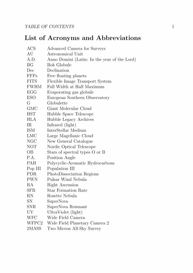
TABLE OF CONTENTS 1
List of Acronyms and Abbreviations
ACS Advanced Camera for SurveysAU Astronomical UnitA.D. Anno Domini (Latin: In the year of the Lord)BG Bok GlobuleDec DeclinationFFPs Free floating planetsFITS Flexible Image Transport SystemFWHM Full Width at Half MaximumEGG Evaporating gas globuleESO European Southern ObservatoryG GlobuletteGMC Giant Molecular CloudHST Hubble Space TelescopeHLA Hubble Legacy ArchivesIR Infrared (light)ISM InterStellar MediumLMC Large Magellanic CloudNGC New General CatalogueNOT Nordic Optical TelescopeOB Stars of spectral types O or BP.A. Position AnglePAH Polycyclic-Aromatic HydrocarbonsPop III Population IIIPDR PhotoDissociation RegionsPWN Pulsar Wind NebulaRA Right AscensionSFR Star Formation RateRN Rosette NebulaSN SuperNovaSNR SuperNova RemnantUV UltraViolet (light)WFC Wide Field CameraWFPC2 Wide Field Planetary Camera 22MASS Two Micron All-Sky Survey

2 TABLE OF CONTENTS
Units and Symbols
In most circumstances cgs units are used, i.e., centimetre for length, gram forweight, second for time, erg for energy and dyn for pressure. One solar mass ofabout 2× 1033 g is denoted by the symbol M�, and one Jupiter mass of about1.9× 1030 g is denoted by MJ . Distances are also frequently given in the unitsAU (astronomical unit) or pc (parsec). 1 AU = 1.496× 1013 cm is the averageearth-sun distance, and 1 parsec = 1 pc = 206 265 AU is the distance fromwhich the radius of the Earth’s orbit around the sun covers an angle of 1′′.However, distances within a nebula are often given in arcseconds, denoted by′′, corresponding to their angular extension in the sky. At the distance of the
Rosette Nebula (RN), i.e., around 1400 parsec, the angle 1′′ corresponds to adistance of 1400 AU = 2.09× 1016 cm.
The expansion of the Universe causes light waves to stretch with time,known as the redshift (z). This is often used as a measure of distance fromus or the age of the Universe. Today, the Universe has z = 0, while 10 billionyears ago z ∼ 2.

Chapter 1
Introduction
On a dark and clear night we can look up towards the sky where we can seea luminous band running across the dark sky, the Milky Way, composed ofhundreds of billions of stars. Earth is one of eight planets orbiting our Sun,located ∼ 8.5 kpc (about 27 700 light years) from the galactic center in oneof the Milky Way’s spiral arms. Discoveries of planets outside of our solarsystem (Mayor & Queloz, 1995) indicate that formation of planetary systemswith rogue planets are as common as stars in the galaxy. A number of isolatedfree-floating planets (FFPs) have been located over the last decade. Recentresults from Mroz et al. (2017) indicate that the upper limit on the number ofJupiter size free floating planets in the Milky Way is about 0.25 planets perstar.
However, The Milky Way does not only consist of planets and stars. Beau-tiful images taken with the Hubble Space Telescope (HST) have made famousgigantic interstellar nebula that floats among the stars (one example can beseen on the front page). Nebula is Latin for cloud (plural: nebulæ). The spacebetween stars is filled with a thin gas and microscopic dust grains, togetherforming the so-called interstellar medium (ISM). The Milky Way has some 10%of its atomic mass in the form of interstellar matter, and of this 90% is gas,while 10% is dust. In general, the ISM is composed mainly of hydrogen andhelium. Only a minor part contains all other heavier elements once created inprevious generations of stars, and including the heavy elements in cosmic raysand dust grains. The interstellar matter can be divided into regions character-ized by the state of hydrogen. H II regions contain ionized atomic hydrogen(H+) and can be found around very hot stars. H I regions are cold neutralhydrogen (H) clouds, while molecular clouds contain molecular hydrogen (H2).
The distribution of interstellar matter is far from uniform, and regions of
3
4 CHAPTER 1. INTRODUCTION
higher and lower densities exist. Volumes with number densities n>10 cm−3
are referred to as interstellar clouds. They are found almost everywhere in ourgalaxy, especially in the galactic spiral arms.
The most obvious and important property of the ISM is that it containsmany different components with very different physical properties, rangingfrom a hot (106 K), low density (10−3 cm−3) gas, to cold (10 K) and dense(n>104 cm−3) material in molecular clouds.
The dust in the ISM is made of tiny, irregularly shaped particles with icymantles. The grains are about 0.1µm in size and as the wavelengths of stellarlight are similar (0.1–1µm), the grains are well matched to absorb and scatterultraviolet and visible light. This effect is called extinction. In regions withdense clouds, light from background stars can be completely blocked. Suchregions are called dark clouds. However, light can also be reflected off theinterstellar dust grains. As the blue light is more easily scattered/reflected,cloud regions close to luminous stars shine in a bluish color. Such bright areasare called reflection nebulæ. In other clouds, with imbedded luminous stars,starlight is absorbed by the gas, and the surrounding gas is heated. The lightis re-emitted in a number of emission lines, and such bright objects are calledemission nebulæ. There is not a well-defined boundary between the two cases,and many objects show both scattered starlight and emission lines from excitednebular gas species.
The brightest and most massive hot stars explodes as supernovae (plural:SNe; singular: SN) at the end of their evolution, recycling enriched materialinto to ISM and by that contributing the birth of new stars. After these ex-plosions thin layers or filaments is surround the supernovae, and these nebulæare called supernova remnants (SNR). During their lives the massive stars areresponsible for a large amount of the momentum and kinetic energy input intothe interstellar gas.
1.1 Objectives
The objective of my research has been to investigate dark small cloudletsof dust and gas, found as dark silhouettes against the bright background ofnebular emission in optical images of H II regions and against the continuumemission in the Crab Nebula.

1.2. RESEARCH QUESTIONS 5
1.2 Research Questions
The goal of this thesis has been to investigate and understand the natureof the cloudlets, known as globulettes, especially their properties, origin andevolution.
- What are their shapes, morphologies, structures, densities and distribu-tions of size and mass?
- What are the physical conditions in these objects?
- Will they disintegrate in the surrounding warm plasma, or is there achance that some may contract under self-gravitation to form smallerobjects? In that case, what is their nature?
- Could a certain fraction of globulettes form FFPs?
- How many globulettes have been formed in the Milky Way over the yearsand how may these contribute to the total FFPs population?
- What is the visible dust mass of the dark cloudlets in the Crab Nebula,and what is the extinction law and the proper motion of these dustyblobs?
1.3 Structure of the Thesis
The outline of the different chapters of the thesis are as follows:Chapter 2 gives a background of the early Universe, gas components and
dust, and a short overview of the formation of stars and planets, H II regionsand supernova remnants.
Chapter 3. An overview of relevant properties and theories are presented,such as interstellar extinction, reddening, virial theorem and proper motion,where multi epoch images from the second generation Wide Field PlanetaryCamera 2 (WFPC2), and third generation Advanced Camera for Surveys(ACS) was used.
Chapter 4 gives the details about how various properties e.g., mass, radiiof the globulettes can be evaluated.
Chapter 5 gives a review over the observations and instrumentations withthe Nordic Optical Telescope (NOT) and the HST, but also which filters havebeen used.
6 CHAPTER 1. INTRODUCTION
Chapter 6 gives a short overview of the observed regions and the summeryof important result from the four papers.
Chapter 7 concludes the thesis by summerising the work with a generaldiscussion. Some suggestions of future research are also given.
Appendix A gives some astronomical background needed to understandsome parts of the thesis.
Appendix B contains images of analyzed H II regions (used in Paper IV),where the observed areas are superimposed on the images.
Appendix C lists the positions in Right Ascension (RA) and Declination(Dec) and their mean radii for additional globulettes introduced in Paper IV.

Chapter 2
Background
Some of the content is taken from the Grenman (2006) licentiate thesis.
2.1 Early Universe and Star Formation Rate
The Big Bang occurred about 13.8 Gyr years ago (Planck Collaboration etal., 2014). The first stars, known as population III (Pop III) stars, formeda few hundred million years after the Big Bang in dark matter mini halos of∼ 106M� (Tegmark et al., 1997). These stars are believed to have been verymassive (102 to 103M�) and consisted mainly of hydrogen and helium (Bromm& Larson, 2004; Schneider et al., 2006; Bromm & Yoshida, 2011). The largemass of the Pop III stars is due to the low cooling effect of the primordial gasesin the stars. These massive stars lived short lives that ended in supernovaeexplosions. These explosions resulted in the enrichment of the ISM of elementsheavier than H and He (usually referred to as metals). Observations of thehigh redshift Universe, about 1 Gyr after the Big Bang, confirm the presenceof a large amount of dust and heavy elements. This metal enrichment byPop III stars leads to the formation of lower mass Pop II stars, as soon asthe critical metallicity 10−6–10−3.5 Z� was reached (Schneider et al., 2012). Agood example of a Pop II environment is the Large Magellanic Cloud (LMC),where the metallicity is about half that of our Sun (Rolleston et al., 2002).
Metals constitute about 1% of the baryon matter in the Universe. Sinceiron is one of the most abundant metals found in stellar spectra, and theoverall stellar metallicity, Z, is often defined using the total iron-content ofthe stellar atmosphere “[Fe/H]”, in terms of mass (Binney & Merrifield, 1998).This abundance ratio is defined as the logarithm of the ratio of a star’s iron
7

8 CHAPTER 2. BACKGROUND
abundance compared to that of the Sun:
[Fe/H] = log10
Fe/H
(Fe/H)�≈ log10
Z
Z�, (2.1)
where the solar metallicity is Z�= 0.0196 (Vagnozzi, 2017).In the Milky Way, metal poor Pop II stars, with about [Fe/H] < −1.0 (e.g.,
10% of Sun’s metallicity), can be found mostly in the globular clusters and inthe thick disk, above and below the galactic plane. In this low metallicityenvironment, planets have been observed orbiting stars with an age of about10 Gyr (Anglada-Escude et al., 2014, and references therein). The theoreticalestimations of the planet formation in the early Universe has been discussedby e.g., Lineweaver (2001), Prantzos (2008), Johnson & Li (2012), Behroozi &Peeples (2015) and Mashian & Loeb (2016).
The amount of gas converted into stars per unit time is known as the starformation rate (SFR), which usually has the unit of [M�/yr]. This shows thetotal star formation activity in a galaxy or in a given area in a galaxy. In ourgalaxy stars forms at a rate of ∼ 1–5M�/yr (Smith et al., 1978; Robitaille& Whitney, 2010; Chomiuk & Povich, 2011) and for a star-forming galaxy ofequal mass, at about 10 billion years ago the SFR was ∼ 30 times larger (Daddiet al., 2007). This implies also that the formation rate of ionized nebula, H IIregions, surrounding newborn stellar clusters was higher then now. In PaperIV, we assume that the number of H II regions is proportional to the SFRand combined with the present day number, this gives the formation rateof H II regions in the early Universe. More discussion around the SFR andthe metallicity history can be found in e.g., Behroozi et al. (2013); Madau &Dickinson (2014).
2.2 Background of Spectroscopic Observations
The gas in the ISM emits detectable electromagnetic radiation and is on theaverage of very low density (about one atom per cubic centimeter) comparedto conditions on the Earth and even compared to vacuums created in labo-ratories (∼ 105–107 cm−3). To extract information from this gas, such as itstemperature or chemical composition, the astronomers observe spectral linesfrom atoms and molecules in the gas.
When an atom absorbs a photon, a distinct amount of energy, E = hc/λ,where λ is the wavelength, is transferred, resulting in an excited atom. Thisgives rise to absorption lines (dark) in the spectra corresponding to these

2.2. BACKGROUND OF SPECTROSCOPIC OBSERVATIONS 9
distinct wavelengths. An electron stays at an excited energy level for a limitedamount of time before returning to the lower energy level, thereby emitting theenergy difference as a photon. This gives rise to bright emisson line spectra,corresponding to the energy difference.
The dominant element in the Universe is hydrogen. In the Milky Way,about 60% of the mass of interstellar hydrogen is atomic (H I), about 20%is ionized (H II) and about 20% is molecular (H2) (Draine & Li, 2001). Thehydrogen atom consists of a proton and an electron, which can occupy anybound energy level, denoted by n = 1, 2, 3 etc. and where n = 1 is the groundstate. At large n values the energy levels are very close together and therecomes a point where the electron is in a unbound state. This electron canoccupy a range of possible continuum levels, where it has a certain free kineticenergy (Dyson and Williams, 1997). Figure 2.2 shows an example of hydrogenatom energy diagrams and its emission and absorption spectra.
In addition to the electronic transitions, molecules have rotational and/orvibrational transitions. These transitions have lower energy and hence theemitted light has longer wavelength. Vibrational transitions come from stretch-ing or bending of the molecules. Together, the vibrational and rotational tran-sitions give rise to ro-vibrational bands.
Usually, an atom, molecule or ion gets excited through a collision with anenergetic particle (e− or H+) and then undergoes radiative de-excitation (spon-taneous or stimulated), emitting a photon. The photon is emitted typicallyafter 10−8 s with spontaneous emission. When this happens, the kinetic energyof the colliding particle will be transferred to radiation, which may escape thecloud, thereby cooling the gas.
In addition, some energy levels in metals (and their ions) are split intomultiple “sublevels” or fine structure levels. Collision with free electrons excitebound electrons in the lower level of atoms to higher levels and take some ofthe kinetic energy of the colliding electrons.
However, observations of the interstellar gas have shown that some spec-tral lines have a low transition probability and that they cannot normally beobserved in the laboratory. The low probability is because the transition isforbidden. This means that the state gets de-exited by collisions rather thanspontaneous emission. These transitions are denoted with a square bracket,for example single ionized Oxygen [O II].
10 CHAPTER 2. BACKGROUND
2.3 Gas Components of the ISM
In the ISM, the gases exist in three states, with rising temperature: the molec-ular, the atomic, and the ionized state. These states are divided in differentphases, since stable balance of heating and cooling at a given pressure oftencan be achieved at more than one temperature. From this classification, themultiple phase structure in the ISM was developed (McKee & Ostriker, 1977).
Observations have shown, that the hot (∼ 106 K), thin, ionized and lowdensity (10−3 cm−3) gas permeates most of the galaxy. Only a few percentof the volume contains cold neutral gas, which is concentrated in thick struc-tures (T ∼ 50–100 K, n ∼ 10–100 cm−3). The cold dense molecular gas (T =10–20 K, n ∼ 104 cm−3) fills up less than 1% and can be found in molecularclouds. Despite the low filling factor, this densest gas contains 30 %–60 % ofthe total gas mass in the ISM. These five phases are in dynamic interactionwith each other. However there is some ionized hydrogen even in the neu-tral regions, because of cosmic ray ionizations, and there is also some neutralhydrogen atoms in ionized regions, because of continuous recombination. Anoverview of different phases from coolest to hottest is given below.
2.4 Molecular Gas
The molecular gases in the ISM are present in the interior of dense clouds thatare shielded from the radiative dissociation by ultraviolet (UV) photons. Thesegases are not hot enough for significant collisional dissociation. Comparisonof molecular and atomic hydrogen abundances in different line of sights haveshown that interstellar gas is almost entirely molecular above a gas columndensity of about N(H I)>1021 cm−2 (self-shield against UV radiation).
In these high density regions, H2 may form rapidly on dust grains (Section2.8). However, if sufficiently free electrons are present, H2 can also form in thegas phase, until all free electrons are used. The first molecular clouds in theUniverse were probably formed in this way, before dust grains condensed fromthe heavy elements. Still these reactions are rare due to the limited electronabundance.
The most important ingredient for star formation is molecular hydrogen,which constitutes about 99% of the mass of these cold and dark molecularclouds. This makes it the most abundant molecule in the Universe. Despitethe large abundance of H2 molecules, they are very difficult to detect becausethey are not sufficiently excited to emit photons at the low temperatures inthe clouds. Molecular hydrogen is a symmetric molecule (consisting of two

2.5. ATOMIC GAS 11
identical atoms) and has no permanent dipole moment. This means that theircenters of mass are also their center of charge and therefore spontaneous vi-brational/rotational transitions cannot occur. Thus, we can only observe H2
in shocked regions, created by e.g., jets from young stars or in very warmconditions near UV stars (Krishna Swamy, 2005).
To trace H2 we observe the second most common molecule, carbon monox-ide (CO), which is one of the first molecules to form in circumstellar envelopesof old stars. These molecules seem to co-exist with H2 molecules and theyhave a strong dipole moment, which means that they can be exited a lowtemperatures (<10 K). Thus, we can use the CO rotational transition linesat radio wavelengths, 2.6 mm (the lowest energy transition) and 1.33 mm totrace the H2 molecule (Graves et al., 2010). With an appropriate conversionfactor, known as the “X factor”, CO emissions can be used as a tracer of H2
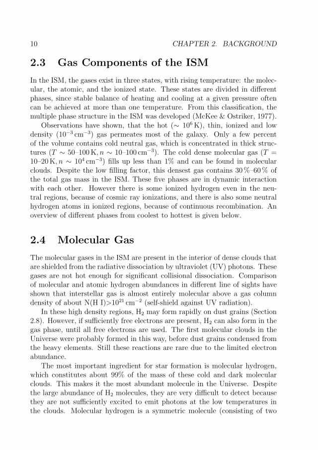
abundances and hence the total mass of the dense clouds. Most of what weknow about the large-scale distribution of molecular hydrogen is therefore de-rived from observations of CO and its isotopic varieties, see Figure 2.1. Morethan one hundred molecular species have been discovered through spectro-scopic observations. The molecular medium is surrounded by neutral atomicgas.
2.5 Atomic Gas
Most of the hydrogen in space is in its ground state and the proton and elec-tron normally spin in the same direction. Observations have shown (Kalberla& Kerp, 2009; Dickey & Lockman, 1990) that neutral hydrogen exists in twophases: cold neutral medium and a more diffuse warm neutral medium. Thesetwo phases are often considered to be in pressure equilibrium (Savage & Sem-bach, 1996; Cox, 2005) but with different temperature and density.
One of the best indicators of the presence of H I in the ISM is the 21 cmline radio emission (Ewen & Purcell, 1951). This line comes from photonemission when the electron flips its spin from parallel (higher energy state) toanti-parallel (slightly lower energy state). Since this is a forbidden transition,the spontaneous spin flip occurs only every 11 million years. However, thetime between collisions is actually much shorter and collisional de-excitationoccurs before most atoms can decay spontaneously. Thus, the population ofthe two states is determined primarily by collisions between atoms or withfree electrons. Even though these emissions occur rarely, there are so manyhydrogen atoms in the ISM that they will produce an observable line at 21 cm,see Figure 2.1.
12 CHAPTER 2. BACKGROUND
Figure 2.1: A selected collection of the Milky Way in 5 different wavelengthbands. The ISM extends over the whole galactic disk. From the top: 1) 21 cmatomic hydrogen emission. 2) 2.6 mm CO radio emission, tracing the galacticmolecular gas. 3) Composite image of mid- and far-infrared, typical tracer ofinterstellar dust emission. 4) Composite near-infrared image, radiation fromcool stars. 5) Optical light, were we can see the regions obscured by dust.Thus dimming is wavelength dependent and in near infrared the plane of theMilky Way is much more transparent, which makes it more easy to observethe galactic bulge surrounding the galactic center. Image and caption credit:NASA Multiwavelength Milky Way project (http://mwmw.gsfc.nasa.gov/).
Roughly half of all neutral hydrogen atoms are in the warm, more diffusephase, which is detectable across the whole sky. This medium (sometimesalso called the warm intercloud medium) has usually a low optical depth andcan be seen only in broad emission spectral lines. The cold neutral mediumforms highly inhomogeneous and structured filaments that may be a result ofturbulence in the interstellar gas. These clouds tend to have a high opticalthickness and are visible both in absorption and emission line spectra. Eventhough these clouds are cold enough to form some simple molecules, theywill never collapse and form stars since they need to be compressed to formmolecular hydrogen.
Actually, the cooling and heating processes in H I region show large resem-blance with photodissociation regions (PDR), also known as photon-dominatedregions. In these regions, the far-UV photons (E = 6–13 eV) can penetrate

2.6. IONIZED INTERSTELLAR GAS 13
into the clouds. Therefore, this medium can be described as a low densityPDR (Hollenbach & Tielens, 1999). The cold and warm neutral phases areembedded into warm and a hot ionized gas (see below) with a filling factorbetween 20% and 70%.
Atomic hydrogen has been used to map out the large scale distributionof atomic clouds. The main application area is to estimate the mass, thedistribution, kinematics, and temperature of the gas.
2.6 Ionized Interstellar Gas
A large fraction of the ISM is filled with ionized gas, which can be found in theH II regions, planetary nebulæ and the hot interstellar medium. As example,the warm ionized gas can be found in H II regions, while the hot gas comesfrom supernova explosions that produce hot bubbles of expanding gas (Spitzer,1990; Wolfire et al., 2003). This hot interstellar medium, can be traced viaUV and X-ray observations (Yao et al., 2009).
2.6.1 H II Formation
The most bright and massive stars in the galaxy are classified as O and Btype stars from their optical spectra. They are formed from the material inthe molecular cloud and they are hot enough to produce large amounts ofhigh energy UV photons, which are able to ionize hydrogen and helium atomsaround them.
H II regions are formed within molecular clouds after photodissociation ofH2 molecules by UV photons with energies >11.2 eV (λ ∼ 110.8 nm, Whit-tet, 1992). Young hot stars subsequently photoionize the neutral hydrogengas with photon energies > IH = 13.6 eV (λ < 91.2 nm), creating a bub-ble of warm ionized gas which then expands. This expansion is known as theStromgren sphere (Dyson and Williams, 1997), where the moving edge is calledthe ionization front, see Section 2.12.
Photoionization occurs when the UV photons knock out the bound elec-trons from hydrogen atoms to the continuum, H I + hν → H II + e−. Inthis process, the excess energy hν − IH , is carried away as kinetic energyby the ejected electron. This electron then transfers its kinetic energy toother atoms, molecules and ions, thereby heating the medium through elasticcollisions. This free electron eventually recombines with an ionized H atom(H II + e− → H I + hν) to form a neutral atom. In this process photonsare emitted as the electron cascades down, creating a number of observable

14 CHAPTER 2. BACKGROUND
spectral lines. The energy levels of these emission lines depend on the kineticenergy of the recombining electron (in its continuum state) and its bindingenergy in the atom.
The transitions in hydrogen atoms down to the first excited level (n = 2)produce the Balmer lines: (in order of decreasing wavelength) Hα, Hβ, Hγ andso on, seen in Figure 2.2. In the visible spectrum, the strongest emission lineis that of Hα with a wavelength λ = 6563 A (0.6563µm) emitted when theelectron decays from the third to the second excited level of the H atom. Thus,the reddish color seen in images of, e.g., the Rosette Nebula (Figure 6.1), ismainly a result of Hα emission. This false-color image, is taken in the light ofHα, [O III], and [S II], reproduced as red, green and blue, respectively. Thus,in H II regions it is also possible to find heavier elements such us oxygen,nitrogen and carbon which are collisionally excited.
Figure 2.2: The hydrogen atom has its ground state (n = 1) at the energy13.6 eV, as compared to its fully ionized state. T he transition from a statewith principal quantum number n = 3 to one with n = 2 is strong in a hydrogenplasma, and produces photons with wavelength λ = 656.3 nm in the red regionof the spectrum. This is why an emission nebula glows in red light on opticalimages. Hydrogen atoms emission and absorption spectrum is also shown inlower part.

2.7. GAS COOLING AND HEATING 15
2.7 Gas Cooling and Heating
The structure of the ISM phases is determined by heating and cooling process.The more the ISM is heated, the more diffuse it becomes. If the coolingprocesses dominate, the inverse processes occur, resulting in a cooler, denser,and more neutral ISM. Since the temperature increases due to gravitationalcontraction, which counteracts a gravitational collapse, a balance is requiredbetween heating and cooling processes in order for star formation to occur.Heating and cooling occur by a variety of processes with radiation as thedominant transport mechanism, with transfer of kinetic energy to and fromatoms, molecules and ions.
There are several radiation sources in the ISM such as stars, X-ray stars,and supernovae. One of the major heating processes is photoionization ofhydrogen. Less important heating processes include shock heating, collisionalionization caused by cosmic rays and photodissociation of molecules.
In contrast to the heating processes, cooling of interstellar gas occurs mainlythrough emission of radiation, such as forbidden line emission. Efficient coolingoccurs when the gas is optically thin, so that emitted photons are not re-absorbed and when there is enough of particles to make collisions frequent.
The dominant cooling lines in the ISM and the PDRs are from Oxygen(e.g., [O I], [O III]), Nitrogen (e.g., [N II]), Sulphur (e.g., [S II]) and Carbon([C II]). Even recombinations of hydrogen and helium to levels other than thenground state contribute somewhat to gas cooling.
Another important cooling process in the ISM is through the rotationalenergy levels of molecules. One such example is the CO rotational transitionlines. Finally, free-free emission contributes somewhat to the cooling, wherefree electrons are accelerated by an ion, thus emitting a photon.
2.8 Dust Grains
Trumpler (Trumpler, 1930) found that light from distant stars was more dimthan expected from using the inverse square law for the flux, F = L/4πD2,where D is the distance and L is the luminosity. Trumpler concluded thatinterstellar space must contain cosmic dust particles which attenuate star light.The presence of dust grains in the ISM has then been proved using four differentmethods: 1. extinction and reddening at UV and optical wavelengths (seeChapter 3); 2. polarization of starlight; 3. reflection nebulæ and 4. thermalemission from the galaxy (Mathis, 1990). Dust plays an important role inthe physics of the ISM and also in the formation of rocky planets, stars and

16 CHAPTER 2. BACKGROUND
galaxies.Dust grains are formed mainly in the cool atmospheres of old (evolved) stars
but also in the ejecta resulting from supernovae outbursts. In this environment,the temperature and pressure are suitable for the formation of heavy elements,see Section 2.13.3. The most abundant ones (∼ 1 atom for each 1000 H atoms)are the “organics” C, O, N, while the “rockies”, such as Mg, Si, Fe have anabundance of ∼ 1 atom for each 10 000 H atoms. Dust that originates fromstars is called “Stardust”. However dust grains may also form by a series ofchemical reactions, where atoms and molecules in the gas phase combine inthe cold cores of molecular clouds (van Steenberg & Shull, 1988; Draine, 2009).
Figure 2.3: From left to right: 1) Typical cosmic dust particle, composedof numerous small grains (NASA Johnson Space Center). 2) A presolar(stardust) onion-like graphite grain, 5 micrometers in diameter, from theMurchison meteorite. Photo courtesy of S. Amuri, Washington University,St.Louis. 3) A presolar grain of silicon carbide, SiC. The grain is 3 mi-crometers across. Photo by Rhonda Stroud, Naval Research Laboratory(http://www.psrd.hawaii.edu/Aug03/stardust.html). 4) Example of thestructure of the PAH molecule. These molecules are flat, with each carbonhaving three neighboring atoms, much like graphite.
Observation of UV extinction and optical scattering of dust grains haveshowed a broad size distribution around 10−4–1µm (Weingartner & Draine,2001), and polarization studies have indicated that large dust grains are non-spherical and aligned along the magnetic field lines. Dust grains can be de-scribed as solid particles with typical radii of ∼ 0.1µm (similar to the size ofsmoke particles from a cigarette) and with densities of about 2 g cm−3. Theo-retical models of the diffuse ISM assume that there is a mixture of mainly smallsize (<0.01µm) carbonaceous materials (graphites, soot) and bigger grains(>0.01µm), amorphous silicates (e.g., olivine), often with mantles of water orCO ice (Kim & Martin, 1994; Whittet et al., 1988). There is also evidence that

2.8. DUST GRAINS 17
Figure 2.4: Schematic representation of a dust grain with ice mantle. At lowtemperature, most gas phase molecules e.g., water, CO, freeze into ice mantelson dust grain. Main formation of H2 happens on dust grain surfaces. Once twoH meet, they form H2, which has no unpaired electron and so H2 is released.Original image form https://www.astrochem.org/sci/.
a population of macro molecules, polycyclic-aromatic hydrocarbons (PAHs),compounds of both gaseous molecules and small solid particles, exist in theISM and can be found in PDRs (Werner et al., 2004), typically ∼ 50 C atomsin an often planar arrangement. Figure 2.3 shows some examples of dust grainsand a structure of the PAH molecule.
Dust absorbs and re-emits about half the visible star light in a typicalgalaxy (Dale et al., 2007) and it is well mixed with gas, although the dust togas ratio can vary between and across galaxies. In our galaxy (Figure 2.1), dustmakes up only about 1% (Chaisson, E. & Steve, M., 2013) of the total massof the ISM, i.e., the gas to dust ratio is 100:1. The interstellar dust, coupledto the gas clouds, forms molecular clouds that come in a variety of shapes,sizes and densities (see Section 2.9). When radiation penetrates through thismedium, it can absorb, scatter or emit electromagnetic radiation (see Sec-tion 3.1). Typically, all processes take place simultaneously, thus shielding theinterior part of the clouds from ionizing radiation and photodissociation.
In this low temperature environment, H2 molecules can form on sticky dustgrain surfaces, see Figure 2.4. As H2 has no unpaired electron, it binds onlyvery weakly on the grain and soon leaves into the gas phase again. Many othermolecules also form in this way, e.g., H2O, though water remains frozen on thedust grains. When most of the hydrogen has been depleted, CO moleculescan condense directly on the ice and coagulate into large grains (Ormel et al.,

18 CHAPTER 2. BACKGROUND
2011). The UV radiation on the ice mantles breaks molecules leading to new,more complex, organic molecules.
However, emission at longer wavelengths also carries information aboutthe dust population. Large grains can be treated as modified blackbodies(“grey bodies”). They are less affected by single photons, but are hit moreoften, leading to a steady temperature of <60 K, referred to as cold dust.These grains are responsible for the extinction of visible and infrared (IR)light and in the low temperature environment, the majority of the energy isemitted at far-IR and submm wavelengths (60–800µm). Small grains can notbe considered as black bodies. They have higher temperatures compared tothe large grains. Most of the emission will take place when they are brieflyheated to high temperatures, probably by the absorption of a single photon(van Dishoeck, 2004). They typically emit their energy in the near-and mid-infrared wavelengths (Draine & Li, 2001) corresponding to temperatures of>60 K, warm to hot dust. Thus, in order to study dust properties, it is anadvantage to use IR telescopes as has been done from the satellites Spitzer(3.6–160µm) for hot and cold dust, and Herschel (55–625µm) for cold dust.Near- to far-IR composite images of the Milky Way are shown in Figure 2.1.
Dust grains are exposed to radiation and get a wide range of temperatureswhen they pass from diffuse to dense clouds and back again. The typical life-time of a dust grain is a few hundred million years before it is either vaporisedby e.g., shock wave fronts from supernovae, by collisions with each other, orthey are integrated into larger objects such as stars (Tielens et al., 1994; Joneset al., 1996).
2.9 Interstellar Cloud Structures
Dark nebulæ have been subject to scientific studies since as far back as the19th century, when Sir William Herschel (1785) noticed regions devoid of starsand remarked “My God, there is a hole in the sky!” He thought that it was aplace where the stars had burned out. These starless regions of the sky werenot studied in detail until 1889 when Edward E. Barnard pictured the MilkyWay and catched the dark patches on photographic plates. In 1919 he pub-lished a catalogue of 182 “dark markings”, and these clouds are now referredto as Barnard objects (Barnard, 1919). Another more detailed catalogue waspublished by Beverly Lynds, which contains 1802 dark nebulæ, identified onthe National Geographic-Palomar Observatory Sky Atlas (Lynds, 1962). Afterthe discovery of an interstellar gaseous medium it was proposed that the darkmarkings are relatively compact objects of interstellar gas. The early investi-
2.9. INTERSTELLAR CLOUD STRUCTURES 19
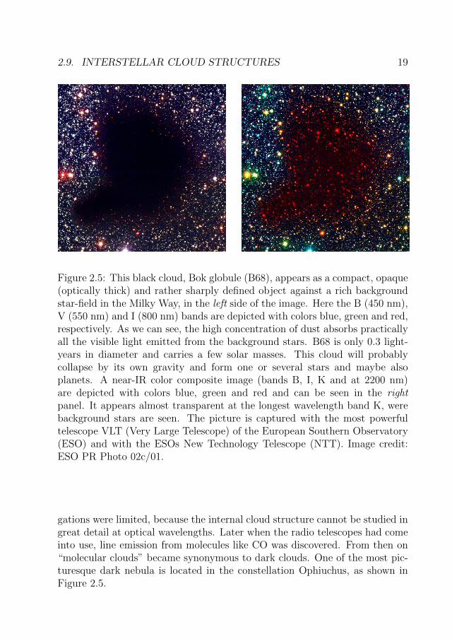
Figure 2.5: This black cloud, Bok globule (B68), appears as a compact, opaque(optically thick) and rather sharply defined object against a rich backgroundstar-field in the Milky Way, in the left side of the image. Here the B (450 nm),V (550 nm) and I (800 nm) bands are depicted with colors blue, green and red,respectively. As we can see, the high concentration of dust absorbs practicallyall the visible light emitted from the background stars. B68 is only 0.3 light-years in diameter and carries a few solar masses. This cloud will probablycollapse by its own gravity and form one or several stars and maybe alsoplanets. A near-IR color composite image (bands B, I, K and at 2200 nm)are depicted with colors blue, green and red and can be seen in the rightpanel. It appears almost transparent at the longest wavelength band K, werebackground stars are seen. The picture is captured with the most powerfultelescope VLT (Very Large Telescope) of the European Southern Observatory(ESO) and with the ESOs New Technology Telescope (NTT). Image credit:ESO PR Photo 02c/01.
gations were limited, because the internal cloud structure cannot be studied ingreat detail at optical wavelengths. Later when the radio telescopes had comeinto use, line emission from molecules like CO was discovered. From then on“molecular clouds” became synonymous to dark clouds. One of the most pic-turesque dark nebula is located in the constellation Ophiuchus, as shown inFigure 2.5.
20 CHAPTER 2. BACKGROUND
2.9.1 Molecular Clouds
The Milky Way contains about 5000 molecular clouds (Scoville & Sanders,1987) and they are formed by a process known as self shielding. In this pro-cess, far-UV photons may destroy molecules forming at the edge of clouds byphotodissociation, thus creating a low density photodissociation region (PDR),which corresponds to diffuse/translucent clouds. As a result, these photons donot penetrate the material which is behind this PDR layer. In this way, themolecules that subsequently form are protected by this envelope, which makesit possible for the cloud to stay bound (McKee & Ostriker, 2007). The maincomponents of a molecular cloud is molecular hydrogen (73 % in mass), atomichelium (25 %), dust particles (1 %), neutral atomic hydrogen (<1 %), and alsoa mixture of interstellar molecules (<0.1 %). The mean molecular weight istherefore between 2.3 and 2.8 u (the universal mass unit) depending on whetherdust particles are included or not.
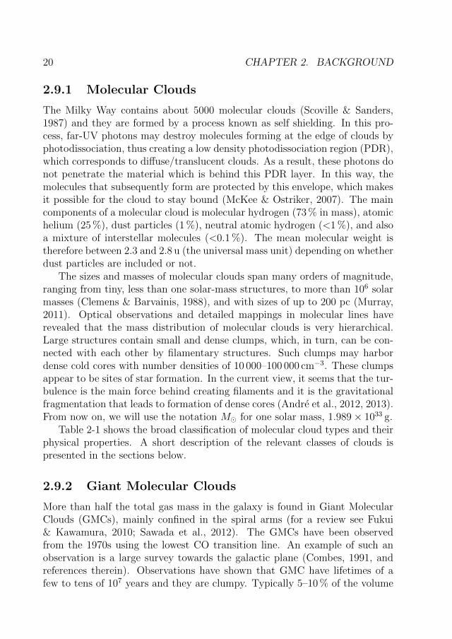
The sizes and masses of molecular clouds span many orders of magnitude,ranging from tiny, less than one solar-mass structures, to more than 106 solarmasses (Clemens & Barvainis, 1988), and with sizes of up to 200 pc (Murray,2011). Optical observations and detailed mappings in molecular lines haverevealed that the mass distribution of molecular clouds is very hierarchical.Large structures contain small and dense clumps, which, in turn, can be con-nected with each other by filamentary structures. Such clumps may harbordense cold cores with number densities of 10 000–100 000 cm−3. These clumpsappear to be sites of star formation. In the current view, it seems that the tur-bulence is the main force behind creating filaments and it is the gravitationalfragmentation that leads to formation of dense cores (Andre et al., 2012, 2013).From now on, we will use the notation M� for one solar mass, 1.989× 1033 g.
Table 2-1 shows the broad classification of molecular cloud types and theirphysical properties. A short description of the relevant classes of clouds ispresented in the sections below.
2.9.2 Giant Molecular Clouds
More than half the total gas mass in the galaxy is found in Giant MolecularClouds (GMCs), mainly confined in the spiral arms (for a review see Fukui& Kawamura, 2010; Sawada et al., 2012). The GMCs have been observedfrom the 1970s using the lowest CO transition line. An example of such anobservation is a large survey towards the galactic plane (Combes, 1991, andreferences therein). Observations have shown that GMC have lifetimes of afew to tens of 107 years and they are clumpy. Typically 5–10 % of the volume

2.9. INTERSTELLAR CLOUD STRUCTURES 21
Table 2-1: Overview of the global properties of molecular clouds
Clouds∗ Clumps Globules Cores Globulettessize (pc) 5− 200 0.5− 10 ≤ 2 ≤0.1 <0.05density (cm−3) >100 103 − 104 103 − 105 104 − 106 103 − 105
mass (M�) 103 − 106 ≤ 103 5− 500 0.5− 5 <0.1temperature (K) 10− 30 10− 20 <15 <15 <15
∗ Ranging from small dark clouds to giant molecular clouds.Most information is adapted form Bergin & Tafalla (2007) and Murray (2011).
consists of clumps (Stutzki & Guesten, 1990). According to existing theories(Bally, 1989; Poidevin et al., 2013, and reference therein), these giant cloudscan be formed in two different ways. In the “bottom-up” model a cloud formsvia coagulation of cold H I clouds, thereby increasing its size and mass untilthe cloud is massive enough to continue its growth due to its gravitation. The“top-down” model (Kim & Ostriker, 2002) suggests that clouds form eithervia large scale gravitational and magnetic instabilities in the ISM or by forcedcompression by supernova, turbulence or shock waves.
It takes about 2 Myr (Clark et al., 2012) from GMC formation before thestar formation begins, forming thousands of low mass star but also a numberof high-mass stars, such as O and B stars. This type of star formation can onlyoriginate from GMCs, where there is sufficient material available to transformlarge amounts of mass into stars.
Once these hot O stars are formed, the GMC starts to disintegrate, dueto the intense emission of UV radiation, which dissociates and ionizes themolecules and atoms by forming H II regions. However, the internal pressurein the GMC is about ten times higher than the pressure in the ambient ISM.This means that these clouds are held together by the mass of the moleculargas within them, otherwise they would disperse in about 10 million years.Examples of GMCs are e.g., the Orion Molecular Complex and the CarinaComplex.
2.9.3 Cold Dark Clouds and Globules
Smaller than the GMCs are the Dark Cloud Complexes, with masses between1000–10 000M� (Mundy, 1994). They are generally associated with sites oflow mass star formation. The so called globules are even smaller and they
22 CHAPTER 2. BACKGROUND
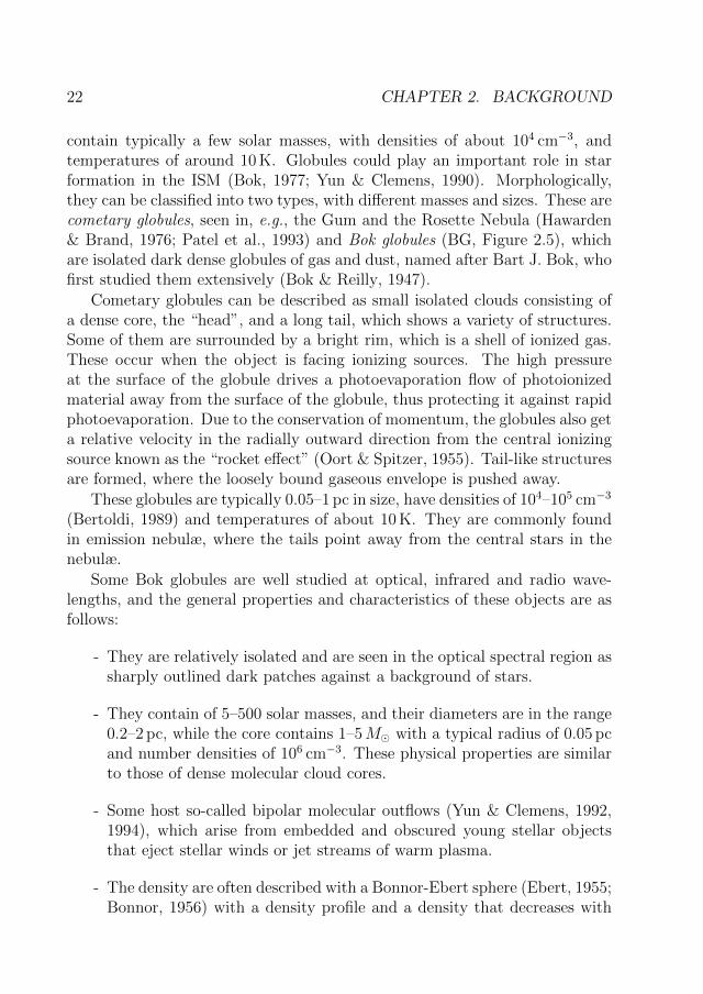
contain typically a few solar masses, with densities of about 104 cm−3, andtemperatures of around 10 K. Globules could play an important role in starformation in the ISM (Bok, 1977; Yun & Clemens, 1990). Morphologically,they can be classified into two types, with different masses and sizes. These arecometary globules, seen in, e.g., the Gum and the Rosette Nebula (Hawarden& Brand, 1976; Patel et al., 1993) and Bok globules (BG, Figure 2.5), whichare isolated dark dense globules of gas and dust, named after Bart J. Bok, whofirst studied them extensively (Bok & Reilly, 1947).
Cometary globules can be described as small isolated clouds consisting ofa dense core, the “head”, and a long tail, which shows a variety of structures.Some of them are surrounded by a bright rim, which is a shell of ionized gas.These occur when the object is facing ionizing sources. The high pressureat the surface of the globule drives a photoevaporation flow of photoionizedmaterial away from the surface of the globule, thus protecting it against rapidphotoevaporation. Due to the conservation of momentum, the globules also geta relative velocity in the radially outward direction from the central ionizingsource known as the “rocket effect” (Oort & Spitzer, 1955). Tail-like structuresare formed, where the loosely bound gaseous envelope is pushed away.
These globules are typically 0.05–1 pc in size, have densities of 104–105 cm−3
(Bertoldi, 1989) and temperatures of about 10 K. They are commonly foundin emission nebulæ, where the tails point away from the central stars in thenebulæ.
Some Bok globules are well studied at optical, infrared and radio wave-lengths, and the general properties and characteristics of these objects are asfollows:
- They are relatively isolated and are seen in the optical spectral region assharply outlined dark patches against a background of stars.
- They contain of 5–500 solar masses, and their diameters are in the range0.2–2 pc, while the core contains 1–5M� with a typical radius of 0.05 pcand number densities of 106 cm−3. These physical properties are similarto those of dense molecular cloud cores.
- Some host so-called bipolar molecular outflows (Yun & Clemens, 1992,1994), which arise from embedded and obscured young stellar objectsthat eject stellar winds or jet streams of warm plasma.
- The density are often described with a Bonnor-Ebert sphere (Ebert, 1955;Bonnor, 1956) with a density profile and a density that decreases with

2.9. INTERSTELLAR CLOUD STRUCTURES 23
the distance, R, from the center, approximately as ∼ R−2 and steepeningat the edge.
Most BGs show no signs of star formation, but there is still a possibility thatthey can host brown dwarfs, see Section 2.11.
2.9.4 Clumps and Cores
In GMCs, the turbulence and density fluctuations leads to dense sub-structures.The structures with higher densities (104–105 cm−3) are often referred to asclumps. They have sizes between 0.5–10 pc and may or may not contain cores(see below) in which single or multiple stars are born. They are referred toas “starless clumps” or “star forming clumps”, respectively (Williams et al.,2000).
The clumps may fragment into cold prestellar cores or pre-brown dwarfcores (Andre et al., 2012). If the cores are gravitationally bound they willcontinue to collapse into individual protostars. Observations from the InfraredSpace Observatory (Kessler et al., 1996) revealed central dust temperatures of10–12 K, while in the outskirts of prestellar cores the temperature is 15–20 K(Ward-Thompson et al., 2002).
2.9.5 Globulettes
In H II regions, one can find many very tiny, isolated objects, which we callglobulettes. They appear as dark spots against the background nebulosity.These objects were noticed by Gahm and Grenman (Paper I, II) and classifiedas a new distinct class of objects, see Figure 2.6 taken from Paper II.
Most globulettes are sharp-edged and well isolated from their surroundings.They are roundish objects, which are much smaller (<10 kAU) than normalglobules, and with number densities between 103–105 cm−3. A majority of theobjects have masses <13MJ (Jupiter masses), and the mass distribution dropsrapidly towards larger values. Very few objects have masses above 100MJ ≈0.1M�. The first survey of such objects was presented by De Marco et al.(2006).
The globulettes can also have tails, bright rims and halos and some of theobjects are connected by thin filaments to large molecular blocks or even toeach other. This suggests that globulettes might have been formed either bythe fragmentation of larger filaments, or by the disintegration of large molec-ular clouds originally hosting compact and small cores. At a later stage glob-

24 CHAPTER 2. BACKGROUND
ulettes might expand, disrupt or evaporate or actually collapse to form browndwarfs and planetary objects.
The calculated lifetime of globulettes suggests that they may survive in theharsh H II environment for a long time, >105 yrs (Gahm et al., 2007; Haworthet al., 2015). This is the reason to suspect that they may be a source of browndwarfs and free floating planetary mass objects in the galaxy as explored inPaper IV.
Figure 2.6: Examples of globulettes found in the Carina Nebula. The mosttypical cases are the dark globulettes shown in the upper four rows followedby objects with bright halos. The last two rows show examples of elongatedobjects with tails, some with bright rims. Note that the scales are differentfrom panel to panel (the dimensions in arcsec are given for each object in thePaper II).

2.10. FORMATION OF STARS AND PLANETS 25
2.9.6 Hot Molecular Cores
When a dense cold core begins to form a massive protostar, the energy pro-duced e.g., from the outflows, heats up the surrounding molecular gas to tem-peratures of >100 K. At these high temperatures molecules that have formedon the surface of dust grains will evaporate, which gives rise to molecular com-plexity in the gas and forming a Hot Core. This core can be described as adense (>107 cm−3) and compact (<0.1 pc) region which represents the mostchemically rich phase of the interstellar medium (Charnley et al., 1992; Kurtzet al., 2000). Based on chemical models, the estimated life time is less than105 years Fontani et al. (2007)
2.10 Formation of Stars and Planets
Star formation takes place in molecular clouds, in many cases seen as darkdust lanes in optical images of the galactic plane (Schneider & Elmegreen,1979; Bally et al., 1987) in Figure 2.1. Most stars in the Milky Way haveformed in stellar clusters. Examples of such star formation regions are shownin Figure 2.7.
The low mass star formation (< 8M�) is more efficient overall and takesplace throughout the cloud (from GMCs to globules). Differently from lowmass stars, high mass star formation (> 8M�) requires larger clump massesand the formation process is faster than in low mass stars. Massive stars mayalready be on the main sequence, which means that stars fuse hydrogen atomsinto helium atoms in their cores. These stars are still deeply embedded inthe dust cloud and they are actively accreting. They cease accreting whenthey reach the final stage of their formation process. These stars have shortlifetimes on the main sequence compared to the low mass star and they havealso relatively low formation rates, which indicates that they are less commonin the galaxy.
2.10.1 The Onset of Star Formation Processes
Clumps in molecular clouds can produce single or multiple cores, dependingon the clump mass but also on the nature of the fragmentation. These coldcompact cores are completely shielded from intensive UV radiation and slowlyapproach the centrally concentrated state. This is known as the pre-stellarphase, which lasts about 106 yr (Shu et al., 1987). If the molecular cloud isin equilibrium, then self-gravity is balanced by internal gas pressure, magnetic

26 CHAPTER 2. BACKGROUND
fields, turbulence, radiation pressure and rotational forces (McKee & Ostriker,2007), see Section 3.6.
Figure 2.7: The left image shows the star formation region G82.65-2.00I inthree-color montage. The colors, red, green, and blue correspond to Herscheldata at wavelengths 160, 250, and 500 µm, respectively. The filament can beseen as a blue rim. The white dots, situated along this filament, are protostars.The distance to the cloud is about 1 kpc and the length of the filament is ∼20pc. Figure credit: Galactic Cold Cores project. The right image shows a starformation region inside the Carina Nebula. In the top of the longest finger ofdust and also in the middle-left part of the image, bipolar outflows, jets can beseen. These are ejected by young stars at speeds of 100 km/s–1000 km/s, andcollide with the surrounding nebula. This produces bright shock fronts thatglow when the gas is heated by friction. This composite image was taken in2010 with the Hubble Space Telescope, using three different color filters. Thecolors correspond to oxygen (blue), hydrogen and nitrogen (green), and sulfur(red). Image Credit: NASA, ESA, M. Livio and the Hubble 20th AnniversaryTeam (STScI).
Simplified, low mass star formation begins when a pre-stellar core, withtemperature about 10–20 K, starts to collapse by gravity that surpasses theinner thermal motion of the gas. The critical mass can be shown to be MJeans,the so-called Jeans mass, (Jeans, 1902), for which star formation can occur,i.e., the smallest mass needed for self-contraction:
MJeans =
(5kBT
GµmH
)3/2(3
4πρ0
)1/2
. (2.2)

2.10. FORMATION OF STARS AND PLANETS 27
Here kB is the Boltzmann constant, T is the local temperature of the cloud, Gis the gravitational constant, µ is the mean molecular weight, mH is the massof the hydrogen atom and ρ0 is the mean density of the cloud. For a cloudwith an initial density of 10−19 g cm−3 and a temperature of T = 10 K, thefree-fall time, τff , given by Shu et al. (1987),
τff =
√3π
32Gρ0
(2.3)
is around 2× 10⁵ years. If the cloud is initially of uniform density, the collapsetime is also uniform throughout the cloud.
However, during the gravitational contraction, the size of a cloud decreasesby several orders of magnitude (from ∼1 pc to ∼100 AU). Conservation ofangular momentum implies that the initial rotation of the system increasesduring the contraction. After some time, infalling matter will have enoughtransversal velocity to prevent direct accretion by the central star. A rotatingdisk-like circumstellar structure is then formed. Both the protostar and thedisk are still surrounded by an envelope of gas and dust. At the same time,this central object can eventually become hot enough to drive strong outflowsin the form of stellar winds and oppositely directed jets, see in Figure 2.7 right.Then, gas and dust falls into the disk and either accretes onto the central staror are driven back into the ISM via outflows. Interaction of the infalling matterstream with high velocity jets carries angular momentum outwards.
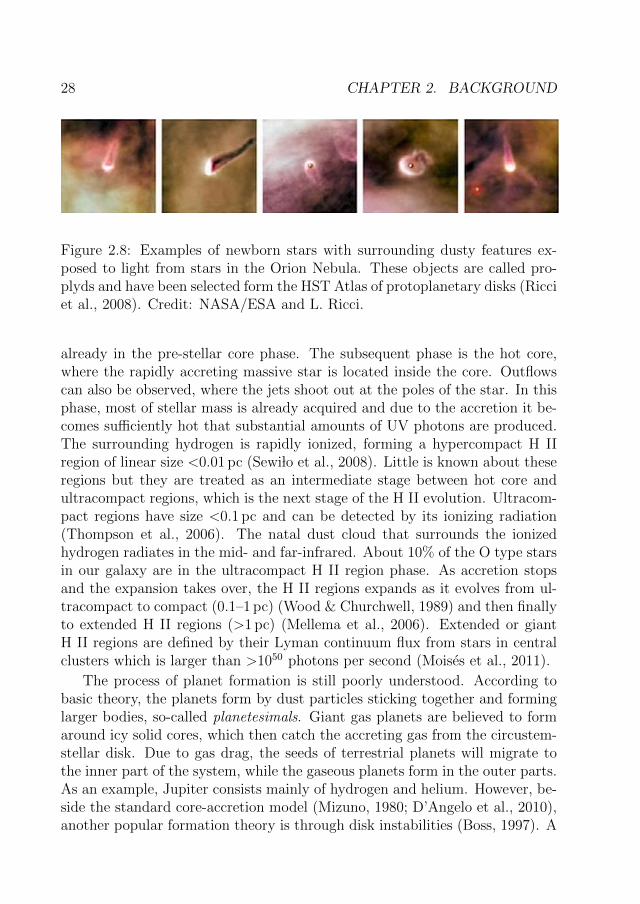
These disks are believed to be the birthplaces of planets, asteroids andcomets and they are called protoplanetary disks. The disks are round and theyare often observed to be ∼ 5–10 times larger than our solar system (Williams& Cieza, 2011). Numerous disks have been imaged with the Hubble SpaceTelescope (HST), indicating that the formation of extrasolar systems, similarto ours, is a rather common process in the Milky Way. One class of disk arecalled proplyds which are disks subject to photoevaporation from the radiationof stars in young clusters. Figure 2.8 contains a composition of young objectswith circumstellar dusty features.
Further gravitational contraction increases the temperature and eventuallyallows the ignition of hydrogen. When this happens, dust close to the star isvaporized while gas close to the star is blown away. After this, only the starand the planets are remaining.
The formation of massive stars is poorly understood, compared to their lowmass equivalents, and various scenarios have been suggested such us monolithiccollapse and competitive accretion (Bonnell et al., 2001; Zinnecker & Yorke,2007; Tan et al., 2014). Simplified, the high mass star formation process starts
28 CHAPTER 2. BACKGROUND
Figure 2.8: Examples of newborn stars with surrounding dusty features ex-posed to light from stars in the Orion Nebula. These objects are called pro-plyds and have been selected form the HST Atlas of protoplanetary disks (Ricciet al., 2008). Credit: NASA/ESA and L. Ricci.
already in the pre-stellar core phase. The subsequent phase is the hot core,where the rapidly accreting massive star is located inside the core. Outflowscan also be observed, where the jets shoot out at the poles of the star. In thisphase, most of stellar mass is already acquired and due to the accretion it be-comes sufficiently hot that substantial amounts of UV photons are produced.The surrounding hydrogen is rapidly ionized, forming a hypercompact H IIregion of linear size <0.01 pc (Sewi lo et al., 2008). Little is known about theseregions but they are treated as an intermediate stage between hot core andultracompact regions, which is the next stage of the H II evolution. Ultracom-pact regions have size <0.1 pc and can be detected by its ionizing radiation(Thompson et al., 2006). The natal dust cloud that surrounds the ionizedhydrogen radiates in the mid- and far-infrared. About 10% of the O type starsin our galaxy are in the ultracompact H II region phase. As accretion stopsand the expansion takes over, the H II regions expands as it evolves from ul-tracompact to compact (0.1–1 pc) (Wood & Churchwell, 1989) and then finallyto extended H II regions (>1 pc) (Mellema et al., 2006). Extended or giantH II regions are defined by their Lyman continuum flux from stars in centralclusters which is larger than >1050 photons per second (Moises et al., 2011).
The process of planet formation is still poorly understood. According tobasic theory, the planets form by dust particles sticking together and forminglarger bodies, so-called planetesimals. Giant gas planets are believed to formaround icy solid cores, which then catch the accreting gas from the circustem-stellar disk. Due to gas drag, the seeds of terrestrial planets will migrate tothe inner part of the system, while the gaseous planets form in the outer parts.As an example, Jupiter consists mainly of hydrogen and helium. However, be-side the standard core-accretion model (Mizuno, 1980; D’Angelo et al., 2010),another popular formation theory is through disk instabilities (Boss, 1997). A

2.11. FREE FLOATING PLANETARY MASS OBJECTS 29
discussion can be found in Boss (2008, 2009).In 1995 the discovery of an planet, orbiting the solar-like star 51 Peg, was
announced by Mayor & Queloz (1995). This type of planet is called extrasolar planets or in short exoplanets. According to extrasolar planets database(http://exoplanet.eu) about 4000 exoplanets have been confirmed and manymore candidates are awaiting confirmation. The majority of the exoplanetshave been discovered by indirect methods, typically by radial velocity tech-nique or transit technique (Perryman, 2000; Santos, 2008).
Observations of exoplanets have shown that their orbital distance can bewithin 0.1 AU. These planets are called “hot Jupiters” because of their highequilibrium temperature, which is due to their small separation from their par-ent star. To explain the existence of these “hot Jupiters”, planetary migrationtheory, known as “Type II”-migration (Ward, 1997; Armitage & Rice, 2005)was developed. In this theory, gravitation interacts with the gaseous disk at anearly stage of the planet formation. However, a change in the orbital periodsof gaseous planets can also occur by planet planet scattering (Chatterjee etal., 2008) or by orbital disruption (Petrovich, 2015).
In later years other types of exoplanets have been discovered, such as exo-Jupiters, at intermediate orbit radii (' 1 AU) and super-Earths. The super-Earths have masses between 1 and 10 Earth masses and may be orbiting atsmall radii or located at several AUs from their star (Cassan, 2014).
2.11 Free Floating Planetary Mass Objects
The International Astronomical Union defines the mass limit of a planet to bebelow the deuterium-burning mass (13 Mj, Boss, 1997), while brown dwarfsand stars populate the mass range above. Stars that are not massive enoughto sustain hydrogen fusion are called brown dwarfs. The existence of thesebrown dwarfs was first suggested by Kumar (1962, 1963), who predicted thatthey could be numerous. The first observations of a brown dwarf was madeby Nakajima et al. (1995), and by now several hundred are known. However,observations have shown that brown dwarfs can have masses that are withinthe official planetary mass range (Caballero et al., 2007) and therefore analternative definition of a brown dwarf has been proposed which would be basedon the formation mechanism rather than on a critical mass limit (Burrows etal., 2001).
A number of isolated free floating planets (FFPs), which are not clearlybound to a host star, have been discovered in young clusters and star for-mation regions e.g., Trapezum cluster, the AB Doradus moving group (Pena

30 CHAPTER 2. BACKGROUND
Ramırez et al., 2012, 2016; Clanton & Gaudi, 2017) and also in the galacticfield (Cushing et al., 2014). These objects extend from brown dwarf massesdown to the regime of giant planets, with M ≥MJ . These rogue planets firstgot the attention when Zapatero Osorio et al. (2000) discovered a populationof free floating planetary object candidates in the σ Orionis star cluster.
Figure 2.9: An artists illustration of the accretion disk of the FFP mass objectOTS 44. OTS 44 may have formed the same way stars are made. Credit:MPIA / A. M. Quetz.
A good method to study these dark cold objects is by microlense obser-vations towards the galactic bulge, where the stellar density is the highest.The microlensing occurs when a compact object (lens) approaches very closelyto the observer’s line of light with a background star (source). The sourceincreases in brightness as the observer, lens and source are aligned in theline of sight and returns to it’s regular intensity as they become unalignedagain. This standard microlensing light curve follows a characteristic sym-metric curve, Paczynski profile (Paczynski, 1986, 1996). For more reading seeGaudi et al. (2008), Gaudi (2010), Gould & Loeb (1992) and Cassan (2014).
This method has been used by the Microlensing Observation in Astro-physics group (MOA-2) (Sumi et al., 2003, 2011; Freeman et al., 2015) and theOptical Gravitational Lensing Experiment (OGLE-III) (Wyrzykowski et al.,2015). Sumi et al. (2011) examined two years of microlensing survey data fromthe MOA-2 collaboration and found that the Jupiter-sized FFPs are about 1.8

2.12. H II REGIONS 31
times as common as main-sequence stars. However, recently presented resultby Mroz et al. (2017) shows a lower number of free floating planet population,with an upper limit of about 0.25 Jupiter sized planets per star. These planetsare defined as unbound, or bound but very distant >100 AU, from any star.
Thus the discovery of what could be free-floating planets in star-rich re-gions, raises the question of their origin, which is not currently known. Theymay have formed in situ from a direct collapse of a molecular cloud by fragmen-tation, similar to star formation (Bowler et al., 2011). In fact, Luhman et al.(2005); Joergens et al. (2015); Fang et al. (2016); Boucher et al. (2016); Bayo etal. (2017) have found four FFPs with an accretion disk. The Figure 2.9 showsan artist’s view of the accreting disk of the free floating planetary mass objectOTS 44 (Joergens et al., 2015). Furthermore, planetary-mass binaries, whichwould be almost impossible to form through planetary formation mechanisms,have also be found by e.g., Best et al. (2017). Another possibility to formFFPs is by forming stellar embryos that are fragmented and photoevaporatedby nearby stars (Whitworth & Zinnecker, 2004). They may also have beenejected after they were formed in circumstellar protoplanteray disks throughgravitational instabilities (Li et al., 2015). Such instabilities can be caused ina triplet star system (Reipurth & Mikkola, 2015) or by the passage throughthe center of a dense star cluster (Wang et al., 2015). Hence the formationmechanism for FFPs is still an open question.
.
2.12 H II regions
The bright emission nebulæ are also called H II regions because they consistprimarily of ionized hydrogen. Although a few of the visually brightest H IIregions are visible to the naked eye, they seem to have remained relativelyunnoticed until the advent of the telescope in the early 17th century. A largenumber of H II regions within our galaxy as well as and in others are now welldocumented. Some well-known examples of H II regions are the Eagle Nebula(Messier 16, M 16) and the Orion Nebula (M 42). The most studied extragalactic H II region lies in the Large Magellanic Cloud and is known as 30Dorados or NGC 2070.
The Eagle Nebula is a prominent H II region lying some 7000 light-yearsaway (Hillenbrand et al., 1993) in the Serpens constellation (Figure 2.10). Inthe center of this nebula there are several young, hot and massive, bright,blue stars, whose light and winds push away the nebular filaments. In thisregion, one notes many opaque, long pillars, looking like fingers, containing

32 CHAPTER 2. BACKGROUND
grains of dust and cold molecular gas. These pillars are warm, with typicaltemperatures of 60 K. Most of the mass is concentrated in the cores at thetip of the fingers, with masses of 10–60M�. These finger tips are known asEGG (evaporating gas globules, see the zoomed in image in Figure 2.10). Theyhave a characteristic radius between 300 and 400 AU and calculations suggestthat most objects do not survive longer than 104 years (Hester et al., 1996).Nevertheless, studies on these objects by McCaughrean & Andersen (2002)showed that ∼ 15% of these contain young low mass stars or brown dwarfs.In Paper IV, very dark globulettes were found in the Eagle Nebula. Most ofthese objects are roundish in shape and they are isolated from the filaments.In this nebula we catalog 46 gloublettes, see Table C1.
The Orion GMC is the nearest giant cloud to us, at a distance of around1500 light-years. The Orion Nebula (Figure 2.11), with an age of about1–5 Myr, is around 6 light-years across and the region is believed to be a“stellar nursery”, which means that numerous new stars are formed out of in-terstellar gas. This nebula contains brown dwarfs and several thousand youngstars, with masses ranging from one solar mass up to type O stars with 40solar masses. The four brightest stars seen in the cluster are approximately100 000 times brighter than the Sun. Within the Orion Nebula, Drass et al.(2016) also discoverd 160 isolated planetary mass object candidates.
An H II region is formed from the moment that a newly formed massive starbegins to ionize its surroundings by emitting UV radiation. Stars of spectraltype O ionize a region out to hundreds of parsecs, whereas B stars ionizeregions with diameters of a few parsecs. Typically, within a giant molecularcloud, stellar clusters containing type O and B stars will form, called OBstars. These stars have surface temperatures of 30 000–50 000 K, masses of20–100M�, and lifetimes of about 1–10 million years. Through the combinedluminosity, the stars ionize a large volume of the surrounding gas and dissociatethe molecular gas beyond the H II region with far-UV photons.
2.12.1 H II regions: Dynamics
The expansion of an H II region depends on several factors, such as temper-atures of the stars, density, and the size of the original molecular cloud. Theincrease in temperature and pressure in a young H II region leads to an expan-sion of the ionized volume into the surrounding molecular gas. This continuesuntil the H II region breaks free of the confining molecular cloud. The OB starsform initially in the center of the H II region, where they create strong stellarwinds, with speeds of around 2000 km s−1, and powerful energetic ionizing ra-

2.12. H II REGIONS 33
Figure 2.10: The Eagle Nebula is located in the constellation Serpens about6000 light-years (1800 pc) from the Earth. This nebula is an example of ablister H II region. It hosts a very luminous open cluster of stars, surroundedby dust and gas. The three pillars at the center of the image have been sculptedby the intense radiation from the hot stars in the cluster. The in-zoomed imageof one of the pillar’s heads (1), shows finger-like objects, so called evaporatinggas globules (EEGs), which contains molecular gas and dust. They are dense,compact objects, where star formation may occur. The radii of these objectsare about 400 AU. The in-zoomed image (2) illustrates the size of our solarsystem compared to a gas globule. The ionization fronts can be seen as brightrims at the edge of the H II region. Dark objects close to the ionizationfronts are shock compressed molecular gas clouds. This image was createdby combining emission line images in Hα (green), oxygen [O III] (blue) andsulphur [S II] (red) and taken from https://www.astronomy.com.
diation. The expansion of an H II region can be approximated as a uniformprocess. In reality, however, the density gradients and the inhomogeneous ma-terial distribution within the molecular cloud cause the majority of the H IIregions to be non spherical. In this case, the warm ionized gas escape in the

34 CHAPTER 2. BACKGROUND
Figure 2.11: The Orion Nebula is an example of compact H II region. Thisis the brightest nebula seen from Earth. It is a suitable laboratory for study-ing how stars are born, because it is relatively close (about 1300 light-yearsaway). The Orion constellation contains many regions rich in interstellargas and dust and sites of recent star formation. At the nebulas center isa group of hot young stars, called the Trapezium cluster. These stars emitstrong UV radiation and stellar winds after having pushed away nearby mat-ter. When the shell reaches the molecular cloud, warm ionized gas escape intothe less dense gas with a high velocity outflow, similar to uncorking a bottleof champagne and hence the name “Champagne flows”, seen in the image. Athin and dense PDR is located between the background molecular cloud andthe ionized gas. The This image is a combination between visible and near-infrared bands, taken from http://hubblesite.org/gallery/album/nebula
collection /emission /pr2006001a/web print.
direction of the less dense gas, into the intercloud medium. These H II regions
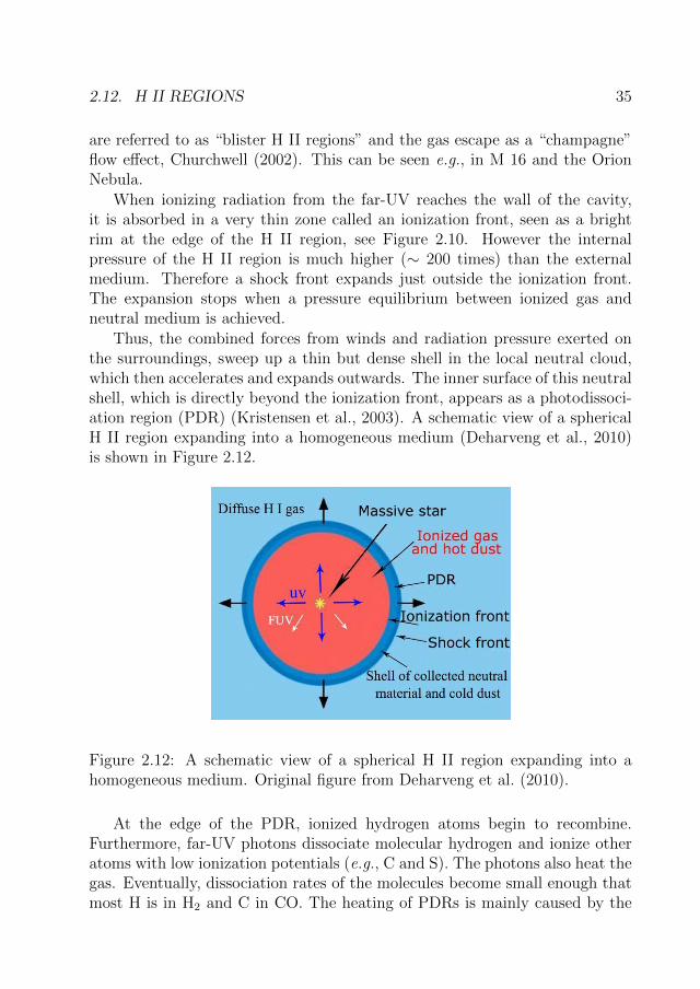
2.12. H II REGIONS 35
are referred to as “blister H II regions” and the gas escape as a “champagne”flow effect, Churchwell (2002). This can be seen e.g., in M 16 and the OrionNebula.
When ionizing radiation from the far-UV reaches the wall of the cavity,it is absorbed in a very thin zone called an ionization front, seen as a brightrim at the edge of the H II region, see Figure 2.10. However the internalpressure of the H II region is much higher (∼ 200 times) than the externalmedium. Therefore a shock front expands just outside the ionization front.The expansion stops when a pressure equilibrium between ionized gas andneutral medium is achieved.
Thus, the combined forces from winds and radiation pressure exerted onthe surroundings, sweep up a thin but dense shell in the local neutral cloud,which then accelerates and expands outwards. The inner surface of this neutralshell, which is directly beyond the ionization front, appears as a photodissoci-ation region (PDR) (Kristensen et al., 2003). A schematic view of a sphericalH II region expanding into a homogeneous medium (Deharveng et al., 2010)is shown in Figure 2.12.
Figure 2.12: A schematic view of a spherical H II region expanding into ahomogeneous medium. Original figure from Deharveng et al. (2010).
At the edge of the PDR, ionized hydrogen atoms begin to recombine.Furthermore, far-UV photons dissociate molecular hydrogen and ionize otheratoms with low ionization potentials (e.g., C and S). The photons also heat thegas. Eventually, dissociation rates of the molecules become small enough thatmost H is in H2 and C in CO. The heating of PDRs is mainly caused by the

36 CHAPTER 2. BACKGROUND
photoelectric effect (Bakes & Tielens, 1994), while the cooling is dominatedby the forbidden transition lines [C II] and [O I]. As mentioned before, thegas is not uniform in density and therefore the ionization front does not moveuniformly into the cloud. When the radiation encounters a dense part of thecloud, the ionization front slows down. As the molecular cloud evaporates, thePDR boundary can develop pillars, which later detach to crate isolated glob-ules or globulettes. The ionization front drives a shock wave into the interiorof the cloud, thus compressing neutral gas, which leads to formation of densecores. Typically, a shock wave moves into globules or globulettes at velocitiesin the order of a few km/s. These dense cores can subsequently collapse toform new stars or planetary mass objects (Lefloch & Cernicharo, 2000).
The effects of photoevaportion on the interstellar clouds have been investi-gated by Bertoldi (1989) and analytical models of radiation driven implosionhas been done by e.g., Bertoldi & McKee (1990), Bisbas et al. (2011) and Ha-worth & Harries (2012). The models explain how a shock wave can compressa spherical clump and produce the cometary shape of the cloud that is in pres-sure equilibrium with the surrounding photoevaporating gas. This theory hasbeen applied to globules in H II regions, such as IC 1848, and also to glob-ulettes, see Paper I. The radiation pressure from the hot stars gradually drivesmost of the gas away and once these stars cool when moving away the mainsequence, they produce drastically less UV radiation. This effectively shutsoff the nebula’s ionizing photons. However, sometimes the H II region willstill have a diffuse radiation field but eventually it will cease, and the nebulastarts to fade and disperse. Thus, an H II region basically lasts only as longas the main sequence lifetime of its ionizing star(s). However, H II regions canlive longer than an ionizing star, either in large star forming regions, involv-ing multiple clusters, progressive star formation (Smith et al., 2010) or whenthere is a spread in stellar ages with co-existing younger (∼ 1 Myr) and older(∼ 10 Myr) stars. In Paper IV, the mean lifetime for H II regions was assumedto be 5 Myrs.
2.13 Supernovae
A massive star evolves until its core collapses under its own gravity and thenit dies in a powerful stellar explosion, a supernova, leaving behind a supernovaremnant (SNR). These remnants consist of the ejected material of circumstellarand interstellar material that has been affected by the shock wave from thesupernova. SNRs can be observed at many different wavelengths and theycan have various morphologies. Their appearance depend mostly on the initial

2.13. SUPERNOVAE 37
conditions of the progenitor star but also on the surrounding environment.Some examples of SNRs are shown in Figure 2.13.
Figure 2.13: These Astronomy Picture of the Day images (from the HST)display some of the complex morphologies observed in supernova remnants.Images 1–2 are remnants after Type Ia supernovae and Images 3–4 are shell-type supernovae remnants. From left to right: 1) SNR 0509-67.5 is a remnantfrom a supernova in the Large Magellanic Cloud. 2) Tycho’s Supernova, dis-covered in the year 1572. 3) Simeis 147, or the Spaghetti Nebula, tracingthe shocked, glowing gas. 4) SNR E0102-72, located in the Small MagellanicCloud. The outer blast wave produced by the supernova is blue, and an innerring of cooler material is red. This inner ring is probably expanding ejectafrom the explosion that is being heated by a shock wave traveling backwardsinto the ejecta.
In the Milky Way there have been about 100 million supernova explosionsover time. They have enriched our galaxy with heavy elements, like oxygen,carbon and iron. The supernova explosions can even trigger star formation inthe disturbed interstellar clouds. The classification of SN is based on opticalspectra and their lightcurves, where the intensity is measured as a function oftime. The SNe can be divided into two main classes: thermonuclear and corecollapse supernova.
In Type Ia, or thermonuclear supernovae, a white dwarf accretes materialfrom a companion star. These can be found in all stellar populations and inall types of galaxies. The core of a white dwarf is very dense with a mass ofabout 0.7–1.4 solar masses and a size of similiar to the Earth. The maximummass limit for white dwarfs is estimated to about 1.4M�, which is called theChandrasekhar mass (Janka et al., 2007).
Core collapse supernovae are divided into Type II and Ib, Ic, where Type IIare divided into subtypes (Filippenko, 1997, and references therein). Type Iband Ic have similar evolutions as the Type II supernova (see below). The maindifference is that the Type II spectra show hydrogen absorption (Minkowski,
38 CHAPTER 2. BACKGROUND
1941). This could be due to the loss of the hydrogen envelope, ejected fromhigh mass stars (Wheeler & Harkness, 1990). The main distinction between thecore collapse and Type Ia is the chemical abundances. Supernova explosionsfrom massive stars emit large abundances of oxygen, while the lighter Type Iasupernova contain a lot of iron.
Core collapse supernova subtypes are defined in the order of increasingprogenitor mass, starting with II-P and ending with Ic (Anderson & James,2008). The most common type are Type II-P SN where the mass range ofthe progenitors is between 8–17M� (Smartt et al., 2009). The progenitors ofII-Ps are mainly red supergiants. Model calculations of the convective layersof these old stars have shown that it is possible for large scale supergranulation(convective surface elements) to provide the dominant photospheric convection.They may be so large that a handful of them may be enough to cover the surfaceof the star. Examples of models of convection in red supergiants can be foundin Freytag (2006), Chiavassa et al. (2009) and Figure 7.1.
When the core collapse supernova explodes, it destroys the star and leaves aremnant in the form of a neutron star, a pulsar or a black hole, while the ejectaexpand into the surrounding ISM. Neutron stars are the smallest and denseststars known to exist. It can be described as a giant atomic nucleus madealmost entirely of neutrons and held together by gravity, which is balanced bydegeneration pressure. As the star’s core collapses, its rotation rate increasesas a result of the conservation of angular momentum. Newly formed neutronstars rotate at up to several hundred times per second. In the beginning of the1960’s it was predicted that core collapse SN would create so called pulsars(Hoyle et al., 1964). The radiation from pulsars is thought to be primarilyemitted from regions near their magnetic poles and if the neutron star happensto be aligned so that the poles face the Earth, we will see the radio waves, everytime one of the poles rotates into our line of sight. Therefore the pulsar appearto blink periodically as seen from the Earth. A star with a mass greater than25M� end its life as a black hole (Carroll & Ostlie, 1996).
There are two types of supernova remnants, shell-type and Crab-like rem-nant or Power Wind Nebula (PWN). A shell-type remnant is an expandingsupernova blast wave that sweeps the surrounding ISM. They have typically asymmetric shell morphology, see Figure 2.13 images 3–4. A PWN has a centralyoung pulsar that produces a wind of energetic particles that are acceleratedin the magnetic field and emit synchrotron radiation. This radiation interactswith the surrounding medium.
The Crab Nebula (Figure 6.4) is thought to be the result of a Type II corecollapse supernova explosion, where the progenitor star was a red supergiant.

2.13. SUPERNOVAE 39
This SNR is the main subject in this thesis and it is therefore described inmore detail below.
2.13.1 Core Collapse Supernova Type II
Gravitation leads to star formation and it also responsible for triggering thecondition that leads to thermonuclear fusion. In massive stars, when morehydrogen is added, the gravitational force increases, which increases the tem-perature in the core. The increased temperature accelerates the burning ofhydrogen into helium, which shortens the time spent on the main sequence.
Core collapse supernova fuse increasingly higher mass elements, from hy-drogen to helium and then to carbon, neon and oxygen, until finally a coreof iron and nickel is produced. In this final stage, no more energy can begenerated. This because iron is in a tightly bound nucleus and has the high-est binding energy per nucleon among all the stable elements. The extremepressure in the core fuses the atoms; protons and electrons will be crushedtogether, forming neutrons in the core and releasing neutrinos. This largeneutrino flux is a sign of a supernova event. The pressure is only held up foras long as the core mass stays below the Chandraskar mass limit. Eventuallythe core becomes too massive to be supported by electron degeneracy pressureand the core subsequently collapses. The radius of the core is only a few tensof km and the density is approximately two times that of the atomic nucleus(∼ 1014 g cm−3). The nuclei are so close together that the strong force becomesrepulsive. As a result, the hard core rebounds and pressure waves are sendback throughout the outer collapsing stellar layers. The material above thecore is now so dense that not all the neutrinos escape immediately. The pres-sure of these trapped neutrinos adds to the energy of the shock, which leads tothe explosion of the star (see for a review, Janka et al., 2007; Carroll & Ostlie,1996). Then the expanding ejecta collides with the slower material outside ofthe star, which results in elements that are heavier than iron.
The duration of every stage of evolution depends on the stage of elementsynthesis and also on the initial mass of the SN. In general, the differentburning stages take less and less time. As an example, the duration of hydrogenburning in a 20M� star lasts for a period of 8 million years, the helium burningphase lasts one million years, carbon burning around 900 years, and the finalstages are matters of a year. Finally, the collapse happens in a matter ofseconds (Heger et al., 2005).

40 CHAPTER 2. BACKGROUND
2.13.2 The Evolution of Supernova Remnants
The evolution of a supernova remnant goes through several stage or phases andis described below (Shu, 1992; Vink, 2012). Theses stages are approximate,because the remnant or the ISM is not homogeneous and different parts of aSNR can be in different phases. For review see Gaensler & Slane (2006).
Thus the energy that is released in a core-collapse supernova explosion isaround 1053 erg (1046 J). Almost all of this energy is radiated away in theform of neutrinos which leaves about 1051 erg (Woosley & Janka, 2005) in theform of kinetic energy deposited by the blast wave into the surrounding ISM.This energy is, however, still enough to drive a shock wave through all ofthe stellar layers above the core, explosively outward at 10% of the speed oflight. This propagates into the medium just behind the blast wave and intothe surrounding medium.
Models by Kifonidis et al. (2003) show that instabilities of stellar layersand neutrino driven convection cause ejecta that form clumps of metal-richgas. This happens within minutes of the explosion and as the gas expands andcools, the clumpiness increases.
The blast wave will sweep up, heat, compress and accelerate the ISM itencounters (McKee & Hollenbach, 1980). This interstellar material is sepa-rated from the freely ejected stellar material by a contact discontinuity, i.e., asurface between two different materials with similar velocity and pressure butdifferent density. This is distinct from a shock front, where all three quantitieschange. Thus, as long as the mass of the ejecta is dominant over the sweptup material mass from the ISM, the expansion of the ejecta behind the shockcan be seen as almost free. This stage is called the ejecta dominated phase. Inthe free expansion, the ejecta velocity is roughly constant with typical valuesof 5000 km s−1(Reynolds, 2008) and it will continue through the first centuryof the SN lifetime. At some point, which is not exactly known, a criticallypressure difference between these two media is developed and behind the con-tact discontinuity a second shock wave is starting to form in the ejected stellarmaterials, driven into the interstellar medium. The velocity of this shock waveis determined by the speed of the fastest moving ejecta. When this shockmoves through the interstellar medium, it is quickly slowed down as it sweepsup mass. This causes a reverse shock, which propagate back toward the ex-plosion center, through the freely expanding ejecta. The shock wave will heatup the gas to high enough temperatures for thermal X-rays to be emitted. Anexample can be found in Figure 2.13, image 4. However, if the ejecta expandsinto vacuum, the formation of a reverse shock will not occur.
From Figure 2.14, the SNR consists now of two shock fronts traveling in
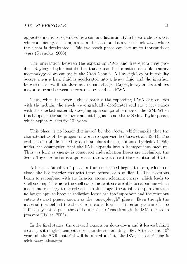
2.13. SUPERNOVAE 41
opposite directions, separated by a contact discontinuity; a forward shock wave,where ambient gas is compressed and heated; and a reverse shock wave, wherethe ejecta is decelerated. This two-shock phase can last up to thousands ofyears (Reynolds, 2008).
The interaction between the expanding PWN and free ejecta may pro-duce Rayleigh-Taylor instabilities that cause the formation of a filamentarymorphology as we can see in the Crab Nebula. A Rayleigh-Taylor instabilityoccurs when a light fluid is accelerated into a heavy fluid and the interfacebetween the two fluids does not remain sharp. Rayleigh-Taylor instabilitiesmay also occur between a reverse shock and the PWN.
Thus, when the reverse shock reaches the expanding PWN and collideswith the nebula, the shock wave gradually decelerates and the ejecta mixeswith the shocked material, sweeping up a comparable mass of the ISM. Whenthis happens, the supernova remnant begins its adiabatic Sedov-Taylor phase,which typically lasts for 104 years.
This phase is no longer dominated by the ejecta, which implies that thecharacteristics of the progenitor are no longer visible (Jones et al., 1981). Theevolution is still described by a self-similar solution, obtained by Sedov (1959)under the assumption that the SNR expands into a homogeneous medium.Thus, as long as energy is conserved and radiation losses are negligible, theSedov-Taylor solution is a quite accurate way to treat the evolution of SNR.
After this “adiabatic” phase, a thin dense shell begins to form, which en-closes the hot interior gas with temperatures of a million K. The electronsbegin to recombine with the heavier atoms, releasing energy, which leads toshell cooling. The more the shell cools, more atoms are able to recombine whichmakes more energy to be released. In this stage, the adiabatic approximationno longer applies because radiation losses are too important and the remnantenters its next phase, known as the “snowplough” phase. Even though thematerial just behind the shock front cools down, the interior gas can still besufficiently hot to push the cold outer shell of gas through the ISM, due to itspressure (Ballet, 2003).
In the final stages, the outward expansion slows down and it leaves behinda cavity with higher temperature than the surrounding ISM. After around 106
years all the SNR material will be mixed up into the ISM, thus enriching itwith heavy elements.

42 CHAPTER 2. BACKGROUND
2.13.3 Dust Formation
There are two main dust producers in Universe, the asymptotic giant branch(AGB) stars and supernovae (see e.g., the review by Gall et al., 2011). AGBstars evolve from lower mass stars and could be the major source of the dustgrains produced within our galaxy. These stars produce dust in their laterstellar phase, in their atmospheres, where the gas is sufficiently cool and densethat molecules may form and stick together to form dust grains. However, it isbelieved that AGB stars cannot be responsible for all dust seen at high redshiftdue to their relatively long lifetimes (in the order of 109 yr). Therefore theearly dust is probably produced mainly by core collapse supernovae (Morgan& Edmunds, 2003; Maiolino et al., 2004).
For these supernova types, dust is mainly produced at the end of theirevolution and also after the supernova explosion. As the ejected materialcools, small dust particles condense out of the gas of heavier elements insidethe ejected material. Thus, early dust formation can take place in a cold denseshell which is behind the forward shock front and also right after the reverseshock has propagated through the medium (Fox et al., 2011; Stritzinger et al.,2012). Figure 2.14 shows a simplified overview of where dust formation wouldtake place. The dust that is formed in a SN can both be hot dust (500–1000 K)and cold dust (<50 K) and it emits mostly at IR wavelengths.
Most of the SN ejecta have shown dust formation, already a few hundreddays after the explosion, with different dust masses (Gomez et al., 2009; Barlowet al., 2010). Dust in a cold dense shell could be formed very early, about 60days after explosion and in some core type SN even earlier (Smith et al., 2012).
Several theoretical models for dust formation have been developed, wherethe results show that each SN (Type II) explosion must produce between0.1–1M� of dust (Dwek et al., 2007) in order to account for the observedmass values in high-redshift galaxies (Bertoldi et al., 2003). However, IR stud-ies of SNs have found no evidence for large quantities of dust particles. Onlysmall amounts of dust have been observed, sometimes a hundred times lowerthan theoretical predictions (Dwek, 2004; Green et al., 2004; Temim et al.,2006). One of the reasons may be that dust is destroyed by erosion and sput-tering in the region between the forward and the reverse shock (Dwek et al.,2008; Kozasa et al., 2009). But this is still puzzling considering the missingdust mass and the unresolved question of how much dust the supernovae createand inject into the ISM.
The sensitivity and resolution of the space telescopes Spitzer and Herschelhas enabled mass estimates of dust for several SNe. For example, for the entireCas A supernova, the total amount of dust was recently estimated to be around
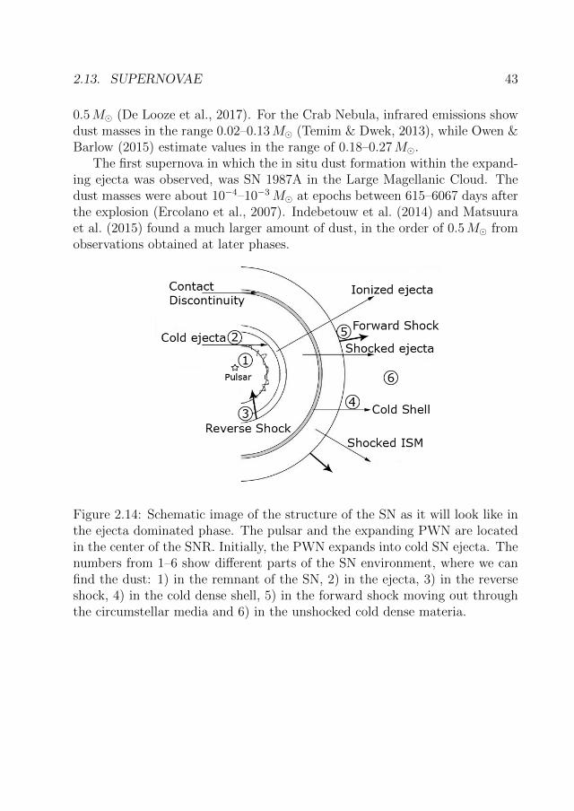
2.13. SUPERNOVAE 43
0.5M� (De Looze et al., 2017). For the Crab Nebula, infrared emissions showdust masses in the range 0.02–0.13M� (Temim & Dwek, 2013), while Owen &Barlow (2015) estimate values in the range of 0.18–0.27M�.
The first supernova in which the in situ dust formation within the expand-ing ejecta was observed, was SN 1987A in the Large Magellanic Cloud. Thedust masses were about 10−4–10−3M� at epochs between 615–6067 days afterthe explosion (Ercolano et al., 2007). Indebetouw et al. (2014) and Matsuuraet al. (2015) found a much larger amount of dust, in the order of 0.5M� fromobservations obtained at later phases.
Figure 2.14: Schematic image of the structure of the SN as it will look like inthe ejecta dominated phase. The pulsar and the expanding PWN are locatedin the center of the SNR. Initially, the PWN expands into cold SN ejecta. Thenumbers from 1–6 show different parts of the SN environment, where we canfind the dust: 1) in the remnant of the SN, 2) in the ejecta, 3) in the reverseshock, 4) in the cold dense shell, 5) in the forward shock moving out throughthe circumstellar media and 6) in the unshocked cold dense materia.


Chapter 3
Theory
This chapter is intended to provide readers with a general background andnotations, necessary for understanding the discussion in the Papers. Some ofthe text content is taken from the Grenman (2006) licentiate thesis.
3.1 Interstellar Extinction
Dark clouds can be seen against the background sky of stars or bright nebulæin optical images. These clouds consist mostly of molecular gas, but also dust.When star light travels through these clouds, some of the light will be absorbedand scattered by dust grains. During the absorption, a photon is absorbedeither by converting into internal energy of the dust grain or by ejecting anelectron from the dust grain. When scattering, a photon is re-emitted at thesame frequency but in a different direction. Particles that are much smallerthan the wavelength 2πa� λ, where a is the radius, cause mainly Rayleighscattering. The combination of processes such as absorption and scattering isknown as extinction, A, measured in magnitudes.
It has been shown that the extinction depends on the wavelength. There-fore, extinction is measured in small wavelength intervals, called photometricbands, from near IR to UV.
The most commonly used photometric system was developed by Johnson &Morgan (1953) and later extended to include near-IR wavelength. The filter-symbols and corresponding central wavelengths are shown in Table 3-1. Thewidth of the filter-bands are of the order of several 100 A, see Section 5.3.Stellar light is generally observed in the range of the visible light spectrum(known as the V band centered at 0.555µm) and therefore the most commonlyused extinction is AV .
45
46 CHAPTER 3. THEORY
Table 3-1: The standard photometric system (Savage & Mathis, 1979), inwhich the central wavelength of each filter is given. The width of the filterbands are of the order of several 100 A. From lower rows, one can see thatthe extinction decreases with increasing wavelength, which is why we use IRimaging to see through the dust. Thus, B (blue), V (green) and R (red) arelocated in the visible band while the J, K and L bands lie in near-IR regionand U lies in the ultraviolet region. The corresponding magnitudes are knownas B, V , etc.
Filter U B V R I J K LMean wavelength, λ (µm) 0.40 0.44 0.55 0.70 0.90 1.25 2.2 3.4Aλ/E(B − V ) 4.40 4.10 3.10 2.32 1.50 0.87 0.38 0.16Aλ/AV 1.53 1.32 1 0.75 0.48 0.26 0.15 0.09
Figure 3.1: The small dust particles scatter blue light more effectively thanlight at longer wavelengths, which passes straight through.
Thus, it can be shown that the blockage is most effective when there isan approximate match between the particle size and wavelength,e.g., the sunlooks red when it is low above the horizon.
This effect applies also to the dust grains, which scatter most efficientlyat wavelengths close to the size of the grain or smaller (Binney & Merrifield,1998), meaning that the extinction is more efficient at short (UV and bluer)than at longer (redder) wavelengths, see Figure 3.1. Thus, the longer thedistance through the ISM, the redder the star appears. This effect is knownas reddening, where the observed intensity is stronger at longer wavelengths.Examples of how extinction and reddening affects the appearance of a dustycloud are shown in Figure 2.5.
To determine the degree of reddening, we can measure the color index of
3.2. VISUAL EXTINCTION 47
an object, which is defined as the difference in magnitude between two filterbands. Often the difference between the magnitudes blue (B) and the visual(V ) band is used, and called (B − V ).
If an “unreddened” star, i.e., one which is not reddened by foregroundinterstellar matter, has the color index (B − V )0, one defines the color excessof an object as
E(B − V ) = (B − V )− (B − V )0 = (B −B0)− (V − V0) = AB − AV . (3.1)
Thus, as E(B − V ) increases, the emitter is considered “redder” and whenit decreases, the emitter is “bluer”. Color excess can also be defined for anyother wavebands and one can similarly define E(λ− V ) = A(λ)− A(V ).
Table 3-1 lists the wavelength dependence of extinction based on the em-pirical measurements by Savage & Mathis (1979), which are valid within theMilky Way. The total extinction can then be determined from the color excessin equation (3.1), using Table 3-1:
E(B − V ) = AB − AV = AV (ABAV− 1) = 0.32AV . (3.2)
The ratio of extinction to color excess is called R (Savage & Mathis, 1979). Inthe visual filter band, it is defined as:
RV =AV
E(B − V ). (3.3)
Using Table 3-1 (Savage & Mathis, 1979) the standard value of RV is found tobe about 3.1. The extinction curve is usually given in a normalized way as
E(λ− V )
E(B − V )or
A(λ)
AV. (3.4)
This is often plotted against 1/λ, see Figure 3.2.
3.2 Visual Extinction
In many observational works, such as this thesis, the gas to dust ratio is as-sumed to be a constant (100:1). Assuming the reddening law (RV = 3.1), anda constant dust to gas ratio, it is possible to convert between the visual extinc-tion, AV and the total number density of particles along the line of sight (totalcolumn density), N (Bohlin et al., 1978; Draine & Bertoldi, 1996) through:
AV =N
1.87× 10²¹[cm2]. (3.5)
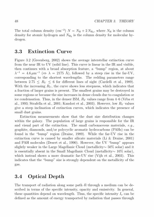
48 CHAPTER 3. THEORY
The total column density (cm−2) N = NH + 2NH2 , where NH is the columndensity for atomic hydrogen and NH2 is the column density for molecular hy-drogen.
3.3 Extinction Curve
Figure 3.2 (Greenberg, 2002) shows the average interstellar extinction curvefrom the near IR to UV (solid line). This curve is linear in the IR and visible,then continues with a broad absorption feature, a “bump” region, at aboutλ−1 = 4.6µm−1 (⇔ λ = 2175 A), followed by a steep rise in the far-UV,corresponding to the shortest wavelengths. The redding parameters rangebetween 2.75 ≤ RV ≤ 6 for different lines of sight (Cardelli et al., 1989).With the increasing RV , the curve shows less steepness, which indicates thata fraction of larger grains is present. The smallest grains may be destroyed insome regions or because the size increases in dense clouds due to coagulation orice condensation. Thus, in the denser ISM, RV values range from 4–6 (Vrba etal., 1993; Strafella et al., 2001; Kandori et al., 2003). However, low RV valuesgive a steep inclination of extinction curves, which indicates the presence ofsmall dust grains.
Extinction measurements show that the dust size distribution changeswithin the galaxy. The population of large grains is responsible for the IRand visual part of the extinction. The small carbonaceous materials, e.g.,graphite, diamonds, and/or polycyclic aromatic hydrocarbons (PAHs) can befound in the “bump” region (Draine, 1989). While the far-UV rise in theextinction curve is caused by smaller silicate materials (Li & Draine, 2001)and PAH molecules (Desert et al., 1990). However, the UV “bump” appearsslightly weaker in the Large Magellanic Cloud (metallicity∼ 50% solar) and itis essentially absent in the Small Magellanic Cloud (metallicity∼ 10% solar),which instead shows a more dramatic far-UV rise (Vijh et al., 2003). Thisindicates that the “bump” size is strongly dependent on the metallicity of thegas.
3.4 Optical Depth
The transport of radiation along some path δl through a medium can be de-scribed in terms of the specific intensity, opacity and emissivity. In general,these quantities depend on wavelength. Thus, the specific intensity Iν can bedefined as the amount of energy transported by radiation that passes through
3.4. OPTICAL DEPTH 49
Figure 3.2: The normalized interstellar extinction curve (solid line), whereRV =3.1. On the top, the various wavelength regions are indicated from in-frared (IR), to red (R), visual (V), blue (B), ultraviolet (U) to far-ultraviolet(FUV). The silicate grains ∼ 0.1µm can be observed in the IR and the visi-ble band (green dash-dot-line). They are also a major fraction of the visibleextinction (red solid line). Very small carbonaceous grains are responsible forthe “bump” in the extinction (short dash line) and small silicate grains andPAHs are responsible for the UV extinction. Large values of RV correspondto a flatter extinction curve, which indicates that the fraction of small grainsis small. However, very large grains would produce gray extinction with thelimit RV → ∞, where the extinction curve is completely flat (long dash line)meaning that all wavelengths are absorbed equally. Thus, if the RV value liesbetween ∼ 3–6, this indicates that interstellar dust is not gray. Dust is trans-parent in the IR, microwave and radio-wave regions, but opaque in the optical,UV and at shorter wavelengths. Original figure from Greenberg (2002).
a unit surface at frequency ν per unit time, per unit solid angle (or area) andper unit frequency. Then presuming that the effect of scattering is small and

50 CHAPTER 3. THEORY
the cloud both emits and absorbs radiation, the change of intensity Iν along aline of sight through a part length dl is given as,
dIν = −ανIdl + jνdl, (3.6)
where jν is the emission coefficient and αν is the absorption extinction coeffi-cient of the medium. Here αν = ρdustκν [cm−1], where ρ [g cm−3] is the massdensity of the material that causes the extinction and κν is the opacity, thecross section for absorption of radiation of wavelength (frequency) per unitmass of gas [cm2 g−1].
Equation (3.6) is the equation of radiation transfer and it can be rewrittenby only considering transfer for pure absorption without the emissivity termas
dIν = −ανIdl ≡ −Iνdτ, (3.7)
where dτ is the change in the optical depth (or optical thickness), see Figure 3.3left. Integration yields ∫ Iν
Iν(0)
dIνIν
= −∫ τ0
0
dτ, (3.8)
and when radiation passing through a length, l , through the cloud, the inten-sity can be written as
Iν = Iν(0)e−τ0 , (3.9)
where the intensity of light entering the cloud is Iν(0) and for a uniform gasτ0 = lαν , which has no unit. By adapting the optical properties of the cloud,such as the number density of absorbing particles, n [cm−3], but also the extinc-tion cross section Cext [cm2], which is the effective blocking area to radiation,the optical depth for uniform gas can be written as τ(l)= nCextl. Thus theinfalling intensity decreases exponentially with the optical depth along the ray.
3.5 Measuring Extinction
The usual method to measure the amount of material in molecular clouds isby the number of particles along the line of sight. However, measuring this di-rectly is difficult. Therefore, indirect methods are used, such as measuring theextinction, A(λ). Thus, the amount of extinction A(λ) at a certain wavelengthλ, can be measured by comparing the observed intensity, I, from the sourcewhere one is affected by dust reddening I(λ) and from an area, which hasnegligible foreground dust I0(λ), see Figure 3.3, right. Interstellar extinction

3.5. MEASURING EXTINCTION 51
in magnitudes is given by:
Aλ = −2.5 log
(I(λ)
I0(λ)
). (3.10)
The relation between the extinction Aλ from equation (3.10) and the opticaldepth in equation (3.9) is given by
Aλ = 2.5 log(eτ ) = 1.086τ, (3.11)
where the optical depth increases with column density of dust particles percm−2, Nd, as τ =
∫nCext dl = Nd σ Qext, where the extinction efficiency factor
Qext is given by the ratio of the extinction cross section Cext to the geometriccross section σ (Li, 2007). This means that equation (3.11) becomes
Aλ = 1.086Ndπa2Qext, (3.12)
where the Qext is the sum of the efficiency factor for scattering and absorptionand each dust grain is assumed to be spherical with the cross section σ = πa2.
Figure 3.3: Left: To measure how opaque a medium is compared to the radia-tion propagating through it, we use optical depth τ , which describes how muchabsorption occurs over a part of length of the cloud. Right: H-alpha imagefrom M 16, where a globulette can be seen in extinction against the brightbackground. In both images, I(0) is the reference field, the intensity that wewould have received in the absence of dust along the line of sight, and I is theintensity we actually received.

52 CHAPTER 3. THEORY
3.6 Cloud Contraction
The virial theorem is a useful tool for describing the overall energy balance of agas system and for analysing its stability. The condition for a thermodynamicalsystem, for instance a globule, to be gravitationally bound can be written as
2 (Kth +Kkin −Kext) +W + Emag =1
2
d2
dt2I, (3.13)
where Kth is the thermal energy, Kkin the kinetic energy and Kext the externalenergy, which, for instance, produce an outer pressure, Pout, from the sur-rounding environment. The term W is the gravitational potential energy andEmag is the magnetic energy. In the presence of a magnetic field of strength B,
the magnetic energy density is B2
8π. The total magnetic energy of a spherical
object with radius R is this energy density times the volume:
Emag =B2
8π
4π
3R3 =
B2R3
6. (3.14)
On the right-hand side of equation (3.13), I is the moment of inertia, whichcan be written as
I =
∫r2dm. (3.15)
The virial theorem describes the rate of change with time, of the size andshape of the cloud. A static cloud with I ∼= 0 is referred to as being in virialequilibrium when the kinetic energy is balanced by the gravitational potentialenergy, if one neglects the magnetic energy and the outer pressure.
The total thermal and kinetic energy inside the cloud is then given by
K =
∫V
(3
2Pth +
1
2ρν2
)dV ≡ 3
2P V. (3.16)
Here, Pth is the local thermal pressure, ν is the local turbulent velocity, V isthe volume of the cloud, and P is the mean gas pressure expressed as for anideal gas:
P =M
µmHVkBT, (3.17)
where µ is the mean atomic mass, mH is the mass of a hydrogen atom andkB is the Boltzmann constant. For a uniform, spherical cloud of mass M andradius R, the gravitational potential energy W can be expressed as
Wsphere = −3GM2
5R, (3.18)

3.7. PROPER MOTION 53
where G is the gravitational constant. Then the virial theorem in equation(3.13) reduces to the simple form (Bertoldi & McKee, 1992)
2K +W = 0 (3.19)
and the virial ratio:
αvir =2K
|W |. (3.20)
If the kinetic and gravitational potential energies would not balance, i.e.,if I 6= 0, the cloud structure would change. Thus, a value of αvir < 1 impliesI < 0, which means that the cloud contracts, and if αvir > 1, this impliesI > 0, which means that the cloud dissipates into space.
If the thermal pressure in the ambient medium is constant at Pout, thenKext = 3/2PoutV . By including Kext in the virial theorem the condition forgravitational contraction is
2K
−W + 3V Pout< 1. (3.21)
In addition, photons carry momentum and when light is absorbed, that mo-mentum is dissipated into the gas or dust that absorbed it. Ionizing radiationis absorbed by neutral hydrogen, while visible light is absorbed by dust. Gen-erally, photons carry momentum away from the source in the direction theyare traveling and the absorbed momentum pushes the absorbed gas away fromthe light source. From simulations of regions close to a star cluster (Krumholz& Matzner, 2009) or in IR optically thick regions (Fall et al., 2010), it has beenshown that it is important to include this radiation pressure, Prad. Further-more, ram pressure, Pram, is also included, in addition to the outer pressure.Pram is the pressure exerted on a globulette (on the surface facing the centralcluster), which is moving through a fluid medium (plasma). It causes a dragforce to be exerted on the body and is defined as
Pram = (∆v)2ρp, (3.22)
where ∆v is difference in velocity between the plasma flow and the globletteand ρp is the plasma density. Thus, the Prad and Pram pressures help to confinethe object on the side that is facing the star.
3.7 Proper Motion
Proper motion, µ, is the astronomical measure of the angular change in positionof a star or object across our line of sight, measured in arcseconds per year,

54 CHAPTER 3. THEORY
see Figure 3.4. Generally, it is measured by calculating the positional changeof the object between two or more images, which are normally taken a fewyears apart and with a fixed frame of reference. Thus, position coordinatesfor an object are given at two times, (α1, δ1) for time 1 and (α2, δ2) for time2, where (α) is in right ascension (RA) and (δ) is the declination (Dec). Thenwe calculate the positional difference and divide them by the time difference∆T , in order to calculate the proper motion as
µ(α, δ) =(α2, δ2)− (α1, δ1)
∆T. (3.23)
The total proper motion of an object can then be written as
µ =√
(µα cos δ)2 + µ2δ , (3.24)
where µα cos δ and µδ are the proper motion components of the change in rightascension and declination, respectively.
The tangential velocity, vt, is given by
vt = µr, (3.25)
where r is the distance of the object from the Sun. If the distance, D, inparsec from Earth to the object is known, the tangential velocity (which isperpendicular to line of sight) in km s−1 can be calculated to
vt = 4.74µD. (3.26)
In order to measure the space velocity of an astronomical object, measure-ments of radial velocity and tangential velocity is needed. Their lengths arerelated by the Pythagorean theorem as
v =√v2r + v2
t , (3.27)
where vr is radial velocity directed along the line of sight (with respect to theEarth and calculated by using Doppler shift).

3.7. PROPER MOTION 55
Figure 3.4: Sketch of the concept of proper motion, where the changes in rightascension and declination of the object is shown.


Chapter 4
Methodology
Most of the material in this chapter is taken from my licentiate thesis, Grenman(2006).
4.1 Positions
In Paper I the images were taken with the Nordic Optical Telescope (NOT)with the ALFOSC camera. This instrument contain no information aboutexact central coordinates and the orientation of the fields in the attachedFlexible Image Transport System (FITS) image header. In order to find thecoordinates of a given object one must convert (x, y) positions in pixel spaceto equatorial coordinates RA and Dec. In this work a commercially availablelanguage for interactive data analysis, the so-called IDL, and a software writtenby Magnus Galfalk, have been used for this operation.
Montenbruck et al. (1994) and Kovalevsky (1995) discuss the problem thatthe (x, y) pixel coordinate system will not be aligned with the optical axis ofthe system. There will most likely be a small tilt by some angle φ, as illustratedby Figure 4.1.
Therefore the relation between the two coordinate systems can be writtenas
RA = Ax+By + C, (4.1)
Dec = Dx+ Ey + F. (4.2)
The six parameters A−F are constants to be determined. Coordinates for starsin a field can be found with the help of, for instance, the Aladin Sky Atlas on-line programme. This is an interactive software sky atlas allowing the user tovisualize digitized images of any part of the sky, in order to superimpose entries
57

58 CHAPTER 4. METHODOLOGY
Figure 4.1: Geometry of the two different coordinate systems: (x, y) and (RA,Dec), rotated an angle φ relative each other.
from astronomical catalogues for all known objects in the studied field. Thecoordinates of an object can be calculated from the pixel locations, providedthe constants for the transformation are known.
It is rather straightforward to determine the plate constants for an image.First, the (x, y) locations of a number of stars in the field with known equatorialcoordinates are measured from the plate. It is preferable to have the standardstars more or less uniformly distributed over the image. Then the coordinatesof these standard stars are found with the help of Aladin, and the equationsabove are solved for the constants. Since there are three unknowns for eachequation, at least three stars are needed for solving the equations. However,in order to improve the accuracy of these crucial constants, up to 14 starshave been used in the analyses in Paper I. This procedure over-determines theplate constants, and the method of least-squares is therefore used to find theiroptimal values. Once the plate constants are known, it is possible to derivethe coordinates for any object in an image. In this way the central positionsof all the selected globulettes were measured.
In Paper II-IV, the central positions of the globulettes in RA and Dec weretaken from HST archives and the Hubble Legacy Archives (HLA). Additionally,in Paper III, in order to improve the accuracy of the coordinates of a givenobject in ASC images, we converted each object’s (x, y) positions in pixel spaceto equatorial coordinates by using an online astrometric position calculator

4.2. SHAPES, DIMENSIONS AND ORIENTATIONS 59
program (Jordan D. Marche1). In this program, we entered positions of 10reference stars, taken from the Sloan Digital Sky Survey and 2MASS catalogueand also their x, y pixel coordinates of its image centroid.
4.2 Shapes, Dimensions and Orientations
For the subsequent analysis of globulettes it is necessary to find their dimen-sions and orientations. At first, the shapes of the globulettes are characterized.It can immediately be concluded that they are not always spherical, as is ev-ident from Figure 4.2. If one insists to assign them a certain shape, they arebest approximated by ellipsoids.
Figure 4.2: This figure illustrates five different shapes of globulettes, with theexamples GRN88, GRN91, GRN94 and GRN95 (all from the Rosette Nebula)and G180517 (from the H II region IC 1805). The green contours define theirforms, as described in the text. Each panel is 10
′′ × 10′′.
First one has to define the size of each globulette, which means definingits contour. In this work, the following method has been used. The contouris defined by the level where the pixel intensity has dropped to 95% of theinterpolated background intensity (remembering that a globulette is darkerthan the background). An example of how a globulette contour (boundary)can be approximated by an ellipse is shown in Figure 4.3 where the contouris marked with dark line, separating the blue from the green. Thereafterellipses are fitted to the contours. In the literature there are numerous methodssuggested for fitting ellipses to closed arrays of data points, all with varyingsuccess. Many of these techniques (Bookstein, 1979; Sampson, 1982) attemptto fit the points to a general conic, defined as an intersection of a plane anda cone. Depending on the angle and location of the intersection, the resultcan be a circle, an ellipse, a parabola or a hyperbola. One has to rely on anadditional constraint in order to force the solution to become an ellipse. An
1http://www.phys.vt.edu/ jhs/SIP/astrometrycalc.html

60 CHAPTER 4. METHODOLOGY
Figure 4.3: An example of how a globulette contour (boundary) can be approx-imated by an ellipse. The contour is defined as the line where the globuletteblocks 5% of the background intensity.
ellipse is conventionally defined in implicit form as the set of coordinates (u, v)obeying
(u− uc)2
α2+
(v − vc)2
β2= 1. (4.3)
Here α and β are the lengths of the semi-major and semi-minor axes of theellipse, and the point (uc, vc) is its center. Fitzgibbon et al. (1996, 1999) pre-sented a direct least-squares based ellipse-specific method, where the generalconic is represented by a second-order polynomial
G(u, v) = au2 + buv + cv2 + du+ ev + f = 0, (4.4)
with the ellipse-specific constraint
b2 − 4ac < 0. (4.5)
The formalism can be put in vector form if we first define the two vectors
S = (a, b, c, d, e, f)T (4.6)
andU = (u2, uv, v2, u, v, 1), (4.7)
4.2. SHAPES, DIMENSIONS AND ORIENTATIONS 61
which simplifies the first equation to
SU = 0. (4.8)
For the actual calculations it is suitable to decompose S further:
S =
[S1
S2
], (4.9)
where S1 = (a, b, c)T and S2 = (d, e, f)T .The problem now is to estimate accurately the best-fit elliptical parameters
a−f with the help of n given coordinates, (ui, vi), i = 1, 2, ..n, on the globulettecontour. Since SU = 0 for an ellipse, it seems appropriate to try to minimizethe corresponding product for the total set of data points. This is best doneby using the least-squares method for minimizing the sum of squares
h =n∑i=1
(au2
i + bu2i vi + cv2
i + dui + evi + f)2
= ‖SW‖2 . (4.10)
Here W = [U1 U2...Un]T . It collects all information about the U matrices forthe contour points:
W =
u2
1 u1v1 v21 u1 v1 1
u22 u2v2 v2
2 u2 v2 1. . .u2n unvn v2
n un vn 1
. (4.11)
W can be decomposed into quadratic and linear forms as follows:
W = [W1 W2] , (4.12)
where
W1 =
u2
1 u1v1 v21
u22 u2v2 v2
2
. . .u2n unvn v2
n
(4.13)
and
W2 =
u1 v1 1u2 v2 1. . .un vn 1
. (4.14)

62 CHAPTER 4. METHODOLOGY
In order to constrain the solutions to ellipses, i.e., with b2 − 4ac < 0,numerous constraints have been proposed in the past (Gander et al., 1982;Rosin, 1982). Here b2 − 4ac = −1 will be used (Fitzgibbon et al., 1996). Thiscan be expressed in matrix form as STKS = 1, where
K =
0 0 2 0 0 00 −1 0 0 0 02 0 0 0 0 00 0 0 0 0 00 0 0 0 0 00 0 0 0 0 0
. (4.15)
Hence, also the constraint matrix K can be decomposed as
K =
[K1 00 0
], (4.16)
where
K1 =
0 0 20 −1 02 0 0
. (4.17)
The constraint equation can therefore be simplified to
ST1 K1S1 = 1. (4.18)
Then by introducing a Lagrange parameter λ, one can formulate the min-imization problem as solving the equations
HS = λKS
STKS = 1(4.19)
Here H is the “scatter matrix” WTW . Thus, an eigensystem with six eigen-vector pairs has been obtained. According to Fitzgibbon et al. (1996, 1999)only one of these pairs will have a positive λ and therefore yield a true localminimum. For a more detailed discussion of the ellipse fitting problems, seeprevious references.
Here Fitzgibbon’s procedure has been implemented in Matlab, in order toderive best-fit ellipses and to determine their parameters. Once the ellipseparameters a − f are found, a new coordinate system (u0, v0) can be defined
4.2. SHAPES, DIMENSIONS AND ORIENTATIONS 63
so that the ellipse axes are parallel to the u0 and v0 axes. The rotation angleθ between the two systems obeys
u = u0 cos θ − v0 sin θ
v = u0 sin θ + v0 cos θ(4.20)
In the (u0, v0) system, the coefficient in front of the term u0v0 in equation (4.4)is 0. Insertion of u and v in equation (4.4), as expressed in u0 and v0, hencegives
−2a sin θ cos θ + 2c sin θ cos θ + b(cos2 θ − sin2 θ
)= 0, (4.21)
which can be solved as
tan (2θ) =b
a− c, (4.22)
for the tilt of the ellipse in the original system.Taking into account all terms in G(u, v) in equation (4.4), one obtains
a (u0 cos θ − v0 sin θ)2 + b (u0 cos θ − v0 sin θ)× (u0 sin θ + v0 cos θ) (4.23)
+c (u0 sin θ + v0 cos θ)2 + d (u0 cos θ − v0 cos θ) + e (u0 sin θ + v0 cos θ)
+f = 0.
This equation makes it possible to find five parameters of the ellipse, such asthe semi-major axis length, α, the semi-minor axis length, β, the center-pointcoordinates, (uc, vc), and the orientation of the ellipse, θ, all illustrated byFigure 4.4.
The results can be written as
θ =1
2arctan
b
a− c, (4.24)
for the rotational angle, and uc = − n1
2m1
vc = − n2
2m2,
(4.25)
for the center-point coordinates. Here
m1 = a cos2 θ + b sin θ cos θ + c sin2 θ, (4.26)
n1 = d cos θ + e sin θ, (4.27)
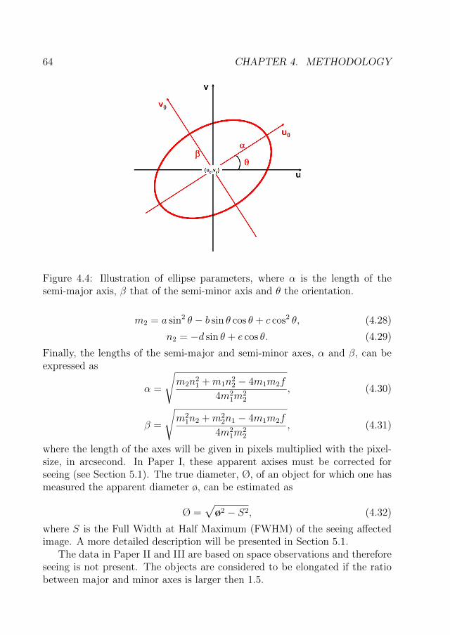
64 CHAPTER 4. METHODOLOGY
Figure 4.4: Illustration of ellipse parameters, where α is the length of thesemi-major axis, β that of the semi-minor axis and θ the orientation.
m2 = a sin2 θ − b sin θ cos θ + c cos2 θ, (4.28)
n2 = −d sin θ + e cos θ. (4.29)
Finally, the lengths of the semi-major and semi-minor axes, α and β, can beexpressed as
α =
√m2n2
1 +m1n22 − 4m1m2f
4m21m
22
, (4.30)
β =
√m2
1n2 +m22n1 − 4m1m2f
4m21m
22
, (4.31)
where the length of the axes will be given in pixels multiplied with the pixel-size, in arcsecond. In Paper I, these apparent axises must be corrected forseeing (see Section 5.1). The true diameter, Ø, of an object for which one hasmeasured the apparent diameter ø, can be estimated as
Ø =√
ø2 − S2, (4.32)
where S is the Full Width at Half Maximum (FWHM) of the seeing affectedimage. A more detailed description will be presented in Section 5.1.
The data in Paper II and III are based on space observations and thereforeseeing is not present. The objects are considered to be elongated if the ratiobetween major and minor axes is larger then 1.5.

4.3. COLUMN DENSITY DISTRIBUTION 65
4.3 Column Density Distribution
Density profiles of the globulettes can in principle be derived from the col-umn density N(H2) as function of distance from the center of the globulette.Most globulettes actually appear to be rather weakly deformed ellipsoids, whileothers are more elongated. But this is not so important for the subsequentanalysis of their possible stability. It is common to assume that the densityfollow a power-law distribution with index γ according to
ρ(r) = ρ0(r
R)−γ (r > 0; γ ≥ 0), (4.33)
where r is the physical distance from the center, and ρ0 is the density at r = R.This law is usually used to describe the radial volume density profile insidemolecular clouds (Yun & Clemens, 1991), and the value of the exponent γ isa measure of the concentration of mass in the cloud.
Since we can measure and analyse only column densities, i.e., N(H2), inthe line of sight, it is necessary to find a formalism for converting these den-sities to a radial function for the density distribution. In the following weassume spherical symmetry, and the basic notions for this analysis are illus-trated by Figure 4.5. The column density profile of a cloud is measured alonga strip through its center, and in the direction of the major axis, as shown inFigure 4.6 a. This strip is five pixels- rows as shown in the left panel top ofFigure 4.5. Then the column density profile along the mean strip is plotted asin the lower part of that panel.
The next step is to find the best-fit “power index” γ in equation (4.33).Therefore, we try to relate the column density profile to a best-fit volumedensity, assuming, for simplicity, a spherical symmetry. In a column, with aprojected distance p from the center of the object, the actual density, ρ(r),varies within the column, and N(p) can be theoretically derived through anintegration along the line of sight:
N(p) = 2
∫ X
0
ρ(√x2 + p2)dx, (4.34)
where x is a running length along the line, and X = (R2−p2)1/2 is its maximalvalue (see Figure 4.5 right). Using equation (4.33), this yields
N(p) ∝∫ X
0
(x2 + p2)−γ/2dx. (4.35)
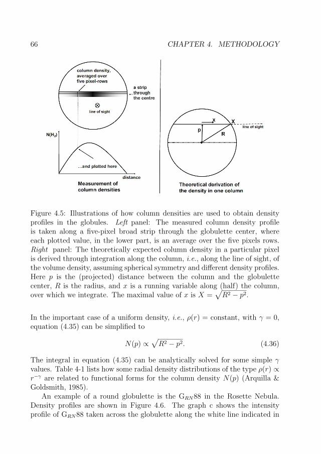
66 CHAPTER 4. METHODOLOGY
Figure 4.5: Illustrations of how column densities are used to obtain densityprofiles in the globules. Left panel: The measured column density profileis taken along a five-pixel broad strip through the globulette center, whereeach plotted value, in the lower part, is an average over the five pixels rows.Right panel: The theoretically expected column density in a particular pixelis derived through integration along the column, i.e., along the line of sight, ofthe volume density, assuming spherical symmetry and different density profiles.Here p is the (projected) distance between the column and the globulettecenter, R is the radius, and x is a running variable along (half) the column,over which we integrate. The maximal value of x is X =
√R2 − p2.
In the important case of a uniform density, i.e., ρ(r) = constant, with γ = 0,equation (4.35) can be simplified to
N(p) ∝√R2 − p2. (4.36)
The integral in equation (4.35) can be analytically solved for some simple γvalues. Table 4-1 lists how some radial density distributions of the type ρ(r) ∝r−γ are related to functional forms for the column density N(p) (Arquilla &Goldsmith, 1985).
An example of a round globulette is the GRN88 in the Rosette Nebula.Density profiles are shown in Figure 4.6. The graph c shows the intensityprofile of GRN88 taken across the globulette along the white line indicated in
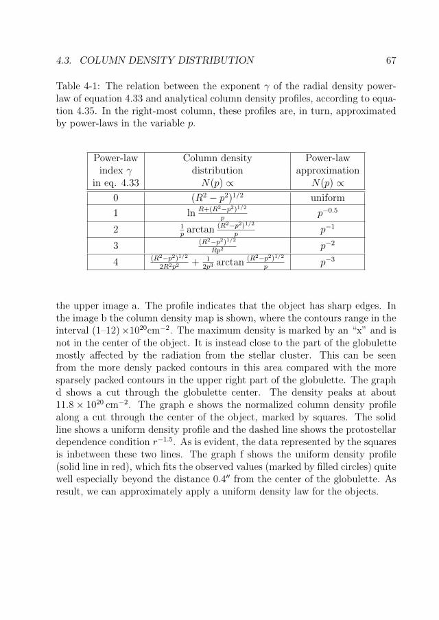
4.3. COLUMN DENSITY DISTRIBUTION 67
Table 4-1: The relation between the exponent γ of the radial density power-law of equation 4.33 and analytical column density profiles, according to equa-tion 4.35. In the right-most column, these profiles are, in turn, approximatedby power-laws in the variable p.
Power-law Column density Power-lawindex γ distribution approximation
in eq. 4.33 N(p) ∝ N(p) ∝0 (R2 − p2)1/2 uniform
1 ln R+(R2−p2)1/2
pp−0.5
2 1p
arctan (R2−p2)1/2
pp−1
3 (R2−p2)1/2
Rp2p−2
4 (R2−p2)1/2
2R2p2+ 1
2p3arctan (R2−p2)1/2
pp−3
the upper image a. The profile indicates that the object has sharp edges. Inthe image b the column density map is shown, where the contours range in theinterval (1–12)×1020cm−2. The maximum density is marked by an “x” and isnot in the center of the object. It is instead close to the part of the globulettemostly affected by the radiation from the stellar cluster. This can be seenfrom the more densly packed contours in this area compared with the moresparsely packed contours in the upper right part of the globulette. The graphd shows a cut through the globulette center. The density peaks at about11.8× 1020 cm−2. The graph e shows the normalized column density profilealong a cut through the center of the object, marked by squares. The solidline shows a uniform density profile and the dashed line shows the protostellardependence condition r−1.5. As is evident, the data represented by the squaresis inbetween these two lines. The graph f shows the uniform density profile(solid line in red), which fits the observed values (marked by filled circles) quitewell especially beyond the distance 0.4′′ from the center of the globulette. Asresult, we can approximately apply a uniform density law for the objects.

68 CHAPTER 4. METHODOLOGY
Figure 4.6: a): The nearly spherical Rosette globulette GRN88 is shown. Themean radius is 2.35′′ and the mass is 18 Jupiter masses. c): The intensityprofile over the white strip is shown. From this profile the globulette displaysharp edges. e): The squares in the figure correspond to the normalized columndensity profile as derived from a cut through the globulette center, after thecorrection for the influence of seeing. The solid line in the same figure is thetheoretical prediction assuming uniform density and the dashed line shows anr−1.5 dependence. Thus the observed column density falls in between thesetwo cases b): The column density map, with contours covering (1− 12)× 1020
cm−2. d): The column density along a cut thorough GRN88, with data pointsand a line-fit. The column density peaks at 11.8× 1020 cm−2. f): The uniformdensity profile fits the data quite well, except possibly near the centre and inthe outmost region.
4.4. EXTINCTION AND RELATION TO MASS 69
4.4 Extinction and Relation to Mass
In the images analyzed in Paper I-III, the objects are seen in silhouette againsta diffuse Hα background, see the right figure in Figure 3.3. They can alsobe seen against a continuum background. This provides an opportunity tomeasure the extinction of the background light caused by the globulette. Fromsuch data one can, in turn, compute the total mass over an area in the line ofsight through the object, the so-called column density.
The extinction, Aλ, at a certain wavelength λ is defined by
Aλ = −2.5 log
(I
I0
), (4.37)
where I is the residual light intensity measured in an area inside the globulette,and I0 is interpolated bright nebular background. See Appendix A for a moreextensive treatment. However, we do not know how much of the backgroundemission that is due to foreground Hα emission from the H II region in front ofthe globulette. We therefore have to consider two extreme cases. In the firstcase, we assume that there is no foreground emission. Hence, all surroundingemission is from the background, and gives the object’s minimal mass. Inthe second case we set the level of the foreground emission to 95% of thedarkest area of the object (with the lowest I value, i.e., the highest extinction),which gives object’s maximum mass. This factor was chosen for “technical”reasons, in order to avoid cases where small areas of zero intensity would lead,numerically, to an infinite mass. In Paper I and II we assumed that the gas todust ratio is the same as in interstellar clouds, namely 100 to 1.
The relation between the extinction as a function of the wavelength, λ, andthe column density of hydrogen gas, N(H2), is given by
N (H2) = 9.4× 10²⁰ AV [cm−2 mag−1], (4.38)
according to Bohlin et al. (1978) for normal interstellar clouds assuming thatall hydrogen is in molecular form. In Paper III we were only interested in thedust fraction and therefore N(H2) was divided with 100.
The visual extinction AV is centered at λ = 5500 A but the observationsin Paper I and II where based on an Hα filter. Hence, the need for a relationbetween the extinction at λ = 6563 A and in the V-band (λ = 5500 A). How-ever data presented in Table 3-1 does not include the Hα passband, so we haveinterpolated the published values to Hα, i.e., to λα = 0.6563µm. We thenarrive at the Hα extinction magnitude Aα:
AαE(B − V )
= 2.58. (4.39)

70 CHAPTER 4. METHODOLOGY
Hence the visual extinction is given by
AV =3.10
2.58Aα = 1.20 Aα. (4.40)
This is applied to equation (4.38) in order to derive the column density at aparticular position in a globulette, once its extinction Aα has been measured.
Since equation (4.38) only gives the column number density we need to takeinto account the mass of a hydrogen molecule and also assume that there isa “cosmic” abundance of other elements, i.e., , that hydrogen makes up only73% of the total mass per volume. Hence, we get for the column mass density:
N = 2× 1.67× 10−24× 1
0.73N(H2) = 4.58× 10⁻²⁴ N(H2) [g cm−2]. (4.41)
Inserting equation (4.38) finally gives
N = 5.17× 10⁻³ Aα [g cm−2 mag−1], (4.42)
where Aα is found from equation (4.40).In Paper III the work was based on the measurements of the visual filter
and by assuming the same cosmic chemical composition, the total columndensity of dust was estimated to
N = 4.3× 10⁻⁷ AV [g cm−2 mag−1]. (4.43)
In all Papers, the mass in grams inside one pixel is then derived as pixelarea times column mass density. Adding the pixel values inside the contour asdefined in Section 4.2 will give total mass of object for the two different cases.The average of these two masses gives the total mass of each object.
In order to test the consistency of this method, 20 different globulettesfrom Rosette Nebula were selected from the criteria that they have all beenimaged on several times, at different occasions and under different conditions.All masses (MJ) have been calculated by one and the same method from theobserved extinctions, and plotted in the graph. We find that the calculatedmass is quite independent of the position of a given object in an image frame,as well as of the period and night of observations and the sky conditions. Thespread in mass obtained from different exposures is only about 5%, see Gren-man (2006).
Moreover Gonzalez-Alfonso & Cernicharo (1994) observed four teardropshaped globules in the Rosette Nebula for CO emission using the 30 m radiotelescope on Pico Veleta, Spain. They derived masses based on column den-sities derived from CO and therefore we have a unique possibility to compare
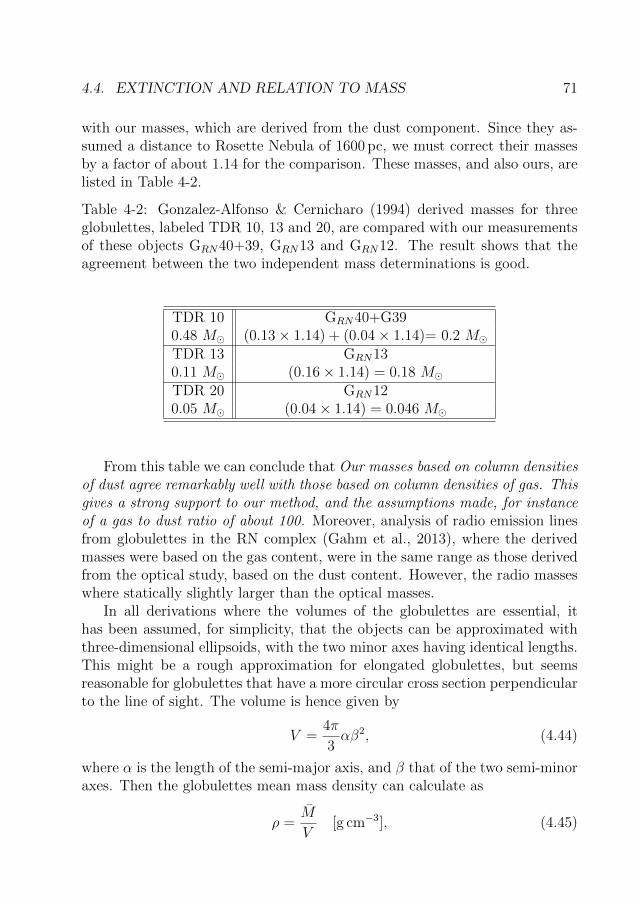
4.4. EXTINCTION AND RELATION TO MASS 71
with our masses, which are derived from the dust component. Since they as-sumed a distance to Rosette Nebula of 1600 pc, we must correct their massesby a factor of about 1.14 for the comparison. These masses, and also ours, arelisted in Table 4-2.
Table 4-2: Gonzalez-Alfonso & Cernicharo (1994) derived masses for threeglobulettes, labeled TDR 10, 13 and 20, are compared with our measurementsof these objects GRN40+39, GRN13 and GRN12. The result shows that theagreement between the two independent mass determinations is good.
TDR 10 GRN40+G390.48 M� (0.13× 1.14) + (0.04× 1.14)= 0.2 M�TDR 13 GRN130.11 M� (0.16× 1.14) = 0.18 M�TDR 20 GRN120.05 M� (0.04× 1.14) = 0.046 M�
From this table we can conclude that Our masses based on column densitiesof dust agree remarkably well with those based on column densities of gas. Thisgives a strong support to our method, and the assumptions made, for instanceof a gas to dust ratio of about 100. Moreover, analysis of radio emission linesfrom globulettes in the RN complex (Gahm et al., 2013), where the derivedmasses were based on the gas content, were in the same range as those derivedfrom the optical study, based on the dust content. However, the radio masseswhere statically slightly larger than the optical masses.
In all derivations where the volumes of the globulettes are essential, ithas been assumed, for simplicity, that the objects can be approximated withthree-dimensional ellipsoids, with the two minor axes having identical lengths.This might be a rough approximation for elongated globulettes, but seemsreasonable for globulettes that have a more circular cross section perpendicularto the line of sight. The volume is hence given by
V =4π
3αβ2, (4.44)
where α is the length of the semi-major axis, and β that of the two semi-minoraxes. Then the globulettes mean mass density can calculate as
ρ =M
V[g cm−3], (4.45)

72 CHAPTER 4. METHODOLOGY
which giving the mean number density of molecules per unit volume
n =ρ
2.4×mH
[cm−3], (4.46)
where µ = 2.4 is the mean molecular weight for an H2 gas plus heavy elements.In Paper III the dust mass calculation was based on assumptions of grain
properties such as grain radii and grain density ρ. These are related to theextinction in magnitudes and grain properties through equation (3.12), wherethe extinction efficiency factor is Q=2.
The column density of dust was estimated as mc = Nd ×mg , where the Nd
is from equation (3.12), AV is from objects intensity profiles, and the grainmass is mg = V ×ρ. Integrating over surface area, the total mass of the objectwas calculated.

Chapter 5
Observations
This chapter gives an overview of the observations done with the Nordic Opti-cal Telescope (NOT) and also a brief introduction to the HST instrumentationand filters. Parts of the material in this chapter is taken from my licentiatethesis, Grenman (2006).
5.1 The Observations with the Nordic Optical
Telescope
Paper I is based on Hα images collected by Gosta Gahm and Helmuth Kristenduring five nights in December 1999 and five nights in November-December2000, using the 2.6 m Nordic Optical Telescope on La Palma, Canary Islands,Spain. The original survey included several fields within ten different H IIregions. The telescope was equipped with the ALFOSC camera with narrow-band filters centered at a wavelength of 6563 A (0.6563 µm). The angularresolutions set by the atmospheric turbulence, called “seeing”, were in therange of 0.7′′–1.1′′ and the field of view was 6.5′ which corresponds to an areaof 33 arcmin2. The astronomical seeing conditions, at a given night and agiven location describe how much the Earth’s atmosphere perturbs the imagesof stars as seen through a telescope. The most common seeing measurementis the Full Width at Half Maximum (FWHM) of the seeing disk of a “point-like” star. The FWHM is defined as the diameter at which the star’s intensitydistribution falls to one-half of its peak value. Seeing values were estimatedwith the Matlab software. Under the best conditions, the seeing disc diameteris around 0.4′′. The scale of the CCD detector was 0.188′′ per pixel, whichdefines the smallest area from which information can be extracted. Most of
73
74 CHAPTER 5. OBSERVATIONS
the exposure times were 1800 s.All images were corrected for instrumental effects, cosmic ray excitations
and the different sensitivities of the individual pixels (including so-called darkcurrent, bias and flat field corrections), with the help of standard techniques,using the IRAF program1. For the calibration of fluxes one also needs tocorrect for the light from the sky in the images. Therefore, exposures of thesky background were collected in fields outside the emission nebulæ. Thenights were dark, except during parts of December 2 and 3, 2000, when therewas moonlight. The majority of the fields are in the Rosette Nebula and in IC1805 and the distribution of observed areas are shown in Paper I.
5.2 The Hubble Space Telescope
The Hα images of the Carina Nebula (Paper II) plus 20 H II regions (Paper IV)were downloaded from the HST archive2. In Paper III optical images of theCrab Nebula were downloaded from the Hubble Legacy Archive (HLA)3 andalso from the HST archive. The distributions over observed areas are shownin Paper II-III and in Appendix B. All analyzed images were taken withthe instruments ACS/WFC, WFPC2, WFPC3/UVIS, see Figure 5.1. Briefdescriptions of these instruments are given below.
1. The Wide Field and Planetary Camera 2 (WFPC2) field of view is cov-ered by four cameras, each of which span 800× 800 pixels in size. Threeof them are arranged in an L-shaped field (134′′ × 134′′) and operatedat a pixel scale of 0.1′′. The fourth one is referred to as the PlanetaryCamera (PC) and operates at a pixel scale of 0.046′′.
2. The Wide Field Camera 3 (WFC3) replaced the WPFC2 camera in 2009.The Ultraviolet-Visible channel (UVIS) uses a mosaic of two CCDs, with0.04 arcsec/pixel, covering a 162′′ × 162′′ field of view. The 2 CCDs arebutted together but have a ∼ 1.4′′ gap between the two chips.
3. The Advanced Camera for Surveys (ACS/WFC) camera contains twoCCDs of 2048 × 4096 pixels glued together with a small gap of approx-imately 50 pixels in between. The pixel size corresponds to 0.05′′ perpixel and the field of view is 202′′ × 202′′.
1http://iraf.noao.edu/2https://archive.stsci.edu/hst/3https://hla.stsci.edu/

5.3. FILTER SYSTEM 75
Figure 5.1: Field of view of the ACS/WFC, WFPC2, WFPC3/UVIS and AL-FOSC instruments are shown. These HST instrumentation images are takenfrom the respective handbooks.
The respective areas for the instruments WFPC2, WFC3 and ACS are es-timated to be 5, 7 and 11 arcmin2. More information about each of theseinstruments can be found in the manuals on the Mast Web site4 and in theNOT manual5.
5.3 Filter System
A filter system is a set of filters (see also Section 3.1). Each filter has a specificcentral wavelength and a specific band width, narrowband (N), intermediate(M) or broadband (W). The width is determied by the FWHM, see Figure 5.2,which is the wavelength/filter width at the transmission point that is 50% ofthe peak transmission. The most used optical system is the Bessell photometricset, UBVRI filters seen in Figure 5.2, top. However there are also a numberof others, such as the Stromgren filter set (uvby).
If we put a filter in front of a CCD camera, we obtain an image containingonly the wavelengths passed by the filter. In this way magnitudes can bemeasured in different bandpasses. If we use a filter with a large bandpass,then we have much more light in the image than in a narrow bandpass. Onthe other hand, the wavelength precision is then reduced.
For the images taken with NOT (Paper I), two different filters were used; in1999 a narrow-band Hα filter with 33 A FWHM, covering the nebular emissionfrom only the Hα line; and in 2000, a filter with 180 A FWHM, including alsothe strong nebular emission lines of [N II] at 6548.1 A and 6583.6 A, flanking
4http://www.stsci.edu/hst/HSToverview/instruments5http://www.not.iac.es/instruments/alfosc
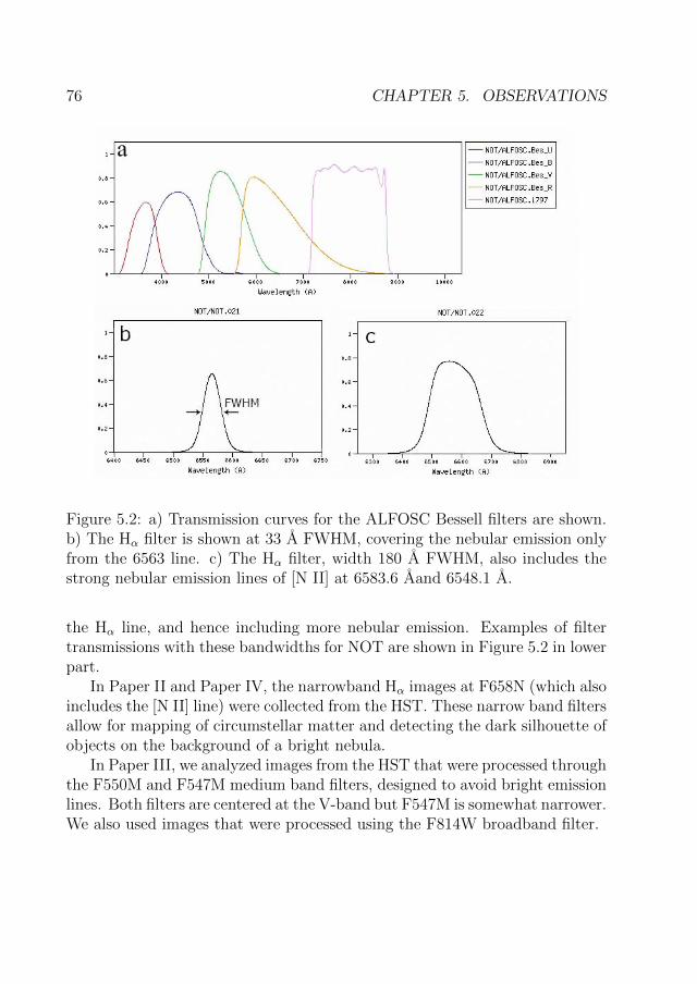
76 CHAPTER 5. OBSERVATIONS
Figure 5.2: a) Transmission curves for the ALFOSC Bessell filters are shown.b) The Hα filter is shown at 33 A FWHM, covering the nebular emission onlyfrom the 6563 line. c) The Hα filter, width 180 A FWHM, also includes thestrong nebular emission lines of [N II] at 6583.6 Aand 6548.1 A.
the Hα line, and hence including more nebular emission. Examples of filtertransmissions with these bandwidths for NOT are shown in Figure 5.2 in lowerpart.
In Paper II and Paper IV, the narrowband Hα images at F658N (which alsoincludes the [N II] line) were collected from the HST. These narrow band filtersallow for mapping of circumstellar matter and detecting the dark silhouette ofobjects on the background of a bright nebula.
In Paper III, we analyzed images from the HST that were processed throughthe F550M and F547M medium band filters, designed to avoid bright emissionlines. Both filters are centered at the V-band but F547M is somewhat narrower.We also used images that were processed using the F814W broadband filter.

Chapter 6
Introduction to Papers
This thesis consist of four journal publications, which are summarized in thefollowing sections. The introduction to Paper I is taken mainly from my licen-tiate thesis, Grenman (2006).
6.1 Paper I
The Rosette Nebula is a good laboratory for studying star formation, as wellas the interaction between an H II region and the surrounding molecular cloud.A colorful image of this nebula is shown in Figure 6.1 where the northern partshows an expanding outer shell, which is very filamentary with a network ofconnected dark filaments. Around these filaments, several elongated teardropshaped objects can be observed, which suggests a close association to them.Pillars of dust are seen pointing towards the central stars. These pillars areelongated, often with wavy or twisted substructures and sometimes with bybright rims. Paper I is based on the material collected from a studies of suchtrunks by Schneps et al. (1980), Carlqvist et al. (2003) and Gahm et al. (2006).It was during this study that we discovered that in the regions surroundingthe elephant trunks there are dark and extremely tiny clouds, which as a ruleare detached from the filamentary shell structures. In some cases these tinyclouds are connected with thin dark threads to the trunks or the shell. Similarclouds were recognized earlier by Thackeray (1950), in the H II region IC 2944,also containing Bok Globules. They were later studied in detail by Reipurthet al. (1997, 2003), who found that the cloud-size distribution shows a peak,indicating typical sizes of 1.5 ′′–2 ′′. On their HST images they also found alarge number of even smaller clouds, of sizes <1 ′′. Only a few clouds have sizesgreater than 10 ′′. The clouds observed in these H II regions are much smaller
77
78 CHAPTER 6. INTRODUCTION TO PAPERS
than those normally called globules and they form a class of tiny cloudlets,which we have named globulettes.
Deep narrow band Hα images of 10 H II region were collected with theNOT in the years 1999 and 2000. The majority of the objects were observedin the Rosette Nebula and IC 1805 and therefore the focus lies on these tworegions.
6.1.1 Rosette Nebula and IC 1805
The Rosette Nebula (NGC 2237-2246) can be described as a large, spheri-cal emission nebula around the young stellar cluster NGC 2244 found in theconstellation of Monoceros. The cluster was first noticed in 1690 by JohnFlamsteed and later studied by John Herschel, the son of William Herschel,who discovered prominent nebular features, and reported them in his generalcatalogue (Herschel, 1864). The cluster age has been estimated to about 3million years (Ogura & Ishida, 1981), and the nebular surrounding containsaround 105M� of gas and dust (Williams et al., 1995). This region is rich infilaments and small globules, as noted by Minkowski (1949), Bok et al. (1949)and Herbig (1974).
The center of the Rosette Nebula, where the cluster lies, is devoid of gas.In some early speculations it was discussed whether the newly formed starsconsume the gas. It is now known that the powerful stellar winds of hot OBstars heat the inner parts of the nebula, and create a warm bubble of plasmain the surrounding molecular cloud. The emission nebula has a radius of about16 pc. The bubble will gradually expand and dissipate until the stars are freefrom nebulosity. The total lifetime of the Rosette Nebula Complex is estimatedto be around 10 million years. Its distance from us has been estimated to be1.4–1.7 kpc (Ogura & Ishida, 1981; Hensberge et al., 2000). The differencesdepend mainly on the selection of the cluster members, but also on calibrations.From the more recent estimates we select a distance of 1400 pc (Gahm et al.,2006). The reddish color seen in the Rosette Nebula image (Figure 6.1) ismainly a result of Hα emission.
The nebula IC 1805, also called the Heart Nebula, is connected to thestellar association Cas OB6, which includes the cluster OCl 352, rich in Ostars. The complex is part of a chain of prominent, massive molecular cloudsin the Perseus arm. Its estimated distance is 2.35 kpc and its age is some 2million years (Gahm et al., 2006). According to Elmegreen (1980) extensivestar formation takes place in the region. The H II region is rich in dark globulesand filaments. However, since IC 1805 is so far away, far less information has
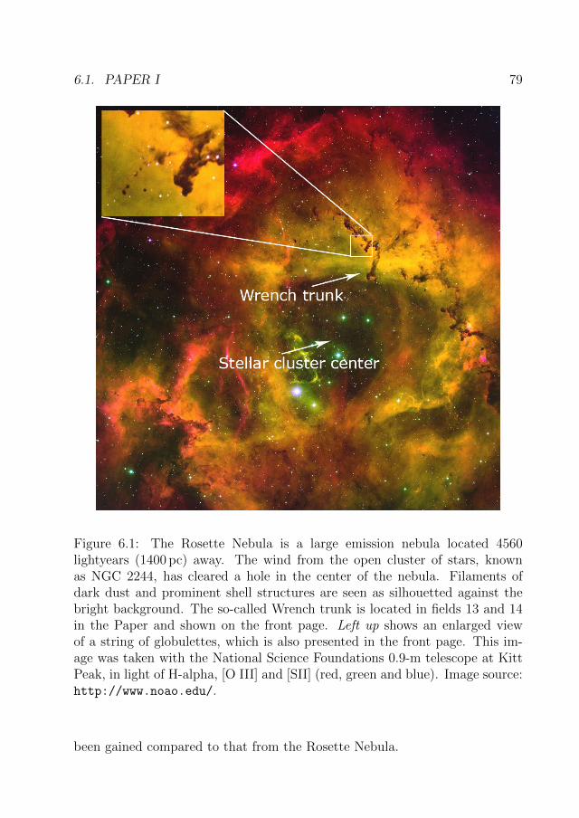
6.1. PAPER I 79
Figure 6.1: The Rosette Nebula is a large emission nebula located 4560lightyears (1400 pc) away. The wind from the open cluster of stars, knownas NGC 2244, has cleared a hole in the center of the nebula. Filaments ofdark dust and prominent shell structures are seen as silhouetted against thebright background. The so-called Wrench trunk is located in fields 13 and 14in the Paper and shown on the front page. Left up shows an enlarged viewof a string of globulettes, which is also presented in the front page. This im-age was taken with the National Science Foundations 0.9-m telescope at KittPeak, in light of H-alpha, [O III] and [SII] (red, green and blue). Image source:http://www.noao.edu/.
been gained compared to that from the Rosette Nebula.

80 CHAPTER 6. INTRODUCTION TO PAPERS
6.1.2 Results
The main conclusions of this study can be summarized as follows.
1. From 10 H II regions, 173 gloublettes were located, mostly from theRosette Nebula and IC 1805. Most of these objects are compact, slightlyelliptical or circular, with sharp edges and well isolated from their sur-roundings, lacking any sign of surface activity. However, some objectswere found diffuse and with fuzzy edges and/or connected to trunks bythin filaments. We also included the objects surrounded by bright ha-los or bright rims, as well as cometary, teardrop and V- and Y-shapedclouds. The bright-rimmed objects observed in the Rosette Nebula haveno central embedded stellar objects and therefore they cannot be proply-des, i.e., they are not protoplanetary discs. However, we cannot excludethat the globulettes host extremely low-mass brown dwarfs or planets.A mosaic over selected globulettes can seen in Figure 4 in Paper I.
2. Most of the globulettes in the Rosette Nebula are found in the fieldscovering the long chain of dark filaments and trunks, just to the northand northwest of the central cavity.
The longest symmetry axis of the globulettes in the Rosette Nebula aredirected inwards toward the central cluster. The same pattern is alsoevident in IC 1805 and other regions with smaller number of objects.
3. Globulette size distribution show that most objects have mean radii<10 kAU and that the peak is at about ∼ 2.5 AU.
4. The number densities are around 104 cm−3 and the mass densities arearound ρ=10−20 g cm−3. The column density profiles show that the dis-tribution is not Gaussian. As a first approximation, we apply a uniformdensity law, which is dropping sharply close to the surface.
5. Mass distributions for both the Rosette Nebula and IC 1805 show that amajority of the objects have masses <13MJ , corresponding to planetarymass objects. There are fewer with larger mass, which means that glob-ulettes of masses 40–60MJ are rare. There are just a few objects in theinterval 70–200MJ . However, objects with masses ∼ 1MJ may escapedetection.
A gas to dust mass ratio of 100:1 has been assumed and extinction mea-surements were used to estimate the mean masses of the globulettes.

6.2. PAPER II 81
Gahm et al. (2013) derived masses for several of the objects from ra-dio observations of CO12 and CO13. These measures, based on the gascontent, agree well with those based on the dust content.
6. The outer pressure from the surrounding warm plasma and also the radi-ation and ram pressure (acting on one side of the globulette) is contribut-ing to confining the objects. It is expected that the initial penetratingshock, generated by photoionization, lead to compression of the inte-riors. Furhtermore, some of the objects seem to be protected againstrapid photoionization by a screen of expanding ionization gas. Thus, wefound that about half of the globuettes studied can survive against pho-toevaporation on a short timescale, <106 yrs, before the ionization fronthas reached far into the interior. Hence, the cores may collapse to formmassive, free-floating planets.
7. Globulettes can be formed by fragmentation processes from evaporatingelephant trunks, larger blocks or shells. As an example, the string ofisolated dark globuletts GRN87–95, seen in the zoomed in part of Fig-ure 6.1, may have formed recently from a filament that became detachedfrom this rotating complex. South of the Wrench trunk (Figure 3 in Pa-per I, middle right) there are diffuse globulettes with bright halos, andtherefore it appears that these are already in a more advanced phase oferosion from photoevaporation and possibly streaming plasma. Thesecould represent an intermediate phase before substellar objects are even-tually formed.
Alternatively, a parent molecular cloud might already contain compactcores, which after some time are exposed when the surrounding thinnergas has evaporated.
8. All globulettes in the Rosette Nebula and IC 1805 have been examinedwith the 2MASS instrument and no evidence of embedded IR-emittingsources, at least related to stellar objects of high or medium mass wasfound. However, Makela et al. (2017) found embedded IR stars in a fewlarger objects.
6.2 Paper II
This paper aims to make an inventory of the population of globulettes in theCarina Nebula. Optical images were downloaded from the HST, based on

82 CHAPTER 6. INTRODUCTION TO PAPERS
observations with the ACS/WFI camera. The camera has a good spatial reso-lution and a large covered area, which gives us the opportunity to investigateglobulettes more closely in the H-alpha images.
6.2.1 Carina Nebula
The Carina Nebula is the southern hemispheres largest giant H II region,where some of the central parts of the nebula are even brighter than the OrionNebula. This region contains ∼ 200 OB stars and more than 60 O type stars,according to Smith et al. (2010a), Smith et al. (2010), Povich et al. (2011) andGaczkowski et al. (2013).
Figure 6.2: Seven star cluster are shown in this image of the Carina complex.The locations of the Eta Car are marked with “+”. Numbers 1-4 are thezoomed in areas shown in Figure 6.3. This image is created by combining thelight from three different filters, tracing emission from oxygen (blue), hydrogen(green), and sulfur (red). (Credit: Nathan Smith, Univ. of Minnesota, NOAO,AURA, NSF, courtesy of NASAs Jet Propulsion Laboratory).

6.2. PAPER II 83
Figure 6.3: Images 1-4 show the zoomed in areas, where 1) shows a close upimage of Eta Car; 2) shows a large fragment with the nickname the ”Fin-ger of God” located in the Tr16; 3) shows the isolated globulette GCN93 inTr14 with a mass of 63M� and 4) shows a large block and a couple of de-tached large globulettes. The white rings in Image 4 indicate the place wherewe detected globulette clustering, see Paper II, Figure B.2, field 11. Credit:http://hubblesite.org.
The distance to the Carina complex has been estimated in several publica-tions with rather different results. A distance of 2.3 kpc has been adopted as akind of standard (Smith, 2008). However, Hur et al. (2012) concluded that themain stellar clusters Trumpler 14 (Tr14) and Tr16 are located at a distance of2.9 kpc, which we also use in this Paper.
Figure 6.2 shows the Carina Nebula, where the most massive stars in ourgalaxy are located, including the famous star Eta Car, a prime candidate forthe next galactic supernova. This star had an estimated initial mass >150M�(Hillier et al., 2001). The position of Eta Car is marked with “+” and thisstar is shown in more detail in Figure 6.3, image 1.
In the center of the Carina Nebula, a prominent V-shaped dark feature lo-cated, associated with the nebular complex and consisting of dust and molec-ular gas. Several star clusters and smaller sub-cluster, such as Tr15, Collinder

84 CHAPTER 6. INTRODUCTION TO PAPERS
228 and 232, and Bochum 10 and 11 are also shown in Figure 6.2. Two largestgroups, Tr14 and Tr16 are situated in the central parts of the emission nebula,where the typical ages for the young stars in Tr14 and Tr16 are 1–3 Myr, whileTr15 is older by a few million years. However, these star clusters are not asdensely packed as those of 30 Doradus in the LMC (Massey & Hunter, 1998),or NGC 3603 in our own galaxy (Moffat et al., 2002).
Feedback (stellar winds and radiation) from the young and massive starshas cleared out the nebulosity in the central region and have revealed a largenumber of elongated structures, so-called pillars (Smith et al., 2000), but alsodark irregular blocks and fragments of all sizes (see Figure 6.3, image 4 ), someof which are very elongated and shaped like worms or long, narrow cylinders,and some show very irregular shapes. The most known fragment is known asthe “Defiant Fingers” described by Smith et al. (2004) surrounded by a numberof smaller cloudlets with irregular shapes, which have probably eroded from thelarger ones. This object is located in Tr16 and shown in Figure 6.3, image 2.The pillars have formed in the outer regions and we can see many of themin the southern part of the image while more regular sized objects, such asglobules and globulettes can be seen all over the region.
6.2.2 Results
The main conclusions of this study can be summarized as follows.
1. From the total observed area of about 700 arcmin2, 288 globulettes werefound, which exceeds the number found in any other H II region. Mostobjects are dark without any bright rims and/or tails and halos, seen inthe first rows in Figure 2.6. However, in the central part of the nebula, theobjects with a bright rim are more numerous than those without, whichindicates that the interaction with the radiation field is more intensecloser to the center. The globulettes are spread over the entire region,but are more abundant along the western part of the V-shaped darkcloud and in areas surrounding Tr14 and Tr16. However, some objectsare classified as round may instead elongated if they are oriented closerto the line of sight and objects surrounded by bright halos may indicatethe presence of bright rims on the remote side.
Objects with an elongated form, or with tails, are oriented in the direc-tion of the massive young star clusters in the area. However, some of theobjects show random orientations, particularly in the central part of thenebula, probably because several O stars are spread over the entire area.

6.3. PAPER III 85
2. None of the 288 globulettes coincides in position with any of the youngstellar object candidates listed in Povich et al. (2011) and Gaczkowskiet al. (2013).
3. The globulettes have radii <1000 AU, and the distribution increasessteeply towards the detection limit.
4. In mass estimates, we followed the procedure described in Paper I. Prac-tically all globulettes found in the Carina Nebula are of planetary mass,and most have masses less than one Jupiter mass. Only 4% of the glob-ulettes are more massive than 10MJ .
5. The average density in the Carina globulettes was estimated to be ρ =2.8 · 10−19 g cm−3, which is higher compared to the Rosette globulettes.The number densities of molecular hydrogen exceed 105 cm−3 in severalCarina globulettes. It appears that the population of tiny globulettes inthe Carina complex are in a more evolved state than those encounteredin other H II regions. One possibility is that this is because they haveeroded faster in the intense radiation field, or they might be older. It islikely that thin envelopes would gradually be lost with time, and thatthe remnant cores may also become denser with time.
6. Most of the objects are quite isolated and located at a projected distanceof >1.5 pc from the closest larger molecular structures, which indicatesthat objects can survive a long time. An example is shown in Figure 6.3,image 3, where GCN93 is located in the Tr14 as an isolated object withvery sharp edges.
However, from virial arguments we conclude that the objects are notbound unless they contain a bit more mass than inferred from the derivedmean mass.
7. We speculate that the objects might contain denser unresolved cores oreven planetary-mass objects that already have formed in their interior.
6.3 Paper III
A number of small dust concentrations are visible as dark spots against thebackground of synchrotron emission in optical images of the Crab Nebula,downloaded from the HST/HLA archive. In this Paper the focus was on

86 CHAPTER 6. INTRODUCTION TO PAPERS
roundish dusty cloudlets. These objects are reminiscent of the so called glob-ulettes present in H II regions. However, the dust found here is “Star dust”which has not yet been mixed with the ISM. This is because the Crab Nebulalies in a low density region. Hence they are of a different nature than theglobulettes, and we refer these objects to Crab globules. A mosaic in Figure 4in the Paper and Figure 6.4 , showing some of the objects.
6.3.1 Crab Nebula
It was William Parsons, third Earl of Rosse, who through his 72 inch (1.8 m)reflecting telescope around 1844 observed a cloudy blob in the sky, which henamed the Crab Nebula. However, some years after his first observation, heobserved this object again with a better telescope and discovered that it showedno similarity to a crab, but the name was difficult to change because it wasalready establish in the society.
The Crab Nebula was also the first supernova remnant to be associatedwith a “guest star” seen by ancient Chinese and Japanese astronomers in 1054AD. This connection was fist done by Lundmark (1921). From the old notes,the new star was visible in daytime for three weeks and in the night sky nearlytwo years before becoming too dim to be seen with the naked eye (Clark &Stephenson, 1977).
The Crab Nebula is also known as M1, the first object in Messier’s catalogueof nebulous objects and is the brightest and best studied relatively youngsupernova remnant, located at a distance of about 2 kpc (Trimble, 1973). Thisnebula was formed by a core collapse supernova, Type II explosion (Chevalier,1977). At the center of the nebula lies one of the first known pulsars, PSRBO531+21, see Figure 6.4, where its current location is marked with “+”.In this figure, also zoomed in image of the pulsar are shown, taken in x-ray(image a) wavelength.
Observations have shown that the Crab pulsar send signals that reachthe Earth every 0.033 seconds, making it one of the fastest pulsars recorded(Matthew & Matteo, 1996). This pulsar powers a surrounding power windnebula (PWN) and sweeps up the freely-expanding SN ejecta that is observedin the form of a bright network of ionized gas. These bright filaments andfinger-like structures, which are produced by Rayleigh-Taylor instabilities, ef-fectively form a cage like structure and confine this synchrotron nebula as canbeen seen in Figure 6.4. The filaments are dense enough so that all three emis-sion lines ([O III], [N II], S[II]) are present, where the two last lines are muchstronger relative to Hα than in typical H II regions. This is because there is

6.3. PAPER III 87
a difference between photoionization from a hot O star and the shock waveionization.The gas is heated and ionized almost instantaneous when the frontstrikes and then cools down by radiation.
Since the explosion the Crab Nebula has been expanding, and several au-thors have measured the proper motion of the optical filaments (Trimble, 1968;Wyckoff, 1977), indicating an accelerated expansion where the synchrotronemitting parts expand more rapidly than the filaments (Bietenholz et al., 2015).The nebula expands outward with a velocity of about 1264 km s−1 (Temim etal., 2006), where the NW portion of the nebula expands faster and is furtheraway from Earth than the SE side (Loll, 2010).
In the Crab Nebula, the presence of dust was first suggest by Glaccum etal. (1982) based on an analysis of the far-infrared spectrum and was laterconfirmed by Marsden et al. (1984). After the initial observation furtheranalyses were based on Spitzer observations (Temim et al., 2006, 2012) giv-ing a total mass of warm dust associated with the filament system between1.2× 10−3–12× 10−3 M�. This can be compared to Hershel telescope observa-tions that give masses between 0.12–0.24 M�, depending on dust temperature,composition and size (Gomez et al., 2011). There have also been several ex-aminations of the continuum images by using narrow-band filters in the visualband. First out was Woltjer et al. (1987) and some years later Hester et al.(1990) and Fesen & Blair (1990), also showing optical evidence of dust viaextinction of the background synchrotron nebula. These authors located andcataloged several dust features and calculated the visible dust mass of the neb-ula to 2× 10⁻⁴M�. The dust appears to be spread over the entire nebula, andis strongly concentrated to the optical filaments. Sankrit et al. (1998) pro-posed the dust is freshly formed in filaments resulting from Rayleigh-Taylorinstabilities acting on the ejecta. The authors also found that the dust to gasratio in NW filament can be as high as 0.1, while Loll (2010) estimated thisvalue to 0.05 which is still a factor of 5 higher than typical ISM ratio of 0.01.However the latest result from Owen & Barlow (2015) showed that the dust togas ratio in the Crab Nebula lies between 0.026 to 0.038 for widespread dustand from their studies the value of 0.03 was used in this Paper. This meansthat the mass of the dust in the filaments is uncertain and different regionscould have different abundances and also different dust to gas ratios.
In addition to the dusty structures, Loh et al. (2011) found a number ofknots emitting in the line of molecular hydrogen at 2.12µm. In our investi-gation we found 5 of these knots to be coincident with globules. However,according Richardson et al. (2013) there are cases where dust free knots couldbe sources of strong H2 emission. Beside molecular hydrogen detection, Bar-

88 CHAPTER 6. INTRODUCTION TO PAPERS
Figure 6.4: Composite HST image from Hester (2008), where the synchrotronemission from the power wind nebula (PWN) is shown in bluish. The CrabNebula consists of three components; The Crab pulsar (marked with “+”),the PWN and the complex of bright filaments composed of 2–5M� of materialejected in the explosion itself. The nebula is shown in the optical lines of [OIII] in red, [S II] in green, and [O I] in blue. More ejecta lie well outside of thefilaments but these are not visible. Image a, is zoomed in image of region ofthe pulsar, taken with the Chandra (X-ray). Fast moving material from thepulsar creates shock waves and X-ray emitting rings. Mosaic of gobules arealso showed.
low et al. (2013) also mapped emission from the molecule ArH+ from several

6.3. PAPER III 89
positions in the nebula.The Crab filaments formed significant amounts of both dust and molecules,
indicating that they went through a phase of very high density and rapidcooling. From Hester (2008) the Crab is expanding inside a cavity, were thefilaments expand at a rate faster than the expected free expansion velocity.Since the supernova occurred in relatively empty region of space the outerblast wave has still not interacted with enough material to be observable andtherefore the reverse shock has not formed yet. Thus the Crab Nebula differfrom the typical Type II SN evolution.
6.3.2 Results
The main conclusions of this study can be summarized as follows.
1. From continuum images of the Crab Nebula we located 92 cold cloudletsseen in extinction against the bright background. These dusty globulesappear as dark, roundish object in the broad and medium band HSTimages. Mean radii of these objects range from 400 to 2000 AU, and40% of the globules are slightly elongated with a ratio between majorand minor axes >1.5. These objects are too small to be distinguished incurrent instruments like Spitzer and Herschel.
2. The globules are distributed over the entire nebula but less abundant inthe region surrounding the central pulsar. Several globules are located atemission filaments where elongated objects are aligned with the filaments.
3. We estimate the amount of extinction in the V band for each objectindividually, with different assumptions on the amount of foregroundemission. From these measurements we obtain the individual masses ofdust using two different methods, the so called Bohlin relation and byusing grain properties. In addition, we estimated the mass of extended,obscuring filaments also present in the nebula.
4. Following Bohlin et al. (1978) derived masses of dust range from 1 to60×10−6M�. The total mass contained in the 92 globules amounts to4.5× 10−4 M�, a fraction of 2% at most of the total dust content of thenebula. Assuming a gas to dust content of 30 the corresponding totalmass amounts to 1.4× 10⁻²M�. In comparison to the Bohlin relationfour spherical objects with smooth density distribution were chosen toestimate the dust mass based on grain properties, with a grain radiusof 2× 10⁻⁵ cm and density 3 g cm−3. The masses of these objects are

90 CHAPTER 6. INTRODUCTION TO PAPERS
approximately a factor two smaller than those derived from the Bohlinrelation.
5. The mass contained in globules and the distribution of sizes are in thesame range as for the smallest globulettes residing in H II region, butlarger than dusty knots found in certain planetary nebula (O’dell & Han-dron, 1996). Beside that the mean density of dust was found to about∼ 2.5× 10⁻²¹ g cm−3, which is comparable to the corresponding valuesderive for globulettes in Rosette Nebula.
6. Dusty globules are typically two orders of magnitude larger than thedusty clumps assumed by Ercolano et al. (2007) to match the energydistribution of SN 1987A.
7. From extinction measurements at wavelengths 5470 A and 8140 A we ac-quire information on the shape of the extinction law for the globules. Asa result, we found that the extinction law for the globules and filamentsmatches a normal interstellar extinction law. Hence, the globules willeventually feed the interstellar medium with grains of interstellar type.
8. From images taken between 1994 and 2014 we derived the proper mo-tion and related transversal velocity of each globule. All globules moveoutwards from the center with transversal velocities of 60 to 1600 km s−1
along with the general expansion of the remnant. For some objects wecould also derive space velocities, as example for two objects in the NWpart of the nebula the velocity was estimated to about 1300 km s−1.
6.4 Paper IV
Globulettes may be a source of brown dwarfs and free floating planetary massobjects in the galaxy. Therefore, it is interesting to know how many globulettesthat could have formed in the Milky Way and how much they could contributeto the total population of free floating planets. In this paper we have examined319 H II regions, whereof 27 were observed with a narrow-band Hα filter. Theposition of these 27 H II regions are shown in Appendix B, where the mapis plotted in galactic coordinates. In this chart, the plane of the Milky Waygalaxy passes across the middle and the zero point of galactic latitude andlongitude are positioned at the galactic center. Images analyzed here are fromNOT observations and from the HST archive.
6.4. PAPER IV 91
6.4.1 Results
The main conclusions of this study can be summarized as follows.
1. The total area (Atot) and observed area (Aobs) of the 27 H II regions wereestimated to 44 413 armin2 and to 3 297 arcmin2, respectively. Distribu-tion over observed HST fields are shown in Appendix B.
2. In Appendix C, Table C1 lists all globulettes found in these regions,besides the globulettes listed in Paper I & II.
3. We estimated the mean radii for each globulette found in the H II re-gions. The majority of the objects have radii <10 kAU but most seemconcentrated around ∼ 0.5 kAU with a small peak at 2.5 kAU.
4. Amongst the 27 H II regions, there are 18 nebulae with <18 observedglobulettes and 8 nebula with no observed globulettes.
5. We postulate that the first globulettes were formed roughly 12 Gyr (T0)ago and that H II regions were 2 times more abundant in the early MilkyWay than they are now (fHII). The number of H II regions, nHII , todayis estimated to 10 000. Globulette production is assumed to take placewhen an H II region is still young, . 5 Myr (THII), and we assume thatwe can find a similar number of objects also on the backside of the nebulæ(fB). The spatial resolution was lower in seven of the H II regions, andthe number of globulettes in these regions was estimated to 346. Thelifetime of globulettes, Tglob, was estimated to 4 Myrs.
The total number of gloublettes, Gtot, was calculated to 951 and the aver-age number of globulettes per H II region was estimated to be about 35.The estimated number of globulettes that have formed in the history ofthe Milky Way (MW) is
GMW =TIITglob
× T0
THII× nHII × fB × fHII ×
AtotAobs
× Gtot
NHII
. (6.1)
The total number of globulettes was estimated to 5.7× 10¹⁰, which canbe considered a conservative value. A less conservative estimate gives2.0× 1011 globulettes.
6. The globulettes could represent a non-negligible source for FFPs in theMilky Way. A less conservative number of globulettes would mean thatthe globulettes could contribute 2.0× 10¹⁰ free floating planets. Then, if
92 CHAPTER 6. INTRODUCTION TO PAPERS
10% of the globulettes of our less conservative estimate form FFPs, thenthe globulettes would contribute to about 11% of all FFPs, as estimatedby Sumi et al. (2011).
7. In the 30 Doradus, the globulettes mean radii has a peak at ∼ 5.7 kAU,which is higher than the peaks of the H II regions within the Milky Way.
Chapter 7
Discussion and Outlook
7.1 Discussion
A number of H II regions have been investigated during the years and it hasbeen found that many regions contain small dark objects with different mor-phologies. These clouds form a specific class of interstellar clouds, which aresimilar to the larger globules in shape and physical state but different regardingsize and mass distribution. This distinguishes them from globules and fromproplyds. In order to cover several different objects given in the literature,such as splinters, cups, nodules etc, we have proposed the name globulette.
After detailed studies of regions such as the Rosette Nebula and the CarinaNebula, the globulettes can be described as small dark objects with sharpedges, round or slightly elliptical.
From the numerical simulation models, the bright rims on the objects oc-cur on the side facing a stellar cluster, because of the interaction with stellarlight. These objects develop into teardrop forms and eventually dusty tailsform, in the opposite direction from the ionizing stars. However, a large num-ber of globulettes show no sign of surface activities in the form of ongoingphotoevaporation and most of our object are dark against the background andwithout tails. One explanation of the absence of bright rims is that the den-sity is higher close the surface layers. This was concluded in both optical andradio/near infrared surveys. The bright rims can also be on the remote sideof the objects or these rims might not be detectable in Hα images. In orderto trace these rims, observations in e.g., near IR and Hα emission were doneby Gahm et al. (2013), Makela et al. (2014), where some of the globulettesshowed evidence of bright thin rims on the remote sides facing the RN cluster.
However, an additional reason for the lack of bright rims can be that dis-
93

94 CHAPTER 7. DISCUSSION AND OUTLOOK
tance between the object and the UV radiation source is large, such as in theCarina Nebula. In these cases, the photodissociation is weak.
Observations have also shown that many globulettes are isolated and lo-cated far from the molecular shells and elephant trunks, while others are seenclustering close to these, see Figure 6.3. There are also objects connected bythin filaments to the large blocks, suggesting that globlettes may form as aconsequence of erosion of the large structures.
The discovery of a population of tiny dense globulettes in the Carina Neb-ula appears to represent a more advanced evolution state than the Rosetteglobulettes. This indicates the possibility that the removal of the thin en-velope caused by a radiation field, can unveil the core, which becomes moredense with time. Therefore, the globulette may lose its bright rim and tail.Thus, globulettes may contain yet unresolved cores or more speculatively, evenJupiter-size planets. This might explain why they appear to have survived forsuch a long time.
However, the high density observed in dark objects indicate that the densitydistributions are more flat than uniform, which was assumed in Paper I, whereit was consistent (to a first approximation) with the column densities derivedas a function of radial position, and inferred by Gahm et al. (2013).
We also observed that some isolated globulettes with dark cores were sur-rounded by bright halos, which may represent an intermediate phase, beforedenser cores have eventually formed. An example of this is a planetary massobject that has been found in its early years in the Orion Nebula, where itmay have been formed from such a low mass globulette (Fang et al., 2016).
It is also possible that the molecular clouds hoste tiny compact cores, andthat after some time, when the cloud disperses, these cores are left free andwill appear as globulettes.
From analyzing the globulettes, the average radii was estimated from about0.1 to 10 kAU, with masses from 0.1 to 100 Jupiter masses and number densitiesranging from 103–105 cm−3. The mass hierarchy of molecular clouds can now bedescribed as: Giant molecular clouds (103–106M�), globules (5–500M�), cores(1–5M�), massive globulettes (30MJ–0.1M�) and planetary mass globulettes(<13MJ).
However, the globulette masses derived here can in some cases be under-estimated since some objects may have developed dense cores that escape de-tection or because we use a normal extinction law. As an example, in severalareas in the Carina Nebula, large values of RV have been found (Hur et al.,2012), and also the globulettes may contain larger dust grains.
By analyzing the Rosette globulettes with the virial theorem, where we also

7.1. DISCUSSION 95
included outer pressure, we concluded that a large fraction of the gloublettescould be unstable and would contract on short timescales, less than 106 yr.In addition, by including also radiation and ram pressure, which act on theside facing the cluster, could stimulate contraction. We also estimated theexpected lifetimes against photoevaporation based on the analytic treatmentof photo evaporation clumps by Mellema et al. (1998), which showed that theymight survive in this harsh H II environment for a relatively long time. Thismeans that many globulettes can collapse to form free floating planetary massobjects before the evaporation is significant.
Lately, many free floating planetary mass objects in the interstellar spacehave been observed. As an example Sumi et al. (2011) estimated the numberof unbound planets in the Milky Way to be about twice the number of mainsequence stars (∼ 100× 109), while Mroz et al. (2017) found about 0.25 plan-ets per star. However, as discussed above, globulettes can be an additionalsource of free floating planetary mass objects. To find out how much the glob-ulettes can contribute to the FFP population, we first estimated the numberof globulettes formed over the life time of the Milky Way. A conservative valuewas found to be 5.7× 10¹⁰ and a less conservative value was 2.0× 10¹¹. Then,by assuming that 10% of the less conservative estimate forms FFPs, this givesabout 0.2 free planets per main sequence star.
Dust can also be found in the remnants of supernovae and we examinethe Crab Nebula, where we found objects, similar to globulettes, but of adifferent origin. The total mass of these objects was estimated 4.5× 10⁻⁴M�or . 2% of the total dust content of the nebula. We concluded that a majorityof the globules are not located wihtin bright filaments and we proposed thatthese objects may be products of cell-like blobs or granules in the atmosphereof the progenitor, that form globules during the passage of the blast waveduring the explosion following the collapse. It may be a coincidence, but thenumber of such granules calculated for red supergiants is in the order of onehundred, which is similar to the total number of globules found, see Figure 7.1.Furthermore, their masses are comparable to the masses of globules by takinginto account the gas to dust ratio of 100.
We also estimated the extinction law for globules and found that the dustgrains are similar to interstellar dust grains. Since they are moving out in thegalactic environment they will contribute the ISM dust population. In addi-tion, estimated transversal velocities where all globules move outwards fromthe center with velocities of 60 to 1600 km s−1 along with the general expan-sion of the remnant. For some objects we could also derive space velocities andfor two objects, located in the NW direction, the velocities were estimated to

96 CHAPTER 7. DISCUSSION AND OUTLOOK
about 1300 km s−1.
Figure 7.1: Granulation on the Sun (left) compared to simulated granu-lation of a red supergiant, (right). The first image to the left is fromhttps://astrobites.org/2012/07/04/a-hot-test-of-gr/and the imageto the right is from https://www.youtube.com/watch?v=6r7YUj42SJ0.These blobs (middle) occur due to the convection below the photosphere, whererising gas is hot and sinking gas is cold. A typical granule lasts about 8 to20 minutes. The surface of the Sun is covered by approximately 3.5–4 milliongranules, while the red supergiant contains only around one hundred.
7.2 Outlook
Over the years, many observational and theoretical studies have been madeof globulettes in the Rosette Nebula and the Carina Nebula. Studies in thenear infrared and in the radio spectrum of the molecular lines of the largestglobulettes in the Rosette Nebula showed that the objects are dense and thatthe gas is molecular, even close to the surface layers (Gahm et al., 2013). Theauthors found that the masses for some objects was similar but systematicallyhigher than the extinction based estimated masses in Paper I. Furthermore,the system of globulettes found in the northern part of the Rosette Nebulawere found to be moving outwards with velocities of about 22 km s−1 relativeto the central cluster. These globulettes show no evidence of a rocket effect,e.g., acceleration form interaction with stellar light.
7.2. OUTLOOK 97
The nature and the fate of the globulettes is still uncertain, such as ifthey collapse to form free floating objects, like brown dwarfs and planetarymass objects. Kuutmann (2007) made 3D numerical simulation of the Rosetteglobulettes and found lifetimes of 104 years, which increases with increasingmass. However, large globulettes may collapse before any signifcant evapora-tion takes place. Kuutmann (2007) also estimated the terminal velocity to be5–10 km s−1 with the respect to the initial rest frame. This means that theglobulettes are expected to move outwards with the same velocity as the shellsand system of trunks.
Haworth et al. (2015) calculated the evolution of globulettes assuming pres-sure confined isothermal Bonner-Ebert spheres. In this model the globulettessurvive for long time (∼ 105 yr) but do not contract into low mass objects,except for the cases where they catch up with the expanding shell. However,the analysis in Grenman (2006) and Gahm et al. (2013) show that the innerstructure of a globulette is very different from that of a Bonner-Ebert sphere.Therefore new calculations have to be done concerning the inner structure ofthe globulettes and their lifetimes.
Images taken with the NOT cannot resolve the dense cores in the glob-ulettes and our estimated masses are possibly underestimated for such objects.In order to resolve these dense cores, we need telescopes with higher spatialresolutions. Therefore, our next project is to follow up the Rosette Nebulawith the higher resolution telescope, using HST, and make new density pro-files, better suited for globulettes. We intend to investigate some regions, suchas M 16, where some of the globulettes are quite isolated and have very darkand sharp edges. Another on-going project is resolving certain globulettes inthe Rosette Nebula using the radio interferometer ALMA for emission lines ofdifferent molecules. The preliminary results show the presence of dense cores,with nH2 . 106 cm−3 in two of the Rosette objects, then supporting the idea offormation of FFPs from globulettes. Another riddle is why some H II regionshave so many tiny objects while others do not. This is a question to explorefurther by surveying more regions.
The origin of the dust in supernova remnants is still an open question andbetter instrumentation is needed for further observations. The Crab Nebulacan be studied in more detail in the future with the James Webb Space Tele-scope. This telescope will resolve infrared images of dusty globules, which canprovide further clues as to whether the dust is warm or cold. More detailedhydrodynamic calculations are needed for the formation of dusty globules fromconvective cells outside the filaments.


Chapter 8
Bibliography
Andre, P., Ward-Thompson, D., & Greaves, J. 2012, Science, 337, 69
Andre, P., Konyves, V., Arzoumanian, D., Palmeirim, P., & Peretto, N. 2013,New Trends in Radio Astronomy in the ALMA Era: The 30th Anniversaryof Nobeyama Radio Observatory, 476, 95
Anderson, J. P., & James, P. A. 2008, MNRAS, 390, 1527
Anglada-Escude, G., Arriagada, P., Tuomi, M., et al. 2014, MNRAS, 443, L89
Armitage, P. J., & Rice, W. K. M. 2005, arXiv:astro-ph/0507492
Arquilla, R., & Goldsmith, P. F. 1985, ApJ, 297, 436
Ballet, J. 2003, EAS Publications Series, 7, 217
Bally, J., Langer, W. D., Stark, A. A., & Wilson, R. W. 1987, ApJ, 312, L45
Bally, J. 1989, European Southern Observatory Conference and WorkshopProceedings, 33, 1
Bakes, E. L. O., & Tielens, A. G. G. M. 1994, ApJ, 427, 822
Barlow, M. J., Krause, O., Swinyard, B. M., et al. 2010, A&A, 518, L138
Barlow, M. J., Swinyard, B. M., Owen, P. J., et al. 2013, Science, 342, 1343
Barnard, E. E. 1919, ApJ, 49,1
Bayo, A., Joergens, V., Liu, Y., et al. 2017, ApJ, 841, L11
99

100 CHAPTER 8. BIBLIOGRAPHY
Behroozi, P. S., Wechsler, R. H., & Conroy, C. 2013, ApJ, 770, 57
Behroozi, P., & Peeples, M. S. 2015, MNRAS, 454, 1811
Best, W. M. J., Liu, M. C., Dupuy, T. J., & Magnier, E. A. 2017,arXiv:1706.01883
Bergin, E. A., & Tafalla, M. 2007, ARA&A, 45, 339
Bertoldi, F. 1989, ApJ, 346, 735
Bertoldi, F., & McKee, C. F. 1990, ApJ, 354, 529
Bertoldi, F., & McKee, C. F. 1992, ApJ, 395, 140
Bertoldi, F., Carilli, C. L., Cox, P., et al. 2003, A&A, 406, L55
Bietenholz, F., M., & Nugent, R. L. 2015, MNRAS, 454, 2416
Binney, J., & Merrifield, M. 1998, Galactic Astronomy. Princeton, NJ: Prince-ton University Press. 11, 13
Bisbas, T. G., Wunsch, R., Whitworth, A. P., Hubber, D. A., & Walch, S.2011, ApJ, 736, 142
Bohlin, R. C., Savage, B. D., & Drake, J. F. 1978, ApJ, 224, 132
Bok, B. J., Olmsted, M., & Boutelle, B. D. 1949, ApJ, 110, 21
Bok, B. J., & Reilly, E. F. 1947, ApJ, 105, 255
Bok, B. J. 1977, PASP, 89, 597
Bonnell, I. A., Bate, M. R., Clarke, C. J., & Pringle, J. E. 2001, MNRAS, 323,785
Bonnor, W. B. 1956, MNRAS, 116, 351
Bookstein, F.L. 1979, Computer Graphics and Processing, 9, 56
Boss, A. P. 1997, Science, 276, 1836
Boss, A. P. 2008, ApJ, 677, 607-615
Boss, A. P. 2009, ApJ, 694, 107

101
Boucher, A., Lafreniere, D., Gagne, J., et al. 2016, ApJ, 832, 50
Bowler, B. P., Liu, M. C., Kraus, A. L., Mann, A. W., & Ireland, M. J. 2011,ApJ, 743, 148
Bromm, V., & Larson, R. B. 2004, ARA&A, 42, 79
Bromm, V., & Yoshida, N. 2011, ARA&A, 49, 373
Brooks, K. J., Storey, J. W. V., & Whiteoak, J. B. 2001, MNRAS, 327, 46
Burrows, A., Hubbard, W. B., Lunine, J. I., & Liebert, J. 2001, Reviews ofModern Physics, 73, 719
Caballero, J. A., Bejar, V. J. S., Rebolo, R., et al. 2007, A&A, 470, 903
Cardelli, J. A., Clayton, G. C., & Mathis, J. S. 1989, ApJ, 345, 245
Carlqvist, P., Gahm, G. F., & Kristen, H. 2003, A&A, 403, 399
Cassan, A. 2014, Extrasolar planets detections and statistics through gravita-tional microlensing. Master thesis. Sorbonne University
Carroll, B. W., & Ostlie, D. A. 2007, Modern Astrophysics. Addison-WesleyPublishing Company, Inc.
Chaisson, E. & Steve, M. 2013, Astronomy today (8th edition)
Chatterjee, S., Ford, E. B., Matsumura, S., & Rasio, F. A. 2008, ApJ, 686,580-602
Charnley, S. B., Tielens, A. G. G. M., & Millar, T. J. 1992, ApJ, 399, L71
Chevalier, R. A. 1977, Supernovae, 66, 53
Chiavassa, A., Plez, B., Josselin, E., & Freytag, B. 2009, A&A, 506, 1351
Chomiuk, L., & Povich, M. S. 2011, AJ, 142, 197
Churchwell, E. 2002, ARA&A, 40, 27
Clanton, C., & Gaudi, B. S. 2017, ApJ, 834, 46
Clark, D. H., & Stephenson, F. R. 1977, Oxford [Eng.] ; New York : PergamonPress, 1977. 1st ed.

102 CHAPTER 8. BIBLIOGRAPHY
Clark, P. C., Glover, S. C. O., Klessen, R. S., & Bonnell, I. A. 2012, MNRAS,424, 2599
Clemens, D. P., & Barvainis, R. 1988, ApJs, 68, 257
Combes, F. 1991, ARA&A, 29, 195
Cox, D. P. 2005,ARA&A, 43, 337
Cushing, M. C., Kirkpatrick, J. D., Gelino, C. R., et al. 2014, AJ, 147, 113
Dale, D. A., Gil de Paz, A., Gordon, K. D., et al. 2007, ApJ, 655, 863
D’Angelo, G., Durisen, R. H., & Lissauer, J. J. 2010, Exoplanets, 319
Daddi, E., Dickinson, M., Morrison, G., et al. 2007, ApJ, 670, 156
Deharveng, L., Schuller, F., Anderson, L. D., et al. 2010, A&A, 523, A6
De Looze, I., Barlow, M. J., Swinyard, B. M., et al. 2017, MNRAS, 465, 3309
De Marco, O., O’Dell, C. R., Gelfond, P., Rubin, R. H., & Glover, S. C. O.2006, AJ, 131, 2580
Desert, F.-X., Boulanger, F., & Puget, J. L. 1990, A&A , 237, 215
Dickey, J. M., & Lockman, F. J. 1990, ARA&A, 28, 215
Draine, B. 1989, Interstellar Dust, 135, 313
Draine, B. T., & Bertoldi, F. 1996, ApJ, 468, 269
Draine, B. T. 2009, Cosmic Dust - Near and Far, 414, 453
Draine, B. T., & Li, A. 2001, ApJ, 551, 807
Drass, H., Haas, M., Chini, R., et al. 2016, MNRAS, 461, 1734
Dwek, E. 2004, ApJ, 607, 848
Dwek, E., Galliano, F., & Jones, A. P. 2007, ApJ, 662, 927
Dwek, E., Arendt, R. G., Bouchet, P., et al. 2008, ApJ, 676, 1029-1039
Dyson, J. E. and Williams, D. A. 1997, The physics of the interstellar medium.
103
Ebert, R. 1955, ZAp, 37, 217
Elmegreen, D. M. 1980, ApJ, 240, 846
Ercolano, B., Barlow, M. J., & Sugerman, B. E. K. 2007, MNRAS, 375, 753
Ewen, H. I., & Purcell, E. M. 1951, Nature, 168, 356
Fall, S. M., Krumholz, M. R., & Matzner, C. D. 2010, ApJ, 710, L142
Fang, M., Kim, J. S., Pascucci, I., Apai, D., & Manara, C. F. 2016, ApJ, 833,L16
Fesen, R., & Blair, W. P. 1990, Apj, 351, L45
Filippenko, A. V. 1997, ARA&A, 35, 309
Fitzgibbon, A. W., Pilu, M., & Fischer, R. B. 1996, in Proc. 13th Intl. Conf.Pattern Recognition, Vol. 1, ed. W. Kropatsch ( Los Alamitos: IEEE Com-put.Soc.), 253
Fitzgibbon, A.W., Pilu, M. & Fisher, R.B. 1999, IEEE Transactions on PatternAnalysis and Machine Intelligence, 21(5), pp. 476
Fontani, F., Pascucci, I., Caselli, P., et al. 2007, A&A, 470, 639
Fox, O. D., Chevalier, R. A., Skrutskie, M. F., et al. 2011, ApJ, 741, 7
Freeman, M., Philpott, L. C., Abe, F., et al. 2015, ApJ, 799, 181
Freytag, B. 2006, EAS Publications Series, 21, 325
Fukui, Y., & Kawamura, A. 2010, ARA&A, 48, 547
Gaczkowski, B., Preibisch, T., Ratzka, T., et al. 2013, A&A, 549, A67
Gaensler, B. M., & Slane, P. O. 2006, ARA&A, 44, 17
Gahm, G. F., Carlqvist, P., Johansson, L. E. B., & Nikolic, S. 2006, A&A,454, 201
Gahm, G. F., Grenman, T., Fredriksson, S., & Kristen, H. 2007, AJ, 133, 1795
Gahm, G. F., Persson, C. M., Makela, M. M., & Haikala, L. K. 2013, A&A,555, A57
104 CHAPTER 8. BIBLIOGRAPHY
Gall, C., Hjorth, J., & Andersen, A. C. 2011, A&A Rev., 19, 43
Gander, W., Golub, G.H. & Strebel, R. 1994, BIT-A Nordic Computer RelatedJournal, 34(4), 558
Gaudi, B. S., Bennett, D. P., Udalski, A., et al. 2008, Science, 319, 927
Gaudi, B. S. 2010, arXiv:1002.0332
Glaccum, W., Harper, D. A., Loewenstein, R. F., Pernic, R., & Low, F. J.1982, BAAS, 14, 612
Gomez, H. L., Dunne, L., Ivison, R. J., et al. 2009, MNRAS, 397, 1621
Gomez, H. L., Krause, O., Barlow, M. J., et al. 2011, ApJ, 760:96
Gonzalez-Alfonso, E., & Cernicharo, J. 1994, ApJ, 430, L125
Gould, A., & Loeb, A. 1992, ApJ, 396, 104
Graves, S. F., Richer, J. S., Buckle, J. V., et al. 2010, MNRAS, 409, 1412
Green, D. A., Tuffs, R. J., & Popescu, C. C. 2004, MNRAS, 355, 1315
Greenberg, J. 2002, Surface Science, 500, 793
Grenman, T. 2006, Globulettes : a new class of very small and dense interstellarclouds. Licentiate thesis. Lulea Univ. Tech
Grenman, T., & Gahm, G. F. 2014, A&A, 565, A107
Hawarden, T. G., & Brand, P. W. J. L. 1976, MNRAS, 175, 19P
Haworth, T. J., & Harries, T. J. 2012, MNRAS, 420, 562
Haworth, T. J., Facchini, S., & Clarke, C. J. 2015, MNRAS, 446, 1098
Heger, A., Woosley, S. E., & Baraffe, I. 2005, The Fate of the Most MassiveStars, 332, 347
Hensberge, H., Pavlovski, K., & Verschueren, W. 2000, A&A, 358, 553
Herbig, G. 1974, PASP, 86, 604
Herschel, W. 1785, Philosophical Transactions Series I, 75, 213

105
Herschel, J. 1864, Phil. Trans. Roy. Soc. Lon., 154, 1
Hester, J. J., Graham, J. R., Beichman, C. A., & Gautier, T. N. 1990, ApJ,357, 539
Hester, J. J., Scowen, P. A., Sankrit, R., et al. 1996, AJ, 111, 2349
Hester, J. J. 2008, ARA&A, 46, 127
Hillenbrand, L. A., Massey, P., Strom, S. E., & Merrill, K. M. 1993, AJ, 106,1906
Hillier, D. J., Davidson, K., Ishibashi, K., & Gull, T. 2001, ApJ, 553, 837
Hollenbach, D. J., & Tielens, A. G. G. M. 1999, Reviews of Modern Physics,71, 173
Hoyle, F., Narlikar, J. V., & Wheeler, J. A. 1964, Nature, 203, 914
Hur, H., Sung, H., & Bessell, M. S. 2012, AJ, 143, 41
Indebetouw, R., Matsuura, M., Dwek, E., et al. 2014, ApJ, 782, L2
Janka, H.-T., Langanke, K., Marek, A., Martınez-Pinedo, G., & Muller, B.2007, Phys. Rep, 442, 38
Jeans, J. H. 1902, Philosophical Transactions of the Royal Society of LondonSeries A, 199, 1
Joergens, V., Bonnefoy, M., Liu, Y., Bayo, A., & Wolf, S. 2015, 18th CambridgeWorkshop on Cool Stars, Stellar Systems, and the Sun, 18, 1019
Johnson, H. L., & Morgan, W. W. 1953, ApJ, 117, 313
Johnson, J. L., & Li, H. 2012, ApJ, 751, 81
Jones, E. M., Smith, B. W., & Straka, W. C. 1981, ApJ, 249, 185
Jones, A. P., Tielens, A. G. G. M., & Hollenbach, D. J. 1996, ApJ, 469, 740
Kandori, R., Dobashi, K., Uehara, H., Sato, F., & Yanagisawa, K. 2003, AJ,126, 1888
Kalberla, P. M. W., & Kerp, J. 2009, ARA&A, 47, 27
Kessler, M. F., Steinz, J. A., Anderegg, M. E., et al. 1996, A&A, 315, L27

106 CHAPTER 8. BIBLIOGRAPHY
Kifonidis, K., Plewa, T., Janka, H.-T., & Muller, E. 2003, A&A, 408, 621
Kim, S.-H., & Martin, P. G. 1994, ApJ, 431, 783
Kim, W.-T., & Ostriker, E. C. 2002, ApJ, 570, 132
Kovalevsky, J. 1995, Modern Astrometry, XIV, 352 pp. 137 figs.. Springer-Verlag Berlin Heidelberg New York. Also Astronomy and Astrophysics Li-brary, 137
Kozasa, T., Nozawa, T., Tominaga, N., et al. 2009, Cosmic Dust - Near andFar, 414, 43
Krishna Swamy, K. S. 2005. Dust in the Universe : similarities and differences.
Kristensen, L. E., Gustafsson, M., Field, D., et al. 2003, A&A, 412, 727
Krumholz, M. R., & Matzner, C. D. 2009, ApJ, 703, 1352
Kumar, S. S. 1962, AJ, 67, 579
Kumar, S. S. 1963, ApJ, 137, 1121
Kurtz, S., Cesaroni, R., Churchwell, E., Hofner, P., & Walmsley, C. M. 2000,Protostars and Planets IV, 299
Kuutmann, A. 2007, Photo-evaporation of Globulettes. Master Thesis. Dep.of Astronomy, Stockholm University
Lefloch, B., & Cernicharo, J. 2000, ApJ, 545, 340
Li, A., & Draine, B. T. 2001, ApJ, 550, L213
Li, A., 2007 https://ned.ipac.caltech.edu/level5/Sept07/Li1/paper.pdf
Li, Y., Kouwenhoven, M. B. N., Stamatellos, D., & Goodwin, S. P. 2015, ApJ,805, 116
Lineweaver, C. H. 2001, ICARUS, 151, 307
Loh, E. D., Baldwin, J. A., Curtis, Z. K., et al. 2011. ApJS, 194:30
Loll, A., 2010, A Northwest-Southeast Asymmetry in the Crab SupernovaRemnant. Thesis. Arizona State University
Luhman, K. L., Adame, L., D’Alessio, P., et al. 2005, ApJ, 635, L93
107
Lundmark, K. 1921, PASP, 33, 225
Lynds, B. T. 1962, ApJS, 7, 1
Madau, P., & Dickinson, M. 2014, ARA&A 52, 415
Maiolino, R., Schneider, R., Oliva, E., et al. 2004, Nature, 431, 533
Marsden, P. L., Gillett, F. C., Jennings, R. E., et al. 1984, ApJ, 278, L29
Mashian, N., & Loeb, A. 2016, MNRAS, 460, 2482
Massey, P., & Hunter, D. A. 1998, ApJ, 493, 180
Matthew, J. B., & Matteo,J. P. 1996, J. Undergrad. Sci. 3: 57-62
Mattila, K., Juvela, M., & Lehtinen, K. 2007, ApJ, 654, L131
Mathis, J. S. 1990, ARA&A, 28, 37
Matsuura, M., Dwek, E., Barlow, M. J., et al. 2015, ApJ, 800, 50
Mayor, M., & Queloz, D. 1995, Nature, 378, 35
McCaughrean, M. J., & Andersen, M. 2002, A&A, 389, 513
McKee, C. F., & Ostriker, J. P. 1977, ApJ, 218, 148
McKee, C. F., & Hollenbach, D. J. 1980, ARA&A, 18, 219
McKee, C. F., & Ostriker, E. C. 2007, ARA&A, 45, 565
Mellema, G., Raga, A. C., Canto, J., et al. 1998, A&A, 331, 335
Mellema, G., Arthur, S. J., Henney, W. J., Iliev, I. T., & Shapiro, P. R. 2006,ApJ, 647, 397
Minkowski, R. 1941, PASP, 53, 224
Minkowski, R. 1949, PASP, 61, 151
Mizuno, H. 1980, Progress of Theoretical Physics, 64, 544
Moffat, A. F. J., Corcoran, M. F., Stevens, I. R., et al. 2002, ApJ, 573, 191
Moises, A. P., Damineli, A., Figueredo, E., et al. 2011, MNRAS, 411, 705
108 CHAPTER 8. BIBLIOGRAPHY
Montenbruck, O., Pfleger, T., & Dunlop, S. 1994, “Astronomy on the PersonalComputer, XIII, 312 pp. 45 figs., 3 1/2” MS-DOS diskette. Springer-VerlagBerlin Heidelberg New York“, 45
Morgan, H. L., & Edmunds, M. G. 2003, MNRA, 343, 427
Mundy, L. G. 1994, Clouds, Cores, and Low Mass Stars, 65, 35
Murray, N. 2011, ApJ, 729, 133
Mroz, P., Udalski, A., Skowron, J., et al. 2017, Nature, 548, 183
Makela, M. M., Haikala, L. K., & Gahm, G. F. 2014, A&A, 567, A108
Makela, M. M., Haikala, L. K., & Gahm, G. F. 2017, A&A, 605, A82
Nakajima, T., Oppenheimer, B. R., Kulkarni, S. R., et al. 1995, Nature, 378,463
O’dell, C. R., & Handron, K. D. 1996, Aj, 111, 1630
Ogura, K., & Ishida, K. 1981, PASJ, 33, 149
Oort, J. H., & Spitzer, L., Jr. 1955, ApJ, 121, 6
Ormel, C. W., Min, M., Tielens, A. G. G. M., Dominik, C., & Paszun, D.2011, A&A, 532, A43
Owen, P. J., & Barlow, M. J. 2015, ApJ, 801, 141
Paczynski, B. 1986, ApJ, 304, 1
Paczynski, B. 1996, Astrophysical Applications of Gravitational Lensing, 173,199
Patel, N. A., Xie, T., & Goldsmith, P. F. 1993, ApJ, 413, 593
Pena Ramırez, K., Bejar, V. J. S., Zapatero Osorio, M. R., Petr-Gotzens,M. G., & Martın, E. L. 2012, ApJ, 754, 30
Pena Ramırez, K., Bejar, V. J. S., & Zapatero Osorio, M. R. 2016, A&A, 586,A157
Perryman, M. A. C. 2000, Reports on Progress in Physics, 63, 1209
Petrovich, C. 2015, ApJ, 799, 27

109
Planck Collaboration, Ade, P. A. R., Aghanim, N., et al. 2014, A&A, 571, A16
Poidevin, F., Falceta-Goncalves, D., Kowal, G., de Gouveia Dal Pino, E., &Mario Magalhaes, A. 2013, ApJ, 777, 112
Povich, M. S., Smith, N., Majewski, S. R., et al. 2011, ApJS, 194, 14
Prantzos, N. 2008, Space Sci. Rev., 135, 313
Reipurth, B., Corporon, P., Olberg, M., & Tenorio-Tagle, G. 1997, A&A, 327,1185
Reipurth, B., Raga, A., & Heathcote, S. 2003, AJ, 126, 1925
Reipurth, B., & Mikkola, S. 2015, AJ, 149, 145
Reynolds, S. P. 2008, ARA&A, 46, 89
Ricci, L., Robberto, M., & Soderblom, D. R. 2008, AJ, 136, 2136-2151
Richardson, C. T., Baldwin, J. A., Ferland, G. J., et al. 2013, MNRAS, 430,1257
Robitaille, T. P., & Whitney, B. A. 2010, ApJ, 710, L11
Rolleston, W. R. J., Trundle, C., & Dufton, P. L. 2002, A&A, 396, 53
Rosin, P.L. 1993, Pattern Recognition Letters, 14, 799
Sampson, P.D. 1982, Computer Graphics and Image Processing, 18, 97
Sankrit, R., Hester, J. J., Scowen, P. A., et al. 1998, ApJ, 504, 344
Santos, N. C. 2008, Nature, 52, 154
Savage, B. D., & Mathis, J. S. 1979, ARA&A, 17, 73
Savage, B. D., & Sembach, K. R. 1996, ARA&A, 34, 279
Sawada, T., Hasegawa, T., & Koda, J. 2012, ApJ, 759, L26
Schneider, S., & Elmegreen, B. G. 1979, ApJS, 41, 87
Schneider, R., Omukai, K., Inoue, A. K., & Ferrara, A. 2006, MNRAS, 369,1437

110 CHAPTER 8. BIBLIOGRAPHY
Schneider, R., Omukai, K., Bianchi, S., & Valiante, R. 2012, MNRAS, 419,1566
Schneps, M. H., Ho, P. T. P., & Barrett, A. H. 1980, ApJ, 240, 84
Scoville, N. Z., & Sanders, D. B. 1987, Interstellar Processes, 134, 21
Shu, F. H., Adams, F. C., & Lizano, S. 1987, ARA&A, 25, 23
Shu, F. H. 1992, The Physics of Astrophysics, Vol.II: Gas Dynamics, UniversityScience Books, p. 230-240
Sedov, L. I. 1959, Similarity and Dimensional Methods in Mechanics, NewYork: Academic Press, 1959
Sewi lo, M., Churchwell, E., Kurtz, S., Goss, W. M., & Hofner, P. 2008, ApJ,681, 350-354
Smartt, S. J., Eldridge, J. J., Crockett, R. M., & Maund, J. R. 2009, MNRAS,395, 1409
Smith, L. F., Biermann, P., & Mezger, P. G. 1978, A&A, 66, 65
Smith, N., Egan, M. P., Carey, S., et al. 2000, ApJ, 532, L145
Smith, N., Bally, J., & Brooks, K. J. 2004, AJ, 127, 2793
Smith, N. 2008, Handbook of Star Forming Regions, Vol. II: The SouthernSky, ASP Monograph Publ., Vol 5. Ed. Bo Reipurth, p. 138
Smith, N., Povich, M. S., Whitney, B. A., et al. 2010, MNRAS, 406, 952
Smith, N., Bally, J., & Walborn, N. R. 2010a, MNRAS, 405, 1153
Smith, N., Silverman, J. M., Filippenko, A. V., et al. 2012, AJ, 143, 17
Spitzer, L., Jr. 1990, ARA&A, 28, 71
Strafella, F., Campeggio, L., Aiello, S., Cecchi-Pestellini, C., & Pezzuto, S.2001, ApJ, 558, 717
Stritzinger, M., Taddia, F., Fransson, C., et al. 2012, ApJ, 756, 173
Stutzki, J., & Guesten, R. 1990, ApJ, 356, 513
Sumi, T., Abe, F., Bond, I. A., et al. 2003, ApJ, 591, 204

111
Sumi, T., Kamiya, K., Bennett, D. P., et al. 2011, Nature, 473, 349
Tan, J. C., Beltran, M. T., Caselli, P., et al. 2014, Protostars and Planets VI,149
Thackeray, A. D. 1950, MNRAS, 110, 524
Thompson, M. A., Hatchell, J., Walsh, A. J., MacDonald, G. H., & Millar,T. J. 2006, A&A, 453, 1003
Tegmark, M., Silk, J., Rees, M. J., et al. 1997, ApJ, 474, 1
Temim, T., Gehrz, R. D., Woodward, C. E., et al. 2006, ApJ, 132,1610
Temim, T., Sonneborn, G., Dwek, E., et al. 2012, ApJ, 753:72
Temim, T., & Dwek, E. 2013, ApJ, 774, 8
Tielens, A. G. G. M., McKee, C. F., Seab, C. G., & Hollenbach, D. J. 1994,ApJ, 431, 321
Trimble, V. 1968, AJ, 73, 535
Trimble, V. 1973, PASP, 85, 579
Trumpler, R. J. 1930, Lick Observatory Bulletin, 14, 154
Vagnozzi, S. 2017, arXiv:1703.10834
van Dishoeck, E. F. 2004, ARA&A, 42, 119
van Steenberg, M. E., & Shull, J. M. 1988, ApJ, 330, 942
Vijh, U. P., Witt, A. N., & Gordon, K. D. 2003, ApJ, 587, 533
Vink, J. 2012, A&ARv, 20, 49
Vrba, F. J., Coyne, G. V., & Tapia, S. 1993, AJ, 105, 1010
Wang, L., Kouwenhoven, M. B. N., Zheng, X., Church, R. P., & Davies, M. B.2015, MNRAS, 449, 3543
Ward, W. R. 1997, Icarus, 126, 261
Ward-Thompson, D., Andre, P., & Kirk, J. M. 2002, MNRAS, 329, 257

112 CHAPTER 8. BIBLIOGRAPHY
Weingartner, J. C., & Draine, B. T. 2001, ApJ, 548, 296
Werner, M. W., Uchida, K. I., Sellgren, K., et al. 2004, ApJs, 154, 309
Wheeler, J. C., & Harkness, R. P. 1990, Reports on Progress in Physics, 53,1467
Whittet, D. C. B., Bode, M. F., Longmore, A. J., et al. 1988, MNRAS, 233,321
Whittet, D. C. B. 1992, Dust in the galactic environment Institute of PhysicsPublishing, 306 p.
Whitworth, A. P., & Zinnecker, H. 2004, A&A, 427, 299
Williams, J. P., Blitz, L., & Stark, A. A. 1995, ApJ, 451, 252
Williams, J. P., Blitz, L., & McKee, C. F. 2000, Protostars and Planets IV, 97
Williams, J. P., & Cieza, L. A. 2011, ARA&A, 49, 67
Wolfire, M. G., McKee, C. F., Hollenbach, D., & Tielens, A. G. G. M. 2003,ApJ, 587, 278
Wood, D. O. S., & Churchwell, E. 1989, ApJS, 69, 831
Woltjer, L., & Veron-Cetty, M.-P. 1987, A&A, 172, L7
Woosley, S., & Janka, T. 2005, Nature Physics, 1, 147
Wyckoff, S., & Murray, C. A. 1977, MNRAS,180, 717
Wyrzykowski, L., Rynkiewicz, A. E., Skowron, J., et al. 2015, ApJS, 216, 12
Yao, Y., Wang, Q. D., Hagihara, T., et al. 2009, ApJ, 690, 143
Yun, J. L., & Clemens, D. P. 1990, ApJ, 365, L73
Yun, J. L., & Clemens, D. P. 1991, ApJ, 381, 474
Yun, J. L., & Clemens, D. P. 1992, ApJ, 385, L21
Yun, J. L., & Clemens, D. P. 1994, ApJS, 92, 145
Zapatero Osorio, M. R., Bejar, V. J. S., Martın, E. L., et al. 2000, Science,290, 103
Zinnecker, H., & Yorke, H. W. 2007, ARA&A, 45, 481

Appendix A
Astronomical Quantities
A.1 Magnitude Scale
The brightness of an astronomical object is measured in the units of appar-ent magnitude mλ (as seen from Earth) or absolute magnitude Mλ (if thestar would have been viewed from distance of 10 pc (32.6 light years). Themagnitude system originated from the first systematic studies of the night skythat were carried out only with the naked eye. The human eye has a roughlylogarithmic response curve, which means that the difference between a fluxof 1 and 10 is perceived the same as the difference between a flux of 10 and100. Meaning that the brighter the star is the smaller the value of its magni-tude. Thus the brightest stars on the sky have magnitudes around one and thefaintest visible star has a magnitude of six. The magnitude scale was slightlyadjusted in a way such that a difference by 5 magnitudes equals a factor 100in flux or intensity (1001/5=2.512). Thus
m1 −m2 = −2.5 logF1
F2
, (A.1)
where the bright star Vega defines the zero point and the m1 and m2 are themagnitudes of two sources and F1 and F2 their fluxes, respectively. Then ina given waveband, for example the V band, the extinction is AV = mV −mV,0 where mV is the apparent V-band magnitude and mV,0 is the apparentmagnitude in the absence of dust.
However we can also write the inverse relation of equation (A.1) as,
F2
F1
= 100.4(m1−m2) (A.2)
113

114 APPENDIX A. ASTRONOMICAL QUANTITIES
A.2 The Celestial Coordinate System
The celestial sphere can be described as an imaginary sphere whose centercoincides with the center of the Earth. The celestial coordinate system isused for indicating the positions of celestial bodies on the celestial sphere.The coordinates are right ascension (RA or alpha) and declination (Dec orgamma). Declination (Dec) of the body is measured in degrees (°), arcminutes(′) and arcseconds (′′) north or south of the celestial equator. Right ascension(RA) is measured in hours (h), minutes (m), and seconds (s) since the Earthneeds 24 hour to rotate around and where 0 corresponds to 0 hours and 360corresponds to 24 hours. That means that one second of right ascension isactually 15 times larger than 1 arcsec. The right ascension is always measuredeastward from the vernal equinox, where we have 0 RA, see Figure A.2.1.
Figure A.2.1: Depiction of the equatorial coordinate system. Origi-nal images from http://kidspicturedictionary.com/encyclopedia/astronomy-encyclopedia/celestial-earth-coordinate-system
A.3 Column Density
In Figure A.3.1 a small long cylinder of hydrogen gas is shown. If we drawa line that passes from observer’s eye thorough the cylinder, then that line iscalled the line of sight. In the same figure the cylinder cross section area (cm2)is also shown. The column density of hydrogen N(H) can be defined as thetotal number of particles enclosed in this cylinder. The total volume densityof hydrogen gas is n(H) in units cm−3, then N(H) is the integral of n(H) along
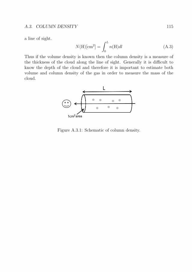
A.3. COLUMN DENSITY 115
a line of sight.
N(H)[cm2] =
∫ L
0
n(H)dl (A.3)
Thus if the volume density is known then the column density is a measure ofthe thickness of the cloud along the line of sight. Generally it is difficult toknow the depth of the cloud and therefore it is important to estimate bothvolume and column density of the gas in order to measure the mass of thecloud.
Figure A.3.1: Schematic of column density.


Appendix B
Images of Fields
B.1 Description of Images
This Appendix contains analyzed images of the studied H II regions fromPaper IV. Their location in celestial coordinates (degrees) are shown on an allsky map (Figure B.1), where the thicker middle line is the equator. All imageswere downloaded from the HST archive and superimposed by the analyzedrectangular areas.
117

118 APPENDIX B. IMAGES OF FIELDS
Fig
ure
B.1
.1:
Loca
tion
ofan
alyze
dH
IIre
gion
sin
the
cele
stia
lco
ord
inat
es(d
egre
es)
are
show
non
all
sky
map
.T
he
thic
ker
mid
dle
lin
eis
the
equ
ator
,w
hic
hco
rres
pon
ds
toth
ega
lact
icp
lan
e.
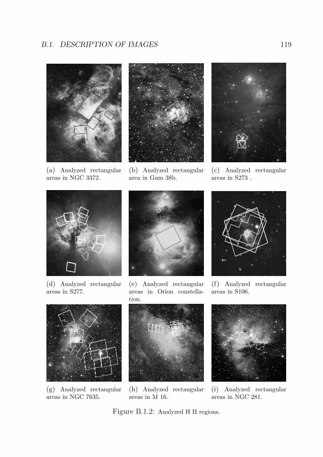
B.1. DESCRIPTION OF IMAGES 119
(a) Analyzed rectangularareas in NGC 3372.
(b) Analyzed rectangulararea in Gum 38b.
(c) Analyzed rectangularareas in S273 .
(d) Analyzed rectangularareas in S277.
(e) Analyzed rectangularareas in Orion constella-tion.
(f) Analyzed rectangularareas in S106.
(g) Analyzed rectangularareas in NGC 7635.
(h) Analyzed rectangularareas in M 16.
(i) Analyzed rectangularareas in NGC 281.
Figure B.1.2: Analyzed H II regions.

120 APPENDIX B. IMAGES OF FIELDS
(a) Analyzed rectangularareas in M 17.
(b) Analyzed rectangularareas in M 20.
(c) Analyzed rectangulararea in S155.
(d) Analyzed rectangularareas in Gum 31.
(e) Analyzed rectangulararea in Gum 29.
(f) Analyzed rectangularareas in IC 434.
(g) Analyzed rectangularareas in NGC 2467.
(h) Analyzed rectangularareas in M 8.
(i) Analyzed rectangularareas in NGC 6357.
(j) Analyzed rectangulararea in IC 2944.
(k) Analyzed rectangularareas in NGC 2174.
(l) Analyzed rectangularareas in 30 Doradus.
Figure B.1.3: Analyzed H II regions.

Appendix C
Data Tables of Globulettes inNebulæ
This Appendix contains the data derived for the studied globulettes from dif-ferent H II regions in Paper IV that have not been described elsewhere. Coor-dinates are measured in RA and Dec in column 2 and 3, sizes in arcsecond, andkAU in column 4 and 5 and shapes (EL = elongated, T = tails and tear-dropforms, C = connected to filaments or each other, BR/BH = marked as brightrims or bright halos) in column 6. This column also contains references to otherworks. The letter “R”+number indicates that the object is from Reipurth etal. (2003), letter“D”+number indicates that the object is from De Marco etal. (2006).
121

122 APPENDIX C. DATA TABLES OF GLOBULETTES IN NEBULÆ
Table C1: Globulettes studied in Paper IV. Coordinates are measured in RAand Dec in column 2 and 3, sizes in arcsecond, and kAU in column 4 and 5and shapes (EL = elongated, T = tails and tear-drop forms, C = connectedto filaments or each other, BR/BH = marked as bright rims or bright halos)in column 6. This column also contains references to other works. The letter“R”+number indicates that the object is from Reipurth et al. (2003), letter“D”+number indicates that the object is from De Marco et al. (2006).
Nr R.A. Dec. r R RemarksJ (2000.0) J (2000.0) (arcsec) (kAU)
(1) (2) (3) (4) (5) (6)
IC 2944, D=2300 pc
1 11:38:10.4 -63:21:02 0.72 1.66 R192 11:38:11.5 -63:21:22 1.30 3.00 R203 11:38:11.5 -63:20:55 2.15 4.95 R364 11:38:13.0 -63:20:38 1.33 3.05 R165 11:38:13.1 -63:20:49 0.79 1.82 R176 11:38:13.2 -63:21:38 0.50 1.15 R217 11:38:14.2 -63:20:46 0.43 0.99 R188 11:38:17.7 -63:21:19 0.36 0.82 C9 11:38:17.8 -63:21:23 0.71 1.63 C10 11:38:18.1 -63:21:21 0.61 1.4 R2511 11:38:18.2 -63:21:14 0.27 0.6212 11:38:18.2 -63:21:40. 1.44 3.31 R2313 11:38:18.7 -63:21:09 0.53 1.2214 11:38:18.8 -63:21:44 1.32 3.04 R2415 11:38:19.0 -63:21:10 0.26 0.6016 11:38:19.8 -63:21:08 0.51 1.17 R2817 11:38:20.5 -63:21:18 0.58 1.33 R2618 11:38:20.5 -63:21:16 0.56 1.29 R2719 11:38:20.8 -63:20:56 1.15 2.65 R1520 11:38:21.0 -63:20:46 2.75 6.33 R1421 11:38:22.5 -63:21:09 0.43 0.99 R3522 11:38:22.8 -63:20:23 1.66 3.82 R3623 11:38:23.8 -63:21:31 1.35 3.11 R3224 11:38:24.2 -63:20:31 1.30 3.00 EL25 11:38:24.5 -63:20:12 1.22 2.80 R3726 11:38:25.3 -63:20:14 0.79 1.82 R3827 11:38:25.8 -63:20:47 0.83 1.91 R1228 11:38:26.3 -63:21:05 1.00 2.30 R3329 11:38:30.7 -63:20:21 0.32 0.74 R4030 11:38:30.9 -63:20:21 0.26 0.6031 11:38:31.1 -63:20:23 0.36 0.83 T32 11:38:31.2 -63:20:51 0.51 1.17 R3933 11:38:33.0 -63:19:43 0.49 1.13 R4234 11:38:33.1 -63:19:51 0.42 0.97 R41
Carina Nebula, D=2800 pc
1 10:40:44.1 -59:51:02 0.31 0.90 T2 10:40:55.9 -59:41:46 0.70 2.033 10:41:05.0 -59:41:08 0.42 1.22 BH4 10:42:58.6 -59:17:31 2.38 6.9 T, BR5 10:43:32.9 -59:16:44 1.30 3.77 BH, EL6 10:43:51.1 -60:04:37 0.63 1.83 BR

123
Table C1: continues
Nr R.A. Dec. r R RemarksJ (2000.0) J (2000.0) (arcsec) (kAU)
Carina Nebula, D=2800 pc
7 10:43:52.9 -59:58:50 0.27 0.738 10:43:53.4 -60:03:20 0.17 0.499 10:43:53.4 -60:04:20 0.27 0.73 BH10 10:43:54.6 -60:03:05 0.10 0.2911 10:43:54.9 -60:03:10 0.41 1.1912 10:43:55.4 -60:02:53 0.19 0.55 BR13 10:44:01.1 -60:02:35 0.20 0.5814 10:44:06.7 -59:45:49 0.43 1.2515 10:44:07.1 -60:25:19 0.76 2.20 T, EL, BR16 10:44:07.4 -59:45:29 0.59 1.7117 10:44:09.2 -60:25:25 0.37 1.0718 10:44:09.3 -60:25:18 0.65 1.89 EL, BR19 10:44:13.2 -60:03:22 0.25 0.7320 10:44:14.9 -60:03:17 0.22 0.6421 10:44:35.7 -60:07:25 0.53 1.5422 10:44:36.2 -60:08:26 0.41 1.1923 10:44:41.5 -59:46:27 1.20 3.4824 10:44:44.8 -59:21:15 0.29 0.84 BH25 10:44:45.0 -59:21:25 0.34 0.9926 10:44:46.8 -60:05:41 1.70 4.9327 10:45:13.0 -60:03:06 1.90 5.51 EL, BR28 10:45:13.1 -60:03:17 0.24 0.70 TD, BH29 10:45:13.2 -60:03:19 0.33 0.96 TD, BH30 10:46:08.2 -59:58:06 0.17 0.49 BR31 10:46:09.9 -59:59:26 0.27 0.78 C32 10:46:10.0 -59:59:22 0.35 1.01 EL33 10:46:12.0 -59:59:26 0.34 0.99 EL34 10:46:13.2 -59:59:01 0.28 0.81 BR35 10:46:14.3 -59:58:56 0.38 1.10 TD,T, BR36 10:46:15.0 -59:59:16 0.16 0.46 BH37 10:46:15.3 -59:59:53 0.26 0.7538 10:46:15.4 -59:59:19 0.075 0.22 BR39 10:46:15.5 -59:58:57 0.27 0.78 BR40 10:46:15.6 -59:59:20 0.09 0.26 BR41 10:46:15.6 -59:59:14 0.21 0.61 BR42 10:46:15.8 -59:59:23 0.10 0.29 BR43 10:46:15.9 -59:59:01 0.27 0.78 BR44 10:46:16.0 -59:59:58 0.21 0,61 EL45 10:46:17.0 -59:59:58 0.36 1.04 EL46 10:46:17.2 -59:59:31 0.075 0.22 BH47 10:46:19.4 -59:59:43 0.14 0.41 C to 4948 10:46:19.5 -59:59:44 0.11 0.32 C to 4749 10:46:19.6 -59:59:44 0.19 0.55 C to 4850 10:46:20.1 -59:59:34 0.14 0.4151 10:46:20.4 -59:59:45 0.24 0.70 T52 10:46:22.0 -59:57:47 0.29 0.84 T53 10:46:23.0 -59:59:15 0.18 0.5254 10:47:39.3 10:47:39 0.75 2.1855 10:47:51.8 -59:59:48 0.43 1.25
M42/43, D=410 pc
1 5:34:21.4 -5:25:23 1.83 0.752 5:35:13.0 -5:23:55 0.21 0.093 5:35:13.4 -5:24:15 0.17 0.07

124 APPENDIX C. DATA TABLES OF GLOBULETTES IN NEBULÆ
Table C1: continues
Nr R.A. Dec. r R RemarksJ (2000.0) J (2000.0) (arcsec) (kAU)
M42/43, D=410 pc
4 5:35:13.5 -5:24:24 0.29 0.125 5:35:13.5 -5:24:25 0.27 0.116 5:35:14.1 -5:23:56 0.27 0.11 T C to 77 5:35:14.1 -5:23:56 0.34 0.14 T C to 68 5:35:14.2 -5:23:52 0.61 0.259 5:35:14.5 -5:24:02 0.34 0.14 T, BR
NGC 2467, D=5000 pc
1 7:52:10.7 -26:26:55 0.46 2.30 D502 7:52:11.2 -26:26:31 0.24 1.20 D533 7:52:11.3 -26:25:30 0.31 1.55 T, BH4 7:52:12.4 -26:25:35 0.13 0.65 BH5 7:52:13.2 -26:25:04 0.17 0.85 D336 7:52:13.4 -26:24:53 0.27 1.35 D327 7:52:13.3 -26:26:10 0.56 2.80 D548 7:52:13.7 -26:25:30 0.31 1.55 D249 7:52:15.2 -26:26:59 0.25 1.25 D4910 7:52:15.5 -26:25:33 0.36 1.80 D2311 7:52:16.2 -26:26:52 0.58 2.90 D4712 7:52:16.6 -26:25:44 0.24 1.20 D2013 7:52:16.7 -26:24:47 0.95 4.75 D2814 7:52:16.8 -26:26:02 0.33 1.65 D1715 7:52:16.8 -26:25:56 0.34 1.70 D1816 7:52:16.8 -26:25:39 0.41 2.05 D2217 7:52:16.8 -26:25:30 0.40 2.0018 7:52:17.0 -26:25:37 0.14 0.7019 7:52:17.0 -26:25:49 1.02 5.10 D1920 7:52:17.1 -26:25:40 0.56 2.80 D2121 7:52:17.2 -26:27:03 0.16 0.80 BH, EL22 7:52:17.4 -26:25:59 0.41 2.0523 7:52:17.5 -26:27:27 0.46 2.30 C24 7:52:17.6 -26:27:28 0.43 2.15 D4525 7:52:17.9 -26:27:23 0.32 1.60 EL26 7:52:18.0 -26:24:55 0.32 1.60 T27 7:52:18.2 -26:27:31 0.24 1.20 T28 7:52:18.4 -26:25:04 0.51 2.55 DE2529 7:52:18.9 -26:27:24 0.13 0.65 BR30 7:52:18.9 -26:25:14 0.53 2.65 D1531 7:52:19.4 -26:28:05 0.14 0.70 D3432 7:52:19.4 -26:25:15 0.47 2.35 T, BR33 7:52:19.5 -26:25:19 0.31 1.5534 7:52:19.8 -26:27:34 0.78 3.90 D3835 7:52:20.0 -26:26:27 0.67 3.3536 7:52:20.4 -26:25:29 0.37 1.85 D1337 7:52:20.5 -26:25:37 0.45 2.2538 7:52:20.5 -26:25:41 0.15 0.7539 7:52:20.6 -26:28:03 0.28 1.40 BR40 7:52:20.8 -26:27:50 0.16 0.80 D3541 7:52:20.8 -26:27:26 0.25 1.25 D4142 7:52:20.9 -26:25:29 0.30 1.5043 7:52:21.0 -26:25:29 0.17 0.85 D1044 7:52:21.0 -26:25:30 0.23 1.1545 7:52:21.1 -26:27:52 0.15 0.75
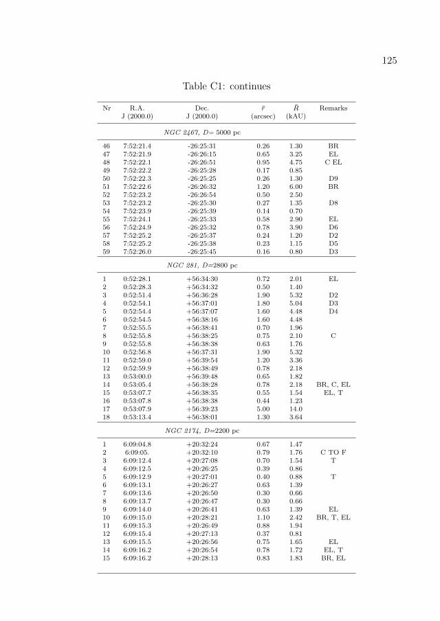
125
Table C1: continues
Nr R.A. Dec. r R RemarksJ (2000.0) J (2000.0) (arcsec) (kAU)
NGC 2467, D= 5000 pc
46 7:52:21.4 -26:25:31 0.26 1.30 BR47 7:52:21.9 -26:26:15 0.65 3.25 EL48 7:52:22.1 -26:26:51 0.95 4.75 C EL49 7:52:22.2 -26:25:28 0.17 0.8550 7:52:22.3 -26:25:25 0.26 1.30 D951 7:52:22.6 -26:26:32 1.20 6.00 BR52 7:52:23.2 -26:26:54 0.50 2.5053 7:52:23.2 -26:25:30 0.27 1.35 D854 7:52:23.9 -26:25:39 0.14 0.7055 7:52:24.1 -26:25:33 0.58 2.90 EL56 7:52:24.9 -26:25:32 0.78 3.90 D657 7:52:25.2 -26:25:37 0.24 1.20 D258 7:52:25.2 -26:25:38 0.23 1.15 D559 7:52:26.0 -26:25:45 0.16 0.80 D3
NGC 281, D=2800 pc
1 0:52:28.1 +56:34:30 0.72 2.01 EL2 0:52:28.3 +56:34:32 0.50 1.403 0:52:51.4 +56:36:28 1.90 5.32 D24 0:52:54.1 +56:37:01 1.80 5.04 D35 0:52:54.4 +56:37:07 1.60 4.48 D46 0:52:54.5 +56:38:16 1.60 4.487 0:52:55.5 +56:38:41 0.70 1.968 0:52:55.8 +56:38:25 0.75 2.10 C9 0:52:55.8 +56:38:38 0.63 1.7610 0:52:56.8 +56:37:31 1.90 5.3211 0:52:59.0 +56:39:54 1.20 3.3612 0:52:59.9 +56:38:49 0.78 2.1813 0:53:00.0 +56:39:48 0.65 1.8214 0:53:05.4 +56:38:28 0.78 2.18 BR, C, EL15 0:53:07.7 +56:38:35 0.55 1.54 EL, T16 0:53:07.8 +56:38:38 0.44 1.2317 0:53:07.9 +56:39:23 5.00 14.018 0:53:13.4 +56:38:01 1.30 3.64
NGC 2174, D=2200 pc
1 6:09:04.8 +20:32:24 0.67 1.472 6:09:05. +20:32:10 0.79 1.76 C TO F3 6:09:12.4 +20:27:08 0.70 1.54 T4 6:09:12.5 +20:26:25 0.39 0.865 6:09:12.9 +20:27:01 0.40 0.88 T6 6:09:13.1 +20:26:27 0.63 1.397 6:09:13.6 +20:26:50 0.30 0.668 6:09:13.7 +20:26:47 0.30 0.669 6:09:14.0 +20:26:41 0.63 1.39 EL10 6:09:15.0 +20:28:21 1.10 2.42 BR, T, EL11 6:09:15.3 +20:26:49 0.88 1.9412 6:09:15.4 +20:27:13 0.37 0.8113 6:09:15.5 +20:26:56 0.75 1.65 EL14 6:09:16.2 +20:26:54 0.78 1.72 EL, T15 6:09:16.2 +20:28:13 0.83 1.83 BR, EL
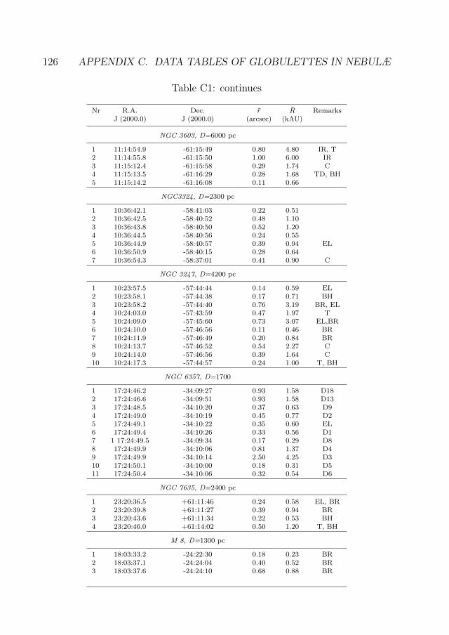
126 APPENDIX C. DATA TABLES OF GLOBULETTES IN NEBULÆ
Table C1: continues
Nr R.A. Dec. r R RemarksJ (2000.0) J (2000.0) (arcsec) (kAU)
NGC 3603, D=6000 pc
1 11:14:54.9 -61:15:49 0.80 4.80 IR, T2 11:14:55.8 -61:15:50 1.00 6.00 IR3 11:15:12.4 -61:15:58 0.29 1.74 C4 11:15:13.5 -61:16:29 0.28 1.68 TD, BH5 11:15:14.2 -61:16:08 0.11 0.66
NGC3324, D=2300 pc
1 10:36:42.1 -58:41:03 0.22 0.512 10:36:42.5 -58:40:52 0.48 1.103 10:36:43.8 -58:40:50 0.52 1.204 10:36:44.5 -58:40:56 0.24 0.555 10:36:44.9 -58:40:57 0.39 0.94 EL6 10:36:50.9 -58:40:15 0.28 0.647 10:36:54.3 -58:37:01 0.41 0.90 C
NGC 3247, D=4200 pc
1 10:23:57.5 -57:44:44 0.14 0.59 EL2 10:23:58.1 -57:44:38 0.17 0.71 BH3 10:23:58.2 -57:44:40 0.76 3.19 BR, EL4 10:24:03.0 -57:43:59 0.47 1.97 T5 10:24:09.0 -57:45:60 0.73 3.07 EL,BR6 10:24:10.0 -57:46:56 0.11 0.46 BR7 10:24:11.9 -57:46:49 0.20 0.84 BR8 10:24:13.7 -57:46:52 0.54 2.27 C9 10:24:14.0 -57:46:56 0.39 1.64 C10 10:24:17.3 -57:44:57 0.24 1.00 T, BH
NGC 6357, D=1700
1 17:24:46.2 -34:09:27 0.93 1.58 D182 17:24:46.6 -34:09:51 0.93 1.58 D133 17:24:48.5 -34:10:20 0.37 0.63 D94 17:24:49.0 -34:10:19 0.45 0.77 D25 17:24:49.1 -34:10:22 0.35 0.60 EL6 17:24:49.4 -34:10:26 0.33 0.56 D17 1 17:24:49.5 -34:09:34 0.17 0.29 D88 17:24:49.9 -34:10:06 0.81 1.37 D49 17:24:49.9 -34:10:14 2.50 4.25 D310 17:24:50.1 -34:10:00 0.18 0.31 D511 17:24:50.4 -34:10:06 0.32 0.54 D6
NGC 7635, D=2400 pc
1 23:20:36.5 +61:11:46 0.24 0.58 EL, BR2 23:20:39.8 +61:11:27 0.39 0.94 BR3 23:20:43.6 +61:11:34 0.22 0.53 BH4 23:20:46.0 +61:14:02 0.50 1.20 T, BH
M 8, D=1300 pc
1 18:03:33.2 -24:22:30 0.18 0.23 BR2 18:03:37.1 -24:24:04 0.40 0.52 BR3 18:03:37.6 -24:24:10 0.68 0.88 BR
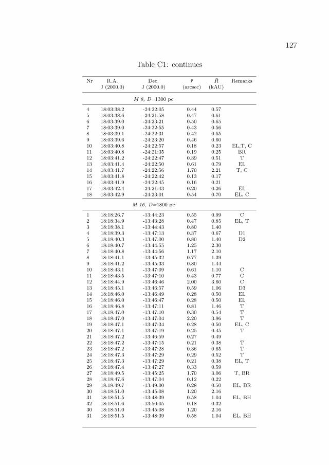
127
Table C1: continues
Nr R.A. Dec. r R RemarksJ (2000.0) J (2000.0) (arcsec) (kAU)
M 8, D=1300 pc
4 18:03:38.2 -24:22:05 0.44 0.575 18:03:38.6 -24:21:58 0.47 0.616 18:03:39.0 -24:23:21 0.50 0.657 18:03:39.0 -24:22:55 0.43 0.568 18:03:39.1 -24:22:31 0.42 0.559 18:03:39.6 -24:23:20 0.46 0.6010 18:03:40.8 -24:22:57 0.18 0.23 EL,T, C11 18:03:40.8 -24:21:35 0.19 0.25 BR12 18:03:41.2 -24:22:47 0.39 0.51 T13 18:03:41.4 -24:22:50 0.61 0.79 EL14 18:03:41.7 -24:22:56 1.70 2.21 T, C15 18:03:41.8 -24:22:42 0.13 0.1716 18:03:41.9 -24:22:45 0.16 0.2117 18:03:42.4 -24:21:43 0.20 0.26 EL18 18:03:42.9 -24:23:01 0.54 0.70 EL, C
M 16, D=1800 pc
1 18:18:26.7 -13:44:23 0.55 0.99 C2 18:18:34.9 -13:43:28 0.47 0.85 EL, T3 18:18:38.1 -13:44:43 0.80 1.404 18:18:39.3 -13:47:13 0.37 0.67 D15 18:18:40.3 -13:47:00 0.80 1.40 D26 18:18:40.7 -13:44:55 1.25 2.307 18:18:40.8 -13:44:56 1.17 2.108 18:18:41.1 -13:45:32 0.77 1.399 18:18:41.2 -13:45:33 0.80 1.4410 18:18:43.1 -13:47:09 0.61 1.10 C11 18:18:43.5 -13:47:10 0.43 0.77 C12 18:18:44.9 -13:46:46 2.00 3.60 C13 18:18:45.1 -13:46:57 0.59 1.06 D314 18:18:46.0 -13:46:49 0.28 0.50 EL15 18:18:46.0 -13:46:47 0.28 0.50 EL16 18:18:46.8 -13:47:11 0.81 1.46 T17 18:18:47.0 -13:47:10 0.30 0.54 T18 18:18:47.0 -13:47:04 2.20 3.96 T19 18:18:47.1 -13:47:34 0.28 0.50 EL, C20 18:18:47.1 -13:47:19 0.25 0.45 T21 18:18:47.2 -13:46:59 0.27 0.4922 18:18:47.2 -13:47:15 0.21 0.38 T23 18:18:47.2 -13:47:28 0.36 0.65 T24 18:18:47.3 -13:47:29 0.29 0.52 T25 18:18:47.3 -13:47:29 0.21 0.38 EL, T26 18:18:47.4 -13:47:27 0.33 0.5927 18:18:49.5 -13:45:25 1.70 3.06 T, BR28 18:18:47.6 -13:47:04 0.12 0.2229 18:18:49.7 -13:49:00 0.28 0.50 EL, BR30 18:18:51.0 -13:45:08 1.20 2.1631 18:18:51.5 -13:48:39 0.58 1.04 EL, BH32 18:18:51.6 -13:50:05 0.18 0.3230 18:18:51.0 -13:45:08 1.20 2.1631 18:18:51.5 -13:48:39 0.58 1.04 EL, BH
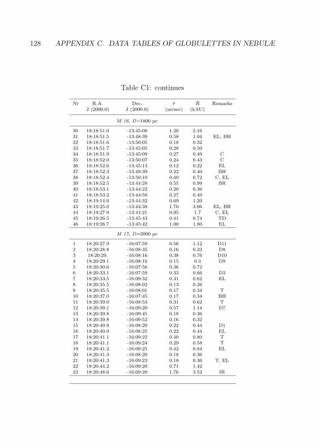
128 APPENDIX C. DATA TABLES OF GLOBULETTES IN NEBULÆ
Table C1: continues
Nr R.A. Dec. r R RemarksJ (2000.0) J (2000.0) (arcsec) (kAU)
M 16, D=1800 pc
30 18:18:51.0 -13:45:08 1.20 2.1631 18:18:51.5 -13:48:39 0.58 1.04 EL, BH32 18:18:51.6 -13:50:05 0.18 0.3233 18:18:51.7 -13:45:05 0.28 0.5034 18:18:51.9 -13:45:09 0.27 0.49 C35 18:18:52.0 -13:50:07 0.24 0.43 C36 18:18:52.0 -13:45:13 0.12 0.22 EL37 18:18:52.3 -13:49:39 0.22 0.40 BH38 18:18:52.4 -13:50:10 0.40 0.72 C, EL39 18:18:52.5 -13:44:28 0.55 0.99 BR40 18:18:53.1 -13:44:22 0.20 0.3641 18:18:53.2 -13:44:58 0.27 0.4942 18:19:14.9 -13:44:32 0.69 1.2043 18:19:25.0 -13:44:38 1.70 3.06 EL, BR44 18:19:27.9 -13:44:21 0.95 1.7 C, EL45 18:19:26.5 -13:45:43 0.41 0.74 TD46 18:19:26.7 -13:45:42 1.00 1.80 EL
M 17, D=2000 pc
1 18:20:27.9 -16:07:59 0.56 1.12 D112 18:20:28.8 -16:08:35 0.16 0.32 D83 18:20:29. -16:08:16 0.38 0.76 D104 18:20:29.1 -16:08:16 0.15 0.3 D95 18:20:30.6 -16:07:56 0.36 0.726 18:20:33.1 -16:07:59 0.33 0.66 D37 18:20:33.5 -16:09:32 0.31 0.62 EL8 18:20:35.5 -16:08:02 0.13 0.269 18:20:35.5 -16:08:01 0.17 0.34 T10 18:20:37.0 -16:07:45 0.17 0.34 BH11 18:20:39.0 -16:08:53 0.31 0.62 T12 18:20:39.1 -16:09:20 0.57 1.14 D713 18:20:39.8 -16:09:45 0.18 0.3614 18:20:39.8 -16:09:52 0.16 0.3215 18:20:40.8 -16:08:20 0.22 0.44 D116 18:20:40.9 -16:08:25 0.22 0.44 EL17 18:20:41.1 -16:09:22 0.40 0.80 T18 18:20:41.1 -16:09:24 0.29 0.58 T19 18:20:41.2 -16:09:25 0.42 0.84 EL20 18:20:41.3 -16:08:20 0.18 0.3621 18:20:41.3 -16:09:23 0.18 0.36 T, EL22 18:20:44.2 -16:09:20 0.71 1.4223 18:20:48.6 -16:09:28 1.76 3.52 IR

Paper I
Globulettes as seeds of brown dwarfs and free-floating planetary mass object
Authors:Gahm, G. F., Grenman, T., Fredriksson, S., & Kristen, H.


GLOBULETTES AS SEEDS OF BROWN DWARFS AND FREE-FLOATINGPLANETARY-MASS OBJECTS1
G. F. Gahm
Stockholm Observatory, AlbaNova , SE-10691 Stockholm, Sweden
T. Grenman and S. Fredriksson
Division of Physics, Lulea University of Technology, SE-97187 Lulea, Sweden
and
H. Kristen
CTO, Imminent Training Technologies AB, IDEON Research Park, SE-22370 Lund, Sweden
Received 2006 November 28; accepted 2006 December 20
ABSTRACT
Some H ii regions surrounding young stellar clusters contain tiny dusty clouds, which on photos look like darkspots or teardrops against a background of nebular emission. From our collection of H� images of 10 H ii regionsgathered at the Nordic Optical Telescope, we found 173 such clouds, which we call ‘‘globulettes,’’ since they aremuch smaller than normal globules and form a distinct class of objects. Many globulettes are quite isolated andlocated far from the molecular shells and elephant trunks associated with the regions. Others are attached to the trunks(or shells), suggesting that globulettes may form as a consequence of erosion of these larger structures. None of ourobjects appear to contain stellar objects. The globulettes were measured for position, dimension, and orientation,and we find that most objects are smaller than 10 kAU. The Rosette Nebula and IC 1805 are particularly rich inglobulettes, for which the size distributions peak at mean radii of �2.5 kAU, similar to what was found by Reipurthand coworkers and De Marco and coworkers for similar objects in other regions. We estimate total mass and densitydistributions for each object from extinctionmeasures and conclude that amajority contain<13MJ , corresponding toplanetary-mass objects.We then estimate the internal thermal and potential energies and find, when also including theeffects from the outer pressure, that a large fraction of the globulettes could be unstable and would contract on shorttimescales,<106 yr. In addition, the radiation pressure and ram pressure exerted on the side facing the clusters wouldstimulate contraction. Since the globulettes are not screened from stellar light by dust clouds farther in, one wouldexpect photoevaporation to dissolve the objects. However, surprisingly few objects show bright rims or teardropforms. We calculate the expected lifetimes against photoevaporation. These lifetimes scatter around 4 ; 106 yr, muchlonger than estimated in previous studies and also much longer than the free-fall time. We conclude that a largenumber of our globulettes have time to form central low-mass objects long before the ionization front, driven by theimpinging Lyman photons, has penetrated far into the globulette. Hence, the globulettes may be one source in theformation of brown dwarfs and free-floating planetary-mass objects in the galaxy.
Key words: H ii regions — ISM: general — ISM: globules — planets and satellites: general — stars: formation
Online material: machine-readable table
1. INTRODUCTION
Star-forming regions containingmassive stars develop expand-ing bubbles of ionized gas, H ii regions, around a central clusterafter the first massive O and B stars appear. Cold molecular ma-terial surrounds the H ii regions, sometimes developing long fil-amentary and rather massive pillars of gas and dust, so-calledelephant trunks, extending from the shell and pointing at the cen-tral young cluster. It was recognized early on that some regionsalso contain a number of smaller clouds that appear as dark ob-jects when silhouetted against the bright background nebulosityon optical images. Some clouds are relatively large and look likeregular globules, but some are much smaller. The clouds may beround or shaped like teardrops pointing at the central hot stars,and many have bright rims indicative of surface activity induced
by the incident stellar UV light and/or the expanding warmplasma in which the clumps are engulfed. The clouds are usu-ally found in the vicinity of the trunks or shells and can be con-nected to these through filamentary threads, but some are quiteisolated (Thackeray 1950; Herbig 1974). The properties of suchglobules have been reviewed by Leung (1985).
Reipurth et al. (1997, 2003) have taken a detailed look at theH ii region IC 2944, first studied by Thackeray, and their HubbleSpace Telescope (HST )material in particular revealed a large num-ber of tiny dark clouds. Several of them are round and isolatedand have no bright rims. It was concluded that they would dis-integrate on timescales of less than 100 yr due to photoevapora-tion unless they were shadowed from stellar light, but no obviousscreen for shadowing was observed. The size distribution, indi-cating two peaks, shows that most objects have characteristic radiiof less than 10 kAU, and it was hinted that the smallest cloudsmayhave masses of only a few Jupiter masses. Similar objects werealso found by Smith et al. (2003) in the Carina Nebula in a searchfor so-called proplyds, photoevaporating circumstellar disks withcentral newborn stars (see, e.g., Bally et al. 2000). HST images
1 Based on observations made with the Nordic Optical Telescope, operatedon the island of La Palma jointly by Denmark, Finland, Iceland, Norway, andSweden in the Spanish Observatorio del Roque de losMuchachos of the Institutode Astrofısica de Canarias.
A
1795
The Astronomical Journal, 133:1795Y1809, 2007 April
# 2007. The American Astronomical Society. All rights reserved. Printed in U.S.A.

taken of the H ii region M16 revealed tiny clumps close to majorelephant trunks, and Hester et al. (1996) speculated that these so-called EGGs (evaporating gaseous globules) would dissolve ontimescales of <104 yr.
Recently, De Marco et al. (2006) surveyed 10 H ii regions forsmall dark clouds and proplyds. In addition to IC 2944, anotherthree H ii regions were found to exhibit a number of similar smallstarless clouds, while in other regions none or only some ob-ject(s) were found. It was suggested that the clumps may be self-gravitating and could form stars, at least if they were shadowedfrom the destructive stellar radiation. The size distributions turnout to be very similar to that obtained by Reipurth et al. (2003),but with only one broad peak with effective radii extending from300 to 5000 AU for IC 2944.
The tiny clouds constitute a specific class of interstellar clouds.They are similar to the much larger starless globules in their shapeand physical state but distinctly different with regard to distribu-tion, and are not the low-mass tail of the globules. In the literaturethey have many names, splinters, nodules, cusps, etc., and herewe propose the name ‘‘globulettes’’ to distinguish them fromglobules.
Isolated free-floating planetary-mass objects have been locatedin interstellar space (Zapatero Osorio et al. 2000; Lucas & Roche2000; Luhman et al. 2005; Jayawardhana & Ivanov 2006a). It hasbeen suggested that such planets once formed in circumstellarprotoplanetary disks from which they were later ejected, or as aresult of stripping of protostellar material through interaction withneighboring stars (see, e.g., Kroupa & Bouvier 2003). The recentdiscovery of an isolated young binary of very low mass impliesthat low-mass objects may originate as a consequence of contrac-tion of isolated small clouds (Jayawardhana & Ivanov 2006b). Inthe present article we investigate whether the tiny clouds discussedabove could also be a source of low-mass objects. Our investiga-tion is based on deep H� images of 10 H ii regions collected withthe Nordic Optical Telescope. The area coverage is much largerthan the HST-based surveys referred to above, but the spatialresolution is lower. On the other hand, most of our regions arecloser than those previously studied (not IC 2944), and in manycases the actual physical resolution is not drastically different. Intotal we have found 173 small clouds in this survey. We make adetailed determination of their masses and discuss the physicalconditions both inside and outside the clouds and whether or notthey may contract. We also discuss their origins and lifetimes.Preliminary results obtained for two regions, namely, IC 1805 andthe Rosette Nebula, were included in a licentiate thesis by T. G.(Grenman 2006), in which our numerical methods for analyzingthe observational data are reviewed in detail.
2. OBSERVATIONS AND REGIONS
Deep narrowband H� images of 50 total fields in 10 H ii re-gions were collected with the 2.6 mNordic Optical Telescope onLa Palma, Canary Islands, Spain. The ALFOSC camera used hasa field diameter of 6.50, and the CCD detector has a scale of0.18800 pixel�1. The exposure times were 1800 s with few excep-tions, and the seeing conditions were generally good, 0.700Y1.100.Two different filters were used: in 1999 a narrowband filter with33 8 FWHM, covering the nebular emission from only the H�line, and in 2000 a filter with 180 8 FWHM, also including thestrong nebular emission lines of [N ii] at 6548.1 and 6583.6 8,flanking the H� line, and hence including more nebular emis-sion. All images were flat-fielded and corrected for cosmic-rayexcitations and bias. For the calibration of the intensity scale onealso needs to correct for the light from the sky background, and
TABLE 1
Central Positions for Observed Fields
Field No. R.A. (J2000.0) Decl. (J2000.0)
Rosette Nebulaa
1................................................. 06 30 24.0 +04 51 00
2................................................. 06 30 29.0 +04 56 00
3................................................. 06 30 40.0 +05 00 00
4................................................. 06 30 44.0 +04 39 00
5................................................. 06 30 48.0 +05 24 30
6................................................. 06 30 50.0 +05 02 00
7................................................. 06 30 50.0 +05 01 10
8................................................. 06 30 50.0 +05 06 30
9................................................. 06 31 10.0 +05 08 00
10............................................... 06 31 12.0 +05 24 50
11............................................... 06 31 18.5 +05 26 58
12............................................... 06 31 22.0 +05 13 00
13............................................... 06 31 32.7 +05 27 30
14............................................... 06 31 35.4 +05 09 00
15............................................... 06 31 35.4 +05 09 00
16............................................... 06 31 35.8 +05 11 55
17............................................... 06 31 47.8 +05 15 13
18............................................... 06 31 55.0 +05 30 00
19............................................... 06 32 02.0 +05 06 13
20............................................... 06 32 16.0 +05 13 13
21............................................... 06 32 19.0 +04 30 00
22............................................... 06 33 18.0 +04 46 00
23............................................... 06 33 33.0 +04 50 00
NGC 6820b
1................................................. 19 43 35.0 +23 21 39
2................................................. 19 43 37.8 +23 21 54
3................................................. 19 43 42.4 +23 23 00
4................................................. 19 43 52.1 +23 21 39
5................................................. 19 43 52.5 +23 19 35
NGC 7822c
1................................................. 00 01 39.3 +67 06 20
2................................................. 00 02 09.0 +67 05 28
3................................................. 00 05 00.0 +67 06 30
IC 1805d
1................................................. 02 35 00.0 +61 09 30
2................................................. 02 35 48.0 +61 17 57
3................................................. 02 36 09.0 +61 22 25
4................................................. 02 36 29.0 +61 25 35
5................................................. 02 36 35.0 +61 22 12
6................................................. 02 36 46.0 +61 25 00
7................................................. 02 37 30.0 +61 25 00
IC 1848e
1................................................. 02 57 25.0 +60 40 00
2................................................. 03 01 15.0 +60 41 45
NGC 2264f
1................................................. 06 36 18.0 +10 25 22
2................................................. 06 38 04.0 +10 16 30
3................................................. 06 38 09.0 +10 10 56
DWB 44g
1................................................. 20 18 12.0 +39 46 28
2................................................. 20 18 42.0 +39 38 27
3................................................. 20 18 48.0 +39 48 40
4................................................. 20 19 12.0 +39 37 50
GAHM ET AL.1796 Vol. 133

therefore, sky exposures were collected in fields outside the emis-sion nebulae. The nights were dark, except during parts of 2000December 2 and 3, when there was moonlight. Several fields wereobserved twice, and some fields overlap. The agreement is excel-lent when comparing parameters derived for the same object ex-posed during different nights (and years) with different night skyconditions and at different positions in overlapping fields. Part ofour Nordic Optical Telescope material was first used for a de-tailed study of elephant trunks in NGC 7822, IC 1805, the RosetteNebula, and DWB 44, and more information on these regions canbe found in Carlqvist et al. (2003) and Gahm et al. (2006).
Table 1 lists the central positions of the fields observed in theH ii regions selected with adopted distances based on the refer-ences quoted. NGC 7822 is relatively nearby and related to theCep OB4 association centered on the young cluster Berkeley 59.IC 1848 and IC 1805 are connected to sites of extensive star for-mation in the Perseus arm. The Rosette Nebula (NGC 2237Y2246) is a magnificent H ii region with numerous elephant trunks.A cavity has developed around the central massive, young stars.NGC 2264 and IC 2177 (related to CMa OB1) are relativelynearby (�1 kpc) regions of star formation. NGC 6820 is related tothe young cluster NGC 6823 and the Vul OB4 association, whilefor DWB 39, DWB44, and an anonymous nebula in the crowded,
TABLE 1—Continued
Field No. R.A. (J2000.0) Decl. (J2000.0)
IC 2177h
1................................................. 07 04 44.4 �10 26 55
DWB 39 i
1................................................. 20 20 51.3 +39 17 00
Cyg X Anonymous j
1................................................. 20 26 32.0 +41 22 12
Note.—Units of right ascension are hours, minutes, and seconds, and units ofdeclination are degrees, arcminutes, and arcseconds.
a Distance of 1.4 kpc (Ogura & Ishida 1981).b Distance of 1.89 kpc (Kharchenko et al. 2005).c Distance of 0.85 kpc (MacConnell 1968).d Distance of 2.35 kpc (Massey 1995).e Distance of 2.2 kpc (Guetter & Vrba 1989).f Distance of 0.76 kpc (Sung et al. 1997).g Distance of 0.72 kpc (Kaltcheva & Hilditch 2000; Gahm et al. 2006).h Distance of 1.0 kpc (Kaltcheva & Hilditch 2000; Tjin A Djie et al. 2001).i Distance of 0.72 kpc (Kaltcheva & Hilditch 2000; Gahm et al. 2006).j Distance of 0.72 kpc (Kaltcheva & Hilditch 2000; Gahm et al. 2006).
Fig. 1.—Observed fields in the Rosette Nebulamarked on awide-field image taken at Kitt PeakNationalObservatory. Dark, prominent shell structures and elephant trunksare seen in silhouette against the bright background. The so-called Wrench trunk is located in fields 13 and 14. The image spans 510 ; 510; north is up, and east to the right.
GLOBULETTES AS SEEDS OF LOW-MASS OBJECTS 1797No. 4, 2007
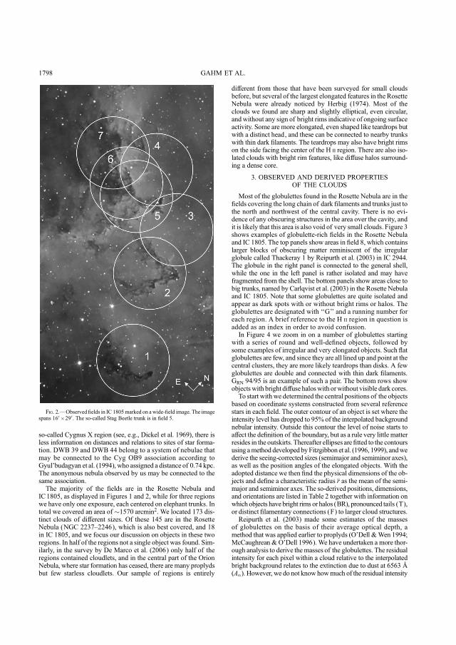
so-called Cygnus X region (see, e.g., Dickel et al. 1969), there isless information on distances and relations to sites of star forma-tion. DWB 39 and DWB 44 belong to a system of nebulae thatmay be connected to the Cyg OB9 association according toGyul’budagyan et al. (1994), who assigned a distance of 0.74 kpc.The anonymous nebula observed by us may be connected to thesame association.
The majority of the fields are in the Rosette Nebula andIC1805, as displayed in Figures 1 and 2, while for three regionswe have only one exposure, each centered on elephant trunks. Intotal we covered an area of�1570 arcmin2. We located 173 dis-tinct clouds of different sizes. Of these 145 are in the RosetteNebula (NGC 2237Y2246), which is also best covered, and 18in IC 1805, and we focus our discussion on objects in these tworegions. In half of the regions not a single object was found. Sim-ilarly, in the survey by De Marco et al. (2006) only half of theregions contained cloudlets, and in the central part of the OrionNebula, where star formation has ceased, there are many proplydsbut few starless cloudlets. Our sample of regions is entirely
different from those that have been surveyed for small cloudsbefore, but several of the largest elongated features in the RosetteNebula were already noticed by Herbig (1974). Most of theclouds we found are sharp and slightly elliptical, even circular,andwithout any sign of bright rims indicative of ongoing surfaceactivity. Some are more elongated, even shaped like teardrops butwith a distinct head, and these can be connected to nearby trunkswith thin dark filaments. The teardrops may also have bright rimson the side facing the center of the H ii region. There are also iso-lated clouds with bright rim features, like diffuse halos surround-ing a dense core.
3. OBSERVED AND DERIVED PROPERTIESOF THE CLOUDS
Most of the globulettes found in the Rosette Nebula are in thefields covering the long chain of dark filaments and trunks just tothe north and northwest of the central cavity. There is no evi-dence of any obscuring structures in the area over the cavity, andit is likely that this area is also void of very small clouds. Figure 3shows examples of globulette-rich fields in the Rosette Nebulaand IC 1805. The top panels show areas in field 8, which containslarger blocks of obscuring matter reminiscent of the irregularglobule called Thackeray 1 by Reipurth et al. (2003) in IC 2944.The globule in the right panel is connected to the general shell,while the one in the left panel is rather isolated and may havefragmented from the shell. The bottom panels show areas close tobig trunks, named by Carlqvist et al. (2003) in the Rosette Nebulaand IC 1805. Note that some globulettes are quite isolated andappear as dark spots with or without bright rims or halos. Theglobulettes are designated with ‘‘G’’ and a running number foreach region. A brief reference to the H ii region in question isadded as an index in order to avoid confusion.In Figure 4 we zoom in on a number of globulettes starting
with a series of round and well-defined objects, followed bysome examples of irregular and very elongated objects. Such flatglobulettes are few, and since they are all lined up and point at thecentral clusters, they are more likely teardrops than disks. A fewglobulettes are double and connected with thin dark filaments.GRN 94/95 is an example of such a pair. The bottom rows showobjectswith bright diffuse haloswith orwithout visible dark cores.To start with we determined the central positions of the objects
based on coordinate systems constructed from several referencestars in each field. The outer contour of an object is set where theintensity level has dropped to 95% of the interpolated backgroundnebular intensity. Outside this contour the level of noise starts toaffect the definition of the boundary, but as a rule very little matterresides in the outskirts. Thereafter ellipses are fitted to the contoursusing amethod developed byFitzgibbon et al. (1996, 1999), andwederive the seeing-corrected sizes (semimajor and semiminor axes),as well as the position angles of the elongated objects. With theadopted distance we then find the physical dimensions of the ob-jects and define a characteristic radius r as the mean of the semi-major and semiminor axes. The so-derived positions, dimensions,and orientations are listed in Table 2 together with information onwhich objects have bright rims or halos (BR), pronounced tails (T),or distinct filamentary connections (F) to larger cloud structures.Reipurth et al. (2003) made some estimates of the masses
of globulettes on the basis of their average optical depth, amethod that was applied earlier to proplyds (O’Dell &Wen 1994;McCaughrean & O’Dell 1996). We have undertaken a more thor-ough analysis to derive themasses of the globulettes. The residualintensity for each pixel within a cloud relative to the interpolatedbright background relates to the extinction due to dust at 6563 8(A�). However, we do not know howmuch of the residual intensity
Fig. 2.—Observed fields in IC 1805marked on awide-field image. The imagespans 160 ; 290. The so-called Stag Beetle trunk is in field 5.
GAHM ET AL.1798

Fig. 3.—Top panels: Two areas in field 8 in the Rosette Nebula. The field is rich in globulettes, which cluster around two large, dark globules. The left panel spans3:10 ; 1:90. The right panel, spanning 4:30 ; 2:40, contains three large globulettes connected to the globule by very long filaments, which point like fingers toward thecentral cluster.Middle left: Area containing a string of globulettes connected with very thin filaments to theWrench trunk. North of the string is the jawlike head of anothertrunkwith helical, filamentary substructures. The panel spans 4:40 ; 3:60.Middle right: Southern part of theWrench trunkwith its jawlike head and the clumpsGRN 73 and79 at the ends. These objects appear to be in the process of detaching from the trunk. Isolated dark globulettes are found in the vicinity. The panel spans 4:20 ; 2:80. South ofthe jaw are several isolated objects with dark cores surrounded by spherical bright halos (see enlarged square). Bottom left: Area in the southeastern part of the Stag Beetletrunk. Besides some isolated globulettes there are clumps with V-shaped filamentary connections to the shell, ‘‘outgrowths.’’ The panel spans 1:50 ; 1:70.
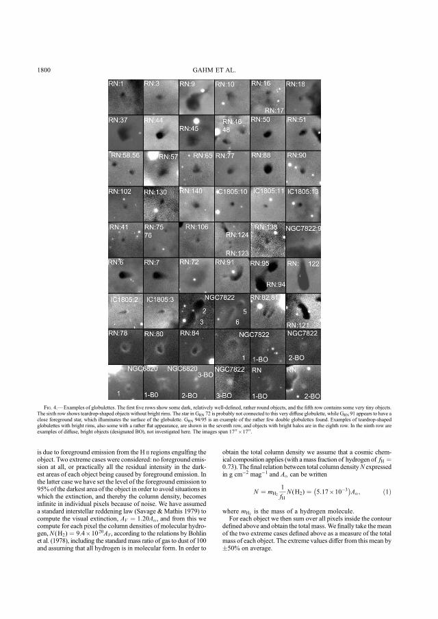
is due to foreground emission from the H ii regions engulfing theobject. Two extreme cases were considered: no foreground emis-sion at all, or practically all the residual intensity in the dark-est areas of each object being caused by foreground emission. Inthe latter case we have set the level of the foreground emission to95% of the darkest area of the object in order to avoid situations inwhich the extinction, and thereby the column density, becomesinfinite in individual pixels because of noise. We have assumeda standard interstellar reddening law (Savage & Mathis 1979) tocompute the visual extinction, AV ¼ 1:20A�, and from this wecompute for each pixel the column densities of molecular hydro-gen,N (H2) ¼ 9:4 ; 1020AV, according to the relations by Bohlinet al. (1978), including the standard mass ratio of gas to dust of 100and assuming that all hydrogen is in molecular form. In order to
obtain the total column density we assume that a cosmic chem-ical composition applies (with amass fraction of hydrogen of fH ¼0:73). The final relation between total column densityN expressedin g cm�2 mag�1 and A� can be written
N ¼ mH2
1
fHN (H2) ¼ 5:17 ; 10�3
� �A�; ð1Þ
where mH2is the mass of a hydrogen molecule.
For each object we then sum over all pixels inside the contourdefined above and obtain the total mass.We finally take themeanof the two extreme cases defined above as a measure of the totalmass of each object. The extreme values differ from this mean by�50% on average.
Fig. 4.—Examples of globulettes. The first five rows show some dark, relatively well-defined, rather round objects, and the fifth row contains some very tiny objects.The sixth row shows teardrop-shaped objects without bright rims. The star in GRN 72 is probably not connected to this very diffuse globulette, while GRN 91 appears to have aclose foreground star, which illuminates the surface of the globulette. GRN 94/95 is an example of the rather few double globulettes found. Examples of teardrop-shapedglobulettes with bright rims, also some with a rather flat appearance, are shown in the seventh row, and objects with bright halos are in the eighth row. In the ninth row areexamples of diffuse, bright objects (designated BO), not investigated here. The images span 1700 ; 1700.
GAHM ET AL.1800

TABLE 2
List of Globulettes
Globulette No. Glob Flag R.A. (J2000.0) Decl. (J2000.0)
�
(arcsec)
�
(arcsec)
r
( kAU)
P.A.
(deg)
Mass
(MJ)
�
(10�20 g cm�3)
NGC 7822 (G7822)
1......................... BR 00 02 22.18 +67 07 26.5 2.3 2.1 1.9 � 1.90 4.24
2......................... BR 00 04 42.33 +67 03 26.6 3.0 2.2 2.2 � 3.77 5.60
3......................... BR 00 04 42.99 +67 03 20.3 3.2 1.7 2.1 �8 2.43 5.68
4......................... T 00 04 52.21 +67 04 10.2 4.2 3.7 3.4 � 12.5 4.78
5......................... BR 00 04 56.88 +67 07 25.0 1.5 1.4 1.2 � 0.38 2.9
6......................... BR 00 04 57.64 +67 07 21.3 4.3 0.7 2.1 �26 0.49 5.4
7......................... 00 05 00.87 +67 03 58.6 1.8 1.0 1.2 � 0.93 10.7
8......................... 00 05 10.58 +67 04 07.3 2.7 2.4 2.2 � 4.05 5.86
9......................... 00 05 18.81 +67 08 09.7 0.6 0.5 0.45 � 0.27 44.0
IC 1805 (G1805)
1......................... T 02 34 50.23 +61 11 07.0 2.9 2.5 6.4 44 36.4 2.04
2......................... BR 02 35 51.29 +61 20 28.5 1.9 1.0 3.4 10 8.08 4.11
3......................... BR 02 35 57.92 +61 18 49.9 2.0 0.6 3.0 11 5.75 8.96
4......................... F 02 35 58.79 +61 18 36.3 7.5 4.3 14 10 255 1.95
5......................... F 02 36 18.00 +61 23 30.6 5.1 2.0 8.3 �23 55.0 2.91
6......................... F 02 36 19.77 +61 23 35.0 2.2 1.5 4.4 3.7 16.7 3.52
7......................... F 02 36 23.10 +61 23 03.7 3.7 2.7 7.4 6.3 61.8 2.46
8......................... F 02 36 24.92 +61 24 59.9 5.6 3.0 10 �9.2 96.6 2.00
9......................... 02 36 25.29 +61 20 49.1 1.5 0.8 2.6 36 5.53 6.50
10....................... 02 36 31.60 +61 21 43.8 1.5 1.3 3.3 � 10.5 4.41
11....................... 02 36 32.68 +61 22 09.5 1.2 0.9 2.5 � 5.43 6.08
12....................... F 02 36 34.55 +61 21 41.4 2.0 1.5 4.1 � 25.2 5.64
13....................... 02 36 38.41 +61 21 47.4 1.4 1.3 3.2 � 9.22 3.99
14....................... 02 36 42.11 +61 19 48.1 2.0 1.0 3.5 �6.0 7.53 3.75
15....................... 02 36 45.19 +61 22 01.1 0.6 0.5 1.3 � 2.67 17.1
16....................... 02 36 46.62 +61 19 17.1 3.4 2.9 7.4 �39 58.8 2.16
17....................... 02 36 47.85 +61 21 57.8 2.5 1.8 5.1 4.5 23.5 3.04
18....................... 02 36 52.65 +61 20 03.0 1.1 0.8 2.2 � 6.03 8.58
Rosette Nebula (GRN)
1......................... 06 30 24.08 +04 48 03.5 1.6 1.3 2.1 � 2.98 5.08
2......................... 06 30 28.99 +04 49 27.8 3.3 2.6 4.1 � 13.0 2.98
3......................... 06 30 31.56 +04 51 26.3 1.7 1.3 2.1 � 5.59 8.93
4......................... T 06 30 31.68 +04 55 34.0 3.9 3.3 5.1 �7.3 28.5 3.27
5......................... F 06 30 32.69 +04 57 34.2 15 10 18 �44 665 2.09
6......................... T 06 30 33.02 +04 50 37.2 3.8 2.2 4.2 �2.8 18.2 5.06
7......................... T 06 30 36.73 +04 55 19.1 3.6 2.5 4.2 �1.5 18.4 4.11
8......................... 06 30 37.39 +04 42 05.2 2.6 2.2 3.4 1.2 9.01 3.41
9......................... 06 30 40.14 +05 01 28.6 5.7 4.6 7.2 � 72.2 3.02
10....................... 06 30 41.72 +04 40 58.1 2.6 2.0 3.2 � 9.63 4.37
11....................... 06 30 42.29 +05 05 41.9 2.3 2.1 3.1 � 8.08 3.95
12....................... T 06 30 43.88 +05 08 42.4 6.3 3.2 6.6 �30 46.9 3.65
13....................... F 06 30 45.33 +04 41 28.1 3.6 2.8 4.5 � 17.6 3.05
14....................... F 06 30 45.47 +04 41 21.4 3.0 2.8 4.1 � 17.0 3.59
15....................... F 06 30 45.60 +04 41 27.4 1.9 1.6 2.4 � 6.39 6.87
16....................... 06 30 45.94 +05 06 29.8 1.6 1.4 2.1 � 4.11 6.31
17....................... 06 30 45.94 +05 06 25.7 1.9 1.5 2.4 � 4.26 4.78
18....................... 06 30 48.48 +05 05 58.9 1.4 1.2 1.8 � 3.05 7.04
19....................... F 06 30 48.58 +05 04 45.2 3.6 1.7 3.7 36 8.22 4.11
20....................... F 06 30 49.12 +05 04 49.0 2.5 2.1 3.3 � 9.76 4.18
21....................... F 06 30 49.53 +05 06 12.9 2.4 1.7 2.9 � 8.63 5.99
22....................... 06 30 49.83 +05 06 15.3 2.7 1.9 3.3 � 10.9 5.21
23....................... 06 30 51.50 +04 39 56.7 1.7 1.4 2.2 � 3.88 5.69
24....................... 06 30 52.79 +05 08 31.4 4.5 4.0 5.9 � 32.9 2.26
25....................... 06 30 52.88 +04 37 01.1 1.6 1.3 2.0 � 3.49 6.71
26....................... 06 30 53.57 +05 09 08.7 2.0 1.2 2.3 3.5 5.54 8.98
27....................... 06 30 54.42 +05 09 12.3 1.7 1.2 2.1 � 4.14 7.73
28....................... T 06 30 54.62 +05 22 30.6 4.9 2.8 5.4 �12 23.9 3.16
29....................... 06 30 54.95 +05 09 17.0 2.1 1.3 2.4 25 4.52 6.19
30....................... T 06 30 55.30 +05 23 09.9 4.0 3.0 4.9 �13 17.9 2.45
31....................... T 06 30 56.66 +05 05 47.8 9.4 7.1 11 �11 155 1.64
TABLE 2—Continued
Globulette No. Glob Flag R.A. (J2000.0) Decl. (J2000.0)
�
(arcsec)
�
(arcsec)
r
(kAU)
P.A.
(deg)
Mass
(MJ)
�
(10�20 g cm�3)
Rosette Nebula (GRN)
32....................... 06 30 57.18 +05 07 10.5 3.2 1.9 3.6 26 12.7 5.68
33....................... 06 30 58.09 +05 07 08.2 3.1 2.1 3.6 �33 12.7 4.87
34....................... 06 31 03.94 +05 07 09.0 4.2 3.3 5.3 � 33.7 3.56
35....................... T 06 31 05.88 +05 05 55.3 7.4 5.9 9.3 � 172 3.30
36....................... T 06 31 06.54 +05 05 24.0 1.4 1.2 1.8 � 4.81 11.8
37....................... 06 31 06.37 +05 06 38.0 4.6 3.6 5.7 � 46.4 3.84
38....................... T 06 31 07.39 +05 05 04.4 7.8 4.0 8.2 �24 96.8 3.90
39....................... T, F 06 31 09.67 +05 06 26.8 4.6 2.9 5.3 �31 42.2 5.30
40....................... T, F 06 31 10.80 +05 06 08.2 6.5 5.7 8.5 �33 123 2.85
41....................... 06 31 11.25 +05 06 56.1 1.0 0.9 1.3 � 2.88 17.7
42....................... 06 31 12.75 +05 08 17.9 1.6 1.1 1.9 39 3.53 9.07
43....................... 06 31 13.75 +05 12 37.2 1.9 1.6 2.5 � 4.63 4.67
44....................... 06 31 13.91 +05 08 06.0 3.3 2.5 4.0 � 16.8 4.01
45....................... 06 31 15.29 +05 11 40.3 3.5 3.2 4.7 � 16.2 2.22
46....................... 06 31 15.58 +05 07 38.4 2.1 1.8 2.7 � 6.00 4.67
47....................... T, F 06 31 16.16 +05 05 58.5 4.6 3.5 5.7 � 27.1 2.32
48....................... 06 31 16.16 +05 07 33.1 2.2 1.4 2.5 �14 4.71 5.62
49....................... 06 31 18.71 +05 07 54.0 3.4 2.8 4.3 � 22.2 4.21
50....................... 06 31 20.14 +05 08 12.1 2.8 2.1 3.4 � 11.4 4.66
51....................... 06 31 20.22 +05 08 29.8 2.8 1.7 3.1 �36 9.46 5.99
52....................... F 06 31 21.18 +05 08 59.0 4.5 4.1 6.0 � 34.7 2.32
53....................... 06 31 21.26 +05 09 12.3 3.4 3.0 4.5 � 20.6 3.42
54....................... 06 31 21.31 +05 09 21.2 2.3 1.6 2.7 � 5.11 4.20
55....................... 06 31 21.56 +05 08 21.5 10 3.6 9.6 �40 67.2 2.49
56....................... 06 31 21.56 +05 08 38.0 1.8 1.7 2.4 � 4.16 4.21
57....................... 06 31 22.31 +05 10 29.7 3.2 2.5 4.0 � 13.4 3.29
58....................... 06 31 22.16 +05 08 41.9 1.9 1.6 2.5 � 4.11 4.10
59....................... 06 31 23.30 +05 08 43.1 2.9 2.4 3.7 � 13.6 4.19
60....................... 06 31 23.77 +05 10 50.6 2.0 1.7 2.6 � 6.27 5.19
61....................... 06 31 24.04 +05 10 52.7 2.5 1.8 3.0 � 8.09 5.02
62....................... 06 31 27.45 +05 13 47.0 3.6 2.2 4.1 17 13.9 3.75
63....................... 06 31 27.45 +05 26 30.0 6.7 4.0 7.5 �24 59.4 2.69
64....................... 06 31 27.96 +05 13 56.8 4.0 2.5 4.5 �20 18.2 3.68
65....................... 06 31 29.70 +05 09 32.2 2.6 2.3 3.5 � 9.22 3.18
66....................... T 06 31 30.82 +05 12 16.8 4.1 2.6 4.7 �30 22.3 4.00
67....................... 06 31 31.40 +05 13 14.1 3.4 2.2 3.9 �15 14.7 4.40
68....................... 06 31 31.55 +05 13 07.1 3.3 2.7 4.2 � 14.9 3.04
69....................... 06 31 31.65 +05 12 04.1 1.6 1.2 1.9 � 2.90 6.63
70....................... BR 06 31 32.15 +05 07 59.3 2.3 1.1 2.4 �14 2.80 4.99
71....................... 06 31 32.17 +05 27 01.1 1.2 1.1 1.5 � 2.61 10.1
72....................... 06 31 32.96 +05 08 57.6 6.5 4.7 7.9 � 42.8 1.45
73....................... BR, F 06 31 34.49 +05 06 58.7 5.8 4.2 7.0 � 51.4 2.49
74....................... 06 31 34.57 +05 06 57.6 1.0 1.0 1.4 � 1.74 7.95
75....................... F 06 31 37.18 +05 09 23.6 1.2 1.1 1.6 � 2.47 8.74
76....................... 06 31 37.59 +05 09 14.4 1.0 0.8 1.3 � 1.48 10.4
77....................... 06 31 37.81 +05 08 54.3 2.5 2.1 3.3 � 8.81 3.79
78....................... BR 06 31 37.95 +05 06 53.3 1.4 1.1 1.7 � 1.50 4.64
79....................... BR, F 06 31 38.41 +05 07 16.9 6.4 5.6 8.4 � 85.1 2.10
80....................... BR 06 31 39.37 +05 06 31.9 1.8 1.1 2.0 27 1.83 4.57
81....................... 06 31 39.73 +05 27 09.3 2.4 1.0 2.4 �38 2.31 5.02
82....................... 06 31 39.88 +05 27 10.4 2.5 1.1 2.5 �16 2.70 4.51
83....................... 06 31 40.39 +05 28 46.4 1.0 0.9 1.3 � 1.45 8.85
84....................... BR 06 31 40.72 +05 06 30.1 2.0 1.1 2.2 �25 2.91 5.85
85....................... 06 31 43.07 +05 12 33.8 4.5 2.5 4.9 �13 33.2 5.61
86....................... 06 31 43.30 +05 12 12.1 1.3 0.9 1.6 � 3.31 13.6
87....................... 06 31 43.84 +05 12 11.3 4.3 2.3 4.6 �36 15.6 3.52
88....................... 06 31 43.90 +05 11 28.6 3.1 2.8 4.2 � 19.6 3.92
89....................... 06 31 44.14 +05 12 19.1 2.7 1.5 2.9 �28 7.94 6.48
90....................... 06 31 44.24 +05 10 36.9 1.8 1.5 2.3 � 5.17 6.32
91....................... 06 31 44.34 +05 12 01.1 2.8 2.5 3.7 � 11.5 3.30
92....................... 06 31 44.63 +05 12 32.1 2.7 1.4 2.9 �30 7.72 7.31
93....................... 06 31 44.80 +05 11 52.8 4.6 2.3 4.8 �40 14.0 2.83
94....................... 06 31 45.73 +05 11 33.9 3.7 2.8 4.5 � 22.4 3.92
95....................... 06 31 46.10 +05 11 24.4 4.5 3.2 5.4 23 36.8 4.00
96....................... F 06 31 52.95 +05 15 33.4 1.5 1.4 2.0 � 3.73 6.74
97....................... F 06 31 56.59 +05 16 38.1 2.3 1.4 2.6 �8.0 5.77 6.46

We also derive the column density profiles of the globulettesfrom the extinction profiles across the globulettes. The observedextinction profiles must be corrected for the influence of seeing,which is of importance only for the smallest objects.Many objectsmay be slightly concentrated toward the center, but not asmuch aswould expected from a standard r�1.5 dependence, representing
protostellar conditions. Therefore, the cores of most objects arerepresented rather well with a density law assuming uniform vol-ume density (see the example in Fig. 5), and we calculate thisaverage density. The total number densities range from 3 ; 103 to1 ; 105 cm�3 and cluster around 104 cm�3. The so-derived massesand densities (with � in 10�20 g cm�3) are entered in Table 2.
TABLE 2—Continued
Globulette No. Glob Flag R.A. (J2000.0) Decl. (J2000.0)
�
(arcsec)
�
(arcsec)
r
( kAU)
P.A.
(deg)
Mass
(MJ)
�
(10�20 g cm�3)
Rosette Nebula (GRN)
98....................... 06 31 57.49 +05 16 44.8 1.6 1.5 2.1 � 4.87 7.22
99....................... F 06 31 57.55 +05 16 37.7 2.9 1.4 3.0 �24 5.48 4.56
100..................... F 06 31 57.78 +05 16 30.5 1.4 1.1 1.8 � 3.02 8.25
101..................... F 06 31 58.45 +05 16 10.9 11 8.1 14 � 234 1.53
102..................... 06 31 59.54 +05 15 52.8 1.2 1.1 1.6 � 2.17 7.48
103..................... 06 31 59.75 +05 17 19.1 2.1 1.3 2.4 � 4.61 6.24
104..................... 06 31 59.92 +05 17 08.2 1.9 1.3 2.3 � 4.54 6.52
105..................... 06 32 00.37 +05 14 42.9 3.4 2.2 3.9 23 17.6 5.46
106..................... 06 32 00.91 +05 16 42.0 1.1 0.9 1.4 � 2.06 10.7
107..................... 06 32 03.14 +05 16 58.8 2.1 1.6 2.6 � 5.69 5.46
108..................... 06 32 04.63 +05 18 02.4 1.9 1.2 2.2 � 3.57 6.16
109..................... 06 32 06.35 +05 19 21.5 2.4 1.4 2.6 �22 4.92 5.34
110..................... F 06 32 07.34 +05 15 57.2 12 7.2 13 6.0 190 1.50
111..................... 06 32 12.18 +05 16 04.4 1.2 1.1 1.6 � 2.04 7.74
112..................... 06 32 12.97 +05 16 13.5 2.0 1.5 2.5 � 5.59 6.07
113..................... 06 32 13.06 +05 13 28.5 6.2 4.3 7.4 � 52.4 2.25
114..................... T 06 32 13.82 +05 12 55.3 9.9 6.2 11 8.0 195 2.52
115..................... F 06 32 14.45 +05 14 15.7 2.2 1.6 2.7 � 7.55 6.29
116..................... T, F 06 32 14.61 +05 14 36.4 1.5 0.8 1.7 35 3.45 15.6
117..................... 06 32 15.31 +05 14 04.9 2.3 1.8 2.9 � 7.60 4.99
118..................... 06 32 15.49 +05 14 33.1 2.4 1.3 2.6 6.0 4.60 5.49
119..................... 06 32 15.90 +05 14 25.9 2.0 1.4 2.3 � 4.07 5.69
120..................... 06 32 15.95 +05 14 33.6 2.6 1.4 2.8 39 6.02 5.97
121..................... 06 32 16.36 +05 14 17.0 5.1 1.7 4.8 26 11.9 3.87
122..................... T 06 32 17.89 +05 12 23.4 9.7 3.0 8.9 6.7 68.0 3.73
123..................... 06 32 18.80 +05 12 36.8 0.5 0.4 0.67 � 0.98 51.2
124..................... 06 32 18.81 +05 12 39.3 0.8 0.6 0.92 � 1.01 21.3
125..................... 06 32 18.90 +05 12 59.3 3.2 1.8 3.5 18 9.56 4.77
126..................... T 06 32 18.95 +05 12 45.5 2.4 1.1 2.4 28 5.66 10.1
127..................... 06 32 19.90 +05 13 56.6 1.8 0.9 1.9 39 2.89 9.99
128..................... 06 32 20.02 +05 12 36.2 0.9 0.6 1.1 � 1.18 17.1
129..................... 06 32 20.35 +05 12 52.2 26 9.4 25 28 691 1.47
130..................... 06 32 21.19 +05 13 41.2 0.8 0.7 1.0 � 1.65 22.3
131..................... 06 32 22.55 +05 13 46.2 1.4 1.2 1.8 � 3.18 7.43
132..................... 06 32 22.66 +05 13 50.3 1.1 0.7 1.3 � 1.60 14.1
133..................... 06 32 22.91 +05 14 33.8 3.0 1.7 3.3 �6.0 7.72 4.53
134..................... 06 32 23.61 +05 14 28.8 1.0 0.6 1.2 10 1.27 15.6
135..................... 06 32 23.62 +05 14 24.3 1.0 0.8 1.3 � 1.46 11.6
136..................... 06 32 23.64 +05 14 12.7 2.7 1.1 2.7 � 4.59 6.33
137..................... 06 32 23.70 +05 14 35.1 1.6 0.6 1.5 �35 2.30 18.3
138..................... 06 32 24.96 +05 13 37.5 0.8 0.7 1.1 � 1.85 22.4
139..................... 06 32 25.49 +05 14 21.2 3.1 1.6 3.3 41 10.0 6.52
140..................... 06 32 26.15 +05 10 41.0 2.9 2.4 3.7 � 12.4 3.61
141..................... 06 33 14.70 +04 47 07.0 5.2 4.4 6.7 � 52.7 2.61
142..................... 06 33 17.11 +04 45 46.9 3.6 3.2 4.8 � 20.1 2.67
143..................... 06 33 18.09 +04 45 06.8 2.9 2.7 3.9 � 17.8 4.22
144..................... T 06 33 31.36 +04 50 53.3 5.4 3.0 5.9 1.5 36.1 3.69
145..................... 06 33 37.17 +04 51 00.4 3.8 3.5 5.1 � 29.1 3.05
NGC 6820 (G6820)
1......................... BR 19 43 27.68 +23 21 24.9 0.9 0.6 0.7 � 0.6 25.6
Notes.—Shown are central positions, dimensions, position angles, mean masses, and densities. (BR) Bright rim or halo; (T) pronounced tail; (F) distinct filamentaryconnection to larger cloud structures. Units of right ascension are hours, minutes, and seconds, and units of declination are degrees, arcminutes, and arcseconds. In the positionangle column, asterisks indicate that the position angle is not well defined (round object). Table 2 is also available in the electronic edition of the Astronomical Journal.
GLOBULETTES AS SEEDS OF LOW-MASS OBJECTS 1803
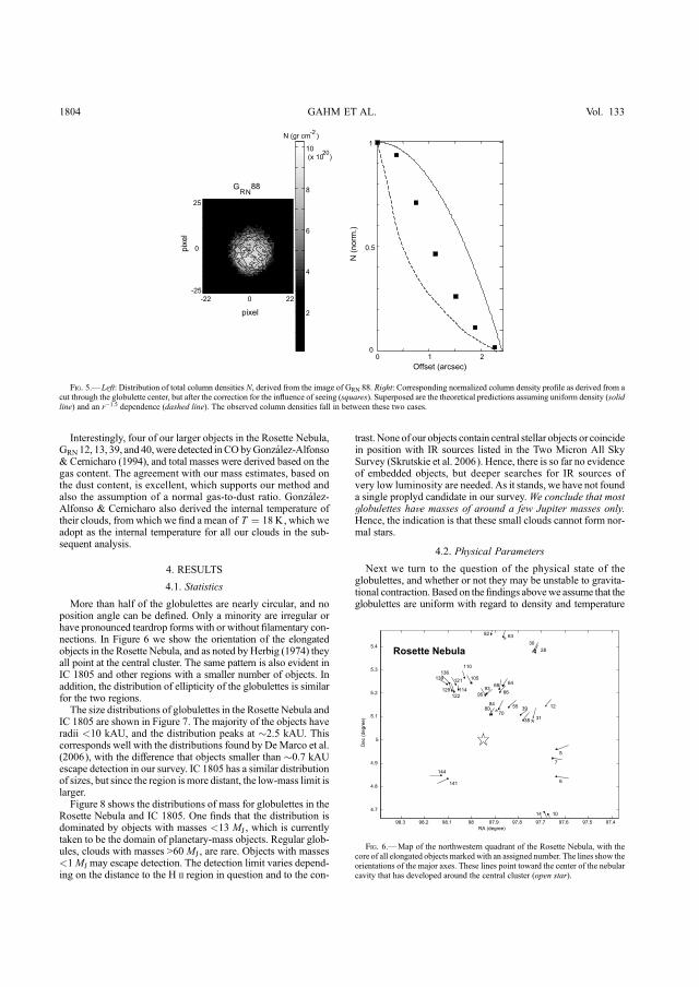
Interestingly, four of our larger objects in the Rosette Nebula,GRN 12, 13, 39, and 40,were detected inCObyGonzalez-Alfonso& Cernicharo (1994), and total masses were derived based on thegas content. The agreement with our mass estimates, based onthe dust content, is excellent, which supports our method andalso the assumption of a normal gas-to-dust ratio. Gonzalez-Alfonso & Cernicharo also derived the internal temperature oftheir clouds, from which we find a mean of T ¼ 18 K, which weadopt as the internal temperature for all our clouds in the sub-sequent analysis.
4. RESULTS
4.1. Statistics
More than half of the globulettes are nearly circular, and noposition angle can be defined. Only a minority are irregular orhave pronounced teardrop forms with or without filamentary con-nections. In Figure 6 we show the orientation of the elongatedobjects in the Rosette Nebula, and as noted by Herbig (1974) theyall point at the central cluster. The same pattern is also evident inIC 1805 and other regions with a smaller number of objects. Inaddition, the distribution of ellipticity of the globulettes is similarfor the two regions.
The size distributions of globulettes in the Rosette Nebula andIC 1805 are shown in Figure 7. The majority of the objects haveradii <10 kAU, and the distribution peaks at �2.5 kAU. Thiscorresponds well with the distributions found by DeMarco et al.(2006), with the difference that objects smaller than �0.7 kAUescape detection in our survey. IC 1805 has a similar distributionof sizes, but since the region ismore distant, the low-mass limit islarger.
Figure 8 shows the distributions of mass for globulettes in theRosette Nebula and IC 1805. One finds that the distribution isdominated by objects with masses <13 MJ , which is currentlytaken to be the domain of planetary-mass objects. Regular glob-ules, clouds with masses >60 MJ , are rare. Objects with masses<1MJ may escape detection. The detection limit varies depend-ing on the distance to the H ii region in question and to the con-
trast. None of our objects contain central stellar objects or coincidein position with IR sources listed in the Two Micron All SkySurvey (Skrutskie et al. 2006). Hence, there is so far no evidenceof embedded objects, but deeper searches for IR sources ofvery low luminosity are needed. As it stands, we have not founda single proplyd candidate in our survey.We conclude that mostglobulettes have masses of around a few Jupiter masses only.Hence, the indication is that these small clouds cannot form nor-mal stars.
4.2. Physical Parameters
Next we turn to the question of the physical state of theglobulettes, and whether or not they may be unstable to gravita-tional contraction. Based on the findings abovewe assume that theglobulettes are uniform with regard to density and temperature
Fig. 5.—Left: Distribution of total column densities N, derived from the image of GRN 88. Right: Corresponding normalized column density profile as derived from acut through the globulette center, but after the correction for the influence of seeing (squares). Superposed are the theoretical predictions assuming uniform density (solidline) and an r�1.5 dependence (dashed line). The observed column densities fall in between these two cases.
Fig. 6.—Map of the northwestern quadrant of the Rosette Nebula, with thecore of all elongated objects markedwith an assigned number. The lines show theorientations of the major axes. These lines point toward the center of the nebularcavity that has developed around the central cluster (open star).
GAHM ET AL.1804 Vol. 133
and that they can be approximated by spheres. The temperatureis set to T ¼ 18 K, from the empirically derived mean by Gon-zalez-Alfonso & Cernicharo (1994) mentioned in x 3. The in-ternal gas pressures were calculated and scatter around 2:5 ;10�11 dyn cm�2. Since we have no evidence of embeddedsources, we expect no mechanism of internal turbulence, whichis hence neglected in the subsequent analysis. In addition, weassume that there is no rotation or any remaining frozen-inmagnetic fields. We then compute the total thermal energy of theglobulettes,K, assuming that all hydrogen is molecular and has astandard mean molecular weight of � ¼ 2:4. The potential en-ergyW ¼ �3GM 2/5r for this type of object, where r is the meanradius defined in x 3. The virial theorem is applied, and in thisfirst step the criterion for a globulette to contract would be2K/(�W ) < 1. One then finds that with the assumptions made,the condition for gravitational contraction is not realized, and that
only a few of the most massive clouds are close to virial equi-librium. One would then expect all globulettes to disintegrate onshort timescales, just as was concluded in earlier surveys. How-ever, the influence of the outer pressure exerted by the warm,turbulent plasma surrounding the objects has been neglected sofar, andwe proceed to estimate its effect on the globulettes in ques-tion, focusing on objects in the Rosette Nebula and IC 1805.
For the Rosette Nebula there is rather detailed information onelectron temperatures Te, electron densities ne, degrees of ioniza-tion and turbulent velocities at different locations within the neb-ula. Most of our globulettes reside in the northern and westernparts. From the non-LTE calculations by Celnik (1985) we adoptTe ¼ 5800 K and ne ¼ 10 cm�3 to represent all our locations.From information on the degree of ionization of the gas and as-suming a cosmic chemical composition, the total number densi-ties nwere calculated, then providing an estimate of the outer gas
Fig. 7.—Size distributions of globulettes in the Rosette Nebula and IC 1805 in terms of the mean radius. The distributions peak at�2.5 kAU. A few observed objectswith sizes >10 kAU fall outside the range.
Fig. 8.—Mass distributions of globulettes found in the Rosette Nebula and IC 1805 in intervals of 13MJ. A few ordinary globules with masses�600MJ are outside therange. Most globulettes have masses of <13 MJ; i.e., they are of planetary mass.
GLOBULETTES AS SEEDS OF LOW-MASS OBJECTS 1805No. 4, 2007

pressure of Pgas ¼ 1:8 ; 10�11 dyn cm�2. Turbulent velocitiesv turb were inferred by Viner et al. (1979) from the width of ra-dio recombination lines. Very high turbulent velocities, v turb ¼36 km s�1, were found in the southeastern quadrant, diminishingto 11 km s�1 to the west and even less in the northwest, v turb <7 km s�1. Taking v turb ¼ 10 km s�1 as representative we calculatean average turbulent pressure of Pturb ¼ 2:9 ; 10�11 dyn cm�2,rather close to the case of equipartition between thermal and tur-bulent energies. For the subsequent calculation of the total outerpressures we simply assumed that such an equipartition holds forall our regions. For IC 1805, Tereby et al. (2003) also found elec-tron densities of�10 cm�3. The conditions in IC 1805 are similarto those of the Rosette Nebula, and therefore, we have used ourestimated average value of the total outer pressure of Pout ¼ 3:6 ;10�11 dyn cm�2 for the subsequent analysis of all our globulettesin both the RosetteNebula and IC 1805. The total outer pressure istypically a factor of �1.5 higher than the internal gas pressures.
Including the outer pressure in the virial theorem, the con-dition for gravitational contraction is 2K/(�W þ 3PoutV ) < 1(where V is the volume). This quantity was computed for theglobulettes in the Rosette Nebula and IC 1805, and the results areshown in Table 3. In contrast to the first calculation made above,we now find that a majority of the globulettes can contract. Ofthese a total of 43 objects have masses below 13 MJ and wouldform planetary-mass objects rather than brown dwarfs.
Hence, we find that the outer pressure is a critical parameterwhen applying the virial theorem to the globulettes. Small changes
in the assumptions leading to the calculated value of Pout will dras-tically change the number of objects that we predict to contract.Even with zero turbulent pressure, a number of objects wouldcontract, and these are marked with an asterisk in Table 3. If thegas temperature is more like 104 K, which is often assumed forH ii regions, then more objects are confined and can contract.This would also happen were the internal temperatures lower thanthe 18 K adopted, like in normal globules (Martin & Barret 1978;Keene 1981). The exact definition of where to draw the outerborder of a given globulette is also of importance, especially inthe cases in which the outskirts are diffuse.However, there are two more pressure forces to consider. One
is the radiation pressure Prad , acting on the globulette on the sidefacing the star. The total luminosity of all cluster stars was foundto be 4:3 ; 106 L� for IC 1805 (Massey 1995), as well as for theRosette Nebula (Cox et al. 1990). Amajority of the globulettes inthe Rosette Nebula are located in areas close to the filamentaryshell from which the Wrench trunk also extends, and this systemis a foreground network of filaments, with the Wrench trunktilted by�45� to the plane of the sky (Schneps et al. 1980; Gahmet al. 2006). Hence, the globulettes are located rather far out inthe spherical nebula. From this we derive a distance to the centralO stars of �8 pc, and the expected radiation pressure at thisdistance is Prad � 8:5 ; 10�11 dyn cm�2. Note that elongated ob-jects in this area are likely to be tilted by�45� to the line of sight,but when including this geometry in the derivation of the meandensity, the differences to the values presented in Table 2 are small.
TABLE 3
Virial Conditions, X ¼ 2K/ �W þ 3PoutVð Þ, of Selected Globulettes in IC 1805 and the Rosette Nebula
Object X Object X Object X Object X Object X Object X
IC 1805
1� ............... 0.35 4� .............. 0.33 7� .............. 0.43 10.............. 0.78 13.............. 0.69 16� ............ 0.37
2................. 0.70 5� .............. 0.50 8� .............. 0.34 11.............. 1.05 14.............. 0.66 17� ............ 0.53
3................. 1.53 6................ 0.62 9................ 1.14 12.............. 0.98 15.............. 2.97 18.............. 1.48
Rosette Nebula
1................. 0.87 26.............. 1.53 51.............. 1.02 76.............. 1.78 101� .......... 0.26 126............ 1.71
2................. 0.51 27.............. 1.32 52� ............ 0.40 77.............. 0.65 102............ 1.29 127............ 1.71
3................. 1.50 28� ............ 0.30 53.............. 0.59 78.............. 2.03 103............ 1.07 128............ 2.92
4................. 0.56 29.............. 1.06 54.............. 0.72 79� ............ 0.36 104............ 1.12 129� .......... 0.24
5� ............... 0.34 30� ............ 0.24 55� ............ 0.43 80.............. 1.24 105� .......... 0.52 130............ 3.76
6................. 0.86 31� ............ 0.28 56.............. 0.73 81.............. 0.87 106............ 1.84 131............ 1.27
7................. 0.70 32.............. 0.97 57.............. 0.57 82.............. 0.78 107............ 0.94 132............ 2.41
8................. 0.58 33.............. 0.83 58.............. 0.71 83.............. 1.51 108............ 1.06 133............ 0.78
9� ............... 0.51 34.............. 0.61 59.............. 0.72 84.............. 1.22 109............ 0.92 134............ 2.66
10............... 0.75 35.............. 0.55 60.............. 0.89 85.............. 0.95 110� .......... 0.25 135............ 1.99
11............... 0.68 36.............. 2.00 61.............. 0.86 86.............. 2.31 111............ 1.32 136............ 1.09
12............... 0.62 37.............. 0.65 62.............. 0.64 87.............. 0.60 112............ 1.04 137............ 3.10
13� ............. 0.52 38.............. 0.66 63� ............ 0.46 88.............. 0.67 113� .......... 0.38 138............ 3.78
14............... 0.62 39.............. 0.89 64.............. 0.63 89.............. 1.11 114� .......... 0.43 139............ 1.11
15............... 1.17 40� ............ 0.48 65.............. 0.55 90.............. 1.08 115............ 1.08 140............ 0.62
16............... 1.08 41.............. 2.98 66.............. 0.69 91.............. 0.57 116............ 2.64 141� .......... 0.24
17............... 0.82 42.............. 1.55 67.............. 0.76 92.............. 1.25 117............ 0.85 142� .......... 0.25
18............... 1.21 43.............. 0.80 68� ............ 0.52 93� ............ 0.49 118............ 0.94 143� .......... 0.40
19............... 0.71 44.............. 0.69 69.............. 1.14 94.............. 0.67 119............ 0.98 144............ 0.63
20............... 0.72 45� ............ 0.38 70.............. 0.86 95.............. 0.68 120............ 1.02 145� .......... 0.52
21............... 1.02 46.............. 0.80 71.............. 1.73 96.............. 1.15 121............ 0.66
22............... 0.89 47� ............ 0.39 72� ............ 0.25 97.............. 1.10 122............ 0.64
23............... 0.97 48.............. 0.97 73� ............ 0.43 98.............. 1.24 123............ 8.39
24� ............. 0.39 49.............. 0.72 74.............. 1.36 99.............. 0.78 124............ 3.62
25............... 1.15 50.............. 0.80 75.............. 1.50 100............ 1.41 125............ 0.82
Note.—Asterisks indicate X < 1, also without external turbulence.
GAHM ET AL.1806 Vol. 133

The globulettes in fields 5, 9, 10, 12, and 17 are at about the samedistance from the center, since they are located closer to the planeof the sky, and for these objects we expect similar values of Prad.The globulettes in IC 1805 are close to the sky plane but at a largerdistance from the central cluster, and for these objects we derivePrad � 1 ; 10�11 dyn cm�2.
If the globulettes are lagging behind in the general expandingplasma in the H ii regions, then additional force from the ram pres-sure Pram will also act on the globulette surface facing the centralcluster. If the difference in velocity between the plasma flow andthe globulettes is �v and the plasma density is �p, then Pram ¼(�v)2�p. It was concluded byGahm et al. (2006) that the elephanttrunks have already accelerated in the expanding plasma, and thatthe difference between flow velocity and trunk velocity can max-imally be a few kilometers per second. Many of our globulettescluster in areas surrounding trunks, and many have no tails, indi-cating substantial interaction with gas flows and radiation. Thisalso indicates that the globulettes are flowing outward, andmay infact once have been detached from the radiallymoving trunks.Witha�v of a fewkilometers per second only,Pram � 10�12 dyn cm�2,i.e., an order of magnitude smaller than the radiation pressure.For the globulettes with evidence of surface activity, and withpronounced teardrop forms, we simply do not know what thetrade-off is between warm plasma flowing around the globulettesand the radiation pressure, both resulting in shaping the objectsand inducing surface activity.
The combined radiation and ram pressures produce an extraforce on one side of the globulette, and one could envision howobjects close to virial equilibrium will become compressed andstart imploding from the side facing the central clusters. How-ever, the globulettes are also subject to disrupting forces. So farwe have regarded the objects to be stationary, but in the follow-ing the dynamic states of the globulettes are also considered.
5. DISCUSSION
The surveys of small, dark clouds, globulettes, in H ii regionsindicate that some regions may host hundreds of such objects,while other regions contain just a few. Many globulettes are dark,round and isolated, and in earlier studies (Reipurth et al. 2003;De Marco et al. 2006) it was speculated that blocks of obscur-ing material closer to the central clusters would screen the objectsfrom direct stellar light, since the timescales for photoevaporationwere expected to be short,<100 yr. The central regions in, for in-stance, the Rosette Nebula and IC 1805 are void of any obscuringstructures, and it appears that the shell structures with the asso-ciated elephant trunks are not always spherically distributed aroundthe expanding H ii regions. The question of their survival againstradiation must be reconsidered, and below we also discuss theorigin and evolution of the globulettes.
5.1. Photoevaporation
The effects of photoevaporation on interstellar clouds havebeen investigated by Bertoldi (1989), Bertoldi &McKee (1990),and Gorti & Hollenbach (2002), and the theory has been appliedto globules in H ii regions such as IC 1848 (Lefloch & Lazareff1995), the Rosette Nebula (White et al. 1997), and NGC 3372(Smith et al. 2004). Similar processes occur in knots developingteardrop shapes in planetary nebulae (see, e.g., Canto et al. 1998;Mellema et al. 1998; Lopez-Martın et al. 2001). A cloud exposedto radiation will go through a two-step process. During the firstphase the impinging photons start to ionize the surface layers.Overpressure leads to outgassing at the surface at the same timeas a shock wave is driven inward, leading to compression and
moderate heating. The time for the shock to pass the entire cloudis relatively short, but next the clump evolves into a ‘‘cometaryphase,’’ in which the object is slowly further compressed andsculpted into a teardrop form. An ionization front is set up in theobject and produces a flow streaming outward, and this flow ab-sorbs incoming photons. Therefore, the short timescales for dis-ruption of globulettes discussed above, relying on the total massavailable for ionization in comparison to the number of incomingphotons, does not apply. Instead, it is more appropriate to considerthe timescale for contraction of clumps during this second phaseof evolution. Following Mellema et al. (1998), the timescale forcomplete ionization of a clump is
tion ¼ t�5
6þ ln 1þ �ð Þ
6�
� �; ð2Þ
where t� ¼ v�h0/c20 , with v� being the velocity of the ionization
front, c0 the sound speed of the neutral medium, and h0 the char-acteristic size of an object, and � is related to the incident flux ofionizing Lyman continuum photons, the recombination coefficient,the size of the object, and the isothermal sound speed in theionized medium.With the parameters relevant to our globulettes,it is realized that the last term in the brackets in equation (2) isnegligible, and tion � t�. Conservatively setting h0 ¼ r, we findthat the expected lifetimes of globulettes against photodisinte-gration scatter around 3:8 ; 106 yr, which is comparable to thecluster age and much longer than the timescales estimated earlier.We conclude that the objects may survive destruction from photo-evaporation for a very long time. This explains the presence ofisolated globulettes in regions unprotected from radiation fromthe central cluster. It also implies that a given clump can detachfrom a filamentary shell, or an elephant trunk, and move far outinto the surrounding plasma without losing much mass. Far fromall our globulettes show clear signs of bright rims indicative ofongoing photoevaporation. Many of these are unstable againstcontraction but may lack the particular implosion phase drivenby photoevaporation.
5.2. Contraction
The timescale for gravitational collapse is given by
tA ¼
ffiffiffiffiffiffiffiffiffiffiffiffiffiffi3�
32G�0
s; ð3Þ
where �0 is the density. For the objects that we found to be un-stable and able to contract in the Rosette Nebula, tff is in the rangeof 2 ; 105Y4 ; 105 yr, and for those in IC 1805 around 6:5 ;105 yr. Thus, the estimated contraction times for the globulettesin the Rosette Nebula and in IC 1805 are much smaller than thetimescale derived above for photoevaporation. Therefore, it ap-pears that our globulettes can contract to form low-mass objects,brown dwarfs or planetary-mass objects, even long before theclouds start to dissolve. One would therefore expect that objectsformed early in the evolution of the expanding H ii region wouldhave long since either disintegrated or formed low-mass objects,which could be one explanation of the absence of globulette-likebodies in the central parts of the Orion Nebula (Bally et al. 2000).The central regions of the Rosette Nebula and IC 1805 are voidof dark markings in optical images, but the elephant trunks inthe outskirts are expanding outward with the shell (Gahm et al.2006). One must therefore assume that the filaments and cloudsonce developed in the central region have already accelerated
GLOBULETTES AS SEEDS OF LOW-MASS OBJECTS 1807No. 4, 2007

and moved outward, which may also be the case in the OrionNebula.
5.3. Origins
So far no survey of an entireH ii region has beenmade to searchfor tiny clouds. Nevertheless, the absence of dark markings onexisting images of the central parts of many regions suggests thatthe globulettes are located farther out, close to the elephant trunksand the shells.We note that Vannier et al. (2001) and Lacomb et al.(2004) discovered a number of tiny clumps embedded in largermolecular clouds. It is of course possible that when a parent mo-lecular cloud disperses these cores are left free and will appear asglobulettes. Regardless of this, we have found that the elephanttrunks are filamentary and contain clumps, and it is natural to as-sume that these clumps are the embryos of the globulettes, whichfragment from the trunks. We have many examples of tiny darkclouds with filamentary connections to shells or trunks. Exam-ples of such semidetached globulettes are G1805 5, 8, and 12 andGRN 13, 52, and 102. One can envision how the dark cores even-tuallywill detach from the filaments and form isolated globulettes.
As pointed out by Gahm et al. (2006), many trunks have jaw-like heads with clumps swinging out in the surrounding plasmawith rotation. A dramatic example is the so-called Batman trunkin DWB 44, where the head has evolved into an extended wingof filamentary and knotty material, which is moving at high an-gular speed. It was also pointed out that many trunk heads havedeveloped filamentary ‘‘strings,’’ which have detached from thetrunks. Structures like these can be expected to erode quicklyand form smaller bodies.
In the area surrounding the Wrench trunk there are several in-teresting features that may be key objects in understanding thecreation of globulettes. Figure 3 (middle left) shows an area tothe northeast of the Wrench trunk, which includes the objectsGRN 87Y95. To the north is a typical jawlike head with helicalfilamentary endings in a trunk extending north. The string of glob-ulettes appears to be connected to theWrench trunk, however, andthe globulettes must have formed as a result of fragmentation of afilament that became detached from the trunk. South of the stringthere are diffuse globulettes with bright halos, some of whichhave faint filamentary connections to the string, and therefore, itappears that these are already in amore advanced phase of erosionfrom photoevaporation and possibly streaming plasma.
Figure 3 (bottom right) shows the area south of the Wrenchtrunk, including the remarkable clumps at the edge of each jaw,GRN 73 and 79, which are still attached to the trunk. South of thejaws are several objects with dark cores and bright sphericalhalos, GRN 78, 80, and 84, and in addition, there are a few diffuseobjects without visible dense cores. The jaw in theWrench rotates,and the whole trunkmoves radially outward from the central clus-ter. The massive head lags behind in the expansion, so the trunk isstretching. The trunk, therefore, is subject to several disruptingforces. The assembly of small clouds could result from an erosionprocess, in which smaller clouds fragment in the head and are be-ing chopped off from the trunk. They start to photoevaporate, andbright rims and halos develop. Some of these still maintaindense cores, while others appear to be almost entirely dissolved.Globulettes originating from clumps in rotating trunks can startmoving away from the trunks.
The relatively large clumps, GRN 73 and 79 attached to thejaws, could then be precursors of isolated globulettes, such asthose found rather far out from the main trunk. The condition ofcontraction is satisfied (see Table 3), and since the ratio of life-times is tA/t�T1 for the objects in question, they will have timeto contract long before they are dissolved by photodisintegra-
tion. The globulettes with dark cores surrounded by bright halossouth of the jaws could represent an intermediate phase beforesubstellar objects are eventually formed. It is puzzling that thehalos around these objects are spherical and not just bright rimsfacing the cluster. They cannot be teardrops with the bright rimon the backside seen from us, in which case they would point in adirection away from the central cluster. As mentioned above, thedirection to the central cluster for these objects is at an angle of�45
�to the plane of the sky. If bright rims are developing on the
side facing the cluster, then wewould observe asymmetric brightrims oriented toward the center. These objects are engulfed in gasand dust, which eroded from the main trunk at an earlier phase. Itis possible that scattered Lyman continuum photons may contrib-ute significantly to the photoevaporation in this environment, inwhich case spherical, bright halos could form from recombination.Another puzzle is that there are isolated objects that lack any sign ofsurface activity. Could it be that the outgassing bubbles are so thinthat they are below the detection threshold of our H� images, orthat most emission originates from the backside of the objects?Our survey has demonstrated that some H ii regions host a
large number of small clouds, which have fragmented from el-ephant trunks and shell structures. These clouds, the globulettes,come in different forms, and although many show evidence ofsurface activity induced by stellar radiation, and possibly alsoplasma flows, there are numerous examples of isolated dark ob-jects without any detected signs of interaction with the environ-ment. The majority of the objects are of planetary mass and areunstable against contraction when considering the influence ofthe outer pressure exerted by the surrounding plasma. In addi-tion, the flow of incident Lyman continuum photons leads tophotoevaporation, inducing an implosion and shock-driven com-pression in the objects. We have shown that the lifetime againstcomplete ionization from photoevaporation is much longer thanthe expected free-fall time, and hence,we conclude that a numberof the globulettes studied are likely to contract to form both browndwarfs and planetary-mass objects long before the surface layershave dissolved. This is opposite to the case for planetary nebulaeknots, which are smaller and thinner.It cannot be excluded that some globulettes already contain
central mass concentrations, and even substellar objects, andit would be of great interest to search for embedded IR low-luminosity objects. It would also be of interest to make a deepersearch for possible faint halos surrounding isolated globulettesfor which we have not detected any evidence of photoevap-oration. A survey of the small globulettes for molecular emissionwould provide independent checks on the mass estimates, andindirectly on the gas-to-dust ratio, in addition to information aboutthe internal temperatures and radial velocities of the objects.
5.4. Conclusions
Our H� images of a number of fields in H ii regions surround-ing young stellar clusters have revealed that some of these re-gions host a large number of tiny clouds, which appear as darkspots or teardrops when silhouetted against the bright nebular back-ground. A total of 173 such objects, which we call ‘‘globulettes,’’were studied in detail. They are much smaller than normal glob-ules and form a distinct class of objects. Most of our objects areround or only slightly elliptical, and only a minority have brightrims facing the central clusters and/or filamentary connectionsto shells or elephant trunks in the area. We measured positions,dimensions, and orientations of all objects. Most elongatedglobulettes point at the central clusters.We derive the size distributions of the globulettes.Most objects
have mean radii <10 kAU. The majority of our globulettes are
GAHM ET AL.1808 Vol. 133

found in the Rosette Nebula and IC 1805, where the distributionspeak at mean radii of �2.5 kAU, similar to what was found in acouple of previous studies of similar objects in other H ii regions.
We estimate the total mass of each globulette bymeasuring theextinction of background light, assuming standard laws of extinc-tion and calibrations of the column densities of dust versus totalcolumn densities. An average mass was calculated from two ex-treme assumptions on the amount of foreground emission presentover the darkest part of each globulette. A few of our mass esti-mates, based on the content of dust, were compared to those basedon the gas content, as derived by others from observations of CO.The agreement between the two independent mass estimates isexcellent.
We find that the globulettes are of substellar mass and that themajority have masses<13MJ , corresponding to planetary-massobjects. None of our objects appear to host embedded stellarsources, unless they are very faint.
From the column density profiles of the globulettes we derivethe distribution of the density, and as a first approximation wecan apply a uniform density law. The total number densities scat-ter around 104 cm�3. We then estimate the internal thermal andpotential energies and find, when also including the effects fromthe outer pressure, that a large fraction of the globulettes could beunstable to gravitational contraction and would form low-massbrown dwarfs or planetary-mass objects on short timescales,<106 yr. In addition, the radiation pressure and ram pressure ex-erted on the side facing the clusters would stimulate contraction.
We show that the isolated globulettes are not screened fromstellar light by dusty clouds in the direction of the central O and
B stars, and we evaluate the effects of photevaporation generatedby the impinging Lyman continuum photons. Following the stan-dard theory developed for photoevaporating knots in planetarynebulae, we estimate the lifetimes for the globulettes to undergototal ionization. These lifetimes scatter around 4 ; 106 yr, muchlonger than estimated in previous studies and also much longerthan the free-fall time. We conclude that a large number of ourglobulettes have time to form central low-mass objects long beforethe ionization front has reached far into the interior. The bright-rimmed globulettes indicate ongoing photoevaporation, but we arepuzzled by the large number of completely dark, round, and iso-lated globulettes lacking any sign of surface activity.
We conclude that the globulettes may very well be seeds ofbrown dwarfs and free-floating planetary-mass objects, and hencethat low-mass objectsmay form in situ in interstellar space and notonly by ejection from, or disruption of, protoplanetary disks. Thenewly discovered binary systems with components of very lowmass may indicate similar formation scenarios.
Finally, we discuss the formation of globulettes with examplessuggesting that they may form from the fragmentation of struc-tures inherent in eroding elephant trunks.
This work was supported by the Carl Trygger Foundation, theSwedish National Space Board, and the Swedish National Grad-uate School of Space Technology. We thank Magnus Galfalk fora coordinate transfer program and Garrelt Mellema for discus-sions about lifetimes of photoevaporating globulettes. We alsothank the referee, CharlesRobertO’Dell, for constructive criticism.
REFERENCES
Bally, J., O’Dell, C. R., & McCaughrean, M. J. 2000, AJ, 119, 2919Bertoldi, F. 1989, ApJ, 346, 735Bertoldi, F., & McKee, C. F. 1990, ApJ, 354, 529Bohlin, R. C., Savage, B. D., & Drake, J. F. 1978, ApJ, 224, 132Canto, J., Raga, A., Steffen, W., & Shapiro, P. R. 1998, ApJ, 502, 695Carlqvist, P., Gahm, G. F., & Kristen, H. 2003, A&A, 403, 399Celnik, W. E. 1985, A&A, 144, 171Cox, P., Deharveng, L., & Leene, A. 1990, A&A, 230, 181De Marco, O., O’Dell, C. R., Gelfond, P., Rubin, R. H., & Glover, S. C. O.2006, AJ, 131, 2580
Dickel, H. R., Wendker, H., & Bieritz, J. H. 1969, A&A, 1, 270Fitzgibbon, A. W., Pilu, M., & Fischer, R. B. 1996, in Proc. 13th Intl. Conf.Pattern Recognition, Vol. 1, ed. W. Kropatsch (Los Alamitos: IEEE Comput.Soc.), 253
———. 1999, IEEE Trans. on Pattern Analysis and Machine Intelligence, 21,476
Gahm, G. F., Carlqvist, P., Johansson, L. E. B., & Nikolic, S. 2006, A&A, 454,201
Gonzalez-Alfonso, E., & Cernicharo, J. 1994, ApJ, 430, L125Gorti, U., & Hollenbach, D. 2002, ApJ, 573, 215Grenman, T. 2006, licentiate thesis, Lulea Univ. Tech.Guetter, H. H., & Vrba, F. J. 1989, AJ, 98, 611Gyul’budagyan, A. L., Oganyan, G. B., & Akhverdyan, L. G. 1994, Astrofizika,37, 577
Herbig, G. 1974, PASP, 86, 604Hester, J. J., et al. 1996, AJ, 111, 2349Jayawardhana, R., & Ivanov, V. D. 2006a, ApJ, 647, L167———. 2006b, Science, 313, 1279Kaltcheva, N. T., & Hilditch, R. W. 2000, MNRAS, 312, 753Keene, J. 1981, ApJ, 245, 115Kharchenko, N. V., Piskunov, A. E., Roser, S., Schilbach, E., & Scholz, R.-D.2005, A&A, 438, 1163
Kroupa, P., & Bouvier, J. 2003, MNRAS, 346, 369Lacombe, F., et al. 2004, A&A, 417, L5
Lefloch, B., & Lazareff, B. 1995, A&A, 301, 522Leung, C. M. 1985, in Protostars and Planets II, ed. D. C. Black & M. S.Matthews (Tucson: Univ. Arizona Press), 104
Lopez-Martın, L., Raga, A. C., Mellema, G., Henney, W. J., & Canto, J. 2001,ApJ, 548, 288
Lucas, P. W., & Roche, P. F. 2000, MNRAS, 314, 858Luhman, K. L., et al. 2005, ApJ, 635, L93MacConnell, D. J. 1968, ApJS, 16, 275Martin, R. N., & Barret, A. H. 1978, ApJS, 36, 1Massey, P. 1995, ApJ, 454, 151McCaughrean, M. J., & O’Dell, C. R. 1996, AJ, 111, 1977Mellema, G., Raga, A. C., Canto, J., Lundqvist, P., Steffen, W., & Noriega-Crespo, A. 1998, A&A, 331, 335
O’Dell, C. R., & Wen, Z. 1994, ApJ, 436, 194Ogura, K., & Ishida, K. 1981, PASJ, 33, 149Reipurth, B., Corporon, P., Olberg, M., & Tenorio-Tagle, G. 1997, A&A, 327,1185
Reipurth, B., Raga, A., & Heathcote, S. 2003, AJ, 126, 1925Savage, B. D., & Mathis, J. S. 1979, ARA&A, 17, 73Schneps, M. H., Ho, P. T. P., & Barret, A. H. 1980, ApJ, 240, 84Skrutskie, M. F., et al. 2006, AJ, 131, 1163Smith, N., Bally, J., & Morse, J. A. 2003, ApJ, 587, L105Smith, N., Barba, R. H., & Walborn, N. R. 2004, MNRAS, 351, 1457Sung, H., Bessell, M. S., & Lee, S.-W. 1997, AJ, 114, 2644Tereby, S., Fich, M., Taylor, R., Cao, Y., & Hancock, T. 2003, ApJ, 590, 906Thackeray, A. D. 1950, MNRAS, 110, 524Tjin A Djie, H. R. E., van den Ancker, M. E., Blondel, P. F. C., Shevchenko, V. S.,Ezhkova, O. V., de Winter, D., & Grankin, K. N. 2001, MNRAS, 325, 1441
Vannier, L., Lemaire, J. L., Field, D., Pineau des Forets, G., Pijpers, F. P., &Rouan, D. 2001, A&A, 366, 651
Viner, M. R., Valle, J. P., & Hughes, V. A. 1979, AJ, 84, 1335White, G. J., Lefloch, B., Fridlund, C. V. M., Aspin, C. A., Dahmen, G.,Minchin, N. R., & Huldtgren, M. 1997, A&A, 323, 931
Zapatero Osorio, M. R., et al. 2000, Science, 290, 103
GLOBULETTES AS SEEDS OF LOW-MASS OBJECTS 1809No. 4, 2007


Paper II
The tiny globulettes in the Carina Nebula
Authors:Grenman, T., & Gahm, G. F.


A&A 565, A107 (2014)DOI: 10.1051/0004-6361/201423532c© ESO 2014
Astronomy&
Astrophysics
The tiny globulettes in the Carina nebula?,??
T. Grenman1 and G. F. Gahm2
1 Applied Physics, Department of Engineering Sciences & Mathematics, Luleå University of Technology, 971 87 Luleå, Swedene-mail: [email protected]
2 Stockholm Observatory, AlbaNova University Centre, Stockholm University, 106 91 Stockholm, Sweden
Received 29 January 2014 / Accepted 18 March 2014
ABSTRACT
Context. Small molecular cloudlets are abundant in many H regions surrounding newborn stellar clusters. In optical images theseso-called globulettes appear as dark silhouettes against the bright nebular background.Aims. We aim to make an inventory of the population of globulettes in the Carina nebula complex, and to derive sizes and masses forcomparisons with similar objects found in other H regions.Methods. The globulettes were identified from Hα images collected at the Hubble Space Telescope.Results. We have located close to 300 globulettes in the Carina complex, more than in any other region surveyed so far. The objectsappear as well-confined dense clumps and, as a rule, lack thinner envelopes and tails. Objects with bright rims are in the minority, butmore abundant than in other regions surveyed. Some globulettes are slightly elongated with their major axes oriented in the directionof young clusters in the complex. Many objects are quite isolated and reside at projected distances >1.5 pc from other molecularstructures in the neighbourhood. No globulette coincides in position with recognized pre-main-sequence objects in the area. Theobjects are systematically much smaller, less massive, and much denser than those surveyed in other H regions. Practically allglobulettes are of planetary mass, and most have masses less than one Jupiter mass. The average number densities exceed 105 cm−3 inseveral objects. We have found a statistical relation between density and radius (mass) in the sense that the smallest objects are alsothe densest.Conclusions. The population of small globulettes in Carina appears to represent a more advanced evolutionary state than thoseinvestigated in other H regions. The objects are subject to erosion in the intense radiation field, which would lead to a removal ofany thinner envelope and an unveiling of the core, which becomes more compact with time. We discuss the possibility that the coremay become gravitationally unstable, in which case free-floating planetary mass objects can form.
Key words. HII regions – dust, extinction – evolution – ISM: individual objects: Carina nebula
1. Introduction
Optical images of galactic H regions show a mix of bright anddark nebulosity. Foreground cold dust clouds obscure the brightbackground of warm and ionized gas. The warm plasma in thesenebulæ accelerates outwards through the interaction with radia-tion and winds from hot and massive stars. The molecular gasis swept up and forms expanding shells, which are sculpted intocomplex filamentary formations, like elephant trunks, pillars thatpoint at O stars in the nebula. Blocks of cold gas can detachfrom the shells and trunks and may fragment into smaller cloudsthat appear as dark patches on optical images of these nebulæ asnoted long ago by Bok & Reilly (1947) and Thackeray (1950).The clumps may be round or shaped like tear drops, some withbright rims facing the central cluster (Herbig 1974).
A number of such H regions have been subject to moredetailed studies, and it has been found that many regions con-tain distinct, but very small clumps, extending over less thanone to a few arcseconds. Several studies have focused on the so-called proplyds, which are photoevaporating discs surroundingvery young stars (e.g. O’Dell et al. 1993; O’Dell & Wen 1994;McCaughrean & O’Dell 1996; Bally et al. 2000; Smith et al.
? Based on observations collected with the NASA/ESA HubbleSpace Telescope, obtained at the Space Telescope Science Institute.?? Appendices are available in electronic form athttp://www.aanda.org
2003). In these studies small cloudlets without any obvious cen-tral stellar objects were also found, as also recognized by Hesteret al. (1996) and Reipurth et al. (1997, 2003) from Hubble SpaceTelescope (HST) images of nebular regions.
More systematic studies of such star-less cloudlets followed,and from the surveys of more than 20 H regions by De Marcoet al. (2006), Grenman (2006), and Gahm et al. (2007; here-after Paper I) it can be concluded that most of the objects haveradii <10 kAU with size distributions that peak at ∼2.5 kAU. InPaper I masses were derived from extinction measures indicatingthat most objects have masses <13 MJ (Jupiter masses), whichcurrently is taken to be the domain of planetary-mass objects.This class of tiny clouds in H regions were called globulettesin Paper I to distinguish them from proplyds and the much largerglobules spread throughout interstellar space. We define glob-ulettes as cloudlets with round or slightly elongated shapes withor without bright rims and/or tails.
Some globulettes are connected by thin filaments to largermolecular blocks and it is then natural to assume that isolatedglobulettes once detached from shells and trunks. They may alsosurvive in this harsh environment for long times, as concludedin Paper I. Follow-up 3D numerical simulations in Kuutmann(2007) predict lifetimes of ∼104 years, increasing with mass.Owing to the outer pressure exerted on the globulettes fromsurrounding warm gas, and the penetrating shock generated byphotoionization, it was found that many globulettes may even
Article published by EDP Sciences A107, page 1 of 19
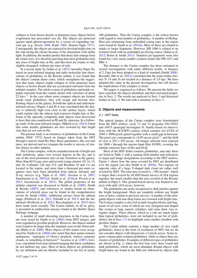
A&A 565, A107 (2014)
collapse to form brown dwarfs or planetary-mass objects beforeevaporation has proceeded very far. The objects are protectedagainst rapid photoevaporation by a screen of expanding ion-ized gas (e.g. Dyson 1968; Kahn 1969; Tenorio-Tagle 1977).Consequently, the objects are expected to develop bright rims onthe side facing the cluster because of the interaction with stellarlight. In addition, the models predict that dusty tails emerge fromthe cloud cores. It is therefore puzzling that most globulettes lackany trace of bright rims in Hα, and that most are round, or onlyslightly elongated, without any trace of tails.
In a recent study by Gahm et al. (2013; hereafter Paper II),based on near-infrared imaging and radio molecular line obser-vations of globulettes in the Rosette nebula, it was found thatthe objects contain dense cores, which strengthens the sugges-tion that many objects might collapse to form planetary-massobjects or brown dwarfs that are accelerated outwards from thenebular complex. The whole system of globulettes and trunks ex-pands outwards from the central cluster with velocities of about22 km s−1. In the case where more compact objects are formedinside some globulettes, they will escape and become free-floating objects in the galaxy. In both the optical and radio/near-infrared surveys (Papers I and II) it was concluded that the den-sity is relatively high even close to the surface layers, whichcould explain why the objects lack extensive bright rims in Hα.Some of the optically completely dark objects were discoveredto have thin rims manifested in Pβ and H2 emission. In a follow-up study of the near-infrared images, Mäkelä et al. (2014) foundthat some smaller globulettes are also crowned by thin brightrims that are not seen in Hα.
The present study is an inventory of globulettes in the Carinanebula (NGC 3372) based on images taken from the HSTthrough a narrow-band Hα filter. Basic parameters, like size andmass, are derived and we compare the results to surveys of sim-ilar objects in other nebulae.
The Carina complex, with its extended network of bright anddark nebulosity, spans over several degrees in the sky and isone of the most prominent sites of star formation in the galaxy.More than 60 O-type stars and several young clusters (Tr 14, 15,and 16; Collinder 228 and 232; and Bochum 10 and 11) arelocated in the region, and more than a thousand pre-main se-quence stars have been identified from optical, infrared, andX-ray surveys (e.g. Tapia et al. 2003; Ascenso et al. 2007;Sanchawala et al. 2007a,b; Smith et al. 2010a,b; Povich et al.2011; Gaczkowski et al. 2013). The global properties of thenebular material was discussed in Smith et al. (2000), Smith& Brooks (2007), and references to studies based on obser-vations of selected areas can be found in the comprehensivereview by Smith (2008). Additional surveys from the submmrange (Preibisch et al. 2011; Pekruhl et al. 2013) and the far-infrared (Preibisch et al. 2012; Roccatagliata et al. 2013) havebeen made more recently. The Carina nebula, in all its glory,is presented in multicolour mosaics found at the Hubble SpaceHeritage webpage.
A number of small obscuring structures in the Carina neb-ula were noted by Smith et al. (2003) from HST images, andwere regarded as possible proplyds. However, the objects studiedwere found to be larger than the standard cases in the Orion neb-ula (Bally et al. 2000). More objects of this nature were recog-nized by Smith et al. (2004) who stated that their nature remainsambiguous: “analogues of Orion’s proplyds, starless cometaryclouds, or something in-between?” Ascenso et al. (2007), how-ever, concluded from near-infrared imaging that these candidatesdo not harbour any stars. Most of these objects are globulettesby our definition and are thereby included in our list of nearly
300 globulettes. Thus the Carina complex is the richest knownwith regard to total number of globulettes. A number of Herbig-Haro jets emanating from embedded young stars in the regionwere found by Smith et al. (2010a). Most of these are related totrunks or larger fragments. However, HH 1006 is related to anisolated cloud with an embedded jet-driving source (Sahai et al.2012; Reiter & Smith 2013). Tentative jet-signatures were alsofound for a few much smaller isolated clouds like HH 1011 andHHc-1.
The distance to the Carina complex has been estimated inseveral investigations with rather different results. A distanceof 2.3 kpc has been adopted as a kind of standard (Smith 2008).Recently, Hur et al. (2012) concluded that the main stellar clus-ters Tr 14 and 16 are located at a distance of 2.9 kpc. We haveadopted this value in the present investigation, but will discussthe implications if the complex is closer.
The paper is organized as follows. We present the fields wehave searched, the objects identified, and their measured proper-ties in Sect. 2. The results are analysed in Sect. 3 and discussedfurther in Sect. 4. We end with a summary in Sect. 5.
2. Objects and measurements
2.1. HST fields
The optical images of the Carina complex were downloadedfrom the HST archive, cycle 13 and 14 programs GO-10241and 10475 (principal investigator N. Smith) based on observa-tions with the ACS/WFI camera, which contains two CCDs of2048 × 4096 pixels glued together with a small gap in between.The pixel size corresponds to ≈0.05 arcsec pixel−1, and the fieldof view is 202 × 202 arcsec. All images selected were exposedfor 1000 s through the narrow-band filter F658N, covering thenebular emission lines of Hα and [N ].
Most of the HST fields contains globulettes, and only theseare listed in Table 1 with a running field number and referencesto target and image designations according to the HST archive.Figure 1 shows how the areas covered by HST are distributedover the region (see also Smith et al. 2010a). Two regions onopposite sides of a large V-shaped dark cloud are rather wellcovered by HST. The total area covered is ∼700 arcmin2, whichis larger than covered by all HST-based surveys of H regionstogether, but much smaller than the area covered of the Rosettenebula in Paper I. This ground-based survey was limited to ob-jects with radii ≥0.8 arcsec, however.
The globulettes are easily recognized as dark patches againstthe bright background. Most are roundish without any brightrims or halos, similar to previous surveys. A number of the elon-gated objects with tear-drop forms are crowned with bright rims.The Carina complex is also rich in dark irregular blocks and frag-ments of all sizes, some of which are very elongated and shapedlike worms or long, narrow cylinders, and some show very ir-regular shapes. These objects, which as a rule are much largerthan typical globulettes, were not included in our list of glob-ulettes, but in Sect. 3.3 we highlight some smaller cloudlets withpeculiar shapes.
The Carina nebula contains a large number of very smallglobulettes, down to the limit of resolution of HST, but we donot consider objects with dimensions ≤3 pixels across. Some re-gions contain quite isolated globulettes, while in others there areclusters of globulettes. Examples of different types of globulettesare shown in Fig. 2, where the first four rows show round anddark globulettes, which are most abundant. Round objects withbright halos are found in the fifth row followed by objects that
A107, page 2 of 19

T. Grenman and G. F. Gahm: The tiny globulettes in the Carina nebula
Table 1. HST archive data used.
Field/Target RA Dec Images(J2000.0) (J2000.0)
1/Pos 30 10:41:27 −59:47:42 J9dk090102/Pos 30 10:41:38 −59:46:17 J9dk090203/Pos 30 10:41:40 −59:44:41 J9dka90104/Pos 19 10:42:23 −59:20:59 J9dk120105/Pos 19 10:42:48 −59:19:44 J9dk320106/Tr 14 10:43:07 −59:29:34 J900c10107/Tr 14 10:43:23 −59:32:06 J900b10108/Tr 14 10:43:24 −59:27:55 J900c20109/Tr 14 10:43:39 −59:34:37 J900a101010/Tr14 10:43:41 −59:30:17 J900b201011/Tr 14 10:43:47 −59:35:53 J9000102012/Tr 14 10:43:55 −59:37:09 J9000101013/HH 666 10:43:58 −59:54:39 J900a901014/Tr 14 10:43:59 −59:32:38 J900a201015/Tr 14 10:44:00 −59:28:05 J900b301016/HH 666 10:44:01 −59:58:42 J900b901017/Tr 16 10:44:05 −59:40:16 J900c501018/Tr 14 10:44:07 −59:33:53 J9000202019/Tr 14 10:44:15 −59:35:09 J9000201020/Tr 14 10:44:17 −59:30:27 J900a301021/Tr 14 10:44:19 −59:25:54 J900b401022/Tr 16 10:44:20 −59:42:48 J900b501023/Tr 16 10:44:22 −59:38:34 J900c601024/Tr 14 10:44:35 −59:33:09 J9000301025/Tr 16 10:44:36 −59:45:19 J900a501026/Pos 27 10:44:40 −59:59:46 J9dk0701027/Pos 27 10:44:43 −59:56:34 J9dk2701028/Tr 16 10:44:44 −59:46:35 J9000502029/Tr 16 10:44:49 −59:37:35 J900b702030/Tr 16 10:44:52 −59:47:51 J9000501031/Tr 14 10:44:54 −59:31:08 J9000401032/Tr 15 10:44:58 −59:26:50 J9dka001033/Tr 16 10:44:58 −59:38:47 J900b701034/Tr 16 10:45:12 −59:45:51 J9000601035/Tr 16 10:45:17 −59:36:38 J900b801036/Tr 15 10:45:23 −59:26:59 J9dk1001037/Tr 16 10:45:44 −59:40:34 J9000802038/Pos 23 10:45:53 −60:08:16 j9001001039/Pos 23 10:45:56 −60:06:42 J9001002040/Pos 22 10:46:32 −60:05:14 J9dk2301041/Pos 21 10:46:47 −60:09:29 J9dk2201042/Pos 20 10:46:58 −60:06:26 J9dk0101043/Pos 20 10:47:01 −60:03:14 J9dk21010
are more elongated or have developed pronounced tails, with orwithout bright rims.
2.2. Measurements
Central positions were measured in terms of x and y coordinatesand RA and Dec according to available HST readouts. The glob-ulettes, designated CN (as Carina nebula plus number), are listedin order of increasing RA in Table 2 showing only the first en-tries. The complete table is found in Table A.1. Finding chartsfor all fields containing globulettes are found in Fig. B.1. Inthese charts we have also marked some objects that we do notconsider to be regular globulettes, like some clumps with pecu-liar shapes (see Sect. 3.3). Some larger fragments are marked asFrag and these features will be commented on in Sect. 4. Mostglobulettes have circular or slightly elliptic shapes. The semi-major and semi-minor axes are given in arcseconds in Cols. 7and 8. These quantites are defined from an outer contour where
Fig. 1. Image of the central region of the Carina nebula, where theHST fields containing globulettes are marked. The locations of the starη Carinæ and four stellar clusters are marked. North is up and east tothe left. The image spans 1.◦3 × 1.◦5 (credit: Nathan Smith, Univ. ofMinnesota, NOAO, AURA, NSF).
Fig. 2. Examples of globulettes found in the Carina nebula numberedaccording to Table A.1. The most typical cases are the dark globulettesshown in the upper four rows followed by objects with bright halos. Thelast two rows show examples of elongated objects with tails, some withbright rims. We note the scales are different from panel to panel (thedimensions in arcsec are given for each object in the tables).
the intensity level has dropped to 95% of the interpolated back-ground nebular intensity. Outside this contour, the level of noisestarts to affect the definition of the boundary, but as a rule verylittle matter resides in the outskirts. Column 9 gives the position
A107, page 3 of 19

A&A 565, A107 (2014)
Table 2. List of globulettes.
CN Field x y RA Dec α β PA r Mass Remarks(J2000.0) (J2000.0) (arcsec) (arcsec) (deg) (kAU) (MJ)
1 F1 360 4020 10:41:13.3 −59:49:00 0.46 0.50 1.39 2.42 F1 660 1084 10:41:18.9 −59:46:38 0.30 0.36 0.96 1.13 F1 1792 3251 10:41:23.6 −59:48:35 0.38 0.40 1.13 1.34 F1 1654 378 10:41:26.2 −59:46:13 0.18 0.19 0.54 0.45 F1 1819 395 10:41:27.2 −59:46:15 0.19 0.27 0.67 0.66 F1 2029 221 10:41:28.8 −59:46:09 0.26 0.33 23 0.86 1.2 T7 F2 670 1907 10:41:28.9 −59:45:53 0.23 0.25 −43 0.69 0.6 BR, T8 F1 2391 1935 10:41:29.1 −59:47:36 0.20 0.22 0.61 0.59 F1 2156 597 10:41:29.2 −59:46:29 0.29 0.33 0.90 1.010 F1 2752 1904 10:41:31.5 −59:47:38 0.54 1.46 8 2.90 8.8 BR, EL, T11 F1 2604 373 10:41:32.4 −59:46:22 0.31 0.51 −38 1.19 2.0 ELcontinued in Appendix A
Notes. The symbols are defined in Sect. 2.2. The complete list of the 288 globulettes measured is presented in Appendix A.
angle of elongated objects, for which the ratio of semi-major andsemi-minor axes is >1.5.
We derive the physical dimensions of the objects assuminga distance of 2.9 kpc (see Sect. 1) and define a characteristicradius, r, as the mean of the semi-major and semi-minor axesexpressed in kAU (Col. 10). For the determination of mass westrictly follow the procedure as described in detail in Paper Iand Grenman (2006). In short, we measure the residual inten-sity for each pixel within a globulette relative to the interpo-lated bright background. This value relates to extinction due todust at λ 6563 Å (Aα). Two extreme cases are considered: thereis no foreground emission at all, or practically all the residualintensity in the darkest areas of each object is caused by fore-ground emission. We assume a standard interstellar reddeninglaw (Savage & Mathis 1979) to compute the visual extinction,AV = 1.20 Aα, and the column densities of molecular hydrogen,N(H2) = 9.4×10²⁰ AV , according to the relations in Bohlin et al.(1978) for each pixel assuming a standard mass ratio of gas todust of 100, and that all hydrogen is in molecular form. The totalcolumn density is derived assuming a cosmic chemical compo-sition. Finally, we sum over all pixels inside the contour definedabove to obtain the total mass, and we select the mean of the twoextreme cases defined above as a measure of the mass of eachobject. Column 11 gives the so derived mean mass of each glob-ulette. The maximum and minimum masses rarely differ fromthe mean by more than a factor of two.
In the last column remarks about individual objects arefound. Elongated globulettes are marked as EL. Some objectshave developed tails or tear-drop forms and are marked T.Objects with pronounced bright rims are marked BR, and thosewith bright halos as BH. The derived masses for the BR andBH objects are lower limits, and their masses are set in italicsin Col. 11. Symbol C indicates that the object is connected bya dark, thin filament to a larger structure, like a nearby trunk,or to another globulette (with number marked). Objects noted inSmith et al. (2003) are marked S in Col. 12 followed by the sym-bol they used, and two HH candidates recognized in Smith et al.(2010a) are also noted.
The derived masses are subject to other uncertainties as well.For instance, uniform density has been assumed, which is con-sistent (to a first approximation) with column densities derivedas a function of radial position (see Paper I). However, the ob-jects may have developed dense cores that escape detection.Another concern is the use of a normal extinction law since
larger-than-normal ratios of R have been found in certain areas(e.g. Thé et al. 1980; Smith 2002; Tapia et al. 2003; Hur et al.2012). Since the globulettes may condense from larger clouds,they may contain larger dust grains than assumed for a normalextinction law. Finally, nebular Hα photons entering a globulettemay scatter into the line of sight to the observer (e.g. Mattilaet al. 2007). This effect would lead to an underestimation ofmass. The effect is expected to be small, but cannot be evalu-ated further until more precise information exists on locationswithin the nebula and local radiation fields.
3. Results
We have found a total of 288 globulettes in the HST-images ofthe Carina complex. Most of the objects are dark without anybright rims or halos, just like those found in surveys of otherH regions. The globulettes are spread over the entire region,but are more abundant along the western part of the V-shapeddark cloud and in areas surrounding Tr 14 and 16. Examplesof quite isolated globulettes can be found in Fields 10 and 25in Fig. B.1. Clusters of globulettes are found in, for example,Fields 12 and 41 in Fig. B.1. The total number of globulettesfound exceeds the number found in any other H region. Thislarge complex is comparatively well covered by HST observa-tions and the number per unit area is comparable to the areasstudied by De Marco et al. (2006).
3.1. Distributions of radii and masses
The left panel in Fig. 3 shows the distribution of average radiiof the Carina globulettes expressed in arcsec, and in kAU inthe middle panel. The bulk of the Carina globulettes have radii<1000 AU, and the distribution increases steeply towards thedetection limit. Hence, the Carina globulettes are, on the whole,significantly smaller than the accumulated distribution for theseven H regions investigated by De Marco et al. (2006), whichpeaks at 2.5 kAU, and with detection limits similar to ours. Wenote that if we instead assume a distance of 2.3 kpc to the Carinacomplex, as advocated by Smith (2008), then the Carina glob-ulettes would be even smaller by ∼20%.
The masses derived for the tiny globulettes in the Carinacomplex are consequently also, on the whole, considerablysmaller than for other regions. Most of the globulettes havemasses well within the domain of planetary masses. The right
A107, page 4 of 19

T. Grenman and G. F. Gahm: The tiny globulettes in the Carina nebula
Fig. 3. Left: distribution of average radii as measured for all globulettes found in the Carina nebula expressed in arcsec. Middle: the correspondingdistribution of average radii expressed in kAU and adopting a distance to the complex of 2.9 kpc. The vertical arrow marks the peak in thecorresponding accumulated size distribution for objects in seven H regions (De Marco et al. 2006). Right: distribution of masses for Carinaglobulettes less massive than 10 MJ, expressed in Jupiter masses.
Fig. 4. In these charts the directions of the major axes of elongated objects are depicted in three areas, labelled I to III. In addition, the directions ofobjects with tails or bright rims present in round or elongated objects are indicated. The locations of these areas are shown in the lower-left panelon a map composed from Spitzer observations at 4.5 µm, This background is used in all areas, and in area III (lower-right) the optical image issuperimposed as well. The symbols used are explained in the bottom-left corner. North is up and east to the left in these images, and CN numbersare marked according to Table A.1.
panel in Fig. 3 shows that the number of such objects increasesrapidly below 3 MJ towards the detection limit. Only 4% of theCarina globulettes are more massive than 10 MJ, the most mas-sive being CN 78 and 80 with ∼130 MJ. This is in sharp contrastto the corresponding distribution in the Rosette nebula that hostsa large number of more massive clumps, some with masses ofseveral hundred MJ (Paper I). However, even though this com-plex is at half the distance to the Carina complex, tiny objectswith masses <2 MJ escape detection in this ground-based sur-vey. The largest objects with masses >20 MJ are located close toand along the V-shaped dust feature (Fields 9, 11, and 12) and tothe south in Field 3, Position 30 (see Fig. 1). They may representrelatively recent detachments from the nearby shell structures.
The Carina globulettes not only differ in size from those inother regions, but also in density. Their average density amountsto ρ = 2.8 × 10⁻¹⁹ g cm−3 compared to ρ = 6.2 × 10⁻²⁰ g cm−3
for those in the Rosette nebula. In terms of number densities
of molecular hydrogen they exceed 105 cm−3 in several Carinaglobulettes.
3.2. Orientations
Elongated globulettes, with or without tails, line up in the samedirection in certain areas, but are more randomly oriented in oth-ers. The lower left panel in Fig. 4 shows the location of three se-lected areas, I to III, projected on a strip composed from imagesobtained from Spitzer/IRAC 4.5 µm images (key No. 23695360).The two upper panels show areas I and II on the 4.5 µm back-ground, while for area III (bottom-right panel) the optical andSpitzer images are superimposed to better illustrate the loca-tions of stars and bright and dark nebulosity. Included are alsoobjects with pronounced bright rims and tails and a few roundobjects surrounded by bright halos that are distinctly brighter atone side. Obviously, some objects classified as round may in fact
A107, page 5 of 19
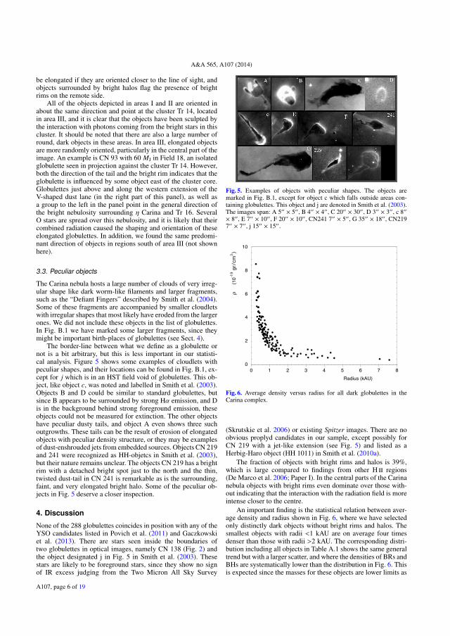
A&A 565, A107 (2014)
be elongated if they are oriented closer to the line of sight, andobjects surrounded by bright halos flag the presence of brightrims on the remote side.
All of the objects depicted in areas I and II are oriented inabout the same direction and point at the cluster Tr 14, locatedin area III, and it is clear that the objects have been sculpted bythe interaction with photons coming from the bright stars in thiscluster. It should be noted that there are also a large number ofround, dark objects in these areas. In area III, elongated objectsare more randomly oriented, particularly in the central part of theimage. An example is CN 93 with 60 MJ in Field 18, an isolatedglobulette seen in projection against the cluster Tr 14. However,both the direction of the tail and the bright rim indicates that theglobulette is influenced by some object east of the cluster core.Globulettes just above and along the western extension of theV-shaped dust lane (in the right part of this panel), as well asa group to the left in the panel point in the general direction ofthe bright nebulosity surrounding η Carina and Tr 16. SeveralO stars are spread over this nebulosity, and it is likely that theircombined radiation caused the shaping and orientation of theseelongated globulettes. In addition, we found the same predomi-nant direction of objects in regions south of area III (not shownhere).
3.3. Peculiar objects
The Carina nebula hosts a large number of clouds of very irreg-ular shape like dark worm-like filaments and larger fragments,such as the “Defiant Fingers” described by Smith et al. (2004).Some of these fragments are accompanied by smaller cloudletswith irregular shapes that most likely have eroded from the largerones. We did not include these objects in the list of globulettes.In Fig. B.1 we have marked some larger fragments, since theymight be important birth-places of globulettes (see Sect. 4).
The border-line between what we define as a globulette ornot is a bit arbitrary, but this is less important in our statisti-cal analysis. Figure 5 shows some examples of cloudlets withpeculiar shapes, and their locations can be found in Fig. B.1, ex-cept for j which is in an HST field void of globulettes. This ob-ject, like object c, was noted and labelled in Smith et al. (2003).Objects B and D could be similar to standard globulettes, butsince B appears to be surrounded by strong Hα emission, and Dis in the background behind strong foreground emission, theseobjects could not be measured for extinction. The other objectshave peculiar dusty tails, and object A even shows three suchoutgrowths. These tails can be the result of erosion of elongatedobjects with peculiar density structure, or they may be examplesof dust-enshrouded jets from embedded sources. Objects CN 219and 241 were recognized as HH-objetcs in Smith et al. (2003),but their nature remains unclear. The objects CN 219 has a brightrim with a detached bright spot just to the north and the thin,twisted dust-tail in CN 241 is remarkable as is the surrounding,faint, and very elongated bright halo. Some of the peculiar ob-jects in Fig. 5 deserve a closer inspection.
4. Discussion
None of the 288 globulettes coincides in position with any of theYSO candidates listed in Povich et al. (2011) and Gaczkowskiet al. (2013). There are stars seen inside the boundaries oftwo globulettes in optical images, namely CN 138 (Fig. 2) andthe object designated j in Fig. 5 in Smith et al. (2003). Thesestars are likely to be foreground stars, since they show no signof IR excess judging from the Two Micron All Sky Survey
Fig. 5. Examples of objects with peculiar shapes. The objects aremarked in Fig. B.1, except for object c which falls outside areas con-taining globulettes. This object and j are denoted in Smith et al. (2003).The images span: A 5′′ × 5′′, B 4′′ × 4′′, C 20′′ × 30′′, D 3′′ × 3′′, c 8′′× 8′′, E 7′′ × 10′′, F 20′′ × 10′′, CN241 7′′ × 5′′, G 35′′ × 18′′, CN2197′′ × 7′′, j 15′′ × 15′′.
0
2
4
6
8
10
0 1 2 3 4 5 6 7 8
Radius (kAU)
!
(1
0-1
9 g
r/cm
3)
Fig. 6. Average density versus radius for all dark globulettes in theCarina complex.
(Skrutskie et al. 2006) or existing Spitzer images. There are noobvious proplyd candidates in our sample, except possibly forCN 219 with a jet-like extension (see Fig. 5) and listed as aHerbig-Haro object (HH 1011) in Smith et al. (2010a).
The fraction of objects with bright rims and halos is 39%,which is large compared to findings from other H regions(De Marco et al. 2006; Paper I). In the central parts of the Carinanebula objects with bright rims even dominate over those with-out indicating that the interaction with the radiation field is moreintense closer to the centre.
An important finding is the statistical relation between aver-age density and radius shown in Fig. 6, where we have selectedonly distinctly dark objects without bright rims and halos. Thesmallest objects with radii <1 kAU are on average four timesdenser than those with radii >2 kAU. The corresponding distri-bution including all objects in Table A.1 shows the same generaltrend but with a larger scatter, and where the densities of BRs andBHs are systematically lower than the distribution in Fig. 6. Thisis expected since the masses for these objects are lower limits as
A107, page 6 of 19

T. Grenman and G. F. Gahm: The tiny globulettes in the Carina nebula
Fig. 7. Three detached fragments in the Carina nebula. From left to right: Fragments 1, 2, and 4 in Fields 7, 9, and 24 in Fig. B.1. These largerblocks contain denser cores, some of which appear to be detaching (see Frag. 1). Fragment 4 is surrounded by smaller cloudlets of different shapes.
pointed out in Sect. 2.2. It is likely that the distribution in Fig. 6reflects how globulettes evolve with time.
4.1. Origin and fate
Most dark formations seen in the optical images are located infront of the central regions of bright nebulosity. For the massestimates we have considered two extreme cases: all residualemission in the darkest parts is due to foreground emission, orthere is (practically) no foreground emission. The Carina regionis very complex, and it is difficult to judge how deeply embeddeda given globulette is in the warm nebulosity. For the same reasonit is hard to determine the geometrical distance between a givenglobulette and other dust formations or clusters in the area. Someglobulettes are quite isolated with projected distances to the clos-est dust complexes of more than 1.5 pc, for example the groupof globulettes in Field 14 containing Tr 14. A possible scenariois that this group is the remnant of a larger cloud that graduallyeroded in the intense radiation field from Tr 14.
It was inferred in Paper I that globulettes in the Rosette neb-ula originate from condensations in elephant trunks and shellfeatures. In the Carina complex there are a number of isolated,larger fragments that must have detached from shell structureslong ago. Such fragments are marked in Fields 7, 9, 12, 24,and 29. Figure 7 shows examples of such fragments and all con-tain condensations with masses similar to those found in glob-ulettes. Fragment 4 is surrounded by a cluster of smaller irreg-ular fragments that appear to be leftovers from a presumablylarger block that once eroded. We note that Fragment 2, whichhosts several condensations, looks like a detached elephant trunkcomposed by a network of thin twisted filaments similar to thethreaded elephant trunks discussed in Carlqvist et al. (2003).
As discussed in Paper II, the lack of distinct bright rims inHα may be traced to a combination of several circumstances.One is that the density distributions are rather flat and that thedensity is high even close to the surface where the gas is inmolecular form as flagged by fluorescent H2 emission. In ad-dition, thin Pβ emitting rims were discovered to be present inseveral objects, rims that in some cases appear to extend over theremote side of the objects. Such thin bright rims, not detected inHα, were also found in several much smaller globulettes in theRosette nebula (Mäkelä et al. 2014). Moreover, the Carina ob-jects could be located at considerable distances from the brightUV-radiating stars, in which case the flux of exciting Lyman con-tinuum photons is moderate producing only weak photodissoci-ation in the outer layer at the dense surface.
The large number of quite isolated globulettes indicates thatthe objects have survived for a long time in the nebula. Most
of these objects are tiny and dense, and unlike the larger ob-jects they lack thin envelopes. It appears that the population oftiny globulettes in the Carina complex are in a more evolvedstate than those encountered in other H regions, either becausethey have eroded faster in the intense radiation field, or becausethey are, on the whole, older. A likely scenario is that glob-ulettes detach from larger molecular blocks, like shell structures,pillars, and fragments. Thin envelopes would gradually be lostwith time, and the remnant cores may become denser with time.This scenario is further supported by the findings presented inFig. 6 showing that the average density is inversely proportionalto radius.
In Paper I we applied simple virial arguments to concludethat most globulettes in the Rosette nebula could be gravita-tionally unstable, especially after considering the influence ofan outer pressure from the surrounding warm plasma. When ap-plying the same analysis to the Carina globulettes we found thatthe globulettes are close to virial equilibrium but none is bound,even when assuming an outer pressure (thermal plus turbulence)of the same magnitude as in the Rosette complex. On the otherhand, the radiation pressure exerted by light from the numerousO stars in Carina should be much higher. This pressure acts onone side of the globulettes. The derived masses are subject to un-certainties (see Sect. 2), and we note that very little extra massis needed to confine the objects, as would be the case if theycontain denser yet unresolved cores, or more speculatively, evenJupiter-sized planets. This would clarify why the globulettes ap-pear to have survived for such a long time, as can be seen bytheir distribution over the nebula, where many objects are quiteisolated and reside far away from larger molecular structures.
The total number of unbound planets in the Milky Way couldamount to several hundred billion (Sumi et al. 2011). Globulettesin H regions may be an additional source of such free-floatingplanetary-mass objects besides an origin in circumstellar pro-toplanetary disks from where they are ejected (e.g. Veras et al.2009).
5. Conclusions
We have made an inventory of globulettes in the Carina nebulacomplex based on existing HST narrow-band Hα images. A to-tal of 288 globulettes were listed and measured for size, mass,and density. Most objects are either round or slightly elongated,and many of the latter are oriented in the direction of massiveyoung clusters in the area. We discuss why only a minority havedeveloped bright Hα emitting rims and/or tails, and we note thatthere is no evidence so far of any embedded young stars.
A107, page 7 of 19

A&A 565, A107 (2014)
The Carina globulettes are, on the whole, much smaller andless massive than those recognized from HST surveys of a num-ber of other H regions. Practically all are of planetary mass,and most have masses less than one Jupiter mass. The corre-sponding mean densities are much higher than in other regions,exceeding number densities of 105 cm−3 in several objects. Wefound a statistical relation between average density and sizein the sense that the smallest globulettes are also the densest.Globulettes may detach from larger blocks of molecular gas, likeisolated fragments, elephant trunks, and shell structures, afterwhich their thinner envelopes evaporate and leave denser cores,which may become even more compressed with time.
From virial arguments we conclude that the objects are notbound unless they contain a bit more mass than inferred from thederived mean mass. Most of the tiny objects are quite isolatedand located at projected distances of >1.5 pc from the closestlarger molecular structures, which indicates that the objects cansurvive for long times in the nebula. We speculate that the ob-jects might contain denser cores or even planetary-mass objectsthat already have formed in their interior.
We suggest that the Carina globulettes are a more evolvedstate than the larger and less dense objects that are abundant inother H regions. Globulettes in H regions may be one sourceof the large number of free-floating planetary-mass objects thathas been estimated to exist in the Galaxy.
Acknowledgements. We thank the referee Bo Reipurth for valuable commentsand suggestions. This work was supported by the Magnus Bergvall Foundation,the Längmanska Kulturfonden, and the Swedish National Space Board.
ReferencesAscenso, J., Alves, J., Vicente, S., & Lago, M. T. V. T. 2007, A&A, 476, 199Bally, J., O’Dell, C. R., & McCaughrean, M. J. 2000, AJ, 119, 2919Bok, B. J., & Reilly, E. J. 1947, ApJ, 105, 255Bohlin, R. C., Savage, B. D., & Drake, J. F. 1978, ApJ, 224, 132Carlqvist, P., Gahm, G. F., & Kristen, H. 2003, A&A, 403, 399De Marco, O., O’Dell, C. R., Gelfond, P., Rubin, R. H., & Glover, S. C. O. 2006,
AJ, 131, 2580Dyson, J. E. 1968, A&AS, 1, 388Gaczkowski, B., Preibisch, T., Ratzka, T., et al. 2013, A&A, 549, A67
Gahm, G. F., Grenman, T., Fredriksson, S., & Kristen, H. 2007, AJ, 133, 1795(Paper I)
Gahm, G. F., Persson, C. M., Mäkelä , M. M., & Haikala, L. K. 2013, A&A, 555,A57 (Paper II)
Grenman, T. 2006, Licentiate thesis, Luleå University of Technology, Sweden(ISSN 1402-1757)
Herbig, G. 1974, PASP, 86, 604Hester. J. J., Scowen, P.A., Sankrit, R., et al. 1996, AJ, 111, 2349Hur, H., Sung, H., & Bessell, M.S. 2012, AJ, 143, 41Kahn, F. D. 1969, Physica, 41, 172Kuutmann, A. 2007, Master’s Thesis, Dep. of Astronomy, Stockholm University,
SwedenMäkelä, M. M., Haikala, L. K., & Gahm, G. F. 2014, A&A, submittedMattila, K., Juvela, M., & Lehtinen, K. 2007, A&A, 654, L131McCaughrean, M. J., & O’Dell, C. R. 1996, AJ, 111, 1977O’Dell, C. R., & Wen, Z. 1994, ApJ, 436, 194O’Dell, C. R., Wen, Z., & Hu, X. 1993, ApJ, 410, 696Pekruhl, S., Preibisch, T., Schuller, F., & Menten, K. 2013, A&A, 550, A29Povich, M. S., Smith, N., Majewski, S. R., et al. 2011, ApJS, 194, 14Preibisch, T., Schuller, F., Ohlendorf, H., et al. 2011, A&A, 525, A92Preibisch, T., Roccatagliata, V., Gaczkowski, B., & Ratzka, T. 2012, A&A, 531,
A132Reipurth, B., Corporon, P., Olberg, M., & Tenorio-Tagle, G. 1997, A&A, 327,
1185Reipurth, B., Raga, A., & Heathcote, S. 2003, AJ, 126, 1925Reiter, M., & Smith, N. 2013, MNRAS, 433. 2226Roccatagliata, V., Preibisch, T., Ratzka, T., & Gaczkowski, B. 2013, A&A, 554,
A6Sahai, R., Güsten, R., & Morris, M. R., 2012, ApJ, 761, L21Sanchawala, K., Chen, W.-P., Ojha, D., et al. 2007a, ApJ, 667, 963Sanchawala, K., Chen, W.-P., Lee H.-T., et al. 2007b, ApJ, 656, 462Savage, B. D., & Mathis, J. S. 1979, ARA&A, 17, 73Skrutskie, M. F., Cutri, R. M., Stiening., R., et al. 2006, AJ, 131, 1163Smith, N. 2002, MNRAS, 331, 7Smith, N. 2008, Handbook of Star Forming Regions, Vol. II: The Southern Sky,
ASP Monograph Publ., ed. Bo Reipurth, 5, 138Smith, N., & Brooks, K. J. 2007, MNRAS, 379, 1279Smith, N., Egan M. P., Carey, S., et al. 2000, ApJ, 532, L145Smith, N., Bally, J., & Morse, J. A. 2003, ApJ, 587, L105Smith, N., Barbá, R. H., & Walborn, N. R. 2004, MNRAS, 351, 1457Smith, N., Bally, J., & Walborn, N. R. 2010a, MNRAS, 405, 1153Smith, N., Povich, N. S., Whitney, B. A., et al. 2010b, MNRAS, 406, 952Sumi, T., Kamiya, K., Bennett, D. P., et al. 2011, Nature, 473, 349Tapia, M., Roth, M., Vázquez, R. A., & Feinstein, A. 2003, MNRAS, 339, 44Tenorio-Tagle, G. 1977, A&A, 54, 517Thackeray, A. D. 1950, MNRAS, 110, 524Thé, A. D., Bakker, R., & Tjin A Djie, H. R. E. 1980, A&A, 89, 209Veras, D. Crepp, J. R., & Ford, E. B. 1998, A&A, 332, L5
Pages 9 to 19 are available in the electronic edition of the journal at http://www.aanda.org
A107, page 8 of 19
T. Grenman and G. F. Gahm: The tiny globulettes in the Carina nebula
Appendix A: Properties of the globulettes in the Carina complex
Table A.1. List of globulettes in the Carina nebula complex.
CN Field x y RA Dec α β PA r Mass Remarks(J2000.0) (J2000.0) (arcsec) (arcsec) (degr.) (kAU) (MJ)
1 F1 360 4020 10:41:13.3 −59:49:00 0.46 0.50 1.39 2.42 F1 660 1084 10:41:18.9 −59:46:38 0.30 0.36 0.96 1.13 F1 1792 3251 10:41:23.6 −59:48:35 0.38 0.40 1.13 1.34 F1 1654 378 10:41:26.2 −59:46:13 0.18 0.19 0.54 0.45 F1 1819 395 10:41:27.2 −59:46:15 0.19 0.27 0.67 0.66 F1 2029 221 10:41:28.8 −59:46:09 0.26 0.33 23 0.86 1.2 T7 F2 670 1907 10:41:28.9 −59:45:53 0.23 0.25 −43 0.69 0.6 BR, T8 F1 2391 1935 10:41:29.1 −59:47:36 0.20 0.22 0.61 0.59 F1 2156 597 10:41:29.2 −59:46:29 0.29 0.33 0.90 1.010 F1 2752 1904 10:41:31.5 −59:47:38 0.54 1.46 8 2.90 8.8 BR, EL, T11 F1 2604 373 10:41:32.4 −59:46:22 0.31 0.51 −38 1.19 2.0 EL12 F2 1207 1745 10:41:32.6 −59:45:50 0.31 0.35 −15 0.96 1.5 T13 F1 2808 667 10:41:33.4 −59:46:38 0.36 0.70 13 1.54 2.7 EL14 F2 1694 1606 10:41:35.9 −59:45:48 0.39 0.46 1.23 1.815 F3 2659 851 10:41:44.9 −59:43:44 1.47 1.67 4.55 4016 F3 2806 1494 10:41:45.2 −59:44:17 0.52 0.71 1.78 4.517 F3 2706 964 10:41:45.2 −59:43:50 0.20 0.21 0.59 0.518 F3 2972 933 10:41:46.9 −59:43:51 0.69 1.82 12 3.64 22 EL, T19 F3 3527 1546 10:41:49.8 −59:44:26 0.31 0.44 1.09 1.320 F3 3656 1501 10:41:50.7 −59:44:25 0.36 0.67 6 1.49 2.5 BR, EL21 F2 3781 272 10:41:51.2 −59:45:02 0.64 1.00 10 2.38 5.6 BR, EL22 F4 2772 3493 10:42:20.7 −59:19:45 0.35 0.40 1.09 1.6 BR23 F5 2719 1339 10:42:43.7 −59:20:16 0.18 0.20 0.55 0.424 F5 1880 938 10:42:48.7 −59:20:42 0.35 0.72 −5 1.55 2.8 BR, EL25 F5 1242 524 10:42:52.4 −59:21:08 0.25 0.47 −3 1.04 1.5 BR, EL26 F8 1029 1467 10:43:15.9 −59:28:07 0.13 0.14 0.39 0.227 F6 3938 1861 10:43:16.1 −59:28:31 0.52 1.22 33 2.52 8.5 EL, T, C28 F8 973 1754 10:43:16.8 −59:28:19 0.21 0.27 0.70 0.829 F6 2697 3970 10:43:17.6 −59:30:33 0.26 0.28 0.78 0.930 F7 1960 1480 10:43:19.9 −59:31:45 0.24 0.38 20 0.90 1.5 EL31 F7 3105 479 10:43:22.1 −59:30:31 0.36 0.61 23 1.41 4.3 EL32 F7 2177 3163 10:43:27.5 −59:32:47 0.35 0.41 1.10 2.433 F13 3571 682 10:43:31.4 −59:55:20 0.49 0.75 −13 1.80 4.0 BH, EL34 F7 2583 3776 10:43:32.0 −59:33:00 0.23 0.26 36 0.71 0.7 T35 F7 2883 4143 10:43:35.1 −59:33:06 0.19 0.25 0.64 0.536 F7 3181 3863 10:43:35.6 −59:32:46 0.23 0.24 0.68 0.737 F7 3360 4002 10:43:37.1 −59:32:46 0.11 0.13 0.35 0.238 F9 3329 499 10:43:39.1 −59:32:57 0.95 1.33 3.31 34 Se39 F9 3552 393 10:43:39.8 −59:32:46 0.39 0.51 1.31 4.0 Se40 F10 1537 3364 10:43:43.8 −59:31:24 0.19 0.21 0.58 0.641 F11 1933 2248 10:43:46.4 −59:36:05 0.18 0.25 0.62 0.542 F11 1935 2353 10:43:46.8 −59:36:09 0.35 0.46 1.17 2.643 F11 2066 2364 10:43:47.6 −59:36:06 0.26 0.34 −10 0.87 1.3 T44 F9 2972 3165 10:43:47.6 −59:34:56 0.33 0.40 1.06 2.145 F9 3255 2797 10:43:47.7 −59:34:33 0.13 0.13 0.38 0.246 F9 3325 2858 10:43:48.3 −59:34:33 0.11 0.13 0.35 0.247 F9 2914 3633 10:43:49.1 −59:35:16 0.13 0.14 0.39 0.248 F9 2893 3668 10:43:49.1 −59:35:18 0.11 0.12 0.33 0.149 F10 2378 3919 10:43:50.4 −59:31:18 0.36 0.44 1.16 3.250 F9 3229 3794 10:43:51.4 −59:35:14 0.30 0.41 1.03 2.051 F12 506 3746 10:43:52.5 −59:39:03 0.56 0.78 1.94 5.052 F16 3116 1570 10:43:52.9 −59:58:49 0.27 0.34 0.88 1.053 F11 2489 3191 10:43:53.0 −59:36:27 0.21 0.30 0.74 0.854 F11 2530 3187 10:43:53.2 −59:36:25 0.33 0.48 1.17 2.7 C to 5655 F11 2573 3152 10:43:53.3 −59:36:23 0.12 0.16 39 0.41 0.3 T56 F11 2554 3196 10:43:53.3 −59:36:25 0.26 0.35 0.88 1.4 C to 5457 F11 2589 3155 10:43:53.4 −59:36:22 0.12 0.13 0.36 0.258 F11 2873 2777 10:43:53.5 −59:35:59 0.25 0.29 0.78 1.059 F11 2611 3162 10:43:53.6 −59:36:22 0.13 0.15 0.41 0.2
Notes. The symbols are described in Sect. 2.2.
A107, page 9 of 19
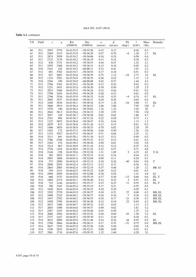
A&A 565, A107 (2014)
Table A.1. continued.
CN Field x y RA Dec α β PA r Mass Remarks(J2000.0) (J2000.0) (arcsec) (arcsec) (degr.) (kAU) (MJ)
60 F11 2952 2770 10:43:53.9 −59:35:56 0.15 0.17 0.46 0.361 F11 2569 3315 10:43:53.9 −59:36:29 0.27 0.70 −6 1.38 2.7 EL62 F11 2874 2959 10:43:54.2 −59:36:06 0.16 0.24 0.58 0.463 F11 2722 3170 10:43:54.2 −59:36:19 0.13 0.14 0.39 0.264 F12 830 3731 10:43:54.2 −59:38:53 0.44 0.47 1.32 2.165 F11 2595 3360 10:43:54.2 −59:36:31 0.15 0.16 0.45 0.266 F16 2341 102 10:43:54.5 −60:00:11 0.33 0.41 1.07 2.267 F12 891 3782 10:43:54.7 −59:38:54 0.17 0.18 0.51 0.368 F12 827 3883 10:43:54.8 −59:38:59 0.75 1.12 −10 2.71 14 EL69 F12 1124 3501 10:43:54.9 −59:38:35 0.36 0.42 1.13 1.570 F16 2304 190 10:43:54.9 −60:00:08 0.42 0.57 1.44 4.271 F11 2766 3381 10:43:55.2 −59:36:26 0.13 0.16 0.42 0.272 F12 1251 3451 10:43:55.4 −59:38:30 0.39 0.50 1.29 2.573 F11 2833 3366 10:43:55.5 −59:36:24 0.12 0.16 0.41 0.274 F11 2790 3454 10:43:55.6 −59:36:29 0.20 0.23 0.62 0.575 F11 2796 3536 10:43:55.9 −59:36:32 0.18 0.33 −9 0.74 0.7 EL76 F11 2805 3527 10:43:56.0 −59:36:31 0.18 0.26 0.64 0.577 F12 1049 3910 10:43:56.1 −59:38:54 0.73 1.34 −16 3.00 17 EL78 F11 2606 3914 10:43:56.4 −59:36:53 2.06 2.80 7.05 128 C79 F17 1970 196 10:43:56.4 −59:39:03 1.16 1.22 3.45 2980 F11 2844 3613 10:43:56.6 −59:36:33 2.30 2.93 7.58 13281 F17 2057 149 10:43:56.7 −59:38:58 0.63 0.65 1.86 4.782 F14 2761 894 10:43:56.7 −59:31:32 0.22 0.28 0.73 1.183 F12 1222 3852 10:43:56.8 −59:38:47 0.34 0.44 1.13 1.384 F14 2839 813 10:43:56.8 −59:31:26 0.13 0.15 0.41 0.285 F12 1406 3654 10:43:56.9 −59:38:33 0.70 0.82 2.20 1086 F17 2182 172 10:43:57.5 −59:38:56 0.44 0.50 1.36 3.087 F12 1314 3927 10:43:57.5 −59:38:47 0.71 0.84 2.25 1288 F14 3211 691 10:43:58.1 −59:31:10 0.13 0.21 0.49 0.389 F11 3786 2786 10:43:58.4 −59:35:32 0.13 0.15 0.41 0.290 F17 2303 274 10:43:58.5 −59:38:56 0.58 0.81 2.02 5.891 F14 3214 863 10:43:58.9 −59:31:16 0.12 0.12 0.35 0.292 F14 2726 1454 10:43:58.9 −59:31:54 0.22 0.27 0.71 0.893 F18 2146 258 10:43:59.6 −59:32:38 1.31 1.69 5 4.35 63 T, Si94 F18 384 3025 10:44:01.1 −59:35:22 0.14 0.16 0.44 0.295 F14 2903 1866 10:44:01.6 −59:32:04 0.09 0.11 0.29 0.196 F18 575 2990 10:44:01.9 −59:35:15 0.18 0.26 −40 0.64 0.8 T97 F14 2890 2055 10:44:02.4 −59:32:12 0.12 0.13 0.36 0.298 F14 2865 2085 10:44:02.4 −59:32:14 0.37 0.46 1.20 3.2 BR, S f99 F18 559 3151 10:44:02.5 −59:35:22 0.20 0.22 0.61 0.5100 F14 2994 2059 10:44:02.8 −59:32:08 0.36 0.54 1.31 4.0 S f101 F18 660 3153 10:44:03.0 −59:35:19 0.17 0.30 −13 0.68 0.6 EL, T102 F12 3489 2374 10:44:03.1 −59:36:40 0.12 0.23 3 0.51 0.3 EL103 F18 722 3146 10:44:03.3 −59:35:17 0.15 0.23 11 0.55 0.5 EL, T104 F18 708 3183 10:44:03.4 −59:35:19 0.17 0.21 0.55 0.5105 F12 3420 2634 10:44:03.8 −59:36:53 0.10 0.10 0.29 0.1106 F12 3392 2729 10:44:03.9 −59:36:57 0.10 0.23 27 0.48 0.2 BH, EL107 F12 3409 2742 10:44:04.1 −59:36:57 0.10 0.16 7 0.38 0.2 BH, EL108 F12 3447 2703 10:44:04.2 −59:36:55 0.10 0.17 21 0.38 0.2 BH, EL109 F12 3450 2789 10:44:04.5 −59:36:58 0.12 0.19 22 0.45 0.2 BH, EL110 F17 2657 1400 10:44:04.7 −59:39:32 0.33 0.45 1.13 2.3111 F17 2603 1490 10:44:04.8 −59:39:37 0.49 0.62 1.61 5.2112 F17 2587 1545 10:44:04.9 −59:39:40 0.43 0.50 1.35 3.2113 F14 2686 2944 10:44:05.2 −59:32:52 0.26 0.69 43 1.38 3.2 EL114 F17 2737 1427 10:44:05.3 −59:39:30 0.11 0.10 0.30 0.1115 F14 3623 2009 10:44:05.8 −59:31:46 0.14 0.24 44 0.55 0.5 EL116 F15 2760 2864 10:44:06.4 −59:28:13 0.17 0.35 −31 0.75 0.8 BH, EL117 F14 2847 3192 10:44:07.0 −59:32:56 0.26 0.38 0.93 1.8118 F14 3190 2832 10:44:07.2 −59:32:31 0.08 0.09 0.25 0.1119 F17 2961 1710 10:44:07.6 −59:39:35 1.22 1.68 4.20 33
A107, page 10 of 19
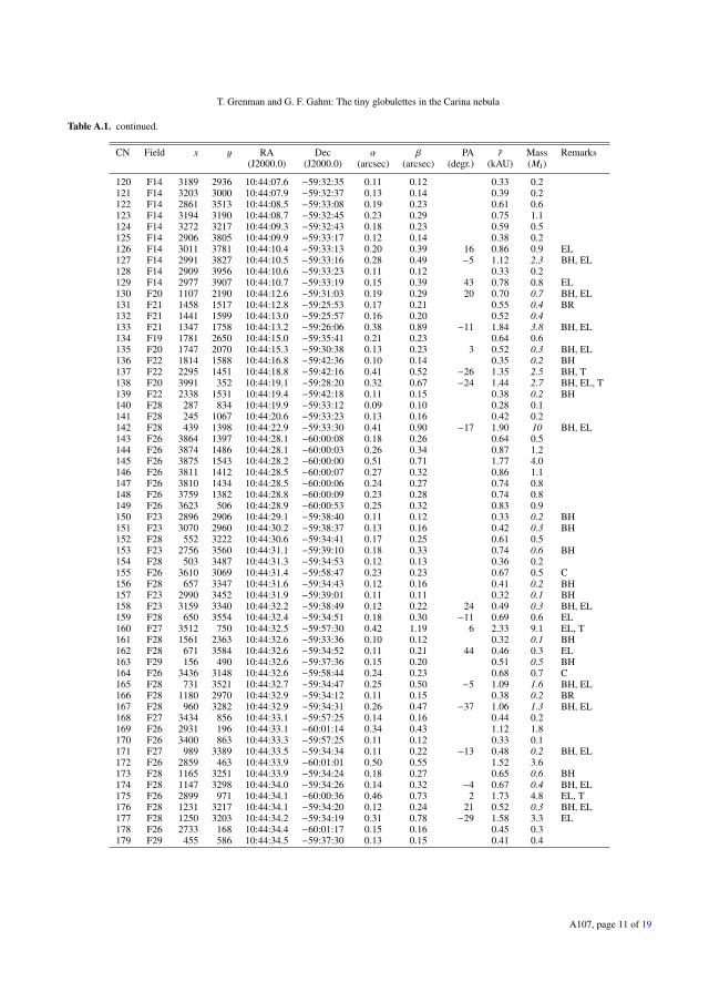
T. Grenman and G. F. Gahm: The tiny globulettes in the Carina nebula
Table A.1. continued.
CN Field x y RA Dec α β PA r Mass Remarks(J2000.0) (J2000.0) (arcsec) (arcsec) (degr.) (kAU) (MJ)
120 F14 3189 2936 10:44:07.6 −59:32:35 0.11 0.12 0.33 0.2121 F14 3203 3000 10:44:07.9 −59:32:37 0.13 0.14 0.39 0.2122 F14 2861 3513 10:44:08.5 −59:33:08 0.19 0.23 0.61 0.6123 F14 3194 3190 10:44:08.7 −59:32:45 0.23 0.29 0.75 1.1124 F14 3272 3217 10:44:09.3 −59:32:43 0.18 0.23 0.59 0.5125 F14 2906 3805 10:44:09.9 −59:33:17 0.12 0.14 0.38 0.2126 F14 3011 3781 10:44:10.4 −59:33:13 0.20 0.39 16 0.86 0.9 EL127 F14 2991 3827 10:44:10.5 −59:33:16 0.28 0.49 −5 1.12 2.3 BH, EL128 F14 2909 3956 10:44:10.6 −59:33:23 0.11 0.12 0.33 0.2129 F14 2977 3907 10:44:10.7 −59:33:19 0.15 0.39 43 0.78 0.8 EL130 F20 1107 2190 10:44:12.6 −59:31:03 0.19 0.29 20 0.70 0.7 BH, EL131 F21 1458 1517 10:44:12.8 −59:25:53 0.17 0.21 0.55 0.4 BR132 F21 1441 1599 10:44:13.0 −59:25:57 0.16 0.20 0.52 0.4133 F21 1347 1758 10:44:13.2 −59:26:06 0.38 0.89 −11 1.84 3.8 BH, EL134 F19 1781 2650 10:44:15.0 −59:35:41 0.21 0.23 0.64 0.6135 F20 1747 2070 10:44:15.3 −59:30:38 0.13 0.23 3 0.52 0.3 BH, EL136 F22 1814 1588 10:44:16.8 −59:42:36 0.10 0.14 0.35 0.2 BH137 F22 2295 1451 10:44:18.8 −59:42:16 0.41 0.52 −26 1.35 2.5 BH, T138 F20 3991 352 10:44:19.1 −59:28:20 0.32 0.67 −24 1.44 2.7 BH, EL, T139 F22 2338 1531 10:44:19.4 −59:42:18 0.11 0.15 0.38 0.2 BH140 F28 287 834 10:44:19.9 −59:33:12 0.09 0.10 0.28 0.1141 F28 245 1067 10:44:20.6 −59:33:23 0.13 0.16 0.42 0.2142 F28 439 1398 10:44:22.9 −59:33:30 0.41 0.90 −17 1.90 10 BH, EL143 F26 3864 1397 10:44:28.1 −60:00:08 0.18 0.26 0.64 0.5144 F26 3874 1486 10:44:28.1 −60:00:03 0.26 0.34 0.87 1.2145 F26 3875 1543 10:44:28.2 −60:00:00 0.51 0.71 1.77 4.0146 F26 3811 1412 10:44:28.5 −60:00:07 0.27 0.32 0.86 1.1147 F26 3810 1434 10:44:28.5 −60:00:06 0.24 0.27 0.74 0.8148 F26 3759 1382 10:44:28.8 −60:00:09 0.23 0.28 0.74 0.8149 F26 3623 506 10:44:28.9 −60:00:53 0.25 0.32 0.83 0.9150 F23 2896 2906 10:44:29.1 −59:38:40 0.11 0.12 0.33 0.2 BH151 F23 3070 2960 10:44:30.2 −59:38:37 0.13 0.16 0.42 0.3 BH152 F28 552 3222 10:44:30.6 −59:34:41 0.17 0.25 0.61 0.5153 F23 2756 3560 10:44:31.1 −59:39:10 0.18 0.33 0.74 0.6 BH154 F28 503 3487 10:44:31.3 −59:34:53 0.12 0.13 0.36 0.2155 F26 3610 3069 10:44:31.4 −59:58:47 0.23 0.23 0.67 0.5 C156 F28 657 3347 10:44:31.6 −59:34:43 0.12 0.16 0.41 0.2 BH157 F23 2990 3452 10:44:31.9 −59:39:01 0.11 0.11 0.32 0.1 BH158 F23 3159 3340 10:44:32.2 −59:38:49 0.12 0.22 24 0.49 0.3 BH, EL159 F28 650 3554 10:44:32.4 −59:34:51 0.18 0.30 −11 0.69 0.6 EL160 F27 3512 750 10:44:32.5 −59:57:30 0.42 1.19 6 2.33 9.1 EL, T161 F28 1561 2363 10:44:32.6 −59:33:36 0.10 0.12 0.32 0.1 BH162 F28 671 3584 10:44:32.6 −59:34:52 0.11 0.21 44 0.46 0.3 EL163 F29 156 490 10:44:32.6 −59:37:36 0.15 0.20 0.51 0.5 BH164 F26 3436 3148 10:44:32.6 −59:58:44 0.24 0.23 0.68 0.7 C165 F28 731 3521 10:44:32.7 −59:34:47 0.25 0.50 −5 1.09 1.6 BH, EL166 F28 1180 2970 10:44:32.9 −59:34:12 0.11 0.15 0.38 0.2 BR167 F28 960 3282 10:44:32.9 −59:34:31 0.26 0.47 −37 1.06 1.3 BH, EL168 F27 3434 856 10:44:33.1 −59:57:25 0.14 0.16 0.44 0.2169 F26 2931 196 10:44:33.1 −60:01:14 0.34 0.43 1.12 1.8170 F26 3400 863 10:44:33.3 −59:57:25 0.11 0.12 0.33 0.1171 F27 989 3389 10:44:33.5 −59:34:34 0.11 0.22 −13 0.48 0.2 BH, EL172 F26 2859 463 10:44:33.9 −60:01:01 0.50 0.55 1.52 3.6173 F28 1165 3251 10:44:33.9 −59:34:24 0.18 0.27 0.65 0.6 BH174 F28 1147 3298 10:44:34.0 −59:34:26 0.14 0.32 −4 0.67 0.4 BH, EL175 F26 2899 971 10:44:34.1 −60:00:36 0.46 0.73 2 1.73 4.8 EL, T176 F28 1231 3217 10:44:34.1 −59:34:20 0.12 0.24 21 0.52 0.3 BH, EL177 F28 1250 3203 10:44:34.2 −59:34:19 0.31 0.78 −29 1.58 3.3 EL178 F26 2733 168 10:44:34.4 −60:01:17 0.15 0.16 0.45 0.3179 F29 455 586 10:44:34.5 −59:37:30 0.13 0.15 0.41 0.4
A107, page 11 of 19
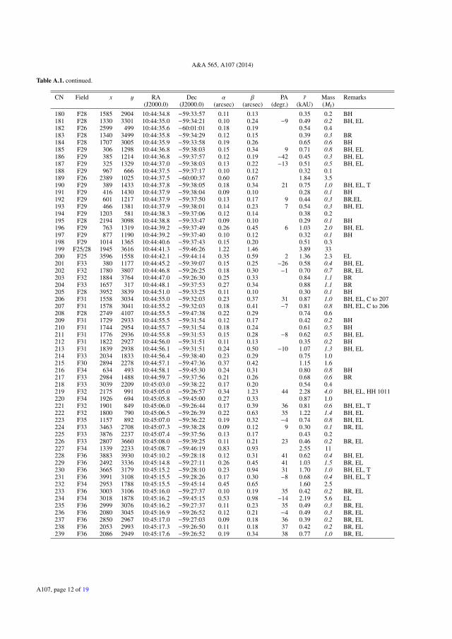
A&A 565, A107 (2014)
Table A.1. continued.
CN Field x y RA Dec α β PA r Mass Remarks(J2000.0) (J2000.0) (arcsec) (arcsec) (degr.) (kAU) (MJ)
180 F28 1585 2904 10:44:34.8 −59:33:57 0.11 0.13 0.35 0.2 BH181 F28 1330 3301 10:44:35.0 −59:34:21 0.10 0.24 −9 0.49 0.2 BH, EL182 F26 2599 499 10:44:35.6 −60:01:01 0.18 0.19 0.54 0.4183 F28 1340 3499 10:44:35.8 −59:34:29 0.12 0.15 0.39 0.3 BR184 F28 1707 3005 10:44:35.9 −59:33:58 0.19 0.26 0.65 0.6 BH185 F29 306 1298 10:44:36.8 −59:38:03 0.15 0.34 9 0.71 0.8 BH, EL186 F29 385 1214 10:44:36.8 −59:37:57 0.12 0.19 −42 0.45 0.3 BH, EL187 F29 325 1329 10:44:37.0 −59:38:03 0.13 0.22 −13 0.51 0.5 BH, EL188 F29 967 666 10:44:37.5 −59:37:17 0.10 0.12 0.32 0.1189 F26 2389 1025 10:44:37.5 −60:00:37 0.60 0.67 1.84 3.5190 F29 389 1433 10:44:37.8 −59:38:05 0.18 0.34 21 0.75 1.0 BH, EL, T191 F29 416 1430 10:44:37.9 −59:38:04 0.09 0.10 0.28 0.1 BH192 F29 601 1217 10:44:37.9 −59:37:50 0.13 0.17 9 0.44 0.3 BR.EL193 F29 466 1381 10:44:37.9 −59:38:01 0.14 0.23 7 0.54 0.3 BH, EL194 F29 1203 581 10:44:38.3 −59:37:06 0.12 0.14 0.38 0.2195 F28 2194 3098 10:44:38.8 −59:33:47 0.09 0.10 0.29 0.1 BH196 F29 763 1319 10:44:39.2 −59:37:49 0.26 0.45 6 1.03 2.0 BH, EL197 F29 877 1190 10:44:39.2 −59:37:40 0.10 0.12 0.32 0.1 BH198 F29 1014 1365 10:44:40.6 −59:37:43 0.15 0.20 0.51 0.3199 F25/28 1945 3616 10:44:41.3 −59:46:26 1.22 1.46 3.89 33200 F25 3596 1558 10:44:42.1 −59:44:14 0.35 0.59 2 1.36 2.3 EL201 F33 380 1177 10:44:45.2 −59:39:07 0.15 0.25 −26 0.58 0.4 BH, EL202 F32 1780 3807 10:44:46.8 −59:26:25 0.18 0.30 −1 0.70 0.7 BR, EL203 F32 1884 3764 10:44:47.0 −59:26:30 0.25 0.33 0.84 1.1 BR204 F33 1657 317 10:44:48.1 −59:37:53 0.27 0.34 0.88 1.1 BR205 F28 3952 3839 10:44:51.0 −59:33:25 0.11 0.10 0.30 0.1 BH206 F31 1558 3034 10:44:55.0 −59:32:03 0.23 0.37 31 0.87 1.0 BH, EL, C to 207207 F31 1578 3041 10:44:55.2 −59:32:03 0.18 0.41 −7 0.81 0.8 BH, EL, C to 206208 F28 2749 4107 10:44:55.5 −59:47:38 0.22 0.29 0.74 0.6209 F31 1729 2933 10:44:55.5 −59:31:54 0.12 0.17 0.42 0.2 BH210 F31 1744 2954 10:44:55.7 −59:31:54 0.18 0.24 0.61 0.5 BH211 F31 1776 2936 10:44:55.8 −59:31:53 0.15 0.28 −8 0.62 0.5 BH, EL212 F31 1822 2927 10:44:56.0 −59:31:51 0.11 0.13 0.35 0.2 BH213 F31 1839 2938 10:44:56.1 −59:31:51 0.24 0.50 −10 1.07 1.3 BH, EL214 F33 2034 1833 10:44:56.4 −59:38:40 0.23 0.29 0.75 1.0215 F30 2894 2278 10:44:57.1 −59:47:36 0.37 0.42 1.15 1.6216 F34 634 493 10:44:58.1 −59:45:30 0.24 0.31 0.80 0.8 BH217 F33 2984 1488 10:44:59.7 −59:37:56 0.21 0.26 0.68 0.6 BR218 F33 3039 2209 10:45:03.0 −59:38:22 0.17 0.20 0.54 0.4219 F32 2175 991 10:45:05.0 −59:26:57 0.34 1.23 44 2.28 4.0 BH, EL, HH 1011220 F34 1926 694 10:45:05.8 −59:45:00 0.27 0.33 0.87 1.0221 F32 1901 849 10:45:06.0 −59:26:44 0.17 0.39 36 0.81 0.6 BH, EL, T222 F32 1800 790 10:45:06.5 −59:26:39 0.22 0.63 35 1.22 1.4 BH, EL223 F35 1157 892 10:45:07.0 −59:36:22 0.19 0.32 −4 0.74 0.8 BH, EL224 F33 3463 2708 10:45:07.3 −59:38:28 0.09 0.12 9 0.30 0.1 BR, EL225 F33 3876 2237 10:45:07.4 −59:37:56 0.13 0.17 0.43 0.2226 F33 2807 3660 10:45:08.0 −59:39:25 0.11 0.21 23 0.46 0.2 BR, EL227 F34 1339 2233 10:45:08.7 −59:46:19 0.83 0.93 2.55 11228 F36 3883 3930 10:45:10.2 −59:28:18 0.12 0.31 41 0.62 0.4 BH, EL229 F36 2492 3336 10:45:14.8 −59:27:11 0.26 0.45 41 1.03 1.5 BR, EL230 F36 3665 3179 10:45:15.2 −59:28:10 0.23 0.94 31 1.70 1.0 BH, EL, T231 F36 3991 3108 10:45:15.5 −59:28:26 0.17 0.30 −8 0.68 0.4 BH, EL, T232 F34 2953 1788 10:45:15.5 −59:45:14 0.45 0.65 1.60 2.5233 F36 3003 3106 10:45:16.0 −59:27:37 0.10 0.19 35 0.42 0.2 BR, EL234 F34 3018 1878 10:45:16.2 −59:45:15 0.53 0.98 −14 2.19 5.6 EL235 F36 2999 3076 10:45:16.2 −59:27:37 0.11 0.23 35 0.49 0.3 BR, EL236 F36 2080 3045 10:45:16.9 −59:26:52 0.12 0.21 −4 0.49 0.3 BR, EL237 F36 2850 2967 10:45:17.0 −59:27:03 0.09 0.18 36 0.39 0.2 BR, EL238 F36 2053 2993 10:45:17.3 −59:26:50 0.11 0.18 37 0.42 0.2 BR, EL239 F36 2086 2949 10:45:17.6 −59:26:52 0.19 0.34 38 0.77 1.0 BR, EL
A107, page 12 of 19
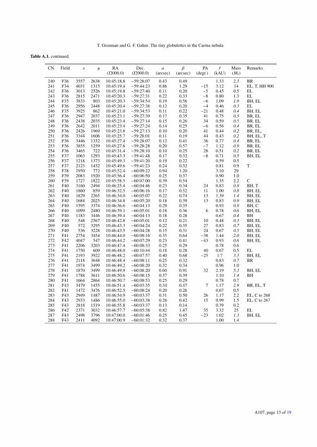
T. Grenman and G. F. Gahm: The tiny globulettes in the Carina nebula
Table A.1. continued.
CN Field x y RA Dec. α β PA r Mass Remarks(J2000.0) (J2000.0) (arcsec) (arcsec) (degr.) (kAU) (MJ)
240 F36 3557 2638 10:45:18.8 −59:28:07 0.43 0.49 1.33 2.3 BR241 F34 4031 1315 10:45:19.4 −59:44:23 0.86 1.29 −15 3.12 14 EL, T, HH 900242 F36 3013 2526 10:45:19.8 −59:27:40 0.11 0.20 −5 0.45 0.5 EL243 F36 2815 2471 10:45:20.3 −59:27:31 0.22 0.33 −8 0.80 1.3 EL244 F35 3833 803 10:45:20.3 −59:34:54 0.19 0.56 −6 1.09 1.9 BH, EL245 F36 2956 2448 10:45:20.4 −59:27:38 0.12 0.20 −4 0.46 0.3 EL246 F35 3925 862 10:45:21.0 −59:34:53 0.11 0.22 −21 0.48 0.4 BH, EL247 F36 2947 2037 10:45:23.1 −59:27:39 0.17 0.35 41 0.75 0.5 BR, EL248 F36 2438 2035 10:45:23.4 −59:27:14 0.15 0.26 34 0.59 0.5 BR, EL249 F36 2642 2011 10:45:23.4 −59:27:24 0.14 0.25 −6 0.56 0.4 BR, EL250 F36 2426 1969 10:45:23.8 −59:27:13 0.10 0.20 41 0.44 0.2 BR, EL,251 F36 3344 1606 10:45:25.7 −59:28:01 0.11 0.19 44 0.43 0.2 BH, EL, T252 F36 3446 1332 10:45:27.4 −59:28:07 0.12 0.41 36 0.77 0.4 BR, EL253 F36 3855 1259 10:45:27.6 −59:28:28 0.20 0.57 −7 1.12 0.9 BR, EL254 F36 3465 722 10:45:31.4 −59:28:10 0.10 0.25 28 0.51 0.2 BR, EL255 F37 1063 1293 10:45:43.3 −59:41:48 0.17 0.32 −8 0.71 0.5 BH, EL256 F37 1218 1373 10:45:49.3 −59:41:20 0.19 0.22 0.59 0.5257 F37 2123 1452 10:45:49.6 −59:41:23 0.24 0.32 0.81 0.9 T258 F38 1950 772 10:45:52.4 −60:09:22 0.94 1.20 3.10 29259 F39 2083 1920 10:45:56.4 −60:06:50 0.25 0.37 0.90 1.0260 F39 1727 1822 10:45:58.5 −60:07:00 0.39 0.54 1.35 2.2 C261 F40 3160 2494 10:46:25.4 −60:04:46 0.23 0.34 24 0.83 0.8 BH, T262 F40 1860 859 10:46:32.5 −60:06:16 0.17 0.52 11 1.00 0.8 BH, EL263 F40 1829 2265 10:46:34.0 −60:05:07 0.22 0.74 13 1.39 1.4 BH, EL264 F40 1684 2025 10:46:34.8 −60:05:20 0.18 0.39 13 0.83 0.9 BH, EL265 F40 1595 3374 10:46:36.6 −60:04:13 0.29 0.35 0.93 0.9 BH, C266 F40 1099 2480 10:46:39.1 −60:05:01 0.18 0.36 6 0.78 0.6 BH, EL267 F40 1183 3446 10:46:39.4 −60:04:13 0.18 0.28 0.67 0.4 BH268 F40 548 2567 10:46:42.8 −60:05:01 0.12 0.21 10 0.48 0.3 BH, EL269 F40 572 3295 10:46:43.3 −60:04:24 0.22 0.35 27 0.83 0.7 BH, EL270 F40 536 3228 10:46:43.5 −60:04:28 0.15 0.31 24 0.67 0.5 BH, EL271 F41 2754 3454 10:46:44.0 −60:08:16 0.35 0.64 −38 1.44 2.0 BH, EL272 F42 4047 547 10:46:44.2 −60:07:29 0.23 0.41 −43 0.93 0.6 BH, EL273 F41 2206 3203 10:46:47.4 −60:08:33 0.25 0.29 0.78 0.6274 F41 1750 609 10:46:48.0 −60:10:44 0.18 0.28 40 0.67 0.5 EL275 F41 2193 3922 10:46:48.2 −60:07:57 0.40 0.68 −25 1.7 3.3 BH, EL276 F41 2118 3648 10:46:48.4 −60:08:11 0.25 0.32 0.83 0.7 BR277 F41 1974 3499 10:46:49.2 −60:08:20 0.32 0.34 0.96 1.0278 F41 1870 3499 10:46:49.9 −60:08:20 0.60 0.91 32 2.19 5.3 BH, EL279 F41 1788 3611 10:46:50.6 −60:08:15 0.37 0.39 1.10 1.4 BH280 F41 1664 2864 10:46:50.7 −60:08:53 0.25 0.29 0.78 0.7281 F43 3479 1455 10:46:51.4 −60:03:35 0.34 0.47 7 1.17 2.9 BR, EL, T282 F41 1472 3476 10:46:52.5 −60:08:24 0.20 0.26 0.67 0.5283 F43 2949 1487 10:46:54.9 −60:03:37 0.31 0.50 26 1.17 2.2 EL, C to 268284 F43 2933 1486 10:46:55.0 −60:03:38 0.26 0.42 15 0.99 1.5 EL, C to 267285 F43 2818 1519 10:46:55.8 −60:03:37 0.13 0.14 0.39 0.2286 F42 2371 3032 10:46:57.7 −60:05:38 0.82 1.47 35 3.32 25 EL287 F43 2498 3796 10:47:00.0 −60:01:46 0.25 0.45 −23 1.02 1.3 BH, EL288 F43 2411 4092 10:47:00.9 −60:01:32 0.32 0.37 1.00 1.4
A107, page 13 of 19
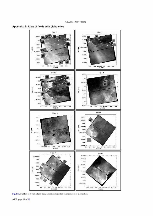
A&A 565, A107 (2014)
Appendix B: Atlas of fields with globulettes
Fig. B.1. Fields 1 to 8 with object designation and inserted enlargements of globulettes.
A107, page 14 of 19

T. Grenman and G. F. Gahm: The tiny globulettes in the Carina nebula
Fig. B.1. continued. Fields 9 to 16.
A107, page 15 of 19

A&A 565, A107 (2014)
Fig. B.1. continued. Fields 17 to 24.
A107, page 16 of 19

T. Grenman and G. F. Gahm: The tiny globulettes in the Carina nebula
Fig. B.1. continued. Fields 25 to 32.
A107, page 17 of 19

A&A 565, A107 (2014)
Fig. B.1. continued. Fields 33 to 40.
A107, page 18 of 19

T. Grenman and G. F. Gahm: The tiny globulettes in the Carina nebula
Fig. B.1. continued. Fields 41 to 43.
A107, page 19 of 19


Paper III
Dusty globules in the Crab nebula
Authors:Grenman, T., Gahm, G. F., & Elfgren, E.

A&A 599, A110 (2017)DOI: 10.1051/0004-6361/201629693c© ESO 2017
Astronomy&Astrophysics
Dusty globules in the Crab Nebula?
T. Grenman1, G. F. Gahm2, and E. Elfgren1
1 Division of Physics, Luleå University of Technology, 97187 Luleå, Swedene-mail: [email protected]
2 Stockholm Observatory, AlbaNova University Centre, Stockholm University, 106 91 Stockholm, Sweden
Received 12 September 2016 / Accepted 19 October 2016
ABSTRACT
Context. Dust grains are widespread in the Crab Nebula. A number of small, dusty globules, are visible as dark spots against thebackground of continuous synchrotron emission in optical images.Aims. Our aim is to catalogue such dusty globules and investigate their properties.Methods. From existing broad-band images obtained with the Hubble Space Telescope, we located 92 globules, for which we derivedpositions, dimensions, orientations, extinctions, masses, proper motions, and their distributions.Results. The globules have mean radii ranging from 400 to 2000 AU and are not resolved in current infrared images of the nebula. Theextinction law for dust grains in these globules matches a normal interstellar extinction law. Derived masses of dust range from 1 to60×10−6 M�, and the total mass contained in globules constitute a fraction of approximately 2% or less of the total dust content of thenebula. The globules are spread over the outer part of the nebula, and a fraction of them coincide in position with emission filaments,where we find elongated globules that are aligned with these filaments. Only 10% of the globules are coincident in position with thenumerous H2-emitting knots found in previous studies. All globules move outwards from the centre with transversal velocities of 60to 1600 km s−1, along with the general expansion of the remnant. We discuss various hypotheses for the formation of globules in theCrab Nebula.
Key words. ISM: supernova remnants – dust, extinction – supernovae: individual: Crab Nebula
1. Introduction
Dust ejected from supernovae has been considered to play an im-portant part in supplying the interstellar medium with dust grains(e.g., Kozasa et al. 2009). Substantial amounts of dust have in-deed been found in young supernova remnants based on observa-tions of infrared emission from dust grains. For Cas A (e.g., Rohet al. 2008) and SN 2003gd (e.g., Sugerman et al. 2006) the totalamount of dust was estimated to be up to a few times 10−2 M�.For SNR 1987A, Ercolano et al. (2007) obtained an upper limitfor dust mass of 7.5×10⁻⁴ M�, assuming a clumpy distribution ofdust, at a phase two years after the explosion. Indebetouw et al.(2014) and Matsuura et al. (2015), however, found much largeramounts of dust, of the order of 0.5 M�, from observations ob-tained at later phases. It was proposed that the dust is formed inthe inner ejecta, the cold remnants of the exploded stellar core,and that grain growth occur in the remnant at later phases.
Here, we will focus on another young and well-known dust-containing supernova remnant named the Crab Nebula, formedafter the supernova in 1054 AD. Based on arguments concerningthe low expansion velocities of the ejecta and the lack of signa-tures of remote, fast-moving gas (Lundqvist et al. 1986, 2012;Wang et al. 2013) in addition to the energy budget of the complex(e.g., Yang & Chevalier 2015), it is has been proposed that theprogenitor was a star in the more massive part of the asymptoticgiant branch (Moriya et al. 2014). At the centre of the nebula liesone of the first known pulsars, PSR B0531+21, surrounded by anexpanding synchrotron radiating nebula and a network of fila-ments radiating in emission lines from various ions. The general? Based on observations collected with the NASA/ESA Hubble Space
Telescope, obtained at the Space Telescope Science Institute.
properties of the Crab Nebula have been reviewed by Davidson& Fesen (1985) and Hester (2008).
The velocity field over the expanding remnant has beenmapped from proper motions of the optical filaments (Trimble1968; Nugent 1998) and related radial velocities (Wykoff et al.1977). Bietenholz & Nugent (2015) also included radio mea-surements to conclude that the synchrotron nebula, fed by en-ergy from a pulsar-wind nebula (see Bühler & Blandford 2014),has been strongly accelerated compared to the filaments.
The presence of dust in the Crab Nebula was first inferredfrom the infrared (IR) excess emission over the synchrotronspectrum noted in Trimble (1977). With the launches of theSpitzer Space Telescope and the Herschel Space Observatory,the distribution of IR-emitting dust could be mapped in greatdetail (e.g., Temim et al. 2006, 2012; Temim & Dwek 2013;Gomez et al. 2012; Owen & Barlow 2015). Dust is spread overthe entire nebula, and strongly concentrated to the optical fila-ments. The total dust content was estimated by these authors tobe in the order of a tenth of a solar mass. Sankrit et al. (1998)proposed that dust is freshly formed in filaments resulting fromRayleigh-Taylor instabilities acting on the ejecta.
Dust was also recognized in optical images as dark fea-tures silhouetted against the bright background in Woltjer &Véron-Cetty (1987). From an examination of photographicplates, Fesen & Blair (1990) catalogued 24 “dark spots” andmeasured the amount of extinction in them, and Hester et al.(1990) draw attention to several optically visible dusty blobs andfilaments. One such blob attached to a dusty filament, coinci-dent with an optically bright filament, was investigated in Sankritet al. (1998) from images taken with the Hubble Space Telescope(HST). Several extended irregular dusty filaments can be seen in
Article published by EDP Sciences A110, page 1 of 11

A&A 599, A110 (2017)
Table 1. Archival HST/HLA data used.
Program ID Filter Exposure time (s) Year Archive data set
5206 F547M 1000 1994 u24r0404t5354 F547M 800–1000 1995 u2bx0501t–u2bx0504t6129 F547M 1000 1995–1996 u2u60101t–u2u60702t
F814W 700, 1200 1995–1996 u2u60106t, u2u60504t7407 F547M 1200 2000–2001 u50v0302r, u50v1201r, u50v2101r, u50v5902m8222 F547M 900 2000 u5d10201r–u5d10601r13510 F550M 2000 2014 jcgt0301013772 F550M 2000 2014 jcp301010
Fig. 1. HST color image composed from images in the F502N, F631N,and F673N filters (courtesy: NASA, ESA, and J. Hester, Arizona StateUniversity). The area investigated here is marked, and the arrow pointsto the location of the pulsar (north is up and east left).
optical continuum HST images and also in narrow band imagescovering certain emission lines (Blair et al. 1997). In additionto these dusty structures, Loh et al. (2011) found a number ofknots emitting in the line of molecular hydrogen at 2.12 µm, fur-ther investigated in Richardson et al. (2013). Barlow et al. (2013)also mapped emission from the molecule ArH+ from several po-sitions in the nebula.
In the present study we focus on the roundish, dusty cloudletsseen in optical images of the Crab Nebula. These are reminis-cent of the so-called globulettes present in H ii regions surround-ing young stellar clusters as studied in Gahm et al. (2007) andGrenman & Gahm (2014), for example, who concluded that theglobulettes are remnants of eroding molecular shells and pillarssurrounding the clusters. The Crab Nebula objects have a dif-ferent origin, and may differ in chemical composition, and in thefollowing we refer to them as globules. We have located 92 glob-ules in the nebula from continuum images taken with HST. Ouraim has been to define central positions, average radii, and theextinction due to dust, providing a measure of the associated ex-tinction law. From these data we have estimated the mass of dustcontained in the globules. In addition, we have measured theproper motion of the globules and determined their transversalvelocities from images taken between 1994 and 2014.
Table 2. Central positions and sizes of the fields containing globules.
Field Central position SizeRA (2000) Dec (2000) (arcsec)
1 5:34:26.72 +22:00:58.6 22 × 302 5:34:26.89 +22:01:47.1 28 × 343 5:34:30.42 +22:00:29.4 52 × 274 5:34:31.05 +22:02:08.0 28 × 285 5:34:31.24 +21:59:55.4 34 × 556 5:34:31.95 +22:01:41.8 21 × 407 5:34:34.63 +22:00:46.4 27 × 548 5:34:35.21 +22:00:18.6 28 × 549 5:34:35.24 +22:01:14.1 28 × 3710 5:34:35.98 +21:59:50.8 25 × 5711 5:34:39.04 +21:59:57.9 37 × 25
The paper is organized as follows. We present the fields con-taining globules and their measured properties in Sect. 2. InSect. 3 we derive extinction and masses, and discuss the distribu-tion and motion of the globules, as discussed further in Sect. 4.We end with a summary in Sect. 5.
2. Archival HST images and measurements
Optical images of the Crab Nebula were downloaded from theHST archive and from the Hubble Legacy Archive (HLA). Ob-servations from programs GO-5206, 5354, 6129, 7407, and 8222were obtained with the WFPC2 camera and from GO-13510 and13772 with the ACS/WFC camera. The pixel sizes correspond toapproximately 0.05 arcsec pixel−1 and 0.1 arcsec pixel−1 for theACS/WFI and WFPC2 camera, respectively. For further detailsabout the image reductions made at the HST centre, see the HSTData Handbooks1.
Areas containing dusty globules were selected for furtheranalysis. In particular, we inspected images in filters not con-taminated by strong emission lines, namely the F547M, F550M,and F814W filters. Comparisons were also made with imagescovering various emission lines. Table 1 summarizes the obser-vational material used, including dates, exposures, and imagedesignations according to the HST/HLA archive. The exposuresdate from 1994 to 2014, hence covering a timespan of 20 yr.The fields in which we found globules are marked in Fig. 2, andthese are listed with central positions and sizes in Table 2. Eachglobule is designated as CrN plus a number. Close-ups of allfields are shown in Appendix B, where globules are numberedand marked with circles, and two examples, fields 8 and 10, areshown in Fig. 3. Figure 4 shows examples of individual globules.
1 https://archive.stsci.edu/hst/
A110, page 2 of 11

T. Grenman et al.: Dusty globules in the Crab Nebula
Fig. 2. Rectangles on this continuum image mark the fields in whichglobules were found. The positions and dimensions of each box arelisted in Table 2.
Fig. 3. Close-ups of fields 8 and 10 (marked in Fig. 2). Globules aremarked with circles and CrN number. The brackets enclose some irreg-ular, filamentary features.
As a rule, they appear as distinct dark patches against the brightsynchrotron continuum. Most of the globules are roundish andslightly elliptical, but some objects have more irregular shapes.We also draw attention to a smaller number of tiny, dark, thin fil-aments, and a few diffuse, patchy structures marked with clam-mers in the figures, but not included in the subsequent analysis.
Proper motions of globules were derived from images col-lected over the entire period, spanning a total of 20 yr. The ac-curacy of these measures was estimated to ∼0.045′′ yr−1 fromthe x and y pixel offsets of reference stars in both the firstand last epoch images. The transversal velocity (in km s−1) isVt = 4.74·µ·D, where µ is the proper motion (in arcseconds/year)
Fig. 4. Examples of globules. The image size differs from panel to panelbut spans 1′′–4′′.
Fig. 5. Examples of globules, where the white contour defines the shapeof each object.
and D is the distance (in parsecs), which has been been estimatedto ∼2 kpc (e.g., Trimble 1968; Davidson & Fesen 1985).
World system coordinates (WSCs) were obtained for theWPFC2 and ASC images by using the Sloan Digital Sky Surveyand 2MASS catalogs. The accuracy of the positions is ∼0.15′′,and the typical absolute astrometric accuracy from the HLA im-ages is ∼0.3′′ in each coordinate. In order to improve the ac-curacy of the coordinates of a given object in an ASC image,we convert the (x, y) positions in pixel space to equatorial co-ordinates by using an astrometric position calculator (Jordan D.Marche2). In this program we entered positions of ten referencestars and the resulting rms residual is 0.09′′.
Central positions of globules were derived from imagestaken in 1994, 1995, 2000, and 2014. In one 2014 ACS image(GO-13772) there are several small objects, with radii less than0.15′′, which were not detected in the WFPC2 images. Some ofthese may be artifacts, and we decided to measure only objectswith average diameters of ≥3 pixels. We define a shape froman outer contour set at a level where the intensity has droppedto 95% of the interpolated nebular background (see examples inFig. 5). Outside this contour the level of noise starts to affectthe definition of the boundary, but, as a rule, very little matterresides in these outskirts. Ellipses were fitted to these contoursfrom which we derive radii of the semi-major and semi-minoraxes as a measure of the shape and size of a globule by using themethod described in Grenman (2006), and the positions are de-fined as the centres of these ellipses. From the mean of these radiiwe assign a mean radius r based on measurements from two dif-ferent years. For irregular objects we measured radii from longand short axes. Position angles (PA) were measured in degrees,from north to east, but only for objects with ratios of major andminor axes ≥1.5.
Table 3 shows the first ten entries of the complete table,Table A.1. The field where the globules reside is shown in thesecond column. The following four columns give measured po-sitions as obtained for the year 2014 followed by mean radii,r, expressed in arcseconds and R in AU (adopting a distance of2 kpc). Column 7 gives position angle (PA) for elongated objects.Columns 8–10 give proper motions, µα and µδ, and the associ-ated transversal velocity Vt. Our estimates of the mass of dust inthe globules are described in Sect. 3.2 and are given in Col. 11.
2 http://www.phys.vt.edu/~jhs/SIP/astrometrycalc.html
A110, page 3 of 11

A&A 599, A110 (2017)
Table 3. Properties of the globules in the Crab Nebula.
CrN Field RA Dec r R PA µα µδ Vt Md RemarksJ(2000.0) J(2000.0) (′′) (AU) (deg) (′′/yr) (′′/yr) (km s−1) (M� × 10−6)
1 2 5:34:25.77 +22:01:40.1 0.5 1000 41 –0.163 +0.064 1660 10 C2 1 5:34:25.86 +22:01:03.6 0.3 600 –16 –0.133 +0.016 1270 3 C3 2 5:34:26.25 +22:01:56.1 0.3 600 –0.145 +0.077 1522 34 2 5:34:26.31 +22:01:54.9 0.2 400 –0.134 +0.093 1546 15 2 5:34:26.34 +22:01:54.3 0.2 400 –33 –0.143 +0.078 1544 26 1 5:34:26.84 +22:00:58.3 0.2 400 –0.113 +0.009 1075 2 C7 1 5:34:26.89 +22:01:00.4 0.3 600 –42 –0.114 +0.016 1091 38 2 5:34:27.06 +22:01:52.5 0.5 1000 –0.114 +0.071 1273 12 Knot 521, 4E2
9 1 5:34:27.20 +22:00:58.5 0.2 400 –0.113 +0.009 1075 1 C to 1010 1 5:34:27.21 +22:00:57.7 0.4 800 –0.118 +0.004 1119 6 C to 9, Irr
Notes. Continued in Appendix A, (1) from Loh et al. (2011), (2) from Fesen & Blair (1990).
Table 4. Extinction measures at 8140 Å and 5470 Å and ratios.
CrN A8140 A5470 A5470/A8140
8 0.144 0.233 1.6243 0.106 0.204 1.9247 0.148 0.277 1.8753 0.131 0.256 1.9563 0.156 0.285 1.8371 0.173 0.321 1.8672 0.173 0.340 1.97
The last column contains remarks, where C indicates that theobject is connected to another globule (numbered) by thin dustythreads, and Irr marks an object of pronounced irregular shape.Objects that have been studied earlier by Fesen & Blair (1990)are introduced by the number assigned by them. Loh et al. (2011)list a number of H2-emitting knots, assigned Knot plus a number,and five of these coincide in position with globules CrN 8, 12,16, 30, and 31 as noted in the remarks. Globule CrN 8, identicalwith Knot 52 and 4E, forms the head of a dusty filament studiedby Sankrit et al. (1998). Also CrN 12, identical with Knot 51 and4D, is part of a filamentary structure, which was studied in depthby Richardson et al. (2013).
3. Results
3.1. Extinction
Images obtained with the F547M and F814W filters offer an op-portunity to estimate the extinction law in the globules. First wemeasure the residual intensity for each pixel within a globule, I,relative to the interpolated bright background I0 in the images.This value relates to the extinction due to dust at wavelength, λ,through Aλ = −2.5 × log(I/I0), provided that the globule lies inthe foreground of the emission nebula. From the average valueof I we derive an average value of the extinction for individualglobules at the central wavelengths of the filters, 5470 Å and8140 Å.
Seven rather dark and distinct globules were selected forextinction measures, since these are likely to be located es-sentially in the foreground of the emission nebulosity. The re-sulting values are given in Table 4 for the two wavelengths(Cols. 2 and 3), and their ratios are listed in the fourth column.The mean value of these ratios is 1.86, which is close to 1.89,the ratio expected from a standard interstellar reddening law
(Savage & Mathis 1979). The spread around the mean is ex-pected from uncertainties in measurements of average extinc-tions. Values >1.9 do not fit any extinction law. Values <1.8could indicate that the grains are larger than normal interstel-lar grains, but it could also mean that the globule is embedded atsome depth inside the emitting bubble. In this case, the extinc-tion values must be calculated for a reduced continuum, sincethe globule is filled with foreground emission.
With the exception of CrN 8, the extinction is in close agree-ment with that of a normal extinction law, which confirms oursuspicion that the selected objects are not deeply embedded innebulosity. Finally, we verified some of the darkest filaments us-ing the same method applied to smaller areas within the fila-ments and found extinction ratios similar to those of the glob-ules. We conclude that the extinction of dust grains in the glob-ules is similar to that of normal interstellar grains.
3.2. Dust masses
In order to estimate the mass of dust in the globules we considertwo extreme cases. In the first case we assume that the resid-ual intensity in the darkest parts of a globule is due entirely toforeground emission. In the second case the object is in the fore-ground and residual intensities in the darkest areas trace onlybackground emission. In both cases, we set the level of residualnebular emission to 95% of the darkest area in the object in or-der to avoid infinite extinction in individual pixels due to noise.We then derive the extinction A5470 for the two cases, and sincethe difference between the extinction in V and that derived fromF547M images is negligible, A5470 is a measure of AV .
The column density of dust in any sightline through a glob-ule can be calculated once the properties of the grains are known.However, since the extinction through the globules appears tomatch a standard interstellar reddening law (Sect. 3.1) we willfirst follow an alternative method for deriving column densitiesof dust that was used for similar studies of globulettes in H ii re-gions in Gahm et al. (2007) and Grenman & Gahm (2014). Thismethod is based on the relationship between column density ofmolecular hydrogen and AV , namely N(H2) = 9.40 × 10²⁰AV ,found by Bohlin et al. (1978) for normal interstellar condi-tions, and in our case we apply a normal mass ratio of dust togas of 1/100 to obtain the dust masses. Assuming solar chem-ical composition, the total column density of dust expressed ing cm−2 mag−1 amounts to Nd = 4.3 × 10⁻⁷AV .
A110, page 4 of 11

T. Grenman et al.: Dusty globules in the Crab Nebula
Fig. 6. Left: individual globules are marked with circles on this HST optical emission line image (blue-white) combined with a Herschel SpaceObservatory 70 µm image (red) – credit: HST and Herschel Space Observatory, ESA, NASA. Right: orientations of elongated objects on thebackground of the HST image shown in Fig. 1.
Table 5. Globule masses based on two different methods.
CrN Md′ Md (Table A)
(M� × 10−6) (M� × 10−6)8 6 1212 9 1647 2 463 2 3
We calculate the total column mass densities of dust for eachpixel in individual globules and sum over all pixels inside thecontours, as defined in Sect. 2, to obtain the total mass of dustin each globule. Since we do not know how deeply the glob-ules are embedded in the nebula we present the mean mass, Md,of the two extremes described above in Col. 11 in Table 3, andcontinued in Table A.1. The difference in mass compared to theextremes is relatively small; a factor 2.5 on average. The dustmasses range from one to several tens of earth masses. Summingover all objects we obtain a total dust mass contained in the CrabNebula globules of 4.5 × 10⁻⁴ M�. The total mass of individualglobules depends on the unknown gas-to-dust ratio in these ob-jects. Owen & Barlow (2015) estimated a gas-to-dust ratio of ap-proximately 30 from their studies of widespread dust. With thisratio the total mass of all globules in our study is 1.4× 10⁻² M�.
From the mass (Md) and volume of individual globules, wederive the mean densities of dust, ρ, for all objects in Table 3. Theresult is that the densities range 8×10⁻²² < ρ < 7×10⁻²¹ g cm−3.
Next, we compare these results with calculations based onassumptions of grain properties. These relate to the extinction inmagnitudes and grain properties through AV = 1.086 Nd · Qeσ,where Nd is the column number density of grains, Qe is the ex-tinction efficiency factor (Spitzer 1978), and σ is the cross sec-tion of a grain. We select four spherical objects with smooth den-sity distributions and apply a grain radius of 2 × 10⁻⁵ cm. Thecorresponding cross section of a grain is thenσ = 1.3×10⁻⁹ cm2.For the grain density we adopt a value of 3 g cm−3 approximatelycorresponding to a mixture of the graphite and silicate materi-als used in Owen & Barlow (2015) resulting in a grain mass of
md = 1.0 × 10⁻¹³ g. The extinction efficiency factor is set toQe = 2 and the column density of dust is mc = Nd ·md (g cm−2).
We find a mean value of AV from the intensity profiles acrosseach globule in the F547 filter images, with the same assump-tions on the amount of foreground emission as used above inthe Bohlin relation. The corresponding value of Nd represents amean value. From the column density mc, integrated over the sur-face area of the globule, we estimate the total mass of dust, M′d,as listed in the second column of Table 5, which can be com-pared with the values taken from Table 3 (third column). Themasses based on grain properties are approximately a factor twosmaller than those derived from the Bohlin relation. Given theuncertainties in these assumptions, we find that the agreement isfair.
The masses are very sensitive to the choice of grain radiusand, to some extent, to the grain density. Similar calculationswere performed by Fesen & Blair (1990), Sankrit et al. (1998),and Loll et al. (2010) based on a smaller grain radius and aslightly lower grain density than that used here. Fesen & Blair(1990) noted that the resulting masses become smaller than thoseinferred from infrared measurements, and also proposed that thegrains are larger than their initial assumptions. The radii adoptedhere are somewhat larger than those assumed by Temim et al.(2006) to match the IR emission at 3.6 and 4.5 µm but in thelower range of radii assumed for dust produced in AGB winds(e.g., Höffner et al. 2016).
3.3. Distributions of globules
We have catalogued a total of 92 globules. The majority of theobjects have radii <1400 AU and the size distribution peaks at500 AU. The dust masses range from 1 to 60 × 10−6 M�, butvery few objects have dust masses >10−5 M�. Their distributionacross the Crab Nebula is shown in the left panel of Fig. 6 on thecombined HST and Herschel Space Observatory image, featur-ing the location of knots and filaments visible both in the opticalemission lines and in the far infrared emission from dust.
The globules are spread over the nebula, but the area sur-rounding the pulsar is void of globules, and the northern partof the nebula contains less objects than the southern part. Many
A110, page 5 of 11
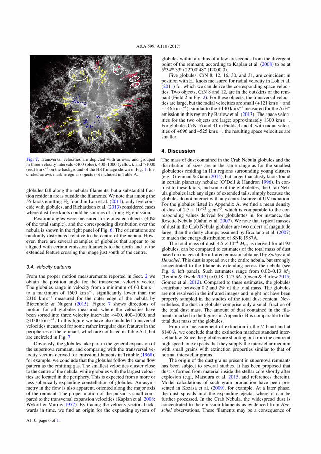
A&A 599, A110 (2017)
Fig. 7. Transversal velocities are depicted with arrows, and groupedin three velocity intervals <400 (blue), 400–1000 (yellow), and ≥1000(red) km s−1 on the background of the HST image shown in Fig. 1. En-circled arrows mark irregular objects not included in Table A.
globules fall along the nebular filaments, but a substantial frac-tion reside in areas outside the filaments. We note that among the55 knots emitting H2 found in Loh et al. (2011), only five coin-cide with globules, and Richardson et al. (2013) considered caseswhere dust-free knots could be sources of strong H2 emission.
Position angles were measured for elongated objects (40%of the total sample), and the corresponding distribution over thenebula is shown in the right panel of Fig. 6. The orientations arerandomly distributed relative to the centre of the nebula. How-ever, there are several examples of globules that appear to bealigned with certain emission filaments to the north and to theextended feature crossing the image just south of the centre.
3.4. Velocity patterns
From the proper motion measurements reported in Sect. 2 weobtain the position angle for the transversal velocity vector.The globules range in velocity from a minimum of 60 km s−1
to a maximum of 1600 km s−1, significantly lower than the2310 km s−1 measured for the outer edge of the nebula byBietenholz & Nugent (2015). Figure 7 shows directions ofmotion for all globules measured, where the velocities havebeen sorted into three velocity intervals: <400, 400–1000, and≥1000 km s−1. In this figure we have also included transversalvelocities measured for some rather irregular dust features in theperipheries of the remnant, which are not listed in Table A.1, butare encircled in Fig. 7.
Obviously, the globules take part in the general expansion ofthe supernova remnant, and comparing with the transversal ve-locity vectors derived for emission filaments in Trimble (1968),for example, we conclude that the globules follow the same flowpattern as the emitting gas. The smallest velocities cluster closeto the centre of the nebula, while globules with the largest veloci-ties are located in the periphery. This is expected from a more orless spherically expanding constellation of globules. An asym-metry in the flow is also apparent, oriented along the major axisof the remnant. The proper motion of the pulsar is small com-pared to the transversal expansion velocities (Kaplan et al. 2008;Wykoff & Murray 1977). By tracing the velocity vectors back-wards in time, we find an origin for the expanding system of
globules within a radius of a few arcseconds from the divergentpoint of the remnant, according to Kaplan et al. (2008) to be at5h34m 33s+22◦00′48′′ (J2000.0).
Five globules, CrN 8, 12, 16, 30, and 31, are coincident inposition with H2 knots measured for radial velocity in Loh et al.(2011) for which we can derive the corresponding space veloci-ties. Two objects, CrN 8 and 12, are in the outskirts of the rem-nant (Field 2 in Fig. 2). For these objects, the transversal veloci-ties are large, but the radial velocities are small (+121 km s−1 and+146 km s−1), similar to the +140 km s−1 measured for the ArH+
emission in this region by Barlow et al. (2013). The space veloc-ities for the two objects are large; approximately 1300 km s−1.For globules CrN 16 and 31 in Fields 3 and 4, with radial veloc-ities of +696 and –525 km s−1, the resulting space velocities aresmaller.
4. Discussion
The mass of dust contained in the Crab Nebula globules and thedistribution of sizes are in the same range as for the smallestglobulettes residing in H ii regions surrounding young clusters(e.g., Grenman & Gahm 2014), but larger than dusty knots foundin certain planetary nebulae (O’Dell & Handron 1996). In con-trast to these knots, and some of the globulettes, the Crab Neb-ula globules lack any signs of extended tails, simply because theglobules do not interact with any central source of UV radiation.For the globules listed in Appendix A, we find a mean densityof dust of 2.5 × 10⁻²¹ g cm−3, which is comparable to the cor-responding values derived for globulettes in, for instance, theRosette Nebula (Gahm et al. 2007). We note that typical massesof dust in the Crab Nebula globules are two orders of magnitudelarger than the dusty clumps assumed by Ercolano et al. (2007)to match the energy distribution of SNR 1987A.
The total mass of dust, 4.5 × 10⁻⁴ M�, as derived for all 92globules, can be compared to estimates of the total mass of dustbased on images of the infrared emission obtained by Spitzer andHerschel. This dust is spread over the entire nebula, but stronglyconcentrated to the filaments extending across the nebula (seeFig. 6, left panel). Such estimates range from 0.02–0.13 M�(Temim & Dwek 2013) to 0.18–0.27 M� (Owen & Barlow 2015;Gomez et al. 2012). Compared to these estimates, the globulescontribute between 0.2 and 2% of the total mass. The globulesare not resolved in the infrared images and might not have beenproperly sampled in the studies of the total dust content. Nev-ertheless, the dust in globules comprise only a small fraction ofthe total dust mass. The amount of dust contained in the fila-ments marked in the figures in Appendix B is comparable to thetotal dust mass of the globules.
From our measurement of extinction in the V band and at8140 Å, we conclude that the extinction matches standard inter-stellar law. Since the globules are shooting out from the centre athigh speed, one expects that they supply the interstellar mediumwith small grains with extinction properties similar to that ofnormal interstellar grains.
The origin of the dust grains present in supernova remnantshas been subject to several studies. It has been proposed thatdust is formed from material inside the stellar core shortly afterexplosion (e.g., Matsuura et al. 2015, and references therein).Model calculations of such grain production have been pre-sented in Kozasa et al. (2009), for example. At a later phase,the dust spreads into the expanding ejecta, where it can befurther processed. In the Crab Nebula, the widespread dust isconcentrated to the emission filaments as evidenced from Her-schel observations. These filaments may be a consequence of
A110, page 6 of 11

T. Grenman et al.: Dusty globules in the Crab Nebula
Rayleigh-Taylor instabilities between the synchrotron nebulaand the denser ejecta (Hester 1996) indicating that the dust be-comes concentrated along the filaments through the same pro-cess (Sankrit et al. 1998). Carlqvist (2015) proposed that elec-tromagnetic forces play a major role in the formation of certainfinger-like filaments in the Crab Nebula, and one may considerit possible that plasma instabilities contribute to the formation ofglobules inside the warm filaments. Grain destruction in reverseshocks in supernovae ejecta can delete the population of smallgrains as modeled in Silvia et al. (2012), for example. Temimet al. (2012) pointed out that the clumping of gas and dust in thefilaments may provide shielding against destruction.
However, the majority of the globules are not located in anybright filaments, and we have no clear idea of how they haveformed and survived. Model calculations of the convective lay-ers in red supergiants have been presented by Chiavassa et al.(2009), for example, and Freytag (priv. comm.) predicts that anumber of small convective surface elements (granules) coverthe surface above the deeper part of the convection zone. Wenote that not only is the expected number of such granules ofthe order of one hundred, similar to the total number of globuleswe have listed, but also that their typical mass is comparable tothe masses of globules corrected for a gas-to-dust ratio of 100.The agreement between these quantities may be a pure coinci-dence but might be worth considering in more detail. Could theglobules in the Crab Nebula be remnants of gas cells in the outerlayers of the progenitor, cells that are confined, compressed andejected during the passage of the blast wave through the stellarsurface and containing the seeds of grains that are further pro-cessed during the expansion?
5. Conclusions
We have located 92 cold cloudlets seen in obscuration against thebackground of continuous synchrotron radiation in optical im-ages of the Crab Nebula. These globules appear as dark, roundishspots in broad and medium band HST images. We present alist of positions, average radii, and orientations of elongated ob-jects. From images taken between 1994 and 2014 we derived theproper motion and related transversal velocity of each globule.We estimate the amount of extinction in the V band for eachobject and with different assumptions on the amount of fore-ground emission. From these measures we obtained the indi-vidual masses of dust using two different methods. In addition,we estimated the mass of extended, obscuring filaments alsopresent in the nebula. From extinction measurements at wave-lengths 5470 Å and 8140 Å we acquire information on the shapeof the extinction law for the globules.
– Mean radii range from 400 to 2000 AU, and 40% of theglobules are slightly elongated with a ratio between majorand minor axes >1.5. The objects are too small to be distin-guished in current infrared images obtained with Spitzer andHerschel.
– The globules are distributed over the entire nebula but lessabundant in the region surrounding the central pulsar. Severalglobules are located at emission filaments where elongatedobjects are aligned with the filaments.
– The extinction law for the globules and filaments matches anormal interstellar extinction law. Hence, the globules willeventually feed the interstellar medium with grains of inter-stellar type.
– Derived masses of dust range from 1 to 60 × 10−6 M�, withmean densities of ∼2.5 × 10⁻²¹ g cm−3.
– The total mass contained in globules amounts to 4.5 × 10⁻⁴,a fraction of 2% at most of the total dust content of the neb-ula. Assuming a gas-to-dust content of 30, the correspondingtotal mass amounts to 1.4 × 10⁻² M�.
– All globules move outwards from the centre with transversalvelocities of 60 to 1600 km s−1 along with the general expan-sion of the remnant. For some objects we could also derivespace velocities.
The question about the origin of dust in supernova remnants re-mains open. Dust grains may form at an early stage of the ex-plosion and be further processed and grow during the expansionof the ejecta. Rayleigh-Taylor instabilities acting on the ejectamay form filaments in which dust production and growth arestimulated, and we point out that electro-magnetic forces mayplay a role in confining globules inside filaments. However, mostglobules are not residing in filaments, and we speculate that theycould be products of cell-like blobs in the atmosphere of the pro-genitor, cells that are collapsing to form globules during the pas-sage of the blast wave during the explosion, possibilities whichcan be tested further with hydrodynamic calculations. The CrabNebula globules can be resolved from infrared imaging withthe coming James Webb Space Telescope, which would provideclues to whether the dust is warm or cold.
Acknowledgements. We thank Peter Lundqvist and Bernd Freytag for valuablecomments. The suggestions from the referee T. Haworth were most helpful inimproving our presentation. This work was supported by the Magnus BergvallFoundation.
ReferencesBarlow, M. J., Swinyard, B. M., Owen, P. J., et al. 2013, Science, 342, 1343Bietenholz, F. M., & Nugent, R. L. 2015, MNRAS, 454, 2416Blair, W. P., Davidson, K., Fesen, R. A., et al. 1997, ApJS, 109, 473Bohlin, R. C., Savage, B. D., & Drake, J. F. 1978, ApJ, 224, 132Bühler, R., & Blandford, R. 2014, Rep. Prog. Phys., 77, 066901Carlqvist, P. 2015, Ap&SS, 357, 47Chiavassa, A., Plez, B., Josselin, E., & Freytag, B. 2009, A&A, 506, 1351Davidson, K., & Fesen, R. A. 1985, ARA&A, 23, 119Ercolano, B., Barlow, M. J., & Sugerman, B. E. K. 2007, MNRAS, 375, 753Fesen, R., & Blair, W. P. 1990, ApJ, 351, L45Gahm, G. F., Grenman, T., Fredriksson, S., & Kristen, H. 2007, AJ, 133, 1795Grenman, T. 2006, Licentiate Thesis, Luleå University of Technology (ISSN
1402-1757)Grenman, T., & Gahm, G. F. 2014, A&A, 565, 107Gomez, H. L., Krause, O., Barlow, M. J., et al. 2011, ApJ, 760, 96Hester, J. J. 2008, ARA&A, 46, 127Hester, J. J., Graham, J. R., Beichman, C. A., & Gautier, T. N. 1990, ApJ, 357,
539Hester, J. J., Stone, J. M., Scowen, P. A., et al. 1996, ApJ, 456, 225Höffner, S., Bladh, S., Aringer, B., & Ahuja, R. 2016, A&A, 594, A108Indebetouw, R., Matsuura, M., Dwek, E., et al. 2014, ApJ, 782, L2IKaplan, D. L., Chatterjee, S., Gaensler, B. M., & Anderson, J. 2008, ApJ, 677,
1201Kozasa, T., Nozava, T., Tominaga, N., et al. 2009, in Cosmic Dust – near and far,
ASP Conf. Ser., 414, 43Loh, E. D., Baldwin, J. A., Curtis, Z. K., et al. 2011, ApJS, 194, 30Loll, A. 2010, Ph.D. Thesis, Arizona State UniversityLundqvist, P., & Tziamtzis, A. 2012, MNRAS, 423, 1571Lundqvist, P., Fransson, C., & Chevalier, R. A. 1986, A&A, 162, L6Matsuura, M., Dwek, E., Barlow, M. J., et al. 2015, ApJ, 800, 50Moriya, T. J., Tominaga, N., Langer, N., et al. 2014, A&A, 569, A57Nugent, R. L. 1998, PASP, 110, 831O’Dell, C. R., & Handron, K. D. 1996, AJ, 111, 1630Owen, P. J., & Barlow, M. J. 2015, ApJ, 801, 141Richardson, C. T., Baldwin, J. A., Ferland, G. J., et al. 2013, MNRAS, 430,
1257
A110, page 7 of 11

A&A 599, A110 (2017)
Rho, J., Kozasa, T., Reach, W. T., et al. 2008, ApJ, 673, 271Sankrit, R., Hester, J. J., Scowen, P. A., et al. 1998, ApJ, 504, 344Savage, B. D., & Mathis, J. S. 1979, ARA&A, 17, 73Silvia, D. W., Smith, B. D., & Shull, J. M. 2012, ApJ, 748, 12Spitzer, L., Jr. 1978, Physical Processes in the Interstellar Medium (New York:
Wiley Interscience)Sugerman, B. E. K., Ercolano, B., Barlow, M. J., et al. 2006, Science, 313,
196Temim, T., & Dwek, E. 2013, ApJ, 774, 8
Temim, T., Gehrz, R. D., Woodward, C. E., et al. 2006, ApJ, 132, 1610Temim, T., Sonneborn, G., Dwek, E., et al. 2012, ApJ, 753, 72Trimble, V. 1968, AJ, 73, 535Trimble, V. 1977, Astrophys. Lett., 18, 145Wang, X., Ferland, G. J., Baldwin, J. A., Koh, E. D., & Richardson, C. T. 2013,
AJ, 774, 112Woltjer, L., & Véron-Cetty, M.-P. 1987, A&A, 172, L7Wyckoff, S., & Murray, C. A. 1977, MNRAS, 180, 717Yang, H., & Chevalier, R. A. 2015, ApJ, 806, 153
A110, page 8 of 11

T. Grenman et al.: Dusty globules in the Crab Nebula
Appendix A: Properties of the globules in the Crab Nebula
Table A.1. Properties of the globules in the Crab Nebula.
CrN Field RA Dec r R PA µα µδ Vt Md RemarksJ(2000.0) J(2000.0) (′′) (AU) (deg) (′′/yr) (′′/yr) (km s−1) (M� × 10−6)
1 2 5:34:25.77 +22:01:40.1 0.5 1000 41 –0.163 +0.064 1660 102 1 5:34:25.86 +22:01:03.6 0.3 600 –16 –0.133 +0.016 1270 33 2 5:34:26.25 +22:01:56.1 0.3 600 –0.145 +0.077 1522 34 2 5:34:26.31 +22:01:54.9 0.2 400 –0.134 +0.093 1546 15 2 5:34:26.34 +22:01:54.3 0.2 400 –33 –0.143 +0.078 1544 26 1 5:34:26.84 +22:00:58.3 0.2 400 –0.113 +0.009 1075 27 1 5:34:26.89 +22:01:00.4 0.3 600 –42 –0.114 +0.016 1091 38 2 5:34:27.06 +22:01:52.5 0.5 1000 –0.114 +0.071 1273 12 Knot 521, 4E2
9 1 5:34:27.20 +22:00:58.5 0.2 400 –0.113 +0.009 1075 1 C to 1010 1 5:34:27.21 +22:00:57.7 0.4 800 –0.118 +0.004 1119 6 C to 9, Irr11 1 5:34:27.25 +22:00:49.7 0.6 1200 –0.108 +0.022 1045 20 1E2, Irr12 2 5:34:27.58 +22:01:52.0 0.6 1200 –0.121 +0.073 1340 16 Knot 511, 4D2
13 1 5:34:27.67 +22:00:52.2 0.2 400 –0.099 +0.008 942 214 3 5:34:28.63 +22:00:19.9 0.3 600 –34 –0.081 –0.024 801 415 3 5:34:29.01 +22:00:42.1 0.2 400 –0.076 –0.001 721 216 3 5:34:29.32 +22:00:30.1 1.0 2000 –0.068 –0.011 653 58 Irr, Knot 531, 1A2
17 3 5:34:29.37 +22:00:27.9 0.3 600 –0.068 –0.016 662 318 3 5:34:29.49 +22:00:30.3 0.6 1200 –44 –0.077 –0.012 739 1519 5 5:34:29.53 +22:00:00.5 0.2 400 22 –0.048 –0.051 664 220 3 5:34:29.59 +22:00:28.7 0.2 400 –0.061 –0.012 589 221 3 5:34:29.59 +22:00:40.5 0.2 400 –4 –0.061 –0.004 580 322 3 5:34:29.66 +22:00:29.2 0.3 600 31 –0.060 –0.015 586 423 3 5:34:30.24 +22:00:24.9 0.2 400 3 –0.052 –0.010 502 224 3 5:34:30.44 +22:00:25.0 0.2 400 –0.045 –0.023 479 225 4 5:34:30.71 +22:01:57.9 0.3 600 40 –0.041 +0.081 861 426 4 5:34:30.75 +22:01:56.0 0.2 400 –0.041 +0.092 955 327 6 5:34:30.79 +22:01:40.3 0.4 800 15 –0.039 +0.050 601 6 4B2
28 5 5:34:31.06 +21:59:53.9 0.2 400 –0.023 –0.057 583 229 6 5:34:31.08 +22:01:37.4 0.3 600 –0.042 +0.063 718 230 6 5:34:31.15 +22:01:47.2 0.7 1400 –0.046 +0.073 818 16 Knot 451, 4C2
31 4 5:34:31.19 +22:02:01.0 0.6 1200 –21 –0.035 +0.086 880 17 Knot 461, 4A2
32 5 5:34:31.20 +22:00:11.7 0.2 400 21 –0.025 –0.032 385 233 5 5:34:31.44 +21:59:56.0 0.4 800 44 –0.016 –0.054 534 634 3 5:34:31.63 +22:00:26.6 0.3 600 –0.018 –0.015 222 435 4 5:34:31.64 +22:02:07.0 0.3 600 –7 –0.042 +0.089 933 436 4 5:34:31.67 +22:02:14.3 0.3 400 –16 –0.027 +0.104 1019 337 4 5:34:31.72 +22:02:13.6 0.2 400 40 –0.025 +0.104 1014 238 3 5:34:31.76 +22:00:28.3 0.4 600 –0.012 –0.015 182 539 3 5:34:32.20 +22:00:18.0 0.2 400 –0.006 –0.021 207 140 5 5:34:32.20 +21:59:59.4 0.2 400 –41 +0.009 –0.050 482 141 5 5:34:32.36 +22:00:06.2 0.3 600 –0.004 –0.032 306 342 5 5:34:32.62 +22:00:06.6 0.2 400 –1 +0.005 –0.034 326 2 2C2
43 5 5:34:32.62 +22:00:05.5 0.3 600 +0.005 –0.036 345 4 2C2
44 6 5:34:32.85 +22:01:35.6 0.2 400 +0.002 +0.053 503 245 5 5:34:32.90 +21:59:45.0 0.2 400 34 +0.013 –0.059 573 146 5 5:34:33.04 +22:00:02.4 0.6 1200 +0.021 –0.029 339 11 2D2, Irr47 5 5:34:33.15 +22:00:05.9 0.3 600 39 +0.013 –0.035 354 448 6 5:34:33.19 +22:01:33.1 0.4 800 +0.005 +0.060 571 6 Irr49 7 5:34:33.18 +22:00:54.4 0.3 600 –35 +0.018 +0.003 173 450 7 5:34:33.18 +22:00:49.5 0.2 400 +0.007 +0.002 69 251 6 5:34:33.25 +22:01:42.6 0.2 400 +0.012 +0.069 664 152 8 5:34:33.32 +22:00:20.5 0.4 800 3 +0.016 –0.021 250 6 C to 53, 2E2
53 8 5:34:33.38 +22:00:18.3 0.4 800 27 +0.017 –0.032 344 7 C to 52, 2E2
54 8 5:34:33.44 +22:00:20.2 0.3 600 –36 +0.019 –0.016 236 455 7 5:34:33.47 +22:00:53.0 0.2 400 +0.008 +0.007 101 156 8 5:34:33.50 +22:00:19.4 0.3 600 +0.026 –0.018 300 357 8 5:34:33.52 +22:00:16.5 0.3 600 +0.024 –0.022 309 458 8 5:34:33.66 +22:00:15.3 0.2 400 +0.029 –0.023 351 259 7 5:34:33.96 +22:00:54.2 0.2 400 +0.021 +0.002 200 260 7 5:34:34.12 +22:00:54.3 0.2 400 +0.034 +0.005 326 2
Notes. Symbols are described in Sect. 2. (1) From Loh et al. (2011), (2) from Fesen & Blair (1990).
A110, page 9 of 11

A&A 599, A110 (2017)
Table A.1. continued.
CrN Field RA Dec r R PA µα µδ Vt Md RemarksJ(2000.0) J(2000.0) (′′) (AU) (deg) (′′/yr) (′′/yr) (km s−1) (M� × 10−6)
61 9 5:34:34.17 +22:01:12.9 0.2 400 +0.024 +0.024 322 162 10 5:34:34.29 +21:59:55.6 0.2 400 +0.039 –0.044 557 163 8 5:34:34.31 +22:00:11.0 0.3 600 +0.034 –0.027 412 364 7 5:34:34.66 +22:00:35.3 0.4 800 +0.043 –0.002 408 665 9 5:34:34.69 +22:01:02.6 0.4 800 –3 +0.039 +0.015 396 8 3E2
66 7 5:34:34.69 +22:00:56.3 0.3 600 –31 +0.024 +0.005 232 567 8 5:34:34.76 +22:00:19.8 0.2 400 +0.044 –0.018 451 2 C to 6968 9 5:34:34.83 +22:01:26.0 0.2 400 24 +0.030 +0.038 459 169 8 5:34:34.84 +22:00:19.1 0.5 1000 33 +0.043 –0.016 435 11 C to 67, 2F2
70 7 5:34:34.85 +22:00:54.2 0.3 600 +0.032 +0.008 313 371 10 5:34:35.18 +21:59:53.3 0.3 600 +0.055 –0.046 680 472 7 5:34:35.40 +22:00:58.9 0.4 800 30 +0.037 +0.017 386 8 3G2
73 10 5:34:35.41 +21:59:42.6 0.2 400 +0.059 –0.057 778 274 8 5:34:35.58 +22:00:23.8 0.2 400 –7 +0.059 –0.007 563 3 C to 7575 8 5:34:35.60 +22:00:23.1 0.3 600 –19 +0.076 –0.005 722 4 C to 7476 10 5:34:35.65 +21:59:49.4 0.2 400 +0.068 –0.049 795 277 8 5:34:35.76 +22:00:26.6 0.2 400 +0.067 –0.016 653 278 9 5:34:35.87 +22:01:12.8 0.3 600 43 +0.047 +0.031 534 479 10 5:34:35.92 +21:59:47.4 0.2 400 +0.064 –0.054 794 280 7 5:34:36.02 +22:00:50.5 0.3 600 +0.063 +0.004 598 5 C to 8181 7 5:34:36.09 +22:00:52.1 0.4 800 +0.058 +0.007 554 7 C to 8082 8 5:34:36.12 +22:00:11.4 0.2 400 +0.077 –0.022 759 283 7 5:34:36.15 +22:00:46.8 0.3 600 +0.072 +0.004 684 484 9 5:34:36.44 +22:01:01.9 0.2 400 +0.058 +0.020 582 2 C to 8585 9 5:34:36.45 +22:01:02.5 0.2 400 –5 +0.060 +0.019 597 2 C to 8486 8 5:34:36.52 +22:00:12.8 0.2 400 +0.084 –0.019 816 287 8 5:34:36.95 +22:00:07.8 0.3 600 +0.097 –0.020 939 488 10 5:34:37.57 +21:59:49.3 0.5 1000 –38 +0.086 –0.060 994 989 11 5:34:38.73 +22:00:08.0 0.2 400 +0.117 –0.041 1175 190 11 5:34:38.82 +22:00:05.4 0.2 400 +0.120 –0.034 1182 291 11 5:34:39.06 +22:00:03.1 0.2 400 –5 +0.091 –0.044 958 292 11 5:34:39.38 +22:00:02.1 0.2 400 +0.100 –0.049 1056 1
A110, page 10 of 11

T. Grenman et al.: Dusty globules in the Crab Nebula
Appendix B: Images of all fields listed in Table 2T. Grenman et al.: The dusty globules in the Crab Nebula
Fig. B.2. Optical images of the fields marked in Fig. 2 and de-scribed in Sect. 2. Globules are marked with circles and CrNnumber.
Fig. B.3.
12
Fig. B.1. Optical images of the fields marked in Fig. 2 and described in Sect. 2. Globules are marked with circles and CrN number.
A110, page 11 of 11

Paper IV
History of gobulettes in the Milky Way
Authors:Grenman, T., Elfgren, E., & Weber, H.

Astrophys Space Sci (2018) 363:28https://doi.org/10.1007/s10509-017-3233-6
ORIGINAL ARTICLE
History of globulettes in the Milky Way
Tiia Grenman1 · Erik Elfgren1 · Hans Weber1
Received: 14 August 2017 / Accepted: 7 December 2017 / Published online: 10 January 2018© The Author(s) 2018. This article is published with open access at Springerlink.com
Abstract Globulettes are small (radii <10 kAU) dark dustclouds, seen against the background of bright nebulae. Amajority of the objects have planetary mass. These objectsmay be a source of brown dwarfs and free floating plane-tary mass objects in the galaxy. In this paper we investigatehow many globulettes could have formed in the Milky Wayand how they could contribute to the total population of freefloating planets. In order to do that we examine H-alpha im-ages of 27 H II regions. In these images, we find 778 glob-ulettes.
We find that a conservative value of the number of glob-ulettes formed is 5.7 × 10¹⁰. If 10% of the globulettesform free floating planets then they have contributed with5.7 × 109 free floating planets in the Milky Way. A lessconservative number of globulettes would mean that theglobulettes could contribute 2.0 × 10¹⁰ free floating planets.Thus the globulettes could represent a non-negligible sourceof free floating planets in the Milky Way.
Keywords Free Floating Planets · Globulettes · H IIregions · ISM · Milky Way
1 Introduction
H II regions, surrounding young stellar clusters are drivenby massive O and early B stars. These regions are associ-ated with dusty gas formations, such as pillars, ‘elephant-trunks’ and isolated dark clouds seen in different sizes andshapes, from large irregular blocks and fragments to smallermore roundish objects. These small-sized globules within
B T. [email protected]
1 Luleå University of Technology, Luleå, SE-971 87 Luleå, Sweden
H II regions were first observed by Bok and Reilly (1947),followed by Thackeray (1950) and Herbig (1974). They aredense, cold and neutral clouds with dark appearance in opti-cal images. The pillars of gas and dust are pointing towardsthe ionizing sources and are usually connected to the molec-ular shell.
In such H II regions, a new distinct class of objects,globulettes, was noted by Gahm et al. (2007) and Grenman(2006). The globulettes are seen as silhouettes against thebackground of bright nebulae in optical images. Typically,they are roundish objects that are much smaller (<10 kAU)than normal globules with a mass of �0.1 M� (Gahm et al.2007). The globulettes can also have tails, bright rims andhalos. Many globulettes are quite isolated, located far fromthe molecular shells and dust pillars associated with the re-gions. However, some of the objects are connected by thinfilaments to large molecular blocks or even each other. Thissuggests that they can either form separately, or via fragmen-tation of large structures. The calculated lifetime of glob-ulettes suggests that they may survive in this harsh environ-ment for a long time, >106 yrs (Gahm et al. 2007; Haworthet al. 2015).
In the Carina Nebula (NGC 3372), a giant H II region, theglobulettes are smaller, more dense and less massive (Gren-man and Gahm 2014) than those recognized in Gahm et al.(2007) and De Marco et al. (2006). This group of glob-ulettes may represent a more advanced evolutionary statein globulette evolution. Schneider et al. (2016) suggestedthat the pillars may evolve first into a globule and theninto a globulette when the lower density gas has photoe-vaporated and left behind a dense and cold core. However,it is also speculated that globulettes might collapse in situto form free floating planets (FFPs with <13 MJ , whereMJ = Jupiter mass) or brown dwarfs (13–75 MJ ), triggeredby external forces from gas and turbulent pressure in the sur-

28 Page 2 of 10 T. Grenman et al.
rounding warm plasma and radiation pressure from stellarphotons. In fact, the result by Gahm et al. (2013) from near-infrared imaging of the Rosette Nebula, revealed very densecores in some of the largest globulettes that might collapseto form FFPs. They also pointed out that these objects ac-celerate outwards from the nebula and eventually ends up inthe interstellar environment.
A more recent example, where globulettes may haveformed planetary mass objects was found in the Orion Neb-ula (M42/43, Fang et al. 2016). This nebula stands out byhaving both dark silhouette disks and bright compact knots.They are known as proplyds (O’Dell et al. 1993; O’Dell andWong 1996; Bally et al. 2000).
The first reports of populations of substellar objects ininterstellar space came in 1995 (Rebolo et al. 1995; Naka-jima et al. 1995). Since then, a number of Jupiter-mass FFPsand FFP candidates have been found in young clusters andstar formation regions (see Lucas and Roche 2000; Bihainet al. 2009; Luhman 2012; Liu et al. 2013; Peña Ramírezet al. 2016, 2012; Clanton and Gaudi 2017, and referencestherein). Planetary mass objects have also been found in thegalactic field (Cushing et al. 2014). Since these substellarobjects are both brighter and warmer at young ages (lessthan 10 Myr, Chabrier et al. 2000), these objects with massesof a few Jupiter masses can be seen e.g. in deep optical andnear-infrared photometric surveys (Zapatero Osorio et al.2000, 2017; Quanz et al. 2010).
Another method to find objects below the deuterium-burning-mass-limit (Jupiter-sized) that are not bound to ahost star is through gravitational microlensing. This type ofstudy has been done by the Microlensing Observation in As-trophysics group (MOA-2; Sumi et al. 2003, 2011; Freemanet al. 2015) and the Optical Gravitational Lensing Experi-ment (OGLE-III; Wyrzykowski et al. 2015).
The origin of these unbound objects is unclear. They mayhave formed in situ from a direct collapse of a molecu-lar cloud by fragmentation, similar to star formation (e.g.Silk 1977; Bowler et al. 2011). In fact, Fang et al. (2016),Luhman et al. (2005), Boucher et al. (2016), Joergens et al.(2015), Bayo et al. (2017) have found four FFPs with ac-cretion disk. Furthermore, planetary-mass binaries, whichwould be almost impossible to from through planetary for-mation mechanisms, have also be found by e.g. Jayaward-hana and Ivanov (2006), Best et al. (2017).
FFPs may also have been formed from stellar embryosthat are fragmented and photoevaporated from nearby stars(see e.g. Kroupa and Bouvier 2003; Padoan and Nordlund2004; Whitworth and Zinnecker 2004). They may also havebeen ejected after they were formed in circumstellar proto-planetary disks through gravitational instabilities (e.g. Boss2009; Stamatellos and Whitworth 2009; Li et al. 2015). Suchinstabilities can be caused by a triplet star system (Reipurthand Mikkola 2015) or by passage through the center of adense star cluster (Wang et al. 2015).
In this work, we present results based on available imagesof H II-regions from the Hubble Space Telescope (HST)archive and taken with the Nordic Optic Telescope (NOT).We create a model of how many globulettes may haveformed in the Milky Way over time and how many of thesethat contribute to the total FFPs population. We have orga-nized the paper as follows. In Sect. 2, we present the resultof both old and new H II regions investigated in the contextof globulettes. We also present mean radii of histograms ofglobulettes for those H II regions, which contain many glob-ulettes. In Sect. 3, the parameters that are used in our modelare presented. The results and discussion regarding FFPs canbe found in Sect. 4 and we conclude the paper in Sect. 5.
2 Archival data and measurements
In this work, we used archival H-alpha images of 16 H IIregions included in earlier studies by De Marco et al. (2006),Gahm et al. (2007) and Grenman and Gahm (2014). Theobservations in these studies are from the HST archive andthe NOT. Most images were taken with the HST instrumentssuch as ACS/WFC, WFPC2, WFPC3/UVIS, while the NOTimages were taken with the ALFOSC instrument. A briefdescription of these instruments is given below.
1. The Wide Field and Planetary Camera 2 (WFPC2) fieldof view is covered by four cameras, each of which span800×800 pixels in size. Three of them are arranged in anL-shaped field and operated at a pixel scale of 0.1′′. Thefourth one is referred to as the Planetary Camera (PC)and operates at a pixel scale of 0.046′′.
2. The Wide Field Camera 3 (WFC3) replaced the WPFC2camera in 2009. The Ultraviolet-Visible channel (UVIS)use a mosaics of two CCDs, with 0.04 arcsec/pixel, cov-ering a 162′′ ×162′′ field of view. The 2 CCDs are buttedtogether but have a ∼1.4′′ gap between the two chips.
3. The Advanced Camera for Surveys (ACS/WFC) cameracontains two CCDs of 2048 × 4096 pixels glued togetherwith a small gap of approximately 50 pixels in between.The pixel size corresponds to 0.05′′ per pixel and the fieldof view is 202′′ × 202′′.
4. The Andalucia Faint Object Spectrograph and Camera(ALFOSC) has a field of view of 6.5′, and the effectivescale of the CCD detector is 0.188′′ per pixel.
The respective areas for the instruments WFPC2, WFC3,ACS and ALFOSC are estimated to 5, 7, 11 and 33 arcmin2.More information about each of these instruments can befound in the manuals on the HST Web site1 and in the NOTmanual.2 All images in the current study are analyzed using
1http://www.stsci.edu/hst/HST_overview/instruments.2http://www.not.iac.es/instruments/alfosc.
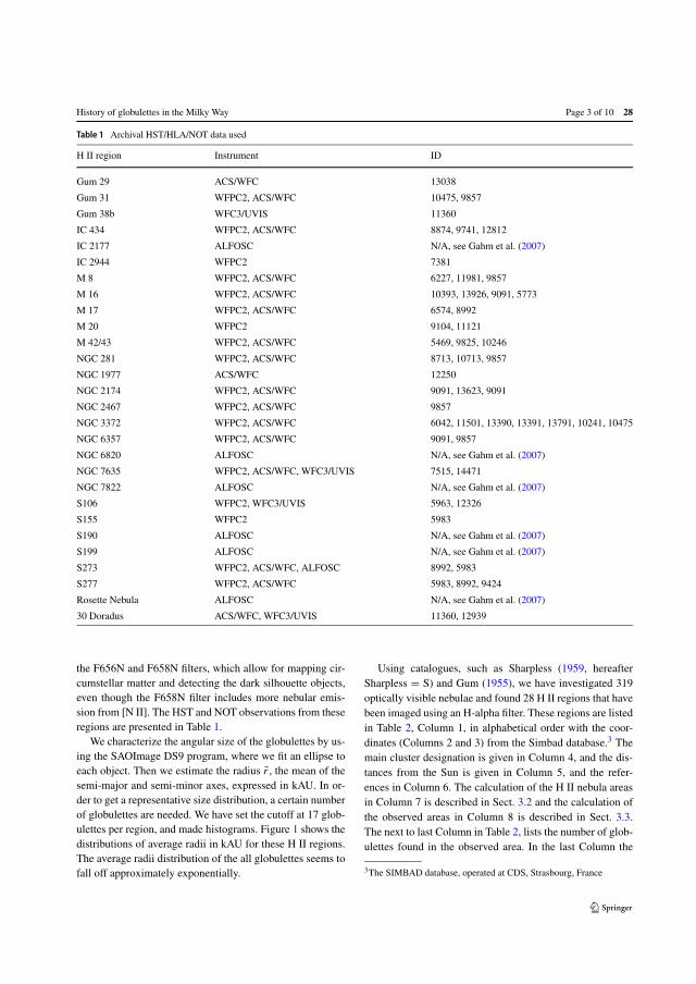
History of globulettes in the Milky Way Page 3 of 10 28
Table 1 Archival HST/HLA/NOT data used
H II region Instrument ID
Gum 29 ACS/WFC 13038
Gum 31 WFPC2, ACS/WFC 10475, 9857
Gum 38b WFC3/UVIS 11360
IC 434 WFPC2, ACS/WFC 8874, 9741, 12812
IC 2177 ALFOSC N/A, see Gahm et al. (2007)
IC 2944 WFPC2 7381
M 8 WFPC2, ACS/WFC 6227, 11981, 9857
M 16 WFPC2, ACS/WFC 10393, 13926, 9091, 5773
M 17 WFPC2, ACS/WFC 6574, 8992
M 20 WFPC2 9104, 11121
M 42/43 WFPC2, ACS/WFC 5469, 9825, 10246
NGC 281 WFPC2, ACS/WFC 8713, 10713, 9857
NGC 1977 ACS/WFC 12250
NGC 2174 WFPC2, ACS/WFC 9091, 13623, 9091
NGC 2467 WFPC2, ACS/WFC 9857
NGC 3372 WFPC2, ACS/WFC 6042, 11501, 13390, 13391, 13791, 10241, 10475
NGC 6357 WFPC2, ACS/WFC 9091, 9857
NGC 6820 ALFOSC N/A, see Gahm et al. (2007)
NGC 7635 WFPC2, ACS/WFC, WFC3/UVIS 7515, 14471
NGC 7822 ALFOSC N/A, see Gahm et al. (2007)
S106 WFPC2, WFC3/UVIS 5963, 12326
S155 WFPC2 5983
S190 ALFOSC N/A, see Gahm et al. (2007)
S199 ALFOSC N/A, see Gahm et al. (2007)
S273 WFPC2, ACS/WFC, ALFOSC 8992, 5983
S277 WFPC2, ACS/WFC 5983, 8992, 9424
Rosette Nebula ALFOSC N/A, see Gahm et al. (2007)
30 Doradus ACS/WFC, WFC3/UVIS 11360, 12939
the F656N and F658N filters, which allow for mapping cir-cumstellar matter and detecting the dark silhouette objects,even though the F658N filter includes more nebular emis-sion from [N II]. The HST and NOT observations from theseregions are presented in Table 1.
We characterize the angular size of the globulettes by us-ing the SAOImage DS9 program, where we fit an ellipse toeach object. Then we estimate the radius r , the mean of thesemi-major and semi-minor axes, expressed in kAU. In or-der to get a representative size distribution, a certain numberof globulettes are needed. We have set the cutoff at 17 glob-ulettes per region, and made histograms. Figure 1 shows thedistributions of average radii in kAU for these H II regions.The average radii distribution of the all globulettes seems tofall off approximately exponentially.
Using catalogues, such as Sharpless (1959, hereafterSharpless = S) and Gum (1955), we have investigated 319optically visible nebulae and found 28 H II regions that havebeen imaged using an H-alpha filter. These regions are listedin Table 2, Column 1, in alphabetical order with the coor-dinates (Columns 2 and 3) from the Simbad database.3 Themain cluster designation is given in Column 4, and the dis-tances from the Sun is given in Column 5, and the refer-ences in Column 6. The calculation of the H II nebula areasin Column 7 is described in Sect. 3.2 and the calculation ofthe observed areas in Column 8 is described in Sect. 3.3.The next to last Column in Table 2, lists the number of glob-ulettes found in the observed area. In the last Column the
3The SIMBAD database, operated at CDS, Strasbourg, France

28 Page 4 of 10 T. Grenman et al.
Fig. 1 The mean radii distribution for those H II regions con-taining most globulettes. The histograms peak at about 0.3 kAUin M 8, 2.5 kAU in the Rosette Nebula, 0.4 kAU in M 16 and
M 17, 2.5 kAU in IC 1805, 0.9 kAU in IC 2944, 1.9 kAU inNGC 281, 0.6 kAU in NGC 3372 and 1.5 kAU in NGC 2467.
minimum detection size of an object (in AU) is given. Ob-
jects with dimensions <3 pixels across are too small to be of
interest (De Marco et al. 2006). For the NOT observations,
there are no objects with a diameter of less than 9 pixels,
which means that they are also clearly resolved. The Carina
Nebula, Rosette Nebula and 30 Doradus contain the most
globulettes. 30 Doradus is an example of a low metallicity
region in the Large Magellanic Cloud (LMC) and we do not
consider it in our calculation of globulettes within the Milky
Way.
Some of the nebulae are giant H II regions, like Carina
Nebula and 30 Doradus. In these regions, the Lyman con-
tinuum flux is >1050 photons per second (Moisés et al.
2011). There is also a young ultracompact H II region, S106
(Crowther and Conti 2003) in our list, where the ionized star
is a pre-main sequence star embedded in its molecular cloud
(Noel et al. 2005). Most of the regions are relatively nearby
(d < 4 kpc) and they are relatively young (�5 Myr). The
distances are based on the references cited below in Table 2.
3 Model parameters
In this section we define the different parameters needed tomodel the number of globulettes as shown in Table 3. To il-lustrate the methodology of this work we chose the RosetteNebula as a representative example, because it contains onlyone main cluster, is symmetric and hold a large amount glob-ulettes. An overview of the Rosette Complex can be foundin Román-Zúñiga and Lada (2008).
3.1 Young Universe and H II formation rate
From model calculations we know that within the first relicH II regions, the massive metal free Population III (Pop III)stars evacuated the primordial gas from their minihalos (Ki-tayama et al. 2004; Alvarez et al. 2006; Abel et al. 2007).As the Pop III stars ended in supernova explosions, theUniverse’s intergalactic medium got progressively enrichedwith heavy metals (i.g. Greif et al. 2007; Wise and Abel2008) and dust.
Cosmological simulations suggest that once the gasreaches the minimum or ‘critical’ metallicity in the range

History of globulettes in the Milky Way Page 5 of 10 28
Table 2 List of H II regions investigated
H II region RA(J2000.0)
Dec.(J2000.0)
Main cluster Distance(kpc)
Ref. Nebula areaarcmin2
Obs. areaarcmin2
Number ofglobulettes
Detectionlimitb (AU)
Gum 29 10 24 −57 46 Westerlund 2 4.2 1 707 11 10 630
Gum 31 10 37 −58 39 NGC 3324 2.3 2 177 43 7 345
Gum 38b 11 15 −61 15 NGC 3603 6.0 3 94 7 5 720
IC 434 05 41 −02 30 Sigma Orionis 0.4 4 471 86 – 60
IC 2177a 07 04 −10 27 N/A 1.3 5 314 33 – 733
IC 2944 11 38 −63 22 Collinder 249 2.3 6 1866 5 34 690
M 8 18 03 −24 23 NCC 6530, 6523 1.3 7 1374 43 18 195
M 16 18 18 −13 48 NGC 6611 1.8 7 825 53 46 270
M 17 18 20 −16 10 NGC 6618 2.0 7 806 16 23 300
M 20 18 02 −22 58 NGC 6514 2.7 7 361 21 – 810
M 42/43 05 35 −05 23 NGC 1976, 1982 0.41 7 1689 639 9 61
NGC 281 00 52 +56 34 IC 1590 2.8 8 589 32 18 420
NGC 1977 05 35 −04 49 NGC 1973, 75 0.41 9 314 44 – 61
NGC 2174 06 09 +20 30 NGC 2175, 75s 2.2 12 589 35 15 330
NGC 2467 07 52 −26 25 Haffner18ab, 19 5.0 10 467 16 59 750
NGC 3372 10 44 −59 53 Tr14/15/16, Bo10/11,Cr232, Cr234/228
2.9 11 10 179 953 343 435
NGC 6357 17 26 −34 12 Pis 24, ESO 392-11,ESO 393-13
1.7 7 911 17 11 255
NGC 6820a 19 42 +23 05 NGC 6823 1.9 13 707 53 1 1072
NGC 7635 23 20 +61 12 [BDS2003]44 2.4 14 94 37 4 288
NGC 7822a 00 01 +67 25 Berkeley 59 0.91 12 1884 72 9 513
S106 20 27 +37 22 S106 IR 1.7 15 3 13 – 204
S155 22 58 +62 31 CepIII 0.84 12 1178 10 – 252
S190a 02 32 +61 27 IC 1805 2.0 12 5281 189 18 1128
S199a 02 51 +60 24 IC 1848, Cl34 1.8 12 5089 66 – 1015
S273a 06 41 +09 53 NGC 2264 0.91 7 2672 126 – 136
S277 05 42 −01 55 NGC 2024 0.41 7 491 107 3 61
RosetteNebulaa
06 31 +04 57 NGC 2244 1.4 16 5281 570 145 790
LMC:30 Doradus
06 31 +04 57 NGC 2070 50 17 176 132 176 2000
References—(1) Vargas Álvarez et al. 2013; (2) Ohlendorf et al. 2013; (3) Brandner et al. 2000; (4) Mookerjea et al. 2009; (5) Bica et al. 2003;(6) Sana et al. 2011; (7) Feigelson et al. 2013, and reference therein; (8) Sato et al. 2008; (9) Menten et al. 2007; (10) Yadav et al. 2015; (11) Huret al. 2012; (12) Foster and Brunt 2015; (13) Kharchenko et al. 2005; (14) Moore et al. 2002; (15) Schneider et al. 2007; (16) Hensberge et al.2000; (17) Pietrzynski et al. 2013aH II regions from Gahm et al. (2007)bThe minimum detection size (diameter in AU) of an object, defined as 3 pixels in this article
10−6–10−3.5 Z� which allows for more efficient cooling.An example of a low metallicity Pop II environment is theLarge Magellanic Cloud (LMC), where the metallicity is∼0.5 Z� (Rolleston et al. 2002).
In Som et al. (2015, Fig. 11) these different metallicityvalues correspond to T0 ∼ 12 Gyr, which we set as our start-ing point for the calculations of the number of globulettes inthe Milky Way.
In the early Universe, the formation rate of the H II re-gions was higher than it is now. We assume that it is propor-tional to the Star Formation Rate (SFR), which combinedwith the present day gives us the formation rate of H II re-gions in the early Universe. Marasco et al. (2015, Fig. 1),show an overview of the SFR evolution as a function of time,where the current SFR is about ∼5 M�/yr. We estimate thetotal area under the curve, which gives us the average SFR
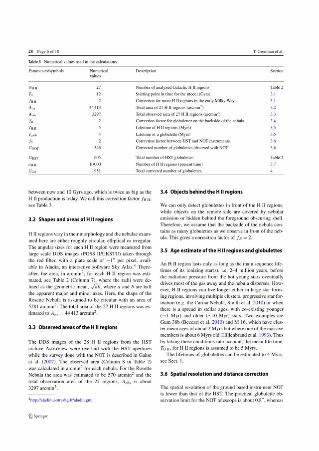
28 Page 6 of 10 T. Grenman et al.
Table 3 Numerical values used in the calculations
Parameters/symbols Numericalvalues
Description Section
NH II 27 Number of analyzed Galactic H II regions Table 2
T0 12 Starting point in time for the model (Gyrs) 3.1
fH II 2 Correction for more H II regions in the early Milky Way 3.1
Atot 44 413 Total area of 27 H II regions (arcmin2) 3.2
Aobs 3297 Total observed area of 27 H II regions (arcmin2) 3.3
fB 2 Correction factor for globuletter on the backside of the nebula 3.4
TH II 5 Lifetime of H II regions (Myrs) 3.5
Tglob 4 Lifetime of a globulette (Myrs) 3.5
fS 2 Correction factor between HST and NOT instruments 3.6
GNOT 346 Corrected number of globulettes observed with NOT 3.6
GHST 605 Total number of HST globulettes Table 2
nH II 10 000 Number of H II regions (present time) 3.7
GTot 951 Total corrected number of globulettes 4
between now and 10 Gyrs ago, which is twice as big as theH II production is today. We call this correction factor fH II,see Table 3.
3.2 Shapes and areas of H II regions
H II regions vary in their morphology and the nebulae exam-ined here are either roughly circular, elliptical or irregular.The angular sizes for each H II region were measured fromlarge scale DDS images (POSS II/UKSTU) taken throughthe red filter, with a plate scale of ∼1′′ per pixel, avail-able in Aladin, an interactive software Sky Atlas.4 There-after, the area, in arcmin2, for each H II region was esti-mated, see Table 2 (Column 7), where the radii were de-fined as the geometric mean,
√ab, where a and b are half
the apparent major and minor axes. Here, the shape of theRosette Nebula is assumed to be circular with an area of5281 arcmin2. The total area of the 27 H II regions was es-timated to Atot = 44 413 arcmin2.
3.3 Observed areas of the H II regions
The DDS images of the 28 H II regions from the HSTarchive AstroView were overlaid with the HST apertureswhile the survey done with the NOT is described in Gahmet al. (2007). The observed area (Column 8 in Table 2)was calculated in arcmin2 for each nebula. For the RosetteNebula the area was estimated to be 570 arcmin2 and thetotal observation area of the 27 regions, Aobs is about3297 arcmin2.
4http://aladin.u-strasbg.fr/aladin.gml.
3.4 Objects behind the H II regions
We can only detect globulettes in front of the H II regions,while objects on the remote side are covered by nebularemission or hidden behind the foreground obscuring shell.Therefore, we assume that the backside of the nebula con-tains as many globulettes as we observe in front of the neb-ula. This gives a correction factor of fB = 2.
3.5 Age estimate of the H II regions and globulettes
An H II region lasts only as long as the main sequence life-times of its ionizing star(s), i.e. 2–4 million years, beforethe radiation pressure from the hot young stars eventuallydrives most of the gas away and the nebula disperses. How-ever, H II regions can live longer either in large star form-ing regions, involving multiple clusters, progressive star for-mation (e.g. the Carina Nebula, Smith et al. 2010) or whenthere is a spread in stellar ages, with co-existing younger(∼1 Myr) and older (∼10 Myr) stars. Two examples areGum 38b (Beccari et al. 2010) and M 16, which have clus-ter mean ages of about 2 Myrs but where one of the massivemembers is about 6 Myrs old (Hillenbrand et al. 1993). Thusby taking these conditions into account, the mean life time,TH II, for H II regions is assumed to be 5 Myrs.
The lifetimes of globulettes can be estimated to 4 Myrs,see Sect. 1.
3.6 Spatial resolution and distance correction
The spatial resolution of the ground based instrument NOTis lower than that of the HST. The practical globulette ob-servation limit for the NOT telescope is about 0.8′′, whereas

History of globulettes in the Milky Way Page 7 of 10 28
Fig. 2 Distribution of averagemeasured radii for allglobulettes found in the H IIregions, expressed in kAU. Thedetection limit of 0.4 kAU isalso marked in the figure
the observation limit for the HST is about 0.15′′. Thus weneed to compensate for the objects that are below the res-olution threshold for the NOT telescope. A histogram ofthe distributions of radii observed with the different instru-ments is shown in Fig. 2. The most significant NOT re-gion is the Rosette nebula, which has an observation limitof r = 0.8′′ × 1.4 kpc = 1.12 kAU. The are about as manyobjects above this limit in the figure as there are objects be-low. Therefore, the correction factor for the Rosette nebulais fS ≈ 2. For the other NOT regions, the correction factorwould be only slightly different. An approximate value forthe total number of globulettes within the NOT regions isGNOT = fS × 173 = 346. Furthermore, some H II regionslie closer to us than others which means that we need tocompensate for the missing objects at large distances. FromFig. 2, we see that the detection limit radii is ∼200 AUfor the more nearby regions. The only regions that are fur-ther away are NGC 2467 and Gum 38b. If we assume thatdoubling the distance, doubles the detection limit, the limitwould be at 400 AU. In Fig. 2, we see that this correctionbetween 200 to 400 AU would correspond to 12% if we as-sume that the distribution is similar. This factor also onlyapplies to the two regions further away. Thus, this correc-tion factor is negligible for the current data set.
3.7 Number of H II regions in the Milky Way
H II regions evolve with time; from hypercompact (linearsize <0.01 pc; e.g. Kurtz and Franco 2002) to ultracompact(<0.1 pc; e.g. Kim and Koo 2003) to compact (0.1–1 pcWood and Churchwell 1989) and then finally to extendedH II regions (>1 pc; Mellema et al. 2006). The evolution-ary stage of a region is inferred from observations in severalspectral windows. The most complete catalog today is com-piled by Anderson et al. (2014, 2015), where about 8000H II regions and H II region candidates in the Milky Wayare registered. A round figure on the total number of H IIregions can be 10 000 (L.D. Andersson, personal communi-cation, 2016).
4 Results and discussion
In this section, we establish a model equation for the num-ber of globulettes that have been formed in the history ofthe Milky Way. We also discuss how many FFPs may formfrom globulettes by taking account different parameters. Inaddition, we also discuss briefly the role played by giantH II regions, like the Carina nebula and 30 Doradus, for pro-ducing globulettes in the early Milky Way. In our scenario,the first globulettes were formed roughly 12 Gyr ago, whenthere was enough metallicity to create dust, (cf. Sect. 3.1).We estimate that H II regions were 2 times more abundantin the early Milky Way than they are now (cf. Sect. 3.1) andthat the number of H II regions, nH II, today is about 10 000(cf. Sect. 3.7). Globulette production can take place whenthe H II region is still young, �5 Myrs (cf. Sect. 3.5) andwe assume that we can find a similar amount of objects alsoon the backside of the nebulae (cf. Sect. 3.4). The lifetimeof globulettes was estimated to 4 Myrs. The spatial resolu-tion was lower in seven of the H II regions and accordingSect. 3.6, the actual number of globulettes, present in theseregions, was estimated to 346 objects.
We list 27 H II regions, where the total area was estimatedto 44 413 arcmin2 and an observed area of 3297 arcmin2.The total number of gloublettes was calculated as GTot =GNOT + GHST = 951 and the average number of globulettesper H II region was estimated to be about 35. According toour model, the number of globulettes that have formed in thehistory of the Milky Way (MW) is
GMW = TII
Tglob· T0
TH II· nH II · fB · fH II · Atot
Aobs· Gtot
NH II. (1)
Using the numerical values from Table 3 we get a total num-ber of globulettes 5.7 × 10¹⁰ formed in the Milky Way overtime, which can be considered a conservative value. It is cur-rently not known what fraction of the globulettes that formFFPs. Their mass and density are likely to affect this fractionbut to what extent is currently unknown. Nevertheless, if weassume that 1% or 10% of the globulettes form FFPs, thenthe number of FFPs originating from globulettes is 5.7×10⁸
and 5.7 × 10⁹, respectively.

28 Page 8 of 10 T. Grenman et al.
Fig. 3 Size distribution of the176 globulettes in 30 Doradus interms of the mean radii. Thedistribution peaks at ∼5.7 kAU.A few larger objects (>10 kAU)where not included in this study
The MOA-2 Galactic bulge microlensing survey (Sumiet al. 2011) found that the Jupiter-sized FFPs are about1.8 times as common as main-sequence stars. These plan-ets are unbound or bound but very distant >100 AU fromany star. It is unclear if some of these objects are low-mass brown dwarfs or super-Jupiters. The difference be-tween these classes of objects is not well defined (Luhman2012; Giannini and Lunine 2013). However the populationof these objects is expected to arise from a variety of pro-cesses, such as in situ formation or from the core accre-tion theory, see Veras and Raymond (2012) and Sect. 1.However, the number of Jupiter-sized FFPs by Sumi et al.(2011) may be overestimated, due to blending or red noisein the data (Bachelet et al. 2015) or the distribution of thetimescale of microlensing events (Di Stefano 2012). Further-more, Clanton and Gaudi (2017) also found a slightly lowervalue (1.2–1.4) of FFPs per main sequence star. Recently,Mróz et al. (2017) found, using microlensing, 0.25 per staras an upper limit on the number of Jupiter sized planets.
A more conservative estimate of the number of Jupiter-sized planets has been calculated by Tutukov and Fedorova(2012) and more recently by Ma et al. (2016), where the FFPpopulation is found to be ∼1.8 · 10−3 of the stellar popula-tion, which corresponds to ∼108 a total number of FFPs.However, these FFPs candidates originate in protoplanetarydisks, while the FFPs considered here are formed in situ.Their value is less than the observed value of Sumi et al.(2011) but it is comparable to our result if 1% of the glob-ulettes form FFPs.
If we increase the factors fH II = 2 → 3, fs = 2 → 5 andfB = 2 → 3, (1) would yield about 2.0 × 10¹¹ globulettes.Then by assuming that 10% of the globulettes form FFPs,the globulettes would then contribute to about 11% of allFFPs, as estimated by Sumi et al. (2011).
A number of candidates of brown dwarfs and Jupitermass objects have been found in several nearby, young starclusters and star-forming regions. Drass et al. (2016) havefound 160 isolated planetary mass object candidates in the
Orion Nebula. However, we only observe 9 dark objects inthis H II region. This can be compared to the Rosette Neb-ula, where we have 16 times more objects in a smaller area.
We note that the total observed area of the H II regions isonly 7% of the total nebula area, and in the 27 H II regionsthere are 18 nebulae with <18 observed globulettes and 8nebulae with no observed globulettes. In these nebulae, thesurveys could simply have missed them or the environmentmight not be favorable for globulette formation.
In 30 Doradus, which is the closest extragalactic source,many filaments and dust clumps in different sizes have beenobserved (Indebetouw et al. 2013; Chevance et al. 2016). Inthis nebula, we discovered 176 globulettes with mean radiiless than 10 kAU. Their size distribution is shown in Fig. 3with a peak at about ∼5.7 kAU. Compared to the globulettesin H II regions within the Milky Way, these globulettes arerather large. Due to its far distance, the detection limit of theobjects in the 30 Doradus is about 4 kAU, which means thatall smaller globulettes have escaped detection.
5 Conclusions
In this paper we have examined 319 H II regions, whereof28 were observed with a narrowband H-alpha filter. In theseH II regions, we have identified small roundish objects,globulettes, which appear dark in the H-alpha images. Wesummarize the present work as follows;
1. The total area and observed area of the 27 H II regionswas estimated to 44 413 arcmin2 and to 3297 arcmin2,respectively.
2. We estimated the mean radii for each globulette foundin the H II regions. The majority of objects have radii<10 kAU but most seem concentrated around ∼0.5 kAU.
3. Amongst the 27 H II regions, there are 18 nebulae with<18 observed globulettes and 8 nebula with no observedglobulettes.

History of globulettes in the Milky Way Page 9 of 10 28
4. In the 30 Doradus, the mean radii had a peak at ∼5.7 kAU,which was higher than the regions within the Milky Way.
5. The total amount of globulettes was estimated to 778 andby correcting for the factor fs (resolution difference be-tween HST and NOT), the number of globulettes was es-timated to 951, which gives an average of 35 globulettesper H II region.
6. Our model gives a conservative estimate on the numberof globulettes formed in the history of the Milky Wayto about 5.7 × 10¹⁰. A less conservative estimate gives2.0 × 1011 globulettes.
7. The globulettes could therefore represent a non-negligiblesource of the FFPs in the Milky Way. For example, if10% of the globulettes of our less conservative estimateform FFPs, then the globulettes would contribute to about11% of all FFPs, as estimated by Sumi et al. (2011).
Acknowledgements We wish to thank professor Gösta Gahm formany fruitful discussions. We also wish to acknowledge the data pro-vided by the NASA/ESA Hubble Space Telescope (HST), obtained atthe Space Telescope Science Institute as well as the Nordic OpticalTelescope (NOT).
Open Access This article is distributed under the terms of the Cre-ative Commons Attribution 4.0 International License (http://creativecommons.org/licenses/by/4.0/), which permits unrestricted use, distri-bution, and reproduction in any medium, provided you give appropri-ate credit to the original author(s) and the source, provide a link to theCreative Commons license, and indicate if changes were made.
References
Abel, T., Wise, J.H., Bryan, G.L.: Astrophys. J. Lett. 659, L87 (2007)Alvarez, M.A., Bromm, V., Shapiro, P.R.: Astrophys. J. 639, 621
(2006)Anderson, L.D., Bania, T.M., Balser, D.S., et al.: Astrophys. J. Suppl.
Ser. 212, 1 (2014)Anderson, L.D., Armentrout, W.P., Johnstone, B.M., et al.: Astrophys.
J. Suppl. Ser. 221, 26 (2015)Bachelet, E., Bramich, D.M., Han, C., et al.: Astrophys. J. 812, 136
(2015)Bally, J., O’Dell, C.R., McCaughrean, M.J.: Astron. J. 119, 2919
(2000)Bayo, A., Joergens, V., Liu, Y., et al.: Astrophys. J. Lett. 841, L11
(2017)Beccari, G., Spezzi, L., De Marchi, G., et al.: Astrophys. J. 720, 1108
(2010)Best, W.M.J., Liu, M.C., Dupuy, T.J., Magnier, E.A.: arXiv:1706.
01883 (2017)Bica, E., Dutra, C.M., Soares, J., Barbuy, B.: Astron. Astrophys. 404,
223 (2003)Bihain, G., Rebolo, R., Zapatero Osorio, M.R., et al.: Astron. Astro-
phys. 506, 1169 (2009)Bok, B.J., Reilly, E.F.: Astrophys. J. 105, 255 (1947)Boss, A.P.: Astrophys. J. 694, 107 (2009)Boucher, A., Lafrenière, D., Gagné, J., et al.: Astrophys. J. 832, 50
(2016)Bowler, B.P., Liu, M.C., Kraus, A.L., Mann, A.W., Ireland, M.J.: As-
trophys. J. 743, 148 (2011)Brandner, W., Grebel, E.K., Chu, Y.-H., et al.: Astron. J. 119, 292
(2000)
Chabrier, G., Baraffe, I., Allard, F., Hauschildt, P.: Astrophys. J. Lett.542, L119 (2000)
Chevance, M., Madden, S.C., Lebouteiller, V., et al.: Astron. Astro-phys. 590, A36 (2016)
Clanton, C., Gaudi, B.S.: Astrophys. J. 834, 46 (2017)Crowther, P.A., Conti, P.S.: Mon. Not. R. Astron. Soc. 343, 143 (2003)Cushing, M.C., Kirkpatrick, J.D., Gelino, C.R., et al.: Astron. J. 147,
113 (2014)De Marco, O., O’Dell, C.R., Gelfond, P., Rubin, R.H., Glover, S.C.O.:
Astron. J. 131, 2580 (2006)Di Stefano, R.: Astrophys. J. Suppl. Ser. 201, 20 (2012)Drass, H., Haas, M., Chini, R., et al.: Mon. Not. R. Astron. Soc. 461,
1734 (2016)Fang, M., Kim, J.S., Pascucci, I., Apai, D., Manara, C.F.: Astrophys. J.
Lett. 833, L16 (2016)Feigelson, E.D., Townsley, L.K., Broos, P.S., et al.: Astrophys. J.
Suppl. Ser. 209, 26 (2013)Foster, T., Brunt, C.M.: Astron. J. 150, 147 (2015)Freeman, M., Philpott, L.C., Abe, F., et al.: Astrophys. J. 799, 181
(2015)Gahm, G.F., Grenman, T., Fredriksson, S., Kristen, H.: Astron. J. 133,
1795 (2007)Gahm, G.F., Persson, C.M., Mäkelä, M.M., Haikala, L.K.: Astron. As-
trophys. 555, A57 (2013)Giannini, E., Lunine, J.I.: Rep. Prog. Phys. 76, 056901 (2013)Greif, T.H., Johnson, J.L., Bromm, V., Klessen, R.S.: Astrophys. J. 670,
1 (2007)Grenman, T.: Globulettes—a new class of very small and dense inter-
stellar clouds. Licentiate thesis, Luleå University of Technology(2006)
Grenman, T., Gahm, G.F.: Astron. Astrophys. 565, A107 (2014)Gum, C.S.: Mem. R. Astron. Soc. 67, 155 (1955)Haworth, T.J., Facchini, S., Clarke, C.J.: Mon. Not. R. Astron. Soc.
446, 1098 (2015)Hensberge, H., Pavlovski, K., Verschueren, W.: Astron. Astrophys.
358, 553 (2000)Herbig, G.H.: Publ. Astron. Soc. Pac. 86, 604 (1974)Hillenbrand, L.A., Massey, P., Strom, S.E., Merrill, K.M.: Astron. J.
106, 1906 (1993)Hur, H., Sung, H., Bessell, M.S.: Astron. J. 143, 41 (2012)Indebetouw, R., Brogan, C., Chen, C.-H.R., et al.: Astrophys. J. 774,
73 (2013)Jayawardhana, R., Ivanov, V.D.: Science 313, 1279 (2006)Joergens, V., Bonnefoy, M., Liu, Y., Bayo, A., Wolf, S.: In: 18th Cam-
bridge Workshop on Cool Stars, Stellar Systems, and the Sun,vol. 18, p. 1019 (2015)
Kharchenko, N.V., Piskunov, A.E., Roeser, S., Schilbach, E., Scholz,R.-D.: VizieR Online Data Catalog. vol. 343 (2005)
Kim, K.-T., Koo, B.-C.: Astrophys. J. 596, 362 (2003)Kitayama, T., Yoshida, N., Susa, H., Umemura, M.: Astrophys. J. 613,
631 (2004)Kroupa, P., Bouvier, J.: Mon. Not. R. Astron. Soc. 346, 369 (2003)Kurtz, S., Franco, J.: Rev. Mex. Astron. Astrofís., Ser. Conf. 12, 16
(2002)Li, Y., Kouwenhoven, M.B.N., Stamatellos, D., Goodwin, S.P.: Astro-
phys. J. 805, 116 (2015)Liu, M.C., Magnier, E.A., Deacon, N.R., et al.: Astrophys. J. Lett. 777,
L20 (2013)Lucas, P.W., Roche, P.F.: Mon. Not. R. Astron. Soc. 314, 858 (2000)Luhman, K.L.: Annu. Rev. Astron. Astrophys. 50, 65 (2012)Luhman, K.L., Adame, L., D’Alessio, P., et al.: Astrophys. J. Lett. 635,
L93 (2005)Ma, S., Mao, S., Ida, S., Zhu, W., Lin, D.N.C.: Mon. Not. R. Astron.
Soc. 461, L107 (2016)Marasco, A., Debattista, V.P., Fraternali, F., et al.: Mon. Not. R. Astron.
Soc. 451, 4223 (2015)

28 Page 10 of 10 T. Grenman et al.
Mellema, G., Arthur, S.J., Henney, W.J., Iliev, I.T., Shapiro, P.R.: As-trophys. J. 647, 397 (2006)
Menten, K.M., Reid, M.J., Forbrich, J., Brunthaler, A.: Astron. Astro-phys. 474, 515 (2007)
Moisés, A.P., Damineli, A., Figuerêdo, E., et al.: Mon. Not. R. Astron.Soc. 411, 705 (2011)
Mookerjea, B., Sandell, G., Jarrett, T.H., McMullin, J.P.: Astron. As-trophys. 507, 1485 (2009)
Moore, B.D., Walter, D.K., Hester, J.J., et al.: Astron. J. 124, 3313(2002)
Mróz, P., et al.: Nature 548, 183 (2017)Nakajima, T., Oppenheimer, B.R., Kulkarni, S.R., et al.: Nature 378,
463 (1995)Noel, B., Joblin, C., Maillard, J.P., Paumard, T.: Astron. Astrophys.
436, 569 (2005)O’Dell, C.R., Wong, K.: Astron. J. 111, 846 (1996)O’Dell, C.R., Wen, Z., Hu, X.: Astrophys. J. 410, 696 (1993)Ohlendorf, H., Preibisch, T., Gaczkowski, B., et al.: Astron. Astrophys.
552, A14 (2013)Padoan, P., Nordlund, Å.: Astrophys. J. 617, 559 (2004)Peña Ramírez, K., Béjar, V.J.S., Zapatero Osorio, M.R., Petr-Gotzens,
M.G., Martín, E.L.: Astrophys. J. 754, 30 (2012)Peña Ramírez, K., Béjar, V.J.S., Zapatero Osorio, M.R.: Astron. Astro-
phys. 586, A157 (2016)Pietrzynski, G., Graczyk, D., Gieren, W., et al.: Nature 495, 76 (2013)Quanz, S.P., Goldman, B., Henning, T., et al.: Astrophys. J. 708, 770
(2010)Rebolo, R., Zapatero Osorio, M.R., Martín, E.L.: Nature 377, 129
(1995)Reipurth, B., Mikkola, S.: Astron. J. 149, 145 (2015)Rolleston, W.R.J., Trundle, C., Dufton, P.L.: Astron. Astrophys. 396,
53 (2002)Román-Zúñiga, C.G., Lada, E.A.: Handbook of Star Forming Regions,
Volume I, The Northern Sky, vol. 4, p. 928 (2008)Sana, H., James, G., Gosset, E.: Mon. Not. R. Astron. Soc. 416, 817
(2011)
Sato, M., Hirota, T., Honma, M., et al.: Publ. Astron. Soc. Jpn. 60, 975(2008)
Schneider, N., Simon, R., Bontemps, S., Comerón, F., Motte, F.: As-tron. Astrophys. 474, 873 (2007)
Schneider, N., Bontemps, S., Motte, F., et al.: Astron. Astrophys. 591,A40 (2016)
Sharpless, S.: Astrophys. J. Suppl. Ser. 4, 257 (1959)Silk, J.: Astrophys. J. 211, 638 (1977)Smith, N., Povich, M.S., Whitney, B.A., et al.: Mon. Not. R. Astron.
Soc. 406, 952 (2010)Som, D., Kulkarni, V.P., Meiring, J., et al.: Astrophys. J. 806, 25 (2015)Stamatellos, D., Whitworth, A.P.: Mon. Not. R. Astron. Soc. 400, 1563
(2009)Sumi, T., Abe, F., Bond, I.A., et al.: Astrophys. J. 591, 204 (2003)Sumi, T., Kamiya, K., Bennett, D.P., et al.: Nature 473, 349 (2011)Thackeray, A.D.: Mon. Not. R. Astron. Soc. 110, 524 (1950)Tutukov, A.V., Fedorova, A.V.: Astronomy Reports. 56, 305 (2012)Vargas Álvarez, C.A., Kobulnicky, H.A., Bradley, D.R., et al.: Astron.
J. 145, 125 (2013)Veras, D., Raymond, S.N.: Mon. Not. R. Astron. Soc. 421, L117
(2012)Wang, L., Kouwenhoven, M.B.N., Zheng, X., Church, R.P., Davies,
M.B.: Mon. Not. R. Astron. Soc. 449, 3543 (2015)Whitworth, A.P., Zinnecker, H.: Astron. Astrophys. 427, 299 (2004)Wise, J.H., Abel, T.: Astrophys. J. 685, 40–56 (2008)Wood, D.O.S., Churchwell, E.: Astrophys. J. Suppl. Ser. 69, 831
(1989)Wyrzykowski, Ł., Rynkiewicz, A.E., Skowron, J., et al.: Astrophys. J.
Suppl. Ser. 216, 1 (2015)Yadav, R.K., Pandey, A.K., Sharma, S., et al.: New Astron. 34, 27
(2015)Zapatero Osorio, M.R., Béjar, V.J.S., Martín, E.L., et al.: Science 290,
103 (2000)Zapatero Osorio, M.R., Béjar, V.J.S., Peña Ramírez, K.: Astrophys. J.
842, 1 (2017)