Dufour Effect on Combined Heat and Mass Transfer by Laminar Mixed Convection Flow from a Vertical Surface under the

Influence of an Induced Magnetic Field

by

Mst. Moslema Khatun

Roll No. 0451503

A thesis submitted in partial fulfillment of the requirement of the degree of

Master of Philosophy in Mathematics

1's

Khulna University of Engineering & Technology Khulna-9203, Bangladesh

December, 2010

Declaration

,/1 E ng

f. \_4

f( 'cu7

) :?

it

L.t'U"

l'his is to certify that the thesis work entitled E)ufbur Effect on Combined I [cat and Mass

Transfer by Laminar Mixed Convection Flow from a Vertical Surface under the Influence

of an Induced Magnetic Field" has been carried out by Mst. Moslema Khatun in the

Department of Mathematics. Khulna university of Engineering & Technology, Khulna.

Bangladesh. The above thesis work or any part of this work has not been submitted

anywhere for the award of any degree or diploma.

('119iVtCL. p:4cJy2.41 U)

Signature of Supervisor Sitmature of Student (1) r,M.ivi. I OUI1IU I lossain) (vlst. Mosema Khatun)

ii

Approval

Ir This is to certify that the thesis work submitted by Mst. Moslema Khatun entitled "Dufour

Effect on Combined Heat and Mass Transfer by Laminar Mixed Convection Flow from a

Vertical Surface under the Influence of an Induced Magnetic Field" has been approved by

the board of examiners for the partial fulfillment of the requirements for the degree of

Master of Philosophy (M. Phil.) in the Department of Mathematics. Khulna university of

Engineering & Technology, Khulna, Bangladesh in October 2010.

BOARD OF EXAMINARS

2-.f1-.lo Dr. M. M. Touhid 1-lossain Chairman

Associate Professor (Supervisor) Department of Mathematics Khulna University of Engineering & Technology Khulna-9203, Bangladesh.

2.

Professor Dr. Md. Bazlar Rahman Member

Head Department of Mathematics Khulna University of Engineering & Technology Khulna-9203, Bangladesh.

3. Dr. Mohammad ArifI-Iosain Member

Professor Department of Mathematics Khulna University of Engineering & Technology Khulna-9203, Bangladesh.

4 Dr. Md. Abul Kalam Azad Professor Member Department of Mathematics Khulna University of Engineering & Technology Khulna-9203, Bangladesh.

5. 1 Dr. Md. Shamsul Alam Sarker Professor Member Department of Applied Mathematics (External)

Rajshahi University Rajshahi, Bangladesh.

Dedication

A-

To my respectable late Father and Mother whose constant

guidance and inspirations helped me to choose the correct

path of life.

To my beloved Husband, affectionate two daughters who

directly and indirectly inspire me for doing research works.

'V

Acknowledgements Od(dy Esh J.

I wish to express my profound gratitude to my supervisor l)r. M. M. 'I'ouhid Ilossain.

Associate Professor, Department of Mathematics, Khulna University of Engineering &

Technology, for his constant guidance and encouragement during my research work and

for his valuable suggestions, criticism and guidance throughout all phases of the research

work. l)r. I lossain has a lot of research experience in this area. lie has been a great source

of ideas, knowledge and feedback for me.

I heartily express my gratefulness to l)r. Md. Baziar Rahman, Professor, Department of

Mathematics, Khulna University of Engineering & 'l'echnology. I us valuable suggestion

throughout the entire period of research work helps me to complete my thesis.

I heartily express my gratefulness to I)r. l'ouzia Rahman. Professor. l)cparlmenl of

Mathematics, who gave me valuable instructions, encouragement and constructive

discussion throughout this research work. I am thankful to all teachers of the Department

of Mathematics for their assistance during my research work. I am also thankful to G. M. FA Moniruzzaman (M. Phil.. 2010). Department of Mathematics for his assistance during my

research ork.

I am obliged to express my heartiest thanks to my husband, B. M. .lohaved Hossain,

Assistant Professor. Govt. B. L. College for his constant inspiration and encouragement. I

want to extend niv gratitude and appreciation towards my two beloved daughters.

V

Abstract

In this study the laminar mixed free and force convection flow and heat transfer of viscous

incompressible electrically conducting fluid above a vertical porous continuously moving

surface is considered under the action of a transverse applied magnetic field. The Dufbur or

diffusion-thermo effect in the presence of induced magnetic tiled is taken into account. The

governing differential equations relevant to the problem are solved by using the

perturbation technique. On introducing the non-dimensional concept and initialing the idea

of usual Boussinesq's approximation, the solutions for velocity field, temperature

distribution, induced magnetic field and current density are obtained under certain

assumptions. The influences of various establish dimensionless parameters on the velocity

and temperature profiles, induced magnetic fields as well as on the shear stress are studied

graphically. The numerical results have also shown that the diffusion-thermo (Dufour)

effect has a great influence in the study of flow and heat transfer process of some types of

fluids considered.

1

vi

List of Publication

1. M. M. Touhid Hossain and Moslema Khatun, "Dufour Effect on Combined Heat

and Mass Transfer by Laminar Mixed Convection Flow from a Vertical Moving

Surface under the Influence of an Induced Magnetic Field", Journal of

Engineering Science, 01(2010), pp 23 - 38.

Ar

VII

-

Contents

Title Page Declaration Approval III

I)cdication iv

Acknowledgement V

Abstract VI

List of Publication vii

Contents viii

List of Figures ix

CHAPTER 1 Available Information Regarding MilD Heat and Mass 1-- 20

Transfer Flows 1.1 Magneto hydrodynamics 1

1.2 Electromagnetic Equations 2

1.3 Fundamental Equations of Fluid Dynamics of Viscous Fluids 3

1.4 MHD Approximations 4

1.5 MHD Equations 5

1.6 Some Important Dimensionless Parameters of Fluid Dynamics 6

and Magneto hydrodynamics

1.7 Suction and Injection 9

1.8 Large Suction 11

1.171 Frcc and three convection 11

.10 Porous Medium 13

1 1 I MI-li) Boundary Layer and Related Transfer Phenomena 14

1 . 12 MHD and Heat Transfer 15

I . 13 Soret and Dufour Effect 19

CHAPTER 2 Introductions and Literature Review 21 - 23

CHAPTER 3 Governing Equations and Solutions 24 - 31

CHAPTER 4 Numerical Solutions and Discussion 32— 65 4.1 Numerical Solutions 32

4.2 Results and Discussion 53

Cl IAPTER 5 Concluding Remarks 66

Reference 67 - 71

I

Vii'

LIST OF FIGURES

I

Figure No Description Page

3.1 Flow configuration and coordinate system 24

1.1 Variation of velocity profiles for different values of Dufour number (D,) 56

with I. =0.71. Cr = 3.0. S = 0.30 and M = 5.0

4.2 Variation of temperature profiles For different values of Dufour number 56

(D1) with P, -0.71. Cr =3.0. S =0.30 and M= 5.0

1.3 Variation of, induced magnetic fields for different values of Dufour number 57

(D1) with /1, = 0.71. G,. = 3.0. S = 0.30 and 41= 5.0

4.4 Variation of velocity profiles for different values of Schmidt number (Se ) 57

with Pr = 0.71. C -3.0. D1 = 0.05 and 41= 3.0

4.5 Variation of velocity profiles for different Prandtl number (P,.) with 58

S. = 0.30. = 3.0. D1 = 0.05 and 41=3.0

4.6 Comparison of the variation of velocity profiles for different Prandtl number 58

(.') and Schmidt number (Se ) with Cr -3.0. D1 -0.0S and 41-5.0

4.7 Variation of temperature profiles for different values of Schmidt number (Se ) 59

with Pr 0.71, G,= 3.0, D, - 0.05 and 41=3.0

4.8 Variation of temperature profiles for different values of Schmidt number (se ) 59

with 3.0. D, = 0.05 and M 3.0

4.9 Comparison of the variation of temperature profiles for different Prandtl 60 number (P,. ) and Schmidt number (Se) with Cr - 3.0. D1 = 0.05 and ?vl= 3.0

4. 10 Variation of induced magnetic fields for different Prandtl number (P ) and 60

Schmidt number (se ) with Gr = 3.0 and M- 3.0

'1.11 Variation of velocity profiles for different Grashol number fu,.) with P, -.- 0.71. 61

= 0.30. D1 =0.05 and M 3.0

1. 12 Variation of, velocity profiles fOr different Grashof number (ci,.) with P, = 7.0. 61

-= 0.30, 1) = 0.05 and 41 = 3.0

4.13 Comparison of the variation of velocity profiles for different Prandtl number 62 (P, ) and Grashof number (C,) with S = 0.30. L) = 0.05 and 41 = 6.0

4.14 Variation of temperature profiles for dilfcrcnt (Irashof number (Cr ) with 62

P, = 0.71 and S = 0.30 D1 = 0.05 and 41- 6.0

4.15 Variation of temperature profiles for different Grashofuuinber (Cr ) with 63

1,. = /.0 and = U. li,1 = 0.05 and W = 6.0

4.16 Comparison of the variation of temperature profiles for different Prandtl number 63

(1.) and Grashof number (G,) with S = 0.30, 0.05 and 41 = 6.0

lx

4.17 Variation of velocity profiles for different Magnetic parameter M and 64 Grashof number (Cr ) with P,. =0.71, S =0.30 and Dy =0.05

4.18 Variation of temperature profiles for different values of Magnetic parameter 64 M with / = 0.71. S. = 0.30, G, = 10 and Df = 0.05

4.19 Variation of magnetic fields for different values of Magnetic parameter M 65 with P, = 0.71, S. = 0.30, Cr =3.0 and D1 = 0.05

•- eS'

CHAPTER 1

Available Information Regarding MHD Heat and Mass Transfer Flows

In this chapter we have discussed some fundamental topics related to the problems of

solving the equations of the fluid mechanics, Magnetohydrodynamics (MHD), heat and

mass transfer process viz, fundamental equations of fluid dynamics, MHD approximations,

MHD equations, dimensionless parameters, free-forced convections, heat and mass transfer

flows, suction etc., which are of interest of this investigation.

1.1 Magnetohydrodynamics (MHD)

Magnetohydrodynamics is that branch of continuum mechanics which deals with the flow

of electrically conducting fluids in presence of electric and magnetic fields. Many natural

phenomena and engineering problems are susceptible to MHD analysis.

Faraday [23] carried out experiments with the flow of mercury in glass tubes placed

between poles of a magnet, and discovered that a voltage was induced across the tube due

to the motion of the mercury across the magnetic field, perpendicular to the direction of

flow and to the magnetic field. He observed that the current generated by this induced

voltage interacted with the magnetic field to slow down the motion of the fluid, and this

current produced its own magnetic field that obeyed Ampere's right hand rule and thus, in

turn distorted the magnetic field.

The first astronomical application of the MHD theory occurred in 1 899 when Bigalow

suggested that the sun was a gigantic magnetic system. Alfaven [12] discovered MIlD

waves in the sun. These waves are produced by disturbance that propagates simultaneously

in the conducting fluid and the magnetic field. The largest interests on MHD in the fluid of

aerodynamics have been presented by Rossow [57] for incompressible fluid of constant

property flat plate boundary layer flow. His results indicated that the skin frictions and the

heat transfer were reduced substantially whiten a transverse magnetic field way applied to

the fluid.

The current trend for the application of magneto fluid dynamics is toward a strong

magnetic field (so that the influence of the electromagnetic force is noticeable) and toward

a low density of the gas (such as in space flight and in nuclear fusion research). Under

these conditions the Hall current and ion slip current become important.

1.2 Electromagnetic Equations

Magnetohydrodynamic equations are the ordinary electromagnetic and hydrodynamic

equations which have been modified to take account of the interaction between the motion

of the fluid and electromagnetic field. The basic laws of electromagnetic theory are all

contained in special theory of relativity. But it is always assumed that all velocities are

small in comparison to the speed of light.

Before writing down the MHD equations we will first of all notice the ordinary

electromagnetic equations and hydromagnetic equations (Cramer and Pai, [181). The

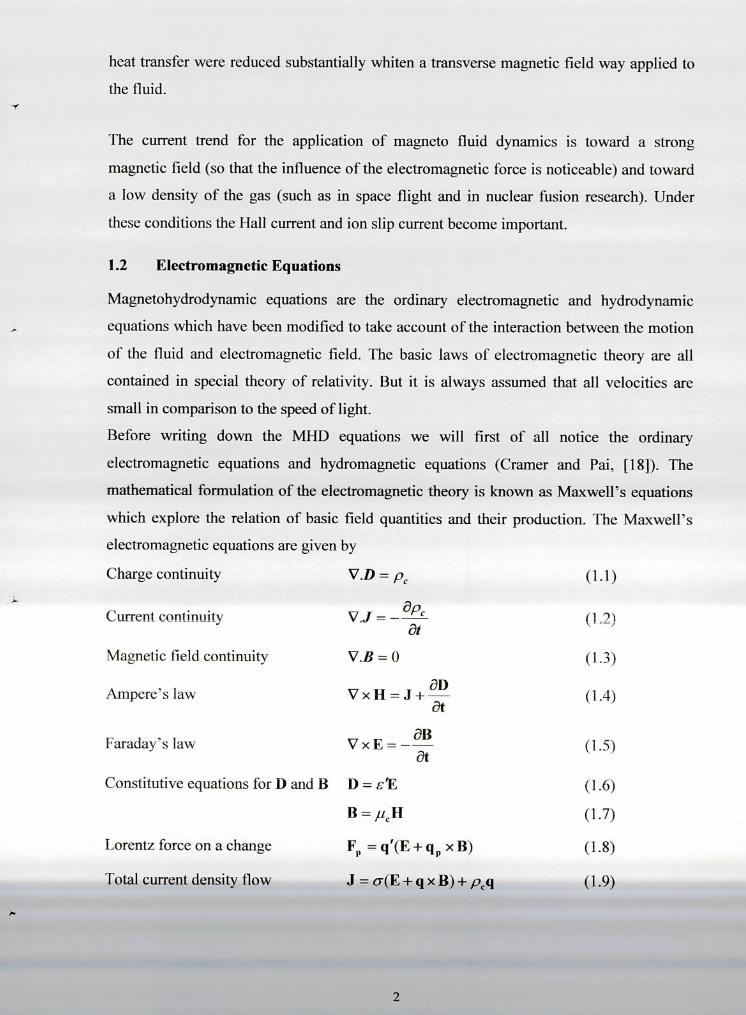
mathematical formulation of the electromagnetic theory is known as Maxwell's equations

which explore the relation of basic field quantities and their production. The Maxwell's

electromagnetic equations are given by

Charge continuity V.D=p (1.1)

Current continuity V.J = lapat

Magnetic field continuity V.B = 0 0 .3)

Ampere'slaw VxH=J+ aD

(1.4)

Riradays la\v V x E -aB at

Constitutive equations for 1) and B I) = 0.6)

B=pH (1.7)

Lorcntz fbrce on a change FP = q'(E + q P x B)

Total current density tiow J = o(E + q x B) + pq (1.9)

2

In equations (1 .1) - (1 .9), D is the displacement current, p, is the charge density, J is the

current density, B is the magnetic induction, H is the magnetic field, E is the electric field,

c' is the electrical permeability of the medium, p is the magnetic permeability of

medium, q velocity of the charge, a is the electrical conductivity, q is the velocity of the

fluid and p q is the convection current due to charges moving with the fluid.

1.3 Fundamental Equations of Fluid Dynamics of Viscous Fluids

In the study of fluid flow one determines the velocity distribution as well as the states of

the fluid over the whole space for all time. There are six unknowns namely, the three

components (u, v, w) of velocity q, the temperature 1, the pressure p and the density p of

the fluid, which are function of spatial co-ordinates and time. In order to determine these

unknown we have the following equations:

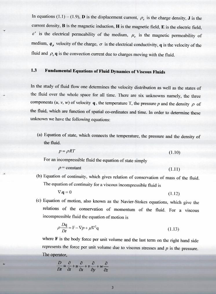
(a) Equation of state, which connects the temperature, the pressure and the density of

the fluid.

p=pRT (1.10)

For an incompressible fluid the equation of state simply

p=constant (1.11)

(h) Equation of continuity, which gives relation of conservation of mass of the fluid.

The equation of continuity for a viscous incompressible fluid is

\7.q = 0 (1.12)

(c) Equation of motion, also known as the Navier-Stokes equations, which give the

relations of the conservation of momentum of the fluid. For a viscous

incompressible fluid the equation of motion is

p -Dq

= F - Vp + iV2q (1.13)

where F is the body force per unit volume and the last term on the right hand side

represents the force per unit volume due to viscous stresses and p is the pressure.

The operator,

- - + U - + V + W - Di at ox Ely Elz

3

is known as the material derivative or total derivative with respect to time which

gives the variation of a certain quantity of the fluid particle with respect to time.

Also V2 represents the Laplacian operator.

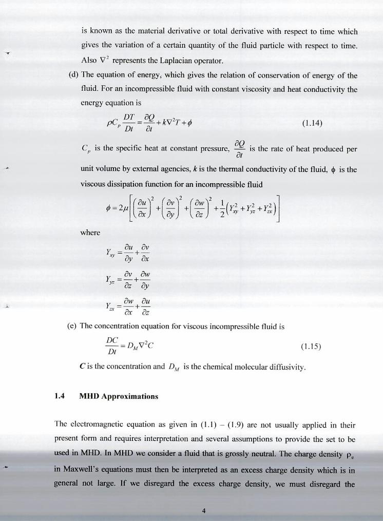
The equation of energy, which gives the relation of conservation of energy of the

fluid. For an incompressible fluid with constant viscosity and heat conductivity the

energy equation is

, 1)7' p( =

50 --+ kVT+Ø (1.14)

C,, is the specific heat at constant pressure, aQ

is the rate of heat produced per at

- unit volume by external agencies, k is the thermal conductivity of the fluid. 4' is the

viscous dissipation function for an incompressible fluid

= 2[() (2 +(&",)2

+ax c)y ) az 2 ç +

where

Su 5v Y =—+— xi -,

(;7y ox

, Sv 5%I' =—+--

5z y

5w all y_ "-V

ox 5z

The concentration equation for viscous incompressible fluid is

DC = D 1 V2C

Di (1.15)

C is the concentration and D 1 is the chemical molecular diffusivity.

1.4 MHI) Approximations

The electromagnetic equation as given in (1.1) - (1.9) are not usually applied in their

present form and requires interpretation and several assumptions to provide the set to he

used in MI-ID. In MHD we consider a fluid that is grossly neutral. The charge density p

in Maxwell's equations must then be interpreted as an excess charge density which is in

general not large. If we disregard the excess charge density, we must disregard the

4

A

A

displacement current. In most problems the displacement current, the excess charge density

and the current due to convection of the excess charge are small (Cramer and Pai, [18]).

The electromagnetic equations to be used are then as follows:

V.D=0 (1.16)

V.J=0 (1.17)

V.B=0

VxH=J .-1c nq

\7xE=0 (1.20)

/ (1.21)

B = p,H Bangladesh

\> (1.22)

J=c(E+qxB) _t

(1.23)

1.5 MHD Equations

We will now modify the equations of fluid dynamics suitably to take account of the

electromagnetic phenomena.

The MUD equation of continuity for viscous incompressible electrically conducting

fluid remains the same

V.q=0 (1.24)

The MIlD momentum equation for a viscous incompressible and electrically

conducting fluid is

p- = F_Vp+pV2q+J x B (1.25) Dt

where F is the body force term per unit volume corresponding to the usual viscous

fluid dynamic equations and the new term J x B is the force on the fluid per unit

volume produced by the interaction of the current and magnetic field (called a

I orentz force).

The MHD energy equation for a viscous incompressible electrically conducting

fluid is

DTôQkv2 J 2 ±q±— (1.26)

" T

Dt5t a

5

The new term is the Joule heating term and is due to the resistance of the fluid 0

to the flow of current.

(4) The MUD equation of concentration for viscous incompressible electrically

conducting fluid remains the same as

Di =D11 V2C (1.27)

1.6 Some Important Dimensionless Parameters of Fluid Dynamics and Magneto

hydrodynamics.

(1) Reynolds Number, Re:

It is the most important parameter of the fluid dynamics of a viscous fluid. It

represents the ratio of the inertia force to viscous force and is defined as

Re = inertial force

= pU 2 J]

= UL

viscous force pUL v

where U, L, p and ,Li are the characteristic values of velocity, length, density and

coefficient of viscosity of the fluid respectively. When the Reynolds number of the

system is small the viscous force is predominant and the effect of viscosity is

important in the whole velocity field. When the Reynolds number is large the

inertia force is predominant, and the effects of viscosity is important only in a

narrow region near the solid wall or other restricted region which is known as

boundary layer. If the Reynolds number is enormously large, the flow becomes

turbulent.

(2) Magnetic Reynolds Number, Rc,.:

It is the ratio of the fluid flux to the magnetic diffusivity and is given by

R = _UL ___

(ur)

It is one of the most important parameter of MI-ID. The magnetic Reynolds number

determines the diffusion of the magnetic field along the stream lines. R a is a

measure of the effect of the flow on the magnetic field. If it is very small compared

6

to unity, the magnetic field is not distorted by the flow when it is very large. The

magnetic field moves with the flow and is called frozen in.

(3) Prandtl Number, Pr :

The Prandtl number is the ratio of kinematics viscosity to thermal diffusivity and

may be written as follows

kinematicviscosjtv u thermal diffusivity ( k

( —PCf' )

The value of v shows the effect of viscosity of fluid. The smaller the value of v

the narrower is the region which is affected by viscosity and which is known as the

boundary layer region when v is very small. The value of shows the thermal pC,)

diffusivitv due to heat conduction . . The smaller the value of k is the narrower is d

pG

the region which is affected by the heat conduction and which is known as thermal

boundary layer when -k--- is small. Thus the Prandtl number shows the relative pcp

importance of heat conduction and viscosity of a fluid. For a gas the Prandtl

number is of order of unity.

(4) Magnetic Prandtl Number, Pm :

The magnetic Prandtl number is a measure of the relative magnitude of the fluid

boundary layer thickness. It is the ratio of the viscous diffusivity to the magnetic

diffusivity and is given by

P 'U V11 I?,

P. is generally small and is a measure of the relative magnitude of the fluid

boundary layer thickness to the magnetic boundary layer thickness. However, when

the magnetic Reynolds number is large, the boundary layer thickness is small and is

of nearly the same size as viscous boundary layer thickness. In this case P. is not

small.

7

Schmidt Number,S:

This is the ratio of the kinematic viscosity to the chemical molecular diffusivity and

is defined as

- (kinematic viscosity)

- I),,, - (chemical molecular diffusivity)

Crashof Number, Gr:

This is defined as

G g0/3(iii)L

and is a measure of the relative importance of the buoyancy of the force and

viscous force. The larger it is the stronger is the convective current. In the above g0

is the acceleration due to gravity, 0' is the co-efficient of volume expansion and 1'

is the temperature of the flow field.

Modified Grashof Number, G :

This is defined as

where *

is the co-efficient of expansion with concentration and C is the species

concentration.

Eckert Number, E:

Eckert number can be interpreted as the addition of heat due to viscous dissipation.

Thus it is the ratio of the kinetic energy and thermal energy and is defined as

E= Cp (1._7i)

8

where U is some reference velocity and 7, - 7 is the difference between two

reference temperatures. It is very small for incompressible fluid and for low

motion.

Soret Number,S0 :

This is defined as

s DT (TW - T)

where I)-,. is the thermal diffusivity, 7, is the temperature at the plate, 7. is the

temperature of the fluid at infinity, C is the concentration at the plate and C. is

the species concentration at infinity.

(10) Duffer Number,D1 :

This is s defined as D mp

CQ

where k, is the thermal diffusion ratio, m is the constant mass flux per unit area,

p is the density of the fluid, Q is the constant heat flux per unit area, C, is the

concentration susceptibility.

Magnetic Parameter, M:

This is obtained from the ratio of the magnetic force to the inertia force and is

defined as M =

HO (crL)2

(pU)2

where H0 is applied magnetic field.

1.7 Suction and Injection

For boundary layer flows with adverse pressure gradients, the boundary layer will

eventually separate from the surface. Separation of the flow causes many undesirable

features over the whole field; for instance if separation occurs on the surface of an airfoil,

9

the lift of the airfoil will decrease and the drag will enormously increase. In some problems

we wish to maintain laminar flow without separation. Various means have been proposed

T to prevent the separation of boundary layer; suction and injection are two of them.

The stabilizing effect of the boundary layer development has been well known for several

years and till to date suction is still the most of efficient, simple and common method of

boundary layer control. 1-fence, the effect of suction on hydro-magnetic boundary layer is

of great interest in astrophysics. It is often necessary to prevent separation of the boundary

layer to reduce the drag and attain high lift values.

Many authors have made mathematical studies on these problems, especially in the case of

10- steady flow. Among them the name of Cobble [20] may be cited who obtained the

conditions under which similarity solutions exist for hydro-magnetic boundary layer flow

past a semi-infinite flat plate with or without suction. Following this, Soundalgekar and

Ramanamurthy [65] analyzed the thermal boundary layer. Then Singh [61] studied this

problem for large values of suction velocity employing asymptotic analysis in the spirit of

Nanbu [47]. Singh and Dikshit [62] have again adopted the asymptotic method to study the

hydro-magnetic effect on the boundary layer development over a continuously moving

plate. In a similar way Bestman [14] studied the boundary layer flow past a semi-infinite

heated porous plate for two-component plasma.

On the other hand, one of the important problems faced by the engineers engaged in high-

speed flow in the cooling of the surface to avoid the structural failures as a result of

frictional heating and other factors. In this respect the possibility of using injection at the

surface is a measure to cool the body in the high temperature fluid. Injection of secondary

fluid through porous walls is of practical importance in film cooling of turbine blades

combustion chambers. In such application injection usually occurs normal to the surface

and the injected fluid may be similar to or different from the primary fluid. In some recent

applications, however, it has been recognized that the cooling efficiency can be enhanced

by vectored injection at an angle other than 900 to the surface. A few workers including

Inger and Swearn [34] have theoretically proved this feature for a boundary layer. In

addition, most previous calculations have been limited to injection rates ranging from

small to moderate. Raptis and Kafoussis [54] studied the free convection effects on the

flow field of an incompressible, viscous dissipative fluid, past an infinite vertical porous

10

plate, which is accelerated in its own plane. He considered that the fluid is subjected to a

normal velocity of suction/injection proportional to j2 and the plate is perfectly insulated,

i.e., there is no heat transfer between the fluid and the plate. Hasimoto [301 studied the

boundary layer growth on an infinite flat plate started at time t = 0, with uniform suction or

injection. Exact solutions of the Navier-Stokes equation of motion were derived for the

case of uniform suction and injection, which was taken to be steady or proportional to t 2•

Numerical calculations are also made for the case of impulsive motion of the plate. In the

case of injection, ve(ocity profiles have injection points. The qualitative nature of the flow

on both the suction the cases are obtained fonn the result of the corresponding studies on

steady boundary layer, so far obtained.

1.8 Large Suction

When the rate of suction is very high then it is called large suction. Singh [61] studied the

problem of Soundalgeker and Ramanamurthy [65] for large value of suction parameter by

making use of the perturbation technique, as has been done by Nanbu [47]. Later Singh

and Dikshit [62] studied the hydro-magnetic flow past a continuously moving semi-infinite

porous plate employing the same perturbation technique. They also derived similarity

solutions for large suction. The large suction in fact enabled them to obtain analytical

solutions those are of immense value that compliment various numerical solutions. For the

present problem studying on MHD free convection and mass transfer flow with thermal

diffusion, Duffer effect and large suction we have to use the shooting method for getting

the numerical solutions.

1.9 Free and Force Convection

Free or natural convection is a mechanism, or type of heat transport, in which the fluid

motion is not generated by any external source (like a pump, fan, suction device, etc.) but

only by density differences in the fluid occurring due to temperature gradients. In natural

convection, fluid surrounding a heat source receives heat, becomes less dense and rises.

The surrounding, cooler fluid then moves to replace it. This cooler fluid is then heated and

the process continues, forming convection current; this process transfers heat energy from

- the bottom of the convection cell to top. The driving force for natural convection is

buoyancy, a result of differences in fluid density. Because of this, the presence of a proper

acceleration such as arises from resistance to gravity, or an equivalent force (arising from

acceleration, centrifugal force or Coriolis force), is essential for natural convection. For

example, natural convection essentially does not operate in free-fall (inertial)

environments, such as that of the orbiting International Space Station, where other heat

transfer mechanisms are required to prevent electronic components from overheating.

Natural convection has attracted a great deal of attention from researchers because of its

presence both in nature and engineering applications. In nature, convection cells formed

from air raising above sunlight warmed land or water, are a major feature all weather

systems. Convection is also seen in the rising plume of hot air from fire, oceanic currents,

and sea-wind formation (where upward convection is also modified by Coriolis forces). In

engineering applications, convection is commonly visualized in the formation of

microstructures during the cooling of molten metals, and fluid flows around shrouded heat-

dissipation fins, and solar ponds. A very common industrial application of natural

convection is free air cooling without the aid of fans: this can happen on small scales

(computer chips) to large scale process equipment.

Forced convection is a mechanism, or type of heat transport in which fluid motion is

generated by an external source (like a pump, fan, suction device, etc.). It should be

considered as one of the main methods of useful heat transfer as significant amounts of

heat energy can be transported very efficiently and this mechanism is found very

commonly in everyday life, including central heating, air conditioning, steam turbines and

in many other machines. Forced convection is often encountered by engineers designing or

analyzing heat exchangers, pipe flow, and flow over a plate at a different temperature than

the stream (the case of a shuttle wing during re-entry, for example). However, in any

forced convection situation, some amount of natural convection is always present

whenever there are g-forces present (i.e., unless the system is in free fall). When the natural

convection is not negligible, such flows are typically referred to as mixed convection.

When analyzing potentially mixed convection, a parameter called the Archimedes number

(Ar) parametrizes the relative strength of free and forced convection. The Archimedes

number is the ratio of Grashof number and the square of Reynolds number I Ar = --

Re

which represents the ratio of buoyancy force and inertia force, and which stands in for the

12

contribution of natural convection. When Ar>> I, natural convection dominates and when

Ar << 1, forced convection dominates.

When natural convection isn't a significant factor, mathematical analysis with forced

convection theories typically yields accurate results. The parameter of importance in forced

( convection is the Peclet number Pc = UL - , which is the ratio of advection (movement by a)

currents) and diffusion (movement from high to low concentrations) of heat.

1.10 Porous Medium:

A porous medium is a material containing pores (voids). The pores are typically filled with

a fluid (liquid or gas). The skeletal material is usually a solid, but structures like foams are

often also usefully analyzed using concept of porous media.

A porous medium is most often characterized by its porosity. Other properties of the

medium (e.g., permeability, tensile strength, electrical conductivity) can sometimes be

derived from the respective properties of its constituents and the media porosity and pores

structure, but such a derivation is usually complex. Even the concept of porosity is only

straight-forward for a poroelastic medium.

Many natural substances such as rocks, soils, biological tissues (e.g. bones, wood), and

man made materials such as cements and ceramics can be considered as porous media.

Many of their important properties can only be rationalized by considering them to be

porous media.

The concept of porous media is used in many areas of applied science and engineering:

filtration, mechanics (acoustics, geomechanics, soil mechanics, rock mechanics),

engineering (petroleum engineering, bio-remediation, construction engineering),

geosciences (hydrogeology, petroleum geology, geophysics), biology and biophysics,

material science, etc. Fluid flow through porous media is a subject of most common

interest and has emerged a separate field of study. The study of more general behaviour of

porous media involving deFormation of the solid frame is called poromechanics.

13

1.11 MHD Boundary Layer and Related Transfer Phenomena

Boundary layer phenomena occur when the influence of a physical quantity is restricted to

small regions near confining boundaries. This phenomenon occurs when the non-

dimensional diffusion parameters such as the Reynolds number and the Peclet number of

the magnetic Reynolds number are large. The boundary layers are then the velocity and

thermal or magnetic boundary layers, and each thickness is inversely proportional to the

square root of the associated diffusion number. Prandtl fathered classical fluid dynamic

boundary layer theory by observing, from experimental flows that for large Reynolds

number, the viscosity and thermal conductivity appreciably influenced the flow only near a

wall. When distant measurements in the flow direction are compared with a characteristic

dimension in that direction, transverse measurements compared with the boundary layer

thickness, and velocities compared with the free stream velocity, the Navier Stokes and

energy equations can be considerably simplified by neglecting small quantities. The

number of component equations is reduced to those in the flow direction and pressure is

then only a function of the flow direction and can be determined from the inviscid flow

solution. Also the number of viscous term is reduced to the dominant term and the heat

conduction in the flow direction is negligible.

MIII) boundary layer flows are separated in two types by considering the limiting cases of

a very large or a negligible small magnetic Reynolds number. When the magnetic field is

oriented in an arbitrary direction relative to a confining surface and the magnetic Reynolds

number. When the magnetic field is oriented in an arbitrary direction relative to a

confining surface and the magnetic Reynolds number is very small; the flow direction

component of the magnetic interaction and the corresponding Joule heating is only a

function of the transverse magnetic field component and local velocity in the flow

direction. Changes in the transverse magnetic boundary layer are negligible. The thickness

of magnetic boundary layer is very large and the induced magnetic field is negligible.

I lowever, when the magnetic Reynolds numbers is large, the magnetic boundary layer

thickness is small and is of nearly the same size as the viscous and thermal boundary layers

and then the MHD boundary layer equations must be solved simultaneously. In this case.

the magnetic field moves with the flow and is called froi.en mass.

14

1.12 MHD and Heat Transfer

With the advent of hypersonic flight, the field of MHD, as defined above, which has been

associated largely with liquid-metal pumping, has attracted the interest of aero dynamists.

It is possible to alter the flow and the heat transfer around high-velocity vehicles provided

that the air is sufficiently ionized. Further more, the invention of high temperature facilities

such as the shock tube and plasma jet has provided laboratory sources of flowing ionized

gas, which provide and incentive for the study of plasma accelerators and generators.

As a result of this, many of the classical problems of fluid mechanics have been

reinvestigated. Some of these analyses arouse out of the natural tendency of scientists to

investigate a new subject. In this case it was the academic problem of solving the equations

of fluid mechanics with a new body force and another source of dissipation in the energy

equation. Sometimes their were no practical application for these results. For example,

natural convection MHD flows have been of interest to the engineering community only

since the investigations are directly applicable to the problems in geophysics and

astrophysics. But it was in the field of aerodynamic heating that the largest interest was

aroused. Rossow [57] presented the first paper on this subject. His result, for

incompressible constant-property flat plate boundary layer flow, indicated that the skin

friction and heat transfer were reduced substantially when a transverse magnetic field was

applied to the fluid. 'I'his encouraged a multitude analysis for every conceivable type of

aerodynamic flow, and most of the research centered on the stagnation point where, in

hypersonic flight, the highest degree of ionization could be expected. The results of these

studies were sometimes contradictory concerning the amount by which the heat transfer

would be reduced (Some of this was due to misinterpretations and invalid comparisons).

Eventually, however, it was concluded that the field strengths, necessary to provide

sufficient shielding against heat fluxes during atmospheric flight, were not competitive (in

terms of weight) with other methods of cooling (Sutton and Gloersen, [661). However, the

invention of new lightweight super conduction magnets has recently revived interests in

the problem of providing heat protection during the very high velocity reentry from orbital

and supper orbital flight (Levy and Petschek, [41]).

15

Processes, heat transfer considerations arise owing to chemical reaction and are often due

to the nature of the process. In processes such as drying, evaporation at the surface of water ly body, energy transfer in a wet cooling tower and the flow in a desert cooler, heat and mass

transfer occur simultaneously. In many of these processes, interest lies in the determination

of the total energy transfer although in processes such as drying, the interest lies mainly in

the overall mass transfer for moisture removal. Natural convection processes involving the

combined mechanisms are also encountered in many natural processes, such as

evaporation, condensation and agricultural drying, in many industrial applications

involving solution and mixtures in the absence of an externally induced flow and in many

chemical processing systems. In many processes such as the curing of plastics, cleaning

and chemical processing of materials relevant to the manufacture of printed circuits,

manufacture of pulp-insulated cables ctc, the combined buoyancy mechanisms arise and

the total energy and material transfer resulting from the combined mechanisms have to be

determined.

The basic problem is governed by the combined buoyancy effects arising from the

simultaneous diffusion of thermal energy and of chemical species. Therefore the equations

of continuity, momentum, energy and mass diffusions are coupled through the buoyancy

terms alone, if there are other effects, such as the Soret and Duffer effects, they are

neglected. This would again be valid for low species concentration levels. These additional

effects have also been considered in several investigations, for example, the work of the

Caldwell [17]. Groots and Mozur [28], 1-lurle and Jakeman [331 and Legros, el al. [46]).

Somers [63] considered combined boundary mechanisms for flow adjacent to a wet

isothermal vertical surface in an unsaturated environment. Uniform temperature and

uniform species concentration at the surface were assumed and an integral analysis was

carried out to obtain the result which is expected to be valid for Pr and S values around

1.0 with one buoyancy effect being small compared with the other. Mathers el al. [45]

treated the problem as a boundary layer flow for low species concentration, neglecting

inertia effects. Results were obtained numerically for Pr =1.0 and S varying from 0.5 to

10. Lowell and Adams [43] and Gill ci al. [27] also considered this problem, including

additional effects such as appreciable normal velocity at the surface and comparable

species concentrations in the mixture. Similar solutions were investigated by Lowell and

Adams [43]. Lightfoot [42] and Saville and Churchill [60] considered come asymptotic

16

solutions. Adams and Mc Fadden [11 presented experimental measurements of heat and

mass transfer parameters, with opposed buoyancy effects. Gebhart and Pera [24] studied

laminar vertical natural convection flows resulting from the combined buoyancy

mechanisms in terms of similarity solutions. Similar analyses have been carried out by

Pera and Gebhart [521 for flow over horizontal surfaces and by Mollendrof and Gebhart

[46] for axisymmetric flows, particularly for the axisymmetric Plume.

Mollendrof and Gebhart [46] carried out an analysis for axis symmetric flows. The

governing equations were solved for the combined effects of thermal and mass diflusion in

an axisymmetric plume flow. Boura and Gebhart [15], Hubbel and Gebhart [321 and

Tenner and Gebhart (1771) have studied buoyant free boundary flows in a concentration

stratified medium. Agrawal el at. [2] have studied the combined buoyancy effects on the

thermal and mass diffusion on MHD natural flows, and it is observed that, for the fixed G

and P, the value of X, (dimensionless length parameter) decreases as the strength of the

magnetic parameter increases. Georgantopoulos et al. [26] discussed the effects of free

convective and mass transfer flow in a conducting liquid, when the fluid is subject to a

transverse magnetic field. Haldavnekar and Soundalgekar [29] studied the effects of mass

transfer on free convective flow of an electrically conducting viscous fluid past an infinite

porous plate with constant suction and transversely applied magnetic field. An exact

analysis was made by Soundalgekar and Gupta [64] of the effects of mass transfer and the

free convection currents on the MHD Stokes (Rayleigh) problem for the flow of an

electrically conducting incompressible viscous fluid past an impulsively started vertical

plate under the action of a transversely applied magnetic field. The heat due to viscous and

Joule dissipation and induced magnetic field are neglected.

During the course of discussion, the effects of heating Gr < 0 of the plate by free

convection currents, and G, (modified Grashof number), S, and M on the velocity and the

skin friction are studied. Nunousis and Goudas [49] have studied the effects of mass

transfer on free convective problem in the Stokes problem for an infinite vertical limiting

surface. Georgantopolous and Nanousis [25] have considered the effects of the mass

transfer on free convection flow of an electrically conducting viscous fluid (e.g. of a stellar

atmosphere, of star) in the presence of transverse magnetic field. Solution for the velocity

17

and skin friction in closed from are obtained with the help of the Laplace transform

technique, and the results obtained for the various values of the parameters, S , P. and M

are given in graphical form. Raptis and Kafoussias [54] presented the analysis of free

convection and mass transfer steady hydro magnetic flow of an electrically conducting

viscous incompressible fluid, through a porous medium, occupying a semi infinite region

of the space bounded by an infinite vertical and porous plate under the action of transverse

magnetic field. Approximate solution has been obtained for the velocity, temperature,

concentration field and the rate of heat transfer. The effects of different parameters on the

velocity field and the rate of heat transfer are discussed for the case of air (Prandtle number

P. = 0.71) and the water vapor (Schmidt number S = 0.60), Raptis and Tzivanidis [55]

considered the effects of variable suction/ injection on the unsteady two dimensional free

convective flow with mass transfer of an electrically conducting fluid past vertical

accelerated plate in the presence of transverse magnetic field. Solutions of the governing

equations of the flow are obtained with the power series. An analysis of two dimensional

steady free convective flow of a conducting fluid, in the presence of a magnetic field and a

foreign mass, past an infinite vertical porous and unmoving surface is carried out by Raptis

(1983), when the heat flux is constant at the limiting surface and the magnetic Reynolds

number of the flow is not small. Assuming constant suction at the surface, approximate

solutions of the coupled non-linear equations are derived for the velocity field, the

temperature field, the magnetic field and for their related quantities. Agrawal el al. [5]

considered the steady laminar free convection flow with mass transfer of an electrically

conducting liquid along a plane wall with periodic suction. The considered sinusoidal

suction velocity distribution is of the form J/' = VO I + C cos_}. where v0 > 0, is the

wavelength of the periodic suction velocity distribution, and is the amplitude of the

suction velocity variation which is assumed to be small quantity. It is observed that near

the plate the velocity is a maximum and decreases as y increases. Also, an increase in the

magnetic parameter the velocity decreases. Agrawal el al. [4] have investigated the effect

of Hall current on the combined effect of thermal and mass diffusion of an electrically

conducting liquid past an infinite vertical porous plate, when the free stream oscillates

about constant nonzero mean. The velocity and temperature distributions are shown on

graphs for different values of parameters. The value of Pr is chosen as 0.71 for air. In

18

selecting the values of S, the Schmidt number, the diffusing chemical species of most

common interest in air are considered. From the figures it is seen that, with the increase air.

Hall parameter, the mean primary velocity decreases, where as the mean secondary

velocity increases for a fixed magnetic parameter M and S. However, for a fixed m, and

increase air magnetic parameter M or S, leads to a decrease in both the primary and the

secondary velocities. The mean shear stresses at the plate due to primary and secondary

velocity and the mean rate of heat transfer from the plate are also given. To study the

behavior of the oscillatory and transient part of the velocity and temperature distribution,

curves are drawn for various values of parameters that describe the flow at Wt = , The p..

non-dimensional shear stress and the rate of heat transfer are obtained. The above problem

has been extended by the same authors (Agrawal et al. 131) when the plate temperature

oscillates in time a constant nonzero mean, while the free stream is isothermal. The

velocity, temperature and concentration distribution, together with the heat and mass

transfer results, have been computed for different values of J, Gr M and m.

1.13 Soret and Duffer Effect

In the above mentioned studies, heat and mass transfer occur simultaneously in a moving

fluid where the relations between the fluxes and the driving potentials are of more

complicated nature. In general the thermal -diffusion effects is of a smaller order of

magnitude than the effects described by Fourier or Flick's laws and is often neglected in

heat and mass transfer process. Mass fluxes can also be created by temperature gradients

and this is Soret or Thermal diffusion effect. There are, however, exceptions. The thermal-

diffusion effect, (commonly known as Soret effect) for instance, has been utilized for

isotope separation and in mixtures between gases with very light molecular weight (142.

He) and of medium molecular weight (N,, air). The diffusion thermo effect was found to

be of such a magnitude that it could not be neglected (Eckert and Drake, [22]). In view of'

the importance of the diffusion thermo effect, Jha and Singh [35] presented an analytical

study for free convection and mass transfer flow for an infinite vertical plate moving

impulsively in its own plane, taking into account the Soret effect. Kaffoussias [36] studied

the Mlii) free convection and mass transfr flow, past an infnitc vertical plate moving on

I 9

its own plane, taken into account the thermal diffusion when (i) the boundary surface is

impulsively started moving in its own plane (ISP) and (ii) it is uniformly accelerated

(UAP). The problem is solved with the help of Laplace transfer method and analytical

expressions are given for the velocity field as well as for the skin friction for the above

mentioned two different cases. The effects of the velocity and skin friction of the various

dimensionless parameters entering into the problem are discussed with the help of graphs.

For the I.S.P. and U.A.P. cases, it is seen from the figures that the effect of magnetic

parameters M is to decrease the fluid (water) velocity inside the boundary layer. This

influence of the magnetic field on the velocity field is more evident in the presence of

thermal diffusion. From the same figures it is also concluded that the fluid velocity rises

due to greater thermal diffusion. Hence, the velocity field is considerably affected by the

magnetic field and the thermal diffusion. Nanousis [48] extended the work of Kafoussias

[36] to the case of rotating fluid taking into account the Soret effect. The plate is assumed

to be moving on its own plane with arbitrary velocity U0 f'(t') where U0 is a constant

velocity and f(t) a non-dimensional function of the time 1'. The solution of the problem

is obtained with the help of Laplace transform technique. Analytical expression is given for

the velocity field and for skin friction for two different cases, e.g., when the plate is

impulsively stared, moving on its own plane (case I) and when it is uniformly accelerated

(case II). The effects on the velocity field and skin friction, of various dimensionless

parameters entering into the problem, especially of the Soret number S0 . are discussed with

the help of graphs. In case of an impulsively started plate and uniformly accelerated plate

(case I and case Il), it is seen that the primary velocity increase with the increase of S0 and

the magnetic parameter M. It has been observed that energy can be generated not only by

temperature gradients but also by composition gradients. The energy flux caused by

composition gradients is called the Duffer or diffusion thermo effect. On the other hand,

mass fluxes can also be created by temperature gradients and this is the Soret or thermal

diffusion effect.

20

CHAPTER 2

Introduction and Literature Review

The convective heat and mass transfer process takes place due to the buoyancy effects

owing to the differences of temperature and concentration, respectively. In dealing with the

transport phenomena, the thermal and mass diffusions occurring by the simultaneous

action of buoyancy forces are of considerable interest in nature and in many engineering

practices, such as geophysics, oceanography etc. Many theoretical and experimental

investigations have been established in the literature involving the studies of heat and mass

transfer over plates by natural, forced or combined convection, and most of these studies

are based upon the laminar boundary layer approach. The mixed free-forced convective

and mass transfer flow has essential applications in separation processes in chemical

engineering or drying processes. The natural convection boundary layer flows induced by

the combined buoyancy effects of thermal and mass diffusion has been investigated

primarily by Gebhart and Pera [24] and Pera and Gebhart [52]. Furthermore, convective

flow through porous media is very important in many physical and natural applications,

namely, heat transfer associated with heat recovery from geothermal systems and

particularly in the field of large storage systems of agricultural products, storage of nuclear

waste, heat removal from nuclear fuel debris, petroleum extraction, control of pollutant

spread in groundwater, etc. The free convection flow past an infinite vertical porous plate

with suction velocity perpendicular to the plate surface was studied by Brezovsky et al.

[16], Kawase and Ulbrecht [38], Martynenko et al. [44] and further extended by Weiss et

al. [67]. A finite difference numerical scheme was considered by Pantokratoras [50] in

order to study the laminar free convection boundary layer flow past over an isothermal

vertical plate with uniform suction or injection. Hassanien et al. [31] has investigated the

natural convection boundary layer flow of micropolar fluid over a semi-infinite plate

embedded in a saturated porous medium where the plate maintained at a constant heat flux

with uniform suction/injection velocity.

1 In recent times, the problems of natural convective heat and mass transfer flows through a

porous medium under the influence of a magnetic field have been paid attention of a

21

number of researchers because of their possible applications in many branches of science,

engineering and geophysical process. Considering these numerous applications, MHD free r convective heat and mass transfer flow in a porous medium have been studied by among

others Raptis and Kafoussias [54], Sattar [58], sattar and Hossain [59] etc. Besides, Kim

[39] has been studied the effect of MHD of a micropolar fluid on coupled heat and mass

transfer, flowing on a vertical porous plate moving in a porous medium. However,

Pantokratoras [51] showed that a moving electrically conducting fluid induced a new

magnetic field, which interacts with the applied external magnetic fields and the relative

importance of this induced magnetic field depends on the relative value of the magnetic

Reynolds number (Rm >> l).

4'

Nevertheless, more complicate phenomenon arises between the fluxes and the driving

potentials when heat and mass transfer occur simultaneously in case of a moving fluid. It

has been observed that an energy flux can be generated not only due to the temperature

gradients but also by composition gradients. The energy flux caused by a composition

gradient is called the Dufour or diffusion-thermo effect, whereas, mass flux caused by

temperature gradients is known as the Soret or thermal-diffusion effect. In general, the

thermal-diffusion and diffusion-thermo effects are of a smaller order of magnitude than the

effects described by Fourier's or Fick's law. This is why, most of the studies of heat and

mass transfer processes, however, considered constant plate temperature and concentration

and have neglected the diffusion-thermo and thermal-diffusion terms from the energy and

concentration equations, respectively. Ignoring the Soret and Dufour effects, Choudhary

and Sharma [19] studied the mixed convection flow over a continuously moving porous

vertical plate with combined buoyancy effects of thermal and mass diffusion under the

action of a transverse magnetic field, when the plate is subjected to constant heat and mass

flux. But in some exceptional cases, for instance, in mixture between gases with very light

molecular weight (112, He) and of medium molecular weight (N2 , air) the diffusion-

thermo (Dufour) effect and in isotope separation the thermal-diffusion (Soret) effect was

found to be of a considerable magnitude such that they cannot be ignored. In view of the

relative importance of these above mentioned effects many researchers have studied and

reported results for these flows of whom the names are, Eckert and Drake [22],

Dursunkaya and Worek [21], etc. Whereas, Kafoussias and Williams [37] studied the same

effects on mixed free-forced convective and mass transfer boundary layer flow with

22

temperature dependent viscosity. Later, Anghel et al. [13] has investigated the composite

Dufour and Soret effects on free convection boundary layer heat and mass transfer over a

vertical surface in a Darcian porous regime. A theoretical steady with numerical solution of

two-dimensional free convection and mass transfer flow past a continuously moving semi-

infinite vertical porous plate in a porous medium is presented by Alam et al. [11], taking

into account the Dufour and Soret effects. Later, a numerical study based on Nachtsheim-

Swigert shooting iteration technique together with sixth order Runge-Kutta integration

scheme have been carried out by Alam and Rahman [8] in order to investigate the Dufour

and Soret effects on mixed convection flow past a vertical porous flat plate with variable

fluid suction. Recently, Alam et al. [9] investigated the diffusion-thermo and thermal-

diffusion effects on unsteady free convection and mass transfer flow past an accelerated

vertical porous flat plate embedded in a porous medium with time dependent temperature

and concentration. Very recently, a mathematical model and numerical study based on the

finite element method has been implemented by Rawat and Bhargava [56] for the viscous,

incompressible heat and mass transfer of a micropolar fluid through a Darcian porous

medium with the presence of buoyancy, Soret/Dufour diffusion, viscous heating and wall

transpiration.

The Dufour and Soret effects on steady MHD free convective heat and mass transfer flow

past a semi-infinite vertical porous plate embedded in a porous medium have been studied

by Alam and Rahman [7]. Next, Alam et al. [10] studied the Dufour and Soret effects on

unsteady MHD free convection and mass transfer flow past an infinite vertical flat plate.

Alam et al. [11] further extensively investigated the Dufour and Soret effects on steady

MHD free-forced convective and mass transfer flow past a semi-infinite vertical plate. In

recent times, a numerical study of the natural convection heat and mass transfer about a

vertical surface embedded in a saturated porous medium under the influence of a magnetic

field has been done by Postelnicu [53], taking into account the diffusion-thermo and

thermal-diffusion effects. Following the study to those of Choudhary and Sharma [19].

Pantokratoras [51] and Postelnicu [53], our main aim is to investigate the Dufour effect on

combined heat and mass transfer of a steady laminar mixed free-forced convective flow of

viscous incompressible electrically conducting fluid above a semi-infinite vertical porous

surface under the influence of an induced magnetic field.

23

CHAPTER 3

Governing Equations and Solutions

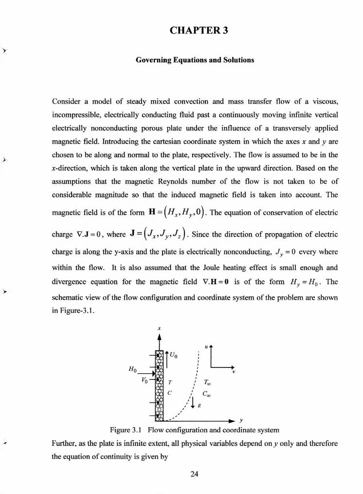
Consider a model of steady mixed convection and mass transfer flow of a viscous,

incompressible, electrically conducting fluid past a continuously moving infinite vertical

electrically nonconducting porous plate under the influence of a transversely applied

magnetic field. Introducing the cartesian coordinate system in which the axes x and y are

chosen to be along and normal to the plate, respectively. The flow is assumed to be in the

x-direction, which is taken along the vertical plate in the upward direction. Based on the

assumptions that the magnetic Reynolds number of the flow is not taken to be of

considerable magnitude so that the induced magnetic field is taken into account. The

magnetic field is of the form H =(H1, H,0). The equation of conservation of electric

charge V.J =0, where J = (J,, J , J, Since the direction of propagation of electric

charge is along the y-axis and the plate is electrically nonconducting. J, = 0 every where

within the flow. It is also assumed that the Joule heating effect is small enough and

divergence equation for the magnetic field V.H = 0 is of the form fI = H0 . The

schematic view of the flow configuration and coordinate system of the problem are shown

in Figure-3.1.

—.tUo Ho__

r

. -

Figure 3.1 Flow configuration and coordinate system

Further, as the plate is infinite extent, all physical variables depend on y only and therefore

the equation of continuity is given by

24

dv

dy --0 (3.1)

whose solution gives v = -, where fr is the constant velocity of suction normal to the

plate and the negative sign indicates that the suction velocity is directed towards the plate

surface. In accordance with the above assumptions and initiating the concept of usual

Boussinesq's approximation, the basic equations related to the problem incorporating with

the Maxwell's equations and generalized Oham's law can be put in the following form:

dH (3.2)

dy dy p dy

(33) dy dy 0-lie dy2

dT k d 2 T v (dU)2+ I (dH"2 DkT d2C

—V0 = —i-

-j + (3.4)

21-

—V0 1--1=D—- (3.5) dy dy

The relevant boundary conditions on the vertical surface and in the uniform stream are

defined as follows:

dT Q dC u=U0, -=--, -=--, H =H, aty=O

dy k dy D (3.6)

u=O,T=T,C=C,H=Owheny—

where g is the acceleration due to gravity, fi is the coefficient of thermal expansion. 1'

denotes fluid temperature, C is concentration of species, T. and C. are the temperature

and species concentration of the uniform flow, /3*

is the concentration expansion

coefficient, v is the Newtonian kinematic viscosity of the fluid, lie is the magnetic

permeability, H. is the applied constant magnetic field, H is induced magnetic field, p

is the density of the fluid, a is the electrical conductivity, k is the thermal conductivity, D is

the chemical molecular diffusivity, CP is the specific heat capacity of the fluid at constant

pressure, C is the concentration susceptibility, kT is the thermal diffusion ratio, U0 is the

25

uniform velocity, Q is the constant heat flux per unit area, rn is the constant mass flux per

unit area and His the induced magnetic field at the wall, respectively. In order to

simplify a numerical solution, we introduce the following transformations, viz:

V0 u VO urn

0*=kVo(T_TQ3);H*= H1 (3 7)

vQ \IpV0

and defining the following dimensionless parameters

pvC F,. = " (Prandtl number)

k

- v2g/3Q

(Grashofi number) Gr kVO4

vg/3 * -

(modified Grashoff number) 0

kV 3 E = ° (Eckert number)

L)Q( ,

D pmkT (I)ufour number)

f QC

V S = - (Schmidt number)

= UV/le (Magnetic diffusivity)

M = (Magnetic parameter), where C is the concentration on the plate wall.

V0 Vp

On introducing the above non-dimensional quantities, in the equations (3.2) - (3.5) with

boundary conditions (3.6) we have

* U U

* or, U=Vu

du du*

dy dy

26

• dy'V0

dy V

Then dy dy*' dy

=-; (3.8) vdy

d2u d (v2du*dy* 2•4y*V ,'jd

71 u

d2 *

= Lo_t4 (39 V ay 2 *)

! fi= V0 p

or, H = 10 F;~

V0H'

Now dH dy dy'dy

= I/'e dy v

vFdH'

;~dY' (3.10)

d2H = d (

VV~2 f dli' '

) Wv'

2 * 1 *1dy YV/Je dYdY

v03 Ijd2H' 02 dy'2

Again,

Cs = V0D(C-C)

mu

or,C - C= muG (3.12) V0D

andO* = '0(TT uQ

or, TTr kV0 (3.13)

Substituting (3.8) -(3.10) and (3.12) -(3.13) in equation (3.2) we get,

g'8 6Q- + g + 0(! LO. d 0 p

rrnVdy k) D ) v dy p ody

or du* + m0C+

Vo3 d 2 02 peH fdIc

v dy kV0 VD V dy V p \I dy

or, + & F~Ee i + du = - gpv2Qo*

-

go*V2mct ,*2

V0 dy* dy* kVO4 DV04 d2u* dH* du*

g,8v2Qe* -

or, dy dy kVO4

d2u* dH* du* or, + M -i- + -G,.9 - G, C*

dy dy dy

where

M=&fi VoVp

gfll) r kk

G=g/3*v2(C-C)---

J o

Putting (3.8), (3.10) - (3.11) in equation (3.3) we have

v2 H

v2 du* I V °

0 f--- d 2H

0+v --

or, - ii+ L& dy J/T p (/ (71!) (/y 2

where M = & V0 p

and J Pe

Again equation (3.4) gives

dT = k d2

—IT v (du2

+ 1 (dH

2 Dk d 2C -J, —+J jl dy pC dy2 C, dy) crp dy) CC,, dy2

28

(3.14)

(3.15)

From equation (3.13) we have

T= 0 +T kV0

dT = d (QvO*

+ T dy dy*kV

)

,, 'y

QvdO V0 kVo dy* v

- Q d9

- k dy*

d2T d (Qde* dy*

y2y* kdy*)

dy

Qd2O* v

- k 72 v

-

QV0 d29*

- ku dy*2

Further from equation (3.12)

muC *

C= +C V0D

dC = d(mu * I.-

dy dy*JTOD ) dy

-

mvdC*dy*

VoDdy* dy

mvdC V0 VoD dy* v

m dC*

D dy*

Hence

d2C = d (mdC* )dy*

dy 2 dy* D dy*

Jdy

2C* md V0

- D dy*2

-

mV d2C*

- Dv dy*2

Therefore equation (3.4) becomes

— Q dO — k QJ' d20* 1 j_2

Dk, my0 d2C*

k dy pC kv dy 2 C, v dy ) crpC ( 1) Pe dy ) Dv dy 2

QV0 d20* QV0 dOt -

v: (du* 2

_ a'H 2

Dk mV0 d2Ct or,

dyt2 rpv2pCpI

dy*) Dv dy*2

or,

d20t +

PVCP dO' -

—kV pvC (*\12 -

kV pvc 1 (dH,)2

k dyt QvC k dy*) QvC, k crvC dye

+- Dkj PUCp

QV0 Dv dy

or,

d 20t + pvC = — kV pvC1, (du*SSt2 kV pvC I (dH

2 mkp d2Ct _)

dyt2 k QvC k — QvC k Pe + CQ dyt2

d29* dOt * 2 (dH2l d2Ct

*2 +_) ]+D1 dy

(3.16) dy dy Pm dy

E = kV where

k - k T' C QvC' =

and D = mk,p

is the 1)ufour number. f CQ

Then equation (3.5) becomes

Ddy Dvdy

dC Dd 2Ct or, --+

dy vdy *

2

v where —=S.

D

The corresponding boundary conditions are now transformed as follows:

y =0 yt =0

u—U0 aty=O=V0u =U0 =u* =

U0—, i.e.,u

* =U

* aty

* =0

V0

30

(3.17)

dT Q Qd0* Q. dO' aty=0=----=--,i.e., --=-1 atv =0 dy k kdy k

dC m mdCi m. dC aty=0=--------=--,i.e., --=-1 aty =0

dy D Ddy D dy

H=H, aty=0 H* =H3 H0Ht =H"°" =H1,.i.e.,H* =hat y =0 fi [H() M

p VO

where h = MH 4 ,

H0

Abs y —* cX => y4 —* c

u =0 when y —* oo => V0U =0, i.e., u =0 when y —> oo

V

T = T when y =0, i.e., O =0 when y kV0

C=Cc when y — c muC i =0. .e..(

* =Owhen y

*

—> oo Dy0

and H =0 when y -_c H i =0, .e., H

* =0 when y

*

—

\1pV

Therefore, ignoring the asterisk (*), we obtain (3.14) -(3.17) as follows:

d 2u dH du —+M--+—=-GO-G C dy dy r 171

1 d 2H du dH - ___

Pm dY2 dy dy

—+P—=-P - +—I—I i+D d 20 dO rEc[))

1 1dHs2l d2C dy2 ,dy PmdY)j fdy2

dC 1d 2C —+—=0 dy S dy2

with corresponding boundary conditions

dO dC y=O :u=U, —=-1,—=-1, H=h (say)

dy dy y-*: u=0, 0=0,C=0,H=0

(3.18)

(3.19)

(3.20)

(3.21)

(3.22)

31

CHAPTER 4

Numerical Solution and Discussion

4.1 Numerical Solution

The simplest solution of equation (3.21) can be obtained as follows:

dC I d 2C

dy Sc dy2 (4.1)

Let the trial solution of(4.l) be C = e" (4.2)

So the auxiliary equation of equation (4.1) is

I - m + in = 0 Sc

( i.e.

in nil = 0

Sc

m=O and nz=—S

Therefore, we have the trial solution C = A + Be "

Applying boundary conditions on C from (3.22) we have

C=O as y—>co =>O=A i.e. A=0

at y=O:then —l= —S.B i.e. dy

1-lence

C = (4.3)

To obtain a complete solution ol the coupled nonlinear system of equations (3.18) (3.20)

under boundary conditions (3.22), we introduce the perturbation approximation. Since the

dependent variables u, H and 0 mostly dependent on y only and the fluid is purely

incompressible one, we expand the dependent variables in powers of Eckert number Er

which is small enough such that the terms in E? and its higher order can be neglected.

Thus we assume

32

u(y)_ui (y)+Eu2 (y)+o(E 2).

H(y)= H (y)+ EH2 (y)+O(E 2)+ (4.4)

O(y)= 01 (y)+E 2 (y)+0(E 2 )+

Now, U

—=u1(y)+Eu2 (y)+ dy

d 2U ,,

--=u1 (y)+Eu2 (y)+......... dy

dH

dy 2 =H1 (y)+EH2 (y)+.........

dO = 911(y)+ EO2'(y)+.........

dy

d28 --=

,,

(y)+Ee2"(y)+......... dy

Substituting equation (4.4) into (3.18), (3.19) and (3.20), we get-

From (3.18):

d 2u dH du + /vi + - = GrO - GmC

dy 2 dy dy

or, I u," (y)+ Eu2" (v)+...} + M{H1' (y)+ EH2'(v)+...} +{u1'(y)+ Eu2'(y)+...1

= Gr {O(y)+ E02(y)+...}—G,,,C

Equating the co-efficient of the like powers of E and neglecting the terms in Ec2 and

higher order, we have

u1" + MH1' + U1' = Gr61 - G 1C (4.5)

u21' + MH2' + u2' = Gr92 (4.6)

From (3.19):

1d2H dH du -___

Pm dY 2 dy dy

or, i{Hi"(y)+ EH2"(Y)+...}+{H1'(y)+ EH 2'(y)+...} + Mju,' (y) + Eu2' (y)+...} =0

33

Separating like terms we get,

=0

• H11' +'In''-'! " + MJu1' = 0 (4.7) • . '

and H2'I + 1,,H2' + M1,3u2' = 0 (4.8)

From (3.20):

I, I é +P,.0 =D1C

12 and 62 + = -I.u112 —

So substituting (4.4) into (3.18), (3.19) and (3.20) and equating the co-efficient of the like

powers of E and neglecting the terms of E 2 and higher order, we obtain the equations of

zero and first order approximations as follows:

Coefficient of (E)° :

U11' + MH' + u' = Jr01 — G11 C (4.9)

H1" + f1' + Il 1u1 0 (4.10)

+ /O' D( " (4.11)

and coefficient of (Eu )': Ar

U 2" + MH2' + u2' Gr02 (4.12)

H21'+P,H21 +MP,,,u2' =0 (4.13)

02" +PO2 =-iu1' 2 H i2 (4.14)

with the corresponding boundary conditions

u=U, u2 =0, H=h, H2 =0, 6 =-1, 02 =0 aty=0 (4.15)

=01 u2 =0, H1 — 0, H2 --> 0, 0 ->0, 02 ->0 as y —+ CO J

Finally, equations (4.9) — (4.14) together with the boundary conditions (4.15) can be

written separately as follows:

d2u +ML+!=_G O _LY (4.16) dv2 dy dy r Sc

34

d 2 IJ dii du

dy2 M dy n dy

± L = SCDfe (4.18)

dy

with boundary conditions

y=O :u1 =U L=_1 Hi=hl dy 1 (4.19)

v-*:u=O, 0=0, H=0

d2u2 + M d,12 + = (4.20)

dy2 dy dy

dH +P dI-i2 +MJ)du2O (4.21) dy dy

d 282 dO =-

1dUl 2±I1.i )2]

(4.22)

dy2 r dy r dy) P dy

with boundary conditions

y=O :u,=0 —=0, H- =0

- dy (4.23)

y-*o:u2 =0, 02 =0, H2 =0

Now we are interested to solve equation (4.16) - (4.18) with boundary conditions (4.19)

and equation (4.20) - (4.22) with boundary conditions (4.23).

From equation (4.18) we have

+ J = SDe- dy dy

Here the auxiliary equation is obtained by

+ "rm =0

or, m(m+P,)=0

and m=-i.

The complementary function is obtained by 01, = A +

Now the particular integral 0/) =

)2 -

35

-- De

- (Pr Sc )

-

D1e_S General solution is 4 = 0k +4,, = A + Be'

Pr Sc

Applying boundary conditions:

4 =0 as y —*oo =>A =O

and

0' =-1 at y=O gives

D .S. ll3Pr+ DY

1r Lc

B=1('l+_DjS

) f F— S,

Hence 01 =111+_DS D1e

Pr . Pr Sc (P,.—S)

or, 0 =.:i1i+ D1S e-p DiSce 1Y

P,. — S) Sc (Pr Sc)

Let us consider D S.

= — S.

Then 4 = --(i + n7)eP," —_Ln7e'

Now we have from (4.16) and (4.17).

Ff + MH1' + u1' = Gr4 — GmC

+ P,,,H' + MPmUi' =0

Now from (4.26) we obtain

1 (H1" + P J-I' MPm

(4.24)

(4.25)

(4.26)

/ U,

iH +PH1 MPm

m

Substituting the above two relations together with (4.3) and (4.24) into equation (4.25) we at

have

36

_ _(ii" ' ' +ii1")+íri1(H,"+P.H.')=-G, +n7) e

MPm ' W. S. Sc

or,

H1" + PmHi" - M 2P,H1' + H1" + m"1' GrMPm 1(1+ i)

e' _e_'}+ G,MP,,J

e'' Sc

I', or, H +(i+ Pm)Hi" +Pm(1_M2)Hi = GrMPrn{(1+fl7) e 1 -e''+

GmMPm e'

Pr Sc J c

Here auxiliary equation is m3 + (1+ P,,, ) m2 + P,, (1_ M2 ) m = 0

For simplicity, let us consider, 1 + P0, = n1 and J(1 - M 2 ) = n2

Then m3 + n1 m 2 + n2m = 0

or, m(m2 +nim+n2)=0

i.e.m=0andm= —n 1

±jnj2 4

fl1- -n( - 4, fl1 f \!fll

The complementary function is 1'1 = A + Be 2 + Ce

Gr {(1- ________ -

'7 e 5'y + ' m } Ci' tiP

Sc Sc Particular integral is H P =

D3 +n1 D2 +n2D

W,,,

+ or, = +n(P) _p

- (-s)3 +n1 (—S)2 -n2S (-S)3 +n1 (-S)2 -n2S

- MP,,:Gr (i + 7 )C MP,zGr n7e

+ MPmG e'

_Pr2( 2 _flh1+h12) _Sc2(Sc2 _n jSc +n2 ) _S 2 (S 2 _nl Sc +n2 ) c"c

Choosing GrMPm =

n3; GmMP,n = n4 ; = n5 and ., = n6

s 2 2 - n1i + n2 - n1sc +

we have H = -n5 (1+ n7 ) e-P + —L n6n7e-S '

- n6e- Scy Gin

= -n5 (1 + n7 )e'' - 1--Sr-n7 ( )e

-Sy

So the general solution is

37

II1 =H1 +Hi =A+Be 2 +Ce 2

Applying boundary conditions:

I-I' = h at y =0, we have

h = A + B + C - n5 (1+ n7 ) - n6( G,,,

- L- fl7)

andat y -+co, H1 =0=>C=0

which gives A=0.

-n5 (1+n7 )e' _n6 [i_9 n7 Je'

Thereforewe have

If we consider n, +Jn

= A1 , then 2

)

.. H1 (Y)={h+n5(l+n7 )+n6 11_9L e

-A1y

G j ( G.. )

Further from (4.25) we have u1" + u1' = - GmC - MH1'

i.e. u1" +u1' = - (1+n7 )e'' +-n7e' --e'' - M[_A1 {h+n5 (l+n7 )

+n I--q,-n7)le

6 ( G. G,11 '77 +1n5 (l+n7)e"

[..o =--(l+n7 i''

Here, auxiliary equation is m2 + m = 0

or, m(m+1)=0

i.e. m=0 and m=-1

Complementary function is u1 = A + Be'

Particular integral is

-M [-A, h + n5 (I + n7 ) + n6 n7 ) e-'41Y + Prn5 (I + n7 )e- P Gr S'Y

.4- D2 --D -

ly + Sn, ( I- Gm n7 )

e-

38

_J (1+n7 )+MIn5 (l+n7 )} S

e' 3' -n7 + Ms G

cn6[1- r e-S' j.

I -tJ

(p)2 p

G n7

J}e u y if?

(-A1 )2 -A1

= _{Gr (1+n7)+ MPr2n5 (1+n7)}e'' {Gm Grfli +MSc2n6[1_6r}r

1) 2 r (11)) - -s(1-s)

.7 )1

}e_i

+ -4(1-A1)

(i,,7

Choosing

M {h + n5 (1+ n7 )+ n6 [1_ 2n7 }

(1-A)

Gr (1+fl7 )+i/I1.2 fl (i +n7 ) -

p2(ip)

Gr - r7

G. 7

=

The particular integral is u P = _nse A ly + +

The general solution is u1 = + = A + Be' - + n)e + fl10e

Using boundary conditions:

At y=O, u1 =U=U=A+B-n8 +n) +n10

i.e. U=A+B-n8 +n9 +n1()

and at y-+c', u1 =O=A=O

Hence B=U+n8 -nQ -n1()

Therefore,

= (U + n8 -n. - n10 ) e' - n8e + n9e + n10e

39

Thus solving the above equations (4.16) - (4.18) under boundary conditions (4.19), we get

u1 (y) = (U + n, - n9 - n10)e' - nse_A1 + ne' + (4.27)

(y) ={h+ (i+)+n6[i_]}El- e - (1+i)e' — i [i_nJe' (4.28)

1

01 (y)=—(l+n7 )e_ , t'_ I

n7e _ , (4.29) Sc

Similarly solving equations (4.20) - (4.22) under boundary conditions (4.23), we get

u2" + + MH2' = Gr02 (4.30)

"2 +P 112'+ MF,7u2' 0

02 + = —i (u1' )2 P( )2

Hl' 'U

From equation (4.32) we have auxiliary equation

+ Prm =0

or, m(m+Pr )=0

i.e. m=0 and m=—F

Hence the complementary function is 02c = A + Be''

(4.31)

(4.32)

Jl

Now the particular integral is 02,, =

2 / ,\ —P.(u, )

_ r ( HI,

Ifl )

2

D2 +Pr D

41

°2p = _{_(u +n8 —n9 —n10 )e" +A1n8e' —e 1 ' _SnioeY}

+PD

[—A, h + n5 (I + n7 ) + n6 n7 ) e 4 1 + I n5 (1+n7 )e '

+Sn41

- Gr --

n7 es,-~']2

J)2 +

[((; 2 . --2.l

=' +n8 -n9 -nj0 ) e +Ariie +P;nc - - +S:ii,e

40

PI

.1-

-2A1n8(U+n8_n9—n10)e_(I+A1);

— _(A~J )i

2Ai Prn8n9e

+2Pn9 (U +n8 —n9 —n10)e_(1+P r )y

+2Sn10 (U +n8 —n9

—2A iScnsnioe( A + 2 PrS n9n1

-+ s)]

2

_[Al2{h+n5(1+n7)+n6 & e 2 ~I 2n (1+n7 )2 1— n7

( Gr e V')Y _2AI n5 (1+n7 ){h+n5 (1+n7 )+n6 1_n7)J +Sfl61fl7 Cm) G.

+2PSn5 n6 (1+n7 )1— G,

ne' _2AiS.no [I_ G

ni ){h+ns (1+ni )+n6 (1_n7)}e_ +)' t\ G ,,

D2 +PD

If we choose 1 = I , the particular integral is

2 I -2A 1 y

[ (U + n3 - ng - n10 )2 e2 +

~h + n,(I+n7)"6 [_ _n7 J} + n8

62p (_2)2 2Pr (_2A)2 2Pr A

e - 2Py SJn1_n7J +no}e2sY

+ G

(_2P)2 - 2Pr 2 (-2s)2 - 2 SC PI.

I,

2A1n8(U+n8_n9_n10)e_(I+Ai)y

+2n9(U+ng_n9_fio)e

{—(1+A 1 )}2 —(I+A 1 ) {(1+)}2 (I+Pr)

+ 2Sn10 (U+n8 —n9 —n10 )

{_(1+Sc.)} 2 _(1+Se )

-(

H A+)} —(A+)

-a

41

2JS{n5n6 (1+n7 )[I_ n7 j+n9n10 } e 'rn +

((1r +s)}2 p(p +s)

2A'S [ n

G — n7 + n5 (1 + n7 )+ n6 i Gr J}+nsnioj

1 e -(A+s)y

(1 , G m

f—(A, +S, )l2 - Pr (A i +s)

A Jh+n5(1+n7 )+nI—G

n7 +n8 e J}

2] -

__

4 21)'

(U+ns _ n9 _ nio)2 e_2Y

—2( —2) —2A 1 (________________________________

.-2A1)

2

s2 P2 {n2 (1+n )2 +n2 }e 2 Y C {n1_ j

2.y

+ + 2].2 2S(1-1r 2Sc )

2An8 (U +n8 —n9 —n10)e-(1+4);' + 2Prn9 (U +fl8 —n —n 0 )e

— _(1+A)(I_1_A1 ) 1+I

+ 2Sn10 (U + n8 - n9 - n10 )e' Sjy

—(1+s)(1. - i - s)

2Ai [n5 (1+n7 ){h+n5 (1+n7 )+n6 [1_ G

n7J}+n8?] e -(.i±i

G. - A1 (A1 +f)

2S G.

+ s(F+s)

1 l 2As.[n611_ G n7 J{h+n5 (1+n7 )+n6 [1_ Gr n7 J}+n8nio je --(A1ts )v

(\ G. G,

—(A 1 +s.)(—A1 —Sc )

j

Further choosing

42

1— r (U+n8 -1Z) —n,Ø )

2 A i {h+fl 5 (l+n7 )+fl6 )

[ G

______

—2(F-2) 2(I_2A1 )

2

Sc n 2 (1 — n7

—n13 ;

+} n(1+n7

2 2

= ; 2 2(P.-2S)

n14

2A1n8 (U+n8 —n9 —n10 ) 2Prn9 (U+n8 —n9 —nio )

_(1+A1)(I_1_A1) =fl15;

1+ P, =n16 ;

2Sfl1o(U+fl8 —fl9 —fl1o)

-(i+s)(i.-1-s)

= n18 ; A l +I.

2P, { 56 (1+ )( Gn I -

n7 J

+ nqnjO }

+ Sc = n19 ;

2A t S.[n6 [1_ n7 J{h+n5 (l+n7 )+n6 [1_n7 J}+nio ]

- T2O — (A1 +s)(i. — A 1 —Sc )

the particular integral is now

- - n + n13e '' - n14e 2 ' - n15e-(I+A')y + n16e't ) ' 02p - p

[n -2;' -A1y

(A1 +1 ( + )y +n19eiS

—n20e I The general solution of 02 is

_(l+A)y f 12 +n13e 21 ' _n14e 2S3' —n15e 02 _92c +02p =A+Be'' _pr [niie_2Y -2A1y

-(I+P)y -(1+S +nj6e +n17e '

)y —ne

Applying the boundary conditions:

+ n19e' +S)y - n20e' +S,

0'=0 aty0 implies

43

0 =-BJ -P1-2nh I + 2Al nI2 -2Jnl3 +2SCnI4 +(I+Al )nI5 _(1+P)nl6 _(I+SC )nl7

+(A, +[~)n,, -(P, +.Sjn,9 +(A, +S,)n,,,]

02 =0 as y —* cc implies A =0

Then B=2n11 _2Ajni2 +2Prni3 _2Seni4 _(1+Ai )fl15 +(l+P)fl16 +(l+S)fl17

_(Ai+Pr )fl18 +(Pr +Sc )fl19 _(Ai +Sc )fl20 ]=A2 (Say)

2y -2A1y 21- _(I+Ai )y 1-lence 2 +n13e - —fl

-(I+S)y _(Ai+Pr)y (P +n17e -n18e +n19e rc)y _n20e_+S4Y] (433)

From (4.31) we have

= — 1 (H2" + I,, H2

MPm /

Substituting u2' and u2I' in equation (4.20) we get.

I, I, / 1_(H+ ,,JJ2

) MP, (H2

„, + /) "i

MPm '

or, H2I,,

+ Pm H2” + H2" + Pm H2' — M 2Pm H2' MP,,iGr 612

or,

I',

H2 +(1+J,,)H21' +1(1_M2)H2' = MI)mGr[A2e-Pr J' — i,.{ntie_2;' 12

-2Ay -2/' rY

A )y -(+1)y -(i+S.)y _{A i+P _n14e_2scY - n15e _(I+ + n16e

i + n17e - n18e

)y+ n19e - n2oe_ )'}]

Now auxiliary equation is

m3 + n1 m2 + n2m = 0

or, m(m2 +nim+n2)=0

i.e. m=O and m= -n1 ±jn -4n

2

- -,jn 72-4 2 -' -1-..Jn -4n2

'l'herefore the complementary function is H2 = A + Be 2 + Ce 2

and the particular integral is

- MP,,, PGr I n1 1e 2 MI i,Gr A2e "2)

= '' ______________________

' (_)3 (_j)2 n1 —n2J. {(_2) +(_2)2 n1 — 2n2

___

n13e 21-' +

(_2A1 )3

+(_2A 1 )2 n1 - 2A1n2 (-2I) +(_2/)2 n, - 2In

2 -(i+Ai )V n4e_ '__ - n15e

(-2.) +(_2S.)2 n —25n2 1—(I+A,)I' +(I+A, )2 _(1+An,

+ n11e

+ n11e

-(I+F)y -(I+S)y

{—(i+)}3 +(1+)2 n1 —(i+)n2 {—(i+S)}3 +(1+S)2 n j — (1+S)n2

n18e _(A1 -i-P)y

+

n19e -(P+Sjy

H A 1 +)}3 +(A1 +)2 ni_(Aj+)n2 {-( +s.)}3 +( +S) n1 — ( +S)n2

-(A1 +S4v n20e

H AI +S,)I' +(A1 +s)2 nj — (Ai+S.)n2

2' -2Ay

- MPm F;.Gr A2e ' ____________

n12e _MPmGr[(

n11e +n2) _2A1 (4A — 2A1 n1 +n2) - 2 ( 2 —n1i. +n2 )

- Pry -2Sy

+ +

—2P,. (4p2 - 2J.n1 + n2 ) —2S (4s 2 - 2Sn1 + n2 )

_(I+A1 )y - (I-t!) n 5e __________________________________ +

_(1+A1){(1+A1)2_ (1+A1 )n, +2} _(1+1){(1+)2 —(1+1)n +n7 }

+

-(1+s.) n17e n18e '

- S

_(1+S){(1+S)2 _ (1+Sc )ni +n2 } _(A1 +r){(A1 +i)2 _(Ai +r)ni +n1}

+

_(f+S){(f+S)2_ (F+S)n1+n2

If we choose

n20e 1 _(AI+sC){(Al+s)2 — (Ai +S)nj + n2 1]

4 - nil - .

f12 -

S -

2(4-2n+n2 ) 2A 1(441_2i1n+172 )

45

I

-4-

fl,3 fl,4 =n24; =n25;

2I(412 —2In, 2) 2s(4s' 2

f15

(l+AI){(l+A,)2_(l+A,)Pr + n2j 26; (l+ Pr ){(l+ Pr )2 _(l+)ni+n2}

=n27;

f17

(i +s){O +S)2 — O +Sc)ni +n2} '

(A, +){(A, + P)2 —(A, + )n,+n2 }

(p, +S')j(Pr +S') 2 —(Pr+S,)n,+"21

fl30; (AI+sc ){(Al+sc )2 _(A,+sc )n,

}_ 73I

and 1 = I, then the particular integral is

41+Ai)y i-r = i'iiq. I—fv- +ne ' -ie + 4e 21

I+i

_(i+sc )y _(A i +Pr )y +n28 e - n29 e + n30e_

r +S.)y - n3ie_ 1+S Y]

General solution of 1-12 is

-fl 2 -4n ,Ju2 4,i

H7 = H2 + H2 = A + Be 2 + Ce 2 + MPrGr I —n2le-

"'Y

-2A1 y -(i+iii)y +n22e 2- —n23e +n24e 21 ' —n25e 25 —n26e +/

-(1~s. )y +n28e —n29e +n30e _(A +i )y -(! +)y —n3 ie1 )

with respect to boundary conditions:

H2 = 0 at y 0 implies

A+ B+ C+ MPrGr [—n2, + n22 - n23 + 1774 1125 fl76 + fri27 + 117 - fi2) + fi () - fl J 0

and H2 =0as p —>ci >C=0.

Hence A0.

Then

B = II rGr [ —n21 + fl,2 - + - 25 26 + 1277 + fl28 - fl29 + 10 - 31 I or, B=MP,.Gr A3

where A. =n,1 —n,, +n21 —n, +n2 +fl2( —fl,7 — fl, +112) fl3 +fi

46

So H2 (y)= MJGr [Ae-,4 1.)' —n21e' +n22e 2 —n23e 2' +n24e21 _n25e2V

-(A ~5 _(Ai+Pr )Y -(P _(1+Ai )y (l+P —n26e + n27e r)Y + n28e -n29 + n30e r+Sc)Y - n31e (4.34)

From (4.20) we have u2 + U 2 = - MI-I,

u21' + = Gr - i {n1 1e 2 - + n13e 2/1

- n14e 2,Sy - n15e

+ / n2oe-(

A, +S, )JI ~] v _(Ai+1)y -(PFS)y

+n16e 1

2,ly _M 21 _ A Gr [_Ai A3e lY +Pn21e" 2 —2n22e +2n23e

- —2Pn24e 2

-(l+Ai )y (1+ c) -(I+S)v

+2Sn25e 2 ' +(1+Ai )n26e —(1+ P,.)n27e - n28e

-(P ~5 +(A,+p)n29eh1Y—(p+S)n30e r

-24 -2A1 y 2P = —Gr A2e + GP {n13e - n12e + n13e - n14e 2 - nl5e_0+h1

-(1+1' +n6e r)y +n17e

(I+SC. —n18e n 19e —n20 )v _(A~)y

+ (~)y e'}

M 2FGr IAi A3e + - 2n22e 2 + 2A1n23e 2 ' - 2Pn24e 21

+2Sn25e 2 ' +(i+ Aj)n26e 0"' —(1+ P, )n27e_(1+1 —(1+S)n7,e s

+(Ai+ Pr )n29e+h1+ Y_( +Sc )n3oe 1 +(, +S)n3ie

= - (G r A 2 + M 2 Pr G r fl 2I )e_ ! + Pr G r [{n1 + 2M n22 - (n12 + 2M 2 A

+ ( ) + 2M2F.n24)e21) _(n 4 + 2M 2Scn25 )e_2 _{n15 + M 2 (1+ Ai)n261e

11.11.1

+{ni6+M2(1+1)n27}eF+{ni7+(1+sc)M2n2}e (!L\jv

+(A1 + ) M2n29} _(A~)) + {n19 +( + S) M2n30} e

1 — {n +(A1 + S)M2n3i5e

-(,I +s )y + M 2PrGr AI A3e_AIY1

The auxiliary equation is m2 +m=Om=0.—1

47

Hence the complementary function is u2 = A + Be -'

and the particular integral is

\ e -2Av

_ [(ii, + 2M 2n,, )e_2

- (n,2 + 2M 2 A1 n 3 ) (Gr A2 +M2P2Gfl2,)e4

+PpG - (P)2 _P

[

(_2)2 — 2 (_2A,)2 — 2A,

)

+'3

+2M2 P,n24)e 2I Y (n14 + 2AtI 2Sn25)e_2 cY {n,5 +(I+A1)M2 fl261e

_(I+A)y

(_2Pr )2 _2P (2s)2 2s

+M2 (I +1)2 n2i}e0+''

+

{n17 +M2 (I +Sc)fl78 }e_(l+Sc)Y -

{n18 +(A1 +J)M2n29 } e _(il+/)

{_(l+ )}2

_(i+j) {-(' +s)}2 -(I+s) {(A1 +)}2 (A +J)

{n19 +M 2 (P. +S)n30 } e (I'~sc)Y {n70 +M 2 (A1 +S) } n31e_)

+ + M 2I)Gr Ai

{_(I

A3eAIY 1

+S.)}2 -(i +S ) - {_( A +S)}2 _(A1+S) (—A,)2 — A, ]

= - (Gr A2 + M 2 ?2G fl2, )e [(n1 , + 2t'f 2n22 )e 2Y (n12 + 2M 2A,n23 )e 2 '

+PrGr J

—P(i+ P,.) 2 _2A,(1 _ 2A1)

I(n,3 + 2M 2Jfl24 ) 21)rY (n14 + 2M 2Sn25 )e_2 {n, 5 +(i + A, )M 2n26 e

+ _2Pr(1 _ 2Pr ) _2S(1 _ 2S) - A(i4A1 )

{n,6+M2(1+i.) fl2-içe _______________________ _______________________

2 ) -(l+J)y

I n,, +(A, +f)M2n2} (/1fi

+ 1 S(l+2s) - _(A,+ J)(1_A, _r)

{ _(il+Sr)

n19 +M 2 (P, +Sc )n3o }e_(I•+Sc)Y {n20 +M 2 (A, +S)n31 I

e M2PrGrAiA3e_A 1 +

_(P +S.)(i - -se ) -(A, +s)(1-A, -se ) + -Al ]-Al) ]

If we substitute

Gr A2 + M 21 2G,n2, PrGr (n,, + 2M 2n22 ) 17333., i (1- P)

32' 2 =

P,.Gr (n,2 + 2A/12 A,n23 ) T'rGr (n, 3 + f2J)

1-1124

34; 2A,(12A,) 2(1_2)

P,X_ir (fl14 +2M 2SC fl 25 ) P,Gr {flI5 +A/I2 (1+A I )fl 2 ,} n36 ; =n37

2S(1-2S) - A,(1+A,)

fGr{flô±(1+Pr)M2fl27} -

!Gr {fli 7 +(1+s)M2n 2 } =

s(i+s)

48

Pi Gr, {n18 +(A1 + P)M 2n29 }

(A1+J)(1-A1-i) =n40;

PrGr I n2O +(A, +s)M2n3i }

(A1+s)(I-A1-s) =fl42

/Gr {n 9 +(i. +SC)Mn3fl} =

(P. +s)(1-I-s) fl4

M'2PrGr/13 =

1—A 1

>

1'

I

'l'hen the particular integral is

u2 = n32e + n33e 2' + n34e - n35e 21 ' + n36e25'' n37e ' ' ' + ne -

+ - n41e_(1 Sy + n47e_h+Si

So the general solution is

= u2 +u2 = A + Be +n32e +n33e

2 V +n34e2hV —n35e21

-(l-*S )y +n36e 2 ' -n37e -n37e +n38e r+fl39C

_(Ai +I)y -(P--S.)v _(A j+S.)y +n40e -n41e +n17e -n43e

Applying the boundary conditions

= 0 at y = 0, we have

A + B + fl32 + fl33 + fl31 - fl ;ç + fl - fl 7 + fl 38+17;) + h7 4Q - 11 + fl fl = 0

as y- then u, =0

Hence A = 0.

Therefore, B 17 32

+ 17 33 -F 17 34 -- 17 35 + 17 36 - fl37 + 17 39 -1- fl 39 ± n40 1741 + --- n)

If .44 -(n3, +n33 +n34 -n35 +n36 -n37 +n38 +n39 +n40 -n41 +n42 _n43), then

u2 (y) = A4e' + n32e ' ' + n33e 2 ' + n34e_2AY - n35e 2" + n36

e_2S -

--( IfPri v (i- i+p + _(A-s( )-

' \ - 35)+n38e + n39e + ne n41e + n42e ii 13 e (4.

Therefore, the solution of above equations(4.16)-(4.18)with boundary conditions (4.19)

and equation (4.20) - (4.22) with boundary conditions (4.23) correspond to the following:

6 (y) = + n7 )e ' -1n7e' (4.36)

49

= pj(1_M 2 ); MP zGr

n3= p2

n3

= 2 - J) +

114

fl6 S2 S

1 ( e

\t (4.37)

G )j Qn )

u1 (y) = (U + n8 - n9 —n10 )e - n8e- A1y

+ n9e' + n10e

62 (y) = 42e' -2 A iY -

p, [n, 1e 2- - n11e + n13e 2!y - n14e 2SrY

- n15e_(I+A1 )y + n1 e

+ni7e_(1 —n18e + n19e (i+s)y - n20e_(A

1+s (439)

H2 () = MPrGr [Ae -A,

- n21e 21' + n22e 2 - n,3e-2A iY + n74e 2 ' - n75e2S) - n26e

_(i+ i)

+n27e + n28e - n29e -(i+S)y -(A

+ n30e +!)y -(!+S)y

- n 1e' (4.40)

u2 (y) = + n32e + n33e + n34e -2A iY

- + n36e 2S v

- n37e_(i+i1);

-(li-P )y + n39e ' + n40e '4' - n4 1e ' + n42e

+S4y - n43e

-Ay(4.41)

A

where

M],1G 7 n4 = S;

D.S n7 =

P - r

MJh+n5(1+n7)+no[1— Gr

n7 G,,7

n. I

1—A 1

Gr (1+fl7 )+MJ.2 fl5(14fl7 ) n9 = P2 (iP)

' 10

L fl7 - Gr fl7 + S 1_ n6

G.

m

s(1—s)

(U+n8 —i—n,0 ) Ai [{h+ns (1+n7 )+n6 [1_

Gn7 J}+n]

2 G. nil = -________________ 2(J.-2)

' 12 2(J._2A1 )

n(1+n7 )2 +n 1113 =

2 s { [

1 n

Gm)

2

+ 10

n14 = 2(Pr 2Sc )

50

2A1n8 (U +n8 —n9 —n10 ) nls=

(1+A1 )(1+A1 _J)

2Pr fl9 (U+fl8 9 flu, =

2Snio (U+n8 —n9 —nio ) 'I7

—(1+s)(1+s—I.)

2[n5 (1+n7 ){h+ns (1+n7 )+fl6 [

fl!8 =

1_n7J}+?];

A1 +I

2J{fl5fl6 (1+fl7 )11_ 9r n7 J+inio } G,

Pr + Sc

2AIS[n6 [1_ n7 J{h+ns (1+ni )+n41__ni J}+nsnio

n20 Gn

(A1 +s)(A1 +s—I)

/

'r

\ flesh

N .

A.

A, fl21 = p(p2 +n2 )'

= 2Ai (4A-2Ai ni +n2 )

fl!4 = 2s.(4s —2Sn1 +n,)

flu5

(1+ A 1 ){(1+ A1 )2 _(i + A1 )I + 2 }

nil

= 2(4-2n1 +n,)'

fl!3 24 =

2I(41 —2fn1 +n,)'

fl'6 n27 =

(1+){(1+)2_(1+Pr)ni+fl2}' 28 =

fl!8 =

(Al+){(AI+)2 _(A1 +)n, + 2 }

flu

(1+ s ) {( 1+ )2 - (i ± c ) n ±

fl, 9

(Pr +Sc){(Pr +Sc)2 _(Pr +Sc)nl+n2}

'2O Gr A2 + M 2 ].2G,,,n21 '

(AI+Sc)(AI+Sc)2_(AI+Sc)flI+fl2}

51

1Gr{flii +2M2n22

} PrGr (fl12 +2M 2A i fl73 ) n33 =

2 '

2A1 (1_2A1 ) -

PrGr(fl13 +2M 2 P,n24

) T.Gr (fli4 +2M 2Sn2 )

2P,(1-2P,.) '

2S(l-2Sj

P,Gr {n15 +(i + A1) I2n} P,Gr {n16 + (1+ Pr) i2,}

A 1 (1+A1 ) i(i+i)

P,(Ir{fl17 +(1+s.)M 2n28 } PrGr {flig +(A I +Pr )M 2 fl2 } 1739 =

s.(1+s) (A1 +])(1_A_1)

PrGr {1719 +(Pr +SC )M 2 fl3O } P,Gr {fl2O +(A I +SC )M 2 flli }

= (1+s)(l— / — se ) '

= (A, +s)(1—A, —se.)

M 2F.Gr A1 1743 =

1—A 1

A1 n. + jn - 4177

= 2

A2 = 2n11 -2A 1 n2 + 2Jn1 —2Sn —(i + A 1 )n1 +(l+ .)nJ(, +(l +5,)ni7 — (A1 + i.)nj

+(i +S)n —(A1 +SC )n7()

A3 = n2172 +n23n24 25 +fl26 —fl27 n28 +fl29 — fl3() + 1731

A4 — (1 2 + /733 +1734—fl35 +1736 - 1737 + 1738 + 1739 + 17 4() - fl4 + /777 -- 17 43 )

The shearing stress at the plate is given by

ôu2 I ( — S

)=() ()

* (aT*

and the rate of heat transfer per unit area of the plate is given by Q = —k -_

\Y y=O

Therefore, the dimensionless heat transfer coefficient, which is usually known as the

Nusselt number (Nu), is obtained by Nu =

-=(' kV0 (r* - T *)

52

I

The rate of mass transfer is given by ni*

*

= —pDI —i- and hence the dimensionless

mass transfer coefficient, which is generally known as the Sherwood number (Sh), is

obtained by s *

= = s. Consequently, it is observed from this PV0D(C _(') C

equation that there exists a linear relationship between the Sherwood number and the

Schmidt number.

4.2 Numerical Results and Discussion

The system of coupled, nonlinear, ordinary differential equations (4.16) - (4.18) and (4.20)

- (4.23) governed by the boundary conditions (4.19) and (4.23), respectively are obtained

by using perturbation technique. In order to get insight into the physical phenomena of the

problem, the approximate numerical results of the first order solutions (4.39) - (4.41)

concerning the velocity, temperature and induced magnetic field have been carried out for

small values of Eckert number E. (which is the measure of the heat produced by friction)

with different selected values of the established dimensionless parameters like Dufour

number (D1-), Grashof number (Gr ), Schmidt number (se ), magnetic parameter (M),

etc. Since the two most important fluids are atmospheric air and water, the values of the

Prandtl number (i.) are limited to 0.71 for air (at 200 C) and 7.0 for water (at 20° C) for

numerical investigation. Following the work of Choudhary and Sharma (2006), other

parameters like magnetic diffusivity (Pm)' modified Grashof number (G,) for mass

transfer, and h are chosen to be fixed values 1.0, 3.0, and 1.0, respectively. It is also

mentioned here that for the sake of brevity the values of the viscosity/temperature

parameter are taken to be positive (Gr > 0, for a cooling Newtonian fluid), which

correspond to a cooling problem that is generally encountered in engineering in connection

with the cooling of reactors. The numerical results obtained for dimensionless velocity,

temperature and induced magnetic field versus y for difierent selected values of the

parameters (DJ,GT,Pr,SC and M) are presented in Figures 4.1 —4.19.

53

The effect of Dufour number on the velocity and temperature profiles and induced

magnetic fields are illustrated in Figures 4.1 - 4.3 for Prandtl number 1. = 0.71 (air), Cr

= 3.0, S = 0.30 and M = 5.0. It is observed from Figure 4.1 that the velocity decreases

quantitatively with the increase of Df from 0.00 to 0.80. Figure 4.2 shows the effect of

Dufour number on the temperature fields. Like velocity, we observe that the temperature

profiles decrease with the increasing value of Df . It is also observed from Figure 4.3 that

an increase in the Dufour number leads to a decrease in the induced magnetic field.

Figures 4.4 —4.8 exhibit the behaviors of velocity, temperature and induced magnetic field

profiles respectively for air (P,. = 0.71) and water (i. = 7.0) taking the different values of

I S (S = 0.30 for helium at 250 C temperature and I atmospheric pressure and S = 0.78

for ammonia) with Gr = 3.0, D1 = 0.05 and M = 3.0.

Figures 4.4 shows the velocity profiles for the variation of Schmidt number (Se ) from 0.30

to 0.78 with Pr = 0.71, Gr =3.0, D1= 0.05 and M = 3.0. We observe that the velocity is

high for helium (se. = 0.30) than ammonia (Se. = 0.78) for air at 250 C temperature and I

atmospheric pressure. But it is observed from Figure 4.5 that for a fixed value of Schmidt

number (S = 0.30) the velocities are found to be dominated highly in the case of air

(Pr = 0.71) than of water (P,. = 7.0). A comparison of the variation of velocity profiles for

different Prandtl number (J.) and Schmidt number (se) with Gr = 3.0, D1 = 0.05 and

M = 5.0 is shown in Figure 4.6. As might be expected, the velocity profiles increase

gradually near the plate, become maximum in the vicinity of the plate. and then decrease

slowly away from the plate.

The effects of ScOfl the temperature profiles are shown for both air (/. =0.71) and water

(Pr = 7.0) in Figures 4.7 and 4.8 respectively. With the increase of S, the temperature

profiles decreases for both air and water. Figure 4.9 shows a comparison of temperature

profiles for the variation of both P. and Sc. It is observed that the influence of Prandtl

number on the temperature profiles is very significant. A rise in F,. through P. = 0.71 (air)

to F,. = 7.0 (water) corresponds to a dramatic decrease of temperature throughout the

domain and therefore leads to a decrease in thermal conductivity of the fluid.

54

Further, Figure 4.10 exhibits that the induced magnetic fields extensively decreased with

increasing S. but the rate of decrease is superior for water, where J. = 7.0, than air, where

P,. =0.71.

Figures 4.11 and 4.12 investigate the variation of velocity profiles for varying Gr

corresponding to the values of P. = 0.71 (air) and /. = 7.0 (water), respectively, with

S = 0.30, Df =0.05 and M= 3.0. A comparative study of the curves is shown in Figure

4.13, which reveal that the values of the velocity increased with an increase in Gr for

J. = 0.71, where as, a reverse effect is observed for F,. = 7.0. Therefore, it implies the

physical fact that higher Gr values boost up flow velocities through air (i. = 0.71) but

slow down through the water (F,. = 7.0).

The variation of temperature profiles for different Grashof numbers in case of air and water

are plotted separately in Figure 4.14 and 4.15 with S, = 0.30, D f = 0.05 and M = 6.0,

where as a comparison of the variation of temperature profiles for different Grashof

number (G) and Prandtl number (F,.) is shown in Figure 4.16. We observed from Figure

4.16 that temperature decrease with the decrease of the Grashof number Gr f or air

(i. = 0.71) but the variation is negligible in case of water.

Figure 4.17 exhibits the variation of velocity profiles for different Magnetic parameter (I) *

and Grashof number (Gr ) with J = 0.71, S. = 0.30 and D.f = 0.05. From the figure it is

noticed that an increase in M gives rise to a decrease of the velocity.

Figure 4.18 observes the effect of the magnetic parameter Mon the temperature profiles for

Pr = 0.71, S = 0.30, ( = 3.() and I) = 0-05 . Here we see that the temperature decreases

with the increase in M.

Figure 4.19 shows the variation of magnetic fields for different values of Magnetic

parameter M with F,. = 0.71 S, = 0.30, Gr = 3.0 and D1 = 0.05. It is observed from the

figure that as A'! rises, the induced magnetic fields are decreased substantially.

55

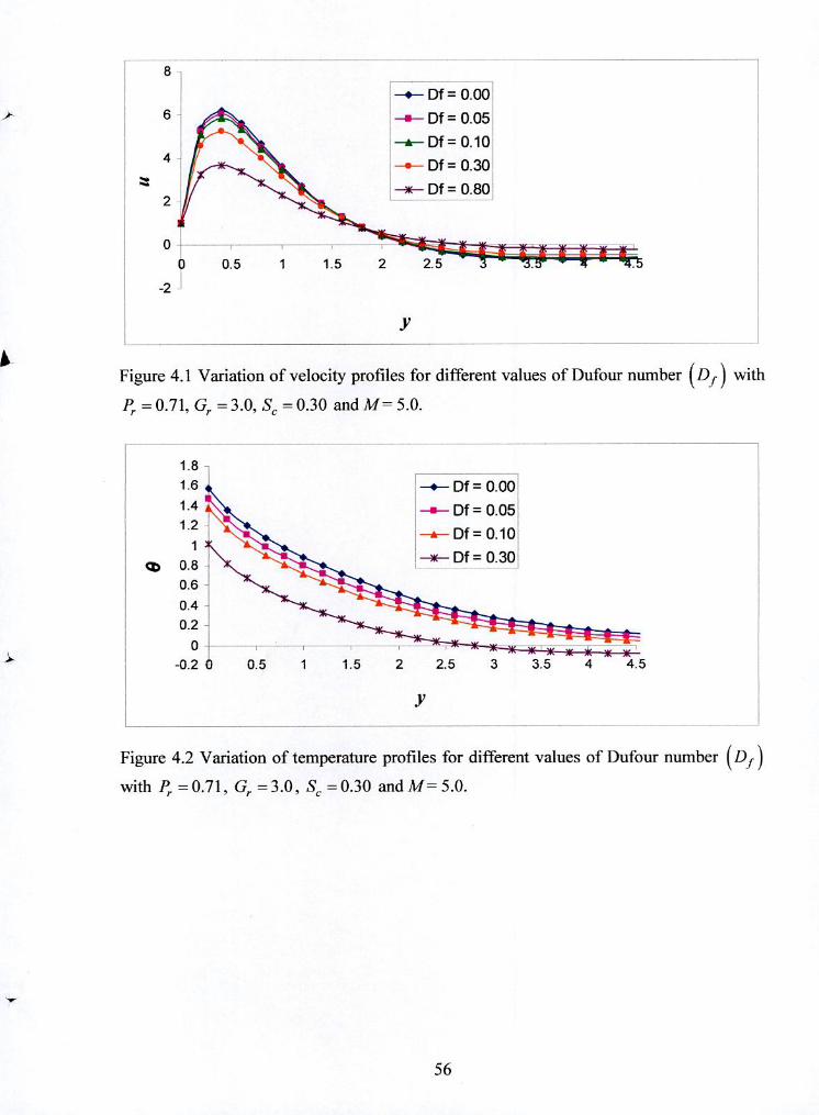
8

-.- Df= 0.00

Df Df Df

Figure 4.1 Variation of velocity profiles for different values of Dufour number (D,.) with

P. = 0.71, Gr = 3.0, S = 0.30 and Al = 5.0.

1.8 1.6 1.4

1.2

0.8 0.6 0.4 0.2

0 -0.2 0 0.5

-.-- Df= 0.00 -.- Df= 0.05

-A.- Df= 0.10

--Df= 0.30

1 1.5 2 2.5 3 3.5 4

y

Figure 4.2 Variation of temperature profiles for different values of 1)ufour number (D,-)

with P =0.71, G,. =3.0, Sc =0.30 and M = 5.0.

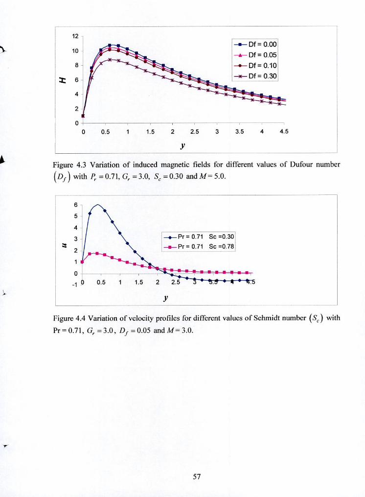
12

005115225335445

Figure 4.3 Variation of induced magnetic fields for different values of Dufour number

(Di ) with P,. = 0.71, Gr = 3.0, S. = 0.30 and M= 5.0.

1 .1 0 0.511522

Figure 4.4 Variation of velocity profiles for different values of Schmidt number (Se.) with

Pr0.71, G,=3.0, D1 =0.05 andM3.O.

57

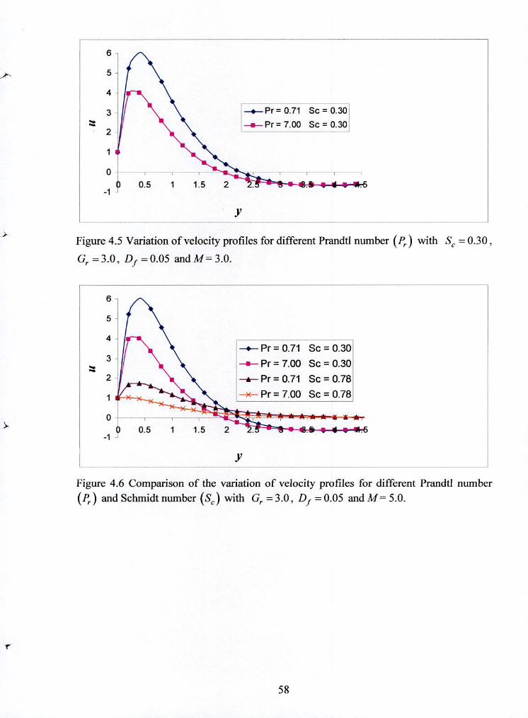
1

a

0

—.---Pr=O.71 Sc=O.30 -.-- Pr = 7.00 Sc = 0.30 —ir--Pr=O.71 Sc=0.78 ---Pr=7.00 Sc=0.78

1.5 2

6

5 j 4

3 H 2

iS

0.5 1 1.5 2

—.—Pr0.71 Sc0.30 —.--Pr=7.00 Sc=0.30

y

Figure 4.5 Variation of velocity profiles for different Prandtl number (f) with S = 0.30

Gr =3.0, Df =O.05 and M3.0.

y

Figure 4.6 Comparison of the variation of velocity profiles for different Prandtl number (i.) and Schmidt number (Se ) with Gr =3.0, Df =0.05 and M5.0.

58

r

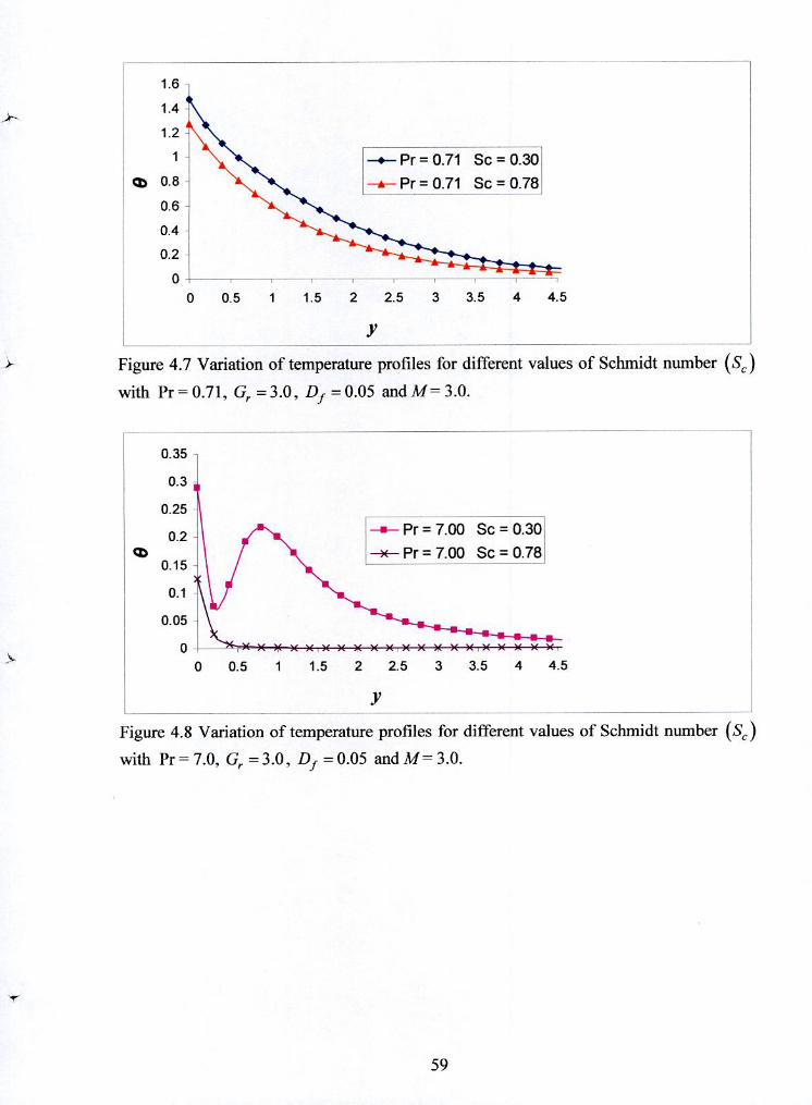
1.6

1.4

1.2

CD 0.8

0.6

0.4

0.2 I'

H-pa.71 Sc = 0.30, -a--Pr_= 0.71 Sc = 0.78

o -, - - - r - I -

0 0.5 1 1.5 2 2.5 3 3.5 4 4.5

y

UP Figure 4.7 Variation of temperature profiles for different values of Schmidt number (se) with Pr = 0.71, Gr =3.0, D1=0.05 andM=3.O.

0.35

0.3

0.25

0.2 -.--Pr=7.00 Sc=0.30 :---Pr=7.00 Sc=0.78

0.15

0.1

0.05

0 0.5 1 1.5 2 2.5 3 3.5 4 4.5

y

Figure 4.8 Variation of temperature profiles for different values of Schmidt number (Se )

with Pr = 7.0, G,. = 3.0, Df = 0.05 and M = 3.0.

59

1.6 1 1.4

0.4

0.2

Figure 4.9 Comparison of the variation of temperature profiles for different Prandtl number

(Pr ) and Schmidt number (S)with Gr=3•0 D1=0.05 and M=3.O.

12 -.- Pr = 0.71 Sc = 0.30

10 —.--Pr= 7.00 Sc= 0.30 -&-- Pr = 0.71 Sc = 0.78

8

o 115 :;5

Figure 4.10 Variation of induced magnetic fields for different Prandtl number (J.) and

Schmidt number (Se ) with Gr = 3.0 and M = 3.0.

60

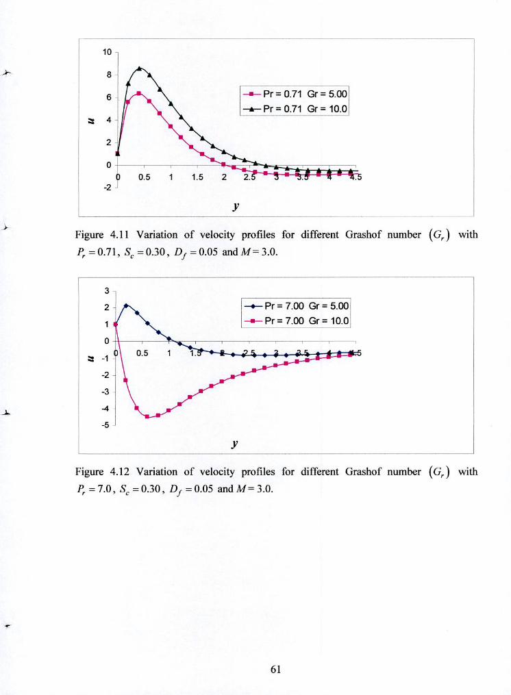
10

8

6

o 0.5

-2 I

—.--Pr= 0.71 Gr= 5.00 —a--- Pr = 0.71 Gr = 10.0

1 1.5 2 2.

y

Figure 4.11 Variation of velocity profiles for different Grashof number (Gr ) with

P,.=0.71, S=0.30, D1=0.05 andM=3.0.

3

2 —.—Pr= 7.00 Gr= 5.00

I —Pr=7.00 Gr= 10.0

0j- 0.5 1

-2

-3

-5

y

Figure 4.12 Variation of velocity profiles for different Grashof number (Gr ) with

P,. = 7.0, S =0.30, Df =0.05 andM3.0.

61

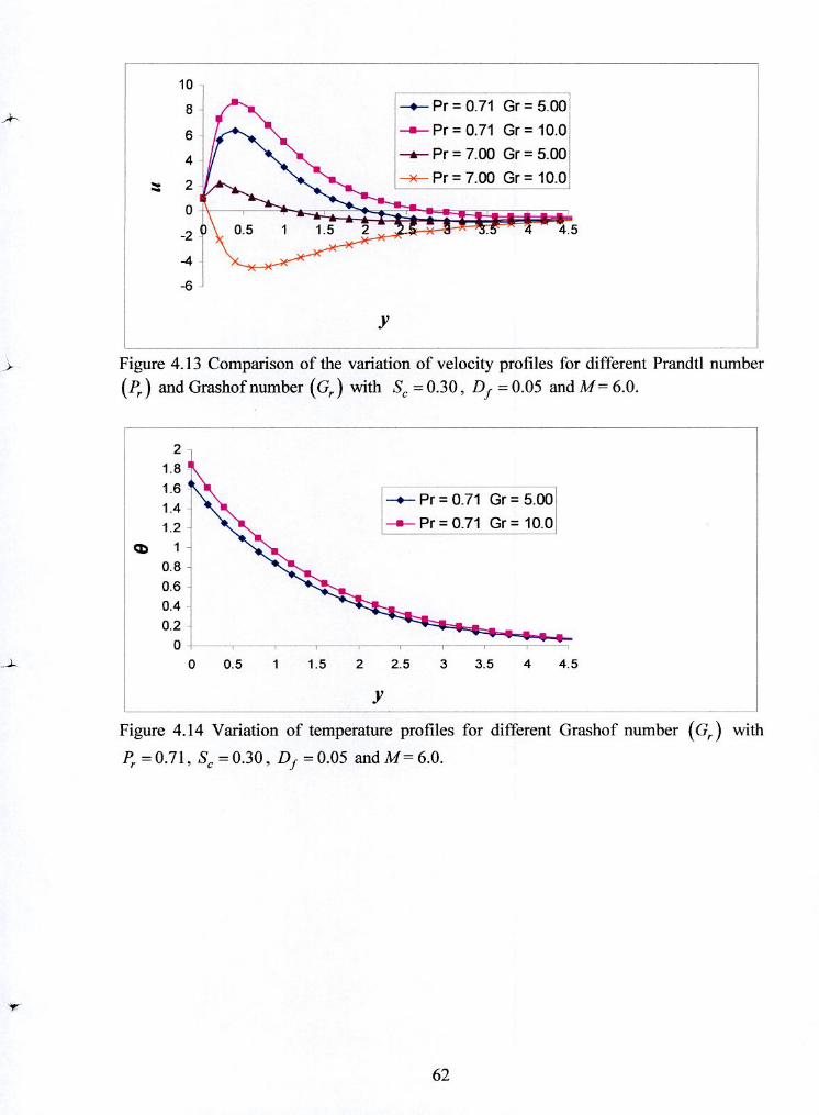
10

8 -.-- Pr = 0.71 Gr = 5.00

6 -.- Pr = 0.71 Gr = 10.0

4 ---Pr= 7.00 Gr5.00

2 0.5 1 1.5 2

Pr= 7.00 Gr= 10.:

4.5

Figure 4.13 Comparison of the variation of velocity profiles for different Prandtl number

(Pr ) and Grashof number (Gr ) with S =0.30, Df =0.05 and M= 6.0.

2

1.8

1.6 Pr= 0.71 Gr= 5.00

0.8

0.6

0.4

0.2

1.4

Figure 4.14 Variation of temperature profiles for different Grashof number (Gr ) with

]. =0.71, Sc =0.30, Df = 0.05 and M6.0.

VA

62

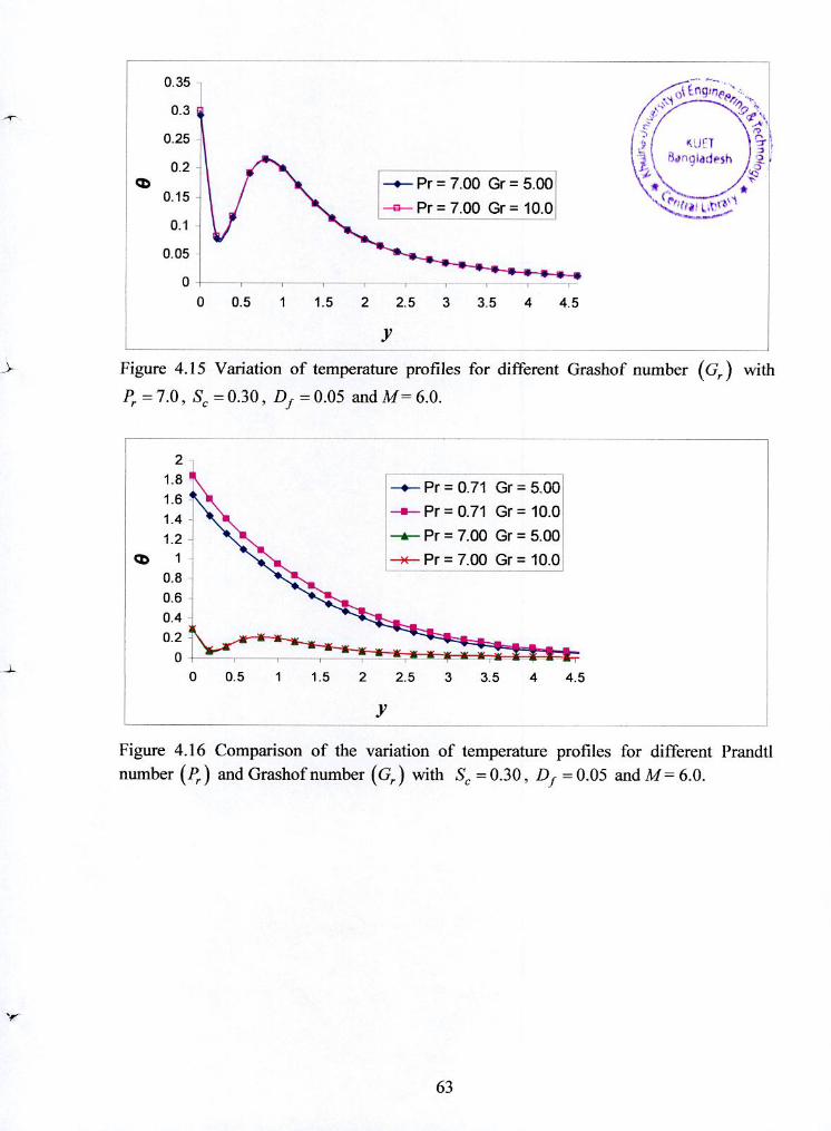
-1

0.35

0.3

0.25

0.2 cb

0.15

0.1

0.05

0-

-.--Pr= 7.00 Gr= 5.00 Eg Pr = 7.00 Gr = 10.0

8dnqIath5h

\\, ••__._

*

" ,st'1

0 0.5 1 1.5 2 2.5 3 3.5 4 4.5

y

Figure 4.15 Variation of temperature profiles for different Grashof number (Gr ) with

J =7.0, S=0.30, D1 =0.05 and M6.0.

2

1.8

1.6

1.4

1.2 UN 0.8

0.6

0.4

0.2

-.-Pr= 0.71 Gr=5.00 Pr = 0.71 Gr = 10.0

-*--Pr= 7.00 Gr= 5.00 -*--Pr= 7.00 Gr= 10.0

1 1.5 2 2.5 3 3.5 4 4.5

y

Figure 4.16 Comparison of the variation of temperature profiles for different Prandtl number (i.) and Grashof number (Gr ) with S = 0.30, Df = 0.05 and M= 6.0.

63

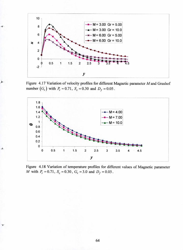
1.8

1.6

1.4

1.2

1

0.8

0.6

0.4

0.2

o

1:

I

6 -*--- M = 6.00 Gr = 5.00

:M1TTTr=b00 4,5 Figure 4.17 Variation of velocity profiles for different Magnetic parameter M and Grashof number (Gr ) with J. = 0.71, S. =0.30 and Df = 0.05.

0 0.5 1 1.5 2 2.5 3 3.5 4 4.5

y

Figure 4.18 Variation of temperature profiles for different values of Magnetic parameter M with J =0.71, S = 0.30, Gr =3.0 and D1 =0.05.

64

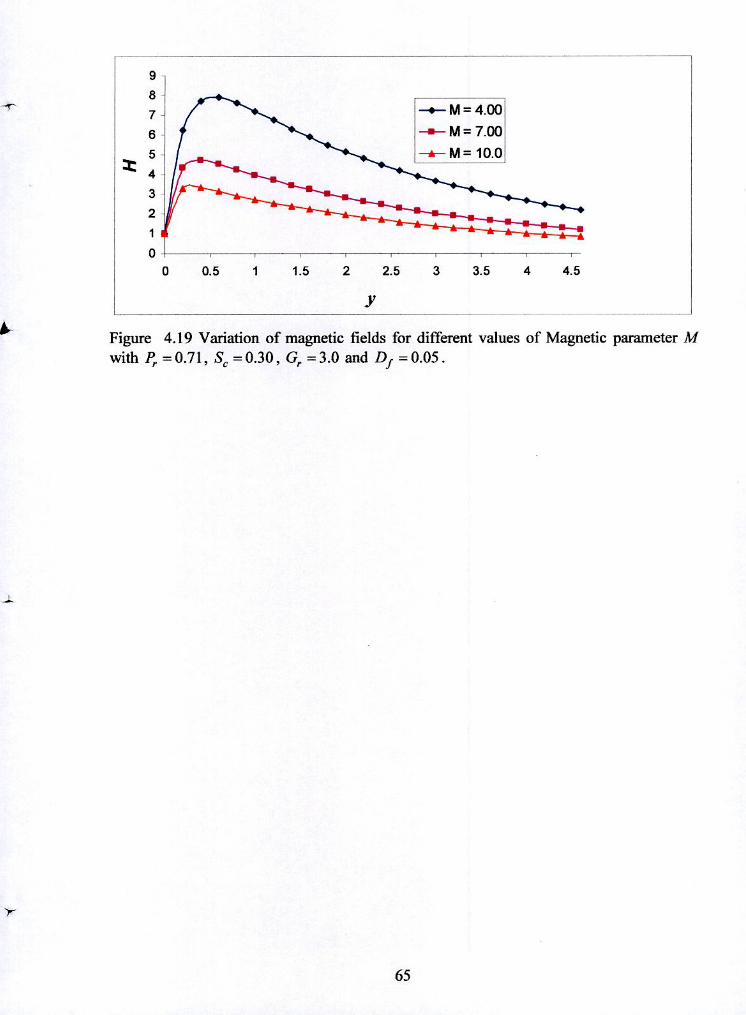
-r [—.—M=4.001 IM= 7.00 ~ M =io.OJ

0 0.5 1 1.5 2 2.5 3 3.5 4 4.5

y

Figure 4.19 Variation of magnetic fields for different values of Magnetic parameter M with I. =0.71, S =0.30, Gr =3.0 and D1=0.05.

65

CHAPTER 5

Concluding Remarks

In this paper we have studied Dufour or diffusion-thermo effect on the laminar mixed free-

force convection flow and heat transfer of viscous incompressible electrically conducting

Iluid above a vertical porous plate under the action of a transverse applied magnetic fieki.

The transformed system of nonlinear, coupled, ordinary differential equations governing

the problem were solved numerically by using perturbation technique. The influences of

various establish parameters on the velocity and temperature profiles as well as induced

magnetic fields for the first order approximation are exhibited in the present analysis. From

the numerical investigation it was observed that the Dufour number has a considerable

effect on some exceptional types of fluids considered. It was also found that the

dimensionless Prandtl number (i.), Grashof number (Gr ), Schmedit number (se ) and

magnetic parameter (M) have an appreciable influence in the study of flow and heat

transfer process. Therefore, it can be confirmly predicted for fluid with medium molecular

weight the Dufour effect can play an important role on the effects of velocity, temperature

and induced magnetic field, so that this effect should be taken into account with other

useful parameters associated. Furthermore, it is necessary to study the Soret (thermo-

diffusion) effect for the problem in order to get more useful results.

66

References

Adams, J. A. and McFadden, P. W.: Journal of American Industrial Chemical

Engineering, 12, 842, 1966.

Agrawal, H. L., Ram, P. C. and Singh, S. S.: Acta, Physics of Academic Science,

Hug, 42, 49, 1977.

Agrawal. H. L., Ram, P. C. and Singh. V.: Progress of Mathematics. 16(1 12). 29.

1982.

Agrawal. I-I. L.. Ram, P. C. and Singh. V.: Astrophysics Space Science. 91, 445,

1983.

151 Agrawal, 11. L., Ram, P. C. and Singh. V.: Proceedings of National Academic

Science, 57(11), 329, 1987.

Alam, M.S., Ferdows, M., Ota, M. and Maleque, M.A.: Dufour and Soret effects on

steady free convection and mass transfer flow past a semi-infinite vertical porous

plate in a porous medium, mt. J. of Appi. Mech. and Engng., 11(3), 535-545, 2006.

Alam, M.S. and Rahman, M.M.: Dufour and Soret effects on MILD free convective

heat and mass transfer flow past a vertical flat plate embedded in a porous medium,

J. Naval Architecture and Marine Engng., 2(1), 55-65, 2005.

Alam, M.S. and Rahman, M.M.: Dufour and Soret effects on mixed convection flow

past a vertical porous flat plate with variable suction, Nonlinear Analysis: Modelling

and Control, 11(1), 3-12, 2006.

1 91 Alam, M.S., Rahman, M.M., Ferdows, M., Kaino, Koji, Mureithi, Eunice, and

Postelnicu, A.: Diffusion-thermo and thermal-diffusion effects on free convective

heat and mass transfer flow in a porous medium with time dependent temperature

and concentration, mt. J. Appi. Engng. Res., 2(1), 81-96, 2007.

[10] Alam, M.S., Rahman, M.M., Maleque, M.A. and Ferdows, M.: Dufour and Soret

effects on steady MHD combined free-forced convective and mass transfer flow

past a semi-infinite vertical plate, Thammasat mt. J. Sci. and Tech., 11(2), 1-12,

2006.

67

[11] Alam, M.S., Rahman. M.M. and Samad M.A.: Dufour and Soret effects on unsteady

MHD free convection and mass transfer flow past a vertical porous plate in a porous

medium, Nonlinear Analysis: Modelling and Control, 2006, 1 ](3). 21 7--226, 2006.

1121 Alfaven, H.: Arkiv F. Mat. Astro. 0. Fysik, 295(2), 1942.

[13] Anghel, M, Takhar, H.S. and Pop, 1.: Dufour and Soret effects on free convection

boundary layer over a vertical surface embedded in a porous medium, Studia

Universitatis Babes-Bolyai, Mathematica XLV(4), 11-21, 2000.

[141 13estman, A. R.: Astrophys, Space Sci, 173, 93, 1990.

Boura, A. and Gebhart, B.: Journal of American Industrial Chemical Engineering,

22, 94, 1976.

Brezovsky, A. A., Martynenko, 0. G. and Sokovishin, Yu A.: J. Engng. Phys. 33,

32, 1977.

Caldwell, D. R.: Journal of fluid mechanics, 64, 347, 1974.

Cramer K. R. and Pai, S. I.: Magneto Fluid Dynamics for Engineers and Applied

Physicists, McGraw Hill, New York, 1973.

Choudhary, R.C. and Sharma, B.K.: Combined heat and mass transfer by laminar

mixed convection flow from a vertical surface with induced magnetic field, J. Appi.

Phys., 99, 03490 1-10, 2006.

Cobble M. 1-1.: Journal of Engineering Mathematics, 11, 249, 1977.

Dursunkaya, Z. and Worek, W.M.: Diffusion-thermo and thermal -d i ffusi on effects

in transient and steady natural convection from a vertical surface. mt. .1. I Icat Mass

Transfer, 35, 2060-2065, 1992.

Eckert, E.R.G. and I)rakc. R. N'l.: Analysis of I leat and Mass I ransFer. Mc( ira'x-

Hill, New York, 1972.

Faraday, M.: Experimental Researches in electrically Phill, 'trans. 15, 175, 1832.

Gebhart, B. and Pera, L.: The nature of vertical natural convection flows resulting

from the combined buoyancy effects of thermal diffusion, mt. J. Heat Mass

Transfer, 14, 2025-2050, 1971.

Georgantopoulos. G. A. and Nanousis, N. D.: Astrophysics Space Science, 67(1),

229, 1980.

Georgantopoulos, G. A., Koullias, J., Goudas. C. L. and Couragenis. C.:

Astroph\sics Space Science. 74. 356. 1981.

68

Gill, W. N., Case!, A. D. and Zch, D. W.: International Journal of I Icat Mass

Transfer, 8, 1131, 1965.

Groots, S. R. T. and Mozur, P.: Non-equilibriem thermodynamics, North Holland

Amsterdam, 1962.

[291 l-laldavnekar, D. D. and Soundalgekar, V. M.: Acta. Physics of Academic Science,

Hungry, 43, (3/4), 243, 1977.

Hasimoto, 1-1. Journal of the Physical Society of Japan, 12(1), 68, 1957.

Hassanien, l.A., Essawy, A.H. and Moursy, N.M.: Natural convection flow of

micropolar fluid from a permeable uniform heat flux surface in porous medium,

Appi. Math. and Comp., 152, 323-335, 2004.

Hubbel, R. H. and Gebhart, B.: Proceedings of 24th 1-Icat Mass Transfer and l'luid

Mechanics, Inst. Corvallis, Oregon(USA). 1974.

Hurle, D. T. J. and Jakeman, E.: Journal of Fluid Mechanics, 47, 667. 1971

134] Inger, G. R. and Sweam, T. F.: Journal of AlAA, 13(5), 616, 1975.

Jha, B. K. and Singh, A. K.: Astrophysics Space Science, 173, 251. 1990.

Kafoussias, N. G.: Astrophysics Space Science, 192, 11, 1992.

Kafoussias, N.G. and Williams, E.M.: Thermal-diffusion and difflision-thenno

effects on mixed free-forced convective and mass transfer boundary layer flow with

temperature dependent viscosity, mt. J. Engng. Sci. 33, 1369-1384, 1995.

Kawase, Y. and Ulbrecht, J.J.: mt. Common. Heat Mass Transfer, 11, 103, 1984.

Kim, Y.J.: Heat and mass transfer in MUD micropolar flow over a vertical moving

porous plate in a porous medium, Transport in Porous Media, 56(1), 17-37, 2004.

1401 Legros, J. C., Van Hook, W. K. and Thoms, G.: Chemical Physics, Lett., 2, 696,

1968.

Levy, R. H. and Petschek, H. E.: Las Paper, 62-100, Los Angeles, California, June,

1962.

Lightfoot, E. N.: Chemical Engineering Science, 23, 931, 1968.

Lowell, R. L. and Adams, J. A.: Journal of AIAA, 5, 1360, 1967.

Martynenko, O.G., Berezovsky, A.A. and Sokovishin, Yu A.: mt. J. Heat Mass

Transfer, 27, 869, 1984.

Mathers, W. G, Maddan, A. J. and Piret, E. L. Induced Chemical Engineering, 49,

961, 1957.

69

1461 Mollendrof, J. C. and Gebhart, B.: Proceedings of 5(h International heat 'l'ransfer

Conference, Tokyo, Japan, 1974.

Nanbu, K.: Journal of AIAA, 9, 1642, 1971.

Nanousis, N. D.: Astrophysics Space Science, 191, 313, 1992.

Nanousis, N. D. and Goudas, C. L.: Astrophysics Space Science, 66(1), 13, 1979.

Pantokratoras, A.: mt. J. Ileat Mass Transfer, 45, 963, 2002.

Pantokratoras, A: Comment on "Combined heat and mass transfer by laminar mixed

convection flow from a vertical surface with induced magnetic field", Journal of

Applied Physics, 102, 076113, 2007.

Pera, L. and Gebhart, B.: mt. J. Heat Mass Transfer, 15, 269, 1971.

Postelnicu, A.: Influence of a magnetic field on heat and mass transfer by natural

convection from vertical surfaces in porous media considering Soret and Dufour

effects, mt. J. 1-leat Mass Transfer, 47, 1467-1472, 2004.

Raptis, A. and Kafoussias, N.G.: Magnetohydrodynamic free convection flow and

mass transfer through porous medium bounded by an infinite vertical porous plate

with constant heat flux, Can. J. Phys., 60(12), 1725-1729, 1982.

Raptis, A. and Tzivanidis, G. J.: Astrophysics Space Science, 94(2), 311, 1983.

Rawat, S. and Bhargava, R.: Finite element study of natural convection heat and

mass transfer in a micropolar fluid-saturated porous regime with soret/dufour

effects, mt. J. of App!. Math. and Mech., 5(2), 58-71, 2009.

Rossow, V. J.: NACATN, 3971, 1957.

[581 Sattar, M.A.: Unsteady hydromagnetic free convection flow with Hall current mass

transfer and variable suction through a porous medium near an infinite vertical

porous plate with constant heat flux, mt. J. Energy Research, 17, I—S. 1993.

Sattar, M.A., Flossain, M.M.: Unsteady hydromagnetic free convection flow with

Hall current and mass transfer along an accelerated porous plate with time-

dependent temperature and concentration, Can. J. Phys., 70, 369-3 74, 1992.

Saville, D. A. and Churchill, 'S. W.: Journal of American Industrial Chemical

Engineering, 16, 268, 1970.

Singh, A. K.: Astrophys, Space Sci, 115, 387, 1980.

Singh, A. K. and Dikshit, C. K.: Astrophys, Space Sci, 148, 249, 1988.

Somers, F. V.: Journal of Applied Mechanics, 23, 295, 1956.

70

Soundalgekar, V. M. and Gupta, S. K.: International Journal of Energy Science,

3(1), 59, 1979.

Soundalgekar, V. M. and Ramanamurthy, T. V.: Journal of Engineering

Mathematics, 14, 155, 1980.

Sutton, G. W. and Gloersen, P.: Physics Today, 14, 18, 1961.

Weiss, Y., Ahoran, Y. and Shai, I.: Proceeding of the Tenth International Heat

Transfer Conference, 7 and 179, 1994.

71