Dual Technological Development in Botswana Agriculture:

A Stochastic Input Distance Function Approach

Xavier Irz and David Hadley1

Abstract: To improve the welfare of the rural poor and keep them in the countryside, the government

has been spending 40% of the value of agricultural GDP on agricultural support services. But can

investment make smallholder agriculture prosperous in such adverse conditions? This paper derives

an answer by applying a two-output six-input stochastic translog distance function, with inefficiency

effects and biased technical change to panel data for the 18 districts and the commercial sector, from

1979 to 1996. This model demonstrates that herds are the most important input, followed by draft

power, land and seeds. Multilateral indices for technical change, technical efficiency and total factor

productivity (TFP) show that the technology level of the commercial sector is more than six times that

of traditional agriculture and that the gap has been increasing, due to technological regression in

traditional agriculture and modest progress in the commercial sector. Since the levels of efficiency are

similar, the same pattern is repeated by the TFP indices. This result highlights the policy dilemma of

the trade-off between efficiency and equity objectives.

JEL classification: O4, Q1

Keywords: Smallholder, Commercial, Agricultural Efficiency, Botswana

Contributed paper selected for presentation at the 25th International Conference of Agricultural

Economists, August 16-22, 2003, Durban, South Africa

Copyright 2003 by Xavier Irz and David Hadley. All rights reserved. Readers may make verbatim

copies of this document for non-commercial purposes by any means, provided that this copyright

notice appears on all such copies.

1 Xavier Irz, Department of Agricultural and Food Economics, University of Reading, Reading RG6 6AR, UK. Email X.T.Irz@reading.ac.uk for correspondence. David Hadley, School of Geography and Environmental Sciences University of Birmingham, Egbaston, Birmingham B15 2TT, UK.

1

Dual Technological Development in Botswana Agriculture:

A Stochastic Input Distance Function Approach

Abstract: To improve the welfare of the rural poor and keep them in the countryside, the government

has been spending 40% of the value of agricultural GDP on agricultural support services. But can

investment make smallholder agriculture prosperous in such adverse conditions? This paper derives

an answer by applying a two-output six-input stochastic translog distance function, with inefficiency

effects and biased technical change to panel data for the 18 districts and the commercial sector, from

1979 to 1996. This model demonstrates that herds are the most important input, followed by draft

power, land and seeds. Multilateral indices for technical change, technical efficiency and total factor

productivity (TFP) show that the technology level of the commercial sector is more than six times that

of traditional agriculture and that the gap has been increasing, due to technological regression in

traditional agriculture and modest progress in the commercial sector. Since the levels of efficiency are

similar, the same pattern is repeated by the TFP indices. This result highlights the policy dilemma of

the trade-off between efficiency and equity objectives.

JEL classification: O4, Q1

Keywords: Smallholder, Commercial, Agricultural Efficiency, Botswana

2

Dual Technological Development in Botswana Agriculture:

A Stochastic Input Distance Function Approach

1. Introduction

Botswana is a landlocked southern African country, bordered to the south and east by South Africa

and Zimbabwe and to the west and north by Namibia. With an area of 566,000 square kilometres and a

population of only about 1.5 million, the population density is unusually low at 2.6 persons per square

km (World Bank, 2002). However the carrying capacity is also low, since the soils are mostly poor

and the climate semi-arid, with frequent droughts, so the vast majority of the land is better suited to

cattle ranching than arable agriculture. Indeed, in the past, beef exports (mainly to the European

Union) were the major source of foreign exchange, but diamonds (Botswana is the world’s leading

exporter in value terms) and tourism are now more important. Although the discovery of diamonds has

rescued Botswana from its former position as one of the poorest countries on earth, mining provides

little employment, so the wealth is not shared and the real importance of agriculture is that it is still the

main source of income for approximately half the population.2 Since it accounts for less than five

percent of GDP (World Bank, 2002), it is clear that the agricultural population is relatively poor and

the distribution within the sector is also extremely unequal. About half the farm families own no cattle

at all, while the politically well connected have accumulated large herds. However, the diamond

revenue allows the government to spend as much as forty per cent of agricultural GDP on support

schemes that are intended to improve the welfare of the agricultural population and keep them in the

rural areas, despite the very harsh conditions (Thirtle et al., 2000).3

This paper investigates the effectiveness of this expensive support program, a question tackled by

Seleka (1999) who investigated the performance of traditional arable agriculture in Botswana for the

1968-90 period. His conclusion was that government support to the sector had a positive effect on the

welfare of rural households but was unsustainable, and that agricultural productivity actually declined

over the study period. The first contribution of our paper is to fill a gap in the existing literature by

evaluating the productivity performance of the whole of Botswana agriculture. Arable agriculture (the

sub-sector studied by Seleka (1999)) accounts for only around 10% of agricultural GDP, so this study

also covers animal production and the growing commercial sector.

The second contribution is to demonstrate the advantages of the parametric distance function

approach to characterising the agricultural technology and decomposing productivity growth in the

context of a low-income country. The only prior example of use of distance functions for this purpose

2 FAOSTAT reports an agricultural labour force of 300,000 in 2000 from a total labour force of 673,000. For the same year, the agricultural population was 686,000 and the non-agricultural population 855,000. 3 This level of expenditure would be impossible without the diamond revenue. Four per cent would be a more usual level, so supporting a sector to this extent is most unusual; but then Botswana is an unusual country.

3

is Brümmer et al. (2002) who investigated farm-level productivity growth in dairy production in three

European countries. The empirical model is a two-output stochastic input distance function that is used

to analyse agriculture efficiency and productivity in the eighteen districts of Botswana and the

commercial sector, for the period from 1979 to 1996. The approach is appropriate, first because it

requires only data on outputs and inputs, which are well recorded, whereas markets for the major

inputs, such as land and labour, are not sufficiently developed for there to be meaningful prices.4

Second, it accounts for noise, which is an advantage over non-parametric methods such as DEA.

Third, tests show that the crop and animal sectors cannot be aggregated, which rules out the use of

stochastic production functions to estimate the technology and efficiency levels. By contrast, distance

functions can accommodate multiple inputs and outputs. The method produces output and input

elasticities and leads to the estimation of indices for technical change, technical efficiency and total

factor productivity. This allows the commercial sector to be compared with traditional agriculture.

The remainder of the paper is organized as follows. Section two discusses the theory and section

three very briefly describes the data. The results are reported in section four, beginning with tests to

determine the appropriate model. Section five presents the efficiency and productivity indices and the

final section concludes by summarising the results and suggesting further developments.

2. The Input Distance Function: Definition, Properties and Interpretation

The input distance function first introduced by Shepard (1970) is defined on the input requirement set

Lt(y) as:

Dit(x,y)=Max{ρ: x/ρ ∈ Lt(y)} (1)

It measures the largest factor of proportionality by which the input vector x can be scaled down in

order to produce a given output vector y with the technology existing at a particular time t. For any

input-output combination (x,y) belonging to the technology set, the distance function takes a value no

smaller than unity, while a value of unity simply indicates technical efficiency. More generally, the

distance function provides a measure of technical efficiency since its reciprocal is the well-known

Farrell (1957) input-based index of technical efficiency.

The input distance function is always homogenous of degree one in inputs and inherits

properties from the parent technology as detailed in Färe and Primont (1995).5 Most useful for the

interpretation of the empirical estimates is the duality between the cost and input distance functions,

which is easily expressed as:

}1),(:{),( ≥= yxDwxMinywC tix

t (2)

4 This prevents the estimation of dual cost and profit functions, which have the additional drawback of imposing restrictive behavioural assumptions. 5 In particular, as described in Hailu and Veeman (2000), the input distance function is non-decreasing and concave in inputs and non-increasing and quasi-concave in outputs.

4

From this minimisation problem, where w denotes a vector of input prices, it is straightforward to

relate the derivatives of the input distance function to the cost function. First, with respect to input

levels xk, one obtains:

),(),(

)),,(( **

yxrywC

wx

yywxD tkt

k

k

tti ==

∂∂

(3)

Hence, the derivative of the input distance function with respect to a particular input k is equal to the

cost-deflated shadow price of that input rk*t, which is therefore expected to take a positive value.6 The

previous equality is more conveniently expressed in terms of the log derivative of the distance

function:

tkt

tkk

k

ti

xD SywC

ywxwxD

kti

==∂∂

=),(

),(lnln *

,ε (4)

Equation (4) states that the log derivative of the input distance function with respect to input k is equal

to its cost share Stk. It therefore captures the relative importance of that input in the production process,

a property that we use to interpret our estimation results. With respect to the output vector y,

application of the envelope theorem to minimisation problem (2) leads to the following equality:

m

t

m

tti

yD yywC

yyywxD

mti ln

),(lnln

)),,((ln *

, ∂∂−=

∂∂

=ε (5)

The elasticity of the input distance function with respect to any output is therefore equal to the

negative of the cost elasticity of that output. It is expected to be negative for all desirable outputs and,

in absolute value, reflects the relative importance of each output.

Finally, and most importantly for our purpose, the distance function can easily inform the

researcher on the evolution of the technology over time. For analytical tractability, this paper follows

Chambers (1988) in assuming that a stable relationship exists between outputs, inputs and time, or:

),,(),( tyxDyxD iti = (6)

Once again, straightforward application of the envelope theorem to minimisation problem (2) leads to:

ttywC

ttytywxDi

tDti ∂

∂−=∂

∂= ),,(ln),),,,((ln *

,ε (7)

Hence, the elasticity of the input distance function with respect to time is equal to the elasticity of cost

reduction and provides a dual measure of the speed of technical change. A negative value for this

elasticity indicates technological regression and a positive value technological progress. This analysis

can be pursued further, by considering a Hicksian-style definition of technical change bias based on

the relative factor shares expressed in equation (4):

txD

tS

Bk

itk

kt ∂∂∂

=∂

∂=

lnln2

(8)

6 x*t(.) denotes the vector of cost-minimising input quantities.

5

A positive (negative) value of Bkt indicates that technical change is biased in favour of (against) input

k.

Finally, note that the distance function can be used to derive virtually all the classical

properties of the underlying technology, such as returns to scale and measures of input and output

substitutability (Färe and Primont (1995), Grosskopf et al. (1995), Morrison Paul et al. (2000), Kim

(2000)). Constant returns to scale are defined in terms of the distance function by: 10, ( , , ) ( , , ) i iD x y t D x y tλ λ λ −∀ > = (9)

The other properties of the distance function are not developed, since they are not used in this

application.

2.1 An Estimable Model

The value of the distance function is not observed so that imposition of a functional form for Di(x,y,t)

does not permit its direct estimation. A convenient way of circumventing this problem was suggested

by Lovell et al. (1994) who exploit the property of linear homogeneity of the input distance function,

expressed mathematically as:

Di(λx,y,t) = λDi(x,y,t) ∀λ >0 (10)

Assuming that x is a vector of dimension K and setting λ=1/x1, where x1 denotes its (arbitrarily

chosen) first component, the previous equation is expressed in logarithmic form as:7

),,/(lnln),,(ln 11 tyxxDxtyxD ii += (11)

Similar reasoning is used to establish that imposing CRS implies the following relationship:

),/,/(lnlnln),,(ln 1111 tyyxxDyxtyxD ii +−= (12)

The next stage of the analysis relies on the idea that the logarithm of the distance function in (11)

measures the deviation of an observation (x,y,t) from the deterministic border of the input requirement

set L(y,t) which, following the stochastic frontier literature, is itself explained by two components. The

first one corresponds to random shocks and measurement errors that can take either positive or

negative values and are described by a symmetric error term -v. The second one corresponds to

technical inefficiencies that are also assumed to be stochastic and are captured by a non-negative

random variable u. At a conceptual level, the presence of inefficiencies can in turn be justified by a

non-uniform distribution of managerial skills across the population of firms using the same

technology. Mathematically, the previous assumptions are summarized by:

lnDi(x,y,t)=u - v (13)

Equations (11) and (13) are now combined to give:

-ln(x1) = lnDi(x/x1,y,t) - u+ v (14)

If CRS is imposed, we obtain a slightly different expression:

-ln(x1)+ln(y1) = lnDi(x/x1,y/y1,t) - u+ v (15)

7 The notation x/x1 is used to denote the K-1 vector of ratios xk/x1, for k≠1.

6

Given a parameterisation of the distance function and distributional assumptions on the random terms,

the previous equations (14) or (15) can be estimated by the maximum likelihood methods that have

now become commonplace in the stochastic frontier literature (summarised in Coelli, Rao and Battese,

1998). All models consider that the random error terms v are iid and follow a normal distribution

N(0,σ2v) but differ with respect to the distribution of inefficiencies u. Extending the seminal model of

Aigner, Lovell and Schmidt (1977), Battese and Coelli (1995) relax the assumption of identically

distributed inefficiency terms in order to identify the determinants of technical inefficiencies and it is

this model that we use in the empirical application. Accordingly, it is assumed that the stochastic terms

uit are obtained by truncation at zero of a normal variable N(µit; σu2) where:8

δµ itit z= (16)

The term zit denotes a vector of observable explanatory variables while δ is a vector of parameters to

be estimated. In this context, the likelihood function can be expressed algebraically and maximised

numerically to produce estimates of both the input distance function and the vector of parameters δ.

Further, while the individual inefficiency levels are not directly observable, the method allows for

calculation of their predictors expressed as (Coelli and Perelman, 1996):

]|)[exp(/1/1 iiiPi

Pi uvuEDTE −== (17)

2.2 Functional Form

The translog is used because imposing linear homogeneity in inputs is not possible for the other

flexible functional forms and the Cobb-Douglas violates the convexity condition, as well as being too

restrictive. The model with K inputs and M outputs therefore takes the following form:

0 ' '1 1 1 ' 1

2' '

1 ' 1 1 1 1 1

1ln ( , , ) ln ln ln ln2

1 1ln ln ln ln ln ln2 2

K M K K

k k m m t kk k kk m k k

M M K M K M

mm m m tt km k m kt k mt mm m k m k m

D x y t x y t x x

y y t x y t x t y

α α β ε α

β ε γ γ γ

= = = =

= = = = = =

= + + + + +

+ + + +

∑ ∑ ∑∑

∑∑ ∑∑ ∑ ∑(18)

The conditions for linear homogeneity in x are:

'1 ' 1 1 1

1; , 0; , 0; 0K K K K

k kk km ktk k k k

k mα α γ γ= = = =

= ∀ = ∀ = =∑ ∑ ∑ ∑ (19)

The empirical application models regional, rather than farm level, production and it is therefore

preferable to impose constant returns to scale (CRS) on the technology. The implied restrictions for

the translog are:

' '1 1 ' 1 1 1

1; , ', 0; , 0; 0M M M M M

m mm mm km mtm m m m m

m m kβ β β γ γ= = = = =

= − ∀ ∀ = = ∀ = =∑ ∑ ∑ ∑ ∑ (20)

Using the two sets of restrictions (19) and (20) produces an estimable equation, which is the special

case of equation (15) for the translog:

8 The individual and time subscripts i and t were ignored up to this point for clarity.

7

* * * *'1 1 0 '

2 2 2 ' 2

* * 2 * * * *''

2 ' 2 2 2 2 2

1ln ln ln ln ln ln2

1 1ln ln ln ln ln ln2 2

K M K K

k m k kk m t kkk m k k

M M K M K M

m m k m k mmm tt km kt mtm m k m k m

x y x y t x x

y y t x y t x t y u v

α α β ε α

β ε γ γ γ

= = = =

= = = = = =

− + = + + + +

+ + + + + − +

∑ ∑ ∑∑

∑ ∑ ∑∑ ∑ ∑

(21)

where xk* denotes the ‘normalised’ input quantity xk/x1 and ym*=ym/y1 denotes the ‘normalised’ output

quantity ym/y1. We further impose symmetry of the distance function by setting:

mmmmkkkk mmkk '''' ,',;,', ββαα =∀∀=∀∀ (22)

Given the dual nature of Botswana agriculture, a dummy variable D is added to allow the technologies

to differ in level in the two sectors and a cross-term between the dummy variable and the time trend

allows different paths of technological change in the two sectors. This gives the full model as: * *

1 1ln ln ( , , , , , , ) D Dtx y TL x y t D Dt u vα β ε γ φ φ− + = + + − + (23)

The limited data available restricted the choice of inefficiency effects and in the end three variables

were selected: a time trend, a cross-term between the commercial dummy and the time trend and

finally the output mix p:

itpitdttit ptDt δδδδµ +++= 0 (24)

This specification allows inefficiencies to vary over time, but in a possibly different manner in the two

sub-sectors.

3. Data

The detail of how the data set was built is given in Annex 1. All series are for 1979 to 1996, giving a

panel of 342 observations. Note that what is referred to as year t corresponds in fact to the agricultural

season between year t and year t+1 and that it is also how the results are reported in the empirical

section of the paper. The outputs are crops and livestock and the components were aggregated using

constant (1995) price weights, so these series are equivalent to physical quantities of output. The input

series include six different factors of production, which are either measured in physical units (land,

labour and draft power) or are constant (1995) price aggregates (seeds, fertilisers and herds). The

output mix variable p was simply defined as the revenue share of livestock in total output.

4. Results

4.1 Tests of hypotheses for model selection

Alternative specifications of the model were evaluated using generalised likelihood ratio tests, which

compare the likelihood functions under the null and alternative hypothesis, represented by the model

8

described in the last section.9 Table 1 first reports the test that compares the frontier with the mean

input distance function, estimated by considering that the inefficiency term u is non-stochastic and

equal to zero. In this context, any deviation from the frontier of the input requirement set is solely

explained by random shocks and the distance function can be conveniently estimated by ordinary least

squares. The significant drop in the likelihood function associated with this model, from –5.34 to –

43.35, implies a clear rejection of the null hypothesis. This is confirmed by the significantly large

value of parameter γ in Table 3 (0.95) that indicates that most of the deviation from the deterministic

border of the input requirement set is due to technical inefficiencies rather than random shocks. Hence,

significant technical inefficiencies exist in Botswana agriculture.

Table 1

The second test determines whether the variables introduced as inefficiency effects improve

the explanatory power of the model. The null hypothesis is rejected at the 1% level, implying that the

distributions of inefficiencies are not identical across individual observations but depend on the

variables included in vector zit. This result gives strong support to the inefficiency model of Battese

and Coelli (1995) as opposed to the simpler models of the older literature. The third test is on the

separability of the inputs and outputs in the input distance function. This hypothesis is defined

mathematically by equating all cross-terms between inputs and outputs (γkm) to zero. These restrictions

are strongly rejected, which implies that it is not possible to aggregate consistently the two outputs

into a single index. This is why the distance function is used rather than a stochastic frontier

production function, which requires output aggregation prior to estimation.

Then, the translog functional form is tested against the null hypothesis that the Cobb-Douglas

represents an acceptable approximation of the true input distance function and again the null is

rejected, implying that the restrictions imposed by the Cobb-Douglas are inappropriate. The fifth test

focuses on the dual nature of Botswana agriculture by considering the null hypothesis that all three

parameters associated with the commercial sector dummy variable are simultaneously equal to zero.

This is rejected, implying that the two sub-sectors have different technological characteristics that will

be investigated further in the next section. Finally, the last test relates to the hypothesis that

technological progress is cost-neutral, meaning that it does not affect factor shares. This proposition is

rejected at the five percent level of significance.

Altogether, the results of these specification tests point to the complexity of technological

relationships in Botswana agriculture: technical inefficiencies are significant, inputs and outputs are

not separable, the Cobb-Douglas which is restrictive in terms of substitution possibilities is not

9That is, we compute the statistic )](ln)([ln2 1HLHHLH o −−=λ , where LH(.) denotes the likelihood function, H0 the null hypothesis and H1 the alternative hypothesis. Under the null, this statistic follows a chi-squared distribution with a number of degrees of freedom equal to the number of restrictions. The estimation results are usually reported in terms of parameters σ2=σu

2+σv2 and γ=σu

2/σ2 rather than in terms of the original variances. If the null hypothesis involves parameter γ, which as a ratio of two variances is necessarily positive, the test statistic follows a mixed chi-squared distribution and the critical values can be found in Kodde and Palme (1986).

9

appropriate, technological change is biased and there is evidence of important differences between

traditional and commercial agriculture. We now turn to the estimation results in order to characterise

the technology and its evolution over time.

4.2 Distance function results

The results are reported only for the model selected on the basis of the tests. The important parameter

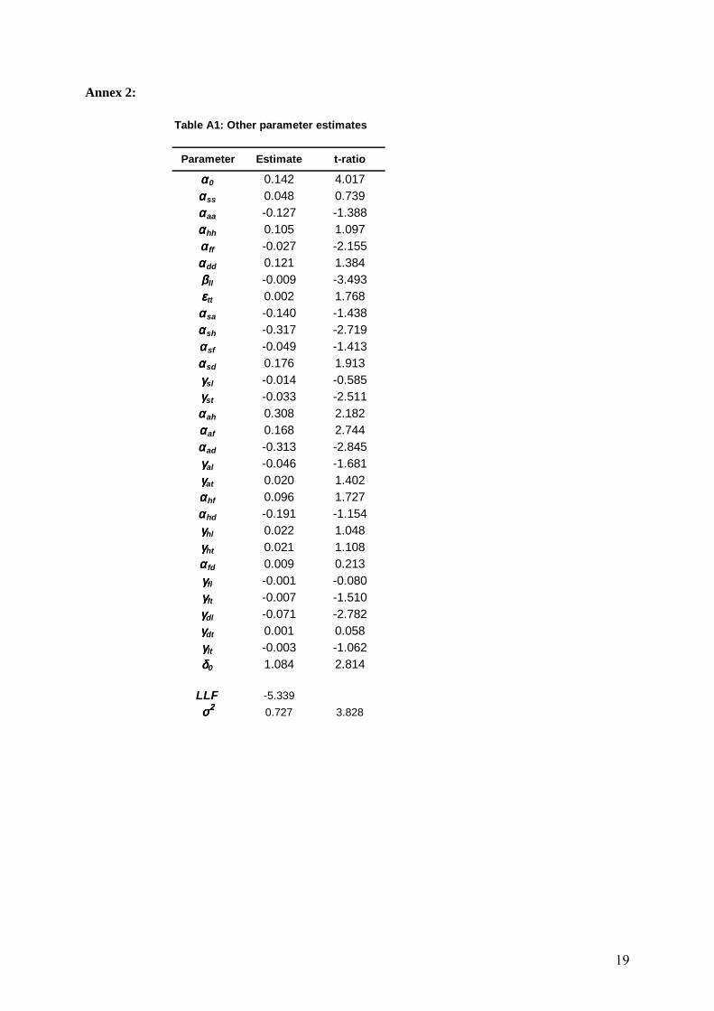
estimates are reported in Tables 2 and 3, while the remaining parameters are relegated to Annex 2,

Table A1. Together the tables show that out of the 44 estimates, 22 are statistically significant at the

5% level.10 The several significant cross product and squared terms in Table A1 show why the test

rejected the Cobb Douglas as inadequate.

Next, the parameter estimates can be interpreted in light of the theory developed in the first

section. All the variables were mean differenced prior to estimation so that the elasticities of the

distance function with respect to input quantities, output quantities and time estimated at the sample

mean correspond simply to the first order coefficients.

Equation (5) established that the elasticity of the distance function with respect to each output

corresponds to the negative of the cost elasticity of that particular output. Table 2 reports that, as

expected, these two elasticities are negative and highly significant. Hence, increasing production of

either of the two outputs results in a substantial increase in cost. The estimates also indicate that the

cost elasticity of livestock output (0.90) is much larger than the corresponding elasticity for crops

(0.10). This result means that a 10% increase in livestock output results in a 9% increase in total cost,

while the corresponding figure for crops is only 1%. Hence, the estimates clearly reflect the

dominance of livestock production in Botswana agriculture.

Table 2

The elasticities of the distance function with respect to input quantities are equal to the cost

shares and therefore reflect the relative importance of the inputs in the production process. Table 2

reveals that four of the six elasticities are positive, as expected, with reasonable levels of statistical

significance. The elasticity with respect to herd size is largest with a value of 0.75 that means that the

cost of that input represents 75% of total cost at the sample mean. This is not an unexpected result

given the importance of livestock production in Botswana agriculture. Draft power comes next in

terms of cost share with a value of 0.21, a result that suggests that soil preparation is crucial for crop

production in Botswana. Land is obviously an important factor of production in agriculture and it is

reflected by an elasticity of 0.11, which is statistically significant at the 10% level. Finally, the seed

input has a positive elasticity equal to 0.07.

Contrary to theoretical expectations, the model also produces two small negative elasticities,

for fertiliser and labour input. The fertiliser result can be explained by the fact that Botswana

10 The subscripts used to report the coefficient estimates are l for livestock, c for crops, s for seeds, a for land, h for herds, f for feeds, d for draft animals and L for labour. Note that Table 2 does not report t-ratios for the elasticities of the distance function with respect to crops and labour. This is so because the values of these parameters are inferred from the restrictions expressed in (19) and (20).

10

agriculture is dominated by extensive ranching, with very little use of chemical fertiliser, relative to

the (unrecorded) extensive use of animal manure. The insignificant elasticity of labour must reflect

the low opportunity cost and productivity of smallholder labour, but is also partly caused by

collinearity with herd size and land area.

5. Dual agricultural development: Efficiency of traditional and commercial agriculture

5.1 Insights from the regression results

The specification tests established that there are substantial technological differences between the

commercial and traditional sectors. Table 3 shows that the parameter of the commercial dummy

variable in the distance function has a positive value of 1.93 and is highly significant. The exponent of

this parameter, which is 6.9, can be interpreted as the ratio of the commercial and traditional distance

functions, meaning that compared to the traditional technology, the commercial technology can

produce the same output with less than one sixth the inputs.11 This is an important result that suggests

that there is a huge technological gap between commercial and traditional agriculture. This large gap is

consistent with the limited evidence available for arable agriculture. Seleka (1999) reports that average

yields for six different crops in the commercial sector over the 1979-93 period were between two and

a half and eleven times those for traditional farming.12

Table 3

Next, we analyse how the technologies evolved over time in the two sub-sectors. The theory

section shows that the derivative of the input distance function with respect to time is equal to the

elasticity of cost reduction and therefore provides a convenient dual measure of the rate of

technological progress. Table 3 reports a value of –0.031 for the parameter εt,, which implies that the

traditional sector of Botswana agriculture has undergone technological regression from 1979 to 1996,

at the rate of 3.1% per annum.

The elasticity of cost reduction in the commercial sector evaluated at the sample mean is equal

to εt+φDt, where the second item is the coefficient of the cross-term between the commercial dummy

and the time trend in the distance function. The estimate of 0.079 for φDt in Table 3 means that the

commercial sector has undergone technological progress at a rate of 4.8% (7.9%-3.1%) per annum

over the period. Thus, the technological gap between traditional and commercial agriculture in

Botswana is not only large but also increasing quickly, as the difference in rates of technological

change in the two sub-sectors is almost 8% over the period.

11 It is straightforward to establish that the values of the distance function in the two sectors Dc and Dtr are related by the following expression for any input-output combination: Dc(x,y,0)/Dtr(x,y,0)=exp(φD). This ratio measures the difference in technological levels between the two sectors. In particular, suppose that the input-output combination (x, y) is technically efficient for the traditional sector, i.e. Dtr(x,y,0)=1. The input distance function for the commercial sector takes a value of exp(φD) which is strictly greater than unity since φD is strictly positive. Hence, in order to produce the output vector y, the input vector x could be scaled down by using the commercial technology. 12 Hence, for maize, average yields in the commercial and traditional sectors were equal to 723 and 66 kg/ha respectively.

11

Table 3 then reports that the overall mean level of technical efficiency in the sample is 85%,

which is coincidentally also the mean efficiency level in the two sub-sectors. Once the difference in

technological levels is taken into account, the two sectors are therefore largely similar in terms of

technical efficiency. More interesting is the evolution of the efficiency indices over time. First, the

coefficient of the time trend, introduced as an inefficiency effect (δt in equation (24)) takes a negative

and highly significant value. Consequently, as time goes by, the mean of the normal distribution that is

truncated at zero to represent inefficiencies in the traditional sector becomes more negative, which

signals an improvement in technical efficiency. Hence, this result suggests that the traditional sector

operates progressively closer to its technological frontier, which is not surprising since we have just

established that this frontier is itself regressing.

In the commercial sector, the evolution of inefficiencies over time follows a different pattern

since the coefficient of the cross term between the dummy variable and the time trend in the

inefficiency component is statistically significant at the 1% level. For this sector, the effect of the time

trend is reflected by the sum δt+δDt, which takes a positive value, indicating a progressive decrease in

efficiency. Finally, the last column of Table 3 demonstrates that farms with a relatively large output

share of livestock tend to be more efficient than farms specialising more heavily in crop production.

In summary of this section, the results show technological dualism between the commercial

and traditional sectors. At a static level, there exists a major technological gap between the two sub-

sectors, with the commercial sector performing much better than its traditional counterpart. There is

also no sign that this situation is improving since, to the contrary, the traditional sector appears to have

experienced a slow technological regression over the study period, while simultaneously the

commercial sector was experiencing technological progress. This pattern of technological change

explains the evolution of technical efficiencies. The traditional sector tends to operate progressively

closer to its regressing frontier, while in the commercial sector there is evidence that inefficiency has

increased.

5.2. Technical Change, Technical Efficiency and TFP Indices

The results reported above are averages over the full period at the sample mean and do not take

account of some important aspects of the model, such as the biases of technological change.13 The

magnitude of the efficiency changes over the whole period and their impact on productivity also

remain to be quantified. Thus, we now present indices of technical change, technical efficiency and

total factor productivity (TFP), which provide a full account of the way in which agriculture has

developed in Botswana. The technology index is obtained by chaining the indices of annual

13 For instance, if a particular region makes relatively more use of a factor against which technological change is biased, that region will experience relatively slow technical change.

12

technological change calculated from equation (7)14 while the efficiency scores are the predictors

described in equation (17). The chained TFP index is then simply the product of the two other indices.

Table 4 begins by reporting multilateral technical change indices. The commercial sector is

given the conventional arbitrary starting value of 100. The first result of the last section was that the

commercial sector was, on average, 6.9 times more efficient than traditional agriculture. Thus, the

average of the technology index for the traditional sector is set at 14.5 (penultimate row), which gives

a starting value of 19.8. With the biases of technological change taken into account, there is

technological regression in traditional agriculture of –2.88% per annum, while the commercial sector

technology improves at 1.42% per annum (last row). This is consistent with the results of the previous

section but the differences in factor proportions in the two sub-sectors tend to reduce the rate of

technological divergence between the two sectors.

Table 4

The annual results in Table 4 show that for the commercial sector there was stagnation in the

first part of the period, followed by growth, as the government began major technological support

projects. This pattern is more easily discerned in Figure 1, which plots the series. The commercial

sector growth rate from 1987 is an impressive 2.7% per annum, but the table and figure show that the

very expensive efforts to aid smallholders, such as the Accelerated Rainfed Arable Programme,

considered by Seleka (1999), did nothing more than stop the regression of technology in the

smallholder sector, where there is still no growth. Since the commercial sector is 97% ranching, these

programmes have concentrated on infrastructure improvements, such as drilling boreholes, although

there have been efforts to improve stock and veterinary services.15

Figure 1

The technical efficiency indices differ far less, with traditional agriculture only about 10%

worse than the commercial sector at the start of the period. Then, confirming the results of the last

section, efficiency improves in traditional agriculture, which can be explained in part by the regressing

frontier. However, the annual figures in Table 4, plotted in Figure 1, suggest that weather conditions

(droughts) also influence technical efficiency in traditional agriculture and are responsible for

relatively large and sudden decreases in years such as 1987 and 1991. Many of the smallholder

programmes are a matter of drought relief, such as distributing free animal feed to prevent slaughter in

bad years. The payoff, in terms of maintaining the livelihoods of the poor may be substantial, but the

cost of these modest efficiency gains, of 0.60% per year, is considerable.

The technical efficiency series for the commercial sector shows the droughts even more

clearly and theses account for much of the efficiency losses, but there is also some increase in

14 The exact method of calculation is similar to that used by Coelli et al. (1998), page 234, for a stochastic production frontier. 15 There have also been programmes to develop irrigated arable agriculture, such as fruits and vegetables, in the commercial sector, but these are not included in the national statistics and require separate evaluation.

13

inefficiency over time, at 0.26% per annum, which suggests that some producers are not assimilating

the new technologies and are falling behind the advancing frontier.

Last, the TFP indices are the product of the technical change and technical efficiency indices

and, as the figure shows, they follow similar paths to the efficiency indices, because technical change

is smoother and more gradual. This combination of technical and efficiency changes results in a TFP

for traditional agriculture that falls from a value of 16, to 10.8, which is a decline of 2.3% per annum.

Thus, despite all the programmes, the smallholder’s productivity has declined over the full period,

although the results for the last five years suggest that this trend has now come to a halt. The

commercial sector has stagnating TFP in the early period, but does seem to have made rapid progress

in the second half of the study period. The annual growth rate for the full period is only 1.16%, but

from 1989, it is 2.94% per annum, driven by rapid technological progress.

If this rate of growth can be maintained, the prospects for commercial agriculture in Botswana

are good, but there is a clear case of dualistic development. Despite massive support programmes,

which may well be excellent in equity terms, the efficiency of traditional agriculture has not improved

at all. Seldom has the trade-off between equity and efficiency objectives resulted in such a clear policy

dilemma.

6. Conclusions

Botswana has used diamond revenues to support agriculture, which accounts for only 4% of GDP, but

supports about half the population. This paper studies the efficiency effects of these programmes,

using a two-output distance function frontier model, with dummies for the commercial sector and

inefficiency effects, which was selected on the basis of extensive tests. The data are a panel of 342

observations, for 18 regions and the commercial sector, over the period from 1979-96, which are

sufficient to support this reasonably sophisticated model. The results show that there is a huge

technology gap between traditional agriculture and the commercial sector, which is more than six

times as technologically advanced. Despite the efforts of the government to improve the livelihoods of

the poor smallholders, their level of productivity has fallen, while the commercial sector, which

specialises heavily in cattle ranching, has progressed. Hence, almost 40 years after the independence,

and despite major investments to support smallholders, agriculture in Botswana has become

increasingly dualistic.

The results show that past agricultural policies have not been successful in efficiency terms

and have made little contribution to the process of economic development. Naturally, these policies

can be justified on equity grounds but the results seem rather unsatisfactory in view of the high level

of government support to agriculture, which would be clearly unsustainable without diamond revenue.

The policies amount to providing a safety net for smallholders and ameliorating many of the effects of

the harsh and variable climate. This is laudable, but the lack of technological progress in the traditional

14

sector suggests that there is little scope for improving the technologies of the resource poor. Those

with no cattle are unlikely to prosper with a few smallstock and low yielding grain crops.

The Ministry of Agriculture continues to introduce new policies that differ from those of the

past. The NAMPAADD16 programme launched in October 2002 focuses on the arable and dairy

sectors and has the explicit aim of trying to ‘enable traditional farmers to transform to commercial

farming’ and to target incentives to ‘beneficiaries and areas where they guarantee a positive change to

farm productivity’ (Ministry of Agriculture, 2003). Whilst it is hard to argue against

commercialisation as the way to improve the incomes of subsistence producers, the scope for this in

arable and dairy farming is limited to a few areas. The majority of the country is suitable for little but

ranching and no other agricultural activity seems particularly viable. For commercialisation to be

based around cattle ranching, the government needs to design schemes to spread ownership to more of

the rural population, or ensure that the benefits from larger herds spill over to the locals who do not

have cattle.

Acknowledgements: The authors are grateful to the Department for International Development for

funding this study and Oxford Policy Management for organizing it. The staff of the Department of

Agricultural Planning and Statistics, Ministry of Agriculture, Botswana contributed to the data

collection and provided local expertise. We particularly thank Howard Sigwele, Mrs K Molefhi and

Stephen Ackroyd.

References Aigner D., K. Lovell and P. Schmidt. (1977), Formulation and Estimation of Stochastic Frontier Models, Journal of Econometrics, 6, 21-37 Battese, G. and T. Coelli (1995). A Model for Technical Efficiency Effects in a Stochastic Frontier Production Function for Panel Data, Empirical Economics, 20, 325-32 Brümmer, B., T. Glauben and G. Thijssen (2002). Decomposition of Productivity Growth Using Distance Functions: The Case of Dairy Farms in Three European Countries, American Journal of Agricultural Economics, 84(3): 628-44 Chambers, R.G. (1988). Applied Production Analysis – A Dual Approach, Cambridge University Press Coelli, T. and S. Perelman (1996). Efficiency Measurement, Multiple-output Technologies and Distance Functions: With Applications to European Railways, University of Liege, CREPP working paper No 96/05 Coelli, T.J., D.S.P. Rao and G.E. Battese. (1998). An Introduction to Efficiency and Productivity Analysis. Boston: Kluwer Academic Publishers Färe, R. and D. Primont (1995). Multi-output Production and Duality: Theory and Applications, Kluwer Academic Publishers

16 National Master Plan for Arable Agriculture and Dairy Development.

15

Farrell, M.J. (1957). The Measurement of Technical Efficiency, Journal of the Royal Statistical Society, 120:253-90 Grosskopf, S., D. Margaritis and V. Valdmanis (1995). Estimating output substitutability of hospital services: A distance function approach, European Journal of Operational Research 80: 575-87 Hailu, A. and T.S. Veeman (2000). Environmentally Sensitive Productivity Analysis of the Canadian Pulp and Paper Industry, 1959-1994: An Input Distance Function Approach, Journal of Environmental Economics and Management, 40: 251-74 Kim, H.Y. (2000). The Antonelli Versus Hicks Elasticity of Complementarity and Inverse Input Demand Systems, Australian Economics Papers, 39(2): 245-61 Kodde, D. A. and F.C. Palme (1986). Wald criteria for jointly testing equality and inequality restrictions, Econometrica, 54(5), 1243-48 Lovell, C.A.K., S. Richardson, P. Travers and L.L. Wood (1994). Resources and Functionings: A New View of Inequality in Australia, W. Eichlorn (ed.), Models and Measurement of Welfare and Inequality, Berlin, Springer-Verlag Ministry of Agriculture (2003). Homepage of Ministry of Agriculture of Botswana at http://www.gov.bw/government/ministry_of_agriculture.html Morrison Paul, C.J., W.E. Johnston and G.A.G. Frengley (2000). Efficiency in New Zealand Sheep and Beef Farming: The Impacts of Regulatory Reform. The Review of Economics and Statistics, 82(2): 325-37 Seleka, T.B. (1999). The performance of Botswana's traditional arable agriculture: growth rates and the impact of the accelerated rainfed arable programme (ARAP), Agricultural Economics, 20:121-133 Shephard, R. W. (1970). Theory of Cost and Production Functions. Princeton: Princeton University Press Thirtle, C., A. Lusigi, K. Molefhi, J. Piesse and K. Suhariyanto (2000). Study to Assess the Socio-economic Impact of Agricultural Research and Development Programmes in Botswana, 1979-1996, final report of project commissioned by the Department of Agricultural Planning and Statistics, Ministry of Agriculture, Botswana and funded by DFID (UK) World Bank (2002). African Development Indicators, World Bank

16

Technological level

Average σu2/(σu

2+σv2)

Commercial Dummy Time trend Time x Dummy Time trend Time x Dummy Share Livestock

Parameter φφφφD εεεεt φφφφDt γγγγ δδδδt δδδδDt δδδδp

Value 1.933 -0.031 0.079 0.850 0.954 -0.256 0.519 -0.058

t-statistic 15.71 -4.87 3.99 - 71.23 -4.28 18.21 -3.93

Inefficiency Effect Parameters

Table 3: Technology in Traditional and Commercial Agriculture

Technical EfficiencyTechnological Change

Table 2: Elasticities of Input Distance Function at Sample Mean

Output Elasticities Input ElasticitiesAnimals Crops Seeds Land Herds Fertiliser Draft Animals Labour

Parameter ββββl ββββc ααααs ααααa ααααh αααα f ααααd ααααL

Value -0.90 -0.10 0.07 0.11 0.75 -0.07 0.21 -0.07

t-statistic -70.16 - 1.52 1.81 14.38 -3.88 4.22 -

Table 1: Tests of Hypothesis

Null Hypothesis Ho Parameter Restrictions λ Critical Values Outcome

(Ho) (H1) 5% (1%)

Mean DF γ= δ 0 = δ t = δ Dt = δ p =0 -43.35 -5.34 76.02 10.37 (14.33) Reject 1%

No Inefficiency Effects δ t = δ Dt = δ p =0 -38.77 -5.34 66.86 7.82 (11.34) Reject 1%

Input-Output separability γ km =0, all k, all m -13.89 -5.34 17.10 11.07 (15.09) Reject 1%

Cobb-Douglas α kk' = β mm' = γ km = φkt = φmt =0 all k, all m -179.91 -5.34 349.14 41.34 (48.28) Reject 1%

No Commercial Dummies φD = φDt = δ Dt =0 -103.56 -5.34 196.45 7.82 (11.34) Reject 1%

Neutral TC γ kt =0, all k, γ mt =0, all m -13.09 -5.34 15.51 12.59 (16.81) Reject 5%

Log-Likelihood

17

Figure 1: Productivity Growth and Its Components

0

20

40

60

80

100

120

1979

1980

1981

1982

1983

1984

1985

1986

1987

1988

1989

1990

1991

1992

1993

1994

1995

1996In

dice

s

TC Trad TC Com TE Trad TE Com TFP Trad TFP Com

Table 4: Technology, Efficiency and Productivity Indices

Year Traditional Commercial Traditional Commercial Traditional Commercial1979 19.80 100.0 80.8 91.8 16.0 91.81980 18.84 98.6 81.3 87.9 15.3 86.71981 17.90 99.0 77.6 90.0 13.9 89.21982 17.00 100.6 80.2 92.4 13.6 93.01983 16.22 100.8 78.6 88.2 12.7 88.91984 15.55 99.6 84.2 91.3 13.1 91.01985 15.01 99.3 89.6 94.1 13.4 93.51986 14.51 99.2 89.5 95.2 13.0 94.51987 13.94 100.3 83.1 89.5 11.6 89.81988 13.38 103.6 87.5 90.8 11.7 94.11989 12.91 108.6 88.5 83.9 11.4 91.11990 12.55 113.6 88.4 86.5 11.1 98.31991 12.30 117.3 82.7 42.5 10.2 49.91992 12.17 118.8 87.8 90.9 10.7 107.91993 12.05 119.5 86.2 84.9 10.4 101.61994 11.99 121.4 89.0 54.8 10.7 66.51995 12.03 124.2 86.3 88.6 10.4 110.01996 12.05 127.1 89.5 87.8 10.8 111.6

Average 14.5 108.4 85.0 85.1 12.2 91.6Annual % Change -2.88 1.42 0.60 -0.26 -2.30 1.16

Technical Change Technical Efficiency Total Factor Productivity

18

Annex 1: Data

The output and input data series required for the estimation were mainly obtained from the key

sources listed below. Some series were recovered from the computerized database of the Central

Statistical Office (CSO) and others were provided by the Botswana Agricultural Marketing Board

(BAMB). All series are for 1979 to 1996, unless otherwise stated, and as mentioned earlier, what is

referred to as year t corresponds in fact to the agricultural season between year t and year t+1.

Livestock

Production: Sales and home slaughter: Number of Cattle, Sheep and Goats for the 18 districts and 6

regions, from the Botswana Agricultural Census Reports and Botswana Agricultural Statistics, CSO,

(1979-1996).

Labour: Livestock labour use per average herd of Cattle, Sheep & Goats from Farm Management

Surveys (Department of Agricultural Planning and Statistics (DAPS), various years).

Herds: Number of Cattle, Sheep and Goats by district and region from Botswana Agricultural Census

Reports and Botswana Agricultural Statistics (CSO, 1979-1996).

Crops

Production: Total production in tonnes of Sorghum, Maize, Millet, Beans/pulses by district and

region from the Botswana Agricultural Census Reports and Botswana Agricultural Statistics (CSO,

1979-1996).

Labour: Total labour used for ploughing and planting by district and region from Botswana

Agricultural Statistics (CSO, 1979-93).

Seed: Seed Planted: Kg/Ha of sorghum, maize, millet, beans/pulses planted by district and region

from Botswana Agricultural Statistics (CSO, 1979-93).

Fertilizer: Total fertilizer used by district and region (CSO Internal Data, 1979-96)

Area: Area planted by district and region of sorghum, maize, millet, beans/pulses by district and

region from Botswana Agricultural Census Reports (1979-93) and Botswana Agricultural Statistics

(CSO, 1979-1996)

Draft Power: Total number of oxen and donkeys from Botswana Agricultural Census Reports

(various years) and Botswana Agricultural Statistics (CSO, 1979-1996).

Data References

Central Statistical Office, (1979-96). Botswana Agricultural Statistics, Division of Agricultural Planning and Statistics, Ministry of Agriculture, Gabarone Central Statistics Office, (various years), Botswana Agricultural Census, Division of Agricultural Planning and Statistics, Ministry of Agriculture, Gabarone Department of Agricultural Planning and Statistics, (various years). Farm Management Survey Results, Government of Botswana, Gabarone

19

Annex 2:

Table A1: Other parameter estimates

Parameter Estimate t-ratio

αααα 0 0.142 4.017αααα ss 0.048 0.739αααα aa -0.127 -1.388ααααhh 0.105 1.097αααα ff -0.027 -2.155ααααdd 0.121 1.384ββββll -0.009 -3.493εεεεtt 0.002 1.768αααα sa -0.140 -1.438αααα sh -0.317 -2.719αααα sf -0.049 -1.413αααα sd 0.176 1.913γγγγsl -0.014 -0.585γγγγst -0.033 -2.511αααα ah 0.308 2.182αααα af 0.168 2.744αααα ad -0.313 -2.845γγγγal -0.046 -1.681γγγγat 0.020 1.402ααααhf 0.096 1.727ααααhd -0.191 -1.154γγγγhl 0.022 1.048γγγγht 0.021 1.108αααα fd 0.009 0.213γγγγfl -0.001 -0.080γγγγft -0.007 -1.510γγγγdl -0.071 -2.782γγγγdt 0.001 0.058γγγγlt -0.003 -1.062δδδδ0 1.084 2.814

LLF -5.339σσσσ2222 0.727 3.828