RESEARCHPAPER

Drivers of b-diversity along latitudinalgradients revisitedHong Qian1*, Shengbin Chen2,3, Lingfeng Mao4,5 and Zhiyun Ouyang3

1Research and Collections Center, Illinois State

Museum, 1011 East Ash Street, Springfield,

IL 62703, USA; 2Nanjing Institute of

Environmental Sciences Ministry of

Environmental Protection, Nanjing, 210042,

China; 3State Key Laboratory of Urban and

Regional Ecology, Research Center for

Eco-Environmental Sciences, Chinese Academy

of Sciences, Beijing 100085, China; 4State Key

Laboratory of Vegetation and Environmental

Change, Institute of Botany, Chinese Academy

of Sciences, Beijing 100093, China; 5Graduate

School of Chinese Academy of Sciences, Beijing

100049, China

ABSTRACT

Aim Ecologists have generally agreed that b-diversity is driven at least in part byecological processes and mechanisms of community assembly and is a key deter-minant of global patterns of species richness. This idea has been challenged by arecent study based on an individual-based null model approach, which aims toaccount for the species pool. The goal of the present study is twofold: (1) to analysedata sets from different parts of the world to determine whether there are signifi-cant latitude–b-diversity gradients after accounting for the species pool, and (2) toevaluate the validity of the null model.

Location Global.

Methods A total of 257 forest plots, each being 0.1 ha in size and having 100.01-ha subplots, were used. We conducted four sets of analyses. A modified versionof Whittaker’s b-diversity index was used to quantify b-diversity for each forestplot. A randomization procedure was used to determine expected b-diversity.

Results The number of individuals per species, which characterizes species abun-dance distribution, alone explains 56.8–84.2% of the variation in observedb-diversity. Species pool (g-diversity) explained only an additional 2.6–15.2% ofthe variation in observed b-diversity. Latitude explains 18.6% of the variation inraw b deviation in Gentry’s global data set, and explains 11.0–11.6% of the varia-tion in standardized b deviation in the global and three regional analyses. Latitudeexplains 33.2–46.2% of the variation in the number of individuals per species.

Main conclusions Species abundance distribution, rather than species pool size,plays a key role in driving latitude–b-diversity gradients for b-diversity in localforest communities. The individual-based null model is not a valid null model forinvestigating b-diversity gradients driven by mechanisms of local communityassembly because the null model incorporates species abundance distributions,which are driven by mechanisms of local community assembly and in turn generateb-diversity gradients.

KeywordsBeta diversity, gamma diversity, latitudinal diversity gradient, mechanisms ofcommunity assembly, null model, species pool, species turnover, woody plants.

*Correspondence: Hong Qian, Research andCollections Center, Illinois State Museum, 1011East Ash Street, Springfield, IL 62703, USA.E-mail: hqian@museum.state.il.us

INTRODUCTION

The latitudinal diversity gradient – the number of species per

unit area decreases from the equator to poles – has been known

for over a century (Darwin, 1859; Wallace, 1878), but the causes

of this diversity gradient remain poorly resolved (Mittelbach

et al., 2007). Species diversity is often described with three

components: a-, b- and g-diversity (Whittaker, 1972). The

a-diversity measures species richness within local sampling

units, g-diversity measures total species richness in a region in

which local sampling units are located and b-diversity quantifies

the variation in species composition among the sampling units

and thus represents the scalar that links a-diversity and

g-diversity and unifies local-regional diversity relationships

(Ricklefs, 1987). Because both latitude and species diversity are

generally related to some environmental factors, particularly

bs_bs_banner

Global Ecology and Biogeography, (Global Ecol. Biogeogr.) (2012) ••, ••–••

© 2012 Blackwell Publishing Ltd DOI: 10.1111/geb.12020http://wileyonlinelibrary.com/journal/geb 1

temperature (Pianka, 1966; Rohde, 1992; Gaston, 2000), latitu-

dinal environmental gradients have been proposed as a major

driver of the latitudinal diversity gradient (Rohde, 1992; Allen

et al., 2002).

Several studies have shown that b-diversity is greater at lower

latitudes (e.g. Qian & Ricklefs, 2007, 2012; Buckley & Jetz, 2008;

Qian, 2009; Qian et al., 2009; Lenoir et al., 2010; Chen et al.,

2011) and in areas with higher environmental energy (e.g. Qian

& Xiao, 2012). Tropical species are expected to be specialists

along environmental gradients, which would result in rapid

species turnover (high b-diversity) among localities (Jankowski

et al., 2009). In contrast, species at high latitudes tend to have

wide distribution ranges and wide tolerance to environmental

variation (Stevens, 1989), leading to low species turnover (low

b-diversity) among localities. Ecologists have generally agreed

that b-diversity is a key determinant of global patterns of species

richness (e.g. Stevens, 1989; Koleff et al., 2003; Qian & Ricklefs,

2012). Greater b-diversity has been considered as a partial cause

of higher regional species richness in tropical regions (Koleff

et al., 2003; Qian & Ricklefs, 2007; Qian et al., 2009; Chen et al.,

2011).

Recently, Kraft et al. (2011) have challenged the idea that

differences in the mechanisms of local community assembly

in temperate versus tropical regions may have played a role

in driving the latitudinal gradient of b-diversity. They used a

null model approach to examine the relationship between

b-diversity and latitude in a data set with 197 forest sites from

different continents. Specifically, they used a modified version of

Whittaker’s (1960) b-diversity index to quantify observed

b-diversity for each forest site, used a randomization procedure

to determine expected b-diversity, and related standard differ-

ences between the observed and expected values of b-diversity

(i.e. standardized b deviation) to absolute latitude. Because they

found that standardized b deviation is not linearly correlated

with absolute latitude, they concluded that there is no need to

invoke differences in the mechanisms of local community

assembly in tropical and temperate regions to explain global

patterns of b-diversity. However, as Qian et al. (2012) point out,

there are several major problems with their study.

One major problem with Kraft et al. (2011) is that they

included all sample sites from different continents across the

world in a single analysis to examine the b-diversity and latitude

relationship. It is well known that environmental factors that

drive species diversity gradients are not constant at any given

latitude; rather, they can vary substantially among regions

within and between continents. For example, temperature is

considered as a key driver of latitudinal diversity gradient; the

same temperature can be found more than 30° of latitude apart

within continents and over 40° of latitude apart between conti-

nents (New et al., 1999). Furthermore, at a given latitude, the

Southern Hemisphere is generally warmer than the Northern

Hemisphere (Ahrens, 2007), and b-diversity at the same latitude

is higher in the Southern Hemisphere than in the Northern

Hemisphere (Chen et al., 2011). Therefore, latitude is a poor

surrogate for the underlying environmental drivers of species

diversity in an analysis including sampling units from different

continents and from both Southern and Northern hemispheres.

Consequently, diversity patterns would be obscured in such

analyses. Our first objective in the present study is to use Kraft

et al.’s null model approach to analyse each regional data set

constrained within a relatively narrow longitudinal band.

Forests in eastern Asia generally form an unbroken latitudinal

gradient of forest vegetation, which extends from the tree line at

the Siberian Arctic and Far East in Russia southward to the tip of

the Malay Peninsula near the equator and is one of the longest

latitudinal continua of forest vegetation in the world. However,

forests in this region are poorly represented in Gentry’s data set

(Fig. S1 in Supporting Information). Accordingly, we include a

new data set with 60 forest sites from the eastern part of China

in this study. This region is ideal for investigating the

b-diversity–latitude relationship because it covers a wide range

of latitudes, includes all major types of forest vegetation in

eastern Asia (i.e. tropical, subtropical, temperate and boreal

forests), and has a great variety of climate types, and thus the

latitudinal gradient in the eastern part of China represents a

strong ecological gradient.

Before we ran Kraft et al.’s (2011) R code of their null model

on our data, we first ran the R code on the data for Gentry’s 197

plots in order to make sure that we have correctly understood

and utilized their null model. After comparing our results with

those from Kraft et al. (2011), we found that values of standard-

ized b deviation can differ by more than four times between

their results and ours for the same plots. We checked the data set

that was used in Kraft et al. (2011) (provided by Nathan Kraft)

and found many errors in their data set. For example, the

number of individuals in the Alto de Cuevas site (CUEVAS) in

Colombia is 424 in Kraft et al.’s data set but is only 358 in

Gentry’s original data set; in contrast, the number of individuals

in the Brise Fer site (BRISEFER) in Mauritius is 1010 in Gentry’s

original data set but is only 426 in Kraft et al.’s data set. Accord-

ingly, in addition to analysing regional data sets, our first objec-

tive also includes the reanalysis of the data of the 197 sites using

Gentry’s original data set to determine the degree to which the

errors in Kraft et al.’s data set have biased their conclusion.

Our second objective is to evaluate the validity of Kraft et al.’s

null model for the question that they investigated, i.e. whether

b-diversity is correlated with latitude after accounting for

species pool (g-diversity).

MATERIALS AND METHODS

Data sets

We used two comprehensive data sets of 0.1-ha forest plots: one

includes 197 plots from Gentry’s data set (Fig. S1), and the other

includes 60 plots from the eastern part of China (Fig. S2). Gen-

try’s entire data set includes 226 plots, but 29 plots are either

not 0.1-ha plots or do not contain 10 subplots. The Gentry’s

197 plots were obtained from the website located at http://

www.wlbcenter.org/gentry_data.htm (the same data set is also

available at http://www.mobot.org/MOBOT/Research/gentry/

transect.shtml and salvias.net/Plots/index.php). These 197 plots

H. Qian et al.

Global Ecology and Biogeography, ••, ••–••, © 2012 Blackwell Publishing Ltd2

were used in Kraft et al. (2011). Each plot includes 10 0.01-ha

subplots. Woody stems equal to or greater than 2.5 cm diameter

at breast height (d.b.h.; at 1.3 m above ground) were measured

and identified to species or morphospecies (Phillips & Miller,

2002). Gentry’s data set includes the number of individuals and

the number of stems for each species in each subplot. Because

some individuals each have two or more stems, the number of

measured stems in a plot is often greater than the number of

individuals in the plot. Kraft et al.’s null model is an individual-

based randomization approach, and they used individual data in

their study; accordingly, we also used individual data in our

study. Of Gentry’s 197 plots, 158 (80%) are located in the New

World; the remaining 39 plots are scattered in the four conti-

nents of the Old World (Fig. S1), and no meaningful latitudinal

gradients can be assembled from those 39 plots. Thus, we assem-

bled two latitudinal gradients from the New World plots: one

includes all 72 plots located south of the equator and the other

includes 79 plots located north of the equator and east of

100° W longitude (Fig. S1). We excluded a few plots in the

western coast of North America because the same temperature

at a latitude in eastern North America can be found at a latitude

more than 20° further north in western North America, or tem-

perature at the same latitude can differ by over 15 °C between

eastern and western North America (Ahrens, 2007). Informa-

tion for latitude, longitude and elevation of each plot was

obtained from Phillips & Miller (2002). The 72 plots in the New

World (south) cover a latitudinal gradient of 40°, and the 79

plots in the New World (north) cover a latitudinal gradient of

47° (Fig. S1).

The 60 forest plots from China were sampled in 15 nature

reserves (Fig. S2). These nature reserves cover a latitudinal gra-

dient of 35° from tropical rain forests to boreal forests. Four

forest plots were sampled in each nature reserve. Each forest plot

was 20 m ¥ 50 m in size and was divided into 10 0.01-ha sub-

plots (10 m ¥ 10 m). Latitude, longitude and elevation of each

plot were measured with a global positioning system (GPS) unit.

Woody individuals with d.b.h. equal to or greater than 3 cm

were measured and identified to species.

Data analysis

We used the same approach as in Kraft et al. (2011) to measure

a-, b- and g-diversity for each plot. Specifically, we define

a-diversity as the number of species in a single 0.01-ha subplot,

the g-diversity of the plot as the total number of species in the 10

subplots of the plot and b-diversity as b = 1 – a/g, where a is the

average of the 10 a-diversity values of the plot.

We used Kraft et al.’s (2011) R code to calculate expected

b-diversity and standardized b deviation based on a null model.

Details of the null model approach are as follows. Consider a

data matrix with N individuals belonging to M species in a set of

10 subplots within a plot as in Kraft et al. First, b-diversity

among the 10 subplots in the raw data is calculated, and the

resulting value is called observed b-diversity. Second, an

individual-based randomization procedure is used to determine

expected b-diversity. In each randomization, the N individuals

are randomly shuffled and then assigned to the 10 subplots; each

subplot receives the same number of individuals as in the raw

data. In other words, each randomization not only maintains the

total number of individuals and the total number of species for

that plot as in the raw data but also preserves the number of

individuals in each subplot (i.e. maintaining species abundance

distribution patterns among the 10 subplots) for that plot as in

the raw data. The value of b-diversity in each randomized data

set is calculated for each randomization, and the average

b-diversity of 1000 randomizations for each plot is calculated

and is called expected b-diversity. Third, raw b deviation is

calculated as the observed b-diversity minus the mean of the

null distribution of b-diversity values. Fourth, standardized bdeviation, which is simply called b deviation in Kraft et al.

(2011), is calculated as raw b deviation divided by the standard

deviation of the null distribution (Kraft et al., 2011). Kraft et al.

consider standardized b deviation as b-diversity after account-

ing for sampling effects of species pool.

We used correlation coefficients and coefficients of determi-

nation from regressions to assess the relationships among lati-

tude, measures of diversity and species abundance distribution.

Because species abundance distribution is a vector of the abun-

dances of each species in a site rather than a univariate variable,

because the vector of the abundances cannot be directly used in

correlation and regression analyses, and because the number of

individuals per species in a site is a characterization of the rela-

tionship between the number of individuals and the number of

species and thus a characterization of species abundance distri-

bution in a site, we used the number of individuals per species as

a summary value for species abundance distribution in correla-

tion and regression analyses.

Elevation varies greatly among plots within each data set and

there are significant relationships between elevation and latitude

(e.g. r = -0.356, P < 0.05, for the New World north date set). The

average temperature lapse rate, at which the air temperature

decreases with elevation, is about 6.5 °C for every 1000 m rise in

elevation (Ahrens, 2007). An upward shift of 100 m is predicted

to translate into a poleward shift of 100 km in the temperate

zone (Jump et al., 2009; Stephenson & Das, 2011). Accordingly,

in addition to using the original latitude of each plot, we also

used adjusted latitudes based on the converter of 100-m eleva-

tion for 100-km latitude (Qian et al., 2012) in analyses with the

three regional data sets. We didn’t use adjusted latitude in the

analysis with the whole set of Gentry’s 197 plots because the

purpose of this analysis is, as noted above, to repeat Kraft et al.’s

(2011) analysis, which only used the original latitudes of the 197

plots.

RESULTS AND DISCUSSION

Latitudinal gradients of b-diversity and b deviation

For the global data set with Gentry’s 197 plots, values of both

observed and expected b-diversity are negatively and signifi-

cantly correlated with latitude (Fig. 1a). Raw b deviation (i.e.

observed b-diversity minus expected b-diversity) is positively

Latitudinal gradients of b-diversity

Global Ecology and Biogeography, ••, ••–••, © 2012 Blackwell Publishing Ltd 3

and significantly correlated with latitude (r = 0.341, P < 0.05;

Fig. 1b), indicating that 11.6% of the variation in b-diversity

was explained by latitude in a linear regression after accounting

for b-diversity generated by the randomization process of the

null model. Standardized b deviation is negatively and signifi-

cantly correlated with latitude (r = -0.175, P < 0.05; Fig. 1c).

This result differs from that of Kraft et al. (2011). We acknowl-

edge that even though we used the same large number of rand-

omizations (n = 1000) in each model run (analysis) as in Kraft

et al., resulting values may vary slightly among different runs

due to the nature of randomization. To examine if the difference

in the results between their and our studies is due to the varia-

tion among different runs of randomizations, we first repeated

the analysis 10 times each with 1000 randomizations and calcu-

lated correlation coefficient between standardized b deviation

and latitude for each run. The 10 correlation coefficients range

from -0.181 to -0.171 (mean � SD, -0.176 � 0.003; P < 0.05 in

all cases). We then ran the data set that Kraft et al. used; we

obtained the same correlation coefficient (r = -0.02) between

standardized b deviation and latitude as in Kraft et al. (2011),

which is far beyond the range of the 10 correlation coefficients

based on our data. All these indicate that the difference in cor-

relation coefficient between their and our analyses is not due to

the variation among different runs of randomizations on the

same data. The relationship between b deviation and latitude

tended to be curvilinear (Fig. 1b, c). Latitude in a second-order

polynomial regression explained 18.6 and 11.0% of the

variation, respectively, in raw b deviation and standardized bdeviation.

The negative relationship between the observed b-diversity

and latitude is significant in all the three regional data sets (i.e.

New World north, New World south and China) regardless of

whether original latitude or adjusted latitude was used (Fig. 2a–

d). The same is true for expected b-diversity (Fig. 2d–f).

Although the linear relationship between b-diversity and origi-

nal latitude tended to be parallel to that between b-diversity and

adjusted latitude, the distance separating the two linear lines of

each region varies among regions. For example, the distance is

larger in China than in the New World. This pattern suggests

that it is necessary to take into account elevations of sampling

units in b-diversity studies, particularly in the case that sampling

units represent local-scale (fine-grain) localities.

Raw b deviation increases with both original and adjusted

latitudes in all three regions, and the positive relationship

between raw b deviation and adjusted latitude is significant (P <0.05) for all regions (Fig. 3a–c). Standardized b deviation sig-

nificantly decreases with original latitude for New World north

and China (Fig. 3d, f). When related to adjusted latitude, stand-

ardized b deviation significantly decreases with latitude for New

World north and China, and significantly increases with latitude

for New World south (Fig. 3). Latitude explained 10.9, 11.6 and

11.2% of the variation in standardized b deviation, respectively,

for New World north, New World south and China. The fact that

the relationship between standardized b deviation and latitude

can be in opposite directions in different regions supports our

notion that latitude-based analyses of biodiversity should be

0 10 20 30 40 50 60

β-di

vers

ity

0.4

0.5

0.6

0.7

0.8

0.9

Absolute latitude (°)

0 10 20 30 40 50 60

Sta

ndar

dize

d β

devi

atio

n

-5

0

5

10

15

20

a)

c)

r = -0.732, P < 0.05

r = -0.175, P < 0.05

r = -0.702, P < 0.05

observed

expected

R2 = 0.110, P < 0.05

0 10 20 30 40 50 60

Raw

β d

evia

tion

-0.05

0.00

0.05

0.10

0.15

0.20

r = 0.341, P < 0.05R2 = 0.186, P < 0.05

b)

Figure 1 (a) Global relations of observed (filled circles andthicker line) and expected (open circles and thinner line)b-diversity of woody plants with latitude, (b) global relation ofraw b deviation with latitude in the first-order (linear regression,grey) and second-order (quadratic regression, black) polynomials,and (c) global relation of standardized b deviation with latitudein the first-order (linear regression, grey) and second-order(quadratic regression, black) polynomials.

H. Qian et al.

Global Ecology and Biogeography, ••, ••–••, © 2012 Blackwell Publishing Ltd4

conducted separately for different regions, rather than conduct-

ing a single analysis including different regions across the globe.

Overall, our study showed that significant correlations were

found in all the four analyses examining the relationship

between standardized b deviation and latitude. Latitude

explained 11–12% of the variation in standardized b deviation

in the global and three regional analyses. However, this amount

of explained variation in standardized b deviation only repre-

sents a small fraction of the variation in b-diversity that may be

driven by mechanisms of community assembly and is related to

latitude. A large amount of the variation in b-diversity in the

sampling units is driven by species abundance distribution (i.e.

the number of individuals of each species in a site), and was

removed by the null model from standardized b deviation.

Species abundance distributions result from mechanisms of

local community assembly and are a major driver of b-diversity

and other macroecological patterns such as the species-area

relationship (Rosenzweig, 1995; He & Legendre, 2002; Ricotta

et al., 2002). When observed b-diversity was regressed on the

number of individuals per species with a linear model, the

number of individuals per species explained 81.4, 80.8, 84.2 and

56.8% of the variation in observed b-diversity, respectively, for

the data sets of Gentry’s 197 plots, New World north, New

World south and China. When observed b-diversity was

regressed on both the number of individuals per species and

g-diversity with a linear model, the two variables explained 86.8,

83.4, 91.8 and 72.0% of the variation in observed b-diversity in

the four respective data sets. In other words, adding g-diversity

to the model explained only an additional 2.6–15% the variation

in observed b-diversity. The number of individuals per species

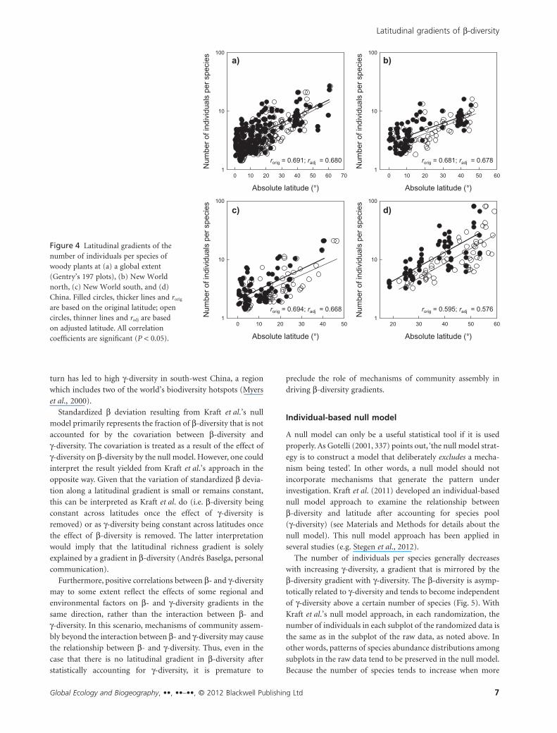
increases with increasing latitude, and latitude explained 33.2–

46.2% of the variation in the number of individuals per species

(Fig. 4). When the variation in observed b-diversity that is

explained by the number of individuals per species was removed

by a second-order polynomial regression, latitude explained

only 0.2–18.6% of the residual of observed b-diversity. This

suggests that the majority of the latitude–b-diversity gradient is

associated with the relationship between b-diversity and species

abundance distributions. Because gradients of species abun-

dance distributions are related to latitude, removing the

b-diversity generated by species abundance distributions

implies that a large part of the relationship between b-diversity

and latitude is removed by the null model (see below for more

discussion). Because standardized b deviation and the number

of individuals per species are largely uncorrelated (e.g. r = 0.017

for the data set with Gentry’s 197 plots), the variation in

b-diversity that would have been explained by latitude would be

much greater than that represented by standardized b deviation

0 10 20 30 40 50

Obs

erve

d β-

dive

rsity

0.4

0.5

0.6

0.7

0.8

0.9

0 10 20 30 40 500.2

0.3

0.4

0.5

0.6

0.7

0.8

0.9

20 30 40 50 600.1

0.2

0.3

0.4

0.5

0.6

0.7

0.8

0.9

a) b) c)

rorig = -0.610, P < 0.05radj = -0.652, P < 0.05

rorig = -0.689, P < 0.05radj = -0.724, P < 0.05

rorig = -0.789, P < 0.05radj = -0.772, P < 0.05

Absolute latitude (°)

0 10 20 30 40 50

Exp

ecte

d β -

dive

rsity

0.4

0.5

0.6

0.7

0.8

0.9

Absolute latitude (°)

0 10 20 30 40 500.2

0.3

0.4

0.5

0.6

0.7

0.8

0.9

Absolute latitude (°)

20 30 40 50 600.1

0.2

0.3

0.4

0.5

0.6

0.7

0.8

0.9

rorig = -0.673, P < 0.05radj = -0.706, P < 0.05

rorig = -0.634, P < 0.05radj = -0.672, P < 0.05

rorig = -0.754, P < 0.05radj = -0.796, P < 0.05

d) e) f)

Figure 2 The relations of (a–c) observed and (d–f) expected b-diversity of woody plants with latitude in (a, d) New World north, (b, e)New World south, and (c, f) China. Filled circles, thicker lines and rorig are for the relationship between b-diversity and original latitude;open circles, thinner lines and radj for the relationship between b-diversity and adjusted latitude.

Latitudinal gradients of b-diversity

Global Ecology and Biogeography, ••, ••–••, © 2012 Blackwell Publishing Ltd 5

if the relationship between b-diversity and species abundance

distributions had not been removed by the null model. Thus, the

conclusion of our study is contrary to that of Kraft et al. (2011)

on the relationship between b-diversity and latitude after

accounting for species pool.

Relationship between b-diversity and g-diversity

Values of b-diversity and g-diversity are positively correlated (r =0.776 for Gentry’s global dataset, r = 0.746 for China’s dataset,

P < 0.05 in both cases). With Kraft et al.’s null model approach,

such correlations are considered as the effect of g-diversity on

b-diversity. Although it has been hypothesized that the size of a

regional species pool (g-diversity) may be a driving force of

b-diversity (Harrison et al., 2011), this hypothesis has not been

adequately tested and mechanisms of species pools driving

b-diversity are unknown.

Conversely, correlations between b-diversity and g-diversity

may, at least in part, reflect the effect of b-diversity on

g-diversity (Pither & Aarssen, 2005; Meynard et al., 2011; Qian

& Ricklefs, 2012). Indeed, when Robert H. Whittaker initially

proposed the relationships among a-, b- and g-diversity, he

illustrated the role of b-diversity in building larger-scale (g)

diversity patterns (Whittaker, 1960). A larger species pool size

may result from higher b-diversity due to, for example, habitat

heterogeneity (Pither & Aarssen, 2005). For example, if two

contiguous areas each have a large proportion of unique

species, and thus have high b-diversity between them, high

g-diversity of the two areas would be expected. Previous

studies (e.g. Qian et al., 2005) have shown that high g-diversity

of a region results, at least in part, from high b-diversity within

the region. Rodríguez & Arita (2004) also showed that the

higher diversity of non-volant mammals in tropical areas of

North America is a consequence of the increase in b-diversity

towards the tropical areas. Another such example is high

g-diversity in south-west China. The collision of the Indian

subcontinent with the Asian continent during the Eocene

(55–45 million years ago; Sengör & Natal’in, 1996) resulted in

enormous rugged mountains (usually > 6000 m high in the

eastern Himalayas and Hengduanshan regions) separated by

deep valleys. A significant number of species became vicariants

on different mountains during the orogenic processes, which

would favour allopatric speciation (Wu & Wu, 1996; Qian &

Ricklefs, 2000; Baselga et al., 2012). High mountains and deep

valleys in south-west China have become natural barriers pre-

venting species from spreading between mountains within the

region (Li et al., 1999). As a result, each mountain range has a

large number of endemic species, and many species in the

region are shared only by few mountains (H.Q., unpublished

data). This has led to high b-diversity in the region, which in

Absolute latitude (°)

0 10 20 30 40 50

Sta

ndar

dize

d β

devi

atio

n

0

5

10

15

20

Absolute latitude (°)

0 10 20 30 40 50

0

5

10

15

20

Absolute latitude (°)

20 30 40 50 60

0

5

10

15

20rorig = -0.392, P < 0.05radj = -0.330, P < 0.05

rorig = 0.232, P > 0.05radj = 0.340, P < 0.05

rorig = -0.500, P < 0.05radj = -0.335, P < 0.05

d) e) f)

0 10 20 30 40 50

Raw

β d

evia

tion

-0.05

0.00

0.05

0.10

0.15

0.20

0.25

0.30

0 10 20 30 40 50-0.05

0.00

0.05

0.10

0.15

0.20

0.25

0.30

20 30 40 50 60-0.05

0.00

0.05

0.10

0.15

0.20

0.25

0.30

a) b) c)rorig = 0.303, P < 0.05radj = 0.343, P < 0.05

rorig = 0.613, P < 0.05radj = 0.639, P < 0.05

rorig = 0.101, P > 0.05radj = 0.271, P < 0.05

Figure 3 The relations of b deviation of woody plants with latitude in (a, d) New World north, (b, e) New World south, and (c, f) China.Filled circles, thicker lines and rorig are for the relationship between b deviation and original latitude; open circles, thinner lines and radj forthe relationship between b deviation and adjusted latitude.

H. Qian et al.

Global Ecology and Biogeography, ••, ••–••, © 2012 Blackwell Publishing Ltd6

turn has led to high g-diversity in south-west China, a region

which includes two of the world’s biodiversity hotspots (Myers

et al., 2000).

Standardized b deviation resulting from Kraft et al.’s null

model primarily represents the fraction of b-diversity that is not

accounted for by the covariation between b-diversity and

g-diversity. The covariation is treated as a result of the effect of

g-diversity on b-diversity by the null model. However, one could

interpret the result yielded from Kraft et al.’s approach in the

opposite way. Given that the variation of standardized b devia-

tion along a latitudinal gradient is small or remains constant,

this can be interpreted as Kraft et al. do (i.e. b-diversity being

constant across latitudes once the effect of g-diversity is

removed) or as g-diversity being constant across latitudes once

the effect of b-diversity is removed. The latter interpretation

would imply that the latitudinal richness gradient is solely

explained by a gradient in b-diversity (Andrés Baselga, personal

communication).

Furthermore, positive correlations between b- and g-diversity

may to some extent reflect the effects of some regional and

environmental factors on b- and g-diversity gradients in the

same direction, rather than the interaction between b- and

g-diversity. In this scenario, mechanisms of community assem-

bly beyond the interaction between b- and g-diversity may cause

the relationship between b- and g-diversity. Thus, even in the

case that there is no latitudinal gradient in b-diversity after

statistically accounting for g-diversity, it is premature to

preclude the role of mechanisms of community assembly in

driving b-diversity gradients.

Individual-based null model

A null model can only be a useful statistical tool if it is used

properly. As Gotelli (2001, 337) points out, ‘the null model strat-

egy is to construct a model that deliberately excludes a mecha-

nism being tested’. In other words, a null model should not

incorporate mechanisms that generate the pattern under

investigation. Kraft et al. (2011) developed an individual-based

null model approach to examine the relationship between

b-diversity and latitude after accounting for species pool

(g-diversity) (see Materials and Methods for details about the

null model). This null model approach has been applied in

several studies (e.g. Stegen et al., 2012).

The number of individuals per species generally decreases

with increasing g-diversity, a gradient that is mirrored by the

b-diversity gradient with g-diversity. The b-diversity is asymp-

totically related to g-diversity and tends to become independent

of g-diversity above a certain number of species (Fig. 5). With

Kraft et al.’s null model approach, in each randomization, the

number of individuals in each subplot of the randomized data is

the same as in the subplot of the raw data, as noted above. In

other words, patterns of species abundance distributions among

subplots in the raw data tend to be preserved in the null model.

Because the number of species tends to increase when more

Absolute latitude (°)

0 10 20 30 40 50 60 70

Num

ber

of in

divi

dual

s pe

r sp

ecie

s

1

10

100

Absolute latitude (°)

0 10 20 30 40 50 60

Num

ber

of in

divi

dual

s pe

r sp

ecie

s

1

10

100

Absolute latitude (°)

0 10 20 30 40 50

Num

ber

of in

divi

dual

s pe

r sp

ecie

s

1

10

100

Absolute latitude (°)

20 30 40 50 60

Num

ber

of in

divi

dual

s pe

r sp

ecie

s

1

10

100

a) b)

c) d)

rorig = 0.691; radj = 0.680 rorig = 0.681; radj = 0.678

rorig = 0.694; radj = 0.668 rorig = 0.595; radj = 0.576

Figure 4 Latitudinal gradients of thenumber of individuals per species ofwoody plants at (a) a global extent(Gentry’s 197 plots), (b) New Worldnorth, (c) New World south, and (d)China. Filled circles, thicker lines and rorig

are based on the original latitude; opencircles, thinner lines and radj are basedon adjusted latitude. All correlationcoefficients are significant (P < 0.05).

Latitudinal gradients of b-diversity

Global Ecology and Biogeography, ••, ••–••, © 2012 Blackwell Publishing Ltd 7

individuals are included in a sampling unit (Gotelli & Graves,

1996), as predicted by probability theory (Sokal & Rohlf, 1981)

and observed in many empirical data sets, including our data at

the subplot scale (r = 0.740 for Gentry’s global data set, n = 1970;

r = 0.632 for China’s data set, n = 600; P < 0.05 in both cases) and

at the plot scale (Fig. 5), as a result the expected number of

species in each subplot is strongly forced to approach the

observed number of species in the subplot. As shown clearly in

Fig. 6, the expected and observed a-diversities not only are

strongly and positively correlated (r = 0.962, P < 0.05, n = 1970)

but also tend to approach to the 1 : 1 line where the expected

and observed a-diversities are identical. Because the total

number of species in each plot is set to be equal to that in the raw

data in each randomization, because expected b-diversity is

solely determined by the ratio of the average of expected

a-diversity (i.e. the average of expected numbers of species) in

the subplots of a plot and the total number of species in that

plot, and because the null model is formulated such that

expected a-diversity of each plot approaches the observed

a-diversity of the plot, preserving species abundance distribu-

tions in the null model would naturally lead to maintaining the

mechanisms that generate b-diversity gradients in the null

model. Consequently, values of expected b-diversity would be

strongly correlated with values of observed b-diversity (e.g. r =0.966 for Gentry’s global data set, r = 0.942 for China’s data set,

P < 0.05 in both cases); expected b-diversity resulting from the

null model has actually included b-diversity that results from

mechanisms of community assembly. Clearly, Kraft et al.’s

null model has incorporated the mechanisms that generate

b-diversity patterns and hence is conceptually and methodo-

logically incorrect because the model violates the fundamental

assumption of a null model, i.e. a null model should not incor-

porate mechanisms that generate the pattern under investiga-

tion (Gotelli, 2001).

γ-diversity

0 50 100 150 200 250 300

Num

ber

of in

divi

dual

s pe

r sp

ecie

s

1

10

100

γ-diversity

0 50 100 150 200 250 300

Num

ber

of in

divi

dual

s pe

r sp

ecie

s

1

10

100

γ-diversity

0 50 100 150 200 250 300

Num

ber

of in

divi

dual

s pe

r sp

ecie

s

1

10

100

γ-diversity

0 20 40 60 80

Num

ber

of in

divi

dual

s pe

r sp

ecie

s

1

10

100

β-diversityIndivid. no. per sp.

Obs

erve

d β -

dive

rsity

Obs

erve

d β -

dive

rsity

0.2

0.3

0.4

0.5

0.6

0.7

0.8

0.9

0.2

0.3

0.4

0.5

0.6

0.7

0.8

0.9

0.2

0.3

0.4

0.5

0.6

0.7

0.8

0.9

0.2

0.3

0.4

0.5

0.6

0.7

0.8

0.9

Obs

erve

d β-

dive

rsity

Obs

erve

d β-

dive

rsity

a) b)

c) d)

Figure 5 The relations of g-diversity(species pool) with observed b-diversity(filled circles) and the number ofindividuals of each species (log scale) ofwoody plants at (a) a global extent(Gentry’s global data set), (b) New Worldnorth, (c) New World south, and (d)China.

Observed α-diversity

0 25 50 75

Exp

ecte

d α-

dive

rsity

0

25

50

75

r = 0.962, P < 0.05

Figure 6 Relationship between observed and expecteda-diversity (number of species in each 0.01-ha subplot) in the1970 subplots of the 197 plots of Gentry’s global data set.Expected a-diversity was generated based on Kraft et al.’s (2011)null model with 1000 randomizations.

H. Qian et al.

Global Ecology and Biogeography, ••, ••–••, © 2012 Blackwell Publishing Ltd8

The number of individuals of each of multiple species in a site

or community produces a species abundance distribution

(Williamson & Gaston, 2005). Species abundance distributions

largely result from deterministic, rather than stochastic, proc-

esses, and have played an important role in the development of

community ecology for over a century (Raunkiaer, 1909; Alonso

et al., 2008) and have been at the heart of the development of

ecological theories, e.g. neutral theory in ecology (Hubbell,

2001) and the more-individuals hypothesis (Hurlbert, 2004;

Evans et al., 2005). It is well known that patterns of species

abundance distributions in biological communities result, at

least in part, from mechanisms of community assembly

(Andrewartha & Birch, 1954; Whittaker, 1965; James &

Rathbun, 1981; Ugland & Gray, 1982; Kolasa & Strayer, 1988;

Tokeshi, 1999; McGill et al., 2007). Species abundance distribu-

tions drive the species–area relationship (Plotkin et al., 2000; He

& Legendre, 2002), and the slope (z-value) of the species–area

relationship has been used as a measure of b-diversity (Cody,

1975; Rosenzweig, 1995; Ricotta et al., 2002). Thus, mechanisms

driving species abundance distributions are closely related to, if

not the same as, the mechanisms driving b-diversity in a local

community. A null model that depends on species abundance

distributions naturally incorporates mechanisms driving

b-diversity.

As discussed above, a large part of the relationship between

b-diversity and latitude is removed from the standardized bdeviation–latitude gradient by the null model. Thus, b-diversity

represented by standardized b deviation may be considered as

the fraction of the b-diversity driven by mechanisms of com-

munity assembly or other processes that is beyond the fraction

of the b-diversity driven by species abundance distributions.

Mechanisms driving b-diversity beyond those driving species

abundance distributions may include, but are not limited to,

niche-based processes (Tokeshi, 1990), habitat filtering (Sven-

ning, 1999) and the priority effect (Young et al., 2001). For forest

communities at a local scale such as 0.1 ha, heterogeneity of

microhabitats, dynamics of forest (light) gaps and biotic inter-

actions within a study site may also be among major factors

influencing b-diversity in local communities. For example, the

behaviour of vertebrate fruit eaters often results in contagious

seed dispersal, in which seeds are deposited in single-species or

multispecies aggregations at sleeping trees or repeatedly used

sites (Schupp et al., 2002). In the case of tree b-diversity at a local

scale, the factors that determine distributions of seeds and seed-

lings around the parent trees (i.e. conspecific tree aggregation)

may also be important in generating patterns of b-diversity.

Clumping of seedlings around parent trees at a scale of metres to

hectares may be expected for species with either limited disper-

sal or specific regeneration requirements (Lambers et al., 2002).

Alternatively, density- and distance-dependent seed and seed-

ling mortality caused by species-specific predators may reduce

conspecific recruitment near the parent trees, as predicted by the

Janzen–Connell hypothesis (Janzen, 1970; Connell, 1971). These

factors may or may not drive b-diversity in the same direction as

that of species abundance distributions. Thus, whether there is a

latitudinal gradient in standardized b deviation resulting from

Kraft et al.’s null model would primarily depend on how well

species abundance distributions can account for the variation in

b-diversity, rather than whether there is a latitudinal gradient of

b-diversity after accounting for species pool.

Another problem with Kraft et al.’s null model is associated

with the method of standardizing raw b deviation in the null

model. The goal of the null model is to determine how much

b-diversity is left after removing the b-diversity that can be

generated by an individual-based randomization approach with

species pool accounted for (i.e. the expected b-diversity) from

observed b-diversity. However, as noted in Materials and

Methods, Kraft et al.’s null model divided raw b deviation (i.e.

the difference between observed and expected b-diversity) by

the standard deviation of the distribution of values of expected

b-diversity (Kraft et al., 2011). Because observed and expected

b-diversity are both in the same unit and both range between 0

and 1, and because the standard deviation of the distribution of

expected b-diversity is strongly correlated with both g-diversity

and latitude (e.g. r = -0.823 for g-diversity and 0.812 for latitude

in the data set with Gentry’s 197 plots; Fig. S3), standardizing

raw b deviation in such a way would introduce a bias in stand-

ardized b deviation (Andrés Baselga, personal communication).

For example, for the data set with Gentry’s 197 plots, latitude

explained 11.6 and 18.6% of the variation in raw b deviation,

respectively, in linear and quadratic regressions (Fig. 1b);

however, when raw b deviation was divided by the standard

deviation of the null distribution of b-diversity value, latitude

explained only 3.1 and 11.0% of the variation in the resulting

values (i.e. standardized b deviation), respectively, in linear and

quadratic regressions (Fig. 1c). Clearly, the standardizing

approach implemented in the null model changes the relation-

ship between b deviation and latitude not only in strength but

also in direction (i.e. changing a positive relationship to a nega-

tive relationship) in most cases (compare Fig. 1b with Fig. 1c

and Fig. 3a–c with Fig. 3d–f).

CONCLUSIONS

We conducted four sets of analyses to examine the relationship

between b-diversity and latitude using Kraft et al.’s (2011) null

model, and we showed that standardized b deviation is signifi-

cantly correlated with latitude in all four sets of analyses. We

demonstrated that Kraft et al.’s null model is not a valid null

model for the study of b-diversity gradient driven by mecha-

nisms of community assembly because the null model incorpo-

rates the mechanisms of community assembly that generate

b-diversity gradients and thus violates a fundamental assump-

tion of the null model. Specifically, expected b-diversity with

Kraft et al.’s null model should not include any part of

b-diversity that is driven by mechanisms of community assem-

bly, but expected b-diversity resulting from the null model in

fact includes the b-diversity that results from species abundance

distributions. Because the majority of the latitude–b-diversity

gradient can be explained by the latitude–species abundance

distribution (represented by the number of individuals per

species) gradient, and because species abundance distributions

Latitudinal gradients of b-diversity

Global Ecology and Biogeography, ••, ••–••, © 2012 Blackwell Publishing Ltd 9

result from mechanisms of community assembly (Andrewartha

& Birch, 1954; Whittaker, 1965; James & Rathbun, 1981; Ugland

& Gray, 1982; Kolasa & Strayer, 1988; Tokeshi, 1999; McGill

et al., 2007), we conclude that the latitude–b-diversity gradient

at a local scale is largely driven by mechanisms of community

assembly. Our conclusion is in contrast to that of Kraft et al.

(2011).

ACKNOWLEDGEMENTS

We are grateful to Andrés Baselga and anonymous referees for

helpful comments, Nathan Kraft for the data set of Gentry’s 197

plots that was used in Kraft et al. (2011) and b deviation values,

Alwyn H. Gentry and his co-workers for their plot data, and the

financial support of the National Basic Research Program

(2009CB421105) to Z.O.

REFERENCES

Ahrens, C.D. (2007) Meteorology today: an introduction to

weather, climate, and the environment, 8th edn. Brooks Cole,

Belmont, CA.

Allen, A.P., Gillooly, J.F. & Brown, J.H. (2002) Global biodiver-

sity, biochemical kinetics, and the energetic-equivalence rule.

Science, 297, 1545–1548.

Alonso, D., Ostling, A. & Etienne, R.S. (2008) The implicit

assumption of symmetry and the species abundance distribu-

tion. Ecology Letters, 11, 93–105.

Andrewartha, H.G. & Birch, L.C. (1954) The distribution and

abundance of animals. University of Chicago Press, Chicago,

IL.

Baselga, A., Gómez-Rodríguez, C. & Lobo, J.M. (2012) Histori-

cal legacies in world amphibian diversity revealed by the

turnover and nestedness components of beta diversity. PLoS

ONE, 7, e32341.

Buckley, L.B. & Jetz, W. (2008) Linking global turnover of

species and environments. Proceedings of the National

Academy of Sciences USA, 105, 17836–17841.

Chen, S., Ouyang, Z., Zheng, H., Xiao, Y. & Xu, W. (2011) Lati-

tudinal gradient in beta diversity of forest communities in

America. Acta Ecologica Sinica, 31, 1334–1340.

Cody, M.L. (1975) Toward a theory of continental species diver-

sities: bird distributions over Mediterranean habitat gradi-

ents. Ecology and evolution of communities (ed. by M.L. Cody

and J.M. Diamond), pp. 214–257. Harvard University Press,

Cambridge, MA.

Connell, J.H. (1971) On the role of natural enemies in prevent-

ing competitive exclusion in some marine animals and in rain

forest trees. Dynamics of populations (ed. by P.J. Den Bour and

P.R. Gradwell), pp. 298–312. Center for Agricultural Publish-

ing and Documentation, Wageningen.

Darwin, C. (1859) The origin of species. Reprinted by Penguin

Books, London.

Evans, K.L., Warren, P.H. & Gaston, K.J. (2005) Species–energy

relationships at the macroecological scale: a review of the

mechanism. Biological Reviews, 80, 1–25.

Gaston, K.J. (2000) Global patterns in biodiversity. Nature, 405,

220–227.

Gotelli, N.J. (2001) Research frontiers in null model analysis.

Global Ecology and Biogeography, 10, 337–343.

Gotelli, N.J. & Graves, G.R. (1996) Null models in ecology. Smith-

sonian Institution, Washington, DC.

Harrison, S., Vellend, M. & Damschen, E.I. (2011) ‘Structured’

beta diversity increases with climatic productivity in a classic

dataset. Ecosphere, 2, art11.

He, F. & Legendre, P. (2002) Species-diversity patterns derived

from species-area models. Ecology, 83, 1185–1198.

Hubbell, S.P. (2001) The unified neutral theory of biodiversity and

biogeography. Princeton University Press, Princeton, NJ.

Hurlbert, A.H. (2004) Species–energy relationships and habitat

complexity in bird communities. Ecology Letters, 7, 714–720.

James, C. & Rathbun, S. (1981) Rarefaction, relative abundance,

and diversity of avian communities. Auk, 98, 785–800.

Jankowski, J.E., Ciecka, A.L., Meyer, N.Y. & Rabenold, K.N.

(2009) Beta diversity along environmental gradients: implica-

tions of habitat specialization in tropical montane landscapes.

Journal of Animal Ecology, 78, 315–327.

Janzen, D.H. (1970) Herbivores and the number of tree species

in tropical forests. The American Naturalist, 104, 501–528.

Jump, A.S., Mátyás, C. & Peñuelas, J. (2009) The altitude-for-

latitude disparity in the range retractions of woody species.

Trends in Ecology and Evolution, 24, 694–701.

Kolasa, J. & Strayer, D. (1988) Patterns of the abundance of

species: a comparison of two hierarchical models. Oikos, 53,

235–241.

Koleff, P., Lennon, J.J. & Gaston, K.J. (2003) Are there latitudinal

gradients in species turnover? Global Ecology and Biogeogra-

phy, 12, 483–498.

Kraft, N.J.B., Comita, L.S., Chase, J.M., Sanders, N.J., Swenson,

N.G., Crist, T.O., Stegen, J.C., Vellend, M., Boyle, B., Anderson,

M.J., Cornell, H.V., Davies, K.F., Freestone, A.L., Inouye, B.D.,

Harrison, S.P. & Myers, J.A. (2011) Disentangling the drivers

of b diversity along latitudinal and elevational gradients.

Science, 333, 1755–1758.

Lambers, J.H.R., Clark, J.S. & Beckage, B. (2002) Density-

dependent mortality and the latitudinal gradient in species

diversity. Nature, 417, 732–735.

Lenoir, J., Gégout, J.-C., Guisan, A., Vittoz, P., Wohlgemuth, T.,

Zimmermann, N.E., Dullinger, S., Pauli, H., Willner, W.,

Grytnes, J.-A., Virtanen, R. & Svenning, J.-C. (2010) Cross-

scale analysis of the region effect on vascular plant species

diversity in southern and northern European mountain

ranges. PLoS ONE, 5, e15734.

Li, H., He, D.-M., Bartholomew, B. & Long, C.-L. (1999)

Re-examination of the biological effect of plate movement:

impact of Shan-Malay Plate displacement (the movement of

Burma–Malaya Geoblock) on the biota of Gaoligong Moun-

tains. Acta Botanica Yunnanica, 21, 407–425.

McGill, B.J., Etienne, R.S., Gray, J.S., Alonso, D., Anderson, M.J.,

Benecha, H.K., Dornelas, M., Enquist, B.J., Green, J.L., He, F.,

Hurlbert, A.H., Magurran, A.E., Marquet, P.A., Maurer, B.A.,

Ostling, A., Soykan, C.U., Ugland, K.I. & White, E.P. (2007)

H. Qian et al.

Global Ecology and Biogeography, ••, ••–••, © 2012 Blackwell Publishing Ltd10

Species abundance distributions: moving beyond single pre-

diction theories to integration within an ecological frame-

work. Ecology Letters, 10, 995–1015.

Meynard, C.N., Devictor, V., Mouillot, D., Thuiller, W., Jiguet, F.

& Mouquet, N. (2011) Beyond taxonomic diversity patterns:

how do a, b and g components of bird functional and phylo-

genetic diversity respond to environmental gradients across

France? Global Ecology and Biogeography, 20, 893–903.

Mittelbach, G.G., Schemske, D.W., Cornell, H.V. et al. (2007)

Evolution and the latitudinal diversity gradient: speciation,

extinction and biogeography. Ecology Letters, 10, 315–331.

Myers, N., Mittermeier, R.A., Mittermeier, C.G., da Fonseca,

G.A.B. & Kent, J. (2000) Biodiversity hotspots for conserva-

tion priorities. Nature, 403, 853–858.

New, M., Hulme, M. & Jones, P. (1999) Representing twentieth-

century space-time climate variability. Part I: development of

a 1961–90 mean monthly terrestrial climatology. Journal of

Climate, 12, 829–856.

Phillips, O. & Miller, J.S. (2002) Global patterns of plant diversity:

Alwyn H. Gentry’s forest transect data set. Missouri Botanical

Garden Press, St Louis.

Pianka, E.R. (1966) Latitudinal gradients in species diversity:

a review of concepts. The American Naturalist, 100, 33–

46.

Pither, J. & Aarssen, L.W. (2005) The evolutionary species pool

hypothesis and patterns of freshwater diatom diversity along a

pH gradient. Journal of Biogeography, 32, 503–513.

Plotkin, J.B., Potts, M.D., Yu, D.W., Bunyavejchewin, S., Condit,

R., Foster, R., Hubbell, S., LaFrankie, J., Manokaran, N., Lee,

H.-S., Sukumar, R., Nowak, M.A. & Ashton, P.S. (2000) Pre-

dicting species diversity in tropical forests. Proceedings of the

National Academy of Sciences USA, 97, 10850–10854.

Qian, H. (2009) Beta diversity in relation to dispersal ability for

vascular plants in North America. Global Ecology and Bioge-

ography, 18, 327–332.

Qian, H. & Ricklefs, R.E. (2000) Large-scale processes and the

Asian bias in species diversity of temperate plants. Nature,

407, 180–182.

Qian, H. & Ricklefs, R.E. (2007) A latitudinal gradient in large-

scale beta diversity for vascular plants in North America.

Ecology Letters, 10, 737–744.

Qian, H. & Ricklefs, R.E. (2012) Disentangling the effects of

geographic distance and environmental dissimilarity on

global patterns of species turnover. Global Ecology and Bioge-

ography, 21, 341–351.

Qian, H. & Xiao, M. (2012) Global patterns of the beta

diversity–energy relationship in terrestrial vertebrates. Acta

Oecologica, 39, 67–71.

Qian, H., Ricklefs, R.E. & White, P.S. (2005) Beta diversity of

angiosperms in temperate floras of eastern Asia and eastern

North America. Ecology Letters, 8, 15–22.

Qian, H., Badgley, C. & Fox, D.L. (2009) The latitudinal gradient

of beta diversity in relation to climate and topography for

mammals in North America. Global Ecology and Biogeography,

18, 111–122.

Qian, H., Wang, X. & Zhang, Y. (2012) Comment on ‘disentan-

gling the drivers of b diversity along latitudinal and eleva-

tional gradients’. Science, 335, 1573.

Raunkiaer, C. (1909) Formationsuntersögelseog formationssta-

tistik. Botanisk Tidsskrift, 30, 20–132.

Ricklefs, R.E. (1987) Community diversity: relative roles of local

and regional processes. Science, 235, 167–171.

Ricotta, C., Carranza, M.L. & Avena, G. (2002) Computing

b-diversity from species–area curves. Basic and Applied

Ecology, 3, 15–18.

Rodríguez, P. & Arita, H.T. (2004) Beta diversity and latitude in

North American mammals: testing the hypothesis of covaria-

tion. Ecography, 27, 547–556.

Rohde, K. (1992) Latitudinal gradients in species diversity: the

search for the primary cause. Oikos, 65, 514–527.

Rosenzweig, M.L. (1995) Species diversity in space and time.

Cambridge University Press, Cambridge.

Schupp, E.W., Milleron, T. & Russo, S.E. (2002) Dissemination

limitation and the origin and maintenance of species-rich

tropical forests. Seed dispersal and frugivory: ecology, evolution,

and conservation (ed. by D.J. Levey, W.R. Silva and M. Galetti),

pp. 19–33. CAB International, Wallingford, UK.

Sengör, A.M.G. & Natal’in, B.A. (1996) Paleotectonics of Asia:

fragments of a synthesis. The tectonic evolution of Asia (ed. by A.

Yin and T.M. Harrison), pp. 486–640. Cambridge University

Press, Cambridge, UK.

Sokal, R.R. & Rohlf, F.J. (1981) Biometry, 2nd edn. W. H.

Freeman, New York.

Stegen, J.C., Freestone, A.L., Crist, T.O., Anderson, M.J., Chase,

J.M., Comita, L.S., Cornell, H.V., Davies, K.F., Harrison, S.P.,

Hurlbert, A.H., Inouye, B.D., Kraft, N.J.B., Myers, J.A.,

Sanders, N.J., Swenson, N.G. & Vellend, M. (2012) Stochastic

and deterministic drivers of spatial and temporal turnover in

breeding bird communities. Global Ecology and Biogeography,

doi:10.1111/j.1466-8238.2012.00780.x.

Stephenson, N.L. & Das, A.J. (2011) Comment on ‘changes in

climatic water balance drive downhill shifts in plant species’

optimum elevations’. Science, 334, 177.

Stevens, G.C. (1989) The latitudinal gradient in geographical

range: how so many species coexist in the tropics. The Ameri-

can Naturalist, 133, 240–256.

Svenning, J.-C. (1999) Microhabitat specialization in a species-

rich palm community in Amazonian Ecuador. Journal of

Ecology, 87, 55–65.

Tokeshi, M. (1990) Niche apportionment or random assortment

– species abundance patterns revisited. Journal of Animal

Ecology, 59, 1129–1146.

Tokeshi, M. (1999) Species coexistence: ecological and evolution-

ary perspectives. Blackwell Scientific, Oxford.

Ugland, K.I. & Gray, J.S. (1982) Lognormal distributions and

the concept of community equilibrium. Oikos, 39, 171–178.

Wallace, A.R. (1878) Tropical nature and other essays. Macmillan,

New York.

Whittaker, R.H. (1960) Vegetation of the Siskiyou Mountains,

Oregon and California. Ecological Monographs, 30, 279–338.

Latitudinal gradients of b-diversity

Global Ecology and Biogeography, ••, ••–••, © 2012 Blackwell Publishing Ltd 11

Whittaker, R.H. (1965) Dominance and diversity in land plant

communities. Science, 147, 250–260.

Whittaker, R.H. (1972) Evolution and measurement of species

diversity. Taxon, 21, 213–251.

Williamson, M. & Gaston, K.J. (2005) The lognormal distribu-

tion is not an appropriate null hypothesis for the species-

abundance distribution. Journal of Animal Ecology, 74, 409–

422.

Wu, C.-Y. & Wu, S.-G. (1996) A proposal for a new floristic

kingdom (realm). Floristic characteristics and diversity of east

Asian plants (ed. by A.-L. Zhang and S.-G. Wu), pp. 3–42.

China Higher Education Press, Beijing.

Young, T.P., Chase, J. & Huddleston, R. (2001) Community suc-

cession and assembly: comparing, contrasting and combining

paradigms in the context of ecological restoration. Ecological

Restoration, 19, 5–18.

SUPPORTING INFORMATION

Additional Supporting Information may be found in the online

version of this article:

Figure S1 Distribution of Gentry’s 197 plots used in Kraft et al.

(2011).

Figure S2 Distribution of 15 nature reserves in China, where the

60 forest plots used in the present study were sampled.

Figure S3 Relationships of the standard deviation of the distri-

bution of expected b-diversity with g-diversity and latitude for

Gentry’s 197 plots used in the present study.

BIOSKETCH

Hong Qian’s research is multidisciplinary and

particularly lies at the interface of ecology and

biogeography. His research involves a wide range of

spatial scales (from local to global) and a variety of

taxa (e.g. bryophytes, vascular plants, vertebrates and

invertebrates). In particular, he is interested in

understanding the relative roles of historical and

present-day factors in determining the patterns in

biodiversity.

Editor: Andres Baselga

H. Qian et al.

Global Ecology and Biogeography, ••, ••–••, © 2012 Blackwell Publishing Ltd12