download PhD-manuscript - Universiteit Gent
452
-
Upload
khangminh22 -
Category
Documents
-
view
0 -
download
0
Transcript of download PhD-manuscript - Universiteit Gent


Universiteit GentFaculteit Toegepaste Wetenschappen
Vakgroep Civiele TechniekLaboratorium voor Hydraulica
Integratie van medische beeldvorming en numeriekestromingsmechanica voor het meten van de bloedstroom in dehalsslagaders
Integrating medical imaging and computational fluid dynamicsfor measuring blood flow in carotid arteries
ir. Fadi Paul Glor
Supervisors: Prof. Dr. Ir. Pascal R. VerdonckDr. Ir. Xiao Yun Xu
Manuscript ingediend voor het behalen vande graad van doctor in de toegepaste wetenschappen
Academiejaar 2003-2004

Dissertation submitted in partial fulfillment of the requirements for the degree of“Doctor in de Toegepaste Wetenschappen”.
The research reported in this dissertation was performed with the financial supportof the Ghent University (BOF grant nrs. 01112500 and 01102403) and Pfizer UK.
ISBN 9-09018-224-1
© Parts of this book may only be reproduced if accompanied by clear reference tothe source
Suggested citation: Glor Fadi Paul. Integrating medical imaging and computationalfluid dynamics for measuring blood flow in carotid arteries. PhD thesis. Gent: GhentUniversity; 2004.

Preface:
A man is at his tallest when he stoops to help a child
The plan wasn’t really to start a PhD. I had a number of things to do that day:work on the MSc thesis, attend some classes and maybe make the best ofthe good weather at the local beer garden. Starting a PhD was not on thelist and wouldn’t fit in. But I had an appointment. Of all days, why did I haveto put the appointment with Prof. P. Verdonck today? Prof. Verdonck wasresponsible of the education called ‘Advanced Studies in Biomedical andClinical Engineering’. Could be interesting. So I went. The poor Professorhad to work with a student who’s vision of the rest of his life was bundledin the sentence: “I would like to do something with engineering and withmedicine and stuff.” This encounter initiated this PhD.
I started on the first of October 2000. My first task was to organise a kartingevent and - together with Kris - provide everybody with strong Belgian beersas a thank you for accepting us in the lab. I fitted in perfectly. Kris D, PeterD, Stefaan DM, Stijn VDB, Patrick S, Dirk DW, Sunny E, Koen M, Robert B,Ronny V, Erik D, Bart M, Martin VD, Stefaan B, Manuella DK, Kristien T, IvoM and Marcel A created a nice work atmosphere. Meanwhile, I was enlight-ened on how to couple medical imaging and computational fluid dynamics.In that context, all credit goes to Prof. J. Vierendeels (FTW, UGent), Mr.P. de Kermel (ESI-group, Rungis, F) and Dr. P. Groenenboom (ESIbv,Krimpen aan den IJssel, NL) for teaching me how to use a workstation toobtain colourful drawings (CFD), and to Dr. Ir. J. Westenberg (Leids Univer-sitair Medisch Centrum, Leiden, NL), who was desperately trying to explainhow magnetic resonance imaging (MRI) works. The latter showered me withdata and advice, and he was definitely one of the persons who carried thisPhD through the early stages.
Due to personifiable circumstances, all funding ended after a year. Whenyou work long enough in certain environments, you can tell why communismfailed. This period was without doubt the toughest of the past four years. Atthat moment, it took a lot of courage to keep on supporting a PhD student likeme. But only dead fish swim with the current. The support from supervisorand colleagues was invaluable here. A small e-mail to Dr. Quan Longwas responded by an invitation to Imperial College London to come andtalk to Dr. X. Yun Xu . She gave me a chance to continue my PhD in thevery best of circumstances. I sincerely think this was better than winningthe lottery. Thanks goes to Erasmus-Belgium who really helped me settlingdown in London. The irony is that now, looking back, I have to thank the

personifiable circumstances. Without them I would never have made it toLondon.
I started on the 9th of October 2001. One month later, I received a tie andcough-links as birthday gifts. I fitted in perfectly. It is not normal for an Arabwith a burgundian Belgian life-style to fit in in England. Bulk of the creditgoes to Fadi and Rimoun Kasborsom , for opening their house, and to Dr.Alexander Augst , for nailing every single nailable problem I encountered.Thanks to the variety of people at Imperial, the work atmosphere was verycolourful. I thank the 414-crew: Pooi-Ling C, Guy G, Guido G, Shunzi Z,Ka-Wai L, Prashant V, Sayful, Lina H and James L, but also Dean B, AndyZ, Sheila B, Mark J, Simone P and Bassam K for the wonderful times in Lon-don. I still have the 414 good-bye gift in front of me every day. Professionally,I was backed by the insights of Prof. A. Hughes , the management of Dr.S. Thom , the witty jokes of Prof. K. Parker and the thorough supervision ofDr. Xu. Nothing could go wrong. Still, for a PhD, you need data. No data,no PhD. My MRI data came from Dr. L. Crowe at the Royal Brompton andthe ultrasound data was the result of the extreme hard work of Dr. Ben Ariffat St Mary’s hospital. Thanks Ben, hope you are better at the play-stationmeanwhile.
Thanks to some kindly acknowledged interventions, I was able to come backto Gent on the second of January 2003. The lab in Gent had lost some peo-ple and won some people. Ilse VT, Tom C, Edawi W, Stein-Inge R, SebastianV, Liesbet DD, Lieve L, Guy M and Masanori N were the new colleagues whohad to put up with me. I cooked bacon and eggs for everyone and was askedto organise a karting event. This time, I didn’t win because I was tricked bythe Verhoeven maffia. On this return, I was welcomed as if I never reallyleft, and the work atmosphere was, if possible, even better than at the startof the PhD. Moreover, I sincerely thank Pascal V, Stijn VDB, Kris D, Ilse VTand Patrick S for their substantial help when I was stuck, or for making mehalt when I was going too fast. I do not want to forget two students, MartinH and Melissa B, who substantially contributed to the work presented in thisbook.
You can learn a lot on international meetings. You open up to the cultureof a different city (Gent, Gent again, Calgary, Boston, Miami, Poitiers orMontpellier) and get to check out when the bars close (never, never, 3am,1am, etc.). More importantly, I found it amazing to see how much you learnfrom simple discussions with colleagues. It is fair to say that my perceptionof the research field underwent severe changes after meeting Ana I andProf. D. Steinman and his co-workers, of which I would like to mention Luca
ii

A and Jonathan T. I also want to sincerely thank the funding instances forsending me to the better conferences: BOF, Pfizer UK, MIT and the Societede biomecanique. Special thanks to Bill V and Jason Z from Pfizer UK forhaving a good nose for restaurants.
I hate reading. Just one of the things I need to work on before I die. Itherefore appreciate deeply the reading and comments on the text grantedby colleagues and friends: Tom C, Lieve L, Guy M, Kris D, Patrick S, TineDe Backer, Albert G, Johan DS and especially Sebastian V.
The environment of a researcher is critical for his achievements. In this con-text, I want to thankfully mention the sportsmen who didn’t complain abouthaving me on their side in the variety of football teams I was fortunate toplay for: Campus, the Hyde Park Wednesday afternoon bunch, Mephis-tow.be, FC De Gaverbeek, FC The Sharks ole ole and the Belgian nationalteam. Thank you for letting me score when my girlfriend was watching. Butman shall not live by football alone. The AIG, CathSoc, ArtSoc, the ‘burgie-bende’, the biomedders, Rotaract Gent-Zuid, and last but not least the VTKall managed to provide me with true leisure or beer or both. Above all, creditto my parents, Paul & Nazli, and my girlfriend Marianne for offering me anideal surrounding.
Thank the Lord for making all pieces fit.
When you see me walking through it,you may think there’s nothing to it,
but I simply can not do italone!
– Valma Kelly (Chicago, the musical)
iii

Supervisors:
Prof. Dr. Ir. Pascal R. VerdonckDr. Ir. Xiao Yun Xu
Laboratorium voor hydraulica Department of Chemical EngineeringVakgroep Civiele techniek (TW15) & Chemical TechnologyFaculteit Toegepaste Wetenschappen (FTW) South Kensington CampusUniversiteit Gent Imperial College LondonSint-Pietersnieuwstraat 41 Exhibition Road9000 Gent London SW7 2AZBELGIE UNITED KINGDOM
Members of the exam committeeProf. Dr. Ir. Ronny Verhoeven
(Chairman , FTW, Universiteit Gent, BELGIE)Prof. Dr. Ir. Patrick Segers
(Secretary , FTW, Universiteit Gent, BELGIE)Prof. Dr. Ir. Pascal Verdonck
(FTW, Universiteit Gent, BELGIE)Dr. Ir. Xiao Yun Xu
(Department of Chemical Engineering& Chemical Technology, Imperial College London, UK)
Prof. Dr. Alun Hughes(Clinical Pharmacology and Therapeutics, Imperial College London, UK)
Prof. Dr. Ir. Ignace Lemahieu(FTW, Universiteit Gent, BELGIE)
Prof. Dr. Ir. David Steinman(Robarts Research Institute, University of Western Ontario, CANADA)
Dr Simon A McG Thom(National Heart and Lung Institute, Imperial College London, UK)
Prof. Dr . Luc Van Bortel(Farmacologie, Universiteit Gent, BELGIE)
Prof. Dr. Ir. Jan Vierendeels(FTW, Universiteit Gent, BELGIE)
iv

Members of the reading committeeProf. Dr. Ir. Pascal Verdonck
(FTW, Universiteit Gent, BELGIE)Dr. Ir. Xiao Yun Xu
(Department of Chemical Engineering& Chemical Technology, Imperial College London, UK)
Prof. Dr. Ir. Patrick Segers(FTW, Universiteit Gent, BELGIE)
Prof. Dr. Ir. David Steinman(Robarts Research Institute, University of Western Ontario, CANADA)
Prof. Dr. Ir. Jan Vierendeels(FTW, Universiteit Gent, BELGIE)
v

vi
CONTENTS
Contents
NEDERLANDSE SAMENVATTING
I Inleiding NL - 7I.1 Anatomie . . . . . . . . . . . . . . . . . . . . . . . . . . . . . . . . . . . . . . NL - 7I.2 Doel van het proefschrift . . . . . . . . . . . . . . . . . . . . . . . . . . . . . NL - 9I.3 De belangrijke parameters . . . . . . . . . . . . . . . . . . . . . . . . . . . . NL - 12I.4 De techniek en zijn toepassingen . . . . . . . . . . . . . . . . . . . . . . . . . NL - 15
II Numerieke stromingsmechanica op basis van medische beelden NL - 17II.1 Overzicht . . . . . . . . . . . . . . . . . . . . . . . . . . . . . . . . . . . . . . NL - 17II.2 Magnetische Resonantie . . . . . . . . . . . . . . . . . . . . . . . . . . . . . NL - 20
II.2.1 Inleiding . . . . . . . . . . . . . . . . . . . . . . . . . . . . . . . . . NL - 20II.2.2 Segmenteren en Reconstrueren . . . . . . . . . . . . . . . . . . . . NL - 22II.2.3 De nauwkeurigheid van MRI gecombineerd met CFD . . . . . . . NL - 23II.2.4 De vergelijking van TOF en BB . . . . . . . . . . . . . . . . . . . . NL - 25
II.3 Ultrageluid . . . . . . . . . . . . . . . . . . . . . . . . . . . . . . . . . . . . . NL - 28II.3.1 Inleiding . . . . . . . . . . . . . . . . . . . . . . . . . . . . . . . . . NL - 28II.3.2 Meetprotocol . . . . . . . . . . . . . . . . . . . . . . . . . . . . . . . NL - 29II.3.3 Segmenteren en reconstrueren . . . . . . . . . . . . . . . . . . . . . NL - 30II.3.4 De nauwkeurigheid van US gecombineerd met CFD . . . . . . . . NL - 30
II.4 De parameters van het model . . . . . . . . . . . . . . . . . . . . . . . . . . NL - 37II.4.1 Randvoorwaarden . . . . . . . . . . . . . . . . . . . . . . . . . . . NL - 37II.4.2 Viscositeit . . . . . . . . . . . . . . . . . . . . . . . . . . . . . . . . NL - 41
II.5 Ultrageluid of Magnetische Resonantie? . . . . . . . . . . . . . . . . . . . . NL - 43
III In vivo Toepassingen NL - 47III.1 Inleiding . . . . . . . . . . . . . . . . . . . . . . . . . . . . . . . . . . . . . . NL - 47III.2 Het draaien van het hoofd . . . . . . . . . . . . . . . . . . . . . . . . . . . . NL - 49
III.2.1 Inleiding en proefopstelling . . . . . . . . . . . . . . . . . . . . . . NL - 49III.2.2 Resultaten . . . . . . . . . . . . . . . . . . . . . . . . . . . . . . . . NL - 49III.2.3 Impact van de studie . . . . . . . . . . . . . . . . . . . . . . . . . . NL - 50
III.3 Impact van bloeddrukverlagende geneesmiddelen . . . . . . . . . . . . . . NL - 51III.3.1 Inleiding . . . . . . . . . . . . . . . . . . . . . . . . . . . . . . . . . NL - 51III.3.2 Proefopstelling en Resultaten . . . . . . . . . . . . . . . . . . . . . NL - 52III.3.3 Besluit . . . . . . . . . . . . . . . . . . . . . . . . . . . . . . . . . . NL - 52
IV Samenvatting en Besluit NL - 55
vii

CONTENTS
ENGLISH TEXT
A INTRODUCTION 5
I Anatomy and Physiology 7I.1 Location of the Carotid Bifurcation in the Blood Supply chain . . . . . . . . 7I.2 Pressure and Flow . . . . . . . . . . . . . . . . . . . . . . . . . . . . . . . . . 11I.3 Arterial Wall Structure . . . . . . . . . . . . . . . . . . . . . . . . . . . . . . 19I.4 Pressure Regulation: baroreceptors . . . . . . . . . . . . . . . . . . . . . . . 21I.5 Oxygen Regulation: chemoreceptors . . . . . . . . . . . . . . . . . . . . . . 22
II Pathology and Diagnosis 23II.1 Carotid Pathology . . . . . . . . . . . . . . . . . . . . . . . . . . . . . . . . . 23
II.1.1 Carotid Dissection . . . . . . . . . . . . . . . . . . . . . . . . . . . . 23II.1.2 Atherosclerosis . . . . . . . . . . . . . . . . . . . . . . . . . . . . . 25II.1.3 Aneurysms . . . . . . . . . . . . . . . . . . . . . . . . . . . . . . . . 31
II.2 Pressure, Geometry and Flow features . . . . . . . . . . . . . . . . . . . . . 33II.2.1 Pressure . . . . . . . . . . . . . . . . . . . . . . . . . . . . . . . . . 33II.2.2 Arterial Geometry . . . . . . . . . . . . . . . . . . . . . . . . . . . . 35II.2.3 Flow . . . . . . . . . . . . . . . . . . . . . . . . . . . . . . . . . . . 40
II.3 Measurement of Designated Markers . . . . . . . . . . . . . . . . . . . . . . 46II.3.1 Pressure . . . . . . . . . . . . . . . . . . . . . . . . . . . . . . . . . 47II.3.2 Arterial Geometry . . . . . . . . . . . . . . . . . . . . . . . . . . . . 49II.3.3 Flow . . . . . . . . . . . . . . . . . . . . . . . . . . . . . . . . . . . 61
III Computational Fluid Dynamics 73III.1 Governing Equations . . . . . . . . . . . . . . . . . . . . . . . . . . . . . . . 73III.2 Meshing . . . . . . . . . . . . . . . . . . . . . . . . . . . . . . . . . . . . . . 75
III.2.1 The advancing front technique . . . . . . . . . . . . . . . . . . . . . 76III.2.2 The in-house carotid mesh builder . . . . . . . . . . . . . . . . . . 76
III.3 Boundary Conditions . . . . . . . . . . . . . . . . . . . . . . . . . . . . . . . 79III.4 Solvers . . . . . . . . . . . . . . . . . . . . . . . . . . . . . . . . . . . . . . . 80
III.4.1 Spatial Discretisation . . . . . . . . . . . . . . . . . . . . . . . . . . 81III.4.2 Temporal Discretisation and Solution . . . . . . . . . . . . . . . . . 83III.4.3 Validation . . . . . . . . . . . . . . . . . . . . . . . . . . . . . . . . 85
III.5 Potential Pitfalls . . . . . . . . . . . . . . . . . . . . . . . . . . . . . . . . . . 87
IV Carotid Haemodynamics and image-based CFD 89
B ESTABLISHING THE TECHNIQUE 93
V Overview 95
VI MRI-based carotid reconstructions 99VI.1 The I in MRI . . . . . . . . . . . . . . . . . . . . . . . . . . . . . . . . . . . . 99
VI.1.1 Brief History . . . . . . . . . . . . . . . . . . . . . . . . . . . . . . . 99VI.1.2 Principles of MRI . . . . . . . . . . . . . . . . . . . . . . . . . . . . 100VI.1.3 Time-Of-Flight . . . . . . . . . . . . . . . . . . . . . . . . . . . . . . 103VI.1.4 Black Blood . . . . . . . . . . . . . . . . . . . . . . . . . . . . . . . 104
viii

CONTENTS
VI.1.5 Cine PC MRI . . . . . . . . . . . . . . . . . . . . . . . . . . . . . . . 105VI.2 Segmentation . . . . . . . . . . . . . . . . . . . . . . . . . . . . . . . . . . . 108
VI.2.1 Region Growing Method . . . . . . . . . . . . . . . . . . . . . . . . 108VI.2.2 Snake Method . . . . . . . . . . . . . . . . . . . . . . . . . . . . . . 110VI.2.3 Manual Corrections . . . . . . . . . . . . . . . . . . . . . . . . . . . 110
VI.3 Reconstruction . . . . . . . . . . . . . . . . . . . . . . . . . . . . . . . . . . . 114VI.3.1 3D Smoothing . . . . . . . . . . . . . . . . . . . . . . . . . . . . . . 114VI.3.2 Spline Fitting . . . . . . . . . . . . . . . . . . . . . . . . . . . . . . . 116VI.3.3 Artery Splitting . . . . . . . . . . . . . . . . . . . . . . . . . . . . . 118
VI.4 Accuracy and Reproducibility . . . . . . . . . . . . . . . . . . . . . . . . . . 121VI.4.1 Accuracy in Phantoms . . . . . . . . . . . . . . . . . . . . . . . . . 121VI.4.2 In Vivo Reproducibility . . . . . . . . . . . . . . . . . . . . . . . . . 125VI.4.3 Conclusion on Accuracy and Reproducibility of MRI-based CFD . 138
VI.5 Black Blood MRI vs Time-Of-Flight . . . . . . . . . . . . . . . . . . . . . . . 140VI.5.1 Introduction . . . . . . . . . . . . . . . . . . . . . . . . . . . . . . . 140VI.5.2 Methods . . . . . . . . . . . . . . . . . . . . . . . . . . . . . . . . . 141VI.5.3 Results . . . . . . . . . . . . . . . . . . . . . . . . . . . . . . . . . . 147VI.5.4 Discussion . . . . . . . . . . . . . . . . . . . . . . . . . . . . . . . . 150VI.5.5 Summary and Conclusion . . . . . . . . . . . . . . . . . . . . . . . 157
VII Three-Dimensional Ultrasound 159VII.1 The I in 3DUS . . . . . . . . . . . . . . . . . . . . . . . . . . . . . . . . . . . 159
VII.1.1 Brief History . . . . . . . . . . . . . . . . . . . . . . . . . . . . . . . 159VII.1.2 B-mode Ultrasound . . . . . . . . . . . . . . . . . . . . . . . . . . . 160VII.1.3 Doppler Ultrasound . . . . . . . . . . . . . . . . . . . . . . . . . . . 162VII.1.4 Imaging Protocol . . . . . . . . . . . . . . . . . . . . . . . . . . . . 164
VII.2 Segmentation . . . . . . . . . . . . . . . . . . . . . . . . . . . . . . . . . . . 166VII.3 Reconstruction . . . . . . . . . . . . . . . . . . . . . . . . . . . . . . . . . . . 167VII.4 Accuracy, Reproducibility and Variability . . . . . . . . . . . . . . . . . . . 170
VII.4.1 3DUS Phantom Study . . . . . . . . . . . . . . . . . . . . . . . . . . 170VII.4.2 in Vivo Reproducibility . . . . . . . . . . . . . . . . . . . . . . . . . 176VII.4.3 Operator Dependence . . . . . . . . . . . . . . . . . . . . . . . . . . 188VII.4.4 3DUS reliability: summary . . . . . . . . . . . . . . . . . . . . . . . 193
VIII Choice of model parameters 195VIII.1 Boundary Conditions . . . . . . . . . . . . . . . . . . . . . . . . . . . . . . . 195
VIII.1.1 In- and Outflow Conditions for MRI-based models . . . . . . . . . 195VIII.1.2 In- and Outflow Conditions for 3DUS-based models . . . . . . . . 216VIII.1.3 The wall as model boundary . . . . . . . . . . . . . . . . . . . . . . 225VIII.1.4 Boundary Conditions: Summary . . . . . . . . . . . . . . . . . . . 227
VIII.2 Viscosity . . . . . . . . . . . . . . . . . . . . . . . . . . . . . . . . . . . . . . 228VIII.2.1 What’s the effect of viscosity on shear? . . . . . . . . . . . . . . . . 228VIII.2.2 Non-Newtonian? . . . . . . . . . . . . . . . . . . . . . . . . . . . . 232
VIII.3 Heart Rate . . . . . . . . . . . . . . . . . . . . . . . . . . . . . . . . . . . . . 239
IX So, which is better? 241IX.1 Motivation for investigating 3DUS . . . . . . . . . . . . . . . . . . . . . . . 241IX.2 Methods . . . . . . . . . . . . . . . . . . . . . . . . . . . . . . . . . . . . . . 242
IX.2.1 Black Blood MRI protocol . . . . . . . . . . . . . . . . . . . . . . . 242IX.2.2 3D Ultrasound . . . . . . . . . . . . . . . . . . . . . . . . . . . . . . 243IX.2.3 Aligning MRI and 3DUS geometry . . . . . . . . . . . . . . . . . . 244
ix

CONTENTS
IX.2.4 Computational Fluid Dynamics . . . . . . . . . . . . . . . . . . . . 244IX.2.5 Compared Parameters . . . . . . . . . . . . . . . . . . . . . . . . . 245IX.2.6 Statistical approach . . . . . . . . . . . . . . . . . . . . . . . . . . . 245
IX.3 Results . . . . . . . . . . . . . . . . . . . . . . . . . . . . . . . . . . . . . . . 247IX.3.1 Geometry Results . . . . . . . . . . . . . . . . . . . . . . . . . . . . 247IX.3.2 Flow Results . . . . . . . . . . . . . . . . . . . . . . . . . . . . . . . 253
IX.4 Discussion . . . . . . . . . . . . . . . . . . . . . . . . . . . . . . . . . . . . . 258IX.4.1 Cross-Comparing MRI and ultrasound . . . . . . . . . . . . . . . . 258IX.4.2 Image Processing . . . . . . . . . . . . . . . . . . . . . . . . . . . . 259IX.4.3 Geometry differences . . . . . . . . . . . . . . . . . . . . . . . . . . 260IX.4.4 Effect on flow . . . . . . . . . . . . . . . . . . . . . . . . . . . . . . 264IX.4.5 Limitations . . . . . . . . . . . . . . . . . . . . . . . . . . . . . . . . 267
IX.5 Summary and Conclusion . . . . . . . . . . . . . . . . . . . . . . . . . . . . 267
C APPLICATIONS 269
X So... what does it do? 271
XI Head Position Study 273XI.1 Introduction . . . . . . . . . . . . . . . . . . . . . . . . . . . . . . . . . . . . 273XI.2 Methods . . . . . . . . . . . . . . . . . . . . . . . . . . . . . . . . . . . . . . 274
XI.2.1 Subjects and Head Positions . . . . . . . . . . . . . . . . . . . . . . 274XI.2.2 3D Ultrasound and CFD . . . . . . . . . . . . . . . . . . . . . . . . 275XI.2.3 Comparative study . . . . . . . . . . . . . . . . . . . . . . . . . . . 276
XI.3 Results . . . . . . . . . . . . . . . . . . . . . . . . . . . . . . . . . . . . . . . 277XI.3.1 Geometry . . . . . . . . . . . . . . . . . . . . . . . . . . . . . . . . . 277XI.3.2 Flow . . . . . . . . . . . . . . . . . . . . . . . . . . . . . . . . . . . 279
XI.4 Discussion . . . . . . . . . . . . . . . . . . . . . . . . . . . . . . . . . . . . . 286XI.4.1 Geometrical and Haemodynamic differences . . . . . . . . . . . . 286XI.4.2 Summary and Implications . . . . . . . . . . . . . . . . . . . . . . . 290XI.4.3 Conclusion . . . . . . . . . . . . . . . . . . . . . . . . . . . . . . . . 292
XII Acute Effect of Anti-Hypertensive Drugs 293XII.1 Hypertension . . . . . . . . . . . . . . . . . . . . . . . . . . . . . . . . . . . 294
XII.1.1 Pathology . . . . . . . . . . . . . . . . . . . . . . . . . . . . . . . . 294XII.1.2 Anti-Hypertensive drugs . . . . . . . . . . . . . . . . . . . . . . . . 295
XII.2 Motivation . . . . . . . . . . . . . . . . . . . . . . . . . . . . . . . . . . . . . 304XII.3 Materials and Methods . . . . . . . . . . . . . . . . . . . . . . . . . . . . . . 306
XII.3.1 Patient & study design . . . . . . . . . . . . . . . . . . . . . . . . . 306XII.3.2 Blood Pressure Measurements . . . . . . . . . . . . . . . . . . . . . 308XII.3.3 Ultrasound of the Right Distal CCA . . . . . . . . . . . . . . . . . . 308XII.3.4 Applanation Tonometry . . . . . . . . . . . . . . . . . . . . . . . . 309XII.3.5 MRI Protocol and coupling with CFD . . . . . . . . . . . . . . . . . 309XII.3.6 3DUS Protocol and coupling with CFD . . . . . . . . . . . . . . . . 311XII.3.7 Measured Parameters . . . . . . . . . . . . . . . . . . . . . . . . . . 313XII.3.8 Statistical analysis . . . . . . . . . . . . . . . . . . . . . . . . . . . . 316
XII.4 Results . . . . . . . . . . . . . . . . . . . . . . . . . . . . . . . . . . . . . . . 316XII.5 Discussion . . . . . . . . . . . . . . . . . . . . . . . . . . . . . . . . . . . . . 317
XII.5.1 Acute effects . . . . . . . . . . . . . . . . . . . . . . . . . . . . . . . 321XII.5.2 The link to Stanton’s study . . . . . . . . . . . . . . . . . . . . . . . 332
x

CONTENTS
XII.6 Summary . . . . . . . . . . . . . . . . . . . . . . . . . . . . . . . . . . . . . . 334
D Future work & Summary 337
XIII Restrictions and Future work 339
XIV Summary 347XIV.1 Introduction . . . . . . . . . . . . . . . . . . . . . . . . . . . . . . . . . . . . 347XIV.2 Establishing the technique . . . . . . . . . . . . . . . . . . . . . . . . . . . . 347
XIV.2.1 Magnetic Resonance Imaging . . . . . . . . . . . . . . . . . . . . . 347XIV.2.2 Three-dimensional Ultrasound . . . . . . . . . . . . . . . . . . . . 348XIV.2.3 Computational Details . . . . . . . . . . . . . . . . . . . . . . . . . 348
XIV.3 Clinical Applications . . . . . . . . . . . . . . . . . . . . . . . . . . . . . . . 349
Bibliography 351
xi

LIST OF FIGURES
List of Figures
I.1 Doodsoorzaken per leeftijdscategorie in Europa volgens de wereld ge-zondheidsorganisatie . . . . . . . . . . . . . . . . . . . . . . . . . . . . . . NL - 7
I.2 De positie van de halsslagaders in het menselijk lichaam . . . . . . . . . . NL - 8I.3 Schuifspanning in gezonde slagaders . . . . . . . . . . . . . . . . . . . . . NL - 9I.4 Endothelial Alignment . . . . . . . . . . . . . . . . . . . . . . . . . . . . . NL - 10I.5 Vooral lage maar ook hoge schuifspanningen komen voor in de halssla-
gader . . . . . . . . . . . . . . . . . . . . . . . . . . . . . . . . . . . . . . . NL - 11
II.1 Illustratie van enkele typische stappen voor het combineren van een beeld-vormende techniek met numerieke stromingsmechanica . . . . . . . . . . NL - 18
II.2 MRA beelden van een halsslagader van een jonge hypertensieve zondervaatvernauwing . . . . . . . . . . . . . . . . . . . . . . . . . . . . . . . . . NL - 20
II.3 Automatische segmentatie van MRI beelden . . . . . . . . . . . . . . . . . NL - 21II.4 OSI distributie in een halsslagader die met verschillende graden van glad-
heid werd gereconstrueerd . . . . . . . . . . . . . . . . . . . . . . . . . . . NL - 23II.5 Nauwkeurigheid van MRI in het bepalen van de doorsnede van een in
vitro carotis . . . . . . . . . . . . . . . . . . . . . . . . . . . . . . . . . . . NL - 24II.6 Artefacten bij BB en TOF MRI . . . . . . . . . . . . . . . . . . . . . . . . . NL - 26II.7 B-mode beeld van de carotis van een gezonde 25 jarige man . . . . . . . . NL - 28II.8 3DUS opstelling . . . . . . . . . . . . . . . . . . . . . . . . . . . . . . . . . NL - 29II.9 Segmentatie van B-mode Ultrageluid beelden . . . . . . . . . . . . . . . . NL - 31II.10 De 3DUS reproduceerbaarheidsstudie voor een vrijwilliger . . . . . . . . NL - 34II.11 Opstelling gebruikt bij de studie van PC MRI . . . . . . . . . . . . . . . . NL - 38II.12 De bestudeerde randvoorwaarden in de PC MRI studie . . . . . . . . . . NL - 39II.13 Snelheden opgemeten in het inlaatvlak geımplementeerd zonder vooraf-
gaande filtering . . . . . . . . . . . . . . . . . . . . . . . . . . . . . . . . . NL - 40II.14 Snelheidsprofielen bekomen met verschillende viscositiets- en turbulen-
tiemodellen . . . . . . . . . . . . . . . . . . . . . . . . . . . . . . . . . . . NL - 42II.15 WSS en OSI distributie in een vrijwilliger opgemeten met zowel MRI als
3DUS . . . . . . . . . . . . . . . . . . . . . . . . . . . . . . . . . . . . . . . NL - 43
III.1 Verandering in arteriele oppervlakte, planariteit, debiet en WSS bij hetdraaien van het hoofd . . . . . . . . . . . . . . . . . . . . . . . . . . . . . NL - 50
III.2 De resultaten van Stanton samengevat . . . . . . . . . . . . . . . . . . . . NL - 52III.3 De WSS distributie voor 3 patienten (rijen) na inname van amlodipine
(Calcium blocker, links), placebo (midden) en lisinopril (ACE-inhibitor,rechts). . . . . . . . . . . . . . . . . . . . . . . . . . . . . . . . . . . . . . . NL - 53
I.1 The position of the carotid arteries in the human body. . . . . . . . . . . . 8I.2 The circle of Willis is the blood supply of the brain . . . . . . . . . . . . . 9
xii

LIST OF FIGURES
I.3 Typical carotid geometry . . . . . . . . . . . . . . . . . . . . . . . . . . . . 10I.4 Pressure and flow during one cardiac cycle . . . . . . . . . . . . . . . . . 13I.5 The profile of blood pressure and velocity in the systemic circulation of a
resting man . . . . . . . . . . . . . . . . . . . . . . . . . . . . . . . . . . . 14I.6 Pressure and Velocity measurements in Common Carotid . . . . . . . . . 15I.7 Flow rate measurements in Carotid arteries . . . . . . . . . . . . . . . . . 19I.8 The layers of an arterial wall . . . . . . . . . . . . . . . . . . . . . . . . . . 21
II.1 Carotid Dissection . . . . . . . . . . . . . . . . . . . . . . . . . . . . . . . 24II.2 Atherosclerotic prone areas . . . . . . . . . . . . . . . . . . . . . . . . . . 26II.3 The atherosclerotic process . . . . . . . . . . . . . . . . . . . . . . . . . . . 27II.4 Carotid Endarterectomy . . . . . . . . . . . . . . . . . . . . . . . . . . . . 28II.5 Carotid Stenting . . . . . . . . . . . . . . . . . . . . . . . . . . . . . . . . . 29II.6 Aortic and carotid aneurysms . . . . . . . . . . . . . . . . . . . . . . . . . 31II.7 Laplace’s Law . . . . . . . . . . . . . . . . . . . . . . . . . . . . . . . . . . 34II.8 Distribution of ‘normal’ values of common carotid artery far wall IMT in
a population of healthy men and women by age range . . . . . . . . . . . 36II.9 Variation of aortic compliance in females compared with males from birth
to 65 years . . . . . . . . . . . . . . . . . . . . . . . . . . . . . . . . . . . . 39II.10 Forces acting on Vessel Wall . . . . . . . . . . . . . . . . . . . . . . . . . . 40II.11 Coordinating and protective roles of NO released by vascular endothelium 42II.12 In the carotid artery, low but also high wall shear stress values are common 43II.13 Schematic representation of the wall shear stress distribution in a stenosed
vessel . . . . . . . . . . . . . . . . . . . . . . . . . . . . . . . . . . . . . . . 43II.14 Endothelial alignment . . . . . . . . . . . . . . . . . . . . . . . . . . . . . 44II.15 Sphygmomanometry . . . . . . . . . . . . . . . . . . . . . . . . . . . . . . 47II.16 The principle of tonometry . . . . . . . . . . . . . . . . . . . . . . . . . . . 48II.17 longitudinal image of the distal carotid artery using B-mode ultrasound . 49II.18 The electromagnetic spectrum . . . . . . . . . . . . . . . . . . . . . . . . . 53II.19 2D and 3D Carotid geometries reconstructed from X-ray imaging . . . . . 55II.20 Using IVUS for the reconstruction of coronary geometry . . . . . . . . . . 56II.21 3DUS system . . . . . . . . . . . . . . . . . . . . . . . . . . . . . . . . . . 58II.22 Definition of Non-Planarity . . . . . . . . . . . . . . . . . . . . . . . . . . 60II.23 SFdef . . . . . . . . . . . . . . . . . . . . . . . . . . . . . . . . . . . . . . . 61II.24 Mathematical definition of OSI and its effectiveness in highlighting oscil-
lating wall shear stress . . . . . . . . . . . . . . . . . . . . . . . . . . . . . 68
III.1 Block structure of the mesh . . . . . . . . . . . . . . . . . . . . . . . . . . 77III.2 Building a structured mesh starting from longitudinal splines . . . . . . . 79III.3 QUICK: The Quadratic Upwind Interpolation Convective Kinematics . . 82III.4 Steady and Unsteady validation . . . . . . . . . . . . . . . . . . . . . . . . 86
V.1 Illustration of the typical steps involved in constructing an image-basedCFD model . . . . . . . . . . . . . . . . . . . . . . . . . . . . . . . . . . . 96
VI.1 Alignment of nuclei by a strong magnetic field . . . . . . . . . . . . . . . 101VI.2 Excitation of nuclei by radio-frequency pulses . . . . . . . . . . . . . . . . 101VI.3 Time-of-flight MRI . . . . . . . . . . . . . . . . . . . . . . . . . . . . . . . 103VI.4 MR images of a carotid bifurcation of a young, non-stenosed hypertensive
using TOF . . . . . . . . . . . . . . . . . . . . . . . . . . . . . . . . . . . . 104VI.5 Black blood MRI . . . . . . . . . . . . . . . . . . . . . . . . . . . . . . . . 105
xiii

LIST OF FIGURES
VI.6 MR images of a carotid bifurcation of a young, non-stenosed hypertensiveusing BB . . . . . . . . . . . . . . . . . . . . . . . . . . . . . . . . . . . . . 106
VI.7 Automatic segmentation of TOF MR images . . . . . . . . . . . . . . . . . 111VI.8 Automatic segmentation of BB MR images . . . . . . . . . . . . . . . . . . 112VI.9 Manual segmentation interface . . . . . . . . . . . . . . . . . . . . . . . . 113VI.10 BB MRI segmentation of the right carotid arteries for a healthy subject . . 113VI.11 Three-Dimensional smoothing . . . . . . . . . . . . . . . . . . . . . . . . 115VI.12 OSI distributions for one particular subject, using different smoothing pa-
rameters in the 3D reconstruction . . . . . . . . . . . . . . . . . . . . . . . 117VI.13 Generation of a computational mesh from cross-sectional contours . . . . 119VI.14 Accuracy of cross-sectional areas reconstructed by MRI . . . . . . . . . . 123VI.15 Centrelines in MR phantom study . . . . . . . . . . . . . . . . . . . . . . 124VI.16 Structured hexahedral meshes for the TOF reproducibility study . . . . . 126VI.17 Flow Rate Data . . . . . . . . . . . . . . . . . . . . . . . . . . . . . . . . . 128VI.18 An example of maximum velocity analysis along I/S axis . . . . . . . . . 132VI.19 Patched WSSAD in ICA for subject 3 . . . . . . . . . . . . . . . . . . . . . 133VI.20 Time-Averaged WSS distribution for subject 4 . . . . . . . . . . . . . . . . 136VI.21 OSI distribution for subject 7 . . . . . . . . . . . . . . . . . . . . . . . . . 137VI.22 3D Meshes for subject 5 using BB and TOF . . . . . . . . . . . . . . . . . . 143VI.23 Determining the optimal number of patches . . . . . . . . . . . . . . . . . 146VI.24 Illustration of BB and TOF images in subject 5 . . . . . . . . . . . . . . . . 148VI.25 Haemodynamic parameters in Subject 5: BB vs TOF . . . . . . . . . . . . 150VI.26 Segmentation errors artefacts in BB and TOF . . . . . . . . . . . . . . . . 153VI.27 Shape factor differences in BB vs TOF study . . . . . . . . . . . . . . . . . 155
VII.1 A and M-mode Ultrasound . . . . . . . . . . . . . . . . . . . . . . . . . . 161VII.2 Carotid B-mode of a healthy 25 year old male . . . . . . . . . . . . . . . . 162VII.3 Carotid (Colour) Doppler . . . . . . . . . . . . . . . . . . . . . . . . . . . 163VII.4 3DUS imaging setup . . . . . . . . . . . . . . . . . . . . . . . . . . . . . . 165VII.5 Segmenting B-mode Ultrasound . . . . . . . . . . . . . . . . . . . . . . . 166VII.6 IMT extrapolation in the carotid arteries . . . . . . . . . . . . . . . . . . . 168VII.7 Oscillatory Shear Index (OSI) distribution in US phantom study . . . . . 172VII.8 Definition of the regions over which the haemodynamic parameters are
averaged . . . . . . . . . . . . . . . . . . . . . . . . . . . . . . . . . . . . . 173VII.9 Average area in CCA, ICA and ECA for all subjects in 3DUS reproducibil-
ity study . . . . . . . . . . . . . . . . . . . . . . . . . . . . . . . . . . . . . 179VII.10 Bland-Altman plot of mean area difference vs. mean area . . . . . . . . . 180VII.11 Area differences between the two sessions in the three arteries . . . . . . 181VII.12 Centrelines for all subjects in both sessions in two views . . . . . . . . . . 182VII.13 Wall Shear Stress (WSS) distribution in all sessions in US reproducibility
study . . . . . . . . . . . . . . . . . . . . . . . . . . . . . . . . . . . . . . . 183VII.14 Oscillatory Shear Index (OSI) distribution in all sessions in US reproducibil-
ity study . . . . . . . . . . . . . . . . . . . . . . . . . . . . . . . . . . . . . 184
VIII.1 Fully developed profiles in bend with circular cross-section at Dean num-bers 66.1, 77.1, 190.9 and 369.5. . . . . . . . . . . . . . . . . . . . . . . . . 197
VIII.2 Setup . . . . . . . . . . . . . . . . . . . . . . . . . . . . . . . . . . . . . . . 198VIII.3 Illustration of U-bend meshes . . . . . . . . . . . . . . . . . . . . . . . . . 202VIII.4 The studied boundary conditions . . . . . . . . . . . . . . . . . . . . . . . 203VIII.5 Inflow velocities without filtering . . . . . . . . . . . . . . . . . . . . . . . 205VIII.6 Axial velocities at the exit of the bend in PILOT study . . . . . . . . . . . 207
xiv

LIST OF FIGURES
VIII.7 Location of planes for velocity comparison . . . . . . . . . . . . . . . . . 207VIII.8 Vertical velocity profiles using different inflow boundary conditions . . . 208VIII.9 Axial velocity profiles calculated with different Boundary Conditions . . 209VIII.10 ‘Simple’ and Womersley methods for deriving flow rates from Doppler
Ultrasound compared to MRI . . . . . . . . . . . . . . . . . . . . . . . . . 220VIII.11 Testing the flow rates acquired by Doppler ultrasound and MRI for mass
conservation . . . . . . . . . . . . . . . . . . . . . . . . . . . . . . . . . . . 221VIII.12 WSS and OSI using MRI and ultrasound for boundary condition acquisition 222VIII.13 Comparisons of wall shear stress magnitudes at two selected locations
between the coupled and its corresponding rigid model . . . . . . . . . . 226VIII.14 Measurement locations for Figure VIII.13 . . . . . . . . . . . . . . . . . . 227VIII.15 Axial velocity profiles acquired with Newtonian model, the Quemada
model and the MRI measurements . . . . . . . . . . . . . . . . . . . . . . 235VIII.16 Secondary velocity profiles acquired with Newtonian model and the Que-
mada model . . . . . . . . . . . . . . . . . . . . . . . . . . . . . . . . . . . 236VIII.17 WSS and OSI in Newtonian and Quemada model . . . . . . . . . . . . . . 237
IX.1 Area differences between 3DUS and diastolic MRI in along the Inferior/Superioraxis in each of the 9 subjects . . . . . . . . . . . . . . . . . . . . . . . . . . 248
IX.2 Average lumen area in CCA, ICA and ECA derived from 3DUS, diastolicMRI and systolic MRI in each of the 9 subjects . . . . . . . . . . . . . . . . 249
IX.3 Bland-Altman plots of the areas measured with 3DUS and BB MRI . . . . 249IX.4 Diameter ratios for all subjects measured with (diastolic) ultrasound, di-
astolic MRI and systolic MRI . . . . . . . . . . . . . . . . . . . . . . . . . 251IX.5 Centreline comparison between diastolic MRI (black) and 3DUS (dark
grey) in each of the 9 subjects . . . . . . . . . . . . . . . . . . . . . . . . . 252IX.6 Shape factor evolution along the I/S axis in each of 9 subjects . . . . . . . 253IX.7 Wall Shear Stress distribution in all subjects and all MRI and 3DUS scans 254IX.8 Oscillatory Shear Index distribution in all subjects and all MRI and 3DUS
scans . . . . . . . . . . . . . . . . . . . . . . . . . . . . . . . . . . . . . . . 255
XI.1 Definition of Head Positions . . . . . . . . . . . . . . . . . . . . . . . . . . 275XI.2 Surface meshes for subject 1 in the two head positions . . . . . . . . . . . 276XI.3 Individual and overall change of cross-sectional area and planarity with
head turns . . . . . . . . . . . . . . . . . . . . . . . . . . . . . . . . . . . . 278XI.4 Centrelines for all subjects . . . . . . . . . . . . . . . . . . . . . . . . . . . 280XI.5 Changes in mean flow rate in the CCA calculated using pulsed-Doppler
ultrasound, velocity parameter Vmax in CCA, ICA and ECA, mean WSSand mean OSI . . . . . . . . . . . . . . . . . . . . . . . . . . . . . . . . . . 282
XI.6 Overview of Time-averaged WSS for all subjects and both head positions 283XI.7 Overview of the OSI for all subjects and both head positions . . . . . . . 284XI.8 Local mean of Haemodynamic Parameters in Head Position study . . . . 285XI.9 Correlation between flow and geometry parameters and haemodynamic
parameters . . . . . . . . . . . . . . . . . . . . . . . . . . . . . . . . . . . . 289
XII.1 Calcium for Muscle Contraction . . . . . . . . . . . . . . . . . . . . . . . . 297XII.2 Renin-Angiotensin-Aldosterone-System (RAAS) . . . . . . . . . . . . . . 300XII.3 The effect of Angiotensin II . . . . . . . . . . . . . . . . . . . . . . . . . . 301XII.4 Bradykinin versus angiotensin II . . . . . . . . . . . . . . . . . . . . . . . 303XII.5 Summary of the results found by Stanton . . . . . . . . . . . . . . . . . . 305XII.6 Acute study setup . . . . . . . . . . . . . . . . . . . . . . . . . . . . . . . . 307XII.7 ‘Time and Area’ representation of the WSS . . . . . . . . . . . . . . . . . . 315
xv

LIST OF FIGURES
XII.8 Statistics used in Acute drug study . . . . . . . . . . . . . . . . . . . . . . 316XII.9 The time-averaged wall shear stress distribution for three subjects in Acute
CFD study . . . . . . . . . . . . . . . . . . . . . . . . . . . . . . . . . . . . 322XII.10 Pressure drops using ACE inhibitors and calcium blockers in literature . 323XII.11 Change in lumen diameter and intima-media thickness using ACE in-
hibitors and calcium blockers in literature . . . . . . . . . . . . . . . . . . 324XII.12 Change in tensile stress using ACE inhibitors and calcium blockers in lit-
erature . . . . . . . . . . . . . . . . . . . . . . . . . . . . . . . . . . . . . . 327XII.13 Change in Mean cross-sectional area and area ratio with both compounds 328XII.14 Centrelines for subject 2 in Acute CFD study . . . . . . . . . . . . . . . . 329XII.15 Changes in Heart Rate using ACE inhibitors and calcium blockers in lit-
erature . . . . . . . . . . . . . . . . . . . . . . . . . . . . . . . . . . . . . . 331
XIII.1 Example of a maximum intensity projection or MIP . . . . . . . . . . . . 341
xvi

LIST OF TABLES
List of Tables
II.1 Fout voor de hemodynamische parameters begroot met de MRI reprodu-ceerbaarheidsstudie . . . . . . . . . . . . . . . . . . . . . . . . . . . . . . . NL - 25
II.2 Statistiek voor de geometrische en stromingsparameters bemeten met 3DUSin combinatie met CFD op een fantoom . . . . . . . . . . . . . . . . . . . NL - 32
II.3 Variantieanalyse voor geometrische en hemodynamische parameters inde in vivo 3DUS variabiliteitsstudie . . . . . . . . . . . . . . . . . . . . . . NL - 36
II.4 Fout op de meting van de oppervlakte van een arteriele sectie gerappor-teerd in de literatuur . . . . . . . . . . . . . . . . . . . . . . . . . . . . . . NL - 44
II.5 De onzekerheid opgemeten voor de hemodynamische parameters bij devergelijking van MRI en 3DUS . . . . . . . . . . . . . . . . . . . . . . . . NL - 45
I.1 The function of the arteries and veins is linked to their cross-sectional size 8I.2 Common carotid lumen diameter as measured by Sass . . . . . . . . . . . 11I.3 Normal pressures in human body . . . . . . . . . . . . . . . . . . . . . . . 12I.4 Definitions of pressure and peak-velocity wave form feature points . . . 15I.5 Average timing and velocity parameters for human CCA wave forms . . 17I.6 Velocities in the carotid branches . . . . . . . . . . . . . . . . . . . . . . . 18I.7 CCA, ICA and ECA time-averaged blood flow according to literature . . 20
II.1 Reproducibility of IMT measurement . . . . . . . . . . . . . . . . . . . . . 50
VI.1 Accuracy of MRI using a carotid phantom. . . . . . . . . . . . . . . . . . . 122VI.2 Mean I/S correlation R for all subjects . . . . . . . . . . . . . . . . . . . . 131VI.3 Mean 2D correlation of the patches for all subjects . . . . . . . . . . . . . 133VI.4 Mean error and RMSE . . . . . . . . . . . . . . . . . . . . . . . . . . . . . 134VI.5 Reproducibility summary for all 8 subjects. . . . . . . . . . . . . . . . . . 134VI.6 Comparison of geometric parameters: BB vs TOF . . . . . . . . . . . . . . 149VI.7 Root Mean Square Error for WSS related parameters in TOF vs BB study 149
VII.1 Statistics for parameters describing area, centreline, shape, WSS and OSIagreement in the 3DUS phantom study . . . . . . . . . . . . . . . . . . . . 174
VII.2 Comparison of bifurcation non-planarity NP between two sessions. . . . 180VII.3 Analysis of Variance for all Parameters in in vivo study . . . . . . . . . . . 191
VIII.1 Reconstruction of geometry and choice of inflow and outflow boundarycondition type . . . . . . . . . . . . . . . . . . . . . . . . . . . . . . . . . . 196
VIII.2 Flow parameters for the steady tests . . . . . . . . . . . . . . . . . . . . . 199VIII.3 Flow parameters for the pulsatile tests. . . . . . . . . . . . . . . . . . . . . 200VIII.4 Parameters for the mesh generation using the advanced front technique. 201VIII.5 Summary of the CFL-factors used for each simulation. . . . . . . . . . . . 205VIII.6 Computed mass-flow in the different cases for the pilot study . . . . . . . 211
xvii

LIST OF TABLES
VIII.7 Effect of different viscosities in a numerical simulation . . . . . . . . . . . 230VIII.8 Effect of different heart rates in a numerical simulation . . . . . . . . . . . 240
IX.1 Comparison of NP determined for 3DUS and MRI for 9 subjects . . . . . 250IX.2 Mean±standard deviation of comparative shape factors in each of 9 sub-
jects. . . . . . . . . . . . . . . . . . . . . . . . . . . . . . . . . . . . . . . . 252IX.3 Differences in Area of overflow/underflow . . . . . . . . . . . . . . . . . 256IX.4 Average Root-Mean-Square error along I/S axis . . . . . . . . . . . . . . . 257IX.5 Summary of the 2D correlation coefficient . . . . . . . . . . . . . . . . . . 257IX.6 Summary of the paired Wilcoxon test (rank-sum test) for all subjects . . . 257IX.7 Summary of the root mean square error in the patched analysis . . . . . . 258IX.8 Uncertainties in cross-sectional area for carotid geometry reconstructions
in literature . . . . . . . . . . . . . . . . . . . . . . . . . . . . . . . . . . . 261
XI.1 Shape Factor for all subjects in Head Position study . . . . . . . . . . . . 279XI.2 Centreline Distance zDIST in Head Position Study . . . . . . . . . . . . . 279XI.3 p-values from Student test for centreline agreement parameters . . . . . . 280XI.4 Mean ± standard deviation (n=9) of the velocity-dependent parameter
Vmax . . . . . . . . . . . . . . . . . . . . . . . . . . . . . . . . . . . . . . . 281XI.5 p-values from Student test for flow and velocity parameters (n=9) . . . . 286
XII.1 Chemical classification of calcium antagonists . . . . . . . . . . . . . . . . 299XII.2 Baseline characteristics for the study group in Acute drug study . . . . . 306XII.3 Order in which the compounds were administered to the subjects . . . . 307XII.4 Statistical Analysis of ‘Pressure’ parameters considered in the Acute CFD
Study . . . . . . . . . . . . . . . . . . . . . . . . . . . . . . . . . . . . . . . 317XII.5 Statistical Analysis of ‘Direct Geometry’ parameters considered in the Acute
CFD Study . . . . . . . . . . . . . . . . . . . . . . . . . . . . . . . . . . . . 318XII.6 Statistical Analysis of ‘3D Reconstruction’ parameters considered in the
Acute CFD Study . . . . . . . . . . . . . . . . . . . . . . . . . . . . . . . . 318XII.7 Statistical Analysis of ‘Flow’ parameters considered in the Acute CFD Study 319XII.8 Statistical Analysis of ‘Vmax’ parameters considered in the Acute CFD
Study . . . . . . . . . . . . . . . . . . . . . . . . . . . . . . . . . . . . . . . 319XII.9 Statistical Analysis of ‘WSS’ parameters considered in the Acute CFD Study 319XII.10 Statistical Analysis of ‘OSI’ parameters considered in the Acute CFD Study 320XII.11 Statistical Analysis of ‘WSSGs’ parameters considered in the Acute CFD
Study . . . . . . . . . . . . . . . . . . . . . . . . . . . . . . . . . . . . . . . 320XII.12 Statistical Analysis of ‘WSSGt’ parameters considered in the Acute CFD
Study . . . . . . . . . . . . . . . . . . . . . . . . . . . . . . . . . . . . . . . 320XII.13 Statistical Analysis of ‘WSSAG’ parameters considered in the Acute CFD
Study . . . . . . . . . . . . . . . . . . . . . . . . . . . . . . . . . . . . . . . 321
xviii

NEDERLANDSE
SAMENVATTING
xix


Alleen dode vissen
zwemmen altijd met de stroom mee.
– M. Muggeridge


Indeling van het proefschrift
Dit proefschrift handelt over een nieuwe techniek om de stroming in de hals-slagader te visualiseren en te berekenen. In een eerste hoofdstuk wordtdieper ingegaan op de anatomie van de halsslagader en de ziektes die indie halsslagader voorkomen. Het tweede hoofdstuk concentreert zich op detechniek. In eerste instantie dient de geometrie van de halsslagader vaneen patient in beeld gebracht te worden. Vervolgens wordt de stroming indie halsslagader numeriek berekend. Tenslotte wordt een beeld gegevenvan de nauwkeurigheid van de verschillende facetten van de techniek, zoalsde gebruikte beeldvormende techniek en de verschillende manieren om eenberekening door te voeren. In het derde hoofdstuk wordt de nieuwe technieksuccesvol ingezet voor de realisatie van twee klinische studies. De eerstestudie handelt over de impact van het draaien van het hoofd op bloedstro-ming in de halsslagaders. De tweede studie onderzoekt gevolgen van bloed-drukverlagende geneesmiddelen. Het vierde en laatste hoofdstuk vat debelangrijkste bevindingen samen.


I. Inleiding
I.1. Anatomie
Hart- en vaatziekten vormen de belangrijkste doodsoorzaak in Westerseculturen. Figuur I.1 toont aan dat cardiovasculaire aandoeningen in Europaverantwoordelijk zijn voor 33.5% van de sterfgevallen op 45 tot 54-jarigeleeftijd en voor 64% van de sterfgevallen bij mensen ouder dan 85.371 In deVerenigde Staten zijn cardiovasculaire aandoeningen in 39.4% de doods-oorzaak.7
Het cardiovasculair systeem bestaat uit het hart, dat het bloed door hetlichaam pompt, de slagaders (arteries), die het bloed naar alle weefselsvan het lichaam leiden en de aders (venen), die het bloed van de weefselsterugbrengen naar het hart.
Figuur I.1.: Doodsoorzaken per leeftijdscategorie in Europa volgens de wereld gezondheids-organisatie (WHO).371
NL - 7

I. Inleiding
(a) Rechter-carotisbifurcatie107 (b) Posities van de aftakkin-
gen van de aortaboog327
Figuur I.2.: De positie van de halsslagaders in het menselijk lichaam.
De halsslagader (arteria carotis of kortweg carotis, Figuur I.2) heeft in dit ver-band om een viertal redenen een bijzonder belang. (1) Vooreerst is het eenarterie die zich opsplitst in 2 takken: de gemeenschappelijke halsslagader(common carotid of CCA) splitst zich in de interne (ICA) en externe hals-slagader (ECA). Dergelijke bifurcaties behoren tot de geometrieen waarintypisch de meeste cardiovasculaire ziektes voorkomen. Zowel slagaderver-kalking (atherosclerosis), aneurysmata (verslapping van de vaatwand waar-door een uitstulping van de slagader optreedt) als dissecties (afscheurenvan de binnenste laag van de slagader) komen voor. (2) De halsslagaderbrengt het bloed naar het hoofd en meer in het bijzonder is het een van deslagaders die instaan voor de doorbloeding van de hersenen. Hierdoor heefteen pathologie van de halsslagader meteen ernstige gevolgen, bijvoorbeeldeen herseninfarct. (3) Daarenboven is de halsslagader een rechtstreekseaftakking van de aorta, waardoor het opmeten van de toestand in de hals-slagader een barometer kan zijn voor de hemodynamische toestand van hethart. (4) Het voordeel van de halsslagader is dat het een zeer oppervlakkigbloedvat is, dat zich gemakkelijk door niet-invasieve technieken laat opme-ten. Om deze redenen is het dan ook van groot belang om te beschikkenover een degelijk meetinstrument voor de visualisatie en kwantificering vande bloedstroming in de halsslagader.
NL - 8

I.2. Doel van het proefschrift
I.2. Doel van het proefschrift
Hart- en vaatziekten omvatten een breed gamma aandoeningen waarvanaangeboren afwijkingen van het hart, lekkende hartkleppen, pathologienvan de hartwand, atherosclerosis en hypertensie de meest voorkomendezijn. In dit proefschrift wordt dieper ingegaan op atherosclerosis en zijnoorzaken. Atherosclerosis wordt geınitieerd door een nefaste biomechani-sche situatie. De normale situatie staat geıllustreerd in Figuur I.3. Hier zietmen hoe een bloedstroming een tangentiele kracht τ uitoefent op de cellenvan vaatwand, het endothelium. Deze schuifspanning τ is het product vande viscositeit van het bloed µ en de afgeleide van de snelheid u naar denormale afstand tot de wand y:
τ = µdu
dy(I.1)
Indien de stromingsrichting definieerbaar is, zullen de cellen van de vaat-wand die in contact staan met het bloed zich aligneren met de bloedstro-ming, zoals weergegeven door Malek208 in Figuur I.4 (a). Vanaf schuifspan-ningen in de buurt van 1.5 N/m2 vinden de endotheelcellen probleemloos
Figuur I.3.: Schuifspanning τ in gezonde slagaders.208 De schuifspanning is de tangentielekracht uitgeoefend op de vaatwand door het stromende bloed. Ze is gelijk aan het productvan de de dynamische viscositeit van het bloed µ en de afgeleide van de snelheid u naar denormale afstand y.
NL - 9
I. Inleiding
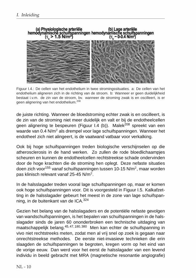
Figuur I.4.: De cellen van het endothelium in twee stromingssituaties. a: De cellen van hetendothelium aligneren zich in de richting van de stroom. b: Wanneer er geen duidelijkheidbestaat i.v.m. de zin van de stroom, bv. wanneer de stroming zwak is en oscilleert, is ergeen alignering van het endothelium.208
de juiste richting. Wanneer de bloedstroming echter zwak is en oscilleert, isde zin van de stroming niet meer duidelijk en valt er bij de endotheelcellengeen alignering te bespeuren (Figuur I.4 (b)). Malek208 spreekt van eenwaarde van 0.4 N/m2 als drempel voor lage schuifspanningen. Wanneer hetendotheel zich niet alingeert, is de vaatwand vatbaar voor verkalking.
Ook bij hoge schuifspanningen treden biologische verschijnselen op dieatherosclerosis in de hand werken. Zo zullen de rode bloedlichaampjesscheuren en kunnen de endotheelcellen rechtstreekse schade ondervindendoor de hoge krachten die de stroming hen oplegt. Deze nefaste situatiesdoen zich voor155 vanaf schuifspanningen tussen 10-15 N/m2, maar wordenpas klinisch relevant vanaf 25-45 N/m2.
In de halsslagader treden vooral lage schuifspanningen op, maar er komenook hoge schuifspanningen voor. Dit is voorgesteld in Figuur I.5. Kalkafzet-ting in de halsslagader gebeurt het meest in de zone van lage schuifspan-ning, in de buitenkant van de ICA.324
Gezien het belang van de halsslagaders en de potentiele nefaste gevolgenvan wandschuifspanningen, is het bepalen van schuifspanningen in de hals-slagader sinds de jaren 60 ononderbroken een technische uitdaging vanmaatschappelijk belang.45,47,180,380 Men kan echter de schuifspanning invivo niet rechtstreeks meten, zodat men al vrij snel op zoek is gegaan naaronrechtstreekse methodes. De eerste niet-invasieve technieken die erinslaagden de schuifspanningen te begroten, kregen vorm op het eind vande vorige eeuw. Dan werd voor het eerst de halsslagader van een levendindividu in beeld gebracht met MRA (magnetische resonantie angiografie)
NL - 10

I.2. Doel van het proefschrift
Figuur I.5.: Vooral lage maar ook hoge schuifspanningen komen voor in de halsslagader.
en gereconstrueerd in drie dimensies om dan de stroming in die halsslag-ader numeriek te berekenen. Het resultaat van deze berekening was hetschuifspanningsveld: voor het eerst leek het mogelijk om de krachten dieeen vloeistof uitoefent op de vaatwand volledig niet-invasief te begroten.
Wanneer aan het huidige onderzoek begonnen werd, ebde de euforie vande eerste successen reeds weg. Gedreven door het grote maatschappelijkbelang, begon men zich af te vragen hoe nauwkeurig deze techniek eigen-lijk wel is, en hoe toepasbaar ze zou blijken. Het is in dat kader dat ditonderzoek past.
Het doel van dit proefschrift bestond er dan ook in een techniek operatio-neel te maken die de halsslagaderdoorstroming in vivo berekent. Hierbijwerd gebruik gemaakt van medische beeldvormende technieken die in staatzijn de 3D geometrie van de slagader te reconstrueren en daarnaast ookeen minimum aan informatie over de bloedstroming te rapporteren. Met be-hulp van een computermodel wordt de stroming in de halsslagader voor eenindividu gereconstrueerd door het oplossen van de Navier-Stokes vergelij-kingen, i.e. de mathematische representatie van fysische wetten waaraaneen fluıdum (dus ook bloed) steeds moet voldoen. Zo wordt het beeld vande stroming bekomen op een patientspecifieke basis, enkel met behulp van
NL - 11

I. Inleiding
niet-invasieve technieken. Op basis van dit beeld van de stroming kunnenschuifspanningen op de slagaderwand bepaald worden.
Behalve het ‘operationeel maken’ van de techniek, was een van de belang-rijkste doelen van dit proefschrift het bepalen van de nauwkeurigheid van deschuifspanning in vivo. Als de techniek inzetbaar is voor klinische toepas-singen, moet de nauwkeurigheid ervan natuurlijk exact begroot worden. Pasdan kan pre-operatief onderzoek geschieden op basis van deze combinatievan een beeldvormende techniek en numerieke stromingsmechanica. Van-daar dat een belangrijk deel van dit proefschrift handelt over de sensitiviteitvan de ontwikkelde technologie.
I.3. De belangrijke parameters
Behalve de schuifspanningen, zijn er een aantal andere diagnostische pa-rameters die in dit proefschrift aan bod komen. Deze lijst is niet begrenzenden is enkel bedoeld om de lezer voeling te geven met de parameters dieverderop voorkomen.
• De IMT of intima-media dikte is de dikte van de binnenste twee lagenvan een slagader. Het is algemeen aangenomen236 dat een hoge IMTeen marker is van een verzwakte vasculaire gezondheid.
• De 3D geometrie van de halsslagader wordt dikwijls herleid tot eenaantal parameters . Hieronder valt o.a. AR, wat staat voor de verhou-ding van de som van de doorstroomoppervlakte van de ICA en ECA,ten opzichte van de doorstroomoppervlakte van de CCA. Tart is verderde kromheid van de arterie art (art = CCA, ICA of ECA).
Tart = 1− kortste afstand inlaat− uitlaat
lengte van arterie(I.2)
De bifurcatiehoek αBIF is de hoek tussen ICA en ECA. SFiart iseen parameter die de vorm van de contouren begroot. Deze para-meter is 1 voor een cirkel, en minder dan 1 voor alle andere vormen.Verder werden de non-planariteitsparameter NP en lineariteitspara-meter Lart gedefinieerd door King.157 NP wordt als volgt berekend.Eerst dienen de middellijnen van de arteries berekend te worden zoalsdat gedaan wordt door Barratt.20 De coordinaten van de middellijnenworden opgeslagen in een matrix. De singulierwaarde factorisatie van
NL - 12

I.3. De belangrijke parameters
deze matrix levert dan 3 singuliere waarden op. De - na schaling -kleinste singuliere waarde is dan de non-planariteitsparameter. Wan-neer alle punten in een vlak liggen, is NP = 0, wanneer alle puntenuniform verdeeld zijn in de ruimte, is NP = 33%. De lineariteitspara-meter L is de grootste singuliere waarde en wordt op analoge wijzeberekend. Deze parameters zijn interessant omdat die gelinkt kun-nen worden aan geometrische eigenschappen die gepaard gaan metkalkafzettingen.
• Het Reynolds-getal wordt als volgt berekend:
Re =Vgem D ρ
µ(I.3)
=Q/(πD2/4) D ρ
µ(I.4)
hier is Vgem de gemiddelde snelheid, D de diameter van het vat, ρde bloed densiteit en µ de dynamische viscositeit. Het Reynolds getaldrukt voor een stroming uit hoe de inertiekrachten zich verhouden t.o.v.de visceuze krachten. Het stromingsprofiel bij hoge Reynolds-getallenwordt bepaald door inertiewetten, terwijl bij lage Reynolds-getallen deviscositeit van het fluıdum het aanblik van de stroming bepaald. In heteerste geval spreekt men van turbulente stroming, in het tweede gevalover laminaire stroming. In een rechte stijve cilindrische buis ligt degrens tussen beide stromingsprofielen in de buurt van een Reynolds-getal van 2300.
• De schuifspanning in een bepaald punt op de vaatwand kan verschil-lende waarden en richtingen aannemen tijdens een hartcyclus. DeOSI (‘Oscillatory Shear Index’) is de fractie van de hartslag waarin deschuifspanning (WSS) niet gericht is volgens de gemiddelde richting.Ze wordt als volgt berekend:
OSI =12
(1− | ∫ T
0 ~τdt|∫ T0 |~τ | dt
)(I.5)
waarbij T de tijd tussen twee opeenvolgende hartslagen is, t de tijds-parameter en −→τ de schuifspanning. Wanneer de WSS altijd in dezelf-de richting acteert is de OSI gelijk aan 0, wanneer echter de schuif-spanning oscilleert rond het nulpunt zal de OSI toenemen, met 0.5 alstheoretisch maximum. De cellen aan de binnenkant van de slagader,
NL - 13
I. Inleiding
de endotheelcellen, wensen zich altijd te orienteren in de richting vande stroom. Wanneer echter de richting van de stroom niet duidelijk ge-definieerd is, zal de endotheelfunctie verstoord zijn hetgeen aanleidingkan geven tot verdikking van de vaatwand en slagaderverkalking.42 DeOSI helpt bij het opsporen van dergelijke zones.
• De schuifspanningsgradi ent wordt traditioneel gelinkt aan de per-meabiliteit van de vaatwand.173 Grote gradienten zullen de vaatwandaantasten en zo de kans geven aan relatief grote cellen, zoals macrofa-gen, om in de vaatwand te diffunderen. Deze situatie bevordert hetverkalkingsproces. De schuifspanning kan zowel naar de tijd als naarde plaats afgeleid worden. In het eerste geval spreekt men van de tem-porele schuifspanningsgradient of WSSGt, in het tweede geval van despatiale schuifspanningsgradient of WSSGs:
WSSGt =1T
∫ T
0
∣∣∣∣∂~τ
∂t
∣∣∣∣ dt (I.6)
WSSGs =1T
∫ T
0
√(∂τm
∂m
)2
+(
∂τn
∂n
)2
dt (I.7)
τm en τn zijn de tijdsafhankelijke componenten van de schuifspannin-gen in het mnl carthesisch assenstelsel. Hierbij is m de richting vande gemiddelde schuifspanning en n de tangentiele richting aan hetoppervlak van de wand en loodrecht op m. Merk op dat de schuifspan-ning gerefereerd dient te worden in het mnl assenstelsel om berekendte worden. Dit assenstelsel in anders voor elk punt van de vaatwand.
• De hoek die gemaakt wordt tussen de schuifspanningen in twee aan-palende punten van de vaatwand is een maat voor de kans dat bloed-partikels zich afzetten op die plek.142 Partikeldepositie bevordert kalk-afzettingen. Afhankelijk van de manier waarop deze parameter wordtbecijferd, refereert men naar deze parameter als de schuifspannings-deviatie (WSSAD) of angulaire schuifspanningsgradient (WSSAG). DeWSSAD is een gemiddelde hoek tussen de gemiddelde schuifspan-ning in een bepaald punt en de omliggende punten (in radialen), terwijlde WSSAG de afgeleide van deze hoek is naar de ruimte (radialen permeter).
De WSSAD wordt als volgt berekend:
WSSAD = C arccos
( −→τi · −→τj
|−→τi | |−→τj |
)(I.8)
NL - 14

I.4. De techniek en zijn toepassingen
waarbij
C = 1 als −→vl,i ·−→li ≥ 0
C = 0 als −→vl,i · li < 0 (I.9)
en
−→τi =1T
∫ T
0
−→τi dt
−→vl,i =1T
∫ T
0
−→vl,i dt (I.10)
Hier is −→τi de gemiddelde schuifspanning in punt i, −→vl,i de gemiddel-
de normale snelheid in de directe nabijheid van het punt i,−→l is de
normaal, subscript i duidt het huidige punt aan terwijl j de index is voorde naburige punten. De factor C benadrukt de potentiele impact vanstroming die de wand nadert. In de meest ernstige situatie is WSSADgelijk aan π.
De WSSAG wordt als volgt berekend:
WSSAG =1
T
Z T
0
���� 1
Ai
ZS
∂φ
∂xdAi
~i +1
Ai
ZS
∂φ
∂ydAi
~j +1
Ai
ZS
∂φ
∂zdAi
~k
���� dt (I.11)
met S is het volledige oppervlak van de halsslagaderwand en Ai deoppervlakte van het deel van de wand gerelateerd aan punt i. Dezeparameter kan berekend worden in eender welk assenstelsel ijk ofxyz. Het scalair veld angulaire verschillen φ is als volgt gedefinieerd:
φ = arccos
(~τi · ~τj
|~τi| |~τj |)
(I.12)
I.4. De techniek en zijn toepassingen
Het proefschrift bestaat uit twee delen. In een eerste deel wordt de techniekdie medische beeldvorming combineert met numerieke stromingsmechani-ca (computational fluid dynamics, CFD) bestudeerd. Daarbij gaat veel aan-dacht naar het kwantificeren en opdrijven van de betrouwbaarheid van de
NL - 15

I. Inleiding
techniek. Twee beeldvormende technieken worden van dichterbij bekeken:magnetische resonantie angiografie (MRA of vasculaire kernspintomogra-fie) in al zijn verschillende vormen en het meer toegankelijke en goedkopereultrageluid (US) of echografie.
In een tweede deel van het proefschrift wordt de techniek in twee klinischestudies succesvol toegepast. Een eerste studie bestudeerde de impact vanhet draaien van het hoofd op de doorstroming van de halsslagader. Eentweede studie gaat na wat de gevolgen van bloeddrukverlagende genees-middelen zijn op de schuifspanningen in de halsslagader.
NL - 16
II. Numerieke stromingsmechanicaop basis van medische beelden
II.1. Overzicht
Om tot een diagnose te komen, doet men beroep op een waaier meetap-paratuur en een breed gamma ingenieurstechnieken. Het bepalen van deschuifspanningen in de halsslagader van een patient bestaat uit de volgendestappen, geıllustreerd in Figuur II.1.
1. Niet-invasieve beeldvorming : Met MRA of US worden de doorsne-den van de slagader gevormd. In de eerste plaats dienen ze voor de3D reconstructie van de halsslagader. In de tweede plaats is de beeld-vorming ook bedoeld voor het meten van de snelheid aan het begin eneinde van het 3D model of het meten van de in- en uitlaatvoorwaarden.
2. Segmentatie : Op de originele beelden wordt de wand van de slaga-ders afgelijnd. Dit kan automatisch of manueel. Het resultaat van dezestap is een reeks contouren, i.e. dwarse secties van de slagader.
3. Reconstructie : De contouren worden in een gemeenschappelijk refe-rentiestelsel geplaatst. Hierdoor wordt de 3D geometrie van de slag-ader zichtbaar gemaakt. Door het glad maken van de 3D reconstruc-tie kan een realistisch computermodel van de halsslagader gecon-strueerd worden.
4. 3D Discretisatie : In deze stap wordt de binnenkant van het model,daar waar het bloed stroomt, gediscretiseerd. Dit houdt in dat het deelvan de 3D ruimte, ingenomen door de bloedstroming, in kleine cel-letjes wordt onderverdeeld. De stromingsvergelijkingen worden lateriteratief in deze celletjes opgelost. Deze stap noemt men ook het‘meshen’.
5. Opleggen van randvoorwaarden en parameters van het model :Vooraleer het oplossen van de stromingsvergelijkingen kan beginnen,
NL - 17

II. Numerieke stromingsmechanica op basis van medische beelden
Figuur II.1.: Illustratie van enkele typische stappen die ondernomen dienen te worden voorhet combineren van een beeldvormende techniek met numerieke stromingsmechanica. Nade beeldacquisitie wordt op de beelden manueel of automatisch de interface tussen lumen envaatwand afgelijnd. Deze lijnen of contouren worden in een 3D referentiesysteem geplaatsten bewerkt om een gladde geometrie te bekomen. De 3D geometrie wordt dan gediscre-tiseerd of ‘gemesht’. Deze ‘mesh’, samen met de stromingsvoorwaarden aan de in- enuitgang van het model, bevat genoeg informatie om de stroming in het model numeriek doorte rekenen m.b.v. een (veelal commercieel) numerieke stromingsmechanica pakket.306
moeten de in- en uitlaatvoorwaarden gekozen worden. Deze zijn ge-baseerd op debiet- en/of snelheidsmetingen uitgevoerd tijdens stap 1.Verder moeten nog enkele vloeistofeigenschappen bemeten worden,zoals de viscositeit en dichtheid van bloed.
6. Numerieke Stromingsmechanica (Computational Fluid Dynamics ofCFD): nu een gediscretiseerd model bestaat en de nodige randvoor-waarden werden opgelegd, kan de volledige tijdsafhankelijke stromingvan het bloed door de halsslagader berekend worden. Hiertoe lostmen de gelineariseerde Navier-Stokes vergelijkingen op in de celle-tjes van de mesh:
NL - 18

II.1. Overzicht
3∑
i=1
∂ui
∂xi= 0 (II.1)
∂ui
∂t+
3∑
j=1
∂
∂xi(uiuj) = Fi +
3∑
j=1
1ρ
∂σij
∂xji = 1, 2, 3 (II.2)
De onafhankelijke variabelen in een cartesiaans assenstelsel zijn deplaatsvector −→x = (x1, x2, x3) en de tijd t. Onder de afhankelijke vari-abelen vallen de snelheidsvector −→u = (u1, u2, u3) en de druk p. Dekrachtenvector
−→F = (F1, F2, F3) is uitgedrukt in N/kg en ~~σ = (σij) is
de spanningstensor uitgedrukt in N/m2, bestaande uit een drukcom-ponent en de viscositeit. ρ is de dichtheid van de vloeistof, hier hetbloed.
Voor het oplossen van de Navier-Stokes vergelijkingen kan men ge-bruik maken van verschillende numerieke modellen en verschillendesoftwarepakketten.
7. Diagnose : Eenmaal het stromingspatroon is gekend, kunnen diag-nostisch parameters berekend worden. Bij de diagnostische parame-ters behoren onder andere de schuifspanningen, de krachtenbalanstussen stroming en arteriele wand, en de omvang en lokalisatie vanrecirculatiezones, i.e. zones waar het bloed gedurende een periodevan de hartcyclus terugstroomt.
In dit hoofdstuk, dat zich vooral over de technische kant van het proefschriftbuigt, worden knelpunten in bovenstaande stappen aangepakt. Deel II.2,magnetische resonantie (MR), gaat na hoe de 3D reconstructie het bestaangepakt worden wanneer men over een MR-scanner beschikt. Analoogwordt in deel II.3, ultrageluid (US), de te ondernemen stappen bij het gebruikvan US uit de doeken gedaan. In beide delen gaat er veel aandacht naar hetkwantificeren van de nauwkeurigheid van de schuifspanning berekend metdeze techniek. Deel II.5 vergelijkt de twee beeldvormende technieken, MRen US. Tussenin (deel II.4) worden keuzes gemaakt voor de parameters vanhet numeriek model. Hierbij wordt vooral gedacht aan de randvoorwaarden,maar ook aan de viscositeit en de invloed van de hartslag.
NL - 19

II. Numerieke stromingsmechanica op basis van medische beelden
II.2. Magnetische Resonantie
II.2.1. Inleiding
Magnetische resonantie beeldvorming (MRI) maakt gebruik van het feit datwaterstofatomen in een groot magneetveld fungeren als magneetjes. Doorin een patient de beweging van die magneetjes na een externe excitatie teregistreren, kan men doorsneden van het menselijk lichaam in beeld bren-gen. Wanneer MRI gebruikt wordt voor het visualiseren van bloed, spreektmen ook van MR angiografie of MRA.
Er bestaan onder meer 3 soorten MRA: ‘Black Blood’ (BB), waar het bloed
Figuur II.2.: MRA beelden van een halsslagader van een jonge hypertensieve zondervaatvernauwing. De bovenste helft zijn BB MRI beelden, de onderste zijn TOF beeldenin dezelfde locaties.
NL - 20

II.2. Magnetische Resonantie
als zwart wordt afgebeeld in een beeld, ‘Time-Of-Flight’ (TOF), waar hetbloed als witte zones wordt afgebeeld, en ‘Cine Phase contrast’ (PC), waarde grijswaarde van het beeld overeenstemt met de snelheid van het bloed.Omwille van hun verschillende toepassingsgebieden werden de drie soortenMRA technieken in afzonderlijke studies onderzocht en vergeleken. Fi-guur II.2 (bovenste helft) geeft een voorbeeld van een set BB MRI beeldengenomen in een jonge, hypertensieve persoon zonder halsslagaderverkal-king. In diezelfde persoon werden ook TOF MRI beelden gemaakt: dezezijn te vinden in de tweede helft van Figuur II.2.
Figuur II.3.: Automatische segmentatie van de MRI beelden uit Figuur II.2. De witte of zwartecontouren zijn de resultaten van de automatische segmentatie van de CCA of ICA, terwijl degrijze contouren de ECA aflijnen.
NL - 21

II. Numerieke stromingsmechanica op basis van medische beelden
II.2.2. Segmenteren en Reconstrueren
Het segmenteren van MRI beelden maakt gebruik van de ‘region growing’methode, waarbij een operator op een beeld een punt moet aanduiden datzich in het bloedvat bevindt. Op basis van dat punt en de omliggende grijs-waarden wordt de contour automatisch teruggevonden. Na afloop gebruiktmen de ‘Snake’ methode.260 Dit is een segmenteringtechniek die de puntenvan een contour beschouwd als massa’s die met veren aan elkaar verbon-den zijn. Door de punten te verschuiven en hun ‘energie’ te minimaliseren,bekomt men de ideale gladde contour. Deze energie is opgesteld uit fac-toren die afhangen van de grijswaarden en van de vorm van de contour.Figuur II.3 toont het resultaat van de opeenvolging van de region growingmethode en de snake methode voor de originele beelden uit Figuur II.2.Na afloop krijgt een operator de kans aanpassingen door te voeren op deafgebeelde contouren.
De contouren die na de segmentatie bekomen werden, worden nu in 3Dafgebeeld in een gemeenschappelijk referentiestelsel. Om de effecten vanruis uit te schakelen, wordt de 3D reconstructie glad gemaakt. Hierbij wor-den de individuele punten
−−→Poud van een afzonderlijke contour verschoven
naar een punt op de as die−−→Poud verbindt met hun zwaartepunt
−−→Coud. Daaren-
boven worden de zwaartepunten van de contouren−−→Coud verschoven naar−−−−→
Cnieuw die op een 3D gladde lijn liggen:
−−−−→Pnieuw =
(−−→Poud −−−→Coud
)×√aratio +
−−−−→Cnieuw (II.3)
Hierbij werd aratio begroot door de eis dat de oppervlaktes van de contou-ren niet te veel mogen fluctueren. Deze operaties verwijderen ‘hoekjes enkantjes’ van de 3D reconstructie hetgeen resulteert in een meer realistische3D voorstelling van de halsslagader. Figuur II.4 toont de distributie van deOSI in een halsslagader die met verschillende graden van gladheid werdgereconstrueerd. Deze distributies tonen aan dat, behalve het wegwerkenvan onrealistische scherpte in de geometrie, het glad maken weinig invloedheeft op de belangrijkste kenmerken van de OSI distributie.
NL - 22

II.2. Magnetische Resonantie
Figuur II.4.: OSI distributie in een halsslagader die met verschillende graden van gladheidwerd gereconstrueerd. a: uitermate glad; b: glad; c: ruw.
II.2.3. De nauwkeurigheid van MRI gecombineerd met CFD
II.2.3.1. In vitro studie
In een eerste studie werd TOF MRI op de korrel genomen. Vooreerst werdeen glad fantoom van de halsslagader gescand en gereconstrueerd. Dezestudie liet toe de nauwkeurigheid van de techniek te bepalen. Enkele re-sultaten zijn geıllustreerd in Figuur II.5, waar de ware oppervlaktes van dedoorsnede van de drie delen van het halsslagadermodel vergeleken wordenmet hetgeen werd bemeten op de 3D reconstructie met TOF MRI. De datapunten zijn de doorsneden van de individuele contouren, de volle grijze lijnis de oppervlakte bemeten bij de gladde reconstructie. Voor de volledigheidwerd ook een BB MRI scan uitgevoerd. De resultaten daarvan zijn mee inde figuur opgenomen. De studie toonde aan dat MRI-gebaseerde CFD klaarwas voor in vivo toepassingen.
II.2.3.2. In vivo studie
Nadat de performantie van TOF MRI in vitro was vastgesteld, werd vervol-gens een TOF reproduceerbaarheidsstudie uitgevoerd. Hierbij werden 8gezonde personen twee keer gescand, met minstens twee weken tussen
NL - 23

II. Numerieke stromingsmechanica op basis van medische beelden
(a) CCA (b) ICA
(c) ECA
Figuur II.5.: Nauwkeurigheid van MRI in het bepalen van de doorsnede van een in vitrocarotis. De oppervlakte van de doorsnede is voorgesteld als een functie van de verticaleas z. De zwarte lijn (CAD) stelt de werkelijke data voor. De data punten zijn opgemetenoppervlaktes, en de grijze lijnen zijn de oppervlaktes in het gladde model.
de twee opnames. Het verschil tussen de twee scans is een maat voor dereproduceerbaarheid. In de simulaties die de hemodynamische parametersberekenen werd in deze studie telkens dezelfde randvoorwaarde gebruikt,dit opdat de opgemeten verschillen enkel te wijten zouden zijn aan het ver-schil in geometrie. Een aparte randvoorwaardestudie volgt in deel II.4. Eenvan de interessantste resultaten van deze studie staat vervat in Tabel II.1: zetoont de te verwachten fout voor de WSS, OSI, WSSGt, WSSGs, WSSADen WSSAG. Deze fout werd berekend door de individuele waarde van deparameter te begroten op individuele segmenten van de halsslagader. Voorelk segment berekent men het absolute verschil tussen de te verwachtenwaarde (het gemiddelde van de waarde in de twee scans) en de opgemetenwaarde (in een van de scans). De ‘fout’ of RMSE is hier gedefinieerd als hetgemiddelde van deze absolute verschillen.
NL - 24

II.2. Magnetische Resonantie
arterie WSS OSI WSSGs WSSGt WSSAD WSSAG[N/m2] [-] [N/m3] [ N
m2.s ] [-] [rad/m]RMSE CCA 0.175 0.0129 114 0.817 0.0969 22.1
ICA 0.543 0.0325 234 2.97 0.120 67.8ECA 0.563 0.0296 213 3.27 0.0972 77.3
SAMEN 0.427 0.0250 214 2.35 0.105 68.1% CCA 35.0 89.9 67.1 20.4 79.5 64.5
ICA 24.9 107 68.9 19.5 121 97.5ECA 39.6 129 56.1 35.0 106 72.0
SAMEN 37.9 123 65.7 30.2 102 79.8
Tabel II.1.: Fout voor de hemodynamische parameters begroot met de MRI reproduceerbaar-heidsstudie (n=8). De ‘fout’ of RMSE is het gemiddelde absolute verschil tussen de waardevan een segment in de eerste scan en de gemiddelde waarde van het overeenkomstigesegment in de twee scans. Het percentage is de fout gedeeld door de gemiddelde waarde.
Door deze studie werd voor het eerst de reproduceerbaarheid van de com-binatie van MRI en CFD gekwantificeerd in vivo. Omdat elke meettech-niek zijn eigen meetfout met zich meebrengt, valt de werkelijke geometrieen halsslagaderdoorstroming in vivo niet ondubbelzinnig te bepalen. Van-daar dat de ‘nauwkeurigheid’, wat gedefinieerd wordt als het verschil tussende gemeten waarde en de werkelijke waarde, niet bemeten kan worden.Dit wordt opgevangen door het begroten van de reproduceerbaarheid, diedankzij deze studie voortaan gekend is en in het verdere verloop van hetproefschrift als referentiewaarde zal worden gebruikt.
Merk op dat deze studie geen eenduidig antwoord kan geven op de vraagof de techniek nu al dan niet reproduceerbaar is. De reproduceerbaarheidis immers afhankelijk van de vereiste nauwkeurigheid in een bepaalde toe-passing. Indien toepassing “A” een nauwkeurigheid van 0.5 N/m2 voor deWSS vereist, dan is de techniek zoals die er hier voorligt reproduceerbaaraangezien de gemiddelde RMSE in Tabel II.1 0.427 N/m2 bedraagt. Indientoepassing “B” echter een strenge nauwkeurigheid van 0.1 N/m2 vereist, isde techniek niet reproduceerbaar genoeg.
II.2.4. De vergelijking van TOF en BB
In een volgende studie werd de nauwkeurigheid van BB MRI onderzocht invivo. Hiertoe werden 8 personen elk zes keer gescand: 3 keer met TOFMRI, en 3 keer met BB MRI. BB MRI heeft enkele inherente voordelen t.o.v.TOF MRI:
NL - 25
II. Numerieke stromingsmechanica op basis van medische beelden
(a) ICA en ECA (b) Distal CCA
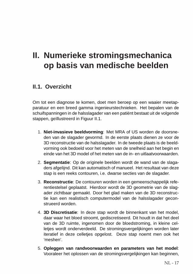
Figuur II.6.: Artefacten bij BB en TOF MRI. a: Proximale CCA coupes: het beeld links-boven is het TOF beeld, er rechts van en eronder staan twee manieren om te segmenteren.Het beeld rechtsonder is het corresponderende BB beeld. b: Distale CCA coupes: hetbeeld linksboven is het BB beeld, er rechts van en eronder staan twee manieren om tesegmenteren. Het beeld rechtsonder is het corresponderende TOF beeld.
• Zoals Figuur II.2 (pagina NL - 20) duidelijk aantoont, heeft BB MRI decapaciteit om de dikte van de vaatwand te begroten.
• De beeldacquisitie bij BB MRI kan gesynchroniseerd worden zonderdat de acquisitietijd de grenzen van een voor de patient aanvaardbaretijdspanne overschrijdt.
Samen met het eerste punt wordt het duidelijk dat BB MRI in staat isde cyclische vervorming van de wand te registreren.
• BB MRI vertoont minder artefacten in het bijzijn van eventuele metalenimplantaten.313
• Figuur II.6 (a) (linksboven) is een TOF beeld van de proximale ICA.Deze kan op verschillende manieren gesegmenteerd worden, zoalswordt aangeduid rechts van en onder het originele beeld. De BB MRItegenhanger van hetzelfde TOF beeld (rechtsonder) is van vergelijk-bare kwaliteit, maar dankzij het feit dat ondanks de grote ruis de vaat-wand goed in beeld werd gebracht, is het segmenteren van het BBbeeld eenvoudiger. BB MRI is dan ook nauwkeuriger in de groterevaten.
Maar ook TOF heeft een aantal belangrijke voordelen:
NL - 26

II.3. Ultrageluid
• TOF is veruit eenvoudiger om automatisch te segmenteren. Dit ver-taalt zich in tijdwinst daar de operator die de automatische segmen-taties dient te verwerken, veel minder werk heeft met het manueelcorrigeren van de contouren.
• Voor de kleinere vaten, zoals de distale ICA en ECA, maar ook voorzones waar de bloedstroming erg complex is, zoals in de distale CCA,bereikt TOF een veel hogere nauwkeurigheid. Getuige hiervan is Fi-guur II.6 (b), waar linksboven een BB MRI beeld is getoond. De wittepijl duidt maanvormige ruis aan. Deze zou kunnen verward wordenmet de vaatwand zodat er twee verschillende segmentaties mogelijkzijn, weergegeven rechts van en onder het originele beeld. Enkelm.b.v. de TOF tegenhanger van dit beeld, dat ook niet van uitmun-tende kwaliteit is, kan men zekerheid verschaffen over de grootte vande distale CCA bij deze persoon.
Het gevolg van dit laatste punt is verregaand. Zo stelde men vast datin deze studie de distale ICA of ECA soms volledig verdween bij deBB MRI scan, maar nog altijd aflijnbaar was bij de TOF MRI scan.
Ondanks het feit dat er in de verwerking van de beelden duidelijke ver-schillen tussen BB en TOF naar boven traden, bleken de kwantitatieve ver-schillen in de schuifspanning en andere hemodynamische parameters nogaltijd van dezelfde grootteorde als die teruggevonden bij de TOF reprodu-ceerbaarheidsstudie in paragraaf II.2.3.2 op pagina NL - 23. Omdat TOFveel snellere en in de distale delen van het model meer betrouwbare re-constructies toelaat, wordt voor de toekomst de voorkeur gegeven aan TOFMRI.
Wanneer de kennis van de dikte van de vaatwand van primordiaal belang is,kan de arts terugvallen op een BB MRI scan. Wanneer men echter zowelnauwkeurige reconstructies van de distale ICA en ECA wilt, gecombineerdmet kennis van de vaatwanddikte, dient men de twee beeldvormende tech-nieken combineren.
NL - 27

II. Numerieke stromingsmechanica op basis van medische beelden
II.3. Ultrageluid
II.3.1. Inleiding
Ultrageluid (US) of echografie is een beeldvormende techniek waarbij gol-ven worden uitgezonden door een probe die men op de huid plaatst. Dezetrillingen zullen weerkaatsen waanneer die het scheidingsoppervlak tus-sen twee stoffen met verschillende impedantiea bereiken. Door gebruik temaken van de teruggekaatste golven, kan men een beeld vormen van deoppervlakken waarop de trillingen werden teruggekaatst. Figuur II.7 is eenvoorbeeld van een ‘B-mode’ beeld van de halsslagader. Het zwarte gebied,in de vorm van een ∞-symbool, omvat het lumen.
Wanneer de golf terugkaatst van een bewegend element, zoals bloed par-tikels, kan tevens de bewegingssnelheid van dat element bepaald worden.Deze techniek heet ‘Doppler Ultrageluid’. Hier is het verschil in frequentievan de uitgestuurde en teruggekaatste golf evenredig met de snelheid vanhet element.
aimpedantie = product van dichtheid en geluidssnelheid
Figuur II.7.: B-mode beeld van de carotis van een gezonde 25 jarige man. De huid bevindtzich bovenaan het beeld, de bifurcatie is de zwarte zone in het midden van het beeld in devorm van een ∞-symbool.
NL - 28
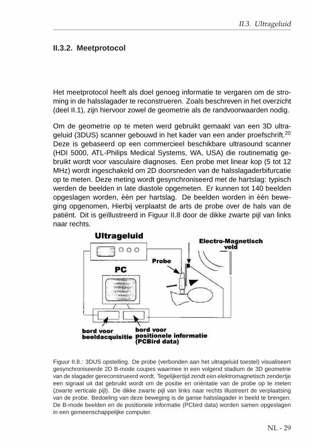
II.3. Ultrageluid
II.3.2. Meetprotocol
Het meetprotocol heeft als doel genoeg informatie te vergaren om de stro-ming in de halsslagader te reconstrueren. Zoals beschreven in het overzicht(deel II.1), zijn hiervoor zowel de geometrie als de randvoorwaarden nodig.
Om de geometrie op te meten werd gebruikt gemaakt van een 3D ultra-geluid (3DUS) scanner gebouwd in het kader van een ander proefschrift.20
Deze is gebaseerd op een commercieel beschikbare ultrasound scanner(HDI 5000, ATL-Philips Medical Systems, WA, USA) die routinematig ge-bruikt wordt voor vasculaire diagnoses. Een probe met linear kop (5 tot 12MHz) wordt ingeschakeld om 2D doorsneden van de halsslagaderbifurcatieop te meten. Deze meting wordt gesynchroniseerd met de hartslag: typischwerden de beelden in late diastole opgemeten. Er kunnen tot 140 beeldenopgeslagen worden, een per hartslag. De beelden worden in een bewe-ging opgenomen, Hierbij verplaatst de arts de probe over de hals van depatient. Dit is geıllustreerd in Figuur II.8 door de dikke zwarte pijl van linksnaar rechts.
Figuur II.8.: 3DUS opstelling. De probe (verbonden aan het ultrageluid toestel) visualiseertgesynchroniseerde 2D B-mode coupes waarmee in een volgend stadium de 3D geometrievan de slagader gereconstrueerd wordt. Tegelijkertijd zendt een elektromagnetisch zendertjeeen signaal uit dat gebruikt wordt om de positie en orientatie van de probe op te meten(zwarte verticale pijl). De dikke zwarte pijl van links naar rechts illustreert de verplaatsingvan de probe. Bedoeling van deze beweging is de ganse halsslagader in beeld te brengen.De B-mode beelden en de positionele informatie (PCbird data) worden samen opgeslagenin een gemeenschappelijke computer.
NL - 29

II. Numerieke stromingsmechanica op basis van medische beelden
Tegelijkertijd registreert een elektromagnetisch positionerings- en oriente-ringstoestel of EPOM (Ascension Technology Inc, Vermont, USA) de positievan de probe. Dit laat toe de positie van het beeld in 3D te berekenen.
Voor de randvoorwaarden dient de arts met Doppler ultrageluid, ter hoogtevan de in- en uitlaat van het bestudeerde segment van de halsslagader, desnelheid op te meten in het centrum van het bloedvat. Aldus bekomt meneen tijdsafhankelijke snelheidsmeting, typisch aan 200 Hz, voor zowel deCCA, ICA en ECA. Kennis van die snelheid samen met de kennis van deoppervlakte van de doorsnede van de slagader ter hoogte van het meetpuntlaat toe, mits het veronderstellen van een rigide vaatwand en een ontwik-keld stromingsprofiel, het debiet of het tijdsafhankelijk snelheidsprofiel teberekenen.140,368 Aldus heeft men aan snelheidsmetingen in het centrumvan het in- of uitlaatvlak genoeg om alle randvoorwaarden af te leiden.
II.3.3. Segmenteren en reconstrueren
Voor de segmentatie en de reconstructie werden in een vorig proefschrift20
een aantal programma’s geschreven. Het segmenteren van de echobeel-den van de halsslagader wordt manueel gedaan, daar de beelden slechtcontrast geven ter hoogte van de vaatwand. Figuur II.9 toont in het rood hoehet plaatje van Figuur II.7 manueel gesegmenteerd zou kunnen worden.Wanneer alle beelden gesegmenteerd zijn, kan men de rode contouren inde 3D ruimte op elkaar plaatsen. Hierbij wordt gebruik gemaakt van depositionele informatie vergaard met de EPOM. Nadat de geometrie is gladgemaakt, bekomt men een 3D voorstelling van en patient-specifieke hals-slagaderbifurcatie die bruikbaar is voor numerieke stromingssimulaties.
In het kader van het huidig proefschrift werd de output van de bestaandeprogramma’s gebruikt om automatisch 3D discretisaties (‘meshes’) te cree-ren gebruik makend van programma’s die geschreven werden voor de re-constructie van de halsslagader op basis van MR-beelden.
II.3.4. De nauwkeurigheid van US gecombineerd met CFD
Toen dit proefschrift in aanraking kwam met US-gebaseerde numerieke si-mulaties, was de nauwkeurigheid van de techniek al bepaald door Dr. A. D.Augst op een fantoom van een halsslagader. Desalniettemin werden hier,naar analogie met de studies die de nauwkeurigheid van MRI bepaalden,
NL - 30

II.3. Ultrageluid
Figuur II.9.: Segmentatie van B-mode ultrageluid doorsnede van de halsslagader van FiguurII.7. Een operator plaatst de rode punten op het B-mode beeld en fit de rode lijn door teklikken op de ‘spline’ knop. Deze rode lijn is dan de segmentatie of de contour van dit beeld.Bovenaan het beeld kan men zien dat dit het 38ste beeld is van 140 opgeslagen beelden.Elk van die beelden is een doorsnede van dezelfde halsslagader.
weer fantoomscans uitgevoerd (deel II.3.4.1). Verder werd de in vivo nauw-keurigheid gedimensioneerd in een reproduceerbaarheidsstudie (deel II.3.4.2).Omdat er bij 3DUS een veel hogere graad van subjectiviteit aanwezig isdan bij MRI, waar de beelden automatisch gesegmenteerd worden, werd ophet eind van dit hoofdstuk een variabiliteitsstudie uitgevoerd (deel II.3.4.3).Deze heeft als doel na te gaan wat de effecten zijn van die subjectiviteit bijhet segmenteren en bij de beeldacquisitie.
II.3.4.1. In vitro studie
Hetzelfde fatoom dat in deel II.2.3.1 (In vitro studie bij MRI) was gebruikt,werd opnieuw aangewend. Het werd gescand en gesegmenteerd door tweepersonen. De eerste persoon (DB) was een 3DUS technieker, de tweede(BA) was een arts zonder ervaring in 3DUS. BA werd niet speciaal opgeleidvooraleer hij de scans uitvoerde.
NL - 31

II. Numerieke stromingsmechanica op basis van medische beelden
Parameter CAD DB BA σinter−op σal(eenheid) Fantoom (n=3) (n=3) (n=2) (n=6)
Data RMSE±σintra−op RMSE±σintra−op
ACCA [mm2] 53.214 +1.427± 1.915 +11.172± 4.102 7.051 6.299(2.68±3.60%) (20.99±7.71%) (13.25%) (11.84%)
AICA [mm2] 37.891 +1.324± 0.176 +9.010± 1.052 5.434 5.167(3.50±0.46%) (23.78±2.78%) (14.34%) (13.64%)
AECA [mm2] 17.309 +0.815± 0.173 +5.027± 0.929 2.978 2.921(4.71±1.00%) (29.04±5.37%) (17.21%) (16.88%)
AR [-] 1.056 +0.103± 0.014 +0.035± 0.028 0.048 0.069(9.77±1.30%) (3.28±2.66%) (4.58%) (6.53%)
TCCA [%] 0.450 +0.185± 0.227 +0.234± 0.270 0.059 0.210(41.07±50.54%) (52.10±60.04%) (13.04%) (46.59%)
TICA [%] 1.606 -0.276± 0.305 -0.373± 0.155 0.127 0.325(17.19±18.99%) (23.23±9.68%) (7.92%) (20.21%)
TECA [%] 1.974 -0.179± 0.136 -0.248± 0.261 0.031 0.213(9.05±6.91%) (12.57±13.23%) (1.55%) (10.81%)
αBIF [°] 149.885 +3.777± 0.787 +1.634± 0.746 1.515 2.706(2.52±0.52%) (1.09±0.50%) (1.01%) (1.81%)
SFiCCA [-] 0.964 +0.011± 0.005 +0.007± 0.001 0.002 0.009(1.13±0.53%) (0.77±0.07%) (0.26%) (0.95%)
SFiICA [-] 0.993 -0.003± 0.004 +0.002± 0.001 0.002 0.002(0.25±0.35%) (0.22±0.13%) (0.18%) (0.24%)
SFiECA [-] 0.993 +0.003± 0.000 +0.002± 0.002 0.001 0.003(0.29±0.03%) (0.21±0.17%) (0.06%) (0.25%)
WSS [N/m2 ] 0.858 -0.064± 0.060 -0.167± 0.060 0.080 0.115(7.43±7.04%) (19.42±7.04%) (9.35%) (13.43%)
WSS iCCA 0.416 +0.016± 0.021 -0.021± 0.033 0.019 0.019(3.87±5.09%) (5.17±7.94%) (4.64%) (4.52%)
WSS eCCA 0.491 +0.290± 0.103 +0.081± 0.037 0.148 0.185(58.93±20.93%) (16.47±7.52%) (30.02%) (37.70%)
WSS buiten ICA 1.026 +0.508± 0.062 +0.479± 0.207 0.021 0.494(49.53±6.08%) (46.70±20.14%) (2.00%) (48.12%)
WSS binnen ICA 1.512 +1.157± 0.072 +0.891± 0.063 0.188 1.024(76.50±4.75%) (58.89±4.16%) (12.45%) (67.69%)
WSS buiten ECA 0.679 +0.297± 0.032 +0.156± 0.044 0.100 0.226(43.72±4.67%) (22.94±6.52%) (14.69%) (33.33%)
WSS binnen ECA 1.131 +0.629± 0.051 +0.387± 0.078 0.171 0.508(55.62±4.52%) (34.22±6.89%) (15.13%) (44.92%)
OSI [-] 0.040 +0.008± 0.003 +0.007± 0.009 0.002 0.007(18.94±7.53%) (17.66±22.21%) (5.32%) (18.30%)
OSI iCCA 0.075 +0.009± 0.009 +0.022± 0.028 0.001 0.015(11.40±12.47%) (29.58±37.21%) (1.43%) (20.49%)
OSI eCCA 0.040 -0.067± 0.002 -0.043± 0.009 0.017 0.055(167.12±4.79%) (107.31±22.97%) (42.29%) (137.22%)
OSI buiten ICA 0.064 +0.025± 0.007 -0.031± 0.032 0.030 0.028(38.17±11.54%) (47.48±49.74%) (47.24%) (42.83%)
OSI binnen ICA 0.001 -0.073± 0.000 -0.068± 0.005 0.004 0.071(5319.63±13.42%) (4953.10±331.48%) (259.17%) (5136.37%)
OSI buiten ECA 0.016 -0.056± 0.006 -0.051± 0.017 0.003 0.054(350.62±39.48%) (320.70±106.17%) (21.15%) (335.66%)
OSI binnen ECA 0.002 -0.072± 0.001 -0.070± 0.001 0.001 0.071(3066.02±55.63%) (2980.37±54.31%) (60.56%) (3023.20%)
Tabel II.2.: Statistiek voor de geometrische en stromingsparameters bemeten met 3DUS incombinatie met CFD op een fantoom. Aart staat voor de gemiddelde oppervlakte van dedoorsnede van de arterie art (art = CCA, ICA of ECA), AR staat voor de verhouding vande som van de doorstroomoppervlakte van de ICA en ECA, en CCA. Tart is de kromheidvan de arterie art (Tart = 1- kortste afstand inlaat−uitlaat
lengte van arterie), αBIF de hoek tussen ICA en ECA
en SFiart is een parameter die de vorm van de contouren begroot. De WSS en OSI wer-den uitgemiddeld over de ganse halsslagader, het deel van de CCA waar de ICA van aftakt(‘iCCA’), het deel van de CCA waar de ICA van aftakt (‘eCCA’), de binnenbocht en de buiten-bocht van de ICA en ECA (‘binnen’ en ‘buiten’ ICA of ECA). Waarden zijn voorgesteld alshet gemiddelde absolute verschil tussen de werkelijke fantoomdata en de gemeten waarde± de standaard deviatie van de verschillen. Het teken geeft aan of de waarden gemiddeldgezien groter (+) dan wel kleiner (-) waren dan de werkelijke waarden. De percenten wer-den verkregen door te delen door de werkelijke waarde. CAD: werkelijke fantoomdata; DB:waarden opgemeten door DB; BA: waarden opgemeten door BA; zie tekst voor de definitievan σinter−op en σal.
NL - 32

II.3. Ultrageluid
Tabel II.2 bevat de meeste resultaten van deze in vitro studie. De resultatenzijn voorgesteld als het gemiddelde absolute verschil tussen de gemetenwaarde en de werkelijke waarde ± de standaard deviatie van het echte ver-schil (RMSE ± σintra−op). De ‘werkelijke’ waarde is weergegeven in kolom‘CAD’. Het teken geeft aan of de opgemeten waarde gemiddeld gezien gro-ter (+) dan wel kleiner (-) was dan de werkelijke waarde. De percentagesworden verkregen door te delen door de werkelijke waarde. σinter−op is destandaard deviatie van de gemiddelden voor elke operator, en is een maatvoor de variatie tussen operatoren onderling. σal is de te verwachten foutwanneer er een enkele meting wordt uitgevoerd door een onervaren opera-tor.
Deze studie maakte volgende vaststellingen:
• σal is over het algemeen klein en vergelijkbaar met de waarden voor degemiddelde RMSE in deel II.2.3.1, hetgeen laat vermoeden dat 3DUSklaar is voor in vivo toepassingen.
• De ervaren operator (DB) werkt veel nauwkeuriger dan BA. De abso-lute fout is immers doorgaans kleiner bij DB. Dit geeft aan dat er tocheen minimum aan training vereist is vooraleer iemand het scannenmet 3DUS en/of het segmenteren van US beelden goed onder de knieheeft.
• σintra−op is vaak een grootte-orde groter dan de RMSE. Dit geeft aandat de waarden verkregen uit twee verschillende scans door eenzelfdeoperator eigenlijk niet veel verschillen.
Merk op dat sommige percentages in Tabel II.2 astronomische waardenaannemen. Dit is het gevolg van het feit dat de werkelijke waarde, weer-gegeven in de kolom ‘CAD’, bijzonder klein is. In deze gevallen heeft hetpercentage natuurlijk weinig waarde, maar de standard deviaties blijven eenmaat voor de foutmarge van de techniek.
Het concept van deze studie, waar de beelden gesegmenteerd werden doorde persoon die de acquisitie deed, liet niet toe na te gaan welk deel vande variantie te wijten is aan fouten in de beeldacquisitie dan wel aan seg-menteringsfouten. De in vivo variabiliteitsstudie van deel II.3.4.3 geeft hierantwoord op.
NL - 33

II. Numerieke stromingsmechanica op basis van medische beelden
II.3.4.2. In vivo studie
Opnieuw naar analogie met de MRI reproduceerbaarheidsstudie, werd hiereen 3DUS reproduceerbaarheidsstudie uitgevoerd. Negen gezonde proef-personen werden 2 keer gescand met 3DUS. De halsslagaderdoorstromingwerd berekend met CFD. In alle simulaties werden dezelfde inlaatvoorwaar-den gebruikt, zodat een verschil in snelheidsprofiel enkel te wijten kon zijnaan een verschil in 3D geometrie. Een aparte randvoorwaardestudie volgtin deel II.4.
Figuur II.10 toont resultaten voor proefpersoon nr. 1. Figuur (a) vergelijktde arteriele oppervlakte van een doorsnede in de twee scans. Hierbij isde I/S as (Inferior/Superior) de as van voeten naar hoofd. Het nulpunt ligtter hoogte van de apex van de beschouwde carotis. Figuur (b) vergelijktdezelfde oppervlakte, maar uitgemiddeld over de I/S as. Figuur (c) tekentde centerlijn van scan 1 in het zwart en van scan 2 in het grijs. Om een3D gevoel te krijgen van de centerlijnen, werden ze over elkaar getekend envanuit twee standpunten weergegeven, 90° t.o.v. elkaar gedraaid. Figuren(d) tot (g) vergelijken de WSS en OSI distributie in beide scans.
(a) Verschil in oppervlakte van ar-teriele secties
(b) Gemiddelde opper-vlakte van arteriele secties
(c) Centerlijnen
(d) WSS 1 (N/m2) (e) WSS 2 (N/m2) (f) OSI 1 (-) (g) OSI 2 (-)
Figuur II.10.: De 3DUS reproduceerbaarheidsstudie voor een vrijwilliger. a: Verschil in op-pervlakte van de arteriele doorsnede tussen de twee sessies voorgesteld als functie van deI/S as. b: Oppervlaktes uitgemiddeld over de I/S as in beide sessies. c: Centerlijn voorsessie 1 (zwart) en 2 (grijs) over elkaar getekend en 90° gedraaid. d-e: schuifspanningsver-deling in sessie 1 (d) en 2 (e). f-g: OSI verdeling in sessie 1 (f) en 2 (g).
NL - 34

II.3. Ultrageluid
Over alle patienten heen werd, vergeleken met MRI, nagenoeg dezelfdegraad van nauwkeurigheid behaald, al bleek 3DUS minder robuust. Voor-eerst zijn er bij de positionering van de patient meer vrijheidsgraden, waar-door de nek en dus ook de halsslagader zich in verschillende posities bevon-den bij eenzelfde patient. Ten tweede splitst de halsslagader zich soms paster hoogte van het kaakbeen, hetgeen niet toegankelijk is met een US probe.Het eerste was een kinderziekte die verholpen werd door een kleine wijzi-ging van het protocol, het tweede is een voorlopig onopgelost probleem datzal blijven bestaan zolang US niet toelaat door het bot metingen uit te voe-ren.
II.3.4.3. Variabiliteitsstudie
Tot slot werd de halsslagader van een gezonde vrijwilliger in totaal 11 keergescand door 4 verschillende artsen (4 ‘DR’s’ die elk 3 of 2 keer de halsslag-ader opmaten). Elk van de artsen werd bijgestaan door een ervaren 3DUSgebruiker bij hun eerste scan. Elke data set werd gesegmenteerd door 3operatoren (3 ‘OP’s’), elk met een verschillende achtergrond en voorken-nis. Aan deze OP’s werd uitgelegd hoe men diende te segmenteren m.b.v.maximaal 10 voorbeeldplaatjes.
De resultaten van deze variabiliteitsstudie staan genoteerd in Tabel II.3.σinter−scan, σinter−DR en σinter−OP zijn respectievelijk de standaard devi-atie van de gemiddeldes per scan (n=3), per DR (n=4) en per OP (n=3).Ze stellen respectievelijk een maat voor voor de reproduceerbaarheid, devariabiliteit te wijten aan de beeldacquisitie en de variabiliteit te wijten aanhet segmenteren van de beelden. σal is de standaard deviatie van alle 33metingen. Het percentage is berekend door te delen door de gemiddeldewaarde, genomen over alle 33 metingen.
Uit deze variabiliteitsstudie kon men volgende conclusies trekken:
• σal, de totale variabiliteit, is vrij gering wanneer die vergeleken wordtmet de waarden die in de reproduceerbaarheidsstudie voor MRI en3DUS werden bekomen. Dit geeft aan dat de totale variabiliteit beperktkan worden door een minimale training van de operatoren
• Doorgaands is σinter−DR groter dan σinter−OP , hetgeen wilt zeggendat de resterende, kleine, variabiliteit, voor het grootste deel te wij-ten is aan de subjectiviteit tijdens het scannen, eerder dan aan desubjectiviteit tijdens het segmenteren.
NL - 35

II. Numerieke stromingsmechanica op basis van medische beelden
Parameter σinter−scan σinter−DR σinter−OP σal
(eenheid) (n=3) (n=4) (n=3) (n=33)ACCA [mm2] 2.2676 (4.59%) 2.4655 (4.97%) 0.5860 (1.18%) 4.0486 (8.17%)AICA [mm2] 0.9320 (2.24%) 2.1353 (5.10%) 1.7138 (4.11%) 3.0903 (7.41%)AECA [mm2] 0.3505 (1.77%) 0.9377 (4.70%) 1.9510 (9.83%) 2.5980 (13.09%)
AR [-] 0.0325 (3.53%) 0.0086 (0.94%) 0.0285 (3.10%) 0.0525 (5.71%)NP [%] 0.8603 (15.32%) 1.1497 (20.64%) 0.0852 (1.53%) 1.6383 (29.34%)
NPCCA [%] 0.2583 (17.58%) 0.2102 (14.52%) 0.0363 (2.52%) 0.5775 (40.07%)NPICA [%] 0.8700 (42.19%) 0.9332 (43.54%) 0.1429 (6.88%) 1.4475 (69.75%)NPECA [%] 0.0345 (8.03%) 0.0485 (11.15%) 0.0568 (13.14%) 0.1764 (40.83%)
LCCA [%] 0.8142 (0.96%) 3.4926 (4.12%) 0.1218 (0.14%) 3.4995 (4.14%)LICA [%] 1.3685 (1.73%) 3.7256 (4.69%) 0.3509 (0.44%) 3.4717 (4.39%)LECA [%] 0.3844 (0.47%) 1.5485 (1.89%) 0.0519 (0.06%) 1.4426 (1.76%)TCCA [%] 0.2196 (15.35%) 0.2743 (19.82%) 0.0803 (5.70%) 0.3801 (26.99%)TICA [%] 0.9291 (52.79%) 1.0038 (54.79%) 0.2358 (13.31%) 1.6469 (92.94%)TECA [%] 0.0573 (8.35%) 0.2734 (38.47%) 0.1110 (16.17%) 0.7280 (105.99%)αBIF [°] 5.5711 (5.54%) 7.5465 (7.53%) 2.7725 (2.76%) 23.7628 (23.67%)
SFiCCA [-] 0.0080 (0.83%) 0.0082 (0.85%) 0.0021 (0.22%) 0.0139 (1.45%)SFiICA [-] 0.0037 (0.38%) 0.0081 (0.82%) 0.0044 (0.45%) 0.0123 (1.26%)SFiECA [-] 0.0062 (0.64%) 0.0035 (0.35%) 0.0095 (0.97%) 0.0133 (1.35%)
Gem. VMAX,CCA [m/s] 0.0080 (3.65%) 0.0083 (3.78%) 0.0047 (2.14%) 0.0151 (6.89%)Gem. VMAX,ICA [m/s] 0.0008 (0.46%) 0.0192 (10.86%) 0.0084 (4.69%) 0.0211 (11.84%)
Gem. VMAX,ECA [m/s] 0.0042 (2.78%) 0.0134 (8.86%) 0.0109 (7.17%) 0.0184 (12.11%)Gem. WSS [N/m2] 0.0087 (1.51%) 0.1155 (20.15%) 0.0467 (8.15%) 0.1204 (20.99%)WSS iCCA [N/m2] 0.0267 (5.66%) 0.0528 (11.26%) 0.0113 (2.40%) 0.0816 (17.42%)
WSS eCCA 0.0235 (5.04%) 0.0794 (16.64%) 0.0160 (3.42%) 0.0853 (18.24%)WSS buiten ICA 0.0267 (4.08%) 0.1760 (26.84%) 0.0850 (12.97%) 0.1934 (29.51%)WSS binnen ICA 0.0193 (2.32%) 0.1350 (16.45%) 0.0927 (11.14%) 0.1789 (21.50%)WSS buiten ECA 0.0095 (1.54%) 0.1722 (28.35%) 0.1246 (20.31%) 0.2139 (34.85%)WSS binnen ECA 0.0084 (1.17%) 0.1557 (21.76%) 0.1263 (17.49%) 0.2036 (28.21%)
Gem. OSI [-] 0.0062 (4.71%) 0.0272 (20.96%) 0.0048 (3.68%) 0.0292 (22.19%)OSI iCCA [-] 0.0162 (10.95%) 0.0134 (8.99%) 0.0016 (1.07%) 0.0313 (20.94%)
OSI eCCA 0.0080 (4.46%) 0.0481 (27.78%) 0.0087 (4.88%) 0.0511 (28.54%)OSI buiten ICA 0.0102 (11.19%) 0.0380 (43.20%) 0.0107 (11.87%) 0.0391 (43.45%)OSI binnen ICA 0.0031 (6.16%) 0.0094 (18.05%) 0.0039 (7.70%) 0.0179 (35.31%)OSI buiten ECA 0.0028 (1.95%) 0.0438 (30.12%) 0.0143 (9.82%) 0.0470 (32.27%)OSI binnen ECA 0.0139 (15.64%) 0.0213 (23.71%) 0.0176 (19.63%) 0.0352 (39.34%)
Gem. WSSGs [N /m3] 4.3955 (1.64%) 48.1821 (18.10%) 19.7994 (7.41%) 50.6818 (18.97%)WSSGs iCCA [N/m3] 4.8100 (2.27%) 14.0448 (6.65%) 3.7906 (1.80%) 20.1137 (9.53%)
WSSGs eCCA 6.1174 (2.81%) 14.4297 (6.62%) 5.6318 (2.59%) 20.1121 (9.25%)WSSGs buiten ICA 16.0475 (5.87%) 79.8826 (29.21%) 39.1111 (14.30%) 88.8939 (32.49%)WSSGs binnen ICA 9.7339 (2.34%) 50.9174 (12.39%) 40.5765 (9.79%) 74.6253 (18.00%)WSSGs buiten ECA 7.8773 (2.60%) 74.5676 (24.81%) 58.1145 (19.19%) 96.4197 (31.83%)WSSGs binnen ECA 2.8716 (0.77%) 51.9867 (13.93%) 54.0293 (14.41%) 85.3588 (22.77%)
Gem. WSSGt [N /(m2s)] 0.1571 (1.61%) 1.4153 (14.55%) 0.6312 (6.49%) 1.5368 (15.80%)WSSGt iCCA 0.2613 (2.80%) 0.6503 (6.96%) 0.2043 (2.20%) 0.9581 (10.30%)WSSGt eCCA 0.3154 (3.40%) 0.8216 (8.81%) 0.3109 (3.36%) 1.0624 (11.47%)
WSSGt buiten ICA 0.4646 (4.71%) 2.1151 (21.50%) 1.0631 (10.79%) 2.3750 (24.10%)WSSGt binnen ICA 0.3785 (3.33%) 2.2206 (19.69%) 1.1720 (10.33%) 2.5295 (22.28%)WSSGt buiten ECA 0.3488 (3.70%) 2.2715 (24.33%) 1.6686 (17.72%) 2.8211 (29.96%)WSSGt binnen ECA 0.1352 (1.38%) 2.3906 (24.55%) 1.6771 (17.09%) 2.8547 (29.09%)
Gem. WSSAG [rad /s] 6.0431 (4.36%) 16.8219 (12.14%) 1.1458 (0.82%) 20.2853 (14.56%)WSSAG iCCA [rad/s] 12.7436 (10.76%) 11.9033 (9.97%) 2.5023 (2.09%) 19.2646 (16.10%)
WSSAG eCCA 1.6659 (1.08%) 27.1428 (17.96%) 4.6647 (3.03%) 30.3898 (19.74%)WSSAG buiten ICA 5.1178 (5.01%) 10.2561 (10.04%) 9.3581 (9.12%) 21.7525 (21.20%)WSSAG binnen ICA 9.2099 (6.07%) 23.2511 (15.14%) 19.0729 (12.50%) 36.9629 (24.22%)WSSAG buiten ECA 4.6484 (2.48%) 32.7465 (17.47%) 1.2163 (0.65%) 40.5739 (21.65%)WSSAG binnen ECA 14.0399 (7.46%) 48.0816 (25.45%) 6.8383 (3.62%) 54.4477 (28.79%)
Tabel II.3.: Variantieanalyse voor geometrische en hemodynamische parameters in de invivo 3DUS variabiliteitsstudie, voorgesteld als standaard deviaties (percentage is de stan-daard deviatie gedeeld door de gemiddelde waarde (n=33)). Parameters zijn gedefinieerd inTabel II.2 en deel I.3: ‘De belangrijke parameters’ (pagina NL - 12).
NL - 36

II.4. De parameters van het model
Deze variabiliteitsstudie gaf dus aan dat operatoren, zowel de persoon diede beelden maakt als de persoon die de beelden segmenteert, een trainingvan slechts enkele uren vereisen vooraleer ze dezelfde nauwkeurigheid alsbij MRI halen. De grootste variabiliteit zit vervat in de beeldvormingtechniek,en niet in de segmentatie.
Tabel II.3 is een interessant eindpunt van deze studie. Het toont aan, vooreen resem parameters, wat de haalbare in vivo nauwkeurigheid is met nu-merieke stromingsmechanica gebaseerd op 3DUS.
II.4. De parameters van het model
II.4.1. Randvoorwaarden
II.4.1.1. MRI
‘Phase Contrast’ (PC) MRI, de MRI techniek die toelaat bloedsnelheden opte meten, werd onderzocht met het oog op het bepalen van de randvoor-waarde voor het computermodel. Doel van deze studie was de nauwkeu-righeid van PC MRI na te gaan, en bovendien te verifieren of het gebruikvan PC MRI als randvoorwaarde de nauwkeurigheid van de simulatie konopdrijven.
Opstelling De opstelling is voorgesteld in Figuur II.11. De pomp is deMRI versie van een ‘UHDCb Flow Pump’ (Numatics 225-3728 24VDC 6.0Watt, Shelly Limited, London Ontario, Canada), die in staat is om een breedgamma aan debietprofielen op te leggen. De pomp bleef buiten de scan-ruimte om te ontsnappen aan het magnetisch veld van de scanner. Lange,versterkte - maar nog steeds flexibele - buizen verbonden de pomp met eenU-bocht uit plexiglas. Een ultrasone debietmeter (HT207 Transonic Flowme-ters, Transonic, Ithaca, New York, USA) was geplaatst op de buis die deU-bocht verlaat.
De nauwkeurigheid van PC MRI In een eerste proef werd een constantdebiet water door het model gepompt (Reynolds getal: 404). Met behulp
bUHDC: University Hospital Development Canada
NL - 37

II. Numerieke stromingsmechanica op basis van medische beelden
(a) U-tube (b) Opstelling
Figuur II.11.: Opstelling gebruikt bij de studie van PC MRI.
van PC MRI werden de snelheden opgemeten in de buis en vergeleken metde werkelijk optredende snelheden. Deze ‘ware’ snelheden in de ganseU-bocht werden bekomen door een numerieke simulatie die het gekendedebiet (ingesteld op de pomp en ook opgemeten door de flow probe) oplegtop de gekende geometrie van de buis. Deze numerieke simulatie werd her-haald met twee soorten randvoorwaarden: een eerste keer met een uni-form instroomprofiel (‘uniform’ model), en een tweede keer met een parabo-lisch instroomprofiel (‘Poiseuille’ model). Dankzij het respecteren van eeninstroomlengte van 8cm bij het uniform model, was er geen verschil tussendeze twee simulaties en konden snelheidsvelden bekomen uit elk van beidesimulaties gebruikt worden voor de vergelijking met snelheidsvelden beme-ten met MRI. Deze studie toonde aan dat de snelheidsmetingen in de axialerichting nauwkeurig zijn tot op 10% van de sensitiviteit, ingesteld door deMRI operator.
Het gebruik van PC MRI als randvoorwaarde Figuur II.12 illustreert in detwee linkse plaatjes de uniforme en parabolische randvoorwaarde. Behalvedeze twee simulaties waarin het gekende debiet opgelegd werd, werdende snelheden in het inlaatvlak (opgemeten met PC MRI) ook gebruikt alsrandvoorwaarde (Figuur II.12, rechts). Ook hier werden twee simulaties uit-gevoerd: een eerste met de opgemeten snelheden in het inlaatvlak zelf(‘MRI’ model), en een tweede met snelheden uitgemiddeld over drie metin-
NL - 38

II.4. De parameters van het model
Figuur II.12.: De bestudeerde randvoorwaarden.−→V is de snelheid opgelegd aan de inlaat;
ct is een constante gelijk aan het debiet gedeeld door de doorstroomoppervlakte; −→eax isde axiale eenheidsvector; −−→esec stelt de eenheidsvector voor van beide richtingen in het vlakvan het beeld; y varieert lineair tussen 0 in het centrum van de buis en R aan de omtrek;f(r) betekent dat de inlaatsnelheden afhangen van de relatieve afstand van het beschouwdepunt tot het centrum van de buis; f(MRI) betekent dat de inlaatsnelheden afhangen van dePC MRI metingen, zij het van de metingen in een vlak (MRI gemeten) of opeenvolgendevlakken (MRI gemiddeld).
gen in de buurt vanc het inlaatvlak (‘MRI gemiddeld’ model), gebaseerd opeen idee van Weston.362
De verschillen in snelheidsprofielen tussen de vier numerieke simulaties -uniform, Poiseuille, MRI of MRI-gemiddeld - waren te wijten aan het feit dathet debiet bij de MR-gebaseerde randvoorwaarden niet altijd correct wasopgemeten (fout van 10%). Dit onderstreept het belang van een juiste de-bietmeting. De ‘MRI-gemiddeld’ simulatie bood geen extra voordelen in ver-gelijking met het ‘MRI’ model. Verder stelde men een verschil in numeriekestabiliteit vast: ruis in de PC MRI snelheidsmeting, zoals weergegeven doorcirkels A en B in Figuur II.13, ondermijnt de stabiliteit van de simulatie. Dezestudie maakte duidelijk dat de inlaatsnelheden (i) gefilterd moeten wordenom destabiliserende ruis weg te halen en (ii) herschaald moeten wordenom in overeenstemming te zijn met een aparte, correcte debietmeting. On-der die voorwaarden kunnen de voordelen van directe snelheidsmetingenmet PC MRI aangewend worden om meer realistische randvoorwaarden tegenereren.
cDe drie metingen omvatten een meting in een vlak 5mm proximaal van het inlaatvlak, eenmeting in het inlaatvlak zelf, en een derde meting 5 mm distaal van het inlaatvlak.
NL - 39

II. Numerieke stromingsmechanica op basis van medische beelden
Figuur II.13.: Snelheden opgemeten in het inlaatvlak en bij wijze van voorbeeld geımplemen-teerd zonder voorafgaande filtering. De grote axiale (A) en secundaire (B) snelheden zullende numerieke simulatie destabiliseren en dienen dus gefilterd te worden.
Na deze initiele proef werden nog 6 proeven gedaan: 3 stationaire en 3 pul-satiele proeven, elk met een 40:60 verhouding glyceryne:water. Het voor-deel t.o.v. water is dat dit mengsel fysische eigenschappen heeft die ver-gelijkbaar zijn met bloed. Opnieuw werden verschillende inlaatvoorwaardengebruikt. De resultaten van deze proeven bevestigden wat in de initiele proefwerd gesuggereerd: wanneer men de opgemeten snelheden filtert en her-schaald naar een gekend debiet, dan biedt PC MRI de beste randvoorwaar-den: (i) er worden immers geen veronderstellingen gedaan met betrekkingtot het snelheidsprofiel, hetgeen resulteert in correctere voorspellingen vande proximale snelheidsprofielen en (ii) men kan de te simuleren 3D ruimteklein (dus snel berekenbaar) houden door de snelheidsmeting uit te voerenin de directe nabijheid van het te diagnoseren stromingsgebied.
II.4.1.2. 3DUS
Tenslotte werd ook bij US een studie uitgevoerd naar de meest nauwkeu-rige manier om snelheidsmetingen te implementeren als inlaatvoorwaarde.
NL - 40

II.4. De parameters van het model
Er wordt telkens uitgegaan van een Doppler snelheidsmeting in het centrumvan de halsslagader ter hoogte van het begin (of einde) van het 3D model.Deze snelheidsmeting, gecombineerd met het oppervlak van de doorsnede,laat toe het bloeddebiet te berekenen.
Hierbij wordt een veronderstelling gemaakt over het snelheidsprofiel ter hoog-te van de snelheidsmeting, i.e. ter hoogte van het in- of uitlaatvlak. Tweesnelheidsprofielen werden uitgetest: een eerste waarbij een in de tijd varie-rend parabolisch snelheidsprofiel gebruikt werd, en een tweede waarbij een‘Womersley’ profiel geprogrammeerd werd, waar het snelheidsprofiel ont-staat uit een combinatie van Besselse functies.368,375 De veronderstellingvan een parabolisch of Womersley snelheidsprofiel laat toe aan de inlaat desnelheden te berekenen op basis van de snelheid opgemeten in het centrumvan het bloedvat. Analoog kan men de fractie van het debiet berekenen datnaar elke tak van de halsslagader stroomt. Doel van de studie was na tegaan welke veronderstelling, de parabolische of de Womersley, de meestrealistische is.
Beide onderstellingen werden uitgetest op een gezonde proefpersoon envergeleken met een PC MRI meting. De studie begrootte het verlies aannauwkeurigheid dat het gebruik van Doppler-metingen als randvoorwaardemet zich meebracht. Uit de studie kan afgeleid worden dat het beter is deparabolische veronderstelling uit te voeren, eerder dan de meer gangbareWomersley veronderstellingen. De studie toonde aan dat het de moeiteloont meer proefpersonen te gaan opmeten vooraleer men verregaandeconclusies trekt.
II.4.2. Viscositeit
Nadat de in- en uitlaatvoorwaarden bestudeerd waren, werden andere nu-merieke parameters onder de loep genomen. Bloed is geen homogenevloeistof: het bestaat uit een gele substantie, het plasma, waarin talrijke ei-witten en andere molecules in opgeloste vorm aanwezig zijn. Daarnaastbevat het bloed de bloedlichaampjes die door het bloed getransporteerdworden. Door deze samenstelling is de viscositeit van het bloed niet con-stant, maar hangt ze - bij eenzelfde temperatuur - af van de diameter vanhet bloedvat, de afschuifsnelheid en de concentratie cellen in het bloed (ofhet hematocriet). Dit gedrag van het bloed werd bestudeerd door talrijke on-derzoekers en gebundeld in een publicatie door Zhang.382 In het kader vandit proefschrift werd de impact nagegaan van het gebruik van een dergelijk
NL - 41

II. Numerieke stromingsmechanica op basis van medische beelden
Newton T4
−3.46
[cm/s]
26.19
55.84
85.48 Newton T12 Newton T20
Quemada T4 Quemada T12 Quemada T20
MRI T4 MRI T12 MRI T20
Figuur II.14.: Snelheidsprofielen bekomen met verschillende viscositeitsmodellen. T4: sys-tole; T12: vroege diastole; T20: late diastole. ‘Newton’: Constante viscositeit, laminairestroming; ‘Quemada’: Quemada viscositeit, laminaire stroming; ‘MRI’: cine PC MRI meting.
numeriek model. Hiertoe werden twee simulaties uitgevoerd: een met vis-cositeitsmodel, en een zonder. Het gekozen viscositeitsmodel was dat vanQuemada, beschreven door Buchanan en Kleinstreuer.42
Enkele resultaten zijn vervat in Figuur II.14. Er werd vastgesteld dat deimpact van het gebruik van de viscositeitsmodellen bijzonder gering was.Destudie besluit dan ook dat een model zonder viscositeitswet de snelste op-lossing is die slechts een kleine toegifte doet naar nauwkeurigheid. Desal-niettemin, om het realisme van de simulatie op te drijven, werden nagenoegalle berekeningen die in het kader van dit proefschrift uitgevoerd werden,met een Quemada viscositeitsmodel uitgevoerd.
NL - 42

II.5. Ultrageluid of Magnetische Resonantie?
II.5. Ultrageluid of Magnetische Resonantie?
In paragrafen II.2 en II.3 werd telkens gefocust op een beeldvormende tech-niek, MRI of US. Traditioneel gebruikt men MRI bij het in kaart brengen vande 3D geometrie van de halsslagader. Nochtans heeft MRI enkele inhe-rente nadelen. Het is niet toegankelijk voor zwaar zieken, claustrofoben ofweerspannige kinderen. De beeldacquisitie neemt veel tijd in beslag (30tot 45 min) en het is vooral duur. Een nieuw toestel kost gemiddeld tus-sen de 0.8 en 1.5 miljoen euro, zonder installatiekosten of bijhorende soft-ware. Vooral dat laatste kan de prijs opdrijven tot 2 miljoen euro (bron:costumer services Philips Medical Belgium). In dit opzicht heeft ultrageluid(US) duidelijke voordelen: het kan tot naast het bed van de patient geroldworden, de beeldacquisitie is uiterst snel (5 tot 10 min) en het toestel kostslechts een fractie van een MR scanner: tussen de 50000 en 150000 euro(bron: costumer services Philips Medical Belgium). Natuurlijk kan menalleen maar overschakelen naar US als dezelfde graad van nauwkeurigheidbehaald wordt. Om die graad van nauwkeurigheid te kennen, werden beidebeeldvormende technieken getest op een groep vrijwilligers.
Om de twee technieken met elkaar te vergelijken, werden er 9 gezonde vrij-willigers elk twee maal gescand: een keer met BB MRI en een andere keermet 3DUS. Zowel geometrische als hemodynamische parameters werdenvergeleken. Figuur II.15 toont de verdeling van de schuifspanning en OSI ineen vrijwilliger op basis van MRI enerzijds en 3DUS anderzijds.
Bij de geometrische parameters behoort de oppervlakte van een gemid-delde doorsnede van de slagader. Tabel II.4 vergelijkt voor die parameterde verschillen gemeten in deze studie met verschillen gemeten in anderestudies die de nauwkeurigheid van MRI of 3DUS bestudeerden. Er wordtvastgesteld dat de verschillen opgemeten in deze studie groter zijn dan deonzekerheid die gerapporteerd werd voor elk van de technieken afzonder-lijk in hun reproduceerbaarheidsstudies,118,332 maar lager zijn dan de vari-
(a) WSS MRI (b) WSS 3DUS (c) OSI MRI (d) OSI 3DUS
Figuur II.15.: WSS [N/m2] en OSI [-] distributie in een vrijwilliger opgemeten met zowel MRIals 3DUS.
NL - 43
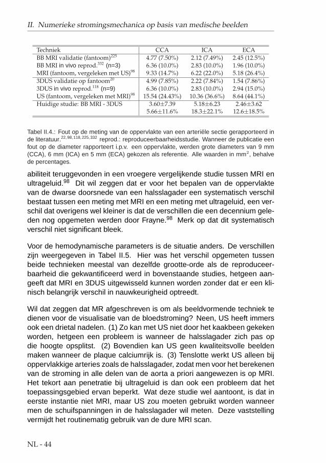
II. Numerieke stromingsmechanica op basis van medische beelden
Techniek CCA ICA ECABB MRI validatie (fantoom)225 4.77 (7.50%) 2.12 (7.49%) 2.45 (12.5%)BB MRI in vivo reprod.332 (n=3) 6.36 (10.0%) 2.83 (10.0%) 1.96 (10.0%)MRI (fantoom, vergeleken met US)98 9.33 (14.7%) 6.22 (22.0%) 5.18 (26.4%)3DUS validatie op fantoom20 4.99 (7.85%) 2.22 (7.84%) 1.54 (7.86%)3DUS in vivo reprod.118 (n=9) 6.36 (10.0%) 2.83 (10.0%) 2.94 (15.0%)US (fantoom, vergeleken met MRI)98 15.54 (24.43%) 10.36 (36.6%) 8.64 (44.1%)Huidige studie: BB MRI - 3DUS 3.60±7.39 5.18±6.23 2.46±3.62
5.66±11.6% 18.3±22.1% 12.6±18.5%
Tabel II.4.: Fout op de meting van de oppervlakte van een arteriele sectie gerapporteerd inde literatuur.22,98,118,225,332 reprod.: reproduceerbaarheidsstudie. Wanneer de publicatie eenfout op de diameter rapporteert i.p.v. een oppervlakte, werden grote diameters van 9 mm(CCA), 6 mm (ICA) en 5 mm (ECA) gekozen als referentie. Alle waarden in mm2, behalvede percentages.
abiliteit teruggevonden in een vroegere vergelijkende studie tussen MRI enultrageluid.98 Dit wil zeggen dat er voor het bepalen van de oppervlaktevan de dwarse doorsnede van een halsslagader een systematisch verschilbestaat tussen een meting met MRI en een meting met ultrageluid, een ver-schil dat overigens wel kleiner is dat de verschillen die een decennium gele-den nog opgemeten werden door Frayne.98 Merk op dat dit systematischverschil niet significant bleek.
Voor de hemodynamische parameters is de situatie anders. De verschillenzijn weergegeven in Tabel II.5. Hier was het verschil opgemeten tussenbeide technieken meestal van dezelfde grootte-orde als de reproduceer-baarheid die gekwantificeerd werd in bovenstaande studies, hetgeen aan-geeft dat MRI en 3DUS uitgewisseld kunnen worden zonder dat er een kli-nisch belangrijk verschil in nauwkeurigheid optreedt.
Wil dat zeggen dat MR afgeschreven is om als beeldvormende techniek tedienen voor de visualisatie van de bloedstroming? Neen, US heeft immersook een drietal nadelen. (1) Zo kan met US niet door het kaakbeen gekekenworden, hetgeen een probleem is wanneer de halsslagader zich pas opdie hoogte opsplitst. (2) Bovendien kan US geen kwaliteitsvolle beeldenmaken wanneer de plaque calciumrijk is. (3) Tenslotte werkt US alleen bijoppervlakkige arteries zoals de halsslagader, zodat men voor het berekenenvan de stroming in alle delen van de aorta a priori aangewezen is op MRI.Het tekort aan penetratie bij ultrageluid is dan ook een probleem dat hettoepassingsgebied ervan beperkt. Wat deze studie wel aantoont, is dat ineerste instantie niet MRI, maar US zou moeten gebruikt worden wanneermen de schuifspanningen in de halsslagader wil meten. Deze vaststellingvermijdt het routinematig gebruik van de dure MRI scan.
NL - 44

II.5. Ultrageluid of Magnetische Resonantie?
arterie WSS OSI WSSGs WSSGt WSSAG[N/m2] [-] [N/m3] [N/(s.m2)] [rad/m]
CCA 0.314 (45.9%) 0.0658 (104%) 56.1 (35.3%) 1.80 (24.8%) 96.2 (78.0%)ICA 0.534 (44.0%) 0.0416 (123%) 164 (54.5%) 3.34 (36.6%) 74.5 (91.6%)ECA 0.397 (40.0%) 0.0420 (193%) 149 (52.8%) 2.11 (28.1%) 90.4 (88.4%)
SAMEN 0.411 (42.7%) 0.0481 (166%) 150 (55.4%) 2.29 (29.1%) 87.6 (86.3%)Thomas332 0.44 (32%) 0.021 (109%) 38 (55%) - 61 (73%)
Glor121 0.43 (37.9%) 0.025 (123%) 214 (65.7%) 2.35 (30.2%) 68.1 (79.8%)
Tabel II.5.: De onzekerheid (RMSE) opgemeten voor de hemodynamische parameters bij devergelijking van MRI en 3DUS. Tabel II.1 legt uit hoe deze waarden begroot worden. Hetpercentage tussen haken is de RMSE gedeeld door de gemiddelde waarde (n=8 en niet n=9omdat 1 vrijwilliger verkeerd gescand werd met 3DUS). Ter vergelijking staan de resultatenvan twee MRI reproduceerbaarheidsstudies aangegeven.121,332
NL - 45

II. Numerieke stromingsmechanica op basis van medische beelden
NL - 46

III. In vivo Toepassingen
III.1. Inleiding
Het eerste deel van dit proefschrift heeft zich gefocust op de techniek zelf.Het opdrijven en het kwantificeren van de nauwkeurigheid stonden daarbijcentraal. Nu de nauwkeurigheid gekend is, kan de techniek ingezet wordenvoor verschillende klinische doeleinden.
Een van de toepassingen waar het meest van verwacht wordt, is pre-opera-tief onderzoek. Hier wordt bijvoorbeeld een patient die een aneurysma terhoogte van de halsslagader heeft, naar de scanner gebracht. Een aneu-rysma is een verzwakking van de vaatwand, waardoor het onder de drukvan het bloed gaat uitstulpen. In een verregaand stadium zal dit aneurysmaopenbarsten hetgeen doorgaans leidt tot de dood. Tegenwoordig zal menop basis van de grootte van het aneurysma beslissen over te gaan tot eenoperatie. Dit is echter een gevaarlijk criterium: sommige aneurysmata gaanbarsten terwijl ze klein zijn, andere zijn nog stevig genoeg bij een belangrij-ke omvang. In het eerste geval moet men sneller ingrijpen, in het tweedegeval is het niet verantwoord om de (zwakke) patient een gevaarlijke en dureoperatie te doen ondergaan. Actueel opereert men bij een alarmerendeomvang van het aneurysma, maar in feite zou de sterkte van de vaatwandeen beter criterium zijn op basis waarvan men zou moeten beslissen omte opereren. Het combineren van een beeldvormende techniek met CFD(computational fluid dynamics of numerieke stromingsmechanica) laat toede schuifspanningen aan de wand te berekenen. De beslissing om overte gaan tot een operatie laten afhangen van waarde van de spanningen inplaats van de omvang van een aneurysma zou een aanzienlijke maatschap-pelijke last verlichten en bovendien een geldbesparing met zich meebren-gen.
Behalve voor aneurysmata heeft deze techniek een belangrijke rol te ver-vullen bij patienten met stenosen of vernauwingen ter hoogte van de hals-slagader. De plaque die in deze zone geconstateerd wordt, kan door eenchirurgische ingreep verwijderd worden (endarterectomie). Deze operatie
NL - 47

III. In vivo Toepassingen
is echter zeer duur waardoor de verzekeringsmaatschappijen dergelijke in-grepen enkel toestaan wanneer het duidelijk is geworden dat de patient lastondervindt van die plaque. Dat wil zeggen dat de operatie pas geschiedtnadat de patient een zogenaamde TIA overleeft (Transient Ischeamic At-tack). Een TIA is een herseninfarct van voorbijgaande aard. De bloedtoe-voer naar een deel van de hersenen wordt dan afgesloten totdat de ob-struerende bloedklonter terug is opgelost. TIA’s kenmerken zich door duize-ligheid, moeite om te spreken, verlamming van gezicht of ledematen of tijde-lijk verlies van de zintuigen. Bij het optreden van een TIA wordt een ingreepzeer acuut en nogal vaak komt de ingreep te laat, i.e. na verlies van eendeel van de hersenactiviteit of sterfte. De bestudeerde techniek kan niet-invasief de krachten begroten die op de plaque inwerken. Kennis van diekrachten en kennis van de morfologie van de plaque laten toe een gefun-deerde uitspraak te maken over de kans dat een stukje kalk zou afbreken.Als de nauwkeurigheid van de techniek gekend is, kunnen prospectieve stu-dies ondernomen worden om na te gaan of het veiliger is op basis van eenverdeling van de krachten over te gaan tot een operatie eerder dan te wach-ten tot de eerste TIA zich voordoet.
Hoewel de techniek in dit proefschrift zich enkel op de halsslagader heeftgefocust, is haar toepassingsgebied niet beperkt tot de slagaders in de hals,maar kan ze net zo goed gebruikt worden bij aneurysmata van de aorta,bypasses van de femoralis (beenslagader), of bij problemen met de nier-doorbloeding. Het combineren van medische beeldvorming en CFD heeftdan ook een zeer breed toepassingsgebied met hoge maatschappelijke re-levantie en is een groeipool binnen het biomedisch ingenieursonderzoek.
Binnen het kader van dit proefschrift werd de techniek ingezet bij twee kli-nische studies. Een eerste studie ging na wat de impact is van het draaienvan het hoofd op de doorstroming in de halsslagader (deel III.2). Een anderproject bestudeerde de veranderingen in geometrie en doorstroming vande halsslagader na orale inname van verschillende anti-hypertensiva (deelIII.3).
NL - 48

III.2. Het draaien van het hoofd
III.2. Het draaien van het hoofd
III.2.1. Inleiding en proefopstelling
In de literatuur werd er vastgesteld dat de halsslagaders zich anders posi-tioneren wanneer men het hoofd draait.314 Dat de geometrie van de hals-slagader een beweging ondergaat bij het draaien van het hoofd was geweten,de impact ervan was echter ongekend. Studies241 suggereerden dat her-seninfarcten te wijten kunnen zijn aan een langdurige slechte doorstromingvan de halsslagader tengevolge van een langdurige slechte positioneringvan het hoofd vb. bij het telefoneren. Het testen van deze suggestie waseen van de doelstellingen van deze studie.
Doel van deze klinische studie was de impact van het draaien van het hoofdop de doorstroming van de halsslagader te bestuderen. Hiertoe werden 9gezonde vrijwilligers gescand met US in twee posities: eenmaal met hetgezicht recht voor zich uit, en een andere maal met het hoofd 90 gradengedraaid naar links. Het belang van de studie ligt hem in het feit dat voor heteerst de veranderingen in geometrie, waarvan men wist dat ze voorkwamen,gekwantificeerd werden. Bovendien werd de impact van deze veranderin-gen op de doorstroming van de halsslagader mee begroot.
III.2.2. Resultaten
Figuur III.1 toont aan hoe de doorstroomoppervlakte van de carotis commu-nis, de planariteit, het bloeddebiet en de gemiddelde schuifspanning wijzig-de bij het draaien van het hoofd. Men stelde vast (Figuur III.1 (a)) dat dedoorstroomoppervlakte niet wijzigde. De positie van de takken van de hals-slagader t.o.v. elkaar (Figuur III.1 (b)), het debiet bloed (Figuur III.1 (c)), deschuifspanningverdeling (Figuur III.1 (d)) en de OSI wijzigden op individuelebasis significant nadat het hoofd gedraaid werd. Samen met de wijzigingenin geometrie werd dus duidelijk dat ook de doorbloeding van de halsslagader(en dus de hersenen) ernstige veranderingen ondergaat.
NL - 49

III. In vivo Toepassingen
Recht Gedraaid20
30
40
50
60
CC
A O
pper
vlak
te [m
m²] (p=0.315)
(a)
Recht Gedraaid0
5
10
15
NP
[%
]
(p=0.565)
(b)
Recht Gedraaid2
3
4
5
CC
A D
ebie
t [m
l/s] (p=0.347)
(c)
Recht Gedraaid0.4
0.6
0.8
1
1.2
1.4
WS
S [
N/m
2 ]
(p=0.822)
(d)
Figuur III.1.: Verandering in arteriele oppervlakte (a), planariteit NP (b), debiet (c) en WSS(d) bij het draaien van het hoofd. Het zwarte punt met de verticale lijn is het gemiddelde± standaard deviatie over alle proefpersonen (n=9) in een bepaalde positie (‘Recht’: hoofdrecht; ‘Gedraaid’: hoofd 90° gedraaid). De grijze punten zijn individuele metingen, 1 per vrij-williger. Metingen die eenzelfde vrijwilliger toebehoren zijn met een streepjeslijn verbonden.De p-waarde test de hypothese dat de gemiddeldes per positie (i.e. de zwarte punten) gelijkzouden zijn.
III.2.3. Impact van de studie
Met deze studie werd gesuggereerd dat plaque in de halsslagader zich ineen veilige situatie kan bevinden in de ene positie, maar ten gevolge vande gewijzigde krachtenverdeling zou kunnen afbreken en een herseninfarctveroorzaken in de andere positie. Gelijkaardige lessen worden getrokkendoor fabrikanten van implantaten voor de halsslagader. ‘Stents’ zijn spiralenuit metaal of kunststof. Deze worden in de halsslagader ingeplant met debedoeling een vernauwd vat terug open te duwen. Stents zijn zeer gevoeligaan revascularisatie: een situatie waarbij de stent overgroeid wordt door het
NL - 50

III.3. Impact van bloeddrukverlagende geneesmiddelen
vaatwandweefsel, wat leidt tot een nieuwe vernauwing van het vat. Om dituit te sluiten, wordt de stroming over de stent bestudeerd: bepaalde stro-mingssituaties zijn behulpzaam bij het vermijden van revascularisatie. Dehuidige studie toont echter aan dat een stromingssituatie goed kan zijn bijeen normale houding van het hoofd, terwijl revascularisatie net in de handkan gewerkt worden in een andere houding. Producenten van stents dienendan ook hun implantaten in verschillende houdingen uit te testen. Dezelfderedenering is geldig voor plaque-omleggingen. Een plaque-omlegging isnet als de stent een implantaat voor de halsslagader, zij het met een anderdoel. Een stent verwijdt de arterie, terwijl een plaque-omlegging afgebrokenplaque omleidt naar weefsels in het hoofd anders dan de hersenen. Alduswordt de patient gespaard van herseninfarcten. Ook dergelijke implantatenworden onderzocht naar revascularisatie en ook hier moet men rekeninghouden met de gewijzigde stromingssituatie bij het draaien van het hoofd.
III.3. Impact van bloeddrukverlagendegeneesmiddelen
III.3.1. Inleiding
In de literatuur werd door Stanton302 melding gemaakt van twee bloeddruk-verlagende geneesmiddelen, amlodipine en lisinopril, die elk met vrucht erinslagen de bloeddruk op lange termijn te verlagen. Deze bloeddrukverlagingging echter gepaard met verschillende veranderingen in de morfologie vande halsslagader: bij lisinopril verkleint de vaatdiameter en de wanddikte,hetgeen te verwachten is na een bloeddrukdaling. De amlodipine behan-deling zal ondanks die bloeddrukdaling toch de diameter handhaven en dewanddikte nog meer doen dalen. Er moet dus een mechanisme zijn dat dediameter verwijdt om de vernauwing tengevolge van de bloeddrukdaling te-niet te doen. Figuur III.2 herneemt de resultaten van Stanton. Amlodipine iseen calcium kanaal blocker, en verlaagt de druk door een perifere relaxatievan de gladde spiercellen hetgeen leidt tot een vasodilatatie en een vermin-derde perifere weerstand. Lisinopril is een ACEa-inhibitor, i.e. een stof diede aanmaak van angiotensine II, een vasoconstrictor, vermijdt.
aACE: angiotensin converting enzyme
NL - 51

III. In vivo Toepassingen
Figuur III.2.: De resultaten van Stanton302 samengevat. De opgemeten verschillen zijn eengevolg van een behandeling van 52 weken met amlodipine (Calcium-kanaal blocker) of lisino-pril (ACE inhibitor). IMT: intima-media dikte, LD: interne diameter van het bloedvat; IMA:wandmassa. ‘*’ is significant (p=0.05).
III.3.2. Proefopstelling en Resultaten
De hypothese in onze studie was dat de veranderingen op lange termijngerelateerd zouden zijn aan acute veranderingen in schuifspanning. Hiertoewerden 10 vrijwilligers met een hoge bloeddruk onderworpen aan achtereen-volgens drie behandelingen die elk 1 week duurden: een amlodipine, eenlisinopril en een placebo behandeling. De meeste (8) werden gescand metTOF MRI en 2 claustrofoben met US.
Figuur III.3 toont de schuifspanningen voor 3 van de 10 bestudeerde hyper-tensieven. Merk op hoe de geometrie van de halsslagader nauwelijks wijzigtna elke behandeling. De schuifspanning nam hogere waarden aan bij eenamlodipine behandeling. Hoge schuifspanningen initieren in de vaatwandeen reflex die het bloedvat zullen doen verwijden, een reflex die tot doelheeft de schuifspanning te normaliseren. Deze adaptieve verwijding vande halsslagader zal de doorstroomoppervlakte vergroten en de vaatwanduitrekken, hetgeen overeen komt met de vaststellingen op lange termijn endus de resultaten van Stanton302 verklaard.
III.3.3. Besluit
Aldus heeft de techniek gebaseerd op de integratie van medische beeld-vorming en biomechanische modellering, bewerkstelligd in dit proefschrift,
NL - 52

III.3. Impact van bloeddrukverlagende geneesmiddelen
Figuur III.3.: De WSS distributie voor 3 patienten (rijen) na inname van amlodipine (Calciumblocker, links), placebo (midden) en lisinopril (ACE-inhibitor, rechts).
bijgedragen tot het begrip van de werking van cardiovasculaire genees-middelen. Een dergelijke studie, die een antwoord bood op een vraag uitde industrie, was enkel mogelijk dankzij de beschikbaarheid van een vol-doende nauwkeurige techniek voor het begroten van de schuifspanningenin de halsslagader.
NL - 53

III. In vivo Toepassingen
NL - 54

IV. Samenvatting en Besluit
Op het eind van vorige eeuw werd duidelijk dat het combineren van beeld-vormende technieken met numerieke stromingsmechanica een middel wasdat in staat zou moeten zijn om niet-invasief schuifspanningen te bepalenin bloedvaten. Ondanks dit besef en vroege bescheiden succesjes bestonder veel scepsis over de nauwkeurigheid van deze techniek. Dat die tech-niek het waard was om verder onderzocht te worden, wordt bewezen doorde vele ziektes die beter begrepen of gediagnosticeerd zouden worden in-dien de schuifspanning met een voldoende nauwkeurigheid bepaald konworden. Daarom werd in een eerste deel van het proefschrift de nadrukgelegd op het kwantificeren en het opdrijven van de nauwkeurigheid voortoepassing op de bloedstroming door de halsslagader. Dit proefschrift toontverder aan dat ultrageluid (echografie) net als magnetische resonantie an-giografie (MRA) in staat is om dienst te doen als initiele beeldvormende tech-niek, hetgeen, gezien de grotere kost van deze laatste, een grote besparingbetekent. Bovendien wordt de techniek toegankelijk voor vele hospitalen,dus ook voor hospitalen die over beperkte middelen beschikken.
Eens de nauwkeurigheid gekend was, lieten de toepassingen niet op zichwachten. In een tweede deel van het proefschrift werden dan ook tweestudies in zeer uiteenlopende domeinen uitgevoerd. De eerste studie on-derzocht de impact van bewegingen van het hoofd op de doorstroming vande halsslagader. Een tweede studie ging - op vraag van de farmaceutischeindustrie - na of er een verschil in stromingssituatie bestaat wanneer tweeeven efficiente bloeddrukverlagende geneesmiddelen ingenomen worden.Deze twee studies toonden aan dat het toepassen van de techniek geenverre droom meer is, maar reeds binnen het kader van dit proefschrift werdgerealiseerd.
NL - 55


ENGLISH
TEXT
1


Statistics is like a Bikini:
what is revealed is suggestive,
but what is concealed is vital.

Preface
The manuscript describes and uses a technique for calculating the flow pro-files in human carotid arteries. The technique is based on medical imagingand numerical modelling: it is called image-based computational fluid dy-namics (CFD). In the introductional part (part A), the anatomy of the carotidarteries is explained, as well as its main pathologies. After an explanationon the numerical tools used in this thesis, the history of the technique ispresented. Subsequently, part B investigates the technique from a tech-nical point of view. The result of this part is a detailed description of thetechnique, together with figures on its accuracy, reproducibility and operatordependence. Once the technique was established, it was successfully usedin two clinical studies described in part C. A first study investigated the effectof head turns on carotid geometry and flow. In a second study, a group ofpatients were administered two anti-hypertensive drugs. Aim was to analysethe effects on carotid geometry and flow. The final part contains a summaryand technical notes aimed at improving the current protocols.
4

Part A.
INTRODUCTION
5


I. Anatomy and Physiology
Calculation of blood flow in the carotid bifurcation is the major topic of inter-est for this thesis. In the introductory section, the location and anatomicalfeatures of the carotid arteries are described (section I.1). In the followingsection, the values for blood pressure and flow in healthy humans are given.The composition of arterial wall is described in section I.3 and finally, the twolast sections discuss specific functions of the carotid bifurcation other thanblood supply.
I.1. Location of the Carotid Bifurcation in the BloodSupply chain
All tissues in the human body require a blood supply for their survival. Bloodis pumped through the body by the contraction of the heart muscle, whichis in fact a cavity which is filled during its relaxation phase (diastole) andcontracts in systole. The contraction of the cavity causes blood to leave theheart at high velocities and pressures. The pressure has to be high sincethe blood needs to travel through the blood vessels and tissues, using theenergy acquired in the heart. The tissues in the upper extremities of thebody, the face and brain, set the target for heart: the blood pressure gener-ated in the heart, needs to be high enough to reach the upper extremities.There are a number of blood vessels that transfer blood through the necktowards the head. The carotid arteries are two of them.
There are 3 carotid arteries on either side of the neck: the Common CarotidArtery (CCA) bifurcates into the Internal (ICA) and the External CarotidArtery (ECA). Arteries in general are vessels that carry blood away fromthe heart and to the tissues. The role of an artery in the vascular tree canbe deduced from its cross-sectional size (see Table I.1).73 The commoncarotid arteries are 2 of several arteries that supply blood to the head. SeeFigure I.1 (a)107 for a schematic diagram showing the position of the rightcarotid bifurcation. Figure I.1 (b)327 shows the relative positions of all the
7

I. Anatomy and Physiology
Vessel Type Diameter (mm) FunctionAorta & Very Large Arteries 4.0 - 25 Pulse dampening and distribution
Large Arteries 1.0 - 4.0 DistributionSmall Arteries 0.5 - 1.0 Distribution and resistance
Arterioles 0.01 - 0.50 Resistance (pressure/flow regulation)Capillaries 0.006 - 0.010 Exchange
Venules 0.01 - 0.50 Exchange, collection, and capacitanceVeins 0.5 - 5.0 Capacitance function (blood volume)
Large Veins and Vena Cava 5.0 - 35 Collection
Table I.1.: The function of the arteries and veins is linked to their cross-sectional size. TheCCA and ICA are both damping and distributing arteries, the ECA is usually smaller and thusjust a distributing artery.
(a) Right Carotid Bifurcation107 (b) Relative positions of arteries origi-
nating in the aortic arch327
Figure I.1.: The position of the carotid arteries in the human body.
arteries originating from the aortic arch. The right common carotid arterybranches from the brachiocephalic artery and extends up the right side ofthe neck. The left common carotid artery branches immediately from theaorta and extends up the left side of the neck. Each carotid artery branchesinto internal and external vessels approximately near the top of the thyroid2
(i.e. the small butterfly-shaped gland, located in the neck, wrapped aroundthe windpipe, behind and below the Adam’s Apple area).
The ICA is the primary blood supply to the brain and the eyes. It anasto-moses with the vertebral arteries and the contralateral internal carotid arteryin the cerebral arterial circle (of Willis) as shown in Figure I.2.227 Note thatthe ICA’s are not the only arteries feeding the brain. At the point where theICA emerges from the common carotid, i.e. immediately after branching, theinternal carotid widens a little. This small widening is know as the carotid
8

I.1. Location of the Carotid Bifurcation in the Blood Supply chain
Figure I.2.: The circle of Willis is the blood supply of the brain.227
sinus or carotid bulb . Its shape, length and width can be very different fromone subject to the other. The ECA branches off to supply oxygenated bloodto the throat, neck, glands, tongue, face, mouth, ear, scalp and dura materof the meninges (i.e. the ensemble of layers covering the brain, separatingit from the skull).
Due to the carotid bifurcation being a complex 3D structure on one handand the large inter-subject variations on the other hand, there is no cleardefinition of a ‘typical’ carotid geometry. Nevertheless, Figure I.3 illustratesthe general features observed in a carotid bifurcation: the CCA widens andbifurcates into the ICA (right) and ECA (left). The carotid bulb marks the ori-gin of the ICA while the ECA is smaller than the ICA. In the past, attempts toquantify carotid geometry have failed to reach an agreement. Gnasso123 re-ported 5.9 mm as typical CCA lumen diameter (LD) (n = 42, mean age 49.0years). Geigy Scientific Tables174 showed 6.1 mm (n = 20, ‘young adults’),Boutouyrie37 found 5.21 mm (n = 15 females, 43±16 years), Ferrara95 re-ported 6.0±0.8 mm (n = 20, 47.0±7 years) and Liang182 5.47±0.08 mm
9

I. Anatomy and Physiology
Figure I.3.: Typical carotid geometry;15 z=0mm is located at the bifurcation apex.
(n = 237) for non-smokers respectively as opposed to 6.09±0.11 mm (n =185, 63.1±6.6 years) for smokers. Sass273 derived the change in CCA LDas a function of age and gender (n = 369). Table I.2 summarises Sass’sfindings. Females between 41 and 45 years have an average LD of 5.17± 0.57 mm (n = 37) which agrees with Boutouyrie’s reports.37 Scheel per-formed a similar study a few years later,275 and found CCA LD’s of 6.0±0.7mm (n = 24, ages 20-39), 6.1±0.8 mm (n = 24, ages 40-59) and 6.2±0.9mm (n = 30, ages 60-85). It is clear from Sass’s and Scheel’s results thata typical carotid bifurcation geometry is impossible to define. Note that theLD in the discussed studies37,95,123,174,182,273,275 was measured by B-modeultrasound (see section II.17 on page 49) in the proximal CCA, i.e. the CCAbefore it starts widening. Studies that include the region of the flow dividerin the definition of the CCA will find a larger CCA LD. Bladin29 found thatthe distal end of the CCA is on average 4% larger than the proximal CCA (n= 125). The bifurcation zone, the most distal part of the CCA, is obviouslylarger.
The subject-variability is even greater for ICA geometry than for CCA LD.Diameter of the ICA bulb has been reported to be 27±20% greater than thatof the proximal CCA.29 A different study conducted by Schulz279 found asmaller disproportion between the proximal CCA LD and the bulb diameter:13±18%. Moving up in the ICA, Schulz278 reported that LD in the proximalICA (after the bulb) is 36±11% smaller than the LD in the distal CCA (beforebulb). The ICA LD, but not the bulb diameter, is larger for women by 13%.279
10

I.2. Pressure and Flow
age 10-12 13-14 15-16 17-18 19-24 35-40 41-45 46-53M=23 M=13 M=20 M=17 M=12 M=19 M=34 M=31F=23 F=24 F=23 F=17 F=21 F=33 F=37 F=22
Male 4.99 4.99 5.14 5.39 5.36 6.01 6.07 5.97±0.41 ±0.39 ±0.44 ±0.50 ±0.60 ±0.46 ±0.62 ±0.57
Female 4.92 4.88 4.87 5.01 4.92 5.09 5.17 5.29±0.54 ±0.45 ±0.36 ±0.49 ±0.44 ±0.46 ±0.57 ±0.51
Table I.2.: Common carotid LD as measured by Sass.273 M=number of participating males.F=number of participating females. All values in mm, reported as mean value ± standarddeviation.
From a study conducted by Long194 using time-of-flight magnetic resonanceimaging (see VI.1), it can be seen that the ICA LD drops from very highvalues (up to 8 mm) in the bulb to below 5 mm. Scheel275 measured ICAdiameters in 78 subject ‘1.5 to 2 cm’ above the carotid bulb. He reported4.8±0.5 (ages 20-39), 4.7±0.6 (ages 40-59) and 4.9±0.8 mm (ages 60-79).
The ECA is not as complex as the ICA: it has no explicit widening of thelumen at the start, making it more comparable to a cylindric tube than theICA. Nevertheless, there are a number of side branches (such as the thy-roid artery) branching off the proximal ECA.308,386 Schulz278 measured thatthe LD in the proximal ECA (before any branching) is 44±12% smaller thanthe LD in the distal CCA (before bulb). Scheel275 measured ECA diame-ters as well: 4.0±0.4 (ages 20-39), 4.1±0.7 (ages 40-59) and 4.3±0.7 mm(ages 60-79). From Long’s study,194 ECA LD is found to be very subject-dependent, varying from 2.5 to 5 mm. Note that errors were found to be largein ECA due to its relatively small size and the presence of side branches.
With knowledge of the LD’s of the separate arteries, their function becomesclear. The CCA and ICA LD are greater than 4.0 mm, belonging to the ‘verylarge arteries’ whose main functions are to damp the pressure pulse (seesection I.2) and to contribute to blood distribution. The ECA can be classifiedas a distribution artery.
I.2. Pressure and Flow
Pressures in the arteries, veins and heart chambers are the result of thepumping action of the heart. Figure I.4 illustrates the pressure variation inthe heart and the aorta during a cardiac cycle in a healthy human. When theventricles of the heart contract, left ventricular (LV) pressure rises until the
11

I. Anatomy and Physiology
Pressure Systolic Diastolic Pulse MeanAorta 100-130 60-90 30-50 70-105Left Ventricle 100-130 4-12 - -Left Atrium 15 4 - 4-12Pulmonary Artery 15-30 6-12 - 9-18Right Ventricle 25-30 0-8 - -CCA PressuresMitchell221 (n = 30, aged 59±10) 119.1±11 n/a n/a n/aMitchell222 (n = 40, aged 57±10) 124±24 n/a n/a 94±12Boutouyrie37 (n = 15, aged 43±16) n/a n/a 47±16 n/aLiang182 (n = 237, aged 62.6±6.8) n/a n/a 36±10 n/aWaddell344 (n = 57, aged 59±9) 116±2 n/a 38±1 n/a
Table I.3.: Normal pressures [mmHg].72 The pulse pressure is the difference between sys-tolic and diastolic pressure.
LV pressure exceeds the aortic pressure. The blood flows from the ventricleto the aorta through the opened aortic valve, the valve separating the aortafrom the LV. As blood enters the aorta, the aortic pressure begins to rise andforms the systolic pulse. When the heart starts relaxing, the pressure dropsto a certain point where the LV pressure is lower than the aortic pressure. Atthis point, the aortic valve closes again. Closure of the aortic valve producesa disturbance or a notch in the aortic pressure called the dicrotic notch .Thanks to the elastic recoil, the aorta now functions as a blood reserve underpressure. It slowly empties into the vascular tree, feeding all body tissueswith blood. Normal blood pressures are shown in Table I.3 as published byDarovic.72
The aortic blood flow resulting from this pressure curve is illustrated in FigureI.4. In a resting state, for a normal adult, the blood flow ranges between 4and 8 litres per minute.72 Velocities in the aorta go up to 2m/s. Furtherdown the branches, blood velocity declines and the pressure and flow ratecurves change significantly in shape. Figure I.5 shows how pressure, meanvelocity and the total perfused cross-sectional area change throughout thevascular tree. Note how pressure can be higher in large arteries distal fromthe aorta. This is due to pressure wave propagation and reflection withinthe arterial tree. These pressure wave reflections originate from pressurewaves bouncing off both distal and proximal bifurcations and the geometricand elastic tapering of the arterial network. In the capillaries, the tiny vesselsat the extremities of the arteries, the mean velocity is brought down to 1mm/s, and the pressure is constant.
Where is the carotid artery situated in this framework? In the commoncarotid artery, closer to the aorta, velocities can be as high as 1.5 m/s. The
12

I.2. Pressure and Flow
Figure I.4.: Pressure and flow during one cardiac cycle.377
carotid artery is one of the arteries where, due to wave reflections, pres-sures can be higher than in the aorta. Both pressure and flow are verypulsatile. Figure I.6 (a) shows a typical pressure wave form,222 see TableI.4 for the definition of the feature points. Table I.3 gives an overview ofmeasured values for carotid pressures, from which we can see that carotidpressures roughly range from 75-85 (diastole) to 110-130 (systole) in rest-ing state. Note that here, ‘systole’ and ‘diastole’ refer to the maximum andminimum carotid pressure as opposed to the state of the heart muscle.
13

I. Anatomy and Physiology
Figure I.5.: The profile of blood pressure and velocity in the systemic circulation of a restingman. The abscissa is distance along the vessels. The greatest fall in pressure occurs acrossarterioles and the tiniest arteries. This is in agreement with Table I.1 where the smallerarteries have been described as resistances regulating the blood flow to particular organs.Mean velocity is the cardiac output divided by total cross-sectional area of the vascular bedat that point. Pressure in the pulmonary artery (PA) is shown as a dotted line. Ao: humanaorta; VC, human vena cava.
14

I.2. Pressure and Flow
(a) Carotid Pressure (b) Centreline velocity
Figure I.6.: a: Typical carotid pressure in one cardiac cycle.222 b: Vessel spatial peak bloodvelocity (Vpeak) in the common carotid artery measured with a vector Doppler-ultrasoundsystem in a normal human subject.140 For a definition of other feature points, see Table I.4.
Parameter Definitiontfoot Time of rise of pressure
ti Inflection point, signaling return of reflected wavetmax Time of peak pressure ( 6= TMAX )
tes End-systolic timePmin Minimum pressure
Pi Pressure at inflection pointPmax Maximum pressure
Pes End-systolic pressure∆PZc Pressure in common carotid when flow rate
in aorta valve reaches 95% of its maximum - Pmin
TRR Cardiac interbeat intervalVCY C Vessel spatial peak velocity, averaged over one cardiac cycleVMIN Minimum diastolic velocityTMIN Time of diastolic minimum velocity
AMAX Maximum accelerationTA MAX Time of maximum accelerationVA MAX Velocity at point of maximum acceleration
VMAX Maximum systolic velocityTMAX Time of maximum systolic peak-velocity ( 6= tmax)VHM VHM = VMAX−VMIN
2 + VMIN
TLHM Time during early systole at which Vpeak = VHM
TFWHM Time period during which Vpeak ≥ VHM
V0 Velocity at cardiac systoleVDN Minimum velocity in dicrotic notchTDN Time of minimum velocity in dicrotic notch
Table I.4.: Definitions of pressure and peak-velocity wave form feature points.140
15

I. Anatomy and Physiology
Figure I.6 (b) shows a typical velocity measurement in a healthy human sub-ject.140 See Table I.4 for the definition of the feature points. At systole (t=0),the flow ejected by the heart into the aorta has not entered the carotids yet:the flow takes a time TMIN to reach the common carotid. After TMIN , the ve-locities rise steeply until they reach a maximum VMAX , and fall again. Thedicrotic notch, caused by the aortic valve closure, is still noticeable in thecarotid velocity profile. Table I.5 quantifies the average timing and velocityparameters for 17 normal volunteers (24 to 34 years).140 The velocity pro-files were measured 2 cm proximal from the bifurcation apex. Table I.5 alsoshows, for comparison, the same parameters as quantified in other stud-ies.123,170,229,275 Velocities are higher in men than in women. This, togetherwith the larger CCA radius for men (Table I.2), shows that the blood flowthrough the carotid arteries is higher for men.
The velocity wave forms in the ICA and ECA are similar to that in the CCAshown in Figure I.6 (b). Due to the damping effect of the compliant vesselwall, peaks are weakened and the dicrotic notch becomes hard to distin-guish, especially in the ICA. Typical values for ICA and ECA VMAX andVCY C are given in Table I.6 based on studies by Ferrara,95 Nagai,229 Lee170
and Scheel.275 Note the important differences in VMAX between Nagai’sand Scheel’s study. For example, the VMAX is 72±18 cm/s in Scheel’sstudy whereas Nagai measures 82 cm/s in men and 93 cm/s in women ofthe same age groups. This is partly due to the large inter-subject variability(see column 4 in Table I.6), but especially due to the fact that the velocitieswere measured at different locations: ‘1.0 to 1.5 cm distal from the tip of flowdivider’ in Nagai’s study229 and ‘1 to 2 cm above the carotid bulb’ in Scheel’sstudy.275 Lee170 measured the velocities at three sites in the ICA: ‘one lo-cation in the bulb, and two locations in the ICA’. Their results illustrate thelarge range of velocities occurring in the ICA.
As mentioned above, the blood flow for a normal adult ranges between 4 and8 litres per minute or approximately 65 to 130 ml/s,72 of which 13% goes tothe brain (approximately 7 to 14 ml/s). As stated in section I.1 and FigureI.2, an important part of the blood supply to the brain happens through theinternal carotid arteries. Figure I.7 shows measurements of the blood flowin the CCA, ECA and ICA of a healthy subject, measured with MRI (seesection VI.1). Note how the CCA flow wave form is substantially differentfrom the aortic flow wave form (Figure I.4), but very similar to the velocitywave form (Figure I.4(b)): there is a steep rise in flow rate, a maximum, afast decrease in flow rate, a dicrotic notch and further slow decrease in flowrate towards the end of the cardiac cycle. Maximum flow rate in this subjectwas around 25 ml/s, average flow around 7 ml/s. Table I.7 summarises
16

I.2. Pressure and Flow
Parameter Unit Mean Standard Deviation Max MinTRR s 0.917 0.119 1.414 0.601
VCY C cm/s 38.8 7.3 58.7 19.4VMIN cm/s 20.9 4.8 36.2 7.0TMIN s 0.055 0.014 0.118 0.011
AMAX cm/s2 2441 456 8048 1233TA MAX s 0.110 0.010 0.154 0.035VA MAX cm/s 47.7 7.2 114.2 6.4
VMAX cm/s 108.2 17.8 171.2 68.2TMAX s 0.153 0.011 0.189 0.118VHM cm/s 64.6 10.2 100.24 39.7
TLHM s 0.116 0.010 0.151 0.088TFWHM s 0.103 0.024 0.257 0.06
VDN cm/s 19.4 6.6 45.6 5.6TDN s 0.398 0.016 0.448 0.342
VMAX n Mean Standard Deviation AgeGnasso123 42 79.8 16.0 49.0±12.4
Lee170 85 75.2 22.1 59±12Scheel275 24 101 22 20-39
24 89 17 40-5930 81 21 60-85
Nagai229 17 men 115 n/a 20-3924 men 97 n/a 40-4922 men 97 n/a 50-5922 men 89 n/a 60-6927 men 81 n/a 70-7925 women 105 n/a 20-3946 women 92 n/a 40-4938 women 87 n/a 50-5926 women 77 n/a 60-6911 women 76 n/a 70-79
VCY C n Mean Standard Deviation AgeFerrara95 20 34.2 4.8 47.0±7.0
Gnasso123 42 36.2 5.4 49.0±12.4Scheel275 24 40 6 20-39
24 42 7 40-5930 36 10 60-85
Table I.5.: Average timing and velocity parameters for human CCA wave forms as mea-sured by Holdsworth in 17 subjects (24 to 34 years)140 and the comparison with other stud-ies.123,170,229,275 See Table I.4 for a definition of the feature points.
17

I. Anatomy and Physiology
n Age Mean VariabilityVMAX ICA Nagai229
17 men 20-39 82 (50-112)24 men 40-49 76 (60-101)22 men 50-59 80 (59-96)23 men 60-69 79 (62-109)27 men 70-79 71 (40-97)25 women 20-39 93 (52-124)46 women 40-49 87 (58-116)38 women 50-59 87 (60-115)26 women 60-69 86 (60-113)11 women 70-79 75 (43-100)VMAX ICA Lee170
85 (bulb) 59 64.6 ± 23.6(proximal ICA) 59.5 ± 17.3(distal ICA) 65.2 ± 17.1VMAX ICA Scheel 275
24 20-39 72 ± 1824 40-59 65 ± 1030 60-79 58 ± 11VMAX ECA Scheel 275
24 20-39 86 ± 1424 40-59 85 ± 1830 60-79 81 ± 30VCY C ICA Ferrara 95
20 47.0±7.0 32.7 ± 3.0VCY C ICA Scheel 275
24 20-39 39 ± 724 40-59 38 ± 630 60-79 33 ± 8VCY C ECA Scheel 275
24 20-39 30 ± 524 40-59 35 ± 730 60-79 33 ± 11
Table I.6.: Velocities in the carotid branches. VMAX : maximum velocity, VCY C : cycle-averaged peak velocity. All values in cm/s and based on studies by Ferrara,95 Nagai,229
Lee170 and Scheel.275 The fourth column represents a measure of variability, shown eitheras ‘± standard deviation ‘or’ (5-percentile 95-percentile) ’.
18
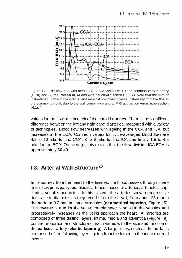
I.3. Arterial Wall Structure
Figure I.7.: The flow rate was measured at two locations: (1) the common carotid artery(CCA) and (2) the internal (ICA) and external carotid arteries (ECA). Note that the sum ofinstantaneous flow in the internal and external branches differs substantially from the flow inthe common carotid, due to the wall compliance and to MRI acquisition errors (see sectionVI.1).49
values for the flow rate in each of the carotid arteries. There is no significantdifference between the left and right carotid arteries, measured with a varietyof techniques. Blood flow decreases with ageing in the CCA and ICA, butincreases in the ECA. Common values for cycle-averaged blood flow are4.5 to 10 ml/s for the CCA, 3 to 6 ml/s for the ICA and finally 1.5 to 4.5ml/s for the ECA. On average, this means that the flow division ICA:ECA isapproximately 60:40.
I.3. Arterial Wall Structure 26
In its journey from the heart to the tissues, the blood passes through chan-nels of six principal types: elastic arteries, muscular arteries, arterioles, cap-illaries, venules and veins. In this system, the arteries show a progressivedecrease in diameter as they recede from the heart, from about 25 mm inthe aorta to 0.3 mm in some arterioles (geometrical tapering , Figure I.5).The reverse is true for the veins; the diameter is small in the venules andprogressively increases as the veins approach the heart. All arteries arecomposed of three distinct layers, intima, media and adventitia (Figure I.8),but the proportion and structure of each varies with the size and function ofthe particular artery (elastic tapering ). A large artery, such as the aorta, iscomprised of the following layers, going from the lumen to the most externallayers:
19

I. Anatomy and Physiology
STUDY N AGE MEAN STANDARD DEVIATION
CCAKeller154 22 23-45 5-8Fitzgerald96 25 42 8.93 ± 1.73Uematsu338 16 21-40 7.98 ± 1.50Uematsu338 14 41-60 7.22 ± 1.15Donis80 66 16-19 6.67 ± 0.45Donis80 50 70-78 5.37 ± 1.90Hamada132 28 71±7 9.57 n/aSchoning277 46 20-63 7.83 ± 2.00Weskott359 174 20-87 6.92 ± 1.45Holdsworth140 17 24-34 6.0 (min-max: 0.4-12.3)Scheel275 24 20-39 7.10 ± 1.65Scheel275 24 40-59 7.23 ± 1.85Scheel275 30 60-85 6.22 ± 1.33ICALeopold175 20 32 4.23 ± 0.93Fortune97 20 33 5.50 ± 0.32Schoning277 46 20-63 4.42 ± 0.43Scheel275 24 20-39 4.62 ± 0.82Scheel275 24 40-59 4.23 ± 0.95Scheel275 30 60-85 3.73 ± 0.72ECASchoning277 46 20-63 2.67 ± 1.1Scheel275 24 20-39 2.42 ± 0.53Scheel275 24 40-59 2.92 ± 1.22Scheel275 30 60-85 2.83 ± 0.87
Table I.7.: CCA, ICA and ECA time-averaged blood flow according to litera-ture.80,96,97,132,140,154,175,275,277,338 Values in ml/s.
1. the lamina intima , or innermost layer, consists of a monolayer of en-dothelial cells separated from the inner layer by a narrow layer of con-nective tissues which anchors the cells to the arterial wall.
2. A large layer of elastic fibres forming the lamina elastica interna .
3. Below this layer are concentric waves of smooth muscle cells inter-mixed with elastic fibres. Elastic lamellae and smooth muscle cells areimbedded in a ground substance rich in proteoglycans. Proteoglycansare formed of disaccharides bound to protein and serve as binding or‘cement’ material in the interstitial spaces.
4. Between the smooth muscle layer and the adventitia (cfr. 5.), thereis again another layer of elastic fibres, the lamina elastica externa .Layers 2, 3 and 4 form the lamina media . The width of layers 1 to 4 isknown as the ‘intima-media thickness’ or IMT.
20

I.4. Pressure Regulation: baroreceptors
Figure I.8.: The layers of an arterial wall.379
5. The outer layer or lamina adventitia is formed of irregularly arrangedcollagen bundles, scattered fibroblasts, a few elastic fibres and bloodvessels which, because of their location, are called vasa vasorum orvessels of the vessels.
This structure of the aorta and large arteries (such as the common carotid)corresponds well to their function which serves as a blood reservoir and tostretch or recoil with the pumping action of the heart. This is the so-calledwindkessel effect .342
The wall of the arterioles contains less elastic fibres but more smooth mus-cle cells than that of the aorta. The arterioles represent the major site ofthe resistance to blood flow and small changes in their caliber cause largechanges in total peripheral resistance.
I.4. Pressure Regulation: baroreceptors
Apart from supplying oxygenated blood, the carotid bifurcations play an im-portant role in the blood pressure regulation. As in the aorta and in the rightheart, the carotid sinus contains baroreceptors . When pressure rises in
21

I. Anatomy and Physiology
the blood circulation, the carotid wall will stretch. Via a cranial nerve (nervenumber ‘IX’) the brain is informed of this pressure rise. At that point, thebrain will incite a series of reactions, aiming to reduce the blood-pressure.The reaction can include decreased heart rate or widening of the arteries(‘vasodilatation’). Thus, when blood pressure rises, this carotid sinus re-flex makes pressure fall.
I.5. Oxygen Regulation: chemoreceptors
The level of carbondioxide (CO2), oxygen (O2) and acidity (H+) in the bloodare closely monitored. The carotid sinus (and the aortic arch) contains in itswall chemoreceptors , bodies that detect changes in blood level of CO2, O2
and H+. If oxygen levels go down or carbon dioxide and hydrogen ion levelsgo up, a signal is sent to the brain, which triggers a rise in blood pressureand influences the breathing. The general purpose is to bring the levels ofCO2, O2 and H+ back to their original values.
22

II. Pathology and Diagnosis
II.1. Carotid Pathology
The carotid artery is susceptible to a number of vascular diseases. Carotiddissection, the pathological condition where blood intrudes the intima media,is defined and discussed in section II.1.1. The most common form of carotiddisease, atherosclerosis, is discussed in section II.1.2. Less frequent butmore severe are carotid aneurysms, a widening of the carotid lumen, whichare explained in section II.1.3.
II.1.1. Carotid Dissection 8,90
Arterial dissection is a condition in which blood penetrates through a tearin the intima, separating and dissecting it from the media. The dissectionmay be focal but more commonly it extends for several centimeters. Themost common sites of arterial dissection are the internal carotid artery (bothintracranially and extracranially, with the former being more rare and severe),and the vertebral artery in its distal extracranial portion where it penetratesthe dura to become intracranial (Figure I.1 (c)). Dissection of intracranial ar-teries, basilar artery and middle cerebral artery, are also possible but muchless common.
See Figure II.1 for an illustration of a carotid dissection. Two streams arevisible in the carotid lumen: a normal stream (red), and a stream underneaththe intima (more colours than just red).106
Cervical artery dissection is a significant cause of stroke in patients youngerthan 40 years. Carotid artery dissections have nonspecific presenting symp-toms such as neurologic deficits and headache and occur at a relativelyyoung age. They often happen in previously healthy individuals and developeither spontaneously or following various degrees of trauma.
23

II. Pathology and Diagnosis
Figure II.1.: A ‘Duplex’ image of common carotid dissection. The black and white image is ac-quired using B-mode Ultrasonography. The black void in the center of the image representsthe CCA lumen. The colours represent blood velocities acquired with Doppler ultrasound(see section VII.1.3). The visualisation of colour Doppler velocities on a B-mode image iscalled a Duplex image. Flow is from left to right. There are two streams visible: a ‘red’ and a‘coloured’ stream. The red stream is the normal blood flow, the coloured stream goes underthe vessel wall and resurfaces further distal.106
While the pathophysiology of carotid artery dissection remains largely un-clear, mechanical factors and other underlying vascular diseases may bethe cause. Dissections usually are subadventitial (between the media andadventitia or within the media), creating a false lumen that can cause steno-sis (LD decrease), occlusion, or pseudoaneurysm of the vessel. Simulta-neously, the dissection may cause the formation of a thrombus (blood clot)from which fragments embolise. Strokes resulting from carotid dissectionthus may have a haemodynamic or embolic origin.
The annual incidence of symptomatic carotid artery dissection is 2.6 per100000.7 The actual incidence may be higher, since many episodes may beasymptomatic or cause only minor transient symptoms and remain undiag-nosed.
Morbidity from carotid artery dissection varies in severity from transient neu-rologic deficit to permanent deficit and death. Intracranial internal carotidartery dissection is associated with a 75% mortality rate. Male-to-femaleratio is 1.5:1.8
Carotid artery dissections are most common in young adults. While themean age for extracranial internal carotid artery dissection is 40 years, in-tracranial dissections are more common in those aged 20-30, with half oc-curring in the first 2 decades. Approximately 20% of strokes in the young
24

II.1. Carotid Pathology
are caused by carotid artery and vertebral artery dissections in the neck,compared to 2.5% in older patients.
II.1.2. Atherosclerosis
II.1.2.1. Definition, Prevalence and Localisation
Arteriosclerosis can be described as: ‘A chronic disease in which thicken-ing, hardening, and loss of elasticity of the arterial walls result in impairedblood circulation. It develops with ageing, and is correlated with hyperten-sion, diabetes, hyperlipidemiaa, and other conditions.’250
Atheroslerosis : ‘A form of arteriosclerosis characterised by the depositionof atheromatous plaques containing cholesterol and lipids on the innermostlayer of the walls of large and medium-sized arteries.’250
Cardiovascular disease (CVD) is responsible for the majority of deaths inboth Europe (33.5% of deaths at 45-54 years of age, 64% of deaths at agesabove 85)371 and the US (39.4% of all deaths in 2000).7 The majority of CVDis attributable to atherosclerosis. The most common form of carotid arterydisease is atherosclerosis. This means that the carotid arteries develop abuild-up of plaque caused by hardening of the arteries. The narrowing ofthe vessel lumen caused by plaque is called a stenosis. When the buildupbecomes very severe, it can cause a stroke.
Other vessels prone to atherosclerosis are the coronary arteries, the visceralbranches of the abdominal aorta, and the infra-renal abdominal aorta andits femoral branches (Figure II.2).75
II.1.2.2. Pathophysiology 131,287
Before elabourating the link with haemodynamics, arteriosclerosis must bewell understood. Figure II.3 shows what happens in the arterial wall. Itusually starts with a subtle damage of the glycocalyx , the layer lining theendothelium. Damage to the glycocalyx leads to damage to the endothelialcells. This lesion will attempt to heal itself by inducing an inflammatory re-action: white blood cells will be called to the lesion by chemicals released
aincreased level of lipids in blood serum
25

II. Pathology and Diagnosis
Figure II.2.: Atherosclerotic plaques tend to form in specific areas of the vascular tree, in-cluding (I) the coronary circulation, (II) the carotid vessels, (III) the visceral branches of theabdominal aorta, and (IV) the infra-renal abdominal aorta and its femoral branches.75
at the lesion site. White blood cells will ingest fatty particles and stay in thelesion zone as so called foam cells . Thus, fatty streaks appear: these arevery common at an early age and some may go away if there are no otherdamaging influences.
Various factors from platelets, white blood cells and the blood plasma makethe muscle cells in the arterial wall increase in number.131 Cholesterol ac-cumulates in these cells causing more damage and further narrowing of theartery. Some of the muscle cells die forming a collection of cholesterol anddead cells (this is the atheromatous plaque ). Calcium may be deposited inthe arterial wall at areas of damage and these areas become scarred form-ing atherosclerotic plaques . Atherosclerotic plaques are characterised by
26

II.1. Carotid Pathology
Figure II.3.: The atherosclerotic process. TIA: transient ischaemic attack; Angina: chestpain; Claudication: predictable pattern of lower leg pain caused by inadequate blood flow toexercising muscle; PVD: peripheral vascular disease; MI: myocardial infarction.131
the accumulation of cholesterol, macrophages, smooth muscle cells and ex-tracellular matrix proteins in the intimal layer of the vessel wall. The tissuesbeyond the narrowing are deprived of a full blood flow and become so-calledischaemic tissues.
At a critical moment, plaque can rupture and blood platelets will clot the le-sion, forming a ‘thrombus’, which may occlude totally the artery (infarction )or may be ripped off, obstructing narrower arteries further downstream theblood-circulation (embolus ). Several factors incite arteriosclerosis, amongthem elevated cholesterol levels, hypertension,315 smoking,31 diabetes mel-litus,66 stress150 and obesity.19 A detailed review of arteriosclerosis wasgiven by Simons.287
The body may be able to dissolve the clot and the situation may revert to anatherosclerotic plaque - usually with more narrowing of the artery.
Instead of narrowing the artery, the above processes may cause the arteryto become weakened so that it balloons out - this is called an aneurysm(See section II.1.3).
II.1.2.3. Treatment
Once a patient has been diagnosed with carotid plaque, several treatmentscan be considered. Anti-hypertensive drugs can be administered, reduc-ing the blood pressure and thus the chances for endothelial or plaque dam-age. Patients are asked to refrain from smoking and from excessive alcohol-
27

II. Pathology and Diagnosis
Figure II.4.: Carotid Endarterectomy. a: Carotid bifurcation clamped and opened. b: CCA-ICA bypass introduced. c: Plaque removal. d: Carotid sewed up.378
consumption. Another medical strategy is the use of platelet anti-aggregants,reducing the chance for blood clotting.
If an artificial widening of the vessel lumen is needed, two treatments arecommonly performed:
1. Carotid Endarterectomy (Figure II.4). Carotid endarterectomy is asurgical procedure where the plaque is removed from the carotid in-ner wall. This ultimately removes the source of material which canpotentially travel from the artery up to the brain causing a stroke. In afirst step (Figure II.4 (a)378), the carotid bifurcation is clamped to pre-vent any blood flow through the bifurcation while an incision is madein the carotid. A piece of flexible tubing is introduced into the carotid,connecting the CCA with the ICA while bypassing the stenosed region(Figure II.4 (b)). The plaque can now be removed (Figure II.4 (c)). Af-ter plaque removal, the carotid is clamped again, the bypass removed,and the vessel wall sewed (Figure II.4 (d)).
2. Carotid Stenting (Figure II.5).300 Carotid stenting is a percutaneoustechnique, i.e. a technique that does not require surgery in the form ofan incision, but requires entry into a peripheral artery i.e. the femoralartery in the groin via a small tube which subsequent catheters andwires are passed through up to the neck where the carotid artery islocated. Once it reaches its destination, the catheter will inflate toopen up the blockage. In some cases, the catheter will leave a ‘stent’at the diseased site: a metal or polymer construction that provides ascaffold to keep blockages from recoiling. Percutaneous techniqueshave the potential for being safer, less traumatic, more cost effective,
28

II.1. Carotid Pathology
Figure II.5.: Carotid stenting: A mechanical device called a ‘balloon’ catheter is inserted intothe narrowed carotid to widen it. The stent, a tiny wire-mesh scaffolding, is then placed inthe newly expanded artery to keep it from narrowing again.300
and feasible in patients at high surgical risk. The procedure needs tobe performed by individuals skilled in using various catheters that haveballoons to open up blockages and/or stents.
Endarterectomy or Stenting? Stenting is less demanding for the patient.The stent is inserted via a catheter, threaded through a small incision inthe groin, up to the neck. Patients typically stay in the hospital overnight. Incontrast, carotid endarterectomy requires general anaesthesia and a two- tothree-day hospital stay. It is performed through an incision in the neck area.However, endarterectomy has been performed since 1954, whereas the firstcarotid stent was placed in 1980. Due to the 26 years of extra experienceand research, carotid endarterectomy is still often regarded as the morereliable technique and thus as the surgical procedure of choice.84,189,267
When is surgery required?
Asymptomatic Carotid Artery StenosisAsymptomatic carotid artery atherosclerosis is highly prevalent in the gen-eral population, particularly the elderly. However, severe (more than 70
29

II. Pathology and Diagnosis
percent area reduction) carotid artery stenosis is rare, especially in asymp-tomatic persons. Compared with symptomatic stenosis, asymptomatic carotidartery stenosis is associated with a relatively low risk of ipsilateralb cerebralinfarction. About 4 percent of adults have asymptomatic neck bruitsc, buta carotid bruit is a poor predictor of extracranial carotid artery disease orhigh-grade stenosis.274
By actuarial analysis, patients with asymptomatic carotid bruits have an es-timated annual risk of stroke of 1.5 percent at one year and 7.5 percent atfive years.366 Asymptomatic carotid artery stenosis of 75 percent or lesscarries a stroke risk of 1.3 percent annually.233 When stenosis is more than75 percent, the combined rate for TIA (transient ischaemic attacque) andstroke is 10.5 percent per year, with most events occurring ipsilateral to thestenosed carotid artery.233
Because of the low risk of stroke in asymptomatic patients, some expertsrecommend surgery only when the degree of stenosis is more than 80 per-cent.28
Symptomaticd Carotid Artery StenosisFor symptomatic patients with carotid artery stenosis, the story is very dif-ferent. Stroke is often caused by atherosclerotic lesions of the carotid arterybifurcation. The degree of internal carotid artery stenosis is the most impor-tant predictor of cerebral infarction among patients with extracranial carotidartery disease.325 The severity of carotid artery bifurcation stenosis is di-rectly related to the risk of stroke.
Through the removal of atherosclerotic plaques, carotid endarterectomy re-stores cerebral blood flow and reduces the risk of cerebral ischemia. Re-sults from three major prospective studies provide compelling evidence forthe benefit of carotid endarterectomy, when performed by experienced sur-geons, in improving the chance of stroke-free survival in high-risk symp-tomatic patients.213,325,351
bIpsilateral: Located on or affecting the same side of the body.250
cA carotid bruit is an abnormal sound, heard when using a stethoscope to listen to bloodflow in the carotid artery. A bruit indicates a fatty buildup.
dtypical symptoms: weakness or total inability to move a body part numbness, loss of sen-sation (tingling), decreased or lost vision (may be partial or temporary), language diffi-culties (aphasia), inability to recognise or identify sensory stimuli (agnosia), loss of mem-ory, loss of coordination, swallowing difficulties, personality changes, mood and emotionchanges, urinary incontinence (lack of control over bladder), lack of control over the bow-els, consciousness changes6
30

II.1. Carotid Pathology
II.1.3. Aneurysms 138
An aneurysm is a bulging out of part of the wall of a blood vessel. Itforms where the wall has weakened, often due to the build-up of plaque.Aneurysms can therefore be, just as stenoses, a consequence of atheroscle-rosis. It may also be an inherited condition or a complication of high bloodpressure (hypertension). Left untreated, aneurysms may tear or burst. Rup-tures are very painful events that cause massive internal bleeding. Thepatient must be treated within minutes in order to have a chance of sur-vival. If an aneurysm bursts in the brain, it could cause a haemorrhagicstroke . If an aneurysm bursts in the chest, there is only a 20 percentchance of survival. Therefore, early diagnosis and treatment are critical.Because aneurysms often produce either no symptoms or mild symptoms(e.g., back pain), routine physical examinations are strongly encouraged sothat a physician can regularly test for warning signs.
There are a number of different types of aneurysms, which include the fol-lowing:138
• Aortic aneurysm: A general condition characterised by the distention,or ballooning out, of part of the wall of the aorta. Typically, the widenedpart of the aorta is considered to be an aneurysm when it is more than1.5 times its normal size. If accompanied by an aortic dissection, it is
(a) Aortic188 (b) Carotid243
Figure II.6.: Aneurysms. a: Different types of aneurysms found in the aorta and its branches:(1) ascending aorta; (2) aortic arch involving the brachiocephalic, carotid, and subclavianarteries; (3) descending portion of the aortic arch; (4) thoracoabdominal aneurysm involvingthe celiac, superior mesenteric, and renal arteries; (5) abdominal aorta and iliac arteries; (6)femoral artery; (7) popliteal artery.188 b: Time-of-flight MR image of a subject with a normalICA on one side and an ICA aneurysm on the other side of the neck.243
31

II. Pathology and Diagnosis
classified as a dissecting aortic aneurysm. Typical aortic aneurysmsare depicted in Figure II.6 (a).188
• Cerebral aneurysm: Also known as a berry aneurysm , this is a bulgein the wall of a blood vessel in the brain (one of the cerebral arteries).A cerebral aneurysm is typically found where the arteries branch atthe base of the brain. The cause is unknown, but smoking increasesa person’s risk of developing this condition.
• Ventricular aneurysm: A bulging or ballooning out of part of the wall ofone of the heart’s lower chambers (ventricles), usually the left. If theaneurysm is present in the wall between the ventricles (the ventricularseptum), it is also known as a ventricular septal aneurysm, an inter-ventricular aneurysm or simply a septal aneurysm. It may be presentsince birth (congenital) or may be a complication of a heart attack orother trauma.
• Carotid aneurysm: In Figure II.6 (b),243 a cross-section of a neck ofa patient has been imaged using time-of-flight magnetic resonanceimaging (TOF MRI). The ICA on one side of the neck is normal, butthe ICA on the other side contains an aneurysm.
• Atrial aneurysm: A bulging or ballooning out of part of the wall of oneof the heart’s upper chambers (atria). If the aneurysm is present inthe wall between the atria (the atrial septum), it is also known as anatrial septal aneurysm (ASA). An ASA has been associated with anincreased risk of stroke and is often accompanied by the presenceof a patent foramen ovale, an opening between the upper chambers(atria) of the heart. Normally, this opening is present in the developingfoetus, and closes shortly after birth. It is often present since birth(congenital).
• Cirsoid aneurysm: The enlargement of a network of blood vesselsthat commonly occurs on the scalp and may result in the formation ofa tumour.
Strategies for preventing an aneurysm include managing high blood pres-sure and preventing the build-up of plaque.
32

II.2. Pressure, Geometry and Flow features
II.2. Pressure, Geometry and Flow features
Now that the carotid diseases are described, the search for potential causesof these diseases can start. Based on its high prevalence and high deathrate, the focus will be on atherosclerosis. It has already been stated (seesection II.1.2) that several factors incite arteriosclerosis, among them ele-vated cholesterol levels, arterial hypertension,315 cigarette smoking,31 dia-betes mellitus,66 stress150 and obesity.19 Other factors include older age,male gender, African-American ethnicity, family history, dyslipidemiae, heartdisease, excessive alcohol intake, abnormal body mass index and low so-cioeconomic status.28 The development of atherosclerotic disease occurs ina localised fashion that spares certain segments of the vascular tree whileaffecting others (see Figure II.2). Cited risk factors for vascular disease aresystemic in nature, and do not explain the specific location of plaques to par-ticular segments of the vascular system. However, there is a strong correla-tion of atherosclerosis with regions of disturbed blood flow, which suggeststhat changes in local haemodynamic forces may affect its development.
In what follows, certain risk factors are studied more closely: pressure, ge-ometry and flow-related features with a clinical significance are defined anddiscussed. In section II.3, these features are translated into physically mea-surable parameters, ‘markers’ of atherosclerosis.
II.2.1. Pressure
A clear relationship between pressure and the presence of atherosclerosishas been established:216 patients undergoing sustained increased bloodpressures have a higher incidence of atherosclerosis. The reason for thisrelationship is not entirely clear. Two theories have been put forward.
1. Atherosclerosis is a hardening of the arterial system. The loss of arte-rial compliance increases the pumping power required for maintainingthe blood circulation. This is achieved by increasing the arterial bloodpressure. In this theory, atherosclerosis is the cause of hypertension.
2. Pressure in the surrounding tissue of an artery is the reference pres-sure, 0 mmHg. Blood pressure is therefore entirely dissipated in the ar-terial wall. This pressure dissipation gives rise to a wall tension which
echanged level of lipids in blood serum
33

II. Pathology and Diagnosis
Figure II.7.: Laplace’s Law. P : pressure in the tube; T : Wall Tension; R: radius. Laplace’slaw can be used to estimate the wall tension in an artery.108 Note that Laplace’s law assumesthin walls, circular tubes and uniform pressures, which is why it can only be used as anapproximation.
can be calculated using Laplace’s law (see Figure II.7): assuming acylindrical shape for the vessel, the tension T is given by
T = P × radius (II.1)
here, P is the blood pressure and the considered radius is the lumenradius. The arterial circumferential wall stress can be derived from thewall tension
σwall =T
IMT=
P × radius
IMT(II.2)
assuming that the pressure is dissipated in the intima and the me-dia. An increased pressure will increase the wall tension. The vesselwall will remodel until it reaches the circumferential wall stress in thenormotensive situation. This is achieved by proliferating the IMT. Thisproliferation enhances the progression of plaque formation.
Apart from its indirect effect on the vessel wall thickness, the pressurehas a direct damaging consequence on the endothelium in the laminaintima. The induced damage could be the onset of the atheroscleroticprocess.
In this second theory, hypertension is the cause of atherosclerosis.
The two theories are probably both happening to a certain extent. In anycase, blood pressure is a clear marker of atherosclerosis.216 It is the mostimportant modifiable risk factor for stroke.28
34

II.2. Pressure, Geometry and Flow features
In a series of publications, Boutouyrie36,37,109,147 and Mitchell221,222 arguedthat not the systolic blood pressure (SBP) or mean arterial pressure (MAP)was the pressure parameter with the highest diagnostic value for atheroscle-rotic pathology, but the pulse pressure (PP). They described how blood pres-sure increased with age in all Western countries, but above the age of 60 theincrease of systolic pressure with age was accompanied by a stabilisationor a decrease in diastolic blood pressure. Since the PP is the difference be-tween systolic and diastolic pressure, there will be a progressive increase inPP despite a stable MAP. This trend results in a growing population with iso-lated or disproportional hypertension: SBP > 160 mmHg and DBP <90mmHg.146 It appears that the PP is an important independent marker ofcarotid intimal thickening in both healthy people and persons with essentialhypertensionf. This is because cyclic stretching (i.e. increased PP) has amore important influence on the expression and growth of smooth musclecells than a static load (i.e. increased blood pressure).36 In conclusion,pulse pressure is, in comparison with systolic or diastolic pressure, a bettermarker for vascular pathology.
II.2.2. Arterial Geometry
II.2.2.1. Basic parameters
Initima-Media Thickness and Lumen Diameter As stated on page 21,the arterial wall consists of three layers: tunica intima, media en externa(Figure I.8). The cumulative thickness of intima and media of large arteries,such as the carotid, is called the intima-media thickness (IMT). The IMT hasbeen widely used as a marker of vascular disease, since it can be a directevidence of the atherosclerotic process. A thickened IMT is either a conse-quence of sustained high blood pressures or evidence of an inflammatoryreaction initiating atherosclerosis as explained on page 25.
A growth in IMT is associated with an increasing chance for stroke or car-diac infarction.34 Moreover, growth in IMT is correlated with a vast spec-trum of other cardiovascular risk factors such as age, male gender, ethnicity,hyperlipidemia, smoking, diabetes mellitus, left ventricle hypertrophy andhypertension.34 Simon285 acquired the IMT in a population of 788 healthysubjects (326 men) of all ages, as shown in Figure II.8. Overall, it can bestated that the IMT increases with age, from values around 390 to 480 µm
fessential hypertension is hypertension with no clearly definable reason
35

II. Pathology and Diagnosis
Figure II.8.: Distribution of ‘normal’ values of common carotid artery far wall IMT in a popula-tion of healthy men and women by age range. Upper and lower limits of bars are 75th upper(P75) and 25th lower percentiles (P25) of IMT distribution within the age range indicated inthe x-axis. Abnormal IMT’s are values above the 75th upper percentile in each category ofage. (n=788 (326 men))285
for young men to 460 to 620 µm for men older than 50. Two more featuresemerge from Figure II.8: (1) women have IMT values significantly lower thanmen and (2) the IMT in the right CCA is larger than that in the left CCA. Thefirst feature can be explained by the fact that men have larger carotid arteries(see Table I.2), the second one has also been reported in other studies77,316
but, as stated by Sun,316 “The mechanism for this asymmetry cannot be elu-cidated from present data and remains unclear” .
The IMT is not constant along the carotid bifurcation.48,76,110,271,316,384 Forhealthy people, Gianaros found that the IMT was 11.1% thicker in the bulb,but 11.1% thinner in the ICA after the bulb than in the CCA, based on 82subjects.110 Similarly, Casiglia found that for hypertensives, the IMT was6.5% thinner in the bulb, and 19.5% thinner in the ICA after the bulb than in
36

II.2. Pressure, Geometry and Flow features
the CCA, based on 97 subjects.48 A separate study suggested that IMT inthe ECA was approximately 87.5% of that in the ICA (post-bulb).384
Derived Parameters Note that the carotid IMT needs to be consideredrelative to the lumen diameter (LD):34 the intima-media layer is subjected tothe pressure difference between the blood in the vessel and the surroundingtissue, according to equation II.2. It shows that the tension in the IMT willbe smaller if LD is smaller. If LD is large, IMT will be adaptively increased,owing to the complex wall remodelling process. Imagine the following fourhypothetical subjects, each with the same blood pressure and carotid bloodflow rate. Subject A has a small LD and a small IMT. Although his IMTmay appear to be low, his IMT/LD will be normal. Subject B has a smallLD and an average IMT. This subject could be classified as normal if onlythe IMT was taken into account. However, his IMT/LD ratio will show thathe has signs of an abnormally thick IMT. Subject C has a large LD and anaverage IMT: the tensile stress in his vessel wall could be relatively high.Subject D has a large LD and a large IMT. Considering the IMT alone, hewould be classified as a pathological case. Considering both IMT and LD,it becomes clear that his IMT needs to be larger in order to alleviate thenormal blood pressure occurring in the vessel. These four examples showthat although IMT is a very valuable marker of atherosclerosis, it shouldalways be considered relative to the local LD.
Another way of taking account of the LD when using the IMT for diagnos-tic purposes, is to calculate the cumulative area of intima and media in anarterial cross-section. This area is called the intima-media area or IMA. Achange in LD could change the IMT passively because of the reduced orincreased tension in the wall. In this case, the vessel wall mass does notchange, it just gets redistributed around the lumen, and the IMA remainsconstant. Taking advantage of the incompressibility of the vessel wall, theIMA (as opposed to the IMT) is therefore a better marker for vascular hyper-trophy since it is independent of variations in blood pressure or LD.
Carotid compliance 167 Arterial compliance is defined as the change inarterial volume induced by a pressure change:
C =∂V
∂p(II.3)
37
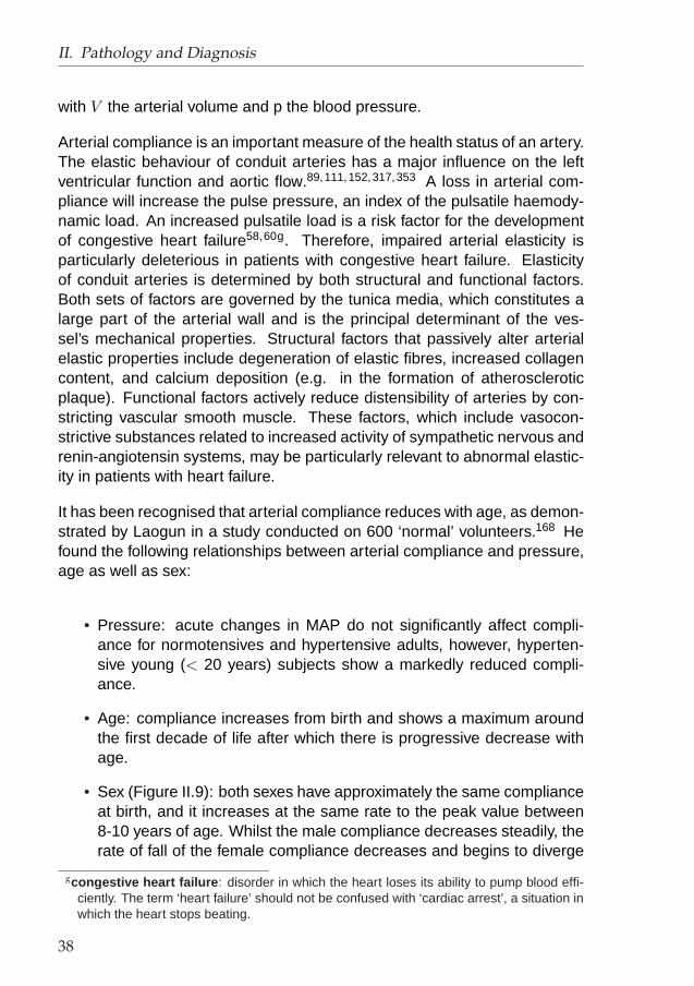
II. Pathology and Diagnosis
with V the arterial volume and p the blood pressure.
Arterial compliance is an important measure of the health status of an artery.The elastic behaviour of conduit arteries has a major influence on the leftventricular function and aortic flow.89,111,152,317,353 A loss in arterial com-pliance will increase the pulse pressure, an index of the pulsatile haemody-namic load. An increased pulsatile load is a risk factor for the developmentof congestive heart failure58,60g. Therefore, impaired arterial elasticity isparticularly deleterious in patients with congestive heart failure. Elasticityof conduit arteries is determined by both structural and functional factors.Both sets of factors are governed by the tunica media, which constitutes alarge part of the arterial wall and is the principal determinant of the ves-sel’s mechanical properties. Structural factors that passively alter arterialelastic properties include degeneration of elastic fibres, increased collagencontent, and calcium deposition (e.g. in the formation of atheroscleroticplaque). Functional factors actively reduce distensibility of arteries by con-stricting vascular smooth muscle. These factors, which include vasocon-strictive substances related to increased activity of sympathetic nervous andrenin-angiotensin systems, may be particularly relevant to abnormal elastic-ity in patients with heart failure.
It has been recognised that arterial compliance reduces with age, as demon-strated by Laogun in a study conducted on 600 ‘normal’ volunteers.168 Hefound the following relationships between arterial compliance and pressure,age as well as sex:
• Pressure: acute changes in MAP do not significantly affect compli-ance for normotensives and hypertensive adults, however, hyperten-sive young (< 20 years) subjects show a markedly reduced compli-ance.
• Age: compliance increases from birth and shows a maximum aroundthe first decade of life after which there is progressive decrease withage.
• Sex (Figure II.9): both sexes have approximately the same complianceat birth, and it increases at the same rate to the peak value between8-10 years of age. Whilst the male compliance decreases steadily, therate of fall of the female compliance decreases and begins to diverge
gcongestive heart failure : disorder in which the heart loses its ability to pump blood effi-ciently. The term ‘heart failure’ should not be confused with ‘cardiac arrest’, a situation inwhich the heart stops beating.
38

II.2. Pressure, Geometry and Flow features
Figure II.9.: Variation of aortic compliance in females compared with males from birth to 65years.168 n denotes number of subjects in each age range for which the compliance is givenas mean ± standard deviation. The compliance is expressed as a percent volume changeper change in pressure of 10 mmHg.
from male at around 14-15 years of life. There is a marked changein the rate of decay in the compliance value for males and females ataround 18 years. Female compliance is now larger than male com-pliance, until the marked fall in female compliance at 45 - 50 years,attributed to the menopause. After the fifth decade, there is no ob-servable difference between the male and the female compliance.
II.2.2.2. Geometric risk factors
As illustrated in Figure II.2, atherosclerosis tends to form at particular sitesin the vascular tree. Especially bifurcations and bends are concerned. In thepast, researchers have attempted to find which geometric features would bemore atherogenic than others.45,100,157,223,289,293,331,334,389 For a bifurca-tion, the planarity, i.e. degree to which the arteries all lie in a plane, havebeen postulated as risk factors for atherogenesis.45,100,157,281,389 Other re-searchers331,334 state that it is not the planarity, but rather the curvature,linearity and tortuosity of an artery that is responsible for the predisposi-tion to atherosclerotic plaque. Bifurcation angles are usually thought to beatherogenic when very large. The definition of a ‘bifurcation angle’ remainsobscure although many suggestions have been made in the literature.289,293
Finally, the bifurcation area ratio, i.e. the ratio of the cross-sectional area dis-tal to and proximal from the apex, has been investigated for its relationshipwith atherogenic sites.223
39

II. Pathology and Diagnosis
It is important to note that it is in fact not geometry per se, but the effectof geometry on the local blood flow that renders specific geometric featuresinteresting in the context of atherogenesis.
II.2.3. Flow
II.2.3.1. What is Wall Shear Stress?
As blood flows through a vessel, it exerts a physical force on the vessel wall.This force can be resolved into two principal vectors.342 Shear stress, beingtangential to the vessel wall, represents the frictional force exerted by theflowing blood at the endothelial surface of the vessel wall. Normal stress, orpressure, is perpendicular to the vessel wall. It represents the dilating forceof blood pressure on the vessel wall. The whole vessel wall, including theendothelium, smooth muscle cells and the extracellular matrix, is exposedto it. In contrast, only the inner surface of the vessel wall, the endothelialcells, are exposed to the frictional force of shear stress. There is some slowtransmural flow around smooth muscle cells in arterial walls, but this force isconsidered insignificant when compared with the normal wall stress to whichthese cells are exposed.19 These haemodynamic forces are affected by fluidviscosity and by vessel diameter, thickness, and distensibility (Figure II.10).Mathematically, instantaneous shear stress in laminar flow is defined as
−→τ = µ∂−→v∂y
(II.4)
Figure II.10.: Schematic of an artery and the haemodynamic forces generated during a sys-tolic pulsation. The shear stress force vector is parallel to the flow of blood and unidirectional.However, the cyclic strain force exerted on the vessel is multi-dimensional and stretches thevascular cells along multiple planes.11
40

II.2. Pressure, Geometry and Flow features
here, −→v is the velocity vector, y is the normal distance from the vessel wall,and µ is the dynamic viscosity. For laminar flow (flow rate Q) in circular tubes(radius r), the shear stress at the wall can be written as
−−−→WSS = −→τw = 4
µ
π
Q
r3−→eax (II.5)
with −→eax the axial unit vector.
II.2.3.2. The effect of Wall Shear Stress
Shear stress and tensile stress are the predominant haemodynamic forcesproduced by the pulsatile blood flow. These forces affect the function, mor-phology, and proliferation of vascular cells, and the local development andprogression of atherosclerotic disease.
In a normal situation, wall shear stress is used to regulate the cross-sectionalarea of the vessel. Endothelial cells ‘sense’ the shear stress using theirouter layer, the glycocalyx, which is approximately 0.5 µm thick and con-sists of substances combining sugar and protein elements. The layer con-tains minute hairs. It is thought to signal to the endothelial cells when moreblood flows through an artery, so that the endothelial cells release nitricoxide (NO). Nitric oxide is one of the pivotal molecules coordinating vas-cular function.343 Figure II.11 (by Powell252) shows the consequences ofa NO release by the vascular endothelium, one of which being vasodilata-tion. The high WSS, which caused the NO release, will decrease with in-creased cross-sectional area at a constant flow rate (see equation II.5). Theendothelium releases NO to protect itself from the damaging influences ofhigh WSS.
The importance of wall shear stress and flow separation regions with regardto atherosclerosis and endothelial lesion has been investigated in a largenumber of studies;11,47,156,187 what follows is a short overview of why vesselwall shear stress became an important research topic.
Several factors contribute to the clinical importance of wall shear stress. Re-gions with low (0.5 N
m2 ) wall shear stress show an increased endothelial cellloss and even desquamationh as the results of apoptotic cell death.63 Sub-sequently, the subendothelium gets exposed to the blood flow, promoting
hDesquamation : endothelial peeling
41

II. Pathology and Diagnosis
Figure II.11.: Coordinating and protective roles of nitric oxide (NO) released by vascular en-dothelium.252 NO is very chemically reactive. Increased blood flow and many agonists thatbind to endothelial cell receptors lead to an influx of calcium into the endothelium, whichresults in increased production of NO. Secretion of NO into the vessel lumen results inreduction of the adhesive properties of platelets and leukocytes. Increased levels of NOwithin endothelial cells dampens metabolic pathways leading to endothelial cell activation.Secretion of NO into the smooth muscle cells of the media causes vasorelaxation (via theinteraction of NO with the enzyme guanylate cyclase).
platelet aggregation and consequently thrombosis. Furthermore, a low wallshear stress increases the production of chemicals attracting monocytesand proliferation of resident macrophages and smooth muscle cells.18 Onthe other hand, non-pulsatile high (2.5 N
m2 ) wall shear stress induces the re-lease of factors from the endothelial cells that inhibit coagulation, migrationof leukocytes and vascular smooth muscle cell proliferation, while simultanu-ously promoting endothelial cell survival. Higher WSS (>10-15 N/m2, prob-lematic from 25-45 N/m2)155 causes endothelial trauma and haemolysis. In
42

II.2. Pressure, Geometry and Flow features
Figure II.12.: In the carotid artery, low but also high wall shear stress values are common.
Figure II.13.: Schematic representation of the wall shear stress distribution in a stenosedvessel. The grey arrows represent blood flow, the black solid lines are the vessel wall, thegrey surface is the stenosis.
the carotid artery, low but also high wall shear stress values are common(Figure II.12).
Knowledge of the wall shear stress is thus important to identify areas proneto plaque formation, but once plaque has formed, knowledge of the wallshear stress remains important , as illustrated in Figure II.13. The area prox-imal from the plaque will show high wall shear stress. Clowes67 showedthat the high wall shear stress reduced the stability of the formed plaque.This may lead to rupture, blood clotting and finally infarction or embolism.
43

II. Pathology and Diagnosis
This hypothesis was supported by Lovett’s recent results which showed thatplaque rupture sites tend to localise to the proximal part of the plaque whereshear stress is highest.202 Tricot336 disagreed and showed that it was notthe area upstream the plaque that would rupture. The distal area, where lowshear stress is usually found, is more susceptible to disruption and subse-quent thrombosis.
II.2.3.3. Oscillating Shear Stress
In the previous section, the consequence of static low or high shear stresseswas described. Oscillating shear stress induces a biological mechanism onits own. It has been shown that endothelial cells tend to align in the directionof the flow.180 Figure II.14, published by Malek,208 illustrates on the left thealignment of endothelial cells. In the absence of a clearly defined flow direc-tion, the endothelial cells do not align and the pattern in Figure II.14 (right)is seen. The lack of alignment in endothelial cells might preferentially acti-vate circulating monocytes and encourage local adhesion and diapedesisi.Moreover, the endothelial cells are encouraged to produce certain mediatorsand growth-factors that perpetuate underlying smooth muscle and fibroblastproliferation. In addition, the endothelial cells will show a reduced produc-tion of clot-resolving enzymes, which may foster focal platelet aggregationand fibrin deposition, accelerating plaque formation and increasing the riskof thromboembolic events.
iDiapedesis: The movement or passage of blood cells, especially white blood cells, throughintact walls into surrounding body tissue.
Figure II.14.: Endothelial alignment. a: Endothelial cells tend to align in the direction of theflow. b: When there is a lack of a clearly defined WSS direction, e.g. in zones of low andoscillating WSS, the endothelial cells will be aligned randomly.208
44

II.2. Pressure, Geometry and Flow features
The absence of a clearly defined flow direction in physiological circumstancesis due to the presence of both pulsatile flow and complex geometry: flowseparation and flow reversal are features typical of stenoses and bifurca-tions.
II.2.3.4. Shear Stress Gradients
Apart from the shear stress and its oscillations, Kleinstrueur’s group arguedthat not so much the WSS, but its gradients (both in time and in space)show a closer relation to the atherogenic behaviour seen in carotid bifurca-tions or femoral grafts.42,43,142,159,160,171,172,173,200,354 The authors42 foundthat areas of high gradients of WSS were related to lesion growth intimal hy-perplasiaj. It is argued173 that for an intact endothelium, the cross-wall masstransfer is mainly via an active transport mechanism, i.e., it is controlled bythe endothelium depending on the need of the arterial wall for different sub-stances. However, when the endothelium is locally injured, possibly due tohigh WSS, it causes, among other things, the intracellular space to widensubstantially. This allows intimal hyperplasia enhancing molecules (such aslow-density lipoprotein (LDL) and even cells (monocytes)) to simply diffusein the intercellular space. The endothelial cell response aims to keep theintegrity of intercellular junctions and prevent endothelial cells from hydrody-namic injury. However, significant and sustained WSSG values will handicapthe cell response, initiating the process of atherosclerosis.
II.2.3.5. Shear Stress Angles
In zones where the endothelial’s defensive function is weakened, flow mov-ing towards the wall is problematic since atherogenic particles and cells suchas monocytes could adhere to the endothelium and migrate into the wall atsites of increased permeability. Examining the shear stress angles is a tech-nique that offers a view on the direction of flow.
jIntimal Hyperplasia : overexpression of the intima, i.e. pathological growth of the en-dothelial layer.
45

II. Pathology and Diagnosis
II.2.3.6. Haemodynamically induced Plaque Formation
Overall, the haemodynamic abnormalities observed in a vessel of complexgeometry can facilitate plaque formation by multiple mechanisms:
• Flow separation and stasis (blood stagnation) allow for prolonged blood-vessel wall interaction with atherogenic particles, which may increasetheir local deposition.11
• Flow stasis, thus, low shear stress, is associated with decreased se-cretion of atheroprotective substances by endothelial cells.
• Flow oscillations are characterised by reversals in the direction of bloodflow during the cardiac cycle, and can disrupt endothelial cells that arenormally aligned in the direction of blood flow. Disruption of the cellalignment can alter the barrier function of the cells and can also facili-tate the deposition of atherogenic substance in the vessel wall.
• High WSS gradients may widen intracellular space impeding the pro-tective mechanism of the vessel wall.
• The atherosclerotic process can be sped up when blood flow is di-rected towards already injured endothelial wall.
Knowledge of the haemodynamics and the quantification of wall shear stress(WSS) in particular is therefore absolutely required in atherogenic research.Note that although the importance of the WSS is widely acknowledged, mostof the mechanisms explained above are still hypotheses that have not thor-oughly been proven.
II.3. Measurement of Designated Markers
The pernicious features discussed in the previous section can be quantifiedusing a variety of parameters. In this section, the parameters are definedand discussed in a first step. In a second step, the techniques available formeasruing these parameters are presented.
46

II.3. Measurement of Designated Markers
II.3.1. Pressure
II.3.1.1. Sphygmomanometry
Blood pressures are routinely measured using a sphygmomanometer (ablood pressure cuff). The cuff was previously attached to either an enu-merated dial or stand. In the models with stands, bars of mercury will line upwith the numbers. the model with dials have an arrow that will point to num-bers as the pressure changes. Nowadays, the pressure is read on a digitaldisplay. Also attached to the cuff is a source for creating pressure. The moremodern versions are inflated automatically by a purpose-built compressor,although usually the pressure source is a hand-held balloon that the exam-iner squeezes to inflate the cuff. In this ‘manual’ model, the balloon has avalve to release air from the cuff. When this valve is closed and the balloon issqueezed, the cuff will inflate and increase its pressure. To lower the pres-sure, turning the valve releases air. Figure II.15 shows how the pressuremeasurement works in practice.14
The cuff is placed over bare skin above the elbow. The arm is passivelyraised to the level of the heart. Moreover, the patient should be as relaxedas possible throughout the exam. This means both physical and emotionalrelaxation. At this point the cuff is inflated to a pressure at which the radial
Figure II.15.: Sphygmomanometry in clinical practice.181
47

II. Pathology and Diagnosis
pulse cannot be palpated in the wrist. This means that the superficial arter-ies of the upper arm are now occluded by the inflated cuff. The examinerthen listens to the radial artery with a stethoscope as the pressure is slowlylowered in the cuff. The point at which the heart exerts enough pressure toovercome the pressure applied via the cuff is the systolic blood pressure.The reason for hearing the blood flow is the fact that a partially occludedartery will cause the flow to ‘spurt’ and create turbulence. This pulse will stillbe heard as the pressure is slowly lowered. At a lower pressure the hearteasily overcomes the pressure of the cuff and no pulse can be heard, this isthe diastolic blood pressure.
II.3.1.2. Tonometry 68
Arterial tonometry is a non-invasive technique that offers the clinician a beat-to-beat blood pressure waveform along with numerical values for systolic,mean and diastolic pressures, as well as pulse rate. It consists of using asensor placed on the wrist over the superficial artery, for example the ra-dial artery (Figure II.16 (a)). This sensor contains piezoelectric pressuretransducers. A pneumatic pump presses the transducer array against theskin and tissue above the artery (Figure II.16 (b)). This pressure is knownas the ‘hold down pressure’ (HDP). To determine optimal HDP, the monitorsearches through a range of pressure values until it measures a signal indi-cating that the artery is of the form in Figure II.16 (b), i.e. the form giving thehighest signal as in Figure II.16 (c). When the artery is partially flattened, agraph can be plotted to show sensor pulse amplitude versus time.
(a) Tonometer placed on ra-dial artery
(b) cross-section through theartery
(c) determining HDP
Figure II.16.: The principle of tonometry. a: Photograph of a tonometer placed on a radialartery. b: The tonometer presses the artery against the underlying bone and senses thepressure pulses in the artery. c: Application of different hold down pressures (HDP’s), differ-ent signals are measured due to the different shapes of the artery.68
48

II.3. Measurement of Designated Markers
For the carotid artery, the graph is of the form measured by Mitchell222 in Fig-ure I.6 (a) on page 15. At this stage, the waveform is not calibrated yet. Forthat purpose, the maximum and minimum in the acquired pressure wave-form can be set equal to the systolic and diastolic pressure measured usinga cuff as in Figure II.15. To complete the calibration, all values between themaximum and minimum pressure are found by linearly interpolating betweenthe systolic and diastolic pressure.
II.3.2. Arterial Geometry
II.3.2.1. Basic Parameters
IMT and LD Measuring the IMT is clinically performed using an ultrasoundmachine. An ultrasound image is formed by transmitting a high-frequency(1-12 MHz) beam into the body, and collecting and analysing the returnedechoes to produce an image whose intensity is related to the echogenicity ofthe tissue and tissue interfaces. Modern ‘B-mode’ ultrasound readily allowsthe visualisation of the intima-media layer of superficial large arteries suchas the common carotid. Figure II.17 shows a B-mode image representing alongitudinal cross-section of the common carotid artery and an amplificationof that same image (Figure II.17 (b)). The black region on top of the imagecorresponds to the carotid lumen. Figure II.17 shows how the LD and IMTare measured on the image.
The principles and validity of B-mode ultrasound measurements of IMT were
(a) longitudinal cross-section of CCA (b) close-up
Figure II.17.: A longitudinal image of the distal carotid artery using B-mode ultrasound. Aregion of the intima media complex is magnified and highlighted for reference. Flow is fromright to left. Note that the distal end of the white box in the upper image corresponds to thestart of the distal end of the common carotid artery
49
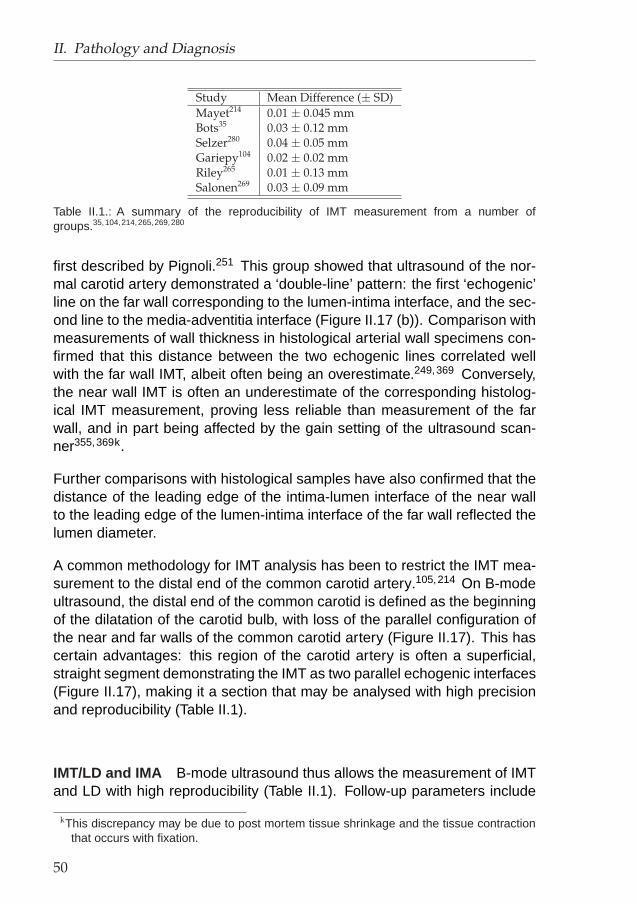
II. Pathology and Diagnosis
Study Mean Difference (± SD)Mayet214 0.01 ± 0.045 mmBots35 0.03 ± 0.12 mmSelzer280 0.04 ± 0.05 mmGariepy104 0.02 ± 0.02 mmRiley265 0.01 ± 0.13 mmSalonen269 0.03 ± 0.09 mm
Table II.1.: A summary of the reproducibility of IMT measurement from a number ofgroups.35,104,214,265,269,280
first described by Pignoli.251 This group showed that ultrasound of the nor-mal carotid artery demonstrated a ‘double-line’ pattern: the first ‘echogenic’line on the far wall corresponding to the lumen-intima interface, and the sec-ond line to the media-adventitia interface (Figure II.17 (b)). Comparison withmeasurements of wall thickness in histological arterial wall specimens con-firmed that this distance between the two echogenic lines correlated wellwith the far wall IMT, albeit often being an overestimate.249,369 Conversely,the near wall IMT is often an underestimate of the corresponding histolog-ical IMT measurement, proving less reliable than measurement of the farwall, and in part being affected by the gain setting of the ultrasound scan-ner355,369k.
Further comparisons with histological samples have also confirmed that thedistance of the leading edge of the intima-lumen interface of the near wallto the leading edge of the lumen-intima interface of the far wall reflected thelumen diameter.
A common methodology for IMT analysis has been to restrict the IMT mea-surement to the distal end of the common carotid artery.105,214 On B-modeultrasound, the distal end of the common carotid is defined as the beginningof the dilatation of the carotid bulb, with loss of the parallel configuration ofthe near and far walls of the common carotid artery (Figure II.17). This hascertain advantages: this region of the carotid artery is often a superficial,straight segment demonstrating the IMT as two parallel echogenic interfaces(Figure II.17), making it a section that may be analysed with high precisionand reproducibility (Table II.1).
IMT/LD and IMA B-mode ultrasound thus allows the measurement of IMTand LD with high reproducibility (Table II.1). Follow-up parameters include
kThis discrepancy may be due to post mortem tissue shrinkage and the tissue contractionthat occurs with fixation.
50

II.3. Measurement of Designated Markers
the IMT/LD ratio and the intima-media area (IMA), estimated as the differ-ence in area between two concentric circles: one with radius LD/2 and an-other with LD/2 + IMT:
IMA = π ×(
LD
2+ IMT
)2
− π ×(
LD
2
)2
= π × IMT × (LD + IMT ) (II.6)
Compliance Many different techniques for calculating the compliance havebeen suggested in literature,36,167,222 some involving the measurement ofthe pulse wave velocity (PWV), i.e. the speed with which a pressure wavetravels through the arterial tree. In this manuscript, the vessel complianceCo will be defined as follows:
Co =∆V
∆P= L
LD2s π4 − LD2
d π4
PP(II.7)
with L the axial vessel length, PP the pulse pressure, LDs and LDd thesystolic and diastolic LD respectively. The compliance per unit length willbe:
C =Co
L=
π
4LD2
s − LD2d
PP(II.8)
Note that the pulse pressure used here, is the local pulse pressure, i.e. theone occurring at the site where compliance is to be quantified. When thePP originating from a cuff measurement is used, there will be an error in theestimation of C.
Young’s modulus and distensibility coefficient Using a method describedby Brands,40 the Young’s modulus is defined as:
E =LDd
IMTd ×DC(II.9)
51

II. Pathology and Diagnosis
where IMTd is measured in diastole, LDd is the lumen diameter in dias-tole and DC is the distensibility coefficient. The distensibility coefficient isdefined as:
DC =1
PP
2×∆LD
LDd(II.10)
where ∆LD is the change in lumen diameter from systole to diastole, andPP the pulse pressure within the common carotid artery measured by arte-rial tonometry.
Wall Tension and Tensile Stress Using Laplace’s law (section II.2.1), anapproximation of the peak (Tp) and mean (Tm) circumferential carotid arterialwall tension can be calculated as:
Tp[Pa m] = SBP × LDs
2(II.11)
Tm[Pa m] = MAP × LDd
2(II.12)
where SBP is the systolic pressure and MAP the mean arterial pressure.LDs and LDd are the lumen diameters measured in systole and diastolerespectively.
Furthermore, peak (σp) and mean (σm) tensile stress can be obtained bydividing the wall tension by the time-dependent IMT:
σp[Pa] =Tp
IMTs(II.13)
σm[Pa] =Tm
IMTd(II.14)
Similar to the definitions of LDd and LDs, IMTd and IMTs are measuredin diastole and systole.
52

II.3. Measurement of Designated Markers
II.3.2.2. Vascular imaging
As described in section II.2.2.2, complex arterial geometry may induce ad-verse haemodynamic situations. A number of parameters have been sug-gested to describe haemodynamic conditions that are prone to atherosclero-sis. In order to calculate most of these parameters, a 3D model of the carotidbifurcation needs to be reconstructed. Several imaging modalities can beused to reconstruct the realistic carotid geometries: X-ray, magnetic reso-nance imaging (MRI) and both intravascular and extravascular ultrasound. Ashort description of each of these techniques, with their advantages and dis-advantages, is provided in what follows. The paragraphs on X-ray angiogra-phy, MRI and ultrasound are based on publications by Steinman,304,305 withpermission.
X-ray angiography 304,305 The electromagnetic (EM) spectrum offers twowindows through which one can explore the human body: the high-energyX-ray range and the low energy radio wave range (Figure II.18). In X-rayimaging, a high-energy ‘X-ray’ beam is sent through the body. These raysare captured by a device behind the body. The attenuation of the beam isa measure of body density and can therefore be used to differentiate par-ticular zones in heterogeneous bodies. Note that X-ray imaging producesprojection images as opposed to cross-sections of a body.
Figure II.18.: The electromagnetic spectrum and its applications. X-ray has a high energyand high frequencies, whereas MRI has the exact opposite: low energies and low frequen-cies.86 A new tool for medical imaging, TeraHertz Imaging , uses intermediate energies andintermediate frequencies, i.e. frequencies in the TeraHertz range.
53

II. Pathology and Diagnosis
The first image-based computational fluid dynamics (CFD) studies of anatom-ically realistic arterial geometries were derived from clinical X-ray angiograms.112
One of the first attempts to reconstruct a carotid bifurcation from medicalimages was published by Gibson.112 In this study, patients were followedfor three years via the so-called cine angiography of their coronary arteriesas part of the Harvard Atherosclerosis Reversibility Project (HARP) to as-sess the rate of change in coronary artery diameter due to dietary versusdrug therapy. Vessel centrelines and boundaries were identified from X-rayangiographic projection images and used to track the change in lumen di-ameter. Assuming circular cross-sections, this data was used to reconstructtwo-dimensional axisymmetric models of the coronary segments at base-line. This particular study illustrates both the advantages and disadvantagesof using projection angiography for image-based studies. The most obviousadvantage is that X-ray angiography remains the gold-standard for quantify-ing atherosclerotic disease, owing to the high resolution and unambiguousdelineation of the lumen made possible via the intra-arterial injection of con-trast agent. This makes it relatively straightforward to derive the modelsfrom what is often readily available clinical data. In the absence of multipleprojections and/or computed tomography (CT) reconstructions (available inother studies306), however, assumptions must be made about the cross-sectional shape of the lumen in order the reconstruct a three-dimensionalmodel. Tascyian322 used a slightly different technique to reconstruct 2D invivo carotid models: single projections were acquired, from which corre-sponding images were digitally subtracted to remove background bone andtissue, further highlighting the vessel lumen. These were then used to re-construct a 2D-model of a carotid bifurcation, shown in Figure II.19 (a). Thistechnique is called digital subtraction angiography or DSA.
Later on, 3D models of the carotid have been reconstructed using X-ray. Re-construction of 3D models requires at least two (ideally orthogonal) projec-tions, and some assumptions about the shape of the lumen cross-sections.Ene-Iordache et al91 successfully reconstructed the geometry of in vivo ar-teriovenous fistulas for haemodialysis using DSA in 2 orthogonal planes. Al-ternatively, recent advances in X-ray imaging technology make possible therapid (4-6 s) acquisition of multiple (200) projection images,92 from whichthe 3D lumen geometry can be reconstructed at high (200-400 µm) spa-tial resolution without the need for a priori assumptions about lumen shape.The last evolution of this technique has been illustrated by Cademartiri44
on a 65-year old symptomatic man. Cademartiri showed that the use ofmultislice (MS) CT scanners offer a spatial resolution high enough to allownot only carotid bifurcation reconstruction (Figure II.19 (b)), but also visual-isation of carotid artery atherosclerosis. The advantage of X-ray angiogra-
54

II.3. Measurement of Designated Markers
(a) 2D322 (b) 3D44
Figure II.19.: 2D and 3D Carotid geometries reconstructed from X-ray imaging. a: Left ,X-ray depiction of a minimally stenosed carotid bifurcation; Right , mesh representation ofthe minimally stenosed carotid bifurcation. b: Direct 3-dimensional volume rendering (A, B,and C) using multislice CT shows the anatomy of the arteries of the neck at the level of thecarotid bifurcation (Car Bif). Clav indicates clavicle; Hyoid, hyoid bone; Jug, jugular vein;Mand, mandible; and Thyr Car, thyroid cartilage. A magnified view of the right (B) and left(C) carotid bifurcations permits recognition of the common carotid artery (CCA), the internaland external carotid arteries (ICA and ECA), and a wall stent (S) at the right side. The leftcarotid bifurcation (C) is patent but is slightly dilated at the origin of ICA. A few calcified spotsalso are present. Note the backflow of iodinated contrast material into the right jugular vein(Jug in A).44
phy over other medical imaging modalities is the superior contrast-to-noiseratio, combined with high temporal and spatial resolution. The price paidfor this quality is the finite risk associated with catheterisation, which is infact greater than the risk associated with the radiation dose itself.25 A lessinvasive alternative is to inject contrast intravenously (as opposed to intra-arterially), and rapidly acquire the 3D volume using single or multiple ringhelical CT scanners. This approach typically produces poorer contrast im-ages of the lumen. As a result, it is difficult to carry out human studies ofearly atherosclerosis and local haemodynamics using X-ray angiography,since it is typically performed only for patients with known or suspected vas-cular disease.
Intravascular Ultrasound (IVUS) 305 In the context of the reconstructionof in vivo carotid geometries, the above-noted disadvantages of projectionangiography can largely be overcome through the incorporation of intravas-cular ultrasound (IVUS), in which case X-ray angiography is used to guide anultrasound probe-tipped catheter and landmark its position for subsequent
55

II. Pathology and Diagnosis
Figure II.20.: Using IVUS for the reconstruction of coronary geometry. a: A single IVUSimage. The image is segmented, delineating the lumen (inner line) and the intima (outerline). b: A number of images are aligned, representing the 3D geometry of the coronaryartery.176
reconstruction of the three-dimensional lumen and wall from the cross-sec-tional ultrasound images. The power of this approach was first demonstratedby Krams,162 who used biplane angiography and IVUS data obtained at end-diastole to construct a three-dimensional model of a segment of a patient’satherosclerotic right coronary artery. This technique has proved its successin other arteries than the coronary. It was also used to reconstruct the 3Dgeometry of a stented coronary artery.275,291,335,357,358 Owing to its abil-ity to resolve the vascular wall in vivo, IVUS is becoming an increasinglypopular approach for vessel reconstruction studies in which invasiveness isnot an issue, such as animal studies or studies on patients already referredfor cardiac catheterisation. Figure II.20 illustrates how 3D geometries areextracted from IVUS images.176
Magnetic Resonance Imaging (MRI) 305 MRI has emerged in the lastdecade as one of the most powerful and flexible imaging techniques, byvirtue of the fact that contrast between tissues can be achieved by exploitingdifferences in the magnetic spin relaxation properties of the various bodilytissues and fluids. In the context of image-based CFD studies of atheroscle-rosis, MRI is particularly attractive since, unlike X-ray angiography, blood it-self can be used as a contrast agent. This can take the form of ‘bright blood’or ‘time-of-flight’ (TOF) techniques, which, just as conventional angiography,enhance the signal from flowing blood at the expense of signal from sur-rounding tissue. When it is necessary to resolve the vessel wall itself, ‘blackblood’ techniques can be used to suppress the lumen signal. Several MRIprotocols have been used in order to reconstruct a carotid geometry (TableVIII.1 on page 196). The detailed description of how in vivo carotid bifurca-
56

II.3. Measurement of Designated Markers
tions are reconstructed in this manuscript is explained in sections VI.2 andVI.3.
Three-dimensional Ultrasound (3DUS) 305 Three-dimensional ultrasound(3DUS) is a relatively recent development that makes it possible to acquirethree-dimensional images of superficial vessels such as the carotid bifur-cation using relatively fast and inexpensive ultrasound imaging techniques.Owing to its novelty, however, applications using 3DUS are comparativelystill in their infancy. The first attempts to reconstruct carotid geometries fromultrasound images were not very successful,114,210 especially in comparisonwith the accuracy obtained by MRI at the time. Recently, two approacheshave been able to overcome the early difficulties encountered.
• In a first approach,20 conventional (two-dimensional) B-mode ultra-sound images are acquired in a long sweep of the ultrasound probeover the subject’s neck. Simultaneously, the probe is tracked in space.The images, together with the knowledge of their positions, are usedto provide geometric parameters for three-dimensional carotid bifurca-tion models. For more details about the practical implementation ofthis approach, see sections VII.2 and VII.3.
• In a second approach, the probe is not swept over the subject’s neck,but the probe’s transducers can make a fan-like movement376 (FigureII.21). After some off-line data processing, which primarily consists of3D interpolation, a 3D data set is extracted.
Note that extravascular ultrasound is limited to superficial vessels such asthe carotid bifurcation. Moreover, when not obscured altogether by the jaw,access to the carotid bifurcation often requires a twisting of the head andneck that may distort the ‘natural’ orientation of the vessel. Furthermore, theneed to sweep the ultrasound probe, often manually, over the length of thecarotid bifurcation renders ultrasound more operator-dependent than otherimaging techniques. Nevertheless, compared to all other imaging modalitiesultrasound is the least expensive, least invasive, and most widely available,which from a practical and economic perspective alone renders it an ex-tremely promising tool for large-scale, prospective investigations of haemo-dynamics and vascular disease.
57

II. Pathology and Diagnosis
Geometrical Features Regardless which of the above imaging techniquesis used, a set of images will be obtained which enable the reconstruction ofthe carotid bifurcation. The following geometrical features can then be cal-culated.
• The average cross-sectional area in CCA, ICA and ECA (ACCA,AICA, AECA).
• Here, the area ratio AR is defined using the area of the most proximalICA and ECA cross-section (aICA and aECA) and the area of the CCAcross-section 2 mm proximal from the considered ICA and ECA area(aCCA):
AR =aICA + aECA
aCCA(II.15)
• The non-planarity parameter NP as defined by King.157 In short,this non-planarity parameter is obtained as follows. First, the centre-lines are calculated as shown below,20 and the coordinates of the cen-trelines are gathered in a matrix. The singular value decomposition(SVD) of this matrix will result in three singular values. The smallestsingular value is a measure of non-planarity. For points on a plane,NP is zero, for points on a sphere, NP is 1
3 or 33%. Figure II.22gives a feel for the non-planarity parameter. The non-planarity can becalculated for each of the three vessels, NPCCA, NPICA and NPECA.
Figure II.21.: Schematics showing the principle of 3-D ultrasound data acquisition and pro-duction of a volumetric data set of the carotid artery.376
58

II.3. Measurement of Designated Markers
The centreline itself consists of the centroids (center of mass) of thecross-sections of the carotid arteries. The centroids of axial cross-sections are calculated by the expression
cx =∫ ∫
xdA
A
cy =∫ ∫
ydA
A(II.16)
Here, cx and cy are the coordinates of the centroid in an (x, y)-orthogonalreference system and A is the surface of the cross-section for whichthe centroid is sought. Equation II.16 reduces to the following for anarbitrary polygon with nodes (xi,yi) (i=1,2,...,n):
cx =1
6 A
n−1∑
i=0
((xi + xi+1)(xi yi+1)− xi+1 yi)
cy =1
6 A
n−1∑
i=0
((yi + yi+1)(xi yi+1)− xi+1 yi) (II.17)
Note that xn is assumed to be x0, in other words the polygon is closed.In order to obtain this formula, the polygon was divided in triangles, forwhich is straightforward to find centroids. The centroid of the polygonis an area-weighted average of the centroids of the triangles.
• A different centreline agreement measure, zDIST , based on a definitionby Long et al,194 is defined as the average distance between the twocentrelines. Because two different sets of centrelines can be totallydifferent yet have the same NP , zDIST is a more robust quantificationof centreline difference.
• Similarly, the largest singular value is a measure of the linearity of thecentrelines, LCCA, LICA and LECA. The theoretical minimum is 33%.Figure II.22 gives a feel for the linearity parameter.
• Apart from the SVD method, the vessel linearity is also reflected by atortuosity parameter defined as
Tvessel = 100×(
1− D
Ds
)[%] (II.18)
59

II. Pathology and Diagnosis
Figure II.22.: The Non-Planarity parameter NP as introduced by King.157 The quadranglerepresents a plane, whereas the lines in the quadrangle are centrelines of the carotid bifur-cation. The centreline starting at the bottom of each figure represents the CCA, which splitsinto two other centrelines: the ICA and ECA. In the first case, the centrelines are straightsegments: NP is 0% and L is 100% for each of the arteries. In the second case, the centre-lines are planar, but not straight: NP is still 0% but L will have taken a value between 33%and 100%. Only in the third case, where the centrelines come in and out of the ‘best-fit’157
plane (at the black dots), NP will differ from 0%.
here, D is the shortest distance between the end-points of the con-sidered vessel whereas Ds is the actual distance along the centrelinebetween the end-points.
• Different ways to define a bifurcation angle have been suggested inthe past. Here, the bifurcation angle αBIF is defined as the anglebetween two vectors,
−−−−−−−−→CCCA, CICA and
−−−−−−−−−→CCCA, CECA. CCCA was the
CCA centroid of the most distal CCA slice. Similarly, CICA and CECA
were the centroids of the ICA and ECA in the most proximal ICA andECA slice.
• It is clear that cross-sectional areas and centrelines alone cannot de-scribe a carotid geometry. In order to ‘quantify’ cross-sectional shapes,the individual shape factor (SFi) has been introduced. It can be de-fined as by Barratt,21 i.e. as the fraction of 4π×area and the squareof the circumference. The SFi is 1 for a circle, and smaller than 1 foranything else.
• The comparative shape factor (SFc) is used when the shape of twocross-sections need to be compared. It can be defined based on apublication by Long.194 It was evaluated here as follows (Figure II.23):(1) the two cross-sections to be compared were scaled to a cross-sectional area of 1, (2) the center points were aligned, (3) the arealying inside both cross-sections was denoted as A, whereas the area
60

II.3. Measurement of Designated Markers
Figure II.23.: Definition of the area’s A and B for comparative shape factor SFc based on apublication by Long.194
outside the overlapping area was B, (4) the ratio B/(A+B) was definedhere as the shape factor. It should be 0% for a perfect match betweentwo shapes. For a hypothetical case where the shape is a circle in onecross-section, and a square in the other, the shape factor is 27%.
II.3.3. Flow
In the previous two sections, pressure and geometric parameters of interesthave been defined. The last group of ‘designated markers’ are the flowparameters. The flow parameters have been divided into 3 sections. A firstset of parameters (section II.3.3.1) concentrates on what can be measuredwithout the need for 3D carotid geometry reconstruction. The calculationof entire flow fields is described in section II.3.3.2, whereas haemodynamicvessel wall parameters are defined in section II.3.3.3.
II.3.3.1. Heart and Flow Rate
Heart Rate The heart rate (HR) is usually expressed as the number ofbeats the heart performs per minute. It is often monitored by an electrocar-diogram, i.e. a test that records the electrical activity of the heart.
61

II. Pathology and Diagnosis
Flow Rate Measuring flow rates in vivo is not always straightforward. Thetwo techniques used in this study are described here.
Phase Contrast MRI
Axial velocities in a particular cross-section of an artery can be measuredusing an MRI technique called cine phase contrast MRI or cine PC MRI(see section VI.1). The flow rate can be calculated by the following twosteps. (1) On the cine PC image, the pixels in the arterial lumen are sepa-rated from the other pixels. (2) Let Vp be the velocity measured by MRI in aparticular pixel and Ap the area of a single pixel. The blood flow rate Q willbe:
Q =∑
p=pixels in lumen
(Vp ·Ap) (II.19)
In section VIII.1.1, the reliability of this technique is investigated.
Pulse Doppler Ultrasound
Carotid flow rate is often39,115,140,367,384 calculated using pulsed Dopplerultrasound (see section VII.1.3). Pulsed Doppler outputs the blood velocityin a control volume with a high temporal resolution (± 200 Hz). For carotidflow rate measurements, the control volume is positioned in the center of aCCA cross-section. This will measure the ‘centreline velocity’, and it is oftenassumed that this centreline velocity represents the peak velocity Vpeak. Itis well known that, for fully developed, laminar, steady flow of a Newtonianfluid in a straight rigid tube of circular cross-section (i.e. parabolic flow pro-file), Vmean=Vpeak/2, and hence it is straightforward to estimate the volumeflow rate given only the peak velocity and vessel cross-sectional area. Un-der fully developed pulsatile flow conditions, however, Vpeak/Vmean is timevarying and depends strongly on the dynamics of the flow field. Assumingthat Vpeak lies on the lumen central axis at all times (a good assumption forthe CCA wave forms), it is possible to compute this time-dependent ratioby invoking Womersley’s analytic solution for velocity profiles under pulsatileflow conditions.39,367,368
The mathematical solution is elabourated here as by Holdsworth.140 Con-sider the Fourier-decomposed, peak-velocity wave form:
62

II.3. Measurement of Designated Markers
Vpeak(t) =∞∑
k=0
Vpeak,k cos(kωt− φk)
=∞∑
k=0
Real[Vpeak,k ei(kωt−φk)
](II.20)
We wish to derive the Fourier-decomposed, mean-velocity wave form, i.e.:
Vmean(t) =∞∑
k=0
Vmean,k cos(kωt− ψk)
=∞∑
k=0
Real[Vmean,k ei(kωt−ψk)
](II.21)
For k = 0 (i.e. the steady flow component), the velocity profile is parabolic,in which case Vmean,0 = Vpeak,0/2. For the k > 0 terms, Womersley’s ana-lytic solution of sinusoidal flow in a straight, rigid tube (expressed here as afunction of the mean velocity) is invoked:
v(y, t) = Real
{Vmean,k
[J0(τk)− J0(τk y)
J0(τk)− 2J1(τk)/τk
]ei(kωt−ψk)
}(II.22)
where J0 and J1 are the zeroth and first Bessel functions of the first kind, i=√−1, Real{.} denotes the real part of a complex quantity, y is the radial
position normalised to the vessel radius (R) and:
τk = αk i−3/2 (II.23)
where αk is the Womersley number of the kth harmonic, i.e.:
αk = R
√kω
ν(II.24)
63

II. Pathology and Diagnosis
and ν is the blood kinematic viscosity. On the centreline (i.e. y=0), equationII.22 reduces to:
v(0, t) = Real
{Vmean,k
[J0(τk)− 1
J0(τk)− 2J1(τk)/τk
]ei(kωt−ψk)
}(II.25)
Recognizing that v(0, t) is simply the kth term of Vpeak,t, equating the argu-ments to Re in equations II.25 and II.20 leads to the following relationshipbetween the Fourier coefficients for Vpeak,t and Vmean,t:
Vmean,k e−iψk = Vpeak,k e−iφk
[J0(τk)− 2J1(τk)/τk
J0(τk)− 1
](II.26)
Thus, given Vpeak,k and φk from the Fourier-decomposed, peak-velocity waveform, and α1, the mean-velocity wave form can be reconstructed from thecomputed Vmean,k and ψk using equation II.21. Finally, the flow wave formis calculated by multiplying Vmean by the CCA cross-sectional area in thesection where the control volume was positioned. In this manner, it is possi-ble to calculate the pulsatile blood-flow wave form that is consistent with theobserved peak blood-velocity wave form, assuming Womersley flow. Thismeans assuming pulsatile laminar flow conditions in a straight, long andrigid tube.
Derived Parameters With the knowledge of the heart rate (HR), flow rate(Q) and geometry, following flow-related characteristic dimensionless num-bers can be calculated. The Reynolds number Re is defined as:
Re =Vmean D ρ
µ(II.27)
=Q/(πD2/4) D ρ
µ(II.28)
here, Vmean is the area and time-averaged blood velocity, D is the vesseldiameter, ρ is the blood density whilst µ is the dynamic viscosity of blood.The Reynolds number expresses the relative importance of the inertial andviscous forces. High Re indicates flow dominated by inertial forces, whileflow with low Re is mainly influenced by viscous forces. For steady flow in
64

II.3. Measurement of Designated Markers
a straight, rigid tube, a Reynolds number less than 2300 indicates laminarflow. Using the values in Tables I.2 and I.7 for D (5 to 9 mm) and Q (4.5to 10 ml/s), and assuming a blood density of 1100 kg/m3 and viscosity of 4mPa.s, a typical Reynolds number for a carotid varies between 175 and 750,which is well within the laminar flow regime. Similarly, Reynolds number varybetween 100 and 600 for the ICA and 100 and 800 for the ECA.
Another dimensionless flow parameter is the Womersley number , intro-duced by Womersley,368 defined as:
α = R
√ωρ
µ(II.29)
=D
2
√(2πHR/60)ρ
µ(II.30)
with HR the heart rate expressed in beats per minute (bpm).
The Womersley number represents the ratio of the inertial force to the vis-cous force in pulsatile flow. Small values mean small inertial forces and willresult in quasi-steady flow with parabolic velocity profiles. However, largevalues indicate highly oscillating flow and will lead to near-wall velocity over-shoots, where the maximum velocity no longer occurs at the centreline. As-suming heart rates between 50 and 100 bpm in ‘resting’ state, the Womer-sley number varies between 3 and 8 (CCA), 2 and 9 (ICA) and 1 and 3.5(ECA).
II.3.3.2. Velocity
If velocities at a particular position are required, performing a Pulse Dopplermeasurement or a cine PC MRI scan as explained in II.3.3.1 (page 61) canbe sufficient. However, if an entire flow field is required, this type of imagingwill take too long and is often of dubious quality.161
Image-based computational fluid dynamics (CFD) offers a solution to thisproblem. In short, image-based CFD consists of the following steps:
1. An imaging modality is used to reconstruct the 3D carotid geometry
65
II. Pathology and Diagnosis
2. Information on the flow situation at the model inlet (the CCA) and out-lets (ICA and ECA) is acquired. These data are called boundary con-ditions (BC’s).
3. The 3D geometry and the flow information allow the reconstructionof the entire flow field between in- and outlets, using CFD. On therationale of CFD, see chapter III.
For the first step, the reconstruction of 3D geometry of the carotid bifurca-tion, X-ray (CT), IVUS, MRI and 3DUS can be used (see section II.3.2.2).Once the 3D models of the carotids have been reconstructed, the geometrycan be discretised for numerical purposes. By imposing the correct BC’s(step 2), CFD will calculate the entire flow field (step 3).
Similar to the variety of techniques available for 3D reconstruction, there areagain a number of techniques capable of offering a reliable tool for boundarycondition acquisition.
X-ray imaging is extremely reliable for geometry extraction, and it can alsobe used to measure blood flow rates in vivo. But flow rate measurementsusing X-ray remain largely experimental, and thus not yet practical for image-based CFD studies.304 Carotid bifurcations reconstructed using IVUS or3DUS can be linked to a Pulsed Doppler flow rate measurement in both thein- and outlet plane. Using equations II.20 to II.26, the velocities in all pointson the in- and outlet planes can be measured. Augst16 was among thefirst to try this purely US-based technique for carotid velocity predictions.He used a 3DUS-technique of the type introduced by Barratt,20 i.e. thetechnique where the operator needs to sweep the tracked probe over thesubject’s neck as opposed to the technique where the probe does a fan-like movement. The most widely used technique for BC acquisition is MRI.Steinman stated:305 “While not capable of detailed velocity measurementsin regions of complex flow,161 techniques such as phase contrast MRI cannevertheless be used to measure the time-varying blood flow rates from themore uniform flows found proximal and distal to these regions.56 This abilityto derive, from a single non-invasive imaging study, all of the necessaryCFD boundary conditions made MRI a popular choice for image-based CFDstudies to characterise the haemodynamic environment of asymptomatic orostensibly normal vessels.”
Obviously, hybrid approaches, where one imaging technique is used for 3Dreconstruction whereas another is used for the measuremnt of BC’s, arefeasible: Zhao387 used the combination of contrast enhanced time-of-flight
66

II.3. Measurement of Designated Markers
MR angiography for 3D geometry reconstruction and Doppler ultrasound forBC acquisition in order to compute the velocities in the carotid bifurcationsof five normal subjects.
A velocity parameter often used in this thesis, is calculated as follows. Ina first step, the maximum velocity at each time-step in each cross-sectionis stored. Consequently, this stored value is averaged along the cardiaccycle. This operation yields for every cross-sectional position z along theI/Sl axis a single value Vmax(z). Finally, Vmax(z) can be averaged along theconsidered artery (CCA, ICA, ECA) to obtain a single value for Vmax. Thehigher this parameter is for a constant flow rate and cross-sectional area,the more peaked the velocity profile is. Conversely, the lower this parameteris for a constant flow rate and cross-sectional area, the blunter the velocityprofile is. The theoretical minimum occurs with plug flow and is equal to theaverage flow rate divided by the luminal cross-sectional area.
II.3.3.3. Vessel Wall Parameters
All vessel wall parameters are derived from the 3D geometry and the near-wall velocities. If wall parameters in a particular position are required as anoutput, performing a pulse Doppler measurement or a cine PC MRI scan canbe sufficient. Usually, an entire WSS distribution is required. If all velocitiesneed to be acquired using Doppler or MRI, imaging will take too long andhas been shown to deliver dubious quality in a study by Kohler.161
Any of the techniques applied for the acquisition of the entire velocity fieldcan give the WSS distribution as calculated by equation II.5 (page 41) ina carotid bifurcation. Apart from the WSS, other wall parameters can bederived:
• The oscillatory shear index (OSI) can be defined as follows:42
OSI =12
(1− | ∫ T
0 ~τdt|∫ T0 |~τ | dt
)(II.31)
here, t is the time-parameter, T is the cardiac period and ~τ is theinstantaneous wall shear stress.
The OSI is 0 when flow is unidirectional. For oscillating flow, the OSIwill be greater than 0 with a maximum of 0.5. Imagine a point on the
lThe I/S axis is the axis from foot to head.
67

II. Pathology and Diagnosis
(a) WSS always in same direction
(b) | R T
0~τdt| (c)
R T
0|~τ |dt
Figure II.24.: Mathematical definition of OSI and its effectiveness in highlighting oscillatingwall shear stress. a: There is no oscillating WSS in this point, thus OSI will be 0. b: Theoscillating flow in this point will make the value of | R T
0~τdt| smaller than
R T
0|~τ | dt (shown in
image (c)), thus resulting in an OSI between 0 and 0.5.
vessel wall where the WSS always has the same direction. Duringthe cardiac cycle, the WSS in that point will vary between two positivevalues as illustrated by Figure II.24 (a). The numerator of the frac-tion in the definition of OSI (| ∫ T
0 ~τdt|) will have the same value as the
denominator in the definition of OSI (∫ T0 |~τ | dt). Thus, the OSI will be
0.5 × (1 − 1) = 0. Now imagine that in this point, the WSS varies be-tween a negative and a positive value as in Figure II.24 (b). Here, thevalue of the numerator, which is the area filled with vertical and hori-zontal lines minus the area filled with white minus signs in Figure II.24(b), will have a value inferior to the denominator, which is the blackarea in Figure II.24 (c).
Therefore, the OSI can be physically regarded as a weighted fractionof a cardiac cycle during which the instantaneous wall shear stress is‘ill-directioned’. The weighing is done using the value of the instan-taneous wall shear stress. For the purpose of illustration, the WSSwas only allowed to change in 1 direction in Figure II.24. In that ex-ample, the ‘good’ direction is the most common one, i.e. the positivedirection in Figure II.24. In the event that the positive direction oc-curs less frequently than the negative direction, the ‘good’ directionwould be the negative direction. In other words: the ‘good’ directionfor a particular point is by definition the direction of the mean WSS. As
68

II.3. Measurement of Designated Markers
a consequence, the OSI can never take values beyond 0.5 since thatwould imply that the ill direction would be more frequent than the meandirection, which contradicts the definition of the ill direction. In practice,the WSS changes along two dimensions. The ‘good’ direction is stilldefined as the direction of the mean WSS.
• The gradients of WSS can be defined in two ways. The first is the spa-tial WSS gradient (WSSGs) which consists of the WSS componentsderived in space in their own direction, averaged over a cardiac cycle:
WSSGs =1T
∫ T
0
√(∂τm
∂m
)2
+(
∂τn
∂n
)2
dt (II.32)
τm and τn are the time-dependent components of the wall shear stressin the mnl coordinate system, where m is the temporal mean wallshear stress direction and n is the tangential to the surface and per-pendicular to m. Note that in order to calculate the WSSGs, the WSShas to be referred to in the mnl reference system. This reference sys-tem is different for every point on the vessel wall. In this manuscript,the WSSGs is defined as above (equation II.32) and never in any dif-ferent way suggested in literature.
Lei, Kleinstrueur and Truskey173 tried to set up a mathematical rela-tionship between the WSSGs and the permeabilitym of the wall. Theycalculated the WSSGs in a rabbit aorto-celic junction and related thatto sites of high permeability in order to establishing a relationship be-tween WSSG and permeability. They found that
P (s) = 4.38 10−10 m
s
[1T
∫ T
0|WSSGs|nd dt
]0.24
= 4.38 10−10 (|WSSGs|nd)0.24 (II.33)
with P(s) the increase in permeability in a point s on the vessel wall.Note that here, the dimensionless WSSGs (|WSSGs|nd) was used asopposed to the regular WSSGs:
|WSSG|nd =|WSSGs|
τ0/d0(II.34)
mPermeability is a parameter describing the behaviour of the wall towards migration ofelements through it.
69
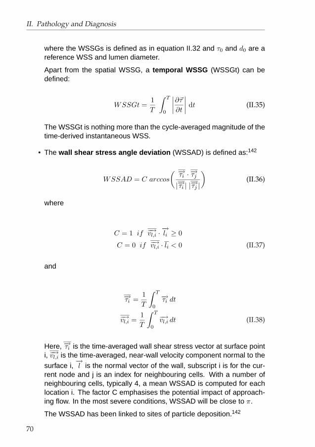
II. Pathology and Diagnosis
where the WSSGs is defined as in equation II.32 and τ0 and d0 are areference WSS and lumen diameter.
Apart from the spatial WSSG, a temporal WSSG (WSSGt) can bedefined:
WSSGt =1T
∫ T
0
∣∣∣∣∂~τ
∂t
∣∣∣∣ dt (II.35)
The WSSGt is nothing more than the cycle-averaged magnitude of thetime-derived instantaneous WSS.
• The wall shear stress angle deviation (WSSAD) is defined as:142
WSSAD = C arccos
( −→τi · −→τj
|−→τi | |−→τj |
)(II.36)
where
C = 1 if −→vl,i ·−→li ≥ 0
C = 0 if −→vl,i · li < 0 (II.37)
and
−→τi =1T
∫ T
0
−→τi dt
−→vl,i =1T
∫ T
0
−→vl,i dt (II.38)
Here, −→τi is the time-averaged wall shear stress vector at surface pointi, −→vl,i is the time-averaged, near-wall velocity component normal to the
surface i,−→l is the normal vector of the wall, subscript i is for the cur-
rent node and j is an index for neighbouring cells. With a number ofneighbouring cells, typically 4, a mean WSSAD is computed for eachlocation i. The factor C emphasises the potential impact of approach-ing flow. In the most severe conditions, WSSAD will be close to π.
The WSSAD has been linked to sites of particle deposition.142
70

II.3. Measurement of Designated Markers
• The final parameter is the wall shear stress angle gradient (WS-SAG):199
WSSAG =1
T
Z T
0
���� 1
Ai
ZS
∂φ
∂xdAi
~i +1
Ai
ZS
∂φ
∂ydAi
~j +1
Ai
ZS
∂φ
∂zdAi
~k
���� dt (II.39)
S is the complete surface of the carotid wall and Ai is the surface ofa cell face i. The WSSAG is calculated in an arbitrary coordinatesystem ijk or xyz. The scalar field of angular differences φ is definedas follows:
φ = arccos
(~τi · ~τj
|~τi| |~τj |)
(II.40)
here, ~τi refers to the stress vector at the location of interest and ~τj
represents the surrounding stress vectors: shear stress and normalstress. The WSSAG was adopted to replace the wall shear stressangle deviation (WSSAD) as a marker for sites of dysfunctional en-dothelial cells. The WSSAG has the advantage of being a mesh inde-pendent parameter.199 In this thesis, both markers are still used.
In summary, the WSSAG represents the magnitude of the shear stressangle deviation. Large WSSAG tends to occur in regions of dysfunc-tional cells, and hence sites of intimal thickening.199
71

II. Pathology and Diagnosis
72

III. Computational Fluid Dynamics
The importance of Computational Fluid Dynamics (CFD) has increased rap-idly in the past decades. After initially (and still) proving its value for militarypurposes,203 CFD has made major contributions to aviation, the automobileindustry, machinery and chemical engineering. In biomedical environments,the use of CFD is widely explored. The simulation of biofluid flow such as airflow in the bronchial tubes,139 blood flow in the cardiovascular system or inanastomoses,281 the investigation of cerebrospinal fluids149 and the study ofthe ion transfer over membranes in artificial lungs103 and kidneys88 are onlya few of the biomedical research topics where CFD is used. For a reviewof the applicability of CFD in biomedical research, see issue 26 (vol. 7) ofArtificial Organs (July 2002). The goal of CFD studies in the cardiovascu-lar system is always similar: calculating variables such as the fluid velocitycomponents and deriving from them parameters such as pressure83 andwall shear stress.253 The latter parameters cannot be measured directly, orinvolve the use of invasive techniques.
This chapter aims at explaining the principles of CFD, without discussing is-sues of stability or convergence. In short, CFD calculates the velocities in adomain by solving the Navier-Stokes equations (section III.1) in a mesh (sec-tion III.2) under appropriate boundary conditions (section III.3). Althoughthe same governing equations are considered, the numerical techniques forsolving the equations are diverse. Two techniques, implemented in PAM-FLOW™ and CFX4™, are presented in section III.4. The final section inthis chapter addresses the potential pitfalls when using CFD.
III.1. Governing Equations
The Navier-Stokes equations are the equations derived from Newton’s laws,describing mathematically the laws any fluid has to physically obey. The firstlaw describes mass conservation, i.e. a fluid can expand, move or evapo-rate, but its total mass always remains constant. Similarly, the second law
73

III. Computational Fluid Dynamics
expresses conservation of momentum. For incompressible, isothermal flow,the physical laws reduce to equations III.1 (mass conservation) and III.2(momentum) in an arbitrary fluid volume:238
3∑
i=1
∂ui
∂xi= 0 (III.1)
∂ui
∂t+
3∑
j=1
∂
∂xi(uiuj) = Fi +
3∑
j=1
1ρ
∂σij
∂xji = 1, 2, 3 (III.2)
The independent variables in a Cartesian coordinate system are the positionvector −→x = (x1, x2, x3) and the time t. The dependent variables are thefluid velocity vector −→u = (u1, u2, u3) and the pressure p. The force vector−→F = (F1, F2, F3) is expressed in N/kg and ~~σ = (σij) is the stress tensor,consisting of a pressure component and a viscous force:
σij = −p δij + τij i, j = 1, 2, 3 (III.3)
Here, δij is the Kronecker delta, and ~~τ represents the viscous stress tensor.For a Newtonian fluid, this tensor can be calculated as:
τij = 2 µ[12
(∂ui
∂xj+
∂uj
∂xi
)− 1
3
3∑
k=1
∂uk
∂xkδij
]i, j = 1, 2, 3 (III.4)
with µ the dynamic viscosity.
In the Navier-Stokes equations (III.2), the first term embodies the inertialforces, the second convective features, and last one models the viscousforces and the impact of the static pressure.
These equations form a system of coupled non-linear partial differentialequations (PDEs). Because of the non-linear terms in these PDEs, ana-lytical methods can yield very few solutions. In general, closed form analyt-ical solutions are possible only if these PDEs can be made linear. This isachieved in some cases because non-linear terms naturally drop out, e.g.fully developed flows in ducts and flows that are inviscous and irrotationaleverywhere. In other cases, non-linear terms are small compared to other
74

III.2. Meshing
terms so that they can be neglected, e.g. creeping flows, small amplitudesloshing of liquid, etc. If the non-linearities in the governing PDEs cannot beneglected, which is the situation for most engineering flows, then numericalmethods are needed to obtain solutions.1
CFD is the art of replacing the differential equations governing the fluid flow,with a set of algebraic equations (the process is called discretisation), whichin turn can be solved with the aid of a computer to obtain an approximatesolution. The best known discretisation methods used in CFD are FiniteDifference Method (FDM), Finite Volume Method (FVM) and Finite ElementMethod (FEM).1 A thorough explanation of these techniques falls beyondthe scope of this work. In short, FDM replaces the derivatives in the equa-tions by differences. FEM splits the fluid domain into a finite number ofsubdomains (elements). It then assumes a simple variation of the depen-dent variables over each computational element. For FVM, the equationsare integrated over an element’s volume.
III.2. Meshing
CFD requires the fluid domain, i.e. the vessel lumen, to be subdivided intosmall cells. The discretised Navier-Stokes equations will be solved in thesecells separately. The meshing techniques utilised here, the advancing fronttechnique and a home-built method, are discussed below.
Meshes can be structured or unstructured. In a structured mesh, the do-main is usually divided into a number of topologically similar blocks whichare then subdivided into smaller cells in a structured manner. In contrastto the structured mesh, the mesh points in an unstructured grid systemare not organised in an orderly manner. Structured grids are most fre-quently built using hexahedral cells, whereas the tetrahedron is the mostcommon element shape of an unstructured grid. Structured grids are usu-ally solved using FVM whereas unstructured grids are used with FEM. Ithas to be noted that this distinction in solver strategy is getting increasinglyoutdated. The main advantage of an unstructured mesh over the structuredmesh is in the handling of extremely complex geometries. In this work, twocommercially available CFD software packages were used. In the first one,PAM-FLOW™ (ESI Group, Krimpen aan den IJssel, The Netherlands), theNavier-Stokes equations are solved using the finite element technique in un-structured grids. The second software package, CFX4™ (AEA Technology,Didcot, Oxfordshire UK), uses the FVM in structured meshes.
75

III. Computational Fluid Dynamics
III.2.1. The advancing front technique
The advancing front technique generates an unstructured mesh, using PAM-GEN3D™, a commercially available CFD software. A front is a triangulatedsurface. In the first step, this technique triangulates all the bounding sur-faces of the domain, i.e. inlet, outlet and walls. The triangulation is per-formed by taking into account spatial variation of the size, stretching, andstretching direction of the elements to be generated. This yields the ini-tial front of faces such as the one shown in Figure VIII.3 (b) on page 202.The second step consists of creating a tetrahedron using a triangle on thefront and a new point, computed by taking into account spatial size variation,stretching, and stretching direction of the elements. The three points of thetriangle and the new point constitute a tetrahedron. A tetrahedron has foursurfaces, at least one of which is already known: the triangle part of the front.This triangle, along with other subsequently known surfaces, is deleted fromthe front and replaced with the new surfaces. This second step is repeateduntil there are no faces left in the front. This means that the whole domainhas been filled by tetrahedrons and the mesh is complete. Details of themesh generation technique can be found in the PAM-GEN3D™ manual.239
III.2.2. The in-house carotid mesh builder
This meshing strategy was based on previous work presented by Long,197
who treated the arteries as three separate distorted cylinders, the CCA,ICA and ECA. Each of the branches was subdivided in the same structure:8 contiguous blocks filled the cylinder. Each block started at the inlet ofthe considered cylinder and ended at the outlet. In a cross-section of theartery, each of the blocks can be visualised as in Figure III.1 (a). FigureXI.2 on page 276 shows meshes generated by Dr. Long for a reproducibilitystudy. Note that the CCA is bounded by two planes perpendicular to theI/S axis. This made it necessary to distort the mesh in the carotid branchesextensively, yielding highly skewed cells in the bifurcation area.
In the enhanced method, the three arteries CCA, ICA and ECA were stillregarded as three separate tubes, each subdivided using the same block-structure. However, now the CCA expanded into the bifurcation area as seenin Figure III.1 (b) and (c). Because of the reduced skewness, this methodyielded better-quality grids. Details about how to define the three sectioningplanes which divided the carotid bifurcation in three arteries are explainedin section VI.3.3.
76

III.2. Meshing
(a)
−10 0 10−20020
−20
−10
0
10
20
30
x[mm]y[mm]
z[m
m]
(b)
(c)
Figure III.1.: a: Block structure of the mesh in a cross-section of CCA. b-c: Surface meshfor a healthy subject. The two black dots represent the points where three set of blocksbelonging to different arteries come together.
77

III. Computational Fluid Dynamics
Mesh generation thus consisted of three steps:
1. Define the longitudinal splines bordering the vessel lumen. Note that‘longitudinal’ refers to splines originating in the proximal CCA and end-ing in the distal ICA or ECA.
2. Separate the arteries in the neighbourhood of the bifurcation apex.
3. Use the separated splines to fill the vessel lumen (or the computationaldomain) with structured cells.
The third step consists of 5 steps itself. First , the splines are subdivided inthe longitudinal direction into a certain number of cells, subject to mesh inde-pendence tests. If there are K cells along a spline, there will consequentlybe K + 1 nodes on each longitudinal spline. In Figure III.2, the kth nodes onall splines are called Mi (i=1,2) and Si (i=1,2,...,2×4n, with n equal to 1/8thof the number of cells along the circumference). The points at one side ofthe line M1M2 belong to splines that all start on one particular plane andend on a different plane. For example, the nodes named S1 till S4n−1 couldall belong to splines of the CCA, starting in the proximal CCA plane and allending at the CCA/ICA planar interface. If all splines were subdivided intoK cells using the same rules, Si on one side of the line M1M2 will be planarfor a given k (1 < k < K). If points Si on either side of the line M1M2 arenot equidistance, they will be redistributed. In the second step, point M isdefined as the center of the line M1M2, and points Di (i=1,2,3,4) are calcu-lated by placing them at a certain fraction f away from M along the radiusMM1 for D1, MSn for D2, etc. So
f =|MD1||MM1| =
|MD2||MSn| =
|MD3||MS3n| =
|MD4||MM2| (III.5)
where the operator |...| denotes the distance between the two points men-tioned in the argument. In the following step, lines D1D2 and D3D4 aresubdivided into n parts (illustrated by the grey points between D1 and D2
in Figure III.2) and simultaneously the line D2D3 is divided into 2× n parts,just as the line D1D4. In fourth step, the points on the ‘D’-lines, i.e. onD1D2, D2D3, etc., are connected to the Si points in the only way in whichthe connecting straight lines do not cross each other. Similarly, the centralblock D1D2D3D4 can be divided into quadrangles by connecting the pointsdefined in the previous step with straight lines. In the final step, the radiallines connecting the D-lines to the vessel wall are subdivided into m parts
78

III.3. Boundary Conditions
Figure III.2.: Building a structured mesh starting from longitudinal splines.
as illustrated in Figure III.2 in the block M1D1D2Sn with m = 4. Repeatingthis procedure for every k (1 < k < K), for both sides of the M1M2 line andfor each of the three arteries, gives all the necessary nodes for defining astructured mesh as illustrated in Figure III.1.
In this thesis, meshes have been generated using in most cases the follow-ing values for n/f/m: 4/0.5/9. This yields meshes with high density cellsnear the wall for increased accuracy for the predicted WSS.
III.3. Boundary Conditions
Equations III.1 and III.2 need to be solved under appropriate boundary con-ditions (BC). The boundaries concerned here are inlets, outlets and walls.An overview of all possible boundary conditions is given in CFD softwaremanuals.3,238
79

III. Computational Fluid Dynamics
On the vessel wall, the so-called no-slip condition is specified, i.e. all ve-locity components are zero. For the inlet and outlets, several BC’s can beimposed:3
• An inlet in the mathematical definition is a boundary where the valuesof variables are specified. This is known as a Dirichlet boundary con-dition. The most common Dirichlet BC, is a prescribed velocity profile.An example is a uniform velocity profile, i.e. all the fluid elements onthe inlet plane have equal velocities.
• Mass flow boundaries are used to model inflow and more commonlyoutflow boundaries where the total mass flow rate into or out of thedomain is known, but the detailed velocity profile is not. In this case,Neumann boundary conditions are imposed on all transported vari-ables (such as velocity or, in thermodynamic simulations, tempera-ture). This means that their normal gradients along the boundary isspecified, rather than their values. This is equivalent to an assumptionof fully developed flow at the outlet. It is most accurate when the outletis placed far downstream, and the width of the flow domain is constantat the outlet. Pressure is extrapolated from upstream.
• Pressure boundaries are used to model inflow and outflow boundarieswhere the surface pressure is known, but the detailed velocity distri-bution is not. This is in fact a combined Dirichlet/Neumann boundarycondition: Dirichlet boundary conditions are imposed on pressure, i.e.it is specified by the user. Neumann boundary conditions, i.e. zeronormal gradients, are imposed on velocity as well as other transportedvariables, temperature, user scalars, volume fractions, etc.
In this thesis, the boundary conditions issues are dealt with in section VIII.1.1by investigating all possible boundary condition types used in literature forimage-based CFD (see table VIII.1).
III.4. Solvers
As mentioned in section III.1, the governing equations are not analyticallysolvable, except for the simplest cases. They are solved numerically, i.e.by meshing the domain first, and then solving the equations in an iterativemanner. A variety of numerical algorithms exist and those adopted in thisthesis are described below.
80

III.4. Solvers
III.4.1. Spatial Discretisation
The Navier-Stokes equations (eq. III.2) contain both time and spatial deriva-tive terms. The first step in CFD is to perform a spatial discretisation. In thisstep, the Navier-Stokes equations are rewritten in each point in the form:
∂u
∂t+ f(uI,t
1 , uIn,t1 , uI,t+1
1 , uIn,t+11 , pI,t
1 , pIn,t1 , pI,t+1
1 , pIn,t+11 , µ) = 0 (III.6)
where we have taken the direction i = 1 as an example, the viscosity asconstant and neglected the external forces F1. Here, f(...) is a function ob-tained by spatial discretisation of the Navier-Stokes equation. The index Irefers to a particular point in the mesh and the index In refers to its neigh-bouring points. The index t stands for the value of the indexed parameter atthe current time-step, whereas t + 1 is the unknown value of the parameterat the next time-step. The spatial discretisation consists of finding a goodfunction f in order to replace the spatial derivatives by solvable equations.If the function f(...) does not contain any values at t + 1, the solver is calledexplicit . Otherwise, the solver is implicit . Any spatial discretisation tech-nique can be implicit or explicit, depending on whether or not the t+1 valueshave been used to estimate the spatial derivatives.
III.4.1.1. CFX4™
As an example, the spatial discretisation used in this work in all the sim-ulations performed using CFX4™ is explained. The differencing schemeused to derive the function f(...) is called the Quadratic Upwind Interpo-lation Convective Kinematics (QUICK) scheme. In short, QUICK worksas follows. Consider a one-dimensional control volume as shown in FigureIII.3. The point P is the node of interest. However, neighbouring nodes W, Eand WW must also be considered. The dashed lines (denoted by lower casesymbols, w and e) denote cell face boundaries and the symbol φ denotes thevalue of the property of the variable being calculated (e.g. u1). The QUICKscheme uses three points with a quadratic interpolation for calculating cellface values. The face value of the variable φ is found by the application of aquadratic function passing through two bracketing nodes (one each side ofthe face) and a node on the upstream side as shown in Figure III.3. Whenboth uw (velocity in point w) and ue are positive, a quadratic fit through WW,
81

III. Computational Fluid Dynamics
Figure III.3.: QUICK: The Quadratic Upwind Interpolation Convective Kinematics.
W and P is used to evaluate φw, and a further quadratic fit through W, P andE used to calculate φe.
For the situation shown in Figure III.3 and for a positive value of uw, thebracketing nodes for the west face, w, are W and P, and the upstream nodeWW and
φw =68φW +
38φP − 1
8φWW (III.7)
Similarly, for positive ue, the bracketing nodes for the east face, e, are P andE, and the upstream node is W and
φe =68φP +
38φE − 1
8φW (III.8)
Thus, in the QUICK-scheme, the variation of φ is assumed to be describedas a quadratic function. This assumption leads to estimates of φ at the cellfaces. The estimates are third order accurate. The estimates are required ifthe function f(...) from equation III.6 is to be solved using the FVM.
III.4.1.2. PAM-FLOW™
The spatial discretisation in PAM-FLOW™ is computed explicitly using theso-called Roe flux-splitting scheme with fourth order diffusion . Themathematical explanation of the Roe flux-splitting scheme falls beyond thescope of this work. Details can be found in the PAM-FLOW™ solver theorymanual.238
82

III.4. Solvers
III.4.2. Temporal Discretisation and Solution
III.4.2.1. CFX4™
The Navier-Stokes equations (equation III.2) can also be written as (vectorialnotation):
ut+1 − ut
∆t+ ut · ∇ut +
1ρ∇pt+1 = ∇µ∇ut (III.9)
In this representation, the term with the time derivation (∂u∂t ) has been dis-
cretised with ∆t the time-step duration (temporal discretisation). The otherterms need to be spatially discretised as illustrated in the previous section(QUICK, ROE flux-splitting scheme, etc.). Note that, apart from the firstterm, there are no velocities with indices t + 1 in equation III.9. This meansthat the discretisation as presented here is explicit for the velocity, but implicitfor the pressures (semi-implicit).
To solve this equation, use the pressure value at the previous time step (t).This will yield
ut+1,∗ − ut
∆t+ ut · ∇ut +
1ρ∇pt+1,∗ = ∇µ∇ut (III.10)
Here, ut+1,∗ is a guess of ut+1 using pt+1,∗, a guess of the pressure at stept + 1. In the first iteration, pt+1,∗ is pt, the pressure value in step t. Substrac-tion of equations III.9 and III.10 yields:
ucorr
∆t+
1ρ∇pcorr = 0 (III.11)
with
ucorr = ut+1 − ut+1,∗ (III.12)pcorr = pt+1 − pt+1,∗ (III.13)
83

III. Computational Fluid Dynamics
This is the point where the condition of mass conservation is used, i.e. equa-tion III.1 or (vectorial):
∇un+1 = 0 (III.14)
By taking the gradient of equation III.11, bearing in mind that ∇un+1 = 0,the following is obtained:
∇ut+1,∗
∆t=
1ρ∇2pcorr (III.15)
Now, with the knowledge of ut+1,∗ from equation III.10, pcorr can be calcu-lated using equation III.15 and thus pt+1 (eq. III.13). This pt+1 is not thecorrect pt+1, but a new guess of pt+1, i.e. pt+1,∗. pt+1,∗ can now be usedto recalculate ut+1,∗ using eq. III.10. The second iteration has now started.This iterative process continues until the changes in pt+1,∗ (or ut+1,∗, de-pending on user’s settings) between two consecutive iterations are withinpreset tolerances. That is how the Navier-Stokes equations are solved nu-merically.
The algorithm presented here is the basis of SIMPLE, implemented in CFX4™and used in all CFX™-related simulation in this work. The acronym SIMPLEstands for Semi-implicit Method for Pressure-Linked Equations. The algo-rithm is semi-implicit and not purely explicit because equation III.9 containsan index t + 1 in the pressure term.
III.4.2.2. PAM-FLOW™
In PAM-FLOW™, an implicit solver is used:
ut+1 − ut
∆t+ ut · ∇ut +
1ρ∇pt+1 = ∇µ∇ [
ut + θ(vt+1 − vt)]
(III.16)
84

III.4. Solvers
with θ the amount of implicitness. Note that when θ = 0, equation III.16becomes equation III.9. Consider the case where θ = 1, equation III.10becomes:
ut+1,∗ − ut
∆t+ ut · ∇ut +
1ρ∇pt+1,∗ = ∇µ∇ut+1,∗ (III.17)
from where ut+1,∗ can be deduced in a different manner when compared tothe explicit method. When it is assumed that
∇µ∇ut+1,∗ = ∇µ∇ut (III.18)
substraction of equations III.16 and III.17 yields again equation III.11. Therest of the sequence is similar to the semi-implicit method.
III.4.3. Validation
CFX4™ has been extensively validated for internal flows, i.e. flows in tubesor arteries, in a preceding PhD thesis.193 However, PAM-FLOW™ has neverbeen used for internal flows by any of the research groups involved, nor bythe code vendor. Therefore, for this work, code validation is necessary.
For validation of the PAM-FLOW™ CFD code, the Hagen-Poiseuille flow ina rigid circular tube was studied. The diameter of the tube was 8 mm, thetube length 50 cm. The fluid used in the computation was water at 20 ◦C,i.e. with a dynamic viscosity of 1mPa.s and a density of 998 kg/m3. At theinlet, a uniform velocity profile of 3.35 cm/s was set, this yields a tubularReynolds number of 268 (see equation VIII.1 on page 199). Because theReynolds number is below 2300, the flow is laminar and a Hagen-Poiseuillevelocity profile is expected within a reasonable length downstream the entryplane.276 For a uniform entry profile, this length l is calculated as follows:362
l
d= 0.065 Ret (III.19)
Which in this case would be 14 cm, well within tube length. Note that severalformulae for l can be found in literature,276,362 the one used here tends tooverestimate the entrance length.
85

III. Computational Fluid Dynamics
(a) Poiseuille Flow
(b) 0.2×T (c) 0.7×T
Figure III.4.: (a) Steady and (b-c) Unsteady validation. Squares or Triangles: calculatedvelocities; line: Poiseuille/Womersley theory. T: period, 0.833 s. The maximum flow occursat a time 0 or T. The dotted line represents the time and area averaged velocity. r is thedistance from the tube centreline and R is the vessel radius. Axial velocity is normalisedusing the mean velocity. (b) Velocity profile at time = 0.2 T. (c) Time = 0.7 T.
Figure III.4 (a) shows a comparison between the theoretical parabolic profile(Hagen-Poiseuille) and the CFD prediction using PAM-FLOW™ at 25 cmdown the tube. The quantitative agreement is very good, the average errorbeing within 0.75 %.
PAM-FLOW™ was further validated for unsteady flow using the Womersleyvelocity profiles in a rigid circular tube. The diameter of the tube was again 8mm, the tube length 20 cm. A 40/60-glycerine/water mixture with a dynamicviscosity of 4.38 mPa.s and a density of 1112.7 kg/m3 was computed. Atthe inlet, a uniform velocity was imposed. The flow rate varied sinusoidallyfrom 1 ml/s to 5ml/s with a frequency of 1.2 Hz (72 bpm). This yields atime-averaged tubular Reynolds number of 125 and a Womersley parame-
86
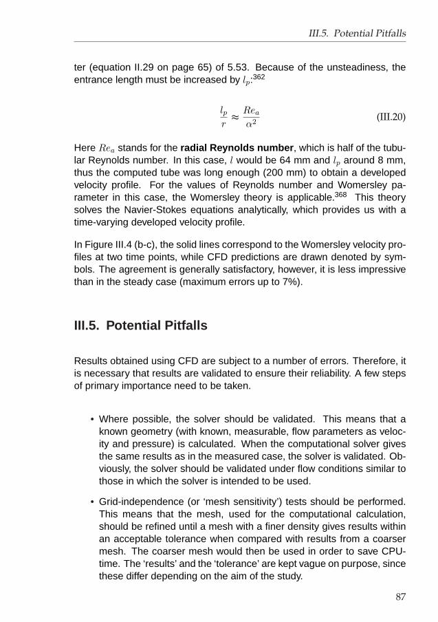
III.5. Potential Pitfalls
ter (equation II.29 on page 65) of 5.53. Because of the unsteadiness, theentrance length must be increased by lp:362
lpr≈
Rea
α2(III.20)
Here Rea stands for the radial Reynolds number , which is half of the tubu-lar Reynolds number. In this case, l would be 64 mm and lp around 8 mm,thus the computed tube was long enough (200 mm) to obtain a developedvelocity profile. For the values of Reynolds number and Womersley pa-rameter in this case, the Womersley theory is applicable.368 This theorysolves the Navier-Stokes equations analytically, which provides us with atime-varying developed velocity profile.
In Figure III.4 (b-c), the solid lines correspond to the Womersley velocity pro-files at two time points, while CFD predictions are drawn denoted by sym-bols. The agreement is generally satisfactory, however, it is less impressivethan in the steady case (maximum errors up to 7%).
III.5. Potential Pitfalls
Results obtained using CFD are subject to a number of errors. Therefore, itis necessary that results are validated to ensure their reliability. A few stepsof primary importance need to be taken.
• Where possible, the solver should be validated. This means that aknown geometry (with known, measurable, flow parameters as veloc-ity and pressure) is calculated. When the computational solver givesthe same results as in the measured case, the solver is validated. Ob-viously, the solver should be validated under flow conditions similar tothose in which the solver is intended to be used.
• Grid-independence (or ‘mesh sensitivity’) tests should be performed.This means that the mesh, used for the computational calculation,should be refined until a mesh with a finer density gives results withinan acceptable tolerance when compared with results from a coarsermesh. The coarser mesh would then be used in order to save CPU-time. The ‘results’ and the ‘tolerance’ are kept vague on purpose, sincethese differ depending on the aim of the study.
87

III. Computational Fluid Dynamics
• For periodic time-varying problems, calculation should be performedfor as many cycles as required until cycle n gives results within anacceptable tolerance when compared with results from cycle n− 1.
• For time-dependent calculations, the time-step is to be considered withgreat scrutiny. Especially when time-steps are ‘chosen’ by the opera-tor, these time-steps should be refined (shortened) until the refinedtime-step yields same results as the coarser time-step. When time-steps are calculated during the simulation, special care must be takenregarding the choice of the Courant-number (CFL-factor):
CFL =∆t V
∆x(III.21)
here, ∆t is the time-step, V the velocity, ∆x the mesh size. A highCFL-number will increase the time-step and decreases the CPU-time,but when the CFL-number is too high, numerical stability is lost.
• Even if all of the above steps were performed satisfactory, it is alwaysgood to regard the results obtained from CFD with a healthy portion ofscepticism.
88

IV. Carotid Haemodynamics andimage-based CFD
‘Hey, shear stress is something funny!’ It was in the late 1960s andearly 1970s that researchers found for the first time that atherosclerosis andlocal haemodynamics had something to do with each other.306 Fry102 sug-gested that high shear rates had a direct damaging influence on the intima,i.e. on the endothelial cells. Caro45 was categorical in his disagreement,stating that “Several workers have proposed a relationship between arterialblood mechanics and the development of atheroma. However, as we sub-sequently show, their appreciation of the mechanics has been erroneous.”Caro showed subsequently that it was not high shear rates, yet cites of lowshear rates that were associated with atherogenic zones. The link betweenatherosclerosis was clearly not fully understood, but the presence of a linkwas acknowledged. This motivated researchers to develop techniques ca-pable of measuring the shear stress. It was only later that effects on (i)smooth muscle cell migration, proliferation and metabolism, (ii) expressionof extracellular matrix, (iii) lipoprotein kinetics and binding, (iv) monocytechemotaxis and conversion to macrophage, and (v) foam cell formation wereinvestigated and modelled in a shear-dependent manner.99
Early CFD and other research techniques CFD made an early introduc-tion in this research field. Friedman101 published one of the first articles us-ing CFD for shear stress prediction, admittedly in a bifurcation of the aorta.The computational models at that time were restricted to 2D idealised mod-els: 3D computations were too expensive and in vivo imaging was slowlyemerging. Together with CFD, numerous other in vitro techniques have beenestablished, all aiming at giving insights into the shear stress distributions inarterial bifurcations. These techniques include fabricating glass185 or elasticphantoms186 and using a variety of measurement techniques, e.g. LaserDoppler Anaemometry184 (LDA). Considering the cost involved in CFD cal-culations, it was not surprising that it had taken another decade before CFDbecame a feasible alternative to building in vitro models.
89

IV. Carotid Haemodynamics and image-based CFD
CFD is taking over An important advantage of CFD lies in the fact that itcan quantify shear stresses in the entire model, whereas a large number oftime-consuming individual measurements need to be done if physical castsare to be used. Moreover, CFD has the advantage of not having to repeatthe laboratory test in case a different parameter is to be measured. Finally,CFD is not sensitive to features such as drift and jitter, typical of measure-ment equipment. This renders CFD a preferred choice to time-consuminglaboratory measurements. Slowly, CFD became a common tool for haemo-dynamic research. At first, CFD simulations were performed on 3D modelspresent at the laboratory.27,244 This gave the researcher a way to validatethe CFD calculations using high-quality laboratory measurements. In fur-ther steps, computational models were built without necessarily having anactual physical phantom.246,247 This was often done in order to investigatea particular feature, such as a new and improved numerical code247 or theeffect of bifurcation angles on shear stresses.246 In an attempt to build morerealistic in vitro models, Goubergrits and Affeld produced 3D vessel casts ofhuman carotid arteries based on post mortem excised arteries.4,125,127 Ina later stage, the internal structure and morphology of the vessel wall werelinked to haemodynamic parameters acquired with CFD.126
While CFD was getting more and more accepted as the main tool for re-search on the carotid blood flow, it was simultaneously ameliorated at dif-ferent levels. Perktold248 was among the first113,382 to examine the effectof shear-dependent behaviour of blood on flow patterns and created a codeto be used in case blood viscosity had to be shear-dependent. The samegroup178,245,249 was again among the first49,50,56,384,386,387 to incorporatemoving vessel walls into computational simulations.
Subject-specific images as a basis The previously mentioned studieshad shown that the carotid geometry (e.g area ratios AR and vessel tortuos-ity) had an important influence on the distribution of WSS. It was becomingincreasingly clear that the dynamics of blood flow in vivo are more com-plex and variable than suggested by idealised models such as the onesused thus far. This aspect combined with the notion of the fact that humancarotid arteries show a large inter-subject geometry variability prompted re-searchers to extract in vivo subject-specific carotid geometries using med-ical images. As explained in section II, a variety of imaging techniquescan be used as a basis for image-based CFD. This technique was at firsttested on simple224,362 and realistic16 phantoms, both rigid16 and elastic.33
The combination of imaging and CFD has only recently been implementedin vivo.56,178,198,219,324,370 “When coupled with ongoing improvements in
90

computing and image processing, it becomes possible to consider CFD asa viable tool for studying, for the first time at the level of an individual patient,the complex and dynamic relationship between haemodynamic forces andatherosclerosis.305”
Direct Methods Recently, several studies have investigated direct WSSmeasurement in vivo. Although in vivo techniques would still not providethe WSS distribution in an entire carotid bifurcation, these techniques arevery interesting from a cost-effective point of view bearing in mind that theybypass the use of CFD. To date, both ultrasound270 and cine PC MRI61,161
have been used for direct WSS estimation, but the techniques seem thus faronly reliable in phantoms.61,161
What shall we do ... ? In conclusion, although the use of CFD is de-manding on computational resources, it is a promising tool for investigatingarterial haemodynamics: it can be made subject-specific, does not requirepost-mortem data, is reproducible (to be demonstrated later), not affectedby drift, and more reliable in comparison to direct methods.
The major objective of this work therefore consists of smoothing away thetechnical difficulties impeding the use of image-based CFD for large-scalestudies. As part of that, one of the aims of this thesis is to define the ‘best’imaging protocols. In this context, ‘best’ means a mix between reliable andfeasible (or fast). Another main objective is to define the ‘best’ way to buildand solve the computational model. What is the difference between the re-sults in a steady simulation and those in a pulsatile simulation? Are theassumptions of newtonian flow and rigid walls justifiable? Once the tech-nique is built, the goal is to put error-bars on haemodynamic parameterssuch as WSS and OSI. The final objective is to use this technique in clinicalstudies.
91

IV. Carotid Haemodynamics and image-based CFD
92

Part B.
ESTABLISHING THE TECHNIQUE
93


V. Overview
Subject-specific image-based CFD makes use of a number of techniques.The following tasks are to be performed and optimised in order to obtain areliable subject-specific simulation of the carotid flow.
1. The first step obviously consists of imaging the carotid bifurcation. Nu-merous questions pop up. Which imaging modality should be used asa basis for carotid CFD? This can be chosen from CT, MRI and 3DUS.In this work, we will focus on the two least invasive: MRI and 3DUS.When the imaging modality is chosen, a good scan protocol needs tobe defined. A ‘good’ scan protocol is fast, easy, robust, accurate, andprovides all the information necessary for reliable CFD simulations.
Another issue, is the output format of images. This is important ifthe images are to be processed in further steps. The aspect of datatransmission has been thoroughly studied by the Digital Imaging andCommunications in Medicine (DICOM) Standards Committee .78 Itexists to create and maintain international standards for communica-tion of biomedical diagnostic and therapeutic information in disciplinesthat use digital images and associated data. The goals of DICOM areto achieve compatibility and to improve workflow efficiency betweenimaging systems and other information systems in healthcare environ-ments worldwide. Every major diagnostic medical imaging vendor inthe world has now incorporated the standard into their product designand most are actively participating in the enhancement of the stan-dard. Most of the professional societies throughout the world havesupported and are participating in the enhancement of the standardas well. In short, a DICOM-file always consists of 2 parts: a headerand the image. The image can be a matrix of greyscales representedby values ranging from 0 to 100. The header contains informationabout the scan, e.g. name of the patient, age, date of imaging, nameof operator, position of the imaging plane, resolution, etc.
2. Carotid images are usually acquired to show 2D cross-sections of asubject’s neck. For the reconstruction of the lumen, the edge of the
95

V. Overview
Figure V.1.: Illustration of the typical steps involved in constructing an image-based CFDmodel of the carotid bifurcation. Following acquisition of the data, manual or computer-assisted techniques are used to outline the lumen boundary from each slice. This seriesof profiles forms the scaffold upon which a continuous surface and, subsequently, the volu-metric finite element mesh are generated. This mesh, plus the assumed or measured inletand outlet flow rates or velocities, provides the necessary input for the CFD modelling soft-ware, which solves for the time-varying velocity field data from which desired haemodynamicindicators can be calculated.306
vessel wall needs to be delineated from the image. This delineation iscalled segmentation. It can be done either manually or automatically.
3. After the segmentation step, a series of 2D contours of the carotid areproduced. By stacking the contours in 3D space, a first approximationof the 3D carotid geometry is reconstructed . After this, the geometryis smoothed in order to eliminate image artefactsa.
4. In the fourth step, the 3D volume obtained from reconstruction must bedescretised into small computational cells, i.e. to generate the mesh.In order to be compatible with the next step, the mesh needs to bevalidated as explained in section III.5 on page 87.
5. The previous steps yield a computational mesh of the carotid bifur-cation, usable in a CFD software package. Before starting the sim-
aIn some cases, segmentation and 3D reconstruction is done at the same time. See publi-cation by Ladak164 for MRI and Gill114 for US.
96

ulations, certain model parameters need to be set, among them theboundary conditions. Apart from the boundary conditions, fluid pa-rameters such as viscosity and density should be specified.
6. When the geometry and model parameters are well defined, the simu-lation can start. After the simulation, the software outputs results suchas velocities, pressures and shear rates, depending on the user’s in-structions.
7. In the final step, computational results are visualised in various waysusing postprocessors, i.e. visualisation software.
See Figure V.1 for a schematic representation of steps 1 to 4.306 In whatfollows, many of the steps above are optimised and discussed. Chapters VIand VII explain how subject-specific 3D carotid geometries can be recon-structed from respectively MRI and 3DUS images. Chapter VIII will discuss(1) the boundary conditions to be used in computational carotid haemody-namics, (2) the effect of parameters such as heart rate and viscosity and (3)the use of viscosity laws. In the last chapter, MRI and 3DUS-based CFDare compared in a cross-comparison study. All technical improvements sug-gested in the following chapters are performed bearing in mind that the totalprocessing time, from image acquisition to final analysis, should be min-imised.
97

V. Overview
98

VI. MRI-based carotidreconstructions
VI.1. The I in MRI
VI.1.1. Brief History 230
Felix Bloch and Edward Purcell, both of whom were awarded the NobelPrize in 1952, discovered the magnetic resonance phenomenon indepen-dently in 1946. In the period between 1950 and 1970, Nuclear MagneticResonance (NMR) was developed and mainly used for chemical and phys-ical molecular analysis. In 1971, Raymond Damadian showed that the nu-clear magnetic relaxation times of tissues and tumours differed, thus mo-tivating scientists to consider magnetic resonance for the detection of dis-ease. In 1973, Magnetic Resonance Imaging (MRI) was first demonstratedon small test tube samples by Paul Lauterbur. In 1975, Richard Ernst pro-posed magnetic resonance imaging using phase and frequency encoding,and the Fourier Transform. This technique is the basis of current MRI tech-niques. In 1977, Raymond Damadian demonstrated MRI of the whole body.Edelstein and coworkers demonstrated imaging of the body using Ernst’stechnique in 1980. A single image could be acquired in approximately fiveminutes by this technique. By 1986, the imaging time was reduced to aboutfive seconds, without sacrificing too much image quality. In 1987, CharlesDumoulin was perfecting Magnetic Resonance Angiography (MRA), whichallowed imaging of flowing blood without the use of contrast agents. In 1991,Richard Ernst was rewarded for his achievements in pulsed Fourier Trans-form MRI with the Nobel Prize (in Chemistry). In 1993, functional MRI (fMRI)was developed. This technique allows the mapping of the function of thevarious regions of the human brain. In 2002, Kurt Wuthrich was awardedthe Nobel Prize (in Chemistry) for his development of nuclear magnetic res-onance spectroscopy for the determination of the three-dimensional struc-ture of biological macromolecules in solution.145 One year later, in 2003,the Nobel Prize (in Medicine) was again awarded to researchers in MRI,
99

VI. MRI-based carotid reconstructions
Paul Lauterbur and Peter Mansfield, ‘for their discoveries concerning MRI’.Paul Lauterbur discovered that the introduction of gradients in the magneticfield made it possible to differentiate structures that could not be visualisedby other techniques.145 Peter Mansfield showed how the detected signalscould be analysed rapidly and effectively and transformed to an image. Thiswas an essential step in order to obtain a practical method. Leuterbur’s andMansfield’s discoveries were done in the seventies, the implementation oftheir techniques became useful in clinical practice a decade later.
In this introduction to MRI, focus will be on the blood visualising methods,i.e. on MRA: Magnetic Resonance Angiography . First, the basis of thetechnique is explained (section VI.1.2). The description of the MRA tech-niques time-of-flight, black blood and cine PC are explained in the followingsections.
VI.1.2. Principles of MRI
The principles of MRI are described here as by Mackiewich.206 At the basis,there is the directional magnetic field, or moment, associated with chargedparticles in motion. Nuclei containing an odd number of protons and/orneutrons have a characteristic motion or precession. Because nuclei arecharged particles, this precession produces a small magnetic moment.
When a human body is placed in a large magnetic field, many of the freehydrogen nuclei align themselves with the direction of the magnetic field.The nuclei precess about the magnetic field direction like gyroscopes. Thisbehaviour is termed Larmor precession .
The frequency of Larmor precession is proportional to the applied magneticfield strength as defined by the Larmor frequency, ωo:
ωo = γBo (VI.1)
where γ is the gyromagnetic ratio and Bo is the strength of the appliedmagnetic field. The gyromagnetic ratio is a nucleus-specific constant. Forhydrogen, γ=42.6 MHz/Tesla.
To obtain an MR image of an object, the object is placed in a uniform mag-netic field, Bo, normally between 0.5 to 1.5 Tesla, although 3.0 Tesla is be-coming increasingly common. As a result, the object’s hydrogen nuclei align
100

VI.1. The I in MRI
Figure VI.1.: Alignment of nuclei by a strong magnetic field. In the absence of a strongmagnetic field, hydrogen nuclei are randomly aligned as in (a). When the strong magneticfield, Bo, is applied, the hydrogen nuclei precess about the direction of the field as in (b).
Figure VI.2.: Excitation of nuclei by radio-frequency pulses. a: The RF pulse, Brf , causesthe nett magnetic moment of the nuclei, M , to tilt away from Bo. The flip angle (FA) in thissketch is around 60°. b: When the RF pulse stops, the nuclei return to equilibrium suchthat M is again parallel to Bo. During realignment, the nuclei lose energy and a send out ameasurable RF signal.
with the magnetic field and create a nett magnetic moment, M , parallel toBo. This behaviour is illustrated in Figure VI.1.
Next, a radio-frequency (RF) pulse, Brf , is applied perpendicular to Bo. Thispulse, with a frequency equal to the Larmor frequency, causes M to tilt awayfrom Bo as in Figure VI.2 (a).
Once the RF signal is removed, the nuclei realign themselves such that
101

VI. MRI-based carotid reconstructions
their nett magnetic moment, M , is again parallel with Bo. This return toequilibrium is referred to as relaxation . During relaxation, the nuclei loseenergy by emitting their own RF signal (see Figure VI.2 (b)). This signalis referred to as the free-induction decay (FID) response signal. The FIDresponse signal is measured by a conductive field coil placed around theobject being imaged. This measurement is processed or reconstructed toobtain 3D grey-scale MR images.
To produce a 3D image, the FID resonance signal must be encoded for eachdimension. The encoding in the axial direction, the direction of z, is accom-plished by adding a gradient magnetic field to Bo. This gradient causes theLarmor frequency to change linearly in the axial direction. Thus, an axialslice can be selected by choosing the frequency of Brf to correspond to theLarmor frequency of that slice. The 2D spatial reconstruction in each axialslice is accomplished using frequency and phase encoding. A ‘preparation’gradient, Gy, is applied causing the resonant frequencies of the nuclei tovary according to their position in the y-direction. Gy is then removed andanother gradient, Gx, is applied perpendicular to y. As a result, the reso-nant frequencies of the nuclei vary in the x-direction due to Gx and have aphase variation in the y-direction due to the previously applied Gy. Thus,x-direction samples are encoded by frequency and y-direction samples areencoded by phase. A 2D Fourier Transform is then used to transform theencoded image to the spatial domain.
In MRI, the imaging protocols are described using a number of parameters.T1 and T2 are relaxation times, linked to the time it takes for M , the nettmagnetic moment of the nuclei in the core of the magnet, to realign with Bo.T1 is related to the relaxation time of the projection of M on the axis of Bo,whereas T2 is related to the relaxation time of the projection of M on theplane perpendicular to Bo. TR, the repetition time , is the time between twoconsecutive RF pulses. TE , the echo time , is related to the time in whichimages are acquired. The NEX or number of excitations is the numberof times the imaging sequence was repeated. Increasing this number willincrease signal to noise ratio (SNR), but will also increase imaging time.The FOV or Field-Of-View is expressed as a length and a width, delineatingthe imaged plane. The flip angle (FA) is the direction of the RF pulse withrespect to the Bo direction, which is also the angle between M and Bo afterthe RF pulse. In Figure VI.2 (a), the FA is approximately 60°. The echo trainlength or ETL denotes the number of ‘echoes’ used in image acquisition.An ‘echo’ occurs when a large number of spins are aligned again after RFexcitation followed by an initial dephasing.
102

VI.1. The I in MRI
VI.1.3. Time-Of-Flight
The TOF method refers to the motion of blood into and out of the plane of thesection as shown in Figure VI.3. The stationary tissues remain in the sectionand are affected repeatedly by a section-selective repetitive RF pulse. If therepetition time of this RF pulse (TR) is shorter than the relaxation time of thetissues, then the magnetisation of the tissues is saturated. Saturated tissuedoes not emit an acute measurable relaxation, and is therefore ‘suppressed’and appears dark.198 On the other hand, blood coming from outside the sec-tion is unaffected by the section-selective RF and is thus fully magnetised.The technique is therefore often referred to as ‘flow related enhancement’.As more unsaturated spins flow into the slice during each TR, overall signalstrength rises and is maximised when all the partially saturated flowing spinsin the slice are replaced during each TR. As seen in Figure VI.3, the imagewill be black where the stationary tissue is, and white where the flowingblood is found. This is why TOF is sometimes called ‘bright blood imaging’.Figure VI.4 gives an example of TOF images acquired in the right carotidbifurcation of a young hypertensive subject, free of any stenosis. The brightwhite zones contain flowing blood. The image at the top left is the most prox-imal cross-section in the CCA. The image right next to it is a cross-sectionlocated 2 mm above the previous image, i.e. inter-slice distance is 2 mm.
Figure VI.3.: Schematic illustration of the time-of-flight method. The imaging slice is mage-tised repetitively until it is saturated (repetition time TR shorter than the relaxation time of thetissues). Fresh blood replaces the saturated blood and yields a white region in the image.198
103

VI. MRI-based carotid reconstructions
Figure VI.4.: MR images of a carotid bifurcation of a young, non-stenosed hypertensive usingTOF. The bright white zones contain flowing blood. The image at the top left is the mostproximal cross-section in the CCA. The image right next to it is a cross-section located 2 mmabove the previous image, i.e. inter-slice distance is 2 mm.
VI.1.4. Black Blood
The ‘black blood’ MRI technique is explained schematically in Figure VI.5.The method has been described by Song299 and consists of a preparationperiod that contains two spin inversion pulses. The first pulse is nonselec-tive, i.e. it inverts all the spins within the sensitive volume of the RF coil.The second pulse, immediately following the first pulse, is slice-selective. Itis the 90° pulse in Figure VI.5. This pulse restores the magnetisation of the
104

VI.1. The I in MRI
Figure VI.5.: Black blood MRI. Two pulses, a nonselective and a slice-selective one, will mag-netise the entire coil volume except for the imaged slice. At the time of image acquisition, theblood in the vessel will appear white if it has not yet been replaced by inflowing magnetisedblood.
spins that lie within the slice of interest to the positive z axis. The nett effectof the two pulses is the inversion of the spins outside the desired slice, whilethose in the slice are unaffected. This is called presaturation . ‘Inverted’blood then flows into the imaging slice, replacing unaffected blood. Whenan image is made (by a 180° pulse as shown in Figure VI.5) at the momentwhere the unaffected blood has flown into the slice, the blood will appearblack (hence ‘black blood’) and the vessel wall white. Figure VI.6 gives anexample of BB images acquired in the right carotid bifurcation of a younghypertensive subject, free of any stenosis. The black ellipse-shaped zonescontain flowing blood. The image at the top left is the most proximal cross-section in the CCA. The image right next to it is a cross-section located 2mm above the previous image, i.e. inter-slice distance is 2 mm. These BBimages are the counterparts of the TOF images shown in Figure VI.4.
VI.1.5. Cine PC MRI
Phase Contrast (PC) imaging refers to a family of MR imaging methods thatexploit the fact that spins that move through magnetic field gradients obtaina different phase than static spins, enabling the production of images withcontrolled sensitivity to flow.198 Protons move along the gradients and go outof phase. The Larmour frequency will change depending on the gradient and
105

VI. MRI-based carotid reconstructions
Figure VI.6.: MR images of a carotid bifurcation of a young, non-stenosed hypertensive usingBB. These images are the BB counterparts of the TOF images shown in Figure VI.4
the spin-position. In PC imaging, a positive gradient is applied first, then anegative one. Spins in stationaire tissue, such as the vessel wall, now havethe same phase. The phase in moving spins, such as spins in blood, willchange due to the gradient switch. The phase shift caused by the positivegradient will not have been corrected by the negative gradient, due to thespin movement.226 When the phase of the signal is measured, the vesselwall can be clearly delineated.
PC MRI is also used for VENC or velocity encoding techniques to determinethe flow velocity of the blood. Thus, MR scanners can be used for acquiring
106

VI.1. The I in MRI
blood velocities in voxelsa in an entire cross-section of the artery. The Venc,or velocity encoding, is a value set by the operator, denoting the range ofvelocities measurable: [−Venc, Venc]. Velocities can be measured in all 3orthogonal directions.
The term ‘cine’ refers to the fact that it is possible to acquire a number ofimages during one cardiac cycle. When the images are sequentially dis-played, they give the impression of a moving fluid using the same principlesof cinema, hence ‘cine’ PC MRI.
avoxel : 3D pixel
107

VI. MRI-based carotid reconstructions
VI.2. Segmentation
Segmenting the raw images is necessary for separating the vessel lumenfrom the surrounding tissue. The delineated contours in 3D space form thebasis of the 3D reconstruction. The method used in this work consists of theregion growing method (RGM) followed by the snake algorithm . In theend, the operator is allowed to refine the automatically segmented contour.The technique presented here is based on the segmenting technique usedin Dr. Long’s PhD thesis193 and personal communications with Dr. P-L.Cheong. The user-interface was based on work performed by Dr. D.C.Barratt for his PhD thesis.20
VI.2.1. Region Growing Method
The region growing method as used in this study consists of 3 steps:
1. An initial guess of the vessel cross-sectional area (Ag) must be made.This initial guess will be used as a threshold to terminate the regiongrowing method. In this work, the initial guess had to be made in theproximal CCA. For each arterial cross-section, another initial guessshould be made since the CCA dilates before the bifurcation. Experi-ence showed that the best results were reached if the initial guess was1.5× Ag in the distal CCA. In the most distal CCA, this was increasedto 2.5 × Ag. For the proximal ICA, usually the position of the bulb, thevalue of the area in the most distal CCA slice was used as the initialguess. Towards the distal ICA, this value was reduced quadraticallyto half of the mean value of the cross-sectional area in the CCA. Inthe ECA, the initial guess was half of Ag. With this algorithm, a singleinitial guess and the notion of the position of each slice provided thevalues for all the slices on the carotid bifurcation.
2. In the second step, the operator needs to initiate the region growingprocess. In practice, this is done by a click of the mouse in the vessellumen. This click denotes the position of the seed point . The seedpoint does not need to be in the exact center of the lumen, its positionis in fact of no importance as long as it lies within the lumen.
3. The seed point is in a first approximation the only point in the ‘region’.Neighbouring points of the seed point are added to the region if the
108

VI.2. Segmentation
grey-scale values of that point fulfil a particular condition. This condi-tion can be any of the following:
• Grey-scale thresholding : if a grey-scale value of a neighbouringpoint is smaller than a preset value, the point is added to theregion.
• Gradient condition : if the difference between the grey scalevalue of a neighbouring point and the point in the region is smallerthan a preset value, the point is added to the region.
In both conditions a ‘preset value’ is required. It is initially very small.This initial value or threshold will create a region with a certain areaARGM . If ARGM lies within Ag±Aref , the region is stored as a potentialoutput of the RGM. Aref is 10% of Ag in the proximal CCA, it increasesquadratically to 30% in the bifurcation and drops back to 15% in thedistal end of the carotid branches. As long as ARGM is smaller thanAg + Aref , the threshold will be increased by a certain increment andthe region is grown again using the new threshold. The output of theRGM is the region found with the largest threshold yielding an areasmaller than Ag + Aref .
From experience, it was clear that RGM was more successful with TOFwhen a gradient condition was used, whereas the grey-scale thresh-olding was preferable in BB images.
In order to increase the effectiveness of the RGM, the images were interpo-lated and filtered beforehand. This was intended to increase contrast and/orreduce image noise. Interpolation was bilinear, increasing image size froman m×n matrix to (2m−1)×(2n−1), thus also increasing the computationalrequirements. In this context, ‘filtering’ meant replacing the grey-scale valuein a certain pixel either by (i) using the values of the neighbouring pixels (lo-cal filtering) or by (ii) calculating a new value for the grey-scale using only theinitial grey-scale value and a mathematical formula (global filtering). Medianfiltering is an example of local filtering: the grey-scale value is replaced bythe median value of the neighbouring grey-scales. The ‘neighbourhood’ canbe defined differently depending on the application, in this work a 3×3 neigh-bourhood gave good results for both TOF as BB images. Gamma filteringis an example of global filtering: the grey-scale value is increased (γ < 1) ordecreased (γ > 1) by a percentage depending on the individual grey-scalevalue and the value of γ. For details on bilinear interpolation, median andgamma filtering, see the MATLAB imaging toolbox manual.329
109

VI. MRI-based carotid reconstructions
In the end, the RGM yields a ‘region’ for each image. The circumferenceof this region, a ‘contour’, will be saved for further use. This contour is notnecessarily smooth, therefore the snake method is implemented in order toadjust the contours.
VI.2.2. Snake Method
The Snake Method attributes an energy to a closed contour or snake. Itwas originally introduced by Kass.153 It considers contour nodes (points)as masses connected by springs. The nodes of the contour are then movedaround in the image until the energy of the contour is minimised. The energyis the consequence of both internal and external forces:373
1. The internal forces are the snake’s tension and rigidity. Tension isrelated to the first derivative of the contour, while rigidity is related tothe second derivative.
2. The external forces relate to the grey-scale value of the nodes. Sev-eral functions can be used to model the external force, such as thegrey-scale values themselves or their gradient, possibly blurred usinga Gaussian function.372
For a detailed description of the Snake Method as used in this study, see Dr.P-L. Cheong’s PhD dissertation.62 Figure VI.7 gives an example of the auto-matic segmentation of TOF images acquired in the right carotid bifurcation ofa young hypertensive subject, free of any stenosis. The white contours sur-rounding white zones are automatically segmented luminal cross-sectionsof the CCA or ICA, while the grey contours delineate the ECA. The imageat the top left is the most proximal cross-section in the CCA. The imageright next to it is a cross-section located 2 mm above the previous image,i.e. inter-slice distance is 2 mm. Figure VI.7 is analogous with Figure VI.4,where the raw images were given. Similarly, Figure VI.8 is the segmentedFigure VI.6.
VI.2.3. Manual Corrections
As seen in Figures VI.7 and VI.8, the segmentation does not always workfor various reasons. The most frequent reason is poor image quality, very
110

VI.2. Segmentation
Figure VI.7.: MR images of a carotid bifurcation of a young, non-stenosed hypertensive usingTOF as shown in Figure VI.4. The white contours surrounding white zones are automaticallysegmented luminal cross-sections of the CCA or ICA, while the grey contours delineate theECA.
common around the bifurcation apex. Another reason for poor automaticsegmentation is an inadequate initial value for the cross-sectional area Ag.In Figure VI.8, the side branches of the ECA are included in the ECA contourbecause of this. An operator always needs to confirm and possibly changethe automatically segmented contours. This is done by running a programon a MATLAB platform (The Mathworks Inc., Cambridge, UK).328 The visualinterface is shown in Figure VI.9. It shows every contour superimposed onthe matching image to the operator who is allowed to add, delete or movearound points on the automatically segmented contour. Because editing
111

VI. MRI-based carotid reconstructions
Figure VI.8.: MR images of a carotid bifurcation of a young, non-stenosed hypertensive usingBB as shown in Figure VI.6. The black contours surrounding black zones are automaticallysegmented luminal cross-sections of the CCA or ICA, while the white contours delineate theECA.
single points can be time-consuming, the program also allows the operatorto move around, shrink or expand a contour if necessary.
As an example, Figure VI.10 (a) shows the raw BB MR image acquired inthe right CCA of a healthy subject. By using the region growing method to-gether with the snake model, a contour is obtained as is shown in FigureVI.10 (b). Figure VI.10 (c) illustrates an example where the semi-automaticsegmentation technique failed. This was due to the presence of the whitesignal at the bottom left corner of the image, caused by slow, recirculating
112

VI.2. Segmentation
Figure VI.9.: Manual segmentation interface, called in MATLAB. The slider at the top is usedto choose the image to be viewed, from the most proximal image (image 1, proximal CCA)to the most distal one. The image viewed here is a TOF image shown in Figure VI.4.
Figure VI.10.: BB MRI segmentation of the right carotid arteries for a healthy subject. a:Raw image. b: Segmentation of image (a). c: Unsuccessful image segmentation. The whitesignal at the lower left corner consists of both the vessel wall and blood. The dotted whiteline is a manual correction. Images (a) and (c) were taken from the same subject, but atdifferent slice locations.
blood particles. The segmentation program treated the white signal as thelumen border, hence giving the contour shown in Figure VI.10 (c). An opera-tor would then have to replace part of this contour, as shown in Figure VI.10(c) by the dotted line. For this purpose, the generated contour is drawn onthe original image and shown to the operator. By keeping the correct partsof the contour and replacing the spurious parts by operator-fitted splines,the final contour was obtained.
113

VI. MRI-based carotid reconstructions
VI.3. Reconstruction
VI.3.1. 3D Smoothing
At the end of the segmentation procedure, a series of parallel lumen con-tours can be lined up in 3D space. Due to potential errors in segmentation,it is necessary to adjust the contours in order to obtain a smooth 3D recon-struction.224 In this work, based on methods suggested by Moore,224 thesmoothing consisted of 2 parts which were conducted at the same time.
• Area smoothing . Cross-sectional areas were calculated for each lu-men contour. For the example of a CCA, this results in a plot such asthe one shown by the black dots in Figure VI.11 (a). A cubic smoothingspline is fitted using these points, as shown by the grey line in FigureVI.11 (a). This is performed for each of the arteries (CCA, ICA andECA) separately. The cross-sectional areas of the most proximal andmost distal contours cannot be altered to avoid a potential mismatchbetween the preceding or following artery.
• Centreline smoothing . For each of the contours, a centroid can bedefined as explained by Barratt.20 These centroids, or ‘centers’ of thelumens, form a line in 3D space: the centreline. This centreline is alsosmoothed using a cubic smoothing spline. Figure VI.11 (b) shows thecentroids as black dots and the smoothing spline as a grey line.
With the knowledge of the new position of the centroid,−−−→Cnew, and the re-
quired enlargement of the cross-sectional area, aratio, the new points on acontour
−−→Pnew can be calculated as
−−→Pnew =
(−−→Pold −−−→Cold
)×√aratio +
−−−→Cnew (VI.2)
using−−→Pold and
−−→Cold, which are the original corresponding points on the con-
tour and the old centroid respectively. Note that the square root of the arearatio is used as a scaling factor, in contrast to using the area ratio as such.This is because the value being changed with a shift to
−−→Pnew and
−−−→Cnew, is in
fact the local cross-sectional radius ratio, which is equal to the squared arearatio.
114

VI.3. Reconstruction
Proximal Distal0
20
40
60
80
Are
a [m
m2 ]
(a) CCA Cross-sectional Area (b)
Figure VI.11.: Three-Dimensional smoothing. a: Smoothing cross-sectional areas: the blackdots represent cross-sectional areas of the 2D equidistance contours acquired after manu-ally correcting the automatically segmented images. The grey line is the new cross-sectionalarea of the contours. b: Smoothing centrelines. The black dots represent the position of thecentroids of the 2D equidistance contours acquired after manually correcting the automati-cally segmented images. The grey line is the 3D smoothed centreline. Note how there wereimportant shifts in the distal end of one of the branches.
Cubic smoothing splines are calculated using the original points in need ofsmoothing, weighting factors and a smoothing parameter p. The weightingfactors can be used to prevent the points at the extremities from moving.The smoothing parameter determines the relative weight placed on the con-tradictory demands of having a smooth cubic spline vs a spline close to thedata. For p = 0, the spline is the least-squares straight line fit to the data,while, at the other extreme, i.e. for p = 1, the spline is the variational, or ‘nat-ural’ cubic spline interpolant. As p varies from 0 to 1, the smoothing splinechanges from one extreme to another.
In order to determine the optimal smoothing parameters, 9 carotid bifurca-tions were reconstructed using the same basic set of data acquired from ahealthy 28-year old male. For the smoothing parameters, values of 0.1, 0.5and 0.9 were chosen for both the area and the centreline smoothing, thusresulting in 9 different carotid bifurcations. The predicted OSI distribution ineach of these bifurcations is shown in Figure VI.12. It is important to notethat the difference in smoothing parameters was the only difference in im-age treatment between the results shown in Figure VI.12. The smoothestreconstruction (p values of 0.1) is illustrated in Figure VI.12 (a). Each row ofimages has the same area smoothing parameter and each column has thesame centreline smoothing parameter. Clearly, the main features of the OSI
115

VI. MRI-based carotid reconstructions
distribution, namely the two peaks of high OSI on both sides of the bifurca-tion area, are preserved throughout the images. High-frequency changes inthe OSI distribution of Figure VI.12 (i), i.e. the roughest reconstruction, arefiltered by both the area as well as the centreline smoothing. This can beillustrated by two examples. In a first example, consider the scattered peaksof high OSI in the CCA of Figure VI.12 (i). Bearing in mind that healthyCCA’s are generally smooth, such scattered and high peaks should not ex-ist. The smoothing implemented here managed to eliminate the scatteredOSI peaks without influencing the OSI distribution. Consider, for the secondexample, the high OSI region found in the ECA of Figure VI.12 (i). This isvery probably due to segmentation complications with ECA side branches.The ECA cross-section proximal from the side branch may widen similarlyto what happens in the distal CCA. Since the side branches of the ECA areneglected when simulating carotid blood flow, the operator may have chosento draw a smaller contour at the location of the widening or at the location ofthe branch itself. This operator-dependent guess of the contour could havebeen too small or slightly shifted in comparison with the distal ECA, givingrise to zones of recirculation after the considered contour. This effect hasbeen compensated for by smoothing.
In conclusion, smoothing is necessary and does not result in loss of impor-tant information. It is therefore recommended to set the smoothing param-eters to 0.1. This is how the most ‘physiologically realistic’ geometries areobtained, based on this subject. Note that this smoothing study has beenperformed on a healthy subject, thus the results retrieved from this study areonly applicable to healthy subjects. It is very likely that these smoothing pa-rameters may not be appropriate for the reconstruction of stenosed carotidbifurcations, where both the centrelines and lumen areas can change moredramatically.
VI.3.2. Spline Fitting
After segmentation and 3D smoothing, the available data consists of 2D con-tours, smoothed and readjusted in 3D space, which allow the reconstructionof a smooth 3D surface. In order to fit a volume to the surface, longitudi-nal splines are fitted through the contours. This is performed by taking Nequally spaced points on two consecutive contours. There are 2×N possi-ble ways to connect the points from each contour with a counterpart on theother contour: point i on the first contour can be connected to point i on thesecond contour, point i+1 to point i+1, etc. But point i can also be connected
116

VI.3. Reconstruction
Figure VI.12.: OSI distributions for one particular subject, using different smoothing parame-ters in the 3D reconstruction. The area smoothing parameter (p1) and centreline smoothingparameter (p2) are reported as (p1)/(p2).
117

VI. MRI-based carotid reconstructions
to point i+1, i+1 to i+2, etc. Finally, point i can be connected to point i just asin the first case, but point i+1 could be connected to point i-1, etc. The bestway to connect two consecutive contours is the one where the cumulativedistance between the connected points from two different contours is mini-mal. The lines connecting the points from different contours are consideredboundaries between vessel wall and lumen.
The above operation decides on how two consecutive contours can be con-nected. This procedure is initiated in the distal ICA and repeated until all ICAcontours have been connected. At that point, the most proximal ICA contouris connected to the most distal CCA contour. Similarly, the ECA can be con-nected to the CCA. Thus, the carotid bifurcation is now represented as theintegration of two parts: one connecting the CCA to the ICA (disregardingthe ECA), the other connecting CCA to ECA (Figure VI.13 (a)).
Note that the splines connecting the contours are in fact piecewise linearsegments. This ensures that no neighbouring splines will overlap with eachother, without compromising smoothness owing to the 3D smoothing per-formed in the previous step.
VI.3.3. Artery Splitting
In order to split the two parts shown in Figure VI.13, the following procedurewas performed. First , a point M was defined as the center of the shorteststraight line that connects the first distinguishable ICA and ECA contoursdistal from the apex (See Figure VI.13 (a)). This plane is located at z=1 mmin an orthogonal reference system where the z-axis coincides with the infe-rior/superior axis (or I/S-axis). In second step, all 360 lines (uniformly radi-ated from M with a 1° interval) that are perpendicular to the Inferior/Superior(I/S) axis (or z-axis) were calculated. Of all lines, only a few did not crossthe ICA or ECA lumen. The average of these lines was the ICA/ECA sep-arating line
−→M (the thick dashed line in Figure VI.13 (b)). The third step
was to determine the bifurcation apex. This was achieved by treating thecarotid bifurcation as the integration of two parts, one connecting the CCAto the ICA (disregarding the ECA), the other connecting CCA to ECA (FigureVI.13 (a)), as explained in section VI.3.2. The two parts were separated byan intersecting plane going through M and defined by the directions
−→M and
z. In Figure VI.13 (c), the intersections of this plane with the CCA-ICA vesselare depicted as black points at -1 mm < z < 1 mm (the intersections with theCCA-ECA as grey points). The intersection point closest to M was chosen
118

VI.3. Reconstruction
CCA
ICA ECA
(a) Carotid bifurcation repre-sented as two integrated parts
M ECAICA
(b) Separating the ICA from the ECA
60
70
80
4045505560
−3
−2
−1
0
1
Cet
B1
A
y[mm]
B2
Cit
x[mm]
z[m
m]
(c) Separating CCA, ICA and ECA (d) Final mesh
Figure VI.13.: Generation of a computational mesh from cross-sectional contours. a: Thecarotid bifurcation represented as the integration of the CCA-ICA (thick black contours andthin black longitudinal splines) and CCA-ECA (thick grey contours and thin grey longitudinalsplines). b: Thick black line: first ICA contour after CCA; thick grey line: first ECA contour;white point M: center of the shortest straight line connecting ICA and ECA contours; greylines: lines through M uniformly radiated with a 1° interval; thick dotted line: line chosen toseparate ICA and ECA. c: Definition of the bifurcation apex A, points B1 and B2, and pointsCit and Cet (see text for details). d: The final surface mesh; the black dots represent thelocations of points B1 and B2.
119

VI. MRI-based carotid reconstructions
as the apex A. In step four , two additional points B1 and B2 were definedas the intersection of the separating plane and the most distal CCA contour(at z=-1 mm in Figure VI.13 (c), i.e. 2 mm below the ICA and ECA contourin step 1). The parabola with its maximum at the z-value of the apex A andgoing through points B1 and B2 (and thus lying in the ICA/ECA separatingplane), created a part of the lumen border. Apart from the plane separatingthe ICA and ECA, two other planes need to be defined in the fifth step: aplane separating the CCA from the ICA and another separating CCA fromECA. These planes were defined by points B1, B2, and a third point C (Ci
and Ce for resp. ICA and ECA) at approximately 4 mm below the bifurcationapex (i.e. at z=-3 mm) and on the CCA wall. Every point on the CCA contourat z=-3 mm was a candidate for points Cx, but only two of them resulted ina plane (formed by B1, B2 and Cx) intersecting with the CCA contour at onepoint only. These two points Cit (ICA) and Cet (ECA), are shown on FigureVI.13 (c), Ci (ICA) and Ce lie 0.1 mm above Cit (ICA) and Cet respectively.
120

VI.4. Accuracy and Reproducibility
VI.4. Accuracy and Reproducibility
An important part of this research has been dedicated to finding the ac-curacy of the WSS and its related parameters when derived using image-based CFD. Accuracy is traditionally determined using phantom studies:the root mean square difference between the measured value and the cor-rect value is then regarded as the accuracy. There are, however, a numberof reasons why in vivo image-based CFD is expected to be less accuratethan in phantoms: the geometry is more complex and unknown. Further-more, imaging is hampered by motion artefacts: both due to respiratorymotion, subject movement (swallowing, sneezing, etc.) or arterial deforma-tion. However, since the technique needs to be validated for use in humansubjects, the accuracy in vivo should be quantified. For in vivo cases, how-ever, the true values of the geometry parameters are not known, thus theaccuracy cannot be evaluated. The ‘reliability’ of the technique is thereforeexpressed by its reproducibility .
In what follows, the accuracy of TOF-based CFD is quantified on a carotidphantom. The subsequent section (VI.4.2) deals with in vivo reproducibility.
VI.4.1. Accuracy in Phantoms
VI.4.1.1. Methods
An anthropomorphic carotid artery phantom (R.G. Shelly Ltd., London, On-tario, Canada) was scanned under static conditions using both BB and TOFMRI. The phantom consists of silicon tubing moulded to the shape of acarotid bifurcation and embedded in agar. The process used to fabricatethe phantom vessel is based on a novel technique using the low meltingpoint metal Cerrolow 117.295 It had been previously shown by Smith294,295
that the phantom had an RMS fabrication accuracy of 0.160 mm in lumenradius, estimated by comparing the input CAD dimensions with those mea-sured from a radiograph at 100 locations.295 Details of the phantom geom-etry have been described elsewhere.294,295 In short, the phantom is planar,has a CCA lumen diameter (LD) of 8 mm which enlarges distally and splitsinto an ICA and ECA. The bulb has an LD of 9 mm which decreases gradu-ally to 5.5 mm in the distal ICA. The ECA LD is 4.5 mm.
121

VI. MRI-based carotid reconstructions
The phantom was filled with tap water, which remained stationary duringthe scan. This involved some changes to the TOF imaging protocol. Twoimaging sequences, both for which a 2-element phased array carotid surfaceRF coil was applied, were performed on this setup. Each scan producedimages at 28 slices of 2 mm. The TOF MRI sequence had TE / TR / FOV/ FA / NEX set to 6.9 ms / 100 ms / 134 × 100 / 50° / 1 yielding an in-plane resolution of 0.52 mm. The BB MRI sequence had TE / TR / FOV /FA / NEX / ETL set to 11 ms / 655 ms / 120 × 24 / 180° / 1 / 11 yieldingan in-plane resolution of 0.47 mm. Both sets of images were segmentedand reconstructed using the techniques explained in sections VI.2 and VI.3.The smoothing parameters used in this study were 0.5 for both area andcentreline.
VI.4.1.2. Results
The results of this study are summarised in Table VI.1. The column labelledCAD contains the true values for mean cross-sectional areas (Aart), area ra-tio (AR), individual shape factor (SFiart), tortuosity (Tart), bifurcation angle(αBIF ) and centreline distance (zDIST ). See section II.3.2.2 for definitionsof these parameters. Next to the true values, the measured values are pre-sented. In order to appreciate the influence of the 3D smoothing performedduring reconstruction, the results of the unsmoothed data are presented aswell.
The accuracy of cross-sectional areas is further detailed in Figure VI.14,
Parameter [unit] CAD TOF BB TOF smooth BB smoothACCA [mm2] = 52.72 53.60 (1.7) 51.98 (-1.4) 53.61 (1.7) 52.93 (0.4)AICA [mm2] = 38.17 35.42 (-7.2) 33.91 (-11.2) 35.10 (-8.1) 34.32 (-10.1)AECA [mm2] = 17.04 15.88 (-6.8) 16.47 (-3.4) 15.90 (-6.7) 17.07 (0.2)
AR [-] = 0.80 0.72 (-9.9) 0.67 (-16.6) 0.72 (-9.9) 0.69 (-14.0)SFiCCA [-] = 0.9557 0.9702 (1.5) 0.9661 (1.1) 0.9702 (1.5) 0.9661 (1.1)SFiICA [-] = 0.9884 0.9928 (0.4) 0.9976 (0.9) 0.9927 (0.4) 0.9980 (1.0)SFiECA [-] = 0.9881 0.9944 (0.6) 0.9967 (0.9) 0.9944 (0.6) 0.9975 (0.9)TCCA [%] = 0.53 0.72 (35.8) 0.56 (5.7) 0.22 (-58.1) 0.36 (-31.3)TICA [%] = 1.68 2.00 (19.2) 1.67 (-0.3) 1.24 (-26.3) 1.36 (-18.9)TECA [%] = 2.03 2.63 (29.5) 2.19 (7.7) 2.00 (-1.4) 1.99 (-2.1)αBIF [°] = 149.67 151.43 (1.2) 151.40 (1.2) 151.63 (1.3) 151.39 (1.1)
zDIST [mm] = 0.00000 0.01486 0.01359 0.01450 0.01371
Table VI.1.: Accuracy of MRI using a carotid phantom. CAD: true values; TOF: Time-of-flight;BB: Black blood; smooth: smoothed geometry. The values in brackets are the percentagedifference with respect to the true (CAD) value. The column zDIST was defined as theaverage distance between the measured centreline and the true centreline. See sectionII.3.2.2 for definitions of the used parameters.
122

VI.4. Accuracy and Reproducibility
−20 −10 0
20
40
60
80
z [mm]
area
[mm
2 ]
(a) CCA
5 10 15 20 25
20
40
60
80
z [mm]
area
[m
m2 ]
(b) ICA
5 10 15 20 25
20
40
60
80
z [mm]
area
[m
m2 ]
CADTOFBBTOF smoothBB smooth
(c) ECA
Figure VI.14.: Accuracy of cross-sectional areas reconstructed by MRI using a carotid phan-tom. The cross-sectional area is presented as a function of the I/S axis z. The black linerepresents the true CAD data. The symbols are measured cross-sectional areas and thegrey lines are smoothing splines through the measurements.
where the cross-sectional area is presented as a function of the I/S axis z.The black line represents the true CAD data. The data points are measuredcross-sectional areas and the grey lines are smoothing splines through thedata points obtained by setting the smoothing parameters to 0.5. FigureVI.15 shows the centrelines of the phantom overlaid by the centrelines foundfrom the TOF-scan (dark grey) and the BB MRI-scan (light grey).
VI.4.1.3. Discussion
In this study, an anthropomorphic carotid artery phantom was scanned un-der static conditions using both BB and TOF MRI. The serial 2D MR imageswere segmented and reconstructed using techniques developed in this the-sis as discussed in sections VI.2 and VI.3. Table VI.1 shows that the ac-
123

VI. MRI-based carotid reconstructions
Figure VI.15.: Centrelines in MR phantom study deduced from true phantom geometry(black), TOF scan (dark grey) and BB MRI (light grey).
curacy in reconstruction for all geometric parameters was very high. Thegood area agreement gave rise to low percentage errors when comparedto a study performed by Frayne,98 who found errors in area measurementsof ±15% (see also Table IX.8 on page 261). It can be noted from FigureVI.14 (b) that the areas were systematically underestimated in the ICA, bothwith TOF and BB. Smoothing was not responsible for this slight discrep-ancy, since the percentage area error was hardly influenced by smoothing(-11.2% before and -10.1% after smoothing, BB ICA mean area error, Ta-ble VI.1). The reason for this error probably lay in the fact that the imagingplanes in the bulb were not perpendicular to the vessel axis, yielding MRIartefacts. Centreline agreement was almost perfect (Figure VI.15), implyingthat the values for centreline agreement parameters, reflected in the tortu-osity, bifurcation angle and zDIST , are good standards for further centrelinecomparison studies. Finally, there was little error in the individual shape fac-tor, partly due to the simple geometry used in this setup. Note that both theTOF and BB scan gave adequate results, which in addition compared verywell to each other.
It is clear that the accuracy found here is only valid for the phantom, andcannot be regarded as the in vivo accuracy. Nevertheless, this phantomstudy provides reference values for the accuracy of a number of param-eters. Moreover, the good agreement between the true data and the 3Dreconstructions encourages the use of MRI-based CFD for in vivo applica-tions. Therefore, the next section will take the technique to the next step, i.e.
124

VI.4. Accuracy and Reproducibility
to study the in vivo reproducibility by scanning a number of healthy subjectstwice and comparing the 3D reconstructions of both scans to each other.
VI.4.2. In Vivo Reproducibility
This study aims to evaluate the reproducibility of the MRI-based CFD ap-proach for the prediction of flow and wall shear stress related parameterswhen applied to in vivo situations. For this purpose, the carotid bifurcationsof 8 healthy subjects were scanned two times. The reproducibility of theapproach for geometry reconstruction has previously been studied.194 Thiswork investigates the reproducibility of the predicted flow field.
VI.4.2.1. Methods
Volunteers and Scanning Protocol Eight healthy volunteers, 5 malesand 3 females aged between 22 and 36, were scanned on two separate oc-casions between 2 to 4 weeks apart. On each occasion the subject lay flatwithin the MRI scanner with his/her head kept in a straight position by meansof a saddle-shaped cushion under the neck. Since changes in neck anglesmight influence the carotid haemodynamics, it was necessary to keep thesubject’s neck in the same position in both scans. Cross-sectional imagesof the right carotid bifurcation were acquired using a GE MR scanner (1.5T,Signa) with a 2D TOF ‘SPGR’b sequence. For further reference, the firstscan will be referred to as scan A and the second scan as scan B, subjectswill be numbered from 1 to 8. Slice thickness was 1.5 mm, 64 parallel im-ages were obtained covering the bifurcation over a region about 100 mm inlength. Other scan parameters were TR=45ms, TE=8.7ms, FA=60 degrees,NEX=2.0, FOV=16x12cm and matrix size 256x192, which gave an in-planeresolution of 0.625 mm. A 5 inch surface RF coil was used for data acqui-sition. The research protocol was approved by the local institutional reviewboard and the local research ethics committee.
Geometry The image segmentation and 3D reconstruction were performedusing the methods described previously.197 These methods are an earlierversion of the techniques found in sections VI.2 and VI.3. For the recol-lection of the reader, the reconstruction method is explained here in short.
bSPGR: SPoiled Gradient Recalled
125

VI. MRI-based carotid reconstructions
Figure VI.16.: Structured hexahedral meshes for subject 5. The geometry in scan A (a)differs from the geometry in scan B (b). The solid black lines show how the mesh is dividedinto a CCA, ICA and ECA block. The grey dashed line shows where the seperate arteriesare ‘cut open’ in order to patch the haemodynamic wall parameter data. (See page 130.)
Once the images were acquired, high quality contours were extracted fromthe 2D images using a region growing method for initial contour definition,and the snake method for final contour extraction. These serial 2D contourswere then aligned to produce a 3D vessel surface geometry. Smoothingwas done in two steps: centreline smoothing and area smoothing. Themesh was generated using an in-house purpose-built mesh generator de-scribed by Long.197 For mesh independence tests, 4 different meshes weregenerated, the coarsest one having 29640 cells, the finest one 54600 cellsfor the same vessel volume of approximately 120 ml. A mesh was consid-ered sufficiently dense when, as suggested by Prakash,253 the values of thewall shear stress were within acceptable tolerance in two simulations usingmeshes of different densities. The coarser mesh would then be used fortime-saving reasons. In this study, multi-block, structured meshes contain-ing 41600 hexahedral cells were adopted. The resulting wall shear stressdifferences between the finest mesh and the used mesh were within 1.0%.Figure VI.16 shows the computational meshes for subject 5 (scan A in Fig-ure VI.16 (a) and scan B in Figure VI.16 (b)). Clear geometric differencesbetween the two scans can be noticed.
126

VI.4. Accuracy and Reproducibility
Computational Details The governing equations were solved numericallyusing the ‘QUICK’ differencing scheme available with CFX4™,.3 The com-putations were performed for two cycles, since the third cycle resulted ininstantaneous WSS differences below 0.01% compared to the second cy-cle. Each cycle was divided into 80 equally spaced time-steps of 0.0125s.This time resolution was considered sufficient since the resulting wall shearstress differed by only 0.1% when a greater time resolution (160 time-stepsper cycle) was used. The dynamic viscosity was set to 4 mPa.s (Newto-nian flow) and the density 1176 kg/m3. Flow simulations were carried outon a SUN Blade 1000 Workstation (Ultrasparc III processor, 512Mb RAM,750 MHz). At the wall, ‘no-slip’ boundary conditions were imposed, i.e. theblood velocity on the wall was set to be the wall velocity itself, which forrigid walls is zero. The rigid wall assumption has been questioned in severalstudies.178,387 Zhao387 showed that the effect of moving walls was a generalreduction in the magnitude of WSS, but the global characteristics of the flowand the stress patterns remained unchanged. In this study, the influence ofgeometric uncertainties on the flow was studied. It is clear that, as shownby Zhao,387 flow in a rigid model will certainly be different from that in a de-formable model. However, since it is very difficult to acquire time-resolvedcarotid images that are of sufficient temporal and spatial resolution for thereconstruction of a deformable CFD model, the rigid wall assumption wasmade.
Several authors have studied the effect of inlet boundary conditions on theCFD predictions of pulsatile flow (See also section VIII.1.1, where differentin- and outflow conditions for MRI-based CFD are discussed and tested).Redaelli261 found that a uniform profile developed faster than a parabolicone. Cebral showed that using MRI measurements as boundary conditions,different results were obtained when measured velocities were imposed oninlet or outlets.49 Shipkowitz282 emphasised the importance of the effectof the secondary velocities at the inlet subsection. We have analysed MRImeasurements (later in the thesis), demonstrating a high reliability of 3Dcine MRI measurements: the measured velocity profiles were not fully devel-oped, but physiologically correct, resulting in correct WSS distribution withminimal entrance effects.
It is therefore important to emphasise that boundary conditions can influencethe flow pattern significantly. By using the same inlet boundary conditionsfor both scans and for each subject, it was ensured that flow pattern differ-ences in this study would only be due to geometrical differences betweentwo scans, and would be completely independent of MR velocity acquisitionerrors. A typical flow wave form (Figure VI.17), obtained from the common
127

VI. MRI-based carotid reconstructions
Figure VI.17.: Flow Rate Data. This flow wave form was obtained from the common carotidof a normal subject using pulsed Doppler (see section II.3.3.1 on page 61). It was used tocalculate time-varying Womersley profiles,368 which were imposed at the inlet of the numeri-cal model.
carotid of a normal subject using pulsed Doppler (see section II.3.3.1 onpage 61), was used to calculate Womersley profiles.368 These time-varyingvelocity profiles were imposed at the inlet. Since the same flow wave formwas used in all simulations, the inlet velocities derived from the Womers-ley theory could be different depending on the inlet area. When analysingthe results, one has to be aware that this solution is an oversimplification,however, the downstream effects of using idealised boundary conditions buttrue flow rates have been shown to be minimal after a short redevelopingdistance (less than 1.5 diameters).122
At the outlet, a constant flow ratio of 70:30 was adopted between the internalcarotid artery (ICA) and external carotid artery (ECA) throughout the wholecardiac cycle.
Derived Parameters Time-averaged wall shear stress (WSS), and severalother WSS derived parameters were evaluated. These included the oscil-latory shear index (OSI, equation II.31), time-averaged spatial wall shear
128

VI.4. Accuracy and Reproducibility
stress gradient (WSSGs, equation II.32), temporal WSSG (WSSGt, equa-tion II.35), wall shear stress angle deviation (WSSAD, equation II.36) andwall shear stress angle gradient (WSSAG, equation II.39). Apart from theWSS, OSI, WSSAD, WSSAG and WSSG, other haemodynamic parameters(such as the maximum WSSGt in a cardiac cycle283) have been introducedand validated in literature. For practical reasons, the flow analysis has beenrestricted to the aforementioned haemodynamic parameters.
Quantitative Analysis of Reproducibility Flow patterns cannot be com-pared in a direct manner. The velocity profile is three-dimensional and time-dependent. The wall shear stress and derived parameters are even lesscomparable: the geometry of the vessel wall in scan A differs (slightly) fromscan B, and it is exactly on the vessel wall that the shear parameters areof high clinical importance. The results on the walls from 2 different scansneed to be compared while making abstraction of the wall itself. The follow-ing ways of analysing these complex patterns were introduced here.
Area of overflow/underflow
Areas of low (< 0.5 N/m2) and high (> 2.5 N/m2) time-averaged WSS wereidentified.208 Thresholds like those for the time-averaged WSS were alsodefined for OSI (> 0.2), WSSGs (> 4 kN/m3),173 WSSGt (> 50 N
s m2 ) andWSSAD (> π
3 ).143 For each case, the area trespassing these thresholdswas calculated and presented as a percentage of the bifurcation area. Thedifference in area percentage between results corresponding to two scansof every subject indicates the error. Dividing this error by the scan-averagedvalue yields a relative error.
Maximum Velocity and I/S Correlation
The Vmax (see section II.3.3.2 on page 67) can be represented as a functionof the I/S axis. Note that the origin of the I/S axis was at the bifurcationpoint for each scan, allowing alignment of the data for comparison betweenscans. This way of representing the results provides information concerningthe ‘equality’ of the velocity pattern in both scans.
A similar approach was used for the wall shear stress parameters. Foreach cross-section, a mean was calculated, allowing the differences be-tween scans to be evaluated at each location. In addition to quantifyingthe difference along this axis by a Root Mean Square method, a correlationcoefficient R was computed, comparing the curves obtained from the two
129

VI. MRI-based carotid reconstructions
scans on each of the subjects. The correlation coefficient is a normalisedmeasure of linear relationship between two sets of data, with R=1 indicatingstraight line relationship and R=0 uncorrelated.
Statistical Analysis
Differences between the reconstructed geometries of the two scans for eachindividual lead to differences in the associated meshes. Consequently, amesh point in mesh A will not coincide with a mesh point in mesh B, makinga point-by-point comparison impossible. Thomas333 described a methodto overcome this difficulty by displaying the wall thickness and the WSSrelated parameters as patched data. In short, ‘patching’ the data in thisstudy consisted of four steps. First, the three arteries were disconnectedfrom each other. Second, the vessel was ‘cut open’ and ‘unwrapped’ untila flat irregular shape was obtained. The line along which the individualarteries were cut depended on the mesh structure (see Figure VI.16). Third,this irregular shape was transformed into a rectangle. Finally, the vesselwall was divided into small rectangular patches, and each patch was colour-coded by the average value of the shear stress parameters in that patch.Patching allowed a paired student test to be performed (p<0.05).
The number of patches differed between every artery and subject. Select-ing too few patches could smooth out important features in a distribution.However, too many patches would cause the patched values to be overde-pendent on local geometry features, allowing small geometrical differencesto introduce large errors. The number of patches in the circumferential andlongitudinal direction of the vessel was therefore chosen based on their abil-ity to minimise the variance of (e.g. WSS) values of the cells lying in a patchand maximise the number of normal error-value distributions. Typically, ahigh number of patches were required along the circumference (up to 12patches, i.e. 1 patch every 30 degrees). There was, however, no preferen-tial number of patches along the longitudinal direction.
For each artery, parameter and subject, two sets of patched data were ac-quired: one for each scan. The ‘resemblance’ between those two scanswas assessed using a linear regression analysis. This would result in a 2Dlinear correlation factor 2DR, which was close to 1 if the ‘resemblance’ washigh. As opposed to the vertical axis analysis, the correlation performedhere was two-dimensional. It should be emphasised that correlation param-eters provide little information about accuracy. For example, if the valuesof the WSSG in scan A were exactly twice those of scan B, 2DR would bemaximal, i.e. 1. The accuracy of measurement, however, would be low. This
130

VI.4. Accuracy and Reproducibility
does not imply that the 2DR should be discarded: the correlation parametersare very useful in assessing the qualitative agreement between two scans:if one scan delivers low values in a particular part of the vessel wall but highvalues in the subsequent scan, then the correlation parameter will be verysmall (i.e. near zero).
VI.4.2.2. Results
Correlation between measurements Three of the comparative tools usedto quantify reproducibility between scan A and scan B, provided a feel for thequalitative agreement. The ‘I/S Correlation’ and 2D Correlation expressedrespectively how good the resemblance was between two scans when trav-elling through a vessel or when unwrapping the vessel wall. Finally, theoverflow/underflow analysis showed whether or not the surface of zones un-dergoing ‘pathologic’ WSS related parameters can be determined.
Figure VI.18 provides an example of the vertical (or I/S) correlation analy-sis. Table VI.2 shows the averaged R-values for every artery and parameter.With the exception of spatial WSSG, all correlations were greater than 0.70,indicating that the qualitative agreement was high when evaluated by travel-ling through a vessel. Predicting locations prone to particle deposition (em-bodied in WSSAD) seemed to be less reproducible in the CCA. Taking allthe derived parameters into account, as shown in Table VI.2, there appearedto be no difference in the reproducibility between arteries.
Figure VI.19 shows the patched WSSAD distribution for the ICA for scanA (left) and scan B (right) for subject 3. The corresponding 2D correlationwas 0.80. Table VI.3 gives the averaged 2DR values for every artery andparameter. The results suggest that combined MRI and CFD achieve an ac-ceptable qualitative reproducibility, as the mean values for every parameter
Artery Vmax WSS OSI WSSGs WSSGt WSSAD meanCCA 0.76 0.71 0.74 0.75 0.78 0.57 0.72ICA 0.83 0.72 0.79 0.54 0.77 0.83 0.75ECA 0.76 0.71 0.83 0.53 0.74 0.83 0.73mean 0.78 0.71 0.79 0.61 0.76 0.74 0.73
Sd 0.04 0.01 0.04 0.13 0.02 0.15 -
Table VI.2.: Mean I/S correlation R for all subjects (n=8). Values closer to 1 have moreimportant resemblance. See Figure VI.18 for an example. Sd is the standard deviation of themean correlation coefficients for different arteries. Small values of Sd indicate less variationsof reproducibility among vessels (CCA, ICA and ECA).
131

VI. MRI-based carotid reconstructions
−0.01 0 0.010.8
0.9
1
1.1
−. CCA − ICA .. ECA
I/S distance [m]
Vel
ocity
[m/s
]Vmax along IS axis, scan A
(a)
−0.01 0 0.010.8
0.9
1
1.1
−. CCA − ICA .. ECA
I/S distance [m]
Vel
ocity
[m/s
]
Vmax along IS axis, scan B
(b)
(c)
Figure VI.18.: An example of maximum velocity VMAX [m/s] analysis along I/S axis [m]: scanA (a), scan B (b) and the difference (c). I/S: inferior-superior axis. The factors R are linearcorrelation parameters. The errors given are root mean square errors.
were greater than 0.70. However, all parameters, except WSS and WSSGs,were not reliably reproducible in the CCA. The relatively low 2DR valueswere due to the fact that the haemodynamic parameters in the CCA wereeither fairly uniformly distributed, or close to zero. The OSI, for instance,is fairly constant in the healthy CCA, and does not differ substantially fromzero. This resulted in a low 2DR value even for a rather small deviation.
Overflow/Underflow analysis Results showed that areas of low WSS(maximum error 9%), high OSI (2%), high WSSAD (1%), high WSSGs (0.15%)and high WSSGt (1.5%) were better reproduced than areas of high WSS(20%).
132

VI.4. Accuracy and Reproducibility
WSS Angle Deviation for ICA
0.00 0.50 1.01
(a)
WSS Angle Deviation for ICA
0.00 0.50 1.01
(b)
Figure VI.19.: Patched WSSAD in ICA for subject 3, scan A (a) and scan B (b). The bottomend of the picture represents the bifurcation, the top end is the ICA outflow. Thus, bloodflow direction is upwards in this representation of the vessel wall. Patching the data allowsstatistical evaluation. Here, the 2DR is 0.80 and the paired t-test yielded a value of 1.548.
Artery WSS OSI WSSGs WSSGt WSSAD meanCCA 0.70 0.58 0.75 0.59 0.63 0.65ICA 0.84 0.75 0.90 0.82 0.78 0.82ECA 0.81 0.82 0.88 0.80 0.83 0.83mean 0.79 0.71 0.84 0.74 0.75 0.76
Sd 0.07 0.12 0.08 0.12 0.10 0.05
Table VI.3.: Mean 2D correlation of the patches for all subjects (n=8). Values closer to 1 havemore important resemblance. See Figure VI.19 for an example. Sd defined in Table VI.2.
Differences between measurements The Root Mean Square of the ve-locity errors along the I/S axis (as defined on page 129) was 2.5% for theCCA, 4% for the ICA and 4.5% for the ECA.
The mean differences (mean of values in scan A minus values in scan B)for all the WSS derived parameters are shown in Table VI.4 with associatedRMSE. The error used to calculate the RMSE is the difference between thevalue of a patch in scan A and scan B and the most likely value, i.e. the meanof the value in scan A and B. All errors are at least one order of magnitudesmaller than the range in which the considered haemodynamic parameteris considered clinically important (see Area of overflow/underflow) and theRMSE is greater than the mean error in all cases. These findings show thatthe haemodynamic error between the two scans is clinically acceptable.
The paired t-test yielded for Figure VI.19 a t-value of 1.548, and thus con-sidered reproducible (p<0.05). The paired T-test is a useful tool as it can
133

VI. MRI-based carotid reconstructions
artery WSS OSI WSSGs WSSGt WSSAD WSSAG[N/m2] [-] [N/m3] [ N
m2.s] [-] [rad/m]
Mean CCA 0.0196 3.13e-04 10.3 -0.177 8.21e-04 0.65error ICA 0.0280 -6.23e-04 50.1 0.277 -4.01e-03 1.23
ECA -0.112 1.74e-03 74.6 -0.867 6.81e-04 5.54mean -0.0216 4.77e-04 45.0 -0.256 -8.35e-04 2.04
RMSE CCA 0.175 0.0129 114 0.817 0.0969 22.1ICA 0.543 0.0325 234 2.97 0.120 67.8ECA 0.563 0.0296 213 3.27 0.0972 77.3mean 0.427 0.0250 214 2.35 0.105 68.1
% CCA 35.0 89.9 67.1 20.4 79.5 64.5ICA 24.9 107 68.9 19.5 121 97.5ECA 39.6 129 56.1 35.0 106 72.0mean 37.9 123 65.7 30.2 102 79.8
Table VI.4.: Mean error and RMSE, (n=8). The ‘error’ is the difference between the valuein a patch from scan A and that from scan B. The error used to calculate the RMSE is thedifference between the value of a patch in scan A and scan B and the mean of the value inscan A and B. The percentage is the RMSE divided by the average value.
Artery WSS OSI WSSGs WSSGt WSSAD TotalCCA 4/7 8/8 3/4 4/4 7/8 26/31ICA 4/6 5/5 5/6 4/6 7/7 25/30ECA 3/6 5/7 6/7 2/5 6/6 22/31Total 11/19 18/20 14/17 10/15 20/21 73/92
Table VI.5.: Reproducibility summary for all 8 subjects. The first number is the number oftimes the T-test gave a reproducible result. The second number is the number of times theerror-value distribution was considered normal (for details, see Bland and Altman30). Themaximum normal distributions per artery and parameter is equal to the number of subjects.
be applied to different carotid geometries, different meshes and to all possi-ble wall related parameters. However, it does assume the error is normallydistributed. The normality of the data distribution was tested using the 95%rule.30 Cases that did not show a normal distribution for the error, wereexamined for a relationship between the error and the scan-averaged value.
The results of the paired T-test are tabulated in Table VI.5. Overall, a re-producibility rate of 79% (73/92) was found. Considering each individualparameter, the WSSAD (95%) and the OSI (90%) did remarkably well whencompared with the WSS (58%) and both WSSGs (82%) and WSSGt (75%).The results also suggested that the parameters were less reproducible inthe ECA than in the other arteries.
Whenever the errors were not normally distributed, the presence of a sys-tematic error was suspected. In the case of the OSI, a linear correlation
134

VI.4. Accuracy and Reproducibility
between errors and values was always found, whereas this was only spo-radically the case for the other parameters.
VI.4.2.3. Discussion
Moore224 has found that the peak error in WSS in a straight tube can be upto 60%, due to limited spatial resolution, image segmentation and model re-construction. Even after geometric smoothing, they reported an uncertaintyof 16%. They noted that this value could in no circumstances be regarded asthe worst case, because of the simple geometry used in their experiments.Considerable efforts have been made to reduce the processing time fromimage acquisition to simulation, and, more importantly, maximising the relia-bility and amount of information obtainable with the combined MRI and CFDapproach. This may be achieved by shortening the acquisition time,262 au-tomating the contour-extraction164,197,262 or the mesh generation,55 speed-ing up the numerical solver203 or writing a user-friendly software that inte-grates all the actions from contour-extraction to CFD data processing.324
The quality of simulation can be improved by using a measurement tech-nique with little artefacts.59,93 Other ways to improve the quality of a simula-tion are: minimising errors in segmentation of geometry,54 generating higherquality grids,54,192 and setting more reliable boundary conditions.49,122,261
In this study, the overall reproducibility of the combined MRI/CFD approachhas been assessed. The three arteries in the carotid bifurcation are anatom-ically very different. The CCA has a significantly larger cross-section thanthe ECA, and the ICA starts with a very individually shaped bulb. Thesefeatures can influence the haemodynamics greatly, and imply that the re-producibility in the three arteries might be different. Moreover, it has beendemonstrated in the past that the geometric accuracy of the reconstructionis related to the artery diameter.194 Our results showed that qualitatively,there was no suggestion that the reproducibility of any of the arteries dif-fered. Quantitatively however, Tables VI.4 and VI.5 suggest the ECA is lessreproducible, albeit slightly. This may be due to relatively smaller dimen-sions of the ECA, making the effect of uncertainties in MR acquisition moreimportant.
Overall, the qualitative agreement between the two scans was very good,demonstrating that the combined MRI/CFD approach is capable of produc-ing highly reproducible patterns of various WSS related parameters. Quan-titatively, the reproducibility varied depending on which parameter was of
135

VI. MRI-based carotid reconstructions
Figure VI.20.: Time-Averaged WSS distribution for subject 4 in scan A (a) and scan B (b).Differences in wall areas having high WSS (in red) are much more pronounced than thosehaving low WSS (in dark blue).
particular interest. However, it should be borne in mind that a number of as-sumptions were made in this study, including Newtonian blood viscosity, rigidwall and idealised inflow velocity profiles. These assumptions will influencethe predicted WSS magnitude, and therefore the flow patterns obtained herewill differ slightly from the physiological ones. Nevertheless, for relative flowcomparisons between two serial scans, these assumptions are consideredjustifiable.
Time Averaged Wall Shear Stress The time-averaged WSS was not ad-equately reproducible (reproducibility rate of 58%). It appears that predictingareas of high time-averaged WSS - occurring near the bifurcation point - isdifficult, making these estimations unreliable. This does not appear to bethe case when quantifying areas of low WSS as illustrated in Figure VI.20.It means that at the bifurcation point, the predicted values of WSS could beunreliable. Modelling and meshing the bifurcation area has proven to be adifficult task in the past, which is why, as suggested by Cebral,55 sophisti-cated meshing programs and detailed geometry reconstruction tools shouldbe applied when high WSS are of particular interest.
Oscillatory Shear Index Areas where the direction of the WSS vectorchanges frequently will have high OSI values which have been related tointimal thickening. The OSI proved to be highly reproducible (reproducibil-ity rate of 90%). Systematic errors tended to occur only with the OSI, asillustrated in Figure VI.21 by the red arrow. Errors in geometric reconstruc-tion can lead to exaggerations in the areas of flow separation predicted byCFD, increasing the OSI. This phenomenon does not appear to involve er-
136

VI.4. Accuracy and Reproducibility
Figure VI.21.: OSI distribution for subject 7 in scan A (a) and scan B (b). Relatively smalldeviations in the geometry can cause OSI peaks to occur in different locations. In scan A(a), an OSI peak is found in the bifurcation region (in the ECA, indicated by the red arrow),whereas this peak is not there in scan B (b). This effect will become clear numerically in aBland-Altman plot. However, this geometrically induced flow difference does not influencethe reproducibility significantly.
rors large enough to significantly affect the reproducibility as assessed bythe paired T-test, or make the error in the area trespassing an OSI value of0.20 significant.
Wall Shear Stress Angle Deviation & Gradient WSSAD was highly re-producible both when assessed qualitatively and quantitatively, suggestingthat MR image-based CFD predictions have a good potential for predictingareas prone to particle deposition and prolonged particle residence time.The RMSE’s for the WSSAG, summarised in Table VI.4, are comparablewith values found in a similar reproducibility study using BB MRI as a ba-sis.332
Wall Shear Stress Gradients The WSSG proved to be a more difficult pa-rameter to reproduce, and the spatial WSSG more than the temporal one.As was the case for the time-averaged WSS, high WSSG values occurred atthe bifurcation point. WSSGs is, because of its derivative nature, very griddependent and therefore sensitive to geometry changes. Whilst quantifyingthe WSSG is difficult, the high 2DR values showed that the WSSG distribu-tion can be done reliably, a finding consistent with those of Siauw,283 whoshowed that the WSSG was very sensitive to changes in computational rhe-ological parameters, whereas the WSSG distribution remained the same.Our findings showed that the WSSG distribution is reliable, although WSSGvalues were not. If WSSG values are to be used for further analysis of wallpermeability - as suggested by Lei171 - imaging and meshing quality willhave to be improved, especially for the area near the bifurcation point. This
137

VI. MRI-based carotid reconstructions
finding sheds a new light on mesh convergence tests. When CFD was firstintroduced, mesh dependence meant making sure the calculated velocitieson a coarser and a finer mesh were the same. Later,253 the WSS field super-seded the velocity field as the determinant for mesh density; WSS requiringa denser mesh for grid convergence. Our data now suggests that WSSGshould be used to determine the mesh density if WSSG values are of greatimportance.
Relation of Flow Errors to Geometrical Errors The area agreement andparameters zDIST and SFc were quantified in a study by Long.194 Sincethe same boundary conditions were used in all the simulations, differencesin predicted haemodynamic parameters were only due to geometric varia-tions. Further study will aim to relate mathematically the haemodynamicerrors to geometric variations. Among the geometrical factors already inves-tigated, were relationships between the error in velocity and cross-sectionalarea, since the flow rate was constant. Classical fluid mechanics theoryalso dictates that for a fully developed flow in a circular tube, WSS is in-versely related to the third power of the tube radius. For more complexgeometries, Thomas334 found that vessel out-of-plane curvature could influ-ence the WSS distribution greatly, whereas non-planarity of the bifurcationdid not, implying that geometric errors would have a more pronounced ef-fect on WSS predictions when vessel out-of-plane curvature is high. Otherfactors, such as difference in cross-sectional shape, may also contribute todifferences in WSS and its derived parameters.
Preliminary results showed that there were no simple relationships betweenhaemodynamic errors and single geometric error. For complex geometriessuch as the carotid artery bifurcation, all geometric parameters includingvessel tortuosity, cross-sectional area or cross-sectional shape may act to-gether to influence the total haemodynamics, making it very difficult to pointout which geometric error is to blame for the occurring haemodynamic dif-ferences.
VI.4.3. Conclusion on Accuracy and Reproducibility ofMRI-based CFD
In section VI.4.1, it was shown that the combination of MRI and CFD wasready for in vivo application: a carotid phantom was scanned using bothTOF and BB MR imaging protocols, and the reconstructions showed good
138
VI.4. Accuracy and Reproducibility
accuracy when compared with the exact geometry (see Table VI.1). In par-allel, it was shown that 3D smoothing, apart from filtering high-frequencychanges in the vessel wall distribution as discussed in section VI.3.1, didnot influence the important geometric features of a 3D carotid reconstruc-tion. Furthermore, it was found that the BB and TOF scans compared verywell to each other.
In the reproducibility study (section VI.4.2), the carotid arteries of 8 healthysubjects were scanned twice. For each scan, the flow patterns were recon-structed using a combination of MRI and CFD. The resemblance betweenflow patterns was assessed by comparing the clinically important haemody-namic parameters both qualitatively and quantitatively.
All differences in flow patterns are due to geometric uncertainties since theeffect of boundary conditions was excluded. The geometric uncertaintiesinfluenced the flow patterns in different ways. Overall, the flow was repro-duced very well. Velocities were reproduced with an accuracy of over 95%,OSI and WSSAD had reproducibility rates above 90%. Poor reproducibilitywas found in the region around the bifurcation apex where WSS is usuallyhigh. Hence, special care should be taken to model the bifurcation apexarea and sophisticated mesh generators should be used if high WSS is ofmain interest. These steps should also be followed if the focus of interestis the WSSG. In addition, grid convergence criteria should be refined untilthe error in WSSG is below a certain threshold, rather than using the errorin WSS or the velocity. Finally, this study has shown that haemodynamicdifferences may not be attributed to a specific geometric factor, but ratherresult from the interaction of the entire set of geometric differences taken asa whole.
139

VI. MRI-based carotid reconstructions
VI.5. Black Blood MRI vs Time-Of-Flight
VI.5.1. Introduction
Time-of-flight (TOF), phase-contrast (PC) and black blood (BB) methods areamong the most common magnetic resonance angiography (MRA) tech-niques. TOF images rely on short repetition times ‘TR’ (in the order of tensof milliseconds) to saturate all stationary tissue. This distinguishes flowingblood from the vessel wall, producing an image with white (‘bright’) blood.Its use is common for cerebral,235 carotid,121 liver,318 pelvic197 and renal an-giography.211 However, signal loss occurs when flow is in-plane and short‘T1’ tissues (such as fat and thrombus) can appear the same as flow. Con-sequently, TOF may not be the optimum imaging method for angiography.PC images contrast the spin phase stability of stationary protons againstthe phase accumulation of flowing protons as they move through an MRgradient field. Thus, PC MRA allows velocity measurement. The majordrawback of PC MRA is the longer imaging time. Furthermore, PC MRArequires larger voxel sizes which makes it susceptible to artefacts in zonesof complex flow such as the carotid bulb. Thanks to the ability to visualiseslowly moving fluids, PC tends to be used for intracranial arteries,52 venousocclusive disease,183 renal arteries211 and arteriovenous malformations.57
Furthermore, PC MRA is used for blood velocity,122,240,361 shear stress161
and strain rate81 measurements. BB imaging saturates the magnetic signalfrom flowing blood, rendering the lumen dark while retaining the magneticsignal from surrounding tissue. As with TOF, BB MRA is relatively insensitiveto slow flow, but it has the ability to visualise blood vessel wall characteris-tics. BB is used for imaging intracranial arteries,190 carotid vessels,71,308
liver perfusion,318 aorta309 and coronary arteries.93
PC MRA has to our knowledge never been used for carotid bifurcation recon-struction, probably because of the extended duration of the scan protocol.When the flow through the reconstructed carotid arteries is to be calculatedwith CFD, PC MRA is very common and reliable as a velocity acquisitiontechnique.56 Traditionally, TOF images have been used for carotid bifurca-tion reconstruction, contrast enhanced at first,50,55,195 but bolusc-free scanshave proved efficient as well.121,194,225,262,384,387 BB MRA gives the advan-tage of allowing wall thickness and wall volume measurements,71 two earlymarkers of atherosclerosis.13,272 Steinman and co-workers have been pio-
cbolus : A concentrated mass of a substance administered intravenously for diagnostic ortherapeutic purposes
140

VI.5. Black Blood MRI vs Time-Of-Flight
neers in the use of BB MRA-based carotid haemodynamics,219,307,308,332,333,334
and their example has been followed by others.119,120
The purpose of this study is to determine which of the TOF or BB MRimaging modality is preferable for carotid geometry and flow reconstruction.Therefore, the right carotid bifurcations of 8 young hypertensive subjectswere scanned 6 times: thrice with BB MRA and thrice with TOF on 3 sepa-rate occasions.
VI.5.2. Methods
VI.5.2.1. Subjects and Scan Timing
Eight subjects were scanned. These subjects were young patients (mean42 (35-52) years) with hypertension (systolic blood pressure >150 mmHgand/or diastolic > 90 mmHg) and were taking part in a randomised, placebocontrolled, double blind cross over study examining the effects of two an-tihypertensive drugs on carotid blood flow. See chapter XII for a detaileddecription of the study protocol. For future reference, the subjects will benumbered 1 to 8. Scans were performed on three separate occasions, eachscan following a week of treatment with either a placebo or one of the stud-ied anti-hypertensive compounds. On each of these three occasions, theright carotid artery was scanned twice, once with BB MRA and once withTOF MRA. Thus, data sets comprised 24 TOF scans and 24 matching BBMRA scans. The scans between sessions were not compared for repro-ducibility as both compounds have been shown to have effects on carotidartery remodelling, albeit at 14 weeks of treatment.302 For reproducibilitystudies for the TOF technique see Glor121 and for BB MRA see Thomas.332
VI.5.2.2. MRA protocol
All MR scans involved were carried out on a Siemens Magnetom Sonata1.5T scanner. The images were acquired using a purpose-built 2-elementphased-array coil.
Black Blood MRA protocol For each subject, two sets of images wereacquired at different phases of the cardiac cycle, typically at mid-to-late di-
141

VI. MRI-based carotid reconstructions
astole and end-systole. In this study, ‘systole’ refers to the moment in thecardiac cycle where the carotid cross-section is maximal. For these volumeselective Turbo Spin Echo (TSE) images, a true (non-interpolated) pixel sizeof 0.47 x 0.47 mm in-plane (zero-filled on reconstruction) and a field-of-view(FOV) of 120 x 24 mm were typical with 28 slices (2 mm thick). An echotrain length of 11 was used to fit the scan within the desired acquisition win-dow (65 ms). For a T1 weighted image, TE was 11ms and gating was everycardiac cycle (TR=RR, the interval between consecutive R-waves). Each 3Dimage acquisition took 3 to 5 minutes, depending on the subject’s heart rate.Further details on the scan protocol have been described by Crowe.71
Time Of Flight MRA Protocol The TOF scan parameters were 28 con-tiguous slices 2mm thick, FOV 130 x 100mm, 0.52 x 0.52 mm pixel size, TR
28 ms, TE 7ms. The TOF images were acquired in the exact same planesas the BB scan.
3D Phase Contrast The BB and TOF series were required for geometryreconstruction. Complementary, PC flow measurements were carried outin the CCA at a slice position in line with geometry scans as close to themost proximal slice as signal to noise ratio (SNR) would allow. A secondscan was taken in the CCA for a slice relatively close to the bifurcation butfar enough to ensure undisturbed flow. ECA and ICA flow were measuredas far distal as possible but before any ECA branching occurred. The in-plane resolution was 1.1 x 0.75mm with a slice thickness of 6mm. Thefirst scan, close to the first slice, will be referred to as the ‘inlet’ scan, theother two scans as ‘midpoint’ and ‘outlet’ scan. For the outlet and midpointscan, temporal resolution was 29ms (1 reference and 1 velocity encodedimage). The inlet flow was measured in 3 orthogonal directions (1 referenceand 3 velocity encoded images) thereby reducing the temporal resolutionby a factor of 2. This reduction in temporal resolution is the price paid foracquisition of velocities in the three orthogonal planes. The assessment ofthe blood flow rate, performed using the ‘midpoint’ scan, is not affected bythis loss of temporal resolution in the ‘inlet’ plane.
VI.5.2.3. 3D Reconstruction
The segmentation and reconstruction procedure has been thoroughly ex-plained in sections VI.2-VI.3. Carotid reconstructions were performed using
142

VI.5. Black Blood MRI vs Time-Of-Flight
the region growing method and snake method, in some cases preceded bya bilinear interpolation, median filter or gamma filter. An operator was al-lowed to make manual corrections. This segmentation protocol only workedif blood was darker than its surroundings, therefore the TOF images were in-verted before segmentation. This was the only difference in image treatmentbetween the TOF and BB images.
MRA yielded serial contours in equidistance planes. With the knowledge ofthe position of the contours in 3D space, they can be positioned accordinglyto produce a 3D vessel surface geometry. Smoothing was performed in twosteps224 using smoothing parameters calculated in a separate study.120
VI.5.2.4. Meshing
The mesh was generated using an enhanced in-house purpose-built meshgenerator described in section III.2.2 (page 76). Figure VI.22 (a) shows amesh reconstructed from BB MRA for subject 5, scan 2, whereas the meshfor the matching TOF scan is given in Figure VI.22 (b).
Figure VI.22.: 3D Meshes for subject 5, scan 2. a: BB MRA; b: TOF MRA. Note the veryhigh tortuosity of the ECA (dark grey) and the good agreement between the BB and TOFscan.
143
VI. MRI-based carotid reconstructions
VI.5.2.5. Computational details
The Navier-Stokes equations for laminar flow were discretised using the‘QUICK’-scheme explained in section III.4.1.1. Two cardiac cycles of 80equally spaced time-steps were simulated. The size of the time-step var-ied according to the measured heart rate. Blood density was 1176 kg/m3,and the Quemada-model was used for modelling the non-Newtonian viscos-ity of blood.42 The wall was modelled as a rigid, no-slip surface. Becauseof the important influence of secondary velocities on carotid blood flow,282
the velocities were measured in 3 dimensions at the inlet of the CCA. Theaxial velocities were filtered for partial volume effects by discarding the ve-locities at the vessel wall if they were higher than 20% of the Venc. In eachvoxel, secondary velocities larger than 30% of the axial velocity were alsodiscarded. The discarded velocities were replaced by interpolated values.Hence, for each voxel, a time-dependent velocity profile was reconstructed.As explained further down the manuscript (section VIII.1.1), the velocitieswere scaled to match a reliable measurement of the flow rate. Flow ratewas evaluated from the ‘midpoint’ cine images. At this location, the veloci-ties were only measured in the axial direction as opposed to the 3 directionsin the inlet plane. As a consequence, a higher time-resolution was achieved(± 28 images as opposed to ±14 images per cycle). Thus, the flow rate de-duced from the ‘midpoint’ scan was more reliable than the ‘inlet’ scan. Flowrate measurements were performed using CMRTools (Imperial College Lon-don, London, UK). In short, the flow rate was found by drawing a contour(representing the lumen border) on the cine image. The velocities insidethe lumen were integrated in space in each image. Per image, this tech-nique yields an instantaneous flow rate. The time-dependent flow rate wasfound by piecewise cubic interpolation. The ‘outflow’ cine series were usedto compute the time-varying ICA and ECA flow rates. From the calculatedoutflow rates, time-dependent mass outflow ratios were deduced and set asboundary conditions on the model outlets.
VI.5.2.6. Comparative Parameters
The aim of this study was to assess the two MR imaging methods for carotidgeometry and flow reconstruction when combined with CFD. For the pur-pose of quantitative analysis, a number of geometry and flow parameterswere computed and compared. The geometry parameters, summarised inTable VI.6, include the average cross-sectional areas in the CCA, ICA andECA (ACCA, AICA, AECA), the area ratio AR, the non-planarity parameter
144

VI.5. Black Blood MRI vs Time-Of-Flight
NP and linearity parameter L as defined by King157 (NP , NPCCA, NPICA
and NPECA, LCCA, LICA and LECA), the tortuosity of the vessel (TCCA,TICA and TECA), the bifurcation angle αBIF and the individual shape factor(SFi). See section II.3.2.2 for a definition of these parameters.
Flow parameters included the 3D distribution of the time-averaged wall shearstress (WSS), the oscillatory shear index (OSI), the time-averaged wall shearstress gradient (both spatial (WSSGs) and temporal (WSSGt)) and the wallshear stress angle gradient (WSSAG). These parameters have been exten-sively defined and described in literature42,119,199 and in section II.3.2.2.
VI.5.2.7. Statistical Analysis
An RMSE (root-mean-square error) was calculated as the mean absolutedifference between the parameter calculated in each imaging technique andthe mean value of the parameter averaged over the two imaging techniques.Finally, the differences were presented as mean ± standard deviation andusing the methods advocated by Bland and Altman for method compar-isons.30
Comparing haemodynamic wall data is often done by evaluating patchesof averaged data.121,332 The patching was performed here using othertechniques than those described in the TOF MRI reproducibility study (sec-tion VI.4.2). Briefly, patching involves separating the three arteries (CCA,ICA and ECA), unwrapping the artery surface and subdividing it into smallpatches. The definition of the ‘end’ of CCA and ‘beginning’ of its branchesis given by the mesh structure as illustrated by the three colours in FigureVI.22.
Figure VI.23 explains how the number of patches per artery was defined.In Figure VI.23 (a), the OSI distribution in subject 1, obtained using BB MRimages, is shown. After separating the arteries and unwrapping the vesselwall, the OSI distribution in the ICA can be displayed as shown in FigureVI.23 (b). Note that the vessel wall was mapped onto a rectangle coordi-nate system for statistical analyses. The mapping was performed using themesh-structure as a basis. In order to avoid any Gibbs-ringing in the follow-ing Fourier decomposition, a two-dimensional Hamming window was usedto filter the OSI distribution.329 The two-dimensional Fourier power spectrumwas then computed as shown in Figure VI.23 (c). The power-spectrum wasused to define the number of patches along the longitudinal and the circum-ferential dimension: for each dimension, the number of patches was equal
145

VI. MRI-based carotid reconstructions
(a) OSI distribution
0.00 0.22 0.45
(b) 2D representation of the ICA ves-sel wall with color-coded OSI (dimension-less)
0.00 0.03 0.07
(c) 2D Fourier power spectrum of Fig-ure VI.23 (b) (unit is fraction of to-tal power spectrum)
0.00 0.09 0.18
(d) patched representation of the ves-sel wall with color-coded OSI (dimension-less)
Figure VI.23.: Determining the optimal number of patches
to the number of rows (columns), counting from the middle row (column),needed to include 99% of the power spectrum. The number of patches islimited to one third of the number of elements along each dimension, in orderto have a minimum of 9 faces per patch. This way, in two corresponding setsof data (e.g. OSI in ICA for subject 1 from BB and from TOF MRI), 2 sets ofpatch sizes are suggested: one set for each imaging technique. The largestone would be used to patch both sets of data, because this set would containat least 99% of the power of both data sets. Once the number of patcheswas defined, the rotational misalignment was compensated by allowing theartery in one of the scans to rotate over its centreline between -30 and 30degrees. The optimal alignment was obtained when the two-dimensionallinear correlation (function corr2 in Matlab Statistics Toolbox330) was max-
146

VI.5. Black Blood MRI vs Time-Of-Flight
imised. Figure VI.23 (d) shows the final patched representation of the OSIin the ICA of subject 1, reconstructed from BB MRI. Here, 19 patches in thelongitudinal and 7 in the circumferential direction were needed.
The main advantage of patching is that it allows parameters correspondingto slightly different points in 3D space to be compared using statistical tools.The two-dimensional correlation between two sets of patched data is a mea-sure of parameter distribution agreement, whereas the Wilcoxon rank-sumtest, the average difference and RMSE are measures of parameter valueagreement. The error used to calculate the RMSE is the difference betweenthe value of a patch in the TOF scan and the BB scan and the mean of thevalue in both scans.
VI.5.3. Results
VI.5.3.1. Reconstruction
Figure VI.24 shows MR angiographies at two locations in subject 5: FiguresVI.24 (a) and (b) are cross-sections of the CCA, whereas Figures VI.24 (c)and (d) cross-sections of the carotid branches. Figures VI.24 (a) and (c) areperformed with the black blood sequence, conversely, Figures VI.24 (b) and(d) were acquired using the time-of-flight procedure. Note how the imagequality is poor in the branches using BB MRA.
The hypothesis that TOF MRA yields better image quality is confirmed whenlooking at the operator intervention rate (OIR). As explained in section VI.2,image segmentation was performed by a manual intervention after an au-tomatic segmentation process, using the region growing method and thesnake model. Images of good quality did not require operator intervention.The operator intervention rate was roughly defined as the ratio of the numberof contours requiring operator intervention and the total number of contours.For TOF MRA images, the OIR varied between 7% and 41% (mean 28%).For BB MRA images, the OIR varied between 15% and 70% (mean 39%).The image quality was poorest in the end of the CCA for both imaging tech-niques. As illustrated by Figure VI.24, the higher OIR for BB MRA was dueto the lower image quality for the ECA.
The automatic segmentation program searches for the best possible imagefilter before running the region growing procedure. In practice, TOF imagesworked best after median filtering (either once or twice). BB MRA images, in
147

VI. MRI-based carotid reconstructions
Figure VI.24.: MR images of subject 5. a: BB MRA in CCA; b: TOF MRA in CCA at samelocation as (a); c: BB MRA in branches; d: TOF MRA in branches at same location as (c).
general, required sequentially 2-dimensional interpolation, median filtering,and a 0.9 gamma filter.
VI.5.3.2. Geometry comparison
Table VI.6 summarises the results for the geometry parameters. The tablecontains the mean± standard deviation of the considered parameter in eachimaging technique and the mean ± standard deviation of the difference be-tween the techniques. Furthermore, a paired Student test was performed,yielding a p-value related to the hypothesis that the considered parameteris equal in both imaging techniques. Finally, the last column of Table VI.6shows the RMSE (as absolute value and as percentage) of the consideredparameter, defined as half the mean absolute difference.
148

VI.5. Black Blood MRI vs Time-Of-Flight
BB TOF TOF-BB p RMSEACCA [mm2] 47.68 ± 11.37 49.07 ± 12.42 1.39 ± 2.39 0.0106 1.17 (2.42%)AICA [mm2] 25.55 ± 6.33 24.82 ± 6.51 -0.73 ± 3.10 0.2688 1.36 (5.41%)AECA [mm2] 18.45 ± 5.20 16.63 ± 3.99 -1.82 ± 4.07 0.0435 1.58 (9.00%)
AR [-] 0.89 ± 0.11 0.81 ± 0.12 -0.09 ± 0.15 0.0104 0.07 (7.95%)NP [%] 4.76 ± 1.80 3.92 ± 1.62 -0.84 ± 0.88 0.0001 0.53 (12.21%)
NPCCA [%] 0.52 ± 0.32 0.45 ± 0.29 -0.07 ± 0.26 0.2037 0.10 (21.19%)NPICA [%] 1.13 ± 0.83 1.08 ± 0.91 -0.05 ± 0.32 0.4909 0.13 (11.45%)NPECA [%] 1.07 ± 0.70 0.93 ± 0.78 -0.14 ± 0.48 0.1817 0.20 (19.56%)
LCCA [%] 90.05 ± 2.55 92.26 ± 2.17 2.21 ± 0.71 0.0000 1.11 (1.21%)LICA [%] 89.02 ± 1.55 91.30 ± 1.59 2.28 ± 0.88 0.0000 1.14 (1.26%)LECA [%] 88.49 ± 2.15 90.63 ± 2.68 2.14 ± 1.32 0.0000 1.14 (1.28%)TCCA [%] 1.30 ± 0.80 1.40 ± 1.06 0.10 ± 1.00 0.6400 0.34 (25.02%)TICA [%] 4.28 ± 4.22 5.24 ± 5.55 0.96 ± 2.47 0.0742 0.81 (16.93%)TECA [%] 5.05 ± 5.09 5.44 ± 4.96 0.39 ± 2.64 0.4864 0.96 (18.37%)αBIF [°] 148.47 ± 7.44 149.00 ± 6.99 0.53 ± 4.15 0.5469 1.47 (0.99%)
SFiCCA [-] 0.96 ± 0.03 0.97 ± 0.01 0.01 ± 0.02 0.1254 0.01 (0.72%)SFiICA [-] 0.97 ± 0.02 0.97 ± 0.02 0.00 ± 0.02 0.7578 0.01 (0.59%)SFiECA [-] 0.96 ± 0.03 0.96 ± 0.04 0.00 ± 0.02 0.5855 0.01 (0.68%)
Table VI.6.: Comparison of geometric parameters. BB: Black blood; TOF: Time-of-flight;p: p-value testing the hypothesis that the considered parameter was the same in BB as inTOF; RMSE: root-mean-square error calculated as the mean absolute difference betweenthe parameter calculated in each imaging technique and the mean value of the parameteraveraged over the two imaging techniques.
VI.5.3.3. Flow comparison
Figure VI.25 shows the WSS, OSI, WSSGs, WSSGt and WSSAG distribu-tion in subject 5, second visit. In Table VI.7, the first 4 lines represent thepatched RMSE found here, whereas the bottom 5 lines show the RMSEfound in a TOF MRA reproducibility study121 and a BB MRA reproducibilitystudy.332
Artery WSS OSI WSSGs WSSGt WSSAGN/m2 - N/m3 N/(m2.t) 1/m
CCA 0.372 (38.1%) 0.0465 (70%) 99.1 (37.8%) 1.74 (23.7%) 84 (43.9%)ICA 0.767 (31.8%) 0.0223 (164%) 197 (39.8%) 3.02 (25%) 64.7 (71%)ECA 1.03 (45%) 0.0233 (179%) 362 (60.6%) 6.33 (38.6%) 86.4 (77.1%)Mean 0.722 (38.3%) 0.0307 (138%) 219 (46.1%) 3.7 (29.1%) 78.4 (64%)Mean BB332 0.44 (32%) 0.021 (109%) 38 (55%) - 61 (73%)CCA121 0.175 0.0129 114 0.82 -ICA121 0.543 0.0325 234 2.97 -ECA121 0.563 0.0296 213 3.27 -Mean TOF121 0.43 (37.9%) 0.025 (123%) 214 (65.7%) 2.35 (30.2%) -
Table VI.7.: Root Mean Square Error for all cases (n=24). Between brackets, the percentRMSE, i.e. 100 x RMSE/(average value). For comparison, the result of two MR reproducibil-ity studies121,332 have been added.
149

VI. MRI-based carotid reconstructions
(a) WSS BB (b) WSS TOF (c) OSI BB (d) OSI TOF
(e) WSSGs BB (f) WSSGs TOF (g) WSSGt BB (h) WSSGt TOF
(i) WSSAG BB (j) WSSAG TOF
Figure VI.25.: Distribution of the haemodynamic parameters in Subject 5, visit 2 using BB(a,c,e,g,i) and TOF (b,d,f,h,j). a-b: WSS [N/m2]; c-d: OSI [-]; e-f: WSSGs [N/m3]; g-h: WSSGt[N/(s m2)]; i-j: WSSAG [rad/m].
VI.5.4. Discussion
In this study, the carotid geometry was measured using two different MRA-based techniques: TOF and BB MRA. Cine PC MRA was used to quan-tify flow at boundaries. For the comparison between TOF and BB MRA,24 scans were performed on 8 different subjects using each imaging tech-nique. The scans were used to reconstruct the 3D geometry of the carotidbifurcation. In addition, cine PC MRA (with 3 orthogonal directions) providedboundary conditions for the numerical simulation of the blood flow.
VI.5.4.1. Chosen Imaging Parameters
The present BB MRA protocol was aimed at increasing the spatial reso-lution, without a loss of SNR. Precision was increased by zero-filling untilan in-plane resolution of 0.47 mm was reached, which is comparable tothe in-plane resolution in the TOF protocol (0.52 mm). This agreement in
150

VI.5. Black Blood MRI vs Time-Of-Flight
in-plane resolution favours comparability of the two techniques. BB MRA-based carotid reconstructions have been successfully performed using ahigher in-plane resolution (approximately 0.20 mm) by Thomas,332 but thisresolution could not be achieved in every subject without a prohibitively longscan time or loss of SNR. On the other hand, the TOF protocol was per-formed using a finer in-plane resolution than earlier protocols: previously0.625 mm,121,194 now 0.52 mm.
Although a maximum of imaging parameters agreement was aimed for, iswas not possible to gate both sequences and to have the same imagingtime. Here, the BB MRA protocol was ECG gated, whereas the TOF pro-tocol was not. This way both scans took approximately the same length oftime. BB has an inversion time before imaging which impedes the use of thewhole cardiac cycle for image acquisition. Moreover, a previous study71 hasshown significant motion of the CCA vessel wall using BB MRI, thereforemotion blurring, occurring in an ungated sequence, was suppressed here.In order to be in accordance with the BB scans, the TOF scan should alsobe gated, but this resulted in unacceptably long imaging times. The use ofcycle-averaged (ungated) instead of gated TOF induced a motion blurringat the vessel wall resulting in an averaged geometry, but as a result of ahigh contrast, TOF images were of high quality despite the motion blurring.In the hypothetical case that BB were ungated, the motion blurring wouldhave had a more severe effect since the narrow wall did not have the samelevel of contrast as the TOF. Motion blurring would have made wall or lumenboundary difficult to distinguish.
VI.5.4.2. Segmentation and reconstruction
It is clear from Figure VI.24, which represents an average quality image inboth the CCA and the branches using each of the two imaging techniques,that the BB image quality gave rise to problems in the segmentation of theECA. The high OIR and dependence on image filters reinforced the state-ment that TOF-based reconstructions were more reliable than the BB MRAcounterparts.
Since BB MRA results in a slightly better in-plane resolution than TOF (0.47mm vs 0.52 mm), it was expected that BB MRA would have been morereliable for carotid reconstructions than TOF. The present results suggestthat BB MRA was hampered by noise in the branches to such an extent that
151

VI. MRI-based carotid reconstructions
the TOF images, with better contrast, yielded better segmentation reliability,despite a coarser resolution.
VI.5.4.3. Geometry Comparison
Areas The BB images were gated in diastole, whereas the TOF imageswere not gated at all: each image represents a time-averaged situation.Since diastole lasts longer than systole, TOF images are expected to mea-sure cross-sectional areas only slightly smaller than with BB MRA. This isnot reflected in the results for the CCA cross-sectional area (first line in Ta-ble VI.6), but the RMSE for the CCA (2.42%) was much lower than the 10%found in BB MRA332 and TOF121 reproducibility studies. This means thatthe differences between TOF areas and BB areas were smaller than the ex-pected variability of each of the techniques. This was also the case for theRMSE in the ICA (5.41%) and ECA (9.00%). However, Table VI.6 showedthat the ECA cross-sectional area was almost 2 mm2 smaller when mea-sured with TOF (p<0.05). Following reasons have been postulated for thesesmall differences.
• TOF images may suffer signal loss in areas of slow flow or at stenoses.Similarly, residual blood signal may be seen on BB MRA, but is oftendistinguishable from the surrounding tissue. Figure VI.26 (a) shows inthe top left corner a TOF image taken in the branches of subject 4. TheICA and ECA are well localised, but the slow flow at the lumen borderdecreases the contrast. Two possible ways of segmenting such animage are presented in Figure VI.26 (a): (i) the image in the top rightincludes all white signal in the lumen, regarding it as ‘slow flow’ thuspart of the lumen. (ii) The image in the bottom left corner regards someof the white signal as an artefact related to the cyclic motion of theartery. The first contour will be greater than the second contour. FigureVI.26 (a) shows the corresponding BB MRA image in the bottom right.Here, despite the higher noise, the vessel wall is well defined thusgiving clarity on the position of the lumen border. In summary, forimages free of obvious artefacts and complex flows, TOF tended tofocus on the main flow, whereas BB MRA achieves better contrast atthe vessel lumen.
• Both imaging techniques have their flaws in regions of complex flow.Figure VI.26 (b) shows in the top left corner a BB image in the distalCCA of subject 4. The distal CCA is marked as a region of complex
152

VI.5. Black Blood MRI vs Time-Of-Flight
(a) Carotid branches (b) Distal CCA
Figure VI.26.: MR images of subject 4. a: Proximal CCA slices: the image at the top left isthe TOF image, segmented in two different ways in the images right of and under it. Thefinal image is the corresponding BB image. b: Distal CCA slices: the image at the top left ifthe BB image, segmented in two different ways in the images right of and under it. The finalimage is the corresponding TOF image.
flow due to the proximity of the flow divider. Two ways to segmentthis image are presented in Figure VI.26 (b): (i) in the top right, theoperator interpreted the white signal marked by the arrow as vesselwall. (ii) in the bottom left, the operator considered all black signalas blood, despite the lack of a clear definition of a vessel wall. TheTOF image in the bottom right, taken at the same position, discardedthe first solution, but based on the BB images alone, the distinctioncould not have been made. In summary, for the bifurcation area, whereblood flow is slow and multidirectional, the shortcomings of the TOFimages seemed easier to adjust for than for the equivalent BB MRAimages, see Figure VI.26 (b). Currently, work is being done on addinga phase sensitive velocity encoding pulse to the BB sequence. With noimportant change to the acquisition protocol, a magnitude and phasereconstruction could be done and used as a threshold to remove slowflow artefact from the lumen. This should increase BB contrast byreducing residual blood signal.
• Images in the carotid branches seemed to be more reliable using TOFthan BB MRA. Apparently, the effect of the low contrast in ECA lu-men pushes the automatic program/operator to overestimate the ECAlumen area.
153

VI. MRI-based carotid reconstructions
The area ratio AR, linked to the development of atheroma,151,278 was ap-parently difficult to predict judging by the standard deviation of the difference(0.15), an important fraction of the inter-individual variability of 0.25.278 Thislow AR reliability is due to the fact that the areas used for the calculation ofthese parameters have low accuracy in both imaging techniques, caused bythe complex flow occurring at these sites.
Centrelines When performing the centreline comparison, the importanceof the reduced quality of the BB MR images becomes clear: in none of the 24cases, the centreline was misregistered for the CCA (0%). However, for theICA and ECA, this went up to respectively 8.3% and 12.5%. Main reason forthis centreline mismatch, is the fact that the ECA was not always distinguish-able from its branches. As a consequence, the operator regarded one of theECA branches as the ECA itself. Judging by the very good correspondencein αBIF (see Table VI.6), the centrelines were in good agreement aroundthe bifurcation apex and potential centreline misregistration only occurred atthe distal extremities of the carotid branches.
Overall, the RMSE in NP did not exceed 1%, i.e. the reproducibility foundin a previous study using TOF MRA.157 However, there were some statis-tically very significant observations: the centrelines were in general moreplanar and more linear in TOF than with BB MRA (see lines 5 and 9-11 inTable VI.6). The present findings is not restricted to the cases with cen-treline registration errors, but occurs in almost all subjects. The change inoverall planarity could not be contributed to any of the arteries in particular,since the arterial non-planarities were similar (lines 6-8 in Table VI.6). Theseobservations are probably due to the lower image quality in the daughterbranches using BB MRA: the lower reliability will introduce noise on cen-treline registration. Noise favours non-planarity and decreases the linearity.Surprisingly, this finding was not illustrated using tortuosity (Tvessel) as amarker for linearity, suggesting that the parameter Lvessel using the singularvalue decomposition was a better measure of linearity than Tvessel.
Shapes Judging by Table VI.6, where shape factors (SFi) show an RMSEof 0.01 for each artery, one could conclude that the SFi was the same ineach imaging modality. When investigating the SFi in more detail usingFigure VI.27, two features were encountered.
154

VI.5. Black Blood MRI vs Time-Of-Flight
BB TOF0.85
0.9
0.95
1
Sha
pe C
CA
[−]
(a) CCA
0.85 0.9 0.95 1−0.1
−0.05
0
0.05
0.1
Mean Shape ECA [−]
∆ S
hape
EC
A [−
]
(b) ECA
Figure VI.27.: Shape factor (SFi). a: CCA SFi for every case studied. The black dot with theblack lines represent the mean±standard deviation. The dotted lines connect the individualvalues found for the CCA SFi. b: ECA SFi: the difference between the two values from 2scans is plotted vs the mean value of the two scans as done by Bland and Altman.30 Thesolid line is the mean error and the dashed line is the confidence interval (p=0.05, pairedStudent Test).
• Figure VI.27 (a) represents the CCA SFi for every case studied. Theblack dot with the black lines represents the mean±standard deviation.The dotted lines connect the individual values found for the CCA SFi.Overall, it can be seen that the SFi variability was much smaller usingTOF images. Three data points in BB MRA (with values around 0.9)seemed to be responsible for this increased variability. When goingback to the original images, it was noticed that these 3 cases with largedifferences belonged to 3 different subjects, suggesting that this differ-ence is independent of the considered subject. They were data setswith poor BB MRA quality. This finding has 3 consequences: (i) TOFMRA is more reliable than BB MRA for estimating CCA cross-sectionalshape. (ii) The CCA SFi for untreated hypertensive subjects is in factvery close to 1. A study by Thomas331 found that ‘mildly diseased’subjects underwent geometrical remodelling of the carotid bifurcation.This statement was underlined by the relatively high tortuosity found inthis study. The SFi in the CCA, however, remains high. (iii) Assuminga circular CCA cross-section, as done in many ultrasound systems forflow140 or WSS270 estimation, is a plausible assumption.
• Figure VI.27 (b) shows a Bland and Altman plot for the ECA SFi.Again, 3 data points fell out of range in comparison with the others(3 points around 0.9 and lower). In this case, the 3 data points allbelong to subject 5, suggesting that error in SFi is related to that par-ticular subject. Some 3D geometries for subject 5 (visit 2) were givenin Figure VI.22. The very high tortuosity of the carotid branches is
155

VI. MRI-based carotid reconstructions
the most remarkable feature of this bifurcation (TCCA=1.77%, TICA=17.78% and TECA=19.56%, values averaged over the TOF and the BBsecond visit). When examining the images (Figure VI.24), it was againclear that the TOF images were of superior quality in comparison tothe BB counterparts regarding ECA contrast. In this particular subject,the ECA was misregistered in two of the 3 sets due to this reducedECA contrast.
In conclusion, TOF was more reliable for artery shape acquisition.
VI.5.4.4. Flow Comparison
Computational Details Subject-specific boundary conditions have beenused in this study. Within every matching set of TOF and BB data, i.e. in oneparticular visit, the same (subject-specific) boundary conditions were used.Thus, differences in flow pattern were not attributable to different boundaryconditions but were all a direct consequence of the geometry differences.For one particular subject, different boundary conditions were acquired indifferent visits. Together with the correction for flow rate (using the midpointscan), the most realistic boundary conditions are used: flow rate accuracywith cine PC MRA is around 10%.122 Furthermore, no assumptions weremade concerning the outflow division ratio: the cine PC MRA measurementsin the ‘outflow’ plane yielded subject-specific outflow conditions.
The only limitation of the current model, was the lack of fluid-structure inter-action and the fact that turbulent flow was neglected. The very low Reynoldsnumbers observed in the carotid bifurcations render turbulence obsolete ex-cept for stenosed regions,341 but the subjects selected for this study werefree of carotid stenosis. The first restriction was introduced due to significantcomplexity of fluid-structure interaction. There are several approaches to ac-commodate fluid-structure interaction, described by Leuprecht,178 Cebral56
and Zhao.384 Since the effect of wall compliance on carotid haemodynam-ics was found to be quantitative387 rather than qualitative, this study wasrestricted to the rigid wall model.
Comparison with Flow Reproducibility studies It can be seen from Fig-ure VI.25 that the agreement between TOF and BB-based carotid haemo-dynamics is very high. Table VI.7 shows how this study relates to separate
156

VI.5. Black Blood MRI vs Time-Of-Flight
TOF and BB reproducibility studies. Note that in the mentioned reproducibil-ity studies, the subjects were scanned twice on different occasions. Here,the compared geometries were acquired at the same visit. This means thatthe agreement between the TOF and BB MRA geometries can be expectedto be better than the one found in the reproducibility studies, since physi-ological changes in geometry can be excluded. On the other hand, smallyet systematic differences in carotid geometry as found in Table VI.6 couldinduce important haemodynamic differences.
The OSI in the CCA was very high for the hypertensive subjects in this study(mean 0.0465/70% = 0.0664). This result is endorsed by the fact that carotidbifurcations tend to be more tortuous in ‘mildly diseased’ subjects.331 As aresult of this discrepancy in mean CCA OSI in this study relative to repro-ducibility studies, the comparison of OSI values between the studies wasslightly impeded.
Although the WSS distribution showed very good agreement between thetwo imaging methods (see Figure VI.25), the RMSE was a poor 0.372 N/m2
(0.175 N/m2 in the TOF reproducibility study, Table VI.7). This effect is at-tributed to the smaller cross-sectional area (ACCA) measured with BB MRA(line 1 in Table VI.6): the theoretical WSS in a long concentric tube withlaminar flow decreases with the third power of the cross-sectional area.232
As a result, the WSS measured with the gated BB sequence was differentfrom the WSS derived from the ungated TOF. The constatation that the per-cent WSSGt RMSE was better in the present study (29.1%) than in the TOFreproducibility study (43.2%) underlines the statement that the high RMSEfor the WSS is due to the different gating protocols rather than to be conse-quences of the differences in image contrast.
Finally, the percent RMSE for WSSGs and WSSAG was similar to the RMSEfound in a reproducibility study (Table VI.7), suggesting that these haemo-dynamic parameters can be well reproduced using either imaging protocol.
VI.5.5. Summary and Conclusion
MRA is the gold standard for image-based numerical blood flow simulation.Accurate geometry acquisition is crucial for the reliability of the blood flowsimulation. For studying carotid blood flow, both BB MRA and TOF MRAhave been used in the past. In this study, the carotid bifurcations of 8 sub-jects were scanned 6 times on 3 occasions: on each of the occasions, therewas one TOF and one BB scan. The black blood protocol had a 10% bet-
157

VI. MRI-based carotid reconstructions
ter in-plane resolution, and any image artefacts in the CCA and proximalICA were easier to correct for than signal losses in TOF images (see Fig-ure VI.24 (a)). BB MRA has 3 other inherent advantages over TOF: (i) BBMRA allows wall thickness and wall volume measurements. (ii) BB MRAallows gating within reasonable acquisition time. Currently it is believed thatcarotid distensibility is an important marker for atherosclerotic disease.109 IfBB images are acquired at peak systole and diastole, distensibility becomesmeasurable.71 An advantage of acquiring images at 2 key instances duringthe cardiac cycle, is the possibility to model a non-rigid vessel wall by im-posing vessel wall motion as done by Leuprecht.178 (iii) BB TSE is not assensitive to artefacts due to metallic implants as TOF.313
Nevertheless, TOF showed superior contrast, in particular at the flow divider(see Figure VI.26 (b)) and at the distal end of the ICA and ECA. As a re-sult, automatic segmentation was much more successful on TOF images.Although cross-sectional areas in the larger vessels seemed easier to delin-eate on BB images, the upper extremities of the carotid branches had bettercontrast using TOF. The reduced contrast using BB induced misregistrationsin the carotid branches, especially when tortuosity was high. Furthermore,the shapes seemed more reliable using TOF.
Differences in haemodynamic parameters such as the WSS, OSI, WSSGand WSSAG compared well with the expected variability within each imagingmodality.
In conclusion, considering the agreement in TOF and BB-based results andthe relative ease in reconstructing carotid bifurcations from TOF images, itis concluded that the 3D reconstruction of the carotid bifurcation should bedone using TOF images. In case the wall thickness measurements or thedistensibility are required, two solutions can be suggested: (i) either performa BB scan, bearing in mind the possible loss of information in the distalcarotid bifurcation, (ii) or, if the image quality in the bifurcation region anddistal ICA/ECA should not be compromised, use a hybrid approach whereboth a TOF and a BB scan are performed.
158

VII. Three-Dimensional Ultrasound
MRI is often regarded as the gold standard 3D-imaging modality for CFD,as it has been introduced as a tool in image-based CFD earlier than 3DUS.The first US-based computational models only started to emerge in the late1990s,114,210 by then, MRI-based CFD was common.198 Moreover, MRIhas been recently successfully validated in reproducibility studies.332 MRI isnon-invasive and can provide quantitative information about the arterial walland carotid geometry, but it remains expensive, time consuming and is oftenlimited in availability and patient tolerability.
Ultrasound provides an alternative non-invasive method for visualising thearterial tree and its haemodynamics. Widespread availability, relatively lowcost, high temporal resolution and ability to provide simultaneous, real-timeacquisition of both flow and vessel wall data have allowed ultrasound tobecome a first line vascular imaging technique. With the development of3DUS techniques, ultrasound can provide an alternative to MRI for acquiringthe 3D geometry of large superficial arteries such as the carotid.
VII.1. The I in 3DUS
VII.1.1. Brief History 41,301
As it often happens with technical innovations, clinical ultrasound finds itsroots in a technique developed for military purposes during a war. At the endof World War I, Paul Langevin, a French professor of physics, developed atool to locate German submarines.87 Ultimately, he developed the SONAR(Sound Navigation and Ranging), but too late to be operationally useful. Thetechnique consists of sending out sound waves and using their reflectionsto reconstruct the image of the body on which they are reflected. Bearingin mind the tragedy with the Titanic in 1912, one of the first applications ofSONAR was to use icebergs as reflecting bodies, allowing ships to navigate
159

VII. Three-Dimensional Ultrasound
safely through the arctic. SONAR subsequently inspired early ultrasoundinvestigators, who explored ways to apply the concept to medical diagnosis.
The use of ultrasound in medicine began during and shortly after the sec-ond World War in various centres around the world. The work of Dr. KarlTheodore Dussik in Austria in 1942 on transmission ultrasound investiga-tion of the brain provides the first published work on medical ultrasonics.82
Shortly after the end of World War II, researchers in Japan began to exploremedical diagnostic capabilities of ultrasound, building the first model of ul-trasonic equipment with A-mode presentation which was followed by workin B-mode presentation of two-dimensional, grey scale images (see sectionVII.1.2). The work on ultrasound in Japan was relatively unknown in theUnited States and Europe until the 1950s. Then, researchers presentedtheir findings on the use of ultrasound to detect gallstones, breast masses,and tumours to the international medical community. Japan was also thefirst country to apply Doppler ultrasound (section VII.1.3), an application ofultrasound that detects internal moving objects for cardiovascular investiga-tion.
From the mid sixties onwards, the advent of commercially available systemsallowed the wider dissemination of the art. Ultrasound pioneers working inthe United States contributed to many innovations and important discoveriesto the field during the following decades. Researchers learned to use ultra-sound to detect potential cancer and to visualise tumours in living subjectsand in excised tissue. Real-time imaging, another significant diagnostic toolfor physicians, enabled the display of ultrasound images directly on the sys-tem’s screen at the time of scanning. The introduction of spectral Dopplerand later colour Doppler depicted blood flow in various colours to indicatespeed of flow and direction of motion.
VII.1.2. B-mode Ultrasound
As mentioned in the previous section, an ultrasound image is formed bytransmitting a high-frequency (1-12 MHz) beam into the body, and collectingand analysing the returned echoes. Figure VII.1 (a) shows the first appli-cation of ultrasound: A-mode ultrasound, now obsolete in medical imaging.The ‘image’ is formed by a single beam, and is nothing more than the in-tensity of the reflected beam. The received signal may show wave spikeswhich reveal the presence of an echogenic surface. An ‘echogenic’ surface
160

VII.1. The I in 3DUS
(a) A-mode (b) M-mode215
Figure VII.1.: a: A-mode Ultrasound. Wave spikes are represented when a single beampasses through objects of different consistency and hardness. The distance between thesespikes (for example A and B) can be measured. b: M-mode ultrasound.215 Each vertical linerepresents a single A-mode image. The horizontal line represents the time. At the bottom,the ECG is displayed.
is a surface which separates two tissues with a different impedance Z, de-fined as
Z = ρ× c (VII.1)
with ρ the density of the considered tissue and c the speed of sound in it.When multiple spikes are measured in an A-mode image (for example Aand B in Figure VII.1 (a)), it means that the beam passes through objects ofdifferent consistency and hardness. The distance between those surfacescan be estimated accurately by multiplying the speed of sound in tissue(1540 m/sec) by half the travel time of the sound.
B-mode imaging, already illustrated in Figures II.1 (page 24) and II.17 (page49) and here again in Figure VII.2, is obtained when a number of beams areused together, each generating an A-mode signal. The beams all lie in asingle plane, and when in this plane the brightness changes correspondingto the amplitude of reflected sound, a B-mode image is acquired.
M-mode imaging uses again only 1 beam. Similar to B-mode imaging, thebrightness of the corresponds to the amplitude of reflected sound. Whenthis is repeated at high frequencies, images as in Figure VII.1 (b)215 are ob-tained. Here, each vertical line represents the signal acquired at the beam.The horizontal axis represents the time of acquisition. Because of its highsampling frequency (up to 1000 pulses per second), M-mode is useful in
161

VII. Three-Dimensional Ultrasound
Figure VII.2.: Carotid B-mode of a healthy 25-year old male. Skin lies at the top of the image,the carotid bifurcation is the hourglass-shaped black region in the center of the image. Fora duplex image of this carotid cross-section, see Figure VII.3 (b). For a segmentation of thisimage, see Figure VII.5.
assessing rates and motion. M-mode imaging is used for tracking rapid (e.g.intra-heart cycle) changes of the CCA LD.
VII.1.3. Doppler Ultrasound
When a sound wave with a certain frequency and amplitude hits an object,it will be reflected. This is the basis of ultrasound imaging. When this objectis moving, the frequency of the reflected sound wave will change. This is theDoppler Effect . This effect can be used for measuring the velocity of bloodparticles.
Pulsed Doppler ultrasound 10 Pulsed Doppler ultrasound is a Doppler ul-trasound technique for measurement of blood-flow velocity using the pulseecho method. This method transmits short pulses of ultrasound with a cer-tain frequency, the pulse repetition frequency. Between pulse transmissions,echoes are continuously returning to the transducer, but most of them arenot analysed. A receiver gate opens only once between each pulse trans-mission to allow estimation of the Doppler frequency shift from only onepredetermined range along the ultrasound beam, the sample volume. ThisDoppler frequency shift is related to the velocity of the element on which the
162

VII.1. The I in 3DUS
(a) Carotid Doppler (b) Carotid colour Doppler
Figure VII.3.: a: Carotid Arterial Flow Velocity in a mouse using pulsed Doppler Ultra-sound.144 The frequency shift (left vertical axis) is directly related to the velocity in the samplevolume (right vertical axis). b: Colour Doppler Ultrasound in right CCA of a healthy 25 yearold male. The colour velocity information is superposed on the B-mode image from FigureVII.2.
beam was reflected. If the sample volume is in the middle of the CCA, as inFigure VII.3 (a), flow rate can be estimated using Womersley’s assumption(see page 61).
The Doppler technique is based on measurement of small changes in ultra-sound frequency from transmission of the pulse to reception of the echo, itis therefore important that the transmitted pulse contains a uniform, narrowbandwidth frequency (i.e. small frequency range). The longer the pulse,the narrower the bandwidth, and the spatial pulse length is therefore usuallylonger than the one used in B-mode imaging (usually 525 cycles per pulse).
Colour Doppler ultrasound 9 Colour Doppler ultrasound is an ultrasoundtechnique producing grey-scale B-mode images with superimposed coloursindicating blood-flow velocity. Unlike pulsed Doppler ultrasound techniques,which acquire Doppler signals at restricted predetermined depths only, colourDoppler sonography acquires Doppler information at multiple locations alongeach scan line, i.e. along each scan line and at each position of the ultra-sound beam. A commonly used method for measuring blood-flow velocity incolour Doppler sonography is autocorrelation, which involves repeating thepulse - echo-sequence several times (typically 48) along the same scan line,and comparing the phase of the echo signal at each depth from one pulse -echo sequence to the next. For stationary reflectors, the phase is the samefrom one echo to the next. For moving reflectors, like red blood cells, thephase of the signal will vary from echo to echo according to the flow velocityand direction. The autocorrelation technique estimates the mean velocity
163

VII. Three-Dimensional Ultrasound
and variance at each depth location and places this information in a colourimage memory, a process which provides data for a single scan line. Theultrasound beam is then moved to the next scan line position, and the pro-cedure repeated. In the final image, each pixel containing flow informationis colour-coded according to blood flow direction and mean velocity. To im-prove time resolution, the colour-coded field may be restricted to only a partof the entire image (rectangle in Figure II.1). Duplex ultrasound is obtainedwhen the colour-coded velocities are superposed on a B-mode image asdone in Figure VII.3 (b).
VII.1.4. Imaging Protocol
The imaging protocol, the segmentation and reconstruction has been devel-oped by Dr. D. C. Barratt and described in his PhD Thesis.20 In short, imag-ing the carotid arteries was performed as follows. The 3DUS scanner wasbased on a commercial ultrasound scanner (HDI 5000, ATL-Philips MedicalSystems, WA, USA) which is routinely used for vascular investigations. A 5to 12 MHz broadband, linear array transducer (L12-5) was used to acquireECG-gated, 2D transverse cross-sections of the carotid bifurcation followinga subject-specific delay relative to the R-wave. B-mode and colour Dopplerimages were acquired simultaneously in order to obtain DUPLEX imageswhich could help during segmentation. Up to 140 images can be acquired,one per cardiac cycle. Images are acquired in one sweep of the probe overthe subject’s neck. So if the heart rate was 60 bpm and 120 images wereacquired, the acquisition would take 2 minutes. An electromagnetic positionand orientation measurement (EPOM) device (Ascension Technology Inc,Vermont, USA) was mounted on the ultrasound transducer and enabled thetransducer, and hence the captured ultrasound images, to be located in 3Dspace. The imaging protocol as suggested by Barratt20 was not changedin this work. See Figure VII.4 for a schematic representation of the 3DUSimaging setup. The error in 3D distance measurements by the EPOM devicewas found to be -0.45±1.30 mm in a previous study.22
164

VII.1. The I in 3DUS
Figure VII.4.: 3DUS imaging setup. The probe, attached to the US machine, captures ECG-gated B-mode images. Simultaneously, a transmitter emits an electro-magnetic field whichtracks the positioning and orientation device on the probe (see black vertical arrow). Thethick black arrow from left to right shows the manual displacement of the probe, aimed atcovering the entire carotid bifurcation including its branches. The B-mode images and theinformation of the position of the probe (PC Bird data) are stored off-line in the same PC.
165

VII. Three-Dimensional Ultrasound
VII.2. Segmentation
Acquired images were segmented using purpose-built software, also intro-duced by Barratt.20 It runs in a MATLAB environment. The software is usedto manually select points on the vessel wall to which a smooth cubic splineor ellipse was fitted. Figure VII.5 shows the visual interface of this program.The image loaded is the B-mode image shown in Figures VII.2 and VII.3.The red dots on the B-mode image are placed by the operator, the red line,a cubic interpolating spline, was fitted by clicking on the ‘spline’ button. Al-ternatively, the user could have fitted an ellipse by clicking on the ‘ellipse’button. The red line is the segmentation of this image. Pressing ‘ColourON/OFF’ toggles the colour Doppler information, which can be useful duringsegmentation. Its use should be discouraged since it is an averaged ratherthan an ECG gated image. Note how on top one can see that this is im-age 38 of a total of 140 stored B-mode images, each a cross-section of thecarotid bifurcation of this particular subject. As mentioned in section VII.1.4,
Figure VII.5.: Segmenting the B-mode ultrasound cross-sectional carotid image shown inFigures VII.2 and VII.3. The operator places the red dots on the B-mode image and fits thered spline by clicking on the ‘spline’ button. This red line is the segmentation of this image.Note how on top one can see that this is image 38 of a total of 140 stored B-mode images,each a cross-section of the carotid bifurcation of this particular subject.
166

VII.3. Reconstruction
there was one image per cardiac cycle and all images were acquired in asingle sweep.
The delineated contour represented the intima-media interface rather thanthe lumen, and hence it needs to be readjusted by subtracting the IMT fromit (assumed to be uniform around the vessel). Measurements of the IMTfor each subject were made approximately 1 cm proximal from the carotidbulb, using a validated semi-automated program (see Figure II.17 on page49 and Table II.1 on page 50) which allows IMT measurements with a repro-ducibility of 10±45µm. Three ways of using the estimate of the IMT to adjustthe vessel contours were evaluated. The first and easiest way was to moveevery point on the contour towards the contour centroid by a constant ra-dial distance, corresponding to the measured IMT. In the second approach,all contour points were moved towards the centroid by a specified fractionof their local radii. This fraction was estimated from the measured IMT ob-tained approximately 1 cm proximal to the carotid bulb, as well as the localcross-sectional area, and was assumed to be constant for the entire bifur-cation. In the third and most realistic approach, the IMT in the ICA and ECAwere estimated based on the knowledge of the ‘normal’ variability of the IMTwithin a carotid bifurcation. As stated in section II.2.2.1, for healthy people,the IMT is 11.1% thicker in the bulb than the reference value in the proximalCCA, but 11.1% thinner in the ICA after the bulb than the reference value.Furthermore, the IMT in the ECA is approximately 87.5% of that in the distalICA. Two sixth-degree polynomial functions were fitted into these data, en-suring a first derivative smooth IMT variation along the carotid bifurcation:one for the IMT in CCA and ICA and another for the ECA. This approachwas implemented here and the bulb dilatation was selected to serve as alandmark for indicating the border between the distal CCA and the carotidbulb. Note that these parametrical polynomials are not valid for hypertensiveor atheromatous subjects. The IMT evolution is illustrated with an examplein Figure VII.6.
VII.3. Reconstruction
The lumen contours, combined with the positioning information from theEPOM device, allowed the 3D geometry of the carotid bifurcation to bereconstructed following alignment and smoothing. The reconstruction pro-gram, provided by Dr. Barratt, used the lumen contours and their positionalinformation to output resliced lumen contours in equidistance planes (at 1
167

VII. Three-Dimensional Ultrasound
−5 0 5 100.35
0.4
0.45
0.5
0.55
I/S axis [mm]
Ext
rapo
late
d IM
T [m
m]
Figure VII.6.: IMT extrapolation in the carotid artery for a healthy 24-year old male. Horizontalaxis is the position z along the I/S axis. Grey line represents the IMT in the CCA and ICA,black line represents IMT in ECA. The IMT (0.47mm) was measured 1cm proximal from thebulb, i.e. z=-16 mm in this graph (position not shown in graph). The bulb starts and ends atz=-6 mm and z=10 mm respectively. It is assumed that the ECA IMT already reaches its mostdistal value at z=10+3 mm. The IMT is maximal (1.111*0.47 mm) at the middle of the bulb, atz=2 mm. Assuming the IMT is constant in the CCA (0.47 mm) and ICA (0.889*0.47 mm) andthat within the bulb IMT changes according to a first order smooth sixth degree polynomial,the above parameters are necessary and sufficient to reconstruct the IMT in the CCA andICA (grey line). Similarly, the IMT along the bulb towards the ECA can be approximatedusing a first order smooth sixth degree polynomial to fit the extrapolated downstream IMTin the ECA (0.889*0.875*0.47 mm), the position of the apex (z=1 mm), the assumption offirst-order smoothness and the presence of an inflection point exactly in the middle betweenz=1 mm and z=10+3 mm. Note that the values for z and IMT can be very different for anothersubject, but the rules to reconstruct the IMT-evolution remain the same.
mm). Details of the 3D reconstruction have been published by Barratt.20,21
Note that centreline smoothing was performed in a slightly different way fromthe procedure applied to MRI data. There was no area smoothing, how-ever, the longitudinal splines were smoothed using modified cubic smooth-ing splines. This was equivalent to the area smoothing in MRI.
In this thesis, a number of functions in the reconstruction program was mod-ified. In the previous version, the points on the segmented contours hadto be defined in order and counter-clockwise. This is no longer required.In the old version of the segmentation program, reslicing of the longitudi-
168

VII.3. Reconstruction
nal splines at equidistance planes was performed using a cubic smoothingspline interpolation. This introduced in some cases ‘border effects’, whichare undesired high-frequency changes in the longitudinal spline, originatingfrom the condition that forced the spline to go through a given set of points.By increasing the number of points through which the interpolating splineneeded to pass, this undesired effect was filtered. The increase of pointswas achieved using linear interpolation.
In order to generate a mesh through the resliced contours, the same tech-niques as explained in sections VI.3.2, VI.3.3 and III.2.2 for MRI were used.
169

VII. Three-Dimensional Ultrasound
VII.4. Accuracy, Reproducibility and Variability
The reader is reminded that an important part of this research has been ded-icated to determining the accuracy of the WSS and its related parameterswhen derived using image-based CFD. Accuracy, traditionally determinedusing phantom studies, has been quantified by Dr. Augst, the pioneer of3DUS-based CFD.16
In what follows, the ‘reliability’ of 3DUS-based CFD is estimated in threestudies. First, the accuracy, reproducibility and operator dependence aretested on a phantom (section VII.4.1). The second study, in section VII.4.2,examines ‘reliability’ using a reproducibility study based on a number ofhealthy subjects. The subsequent section (VII.4.3), is concerned with op-erator dependence. It involved 4 ultrasound-trained physicians and 3 im-age processing operators with various experiences using 3DUS. Each ofthe physicians scanned the same carotid bifurcation a number of times, andeach of the scans was reconstructed by each of the image processing oper-ators.
VII.4.1. 3DUS Phantom Study
Although the accuracy of carotid 3DUS-based CFD had been assessed ina previous study,16 a phantom study has been performed in order to obtainbaseline data on the accuracy and reproducibility of carotid geometry andflow reconstruction. In this study, the anthropomorphic carotid artery phan-tom (R.G. Shelly Ltd., London, Ontario, Canada) used for the accuracy studyin MRI (section VI.4.1) was scanned under static conditions using 3DUS by2 operators.
VII.4.1.1. Methods
Phantom and Operators The details of the phantom are explained in sec-tion VI.4.1. In short, the phantom was made from polyester tubing mouldedinto the shape of a carotid bifurcation with dimensions derived by averag-ing angiographic measurements. The phantom was embedded in an agar-based tissue mimicking material to facilitate ultrasound imaging. Connectorsat the proximal and distal ends of the phantom enable fluid to be pumpedthrough the phantom, although in the experiments carried out for this study,
170

VII.4. Accuracy, Reproducibility and Variability
the phantoms were filled with a static water-glycerol solution with a speed ofsound comparable to that of blood.
The phantom was scanned using 3DUS 3 times by 2 operators, i.e. a totalof 6 scans. The first operator was a 3DUS expert (DB), and the secondoperator was a physician experienced in conventional ultrasound but notin 3DUS (BA). He was not especially instructed before starting the scans.The scans were performed using the imaging protocol described in sectionVII.1.4, using the HDI 5000 for B-mode image acquisition and an EPOMdevice to track the probe in 3D space.
Reconstruction and Computation The scans were segmented and re-constructed in MATLAB by the operator who scanned the phantom usingthe methods described in sections VII.2 and VII.3, except that IMT mea-surement for contour adjustment was not necessary. Two operators scannedand processed the data three times yielding 6 sets of contours which werereconstructed and meshed using the methods described in section VII.3.
Computational details were the same as those for the 3DUS reproducibilitystudy (see the next section, VII.4.2), except for the viscosity for which aQuemada (non-Newtonian) model was used (see section VIII.1.1).
In addition to the 6 scans, a CFD model was also built using the exact ge-ometry of the phantom. The subsequent simulation returned the ‘true’ WSSand OSI distributions.
Statistics Using the data from the reconstructed models and those fromthe exact phantom, the following statistical values were computed for theconcerned parameters.
• RMSE, the mean absolute difference between the values found by theoperators and the true values from the known geometry. This providesa measure of the accuracy of the technique.
• σintra−op, the standard deviation on the values obtained by 1 operator.This is a measure of the reproducibility of the technique.
• For each operator, each parameter was averaged over the scans.σinter−op, found by taking the standard deviation of these averages,is a measure of operator dependence.
171

VII. Three-Dimensional Ultrasound
• Finally, σall was computed as the standard deviation of all absolutedifferences between the values found by the operators and the truevalues from the known geometry set. It can be regarded as the error-bar when a single measurement is made.
VII.4.1.2. Results
Figure VII.7 shows the OSI distribution in the phantom (Figure VII.7 (a)), inthe three scans by operator DB (Figure VII.7 (b-d)) and operator BA (FigureVII.7 (e-g)).
(a) True Geometry
(b) DB1 (c) DB2 (d) DB3
(e) BA1 (f) BA2 (g) BA3
Figure VII.7.: Oscillatory Shear Index (OSI) distribution in true geometry (a), in the threescans performed by DB (b-d) and BA (e-g) (dimensionless).
172

VII.4. Accuracy, Reproducibility and Variability
Figure VII.8.: Definition of the regions over which the haemodynamic parameters are aver-aged.
Table VII.1 summarises the statistics performed on parameters describingarea, centreline, shape, WSS and OSI agreement. The parameters WSSand OSI are area-averaged over the entire bifurcation, the part of the CCAfrom which the ICA emerges (marked as ‘iCCA’), the part of the CCA fromwhich the ECA emerges (‘eCCA’), the inner and outer ICA and ECA, ‘inner’referring to the part containing the apical region. See Figure VII.8 for a def-inition of the regions over which the parameters were averaged. The otherparameters described here are defined in section II.3.2.2. In the columns la-belled ‘DB’ and ‘BA’, values are presented as the mean absolute differencebetween the true phantom value and the measured value averaged overthree scans ± standard deviation (of the true difference). The reported signdenotes whether the values were on average over- (+) or underestimated (-)by the operator. The mean value is a measure of accuracy (RMSE) whereasthe standard deviation is a measure of reproducibility (σintra−op). Note thatthe ‘true phantom value’ of the WSS and OSI were obtained from the CFDmodel of the true phantom using the same boundary conditions as in thereconstructed models. The values in percentage were obtained by dividingthe considered statistical measure by the true value, found in the columnlabelled ‘CAD’.
173

VII. Three-Dimensional Ultrasound
Parameter [Unit] CAD DB BA σinter−op σallPhantom RMSE±σintra−op RMSE±σintra−op
Data (n=3) (n=3) (n=2) (n=6)ACCA [mm2] 53.214 +1.427± 1.915 +11.172± 4.102 7.051 6.299
(2.68±3.60%) (20.99±7.71%) (13.25%) (11.84%)AICA [mm2] 37.891 +1.324± 0.176 +9.010± 1.052 5.434 5.167
(3.50±0.46%) (23.78±2.78%) (14.34%) (13.64%)AECA [mm2] 17.309 +0.815± 0.173 +5.027± 0.929 2.978 2.921
(4.71±1.00%) (29.04±5.37%) (17.21%) (16.88%)AR [-] 1.056 +0.103± 0.014 +0.035± 0.028 0.048 0.069
(9.77±1.30%) (3.28±2.66%) (4.58%) (6.53%)TCCA [%] 0.450 +0.185± 0.227 +0.234± 0.270 0.059 0.210
(41.07±50.54%) (52.10±60.04%) (13.04%) (46.59%)TICA [%] 1.606 -0.276± 0.305 -0.373± 0.155 0.127 0.325
(17.19±18.99%) (23.23±9.68%) (7.92%) (20.21%)TECA [%] 1.974 -0.179± 0.136 -0.248± 0.261 0.031 0.213
(9.05±6.91%) (12.57±13.23%) (1.55%) (10.81%)αBIF [°] 149.885 +3.777± 0.787 +1.634± 0.746 1.515 2.706
(2.52±0.52%) (1.09±0.50%) (1.01%) (1.81%)SFiCCA [-] 0.964 +0.011± 0.005 +0.007± 0.001 0.002 0.009
(1.13±0.53%) (0.77±0.07%) (0.26%) (0.95%)SFiICA [-] 0.993 -0.003± 0.004 +0.002± 0.001 0.002 0.002
(0.25±0.35%) (0.22±0.13%) (0.18%) (0.24%)SFiECA [-] 0.993 +0.003± 0.000 +0.002± 0.002 0.001 0.003
(0.29±0.03%) (0.21±0.17%) (0.06%) (0.25%)VMAX,CCA [m/s] 0.292 +0.004± 0.006 -0.003± 0.002 0.005 0.004
(1.44±2.20%) (1.16±0.64%) (1.69%) (1.30%)VMAX,ICA [m/s] 0.291 -0.009± 0.010 -0.015± 0.019 0.005 0.012
(2.98±3.56%) (5.07±6.62%) (1.81%) (4.03%)VMAX,ECA [m/s] 0.235 +0.006± 0.010 -0.016± 0.008 0.014 0.011
(2.65±4.09%) (7.00±3.29%) (5.97%) (4.82%)WSS [N/m2 ] 0.858 -0.064± 0.060 -0.167± 0.060 0.080 0.115
(7.43±7.04%) (19.42±7.04%) (9.35%) (13.43%)WSS in iCCA [N/m2] 0.416 +0.016± 0.021 -0.021± 0.033 0.019 0.019
(3.87±5.09%) (5.17±7.94%) (4.64%) (4.52%)WSS in eCCA [N/m2] 0.491 +0.290± 0.103 +0.081± 0.037 0.148 0.185
(58.93±20.93%) (16.47±7.52%) (30.02%) (37.70%)WSS in outer ICA [N/m2] 1.026 +0.508± 0.062 +0.479± 0.207 0.021 0.494
(49.53±6.08%) (46.70±20.14%) (2.00%) (48.12%)WSS in inner ICA [N/m2] 1.512 +1.157± 0.072 +0.891± 0.063 0.188 1.024
(76.50±4.75%) (58.89±4.16%) (12.45%) (67.69%)WSS in outer ECA [N/m2] 0.679 +0.297± 0.032 +0.156± 0.044 0.100 0.226
(43.72±4.67%) (22.94±6.52%) (14.69%) (33.33%)WSS in inner ECA [N/m2] 1.131 +0.629± 0.051 +0.387± 0.078 0.171 0.508
(55.62±4.52%) (34.22±6.89%) (15.13%) (44.92%)OSI [-] 0.040 +0.008± 0.003 +0.007± 0.009 0.002 0.007
(18.94±7.53%) (17.66±22.21%) (5.32%) (18.30%)OSI in iCCA [-] 0.075 +0.009± 0.009 +0.022± 0.028 0.001 0.015
(11.40±12.47%) (29.58±37.21%) (1.43%) (20.49%)OSI in eCCA [-] 0.040 -0.067± 0.002 -0.043± 0.009 0.017 0.055
(167.12±4.79%) (107.31±22.97%) (42.29%) (137.22%)OSI in outer ICA [-] 0.064 +0.025± 0.007 -0.031± 0.032 0.030 0.028
(38.17±11.54%) (47.48±49.74%) (47.24%) (42.83%)OSI in inner ICA [-] 0.001 -0.073± 0.000 -0.068± 0.005 0.004 0.071
(5319.63±13.42%) (4953.10±331.48%) (259.17%) (5136.37%)OSI in outer ECA [-] 0.016 -0.056± 0.006 -0.051± 0.017 0.003 0.054
(350.62±39.48%) (320.70±106.17%) (21.15%) (335.66%)OSI in inner ECA [-] 0.002 -0.072± 0.001 -0.070± 0.001 0.001 0.071
(3066.02±55.63%) (2980.37±54.31%) (60.56%) (3023.20%)
Table VII.1.: Statistics for parameters describing area, centreline, shape, WSS and OSIagreement in the phantom study. The parameters WSS and OSI are area-averaged overthe entire bifurcation, the part of the CCA from which the ICA emerges (marked as ‘iCCA’),the part of the CCA from which the ECA emerges (‘eCCA’), the inner and outer ICA andECA, ‘inner’ referring to the part containing the apex. See section II.3.2.2 for a definition ofthe other parameters. Values are presented as the mean absolute difference between thetrue phantom value and the measured value averaged over three scans ± standard deviationof the true difference. The reported sign denotes whether the values were on average over-(+) or underestimated (-) by the operator. The values in percentages are obtained by dividingthe error-measure by the true value. CAD: true phantom data; DB: values found by DB; BA:values found by BA; see the text for definitions of σinter−op and σall.
174

VII.4. Accuracy, Reproducibility and Variability
VII.4.1.3. Discussion
Study setup In this study, an anthropomorphic carotid phantom was usedto assess accuracy, reproducibility and operator dependence of in vitro 3DUS-based CFD. Two operators each scanned the phantom 3 times, yielding 6data sets. These data sets were compared to the true values provided by themanufacturer of the phantom. The first operator (DB) was a skilled 3DUStechnician whereas the second (BA) was a skilled US physician who hadnever used 3DUS before and was not trained for it before using the 3DUSprotocol. This choice of operators allowed the 3DUS researchers to as-sess how robust the technique was, and whether or not operators shouldbe specifically trained before they can perform a 3DUS scan. The setupof this study, where each person segmented his own scan, did not revealwhether the inter-operator differences were due to differences in imaging orsegmentation.
Accuracy and Error-bars The accuracy of the technique can be found inTable VII.1 in the columns labelled ‘DB’ and ‘BA’. It is the scan-averagedabsolute difference between the true and the measured values and thus theRMSE. For example, the accuracy in the average CCA cross-sectional area(ACCA) is 2.68% and 20.99% for operators DB and BA, respectively.
It is immediately clear that, especially for the geometry parameters, the ac-curacy was higher for the trained 3DUS technician (DB) than for the USphysician (BA). This highlighted the impact of experience and training withthe use of 3DUS. The accuracy achieved with operator DB is the expectableaccuracy by a trained operator, whereas the error registered for operator BAcan be considered as the typical error for an inexperienced operator. Thisalso means that the values found for DB rather than σall should be regardedas the error-bar of the technique, unless untrained operators are to be per-forming and segmenting 3DUS-scans.
In a study performed by Augst,16 the WSS in selected cross-sections wasused to identify WSS accuracy and reproducibility. He found an accuracyof 0.29 N/m2 in the considered sections, which represented the worse casescenario. Here, the accuracy for region-averaged WSS and OSI has beenpresented, showing a smaller RMSE for the WSS in the CCA (σall=0.019and 0.185 N/m2 < 0.29 N/m2), but higher values in the ICA and inner ECA.The apex region, part of inner ECA and inner ICA, had the largest errors.
175

VII. Three-Dimensional Ultrasound
Reproducibility The intra-observer variability, measured by σintra−op inTable VII.1, is generally low. This meant that the variability in the results wassmall in comparison to the exhibited error. For example, the error in AICA
(3.50%) was an order of magnitude larger than the reproducibility (0.46%)(DB).
Operator Dependence The values found by each operator change verylittle between the different scans, but differ from one operator to the other.For example, σinter−op for the ACCA (13.25%), a measure of operator depen-dence, is much greater than σintra−op found for each operator independently(3.60 and 7.71%). It is clear that the trained operator gave the best accu-racy, showing that there is a need for at least a minimum of training before3DUS-based CFD can be used by an US physician with no experience in3DUS. Since the current study setup has one trained and one untrained op-erator, the uncertainty when an untrained physician performs the scans andthe segmentations is given by the σinter−op column in Table VII.1. The setupof the phantom study, where each person segmented his own scan data, didnot reveal whether the inter-operator differences were due to differences inimaging or segmenting habits.
VII.4.1.4. 3DUS Phantom study: the conclusion
In conclusion, the present phantom study quantified the accuracy of in vitro3DUS-based CFD. Operator dependence was rather high, probably due tothe lack of training of one of the operators. The reproducibility of the tech-nique was very high, implying that there is no real need for different scans tobe performed by the same operator. The phantom study showed that 3DUS-based CFD was ready for in vivo applications. Therefore, in the followingsection, the in vivo reproducibility (section VII.4.2) and variability (sectionVII.4.3) of the technique will be assessed.
VII.4.2. in Vivo Reproducibility
It is important to realise that the accuracy and reproducibility of 3D ultrasound-based CFD have been defined for in vitro phantom studies16 and that thetechnique has been successfully applied to in vivo studies of carotid bifur-cations.17 However, the reproducibility of this approach in the latter case is
176

VII.4. Accuracy, Reproducibility and Variability
yet to be assessed. This study was therefore designed to investigate thereproducibility of 3D carotid bifurcation reconstruction using ultrasound, andits effects on predicted blood flow using CFD.
VII.4.2.1. Materials and Methods
Data Acquisition Nine healthy volunteers were scanned by a single ob-server on two separate occasions, at least two weeks (max four weeks)apart using the 3DUS system described previously in this chapter.
Geometry Reconstruction and Mesh Generation Acquired images weresegmented using the custom written software illustrated in section VII.2. Inshort, the software was used to manually define points on the vessel wallto which a smooth cubic spline or ellipse was fitted, as appropriate. Thismanual segmentation was performed on every B-mode image obtained.On transverse B-mode images, the lumen-intima border is rather obscure,therefore the points were chosen to delineate the media-adventitia border.Since the flow needs to be calculated within the lumen volume, the fittedsplines were then adjusted to allow for the thickness of the intima-mediacomplex. IMT was measured using B-mode ultrasound as described in Fig-ure II.17 on page 49. Thus, a series of readjusted cross-sectional contours,defining the lumen geometry of the carotid bifurcation, were produced. Thecentreline formed by the centroids of each of these contours was smoothedand used to realign the cross-sectional contours. Finally, the vessel innersurface was reconstructed by fitting smoothing splines to successive con-tour points.20 A detailed description of the reconstruction protocol, includingthe smoothing algorithms, has been presented by Barratt.21
The mesh was generated using the in-house purpose-built mesh generatordescribed in section III.2.2. The meshes in Figure III.1 (page 77) belong tosubject 1 (session 2) in this study. For mesh sensitivity tests, six meshes ofdifferent axial, radial and circumferential mesh densities were generated andtheir time-dependent wall shear stress distributions were compared. Theresulting wall shear stress253 differences between the finest mesh and thechosen mesh were within 0.15 N/m2 (RMSE: 3.94%). This mesh had 32cells along the circumference, and 26 or 27 across a diameter. The axialdistance between two cells was an average of 0.42 mm (maximum 0.55mm).
177

VII. Three-Dimensional Ultrasound
Computational Fluid Dynamics The Navier-Stokes equations for laminarflow were discretised using the QUICK differencing scheme and then solvedusing the SIMPLEC algorithm implemented in CFX4™,.3 The computationswere carried out for two cycles, since the third cycle resulted in instanta-neous wall shear stress differences below 0.01% compared to the secondcycle. Each cycle was divided into 80 equally spaced time-steps of 12.5ms,based on previous experience. The dynamic viscosity of blood was set to be4 mPa.s (Newtonian fluid), the density was 1176 kg/m3 and the walls wereassumed to be rigid. With pulsed wave Doppler, time-dependent velocitiesat the center of the CCA of a representative subject were recorded. Theflow wave form was computed from the centreline velocities based on theWomersley theory.368 Finally, the Womersley velocity profiles were derivedand imposed at the inlet. Since the same flow wave form was used in allsimulations, the inlet velocities derived from the Womersley theory could bedifferent depending on the inlet area. At the outlet, a constant flow ratio of70:30 was adopted between the ICA and ECA throughout the cardiac cy-cle. Flow simulations were carried out on a SUN Blade 1000 Workstation(Ultrasparc III processor, 512Mb RAM, 750 MHz).
VII.4.2.2. Results
Geometrical Reproducibility Cross-sectional areas were averaged alongthe considered artery i and presented in Figure VII.9 for all subjects as Ai
± the standard deviation. The Bland-Altman plots30 for each carotid seg-ment are shown in Figure VII.10. Figure VII.11 shows the percentage areadifference along the Inferior/Superior (I/S) axis:
percent difference at z =Az,1 −Az,2
12 (Alocal,1 + Alocal,2)
(VII.2)
here, Az,1 was the cross-sectional area at position z along the I/S axis inthe first scan, with z=0 mm being at the apex, z<0 mm in the CCA and z>0mm in the carotid daughter branches. Similarly, Az,2 is the cross-sectionalarea at position z along the I/S axis in the second scan, Alocal,1 is the meanarea measured in the first scan (averaged over 1.5 mm) and again, Alocal,2
is the mean area measured in the second scan (averaged over 1.5 mm).
Subject-averaged difference in the CCA is 5.75 ± 6.17 mm2, in the ICA 3.54± 3.64 mm2 and in the ECA 2.02± 1.28 mm2 (mean error± 95% confidenceintervals at n=9 (number of subjects)). It can be seen from Figure VII.9 and
178

VII.4. Accuracy, Reproducibility and Variability
CCA ICA ECA0
20
40
60
80A
rea
[mm
2 ]Session 1Session 2
(a) Subject 1
CCA ICA ECA0
20
40
60
80
Are
a [m
m2 ]
(b) Subject 2
CCA ICA ECA0
20
40
60
80
Are
a [m
m2 ]
(c) Subject 3
CCA ICA ECA0
20
40
60
80
Are
a [m
m2 ]
(d) Subject 4
CCA ICA ECA0
20
40
60
80
Are
a [m
m2 ]
(e) Subject 5
CCA ICA ECA0
20
40
60
80
Are
a [m
m2 ]
(f) Subject 6
CCA ICA ECA0
20
40
60
80
Are
a [m
m2 ]
(g) Subject 7
CCA ICA ECA0
20
40
60
80
Are
a [m
m2 ]
(h) Subject 8
CCA ICA ECA0
20
40
60
80
Are
a [m
m2 ]
(i) Subject 9
Figure VII.9.: Average area in CCA, ICA and ECA for all subjects in both sessions. Theerror-bar on the blocks represent the standard deviation on the measured area.
Figure VII.11 that the large area difference in subjects 3 and 4 accounted formost of this area discrepancy.
The centrelines are shown in Figure VII.12. Table VII.2 uses the singu-lar value decomposition (SVD) approach described in section II.3.2.2 as ameasure of centreline agreement.157
Flow Reproducibility Figure VII.13 shows the WSS distribution for allsubjects, whereas the OSI distribution is given in Figure VII.14. Each ofthese figures contains 18 3D views of WSS or OSI distributions: 1 view perscan and per subject.
179

VII. Three-Dimensional Ultrasound
30 40 50−20
−10
0
10
20
Mean area [mm2]
Are
a d
iff
[mm
2 ] CCA
(a) CCA
20 30 40 50−20
−10
0
10
20
Mean area [mm2]
Are
a d
iff
[mm
2 ] ICA
(b) ICA
8 10 12 14 16 18
−5
0
5
Mean area [mm2]
Are
a d
iff
[mm
2 ] ECA
(c) ECA
Figure VII.10.: Bland-Altman plot of mean area difference vs. mean area in CCA (a), ICA (b)and ECA (c). ‘Area diff’ stands for the difference in measured mean arterial area betweenthe first and the second scan. The solid line is the mean difference, the dashed lines are the95% confidence limits (n=9 subjects).
Subject Session 1 [%] Session 2 [%] difference [%]1 5.45 6.80 1.352 2.51 3.24 0.743 2.90 2.67 0.244 1.40 2.53 1.135 5.32 4.09 1.236 2.47 2.15 0.327 2.14 3.41 1.268 4.87 3.89 0.989 9.71 4.03 5.69Mean±Standard Deviation 4.10±2.61 3.65±1.37 1.44±1.66
Table VII.2.: Comparison of bifurcation non-planarity NP between two sessions.
VII.4.2.3. Discussion
Areas Figure VII.9 shows that the mean areas (averaged along an artery)are generally well reproduced. With the exception of the CCA area in sub-jects 3 and 4, differences in mean area are fairly small (<10% of the mean inCCA and ICA, <15% in the ECA, although they can be higher around the bi-furcation apex, see Figure VII.11). Barratt22 used a phantom and found thatthe error in 3D distance estimation was -0.53±3.39%, corresponding to aprojected uncertainty of 8% (=2.(0.53+3.39)%) in area. The implementationof 3DUS in vivo in terms of the error in cross-sectional area measurement istherefore only marginally inferior to its performance in vitro. 3DUS compareswell to black blood MRI (the more standardised technique for obtaining vas-cular geometry): Thomas332 showed an average in vivo reproducibility of 5%for vessel radius, thus of 10% for vessel area. The Bland-Altman plots (Fig-ure VII.10) show that zero is within the mean error±95% confidence marginsfor the CCA and ICA, suggesting there is no evident bias for area measure-
180

VII.4. Accuracy, Reproducibility and Variability
−20 −10 0 10 20 30−100
−50
0
50
100
I/S axis [mm]
Are
a di
ff [%
]
(a) Subject 1
−30 −20 −10 0 10−100
−50
0
50
100
I/S axis [mm]
Are
a di
ff [%
]
(b) Subject 2
−40 −30 −20 −10 0 10−100
−50
0
50
100
I/S axis [mm]
Are
a di
ff [%
]
(c) Subject 3
−50 −40 −30 −20 −10 0−100
−50
0
50
100
I/S axis [mm]
Are
a di
ff [%
]
(d) Subject 4
−50 −40 −30 −20 −10 0 10−100
−50
0
50
100
I/S axis [mm]
Are
a di
ff [%
]
(e) Subject 5
−20 −10 0 10−100
−50
0
50
100
I/S axis [mm]
Are
a di
ff [%
]
(f) Subject 6
−30 −25 −20 −15 −10 −5 0−100
−50
0
50
100
I/S axis [mm]
Are
a di
ff [%
]
(g) Subject 7
−30 −20 −10 0 10 20−100
−50
0
50
100
I/S axis [mm]
Are
a di
ff [%
]
(h) Subject 8
−20 −10 0 10 20−100
−50
0
50
100
I/S axis [mm]
Are
a di
ff [%
]
(i) Subject 9
Figure VII.11.: Area differences between the two sessions in the three arteries (CCA, ICAand ECA), along the Inferior/Superior (I/S) axis in each of the 9 subjects. The CCA and ICAare represented by the solid lines, respectively at I/S positions < and > zero, the ECA isrepresented by the dashed line. The percent difference is defined by equation VII.2.
ments. For the ECA, the 95% confidence margins just exclude zero, but theabsolute error is very small (maximal error of 4.65 mm2).
The following possible causes for errors have been suggested:
1. Although the two scan sessions were performed under standardisedconditions, physiological differences may contribute. Influences suchas recent medication, salt loading, exercise and mental activity mayhave had important haemodynamic effects on cardiac output, bloodpressure and cerebral blood flow. Blood pressure was measured onboth occasions and while no significant difference was found, it hasto be noted that the variability of repeated blood pressure measure-
181

VII. Three-Dimensional Ultrasound
−10 0 10
−30
−10
10
30
[mm
]
1
(a)−10 0 10
−30
−10
10
30
[mm
]
2
(b)−5 0 5
−30
−10
10
30
[mm
]
3
(c)
−5 0 5
−30
−10
10
30
[mm
]
4
(d)−10 0 10
−30
−10
10
30
[mm
]
5
(e)−5 0 5
−30
−10
10
30[m
m]
6
(f)
−5 0 5
−30
−10
10
30
[mm
]
7
(g)−10 0 10
−30
−10
10
30
[mm
]
8
(h)−5 0 5
−30
−10
10
30
[mm
]
9
(i)
Figure VII.12.: Centrelines for all subjects in both sessions in two views. Session 1 is inblack, session 2 in grey. Subject number at the top right-hand corner.
182

VII.4. Accuracy, Reproducibility and Variability
(a) 1/1 (b) 1/2 (c) 2/1 (d) 2/2
(e) 3/1 (f) 3/2 (g) 4/1 (h) 4/2
(i) 5/1 (j) 5/2 (k) 6/1 (l) 6/2
(m) 7/1 (n) 7/2 (o) 8/1 (p) 8/2
(q) 9/1 (r) 9/2
Figure VII.13.: Time-averaged wall shear stress (WSS) distribution in all sessions (subjects1-9). Subcaptions encoded as subject/session. (N/m2, logarithmic scale)
183

VII. Three-Dimensional Ultrasound
(a) 1/1 (b) 1/2 (c) 2/1 (d) 2/2
(e) 3/1 (f) 3/2 (g) 4/1 (h) 4/2
(i) 5/1 (j) 5/2 (k) 6/1 (l) 6/2
(m) 7/1 (n) 7/2 (o) 8/1 (p) 8/2
(q) 9/1 (r) 9/2
Figure VII.14.: Oscillatory Shear Index (OSI) distribution in all sessions (subjects 1-9). Sub-captions encoded as subject/session (dimensionless).
184

VII.4. Accuracy, Reproducibility and Variability
ments is in the range of 10%.124 Variation in blood pressure is likely tocontribute to variability of carotid cross-sectional area.
2. The diversity of the techniques involved is considerable. Ultrasoundis used for IMT measurements and 3D carotid geometry acquisition.An EPOM device provides the 3D coordinates of the ultrasound probeduring the scan. The contours are smoothed and discretised beforearea assessment. Each of the techniques introduces errors due toinherent uncertainties.
3. Ultrasound scan quality increases when the imaging slices are per-pendicular to the vessel centreline. Because the ultrasound probe hasto follow neck skin curvature rather than carotid centreline curvature,orthogonality could not be maintained throughout.
4. Due to the semi-automatic nature of the reconstruction technique, re-construction will be, to some extent, operator dependent and subjectto intra-observer variability. Inter-observer variability in reconstructionis not relevant as all scans were analysed by a single operator. Theeffect of operator variability is studied in the next section.
5. IMT measurements were made at a single location approximately 1cm proximal to the carotid bulb, and with that measurement, the IMTvalues in the carotid tree were estimated using subject-specific poly-nomial functions. Although this mathematical approximation is likelyto be a realistic way of estimating the IMT in the carotid tree, subject-variability is known to be high and errors are certainly introduced bythese assumptions.
For subjects 3 and 4, the rather large differences are probably a combinationof several influences. For subjects 1, 2, 7, 8 and 9, where areas in session1 seem to be proportional to those in session 2, it can be speculated thatthe area difference in those subjects is either due to operator-dependenceor physiological changes.
Centrelines Figure VII.12 shows that the reproducibility of the reconstructedvessel centrelines is rather poor. Although only subject 9 has a difference innon-planarity parameter (NP ) of more than 1.5% (see Table VII.2), subjects2, 3, 5 and 6 show noticeable centreline differences. The fact that thesedifferences do not show in the non-planarity parameter NP , is because thisparameter represents the deviation of the centreline from the best fit plane.
185

VII. Three-Dimensional Ultrasound
That particular plane or the way the centreline deviates can be different inthe two sessions, while the non-planarity parameter may change very little.The errors induced by the pcBird positioning system reported by Barratt22
may play a role but cannot be the sole cause of it. A likely explanation forthe rather poor centreline reproducibility is the variation in subject’s head andneck positioning between scans. Although a standard scanning position wasadopted by each subject, no fixed constraint was imposed on them, hencemodest variations in neck angles between scans could have occurred. An-other factor that may influence the centrelines, is the alignment techniqueused. Here, the apices have been overlaid in order to perform the numericalcomparison. It is clear that an error in apex registration will induce an error incentreline agreement quantification. Since for the subjects with poor centre-line agreement in Figure VII.12 the centrelines around the bifurcation apicesseem to correspond well but diverge rather randomly after the bifurcationzone, it is thought that the effect of misalignment is negligible.
Time-averaged Wall Shear Stress and Oscillatory Shear Index distribu-tion. It is worth noting that the same boundary conditions were used forall simulations. The ‘typical wave form’ was acquired in one subject andused in all simulations. It is clear that patient-specific flow wave forms wouldhave been clinically more realistic. However, it would have been impossibleto ascertain whether flow differences were due to flow measurement uncer-tainties rather than geometrical differences. The aim of this study was toassess the effect of geometric uncertainties on the flow, therefore, the flowboundary conditions were constrained.
The effect on the flow of the described geometrical differences can be eval-uated in Figure VII.13 for the WSS and Figure VII.14 for the OSI. Althoughabsolute average WSS differences are often greater than the 0.29 N/m2 re-ported by Augst16 on a carotid phantom, the agreement in WSS patternsis generally satisfactory. Noticeable differences can be observed in regionswhere area error is large (see subjects 3 and 4). Centreline variations seemto have a less important effect on WSS, although the WSS patterns in sub-jects 6 and 9 are clearly influenced by the change in centreline. On the otherhand, subjects with obvious centreline differences (subjects 2, 3, 5, 6 and9) all show an altered OSI distribution. Moreover, subjects with poor areaagreement but good centreline agreement, show similar OSI distributions.High OSI values correspond to areas of flow recirculation. Although lumenarea is an important factor in determining the presence or absence, locationand size of recirculation, changes in curvature and non-planarity of vesselcentrelines appear to have a more significant influence on OSI. Overall, the
186

VII.4. Accuracy, Reproducibility and Variability
WSS and OSI distributions were reproduced well, but the absolute valuesof WSS and OSI were influenced by respectively the area and centrelinedifferences.
Limitations and Further work In this study, inlet velocities were calcu-lated theoretically, based on the same carotid flow wave form. Flow datais, however, very subject dependent, and individual flow rate measurementsshould ideally be used. The reproducibility of incorporating subject-specificpulsed wave Doppler measurements into carotid flow simulations will be in-vestigated in the future.
Although 3DUS of the carotid bifurcation is possible, its applicability can besignificantly impaired if there is insufficient visualisation of the bulb, internaland external carotid arteries. This is particularly the case when the bifurca-tion point is high in the neck and the carotid bulb is large. In such cases, theangle of the jaw physically impedes the access of the ultrasound probe tothe vessels of interest. Unfortunately, these are not uncommon anatomicalfeatures,16 suggesting that this restriction may be an important drawback ofthis technique.
Given the current degree of reproducibility and the promise of further im-provements in both ultrasound imaging techniques and carotid reconstruc-tion programs, ultrasound can be a useful and relatively inexpensive alter-native to MRI for geometry acquisition of the carotid artery.
VII.4.2.4. 3DUS in vivo reproducibility: summary
In this study, the carotid bifurcations of 9 healthy volunteers were scannedtwice with 3D ultrasound at least two weeks apart. From the ECG gatedtransverse 2D images, their 3D geometries were reconstructed and bloodflow was calculated numerically.
Geometric reproducibility was assessed by examining area differences, areachanges, centreline differences and non-planarity. Areas proved to be veryreproducible, whereas centrelines appeared to be more sensitive. Veryprobably, variations in subjects’ neck and head positions between the twoscans were responsible for this finding. In future, the 3DUS protocol will beimproved to reduce neck- and head position effects as much as possible.
187

VII. Three-Dimensional Ultrasound
Flow reproducibility was judged by evaluating velocities and the clinicallymore relevant parameters, namely WSS and OSI. WSS and to a lesser ex-tent OSI distributions showed satisfactory reproducibility, although WSS hada low tolerance for area errors and OSI distributions were more sensitive tocentreline variations. With standardisation of the ultrasound scan protocol,3DUS has a great potential to become a useful and inexpensive alternativeto MRI for geometry acquisition of superficial vessels.
VII.4.3. Operator Dependence
The previous section (VII.4.2) focussed on how reproducible the 3DUS tech-nique is. The study showed, among other things, that the operator depen-dence could be a potential reason for the measured error. The phantomstudy had shown that operator dependence could indeed be an importantsource of error. Operator dependence can be subdivided into two parts: thevariability due to the use of different scan operators (‘SO’) and the variabilitydue to the use of different image processing operators (‘IO’). The phantomstudy did not allow differentiation between variability caused by imaging andvariability caused by segmentation since the images were segmented by thesame person who performed the scans. In the current in vivo study, the op-erator dependence was therefore evaluated using 4 physicians and 3 IO’s.Aim of the present study is to quantify the expected variability on a 3DUSmeasurement.
VII.4.3.1. Methods
Volunteer, Physicians and Operators The right carotid bifurcation of ahealthy 25 year old male sexy football phenomenon was scanned in total11 times by 4 different physicians using the imaging protocol described insection VII.1.4. The subject’s head was kept in the same position throughoutthe examination in order to avoid potential changes in the carotid geometrydue to changes in head- or neck angles.
The SO with the largest experience using 3DUS (BA) scanned the subjecttwice, whereas the other physicians (AZ, SB and MJ) scanned the subjectthree times, assisted by BA at their first scan. AZ, SB and MJ had a largeexperience with cardiovascular US, but not with 3DUS. In order to eliminatepotential physiological changes in the carotid bifurcation, all scans were per-formed in one afternoon.
188

VII.4. Accuracy, Reproducibility and Variability
Reconstruction and Computation The 11 right carotid bifurcations weresegmented and reconstructed by 3 operators using the methods describedin sections VII.2 and VII.3. In short, acquired images were segmented usingpurpose-built software in a MATLAB environment. A single IMT measure-ment was used for contour adjustment. Operator FG, a 3DUS technician,had the largest experience with segmentation. Operator MB was a physio-therapy student with limited experience in dealing with US images. OperatorMA was a technician with no experience interpreting US images. IO’s MBand MA were assisted by FG for their first segmentations (max. 10 images).Each of the operators segmented each of the 11 scans, yielding 33 setsof contours which were reconstructed and meshed using the methods de-scribed in section VII.3.
Computational details were the same as those for the 3DUS reproducibilitystudy (section VII.4.2), except for the viscosity for which a Quemada (non-Newtonian) model was used (see section VIII.2).
Statistical Analysis Parameters describing area, centreline, shape andhaemodynamic wall parameter agreement were computed for each simula-tion, which resulted in 33 values for each of the parameters. Using thesevalues, the following standard deviations were computed:
• For each parameter examined, SO- and IO-mean values were calcu-lated for each of the 3 scans, resulting in 3 values per parameter: onefor each scan. σinter−scan is the standard deviation of these means,n=3. The value of σinter−scan is related to the level of repeatabilityachieved by a scan and image processing operator.
• σinter−SO, the standard deviation of the means for each physician, i.e.n=4. To acquire the 4 values for a particular parameter, the parameterwas averaged over the operators and scans. σinter−SO is related to theamount of the aforementioned variability that can be attributed to thefact that different physicians acquired the images.
• Averaging all values obtained by a particular image processing oper-ator yielded 3 values for each parameter: 1 for each IO. σinter−IO isthe standard deviation of these 3 values, and it measures the inter-IOvariability.
• σall, the standard deviation of the entire set of data, i.e. n=33. It givesan impression of the potential error if an untrained operator segmentedthe scan of an untrained physician.
189

VII. Three-Dimensional Ultrasound
VII.4.3.2. Results
Table VII.3 gives the standard deviations for the average arterial cross-sectional area, the area ratio, the overall and arterial non-planarity, the arte-rial linearity and tortuosity, the arterial shape and the bifurcation angle. Fordefinitions of these parameters, see section II.3.2.2. Similar to Table VII.1,haemodynamic parameters have been presented as area-averaged means.Together with the WSS and OSI, WSSGs, WSSGt and WSSAG have beencalculated. See section II.3.3.3 for a definition of these haemodynamic pa-rameters. The bracketed values in Table VII.3 next to the considered σ areσ as a percentage of the mean (n=33).
VII.4.3.3. Discussion
Study setup In this study, 3 image processing operators (‘IO’) reconstruct-ed the right carotid bifurcation of a 25 year old male with no history of car-diovascular disease, using the scans of 4 different scanning operators (‘SO’)who each imaged the subject several times. All scans were performed ina single session in order to avoid important physiological changes in thecarotid artery geometry and flow. Although only 1 subject was used in thisstudy, the amount of data acquired on this subject was sufficient to get arepresentative value for the 3DUS operator dependence, especially bearingin mind that carotid B-mode ultrasound image quality has a small variabilityfrom one subject to the other.289
Prompted by the results of the in vitro study, operators were granted a mini-mum training: physicians were assisted by a trained 3DUS operator for theirfirst scan, and IO’s were taught how to segment using a maximum of 10didactic B-mode images.
Statistics The statistical analysis was performed here by reporting stan-dard deviations rather than performing an ANOVA-test for each consideredparameter. The goal of this study was to quantify the uncertainty of the pa-rameters estimated using a combination of 3DUS and CFD. An ANOVA testinforms on whether or not means of different groups (scans, physicians oroperators) are significantly different, but the applicable significance level isvery hard to determine, and depends on the application. The experiencedstandard deviation gives a measure of the expectable uncertainty, which isof greater clinical value.
190

VII.4. Accuracy, Reproducibility and Variability
Parameter [Unit] σinter−scan σinter−SO σinter−IO σall
(n=3) (n=4) (n=3) (n=33)ACCA [mm2] 2.2676 (4.59%) 2.4655 (4.97%) 0.5860 (1.18%) 4.0486 (8.17%)AICA [mm2] 0.9320 (2.24%) 2.1353 (5.10%) 1.7138 (4.11%) 3.0903 (7.41%)AECA [mm2] 0.3505 (1.77%) 0.9377 (4.70%) 1.9510 (9.83%) 2.5980 (13.09%)
AR [-] 0.0325 (3.53%) 0.0086 (0.94%) 0.0285 (3.10%) 0.0525 (5.71%)NP [%] 0.8603 (15.32%) 1.1497 (20.64%) 0.0852 (1.53%) 1.6383 (29.34%)
NPCCA [%] 0.2583 (17.58%) 0.2102 (14.52%) 0.0363 (2.52%) 0.5775 (40.07%)NPICA [%] 0.8700 (42.19%) 0.9332 (43.54%) 0.1429 (6.88%) 1.4475 (69.75%)NPECA [%] 0.0345 (8.03%) 0.0485 (11.15%) 0.0568 (13.14%) 0.1764 (40.83%)
LCCA [%] 0.8142 (0.96%) 3.4926 (4.12%) 0.1218 (0.14%) 3.4995 (4.14%)LICA [%] 1.3685 (1.73%) 3.7256 (4.69%) 0.3509 (0.44%) 3.4717 (4.39%)LECA [%] 0.3844 (0.47%) 1.5485 (1.89%) 0.0519 (0.06%) 1.4426 (1.76%)TCCA [%] 0.2196 (15.35%) 0.2743 (19.82%) 0.0803 (5.70%) 0.3801 (26.99%)TICA [%] 0.9291 (52.79%) 1.0038 (54.79%) 0.2358 (13.31%) 1.6469 (92.94%)TECA [%] 0.0573 (8.35%) 0.2734 (38.47%) 0.1110 (16.17%) 0.7280 (105.99%)αBIF [°] 5.5711 (5.54%) 7.5465 (7.53%) 2.7725 (2.76%) 23.7628 (23.67%)
SFiCCA [-] 0.0080 (0.83%) 0.0082 (0.85%) 0.0021 (0.22%) 0.0139 (1.45%)SFiICA [-] 0.0037 (0.38%) 0.0081 (0.82%) 0.0044 (0.45%) 0.0123 (1.26%)SFiECA [-] 0.0062 (0.64%) 0.0035 (0.35%) 0.0095 (0.97%) 0.0133 (1.35%)
Mean VMAX,CCA [m/s] 0.0080 (3.65%) 0.0083 (3.78%) 0.0047 (2.14%) 0.0151 (6.89%)Mean VMAX,ICA [m/s] 0.0008 (0.46%) 0.0192 (10.86%) 0.0084 (4.69%) 0.0211 (11.84%)
Mean VMAX,ECA [m/s] 0.0042 (2.78%) 0.0134 (8.86%) 0.0109 (7.17%) 0.0184 (12.11%)Mean WSS [N/m2] 0.0087 (1.51%) 0.1155 (20.15%) 0.0467 (8.15%) 0.1204 (20.99%)
WSS in iCCA [N/m2] 0.0267 (5.66%) 0.0528 (11.26%) 0.0113 (2.40%) 0.0816 (17.42%)WSS in eCCA [N/m2] 0.0235 (5.04%) 0.0794 (16.64%) 0.0160 (3.42%) 0.0853 (18.24%)
WSS in outer ICA [N/m2] 0.0267 (4.08%) 0.1760 (26.84%) 0.0850 (12.97%) 0.1934 (29.51%)WSS in inner ICA [N/m2] 0.0193 (2.32%) 0.1350 (16.45%) 0.0927 (11.14%) 0.1789 (21.50%)
WSS in outer ECA [N/m2] 0.0095 (1.54%) 0.1722 (28.35%) 0.1246 (20.31%) 0.2139 (34.85%)WSS in inner ECA [N/m2] 0.0084 (1.17%) 0.1557 (21.76%) 0.1263 (17.49%) 0.2036 (28.21%)
Mean OSI [-] 0.0062 (4.71%) 0.0272 (20.96%) 0.0048 (3.68%) 0.0292 (22.19%)OSI in iCCA [-] 0.0162 (10.95%) 0.0134 (8.99%) 0.0016 (1.07%) 0.0313 (20.94%)OSI in eCCA [-] 0.0080 (4.46%) 0.0481 (27.78%) 0.0087 (4.88%) 0.0511 (28.54%)
OSI in outer ICA [-] 0.0102 (11.19%) 0.0380 (43.20%) 0.0107 (11.87%) 0.0391 (43.45%)OSI in inner ICA [-] 0.0031 (6.16%) 0.0094 (18.05%) 0.0039 (7.70%) 0.0179 (35.31%)
OSI in outer ECA [-] 0.0028 (1.95%) 0.0438 (30.12%) 0.0143 (9.82%) 0.0470 (32.27%)OSI in inner ECA [-] 0.0139 (15.64%) 0.0213 (23.71%) 0.0176 (19.63%) 0.0352 (39.34%)
Mean WSSGs [N /m3] 4.3955 (1.64%) 48.1821 (18.10%) 19.7994 (7.41%) 50.6818 (18.97%)WSSGs in iCCA [N/m3] 4.8100 (2.27%) 14.0448 (6.65%) 3.7906 (1.80%) 20.1137 (9.53%)WSSGs in eCCA [N/m3] 6.1174 (2.81%) 14.4297 (6.62%) 5.6318 (2.59%) 20.1121 (9.25%)
WSSGs in outer ICA [N/m3] 16.0475 (5.87%) 79.8826 (29.21%) 39.1111 (14.30%) 88.8939 (32.49%)WSSGs in inner ICA [N/m3] 9.7339 (2.34%) 50.9174 (12.39%) 40.5765 (9.79%) 74.6253 (18.00%)
WSSGs in outer ECA [N/m3] 7.8773 (2.60%) 74.5676 (24.81%) 58.1145 (19.19%) 96.4197 (31.83%)WSSGs in inner ECA [N/m3] 2.8716 (0.77%) 51.9867 (13.93%) 54.0293 (14.41%) 85.3588 (22.77%)
Mean WSSGt [N /(m2s)] 0.1571 (1.61%) 1.4153 (14.55%) 0.6312 (6.49%) 1.5368 (15.80%)WSSGt in iCCA [N/(m2 t)] 0.2613 (2.80%) 0.6503 (6.96%) 0.2043 (2.20%) 0.9581 (10.30%)WSSGt in eCCA [N/(m2 t)] 0.3154 (3.40%) 0.8216 (8.81%) 0.3109 (3.36%) 1.0624 (11.47%)
WSSGt in outer ICA [N/(m2 t)] 0.4646 (4.71%) 2.1151 (21.50%) 1.0631 (10.79%) 2.3750 (24.10%)WSSGt in inner ICA [N/(m2 t)] 0.3785 (3.33%) 2.2206 (19.69%) 1.1720 (10.33%) 2.5295 (22.28%)
WSSGt in outer ECA [N/(m2 t)] 0.3488 (3.70%) 2.2715 (24.33%) 1.6686 (17.72%) 2.8211 (29.96%)WSSGt in inner ECA [N/(m2 t)] 0.1352 (1.38%) 2.3906 (24.55%) 1.6771 (17.09%) 2.8547 (29.09%)
Mean WSSAG [rad /s] 6.0431 (4.36%) 16.8219 (12.14%) 1.1458 (0.82%) 20.2853 (14.56%)WSSAG in iCCA [rad/s] 12.7436 (10.76%) 11.9033 (9.97%) 2.5023 (2.09%) 19.2646 (16.10%)WSSAG in eCCA [rad/s] 1.6659 (1.08%) 27.1428 (17.96%) 4.6647 (3.03%) 30.3898 (19.74%)
WSSAG in outer ICA [rad/s] 5.1178 (5.01%) 10.2561 (10.04%) 9.3581 (9.12%) 21.7525 (21.20%)WSSAG in inner ICA [rad/s] 9.2099 (6.07%) 23.2511 (15.14%) 19.0729 (12.50%) 36.9629 (24.22%)
WSSAG in outer ECA [rad/s] 4.6484 (2.48%) 32.7465 (17.47%) 1.2163 (0.65%) 40.5739 (21.65%)WSSAG in inner ECA [rad/s] 14.0399 (7.46%) 48.0816 (25.45%) 6.8383 (3.62%) 54.4477 (28.79%)
Table VII.3.: Analysis of Variance for all Parameters in in vivo study represented as standarddeviation (percentage is standard deviation divided by the overall mean (n=33))
191

VII. Three-Dimensional Ultrasound
Geometry Table VII.3 summarises the statistical analysis for the in vivostudy. σall, a measure of the uncertainty on a single measurement per-formed by an inexperienced physician and segmented by an inexperiencedoperator, is very low for the considered parameters (e.g. 8.17% for ACCA).For the geometry parameters, this uncertainty is mainly due to the fact thatimages were acquired by different physicians, more than the fact that imageswere segmented by different operators (σinter−IO in general smaller thanσinter−SO). The inter-scan differences show similar variability to the inter-physician variability. For the velocity and WSS-related parameters, variabil-ity is mainly caused by σinter−SO, suggesting that different physicians givedifferent results, albeit slightly.
Flow For the flow parameters, σinter−scan has dropped in importance incomparison to the σinter−scan for geometry parameters, which means thatthe learning curve reaches its maximum level using the minimal amount oftraining to which the physicians and operators were subjected in this study.Furthermore, the same features are observed as for the geometry parame-ters: σinter−SO makes in general the largest contribution to σall. The subjectreported differences in probe pressure between physicians: these small dif-ferences in scan techniques could be the reason for the relative importanceof σinter−SO for flow parameters. Moreover, the operators reported differ-ences in image quality related to the physicians: some physicians madeeasily segmentable images in comparison to others. One would expect thephysician with the largest 3DUS experience to be the one generating thebest quality images, but in fact it was the physician with the largest expe-rience in regular 2D US who created the images with the best contrast.This should not surprise since 3DUS makes use of conventional 2D B-modeimaging. Thus, our results suggest that the imaging rather than the segmen-tation caused the main part of the total uncertainty.
VII.4.3.4. 3DUS in vivo variability: summary
In this study, 4 physicians (of which 3 were inexperienced) scanned theright carotid bifurcation of a healthy volunteer a total of 33 times. Thesescans were segmented by 1 experienced and 2 inexperienced operators. Itwas shown that 3DUS-based CFD is a robust, reproducible and operator-independent technique for assessing carotid haemodynamics. The residualuncertainty was mainly due to the uncertainty in B-mode imaging rather thanto the 3D reconstruction.
192

VII.4. Accuracy, Reproducibility and Variability
Table VII.3 is an interesting end-point of this study. It gives the expected un-certainty on a single scan, but also the cause of this uncertainty. If, in future,a study was to be performed by a single operator, the minimal detectablechange in a parameter’s value can be found in Table VII.3 in the columns la-belled σinter−scan or σinter−IO. For example, the minimal detectable changein overall NP is of the order of 0.9%, consistent with values found for NPreproducibility using MRI for carotid reconstructions.157
VII.4.4. 3DUS reliability: summary
In this section, the ‘reliability’ of 3DUS-based CFD was assessed in a num-ber of ways. In a first study, the accuracy, reproducibility and operator de-pendence were judged on a phantom study. Table VII.1 shows the results ofthese quantifications for both the geometry and flow parameters. The studyshowed that 3DUS-based CFD can be very accurate provided that operatorsreceive at least a minimum of training. It was clear that 3DUS-based CFDwas ready for the next step: the assessment of in vivo reproducibility. In thisstudy, 9 healthy subjects were scanned twice and the agreement betweenthe two scans was quantified. It was found that cross-sectional area agree-ment was good, but centreline agreement was less so. The reproducibility ofthe haemodynamic parameters WSS and OSI seemed linked to respectivelythe reproducibility of cross-sectional areas and centrelines.
Because there was a need for a clear definition of the reliability of in vivo3DUS-based CFD, a large operator dependence study was set up. Here,the operator dependence was divided into imaging and segmenting depen-dence, using 4 physicians for the image acquisition and 3 operators for thesegmentation. The physicians were assisted at their first scan by an experi-enced 3DUS physician. The operators with no segmenting experience weregiven a minimum of training as suggested by the phantom study. Admittedly,only 1 subject was used in this variability study and the values for the vari-ability could be subject-dependent. Nevertheless, a total of 33 simulationswere performed using this subject’s right carotid bifurcation, which is a vastdata set enabling the user to acquire good insights on operator dependence.It was found that with a minimum of training, operator dependence can beminimised. Table VII.3 is an interesting end-point. It quantifies, for a largenumber of geometry and flow parameters, the answers on questions suchas:
• ‘How accurate is 3DUS-based CFD?’
193

VII. Three-Dimensional Ultrasound
• ‘How reproducible is 3DUS-based CFD?’
• ‘What is the minimum detectable change in 3DUS-based CFD?’
194

VIII. Choice of model parameters
In this chapter, computational details of image-based modelling are dis-cussed. These include issues related to the boundary conditions (sectionVIII.1), non-Newtonian models (section VIII.2) and heart rate (section VIII.3).
VIII.1. Boundary Conditions
Image-based CFD requires all of the following: (1) the reconstruction ofarterial geometries based on medical images, (2) boundary conditions atthe inlet and outlet of the model and (3) a computational solver for obtainingthe solutions to the governing equations. This section will be focussed onthe boundary conditions.
VIII.1.1. In- and Outflow Conditions for MRI-based models
VIII.1.1.1. Study Motivation
The question on the choice of boundary conditions has been examined ina number of studies. Wood370 was one of the first to raise the question intheir study describing the haemodynamics in the descending aorta. Others,such as Ladak,164 Milner,219 Thomas,334 Cebral,50 Zhao387 and Long195 in-vestigated this in the carotid arteries. In other studies,196,197,198,374 Longand Xu concentrated on the abdominal bifurcation. Saber268 used in vivoMRI measurements of a left ventricle to investigate the possibilities of CFDin capturing the three-dimensional contraction and expansion phases of en-docardial motion in the left ventricle.
Although most of the studied vessels have similar sizes and flow conditions,it is striking to realise that a wide range of different boundary conditions havebeen used: a summary is given in Table VIII.1. It indicates that in vivo MRI
195

VIII. Choice of model parameters
WORK TARGET GEOMETRY RE- INFLOW OUTFLOWCONSTRUCTION
Milner219 Carotid bif. Manually MR-developed mass (ICA),Moore223 Abdominal bif. Prewitt developed massMoore225 Carotid bif. Prewitt developed Uniform pressure (ICA),
mass (ECA)Ladak164 Carotid bif. 3D Snake MR-developed MR-developed (ECA),
mass (ICA)Thomas334 MR-developed (ECA)
Steinman308 Carotid bif. Snake MR-developed Uniform pressure (ICA),MR-developed (ECA)
Thomas332 Carotid bif. Snake MR-developed MR-developed (ICA),mass (ECA)
Weston362 U-tube Prescribed MR (steady) MR+mass,Plug (puls.)
Wood370 Descending aorta CFD software MR Uniform pressureSaber268 Left ventricule By hand Mass Mass
Long197, 198 Abdominal bif. RGM & Snake Mass MRXu374 Abdominal bif. RGM & Snake MR+mass MR
Long195 Carotid bif. RGM & Snake MR+mass MRLong196 Abdominal bif. RGM & Snake MR+mass MRZhao387 Carotid bif. RGM & Snake Uniform pressure mass-dev. (Dop)
Kohler161 Carotid bif. model RGM & Snake MR massZhao384 Carotid bif. RGM & Snake mass-dev. (Dop) mass-dev. (Dop) (ICA),
Uniform pressure (ECA)Zhao385 Carotid bif. RGM & Snake MR massBotnar33 Carotid bif. WLS MR n.a
Leuprecht177, 178 Descending aorta n.a. MR Uniform pressureCebral50 Carotid bif. model TDF MR-parabolic uniform pressure (ICA),
MR-parabolic (ECA)Cebral54 Circle of Willis RGM & DT Chosen Uniform pressureCebral56 Carotid bif. TDF Uniform pressure MRCebral53 Circle of Willis RGM & DT MR-developed MR-developed or
Uniform pressureRedaelli262 Carotid bif. RGM n.a. (steady) massStroud311 Ex vivo n.a. Plug Uniform pressure
Carotid stenosisWalker346, 347 Carotid bif. Manual MR n.a.
Table VIII.1.: Reconstruction of geometry and choice of inflow and outflow boundary condi-tion type in different studies combining MRI and CFD. Key to geometry reconstruction mod-els: Snake: snake model; RGM: region growing method; Prewitt: Prewitt edge detectionalgorithm; DT: direct tesselation; TDF: tubular deformable model; Balloon: virtual inflatedballoon model; WLS: surface modelling using weighted least-squares splines. Key to bound-ary conditions: MR: MRI velocity measurements; MR+mass: MRI velocity measurementsscaled to match the flow rate; mass: mass conservation; developed: a developed velocityprofile was set, based on the knowledge of the flow rate; Plug: plug flow or uniform veloc-ity flow; MR-developed: here, MRI velocity measurements provided the flow rate, this wasused to calculate an pulsatile developed flow profile and then set as boundary condition;mass-dev. (Dop): same as ‘MR-developed’ but with flow rate acquired from pulsed Doppler;Uniform pressure: a uniform pressure distribution is set on the boundary; MR-parabolic: aparabolic velocity profile is set, resulting of a flow rate measured by MRI. n.a.: not available
196

VIII.1. Boundary Conditions
measured velocities can be used as inflow boundary conditions in a numberof ways. However, little is known about the effect of different inflow andoutflow boundary conditions on predicted flow parameters. Some of theseeffects are examined in detail in this section.
VIII.1.1.2. Study Setup
Because it was believed that a U-tube could be used as a simplified modelof the human aorta, both steady and pulsatile flows in a U-tube have beenstudied extensively by a number of research groups since the early seven-ties.5,38,64,65,133,134,141,205,228,237,288,292,296,297,298,319,320 A U-tube phan-tom was chosen in this study to investigate the effects of in- and outflowboundary conditions. Collins and Dennis published fully developed steadyaxial velocity profiles69 for Dean numbers 66.1, 77.1, 190.9 and 369.5. Thefully developed profiles in the bend are shown in Figure VIII.1. Soh andBerger296 did a similar study for Dean numbers 108.2 and 182.9. Here,these velocity profiles were compared with those obtained from MRI-basedsimulations using different boundary conditions.
(a) 66.1 (b) 77.1
(c) 190.9 (d) 369.5
Figure VIII.1.: Fully developed profiles in the bend at Dean numbers κ = 66.1 (a), 77.1 (b),190.9 (c) and 369.5 (d) as published by Collins.69 The pilot study was performed at κ = 163,the steady tests at κ = 66.1, 77.1 and 191 (see Table VIII.2).
197

VIII. Choice of model parameters
Phantom All the tests were performed on the same U-bend, made of agargel, which gives very good MRI-contrast. Its internal diameter D is 8 mm(D=2 r). The bend radius R is 25 mm, yielding a curvature ratio δ of 0.16,defined as the ratio of the internal radius to the bend radius (δ = r/R).
Setup The pump used in this setup (Figure VIII.2) is the MRI version of aUHDCa Flow Pump (Numatics 225-3728 24VDC 6.0 Watts, Shelly Limited,London Ontario, Canada), capable of generating a range of time-varyingflow profiles. The pump was placed outside the scanner chamber in order tostay away from the magnetic field of the scanner during flow measurements.Reinforced (but still flexible) tubes, passing through a hole in the wall, con-nected the phantom to the pump. To extend the entrance length, a straightrigid 8 mm tube with a length of 40 cm was connected to the U-bend, bring-ing the total rigid entrance length L over 50 cm. This was necessary for theflow to become fully developed.276
aUHDC: University Hospital Development Canada
Figure VIII.2.: Setup
198
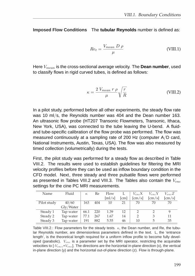
VIII.1. Boundary Conditions
Imposed Flow Conditions The tubular Reynolds number is defined as:
Ret =Vmean D ρ
µ(VIII.1)
Here Vmean is the cross-sectional average velocity. The Dean number , usedto classify flows in rigid curved tubes, is defined as follows:
κ =2 Vmean r ρ
µ
√r
R(VIII.2)
In a pilot study, performed before all other experiments, the steady flow ratewas 10 ml/s, the Reynolds number was 404 and the Dean number 163.An ultrasonic flow probe (HT207 Transonic Flowmeters, Transonic, Ithaca,New York, USA), was connected to the tube leaving the U-bend. A fluid-and tube-specific calibration of the flow probe was performed. The flow wasmeasured continuously at a sampling rate of 200 Hz (computer A/D card,National Instruments, Austin, Texas, USA). The flow was also measured bytimed collection (volumetrically) during the tests.
First , the pilot study was performed for a steady flow as described in TableVIII.2. The results were used to establish guidelines for filtering the MRIvelocity profiles before they can be used as inflow boundary condition in theCFD model. Next , three steady and three pulsatile flows were performedas presented in Tables VIII.2 and VIII.3. The Tables also contain the Venc
settings for the cine PC MRI measurements.
Name Fluid κ Re Flow L VencX VencY VencZ[ml/s] [cm] [cm/s] [cm/s] [cm/s]
Pilot study 40/60 163 404 10 21 70 70 70Gly/Water
Steady 1 Tap water 66.1 220 1.39 12 2 2 9Steady 2 Tap water 77.1 267 1.67 14 2 3 11Steady 3 Tap water 191 882 5.55 46 10 5 35
Table VIII.2.: Flow parameters for the steady tests. κ, the Dean number, and Re, the tubu-lar Reynolds number, are dimensionless parameters defined in the text. L, the ‘entrancelength’, is the theoretical length required for a uniform inflow profile to become fully devel-oped (parabolic). Venc is a parameter set by the MRI operator, restricting the acquirablevelocities to [-Venc,+Venc]. The directions are the horizontal in-plane direction (x), the verticalin-plane direction (y) and the horizontal out-of-plane direction (z). Flow is through-plane.
199

VIII. Choice of model parameters
Name Re κ α Qm Qp f VencX VencY VencZ[ml/s] [ml/s] [bpm] [cm/s] [cm/s] [cm/s]
Pulsatile 1 101 40.5 11 1.22 4 72 4 4 15Pulsatile 2 177 70.8 11 2.14 7 72 7 4 25Pulsatile 3 253 101 11 3.055 10 72 10 6 35
Table VIII.3.: Flow parameters for the pulsatile tests. Here, the dimensionless parameter α,known as the Womersley parameter, reflects the influence of the periodicity; Qm: mean flow;Qp: peak flow; f : frequency in beats per minute. See Table VIII.2 for the definition of otherparameters.
The pilot study was intended to assess the reliability of velocity measure-ments with MRI. It was performed with a 40/60 glycerine/water mixture.The dynamic viscosity, measured with a capillary viscosimeter, was 4.38mPa.s. The density of 1112.7 kg/m3 was read from a densimeter (Avensis,Namur, Belgium). Both values for viscosity and density were measured at 22°C. The other steady flow tests were performed with water at 22 °C, yieldinga density of 998 kg/m and a viscosity of 0.9596 mPa.s.
MRI measurements Velocities were measured using the cine 3D PhaseContrast technique. A 1.5 T MRI Scanner (Philips Medical Systems, Best,The Netherlands) was used, the principal scanner settings for the gradient-echo velocity acquisition sequences were: TE = 9.39 ms (shortest), TR =18.72 ms (shortest), flip angle (FA) = 10 degrees, Number of Excitations(NEX) = 2, matrix size = 256x256, Field of View = 160 mm and slice thick-ness = 5 mm. This sequence was used to measure the axial and secondaryvelocities in cross-sectional planes. For the pulsatile scans, 16 equally dis-tributed time frames were imaged.
Meshes & Solver The true geometry of the tube was meshed using theadvancing front technique implemented in PAM-GEN3D™.239 Table VIII.4shows the specifications of the used meshes. The meshes A, B, E, F, H, J,K and L are for half of the tube, taking advantage of the symmetry. Thesewere used in simulations where symmetric boundary conditions were im-plemented. The meshes described in Table VIII.4 were obtained after gridconvergence tests as described in section III. For instance, in the caseof mesh E, two other grids were tested, one with 45957 elements (meshE’) and another with 127939 elements (mesh E”). The results of mesh E(58814 elements) compared very well with those in the fine mesh but dif-fered from the results of the coarse mesh. In order to restrict CPU time,mesh E was chosen above mesh E”, the only two meshes yielding a correct
200

VIII.1. Boundary Conditions
Mesh Nelem CV BEZ Th PL PR N Refining REZ[cm3] [mm] [mm] [-] in ... [mm]
A 92547 12.03 0.8 3 Log 1.2 7 Bend 0.6B 51056 5.74 1.8 3 Power 1.2 7 Bend 0.6C 152261 13.50 1 - - - - Bend 0.33
Outflow leg 0.33D 112387 10.99 0.6 - - - - Bend 0.33
Outflow leg 0.33E 58814 7.00 0.8 2 Log 1.25 10 Bend 0.4F 45305 4.24 0.8 2 Log 1.25 10 Bend 0.4G 42053 3.48 0.7 - - - - Bend 0.4H 96581 14.79 0.8 2 Log 1.25 10 Bend 0.65J 60548 5.87 0.8 2 Log 1.25 10 Bend 0.4K 67781 7.83 0.8 2 Log 1.25 10 Bend 0.4L 79559 9.52 0.8 2 Log 1.25 10 Bend 0.4
Table VIII.4.: Parameters for the mesh generation using the advanced front technique. CV:computing volume; PAMFLOW™ parameters: Nelem: number of elements; BEZ: Basic ele-ment size; Th: boundary layer thickness; PL: progression law: a mathematical rule describ-ing how the element size changes from the wall inwards; PR: progression rate: a parameterrequired by the progression law; Refining in ...: the region where the mesh was refined;REZ:refined element size: the minimum element size required. See PAM-GEN3D™ manual239 fordetails.
flow profile. The definition of the parameters of the boundary layer meshes(thickness Th, number of elements N and progression rate PR) is shown onFigure VIII.3 (b). Figure VIII.3 (d) gives an overview of the surface mesh G,whereas Figure VIII.3 (c) is a close-up of the part where the coarse mesh isrefined before entering the bend.
In this work, PAMFLOW™ was used to solve the Navier-Stokes equationsand the numerical algorithm employed are well documented.238
Boundary Conditions On the tube wall, no-slip boundary conditions wereimposed. The outflow boundary condition was set at a constant pressure.Four types of inlet boundary conditions were used (see Figure VIII.4) :
• Uniform : When using the uniform boundary condition, the mean ve-locity Vmean was set in all points of the inlet plane. In the pulsatile case,uniform meant that a time-varying flow rate with a uniform velocity pro-file at each time point was set. The uniform profile was preferable incomparison with a parabolic profile because it reaches a developedprofile more quickly, as found by Redaelli.261
201

VIII. Choice of model parameters
Figure VIII.3.: a: Geometry of the U-bend. Inflow and outflow length L 135 mm, diameter D8 mm, bend radius R 25 mm. The picture shows only half of the U-tube, due to symmetry. b:Boundary layer mesh at inflow plane using a logarithmic progression rate. Th, the boundarylayer thickness, shows how far the boundary layer extends. N is the number of layers. Thethickness of every layer can be calculated from the thickness of the preceding layer followinga mathematical rule, called the progression rate.238 Examples of progression rates are:uniform, logarithmic, exponential or no progression rate. c: Detail of surface mesh G. Thismesh is used for coupling with MRI velocity measurements (inlet is left on the image). d:Overview of the same surface mesh G. See PAM-GEN3D™ manual239 for details.
• Parabolic : A parabolic inlet boundary condition is a Poiseuille velocityprofile:
v(r) = 2 Vmean
(1− 4r2
D2
)(VIII.3)
where v is the velocity and r is the radial distance to the centre of the(circular) tube.
202

VIII.1. Boundary Conditions
Figure VIII.4.: The used boundary conditions. ~V is the velocity set at the inlet; ct is a constantequal to the flow rate divided by the lumen area; −→eax is the axial unit vector (the unit vectorin the I/S axis); −−→esec represents both in-plane unit vectors; y varies linearly between 0 inthe centre of the tube and the tube radius R at the circumference; f(r) means that the setvelocities depend on the relative distance from the considered point to the tube centre; f(MRI)means that the set velocities depend on the velocities measured in MRI, either in a singleplane (MRI measured) or consecutive planes (MRI averaged).
• MR measured : velocity measurements were made with MRI at ex-actly 5 mm proximal from the bend/straight tube interface. The velocityvalues were extracted and implemented as inlet boundary condition.When using MRI velocity measurements as boundary condition, notonly the axial velocities but also the secondary velocities were used,since they have important haemodynamic influences.282 Note that al-though the velocities were measured at the end of the straight tube,there could be secondary velocities due to the upstream influence ofthe bend.38 In the pilot study, the measured velocities were used ‘assuch’, i.e. without any smoothing or filtering. In the other studies, thevelocities were filtered and scaled to match the flow rate as explainedsubsequently.
• MR averaged : Weston362 observed in their velocity measurementswith MRI unexpected flow profiles showing random asymmetries. Theauthors therefore suggested that a more reliable velocity profile for theinflow boundary condition should be derived by averaging the veloc-ity measurements made at two or more upstream planes. The MRaveraged boundary condition used the velocity profile resulting fromaveraging the profiles measured at three sections: the inlet, the sec-tion 5 mm distal from the inlet, and the section 5 mm proximal from
203
VIII. Choice of model parameters
the inlet. Velocities were averaged for each of the three components.Similar to the ‘MR’ boundary condition, the measured velocities wereused ‘as such’ in the pilot study, whereas in the other simulations, thevelocities were filtered and scaled to match the flow rate as explainedsubsequently.
Hence, the only difference in inlet boundary conditions between the simu-lations was the shape of velocity profiles (uniform, parabolic, MRI or MRIaveraged). Note that the position of the inlet relative to the bend differedbetween the cases: e.g. when using a uniform velocity profile, the inflowplane was chosen far enough from the bend to allow for full developmentof the flow. In simulations that used MRI data as inlet boundary conditions,the model started at the acquisition plane (5mm proximal from the straighttube/bend interface). In Figure VIII.3 (d), the MRI acquisition plane wasvery close to the bend, resulting in a truncated inflow leg. Note that this re-duces the computational domain drastically. Another implication of the useof MR measured boundary conditions, was the loss of symmetry . For thesimulations with assumed inflow velocity profiles, the U-tube could be splitinto two symmetrical parts and simulated for half only, as mentioned above.However, when using MRI measured velocities as boundary condition, thewhole domain had to be used and simulated since these velocities are notnecessarily symmetric.
The MR velocity Filter Figure VIII.5 shows the measured profile at theentry to the bend before filtering. The directions of the arrows on the pic-ture correspond to the velocity directions and the length of the arrows cor-responds to the velocity magnitude. Clearly, the three arrows encircled bycircle A, which occur at the border, are unrealistically large. Other veloci-ties, encircled by circle B, have secondary velocities higher than the primaryvelocities. Filtering the velocity measurements is required.
Nevertheless, the ‘MR’ boundary conditions described above were imple-mented without smoothing or filtering in the pilot study. Comparison of thepilot study with the studies under steady flow conditions allows the effect offiltering to be examined. The consequences can be seen clearly when eval-uating the CFL-numbers (Courant number)b required in the different sim-ulations238 (Table VIII.5). A high CFL-number will increase the time stepand thus reduce the CPU time. However, stability is weakened with increas-ing CFL-numbers. Measurement errors, such as those illustrated in Figure
bFor a definition of the CFL number, see equation III.21 on page 88.
204

VIII.1. Boundary Conditions
Figure VIII.5.: Inflow velocities without filtering.
VIII.5, favour instability. Therefore, in order to establish a stable simulationin the situations where no velocity filters were used, a sufficiently low CFL-number had to be set: 0.1 and 0.15 in the non-filtered cases, versus 0.3 infiltered cases.
The filtering consisted of two criteria.
CFL-factor Uniform Parabolic MR MR averagedPilot Study 0.3 0.3 0.15 0.1
Steady 1 0.3 0.3 0.3 0.3Steady 2 0.3 0.3 0.3 0.3Steady 3 0.3 0.3 0.3 0.3
Pulsatile 1 0.1 - 0.3 0.3Pulsatile 2 0.1 - 0.3 0.3Pulsatile 3 0.1 - 0.3 0.3
Table VIII.5.: Summary of the CFL-factors used for each simulation.
205

VIII. Choice of model parameters
1. When MRI velocity measurements were used as the inflow boundarycondition, the location of the measurement plane was chosen proximalto the bend so that secondary velocities were very small in compari-son to the axial velocities.5,320 Therefore, secondary velocities greaterthan 10% of the axial velocity were set to 0 cm/s.
2. Near the wall, large errors in the MRI measured velocities may occurdue to the partial volume effect (PVE). The PVE is an undesired ef-fect which occurs in pixels consisting of partly moving fluids and partlystationary tissue. Therefore, near-wall axial velocities larger than 20%of the maximum absolute value defined for the acquisition (Venc) wereset to 0 cm/s.
VIII.1.1.3. Results
Figure VIII.6 (a) shows a comparison of the axial velocity profiles for simula-tions using different inflow boundary conditions in the pilot study (see TableVIII.2 for flow parameters). The velocities are shown in the plane separat-ing the bend and the outflow leg of the U-tube, marked ‘exit bend’ in FigureVIII.7. The measured axial velocity profile in this plane is shown in FigureVIII.6 (b). Figure VIII.8 (a-d) shows the secondary velocity profiles for simu-lations using different inflow boundary conditions in the second steady case.Table VIII.2 shows the flow parameters for these steady cases. Figure VIII.8(e) gives for comparison the secondary velocity profile measured with MRI.Finally, Figure VIII.9 compares MRI axial velocity measurements (upper row)with predictions done by CFD using different types of inflow boundary con-ditions for the third pulsatile test case (see Table VIII.3 for flow parameters).The velocities in Figures VIII.8 and VIII.9 are shown in the section 120 de-grees downstream the inflow of the bend, as defined in Figure VIII.7.
VIII.1.1.4. Discussion
Filtering The CFL-factor for the Pilot Study was significantly lower than inthe studies where the MRI velocities were filtered (Table VIII.5). Loweringthe CFL-factor was necessary in order to obtain a stable numerical simu-lation. At the lumen border, unrealistically high blood velocities (for largepart due to the partial volume effect) could induce a strong swirling motionin the tube. Similarly, errors in in-plane velocity measurements could cause
206

VIII.1. Boundary Conditions
(a) Calculated (b) Measured
Figure VIII.6.: Axial velocities at the exit of the bend in PILOT study. a: Calculated velocitiesfor the uniform inflow boundary condition (upper left ); for the parabolic boundary condition(upper right ); for the boundary condition extracted from the measured velocities withoutaveraging (lower left ); for the boundary condition extracted from the measured velocitieswith averaging (lower right ). b: Measured axial velocities
Figure VIII.7.: Location of planes for velocity comparison: Figures VIII.8 and VIII.9 showvelocities at 120° through the bend, whereas Figure VIII.6 compares velocities at the exitplane.
207

VIII. Choice of model parameters
Figure VIII.8.: Vertical velocity profiles in the tube at 120 degrees through the bend, usingdifferent inflow boundary conditions: white is upwards and black is downwards velocities.Note that the secondary velocity is composed of the horizontal in-plane velocity Vx and thevertical in-plane velocity Vy (see Table VIII.2). a: Uniform inflow; b: Parabolic inlet; c: cine PCMRI measurements as inlet boundary condition; d: averaged cine PC MRI measurementsas inlet boundary condition. e: Velocity profile at 120° as measured by cine PC MRI.
spurious swirl. This swirling motion impeded simulation stability, therefore fil-tering erroneous velocities was imperative. In the case of a simple U-bend,setting filters for ‘realistic’ and ‘unrealistic’ velocities are fairly easy. Basedon literature concerning U-tube flows,69,296 a threshold of 20% of the Venc
was chosen for the axial velocities at the tube wall, and secondary velocitieslarger than 10% of the axial velocities were set to 0 as well. When velocitiesare measured in vivo, velocities will still need to be filtered, but two changesneed to be made in comparison with the present filtering protocol:
• The used filtering thresholds need to be evaluated. If the velocitieswere acquired in a section showing skewed flow, velocities at the lu-men border could be higher than 10% of the Venc.
• Instead of replacing the rejected velocities by 0, the velocities shouldbe calculated by interpolating velocity values either from neighbouringpoints or neighbouring time steps or a combination of both.
Pilot Study - κ = 163 First, Figure VIII.6 (a) (upper left, uniform inflow)and Figure VIII.6 (a) (upper right, parabolic inflow) are compared with the
208

VIII.1. Boundary Conditions
Figure VIII.9.: The upper row are MRI measurements at 120 degrees through the bend attime-points a, b, c and d as shown at the lower right corner, which shows the measuredflow wave form at the exit of the bend. This differs from the imposed flow rate becauseof the length and compliance of the tubes connecting the pump outside the MRI scannerroom to the phantom in the centre of the magnet. The second row are the results of thesimulation using a uniform velocity profile as inflow. The third row represents the results ofthe simulation with ‘MRI’ boundary condition.
theoretical results of Collins and Dennis69 (Figure VIII.1). The two Figuresshow favourable qualitative and quantitative agreement with the theoreticalvelocity profiles, however there are two main differences:
1. the predicted velocity profile is less shifted towards the outer bend;
2. the moon- or mushroom-shape in an iso-velocity plot, a typical featurein curved tubes, is more pronounced in the theoretical cases than inthe calculated upper cases of Figures VIII.6. The mushroom-shape isa consequence of the tendency of the velocity profile to evolve to athin layer of high velocities near the outer bend. This will be more pro-nounced for larger Dean numbers, as illustrated by Collins69 (FigureVIII.1).
The main reason for the observed differences is the fact that the theoreti-cal profiles are for fully developed flow, whereas at the exit plane, imagedin Figure VIII.6, the flow is not fully developed. This is because of the up-stream influence of the straight part after the bend which is changing the
209

VIII. Choice of model parameters
velocity profile back to the parabolic shape.38 The documented profiles69
are only valid in the developed case, far enough from the bend inlet but alsofar enough from the bend outlet.133 This is confirmed by Chung65 who madethe same comments when comparing his results to the ones calculated byOlson and Snyder.237
Second , when comparing Figure VIII.6 (a) (upper row) with the MRI veloc-ities measured at the exit of the bend (Figure VIII.6 (b)), the same obser-vations 1 and 2 are made as when comparing upper Figures VIII.6 (a) tothe theory.69 This also means that the MRI velocity profile is qualitativelyvery close to the theoretical one. Quantitatively, the agreement betweentheory and MRI is less satisfactory, showing errors in velocities up to 25%.Nevertheless, the correct velocity profile is a smoothed version of the mea-sured data, as found by Weston.362 The comparison between MRI velocitymeasurements and CFD predicted flow patterns was made at 15 sectionswhich were 5 mm apart, all showed very good qualitative and reasonablequantitative agreement.
Third , the lower part of Figure VIII.6 (a) is considered. The contour ploton the left corresponds to results obtained using direct MRI velocity mea-surements at the inlet, whereas for the case shown on the right, velocitiesaveraged over three slices near the inlet were used. These results comparebetter with the theoretical solutions than those with assumed profiles. Thereare noticeable differences between the two results. Figure VIII.6 (a) (lowerright) contains less curvature, a smaller maximum velocity and less signif-icant moon-shape. The reason for these differences becomes clear whencomparing the computed mass-flow in Table VIII.6, which can be obtainedonly after the simulation has been performed. For the simulation using the‘MR’ boundary condition, the flow rate is underestimated by approximately5%. For the MR averaged case, this becomes 10%. The incorrect flow rateis directly linked to the differences observed between the lower plots in Fig-ure VIII.6. This indicates that averaging the MRI velocity data between threeplanes, as suggested by Weston,362 does not improve the results. Instead,the comparison between the lower figures in Figure VIII.6 (a) clearly showsthe importance of the correct flow rate.
Steady Test Cases When comparing MRI measurements with CFD-pre-dictions using several inflow boundary conditions, very high qualitative agree-ment is found. Because of a different velocity acquisition range (Venc) forsecondary velocities, the quantitative agreement is impressive in compari-son to the pilot study (maximal errors around 10%), even for secondary ve-
210

VIII.1. Boundary Conditions
Case Inflow [ml/s] outflow [ml/s] Averaged error [%]Uniform 9.89 10.05 0.32Parabolic 10.07 9.89 0.14
MR measured 9.54 9.39 5.36MR averaged 9.01 9.04 9.72
Table VIII.6.: Computed mass-flow in the different cases for the pilot study. The prescribedin- and outflow is 10 ml/s. This flow rate is used to calculate the (flow rate) error.
locity components (17% for horizontal, in-plane velocities; up to 55% for ver-tical, in-plane velocities). These seem to be high, however large relative er-rors occur where velocities are very low, therefore absolute errors are ratherinsignificant. The results compare very well with those of Collins69 (Fig-ure VIII.1). The different simulations for the same steady case predict thesame velocity profile, allowing for typical visualisation errors as describedby Long.198 The secondary velocities for the second steady case shown inFigure VIII.8 are in good agreement with each other. It even seems that thesimulations done using MRI velocities as boundary condition compare bet-ter with the MRI measurements. The explanation for this observation canbe found in the fact that (i) the computational model uses the accurate ge-ometry specifications provided. Furthermore, (ii) we must take into accountthat the phantom is included in a flow circuit applying a theoretically speci-fied flow . In reality, the geometry and (more probably) the flow profile is notperfect, changing the flow in a way detectable by MRI. This means that set-ting a disturbed flow as boundary condition (measured by MRI), will resultin a different flow profile, which is closer to the true profile. This observationdenotes clearly the advantage of using scaled MRI velocity data as inflowboundary condition. In this context, ‘scaled’ means scaling up the velocitiesacquired from cine 3D PC MRI in order to obtain the correct flow rate.
Pulsatile Cases It is clear from Figure VIII.9 that the quantitative agree-ment is less satisfactory than in the steady cases, however very good qual-itative agreement is reached almost throughout the cycle. Comparison ofthe results between the different simulations in all available planes and timesteps yields the same conclusion as for the steady case: when scaled formass flow rate, using the MRI velocity data as inflow boundary conditionprovides more reliable results than in the case where a uniform inflow wasset far from the region of interest.
211

VIII. Choice of model parameters
CPU time It is important to emphasise that the use of different inflowboundary conditions - uniform, parabolic, filtered MRI measurements or av-eraged MRI measurements - all produce nearly the same, correct flow fieldfor flow in a U-bend. CPU time should also be considered when deciding onthe type of boundary condition. Because all the geometries show compara-ble mesh densities, a large computing volume will have more elements andthus demands more CPU time. Evaluating the boundary conditions in termsof CPU costs, the following descending order is obtained: uniform, parabolic,MRI averaged, MRI. This sequence is logical when related to the comput-ing volume. Using the uniform inflow boundary condition requires a (long)entrance length before realistic flow can be computed. Using the developedflow, a certain distance from the region of interest is required because of up-stream influences of the geometry (e.g. a bend) on the flow.38 The ‘MRI’ and‘MRI averaged’ boundary condition can be obtained in the immediate vicin-ity of the region of interest, yielding a small computing volume (see meshG in Figure VIII.3) and a shorter CPU time. When evaluating the boundaryconditions in terms of CPU time, the CPU time required in the simulationsin half geometries was doubled, since the entire arterial geometry will haveto be simulated in in vivo cases. Thus, the most interesting boundary condi-tion is the MRI velocity measurement. The extra computations due to spatialand temporal interpolations required in the ‘MRI’ boundary condition, did notincrease the CPU time significantly.
Summary Three types of inflow boundary conditions were tested: a uni-form profile, a fully developed profile, and MR measured velocities. The firstone is simple, but requires a long inflow tube, and is not physiological. Thesecond one reduces CPU time significantly, but assumes a developed flow,which is an assumption that cannot be made for most of the arteries.342
The third one has to be filtered and scaled, but can save CPU time evenmore if the acquisition plane is chosen near the region of interest. Notethat the gain in CPU time is more important than the extra time needed forvelocity acquisition. The choice of the filtering thresholds is operator depen-dent and therefore subjective. However, different thresholds have shown togenerate comparable results on the general flow field. This option is pre-ferred especially for in vivo applications, but requires reliable cine PC MRImeasurements. This reliability of velocity measurements is discussed in twoparts: the velocity profile, and the mass flow.
The velocity profile generated using 3D Phase Contrast velocity encodedMRI is accurate to 10% of the used Venc, as illustrated in Figures VIII.6,VIII.8 and VIII.9. The flow rate, however, is subject to large errors (see Table
212

VIII.1. Boundary Conditions
VIII.6). Therefore, it is concluded that additional flow measurement is re-quired. The challenge now is how to perform reliable flow rate measurement.Chatzimavroudis59 state that MRI can produce extremely reproducible flowrate measurements in vivo. Their conclusions hold for the cycle-averagedflow rate. But for use as boundary condition in a CFD simulation, the flowrate has to be correct for every time step. Furthermore, their results showthat significant errors can occur when mass flow is low. Unfortunately, theregions of interest (bifurcations, aorta, left ventricle) usually show complexflow patterns, where MRI velocity measurements are less reliable.
Comparison with Literature To our knowledge, no previous study hasused the mass scaled MRI velocities as boundary condition (Table VIII.1)using a separate mass flow rate measurement. An important number ofauthors33,195,197,198,362,370,374 set velocities as measured by MRI on all theinlets and outlets except for one. For the last boundary condition, thereare several options: a scaled MRI-velocity profile,195,196,362,374 a uniformvelocity profile,362 a mass-flow boundary197,198 or a uniform pressure dis-tribution on an inflow or outflow plane.370 A second group of authors setdeveloped profiles - or calculate the developed flow-profiles using a long en-trance length - on all inflow and outflow boundaries but one. These profilesare calculated in advance using time-varying flow rates assessed either byMRI50,164,219,334 or Doppler.387
The lack of reliability in the flow measurements will inevitably introduce er-rors in the simulation, an aspect which will play an important role in the afore-mentioned studies for the first group of authors, who use MR measurementsas boundary conditions. With MRI, Weston362 measured a flow rate for asteady case which was 16% higher than the flow rate measured volumetri-cally. For a pulsatile case, the mean flow rate obtained with MRI was also15% higher than measured with timed collection. The observation that toour knowledge no authors have successfully set MRI velocity data on all theboundaries is related to the accuracy in measuring the flow rate. In order tobe able to set velocities on all boundary conditions, the accuracy on the flowrate should be higher than the machine accuracy of the platform on whichthe CFD simulations are solved.3 As a consequence, MRI-velocities can beset on all the boundaries, but the last one has to be scaled in order to satisfymass conservation required for a stable simulation. In a simulation with MRImeasurements as boundary condition, the simulated flow rate is deducedfrom the velocity measurements used as boundary condition; unfortunately,this flow rate is not necessarily correct. This uncertain flow rate might ex-plain the relatively large discrepancies found between measured MRI data
213

VIII. Choice of model parameters
and calculated flow profiles during the flow deceleration in Long.195 In theirwork on a human descending aorta, Wood370 observed differences in thetime-mean flows: 5.0 litres/minute at inlet, and 3.5 litres/minute at outlet(30% less). These discrepancies are attributed to measurement uncertain-ties, outflow to small branches and the neglect of compliance effects. Anuncertainty on the flow rate of ± 28% was defended. The authors concludethat the discrepancy between inlet and outlet flows falls broadly within uncer-tainty limits. Although this is a justified statement, it exposes the vulnerabilityof in vivo MRI flow measurement.
The importance of Mass Flow Rate The present study underlines theimportance of making use of the correct flow rate. There is a need for agood understanding and treatment of the parameters that lead to the currentuncertainty in flow rate measurement.
One of these uncertainties is due to the neglect of arterial distensibility . Dur-ing a cardiac cycle, the diameter of the common carotid artery can changeup to 17%.264 Flow rate is obtained by multiplying the mean velocity with across-sectional area, so uncertainties on the lumen diameter (LD) measure-ment (due to compliance) will induce uncertainties in flow rate measure-ments. Because of this, the cycle-averaged LD is usually used, however,the closer the arteries are to the heart, the more important the diameterchanges will become and the less correct the use of an average artery LDwill be. Note that the neglect of compliance also contributes to the error inthe flow rate in a different way. The blood entering the carotid bifurcation,does not necessarily need to leave the carotid bifurcation instantaneously,since the vessel walls can expand. Therefore, the measured instantaneousinlet flow rate would not be the same at the outlets. In the present study,MRI-velocity measurements result in significant flow rate errors although nocompliance is present, so the error in the flow rate cannot be explained withcompliance alone, and has to be due to velocity measurement errors. Notethat compliance can be successfully implemented in the flow simulation asshowed by Zhao387 for the carotid bifurcation. Their results reveal veloc-ity profiles that are different from those found with idealised models, suchas stronger secondary flows, lower wall shear stress and larger backflows.The computational cost of the coupling between MRI, CFD and solid me-chanics (fluid-structure interaction ) is currently the main drawback of thismodelling approach.
214

VIII.1. Boundary Conditions
What about outflow boundary conditions? This study has concentratedon inflow boundary conditions by performing simulations which differed onlyin their implementation of the conditions at the inlet. Nevertheless, the sameconsiderations are valid at the outflow as well. This study recommends mea-suring velocities at the outflow plane, and using the ‘filtered’ and ‘scaled’velocities as boundary conditions. Note that it is not recommended to setvelocities on all boundaries, unless the flow rate can be set as accurate asmachine accuracy. In some cases it is not even possible to acquire enoughvelocity information at the outlets, usually due to time restrictions. Severalsolutions can be put forward. Admittedly, all the suggestions cited belowdo not give any information on secondary flow in the outlet planes, which isagainst Shipkowits’s recommendations.282 Nevertheless, they provide phys-iological boundary conditions suitable for coupling with CFD.
• Instead of performing velocity measurements in three directions, onlythe axial velocity could be measured. This shortens the acquisitiontime considerably, and it also yields a mass flow rate measurementusing the most reliable in vivo technique.
• Recently, other techniques for setting outflow boundary conditions havebeen investigated by Cebral53 for MRI-based CFD in the circle of Willis.Under normal conditions, four feeding vessels supply the circle of Willis:two internal carotids and two vertebral arteries (see Figure I.1 (b)). Theflow rates in these vessels can be measured by PC MRI techniquesand used to impose inflow boundary conditions during the solution ofthe flow equations. Furthermore, in many cases all these flows canbe measured with only one PC-MRI sequence. However, in general itis difficult to measure flow rates in all the efferent vessels of the circleof Willis. This would require MRI exams that are too long and the flowmeasurements in some of the smaller vessels may not be very reliable.Therefore, in such cases the outflow boundary conditions must be de-rived using models of the distal vascular bed. This means that the dis-tal parts of the vessels, beyond the outlet of the model, are replacedby a mathematical representation and implemented in the model. Thismathematical representation can be based on an analogy between thedistal vascular bed and series of resistors in parallel, structured fractaltrees or porous media. However, Cebral53 clearly denotes that thesetechniques are still in their infancy and that further research is neces-sary before they can replace cine PC MRI measurements.
215

VIII. Choice of model parameters
VIII.1.1.5. Conclusion
For in vivo haemodynamic studies combining CFD to MRI velocity measure-ments, the boundary conditions need to be handled with special care. Astudy of the effect of different inflow boundary conditions on flow simulationsin a rigid U-bend phantom has been presented. A pilot study revealed thekey role played by a correct flow rate. Comparing MRI velocity measure-ments with CFD predictions showed that both axial and secondary veloc-ities can be measured reliably with cine PC MRI (maximum error 10% foraxial velocities in a rigid tube under laboratory conditions). This study hasdemonstrated that MRI velocities could be used as boundary conditions in aCFD-simulation. The raw velocity data needs to be
1. filtered for partial volume effects: axial velocities at the lumen borderhave poor accuracy and should be replaced by interpolation if theirvalues exceed a certain threshold (here: 20% of the Venc).
2. filtered for errors in secondary flow: secondary velocities greater thana certain percentage (here: 10%) of the axial velocities can often beblamed on measurement uncertainty and can thus be replaced by in-terpolation.
3. rescaled to match a reliable flow rate measurement.
These procedures can help to obtain a reliable and cost-effective CFD sim-ulation. Our study suggests not to use a uniform or developed boundarycondition unless no other information is available about the inlet velocityprofile.
VIII.1.2. In- and Outflow Conditions for 3DUS-based models
VIII.1.2.1. Introduction
The problem with Doppler Preferably, velocities should be acquired atthe entire inlet plane. Cine PC MRI is ideally suited for this purpose: it gen-erates velocities in all three orthogonal directions with a reasonable spatialresolution (±1mm × 1mm) at a sampling rate up to 25 acquisitions per cy-cle.347 In Doppler ultrasound, there are 2 methods for velocity acquisition(see section VII.1.3).
216

VIII.1. Boundary Conditions
• Pulsed wave Doppler outputs velocities at a very high sampling rate,typically 200 Hz: much better than the 25 images per cycle in cinePC MRI. However, Doppler velocities originate from a single samplevolume of 1.5 mm2, whereas in MRI an entire transverse section canbe imaged. The technique can be altered to scan velocities along aline as opposed to a single point,270 only with some marginal loss oftemporal resolution. Nevertheless, pulsed wave Doppler still standsfar from the spatial resolution achievable with MRI.
• Colour Doppler generates a high spatial resolution, theoretically equalto the inverse of the used wavelength, but is by definition cycle-aver-aged.
Clearly, the use of Doppler Ultrasound to acquire velocities for boundaryconditions has its limitations in comparison with cine PC MRI. Nevertheless,in the absence of MRI velocity data, Doppler velocity can be analysed andprocessed to give time-varying velocity profiles by making a few assump-tions.
Making use of Doppler Doppler measurements can be made in the cen-tre of a proximal CCA cross-section. This yields images such as Figure VII.3(a) on page 163. Since Doppler ultrasound can only measure the flow ve-locity in a small sample volume, two methods were devised to calculate theactual volumetric flow rate.
The first method, henceforth known as the ‘Simple’ method, applied theassumption of a parabolic flow profile at every instant and that the measuredDoppler velocity was its peak. Hence, the volumetric flow rate could becalculated by
Q =VPEAK
2×A (VIII.4)
where Q is the volumetric flow rate, VPEAK is the centre stream velocityand A is the cross-sectional area of the vessel. The measurement site forthe CCA should be at a location proximal to the bifurcation point where thevessel is relatively straight and flow could be considered undisturbed. Notethat a fully developed profile in pulsatile flow would be the Womersley pro-file, which can be very different from the parabolic profile suggested in thismethod. This simplification is the reason for the name ‘Simple’ method.
217

VIII. Choice of model parameters
The second method was based on the Womersley solution for pulsatile flow,assuming again the measured velocity to be the centre stream velocity. AMATLAB-based program was developed to perform this calculation, whichrequired the input of time varying velocities VPEAK as well as the radius ofthe vessel. For details of this method, see section II.3.3.1.
Both methods, the ‘Simple’ and ‘Womersley’ method, use the centreline ve-locity in the proximal CCA to extrapolate a flow rate and a velocity profile inthe entire inlet section. But in both cases, an assumption was made con-cerning the velocity profile: a pulsatile parabolic profile was imposed in theSimple case, and a Womersley profile in the second method.
VIII.1.2.2. Study setup
In a first attempt to validate the solutions proposed in the previous section,the two calculation methods, namely the Simple and the Womersley method,based on Doppler ultrasound, were compared to cine PC MRI for obtain-ing the inlet mass flow boundary conditions in the CCA. For this purpose,a healthy male subject was scanned using Doppler ultrasound and PhaseContrast (PC) MRI. Moreover, the carotid geometry was assessed usingTime of Flight (TOF) MRI. The study had 3 goals:
• Goal 1: Assess how the Simple and Womersley methods comparewith the PC MRI data.
• Goal 2: Assess which boundary conditions to set at the flow outlet.
• Goal 3: Study the effect of using MR or US-based boundary condi-tions.
The study has been performed in a collaboration with Augst.15
Doppler Ultrasound CCA centreline velocities were obtained using a stan-dard 2D ultrasound scanner (HDI 5000 with a L12-5 (5-12MHz) linear arraytransducer, ATL-Phillips Ltd., Bothell, MA, USA). This returned velocities inthe proximal CCA at a sampling rate of 200 Hz. The procedure was repeatedto measure the centreline velocities in the daughter vessels. ECA and ICAflow measurements were influenced by the position of the bifurcation point
218

VIII.1. Boundary Conditions
relative to the jaw bone. Since these were taken as far distal as possible, thisposition is approximately 1.5 CCA diameters distal to the bifurcation point.
From the raw flow data acquired, the following parameters were calculatedand compared. Firstly, the volumetric flow rates in the CCA were computed.Secondly, the flow rates in the ICA and ECA were computed. Thirdly, totest for conservation of mass and to determine what to set as outlet bound-ary condition, the sums of ICA and ECA flow were set against the CCA.Lastly, outflow ratios were computed using two different schemes. Scheme1 computed the ratio of the ICA and ECA flow from measurements madein the respective vessels, whereas Scheme 2 estimated flow in the ECA bysubtracting the ICA flow from the CCA.
MRI protocol For comparison, the velocities were also measured with cinePC MRI. The MRI scan was carried out using a Siemens Magnetom SonataScanner 1.5T. The phase encoding resolution was 1.1mm, the frequencyencoding resolution was 0.75 mm with a slice thickness of 6 mm. Temporalresolution was 29 ms. PC flow measurements were carried out in the CCAin a region relatively close to the bifurcation but far enough to ensure undis-turbed flow while ECA/ICA were measured as far distal as possible but be-fore any branching occurred. Magnitude and phase images were processedwith phase image intensities related to velocity. To determine the volumetricflow rate, the vessel cross-section was drawn manually on the magnitude im-age and copied to the corresponding phase image. The regions on imagesat different time points were adjusted to fit the vessel outline, determinedfrom the initial magnitude image where the lumen boundary is clearly de-fined. The through-plane flow was calculated using the analysis package onthe scanner.
3D reconstruction and computational details The lumen geometry ofthe subject was reconstructed from TOF MRI images and a computationalmesh was generated. Details of the imaging protocol can be found in sectionXII.3. The mesh had 60544 hexahedral cells in a fully structured multi-blockarrangement suitable for the designated CFD solver, i.e. the commerciallyavailable finite volume package CFX4™. Simulations were carried out us-ing MRI and the Simple ultrasound CCA boundary conditions and a fixed60:40 outlet mass flow ratio. The MRI velocities were filtered as explainedin section VIII.1.1, and scaled using an extra cine PC MR image series forflow rate measurement. The ‘MR measured’ boundary condition contained
219

VIII. Choice of model parameters
velocity information for all three vector components while the ultrasound de-rived ones assumed parabolic profiles with zero secondary velocities. TheQuemada model as presented by Buchanan42 was used to model the non-Newtonian behaviour of blood and its density was set to 1176 kg/m3. Time-averaged wall shear stress (WSS) and oscillatory shear index (OSI) werecomputed and compared.
VIII.1.2.3. Results
Figure VIII.10 (a) shows the computed volumetric flow rates for both imag-ing modalities, using the Womersley and Simple calculation methods forultrasound. Figure VIII.10 (b) shows the flow wave in the daughter vessels.These Figures allow comparison of the Simple and Womersley method tothe cine PC MRI method for flow rate measurement (Goal 1). Note that thewaves were truncated at the last measured value from ultrasound. FigureVIII.11 (a) shows the sum of the flow leaving ECA and ICA compared to themeasured CCA rates. Figure VIII.11 (b) shows the outflow ratios as mea-sured (solid) and as computed from measured CCA and ICA alone (dashed)for ultrasound (black), and MRI (grey) (Goal 2). Figure VIII.12 shows cir-cumferential plots of WSS and OSI at selected locations defined by z, theirposition along the I/S axis. Note that in Figure VIII.12, TAWSS stands forTime-Averaged WSS.
(a) CCA (b) Branches
Figure VIII.10.: ‘Simple’ and Womersley method for deriving flow rates from Doppler Ultra-sound compared to MRI. a: Volumetric flow waves in the CCA computed from MRI (grey)and ultrasound (black). With ultrasound, flow waves have been derived using the Simplemethod (solid) and Womersley’s solution (dashed). b: Volumetric flow waves in the ICA(solid) and ECA (dashed) computed from MRI (grey) and from ultrasound (black) using theSimple method.
220

VIII.1. Boundary Conditions
(a) CCA vs ICA+ECA (b) ICA/ECA
Figure VIII.11.: Testing the flow rates acquired by Doppler ultrasound for mass conservation.a: Volumetric flow waves in the CCA as measured (solid) and as sum of the ICA and ECAflow rates (dashed) computed from ultrasound (black) using the Simple method and MRI(grey). b: Outflow ratios as measured (solid) and as computed from measured CCA and ICAalone (dashed) for ultrasound (black), and MRI (grey).
VIII.1.2.4. Discussion
In this study, the CCA centreline velocity, acquired using pulsed wave Dopp-ler, was used to derive carotid flow rate and velocities for the inlet boundarycondition. Two methods for this derivation have been proposed (Simple andWomersley) and compared to cine PC MRI measurements. The aim of thestudy was to (i) assess whether the Simple or Womersley methods com-pares better with the PC MRI scan, (ii) assess which boundary conditionsto set at the flow outlet and (iii) study the effect of using MR or US-basedboundary conditions.
Since the cross-sectional area was kept the same for all the methods, thederived volumetric flow rates depended entirely on the velocity data and thecalculation method employed. Even though the results of only one sam-ple subject were presented, some generally relevant observations could bemade. From Figure VIII.10 (a), it can be seen that the ultrasound derivedflow rate calculated by the Simple method agrees much better with the MRImeasured flow rate, than the commonly used Womersley solution. Thisshows that the assumptions made on the shape of velocity profiles in theWomersley method may not be physiologically realistic. However, imple-menting the flow rate calculated from the Simple method on a straight tubewill lead to a considerable underestimation of centreline velocity at peaksystole, hence leading to a mismatch with the measured Doppler velocitywave. This shows that it is difficult to obtain an accurate simultaneous rep-resentation of both flow rate and profile from Doppler ultrasound. The site of
221

VIII. Choice of model parameters
Figure VIII.12.: WSS [N/m2] and OSI [-] at cross-sections using MRI (solid) and ultrasound(dots) for boundary condition acquisition. The position of the cross-section is determined bythe parameter z, denoting the position along the I/S axis (z < 0 is in CCA, z >0 in ECA/ICA).
velocity measurement is unlikely to have had an influence on the data dueto the relatively straight vessel geometry and undisturbed flow in the region.
Similar issues can be addressed considering the results in Figure VIII.10(b). Here, another factor affecting flow wave forms may be present, namelythe downstream location of measurement. As mentioned earlier, the thyroidartery and possibly a number of smaller branches can affect flow velocityand flow rate in the ECA. It can be seen that the ultrasound measured wavedisplays a much higher flow rate than its MRI counterpart with similar wave
222

VIII.1. Boundary Conditions
form. This may indicate a source of varying resistance nearby, i.e. the pres-ence of a vessel side branch and/or a measurement error due to a stronglyskewed velocity profile. Since both effects were ignored in the CFD parts ofthe present study, this must be considered an undesired error. It must bekept in mind, though, that there may be an error also in the MRI measure-ment for similar reasons.
The ICA measurements show good agreement in terms of total flow whilethe wave forms differ in shape. This is interesting, since the scan locationcan also be influential for the ICA velocity measurements, due to the accel-eration of fluid out of the bulb. It seems however, that this undesired effecthas been largely avoided here. More importantly, the velocity profiles maybe relatively complex in this region, which can be picked up by MRI but notby Doppler, hence possibly introducing an error in the ultrasound measure-ments.
The suspicions about a possible underestimation in MRI measurements inthe ECA were confirmed in Figure VIII.11 (a, grey lines). There is a con-stant, relatively small underestimation of flow out of the daughter vesselscompared to the inflow, most likely due to the loss from branching vesselsand possible induced flow disturbances. In case of Doppler measurements,the overestimation of the ECA flow suspected from Figure VIII.10 (b) wasconfirmed (black dashed line higher than black solid line in Figure VIII.10(a)). The underestimation of total outflow during systole was mostly due tothe ICA wave form. This has strong implications on the calculations of out-flow ratios shown in Figure VIII.11 (b). It can be seen that the two outflowcalculation methods show good agreement for MRI, confirming the relativelyhigh accuracy of measurement in this case. But this is not the case for ultra-sound, where Scheme 2 (estimating ECA flow from measured CCA and ICAflows) yields a much higher ICA to ECA flow ratio with strong temporal vari-ations, while Scheme 1 (using measured ICA and ECA flows) shows a goodagreement with the MRI data. At this stage, another problem with Dopplerultrasound is worth pointing out, which is not present with MRI. While flowmeasurements in both vessels were made simultaneously during the MRIscan, this was not possible for Doppler ultrasound. Hence, beat-to-beat dif-ferences are inevitable, possibly accounting for some of the errors in FigureVIII.11. The problems with Scheme 2 for Doppler ultrasound may be spe-cific for this case, as the large discrepancy to Scheme 1 between 300 and400 ms is induced by the closeness of ICA and CCA flow rates. Hence, theusefulness of Scheme 2 to alleviate the problems of ECA measurement maybe questionable.
223

VIII. Choice of model parameters
The plots of WSS and OSI shown in Figure VIII.12 exhibit great similarity be-tween MRI and Doppler. As expected from the flow waves in Figure VIII.10(a), the WSS for MRI is generally higher due to the higher average inflowvelocity. This effect increases downstream due to higher momentum and astronger skewed velocity profile. The OSI overall is higher for the Dopplerset, most probably due to the more pronounced peak and dicrotic notch.Overall, the differences can be regarded as small considering the range ofvalues present in this data set.
VIII.1.2.5. Conclusion
Two techniques for extrapolating inlet boundary conditions from a centrelinevelocity measurement acquired from Doppler Ultrasound were presented.In the first one, ‘Simple’, a parabolic profile is imposed on the inlet section,whereas in the second one, ‘Womersley’, Womersley profiles are derived.This study, performed in one subject, showed that the flow rate derived withthe Simple method agreed better with the flow rate acquired from cine PCMRI. This is surprising since it is less realistic considering that in a straighttube with pulsatile flow, the Womersley flow should develop.232 Neverthe-less, the assumption of developed flow could be fundamentally wrong, andthe complex profile occurring instead of a Womersley profile may be closerto a parabolic one. More subjects are needed to see whether this finding isstatistically significant.
At the boundary outlets, it was noted that both the ICA and ECA flow ratewere overestimated using Doppler. When setting a (time-varying) mass di-vision at the model outlets, it is recommended to use the mass flow ratioderived from the ICA and ECA measurements as opposed to derive it fromthe CCA and ICA measurement.
The WSS and OSI patterns showed high qualitative agreement. There was,however, a clear overestimation of the WSS in the study with the highest flowrate. This confirms what was seen in the previous section (section VIII.1.1 onboundary conditions in MRI-based CFD), namely that the WSS patterns arehighly influenced by the flow rate. Using a suboptimal boundary conditionsin combination with the correct flow rate, is therefore only important in aredeveloping zone.
224

VIII.1. Boundary Conditions
VIII.1.3. The wall as model boundary
The easiest way to model the boundary wall, is to represent it as a rigid,‘no slip’ surface. This means that the vessel wall remains in its positionand that the fluid at the vessel wall is stationary. In reality, the vessel wallis compliant. Several groups have introduced compliance into their image-based models. Noteworthy are Leuprecht’s,177,178 Zhao’s387 and Cebral’s56
solution for computational modelling of carotid vessel walls.
Leuprecht177,178 uses cine PC MRI to extract geometries from a descendingaorta. Since this technique gives several images along a cardiac cycle,‘cine’ PC MRI yields not 1 but several reconstructions of the aorta, each onecorresponding to a different point in the cardiac cycle. The aorta geometriesare used to impose the movement of the vessel wall. The velocity of the fluidon the vessel wall is equal to the velocity of the vessel wall, i.e. the no-slipcondition is applied.
Zhao introduced vessel wall movement to the carotids.387 Here, the solidmotion equations are solved together with the Navier-Stokes equations, thetechnique is termed fluid-structure interaction. The subject-specific walldata, required for the solid equations (elasticity, etc.), were acquired with B-mode ultrasound. Zhao387 found that the effect of introducing fluid-structureinteraction was an overall decrease of the WSS, while keeping the WSSdistribution. See Figures VIII.13 and VIII.14 for an extract of Zhao’s results.
Cebral56 used an assumed value for the elastic modulus and pressure val-ues at the in- and outlets of the model. The knowledge of the pressure fieldand the elastic modulus combined with the velocity boundary conditions onthe outlet of the model allowed reconstruction of the entire flow field andwall movement using fluid-structure interaction. The pressures at the lumenboundaries were estimated using the flow rates (measured with cine PCMRI) at inlet and outlet.
The comparison of different techniques to model vessel wall compliance fellout of the scope of this work. But the effect of wall compliance on calculatedWSS can be found in Figure VIII.13.
225

VIII. Choice of model parameters
(a)
(b)
Figure VIII.13.: Comparisons of wall shear stress magnitudes at two selected locations (aand b) in the internal carotid artery between the coupled and its corresponding rigid model.a: carotid sinus; b: one-diameter downstream of (a), as shown in Figure VIII.14. At eachlocation, results are given on the Posterior, Right, Anterior, and Left wall (from Zhao387).
226

VIII.1. Boundary Conditions
Figure VIII.14.: Measurement locations for Figure VIII.13 (from Zhao387).
VIII.1.4. Boundary Conditions: Summary
This summary describes which boundary conditions should be used in fu-ture studies using image-based CFD as a tool for investigating carotid haemo-dynamics.
For MRI-based CFD, the velocities in 3 directions will be measured at theinlet and outlet planes. The velocities are filtered for the partial volume effectand for noise in the secondary velocity components. An additional flow ratemeasurement is required, which can be performed at a location with an extracine PC MR imaging sequence in a location with good signal. This flow rateis used to rescale the axial velocities at the inlet.
At the outlet, flow rates will be estimated from the cine PC MRI images andused to describe mass flow boundary conditions using a mass division ratio.
For an example where 3DUS-based CFD was used as a tool for investigatingcarotid haemodynamics using the above boundary conditions, see sectionXII (The Acute Effect of Hypertensive Drugs).
For 3DUS-based CFD, the secondary velocities will be discarded. The axialvelocities will be derived from centreline velocity measurement in the CCAusing the Womersley method. The Womersley method was preferred here
227

VIII. Choice of model parameters
to the Simple method because it is still widely used in the absence of truevelocity data.
At the outlet, a mass division ratio is set just as for the MRI-based CFDstudies. The problem of how the outflow ratio should be calculated remainsto be dealt with. First, the flow rates are calculated in CCA, ICA and ECAusing centreline measurements and the Womersley assumption. Then, out-flow ratio can be calculated from the ICA and ECA, CCA and ICA and evenCCA and ECA. Although the study in section VIII.1.2 suggested to use theICA and ECA, in practice, the ratio will be calculated using the flow ratesyielding a division ratio closest to the expectable 55:45 (ICA:ECA). This al-lows to filter out major acquisition errors. In order to deal with the potentialhigh-frequency changes seen in the black dashed line in Figure VIII.11 (b),the time-dependent outflow ratio is smoothed. Note that the presence of astenosis will alter the flow division dramatically, which makes the expectationof a flow ratio of 55:45 unrealistic. Thus, the used technique of setting outletboundary conditions is only plausible in non-stenosed carotid bifurcations.
For an example where 3DUS-based CFD was used as a tool for investigatingcarotid haemodynamics using the above boundary conditions, see chapterXI (The Head Position Study).
Both for MRI and 3DUS-based CFD, the wall will be modelled as a rigid wallwith no slip. The reader should be aware of the fact that the calculated WSSis therefore slightly higher than the true WSS387c.
VIII.2. Viscosity
VIII.2.1. What’s the effect of viscosity on shear?
VIII.2.1.1. Introduction
The viscous force is a force exerted by a fluid as a resistance to flow. Thedynamic viscosity is the degree to which a fluid resists flow under an appliedforce, measured by the tangential friction force per unit area divided by the
cNote that the reason why the WSS was found to be lower in the compliant model wasbecause the geometry used in the rigid model was taken as the geometry in diastolewhen pressure was the lowest. If it was taken as the systolic geometry in the compliantmodel, the conclusion would have been different.
228

VIII.2. Viscosity
velocity gradient under conditions of streamline flow. In a numerical flowsimulation, the viscosity is an important fluid property and needs to be set.If we consider that the dynamic viscosity of blood is within the range of 3to 5 mPa.s, the question of which value to set for the simulation is raised.However, before the value of the viscosity is questioned, the effect of settingdifferent viscosities needs to be studied.
VIII.2.1.2. Study setup
In this study, the right carotid bifurcation with no stenosis acquired with BBMRI from a hypertensive 38 year old subject was imaged, segmented, re-constructed and meshed as explained in sections XII.3 (imaging protocol),VI.2 (segmentation), VI.3 (reconstruction and mesh generation).
On this mesh, three simulations were performed. Velocities measured withPC MRI at the inlet were filtered and scaled (as explained in section VI.5.2.5)for use as inlet boundary conditions. The wall was modelled as a no-slip,rigid surface. Blood density was 1176 kg/m3. Three simulations were un-dertaken. Each had a different value for the viscosity: 3, 4 and 5 mPa.s.This was the only difference between the simulations. The simulation wasperformed using CFX4™,3 over 2 cycles of 80 time-steps of 9.1 ms each.Validation and mesh independence tests were performed in other studies(section XII.3.5.4).
VIII.2.1.3. Results
The results are given in Table VIII.7. It shows the values of WSS, OSI,WSSG, WSSGt, WSSGs and WSSAG averaged over certain zones of thecarotid for each of the three simulations. See section II.3.3.3 for a definitionof these parameters, and see Figure VII.8 (page 173) for a definition of thezones in which the averaging was done.
VIII.2.1.4. Discussion and Implications
In this study, three simulations were performed. The only difference in thesimulations, was the value set for the dynamic viscosity. Note that a New-
229

VIII. Choice of model parameters
Parameter [Unit] µ=3 mPa.s µ=4 mPa.s µ=5 mPa.sWSS ALL [N/m 2] 2.631 3.083 3.522
WSS CCA [N/m2] 1.774 2.140 2.511WSS iCCA [N/m2] 1.832 2.236 2.645WSS eCCA [N/m2] 1.697 2.015 2.335
WSS ICA [N/m2] 3.478 4.001 4.479WSS outer ICA [N/m2] 2.766 3.169 3.545WSS inner ICA [N/m2] 4.689 5.418 6.069
WSS ECA [N/m2] 3.939 4.573 5.182WSS outer ECA [N/m2] 1.887 2.238 2.615WSS inner ECA [N/m2] 3.939 4.573 5.182
WSS bulb [N/m2] 2.352 2.739 3.116OSI ALL [-] 0.030 0.021 0.016OSI CCA [-] 0.055 0.038 0.027
OSI iCCA [-] 0.045 0.026 0.016OSI eCCA [-] 0.067 0.053 0.042
OSI ICA [-] 0.019 0.016 0.013OSI outer ICA [-] 0.027 0.024 0.018OSI inner ICA [-] 0.004 0.004 0.004
OSI ECA [-] 0.005 0.003 0.002OSI outer ECA [-] 0.012 0.007 0.004OSI inner ECA [-] 0.005 0.003 0.002
OSI bulb [-] 0.035 0.024 0.017WSSGs ALL [N/m 3] 734 817 891
WSSGs CCA [N/m3] 462 532 600WSSGs iCCA [N/m3] 474 544 617WSSGs eCCA [N/m3] 446 517 578
WSSGs ICA [N/m3] 847 937 1014WSSGs outer ICA [N/m3] 630 697 757WSSGs inner ICA [N/m3] 1216 1346 1452
WSSGs ECA [N/m3] 1417 1558 1672WSSGs outer ECA [N/m3] 567 613 657WSSGs inner ECA [N/m3] 1417 1558 1672
WSSGs bulb [N/m3] 531 591 647WSSGt ALL [N/(m 2 × s)] 11.51 13.01 14.42
WSSGt CCA [N/(m2 × s)] 9.24 10.77 12.25WSSGt iCCA [N/(m2 × s)] 9.21 10.85 12.42WSSGt eCCA [N/(m2 × s)] 9.26 10.68 12.03
WSSGt ICA [N/(m2 × s)] 14.90 16.89 18.70WSSGt outer ICA [N/(m2 × s)] 13.65 15.55 17.33WSSGt inner ICA [N/(m2 × s)] 17.03 19.16 21.03
WSSGt ECA [N/(m2 × s)] 13.56 14.81 15.99WSSGt outer ECA [N/(m2 × s)] 8.47 9.09 9.66WSSGt inner ECA [N/(m2 × s)] 13.56 14.81 15.99
WSSGt bulb [N/(m2 × s)] 11.70 13.41 15.03WSSAG ALL [rad/m] 171.2 146.8 129.8
WSSAG CCA [rad/m] 219.9 182.9 159.8WSSAG iCCA [rad/m] 228.9 177.2 148.2WSSAG eCCA [rad/m] 208.3 190.3 175.0
WSSAG ICA [rad/m] 154.7 145.2 130.3WSSAG outer ICA [rad/m] 186.2 173.7 152.3WSSAG inner ICA [rad/m] 101.2 96.6 92.7
WSSAG ECA [rad/m] 151.8 120.6 106.0WSSAG outer ECA [rad/m] 93.2 78.2 70.8WSSAG inner ECA [rad/m] 151.8 120.6 106.0
WSSAG bulb [rad/m] 172.2 146.4 127.1
Table VIII.7.: Effect of different viscosities on predicted wall shear stress (WSS), oscillatoryshear index (OSI), wall shear stress gradient (WSSGt: temporal; WSSGs: spatial) and wallshear stress angle gradient (WSSAG).
230

VIII.2. Viscosity
tonian fluid has been assumed here, for a discussion on the validity of thisassumption, see section VIII.2.2 (page 232).
WSS and WSSG Since the shear stress is calculated as the product ofthe dynamic viscosity and the shear rate, the shear stress could have beenexpected to increase linearly with the increase in viscosity. However, changein viscosity also affects the shear rate, so the expectable change is not easilypredicted. Table VIII.7 shows that the values of WSS and WSSG increasewith increasing viscosity, albeit not linearly.
OSI Since viscous fluids have a higher resistance to flow, they are notexpected to recirculate easily. When there is no recirculation, the WSS willrefrain from oscillating. This behaviour is confirmed by Table VIII.7 where theOSI, the parameter linked to flow recirculation, decreases with increasingviscosity.
WSSAG Bearing in mind (1) that the WSSAG embodies the difference inflow direction of two neighbouring points on the vessel wall, and (2) thatviscous fluids have a higher resistance to flow, the WSSAG is expected todecrease for viscous fluids. This is confirmed in Table VIII.7.
Effect Table VI.4 (page 134) summarises the reproducibility of an in vivoMRI-based carotid flow simulation. The RMSE was 0.427 N/m2, 0.0250, 214N/m3, 2.35 N/(s.m2) and 68.1 rad/m for the WSS, OSI, WSSGs, WSSGt andWSSAG respectively. The differences between the simulations were approx-imately of 0.4 N/m2, 0.08, 80 N/m3, 1.5 N/(s.m2) and 20 rad/m, respectively,as illustrated in Table VIII.7. These differences are a significant fraction ofthe RMSE, which means that the implementation of the wrong value for theviscosity has significant effects on the calculated haemodynamic parame-ters.
Consequences The knowledge that the value of the viscosity has a signif-icant effect on the quantification of haemodynamic parameters implies thatindividual viscosity measurements should be made for each subject. One ofthe main problems with in vivo viscosity measurements is that they are in-vasive, even when a viscosity is derived from other measurements.270 The
231

VIII. Choice of model parameters
concept of performing invasive measurements does not rime with the goalof this research, which is to create a fully non-invasive technique for quanti-fying blood flow and shear stresses in the carotid arteries. However, bloodsamples are often taken from patients for a variety of reasons and usually,the haematocritd is then measured. From this cell count, a viscosity can bededuced as explained by Samijo.270 This way, the subject-specific viscositycan be obtained, without any additional invasive tests.
Men and women have different typical haematocrit values: 40% for womenand 45% for men.32 This induces differences in blood viscosity. It is thereforerecommended to set lower values for the viscosity for women.
VIII.2.1.5. Conclusion
This study concluded that the effect of different viscosities is not minor. In or-der to improve reliability of the predictive tool, the individual viscosity needsto be estimated. This estimation is hampered by the lack of non-invasivetechniques for the measurement of blood viscosity. For this research, theblood viscosity implemented in most of the simulations will be set to 4 mPa.sin order to avoid invasive tests. For clinical studies where blood tests areperformed, it is recommended to set an individually measured viscosity.
VIII.2.2. Non-Newtonian?
VIII.2.2.1. Introduction
Blood consists of a faintly yellow fluid, the plasma or liquor sanguinis , inwhich are suspended numerous minute particles, the blood cells, the major-ity of which are coloured and give the blood its red tint (erythrocytes or redblood cells). Due to this composition, blood does not behave as a Newtonianfluid, i.e. a fluid with a shear-independent viscosity. Increasing the haema-tocrit renders the blood thicker and thus more viscous. Furthermore, bloodviscosity is known to increase as flow decreases, because red blood cellsadhere to each other, and to the vessel walls. When red blood cells pass
dhaematocrit : The ratio of the volume of red cells to the volume of whole blood. Normalrange for haematocrit is different between the sexes and is approximately 42 - 54% formen and 36 - 48% for women.32
232

VIII.2. Viscosity
through small vessels, they line up, reducing the blood viscosity (Fahraeus-Lindqvist effect ).
Many researchers have tried to model the non-Newtonian behaviour of invivo blood, determining the blood viscosity as a function of shear, haema-tocrit and/or vessel diameter. See for instance the models documented byWhitmore,364,365 Haynes,136 Quemada,255,256,257,258,259 Carreau, Cross,70
Casson, Luo-Kuang,204 Wang,348,349,350 Weaver,352 Walburn345 and Zhang.382
The latter has written a comprehensive overview of all common viscousmodels. As a consequence, several authors employed viscosity modelsin their CFD simulations. Augst16 implemented a Quemada-model in theirnumerical code for calculating in vivo carotid haemodynamics based on3DUS imaging. Perktold and Rappitsch247 used a modified Cross modelwhen studying haemodynamics in an elastic carotid phantom. Other mod-els have been employed for carotid haemodynamics, including the Carreau-Yasuda113 and the Casson model.246 Clearly, mathematical representationsof the viscous behaviour of blood are complex and non-unified, but thereseems to be a consensus that blood should not be presented as a New-tonian fluid in a computer simulation. On the other hand, one needs torealise that the viscosity law equations are solved together with the Navier-Stokes equations (equations III.2) in a numerical simulation, therefore, anon-Newtonian model requires more processing time.
The present study performs two simulations that differ only in the viscos-ity model used: the first simulation is performed with constant viscosity,whereas in the second simulation, the Quemada model was imposed.
VIII.2.2.2. Methods
For this study, a carotid bifurcation with no stenosis acquired with BB MRIfrom a hypertensive 38 year old subject was imaged, segmented, recon-structed and simulated. Note that the imaging protocol included amongother things an inlet velocity measurement in three directions (cine PC MRI),and another velocity measurement at a location in the distal CCA, in the I/Sdirection only. The second measurement was made to obtain flow rate withhigher time resolution than the inlet velocity measurements, thus this flowrate was more reliable than the flow rate measured from the inlet velocitiesdirectly. As explained in the previous section (In- and Outflow Conditions forMRI-based models, section VIII.1.1), this more reliable flow rate was usedto scale the axial velocities at the inlet. Moreover, the velocities from the
233

VIII. Choice of model parameters
second measurement were compared with the velocities obtained from thesimulation. These velocities measured with cine PC MRI will therefore bereferred to as the ‘validation’ velocities.
Two simulations were performed. For the first simulation, the computationalsettings were the same as for the 3DUS reproducibility study, found onpage 177. This included Womersley inlet flow and a Newtonian viscosityof 4 mPa.s. The second simulation used the Quemada model as imple-mented by Augst16 and documented by Buchanan.42 The viscosity µ isgiven by:42,258,259
µ =(√
µx +√
τo√λ +
√γ
)2
(VIII.5)
here, γ is the shear rate, µx, τo and λ are constants with the dimensionsof viscosity, shear stress and shear rate respectively. Buchanan42 gener-ated these constants using a least squares regression to match the rhe-ologic data of Merril217 for a typical haematocrit of 40% and found µx =2.65 mPa.s, τo = 0.00432 N/m2 and λ = 0.0218/s. Note that these valuesshould be changed if individual haematocrit value is available. EquationVIII.5 yields an apparent viscosity: this viscosity is not the true velocity, buta value which, when used in the Navier-Stokes equations, allows the calcu-lation of the correct flow field.
VIII.2.2.3. Results
Figure VIII.15 shows a comparison between velocity profiles acquired withthe Newtonian model, the Quemada model and the actual cine PC MRImeasurements. There were 26 images with MRI, numbered from 1 to 26.The title of each figure contains the number of the compared frame after the‘T’. Frame 3 corresponds to the accelaration phase, 5 to peak systole, 8 todeceleration phase and 21 to late diastole.
Figure VIII.16 does the same as Figure VIII.15 but for the secondary ve-locities. There were no MR measurements of secondary velocities in thevalidation plane. Note that white means high positive velocity components,and black means high negative velocity components. The positive directionis up for the vertical velocity component and right for the horizontal compo-nent.
234

VIII.2. Viscosity
Newton T3
−3.80
[cm/s]
15.75
35.29
54.84
(a)
Quemada T3
(b)
MRI T3
(c)
Newton T5
(d)
Quemada T5
(e)
MRI T5
(f)
Newton T8
(g)
Quemada T8
(h)
MRI T8
(i)
Newton T21
(j)
Quemada T21
(k)
MRI T21
(l)
Figure VIII.15.: Comparison between axial velocity profiles acquired with the Newtonianmodel, the Quemada model and the actual cine PC MRI measurements. The number af-ter ‘T’ denotes the time-point in the cardiac cycle, 3 corresponds to the acceleration phase,5 to peak systole, 8 to deceleration phase and 21 to late diastole.
235

VIII. Choice of model parameters
Newton T3
−2.42
[cm/s]
−0.26
1.89
4.05
(a)
Quemada T3
(b)
Newton T5
(c)
Quemada T5
(d)
Newton T8
(e)
Quemada T8
(f)
Newton T21
(g)
Quemada T21
(h)
Newton T3
−4.75
[cm/s]
−1.79
1.17
4.13
(i)
Quemada T3
(j)
Newton T5
(k)
Quemada T5
(l)
Newton T8
(m)
Quemada T8
(n)
Newton T21
(o)
Quemada T21
(p)
Figure VIII.16.: Comparison between secondary velocity profiles acquired with the Newto-nian model and the Quemada model. a-h: horizontal component; i-p: vertical component.The number after ‘T’ denotes the time-point in the cardiac cycle, 3 corresponds to the ac-celeration phase, 5 to peak systole, 8 to deceleration phase and 21 to late diastole. Notethat white means high positive velocity components, and black means high negative velocitycomponents. The positive direction is up for the vertical velocity component and right for thehorizontal component.
236

VIII.2. Viscosity
(a) WSS with Newtonian model (b) WSS with Quemada model
(c) OSI with Newtonian model (d) OSI with Quemada model
Figure VIII.17.: Wall shear stress (WSS) [N/m2, logarithmic scale] and oscillatory shear index(OSI) [-] in Newtonian and Quemada model.
The WSS and OSI distribution in the carotid bifurcation can be found inFigure VIII.17.
VIII.2.2.4. Discussion
Figure VIII.15 compares the axial velocity profile found in the Quemadamodel to the one in the Newtonian model. It is clear that in general, theagreement between the models is very good. At peak systole (T5), theprofiles originating from the Quemada model seem slightly blunter than theNewtonian ones. Figure VIII.15 also allows the comparison between simu-lated and measured velocity profiles. It is clear that the differences betweenmeasured and simulated velocities are larger than the differences causedby using different viscosity laws. This means that with the current study, it is
237

VIII. Choice of model parameters
impossible to state whether the introduction of non-Newtonian viscosity wasan improvement.
Bearing in mind that velocity measurements such as those in Figure VIII.15are used as boundary conditions and flow rate estimation, it is clear that theuncertainty in MRI-based CFD will be mainly caused by the uncertainty ofMRI velocity measurements rather than the use of a particular viscosity law.Therefore, the extra computational cost needed by the viscosity law is notnecessary.
Figure VIII.17, which compares the WSS and OSI distribution found usingthe different models, further confirms the statement that the differences be-tween the Newtonian and the non-Newtonian model are marginal for thepurposes served in this study. Therefore, further investigations on the useof different non-Newtonian models were not pursued.
VIII.2.2.5. Conclusion
In conclusion, the differences between simulations using Newtonian vs non-Newtonian fluids are several orders of magnitude smaller than the differ-ences seen between simulated and measured flow fields, implying that thepotential error induced by the use of a Newtonian fluid is much lower thanthe error induced by using cine PC MRI data - the most reliable techniquefor non-invasive in vivo flow rate measurements - as inlet boundary condi-tion. Cebral stated:56 “It is known that, since blood consists in a suspen-sion of particles (red blood cells, white blood cells, platelets) in an aqueousmedium, it behaves as a non-Newtonian fluid. Although typically neglectedfor large arteries, recent studies23 suggest that non-Newtonian effects maybe important in regions of low flow and during some portions of the cardiaccycle.51 In addition, the use of non-Newtonian models does not increase thecomputing time substantially. Therefore, to be on the safe side we prefer toalways include these effects.”
So for all future studies, such as the ones in part C, the Quemada model willbe used as presented here. That puts us on the safe side.
238

VIII.3. Heart Rate
VIII.3. Heart Rate
Similar to section VIII.2.1, where the effect of setting different viscosities wasstudied, this section examines the effect of different heart rates on predictedshear stresses.
The geometry and computational details used in section VIII.2.1 were em-ployed here in 5 simulations. In these simulations, the viscosity was con-stant at 4 mPa.s and the cardiac period was set to 700, 800, 900, 1000and 1100ms respectively (equivalent to heart rates of 86, 75, 67, 60 and 55beats per minute, normal values for the resting state). The simulation wasstill performed using 80 equally spaced time-steps, but the time-steps variedfrom one simulation to the other, depending on heart rate. The flow profilewas scaled in order to keep the carotid blood flow rate constant.
The results are given in Table VIII.8. It shows the values of WSS, OSI,WSSG, WSSGt, WSSGs and WSSAG averaged over certain zones of thecarotid for each of the three simulations. See section II.3.3.3 for a definitionof these parameters, and see Figure VII.8 (page 173) for a definition of thezones in which the averaging was done.
The differences here are again put into perspective by using the results ofthe reproducibility study. Table VI.4 (page 134) summarises the reproducibil-ity of a single in vivo MRI-based carotid flow simulation. The RMSE foundthere was 0.427 N/m2, 0.0250, 214 N/m3, 2.35 N/(s.m2) and 68.1 rad/m forthe WSS, OSI, WSSGs, WSSGt and WSSAG respectively. The differencesbetween the simulations here were approximately of 0.003 N/m2, 0.02, 5N/m3, 0.4 N/(s.m2) and 3 rad/m, respectively, as illustrated in Table VIII.8.Thus, contrary to the viscosity, the heart rate has no significant influence onthe shear stresses.
239

VIII. Choice of model parameters
Parameter [Unit] / cardiac period : 700 ms 800 ms 900 ms 1000 ms 1100 msWSS ALL [N/m 2] 3.083 3.081 3.080 3.079 3.078
WSS CCA [N/m2] 2.142 2.137 2.134 2.132 2.130WSS iCCA [N/m2] 2.237 2.233 2.231 2.229 2.227WSS eCCA [N/m2] 2.017 2.012 2.008 2.005 2.003
WSS ICA [N/m2] 4.002 3.999 3.996 3.994 3.993WSS outer ICA [N/m2] 3.171 3.165 3.161 3.158 3.156WSS inner ICA [N/m2] 5.418 5.418 5.417 5.417 5.417
WSS ECA [N/m2] 4.572 4.576 4.579 4.582 4.584WSS outer ECA [N/m2] 2.238 2.239 2.240 2.241 2.241WSS inner ECA [N/m2] 4.572 4.576 4.579 4.582 4.584
WSS bulb [N/m2] 2.741 2.736 2.733 2.731 2.729OSI ALL [-] 0.022 0.020 0.019 0.018 0.018OSI CCA [-] 0.038 0.036 0.033 0.032 0.030
OSI iCCA [-] 0.027 0.024 0.022 0.020 0.019OSI eCCA [-] 0.054 0.051 0.049 0.047 0.046
OSI ICA [-] 0.017 0.015 0.014 0.014 0.013OSI outer ICA [-] 0.024 0.022 0.021 0.019 0.018OSI inner ICA [-] 0.004 0.004 0.004 0.004 0.004
OSI ECA [-] 0.003 0.003 0.003 0.003 0.003OSI outer ECA [-] 0.007 0.007 0.007 0.007 0.006OSI inner ECA [-] 0.003 0.003 0.003 0.003 0.003
OSI bulb [-] 0.025 0.022 0.021 0.019 0.018WSSGs ALL [N/m 3] 818 814 811 809 807
WSSGs CCA [N/m3] 534 528 524 520 518WSSGs iCCA [N/m3] 546 540 536 533 531WSSGs eCCA [N/m3] 519 512 508 504 501
WSSGs ICA [N/m3] 939 934 930 928 926WSSGs outer ICA [N/m3] 699 692 687 684 681WSSGs inner ICA [N/m3] 1348 1345 1344 1343 1343
WSSGs ECA [N/m3] 1557 1558 1557 1558 1558WSSGs outer ECA [N/m3] 613 612 611 610 609WSSGs inner ECA [N/m3] 1557 1558 1557 1558 1558
WSSGs bulb [N/m3] 593 586 581 576 574WSSGt ALL [N/(m 2 × s)] 13.10 12.81 12.61 12.45 12.34
WSSGt CCA [N/(m2 × s)] 10.88 10.55 10.31 10.14 10.00WSSGt iCCA [N/(m2 × s)] 10.95 10.63 10.40 10.22 10.09WSSGt eCCA [N/(m2 × s)] 10.78 10.45 10.20 10.02 9.88
WSSGt ICA [N/(m2 × s)] 17.03 16.59 16.29 16.08 15.95WSSGt outer ICA [N/(m2 × s)] 15.73 15.16 14.74 14.43 14.19WSSGt inner ICA [N/(m2 × s)] 19.23 19.01 18.92 18.90 18.94
WSSGt ECA [N/(m2 × s)] 14.80 14.83 14.87 14.91 14.93WSSGt outer ECA [N/(m2 × s)] 9.13 8.96 8.80 8.65 8.52WSSGt inner ECA [N/(m2 × s)] 14.80 14.83 14.87 14.91 14.93
WSSGt bulb [N/(m2 × s)] 13.57 13.06 12.69 12.41 12.20WSSAG ALL [rad/m] 147.3 145.5 143.9 142.4 141.3
WSSAG CCA [rad/m] 183.8 180.6 177.7 175.3 173.2WSSAG iCCA [rad/m] 178.2 174.8 171.6 168.4 165.8WSSAG eCCA [rad/m] 191.1 188.3 185.7 184.2 182.8
WSSAG ICA [rad/m] 145.5 144.2 142.9 141.6 140.9WSSAG outer ICA [rad/m] 174.3 172.3 170.3 168.3 167.1WSSAG inner ICA [rad/m] 96.7 96.5 96.3 96.2 96.1
WSSAG ECA [rad/m] 120.8 120.2 119.8 119.5 119.3WSSAG outer ECA [rad/m] 78.4 78.0 77.7 77.6 77.5WSSAG inner ECA [rad/m] 120.8 120.2 119.8 119.5 119.3
WSSAG bulb [rad/m] 147.3 144.3 141.8 139.6 138.1
Table VIII.8.: Effect of different heart rates on predicted wall shear stress (WSS), oscillatoryshear index (OSI), wall shear stress gradient (WSSGt: temporal; WSSGs: spatial) and wallshear stress angle gradient (WSSAG).
240

IX. So, which is better?
IX.1. Motivation for investigating 3DUS
Knowing that both MRI (black blood or time-of-flight) and 3DUS can be usedfor image-based haemodynamics, the question of which technique is betterarises. Inherently, MRI has a number of advantages over 3D ultrasound(3DUS): images are easier to segment and the technique is not restricted tosuperficial arteries such as the carotid bifurcation, the femoral or the radialarteries. Nevertheless, 3DUS has very interesting advantages making it animaging technique capable to compete with MRI as imaging tool of choicefor image-based haemodynamics.
• Ultrasound scanners are an order of magnitude cheaper than MRIscanners.
• The 3DUS protocol requires 20 minutes of a patient’s time. The imag-ing part only takes 2 minutes - a big difference with the 20 to 30 min-utes of immobility required from a patient in the MRI protocol.
• MRI is inaccessible to patients with pacemakers, claustrophobia orbearers of metal implants. Scanning children or hyperkinetic patientsis feasible but very difficult due to the subject’s inability to lay still. Forthese people, 3DUS is the preferred imaging modality when diagnos-ing flow patterns in superficial arteries.
• Data for reconstructing the carotid bifurcation consists of a number (±30) of contours in equidistance planes in MRI, whereas in 3DUS, theamount of contours from which the reconstruction is initiated generallylies between 80 and 140, which means that a higher spatial resolutioncan be achieved for 3DUS.
While the advantages of 3DUS are clear, its in vivo reliability needs to bequantified. In this chapter, 9 subjects were scanned using both imaging
241

IX. So, which is better?
modalities. Aim is to quantify the differences measured between imagingmethods, and to investigate how these differences relate to the expecteduncertainty of MRI found in in vivo reproducibility studies.121,332
IX.2. Methods
IX.2.1. Black Blood MRI protocol
Details on the scan protocol can be found in Crowe.71 Nine healthy volun-teers (8 males and 1 female), aged between 24 and 56, participated in thestudy.
• Imaging Protocol: Subjects were scanned while lying supine withtheir head held in a straight position. The subjects will be referredto as subjects 1 to 9. All MRI scans were carried out on a SiemensMagnetom Sonata 1.5 T scanner. The images were acquired using apurpose-built 2-element phased-array coil. For each subject, two setsof images were acquired at different phases of the cardiac cycle, typ-ically during mid-to-late diastole when the pressure was minimal andpeak-systole when the pressure was at its peak. For the volume se-lective Turbo Spin Echo (TSE) images, a true (non-interpolated) pixelsize of 0.47 mm x 0.47 mm in-plane and a field-of-view of 120 mm x 24mm were typical with 28 slices (2 mm thick). An echo train length of 7was used to fit the scan within the desired acquisition window (65 ms).For a T1 weighted image, TE was 9 ms and gating was every cardiaccycle, thus TR=RR, the interval between consecutive R-waves. Each3D image acquisition took 3 to 5 minutes, depending on the subject’sheart rate. For systolic TSE imaging, a modified sequence with darkblood preparation at the end of the preceding cardiac cycle was used.
• Segmentation: The BB MR images were segmented semi-automat-ically using the region growing method and a snake model as de-scribed in section VI.2. Due to acquisition artefacts inherent to BBMRI as described by Steinman,307 it was necessary to evaluate thesegmented contours and make manual adjustments where appropri-ate.
• Reconstruction: The 3D carotid geometry was reconstructed fromthe contour segments as described in section VI.3. In short, the 3D
242

IX.2. Methods
geometry was obtained by stacking the 2D contours in 3D space.Smoothing was performed in two steps: first , the areas of consecu-tive cross-sections were smoothed using a cubic smoothing spline andin a second step, the centrelines were smoothed using cubic splines.The smoothing parameters were both set to 0.1. See Figure VI.12on 117 for the rationale for smoothing and for details concerning thesmoothing parameters.
• Mesh Generation: After obtaining the 3D geometry, a fully structuredmesh was fitted into the geometry as described in section III.2.2.
IX.2.2. 3D Ultrasound
The same 9 subjects were scanned with 3DUS within 2 to 6 weeks. The3DUS protocol used here is the one described in chapter VII. In short, thecarotid imaging and reconstruction was performed using following steps:
• Imaging: The Philips ultrasound scanner (ATL-Philips Medical Sys-tems, WA, USA), equipped with the conventional 5 to 12 MHz broad-band linear array transducer (HDI 5000, ATL-Philips Medical Systems,WA, USA) was used to acquire the ECG gated 2D transverse imagesof the carotid bifurcation.
• Positional information: Meanwhile, an electromagnetic position andorientation measurement (EPOM) device (Ascension Technology Inc,Vermont, USA), mounted on the probe, recorded the position and ori-entation of the probe in 3D space.
• Segmenting: The acquired images were segmented manually usingpurpose-built software in a MATLAB environment (see section VII.2).
• Contour adjustment: The delineated contour represents the media-adventitia border rather than the lumen-intima border, hence it needsto be adjusted by subtracting the IMT from it. Measurements of the IMTwere made approximately 1cm proximal to the carotid bulb, using lon-gitudinal B-mode ultrasound images from at least three projections foreach subject.214 IMT in the ICA and external carotid artery ECA wereestimated based on the IMT measured in the CCA and the methoddescribed in section VII.2.
• Recontruction: The resultant lumen contours were combined with thepositional information from the EPOM device to allow the 3D geometry
243

IX. So, which is better?
of the carotid bifurcation to be reconstructed. In the final step, contoursoriginating from non-parallel slices were registered in a fixed 3D space,smoothed and then resliced in order to obtain a set of parallel sliceswith an inter-slice distance of 1 mm. In the rest of this section, the ‘first’slice will refer to the slice most proximal to the heart, whereas the ‘last’slice will be the slice most distal from the heart.
• Mesh Generation: Similar to the mesh generation in MRI, the reslicedcontours were used to fit a fully structured mesh into the geometry (seesection III.2.2).
IX.2.3. Aligning MRI and 3DUS geometry
For the purpose of comparison, the reconstructed carotid arteries need tobe aligned. First, three points were used to define a geometrical centre ofthe bifurcation. The first point (CICA) was the centroid of the most proximalcross-section of the ICA. For BB MR images, CICA was the centroid of theICA in the first image where ICA and ECA could be distinguished. Similarlyfor 3DUS, the CICA was the first centroid in the ICA in the resliced represen-tation of the carotid bifurcation. CECA was found as the centroid of the firstcross-section of the ECA. The third point, CCCA, was found as the centroidof the CCA cross-section 2 mm below the cross-section in which CICA andCECA were defined. In BB MR images, CCCA was the CCA centroid of themost distal image where the cross-section of carotid bifurcation consisted ofa single artery. In 3DUS images, CCCA was the centroid in the last-but-oneCCA cross-section in the resliced representation of the carotid bifurcation.The centre of the bifurcation was defined as the centre of gravity of the tri-angle formed by the three points, CCCA, CICA and CECA. After definition ofthe bifurcation centrepoints, they were translated to the centre of the carte-sian reference system. Finally, the 3DUS carotid centrelines were rotatedalong each of the three orthogonal axes by such an angle that the summedsquared distance between the centrelines of the two reconstructions wasminimised.
IX.2.4. Computational Fluid Dynamics
The computational details applied here were the same for MRI- and 3DUS-based CFD. They can be found in the 3DUS reproducibility study: sectionVII.4.2.1 on page 177. Note that blood parameters included in the model
244

IX.2. Methods
were dynamic viscosity 4x10⁻³Pa.s (Newtonian flowa) and density 1176kg/m3. At the inlet, Womersley profiles were derived from a typical flowwaveform measured in the common carotid. The same flow waveform wasused in all simulations, therefore the inlet velocities derived from the Wom-ersley theory could be different depending on inlet section area, but the flowrate was the same in all subjects.
IX.2.5. Compared Parameters
The compared parameters can be divided into two groups: a set of geometryrelated parameters, deduced from the 3D reconstructions, and a set of flowrelated parameters, deduced from the simulations.
• Geometry parameters included average cross-sectional area’s (ACCA,AICA and AECA), non-planarity (NP), centreline agreement (zDIST )and the comparative shape factor (SFcCCA, SFcICA and SFcECA). Seesection II.3.2.2 for definitions of these parameters. Moreover, diameterratios, calculated as
√Aart1/
√Aart2, have been quantified.
• One of the aims of this study was to quantify the differences in flow pat-terns reconstructed by coupling two different imaging techniques (BBMRI and 3DUS) to CFD. This is traditionally done by comparing veloc-ity profiles, however, the use of haemodynamic wall parameters, de-rived from predicted velocities, is more interesting for clinical-orientedstudies, since they are associated with intimal thickening and thrombo-sis formation. Therefore, the flow was compared by evaluating both thevelocity parameter VMAX and the 3D distribution of the time-averagedWSS, the oscillatory shear index (OSI), the time-averaged wall shearstress gradient (both spatial (WSSGs) and temporal (WSSGt)) and thewall shear stress angle gradient (WSSAG). See sections II.3.3.2 andII.3.3.3 for the definition of these haemodynamically important param-eters.
IX.2.6. Statistical approach
The statistical approach for comparing geometry parameters is rather straight-forward and are therefore evident when the results are presented. The fo-
asee page 267 for a discussion on the use of the Newtonian flow assumption.
245

IX. So, which is better?
cus of this section is to explain how the comparison of the WSS-derivedparameters was performed. The statistics are based on those used for theTOF-based CFD reproducibility study in section VI.4.2.
IX.2.6.1. Area of overflow/underflow
The chosen haemodynamic parameters have all been proposed to be re-lated to atherogenic process. When the parameters trespass a certainvalue, the haemodynamic situation becomes potentially harmful. It is dif-ficult to define correct thresholds for ‘good’ and ‘bad’ flow, since they needto be considered in conjunction with the time during which a cell is exposedto a certain WSS threshold.179 In this study, areas at a WSS lower than 0.4N/m2 or higher than 2.5 N/m2, an OSI higher than 0.2, a WSSGt higher than50 N/s m2, a WSSGs higher than 4 kN/m3 and a WSSAG beyond 350 rad/mwere considered ‘undesirable’. The choice of these thresholds is based onresults from several haemodynamic studies.137,155,171,179,208,332
IX.2.6.2. Analysis along Inferior/Superior axis
Haemodynamic wall parameters were averaged along the circumferenceof a carotid cross-section, and shown in a plot with abscissa representingdistance along the I/S axis. The linear correlation R and the root meansquare error (RMSE) between the BB MRI and 3DUS results are measuresof haemodynamic agreement. The velocity parameter Vmax was also exam-ined along the I/S axis.
IX.2.6.3. Patched Analysis
The patched analysis was explained in Figure VI.23 on page 146. In short,the vessel data were averaged in ‘patches’, small parts of the vessel wallcontaining a number of computational cells. The patch size was chosensuch that it kept 99% of the 2D Fourier power spectrum of the unpatchedrepresentation of the vessel wall. The error used to calculate the RMSEis the difference between the value of a patch in the 3DUS scan and thevalue in the MRI scan and the mean of the value in both scans. A param-eter 2DR was defined as the linear regression coefficient between patched
246

IX.3. Results
data. Finally, a paired rank-sum test was performed on each matching setof patched data.
IX.3. Results
IX.3.1. Geometry Results
IX.3.1.1. Areas
Comparisons of average lumen areas derived from the MR images showedthat areas measured in diastole were on average 1.50 mm2 smaller thanthose measured in systole. This area change was more obvious in the CCA(average vessel enlargement of 2.85 ±4.93 mm2 in systole, including theresults for subject 1, where the CCA area was clearly overestimated in dias-tole). In the branches, the area change was not always noticeable (averageshrinkage of 0.31 ±3.39 mm2 in the ICA and expansion of 0.40 ±2.38 mm2
in ECA).
In Figure IX.1, differences in cross-sectional area between (diastolic) 3DUSand diastolic MRI are given as a percentage along the I/S axis. Each of thepoints in Figure IX.1 was calculated as follows:
percent difference at z =Az,3DUS −Az,MRI
12 (Alocal,3DUS + Alocal,MRI)
(IX.1)
This definition is similar to the percent difference defined in the 3DUS repro-ducibility study in equation VII.2. Az,3DUS is the cross-sectional area at posi-tion z along the I/S axis in 3DUS, with z=0 mm being at the apex, z<0 mm inthe CCA and z>0 mm in the carotid daughter branches. Similarly, Az,MRI isthe cross-sectional area at position z along the I/S axis in MRI, Alocal,3DUS
is the mean area measured with 3DUS (averaged over 1.5 mm) and again,Alocal,MRI is the mean area measured with MRI (averaged over 1.5 mm).Note that in Figure IX.1, no data are given in the region of the bifurcationapex. This is because cross-sectional areas at the bifurcation point werenot available and hence were extrapolated from the nearest cross-sectionsby making mathematically expressible assumptions on the geometry.
247

IX. So, which is better?
−10 0 10 20−100
−50
0
50
1001
I/S axis [mm]
Are
a di
ff [%
]
−30 −20 −10 0 10−100
−50
0
50
1002
I/S axis [mm]
Are
a di
ff [%
]
−30 −20 −10 0 10−100
−50
0
50
1003
I/S axis [mm]
Are
a di
ff [%
]
−20 0 20−100
−50
0
50
1004
I/S axis [mm]
Are
a di
ff [%
]
−40 −20 0−100
−50
0
50
1005
I/S axis [mm]
Are
a di
ff [%
]
−20 0 20−100
−50
0
50
1006
I/S axis [mm]
Are
a di
ff [%
]
−30 −20 −10 0 10−100
−50
0
50
1007
I/S axis [mm]
Are
a di
ff [%
]
−10 0 10−100
−50
0
50
1008
I/S axis [mm]
Are
a di
ff [%
]
−20 0 20−100
−50
0
50
1009
I/S axis [mm]
Are
a di
ff [%
]
Figure IX.1.: Area differences between 3DUS and diastolic MRI in the three arteries (CCA,ICA and ECA), along the Inferior/Superior (I/S) axis in each of the 9 subjects (numberedin top right corner). The CCA and ICA are represented by the solid lines, respectively atI/S positions lower and larger than zero, the ECA is represented by the dashed line. Thepercentage difference is defined by equation IX.1.
The mean areas for each individual artery are shown in Figure IX.2. Theerror bars denote the measurement uncertainty (10% for CCA and ICA and15% for ECA) based on separate BB MRI and 3DUS reproducibility stud-ies.118,332 A Bland-Altman30 plot of the average cross-sectional area hasbeen made: the cross-sectional area averaged over the artery and overthe two modalities is plotted against the area difference (3DUS area - MRIarea) in Figure IX.3 to illustrate the agreement/disagreement in mean arteryarea. It was found that areas estimated from MRI were larger than thosefrom 3DUS by 3.60±7.39 mm2 in CCA, by 5.18±6.23 mm2 in ICA and by2.46±3.62 mm2 in ECA (mean and 95% confidence interval), although in allcases the 95% confidence interval included zero.
248

IX.3. Results
CCA ICA ECA0
20
40
60
Mea
n A
rea
[mm
2] 3DUS diastoleMRI diastoleMRI systole
CCA ICA ECA0
20
40
602
Mea
n A
rea
[mm
2]
CCA ICA ECA0
20
40
603
Mea
n A
rea
[mm
2]
CCA ICA ECA0
20
40
604
Mea
n A
rea
[mm
2]
CCA ICA ECA0
20
40
605
Mea
n A
rea
[mm
2]
CCA ICA ECA0
20
40
606
Mea
n A
rea
[mm
2]
CCA ICA ECA0
20
40
607
Mea
n A
rea
[mm
2]
CCA ICA ECA0
20
40
608
Mea
n A
rea
[mm
2]
CCA ICA ECA0
20
40
609
Mea
n A
rea
[mm
2]
Figure IX.2.: Average lumen area in CCA, ICA and ECA derived from 3DUS, diastolic MRIand systolic MRI in each of the 9 subjects (numbered in top right corner). The error bars areexpected uncertainties of 10% for CCA and ICA and 15% for ECA, a percentage based onBB MRI and 3DUS reproducibility studies.118,332
30 40 50 60 70−20
−10
0
10
20
average area [mm2]
3DU
S−
MR
I
CCA
20 30 40 50−20
−15
−10
−5
0
5
10
average area [mm2]
3DU
S−
MR
I
ICA
10 15 20−10
−5
0
5
average area [mm2]
3DU
S−
MR
I
ECA
Figure IX.3.: Bland-Altman30 plots of the CCA, ICA and ECA areas measured with 3DUS andBB MRI. The solid line is the mean difference, the dashed lines are the limits of agreementat p=0.05 and n=9.
249
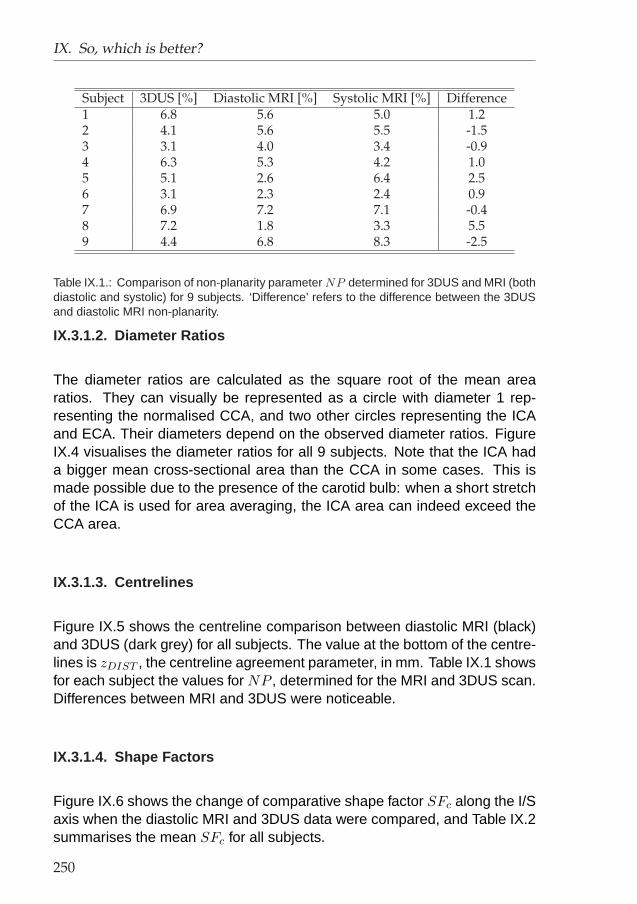
IX. So, which is better?
Subject 3DUS [%] Diastolic MRI [%] Systolic MRI [%] Difference1 6.8 5.6 5.0 1.22 4.1 5.6 5.5 -1.53 3.1 4.0 3.4 -0.94 6.3 5.3 4.2 1.05 5.1 2.6 6.4 2.56 3.1 2.3 2.4 0.97 6.9 7.2 7.1 -0.48 7.2 1.8 3.3 5.59 4.4 6.8 8.3 -2.5
Table IX.1.: Comparison of non-planarity parameter NP determined for 3DUS and MRI (bothdiastolic and systolic) for 9 subjects. ‘Difference’ refers to the difference between the 3DUSand diastolic MRI non-planarity.
IX.3.1.2. Diameter Ratios
The diameter ratios are calculated as the square root of the mean arearatios. They can visually be represented as a circle with diameter 1 rep-resenting the normalised CCA, and two other circles representing the ICAand ECA. Their diameters depend on the observed diameter ratios. FigureIX.4 visualises the diameter ratios for all 9 subjects. Note that the ICA hada bigger mean cross-sectional area than the CCA in some cases. This ismade possible due to the presence of the carotid bulb: when a short stretchof the ICA is used for area averaging, the ICA area can indeed exceed theCCA area.
IX.3.1.3. Centrelines
Figure IX.5 shows the centreline comparison between diastolic MRI (black)and 3DUS (dark grey) for all subjects. The value at the bottom of the centre-lines is zDIST , the centreline agreement parameter, in mm. Table IX.1 showsfor each subject the values for NP , determined for the MRI and 3DUS scan.Differences between MRI and 3DUS were noticeable.
IX.3.1.4. Shape Factors
Figure IX.6 shows the change of comparative shape factor SFc along the I/Saxis when the diastolic MRI and 3DUS data were compared, and Table IX.2summarises the mean SFc for all subjects.
250

IX.3. Results
MRI Diastole MRI Systole
Ultrasound
CCAICAECA
(a) Subject 1
MRI Diastole MRI Systole
Ultrasound
CCAICAECA
(b) Subject 2
MRI Diastole MRI Systole
Ultrasound
CCAICAECA
(c) Subject 3
MRI Diastole MRI Systole
Ultrasound
CCAICAECA
(d) Subject 4
MRI Diastole MRI Systole
Ultrasound
CCAICAECA
(e) Subject 5
MRI Diastole MRI Systole
Ultrasound
CCAICAECA
(f) Subject 6
MRI Diastole MRI Systole
Ultrasound
CCAICAECA
(g) Subject 7
MRI Diastole MRI Systole
Ultrasound
CCAICAECA
(h) Subject 8
MRI Diastole MRI Systole
Ultrasound
CCAICAECA
(i) Subject 9
Figure IX.4.: Diameter ratios for all subjects measured with (diastolic) ultrasound, diastolicMRI and systolic MRI.
251

IX. So, which is better?
0.53
1
_________________________________________
_________________________________________
0.17
2
_________________________________________
_________________________________________
0.08
3
_________________________________________
_________________________________________
0.03
4
_________________________________________
_________________________________________
0.11
5
_________________________________________
_________________________________________
0.08
6
_________________________________________
_________________________________________
0.30
7
_________________________________________
_________________________________________
0.83
8
_________________________________________
_________________________________________
0.13
9
_________________________________________
_________________________________________
Figure IX.5.: Centreline comparison (in two different views rotated 90 degrees relative toeach other) between diastolic MRI (black) and 3DUS (dark grey) in each of the 9 subjects(numbered in top right corner). The value at the bottom of the centrelines is zDIST , thecentreline agreement parameter, in mm.
Subject CCA ICA ECA1 4.6 ± 2.0 5.9 ± 2.2 8.8 ± 5.42 4.3 ± 2.2 4.5 ± 1.0 7.9 ± 4.73 5.2 ± 2.2 4.3 ± 1.1 12.1 ± 7.24 9.0 ± 5.4 6.5 ± 2.3 13.3 ± 5.75 8.8 ± 2.3 5.2 ± 2.1 17.3 ± 7.46 14.3 ± 7.3 6.1 ± 2.2 9.6 ± 4.87 8.4 ± 6.6 8.8 ± 4.8 7.6 ± 4.78 7.4 ± 2.3 4.9 ± 1.2 11.7 ± 5.29 7.7 ± 2.7 4.7 ± 2.1 9.1 ± 5.3Mean 7.7 ± 3.1 5.7 ± 1.4 10.8 ± 3.1
Table IX.2.: Mean±standard deviation of comparative shape factors [%] in CCA, ICA andECA in each of 9 subjects. These values correspond to the average of data in Figure IX.6.
252

IX.3. Results
IX.3.2. Flow Results
Figures IX.7 and IX.8 show respectively the WSS and OSI distribution forall subjects. The most favourable agreement between MRI and 3DUS de-rived WSS was found in subject 4, whereas subject 8 exhibited the largestdiscrepancy. The OSI distribution agreed extremely well in subject 2, butdiffered significantly in subject 6.
−10 0 10 200
10
20
30
40
50
I/S axis [mm]
Sha
pe F
acto
r [%
]
1
−30 −20 −10 0 100
10
20
30
40
50
I/S axis [mm]
Sha
pe F
acto
r [%
]
2
−30 −20 −10 0 100
10
20
30
40
50
I/S axis [mm]
Sha
pe F
acto
r [%
]
3
−20 −10 0 10 200
10
20
30
40
50
I/S axis [mm]
Sha
pe F
acto
r [%
]
4
−40 −20 00
10
20
30
40
50
I/S axis [mm]
Sha
pe F
acto
r [%
]
5
−20 −10 0 10 200
10
20
30
40
50
I/S axis [mm]
Sha
pe F
acto
r [%
]
6
−30 −20 −10 0 100
10
20
30
40
50
I/S axis [mm]
Sha
pe F
acto
r [%
]
7
−10 0 100
10
20
30
40
50
I/S axis [mm]
Sha
pe F
acto
r [%
]
8
−20 −10 0 10 200
10
20
30
40
50
I/S axis [mm]
Sha
pe F
acto
r [%
]
9
Figure IX.6.: Shape factor evolution along the I/S axis in each of 9 subjects (numbered intop right corner). The CCA and ICA are represented by the solid lines, respectively at I/Spositions lower and larger than zero, the ECA is represented by the dashed line. The shapefactors were derived from the matching sets of diastolic MRI and 3DUS contours. The mean± standard deviation of the SFc can be found in Table IX.2.
253
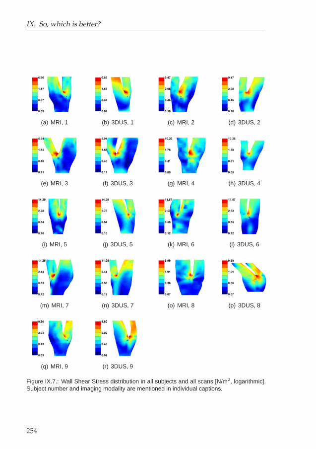
IX. So, which is better?
(a) MRI, 1 (b) 3DUS, 1 (c) MRI, 2 (d) 3DUS, 2
(e) MRI, 3 (f) 3DUS, 3 (g) MRI, 4 (h) 3DUS, 4
(i) MRI, 5 (j) 3DUS, 5 (k) MRI, 6 (l) 3DUS, 6
(m) MRI, 7 (n) 3DUS, 7 (o) MRI, 8 (p) 3DUS, 8
(q) MRI, 9 (r) 3DUS, 9
Figure IX.7.: Wall Shear Stress distribution in all subjects and all scans [N/m2, logarithmic].Subject number and imaging modality are mentioned in individual captions.
254

IX.3. Results
(a) MRI, 1 (b) 3DUS, 1 (c) MRI, 2 (d) 3DUS, 2
(e) MRI, 3 (f) 3DUS, 3 (g) MRI, 4 (h) 3DUS, 4
(i) MRI, 5 (j) 3DUS, 5 (k) MRI, 6 (l) 3DUS, 6
(m) MRI, 7 (n) 3DUS, 7 (o) MRI, 8 (p) 3DUS, 8
(q) MRI, 9 (r) 3DUS, 9
Figure IX.8.: Oscillatory Shear Index distribution in all subjects and all scans [-]. Imagingmodality and subject number are mentioned in individual captions.
255

IX. So, which is better?
Parameter Threshold ε1 [%] ε2 [%] ε1 [%] (Threshold)WSS < 0.40 N/m2 16.08±10.75 49.36±26.48 9% (0.5)WSS > 2.50 N/m2 1.85±1.23 55.48±26.96 20%OSI > 0.20 5.40±5.01 25.79±22.36 2%WSSGs > 4000 N/m3 0.22±0.11 70.55±24.73 15% (25000)WSSGt > 15 N/(s m2) 2.15±2.20 86.56±38.59 1.5% (50)WSSAG > 350 rad/m 6.49±6.94 42.86±18.02 -
Table IX.3.: Differences in Area of overflow/underflow. See text for a definition of ε1 and ε2.The result is given as mean±standard deviation (n=8 instead of n=9 because of omissionof subject 8, see discussion). The last column is copied from the TOF MRI reproducibilitystudy,121 reported in section VI.4.2. Note that the thresholds from that study121 are shownbetween brackets when different.
IX.3.2.1. Area of overflow/underflow
Table IX.3 shows the average difference±standard deviation in estimatingthe area of overflow/underflow. The difference considered is the followingerror measure:
ε1 =(A)MRI
AbifMRI− (A)3DUS
Abif3DUS(IX.2)
Here, the ‘bifurcation area’ Abif is the vessel wall area within a verticaldistance of 1.5 cm of the bifurcation apex. The area of overflow/underflow inMRI and 3DUS is respectively (A)MRI and (A)3DUS . Another error measure,ε2, quantifies the relative error:
ε2 = 2× (A)MRI − (A)3DUS
(A)MRI + (A)3DUS(IX.3)
IX.3.2.2. Analysis along Inferior/Superior axis
Table IX.4 gives the average RMSE of all considered haemodynamic pa-rameters when analysed along the I/S axis. Note that the analysis alongthe I/S axis is equivalent to choosing an infinite number of patches in thelongitudinal direction, and only 1 patch in the circumferential direction.
256

IX.3. Results
Parameter CCA ICA ECA mean Sd
Vmax [m/s] 0.0323 0.0310 0.0242 0.0291 0.0044WSS [N/m2] 0.158 0.395 0.311 0.288 0.120OSI [-] 0.0234 0.0235 0.0223 0.0231 0.0007WSSGs [N/m3] 26.6 98.6 78.7 68.0 37.2WSSGt [N/(s m2)] 1.02 2.53 1.97 1.84 0.765WSSAG [rad/m] 41.1 44.2 53.9 46.4 6.68
Table IX.4.: Average Root-Mean-Square error along I/S axis (n=8 instead of n=9 because ofomission subject 8, see discussion). Sd is the standard deviation of the mean of each artery.Large Sd denotes important differences between arteries.
Parameter CCA ICA ECA mean Sd
WSS 0.45±0.14 0.68±0.10 0.78±0.09 0.59±0.18 0.15OSI 0.46±0.15 0.63±0.29 0.50±0.28 0.55±0.22 0.08WSSGs 0.47±0.22 0.77±0.12 0.94±0.04 0.69±0.21 0.17WSSGt 0.67±0.16 0.61±0.17 0.65±0.12 0.65±0.14 0.02WSSAG 0.47±0.21 0.60±0.11 0.63±0.11 0.60±0.16 0.08mean 0.50±0.20 0.66±0.19 0.70±0.22 0.62±0.19 -
Table IX.5.: Summary of the 2D correlation coefficient (n=8 instead of n=9 because of omis-sion subject 8, see discussion). The results is shown as mean±standard deviation. Sd
defined in Table IX.4.
Artery WSS OSI WSSGs WSSGt WSSAG TotalCCA 4 / 8 4 / 8 3 / 8 5 / 8 2 / 8 18/ 40ICA 3 / 8 3 / 8 2 / 8 2 / 8 1 / 8 11/ 40ECA 2 / 8 2 / 8 2 / 8 1 / 8 1 / 8 8/ 40Total 9 / 24 9 / 24 7 / 24 8 / 24 4 / 24 37 / 120
Table IX.6.: Summary of the paired Wilcoxon test (rank-sum test) for all subjects (n=8 insteadof n=9 because of omission of subject 8, see discussion). The results are presented as‘number of positive results / maximum number of positive results’ (p<0.05).
IX.3.2.3. Patched Analysis
Table IX.5 summarises the results for the 2D linear correlation coefficientsbetween the patched data from MRI and 3DUS. In Table IX.6, the results ofthe paired rank-sum test, performed on every matching set of patched data,are summarised. The root-mean-square error (RMSE) in patched value isshown in Table IX.7.
257

IX. So, which is better?
Artery WSS OSI WSSGs WSSGt WSSAG[N/m2] [-] [N/m3] [N/(s m2)] [rad/m]
CCA 0.314 (45.9%) 0.0658 (104%) 56.1 (35.3%) 1.80 (24.8%) 96.2 (78.0%)ICA 0.534 (44.0%) 0.0416 (123%) 164 (54.5%) 3.34 (36.6%) 74.5 (91.6%)ECA 0.397 (40.0%) 0.0420 (193%) 149 (52.8%) 2.11 (28.1%) 90.4 (88.4%)mean 0.411 (42.7%) 0.0481 (166%) 150 (55.4%) 2.29 (29.1%) 87.6 (86.3%)
Thomas332 0.44 (32%) 0.021 (109%) 38 (55%) - 61 (73%)Glor121 0.43 (37.9%) 0.025 (123%) 214 (65.7%) 2.35 (30.2%) 68.1 (79.8%)
Table IX.7.: Summary of the root mean square error (RMSE) in the patched analysis. Be-tween brackets, the percent RMSE, i.e. 100 x RMSE/(average value) (n=8 instead of n=9because of omission subject 8, see discussion). For comparison, the result of two MR repro-ducibility studies121,332 have been added.
IX.4. Discussion
IX.4.1. Cross-Comparing MRI and ultrasound
This study cross-compared 3DUS with BB MRI to assess the quantitativedifferences between the two imaging modalities in reconstructing in vivocarotid bifurcation geometry. A similar study was performed by Frayne98
on a carotid phantom. It was reported that the geometry could be suc-cessfully reconstructed using either (3DGRASS) MR, X-ray or ultrasound.Root-mean-square deviations in radius between ultrasound, MRI and pro-jection radiography measurements on the phantom (considered to be thegold standard) were estimated to be 0.55 mm and 0.33 mm respectively.However, to our knowledge, comparative studies on in vivo imaging for 3Dreconstruction are lacking. The two methods employed here are capable ofacquiring not only geometrical data suitable for constructing CFD models ofthe carotid bifurcation, but also wall data such as IMT and wall compliance(when combined with systolic and diastolic blood pressures). Crowe71 usedBB MRI for in vivo carotid IMT and area measurements, and compared MRIdata with the more commonly accepted ultrasound measurements. The re-sults showed good agreement when the average change in lumen diameterover the length of the common carotid in MRI was compared to the averagedlumen diameter resulting from 3 planes for ultrasound. In that study, BB MRIvalues for wall thickness were consistently about 0.35 mm higher than ultra-sound IMT measurements. The authors concluded that this difference arosebecause BB MRI measures total wall thickness (i.e. media-adventitia thick-ness plus IMT), whereas ultrasound only measures IMT. To our knowledge,no studies have so far addressed the differences between MRI and 3DUSfor in vivo carotid geometry reconstruction.
MRI is currently regarded as the modality of choice for large artery CFD
258

IX.4. Discussion
modelling, but has the disadvantage of being expensive, time consumingand of limited availability. 3DUS offers a cost-effective way of imaging super-ficial vessels prone to atherosclerosis, such as the carotid artery. However,the in vivo applicability of 3DUS to the carotids is affected by the locationof the bifurcation point in the neck. In those subjects with relatively highbifurcation points, the jaw bone often physically limits the accessibility ofthe ultrasound transducer to the carotid bulb, and/or the internal and exter-nal carotid arteries. This can lead to insufficient geometrical information forsubject-specific flow simulations.
IX.4.2. Image Processing
It is important to note that image segmentation and the geometry recon-struction were performed in very different ways with the two types of images.In MRI, a semi-automatic contour detection algorithm was used, whereas lu-men contours were defined manually in 3DUS. Ultrasound images were usu-ally found not to be defined well enough to allow automatic segmentation.Automated segmentation of ultrasound images using a technique similar tothat used for BB MRI would undoubtedly result in time gain, but contour ac-curacy would have been compromised. Mao210 presented a segmentationprocess based on a deformable model method with only one seed point,and compared the results from the automatic segmentation to the manuallysegmented counterparts. Although they described manual segmentationfor ultrasound as tedious, prone to variability and requiring substantial ex-perience, they still considered the manual segmentation as more reliablethan their particular segmentation algorithm. The reproducibility of the ultra-sound segmentation protocol adopted in this study was investigated both ona carotid phantom16 and on healthy volunteers,117 for which an experiencedoperator performed all the manual segmentations.
Another difference between the MRI and 3DUS data was the number oftransverse images along the vessel length. MRI data were available in 28slices whereas in 3DUS anything between 80 and 140 images were ac-quired. With those slices and with the information from the EPOM device,the carotid geometry was resliced into about 50 slices with a constant inter-slice distance of 1 mm. While this may be regarded as a limitation of thecomparison, we think different reconstruction techniques are inevitable be-cause of the different configuration of the data. In this study, the most ap-propriate and well tested reconstruction techniques were used, although thismeant using different reconstruction techniques for MRI and 3DUS.
259

IX. So, which is better?
IX.4.3. Geometry differences
IX.4.3.1. Areas
Figure IX.2 shows that for subjects 2, 3, 4, 8 and 9, areas measured with3DUS were similar to those measured with BB MRI. In subject 1, the onlysubject where the mean diastolic area of CCA was larger than its systolicvalue, the BB MRI-based carotid reconstruction clearly overestimated thediastolic CCA. In the carotid daughter vessels, the BB MRI protocol failed todetect the expected change in cross-sectional area, partly because of thetechnical difficulties involved in visualising small sized vessels, and partlybecause the anticipated cyclic area change in the smaller daughter vesselis much smaller than in the CCA. Figure IX.3 shows that there was no sta-tistically significant difference in areas measured by 3DUS and BB MRI, butareas measured by BB MRI tended to be greater, and the variability of dif-ferences in measured areas was rather high.
Barratt20 found that with 3DUS, error in 3D distance measurements on aphantom was up to -0.53±3.39% (mean±standard deviation). Assumingthat the diameter of the CCA is 9 mm, which is large but not uncommon, thiswould result in an uncertainty in area of 4.99 mm2 (=uncertainty in radius ×circumference = abs((-0.53%-3.39%) × 4.5 mm × 9 mm × π)). Values forICA (2.22 mm2) and ECA (1.54 mm2) were found using estimated diame-ters of 6 mm and 5 mm respectively. Moore225 reported an uncertainty of0.15 mm on the 4 mm radius of a carotid phantom reconstructed from BBMRI, giving a relative uncertainty of 3.75% (=100× 0.15 mm/4 mm). For theCCA radius used for comparison purposes in the present study, this wouldresult in an error of 4.77 mm2 (=3.75% × 4.5 mm × 9 mm × π = uncertaintyin radius × circumference). Similarly, values of 2.12 mm2 and 2.45 mm2
have been found for ICA and ECA. Apart from being validated on phantomsin 3DUS20 and BB MRI,225 the reproducibility of both carotid reconstructiontechniques has also been investigated. In section VII.4.2 (page 176), wedemonstrated that lumen area reconstructed from 3DUS was reproducedwithin 10% for CCA and ICA (or 10% × π×(4.5 mm)2=6.36 mm2 for a largeCCA) and 15% for the ECA. Long194 showed that carotid bifurcations re-constructed with TOF-MRI were reproducible using 8 subjects. Similarly,Thomas332 performed a separate reproducibility study using BB MRI andreported lumen diameter to be precise to within 5%. Referring this resultto an area error, the same uncertainty of 6.36 mm2 (=5% × 4.5 mm × 9mm × π) was found. In the comparative study on a carotid bifurcation phan-tom,98 root-mean-square errors of 0.55 mm and 0.33 mm in artery radius
260

IX.4. Discussion
Technique CCA ICA ECABB MRI validation on phantom225 4.77 (7.50%) 2.12 (7.49%) 2.45 (12.5%)BB MRI in vivo reproducibility332 (n=3) 6.36 (10.0%) 2.83 (10.0%) 1.96 (10.0%)MRI on phantom (for cross-comparison)98 9.33 (14.7%) 6.22 (22.0%) 5.18 (26.4%)3DUS validation on phantom20 4.99 (7.85%) 2.22 (7.84%) 1.54 (7.86%)3DUS in vivo reproducibility118 (n=9) 6.36 (10.0%) 2.83 (10.0%) 2.94 (15.0%)US on phantom (for cross-comparison)98 15.54 (24.43%) 10.36 (36.6%) 8.64 (44.1%)Present study: difference between BB MRI and 3DUS 3.60±7.39 5.18±6.23 2.46±3.62mean ± standard deviation (n=9) 5.66±11.6% 18.3±22.1% 12.6±18.5%
Table IX.8.: Uncertainties in cross-sectional area for carotid geometry reconstructions in lit-erature.22,98,118,225,332 When the publication mentions a cross-sectional diameter instead ofan area, large carotid diameters of 9 mm (CCA), 6 mm (ICA) and 5 mm (ECA) were cho-sen as a reference. The percentage is calculated using these reference values. BB MRI:Black blood MRI; 3DUS: Three-dimensional Ultrasound. All values in mm2, except thosewith percent sign.
were found for US and MRI respectively. Referring this to an arbitrary CCAwith diameter 9 mm, this translates to a 12.22% (=0.55 mm/4.5 mm) errorin radius or an uncertainty of 15.54 mm2 (=0.55 mm × 9 mm × π = uncer-tainty in radius × circumference) for US. Summarising all this information interms of area in Table IX.8, we can appreciate the level of correspondencebetween 3DUS and BB MRI in terms of quantifying cross-sectional areas:the present variability is higher than the uncertainty reported in the repro-ducibility studies of each of the techniques separately,118,332 but lower thanthe variability found in the comparative study of MRI and US on a carotidphantom.98 This variability is likely to be related to several factors inherentto in vivo acquisition:
• When an ultrasound image is of poor quality, the boundaries betweenvessel lumen and vessel wall, and between lamina adventitia and me-dia, become blurred, which can cause the operator to make a segmen-tation error.
• A known artefact in BB MRI is ‘residual signal’,307 which causes slowlymoving or recirculating blood to appear white instead of black, makingit look as if it was part of the wall or possible plaque. This effect cancause the IMT to be overestimated and the cross-sectional area to beunderestimated (see Figure VI.10 (c)). Recently, a similar segmen-tation technique has proved reliable165 in similar studies with healthysubjects, but in diseased vessels, with moderate or severe stenoses,BB MR image segmentation is yet to be validated.
• When an artery cross-section is not imaged perpendicular to its axis,artefacts like vessel boundary blurring can occur. These effects aremore pronounced in 3DUS than MRI, since the US-probe has to follow
261

IX. So, which is better?
the patient’s neck curvature which is not necessarily the same as thecarotid bifurcation curvature.
In subjects 1, 6 and 9, the quantitative area agreement is not as good as insubjects 2, 3, 4 and 8, but the ratios between the branch (ICA or ECA) areaand CCA area correspond remarkably well (Figure IX.4). This suggests thatthere might be a systematic (yet over all subjects statistically insignificant atp=0.05, Figure IX.3) area difference in these subjects. The following sys-tematic errors might contribute to the observed differences between the BBMRI and 3DUS reconstructed carotid geometries.
• BB MR images with a lot of residual signals are likely to cause an un-derestimation of the lumen. Our results showed that, on the contrary,areas deduced from BB MRI tended to be greater than those from3DUS. Possibly the 3DUS areas were in some cases underestimatedeven more due to the IMT deduction (see next point).
• IMT measurements were only made 1 cm proximal to the carotid bulb,and with that measurement, the IMT in the carotid tree was estimatedas explained in Figure VII.6 on page 168. Although this mathemati-cal approximation is likely to be clinically realistic, subject-variability isknown to be very high and a poor estimate of the IMT will result insystematically over- or underestimated cross-sectional areas.
• Although the two scan modalities were performed under standardisedconditions, physiological differences may have been involved. Influ-ences such as recent medication, salt loading, exercise and mentalactivity may have important haemodynamic effects on cardiac out-put, blood pressure and cerebral blood flow. Blood pressure wasmeasured on both occasions and no significant difference was found.However, it is possible that an individual’s carotid cross-sectional areacould be very pressure dependent. Sugawara312 demonstrated thatmild changes in blood pressure (<20 mmHg) can induce a diameterchange of up to 1 mm. Their findings showed that this effect is verysubject-dependent.
In subjects 5 and 7, where both diameter ratios and mean areas failed toagree, the error was likely to be due to a combination of the aforementionedreasons and to the diversity of the techniques involved. Ultrasound wasused for IMT measurements and 3D carotid geometry acquisition. An EPOMdevice provided the 3D coordinates of the ultrasound probe during the scan.
262

IX.4. Discussion
The contours were smoothed before area assessment. MR images wereacquired with a slice thickness of 2 mm, which led to a rather sparse sam-pling of the vessel geometry compared to 3DUS. MR image segmentationinvolved some degree of manual adjustment and smoothing was also per-formed. Each of the techniques has inherent uncertainties.
IX.4.3.2. Centrelines
Figure IX.5 shows the centreline comparison between diastolic MRI, drawnin black, and diastolic ultrasound, drawn in grey. In subjects 3, 4, 5 and 6, theagreement is satisfactory. However, major differences can be observed insome subjects. This is reflected by the poor agreement in the non-planarityparameter NP (in Table IX.1) and zDIST (in Figure IX.5). The centreline mis-match in subjects 1, 2, 7 and 9 was very likely to be caused by the differentscan positions in MRI and 3DUS. For MRI, the patient’s head is usually heldin a straight position. In contrast, it is often necessary for the ultrasonogra-pher to reposition the subject’s neck to achieve better ultrasound images ormore coverage of the carotid branches. Different head- and neck angles arelikely to influence the centreline and the non-planarity parameter. This pointis addressed in chapter XI.
Another reason for centreline mismatch is due to practical problems duringimage acquisition. A subject might sneeze, move or swallow when lyingin the MRI scanner or on the ultrasound couch. The error in subject 8,where the 3DUS centrelines take an unphysiological twist immediately afterthe bifurcation apex, is more likely to be due to this cause. In view of this,two additional points make MRI preferable: (1) the narrow MRI bore hasmore restrictions on the head movement as compared to the couch usedfor US. (2) The slice orientation information in MRI is more reliable than theEPOM device, used to track the position and orientation of the probe. Whenpatients succeed in lying still and in the absence of head- and neck angledifferences, the centrelines scanned by 3DUS were similar to those scannedby BB MRI.
IX.4.3.3. Shape Factor
Two issues can influence the shape factor negatively:
263

IX. So, which is better?
1. In MRI, the semi-automatic segmentation technique could result in ir-regular shapes, whereas in 3DUS, the operator was allowed to fit anellipse when deemed appropriate.
2. The operator needed to press the probe onto the patient’s skin in orderto obtain an image in 3DUS. The harder the operator presses, themore the shape of the vessels might deform.
The results in Table IX.2 and Figure IX.6 show a very good agreement incontour shape in the CCA and ICA. This helps to justify the use of the sim-plified contour shape in 3DUS segmentation. From this result, it can alsobe concluded that the effect of probe pressure on vessel shape is almostnegligible. However, for the ECA, the shape factor was less satisfactory.Apart from the aforementioned factors, the shape of ECA is also influencedby the way its side branches are treated. The thyroid artery originates in theECA and does show up in both US and MRI scans as an additional branch.Because flow in the thyroid artery is of less interest and because of thenon-negligible technical difficulties involved in incorporating the ECA’s sidebranches in CFD models, the thyroid artery is usually neglected in carotidbifurcation models.386 In the thyroid bifurcation zone, the operator wouldexclude the thyroid branch by drawing a small segment of a contour acrossthe inlet of the thyroid artery. It is clear that contour shapes in this region arehighly operator dependent.
IX.4.4. Effect on flow
From the WSS and OSI distributions in Figures IX.7 and IX.8, two obser-vations can be made. (1) In subject 8, the carotid branches (ICA and ECA)derived from 3DUS are strongly skewed towards one side, a feature which isabsent in the MRI-derived geometry. This is very probably due to a suddenmovement of the subject deemed unimportant by the operator. For this rea-son, subject 8 has been eliminated from the statistical analysis. (2) Exceptfor subject 8, the overall agreement in WSS and OSI distribution is satisfac-tory: two matching sets of carotid bifurcations show sufficient agreement tobe recognised as a single bifurcation belonging to a single person.
264

IX.4. Discussion
IX.4.4.1. Comparison of Haemodynamic Parameters
Among the haemodynamic parameters related to the atherogenic process,the WSS and OSI are the most commonly quoted haemodynamic param-eters. In the present study, the WSSG and WSSAG have also been eval-uated. Sites of high WSSG are linked to intimal hyperplasia, formation ofatherosclerotic lesions inside the arteries, and increased vessel wall perme-ability.159 The WSSAG represents the magnitude of the shear stress angledeviation. Large WSSAG tends to occur in regions of dysfunctional cells,and hence sites of intimal thickening.199
Velocity Table IX.4 shows that the velocity parameter, representing thecorrespondence in flow profile, agrees very well in all arteries. In the regionof complex flow in the ICA, which is very geometry dependent, the uncer-tainty in Vmax was only 3 cm/s, corresponding to a 10.9% uncertainty.
WSS According to Table IX.6, the WSS was reproduced most closely bythe two imaging techniques. The uncertainty in measuring areas of lowWSS was higher in the present cross-comparison study than in the MR re-producibility study121 (Table IX.3), but the uncertainty in quantifying areasof high WSS was lower (Table IX.3), probably due to the improved meshingtechnique. Overall, values for the RMSE in WSS (both circumferential (Ta-ble IX.4) and patch-wise (Table IX.7)) fall within the 0.45 N/m2 found in MRIreproducibility studies.121,332
OSI In Table IX.6, the OSI - similar to the WSS - seemed to be one of themost robust haemodynamic parameters when switching between MRI and3DUS-based CFD. Quantification of the vessel wall area overflowing an OSIof 0.2 proved to be a reliable process (Table IX.3). The high percent RMSEis due to the fact that the OSI is 0 in the majority of the vessel wall. Therather low 2DR value of 0.54 (Table IX.5) combined with the small RMSE inTable IX.4 showed that the OSI peaks were well localised along the I/S axis,but less reliably along the circumference. Overall, the RMSE for the OSIis below 0.07, which is larger than what has been found in reproducibilitystudies, but still very small considering that the OSI ranges from 0 to 0.5.
265

IX. So, which is better?
WSSG Table IX.6 shows that although the WSSG values had a less fa-vourable agreement than the WSS or OSI values, the WSSG distributionwas extremely robust (Table IX.5: highest 2DR off all parameters). This wasechoed by fairly small ε-values when compared with other studies (TableIX.3). The spatial WSSG had a percent RMSE of 55% and the temporalWSSG an RMSE of 2.42 N/(s m2), which compared well with values foundin MRI reproducibility studies.
WSSAG Of all parameters, the WSSAG had the worst result in the rank-sum test. Measuring areas of high WSSAG seemed easier than areas ofother parameters, but a comparison with MRI reproducibility studies cannotbe done. The RMSE (circ: 46.4 rad/m; patch-wise: 87.0 rad/m) was 26rad/m higher than the patch-wise RMSE found for MRI reproducibility (61rad/m).
Summary Thomas332 published a BB MRI-based flow reproducibility studyusing the same haemodynamic parameters. For most parameters, the RM-SEs found in their study are comparable to those given in Table IX.7 whichsuggests that the differences in predicted flow between MRI and 3DUS areat a similar level to the uncertainties involved in using each of the imagingmodalities alone.
IX.4.4.2. Comparison of Arteries
Table IX.6 shows that the reliability of parameter values was usually higherin the CCA than in the daughter branches. The overall low 2DR in CCA(Table IX.5) seems to contradict the statement that the correspondence inthe CCA was high, but linear correlation can be misleading when comparingtwo sets of patched data with little variation. For example, the time-averagedWSS tends to be fairly constant around a value of 0.7 Pa in a CCA in typicalcircumstances. A significantly better reliability of the proximal CCA couldhave been expected because of two reasons. (1) BB MR image qualitytends to be better for the proximal CCA than for the branches.71 As a con-sequence, the bulb location can match quite well between MRI and 3DUS,but the largest differences in both cross-sectional area and cross-sectionalshape occur in the bulb.120 (2) Flow patterns are less complex proximal fromthe apex, resulting in better image quality.
266

IX.5. Summary and Conclusion
No obvious difference between ICA and ECA reliability was found. Whenexamining each parameter in more detail (Table IX.7), it can be seen that theWSS and WSSG agreed better in the CCA than in the daughter branches,but the opposite was true for the OSI and WSSAG, suggesting that geometrydifferences had different effects on different haemodynamic parameters.
IX.4.5. Limitations
A first simplification of the model, was the fact that blood was modelled asa Newtonian fluid, i.e. with a constant blood velocity. Bearing in mind thatthe use of a non-Newtonian model would result in similar changes in flowprofiles for both the MRI- and 3DUS-based models, the difference foundwith the Newtonian model presented here should be expected to representwhat would be found with a non-Newtonian model. Therefore, a Newtonianmodel was used in this study to save processing time. See section VIII.2on page 228 for a discussion on the necessity of the implementation of non-Newtonian viscosity models.
Due to significant complexity of fluid-structure interaction, rigid walls havebeen assumed in the simulations. This is another simplification of the mod-els. See section VIII.1.3 on page 225 for a discussion on the necessity ofthe implementation of fluid-structure interaction.
The subjects in this study were all healthy, normotensive volunteers. In el-derly people, the potential presence of plaque will introduce difficulties insegmenting images acquired with BB MRI due to possibilities of confusingresidual signal304 in blood on one hand and plaque on the other. In 3DUSthe potential presence of plaque will discourage the use of the IMT sub-straction model because it assumes constant IMT along a circumference.Furthermore, in the presence of calcified plaque the use of 3DUS will beimpeded. Because of the possible complications in pathological cases, theflow differences found between MRI and US in this study cannot be regardedas a worst case scenario.
IX.5. Summary and Conclusion
The carotid bifurcations of nine subjects were scanned twice: once withblack blood MRI, and once with 3D ultrasound. The aim of the study was
267

IX. So, which is better?
to assess the differences of two imaging modalities when applied to in vivocarotid geometry reconstruction. Although image artefacts such as residualsignals in BB MRI and indiscernible lumen-intima borders with ultrasoundhamper the reliability of both techniques, lumen cross-sectional areas esti-mated from the two imaging modalities showed a good agreement. Centre-line agreement is rather poor and this was very probably due to the inabilityto scan the subjects with the same head- and neck angles in MRI and 3DUS.Overall, 3DUS proves to be able to reconstruct 3D in vivo carotid geometrieswhich are suitable for CFD simulations, and the reconstructed geometriesare comparable to those obtained from MRI. The inter-technique flow differ-ences are comparable to intra-technique flow differences, suggesting thatBB MRI and 3DUS are interchangeable for carotid flow reconstruction. MRIhas several advantages over 3DUS, including (1) the ability to scan vesselsbeyond the physical restriction of the jaw-bone and the ability to scan nonsuperficial arteries and (2) the inherent robustness of 3D MRI for centrelineregistration due to the restricted freedom of movement. The advantagesof 3DUS are (1) the low relative cost of a set of images, (2) the easy ac-cessibility of the scanner couch as opposed to the MRI scanner for children,claustrophobic patients and people wearing pacemakers, (3) the widespreadavailability of US scanners and (4) the speed of imaging in US.
In future, the 3DUS protocol will aim for standardisation in order to avoidcentreline differences due to arbitrary head- and neck angles. Two sugges-tions can be made: (1) patients can be scanned in an anterior position byconvention, or (2) patients can be scanned in different positions and takea weighted mean. The first suggestion assumes the anterior head positionto be overwhelmingly more common than any other positions, the secondrecommendation accounts for possibilities that patients may adopt other po-sitions that are comfortable to them, such as subject who sleep in the proneposition. Furthermore, IMT measurements will need to be made along thecarotid tree instead of using a single site IMT measurement for the entiretree, and ways to extend the ICA and ECA geometry beyond the physicalrestriction of the jaw-bone need to be investigated. With the current level ofagreement achieved between BB MRI and 3DUS, and with the promise ofimaging and reconstruction improvements, 3D ultrasound has the potentialto become a relatively inexpensive, fast and accurate alternative to MRI forimage-based subject-specific carotid haemodynamic simulations.
268

Part C.
APPLICATIONS
269


X. So... what does it do?
In part B, image-based CFD has been optimised, both for 3DUS and forMRI-based simulations of carotid flow. Furthermore, the achievable repro-ducibility, accuracy and variability have been quantified in various studies.Now that the ‘reliability’ of the technique is known, it can be used to performin vivo studies which investigate the carotid blood flow.
In the past, CFD has been used to explain MRI flow artefacts. Here, thevoids in MR images are linked to flow features disturbing the expected mag-netisation.148,307 These studies are performed in the conviction that a thor-ough understanding of MRA demands a careful analysis of flow-related ef-fects. These early studies linking imaging and CFD do, however, not incor-porate a geometry reconstruction based on MR images: their aims can beachieved by performing an MRI (phantom) experiment and a CFD simula-tion using data originating from pumps and phantom manufacturers. No MRIdata is required for the CFD simulation, therefore the techniques of MRI andCFD are not really ‘combined’.
The first applications of image-based CFD were aimed at understanding theeffects of flow on the process of atherosclerosis.91,162,199,191,324,356 Thesestudies have investigated the role of haemodynamic parameters (WSS, OSI,etc.) in the initiation and progression of atherosclerosis.
One of the potential applications of image-based CFD is in pre-operativeplanning. Taylor323 suggested building a Simulation-Based Medical Plan-ning Suite at Stanford University. Here, a patient’s vasculature can be scan-ned and reconstructed in 3D. Before the operation, the effect of implantinga vascular graft or stent can be simulated and adjusted. The surgeon wouldgain important information from such a simulation. ‘How should the inci-sions be made?’, ‘Where does the stent need to be placed’, ‘Which stentis suited for this patient’, ‘Is there a need at all for the operation, or can wewait and see how the pathology evolves?’. These and many other importantquestions can be answered using patient-specific image-based CFD.
271

X. So... what does it do?
A recent study303 used 3DUS-based CFD to investigate the effects of hy-peroxiaa and hypoxic hypercapniab on carotid artery local haemodynamics.Distinct changes in local haemodynamic patterns between these two physi-ological states were demonstrated, despite little change in the overall carotidblood flow rate.
Along those lines, Ariff12 performed a study in which the differing effect ofangiotensin- vs. β-receptor blockers is compared on carotid IMT, left ven-tricular mass index, and carotid haemodynamics. From their data it couldbe suggested that one particular drug performed better in lowering bloodpressure and made a more positive effect on haemodynamic risk factors,i.e. in reducing OSI and raising WSS. The identity of the drug could not bedisclosed yet.
In our labs, two studies were performed using the combination of imagingand CFD: the Head Position Study (chapter XI) and the study on the AcuteEffect of Hypertensive Drugs (chapter XII). In the Head Position study, 9 sub-jects were scanned in two head positions: head straight, and head turnedleft. The geometry of their right carotid bifurcation was reconstructed andthe subject-specific flow fields were simulated in order to study the effect ofhead rotations on the haemodynamic situation in the carotid arteries. Thestudy has an effect on two levels. First , it informs the 3DUS technicianswhether or not diagnoses obtained in one head position are still valid in an-other head position. Second , the study has a more clinical effect: it warnsmanufacturers of carotid stents or emboli diverters on potential pitfalls typi-cal of the carotid site, it also shows the variety of forces vulnerable plaque isexposed to.
In the study on the acute effect of hypertensive drugs, the aim is to inspectacute effects of two types of anti-hypertensive drugs on the haemodynamicsof the carotid artery. A second aim is to explain the results found by Stan-ton302 in a long-term study comparing the same compounds. It was foundthat one type of drugs preserved luminal diameter (LD) and decreased IMTand IMA. Another compound reduces LD, and showed a smaller decreasein IMT with a similar decrease in IMA.
aHyperoxia : An abnormal increase in the amount of oxygen in the tissues and organs.bHypoxic Hypercapnia : The presence of an abnormally high level of carbon dioxide in the
circulating blood, induced by a lack of oxygen in the air
272

XI. Head Position Study
XI.1. Introduction
The effects of body posture and head positions on respiration and cerebralhaemodynamics have been investigated in a number of studies.
The effects on respiration seem to suggest that body posture rather thanhead position has the greatest effects.24 In infants, sleeping in a prone posi-tion has been shown to be associated with increases in heart and respiratoryrates, decreases in oxygen saturation and marked pallor in comparison toinfants sleeping in a supine position.290 These changes, however, do notoccur with changes in head positions alone.79 In adults, changes in headposition also do not seem to change oxygenation or maximum inspiratorypressure.79 Adopting a supine position, however, increases pharyngeal re-sistance337 and has been shown to worsen apnoeic episodes in those suf-fering from obstructive sleep apnoea.24
The haemodynamic effects of body posture and head position have alsobeen examined. In infants, while cerebral blood flow rate remains con-stant during head rotations in the supine position, keeping the head straightfavours cerebral venous drainage and helps to prevent an elevation of cere-bral blood volume.242 Eichler85 showed that in infants, blood velocity profileschanged in the internal carotid artery (ICA), basilar and vertebral artery withhead rotations. Kinking of the vertebral artery at the base of the skull withhead rotation may explain the change in flow in the vertebral and the basilarartery.135 The altered velocity profile in the ICA was not accompanied by achange in flow rate.
Studies in adults have shown marked changes in geometry and the relativepositions of the carotid arteries and the internal jugular vein when rotatingthe head.314 In addition, rotation of the head is accompanied by significantchanges in blood flow patterns and blood velocity profiles in the vertebraland basilar arteries207,266 as well as in the ICA,263 although total cerebralblood flow is kept constant.263 The blood flow patterns in the ICA and verte-
273

XI. Head Position Study
bral arteries also differ from left to right: e.g. the right ICA shows increasedblood flow rates with rotation to the contra-lateral position, but the left ICAdid not show the same trend.263
With the knowledge of potential changes to the carotid geometry and haemo-dynamics on one hand, and the elucidated link between blood flow patternsand atherosclerosis on the other hand,47,380 the question of how impor-tant the impact of the potential haemodynamic changes is on the risk foratherosclerosis is raised. Therefore, the aim of this study was to investigatethe effect of the change in geometry on carotid haemodynamics as a resultof head rotation. Haemodynamic wall parameters such as wall shear stress(WSS) and oscillatory shear index (OSI) were evaluated, as these have beenlinked to different stages of the atherosclerotic process. To our knowledge,this is the first study to examine the 3D carotid blood flow patterns in dif-ferent head positions using in vivo, subject-specific data. The hypothesis isthat turning the head has an important effect on both the carotid geometry,as suggested by Sulek,314 and the carotid haemodynamics. This would im-ply that the risk for atherosclerosis to develop in the carotid arteries, whichis thought to be associated with low WSS and/or high OSI, may vary withhead position. The altered distribution of heamodynamical forces could alsobe the cause of so-called ‘Telephone Strokes’:241 strokes occurring at theoccasion of prolonged telephone calls during which the patient holds thephone with shoulder and ear.
XI.2. Methods
XI.2.1. Subjects and Head Positions
The right carotid arteries of nine healthy subjects, 1 male and 8 female, aged26.6±3.0 years, were investigated with ultrasound by a single operator. Allof the subjects were normotensives with no history of vascular diseases.They were scanned twice serially in a supine position. In the first scan, thesubject’s head was positioned face up with a purpose-built cushion. In thesecond scan, the subject was asked to turn his/her head far to the left and tofix on a point on the wall. The two scans will be referred to as ‘Straight’ and‘Turned’ scan, respectively. See Figure XI.1 for an illustration of the headpositions. In both scans, the subject’s head was tilted forward a little fromthe supine position because of the cushion. The head tilt was the same forevery subject.
274
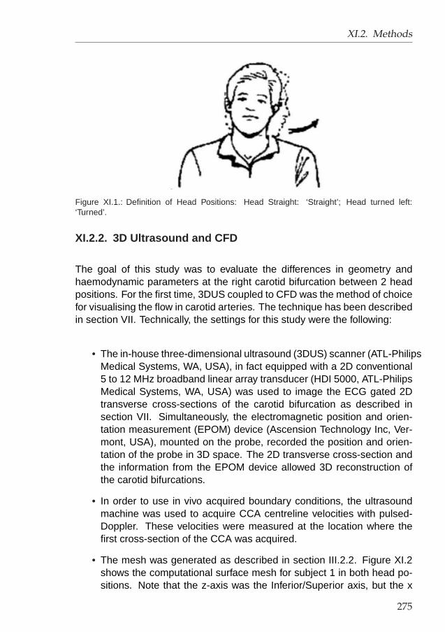
XI.2. Methods
Figure XI.1.: Definition of Head Positions: Head Straight: ‘Straight’; Head turned left:‘Turned’.
XI.2.2. 3D Ultrasound and CFD
The goal of this study was to evaluate the differences in geometry andhaemodynamic parameters at the right carotid bifurcation between 2 headpositions. For the first time, 3DUS coupled to CFD was the method of choicefor visualising the flow in carotid arteries. The technique has been describedin section VII. Technically, the settings for this study were the following:
• The in-house three-dimensional ultrasound (3DUS) scanner (ATL-PhilipsMedical Systems, WA, USA), in fact equipped with a 2D conventional5 to 12 MHz broadband linear array transducer (HDI 5000, ATL-PhilipsMedical Systems, WA, USA) was used to image the ECG gated 2Dtransverse cross-sections of the carotid bifurcation as described insection VII. Simultaneously, the electromagnetic position and orien-tation measurement (EPOM) device (Ascension Technology Inc, Ver-mont, USA), mounted on the probe, recorded the position and orien-tation of the probe in 3D space. The 2D transverse cross-section andthe information from the EPOM device allowed 3D reconstruction ofthe carotid bifurcations.
• In order to use in vivo acquired boundary conditions, the ultrasoundmachine was used to acquire CCA centreline velocities with pulsed-Doppler. These velocities were measured at the location where thefirst cross-section of the CCA was acquired.
• The mesh was generated as described in section III.2.2. Figure XI.2shows the computational surface mesh for subject 1 in both head po-sitions. Note that the z-axis was the Inferior/Superior axis, but the x
275

XI. Head Position Study
−10 0 10 20−10
010
−15
−10
−5
0
5
x[mm]y[mm]
z[m
m]
(a) Straight
−5 0 5 10−100
10
−15
−10
−5
0
5
x[mm]y[mm]
z[m
m]
(b) Turned
Figure XI.2.: Surface meshes for subject 1 in the two head positions: Straight (head straight)and Turned (i.e. head turned to the left).
and y-axis move with the ultrasound probe and were not the same inboth scans.
• The computational settings were the following. The vessel wall wasassumed to be rigid with no mass transfer and zero-velocity (no-slip)condition. At the inlet, Womersley profiles derived from the measuredflow waveform in the common carotid were imposed. The flow wave-form was acquired from the centreline velocity, assuming developedWomersley flow in the CCA.368 At the outlet, a constant flow ratio of55:45 was adopted between the internal (ICA) and external carotidartery (ECA) throughout the whole cardiac cycle. The Navier-Stokesequations were solved using the ‘QUICK’ differencing scheme imple-mented in CFX4™,3 on a SUN Blade 1000 Workstation (Ultrasparc IIIprocessor, 512Mb RAM, 750 MHz) as mentioned in section III.3. Twocardiac cycles, each consisting of 80 equally spaced time-steps, weresimulated. Refinement of time-step or increase in simulated cyclesresulted in instantaneous WSS differences below 0.5% and 0.01% re-spectively. For the fluid properties, a blood density of 1176 kg/m3 wasset. The non-Newtonian behaviour of blood viscosity was incorporatedusing the Quemada-model.42
XI.2.3. Comparative study
The effect of change in head position was quantified by geometric andhaemodynamic parameters. The first geometric parameter is the mean lu-men area ACCA, AICA and AECA. The bifurcation non-planarity (NP ) intro-
276

XI.3. Results
duced by King157 was used. Furthermore, zDIST ,194 defined as the averagedistance between the two centrelines, was computed. In addition to non-planarity (NP ) and zDIST , the linearity157 L was also derived for each ofthe three arteries. The final geometric parameter was the cross-sectionalcomparative shape factor introduced by Long.194 As a general guide, shapefactor of below 10% could be considered acceptable,194 but with 3DUS, theaccuracy of the shape factor is restricted to 15% in the ECA (see sectionIX). See section II.3.2.2 (page 53) for a clear definition of the used geome-try parameters.
The haemodynamic parameters comprise the velocity-dependent parameterVmax, the time-averaged wall shear stress (WSS) and the oscillatory shearindex (OSI). See section II.3.3.3 (page 67) for a definition of these parame-ters.
The average WSS and OSI values alone are not sufficient as markers foratherogenecity. The localisation and area of the vessel wall experiencingWSS and OSI above certain limits may also be important. For statisticalpurposes, the average WSS and OSI on the inner and outer walls of the ICAand ECA have been calculated separately. Here, ‘inner wall’ stands for thehalf of the daughter vessel on the flow divider side, whereas ‘outer’ standsfor the other half of the wall, i.e. the half that could be viewed as the outerbend of the vessel. Similarly, the CCA has been divided into two portions:one on the ICA side and another on the ECA side. See Figure VII.8 (page173) for a definition of the regions over which the parameters were averaged.
XI.3. Results
XI.3.1. Geometry
Figure XI.3 (a-c) summarises the findings for the arterial cross-sectionalareas: both the sample-averaged means (black dots) and the individualchanges (dotted lines) are represented. Note that ‘sample-averaged mean’stands for the value averaged over all subjects in one head position. Thep-value in Figure XI.3 is obtained by testing the hypothesis that the sample-averaged means in the two head positions are equal (paired Student test).For clarity, a p-value close to zero rejects the hypothesis and suggests thatthe sample-averaged means are different, whereas a p-value close to 1 con-cludes that the sample-averaged means are equal. Note that the uncertainty
277

XI. Head Position Study
of 3DUS for cross-sectional area measurement is around 10% for the CCAand ICA and 15% for the ECA.118 Table XI.1 gives the shape factor, i.e., theparameter describing the correspondence in cross-sectional shape betweenthe Straight and Turned scans. Long’s reproducibility study194 suggestedthat the cross-sectional shape could be considered unchanged when thecomparative shape factor was smaller than 10% for the CCA and ICA andsmaller then 15% for the ECA. Figure XI.4 overlays the centrelines of theStraight and Turned scans. The quantitative analysis is done in Figure XI.3(d) using the non-planarity parameter NP presented by King.157 This pa-rameter is reproducible to within 1%.157 Furthermore, Table XI.2 shows theother measure of vessel planarity, zDIST , deduced from Long’s study.194
Straight Turned20
30
40
50
60
CC
A a
rea
[mm
²]
(p=0.315)
(a)
Straight Turned10
20
30
40
50
ICA
are
a [m
m²]
(p=0.976)
(b)
Straight Turned5
10
15
20
25
EC
A a
rea
[mm
²]
(p=0.098)
(c)
Straight Turned0
5
10
15
Non
−Pla
narit
y [%
]
(p=0.565)
(d)
Figure XI.3.: a-c: Individual and overall change of cross-sectional area with head straightand turned. The black dot on the vertical line gives the sample-averaged mean±standarddeviation. Each of the dotted lines corresponds to a single subject. d: Non-Planarity (NP ).The p-value tests the hypotheses that the sample-averaged means in the two head positionsare different (paired Student test).
278

XI.3. Results
Subject CCA ICA ECA1 2.53 6.09 5.952 4.08 2.02 11.023 6.05 6.78 5.664 1.54 2.90 5.805 1.54 6.53 10.456 3.25 6.88 4.937 2.51 4.57 3.528 1.39 8.04 4.809 3.36 6.51 5.66Mean 2.92±1.50 5.59±2.00 6.42±2.56
Table XI.1.: Shape Factor for all subjects [%] (n=9). Subject-Mean results are given as mean± standard deviation.
Subject zDIST [µm]1 106.92 91.43 37.24 63.45 35.86 111.87 111.38 60.19 67.7Mean 76.2±30.3
Table XI.2.: Centreline Distance zDIST (deduced from Long’s study194) for all subjects (n=9).Subject-Mean results are given as mean ± standard deviation.
In Table XI.3, a statistical analysis of the centreline agreement is presented.In the first column, the studied centreline-related parameter is named. Thesecond column gives the tested hypothesis, and the last column gives the p-value for this hypothesis using a Student test. Whether the Student test wasone- or two-tailed, is reported in the third column. The table compares zDIST
(the parameter showing overall centreline mismatch), NP (the non-planarityparameter) and L (the linearity parameter) between the two scans.
XI.3.2. Flow
Figure XI.5 (a) shows the mean flow rate in the CCA for all subjects inall scans, and Figure XI.5 (b-d) contains the velocity-dependent parame-ter Vmax. Table XI.4 shows in the first three rows the Vmax averaged over
279

XI. Head Position Study
1 2 3
4 5 6
7 8 9
Figure XI.4.: Vessel centrelines for all subjects. Black: Straight scan, Grey: Turned scan. Foreach subject, two views are presented, rotated by 90o with respect to each other. The gravitypoint of the triangle formed by the most distal CCA centroid and the most proximal ICA andECA centroid was used for aligning the centrelines. Subject number in top right corner.
Parameter Hypothesis tailed p-valuezDIST <0µm one 3.3 10−5
NP difference =0% two 0.57NP difference CCA >0% one 5.3 10−3
NP difference ICA =0% two 0.99NP difference ECA =0% two 0.31L difference CCA =0% two 0.33L difference ICA =0% two 0.42L difference ECA =0% two 0.12
Table XI.3.: p-values from Student test for centreline agreement parameters. ‘difference’stands for the signed value of the difference between the Turned and the Straight position.(n=9)
280

XI.3. Results
Artery Straight [cm/s] Turned [cm/s] diff [%]CCA 23.91±5.09 21.19±5.91 -12.89±25.51ICA 19.39±4.77 17.49±5.90 -11.80±28.00ECA 21.41±8.14 21.52±11.03 -2.93±36.02CCA 25.18±4.89 24.74±3.73 -0.98±8.65ICA 22.17±4.13 22.39±3.24 1.68±9.11ECA 19.40±3.63 19.29±3.98 -1.16±8.84
Table XI.4.: Mean ± standard deviation (n=9) of the velocity-dependent parameter Vmax
[cm/s]. diff: The difference in percentage is the fraction of the difference in Vmax and themean Vmax. The last three lines return the results in case the same boundary conditions (a.i.the same flow rate) were imposed in the two head positions instead of using the flow ratecalculated in each head position. The standard deviation on the difference can be regardedas an RMSE.
the subjects (mean±standard deviation) in each of the arteries and each ofthe head positions. Similarly, the last three rows are the results obtainedwhen the same boundary conditions (i.e. the same flow rate) were imposedin the two head positions. Therefore, Table XI.4 quantifies the change inVmax, and, with results given in the last three rows, suggests how much ofthe change can be attributed to the change in mean flow rate. Table XI.5provides the statistical analysis of the velocity related parameter Vmax. Sim-ilar to Table XI.3, the studied parameter is in the first column, the hypothesiscan be found in the second column, and the last column gives the p-valuefor this hypothesis using a Student test. Whether the Student test was one-or two-tailed, is reported in the third column. A previous study118 showedthat the Vmax was reproducible within 10%.
In order to acquire an overall feel for the haemodynamic effect of head ro-tation on the distribution of vessel wall parameters, the WSS and OSI dis-tribution in all subjects and all scans are shown in Figures XI.6 and XI.7.Note that low values of WSS (< 0.4 N/m2) have been associated withintima-media complex thickening, an early marker of atherosclerosis. WSSvalues above the threshold of 400 N/m2 can cause direct endothelial celldamage.171 It is well known that shear affects many functions of the arterialwall, but the exact thresholds for pathologically low and high WSS are dis-putable. Similarly, it is known that areas where the OSI is elevated are proneto intimal thickening. No clear thresholds for ‘good’ or ‘bad’ OSI values havebeen defined in literature.
The average WSS and OSI values in the vicinity of the apex are shown inFigure XI.5 (e-f). The ‘vicinity of the apex’ is defined here as 10 mm aboveand 20 mm below the apex. In Figure XI.8, the differences in WSS and OSIin different regions of the arteries are given.
281

XI. Head Position Study
Straight Turned2
3
4
5
Flo
w R
ate
[ml/s
]
(p=0.347)
(a)
Straight Turned10
20
30
40
CC
A V
max
[cm
/s] (p=0.462)
(b)
Straight Turned10
20
30
40
ICA
Vm
ax [
cm/s
]
(p=0.612)
(c)
Straight Turned10
20
30
40
EC
A V
max
[cm
/s] (p=0.726)
(d)
Straight Turned0.4
0.6
0.8
1
1.2
1.4
WS
S [
N/m
2 ]
(p=0.822)
(e)
Straight Turned0
0.1
0.2
0.3
0.4
OS
I [−]
(p=0.813)
(f)
Figure XI.5.: a: Mean flow rate in the CCA calculated using pulsed-Doppler ultrasound. b-d:Velocity parameter Vmax in CCA, ICA and ECA. e: Mean WSS. f: Mean OSI. The blackdot on the vertical line gives the sample-averaged mean±standard deviation. Each of thedotted lines corresponds to a single subject. d: Non-Planarity (NP ). The p-value tests thehypotheses that the sample-averaged means in the two head positions are different (pairedStudent test).
282

XI.3. Results
(a) S1 (b) T1 (c) S2 (d) T2
(e) S3 (f) T3 (g) S4 (h) T4
(i) S5 (j) T5 (k) S6 (l) T6
(m) S7 (n) T7 (o) S8 (p) T8
(q) S9 (r) T9
Figure XI.6.: Overview of Time-averaged WSS for all subjects and both head positions. Unitsare N/m2 on a logarithmic scale. S: Straight; T: Turned; the number after the S or T standsfor the subject number.
283

XI. Head Position Study
(a) S1 (b) T1 (c) S2 (d) T2
(e) S3 (f) T3 (g) S4 (h) T4
(i) S5 (j) T5 (k) S6 (l) T6
(m) S7 (n) T7 (o) S8 (p) T8
(q) S9 (r) T9
Figure XI.7.: Overview of the OSI for all subjects and both head positions. The OSI is dimen-sionless. S: Straight; T: Turned; the number after the S or T stands for the subject number.
284

XI.3. Results
Straight Turned0.4
0.6
0.8
1
1.2
1.4
WS
S in
inn
er C
CA
[N
/m2 ]
(p=0.720)
(a)
Straight Turned0
0.5
1
1.5
WS
S in
inn
er IC
A [
N/m
2 ]
(p=0.981)
(b)
Straight Turned0
1
2
3
4
5
WS
S in
inn
er E
CA
[N
/m2 ]
(p=0.454)
(c)
Straight Turned0.4
0.6
0.8
1
1.2
1.4
WS
S in
ou
ter
CC
A [
N/m
2 ]
(p=0.948)
(d)
Straight Turned0.5
1
1.5
2
2.5
WS
S in
ou
ter
ICA
[N
/m2 ]
(p=0.937)
(e)
Straight Turned0
2
4
6
WS
S in
ou
ter
EC
A [
N/m
2 ]
(p=0.554)
(f)
Straight Turned0
0.1
0.2
0.3
0.4
OS
I in
inne
r C
CA
[−] (p=0.414)
(g)
Straight Turned0
0.1
0.2
0.3
0.4
OS
I in
inne
r IC
A [−
] (p=0.890)
(h)
Straight Turned0
0.1
0.2
0.3
0.4
OS
I in
inne
r E
CA
[−] (p=0.226)
(i)
Straight Turned0
0.1
0.2
0.3
0.4
OS
I in
oute
r C
CA
[−] (p=0.526)
(j)
Straight Turned0
0.05
0.1
0.15
0.2
OS
I in
oute
r IC
A [−
] (p=0.281)
(k)
Straight Turned0
0.05
0.1
0.15
0.2
OS
I in
oute
r E
CA
[−] (p=0.078)
(l)
Figure XI.8.: Haemodynamic Parameters averaged over specific regions of the carotid vesselwall. The black dot on the vertical line gives the sample-averaged mean±standard deviation.Each of the dotted lines corresponds to a single subject. d: Non-Planarity (NP ). The p-valuetests the hypotheses that the sample-averaged means in the two head positions are different(paired Student test).
285

XI. Head Position Study
Parameter Hypothesis tailed p-valueChange in CCA Vmax <10% one 0.016Change in ICA Vmax <10% one 0.0053Change in ECA Vmax <10% one 0.0010Difference in CCA Vmax =0% two 0.30Difference in ICA Vmax =0% two 0.42Difference in ECA Vmax =0% two 0.98Change in CCA Vmax <10% one 0.95Change in ICA Vmax <10% one 0.93Change in ECA Vmax <10% one 0.94
Table XI.5.: p-values from Student test for flow and velocity parameters (n=9). ‘Difference’stands for the value in the Turned position subtracted from the value in the Straight position.The difference in percentage is the fraction of the difference in Vmax and the mean Vmax.‘Change’ stands for the absolute value of the difference. The last three lines return theresults in case the same boundary conditions (a.i. the same flow rate) were imposed in thetwo head positions instead of using the flow rate calculated in each head position.
XI.4. Discussion
XI.4.1. Geometrical and Haemodynamic differences
XI.4.1.1. Geometry
In Figure XI.3 (a-c), it can be seen that the sample-averaged mean of thearterial cross-sectional area did not change significantly (p>0.05). Individ-ual area changes were considered insignificant given that the 3DUS repro-ducibility in measuring cross-sectional area was around 10% for the CCAand ICA, and 15% for the ECA. In a separate validation study,120 it wassimilarly shown that the shape factor was reproducible to within 10% for theCCA and ICA, and 15% for the ECA. Table XI.1 shows that all values for theshape factor are lower than these thresholds, therefore changes in cross-sectional shapes are considered as insignificant.
Although cross-sectional areas and shapes were little affected by head rota-tion, the vessel centrelines showed marked differences. Figure XI.4 gives ageneral impression of how much the centrelines changed with head rotation,noting the large changes for subjects 1, 2, 6 and 7. Interestingly, this obser-vation was consistent with the values of zDIST in Table XI.2. Conversely, thenon-planarity parameter NP seemed to be less of an indicative parameter,supporting the statement that zDIST is a better measure of centreline agree-ment than a non-planarity parameter. Figure XI.3(d) shows that individualchanges in non-planarity can be significant (i.e. > 1%), but the sample-
286

XI.4. Discussion
averaged mean is not affected (p=0.565, see both Figure XI.3(d) and TableXI.3). Table XI.3 also provides the non-planarity and linearity in each of thethree branches (CCA, ICA and ECA) separately with the paired Student test.It was seen that the CCA became more planar (overall Straight CCA non-planarity > overall Turned CCA non-planarity, p=0.0053, one-tailed pairedStudent test) with head rotation, but this was the only general observation(p<0.05).
XI.4.1.2. Haemodynamics
From Figure XI.5 (a), it can be seen that the individual time-averaged flowrate in the right CCA changed considerably when the head was turned to theleft. Examining the data at an individual level, subjects 3, 4 and 5 showedsharp increase in mean flow rate from the straight head to head turned po-sition (+26.7 ± 4.5%), whereas subjects 1, 2, 6, 7 and 9 showed a consider-able reduction in flow rate (-35.1 ± 13.5%). However, the sample-averagedcommon carotid flow rate showed a relatively small change (-10.6± 31.8%).
In Table XI.4, it can be seen that change in Vmax with turning of the headshould not be ignored: the RMSE exceeded the 10% uncertainty found in aprevious study.118 Figure XI.5 (b-d) and the first three lines of Table XI.5 con-firmed this statement: the average change in Vmax was found to be greaterthan 10% with a significance p<0.05 (one-tailed paired Student-test). Again,there was certainty of change in the velocity profile, but it was impossible topredict whether the velocity parameter would increase or decrease: in Ta-ble XI.5 (rows 4-6), the sample-averaged means proved to be equal (meandifference in Vmax=0%, p>0.05). The question of what causes the Vmax tochange is raised. With little differences in areas and shapes of carotid arterycross-sections, the change has to be caused by the altered centreline or flowrate. The simulations were repeated with identical flow rates as boundaryconditions for both head positions in order to address this point more thor-oughly. From Table XI.4, it can be seen that here, the Vmax RMSE here didnot exceed the 10% uncertainty. This was confirmed in Table XI.5, wherethe change in Vmax proved smaller than 10% (p>0.9 for all arteries, one-tailed paired Student-test), which suggested that the difference in flow ratecontributed more to the changes in velocities than the centreline changes. AGauss-Newton non-linear data-fit also revealed more important dependenceof the velocity on the flow rate rather than the centreline.
It is clear from Figures XI.5 (e-f), XI.6, XI.7 and XI.8 that WSS and OSI
287

XI. Head Position Study
patterns can change significantly with head rotation. In some cases, thesechanges were only quantitative: subject 6 had a high OSI zone in the Straightposition (Figure XI.7 (k)), and when the head was turned, this high OSI zonewas still present at almost the same location (Figure XI.7 (l)). In other sub-jects, patches of high OSI either changed positions (subject 2, Figure XI.7(c-d)) or magnitude (subject 3, Figure XI.7 (e-f)). The largest WSS differ-ences were found in the daughter vessels (high variance in Figure XI.8 (b-cand e-f)), whereas the inner walls of the ICA and ECA were the most af-fected by changes in OSI (Figure XI.8 (h-i)). The first question arising fromthis finding, was whether or not the change in haemodynamic parameterdistributions could be correlated to head rotations. Subjects 2, 6, 7 and 9all experienced a reduction in OSI in the vicinity of the apex (Figure XI.5(f)), suggesting that turning the head to the left might produce a more ad-vantageous haemodynamic environment in the right carotid arteries. Theopposite was true for subjects 1, 3, 4, 5 and 8, whose right carotid OSI in-creased (Figure XI.5 (f)). Similar findings were made for the WSS (FigureXI.5 (e)). Therefore, there was no straightforward relationship between headposition and the haemodynamic effect.
XI.4.1.3. Correlations between geometric and haemodynamicchanges
The second question arising from the differences in haemodynamic wall pa-rameter distributions, was whether or not these differences could be cor-related to changes of flow rate, centreline or any other geometric property.Unsurprisingly, the change in the velocity parameter was directly related tothe change in flow rate (linear correlation R of 0.97, 0.95 and 0.75 for thecorrelation between change in flow rate and change in velocity-parameterin CCA, ICA and ECA, respectively). This correlation can also be seen inFigure XI.5 (a-d) where a rise in flow rate (Figure XI.5 (a)) is accomplishedby an increase in Vmax (Figure XI.5 (b-d)). The WSS correlated with theflow rate in the CCA (R=0.77 and 0.87 for the CCA on the ICA and ECAsides respectively) and inner part of the ICA (R=0.81). Furthermore, theflow rate was correlated to the OSI (Figure XI.9 (a-b)): with an increase inflow rate, the OSI decreased. This was not surprising since high OSI occursin regions of slow and recirculating flow, thus, slightly elevated flow rate islikely to discourage flow recirculation. This effect was highly noticeable inthe part of the CCA from where the ECA emerges (R=0.81, Figure XI.9 (a))and in the outer wall of the carotid bulb (R=0.78, Figure XI.9 (b)). The mean
288

XI.4. Discussion
−4 −2 0 2−0.2
−0.1
0
0.1
0.2
∆ Flow [ml/s]
∆ O
SI C
CA
ext
[−]
(a)
−4 −2 0 2−0.2
−0.1
0
0.1
0.2
∆ Flow [ml/s]
∆ O
SI I
CA
out
[−]
(b)
−10 0 10−1
0
1
2
∆ non−planarity [%]
∆ W
SS
ICA
inn
[P
a]
(c)
Figure XI.9.: a: Correlation between flow rate difference and difference in mean OSI in CCApart from which ECA emerges. b: Correlation between flow rate difference and difference inmean OSI in outer part of ICA. c: Correlation between overall non-planarity and differencein mean WSS in inner part ICA. ‘∆’ stands for the true difference between the Straight andTurned position.
flow rate did not correlate with any of the described geometric parameters:cross-sectional areas and shapes, zDIST , NP and L.
The velocity-parameter, the WSS and OSI correlated to certain geomet-ric parameters. Apart from the dependence on the flow rate, Vmax in theECA correlated to the CCA non-planarity (R=0.81): with planarification ofthe CCA, the Vmax was lowered in the ECA. This means that the flow pro-file in the ECA was less peaked when the CCA became more planar. Thechange in overall non-planarity influenced the WSS on the inner wall of theICA (R=0.79, Figure XI.9 (c)), i.e. the high shear rate region at the apexand inner wall of the bulb was reduced with overall planarification. Further-more, zDIST , the parameter linked to centreline changes, correlated to Vmax
in the ICA (R=0.77), with the WSS on the inner wall of the ICA (R=0.83) andmore importantly with the WSS on the outer wall of the ICA (R=0.78), whichis the region prone to plaque formation.324 When the centreline differencewas large, values of WSS on the outer wall of the bulb were lowered. Thismeant that when the head was turned from a straight position to the left, alarger region of the bulb was exposed to a WSS lower than 0.4 N/m2, thesuggested threshold for atherogenic cellular behaviour.208
XI.4.1.4. Reports of atherogenic carotid geometries
The number of studies examining the atherogenic geometric features of acarotid geometry is not overwhelming. Caro46 made the first suggestionsaying that non-planarity was an important factor influencing arterial flows.Figure XI.9 (c), which shows the correlation between non-planarity and highshear regions, provide further evidence for this statement. Thomas334 inves-
289

XI. Head Position Study
tigated the effect of planarity and curvature on carotid haemodynamics andconcluded that overall vessel curvature rather than (non-)planarity had amore important effect as a potential geometric risk for atherogenesis. Here,the constatation that the overall centreline difference (zDIST ) correlated bet-ter to haemodynamic changes than the overall non-planarity, agreed withThomas’s results.
XI.4.2. Summary and Implications
The first outcome of this study was the quantification of the changes ingeometry in the carotid bifurcation. In a second step, the effect of thesechanges in geometry on the flow have been investigated. Finally, correla-tions between changes in geometry and haemodynamic effect have beensuggested.
Cross-sectional areas and shapes were only slightly influenced by head ro-tation, but the positions of the vessels changed. The only general observa-tion, was a planarification of the CCA. Other geometrical changes in non-planarity, linearity or overall centreline agreement were subject-dependent.Similar findings were made for the mean CCA flow rate: the sample-averagedmean CCA flow rate changed only slightly from one head position to another,but significant changes in individual flow rates were observed.
The changes in geometry and flow rate were mirrored in haemodynamicchanges: flow profiles, WSS and OSI distributions were affected in variousways. The change in OSI distribution appeared to be linked to the changein flow rate, especially on the outer wall of the bulb (Figure XI.9 (a-b)).
Our data suggested the following relations between geometrical and haemo-dynamic changes:
• When the bifurcation became more planar with head rotation, the WSSat the apex decreased. Conversely, when the bifurcation curled up withhead rotation, the WSS at the apex increased.
• The WSS on the outer wall of the bulb decreased when centrelinedifference between head positions was large. The change in WSSwas correlated with the change in centreline.
Considering that the centreline difference is relatively large in most of thesubjects, and that WSS reduction on the outer wall of the bulb is usually an
290

XI.4. Discussion
adverse haemodynamic phenomenon, one could conclude that the straighthead position is haemodynamically preferable to the left-turned head po-sition for the right carotid arteries. However, the large variety of possi-ble haemodynamic conditions following head rotation undermines such ageneric statement.
The fact that haemodynamic situations can be very different in the studiedhead positions, sheds a new light on 3DUS scan protocol. Until recently,the ultrasound operator positions the patient in order to find a head positionyielding a good US signal and good coverage of the bifurcation. The chosenhead position is very subject- and operator-dependent, thus the recordedanatomical and flow data may differ substantially from the physiologicallynormal case. As elucidated in section IX.5 on 267, two suggestions canbe made: (1) scan patients in an Straight position by convention, and (2)scan patients in different positions and take a weighted mean. The firstsuggestion assumes the Straight head position to be overwhelmingly morecommon than any other positions, the second recommendation accounts forpossibilities that patients may adopt other positions that are comfortable tothem, such as sleeping in the prone position.
The fact that the present study did not show noticeable changes in cross-sectional area, means that either there were indeed no changes, or the tech-nique was not sensitive enough to measure the changes in cross-sectionalarea. Nevertheless, the study was sensitive enough to quantify changesin WSS and OSI in the specified zones (see section VII.4.3 for a detaileddescription of the sensitivity of all geometrical and haemodynamic param-eters). This has as an important implication that 3DUS-based CFD offerssufficient sensitivity for vascular studies such as this one.
The altered haemodynamic conditions in different head positions has an ef-fect on studies concerning the potential pitfalls of carotid implants such ascarotid stents130 or carotid emboli diverters:321 the carotid stent could workas planned in a certain head position, but could, for a particular patient, besubjected to low WSS values in a different head position, yielding a situa-tion prone to restenosis. Similar lessons can be learned for studies on thevulnerability of carotid plaque. Apart from the composition of the carotidplaque,212 the haemodynamic forces acting on the plaque are the main pa-rameters when predicting plaque rupture.94 Plaque can be harmless in onehead position, but could be undergoing severe shear forces in another headposition. Therefore, plaque can rupture in altered head positions and thiscould be the cause of ‘Telephone Strokes’.
291

XI. Head Position Study
XI.4.3. Conclusion
With the important incidence of atherosclerosis on one hand, and the corre-lation between regional haemodynamics and the atherosclerotic process onthe other hand, carotid flow behaviour becomes a topical subject. Here, theright carotid arteries of nine subjects were investigated in supine positionwith straight and left turned head positions respectively.
The 3D geometry was reconstructed using 3DUS and the carotid haemody-namics were calculated by combining 3DUS with CFD. The centreline wasthe only geometrical feature that showed noticeable change, whereas cross-sectional shape and area were altered little by head rotation. The planari-fication of the CCA with head rotation was the only general feature. Theoverall centreline difference proved to have a more powerful effect on theflow than non-planarity on its own. It was shown that haemodynamic differ-ences between two head positions were important: flow rate, WSS and OSIdistribution changed significantly. Therefore, unnatural, long lasting headpositions cannot be left out in the search for possible causes for telephonestrokes. Correlations between geometrical changes and changes in flowproperties were suggested. Based on this likely relationship between geom-etry and flow, defining atherogenic carotid geometries may become feasible.Furthermore, this study showed that there is a need for standardisation con-sidering the choice of head position in the 3DUS scan protocol. Finally, itwas shown that carotid plaque and carotid stents need to be studied in sev-eral head positions before they can be considered safe.
292

XII. Acute Effect ofAnti-Hypertensive Drugs
Many pharmacological compounds aim to influence the patient’s haemo-dynamics and/or the morphology, structure or function of the vessel wall.When such compounds are in the research stage, their haemodynamic ef-fect needs, among other things, to be investigated and well understood. Forthe pharmacological industry, a technique that visualises and quantifies theblood flow in the carotid arteries may yield valuable information on top ofstandard haemodynamic parameters.
In this particular study, the haemodynamic effect of two antihypertensivedrugs was studied in a double-blind, placebo-controlled crossover compari-son. A group of hypertensive patients was treated with amlodipine, lisinopriland a placebo in a random sequence. The follow-up of each patient was1 week for each drug, which is why the study is referred to as an ‘(sub-)acute’ study. Among other parameters, the distribution of haemodynamicwall parameters such as the WSS and the OSI as a result of the intake ofa compound was quantified using a combination of TOF MRI or 3DUS andCFD, which is why the study is sometimes referred to as a ‘CFD’ study.
In the first section (section XII.1), the treated pathology of hypertension willbe explained. The currently commonly used antihypertensive drugs are dis-cussed briefly, with a clear focus on Angiotensin Converting Enzyme (ACE)inhibitors (such as lisinopril) and calcium channel blockers (such as am-lodipine). It is important to understand the function of ACE inhibitors andcalcium channel blockers in order to acquire the broadest possible view overall factors influencing the vessel wall. The following section (section XII.2)focusses on the motivation of this study. In the third section (section XII.3),the used study protocol will be explained. In that same section, the imag-ing parameters and computational details used in this particular study aredescribed. Sections 4 (section XII.4) and 5 (section XII.5) present the re-sults and the discussion, respectively. The study is summarised in the finalsection (section XII.6).
293

XII. Acute Effect of Anti-Hypertensive Drugs
XII.1. Hypertension
XII.1.1. Pathology
Blood pressure (BP) rises with age, but the term hypertension is only usedwhen pressure remains above 140/90 mmHg (systolic/diastolic blood pres-sure). Mean arterial blood pressure (MAP) increases either due to an in-creased blood flow rate or an increased flow resistance.
∆P = Q×R (XII.1)
Here, ∆P is the pressure drop from aorta to vena cava, Q is the blood flowrate and R is the resistance of the entire vascular tree. When the total ar-terial compliance changes, the pulse pressurea will increase, but the meanarterial pressure is not affected. In these cases, the high systolic bloodpressure will be referred to as isolated systolic hypertension. Currently, theincreased vascular resistance, i.e. vascular constriction, is the cause of hy-pertension in most cases. The cause of the arteriolar constriction is knownonly in a few cases. In the case of renal hypertension, the blood flow to thekidneys is limited (due to a stenosis in the renal artery) or the kidneys aredysfunctional. In both cases, renin will be released by the kidneys, causing asystemic vasoconstriction aimed at establishing a correct flow rate towardsthe kidneys. Renal hypertension is only one of the causes of hypertension;in more than 95% of the cases, the cause of hypertension is unknown andthis is then called primary or essential hypertension.
Several hypotheses for the cause of vasoconstriction have been investi-gated. It is believed that an excessive salt retention in salt-sensitive subjectsis one of the main causes.254,310 Although the relationship remains contro-versial, a decrease in blood pressure is seen after salt-poor diets.218 A dietenriched in calcium (Ca) seems to attribute to a pressure drop in patientswith essential hypertension, because Calcium suppresses vitamin D, a sub-stance that increases the uptake of calcium in the vascular smooth musclecellsb and thus a substance that constricts vessels.381 Obesity is also a riskfactor for hypertension: sports and weight loss are frequently effective atlowering the blood pressure. Besides salt retention, low calcium diets andobesity, cigarette smoking is also a risk factor.
aPulse Pressure PP=systolic blood pressure SBP - diastolic blood pressure DBPbMuscle tissue includes 3 types of tissue: skeletal muscles, also called voluntary muscle,
smooth muscles, such as the muscles that surround the stomach, and cardiac muscles.
294

XII.1. Hypertension
Hypertension may induce an important number of subsequent pathologies.The left ventricle of a hypertensive person has to pump the blood againsta higher pressure. The heart muscle will increase in mass (left ventric-ular hypertrophy ) in order to be able to generate enough power to ob-tain the pressure required. In the early stage of the disease, this helpsthe heart to maintain its role as a blood pump. In a later stage, the heartmuscle cells (myocard cells) may show a reduced contractilityc which canlead to heart failure. As stated in section II.2.1, hypertension can be thecause or the accelerating factor of atherosclerosis . Furthermore, hyperten-sion has a detrimental effect on kidney function and increases the chancefor a cerebrovascular accident (haemorrhagicd or thrombotice stroke) andbrain damage .340
XII.1.2. Anti-Hypertensive drugs
Anti-Hypertensive drugs are classified in 5 groups. All the drugs lower theflow rate, the total vascular resistance, or both (see equation XII.1).
1. Diuretics increase the secretion of salt and water through the urine.Diuretics reduce the blood volume contained in the cardiovascular sys-tem.
2. Beta-blockers block the receptors which, when activated, increaseheart rate, contractility and cardiac conductivityf (beta receptors).340
The antihypertensive effect is due to a decrease in heart rate.
3. Calcium channel blockers or calcium antagonists limit the calciumflow to the vascular smooth muscle cells, with vasodilatation as a con-sequence. This reduces the vascular resistance. The detailed car-diac and other effects of calcium antagonists is explained in sectionXII.1.2.1.
4. ACE inhibitors inhibit the angiotensin converting enzyme (ACE). Thedecrease in ACE will consequently decrease the production of an-giotensin II, which is a vasoconstrictor. As a consequence, ACE in-hibitors lower blood pressure by a decrease in vascular resistance.The detailed cardiac and other effects of ACE inhibitors is explained
cContractility : intrinsic ability of the cardiac muscle to contract and generate force.dHaemorrhagic stroke involves bleeding within the brain, damaging adjacent brain tissue.eThrombotic stroke is an obstruction of a cerebral vessel by aggregated blood.fConductivity : the ability of a nerve or muscle cell to transmit a wave of excitation.
295

XII. Acute Effect of Anti-Hypertensive Drugs
in section XII.1.2.2. Similarly, Angiotensin II receptor blockers lowerblood pressure by blocking the receptors to which angiotensin II needsto bind to cause vasoconstriction. Note that ACE inhibitors, as op-posed to angiotensin II receptor blockers, lower blood pressure throughseveral other pathways, including the elevation of bradykinin plasma-concentration, a powerful vasodilator. Another important differencebetween ACE inhibitors and angiotensin II receptor blockers lies in thefact that angiotensin II can be formed via other events not requiring thepresence of ACE. Thus angiotensin II is formed despite the presenceof the ACE-inhibitor. Therefore, the angiotensin II receptor blockerscan be more effective at eliminating the effects of angiotensin II.
5. Drugs that interfere with one or more components of the sympatheticnervous system . The most important effect of these drugs is thereduction of sympathetic mediated stimulation of the vascular smoothmuscle cells. This has a reduction of the total vascular resistance asa consequence. These substances include centrally acting drugs thatactivate certain sympathetic centra in the brain and peripherally actingdrugs such as alfa-receptor-blockers (alpha-receptors cause vascularconstriction when excited with (nor)adrenaline).
Amlodipine is a calcium channel blocker produced by Pfizer (Sandwich,UK). It can be used in combination with other antihypertensive drugs. Lisino-pril is an ACE inhibitor, a product of AstraZeneca (London, UK). The func-tion of Ca-channel blockers and ACE inhibitors is explained in the followingsections.
XII.1.2.1. Calcium Antagonists
Calcium for the muscles Calcium antagonists are a heterogenous groupof drugs which have one thing in common: they all limit the transmembraneflux of calcium into the smooth muscle cells. Their impact can be lifted by in-creasing the concentration of extra-cellular calcium. They also have severaleffects on the heart: they weaken the excitation-contraction coupling amongother things. The excitation-contraction coupling is a number of sequen-tial events, involving an action potential reaching a muscle cell leading to itscontraction. Both in cardiac, smooth as in skeletal muscles, the contractionis initiated by an increase in intra-cellular calcium. The process starts whenthe action potential reaches the muscle cell (see (1) in Figure XII.1). Thisactivation can be due to a membrane depolarisation caused by an exciting
296

XII.1. Hypertension
Figure XII.1.: Calcium for Muscle Contraction.340
neurotransmitter. This opens calcium channels in the muscle membrane.Consequently, Ca2+ ions flow into the cell through these channels. The pen-etrated calcium causes an additional release of calcium from intra-cellularstorages, especially from the sarcoplasmatic reticulum (‘lateral sac’ in Fig-ure XII.1). As a consequence of all this inflow of calcium, the intra-cellularcalcium concentration will have increased ((2) in Figure XII.1). The freeCa2+ radicals will bind to a regulating peptide ((3) in Figure XII.1): troponinC in skeletal or cardiac muscles, and calmodulin in vascular muscles. Thisbinding starts a chain of reactions, leading to a mechanical interaction be-tween actin and myosin fibres , causing the contraction of the muscle ((4)in Figure XII.1). The role of calcium in this chain of events is crucial, and it is
297

XII. Acute Effect of Anti-Hypertensive Drugs
clear that a lack of intra-cellular calcium will weaken the muscle contraction,both in the heart as in the vascular smooth muscle cells. Note that there are2 sources of intra-cellular Ca: (1) extra-cellular calcium coming through thecell membrane, and (2) calcium released from the sarcoplasmatic reticulum.
Cardiac and smooth muscle cells contain less intra-cellular stored calciumthan skeletal muscle cells. As a consequence, an important fraction of thecalcium required for contraction needs to enter the cell through the cell mem-brane.
Cardiac Calcium Apart from being required for the contraction of cardiacmuscle cells, calcium is required in the process which causes automatic de-polarisation of cardiac pacemaker cells, and in the conductivity of the heart.A shortage of extra-cellular free Ca2+-ions will impede the pacemaker ac-tivity, and initially slow down the heart rate. Note that a systemic reflex canannihilate the drop in heart rate129 Furthermore, contractility will decrease.
Muscle Selectivity In order to assess the consequences of the intake ofcalcium blockers, it is important to find out how dependent each musclecell is on extra-cellular calcium. The vascular smooth muscle cells of smallarteries depend more on extra-cellular calcium than large arteries. Thismeans that the tonus of precapillary arterioles (the smallest muscular arter-ies) is highly dependent on calcium influx, whereas the large vessels, suchas the carotid arteries, are less sensitive to the extra-cellular calcium con-centration. In general, vascular smooth muscle cells are more dependenton calcium influx than smooth muscle cells in the gastric-intestinal and therespiratory tractus. The role played by calcium influx in skeletal muscle cellsis minimal, thus calcium antagonists do not influence the function of skeletalmuscle cells substantially.
Since different cells are dependent on the calcium influx to different levels,the impact on different cells is different. Moreover, certain calcium antago-nists are known to have a more important impact on cardiac cells than onvascular cells. Note that calcium influx plays an important role in the secre-tion of exocrine and endocrine glands, and in the release of neurotransmit-ters, but calcium antagonists do not seem to interfere there.
In summary, calcium blockers lead to a decrease in heart contractility, heartrate and conductivity. In the arteries, gastric-intestinal and respiratory sys-
298

XII.1. Hypertension
tem, there is an overall relaxing effect. The level of relaxation is different forevery cell and depends on the used drug.
Based on their effects on myocard contraction, on the heart rate and con-ductivity, and on vascular smooth muscle cells, calcium antagonists have abroad range of applications in cardiovascular pharmacology.
Classification of Calcium Antagonists There are different ways to clas-sify calcium antagonists. A chemical classification is given in Table XII.1.360
Group Extension Drugfenylalkylamines -pamil verapamil, gallopamil, tiapamildihydropyridines -dipine nifedipine, nicardipine, nitrendipine,
nisoldipine, felodipine, isradipine,amlodipine , lercanidipine, nisoldipinenimodipine, lacidipine
benzothiazepines -zem dilitiazemdifenylpiperazine derivatives -zine cinnarizine, lidoflazine, flunarizine
tetralol derivatives -adil mibefradil
Table XII.1.: Chemical classification of calcium antagonists.360
Calcium antagonists can also be classified pharmacologically: Fenylalky-lamines, dihydropyridines and benzothiazepines have an influence on thecalcium uptake by both smooth muscle cells and cardiac cells. These areused against hypertension, chest pain and arrythmia. Dihydropyridines canbe recognised by their ‘-DIPINE’ extension. They act mainly on the arte-rial vasculature, whereas the fenylalkylamines and benzothiazepines havean influence on the heart muscle as well. Difenylpiperazine derivatives areregarded as a separate pharmacological class. They are used to combatmigraine and dizziness. Mibefradil has mainly antihypertensive and anti-ischaemic effects.
XII.1.2.2. ACE inhibitors and angiotensin II-receptor antagonists
The Renin Angiotensin Aldosterone System The Renin-Angiotensin-Aldosterone-System (RAAS, Figure XII.2 by Wesseling360) is a complexregulatory system which is both enzymatic and hormonal. It plays an impor-tant role in the regulation of the electrolyte balance, fluid volume and bloodpressure. Note that there is a difference between the Renin-Angiotensin-Aldosterone-System (RAAS) in blood plasma and the Renin-Angiotensin-
299

XII. Acute Effect of Anti-Hypertensive Drugs
Figure XII.2.: Renin-Angiotensin-Aldosterone-System (RAAS).360
System (RAS) in certain tissues such as vessel, lung, myocard, brain, kid-ney and testes tissue. Stimulation of the RAAS and the subsequent salt andwater retention forms, together with an increased sympathetic tonus, oneof the most important aspects of the pathophysiology of patients with heartfailure.
Renin is an enzyme that is secreted in the kidney by the juxtaglomerularapparatusg, but several other organs produce renin as well, including thebrain, the arterial wall, the adrenal gland, the salivary glands and the gen-itals. Renin separates a decapeptide from angiotensinogen , a product ofthe liver circulating in the blood plasma. This decapeptide is angiotensinI or A-I. It is as such biologically inactive, but it is converted into a biologi-cally active octapeptide, angiotensin II or A-II. The conversion is done bythe angiotensin converting enzyme (ACE), a carboxypeptidase. ACE isa membrane enzyme which can be found on vascular endothelial surfaces,especially in the lung circulation. A-I can also be converted to A-II by otherenzymes, chymase among others. A-II is further converted to angiotensinIII (A-III) by angiotensinase A . Finally, A-II and A-III are converted into in-active fragments by angiotensinases .
gjuxtaglomerular apparatus is a group of specialised smooth muscle cells, located in thetunica media of the afferent glomerular arterioles. They contain granules for renin secre-tion.
300

XII.1. Hypertension
Angiotensin II Angiotensin II has the following effects (numbers betweenbrackets referring to Figure XII.3 by Klabunde158): vasoconstriction (1), stim-ulation of aldosterone secretion (2), sodium- and water retention (3), cardiacand vascular hypertrophy (5) and activation of the sympathetic nervous sys-tem (6). All the effects together are aimed at raising the blood pressure.
Vasoconstriction (1): angiotensin II is very effective at increasing blood pres-sure. There is a direct interaction between A-II and vascular smooth mus-cles. This causes a vasoconstriction, which consequently causes bloodpressure to rise. The mechanism is initiated when the kidneys are hypoper-fused: the rise in blood pressure will increase the blood flow to the kidneys,recovering the required perfusion. This recovery is established at the costof an increased work load for the heart.
Aldosterone secretion (2): A-II stimulates the secretion of aldosterone bythe cells in the zona glomerulosa in the adrenal gland. This effect is no-ticeable at very low A-II concentrations, and occurs before any blood pres-
Figure XII.3.: The effect of Angiotensin II (AII). ADH: anti-diuretic hormone, takes care of theresorption of water in the kidneys; AI: angiotensin I; pituitary: hypophyses; adrenal cortex:adrenal gland outer wall.158
301
XII. Acute Effect of Anti-Hypertensive Drugs
sure change has taken place. Aldosterone increases the sodium retentionby the renal distal tubuli. As a consequence, there is an additional waterreabsorption and thus an increase in blood volume. This helps to restorethe perfusion of vital organs. However, an increased blood volume is moredemanding on the heart.
Sodium- and water retention (3): A-II causes an additional sodium and waterretention in the kidneys by contracting the afferenth arterioles. This reducesthe perfusion of the kidneys. Moreover, A-II contracts the efferent renal arte-rioles, which causes a low peritubular renal capillary pressure. Low capillarypressure will keep the water in the blood, as opposed to forcing it throughthe vessel wall. The result is an additional increase of the blood volume andblood pressure.
The cardiovascular system (5): A-II stimulates the growth of myocytes (car-diac cells) and vascular smooth muscle cells. On the long-term, A-II causesvascular and ventricular hypertrophy. These long-term effects have an im-portant impact on the pathogenesis in hypertensive cardiovascular patients.
Activation of the sympathetic nervous system (6): A-II releases catecholam-ine from the adrenal gland, stimulates autonomous ganglion cells, facilitatesnoradrenalin release from nervous cell extremities, blocks the uptake of no-radrenaline and stimulates the activation of tyrosine hydroxylase. All theseevents excite the autonomous (sympathetic) nervous system, which causesvasoconstriction and heart rate increase. This means that A-II causes anadditional vasoconstriction through the nervous system.
Furthermore, A-II causes the subject to be thirsty through a centrally medi-ated system. It also causes the secretion of ADH i from the pituitary. Theseevents cause an additional, nervous system mediated, water retention.
Bradykinin ACE is also called kininase II . In that context, it is known tobe involved in the conversion of bradykinin, a powerful vasodilator, into aninactive heptapeptide (Figure XII.4).169 Bradykinin has a relaxing effect onthe vascular smooth muscle cells. Furthermore, it stimulates the excretionof sodium, urine and renal prostaglandins (vasodilators). Thus, A-II andbradykinin have outspoken opposite effects. The effect of ACE inhibitors
hAfferent renal arterioles bring blood from the heart to the kidney. Efferent renal arteriolesare blood vessels between 2 different parts of the kidney.
iADH: anti-diuretic hormone, a vasopressin, takes care of the resorption of water in thekidneys
302

XII.1. Hypertension
Figure XII.4.: Bradykinin and angiotensin II have opposite effects.169
can therefore also be explained by the fact that they limit the conversion ofbradykinin.
Total effect of ACE inhibitors ACE inhibitors inhibit the enzymatic con-version of A-I to A-II. As a consequence, the plasma concentration of A-Iincreases and that of A-II decreases. The effects of A-II, summarised inFigure XII.3, will be impeded. Less aldosterone will be released, thus lesssodium and water will be retained. The decrease in A-II plasma concentra-tion will relax the vascular smooth muscle cells. The total effect is a bloodpressure drop. A-II is not only present in plasma, but also in tissue. Inthe long-term, the reduction of A-II in the tissues is the main reason for thesustained pressure drop.
ACE inhibitors also inhibit the conversion of bradykinin into inactive products.This causes an increased concentration of bradykinin in the tissues with va-sodilatation and pressure drop as a consequence. In addition, the increasedbradykinin concentration will stipulate the production of more NO and prosta-cyclin by endothelial cells. These products are vasodilators, causing an ad-ditional pressure drop. Moreover, NO and prostacyclin work against vascularsmooth muscle cell proliferation and decrease platelet adhesion. This way,ACE inhibitors have a positive influence on the endothelial function. Notethat although the higher concentration of bradykinin undoubtedly causes anadditional pressure drop, it is believed that this contribution to the pressuredrop is very small in comparison with the pressure drop due to the inhibitionof A-II.
303

XII. Acute Effect of Anti-Hypertensive Drugs
Summary ACE inhibitors have the following effects. They decrease theconcentration of angiotensin II, which causes directly a vasodilation and in-directly a loss of sodium and blood volume. The concentration of bradykininand subsequently those of NO and prostacyclin rise, which all cause a va-sodilation. The latter also results in a regression of vascular hypertrophy.The loss of blood volume and the vasodilation have a pressure drop as aconsequence.
XII.2. Motivation
Stanton302 has shown that 52 weeks of active treatment with either amlodip-ine or lisinopril yields (i) differences in the rates of regression of the intima-media complex and (ii) structural remodelling of the common carotid arteryoccur. Stanton’s results are summarised in Figure XII.5 (a): the IMT showedimportant regression for the patients using the amlodipine regimen. Impor-tant IMT regression with calcium blockers such as amlodipine is a commonfeature in literature.326 This drop in IMT was not accompanied by a signif-icant change in lumen diameter (LD). The decrease in IMT was less spec-tacular in the lisinopril regimen, but the LD decreased significantly here.The intima-media area (IMA) decreased significantly for both compounds,without differences between compounds. These morphological differencesoccurred despite a similar blood pressure reduction. The striking differencein the morphological changes to the common carotid artery (Figure XII.5(b)) raises the question as to whether the differences may relate to varyinginfluences of the drugs on local carotid haemodynamics.
The aims of this study are therefore twofold. In the first place, the aim was tocompare the acute effects of amlodipine and lisinopril on local carotid arteryhaemodynamics using CFD combined with MRI or ultrasound. The secondaim was to relate the findings of the acute study to the observations madein the 52 week study with amlodipine and lisinopril. The present study in-vestigates whether the changes in CCA morphology are a result of differenthaemodynamic situations.
304
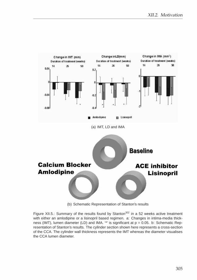
XII.2. Motivation
(a) IMT, LD and IMA
(b) Schematic Representation of Stanton’s results
Figure XII.5.: Summary of the results found by Stanton302 in a 52 weeks active treatmentwith either an amlodipine or a lisinopril based regimen. a: Changes in intima-media thick-ness (IMT), lumen diameter (LD) and IMA. ‘*’ is significant at p = 0.05. b: Schematic Rep-resentation of Stanton’s results. The cylinder section shown here represents a cross-sectionof the CCA. The cylinder wall thickness represents the IMT whereas the diameter visualisesthe CCA lumen diameter.
305

XII. Acute Effect of Anti-Hypertensive Drugs
XII.3. Materials and Methods
XII.3.1. Patient & study design
Both male and female patients with untreated hypertension (office systolicBP 150j-220 and / or diastolic BP 90-120mmHg) were recruited into thisdouble-blind, placebo controlled, randomised, 3 way crossover clinical trial.Individuals were excluded if they had evidence of accelerated or malignanthypertension; major organ dysfunction identified clinically or with blood sam-pling; a previous cardiovascular event; contraindications to the study drugs;diabetes mellitus; familial hypercholesterolaemia; glaucoma; cataracts; orplaque in their right common, internal or external carotid artery. All partic-ipants were recruited from a single clinical centre, the Peart-Rose Hyper-tension and Cardiovascular Disease Prevention Clinic at St Mary’s Hospital,London, U.K. All subjects gave written informed consent, the local researchcommittee approved the study protocol, and the research was carried out inaccordance with the Declaration of Helsinki (1989) of the World Medical As-sociation. Eligible patients were randomised to receive placebo, amlodipine(5mg oral dose (OD)) or lisinopril (10mg OD). The baseline characteristicsof the study group are summarised in Table XII.2.
A full physical examination including 24 hour ambulatory blood pressure,ECG, baseline blood tests and screening carotid ultrasound were performedto ensure eligibility prior to randomisation. The office blood pressure recordedat the start of the study served as the comparison blood pressure for sub-sequent visits. Each subject was taught to record his or her own bloodpressure using a validated semi-automated blood pressure cuff. After threedoses of their randomised treatment, patients were required to record their
jNote that this recruiting parameter is more severe than the ‘definition’ of systolic hyperten-sion on page 294
Male / Female 7 / 3Age (years) 42 (35-52)
SBP (mmHg) 151 ± 12DBP (mmHg) 96 ± 10
IMT (mm) 0.54 ± 0.09LD (mm) 6.56 ± 0.58
IMA (mm2) 12.1 ± 2.3
Table XII.2.: Baseline characteristics for the study group.
306

XII.3. Materials and Methods
Figure XII.6.: Acute study setup. The study lasted for 6 weeks, divided into three times twoweeks. Each of these two weeks consisted of a washout period of a week and a week ofdrug intake. The grey rectangles at the top represent a period of drug dispensing: each drughas a different colour, but the subjects and physicians were blinded. The arrows show whenUS and MRI scans were performed.
Subject Visit 3 Visit 5 Visit 71 placebo amlodipine lisinopril2 placebo amlodipine lisinopril3 placebo lisinopril amlodipine4 placebo amlodipine lisinopril*5 placebo lisinopril amlodipine6 placebo amlodipine lisinopril*7 placebo amlodipine* lisinopril*8 placebo lisinopril amlodipine9 placebo lisinopril amlodipine
10 placebo amlodipine lisinopril
Table XII.3.: Order in which the compounds were administered to the subjects. The time-lines can be found in Figure XII.6. ‘*’ means that the dose was up-titrated.
blood pressure prior to taking the fourth dose and inform the study physi-cian of these results. A decision was made to up-titrate the dose to am-lodipine (10mg OD) or lisinopril (20mg OD) if a target of 10 mmHg systolicblood pressure reduction compared to baseline was not achieved. MRI,Doppler ultrasound, IMT measurement and applanation tonometry of theright carotid artery and blood pressure data were collected on day sevenof each treatment. This was followed by a period of a week for washoutand then crossover to another treatment. Figure XII.6 represents the drugstudy schematically. Table XII.3 shows the order in which the different com-pounds were administered to the subjects. Note that all subjects started on
307

XII. Acute Effect of Anti-Hypertensive Drugs
a placebo treatment. This reduces variability and makes the results moresignificant, but it also indicates that the study was in fact only randomised to-wards amlodipine and lisinopril, i.e. the changes seen between the placeboand amlodipine or placebo and lisinopril treatment could be influenced bysequence effects.
XII.3.2. Blood Pressure Measurements
Blood pressure was measured from the right arm using a validated fullyautomated sphygmomanometer (Omron HEM-705-CP, West Sussex, UK),which works according to the principles explained in section II.3.1.1 on page47. Five pre-dose readings of BP and pulse were taken after 5 minutes restand with at least one-minute interval between readings. The two extremevalues (highest and lowest) were discarded, and BP was calculated as theaverage of the remaining three values.
XII.3.3. Ultrasound of the Right Distal CCA
All carotid scans were performed on the right carotid artery using a 7.5MHz ultrasound transducer (12-5 scan head probe) with an HDI 5000 ul-trasound scanner (ATL-Philips Medical Systems, WA, USA). Ten subjectswere examined in the supine position with the neck extended and rotated45 degrees towards the contra-lateral side. Common carotid artery B-modeimages were obtained from the anterior, antero-lateral and posterior planes.The bulb dilatation served as a landmark indicating the border between thedistal vessel and the bifurcation area. Images focussed on the far wall wererecorded as cine loops with concomitant ECG traces to allow retrospectivegating of images. At least 6 cardiac cycles were recorded and saved to a PCfor subsequent analysis. Stored images were viewed using HDI Lab, (Soft-ware version 1.86, ATL, WA, USA) and analysed ‘off-line’. Images obtainedduring diastole (peak of the R-wave), and systole (end of the T-wave) fromeach of the three planes were analysed using a validated semi-automatedIMT analysis package (AMS V6 Chalmers University, Gothenburg, Sweden).Average common carotid and bulb IMT and lumen diameter (LD) were mea-sured over a 5-15 mm segment for each projection of the right carotid artery.The mean value of all 3 projections was used as measurement for each sub-ject. This technique has shown to have a reproducibility of 10 ± 45 µm onIMT measurements.214
308

XII.3. Materials and Methods
Carotid blood flow velocity was measured using pulsed Doppler. Recordingswere made in the centre of the right common carotid artery at a distance of2 cm proximal to the bulb using a sample volume of 1.5 mm2, and ultra-sound beam positioned at 60° to the direction of blood flow. The pulsedDoppler data and simultaneous ECG trace were acquired continuously for10 cardiac cycles and saved to hard disk for subsequent analysis. Peakvelocity wave forms were analysed using HDI Lab, (Software version 1.86,ATL, WA, USA) and custom software written in MATLAB. At least 6 Dopplerwave forms were ensemble averaged to give a representative wave formfor measurement and further analyses. Volumetric blood flow in the carotidartery was calculated from the lumen diameter of the common carotid arteryin diastole and by analytical solution of Womersley flow conditions using thepeak velocity wave form, as explained in section II.3.3.1.
XII.3.4. Applanation Tonometry
Applanation tonometry was used to record arterial pressure wave formsfrom the right common carotid artery using a high fidelity strain-gauge tippedpencil probe (SPT 301, Millar instruments Inc, Houston, Texas, USA). Thesignal generated was amplified (TCB-500 pre-amplifier, Millar instrumentsInc, Houston, Texas, USA), and at least 20 cardiac cycles were digitised at200Hz and transferred to a PC for subsequent analysis. Minimum 6 con-tiguous pressure wave forms were ensemble averaged using custom soft-ware within the MATLAB programming environment. The ensemble aver-aged wave form was calibrated to diastolic and mean arterial pressure, andused to provide carotid systolic pressure measurements.
XII.3.5. MRI Protocol and coupling with CFD
The MRI protocol and the technique for coupling MRI with CFD was thesame as the one applied in the study comparing BB MRI to TOF MRI. Here,the TOF scans were used in accordance with the same study, presented insection VI.5.
309

XII. Acute Effect of Anti-Hypertensive Drugs
XII.3.5.1. Time Of Flight MRI protocol
All MRI scans involved were carried out on a Siemens Magnetom Sonata1.5T scanner. The images were acquired using a purpose-built 2-elementphased-array coil. For the acquisition of the 3D carotid geometry, axialcross-sections of the carotid arteries were imaged using a 2D time-of-flightprotocol. The TOF scan parameters used 28 contiguous slices of 2mm thick-ness, a Field of View (FOV) of 130 x 100mm and in-plane resolution of 0.52x 0.52 mm pixels. Other scan parameters include TR 28 ms and TE 7 ms.
XII.3.5.2. 3D Cine PC MRI
The velocity and flow measurements were performed using a 3D cine PCMRI sequence. MRI flow measurements were carried out in the CCA at aslice position in line with geometry scans as close to the first slice as signalto noise ratio (SNR) would allow (‘inlet’ scan). A second scan was taken inthe CCA for a slice relatively close to the bifurcation, but far enough to en-sure undisturbed flow (‘midpoint’ scan). ECA and ICA flow were measuredas far distal as possible but before any ECA branching occurred (‘outlet’scan). The in-plane resolution was 1.1 x 0.75 mm with a slice thicknessof 6 mm. The first scan, close to the first slice, will be referred to as the‘inlet’ scan, the other two scans as ‘midpoint’ and ‘outlet’ scan. For the out-let and midpoint scan, temporal resolution was 29 ms. The inlet flow wasmeasured in 3 orthogonal directions (1 reference and 3 velocity encodedimages) thereby reducing the temporal resolution by a factor of 1.5 to 2, de-pending on heart rate. The velocity encoding (Venc) was 100 cm/s for axialvelocities and 20 cm/s for in-plane (or secondary) velocities.
XII.3.5.3. Image Segmentation and 3D reconstruction
Each TOF MR image was segmented using the region growing method (seesection VI.2.1, page 108) and snake method (see section VI.2.2, page 110).This results in a contour for each TOF MR image. The contours were super-imposed on the image and shown to the operator. At this point, the operatorwas allowed to edit the contours if deemed necessary.
After segmentation, MRI resulted in serial contours in equidistance planes.With the knowledge of the position of the contours in 3D space, the con-
310

XII.3. Materials and Methods
tours can be positioned adequately to produce a 3D vessel surface geome-try. Smoothing was performed in two steps as discussed in section VI.3.1.First, the areas of consecutive cross-sections were smoothed using a cubicsmoothing spline (p = 0.1). In a second step, the centrelines, i.e. the linethat goes through the centroids of vessel cross-sections in the transverseplane, were smoothed using cubic splines (p = 0.5). This was achieved byshifting the centroids and associated contours until a smooth centreline wasobtained.
XII.3.5.4. Mesh generation and computational details
The mesh was generated using the mesh generator explained in sectionIII.2.2 (page 76). The mesh generator constructs a multi-block structuredmeshes of hexahedral cells (Figures III.1 and III.2). Figure VI.22 (page 143)shows a mesh reconstructed from TOF MRA for subject 5, scan 2.
The Navier-Stokes equations for laminar flow were discretised using the‘QUICK’ (Quadratic Upwind Interpolation Convective Kinematics) differenc-ing scheme explained in section III.4.1.1 and then solved using the SIM-PLEC algorithm implemented in CFX4™,.3 Based on previous experience,two cardiac cycles of 80 equally spaced time-steps were simulated. Thelength of the time-step varied according to the measured heart rate. Blooddensity was considered 1176 kg/m3. The Quemada-model was used formodelling the non-Newtonian behaviour of blood.42 The wall was modelledas a rigid, no-slip surface. The velocities measured with cine PC MRI in theinlet plane were filtered and scaled for mass flow rate as explained in sec-tion VIII.1.1. The mass flow rate used in the scaling was obtained from themidpoint scan. Flow rate measurements were performed using CMRTools(Imperial College London, London, UK). The outflow cine series was usedto compute a time-dependent ICA and ECA flow rate. From the calculatedoutflow rates, a time-dependent mass outflow ratio was deduced and set asboundary condition on the model outlets.
XII.3.6. 3DUS Protocol and coupling with CFD
In 2 of the 10 cases, the subjects could not be imaged using MRI due toclaustrophobia. Here, the scans were performed using a 3DUS protocol.The 3D, time-varying flow profiles were obtained by performing the stepsexplained in section XI.2.2.
311

XII. Acute Effect of Anti-Hypertensive Drugs
XII.3.6.1. Ultrasound imaging and Slice Positioning Information
The 3DUS imaging protocol is explained in section VII.1.4. The protocolresults in 2D B-mode cross-sections of the carotid bifurcation on one handand the position of these slices on the other hand. In addition, velocity waveforms were obtained using pulsed-wave Doppler from the centre-stream ofthe CCA, approximately at the location corresponding to that of the mostproximal slice of the 3DUS scan. Similarly, centreline velocities were mea-sured in the ICA and ECA. These velocities were used to calculate the massflow rate using the technique described in section II.3.3.1.
XII.3.6.2. Image Segmentation and Carotid Reconstruction
Acquired images were segmented using purpose-built software in a MAT-LAB environment. The software was used to manually select points on thevessel wall to which a smooth cubic spline or ellipse was fitted. The finallumen contours, combined with the positioning information from the EPOMdevice, allowed reconstruction of a smooth 3D geometry of the carotid bifur-cation.
XII.3.6.3. Mesh Generation and computational details
The mesh was generated using the in-house purpose-built mesh generatordescribed in section III.2.2. The vessel wall was assumed to be rigid withno mass transfer and zero-velocity (no-slip condition). At the inlet, Wom-ersley profiles derived from the measured flow wave form in the commoncarotid were imposed. The flow wave form was acquired from the centrelinevelocity, assuming developed Womersley flow in the CCA.368 At the outlet,a time-dependent outflow ratio was imposed. To calculate the outflow ra-tio, the flow rates were calculated in CCA, ICA and ECA using centrelinemeasurements and the Womersley assumption. Then, outflow ratio can becalculated from the ICA and ECA, CCA and ICA and even CCA and ECA.The ratio was calculated using the flow rates yielding a division ratio closestto the expectable 55:45 (ICA:ECA). This allows to filter out major acquisitionerrors. See section VIII.1.2 (page 216) for a discussion on the use of theseboundary conditions.
312

XII.3. Materials and Methods
With the knowledge of vessel geometry and boundary conditions, the partialdifferential equations describing the movement of the fluid (mass conser-vation law and Navier-Stokes equation) were solved numerically using thesame settings as for the simulations performed using MRI as a basis, ex-plained in section XII.3.5.4.
XII.3.7. Measured Parameters
For each visit, the following set of parameters were measured or calculated.They can be subdivided into pressure-related parameters, direct geometryparameters, 3D reconstruction parameters, flow parameters and haemody-namic parameters. Eight patients were scanned using MRI, 2 claustrophobicpatients were examined with 3DUS.
XII.3.7.1. Pressure Parameters
The pressure parameters included clinically measured blood pressure atdiastole (DBP) and systole (SBP), mean arterial pressure (MAP = SBP/3+2×DBP/3) and pulse pressure (PP= SBP-DBP).
XII.3.7.2. Direct geometry parameters
The direct geometry parameters are called ‘direct’ because they do not re-quire 3D reconstruction of the carotid bifurcation in order to be quantified.The parameters include the IMT and LD, both in systole and in diastole.The cyclic difference in IMT and LD (largest value-smallest value) were alsocalculated. The IMT was also measured in the carotid bulb. Furthermore,IMT/LD ratio and IMA were calculated. For more information concerning therationale of these parameters, see section II.2.2.1.
When geometry and pressure parameters are combined, the compliance Ccan be calculated as in equation II.8 (page 51). Other derived parametersinclude the distensibility coefficient (DC, equation II.10, page 52), Young’smodulus (E, equation II.9, page 51), mean and peak wall tension (Tm andTp, equation II.12, page 52) and mean and peak tensile stress (σm and σp,equation II.14, page 52).
313

XII. Acute Effect of Anti-Hypertensive Drugs
XII.3.7.3. 3D reconstruction parameters
The 3D reconstruction parameters are geometry parameters which necessi-tate the 3D reconstruction of the carotid bifurcation. They include the meancross-sectional area (Aart with art=CCA, ICA or ECA), area ratio (AR),mean individual shape factor (SFi art), overall (NP ) and arterial (NPart)non-planarity, arterial linearity (Lart), arterial tortuosity (Tart) and bifurcationangle (αBIF ). For elabourate definitions of these parameters, see sectionII.3.2.2, page 53.
XII.3.7.4. Flow parameters
Flow parameters are measures that require a velocity or mass flow rate mea-surement in order to be quantified. The heart rate is conventionally part ofthe flow parameters. The basis of all other flow parameters is a flow ratemeasurement, either using 3D cine PC MRI or Pulsed Doppler ultrasound.See section II.3.3.1 for the derivation of a flow rate using these measure-ment techniques. Other flow parameters include the Reynolds number (Re,equation II.28, page 64) and the Womersley number (α, equation II.29, page65).
XII.3.7.5. Haemodynamic parameters
The haemodynamic parameters are calculated from the 3D CFD simulation.They include the velocity parameter VMAX (see page 67) and the wall pa-rameters WSS, OSI, WSSGs, WSSGt and WSSAG. These parameters areexplained in section II.3.3.3 which starts on page 67. The wall parametersare averaged over the entire bifurcation, and over 10 other zones: (i) theCCA half adjacent to the ICA (marked ‘iCCA’); (ii) the CCA half closer to theECA; (iii) the inner ICA, i.e. the half of the ICA which contains the apicalregion; (iv) the outer ICA; (v) the inner and (vi) outer ECA; (vii) the entireCCA; (viii) ICA; (ix) ECA and (x) the outer part of the bulb, i.e. part of theouter ICA and iCCA.
Figure XII.7 (a) shows an alternative way of displaying WSS information.The WSS values can be found on the horizontal axis. The time, representedas a percentage of the cardiac cycle, is found in the vertical axis. The vesselwall area, represented as a percentage of the total carotid bifurcation wall
314

XII.3. Materials and Methods
0.12 0.46 1.73 6.47
20
40
60
80
WSS [N/m²]
TIM
E [%
]
5 10 AREA [%] 40 50%
(a) Entire Geometry
0.12 0.46 1.73 6.47
20
40
60
80
WSS [N/m²]
TIM
E [%
]
5 10 AREA [%] 40 50%
(b) Bulb
Figure XII.7.: ‘Time and Area’ representation of the WSS. The WSS values can be foundon the horizontal axis. The time, represented as a percentage of the cardiac cycle, is foundin the vertical axis. The vessel wall area, represented as a percentage of the total carotidbifurcation wall area, is colour coded in the legend and mapped on the graph. The blackcross is the gravity point.
area, is colour coded in the legend and mapped on the graph. The crosson the image represents the center of gravity when the colours are used asweight factors. The cross in Figure XII.7 (a) lies in a blue area at approximate1.2 N/m2 and 10%. This means that approximately 8% of the carotid wallarea (blue) undergoes a WSS in the range of 1.2 N/m2 for 10% of the time.Because Figure XII.7 gives information on the value of WSS, its durationand importance with respect to the involved area, these images are called‘Time and area’ representations of the WSS.
The presented example was obtained by considering the entire vessel wall.This can be performed for the bulb area as well. See Figure XII.7 (b) for anexample from the same set of data as Figure XII.7 (a).
The red vertical line in Figures XII.7 is drawn at a threshold of 0.4 N/m2. Thisis the threshold for ‘atherogenic’ WSS values as defined by Malek.208 Thefurther to the right the gravity points lies, the better. The distance betweenthe gravity point and the red line has been quantified for all subjects in allvisits.
The higher the gravity point lies in a Time and Area image, the less fluc-tuations occur in the WSS. This distance, subsequently referred to as thesteadiness , has been quantified for all subjects in all visits.
315

XII. Acute Effect of Anti-Hypertensive Drugs
XII.3.8. Statistical analysis
The performed statistics are summarised in Figure XII.8 which gives the re-sults for the heart rate measurements. Figure XII.8 (a) shows all the data inone plot. The black dots represent the general means, e.g. with amlodipine,the mean heart rate was approximately 73 bpm. The black line through thegeneral mean shows the standard deviation. The grey dots represent theindividually measured values. Figure XII.8 (b) performs a 2-way anova (10subjects, 3 compounds) followed by the ‘Least Square Difference’ (‘LSD’)post hoc test. The blue dots represent the means of the considered param-eter using a particular compound. The line through the point denotes halfof the confidence interval using a significance level of 0.05. The advantageof showing half instead of the entire confidence interval lies in the fact thata ‘significant’ difference between means is now represented as a lack ofoverlap between the presented lines. In the current example, there was nodifference between the heart rate measured using the placebo or any of thedrugs, but there was a significant difference between the heart rate in thelisinopril compared to the amlodipine regimen.
XII.4. Results
Each patient required up-titration of the placebo. One patient required adoubling of amlodipine dose (i.e. 10mg) to reach target blood pressure, andthree patients required a doubling of lisinopril dose (20mg) to reach target
Am Pl Li50
60
70
80
90Heart Rate
[bp
m]
(a) ALL DATA (b) 2-WAY ANOVA
Figure XII.8.: Statistics used in Acute CFD study. Illustration using the heart rate as com-pared parameter. Am: amlodipine; Pl: placebo; Li: lisinopril.
316

XII.5. Discussion
Parameter amlodipine placebo lisinopril ANOVACalcium blocker ACE inhibitor
Diastolic Pressure [mmHg] 85.6 ± 5.1 ∗∗ 95.6 ± 9.9 83.2 ± 9.0 ++ 0.002 ¦¦Systolic Pressure [mmHg] 138.1 ± 10.2 ∗∗ † 150.6 ± 12.4 130.2 ± 14.5 ++ † 0.000 ¦¦Pulse Pressure [mmHg] 52.5 ± 8.9 † 55.0 ± 5.7 47.1 ± 8.1 ++ † 0.031 ¦¦Mean Arterial Pressure [mmHg] 103.1 ± 5.9 ∗∗ 113.9 ± 10.4 98.8 ± 10.4 ++ 0.000 ¦¦Heart Rate [bpm] 72.8 ± 5.6 †† 69.2 ± 8.6 65.6 ± 9.5 †† 0.027 ¦¦
Table XII.4.: Statistical Analysis of ‘Pressure’ parameters considered in the Acute CFD Study.Values are mean± standard deviation. ‘∗’ denotes significant difference between amlodipineand placebo; ‘+’ denotes significant difference between lisinopril and placebo; ‘†’ denotessignificant difference between lisinopril and amlodipine; a single sign denotes p<0.1, if thesign is doubled, significance is p<0.05. ‘¦’ denotes significant difference between compoundmeans (p<0.1 or p<0.05 if double sign).
blood pressure. The patients requiring up-titration are marked with a star inTable XII.3.
Tables XII.4 to XII.13 show the mean ± standard deviation for all variablesusing the amlodipine, placebo or lisinopril. The statistics are performed asexplained in section XII.3.8. The column ANOVA returns the p-value for thehypotheses that all compound-means are equal. For clarity, this means thatp close to 0 casts doubt on the hypothesis and suggests that at least oneof the means, using placebo, lisinopril or amlodipine, is different from theothers. If p is sufficiently low (e.g. <0.2), a post hoc test can be performedin order to learn which of the means is significantly different from the others.Here, the ‘lsd’ post hoc test was used to identify the compound yielding amean value different from the other compounds. The signs ‘*’, ‘+’, ‘†’, ‘¦’have been used to emphasise on significance as explained in Table XII.4.
Finally, Figure XII.9 shows the time-averaged wall shear stress (WSS) dis-tribution for three subjects after each week of treatment.
XII.5. Discussion
The reader is reminded that the aims of this study were double: in the firstplace, the aim was to compare the acute effects of amlodipine and lisinoprilon local carotid artery haemodynamics, and in a second step, the goal wasto relate the findings of the acute study to the observations made in the52 week study with amlodipine and lisinopril performed by Stanton.302 Thediscussion contains two section, each section deals with one of the aims ofthis study.
317

XII. Acute Effect of Anti-Hypertensive Drugs
Parameter amlodipine placebo lisinopril ANOVACalcium blocker ACE inhibitor
Diastolic IMT [mm] 0.570 ± 0.087 ∗∗ 0.541 ± 0.085 0.563 ± 0.101 + 0.076 ¦Systolic IMT [mm] 0.520 ± 0.080 0.507 ± 0.077 0.521 ± 0.092 0.419IMT Difference [mm] 0.049 ± 0.034 0.033 ± 0.025 0.042 ± 0.024 0.423Bulb IMT [mm] 0.678 ± 0.082 0.645 ± 0.094 0.668 ± 0.102 0.315Diastolic LD [mm] 6.57 ± 0.57 6.56 ± 0.58 6.47 ± 0.72 0.694Systolic LD [mm] 6.96 ± 0.62 7.02 ± 0.65 6.84 ± 0.88 0.511Diameter Difference [mm] 0.39 ± 0.12 ∗∗ 0.45 ± 0.11 0.37 ± 0.19 + 0.180Diastolic IMT/Diastolic LD [-] 0.087 ± 0.012 ∗ 0.083 ± 0.014 0.087 ± 0.014 + 0.097 ¦Systolic IMT/Systolic LD [-] 0.075 ± 0.011 0.073 ± 0.012 0.077 ± 0.014 0.169Diastolic IMA [mm2] 12.8 ± 2.7 ∗ 12.1 ± 2.3 12.5 ± 3.2 0.284Systolic IMA [mm2] 12.3 ± 2.5 12.0 ± 2.3 12.1 ± 3.2 0.866Compliance [ mm2
kPa] 0.594 ± 0.172 0.670 ± 0.200 0.682 ± 0.495 0.771
Distensibility Coefficient [1/MPa] 17.02 ± 4.59 18.92 ± 4.18 18.62 ± 10.88 0.809Young’s Modulus [kPa] 749 ± 319 682 ± 176 876 ± 525 0.485Peak Wall Tension [Pa.m] 64.0 ± 7.6 ∗∗ †† 70.6 ± 9.3 59.5 ± 11.0 ++ †† 0.000 ¦¦Mean Wall Tension [Pa.m] 45.1 ± 4.1 ∗∗ 49.9 ± 6.8 42.7± 7.3 ++ 0.001 ¦¦Peak Tensile Stress [kPa] 126.1 ± 27.1 ∗∗ † 141.9 ± 28.3 117.9 ± 34.2 ++ † 0.001 ¦¦Mean Tensile Stress [kPa] 81.0 ± 16.1 ∗∗ 94.3 ± 19.5 78.1 ± 20.2 ++ 0.001 ¦¦
Table XII.5.: Statistical Analysis of ‘Direct Geometry’ parameters considered in the AcuteCFD Study. Values are mean ± standard deviation. See Table XII.4 for a legend.
Parameter amlodipine placebo lisinopril ANOVACalcium blocker ACE inhibitor
CCA Mean Area [mm2] 50.7 ± 13.1 49.3 ± 9.7 51.0 ± 15.0 0.716ICA Mean Area [mm2] 29.2 ± 11.1 28.6 ± 10.4 29.1 ± 12.3 0.787ECA Mean Area [mm2] 18.8 ± 5.4 17.9 ± 3.9 18.5 ± 5.4 0.530Area Ratio [-] 0.808 ± 0.099 0.884 ± 0.127 0.809 ± 0.119 0.062 ¦CCA Shape [-] 0.967 ± 0.011 †† 0.971 ± 0.016 0.960 ± 0.015 ++ †† 0.015 ¦¦ICA Shape [-] 0.973 ± 0.023 ∗∗ 0.981 ± 0.018 0.972 ± 0.020 + 0.046 ¦¦ECA Shape [-] 0.964 ± 0.032 0.965 ± 0.040 0.961 ± 0.045 0.761Non-Planarity [%] 3.9 ± 1.6 4.2 ± 1.9 4.0 ± 1.9 0.227Non-Planarity CCA [%] 0.4 ± 0.3 0.5 ± 0.3 0.4 ± 0.3 0.367Non-Planarity ICA [%] 0.9 ± 0.9 1.0 ± 0.9 0.9 ± 1.0 0.143Non-Planarity ECA [%] 0.8 ± 0.8 0.9 ± 0.7 1.0 ± 1.1 0.705Linearity CCA [%] 93.2 ± 2.5 92.9 ± 2.2 92.9 ± 2.5 0.225Linearity ICA [%] 92.4 ± 1.3 91.8 ± 1.7 92.0 ± 1.7 0.166Linearity ECA [%] 91.8 ± 2.1 91.0 ± 2.7 91.0 ± 3.4 0.188alpha BIF [°] 138.1 ± 23.2 145.3 ± 17.1 146.8 ± 7.4 0.317Tortuosity CCA [%] 1.2 ± 0.8 1.2 ± 1.0 1.4 ± 0.9 0.616Tortuosity ICA [%] 4.3 ± 4.8 4.6 ± 5.0 4.1 ± 5.6 0.641Tortuosity ECA [%] 4.0 ± 5.3 4.1 ± 4.0 3.8 ± 5.9 0.875
Table XII.6.: Statistical Analysis of ‘3D Reconstruction’ parameters considered in the AcuteCFD Study. Values are mean ± standard deviation. See Table XII.4 for a legend.
318

XII.5. Discussion
Parameter amlodipine placebo lisinopril ANOVACalcium blocker ACE inhibitor
Heart Rate [bpm] 72.8 ± 5.6 †† 69.2 ± 8.6 65.6 ± 9.5 †† 0.027 ¦¦CCA Flow Rate [ml/s] 7.8 ± 1.7 †† 7.8 ± 2.8 6.3 ± 1.3 †† 0.135ICA Flow Rate [ml/s] 4.6 ± 1.1 †† 4.7 ± 1.7 3.7 ± 0.6 †† 0.218ECA Flow Rate [ml/s] 3.2 ± 0.7 † 3.1 ± 1.3 2.6 ± 0.9 † 0.160Reynolds CCA [-] 362 ± 37 †† 366 ± 144 297 ± 32 †† 0.196Reynolds ICA [-] 299 ± 33 †† 313 ± 113 250 ± 26 †† 0.199Reynolds ECA [-] 256 ± 32 †† 246 ± 91 206 ± 47 †† 0.126Womersley CCA [-] 5.91 ± 0.64 5.69 ± 0.41 5.69 ± 0.89 0.393Womersley ICA [-] 4.46 ± 0.86 4.32 ± 0.87 4.30 ± 1.10 0.453Womersley ECA [-] 3.60 ± 0.52 3.44 ± 0.47 3.44 ± 0.65 0.349
Table XII.7.: Statistical Analysis of ‘Flow’ parameters considered in the Acute CFD Study.Values are mean ± standard deviation. See Table XII.4 for a legend.
Parameter amlodipine placebo lisinopril ANOVACalcium blocker ACE inhibitor
CCA Mean Vmax [m/s] 0.44 ± 0.06 †† 0.39 ± 0.11 0.36 ± 0.03 †† 0.163ICA Mean Vmax [m/s] 0.40 ± 0.06 † 0.39 ± 0.12 0.33 ± 0.04 † 0.177ECA Mean Vmax [m/s] 0.38 ± 0.04 0.38 ± 0.14 0.33 ± 0.11 0.341
Table XII.8.: Statistical Analysis of ‘Vmax’ parameters considered in the Acute CFD Study.Values are mean ± standard deviation. See Table XII.4 for a legend.
Parameter amlodipine placebo lisinopril ANOVACalcium blocker ACE inhibitor
WSS ALL [N/m2] 1.378 ± 0.492 †† 1.354 ± 0.665 1.138 ± 0.375 †† 0.192WSS CCA [N/m2] 0.754 ± 0.245 0.735± 0.406 0.628 ± 0.164 0.542WSS iCCA [N/m2] 0.807 ± 0.286 0.787± 0.424 0.688 ± 0.259 0.646WSS eCCA [N/m2] 0.688 ± 0.241 0.672± 0.387 0.552 ± 0.110 0.418WSS ICA [N/m2] 1.705 ± 0.681 † 1.702 ± 0.936 1.390 ± 0.549 † 0.263WSS outer ICA [N/m2] 1.376 ± 0.586 1.390± 0.778 1.118 ± 0.485 0.285WSS inner ICA [N/m2] 2.283 ± 0.856 †† 2.248 ± 1.221 1.836 ± 0.701 †† 0.200WSS ECA [N/m2] 2.275 ± 1.051 † 2.276 ± 1.318 1.891 ± 0.999 † 0.269WSS outer ECA [N/m2] 1.482 ± 0.648 1.455± 0.830 1.299 ± 0.672 0.417WSS inner ECA [N/m2] 2.275 ± 1.051 † 2.276 ± 1.318 1.891 ± 0.999 † 0.269WSS bulb [N/m2] 1.103 ± 0.400 † 1.138 ± 0.595 0.904 ± 0.316 † 0.239Area with Low WSS [%] 20.561 ± 26.859 21.003± 27.172 23.894 ± 22.802 0.481Area with High WSS [%] 15.277 ± 9.025 †† 14.394 ± 12.497 9.757 ± 6.516 †† 0.161Dist from 0.4 [N/m2] 0.609 ± 0.054 †† 0.601 ± 0.032 0.585 ± 0.055 †† 0.278Dist from 0.4 BULB [N/m2] 0.553 ± 0.053 †† 0.543 ± 0.026 0.522 ± 0.054 †† 0.139
Table XII.9.: Statistical Analysis of ‘WSS’ parameters considered in the Acute CFD Study.Values are mean ± standard deviation. See Table XII.4 for a legend.
319

XII. Acute Effect of Anti-Hypertensive Drugs
Parameter amlodipine placebo lisinopril ANOVACalcium blocker ACE inhibitor
OSI ALL [-] 0.084 ± 0.083 ∗ 0.078 ± 0.083 0.084 ± 0.082 0.275OSI CCA [-] 0.120 ± 0.086 0.122 ± 0.097 0.120 ± 0.086 0.974OSI iCCA [-] 0.107 ± 0.078 0.106 ± 0.089 0.112 ± 0.087 0.703OSI eCCA [-] 0.140 ± 0.102 0.143 ± 0.111 0.131 ± 0.095 0.733OSI ICA [-] 0.056 ± 0.076 ∗∗ 0.043 ± 0.068 0.052 ± 0.073 ++ 0.020 ¦¦OSI outer ICA [-] 0.070 ± 0.095 ∗∗ 0.056 ± 0.085 0.069 ± 0.089 ++ 0.025 ¦¦OSI inner ICA [-] 0.024 ± 0.025 ∗ 0.015 ± 0.021 0.021 ± 0.039 0.361OSI ECA [-] 0.044 ± 0.068 ∗ 0.023 ± 0.039 0.040 ± 0.065 0.234OSI outer ECA [-] 0.082 ± 0.098 0.057 ± 0.069 0.082 ± 0.091 + 0.096 ¦OSI inner ECA [-] 0.044 ± 0.068 ∗ 0.023 ± 0.039 0.040 ± 0.065 0.234OSI bulb [-] 0.098 ± 0.084 0.093 ± 0.091 0.103 ± 0.085 0.117Area with High OSI [%] 16.646 ± 20.055 ∗∗ 13.961 ± 19.782 18.091 ± 19.548 ++ 0.003 ¦¦Steadiness [%] 10.749 ± 2.526 11.066 ± 2.711 10.380± 2.282 0.298Steadiness BULB [%] 10.494 ± 2.621 10.845 ± 2.763 10.476± 2.480 0.535
Table XII.10.: Statistical Analysis of ‘OSI’ parameters considered in the Acute CFD Study.Values are mean ± standard deviation. See Table XII.4 for a legend.
Parameter amlodipine placebo lisinopril ANOVACalcium blocker ACE inhibitor
WSSGs ALL [N/m3] 420 ± 104 †† 397 ± 157 368 ± 97 †† 0.375WSSGs CCA [N/m3] 231 ± 56 222 ± 89 210 ± 51 0.761WSSGs iCCA [N/m3] 228 ± 56 220 ± 93 209 ± 63 0.830WSSGs eCCA [N/m3] 235 ± 64 226 ± 84 213 ± 45 0.679WSSGs ICA [N/m3] 461 ± 196 429 ± 209 387 ± 161 0.522WSSGs outer ICA [N/m3] 347 ± 161 328 ± 166 298 ± 143 0.666WSSGs inner ICA [N/m3] 659 ± 248 † 606 ± 287 534 ± 200 † 0.327WSSGs ECA [N/m3] 819 ± 284 784 ± 298 728 ± 197 0.530WSSGs outer ECA [N/m3] 476 ± 154 462 ± 183 453 ± 180 0.885WSSGs inner ECA [N/m3] 819 ± 284 784 ± 298 728 ± 197 0.530WSSGs bulb [N/m3] 293 ± 100 284 ± 124 258 ± 94 0.646
Table XII.11.: Statistical Analysis of ‘WSSGs’ parameters considered in the Acute CFDStudy. Values are mean ± standard deviation. See Table XII.4 for a legend.
Parameter amlodipine placebo lisinopril ANOVACalcium blocker ACE inhibitor
WSSGt ALL [N/(m2 × s)] 10.65 ± 3.82 9.94 ± 3.66 10.20 ± 4.00 0.788WSSGt CCA [N/(m2 × s)] 7.61 ± 3.09 7.09 ± 2.80 7.13 ± 2.89 0.709WSSGt iCCA [N/(m2 × s)] 7.58 ± 3.16 7.12 ± 2.81 7.09 ± 2.94 0.771WSSGt eCCA [N/(m2 × s)] 7.66 ± 3.09 7.07 ± 2.85 7.20 ± 2.91 0.614WSSGt ICA [N/(m2 × s)] 11.35 ± 7.25 10.12 ± 5.16 10.20 ± 6.39 0.814WSSGt outer ICA [N/(m2 × s)] 9.81 ± 6.10 8.95 ± 4.58 8.77 ± 5.53 0.841WSSGt inner ICA [N/(m2 × s)] 13.95 ± 9.03 12.19 ± 6.29 12.49 ± 7.76 0.773WSSGt ECA [N/(m2 × s)] 16.22 ± 8.63 16.23 ± 9.84 16.86 ± 8.53 0.957WSSGt outer ECA [N/(m2 × s)] 12.37 ± 6.04 12.13 ± 7.17 13.17 ± 6.59 0.857WSSGt inner ECA [N/(m2 × s)] 16.22 ± 8.63 16.23 ± 9.84 16.86 ± 8.53 0.957WSSGt bulb [N/(m2 × s)] 8.46 ± 4.05 8.02 ± 3.35 7.68 ± 3.48 0.832
Table XII.12.: Statistical Analysis of ‘WSSGt’ parameters considered in the Acute CFD Study.Values are mean ± standard deviation. See Table XII.4 for a legend.
320

XII.5. Discussion
Parameter amlodipine placebo lisinopril ANOVACalcium blocker ACE inhibitor
WSSAG ALL [rad/m] 169.9 ± 43.5 ∗∗ † 151.6 ± 36.1 152.8 ± 31.0 † 0.059 ¦WSSAG CCA [rad/m] 197.0 ± 71.1 184.1 ± 70.5 175.5 ± 42.0 0.289WSSAG iCCA [rad/m] 188.1 ± 76.3 172.3 ± 66.0 168.4 ± 54.9 0.260WSSAG eCCA [rad/m] 210.1 ± 68.8 201.5 ± 85.9 183.5 ± 31.4 0.450WSSAG ICA [rad/m] 138.9 ± 55.5 118.4 ± 49.6 123.4 ± 50.3 0.204WSSAG outer ICA [rad/m] 134.9 ± 51.2 118.5 ± 56.3 122.6 ± 53.3 0.501WSSAG inner ICA [rad/m] 147.5 ± 79.6 117.9 ± 56.1 125.9 ± 54.3 0.268WSSAG ECA [rad/m] 182.8 ± 79.3 160.2 ± 66.8 168.3 ± 76.9 0.573WSSAG outer ECA [rad/m] 172.8 ± 60.7 142.2 ± 43.6 161.1 ± 60.4 0.208WSSAG inner ECA [rad/m] 182.8 ± 79.3 160.2 ± 66.8 168.3 ± 76.9 0.573WSSAG bulb [rad/m] 186.2 ± 47.9 ∗ 160.0 ± 45.8 165.0 ± 31.1 0.092 ¦
Table XII.13.: Statistical Analysis of ‘WSSAG’ parameters considered in the Acute CFDStudy. Values are mean ± standard deviation. See Table XII.4 for a legend.
XII.5.1. Acute effects
XII.5.1.1. Pressure Changes
There have been several studies comparing the effects of calcium blockersand ACE inhibitors on blood pressure. The cascade of events causing pres-sure drop following the intake of a calcium blocker is described in sectionXII.1.2.1. Figures XII.10 (a-d) show the systolic and diastolic pressure dropdue to the administration of ACE inhibitors or calcium blockers in studies per-formed by Naidu,231 Lorimer,201 Lafleche,166 Sihm284 and Stanton.302 Thestudies are sorted according to their follow-up period: Naidu’s study lastedfor 4 weeks, whereas the follow-up was 1 year in Stanton’s study. FiguresXII.10 (a,c) seem to suggest that the pressure drop is greater in studies withlonger follow-ups, and that the diastolic pressure drop is a fraction smallerthan the systolic. In this study a target of 10 mmHg systolic blood pressurereduction was set. When not achieved, the oral dose was doubled. The av-erage systolic pressure drop for the calcium blocker, amlodipine, was 12.5mmHg, which meets the target.
Figures XII.10 (b,d) show the systolic and diastolic pressure drop after ad-ministration of calcium blockers recorded in literature. The studies illus-trated are those of Naidu,231 Lorimer,201 Mitchell,220 Lafleche,166 Girerd,116
Boutouyrie36 and Stanton,302 again sorted according to the follow-up time.Similar trends as Figures XII.10 (a,c) are found. Lorimer201 and Stanton302
did a comparative study between amlodipine and lisinopril. Lorimer foundthat amlodipine lowered the pressure more effectively than lisinopril, whereasStanton did not report a significant difference between the two treatments.
321

XII. Acute Effect of Anti-Hypertensive Drugs
Figure XII.9.: The time-averaged wall shear stress distribution for three subjects (rows) afteramlodipine (left), placebo (middle) and lisinopril (right) intake.
In our study, the systolic pressure drop with lisinopril was 20.4 mmHg, whichhas the tendency to be larger (p = 0.0683, LSD) than the pressure drop withamlodipine. Note that the lisinopril dose had to be doubled on three occa-sions, whereas the amlodipine dose was only doubled once (Table XII.3).
XII.5.1.2. Direct geometry parameters
The direct geometry parameters include IMT, LD and related parametersIMA and IMT/LD ratio. Other parameters, such as compliance, distensibility,
322

XII.5. Discussion
0 100 200
Stanton (52)
Sihm (40)
Lorimer (12st)
Lorimer (12si)
Naidu (4st)
Naidu (4f)
Systolic BP: Ca Block
[mmHg]
(a) Ca blocker
0 100 200Stanton (52)
Boutouyrie (24)
Girerd (24)
Lorimer (12st)
Lorimer (12si)
Naidu (4st)
Naidu (4f)
Systolic BP: ACE inh
[mmHg]
(b) ACE inhibitor
0 100 200
Stanton (52)
Sihm (40)
Lorimer (12st)
Lorimer (12si)
Naidu (4st)
Naidu (4f)
Diastolic BP: Ca Block
[mmHg]
(c) Ca blocker
0 100 200Stanton (52)
Boutouyrie (24)
Girerd (24)
Lorimer (12st)
Lorimer (12si)
Naidu (4st)
Naidu (4f)
Diastolic BP: ACE inh
[mmHg]
(d) ACE inhibitor
0 50 100
Sihm (40)
Lafleche (16)
Lafleche (12)
Lorimer (12)
Naidu (4)
PP: Ca Block
[mmHg]
(e) Ca blocker
0 50 100Boutouyrie (22)
Girerd (22)
Lafleche (16)
Lafleche (12)
Mitchell (12)
Naidu (4)
De Ponti (1)
PP: ACE inh
[mmHg]
(f) ACE inhibitor
Figure XII.10.: Pressure drops using ACE inhibitors and calcium blockers in literature. Thevertical axis shows the study considered. Between brackets: the number of weeks follow-up,and the position in which the subject was when blood pressure was taken. f: flat; si: sitting;st: standing. For each study, the top bar is the baseline (light grey), the middle bar is theresult after treatment (dark grey) and the final bar is the difference (black). Data comes fromstudies by Naidu,231 Lorimer,201 Lafleche,166 Sihm,284 Mitchell,220 Girerd,116 Boutouyrie,36
De Ponti74 and Stanton302 and are sorted according to the follow-up time. Baseline andend-study values were not stated by Stanton.302
323

XII. Acute Effect of Anti-Hypertensive Drugs
young’s modulus, wall tension and wall stress, are obtained when combinedwith the pressure data.
Lumen Diameter With the pressure drop, the vessel is expected to relax.This can be compared to a balloon which is slightly deflated. The effectof the pressure drop will thus be a decrease in carotid LD. This contradictsthe fact that both compounds work as vasodilators, but since vasodilatorsmainly act on the arterioles, which are the smaller, pressure regulating ar-teries (Table I.1 on page 8), the carotid arteries are expected to be onlymarginally affected by this dilatation. As summarised by Figure XII.11 (a),the carotid LD has been found to decrease in other pharmacological studiesby Boutouyrie,36 Girerd,116 Stanton,302 Ariff12 and Simon.286 In this acutestudy, we expect the diameter to drop according to the pressure drop. Ta-ble XII.5 shows that the drop in LD occurred at very low significance. Thisprobably means that the relaxation of the vascular smooth muscle cells dueto the vasodilatory effects of the compounds are more important than orig-inally expected. Note that the ‘diameter difference’, i.e. the difference inLD between systole and diastole, tends to decrease in both treatments (am-lodipine: p = 0.0378; lisinopril: p = 0.0856, LSD). This decrease in cyclicLD is caused by the drop in pulse pressure, which is more important in thelisinopril group.
0 5 10
Simon (4 x 52)
Stanton (52)
Ariff (52)
Stanton (52)
Girerd (22)
Boutouyrie (22)
CaBl
ACEi
Lumen Diameter
[mm]
(a) LD
0 200 400 600 800
Stanton (52)
Terpstra (26)
Ariff (52)
Stanton (52)
Girerd (22)
Boutouyrie (22)
CaBl
ACEi
Intima−Media Thickness
[µm]
(b) IMT
Figure XII.11.: Change in lumen diameter and intima-media thickness using ACE inhibitors(ACEi) and calcium blockers (CaBl) in literature. The vertical axis shows the study consid-ered. Between brackets: the number of weeks follow-up. For each study, the top bar is thebaseline (light grey), the middle bar is the result after treatment (dark grey) and the final baris the difference (black). Data comes from studies by Boutouyrie,36 Girerd,116 Stanton,302
Ariff,12 Terpstra326 and Simon286 and are sorted according to the follow-up time. Baselineand end-study values were not stated by Stanton.302
324

XII.5. Discussion
IMT, IMA and IMT/LD A change in LD will induce a change in IMT. The IMAcan be calculated as the product of the IMT and the circumference. Chang-ing the IMA or vessel wall mass involves vascular regression or hypertrophywhich is a slow process (in the order of several weeks). It is therefore fair toassume that the IMA remains constant after a sudden pressure drop. Theacute pressure drop will lead to drop in LD as mentioned earlier. When theLD decreases, the lumen circumference decreases as well, which meansthat the IMT has to increase if IMA is to be kept constant.
The decrease in blood pressure has an important impact on the vessel mor-phology in the long term as well. As explained by Laplace’s law (sectionII.2.1, page 33), a decrease in blood pressure will lower the wall tension.In the long term, the IMT, which is exposed at smaller tensile stresses, willdecrease since there is no need for a thick wall any more. All studies pre-sented in Figure XII.11 show a decrease in IMT in long-lasting studies. Fur-thermore, both compounds have anti-hypertrophic effects, resulting in a de-crease in myocard mass and vessel musculature.163,388
Considering that this study was performed over a week, the long-term effectswere not expected to occur and an increase in IMT was expected. TableXII.5 shows that the IMT indeed increases both in the CCA as in the bulb,both in diastole as in systole. The increase in IMT was the most significant(29 µm) with the amlodipine treatment (p = 0.0326, LSD). The IMA remainedconstant as assumed by the above reasoning. Since the LD decreased andthe IMT increased, the IMT/LD ratio tended to increase (amlodipine: p =0.0564; lisinopril: p = 0.0948, LSD).
Compliance The compliance is estimated here as the change in cross-sectional CCA area divided by the pulse pressure (see also section II.3.2.1on page 49). In literature, the effects of ACE inhibitors on arterial compli-ance have been widely investigated.36,116,166,167,220 A very short term study(1-3 hours follow-up) conducted by Lage167 sees a steep increase in com-pliance, suggesting that the arterial compliance is inversely related to theplasma angiotensin concentration. Unfortunately, Lage167 did not provide aphysiological explanation for this potential relation between ACE inhibitorsand arterial compliance.
The long-term studies36,116,166,220 (6 months to 1 year) suggest a slight gainin compliance. This is mainly due to the drop in IMT which renders the ves-sels less stiff. Note that the variety in definitions used to quantify compliancerenders it difficult to compare numerical values between studies.
325

XII. Acute Effect of Anti-Hypertensive Drugs
In this study, a decrease in PP and ‘diameter difference’ was expected. Whatwould happen with ratio of these two values was difficult to predict, but theresults by Lage167 suggest that important increases in compliance couldbe expected. Surprisingly, this study found that the compliance was un-changed using lisinopril (p = 0.9353, LSD). This discrepancy between ourresults and those of Lage167 could be due to the difference in the definitionof the compliance: C = π×LDd
2 ×LDs−LDdPP (Lage) as opposed to equation II.8
(page 51). The compliance was recalculated using Lage’s definition, but nodifferent conclusions were drawn in comparison with the original definition(p = 0.9306, LSD). Another possible reason for the discrepancy is the factthat a different ACE inhibitor, enalaprilat, was used by Lage.167 Moreover,Lage’s results were registered after a few hours, whereas this study per-formed measurements after a week. A final reason for the differences foundbetween Lage’s study167 and the present study is the fact that in Lage’sstudy,167 the compound was administered to patients with cardiac heart fail-ure, whereas in the present study, young hypertensive subjects were exam-ined.
Studies on the effect of calcium channel blockers on arterial compliance arevery rare. Lafleche166 finds an increase of arterial compliance after 12 and16 weeks of treatment with a variety of calcium antagonists. He also statesthat the acute changes in compliance are minimal, and that the changesin compliance are mainly pressure-mediated and depend on the location ofmeasurement. Van Merode339 administered the calcium blocker Verapamilto 19 patients for 4 weeks and measured an increase in arterial complianceof 18% and 27% for respectively the left and right carotid artery. However,based on Lafleche’s statements, the present study expected no change incompliance. This was confirmed by the results (p = 0.2175, LSD).
Distensibility and Young’s Modulus The change in distensibility coeffi-cient and Young’s modulus are difficult to predict since studies investigatingon the impact of anti-hypertensive compounds on the carotid wall’s elasticityare lacking. This study found that both parameters did not change signifi-cantly with either regimen.
Wall Tension and Tensile Stress Wall tension is quantified by the prod-uct of the blood pressure and the lumen radius (LD
2 ). Since both values areexpected to decrease for both compounds, the wall tension will decreaseas well. The tensile stress (σ) is the wall tension divided by the IMT. Sincethe IMT is expected to increase acutely, σ will decrease. Bearing in mind
326

XII.5. Discussion
0 100 200
Stanton (52)
Stanton (52)
Ariff (52)
Boutouyrie (22)
CaBl
ACEi
Tensile Stress
[kPa]
Figure XII.12.: Change in tensile stress using ACE inhibitors (ACEi) and calcium blockers(CaBl) in literature. The vertical axis shows the study considered. Between brackets: thenumber of weeks follow-up. For each study, the top bar is the baseline (light grey), themiddle bar is the result after treatment (dark grey) and the final bar is the difference (black).Data comes from studies by Boutouyrie,36 Ariff,12 and Stanton302 and are sorted accordingto the follow-up time. Baseline and end-study values were not stated by Stanton.302
that a vessel wall undergoing high tensile stress is prone to atherosclero-sis,34 it is easy to understand that the decrease in σ is a wanted effect of thedrug. Figure XII.12 shows how important the decrease in σ was in studiesby Boutouyrie,36 Ariff12 and Stanton.302 The current results show decreasesin diastolic and systolic wall tension and tensile stress with very high signif-icance for the lisinopril treatment (p<0.01, LSD as opposed to p<0.05 foramlodipine), probably due to the higher pressure drops acquired with lisino-pril.
XII.5.1.3. 3D Reconstruction parameters
The ‘3D reconstruction parameters’ involve all parameters that require the3D reconstruction of the carotid bifurcation for their quantification. This in-cludes the mean arterial cross-sections and shapes, and the centreline pa-rameters (planarity, linearity, tortuosity and bifurcation angles). To our knowl-edge, there have been no studies examining the change in 3D reconstruc-tion parameters induced by anti-hypertensive compounds.
Mean area and Area ratio Similar to the lumen diameter, one expects theaverage arterial cross-sectional area to decrease as a result of the pressuredrop. In reality, the cross-sectional area remained unchanged throughoutthe study. See Figure XII.13 for a representation of all measurements. Thisresult confirms what was found for the LD, where very small decreases with
327

XII. Acute Effect of Anti-Hypertensive Drugs
Am Pl Li20
40
60
80CCA Mean Area
[mm
2 ]
Am Pl Li0
20
40
60ICA Mean Area
[mm
2 ]
Am Pl Li0
10
20
30ECA Mean Area
[mm
2 ]
Am Pl Li0
0.5
1
1.5Area Ratio
[−]
Figure XII.13.: Change in mean cross-sectional area and area ratio with both compounds.See Figure XII.8 (a) for a description of the images.
small significance were registered. Surprisingly, the area ratio, defined asaICA+aECA
aCCAwhere a stands for the cross-sectional area in the slice most
proximal to the apex, drops approximately 0.075 with both compounds (am-lodipine: p = 0.1513; lisinopril: p = 0.1625, LSD). This suggest that the CCAdilates more (or contracts less) than the ICA or ECA, probably due to (1)the fact that smaller arteries are more susceptible to systemic vasoconstric-tion (ACE inhibitor) or (2) the fact that the LD of smaller arteries are moresensitive to variations in extracellular calcium (calcium blocker).
Individual Shape Factor When a balloon is deflated, it loses its regularcircular cross-sectional shape. The same applies for the cross-section ofan artery. Mathematically, this means that the individual shape factor SFi
will decrease. This is confirmed by our findings, which include significantchanges in CCA and ICA cross-sectional shape. This finding should, how-ever, be treated with caution since the difference in mean SFi is smaller thanits variability found in part B of this work.
328

XII.5. Discussion
Figure XII.14.: Centrelines in subject 2 (MR scanned). Black: placebo scan; Dark grey:amlodipine scan; Light grey: lisinopril scan.
Centrelines Figure XII.14 shows the carotid centrelines for subject 2 usingthe different compounds. The centrelines after each treatment were super-imposed on each other using different shades of grey. Figure XII.14 illus-trates a very good agreement between the centrelines. This agreement isquantified by the non-planarity, linearity, tortuosity and bifurcation angle, allof which do not change significantly (Table XII.6).
Summary for 3D reconstruction parameters In general, the changesmade on the overall carotid geometry by the anti-hypertensiva are minimal.This means that the geometry of the carotid bifurcation is robust to suddenpressure drops. It also means that any humoral or nervous reactions, initi-ated by the drugs and which may change the 3D geometry, take longer thanone week to be effective.
XII.5.1.4. Flow parameters
The flow parameters are summarised in Table XII.7. They include bloodflow rate, heart rate, Reynolds and Womersley numbers. Note that it ismore common to discuss heart rate together with the pressure parameters,which are then catalogued as baseline haemodynamic parameters. Nev-ertheless, in this study, the impact of the heart rate is best noticeable on
329

XII. Acute Effect of Anti-Hypertensive Drugs
the flow parameters, thus the heart rate and flow parameters are discussedsimultaneously.
Heart Rate A remarkable result from Table XII.7, is the fact that the heartrate increases with the amlodipine treatment, whereas it decreases with thelisinopril treatment (See also Figure XII.8 on page 316). This result seemsto contradict literature36,116,128,166,220,231,284 (Figure XII.15) which suggeststhat there should be no significant change in heart rate in either one of theused anti-hypertensives. For lisinopril, the ACE-inhibitor, the decrease inheart rate found here can be explained by the lack of excitation of the sym-pathetic nervous system when ACE is inhibited (see also section XII.1.2.2where the effects of Angiotensin-II are elabourated). For amlodipine, thedihydropyridine (Table XII.3), there should be no change in heart rate sincedihydropyridines do not interfere with the heart muscle. Despite all this, anincrease in heart rate is measured with amlodipine in comparison with lisino-pril (7.18 bpm, p = 0.0287, LSD).
Manzo209 compared the effects of amlodipine and felodipine in 283 hyper-tensive men and found that amlodipine raised the heart rate significantlyby 4.2 bpm. Grossman and Messerli129 combined data from 63 studiesin a total of 1252 hypertensive subjects on a treatment with a variety ofcalcium channel blockers. The effects of calcium channel blockers were di-vided into the effects of dihydropyridines and nondihydropyridines (see TableXII.1, page 299)), short- and long-acting compounds, and on the duration oftreatment. Amlodipine is classified as a long-acting dihydropyridine. Theyfound that in general, the dihydropyridines showed an increased heart ratein comparison with the nondihydropyridines, a constatation that agrees withthe findings in the present study. Grossman and Messerli129 pone that theincreased heart rate, which is more evident in acute studies, is caused by“the precipitous reduction in arterial pressure associated with a reflexive in-crease in sympathetic stimulation, heart rate, cardiac output, and left ven-tricular stroke work”. This sympathetic reflex is started by the baroreceptorsin the right heart, aorta and carotid bifurcation (carotid sinus reflex, see page21). The reflex is more noticeable in short-acting calcium channel blockers(such as nifeldipine383) and there often causes an unwanted tachycardiak.
One would expect this sympathetic reflex to occur for every pressure drop,whether it is induced by amlodipine or lisinopril, but this not present in pa-
ktachycardia : heart rate that is faster than normal
330

XII.5. Discussion
−50 0 50 100Sihm (40)
Ohtsuka (26)Lafleche (16)Lafleche (12)White** (12)White* (12)Grassi (8)Naidu (4)
Heart Rate: Ca Block
[bpm]
(a) Ca blocker
0 50 100
Boutouyrie (22)
Girerd (22)
Lafleche (16)
Lafleche (12)
Mitchell (12)
Naidu (4)
Heart Rate: ACE inh
[bpm]
(b) ACE inhibitor
Figure XII.15.: Changes in Heart Rate (HR) using ACE inhibitors and calcium blockers inliterature. The vertical axis shows the study considered. Between brackets: the number ofweeks follow-up. For each study, the top bar is the baseline (light grey), the middle bar isthe result after treatment (dark grey) and the final bar is the difference (black). Data comesfrom studies by Naidu,231 Grassi,128 Mitchell,220 Lafleche,166 Sihm,284 Girerd,116 Ohtsuka,234
White363 and Boutouyrie36 and are sorted according to the follow-up time. White studied 2calcium channel blockers: amlodipine (*) and nisoldipine (**).
tients on lisinopril treatment. This is due to the suppression of sympatheticactivity by all ACE inhibitors.
Flow Rate and dimensionless parameters Thus, the reason for a dis-crepancies between the results for amlodipine and lisinopril lie in the factthat the reflexive increase in sympathetic tonus is suppressed with lisinopril,but unaffected by amlodipine. This explains the differences in heart rate,but also the differences in flow rate: the CCA flow rate is on average 1.5ml/s higher (p = 0.0067, LSD) with the amlodipine treatment in comparisonwith lisinopril (See Table XII.7). These systemic effects are reflected in theReynolds and Womersley numbers (equations II.28 and II.29 on page 64)which are higher for the amlodipine regimen in all branches. This meansthat lisinopril yields the flow more laminar (greater reduction in Reynoldsnumbers) and less disturbed (Womersley number kept lower than in am-lodipine treatment, Table XII.7). Both the effect on the Reynolds and on theWomersley number favour the choice for lisinopril in patients with a stenosis:the drop in these dimensionless flow parameters will decrease fluid forceson the stenosis. On the other hand, the amlodipine treatment ensures bloodflow to the brain, which can be used to fight dizziness. Furthermore, a higherblood flow will increase WSS which is an atheroprotective situation.
331

XII. Acute Effect of Anti-Hypertensive Drugs
XII.5.1.5. CFD parameters
‘CFD parameters’ are parameters which could not have been obtained with-out simulating the blood flow in the 3D geometry obtained from the in vivoscans. They include VMAX , WSS, OSI, WSSG, WSSAG and the coordi-nates of the gravity point found on ‘Time and Area’ images (Figure XII.7):the horizontal distance from the red line at 0.4 Pa (‘DIST from 0.4’) and thevertical distance from the horizontal axis (‘steadiness’), both in the entire bi-furcation as well as in the bulb. Results are summarised in Tables XII.9 toXII.13.
It should not surprise that, with changes in the flow rate and minor changesin geometry, the changes in velocity parameter are highly correlated with thechanges in flow rate. The same reasoning can be made for the WSS: theWSS is higher with the use of amlodipine, caused by the higher flow rate.This feature is most significant considering the mean WSS (‘WSS ALL’, p= 0.0038, LSD), ‘Dist from 0.4’ (p = 0.0149, LSD), ‘Dist from 0.4 BULB’(p = 0.0248, LSD), ‘WSS inner ICA’ (p = 0.0169, LSD) and the ‘area withhigh WSS’ (p = 0.0283, LSD), suggesting that the WSS is lowered in theentire bifurcation, but it is the apical region that undergoes the most impor-tant changes. This is illustrated in Figure XII.9 where, for the three reportedsubjects, WSS is higher using amlodipine than under lisinopril treatment.Similar findings were made for the WSSGs (Table XII.11) and WSSAG (Ta-ble XII.13): the values found with the amlodipine treatment are higher thanthe values found with lisinopril, caused by the discrepancy in flow and/orheart rate. This effect is not noticeable in the WSSGt (Table XII.12), whichis a parameter that appears to be more dependent on the geometry than onthe flow rate.
The OSI (Table XII.10) increases slightly with both treatments. This changeis best noticeable in the outer ICA (amlodipine: p = 0.0176; lisinopril: p= 0.0204, LSD), i.e. in the region where the highest OSI values are ex-pected. This result suggests that the antihypertensive treatment destabilisesendothelial function, albeit slightly.
XII.5.2. The link to Stanton’s study 302
One of the aims of this study is to explain the results from the study by Stan-ton summarised in Figure XII.5. It was reported that, after a follow-up of ayear, hypertensive patients showed similar decrease in blood pressure us-
332

XII.5. Discussion
ing either an amlodipine or lisinopril regimen. Morphologically, the carotidvessel wall had changed in different ways. The amlodipine group showedequal luminal diameter (LD), thinner IMT and decreased IMA when com-pared to the baseline data. In the lisinopril group, the LD decreased, theIMT showed a less important thinning whereas the IMA had a decrease ofthe same order as in the amlodipine group.
Section XII.1.2 explained how both calcium channel blockers and ACE in-hibitors lower the blood pressure. The effect of a sustained pressure drop isa drop in LD (analogy with the deflation of a balloon) and a drop in IMA (dueto reduced wall tension). This explains the long-term drop in IMA and IMToccurring with both compounds, and why the LD should have decreased.Section XII.1.2 also explains how both compounds have anti-hypertrophiceffects. This results in an additional long-term decrease in IMT and IMA.
The problem with the above reasoning lies in the fact that it does not explainthe differences spotted between the amlodipine and lisinopril long-term mor-phology, i.e. the smaller IMT and higher LD in the amlodipine group is notexplained by pressure changes or anti-hypertrophic effects.
The hypothesis at the beginning of this study was that the acute effects on lo-cal haemodynamics are responsible for the differences in long-term carotidmorphology. Another hypothesis for the larger LD using calcium blockerscould have investigated the fact that calcium blockers have more relaxingeffects on the vascular muscles. This study was aimed at quantifying thechange in shear stresses in the carotid arteries induced by amlodipine orlisinopril. The results show that the WSS is higher in the amlodipine than inthe lisinopril regimen. The endothelium reacts to high WSS by releasing ni-tric oxide (NO) as explained in section II.2.3.2 (page 41). NO has a relaxingimpact on the vascular smooth muscle cells. The consequent vasodilatationcauses the WSS to decrease, which is the aim of the NO release. This way,the shear forces acting on the endothelium are regulated through the en-dothelium itself. Bearing in mind that the WSS is higher for the amlodipinetreatment, it is straightforward to pone that the differences in long-term LDbetween amlodipine and lisinopril are due to the endothelial reflex to WSS:the higher WSS with amlodipine treatment releases NO, dilates the lumenand causes, with preservation of wall mass, a decrease in IMT. Note that NOhas dilating as well as anti-hypertrophic effects, which gives further insighton the differences in IMT between amlodipine and lisinopril.
333

XII. Acute Effect of Anti-Hypertensive Drugs
XII.6. Summary
In this chapter, the combination of MRI and CFD as well as the combinationof 3DUS and CFD were used to perform a pharmacological study inves-tigating the impact of anti-hypertensive drugs on carotid haemodynamics.Section XII.1.2 details the cascade of events caused by calcium channelblockers and ACE inhibitors, the two types of anti-hypertensiva used in thisstudy. Ten subjects were submitted to a double-blind, placebo controlled,randomised, 3 way crossover clinical trial. The protocol involved one weekof treatment with amlodipine (calcium blocker), lisinopril (ACE inhibitor) orplacebo, followed by a wash-out of a week. Pressure, geometry, flow andvessel wall parameters were assessed after every treatment. Of the 10subjects, 8 subjects were scanned using TOF MRI and 2 claustrophobicsubjects were assessed with 3DUS.
The results seem to indicate that the acute pressure drop with ACE inhibitorsis more important than with calcium blockers. Both compounds induce aslight decrease in LD, an increase in IMT, a conservation of IMA, a drop inwall tension and tensile stress as a result of the acute pressure drop. Com-pliance, distensibility and Young’s modulus remain unchanged. Similarly,the period of 1 week appears to be too short for major geometry changes tooccur.
Although both compounds are not intended to influence the heart rate, therewas a distinct difference between the lisinopril and the amlodipine treatment.Lisinopril suppresses sympathetic activity and therefore decreases the heartrate. On one hand, amlodipine slows down pacemaker activity but on theother hand, it does not suppress the sympathetic reflex aimed at restoringthe blood pressure level, causing a nett increase in heart rate. The nettresult of both effects resulted in an increased heart and carotid blood flowrate. This means that amlodipine maintains the blood supply to the brain,causing less dizziness than with other anti-hypertensives. The higher bloodflow rate in turn resulted in increased Reynolds and Womersley numbers,and finally increased WSS, OSI, WSSGs and WSSAG values.
The long-term effects of lisinopril include a decrease in IMT, IMA and LD.Amlodipine causes a stronger drop in IMT, an equal change in IMA and anunchanged LD. The sustained pressure drop and anti-hypertrophic effectsof these compounds explain the decrease in IMT, IMA and LD. The LD de-crease due to the pressure drop must be compensated by an equal increaseof LD with the amlodipine treatment. In this study, it is suggested that the
334

XII.6. Summary
higher WSS observed with the present acute amlodipine treatment, causesa reflexive NO release which dilates the LD. Simultaneously, the NO releasecould be stretching the IMT and intensifying anti-hypertrophic behaviour.
335

XII. Acute Effect of Anti-Hypertensive Drugs
336

Part D.
Future work & Summary
337

XIII. Restrictions and Future work
The technique, as it is now available, still has a number of drawbacks whenit is used for applications other than the study of blood flow patterns in thecarotid bifurcation with no stenosis.
3DUS imaging The biggest disadvantage of the imaging protocol in 3DUS,is that it does not allow making images of the carotid when it is hidden bythe jaw-bone. Three solutions to this problem have been postulated.
1. Extrapolation. Instead of ending the geometrical model at the jaw-bone, the model may be extended by extrapolating the last segment ofthe ICA and/or the ECA. This extrapolation can be linear.17 This tech-nique assumes that the area of the extended vessel does not changedownstream.
2. Longitudinal Rotation. By using the free-hand 3DUS in different scan-ning planes, a longitudinal cross-sectional image can still be acquired.Such an image shows a longitudinal cross-section of the ICA from thebifurcation apex towards the distal end of the ICA, i.e. more distal thanpossible with the in-plane images. This cross-section can be usedto extract a longitudinal contour along the vessel wall. This contourcan then be rotated to reconstruct the ICA beyond the last segmentacquired with conventional (in-plane) 3DUS.
3. Longitudinal Reconstruction. As in the previous method, a longitudinalsegmentation could be performed on the longitudinal image. In thiscase, instead of only reconstructing one longitudinal vessel wall com-ponent, more components could be extracted and assembled to forman extended ICA.
The further advantage of using the longitudinal image is that it provides anestimate of the IMT along the entire bifurcation. This eliminates the errors
339
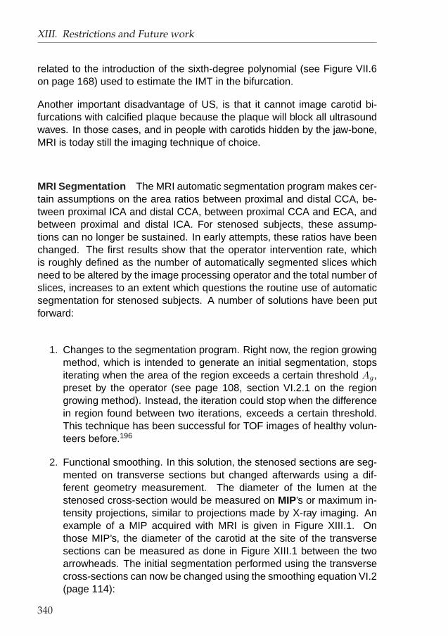
XIII. Restrictions and Future work
related to the introduction of the sixth-degree polynomial (see Figure VII.6on page 168) used to estimate the IMT in the bifurcation.
Another important disadvantage of US, is that it cannot image carotid bi-furcations with calcified plaque because the plaque will block all ultrasoundwaves. In those cases, and in people with carotids hidden by the jaw-bone,MRI is today still the imaging technique of choice.
MRI Segmentation The MRI automatic segmentation program makes cer-tain assumptions on the area ratios between proximal and distal CCA, be-tween proximal ICA and distal CCA, between proximal CCA and ECA, andbetween proximal and distal ICA. For stenosed subjects, these assump-tions can no longer be sustained. In early attempts, these ratios have beenchanged. The first results show that the operator intervention rate, whichis roughly defined as the number of automatically segmented slices whichneed to be altered by the image processing operator and the total number ofslices, increases to an extent which questions the routine use of automaticsegmentation for stenosed subjects. A number of solutions have been putforward:
1. Changes to the segmentation program. Right now, the region growingmethod, which is intended to generate an initial segmentation, stopsiterating when the area of the region exceeds a certain threshold Ag,preset by the operator (see page 108, section VI.2.1 on the regiongrowing method). Instead, the iteration could stop when the differencein region found between two iterations, exceeds a certain threshold.This technique has been successful for TOF images of healthy volun-teers before.196
2. Functional smoothing. In this solution, the stenosed sections are seg-mented on transverse sections but changed afterwards using a dif-ferent geometry measurement. The diameter of the lumen at thestenosed cross-section would be measured on MIP’s or maximum in-tensity projections, similar to projections made by X-ray imaging. Anexample of a MIP acquired with MRI is given in Figure XIII.1. Onthose MIP’s, the diameter of the carotid at the site of the transversesections can be measured as done in Figure XIII.1 between the twoarrowheads. The initial segmentation performed using the transversecross-sections can now be changed using the smoothing equation VI.2(page 114):
340

Figure XIII.1.: Example of a maximum intensity projection or MIP. The distance between thearrow tips can be used as an input in the smoothing algorithm.
−−→Pnew =
(−−→Pold −−−→Cold
)×√aratio +
−−−→Cnew (XIII.1)
Since the functional smoothing as defined here only changes the cross-sectional area and not the centrelines,
−−−→Cnew =
−−→Cold. aratio would be
calculated as the ratio between the cross-sectional area deduced fromthe diameter measurement from the MIP (Figure XIII.1) and the oldcross-sectional area found after the initial segmentation.
3. Carotid reconstruction from MIP’s. In this solution, the 3D carotid ge-ometry is no longer reconstructed from serial transverse cross-sections,but from the MIP.
3DUS Segmentation Although it has been shown in section VII.4.3 thatthe operator-dependence due to manual segmentation is minor, the processof segmentation of B-mode images remains very labour-intensive. Mao210
341

XIII. Restrictions and Future work
and Gill114 suggested that the segmentation could be done automatically,but they admit that the current level of image quality is not satisfactory. Ifthe US image could be segmented automatically, either by improvements inimage quality or segmentation procedure, this would induce a serious im-provement of the applicability of 3DUS-based CFD since it would decreasethe manual labour in the order of an hour.
3D Reconstruction using MRI The 3D reconstruction program is veryflexible. This has been proven by the ability to reconstruct highly tortuouscarotid bifurcations such as the ones in Figure VI.22 (page 143). Neverthe-less, the program has illustrated a number of flaws:
1. Flaws in Smoothness. In some cases, the smoothness at the bifur-cation is not satisfactory. It is not the smoothness at site of the apexthat gives rise to problems, but at the interface between CCA and itsbranches or at the border between inner and outer ICA or ECA (seeFigure VII.8, page 173 for a definition of ‘inner’ and ‘outer’). This effectis clear in Figure VII.13 (m) (page 183), where lines of high WSS arevisible. These lines originate from the points B1 and B2, i.e. the pointswhere the three carotid arteries come together (see Figure VI.13, page119, for a definition of the carotid feature points). In order to eliminatethose effects in the current studies, the haemodynamic wall parame-ters were filtered using 3x3 median filtering, i.e. the values of e.g. theWSS in a certain point on the vessel wall was replaced by the medianof the 9 values formed by the WSS of its 8 neighbours and its initialWSS value. In a smoother 3D reconstruction, this filtering would beobsolete.
A number of solutions have been put forward:
a) Longitudinal spline fitting. In the present situation, the longitu-dinal splines consist of piecewise linear segments. Fitting longi-tudinal cubic splines through the nodes of the current lines willsmooth the geometry. This solution has a number of drawbacks.First, it will change the geometry at sites where no change isneeded. Second, it only deals with the smoothness at the inter-section of CCA and its branches, but does not assess the problemat the intersection of inner and outer ICA or ECA. Third, it couldmake neighbouring longitudinal splines cross each other, espe-cially when there is a small cross-section and the longitudinal
342

splines thus all lie close to each other. Nevertheless, longitudi-nal smoothing is a common procedure in 3D reconstructions andif its drawbacks could be eliminated, it could be a good solution.
b) Local smoothing. This solution has been used for the smoothingat the apex. For the reader’s recollection, at the apex a parabolawas fitted through the apex and two points (B1 and B2) on themost distal CCA slice (see Figure VI.13, page 119). This parabolawas the (smooth) border between ICA and ECA. For the CCA/ICAand CCA/ECA intersection, something similar can be done. Twoexamples are given below. In the first example, another parabolacan be fitted between points C, B1 and B2 (see Figure VI.13,page 119, for a definition of the carotid feature points). This so-lution denies some data acquired in the most distal CCA slice. Asecond example fits a longitudinal smoothing spline through themost distal parts of the CCA and the proximal ICA or ECA locally ,which is a difference with the longitudinal spline fitting explainedin the previous section. This generates 1 longitudinal spline perpoint on the CCA contour. Each of this splines goes through theplane intersecting between CCA and ICA or ECA once. The lineformed by these intersecting points can be used to fit a smoothingparabola. The intersections of the longitudinal splines can now beshifted towards the parabola, resulting in a smoother geometry.
c) Circumferential smoothing. The two previous solutions do notchange the geometry at the intersection between inner and outerbranch. To this purpose, the circumferential instead of the lon-gitudinal splines could be smoothed. A circumferential spline isformed by every nth point of the longitudinal spline.
2. Early tests have shown that the 3D reconstruction of stenosed arteriescan be problematic when the most proximal ICA and ECA slice donot overlap with the most distal CCA slice. In this case, the verticalplane through the line
−→M which separates ICA and ECA (see Figure
VI.13 (b) on page 119) may not intersect with the most distal CCAslice (Figure VI.13 (c)). In this case, no intersection between CCA andeither ICA or ECA can be defined. A possible solution to this problemis to define the intersection plane between ICA and ECA as the planethrough
−→M and two particular points on the most distal CCA contour
as opposed to the present definition (through−→M and the I/S axis). The
particular points on the CCA contour could be those which (1) dividethe considered CCA cross-section into two equal areas and (2) canbe connected by
−→M . This solution has an important drawback: since
343
XIII. Restrictions and Future work
the intersecting plane is no longer parallel with the I/S axis, it will nolonger bisect the other intersecting planes (between CCA and ICA orECA) and symmetry is lost. As a consequence, the skewness of thecells which will be fitted using the intersecting planes as a scaffold willincrease. This decreases mesh quality.
3D Reconstruction using 3DUS The 3D reconstruction program used inthis study is very user-friendly, yet it shows two important flaws. Both flawsrelate to the fact that longitudinal splines are being fitted and smoothed usingcubic smoothing splines.
• The reconstruction procedure contains a step in which the longitudinalsplines are smoothed using cubic smoothing splines (the same tech-nique as explained in point 1a on page 343). It is important to realisethat some smoothing splines originate in the CCA and end in the ICAor ECA, other splines originate in the apical region and end in theICA or ECA. These are two separate sets of splines. When they aresmoothed, it occurs that the splines of one set intersect with splinesof the other set, or that the splines of one set do not have a smoothtransition to the other set. This makes it impossible to generate a vol-ume from these splines. In the cases where this intersection occurred,smoothing was kept to a minimum. Future version of the 3DUS pro-gram should question the use of longitudinal smoothing, and maybeintroduce the centreline and area smoothing as performed with MRIdata.
• The longitudinal splines that form the output of the 3DUS program,are polynomial (cubic) interpolations between the smoothed points (ornodes). The problem with polynomial interpolations is that it can gen-erate high-frequency side-effects, i.e. unrealistic twists induced by thefact that the polynomial is forced to go through certain end-points.The importance of the side-effect is related to the distance betweenthe nodes. Again, it is not possible to generate a volume from suchsplines. The current 3DUS reconstruction program has therefore beenaltered by increasing the number of nodes between which the poly-nomial fitting is to be performed. This reduced the distance betweenthe nodes, and thus decreased the effect of the polynomial side-effectmarkedly. This is obviously not a final solution to the problem. Thenext version of the 3DUS reconstruction program should investigatethe need for polynomial interpolation and possibly shift towards piece-wise linear interpolation, which is used in the MRI reconstructions.
344

Meshing Program For future use, the restriction to building structuredhexahedral meshes is too limiting. In our lab, a program has been writ-ten by Ir. S. Vermeersch (unpublished) which allows to output the current3D reconstructions to a format readable by all commercial mesh generators.This makes it possible to fit unstructured meshes in the 3D volumes createdby the programs written for this thesis.
Computational Details The current technique has been developed forstudying the shear stresses in the carotid arteries without stenoses. It isplausible that the computational details should be changed if the techniqueis to be used in other circumstances, other applications, or at another accu-racy.
• It is very likely that turbulence will occur in stenosed subjects. Severalstudies311,341 have investigated the use of turbulence models for bloodflow simulation.
• In the present studies, the viscosity has been chosen as done byBuchanon.42 In true life, the viscosity shows large variability and shouldtherefore be estimated individually (e.g. using the haematocrit as doneby Samijo270). Because this involves invasive blood tests, viscositymeasurements have not been performed here. The effect of differ-ences in viscosity values and viscosity models has been described insection VIII.2 (page 228).
• Currently, all simulations have been performed in carotid models withrigid walls. The introduction of compliant walls increases the realismof the computer model, but simultaneously increases the required pro-cessing time (approximately by a factor 10). Currently, it is thereforenot possible to simulate the amount of simulations performed in thisstudy within a reasonable time-scale. The effect of compliant wallshas been studied by Zhao384 and discussed in section VIII.1.3. If com-pliant walls would be used, there could be a gain in model accuracycomparable to the differences spotted in Zhao’s studies.384,385,387
• Recent studies have expanded the output of a simulation from shearstresses to the LDL transport346,347 or blood/plasma flow through wall.These are new diagnostically important parameters which, to a dif-ferent extent, all require changes to the computational details of thesimulation as presented here.
345

XIII. Restrictions and Future work
346

XIV. Summary
XIV.1. Introduction
When this study was started in 2000, it was becoming increasingly clear thatthe combination of medical imaging and computational fluid dynamics (CFD)might be a technique which would allow estimation of in vivo shear stressusing non-invasive techniques.34,197,219 Despite early success, there was asubstantial scepticism towards the achievable in vivo accuracy. Consideringthe amount of pathologies initiated or enhanced by certain values of shearstresses, and the effect of these pathologies on westernised societies, thequantification and increase of the accuracy of the technique was highly nec-essary. Before any studies could have been performed using image-basedCFD, its reproducibility, accuracy and operator dependency needed to be in-vestigated. Consequently, the first part of this thesis dealt with image-basedCFD as a technique.
XIV.2. Establishing the technique
XIV.2.1. Magnetic Resonance Imaging
Magnetic Resonance Imaging (MRI) was traditionally considered the ‘goldstandard’ in the choice of an imaging technique for combination with CFD.The process of extracting a 3D geometry of a carotid bifurcation was auto-mated. In this context, it is noteworthy to mention that the segmentation,reconstruction and meshing of a carotid bifurcation imaged with MRI takesnow less than 2 hours of which an operator is only required for 30 minutes,whereas previously it took several hours of an operator’s time. The accuracyof MRI-based CFD was estimated using a carotid phantom, and the repro-ducibility was quantified using 8 healthy subjects. A final study comparedtwo types of MRI protocols, black blood (BB) and time-of-flight (TOF) and
347

XIV. Summary
concluded that TOF MRI resulted in faster 3D reconstructions which were ofsuperior quality.
XIV.2.2. Three-dimensional Ultrasound
Simultaneously, three-dimensional ultrasound (3DUS) was investigated asimaging technique of choice for image-based CFD. Again, the process ofextracting 3D geometries suitable for CFD modelling was automated, basedon ground-levelling work by Barratt20 and Augst.16 Although segmentationof B-mode ultrasound images still happens manually, the time-gain achievedhere was in the order of several hours. Similar to the studies performedfor MRI-based CFD, the accuracy of 3DUS was analysed using the samephantom used for assessing the accuracy of MRI. Subsequently, nine sub-jects participated in a study aimed at quantifying the reproducibility of shearstress measurements using 3DUS-based CFD. Due to the higher frequencyof operator intervention for 3DUS in comparison with MRI, the operator de-pendency was quantified using an in vivo variability study in which 4 imagingoperators and 3 segmenting operators participated. Overall, it was foundthat the accuracy and reproducibility of 3DUS-based CFD was in the sameorder of magnitude of MRI-based CFD.
A comparative study showed that MRI can be replaced by 3DUS without lossof accuracy. This conclusion makes it possible to replace expensive MRIinvestigations by the relatively cheap 3DUS alternative available in manyhospitals.
XIV.2.3. Computational Details
With the eye on increasing realism, accuracy and reliability of image-basedCFD, several studies investigating a number of computational details wereundertaken. These studies resulted in suggestions on the use of both MRIand Doppler Ultrasound velocity measurements for the model boundary con-ditions. Furthermore, the effect of the use of viscosity (models) and heartrate changes on the overall shear stress distribution was investigated. Fol-lowing these studies, guidelines for the setup of the most realistic CFDmodel were suggested.
348

XIV.3. Clinical Applications
XIV.3. Clinical Applications
Once the accuracy of image-based CFD was known, the applications werequeuing up. Within the time-limit set for this thesis, two studies were finished.
A first study investigated the changes in carotid geometry and flow with headturns. It was concluded that the centrelines changed substantially from onehead position to another. Together with the changes in geometry, therewas a significant change in carotid blood flow rate. The two things togetherinduced important changes in shear stress patterns.
A second study investigated the effect of two anti-hypertensive drugs in anacute, randomised, double blind, three-way cross-over study. The techniqueshowed higher shear stresses with one of the compounds. This findingmanaged to relate long-term changes in carotid morphology with the acutechanges measured with image-based CFD.
These two studies illustrated that the in vivo applications of this techniqueare no longer a distant dream, but have been successfully fulfilled.
349

XIV. Summary
350

Bibliography
[1] A. Salih, Computational Fluid Dynamics , Available at: http://www.sali.freeservers.com/engi-neering/cfd/, Accessed January 6, 2004.
[2] Abrahams P , The Altas of the Human Body . San Diego, CA: Thunder Bay Press, 2002.[3] AEATechnology , CFX-4.4 Programming and Operating Manual, 1999.[4] Affeld K, Goubergrits L, Fernandez-Britto J, and Falcon L , Variability of the geometry of the
human common carotid artery. A vessel cast study of 31 specimens. Pathology Research andPractice 194: 597–602, 1998.
[5] Agrawal Y, Talbot L, and Gong K , Laser Anemometer Study of Flow Development in CurvedCircular Pipes. J Fluid Mech 85: 497–518, 1978.
[6] allrefer.com, Health, Diseases & Conditions, Stroke Secondary to Carotid Stenosis , Avail-able at: http://health.allrefer.com/health/stroke-secondary-to-carotid-stenosis-symptoms.html,Accessed January 4, 2004.
[7] American Heart Association , Heart Disease and Stroke Statistics - 2003 Update. Dallas, Tex.:American Heart Association, 2003.
[8] Amersham Health, Medcyclopedia, carotid dissection , Available at:http://www.amershamhealth.com/medcyclopaedia/Volume%20VI%201/DISSEC-TION%20ARTERIAL.asp, Accessed January 4, 2004.
[9] Amersham Health, Medcyclopedia, Colour Doppler sonography , Availableat: http://www.amershamhealth.com/medcyclopaedia/Volume%20I/colour%20Dopp-ler%20sonography.asp, Accessed January 21, 2004.
[10] Amersham Health, Medcyclopedia, Pulsed Doppler ultrasound , Available at:http://www.amershamhealth.com/medcyclopaedia/Volume%20I/pulsed%20Doppler%20ultra-sound.asp, Accessed January 21, 2004.
[11] Araim O, Chen AH, and Sumpio B , Hemodynamic Forces: Effects on Atherosclerosis. New Surgery 1: 112–115, 2001.
[12] Ariff B, Stanton A, Barratt D, Augst A, Glor F, Poulter N, Sever P, Xu Y, Hughes A, andThom SA , Comparison of the effects of antihypertensive treatment with angiotensin II blockadeand beta-blockade on carotid wall structure and haemodynamics: protocol and baseline demo-graphics. Journal of the Renin Angiotensin Aldosterone Sys tem 3: 116–122, 2002.
[13] Ariff BB, Zambanini A, Mayet J, Hughes AD, and Thom SM , Intima-medial area: A more robustmethod than intima media thickness for analysing non-cardiac gated common carotid images.Circulation 102: 3525, 2000.
[14] Arizona Governor Janet Napolitano, Governor’s Nursing Shortage Task Force Minutes ,Available at: http://www.governor.state.az.us/nurse/minutes.cfm, Accessed January 4, 2004.
[15] Augst A, Glor F, Ariff B, Crowe L, Firmin D, Hughes A, Thom S, and Xu X , Flow boundaryconditions for CFD models in human carotid artery bifurcations: Comparison of Doppler ultra-sound and MRI. Journal of Biomechanical Engineering , unpublished.
[16] Augst AD, Barratt DC, Hughes AD, Glor FP, Thom SAM, and Xu XY , Accuracy and Repro-ducibility of CFD predicted Wall Shear Stress using 3D Ultrasound Images. Journal of Biome-chanical Engineering Transactions of the ASME 125: 218–222, 2003.
[17] Augst AD, Barratt DC, Hughes AD, Thom SAM, and Xu XY , Various issues relating to CFDsimulations of carotid bifurcation flow based on models reconstructed from 3D Ultrasound images.Journal of En gi neer ing in Med i cine Proceedings of the institue of Mechanical Engineers PartH 217: 393–403, 2003.
351

Bibliography
[18] Bakker SJL and Gans ROB , About the role of shear stress in atherogenesis. CardiovascularResearch 45: 270–272, 2000.
[19] Bakker SJL, Ijzerman RG, Teerlink T, Westerhoff HV, Gans ROB, and Heine RJ , Cytoso-lic triglycerides and oxidative stress in central obesity: the missing link between excessiveatherosclerosis, endothelial dysfunction, and beta-cell failure? Atherosclerosis 148: 17–21, 2000.
[20] Barratt DC , Quantification of carotid disease using Three-Dimensional Ultrasound Imaging. Ph.D.thesis, London University, 2002.
[21] Barratt DC, Ariff BB, Humphries KN, Thom SAM, and Hughes AD , Reconstruction and Quan-tification of the Carotid Artery Bifurcation from 3D Ultrasound Images. IEEE Trans Med Imaging ,In press (May Edition), Manuscript #TMI-2003-0475.
[22] Barratt DC, Davies AH, Hughes AD, Thom SA, and Humphries KN , Accuracy of an electro-magnetic three-dimensional ultrasound system for carotid artery imaging. Ultrasound in Medicineand Biology 27: 1421–1425, 2001.
[23] Basombrio FG, Dari EA, Buscaglia GC, and Feijoo RA , Numerical experiments in complexhaemodynamics flows. Non-Newtonian effects. In XI Congress on Numerical Methods and TheirApplications ENIEF , San Carlos de Bariloche, Argentina, 2000.
[24] Berg S, Cole P, Hoffstein V, and Haight JSJ , Upper airway pressures in snorers and nonsnorersduring wakefulness and sleep. J Otolaryngol 30: 69–74, 2001.
[25] Bergeron P, Carrier R, Roy D, Blais N, and Raymond J , Radiation-Doses to Patients in Neu-rointerventional Procedures. American Journal of Neuroradiology 15: 1809–1812, 1994.
[26] Berkeley University, Types and Structures of Arteries , Available at: http://mcb.berke-ley.edu/courses/mcb135e/arteries.html, Accessed January 4, 2004.
[27] Bharadvaj BK, Mabon RF, and Giddens DP , Steady Flow in a Model of the Human CarotidBifurcation .1. Flow Visualization. Journal of Biomechanics 15: 349–362, 1982.
[28] Biller J and Thies WH , When to operate in carotid artery disease. American Family Physician61: 400–406, 2000.
[29] Bladin CF, Alexandrova NA, Murphy J, Alexandrov AV, Maggisano R, and Norris JW , Theclinical value of methods to measure carotid stenosis. International Angiology 15: 295–299, 1996.
[30] Bland JM and Altman DG , Measuring agreement in method comparison studies. Stat MethodsMed Res 8: 135–160, 1999.
[31] Blann AD, Kirkpatrick U, Devine C, Naser S, and McCollum CN , The influence of acute smok-ing on leucocytes, platelets and the endothelium. Atherosclerosis 141: 133–139, 1998.
[32] Blood count , Available at: http://www.chclibrary.org/micromed/00040090.html, Accessed April22, 2004.
[33] Botnar R, Rappitsch G, Scheidegger MB, Liepsch D, Perktold K, and Boesiger P , Hemody-namics in the carotid artery bifurcation: a comparison between numerical simulations and in vitroMRI measurements. Journal of Biomechanics 33: 137–144, 2000.
[34] Bots ML, Hofman A, and Grobbee DE , Increased common carotid intima-media thickness -Adaptive response or a reflection of atherosclerosis? Findings from the Rotterdam study. Stroke28: 2442–2447, 1997.
[35] Bots ML, Mulder PGH, Hofman A, Vanes GA, and Grobbee DE , Reproducibility of CarotidVessel Wall Thickness Measurements - the Rotterdam Study. Journal of Clinical Epidemiology47: 921–930, 1994.
[36] Boutouyrie P, Bussy C, Hayoz D, Hengstler J, Dartois N, Laloux B, Brunner H, and LaurentS, Local pulse pressure and regression of arterial wall hypertrophy during long-term antihyper-tensive treatment. Circulation 101: 2601–2606, 2000.
[37] Boutouyrie P, Germain DP, Tropeano AI, Laloux B, Carenzi F, Zidi M, Jeunemaitre X, andLaurent S , Compressibility of the carotid artery in patients with pseudoxanthoma elasticum. Hy-pertension 38: 1181–1184, 2001.
[38] Bovendeerd PHM, Vansteenhoven AA, Vandevosse FN, and Vossers G , Steady Entry Flow ina Curved Pipe. J Fluid Mech 177: 233–246, 1987.
[39] Brands PJ, Hoeks APG, Hofstra L, and Reneman RS , A Noninvasive Method to Estimate WallShear Rate Using Ultrasound. Ultrasound in Medicine and Biology 21: 171–185, 1995.
[40] Brands PJ, Willigers JM, Ledoux LAF, Reneman RS, and Hoeks APG , A noninvasive methodto estimate pulse wave velocity in arteries locally by means of ultrasound. Ultrasound in Medicineand Biology 24: 1325–1335, 1998.
352

Bibliography
[41] British Medical Ultrasound Society, History of Ultrasound , Available at:http://www.bmus.org/history of ultrasound.htm#med, Accessed January 21, 2004.
[42] Buchanan JR and Kleinstreuer C , Simulation of particle-hemodynamics in a partially occludedartery segment with implications to the initiation of microemboli and secondary stenoses. Journalof Biomechanical Engineering Transactions of the ASME 120: 446–454, 1998.
[43] Buchanan JR, Kleinstreuer C, and Comer JK , Rheological effects on pulsatile hemodynamicsin a stenosed tube. Comput Fluids 29: 695–724, 2000.
[44] Cademartiri F, Mollet N, Nieman K, Krestin GP, and de Feyter PJ , Neointimal hyperplasia incarotid stent detected with multislice computed tomography. Circulation 108: E147–E147, 2003.
[45] Caro C, Fitz-Gerald J, and Schroter R , Atheroma and Arterial Wall Shear observation, Corre-lation and Proposal of a Shear Dependent Mass Transfer Mechanism for Atherogenesis. In Pro-ceedings of the Royal Society , London: JSTOR, 1971, vol. 177 of Series B, Biological Sciences,pp. 109–133.
[46] Caro CG, Doorly DJ, Tarnawski M, Scott KT, Long Q, and Dumoulin CL , Non-planar curvatureand branching of arteries and non-planar- type flow. Proc R Soc London Ser A Math Phys EngSci 452: 185–197, 1996.
[47] Caro CG, Fitz-Gerald JM, and Schroter RC , Arterial wall shear and distribution of earlyatheroma in man. Nature 223: 1159–1160, 1969.
[48] Casiglia E, Palatini P, Da Ros S, Pagliara V, Puato M, Dorigatti F, and Pauletto P , Effect ofblood pressure and physical activity on carotid artery intima-media thickness in stage 1 hyperten-sives and controls. American Journal of Hypertension 13: 1256–1262, 2000.
[49] Cebral J, Lohner R, Soto O, and Yim P , On the modeling of carotid artery blood flow frommagnetic resonance images. In Proc. ASME-BED Bioengineering Conference, 2001, vol. 50, pp.619–620.
[50] Cebral J, Yim P, Lohner R, Soto O, Marcos H, and Choyke P , New Methods for Computa-tional Fluid Dynamics of Carotid Artery From Magnetic Resonance Angiography. In SPIE MedicalImaging, edited by Chin-Tu Chen AV , San Diego, 2001, vol. 4321, pp. 177–187.
[51] Cebral JR , Realistic modeling of arterial hemodynamics from anatomic and physiologic imagedata. In 14th U.S. National Congress in Theoretical and Applied Mechanics, edited by Batra RCand Henneke EG , Blacksburg, VA, 2002, p. 79.
[52] Cebral JR, Castro M, Lohner R, Soto O, Yim PJ, and Alperin N , Realistic cerebral circula-tion models from medical imaging data. In 2003 Summer Bioengineering Conference, edited bySoslowsky LJ, Skalak TC, Wayne JS, and Livesay GA , Key Biscayne, FL, 2003, pp. 781–782.
[53] Cebral JR, Castro MA, Soto O, Lohner R, and Alperin N , Blood-flow models of the circle ofWillis from magnetic resonance data. Journal of En gi neer ing Mathematics 47: 369–386, 2003.
[54] Cebral JR and Lohner R , From medical images to anatomically accurate finite element grids. IntJ Numer Methods Eng 51: 985–1008, 2001.
[55] Cebral JR, Lohner R, Choyke PL, and Yim PJ , Merging of intersecting triangulations for finiteelement modeling. Journal of Biomechanics 34: 815–819, 2001.
[56] Cebral JR, Yim PJ, Lohner R, Soto O, and Choyke PL , Blood flow modeling in carotid arterieswith computational fluid dynamics and MR imaging. Acad Radiol 9: 1286–1299, 2002.
[57] Cellerini M, Mascalchi M, Mangiafico S, Ferrito GP, Scardigli V, Pellicano G, and Quilici N ,Phase-contrast MR angiography of intracranial dural arteriovenous fistulae. Neuroradiology 41:487–492, 1999.
[58] Chae CU, Pfeffer MA, Glynn RJ, Mitchell GF, Taylor JO, and Hennekens CH , Increased pulsepressure and risk of heart failure in the elderly. Jama Journal of the American Med i cal Associa-tion 281: 634–639, 1999.
[59] Chatzimavroudis GP, Oshinski JN, Franch RH, Walker PG, Yoganathan AP, and PettigrewRI, Evaluation of the precision of magnetic resonance phase velocity mapping for blood flowmeasurements. J Cardiov Magn Reson 3: 11–19, 2001.
[60] Chen YT, Vaccarino V, Williams CS, Butler J, Berkman LF, and Krumholz HM , Risk factorsfor heart failure in the elderly: A prospective community-based study. American Journal of Med icine 106: 605–612, 1999.
[61] Cheng CP, Parker D, and Taylor CA , Quantification of wall shear stress in large blood vesselsusing lagrangian interpolation functions with cine phase- contrast magnetic resonance imaging.Annals of Biomedical Engineering 30: 1020–1032, 2002.
353

Bibliography
[62] Cheong PL , Mahnetic Resonance Imaging and Computer simulation of haemodynamics at thehuman aortic bifurcation. Ph.D. thesis, London Universityn, 2004.
[63] Cho A, Mitchell L, Koopmans D, and Langille BL , Effects of changes in blood flow rate on celldeath and cell proliferation in carotid arteries of immature rabbits. CircRes 81: 328–337, 1997.
[64] Choi US, Talbot L, and Cornet I , Experimental-Study of Wall Shear Rates in the Entry Regionof a Curved Tube. J Fluid Mech 93: 465–489, 1979.
[65] Chung KY, Belfort G, Edelstein WA, and Li XM , Dean Vortices in Curved Tube Flow .5. 3-DMRI and Numerical- Analysis of the Velocity-Field. AICHE J 39: 1592–1602, 1993.
[66] Clarkson P, Celermajer DS, Donald AE, Sampson M, Sorensen KE, Adams M, Yue DK, Bet-teridge DJ, and Deanfield JE , Impaired vascular reactivity in insulin-dependent diabetes mellitusis related to disease duration and low density lipoprotein cholesterol levels. J Am Coll Cardiol 28:573–579, 1996.
[67] Clowes AW and Berceli SA , Mechanisms of vascular atrophy and fibrous cap disruption. InAtherosclerosis V: the Fifth Saratoga Conference, New York: New York Acad Sciences, vol. 902of Annals of the New York Academy of Sciences, pp. 153–162, 2000.
[68] Colin Europe , Available at: http://www.colin-europe.com/pages/tonometry.html, Accessed De-cember 31, 2003.
[69] Collins WM and Dennis SCR , Steady Motion of a Viscous-Fluid in a Curved Tube. Q J MechAppl Math 28: 133–156, 1975.
[70] Cross MM , Rheology of non-Newtonian fluids: a new flow equation for pseudo-plastic system.Journal of Colloid Science 20: 417–437, 1965.
[71] Crowe LA, Gatehouse P, Yang GZ, Mohiaddin RH, Varghese A, Charrier C, Keegan J, andFirmin DN , Volume Selective 3D Turbo Spin Echo Sequence For Vascular Wall Imaging andDistensibility Measurement. Journal of Magnetic Resonance Imaging 17: 572–580, 2003.
[72] Darovic GO , Hemodynamic monitoring: invasive and noninvasive clinical application. Philadel-phia: W.B. Saunders Company, 2nd ed., 1995.
[73] De Ley G , Physiology and Anatomy . Gent: Universiteit Gent, 1996.[74] De Ponti F, Marelli C, D’Angelo L, Caravaggi M, Bianco L, Lecchini S, Frigo GM, and Crema
A, Pharmacological activity and safety of trandolapril (RU 44570) in healthy volunteers. EuropeanJournal of Clinical Pharmacology 40: 149–153, 1991.
[75] DeBakey ME and Glaeser DH , Patterns of atherosclerosis: Effect of risk factors on recurrenceand survival-analysis of 11,890 cases with more than 25-year follow-up. American Journal ofCardiology 85: 1045–1053, 2000.
[76] Delfino A, Stergiopulos N, Moore JE, and Meister JJ , Residual strain effects on the stress fieldin a thick wall finite element model of the human carotid bifurcation. Journal of Biomechanics 30:777–786, 1997.
[77] Denarie N, Gariepy J, Chironi G, Massonneau M, Laskri F, Salomon J, Levenson J, andSimon A , Distribution of ultrasonographically-assessed dimensions of common carotid arteries inhealthy adults of both sexes. Atherosclerosis 148: 297–302, 2000.
[78] Dicom Standards Committee , Available at: http://medical.nema.org/, Accessed January 7,2004.
[79] Dimitriou G, Greenough A, Pink L, McGhee A, Hickey A, and Rafferty GF , Effect of posture onoxygenation and respiratory muscle strength in convalescent infants. Arch Dis Child 86: 147–150,2002.
[80] Donis J, Graf M, and Sluga E , Carotid-Artery Flow Measurements by Means of Duplex Sonog-raphy (Results in Normal Persons). Ultraschall in Der Medizin 9: 216–222, 1988.
[81] Draney MT, Herfkens RJ, Hughes TJR, Pelc NJ, Wedding KL, Zarins CK, and Taylor CA ,Quantification of vessel wall cyclic strain using cine phase contrast magnetic resonance imaging.Annals of Biomedical Engineering 30: 1033–1045, 2002.
[82] Dussik K , On the possibility of using ultrasound waves as a diagnostic aid. Neurol Psychiat 174:153–168, 1942.
[83] Ebbers T, Wigstrom L, Bolger AF, Engvall J, and Karlsson M , Estimation of relative cardiovas-cular pressures using time- resolved three-dimensional phase contrast MRI. Magnetic Resonancein Medicine 45: 872–879, 2001.
[84] Eckstein HH , Surgical therapy for extracranial stenosis of the carotid. Chirurg 75: 93–109, 2004.
354

Bibliography
[85] Eichler F, Ipsiroglu O, Arif T, Popow C, Heinzl H, Urschitz M, and Pollak A , Position dependentchanges of cerebral blood flow velocities in premature infants. Eur J Pediatr 160: 633–639, 2001.
[86] Electromagnetic Spectrum , Available at: http://www.electro-optical.com/bb rad/emspect.htm,Accessed December 31, 2003.
[87] Electronics Modern Magic, Paul Langevin , Available at: http://mediatheek.thinkquest.nl, Ac-cessed January 21, 2004.
[88] Eloot S, De Wachter D, Van Tricht I, and Verdonck P , Computational flow modeling in hollow-fiber dialyzers. Artificial Organs 26: 590–599, 2002.
[89] Elzinga G and Westerho.N , Pressure and Flow Generated by Left Ventricle against DifferentImpedances. Circulation Research 32: 178–186, 1973.
[90] emedicine, carotid dissection , Available at: http://www.emedicine.com/emerg/byname/dissec-tion-carotid-artery.htm, Accessed January 4, 2004.
[91] Ene-Iordache B, Mosconi L, Remuzzi G, and Remuzzi A , Computational fluid dynamics of avascular access case for hemodialysis. Journal of Biomechanical Engineering Transactions of theASME 123: 284–292, 2001.
[92] Fahrig R, Fox AJ, Lownie S, and Holdsworth DW , Use of a C-arm system to generate truethree-dimensional computed rotational angiograms: Preliminary in vitro and in vivo results. Amer-ican Journal of Neuroradiology 18: 1507–1514, 1997.
[93] Fayad ZA, Fuster V, Fallon JT, Jayasundera T, Worthley SG, Helft G, Aguinaldo JG, BadimonJJ, and Sharma SK , Noninvasive in vivo human coronary artery lumen and wall imaging usingblack-blood magnetic resonance imaging. Circulation 102: 506–510, 2000.
[94] Feldman CL and Stone PH , Intravascular hemodynamic factors responsible for progression ofcoronary atherosclerosis and development of vulnerable plaque. Current Opinion in Cardiology15: 430–440, 2000.
[95] Ferrara LA, Mancini M, Iannuzzi R, Marotta T, Gaeta I, Pasanisi F, Postiglione A, and GuidaL, Carotid Diameter and Blood Flow Velocities in Cerebral Circulation in Hypertensive Patients.Stroke 26: 418–421, 1995.
[96] Fitzgerald DE, Oshaughnessy AM, and Keaveny VT , Pulsed Doppler - Determination of BloodVelocity and Volume Flow in Normal and Diseased Common Carotid Arteries in Man. Cardiovas-cular Research 16: 220–224, 1982.
[97] Fortune JB, Bock D, Kupinski AM, Stratton HH, Shah DM, and Feustel PJ , HumanCerebrovascular Response to Oxygen and Carbon-Dioxide as Determined by Internal Carotid-Artery Duplex Scanning. Journal of Trauma Injury Infection and Critical Care 32: 618–628, 1992.
[98] Frayne R, Gowman LM, Rickey DW, Holdsworth DW, Picot PA, Drangova M, Chu KC, Cald-well CB, Fenster A, and Rutt BK , A Geometrically Accurate Vascular Phantom For Comparative-Studies of X-Ray, Ultrasound, and Magnetic-Resonance Vascular Imaging - Construction and Ge-ometrical Verification. Med Phys 20: 415–425, 1993.
[99] Friedman MH , A Biologically Plausible Model of Thickening of Arterial Intima under Shear. Arte-riosclerosis 9: 511–522, 1989.
[100] Friedman MH and Ding ZH , Variability of the planarity of the human aortic bifurcation. MedicalEngineering Physics 20: 469–472, 1998.
[101] Friedman MH, Obrien V, and Ehrlich LW , Calculations of Pulsatile Flow through a Branch -Implications for Hemodynamics of Atherogenesis. Circulation Research 36: 277–285, 1975.
[102] Fry DL , Acute vascular endothelial changes associated with increased blood velocity gradients.Circulation Research 22: 165–197, 1968.
[103] Gage KL, Gartner MJ, Burgreen GW, and Wagner WR , Predicting membrane oxygenator pres-sure drop using computational fluid dynamics. Artificial Organs 26: 600–607, 2002.
[104] Gariepy J, Massonneau M, Levenson J, Heudes D, and Simon A , Evidence for in-Vivo Carotidand Femoral Wall Thickening in Human Hypertension. Hypertension 22: 111–118, 1993.
[105] Gariepy J, Salomon J, Denarie N, Laskri F, Megnien JL, Levenson J, and Simon A , Sex andtopographic differences in associations between large- artery wall thickness and coronary riskprofile in a French working cohort - The AXA Study. Arteriosclerosis Thrombosis and VascularBiology 18: 584–590, 1998.
[106] GE systemas medicos, Ultrasonido, cursos online, Imgen de Doppler Carotideo , Availableat: http://www.gemedicalsystems.com/laes/rad/us/education/msucmecd.html, Accessed January4, 2004.
355

Bibliography
[107] General anaesthetic versus local anaesthetic for carotid surgery (GALA trial),General anaesthetic versus local anaesthetic for carotid surgery , Available at:http://www.dcn.ed.ac.uk/gala/June%2002.htm, Accessed January 4, 2004.
[108] Georgia State University, Department of Physics and Astronomy, Hyperphysics, Wall Ten-sion , Available at: http://hyperphysics.phy-astr.gsu.edu/hbase/ptens.html, Accessed January 4,2004.
[109] Germain DP, Boutouyrie P, Laloux B, and Laurent S , Arterial remodeling and stiffness in pa-tients with pseudoxanthoma elasticum. Arteriosclerosis Thrombosis and Vascular Biology 23:836–841, 2003.
[110] Gianaros PJ, Jennings JR, Olafsson GB, Steptoe A, Sutton-Tyrrell K, Muldoon MF, andManuck SB , Greater intima-media thickness in the carotid bulb is associated with reduced barore-flex sensitivity. American Journal of Hypertension 15: 486–491, 2002.
[111] Giannattasio C, Failla M, Stella ML, Mangoni AA, Turrini D, Carugo S, Pozzi M, Grassi G, andMancia G , Angiotensin-Converting Enzyme-Inhibition and Radial Artery Compliance in Patientswith Congestive-Heart-Failure. Hypertension 26: 491–496, 1995.
[112] Gibson CM, Diaz L, Kandarpa K, Sacks FM, Pasternak RC, Sandor T, Feldman C, and StonePH, Relation of Vessel Wall Shear-Stress to Atherosclerosis Progression in Human Coronary-Ar-teries. Arteriosclerosis and Thrombosis 13: 310–315, 1993.
[113] Gijsen FJH, van de Vosse FN, and Janssen JD , The influence of the non-Newtonian proper-ties of blood on the flow in large arteries: steady flow in a carotid bifurcation model. Journal ofBiomechanics 32: 601–608, 1999.
[114] Gill JD, Ladak HM, Steinman DA, and Fenster A , Accuracy and variability assessment of asemiautomatic technique for segmentation of the carotid arteries from three- dimensional ultra-sound images. Med Phys 27: 1333–1342, 2000.
[115] Gill RW , Measurement of Blood-Flow by Ultrasound - Accuracy and Sources of Error. Ultrasoundin Medicine and Biology 11: 625–641, 1985.
[116] Girerd X, Giannattasio C, Moulin C, Safar M, Mancia G, and Laurent S , Regression of radialartery wall hypertrophy and improvement of carotid artery compliance after long-term antihyper-tensive treatment in elderly patients. Journal of the American College of Cardiology 31: 1064–1073, 1998.
[117] Glor FP, Ariff B, Augst AD, Barratt DC, Hughes AD, Thom SA, Verdonck PR, and Xu XY , 3DUltrasound-based CFD for carotid flow prediction: a reproducibility study. In 2nd MIT Conferenceon Computational Fluid and Solid Mechanics, edited by Bathe KJ , Cambridge, MA: Elsevier,2003, vol. 2 of Computational Fluid and Solid Mechanics, pp. 1701–1704.
[118] Glor FP, Ariff B, Augst AD, Barratt DC, Hughes AD, Thom SAM, Verdonck PR, and Xu XY , 3Dultrasound-based CFD for carotid flow prediction: a reproducibility study. Ultrasound in Medicineand Biology , unpublished.
[119] Glor FP, Ariff B, Crowe LA, Firmin D, Hughes AD, Thom SAM, Barratt DC, Verdonck PR,and Xu XY , CFD-based carotid flow reconstruction: a comparison between MRI and Ultrasound.Journal of Biomechanics , unpublished.
[120] Glor FP, Ariff B, Crowe LA, Hughes AD, Cheong PL, Thom SA, Verdonck P, Firmin DN,Barratt DC, and Xu XY , Carotid geometry reconstruction: a comparison between MRI and ultra-sound. Medical Physics 30: 3251–3261, 2003.
[121] Glor FP, Long Q, Hughes AD, Augst AD, Ariff B, Thom SA, Verdonck P, and Xu XY , Repro-ducibility study of MR-image based CFD prediction of carotid bifurcation flow. Annals of Biomedi-cal Engineering 31: 142–151, 2003.
[122] Glor FP, Westenberg JJM, Vierendeels J, Danilouchkine M, and Verdonck P , Validation of thecoupling of magnetic resonance imaging velocity measurements with computational fluid dynam-ics in a U bend. Artificial Organs 26: 622–635, 2002.
[123] Gnasso A, Motti C, Irace C, Carallo C, Liberatoscioli L, Bernardini S, Massoud R, MattioliPL, Federici G, and Cortese C , Genetic variation in human stromelysin gene promoter and com-mon carotid geometry in healthy male subjects. Arteriosclerosis Thrombosis and Vascular Biology20: 1600–1605, 2000.
[124] Goonasekera CDA and Dillon MJ , Random Zero Sphygmomanometer Versus Automatic Oscil-lometric Blood-Pressure Monitor Is Either the Instrument of Choice. Journal of Human Hyperten-sion 9: 885–889, 1995.
356

Bibliography
[125] Goubergrits L, Affeld K, Fernandez-Britto J, and Falcon L , Atherosclerosis in the human com-mon carotid artery. A morphometric study of 31 specimens. Pathology Research and Practice197: 803–809, 2001.
[126] Goubergrits L, Affeld K, Fernandez-Britto J, and Falcon L , Atherosclerosis and flow in carotidarteries with authentic geometries. Biorheology 39: 519–524, 2002.
[127] Goubergrits L, Affeld K, Fernandez-Britto J, and Falcon L , Geometry of the human commoncarotid artery. A vessel cast study of 86 specimens. Pathology Research and Practice 198: 543–551, 2002.
[128] Grassi G, Seravalle G, Turri C, Bolla G, and Mancia G , Short-versus long-term effects of dif-ferent dihydropyridines on sympathetic and baroreflex function in hypertension. Hypertension 41:558–62, 2003.
[129] Grossman E and Messerli FH , Effect of calcium antagonists on plasma norepinephrine levels,heart rate, and blood pressure. American Journal of Cardiology 80: 1453–1458, 1997.
[130] Grube E, Colombo A, Hauptmann E, Londero H, Reifart N, Gerckens U, and Stone GW , Initialmulticenter experience with a novel distal protection filter during carotid artery stent implantation.Catheterization and Cardiovascular Interventions 58: 139–146, 2003.
[131] H. S. Khaira, Atherosclerosis , Available at: http://gensurg.co.uk/atherosclerosis.htm, AccessedJanuary 4, 2004.
[132] Hamada T, Takita M, Kawano H, Nohtomi A, and Okayama M , Difference in Blood-Flow Volumeof the Common Carotid-Artery between Vascular and Nonvascular Dementia Detected by ColorDuplex Sonography. Journal of Neurology 240: 191–194, 1993.
[133] Hamakiotes CC and Berger SA , Fully-Developed Pulsatile Flow in a Curved Pipe. J Fluid Mech195: 23–55, 1988.
[134] Hamakiotes CC and Berger SA , Periodic Flows Through Curved Tubes - the Effect of the Fre-quency Parameter. J Fluid Mech 210: 353–370, 1990.
[135] Haynes MJ, Cala LA, Melsom A, Mastaglia FL, Milne N, and McGeachie JK , Vertebral ar-teries and cervical rotation: Modeling and magnetic resonance angiography studies. Journal ofManipulative and Physiological Therapeutics 25: 370–383, 2002.
[136] Haynes WM , Viscosity of Saturated Liquid Methane. Physica 70: 410–412, 1973.[137] He XJ and Ku DN , Pulsatile flow in the human left coronary artery bifurcation: Average conditions.
Journal of Biomechanical Engineering Transactions of the ASME 118: 74–82, 1996.[138] HeartCenterOnline For Patients, Aneurysm overview , Available at: http://www.heartcen-
teronline.com/myheartdr/common/articles.cfm?ARTID=551, Accessed January 4, 2004.[139] Hofmann W, Balashazy I, and Heistracher T , The relationship between secondary flows and
particle deposition patterns in airway bifurcations. Aerosol Sci Technol 35: 958–968, 2001.[140] Holdsworth DW, Norley CJD, Frayne R, Steinman DA, and Rutt BK , Characterization of com-
mon carotid artery blood-flow waveforms in normal human subjects. Physiological Measurement20: 219–240, 1999.
[141] Humphrey JAC, Iacovides H, and Launder BE , Some Numerical Experiments On DevelopingLaminar-Flow in Circular-Sectioned Bends. J Fluid Mech 154: 357–375, 1985.
[142] Hyun S, Kleinstreuer C, and Archie JP , Computer simulation and geometric design of en-darterectomized carotid artery bifurcations. Crit Rev Biomed Eng 28: 53–59, 2000.
[143] Hyun S, Kleinstreuer C, and Archie JP , Hemodynamics analyses of arterial expansions withimplications to thrombosis and restenosis. Med Eng Phys 22: 13–27, 2000.
[144] Indus Instruments, Carotid Arterial Flow Velocity Spectrogram of a Mouse , Available at:http://www.indusinstruments.com/oldWebsite, Accessed January 22, 2004.
[145] Iternational Society of Magnetic Resonance in Medicine, Press Releases, The 2003Nobel Prize in Physiology or Medicine , Available at: http://www.nobel.se/medicine/laure-ates/2003/press.html, Accessed January 12, 2004.
[146] James M, Watt P, Potter J, Thurston H, and Swales J , Pulse pressure and resistance arterystructure in the elderly. Hypertension 26: 301–306, 1995.
[147] Jondeau G, Boutouyrie P, Lacolley P, Laloux B, Dubourg O, Bourdarias JP, and Laurent S ,Central pulse pressure is a major determinant of ascending aorta dilation in Marfan syndrome.Circulation 99: 2677–2681, 1999.
[148] Jou L, vanTyen R, Berger A, and Saloner D , Calculation of the magnetization distribution forfluid flow in curved vessels. Magnetic Resonance in Medicine 35: 577–584, 1996.
357

Bibliography
[149] Kadowaki C, Hara M, Numoto M, Takeuchi K, and Saito I , Cine Magnetic-Resonance-Imagingof Aqueductal Stenosis. Childs Nerv Syst 11: 107–111, 1995.
[150] Kamarck TW, Everson SA, Kaplan GA, Manuck SB, Jennings JR, Salonen R, and SalonenJT, Exaggerated blood pressure responses during mental stress are associated with enhancedcarotid atherosclerosis in middle-aged Finnish men - Findings from the Kuopio Ischemic HeartDisease Study. Circulation 96: 3842–3848, 1997.
[151] Karino T and Goldsmith HL , Particle Flow Behavior in Models of Branching Vessels .2. Effectsof Branching Angle and Diameter Ratio on Flow Patterns. Biorheology 22: 87–104, 1985.
[152] Kass DA, Shapiro EP, Kawaguchi M, Capriotti AR, Scuteri A, deGroof RC, and Lakatta EG ,Improved arterial compliance by a novel advanced glycation end-product crosslink breaker. Cir-culation 104: 1464–1470, 2001.
[153] Kass M, Witkin A, and Terzopoulos D , Snakes - Active Contour Models. International Journalof Computer Vision 1: 321–331, 1987.
[154] Keller HM, Meier WE, Anliker M, and Kumpe DA , Noninvasive Measurement of Velocity Profilesand Blood-Flow in Common Carotid-Artery by Pulsed Doppler Ultrasound. Stroke 7: 370–377,1976.
[155] Kessler M , Section III. Biocompatibility. Nephrol Dial Transplant 17: 32–44, 2002.[156] Keynton RS, Evancho MM, Sims RL, Rodway NV, Gobin A, and Rittgers SE , Intimal hyper-
plasia and wall shear in arterial bypass graft distal anastomoses: An in vivo model study. Journalof Biomechanical Engineering Transactions of the ASME 123: 464–473, 2001.
[157] King E, Xu XY, Hughes AD, Long Q, Thom SA, and Parker KH , Quantification of the non-planarity of the human carotid bifurcation. Biorheology 39: 419–424, 2002.
[158] Klabunde RE , Cardiovascular physiology concepts, 1999.[159] Kleinstreuer C, Hyun S, Buchanan JR, Longest PW, Archie JP, and Truskey GA , Hemody-
namic parameters and early intimal thickening in branching blood vessels. Critical Reviews inBiomedical Engineering 29: 1–64, 2001.
[160] Kleinstreuer C, Lei M, and Archie JP , Flow input waveform effects on the temporal and spatialwall shear stress gradients in a femoral graft-artery connector. Journal of Biomechanical Engi-neering Transactions of the ASME 118: 506–510, 1996.
[161] Kohler U, Marshall I, Robertson MB, Long Q, Xu XY, and Hoskins P , MRI measurement ofWall Shear Stress Vectors in Bifurcation Models and Comparison With CFD Predictions. Journalof Magnetic Resonance Imaging 14: 563–573, 2001.
[162] Krams R, Wentzel JJ, Oomen JAF, Vinke R, Schuurbiers JCH, deFeyter PJ, Serruys PW,and Slager CJ , Evaluation of endothelial shear stress and 3D geometry as factors determiningthe development of atherosclerosis and remodeling in human coronary arteries in vivo - Combin-ing 3D reconstruction from angiography and IVUS (ANGUS) with computational fluid dynamics.Arterioscler Thromb Vasc Biol 17: 2061–2065, 1997.
[163] Kwoon SM, Ru TF, and Guang XX , Effects of des-aspartate-angiotensin I on neointima growthand cardiovascular hypertrophy. Regulatory Peptides 117: 213–217, 2004.
[164] Ladak HM, Milner JS, and Steinman DA , Rapid three-dimensional segmentation of the carot-id bifurcation from serial MR images. Journal of Biomechanical Engineering Transactions of theASME 122: 96–99, 2000.
[165] Ladak HM, Thomas JB, Mitchell JR, Rutt BK, and Steinman DA , A semi-automatic techniquefor measurement of arterial wall from black blood MRI. Medical Physics 28: 1098–1107, 2001.
[166] Lafleche A, Gautier S, Topouchian J, Wilmet CS, Girerd X, Safar ME, and Benetos A , Dif-ferential responses of the heart and vasculature to chronic blood pressure reduction in essentialhypertension. Clinical Pharmacology Therapeutics 64: 96–105, 1998.
[167] Lage SG, Kopel L, Medeiros CCJ, Carvalho RT, and Creager MA , Angiotensin II contributes toarterial compliance in congestive heart failure. American Journal of Physiology Heart and Circu-latory Physiology 283: H1424–H1429, 2002.
[168] Laogun AA and Gosling RG , In vivo arterial compliance in man. Clin Phys Physiol Meas 3:201–212, 1982.
[169] Laragh JH and Brenner BM , Hypertension Pathophysiology, Diagnosis and Management, vol. 1.Raven Press New York, 1990.
[170] Lee VS, Hertzberg BS, Kliewer MA, and Carroll BA , Assessment of stenosis: Implications ofvariability of Doppler measurements in normal-appearing carotid arteries. Radiology 212: 493–498, 1999.
358

Bibliography
[171] Lei M, Kleinstreuer C, and Archie JP , Geometric design improvements for femoral graft-arteryjunctions mitigating restenosis. Journal of Biomechanics 29: 1605–1614, 1996.
[172] Lei M, Kleinstreuer C, and Truskey GA , Numerical Investigation and Prediction of AtherogenicSites in Branching Arteries. Journal of Biomechanical Engineering Transactions of the ASME 117:350–357, 1995.
[173] Lei M, Kleinstreuer C, and Truskey GA , A focal stress gradient-dependent mass transfer mech-anism for atherogenesis in branching arteries. Med Eng Phys 18: 326–332, 1996.
[174] Lentner C , Geigy Scientific Tables: Heart and Circulation, vol. 5 of Geigy Scientific Tables. Basel,Switzerland: Ciba-Geigy Corporation, 8 ed., 1990.
[175] Leopold PW, Shandall AA, Feustel P, Corson JD, Shah DM, Popp AJ, Fortune JB, LeatherRP, and Karmody AM , Duplex Scanning of the Internal Carotid-Artery - an Assessment of Cere-bral Blood-Flow. British Journal of Surgery 74: 630–633, 1987.
[176] Lerner Research Institute, The Cleveland Clinic, Vascular Imaging , Available at:http://www.tmc.edu/thi/carotida.html, Accessed January 1, 2004.
[177] Leuprecht A, Kozerke S, Boesiger P, and Perktold K , Blood flow in the human ascending aorta:a combined MRI and CFD study. Journal of En gi neer ing Mathematics 47: 387–404, 2003.
[178] Leuprecht A, Perktold K, Kozerke S, and Boesiger P , Combined CFD and MRI study of bloodflow in a human ascending aorta model. Biorheology 39: 425–429, 2002.
[179] Leverett LB, Lynch EC, Alfrey CP, and Hellums JD , Red Blood-Cell Damage By Shear-Stress.Biophys J 12: 257–271, 1972.
[180] Levesque MJ and Nerem RM , The Elongation and Orientation of Cultured Endothelial-Cells inResponse to Shear-Stress. Journal of Biomechanical Engineering Transactions of the ASME 107:341–347, 1985.
[181] Li JKJ , The arterial Circulation. Physical principles and clinical applications.. Totowa, New Jersey:Humana Press Inc., 2000.
[182] Liang YL, Shiel LM, Teede H, Kotsopoulos D, McNeil J, Cameron JD, and McGrath BP , Ef-fects of Blood Pressure, Smoking, and Their Interaction on Carotid Artery Structure and Function.Hypertension 37: 6–11, 2001.
[183] Liauw L, van Buchem MA, Spilt A, de Bruine FT, van den Berg R, Hermans J, and WasserM, MR angiography of the intracranial venous system. Radiology 214: 678–682, 2000.
[184] Liepsch D , Study of Flow Processes in Branching Models of Coronary Vessels with a LaserDoppler Probe. Chemie Ingenieur Technik 47: 347–347, 1975.
[185] Liepsch D , Pressure Measurements at Wall after Bifurcation and Visual Observation of StreamingFluid in Glass Models of Bifurcations. South African Mechanical Engineer 28: 143–148, 1978.
[186] Liepsch D and Zimmer R , Method for Preparation of True-to-Scale Inflexible and Natural ElasticHuman Arteries. Biomedizinische Technik 23: 227–230, 1978.
[187] Liepsch D and Zimmer R , The dynamics of pulsatile flow in distensible model arteries. Technol-ogy and Health Care 3: 185–199, 1995.
[188] Lindsay JJ, DeBakey ME, and Beall AC , Diagnosis and Treatment Of Diseases of the Aorta. InHurst’s The Heart , edited by Schlant RC , New York: McGraw Hill, p. 2168, 8 ed., 2001.
[189] Linfante I, Hirsch JA, Selim M, Schlaug G, Caplan LR, and Reddy AS , Safety of latest-generation self-expanding stents in patients with NASCET-ineligible severe symptomatic extracra-nial internal carotid artery stenosis. Archives of Neurology 61: 39–43, 2004.
[190] Liu KC and Margosian P , Multiple contrast fast spin-echo approach to black-blood intracranialMRA: Use of complementary and supplementary information. Magn Reson Imaging 19: 1173–1181, 2001.
[191] Liu Y, Lai Y, Nagaraj A, Kane B, Hamilton A, Greene R, McPherson DD, and Chandran KB ,Pulsatile flow simulation in arterial vascular segments with intravascular ultrasound images. MedEng Phys 23: 583–595, 2001.
[192] Lohner R and Parikh P , Generation of 3-Dimensional Unstructured Grids By the Advancing-FrontMethod. International Journal of Numerical Methods in Fluids 8: 1135–1149, 1988.
[193] Long Q , Numerical investigation of blood flow in human arterial bifurcation model by the combi-nation of CFD and MRI. Phd, City University, London, 1998.
[194] Long Q, Ariff B, Thom SA, Hughes AD, and Xu XY , Reproducibility study of 3D geometricalreconstruction of the human carotid bifurcation from magnetic resonance images. Magnetic Res-onance in Medicine 49: 665–674, 2003.
359
Bibliography
[195] Long Q, Xu XY, Ariff B, Thom SA, Hughes AD, and Stanton AV , Reconstruction of blood flowpatterns in a human carotid bifurcation: A combined CFD and MRI study. Journal of MagneticResonance Imaging 11: 299–311, 2000.
[196] Long Q, Xu XY, Bourne M, and Griffith TM , Numerical study of blood flow in an anatomicallyrealistic aorto-iliac bifurcation generated from MRI data. Magnetic Resonance in Med i cine 43:565–576, 2000.
[197] Long Q, Xu XY, Collins MW, Bourne M, and Griffith TM , Magnetic resonance image processingand structured grid generation of a human abdominal bifurcation. Comput Meth Programs Biomed56: 249–259, 1998.
[198] Long Q, Xu XY, Collins MW, Griffith TM, and Bourne M , The combination of magnetic reso-nance angiography and computational fluid dynamics: A critical review. Crit Rev Biomed Eng 26:227–274, 1998.
[199] Longest PW , Computational Analyses of Transient Particle Hemodynamics with Applications toFemoral Bypass Graft Designs. Ph.D. thesis, NC State University, Raleigh, NC, 2002.
[200] Longest PW and Kleinstreuer C , Computational haemodynamics analysis and comparisonstudy of arterio-venous grafts. J Med Eng Technol 24: 102–110, 2000.
[201] Lorimer AR, Lyons D, Fowler G, Petrie JC, and Rothman MT , Differences between amlodipineand lisinopril in control of clinic and twenty-four hour ambulatory blood pressures. Journal ofHuman Hypertension 12: 411–416, 1998.
[202] Lovett JK and Rothwell PM , Site of carotid plaque ulceration in relation to direction of blood flow:An angiographic and pathological study. Cerebrovascular Diseases 16: 369–375, 2003.
[203] Luo H, Baum JD, and Lohner R , An accurate, fast, matrix-free implicit method for computingunsteady flows on unstructured grids. Comput Fluids 30: 137–159, 2001.
[204] Luo XY and Kuang ZB , Non-Newtonian Flow Patterns Associated with an Arterial-Stenosis.Journal of Biomechanical Engineering Transactions of the Asme 114: 512–514, 1992.
[205] Lyne WH , Unsteady viscous flow in a curved pipe. J Fluid Mech 45: 13–31, 1970.[206] Mackiewich B , Intracranial Boundary Detection and Radio Frequency Correction in Magnetic
Resonance Images. Msc, Simon Fraser University, 1995.[207] Malek AK, Hilgertner L, and Szostek M , The Effect of Internal Carotid-Artery Elongation On
Intracranial Blood-Flow. European Journal of Vascular Surgery 8: 677–681, 1994.[208] Malek AM, Alper SL, and Izumo S , Hemodynamic shear stress and its role in atherosclerosis. J
Am Med Assoc 282: 2035–2042, 1999.[209] Manzo BA, Matalka MS, and Ravnan SL , Evaluation of a therapeutic conversion from amlodipine
to felodipine. Pharmacotherapy 23: 1508–1512, 2003.[210] Mao F, Gill J, Downey D, and Fenster A , Segmentation of carotid artery in ultrasound images:
Method development and evaluation technique. Med Phys 27: 1961–1970, 2000.[211] Marchand B, Hernandez-Hoyos M, Orkisz M, and Douek P , Diagnosis of renal artery stenosis
with magnetic resonance angiography and stenosis quantification. J Mal Vasc 25: 312–320, 2000.[212] Maseri A and Fuster V , Is there a vulnerable plaque? Circulation 107: 2068–2071, 2003.[213] Mayberg MR, Wilson SE, Yatsu F, Weiss DG, Messina L, Hershey LA, Colling C, Eskridge
J, Deykin D, and Winn HR , Carotid Endarterectomy and Prevention of Cerebral-Ischemia inSymptomatic Carotid Stenosis. Jama Journal of the American Medical Association 266: 3289–3294, 1991.
[214] Mayet J, Stanton AV, Sinclair AM, Mackay J, Shahi M, Foale RA, Nicolaides A, Poulter NR,Sever PS, Thom SAM, and Hughes AD , The Effects of Antihypertensive Therapy on CarotidVascular Structure in Man. Cardiovascular Research 30: 147–152, 1995.
[215] Medasys, the medical imaging company, definition M-mode , Available at:http://www.medasys.co.jp/page/deff.htm, Accessed January 21, 2004.
[216] van der Meer IM, del Sol AI, Hak AE, Bots ML, Hofman A, and Witteman JCM , Risk factorsfor progression of atherosclerosis measured at multiple sites in the arterial tree - The RotterdamStudy. Stroke 34: 2374–2379, 2003.
[217] Merril EW , Rheology of Blood. Physiological Reviews 26: 863–888, 1969.[218] Milan A, Mulatero P, Rabbia F, and Veglio F , Salt intake and hypertension therapy. Journal of
Nephrology 15: 1–6, 2002.[219] Milner JS, Moore JA, Rutt BK, and Steinman DA , Hemodynamics of human carotid artery
bifurcations: Computational studies with models reconstructed from magnetic resonance imagingof normal subjects. J Vasc Surg 28: 143–156, 1998.
360

Bibliography
[220] Mitchell GF, Izzo JL, Lacourciere Y, Ouellet JP, Neutel J, Qian CL, Kerwin LJ, Block AJ,and Pfeffer MA , Omapatrilat reduces pulse pressure and proximal aortic stiffness in patientswith systolic hypertension - Results of the conduit hemodynamics of Omapatrilat InternationalResearch Study. Circulation 105: 2955–2961, 2002.
[221] Mitchell GF, Lacourciere Y, Ouellet JP, Izzo JL, Neutel J, Kerwin LJ, Block AJ, and PfefferMA, Determinants of elevated pulse pressure in middle-aged and older subjects with uncompli-cated systolic hypertension - The role of proximal aortic diameter and the aortic pressure-flowrelationship. Circulation 108: 1592–1598, 2003.
[222] Mitchell GF, Tardif JC, Arnold JMO, Marchiori G, O’Brien TX, Dunlap ME, and Pfeffer MA ,Pulsatile Hemodynamics in congestive heart failure. Hypertension 38: 1433–1439, 2001.
[223] Moore JA, Rutt BK, Karlik SJ, Yin K, and Ethier CR , Computational blood flow modeling basedon in vivo measurements. Annals of Biomedical Engineering 27: 627–640, 1999.
[224] Moore JA, Steinman DA, and Ethier CR , Computational blood flow modelling: Errors asso-ciated with reconstructing finite element models from magnetic resonance images. Journal ofBiomechanics 31: 179–184, 1998.
[225] Moore JA, Steinman DA, Holdsworth DW, and Ethier CR , Accuracy of computational hemody-namics in complex arterial geometries reconstructed from magnetic resonance imaging. Annalsof Biomedical Engineering 27: 32–41, 1999.
[226] MRI on the web , Available at: http://members.lycos.nl/themerlin/Nieuw/flowmraeng.htm, Ac-cessed January 10, 2004.
[227] MSCD Biology Department Faculty, The circle of Willis , Available at: http://www.mscd.edu/ bi-ology/2320course/2320images/Willis.gif, Accessed January 4, 2004.
[228] Mullin T and Greated CA , Oscillatory Flow in Curved Pipes .1. the Developing-Flow Case. JFluid Mech 98: 383–395, 1980.
[229] Nagai Y, Kemper MK, Earley CJ, and Metter EJ , Blood-flow velocities and their relationships incarotid and middle cerebral arteries. Ultrasound in Medicine and Biology 24: 1131–1136, 1998.
[230] Nagasaki University school of medicine, Department of Radiology, Introduction to MRI -History , Available at: http://www.med.nagasaki-u.ac.jp/radiolgy/MRIhistory.html, Accessed Jan-uary 12, 2004.
[231] Naidu MUR, Usha PR, Rao TRK, and Shobha JC , Evaluation of amlodipine, lisinopril, and acombination in the treatment of essential hypertension. Postgraduate Med i cal Journal 76: 350–353, 2000.
[232] Nichols WW and O’Rourke MF , The nature of flow of a fluid . McDonalds’s Blood Flow in arteries,London: Hodder and Stoughton Limited, 1990.
[233] Norris JW, Zhu CZ, Bornstein NM, and Chambers BR , Vascular Risks of Asymptomatic CarotidStenosis. Stroke 22: 1485–1490, 1991.
[234] Ohtsuka S, Yamazaki A, Oyake Y, and Yamaguchi I , Amlodipine improves vascular functionin patients with moderate to severe hypertension. Journal of Cardiovascular Pharmacology 42:296–303, 2003.
[235] Okahara M, Kiyosue H, Yamashita M, Nagatomi H, Hata H, Saginoya T, Sagara Y, and MoriH, Diagnostic accuracy of magnetic resonance angiography for cerebral aneurysms in correlationwith 3D-digital subtraction angiographic images - A study of 133 aneurysms. Stroke 33: 1803–1808, 2002.
[236] O’Leary DH and Polak JF , Intima-media thickness: A tool for atherosclerosis imaging and eventprediction. Am J Cardiol 90: 18L–21L, 2002.
[237] Olson DE and Snyder B , The Upstream Scale of Flow Development in Curved Circular Pipes. JFluid Mech 150: 139–158, 1985.
[238] PAM System International, S.A. , PAM FLOW™ Solver Theory Manual. Paris, 1999.[239] PAM System International, S.A. , PAM GEN3D™ Theory Manual. Paris, 1999.[240] Papaharilaou Y, Doorly DJ, and Sherwin SJ , Assessing the accuracy of two-dimensional phase-
contrast MRI measurements of complex unsteady flows. Journal of Magnetic Resonance Imaging14: 714–723, 2001.
[241] Parmar MS , Telephone stroke. Canadian Medical Association Journal 167: 1104–1104, 2002.[242] Pellicer A, Gaya F, Madero R, Quero J, and Cabanas F , Noninvasive continuous monitoring of
the effects of head position on brain hemodynamics in ventilated infants. Pediatrics 109: 434–440,2002.
361

Bibliography
[243] Peripheral Vascular Surgery Society, The Steps in the conduct repairing a Giant InternalCarotid Aneurysm , Available at: http://www.pvss.org/ICA/ICA1.htm, Accessed January 4, 2004.
[244] Perktold K and Hilbert D , Numerical-Simulation of Pulsatile Flow in a Carotid Bifurcation Model.J Biomed Eng 8: 193–199, 1986.
[245] Perktold K, Hilbert D, and Siekmann J , Numerical-Analysis of Pulsatile Flow of a Non-Newtonian Fluid in an Elastic Tube. Zeitschrift Fur Angewandte Mathematik Und Mechanik 72:T373–T377, 1992.
[246] Perktold K, Peter RO, Resch M, and Langs G , Pulsatile Non-Newtonian Blood-Flow in 3-Dimensional Carotid Bifurcation Models - a Numerical Study of Flow Phenomena Under DifferentBifurcation Angles. J Biomed Eng 13: 507–515, 1991.
[247] Perktold K and Rappitsch G , Mathematical modeling of arterial blood flow and correlation toatherosclerosis. Technology and Health Care 3: 139–151, 1995.
[248] Perktold K, Resch M, and Florian H , Pulsatile Non-Newtonian Flow Characteristics in a 3-Dimensional Human Carotid Bifurcation Model. Journal of Biomechanical Engineering Transac-tions of the Asme 113: 464–475, 1991.
[249] Perktold K, Thurner E, and Kenner T , Flow and Stress Characteristics in Rigid Walled andCompliant Carotid-Artery Bifurcation Models. Medical Biological En gi neer ing Computing 32:19–26, 1994.
[250] Pickett JP , The American Heritage Dictionary of the English Language. Boston: Houghton MifflinCompany, 4 ed., 2000.
[251] Pignoli P, Tremoli E, Poli A, Oreste P, and Paoletti R , Intimal Plus Medial Thickness of theArterial-Wall - a Direct Measurement with Ultrasound Imaging. Circulation Merate HospDeptSurgMerateItaly Ente Osped Niguarda Ca GrandeInst PatholMilanItaly 74: 1399–1406, 1986.
[252] Powell J , Vascular Biology. In Comprehensive Vascular and Endovascular Surgery , edited byHallett JW, Earnshaw JJ, and Reekers JA , Mosby, p. 728, 2003.
[253] Prakash S and Ethier CR , Requirements for mesh resolution in 3D computational hemodynam-ics. Journal of Biomechanical Engineering Transactions of the ASME 123: 134–144, 2001.
[254] Preuss HG , Diet, genetics and hypertension. Journal of the American College of Nutrition 16:296–305, 1997.
[255] Quemada D , Rheology of Concentrated Suspensions and Blood - Discussion of a Concentration-Dependence of Viscosity, Deduced from an Extremal Energy Dissipation Principle. Comptes Ren-dus Hebdomadaires Des Seances De L Academie Des Sciences Serie B 280: 793–795, 1975.
[256] Quemada D , Rheology of Concentrated Suspensions and Blood - Thixotropy of Red Blood-CellSuspensions and Viscosity Shear Rate Relation. Comptes Rendus Hebdomadaires Des SeancesDe L Academie Des Sciences Serie B 281: 69–72, 1975.
[257] Quemada D , New Method of Characterizing Blood-Viscosity. Comptes Rendus HebdomadairesDes Seances De L Academie Des Sciences Serie D 282: 1905–1908, 1976.
[258] Quemada D , Rheology of Concentrated Disperse Systems .2. Model for Non-Newtonian ShearViscosity in Steady Flows. Rheologica Acta 17: 632–642, 1978.
[259] Quemada D , Rheology of Concentrated Disperse Systems .3. General Features of the ProposedNon-Newtonian Model - Comparison with Experimental-Data. Rheologica Acta 17: 643–653,1978.
[260] Ranganath S , Contour Extraction From Cardiac Mri Studies Using Snakes. IEEE Trans MedImaging 14: 328–338, 1995.
[261] Redaelli A, Boschetti F, and Inzoli F , The assignment of velocity profiles in finite element simu-lations of pulsatile flow in arteries. Comput Biol Med 27: 233–247, 1997.
[262] Redaelli A, Rizzo G, Arrigoni S, Di Martino E, Origgi D, Fazio F, and Montevecchi F , Anassisted automated procedure for vessel geometry reconstruction and hemodynamic simulationsfrom clinical imaging. Computerized Medical Imaging and Graphics 26: 143–152, 2002.
[263] Refshauge KM , Rotation - a Valid Premanipulative Dizziness Test - Does It Predict Safe Manip-ulation. J Manip Physiol Ther 17: 15–19, 1994.
[264] Reneman RS, Hoeks A, and Westerhof N , Non-invasive assessment of artery wall properties inhumans - methods and interpretation. J Vasc Invest 2: 53–64, 1996.
[265] Riley WA, Barnes RW, Applegate WB, Dempsey R, Hartwell T, Davis VG, Bond MG, andFurberg CD , Reproducibility of Noninvasive Ultrasonic Measurement of Carotid Atherosclerosis -the Asymptomatic Carotid-Artery Plaque Study. Stroke 23: 1062–1068, 1992.
362

Bibliography
[266] Rivett DA, Sharples KJ, and Milburn PD , Effect of premanipulative tests on vertebral artery andinternal carotid artery blood flow: A pilot study. J Manip Physiol Ther 22: 368–375, 1999.
[267] Roubin GS, New G, Iyer SS, Vitek JJ, Al-Mubarak N, Liu MW, Yadav J, Gomez C, and KuntzRE, Immediate and late clinical outcomes of carotid artery stenting in patients with symptomaticand asymptomatic carotid artery stenosis - A 5-year prospective analysis. Circulation 103: 532–537, 2001.
[268] Saber NR, Gosman AD, Wood NB, Kilner PJ, Charrier CL, and Firmin DN , Computational flowmodeling of the left ventricle based on in vivo MRI data: Initial experience. Annals of BiomedicalEngineering 29: 275–283, 2001.
[269] Salonen JT and Salonen R , Ultrasonographically Assessed Carotid Morphology and the Risk ofCoronary Heart-Disease. Arteriosclerosis and Thrombosis 11: 1245–1249, 1991.
[270] Samijo SK, Willigers JM, Brands PJ, Barkhuysen R, Reneman RS, Kitslaar P, and HoeksAPG, Reproducibility of shear rate and shear stress assessment by means of ultrasound in thecommon carotid artery of young human males and females. Ultrasound in Medicine and Biology23: 583–590, 1997.
[271] Sander D and Klingelhofer J , Early carotid atherosclerosis of the internal and external carotidartery related to twenty-four-hour blood pressure variability. Cerebrovascular Diseases 7: 338–344, 1997.
[272] Sander D, Kukla C, Klingelhofer J, Winbeck K, and Conrad B , Relationship between circadianblood pressure patterns and progression of early carotid atherosclerosis - A 3-year follow- upstudy. Circulation 102: 1536–1541, 2000.
[273] Sass C, Herbeth B, Chapet O, Siest G, Visvikis S, and Zannad F , Intima-media thickness anddiameter of carotid and femoral arteries in children, adolescents and adults from the Stanislascohort: effect of age, sex, anthropometry and blood pressure. Journal of Hypertension 16: 1593–1602, 1998.
[274] Sauve JS, Thorpe KE, Sackett DL, Taylor W, Barnett HJM, Haynes RB, and Fox AJ , CanBruits Distinguish High-Grade from Moderate Symptomatic Carotid Stenosis. Annals of InternalMedicine 120: 633–637, 1994.
[275] Scheel P, Ruge C, and Schoning M , Flow velocity and flow volume measurements in the ex-tracranial carotid and vertebral arteries in healthy adults: Reference data and the effects of age.Ultrasound in Medicine and Biology 26: 1261–1266, 2000.
[276] Schlichting H , Boundary-Layer Theory , vol. 17 of McGraw-Hill Series in Mechanical Engineering.New York; London: McGraw-Hill, 1979.
[277] Sch oning M, Walter J, and Scheel P , Estimation of Cerebral Blood-Flow through Color DuplexSonography of the Carotid and Vertebral Arteries in Healthy-Adults. Stroke 25: 17–22, 1994.
[278] Schulz UGR and Rothwell PM , Major variation in carotid bifurcation anatomy - A possible riskfactor for plaque development? Stroke 32: 2522–2529, 2001.
[279] Schulz UGR and Rothwell PM , Sex differences in carotid bifurcation anatomy and the distributionof atherosclerotic plaque. Stroke 32: 1525–1531, 2001.
[280] Selzer RH, Hodis HN, Kwongfu H, Mack WJ, Lee PL, Liu CR, and Liu CH , Evaluation ofComputerized Edge Tracking for Quantifying Intima-Media Thickness of the Common Carotid-Ar-tery from B-Mode Ultrasound Images. Atherosclerosis 111: 1–11, 1994.
[281] Sherwin S, Shah O, Doorly D, Peir J, Papaharilaou Y, Watkins N, Caro CG, and Dumoulin C ,The influence of Out-of-Plane Geometry on the Flow Within a Distal End-to-Side Anastomosis.Journal of Biomechanical Engineering 122: 86–94, 2000.
[282] Shipkowitz T, Rodgers VGJ, Frazin LJ, and Chandran KB , Numerical study on the effect ofsecondary flow in the human aorta on local shear stresses in abdominal aortic branches. Journalof Biomechanics 33: 717–728, 2000.
[283] Siauw WL, Ng EYK, and Mazumdar J , Unsteady stenosis flow prediction: a comparative studyof non-Newtonian models with operator splitting scheme. Med Eng Phys 22: 265–277, 2000.
[284] Sihm I, Schroeder AP, Aalkjaer C, Mulvany MJ, Thygesen K, and Lederballe O , Effect ofantihypertensive treatment on cardiac and subcutaneous artery structure - A comparison betweencalcium channel blocker and thiazide-based regimens. American Journal of Hypertension 11:263–271, 1998.
[285] Simon A, Gariepy J, Chironi G, Megnien JL, and Levenson J , Intima-media thickness: a newtool for diagnosis and treatment of cardiovascular risk. Journal of Hypertension 20: 159–169,2002.
363

Bibliography
[286] Simon A, Gariepy J, Moyse D, and Levenson J , Differential effects of nifedipine and co-amilozide on the progression of early carotid wall changes. Circulation 103: 2949–2954, 2001.
[287] Simons W , Atherosclerosis ans Shear Stress. Msc biomedical engineering, Ghent University,2001.
[288] Singh MP, Sinha PC, and Aggarwal M , Flow in Entrance of Aorta. J Fluid Mech 87: 97–120,1978.
[289] Sitzer M, Puac D, Buehler A, Steckel DA, von Kegler S, Markus HS, and Steinmetz H , Internalcarotid artery angle of origin - A novel risk factor for early carotid atherosclerosis. Stroke 34: 950–955, 2003.
[290] Skadberg BT and Markestad T , Infant behaviour in response to a change in body position fromside to prone during sleep. Eur J Pediatr 155: 1052–1056, 1996.
[291] Slager CJ, Wentzel JJ, Schuurbiers JCH, Oomen JAF, Kloet J, Krams R, von Birgelen C,van der Giessen WJ, Serruys PW, and de Feyter PJ , True 3-dimensional reconstruction ofcoronary arteries in patients by fusion of angiography and IVUS (ANGUS) and its quantitativevalidation. Circulation 102: 511–516, 2000.
[292] Smith FT , Pulsatile Flow in Curved Pipes. J Fluid Mech 71: 15–42, 1975.[293] Smith FT, Purvis R, Dennis SCR, Jones MA, Ovenden NC, and Tadjfar M , Fluid flow through
various branching tubes. Journal of En gi neer ing Mathematics 47: 277–298, 2003.[294] Smith RF, Rutt BK, Fox AJ, and Rankin RN , Geometric characterization of stenosed human
carotid arteries. Academic Radiology 3: 898–911, 1996.[295] Smith RF, Rutt BK, and Holdsworth DW , Anthropomorphic carotid bifurcation phantom for MRI
applications. Journal of Magnetic Resonance Imaging 10: 533–544, 1999.[296] Soh WY and Berger SA , Laminar Entrance Flow in a Curved Pipe. J Fluid Mech 148: 109–135,
1984.[297] Soh WY and Berger SA , Numerical-Solution For Entry Flow in Curved Pipes of Arbitrary Curva-
ture Ratio. Lecture Notes in Physics 218: 526–530, 1985.[298] Soh WY and Berger SA , Fully-Developed Flow in a Curved Pipe of Arbitrary Curvature Ratio. Int
J Numer Methods Fluids 7: 733–755, 1987.[299] Song HK, Wright AC, Wolf RL, and Wehrli FW , Multislice double inversion pulse sequence for
efficient black-blood MRI. Magnetic Resonance in Medicine 47: 616–620, 2002.[300] South Florida Vascular Associates, Carotid Stenting , Available at: http://sfva.vascu-
lardomain.com/images/uploaded/sfva/carotid stenting.cfm, Accessed January 4, 2004.[301] Southern California Mobile Imaging, History of Ultrasound , Available at:
http://www.scmobileimaging.com/history.html, Accessed January 21, 2004.[302] Stanton AV, Chapman JN, Mayet J, Sever PS, Poulter NR, Hughes AD, and Thom SAM ,
Effects of blood pressure lowering with amlodipine or lisinopril on vascular structure of the com-mon carotid artery. Clinical Science 101: 455–464, 2001.
[303] Starmans-Kool MJ, Stanton AV, Zhao SZ, Xu XY, Thom SAM, and Hughes AD , Measurementof hemodynamics in human carotid artery using ultrasound and computational fluid dynamics.Journal of Applied Physiology 92: 957–961, 2002.
[304] Steinman DA , Image-based computational fluid dynamics modeling in realistic arterial geome-tries. Annals of Biomedical Engineering 30: 483–497, 2002.
[305] Steinman DA , Image-based Computational Fluid Dynamics: A New Paradigm for MonitoringHemodynamics and Atherosclerosis. Current Drug Targets Cardiovascular and HaematologicalDisorders , in press.
[306] Steinman DA, Milner JS, Norley CJ, Lownie SP, and Holdsworth DW , Image-based computa-tional simulation of flow dynamics in a giant intracranial aneurysm. American Journal of Neurora-diology 24: 559–566, 2003.
[307] Steinman DA and Rutt B , On the nature and reduction of plaque-mimicking flow artefacts inblack blood MRI of the carotid bifurcation. Magnetic Resonance in Medicine 39: 635–641, 1998.
[308] Steinman DA, Thomas JB, Ladak HM, Milner JS, Rutt BK, and Spence JD , Reconstructionof carotid bifurcation hemodynamics and wall thickness using computational fluid dynamics andMRI. Magnetic Resonance in Med i cine 47: 149–159, 2002.
[309] Stemerman DH, Krinsky GA, Lee VS, Johnson G, Yang BM, and Rofsky NM , Thoracic aorta:Rapid black-blood MR imaging with half-Fourier rapid acquisition with relaxation enhancementwith or without electrocardiographic triggering. Radiology 213: 185–191, 1999.
364

Bibliography
[310] Strazzullo P, Galletti F, and Barba G , Altered renal handling of sodium in human hypertension -Short review of the evidence. Hypertension 41: 1000–1005, 2003.
[311] Stroud JS, Berger SA, and Saloner D , Numerical analysis of flow through a severely stenoticcarotid artery bifurcation. Journal of Biomechanical Engineering Transactions of the Asme 124:9–20, 2002.
[312] Sugawara M, Niki K, Furuhata H, Ohnishi S, and Suzuki S , Relationship between the pressureand diameter of the carotid artery in humans. Heart Vessels 15: 49–51, 2000.
[313] Suh JS, Jeong EK, Shin KH, Cho JH, Na JB, Kim DH, and Han CD , Minimizing artifactscaused by metallic implants at MR imaging: Experimental and clinical studies. American Jour-nal of Roentgenology 171: 1207–1213, 1998.
[314] Sulek CA, Gravenstein N, Blackshear RH, and Weiss L , Head rotation during internal jugularvein cannulation and the risk of carotid artery puncture. Anesth Analg 82: 125–128, 1996.
[315] Sun P, Dwyer KM, Merz CNB, Sun W, Johnson CA, Shircore AM, and Dwyer JH , Blood pres-sure, LDL cholesterol, and intima-media thickness - A test of the “response to injury”hypothesisof atherosclerosis. Arterioscler Thromb Vasc Biol 20: 2005–2010, 2000.
[316] Sun Y, Lin CH, Lu CJ, Yip PK, and Chen RC , Carotid atherosclerosis, intima media thicknessand risk factors-an analysis of 1781 asymptomatic subjects in Taiwan. Atherosclerosis 164: 89–94, 2002.
[317] Sunagawa K, Maughan WL, and Sagawa K , Stroke Volume Effect of Changing Arterial InputImpedance over Selected Frequency Ranges. American Journal of Physiology 248: H477–H484,1985.
[318] Suto Y, Ohuchi Y, Kimura T, Shirakawa T, Mizuuchi N, Takizawa O, Yamane T, Kamba M,Moriyama S, and Ohta Y , 3-Dimensional Black Blood Mr-Angiography of the Liver During Breath-Holding - a Comparison With 2-Dimensional Time-of-Flight Mr-Angiography. Acta Radiol 35: 131–134, 1994.
[319] Swanson JC, Stalp SR, and Donnelly R , Expirimental investigation of periodic flow in curvedpipes. Journal of Fluid Mechanics 256: 69–83, 1993.
[320] Talbot L and Gong KO , Pulsatile Entrance Flow in a Curved Pipe. J Fluid Mech 127: 1–25, 1983.
[321] Tanne D, Nishri B, Oz O, Harris D, Assaf Y, Yodfat O, and Grad Y , The diverter - a novelpermanent arterial filtration-diversion device for embolic stroke prevention. Stroke 34: 306–307,2003.
[322] Tasciyan TA, Banerjee R, Cho YI, and Kim R , 2-Dimensional Pulsatile Hemodynamic Analysisin the Magnetic-Resonance Angiography Interpretation of a Stenosed Carotid Arterial Bifurcation.Medical Physics 20: 1059–1070, 1993.
[323] Taylor CA , Simulation-based medical planning for cardiovascular disease: challenges and op-portunities. In 2003 Summer Bioengineering Conference, edited by Soslowsky LJ, Skalak TC,Wayne JS, and Livesay GA , Key Biscayne, FL, 2003, pp. 791–792.
[324] Taylor CA, Hughes TJR, and Zarins CK , Finite element modeling of blood flow in arteries.Comput Meth Appl Mech Eng 158: 155–196, 1998.
[325] Taylor DW , Beneficial Effect of Carotid Endarterectomy in Symptomatic Patients with High-GradeCarotid Stenosis. New England Journal of Medicine 325: 445–453, 1991.
[326] Terpstra WF, May JF, Smit AJ, De Graeff PA, and Crijns H , Effects of nifedipine on carotid andfemoral arterial wall thickness in previously untreated hypertensive patients. Blood Pressure 12:22–29, 2003.
[327] Texas Heart Institute, Carotid Artery Disease , Available at:http://www.lerner.ccf.org/bme/ip/vascular/ivuslab.php, Accessed January 4, 2004.
[328] The Math Works Inc. , The Student Edition of MATLAB. New Jersey: Prentice Hall, 1992.
[329] The Mathworks Inc. , Image Processing Toolbox for use with MATLAB - User’s Guide. ImageProcessing Toolbox for use with MATLAB - User’s Guide, Natick, MA: The Mathworks Inc., 2002.
[330] The Mathworks Inc. , Statistical Toolbox for use with MATLAB - User’s Guide. Statistical Toolboxfor use with MATLAB - User’s Guide, Natick, MA: The Mathworks Inc., 2002.
[331] Thomas JB, Che SL, Milner JS, Antiga L, Rutt BK, Spence D, and Steinman DA , Geometriccharacterization of the normal and mildly diseased human carotid bifurcation. In 2003 SummerBioengineering Conference, edited by Soslowsky LJ, Skalak TC, Wayne JS, and Livesay GA ,Key Biscayne, FL, 2003, pp. 323–324.
365

Bibliography
[332] Thomas JB, Milner JS, Rutt BK, and Steinman DA , Reproducibility of Image-Based Computa-tional Fluid Dynamics Models of the Human Carotid Bifurcation. Annals of Biomedical Engineering31: 132–141, 2003.
[333] Thomas JB, Milner JS, and Steinman D , On the reproducibility of computationally imaged ca-rotid bifurcation models. In ASME Bioengineering Conference, 2001, vol. 50, pp. 559–560.
[334] Thomas JB, Milner JS, and Steinman DA , On the influence of vessel planarity on local hemo-dynamics at the human carotid bifurcation. Biorheology 39: 443–448, 2002.
[335] Thury A, Wentzel JJ, Janssen EH, Krams R, Oomen JA, Schuurbiers JCH, Ligthart JMR,Serruys PW, and Slager CJ , Novel method for in vivo calculation of absolute sheer stress at anylocation of a stented human coronary artery. Journal of the American College of Ccardiology 37:298A–299A, 2001.
[336] Tricot O, Mallat Z, Heymes C, Belmin J, Leseche G, and Tedgui A , Relation between endothe-lial cell apoptosis and blood flow direction in human atherosclerotic plaques. Circulation 101:2450–2453, 2000.
[337] Tvinnereim M, Cole P, Haight J, Mateika S, and Hoffstein V , Postural changes in respiratoryairflow pressure and resistance in nasal, hypopharyngeal, and pharyngeal airway in normal sub-jects. Ann Otol Rhinol Laryngol 105: 218–221, 1996.
[338] Uematsu S, Yang A, Preziosi TJ, Kouba R, and Toung TJK , Measurement of Carotid Blood-Flow in Man and Its Clinical-Application. Stroke 14: 256–266, 1983.
[339] Van Merode T, Van Bortel L, Smeets FAM, B ohm R, Mooij J, Rahn KH, and Reneman RS ,The Effect of Verapamil on Carotid Artery Distensibility and Cross-Sectional Compliance in Hy-pertensive Patients. Journal of Cardiovascular Pharmacology 15: 109–113, 1989.
[340] Vander A, Sherman J, and Luciano D , Human Physiology . Mc Graw-Hill Education, 7 ed., 1998.[341] Varghese SS and Frankel SH , Numerical modeling of pulsatile turbulent flow in stenotic vessels.
Journal of Biomechanical Engineering Transactions of the Asme 125: 445–460, 2003.[342] Verdonck P and Perktold K , eds., Intra- and extracorporeal cardiovascular fluid dynamics: Fluid-
Structure interaction, vol. 2 of Advances in Fluid Dynamics. Southampton: WITPress, 2000.[343] Verma S and Anderson TJ , Fundamentals of endothelial function for the clinical cardiologist.
Circulation 105: 546–549, 2002.[344] Waddell TK, Dart AM, Medley TL, Cameron JD, and Kingwell BA , Carotid pressure is a better
predictor of coronary artery disease severity than brachial pressure. Hypertension 38: 927–931,2001.
[345] Walburn FJ and Schneck DJ , Constitutive Equation for Whole Human-Blood. Biorheology 13:201–210, 1976.
[346] Walker PG, Turner JG, Frund T, Wu S, Ringgaard S, and Pedersen EM , MRI guided CFD sim-ulations of LDL transport in subject specific carotid arteries: an initial methodology. In 2003 Sum-mer Bioengineering Conference, edited by Soslowsky LJ, Skalak TC, Wayne JS, and LivesayGA, Key Biscayne, FL, 2003, pp. 507–508.
[347] Walker PG, Turner JG, Frund T, Wu S, Ringgaard S, and Pedersen EM , MRI guided CFD sim-ulation of species transport in subject specific carotid arteries: effect of wall reaction mechanism.In International Bio-Fluid Mechanics Symposium and Workshop, edited by Einav S , Pasadena,CA, USA: US National Committee on Biomechanics, 2003.
[348] Wang X and Stoltz JF , Blood Non-Newtonian Behavior and Red-Cells Transport. Journal DesMaladies Vasculaires 19: 137–141, 1994.
[349] Wang X and Stoltz JF , Characterization of Pathological Bloods with a New Rheological Relation-ship. Clinical Hemorheology 14: 237–244, 1994.
[350] Wang X and Stoltz JF , Influence of Non-Newtonian Properties of Blood on the Global Transportof Red-Blood-Cells. Clinical Hemorheology 14: 789–796, 1994.
[351] Warlow C , Mrc-European-Carotid-Surgery-Trial - Interim Results for Symptomatic Patients withSevere (70-99-Percent) or with Mild (0-29-Percent) Carotid Stenosis. Lancet 337: 1235–1243,1991.
[352] Weaver JPA, Evans A, and Walder DN , The effect of increased fibrinogen content on the vis-cosity of blood. Clinical Science 36: 1–10, 1969.
[353] Weber KT, Janicki JS, Hunter WC, Shroff S, Pearlman ES, and Fishman AP , The ContractileBehavior of the Heart and Its Functional Coupling to the Circulation. Progress in Cardiovas cu larDiseases 24: 375–400, 1982.
366

Bibliography
[354] Wells DR, Archie JP, and Kleinstreuer C , Effect of carotid artery geometry on the magnitudeand distribution of wall shear stress gradients. Journal of Vascular Surgery 23: 667–678, 1996.
[355] Wendelhag I, Gustavsson T, Suurkula M, Berglund G, and Wikstrand J , Ultrasound Mea-surement of Wall Thickness in the Carotid-Artery - Fundamental Principles and Description of aComputerized Analyzing System. Clinical Physiology 11: 565–577, 1991.
[356] Wentzel JJ, Janssen E, Vos J, Schuurbiers JC, Krams R, Serruys PW, de Feyter PJ, andSlager CJ , Extension of Increased Atherosclerotic Wall Thickness Into High Shear Stress Re-gions Is Associated With Loss of Compensatory Remodeling. Circulation 108: 17–23, 2003.
[357] Wentzel JJ, Krams R, Schuurbiers JCH, Oomen JA, Kloet J, van der Giessen WJ, SerruysPW, and Slager CJ , Relationship between neointimal thickness and shear stress after wallstentimplantation in human coronary arteries. Circulation 103: 1740–1745, 2001.
[358] Wentzel JJ, Whelan DM, van der Giessen WJ, van Beusekom HMM, Andhyiswara I, SerruysPW, Slager CJ, and Krams R , Coronary stent implantation changes 3-D vessel geometry and3-D shear stress distribution. Journal of Biomechanics 33: 1287–1295, 2000.
[359] Weskott HP and Holsing K , US-based evaluation of hemodynamic parameters in the commoncarotid artery: A nomogram trial. Radiology 205: 353–359, 1997.
[360] Wesseling H, Neef C, de Graeff PA, Dupont AG, Henning RH, Lefebvre R, Lekkerkerker JFF,Seegers AJM, and Zaagsma J , Algemene Farmacotherapie Het geneesmiddel in theorie enpraktijk . Bohn Stafleu Van Loghum, 7th edition ed., 1999.
[361] Westenberg JJM, Wasser M, van der Geest RJ, Pattynama PMT, de Roos A, VanderschootJ, and Reiber JHC , Variations in blood flow waveforms in stenotic renal arteries by 2D phase-contrast cine MRI. Journal of Magnetic Resonance Imaging 8: 590–597, 1998.
[362] Weston SJ, Wood NB, Tabor G, Gosman AD, and Firmin DN , Combined MRI and CFD anal-ysis of fully developed steady and pulsatile laminar flow through a bend. Journal of MagneticResonance Imaging 8: 1158–1171, 1998.
[363] White WB, Saunders E, Noveck RJ, and Ferdinand K , Comparative efficacy and safety ofnisoldipine extended-release (ER) and amlodipine (CESNA-III study) in African American patientswith hypertension. American Journal of Hypertension 16: 739–745, 2003.
[364] Whitmore RL , The Influence of Erythrocyte Shape and Rigidity on the Viscosity of Blood. Biorhe-ology 18: 557–562, 1981.
[365] Whitmore RL , The Influence of Particle-Shape and Rigidity on the Viscosity of a Dispersed Sus-pension. Journal of Rheology 28: 656–656, 1984.
[366] Wiebers DO, Whisnant JP, Sandok BA, and Ofallon WM , Prospective Comparison of a Cohortwith Asymptomatic Carotid Bruit and a Population-Based Cohort without Carotid Bruit. Stroke 21:984–988, 1990.
[367] Willink R and Evans DH , Volumetric Blood-Flow Calculation Using a Narrow Ultrasound Beam.Ultrasound in Medicine and Biology 21: 203–216, 1995.
[368] Womersley J , Method for the calculation of velocity, rate of flow and viscous drag in arteries whenpressure gradient is known. J Physiol 127: 553–563, 1955.
[369] Wong ML, Edelstein J, Wollman J, and Bond MG , Ultrasonic Pathological Comparison of theHuman Arterial-Wall - Verification of Intima Media Thickness. Arteriosclerosis and Thrombosis13: 482–486, 1993.
[370] Wood N, Weston S, Kilner P, Gosman A, and Firmin D , Combined MR imaging and CFDsimulation of flow in the human descending aorta. Journal of Magnetic Resonance Imaging 13:699–713, 2001.
[371] World Health Organisation Regional Office for Europe , Atlas of health in Europe. Copen-hagen: World Health Organisation Regional Office for Europe, 2003.
[372] Xu CY and Prince JL , Generalized gradient vector flow external forces for active contours. SignalProcessing 71: 131–139, 1998.
[373] Xu CY and Prince JL , Snakes, shapes, and gradient vector flow. Ieee Transactions on ImageProcessing 7: 359–369, 1998.
[374] Xu XY, Long Q, Collins MW, Bourne M, and Griffith TM , Reconstruction of blood flow patternsin human arteries. Proc Inst Mech Eng Part H J Eng Med 213: 411–421, 1999.
[375] Xu Y, Numerical Analysis of 3D Blood Flow in Arterial Bifurcations.. Phd, London Universityn,1992.
367

Bibliography
[376] Yao JF, van Sambeek M, Dall’Agata A, van Dijk LC, Kozakova M, Koudstaal PJ, and Roe-landt J , Three-dimensional ultrasound study of carotid arteries before and after endarterectomy- Analysis of stenotic lesions and surgical impact on the vessel. Stroke 29: 2026–2031, 1998.
[377] Yellin E , The momentum of mass, the momentum of ideas, and diastolic function. In Systolic anddiastolic function of the heart , edited by Ingels NB, Daughters G, and Baan J , Amsterdam: IOSPress, 1995.
[378] York Neurosurgical Associates, Carotid Endarterectomy , Available at:http://www.yna.org/New%20Pages/CarotidEndarterectomy.html, Accessed January 4, 2004.
[379] YourSurgery.com, Arterial Surgery of the Leg , Available at: http://www.yoursurgery.com/Pro-cedureDetails.cfm?BR=5&Proc=33, Accessed January 4, 2004.
[380] Zarins CK, Giddens DP, Bharadvaj BK, Sottiurai VS, Mabon RF, and Glagov S , Carotid Bifur-cation Atherosclerosis Quantitative Correlation of Plaque Localization with Flow Velocity Profilesand Wall Shear- Stress. Circulation Research 53: 502–514, 1983.
[381] Zemel MB , Calcium modulation of hypertension and obesity: Mechanisms and implications. Jour-nal of the American College of Nutrition 20: 428S–435S, 2001.
[382] Zhang JB and Kuang ZB , Study on blood constitutive parameters in different blood constitutiveequations. Journal of Biomechanics 33: 355–360, 2000.
[383] Zhang WG and Wang ZY , Resetting baroreceptors to a lower arterial pressure level by enalaprilavoids baroreflex mediated activation of sympathetic nervous system by nifedipine. Life Sciences68: 2769–2779, 2001.
[384] Zhao SZ, Ariff B, Long Q, Hughes AD, Thom SA, Stanton AV, and Xu XY , Inter-individualvariations in wall shear stress and mechanical stress distributions at the carotid artery bifurcationof healthy humans. Journal of Biomechanics 35: 1367–1377, 2002.
[385] Zhao SZ, Papathanasopoulou P, Long Q, Marshall I, and Xu XY , Comparative study of mag-netic resonance imaging and image-based computational fluid dynamics for quantification of pul-satile flow in a carotid bifurcation phantom. Annals of Biomedical Engineering 31: 962–971, 2003.
[386] Zhao SZ, Xu XY, Collins MW, Stanton AV, Hughes AD, and Thom SA , Flow in carotid bifurca-tions: effect of the superior thyroid artery. Med Eng Phys 21: 207–214, 1999.
[387] Zhao SZ, Xu XY, Hughes AD, Thom SA, Stanton AV, Ariff B, and Long Q , Blood flow and ves-sel mechanics in a physiologically realistic model of a human carotid arterial bifurcation. Journalof Biomechanics 33: 975–984, 2000.
[388] Zhou MS, Jaimes EA, and Raij L , Inhibition of oxidative stress and improvement of endothelialfunction by amlodipine in angiotensin II-infused rats. American Journal of Hypertension 17: 167–171, 2004.
[389] Zhu H and Friedman MH , Relationship between the dynamic geometry and wall thickness of ahuman coronary artery. Arteriosclerosis Thrombosis and Vascular Biology 23: 2260–2265, 2003.
368

Bibliography
Need a hand?Newton said he was standing on the shoulders of giants. I believe everyresearcher has to rely on his colleagues if he wants to achieve some results.The days in which a scientist sat in his room for ages and still managed toperform outstanding research are probably over. Admittedly, you save a lotof time not having to shave, but the input of colleagues with skills other thanyour own can reach high levels of productivity. Many people contributed tothis manuscript, I would just want to mention following individuals:
• By far the largest contributions to this research were performed by Dr.B. Ariff . Not only was he a key figure in the recruitment of healthy orhypertensive subjects, he also generated a vast amount of 3DUS data.Discussions with Dr. Ariff were edifying. In the study on the variabilityof 3DUS-based CFD (section VII.4.3), he was assisted by Dr. S. Byrd ,Dr. A. Zambadini and Dr. M. Jackson .
• Dr. Ir. A. D. Augst has made enormous contributions to the math-ematical CFX model. He shared his numerical codes which workedinspiring in writing my own user defined functions. More notably, Dr.Augst programmed the non-Newtonian model. His experience in themesh generation for carotid bifurcations based on segmented 3DUSimages was an excellent source of inspiration when automating theprocess. The study on generating boundary conditions from Dopplerultrasound measurements (VIII.1.2) was for a large part performed byDr. Augst: he performed the simulations and wrote the discussion; mycontribution here lies in generating the meshes and boundary condi-tions, and in the post-processing.
• Dr. Ir. D. C. Barratt is the 3DUS-based reconstruction king. In hisPhD, he wrote a MATLAB-based code for the segmentation of axialB-mode ultrasound images and the reconstruction of carotid bifurca-tions. Although the reconstruction protocol needed to be altered on anumber of points before they could be used for numerical simulations,he has done far more than paving the way for this manuscript. After hisgraduation, he was always present for solving reconstruction problemswe encountered.
• Ms. M. Bol has been very elucidating in the study on anti-hypertensivedrugs (Chapter XII). Her literature study was indispensable for under-standing the function of amlodipine and lisinopril.
369

Bibliography
• Dr. Ir. P.-L. Cheong wrote the original code for the region growing andthe snake model (sections VI.2.1 and VI.2.2).
• Dr. Ir. L. A. Crowe (from the group of Prof. Dr. Ir. D. N. Firmin ) hasperformed almost all MRI-scans. By doing this, she was one of thebiggest contributors to this research. The MRI scans for the study onthe use of MRI-based boundary conditions were performed by Dr. Ir.J. J. M. Westenberg in Leiden (section VIII.1.1).
• Ir. M. Hosp has performed excellent post-processing for the study onMRI-based boundary conditions (section VIII.1.1).
• The first names that come to mind with the word ‘statistics’ have to beDr. A. D. Hughes and Prof. Dr. Ir. P. Segers . They were extremelydemystifying in their views on the statistics.
• Dr. Ir. Q. Long generated the meshes for the MRI-based CFD repro-ducibility study (section VI.4.2). At my arrival in London, he was aninvaluable MRI-based CFD instructor.
• Prof. Dr. Ir. K. Parker is one the founding fathers of the non-planarityparameter. Whenever he switched to ‘teaching-mode’, his patienceand clarity were very much appreciated.
• The natural leadership of Dr. S. McG. Thom is one of the main rea-sons why the group at Imperial College is achieving the results theycan look back on. His efforts at redirecting research paths and adviceon presentation contents are gratefully acknowledged.
• The merit of Prof. Dr. Ir. P. Verdonck lies in the leadership displayedat the Cardiovascular Mechanics and Biofluid Dynamics Unit, and hisability to take important political decisions. He provided the idea andthe guidelines for many studies.
• Dr. Ir. X. Y. Xu is an extremely knowledgable supervisor, always therewith good answers for scientific questions. Many of the text writtenin this manuscript are based on discussions with her. The role sheplayed in the manuscript review process was of an impressive quality.
A sincere “thank you” to all of you!
370


Integratie van medische beeldvorming en numerieke stromingsmechanicavoor het meten van de bloedstroom in de halsslagaders
Ir. Fadi Paul Glor
2003-2004