An Evolving and Mass-dependent σsSFR–Må Relation for Galaxies

Antonios Katsianis1,2,3, Xianzhong Zheng4,5 , Valentino Gonzalez5,6 , Guillermo Blanc7, Claudia del P. Lagos8,9,Luke J. M. Davies10, Peter Camps11 , Ana Trčka11, Maarten Baes11 , Joop Schaye12 , James W. Trayford12,

Tom Theuns13, and Marko Stalevski3,11,141 Tsung-Dao Lee Institute, Shanghai Jiao Tong University, Shanghai 200240, People’s Republic of China; kataunichile@gmail.com, kata@sjtu.edu.cn

2 Department of Astronomy, Shanghai Key Laboratory for Particle Physics and Cosmology, Shanghai Jiao Tong University, Shanghai 200240,People’s Republic of China

3 Department of Astronomy, Universitad de Chile, Camino El Observatorio 1515, Las Condes, Santiago, Chile4 Purple Mountain Observatory, CAS, 8 Yuanhua Road, Nanjing, People’s Republic of China

5 Chinese Academy of Sciences South America Center for Astronomy, China-Chile Joint Center for Astronomy, Camino del Observatorio 1515, Las Condes, Chile6 Centro de Astrofísica y Tecnologías Afines (CATA), Camino del Observatorio 1515, Las Condes, Santiago, Chile

7 Observatories of the Carnegie Institution for Science, Pasadena, CA, USA8 International Centre for Radio Astronomy Research, University of Western Australia, 35 Stirling Hwy, Crawley, WA 6009, Australia

9 Cosmic Dawn Center (DAWN), Denmark, Norregade 10, DK-1165 Kobenhavn, Denmark10 International Centre for Radio Astronomy Research (ICRAR), M468, University of Western Australia, 35 Stirling Hwy, Crawley, WA 6009, Australia

11 Sterrenkundig Observatorium, Universiteit Gent, Krijgslaan 281, B-9000 Gent, Belgium12 Leiden Observatory, Leiden University, PO Box 9513, NL-230 0 RA Leiden, The Netherlands

13 Institute for Computational Cosmology, Department of Physics, University of Durham, South Road, Durham, DH1 3LE, UK14 Astronomical Observatory, Volgina 7, 11060 Belgrade, Serbia

Received 2018 September 14; revised 2019 April 12; accepted 2019 May 5; published 2019 June 26

Abstract

The scatter (σsSFR) of the specific star formation rates of galaxies is a measure of the diversity in their starformation histories (SFHs) at a given mass. In this paper, we employ the Evolution and Assembly of GaLaxies andtheir Environments (EAGLE) simulations to study the dependence of the σsSFR of galaxies on stellar mass (Må)through the σsSFR–Må relation in z∼0–4. We find that the relation evolves with time, with the dispersiondepending on both stellar mass and redshift. The models point to an evolving U-shaped form for the σsSFR–Må

relation, with the scatter being minimal at a characteristic mass Må of 109.5 Me and increasing both at lower andhigher masses. This implies that the diversity of SFHs increases toward both the low- and high-mass ends. We findthat feedback from active galactic nuclei is important for increasing the σsSFR for high-mass objects. On the otherhand, we suggest that feedback from supernovae increases the σsSFR of galaxies at the low-mass end. We also findthat excluding galaxies that have experienced recent mergers does not significantly affect the σsSFR–Må relation.Furthermore, we employ the EAGLE simulations in combination with the radiative transfer code SKIRT toevaluate the effect of SFR/stellar mass diagnostics in the σsSFR–Må relation, and find that the SFR/Må

methodologies (e.g., SED fitting, UV+IR, UV+IRX–β) widely used in the literature to obtain intrinsic propertiesof galaxies have a large effect on the derived shape and normalization of the σsSFR–Må relation.

Key words: cosmology: theory – galaxies: star formation – surveys

1. Introduction

The scatter (σsSFR) of the specific star formation rate (sSFR)(the ratio of star formation rate (SFR) and stellar mass)-stellarmass (Må) relation provides a measurement of the variation ofstar formation across galaxies of similar masses with physicalmechanisms important for galaxy evolution making theirimprint to it. These processes include gas accretion, minormergers, disk dynamics, halo heating, stellar feedback, andactive galactic nucleus (AGN) feedback. The above are typicallydependent on galaxy stellar mass and cosmic epoch (Cano-Díazet al. 2016; Abbott et al. 2017; Chiosi et al. 2017; García et al.2017; Wang et al. 2017; Cañas et al. 2019; Eales et al. 2018;Qin et al. 2018; Sánchez et al. 2018; Blanc et al. 2019), and mayaffect the shape of the σsSFR–Må differently. However, it isdifficult to study—and especially so to quantify—the effect ofthe different prescriptions important for galaxy evolution to thescatter solely by using insights from observations.

In addition, the shape of the σsSFR–Må relation and the valueof the dispersion is a matter of debate in the literature. Thescatter is usually reported to be constant (∼0.3 dex) withstellar mass in most studies, especially those addressing thehigh- and intermediate-redshift universe (z> 1). For example,

Rodighiero et al. (2010) and Schreiber et al. (2015), usingmostly UV-derived SFRs, suggest that the dispersion isindependent of galaxy mass and constant (∼0.3 dex) over awide Må range for z∼2 star-forming galaxies (SFGs)(109–1011 Me). Whitaker et al. (2012) reported a variation of0.34 dex from Spitzer MIPS observations. Similarly, Noeskeet al. (2007) and Elbaz et al. (2007) reported a 1σ dispersion inlog SFR( ) of around 0.3 dex at z∼1 for their flux-limitedsample. However, other studies suggest that the dispersiontends to be larger for more massive objects and in the lower-redshift universe (Guo et al. 2013; Ilbert et al. 2015), implyingthat mechanisms important for galaxy evolution are prominentand contribute to a variety of star formation histories formassive galaxies. On the other hand, Santini et al. (2017)suggested that the scatter decreases with increasing mass, andthis implies that mechanisms important for galaxy formation givea larger diversity of star formation histories (SFHs) to low-massobjects. In addition, Boogaard et al. (2018), using the MUSEHubble Ultra Deep Field Survey, suggest that the intrinsic scatterof the relation at the low-mass end is ∼0.44 dex, which is largerthan what is typically found at higher masses. In disagreementwith all of the above, Willett et al. (2015), using the Galaxy Zoo

The Astrophysical Journal, 879:11 (17pp), 2019 July 1 https://doi.org/10.3847/1538-4357/ab1f8d© 2019. The American Astronomical Society. All rights reserved.

1

survey for z<0.085, find a dispersion that actually decreaseswith mass at 108–1010 Me from σ=0.45 to 0.35 dex andincreases again at 1010–1011.5 Me to reach a scatter of ∼0.5 dex.All the above observational studies have conflicting results, andthis is possibly because they are affected by selection effects,uncertainties originating from star formation rate diagnostics(Katsianis et al. 2016; Davies et al. 2017), and differentseparation criteria for passive/SFGs (Renzini & Peng 2015).Furthermore, they usually focus on different redshifts and masses,and the observed scatter can be different than the intrinsic value.More specifically, at the high-mass end, an increased scatter canbe inferred due to the uncertainties in removing passive objects,while at the low-mass end, an increased scatter can be due to poorsignal-to-noise ratio.15 Because of the above conflicting resultsand limitations, if one relies solely on observations, it is almostimpossible to decipher whether there is an evolution in thescatter of the relation and whether or not it is dependent onmass/redshift.

Cosmological simulations are able to reproduce realisticstar formation rates and stellar masses of galaxies (Furlonget al. 2015; Katsianis et al. 2015; Tescari et al. 2014; Katsianiset al. 2017a; Pillepich et al. 2018), and thus are a valuable toolto address the questions related to the shape of the σsSFR–Må,the value of the dispersion, and the way mechanismsimportant to galaxy evolution affect it. Simulations havelimitations in resolution and box size. Thus, they suffer fromsmall number statistics of galaxies at a given mass, especiallyat the high-stellar mass end, and cosmic variance due to finitebox size. However, despite their limitations, the retrievedproperties of galaxies do not suffer from poor signal-to-noiseat the low-mass end or uncertainties brought by differentmethodologies employed in observational studies (Katsianiset al. 2016, 2017b), and thus they can provide a useful guideto future surveys or address controversies in galaxy formationphysics. Dekel et al. (2009) point out that the scatter of thespecific star formation rate–stellar mass relation in cosmolo-gical simulations is about 0.3 dex and driven mostly by thegalaxies’ gas accretion rates. Hopkins et al. (2014), using theFIRE zoom-in cosmological simulations, have studied thedispersion in the SFR smoothed over various time intervalsand point out that the star formation main sequence anddistribution of specific SFRs emerge naturally from the shapeof the galaxies’ star formation histories, from Må∼108–1011

Me at z∼0–6. The authors suggest that the scatter is largeron small timescales and masses, while dwarf galaxies (<108)exhibit much more bursty SFHs (and therefore larger scatter)due to stochastic processes like star cluster formation, andtheir associated feedback. Matthee & Schaye (2019) arguethat the scatter of the main sequence σsSFR–Må relation,defined by a sSFR cut in galaxies, is mass-dependent anddecreasing with mass at z∼0, while presenting a comparisonbetween the Evolution and Assembly of GaLaxies and theirEnvironments (EAGLE) reference model and Sloan DigitalSky Survey (SDSS) data. The authors suggest that the scatterof the relation originates from a combination of fluctuationson short timescales (ranging from 0.2 to 2 Gyr) that arepresumably associated with self-regulation from cooling, starformation, and outflows (which have a stochastic nature), butis dominated by long-timescale variations (Hopkins et al.2014; Torrey et al. 2017) that are governed by the SFHs of

galaxies, especially at high masses ( M Mlog 10.0 >( ) ).16Dutton et al. (2010), using a semi-analytic model, suggest thatthe scatter of the SFR sequence appears to be invariant withredshift and with a small value of <0.2 dex.The Virgo project EAGLE (Crain et al. 2015; Schaye et al.

2015) is a suite of cosmological hydrodynamical simulations incubic, periodic volumes ranging from 25 to 100 comoving Mpcper side. The reference model reproduces the observed starformation rates of z∼0–8 galaxies (Katsianis et al. 2017a) andthe evolution of the stellar mass function (Furlong et al. 2015).In addition, EAGLE allows us to investigate this problem withsuperb statistics (several thousands of galaxies at each redshift)and investigate different configurations that include differentsubgrid physics. All the above provide a powerful resource forunderstanding the σsSFR–Må relation, address the shortcomingsof observations, study its evolution across cosmic time, anddecipher its shape.In this paper, we examine the dependence of the sSFR

dispersion on Må using the EAGLE simulations (Crain et al.2015; Schaye et al. 2015; Katsianis et al. 2017a). In Section 2,we present the simulations used for this work. In Section 3, wediscuss the evolution of the σsSFR–Må relation (Section 3.1presents the reference model) and how different feedbackprescriptions (Section 3.2) and ongoing mergers (Section 3.3)affect its shape. In addition, we employ the EAGLE+SKIRTdata (Camps et al. 2018), which represent a post-processing ofthe simulations with the radiative transfer code SKIRT, in orderto decipher how star formation rate and stellar mass diagnosticsaffect the relation in Section 4. Finally, in Section 5, we drawour conclusions. Studies of the dispersion that rely solely on2D scatter plots (i.e., displays of the location of the individualsources in the plane) are not able to provide quantitativeinformation regarding how galaxies are distributed around themean sSFR, and cannot account for galaxies that could beundersampled or missed by selection effects, so we extend ouranalysis of the dispersion of the sSFRs at different massintervals on their distribution/histogram, namely the specificstar formation rate function (sSFRF), by comparing the resultsof EAGLE with the observations present in Ilbert et al. (2015).In the Appendix, we present the evolution of the simulatedsSFRF, in order to illustrate how the sSFRs are distributed.

2. The EAGLE Simulations Used for This Work

The EAGLE simulations track the evolution of baryonic gas,stars, massive black holes, and non-baryonic dark matterparticles, from a starting redshift of z=127 down to z=0.The different runs were performed to investigate the effects ofresolution, box size, and various physical prescriptions (e.g.,feedback and metal cooling). For this work, we employ thereference model (L100N1504-Ref), a configuration with asmaller box size (50 Mpc) but the same resolution and physicalprescriptions (L50N752-Ref), a run without AGN feedback(L50N752-NoAGN), and a simulation without SN feedbackbut with AGN included (L50N752-OnlyAGN). We outline asummary of the different configurations in Table 1.

15 According to Kurczynski et al. (2016), the intrinsic scatter is ∼0.10/∼0.15dex lower than the observed value at z∼0.5–1.0 /∼2.5–3.0.

16 The authors point out that the total scatter of ∼0.4 is driven by a combinationof short- and long-timescale variations, while for massive galaxies( M Mlog 10.0 11.0 =( ) – ), the contribution of stochastic fluctuations (Kelson2014) is not significant (<0.1 dex). For objects with M Mlog 10.0 <( ) , thecontribution of fluctuations on short timescales, which have a more stochasticnature, becomes relatively more important (∼0.2 dex).

2

The Astrophysical Journal, 879:11 (17pp), 2019 July 1 Katsianis et al.

The EAGLE reference simulation has 2×15043 particles (anequal number of gas and dark matter elements) in an L=100comoving Mpc volume box, initial gas particle mass ofmg=1.81×106Me, and mass of dark matter particles ofmg=9.70×106Me. The simulations were run using animproved and updated version of the N-body TreePM smoothedparticle hydrodynamics code GADGET-3 (Springel 2005), andemploy the star formation recipe of Schaye & Dalla Vecchia(2008). In this scheme, gas with densities exceeding the criticaldensity for the onset of the thermo-gravitational instability(nH∼ 10−2

–10−1 cm−3) is treated as a multiphase mixture ofcold molecular clouds, warm atomic gas, and hot ionizedbubbles, which are all approximately in pressure equilibrium(Schaye 2004). The above mixture is modeled using a polytropicequation of state P k eosr= g , where P is the gas pressure, ρ is thegas density, and k is a constant that is normalized toP/k=103 cm−3 K at the density threshold nH

, which marksthe onset of star formation. The simulations adopt the stochasticthermal feedback scheme described in Dalla Vecchia & Schaye(2012). In addition to the effect of reheating interstellar gas fromstar formation, which is already accounted for by the equation ofstate, galactic winds produced by Type II Supernovae are alsoconsidered. EAGLE models AGN feedback by seeding galaxieswith black holes (BHs) as described by Springel (2005), whereseed BHs are placed at the center of every halo more massivethan 1010 Me/h that does not already contain a BH. When aseed is needed to be implemented at a halo, its highest-densitygas particle is converted into a collisionless BH particleinheriting the particle mass. These BHs grow by accretion ofnearby gas particles or through mergers. A radiative efficiency ofòr=0.1 is assumed for the AGN feedback. Other prescriptions,such as inflow-induced starbursts, stripping of gas due todifferent interactions between galaxies, or stochastic initial massfunction (IMF) sampling, and variations to the AGN feedbackprescription, such as torque-driven accretion models (Anglés-Alcázar et al. 2017) or kinetic feedback (Weinberger et al.2017),are not currently modeled in EAGLE. The EAGLEreference model and its feedback prescriptions have beencalibrated to reproduce key observational constraints into thepresent-day stellar mass function of galaxies (Li & White 2009;Baldry et al. 2012), the correlation between the black hole andbulge masses (McConnell & Ma 2013), and the dependence of

galaxy sizes on mass (Baldry et al. 2012) at z∼0. Alongsidethese observables, the simulation was able to match many otherkey properties of galaxies in different eras, such as molecularhydrogen abundances (Lagos et al. 2015), colors and luminos-ities at z∼0.1 (Trayford et al. 2015), supermassive black holemass function (Rosas-Guevara et al. 2016), angular momen-tum evolution (Lagos et al. 2017), atomic hydrogenabundances (Crain et al. 2017), sizes (Furlong et al. 2017),SFRs (Katsianis et al. 2017a), large-scale outflows (Tescariet al. 2018), and ring galaxies (Elagali et al. 2018). Inaddition, Schaller et al. (2015) point out that there is a goodagreement between the normalization and slope of the mainsequence present in Chang et al. (2015) and the EAGLEreference model. Katsianis et al. (2016) have demonstratedthat cosmological hydrodynamic simulations like EAGLE,Illustris (Sparre et al. 2015), and ANGUS (Tescari et al. 2014)produce very similar results for the SFR–Må relation, with anormalization in agreement with that found in observations atz∼0–4 (Kajisawa et al. 2010; Bauer et al. 2013; De LosReyes et al. 2014; Salmon et al. 2015) and a slope close tounity. In this work, galaxies and their host halos are identifiedby a friends-of-friends (FoF) algorithm (Davis et al. 1985),followed by the SUBFIND algorithm (Springel et al. 2001;Dolag & Stasyszyn 2009), which is used to identifysubstructures or subhalos across the simulation. The starformation rate of each galaxy is defined to be the sum of thestar formation rate of all gas particles that belong to thecorresponding subhalo and are within a 3D aperture withradius 30 kpc (Crain et al. 2015; Schaye et al. 2015; Katsianiset al. 2017a).

3. The Evolution of the Intrinsic σsSFR–Må Relation

In this section, we present the evolution of the σsSFR–Må

relation, in order to quantify and decipher its evolution and itsdependence (or not) upon stellar mass and redshift. InSection 3.1, we present the results of the EAGLE referencemodel and the compilation of observations used in this work,while Sections 3.2 and 3.3 are respectively focused on theeffects of feedback and mergers on the σsSFR–Må relation. Forthe simulations, we split the sample of galaxies at each redshiftinto 30 stellar mass bins from M Mlog 6.0 ~( ) to

M Mlog 11.5 ~( ) (stellar mass bins of 0.18 dex at z∼ 0)and measure the 1σ standard deviation log sSFR10s ( ) ineach bin.We compare our simulated results with a range of

observational studies in which different authors usually employdifferent techniques to exclude quiescent objects in theirsamples. In order to select only SFGs, the authors may selectonly blue cloud galaxies (Peng et al. 2010), or use the B–Zversus Z–K two-color selection (Daddi et al. 2007b) thestandard Baldwin–Phillips–Terlevich (Baldwin et al. 1981)criterion, the rest-frame U–V versus V–J selection (Whitakeret al. 2012; Schreiber et al. 2015), or an empirical colorselection (Rodighiero et al. 2010; Guo et al. 2013; Ilbert et al.2015), or specify a sSFR separation criterion (Guo et al. 2015).All these criteria should, ideally, cut out galaxies with lowsSFR, but the thresholds differ significantly in value from onestudy to another, with some being redshift-dependent andothers not (Renzini & Peng 2015). In order to surpass thiscomplication and the uncertainty regarding the effectiveness of

Table 1The EAGLE Cosmological Simulations Used for this Work

Run L (Mpc) NTOT Feedback(1) (2) (3) (4)

L100N1504-Ref 100 2×15043 AGN + SNL100N1504-Ref+SKIRT 100 2×15043 AGN + SNL50N752-Ref 50 2×7523 AGN + SNL50N752-NoAGN 50 2×7523 NoAGN + SNL50N752-OnlyAGN 50 2×7523 AGN + No SN

Note.Summary of the different EAGLE simulations used in this work.Column 1 gives the run name; Column 2, the box size of the simulation incomoving Mpc; Column 3, the total number of particles (NTOT=NGAS + NDM

with NGAS=NDM); and Column 4, the combination of feedback implemented.The mass of the dark matter particle mDM is 9.70×106 [Me], the mass of theinitial mass of the gas particle mgas is 1.81×106 [Me], and the comovinggravitational softening length òcom is 2.66 in KPc in all configurations.

3

The Astrophysical Journal, 879:11 (17pp), 2019 July 1 Katsianis et al.

excluding “passive objects” in observational studies, in thefollowing subsection we present:

1. The σsSFR–Må of the full (Star-forming + Passive)EAGLE sample.

2. The σsSFR,MS–Må relation of a “main sequence” defined byexcluding passive objects with sSFRs <10−11 yr−1,<10−10.8 yr−1, <10−10.3 yr−1, <10−10.2 yr−1,<10−9.9 yr−1, <10−9.6 yr−1, <10−9.4 yr−1, <10−9.1 yr−1

for redshifts z=0, z=0.35, z=0.615, z=0.865,

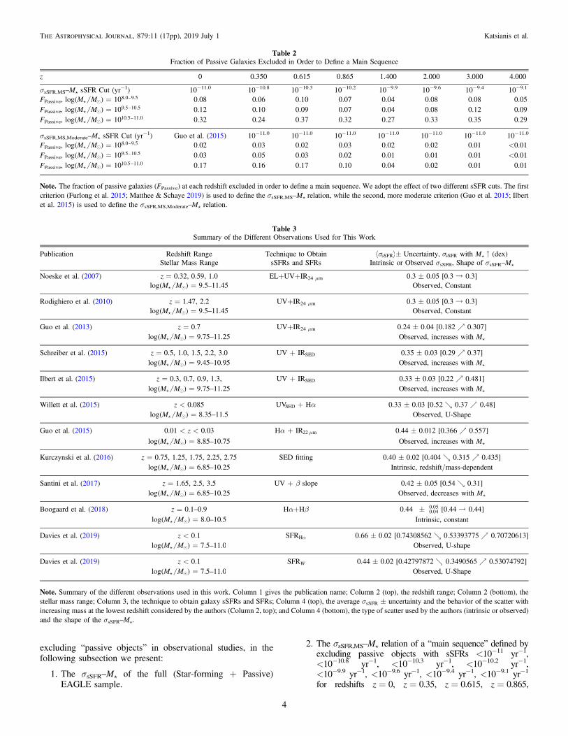
Table 2Fraction of Passive Galaxies Excluded in Order to Define a Main Sequence

z 0 0.350 0.615 0.865 1.400 2.000 3.000 4.000

σsSFR,MS–Må sSFR Cut (yr−1) 10−11.0 10−10.8 10−10.3 10−10.2 10−9.9 10−9.6 10−9.4 10−9.1

FPassive, M Mlog 108.0 9.5 =( ) – 0.08 0.06 0.10 0.07 0.04 0.08 0.08 0.05

FPassive, M Mlog 109.5 10.5 =( ) – 0.12 0.10 0.09 0.07 0.04 0.08 0.12 0.09

FPassive, M Mlog 1010.5 11.0 =( ) – 0.32 0.24 0.37 0.32 0.27 0.33 0.35 0.29

σsSFR,MS,Moderate–Må sSFR Cut (yr−1) Guo et al. (2015) 10−11.0 10−11.0 10−11.0 10−11.0 10−11.0 10−11.0 10−11.0

FPassive, M Mlog 108.0 9.5 =( ) – 0.02 0.03 0.02 0.03 0.02 0.02 0.01 <0.01

FPassive, M Mlog 109.5 10.5 =( ) – 0.03 0.05 0.03 0.02 0.01 0.01 0.01 <0.01

FPassive, M Mlog 1010.5 11.0 =( ) – 0.17 0.16 0.17 0.10 0.04 0.02 0.01 0.01

Note.The fraction of passive galaxies (FPassive) at each redshift excluded in order to define a main sequence. We adopt the effect of two different sSFR cuts. The firstcriterion (Furlong et al. 2015; Matthee & Schaye 2019) is used to define the σsSFR,MS–Må relation, while the second, more moderate criterion (Guo et al. 2015; Ilbertet al. 2015) is used to define the σsSFR,MS,Moderate–Må relation.

Table 3Summary of the Different Observations Used for This Work

Publication Redshift Range Technique to Obtain sSFRsá ñ±Uncertainty, sSFRs with Må(dex)Stellar Mass Range sSFRs and SFRs Intrinsic or Observed σsSFR, Shape of σsSFR–Må

Noeske et al. (2007) z=0.32, 0.59, 1.0 EL+UV+IR24 μm 0.3±0.05 [0.3 0.3]M Mlog 9.5 11.45 =( ) – Observed, Constant

Rodighiero et al. (2010) z=1.47, 2.2 UV+IR24 μm 0.3±0.05 [0.3 0.3]M Mlog 9.5 11.45 =( ) – Observed, Constant

Guo et al. (2013) z=0.7 UV+IR24 μm 0.24±0.04 [0.182 0.307]M Mlog 9.75 11.25 =( ) – Observed, increases with Må

Schreiber et al. (2015) z=0.5, 1.0, 1.5, 2.2, 3.0 UV IRSED+ 0.35±0.03 [0.29 0.37]M Mlog 9.45 10.95 =( ) – Observed, increases with Må

Ilbert et al. (2015) z=0.3, 0.7, 0.9, 1.3, UV IRSED+ 0.33±0.03 [0.22 0.481]M Mlog 9.75 11.25 =( ) – Observed, increases with Må

Willett et al. (2015) z<0.085 UV HSED a+ 0.33±0.03 [0.52 0.37 0.48]M Mlog 8.35 11.5 =( ) – Observed, U-Shape

Guo et al. (2015) 0.01<z<0.03 H IR22 ma + m 0.44±0.012 [0.366 0.557]M Mlog 8.85 10.75 =( ) – Observed, increases with Må

Kurczynski et al. (2016) z=0.75, 1.25, 1.75, 2.25, 2.75 SED fitting 0.40±0.02 [0.404 0.315 0.435]M Mlog 6.85 10.25 =( ) – Intrinsic, redshift/mass-dependent

Santini et al. (2017) z=1.65, 2.5, 3.5 UV + β slope 0.42±0.05 [0.54 0.31]M Mlog 6.85 10.25 =( ) – Observed, decreases with Må

Boogaard et al. (2018) z=0.1–0.9 Hα+Hβ 0.44 0.040.05 [0.44 0.44]

M Mlog 8.0 10.5 =( ) – Intrinsic, constant

Davies et al. (2019) z<0.1 SFRHa 0.66±0.02 [0.74308562 0.53393775 0.70720613]M Mlog 7.5 11.0 =( ) – Observed, U-shape

Davies et al. (2019) z<0.1 SFRW 0.44±0.02 [0.42797872 0.3490565 0.53074792]M Mlog 7.5 11.0 =( ) – Observed, U-Shape

Note.Summary of the different observations used in this work. Column 1 gives the publication name; Column 2 (top), the redshift range; Column 2 (bottom), thestellar mass range; Column 3, the technique to obtain galaxy sSFRs and SFRs; Column 4 (top), the average σsSFR±uncertainty and the behavior of the scatter withincreasing mass at the lowest redshift considered by the authors (Column 2, top); and Column 4 (bottom), the type of scatter used by the authors (intrinsic or observed)and the shape of the σsSFR–Må.

4

The Astrophysical Journal, 879:11 (17pp), 2019 July 1 Katsianis et al.

z=1.485, z=2.0, z=3.0, z=4.0, respectively (Furlonget al. 2015; Matthee & Schaye 2019).

3. The σsSFR,MS,Moderate–Må relation of a “main sequence”defined by more conservative sSFR cuts (that ensure amore complete SF sample at the expense of somepossible passive galaxy contamination) of < 10−11.0 yr−1

for z>0 and Mlog 10 sSFR 0.18 log 10 < ´ -( ) ( )4.5 Gyr 1- for z=0 (Guo et al. 2015; Ilbert et al. 2015).

The differences between observations used in this workin terms of assumed methodology to exclude (or include)quiescent objects is described in the previous paragraph andTable 2. The different data sets and methodologies to obtain SFRsfor the same studies are described below and in Table 3. Noeskeet al. (2007) used 2095 field galaxies from the All-wavelengthExtended Growth Strip International Survey (AEGIS) and derivedSFRs from emission lines, GALEX, Spitzer MIPS, and 24μmphotometry. Guo et al. (2013) used 12,614 objects from themultiwavelength data set of COSMOS, while SFRs are obtainedby combining 24μm and UV luminosities. Schreiber et al. (2015)used GOODS-North, GOODS-South, UDS, and COSMOSextragalactic fields, and derived SFRs using UV+FIR luminos-ities. Ilbert et al. (2015) based their analysis on a 24μm selectedcatalog combining the COSMOS and GOODS surveys. Theauthors estimated SFRs by combining mid- and far-infrared datafor 20,500 galaxies. Willett et al. (2015) used optical observationsin the SDSS DR7 survey, while stellar masses and star formationrates are computed from optical diagnostics and taken from theMPA-JHU catalog (Salim et al. 2007). Guo et al. (2015) usedSDSS Data Release 7, while SFRs are estimated from Hα incombination with 22μm observation from the Wide-field InfraredSurvey Explorer (WISE). Santini et al. (2017) used the HubbleSpace Telescope Frontier Fields, while SFRs are estimated fromobserved UV rest-frame photometry (Meurer et al. 1999;Kennicutt & Evans 2012). Davies et al. (2019) used 9005 galaxiesfrom the Galaxy And Mass Assembly (GAMA) survey (Driveret al. 2011, 2016b). The SFR indicators used are described atlength in Driver et al. (2016a). They include: (a) the SpectralEnergy Density (SED) fitting code magphys, (b) a combination ofUltraviolet and Total Infrared (UV+TIR), (c) the Hα emissionline, (d) the WISE W3-band (Cluver et al. 2017), and (e)extinction-corrected u-band luminosities derived using the GAMArest-frame u-band luminosity and u–g colors.

3.1. The Evolution of the σsSFR–Må, σsSFR,MS–Må, andσsSFR,MS,Moderate–Må Relations in the EAGLE Model

In Figure 1, we present the evolution of the σsSFR–Må, whichincludes both passive and star-forming objects (represented bythe red solid line), and the “main sequence” σsSFR,MS–Må

(represented by the black dotted line) and σsSFR,MS,Moderate–Må

(represented by the blue dashed line) relations in the EAGLEL100N1504-Ref at M Mlog 7.0 ~( ) to M Mlog 11.5 ~( )and compare them with observations. The two vertical dottedlines represent the mass resolution limit of 100 baryonicparticles ( M Mlog 8.25 ~( ) ) and the statistic limit wherethere are fewer than 10 galaxies at the low- and high-mass ends(Furlong et al. 2015; Katsianis et al. 2017a). The shadedregions represent the 95% bootstrap confidence interval for5000 resamples of the σsSFR–Må relation.

Starting from redshift z=4.0 (top left panel of Figure 1),we see that the σsSFR–Må of the reference model has aU-shaped form. The dispersion decreases with mass at the

M Mlog 8.5 9.5 ~( ) – interval from σsSFR=0.4 to 0.2 dex,while it increases with mass at the M Mlog 9.5 10.5 ~( ) –interval from σsSFR∼0.2 to 0.6 dex. For the “main sequence,”σsSFR,MS–Må relation, defined by the exclusion of objects with<10−9.1 yr−1 (Furlong et al. 2015; Matthee & Schaye 2019), thescatter increases more moderately at the high-mass end (from 0.2to 0.3 dex), because passive objects that would increase thedispersion are excluded using a sSFR cut. We note that thefraction of quiescent galaxies is expected to be small at this era,ergo the exclusion of quiescent objects should not significantlyaffect the relation (especially at the low-mass end), and it is verypossible that the above selection criterion is too strict. However, amore moderate cut of < 10−11.0 yr−1 (Ilbert et al. 2015) results ina relationship that is closer to that of the full EAGLE sample,because the exclusion of quenched objects is less severe. We notethat the observations of Santini et al. (2017) are broadly consistentwith the σsSFR,MS,moderate–Må (represented by the black dottedline) and σsSFR–Må (represented by the red solid line) relations(green filled circles representing the observations of Santini et al.(2017) within 0.1 dex with respect to the simulated results). Asimilar behavior is found for lower redshifts up to z∼2.0. This ispossibly due to the fact that the moderate sSFR cut of < 10−11.0

yr−1 (Ilbert et al. 2015) more closely resembles the selectionperformed by Schreiber et al. (2015) and Santini et al. (2017).At redshift z∼1.4 (middle left panel of Figure 1), we find

that there is an increment of scatter with mass for the EAGLEσsSFR–Må and σsSFR,MS,Moderate–Må relations at the high-massend ( M Mlog 9.5 11.0 ~( ) – ) from ∼0.2 dex to 0.45 and0.65 dex, respectively. On the other hand, the σsSFR,MS–Må

relation has an almost constant scatter of ∼0.2 dex with mass atM Mlog 10.0 11.0 ~( ) – . The observations for this mass

interval (Rodighiero et al. 2010; Guo et al. 2013; Ilbert et al.2015; Schreiber et al. 2015) typically lay between thetwo “main sequence” relations σsSFR,MS,Moderate–Må andσsSFR,MS–Må, something that may be related to the uncertain-ties of removing quiescent objects in the literature (Renzini &Peng 2015). The observations of Ilbert et al. (2015) andSchreiber et al. (2015) imply an increasing scatter with mass,while those of Noeske et al. (2007) and Rodighiero et al. (2010)imply a constant (∼0.3 dex). On the other hand, for the low-mass end ( M Mlog 8 9.5 ~( ) – ), the EAGLE reference modelindicates a decrement with mass, in agreement with Santiniet al. (2017). Similarly, at higher redshifts, the σsSFR–Må andσsSFR,MS,Moderate–Må relations have a U-shaped form. The samebehavior is found for lower redshifts up to z∼0.35, whichreflects the fact that both low- and high-mass galaxies have alarger scatter/diversity of star formation histories than Må

(characteristic mass) objects. For z∼0 (bottom right panelof Figure 1), the scatter is constant with mass for boththe σsSFR–Måand σsSFR,MS,Moderate–Må relations for the

M Mlog 8.5 9.5 ~( ) – interval at ∼0.4 dex. The scatterincreases to 0.9 dex for the high-mass end when both passiveand SFGs are included. The increment is more moderate whencuts similar to the ones of Guo et al. (2015) are applied. On theother hand, the scatter decreases with mass for the “mainsequence” σsSFR,MS–Må relation from 0.4 to 0.2 dex.We note that the EAGLE reference model suggests that both

σsSFR,MS,Moderate–Må and σsSFR,MS–Må relations are evolvingwith redshift and are not independent of time. In Figure 2, wepresent the evolution of the σsSFR,MS,Moderate at z∼0–4 forthe stellar masses of M Mlog 8.5 ~( ) (blue solid line),

M Mlog 9.5 ~( ) (black dotted line), and M Mlog ~( )

5

The Astrophysical Journal, 879:11 (17pp), 2019 July 1 Katsianis et al.

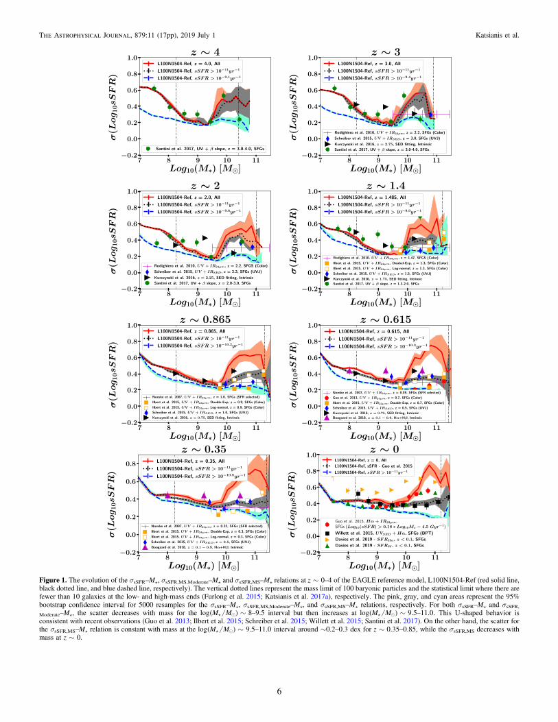
Figure 1. The evolution of the σsSFR–Må, σsSFR,MS,Moderate–Må and σsSFR,MS–Må relations at z∼0–4 of the EAGLE reference model, L100N1504-Ref (red solid line,black dotted line, and blue dashed line, respectively). The vertical dotted lines represent the mass limit of 100 baryonic particles and the statistical limit where there arefewer than 10 galaxies at the low- and high-mass ends (Furlong et al. 2015; Katsianis et al. 2017a), respectively. The pink, gray, and cyan areas represent the 95%bootstrap confidence interval for 5000 resamples for the σsSFR–Må, σsSFR,MS,Moderate–Må, and σsSFR,MS–Må relations, respectively. For both σsSFR–Må and σsSFR,Moderate–Må, the scatter decreases with mass for the M Mlog 8 9.5 ~( ) – interval but then increases at M Mlog 9.5 11.0 ~( ) – . This U-shaped behavior isconsistent with recent observations (Guo et al. 2013; Ilbert et al. 2015; Schreiber et al. 2015; Willett et al. 2015; Santini et al. 2017). On the other hand, the scatter forthe σsSFR,MS–Må relation is constant with mass at the M Mlog 9.5 11.0 ~( ) – interval around ∼0.2–0.3 dex for z∼0.35–0.85, while the σsSFR,MS decreases withmass at z ∼ 0.

6

The Astrophysical Journal, 879:11 (17pp), 2019 July 1 Katsianis et al.

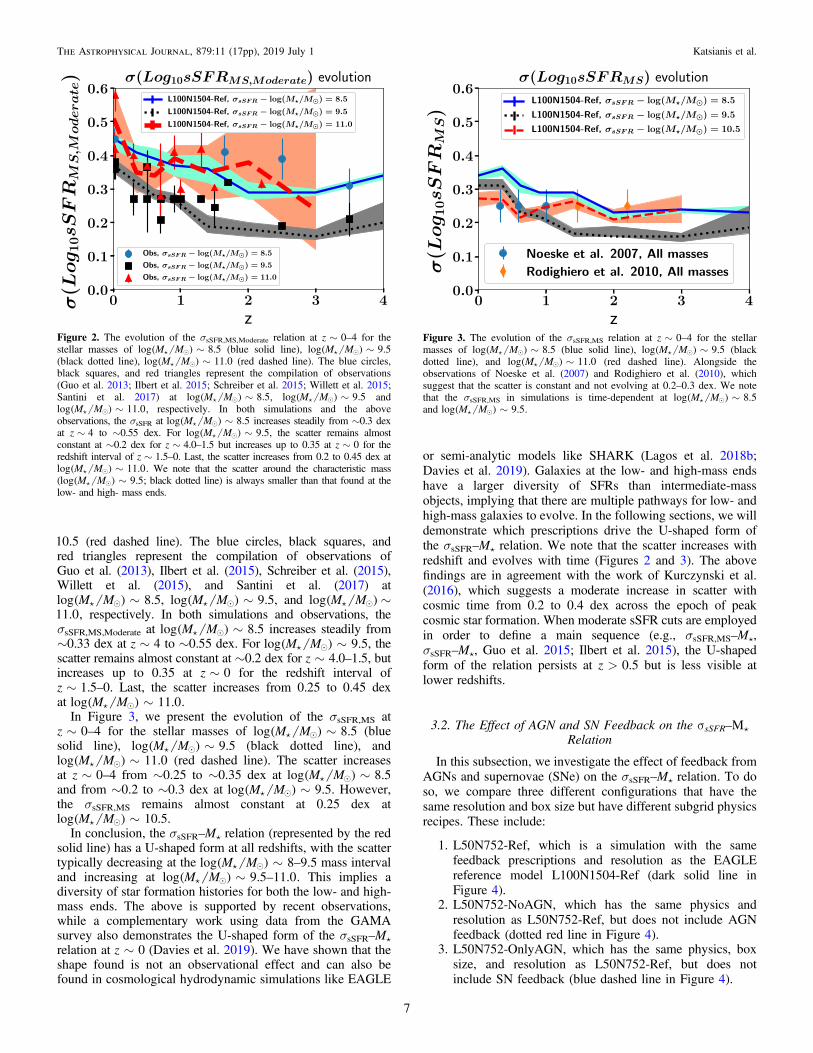
10.5 (red dashed line). The blue circles, black squares, andred triangles represent the compilation of observations ofGuo et al. (2013), Ilbert et al. (2015), Schreiber et al. (2015),Willett et al. (2015), and Santini et al. (2017) at

M Mlog 8.5 ~( ) , M Mlog 9.5 ~( ) , and M Mlog ~( )11.0, respectively. In both simulations and observations, theσsSFR,MS,Moderate at M Mlog 8.5 ~( ) increases steadily from∼0.33 dex at z∼4 to ∼0.55 dex. For M Mlog 9.5 ~( ) , thescatter remains almost constant at ∼0.2 dex for z∼4.0–1.5, butincreases up to 0.35 at z∼0 for the redshift interval ofz∼1.5–0. Last, the scatter increases from 0.25 to 0.45 dexat M Mlog 11.0 ~( ) .

In Figure 3, we present the evolution of the σsSFR,MS atz∼0–4 for the stellar masses of M Mlog 8.5 ~( ) (bluesolid line), M Mlog 9.5 ~( ) (black dotted line), and

M Mlog 11.0 ~( ) (red dashed line). The scatter increasesat z∼0–4 from ∼0.25 to ∼0.35 dex at M Mlog 8.5 ~( )and from ∼0.2 to ∼0.3 dex at M Mlog 9.5 ~( ) . However,the σsSFR,MS remains almost constant at 0.25 dex at

M Mlog 10.5 ~( ) .In conclusion, the σsSFR–Må relation (represented by the red

solid line) has a U-shaped form at all redshifts, with the scattertypically decreasing at the M Mlog 8 9.5 ~( ) – mass intervaland increasing at M Mlog 9.5 11.0 ~( ) – . This implies adiversity of star formation histories for both the low- and high-mass ends. The above is supported by recent observations,while a complementary work using data from the GAMAsurvey also demonstrates the U-shaped form of the σsSFR–Må

relation at z∼0 (Davies et al. 2019). We have shown that theshape found is not an observational effect and can also befound in cosmological hydrodynamic simulations like EAGLE

or semi-analytic models like SHARK (Lagos et al. 2018b;Davies et al. 2019). Galaxies at the low- and high-mass endshave a larger diversity of SFRs than intermediate-massobjects, implying that there are multiple pathways for low- andhigh-mass galaxies to evolve. In the following sections, we willdemonstrate which prescriptions drive the U-shaped form ofthe σsSFR–Må relation. We note that the scatter increases withredshift and evolves with time (Figures 2 and 3). The abovefindings are in agreement with the work of Kurczynski et al.(2016), which suggests a moderate increase in scatter withcosmic time from 0.2 to 0.4 dex across the epoch of peakcosmic star formation. When moderate sSFR cuts are employedin order to define a main sequence (e.g., σsSFR,MS–Må,σsSFR–Må, Guo et al. 2015; Ilbert et al. 2015), the U-shapedform of the relation persists at z>0.5 but is less visible atlower redshifts.

3.2. The Effect of AGN and SN Feedback on the σsSFR–Må

Relation

In this subsection, we investigate the effect of feedback fromAGNs and supernovae (SNe) on the σsSFR–Må relation. To doso, we compare three different configurations that have thesame resolution and box size but have different subgrid physicsrecipes. These include:

1. L50N752-Ref, which is a simulation with the samefeedback prescriptions and resolution as the EAGLEreference model L100N1504-Ref (dark solid line inFigure 4).

2. L50N752-NoAGN, which has the same physics andresolution as L50N752-Ref, but does not include AGNfeedback (dotted red line in Figure 4).

3. L50N752-OnlyAGN, which has the same physics, boxsize, and resolution as L50N752-Ref, but does notinclude SN feedback (blue dashed line in Figure 4).

Figure 2. The evolution of the σsSFR,MS,Moderate relation at z∼0–4 for thestellar masses of M Mlog 8.5 ~( ) (blue solid line), M Mlog 9.5 ~( )(black dotted line), M Mlog 11.0 ~( ) (red dashed line). The blue circles,black squares, and red triangles represent the compilation of observations(Guo et al. 2013; Ilbert et al. 2015; Schreiber et al. 2015; Willett et al. 2015;Santini et al. 2017) at M Mlog 8.5 ~( ) , M Mlog 9.5 ~( ) and

M Mlog 11.0 ~( ) , respectively. In both simulations and the aboveobservations, the σsSFR at M Mlog 8.5 ~( ) increases steadily from ∼0.3 dexat z∼4 to ∼0.55 dex. For M Mlog 9.5 ~( ) , the scatter remains almostconstant at ∼0.2 dex for z∼4.0–1.5 but increases up to 0.35 at z∼0 for theredshift interval of z∼1.5–0. Last, the scatter increases from 0.2 to 0.45 dex at

M Mlog 11.0 ~( ) . We note that the scatter around the characteristic mass( M Mlog 9.5 ~( ) ; black dotted line) is always smaller than that found at thelow- and high- mass ends.

Figure 3. The evolution of the σsSFR,MS relation at z∼0–4 for the stellarmasses of M Mlog 8.5 ~( ) (blue solid line), M Mlog 9.5 ~( ) (blackdotted line), and M Mlog 11.0 ~( ) (red dashed line). Alongside theobservations of Noeske et al. (2007) and Rodighiero et al. (2010), whichsuggest that the scatter is constant and not evolving at 0.2–0.3 dex. We notethat the σsSFR,MS in simulations is time-dependent at M Mlog 8.5 ~( )and M Mlog 9.5 ~( ) .

7

The Astrophysical Journal, 879:11 (17pp), 2019 July 1 Katsianis et al.

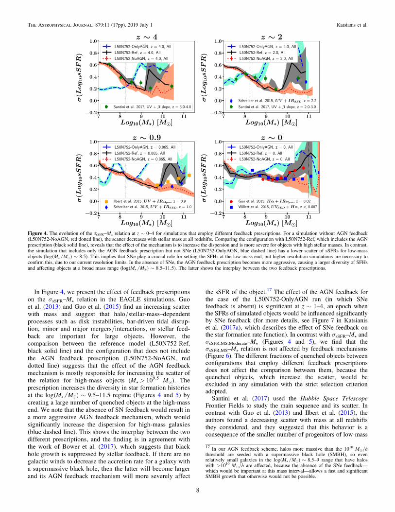
In Figure 4, we present the effect of feedback prescriptionson the σsSFR–Må relation in the EAGLE simulations. Guoet al. (2013) and Guo et al. (2015) find an increasing scatterwith mass and suggest that halo/stellar-mass–dependentprocesses such as disk instabilities, bar-driven tidal disrup-tion, minor and major mergers/interactions, or stellar feed-back are important for large objects. However, thecomparison between the reference model (L50N752-Ref,black solid line) and the configuration that does not includethe AGN feedback prescription (L50N752-NoAGN, reddotted line) suggests that the effect of the AGN feedbackmechanism is mostly responsible for increasing the scatter ofthe relation for high-mass objects (Må> 109.5 Me). Theprescription increases the diversity in star formation historiesat the M Mlog 9.5 11.5 ~( ) – regime (Figures 4 and 5) bycreating a large number of quenched objects at the high-massend. We note that the absence of SN feedback would result ina more aggressive AGN feedback mechanism, which wouldsignificantly increase the dispersion for high-mass galaxies(blue dashed line). This shows the interplay between the twodifferent prescriptions, and the finding is in agreement withthe work of Bower et al. (2017), which suggests that blackhole growth is suppressed by stellar feedback. If there are nogalactic winds to decrease the accretion rate for a galaxy witha supermassive black hole, then the latter will become largerand its AGN feedback mechanism will more severely affect

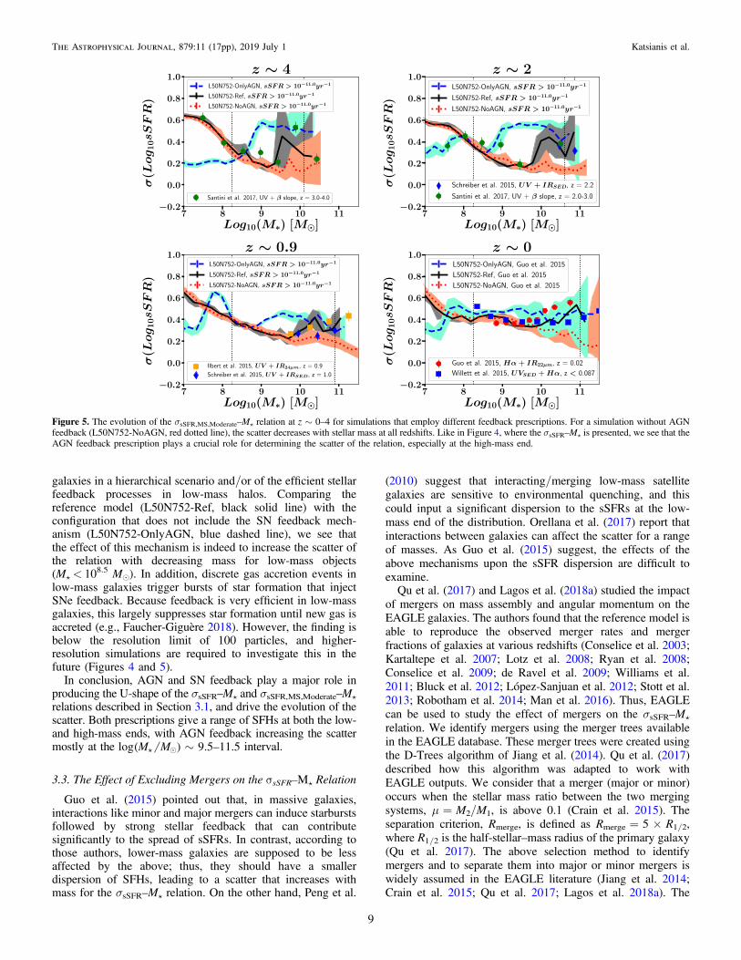
the sSFR of the object.17 The effect of the AGN feedback forthe case of the L50N752-OnlyAGN run (in which SNefeedback is absent) is significant at z∼1–4, an epoch whenthe SFRs of simulated objects would be influenced significantlyby SNe feedback (for more details, see Figure7 in Katsianiset al. (2017a), which describes the effect of SNe feedback onthe star formation rate function). In contrast with σsSFR–Må andσsSFR,MS,Moderate–Må (Figures 4 and 5), we find that theσsSFR,MS–Må relation is not affected by feedback mechanisms(Figure 6). The different fractions of quenched objects betweenconfigurations that employ different feedback prescriptionsdoes not affect the comparison between them, because thequenched objects, which increase the scatter, would beexcluded in any simulation with the strict selection criterionadopted.Santini et al. (2017) used the Hubble Space Telescope

Frontier Fields to study the main sequence and its scatter. Incontrast with Guo et al. (2013) and Ilbert et al. (2015), theauthors found a decreasing scatter with mass at all redshiftsthey considered, and they suggested that this behavior is aconsequence of the smaller number of progenitors of low-mass

Figure 4. The evolution of the sSFRs –Må relation at z∼0–4 for simulations that employ different feedback prescriptions. For a simulation without AGN feedback(L50N752-NoAGN, red dotted line), the scatter decreases with stellar mass at all redshifts. Comparing the configuration with L50N752-Ref, which includes the AGNprescription (black solid line), reveals that the effect of the mechanism is to increase the dispersion and is more severe for objects with high stellar masses. In contrast,the simulation that includes only the AGN feedback prescription but not SNe (L50N752-OnlyAGN, blue dashed line) has a lower scatter of sSFRs for low-massobjects ( M Mlog 8.5 ~( ) ). This implies that SNe play a crucial role for setting the SFHs at the low-mass end, but higher-resolution simulations are necessary toconfirm this, due to our current resolution limits. In the absence of SNe, the AGN feedback prescription becomes more aggressive, causing a larger diversity of SFHsand affecting objects at a broad mass range ( M Mlog 8.5 11.5 ~( ) – ). The latter shows the interplay between the two feedback prescriptions.

17 In our AGN feedback scheme, halos more massive than the 1010 Me/hthreshold are seeded with a supermassive black hole (SMBH), so evenrelatively small galaxies in the M Mlog 8.5 9 ~( ) – range that have haloswith >1010 Me/h are affected, because the absence of the SNe feedback—which would be important at this mass interval—allows a fast and significantSMBH growth that otherwise would not be possible.

8

The Astrophysical Journal, 879:11 (17pp), 2019 July 1 Katsianis et al.

galaxies in a hierarchical scenario and/or of the efficient stellarfeedback processes in low-mass halos. Comparing thereference model (L50N752-Ref, black solid line) with theconfiguration that does not include the SN feedback mech-anism (L50N752-OnlyAGN, blue dashed line), we see thatthe effect of this mechanism is indeed to increase the scatter ofthe relation with decreasing mass for low-mass objects(Må< 108.5 Me). In addition, discrete gas accretion events inlow-mass galaxies trigger bursts of star formation that injectSNe feedback. Because feedback is very efficient in low-massgalaxies, this largely suppresses star formation until new gas isaccreted (e.g., Faucher-Giguère 2018). However, the finding isbelow the resolution limit of 100 particles, and higher-resolution simulations are required to investigate this in thefuture (Figures 4 and 5).

In conclusion, AGN and SN feedback play a major role inproducing the U-shape of the σsSFR–Må and σsSFR,MS,Moderate–Må

relations described in Section 3.1, and drive the evolution of thescatter. Both prescriptions give a range of SFHs at both the low-and high-mass ends, with AGN feedback increasing the scattermostly at the M Mlog 9.5 11.5 ~( ) – interval.

3.3. The Effect of Excluding Mergers on the σsSFR–Må Relation

Guo et al. (2015) pointed out that, in massive galaxies,interactions like minor and major mergers can induce starburstsfollowed by strong stellar feedback that can contributesignificantly to the spread of sSFRs. In contrast, according tothose authors, lower-mass galaxies are supposed to be lessaffected by the above; thus, they should have a smallerdispersion of SFHs, leading to a scatter that increases withmass for the σsSFR–Må relation. On the other hand, Peng et al.

(2010) suggest that interacting/merging low-mass satellitegalaxies are sensitive to environmental quenching, and thiscould input a significant dispersion to the sSFRs at the low-mass end of the distribution. Orellana et al. (2017) report thatinteractions between galaxies can affect the scatter for a rangeof masses. As Guo et al. (2015) suggest, the effects of theabove mechanisms upon the sSFR dispersion are difficult toexamine.Qu et al. (2017) and Lagos et al. (2018a) studied the impact

of mergers on mass assembly and angular momentum on theEAGLE galaxies. The authors found that the reference model isable to reproduce the observed merger rates and mergerfractions of galaxies at various redshifts (Conselice et al. 2003;Kartaltepe et al. 2007; Lotz et al. 2008; Ryan et al. 2008;Conselice et al. 2009; de Ravel et al. 2009; Williams et al.2011; Bluck et al. 2012; López-Sanjuan et al. 2012; Stott et al.2013; Robotham et al. 2014; Man et al. 2016). Thus, EAGLEcan be used to study the effect of mergers on the σsSFR–Må

relation. We identify mergers using the merger trees availablein the EAGLE database. These merger trees were created usingthe D-Trees algorithm of Jiang et al. (2014). Qu et al. (2017)described how this algorithm was adapted to work withEAGLE outputs. We consider that a merger (major or minor)occurs when the stellar mass ratio between the two mergingsystems, μ=M2/M1, is above 0.1 (Crain et al. 2015). Theseparation criterion, Rmerge, is defined as Rmerge=5×R1/2,where R1/2 is the half-stellar–mass radius of the primary galaxy(Qu et al. 2017). The above selection method to identifymergers and to separate them into major or minor mergers iswidely assumed in the EAGLE literature (Jiang et al. 2014;Crain et al. 2015; Qu et al. 2017; Lagos et al. 2018a). The

Figure 5. The evolution of the σsSFR,MS,Moderate–Må relation at z∼0–4 for simulations that employ different feedback prescriptions. For a simulation without AGNfeedback (L50N752-NoAGN, red dotted line), the scatter decreases with stellar mass at all redshifts. Like in Figure 4, where the σsSFR–Må is presented, we see that theAGN feedback prescription plays a crucial role for determining the scatter of the relation, especially at the high-mass end.

9

The Astrophysical Journal, 879:11 (17pp), 2019 July 1 Katsianis et al.

fraction of mergers in the reference model at z∼0 increasestoward higher masses (Lagos et al. 2018a). Thus, it would beexpected that the mechanism affects mostly the SFHs of high-mass objects (Guo et al. 2015).

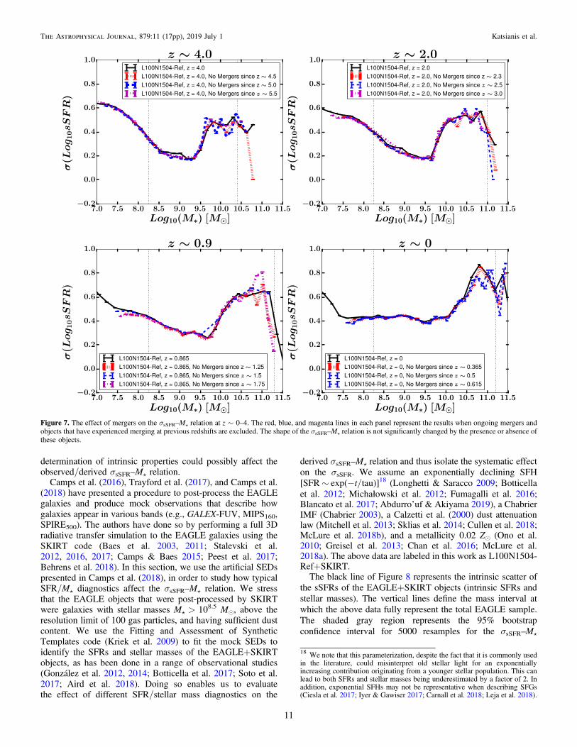
In Figure 7, we present the effect of mergers on theσsSFR–Må relation in the EAGLE simulations at z∼0–4. In thebottom panel, the black line represents the reference model atz∼0, in which all galaxies are considered. The red dotted linerepresents the same but when ongoing mergers and objects thathave experienced merging from z∼0.365 are not included inthe analysis. The blue dashed line describes the results whenobjects that have experienced merging from z∼0.5 areexcluded. The magenta represents the same when galaxies thathave experienced merging from z∼0.615 are excluded. Theabove analysis allows us to quantify the effect of ongoing (atz= 0), ongoing + recent (z∼ 0–0.35), and ongoing + recent +past (z∼ 0–0.65) mergers to the σsSFR–Må relation, and hasbeen done similarly for z∼0, 0.9, 2, and 4. We see that,according to the reference model, mergers do not induce asignificant dispersion in the star formation histories of galaxies.The above findings can be seen at all redshifts considered. Thisimplies that recent mergers, despite their importance for galaxyformation and evolution, do not impart a significant scatter onthe σsSFR–Må relation.

4. The Effect of SFR and Stellar Mass Diagnostics on theσsSFR–Må Relation

vTo obtain the intrinsic properties of galaxies, observershave to rely on models for the observed light. Stellar masses aretypically calculated via the SED fitting technique, whiledifferent authors employ different methods to calculate SFRs:e.g., conversion of IR+UV luminosities to SFRs (Arnouts et al.2013; Whitaker et al. 2014); SED fitting (Bruzual &Charlot 2003); or conversion of UV, Hα, and IR luminosities(Katsianis et al. 2017a)). However, there is an increasingnumber of reports that different techniques give differentresults, most likely due to systematic effects affecting thederived properties (Bauer et al. 2011; Fumagalli et al. 2014;Utomo et al. 2014; Davies et al. 2016, 2017; Katsianis et al.2016). Boquien et al. (2014) argue that SFRs obtained fromSED modeling, which take into account only FUV and Ubands, are overestimated. Hayward et al. (2014) note that theSFRs obtained from IR luminosities (e.g., Noeske et al. 2007;Daddi et al. 2007b) can be artificially high. Ilbert et al. (2015)compared SFRs derived from SED and UV+IR, and find atension reaching 0.25 dex. Guo et al. (2015) suggest that sSFRbased on mid-IR emission may be significantly overestimated(Salim et al. 2009; Chang et al. 2015; Katsianis et al.2017a, 2017b). All the above uncertainties on the

Figure 6. The evolution of the σsSFR,MS–Må relation at z∼0–4 for simulations that employ different feedback prescriptions (L50N752-OnlyAGN is represented by ablue dashed line, L50N752-Ref by a black solid line, and L50N752-NoAGN by a red dashed line). The exclusion of passive objects is severe, and objects, affected bythe AGN feedback prescription are not taken into account. Thus, when quenched objects are excluded from the analysis the mechanism does not make its imprint uponthe σsSFR,MS–Må relation, with the difference between the three different configurations being small.

10

The Astrophysical Journal, 879:11 (17pp), 2019 July 1 Katsianis et al.

determination of intrinsic properties could possibly affect theobserved/derived σsSFR–Må relation.

Camps et al. (2016), Trayford et al. (2017), and Camps et al.(2018) have presented a procedure to post-process the EAGLEgalaxies and produce mock observations that describe howgalaxies appear in various bands (e.g., GALEX-FUV, MIPS160,SPIRE500). The authors have done so by performing a full 3Dradiative transfer simulation to the EAGLE galaxies using theSKIRT code (Baes et al. 2003, 2011; Stalevski et al.2012, 2016, 2017; Camps & Baes 2015; Peest et al. 2017;Behrens et al. 2018). In this section, we use the artificial SEDspresented in Camps et al. (2018), in order to study how typicalSFR/Må diagnostics affect the σsSFR–Må relation. We stressthat the EAGLE objects that were post-processed by SKIRTwere galaxies with stellar masses Må>108.5 Me, above theresolution limit of 100 gas particles, and having sufficient dustcontent. We use the Fitting and Assessment of SyntheticTemplates code (Kriek et al. 2009) to fit the mock SEDs toidentify the SFRs and stellar masses of the EAGLE+SKIRTobjects, as has been done in a range of observational studies(González et al. 2012, 2014; Botticella et al. 2017; Soto et al.2017; Aird et al. 2018). Doing so enables us to evaluatethe effect of different SFR/stellar mass diagnostics on the

derived σsSFR–Må relation and thus isolate the systematic effecton the σsSFR. We assume an exponentially declining SFH[SFR∼ exp(−t/tau)]18 (Longhetti & Saracco 2009; Botticellaet al. 2012; Michałowski et al. 2012; Fumagalli et al. 2016;Blancato et al. 2017; Abdurro’uf & Akiyama 2019), a ChabrierIMF (Chabrier 2003), a Calzetti et al. (2000) dust attenuationlaw (Mitchell et al. 2013; Sklias et al. 2014; Cullen et al. 2018;McLure et al. 2018b), and a metallicity 0.02 Ze (Ono et al.2010; Greisel et al. 2013; Chan et al. 2016; McLure et al.2018a). The above data are labeled in this work as L100N1504-Ref+SKIRT.The black line of Figure 8 represents the intrinsic scatter of

the sSFRs of the EAGLE+SKIRT objects (intrinsic SFRs andstellar masses). The vertical lines define the mass interval atwhich the above data fully represent the total EAGLE sample.The shaded gray region represents the 95% bootstrapconfidence interval for 5000 resamples for the σsSFR–Må

Figure 7. The effect of mergers on the σsSFR–Må relation at z∼0–4. The red, blue, and magenta lines in each panel represent the results when ongoing mergers andobjects that have experienced merging at previous redshifts are excluded. The shape of the σsSFR–Må relation is not significantly changed by the presence or absence ofthese objects.

18 We note that this parameterization, despite the fact that it is commonly usedin the literature, could misinterpret old stellar light for an exponentiallyincreasing contribution originating from a younger stellar population. This canlead to both SFRs and stellar masses being underestimated by a factor of 2. Inaddition, exponential SFHs may not be representative when describing SFGs(Ciesla et al. 2017; Iyer & Gawiser 2017; Carnall et al. 2018; Leja et al. 2018).

11

The Astrophysical Journal, 879:11 (17pp), 2019 July 1 Katsianis et al.

relation. For clarity, we present the above only for the referencemodel. The main results are the following:

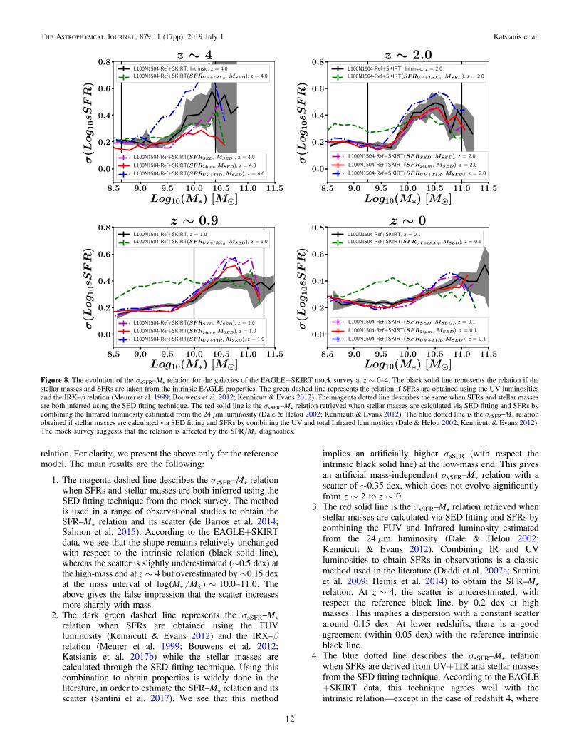
1. The magenta dashed line describes the σsSFR–Må relationwhen SFRs and stellar masses are both inferred using theSED fitting technique from the mock survey. The methodis used in a range of observational studies to obtain theSFR–Må relation and its scatter (de Barros et al. 2014;Salmon et al. 2015). According to the EAGLE+SKIRTdata, we see that the shape remains relatively unchangedwith respect to the intrinsic relation (black solid line),whereas the scatter is slightly underestimated (∼0.5 dex) atthe high-mass end at z∼4 but overestimated by∼0.15 dexat the mass interval of M Mlog 10.0 11.0 ~( ) – . Theabove gives the false impression that the scatter increasesmore sharply with mass.

2. The dark green dashed line represents the σsSFR–Må

relation when SFRs are obtained using the FUVluminosity (Kennicutt & Evans 2012) and the IRX–βrelation (Meurer et al. 1999; Bouwens et al. 2012;Katsianis et al. 2017b) while the stellar masses arecalculated through the SED fitting technique. Using thiscombination to obtain properties is widely done in theliterature, in order to estimate the SFR–Må relation and itsscatter (Santini et al. 2017). We see that this method

implies an artificially higher σsSFR (with respect theintrinsic black solid line) at the low-mass end. This givesan artificial mass-independent σsSFR–Må relation with ascatter of ∼0.35 dex, which does not evolve significantlyfrom z∼2 to z∼0.

3. The red solid line is the σsSFR–Må relation retrieved whenstellar masses are calculated via SED fitting and SFRs bycombining the FUV and Infrared luminosity estimatedfrom the 24 μm luminosity (Dale & Helou 2002;Kennicutt & Evans 2012). Combining IR and UVluminosities to obtain SFRs in observations is a classicmethod used in the literature (Daddi et al. 2007a; Santiniet al. 2009; Heinis et al. 2014) to obtain the SFR–Må

relation. At z∼4, the scatter is underestimated, withrespect the reference black line, by 0.2 dex at highmasses. This implies a dispersion with a constant scatteraround 0.15 dex. At lower redshifts, there is a goodagreement (within 0.05 dex) with the reference intrinsicblack line.

4. The blue dotted line describes the σsSFR–Må relationwhen SFRs are derived from UV+TIR and stellar massesfrom the SED fitting technique. According to the EAGLE+SKIRT data, this technique agrees well with theintrinsic relation—except in the case of redshift 4, where

Figure 8. The evolution of the σsSFR–Må relation for the galaxies of the EAGLE+SKIRT mock survey at z∼0–4. The black solid line represents the relation if thestellar masses and SFRs are taken from the intrinsic EAGLE properties. The green dashed line represents the relation if SFRs are obtained using the UV luminositiesand the IRX–β relation (Meurer et al. 1999; Bouwens et al. 2012; Kennicutt & Evans 2012). The magenta dotted line describes the same when SFRs and stellar massesare both inferred using the SED fitting technique. The red solid line is the σsSFR–Må relation retrieved when stellar masses are calculated via SED fitting and SFRs bycombining the Infrared luminosity estimated from the 24 μm luminosity (Dale & Helou 2002; Kennicutt & Evans 2012). The blue dotted line is the σsSFR–Må relationobtained if stellar masses are calculated via SED fitting and SFRs by combining the UV and total Infrared luminosities (Dale & Helou 2002; Kennicutt & Evans 2012).The mock survey suggests that the relation is affected by the SFR/Må diagnostics.

12

The Astrophysical Journal, 879:11 (17pp), 2019 July 1 Katsianis et al.

the derived relation is mass-independent with a scatterof 0.2 dex. The scatter of the magenta line, whichrepresents the results from SED fitting, is similarlyoverestimated (by 0.15 dex) with respect to the referenceblack line, for high-mass objects at the mass interval of

M Mlog 10.0 11.0 ~( ) – at z∼0.9.

In conclusion, according to the EAGLE+SKIRT data, theinferred shape and normalization of the σsSFR–Må relation canbe affected by the methodology used to derive SFRs and stellarmasses in observations. This can affect conclusions about itsshape, and it is important for future observations to investigatethis further (Davies et al. 2019). However, we note that havingaccess to IR data and deriving SFRs and stellar masses fromSED fitting or combined UV+IR luminosities typically gives aσsSFR–Må relation close to the intrinsic simulated relation,and can successfully probe the shape of the relationfor M Mlog 9.0 11.0 ~( ) – .

5. Conclusion and Discussion

The σsSFR–Må relation reflects the diversity of star formationhistories for galaxies at different masses. However, it is difficultto decipher the true shape of the relation, the intrinsic value ofthe scatter, and which mechanisms important for galaxyevolution govern it, if solely relying on observations. In thispaper, we have presented the evolution of the intrinsicσsSFR–Må relation employing the EAGLE suite of cosmologicalsimulations and a compilation of multiwavelength observationsat various redshifts. We deem the EAGLE suite appropriate forthis study, as it is able to reproduce the observed star formationrate and stellar mass functions (Furlong et al. 2015; Katsianiset al. 2017a) for a wide range of SFRs, stellar masses, andredshifts. The investigation is not limited by the shortcomingsencountered by galaxy surveys and addresses a range ofredshifts and mass intervals. Our main conclusions aresummarized as follows:

1. In agreement with recent observational studies (Guo et al.2013; Ilbert et al. 2015; Willett et al. 2015; Santini et al.2017), the EAGLE reference model suggests that theσsSFR–Må relation is evolving with redshift and thedispersion is mass-dependent (Section 3.1). This is incontrast with the widely accepted notion that thedispersion is independent of mass/redshift, with aconstant scatter σsSFR∼0.2–0.3 (Elbaz et al. 2007;Noeske et al. 2007; Rodighiero et al. 2010; Whitakeret al. 2012). We find that the σsSFR–Må relation has aU-shaped form, with the scatter increasing both at thehigh- and low-mass ends. Any interpretations of anincreasing (Guo et al. 2013; Ilbert et al. 2015) ordecreasing dispersion (Santini et al. 2017) with mass maybe misguided, because they usually focus on limited massintervals (Section 3.2). The finding about the U-shapedform of the relation is supported by results relying on theGAMA survey (Davies et al. 2019) at z∼0.

2. AGN and SN feedback drive the shape and evolution ofthe σsSFR–Må relation in the simulations (Section 3.2).Both mechanisms cause a diversity of star formationhistories for low-mass (SN feedback) and high-massgalaxies (AGN feedback).

3. Mergers do not play a major role in the shape of theσsSFR–Må relation (Section 3.3).

4. We employ the EAGLE/SKIRT mock data to investigatehow different SFR/Må diagnostics affect the σsSFR–Må

relation. The shape of the relation remains relativelyunchanged if both the SFRs and stellar masses areinferred through SED fitting or combined UV+IR data.However, SFRs that rely solely on UV data and the IRX–β relation for dust corrections imply a constant scatterwith stellar mass with almost no redshift evolution. Themethodology used to derive SFRs and stellar masses canaffect the inferred σsSFR–Må relation in observations, andthus compromise the robustness of conclusions about itsshape and normalization.

We would like to thank the anonymous referee forsuggestions and comments that significantly improved ourmanuscript. In addition, we would like to thank Jorryt Mattheefor discussions and suggestions. This work used the DiRACData Centric system at Durham University, operated by theInstitute for Computational Cosmology on behalf of the STFCDiRAC HPC Facility (www.dirac.ac.uk). A.K. has beensupported by the Tsung-Dao Lee Institute Fellowship,Shanghai Jiao Tong University and CONICYT/FONDECYTfellowship, project number: 3160049. G.B. is supportedby CONICYT/FONDECYT, Programa de Iniciacion, Folio11150220. V.G. was supported by CONICYT/FONDECYTiniciation grant number 11160832. X.Z.Z. is thankful forsupport from the National Key Research and DevelopmentProgram of China (2017YFA0402703), NSFC grant (11773076),and the Chinese Academy of Sciences (CAS) through a grant tothe CAS South America Center for Astronomy (CASSACA) inSantiago, Chile. M.S. acknowledges support by the Ministry ofEducation, Science, and Technological Development of theRepublic of Serbia through the projects Astrophysical Spectrosc-opy of Extragalactic Objects (176001) and Gravitation and theLarge Scale Structure of the Universe (176003). A.K. would liketo thank his family and especially George Katsianis, AggelikiSpyropoulou John Katsianis, and Nefeli Siouti for emotionalsupport. He would also like to thank Sophia Savvidou for her ITassistance.

AppendixThe Evolution of the sSFRF

In this appendix, we base our analysis of the dispersion ofthe sSFRs at different mass intervals on their distribution/histogram, namely the sSFRF, following Ilbert et al. (2015),because studies of the dispersion that rely solely on 2D scatterplots (i.e., displays of the location of the individual sources inthe plane) are unable to provide quantitative informationregarding how galaxies are distributed around the mean sSFRand cannot account for galaxies that could be undersampled ormissed by selection effects. In Section 3.1, we present theevolution of the σsSFR–Må relation at z∼0–4 in order tovisualize the scatter across galaxies, its shape, and its evolution.We present the distribution of the sSFR of the EAGLEreference model (L100N1504-Ref) and compare it withobservations (Ilbert et al. 2015) in Figure 9 (z∼ 0.8–1.4) andFigure 10 (z∼ 0.2–0.6). The EAGLE SFRs are reported to be0.2 dex lower than observations, but are able to replicate theobserved evolution and shape of the cosmic star formationrate density (Furlong et al. 2015; Katsianis et al. 2017a), theevolution of the star formation rate function (Katsianis et al.

13

The Astrophysical Journal, 879:11 (17pp), 2019 July 1 Katsianis et al.

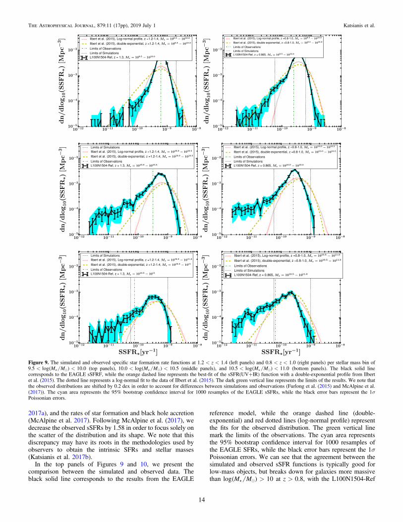
2017a), and the rates of star formation and black hole accretion(McAlpine et al. 2017). Following McAlpine et al. (2017), wedecrease the observed sSFRs by 1.58 in order to focus solely onthe scatter of the distribution and its shape. We note that thisdiscrepancy may have its roots in the methodologies used byobservers to obtain the intrinsic SFRs and stellar masses(Katsianis et al. 2017b).

In the top panels of Figures 9 and 10, we present thecomparison between the simulated and observed data. Theblack solid line corresponds to the results from the EAGLE

reference model, while the orange dashed line (double-exponential) and red dotted lines (log-normal profile) representthe fits for the observed distribution. The green vertical linemark the limits of the observations. The cyan area representsthe 95% bootstrap confidence interval for 1000 resamples ofthe EAGLE SFRs, while the black error bars represent the 1σPoissonian errors. We can see that the agreement between thesimulated and observed sSFR functions is typically good forlow-mass objects, but breaks down for galaxies more massivethan M Mlog 10 >( ) at z>0.8, with the L100N1504-Ref

Figure 9. The simulated and observed specific star formation rate functions at 1.2<z<1.4 (left panels) and 0.8<z<1.0 (right panels) per stellar mass bin ofM M9.5 log 10.0< <( ) (top panels), M M10.0 log 10.5< <( ) (middle panels), and M M10.5 log 11.0< <( ) (bottom panels). The black solid line

corresponds to the EAGLE sSFRF, while the orange dashed line represents the best-fit of the sSFR(UV+IR) function with a double-exponential profile from Ilbertet al. (2015). The dotted line represents a log-normal fit to the data of Ilbert et al. (2015). The dark green vertical line represents the limits of the results. We note thatthe observed distributions are shifted by 0.2 dex in order to account for differences between simulations and observations (Furlong et al. (2015) and McAlpine et al.(2017)). The cyan area represents the 95% bootstrap confidence interval for 1000 resamples of the EAGLE sSFRs, while the black error bars represent the 1σPoissonian errors.

14

The Astrophysical Journal, 879:11 (17pp), 2019 July 1 Katsianis et al.

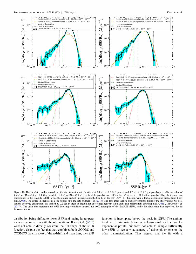
distribution being shifted to lower sSFR and having larger peakvalues in comparison with the observations. Ilbert et al. (2015)were not able to directly constrain the full shape of the sSFRfunction, despite the fact that they combined both GOODS andCOSMOS data. In most of the redshift and mass bins, the sSFR

function is incomplete below the peak in sSFR. The authorstried to discriminate between a log-normal and a double-exponential profile, but were not able to sample sufficientlylow sSFR to see any advantage of using either one or theother parameterization. They argued that the fit with a

Figure 10. The simulated and observed specific star formation rate functions at 0.4<z<0.6 (left panels) and 0.2<z<0.4 (right panels) per stellar mass bin ofM M9.5 log 10.0< <( ) (top panels), M M10.0 log 10.5< <( ) (middle panels), and M M10.5 log 11.0< <( ) (bottom panels). The black solid line

corresponds to the EAGLE sSFRF, while the orange dashed line represents the best-fit of the sSFR(UV+IR) function with a double-exponential profile from Ilbertet al. (2015). The dotted line represents a log-normal fit to the data of Ilbert et al. (2015). The dark green vertical line represents the limits of the observations. We notethat the observed distributions are shifted by 0.2 dex in order to account for differences between simulations and observations (Furlong et al. (2015), McAlpine et al.(2017)). The cyan area represents the 95% bootstrap confidence interval for 1000 resamples of the EAGLE sSFRs, while the black error bars represent the 1σPoissonian errors.

15

The Astrophysical Journal, 879:11 (17pp), 2019 July 1 Katsianis et al.

double-exponential function is more suitable than the log-normal function at z∼0. The EAGLE reference modelindicates that the sSFRF of the different mass bins andredshifts follows a double-exponential function. However, forhigher redshifts, the simulated distributions are slightly flatterthan the double-exponential fits of the observations. A double-exponential profile, which is not commonly used to describethe sSFR distribution (Ilbert et al. 2015), allows a significantdensity of SFGs with a low sSFR, and the confirmation of thisshape in future observations is important.

ORCID iDs

Xianzhong Zheng https://orcid.org/0000-0003-3728-9912Valentino Gonzalez https://orcid.org/0000-0002-3120-0510Peter Camps https://orcid.org/0000-0002-4479-4119Maarten Baes https://orcid.org/0000-0002-3930-2757Joop Schaye https://orcid.org/0000-0002-0668-5560Marko Stalevski https://orcid.org/0000-0001-5146-8330

References

Abbott, T., Cooke, J., Curtin, C., et al. 2017, PASA, 34, e012Abdurro’uf, & Akiyama, M. 2019, arXiv:1902.07712Aird, J., Coil, A. L., & Georgakakis, A. 2018, MNRAS, 474, 1225Anglés-Alcázar, D., Faucher-Giguère, C.-A., Quataert, E., et al. 2017,

MNRAS, 472, L109Arnouts, S., Le Floc’h, E., Chevallard, J., et al. 2013, A&A, 558, A67Baes, M., Davies, J. I., Dejonghe, H., et al. 2003, MNRAS, 343, 1081Baes, M., Verstappen, J., De Looze, I., et al. 2011, ApJS, 196, 22Baldry, I. K., Driver, S. P., Loveday, J., et al. 2012, MNRAS, 421, 621Baldwin, J. A., Phillips, M. M., & Terlevich, R. 1981, PASP, 93, 5Bauer, A. E., Conselice, C. J., Pérez-González, P. G., et al. 2011, MNRAS,

417, 289Bauer, A. E., Hopkins, A. M., Gunawardhana, M., et al. 2013, MNRAS,

434, 209Behrens, C., Pallottini, A., Ferrara, A., Gallerani, S., & Vallini, L. 2018,

MNRAS, 477, 552Blanc, G. A., Lu, Y., Benson, A., Katsianis, A., & Barraza, M. 2019, ApJ,

877, 6Blancato, K., Genel, S., & Bryan, G. 2017, ApJ, 845, 136Bluck, A. F. L., Conselice, C. J., Buitrago, F., et al. 2012, ApJ, 747, 34Boogaard, L. A., Brinchmann, J., Bouché, N., et al. 2018, A&A, 619, A27Boquien, M., Buat, V., & Perret, V. 2014, A&A, 571, A72Botticella, M. T., Cappellaro, E., Greggio, L., et al. 2017, A&A, 598, A50Botticella, M. T., Smartt, S. J., Kennicutt, R. C., et al. 2012, A&A, 537, A132Bouwens, R. J., Illingworth, G. D., Oesch, P. A., et al. 2012, ApJ, 754, 83Bower, R. G., Schaye, J., Frenk, C. S., et al. 2017, MNRAS, 465, 32Bruzual, G., & Charlot, S. 2003, MNRAS, 344, 1000Calzetti, D., Armus, L., Bohlin, R. C., et al. 2000, ApJ, 533, 682Camps, P., & Baes, M. 2015, A&C, 9, 20Camps, P., Trayford, J. W., Baes, M., et al. 2016, MNRAS, 462, 1057Camps, P., Trcka, A., Trayford, J., et al. 2018, ApJS, 234, 20Cañas, R., Elahi, P. J., Welker, C., et al. 2019, MNRAS, 482, 2039Cano-Díaz, M., Sánchez, S. F., Zibetti, S., et al. 2016, ApJL, 821, L26Carnall, A. C., McLure, R. J., Dunlop, J. S., & Davé, R. 2018, MNRAS,

480, 4379Chabrier, G. 2003, PASP, 115, 763Chan, J. C. C., Beifiori, A., Mendel, J. T., et al. 2016, MNRAS, 458, 3181Chang, Y.-Y., van der Wel, A., da Cunha, E., & Rix, H.-W. 2015, ApJS, 219, 8Chiosi, C., Sciarratta, M., Donofrio, M., et al. 2017, ApJ, 851, 44Ciesla, L., Elbaz, D., & Fensch, J. 2017, A&A, 608, A41Cluver, M. E., Jarrett, T. H., Dale, D. A., et al. 2017, ApJ, 850, 68Conselice, C. J., Chapman, S. C., & Windhorst, R. A. 2003, ApJL, 596, L5Conselice, C. J., Yang, C., & Bluck, A. F. L. 2009, MNRAS, 394, 1956Crain, R. A., Bahé, Y. M., Lagos, C. d. P., et al. 2017, MNRAS, 464, 4204Crain, R. A., Schaye, J., Bower, R. G., et al. 2015, MNRAS, 450, 1937Cullen, F., McLure, R. J., Khochfar, S., et al. 2018, MNRAS, 476, 3218Daddi, E., Alexander, D. M., Dickinson, M., et al. 2007a, ApJ, 670, 173Daddi, E., Dickinson, M., Morrison, G., et al. 2007b, ApJ, 670, 156Dale, D. A., & Helou, G. 2002, ApJ, 576, 159Dalla Vecchia, C., & Schaye, J. 2012, MNRAS, 426, 140

Davies, L. J. M., Driver, S. P., Robotham, A. S. G., et al. 2016, MNRAS,461, 458

Davies, L. J. M., Huynh, M. T., Hopkins, A. M., et al. 2017, MNRAS,466, 2312

Davies, L. J. M., Lagos, C. d. P., Katsianis, A., et al. 2019, MNRAS, 483, 1881Davis, M., Efstathiou, G., Frenk, C. S., & White, S. D. M. 1985, ApJ, 292, 371de Barros, S., Schaerer, D., & Stark, D. P. 2014, A&A, 563, A81De Los Reyes, M., Lee, J. C., Ly, C., et al. 2014, AAS Meeting Abstracts, 223,

227.02de Ravel, L., Le Fèvre, O., Tresse, L., et al. 2009, A&A, 498, 379Dekel, A., Birnboim, Y., Engel, G., et al. 2009, Natur, 457, 451Dolag, K., & Stasyszyn, F. 2009, MNRAS, 398, 1678Driver, S. P., Andrews, S. K., Davies, L. J., et al. 2016a, ApJ, 827, 108Driver, S. P., Hill, D. T., Kelvin, L. S., et al. 2011, MNRAS, 413, 971Driver, S. P., Wright, A. H., Andrews, S. K., et al. 2016b, MNRAS, 455, 3911Dutton, A. A., van den Bosch, F. C., & Dekel, A. 2010, MNRAS, 405, 1690Eales, S., Smith, D., Bourne, N., et al. 2018, MNRAS, 473, 3507Elagali, A., Lagos, C. D. P., Wong, O. I., et al. 2018, MNRAS, 481, 2951Elbaz, D., Daddi, E., Le Borgne, D., et al. 2007, A&A, 468, 33Faucher-Giguère, C.-A. 2018, MNRAS, 473, 3717Fumagalli, M., Franx, M., van Dokkum, P., et al. 2016, ApJ, 822, 1Fumagalli, M., Labbé, I., Patel, S. G., et al. 2014, ApJ, 796, 35Furlong, M., Bower, R. G., Crain, R. A., et al. 2017, MNRAS, 465, 722Furlong, M., Bower, R. G., Theuns, T., et al. 2015, MNRAS, 450, 4486García, L. A., Tescari, E., Ryan-Weber, E. V., & Wyithe, J. S. B. 2017,

MNRAS, 470, 2494González, V., Bouwens, R., Illingworth, G., et al. 2014, ApJ, 781, 34González, V., Bouwens, R. J., Labbé, I., et al. 2012, ApJ, 755, 148Greisel, N., Seitz, S., Drory, N., et al. 2013, ApJ, 768, 117Guo, K., Zheng, X. Z., & Fu, H. 2013, ApJ, 778, 23Guo, K., Zheng, X. Z., Wang, T., & Fu, H. 2015, ApJL, 808, L49Hayward, C. C., Lanz, L., Ashby, M. L. N., et al. 2014, MNRAS, 445, 1598Heinis, S., Buat, V., Béthermin, M., Bock, J., et al. 2014, MNRAS, 437, 1268Hopkins, P. F., Kereš, D., Oñorbe, J., et al. 2014, MNRAS, 445, 581Ilbert, O., Arnouts, S., Le Floc’h, E., et al. 2015, A&A, 579, A2Iyer, K., & Gawiser, E. 2017, ApJ, 838, 127Jiang, L., Helly, J. C., Cole, S., & Frenk, C. S. 2014, MNRAS, 440, 2115Kajisawa, M., Ichikawa, T., Yamada, T., et al. 2010, ApJ, 723, 129Kartaltepe, J. S., Sanders, D. B., Scoville, N. Z., et al. 2007, ApJS, 172, 320Katsianis, A., Blanc, G., Lagos, C. P., et al. 2017a, MNRAS, 472, 919Katsianis, A., Tescari, E., Blanc, G., & Sargent, M. 2017b, MNRAS, 464, 4977Katsianis, A., Tescari, E., & Wyithe, J. S. 2016, PASA, 33, e029Katsianis, A., Tescari, E., & Wyithe, J. S. B. 2015, MNRAS, 448, 3001Kelson, D. D. 2014, arXiv:1406.5191Kennicutt, R. C., & Evans, N. J. 2012, ARA&A, 50, 531Kriek, M., van Dokkum, P. G., Labbé, I., et al. 2009, ApJ, 700, 221Kurczynski, P., Gawiser, E., Acquaviva, V., et al. 2016, ApJL, 820, L1Lagos, C. d. P., Crain, R. A., Schaye, J., et al. 2015, MNRAS, 452, 3815Lagos, C. d. P., Stevens, A. R. H., Bower, R. G., et al. 2018a, MNRAS,

473, 4956Lagos, C. d. P., Theuns, T., Stevens, A. R. H., et al. 2017, MNRAS, 464, 3850Lagos, C. d. P., Tobar, R. J., Robotham, A. S. G., et al. 2018b, MNRAS,

481, 3573Leja, J., Johnson, B. D., Conroy, C., & van Dokkum, P. 2018, ApJ, 854, 62Li, C., & White, S. D. M. 2009, MNRAS, 398, 2177Longhetti, M., & Saracco, P. 2009, MNRAS, 394, 774López-Sanjuan, C., Le Fèvre, O., Ilbert, O., et al. 2012, A&A, 548, A7Lotz, J. M., Davis, M., Faber, S. M., et al. 2008, ApJ, 672, 177Man, A. W. S., Zirm, A. W., & Toft, S. 2016, ApJ, 830, 89Matthee, J., & Schaye, J. 2019, MNRAS, 484, 915McAlpine, S., Bower, R. G., Harrison, C. M., et al. 2017, MNRAS, 468, 3395McConnell, N. J., & Ma, C.-P. 2013, ApJ, 764, 184McLure, R. J., Dunlop, J. S., Cullen, F., et al. 2018a, MNRAS, 476, 3991McLure, R. J., Pentericci, L., Cimatti, A., et al. 2018b, MNRAS, 479, 25Meurer, G. R., Heckman, T. M., & Calzetti, D. 1999, ApJ, 521, 64Michałowski, M. J., Dunlop, J. S., Cirasuolo, M., et al. 2012, A&A, 541, A85Mitchell, P. D., Lacey, C. G., Baugh, C. M., & Cole, S. 2013, MNRAS,

435, 87Noeske, K. G., Weiner, B. J., Faber, S. M., et al. 2007, ApJL, 660, L43Ono, Y., Ouchi, M., Shimasaku, K., et al. 2010, MNRAS, 402, 1580Orellana, G., Nagar, N. M., Elbaz, D., et al. 2017, A&A, 602, A68Peest, C., Camps, P., Stalevski, M., Baes, M., & Siebenmorgen, R. 2017,

A&A, 601, A92Peng, Y.-j., Lilly, S. J., Kovač, K., et al. 2010, ApJ, 721, 193Pillepich, A., Springel, V., Nelson, D., et al. 2018, MNRAS, 473, 4077Qin, Y., Duffy, A. R., Mutch, S. J., et al. 2018, MNRAS, 477, 1318

16

The Astrophysical Journal, 879:11 (17pp), 2019 July 1 Katsianis et al.

Qu, Y., Helly, J. C., Bower, R. G., et al. 2017, MNRAS, 464, 1659Renzini, A., & Peng, Y.-j. 2015, ApJL, 801, L29Robotham, A. S. G., Driver, S. P., Davies, L. J. M., et al. 2014, MNRAS,

444, 3986Rodighiero, G., Cimatti, A., Gruppioni, C., et al. 2010, A&A, 518, L25Rosas-Guevara, Y., Bower, R. G., Schaye, J., et al. 2016, MNRAS, 462, 190Ryan, R. E., Jr., Cohen, S. H., Windhorst, R. A., & Silk, J. 2008, ApJ, 678, 751Salim, S., Dickinson, M., Michael Rich, R., et al. 2009, ApJ, 700, 161Salim, S., Rich, R. M., Charlot, S., et al. 2007, ApJS, 173, 267Salmon, B., Papovich, C., Finkelstein, S. L., et al. 2015, ApJ, 799, 183Sánchez, S. F., Avila-Reese, V., Hernandez-Toledo, H., et al. 2018, RMxAA,

54, 217Santini, P., Fontana, A., Castellano, M., et al. 2017, ApJ, 847, 76Santini, P., Fontana, A., Grazian, A., et al. 2009, A&A, 504, 751Schaller, M., Dalla Vecchia, C., Schaye, J., et al. 2015, MNRAS, 454, 2277Schaye, J. 2004, ApJ, 609, 667Schaye, J., Crain, R. A., Bower, R. G., et al. 2015, MNRAS, 446, 521Schaye, J., & Dalla Vecchia, C. 2008, MNRAS, 383, 1210Schreiber, C., Pannella, M., Elbaz, D., et al. 2015, A&A, 575, A74Sklias, P., Zamojski, M., Schaerer, D., et al. 2014, A&A, 561, A149Soto, E., de Mello, D. F., Rafelski, M., et al. 2017, ApJ, 837, 6Sparre, M., Hayward, C. C., Springel, V., et al. 2015, MNRAS, 447, 3548Springel, V. 2005, MNRAS, 364, 1105

Springel, V., Yoshida, N., & White, S. D. M. 2001, NA, 6, 79Stalevski, M., Asmus, D., & Tristram, K. R. W. 2017, MNRAS, 472, 3854Stalevski, M., Jovanović, P., Popović, L. Č., & Baes, M. 2012, MNRAS,

425, 1576Stalevski, M., Ricci, C., Ueda, Y., et al. 2016, MNRAS, 458, 2288Stott, J. P., Sobral, D., Smail, I., et al. 2013, MNRAS, 430, 1158Tescari, E., Cortese, L., Power, C., et al. 2018, MNRAS, 473, 380Tescari, E., Katsianis, A., Wyithe, J. S. B., et al. 2014, MNRAS, 438,

3490Torrey, P., Hopkins, P. F., Faucher-Giguère, C.-A., et al. 2017, MNRAS,

467, 2301Trayford, J. W., Camps, P., Theuns, T., et al. 2017, MNRAS, 470, 771Trayford, J. W., Theuns, T., Bower, R. G., et al. 2015, MNRAS, 452, 2879Utomo, D., Kriek, M., Labbé, I., Conroy, C., & Fumagalli, M. 2014, ApJL,

783, L30Wang, L., Chen, D.-M., & Li, R. 2017, MNRAS, 471, 523Weinberger, R., Springel, V., Hernquist, L., et al. 2017, MNRAS, 465, 3291Whitaker, K. E., Franx, M., Leja, J., et al. 2014, ApJ, 795, 104Whitaker, K. E., van Dokkum, P. G., Brammer, G., & Franx, M. 2012, ApJL,

754, L29Willett, K. W., Schawinski, K., Simmons, B. D., et al. 2015, MNRAS,

449, 820Williams, R. J., Quadri, R. F., & Franx, M. 2011, ApJL, 738, L25

17

The Astrophysical Journal, 879:11 (17pp), 2019 July 1 Katsianis et al.