IMF Working Paper

© 1997 International Monetary Fund

This is a Working Paper and the author(s) would welcome_ any comments on the present text. Citations should refer to a Working Paper of the International Monetary Fund. The views expressed are those of the author(s) and do not necessarily represent those of the Fund.

WP/97/61 INTERNATIONAL MONETARY FUND

Research Department

Co integration and Long-Horizon Forecasting

Prepared by Peter F. Christoffersen and Francis X. Dieboldl

Authorized for distribution by David Folkerts-Landau

May 1997

Abstract

Imposing cointegration on a forecasting system, if cointegration is present, is believed to improve long-horizon forecasts. Contrary to this belief, at long horizons nothing is lost by ignoring cointegration when the forecasts are evaluated using standard multivariate forecast accuracy measures. In fact, simple univariate Box-Jenkins forecasts are just as accurate. Our results highlight a potentially important deficiency of standard forecast accuracy measures-they fail to value the maintenance of cointegrating relationships among variables-and we suggest alternatives that explicitly do so.

JEL Classification Numbers: C32, C53

Key Words: Cointegration, Unit Roots, Forecasting, Loss Functions

Authors' E-Mail Addresses: pchristoffersen@imforg; fdiebold@mai1.sas.upenn.edu

lThis research work was completed before Mr. Christoffersen joined the IMF, and it has been submitted for outside publication. Francis X. Diebold is Professor of Economics at the University of Pennsylvania. Helpful discussion was provided by Dave DeJong, Rob Engle, Clive Granger, Bruce Hansen, Dennis Hoffinan, Jim Stock, Ruey Tsay, Ken Wallis, Chuck Whiteman, Mike Wickens, Tao Zha, and participants at the July 1996 NBERINSF conference on Forecasting and Empirical Methods in Macroeconomics. All remaining inadequacies are ours alone. We thank the National Science Foundation, the Sloan Foundation and the University of Pennsylvania Research Foundation for support.

- 2 -

Contents Page

Summary ............................................................... 3

I. Introduction.......................................................... 4

II. Multivariate and Univariate Forecasts of Co integrated Variables .................. 5

III. Simple Example . . . . . . . . . . . . . . . . . . . . . . . . . . . . . . . . . . . . . . . . . . . . . . . . . . . . . . 9

IV. Accuracy Measures and Cointegration . . . . . . . . . . . . . . . . . . . . . . . . . . . . . . . . . . . . 15

V. Understanding Earlier Monte Carlo Studies ................................ 19

VI. Summary and Concluding Remarks ...................................... 21

Figure 1.

Figure 2.

Figure 3.

Figure 4.

Figure 5.

Figure 6.

Trace MSE Ratio - Univariate vs. System Forecasts. Bivariate Example, l=q=1 ..................................... 23 Trace MSEtri Ratio - Univariate vs. System Forecasts. Bivariate Example, l=q=1 ..................................... 24 Trace MSE Ratio and Trace MSEtri Ratio - Univariate vs. System Forecasts, Estimated Parameters - Bivariate Example, l=q=1 ... 25

Trace MSE Ratio - Levels V AR vs. Cointegrated System Forecasts, Estimated Parameters - Bivariate Example, l=q=1 .......... 26 Trace MSE Ratio - Differenced V AR vs. Cointegrated System Forecasts, Estimated Parameters - Bivariate Example, l=q=1 .......... 27 Trace MSEtri Ratio - Differenced V AR vs. Cointegrated System Forecasts, Estimated Parameters - Bivariate Example, l=q=1 ... 28

References ............................................................. 29

- 3 -

SUMMARY

Imposing cointegration on a forecasting system, if cointegration is present, is believed to improve long-horizon forecasts. Contrary to this belief, at long horizons nothing is lost by ignoring cointegration when the forecasts are evaluated using standard multivariate forecast accuracy measures. In fact, simple univariate Box-Jenkins forecasts are just as accurate. The results highlight a potentially important deficiency of standard forecast accuracy measures-they fail to value the maintenance of co integrating relationships among variables-and the paper suggests alternatives that explicitly do so.

Specifically, The analysis shows, first, that imposing cointegration does not improve long-horizon forecast accuracy when forecasts of cointegrated variables are evaluated using the standard trace MSE ratio; in contrast to the impression created in the literature, imposing cointegration is helpful for short- but not long-horizon forecasting. Second, the variance of the cointegrating combination ofthe long-horizon forecast errors is finite of whether or not cointegration is imposed; the variance of the error in forecasting the cointegrating combination is smaller, however, for the cointegrated system forecast errors, and we use this finding to define an alternative forecast accuracy measure. Third, the theoretical results are entirely consistent with several well-known Monte Carlo analyses; imposition of integration, not cointegration, is responsible for the repeated finding that the long-horizon forecasting performance of cointegrated systems is better than that of V ARs in levels.

The general message is that in forecast evaluation one must carefully consider the characteristics that make a good forecast good, and how best to measure those characteristics. Omnibus measures such as trace MSE, although certainly useful in many situations, are inadequate in others.

-4-

I. INTRoDUCTION

Cointegration implies restrictions on the low-frequency dynamic behavior of multivariate time series. Thus, imposition of cointegrating restrictions has immediate implications for the behavior of long-horizon forecasts, and it is widely believed that imposition of cointegrating restrictions, when they are in fact true, will produce superior long-horizon forecasts. Stock (1995, p. 1), for example, provides a nice distillation of the consensus beliefwhen he asserts that "If the variables are cointegrated, their values are linked over the long run, and imposing this information can produce substantial improvements in forecasts over long horizons." The consensus belief stems from the theoretical result that long-horizon forecasts from cointegrated systems satisfy the cointegrating relationships exactly, and the related result that only the cointegrating combinations of the variables can be forecast with finite long-horizon error variance. Moreover, it appears to be supported by a number of independent Monte Carlo analyses (e.g., Engle and Yoo, 1987; Reinsel and Ahn, 1992; Clements and Hendry, 1993, Lin and Tsay, 1996).

This paper grew out of an attempt to reconcile the popular intuition sketched above, which seems reasonable, with a competing conjecture, which also seems sensible. Forecast enhancement from exploiting cointegration comes from using information in the current deviations from the cointegrating relationships. That is, knowing whether and by how much the cointegrating relations are violated today is valuable in assessing where the variables will go tomorrow, because deviations from cointegrating relations tend to be eliminated. However, although the current value of the error-correction term clearly provides information about the likely near-horizon evolution of the system, it seems unlikely that it provides information about the long-horizon evolution of the system, because the long-horizon forecast of the error-correction term is always zero. (The error-correction term, by construction, is covariance stationary with a zero mean.) From this perspective, it seems unlikely that cointegration could be exploited to improve long-horizon forecasts.

Motivated by this apparent paradox, we provide a precise characterization of the implications of cointegration for long-horizon forecasting. In Section 2 we show that, contrary to popular belief, nothing is lost by ignoring cointegration when long-horizon forecasts are evaluated using standard accuracy measures; in fact, even univariate Box-Jenkins forecasts are equally accurate. In Section 3 we illustrate our results with a simple bivariate cointegrated system. In Section 4, we address a potentially important deficiency of standard forecast accuracy measures highlighted by our analysis-they fail to value the maintenance of cointegrating relationships among variables-and we suggest alternative accuracy measures that explicitly do so. In Section 5, we consider forecasting from models with estimated parameters, and we use our results to clarify the interpretation of a number of well-known Monte Carlo studies. We conclude in section 6.

- 5 -

II. MULTIVARIATE AND UNIVARIATE FORECASTS OF COINTEGRATED VARIABLES

In this section we will establish the general notation, layout the standard results on multivariate forecasts of cointegrated variables, add some new results on univariate forecasts of cointegrated variables, and compare the two. First, let us establish some notation.

Assume that the Nx1 vector process of interest is generated by

(l-L)~ = ~ + C(L)Et,

where ~ is a constant drift term, C(L) is an NxN matrix lag operator polynomial of possibly infinite order, and Et is an i.i.d. innovation. Then, under regularity conditions, the existence of r linearly independent cointegrating vectors is equivalent to rank(C(1» = N-r, and the cointegrating vectors are given by the rows of the rxN matrix a', where a'C(l) = a'~ = o. That is, Zt=a'Kt is an r-dimensional stationary zero-mean time series. We will assume that the system is in fact cointegrated, with O<rank(C(l»<N. For future reference, note that following Stock and Watson (1988) we can use the decomposition C(L)=C(l)+(1-L)C *(L), where

Cj * = - L Ci, to write the system in "common-trends" form, i=j+ I

t

where ~ = LEi' i=l

xt = ~t + C(l)~ + C *(L)Et,

We will compare the accuracy of two forecasts of a multivariate cointegrated system that are polar extremes in terms of cointegrating restrictions imposed-first, forecasts from the multivariate model, and second, forecasts from the implied univariate models. Both forecasting models are correctly specified from a univariate perspective, but one imposes the cointegrating restrictions and the other does not. 2

We will make heavy use of a ubiquitous forecast accuracy measure, mean squared error, the multivariate version of which is

/ MSE = E( et+hKet+h),

2 The work of Clements and Hendry (1994, 1995) is closely related to ours. They compare forecasts from the true V AR to forecasts from a misspecified V AR in differences, whereas we compare forecasts from the true V AR to exact forecasts from correctly-specified univariate representations. More importantly, our motivation and focus are very different from Clements and Hendry, as will become clear shortly.

- 6 -

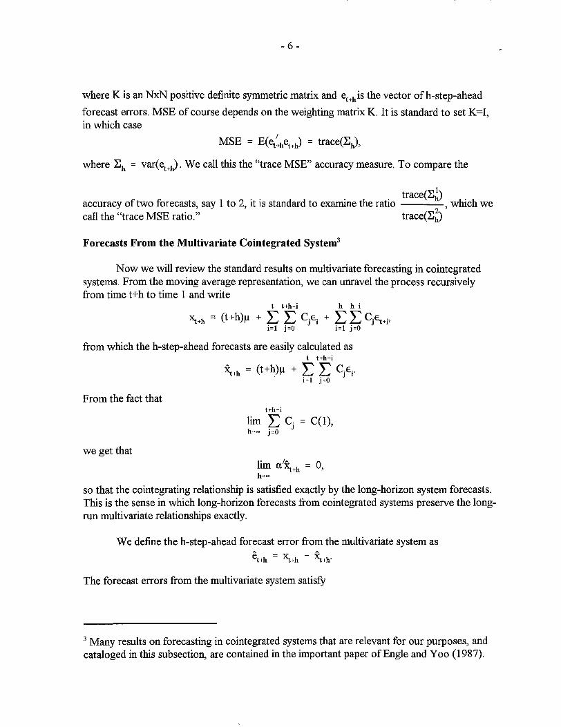
where K is an NxN positive definite symmetric matrix and et+his the vector ofh-step-ahead

forecast errors. MSE of course depends on the weighting matrix K. It is standard to set K=I, in which case

where :Eh = var( et +~. We call this the "trace MSE" accuracy measure. To compare the

trace(:EJ accuracy of two forecasts, say 1 to 2, it is standard to examine the ratio , which we

2 call the "trace MSE ratio." trace(:Eh)

Forecasts From the Multivariate Co integrated System3

Now we will review the standard results on multivariate forecasting in cointegrated systems. From the moving average representation, we can unravel the process recursively from time t+h to time 1 and write

t t+h-i h h-i ~+h = (t+h)/l + L L CjEi + L L CjEt+i,

i=l j=O i=l j=O

from which the h-step-ahead forecasts are easily calculated as t t+h-i

From the fact that

we get that

~+h = (t+h)/l + L L CjEi· i=l j =0

t+h-i lim L c. = C(1), h-oo j=O J

1· !~ 0 1m ex ~+h = , h-oo

so that the cointegrating relationship is satisfied exactly by the long-horizon system forecasts. This is the sense in which long-horizon forecasts from cointegrated systems preserve the long-run multivariate relationships exactly.

We define the h-step-ahead forecast error from the multivariate system as

et+h = ~+h - ~+h'

The forecast errors from the multivariate system satisfy

3 Many results on forecasting in cointegrated systems that are relevant for our purposes, and cataloged in this subsection, are contained in the important paper of Engle and Y 00 (1987).

- 7 -

so the variance of the h-step-ahead forecast error is

var[",..] ~ M( Fo Cj H Fo c/)l where Q is the variance of Et.

From the definition of et +h we can also see that the system forecast errors satisfy h

et+h - et+h-1 = L Ch-iEt+i = C(L)Et+h' i= 1

where the last equality holds if we take Ej=O for all j<t. That is, when we view the system forecast error process as a function of the forecast horizon, h, it has the same stochastic structure as the original process, ~, and therefore is integrated and cointegrated. Consequently, the variance of the h-step ahead forecast errors from the cointegrated system is of order h, that is increasing at the rate h,

var[et +h] = O(h).

In contrast, the cointegrating combinations of the system forecast errors, just as the error-correction process Zt, will have finite variance for large h,

var[cx'e ] = cx'Qcx < 00 t+h ,

where the matrix Q is a constant function of the stationary component of the forecast error. Although individual series can only be forecast with increasingly wide confidence intervals, the cointegrating combination has a confidence interval of finite width, even as the forecast horizon goes to infinity.

Forecasts from the Implied Univariate Representations

Now consider ignoring the multivariate features of the system, forecasting instead using the implied univariate representations. We can use Wold's decomposition theorem and write for any series (the n-th, say),

(l-L)xn,t = Iln + L 6njun,t-j' j=O

where 6n,o = 1 and un,t is white noise. It follows from this expression that the univariate time-t forecast for period t+h is,

xn,t+h = hlln + xn,t + (t 6n,i)Un,t + (~6n,i)Un,t-1 + ... 1=1 1=2

- 8 -

Using obvious notation we can write Xn,t+h = hlln + xn,t + 6n(L)un,t,

and stacking the N series we have ~+h = hll + ~ + 8(L)ut,

where 8(L) is a diagonal matrix polynomial with the individuaI6n(L),s on the diagonal.

Now let us consider the errors from the univariate forecasts. We will rely on the following convenient orthogonal decomposition

et+h == ~+h - ~+h = (~+h - xt+J + (xt+h - ~+J = et+h + (xt+h - ~+J.

Recall that the system forecast is t t+h-i

xt+h = Il(t+h) + L L CjEi ~ Il(t+h) + C(1)~t> i=l j=O

where the approximation holds as h gets large. Using univariate forecasts, the decomposition for et+h, and the approximate long-horizon system forecast, we get

et+h ~ et+h + (Il(t+h) + C(l)~J - (~ + Ilh + 8(L)uJ.

Now insert the common trends representation for X t to get

et+h ~ et+h + Il(t+h) + C(l)~t - (Ilt + C(l)~ + C *(L)Et + Ilh + 8(L)uJ,

and finally cancel terms to get

et+h ~ et+h - (C *(L)Et + 8(L)uJ.

Notice that the et's are serially uncorrelated and the lit'S only depend on current and past et's; thus, et+h is orthogonal to the terms in the parenthesis. Notice also that the second term is just a sum of stationary series and is therefore stationary; furthermore, its variance is constant as the forecast horizon h changes. We can therefore write the long-horizon variance of the univariate forecasts as

var(et+J = Var(et+J + 0(1) = O(h) + 0(1) = O(h),

which is of the same order of magnitude as the variance of the system forecast errors. Furthermore, the trace MSE ratio goes to one. Thus, when comparing accuracy using the trace MSE ratio, the univariate forecasts perform as well as the cointegrated system forecasts as the horizon gets large. This is the opposite of the folk wisdom-it turns out that imposition of cointegrating restrictions helps at short, but not long, horizons. Quite simply, when accuracy is evaluated with the trace MSE ratio, there is no long-horizon benefit from imposing cointegration; all that matters is getting the level of integration right. We summarize the result as:

- 9 -

Proposition 1

1. trace(var(et+J) 1m = 1.

h .... oo trace(var(et+J)

Proposition 1 provides the theoretical foundation for the results ofHoffinan and Rasche (1996), who find in an extensive empirical application that imposing cointegration does little to enhance long-horizon forecast accuracy, and Brandner and Kunst (1990), who suggest that when in doubt about how many unit roots to impose in a long-horizon forecasting model, it's less harmful to impose too many than to impose too few.

Now let's consider the variance of cointegrating combinations of univariate forecast errors. Above we recounted the Engle-Y 00 (1987) result that the cointegrating combinations of the system forecast errors have finite variance as the forecast horizon gets large. Now we want to look at the same cointegrating combinations of the univariate forecast errors. From our earlier derivations it follows that

Again we can rely on the orthogonality of a'et+h to the terms in the parenthesis. The first term, a 'et+h' has finite variance, as discussed above. So too do the terms in the parenthesis, because they are linear combinations of stationary processes. Thus we have

Proposition 2 var(a'et+J = a'Qa + a'var(C *(L)Et + 8(L)uJa = 0(1).

The cointegrating combinations of the long-horizon errors from the univariate forecasts, which completely ignore cointegration, also have finite variance. Thus, it is in fact not imposition of cointegration on the forecasting system that yields the finite variance of the cointegrating combination of the errors; rather it is the cointegration property inherent in the system itself

ill. A SIMPLE EXAMPLE

In this section, we illustrate the results from Section II in a simple multivariate system. The simplicity allows us to explicitly derive the univariate representation of the multivariate system, and thus to obtain its prediction-error variances in a closed form.

Consider the simple bivariate cointegrated system,

~ = 11 + ~-l + Et

where the disturbances are orthogonal at all leads and lags. The moving average representation is

- 10-

[ ~) [fl) [1 ° )[Et) [fl) [Et) (1-L) = + == + e(L) Yt Afl A 1-L vt Afl vt '

and the error-correction representation is

[ ~) [fl) [0) [~-l) [ Et ) (1-L) = + (A - 1) +

Yt Afl 1 Yt-l AEt+Vt .

The system's simplicity allows us to compute exact formulae that correspond to the qualitative results derived in the previous section.

Univariate Representations

Let us first derive the implied univariate representations for x and y. The univariate representation for x is of course a random walk with drift, exactly as given in the first equation of the system,

Derivation of the univariate representation for y is a bit more involved. From the moving-average representation of the system, rewrite the process for Yt as a univariate two-shock process,

= Afl + y + Z t-l t' where ~ = (1-L )vt + AEt . The auto covariance structure for ~ is

Y i O) = 20; + A 20~

Y i1) = Y i -1) = - 0; Yir:) = 0, 1r:1 ~ 2.

The only non-zero positive autocorrelation is therefore the first, 2

°v 1 ----=

2 2 2 20 + A 0 V E

where q = o~/o; is the signal to noise ratio. This is exactly the autocorrelation structure of an MA(1) process, so we write Zt = eUt_1 + ut. To find the value for e, match auto correlations at lag 1, yielding

e 1 =

- 11 -

This gives a second-order polynomial in a, with invertible solution

Finally, we find the variance of the univariate innovation by matching the variances, yielding

or

a;(2+}.?q)

(1 +82)

Forecasts From the Multivariate Cointegrated System

First consider forecasting from the multivariate cointegrated system. Write the time t+h values in terms of time t values and future innovations as

h

xt+h = Ilh + xt + L Et+i i=l

h

Yt+h = A(llh + xt) + A L Et+i + Vt+h' i= 1

The h-step-ahead forecasts are

and the h-step-ahead forecast errors are h

ex,t+h = L Et+i i=l

h

ey,t+h = A L Et+i + vt +h ' i= 1

Note that the forecast errors follow the same stochastic process as the original system (aside from the drift term),

[ Et+h ) ( 1 0) [ Et+h) [ Et+h) (l-L)et +h = = = C(L) .

AEt+h +(l-L)vt+h A l-L Vt+h Vt+h

Finally, the corresponding forecast error variances are

- 12 -

Both forecast error variances are O(h). As for the variance of the cointegrating combination, we have

var [ey,t '. -A e., ... ] = vai( At "",+vt,.) - A( t "',,) 1 = a;, for all h, because there are no short run dynamics.4 Similarly, because we have no short-run dynamics, the forecasts satisfy the cointegrating relationship at all horizons, not just in the limit. That is,

Yt+h - AXt+h = 0, 'II h = 1, 2,

Forecasts From the Implied Univariate Representations

Now consider forecasting from the implied univariate models. Immediately, the univariate forecast for x is the same as the system forecast,

Thus,

so that

~+h = Ilh + ~.

h

ex,t+h = ex,t+h = L Et +i, i=l

To form the univariate forecast for y, write h h

Yt+h = hAil + Yt + L ~+i = hAil i= 1

+ Yt + BUt + ut +1 + L ~+i' i=2

The time t forecast for period t+h is Yt+h = hAil + Yt + But,

and the corresponding forecast error is

yielding the forecast error variance

h

+ L~+i i=2

h-l

= (1 +8) L ut +i i=l

4 We are using the fact that var[(A, -l)et+h] = var[- (A, -l)et+J.

- 13 -

Notice in particular that the univariate forecast error variance is O(h), as is the system forecast error vanance.

Now let us compute the variance of the cointegrating combination of univariate forecast errors. We have

To evaluate the covariance term, use the fact that

and the decomposition result from Section II to write h

ey,t+h = ey,t+h + (Yt+h - yt+J = A L Et+i + Vt+h - vt - But· i=l

Now recall the formula for the forecast error ofx and the fact that future values of E are uncorrelated with future and current values of v, and with current values ofu, so that

COVfy,hh,e,hh) = E[( t ~.i)( At Et,i + vt.h - vt - aut) 1 = Aha;,

Armed with this result, we have that5

var[eyt+h -Ae t+h] = (2+8)a~ < 00 Vh, , x,

which of course accords with our general result derived earlier that the variance of the cointegrating combination of univariate forecast errors is finite.

Forecast Accuracy Comparison

Finally, compare the forecast error variances from the multivariate and univariate representations. Of course x has the same representation in both, so the comparison hinges on y. We must compare

to

5 Keep in mind that 6 is a function of q =a~ / a~ .

- 14 -

Expanding the product in the expression for var(e t+J yields y,

var(ey,t+J = [(1 +8)2h - 8(2+8)]a~.

Substituting for a~, and using the fact that 8 1

=> (1 +8? = A2q

1+82 2+A2q'

we get

Thus,

var(ey,t+J = var(ey,t+h) + (1 +8)ae.

The error variance of the univariate forecast is greater than that of the system forecast, but it grows at the same rate.

Assembling all of the results, we have immediately that

trace(var(et+h» = var(eX,t+h) + var(ey,t+J = qh + A 2qh + 2 + 8

trace(var(et+J) var(ex,t+h) + var(ey,t+J qh + 1 + A 2hq

In Figure 1 we show the values of this ratio as h gets large, for q = A. = 1. Note in particular the speed with which the limiting result,

lim trace(var(et+J) = 1,

h .... oo trace(var(et+h» obtains.

In closing this section, we note that in spite of the fact that the trace MSE ratio approaches 1, the ratio of the variances of the cointegrating combinations of the forecast errors does not approach 1 in this simple model; rather,

var[e -Ae ] ~y,t+h ~ x,t+h = (2+8) > 1, V h.

var[ ey,t+h - Aex,t+h]

This observation turns out to hold quite generally, and it forms the basis for an improved class of accuracy measures, to which we now turn.

- 15 -

IV. ACCURACY MEASURES AND COINTEGRATION

Accuracy Measures I: Trace MSE

We have seen that long-horizon univariate forecasts of cointegrated variables (which completely ignore cointegrating restrictions) are just as accurate as their system counterparts (which explicitly impose cointegrating restrictions), when accuracy is evaluated using the standard trace MSE criterion. So on traditional grounds there is no reason to prefer long-horizon forecasts from the cointegrated system.

One might argue, however, that the system forecasts are nevertheless more appealing because " ... the forecasts oflevels of co-integrated variables will 'hang together' in a way likely to be viewed as sensible by an economist, whereas forecasts produced in some other way, such as by a group of individual, univariate Box-Jenkins models, may well not do so" (Granger and Newbold, 1986, p. 226). But as we have seen, univariate Box-Jenkins forecasts do hang together if the variables are cointegrated-the cointegrating combinations, and only the cointegrating combinations, of univariate forecast errors have finite variance.

Accuracy Measures II: Trace MSE in Forecasting the Co integrating Combinations of Variables

But all is not lost. The long-horizon system forecasts do a better job of satisfying the cointegrating restrictions than do the univariate forecasts-the long-horizon system forecasts always satisfy the cointegrating restrictions, whereas the long-horizon univariate forecasts do so only on average. That is what is responsible for our earlier result in our bivariate system that, although the cointegrating combinations of both the univariate and system forecast errors have finite variance, the variance of the cointegrating combination of the univariate errors is larger.

Such effects are lost on standard accuracy measures like trace MSE, however, because the loss functions that underlie them do not explicitly value keeping the multivariate long-run relationships oflong-horizon forecasts. The solution is obvious-if we value maintenance of the cointegrating relationship, then so too should the loss functions underlying our forecast accuracy measures. One approach, in the spirit of Granger (1996), is to focus on forecasting the cointegrating combinations of the variables, and to evaluate forecasts in terms of the variability ofthe cointegrating combinations of the errors, a'et+h.

Accuracy measures based on cointegrating combinations of the forecast errors require that the cointegrating vector be known. Fortunately, such is often the case. Horvath and Watson (1995, pp. 984-985), for example, note that6

6 See also Watson (1994) and Zivot (1996).

- 16 -

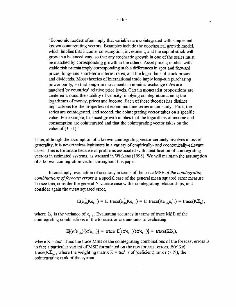
"Economic models often imply that variables are cointegrated with simple and known cointegrating vectors. Examples include the neoclassical growth model, which implies that income, consumption, investment, and the capital stock will grow in a balanced way, so that any stochastic growth in one of the series must be matched by corresponding growth in the others. Asset pricing models with stable risk premia imply corresponding stable differences in spot and forward prices, long- and short-term interest rates, and the logarithms of stock prices and dividends. Most theories of international trade imply long-run purchasing power parity, so that long-run movements in nominal exchange rates are matched by countries' relative price levels. Certain monetarist propositions are centered around the stability of velocity, implying cointegration among the logarithms of money, prices and income. Each of these theories has distinct implications for the properties of economic time series under study: First, the series are cointegrated, and second, the cointegrating vector takes on a specific value. For example, balanced growth implies that the logarithms of income and consumption are cointegrated and that the cointegrating vector takes on the value of(1, -1)."

Thus, although the assumption of a known cointegrating vector certainly involves a loss of generality, it is nevertheless legitimate in a variety of empirically- and economically-relevant cases. This is fortunate because of problems associated with identification of cointegrating vectors in estimated systems, as stressed in Wickens (1996). We will maintain the assumption of a known cointegration vector throughout this paper.

Interestingly, evaluation of accuracy in terms of the trace MSE of the cointegrating combinations offorecast errors is a special case of the general mean squared error measure. To see this, consider the general N-variate case with r cointegrating relationships, and consider again the mean squared error,

where ~h is the variance of et +h. Evaluating accuracy in terms of trace MSE of the cointegrating combinations of the forecast errors amounts to evaluating

E(ulet+J/(ulet+J) = trace E(ulet+h)/(ulet+J) = trace~h)'

where K = uu'. Thus the trace MSE of the cointegrating combinations of the forecast errors is in fact a particular variant ofMSE formulated on the raw forecast errors, E(e'Ke) = trace(~h)' where the weighting matrix K = uu' is of (deficient) rank r « N), the cointegrating rank of the system.

- 17 -

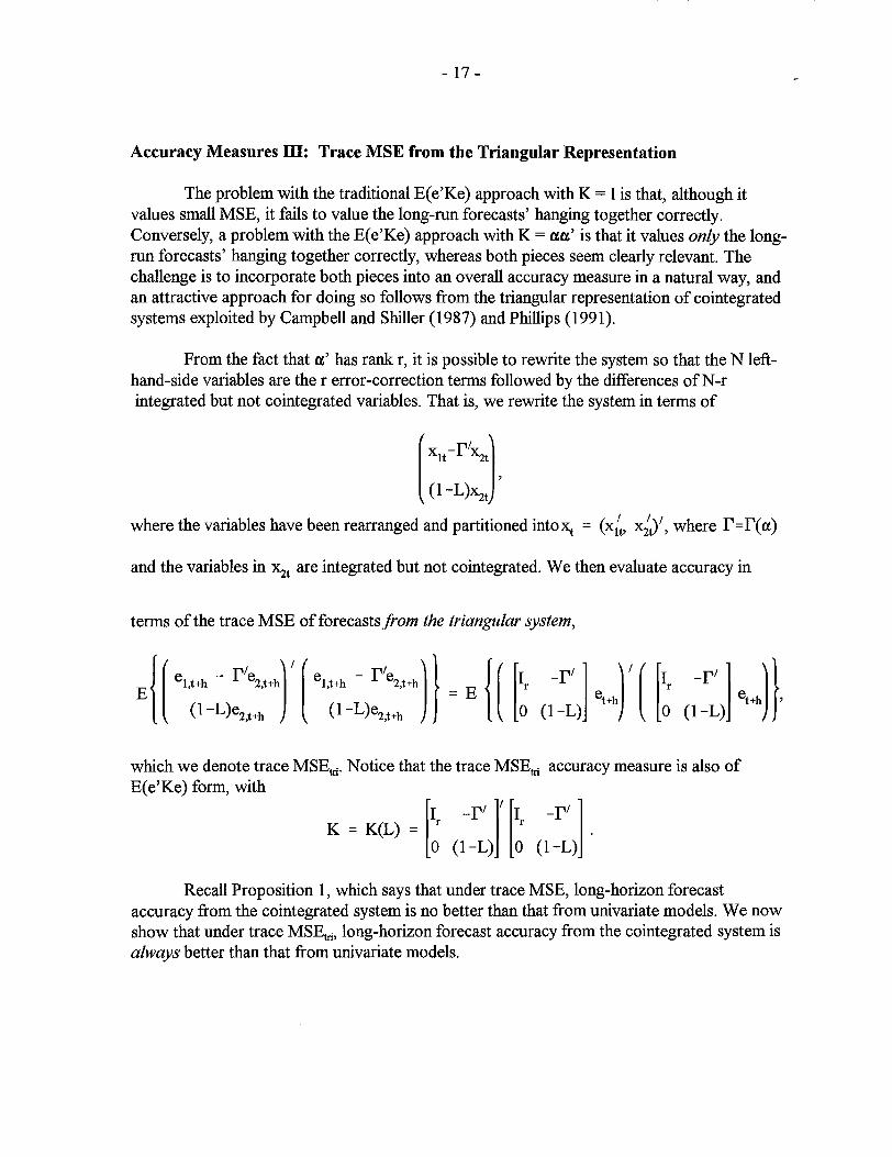
Accuracy Measures m: Trace MSE from the Triangular Representation

The problem with the traditional E( e'Ke) approach with K = 1 is that, although it values small MSE, it fails to value the long-run forecasts' hanging together correctly. Conversely, a problem with the E( e'Ke) approach with K = aa' is that it values only the long-run forecasts' hanging together correctly, whereas both pieces seem clearly relevant. The challenge is to incorporate both pieces into an overall accuracy measure in a natural way, and an attractive approach for doing so follows from the triangular representation of cointegrated systems exploited by Campbell and Shiller (1987) and Phillips (1991).

From the fact that a' has rank r, it is possible to rewrite the system so that the N left-hand-side variables are the r error-correction terms followed by the differences ofN-r integrated but not cointegrated variables. That is, we rewrite the system in terms of

[

xIt - r/'St) , (l-L)'St

where the variables have been rearranged and partitioned into~ = (x:t, x.;;y, where r=r(a)

and the variables in 'St are integrated but not cointegrated. We then evaluate accuracy in

terms of the trace MSE of forecasts from the triangular system,

e1t+h re2t+h e1t+h re2t+h 1 -r I-r

{[ - 1 )/[ - 1 )} {[ [ I] )/[ [ I])} E '(l-L)e2,t+~ '(l-L)e2,t+~ = E ; (l-L) et+h

; (1-L) et+h ,

which we denote trace MSEtrl. Notice that the trace MSEtri accuracy measure is also of E(e'Ke) form, with

[I _r/]1 [I -rl ] K = K(L) = r r .

o (1-L) 0 (1-L)

Recall Proposition 1, which says that under trace MSE, long-horizon forecast accuracy from the cointegrated system is no better than that from univariate models. We now show that under trace MSEtrl, long-horizon forecast accuracy from the cointegrated system is always better than that from univariate models.

- 18 -

Proposition 3

lim trace MSEtri > 1.

h .... oo trace MSEtri

Proof: Consider a cointegrated system in triangular form, that is, a system such that a' = [I -r']. We need to show that for large h,

r N r N

L var[a[et+h] + L var[(l-L)ej,t+h] < L var[a[et+h] + L var[(1-L)ejt+h] i=l j=r+l i=l j=r+l '

and r N

L var[a[et+h] + L var[(1-L)ej,t+h] < 00.

i=l j=r+l

To establish the first inequality it is sufficient to show that r r

L var[ a[et+h] < L var[ ex[et+h]. i=l i=l

We showed earlier that for large h,

var(exlet+J = exlQex + ex/var(C *(L)Et + 9(L)uJex == ex/(Q+S)ex,

where Q == var(et+J, S == var(C *(L)Et + 8(L)uJ, and from which it follows that r r

L var[ ex[et+h] - L var[ ex[et+h] = tr( ex IS ex) > 0, i=l i=l

because S is positive definite. To establish the second inequality, recall that h

so that

et+h - et+h-1 = L Ch-iEt+i = C(L)Et+h' i= 1

var[(J-L)euhl = [~Cj) o[ ~ C;') " C(!)O C(J)' as h"oo, Let ~-r<l) be the last N-r rows ofC(1); then altogether we have

r N

L var[ex[et+h] + L var[(I-L)ej,t+h] = tr(exIQex) + tr(CN _r(I)QCN _r(1») < 00,

i=l j=r+l

and the proof is complete.

The Bivariate Example, Revisited

In our simple bivariate example all we have to do to put the system in the triangular form sketched above is to switch x and y in the autoregressive representation, yielding

- 19 -

For the system forecasts we have

A { (ey,t+h - )..eX,t+h) I (ey,t+h - )..eX,t+h) } 2 2 trace MSEtri = E A A = a v + a E •

(l-L)ex,t+h (1-L)ex,t+h

For the univariate forecasts we have

~ { (ey,t+h - )..eX,t+h) I (ey,t+h - )..eX,t+h)} 2 trace MSEtri = E ~ ~ = (2 +8)av

(1-L)ex,t+h (l-L)ex,t+h

Thus we see that the trace MSEtri ratio does not approach one as the horizon increases; in particular, it is constant and above one for all h,

trace MSEtri = 1 + (2 +8)q

trace MSEtri

1 + q = 1 + (1 + 8)q > 1, Vh.

l+q

In Figure 2 we plot the trace MSEtri ratio vs. h, for )..=1 and a; = a~ = q = 1. In this case, the ratio is simply a constant (> 1) for all h since the systems contains no short-run dynamics.

In summary, although the long-horizon performances of the system and univariate forecasts seem identical under the conventional ratio trace MSE accuracy measure, they differ under the ratio trace MSEtri measure. The system forecast is superior to the univariate forecast under trace MSEm, because the system forecast is accurate in the conventional "small MSE" sense and it hangs together correctly, i.e. it makes full use of the information in the cointegrating relationship.

v. UNDERSTANDING EARLIER MONTE CARLO STUDIES

Here we clarify the interpretation of earlier influential Monte Carlo work, in particular Engle and Yoo (1987), as well as Reinsel and Ahn (1992), Clements and Hendry (1993), and Lin and Tsay (1996), among others. We do so by performing a Monte Carlo analysis of our own, which reconciles our theoretical results and the apparently conflicting Monte Carlo results reported in the literature, and show how the existing Monte Carlo analyses have been misinterpreted. Throughout, we use our simple bivariate system (which is very similar to the one used by Engle and Y 00), with parameters set to )..= 1, /l =0 and a; = a~ = 1 . We use a

- 20-

sample size of 100 and perform 4000 Monte Carlo replications. In keeping with our earlier discussion, we assume a known cointegrating vector, but we estimate all other parameters.7

Let us first consider an analog of our theoretical results, except that we now estimate parameters instead of assuming them known. In Figure 3 we plot the trace MSE ratio and the trace MSEtri ratio vs. h. Using estimated parameters changes none of the theoretical results reached earlier under the assumption of known parameters. Use of the trace MSE ratio obscures the long-horizon benefits of imposing cointegration, whereas use of trace MSEtri

reveals those benefits clearly.

How then can we reconcile our results with those of Engle and Yoo (1987) and the many subsequent authors who conclude that imposing cointegration produces superior long horizon forecasts? The answer is two-part: Engle and Y 00 make a different and harder-to-interpret comparison than we do, and they misinterpret the outcome of their Monte Carlo experiments.

First consider the forecast comparison. We have thus far compared forecasts from univariate models (which impose integration) to forecasts from the cointegrated system (which impose both integration and cointegration). Thus a comparison of the forecasting results isolates the effects of imposing cointegration. Engle and Y 00, in contrast, compare forecasts from a VARin levels (which impose neither integration nor cointegration) to forecasts from the cointegrated system (which impose both integration and cointegration). Thus differences in forecasting performance in the Engle-Y 00 setup cannot necessarily be attributed to the imposition of cointegration-instead, they may simply be due to imposition of integration, irrespective of whether cointegration is imposed.

Now consider the interpretation of the results. The VARin levels is of course integrated, but in finite samples the well-known Dickey-Fuller-Hurwitz bias tends to produce parameter estimates in the covariance stationary region. Thus it's no surprise that forecasts from the V AR estimated in levels perform poorly, with performance worsening with horizon, as shown Figure 4. It is tempting to attribute the poor performance of the V AR in levels to its failure to impose cointegration, as do Engle and Yoo. The fact is, however, that the VARin levels performs poorly because it fails to impose integration, not because it fails to impose cointegration- estimation of the cointegrated system simply imposes the correct level of integration a priori. To see this, consider Figure 5, in which we compare the forecasts from an estimated V AR in differences to the forecasts from the estimated cointegrated system. At long horizons, the forecasts from the V AR in differences, which impose integration but completely ignore cointegration, perform just as well. In contrast, if we instead evaluate forecast accuracy

7 This simple design allows us to make our point forcefully and with a minimum of clutter. The results are robust to changes in parameter values and sample size.

- 21 -

with the trace MSEtri ratio that we have advocated, the forecasts from the V AR in differences compare poorly at all horizons to those from the cointegrated system, as shown in Figure 6.

In our simple bivariate system, we are restricted to studying models with exactly one unit root and one cointegration relationship. It is also of interest to examine richer systems; conveniently, the literature already contains relevant (but unnoticed) evidence, which is entirely consistent with our theoretical results. Reinsel and Ahn (1992) and Lin and Tsay (1996), in particular, provide Monte Carlo evidence on the comparative forecasting performance of competing estimated models. Both study a four-variable V AR(2), with two unit roots and two cointegrating relationships. Their results clearly suggest that under the trace MSE accuracy measure, one need only worry about imposing enough unit roots on the system. Imposing three (one too many) unit roots is harmless at any horizon, and imposing four unit roots (two too many, so that the V AR is in differences) is harmless at long horizons. As long as you impose enough unit roots, at least two in this case, the ratio MSE will invariably go to one as the horizon increases.

VI. SUMMARY AND CONCLUDING REMARKS

First, we have shown that imposing cointegration does not improve long-horizon forecast accuracy when forecasts of cointegrated variables are evaluated using the standard trace MSE ratio. Ironically enough, although cointegration implies restrictions on low-frequency dynamics, imposing cointegration is helpful for short- but not long-horizon forecasting, in contrast to the impression created in the literature. Imposition of cointegration on an estimated system, when the system is in fact cointegrated, helps the accuracy oflong-horizon forecasts relative to those from systems estimated in levels with no restrictions, but that is because of the imposition of integration, not cointegration. Univariate forecasts in differences do just as well!

Second, we have shown that the variance of the cointegrating combination of the long-horizon forecast errors is finite regardless of whether cointegration is imposed. The variance of the error in forecasting the cointegrating combination is smaller, however, for the cointegrated system forecast errors. This suggests that accuracy measures that value the preservation oflong-run relationships should be defined, in part, on the cointegrating combinations of the forecast errors. We explored one such accuracy measure based on the triangular representation of the cointegrated system.

Third, we showed that our theoretical results are entirely consistent with several well-known Monte Carlo analyses, whose interpretation we clarified. The existing Monte Carlo results are correct, but their widespread interpretation is not. Imposition of integration, not cointegration, is responsible for the repeated finding that the long-horizon forecasting performance of cointegrated systems is better than that of V ARs in levels.

We hasten to add that the message of this paper is not that cointegration is of no value in forecasting. First, even under the conventional trace MSE accuracy measure, imposing cointegration does improve forecasts. Our message is simply that under the conventional accuracy measure it does so at short and moderate, not long, horizons, in contrast to the folk

- 22-

wisdom. Second, in our view, imposing cointegration certainly may be of value in long-horizon forecasting-the problem is simply that standard forecast accuracy measures don't reveal it. The upshot is that in forecast evaluation we need to think hard about what characteristics make a good forecast good, and how best to measure those characteristics. 8

Seemingly omnibus measures such as trace MSE, although certainly useful in many situations, are inadequate in others.

In closing, we emphasize that the particular alternative to trace MSE that we examine in this paper, trace MSEtrl, is but one among many possibilities, and we look forward to exploring variations in future research. The key insight, it seems to us, is that if we value preservation of cointegrating relationships in long-horizon forecasts, then so too should our accuracy measures, and trace MSEtrl is a natural loss function that does so.

Interestingly, it is possible to process the trace MSE differently to obtain an accuracy measure that ranks the system forecasts as superior to the univariate forecasts, even as the forecast horizon goes to infinity. One obvious candidate is the trace MSE difference, as opposed to the trace MSE ratio. It follows from the results of Section 2 that the trace MSE difference is positive and does not approach zero as the forecast horizon grows. As stressed above, however, it seems more natural to work with alternatives to trace MSE that explicitly value preservation of cointegrating relationships, rather then simply processing the trace MSE differently. As the forecast horizon grows, the trace MSE difference becomes negligible relative to either the system or the univariate trace MSE, so that the trace MSE difference would appear to place too little value on preserving cointegrating relationships.

8 In that respect this paper is in the tradition of our earlier work, such as Diebold and Mariano (1995), Diebold and Lopez (1996), and Christoffersen and Diebold (1996a, 1996b), in which we argue the virtues of tailoring accuracy measures in applied forecasting to the specifics of the problem at hand.

1.4

1.35

0 :0:; 1.3 co 0::: W CJ) 1.25 :?! Q) u ~ 1.2 I-

1.15

1.1

1.05

1 5 10

- 23 -

Figure 1 Trace MSE Ratio

Univariate vs. System Forecasts Bivariate Example, A=q=l

15 20 25 30 35 40

Forecast Horizon

45 50

Notes to Figure: We plot the trace MSE ratio (univariate / cointegrated system) against the forecast horizon.

1.4

1.35 0

+=l ro 1.3 0::::

·c ..... W en 1.25 ~ (J) u ro

1.2 '-I-

1.15

1.1

1.05

1 5 10

- 24-

Figure 2 Trace MSEtri Ratio

Univariate vs. System Forecasts Bivariate Example, A=q=l

15 20 25 30 35 40

Forecast Horizon

45 50

Notes to Figure: We plot the trace MSEtri ratio (univariate / cointegrated system) against the forecast horizon.

1.4

1.35

>. u ~ 1.3 ::::s u u « 1.25 Q)

> +=l ttl Q) 1.2 c::::

1.15

1.1

1.05

1

- 25 -

Figure 3 Trace MSE Ratio and Trace MSEtri Ratio

Univariate vs. System Forecasts, Estimated Parameters Bivariate Example, l=q=l

Trace MSEtri

Trace MSE

5 10 15 20 25 30 35 40 45

Forecast Horizon

50

Notes to Figure: We plot the trace MSE ratio and the trace MSEIri ratio (univariate / cointegrated system) against the forecast horizon

0 ~ co 0::: w (f)

~ Q) u ~ I-

- 26-

Figure 4 Trace MSE Ratio

Levels V AR vs. Co integrated System Forecasts, Estimated Parameters Bivariate Example, l=q=l

2.5,-~ ____ ~ __ -. ____ ~ __ ~ __ ~ ____ ,-__ ~ ____ ~~

2

1.5

1~--~--~~~~--~~~~--~ __ --~---7~--~---; 5 10 15 20 25 30 35 40 45 50

Forecast Horizon

Notes to Figure: We plot the trace MSE ratio for (VARin levels / cointegrated system) against the forecast horizon.

0 :;::::; co 0:: w en ::?! Q) <.) co L..

I-

- 27-

Figure 5 Trace MSE Ratio

Differenced V AR vs. Cointegrated System Forecasts, Estimated Parameters Bivariate Example, l=q=l

1.4

1.35

1.3

1.25

1.2

1.15

1.1

1.05

1 5 10 15 20 25 30 35 40 45 50

Forecast Horizon

Notes to Figure: We plot the trace MSE ratio (VARin differences / cointegrated system) against the forecast horizon.

0 :;::::; co 0:: ·c ..... W en :::?! Q) 0 ~ I-

- 28-

Figure 6 Trace MSEtri Ratio

Differenced V AR vs. Co integrated System Forecasts, Estimated Parameters Bivariate Example, l=q=l

1.4

1.35

1.3

1.25

1.2

1.15

1.1

1.05

1 5 10 15 20 25 30 35 40 45 50

Forecast Horizon

Notes to Figure: We plot the trace MSEtri ratio (VARin differences / cointegrated system) against the forecast horizon.

- 29-

References

Brandner, P. and Kunst, RM. (1990), "Forecasting Vector Autoregressions - The Influence of Cointegration: A Monte Carlo Study," Research Memorandum No. 265, Institute for Advanced Studies, Vienna.

Campbell, lY. and Shiller, Rl (1987), IICointegration and Tests of Present Value Models,1I Journal of Political Economy, 95, 1062-1088.

Christoffersen, P.F. and Diebold, F.X. (1996a), IIOptimal Prediction Under Asymmetric Loss, II Econometric Theory, forthcoming.

Christoffersen, P.F. and Diebold, F.X. (1996b), IIFurther Results on Forecasting and Model Selection Under Asymmetric Loss, II Journal of Applied Econometrics, 11, 561-571.

Clements, M.P. and Hendry, D.F. (1993), "On the Limitations of Comparing Mean Square Forecast Errors," Journal of Forecasting, 12, 617-637.

Clements, M.P. and Hendry, D.F. (1994), "Towards a Theory of Economic Forecasting," in C.P. Hargreaves (ed.), Nonstationary Time Series and Cointegration. Oxford: Oxford University Press.

Clements, M.P. and Hendry, D.F. (1995), "Forecasting in Cointegrated Systems," Journal of AppliedEconometrics, 10, 127-146.

Diebold, F.X. and Lopez, l (1996), IIForecast Evaluation and Combination,1I in G.S. Maddala and C.R Rao (eds.), Handbook of Statistics. Amsterdam: North-Holland, 241-268.

Diebold, F.X. and Mariano, RS. (1995), IIComparing Predictive AccuracY,1I Journal of Business and Economic Statistics, 13,253-265.

Engle, RF. and Yoo, B.S. (1987), "Forecasting and Testing in Cointegrated Systems," Journal of Econometrics, 35, 143-159.

Granger, C.W.l (1996), "Can We Improve the Perceived Quality of Economic Forecasts?," Journal of Applied Econometrics, 11,455-473.

Granger, C.W.l, and Newbold, P. (1986), Forecasting Economic Time Series, Second Edition. New York: Academic Press.

Hoffinan, D.L. and Rasche, RH. (1996), IIAssessing Forecast Performance in a Cointegrated System, II Journal of Applied Econometrics, 11, 495-517.

Horvath, M.T.K. and Watson, M.W. (1995), "Testing for Cointegration When Some ofthe Cointegrating Vectors are Known," Econometric Theory, 11,984-1014.

- 30-

Lin, l-L. and Tsay, RS. (1996), "Cointegration Constraints and Forecasting: An Empirical Examination," Journal of Applied Econometrics, 11,519-538.

Phillips, P.C.B. (1991), "Optimal Inference in Cointegrated Systems," Econometrica, 59,283-306.

Reinsel, G.C. and Ahn, S.K. (1992), "Vector Autoregressive Models with Unit Roots and Reduced Rank Structure: Estimation, Likelihood Ratio Test, and Forecasting," Journal of Time Series Analysis, 13, 353-375.

Stock, J.B. (1995), "Point Forecasts and Prediction Intervals for Long Horizon Forecasts," Manuscript, J.F.K. School of Government, Harvard University.

Stock, lB. and Watson, M.W. (1988), "Testing for Common Trends," Journal of the American Statistical Association, 83, 1097-1107.

Watson, M.W. (1994), "Vector Autoregressions and Cointegration," in RF. Engle and D. McFadden (eds.), Handbook of Econometrics, Vol. IV, Chapter 47. Amsterdam: North-Holland.

Wickens, M.R (1996), "Interpreting Cointegrating Vectors and Common Stochastic Trends," Journal of Econometrics, 74, 255-271.

Zivot, E. (1996), "The Power of Single Equation Tests for Cointegration when the Cointegrating Vector is Prespecified," Manuscript, Department of Economics, University of Washington.