Barriers to Integration in the Insurance Sector - IMF eLibrary
Upload
khangminh22Category
view
2download
0
©International Monetary Fund. Not for Redistribution
at the Crossroads SUSTAINING GROWTH AND REDUCING POVERTY

©International Monetary Fund. Not for Redistribution
This page intentionally left blank

©International Monetary Fund. Not for Redistribution
at the Crossroads SUSTAINING GROWTH AND REDUCING POVERTY
EDITED BY
Tim Callen Patricia Reynolds Christopher Towe
INTERNATIONAL MONETARY FUND
©International Monetary Fund. Not for Redistribution
© 2001 International Monetary Fund
Production: IMF Graphics Section Cover design: Lai Oy Louie
Library of Congress Cataloging-in-Publication Data
India at the crossroads p. em.
ISBN 1-55775-992-8 (alk. paper) 1. India--Economic policy--1980. 2. India--Economic conditions--1947- 3. Fiscal
policy--India. 4. Sustainable development--India.
HC435.2 .1484 2001 330.954--dc21
Price: $2 7.00
Address orders ro: External Relations Department, Publication Services
International Monetary Fund, Washington D.C. 20431 Telephone: (202) 623-7430; Telefax: (202) 623-7201
E-mail: [email protected] Internet: http:l/www.imf.org
00-054132
©International Monetary Fund. Not for Redistribution
Contents
Page
Foreword . . . . . . . . . . . . . . . . . . . . . . . . . . . . . . . . . . . . . . . . . . . vii
Acknowledgments . . . . . . . . . . . . . . . . . . . . . . . . . . . . . . . . . . . . ix
1. Overview Christopher Towe
PART I. Preserving External Stability
2. India and the Asia Crisis
1
Christopher Towe . . . . . . . . . . . . . . . . . . . . . . . . . . . . . . . 11
3. Assessing India's External Position Tim Callen and Paul Cashin . . . . . . . . . . . . . . . . . . . . . . . 28
PART II. Fiscal Challenges
4. Tax Smoothing, Financial Repression, and Fiscal Deficits in India
Paul Cashin, Nilss Olekalns, and Rama Sahay . . . . . . . . . . 53
5. Fiscal Adjustment and Growth Prospects in India Patricia Reynolds . . . . . . . . . . . . . . . . . . . . . . . . . . . . . . . . 75
PART III. Monetary and Financial Sector Policies
6. Modeling and Forecasting Inflation in India Tim Callen . . . . . . . . . . . . . . . . . . . . . . . . . . . . . . . . . . . . 105
7. The Unit Trust of India and the Indian Mutual Fund Industry
Anna Ilyina . . . . . . . . . . . . . . . . . . . . . . . . . . . . . . . . . . . 122

©International Monetary Fund. Not for Redistribution
vi CONTENTS
PART IV. Growth, Poverty, and Structural Policies
8. Growth Theory and Convergence Across Indian States: A Panel Study
Shekhar Aiyar . . . . . . . . . . . . . . . . . . . . . . . . . . . . . . . . . . 143
9. Structural Reform in India Daniel Kanda, Patricia Reynolds, and Christopher Towe . . . 170
List of Contributors . . . . . . . . . . . . . . . . . . . . . . . . . . . . . . . . . . . 191

©International Monetary Fund. Not for Redistribution
Foreword
India is a Land of contrasts. One billion people Live in a vast territory among architectural and sculptural wonders that give vivid testimony to its ancient and rich history, as well as to its powerful and age-old customs. Yet, there is also a very modem face of India, which is responding to the growing forces of globalization and where information technology has found a fertile environment.
These contrasts and the force of tradition appear to have contributed to a cautious approach to change. Tentative and slow moving attempts to free the economy from pervasive controls were started in the 1980s, but it was not until the serious balance of payments and macroeconomic crisis of the early 1990s that India introduced significant and wideranging policy reforms. These reforms are widely considered to have been successful in promoting a marked improvement in macroeconomic performance. Nevertheless, the subsequent pace of reform has been Less even and bold, and the question remains whether the basis has been laid for the sustained and rapid growth that wiLL be necessary to alleviate the deep poverty that still afflicts more than a third of the population.
That India emerged relatively unscathed from the financial crisis that affected most of Asia as well as many emerging economies is testimony to the country's resilience. Many sectors of the economy-and above all the information technology sector-have shown extraordinary dynamism and remarkable vitality. At the same time, India is roday at a crossroads and a number of macroeconomic indicators display worrisome trends. In particular, the fiscal situation has worsened in recent years and requires concentrated and determined attention to reduce the risk of financial instability. Fiscal consolidation in combination with more rapid pace of structural reform, liberalization, and infrastructure development is also necessary to lay the foundation for strong growth. The chaLLenge for the government is to forge a political consensus across a diverse range of interest groups that is necessary to sustain rapid and consistent reform on broad range of fronts.
The chapters in this volume seek to address the implications of these challenges and opportunities. For the most part, they were written during
vii

©International Monetary Fund. Not for Redistribution
viii FOREWORD
1999-2000 in the context of the lMF staff's ongoing policy discussions with India. By bringing these issues together in a single volume, the macroeconomic and structural challenges that are highlighted can be given greater prominence and thus contribute to the policy debate, both in India and, more broadly, in other reform-oriented economies.
MARIO I. BLEJER Senior Advisor Asia and Pacific Department

©International Monetary Fund. Not for Redistribution
Acknowledgments
The papers included in this volume were largely prepared in the context of the IMF's Article IV consultation discussions with India during 1999-2000, under the leadership of Mario I. Blejer. His support and encouragement during this process are gratefully acknowledged. The papers also benefited from comments received from Dr. V. Kelkar, IMF Executive Director; his Advisor, Dr. N. Jadhav; and from the staff of the Reserve Bank of India and the Indian Ministry of Finance. The authors would also like to thank Mary Abraham and Irene Aquino for their infinite care and patience in preparing the manuscripts, and Alex Hammer and Aung Thurein Win for their research assistance. Sean M. Culhane, of the IMF's External Relations Department, edited the volume and was masterful in guiding it to completion.
The views expressed in this book are those of the authors, and do not necessarily represent those of the Indian authorities, IMF Executive Directors, or other IMF staff.
ix

©International Monetary Fund. Not for Redistribution
This page intentionally left blank

©International Monetary Fund. Not for Redistribution
1 Overview
CHRISTOPHER TOWE
India's macroeconomic performance during the past decade has in many respects been remarkable. Since the early 1990s, India has been among the fastest growing economies in the world, inflation has been relatively well contained, and the balance of payments has been maintained at comfortable levels. This performance was achieved despite poor weather that caused negative agricultural growth in fiscal year (FY) 1995/96 and again in FY 1997/98, the Asian financial crisis in 1997 and 1998, international sanctions imposed on India and Pakistan following tests of nuclear devices in 1998, and the considerable volatility in world oil and commodity prices that occurred in 1998-2000.1
Much of India's economic strength during the early and mid-1990s can be ascribed to the broad-ranging fiscal and structural reforms undertaken following the 1991 balance of payments crisis. These included reforms to the tax system, substantial cuts in the deficit of the consolidated public sector, liberalization and deregulation in the industrial sector, trade and tariff reforms, and measures to recapitalize and strengthen the supervision of banks and other financial intermediaries. These policies helped spur a strong recovery, with real GOP growth accelerating to an average of 7 Y4 percent in the mid-1990s from as low as \12 of 1 percent at the beginning of the decade.
Although economic activity slowed somewhat in subsequent yea�s, it remained relatively robust, especially when compared with the other emerging markets that were buffeted by the Asian financial crisis. During the last two years of the 1990s, growth averaged 6\12 percent, as
1The Indian fiscal year begins on April 1 .
1

©International Monetary Fund. Not for Redistribution
2 OVERVIEW
agricultural output recovered strongly from poor weather in late 1997 and industrial production rebounded in response to the turnaround in agricultural incomes and the recovery elsewhere in the region. India's inflation performance has also been relatively favorable-inflation generally trended downward during the 1990s, reaching as low as 3112 percent by FY 1999/00.
Following the 1991 crisis, India's balance of payments also strengthened. Indeed, in the latter half of the decade, despite the effect of the regional crisis on merchandise exports, the current account deficit began narrowing. The deficit fell to less than 1 percent of GOP in FY 1 999/00, partly reflecting the impact of India's growing exports of information technology (IT)-related services. Although inward portfolio and foreign direct investment were hurt by the erosion of international market sentiment in 1997 and 1998, other private inflows were maintained, and with the recovery in international investor sentiment in FY 1999/00, India's foreign exchange reserves reached $38 billion by March 2000, a gain of almost $12 billion from three years earlier.
By the end of the decade these favorable macroeconomic trends contributed to growing optimism about India's longer-term growth prospects. Indian equity prices strengthened enormously, benefiting from the global boom in IT stocks, and private sector forecasters steadily revised upward their projections for GOP growth to 7 percent or more. This optimism carried over to the political arena, with the new government elected in late 1 999 setting a growth target of 7-8 percent over the medium and longer terms-recognizing the importance of fast growth for improving the welfare of the large share of India's population still in poverty.
However, macroeconomic developments during 2000-including a rebound of inflation, slowing industrial production, and downward pressure on the rupee and stock prices-have tempered some of this optimism. They also underscore the longer-standing question of whether the basis for achieving sustained and rapid growth has yet been established. Most notably:
• Fiscal policy. After considerable progress following the 1991 balance of payments crisis, the fiscal situation deteriorated from the mid-1990s. Weak revenue performance and lack of expenditure control at both the central and state government levels caused the consolidated deficit of the public sector to rise sharply to over 1 1 percent of GOP in FY 1999/00, with public sector debt exceeding 80 percent of GOP This raises the question of how India has been able to achieve high growth and a relatively comfortable balance of payments position despite massive public sector deficits. It also creates doubt about whether this favorable performance can
©International Monetary Fund. Not for Redistribution
Christophel' Towe 3
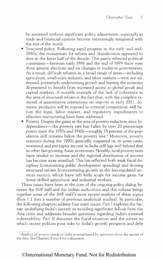
be sustained without significant policy adju·tment , especially as trade and financial systems become increasingly integrated with the rest of the world.
• Sn·uctural policy. Following rapid progress in the early and midl990s, the momentum for reform and liberaliz<nion appeared to slow in the latter half of the decade. This partly reflected political constraints-between early 1996 and the end nf 1999 there were three general elections and six changes in co(llitinn governments. As a result, difficult reforms in a broad range of areas-including agriculture, small-scale industry, and labor markers-were nor addressed, potentially undermining growth and leaving the economy ill-prepared to benefit from increased access ro glohal goods and capital markets. A notable example of the lack of coherence in the area of structural reform is the fact that, with the complete removal of quantitative restrictions on imports in early 2001. domestic producers will be exposed to external competition well before the legal, labor market, and regulatory impediments to effective restructuring have been addressed.
• Poverty. Despite the gains in the area of poverty reduction since Independence-the poverty rate has fallen by over 20 percentage points since the 1950s and l960s-roughly 35 percent of the population still remains below the poverty line. 2 Moreover, poverty statistics during the 1990s generally stagnated or, in some cases, worsened, and per capita income in India still lags well behind that in other fast-growing Asian economies. Notably, rural poverty rates have tended to increase and the regional distribution of income has become more stratified. This has reflected both weak fiscal discipline (constraining public development spending) and slowing structural reform (concentrating growth in the less-regulated services sector), which have left little scope for income gains for lower-skilled agricultural and industrial workers.
These issues have been at the core of the ongoing policy dialog between the IMF staff and the Indian authorities, and this volume brings together some of the IMF staff's more recent analysis of these topics (Box 1 . 1 lists a number of previous analytical studies). ln particular, the following chapters address four main issues. Part I explores the factors underlying India's success in avoiding significant fallout from rhe Asia crisis and addresses broader questions regarding India's external vulnerabil ity. Part II discusses the fiscal situation and the extent ro which recent policies pose risks to India's growth prospects and debt
2Analysis of pnverty trends in India is complicated by que$tion' ;.�hnur rhe qu;1lity of the data. See Chapters 8 and 9 for a discussion.

©International Monetary Fund. Not for Redistribution
4 OVERVIEW
Box 1.1. Recent Staff Studies, 1995-98
India-Selected Issues, IMF Staff Country Paper No. 98/205 (August 1998)
• Tax Revenue Performance in rhe Pose-Reform Period, by Martin Muhleisen
• Foreign Exchange Markets: Developments and Jssucs, by Martin Muhleisen
• ExportS and Competitiveness, by D1mitri Tzanninis • The Financial Performance of Public Sector Commercial Banks in
India, by Ttm Callen • Nonbank Finance Companies in india: Development Issues, by Nir
mal Mahaney
India-SeLected Issues, IMF Staff Country Report No. 97/154 (June 1997)
• The Virtuous Circle of Growth and Saving: Lessons from the Experi-ence of Selected Asian Countries, by Kalpana Kochhar
• Petroleum Price Liberalization, by Richard Hemming • The States' Fiscal Problem, by Dimitri T zanninis • Trade Reforms and Economic Response, by Martin Muhleisen
India-Selected Issues, IMF Staff Country Report No. 96/260 (October 1996)
• Medium-Term Macroeconomic Outlook, by Martin Muhleisen • Improving Domestic Savings Performance, by Martin Muhleisen • Poverty in India, by Martin Muhleisen • Controlling Central Government Expenditures, by Dimitri Tzanninis • Strengthening Public Enterprise Performance, by Richard Hemming • Public Seccor Banking Reform, by Marjorie Rose • Long-Term Savings Instruments, by Martin Muhleisen • Capital Account Liberalization, by Peter Dartels
India-Ecorwmic Reform and Growth, IMF Occasional Paper No. 134 (December 1995)
• Overview, by Ajai Chopra and Charles Collyns • Long-Term Growth Trends, by Ajai Chopra • The Adjustment Program of 1991/92 and Its Initial Results, by Ajai
Chopra and Charles Collyns • The Behavior of Private Investment, by Karen Parker • Fiscal Adjustment and Reform, by Richard Hemming • Recent Experience with a Surge in Capital Inflows, by Charles Collyns • Structural Reforms and the Implications for lnvestmenr, by Ajai
Chopra, Woosik Chu, and Oliver Fratzscher

©International Monetary Fund. Not for Redistribution
Chriscopher Towe 5
sustainability. Monetary policy and financial secror reform are considered in Part III , and structural issues-including those related to poverty and interstate growth and structural policy implementationare covered in Part IV.
Having experienced a balance of payments crisis only ten years ago, issues related tO external vulnerability remain extremely tOpical in India. Against this background, Chapter 2, "India and the Asia Crisis," reviews India's experience during the Asia crisis and the factors that helped insulate it from the worst of the financial market turmoil that afflicted the rest of the region. The chapter explains India's success in terms of its strong macroeconomic fundamentals, modest systemic vulnerability in the banking and corporate sectors, flexible exchange rate management, the relatively closed nature of the economy, and capital controls. However, the chapter cautions that, as capital controls are gradually eased and trade barriers reduced, it will become increasingly important to ensure sound macroeconomic policies-including with regard to the fiscal position-and strong prudential and supervisory systems.
India's external vulnerability is examined in more detail in Chapter 3, "Assessing India's External Position," by estimating models of the equilibrium current account. The results illustrate that India's equilibrium current account deficit has been constrained by its lack of openness on both the capital and trade accounts and suggests that deficits in the range of 1 !12-21;2 percent of GDP appear sustainable, given India's stage of development. The paper uses the experience of the 1991 balance of payments crisis, however, tO illustrate risks to the external position from weak fiscal policies, low reserves, short-term debt exposure, and exchange rate overvaluation.
Issues related to fiscal sustainability are the focus of the subsequent two chapters. Chapter 4, "Tax Smoothing, Financial Repression, and Fiscal Deficits in India," examines data through 1996/97 and asks whether fiscal policy has been effective in avoiding disruptive changes in tax rates in the face of temporary shocks, and whether there has been a bias toward deficit financing. The results suggest that fiscal policies in India have been consistent with tax-smoothing behavior. However, there also appears to be evidence pointing tO a significant bias roward deficit financing, leading tO excessive public borrowing, as well as resort to seigniorage and financial repression. Consequently, the authors argue that government debt is well in excess of levels that would be considered optimal or consistent with intertemporal solvency.
Fiscal sustainability and developments since FY 1996/97 are explored further in Chapter 5, "Fiscal Adjustment and Growth Prospects in India." Using a simple growth model, the chapter illustrates that India's

©International Monetary Fund. Not for Redistribution
6 OVERVIEW
ability to avoid a fiscal crisis, despite high deficits, has largely reflected a favorable differential between real interest rates and overall economic growth. The simulations suggest, however, that a continuation of recent policies would risk putting India on an explosive debt path, by undermining growth and putting upward pressure on interest rates. This risk would be exacerbated as financial sector reform and liberalization reduce the scope for the government to place its debt with captive financial institutions at nonmarket rates. The paper concludes that ambitious fiscal reforms are needed to ensure sustainability, including measures to improve fiscal discipline at the state level, tax measures to boost the revenue/GOP ratio, and cuts in unproductive spending that would provide greater room for needed infrastructure investment.
Monetary policy and financial secror issues are addressed in Chapter 6, "Modeling and Forecasting Inflation in India." The chapter discusses the Reserve Bank of India's (RBI) downgrading of the money supply as an intermediate target in response to financial secror liberalization and innovation, which has reduced the strength of the statistical relationship between money and economic activity. The paper tests the extent to which money versus other indicators provide useful leading infonnation of inflation pressures and cautions that the monetary aggregates continue to be useful for predicting inflation, albeit with significant lags. The paper concludes by suggesting that improvements in the quality of the monetary and price data could further strengthen the RBI's ability tO implement monetary policy, but it also cautions that, until a more reliable anchor for monetary policy is found, the RBI will need to be especially careful to avoid undermining the credibility of its commitment to reasonable price stability.
Chapter 7, "The Unit Trust of India and the Indian Mutual Fund industry," explores the issue of financial sector reform and regulation from the perspective of the mutual fund industry. In particular, while the mutual fund industry has played an important role in mobilizing financial saving in India, its systemic vulnerability was illustrated in 1998 when India's largest fund, the government-sponsored Unit Trust of India, faced significant financial difficulties. As the chapter notes, this episode provided a stark illustration of the importance of continued efforts to strengthen regulation and transparency in the mutual fund industry, a conclusion that applies more generally to the financial secror as a whole.
Structural issues are explored in more detail in the final two chapters. There is deep concern about the apparent widening of regional income disparities, as it suggests a risk that growth will not be sustained or be of a high quality. In Chapter 8, "Growth Theory and Convergence Across Indian States: A Panel Study," interstate growth differentials are

©International Monetary Fund. Not for Redistribution
Cltriswp/te,- Towe 7
examined and the empirical evidence pointing to a widening of per capita income gaps is presented. This lack of convergence is determined to have been partly due to differences across states in Literacy and private investment rates. The chapter then demonstrates that these rates appear to have been adversely affected by inadequate public funding of social and public infrastructure investmenr. Thus, the chapter provides a strong illustration of the damaging effect that weak fiscal policies have had on slower-growing states.
Finally, "Structural Reform in India" provides an overview of structural reform policies that have been implemented since the 1991 balance of payments crisis. The chapter describes empirical evidence that suggests that reforms can significantly enhance India's growth potential and points tO signs that the apparent slowing of the momentum for reform has adversely affected productivity, especially in the agricultural and industriai sectors. The chapter concludes by stressing the need to
reinvigorate the reform process and by summarizing the areas where policies are needed tO support strong and sustained growth over the medium term.
Taken together, these papers suggest that lndia stands at the crossroads. The experience of the Last decade has illustrated the enormous capacity that lndia has for absorbing structural change and the significant benefits that sound policies can yield. At the same time, however, the process of structural reform is unfinished and much of the fiscal adjustment that was achieved has been reversed. This book suggests that ensuring strong, sustained, and high-quality growth in the coming decade will require a broad-based and deep commitment tO fiscal deficit reduction, wide-ranging structural reform, and prudent and careful management of monetary and exchange rate policies.

©International Monetary Fund. Not for Redistribution
This page intentionally left blank

©International Monetary Fund. Not for Redistribution
PART I
Preserving External Stability

©International Monetary Fund. Not for Redistribution
This page intentionally left blank

©International Monetary Fund. Not for Redistribution
2 India and the Asia Crisis
CHRISTOPHER TOWE
Introduction
India's recent economic performance has been remarkable, particularly in view of the economic and financial turmoil thar afflicted the region during 1997-99. In the face of the Asia crisis, as well as the imposition of international sanctions in early 1998, volatility in domestic financial markets and the exchange rate was contained and overall economic activity accelerated in 1998/99. Spillovers to India's balance of payments were also comparably modest-the current account deficit was held to around 1 percent of GOP in 1998/99, capital inflows were sustained, and official reserves increased.
This chapter describes the factors that helped insulate India from the regional turmoil. The following section examines the extent to which tandard indices would have signaled external vulnerability and con
cludes that India's financial and macroeconomic fundamentals were significantly stronger than those economies affected by the crisis. The third section discusses in more detail India's capital controls and their role in reducing India's external vulnerability.
The chapter concludes on a cautionary note, stressing that the favorable experience during the past two years should not lead to complacency. India's previous balance of payments crises clearly demonstrated that the balance of payments is vulnerable to external shocks.1 This vulnerability
11nJi;� experienced balance of paymems crises in 1980 and \990/91, necessitating Fund program». The 1990/91 crisis was precipirared by the Gulf war, which resulted in a sharp
11

©International Monetary Fund. Not for Redistribution
l2 INDIA AND THE ASIA CRISIS
has likely increased as a result of the ongoing Liberalization of domestic financial markets, as well as the gradual easing of controls over capital inflows that has taken place in recent years. This only increases the importance of ensuring a sound macroeconomic environment, including a more sustainable fiscal position, and of continuing to promote a strong prudential and supervisory framework for the financial system.
Macroeconomic and Structural Factors
A broad range of macroeconomic and structural facrors help explain why India was relatively unscathed by the recent crisis. In particular, when the regional crisis arose in 1997, India did not exhibit many of the macroeconomic, financial sector, and external imbalances that afflicted other countries in the region, in large part owing to the years of structural and macroeconomic reforms that had followed India's 1990/91 balance of payments crisis. As a result, estimates of crisis probabilities based on macroeconomic fundamentals-including the real exchange rate, the current account, reserves, export growth, and shortterm debt exposure-were relatively benign in the case of India in late 1996, especially when compared ro other Asian economies (Figure 2.1).2 Besides these relatively good macroeconomic fundamentals, India was also insulated from financial market contagion and trade spillovers by the relatively closed nature of its economy, a long history of capital controls, and modest financial links with the region.
India's external current account going into the crisis was relatively strong. The current account deficit had fallen to only 1 Y4 percent of GOP in 1996/97, reflecting the effect of strong export growth in previous years, as well as a surge in inward remittances. Although the crisis contributed
increase in India's oil import bill, as well as a reduction in remittances from Indians abroad. However, the economy's vulnerability to rhe external shock reflected underlying structural weaknesses, including a deterioration in the fiscal position (the overall public sector deficit rose to over 12 percent of GOP), excessive monetary growth, large external debt servicing requirements (partly related to previous JMF loans), and a growing current account deficit.
2The crisis probabilities shown are estimates of the probability of balance of payments crisis 24 monrhs hence, and are based on a model mainrained by the Developing Country Studies Division of the IMF's Research Department. This model and other studies, including those by J. Sachs, A. Torncll, and A. Velasco (1996), J. Frankel and A. Rose (1996), and G. Kaminsky, S. Lizondo, and C. Reinhart ( 1998), identify a range of variables that can help signal crisis, including real exchange rate appreciation, banking crises, growth of M2/reserve growth, stock price inflation, export growth weakness, output growth slowdown, excess M l balances, falling external reserves, excess domestic creuir growth, high real interest rates, and a decline in the terms of trade.

©International Monetary Fund. Not for Redistribution
Figure 2.1. Crisis Probabilities, December 1 996 (In percent)
India Philippines Taiwan PRC
Korea
Christopher Towe 13
Malaysia Indonesia Thailand
tO a weakening of export growth, owing to the decline in regional demand and a fal l in export unit values, this effect was partly offset by lower oil prices and the strength of IT-related services exports. Spillovers from the Asia crisis were also moderated by the relatively closed nature of the Indian economy-exports represent less than 10 percent of India's GOP, and the share directed to Asia was relatively small (less thar\ 2 percent of GOP). The current account deficit remained at 1 Y4 percent of GOP in 1997/98, and fell to 1 percent of GOP in 1998/99.
The impact of the crisis and sanctions on capital flows was also relatively modest, partly reflecting the fact that capital controls have limired India's dependence on foreign saving. Private capital inflows reached just over $10 billion in 1996/97, owing tO increases in foreign direct investment (FOI), commercial borrowing, and deposit inflows by nonresident Indians (NRis), but fell only marginally in the following two years to an average of around $9 billion. While portfolio investment, short-term credits, and NRI deposits were adversely affected, FDI and commercial borrowing were sustained, and capital inflows were also bolstered by the authorities' issue of the Resurgent India Bond. 3 As a result, India's external reserves actually increased over the crisis period, and stood at almost $35 billion at end- 1999, the equivalent of over six months of imports of goods and services.
3The Resurgent India Bond (RIB) was marketed ro nonresident Indians hy the State Bank of India (which is mainly owned by the central bank). The RIB is a five-year bond, denominated in U.S. dollars, pounds sterling, or deutsche marks (paying an interest rate of

©International Monetary Fund. Not for Redistribution
14 INDIA AND THE ASIA CRISIS
Table 2.1. External Debt, 19971 (In percent of GOP)
India Indonesia
Total 24.4 61.3 Of which: Short-term 1.8 10.0
'Data for India are at end-March 1997.
Korea Malaysia Philippines Thailand
33.2 38.7 59.3 62.0
13.3 13.5 23 1
India's external debt position (Table 2 . 1 ) had also improved considerably during the mid-1990s. Total external debt as a share of G DP had fallen to 24 percent of GOP in 1996/97 from 33 percent of GOP at end 1993/94, while short-term debt remained under 2 percent of GOP during the same period.4 Accordingly, the debt service ratio improved considerably, falling to 22 percent in 1996/97 from 3 2 percent of exports of goods and services in 1990/91 . The structure of external debt was also relatively favorable. Although concessional debt fell slightly as a share of total external debt during the mid-1990s, by end 1996/97 it remained around 40 percent.
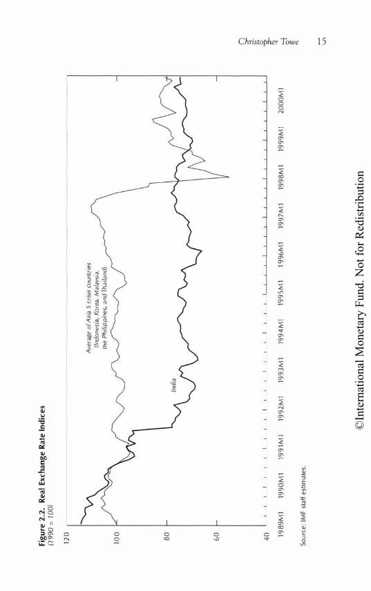
The fact that the rupee's exchange rate was not obviously overvalued at the beginning of the crisis, and that monetary policy was geared toward allowing the exchange rate to depreciate in an orderly fashion in the face of market pressures, also helped sustain financial market confidence (Figure 2.2). The rupee had already depreciated sharply following India's balance of payments crisis in 1991, and by March 1997 it was roughly 25 percent below its 1990 value in real terms, a level that most indicators suggested was broadly in line with medium-term fundamentals.s This movement in the real exchange rate was facilitated by the shift in the exchange rate regime from a basket peg system to a managed float following the 1991 crisis.
The Asia crisis did result in pressures on the rupee in the latter half of 1997 and early 1998. The authorities responded by tightening money market conditions while permitting an 18 percent depreciation against the U.S. dollar. However, the interest rate hikes and the depreciation in real terms were considerably less than what was experienced among the
73/4 percent, 8 percent, and 61/4 percent per year, respectively). The proceeds were used ro make rupee loans at L2Y2-t3 percent ro developmenr institutions, which were supposed ro fund their loans for infrastructure projects. The exchange loss, if any, would he shared between the Stare Bank of India (SBI) and rhe Reserve Bank of India (RBI}, although the SBI's liability is limited ro 1 percenr per annum of rhe rupee value of the original amount credited to the institution plus accrued interest.
4Note that these debt figures understate the vulnerability of many southeast Asian economies, since they do not include off-balance sheer liabilities, which in some cases were substantial.
5See the analysis of misalignments by D. Tzanninis ( L998), and Chapter 3.
©In
tern
atio
nal M
onet
ary
Fund
. Not
for R
edis
tribu
tion
Figu
re 2
.2.
Rea
l Ex
chan
ge R
ate
Ind
ices
(19
90 =
100)
120
100
80
60
40
1989
M1
199
0M
1
Sour
ce: I
MF
staff
est
imat
es.
199
1M1
199
2M
1 19
93
M1
Av
erag
e o
f Asi
a 5 c
risi
s c
ou
ntr
ies
(In
do
nes
ia,
Ko
rea,
Ma
lays
ia,
the
Ph
ilip
pin
es,
an
d T
ha
ilan
d)
199
4M
1 19
95
M1
1996
M1
199
7M
1 19
98
Ml
199
9M
1 20
00
Ml
......
V1

©International Monetary Fund. Not for Redistribution
16 INDIA AND TliE ASIA CRISIS
Asia crisis countries, and the rupee settled in a relatively narrow trading range after August 1998.6
India's success in resisting the crisis also reflected the fact that corpo� rale and household balance sheets did not exhibit the same fragilities found in many crisis countries. For example, debt-equity ratios for the manu� facturing sector declined from over 200 percent in 1991/92 to a more manageable 121 percent in 1997/98.7 Moreover, although stock prices fell sharply (by roughly 40 percent) following the onset of the Asia cri� sis and the imposition of sanctions, this had not preceded a long-term run-up in equity prices fueled by excessive credit creation, which was seen in many other emerging markets ahead of the crisis. Indeed, most monetary indicators were comparably benign ahead of the crisis; credit growth had been decelerating since the beginning of 1995, and the ratio of broad money to reserves had declined sharply since early 1996.
The banking sector was also comparatively less vulnerable than elsewhere in Asia, partly reflecting the effort of the reforms that had been initiated in the early 1990s. For example, risk-weighted capital adequacy ratios (CARs) had risen to nearly 1 2 percent by 1997/98, largely as a result of substantial capital injections by the public sector. Nonperforming loans as a percent of total loans had fallen to around 8 percent in 1997/98 from around 1 1 percent in 1994/95. Systemic risks also were moderated by the fact that roughly 80 percent of the system was already state owned. Credit and market risk was mitigated by the fact that roughly half of bank assets were taken up by reserve and liquidity requirements-including holdings of government debt-and loans to the property sector were relatively modest. In addition, extensive capital controls restricted the size and term of external bank borrowing, minimizing banks' exposure to regional and foreign exchange risk.
Although India's fiscal situation was considerably weaker than the Asia crisis economies, the public sector deficit had been on a downward trend in the period leading up to the crisis. The deficit had fallen to a recent low of 8 percent of GOP in 1997/98 from almost 1 2 percent of GOP in 1989/90, owing to a sharp compression of capital and other spending. As a result, the public sector debt-to-GOP ratio had begun tO decline, reaching as low as 75 percent at end-1996/97.
6RBI exchange rare policy has been characterized as aimed at maintaining "orderly condirions in rhe foreign exchange market, and ro curb destabilizing and self-fulfilling speculative activities." Sec Dr. Y.V. Reddy, Deputy Governor, Reserve Bank of India (RBI), address ro the Fourth Securities lndusrry Summit, May 26, 1999.
7 Alrhough this gearing ratio compares favorably with a number of orher emerging markets in Asia, some analysts express concern with the leverage of Indian businesses, and the extent to which public sector banks are required ro provide financing to loss-making firms.

©International Monetary Fund. Not for Redistribution
Ch1·iswpher Towe 1 7
Broader macroeconomic developments in India were also favorable. In a number of economies, a sharp slowdown in domestic growth, following years of rapid expansion, was an important precursor to crisis. Slow growth contributed to weaknesses in the financial and corporate sectOrs, since large (often foreign currency) loans had been made on the assumption of continued strong growth and limited the scope for central banks to raise interest rates ro defend existing exchange rate parities. Although growth did slow in India during 1997/98, it remained relatively robust at just under 5 percent. The slowdown also reflected mainly domestic supply shocks, such as the effect of weather-related problems on agricultural output, rather than the precrisis slowdown in export growth that afflicted many other countries in the region.
The importance of macroeconomic and other fundamental facrors as preconditions for crisis has been illustrated by statistical analysis in the IMF's May 1999 World Economic Outlook (Figure 2.3 ) . This study
Figure 2.3. Crisis Vulnerability Indicators (Difference of crisis to noncrisis economies)
25 -
20 -
1 5 -"' <:: .g 1 0 -
.�
T "' "' 5 -a ! � • -§ 0 <:: 1 • • Ol -5 -
j - 1 0 -
-15 -
-20 -
� 1.) � "' c t: � -� � eo o 8. 3 c: ·-l? "' 0 "' ;;; X 0 � CD � ·- .. � "" .., 1.) 0.. X Oi -� -"'0 ·'"= "' a. V> .. 0 ... � tJ "' a. •t � "' � I.> "' \i) E � "'
·� � d: '5 �
:r
2 '6 � u c: 0 E E 0
u
90% Confidence interval for crisis economies
/
I •
.. .. c 0.. ·5 � ·� 0 15 � �·� c:
� � c. :> 0 � � � 1.) 1.) "' "' ..., c � 8
I I
· � India
� 15 c ., � � X "' "' E E � � � t:" .J:> 0 "' 6; "0
- � "' "' !: C: � � X Oi .. � E :E � "' � "0 .: 0 � Vl
Composite Indicators
--
-
I --•
•
-
-
-
-
� � (: � .. ;;; V> "' � � .S � "' "' "'

©International Monetary Fund. Not for Redistribution
18 INDIA AND THE ASIA CRISIS
showed that a number of economic fundamentals for crisis economies were different than those for noncrisis countries. For example, in Figure 2.3, real effective exchange rates for 90 percent of those economies that fell into crisis were significanrly higher than that exhibited by noncri ·is economies during the Asia and earlier Mexico crises. Of tht! variable:. examined, exchange rate overvaluation, current account deficits, :,hortterm external debt, real interest rates, and common creditors were found to be significant signals of crisis.8
Most of the variables that provided an indicator of crisis vulnerability in other countries did not signal vulnerability for lndia during the 1997/98 period. Notably, India's reserves, current account deficit, real interest rate, and exchange rate movements were not typical of the behavior shown by crisis economies. In addition, crisis economies typically were more exposed to a common creditor-i.e., had a larger proportion of international bank loans from a single creditor country-but this was not the case for India. Real interest rates also did nm signal a risk of crisis. The only variables that did appear to point to vulnerability for India were those that proxied the spil lover of crises in other countries on India's real exchange rate and export growth.
Composite vulnerability indices also suggest the same conclusion. Only four of these indices appear to signal vulnerability (Figure 2.4 ): reserve adequacy, reflecting the high level of M2/reserves; trade spillovers, owing to India's trade links to other crisis countries; the composite financial indicator, again owing to the high M2/reserves ratio; and domestic macroeconomic imbalances, owing to the large fiscal deficit/GOP ratio.9 Although the external imbalance and portfolio spillover variables were significant, the indian data did not signal vulnerabil ity. While the value of the index for domestic macroeconomic imbalances was relatively high in the case of India, reflecting the large fiscal deficit and high monetary growth, this variable did not provide a reliable signal of crisis vulnerability for other crisis economies.
111n Figure 2.3, the venical lines represent the 90 percent range for cnSI> ccunomu.>> ul each v:uiable, norm11lized by the >ample stamhud deviation le>> tht:! CIVt:!rage for rhe noncrisi� ,ample. In <Jther words. the line> repre,ent the >tanJardiZC::d d1fft:re::nce hetw..:.:n 90 percent oi the crisis economies <1nd the noncri>is .:conomu:�s. Denub an� pr<lVIded 111 the IMF's May 1999 World Economic Outlook. The figures for India were calculated un the basis of data available during August-November 1998.
9'fhc M2/reserve> ratio proxies both the effect uf reserve inade4uacy (of [e, cun.;ern in the case of a country such as India with a floating exchange rate) <ll1d also cxct:»
credit creation. In the WEO study, this variable was found to be a sigmficant crisis mdl· cator in the composite indices.

©International Monetary Fund. Not for Redistribution
Figure 2.4. Crisis Vulnerability Indicators (Difference of crisis to noncrisis economies)
·� .� � "' a 1? � c: "' V)
2.5 1-2.0 1-1.5 1- Iii
1 .0 1-0.5 r-0.0 D
-0.5 -
-1.0 -I
Domestic External macroeconomic imbalances
conditions
I
India
D/ I
Portfolio spillovers
Chriscopher Towe 19
90% Confidence interval for crisis economies
1/ •
I Reserve
adequacy
_/
I I
I Trade
spillovers
-
-
-
-
1 -
-
-
Composite financial
indicators Composite Indicators
The Role of Capital Controls10
India's macroeconomic and other fundamentals were not uniformly favorable, and this suggests that capital controls contributed to India's favorable experience during the regional crisis. In particular, India's relatively closed capital account meant that external debt-especially short-term external debt-was modest, and restrictions on capital movements also helped lessen the impact of the sharp turnaround in investor sentiment on the capital flows. Indeed, this view is confirmed by statistical analysis suggesting that capital controls may have helped insulate countries during the Asia and Mexico crises (see the May 1999 World Economic Outlook).
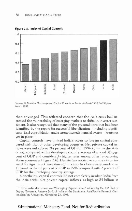
India maintains relatively strict control over capital flows, and the IMF's index of capital controls places India among the most restrictive economies. In general, outflows by residents are prohibited, and inflows by nonresidents are subject to constraints (Figure 2.5 and Box 2 . 1 ). Although a timetable for the phased withdrawal of most capital account controls over the 1997/98-1999/2000 period was established in June 1997, progress toward capital account liberalization has been slower
1"This section draws upon K. Habermeier (2000).
©International Monetary Fund. Not for Redistribution
20 INDIA AND THE ASIA CRISIS
Figure 2.5. Index of Capital Controls
1 .0 .--------------------------------.
0.8
0.6
0.4
0.2
� c ·a. .9-.r. 0...
"' ·;;; � c 0 -o c
-o c � "' .r.
I-
"' .� .r. u .� u c
Source: N. Tamiri�a. "Exchange and Capital Controls as Barriers to Trade," IMF Staii Papers, March 1999.
than envisaged. This reflected concern that the Asia crisis had increased the vulnerability of emerging markets to shifts in invesror sentiment. It also recognized that many of the preconditions that had been identified by the report for successful liberalization-including significant fiscal consolidation and a strengthened financial system-were not yet in place. 1 1
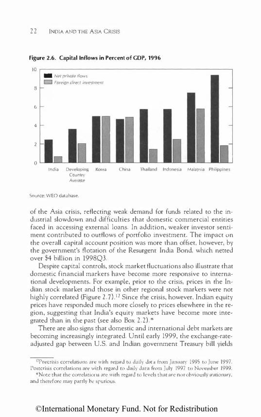
Capital controls have limited India's access tO foreign capital compared with that of other developing countries. Net private capital inflows were only about 2 1/2 percent of GOP in 1996 (prior ro the Asia crisis), compared with a developing country average of around 3 Y:! percent of GOP and considerably higher rates among other fast-growing Asian economies (Figure 2.6). Despite less restrictive constraints on inward foreign direct investment, this roo has been very modest in India-less than 1 percent of GOP in 1996 compared with 2 percent of GOP for the developing country average.
Nonetheless, capital controls did not completely insulate India from the Asia crisis. Net private capital inflows, as high as $5 billion in
1 1 For a useful discussion, see "Managing Capiral Flows,'' adc.lress by Dr. Y.V. Reddy, Deputy Governor, Reserve Bank of India, at the Seminar at Asia/Pacific Research Cen· ter, Stanford University, November 23, 1998.

©International Monetary Fund. Not for Redistribution
Chriscopher Towe 2 1
Box 2.1. Capital Controls
• Loans. Generally, Indian residents are prohibited from borrowing from nonresidents. However, there is a window that permits external commercial borrowing (ECB) by Indian corporate emities, subject to government approval. Indian corporations are allowed to apply for permission to borrow abroad, but the total amount of loans made to all corporations is subject co an annual ceiling ($8.5 billion in 1999/00). Companies are restricted from paying more than 350 basis points above UBOR/U.S. Treasuries.
• Portfolio flows. Portfolio outflows by residents are subject to prior approval. Indian-registered mutual funds may invest in overseas markets up to a maximum of $500 million. Portfolio inflows by nonresidents are permitted by registered foreign institutional investors (Als) subject to certain Limits. ln particular, a single AI's ownership share in Indian companies cannot exceed 10 percenc, and short sales by Als are prohibited. The aggregate permissible holdings of an Indian company by Fils has been increased to 40 percent, subject to Board approval. Portfolio investments by nonresident Indians also are permitted. In both cases, there are no restrictions on repatriation. ln addition, resident corporations are permitted to raise equity abroad by issuing Global or American Depository Receipts.
• Foreign direct invesrment. Inward foreign direct investment is permissible subject to prior notification and approval, as well as restrictions on the foreign ownership of projects. However, "automatic" approval is permitted for smaller amounts, or investments directed toward sectors not on a negative list. Limits on equity participation are also relaxed for high-priority sectors. Restrictions on outward direct invest· ment by residents were eased in 1999, with the limits for fast-track approval raised to $15 million; otherwise prior approval is required.
• Bank deposits. Deposits by residents abroad and resident deposits in foreign currency are permitted, subject to prior approval. Deposits to Indian banks by nonresident Indians (NRis) and overseas corporate bodies (OCBs; i.e., corporations owned by NRls) are permitted, both in rupees and foreign currencies. Depending on the scheme, such deposits can be repatriated. Restrictions are placed on the interest paid to NRI deposit holders.
1997Q2, tapered off in the latter half of 1997, and, except for a spike in 1998Ql related to unidentified capital inflows, were relatively modest inro 1 999. The weakening in capital inflows largely reflected bankrelated outflows; nonresident Indian deposits fell sharply in late 1997 and other net bank foreign assets also declined from 1997Q3. However, a drop in investment and nonbank flows was also evident after the onset
©International Monetary Fund. Not for Redistribution
22 INDIA AND THE ASIA CRISIS
Figure 2.6. Capital Inflows in Percent of COP, 1996
10 .----------------------------------------------------. - Net private t1ows
D Foreign clirect investment
8
b
4
2
0 India Developing Korea China Thailand Indonesia Malaysia Philippines
Country Average
Source: WEO database.
of the Asia crisis, reflecting weak demand for funds related to the industrial slowdown and difficulties that domestic commercial entities faced in accessing external loans. In addition, weaker investor sentiment contributed to outflows of portfolio investment. The impact on the overall capital account position was more than offset, however, by the government's flotation of the Resurgenr India Bond, which netted over $4 billion in 1998Q3.
Despite capital controls, stock market fluctuations also illustrate that domestic financial markers have become more responsive to international developmenrs. For example, prior to the crisis, prices in the Indian stock market and those in other regional stock markers were not highly correlated (Figure 2 . 7). 12 Since the crisis, however, Indian equity prices have responded much more closely to prices elsewhere in the region, suggesting rhat India's equity markets have become more integrated than in the past (see also Box 2.2) .*
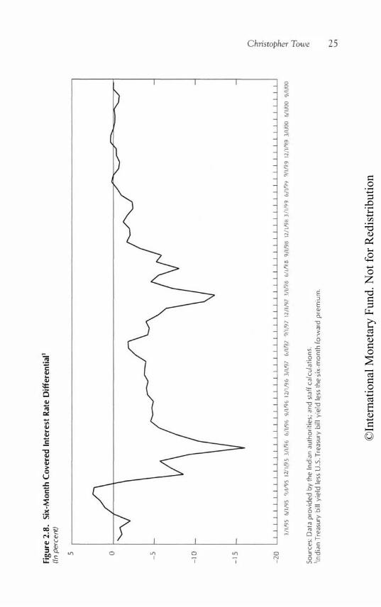
There are also signs that domestic and international debt markets are becoming increasingly integrated. Until early 1999, the exchange-rateadjusted gap between U.S. and Indian governmenr Treasury bill yields
11Precrisis correlation;, are with regard to dnily d<lt<1 from January 1995 to June 1997. Postcrisis correlations an� with regard tO daily Jara from July 1997 to November 1999.
*Note that the correlations arc with regard ro levels that are nor obviously srarionary, and therefore may parrly he spurious.

©International Monetary Fund. Not for Redistribution
ChristOpher Towe 23
Figure 2.7. Correlation Between Indian and Regional Stock Prices
HKSAR Taiwan
Source: CEIC.
Indonesia Korea Singapore Malaysia Thailand
Box 2.2. Regional Stock Market SpilloversPre- and Post-Asia Crisis
In order to examine the proposition that spillovers from Asian stock markets to India have increased following the Asia crisis, regressions were estimated relating the daily log change in the Indian Bombay SENSEX index (r,) as a function of its lagged value, and the log change in other regional markets (r',}-consrant terms and ocher lags were not found to be significant:
The regressions were estimated over a precrisis period (October 1994-May 1996) and during rhe postcrisis period (July 1997-November 1999). The estimated impact of regional stock markets is proxied by the c1 coefficients, which are reported below ("-" indicates that the coefficient is insignificant from zero at the 95 percent confidence level). As can be seen, except for the case of Korea, the proposition that rhe impact of regional stock market developments on the domestic stock market has increased since the Asia crisis cannot be rejected.
HKSAR Indonesia Korea Malaysia Singapore Thailand Taiwan
Precrisis Postcrisis 0.12 0.80
0.17 0.08 0.07 0.10 0.07

©International Monetary Fund. Not for Redistribution
24 INDIA AND THE ASIA CRISIS
was large, with the yield on U.S. securities tending ro exceed that on Indian securities, pointing to an inability of financial markets ro arbitrage unexploited profits. Since the beginning of 1 999, however, this gap has narrowed considerably, and, while it remains significantly different from zero, there are indications that marker participants are becoming better able to arbitrage the difference between domestic and foreign yields (Figure 2.8). 1 3
Finally, the growing stock of the more volatile sources of financing is significant and a potential source of vulnerability. Cumulative portfolio inflows-on which there are no repatriation restrictions-totaled over $ 1 5 billion during 1990Ql-1999Ql , and the outstanding stock of repatriable NRI deposits was around $14.5 billion at end-March 1999.
Concluding Remarks
This discussion has suggested that India's favorable economic performance in the face of the recent regional financial crisis can be a cribeJ to a combination of relatively strong fundamentals, the closed nature of the economy, and a legacy of capital controls that insulated India from contagion effects. India's past balance of payments crises, however, and the experience of the rest of the region during the pa t several years suggest a number of important lessons:
• Effective exchange rate management. During the Asia crisis, the RBI was effective in facilitating an orderly adjustment in the rupee/dollar exchange rate. This experience, and the experience of other countries in the region that had more rigid nominal parities against the dollar, illustrates rhe advantage of a flexible exchange rare system and highlights the risks that arise when the monetary authorities seek to maintain an excessively stable exchange rate against one particular currency.
• The importance of sustaining che macroeconomic adjustment. The multicounrry studies described above i llustrate the importance of macroeconomic fundamentals-a sustainable current account balance, an appropriate and flexible exchange rare, high levels of reserves, and low levels of shorr�rerm external debt-for avoiding balance of payments crisis. Although India was well positioned
JJCapiral controls constrain the scope for arbitrage. hut. a� domestic corporate> can borrow abroad, this rends to limit the extent co which domestic rates c<ln exceed foreign rates. For a d1scussion of the imcrest parity conditions in India, see H. Joshi ::�nd M. Sag· ger ( 1998). The increasing integration of the domestic capital, money, and foreign ex· change is discussed by B.K. Bhoi and S.C. Dhal ( L999).
©In
tern
atio
nal M
onet
ary
Fund
. Not
for R
edis
tribu
tion
Figu
re 2
.8.
Six-
Mon
th C
over
ed I
nter
est
Rate
Diff
eren
tial
1
(In pe
rcent)
5 0 -5
- 10
- 15
-20
l/
1,"}5
6/
1,")5
9
/1/9
5
12/1,"}
5 1
/1,"}
6
6/1
,")6
9
/1/9
6
12/1,")
6 3
/1,")
7
6/1
,"}7
91
1,")7
12
/1,")
7 l
/1,")
8
6/1,")
8
9/1
,")8
12
/1,"}
6 3
11,")
9
6/1
/9�
9/
1,"}9
12
/1/')
9 3
/1,0
0 6/
1,00
9/1
,00
Sour
ces:
Dat
a p
rovi
ded
by
lhe
Ind
ian
auth
orit
ies;
and
sta
ff c
alcu
latio
ns.
11nd
ian
Tre
asur
y bi
ll yi
eld
less
U.S
. Tre
asur
y b
ill y
ield
less
the
six-
mo
nth
forv
vard
pre
miu
m.

©International Monetary Fund. Not for Redistribution
26 INDIA AND THE ASIA CRISIS
ahead of the Asia crisis, this was mainly the result of policy measures that had been set in train in response to India's earlier balance of payments crisis, including trade liberalization, tax reform, fiscal adjustment, and financial sector reform. However, progress along many of these fronts in recent years has been less favorable. For example, the momentum for structural reform appears to have slowed in the latter half of the 1990s, and most of the progress in reducing the fiscal deficit has been eroded. Thus, in the absence of ambitious measures to improve public saving and reinvigorate the structural reform process, balance of payments vulnerability, especially in the face of adverse external shocks, cannot be ruled our.
• Capital controls and financiaL sector stability. India's capital controls also played an important role in helping ro insulate it from the financial contagion that afflicted other countries in the Asia region. The same can be said for the pervasive government control over the banking sector and the relatively modest pace of liberalization in the domestic financial sector, since high reserve and liquidity requirements, priority lending regulations, and an underdeveloped domestic debt market discouraged the asser price inflation and balance sheet weaknesses seen elsewhere in Asia. As liberalization continues, however, the systemic vulnerabilities to contagion increase. The balance of payments is becoming more dependent on gross private inflows of portfolio inve tment, as well as investments by nonresident Indians. In addition, recent fi.nancial market developments have increased the scope for arbirrage.11 This only increases the importance of ensuring that the prudential and supervisory systems covering the domestic financial sector are strong and that macroeconomic imbalances are addressed.
References
Bhoi, B.K., and S.C. Dhal, 1999, lnregracion of Financial Markecs in lndia: An Empirical Evaluation, RBI Occasional Paper, April 7.
Frankel, ]., and A. Rose, 1996, "Exchange Rare Crashes in Emerging Marker�: An Empirical Treatment," journal of lncemational Economics, VoL 4 1 , pp. 351-66.
Habermeier, Karl, 2000, "India-Experience with the Liberalization of Capital Flows Since 1991," in Capital ComTois: CountT)' Experiences with Their Use and
14Airhough the RBI sought ro restrict foreign exchange market spccul:.lrion in 1998 hy restricting rhe ability of participants to cancel and rebook forward contl<lct�, the nc>mkliverable forward marker for Indian rupees in Singapore remains an :lvenue for ht:dging. Moreover, swap transactions have recently been permitted in India.

©International Monetary Fund. Not for Redistribution
Christopher Towc 27
Liberalization, A. Ariyoshi, K. Habermeier, B. Laurens, I. Otker-Robe, J.l. Canales-Kriljenko, anti A. Kirilenko, eJs. (Washington: lmemational Monetary Fund), Chapter II.
Joshi, H., and M. Sagger, 1998, Excess Rerums, Risk-Premia, arul Efficiency of the Foreign Exchange Market, RBI Occasional Paper, Vol. 19, No. 2.
Kaminsky, G., S. Lizonc.lo, and C. Reinhart, 1998, "Leading IndicatOrs of Currency Crises," Staff Papers, 1ntemational Monetary Fum!, Vol. 45 (March), pp. 1-48.
Sachs,)., A. Tomell, anJ A. Velasco, 1996, "Financial Crises in Emerging Markets: The Lessons from 1995," Brookings Papers on Economic Activity (May), pp. 1 4 7-98.
Tzanninis, D., 1998, "Exports and Competitiveness," lndia: Selected Issues, IMF Staff Counrry Report No. 98/ 1 1 2 (October), pp. 66-9 1 .

©International Monetary Fund. Not for Redistribution
3 Assessing India's External Position
TIM CALLEN AND PAUL CASHIN
Introduction
India has generally followed camious external sector policies, with trade intervention and capital controls used extensively as instruments of balance of payments control and adjustment. It has nonetheless experienced several balance of payments crises, most recently in 1991. The policy of restricting trade and capital flows may also have entailed costs in terms of forgone resources. Despite recent reforms, India retains one of tl<e world's most restrictive trade regimes, and the inflow of foreign capital remains well below that of other countries in Asia.
This paper uses a number of methods to assess developments in India's external position. First, an intertemporal model of the current account and a composite model of external vulnerability indicators, which generates probabilities of the occurrence of a balance of payments crisis, are used to consider the solvency, sustainability, and optimality of the external position. Second, a model of the medium-term saving-investment balance is used to derive estimates of the "equilibrium" current account balance against which the actual balance can be compared. Lastly, the possible sustainable current account deficit over the medium term is examined through conditions for intertemporal solvency under different economic scenarios.
The results indicate chat India's current account deficits have been consistent with intertemporal solvency, but the evidence on whether
28

©International Monetary Fund. Not for Redistribution
Trm Callen and Paul Cashin 29
external borrowing has been optimal, even when allowance is made for capital controls, is mixed. However, the path of the current account prior ro 1991 is found not to have been consistent with solvency. The composite model of external vulnerability indicators also raised questions about external sustainability during this period, while estimates of the equilibrium current account deficit were smaller than the actual outcomes during the 1980s. Since 1991, the estimated probabilities of external crisis in India have remained low, and they rose little during the Asia crisis, while the current account deficit is currently around its estimated equilibrium level. Finally, estimates of d1e sustainable level of the current account deficit over the medium term range from L Y2 to 2Y2 percent of GOP, depending on the growth rate and the cost of external finance. The remainder of the chapter provides a brief overview of external sector developments and policies in India, and a discussion of the methodologies for assessing external sector developments.
Overview of External Sector Developments and Policies
Following independence, economic policies focused on rapid industrialization with the aim of achieving economic self-sufficiency. This goal resulted in a trade system that strictly regulated imports through exchange controls and trade restrictions, which were supplemented by a tariff structure with high and differentiated rates across industries (Joshi and Little, 1994). Little emphasis was placed on promoting exports, and the inefficiency of domesti-. industry, engendered by extensive protection, resulted in a distinct anti-export bias. The investments in goods essential for industrialization and the continuing need to import many essential consumer items, including food during periods of drought, resulted in strong import growth in the late 1950s and early 1960s. With export performance remaining poor, the trade deficit widened, and the current account deficit increased tO around 2 Y2 percent of GOP as the surplus on the invisibles account also narrowed (Figure 3.1 , top panel).
Improved export performance in the late 1960s and 1970s, aided by the expansion of world trade and a depreciation of the real exchange rate, led to an improvement in the current account position. While this was temporarily reversed in the aftermath of the oil price shock of 1973, a tightening of import controls and restraint of domestic expenditures brought import growth down. Remittances also increased during the 1970s as the number of Indians employed in the oil-producing nations of the Middle East increased, and the current account position improved,

©International Monetary Fund. Not for Redistribution
30 ASSE SING INDIA'S EXTERNAL POSITION
Figure 3.1. Current Account Balance, 1 950/51-1 998/99 (In percent of COP)
2 .-----------------------------------------------------�
-1
-2
-3
-4
Current account
\ \ " ,, \ ,-.. I \ I Trade bal,1nce \ / \' '�
I / I ( I'
-5
LLLLLLLLLL��������-ULLLLLLLLLLLLLL����
50/51 56/57 62/63 68/69 74/75 80/81 86/87 92/93 98/99
3.0.-----------------------------------------------� 2.5
2.0
1 .5
1 .0
0.5
0.0 1----.���----------��=-----��------------�--4 .... .... \ ' - ..... ... / , _ , -0.5 lnvestmenl income--',------..; ' ........ balance ' �.0 \
\ / -1.5 ������������������������\�J��LL�
50/5 1 56/57 62/63 68/69
Source: Data provided by the Indian authorities.
74/75 80/81 86/87 92/93 98/99
recording a surplus in a number of years during the second half of the 1970s (Figure 3 . 1 , bottom panel).
The current account was largely financed by concessional aid flows prior ro the 1980s. Recourse was also made to IMF financing on several occasions. Private capital movements were limited as foreign investment policy was marked by very tight regulation during the late 1960s and 1970s, particularly with the introduction of the Foreign Exchange Regulation Act (FERA) in 1973 (Kapur, 1997).

©International Monetary Fund. Not for Redistribution
Tim Callen and Part! Cashin 3 1
The 1 980s witnessed a gradual deterioration in the current account position and a profound change in its financing. The second oil price shock in 1979 placed considerable pressure on the balance of payments. Imports rose, exports slowed in response to the worldwide recession and the appreciation of the real exchange rate, and the current account moved back into deficit. As reserves fell critically low, India entered into a program with the lMF in 1981. However, unlike after the first oil price shock, no significant current accoum adjustment followed, and with large macroeconomic imbalances developing in the second half of the 1980s, particularly a deterioration in public finances, the current account deficit rose to a peak of 3 percent of GOP in 1990/91.1
The proportion of cor1eessional debt in total external debt declined from over 80 percent at the beginning of the 1980s to under 45 percent by the end, due to the widening of the current account deficit and constraints on access to concessional funds. The additional financing came from private sources, mainly rupee and foreign currency deposits from nonresident Indians (NRis) and external commercial borrowing from international banks (Figure 3.2, top panel). Much of the latter was undertaken by public enterprises and used to finance projects in the oil, power, aluminum, steel, and transportation sectors, and for on-lending by official financial institutions. While foreign direct investment (FOI) increased slightly, it remained a marginal source of funds, and portfolio investment was not permitted.
External debt rose rapidly from l l to 3 1 percent of GOP between 1980/81 and 1991/92, with short-term debt representing around 10 percent of this total from the mid-1980s compared to negligible amounts pre-1980 (Figure 3.2, bottom panel). The debt servicing ratio also increased to over 30 percenr of exports. These problems came to a head with a sovereign debt rating downgrade in October 1990 (subsequent downgrades followed in March and May 1991) . The rollover of shortterm loans became more difficult, and expectations of a depreciation of the rupee rose, leading to a loss of confidence among investors and a flight ofNRI deposits out of the country. With the rise in oil prices and the decline in remittances following the crisis in the Gulf region, the external position became untenable. As reserves declined, India was brought to the brink of default in january 1991 (]alan, 1992). This was avoided by purchases through the IMF's Compensatory Financing Facility (in January and july 199 1 ) and by the adoption of an IMF program in October 1991.
The reforms implemented in the wake of the 1991 balance of payments crisis have resulted in a more open external sector (Box 3 . 1 ).
1The fiscal year in India runs from April 1 to March 31.

©International Monetary Fund. Not for Redistribution
32 ASSESSING INDIA'S EXTERNAL POSITION
Figure 3.2. Capital Flows and External Liabilities, 1971/72-1998/99 (In percent of COP)
3.5 r--------------------------------------------------,
3.0
2.5
2.0
1 .5
1.0
0.5
0.0
-0.5
-1.0
-1.5
Capital Flows'
• Portfolio . FDI 0 Nonresident Indian deposits and commercial borrowing • External assistance
71/"! ;1/74 75/76 77/7/J 79/80 81/82 83/84 85186 87/88 89/90 91/92 93/94 95/9b 97/98 99/0()
40 .----------------------------------------------------,
35
30
25
20
1 5
10
5
0
External Liabilities
0 Equity • Short·tcrm /i,1bilities [:!! Long-term l1abilities
71/72 73/74 75/76 77/78 79/80 81/62 83/IJ4 65/86 87/88 89/90 91/92 93/94 9'/96 97/98 99/llO
Sources: Data provided by the Indian authorities; and the World Bank Global Development Finance Database. 1Not all components of the capital account are shown; hence, components do not sum to total capital flows.

©International Monetary Fund. Not for Redistribution
Tim Callen and Paul Cashin 33
Exports and imports have both risen as a share of GOP. Exports have responded strongly to the liberalization measures and the decline in rhe real exchange rate, while imports have grown rapidly in response to strong domestic growth and the reduction in tariffs and quantitative restrictions. The current account deficit has been markedly smaller than in the 1980s, averaging only l percent of GOP.
The financing of the deficit has also been much different in the 1990s, with a shift away from short-term debt financing roward equity and longer-term debt flows as restrictions on FOl and portfolio inflows have been eased. Restrictions on debt flows, particularly of a short-term nature, however, have been tightened. Strict controls have been placed on short-term debt, medium-term borrowing from private commercial sources has been made subject to annual caps and minimum maturity requirements, and interest rates or interest rate ceilings have been specified for NRI deposits of different maturities and under different schemes (Acharya, 1999).2 Consequently, between 1991/92 and 1998/99, FDl accounted for 2 1 percent of total capital inflows, and portfolio investment a further 25 percent. Meanwhile, the outstanding stOck of external debt fell to around 23 percent of GOP. By March 1999, short-term debt (on a contracted maturity basis) accounted for only 4Y2 percent of total external debt.
Assessing India's External Position
Several approaches to assessing India's external secror developments are discussed in this section. First, issues of external solvency, sustainability, and optimality are examined. Second, estimates of the "equilibrium" current account are presented against which actual developments can be compared. Lastly, the issue of what is likely to be a sustainable current account deficit over the medium term is considered.
Solvency, Sustainability, and Optimality
Three questions are usually asked when evaluating a country's external position:
• Is the debtor country solvent? Solvency requires that the present discounted value of future current account surpluses equals the value of its existing net external liabilities. In other words, a country is
2Jn October 1999, the Reserve Bank of India (RBI) announced that the minimum maturity for foreign-currency-denominated NRI deposits would be raised from six momhs to one year.

©International Monetary Fund. Not for Redistribution
34 ASSESSING INDIA'S EXTERNAL POSITION
Box 3.1. External Sector Liberalization in the 1990s
Some progress was made in liberalizing current account transactions during the 1980s, but it was not until the early 1990s that significant steps were taken. The Export and Import Policy in April 1992 focused on the gradual removal of quantitative restrictions on machinery and equipment and manufactured intermediate goods, reduction in tariff rates, and the modification of export promotion measures. Subsequem policies have continued this trend, and India has committed to remove all quantitative restrictions by April 2001. In August 1994, India accepted the obligations of Article Vlll of the IMF's Articles of Agreement and the rupee was made fully convertible for current accoum transactions.
On the capital account side, given the experience with the buildup of short-term, high-cost borrowing in the 1980s, policies in the 1990s have focused on encouraging equity and Long-term debt flows. Measures include
• Fareign direct investment (FDI) . Liberalization began with the new industrial policy in July 1991. Initially, automatic approval hy the Reserve Bank of India (RBI) for FDI of up to 51 percent of equity in 35 priority industries was permitted. Over time it was expanded. In February 2000, the government announced that FDI under Rs 6 billion would be available through rhe RBI automatic route except for 13 sectors that have been placed on a negative list, areas reserved for the small-scale sector where foreign investment already exceeds 24 percent, and seven sectors where sectoral investment caps apply. To invest in these sectors, or above the investment caps, permission is required from the Foreign Investment Promotion Board.
• Portfolio investment. In September 1992, approved foreign institutional investors (Fils) were permitted co invest in primary and secondary markets for listed securities, and foreign brokerage firms were allowed to operate in lndia the following fiscal year. While there is no restriction on the total volume of inflows, roral holdings by Fils
expected to generate sufficient earnings ro repay all its external liabilities.
• Is the extent of international capiwl flows optimal' Optimality of capital flows requires char, in the face of shtlcks to net output, capital flows are used to smooth the path of consumption to ensure there are no avoidable welfare losses.
• Is che external posicion sustainable! Even if a debtor country is technically solvent, questions may arise ahnut the sustainability of its current account if lenders perceive that the intertempnral falls in consumption, implied by the path of the current account imbalances, raise doubts about the willingne::.s of the debtor ro meet its

©International Monetary Fund. Not for Redistribution
Tim Callen and Paul Cashin 35
cannot exceed 24 percent (can now be raised to 40 percent by the company's Board), and total holdings of a single FII cannot exceed 10 percent. Nonresident Indians (NRis) and overseas corporate bodies can hold an additional l O percent (this can be raised ro 24 per• cent through a general resolution of rhe company}, with a 5 percent mdividual limit. To provide an incentive to longer-term investors, the capital gains tax rate is 10 percent if the investment is held for over one year (30 percent otherwise). More recently, foreign investors have been allowed to invest in Treasury bills. In February 1992, Indian companies were allowed to issue Global Depository Receipts on approval of the Ministry of Finance and subject to rules relating to repatriation and end use of funds. Since january 2000, no prior approval has been required.
• External borrowing. Approval from the Ministry of Finance is required for all external commercial borrowing and is subject to an annual indicative ceiling (borrowing in excess of 8 and 16 years' maturity is outside the ceiling if the loan amount exceeds $200 million and $400 million, respectively). Borrowing is also subject to minimum average marurities, although, more recently, companies have been given some scope to prepay outstanding borrowing. Terms permitted on NRl deposits have been made considerably Less attractive than those available in the late 1980s, and interest rates have been linked to LIBOR/swap rates. In April 1998, the interest rate ceiling on nonresident foreign currency deposits of one year and above was raised, and the ceiling on maturities of less than one year was lowered. In October 1999, the RBI announced that the minimum maturity would be raised from six months to one year.
• Outward capital flows. Controls on such flows remain quite stringent. Banks have recently been allowed to invest up to 15 percent of their Tter I capital in foreign currency assets, while mutual funds have also been allowed to invest overseas up to certain limits.
payment obligations (Milesi-Ferretti and Razin, 1996; Cashin and McDermott, 1998).
Capital Controls and the Consumption-Smoothing Approach to the Current Account
The question of whether a given current account position is appropriate can be answered only within the context of a model that yields predictions about the optimal path of external imbalances and liabilities. The most common such model is the intertemporal model of the current account, in which the current account is used to smooth consumption

©International Monetary Fund. Not for Redistribution
36 ASSESSING INDIA'S EXTERNAL POSITION
and maximize welfare in the face of temporary shocks to the net income of an economy-usually defined as output less investment and government consumption. The basic model derives from the permanent income theory of consumption, in the context of a small open economy with access to world capital markets, and under the assumptions of a given world real interest rate, a government that has access to lumpsum taxation to finance expenditure and chooses a spending and taxation path that ensures intertemporal solvency, and outpllt that is determined by exogenously given investment.3
The consumption-smoothing model predicts that the current account will be in deficit when future changes in net income are expected to be positive. Future income is then transferred to the present (by external borrowing) to smooth the path of consumption. For example, a temporary adverse shock to exports implies that expected future net income will be higher, and that the consumption-smoothing component of the current account deficit will widen. Permanent shocks, in contrast, which by implication have no effect on expected changes in net income, will have no impact on the current account.4
A limitation of the standard intertemporal model for analyzing India is the assumption of unfettered access ro world capital markets, as controls on capital movements are an important component of India's external policies.5 Deviations of the current account from an optimal benchmark derived on the assumption of free capital mobility could simply reflect the presence of capital controls. The standard model can, however, be extended to incorporate capiral controls by allowing for asymmetric behavior on the part of economic agents in seeking to respond to temporary shocks to net income (Kent, 1997). Specifically, agents are constrained from responding tO a temporary reduction in net income (they are unable to borrow externally), but they are able to respond to temporary increases in net income (capital outflows are not restricted) . 6
1Details of the model and its application to India are presented in Callen and Cashin (1999).
1As noted by Sachs ( 1982), movements in the current account can be decomposed into a consumption-tilting component, where the country tilts consumption toward the presenr or future, driven by differences between its discount rate and the world real interest rare, and the consumption-smoothing component.
5While a number of studies have suggested that the degree of effective capital mobility in developing countries is higher than generally supposed due to widespread evasion of capital controls, Montiel ( 1994) finds that capital controls in India have been relatively effective.
6Given that controls on outflows also exist, this is still not an ideal characterization. Further, the degree of controls on inflows has varied over rime so that the assumption of no capital inflows in the constrained model is extreme for some time periods.

©International Monetary Fund. Not for Redistribution
Tim Callen and Paul Cashin 3 7
India's external solvency can be tested in this framework by examining the relationship between consumption and net income less payments on the outstanding stock of external liabilities during the sample period ( 1952/53-1998/99). If these variables are cointegrated, then, over rhe long run, consumption does not deviate too far from movements in rhe available resources of the economy and the solvency constraint is ·arisfied. If the variables are not cointegrated, then consumption may he growing in excess of what is supportable from the resources availahle to the country. The results of the cointegration test indicated that capital inflows to India were not in breach of the solvency condition. When the regression was run on data up to the 1991 crisis, however, evidence l)f cointegration could not be found, indicating that during this period private consumption tended to deviate from movements in the an1ilahk resources of the economy. Accordingly, under unchanged policies, cu,�ital inflows during this period were not consistent with the intertemporHI budget constraint, and a return to smaller current account deficits dtJring the 1990s was needed to reestablish solvency.
The actual current account and estimates of the unconstrained (assuming no capital controls) and the constrained (assuming control nn inward capital flows) current accounts are shown in Figure 3. 3 .' A-, would be expected, the constrained current account is generally in a smaller deficit than the unconstrained measure. The unclmsrnuneJ deficit has typically been larger than the actual deficit, indicating rh.H in the absence of constraints on capital flows more external bnrrnwing would have been appropriate to smooth consumption in the pre ·ence nf net income shocks experienced during the period. During rhe 1970�, the actual current account position was in a smaller deficit (and ev...-n in surplus in some years) than implied by eirher the constrained or unconstrained models. This probably reflects the tightening of controls nn
capital flows during this period and the models' inability to pick rhh u1� because of its assumption of no restrictions on capital ourflnws. Dunng the 1980s, however, the actual deficit was generally larger than th.:- cnnstrained deficit, and toward the end of the decade it also exceeded the unconstrained deficit. This was corrected in the wake of the 199 L cri�i,, and the difference between rhe actual and constrained deficits ha:-. narrowed substantially in the 1990s.
'While the Central Statistical Office (CSO) ha� rec.,ntly rc1·iscd <tnd reh,,,,.,l lt<• 1993/94) national account� data, the old GOP series W<l> u:,o::J 111 the csmn;H 1<>n m •rk "'· at the time, a comprehensive breakdown on the exrendiwr<;: ,,d,· llf th<: acc<HII11' 111 rh,· new data was not available. As the newly revist:d sene> n11sed dw "'rim.nc:d k,·d �>I nominal GOP by around 10 rercent relative to the old >Nit!>. the mtio, £<• (�1)1' pr''":nl in this section need to be scaled Jown by abc,ut 10 rercenr. All n••min:li "-ric' 11c·r..- J, .. flared by the implicit GOP deflamr.

©In
tern
atio
nal M
onet
ary
Fund
. Not
for R
edis
tribu
tion
Figu
re 3
.3.
Cur
rent
Acc
ount
Bal
ance
, 19
52
/5
3-
199
8/
99
(I
n p
erce
nt o
f GO
P)
8.-
--------------------------------------------------------------------------------.
7 6 5 4 3 2 0 -1
-2
-3
-4
-5
-6
54/5
5 58
/59
62/63
66/6
7 70
/71
74/7
5
Sour
ces:
Dat
a pr
ovid
ed b
y th
e In
dia
n au
thor
ities
; and
sta
ff c
alcu
latio
ns.
78/7
9 82
/83
86/8
7 90
/91
94/9
5 9 8
/99

©International Monetary Fund. Not for Redistribution
Tim Callen and Paul Cashin 39
A simple method to examine the relative performance of the two models is to compare the correlation between the actual current account and the unconstrained and constrained current accounts over the sample period. The correlation for the unconstrained model is actually much higher over the whole sample period than for the constrained model (0. 7 against 0.23 ). The ability of the models to track the data, however, varies substantially during different time periods. The correlation of the unconstrained model with the actual deficit is high in the 1950s and 1980s, while the correlation between the actual and constrained current accounts is much higher during the 1960s-70s and the 1990s.
Formal tests of the appropriateness of the two models are mixed. While evidence from Granger causality tests indicates that the constrained model performs better (as a predictor of changes in net income) than the unconstrained model, a Wald test is unable to reject the unconstrained model in favor of the constrained model, possibly due to the lack of precision with which the latter model is estimated.
A Composite Model for Assessing External Sustainability
While the above results indicate that India satisfies its intertemporal budget constraint, questions may still arise as to the sustainability of its current account imbalances if lenders perceive that the intertemporal adjustments to consumption implied by the path of the imbalances raises doubts as ro the willingness of a country to meet its external obligations.
A recent approach to assessing external sustainability is to develop an empirical framework for predicting balance of payments crises (a socalled "early warning system") using economic and financial indicators likely to provide timely indications of a country's potential vulnerability. This approach attempts to determine if a country is vulnerable to the imposition of liquidity constraints by foreign investors who may become unwilling to continue lending on current terms if economic difficulties are experienced. These limits may be over and above those imposed by intertemporal solvency of the current account, the traditional approach to gauging external sustainability.
The predictability of balance of payments crises has been examined in a number of recent papers (Kaminsky, Lizondo, and Reinhart, 1998; and Berg and Pattillo, 1999). In this section we apply rhe model developed by Berg and Pattillo to India. The approach is basically a multivariate probit model estimated on monthly data for a panel of 23 developing economies. The dependent variable takes a value of one if there is a balance of payments crisis within rhe next 24 months and zero otherwise. A crisis occurs when a weighted average of monthly percentage exchange rate depreciations and monthly percentage declines

©International Monetary Fund. Not for Redistribution
40 ASSESSING INDIA'S EXTERNAL POSITION
in reserves exceeds the mean by more than three standard deviations. Berg and Pattillo find that the probability of a crisis increases when the bilateral real exchange rate is relatively overvalued, reserve growth and export growth are low, and the ratio of the current account deficit to GOP and short-term debt to reserves are high.
The estimated coefficients from the model can be used to generate predictions in the form of the probability of a crisis occurring in any one country during the next 24 months, given the current values of the explanatory variables in that country. Predicted probabilities above a certain threshold (typically taken as either 25 or 50 percent) indicate that the model is signaling the likelihood of a crisis (assuming unchanged policies) within the next 24 months. The signaling of an imminent crisis is, in effect, tantamount to the model indicating that under unchanged policies the external position is unsustainable. Of course, a crisis may not eventuate if appropriate policy actions are taken to address the underlying problems.
The estimated probability of a crisis in India was high and rising during the second half of the 1980s, and well above the 25 percent threshold (Figure 3.4 ) . Had the threshold level instead been 50 percent, this was crossed on two occasions in mid- 1988 and late 1 990. The crisis probability reached a peak in May 1991 at over 60 percent, just five months before the commencement of the IMF program. Crises, as defined in the model , occurred in April and July 1991 and also in March 1993 (represented by the bold vertical lines in the figure).8 These results are in line with evidence from the previous section that India breached its solvency constraint prior to 1991 by running excessive current account deficits in the 1 980s.
The aggregate crisis probability can be decomposed into the contributions of each of the five variables. As can be seen, the steadily rising probabilities during the second half of the 1980s were largely due to the widening current account deficit and the increase in shorr-term debt. The crisis probabilities declined quickly following the reform program implemented after the 1991 crisis and have generally remained low since. During 1997 and 1998, when the economy was buffeted by the Asia crisis, sanctions following the nuclear tests in May 1998, and the turmoil in world financial markets following the Russian default in August 1998, the crisis probabilities rose only moderately and remained well below the 25 percent threshold. This suggests that the reforms undertaken since the early 1990s, which have sought to encourage equity
8The model's dating of the third crisis of March 1993 can be explained by that month's unification of the dual exchange rate system that had been in place since 1991, which resulted in a large effective devaluation of the rupee.

©In
tern
atio
nal M
onet
ary
Fund
. Not
for R
edis
tribu
tion
Figu
re 3
.4.
24-M
onth
Ahe
ad C
risi
s Pr
obab
ility
and
Rel
ativ
e C
ontr
ibut
ions
of
Econ
omic
Fac
tors
, 19
86-9
91
80
70
60
50
40
30
20
10 0
• Sho
rr-te
rm deb
r/re
serv(.'
s
• Exp
ort
gro
wth
• Res
erve
gro
wth
D lurr
en
t ac
co
un
t d
efi
cit
• Ove
rval
ua
tio
n
1/8
6
7/8
6
1/8
7
7/8
7
1/8
8
7/8
8
1/8
9
7/8
9
1/9
0
7/9
0
1/91
7/9
1 1/
92
7/9
2 1/
93
7
/93
1/9
4
7/9
4 1/
95
7/9
5 1/
96
7/9
6 1/
97
7
/97
1/
98
7
/98
1/
99
7/9
9
Sour
ce: S
taff
cal
cula
tio
ns.
'Cal
cula
tions
are
bas
ed o
n th
e Be
rget
al.
(19
99
) m
od
el. T
he s
olid
ver
tica
l lin
es re
pres
ent c
risi
s d
ates
(as d
efin
ed in
the
mo
del).

©International Monetary Fund. Not for Redistribution
42 ASSESSING INDIA'S EXTERNAL POSITION
and longer-term debt flows while also liberalizing current account transactions, have laid the foundation for a more sustainable external position.
Estimating the "Equilibrium" Current Account Deficit
Several recent studies have applied a medium-term saving-investment balance approach to derive the fundamental or "equilibrium" current account position, although most of this work has focused on industrial countries (see lsard and Faruqee, 1998). A recent exception is the work of Chinn and Prasad (2000) who apply this framework to a large panel of industrial and developing countries. While this approach does not directly address the question of current account sustainability, it provides an indication of the current account level that may be considered "normal" based on the country's structural and macroeconomic attributes.
Several factors affect saving and investment and the medium-term current account balance:
• Fiscal policy will affect national saving through changes in public saving unless full Ricardian equivalence holds. Fiscal policy may also affect investment through real interest rates and its impact on business confidence.
• Demographic factors affect private saving if, as the life cycle hypothesis suggests, older people save less. If a country has a relatively low dependency ratio, it would be expected to have a higher private saving rate than one with a higher dependency ratio. The dependency ratio may also affect public saving through its impact on the fiscal accounts. To the extent that capital-labor ratios are affected by the number of available workers, demographics may also affect investment.
• The relative stage of a country's development also matters, as a country starting from a low-income base would be expected to narrow this gap over time. To do this it will need to undertake a higher rate of investment during the catch-up period.
• Terms of trade volatility may induce countries to save more as a buffer against the variability of their income. Systematic changes in terms of trade volatility could affect saving and the current account balance.
• Countries with a greater degree of openness to international trade may be able to finance larger current account deficits in the short run, as more open economies can have a greater capacity to generate foreign exchange earnings through exports, and hence be better able to service external debt.
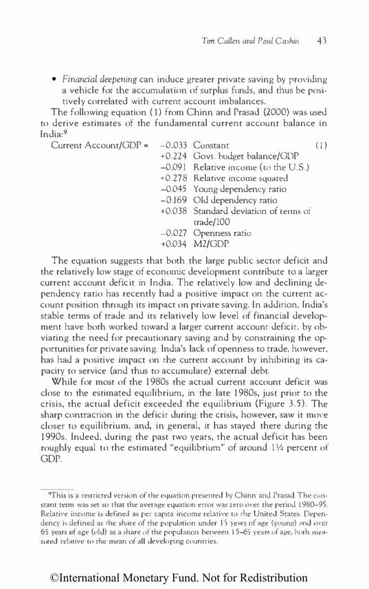
©International Monetary Fund. Not for Redistribution
Trm Callen and Paul Cashin 43
• Financial deepening can induce greater private saving by providing a vehicle for the accumulation of surplus funds, and thus be positively correlated with current account imbalances.
The following equation ( 1 ) from Chinn and Prasad (2000) was used to derive estimates of the fundamental current account balance in India:9
Current Account/GOP = -0.033 Constant ( I ) +0.224 Govt. budget balance/GOP -0.091 Relative income (to the U.S.) +0.278 Relative income squared -0.045 Young dependency ratio -0.169 Old dependency ratio +0.038 Standard deviation of terms of
trade/100 -0.027 Openness ratio +0.034 M2/GOP
The equation suggests that both the large public sector deficit and the relatively low stage of economic development contribute to a larger current account deficit in India. The relatively low and declining dependency ratio has recently had a positive impact on the current account position through its impact on private saving. In addition, India's stable terms of trade and its relatively low level of financial development have both worked tOward a larger current account deficit, by obviating the need for precautionary saving and by constraining the opportunities for private saving. India's lack of openness to trade, however, has had a positive impact on the current account by inhibiting its capacity tO service (and thus to accumulate) external debt.
While for most of the 1980s the actual current account deficit was close to the estimated equilibrium, in the late 1980s, just prior to the crisis, the actual deficit exceeded the equilibrium (Figure 3.5) . The sharp contraction in the deficit during the crisis, however, saw it move closer tO equilibrium, and, in general, it has stayed there during the 1990s. Indeed, during the past two years, the actual deficit has been roughly equal to the estimated "equilibrium" of around 1 114 percent of GOP.
9Th is is a resrricred version of rhe equation presented by Chinn and Prasad. The C<>n· stant term was set so that the aver:tge equation error was zero over the period I 980-95. Relative income is defined as per capita income relative tO rhe United States. Dependency is defined as the share of the popul<ltion under I 5 ye;us of age ( ynung) ;md over 65 years of age (old) as a share of rhe popul:nion berween I 5-65 ye:us of a_ge, borh measured relative ro rhe mean of all developing counrries.

©In
tern
atio
nal M
onet
ary
Fund
. Not
for R
edis
tribu
tion
Figu
re 3
.5.
Act
ual a
nd F
itte
d C
urre
nt A
ccou
nt B
alan
ce,
198
0-9
9
(In
perc
ent o
f GO
P)
-0.5
-1.
0
-1.
5
-2.
0
-2.
5
-3.
0
"
� \
� \
��
\ �
\ ,.
,.
\
-..
...... ._.,
,..'
\ \ \
, ..
. \
___
__,,
Ac
tual
"' �
' I
' c
urre
nt
.1c
co
un
t I
' ,
,' \
I I I I , , ,
I
r'"'" ,-"
, I , t I \
I \
I 'o�
I \
I \
I \
I \
I \
I \.
-I
- -..!
I" I \
I \ \ I I I I I I
I I
I \I
198
0
198
1 19
82
19
83
19
84
19
85
198
6
198
7
198
8
198
9
199
0
199
1 19
92
199
3
199
4
199
5
199
6
199
7
199
8
199
9
Sour
ces:
Dat
a pr
ovid
ed b
y th
e In
dia
n au
tho
ritie
s; a
nd s
taff
cal
cula
tio
ns.

©International Monetary Fund. Not for Redistribution
Tim Callen and Paul Cashin 45
Assessing the Sustainable Current Account Over the Medium Term
While the previous section provided an assessment of historic external sector developments, the methodologie employed generally do not permit an assessment of what current account deficit may be appropriate in the future. This is an important question, however, given that capital inflows have the potential to aid India's development process, while there is also a need to ensure these inflows are sustainable and used in an efficient manner. Addressing the issue of what is the appropriate current account level is difficult, and the answer will depend on many different factOrs. The 1993 High Level Committee on the Balance of Payments recommended that the current account deficit be contained to 1 .6 percent of GOP "given the level of normal capital flows,"10 while in its 1996/97 Annual Report, the Reserve Bank of India suggested that under the circumstances prevailing at the time, India could sustain a current account deficit of 2 percent of GOP.
A common approach to assessing the sustainability of a given path of the current account is to project into the future the current stance of macroeconomic policy and private secror behavior, and calculate the path of the current account that ensures the cotmtry's intertemporal budget constraint is not breached. This typic<'llly involves en uring that the ratio of net external liabilities (NEL) to GOP remains at its current level (on the assumption thar if this level is currently sustainable, then it should remain sustainable into the future).
The dynamics of NEL (and thus the current account balance) can be shown to be determined by the following equation (assuming the "no Ponzi game" constraint is valid): (r - y- A.E - YAE )
6b',+ I = ( 1 + y)( 1 + AE ) b', - q',
(Z)
where ' indicates that the variable is a ratio to GOP, yis the growth rate, A. is the fraction of NEL denominated in foreign currency, 11 r is the real rate of return on foreign liabilities, E is the rate of real appreciation of the domestic currency, b, is NEL, and q, is the current account balance net of payments on foreign liabilities. From equ<ltion (2) , the q� reqt�ired to achieve any given level of b� can be calculated given assumptions
10Report of rhe High L.:vel C<)mmirtt:.: on Balance of Pllyment� (Ch<Jirman: Dr. C. Rangarajan), 1993, Re$erve Bank of India Bulletin, August.
1 1 At end-1998, around l l percent of India's external dehr was denomm<tted in rupees (Government of India, 1999). In the ldlowing su$tainabiliry scenarios, we assume rhm this ratic) also applies to rota! extcrnal liabilinc$.

©International Monetary Fund. Not for Redistribution
46 ASSESSING INDIA'S EXTERNAL POSITION
about economic growth, the exchange rate, and the rate of return on foreign liabilities.
In the first scenario (Table 3 . 1 ) , the current account deficit that stabilizes the NEL-to-GOP ratio at irs end-1998/99 level of 3 1 percent is calculated, given a constant real exchange rate and varying assumptions about the real growth rate and the real cost of foreign liabilities.12 For example, assuming that real GOP grows at 5 percent a year and the real cost of foreign liabilities is 4 percent, then the deficit on goods, services, and transfers must average 0.3 percent of GOP to maintain the NEL-toGOP ratio at 3 1 percent. With the cost of servicing the outstanding stock of external liabilities at 1.2 percent of GOP, this results in an overall annual current account deficit of 1 . 5 percent of GOP (compared to the actual deficit of 1 .0 percent of GOP in 1 998/99). lf a higher growth rate of 7 percent per annum is achieved, a current account deficit of around 2.1 percent of GOP could be run. For eacl1 1 percentage point increase in the cost of external liabilities or fall in the growth rate, the required increase in the goods, services, and transfers balance, required to keep the ratio of NEL-to-GOP constant, is about 0.3 percent of GOP. If, instead, a real depreciation of the rupee of 1 percent per year is assumed, a current account deficit of 1 .3 percent of GOP would stabilize the NEL-to-GOP ratio at 3 1 percent of GOP with a growth rate of 5 percent per annum (Scenario 2) .
Given that the choice of maintaining a constant NEL-to-GOP ratio is somewhat arbitrary, two other scenarios are presented for comparison. In Scenario 3 the objective is to lower the NEL ratio to 2 1 percent of GOP over the next ten years. Under the same growth and interest rate assumptions as above, a current account deficit of only 0.5 percent of GOP could be run. If a rise in the NEL ratio tO 41 percent of GOP could be accommodated-perhaps through an increase in foreign direct investment-a much larger current account deficit of 2.5 percent of GOP could be run (Scenario 4 ).
These scenarios are designed only to be illustrative of the size of the current account deficits that could be sustainable into the future. What will actually prove sustainable will also depend on a large number of
12While official estimates of external debt are regularly puhlished, no estimates of equity liabilities are readily available. To derive an estimate of the <)Utsranding stock of NEL, we therefore added the stock of external debt (23 percent uf GDP at end-1998/99) to an estimate of the smck of equity liabilities calculated by accumulating (from 1970 onward) the flows of foreign direct and portfolio investment flows in the capit;�l ;�cc<Junt of the balance of paymencs. This methodology obviously does nor allow for valuation changes that have occurred since the flows were received. Using this method, the ourstanding stock of equity liabilities was estimated ar about 8 percent of GDP ar end-1998/99.

©In
tern
atio
nal M
onet
ary
Fund
. Not
for R
edis
tribu
tion
Tabl
e 3
.1.
Scen
ario
s of
the
Cur
rent
Acc
ount
Pos
itio
n (I
n p
erc
ent
of G
OP)
Scen
ario
1
Rea
l (S
tab
iliz
e N
EL)
Inte
rest
G
row
th R
ate
of
Rat
e N
et I
nves
tme
nt
Re
al
Inco
me
(p
erc
ent)
B
alan
ce
3.00
5.0
0 7.
00
2 -0
.62
-0.9
2 -
1.51
-2
.07
3 -0
.93
-0.9
3 -1
.52
-2.0
9 4
-
1.2
4
-0
.94
-
1.5
4
-2.
11
5 -1
.55
-0.9
5 -
1.55
-2
.13
6 -
1.86
-0
.96
-1.5
6 -2
.15
Scen
ario
2
(Sta
biliz
e N
EL
Scen
ario
3
wit
h d
epre
ciat
ion
) (R
educ
e N
EL)
Gro
wth
Rat
e o
f G
row
th R
ate
of
Re
al In
com
e
Rea
l Inc
om
e
3.00
5.0
0 7.
00
3.00
5.
00
7.00
Cur
rent
Acc
oun
t B
alan
ce
-0.6
5 -
1.24
- 1
.80
0.08
- 0
.51
-1. 0
7 - 0
.65
-1.
25
-1.8
2 0.
07
- 0.5
2 - 1
. 09
-0.6
6 -
1.26
-
1.8
4
0.06
- 0
.54
-
1.11
-0
.66
-1.2
7 -
1.8
6
0.05
-0
.55
-1.
13
-0.
67
-1.2
8
- 1.8
7 0 .
04
- 0.5
6 -
1.15
Of
wh
ich
: Go
ods
, Se
rvic
es,
and
Tra
nsfe
rs B
alan
ce
-0.3
0 - 0
.89
-1.4
5 -0
.03
-0.6
2 -
1.18
0.
70
0.11
- 0
.45
0.00
-0
.59
-1 .
16
0.28
-0
.32
- 0.8
9 1.
00
0.41
-0
.16
0.30
-0
.30
-0.8
7 0.
58
- 0.0
2 - 0
.60
1.
30
0.70
0.
13
0.60
0
.00
-0
. 58
0.
89
0.2
8
-0.3
1 1.
60
1.00
0.
42
0.90
0.
30
- 0.2
9
1.19
0.
58
- 0
.01
1.9
0
1.30
0.
71
Scen
ario
4
(Incr
ease
NEL
)
Gro
wth
Ra
te o
f R
eal
Inc
om
e
3.00
5.
00
7.00
-1.9
2 -2
.51
-3.
07
-1.9
3 -2
. 52
-3.0
9 -1
.94
-2.
54
-3.1
1 -
1 .95
-2
.55
-3.1
3 -
1.96
-2
.56
-3.1
5
- 1. 3
0 - 1
. 89
-2.4
5 -
1 .00
-1
.59
- 2.1
6
- 0.7
0 -
1.30
-1
.87
-0.4
0 - 1
.00
-1.
58
-0
.10
-0.7
0 - 1
.29
No
tes:
Th
e e
ntri
es i
n th
e u
ppe
r pan
el o
f the
tab
le a
re t
he
min
imum
cur
rent
acc
oun
t bal
ance
s re
quire
d to
mee
t cer
tain
ob
ject
ives
. The
ob
ject
ive
und
er S
cena
rio
1 i
s to
sta
bili
ze I
ndia
's n
et e
xter
nal
liab
ilitie
s (N
ELl
at it
s cu
rren
t le
vel o
f 31
per
cent
of G
OP,
und
er th
e as
sum
ptio
n of
a c
ons
tant
rea
l exc
hang
e ra
te. T
he o
bjec
tiv
e un
der S
cena
rio 2
is to
sta
bili
ze N
EL a
t its
cur
rent
lev
el o
f 31 p
erce
nt o
f G
OP,
giv
en a
rea
l ex
chan
ge r
ate
dep
reci
atio
n of
1 p
erce
nt p
er y
ear.
The
obj
ecti
ve
und
er Sc
enar
io 3
is t
o r
educ
e N
EL to
21
perc
ent o
f G
OP
by
the
year
200
8/0
9, u
nder
the
ass
ump
tion
of
a co
nsta
nt r
eal e
xcha
nge
rate
. Th
e o
bje
ctiv
e un
der S
ce
nario
4 is
to r
aise
NEL
to 4
1 pe
rcen
t o
f G
OP
by
the
real
exc
han
ge ra
te. I
n Sc
enar
io 2,
it is
assu
med
that
the
sha
re o
f ext
erna
l deb
t, w
hich
is d
enom
inat
ed in
for·
e
ign
curr
ency
, is
89
perc
ent.

©International Monetary Fund. Not for Redistribution
48 ASSESSING lNDIA'S EXTERNAL POSITION
other factors. For example, if the deficits were tO be financed mainly from direct investment flows, a larger outstanding stock of foreign liabilities could be maintained than if they were financed out of short-term debt flows (as was the case in the second half of the 1980s). Further, the sustainable level of capital flows is likely to be dependent on the continuation of structural reforms in the domestic economy, which will influence the return on the investment projects undertaken (represented by the high-growth scenarios in Table 3 . 1 ). As previously indicated, what may be a sustainable deficit under certain conditions in world capital markets may prove to be unsustainable under different circumstances. For example, a downturn in international investor confidence in developing markets may result in a reduction in capital inflows to India.
Summary and Conclusions
This paper has applied a number of methodologies to examine India's external developments. The results indicate that the path of the current account deficit has been consistent with intenemporal solvency as it did not breach the intertemporal budget <.onstrainr. There is evidence, however, that the intertemporal budget constraint was not satisfied in the period up to 1 990/9 1 , and the return to smaller current account deficits in the 1990s has been needed to reestablish solvency. The composite model of early warning indicators also indicated that the path of the current account deficit in the period preceding the 1991 crisis was not sustainable, while the actual deficit was above its estimated equilibrium for much of the 1 980s. The economic reforms undertaken since the early 1990s have brought about a more sustainable external position. The crisis probabilities also remained low during the Asia economic crisis, while the current account deficit appears to be around its equilibrium level at present. Estimates of what could be a sustainable current account deficit for India over the medium term indicate a range of 1 Y:!-2 Y2 percent of GOP, although this is dependent on the economic and policy environment.
References
Acharya, Shankar, 1999, "Managing External Economic Challenges in the Nineties: Lessons for the Future," Anniversary Lecture to the Centre for Banking Studies, Central Bank of Sri Lanka, Colombo, September.
Berg, Andrew, and Catherine Pattillo, 1999, "Predicting Currency Crises: The Indicators Approach and an Alternative," )oumal of lncernational Money and Finance, Vol. 18, No. 4, pp. 561-86.

©International Monetary Fund. Not for Redistribution
Tim Callen and Paul Cashin 49
Callen, 11m, and Paul Cashin, 1999, "Assessing External Sustainability in India," IMF Working Paper 99/181 (WashingtOn: International Monetary Fund).
Cashin, Paul, and C. John McDermott, 1998, "International Capital Flows and National Creditworthiness: Do rhe Fundamental Things Apply as Time Goes By?" IMF Working Paper 98/172 (Washington: International Monetary Fund).
Chinn, M., and E. Prasad, 2000, "Medium-Term Determinants of Current Accounts in Industrial and Developing Countries: An Empirical Exploration," IMF Working Paper 00/46 (Washington: International Monetary Fund).
Debelle, Guy, and Hamid Faruqee, 1996, "What Determines the Current Account? A Cross-Sectional and Panel Approach," !MF Working Paper 96/58 (Washington: International Monetary Fund).
Government of India, 1999, India's External Debt: A Scaw.s Report, Government of India Printer (India: New Delhi).
Isard, Peter, and Hamid Faruqee, 1998, Exchange Rate Assessment: Extensions of the Macroeconomic Balance Approach, IMF Occasional Paper No. 167 (Washington: International Monetary Fund).
Jalan, Sima\, 1992, "Balance of Payments, 1956-1991," in Bimal ]alan (ed.), The Indian Economy: Problems and Prospects (India: New Delhi).
Joshi, Vijay, and Jan Little, 1994, India: Macroeconomics and Political Economy, 1964-1991 (Washington: The World Bank).
Kaminsky, Graciela, Saul Lizondo, and Carmen Reinhart, 1998, "Leading Indicators of Currency Crises," Staff Papers (Washington: International Monetary Fund), Vol. 45, pp. 1-48.
Kapur, Muneesh, 1997, "India's External Sector Since Independence: From Inwardness to Openness," Reserve Bank of India Occasional Papers, Vol. 18, Nos. 2 and 3, June and September.
Kent, Christopher, 1997, "Essays on the Current Account, Consumption Smoothing, and the Real Exchange Rare" (Ph.D. dissertation; Cambridge, Massachusetts: Massachusetts Institute of Technology).
Milesi-Ferretti, Gian-Maria, and Assaf Razin, 1996, Current Account Su.stainabilicy, Princeton Studies in International Finance No. 81, October, International Finance Section (Princeron, New Jersey: Princeton University).
Montiel, Peter, 1994, "Capital Mobility in Developing Countries: Some Measurement Issues and Empirical Estimates," The World Bank Economic Review, Vol. 8, No. 3, pp. 3 1 1-50.
Report of the High Level Committee on Balance of Payments (Chairman: Dr. C. Rangarajan), 1993, Reserve Bank of India Bulletin, August.
Reserve Bank of India, Annual Report, various issues.
Sachs, Jeffrey, 1982, "The Current Account in the Macroeconomic Adjustment Process," Scandinavian journal of Economics, Vol. 84, No. 2, pp. 147-59.

©International Monetary Fund. Not for Redistribution
This page intentionally left blank

©International Monetary Fund. Not for Redistribution
PART II
Fiscal Challenges

©International Monetary Fund. Not for Redistribution
This page intentionally left blank

©International Monetary Fund. Not for Redistribution
4 Tax Smoothing, Financial Repression, and Fiscal Deficits in India
PAUL CASHIN, NILSS 0LEKALNS, AND RATNA SAHAY1
Introduction
Budget imbalances are pervasive in developing countries. Yet there are few studies asking whether this outcome is consistent with optimal fiscal policy. Five decades of time series data for India are examined to answer this question.
The optimality criteria used to examine Indian fiscal policy is based on the concept of tax smoothing. Tax smoothing recognizes that in the presence of an increasing marginal social cost of raising tax revenue, it is optimal if the planned tax rate is constant (smoothed) over time (Barro, 1979).2 A smooth tax rate implies that temporary shocks to government spending and output yield fiscal imbalances, and it provides a rationale for the issuance of public debt. In this sense, the tax-smoothing hypothesis is the fiscal analog of Campbell's ( 1987) consumptionsmoothing model.
1The aU[hors are grateful to Eduardo Borenszrein, Timothy Callen, Ajai Chopra, Pierro Garibaldi, Nadeern Ul Haque, Mohsin Khan, Paul Masson, John McDerrnon, Xavier Sala-i-Marrin, Patricia Reynolds, Parthasarathi Shome, M.R. Sivaraman, Peter Wickham, and especially Martin Miihleisen for their valuable comments and suggestions on earlier drafts, and Manzoor Gill for valuable research assisrance. Any remaining errors are our responsibility.
2As noted by Barro ( 1979, 1995), for a given amoum of public expenditure, if taxes are lump sum and the other conditions for Ricardian equivalence are presem, there are no
53

©International Monetary Fund. Not for Redistribution
54 TAX SMOOTHING, FINANCIAL REPRESSION, AND FISCAL DEFICITS
This paper tests for the presence of tax-smoothing behavior in India using data from 1951/52-1996/97 and the vector autoregressive approach of Huang and Lin ( 1 993) and Ghosh ( 1995). This approach generates a time series for the optimal budget surplus, assuming that the government tax smooths, which is compared to the actual surplus. If smoothing is to hold, any differences between the two series should be quite small. We are also able to control for nontax-smoothing causes of fiscal deficits, enabling a more accurate test of the tax-smoothing model.
The intertemporal tax-smoothing model successfully explains the behavior of Indian fiscal deficits. Our results also confinn previous findings that financial repression traditionally made a significant contribution to Indian net revenues. The financial repression-induced overborrowing of the 1970s and 1980s has yielded a stock of liabilities that deviates from the stock of liabilities generated from the series of optimal (tax-smoothing) fiscal deficits. As of 1996/97, the government's actual stock of public liabilities was about 1 8 percent of GOP higher than it would have been under optimal tax-smoothing policies, implying that fiscal surpluses (or at least smaller deficits) will need to be run in the future to ensure intertemporal solvency.
The paper presents an overview of some features of Indian public finance. Key issues involved in testing for tax smoothing are then outlined, followed by a description of the econometric methodology and relevant data. The results from tests of tax smoothing and fiscal sustainabiliry are then presented, and are followed by some concluding comments.
Issues in Indian Public Finance
Indian Fiscal Outcomes
Figure 4.1 (top panel) plots the fiscal position (gross fiscal deficit) of the Indian central government (CENGFD) between 1951/52 and 1996/97, where the gross fiscal deficit is the excess of aggregate disbursements (net of recovery of loans and advances) over receipts (revenue receipts, including external grants, plus nondebt capital receipts of government).J The fiscal deficits of the center can be financed by borrowing
real effects from shifts between taxes and the issuance of public debt as modes of financing fiscal imbalances. However, if taxes are distorting then the timing of taxes will matter, and it will be desirable to smooth tax rates over time, financing any temporary difference between public revenue and public expenditure by creating public debt.
1The deflnition of the gross fiscal deficit follows that of the publications of the government of India, as it includes the proceeds from disinvestment in public sector enterprises in the center's revenue.
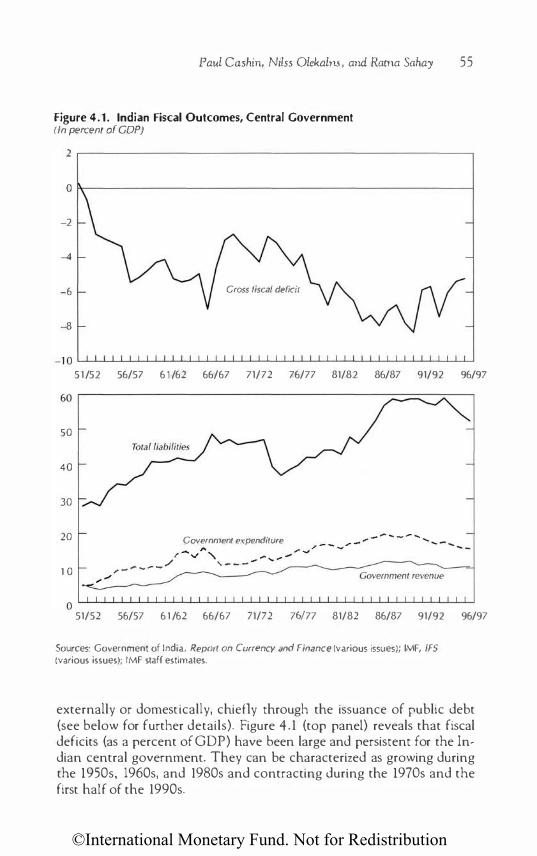
©International Monetary Fund. Not for Redistribution
Paul Cashin, Nilss Olekalns , and Ratna Sahay 55
Figure 4.1. Indian Fiscal Outcomes, Central Government (In percent of COP)
2 .--------------------------------------------------,
0 �--------------------------------------------------�
-2
-4
-6 Gross fiscal deficit
-8
-]QLL���LLLL���LL���LLLL���LLLL���LLLL�
50
40
30
20
1 0
51/52 56/57 6 1 /62 66/67 71/72 76/77 81/82 86/87 91/92 96/97
-- �
Governn1ent expenditure ,. - - - -""' ...... -� , � , - - _ , -
, --../ ' - -..... ..... ..., , _ ..,.. _ _ _ / , _ _ _ ---------
OLL���LL���LLLL���LLLL���LL���LLLL�� 51/52 56/57 6 1 /62 66/67 71/72 76/77 81/82 86/87 91/92 96/97
Sources: Government of India, Report on Currency and Finance (various issues); IMF, IFS (various issues); IMF staff estimates.
externally or domestically, chiefly through the issuance of public debt (see below for further details). Figure 4.1 (top panel) reveals that fiscal deficits (as a percent of GOP) have been large and persistent for the Indian central government. They can be characterized as growing during the 1950s, 1960s, and 1980s and contracting during the 1970s and the first half of the 1990s.

©International Monetary Fund. Not for Redistribution
56 TAX SMOOTHING, FINANCIAL REPRESSION, AND FISCAL DEFICITS
The balance of payments crisis of 1991 resulted in the near exhaustion of India's foreign exchange reserves, largely caused by rhe withdrawal of foreign currency deposits by nonresident Indians. While the trigger for the crisis lay in domestic political difficulties and the Persian Gulf war, concern over the sustainability of Indian fiscal policy, due to rising debt and debt servicing, was a key factor underlying the crisis (see Chopra et al., 1995, for details). Prior to the crisis, India financed its fiscal deficits Largely through financial repression, with high reserve deposit requirements and statutory liquidity ratios inducing commercial banks to hold below-market-yielding public debt. Following liberalization of the financial system beginning in 1991, the government increasingly had to borrow at close to market rates of interest. This shift to market borrowing in the context of high primary deficits resulted in a sharp increase in the government interest bill. For example, central government interest payments (CENINT) rose by almost V2 of 1 percent of GOP between 1990/91 and 1996/97, even though the center's liabilities fell by over 6 percent of GOP over the same period. Figure 4.1 (bottom panel) illustrates that central government liabilities (CENUAB) doubled as a percentage of GOP between the early 1950s and mid-1990s.
Indian Financial Repression
As in many developing countries, governments in India have found it difficult tO satisfy their intertemporal budget constraint with conventional revenue and borrowings of the type discussed above. In addition to market borrowing as a means of deficit financing, governments have also used the implicit taxation of financial intermediation, using quasifiscal activities such as seigniorage and financial repression as sources of fiscal revenue and reduced interest costs, respectively.
Seigniorage-the purchasing power over real goods and services that comes about due to a central bank's monopoly over the issuance of reserve money-is typically passed on to the government either through central bank profits or via no- or low-interest loans to the government. Seigniorage taxes-the change in reserve money as a share of GOPwere an important component of Indian taxation over the period 1960/61-1994/95, representing on average 1 .5 percent of GOP per year. Similarly, Fischer ( 1982) calculated that annual average Indian seigniorage revenues amounted to about 1 percent of GNP between 1960-76, or about 1 0 percent of government revenue. Click ( 1998) also recently calculated that annual average Indian seigniorage revenues over the period 1971-90 were about 1 . 7 percent of GOP, or about 12 percent of government spending.

©International Monetary Fund. Not for Redistribution
Paul Cashin, Nilss Olekalns, and Rama Sahay 57
Financial repression in India traditionally involved domestic borrowing by the government at below-market interest rates, owing to banking regulations.4 The Indian cash reserve ratio (CRR) historically ranged between 4-7 percent of bank deposits, yet was steadily raised to 1 5 percent by the late 1980s to bolster demand for reserve money. Similarly, the statutory liquidity requirement (SLR) was raised from about 20 percent of deposits in the early 1 960s to 38.5 percent in the early 1990s. Both requirements enabled the government to garner about half of all credit extended by the banking system between the early 1 960s and early 1990s, at interest rates below those required to voluntarily acquire the debt. Consequently, banks invested in assets (consistent with CRR and SLR requirements) that barely covered their cost of funds (see Joshi and Little, 1996; IMF, 1996, 1 997). At end- 1999, the CRR and SLR (as shares of bank deposits) stood at 9 and 25 percent, respectively.
Financial repression was also facilitated by a network of publicly controlled financial institutions. Nominal ceilings on institutional interest rates were used to limit competition from the private sector for the pool of loanable funds. Thus financial intermediaries typically set loan rates on private domestic credit that differed from the exchange-rateadjusted world interest rate. Indian governments also required their public financial institutions to undertake additional quasi-fiscal operations, involving activities such as the promotion of subsidized credit to priority areas of the private sector (such as agriculture and small-scale manufacturing), the setting of credit ceilings and floors, exchange rate guarantees, loan rate ceilings, and loan guarantees. The liberalization of India's financial sectOr in the 1990s, however, reduced the impact of many of these quasi -fiscal activities. For example, exchange guarantees were transferred to the government from the central bank, reserve requirements on commercial banks were reduced, and there occurred the removal of many of the restrictions on the setting of commercial bank interest rates (see Joshi and Little, 1 996; IMF, 1996, 1997).
Sustainability of Indian Fiscal Policies
India has a low level of public saving relative ro other developing countries and experienced a steady decline in public saving over the pa t two decades (Muhleisen, 1997). Previous work examining the historical
;Annual average revenue frorn financial repressitm in India has heen escimatcd by Giovannini and Je Melo ( 1993) ac a �izable 2.86 perc em of GOP and over 22 percent of government revenue (excluding revenue from financial repression) for rhe period 1980-85.

©International Monetary Fund. Not for Redistribution
58 TAX SMOOTHING, FINANCIAL REPRESSION, AND FISCAL DEFICITS
path of India's fiscal imbalances found that continuation of rhe trend of growing fiscal deficits during the 1 980s was not consistenr with the eventual repayment of public sector debt, and that there was little scope for seigniorage revenues to fill the fiscal gap (see, for example, Suiter and Patel, 1992). In addition, these studies argued that the positive value of India's primary fiscal deficit was inconsistent with a shrinking present discounted value of the debt stock. That is, if nominal interest rates exceed rhe GOP growth rate, primary surpluses (which have not been forthcoming) would be required to stabilize the debt-to-GOP ratio and ensure the sustainability of fiscal imbalances (see Reynolds, 2000, for a discussion of fiscal sustainability and solvency).
Testing the Tax-Smoothing Hypothesis
The previous section highlighted how Indian governments have used revenues from financial repression to compensate for a shortfall in revenues from more conventional sources. This and later sections consider whether the raising of these revenues, with respect to both their magnitude and timing, has been optimal. This analysis uses the tax-smoothing model as our optimality benchmark. It also examines whether the accumulation of public liabilities, which involves both the tax-smoothing and tax-tilting components of fiscal deficits, is on a sustainable path.
The tax-smoothing model assumes that, in the absence of a first-best system of lump-sum taxes, the government seeks to minimize the welfare losses arising from its choice of tax rate. These losses are assumed to be an increasing, convex, and time-invariant function of the average tax rate. The government's ability to minimize the tax-induced distortions is conditioned by its adherence to the intertemporal budget constraint. This requires the present value of tax receipts tO be sufficient to cover all current and future government spending together with the government's initial debt. In order to meet the intertemporal budget constraint, taxes cannot remain invariant to changes in either current or expected future expenditure. Welfare losses will be minimized, however, if, in response to newly acquired information indicating a furure change in government expenditure, the government smooths the implied tax change over time.
Following the approach of Barre ( 1 979), Ghosh ( 1995), and Olekalns ( 1 997), the optimal budget surplus at time t (sur,*) is given by
( 1 )
where it is assumed that the effective interest rare faced by the government is R; the expectations operator is E; the information set available

©International Monetary Fund. Not for Redistribution
Paul Cashin, Nilss Olekalns, and Rarna Sahay 59
to the government at time c is 1,; 6 is the first difference operator; and g, is (exogenously given) government outlays excluding interest payments, G., normalized by the level of output, Y,. 5
Implications of the Tax-Smoothing Hypothesis
Equation ( 1 ) states that the optimally chosen budget surplus is a linear function of expected future changes to government expenditure. The implication of an expected decline in government expenditure is that the government wiLL reduce its budget surplus (possibly running a budget deficit), so that the tax reduction can be smoothed over time. An increase in the budget surplus is a signal that the government is anticipating an increase in its expenditure and is seeking to smooth the tax increase. The government's behavior is analogous to that of a consumer in consumption-smoothing models, who adjusts savings based on the expectation of future "rainy days" (see Campbell, 1987).
There are four testable implications of tax smoothing that can be derived from equation ( 1 ). These are
1 . The optimal tax rate changes only if there is new information concerning government expenditure. Accordingly, under rational expectations, tax changes should not be forecastable and should follow a random walk.
2. The budget surplus should Granger-cause (help predict) changes in government spending. This will be true whenever the government has better information about the future path of its expenditure than is contained in past values of the expenditure series.
3. The smoothed budget surplus should be stationary. Assuming that g, is I(l) , then Ag, will be 1(0); since under the null hypothesis the actual (tax-smoothed) budget surplus is the discounted sum of 6g, (see equation ( l ) ) , then the smoothed budget surplus wiLL also be 1(0).
4. The optimal smoothed surplus derived from equation ( l ) should differ from the actual, smoothed surplus by at most a random sampling error.
Why Run Deficits? Separating Tax Smoothing and Tax Tilting
There are two broad considerations motivating any government to
run a budget deficit: tax tilting and tax smoothing. The analysis, up to
5When rhe rare of real output growth, n, is positive, the effective inreresr rare faced by the government (R-1 = (l +r)/( 1 +n)) will be smaller than the actual marker interest rare, ( 1 +r), where r is the assumed (constant) real rate of interest.

©International Monetary Fund. Not for Redistribution
60 TAX SMOOTHING, FINANCIAL REPRESSION, AND FISCAL DEFICITS
this point, has assumed that only tax smoothing motivates the government to run either a budget deficit or a budget surplus. However, other intertemporal incentives for running unbalanced budgets exist. Even if we assume that government spending as a share of GOP will remain constant into the future (in which case there would be no need for rax smoothing), if the government's subjective discount rate (reflecting the preference for current taxation over future taxation), p, differs from the effective interest rate, R, then the optimal tax rate will be affected by the government's desire to engage in tax tilting. As noted by Ghosh ( 1995), the relationship between P and R is given by y=[(l-(R/P)R)/(1-R)], where y, the tax-tilting parameter, accounts for the fact that the optimal tax rate incorporates incentives for the government to defer taxes or enlarge surpluses, depending on the relationship between P and R. That is, when p:;rR (y;t:l), the government's optimal tax profile will be "tilted." Tax tilting results in a bias toward either budget deficits or budget surpluses, which are created in a manner consistent with intertemporal solvency. For example, if P<R (y< 1 ) , the government's incentive is ro shift taxes into the future, run fiscal deficits, increase its current level of liabilities, and gradually raise taxes over time. Such a government has a relatively high discount rate. It would choose to have a low tax rate in the present period but would raise taxes over time to service its accumulating stock of debt. Conversely, if P>R, the government has an incentive to bring tax increases forward, run fiscal surpluses, build up its stock of assets, and gradually lower taxes over time.
Since tax tilting has implications for the budget surplus that are entirely distinct from tax smoothing, it is important to ensure that the optimal surplus derived from equation ( 1 ) is compared to only that component of the budget surplus that relates ro tax smoothing and not to the actual budget surplus, which potentially includes both tax-smoothing and tax-tilting components.6 This requires that tax tilting be filtered from the actual budget surplus, with the tax-smoothing component of the surplus defined as
(2 )
where dt is the srock of debt (liabilities) in period t , D" normalized by the level of output, Y,; and rt is the average rate of tax at time t. In equation (2), when R>P (and y < l ). the tax-smoothing surplus sur/"' will be larger than the measured budget surplus, since the incentive is
6The tax-tilting (nonstationary) component of the actual fiscal surplus is removed ro construct the tax-smoothing (stationary) component of the fiscal surplus. BeyonJ our desire to focus on tax smoothing, thi.s is necessary to ensure the validity of standard statistical inference techniques, which will be used for hypothesis testing below.

©International Monetary Fund. Not for Redistribution
Paul Cashin, Nilss Olekalns, and Ratna Sahay 61
for the government to defer tax collections into the future (and so run a budget deficit in the present on tax-tilting grounds). This paper focuses on the tax-smoothing component of budget surpluses, because without an explicit model of intergenerational welfare it is not possible to decide whether deferring/bringing forward tax collections (that is, tax tilting) is desirable. However, as long as the government's objective function involves the minimization of the distortionary costs of taxation (which are assumed to rise quadratically with "t1), then there will be avoidable deadweight costs from a failure to tax smooth (Ghosh, 199 5) .
Econometric Methodology
The estimation and testing procedure is carried out in four steps. The first step is to obtain an estimate of y-1, the tilting parameter, in order to construct the stationary (tax-smoothing) component of the fiscal balance by removing from the data the nonstationary (tax-tilting) component of the fiscal balance. Given that '!1 and [g1 + (r-n)d1] are both I ( 1 ) variables, then this estimate of y-1 can be obtained from equation (2), as the cointegrating parameter from a regression of [g1 + (r-n)dJ on -rr- This relationship is best estimated using the Phillips-Hansen ( 1990) fully modified (FM) method, which yields an asymptotically correct variance-covariance estimator in the presence of serial correlation and endogeneity. To confirm that the regression is indeed cointegrated, the Phillips-Ouliaris ( 1 990) residual-based cointegration test is employed; the actual (tax-smoothing) component of the fiscal balance, sur/m, is defined by the residuals of the cointegrated regression of equation (2) .
The second step is to calculate the optimal tax-smoothing component of the budget surplus. The derivation of the optimal budget surplus requires a measure of anticipated future changes to governmem expenditure. Following Campbell and Shiller (1987), an obvious way of deriving such a measure is to exploit the fact that, under the null hypothesis that tax smoothing is valid, the budget surplus contains all the known information about future changes to the government's spending plans and should help predict future changes in government expenditure. Because the smoothed budget surplus (sur/m) responds to expected future changes in government spending, it is a relevant information variable to forecast future changes in government expenditure. In addition, we can exploit the information concerning future expenditure plans contained in current and lagged values of Llgr - This means that forecasts of future changes to government spending can be recovered from a bivariate vector autoregression (VAR) in L\g1 and sur1sm.

©International Monetary Fund. Not for Redistribution
62 TAX SMOOTHING, FINANCIAL REPRESSION, AND FISCAL DEFICITS
As a result, we estimate a first-order unrestricted VAR of the form W, = A w,_, + E [ > where w, = (�g[> sur/m)', E I is a 2xl vector of disturbance terms, and A is a 2x2 matrix of coefficients. With the estimate of A from the VAR and using the fact that EJW,+i] = Ai W" an estimate of the optimal tax-smoothing component of the budget surplus can be computed as
sur,*•m = [ 1 O] R A [I2 - R A)-1 W, = AW, (3) where 12 is the 2x2 identity matrix and A is a lx2 matrix of coefficients.7 Equation (3) is valid as long as both the infinite sum in equation ( 1 ) converges, and the variables appearing in the W matrix of the VAR system are stationary. If g, is 1( 1 ), �g, will be 1(0). Since under the null hypothesis the actual (tax-smoothing) budget surplus (sur/m) is equal to sur/-which from equation ( 1 ) is a discounted sum of �g.then surt" will also be I(O). The validity of the tax-smoothing hypothesis can be tested by comparing the estimate of the optimal (taxsmoothing) budget surplus derived from equation (3) with the estimated actual (tax-smoothing) budget surplus derived from equation (2).
The third step is to conduct a series of hypothesis tests to evaluate the validity of several implications of the tax-smoothing model. As mentioned above, these are: the tax rate should follow a random walk; the smoothed budget surplus should be stationary; and the government's budget surplus helps predict changes in government expenditure. The final test examines whether the VAR parameters in equation (3) conform to the nonlinear restriction
A = [ 1 0] R A [12 - R A]-1 = [0 1 ] . (4)
TI1is restriction implies that movements of the actual (tax-smoothing) budget surplus reflect those of the optimal (tax-smoothing) fiscal surplus; failure of this restriction implies that the government is not optimally smoothing its taxation path. Examination of whether the optimal and actual (smoothed) fiscal surpluses are similar, which would be a finding supportive of the tax-smoothing hypothesis, can be done by inspection of a plot of the respective series or, more formally, by estimation of the equation
sur,*•m = A W, = A-1 tlg, + � sur,sm . (5)
7The assumption of a consram real imeresr rare (r) assisrs in rhe derivation of equation (3), by allowing for the summation of a matrix geometric series. It also implies that the tax-tilting parameter is constant, which allows for stochastic de trending of the actual budget surplus data to focus on the stationary tax-smoothing component of the budget surplus.

©International Monetary Fund. Not for Redistribution
Paul Cashin, Nilss Olekalns, and Rama Sahay 63
Optimal tax smoothing implies the joint parameter restriction A.1 = 0
and A.2 = 1 , and nonrejection of these joint restrictions implies that movements in sur,*sm fully reflect movements in sur/'".
The fourth and final step in this analysis concerns whether the path of public liabilities is sustainable. Sustainability focuses on whether fiscal policies couUl be continued indefinitely, in contrast to the taxsmoothing analysis above that focuses on the optimality of fiscal policies-that is, whether they shouUl be continued. To address this issue, we develop a test based on a multi-period application of the singleperiod budget constraint and examine the time series properties of the stock of public liabilities. This is done to characterize the data-generating process and make inferences about whether the path of fiscal policies is consistent with solvency. By iterating the standard dynamic budget constraint forward we have [ T-1 J D, = E, pTDT - .r. P' DEF,+, o•O
(6)
where the fiscal deficit is DEF, = G, - -r,Y,. lf the tax-smoothing model is valid, then we also have [ T-1 J D,* = E, - lim .r. pi DEF,:, T->- o=O (7)
where the optimal fiscal deficit is DEF; = G , - -r,*Y., the optimal tax rate is -r,*, and p= l/( l +r). Equation (7) states that the present discounted value of future fiscal deficits (or surpluses) must be matched by initial assets (or liabilities). Abstracting from tax-tilting causes of any change in the stock of public liabilities, since the stock of public liabilities consistent with the (tax-smoothing) model-generated path of fiscal deficits (0�) is sustainable by construction, the difference between the actual stock of public liabilities (0) and the stock consistent with the taxsmoothing model (0, - o;) must be stationary if Indian fiscal policy is to be sustainable. That is, Indian fiscal policy can be sustained without the need for reform if the series calculated as the difference in the two stocks of public liabilities (0, - 0;) is Stationary; if not, then the actual stock of public liabilities is not sustainable on unchanged fiscal settings, and a change in fiscal policy is required.
Data Sources and Definitions
The data are taken from official sources-definitions and descriptions of the various data manipulations are detailed in Appendix 4 . 1 . The period covered ranges from 1951/52 ( marking the beginning of India's first five-year plan) to 1996/97. Expenditures and revenues are measured, respectively, by aggregate disbursements (current expenditure,

©International Monetary Fund. Not for Redistribution
64 TAX SMCX)THING, FINANCIAL REPRESSION, AND fiSCAL DEFICITS
capital outlays, and loans and advances), net of recovery of loans and advances of the central government (CENEXP), and the sum of revenue receipts (including external grants) plus nondebt capital receipts of the central government (CENREV). Accordingly, the fiscal deficit measure includes the center's loans and grants to the states on the expenditure side and its receipt of interest and loan repayments from the states on the revenue side. This is done as the center may need to raise (lower) taxes as a result of this expenditure (revenue raising), and hence such fiscal actions will be affected by tax-smoothing considerations.8
Our measure of the budget surplus is constructed by substituting the above concepts of expenditure and revenue into the right-hand side of the government's dynamic budget constraint written in terms of GOP, which is given by ( 1 +n)(d,-d,+1) = -r,-g, + (n-r)d,. The debt stock is measured by the total liabilities of the central government (CENUAB).9 In Indian public finance, the excess of expenditure (CENEXP) over revenue (CENREV) yields the government's gross fiscal deficit (CENGFD).
A measure of the real interest rate and real growth rate is required to derive the optimal smoothed budget surplus. Two different nominal interest rates are tested. The first divides the central government's interest payments (CENINT) by irs liabilities (CENLIAB), and the second is a weighted arithmetic average of the interest rates at which money is accepted by selected commercial banks in Bombay (INT). The results proved to be insensitive to the choice of nominal interest rate; the reported results use the second of these two measures.10 Nominal gross domestic product at market prices (NGDP) is used to normalize the variables where appropriate, and real gross domestic product (RGDP) is used to calculate the real growth rate for the economy. Finally, the tax-smoothing component of the budget surplus is derived according to equation (2).
Empirical Results: Testing for Tax Smoothing and Fiscal Sustainability
The Phillips-Hansen ( 1990) fully modified OLS estimator yielded a value for r1 in equation (2) of 1.402, with an associated standard error
8See Cashin, Olekalns, and Sa hay ( 1998) for additional details. 9As wid1 many developing countries, mere are two main reasons why India's srock of
public debt may not be willingly held by market agents. First, part of India's external debt was obtained on concessional terms from official bilateral and multilateral sources, and, second, pan of India's domestic debt is held by financial institutions at below-market rates of rewm to satisfy liquidity requirements.
10When calculating the surplus, r and n are set equal to meir respective average values. The consumer price index (CPI) is used ro convert these nominal rates to real rates.

©International Monetary Fund. Not for Redistribution
Paul Cashin , Nilss Olekalns, and Rama Sahay 65
of 0.040. 1 1 The value of this estimate shows that tax tilting has been very important for the Indian government and has led deficits to be much larger than they otherwise would be. It also implies that the government has a preference for deficits falling over time. An important source of this incentive to tilt deficits toward the current period has been the extensive quasi-fiscal activities of India's public financial institutions, chiefly the large-scale taxation of financial incermediation through seigniorage and financial repression. These quasi-fiscal activities resulted in India's real rate of interest (r) being low (and often negative) for much of the sample period, yielding low values for the effective interest rate faced by government (R-1 = ( l+r)/(l+n)), indicating that the government has a high discount rate (�<R) and hence y-1 is much greater than one.
The value of y-t for India far exceeds the value of this parameter in previous empirical work for developed countries of Australia (Oiekalns, 1997, y-t = 0.96), Canada (Ghosh, 1995, 0.93), and the United States (Ghosh, 1995, 0.94).12 This result reflects the fact that tax tilting, carried out through seigniorage and financial repression, is a much more important source of net revenue for India than the other (all developed) countries that have been examined in the literature for evidence of tax-smoothing fiscal behavior. The value of y-t = 1.40 indicates that the component of the actual Indian fiscal deficit attributable to tax tilting is equivalent to forgoing 40 percent of taxation revenue in the near term, and subsequently raising taxes over time to clear the accumulated stock of liabilities. Some indication of the respective magnitudes of tax tilting can be gauged from Figure 4.2, which shows the actual deficit and the tax-smoothed deficit (with the tax-tilting component removed) .
Table 4.1 reports the results of three different tests of the unit root and stationarity hypotheses. The tests are used tO evaluate the predictions made by the tax-smoothing model that the average tax rate follows a random walk, and the smoothed budget surplus is stationary. The table shows the results from the augmented Dickey-Fuller (AOF) and Phillips-Perron ( 1 988) (PP) unit root tests, and the Kwiatkowski et al. ( 1992) (KPSS) test for stationarity. These results support the taxsmoothing hypothesis. The ADF and PP tests are unable tO reject the
11Phillips-Perron unit root tests (using an intercept and trend) reveal that both 't, (-1.317) and [g, + (r-n)d.] (-2.037) are integrated of order one (the null hypothesis of a unit root cannot be rejected at the 5 percent level of significance), and so the possibility of cointegration exists.
121n contrast, the estimate of y-1 for India is close to that found for Pakistan, where f""1 = 1.23 (Cashin, Haque, and Olekalns, 1999).

©International Monetary Fund. Not for Redistribution
66 TAX SMOOTHING, FINANCIAL REPRESSION, AND FISCAL DEFICITS
Figure 4.2. Central Government, Actual and Smoothed Budget Surpluses (In percent of GOP)
0.04 .-------------------------------., 0.03
0.02
O.Ql 0.00 f-:T-I-<\-------A--+-------\----.,----=---I-�1-----1
-0.01
-0.02 , _ _ '-"\ " ,' \. ..... ,, \ -\ -0.03 ' I I f I
\ I I I v I -0.04 I I I I \ /1
I .) I I Actual \ /\ I -0.05
� \1 1 I \ /''\ I - ' I ' I -{). 06 L..L.J....J.....L...I-'--'--L.J....J.....L...I-'--'--L.J....J.....L...I-'--'--L.J....J.....L...I-'--'--L.J....J.....L...I ... _,__-..... -.J....J.....!...!"'.o.�-L...L....L.J....l..J
51/52 56/57 61/62 66/67 71/72 76/77 81/82 86/87 91/92 96/97
unit root hypothesis for the average tax rate, and this is consistent with the KPSS test, which rejects stationarity. The respective tests also show that the first difference of government expenditure is clearly stationary, and, under the tax-smoothing hypothesis, the smoothed component of the budget surplus should also be stationary. This is confirmed by the respective tests. 13
Table 4.2 shows the results from the Granger causality test. The hypothesis that the budget surplus Granger-causes (helps predict) changes in government expenditure is rejected by the data at the 5 percent level of significance. The hypothesis cannot be rejected, however, at the 1 0 percent level, and this provides some evidence that the central government's budget surplus is informative about future changes to central government expenditure, which is consistent with tax smoothing.
The actual ( tax-smoothed) budget surplus derived from equation (2) and the optimal (tax-smoothed) budget surplus derived from equation (3) are graphed in Figure 4.3. There is a close correspondence between the actual and optimal smoothed surpluses. This is confirmed by a Wald test of the parameter restrictions implied by the tax-smoothing hypothesis, which examines whether there is a close association between movements in the actual (tax-smoothed) budget surplus and the optimal (tax-smoothed) budget surplus. The test shows that the parameter
1 1Using the critical values from the Phillips-Ouliaris (1990) Z(c) residual-based coin· regrntion test, we find that the null hypothesis of a unit root for sur,"" can be rejected at rhe 5 percent significance level in favor of stationarity. Accordingly, we accept that equation ( 2) is a cointegrated regression.

©International Monetary Fund. Not for Redistribution
Paul Cashin, Nilss Olekalns, and Ratna Saha)' 67
Table 4.1. Unit Root and Stationarity Tests
1:, sur,sm g, t!.g,
ADF Test -1.303 -3.599* -2.341 -7.128* PP Test -1.317 -3.639* -2.379 -7.116. KPSS Test 1.401* 0.129 1 .343* 0.283
Notes: ADF and PP refer to the augmented Dickey-Fuller (1979) and Phillips-Perron (1 988) unit root tests, and KP5S refers to the Kwiatkowski et al. ( 1 992) test for stationarity. The lag length for the ADF test is determined using the lag deletion technique recommended by Campbell and Perron (1991 ), where lags are successively deleted until a significant lag is reached. The maximum lag was set at four. For the PP test, the lag length was set at three periods for all variables; the results did not change appreciably for other lag lengths. Both the ADF and PP test regressions include an intercept term. The results for the KPSS tests are for two lags (the results did not change appreciably for other lag lengths). A • indicates that the null hypothesis of a unit root ((or the ADF and PP tests) or the null hypothesis of stationarity (for the KPSS test) can be rejected at (at least) the 5 percent significance level. The 1 percent, 5 percent, and 10 percent critical values are -3.58, -2.93, and -2.60 (for the ADF and PP tests), and 0.739, 0.463, and 0.347 (for the KPSS test). re-
Table 4.2. Granger Causality Test
sur,'"' � t!.g,
p p t!.g, = r a.flg,_; + .r �;sur,''," t=al ,.1
Lag
-0.01 6 (0.157)
�I
0.289 (0.163)
F
3.139*
Notes: The Granger causality test is an F-test to determine if the (smoothed) budget surplus causes (helps predict) changes in government expenditure, that is, whether 131=0. The lag length, p, was chosen by minimizing the Schwarz Bayesian Criterion; the maximum lag length tried was p:4. The figure in parentheses is the (heteroskedastic-consistent) standard error. A • denotes that the null hypothesis of no causation can be rejected at the 1 0 percent level of significance, indicating that the current budget surplus does have predictive power for future changes in govern· ment expenditure.
restrictions implied by tax smoothing on the VAR are not rejected by the data at the 1 percent level of significance, indicating that the differences between the actual (tax-smoothed) and optimal (taxsmoothed) surpluses observed in Figure 4.3 just represent random sampling error. In particular, the estimated coefficient on A.1 is not significantly different from zero, and the estimated coefficient on A.2 is not significantly different from on.e. 14
The results, therefore, support the hypothesis that the central government of India has engaged in tax-smoothing behavior over the period analyzed. In other words, it responded to expected future changes in government spending by running budget imbalances rather than altering
14The coefficients 1, and 12 are the estimated parameters from equat it)n (5), anJ their values (with heteroskedastic standard errors in parentheses) are 1, =0.002 (0.125) and 11=0.878 (0.455).

©International Monetary Fund. Not for Redistribution
68 TAX SMOOTHING, FINANCIAL REPRESSION, AND FISCAL DEFICITS
Figure 4.3. Central Government, Actual and Optimal Smoothed Surpluses (In percent of COP)
0 025 ,.--------------------------,
0.020
0.015
0.010
0.005
0.000 f.""'-1-----1-tr---.f--------+--------l--1--+----1 -0.005
-0.010
-O.Dl 5
-0.0 20 L...l-....I-L...L-J-L-._._.L...L....L...L...L-J-L-._._.L...L._._._,_._._.L...L...l-L--'--J-'-l-L...L...L...J....L....J-1-L-l-L...J..J 53/54 58/59 63/64 68/69 73/74 78/79 83/84 88/89 93/94
contemporaneous government revenue. While the observed behavior is consistent with tax smoothing, the smoothness of taxes was most likely due to the traditional inability of the government to satisfy its intertemporal budget constraint from conventional (rax and nonrax) revenue sources, which resulted in changes in public borrowing as the preferred response to expected future shocks to government spending. This inability to garner sufficient revenue has stemmed largely from the narrowness of the tax base, widespread tax evasion and exemptions, weak tax administration, the poor economic performance of revenue-earning public enterprises, and the fact that a large part of economic activity is undertaken in the underground economy (see Joshi and Little, 1994, 1996).
The above results point to the broad consistency of India's fiscal data with the predictions made by the tax-smoothing hypothesis. It is important to remember when interpreting these results, however, that they relate only to the smoothed component of India's fiscal imbalances. The magnitude of the tax tilting that has occurred is sufficiently large that there can still be concerns about the sustainability of India's overall fiscal imbalances, even if the stationary component of the budget surplus adheres to the tax-smoothing hypothesis. To gain some insight, the consistency of the actual srock of public liabilities with inrertemporal solvency is investigated. The rationale is ro see whether the srock of liabilities consistent with the optimal path of fiscal deficits generated by the tax-smoothing model, (D,•) , evolves in tandem with the actual srock of public liabilities, (D,), as set out in equations (7) and (6), respectively. This test is conducted by examining whether (D, - D,*), the implied excess

©International Monetary Fund. Not for Redistribution
Paul Cashin, Nilss Olekalns, and Rama Sahay 69
accumulation of public liabilities, is stationary. The tax-smoothing model generates conditions under which the stock of public liabilities can be repaid, and fiscal deficits derived under the model are, by definition, sustainable. Accordingly, if the actual stock of public liabilities (which includes a tax-tilting component) is rising more rapidly than the stock of liabilities implied by the tax-smoothing model, then the current path of fiscal deficits under unchanged policies is unsustainable.
To formally test for the presence of nonstationarity in (D, - D,*), we use the ADF test, and construct D,* assuming that the 1953/54 actual stock of liabilities equals the stOck of liabilities consistent with the optimal path of fiscal deficits generated by the tax-smoothing model. The result for the liabilities of the central government (CENLIAB) indicates that the ADF test statistic has a value of -2.305, which fails to reject the null hypothesis of nonstationarity in the difference between the actual and tax-smoothing-based stocks of liabilities at the 5 percent level of significance. Accordingly, the difference between the actual and tax-smoothing-based stocks of liabilities contains a unit root, implying that the two series deviate and have no tendency to follow one another. That is, under unchanged fiscal policies, India's stock of public liabilities is not sustainable.15
This result can also be seen in Figure 4.4, which shows (after normalizing the debt stock by GOP) the actual (d.) and tax-smoothingbased (d,*) stocks of liabilities, as well as the implied excess accumulation of public liabilities (c4 - d.*). Over the period 1953/54-1996/97, the excess accumulation of liabilities has been rising, indicating that public borrowing is in excess of what expected future fiscal surpluses can service. While the excess accumulation was relatively small until the early 1970s (the scock of actual liabilities was less than 5 percent of GOP greater than its optimum level), the difference between the two stocks of liabilities grew rapidly during the 1970s and 1980s, peaking in the late 1980s at about 25 percent of GOP. During the first half of the 1990s, the excess accumulation declined as a result of the central government's program of fiscal consolidation, so that in 1996/97 the actual srock of public liabilities was about 18 percent of GOP higher than the level consistent with the optimal path of fiscal deficits generated by the taxsmoothing model.
The actual stock of public liabilities reflects both tax smoothing and tax-tilting considerations. Given that the Indian central government
1'Recent work by Olekalns and Cashin (2000) and Reynolds (2000) also finds rhar, under unchanged fiscal policies, India's fiscal imbalances are not consistent with intertemporal solvency. See also Srinivasan (2000) for a recent analysis of India's fiscal situation.

©International Monetary Fund. Not for Redistribution
70 TAX SMOOTHING, FINANCIAL REPRESSION, AND FISCAL DEFICITS
Figure 4.4. Central Government, Actual and Implied Optimal Debt Stocks (In percent of COP)
0.6,---------------------:::;:::::=;;::::--:;;;;:---, 0.30 0.5
0.4
0.3 0.2
0.1
/' / \ , ..; I I ,..,, \ I
,. .... )1 "Actual-optimal (right scale) ""' , .... �
I "'.,.. _ , _.. I
0.25
0.20 0.15
0.10
0.05 0.0 1+---------------------------l 0.00
-0. 1 L.....L...L...I--L..L...J.....J....J.....l....J....L...L....I.....L...;L....L....l....J......L..J--L..L...J.....J....J.....l....J....L...L....I.-I-L....L....l....J.....L...I--L..L...J.....J....J._J -0.05 53/54 58/59 63/64 68/69 73/74 78/79 83/84 88/89 93/94
was found to tax smooth, then the bulk of its excessive public borrowing can be attributed to tax tilting, with the government levying low taxes in the present and (implicitly) higher taxes in the future so that intertemporal solvency can be satisfied. This requires that at some future point in time taxes wiLL need to be raised and fiscal surpluses (or smaller fiscal deficits) will need to be run to service the government's stock of liabilities.
Conclusion
This paper examined evidence for tax-smoothing behavior in India over the period 1951/52-1996/97. In response to a temporary increase in government spending, the tax-smoothing approach predicts that the tax burden of funding this expenditure will be spread over time, and so the government will run a fiscal deficit in the short-run. Conversely, a permanent increase in spending should be financed by raising contemporaneous taxes, resulting in no fiscal deficit. The intertemporal tax-smoothing model is successful in explaining the behavior of the fiscal deficits of the Indian government, and so the government does keep its tax rate relatively constant (smooth) in the presence of temporary shocks to expenditure. We argue that the traditional inability of the government to satisfy its intertemporal budget constraint from conventional (tax and nontax) revenue sources resulted in public borrowing being its preferred response to shocks to government spending-behavior consistent with

©International Monetary Fund. Not for Redistribution
Paul Cashin, Nilss Olekalns, and Ratna Sahay 7 1
the tax-smoothing hypothesis. Moreover, this same inability to garner sufficient receipts from conventional revenue sources results in taxtilting behavior by the government, with quasi-fiscal activities such as seigniorage and financial repression being important sources of net revenue.
An analysis based on long-term trends indicates that during the period 1953/54-1996/97, under unchanged policies, India's stock of liabilities was not on a sustainable path. In particular, the tax-tilting-induced overborrowing of the 1970s and 1980s yielded a stock of liabilities that deviates significantly from the stock of liabilities generated from the series of optimal (tax-smoothing) fiscal deficits. By 1996/97, the actual stock of public liabilities was about 1 8 percent of GOP higher than it would have been under tax smoothing. This implies that fiscal surpluses (or at least smaller fiscal deficits) will need to be run in the future to ensure intertemporal solvency. This result emphasizes the importance of enhancing the process of fiscal consolidation that began in the early 1990s.
References
Barro, Robert J., 1979, "On the Determination of the Public Debt," journal of Political Economy, Vol. 87 (October), pp. 940-7 1 .
---, 1995, "Optimal Debt Management," Working Paper No. 5327 (Cambridge, Massachuseus: National Bureau of Economic Research), pp. 1-36.
Buiter, Willem H., and Urjit R. Patel, 1992, "Debt, Deficits and Inflation: An Application to the Public Finances of India," Journal of Public Economics, Vol. 4 7 (March), pp. 172-205.
Campbell, John, 1987, "Does Saving Anticipate Declining Labor Income, An Alternative Test of the Permanent Income Hypothesis," Econometrica, Vol. 55 (November), pp. 1249-73.
---, and Roberr Shiller, 1987, "Cointegrarion and Tests of Present Value Models," Journal of Polirical Economy, Vol. 95 (Ocrober), pp. 1062-88.
Campbell, John Y., and Pierre Perron, 1991, "Pitfalls and Opportunities: What Macroeconomists Should Know about Unit Roots," Research Memorandum, Econometric Research Program, Princeton University, No. 360 (April), pp. 1-67.
Cashin, Paul, Nilss Olekalns, and Rama Sahay, 1998, "Tax Smoothing in a Financially Repressed Economy: Evidence from India," IMF Working Paper WP/98/122 (Washington: International Monetary Fund).
Cashin, Paul, Nadeem Ul Haque, and Nilss Olekalns, 1999, "Spend Now, Pay Later? Tax Smoothing and Fiscal Sustainability in South Asia," IMF Working Paper WP/99/63 (Washington: International Monetary Fund).
Central Statistical Organization, 1996, National Accounts Statistics , Ministry of Planning and Program Implementation, New Delhi.

©International Monetary Fund. Not for Redistribution
72 TAX SMOOTHING, FINANCIAL REPRESSION, AND FISCAL DEFICITS
Chopra, Ajai, Charles Collins, Richard Hemming, and Karen Parker, 1995, "India: Economic Reform and Growth," IMF Occasional Paper 134 (Washingron: International Monetary Fund).
Click, Reid W., 1998, "Seigniorage in a Cross-Section of Countries," Journal of Money, Credit and Banking, Vol. 30 (May), pp. 154-7L.
Dickey, David A., and Wayne A. Fuller, 1979, Distribution of the Estimators for Autoregressive Ttme Series with a Unit Root," Journal of the American Statistical Association, No. 74, pp. 427-3 1 .
Fischer, Stanley E, 1982, "Seigniorage and the Case for a National Money," Journal of Political Economy, Vol. 90 (April), pp. 295-3 13.
Ghosh, Atish R., 1995, "lntertemporal Tax Smoothing and the Government Budget Surplus: Canada and the United States," Journal of Money. Credit and Banking, Vol. 27 (November), pp. 1031-45.
Giovannini, Alberto, and Martha de Melo, 1993, "Government Revenue from Financial Repression," American Economic Review, Vol. 83 (September), pp. 953-63.
Huang, Chao-Hsi, and Kenneth S. Lin, 1993, "Deficits, Government Expenditures, and Tax Smoothing in the United States: 1929-1988," Journal of Monetary Economics, Vol. 3 1 (June), pp. 3 1 7-39.
International Monetary Fund, 1996, "India-Selected Issues," IMF Staff Country Report 96/132 (Washington: International Monetary Fund).
--, 1997, "India-Selected Issues," IMF Staff Country Report 97/74 (Washington: International Monetary Fund).
Joshi, Vijay, and Ian M.D. Litrle, 1994, /ndia: Macroeconomics and Political Economy, 1964-91 (Washington: World Bank).
---, 1996, India's Economic Reforms, 1991-2001 (Oxford: Clarendon Press).
Kwiatkowski, Denis, Peter Phillips, Peter Schmidt, and Yoncheol Shin, 1992, "Testing the Null Hypothesis of Stationarity Against the Alternative of a Unit Root: How Sure Are We That Economic Time Series Have a Unit Root?" Journal of Econometl·ics, Vol. 54 (October-December), pp. 159-78.
Ministry of Finance, 1966, Budget for 1965-66, and various issues (Delhi, India: Government of India Press).
Muhleisen, Martin, 1997, "Improving India's Saving Performance," IMF Working Paper WP/97/4 (Washington: International Monetary Fund).
Olekalns, Nilss, 1997, "Australian Evidence on Tax Smoothing and the Optimal Budget Surplus," Economic Record, Vol. 73 (September), pp. 248-57.
---, and Paul Cashin, 2000, "An Examination of the Sustainability of Indian Fiscal Policy," Research Paper 748, Department of Economics, University of Melbourne.
Phillips, Peter C.B., and Bruce E. Hansen, 1990, "Statistical Inference in Instrumental Variables Regression with 1(1) Processes," Review of Economic Studies, Vol. 57 (January), pp. 99-125.

©International Monetary Fund. Not for Redistribution
Paul Cashin, Nil�s Olekalns, and Rama Sahay 73
Phillips, Peter C. B., and Samuel Ouliaris, 1990, "Asymproric Properties of Residual-Based Tests for Cointegration," Econometrica, Vol. 58 (January), pp. 165-93.
Phillips, Peter C. B., and Pierre Perron, 1988, "Testing for a Unit Root in Time Series Regression," Biometrika, Vol. 75 (June), pp. 335-46.
Reserve Bank of India, 1997, Report on Currency and Finance , 1996-97, and earlier issues (Mumbai, India: Reserve Bank of India).
Reynolds, Patricia, 2000, "Fiscal Adjustment and Growth Prospects in India," in India at the Crossroads: Sustaining Growth and Poverty Reduction Ten Years After Crisis , M. Blejer and C. Towe, eds. (WashingtOn: International Monetary Fund), Chapter 5.
Srinivasan, TN., 2000, "India's Fiscal Situation: Is a Crisis Ahead?," mimeo, Yale University.
Appendix 4. 1 : Data Appendix
All data used have been derived from official sources, and are annual in frequency. It should be noted that they are for financial years ending March 3 1 ; for example, 1 994/95 refers to the year ending March 3 1 , 1995.
1. INT is the call money rate for scheduled commercial banks in Bombay for the period 195 1/52-1956/7, then the money market rate (rate offered in the Bombay interbank market) from 195 7/58 onwards, both taken from IMF, International Finance Statistics (IFS), line 60b.
2. NGOP is nominal GOP at market prices, in billions of rupees (Rs. crore) , taken from IMF, IFS line 99b and Central Statistical Organization ( 1996).
3. RGOP is real GOP at market prices, in billions of 1990/91 rupees (Rs. crore), taken from IMF, IFS line 99b and Central Statistical Organization (1996).
4. GOPOEF is the GOP deflator (base 1990/91= 100), derived from NGOP and ROGP.
5 . CPI is the consumer price index for industrial workers for 50 centers of India, taken from IMF, IFS line 64 and Central Statistical Organization ( 1996).
6. CENREV is the sum of revenue receipts ( including external grants) plus nondebt capital receipts of the Government of India, GOI, in billions of rupees (Rs. crore), taken from Budgetary Position of GOI, Revenue Receipts of GOI and Capital Receipts of

©International Monetary Fund. Not for Redistribution
74 TAX SMOOTHING, FINANCIAL REPRESSION, AND FISCAL DEFICITS
GOI tables of the Reserve Bank of India's Report on Currency and Finance, and IMF staff estimates.
7. CENEXP is aggregate disbursements (revenue expenditure, capital outlays, and loans and advances), net of recovery of loans and advances of the central government, in billions of rupees (Rs. crore), taken from Budgetary Position of GOI, Revenue Expenditure of GOI and Capital Disbursements of GOI tables of Report on Currency and Finance, and IMF staff estimates.
8. CENGFD is the gross fiscal deficit of the central government, and is calculated as the excess of CENEXP over CENREV. It is financed by external borrowing and domestic borrowing, where the latter comprises market borrowing (chiefly from publicly owned financial institutions), treasury bills, changes in cash balances with the Reserve Bank of India (RBI), small savings scheme, and state provident funds.
9. CENINT is interest paymentS made by the central government, in billions of rupees (Rs. crore), taken from Revenue Expenditure (nondevelopment expenditure) table of Report on Currency and Finance . This measure is for total interest payments, involving interest payments on internal debt, external debt, small savings and provident funds, reserve funds, and other obligations.
10. CENLIAB is total liabilities of the central government on March 3 1 , in billions of rupees (Rs. crore) , taken from Liabilities and Capital Investments and Loans Advanced by Central Government table of Report on Currency and Finance and Ministry of Finance, Budget Papers, various issues. Total liabilities includes public debt, small savings scheme, provident funds, and reserve funds and deposits.

©International Monetary Fund. Not for Redistribution
5 Fiscal Adjustment and Growth Prospects in India
PATRICIA REYNOLDS
Introduction The overall deficit of the consolidated public sector1 has been rising
in recent years, following a modest decline during the first half of the 1990s (Figure 5 . 1 ) . The significant adjustment after the 1990/91 balance of payments crisis was the result of sharp cuts (relative to GOP) in central government expenditures on defense, subsidies, and capital items, as
well as more modest adjustments by state governments and public sector undertakings (PSUs). Consequently, the deficit was cut by 3 percent of GOP, to just over 8 percent of GOP. Since 1995/96, however, this trend has reversed as expenditures at both the central and state levels have picked up, and the public sector deficit is estimated to have exceeded 1 1 percent of GOP in 1999/2000. As a result of these large deficits, the public sector debt ratio has remained high throughout the decade-above 75 percent of GOP.
The costs typically associated with a fiscal imbalance of this magnitude are well known: high inflation; weak growth as private investment is crowded out; constraints on public spending on infrastructure and social priorities owing to high debt service costs; and pressures on the ex
ternal current account owing to weak national saving. There is also the
1The consolidated public secror comprises the central and state governments, central government public enterprises, and the Oil Coordinating Committee.
75

©International Monetary Fund. Not for Redistribution
76 FISCAL ADJUSTMENT AND GROWTH PROSPECTS IN INDIA
Figure 5.1. Government Deficits and Debt, 1950/51-1999/2000 (In percent of GOP)
Government Deficits
1 0
8
6
4
2
1\ A I '
/ '-"'""', I , _ ,.. _,. ,,
' ... "'"'
State governments
0 LL���WL����WL���-L����WL����WL����� 50/51 56/57 62/63 68/69 74/75 80/81 86/87 92/93 98/99
100 .--------------------------------------------------
. Government Debt
80 - C�-public sector'
60 - --Central government
� 40 - -
State governments 20 r - - - -- - - - - - - - - - - - - - - - - - - -- - - - - - - - - - - ----
80/81 82/83 84/85 86/87 88/89 90/91 92/93 94/95 96/97 98/99
Sources: Reserve Bank of India; Union Budget documents; Public Enterprises Survey; and staff estimates. 1The consolidated public sector comprises the central and state governments, central government public enterprises, and the Oil Coordinating Committee.
risk that the fiscal situation could become unsustainable and trigger a financial crisis.
For India, the costs of large fiscal deficits appear tO have been significant. While inflation has remained low over the past three decades (Figure 5.2)-indicating that the recourse to monetary financing has been contained-the impact of fiscal indiscipline can be seen elsewhere. The strong negative correlation between the public sector balance and private investment spending relative tO GOP suggests that

©In
tern
atio
nal M
onet
ary
Fund
. Not
for R
edis
tribu
tion
Figu
re 5
.2.
Gro
wth
, Int
eres
t Ra
tes,
and
Infl
atio
n, 1
95
1/5
2-
199
9/
20
00
(I
n p
erce
nt)
20
1 5
10
5
0
-5
-10
-15
-20
I I
I I
I I
I I
II
I I
' I
I I
I I
I I
I "
f
I,
I '\
I
/nfla
lion
1 (G
OP
defla
tor)
: I Real
imere
st r
ale
on c
en1r
al g
ove
rnm
enl d
ebt1
51/
52
54/5
5 57
/58
60
/61
63/6
4
66/6
7 69
/70
72/7
3 75
/76
78/7
9 8
1/8
2
84/8
5 87
/88
90/9
1 93
/94
96/9
7 99
/00
Sour
ces:
Cen
tral
Sta
tist
ical
Org
aniz
atio
n; R
ese
rve
Ban
k o
f In
dia
; Uni
on
Bud
get d
ocu
men
ts;
Pu
blic
En
terp
rise
s S
urv
ey;
and
sta
ff es
timat
es.
'Cal
cula
ted
as
tota
l in
t ere
st p
aym
ent
s d
ivid
ed
by
out
stan
ding
deb
t.

©International Monetary Fund. Not for Redistribution
78 FISCAL ADjUSTMENT AND GRO\VTH PROSPECTS IN INDIA
Figure 5.3. Private Investment Spending and Public Sector Deficits, 1986/87-1 999/2000
o:- 20 a \J '-. 0 95/96 t: • 96/97 • • � <1.> 97/98 98/99 99/00
1 5 .s. • •
g§l 2ZI93 23/94 90/91 • "0 • 21/9Z c: 94/95 <1.> .;} • • t: 88/89 87/88 <l.> 1 0
86/87 § • "' � .s .!!:! � d: 5
8 9 1 0 1 1
Public Sector Deficit (percent of COP)
Sources: Central Statistical Organization; Union Budget documents; and staff estimates.
89/90 •
1 2
investment has been adversely affected (Figure 5.3 ) , and the rapid increase in debt service payments has contributed to a sharp decline in capital expenditures and outlays on social programs (Figure 5.4 ). Moreover, while the current account deficit has generally remained low due, in part, to a high private saving rate, the 1990/91 balance of payments crisis illustrates that fiscal imbalance leaves India highly vulnerable to external shocks. These risks are often acknowledged by policymakers in India. Most recently, the Reserve Bank of India's May 2000 Monetary and Credit Policy Statement noted that "such high levels of fiscal deficits are not sustainable over the medium rerm."2
This paper considers in greater detail the costs and sustainability of large fiscal imbalances in India and, more broadly, the implications of alternative fiscal policies for long-run growth and external viability. The next section discusses how one might judge the sustainabiliry of a particular fiscal strategy, and the critical role played by interest rates and growth rates in such an analysis. A description of a long-term macroeconomic simulation model that can be used to evaluate alternative fiscal strategies follows. This model is then used to study the implications of
2Statemem by Dr. Bimal )alan, Governor, Reserve Bank of India on Monetary and Credit Policy for the year 2000-01, April 27, 2000.

©In
tern
atio
nal M
onet
ary
Fund
. Not
for R
edis
tribu
tion
Figu
re 5
.4.
Cen
tral
Gov
ernm
ent
Expe
ndit
ures
, 1
97
4/
75
-19
99
/2
00
0
(In
per
cent
of
GO
P)
8 7
6
5 4
3 2
Non
-def
ence
ca
pit
al e
xpen
ditu
res
and
net
lend
ing1
Educ
atio
n ex
pend
iture
il
Hea
lth e
xpen
ditu
res'-
I --
--
----
--
---
---
�--
--
--
---,
0
19
74/7
5 19
76/7
7 19
78/
79
198
0/8
1 19
82/
83
198
4/8
5 19
86/8
7 19
88/
89
19
90/
91
19
92/9
3
Sour
ces:
IMF,
Go
vern
men
t Fin
ance
Sta
tisti
cs;
Rese
rve
Bank
of
Ind
ia;
and
staff
est
imat
es.
1199
8/99
valu
es a
re re
vise
d es
timat
es; 1
999/
200
0 va
lues
are
bud
get e
stim
ates
. 11
997/
98 v
alue
s ar
e re
vise
d es
timat
es;
1998
/99
valu
es a
re b
udge
t est
imat
es.
Inte
rest
pay
me
nts
'
--
--
---
--
--
--
199
4/9
5 1
996
/97
199
8/9
9
©International Monetary Fund. Not for Redistribution
80 FISCAL ADJUSTMENT AND GROWTH PROSPECTS IN INDIA
three main scenarios: the continuation of present fiscal policies, aggressive fiscal adjustment, and an intermediate case of slower and more modest fiscal consolidation.
The analysis suggests that current policies are unlikely to be sustainable over the long run. Continued large fiscal deficits would be expected to lead to an increasing debt ratio and increasing pressure on real interest rates, depressing economic growth and national saving, and causing the external position to deteriorate. As interest rates rise above the rate of economic growth, the debt dynamics would become increasingly precarious. The Indian economy would also be highly vulnerable to external shocks-especially a loss of investor confidence that caused a further increase in interest rates. A truly sustainable fiscal strategy that facilitates the achievement of high economic growth would require a significant front-loaded adjustment.
Fiscal Sustainability and Solvency
Fiscal policies are considered to be sustainable if the government is able to service the stock of public debt over the foreseeable future. In particular, Fischer and Easterly ( 1 990) suggest that fiscal policy sustainability be defined in terms of the projected future course of the debt-toGOP ratio in the context of a model of the macroeconomy. If the debtto-GOP ratio is projected to rise continually, fiscal policies are unlikely to be sustainable, and an adjustment must be made.
Analysis of fiscal sustainability ofren begins with consideration of fiscal solvency, since this is a relatively easier concept to define. Solvency simply requires that the expected discounted value of future primary surpluses (plus seigniorage revenues) be at least sufficient to repay the current stack of government debt. Equivalently, solvency requires that the present value of the government's debt stock must tend to zero over time. (Appendix 5 . 1 provides a derivation of these conditions and a more detailed discussion of some of the issues that follow.)
It is useful to recognize that there are situations where a fiscal strategy might violate the solvency condition but still be sustainable, at least in the short-run. To understand why, note that solvency depends in part on the relationship between the long-run real (nominal) interest rate and the long-run real (nominal) rate of GOP growth. First consider the case where an economy's rate of GOP growth exceeds its interest rate. In this situation, a government might be able to continually borrow to repay interest, since the relative size of the debt stock would be eroded over time by the relatively high economic growth rate. Thus, fiscal policy might be sustainable for many years-as long as the interest rate remains below the

©International Monetary Fund. Not for Redistribution
Patricia Reynolds 81
growth rate. The government would be insolvent by the above definition, however, since it would never actually repay the principal of its debt.
In the long run, however, economic development and financial liberalization would be expected to erode such a favorable growth-interest rate differential and make fiscal sustainability more difficult to achieve. Consider the situation where an economy has a rate of GOP growth equal to or less than its interest rate. If the government attempts to maintain a primary deficit over the long run,3 rising interest payments will increase the need for new debt more rapidly than the relative size of the current debt stock is eroded by GOP growth. In this case, the debt-to-GOP ratio would explode in both discounted and undiscounted terms, and the government would be both insolvent and pursuing an unsustainable fiscal strategy.
Since rhe solvency condition implies that the present value of the outstanding debt stock should tend toward zero over time, empirical studies of fiscal solvency often examine the path of the historical debe stock, discounted back co a given date, for srationariry. Several studiesincluding Rajaraman and Mukhopadhyay (2000), Serven ( 1996), Buiter and Patel ( 1992), and Chapter 4 of this book-followed this tack using data on various measures of government debt in India, over various time periods between 195 1/52 and 1997/98.4 None of these authors was able to reject the hypothesis of an explosive discounted debt path, and each therefore concluded that prevailing fiscal policies in India were inconsistent with the eventual repayment of public sector debt.
Do these results also imply that the prevailing fiscal strategy was unsustainable! Possibly not, at least over the short run. Figure 5.1 illustrates that the debt-co-GOP ratio has been fairly stable or declining since the early 1990s. Figure 5.2 illustrates that, although the average real inrerest rate on Indian government debt has risen significantly during the sample periods (and subsequently), it has fallen well short of the real GOP growth rate. The relatively low average interest rate on government debt has allowed new borrowing to be undertaken in order to service existing debt, at a slower rate than the speed at which the value of government debt relative to GOP has been eroded by the higher rate of economic growth. Although indefinite pursuit of this strategy would lead to public sector insolvency-since by definition government debt will never be repaid-the favorable growth-interest rate differential has allowed these policies to be sustained in recent decades, without triggering a debt explosion. Moreover, the rise in the private saving rate-
lMore precisely, the solvency condition will be violated if the government maintains a primary deficit that is sufficiently large relative tO long-run seignornge revenues.
41n Chapter 4, Cashin, Olekalns, and Sahay follow a slightly differem :1pproach. by examining the starionariry of the difference between the actual debt stock and rhe taxsmoothed debt stock (which is consistent with solvency by construction).

©International Monetary Fund. Not for Redistribution
82 FISCAL ADJUSTMENT AND GROWTH PROSPECTS IN INDIA
owing to financial sector development, the growth of the formal sector, and favorable demographic trends-has helped to offset the adverse impact of low public sector saving on the current account deficit.
It seems unlikely, however, that this favorable differential will persist indefinitely. Economic development should bring an increase in average interest rates on government borrowing, as external concessional loans decline and as domestic financial market liberalization limits the scope for domestic government borrowing at below-market rates.s Excessive government borrowing could also lead to an increase in risk premiums, especially if market participants become concerned that the government's fiscal strategy does not allow for full repayment of principal. lndeed, average interest rates on Indian government debt have exhibited a trend increase over the past two decades.6
There are also factors that could erode the favorable differential by lowering the GOP growth rate. Continued high deficits could crowd out public and private investment spending on both physical and human capital-refer again to Figures 5.3 and 5.4. Finally, in the very long run, growth theory suggests that economic growth rates should slow in the latter stages of economic development, as the marginal product of capital converges to the levels in more developed economies.?
Concern regarding both the desirability and sustainability of fiscal policies in India has been heightened in recent years with the slowdown in industrial growth and the erosion of fiscal discipline since the mid-1990s.8 ln order to illustrate the risks of present policies and the benefits of fiscal consolidation, the following section describes a simple neoclassical growth model, which builds on the work of Parker and Kastner (1993). This model is calibrated to fit the Indian economy and then used to examine the implications of alternative fiscal policies on longer macroeconomic trends.
'Giovannini and de Melo (1993) estimated that the government of India earned an average of 2.86 percent of GOP annually in revenues from financial repression during the period 1980-85 (where revenue from financial reprc�sion is calculated as the ex post di fferential between foreign and domestic interest rates, times the stock of governmem debt held outside the central bank). Moreuver, this discussion does not fully capture the effect of tax concessions on governmenr debt, and the debt dynamics.
6This is true for average interest rates measured either as total interest payments divided by outstanding debt (as in Figure 5.2), or as the weighted average government securities rate.
7Jn standard models that allow for productivity growth, the "golden rule" capiral-labor ratio-the ratio that maximizes per capita consumption along the steady state growth path-implies that the real interest rate (marginal product of capital) will equal the growth rnte of real output.
8ln particular, rhese concerns are highlighted in Reserve Bank of India ( 1999b). pp. 143-44 and Reserve Bank of India ( 1999c), pp. V-12-V-13.

©International Monetary Fund. Not for Redistribution
Patricia Reynolds 83
A Framework for Assessing the Implications of Fiscal Policy
The growth model underlying the scenarios presented below is based on a saving-investment framework (Appendix 5.2 provides details). Output growth is driven by private and public sector decisions about investment, combined with structural factors that influence investment efficiency. In particular, the projected growth rate of real GOP in any given period is assumed to depend on the rate of total investment spending and the incremental capital-output ratio (ICOR).9
Private and public investment decisions, combined with public and private saving decisions, determine the current account balance and the amount of required external financing. Public investment and saving decisions, taken together, determine the government's financing need, which must be satisfied by some combination of external borrowing, domestic borrowing, and the inflation tax. Choice of the inflation tax determines the money supply rule and, together with the real growth rate, the inflation rate.
There are several policy choices that therefore impact the macroeconomic outcome.IO
• The overall public sector primary deficit. Given interest payments (determined by the public debt stock and the prevailing interest rate) and private sector saving and investment decisions (discussed below), the government's primary deficit determines the current account balance. 11
• The composition of deficit financing. Private sector external borrowing and net foreign direct investment flows are both assumed to depend on the level of GOP, as well as the degree of capital account liberalization. Given an overall borrowing requirement, the public sector's external borrowing therefore adjusts ro ensure that the capital account balance offsets the current account balance. The government must also decide on a combination of domestic borrowing and the inflation tax to finance the remainder of the
9Reliable estimates of an aggregate production function for India are nor available, mainly owing to poor data on labor input (since labor force estimates do not cover workers in the large informal sector).
IOSeveral simplifying assumptions are also employed, in particular: (i) the reserve money multiplier is assumed to be constant at 3.8 (its value in 1998/99); (ii) broad money velocity is assumed to decline by about 1.5 percent per year, consistent with the trend over the last decade; (iii) official reserves are assumed constant at 7.6 percent of GDP (the ratio as of end 1998/99); and (iv) the real effective exchange rate is assumed to be constant, as is foreign inflation--changes in the nominal exchange rate are therefore dictated by the choice of the domestic inflation rare.
11Nore that the model focuses on the gross debt stock; the rerum on assets is subsumed in the primary deficit.

©International Monetary Fund. Not for Redistribution
84 FISCAL ADJUSTMENT AND GROWTH PROSPECTS IN INDIA
fiscal deficit. In keeping with India's recent inflation experience, the examples that follow all assume a constant annual inflation rate for the GOP deflator of 6.2 percent.
• The pace of structural reforms-such as deregulation of the industrial sector and privatization of public enterprises, labor market policies, trade liberalization, infrastructure development, and financial market reform-would directly impact the lCOR, private capital inflows from abroad, and also private saving and investment (see below). In order to isolate the impact of fiscal policies, however, all scenarios presented in the next section assume a common, gradual fall in the !COR from an estimated 3.95 in 1999/00 to 3.75 by 2019/20--consistent with a modest improvement in investment efficiency.
Interest rates, as well as private saving and investment decisions, are internally determined and are influenced by policy variables both directly and indirectly:
• The risk premium on Indian government debt over international real interest rates is assumed to increase with the level of public sector indebtedness. Moreover, real interest rates on government debt are assumed to increase over time, as concessional debt matures and the Indian financial sector becomes more integrated with world markets. 12
• Private saving is projected to depend positively on real per capita GOP, and negatively on the age-dependency ratio and the public saving rate.l3 Of these variables, real per capita GOP growth is internally determined, while the public saving rate is the direct result of policy decisions. The age-dependency ratio--which has an irtlportant impact on saving-is taken as external and is assumed to decline sharply over the next two decades.14
LlThe risk-free real interest rates on domestic and external debt are assumed m increase from estimated levels of 2.2 and 0.8 percent, respectively. in 1999/00 to 4 percent by 2019/20.
LlCoefficients were set with reference to estimations done by Miihleisen ( 1996) and Salgado (1995) using Indian data, and by Masson, Bayoumi, and Samiei (1995) using a developing country panel dataseL The specific equations estimated by these authors were not used, owing ro poor our-of-sample predictive power and because the model does not generate projections for some of the required explanarory variables.
14According to World Bank projections of population by age category, the dependency ratio (the percent of the population less than 15 years of age or over 64 years of age, divided by the percent of the population between ages 14 and 64) will decline from 66.7 percent in 1995 to 44.8% by 2020. This trend is primarily driven by the youth-dependency ratio, which is projected to fall from 59 percent in !995 to 35.3 percent by 2020. In contrast, the old age-dependency ratio is expected to rise from 7.7 percent to 9.6 per· cent during the same period.

©International Monetary Fund. Not for Redistribution
Patricia Reyno/as 85
• Private investment spending is assumed to depend positively on lagged real GOP growth and public investment spending, and negatively on the real interest rate.15 Of these variables, public investment spending and the real interest rate (through the channels discussed above) are directly influenced by policy variables.
Alternative Fiscal Scenarios
The baseline scenario seeks to illustrate the outcome that is likely to result if no further fiscal adjustment is undertaken. The key assumptions under this scenario are (i) the consolidated public secror primary deficit remains constant at 4. 7 percent of GOP (the estimated out turn for 1 999/00) ; and (ii) the public sector revenue, investment, and noninterest consumption ratios all remain constant relative to GOP.16
The lack of fiscal reform results in a relatively poor macroeconomic outcome over the medium term and an exploding debt-to-GOP ratio by the end of the 20-year projection horizon (Figure 5 .5 and Table 5 . 1 ). Initially, GOP growth stagnates at around Sl/2 percent, as private investment spending is crowded out by the public sector's borrowing requirement, and the current account deficit is projected to remain manageable, as the decline in public saving is offset by the decline in private investment spending as well as higher private saving (driven by Ricard ian effects and the declining dependency ratio).
From the middle of the projection period, however, the debt dynamics turn explosive. Given a constant primary deficit (by assumption), the evolution of the overall deficit is determined by the path of interest payments on public debt. As the average real interest rate on domestic and external debt is projected to remain lower than the real growth rate of GOP during the first decade, total interest payments are projected co fall relative to GOP. However, rising real interest rates--due both to the assumed increase in risk-free rates as well as to the effect of the rising debt stock on the risk premium-during the second decade cause an accelerated increase in interest payments and the debt-to-GOP ratio. Associated declines in the private investment rate yield a slowdown in growth, while the improvement in the private saving-investment balance is outweighed
15Coefficients were set with reference to estimations done by Parker (1995) using Indian data, and by Greene and Villanueva (1990) using a developing country panel dataset. Again, the specific equations estimated by these authors were nor used, owing to poor our-of-sample predictive power and because the model does not generate projections for some of the required explanatory variables.
l6September 1999 WEO projections for 1999/00 were used as the starting point for all scenarios.

©In
tern
atio
nal M
onet
ary
Fund
. Not
for R
edis
tribu
tion
Figu
re 5
.5.
No
Fis
cal A
djus
tmen
t Sc
enar
io,
199
8/
99
-2
019
/2
0
120 90
60
30
PerC
Mt
Pu
b I ic
Se
cto
r D
eb
t
Ex
tern
al d
eb
t _
_ -
--
--
--
--
--
--
--
--
--
98 9
9 00
01
02 0
3 04
OS
06 0
7 08
09
10 1
1 12
13
14 1
S 16
17
18 1
9
Gro
wth
, ln
Oa
tio
n,
an
d I
nte
rest
Ra
tes
10,-
----------------------------------------------�/�
6 4 2 r-
\ Infl
ation r
are
--
,.-
--
I 1 R
ea
l inr
eresr ,,
,re
I I
... -
->
-
-
..-'-
,, ��
�"
�� /
/
Re
al
CO
P g
row
r/J
rare--
98 9
9 00
0 I
02 0
3 04
OS
06 0
7 08
09
1 0 1
1 I 2
13
14 1
5 16
17 1
6 19
Sour
ce: I
MF
sta
ff e
stim
ate
s.
Per
cent
of G
DP
P
ub
lic S
ec
tor
De
fic
it
2S,-
----------------------------------------�
20
IS
10 5
Prim
ary
de
fic
it
98 9
9 00
01
02 0
3 04
05
06 0
7 08
09
1 0 I
I 12
13
14 1
5 16
17
HI 1
9
Perc
ent o
f GOP
C
urr
en
t A
cco
unt,
Pri
vate
Sav
ing
and
Inv
est
me
nt
30�---------------------------------------------,
25 r
-
20 r-
15 r
-10
r - 5r-
Priva
te �
vins
or-�
----
----
----
----
----
----
----
----
----
--�
--�
�--
�--
----
----
� -5
r -Cu
rrent
,1Ccou
nr b.1l
ance
--_
-IO��
��������������������_J 98
99
00 0
1 02
03
04 0
5 06
07
06 0
9 1 0
II
12 1
3 14
15
16 1
7 18
19
00
"'

©International Monetary Fund. Not for Redistribution
Patricia Reynolds 87
Table 5.1. No Fiscal Adjustment Scenario, 1 999/2000-201 9/20
Variable 99/00 04/05 09/1 0 14/15 19/20
Real Real GOP growth (percent) 5.7 5.7 5.6 5.4 4.9 Real per capita GOP (1998/99 US$) 456 563 703 872 1 066 Private saving (percent of GOP) 22.4 23.7 25.2 26.8 28.7 Private investment (percent of GOP) 15 .7 15.5 14.8 1 3.8 1 1 .5 Inflation rate (percent) 6.2 6.2 6.2 6.2 6.2
Fiscal Public sector overall deficit (percent of GOP) 10.8 12.6 14.6 1 7.6 24.5 Public sector primary deficit (percent of GOP) 4.7 4.7 4.7 4.7 4.7 Public sector revenue ratio (percent of GOP) 18.9 18.9 18.9 18.9 18.9 Public consumption rate (percent of GOP) 22.8 24.6 26.6 29.6 36.5
Of which: Non interest expenditures 16.8 16.8 16.8 16.8 16.8 Public investment rate (percent of GOP) 6.8 6.8 6.8 6.8 6.8 Public sector debt (percent of GOP) 77.1 85.1 96.9 114.3 146.4
Domestic debt 63.6 71.9 81.9 95.2 1 1 6.3 External debt 13.4 13.2 15.0 19.1 30.2
Monetary Real interest rate on domestic debt (percent) 3.6 4.7 5.7 7.0 9.8 Real interest rate on external debt (percent) 2.2 4.0 5.4 6.9 9.8 Risk premium (percent) 1 .4 1 .7 2.2 3.2 5.9
External Current account balance (percent of GOP) -1.5 -2.7 -3.1 -4.0 -6.9
Assumptions Dependency ratio 63.8 58.7 5 1 .8 46.6 44.8 I COR 3.9 3.9 3.8 3.8 3.7
Sources: IMF staff estimates; 1 999/2000 figures based on September 1999 WEO projections.
by the rapid deterioration of the public saving-investment balance, and the current account deficit increases precipitously.
This simulation suggests that a continuation of current policies would be unsustainable over the long run. Moreover, it is worth noting that the lack of forward-looking expectations in this model tends to underestimate the speed at which the economic situation would deteriorate. To the extent that investors recognize the risk of future crisis, a much earlier and steeper rise in the risk premium would be expected. In fact, several empirical studies (e.g., IMF, 1999) have shown that a large fiscal imbalance is a significant factor underlying increasing incidence of crisis or vulnerability to contagion.
Consider a strong adjustment scenario, Ln contrast, embracing: (i) elimination of the public sector primary deficit over a period of six years (a reduction equivalent to 4. 7 percent of GOP); and (ii) a strong reallocation of public expenditures coward infrastructure and development spending. 17
l7Jn particular, it is assumed that each I percentage poim of GOP reduction in the pri· mary deficit is realized via a l percentage point reduction in the public consumprion

©International Monetary Fund. Not for Redistribution
88 FISCAL ADJUSTMENT AND GRO\VfH PROSPECTS IN INDIA
Table 5.2. Fast Fiscal Adjustment Scenario, 1999/2000-2019/20
Variable 99/00 04/05 09/10
Real Real GOP growth (percent) 5.7 6.7 7.3 Real per capita GOP (1 998/99 US$) 456 578 774 Private saving (percent of GOP) 22.4 22.6 23.4 Private investment (percent of GOP) 15.7 18.0 19.9 Inflation rate (percent) 6.2 6.2 6.2
Fiscal Public sector overall deficit (percent of GOP) 10.8 7.0 4.7 Public sector primary deficit (percent of GOP) 4.7 0.5 0.0 Public sector revenue ratio (percent of GOP) 18.9 20.3 20.4 Public consumption rate (percent of GOP) 22.8 19.0 16.8
Of which: Non interest expenditures 16.8 12.6 12.1 Public investment rate (percent of GOP) 6.8 8.2 8.4 Public sector debt (percent of GOP) 77.1 68.6 49.3
Domestic debt 63.6 59.1 41.7 External debt 13.4 9.5 7.5
Monetary Real interest rate on domestic debt (percent) 3.6 4.3 4.2 Real interest rate on external debt (percent) 2.2 3.6 3.9 Risk premium (percent) 1.4 1.3 0.8
External Current account balance (percent of GOP) -1 .5 -0.7 -0.2
Assumptions Dependency ratio 63.8 58.7 51.8 I COR 3.9 3.9 3.8
14/15 19/20
7.6 7.9 1 056 1462 24.3 24.8 20.7 21.3
6.2 6.2
3.0 1 . 5 0.0 0.0
20.4 20.4 1 5 . 1 13.6 12.1 12.1
8.4 8.4 30.6 13.3 26.6 1 3. 1
4.0 0.2
4.2 4.1 4.1 4. 1 0.4 0.2
1 . 1 2.3
46.6 44.8 3.8 3.7
Sources: IMF staff estimates; 1999/2000 figures based on September 1999 WEO projections.
In the context of the model described above, this strong adjustment package would achieve a sharp reduction in the public sector debt ratio, higher GOP growth rates, and a comfortable external position (Figure 5.6 and Table 5.2). The swift decline in the primary deficit would immediately put the public sector debt ratio on a downward path and, in turn, lower the risk premium on government debt. Real interest rates would then stabilize, as the declining risk premium offsets the impact of financial liberalization and maturing concessional debt.
Given more stable interest rates and higher public investment spending, private investment rates would rise, and annual GOP growth would average 7-8 percent during the projection period, resulting in a 220 percent increase in per capita GOP by 2019/20. The current account deficit would also improve in this scenario, turning to surplus by the middle of the projection horizon, as public saving increases and rising private investment is accommodated by the favorable trend in private saving.
ratio, a Y.l percentage point increase in the public investment ratio, and a 'h percenmge point increase in the revenue ratio.

©In
tern
atio
nal M
onet
ary
Fund
. Not
for R
edis
tribu
tion
Figu
re 5
.6.
Fast
Fis
cal A
djus
tmen
t Sc
enar
io,
199
8/
99
-2
019
/2
0
Pub
lic S
ect
or
De
bt
Perce
nt o
r CO
P
80r-�=
=��--------------------------, 70
60
50
40
30
20
10
--
--
--
--
Exte
rnal
deb
t -
--
--
--
--
98 9
9 00
01
02 0
3 04
OS
06 0
7 06
09
10 I
1 12
13
14 I
S t 6
17
16 1
9
Perc
ent o
f CO
P
Pu
blic
Sec
tor
De
fic
it 12
,--------------------------------------------,
10 6 6 4
.... ,
/
' ' '
Prim
ary defi
cit ' ' ..
. .........
98 9
9 00
01
02 0
3 04
05
06 0
7 08
09
10 1
1 12
13
14 1
5 16
17
18 1
9
Perc
ent
Gro
wth
, In
flati
on
, and
Inte
rest
Rat
es
Perc
ent o
r GO
P
Curr
ent
Ac
coun
t, P
riva
te S
avin
g an
d In
vest
me
nt
llr---
--
--
--
--==
=�
�:=
=1
2Sr-=
==
==
==
====
===
==
�,
6 5 4
Re:t!
GO
P
grow
th ra
te
--- -
---
--
---
---
---
-;
-Re
al in
ter�t- r; t;
--
--
--
--
--
98 9
9 00
01
02 0
3 04
OS0
607
08 0
910
11
12 1
314
1516
1718
19
Sourc
e: IM
F st
aff
estim
ates
.
20
---
-----
-----
----
----
----
- ---
--___
_ ---
---
Pri
vate
inve
strn
ent
Priv
ate
savi
ng
15
-10
s Cu
rrent ,1
ccou
nt ba
lanc
e 0 b
:::::::==
;;;:;;:::.::_�
�==
==-i
98 9
9 00
0 I
02 0
3 04
OS
06 0
7 08
09
10 1
I 12
13
14 1
5 16
17
18 I
9

©International Monetary Fund. Not for Redistribution
90 FISCAL ADJUSTMENT AND GROWTH PROSPECTS IN INDIA
Table 5.3. Slow Fiscal Adjustment Scenario, 1999/2000-2019/20
Variable 99/00 04/05 09/10
Real Real GOP growth (percent) 5.7 6.1 6.5 Real per capita GOP (1 998/99 US$) 456 568 733 Private saving (percent of GOP) 22.4 23.3 24.2 Private investment (percent of GOP) 15.7 16.4 17.4 Inflation rate (percent) 6.2 6.2 6.2
Fiscal Public sector overall deficit (percent of GOP) 1 0.8 10.5 9.3 Public sector primary deficit (percent of GOP) 4.7 3.1 1 . 9 Public sector revenue ratio (percent of GOP) 18.9 19.4 19.8 Public consumption rate (percent of GOP) 22.8 22.5 21.3
Oi which: Non interest expenditures 16.8 15.2 14.0 Public investment rate (percent of GOP) 6.8 7.3 7.7 Public sector debt (percent of GDP) 77.1 79.1 74.3
Domestic debt 63.6 68.3 66.9 External debt 13.4 10.8 7.4
Monetary Real interest rate on domestic debt (percent) 3.6 4.6 4.9 Real interest rate on external debt (percent) 2.2 3.8 4.6 Risk premium (percent) 1 .4 1 .5 1 .4
External Current account balance (percent of GDP) -1.5 -2.0 -1.4
Assumptions Dependency ratio 63.8 58.7 51.8 I COR 3.9 3.9 3.8
14/15 19/20
6.9 7. 1 965 1 287
25.1 25.7 18.3 18.9
6.2 6.2
8.3 7.3 1 . 7 1 .7
19.9 19.9 20.4 19.4 1 3.8 13.8
7.8 7.8 65.1 54.7 62.2 54.6
3.0 0.1
4.9 4.8 4.8 4.8 1 . 1 0.8
-0.9 -{).2
46.6 44.8 3.8 3.7
Sources: IMF staif estimates; 1999/2000 figures based on September 1999 W£0 projections.
A third, intermediate case worthy of consideration is the moderate adjustment scenario. Here, it is assumed that ( i ) the public sector primary deficit is reduced by 3 percentage points over a period of 1 1 years; and ( ii) there is a moderate reallocation of public expenditures toward infrastructure and development spending.t8
Not surprisingly, the outcome of this moderate adjustment scenario is somewhere in between the no adjustment and the strong adjustment scenarios already considered (Figure 5. 7 and Table 5.3 ). The amount of fiscal consolidation appears sufficient to yield sustainable debt and extemal positions-with the public sector debt-to-GOP ratio projected to decline gradually to about 55 percent of GOP by 2019/20, and the current account deficit remaining under 2 percent of GOP. However, average GOP
18Again, it is assumed that each 1 percentage point of GOP reduction in the primary deficit is realized via a l percentage point reduction in the public consumption ratio, a Y. percent<lge po int increase in the public investment ratio, and a YJ percentage point increase in the revenue ratio.

©In
tern
atio
nal M
onet
ary
Fund
. Not
for R
edis
tribu
tion
Figu
re 5
.7.
Slow
Fis
cal A
djus
tmen
t Sc
enar
io,
199
8/9
9-
20
19/2
0
Pu
blic
Se
c1o
r D
ebl
Perc
en1 o
f GO
P
80r-�=
=====----==��---------------------, 70
60
Domes
tic" de
b t 50
40
30
20
Exte
rnal
debt
10
-
--- -
-- -
o��_J��_L_L_L_L����L-L-�����-L�
98 9
9 00
01
02 0
3 04
05
06 0
7 08
09
1 0 1
I 12
13
14 1
5 1 &
1 7
18 1
9
Perc
enl o
f G
OP
P
ub
lic
Se
c10
r D
efic
it 12,-
-------------------------------------------,
4 /�
, "
.._
.._ -
-P
rima
ry de
ficit
--
--
--
---
--
--
--
--
-2
96 9
9 00
01
02 0
3 04
05
06 0
7 08
09
1 0 1
I 12
13
14 1
5 1 6
17
18 1
9
P<•r
ccnl
C
row
rh, l
nila
tio
n,
and
lnt
ere
sl R
ates
Pe
rcen
1 of G
OP
C
urr
en
! Ac
cou
nl,
Pri
vJie
Savin
g �nd
lnve
slm
enl
10,--------------------------------------------,
30,-----------------------------------�-------.
8 Jn(
/c":rtion
rate
.... 1�
I I I
--
--
-
Re.1/G
DP
growth
rate
--
--
--
--
--
--
--
-Rea
l irrte
rest
rJte
-
98 Y
'l 00
0 I
02 O
J 04
05
Ob 0
7 08
09
I 0 I
I 12
13
14 I
5 16
17
18 1
9
Sour
ce: I
MF
sta
rr e
s1im
ates
.
25
Pri
vate
savi
ng
20
--
--
--
--
--
--
--
--
--
Priw
Jl(' in
vcstnw
nt 15
10
9119
9 00
OJ
02 0
3 04
05
06 0
7 Oil
09
10 I
I 12
11
14 1
5 16
17
HI 19

©International Monetary Fund. Not for Redistribution
92 FISCAL ADjUSTMENT AND GRO\VTH PROSPEC..IS IN INDIA
growth is projected at 6-7 percent, implying that per capita GOP would rise by 180 percent during the 20-year period and would be 20 percent lower than under the fast adjustment scenario. An important reason for the slower growth in this scenario is that the higher government debt ratio, and the associated interest payments, reduce the scope for the government to raise its investment rate.
It should be noted that there are several key components of the model that underpin these results-in particular, the behavioral equations for private saving and investment, the response of the risk premium to the public debt ratio, the ICOR trajectory, and the trend increase in risk-free interest rates. Certainly, significant changes in any of these components could alter the results. Notably:
• A faster pace of structural reform in India-which would elicit a faster rate of decline in the !COR-would improve the outcome in any of the scenarios. Moreover, any direct impact of fiscal consolidation or changes in the composition of spending on the ICOR would amplify the improvemems obtained under the adjustment scenarios.
• A slower rate of increase in the risk-free interest rate could allow a high-deficit strategy to be sustained over a longer period of time, while a sudden and sharp increase in the risk premium (perhaps initiated by an external shock) could make a seemingly sustainable strategy suddenly untenable.
• Greater sensitivity of private saving to the age-dependency ratio could imply larger private saving and a more comfortable external position, l9 while a smaller substitution effect of public saving on private saving would lead to a more vulnerable external position.
Nevertheless, the basic conclusion of the exercises in this sectionthat current fiscal policies are unlikely to be sustainable in the long run, and that the growth costs of delaying the inevitable adjustment are significant-is fairly robust to sensible modifications of the model.
One additional point that should be acknowledged is that the model does not allow for the possibility of short-term costs associated with the consolidation process. However, such costs would likely be incurred under a forced consolidation, as well as a planned consolidation and, in fact, could be higher the more abrupt the adjustment. This would argue even more strongly in favor of early action during the present economic recovery.
19Note, however, that some swdies (e.g., Modigliani, 1970; Horioka. 1986, 1991) suggest that the impact on the saving rate of the old-age dependency ratio (which is expected ro increase in India) is considerably larger chan the youth dependency ratio. Thus, the impact of demographic trends on saving in India may be ambiguous.
©International Monetary Fund. Not for Redistribution
Agenda for Fiscal Reform
Patricia Reynolds 93
The foregoing discussion suggests the need for strong and ambitious fiscal adjustment in order to ensure fiscal sustainability and improve growth prospects. Factors that have contributed to the present weakness in the fiscal position and that would need to be addressed in the context of a fiscal consolidation program include fiscal weaknesses at the state level, lack of buoyancy of central government tax revenues, excessive and unbalanced central government expenditures, and an unprofitable public enterprise sector. 20
Reform of State Government Finances and the Fiscal-Federal System
There is a well-established need for measures by the states to raise user charges, promote civil service reform, reduce subsidies, and enhance tax revenues (Government of India, 1999b and 1997; Kurian, 1999; Tzanninis, 1997). The incentives for state action in these areas have been strengthened during 1999/00 with the signing of memoranda of understanding between several states and the central government. Incentives could be further improved by amending systems of central government transfers and revenue-sharing arrangements to promote good fiscal performance (Bajpai and Sachs, 1999; Rao and Sen, 1996; Chelliah, 1993). In particular, adoption of the amendments to rax-sharing arrangements recommended by the Tenth Finance Commission would provide states with a buoyant revenue base that supports their reform efforts.2 1 Fiscal discipline and transparency could be improved by tying the allocation of grants more tightly to state fiscal performance and by forcing the states to increase the share of borrowing from the market, rather than from captive sources such as the banking sector and the central government. States' budget constraints could also be hardened if their borrowing Limits, which are set annually by the central government, were adjusted for unbudgeted changes in receipts from smaLL savings schemes, borrowing from provident funds, and contingent liabilities (Reserve Bank of India, 1999a; World Bank, 1998).
Tax Reform
The tax-to-GOP ratio in India is low by international standards (more than 3 percentage points below that of the fast-growing East
20See also Srinivasan (2000) for a comprehensive discussion of many of the issues rhat follow.
21A bill ro that effecr was passed by Parliament in May 2000.

©International Monetary Fund. Not for Redistribution
94 FISCAL ADJUSTMENT AND GROWTH PROSPECTS IN INDIA
Asian economies), relatively inelastic, and excessively dependent on customs tariffs (Mohleisen, 1998). The initial emphasis could be on completing the unfinished agenda of the 1991 Tax Reforms Committee and expanding the tax base in order to allow for further reductions of customs and excise duty rates, which are still too high. Specific measures should focus on extending the tax net to the agricultural and services sectors, sharp reductions in corporate and personal income tax exemptions (particularly for the export and small-scale secrors), strengthening tax administration, and moving toward a full-fledged VAT (World Bank, 1998; Shome, 1997).
Expenditure Reform Insufficient resources have flowed to needed infrastructure invest
ment in India, while expenditures on health and education are well below that in other Asian economies, contributing to poor literacy and health outcomes (World Bank, 1998). Steps are needed to cut unproductive outlays in order to make room for investments in these areas. The immediate priority should be on reducing implicit and explicit subsidies , which are excessive, distortionary, and poorly targeted, especially with regard to the public distribution system, fertilizer subsidies, water and power, and the railways (Government of India, 1997; Tzanninis, 1996). There would also seem. scope for rationalizing military outlays, which are large in absolute terms and compared with the developing country average. Civil service reforms are needed to reduce the public sector wage bill and improve efficiency, including by implementing the 30 percent staff cuts already recommended by the Fifth Pay Commission, improving mechanisms to adjust pay scales, and through further increases in the retirement age to address longer-term pressures on pension outlays (Tzanninis, 1996). Finally, improvements in publ.ic expenditure management are needed so that program performance is monitored and resources are allocated in a manner that rewards successful implementation of projects.
Public Enterprise Reform and Privatization
The public enterprise sector has shackled economic growth in India with low returns on investment and weak governance and efficiency. Closure of nonviable and loss-making firms and a more ambitious privatization program would reduce government expenditures and provide significant resources for paying down the public sector debt (Government of india, 1999a; Hemming, 1996).

©International Monetary Fund. Not for Redistribution
Summary and Conclusions
Patricia Reynolds 95
This paper has assessed the susrainability of current fiscal policies in India and the potential macroeconomic benefits that could be derived from fiscal consolidation using a simple long-horizon growth model. The baseline scenario illustrated that, while the maintenance of high fiscal deficits in India might be sustainable for several more years, this strategy would eventually lead to ever-higher debt-to-GOP ratios and an increasingly vulnerable external position. Growth would stagnate at a rate insufficient to make significant improvements in poverty, and adjusnnenr would be forced-perhaps sharply-by rising real interest rates and, eventually, the refusal of investors to purchase additional government debt. The adjustment would then necessarily include a reduction in the public sector deficit.
Such a forced adjustment may come sooner rather than later, since the large debt-to-GOP ratio and rising current account deficit would leave the Indian economy highly vulnerable to shocks. Unanticipated increases in interest rates would be particularly damaging, since the favorable growth-interest rate differential that underpins the maintenance of a high primary deficit would be eroded, or even reversed. A decline or reversal of private capital inflows could also precipitate a crisis, particularly as the current account deficit deteriorates.
The second scenario considered in this paper suggests that an aggressive, front-loaded fiscal adjustment would promote high and sustained growth, which after two decades would leave per capita income almost 40 percent higher than otherwise. This strong adjustment scenario would require a fairly rapid elimination of the public secror's primary deficit during the next six years and would imply a reduction in the debtto-GOP ratio tO about 13 percent by 2019/20. Resources freed by the reduction in debt servicing costs could be used to increase spending on public infrastructure and social priorities. Pressures on interest rates would also be reduced and, in combination with higher public investment spending, would give impetus to private investment spending.
The third scenario discussed in this paper illustrated that a somewhat slower, less ambitious adjustment might still be sufficient to generate sustainable debt and current account positions. Yet, it is important to stress that the cost of slower adjustment would be lower growth. This would result from the pressure on interest rates and private investment exerted by the government's still high borrowing requirement. In addition, despite the maintenance of primary deficits, the government would be unlikely to fund as large an increase in public investment as under the strong adjustment scenario, since government debt service requirements would remain large.

©International Monetary Fund. Not for Redistribution
96 FISCAL ADJUSTMENT AND GROWTH PROSPECTS IN INDIA
The conclusion that can be drawn from these simulations is that current fiscal policies are unlikely to be sustainable over the long run, or even over the short run, given the increased risk of crisis that is often associated with high deficit and debt levels. Moreover, the growth costs of delaying the inevitable adjustment are likely to be significant, owing to high interest rates and crowding out of private sector activity, and to the heavy public sector interest burden and consequent reduction in resources for more socially desirable spending.
Encouragingly, the new government has introduced a number of important structural measures to address some of the areas of fiscal weakness discussed in the previous section. The 2000/01 budget-passed by Parliament in May-included a phased withdrawal of the tax exemption on export earnings and a restructuring of the central excise tax system toward a single-rate VAT. Budgeted fertilizer and food subsidies were reduced, an Expenditure Reforms Commission was established, the system of zero-based budgeting was expanded, and 10 percent of privatization receipts are to be used for retiring government debt. A Fiscal Responsibility Act has been drafted and is under consideration by Parliament. In late July, the 1 1 th Finance Commission recommended that tax transfers from the center to the states be linked more closely with states' efforts toward fiscal discipline, and targeted the consolidated deficit of the central and state governments at 6'12 percent by 2004/05.
At the same time, however, the central government's 2000/01 budget targets only modest deficit reduction in the current fiscal year. While recent measures are steps in the right direction, fiscal consolidation clearly remains a critical challenge.
References
Bajpai, N., and J. Sachs, 1999, "The State of State Government Finances in India," Harvard University Development Discussion Paper No. 719, September.
Suiter, W., and U. Patel, 1995, "Budgetary Aspects of Stabilization and Structural Adjustment in India: The Painful Road to a Sustainable Fiscal-FinancialMonetary Plan," Center for Economic Performance, London School of Economics and Political Science.
---, 1992, "Debt, Deficits, and Inflation: An Application to the Public Finances of India," Journal of Public Economics, Vol. 47 (March), pp. 17 1-205.
Cashin, P., N. Olekalns, and R. Sahay, 2001, "Tax Smoothing, Financial Repression, and Fiscal Deficits in India," in India at the Crossroads: Sustaining Growth and Reducing Poverty, ed. by Tim Callen, Patricia Reynolds, and Christopher Towe (Washington: International Monetary Fund), Chapter 4.

©International Monetary Fund. Not for Redistribution
Patricia Reynolds 97
Chelliah, R.J., 1993, "Intergovernmental Fiscal Relations and Macroeconomic Management in India," !CRIER Symposium on Intergovernmental Fiscal Relations and Macroeconomic Management in Large Countries, February.
Fischer, S., and W. Easterly, 1990, "The Economics of the Government Budget Constraint," The World Bank Research Observer, Vol. 5, No. 32, pp. 127-42.
Giovannini, A., and M. de Melo, 1993, "Government Revenue from Financial Repression," American Economic Review, Vol. 83, No. 4, pp. 953-63.
Government of India, 1999a, Report IX of the Disinvestment Commission, New Delhi, March.
---, 1999b, Medium-Term Fiscal Reforms Stracegy for Scares , Discussion Paper of the Planning Commission, New Delhi, June.
---, 1997, Govemmenc Subsidies in India, Discussion Paper of the Department of Economic Affairs, Ministry of Finance, New Delhi.
Greene, J., and D. Villanueva, 1990, "Private Investment in Developing Countries: An Empirical Analysis," lMF Working Paper 90/40.
Hemming, R., 1996, "Strengthening Public Enterprise Performance,'' India: Selected Issues , IMF SM/96/132, pp. 75-90.
Horioka, C., 1986, "Why Is Japan's Private Saving Rate So High?" lMF mimeo, June.
---, 1991, "The Determinants of Japan's Saving Rate: The Impact of the Age Structure of the Popu lation and Other Factors," Economic Studies Quarcerly, Vol. 42 (September), pp. 237-53.
International Monetary Fund, 1999, "International Financial Contagion," in World Economic Outlook, Chapter 3 .
Kurian, N.J., 1999, "State Government Finances: A Survey ofRecenr Trends," Economic and Political Weekly, May 8, pp. 1 1 15-25.
Masson, P., T Bayoumi, and H. Samiei, 1995, "Saving Behavior in Industrial and Developing Countries," Scaff Studies for rhe World Economic Outlook, pp. 1-27.
Modigliani, F., 1970, "The Life Cycle Hypothesis of Saving and Intercountry Dif
ferences in the Saving Ratio," in Induction, Growth and Trade, ed. by W.A. Eltis, M.F. Scott, and J.N. Wolfe (Oxford: Clarendon Press), pp. 197-225.
Mohleisen, M., 1996, "Improving Domestic Saving Performance," India: Selected Issues, IMF SM/96/260.
---, 1998, ''Tax Revenue Performance in the Post-Reform Period," India: Selected Issues, IMF SM/98/1 1 2 , pp. 5-43.
Parker, K., 1995, "IV: The Behavior of Private Investment," India: Economic Reform and Growth, IMF Occasional Paper 134 (Washington: International Monetary Fund).
---, and S. Kastner, 1993, "A Framework for Assessing Fiscal Sustainability and External Viability, with an Application to India," IMF Working Paper 93/78, (Washington: International Monerary Fund).

©International Monetary Fund. Not for Redistribution
98 FISCAL ADJUSTMENT AND GROWTH PROSPECTS IN INDIA
Parrnaik, R.K., S.M. Pillai, and S. Das, 1999, "Budget Deficit in India: A Primer on Measurement," RBI Scaff Srudies, No. S S (DEAP): 1/99, June.
Rajaraman, 1., and A. Mukhopadhyay, 2000, "Susrainability of Public Domestic Debt in India," unpublished manuscript, February.
Rao, M.G., and T.K. Sen, 1996, Fiscal Federalism in India: TheOT)' and Practice (New Delhi: Macmillan India Ltd.).
Reserve Bank of India, 1999a, Ret>ort of the Technical Committee on State Government Guarantees, Mumbai, February.
---, J999b, Annual Repon 1998/99, Mumbai.
---, 1999c, Report on Cunency and Finance 1998/99, Mumbai.
Salgado, R., 1995, "Saving Trends in India: Long-Run Determinants, Short-Run Dynamics, and Recent Developments," IMF mimeo.
Serven, L., 1996, "Fiscal Deficits and Public Sector Solvency in India," World Bank mimeo.
Shome, P., 1997, India: Tax Polic)' for the Ninth Five Year Plan, Report of the Working Group on Tax Policy of the Steering Group on Financial Resources, New Delhi.
Srinivasan, T.N., 2000, "India's Fiscal Situation: Is a Crisis Ahead?" Yale University unpublished mimeo, July.
Tzanninis, D., 1997, "The Stares' Fiscal Problem," India: Selected Issues, IMF SM/97/74, pp. 34-52.
---, 1996, "Controlling Central Government Expenditure," India: Selected Issues, IMF SM/96/132, pp. 60-74.
World Bank, 1998, India: 1998 Macroeconomic Update, Report No. 18089-IN, June.
Appendix 5 . 1 : Debt Dynamics and Fiscal Solvency
This appendix discusses the distinction between fiscal solvency and fiscal sustainability, and the role played by the relative levels of interest and growth rates.
As a starting point, it is useful to recall that the government's net stock of debt1 must evolve according to the following difference equation:
B, = ( 1 + i,)B,_1 + 0, - S, (1)
where 8, is the net srock of debt (bonds) at the end of period t , i, is the average interest rate on net government debt during period t, D, is the
1For ease of exposition, external and domestic debt are aggregated in the discussion thar follows. However, it is important to note that, in practice, these are not necessarily perfect substitutes from the point of view of sustainability or solvency.

©International Monetary Fund. Not for Redistribution
Patricia Reynolds 99
primary deficit (defined as a positive number) during period t , and S, is seigniorage revenue raised during period t. The intuition behind th iidentity is that the government's net obligations during any periodthe primary deficit and interest payments on existing debt-must be financed by some combination of new debt and money creation.
A fiscal policy is considered tO be sustainable if the government is expected tO be able to maintain its capacity tO service the corresponding stock of public debt-i.e., if the required amount of new debt-8, in equation ( 1 )-is realizable in each period t over the foreseeable future.
To discuss fiscal solvency, note that the identity ( 1 ) can also be rewritten with debt, the primary deficit, and seigniorage revenue expressed as ratios to GOP (denoted by lower case letters): (1 + i, )
b, = 1 + y,
b,_, + d, - s, (2)
where y, is the rate of growth of nominal GOP. Note that this form of the identity highlights the fact that the debt ratio will be eroded by higher rates of GOP growth.
Setting y, = y and i, = i for all t, for ease of exposition, and solving forward, we can derive the present value budget constraint: ( 1 + y)N N-1 (1 + y)k+ l
b,_1 = T+i b,+N + k!Q T+i (s,+k - d,+k) ( 3 )
This implies that the initial stOck of debt must equal the present value of the stock of debt any arbitrary N periods intO the future, plus the present value of future primary surpluses (-d) and seigniorage revenues over the subsequent N-1 periods.
A government is solvent if the present value of its net worrh is nonnegative. Thus, the present value of all future primary surpluses plus seigniorage revenues must be greater than or equal to the current value of the government's debt:
N-1 ( 1 + y)k+ l b,_1 $ lim � -1--. (s,+k- d,+k) N ....... k•O + I
(4)
Equivalently, from equation (3), the present value of the government's future debt must tend to a non-positive number as time increases without bound: ( 1 + y)N
lim -1--. b,+N $ 0 N-+- + t ( 5)
Now, consider how the debt dynamics are affected by the difference between the nominal growth rate of the economy, y , and the nominal

©International Monetary Fund. Not for Redistribution
100 FISCAL ADJUSTMENT AND GRO\VTH PROSPECTS IN INDIA
interest rate, i. Clearly, if y>i, a Ponzi scheme-whereby the government continually rolls over its debt-would be possible since the size of the debt relative ro GOP would be eroded more quickly than new debt would need to be accumulated in order to finance interest payments. lf the positive gap between y and i were ro persist indefinitely, it can be seen from equation (2) that the government could sustain a primary deficit that is greater than its seigniorage revenue for as long as it likes, without facing an exploding debt-to-GOP ratio.2· 3 Yet, the technical definition of solvency-satisfaction of the terminal condition (5)would be violated, since the government would never actually be able to repay the principal of its debt.4
ln the other case, where y�i, the terminal condition would be satisfied, so long as the growth rate of the debt-to-GOP ratio did not exceed the difference between the two rates or, equivalently, so long as the growth of the debt stock did not exceed the nominal interest rate. This would imply that the government could still, if it wanted, run a primary deficit indefinitely, although the long-run size of the deficit must be less than long-run seigniorage revenues.5, 6
In summary, if an economy's long-run growth rate exceeds its longrun interest rate, it would theoretically be possible for the government to finance a permanent deficit via a Ponzi scheme. Such a strategy, however, would imply government insolvency and is not likely to be sustainable indefinitely since the favorable growth-interest rate differential is not likely to persist forever. In the more probable case that an economy's long-run growth rate equals or falls short of its long-run interest
2For example, the debt-m-GDP ratio could be kept constant at some level b by nm
ning a deficit equal m b V: ;) + s (which is greater than seignorage revenues, s).
lHowever, the second section of the paper discusses why the situation y>i cannot be expected to persist indefinitely; hence, we should not really think of this case as a sustainable fisca I strategy.
4Hence, in the case where )'>i, solvency would require Ponzi financing to be ruled out, with b, tending to zero as time increases without bound.
SFrom equation (3), if d,+k = s,.k for all k, then b,_1 = ( �: �)N b,.N· Substituting inro
the terminal condition, we find that lim (11 + y)N b,.N = b,_1 � 0. Hence, if b,_1>0, the N� + J
primary deficit must be somewhat less than seigniorage revenues. 6Note that satisfaction of the terminal condition in this case implies that the debt-to
GDP ratio can increase without bound over time, so long as it increases at a slower rate than i-y. Although this policy would technically be consistent with government soLvency, it would likely not he susrainable. As the debt-to·GDP ratio rises, investors would require ever-higher interest rates ro persuade them to increase their portfolio allocation on government bonds until, eventually, it would be impossible (or prohibitively expensive) for the government ro sell more debt.

©International Monetary Fund. Not for Redistribution
Patricia Reynolds 101
rate, a solvent government can only run a permanent deficit that is less than its long-run seignorage revenue. For this strategy to be sustainable, any permanent deficit might have to be smaller still.
Appendix 5.2: A Simple Model of the
Indian Economy
Production: y, == ICOR,(vg.• + vp .• )
Private saving: Llsp.< == 0.02 (P�p.)- 0.20Llsg.r - O.lOLlDep,
Private investment: Llvp,r == 1.50.::ly,_1 + 0. 75Lly,_2 + 0.50Llvp.r-l - 0.50-::lr,
1 Broad money demand: M� == Vel,
P,Y,
Broad money supply: M.S = 3.8 RM,
Government budget constraint: OD, = D, + i,Bg,r-1 + i:B;.,_1 = LlBg.• + E,LlB" g.• + LlRM, = Rev, - Vg.• - Cg.•
National income accounting identity: CA, = (Sp,r - Vp) - OD,
Balance of payments accounting identity: CA, = - E,LlB; .• - E,.::lB;., -E,FDI, - E,LlR,
Private external debt: E,B;,, = lj/Yp.r Bg r-1 + E,Bg ,_,
Net FDI flows: E,FDI, = 0.014¥1,.,
[ ( • ) ] Domestic real interest rate: r, = r,rf + 0.004•exp 2 · Y,_, · - 1
[ (Bg •-I + E,B; •-1) ] External real interest rate: r; = r;rf + 0.004•exp 2 · Y,_, · - 1
Nominal interest rates: ( 1 + iJ = ( 1 + rJ( l + �) ; ( 1 + ij = ( 1 + r�) ( l + n7)
Nominal exchange rate: ( 1 + £,) = ( 1 + e,) �! : :� Notation: Choice variables at time t:
D nominal public sector primary deficit Bg nominal public sector domestic debt (end-period) a; nominal public sector external debt (end-period)

©International Monetary Fund. Not for Redistribution
102 FISCAL ADJUSTMENT AND GROWTH PROSPECTS IN INDIA
vg public sector investment rate (Vg = nominal) Rev nominal public sector revenues Cg nominal public sector consumption expenditure RM nominal reserve money R nominal gross official reserves
Exogenous variables: lCOR incremental capital output ratio (assumed w decline by
Dep
Pop
e Vel
a· p
FDI
0. 01 percenr.age points per year) dependency ratio (assumed w decline in line with World Bank forecasts) population (assumed w grow in line with World Bank fore� casts) foreign inflation rate (assumed consr.ant at 3 percent, in line with WEO forecasts) . real exchange rate (assumed consr.ant) velocity (assumed to decline by 1 .5 percent per year) real domestic/external risk-free rate of return (assumed to rise to 4 percent by 2019/20) nominal private sector external debt (assumed proportional co nominal GDP) nominal net foreign direct investment flows (assumed pro� ponional co nominal G D P)
Endogenous variables: y real output (¥=nominal) Sp private sector saving rate (Sp=nominal) vp private sector investment rate (Vp=nominal) Sg public sector saving rate CA nominal current account balance M nominal broad money OD nominal overall public sector deficit P domestic price level rc,rc* domestic/foreign inflation rate r, r· real interest rate on domestic/external debt i, i* nominal interest rate on domestic/external debt E nominal exchange rate

©International Monetary Fund. Not for Redistribution
PART III
Monetary and Financial Sector Policies

©International Monetary Fund. Not for Redistribution
This page intentionally left blank

©International Monetary Fund. Not for Redistribution
6 Modeling and Forecasting Inflation in lndia1
TIM CALLEN
Introduction and Motivation
Maintaining a reasonable degree of price stability while ensuring an adequate expansion of credit to assist economic growth have been the primary goals of monetary policy in India (Rangarajan, 1998). The concem with inflation emanates not only from the need to maintain overall macroeconomic stability, but also from the fact that inflation hits the poor particularly hard as they do not possess effective inflation hedges. Prime Minister Vajpayee recently stated that "inflation is the single biggest enemy of the poor." Consequently, maintaining low inflation is seen as a necessary part of an effective antipoverty strategy.
By the standards of many developing countries, India has been reasonably successful in maintaining an acceptable rate of inflation. Since the early 1980s, inflation has not exceeded 1 7 percent (measured by the year-on-year change in the monthly wholesale price index (WPI)) and has averaged about 8 percent. While this is only on par with other countries in the Asian region, it compares well with an average inflation rate in all developing countries of around 3 5 percent over this period.
The Reserve Bank of India (RBI) has largely conducted monetary policy through an intermediate target for credit or broad money growth.
1This chapter is based on Callen, T., and D. Chang, 1999, "Modeling and Forecasting Inflation in India," IMF Working Paper, WP/99/1 19.
105

©International Monetary Fund. Not for Redistribution
l06 MODELING AND FORECASTING INFLATION IN INDIA
Prior to 1985/86, the implementation of monetary policy was based on an annual target for credit expansion (either a nominal target for total or nonfood credit, or a targeted incremental credit-to-deposit ratio). In 1985/86, the RBI switched to an annual target for broad money growth. Initially this was fixed on the basis of actual monetary growth in the preceding year (or average of several years). In 1990/91 , the target became more forward-looking based on projections for real GOP growth, inflation, and velocity. Success in achieving the announced targets, however, was limited, with the target being hit in only four years between 1985/86 and 1997/98 (Mohanty and Mitra, 1999).
In its April 1998 Monetary and Credit Policy Statement the RBI announced a move away from the broad money target toward a "multiple indicators" approach to the conduct of policy (although it still announced a projected range for M3 growth). As Kannan ( 1999) points out, however, this change was not really a discrete shift in the way policy is conducted, but rather the formal recognition of changes that had gradually taken place in the policy framework over several years. The appropriateness of using broad money as the intermediate target for monetary policy had become a growing issue. While the majority of empirical studies still point to a stable money demand function in India despite the ongoing process of financial deregulation (Arif, 1996; and Reserve Bank of India, 1998),2 the experiences with monetary targets in other countries following financial deregulation and India's own limited success in meeting its announced targets raised doubts about the continued usefulness of the monetary target.
In adopting a multiple indicators approach, it is necessary to know which of the many potential indicators provide the most reliable and timely indications of future developments in the target variable(s), and which should therefore be most closely monitored. In this paper, we assess which variables are the most useful indicators of future inflation developments. We approach this in two ways. First, we estimate two models of the inflation process in India (one based on a monetary approach, the other using an output gap) and then assess their ability to forecast recent inflation developments. Second, we use a series of vector autoregressions (VARs) to identify the indicators that contain predictive information about future inflation.
The remaining sections of the chapter outline the measures of inflation available in India; describe recent inflation developments; discuss studies of inflation in India, outline the models used in the estimation
2Financial deregulation began in earnest in the early 1990s, although imporranr changes in the structure of the financial sector had already starred in the 1980s with the growth of the Nonbank Finance Companies (NBFCs). The rapid growth of deposits into

©International Monetary Fund. Not for Redistribution
Tim Callen 1 07
work, and present the results; and conclude with a discussion of rhe implications of the results.
Measures of Inflation in India
Three different price indices are published in India: the wholesale price index (WPI); the consumer price index (CPI), which is calculated for three different types of employees (those in the industrial, urban nonmanual, and agricultural/rural sectors); and the GOP deflater. The WPI is available weekly, with a lag of two weeks for the provisional index and eight weeks for the final index. The CPI is available monthly, with a lag of about one month, and the GOP deflaror is available only annually (and is not considered further in this paper).
In most countries, rhe main focus for assessing inflationary trends is placed on the CPL because it is usually the index where most statistical resources are placed and because it most closely represents the cost of Living (and is therefore most appropriate in terms of the welfare of individuals in the economy). In India, however, the main focus is placed on the WPI because it has a broader coverage and is published on a more frequent and timely basis than the CPl. However, the CPI remains important because it is used for indexation for many wage and salary earners.
The WPI is heavily weighted toward manufactured productS, which comprise 64 percent of the index; primary articles, consisting mainly of food items, account for 22 percent of the index; and fuel and energy the remaining 14 percent (the prices of many of these items are administered by the government). However, being a combination of primary and intermediate products, the WPL is not representative of the consumption basket of the average Indian household. The CPT is more relevant in measuring inflation as it impacts on households, bur its coverage and quality are often questioned. The CPI for industrial workers, the most commonly quoted of the three CPl measures, is more heavily weighted toward food items, which accow1t for nearly 60 percent of the total index.
In recent years, a number of countries have developed measures of "underlying" or "core" inflation that attempt to identify permanent trends in inflation by eliminating from the index temporary price fluctuations and elements that are under government control. 3 Core inflation
these institutions may already have begun to affect the interpretation of the monetary aggregates pre-1990.
1Since prices of controlled items generally adjust slowly, and nor always completely, ro changes in underlying market prices, price indices that include them may nor fully reflect underlying inflationary trends.

©International Monetary Fund. Not for Redistribution
108 MODELl G AND FORECASTING INFLATION IN INDIA
is generally associated with the demand pressure component of measured inflation and is often viewed as being important for the determination of inflation expectations.
In India, no measure of "core" inflation is publicly available. Given the importance of supply shocks on primary prices, however, (see discussion below) and the presence of price controls on a number of items in the measured indices, a measure of underlying inflation is important from a monetary policy perspective. An obvious and immediately available proxy is the manufactured price subcomponent of the WPl. This eliminates primary products (whose prices are most likely robe subject to temporary supply shocks) and fuel and energy (whose prices are mainly administered, although these are being liberalized) from the WPl. It is not a perfect proxy, however, because agricultural processing is an important aspect of Indian manufacturing, so agricultural supply still impacts the manufacturing price i.ndex. Further, the mean of primary product inflation has exceeded that of manufacturing inflation, indicating that a focus on manufacturing inflation alone will likely underestimate "permanent" inflation.
Inflation During the 1 980s and 1990s4
WPI inflation was relatively stable during the 1980s, averaging about 6¥4 percent, recording a low of 3 percent in early 1986, and a high of a little over 10 percent in early 1 988 (Figure 6.1 and Table 6.1) . In the 1990s, inflation was, on average, higher at 8 percent, and considerably more variable. Inflation rose sharply in the early 1990s, reaching a peak of a little over 16 percent in late 1991, as primary product prices rose sharply and the balance of payments crisis resulted in a sharp depreciation of the rupee and upward pressure on the price of industrial inputs. As the agricultural secror rebounded, however, industrial activity slowed, and financial stability was restored, while inflation declined to 7 percent by mid-1993. lt accelerated again to over 10 percent during 1994 and 1995 as economic activity recovered. In response, the RBI moved ro tighten monetary policy, and inflation was brought down gradually. Inflation reignited in the second half of 1998 as adverse supply conditions m key commodiry markets put upward pressure on food prices (although overall monsoon conditions were regarded as normal). As these conditions eased, inflation again fell sharply ro 2 percent by mid-1999, before again rising to around 6112 percent in mid-2000 as fuel and energy prices rose sharply.
4The WPL series was revised in April 2000. The series was rebased to L 993/94 and the weights updated.

©In
tern
atio
nal M
onet
ary
Fund
. Not
for R
edis
tribu
tion
Figu
re 6
.1.
CPI
and
WPI
Infl
atio
n, 1
983-
2000
(1
2-m
ont
h p
erce
ntag
e ch
ange
)
20
15
10 5 0
Ap
ril
84
Ap
ril
85
Apr
il 8
6
Ap
ril
87
Apr
il 8
8
Ap
ril
89
Ap
ril
90
Sour
ces:
Dat
a pr
ovid
ed b
y In
dia
n a
utho
riti
es; a
nd
staff
cal
cula
tio
ns.
Ap
ril
91
Ap
ril
92
A
pri
l 9
3 A
pril
94
A
pri
l 95
CP
I
(indu
stria
l work
ers)
I' II II I I
I I I:
; l
Ap
ril
96
/' \ ' I I I
Ap
ril
97
I I I I I I I
Apr
il 98
I I I I I I I I I .. '\ \
Ap
ril
99
Ap
ril
00

©International Monetary Fund. Not for Redistribution
1 10 MODELING AND FORECASTING INFLATION IN INDIA
Table 6.1. Inflation-Characteristics of Inflation, 1983-2000
1 983Q2-2000Q2 1983Q2-1990Ql
Mean inflation rate Overall WPI 7.45 6.75 Primary sector 7.96 6.39 Manufacturing sector 7.00 7.23 Fuel and energy 8.74 5.68 CPI 8.96 8.31
Standard deviation Overall WPI 2.90 1.65 Primary sector 5.38 4.56 Manufacturing sector 3.24 2.53 Fuel and energy 5.49 2.50 CPI 3.18 2.40
1990Q2-2000Q2
7.92 9.04 6.84
10.83 9.40
3.45 5.68 3.66 6.00 3.58
Within the three subcomponents of the WPI, prices in the manufacturing sector were lower and more stable, ranging from 2 to 1 3 percent (Figure 6.2). Inflation in both primary products and fuel and energy was considerably higher in the 1990s than in the 1980s. Both indices have also been volatile. Within the fuel and energy category, the sharp rise in prices in recent years was partly due to the government moving more toward market-based prices, although given the administered nature of these prices, such adjustments tended to occur at irregular intervals leading to sharp swings in the index.
Inflation in the primary products category has ranged from a peak of over 2 1 percent in late 1991 to a low of negative 2 percent in 1985. While the government intervenes in the price determination of essential food items by fixing procurement or minimum support prices for producers and issue prices for consumers, at the margin, agricultural prices are determined by market forces.5 With around two-thirds of agricultural land in India still unirrigated, the monsoon remains the key factor for agricultural production and prices (imports of agricultural products are heavily restricted so that shortfalls in domestic production quickly translate into higher prices). Consequently, years of drought ( 1982/83, 1985/86, 1987/88, and 1 990/91 ) have been associated with a sharp rise in inflation, while years following these droughts, or years with bumper harvests, have seen a decline in inflation.
5Major food grains such as rice and wheat and commodities such as sugar and edible oil are partly supplied through the public distribution system (PDS), which runs in parallel with the market system. Supplies for the PDS are purchased from producers at preannounced procurement prices and are sold to consumers at a subsidized issue price (any individual with a registered residential address is eligible for a ration card that entitles them ro buy a fixed quota of goods at the issue price). The Food Corporation of India (FCI) maintains a buffer stock of items sold through the POS.

©In
tern
atio
nal M
onet
ary
Fund
. Not
for R
edis
tribu
tion
Fig
ure
6.2
. C
om
pone
nts
of t
he W
PI,
19
83
-2
00
0
(12
-mo
nth
per
cent
age
chan
ge)
25
20
15
10
5 0
-5
Ap
ril
84
1... I
.....)
Ap
ril
85
Apr
il 86
A
pril
87
Apr
il 88
A
pri
l 8
9 A
pril
90
Sour
ces:
Dat
a pr
ovid
ed b
y In
dian
aut
hori
ties;
and
sta
ff c
alcu
latio
ns.
Apr
il 9
1
WP
I (a
// co
mm
oditi
es)
Apr
il 9
2
I I "' ,/
"'
Apr
il 9
3
Ap
ril
94
Apr
il 95
A
pril
96
WPI
4 (p
rimar
y ar
ticle
s) /
1 II
II
II
I
I
Ap
ril
97
('-':
I I
I 1
I I
I
Ap
ril
98
A
pril
99
A
pri
l 00
,_. ...... ,_.

©International Monetary Fund. Not for Redistribution
1 12 MODELING AND FORECASTING INFLATION IN INDIA
Although the CPI has tended to give a higher estimate of inflation than the WPI or the manufacturing price index during this sample period,6 the choice between the three indices as the main policy measure of inflation has been largely irrelevant for most of the 1 980s and 1990s as there has been little sustained difference in their broad trends. However, there have been several periods where this has not been the case: ( i ) from mid-1983 tO mid-1984 when CPI inflation increased to nearly 14 percent, but the WPI rate remained broadly unchanged at around 7 percent; ( i i) from early 1995 to late 1996 when WPI inflation fell sharply from 1 2 percent to 4 percent, but CPI inflation remained around 8-10 percent; and (iii) between 1997 and early 1999 when industrial price inflation remained broadly unchanged in the 4-5 percent range, while the rates of overall WPI and CPI inflation swung quite widely. Further, during 1998, CPI inflation accelerated much more rapidly than WPI inflation, and a significant gap opened between the two measures. Samanta and Mitra ( 1998) find that the difference in the commodity basket and weighting patterns in the two indices explain part of this divergence, with the much higher weighting on food items in the CPI being important. However, other factors also appear to be at work, although their study does not identify these.
Modeling Inflation in India
Recent studies of inflation in India have generally followed either a monetarist or "structuralist" approach. The monetarist approach is well known, and recent examples of its application to India include Kumar Das ( 1992) and Pradhan and Subramanian ( 1998). The structuralist approach sees inflation as the result of structural disequilibrium in the economy and examines inflation in a sector-specific manner. In general, with agricultural output given in the short run by the size of the crop (unless imports are freely allowed or significant stocks are held), agricultural prices are viewed as adjusting tO clear excess demand. Within agricultural prices, the price of foodgrains (wheat and rice in particular) are considered to be the most important given theiir large share in family budgets (Buragohain, 1997). In the industrial sector, scope is seen for changes in output even with fixed capacity in the short run, and industrial prices are not so much driven by demand as by cost factors. Price developments in the agricultural sector have implications for industrial costs and prices: excess demand for agricultural products leads to higher
6However, this does not appear to be true over longer time periods (see Reserve Bank of India, Annual RepQT!, 1996/97).

©International Monetary Fund. Not for Redistribution
Tim Callen 1 13
agricultural prices and this, in turn, feeds into industrial prices because agricultural prices are a direct input into the production process and because wage pressures increase as the price of food items rises (as noted earlier, many wages and salaries are directly indexed to the CPI).
In applying the structuralist approach to India, Balakrishnan (1991, 1992) models industrial prices through an error-correction specification based on a markup pricing rule using annual data for 1952-80. Labor and raw material costs are both found to be significant detenninants of inflation in the industrial sector. Foodgrain prices are modeled as a function of per capita output, per capita income of the nonagricultural sectOr, and government procurement of foodgrains through the public distribution system (PDS). Balakrishnan ( 1994) finds the structuralist model outperforms the monetarist model on the basis ofF-tests and the Cox test when estimated on annual data over the period 1952-80. This view of the superiority of the structuralist model over the monetarist model in the case of India is supported by Bhattacharya and Lodh ( 1990).
Demand pull models of inflation have been less commonly applied to India. An exception is Chand ( 1996) who modeled the GOP deflator over the period 1972-91 using an output gap approach. His results indicated that excess demand is an important determinant of inflation, and there is some weak evidence of asymmetry in the effect of periods of excess demand and excess supply, with periods of excess demand exerting greater upward pressure on inflation than periods of excess supply exert in a downward direction.7 However, Coe and McDermott ( 1997), in a study of the output gap model in Asia, found that India was one of the few countries where the output gap model did not work-to derive a satisfactory model of the Indian inflation process they added a "money gap" term to the equation.
Indeed, while considerable empirical support is provided for the output gap model in studies of industrial countries, and by Coe and McDermott for a number of Asian countries, it is not clear how applicable such a specification is for India, which has a large (and protected) agricultural sector and is vulnerable to numerous supply shocks. The usual interpretation of the output gap model is that a positive demand shock causes actual output to rise above its potential level (i.e., a positive output gap develops), and this leads to an increase in inflationary pressures. If instead, output rises above its potential level because of a positive supply shock (a favorable monsoon that leads to a large increase in agricultural production), this is likely to result in lower inflation in the agricultural
7Several �tudies on indu�trial countries have argued char a nonlinear Phillips curve provides a better representation of the data than the linear schedule (see Dehelle and Laxron, 1997).

©International Monetary Fund. Not for Redistribution
1 1 4 MODELING AND FORECASTING INFLATION IN INDIA
sector and a decline in general inflation, at least in the first round.s The appropriateness of the output gap model is likely to depend on whether demand or supply shocks dominate in the economy.9 For India, this suggests two possible lines could be considered for estimating an output gap model: ( i) the estimation could be confined to industrial prices where the output gap specification is likely tO be relevant; or (ii) separate output gap terms reflecting the state of the industrial and agricultural sectors could be used with the expectation that a move in industrial output above potential will, other things being equal, result in an increase in inflationary pressures, but that a move in agricultural production above trend will result in a decline in inflation.
Most of the studies discussed above used annual data in the estimation. However, if the primary interest is to develop a model that could be used to forecast inflation as an input into the formulation of monetary policy, a major consideration is tO use variables for which data are published on a regular and timely basis. This places a constraint on adopting some of the approaches discussed above; the lack of information on the cost side, particularly on wages and productivity, means that the cost-push models of industrial prices estimated by Balakrishnan could not be considered.
The main focus here is on modeling and forecasting the quarterly WPl and the manufacturing price subcomponent of the index. Two models are estimated: a monetarist model of the price level in which cointegration techniques are used to model the long-run behavior of prices, and then a dynamic equation for inflation is derived based on these results; and an output gap model.
For the monetarist model, a single cointegrating relationship between the WPI, broad money, output, and the interest rate is found, but to obtain a cointegrating vector for manufactured prices, foreign prices need to be included in the regression. The preferred dynamic specifications of the two equations are presented in Table 6.2. The error-correction (ECM) terms from the deviation of actual prices from their long-run equilibrium level were found ro be significant and correctly signed with a lag of four quarters in all equations. However, the speed of adjustment to the equilibrium is slow, while the sum of the coefficients on lagged inflation in the WPI regression, at around 0.3, also suggests inertia in the inflation process. The first lags of money and output growth were found
l!()f course, second round effects from the rise in incomes in the agricultural sector may lead to higher demand for manufactured products and a rise in inflation.
90n similar lines. De Masi ( 1997) argues that "the concept of potential output is less meaningful for countries in which a large proportion of output is accounted for by primary commodities whose production is supply determined, or which are experiencing large inflows or outflows of labor."

©International Monetary Fund. Not for Redistribution
Table 6.2. Inflation Equations
(1) Dependent Variable DWPI DWPIM
Constant O.D13 (2.78)
DWPI (-1) 0.306 (2.72)
DWPI (-2) -0.024 (0.21)
DWPI (-3) -0.368 (3.03)
DWPI (-4) -0.320 (2.66)
DM3 (-1) 0.161 (2.18)
DIP (-1) -().122 (4.19)
MONG3 (-1)
DERATE (-3)
DUSPPI (-1)
DUSPPI (-3)
DWPIP (-3)
ECM (-4) -0.083 (2.59)
R2 0.505 R2 0.404 LM ( 1 ) 7.49 White 20.03 )arque-Bera 0.9
(2) DWPI
0.015 (4.22) 0.308
(2.76) -0.030 (0.26) 0.363
(3.03) 0.309
(2.63)
0.126 (4.56)
-0.084 (2.61 ) 0.502 0.412 8.2�
19.39 0.91
11m Callen 1 1 5
(3) (4) DWPIM
0.004 0.007 (0.94) (3.19)
0.174 (2.63) -0.098 (3.66)
0.107 (4.22)
0.063 0.066 (2.73) (2 86) 0.230 0.229
(2.53) (2.53) 0.322 0.312
(3.38) (3.29) 0.207 0.202
(4.49) (4.39) -0.1 1 6 -(). 1 1 8 (3.24) (3.29) 0.722 0.716 0.666 0.666 4.54 4.88
18.75 16.58 2.97 1.53
Note: Sample period: 1982Q2-1998Q2. !-statistics in parentheses. All variables in logs. D de· notes the first difference operator. WPI-wholesale price index; WPIM-manufacturing WPI; M3-broad money; IP-industrial production index; ERATE-<.lollar/rupee exchange rate; USPPI-U.S.
tO be significant in both equations, and imposing equal and opposite coefficients on these terms was not rejected. This term can be interpreted as a "money gap," with monetary growth in excess of output growth leading to an increase in inflationary pressures. However, its short-run elasticity is quite low in both cases (0.13 and 0.11, respectively), indicating that excess monetary growth feeds slowly into inflation.
For manufactured price inflation, imported inflation, the exchange rate, and primary product inflation were also found to be significant and correctly signed. The significance of imported inflation for manufactured inflation, but not overall inflation, reflects the greater import propensity of the manufacturing sector. Indeed, one important factOr

©International Monetary Fund. Not for Redistribution
1 1 6 MODELING AND FORECASTING INFLATION IN INDIA
behind the relatively subdued inflation in the manufacturing sector in recent years is most likely the opening up of domestic industry to greater external competition. In fact, this equation specification will not capture the full impact of trade liberalization on industrial price inflation as it uses U.S. producer prices rather than actual Indian import prices. The significance of primary product inflation is consistent with the feed through from the agricultural sector to the industrial sector emphasized by the structuralist models. As would be expected given the difficulties in modeling the variability of primary prices, the fit of the equation for manufactured inflation is better than for overall WPI inflation.
The dynamic forecasts from the preferred equations over the period 1997Q2-1998Q2 indicate, however, that while the equations predict inflation developments moderately well, there is considerable uncertainty around the forecasts (Figure 6.3). While formal tests failed to detect a structural break following financial deregulation in the early 1990s, reestimation of the equations over the more recent time period suggested some interesting changes (although caution should be attached to these results given the short sample period). First, the fit of both equations improved. Second, the importance of the monetary terms and imported prices increased significantly. Third, for manufactured inflation, the importance of primary product inflation fell, possibly suggesting that as the domestic economy has been opened to foreign competition the links between domestic agriculture and industry have been weakened.
The output gap models failed to provide a satisfactory explanation of inflation developments. While the sum of the output gap terms was correctly signed and significant for overall WPI inflation, it was incorrectly signed and significant for industrial prices. Given the output gap is based on industrial output, rather than overall GOP, these results are counterintuitive.10 The output gap was also insignificant and/or incorrectly signed when included in the preferred monetary equation.
To further explore the properties of the output gap model, and to check the robustness of the other results derived from the quarterly data, the equations for OWPI were reestimated using annual data ( 1 957/58-1997 /98) with real GOP as the activity variable instead of industrial production (Table 6.3). The results were broadly similar to those obtained from the quarterly data, again showing a slow pace of adjustment to the long-run equilibrium.11
10()f course, this does nm necessarily imply that the omput gap model docs nor. work for India. Rather, it may be that the Hodrick-Prescon filter does not provide a good characterization of potential output in India.
11Jadhev ( 1994) finds strucwral breaks in a quarterly money demand function around 1975 and Ln 1982/83. Such breaks were not rested for in this specification.
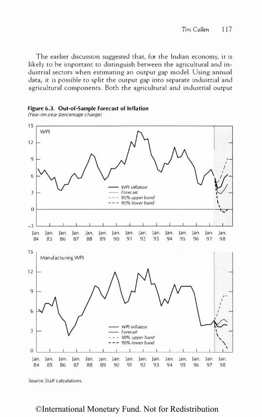
©International Monetary Fund. Not for Redistribution
Tim Callen 1 1 7
The earlier discussion suggested that, for the Indian economy, it is likely to be important to distinguish between the agricultural and industrial sectors when estimating an output gap model. Using annual data, it is possible to split the output gap into separate industrial and agricultural components. Both the agricultural and industrial output
Figure 6.3. Out-of-Sample Forecast of Inflation (Year-on-year percentage change) 1 5
WPI
1 2
9
6
-- WPI inflation 3 - Forecast
- - - 90% upper band -- - 90% lower band
0
-3 )an. )an. )an. Jan. jan. jan. jan. jan. Jan. jan. jan. jan. jan. jan. )an. 84 85 86 87 88 89 90 9 1 92 93 94 95 96 97 98
15 Manufacturing WPI
1 2
9
6
3 -- WPI inflation -- Forecast - - - 90% upper band - -- 90% lower band
0
Jan. jan. jan. Jan. )an. )an. )an. )an . )an. )an. )an. )an. Jan. )an. )an. 84 85 86 87 88 89 90 91 92 93 94 95 96 97 98
Source: Staff calculations.

©International Monetary Fund. Not for Redistribution
1 18 MODELING AND FORECASTING INFLATION IN INDIA
Table 6.3. Estimates of Inflation Equations on Annual Data
(1) (2) (3) Dependent Variable OW PI OW PI OW PI
Constant 0.025 0.01 1 0.065 (1 .24) (0.89) (5.16)
DWPI (-1) 0.206 0.220 0.045 (1.91) (2.08) (0.31)
DM3 (-1) 0.405 (3 .23)
DGDP(-1) -0.571 (3.62)
MONG3 H l 0.467 (4.53)
DOIL(-1) 0.079 0.078 0.11 (4.28) (4.24) (4.61)
ECM (-1) -0.235 -0.242 (3.44) (3.59)
OGAP (-1) -0.502 (1 .57)
OGAPA (-1)
OGAPI (-1)
R2 0.685 0 678 0.428 R2 0.637 0.640 0.379 LM ( 1 ) 0.27 0.02 4.84 White 8.78 5.13 2.95 Jarque-Bera 0.78 0.62 0.07
(4) OW PI
0.063 (5.39) 0.090
(0.66)
0.103 (4.62)
-0.41 3 (2.72) 0.373
(1 .66) 0.516 0.459 3.60 4.77 0.24
Note: Sample period: 1957/58-1997/98. !-statistics in parentheses. All variables in logs. D de-notes the first difference operator. WPI-wholesale price index; M3-broad money; GOP-real GOP; OIL-oil price; OGAP-output gap, OGAPA-agricultural output gap; OGAPI-industrial output gap; MONG3=DM3-DGDP; ECM�rror correction term.
gaps were correctly signed when entered individually (i.e., agricultural output above trend results in lower inflation, while industrial output above trend leads tO higher inflation), although only the agricultural gap was significant. This highlights the importance of sectoral aspects of the Indian inflation process and indicates the importance of accounting for supply shocks in explaining inflation in India.
Results from bivariate Granger-causality tests and variance decompositions broadly support the regression results.12 The results indicate that the money gap has the highest degree of predictive content for inflation, although this comes mainly from industrial production rather than the monetary aggregates over the whole sample period. During the more recent period ( 1 992Q2-1998Q2), however, the predictive content of the monetary aggregates, particularly M l , increases, especially at short time horizons. Foreign inflation also has some predictive content
12For further details, see Callen and Chang (1999).

©International Monetary Fund. Not for Redistribution
Trm Callen 1 19
over short time horizons. For manufactured price inflation, the money gap again has significant predictive power, although in this case Ml on its own is significant. Foreign inflation also has strong predictive content, while agricultural price inflation has some predictive content. In contrast to the results for the aggregate WPI, however, the predictive content of the money gap terms weaken substantially, particularly over short time horizons, during the more recent period.
Conclusions and Policy Implications
In its recent policy statements, the RBI has indicated that it is moving away from a broad money target coward a "multiple indicators" approach to the conduct of monetary policy. This paper has assessed which of the potential indicators available give the most reliable and timely indications of future inflationary developments. This has been carried out both by developing a model of inflation and by estimating a series of bivariate VARs. The results indicate a number of important issues in modeling and forecasting inflation in India.
• Developing an adequate model of inflation is complicated by the swings in the prices of primary articles, which, year-co-year, are largely driven by climatic conditions and by changes in administered prices. A model of manufacturing prices fits better than one for the overall WPI.
• Developments in monetary aggregates appear to contain the best information about future inflation, particularly when judged against developments in activity. The information content of the monetary aggregates appears to have increased since financial deregulation. An output gap specification, unlike in many other countries, does not perform well on Indian data.
• With regard to manufacturing prices, import and primary product prices and the exchange rate also provide useful information about future inflation developments.
The results also have a number of policy implications and raise a number of issues for the monetary authorities:
• While the RBI is moving away from announcing an explicit monetary target, the monetary aggregates continue to provide important information about future inflationary developments and will need to continue to be closely monitored.
• The manufacturing subcomponent of the WPl has been used in this paper as a measure of core inflation. Recent work at the Reserve Bank, however, has begun to develop a core inflation index that will give a clearer picture of underlying inflation developments than

©International Monetary Fund. Not for Redistribution
120 MODELING AND FORECASTING INFLATION IN INOlA
the currently published price indices (Samanta, 1999; Mohanty, Rath, and Ramaiah, 2000). Of course, in its current conduct of policy, the Reserve Bank at times implicitly focuses on a core measure of inflation by discounting price movements that are expected to be reversed in the short run (for example, the sharp rise in primary product prices in 1 998). But the publication of an explicit core inflation index would improve the transparency of policy. However, this does not mean that developments in the headline price index can be totally discounted. The results presented here indicate that there are important links between developments in the primary sector and other areas of the economy, and the RBI needs to take this into account in its policy formation.
• The publication of a wider measure of liquidity that includes public deposits held with financial institutions and NBFCs, as set out in the report of the Working Group on ''Money Supply: Analytics and Methodology of Compilation," would provide important additional information given the growing role of nonbank institutions.
• The change in the RBI's policy approach entails some risks. The broad money target has formed the backbone of monetary policy for a number of years, is well understood by the public, and provides an anchor for inflation expectations (Rangarajan, 1998). During the transition period, the RBI will need to be vigilant and quickly respond to any rise in inflation pressures to ensure there is no suggestion of weakening its commitment to maintain reasonable price stability.
• An important question not addressed in this paper is whether the swings in primary product prices are accentuated by import restrictions and by poor distribution. If so, liberalizing the import of agricultural products and improving distribution would help macroeconomic stability.
References
Arif, R., 1996, "Money Demand Stability: Myth or Reality-An Econometric Analysis," Development Research Group Study 13, Reserve Bank of India, Mumbai.
Balakrishnan, P., 1991, Pricing and lnflacion in India (Dehli, India: Oxford University Press).
---, 1992, "Industrial Price Behaviour in India: An Error-Correction Model," Journal of Development Economics , Vol. 37, pp. 309-26.
---, 1994, "How Best to Model ln.flation in India," Journal of Policy Modeli11g (December), pp. 677-83.

©International Monetary Fund. Not for Redistribution
Tim Callen 1 2 1
Bhattacharya, B.B., and M. Lodh, 1990, "Inflation in India: An Analytical Survey," Artha Vijnana, Vol. 32, pp. 25-68.
Buragohain, T., 1997, "The Role of Sectoral Prices in Indian Inflation," lndian}ournal ofQULinticative Economics, pp. 89-102.
Callen, T., and D. Chang, 1999, "Modeling and Forecasting Inflation in India," IMF Working Paper, WP/99/1 19.
Chand, S., 1996, "Fiscal and Other Determinants of the Indian Inflation Rate," National Institute of Public Finance and Policy Working Paper No. 7.
Coe, D., and J. McDermott, 1997, "Does the Gap Model Work in Asia?" Scaff Papers, International Monetary Fund, Vol. 44 (March), pp. 59-80.
Debelle, G., and D. Laxton, 1997, "Is the Phillips Curve Really a Curve? Some Evidence for Canada, the United Kingdom, and the United States," Scaff Papers, International Monetary Fund, Vol. 44, (June), pp. 249-82.
De Masi, P., 1997, "IMF Estimates of Potential Output: Theory and Practice," IMF Working Paper 97/177 (Washington: International Monetary Fund).
Kannan, R., 1999, "Inflation Targeting: Issues and Relevance for India," Economic and Political Weekly, january 16-23, pp. 1 1 5-22.
Kumar Das, D., 1992, "An Empirical Test of the Behaviour of Money Supply, Government Expenditure, Output and Prices: The Indian Evidence," Indian Economic Journal, Vol. 40, pp. 63-81.
Jadhev, N., 1994, Monetary Economics for India (Dehli, India: Macmillan India Ltd.).
Mohanty, D., and A. Mitra, 1999, "Experience with Monetary Targeting in India," Economic and Political Weekly, January 16-23, pp. 123-32.
Mohanty, D., D. Rath, and M. Ramaiah, 2000, "Measures of Core Inflation in India," Economic and Political Weekly, January 29, pp. 273-82.
Pradhan, B.K., and A. Subramanian, 1998, "Money and Prices: Some Evidence from India," Applied Economics, Vol. 30, pp. 821-27.
Rangarajan, C., 1998, "Development, Inflation, and �lonetary Policy," in India's Economic Reforms and Developments: Essays for Manmohan Singh, eds. I . Ahluwalia and I. Little, New Delhi.
Reserve Bank of India, 1998, "Money Supply: Analytics and Methodology of Com-pilation," Report of the Working Group, June.
---, AnnULI! Report, various issues.
---, Monetary and Credit Policy Sracemem, various issues.
Samanta, G., and S. Mitra, 1998, "Recent Divergence between Wholesale and Consumer Prices In India-A Statistical Exploration," Reserve Bank of India Occasional Papers, Vol. 19, No. 4.
Samanta, G., 1999, "Core Inflation in India: Measurement and Policy Perspectives," Reserve Bank of India Occasional Papers, Vol. 20, No. 1 .

©International Monetary Fund. Not for Redistribution
7 The Unit Trust of India and the Indian Mutual Fund Industry
ANNA lLYINA
Overview of the Indian Equity Market
The Indian stock market and mutual fund industry have grown rapidly since the early 1980s, supported by government policy. ln particular, the government actively promoted the development of the capital markets once it became apparent that its development objectives could not be met solely by using development finance institutions and commercial banks to channel domestic savings tO priority secrors (Singh, 1998). In the initial stages, reforms encompassed the removal of the monopoly in the mutual fund industry, permitting a larger number of companies tO raise funds through the equity market, and encouraging equity ownership through tax incentives. The governrnent also established a regulatory agency, the Securities and Exchange Board of India (SEBI), in 1988 to oversee all aspects of the market, although initially without any !:itatutory powers.
Capital market reforms were broadened beginning in 1992 as further liberalization was combined with the creation of an effective regularory framework. SEBl was given statutory powers as the regulatOr of the securities industry with the enactment of the SEBl Act. The Controller of Capital Issues was abolished, and statutory control over capital issues was replaced with disclostJre rules in offer documents. Indian companies were permitted to raise capital abroad in the form of global depository
1 22

©International Monetary Fund. Not for Redistribution
Anna Ilyina 123
receipts (GORs), and foreign institutional investors (Fils) were allowed ro invest in Indian primary and secondary markets for listed securities. Deficiencies in trading and settlement procedures at the Indian stock exchanges, which were raising the cost of capital, were also addressed by improving brokerage practices, increasing the transparency of trade executions, and enhancing investor protection. The establishment of the National Stock Exchange (NSE) in November 1994, with a screenbased trading system, helped increase stock market efficiency and encouraged the Bombay Stock Exchange (BSE) to speed up the automation of irs trading system and improve its clearing and settlement procedures. The existing settlement system, which required physical delivery of scripts, was replaced with an electronic book-entry system in October 1996.
More recendy, SEBI has approved a modified takeover code aimed at protecting the interests of minority shareholders and making the takeover process more transparent; introduced norms for derivatives trading and securities lending to increase the liquidity of the stock marker; and introduced risk management guidelines, including capital adequacy norms for brokers and intra-day trading and exposure limits, to protect the integrity of the market. In 1998/99, companies were permitted ro buy back shares subject to certain regulations, while the NSE initiated the introduction of stock index futures as a first step toward derivatives trading in India.
As a result of these reforms, the Indian stock marker has grown rapidly since the early 1980s. Market capitalization peaked at 53 percent of GOP in the early 1990s, before falling back to around 3 2 percent of GOP in 1999/00 (Figure 7.1 ). The number and value of new equity issues also increased dramatically in the mid-1990s, although these have declined in recent years, partly as a result of a tightening in new issue requirements by SEBI.
A large number of domestic and foreign investors have been attracted to the Indian stock market. Household participation has increased sharply during the past 1 5 years, with the number of mutual fund invesrors rising from 2 million to around 50 million. The growth in srock market activity contributed to the higher rate of household financial saving. There was also substantial portfolio substitution from bank deposits to stock market investments in the early 1990s, although this has reversed in recent years. Foreign participation, about 5 percent of market capitalization, is still limited (although foreign investors account for a higher proportion of turnover).
Srock market capitalization in India remains low compared with other East Asian economies. The scope and depth of the market is relatively limited, comprising a large number of relatively small companies-the

©International Monetary Fund. Not for Redistribution
124 THE UNIT TRUST AND THE MUTUAL FUND INDUSTRY
Figure 7 .1 . Stock Market Indicators, 1982/83-1998/99
5000 60 Bombay Stock Exchange Market Capitalization Sensex Index (/n percent of GOP)
50
40
30
2000
20
1000 t O
0 .... "' " "' � � "' " 17> M .,., " "' � ,.., � I!< � � � $ � � � � � � ... ... ., ., co co "' "' "' "' "' co co ., co "' "'
2000 300 6
.,., � "'
New Capital Issues Cumulative Fll Investment
" $ .,..
Value of new capital 1/n percent of market capitalizatiOn/
(In billions of rupees) fright sc.>le/
250 5 1500 � 200
1000 I 150 3 I I I I
100 2
I 50 I
0 0 '"' "' " "' � ...., ·� � "' � � " "' � ,.., ·� " � � � � � $ � 1!: i � � $ ... .., "' � "' ... co ., "' co "' "' "' "' "' "' ., "' "' "' "'
Sources: Data provided by the Indian authorities; and IMF staff calculations.
� � 0'
.,.. q: ., "'
average market capitalization of companies listed on the BSE is less than $30 million. 1 Trading also remains fragmented with over 20 stock exchanges spread across the country, many of which are still not fully integrated into a single trading system. Financial institutions owned by,
1The average market capitalization of companies listed on the NYSE is around $4 billion.

©International Monetary Fund. Not for Redistribution
Anna llyina 125
or affiliated with, the government continue to be key participants in the market. The Unit Trust of India (UTI), the two insurance companies (the Life Corporation of India (LIC) and the General Insurance Corporation of India (GIC) ), and the development finance institutions (DFls) are all important players.
The Mutual Fund Industry in India
Evolution of the Mutual Fund Industry
Mutual funds have played a key role in mobilizing household savings in India. Since the establishment of the first mutual fund in 1963, investible resources raised by the mutual fund industry have grown from Rs 0.2 billion in 1964/65 to Rs 1 ,152 billion in 1999/00 (see Table 7.1). The rapid growth of mutual funds has been due to several factors. Investors have generally viewed mutual funds as more liquid and less risky
Table 7.1. Cumulative Resources Raised by Mutual Funds1 (In Rs billions)
Other Public Private UTI Sector Sector Total
1990/91 21 3.8 1 6.8 230.6 93 7 100
1991/92 318.1 56.7 374.8
85 15 100 1992/93 389.8 80.1 469.9
83 17 100 1 993/94 517.1 93.2 1 5.6 625.9
83 15 2 100 1994/95 615.9 101.6 27.7 745.1
83 14 4 700 1995/96 690.6 1 08.9 35.7 835.2
83 73 4 100 1996/97 717.7 1 06.2 34.3 858.2
84 12 4 700 1997/98 808.7 1 09.5 54.0 972.3
83 11 6 100 1998/99 781.0 1 1 3.0 69.0 963.0
8 1 12 7 700 1999/00 827.0 1 05.0 220.0 1 1 52.0
72 9 19 100 Memorandum items: Net inflows
1 997/98 91.0 3.0 20.0 1 1 4. 1 1 998/99 -27.4 3.0 15.0 -9.5 1999/00 45.5 -7.0 152.0 1 89.7
Sources: Securities and Exchange Board of India, Annual Reports; and press releases. 1Excludes redemption/repurchase of units. Numbers in italics are in percent of the total.

©International Monetary Fund. Not for Redistribution
126 THE UNIT TRUST AND THE MUTUAL FUND INDUSTRY
than stocks and private bonds, while the distribution network of mutual funds has made such investments more readily available ro small investors. Moreover, rhe assured return schemes promoted by UTI and other public sector mutual funds have offered higher yields than those available on bank deposits, while tax benefits have provided further incentives for investors to shift from bank deposits into mutual funds.
Mutual funds in India are constituted in the form of trusts under rhe Indian Trusts Act of 1882. The trust deed executed by the fund's sponsor in favor of the trustees outlines the obligations and liabilities of the trust in relation to the unit holders, and it is now subject to SEBI approval. Under SEBI regulations, any financial institution can sponsor a mutual fund provided it has a "sound track record"-defined as at least five years of experience in financial services and a positive net worth in all the preceding five years. It must also contribute at least 40 percent of the net worth of the Asset Management Company (AMC). The dayto-day operations of the fund are carried out by the AM C. The board of trustees oversees the fund's activities and enters into a management agreement with the AMC. The primary responsibility of the trustees is to ensure there is no conflict between the interests of the unit holders and the manner in which the AMC deploys the fund's resources. 2
The first mutual fund, the Unit Trust of India (UTI), was set up by an Act of Parliament in 1963 with the objective of mobilizing small household savings. In 1964, UTI launched irs first, and still largest, investment scheme, Unit Scheme-1964 (US-64 ). UTI's monopoly of the mutual fund industry was broken in 1987 when public sector banks and financial institutions were permitted to sponsor mutual funds. In 1993, private companies were also allowed to enter the industry. As of March 1999, 40 mutual fund companies were registered with SEBI (UTI is not registered with SEBI), of which nine were sponsored by public secror institutions. However, three of these companies have been suspended by SEBl and prohibited from launching new schemes. Despite the entry of rhe new participants into the marker, UTI continues to dominate the industry, accounting for 67 percent of net assets, while the public and private mutual funds account for 10 percent and 23 percent, respectively, as of end-March 2000.
Mutual funds in India are not liable to pay income tax provided rhey satisfy certain conditions. In particular, a mutual fund set up by a public sector bank or financial institution, or authorized by SEBl, is exempted from income tax provided that it distributes 90 percent of profits to unit holders. A flat tax of 10 percent on dividends distributed by mutual
2Under current regulations, the AMC is obligated to submit quarterly reports to the trustees on its activities and its compliance with the regularions.

©International Monetary Fund. Not for Redistribution
Anna llyina 12 7
funds was introduced in the 1999/2000 budget, which brought their tax treatment in line with that of dividends paid by domestic companies in lndia.3 However, the budget exempted dividends distributed by openended equity schemes (where the equity component is more than 50 percent) from the 10 percent tax for a period of three years starting from 1999/2000.
Domestic mutual fund investors also enjoy ignificant tax benefits. Income from mutual fund investments are treated more favorably than other personal income ( including interest income) under current tax arrangements. The tax benefits include
• Exemption of investments from the wealth tax. • Exemption of dividends from income tax. • Exemption of investments from the gift tax (up to Rs 30,000 per
annum, applies to individual investors only). • Exemption from capital gains tax of proceeds from the sale of long
term assets that are invested within a period of six months after the date of sale in the units of approved mutual funds (applies to individual investors only).
• Capital gains in respect of units held for a period of 12 months are taxed at a concessional rate of 20 percent, where capital gains are computed after taking into account the cost of acquisition adjusted for inflation.
Regulation of the Mutual Fund Industry
The first compreher.sive set of mutual fund regulations were adopted in 1993. These placed SEBI as the primary regulator of the mutual fund industry and laid down the eligibility criteria for fund sponsors. The regulations prescribed disclosure requirements, procedures for calculating and declaring net asset values (NAYs) of mutual fund schemes, accounting standards, and a code for advertisements. Further, in order to ensure an arm's-length relationship between the trustees and the AMC, SEBI required at least one-half of the AMC/board of trustees to be composed of independent directors/trustees.
Revisions to the regulations in 1996 tightened the accounting and disclosure requirements and stressed the trustees' key obligation in overseeing the AMC. The revisions had the dual objective of improving investor protection-by imposing more stringent disclosure norms in offer documents and uniform rules with respect to asset valuation and accounting practices-and increasing diversity in the design of fund
3Effective June I, 1997, in addition tO the corporate income tax. all domestic companies are liable to pay 10 percent mx on dividends declared, distributed, or paid.

©International Monetary Fund. Not for Redistribution
128 THE UNIT TRUST AND THE MUTUAL FUND INDUSTRY
schemes-by giving greater freedom to asset managers to structure schemes according to investor preference and replacing quantitative restrictions on mutual funds' investments with prudential supervision. In order to ensure that the AMCs are well capitalized, they were required to increase their net worth (paid-in capital plus free reserves) from Rs 50 million to Rs 100 million. At the same time, AMCs were allowed to provide investment management services to offshore funds, venture capital funds, insurance companies, and other mutual funds. As the primary regulator of the mutual fund industry, SEBI was granted the right to approve the entry of new schemes, to inspect any registered mutual fund, and to take actions against any regulatory infraction.
Existing regulations specify a number of restrictions on investments by mutual funds:
• Money collected can only be invested in transferable securities in accordance with the investment objectives specified in the fund's offer documents.
• Funds can only borrow to meet temporary liquidity needs (not more than 20 percent of the net assets of a scheme and for no longer than six months).4
• They cannot advance loans for any purposes, and the resources of investment schemes cannot be used in option trading, short selling, or carry forward transactions.
• No mutual fund may own more than 10 percent of a company's paid-up capital carrying voting rights.
• They can only invest in investment grade debt instruments as rated by an authorized credit rating agency.
• Any inter-scheme asset transfer within the same mutual fund company must be done at prevailing market prices and should conform to the investment objective of the scheme to which the transfer is made.
• The value of a scheme's investments in other schemes managed by the same AMC or other mutual funds cannot exceed 5 percent of its NAY.
• Excess cash flow can only temporarily be placed in short-term bank deposits (pending the deployment of funds in securities according to the fund's objective).
The regulations contain specific guidelines for the pricing of mutual fund units, although these leave some scope for prices to deviate from net asset values. For open-ended schemes, the redemption price cannot be lower than 93 percent and the sale price not higher than 107 percent
4Silver ( 1998) notes that this could be interpreted tO mean that schemes can be continually leveraged up to 20 percent.

©International Monetary Fund. Not for Redistribution
Anna Ilyina 129
of the NAY, while the difference between the redemption and sale price should not exceed 7 percent of the sale price. For close-ended schemes, the redemption price of units should not be lower than 95 percent of the NAY. Assured return schemes can be launched provided the returns are guaranteed by the sponsor or AMC and sufficient funds are <wailable tO meet the guarantees.
Further amendments were made tO the regulations in 1998. These included
• Mandatory disclosure of the fund's full portfolio in its annual repon. • The fundamental attributes of the scheme (type of the scheme, in
vestment objective, and terms of issue) must be clearly defined, and any amendments tO these attributes would require the consent of at least three-quarters of the unit holders.
• Independent members should constitute at least two-thirds of the board of trustees.
• Investments in affiliates of the mutual fund's sponsor should be restricted to a maximum of 25 percent of the fund's net assets. Investment in unlisted and privately placed securities of the splmsor's affiliate companies is prohibited.
Restrictions on investment in foreign securities have recently been c::asc::J. lu October 1997, the Reserve Bauk u( lnuia Gllllll>LIItced then Indian fund managers ( including mutual funds) registered with SEI31 could invest in overseas markets, initially within an overall limit of $500 million and a ceiling of $50 million for an individual mutual funJ. SEBI also established a committee to develop more detailed guideline:. on foreign investment by mutual funds.
During 1 998/99, inspections of all active mutual funds, including UTI, were undertaken by SEBI. These inspections were conducted 1)\' independent chartered accountancy firms, but subject to a dewiled guidance note issued to them by SEBI. The auditor were reqtlired w comment on the fund's compliance with each regulation in their rerlm. On the basis of the reports, warning and deficiency reports have been issued to many mutual funds, and they were advised to take correcti,·e action and report back to SEBI.
The Unit Trust of India (UTI)
History and Recent Developments
The Unit Trust of India (UTI) is a statutory body set up by an Act of Parliament (the UTI Act). It is not bound by the mutual funds regulations but by the UTI Act and UTI general regulations, although under

©International Monetary Fund. Not for Redistribution
130 THE UNIT TRUST AND THE MUTUAL FUND INDUSTRY
a voluntary arrangement SEBI oversees the investment schemes launched by UTI since 1994. UTI operates without ownership capital, under an independent Board of Trustees who oversee the general management of the Trust's operations. The Chairman of the Board is appointed by the government.
The organizational structure of UTI is different from other mutual funds. First, it is a statutory body rather than a trust established under the Indian Trusts Act. Second, there is no separate AMC with a separate Board of Directors. The Executive Committee and Board of UTI perform the functions of the AMC and Board of Trustees. The sponsors also cannot hold any equity in the AMC or Trustee company as neither of these exist. Third, there has traditionally been no separation between the asset management groups managing the schemes launched before 1994 (the mutual funds regulations only apply to schemes established after 1994).
The first scheme launched by UTI was the Unit Scheme-1964 (US-64), and this remains UTI's largest scheme. Under the provi ions of US-64, several institutions, including the Reserve Bank of India (RBI), the Life Insurance Corporation (LIC), and the State Bank of India (SBI), as well as other banks and financial institutions, contributed the initial capital of Rs 50 million. In 1976, the RBI's contribution was taken up by the Industrial Development Bank of India (lOBI).
Due to its extensive distribution network (53 offices and 320 chief representatives), UTI has a much larger investor base of 45 million accounts (as of end-1999) than any other mutual fund. At present, UTI manages almost 100 investment schemes and is the largest institutional investor in the equity market. During the 1990s, UTI's portfolio shifted markedly toward equity investments-the share of equity in total investible funds rose from 28 percent in 1990/91 to more than 50 percent in 1997/98. (The equity share in the US-64 scheme was even largersee Table 7.2.) This trend reflected low interest rates, a booming stock market in the early 1990s, which made investment in equities increa -ingly attractive, and UTI's active support of the government's divestment program.
Although their holdings have declined in recent years, partly due to the withdrawal of some of the tax benefits previously enjoyed, the corporate sector still holds around 40 percent of outstanding US-64 units. With mutual funds being given voting powers similar to rho e of other shareholders in 1996, some analysts have raised concerns regarding the effect of these large cross-shareholdings on corporate governance.
Because its pre-1994 schemes are not regulated by SEBI, there are areas where practices at some UTI funds (most notably US-64) differ from those at other mutual funds. Most importantly:

©In
tern
atio
nal M
onet
ary
Fund
. Not
for R
edis
tribu
tion
Tab
le 7
.2.
PaH
ern
of In
vest
men
ts o
f P
ub
lic S
ecto
r M
utua
l Fu
nds
(In
per
cent
of t
he to
tal)
Inst
rum
ent s
19
90/9
1 19
91/
92
199
2/93
19
93/
94
1994
/95
199
5/9
6
199
6/97
19
97/
98
UT
I Equi
ty s
hare
s 2
8.2
39
.5
47
.3
46
.9
47
.8
50.0
4
8.9
52
.5
Deb
entu
res/
bo
nds
31.
9
28
.7
27
.2
25
.5
20
.0
24
.6
28
.3
31.
0
Go
vern
me
nt s
ecur
ities
(in
clud
ing
26
.0
24.0
12
.3
18.1
16
.4
11.1
7.
9 4
.5
Trea
sury
bill
s)
Oth
er
12.6
12
.5
11.8
9
.4
15.8
14
.4
14.9
12
.0
Tot
al n
um
ber
of s
che
me
s 4
9
54
59
6
6
73
79
U$
-64
Eq
uity
sha
res
33
.5
39
.5
50.6
6
6.2
6
5.7
6
9.7
D
eben
ture
s/bo
nds
33
.5
23
.0
17.5
17
.8
19.1
17
.1
Go
vern
me
nt s
ecu
ritie
s {i
nclu
din
g
0.0
19
.3
21.
9
13.1
9
.9
7.8
T
reas
ury
bills
)
Oth
er
33
.1
18.2
10
.0
2.9
5
.3
5.4
Shar
e o
f U
$-64
inv
estib
le f
und
s 3
3.5
39
.0
42
.0
35.8
3
1.1
32
.1
in th
e to
tal
inv
estib
le f
und
s o
f U
TI
(in p
erce
nt)
Oth
er m
utua
l fun
ds1
Eq
uity
sha
res
38.7
4
6.6
4
9.0
60
.4
Deb
entu
res/
bond
s 3
4.1
4
2.0
32
.9
30.7
)>
G
ove
rnm
ent s
ecu
ritie
s (i
ncl
udin
g
4.5
1.
1 3.
3 1.
7
::l
::l
Tre
asur
y b
i lis)
�
-O
ther
23
.4
10.5
14
.7
7.2
..:z- :r
�
Sour
ces:
Uni
t Tru
st o
f In
dia
, An
nu
al
Re
po
rts;
an
d P
ahig
rah
i (1
99
6).
I Pa
hig
rah
i (19
96
). ..
..... w
,_.

©International Monetary Fund. Not for Redistribution
132 THE UNIT TRUST AND THE MUTUAL FUND INDUSTRY
• Dividend polici.es and accounting practices deviate from industry stan, dards. Unlike other mutual funds, which pass on 90 percent of their earnings to their unit holders, UTI's dividends, in particular those of US-64, are set in order to at least maintain (and often exceed) the previous year's dividend rate. To do this, a scheme holds a reserve that it adds to in "good" years and draws down in "bad" years. Also, unlike other mutual funds, which are required to mark all investments to market, UTI's investments have traditionally (and until recently) been carried on its balance sheet at historical book value.5
• Policies with regard co the sale and redemption prices of the units of its open,ended investment schemes also differ from chose of other mutual funds. For example, US-64 unit prices are not directly linked to its net asset value (NAY), but are announced at the beginning of UTI's accounting year (July 1-June 30), and can be changed on a month-to-month basis. The secondary market price of the units usually fluctuates within the boundaries of the sale and redemption prices set by the UT1.6 NAYs of most of its unit schemes are published on a regular basis (monthly or weekly). UTI believes that in the case of US,64, however, it is difficult to make an accurate and timely estimation of the NAY due to the nature of its investments, which include term loans and nontransferable debentures.
Further, UTI has evolved into an institution with a wide range of functions from mobilizing savings through assured return savings schemes to acting as an investment and term-lending institution. Multiple autonomous business units have been established under the um, brella of the UTI, such as the UTI Bank, the UTI Securities Ltd., the UTI Investor Services Ltd., and the UTI Investment Advisory.
The October 1998 Crisis and the Restructuring of UTI
The decline in stock prices during May-June 1998 resulted in significant valuation losses for US-64 on its investment portfolio. Despite these losses, however, UTI decided to maintain a dividend rate of 20
I However, schedules annexed to the annual reports of the differenr schemes do provide information on investmenrs on a marker value basis. In addition, UTI has recenrly started providing the NAV updates for many of its investment schemes on a weekly/ monthly basis through its website.
6The spread between sale and repurchase prices is typically less than 3 percent (on the basis of the sale price) and is sufficient w cover administrative costs.

©International Monetary Fund. Not for Redistribution
Anna llyina 133
percent for the 1997/98 financial year.7 At the same time, the decision was taken by the fund's management to revise the accounting practices followed by US-64 so as to account for the unrealized capital losses. These developments resulted in the balance in the US-64's reserve account turning negative in june 1998, and when this became public with the release ofUTI's 1997/98 Annual Report in the fall of 1998, investor confidence in the US-64 scheme deteriorated sharply.
lf UTI had been following the standard valuation and pricing procedures prescribed by SEBI, the sharp decline in the market value of its assets between May and June 1998 would have resulted in a proportionate revision of the NAY and a lower sale price. Instead, after it was revealed that US-64's reserves were negative, UTI raised the sale price of its units in line with its usual annual pricing policy. Redemption pressures continued to build, and the unit capital of US-64 declined from Rs 156 billion in June 1998 to Rs 148 billion in December 1998. Following the Ocrober 1998 difficulties, UTI constituted a committee (the Oeepak Parekh Committee) tO undertake a comprehensive review of the functioning of US-64 and recommend measures for sustaining investOr confidence and strengthening the operations of the scheme.
The Committee's report was released in March 1999 and its view was that the problems at US-64 were due to the excessively high yield offered by the scheme, combined with itS large equity exposure. Consequently, it recommended that the equity exposure be gradually reduced, the pricing of the scheme become NAY driven, and its dividend distribution policy become more responsive to changes in market conditions (Box 7.1 ).
As part of the restructuring of UTI, the government has recently undertaken a debt-for-equity swap with US-64 along the lines of the Committee's recommendations. A number of poorly performing Public Sector Undertakings (PSU) shares, valued at Rs 3.3 billion, have been placed in a new scheme, the Special Unit Scheme 1999 (SUS-99), and in return the government issued five-year maturity bonds to US-64.8 UTI has also implemented a number of other reforms in line with the recommendations of the Committee. Separate Asset Management Companies (AMCs)-equity and debt schemes, each with seven members (five outside experrs and two senior UTI officials)-have been established for US-64. The dividend on US-64 was also lowered to 13.5 percent ( implying a yield of 10 percent on the July 1999 sale price). Given the tax exemption, however, the after-tax yield was largely unchanged from the previous year, while the sale and redemption prices
7UTI's financial year runs july l-june 30. 8UTI also benefited from increased investmem by public SeC[Or banks in US-64 units,
totaling a reported Rs l.S billion in 1998/99

©International Monetary Fund. Not for Redistribution
134 THE UNIT TRUST AND THE MUTUAL FUND INDUSTRY
Box 7 . 1 . Deepak Parekh Committee Recommendations for Restructuring US-64
(i) Recapicalizarion. Contributors to the UTI's initial capital ofRs 50 million should infuse at least Rs 5 billion immediately into US-64 as a onetime measure. This should prompt them to seek more accountability from the Trust and be a signal to investors that the sponsors would stand by their fiduciary obligations.
(ii) Swap of Public Secwr Undertakings (PSU) shares for government securities. The US-64's PSU portfolio would be transferred to a Special Unit Scheme-99 (SUS-99) at book value; the govemment would subscribe co this new scheme through the issue of government securities, which would then be transferred to US-64.
(iii) Reduction of eflUity exposure. ln order to bring down the US-64 equity holdings, the Cornmlttee recommended chat US-64 should make strategic sales by negotiation to the highest bidder.
(iv) The US-64 should become a NAV-driven scheme, i.e., its units should be priced in line with the scheme's NAY.
were reduced in July to bring them closer to the NAV.9 UTI also announced that starting in July 2000, the NAY of US-64 would be declared on a fortnightly basis, and UTI was required to submit regular compliance reports to the Ministry of Finance on progress toward meeting the Parekh Committee's recommendations.
Outstanding Policy Issues
The mutual fund industry has played an important role in the mobilization of domestic savings and the development of capital markets in India. Substantial progress has also been made in strengthening the regulation and improving the transparency and uniformity of the standards in the mutual fund industry through the SEBI (Mutual Funds) Regulations of 1996, and the subsequent amendments in 1998. However, a number of areas remain where further improvement to the regulatory regime would be beneficial, and, in the case of UTI, the challenges remain considerable. Bringing UTI under SEBI's purview, as well as the introduction and implementation of international accounting principles
9UTI reported that US-64's reserves had turned significanrly positive by end-March 2000, while the sale and repurchase prices were raised to Rs 14.85 and Rs 14.55, respectively, in May 2000.

©International Monetary Fund. Not for Redistribution
Anna Ilyina 135
( v) The dividend distribution policy should be more responsive to market conditions, and the practice of promoting assured return schemes should be abandoned.
(vi) Tax rebates to the unit holders. The Unit Scheme-64 should be rendered tax-free for the next three years.
(vii) Amendments to the UTI Act should require: • the appointment of separate and independent teams of fund man
agers for each scheme and, in particular, the creation of a separate asset management company for US-64 with an independent board of directors;
• all inter-scheme transfers to be carried out on the basis of independent decisions of the fund managers of the concerned schemes and at market-determined prices;
• an increase in the size of the board of trustees and inclusion of five additional independent trustees, bringing UTI under the purview of the SEBI Act.
(lAP) across the whole of the mutual fund industry, will increase the soundness and stability of the sector. Some of the other outstanding issues are discussed below.
Mutual Fund Regulation
• Valuation standards. Existing regulations appropriately require that the sale and redemption prices of funds should be based on their NAYs, which should be computed according to the uniform rules specified in the regulations. There is scope, however, for improvements in at least two areas. First, while the regulations have introduced broad guidelines for the valuation of thinly traded or nontraded securities, the AMCs still have considerable room for discretion in the valuations they adopt. Second, mutual funds are currently only required to revise and publish NAYs on a weekly, rather than daily, basis.10 A second-best option would be to require the repricing of units in the event of a "material market move" (when the scheme's NAY, if revalued, would differ by more than 5 percent from the last valuation point).
lOMonthly income schemes are allowed ro publish their NAV either at monthly or at quarterly intervals. The UTI is not obligated to adhere to these rules for any of its pre-1994 schemes (including the US-64).

©International Monetary Fund. Not for Redistribution
136 THE UNIT TRUST AND THE MUTUAL FUND INDUSTRY
• The legal and regulator)' relarionship between the sponsor, the AMC, the unit holders, and the trustees. Several issues relating to governance are raised by current regulations. At present, the sponsor of a fund may hold up to 100 percent of the AMC's capital, can contribute to the trustee company's capital, and can appoint the trustees. But while there is considerable scope for rhe sponsor to indirectly influence the asset management and other operational decisions of the trustees and/or rhe AMC, the regulations do not hold the sponsor liable for such decisions. The sponsor is financially liable only in the event of a shortfall in the net worth of the AMC or if a mutual fund's income is insufficient to cover the distributions under the assured return schemes guaranteed by the sponsor. Moreover, the regulatory constraints aimed at limiting rhe potential conflicts of interest appear to be relatively lax by international standards. For example, the 1998 amendments imposed constraints on mutual fund investments in the companies affiliated with the sponsor by setting a limit of 25 percent of the fund's net assets. The best practice in this area is to not allow a mutual fund tO invest in the management and/or trustee company or in any of their affiliates. In order to address these issues, the 1996 Kaul Committee recommended the enactment of separate legislation governing the management, responsibilities, and functioning of mutual funds.
• The relationship between mutual funds and the corporate sectOr. Current arrangements raise both prudential and governance issues. The regulations stipulate that a fund's ownership in any single company should not exceed 1 0 percent of its voting shares, although there appears to be no upper limit on the total holdings of voting and nonvoting (ordinary and preference) shares of any single company.1 1 In addition, while corporate sectOr holdings ofUS-64 units have declined following the withdrawal of certain tax benefits, there is an issue of whether the regulators need to impose restrictions on corporate or financial institutions' investments in assured return schemes of mutual funds, in order to prevent the buildup of large cross-shareholdings.12
• The role of the government in the mutual fund industry. UTI, which is a statutory body, accounts for more than 70 percent of the mutual fund industry's investible resources. This, coupled with the fact
11However, there are relatively few issues of preferred stocks, and these are held mainly by insurance companies.
lZUnits of assured retum schemes, along with T-bills and bank term deposits, can effectively be used by companies for liquidity management.

©International Monetary Fund. Not for Redistribution
Anna Ilyina 13 7
that the life insurance and banking sectors are also largely publicly owned, means that the government has a major influence on the domestic financial markets. In the past, this meant that mutual fund and other financial sector entities were overly involved in supporting the government's divestment program, with adverse implications for the financial soundness of the institutions.
• Futures and other derivar:ive markets. In view of the authorities' intention to promote deri vari ves markets, prudential regulations will need to be developed in order to prevent the misuse of such instruments. As a first step in the right direction, the Gupta Committee on Derivatives recommended that mutual funds be allowed to trade derivatives only to the extent authorized by their Board of Trustees and to disclose their intention to engage in derivatives trading in their offer documents. Also, existing funds would need to obtain approval from unit holders to carry out derivatives transactions.
• Assured retum schemes. The Parekh Committee report concluded that assured return schemes were no longer appropriate in view of the financial market liberalization that had taken place in recent years. While regulations now require that fund sponsors or AMCs guarantee returns and provide sufficient funds to meet this obligation, there does not yet seem to be a framework that would discourage this practice among public sector mutual funds. Indeed, UTI launched an assured return scheme in early 1999. SEBI has reported that by March 1999, Rs 13.5 billion had been paid by mutual funds to investors to honor the assured return commitments.
• Taxation. Tax benefits have served a useful role in developing the mutual fund industry, but they place other financial intermediaries at a relative disadvantage and distort investment decisions. For example, the 1999/00 budget proposed taxing distributions by debt schemes at a flat rate of 10 percent, while the income from bank deposits is taxed at standard income tax rates. In addition, the budget provided a three-year dividend tax exemption for distributions by equity schemes, and the Parekh Committee suggested this be extended to US-64 regardless of future changes in its debt/equity ratio.
Reform of UTI
The reforms proposed by the Parekh Commirree provide a useful blueprint for restructuring UTI. In particular, it is critical for US-64 to move quickly to a NAY-based pricing system to bring it in line with industry standards and to improve investor protection. The reduction of US-64

©International Monetary Fund. Not for Redistribution
138 THE UNIT TRUST AND THE MUTUAL FUND INDUSTRY
equity exposure will help align rhe scheme's investments with its objective of providing unit holders with a regular income flow. Further, the establishment of an independent board of trustees and an AMC with an independent board would bring it more in line with rhe mutual fund regulations, leading to significantly improved accountability.
Questions regarding the scope and implementation of the Committee's recommendations remain. A critical issue is the systemic importance and role of UTI in Indian financial markers. UTI operates as a financial conglomerate, which is involved in virtually every segment of the financial system. Also the size of UTI's flagship fund, US-64, affects the flexibility of its operations as active portfolio management becomes difficult and costly when the size of transactions has significant impact on prices of individual stocks being rraded. Moreover, the size and complexity of UTI has made irs regulations more challenging.
The size of UTI relative to overalil stock market capitalization and the number of actively traded srocks can make it difficult for the Trust to meet prudential norms specified in mutual fund regulations. Under the regulations, a mutual fund may not own more than 10 percent of a company's voting capital. At the same time, UTI's own prudential guidelines stipulate that no scheme can invest rnore than 5 percent of irs resources in the equity of any single company. Given the size of UTI, however, 5 percent of its investible resources can easily exceed 10 percent of voting capital of large publicly traded companies. For example, as of June 1 998,
UTI owned more than I 0 percent of the outstanding shares of at least 6 of the tap 25 companies listed on the BSE, although only one company's share in tOtal resources of US-64 exceeded 5 percent.
The pricing and dividend policies of US-64 also have to be fully reconciled. Although the Oeepak Parekh Committee recommended a move toward NAY-based pricing, this is to take place over a three-year horizon with rhe phased approach reflecting the fact that an immediate shift to NAV pricing would have resulted in a sharp drop in the value of US-64 units. This problem appears to have been mitigated by capital injections and a widening of the spread between sale and redemption prices of units. In addition, UTI subsequently made a commitment to announce the NAV on a fortnighdy basis starring from july 2000, and to gradually shift to publishing the NAV on a daily basis, although it set no time frame for this.
Concluding Remarks
The mutual fund industry, and UTI in particular, has played an important role in promoting private saving and developing the Indian

©International Monetary Fund. Not for Redistribution
Anna Jlyina 139
capital market, and its growth potential remains high. The government has sought to ensure that the regulatory and supervisory framework governing mutual funds has kept pace with their growing importance. To a large degree, recent changes in the regulatory regime have been successful in achieving this objective, but further improvements are needed tO enhance governance and ensure the soundness and stability of the mutual fund industry.
The Deepak Parekh Committee's proposals represent a substantial step toward improving the operations and transparency of UTI. The recent improvement in the financial position of US-64 would seem tO make a rapid move to NAY-based pricing both possible and desirable. Further, the size and systemic importance of UTI, and US-64 in particular, continue tO raise issues both for the operation of UTI and for capital markets in general.
References
Pahigrahi, M., 1996, "Mutual Funds: Growth, Performance and Prospects," Economic and Policical Weekly, March 23.
Securities and Exchange Board of India, Annual Report, various issues.
Silver, David, 1998, "Reflections on Regulation: The Role of Industry," paper presented at the 2nd Annual Conference on rhe Future of Fund Management in India, April.
Singh, Ajit, 1998, "Liberalization, the Stock Market, and the Market for Corporate Control: A Bridge Too Far for the Indian Economy," in India's Economic Reforms and Developments: Essays for Manmohan Singh, eds. I. Ahluwalia and !. Little (New Delhi: Oxford University Press).
Unit Trust of India, Annual Report, various issues.

©International Monetary Fund. Not for Redistribution
This page intentionally left blank

©International Monetary Fund. Not for Redistribution
PARr IV
Growth, Poverty, and Structural Policies

©International Monetary Fund. Not for Redistribution
This page intentionally left blank

©International Monetary Fund. Not for Redistribution
8 Growth Theory and Convergence Across Indian States: A Panel Study
SHEKHAR AIYAR
Introduction
India is a land of extraordinary diversity. Regions differ enormously in social, geographic, demographic, and linguistic terms. There are significant differences in levels of economic development, which have been an important preoccupation of policymakers since independence. The importance that has been placed on reducing these disparities has partly reflected the view that regional inequality is intrinsically unfair and could undermine the ability to achieve a consensus among the states on broader policy issues. Moreover, it has long been noted that poverty and other kinds of social deprivation are disproportionately the burden of low-income states. A more equitable income distribution among states, therefore, is consistent with the broader objective of poverty reduction.
There has been a surge of interest recently in analyzing trends in regional disparities from within the framework of neoclassical growth theory. Several papers have tried to ascertain whether the empirical record shows convergence or divergence among the Indian states, and they discuss the factors responsible. These papers have examined different samples of states over different time periods and arrived at sometimes conflicting conclusions. This study will argue, however, that they are all characterized by an inadequate appreciation of the way in which growth theory should treat India's diversity. In particular, once the central
143

©International Monetary Fund. Not for Redistribution
144 GROWTH THEORY AND CONVERGENCE ACROSS lNDIAN STATES
distinction between absolute and conditional convergence has been appropriately drawn, it is possible to obtain a much clearer picture of the experience of the Indian states and the lessons that this experience holds for policymakers.
The subsequent section discusses some of the theory relevant to the empirical work that follows. In this context, some of the existing papers on regional economic development tn India are reviewed and critiqued. The third section summarizes the facts about regional economic development Ln India. Correlations are explored between real income per capita and other variables that may play a role in the growth process. The fourth section presents the econometric study, along with a brief description of the methodology used and an interpretation of the results. This is followed by a conclusion.
Growth Theory
Steady States and Convergence
The traditional starting point for a study of growth is the SolowSwan model,' which makes restrictive assumptions about how the world works, and, in turn, yields well-defined and testable predictions. It assumes a constant returns-to-scale technology that is available to all countries in the world, as well as external technological change, savings rates, and population growth rates. On the basis of these assumptions it concludes that countries will converge toward a "steady state" in which output per capita grows at the rate of technological change and output per effective worker remains constant.2 In transition, the speed of per capita growth depends inversely on distance from the steady state, an effect due to diminishing returns to capital. Thus a poor country with a relatively low capital-labor ratio will enjoy high rates of return on capital, and consequently will grow faster than a rich country with a high capital-labor ratio and low rates of return on capital.
This last prediction-called convergence-has been examined empirically by many authors in recent years. The convergence predicted by theory is, however, contingent on the assumptions and parameters of the model; notably the assumptions of exogenous rates of technological change, saving, depreciation, and population growth. There is, however, no reason to believe that these parameters should be common to
1See, for example, Solow (1956). lOutput per effective worker refers to output produced by labor as measured in effi
ciency units; with exogenous labor-augmenting technological change, each unit of labor becomes more productive in each successive period.

©International Monetary Fund. Not for Redistribution
Shekhar Aiyar 14 5
all countries, and the most cursory examination of the facts shows otherwise. Therefore, what the Solow model really predicts is "conditional convergence"-a country will converge to a steady state that is determined by parameters that are specific to that country, and this steady state may be entirely different from that of another country with a different set of parameters.
Thus, there is a crucial difference between conditional convergence and absolute convergence. Studies show that, for a heterogeneous group of countries, the former often holds in the absence of the latter. l That is, if we control for possible differences in the steady states of countries, the evidence supports convergence; without controls, the data suggest divergence.
More recent research has led to the developmenr of a range of neoclassical models in which a broader set of factors can affect the steady state of a country. These models incorporate optimizing behavior on the part of households and firms within an economy-typically embedded in the framework developed by Ramsey ( 1928)-and show that rates of time preference, the degree of openness to trade, the level of services provided by governments, and the degree of protection of property rights can influence the steady state of an economy.4 In addition, models that incorporate human as well as physical capital, e.g., Uzawa (1965) and Lucas ( 1988), illustrate that long-run growth can occur in the absence of technological change (as long as there is an accumulable factor not subject to diminishing returns), and that the speed of convergence depends on the stock of both human and physical capital.
Of course, in all these models, the rate of a counrry's growth is affected by both the distance from the steady state (the more distant the steady state, the faster the growth) and shifts in the steady state itself. Indeed, there is some evidence that for many countries the most important part of the growth process is not the mechanics of convergence ro a given steady state but factors leading to changes in the steady state itself (Islam, 1995). lf policy activism can increase the steady state level of output per capita, then the growth rate of a country should jump up in response to the fact that the steady state is now further away.
Growth Theory and Regional Analysis
Growth theory has been used to analyze not just samples of several countries, but also samples of different regions within a country. The
3The cross-country growth literature is too vast to document here. Example:. are Baumol (1982), Barro (1991), and Mankiw, Romer, and Weil (1992).
4For a survey of such models, see Barro and Sala-i-Martin ( 1995).

©International Monetary Fund. Not for Redistribution
146 GROWTH THEORY AND CONVERGENCE ACROSS INDIAN STATES
major theoretical difficulty with this approach is that, in the models discussed so far, economies are assumed to be closed to flows of both labor and capital. Obviously this is not usually the case across state boundaries within a particular country. On the other hand, if we assume unconstrained capital flows across regions, the Ramsey model yields the prediction of instantaneous convergence, which is never observed. Barra, Mankiw, and Sala-i-Martin (1995), however, have shown that if we assume that capital markets are not perfect-in the sense that a certain part of the capital stock (which includes human capital) cannot be used as collateral in interregional credit transactions-then the speed of convergence is not infinite, and lies within a plausible range for reasonable parameter values. The greater the mobility of capital, the quicker the convergence.
Examples of the empirical literature on regional growth are Easterlin ( 1960a and 1960b) and Barro and Sala-i-Martin ( 1992a), who examine convergence across the states of the United States; Cashin ( 1995) for the regions of Australia; and Barra and Sala-i-Martin ( 1992b) and Shioji ( 1993), who look at convergence across Japanese prefectures. It is conventional in studies of this type ro argue that conditional convergence may be approximated by absolute convergence, with the assumption of a common steady state across regions justified in view of the homogeneity in preferences, culture, and technology within a country, as well as the existence of a common central authority and similar institutional arrangements.
It is questionable, however, whether this assumption can be applied to the different regions of India, since their differences make it less likely that they would tend toward identical steady states. This diversity is reflected in a number of indicators including life expectancy, literacy rates, rates of investment, population density, the structure of economic activity, the degree of urbanization, and the prevalence of the rule of law. The section on regional disparities (below) documents some of this diversity, illustrating the proposition that differences between Indian states are stark enough to warrant the hypothesis of different steady states.
Earlier Work on India
There is already a sizable body of work that examines differences in regional economic development within India, including Chaudhry ( 1966), Nair (1985), Majumdar and Kapur ( 1980), Rao ( 1985), and Ghuman and Kaur ( 1 993 ). However, these contributions are devoted to an analysis of income trends or movements in the rankings of states ac-
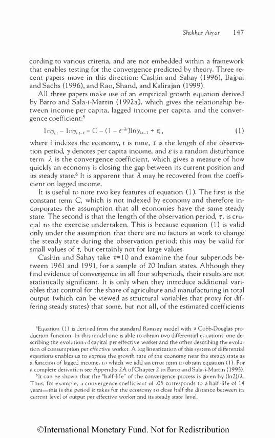
©International Monetary Fund. Not for Redistribution
Shekhar Ai)•ar 14 7
cording to various criteria, and are not embedded within a framework that enables testing for the convergence predicted by theory. Three recent papers move in this direction: Cashin and Sahay ( 1 996), Bajpai and Sachs ( 1 996), and Rao, Shand, and Kalirajan ( 1 999).
All three papers make use of an empirical growth equation derived by Barro and Sala-i-Martin ( 1 992a), which gives the relationship between income per capita, lagged itKome per capita, and the convergence coefficient:s
1 nyi,r - 1 ny,,,_r = c - ( 1 - e-).r)lnyi,r-r + e,,, ( 1 )
where i indexes the economy, t is time, r is the length of the observation period, y denotes per capita income, and e is a random disturbance term. A. is the convergence coefficient, which gives a measure of how quickly an economy is closing the gap between its current position and its steady state.6 It is apparent that A. may be recovered from the coefficient on lagged income.
It is useful to note two key features of equation ( 1 ). The first is the constant term C, which is not indexed by economy and therefore incorporates the assumption that all economies have the same steady state. The second is that the length of the observation period, -r, is crucial to the exercise undertaken. This is because equation ( 1 ) is valid only under the assumption that there are no facrors at work to change the steady state during the observation period; this may be valid for small values of -r, but certainly not for large values.
Cashin and Sa hay take r= 1 0 and examine the four subperiods between 1961 and 1991 , for a sample of 20 Indian states. Although they find evidence of convergence in all four subperiods, their results are not statistically significant. It is only when they introduce additional variables that control for the share of agriculture and manufacturing in total output (which can be viewed as structural variables that proxy for differing steady states) that some, but not all, of the estimated coefficienrs
;Equation ( 1 ) is derived from the standard Ramsey model with a Cobb-Douglas production function. In this model one is able to obrain two differential equations: one describing the evolll[ion ,,f capiral per effective worker and the other describing the evolution of consumption per effective worker. A Log linearization of this system of differential equations enables us to express the growth rate of the economy near the steady state as a function of lagged income, to which we add an error term to obtain equation ( I ). For a complete derivation see Appendix 2A of Chapter 2 in Barra and Sala-i-Manin ( 1995).
61t can he shown that the "h11lf-life" of the convergence process is given by (ln2)/A.. Thus, for example, :. convergence coefficient of .05 corresponds to a half-life of 14 years-this is the period it rakes for the economy ro close half the distance between its current level of outpur per effective worker and its steady state level.

©International Monetary Fund. Not for Redistribution
148 GROWfH THEORY AND CONVERGENCE ACROSS INDIAN STATES
become significant. They conclude that there is evidence of (weak) convergence over the period taken as a whole.7
Bajpai and Sachs follow a very similar approach, examining a sample of 19 Indian states between 1961 and 1993, which is subdivided into three periods. They, too, have difficulty in obtaining statistically significant results. Only for the subperiod 1961-71 do they find evidence of convergence; for the period as a whole, the hypothesis of convergence is rejected. When the initial share of agriculture in output is included as a control variable, the results improve marginally but their qualitative conclusions are not altered.
Rao, Shand, and Kalirajan look at a sample of 14 states over the period 1965-94, divided into various subperiods. They find evidence of divergence in every subperiod they consider, both in the basic regression and the regression with the share of the primary sector as a control. The difference between their results and those of the other two papers mentioned is startling. So, it is worth emphasizing that they work with a smaller sample of states and that their data source for state product estimates is different.
Certain common points may be noted about all three papers. First, they assume a common intercept for different regions, implying that all the states of India have an identical steady state toward which they are converging or from which they are diverging. In doing this, they follow in the tradition of the intenegional empirical work discussed earlier.
Second, all these studies introduce an explanatOry variable-such as the share of agriculture, the share of manufacturing, or a weighted sectoral index-to control for production shocks that are correlated across regions. As would be expected if there were heterogeneous steady states, the introduction of these additional variables causes an increase in the estimate of A.. For example, Cashin and Sahay find that introducing the control not only leads co a significant estimate of il for the period as a whole, but also drastically raises the estimate. Similarly, in Bajpai and Sachs, the one significant convergence coefficient found (for the period 1961-71) is raised with the introduction of the control. ln Rao et al., the speed of divergence is reduced for every subperiod that they examine once the share of the primary seccor is taken intO account. While these earlier studies point in the direction of conditional convergence, however, the fact that they do not explicitly consider the possibility of different intercepts is an important drawback.
7Cashin and Sahay also carry out an exercise rhar is nor repeateJ in rhis paper: rhey examine rhe role of inrersrare migrarion in rhe convergence process. They find rhar rhc response of migrarion co inte rstate differences in income is "anemic,'' and rhar controlling for migration makes very lirtle difference to rheir estimate of convergence.

©International Monetary Fund. Not for Redistribution
Regional Disparities: The Empirical Record
Facts
Shekhar Aiyar 149
Tables 8.1-8.4 and Figures 8.1-8.3 (on the following pages) highlight some of the regional disparities among 19 of India's states for which data have been gathered. lt will be immediately apparent that these disparities are both enormous and persistent. The dispersion of per capita income, literacy rates, rates of urbanization, and other social and demographic indicators are all greater than those commonly found in relatively homogenous groups of countries (such as the OECD, or Europe).
Table 8.1 and Figures 8.1 and 8.2 summarize movements in per capita real income during the 1971-96 period. The states can be conveniently grouped into three categories according to their status in 1971: the six poorest-Manipur, Bihar, Orissa, Madhya Pradesh, Uttar Pradesh, and Tripura; seven middle-income states-Assam, Jammu and Kashmir, Tamil Nadu, Andhra Pradesh, Kerala, Rajasthan, and Himachal Pradesh; and the five richest states-Punjab, Haryana, Gujarat, Maharashtra, and West Bengal.
The income gaps have been profound. In 1971 , Punjab, the richest state, was more than twice as rich as the poorest state, Manipur; by 1996 the difference was even more marked, with Punjab enjoying more than three times the income-level of the poorest state, Bihar. Differences in growth rates also have been large. For example, Maharashtrian incomes grew annually at a rapid pace of 3.4 percent over the period as a whole, while Bihari incomes remained almost stagnant, increasing at an annual rate of only 0.2 percent. There has also been considerable variation in performance within the three groups.
Regional disparities are seen in other indicators of development (Table 8.2). Annual population growth in the two southernmost states of India, Tamil Nadu and Kerala, was only about 1.4 percent and 1 .5 percent, respectively, during the period, whereas population growth reached 2 .5 percent in Rajasthan and 2.4 percent in Manipur. There are significant differences in urbanization across states-for example, Himachal Pradesh in 1991 was still overwhelmingly rural, while in Maharashtra the proportion of city dwellers was approaching 40 percent.
Table 8.3 and Figure 8.3 document literacy across states. In 1971, Kerala, with a literacy rate of 60 percent, was well ahead of any other state; all other states had a rate under 40 percent. In 1991, Kerala remained at the top of the list, and Bihar and Rajasthan remained the most illiterate states.8 During this 20-year period, literacy improved in every state
8Kerala is exceptional among the Indian states for the sharp and persistenr dichotomy between its social indicators, which are of an almost first-world standard, and its levels

©In
tern
atio
nal M
onet
ary
Fund
. Not
for R
edis
tribu
tion
Tab
le 8
.1.
Per
Cap
ita
Rea
l In
com
e, 1
97
1-9
6
.......
Vl
An
nua
lized
0
Inco
me
in 1
97
1 In
com
e in
19
96
G
row
th R
ate
(19
90/9
1 p
rices
) R
ank
in 1
97
1 (1
99
0/9
1 p
rices
) Ra
nk i
n 19
96
1 9 7
1-9
6 (p
erce
nt)
Rank
0
A
nd
hra
Prad
esh
2,9
92
10
5,50
4
7
2.4
5
0 A
ssam
2,
737
13
3,
87
2 14
1.
4
14
� B
ihar
2,
056
18
2
,17
0
19
0.2
1 9
:r:
Guj
arat
4
,24
0
3 7
,37
5 4
2.
2 8
..
.., :r:
H
arya
na
4,4
86
2 8
,324
3
2.5
4
8 H
imac
hal
Prad
esh
3,4
68
6
5,38
6
8
1.8
12
""
Ja
mm
u an
d K
ash
mir
2,
80
3 12
3,
80
6 16
1.
2
16
-< > K
arna
taka
3,
279
8
5,
778
6
2.
3 7
z
Ker
ala
3,0
38
9
5,1
26
10
2
.1
9
0 M
adhy
a Pr
ades
h 2,
476
16
4
,014
13
1 .
9
10
g M
ahar
asht
ra
4,0
05
4
9,5
18
2 3.
4
1 z
M
anip
ur
1,9
49
19
4
,257
12
3
.1
2 <
m
O
rissa
2,
44
5 17
3
,813
15
1.
8
11
"" 0
Pun
jab
5,
473
1
9,8
79
1 2.
4
6
m
z
Raj
asth
an
3,33
0
7
4,2
85
11
1.0
17
()
m
T
amil
Nad
u 2,
97
2 11
6
,294
5
3.0
3
)>
Trip
ura
2,56
8
14
3,1
30
18
0
.8
18
()
Utt
ar P
rade
sh
2,4
86
15
3,6
17
17
1 .
5
13
"" 0
Wes
t Be
ngal
3,
693
5 5
,178
9
1.
4
15
(/)
(/)
Sour
ce: C
entr
al S
tatis
tical
Org
aniz
atio
n.
z 0 > z
Ul )! '-j
!}l

©International Monetary Fund. Not for Redistribution
Shekhar Aiyar 1 5 1
Figure 8.1. Per Capita Income in Selected States, 1971-96
10000 Two Initially Poor States
6000
6000
4000
� 2000 =
1971 1976 1981
10000 Two Initially Mid-Income States
6000
6000
4000 = - - -
2000 1971 1976 1981
10000 Two Initially Rich States
6000
6000
4000
2000 1971 1976 1981
Source: Central Statistical Organization.
1966
1986
1986
Manipu� ..... - Bihar - ..
1991 1996
Kamal� " Kerala
1991 1996
1991 1996
without exception, but not at a rapid pace (apart from Haryana and Himachal Pradesh, which both doubled their literacy rates over 20 years).
The literacy charts for 1996 show a remarkable improvement for almost every state.9 Bihar and Rajasthan are now the only states in India
of per capita income and growth performance, which are relatively mediocre. For a discussion of this issue, see Ramachandran ( 1997).
9Statistics like this inevitably lead to suspicions abour the quality of data available. In fact the literacy chartS for 1991 ar.e from the population census while the charcs for 1996

©In
tern
atio
nal M
onet
ary
Fund
. Not
for R
edis
tribu
tion
152 GROWTH THEORY AND CONVERGENCE ACROSS INDIAN STATES
I 1 1- l .. � L I West Bengal
l 1 Uttar Pradesh
I j Tripura
L I Tamil Nadu
L I Rajasthan
• Punjab
I Orissa
I Manipur
L Maharashtra
I Madhya Pradesh
� .!!! V'l I I Kerala
"' "' e I Karnataka 1.1 < I Q.l jammu and Kashmir E 0 1.1 I .: Himachal Pradesh .!!! ·a. I "' Haryana u ... & � Q.l Gujarat
a:: ....
0 Bihar c:: .2 'S 0 Assam - "' > " "' loi.I <A "' "' Ql cu - -
¢: � 1 0 Andhra Pradesh .... <'i -
= � Q.I O'I 0 0 0 0 0 0 ... 0'1 ;::, - 0 0 0 0 0
.!!.0 c; 0 0 0 0 0 � c:o -D "<!" N ""' ::::.
c: Q ;;; N ·e: "' ::.0 0 � :� � � c v u Oi � ::> 0 V>

©In
tern
atio
nal M
onet
ary
Fund
. Not
for R
edis
tribu
tion
Tab
le 8
.2.
Popu
lati
on
and
Urb
aniz
atio
n, 1
97
1-9
6 A
nnu
aliz
ed
Po
pu
latio
n P
op
ulat
ion
U
rban
U
rban
Po
pul
atio
n
Popu
latio
n P
opu
latio
n D
ensi
ty 1
97
1 D
ensi
ty 1
99
6
Popu
latio
n P
op
ulat
ion
197
1 19
96
G
row
th R
ate
Lan
d A
rea
(per
sons
per
(p
erso
ns p
er
196
1 19
91
(mill
ion
s (m
illio
ns
197
1-96
(s
qua
re
squa
re
squa
re
(per
cent
of
(per
cent
of
of
pers
ons)
of
per
sons
) (p
erce
nt)
kilo
met
ers)
kilo
met
er)
kilo
met
er)
pop
ulat
ion
) p o
pu
latio
n)
And
hra
Prad
esh
43.
5 72
.0
2.0
27
5,0
45
158
26
2 17
.4
26.8
A
ssam
14
.6
26
.7
2.4
78
,438
18
6
340
7.
2 11
.1
Bih
ar
56.4
9
5.4
2
.1
173,
877
32
4
549
8
.4
13.2
G
ujar
at
26.7
4
4.8
2
.1
196
,024
13
6
229
25
.8
34.4
H
arya
na
10.0
18
.2
2.4
4
4,2
12
226
4
12
17.3
24
.8
Him
ach
al P
rad
esh
3.5
5.6
1.
9
55
,67
3 63
10
1 6.
4
8.7
Ja
mm
u an
d K
ashm
ir
4.6
8
.5
2.5
10
1,23
6
45
84
16.6
23
.8
Kar
nata
ka
29.3
4
8.2
2.
0
191,
791
153
25
1 2
2.3
30
.9
Ker
ala
21.
3
31.
0
1 .5
38
,863
54
8
798
15
.1
26.5
M
adhy
a Pr
ades
h 4
1.7
7
2.5
2.
2 4
43,
44
6 9
4 16
3
14.3
23.2
M
ahar
asht
ra
50.4
8
6.3
2.
2 3
07
,713
16
4
280
28
.2
38.7
M
anip
ur
1.1
2.0
2.
4
22
,32
7
49
90
9.0
27
.7
Oris
sa
21.
9
34.4
1.
8
155
,70
7
141
22
1 6
.3
13.4
P
unja
b
13.6
2
2.1
1.
9
50,3
62
270
4
39
23
.1
29.7
R
aja
stha
n
25.8
4
8.4
2.
5 34
2,23
9
75
141
16.3
22
.9
Tam
il N
adu
41.
2
58.4
1.
4
130
,058
3
17
44
9
26
.7
34
.2
Trip
ura
1.6
3
.0
2.5
10
,48
6
153
28
6 8
.8
15.3
U
ttar
Pra
desh
8
8.3
15
0.7
2
.1
294
,411
30
0
512
12
.9
19.9
Vl
W
est
Ben
gal
44
.3
73
.6
2.0
8
8,7
52
499
829
24.5
27
.4
;::.-
"' s:
Sour
ce: C
entr
al S
tatis
tical
Org
aniz
atio
n.
!:>
-< )>
�·
!:>
-< ......
l.n
\.,.)

©In
tern
atio
nal M
onet
ary
Fund
. Not
for R
edis
tribu
tion
Tab
le 8
.3.
lite
racy
, 19
71-
96
- '-"
Lite
racy
in
197
1 Li
tera
cy i
n 1
99
1 Li
tera
cy i
n 19
96
�
(per
cent
of
(per
cent
of
(per
cen
t of
pop
ulat
ion)
R
ank
in 1
97
1 p
op
ulat
ion)
R
ank
in 1
99
1 po
pu
lati
on)
R
ank
in 1
99
6
0
;;o A
ndhr
a Pr
ades
h 25
14
44
16
5
1 16
§
Ass
am
29
11
53
12
73
3
Biha
r 20
17
38
19
44
19
:I:
Guj
arat
36
4
6
2 5
66
10
-l
:I:
Har
yana
27
12
5
6
11
62
11
8 H
imac
hal
Pra
desh
32
8
6
4
3 7
1 5
;;o
Jam
mu
and
Kas
hmir
1 9
19
4
8
14
58
12
-< )> K
arn
atak
a 3
1 9
56
10
5
7
14
z K
eral
a 6
0
1 9
0
1 9
1 1
0
Mad
hy
a Pr
ades
h 22
1 5
4
4
15
52
15
()
M
ahar
asht
ra
39
3
65
2 72
4
�
Man
ipu
r 33
7
60
7 68
6
< m O
riss
a 2
6
13
49
13
57
13
;;o 0
Pun
jab
34
5
58
8
66
9
�
Raj
asth
an
19
18
38
18
48
18
0 m Ta
mil
Nad
u 39
2
63
4
66
8
)>
T
ripur
a 3
1 10
60
6
76
2
0 U
ttar
Pra
des
h 22
16
4
2 17
50
17
0
Wes
t B
eng
al
33
6
58
9
66
7
(f) (f)
Sour
ce: N
atio
nal S
amp
le S
urve
y O
rgan
izat
ion.
z 0 > z (/)
);' '-1 rn

©In
tern
atio
nal M
onet
ary
Fund
. Not
for R
edis
tribu
tion
., Q.l � ell: G � � :::;
-0 c ,g 'S 0 > w Q.l J!: (Y') � • c: CO <!> Q.l � ... <I> .�� 1.1.. ;::::.
- \0 " "' "' "'
1 0
0 0 0 co 0 ..0
-----------------
0 """ 0 N 0
Shekhar Aiyar 155
West Bengal
Uttar Pradesh
Tripura
Tamil Nadu
Rajasthan
Punjab
Orissa
Manipur
Maharashtra
Madhya Pradesh
Kerala
Karnataka
jammu and Kashmir
Himachal Pradesh
Haryana
Gujarat
Bihar
Assam
Andhra Pradesh
c: .Q iii N ·c &, 0 � .. v; :: c � iii l::! ::l .)1

©International Monetary Fund. Not for Redistribution
156 GROWTH THEORY AND CONVERGENCE ACROSS INDIAN STATES
Figure 8.4. Standard Deviation of Log Real Income
0.35
0.33
0.31
0.29
1981 -• • - • 0.27
1977 1976 1986 0.25
1965 1970 1975 1980 1985
Source: Central Statistical Organization.
1991 •
1990
1996 •
1995 2000
with a literacy rate under 50 percent, and Kerala is approaching OECD standards of literacy. The dispersion of literacy rates, as shown in Figure 8.4, after increasing steadily up to the 1990s, also diminished over the last five years. Regional disparities remain profound, however, and female literacy continues to lag in every state. In Bihar and Rajasthan female literacy in 1996 was only 29 percent.
Other social indicators also vary widely across the states (Table 8.4 ). For example, the gap between infant mortality and poverty rates in the best-off and worst-off states is enormous in both cases. In the case of infant mortality, Kerala's record is again outStanding, and that of the "heartland" states is dismal. In accordance with the conventional wisdom that diverse social indicators tend to move together, the infant mortality rate is fairly closely correlated with the literacy rate across the Indian statesin 1996 the correlation was 0.74, with the expected negative sign.
Patterns
The evidence surveyed so far presents a picture of large disparities in both levels and growth rates of per capita income. Some interesting patterns may be gleaned from this record, which have a bearing on whether or not the convergence predicted by growth theory has been at work, and, if it has, whether it is conditional or absolute in nature.
are from the 52nd round of the National Sample Survey. While the two sources often ar· rive at different estimates of the number of people in the economy, the number of literate persons, etc., their estimates of literacy rares are usually thought to be comparable.

©In
tern
atio
nal M
onet
ary
Fund
. Not
for R
edis
tribu
tion
Tabl
e 8
.4.
Soci
al I
ndic
ator
s, 1
97
6-
96
Infa
nt
Mo
rtal
ity
Infa
nt M
ort
ality
P
ove
rty
Rat
e 19
78
Po
vert
y R
ate
199
4
Ann
ualiz
ed
R
ate
19
76
R
ate
199
6
(per
cent
of
(per
cent
of
Perc
ent
(per
cent
of
Ran
k (p
erce
nt
of
Ran
k p
op
ulat
ion
bel
ow
po
pu
latio
n b
elo
w
Cha
nge
in
live
birt
hs)
in 1
97
6
live
bir
ths)
in
19
96
po
vert
y lin
e)
pove
rty
line
) Po
vert
y R
ate
An
dhr
a P
rad
esh
123
9
6
3
9
47
.0
29
.4
2.9
A
ssam
14
4
10
76
1
2
Bih
ar
73
1
1
64
.8
60
.4
0.4
G
ujar
at
154
1
3
62
7
3
9.9
3
3.8
1.
0
Har
yan
a 11
4
7
69
10
H
imac
hal
Pra
des
h 11
5
8
61
6
Jam
mu
and
Kas
hm
ir
68
2
K
arn
atak
a 8
0
3 6
2
7
52
.9
37.6
2
.1
Ker
ala
54
1
15
1
53
.2
29
.2
3.7
M
adhy
a P
rad
esh
151
12
99
1
5
63
.9
44
.1
2.3
M
ahar
asht
ra
92
4
55
4
6
7.8
4
3.5
2
.7
Man
ipu
r O
rissa
14
9
11
103
1
6
62
.1
40
.3
2.7
P
unja
b
98
5
5
4
2
26
.9
21.
6
1.4
R
ajas
than
15
5
14
86
1
3
51.
6
43
.5
1.1
Tam
il N
adu
112
6
5
4
2
54
.9
34
.9
2.8
Tr
ipur
a U
ttar
Pra
des
h 19
8
15
8
6
13
4
6.7
4
0.2
0
.9
Wes
t B
eng
al
58
5
5
1.8
2
6.0
4
.2
(./1
Sour
ce: T
he W
orld
Ban
k. ;:r
"'
,.,.
.. � )>
Q·
1:>
-<
......
Vl
....,_]

©International Monetary Fund. Not for Redistribution
158 GROWTH THEORY AND CONVERGENCE ACROSS INDIAN STATES
It is generally the case that initially rich states have tended to remain rich and initially poor states have tended to remain poor. This implies a positive correlation between initial income and final income. Bur, more ttoublingly, there is also a positive correlation between initial income and growth. Table 8.5 shows the simple correlation coefficient between growth rates (broken up by decade) and the initial values of certain variables. The correlation between income at the beginning of the decade and the growth rate over the decade is negative only for the 1970s. It is small but positive for the 1980s, and large and positive for the five years of the 1990s. For the period as a whole, the correlation between initial income and growth is positive. All this is at least suggestive of absolute divergence since the 1980s (if not before) and, moreover, of accelerating divergence.
This conjecture is reinforced by Figure 8.5, which depicts the standard deviation of the log of real per capita income over time.10 Again, there is a clear upward trend for the period as a whole, which grows more pronounced from the mid-1980s onward. It is interesting that the rapid absolute divergence of the 1990s coincides with the period of India's economic liberalization program. Although the precise relationship between liberalization and divergence must await a study that focuses specifically on this issue, liberalization appears to have disproportionately benefited those states with high current per capita incomes. One possible explanation is that these states had better social and economic infrastructures in place and were in a better position to take advantage of the reduction in impediments to private economic activity.
Conditional convergence is examined by considering two variables that might have a bearing on a region's steady state, the literacy rate (LIT) and private capital investment (PVK), the latter of which is proxied by the amount of credit extended in a region by India's Scheduled Commercial Banks (SCB).1 1 The correlation of private investment in the initial year with growth in the subsequent decade is positive for all three subperiods. Moreover, in each subperiod, this correlation is stronger than the correlation with initial income. As with initial income, the correlation is weakest in the 1970s and strongest in the 1990s.
10A narrowing trend for this measure of dispersion is sometimes referred to as <J· convergence, which is quire differem from the 13-convergence discussed in this paper.
1 1PVK is measured in thousands of rupees per person. There are reasons to be somewhat wary of this proxy. Although lending by the SCBs to the private sector dwarfs lending by other institutions, credit tends to be extended not just for new investmems but also as working capital. Nonetheless, we would expect there to be a strong correlation between credit extended for the two differenr purposes. This is certainly the case at the national level-the correlation berween SCB credit extended and gross private capital formation was 0.93 over the period in question.

©International Monetary Fund. Not for Redistribution
Shekhar Aiyar 159
Table 8.5. Correlations Between Growth Rates and Initial Values of State and Control Variables
Annualized Annualized Annualized Annualized Growth Growth Growth Growth
Rate Rate Rate Rate 1971-81 1981-91 1991-96 1971-96
Log Real Per Capita Income 1971 -0.26 0.33 Log Real Per Capita Income 1981 0.04 Log Real Per Capita Income 1991 0.60
Literacy Rate 1971 0.11 0.48 Literacy Rate 1981 0.04 Literacy Rate 1991 0.53
Literacy Rate (excluding Kerala) 1971 0.18 0.66 Literacy Rate (excluding Kerala) 1981 0.16 Literacy Rate (excluding Kerala) 1991 0.56
PVK 1971 0.01 0.51 PVK 1981 0.34 PVK 1991 0.69
Figure 8.5. Standard Deviation of Literacy Rate
1 3
':' 1986 1996
• • 1 2
1 1 1976 •
• 1981 • 1 0
9 f911
l ��
1965 1970 1975 1980 1985 1990 1995 2000
Source: Central Statistical Organization.
As expected, initial literacy is also positively correlated with growth in every subperiod. For the period as a whole, this correlation is stronger than that with initial income. As noted earlier, Kerala is also an outlier with respect to the other states in our sample. Excluding Kerala leads to much higher correlations in every subperiod, and a very high positive correlation for the period as a whole. Correlations by themselves establish very little, but Table 8.5 does comprise circumstantial evidence that literacy and private investment are variables that influence subsequent growth, and that should therefore be controlled for in ascertaining conditional convergence.

©International Monetary Fund. Not for Redistribution
160 GROWTH THEORY AND CONVERGENCE ACROSS INDIAN STATES
Econometric Analysis
Methodology
The previous discussion strongly suggests that an econometric study of convergence across regions in India needs to control for differences in steady states. This can be achieved in a framework consisting of a dynamic panel with fixed effects, as described in Knight, Loayza, and Villanueva ( 1993), Islam ( 1995), and Lancaster and Aiyar ( 1999).
Our general specification is described by the following equation:
lny;,, = ylnyi,t-T + o'W;,, + TJ, + G,t (2)
where i indexes the region, t the time period, y denotes real per capita income, -r denotes the number of years between each successive observation, Tf is a region-specific time invariant fixed effect, and E is a random disturbance term. W is a vecror of explanatory variables, which in our case comprises two variables, LIT and PVK. 0 is the corresponding coefficient vector. The coefficient on the log of lagged income, y, is equal to e-.1.1', where A. is the convergence coefficient.
This fixed-effects formulation allows us to control for unobserved differences between the steady states of regions in addition ro the observed differences captured by the W vector.12 Identification of the fixed effects is only possible in a panel framework-the previously cited studies of Indian regional development all used a cross-section approach and so could not identify fixed effects. To the extent that the fixed effects are correlated with the explanatory variables (including lagged income), their omission leads to an omitted-variable bias. Since the presumed correlation with lagged income is positive, the coefficient for this variable would be biased upward in a cross-section study, implying that the convergence coefficient A. will be underestimated.13 Thus, consideration of a fixed-effects framework would be expected ro yield higher estimates of convergence relative to the cross-section studies that have gone before.
12The reason for adopting a fixed-effects formulation instead of a random effects one is that, in the Iauer approach, one must assume that the effects are uncorrelated with the exogenous variables included in the model. This is almost certainly not the case in the framework assumed above. The fixed effect may be thought of as representing "technology," or the efficacy with which inputs are transformed into outputs; it seems inevitable that this is not independent of an explanatory vector of variables important w the growth process.
13This is just another way of making the point that absolute convergence differs from conditional convergence: the former will always tend to be smaller than the Iauer because of the bias arising from the omission of appropriate conditioning variables.

©International Monetary Fund. Not for Redistribution
Shekhar Aiyar 161
Estimation of a dynamic panel with fixed effects presents technical difficulties. Lancaster ( 1997) describes a method for obtaining consistent, likelihood-based estimates by seeking an orthogonal reparameterization of the fixed effects in the model. Unfortunately, this estimator is not applicable in the present case since it does not allow for the possibility of heteroskedasticity in the sample. Chamberlain's 0-matrix approach has been widely used for panel studies of this nature. Its use is precluded here, however, since we have only 19 states in our sample, and the weighting matrix becomes nearly singular. We therefore employ the Least Squares with Dummy Variables (LSDV) estimator. This estimatOr is known tO be inconsistent in the direction of N, but Amemiya ( 1967) has shown that it is consistent in the direction ofT and asymptotically equivalent tO maximum likelihood estimation. Moreover, it seems that in practice the estimates obtained by LSDV and the nmatrix approach are very similar, at least in cross-country panel studies (Islam, 1995).
Using data for each consecutive year has the disadvantage of increasing the likelihood of serial correlation due to business cycle effects. Using long period averages, however, risks obscuring changes in the steady state that have occurred during the period. In order ro balance these two concerns, the present study uses a panel of five-year spans ( -r= 5). For example, for the first observation, the dependant variable is the log of real per capita net state domestic product in 1976, and lagged income on the right-hand side (RHS) is for the year 1971. To minimize the risk of simultaneity bias, the other control variables are also lagged five years. Standard errors are estimated using White's variance-covariance matrix, which is robust tO heteroskedasticity of an unknown form.
Results
Table 8.6 presents the results of two regressions. Regression 1 illustrates the statistical effect of assuming a common steady state. In this case, a common intercept is assumed for every region and the other control variables are omitted. The results are dramatic-the coefficient on lagged income is a Statistically significant 1.07, with an implied convergence rate of minus 0.013. In other words, we find evidence of absolute divergence at the rate of 1.3 percent over a five-year period.
Regression 2 includes fixed-effects coefficients for each state, and the control variables, LIT and PVK. An F-test rejectS, at the 5 percent level of significance, the null hypothesis that all the fixed effects are equal to one another. In other words, the hypothesis of a common steady state is implausible.

©International Monetary Fund. Not for Redistribution
162 GROWTH THEORY AND CONVERGENCE ACROSS INDIAN STATES
Table 8.6. Regressions with the Log of Real Per Capita Income as the Dependent Variable1
Constant Yi,t-t LIT PVK Lambda2 R-squared Adjusted R-squared
1Standard errors reported in parentheses. 2Coefficient of convergence.
Regression 1
-0.469 (0.272) 1 .069 (0.033)
-0.013 (0.006) 0.902 0.902
Regression 2
0.369 (0.129) 0.762 (0.277) 0.147 (0.035) 0.199 (0.070) 0.946 0.930
Both control variables have a posmve and significant effect on growth. The coefficient on LIT is 0. 76, which implies that a 1 percentage point increase in literacy corresponds to an increase in the five-year period growth rate of per capita income of almost 8/lo of a percentage point. The strength of this relationship probably reflects the fact that literacy proxies for other social indicators that tend to move in a similar direction, such as life expectancy and various measures of health. The coefficient on PVK is 0.15, which implies that a 1 percentage point increase in investment per person raises the growth rate by 0.1 5 percentage points.
The effect of the conditioning variables in Regression 2 is extremely strong, and so we would expect to find much stronger convergence than that found by previous studies. This is indeed the case; the coefficient on lagged income is 0.0379, which implies an extremely high convergence coefficient of 0.199 and a half-life of about 3 Y2 years.14
Table 8.7 lists the fixed effects recovered from Regression 2. Since we did not, in our study, work from an explicit production function, it is not possible to attach a precise interpretation to these region-specific effects, other than to note that they act as proxies for each region's steady state. l5 However, in their role as steady state proxies, and given
14Although this convergence coefficient is quite high, it is worth bearing in mind thar this is the rate of convergence after controlling for steady states, and that inequalities of income and growth in India are seemingly driven by wide differences in steady states rather than by slow convergence. Other studies have also found very high rates of convergence with the introduction of suitable control variables-notably Caselli, Esquivel, and Lefort ( 1996), who estimated a convergence rare of 0.128 (implying a half-life of 51n years) for a sample of97 heterogeneous countries.
lSKnight, Loayza, and Villanueva ( 1993) and Islam (1995) start with an explicit neoclassical production function, and are thus able to derive the relationship J.l, = ( 1 -c<r)lnA(O)., where J.l is the fixed effect and A(O) represents "technology" broadly defined in the initial period of observation.

©International Monetary Fund. Not for Redistribution
Shckhar Aiyar 163
that we have already controlled for literacy and the amount of investment, we may regard them as a measure of the efficiency with which the different regions are converting inputs into outputs. Thus they are related to the conventional notion of total factor productivity (TFP) with the important difference that TFP is computed for individual economies on the basis of only their own time series data, whereas the fixed effects here are inherently based on an interregional comparison.
We find that the fixed effects are highly and positively correlated with initial income; the simple correlation coefficient is 0.65. Their correlation with growth rates over the period as a whole is also positive at 0.32. These results are in line with what we would expect from studies of samples of heterogeneous countries. An examination of the regions by rank of their fixed effects yields one rather striking result, namely, Kerala's place at the bottom of the table, comfortably under even Bihar. This would be an indication that Kerala has been inefficient in translating its enviable human capital resources into commensurate increases in output per capita, but may also reflect the fact that much of Kerala's educated population has been able to migrate elsewhere. Punjab and Haryana top the table, and, in general, initial income is a good predictor of a state's rank by this measure. Note that the large values obtained for the fixed effects and their considerable dispersion suggest that there are important factors determining the steady states of regions that are not accounted for by this study.
Table 8.7. Fixed-Effects Estimates
Fixed Effect Rank
Andhra Pradesh 4.891 5 Assam 4.769 1 4 Bihar 4.631 18 Gujarat 4.917 3 Haryana 5.130 1
Himachal Pradesh 4.887 6 jammu and Kashmir 4.897 4 Karnataka 4.800 I 2 Kerala 4.550 1 9 Madhya Pradesh 4.857 8 Maharashtra 4.846 9 Manipur 4 828 1 0 Orissa 4.760 1 5 Punjab 5.130 2 Rajasthan 4.867 7 Tamil Nadu 4.716 1 6 Tripura 4.697 1 7 Uttar Pradesh 4.802 1 1 West Bengal 4.779 1 3

©International Monetary Fund. Not for Redistribution
164 GROWTH THEORY AND CONVERGENCE ACROSS INDIAN STATES
Policy Implications
These results strongly suggest that states in India are converging tO different steady states, and that these steady states are determined, at least in part, by literacy rates and private investment. The question then naturally arises as tO what governments can do tO improve literacy and attract private investment, thus raising the steady state output of their region and generating rapid growth. There are undoubtedly numerous factOrs that determine LIT and PVK for a given region. Here we consider only two that are amenable to direct manipulation by policymakers---capital expenditures by state governments on social infrastructure (SOC) and capital expenditures by state governments on economic infrastructure (ECO). The first variable measures expenditures on categories such as education, water supply, sanitation, and medical and public health, while the second variable represents expenditures on transportation, power and electricity, telecommunications, and irrigation projects. Both variables are measured in thousands of Rs per person.
It seems reasonable that government spending in these areas contributes to human capital and promotes private investment.16 Therefore we regress LIT and PVK in turn on both SOC and ECO, in the same fixed-effects panel framework followed thus far. Table 8.8 documents the results, which suggest that both SOC and ECO are significant in accounting for the literacy rate, with coefficients of 2.54 (0.50) and 0.69 (0.22), respectively. These policy variables appear tO play an even more imporrant role in influencing private investment; in the equation for PVK, the coefficients on SOC and ECO are 4.77 ( 1 .77) and 3.64 ( 1 .03), respectively. These regressions are therefore indicative of two channels through which governments can attempt tO alter the steady states of their economies.
To test the robustness of these results, we also fit a Cobb-Douglas "production function" with LIT and PVK taken one by one as the outputs; the inputs are SOC and ECO, along with a multiplicative regionspecific efficiency parameter. The results of this regression, in which coefficients represent elasticities, are detailed in Table 8.9. The elasticities of the literacy rate with respect to SOC and ECO are, respectively, 0.24 (0.05) and 0.10 (0.08), although the latter estimate is no longer statistically significant. The elasticities of private investment with respect to SOC and ECO are, respectively, 0.65 (0.10) and 0.46 (0.15). These elasticity estimates, which are both large and highly significant, appear tO confirm the efficacy of government investment in infrastructure in
16Studies indicating a complememarity lbenveen public infrastructure and private investment include Greene and Villanueva ( I 991) and Seitz and Licht ( 1992).

©International Monetary Fund. Not for Redistribution
Shekhar Aiyar 165
Table 8.8. "Production Function" Regressions with LIT and PVK as Outputs1
Dependent Variable LIT PVK
soc ECO R-squared
'Standard errors reported in parentheses.
2.54 (0.50) 0.69 (0.22) 0.64
4.77 (1 .77) 3.64 (1.0 l) 0.78
Table 8.9. "Production Function" Regressions with In (LIT) and In (PVK) as Outputs1
Dependent Variable
In (SOC) In (ECO) R-squared
'Standard errors reported in parentheses.
In (LIT)
0.24 (0.05) 0.10 (0.09) 0.61
In (PVK)
0.65 (0.1 01 0.46 (0. 15 1 0.81
attracting private investment and improving the stock of human capital. It is noteworthy that the regressions indicate that social expenditures have an even greater impact than expenditure on physical infrastructure.17
Conclusion
One of the main purposes of this study was to show that in a country as diverse as India, there is a meaningful difference between conditional and absolute convergence. It has been shown that the neoclassical model's prediction of convergence is of a conditional nature and that convergence among the Indian states is proceeding apace. By demonstrating a concomitant process of absolute divergence, however, our work suggests that the really important and interesting feature of regional growth is not an economy's distance from its steady state (that is being closed rapidly at any point in time), but the factors that determine that steady state. This conclusion is important, since it suggests that there is scope for policy to improve the growth rate of per capita incomes.
We have identified two factors that seem to be extremely important in determining a region's steady state level of income: literacy and per capita private investment. In particular, even modest improvements in literacy and private investment appear to have a substantial positive effect on growth. Furthermore, the results suggest that both literacy and
17The positive impact of state government heald1 and educ;�titln o.:xpcnditun." nn human capital formation has also been studied in Re�erve Bank of India ( 1993 ).

©International Monetary Fund. Not for Redistribution
166 GROWTH THEORY AND CONVERGENCE ACROSS INDIAN STATES
private investment can be influenced by policy, and hence individual state governments can play an important role in enhancing their own growth prospects.
In practice, however, the ability of state governments to increase expenditures on social and economic infrastructure is greatly dependent on their financial positions. This ability has been adversely affected by rising deficits in recent years, owing to stagnant revenue collections and increasing expenditures on civil service salaries and interest payments. Thus, fiscal reform-particularly at the state level and with respect to fiscal-federal relations-will be an important ingredient for improving steady state levels of incomes across India. Enhancing the flow of private investment spending on infrastructure will also be important. Recent efforts by some states to liberalize private sector participation in the power sector and to implement Build, Operate, and Transfer systems for roads and bridges are encouraging and would be bolstered by further liberalization and deregulation at the central government level.
In addition, significant differences in growth performance and steady states have been found that are not explained by literacy and private investment rates. If cross-country studies and anecdotal evidence are anything to go by, we would suspect the fixed effects to capture factors like the degree to which the rule of law is observed and enforced, the degree of bureaucratic control and inefficiency in the economy (which bears a strong relationship to the pervasiveness of corruption) , the relations between organized labor and industry and the laws governing these relations, the laws pertaining to other spheres such as land reform, tax regimes, and urban regulation, and the extent to which foreign investment permits diffusion of new technologies and products and breeds competition. This study does not establish these relationships. By showing how important differences in steady states are, however, and by assessing the importance of two key variables in their determination, it does leave the door open for future research (which must await the availability of appropriate data) to investigate the role played by these other suggested factors.
References
Amemiya, T., 1967, "A Note on the Estimation of Balestra-Nerlove Models," Technical Report No. 4, Institute for Mathematical Studies in Social Sciences, Stanford University.
Bajpai, N., and J.D. Sachs, May 1996, "Trends in Inter-State Inequalities of Income in India," Development Discussion Papers, Harvard Institute for International Development, No. 528.

©International Monetary Fund. Not for Redistribution
Shekhar Aiyar 167
Barro, R.J., 1991, "Economic Growth in a Cross-Section of Countries," Quarterly ]ouma.l of Economics, Vol. 106, No. 2 (May), pp. 407-43.
---, and X. Sala-i-Manin, 1992a, "Convergence," Journal of Political Economy, Vol. 100 (April), pp. 223-5 l .
---,1992b, "Regional Growth and Migration: A Japan-United States Comparison," )oumal of the Japanese and the lncemational Economy, Vol. 6 (December), pp. 312-46.
---, 1995, Economic Growth (New York: McGraw-Hill).
Barro, R.j., N.G. Mankiw, and X. Sala-i-Martin, 1995, "Capital Mobility in Neoclassical Models of Growth," American Economic Review, Vol. 85 (March), pp. 103-15.
Baumol, W.J., 1982, "Productivity Growth, Convergence and Welfare: What the Long-Run Data Show," American Economic Review, Vol. 6 (December), pp. 1072-85.
Caselli, D., G. Esquivel, and F. Lefort, 1996, "Reopening the Convergence Debate: A New Look at Cross-Country Growth Empirics," Joumal of Economic Growth, Vol. 1, pp. 363-89.
Cashin, P.A., 1995, "Economic Growth and Convergence Across the Seven Colonies of Aust ralasia: 1861-1991," Economic Record, Vol. 71 (June), pp. 132-44.
---, and N. Loayza, 1995, "Paradise Lost? Growth, Convergence, and Migration in the South Pacific," IMF Staff Papers, International Monetary Fund, Vol. 42 (September), pp. 608-41.
Cashin, P.A., and R. Sahay, 1996, "Internal Migration, Center-State Grants, and Economic Growth in the States of India," IMF Scaff Papers , International Monetary Fund, VoL 43 (March), pp. 123-71 .
Chamberlain, G., 1983, "Panel Data," i n Handbook of Econometrics, Vol. II, ed. by Z. Griliches and M.D. lntriligaror (Amsterdam: North Holland).
Chaudhry, M.D., 1966, Regional Income Accounting in an Underdeveloped Economy: A Case Study of India (Calcutta: Firma K. L. Mukhopadhyay).
Easterlin, R.A., 1960a, "Regional Growth and Income: Long Term Tendencies," in Population Redistribution and Economic Growth: United States 1870-1950, Vol.2: Analyses of Economic Change, ed. by S. Kuznets, A.R. Miller, and R.A. Easterlin (Philadelphia: American Philosophical Society).
---, 1960b, "Interregional Differences in Per Capita Income, Population and Total Income, 1840-1950," in Trends in the American Economy in the Nineteenth Century, VoL 24 ofNBER Studies in Income and Wealth.
Ghuman, B.S., and D. Kaur, 1993, "Regional Variations in Growth and Inequality in the Living Standard: The Indian Experience," Margin, Vol. 25 (April-June), pp. 306-13.
Govinda Rao, M., R.T. Shand, and K.P. Kalirajan, 1999, "Convergence of Incomes Across Indian States: A Divergent View," Economic and Political We.ekly, Vol. 34 (March 27), pp. 769-78.

©International Monetary Fund. Not for Redistribution
168 GROWTH THEORY AND CONVERGENCE ACROSS INDIAN STATES
Greene, ]., and D. Villanueva, i991, "Private Investment in Developing Countries," IMF Scaff Papers, International Monetary Fund, Vol. 38 (March), pp. 33-58.
Islam, N., 1995, "Growth Empirics: A Panel Data Approach," Quarterly journal of Economics, Vol. tiO (November), pp. 1 1 27-70.
Knight, M., N. Loayza, and D. Villanueva, i993, "Testing the Neoclassical Theory of Economic Growth: A Panel Data Approach," IMF Staff Papers, International Monetary Fund, Vol. 40 (September), pp. 5 1 2-41.
Lall, S.V., 1999, "The Role of Public Infrastructure Investments in Regional Development: Experience of Indian States," Economic and Political Weekly (March 20).
Lancaster, T., 1997, "Orthogonal Parameters and Panel Data," Brown University Working Pape1·, No. 97-32 (April).
---, and S. Aiyar, S., 1999, "Econometric Analysis of Dynamic Models: A Growth Theory Example," Brown University Working Paper, No. 99-28 (May).
Lucas, R., 1988, "On the Mechanics of Development Planning," journal of Monetary Economics, Vol. 2 2 (July), pp. 3-42.
Majumdar, G., and J.L. Kapur, 1980, "Behaviour of Inter-State Income Inequalities in India," journal of Income and Wealth, Vol. 4, No. I (January), pp. 1-8.
Mankiw, N.G., D. Romer, and D.N. Wei!, 1992, "A Contribution to the Empirics of Economic Growth," Quarterly journal of Economics, Vol. 107 (May), pp. 407-37.
Nair, K.R.G., 1985, "A Note on Inter-State Income Differentials in India i970-7i ro 1979-80," in Regional Structure of Growth and Development in India, Vol. I , ed. by G.P. Misra (New Delhi: Ashish Publishing House).
Ramachandran, V.K., 1997, "On Kerala's Development Achievements," in Indian Development: Selected Regional Perspectives, ed. by]. Dreze and A. Sen (Oxford: Oxford University Press).
Ramsey, E, 1928, "A Mathematical Theory of Saving," Economic Journal, Vol. 38, No. 1 5 2 (December), pp. 543-59.
Rao, H., 1985, "Inter-State Disparities in Development in India," in Regional Structure of Growth and Development in India, ed. by G.P. Misra, (New Delhi: Ashish Publishing House).
Reserve Bank of India, 1993, "Social Sector Expenditures and Human Development-A Study of Indian States,'' Development Research Group Study.
Seitz, H., and G. Licht, 1992, "The Impact of the Provision of Public Infrastructures on Regional Development in Germany," Discussion Papers, Zentrum fur Europaische Wirtschaftsforschung Gmbh, No. 93-U.
Shioji, E., 1993, "Regional Growth in Japan," unpublished manuscript, Yale University.
Solow, R.M., 1956, "A Contribution to the Theory of Economic Growth," Quarterly ]oumal of Economics, Vol. 50 (February), pp. 65-94.

©International Monetary Fund. Not for Redistribution
Shekhar Aiyar 169
Swan, T.W., 1956, "Economic Growth and Capital Accumulation," Economic Record, Vol. 32, No. 63 (November), pp. 334-6 l .
Uzawa, H . , 1965, "Optimal Technological Change i n an Aggregative Model o f Economic Growth," International Economic Review, Vol. 6 (January), pp. 18-3 1 .
Appendix 8. 1 : Data
An important starting point for constructing the database used was data provided by Cashin and Sahay, which is gratefully acknowledged. This data was extended and updated using data on Net Domestic Product for each state taken from the consolidated series prepared by the Central Statistical Organization (CSO). Population charts were from the census for those years in which the census was conducted; midyear estimates are available in different issues of CSO publications such as the Statistical Pocket Book of India and the Statistical Abstract of India. Literacy rates were obtained from census data when available and survey rounds conducted by the National Sample Survey Organization (NSSO) otherwise. Survey results are reported in the NSSO's journal, Sankhya. For 1976 and 1986 literacy rates were constructed by linear interpolation. Infant mortality rates and poverty charts were based on World Bank estimates.
The charts for state capital expenditures on social and economic infrastructure were taken from various monthly issues of the Reserve Bank of India Bulletin and Supplements tO the Bulletin. Data on credit extended by India's Scheduled Commercial Banks are available at the state level in different issues of the Reserve Bank of India's Statistical Tables Relating to Banking. Urbanization charts were taken from census data.

©International Monetary Fund. Not for Redistribution
9 Structural Reform in India
DANIEL KANDA, PATRICIA REYNOLDS, AND CHRISTOPHER TOWE
Introduction
Tremendous strides have been taken during the past decade in unshackling the Indian economy from widespread regulatory and other structural impediments. Nonetheless, there is widespread agreement among policymakers and analysts that more needs to be done in order to sustain and improve India's recent growth performance, and to reduce the large share of the population that remains below the poverty line. This consensus was most striking during the general elections of 1999, where the manifestos of both major parties-the National Democratic Alliance and the Congress Party-demonstrated remarkably similar calls for a "second wave" of reform.
Following the elections in October 1999, the new government established an ambitious objective for growth of at least 7-8 percent, and acknowledged that achieving this objective would require both sound macroeconomic policies and broad-based reform. Policy action was swift and included legislation to open the insurance sector, liberalization of the foreign exchange system, and tax reforms. However, a well-defined medium-term strategy and implementation timetable has yet to emerge.1
1This deficit appears to have been acknowledged by the government, which requested the Economic Advisory Council in July 2000 to prepare a strategy paper identifying reform priorities, as a vehicle for establishing a political consensus for action on a broad front.
170

©International Monetary Fund. Not for Redistribution
Daniel Kanda, Patricia Reynolds, and Christopher Towe 171
This chapter provides a brief overview of the recent experience in the area of structural reform, and suggests a number of areas where priority is needed in the period ahead. In particular, the next section broadly describes the post-1991 balance-of-payments crisis liberalization and discusses the cross-country evidence on the link between growth and .reform. A more detailed discussion of the areas where reforms should be focused in the period ahead is presented later.
Recent Reforms and Their Implications
Important structural reforms were initiated in India in the mid-1980s, and the pace of reform accelerated following the balance-of-payments crisis in 1991. Prior to this period, government policies were predominantly inward looking and involved significant regulation and public ownership in all areas of the economy, with the objective of building industrial and agricultural self-sufficiency and reflecting a strongly socialist political environment. During the past 15 years, however, partly in response to concerns regarding India's halting growth and vulnerability to external crises, deregulation and liberalization have been significant. Notably:
• In the industrial secror, licensing requirements were dismantled, and steps were taken tO liberalize investment approvals procedures. Also, many areas of the economy that had previously been reserved for the public sector were opened for private investment, including power, telecommunications, mining, ports, roads, river transport, air transport, and banking.
• External sector reforms included reductions in tariffs, the easing of import licensing requirements, a relaxation of controls on foreign direct and portfolio investment, and greater exchange rate flexibility. Cuts reduced the import-weighted tariff rate from 87 percent in 1990/91 to 25 percent by 1996/97, and there were substantial reductions in the number of quantitative restrictions on imports. The approvals process for foreign direct investment (FDI) was simplified, portfolio investment was allowed for registered foreign institutional investors, and Indian companies were allowed to issue global depository receipts (GDRs), subject to restrictions. The exchange rate regime was also liberalized. The rupee was floated in March 1992, and full current account convertibility was established in August 1994, earning India Article VIII status with the IMF.
• Liberalization and reform in the financial sector were particularly significant during the 1990s. Interest rates were liberalized,

©International Monetary Fund. Not for Redistribution
172 STRUCTURAL REFORM I N INDIA
prudential norms and supervision were strengthened, private sector competition in the banking system was increased, and measures were taken to develop and strengthen capital and debt markets. These measures enabled a gradual shift toward implementing monetary policy by means of indirect rather than direct instruments.
• Fiscal reforms focused on rationalizing tax rates, cutting expenditures, and privatizing public enterprises. The public sectOr deficit, at the same time, which reached just over 1 1 percent before the 1991 crisis, was lowered tO 8\14 percent by 1995/96.
These effons appear to have paid important dividends. The recovery from the 1991 crisis was rapid, with a sharp rise in private investment and an increase in real GOP growth tO 7% percent by 1995/96 (Table 9.1). Significant improvements in productivity were also achieved-as evidenced by increased total factOr productivity growth at both the aggregate and firm levels (World Bank, 2000; Krishna and Mitra, 1998). Most impressive was the performance of the services sector. Out of average GOP growth of 5314 percent in the 1990s, the service sectOr contributed 3 14 percentage points, compared to only 1 1f2 percentage points out of average GOP growth of 3314 between 1951/52 and 1979/80. This rising contribution was accompanied by a steady decline in the incremental capital output ratio (ICOR) in the provision of services, indicating that rising productivity played an important role in fostering high-quality growth in this sector.
There is the perception that the reform process has slowed over the past few years, however, owing largely to political difficulties, and recent economic performance raises questions about the sustainability of the strong growth that was experienced in the mid-1990s--or the feasibility of achieving even more rapid growth. In particular:
• The fiscal situation deteriorated significantly from FY 1996/97, with the consolidated deficit of the public sector is estimated to have exceeded 1 1 percent of GDP in FY 1999/2000. The weakening of the fiscal position reflected stagnant revenue collections, sharp increases in civil service wages and subsidies, and rising debt service payments-all of which have limited the scope for funding needed for infrastructure and other investments.
• Real growth has slowed since the mid-1990s-averaging around 6 percent in 1997/98-1999/2000. While this partly reflected temporary factors such as agricultural supply shocks and the adverse effect of the 1997 regional crisis, structural impediments may also have been significant. In particular, the relatively weak performance of the agricultural and industrial sectors, relative tO the services sector, supports anecdotal and other evidence that infrastructure and regulatory constraints have helped to restrain

©International Monetary Fund. Not for Redistribution
Daniel Kanda, Patricia Reynolds, and Christopher Towe 173
Table 9.1. Expenditure and Sectoral Components of Growth in India, 1951/52-1999/20001 (In percent)
Average
195 1/52- 1 980/8 1- 1992/93- 1997/98-1979/802 1990/9 1 1 996/97 1999/20003
Real GOP growth4 3.7 5.9 6.4 5.9 Real per capita GOP growth4 1 . 5 3.8 4.5 4.3
Contribution to growth, by expenditure item:• Consumption 2.6 4.2 4.4 4.4
Private consumption 2.1 3.5 3.9 2.7 Public consumption 0.4 0.7 0.5 1 . 6
Gross fixed investment 0.7 1 . 4 1.9 1 . 0 Private investment 0.8 2.1 0.6 Public investment 0.5 -0.2 0.4
Net exports> 0.6 0.2 0.6
Contribution to growth, by sector:6 Public 1 . 1 1 . 7 1 . 3 3.9 Private 2.2 4.2 5.7 2.2
Contribution to growth, by sector:6 Agriculture 1.0 1 .5 1.4 0.6 Industry 1 . 1 1 .9 2.1 1 .6 Services 1.4 2.4 3.2 3.9
ICORs, by sector:7 Overal l 4.2 4.1 4.8
Agriculture 2.0 1 .5 2.6 Industry 5.7 6.8 10.7 Services 4.0 2.9 2.1
Sources: Central Statistical Organization (CSOl; National Accounts Statistics. 'Calculations based on constant price data; base year is 1980/81 for data until 1993/94, and
1 993/94 thereafter. 2Average contributions of consumption spending, and public and private sectors are calculated
over 1 961/62-1979/80. 31 999/2000 figures on GOP and sectoral production are CSO revised estimates; 1999/2000 fig·
ures on expenditure categories and 1998/99 and 1999/2000 figures on public and private sector GOP are staff estimates; incremental capital output ratios (ICORs) computed over 1 997/98-1998/99.
•Measured at market prices. 51ncludes statistical discrepancy. 6Measured at factor cost. 7The I COR is the ratio of the investment rate to the GOP growth rate; a Ia !Iing ICOR over time
therefore indicates improved capital productivity.
growth. In addition, the sharp decline in the contribution of private investment spending to overall growth, at the same time that the growth contribution of government consumption has increased sharply, suggests that higher fiscal deficits have crowded out private activity.

©International Monetary Fund. Not for Redistribution
174 STRUCTURAL REFORM IN INDIA
• There also is concern that progress toward poverty reduction has slowed during the past decade. Although the poverty rate fell from 55 percent in 1973/74 to 36 percent in 1993/94, unofficial survey data point to relatively modest progress in reducing the poverty rate during the 1990s. At the same time, there is evidence that the income distribution across Indian states has become increasingly skewed.2
These suggest that the more recent pace and scope of structural reform may not be sufficient to sustain needed income gains. Indeed, a number of analysts-both inside and outside the policymaking sphere in India-have argued for the establishment of an ambitious "second wave" of reform to address a number of difficult issues that have so far remained relatively untouched (see, in particular, Kelkar, 1999).
Indeed, a number of analytical studies have stressed that, notwithstanding the experience of the mid-1990s, India's GOP growth performance has lagged behind a number of other Asian economies, and the benefits from deeper structural reform could be significant (Table 9.2). These include studies that have analyzed the nature of the structural impediments in India (World Bank, 1998; Bajpai and Sachs, 1997), the reasons for the differences in the growth performances of India relative to China and other developing countries (World Bank, 2000; Bajpai, }ian, and Sachs, 1999), and the effects of structural reforms at the state level (Chapter 9; Bajpai and Sachs, 1999).
For example, Bajpai and Sachs ( 1 997) estimated that annual per capita growth in India could be raised by as much as 3.5 percentage points by adopting extensive market reforms, including domestic deregulation, greater openness, and reforms to exit policies and labor and land laws (Table 9.2). Empirical work by Kongsamut and Vamvakidis (2000) confirms the potential for structural reform to promote faster growth in India. In particular, their analysis suggests that measures to promote private investment, FDI, trade, and educational attainment could add 3.4 percentage points to average growth.
Comparisons of India and China have also concluded that the much higher growth rates experienced by China-over 4 percentage points during 1980-96-have been due to the more liberal regulatory environment enjoyed by China's non-state sector (particularly with respect
21nterpretation of poverty trends is complicated by the fact that the results of more recent smaller-sample surveys have not yet been confirmed by the official large-sample survey that is due to be released in 200 I. Moreover, analysts have suggested that the decline in poverty in the 1970s and 1980s was overstated by underestimates of in-kind income during the early part of the period, while other analysts argue that the downward trencl has been underestimated by overestimates of inflation. For a discussion, see Chapter 8 and Ahluwalia (2000).

©In
tern
atio
nal M
onet
ary
Fund
. Not
for R
edis
tribu
tion
Tab
le 9
.2.
Exp
lain
ing
Indi
a's
Rela
tive
Gro
wth
Per
form
ance
Fact
ors
co
ntr
ibut
ing
to g
row
th d
urin
g 1
97
0-
95
, as
es
timat
ed b
y K
ong
sam
ut a
nd V
amva
kidi
s (2
00
0):
In
vest
men
t/G
OP
N
et
FDI/
GD
P
Trad
e/G
DP
G
ove
rnm
en
t co
nsum
ptio
n/G
OP
Se
cond
ary
sch
oo
l e
nro
llme
nt
rate
C
PI
inn
ati
on
rat
e
Co
nver
gen
ce e
ffec
t an
d o
the
r fac
tors
Real
per
cap
ita G
DP
gro
wth
(19
70
-9
5 a
vera
ge)
Fact
ors
co
ntr
ibut
ing
to g
row
th d
uri
ng
19
92
-9
5,
as
estim
ated
by
Baj
pai
and
Sac
hs
(19
97
):
Savi
ng/G
OP
Ef
ficie
ncy
ind
ex
Co
nver
genc
e ef
fect
and
oth
er fa
cto
rs
Re
al p
er
cap
ita G
DP
gro
wth
(19
92
-9
5 a
vera
ge)
Sour
ces:
Ko
ngsa
mut
an
d V
amva
kidi
s, 2
00
0;
Bajp
ai a
nd S
achs
, 19
97.
Ave
rage
Val
ue (
in p
erce
nt)
Ind
ia
East
Asi
a
21.9
2
9.6
0.1
2
.5
4.5
1
13
.5
10.3
10
.4
35
.2
50
.5
8.8
8.4
2.4
5.7
22
.4
35
.0
-0
.7
0.6
3.6
6
.3
Estim
ate
d D
iffer
ence
in
Gro
wth
Rat
es'
(i
n p
erc
ent
age
po
ints
)
-1.2
-
0.8
-
1.1
0.0
-0
.3
0.0
0.2
-3.
3
-1
.2
-3
.6
2.1
-2.
7
'Cal
cula
ted
as th
e e
stim
ated
co
effic
ient
tim
es th
e d
iffe
renc
e in
the
ind
epen
dent
var
iabl
e va
lue
(Ind
ia-E
ast
Asi
a). R
epor
ted
diff
eren
ce i
n g
row
th r
ates
of
real
pe
r cap
ita G
DP
are
act
ual
s.

©International Monetary Fund. Not for Redistribution
176 STRUCTURAL REFORM IN INDIA
to agricultural sector pricing and labor laws), as well as the more attractive incentives offered by its Special Export Zones. A study of the effects of structural reforms at the state level in India found that reform-oriented states (such as Gujarat, Tamil Nadu, and Maharashtra) grew faster and attracted much more private investment-both domestic and foreign-than those that have lagged behind in the reform process (Bajpai and Sachs, 1999).
The Outstanding Agenda
As noted above, there is a widespread consensus in India on the need for a reinvigoration of the momentum for reform. There is also considerable agreement on where the emphasis needs to be placed. A brief summary of the principal issues that a number of analysts-in both the public and private sectors-have raised follows.3
Financial Sector
Considerable progress has been made in reforming the financial sector since the early 1990s, following blueprims laid uul by a serie:s uf government commissions. In the banking sector, for example, capital adequacy has been improved, interest rates have been largely deregulated, priority-lending requirements were eased, and new entrants have increased competition. More recent reforms included the opening up of the insurance sector-long dominated by the state-owned Life Insurance Corporation and the General Insurance Corporation-to private and foreign competition beginning in 2000. In capital markets, other recent initiatives include the passage of legislation to provide a framework for trading in derivatives, allowing mutual funds to trade in derivatives, relaxing entry norms for initial public offerings, and establishing regulations to allow employee stock options. The Foreign Exchange Management Bill was passed in 1999, which significantly streamlined foreign exchange regulations
Nonetheless, significant challenges remain to be addressed in order to ensure that the financial sector is well placed tO provide the necessary underpinning for strong growth. Government-owned banks still account for roughly 80 percent of the banking sector, which has contributed to
>tn particular, see the discussions by the Ministry of Finance and Reserve Bank of lndia in various issues of the Economic Survey and Annual Report, respectively; Ahluwalia (1999); Acharya (1999); Rajiv Gandhi Instirute for Contemporary Studies (1998); World Bank (2000); and Desai ( 1999).

©International Monetary Fund. Not for Redistribution
Daniel Kanda, Patricia Reynolds, and Christopher Towe 177
weak governance and efficiency. Despite repeated commitments to reducing government ownership, progress has been slow, due in large part to union resistance. The government announced in February 2000 its intention ro reduce minimum public ownership share ro 33 percent, although this was accompanied by statements that employment levels and the "public sector character" of these institutions would be preserved.
Further improvements in the regulatory and supervisory system are needed. These include the early increase in the capital adequacy requirement to 10 percent, reductions in cash and statutory liquidity requirements, an easing of restrictions on foreign bank branches, and the abolition of remaining interest rate regulations and priority-lending requirements. In addition, the lack of an effective and rules-based exit strategy for chronically undercapitalized banks continues ro undermine governance and creates significant moral hazard. The growing importance of nonbank financial institutions and the trend toward universal banking also pose important challenges to the regulatory and supervisory system.
Another important issue is the appropriateness of existing systems for administering interest rates on postal saving and provident funds. Notwithstanding recent rate reductions, these deposits earn very high rates of return, especially given their tax advantage, and are not flexibly adjusted in line with market conditions-the government's decision in early 2000 to lower the rate on deposits with the Employee Provident Fund (EPF)-for the first time since the early 1990s-from 12 percent ro 1 1 percent was overturned in July by the EPF's trustees. High rates on these deposits have put the banking secror at a competitive disadvantage while imposing a significant fiscal burden. The fact that 80 percent of many of these deposits are automatically loaned to the states also has the effect of undermining their fiscal discipline. As a number of commentators have suggested, the medium-term objective should be to reduce the government's role as a financial intermediary by privatizing the functions of the postal saving and provident funds and reducing restrictions on their investment.
Recently approved liberalization of the insurance sector promises to provide a significant opportunity ro deepen capital markets and increase the funding for productive investment. However, it remains to be seen whether foreign ownership limits will unduly restrict the scope for private sector participation, so that new entrants will be largely funded by the banking sector, itself dominated by public institutions. Moreover, existing public sector insurers continue to be responsible for significant quasi-fiscal activities-including the provision of subsidized insurance to low-income households-and these activities would need to be eliminated and/or brought on budget. It will also be important ro

©International Monetary Fund. Not for Redistribution
178 STRUCTURAL REFORM IN INDIA
resist pressure to impose similar quasi-fiscal responsibilities on new entrants-including priority sector requirements.
Infrastructure
Infrastructure deficiencies-particularly in power, transportation, and communications-are among the most important impediments to growth in India. The 1998 Global Competitiveness Report of the World Economic Forum, which examined the strengths and weaknesses of 53 countries and provided an assessment of their medium-term growth prospects, ranked India's overall infrastructure fifty-third. All aspects of infrastructure were found to have severe weaknesses.
The lack of consistent and reliable access tO power remains an important obstacle to growth. Although capacity has grown rapidly in recent years-61/z percent in 1998/99-energy and peaking shortages remained high at 6 percent and 14 percent, respectively. An important factOr is the inefficiency of thermal plants and the State Electricity Boards (SEBs), which distribute electricity to most customers. SEBs have typically provided energy to the agriculture sectOr at well below cost, leading to heavy financial losses. Operational inefficiencies have also meant that the SEBs' transmission and distribution losses-estimated at 25 percent by the authorities and at 40 percent by the World Bank-are among the highest in the world. In 1997/98, only three SEBs had a rate of return higher than the legally mandated minimum of 3 percent, which has limited the ability of the SEBs to invest in capacity.
In response, power sector reforms have begun both at the state and central government levels. Several states, including Orissa and Andhra Pradesh, have enacted legislation to reform their power sectors and ro establish independent State Electricity Regulatory Commissions (SERCs). Reforms at the central government level include the promotion of "mega" power projects,4 the creation of a Power Trading Corporation that will purchase energy from large power projects and sell only tO states that have embarked on reforms, and the provision of tax incentives for private power projects. A new Electricity Bill, which could introduce further reforms, including compulsory metering and the gradual reduction of subsidies, is slated to be discussed in Parliament during FY 2000/01 .
The telecommunications system also represents an important challenge. Notwithstanding rapid growth in capacity in recent years, telephone density in India remains among the lowest in the world and regulatory
4Mega power projects are defined as thermal plams that will generate at least 1,000 mw annually, or hydro plants that will generate at least 500 mw annually.

©International Monetary Fund. Not for Redistribution
Daniel Kanda, Patricia Reynolds, and Christopher Towe 179
constraints are significant.5 To enhance private sector participation in the sector, the government announced a new telecom policy in 1999 that allowed multiple fixed service operators, opened domestic long distance telecom services to private operators, and permitted private operators to provide international long distance service in 2000. It also allowed the migration of telecom operators from the previous fixed-fee regime to a revenue-sharing arrangement. In August 2000, the government permitted the sale of equity stakes between foreign partners in the industry, although total foreign equity participation remains capped at 49 percent.
Further reforms to the telecommunications sector should include a clearer delineation of the roles of the Telecom Regulatory Authority of India (TRAI) and the Department of Telecommunications, which have clashed frequently in the past over jurisdiction and policies, creating unease among current and potential investors. To this end, TRAI was reconstituted in January 2000 to give a clearer distinction between its advisory and regulatory functions; however, the extent of its independence is still to be tested.
India faces significant transportation bottlenecks. The national highways, which account for about 40 percent of the movement of goods and passengers, are very congested. As a result, commercial vehicles are only able to run 200-250 km per day compared tO 600 km per day in developed countries. The government has estimated that an additional 1 5 ,766 km of highway will be required by the year 2020, out of which 4,885 km is needed by 2005. Port capacity is also insufficient to meet existing demand. The major ports (handling 90 percent of all cargo) processed 252 million tons of cargo as of end-March 1999, in excess of their 240-million-ton capacity, resulting in substantial delays in pre-berthing and turnaround. Productivity at Indian ports is considered much lower than that of other ports in the Asian region.6 The railway system also suffers from undercapacity (capacity utilization is estimated at 100-120 percent along major routes), pressures to maintain and add uneconomic passenger lines, and weak revenue generation. These problems are exacerbated by a fare system that requires freight traffic to cro�s-subsidize passengers, encouraging a diversion of freight traffic to other transport modes, including roads.
Recent government initiatives have sought to address these shortcomings. A National Highway Development Program aims to upgrade
5In particular, switching capacity increased by 23 percent in 1998/99 alone. However, telephone density in India is l. 7 percent, compared to l 1.4 percent in Thailand, 7.3 percent in China, and 2.9 percent in Indonesia (World Bank, 2000}.
6Average turnaround time fell from 6.6 days in 1997/98 to 5.9 days in 1998/99, compared to about 8 hours turnaround in competitor ports.

©International Monetary Fund. Not for Redistribution
180 STRUCTURAL REFORM IN INDIA
highways linking the "golden quadrilateral" of Delhi, Mumbai, Chennai, and Calcutta, and excises on petrol and diesel have been earmarked to finance road projects. Private sector participation in road transport is being encouraged through Build-Operate-Transfer (BOT) schemes. Greater private sector investment is also being encouraged in ports (including airports) and at the state level.
Despite recent steps to address infrastructure bottlenecks, deeper and more rapid progress will be needed to provide the basis for sustained and strong economic growth. First, the conditions necessary to encourage greater private sector participation-including through privatizationneed to be established. These should include the development of more rational pricing policies, which would remove or substantially reduce subsidies, and the enforcement of a sound regulatory environment. Bureaucratic and other impediments to private sector participation also need to be addressed, including nontransparent approval procedures.?
Second, fiscal reforms are urgendy needed to increase the availability of public funds for infrastructure investment and maintenance. The deterioration in the overall fiscal situation at both the central and state levels has diverted resources from public investment toward debt service and other current spending-especially wages and salaries. As the World Bank notes, while private sector investment could take up part of the slack, the significant externalities associated with infrastructure suggests that the major role will need to be taken by the public sector.
External Sector8
Openness has increased significantly since before the 1991 crisis. On the trade side, reforms have reduced tariffs by more than two-thirds, and licensing requirements were liberalized for imports of capital goods, raw materials, and components. Since 1997, substantial progress has been made toward phasing out remaining quantitative restrictions (QRs) on agricultural, textile, and industrial products, and the government has announced that remaining QRs will be removed by April 2001.
A number of measures have also been adopted recently to ease restrictions on capital flows. In February 2000, the use of External Commercial Borrowings (ECBs) was opened to all sectors except real estate
7 An important example of the adverse effects of these regulatory problems is the recent decision by the U.S. company Cogentrix tO pull out of a power project in Karnataka, after 10 years and $27 million in expenditures, due to clearance delays. Approval of power purchase agreements at the state level can require clearances by as many as 27 interministerial committees (Economist lmelligence Unit, 2000).
BA discussion of recent trade policy developments is contained in Herderschee (2000).

©International Monetary Fund. Not for Redistribution
Daniel Kanda, Patricia Reynolds, and Christopher Towe 181
and the capital market, and quantitative limits were relaxed.9 In order tO promote FDI, the central government established a system of automatic approvals for FDI for investments up tO Rs 6 billion, and constituted the Foreign Investment Implementation Authority (FilA) as a single interface for foreign investors in obtaining all necessary approvals and to approve FDI proposals not covered under the automatic approvals route. In addition, restrictions on the ability of Indian corporations tO issue equity abroad through American Depository Receipts (ADRs) and Global Depository Receipts (GDRs) were liberalized in January 2000, so that prior government approval is no longer requiredalthough companies are subject to reporting requirements and caps on the percentage of foreign ownership of equity.
Notwithstanding this liberalization, the level of protection in India remains very high. The import-weighted average tariff rate, at 25 percent, is well above the world average of 7 percent. A sizable FDI negative list remains, including investment in agriculture, the petroleum industry, defense-related equipment, and industrial explosives. Pervasive caps on foreign equity in various industries have also served as a disincentive for foreign investors. tO The approvals process-particularly at the state level-is still dogged by long bureaucratic procedures and delays.11 The IMF's index of capital controls places India among the most restrictive economies.
Consequently, trade (exports plus imports) is relatively low as a share of GDP-27 percent in 1999/2000. Capital inflows are similarly small; for example, in 1998, FDI in China was $45.5 billion-about 20 rimes larger than for India ($2.3 billion).12 In order tO reap the benefits from trade and capital mobility achieved elsewhere in the region, future reforms in India should focus on reducing remaining bureaucratic and regulatory impediments to direct investment at both the central and state government levels, relaxing caps on foreign equity participation in
9Companies implememing infrasnucture projects via subsidiary joint ventures are permitted ro tap ECB up ro $200 million (the previous limit was $50 million), and ECB exposure limits on infrastructure projects have been increased to 50 percem from 35 percent (the limit can also exceed 50 percent in special cases). Export units are now allowed ECB exposure up to 60 percent of project cost. ECB clearance procedures were simplified, and 100 percent prepayment of borrowing through expon earnings is now allowed.
1°For example, foreign ownership of equity is limited to 49 percent in telecommunications; 74 percent in bulk pharmaceuticals, mining of diamonds and precious stones, and advertising; and 51 percent in hotels and tourism-related industry. Also, foreign investment in small-scale industries is limited ro 24 percem of capital.
11See footnote 7 for an example. '!Chapter 2 contains a more detailed discussion of capital accoum resnictions and
their impact in recent years.

©International Monetary Fund. Not for Redistribution
182 STRUCTURAL REFORM IN INDIA
Indian ventures, and improving the fiscal situation-which has impeded implementation of the government's recent commitment to reduce tariff rates to "Asian levels."
Agriculture Although only about one-quarter of GOP is derived frotTI the agri
cultural sector, down from about one-third two decades ago, some 70 percent of the labor force still relies on the land for its livelihood. Thus, the slowdown of growth in rhe agricultural sector during the 1990s (Table 9. 1 ) has been directly correlated with the stagnation and worsening of rural poverty rates. The growth slowdown can be partly ascribed to the conclusion of the "green revolution" that significantly boosted production and efficiency in previous decades, as well as to adverse weather conditions. However, structural factors have also contributed to low investment rates and productivity-the rate of capital formation in agriculture fell from over 20 percent during the 1970s and 1980s to only around 7 percent in the 1990s-and, for example, the lack of cold srorage facilities is estimated to have resulted in substantial losses of perishable fruits and vegetables.
As a result, most commentators agree that there is enormous potential for agricultural reform to improve rural living standards (see, in particular, Tendulkar, 1998). While recent efforts to increase fertilizer prices, improve foodgrain storage and distribution, and liberalize some agro-processing industries are steps in the right direction, key issues that still need to be addressed include the following:
• Subsidies on power, water, and fertilizer inputs have distorted production decisions and contributed to environmental degradation, which has adversely affected productivity. Their high cost, moreover, has crowded out public spending on much needed agricultural investment, in particular rural roads and irrigation.
• The operations of the Food Corporation of India (FCI) and the Public Distribution System (PDS) have distorted normal regional and seasonal commodity price variations, prevented or constrained efficient private trade, and distOrted production decisions. 1 3 Most recently, distorted pricing has led to significant overaccumulation of foodgrains by the FCI, implying an even greater fiscal burden.
• Trade distortions have also prevented the proper functioning of market mechanisms, with most agricultural imports and exports
1 10perations of the FCI and PDS are discussed in greater detail in Radhakrishna and Subbarao (1997) and Tzanninis (l996).

©International Monetary Fund. Not for Redistribution
Daniel Kanda, Patricia Reynolds, and Christopher Towe 183
( including farm inputs) subject to high tariffs, licensing requirements, and/or "canalization"-which grants monopoly rights for trade in particular commodities.
• Reservation policies, which restrict domestic production of most processed agricultural commodities and farm inputs to small-scale manufacturers, have adversely affected product quality, the level of technology, and marketing (see below).
Small-Scale Industries
As noted by the government-commissioned Hussain Committee report in 1997, the reservation of certain products for exclusive production by small-scale industries (SSI reservation) has crippled the growth of several industrial sectors. SSI reservation also has restricted exports in many areas-including garments, toys, leather products, and agroprocessing-where India has a potential comparative advantage.14 SSI reservation has also been an impediment to FDI, since many of the industries that would otherwise be attractive to foreign investors are reserved.
The need tO eliminate SSI reservation has recently become more urgent, as the removal of quantitative import restrictions in April 2001-in line with India's World Trade Organization (WTO) commitments-will create an anomalous situation where small-scale industries face competition from imports, while large domestic firms are restricted from entry into those industries. Similarly, the elimination of quotas under the Multi Fibre Agreement by 2005 is likely tO increase competitive pressures on the Indian textiles industry, which is also reserved for small-scale units.
The July 2000 interim report of a government Study Group on the SSl sector recognized that globalization and India's commitments to trade liberalization will place increasing pressures on small-scale industries, and that liberalization is required tO promote domestic efficiency and competitiveness. Against this background, however, the report would only reduce the many advantages enjoyed by the sector, and did not acknowledge the need to eventually eliminate reservations. In particular, the exemption from excise taxes and priority lending from banks at subsidized interest rates would be continued under the Study Group's recommendations.15 As a number of analysts have suggested, the
14Small-scale industries are defined as firms with investment in plant and machinery not exceeding Rs I million-the limit was reduced to this level in FY 1999/2000. after having been increased from Rs 30 million to Rs 50 million in FY 1998/99. Production of over 800 manufactured items is reserved for SSis, and rhey account for roughly 40 percent of manufacturing. See Hussain Commirree ( 1997).
1;The report suggested reducing the export requirement for larger firms producing reserved items from 50 percent to 30 percent, indexing of investment ceilings, raising rhe

©International Monetary Fund. Not for Redistribution
184 STRUCTURAL REFORM IN INDIA
system's web of relatively arbitrary investment limits and tax advantages for small units, as well as the complex bureaucracy and regulations involved, will continue to undermine the productivity and efficiency of the sector. Delaying the complete dismantlement of the system is only likely to exacerbate the ultimate costs.
Labor Markets About 8 percent of India's labor force is employed by the "organized"
sector, which enjoys extensive social protection and effectively guarantees lifetime employment under the Industrial Disputes Act, the Companies Act, and the Sick Industrial Companies Act. A range of other labor legislation has been introduced at both the central and state government levels, leading to considerable interstate variation in definitions and coverage of requirements for minimum wage, social security, job security, etc. In contrast, the "unorganized" sector is largely marketdriven and subject to little regulation or protection.
The 1998 Global Competitiveness Report ranked India's labor market flexibility forty-fifth out of 53 countries. Labor relations are considered extremely fractious-roughly 22 million work days were lost in 1998 due to strikes and lockout (Government of India, Economic Survey, 1 999-2000), and Basu et al. ( 1 999) note that, on a per worker basis, India ranks well above most industrial countries in days lost. The link between wages and productivity in the industrial sector is also undermined by the large role played by periodic Pay Commissions established for the central government (Industrial Labour Organization, 1996). Surveys of industry carried out by the World Bank and the Confederation of Indian Industry (World Bank, 2000) identified labor regulations as the second biggest obstacle to business operations and growth.
In late 1998, a new National Labour Commission was established to prepare proposals for the rationalization of existing legislation and for extending legislation to the unorganized sector. Numerous studies, however, have already identified several of the major areas where reform is urgently needed:16
• Simplification and harmonization. There are roughly 45 separate labor laws at the central level alone, many of which overlap with state-level legislation. This has resulted in substantial variation in regulation of hours, minimum wages, pension benefits, child labor,
investment ceilings for six sectors, trimming the list of reserved items, and raising the limit on foreign equity participation in SSI units from 24 percent tO 49 percent.
16See for example the Rajiv Gandhi Institute ( 1998); Basu, Fields, and Desgupta (1999); Zagha ( 1998); and International Labour Organization ( 1996).

©International Monetary Fund. Not for Redistribution
Daniel Kanda, Patricia Reynolds, and Christopher Towe 185
etc. across industries and regions. Simplification and harmonization of regulations would improve compliance and worker protection, while reducing the scope for corruption.
• Flexibility and coverage. Existing legislation imposes a significant burden on the organized sector. The use of contract labor is severely constrained, and firms employing 100 workers or more are required to seek prior government permission for layoffs or plant closure, which appears difficult to obtain. At the same time, legislation that ensures worker protection does not apply to the unorganized sector-for example, the Factories Act covers only firms with 20 or more people. As Basu et al. ( 1999) note, there is considerable empirical evidence to suggest that this has significantly reduced the demand for labor in the organized sector, adversely affecting wages and reducing productivity. However, workers in the unorganized sector-comprising over 90 percent of the workforce-are left without mandatory pension and medical benefits, and other legal protections. Legislative reform is needed, therefore, to gradually increase the scope for firms to restructure, to extend the scope of labor protections to the unorganized sector, and to establish a well-funded social safety net.
• The role of government in dispute resolution. As Zagha ( 1998) notes, disputes between employers and employees are frequently protracted-most take over one year to settle, and 20 years is not uncommon. The Industrial Disputes Act requires a government arbitrator to be involved in all disputes, rather than only after negotiations have broken down. This has impeded the speedy resolution of disputes and also has increased the scope for parties to challenge arbitration decisions in the courts.
Legal Framework for Corporate Restructuring
Industrial and corporate restructuring, contract enforcement, and debt recovery have been impeded frequently by the enormous backlog of cases and excessively complex legislative and administrative procedures. In particular, the Sick Industrial Companies Act (SICA) operates as an important disincentive to early restructuring by providing protection from creditors only after a company's net worth has been completely eroded. Once a medium-sized or large company is declared "sick," it no longer has the power to restructure on its own, as SICA requires that restructuring of such units be handled by the Board of industrial and Financial Reconstruction (BIFR). Procedures employed by the BIFR encourage long delays, undermine governance of sick units, and adversely affect creditors ( including banks), since they require

©International Monetary Fund. Not for Redistribution
186 STRUCfURAL REFORM IN INDIA
consensus by all concerned parties at every stage of the restructuring process.17
Weaknesses in the legal framework, particularly those dealing with debt recovery, have been blamed for a substantial portion of the high nonperfonning assets of the banking system. In recognition of this, debt recovery tribunals (DRTs) were formed. New legislation has been passed recently strengthening the powers of DRTs over debt recovery cases in the banking sector. However, more fundamental reforms-many of which were spelled out in the report of the National Task Force on Judicial Reforms in 1996-are needed to simplify, strengthen, and improve the efficiency of the entire legal framework (World Bank, 2000).
Divestment of Public Sector Undertakings (PSUs)
There are about 240 central public enterprises in India, operating in a wide range of industries and services, and accounting for about 7 percent of employment in the organized sector. Given their quasi-governmental nature, many PSUs carry out activities that would not be justifiable on purely commercial grounds. This has reduced incentives for profit maximization and efficiency and, as a result, after-tax profits averaged less than 4 percent of capital employed between 1990/91 and 1997/98-a very low return on the government's large cumulative investment in PSUs.18 Moreover, nearly half of all PSUs made losses throughout the 1990s. A number of these PSUs have been registered with the Board for Industrial and Financial Reconstruction and received substantial government support-roughly Rs 33 billion has been channeled to 1 2 PSUs under the control of the Ministry of Heavy Industry since 1995.
The resulting drain on the central government's budget has highlighted the need for a strong divestment program, which would improve PSU governance and efficiency, as well as the fiscal position of the public sector. However, progress in divesting PSUs has been disappointing. Of the 3 7 PSUs that were recommended for strategic sale between 1991 and 1997, only one occurred, and the government has appeared unwilling to act on the recommendations of the Disinvestment Commission that was established in 1996-indeed, the Commission was disbanded in 1999. Key impediments appear to be the large fiscal burden that would be associated with funding early retirement schemes for employees of
17As of end-November 1999, less than I percem of companies referred to the BIFR had been revived.
t8The operations and profitability of PSUs are discussed in greater detail in Hemming ( 1996).

©International Monetary Fund. Not for Redistribution
Daniel Kanda, Patricia Reynolds, and Christopher Towe 187
uneconomic PSUs, and an unwillingness of ministries to give up control over the enterprises they administer.
During the past year, there have been signs of renewed commitment to divestment. The government announced its willingness to reduce its ownership in nonstrategic PSUs up to 100 percent.19 A new Department of Disinvestment was constituted in December 1999 to administer the divestment process, and the February 2000 budget set an ambitious Rs 100 billion target for divestment receipts. More recently, however, there has been continued evidence of reluctance to divest several large enterprises, including in the oil, telecommunications, and auto sectors. Against this background, the recommendations of the Divestment Commission just prior to its dissolution appear to remain important priorities, namely to:20
• Establish a vehicle for effective, coordinated, and timely implementation of government decisions on divestment.
• Delink divestment from short-term budgetary priorities, by establishing an extra budgetary Disinvestment Fund into which all divestment proceeds would be channeled, to be used either for funding voluntary retirement schemes, social infrastructure projects, or government debt reduction.
Concluding Observations
There is broad agreement in India that further reforms are needed. The experience of the early 1990s has demonstrated the potential benefits of reform, and consistent views on many of the key issues emerged from the major parties during the October 1999 election. In particular, faster growth would require durable fiscal consolidation to raise national saving and crowd-in private investment; further liberalization of foreign trade and investment flows; additional reforms to labor markets and the legal framework; and greater liberalization of the agricultural, industrial, infrastructure, and financial sectors to promote greater efficiency and export competitiveness. These reforms need to include removal of domestic pricing distortions; enforcement of a sound, transparent, and efficient regulatory system; improvements to bankruptcy procedures; an easing of
19PSUs in strategic sectors-defense, railways, and atomic energy-would not be divested.
20Report IX, Disinvestment Commission, March l999. ln 1998, then Finance Secretary Kelkar also proposed to overcome bureaucratic resistance ro assets sales by transferring majority ownership of PSUs to a Special Purpose Vehicle, which would then be responsible for asset sales.

©International Monetary Fund. Not for Redistribution
188 STRUCfURAL REFORM IN INDIA
restrictions on firm size; and reform of regulations that make it difficult to shed labor (and therefore impede job creation). Fiscal priorities also need to be redirected toward investment in human and physical capital.
The new government has taken a number of important initiatives in many of these areas, suggesting a strengthened commitment to structural reform. Measures have included the liberalization of the insurance sector, the adoption of automatic clearance for foreign direct investment in many sectors, and a landmark agreement on state sales tax rationalization. At the same time, however, a clearly defined agenda for reform has yet to be established, and critical and difficult challenges remain to be addressed.
References
Acharya, S., 1999, "Managing External Economic Challenges in the Nineties: Lessons for the Future," Anniversary Lecture delivered at the Centre for Banking Studies, Central Bank of Sri Lanka, September 19.
Ahluwalia, M.S., 2000, "Economic Performance of States in Post-Reforms Period," Economic and Political Weekly, May 6, pp. 1637-48.
---, 1999, "Priorities for Economic Reforms," 13th Jawaharlal Nehru Memorial lFFCO Lecture, November.
Aiyar, S., 2001, "Growth Theory and Convergence Across States: A Panel Study," in India: Pmspects and Challenges, ed. by T. Callen, P. Reynolds, and C. Towe (Washington: International Monetary Fund), Chapter 8.
Bajpai, N., T. )ian, and J.D. Sachs, 1999, "Economic Reforms in China and India: Selected Issues in Industrial Policy," Development Discussion Paper No 580, Harvard Institute for International Development.
Bajpai, N., and J.D. Sachs, 1997, "India's Economic Reforms: Some Lessons from East Asia," The Journal of International Trade & Economic Development, Vol. 6, No. 2, pp. 135-64.
---, 1999, "The Progress of Pol icy Reform and Variations in Performance at the Sub-National Level in India," Development Discussion Paper No. 730, Harvard Institute for International Development.
Basu, K., G.S. Fields, and S. Desgupta, 1999, "Retrenchment, Labor Laws and Government Policy: An Analysis with Special Reference to India," World Bank, unpublished mimeo.
Desai, A.V., 1999, "The Economics and Politics of Transition to an Open Market Economy," OECD Technical Paper No. 155, October.
Economist Intelligence Unit, 2000, India Country Report, First Quarter.
Government of India, Ministry of Finance, Economic Survey, various issues.

©International Monetary Fund. Not for Redistribution
Daniel Kanda, Patricia Reynolds, and Christopher Towe 189
Hemming, R., 1996, "Strengthening Public Enterprise Performance," in India-Selected Issues (IMF Staff Country Report No. 96/132, January).
Herderschee, J., 2000, "Trade Policy Developments," in India-Recent Economic Developments (IMF Staff Country Report No. 00/106).
Hussain Committee, 1997, Reporc of che Expert Committee on Small Enterprises, New Delhi.
International Labour Organization, 1996, "India: Economic Reforms and Labour Policies" (New Delhi: UNDP).
Kelkar, Y., 1999, "India's Emerging Economic Challenges," Economic and Political Weekly, August 14-20.
Kongsamut, P., and A. Vamvakidis, 2000, "Economic Growth," in The Philippines: Toward Sustainable and Rapid Growth, IMF Occasional Paper 187 (Washington: International Monetary Fund).
Krishna, P., and D. Mitra, 1998, "Trade Liberalization, Market Discipline and Productivity Growth: New Evidence from India," Journal of Development Economics, Vol. 56 (August), pp. 447-62.
Radhakrishna, R., and K. Subbarao, 1997, "India's Public Distribution System: A National and International Perspective," World Bank Discussion Paper No. 380, November.
Rajiv Gandhi Institute for Contemporary Studies, 1998, Agenda for Change, March.
Reserve Bank of India, Annual Report, various issues.
Tendulkar, S., 1998, "Indian Economic Policy Reforms and Poverty: An Assessment," in India's Economic Reforms and Development: Essays for Manmohan Singh, ed. by !.]. Ahluwalia and !.M.D. Little (Delhi: Oxford University Press).
Tzanninis, D., 1996, "Controlling Central Government Expenditure," in India-SeLected Issues (IMF Staff Country Report No. 96/132, January).
World Bank, 1998, India: Macroeconomic Update 1998.
---, 2000, India: Policies co Reduce Poverty and Accelerate Sustainable Development, Report No. 19471-IN, January.
World Economic Forum, 1998, 1998 Global Competitiveness Report.
Zagha, Roberto, 1998, "Labor and India's Economic Reforms," Policy Reform, Vol. 2 (September), pp. 403-26.

©International Monetary Fund. Not for Redistribution
This page intentionally left blank

©International Monetary Fund. Not for Redistribution
List of Contributors
Shekhar Aiyar is a doctoral student at Brown University. He was an intern in the IMF's Asia and Pacific Department while the work presented in this book was being prepared.
Tim Callen is a Senior Economist in the lMF's Asia and Pacific Department. Prior to joining the IMF, he worked for the Bank of England, the Reserve Bank of Australia, and Hambros Merchant Bank. He holds a master's degree from Warwick University.
Paul Cashin is an Economist in the Commodities and Special Issues Division of the lMF's Research Department. During his career at the IMF he has undertaken research on industrial and developing countries, including fiscal and current account sustainability issues. He holds a doctorate from Yale University.
Anna l lyina is an Economist in the lMF's Research Department. While the work for this book was being prepared, she was in the IMF's Asia and Pacific Department. She holds a doctorate from the University of Pennsylvania.
Daniel Kanda is an Economist in the IMF's Asia and Pacific Department. He holds a doctorate from Queen's University.
NiJss OJekaJnc5 is Associate Professor of economics in che Department o( Economics of the University of Melbourne, Australia. While the work on this book was being prepared, he was a Visiting Scholar in the IMF's Research Department. He holds a doctorate from La Trobe University.
Patricia Reynolds is a Senior Economist in the IMF's Asia and Pacific Department. Prior to joining the IMF, she was Assistant Professor at the University of Southern California. She holds a doctorate from Northwestern University.
Ratna Sahay is the Advisor to the First Deputy Managing Director of the IMf While work for this book was completed, she was in the IMF's
191

©International Monetary Fund. Not for Redistribution
192 LIST OF CONTRIBUTORS
Research Department, where she worked on a variety of issues related tO developing and transition countries. She holds a doctorate from New York University.
Christopher Towe is a Division Chief in the IMF's Asia and Pacific Department. Prior to joining the Fund, he worked at the Bank of Canada and holds a Ph.D. from the University of Western Ontario.
Copyright © 2022 FDOKUMEN