
Does job insecurity affect household consumption
40
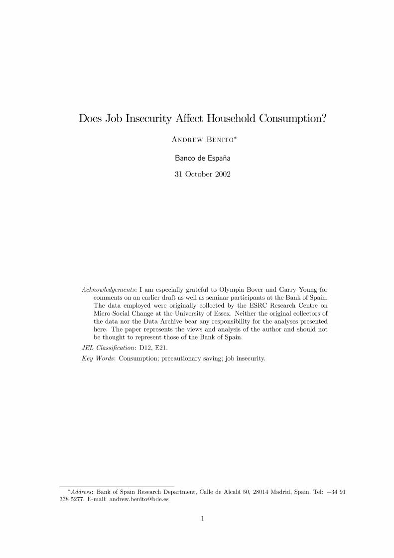
Banco de España Andrew Benito DOES JOB INSECURITY AFFECT HOUSEHOLD CONSUMPTION? Banco de España — Servicio de Estudios Documento de Trabajo n.º 0225
Transcript of Does job insecurity affect household consumption

DOES JOB INSECURITY AFFECT HOUSEHOLD
CONSUMPTION?
Banco de EsDocum
Andrew Benito
Banco de España
paña — Servicio de Estudios ento de Trabajo n.º 0225
Does Job Insecurity Affect Household Consumption?
Andrew Benito∗
Banco de España
31 October 2002
Acknowledgements: I am especially grateful to Olympia Bover and Garry Young forcomments on an earlier draft as well as seminar participants at the Bank of Spain.The data employed were originally collected by the ESRC Research Centre onMicro-Social Change at the University of Essex. Neither the original collectors ofthe data nor the Data Archive bear any responsibility for the analyses presentedhere. The paper represents the views and analysis of the author and should notbe thought to represent those of the Bank of Spain.
JEL Classification: D12, E21.
Key Words: Consumption; precautionary saving; job insecurity.
∗Address : Bank of Spain Research Department, Calle de Alcalá 50, 28014 Madrid, Spain. Tel: +34 91338 5277. E-mail: [email protected]
1

Abstract:
The paper confronts a key implication of the precautionary model of saving/consumption,using micro-data on British households. The results provide support for the key propositionthat job insecurity affects consumption. A one standard deviation increase in unemploymentrisk for the head of household is estimated to reduce consumption by 2.7 per cent. Thiseffect is greater for the young, those without non-labour income and manual workers—forwhom precautionary effects might be expected to be stronger a priori. Consumer durablespurchases are also found to be inversely related to unemployment risk.
2

1 Introduction
The risk of job loss represents a major source of income uncertainty facing most households.
The hypothesis that such uncertainty gives rise to a precautionary motive for saving has been
put forward as a significant development of the standard life-cycle model of consumption
(eg. Carroll (2001), Caballero (1990)). Such models of precautionary saving have many
attractive features. In principle, they appear able to account for a number of stylised
facts associated with consumption patterns and the life-cycle, such as the apparent excess
sensitivity of consumption to anticipated income, that the canonical life-cycle model cannot
explain.1 However, the relatively few attempts that have been made to identify evidence of
a precautionary motive have produced mixed results. Although Carroll et al. (1999) and
Lusardi (1998) find evidence supporting the basic proposition, other studies find little or
no such evidence (eg. Dynan (1993), Starr-McCluer (1996)).
The issue of job insecurity has also attracted increasing attention, particularly in
Britain. This has been partly motivated by the apparently large increases in perceived job
insecurity despite relatively small movements in separation rates (Nickell et al. (2002)). But
what are the effects of job insecurity? Might job insecurity affect consumption behaviour as
implied by the precautionary motive for saving? The issue also has important implications
for the aggregate behaviour of consumption and conditions in the labour market. Carroll
and Dunn (1997) examine the time-series behaviour of US consumption and unemployment
expectations and argue that the latter have played a key role in the cyclical behaviour of
consumers’ expenditure and the US economy.
The present paper confronts a key empirical implication of the precautionary model of
consumption with micro data for British households. Specifically, the hypothesis considered
is whether consumption levels are related to job insecurity.2 As noted above, there have
been relatively few previous attempts to consider this question, none of which use data for
Britain. Closest in spirit to the present paper are the studies by Carroll et al. (1999) and
Lusardi (1998). Carroll et al. (1999) construct individual-level predicted probabilities of job1Pemberton (1997) for instance, calibrates the standard life-cycle model under perfect capital markets
and argues that the results are inconsistent with basic stylised facts of consumption.2The use of the term job insecurity here refers specifically to the likelihood of job loss. Nickell et al.
(2002) discuss other interpretations including wage flexibility.
BANCO DE ESPAÑA/DOCUMENTO DE TRABAJO N.0225 3

loss and include this variable in models for savings finding significant evidence of additional
saving by those households whose head of household faces greater job insecurity. Lusardi
(1998) instead employs a self-reported likelihood of job loss for a sample of men close to
retirement in the United States with results indicating that saving is positively related to the
indicator of job insecurity. The present paper borrows from both approaches, employing
a model-based predicted likelihood of job loss and subjective job insecurity measure for
households in Britain from the British Household Panel Survey and considers a role for
these variables in influencing household-level consumption. The key contribution is to
provide evidence of significant precautionary saving effects associated with unemployment
risk in shaping non-durable consumption for households in Britain for the first time. More
specifically, the estimates imply that a one standard deviation increase in unemployment
risk lowers consumption by 2.7 per cent. This effect is estimated to be stronger among the
young, those without non-labour sources of income and manual workers, as we might be led
to expect a priori. Moreover, a further contribution is to provide evidence that consumer
durables purchases are inversely related to unemployment risk.
The remainder of the paper is organised as follows. Section 2 provides some further
economic and theoretical background to the paper. Section 3 sets up the econometric model
and presents the hypotheses of interest. Section 4 discusses the data and estimation results
derived from the British Household Panel Survey. Section 5 concludes.
2 Economic background
Precautionary saving models extend the standard life-cycle approach to allow for undesirable
(and uninsurable) income uncertainty.3 A result of Caballero (1990) illustrates the role of
uncertainty and precautionary saving most neatly, by assuming the within-period utility
function is exponential. With (constant) coefficient of absolute risk aversion κ, this is
U(ct) = − 1κ exp(−κct), where c is consumption. It is further assumed that income, y,takes the form yt = λyt−1 + (1 − λ)by + εt, where εt ∼ iid(0,σ2), by is the deterministiccomponent of income and λ measures the degree of persistence in income shocks, εt. The
3More specifically, the precautionary motive arises from a positive third derivative of the utility function.
This precludes the case of a quadratic utility function combined with labour income uncertainty, which gives
rise to the standard certainty equivalence result.
BANCO DE ESPAÑA/DOCUMENTO DE TRABAJO N.0225 4

consumer chooses a path for consumption maximising expected intertemporal utility from
consumption subject to the income process and the budget constraint, wt = Rtwt−1+yt−ct.,where wt is end-of-period t wealth and R is the interest factor (1 + r).
Caballero (1990) shows that the solution to this problem is the sum of two com-
ponents. The first component is the certainty equivalence level of consumption, whilst the
second is that associated with the precautionary motive for saving.4 When the income shock
is normally distributed, this latter term simplifies to κσ2/(R− λ) such that precautionary
saving is increasing in the variance of shocks to income, σ2, the degree of persistence of
income shocks, λ, and the degree of risk aversion, κ.5 The level of consumption is decreas-
ing in each of these terms. The assumption of exponential utility is of course, restrictive,
but under more general conditions it can be shown that greater income uncertainty lowers
the optimal level of consumption. Skinner (1988) assumes the one-period utility function
takes the constant relative risk aversion (CRRA) form in place of the constant absolute risk
aversion (CARA) form used by Caballero (1990). Again the result obtains that optimal
consumption is a negative function of income uncertainty. This result is also found using
numerical methods by Zeldes (1989) for the CRRA case. It is the key message from the
literature on precautionary savings and consumption that we wish to confront with data.6
A number of empirical attempts exist at confronting this message from the literature
on the precautionary motive for saving. Carroll et al. (1999) estimate models for the
individual probability of unemployment for a sample of US households, relating saving
behaviour to this variable and find evidence of a significant precautionary effect at modest
and higher levels of income. Guiso et al. (1992) employ Italian household-level survey data
including self-reported earnings uncertainty and also find evidence consistent with the basic4This is when r = δ where δ is the rate of time preference. When r 6= δ, the consumption function
may still be decomposed into two components, one of which relates to precautionary saving but the other
component is not the certainty equivalence level.5Under exponential utility, the coefficient of absolute risk aversion, κ, coincides with the degree of pru-
dence, defined as the ratio of the third to the second derivative of the within-period utility function (Kimball,
1990). One unattractive feature of this function is that it does not rule out negative consumption.6 In models of precautionary saving such as Carroll (1992), it is the probability of a near-zero income that
is the key determinant of the precautionary saving motive. Carroll (1992) suggests that unemployment comes
closest to such an event. This provides a further link between these models and the use of the probability of
job loss as the relevant measure of labour income uncertainty below. Earlier models include Sandmo (1970).
BANCO DE ESPAÑA/DOCUMENTO DE TRABAJO N.0225 5

hypothesis.
For the UK, Miles (1997) and Guariglia and Rossi (2002) find evidence of precaution-
ary motives at work based on constructing estimates of the income risk facing households
and including these in household consumption functions or Euler equation in the case of
Guariglia and Rossi (2002). For the measure of income risk, Miles (1997) uses the squared
residual from an income equation whilst Guariglia and Rossi (2002) employ the variance
of each household’s residual over the three years (or more, depending upon the number
of observations per household and year in question) up to year t. The squared residual
employed by Miles (1997) could pick up any convexity whilst basing a variance measure
on as few as three observations, as in Guariglia and Rossi (2002), (and with the number
of observations varying across households and time) is clearly problematic. Banks et al.
(2001), adopt an approach based on the construction of a cohort-based quasi-panel, which
distinguishes between cohort-specific and common income risks. Their results find strong
evidence of precautionary saving, in particular associated with the cohort-specific income
risk component. This paper instead focuses exclusively on unemployment risk of the house-
hold head as the source of risk facing the household, in part in order to understand the
effects of job insecurity.
The relation between consumer durables purchases and unemployment expectations
is considered by Carroll and Dunn (1997) using aggregate US data. As a basis to their
analysis, they develop an (S,s) model of consumer durables purchasing with a role for income
uncertainty. In this framework an increase in unemployment risk leads to the postponement
of the purchase of consumer durables as households instead opt to add to their precautionary
assets which are used as a buffer-stock. That is, the lower trigger of the (S,s) rule for the
ratio of the value of durable goods to permanent labour income falls. Households instead
wish to accumulate more savings which they use as a buffer against the higher level of
uncertainty resulting from job insecurity.7 In this way, those facing greater job insecurity7The value of consumer durables depreciates over time, whilst permanent income grows over time, such
that the ratio of the value of durables to permanent labour income drifts downwards. When the ratio has
fallen sufficiently, it is optimal to make a purchase. An increase in labour income uncertainty raises the
marginal utility of precautionary assets held as a buffer against uncertainty, such that the durables purchase
decision is delayed. This model is related to, but remains quite different from, the notion that uncertainty
increases the ‘option value’ of waiting.
BANCO DE ESPAÑA/DOCUMENTO DE TRABAJO N.0225 6

should be less likely to have recently purchased household consumer durables, controlling
for other demographic characteristics of the household. This is an additional hypothesis
confronted with data below.
3 Estimation strategy
In order to address the basic hypothesis—that household consumption levels are a function
of job insecurity—there are a number of econometric issues to be confronted. The estimation
strategy is largely geared towards addressing these issues which relate to the construction of
permanent income from cross-sectional data, the grouped nature of the data on consumption
and identification.
The basic model for consumption involves estimating a consumption function of the
following form:
cit = α+ θ1yPit + θ2y
Tit + θ3y
Wit + δbuit +Xitβ + γt + εit (1)
where i indexes individuals (heads of household), i=1,2..N and t indexes waves of the
survey, t=1992...1998. c is log household consumption, yP is permanent labour income, yT
is transitory labour income and yW is investment income.8 bu is the measure of job insecurity.This consists of either the subjectively-perceived degree of job insecurity or a predicted risk
of job loss. Xit represents a vector of regressors with associated parameter vector, β. The
regressor set X includes controls for household and head of household demographics (family
size, composition, educational attainment etc., see Table 3 for more details).9 γt denotes a
set of common year effects with error term, εit.
Permanent Income
The standard definition of permanent income is the annuity value of the sum of
the present discounted value of expected future labour income (ie. human wealth) and
non-human wealth. Following King and Dicks-Mireaux (1982) and Guiso et al. (1992)8The income terms are considered in levels rather than logs since transitory income takes on negative
values. Consumption is considered in logs since in levels its distribution is skewed.9The head of household is defined as the principal owner or renter of the property and (where there is
more than one) the eldest takes precedence.
BANCO DE ESPAÑA/DOCUMENTO DE TRABAJO N.0225 7

permanent labour income yP , is defined as normal (weekly) labour income adjusted for age
and cohort effects. Transitory income yTit , is defined as the difference between current and
permanent labour incomes. Non-human wealth is not measured explicitly here and its role
is captured through the investment income term, yW , as in Miles (1997).10 Note that this
excludes housing wealth.
Permanent income differs from current household income for various reasons and in
particular through life-cycle effects and transitory income differentials. The calculation of
permanent income involves taking the predicted values from a random effects equation for
log household labour income as a function of a range of household demographic variables
and then obtaining a ‘permanent’ value from a projection of this value forwards until re-
tirement (assumed 65 for men, 60 for women) for each household also using estimates of
how household incomes vary with age. Estimates of this differential obtained from cross-
sectional data conflate the age effect with a cohort effect (Shorrocks, 1975) since in any
cross-section older household heads also belong to earlier cohorts, who have lower lifetime
income owing to productivity growth. In order to separate out the cohort- from the age-
effect, separate evidence from Benito (2001) on the magnitude of the age effects is used.
The estimation of the age effects did not restrict the form of the effects, instead using sepa-
rate age dummies in a cohort/age quasi-panel constructed from Family Expenditure Survey
data for the years 1972 to 1998.11 This is clearly much less restrictive than the approach
of Guiso et al. (1992) and Miles (1997) both of which imposed a quadratic relation in age.
Mean (median) weekly permanent income (1995 prices) is calculated as £438.74 (£401.61),
transitory income, £62.15 (£50.97) and investment income £12.26 (£2.20).12
The form of estimating equation is similar to that of Carroll (1994) and Guiso et al.
(1992) who use Italian household data focusing on the impact of a self-reported measure
of earnings uncertainty on consumption. The use of consumption data for the dependent
variable avoids specification issues arising in studies that have employed net worth data
as the dependent variable, in particular where this possesses negative values but a log10Non-human wealth would equal yW /r where r is the instantaneous interest rate.11For a description of pseudo-panel methods, see also Attanasio (1999). The identifying restriction imposed
consisted of assuming that the year effects for the period 1972 to 1998, intended to reflect cyclical factors,
averaged zero. The age and cohort effects on income were unrestricted.12The definition of transitory income does not require that it is mean zero.
BANCO DE ESPAÑA/DOCUMENTO DE TRABAJO N.0225 8

specification seems justified.13 Data for specifically food and groceries expenditures would
not be the preferred measure of consumption. However, as in studies such as Guariglia
and Rossi (2002), Kuehlwein (1991) and Hall and Mishkin (1982), its use can be justified
as an empirically important component of non-durable expenditure and by an assumption
of separability of utility from food and other forms of consumption. Nevertheless, to the
extent that uncertainty leads households to cut back on expenditures and in particular
on those items that are not essentials, the use of food and grocery expenditure as the
dependent variable will bias the results against finding evidence of precautionary saving.
Further analysis below will also consider the relation between consumer durables purchases
and unemployment risk.14
The sole previous attempt to estimate a consumption function of this form on British
or UK data is that by Miles (1997) who employed separate waves of the Family Expenditure
Survey (FES). Miles (1997) estimated an elasticity of consumption with respect to household
permanent income of 0.82 and with respect to transitory income of 0.61. Note that in the
present case the dependent variable consists of a subset of all consumption, namely that
on food and groceries for which an the elasticity with respect to permanent income should
be expected to be well below unity. The discussion of precautionary saving motivates the
consideration of the further hypothesis, Ho: δ = 0 versus HA: δ < 0, under precautionary
saving, which will be the focus of attention here.
Grouped consumption data
The data on consumption are grouped, specifying a particular interval or range for
the level of weekly expenditure on food and groceries.15 Use of grouped data raises par-
ticular estimation issues. To explicitly allow for this, a maximum likelihood method is13King and Dicks-Mireaux (1982) for instance, dropped observations where annual earnings were less than
$2,500. This is likely to introduce a substantial sample selection effect although they do attempt to correct
for it; Carroll et al. (1999) adopt an inverse hyperbolic sine functional form for this reason.14Carroll (1992, p.107) reports results suggesting that aggregate food consumption in the US is as sensitive
to unemployment expectations as total non-durable expenditures. Browning and Crossley (1999) find that
households cut back on ‘small’ durables (eg. clothing) to a greater extent than food during an actual
unemployment spell.15The bands are the following: below £10; £10 to £19; £20 to £29; £30 to £39; £40 to £49; £50 to £59;
£60 to £79; £80 to £99; £100 to £119; £120 to £139; £140 to £159; above £160.
BANCO DE ESPAÑA/DOCUMENTO DE TRABAJO N.0225 9

employed that allows for the fact that the actual level within each band (with one open-
ended category) is unobserved (see Stewart, 1983). A common alternative, that of using
the mid-points to the bands, and then treating the variable as if it were continuous, will
not in general provide consistent parameter estimates. This latter approach is adopted by
Guariglia and Rossi (2002) in estimating Euler equations by GMM using BHPS data. The
grouped dependent variable (GDV) estimator has been used most extensively in studies
of earnings determination where, in British survey data, this has often been grouped into
intervals (eg. Stewart, 1990).16
This paper employs two approaches to consider the hypothesis δ = 0. These ap-
proaches differ in their construction of the unemployment expectations or job insecurity
term, bu. The first approach takes head of household responses to a question in the BHPS ofall employed individuals concerning the likelihood that they will become unemployed in the
next twelve months (see below for further details). This is straightforward to implement.
The second approach estimates the individual probability of becoming unemployed in twelve
months for the sample of employed heads of households. This is derived as the predicted
probability from a probit model:
uit = 1{Zit$ + υit > 0} (2)
where 1{A} is an indicator function of the event A such that uit = 1 if the individualbecomes unemployed at the time of the subsequent BHPS interview and zero otherwise.
The set of regressors, Zit includes a set of regional and year dummies to control for regional
and aggregate effects as well as the other individual and household characteristics contained
in Xit in (1). Under the probit assumption, υit ∼ N(0,σ2u), the predicted probabilities arethen calculated as Φ(Zit b$) where Φ(·) is the standard normal distribution function andb$ are the maximum likelihood probit estimates of (2). The potential advantage of this
approach compared to the self-reported response to the job insecurity question is that in
being based on a continuous variable, the predicted probabilities provide more variation in16Note that the grouping of data in bands is not necessarily a weakness of the data. For example, in the
1991 wave of the BHPS, the food consumption data were not grouped but show clear evidence of rounding
(at £5 and £10 intervals). Rather than taking such data at face value, in the presence of such rounding it
is preferable to treat the data as if it were grouped and to employ the GDV estimator.
BANCO DE ESPAÑA/DOCUMENTO DE TRABAJO N.0225 BANCO DE ESPAÑA/DOCUMENTO DE TRABAJO N.0223 10BANCO DE ESPAÑA/DOCUMENTO DE TRABAJO N.0223 3 BANCO DE ESPAÑA/DOCUMENTO DE TRABAJO N.0223 3

job insecurity levels which can be exploited to identify the relationship between consumption
and job insecurity. The complication it introduces is that associated with identification.
Identification
For the model to be identified, exclusion restrictions on the consumption equation
are required. This requires the isolation of at least one variable that influences income and
job loss risk directly but does not affect consumption independent of the effects through
income and/or risk of job loss. These exclusion restrictions are then the instruments for
the respective income and job insecurity terms. This paper claims to pay special attention
to this identification problem. By comparison, this issue is not discussed by Guiso et al.
(1992). Moreover, inspecting their income and consumption equations indicates that no
exclusion restrictions are imposed on the latter. This makes interpretation of their results
difficult.
A number of alternative instrument sets will be considered below. The choice of
exclusion restrictions needs to be justified on a priori grounds. On such grounds, the
favoured instrument set for both income and job loss risk consists of the experience of
unemployment in the previous year, the size of the household head’s employer and his/her
union status, although alternatives and sensitivities will be considered. The rationale for
these is as follows. There is a significant body of evidence suggesting that unemployment
experience has ‘scarring’ effects on subsequent employment and re-employment earnings (eg.
Arulampalam et al. 2000, 2001). This leads us to expect significant effects from experience
of unemployment in the previous year on the probability of job loss and household income.
These hypotheses are confirmed in the analysis below. Since the favoured interpretation
of this result is that unemployment adversely affects human capital, then there seems no
reason a priori why this should be correlated with consumption behaviour independent of
its effect on human capital and thereby on job insecurity and income.
A second favoured candidate for a valid instrument is that of employer (workplace)
size. The earnings differential by workplace size is a key wage differential in the labour
market and is quantitatively large (eg. Green et al. 1999). A favoured interpretation of this
differential is one of reflecting (dynamic) monopsony associated with labour turnover costs
such that larger employers bid up wage rates. There seems no reason why the resulting
BANCO DE ESPAÑA/DOCUMENTO DE TRABAJO N.0225 11

differential should be related to consumption behaviour. In terms of the risk of job loss
equation, it may also be the case that jobs at larger establishments are more secure, due to
larger employers possessing greater market power or that for a given employer the closure
of smaller establishments incurs lower re-organisation costs. Again, it seems unlikely that
this characteristic should be related to consumption independent of any effect via income
or job insecurity.
Union status is also considered as a zero restriction in the consumption equations.
Unions raise earnings, with this differential being associated with coverage and individual
membership. Owing to the emphasis unions impose on due process they are also likely to
improve job security. This leads us to expect a role for union status in both the income and
job security equations. Again it seems highly unlikely that these characteristics should be
related to consumption independent of the effects through household income and/or risk of
job loss. A number of other candidates for valid instruments are also available and several
of these are considered below. These include region, which was employed by Carroll et
al. (1999) as the instrument for job loss and income in their analysis. Another possibility
is being on a temporary contract which is significantly related with the probability of job
loss. Nevertheless, willingness to accept a job with a temporary contract may be related to
attitudes to risk which could thereby imply a relationship with consumption. Miles (1997)
uses sex of the household head, education, region and occupation; their a priori justification
is slightly more questionable with the strongest case for exclusion from consumption being
with region of residence. In the light of this discussion, the preferred instrument set consists
of past unemployment experience, employer size and union presence.17 As well as these
terms, job loss risk from the probit model is also identified through the non-linear functional
form of the probit model.17Occupation is another possible instrument for job loss risk that has been used in the literature (eg.
Skinner, 1988). The difficulty here is that occupational choice may be a function of attitudes to risk,
rendering the resulting estimates based on excluding the occupation terms from the consumption function,
inconsistent. In a similar vein, education is likely to be correlated with individuals’ rates of time preference.
BANCO DE ESPAÑA/DOCUMENTO DE TRABAJO N.0225 12

4 Data and Estimation Results
4.1 Data description
The overwhelming majority of studies of consumption over the life-cycle and in particular
the limited number of studies that investigate the precautionary motive, have been con-
ducted using data for the United States. This paper instead employs a British data source,
the British Household Panel Survey (BHPS). The BHPS consists of an annual panel-based
survey of approximately 5,500 households in Britain beginning in 1991. The dataset provides
detailed information on employment, education, income and demographic characteristics of
households but also contains some information on consumption. The paper employs data
from the BHPS for the years 1992 to 1998.18 Since the key variable of interest concerning
self-reported job insecurity was only asked of respondents in waves 6 and 7 of the survey,
the data employed for the specifications using self-reported job insecurity are restricted to
those two cross-sections of data. The specifications that employ the estimated probability
of job loss do not require this restriction.
In the BHPS, each household is asked how much (approximately) the household
spends each week on food and groceries. Responses to the consumption question were
banded into 12 intervals (at source), giving rise to the use of the grouped dependent vari-
able estimator referred to in Section 3.
For self-reported unemployment expectations, in waves 6 and 7 of the survey each
employed individual is asked:
“In the next twelve months, how likely do you think it is that you will becomeunemployed?”
Responses fall into one of four categories, ‘very likely’ (3.0 percent), ‘likely’ (6.9
percent), ‘unlikely’ (50.7 percent) and ‘very unlikely’ (39.4 percent). In view of the small
proportion that respond in the ‘very likely’ group, for subsequent analysis this is merged
with the ‘likely’ response thereby forming a ‘likely or very likely’ group.18The survey question concerning consumption was slightly different in 1991 so this year is omitted from
the analysis.
BANCO DE ESPAÑA/DOCUMENTO DE TRABAJO N.0225 13

The sample of households is selected on the basis of being employed, heads of house-
hold aged between 21 and 65 and providing the necessary information for each of the vari-
ables used in the analysis. This produces a sample of 10,557 heads of household available
for the main analysis of household consumption functions.
4.2 Estimation results
Before examining the consumption functions, the models for unemployment risk are first
considered. The specifications reported differ in their definition of the job insecurity term—
whether this is the self-reported measure or the estimated risk of job loss.
4.2.1 Job insecurity
What factors are correlated with job insecurity or the perceived probability of job loss? Ta-
ble 1 presents probit estimates for the propensity for individuals’ self-reported job insecurity
based on likely or very likely versus unlikely or very unlikely unemployment responses for
12 months hence.
The results accord with standard economic priors. Individuals on temporary or sea-
sonal contracts, those with exp erience of unemployment i n the previous year, those with
poor health, all have a higher propensity for job insecurity, controlling for the other charac-
teristics, whilst the degree-educated have a significantly lower probability of job insecurity.
By tenure, those with 1-2 years have higher levels of job insecurity than those with longer
tenure. The marginal effects reported for the probit model indicate that the variables with
the strongest relationship to job insecurity are being on a temporary contract, being in
poor health and having experienced unemployment over the previous year. Being on a
temporary contract increases the probability of feeling insecure about one’s job over the
subsequent year by 0.24; poor health increases this probability of job insecurity by 0.12
and a recent spell of unemployment by 0.10. By comparison, having a degree qualification
(relative to having no formal qualifications) is associated with a reduction in the probability
of experiencing job insecurity by 0.04.
The results for the unemployment risk models—that is of the probability of becoming
unemployed in one year, from our sample of employed heads of household—are reported
in Table 2. Unemployment risk is considerably higher amongst those who have previous
BANCO DE ESPAÑA/DOCUMENTO DE TRABAJO N.0225 14

experience of unemployment, controlling for other characteristics and those on temporary
contracts. The marginal effect of a spell of unemployment in the previous year is an increase
in the probability of becoming unemployed of 0.02 (‘t-ratio’=3.98), whilst being on a
temporary contract has a marginal effect of 0.033 (‘t-ratio’=5.23). Given that the raw
probability of entering unemployment is 0.023, these are large effects. Larger employers tend
to be associated with greater job security, although the marginal effects are non-linear. The
employer size variables are jointly significant (χ2(7) = 25.47, p-value=0.00). Unemployment
risk is significantly lower among the degree-educated, with a degree being associated with a
decline in the probability of entering unemployment of 0.01 (‘t-ratio’=-2.42) relative to the
case of no-qualifications. Union presence in the form of union recognition but not individual
union membership is also significantly and inversely related to the propensity to entering
unemployment, and also has a marginal effect close to -0.01. Higher levels of tenure are also
associated with lower unemployment risk. The pattern of results is highly plausible. Note
also that the predicted probability of becoming unemployed is increasing in the self-reported
job insecurity measure. The mean predicted probabilities by subjective chance of becoming
unemployed are 0.0137 (“very unlikely”), 0.0153 (“unlikely”) and 0.0285 (“likely or very
likely”).
4.2.2 Consumption
The main estimation results for the consumption functions are presented in Table 3. Follow-
ing equation (1), household consumption is considered as a function of permanent, transitory
and investment incomes, job insecurity and a set of controls.
Column 1 presents results for the specification which considers the job insecurity
variable as the self-reported measure. A standard set of controls is employed, in particular
through the inclusion of terms for educational attainment, number of household members
in employment, family size and composition. These terms attract plausible coefficients.
Household consumption is increasing in the number of children in the household and the
number of employed adults.
The results in column 1 do not reject the null hypothesis δ = 0, that job insecurity
has no influence on household consumption, contrary to the precautionary saving model.
The coefficient (standard error) on the job insecurity term is -0.012 (0.024). Employing a
BANCO DE ESPAÑA/DOCUMENTO DE TRABAJO N.0225 15

slightly modified definition of self-reported job insecurity that distinguishes between three
different responses in terms of the level of job insecurity does not alter this result. Although
negatively signed, the results fail to indicate that job insecurity depresses consumption
significantly.
As emphasised above, the limited degree of variation in the categorical variable for
self-reported job insecurity may mitigate against finding a significant relation between this
variable and consumption. Recall that less than 10 per cent of the sample reports that be-
coming unemployed is either likely or very likely. Since there will be degrees of job insecurity
a case can be made for attempting to exploit such variation as a basis to the estimation.
This motivates the use of the probit model for the predicted risk of becoming unemployed
for our sample of employed heads of household. That there is significant variation across
the sample in the predicted risk of becoming unemployment is therefore important. The co-
efficient of variation for this variable exceeds one (standard deviation, 0.028; mean, 0.025).
The latter approach also means that the analysis is no longer restricted to the 1996 and
1997 waves of the survey that contained the self-reported job insecurity question.
Column 2 reports results for the benchmark case where zero restrictions are imposed
on the unemployment experience in the previous year, employer size and union status terms.
Note that these instruments are jointly significant in the income equation (reported in the
Appendix) and in the unemployment risk equation (Table 2). The coefficient (standard er-
ror), multiplied by 1000, on permanent income is 0.418 (0.027) and compares to 0.112 (0.017)
on transitory income and 0.391 (0.100) on investment income. A test of the equality of the
permanent and transitory labour income coefficients easily rejects the null, χ2(1) = 85.63
(p-value=0.00). The estimate of θ1 corresponds to an elasticity of food consumption with
respect to permanent income of 0.18, evaluated at mean permanent income. Recall that
these estimates compare to permanent and transitory income elasticities of total consump-
tion estimated by Miles (1997) of 0.82 and 0.61, respectively. The lower elasticities here
likely reflect the fact that the measure of consumption, of necessity, is restricted to food and
grocery expenditures which are likely to be less income elastic than other categories of con-
sumption. The results generally do not suggest a different responsiveness of consumption
to permanent and investment incomes.
Crucially, the unemployment risk term is now significantly negative, attracting a
BANCO DE ESPAÑA/DOCUMENTO DE TRABAJO N.0225 16

‘t-ratio’ of -4.41, supporting the key hypothesis associated with the precautionary saving
approach.19 This is the first finding of its kind for British data. For a one standard deviation
increase in unemployment risk, this estimate implies that consumption declines by 2.7 per
cent. This compares to an estimate obtained by Carroll (1994) that a one standard deviation
increase in predicted future income uncertainty reduces consumption by around 3 per cent,
although in several of Carroll’s (1994) specifications this was not statistically significant.
Columns 3 to 5 consider various alternative specifications of the instrument set in order to
consider the robustness of the results. These results are also favourable to the precautionary
saving hypothesis that unemployment risk depresses consumption at the micro-level as well
as further supporting the hypothesis that consumption responds more strongly to permanent
income than to transitory income. The results also indicate a role for demographic factors
associated with the size and composition of the household, consistent with results obtained
by Miles (1997).
A further hypothesis considered is that theory might suggest that the effect of unem-
ployment uncertainty should be non-linear. Thus income uncertainty, that is the variance of
income associated with unemployment risk, would in principle be given by p(1−p)(1−R)2Y 2,where p is the predicted probability of job loss, R is the replacement ratio in the event of un-
employment and Y is current earnings of the household head. In effect, income uncertainty
should be at its peak when the probability of job loss is 0.5 since as the likelihood of job
loss approaches 1 it becomes more certain that future income will be RY .20 Since R is not
known, the income risk term considered in column 6 assumes it is zero, defining income risk
as bσ2 = p(1− p)Y 2 thereby attempting to pick up the notion that income at risk is greaterfor those with higher current earnings, ceteris paribus. This term is far from significant
however such that the attempt at isolating a role for job insecurity is more successful than
the attempt at constructing a proxy for income risk. The remainder of the paper focuses
on the specific question of the role of job insecurity.
One possible alternative interpretation of the estmated unemployment risk effect mer-
its discussion. The estimate of permanent income does not allow for the fact that an unem-19The standard errors are not adjusted for the presence of a generated regressor (Pagan, 1984). As in
Miles (1997), it is unlikely that this would render the key terms insignificant.20 In practice, none of the sample have a predicted probability at this level, with the maximum predicted
probability of job loss over the next year in the sample being 0.371.
BANCO DE ESPAÑA/DOCUMENTO DE TRABAJO N.0225 17

ployment spell will have an effect on permanent income. This point, which applies equally
to previous studies, implies that the estimated unemployment risk effect could be picking
up a permanent income effect. The response to this however is that the estimated job
insecurity effect appears much too large to be accounted for by an implied reduction in
permanent income. Taking an estimated food elasticity with respect to permanent income
of 0.18, moving from someone with zero unemployment spells to someone who spent only
2.8 per cent of their time unemployed would need to imply a reduction in permanent income
of 15 per cent (ie. 0.027/0.18) to account for the estimated reduction in consumption. More
plausible estimates of the likely effect on permanent income suggest that this could account
for around one-fifth of the estimated effect associated with unemployment risk.
Three further experiments are now considered. The first examines whether there is
any variation in the precautionary motive by age. In a precautionary saving model, it is
likely that unemployment risk should have a greater effect for the young than the old. This
point is made by Miles (1997, p.12), who suggests that income uncertainty is probably not
independent of the number of periods lying ahead. As individuals age they accumulate
liquid assets which in part act as a buffer to unemployment and their consumption should
therefore be less sensitive to unemployment risk The framework of Carroll (1994, p.140)
maintains that “young and middle-aged households are trying to build up a buffer stock,
but by the time they have reached their peak earning years, 45-54, they have achieved a large
enough buffer and so do not need to continue depressing consumption to continue building
up the stock further.” This hypothesis is considered here by interacting the unemployment
risk term with the age of the household head. The results, also presented in Table 4, provide
strong evidence in support of such an effect. The interaction term attracts a significantly
positive coefficient, (with a ‘t-ratio’ of around 4.2) indicating that the negative effect of
unemployment risk upon consumption weakens with age. The estimates imply that at age
25 a one standard deviation increase in unemployment risk reduces consumption by 5.2 per
cent whilst at age 60, the effect is zero.
A second hypothesis is that individuals may respond to unemployment risk differently
according to how dependent they are on earnings as a source of income. In particular,
household consumption could be less sensitive to unemployment risk where households
BANCO DE ESPAÑA/DOCUMENTO DE TRABAJO N.0225 18

have other sources of income in addition to labour income. This possibility was noted by
Zeldes (1989) and Miles (1997) and is considered in Table 4, through the addition of an
interaction between the unemployment risk term and a dummy for whether the household
reports having positive investment income—72.7 per cent of households indicate that this
is the case. The results provide support for this hypothesis as the interaction term is
positively signed and statistically significant. The negative impact of unemployment risk
on households’ consumption is muted where households possess other sources of income. For
those without investment income, the one standard deviation increase in unemployment risk
lowers household consumption by 4.2 per cent. Note also that the point estimate on the
interaction term, at 0.969, is less in absolute terms that the coefficient on the unemployment
risk term, -1.514, suggesting that a consumption effect from unemployment risk is not
removed entirely by the possession of some investment income. Given the scale of most
households’ investment incomes this is not surprising.21
A final possibility is to consider whether the scale of the estimated effect from unem-
ployment risk is greater for households for whom the impact on household finances of an
unemployment spell may be greater. The expected duration of any unemployment spell and
the wage at which re-employment occurs will be key factors in determining this expected
cost of job loss. These factors can be thought of as increasing the value of λ, that is the
persistence of an income shock (such as unemployment), in section 2. As an, albeit some-
what crude, attempt to pick up any tendency for such effects, the impact of job insecurity is
estimated separately for manual and non-manual employees. The economic intuition here
leads us to expect that the precautionary motive should be stronger for manual workers,
partly since unemployment durations are typically longer for manual workers. The coeffi-
cient (standard error) on the unemployment risk term for manual workers is -1.154 (0.301),
whilst for non-manual workers it is at the margin of significance with a coefficient (standard
error) of -0.670 (0.342). The point estimate for the unemployment risk term for manual
workers implies that a one standard deviation increase in unemployment risk, reduces con-
sumption by 3.2 per cent, whilst that for non-manual workers implies a 1.9 per cent fall in21 In a similar vein, the possibility that multiple earner households’ consumption might be less sensitive
to the unemployment risk of the household head was considered. No evidence for such variation was found
however.
BANCO DE ESPAÑA/DOCUMENTO DE TRABAJO N.0225 19

consumption. Job insecurity has a stronger effect on the consumption behaviour of certain
workers for whom the costs of job loss might be expected to be greater.
Durables purchases
The relation between durables expenditures and job insecurity is now considered.
Indeed, it may be the case that unemployment risk is more likely to cause households to
cut back or delay durables purchases than non-durables consumption, particularly food
consumption, the case considered above. As noted above, the model of Carroll and Dunn
(1997) of consumer durables purchases has this key implication, that greater labour income
uncertainty delays the purchase of durables, as it is optimal for households to add further
to their precautionary assets. Carroll and Dunn (1997) examine aggregate data on durables
purchases and unemployment expectations in the US and their results lend support to
this implication. They recommend however, that a household-level probit model be run
regressing durables purchases on job insecurity data.
Data on durables expenditures at the micro-level are limited but available data from
the BHPS justify such an exercise. The BHPS includes information on whether the house-
hold has purchased nine listed consumer durables in the past year.22 The procedure em-
ployed here is to consider the propensity for a household to have purchased any of these
consumer durables in the previous year as a function of the job insecurity of the household
head, according to both the self-reported and estimated unemployment risk, and the full
set of household- and individual-level controls. This is estimated as a probit model with
the results presented in Table 4.
The probability of having recently purchased consumer durables for the household
varies inversely with job insecurity. This provides empirical support for the notion that
unemployment risk delays consumer durables purchases. Employing the model-based pre-
dicted risk of unemployment, the term is on the margin of significance. For the durables
purchase probits, the results using the self-reported measure of job insecurity indicate a
stronger role for unemployment expectations, as the term attracts a coefficient (standard
error) of -0.182 (0.081). The marginal effect implies that reporting some level of job inse-22The consumer durables are the following: colour TV, VCR, freezer, washing machine, tumble dryer,
dish washer, microwave, home computer and CD player. The proportion of households that undertake any
such purchase in the previous year is 0.465.
BANCO DE ESPAÑA/DOCUMENTO DE TRABAJO N.0225 20

curity is associated with a 0.07 lower probability of having recently purchased a consumer
durable. Relative to an overall proportion of households that report any consumer durable
purchase in the past year of 0.465, this is by no means a small effect.
5 Conclusions
This paper has confronted several implications of the precautionary model of consump-
tion/saving with micro data on British households for the first time. By relating consump-
tion to job insecurity, controlling for other characteristics including estimated permanent
income, evidence in favour of a precautionary motive for saving associated with unemploy-
ment risk has been found. The analysis can also be considered an attempt to examine some
of the effects of job insecurity, a phenomenon which has attracted significant interest in
Britain (eg. Nickell et al. 2002). Despite the large literature that has developed assessing
job insecurity in the British labour market, there has been little if any attempt to con-
sider how job insecurity might affect household decision-making. This paper has considered
household consumption as a potential such case, at the same time assessing the empirical
merit of a central implication of the precautionary model of saving.
As a test of the precautionary model of saving the approach adopted here, through the
use of estimated and self-reported unemployment risk, is preferable over other attempts that
have attempted to define income uncertainty on the basis of the variability in income over
a (very) limited number of years or through an additional non-linearity in the relationship
between consumption and income. Unemployment risk is likely to represent the dominant
form of income uncertainty to households of working age, is less likely to be due to voluntary
(and anticipated) changes in behaviour and can arguably be more reliably measured than
previous measures of income risk.
The results have been broadly favourable to the key implication of precautionary sav-
ing, namely that greater unemployment risk should depress levels of household consumption.
This result was found in the models that constructed a predicted probability of becoming
unemployed for a sample of employed heads of household. Across the sample as a whole,
the estimates implied that a one standard deviation increase in unemployment risk lowers
household (food) consumption by 2.7 per cent. This represents an appreciable impact. It
BANCO DE ESPAÑA/DOCUMENTO DE TRABAJO N.0225 21

was also found that the unemployment risk effect is stronger for the young as implied by
a buffer-stock model of saving such as Carroll (1994) where individuals accumulate assets
earlier in their working life as a precautionary buffer to income shocks. At age 25, a one
standard deviation increase in unemployment risk is estimated to reduce consumption by
5.2 per cent whilst by age 60, the effect is zero. Those that are more reliant upon labour
income, that is do not have investment income are also found to be more sensitive in terms
of their consumption to unemployment risk as we would expect. For those without invest-
ment income, the one standard deviation increase in unemployment risk lowers household
consumption by 4.2 per cent. Further, variation by occupational group was also consid-
ered. The consumption of manual workers, for whom the persistence of a shock to income
induced by unemployment is likely to be greater given typically longer unemployment du-
rations, were found to be more sensitive to job insecurity.
The paper has also explored the relation between consumer durables purchases and job
insecurity. In so doing the analysis has responded to Carroll and Dunn’s (1997) concluding
recommendation for future research. The probability of the household having recently
purchased consumer durables varied inversely with job insecurity of the household head.
This provides empirical support for the notion that unemployment risk causes households
to delay consumer durables purchases as in the model of Carroll and Dunn (1997). In this
model, an increase in labour income uncertainty such as that originating from greater job
insecurity leads households to delay purchase of consumer durables as households instead
opt to add to their precautionary assets which are used as a buffer against the higher level
of uncertainty. In the estimates presented here, use of the self-reported measure of job
insecurity implied that some degree of job insecurity was associated with a reduction in the
probability of having recently purchased a consumer durable of 0.07—by no means a small
effect.
For the UK, the most persuasive prior evidence of precautionary saving is that of
Banks et al. (2001), who adopt an approach based on the construction of a cohort-defined
quasi-panel, which distinguishes between cohort-specific and common income risks. Their
results find strong evidence of precautionary saving, in particular associated with the cohort-
specific income risk component. This paper has instead focused specifically on unemploy-
ment risk as a potentially major source of disruption to income and in order to consider the
BANCO DE ESPAÑA/DOCUMENTO DE TRABAJO N.0225 22

possible effects of job insecurity. Banks et al. (2001) suggest that income uncertainty was
increasing through much of the 1980s and early 1990s in the UK. Unemployment risk, at
least since the early 1990s, has likely been falling. This may point to other sources of income
risk as increasing in importance. Future research might therefore consider these other forms
of income uncertainty, such as wage flexibility, which may have increased in importance in
the British labour market, as well as in Spain, in giving rise to a precautionary motive for
saving.
BANCO DE ESPAÑA/DOCUMENTO DE TRABAJO N.0225 23

Table 1: Self-reported Job Insecuritycoefficient (standard error) marginal effect
Education (highest qualification)Degree -0.292 (0.132) -0.038Other Higher QF -0.170 (0.102) -0.024A-levels -0.087 (0.119) -0.012O-levels or equivalent -0.176 (0.105) -0.024CSEs, commercial QF or other 0.008 (0.121) 0.001unemployed in previous year 0.467 (0.123) 0.099temporary contract 0.977 (0.108) 0.244aged 30 to 39 0.181 (0.104) 0.028aged 40 to 49 0.410 (0.102) 0.070aged 50 or more 0.449 (0.107) 0.080poor health 0.581 (0.115) 0.122covered union member 0.065 (0.073) 0.010covered non-union member 0.054 (0.084) 0.008married -0.027 (0.092) -0.004white -0.279 (0.156) -0.050male -0.008 (0.091) -0.001tenure: 7-12 months 0.062 (0.117) 0.010tenure: 1-2 years 0.217 (0.105) 0.036tenure: 2-4 years 0.206 (0.103) 0.033tenure: 4 years or more 0.046 (0.096) 0.007workplace size:10 to 24 employees -0.118 (0.108) -0.01625 to 49 employees 0.007 (0.107) 0.00150 to 99 employees -0.146 (0.115) -0.020100 to 199 employees -0.033 (0.113) -0.005200 to 499 employees 0.043 (0.102) 0.007500 to 999 employees -0.167 (0.132) -0.0231000 or more employees -0.125 (0.114) -0.017occupation dummies yes (8)region dummies yes (18)wave dummy yes
log-likelihood -1211.229pseudo R-squared 0.098observations 4,211
Note: Table reports maximum likelihood probit estimates for self-reported job inse-curity. Standard errors corrected for multiple observations in parentheses. The referencegroups are no qualifications; aged 21-29; 1-6 months’ tenure with a workplace size of 1-9employees; Other higher QF refers to teaching, nursing or other higher qualifications.
BANCO DE ESPAÑA/DOCUMENTO DE TRABAJO N.0225 24

Table 2: Unemployment Riskcoefficient (standard error) marginal effect
Education (highest qualification)Degree -0.292 (0.121) -0.009Other Higher QF -0.129 (0.086) -0.005A-levels 0.096 (0.095) 0.004O-levels or equivalent -0.043 (0.086) -0.002CSEs, commercial QF or other 0.015 (0.097) 0.001unemployed in previous year 0.380 (0.095) 0.022temporary contract 0.503 (0.096) 0.033covered union member -0.198 (0.062) -0.007covered non-union member -0.288 (0.082) -0.009aged 30 to 39 -0.022 (0.076) -0.001aged 40 to 49 0.076 (0.080) 0.003aged 50 or more 0.224 (0.086) 0.010poor health 0.218 (0.115) 0.011married -0.194 (0.080) -0.009white -0.170 (0.132) -0.008male 0.092 (0.079) 0.003tenure:7-12 months 0.001 (0.091) 0.0001-2 years -0.081 (0.092) -0.0032-4 years -0.103 (0.088) -0.0044 years or more -0.277 (0.082) -0.011workplace size:10 to 24 employees -0.258 (0.086) -0.00825 to 49 employees -0.178 (0.090) -0.00650 to 99 employees -0.239 (0.099) -0.008100 to 199 employees -0.034 (0.088) -0.001200 to 499 employees -0.377 (0.092) -0.012500 to 999 employees -0.284 (0.115) -0.0091000 or more employees -0.250 (0.110) -0.008occupation dummies yes (8)region dummies yes (17)wave dummies yes (6)
log-likelihood -1320.979pseudo R-squared 0.098observations 13,288
Notes: Table reports maximum likelihood probit estimates for risk of job loss. Stan-dard errors in parentheses.
BANCO DE ESPAÑA/DOCUMENTO DE TRABAJO N.0225 25
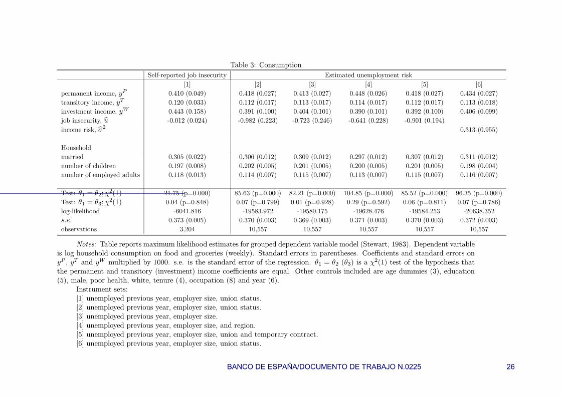
Table 3: ConsumptionSelf-reported job insecurity Estimated unemployment risk
[1] [2] [3] [4] [5] [6]permanent income, yP 0.410 (0.049) 0.418 (0.027) 0.413 (0.027) 0.448 (0.026) 0.418 (0.027) 0.434 (0.027)transitory income, yT 0.120 (0.033) 0.112 (0.017) 0.113 (0.017) 0.114 (0.017) 0.112 (0.017) 0.113 (0.018)investment income, yW 0.443 (0.158) 0.391 (0.100) 0.404 (0.101) 0.390 (0.101) 0.392 (0.100) 0.406 (0.099)job insecurity, bu -0.012 (0.024) -0.982 (0.223) -0.723 (0.246) -0.641 (0.228) -0.901 (0.194)income risk, bσ2 0.313 (0.955)
Householdmarried 0.305 (0.022) 0.306 (0.012) 0.309 (0.012) 0.297 (0.012) 0.307 (0.012) 0.311 (0.012)number of children 0.197 (0.008) 0.202 (0.005) 0.201 (0.005) 0.200 (0.005) 0.201 (0.005) 0.198 (0.004)number of employed adults 0.118 (0.013) 0.114 (0.007) 0.115 (0.007) 0.113 (0.007) 0.115 (0.007) 0.116 (0.007)
Test: θ1 = θ2;χ2(1) 21.75 (p=0.000) 85.63 (p=0.000) 82.21 (p=0.000) 104.85 (p=0.000) 85.52 (p=0.000) 96.35 (p=0.000)
Test: θ1 = θ3;χ2(1) 0.04 (p=0.848) 0.07 (p=0.799) 0.01 (p=0.928) 0.29 (p=0.592) 0.06 (p=0.811) 0.07 (p=0.786)
log-likelihood -6041.816 -19583.972 -19580.175 -19628.476 -19584.253 -20638.352s.e. 0.373 (0.005) 0.370 (0.003) 0.369 (0.003) 0.371 (0.003) 0.370 (0.003) 0.372 (0.003)observations 3,204 10,557 10,557 10,557 10,557 10,557
Notes: Table reports maximum likelihood estimates for grouped dependent variable model (Stewart, 1983). Dependent variableis log household consumption on food and groceries (weekly). Standard errors in parentheses. Coefficients and standard errors onyP , yT and yW multiplied by 1000. s.e. is the standard error of the regression. θ1 = θ2 (θ3) is a χ2(1) test of the hypothesis thatthe permanent and transitory (investment) income coefficients are equal. Other controls included are age dummies (3), education(5), male, poor health, white, tenure (4), occupation (8) and year (6).
Instrument sets:[1] unemployed previous year, employer size, union status.[2] unemployed previous year, employer size, union status.[3] unemployed previous year, employer size.[4] unemployed previous year, employer size, and region.[5] unemployed previous year, employer size, union and temporary contract.[6] unemployed previous year, employer size, union status.
BANCO DE ESPAÑA/DOCUMENTO DE TRABAJO N.0225 26

Table 4: Further ExperimentsConsumption Pr(any durables purchase in previous year)
Age interaction Investment income Manual Non-manual Self-reported bu Model-based bupermanent income, yP 0.420 (0.026) 0.413 (0.027) 0.479 (0.051) 0.410 (0.030) 0.226 (0.164) 0.289 (0.085)transitory income, yT 0.112 (0.017) 0.112 (0.017) 0.390 (0.050) 0.083 (0.019) 0.292 (0.124) 0.110 (0.054)investment income, yW 0.385 (0.100) 0.355 (0.101) 0.038 (0.278) 0.442 (0.110) -0.406 (0.546) -0.000 (0.321)job insecurity, bu -3.243 (0.586) -1.514 (0.257) -1.154 (0.301) -0.670 (0.342) -0.182 (0.081) -1.333 (0.687)job insecurity X age 0.055 (0.013)job insecurity X (yW > 0) 0.969 (0.234)
Test: θ1 = θ2;χ2(1) 87.35 (p=0.000) 83.20 (p=0.000) 1.56 (p=0.212) 69.97 (p=0.00) 0.09 (p=0.762) 2.89 (p=0.090)
Test: θ1 = θ3;χ2(1) 0.11 (p=0.744) 0.30 (p=0.586) 2.34 (p=0.126) 0.07 (p=0.788) 1.15 (p=0.283) 0.76 (p=0.384)
log-likelihood -19575.271 -19575.43 -7772.664 -11725.44 -2116.443 -7939.840s.e. 0.369 (0.003) 0.369 (0.003) 0.347 (0.004) 0.381 (0.004) - -observations 10,557 10,557 4,297 6,260 3,203 11,775
Notes: Consumption equations are maximum likelihood estimates as in Table 3. See notes to Table 3. All consumptionequations use predicted unemployment risk as the measure of job insecurity. Instruments are unemployed previous year, employersize dummies and union status.
Any durables purchase refers to the purchase of consumer durables in the previous year, estimated as a probit model.
BANCO DE ESPAÑA/DOCUMENTO DE TRABAJO N.0225 27

Data Appendix
The data are derived from the British Household Panel Survey, obtained through theData Archive at the University of Essex. Full details of the survey design are available fromTaylor et al. (1999). This Data Appendix describes the construction of the some of thekey variables and provides summary statistics. Labels referred to in square parentheses [.]below are the original BHPS variable names (where ‘W’ varies according to the wave of thesurvey).
Variable Construction
ConsumptionThe 12-way categorical response is derived from household-level responses to the
following question, “Tell me approximately how much your household spends each week onfood and groceries?” [Wxpfood]
Current incomeHousehold income in month prior to survey [Wfihhmn]. Imputed values [Wfihhmni=1]
on this variable are omitted from the analysis. Converted to weekly equivalent values anddeflated using the GDP deflator.
Permanent IncomeThe construction of the measure of permanent income takes as its starting point a
regression for current household labour income on observable characteristics, Zit. Definingthe age- and cohort-effects as π(α)i and φ(c)i , respectively gives the following cross-sectionalequation for log current household income, yit:
yit = Zitϕ+ π(α)i + φ(c)i + υit (3)
The cohort effects φ(c)i cannot be separately identified from the age effects π(α)i incross-sectional data. External estimates of the age effects from Benito (2001) are thereforeemployed to produce cohort-adjusted estimates of the age effects on current householdincome, bπ(α)i.The error term, υit in (3) consists of an unobserved (permanent) heterogeneitycomponent, vi and transitory income component, ²it
υit = vi + ²it.
The income equation (3) is therefore estimated as a random effects model allowing forthe unobserved heterogeneity through the random effects error component, vi.As in Guisoet al. (1992), under the assumption that the interest rate equals the rate of productivitygrowth, permanent labour income is then calculated as
yPit =¡TR − αi
¢−1 TRXα=αi
(Zitbϕ+ bπ(α)i + vi)where TR is retirement age (assumed 65 for men and 60 for women) and α is current
age.
BANCO DE ESPAÑA/DOCUMENTO DE TRABAJO N.0225 28

Transitory IncomeTransitory income is defined as the difference between current and permanent income.
Investment incomeAmount received in the form of dividends or interest from any savings and invest-
ments.
Job insecurityTwo approaches to job insecurity are employed. The first considers a self-reported
measure derived from head of household responses to the question, “In the next twelvemonths, how likely do you think it is that you will become unemployed?” [Weprosc]
The second approach estimates probit models for the probability of becoming unem-ployed, as described in the text.
DemographicsThe additional variables included in the analysis are indicators for a range of demo-
graphic characteristics. Summary statistics for these and the variables described above arereported in Table A.1.
BANCO DE ESPAÑA/DOCUMENTO DE TRABAJO N.0225 29

Table A.1: Summary statisticsVariable
current income 499.77 (319.66)permanent income 438.74 (209.59)transitory income 62.15 (217.73)investment income 12.26 (38.13)estimated unemployment risk 0.025 (0.028)self-reported job insecurity (binary coding) 0.095Education (highest qualification)Degree 0.164Other Higher QF 0.267A-levels 0.129O-levels or equivalent 0.197CSEs, commercial QF or other 0.085unemployed in previous year 0.045temporary contract 0.040covered union member 0.395covered non-union member 0.153aged 30 to 39 0.335aged 40 to 49 0.287aged 50 or more 0.195poor health 0.037married 0.744white 0.966male 0.807number of children 0.706 (0.986)number of employed adults in household 1.788 (0.733)tenure: 1-6 months 0.148tenure: 7-12 months 0.091tenure: 1-2 years 0.134tenure: 2-4 years 0.191tenure: 4 years or more 0.436workplace size:10 to 24 employees 0.13325 to 49 employees 0.12450 to 99 employees 0.129100 to 199 employees 0.118200 to 499 employees 0.166500 to 999 employees 0.0841000 or more employees 0.115
Note: Table reports sample means (standard deviations in parentheses, where ap-plicable) for sample used in the unemployment risk regression (n=13,288).
BANCO DE ESPAÑA/DOCUMENTO DE TRABAJO N.0225 30

Table A.2: Household labour incomelog current household income
Education (highest qualification)Degree 0.443 (0.021)Other Higher QF 0.216 (0.017)A-levels 0.191 (0.020)O-levels or equivalent 0.146 (0.018)CSEs, commercial QF or other 0.066 (0.023)unemployed in previous year -0.087 (0.014)temporary contract -0.065 (0.015)covered union member 0.088 (0.009)covered non-union member 0.016 (0.010)poor health -0.018 (0.014)married 0.272 (0.011)white 0.101 (0.033)male 0.192 (0.016)number of children -0.031 (0.004)number of employed adults 0.281 (0.005)tenure:7-12 months 0.006 (0.009)1-2 years -0.001 (0.008)2-4 years 0.011 (0.008)4 years or more 0.016(0.008)workplace size:10 to 24 employees 0.030 (0.011)25 to 49 employees 0.049 (0.012)50 to 99 employees 0.076 (0.012)100 to 199 employees 0.081 (0.012)200 to 499 employees 0.080 (0.011)500 to 999 employees 0.107 (0.013)1000 or more employees 0.103 (0.013)occupation dummies yes (8)region dummies yes (18)wave dummies yes (7)
R-squared 0.542ρ 0.713observations 12,192
Note: Table reports maximum likelihood estimates of a random effects model. ρrepresents the proportion of the total variance accounted for by the panel individual-specificcomponent. Standard errors in parentheses.
BANCO DE ESPAÑA/DOCUMENTO DE TRABAJO N.0225 31

Annex: Dissaving, Income Expectations and Job Insecurity
I. Introduction
Do people save for a rainy day? This implication of the permanent income model ishighlighted by Campbell (1987) and confronted with quarterly data for the U.S. High levelsof saving are found to precede slower than average growth in (labor) income, supportingthe key hypothesis. However, Campbell (p.1272) concluded that “An important task forfuture research is to apply the methods of this paper... to disaggregated data sets”.
Carroll (1992) also considers Campbell’s (1987) saving for a rainy day hypothesis butuses survey data concerning attitudes to drawing down saving and to borrowing as wellas income and unemployment expectations. However, Carroll’s (1992) analysis is also con-ducted at the aggregate level. A further motivation for Carroll’s (1992) study is to examinethe implication under a precautionary saving model that unemployment expectations affectintentions to save controlling for expectations regarding income.
In this Annex I use individual-level survey responses to questions identical to thoseemployed by Carroll (1992) that were present in the British Household Panel Survey (BHPS)in the period 1993-1995. This provides the basis to the microeconomic consideration ofCampbell’s (1987) hypothesis above with the further contribution being to consider whetherhouseholds’ attitudes to dissaving and/or borrowing are influenced by their level of jobinsecurity as considered by Carroll (1992) but by employing disaggregated data.
II. The Data
The British Household Panel Survey (BHPS) is an individual- and household-levelsurvey carried out annually in Britain since 1991.23 The data provide detailed labour mar-ket, education and demographic information and the 1993 to 1995 waves of the surveycontain information on the attitudes of individuals to running down their savings and totaking on additional debt as well as their (qualitative) expectations for their financial situ-ations over the next year. Specifically, in order to examine attitudes to dissaving and debt,responses to the following questions are employed.
DissavingThe willingness of the household head to dissave is considered as the response ‘all
right’ to the following question. “If there were a major purchase that you wanted to make,do you think that now is a time when it would be all right to use some of your savings, oris now a time when you would be especially reluctant to use some of your savings?”
As in Carroll (1992) a reasonable assumption is that those individuals that are morewilling to dissave are relatively less keen to save and vice versa.
Attitude to credit23That is, each adult member in a representative sample of around 5,500 households in Britain in 1991
was interviewed. These Original Sample Members are then re-interviewed at subsequent waves, as are otheradults with whom they form new households.
BANCO DE ESPAÑA/DOCUMENTO DE TRABAJO N.0225 32

Willingness to use credit is considered as the response ‘all right’ to the followingquestion. “If there were something big that you wanted to buy, do you think that now is atime when it would be all right for you personally to buy on credit, or is now a time whenyou would be especially reluctant to take on a new debt?”
Financial expectationsPositive financial expectations are defined as the response ‘better than now’ to the
question. “Looking ahead, how do you think you will be financially a year from now?”Negative financial expectations will be considered as a dummy for the response ‘worse thannow’. Saving for a rainy day implies that willingness to dissave is a negative function ofadverse income expectations.
These three questions are identical to those used by Carroll (1992), from the Universityof Michigan Surveys of Consumers. Carroll (1992) regressed the proportion of households ineach month that responded that they were especially reluctant to dissave less the proportionstating it would be ‘OK’ to dissave on the proportion reporting they expect their householdincome to increase less the proportion expecting it to fall and a measure of unemploymentexpectations. The latter consisted of the proportion of respondents expecting unemploy-ment to rise less the proportion expecting it to fall. It was found that reluctance to dissavewas positively related to adverse income expectations, though this effect was generally lessrobust than that associated with expectations regarding unemployment. This led to theconclusion that there was some evidence of individuals saving for a rainy day in terms oftheir income expectations but stronger evidence for the role of job insecurity consistent witha precautionary motive.24
The contribution of the present analysis is to conduct a similar analysis at theindividual-level. This is important for the following reasons. First, at the aggregate levelissues of endogeneity are likely to be much more severe. Additional saving in response tosome other shock, may increase unemployment and unemployment expectations as aggre-gate demand declines. Such effects are clearly less problematic in corrupting micro-basedestimates. Second, both of the key variables, short-term income expectations and job in-security may be correlated with permanent income. In the present analysis a permanentincome variable can be constructed and added to control for this effect. More generally,there are likely to be substantial benefits in carrying out this exercise using micro-data andexploiting variation between households, whilst essentially holding the state of the aggre-gate economy constant. Third, Zeldes (1992, p.146-9) discusses a number of other problemsin using responses to these questions, when aggregated across households. For example,Zeldes (1992) argues that Carroll’s (1992) use of the proportion of households expectingunemployment to rise less the proportion expecting unemployment to fall over the year is ameasure of the concensus regarding future unemployment rather than unemployment riskper se. This is avoided in using the individual-level responses.
The sample is selected on being employed, heads of household of working age, whilstproviding relevant information for the construction of each on the variables used in theanalysis in at least two years of the survey.
24Kuehlwain (1991) provides an example of a micro-based study of precautionary saving based on anattempt to estimate an Euler equation. The results are relatively unfavourable to the precautionary savingapproach.
BANCO DE ESPAÑA/DOCUMENTO DE TRABAJO N.0225 33

III. Estimation and results
Random effects probit models are estimated, represented by the following.
dissaveit = 1{αi + β1ye−it + β2y
e+it + γbuit +X 0
itθ + εit > 0} (4)
where i indexes individual heads of household i=1,2..N and t indexes years t=1993,1994, 1995. 1{A} is an indicator function for the event A, where this reflects being ‘allright’ to dissave. αi denotes an unobserved individual-specific component that is assumedrandom across individuals with αi ∼ N(0, s2α). εit ∼ (0, s2ε) represents random error andis assumed to be independent of αi. αi and εit are also assumed orthogonal to the setof covariates, which consist of the indicators for negative expectations over the followingyear (ye−) positive expectations (ye+), job insecurity (bu, defined below) and the set ofcontrolsX, which includes a set of individual and household demographic variables includingan estimate of permanent income with associated parameter vector θ. Estimation is bymaximum likelihood.25
The canonical permanent income model asserts that β1 < 0, and β2 > 0, where bothcoefficients are relative to the base group of the person’s financial situation being ‘aboutthe same’ over the next year.26 The precautionary saving model adds to this hypothesisthat γ < 0. Even controlling for income expectations, job insecurity has an independenteffect, which it does not have in the permanent income model. As in Carroll (1992) it isalso of interest to look at individuals’ attitudes to credit and how these are influenced byincome expectations and job insecurity. I therefore repeat the analysis above consideringan indicator for ‘all right’ to borrow as the relevant measure of attitudes to credit.
Two further measurement issues arise: first concerning job insecurity and secondconcerning permanent income. A model is constructed for the probability that the em-ployed head of household becomes unemployed the following year. This is estimated as astandard probit model for the heads of household. Using the derived maximum likelihoodestimates, predicted probabilities of job loss are then constructed for each head of householdin the sample. Since this is likely to be measured with error, the job insecurity measure isinstrumented using the previous experience of unemployment and employer size as instru-ments for job insecurity. These terms are highly correlated with the propensity to becomeunemployed.
For permanent income, this is estimated as an age- and cohort-adjusted present valueof future income, derived from a random effects panel regression for log household income(see also Guiso et al. 1992). The same instruments as for job insecurity are used, namelythe experience of unemployment in the previous year and employer size. Again these termsare highly significant in the log household income equation and, independent of any effectoperating via income and job insecurity should not be expected to be related to consump-tion/saving.
Estimation results are presented in Table 1. The key results are the following. First,the willingness of an individual to dissave is significantly lower for those who believe they25See STATA manual (StataCorp, 2001) for the likelihood function.26The sample proportions of individuals reporting ‘better than now’, ‘worse than now’ and ‘about the
same’ financial expectations are 31.7%, 14.9% and 53.4%, respectively.
BANCO DE ESPAÑA/DOCUMENTO DE TRABAJO N.0225 34

will be worse off in a year’s time. This is consistent with the key hypothesis of savingfor a rainy day. The ‘worse than now’ income expectations dummy attracts a coefficient(standard error) of -0.333 (0.086), relative to the base group of income expectations ‘aboutthe same’. Second, willingness to dissave is inversely related to unemployment risk, withthe job insecurity coefficient (standard error) estimated at -6.635 (2.463). The marginaleffect associated with this estimate implies that a one standard deviation (su=0.028) in-crease in unemployment risk, reduces the probability of being willing to dissave by -0.048.27
Relative to a proportion of those willing to dissave of 0.301, this is an appreciable effect.This unemployment risk effect on willingness to (dis)save is inconsistent with the canonical(certainty equivalent) permanent income model but is consistent with the implication of aprecautionary saving model where labour income uncertainty is important.28
Results for willingness to use credit are qualitatively similar to those described abovefor dissaving. Finally, results are presented for willingness to either dissave or use credit.This is found to be significant lower for households with adverse expectations for theirfinancial position over the next year and significantly lower for those at greater risk oflosing their jobs.
IV. Conclusion
This Annex has examined saving, income expectations and job insecurity and providesa micro-data based treatment of the aggregate studies by Campbell (1987) of the relationbetween saving and income expectations and by Carroll (1992) who considers buffer-stocksaving in response to job insecurity. Using individual-level survey responses from the BritishHousehold Panel Survey (BHPS), for questions identical to those studied by Carroll (1992)at an aggregate level for the U.S., the analysis finds evidence of an individual’s willingnessto save increasing when s/he expects his or her financial situation to deteriorate over thenext year—ie.‘saving for a rainy day’—with a further effect from job insecurity as measured bythe risk of job loss. These results are consistent with a forward-looking life-cycle/permanentincome model of saving supplemented by a precautionary motive for saving.
27This marginal effect is calculated using the formula presented by Arulampalam (1999) for the randomeffects probit model.28The one counterintuitive aspect of the estimation results is that the term for improved financial ex-
pectations over the next year is also negatively signed, suggesting that individuals are also less willing todissave when income expectations are positive. The point estimate on this term is, however, smaller thanthat on income expectations ‘worse than now’. Moreover, a test of the hypothesis that the coefficientson the better than now and worse than now financial expectations are equal is rejected at the 5 per centlevel. (χ2(1) = 3.88, p-value=0.049). When the permanent income control is added to the specification fordissaving the counter-intuitive result for improved financial expectations, becomes insignificant.
BANCO DE ESPAÑA/DOCUMENTO DE TRABAJO N.0225 35

Table 1: Estimation results
Dissaving Credit Dissaving or creditFinancial expectationsworse than now -0.333 (0.086) -0.304 (0.090) -0.317 (0.090) -0.301 (0.094) -0.314 (0.079) -0.283 (0.082)better than now -0.142 (0.069) -0.128 (0.072) -0.033 (0.069) -0.022 (0.072) -0.097 (0.063) -0.100 (0.066)
Unemployment risk -6.635 (2.463) -5.693 (2.507) -5.355 (2.675) -3.562 (2.719) -5.490 (2.189) -3.924 (2.227)Permanent income* 0.140 (0.025) 0.079 (0.025) 0.120 (0.024)
log-likelihood -2,154.57 -1,990.85 -1,946.37 -1,805.32 -2,398.71 -2,219.61ρ 0.454 (0.030) 0.451 (0.032) 0.404 (0.033) 0.409 (0.035) 0.389 (0.029) 0.388 (0.031)observations 3,840 3,572 3,854 3,581 3,835 3,565Notes: Maximum likelihood random effects probit estimates. Standard errors in parentheses.* denotes coefficient and standard error multiplied by 100.ρ indicates the proportion of the total variance accounted for by the panel component. Set of other controls included: Educational
qualifications (5 dummies), union presence (membership, coverage), married, male, children, number of employees in household, poor health,temporary contract, white, tenure (4), occupation (8), region (18), year (2).
BANCO DE ESPAÑA/DOCUMENTO DE TRABAJO N.0225 36

References
Arulampalam, W, Booth, A L and Taylor, M P (2000), ‘Unemploymentpersistence’, Oxford Economic Papers, Vol. 52, pages 24-50.
Arulampalam, W, Gregg, P and Gregory, M (2001), ‘Unemployment scar-ring’, Economic Journal, Vol. 111, pages F577-584.
Arulampalam, W (1999), ‘A note on estimated coefficients in random effects probitmodels’, Oxford Bulletin of Economics and Statistics, Vol. 61, pages 507-602.
Attanasio, O P (1999), ‘Consumption’, in Handbook of Macroeconomics, edited byJ Taylor and M Woodford. Elsevier Science.
Banks, J, Blundell, R and Brugavini, A (2001), ‘Risk pooling, precautionarysaving and consumption growth’, Review of Economic Studies, Vol. 68, pages 757-779.
Benito, A (2001), ‘Household-level consumption functions: life-cycle, cohort andaggregate effects in Britain’, mimeo, Bank of England.
Browning, M and Crossley, T (1999), ‘Shocks, stocks and socks: consumptionsmoothing and the replacement of durables during an unemployment spell’, mimeo, Mc-Master University.
Caballero, R J (1990), ‘Consumption puzzles and precautionary savings’, Journalof Monetary Economics, Vol. 25, pages 113-136.
Campbell, J Y (1987), ‘Does saving anticipate declining labor income?’, Economet-rica, Vol. 55, pages 1249-1273.
Carroll, C D (2001), ‘A theory of the consumption function, with and withoutliquidity constraints’ Journal of Economic Perspectives, Vol. 15, pages 23-45.
Carroll, C D (1994), ‘How does future income affect current consumption?’, Quar-terly Journal of Economics, Vol. 109, pages 111-148.
Carroll, C D (1992), ‘The buffer-stock theory of saving: some macroeconomicevidence’, Brookings Papers on Economic Activity, pages 61-156.
Carroll, C D, Dynan, K E and Krane, S D (1999), ‘Unemployment risk andprecautionary wealth: Evidence from households’ balance sheets’, mimeo, Johns HopkinsUniversity.
Carroll, C D and Dunn, W E (1997), ‘Unemployment expectations, jumping(S,s) triggers and household balance sheets’, NBER Macroeconomics Annual. Bernanke, BE and Rotemberg, J (eds.). MIT Press, Cambridge, MA.
Dynan, K E (1993), ‘How prudent are consumers?’, Journal of Political Economy,Vol. 101, pages 1104-1113.
BANCO DE ESPAÑA/DOCUMENTO DE TRABAJO N.0225 37

Green, F, Machin, S and Manning, A (1997), ‘The employer-size wage effect:Can dynamic monopsony provide the explanation?’ Oxford Economic Papers, Vol. 48,pages 433-455.
Guariglia, A and Rossi, M (2002), ‘Consumption, habit formation and precau-tionary saving: Evidence from the British Household Panel Survey’, Oxford Economic Pa-pers, Vol. 54, pages 1-19.
Guiso, L, Jappelli, T and Terlizzese, D (1992), ‘Earnings uncertainty andprecautionary saving’ Journal of Monetary Economics, Vol. 30, pages 307-337.
Hall, R E and Mishkin, F S (1982), ‘The sensitivity of consumption to transitoryincome: Estimates from panel data on households’, Econometrica, Vol. 50, pages 461-81.
Kimball, M S (1990), ‘Precautionary saving in the small and in the large’, Econo-metrica, Vol. 58, pages 53-73.
King, M A and Dicks-Mireaux, L-D L (1982), ‘Asset holdings and the life-cycle’,Economic Journal, Vol. 92, pages 247-167.
Kuehlwein, M (1991), ‘A test for the presence of precautionary saving’, EconomicsLetters, Vol. 37, pages 471-475.
Lusardi, A (1998), ‘On the importance of the precautionary saving motive’, Amer-ican Economic Review, Papers and Proceedings, Vol. 88, pages 449-453.
Miles, D (1997), ‘A household level study of the determinants of consumption andincome’, Economic Journal, Vol. 107, pages 1-25.
Nickell, S, Jones, P and Quintini, G (2002), ‘A picture of job insecurity facingBritish men’, Economic Journal, Vol. 112, pages 1-27.
Pagan, A (1984), ‘Econometric issues in the analysis of regressions with generatedregressors’, International Economic Review, Vol. 25, pages 221-247.
Pemberton, J (1997), ‘The empirical failure of the life cycle model with perfectcapital markets’, Oxford Economic Papers, Vol. 49, pages 129-151.
Sandmo, A (1070), ‘The effect of uncertainty on saving decisions’, Review of Eco-nomic Studies, Vol. 37, pages 353-360.
Shorrocks, A F (1975), ‘The age-wealth relationship: A cross-section and cohortanalysis’, Review of Economics and Statistics, pages 155-163.
Skinner, J (1988), ‘Risky income, life cycle consumption, and precautionary savings’,Journal of Monetary Economics, Vol. 22, pages 237-255.
Starr-McCluer, M (1996), ‘Health insurance and precautionary saving’, AmericanEconomic Review, Vol. 86, pages 285-295.
BANCO DE ESPAÑA/DOCUMENTO DE TRABAJO N.0225 38

StataCorp (2001) Stata Statistical Software: Release 7.0. College Station, Texas:Stata Corporation.
Stewart, M B (1990), ‘Union wage differentials, product market influences and thedivision of rents’, Economic Journal, Vol. 100, pages 1122-1137.
Stewart, M B (1983), ‘On least squares estimation when the dependent variable isgrouped’, Review of Economic Studies, Vol. 50, pages 737-753.
Taylor, M (ed.) (1999), British Household Panel Survey User Manual Volume A:Introduction, Technical Reports and Appendices, ESRC Research Centre on Micro-SocialChange, University of Essex, Colchester.
Zeldes, S P (1992), Comments on Carroll (1992) Brookings Papers on EconomicActivity, pages 141-49.
Zeldes, S P (1989), ‘Optimal consumption with stochastic income: Deviations fromcertainty equivalence’, Quarterly Journal of Economics, Vol. 104, pages 275-298.
BANCO DE ESPAÑA/DOCUMENTO DE TRABAJO N.0225 39