HAL Id: halshs-00877409https://halshs.archives-ouvertes.fr/halshs-00877409

Preprint submitted on 28 Oct 2013

HAL is a multi-disciplinary open accessarchive for the deposit and dissemination of sci-entific research documents, whether they are pub-lished or not. The documents may come fromteaching and research institutions in France orabroad, or from public or private research centers.

L’archive ouverte pluridisciplinaire HAL, estdestinée au dépôt et à la diffusion de documentsscientifiques de niveau recherche, publiés ou non,émanant des établissements d’enseignement et derecherche français ou étrangers, des laboratoirespublics ou privés.

Does Inflation Targeting Matter ? An ExperimentalInvestigation

Camille Cornand, Cheick Kader M’Baye

To cite this version:Camille Cornand, Cheick Kader M’Baye. Does Inflation Targeting Matter ? An Experimental Inves-tigation. 2013. �halshs-00877409�

GROUPE  D’ANALYSE  ET  DE  THÉORIE  ÉCONOMIQUE    LYON  -­‐  ST  ÉTIENNE      

 

 

 

 

 

 

 

 

 

 

 

 

 

 

 

 

 

 

 

 

 

 

 

 

 

WP  1330  

   

Does  Inflation  Targeting  Matter?  An  Experimental  Investigation  

   

Camille  Cornand,  Cheick  Kader  M'baye      

October  2013  

 

 

 

 

 

 

 

 

Docum

ents  de  travail  |  W

orking  Papers  

                               GATE  Groupe  d’Analyse  et  de  Théorie  Économique  Lyon-­‐St  Étienne    93,  chemin  des  Mouilles    69130  Ecully  –  France  Tel.  +33  (0)4  72  86  60  60    Fax  +33  (0)4  72  86  60  90    6,  rue  Basse  des  Rives  42023  Saint-­‐Etienne  cedex  02  –  France    Tel.    +33  (0)4  77  42  19  60  Fax.  +33  (0)4  77  42  19  50    Messagerie  électronique  /  Email  :    gate@gate.cnrs.fr  Téléchargement  /  Download  :  http://www.gate.cnrs.fr    –  Publications  /  Working  Papers      

Does Inflation Targeting Matter? An Experimental

Investigation∗

Camille Cornand

Cheick Kader M’baye†

October 17, 2013

Abstract

We use laboratory experiments with human subjects to test the relevance of diffe-

rent inflation targeting regimes. In particular and within the standard New Keynesian

model, we evaluate to what extent communication of the inflation target is relevant

to the success of inflation targeting. We find that if the central bank only cares about

inflation stabilization, announcing the inflation target does not make a difference in

terms of macroeconomic performances compared to a standard active monetary policy.

However, if the central bank also cares about the stabilization of the economic activity,

communicating the target helps to reduce the volatility of inflation, interest rate, and

output gap although their average levels are not affected. This finding is consistent

with those of the theoretical literature and provides a rationale for the adoption of a

flexible inflation targeting regime.

Keywords: Inflation targeting; inflation expectations; monetary policy; New Key-

nesian model; laboratory experiments.

JEL Classification: E58; E52; C91; C92.

1 Introduction

Inflation targeting (IT) is a monetary policy strategy mainly characterized by: (a) an

explicit announcement of a numerical or band target for inflation to the public, (b) a

clear central bank’s mandate to pursue inflation stabilization as the primary objective of

monetary policy, and (c) a high degree of transparency and accountability. Empirically,

there is a large variety of IT regimes depending on the degree with which these criteria

are applied. As the benefits of explicitly adopting an IT regime are still debated in the

∗We are thankful to the ANR-DFG joint grant for financial support (ANR-12-FRAL-0013-01 StabEX).We thank Professors Frank Heinemann, Andrew Hughes-Hallett, Bernd Hayo, Marc-Alexandre Senegas,Jean-Pierre Allegret, and Ousmane Samba Mamadou for their useful comments. All remaining errors areour own.†University of Lyon, Lyon, F-69007, France; University of Lyon 2, Lyon, F-69007, France; Ecole Normale

Superieure de Lyon, Lyon, F-69007, France; CNRS, GATE Lyon St Etienne, Ecully, F-69130, France.Emails: cornand@gate.cnrs.fr; mbaye@gate.cnrs.fr.

1

literature, this paper experimentally investigates to what extent (a) and (b) matter in

terms of macroeconomic outcomes.

While a large part of the literature suggests that explicit IT regimes are generally

associated with higher macroeconomic performances (Levin et al., 2004; Roger and Stone,

2005; Roger, 2009), some studies including Ball and Sheridan (2005), Lin and Ye (2007),

Angeriz and Arestis (2008), and Willard (2012) find that there is no evidence that these

performances are attributable to IT in OECD countries: both targeting and non-targeting

economies have been successful in achieving and maintaining low inflation, suggesting that

a central bank does not need to implement an IT regime to achieve higher macroeconomic

performances. To explain these findings, Svensson (2010) argues that many non-IT deve-

loped countries have adopted a monetary policy framework that is very similar to IT,

which makes the real role of the latter hardly interpretable. Although there seems to

be a consensus on the relevance of IT in emerging countries (Fraga et al., 2003; Lin

and Ye, 2009), Brito and Bystedt (2010) among others also find that such regime has no

significant impact on macroeconomic outcomes in these countries. The empirical literature

thus questions the relevance of IT in terms of economic performance.

Built on a standard New Keynesian framework, this paper precisely aims at re-stating

the macroeconomic performances (in terms of inflation, output gap, and interest rate

stabilization and volatility) of a variety of IT regimes owing to a laboratory experiment

with human subjects. More precisely, we evaluate:

• The role of announcing the target

To highlight the role of the target, we follow Svensson (2010)’s remarks by comparing

two monetary policy rules which are the same in their specifications except for the

public nature or not of the target. The first policy rule is implemented by an explicit

IT central bank in the sense that it clearly announces its target for inflation to the

public. The second policy configuration is pursued by an implicit IT central bank

in the sense that it does not communicate its target to the public.1

• The role of central bank’s objectives

Following the literature, we also distinguish two different IT regimes: the strict

IT regime2 where the monetary authorities care only about inflation stabilization

without considering the stability of the real economy, and the flexible IT regime in

which the central bank targets inflation but also gives some weight to the stabilization

of the output gap.

Our results indicate some interesting insights. Indeed, we find that if the central

bank only cares about inflation stabilization, announcing the inflation target does not

make a difference in terms of macroeconomic performance compared to a monetary policy

that follows the Taylor principle. This suggests that an inflation nutter does not need to

1This comparison is motivated by the fact that in practice, all central banks acknowledge the importanceof price stability for promoting economic activity although some of them make the choice not to clearlycommunicate their numerical inflation objectives.

2A strict IT central bank is also called an inflation nutter in the terminology of King (1997).

2

implement an inflation targeting framework to achieve higher macroeconomic performance.

A standard active monetary policy is sufficient to achieve the same economic performances.

However, if the central bank also cares about the stabilization of the economic activity,

communicating the target helps to reduce the volatility of inflation, interest rate, and

output gap although their average levels are not affected. The relevance of announcing

the target in this context is mainly due to the target’s ability to reduce uncertainty about

policy objectives faced by agents.

The rest of the paper is organized in the following way. Section 2 describes the sim-

plified New Keynesian model underlying our experimental economy. Section 3 presents

the methodology and the design of our experiment. Section 4 focuses on the analysis of

agents’ inflation expectations formation process across treatments. This step is useful to

explain pairwise comparison results among our treatments in Section 5. Finally, Section

6 concludes the paper.

2 The model

We present the simplified New Keynesian underlying theoretical model of the economy that

is used for the purpose of our experiment. The model is based on three main equations that

are (1) an aggregate demand equation (IS curve), (2) a supply function (New Keynesian

Phillips curve), and (3) a reaction function of the central bank (the interest rate rule):

yt = yet+1 − α(it − πet+1) + gt, (1)

πt = βπet+1 + λyt + ut, (2)

it = πT + φπ(πt − πT ) + φyyt, (3)

where yt and yet+1 respectively represent the current and average expected output gap, πt

and πet+1 respectively represent the current and average expected inflation, it is the short-

term nominal interest rate, and πT is the central bank’s inflation target. The parameters

α, β, λ, φπ and φy are positive, gt and ut respectively represent white noise exogenous

demand and supply shocks. The coefficients φπ and φy respectively measure the response

of the central bank to deviations of actual inflation from its target πT , and to deviations

of current output from its potential level. We also realistically assume that the reaction

function of the central bank respects the Taylor principle that is, reacting more strongly

(φπ > 1%) to deviations of actual inflation from the target value. Indeed, in an IT regime,

the weight attributed to inflation stabilization is more important.

One of the main implications of the New Keynesian framework is that agents have to

forecast both inflation and the output gap. However, in experimental studies, it is difficult

for subjects to provide forecasts on two variables at the same time. This is why experi-

mental papers including Pfajfar and Zakelj (2010), and Assenza et al. (2011) consider only

inflation forecasts, and make an assumption about output gap expectations. These papers

assume naive expectations on the output gap that is, the expected output gap is equal to

3

the lagged output gap (yet+1 = yt−1). We also make this assumption. Considering expec-

tations on the output gap as given, subjects only have to forecast inflation. Substituting

equation (3) into (1), the above system is transformed as follows:

yt =1

1 + αφyyt−1 −

αφπ1 + αφy

πt +α

1 + αφyπet+1 +

α(φπ − 1)

1 + αφyπT +

1

1 + αφygt, (4)

πt = βπet+1 + λyt + ut. (5)

Manipulating the above system yields the following inflation equation:

πt = A+αλ+ β(1 + αφy)

1 + α(φy + λφπ)πet+1 +

λ

1 + α(φy + λφπ)yt−1 + εt, (6)

where A = αλπT (φπ−1)1+α(φy+λφπ)

is a constant, and εt = λ1+α(φy+λφπ)

gt +1+αφy

1+α(φy+λφπ)ut is the set of

exogenous shocks.

Hence, actual inflation depends on a constant including the inflation target, agents’

average inflation forecasts, the lagged output gap, as well as the shocks affecting the econ-

omy. The fundamental shocks considered here are i.i.d. white noises as in Assenza et al.

(2011), instead of assuming an AR(1) noise process as in Pfajfar and Zakelj (2010) so that

potential fluctuations in inflation must be endogenously driven by agents’ expectations.

The experiment consists in asking subjects for inflation expectations, which will be

put back into the model yielding economic outcomes.

3 The experiment

Although a large empirical literature on inflation expectations and monetary policy is

based on survey data3, part of the literature explains agents’ inflation expectations for-

mation process and its relation with monetary policy using laboratory experiments with

human subjects. These studies refer to the so-called learning to forecast experiments

(LtFEs).4

Our experimental study is close to Pfajfar and Zakelj (2010) and Assenza et al. (2011),

in the sense that we use the same model and the results come from agents’ inflation ex-

pectations.5 However, first, while these papers focus on the agents’ inflation expectations

formation process and their interplay with monetary policy in stabilizing inflation, our

analysis focuses on the role of the announced inflation target on agents’ inflation expecta-

3See e.g. Branch (2004), and Capistran and Timmermann (2009).4See Hommes (2011) for an overview of learning to forecast experiments to analyze expectations for-

mation. Some of these experimental studies including Marimon and Sunder (1995), and Bernasconi andKirchkamp (2000) analyze agents’ expectations formation process within overlapping generation modelsand compare the effectiveness of different monetary rules.

5Pfajfar and Zakelj (2010), Assenza et al. (2011), and Adam (2007) analyze inflation expectations’formation process within the standard New Keynesian framework. Pfajfar and Zakelj (2010) and Assenzaet al. (2011) also analyze how monetary policy should be conducted to better stabilize inflation volatilityusing different alternatives of the Taylor rule.

4

tions and on macroeconomic outcomes. Second, the reaction function of the central bank

is also different. While Pfajfar and Zakelj (2010) and Assenza et al. (2011) assume that

the central bank only cares about inflation stabilization, we more realistically allow for

the possibility of having in addition a central bank which takes into account (but with less

weight) output gap stabilization.

For experimental purpose, we calibrate the model parameters as Clarida et al. (2000):

β = 0.99, α = 1, and λ = 0.3, and we set the central bank’s target value at πT = 5.6

This section presents the methodology and the procedure of our experiment.

3.1 Methodology

The experiment consists in retrieving subjects’ inflation expectations in the lab, and intro-

ducing them into the theoretical model in order to derive the current values of inflation,

output gap and interest rate. For instance, to determine the actual inflation in the next

period, we average subjects’ inflation forecasts for this next period and introduce them

into the new Keynesian theoretical model of our computer program. Given the model pa-

rameters, the program computes the current values of the main macroeconomic variables

(inflation, output gap, and interest rate). Period after period, we obtain time series of the

main variables.

As mentioned earlier, the main objectives of this study are first to assess the relevance

of the target announcement and second to evaluate how the objectives of the central bank

matter for economic performances7. To these aims, we consider four different treatments

in which subjects’ task is to forecast next period inflation at each of the 60 periods of the

session8:

• Treatment 1 - Implicit strict IT: the central bank does not announce its inflation

target to the public and its sole objective is to stabilize inflation.

• Treatment 2 - Explicit strict IT: the central bank explicitly communicates its 5%

inflation target (that it commits to reach within 2 periods) and its unique objective is

to stabilize inflation (as in Treatment 1). Given the various random shocks affecting

the economy, the central bank allows itself a margin error of +/-1% around its target.

• Treatment 3 - Implicit flexible IT: the central bank does not announce its target

for inflation to the public (as in Treatment 1) and the central bank both has an

inflation and an output gap stabilization objective.

6We opted for this arbitrary value of the target instead for example of πT = 2 because, we feared thatsubjects naturally coordinated their expectations towards 2, as it may be well-known to participants thatthe European Central Bank aims at stabilizing inflation around 2 % (media disclosure).

7More precisely, we analyze how the central bank may stabilize agents’ inflation expectations in anenvironment characterized by high inflation. This is the reason why in the experiment, first periods startby a high level of inflation.

8This forecasting process is simpler for subjects instead of forecasting inflation two periods ahead assuggested by the New Keynesian framework. This specification is also used by Pfajfar and Zakelj (2010).

5

• Treatment 4 - Explicit flexible IT: the central bank explicitly communicates its

target for inflation (as in Treatment 2) and the central bank both has an inflation

and an output gap stabilization objective (as in Treatment 3).

For each treatment, we conducted four sessions with 6 subjects each, yielding 4 inde-

pendent observations per treatment, as stated in Table 1 below9.

Treatment φπ φy Nb. of sessions (obs.) Target

Implicit strict IT 2 0 4 Not announced

Explicit strict IT 2 0 4 Announced

Implicit flexible IT 1.5 0.5 4 Not announced

Explicit flexible IT 1.5 0.5 4 Announced

Table 1: Summary of sessions

3.2 Procedure

The experiment was run at the GATE-LSE laboratory (University of Lyon). Most subjects

were undergraduate students from economics, and business administration. Participants

earned about e16 on average depending on the accuracy of their forecasts. Sessions lasted

3/4 of an hour on average. The program was written using z-Tree experimental software

(Fischbacher, 2007).

At the beginning of each session, subject were given written instructions10 describing

some general information about the variables that composed the economy. Participants

were instructed about their role as forecasters in the economy. The economy was described

by four main macroeconomic variables : inflation, output gap, interest rate and central

bank’s inflation target. Participants observed on the screen time series of the first three

variables up to the current period. Subjects also knew that the actual values of inflation

and output gap mainly depended on their own predictions, as well as other subjects’

inflation forecasts. They also knew that these macroeconomic outcomes depended on

the lagged output gap, on small random shocks that affected the economy, as well as on

the central bank’s inflation target. However, participants were not informed on the true

model underlying the economy, nor did they observe other subjects’ inflation forecasts.

Moreover, in both implicit IT treatments (Treatments 1 and 3), agents did not know the

central bank’s inflation target. For comparison purpose, all treatments had exactly the

same random shocks.

Participants’ payoff function was described as follows:

max

{160

1 + f− 40, 0

},

9The choice of the parameters φπ and φy is mainly justified by the fact that in practice, the policyreaction to inflation is stronger in a strict IT regime than in a flexible IT one.

10Appendix C provides a translation from French to English of instructions for Treatment 4. AppendixD shows some examples of the screens.

6

where f =| πt − πit/t−1 | denoted the absolute value of the forecasting errors made by

subject i, and was expressed in percentage points. The above payoff function implies that

a subject i gets some points whenever its forecasting error is less than 3%. The smaller

this forecasting error, the higher the payoff.

4 Formation of individual inflation expectations

We analyze the formation of individual inflation expectations (as they mainly influence

macroeconomic outcomes11) owing to time series data that the experiment allowed to

collect for all subjects.

We consider the main expectations formation models supported in the literature.12

Subjects behave like econometricians and select both the given rule and its parameters to

forecast inflation. As exogenous shocks were not directly observable in our experiment,

we do not include them in the given expectation models. As in Assenza et al. (2011), we

assume that subjects need to have first a learning step before completely forming their

forecasting rules. Therefore, we drop the first 10 periods of the experiment out of our

regression samples. The methodology we apply here is the following. For each subject

of each session (each including 4 treatments), we estimate the coefficient(s) of interest of

the given expectation model (OLS estimation). Then and conditional on the significance

of the estimated parameter(s), we compute for each treatment the percentage of subjects

using such and such forecasting rule.

We first present the model testing for the anchoring effect of the announced inflation

target (in explicit IT treatments (Treatments 2 and 4)). Following the work of Pfajfar and

Zakelj (2010) and Assenza et al. (2011), we present the other expectation models that can

be applied to all treatments.

4.1 Credibility and the anchoring effect of the target

To evaluate the credibility and the anchoring effect of the inflation target, we rely on

Bomfin and Rudebusch (2000). In their model, the long-run average inflation expectations

at period t are a weighted average of the inflation target and the inflation of the last period.

11It is widely accepted in modern macroeconomic theory that maintaining a stable monetary policylargely depends on the ability of the monetary authorities to control agents’ expectations (see e.g. Woodford(2005)).

12Since the influential contribution of Muth (1961), the rational expectations (RE) hypothesis has be-come the foremost theory explaining agents’ expectations formation and has been widely used in policymodels. According to the RE hypothesis, all agents form expectations that match economic outcomeson average, without systematic forecasting errors by using all available information. However, given thestrong assumptions implied by RE theory, a recent literature on learning to forecast (Evans and Honkapoh-ja (2001), Bullard and Mitra (2002), Orphanides and Williams (2005, 2007), which suggests that agentsform expectations that are model-inconsistent, has explored models of expectations formation that rely onlearning dynamics. Agents are instead submitted to perpetual learning from their economic environmentin order to improve their expectations of macroeconomic outcomes. This literature stipulates that agentshave imperfect knowledge and heterogeneous information about the true economic model and need toconstantly learn from the economic environment in forming their expectations. These expectations areupdated each period based on incoming economic data.

7

Applied to our case, the model can be presented in the following way:

πit+2/t = µπT + (1− µ)πt−1, (M1)

where πit+2/t denotes the two-periods-ahead inflation expectations of subject i at the cur-

rent period t, µ ∈ [0, 1] measures the degree of credibility of the target, πt−1 represents

inflation at time t − 1, and πT denotes the central bank’s inflation target. We opt for

the time horizon of two periods because in our experiment and especially in explicit IT

treatments, the central bank commits to stabilize inflation around the target within two

periods. This allows to directly measure the credibility of the announcement. If µ = 1,

inflation expectations are perfectly anchored to the target and the latter is perfectly cred-

ible. By contrast if µ = 0, the target is not trusted and inflation expectations follow the

behavior of past inflation.

We assume three possible situations to interpret our results: a low level of credibility

(µ ∈ [0, 0.5[), an intermediate level of credibility (µ ∈ [0.5, 0.7[), and a high level of

credibility (µ ∈ [0.7, 1]). Our results indicate that in Treatment 2 (explicit strict IT),

12.5% of subjects attribute a low level of credibility to the target, while the remaining

87.5% attribute a high level of credibility. Concerning Treatment 4 (explicit flexible IT),

we find that 45.8% of subjects give little consideration to the inflation target, 29.2% of

them attribute an intermediate level of credibility to it, while the remaining 25% accord

a high level of credibility to the target.

Two observations stems from this econometric analysis. First, due to the learning

environment, most subjects consider the announced target as valuable information in

forming their expectations. Whether this credibility effect makes a difference will be

analyzed in the pairwise comparison’s section. Second, in an explicit IT regime, the gain

in credibility is more important when the central bank opts for a strict IT than when it

conducts a flexible IT policy. This is not surprising since disinflation is usually faster in an

explicit strict IT than in a flexible IT as in the former the central bank only cares about

inflation stabilization.

4.2 Alternative expectations formation models

In this subsection, we consider the main expectations formation models by following Pfa-

jfar and Zakelj (2010) and Assenza et al. (2011). We first present these models and their

different theoretical predictions. Then we compute and analyze for each treatment, the

percentage of subjects using such and such forecasting rule.

4.2.1 Prediction models

Naive expectations model: This forecasting model can be described as follows:

πit+1/t = α0 + α1πt−1, (M2)

8

where πit+1/t denotes subject i ’s (where i=1, 2, ..., 96) inflation expectation made at time

t for t+ 1, πt−1 represents the past period inflation rate, and α0 and α1 are the estimating

parameters. According to this forecasting rule, agents simply form their expectations for

the next period conditional on the past period inflation rate.

AR(1) expectations model: This expectations model can be defined as follows:

πit+1/t = β0 + β1πit/t−1, (M3)

where πit+1/t denotes subject i ’s inflation expectation made at time t for t + 1, πit/t−1represents its past period forecast, and β0 and β1 are the estimating parameters. This

forecasting rule suggests that agents form their next period expectations by only taking

into account their last inflation forecasts.

Trend extrapolation model: This forecasting rule can be presented as follows:

πit+1/t = γ0 + πt−1 + γ1(πt−1 − πt−2), (M4)

where γ0 and γ1 are the estimating parameters. According to this prediction rule, agents

form their inflation forecasts based on past inflation, but also on the trend of past inflation.

In other words, if γ1 ≥ 0, agents expect that the upward or downward movements in

inflation will continue in the next period. Conversely, if γ1 < 0, agents expect that the

upward (downward) movements in inflation will be followed by the downward (upward)

movements in the next period. This type of forecasting rule is found to be an important

rule for expectations formation process in the experimental literature.

Adaptive expectations model: This model can be defined in the following way:

πit+1/t = πit−1/t−2 + η(πt−1 − πit−1/t−2), (M5)

where η ≥ 0 is the constant gain parameter. In this version of adaptive learning rule,

agents revise their expectations based on their last observed errors. The revision concerns

the previous period forecast (for time t− 1 which is made at t− 2).

4.2.2 Econometric results

Table 2 below presents for each treatment the percentage of subjects using the given

expectations model.

As in Pfajfar and Zakelj (2010), and Assenza et al. (2011), subjects switch between

different rules13.

13We find for instance that in the implicit strict IT treatment (column 2), 58.33% of subjects use themodel M2 in their forecasting decisions, 8.33% of them use M3, 58.33% use M4, while 95.83% of them usethe model M5 to predict inflation. Pfajfar and Zakelj (2010), and Assenza et al. (2011) show that instead

9

Model Implicit strict IT Explicit strict IT Implicit flexible IT Explicit flexible IT

M2 58.33 37.5 50 66.67

M3 8.33 8.33 45.83 20.83

M4 58.33 58.33 37.5 44.83

M5 95.83 79.17 91.67 69.67

Table 2: Percentage of subjects using M2, M3, M4 and M5 expectation models for eachtreatment

We also observe some differences across treatments as to which forecasting rule is

more relevant. Indeed, we find that the explicit flexible IT treatment is the one which has

the highest proportion (66.67%) of subjects that use the naive expectations model (M2)

to forecast inflation, while the explicit strict IT treatment is associated with the lowest

proportion (37.5%) of subjects that use this forecasting rule to form their expectations. We

also explore whether the behavior of individual inflation expectations among treatments

is consistent with the AR(1) model. We find that in general, subjects do not really use

this forecasting rule to predict inflation.

Of particular interest are the remaining two forecasting models i.e. trend extrapolation

(M4) and adaptive expectations (M5) models. Indeed, we find that both prediction rules

play an important role in the dynamics of inflation expectations formation as all subjects in

each treatment use on average these models to forecast inflation. The strict IT treatments

(implicit and explicit) are associated with the highest proportion (58.33%) of subjects

using M4, while both implicit IT treatments (Treatment 1 and 3) are associated with the

highest proportion of subjects using adaptive learning rule to predict inflation. These

results are consistent with those of Pfajfar and Zakelj (2010), and Assenza et al. (2011)

who find in their implicit strict IT treatments that subjects most use M4 and M5 to form

their expectations. Moreover, we find that for trend extrapolation model, the significant

coefficient γ1 is < 0 for a large proportion of subjects in all treatments. This suggests

that on average and in all treatments, subjects using this rule expect that the upward

(downward) movements in inflation in the current period will be followed by the downward

(upward) movements in the next period.

After having established the role played by forecasting rules in the dynamics of indi-

vidual inflation expectations in each treatment, we now look for the prediction model that

best explains the formation of average inflation expectations within each treatment. To do

so, for each session of each treatment, we consider average inflation expectations and look

at all prediction models to select the one that yields the highest adjusted R2. After doing

that, we select the most relevant forecasting rule for a whole treatment. We find that

the trend extrapolation rule appears to be the forecasting model which best explains the

formation of average inflation expectations in all treatments except explicit flexible IT. In

particular we find that 3 out of 4 sessions in the implicit strict IT treatment most use M4

of using only one forecasting rule, agents switch between different rules during the cycle. We observethe same patterns in our experiment as the sum of percentages within each treatment is greater than100% suggesting that depending on their forecast performances, some agents use different rules during theexperiment.

10

on average, 2 out of 4 sessions in both explicit strict and implicit flexible IT treatments

most use M4 on average, while only one out of 4 sessions in explicit flexible IT treatment

most uses M4. For the latter treatment, M2 is best representative of inflation expectations

in 2 out of 4 sessions on average suggesting that in these two sessions, agents use the naive

expectations model when oscillations decrease and actual inflation converges towards the

inflation target.

5 Economic outcomes

This section analyzes the macroeconomic outcomes of our experimental economy. Figure

1 presents the evolution of average inflation and inflation expectations across treatments.

(a) Implicit strict IT (b) Explicit strict IT

4

6

8

10

12

14

5 10 15 20 25 30 35 40 45 50 55 60

Inflation expectations

Inflation

Inflation target

4

6

8

10

12

14

5 10 15 20 25 30 35 40 45 50 55 60

Inflation expectations

Inflation

Inflation target

(c) Implicit flexible IT (d) Explicit flexible IT

4

6

8

10

12

14

5 10 15 20 25 30 35 40 45 50 55 60

Inflation expectations

Inflation

Inflation target

4

6

8

10

12

14

5 10 15 20 25 30 35 40 45 50 55 60

Inflation expectations

Inflation

Inflation target

Figure 1: Average inflation and inflation expectations across treatments

All four treatments exhibit similar patterns as both inflation and inflation expectations

11

converge towards the target. In this section, we perform a pairwise comparison of treat-

ments in terms of macroeconomic outcomes (inflation, interest rate, and the output gap),

by using non-parametric statistical tests in order to evaluate the best targeting strategy.

More specifically, we analyze whether explicitly announcing the target is relevant in terms

of macroeconomic performance. Before analysing the role of the target announcement in

both strict and flexible IT regimes, we first compare the effectiveness of these regimes in

terms of macroeconomic performance.

5.1 Strict versus flexible IT regimes

Figure 2 presents the evolution of average inflation and output gap series14 for both implicit

IT treatments on the one hand, and both explicit IT treatments on the other hand (over

four independent sessions for each treatment).

Inflation series in both cases show quite similar trend-convergence although there is

a faster convergence towards the target in the strict IT regimes. Output gap series also

exhibit similar trends.

To distinguish differences between treatments, we present in Appendix B statistical

tests regarding comparisons in macroeconomic outcomes series. The Mann-Whitney-

Wilcoxon15 procedure is used to test for equality of medians between macroeconomic

series of treatments, while Siegel-Tukey’s test is used to assess whether there is a differ-

ence in terms of variances between series. The null hypothesis is that there is equality

between series of interest in terms of medians or variances. The statistical tests (over four

independent sessions for each treatment) indicate that the average inflation is significantly

lower in a strict IT regime than in a flexible IT framework. This could be explained by

the faster and more important disinflation in the former regime. However, there is no

significant difference between both regimes in terms of volatility of inflation16. Moreover,

we find that although the average level of output gap is significantly lower in the explicit

flexible treatment, there is no significant differences in terms of its variances between strict

and flexible IT regimes. We also find ambiguous results concerning the interest rate. In-

deed, while its average level is significantly lower in a strict IT regime, its volatility is on

the contrary significantly lower in a flexible IT regime.

To summarize, the advantages of one IT regime over the other are not obvious. This

result is in line with the constant debate in the literature about the trade-off faced by

central banks between credibility and flexibility. On the one hand, in a strict IT regime,

monetary authorities can gain high credibility (due to faster disinflation) but at the cost of

higher output gap. On the other hand, in a flexible IT regime, the central bank can close

the output gap but at the expense of higher inflation rate. In terms of policy implications,

we argue that both IT regimes could subsequently be applied as a framework for monetary

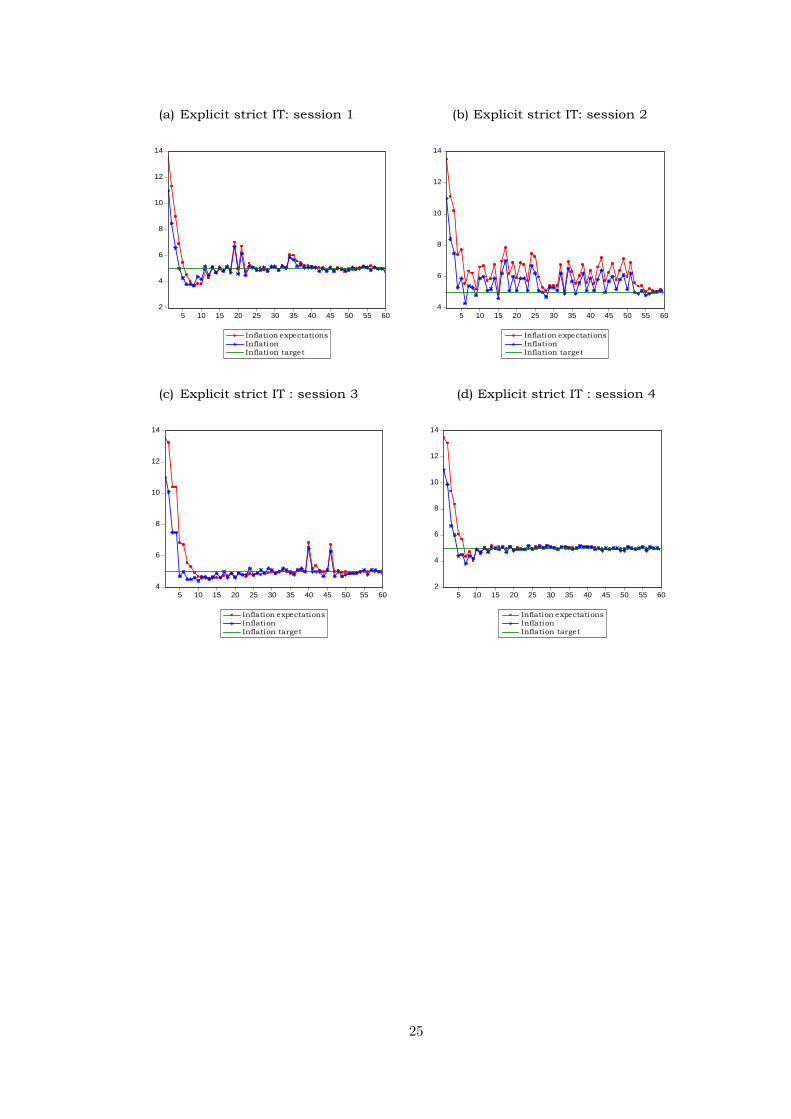
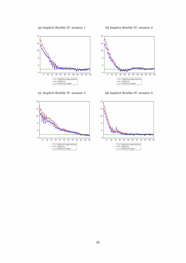
14Appendix C provides figures showing the evolution of inflation and average inflation expectations foreach session of each treatment.

15This non-parametric test is equivalent to the test of differences of means in parametric tests, whileSiegel-Tukey test is equivalent to the analysis of variances (ANOVA) in parametric tests.

16See also Appendix A for the descriptive statistics of all treatments.

12

(a) Implicit strict versus implicit flexible IT

4

5

6

7

8

9

10

11

12

5 10 15 20 25 30 35 40 45 50 55 60

Implicit strict IT (inflation)

Implicit flexible IT (inflation)

Inflation target

-10

-8

-6

-4

-2

0

2

5 10 15 20 25 30 35 40 45 50 55 60

Implicit strict IT (output gap)

Implicit flexible IT (output gap)

(b) Explicit strict versus explicit flexible IT

4

5

6

7

8

9

10

11

12

13

5 10 15 20 25 30 35 40 45 50 55 60

Explicit strict IT (inflation)

Explicit flexible IT (inflation)

Inflation target

-10

-8

-6

-4

-2

0

2

5 10 15 20 25 30 35 40 45 50 55 60

Explicit strict IT (output gap)

Explicit flexible IT (output gap)

Figure 2: Average inflation and output gap series for strict versus flexible IT regimes

policy particularly for central banks which lack credibility. A strict IT regime could first

be applied to establish credibility of the regime and then, a flexible IT regime should follow

the former regime to reduce adjustment costs and stabilize the economic environment.

We now investigate the role of the target announcement in each IT regime.

5.2 Implicit versus Explicit strict IT

Figure 3 presents the evolution of average inflation and output gap series for implicit and

explicit strict IT treatments.

Regarding inflation, we can observe that these series show quite similar trend-convergence

although there is a faster convergence towards the target in the explicit strict IT case (aver-

age inflation first reaches the target at the fifth period while in the case of implicit strict IT,

average inflation first reaches the target at the fifteenth period). We use similar statistical

13

4

5

6

7

8

9

10

11

12

5 10 15 20 25 30 35 40 45 50 55 60

Implicit strict IT (inflation)

Explicit strict IT (inflation)

Inflation target

-10

-8

-6

-4

-2

0

2

5 10 15 20 25 30 35 40 45 50 55 60

Implicit strict IT (output gap)

Explicit strict IT (output gap)

Figure 3: Average inflation and output gap series for implicit versus explicit strict IT

tests as earlier to check whether there are differences between both treatments in terms

of macroeconomic outcomes series. Tests indicate that there are no significant differences

at all conventional levels in terms of medians (or means) and variances of macroeconomic

outcomes between both treatments.

Our analysis implies that a central bank that only cares about inflation stabilization

does not need to implement an explicit IT announcement to gain higher macroeconomic

performances. Instead it is sufficient to respect the Taylor principle. Implementing an

explicit strict IT is useful only for rapid disinflation due to the credibility of the regime as

shown by Figure 3 and as stressed in the credibility analysis. Indeed, we find in Section

3.4.1 that 87.5% of subjects in the explicit strict IT treatment attribute a high level of

credibility to the target. A possible explanation of the insignificant difference between

both treatments in terms of macroeconomic outcomes can be found in the policy reaction

function. As the central bank’s objective is unique and clear in this regime, uncondi-

tional of whether it announces its target for inflation or not, the strong policy reaction

to inflation allows subjects to understand quickly the target and thus to coordinate their

expectations on this target. Hence, the role of the announced target in this context is

rather insignificant.

Finally, our finding questions some results of the literature (Friedman and Kuttner, 1996),

as we find that there is no evidence that adopting an explicit IT regime leads to higher

output gap volatility.17 We can summarize our findings as follows.

17We instead find that the average standard deviation in explicit strict IT treatment is lower (2.20) thanthe one in implicit strict IT (2.43) although this difference does not appear to be statistically significant.

14

Result 1. If the central bank is an inflation nutter, inflation targeting does not make

a difference in terms of macroeconomic outcomes compared to a standard monetary policy

that just respects the Taylor principle. The announcing effect of the inflation target is

however beneficial in terms of more rapid disinflation due to the credibility of the regime.

5.3 Implicit versus explicit flexible IT

We now investigate the potential differences between implicit and explicit flexible IT treat-

ments in terms of macroeconomic outcomes. Figure 4 presents the evolution of average

inflation series for both implicit and explicit flexible IT treatments.

4

5

6

7

8

9

10

11

12

13

5 10 15 20 25 30 35 40 45 50 55 60

Implicit flexible IT (inflation)

Explicit flexible IT (inflation)

Inflation target

-5

-4

-3

-2

-1

0

1

5 10 15 20 25 30 35 40 45 50 55 60

Implicit flexible IT (output gap)

Explicit flexible IT (output gap)

Figure 4: Average inflation series for implicit versus explicit flexible IT

As in the previous analysis, we observe that both inflation series show quite similar

trend-convergence although there is a faster convergence towards the target in the explicit

flexible IT case (average inflation first reaches the target at the twentieth period of the

experiment while in the case of implicit flexible IT, average inflation first reaches the target

at the twenty eighth period).

Tests indicate that there are significant differences between both treatments in terms

of volatility of macroeconomic outcomes but not in terms of their average levels. More

precisely, we find that the average standard deviations of inflation, interest rate, and

output gap are significantly lower in the explicit flexible IT treatment than in the implicit

flexible IT treatment. This finding is in line with the theoretical result of Demertzis and

Hughes-Hallett (2007) who find that when agents are uncertain about the central bank’s

objectives and especially its output gap objective, greater transparency negatively affects

the variability of inflation and output gap but not their average levels.

15

Three reasons can be put forward to explain the relevance of announcing the target in

the flexible IT regime. The first explanation can be found in the policy objectives of the

central bank. Indeed, as the objectives of the central bank are both to stabilize inflation

and the output gap, agents may find it more difficult to undertsand these goals than a

single objective. In this context, the announcement of the target is important as it helps

to clarify these objectives. The second reason may be due to the fact that a flexible IT

regime seems more sensitive to fluctuations in inflation forecasts than a strict IT regime18.

This should make it more difficult to stabilize the economy because subjects take much

longer time to reach the target. Hence, the announcement of the target for inflation is

more helpful in reducing forecast errors. Finally the third explanation which is closely

related to the second one is the role of the forecasting rules used by subjects. As noted

in section 4.2, the trend extrapolation rule (agents expect that the upward (downward)

movements in inflation will be followed by the downward (upward) movements in the next

period) better explains the evolution of average inflation expectations in the implicit flex-

ible IT treatment than in the explicit flexible IT treatment. Following this rule requires

more frequent and aggressive adjustments in the policy reaction function to mitigate the

high volatility in inflation and output gap in the case of implicit flexible IT compared

to the case of explicit flexible IT. As Orphanides and Williams (2005, 2007) argue, the

communication of the target reduces the uncertainty faced by agents in their estimating

rules and consequently, helps them learn about the true economic model. We can thus

summarize our findings in the following way.

Result 2. If the central bank cares about the stabilization of both inflation and output

gap, communicating the target helps to reduce the volatility of inflation, interest rate, and

the output gap although their average levels are not affected. The announcement effect of

the inflation target reduces the uncertainty faced by agents in their expectation formation

rules.

6 Concluding remarks

Using laboratory experiments with human subjects, we analyze to what extent communi-

cation of the inflation target is relevant in an inflation targeting framework. To be able

to interpret the role of the announced target – which has been difficult to highlight in

the empirical literature with real data –, we compare two monetary policy rules which

differ only with respect to whether the target is announced (explicit IT treatments), or

18This can be seen from equation (6). Recalling this equation:

πt = A+αλ+ β(1 + αφy)

1 + α(φy + λφπ)πet+1 +

λ

1 + α(φy + λφπ)yt−1 + εt.

Let Γ =αλ+β(1+αφy)

1+α(φy+λφπ)be the coefficient of average inflation forecasts. By replacing all the parameters by

their given values one obtains for a strict IT regime Γ = 0.81, and for a flexible IT regime Γ = 0.92. Notethat Γ is larger for the flexible IT regime. Consequently, flexible IT seems more sensitive to fluctuationsin inflation expectations.

16

not (implicit IT treatments).

First, we find that when the central bank is an inflation nutter that is, a central

bank that only cares about inflation stabilization, announcing the inflation target does

not make a difference in terms of stabilizing macroeconomic outcomes compared to a

standard active monetary policy. This suggests that an inflation nutter does not need to

implement an inflation targeting framework to achieve higher macroeconomic performance.

A simple monetary policy which respects the Taylor principle is sufficient to achieve the

same economic performances. Second, we find that if the central bank also cares about the

stabilization of the output gap, communicating the target helps to reduce the volatility of

inflation, interest rate, and output gap although their average levels are not affected.

While our experimental study has been conducted in a controlled environment and

the applicability of our results should be handled carefully, we argue that the irrelevance

of explicit inflation targeting when the central bank is an inflation nutter does not mean

that opponents (Ball and Sheridan, 2005; Angeris and Arestis, 2008 among others) of

inflation targeting are right. As noted by Svensson (2010), in practice inflation targeting

is never strict but always flexible as central banks also care about the stabilization of

the real economy or of the financial system. The relevance of explicitly announcing the

inflation target in our second result provides a rationale for the adoption of flexible inflation

targeting by all inflation targeting countries.

17

References

Adam, K. (2007). Experimental evidence on the persistence of output and inflation.

Economic Journal, 117:603–636.

Angeriz, A. and Arestis, P. (2008). Assessing inflation targeting through intervention

analysis. Oxford Economic Papers, 60(2):293–317.

Assenza, T., Heemeijer, P., Hommes, C., and Massaro, D. (2011). Individual expecta-

tions and aggregate macro behavior. Technical report, CeNDEF Working Papers 11-01,

Universiteit van Amsterdam, Center for Nonlinear Dynamics in Economics and Finance.

Ball, L. and Sheridan, N. (2005). Does Inflation Targeting Matter?, chapter In Ben

Bernanke and Michael Woodford (Ed), The Inflation Targeting Debate, pages 249–276.

University of Chicago Press.

Bernasconi, M. and Kirchkamp, O. (2000). Why do monetary policies matter? an exper-

imental study of saving and inflation in an overlapping generations model. Journal of

Monetary Economics, 46:315–343.

Bomfin, A. and Rudebusch, G. (2000). Opportunistic and deliberate disinflation under

imperfect credibility. Journal of Money, Credit and Banking, 32:707–721.

Branch, W. (2004). The theory of rationally heterogeneous expectations: Evidence from

survey data on inflation expectations. Economic Journal, 114(497):592–621.

Brito, R. and Bystedt, B. (2010). Inflation targeting in emerging economies : Panel

evidence. Journal of Development Economics, 91(2):198–210.

Bullard, J. and Mitra, K. (2002). Learning about monetary policy rules. Journal of

Monetary Economics, 49(6):1105–1129.

Capistran, C. and Timmermann, A. (2009). Disagreement and biases in inflation expec-

tations. Journal of Money, Credit and Banking, 41:365–396.

Clarida, R., Gali, J., and Gertler, M. (2000). Monetary policy rules and macroeconomic

stability: Evidence and some theory. Quarterly Journal of Economics, 115(1):147–180.

Demertzis, M. and Hughes-Hallett, A. (2007). Central bank transparency in theory and

practice. Journal of Macroeconomics, 29(4):760–789.

Evans, G. and Honkapohja, S. (2001). Learning and expectations in macroeconomics.

Princeton University Press.

Fischbacher, U. (2007). z-tree: Zurich toolbox for ready-made economic experiments.

Experimental Economics, 10(2):171–178.

Fraga, A., Goldfajn, I., and Minella, A. (2003). Inflation targeting in emerging market

economies. Technical report, NBER Working Paper No. 10019.

18

Friedman, B. and Kuttner, K. (1996). A price target for u.s. monetary policy? lessons

from the experience with money growth targets. Brookings Papers on Economic Activity,

1:77–146.

Hommes, C. (2011). The heterogeneous expectations hypothesis: Some evidence from the

lab. Journal of Economic Dynamics and Control, 35:1–24.

King, M. (1997). The inflation target five years on. Bank of England Quaterly Bulletin,

37:434–442.

Levin, A., Natalucci, F., and Piger, J. (2004). The macroeconomic effects of inflation

targeting. Federal Reserve Bank of St. Louis Review, 86(4):51–80.

Lin, S. and Ye, H. (2007). Does inflation targeting really make a difference? evaluating the

treatment effect of inflation targeting in seven industrial countries. Journal of Monetary

Economics, 54:2521–2533.

Lin, S. and Ye, H. (2009). Does inflation targeting make a difference in developing coun-

tries? Journal of Development Economics, 89:118–123.

Marimon, R. and Sunder, S. (1995). Does a constant money growth rule help stabilize

inflation?: Experimental evidence. Carnegie-Rochester Conference Series on Public

Policy, 43:111–156.

Muth, J. (1961). Rational expectations and the theory of price movements. Econometrica,

29(3):315–335.

Orphanides, A. and Williams, J. C. (2005). Imperfect Knowledge, Inflation Expectations

and Monetary Policy, chapter In Ben Bernanke and Micheal Woodford (Ed), Inflation

Targeting. University of Chicago Press.

Orphanides, A. and Williams, J. C. (2007). Inflation Targeting under Imperfect Knowledge,

volume Vol. XI, chapter In Frederic Mishkin and Klaus Schmidt-Hebbel (Ed), Monetary

Policy Under Inflation Targeting. Banco central de Chile, Santiago, Chile.

Pfajfar, D. and Zakelj, B. (2010). Inflation expectations and monetary policy design:

Evidence from the laboratory. Technical report, Tilburg University.

Roger, S. (2009). Inflation targeting at 20 : Achievements and challenges. Technical

report, IMF working paper 09/236, International Monetary Fund.

Roger, S. and Stone, M. (2005). On target? the international experience with achiev-

ing inflation targets. Technical report, IMF working paper No. 05/163, International

Monetary Fund.

Svensson, L. E. (2010). Inflation Targeting, chapter In Benjamin Friedman and Michael

Woodford (Ed), Handbook of Monetary Economics, pages 1237–1302. Elsevier.

19

Willard, L. B. (2012). Does inflation targeting matter ? a reassessment. Applied Eco-

nomics, 44(17):2231–2244.

Woodford, M. (2005). Central bank communication and policy effectiveness. Working

Paper 11898, National Bureau of Economic Research.

20

Appendix A: Descriptive statistics

A.1. Strict inflation targeting

Inflation expectations

Stat. by session (S) Implicit strict IT Explicit strict IT

S1 S2 S3 S4 Avg S1 S2 S3 S4 Avg

Mean 5.6 5.67 5.45 5.83 5.64 5.40 6.39 5.51 5.39 5.67

Median 5.15 5.11 5.02 5.20 5.13 5.06 6.13 4.98 4.98 5.23

SdtDev 1.68 1.72 1.91 1.61 1.68 1.54 1.47 1.83 1.66 1.55

Inflation

Stat. by session (S) Implicit strict IT Explicit strict IT

S1 S2 S3 S4 Avg S1 S2 S3 S4 Avg

Mean 5.25 5.29 5.18 5.37 5.27 5.15 5.64 5.20 5.14 5.29

Median 5.10 5 5 5.10 5.08 5 5.30 4.90 5 5.08

SdtDev 1.03 1.07 1.19 0.99 1.03 1.03 1.01 1.16 1.06 1.00

Output gap

Stat. by session (S) Implicit strict IT Explicit strict IT

S1 S2 S3 S4 Avg S1 S2 S3 S4 Avg

Mean -0.96 -1.11 -0.75 -1.36 -1.05 -0.65 -2.27 -0.83 -0.65 -1.10

Median -0.15 -0.15 0 -0.40 -0.18 -0.10 -2 0 0.10 -0.45

SdtDev 2.44 2.45 2.67 2.30 2.43 2.05 1.81 2.64 2.31 2.20

Interest rate

Stat. by session (S) Implicit strict IT Explicit strict IT

S1 S2 S3 S4 Avg S1 S2 S3 S4 Avg

Mean 5.51 5.57 5.35 5.74 5.54 5.30 6.28 5.41 5.29 5.57

Median 5.20 5 5 5.20 5.15 5 5.60 4.80 5 5.15

SdtDev 2.06 2.13 2.39 1.97 2.14 2.06 2.03 2.32 2.13 2.00

21

A.2. Flexible inflation targeting

Inflation expectations

Stat. by session (S) Implicit flexible IT Explicit flexible IT

S1 S2 S3 S4 Avg S1 S2 S3 S4 Avg

Mean 6.36 6.10 7.04 6.36 6.46 7.01 5.62 5.95 5.98 5.89

Median 5.30 5.18 6.28 4.95 5.34 5.10 5 5.07 5.53 5.18

SdtDev 2.26 2.19 2.11 2.49 2.21 1.96 1.65 1.89 1.45 1.70

Inflation

Stat. by session (S) Implicit flexible IT Explicit flexible IT

S1 S2 S3 S4 Avg S1 S2 S3 S4 Avg

Mean 6.08 5.87 6.64 6.08 6.17 5.79 5.46 5.74 5.76 5.69

Median 5.20 5.20 6.10 5 5.30 5.10 5 5.10 5.40 5.19

SdtDev 1.86 1.81 1.74 2.06 1.82 1.60 1.35 1.55 1.19 1.38

Output gap

Stat. by session (S) Implicit flexible IT Explicit flexible IT

S1 S2 S3 S4 Avg S1 S2 S3 S4 Avg

Mean -0.72 -0.59 -1.07 -0.72 -0.77 -0.53 -0.33 -0.50 -0.50 -0.47

Median -0.10 -0.10 -0.60 0 -0.15 -0.10 0 -0.05 -0.30 -0.11

SdtDev 1.21 1.22 1.12 1.33 1.20 1.09 0.95 1.07 0.86 0.98

Interest rate

Stat. by session (S) Implicit flexible IT Explicit flexible IT

S1 S2 S3 S4 Avg S1 S2 S3 S4 Avg

Mean 6.28 6.04 6.95 6.28 6.39 5.94 5.55 5.87 5.91 5.82

Median 5.30 5.20 6.40 5 5.40 5.20 5 5.10 5.60 5.31

SdtDev 2.18 2.10 2.06 2.42 2.13 1.87 1.58 1.80 1.38 1.60

22

Appendix B: Statistical tests results

In the following tables, p-values are reported in brackets. ***, ** and * respectively

indicate significance at 1%, 5% and 10% conventional levels.

B.1. Pairwise comparison: implicit strict versus implicit flexible IT

Mann-Whitney-Wilcoxon test Siegel-Tukey test

Macroeconomic outcomes Statistical equality of medians? Statistical equality of variances?

Inflation No*** (0.0001) Yes (0.2887)

Output gap Yes (0.6900) Yes (0.7005)

Interest rate No*** (0.0006) Yes (0.8949)

B.2. Pairwise comparison: explicit strict versus explicit flexible IT

Mann-Whitney-Wilcoxon test Siegel-Tukey test

Macroeconomic outcomes Statistical equality of medians? Statistical equality of variances?

Inflation No*** (0.0075) Yes (0.2599)

Output gap No*** (0.0013) Yes (0.1885)

Interest rate No** (0.0406) No** (0.0177)

B.3. Pairwise comparison: implicit versus explicit strict IT

Mann-Whitney-Wilcoxon test Siegel-Tukey test

Macroeconomic outcomes Statistical equality of medians? Statistical equality of variances?

Inflation Yes (0.5940) Yes (0.8779)

Output gap Yes (0.1637) Yes (0.5761)

Interest rate Yes (0.5868) Yes (0.9202)

B.4. Pairwise comparison: implicit versus explicit flexible IT

Mann-Whitney-Wilcoxon test Siegel-Tukey test

Macroeconomic outcomes Statistical equality of medians? Statistical equality of variances?

Inflation Yes (0.2001) No** (0.0489)

Output gap Yes (0.1272) No* (0.0931)

Interest rate Yes (0.2293) No** (0.0444)

23

Appendix C: Inflation and average inflation expectations se-

ries across sessions by treatment

(a) Implicit strict IT: session 1 (b) Implicit strict IT: session 2

2

4

6

8

10

12

14

5 10 15 20 25 30 35 40 45 50 55 60

Inflation expectations

Inflation

Inflation target

4

6

8

10

12

14

5 10 15 20 25 30 35 40 45 50 55 60

Inflation expectations

Inflation

Inflation target

(c) Implicit strict IT: session 3 (d) Implicit strict IT: session 4

2

4

6

8

10

12

14

5 10 15 20 25 30 35 40 45 50 55 60

Inflation expectations

Inflation

Inflation target

4

6

8

10

12

14

5 10 15 20 25 30 35 40 45 50 55 60

Inflation expectations

Inflation

Inflation target

24

(a) Explicit strict IT: session 1 (b) Explicit strict IT: session 2

2

4

6

8

10

12

14

5 10 15 20 25 30 35 40 45 50 55 60

Inflation expectations

Inflation

Inflation target

4

6

8

10

12

14

5 10 15 20 25 30 35 40 45 50 55 60

Inflation expectations

Inflation

Inflation target

(c) Explicit strict IT : session 3 (d) Explicit strict IT : session 4

4

6

8

10

12

14

5 10 15 20 25 30 35 40 45 50 55 60

Inflation expectations

Inflation

Inflation target

2

4

6

8

10

12

14

5 10 15 20 25 30 35 40 45 50 55 60

Inflation expectations

Inflation

Inflation target

25

(a) Implicit flexible IT: session 1 (b) Implicit flexible IT: session 2

4

6

8

10

12

14

5 10 15 20 25 30 35 40 45 50 55 60

Inflation expectations

Inflation

Inflation target

4

6

8

10

12

14

5 10 15 20 25 30 35 40 45 50 55 60

Inflation expectations

Inflation

Inflation target

(c) Implicit flexible IT: session 3 (d) Implicit flexible IT: session 4

4

6

8

10

12

14

5 10 15 20 25 30 35 40 45 50 55 60

Inflation expectations

Inflation

Inflation target

4

6

8

10

12

14

5 10 15 20 25 30 35 40 45 50 55 60

Inflation expectations

Inflation

Inflation target

26

(a) Explicit flexible IT: session 1 (b) Explicit flexible IT: session 2

4

6

8

10

12

14

5 10 15 20 25 30 35 40 45 50 55 60

Inflation expectations

Inflation

Inflation target

4

6

8

10

12

14

5 10 15 20 25 30 35 40 45 50 55 60

Inflation expectations

Inflation

Inflation target

(c) Explicit flexible IT : session 3 (d) Explicit flexible IT : session 4

4

6

8

10

12

14

5 10 15 20 25 30 35 40 45 50 55 60

Inflation expectations

Inflation

Inflation target

4

6

8

10

12

14

5 10 15 20 25 30 35 40 45 50 55 60

Inflation expectations

Inflation

Inflation target

27

Appendix D: Instructions

We present a translation from French to English of the instructions for Treatment 4 (ex-

plicit flexible inflation targeting). Instructions for other treatments are available from the

authors upon request.

General information

Thank you for your participation to this economic experiment in which you can earn

money. Your earnings will depend on both your actions and those of the other participants

and will be paid in cash at the end of the experiment. From now until the end of the

experiment, you are not allowed to communicate with each other. If you have any question,

please raise your hand and we will come to you.

You are a group of 6 participants. The rules are the same for all participants. The

experiment consists of 60 periods. Your role is to predict future values of a given economic

variable. Your earnings will depend on the accuracy of your predictions. At each of the 60

periods, the economy will be characterized by the following variables: the inflation rate,

the output gap, the interest rate, and the inflation target of the central bank.

Information about economic variables

To better understand the economic variables that you will use to make your decisions, we

explain these variables as follows.

Inflation: is defined as the generalized rise in prices in the economy. Inflation will depend

in each period on agents’ average inflation forecasts in the economy (that is, both your

forecast and the forecasts of the 5 other participants), on the output gap, as well as on a

random shock affecting the economy.

The output gap: describes the gap between the current output and the potential output

(that is, the level of output the economy can achieve by using the maximum of its produc-

tive capacity). If the output gap is positive, the economy is producing beyond its potential

level. Conversely, if it is negative, the economy is producing below its potential level. The

output gap also depends in each period on the agents’ average inflation forecasts (your

prediction and the predictions of the 5 other participants), the lagged output gap, the

interest rate as well as a random shock affecting the economy.

The interest rate: is defined as the price of borrowing money for a period, and is set

by the central bank of the economy. The interest rate mainly depends on inflation (and

therefore indirectly on inflation forecasts), the output gap and the inflation target of the

central bank.

The inflation target: is clearly announced to all participants by the central bank in the

form of a numerical target of 5% with a tolerance interval of +/-1% around the target.

The inflation target is announced in a context of high inflation in the economy, and re-

flects the central bank’s determination to reduce this high inflation. So the central bank

commits to reach its inflation target of 5%. However, given the various random shocks

affecting the economy, the central bank allows itself a margin error of +/-1% around its

28

target. The inflation target then corresponds to a commitment of the central bank which

has to ensure (via the interest rate) that inflation in the economy will converge towards

this target.

The central bank has two goals: one primary, and the other secondary.

The primary goal, the most important is for the central bank to stabilize inflation that

is, to make as quickly as possible actual inflation converge towards its inflation target. The

central bank uses the interest rate to stabilize inflation. Positive and significant deviations

of actual inflation from the target (that is, actual inflation is not equal to the numerical

target of 5%, and is above the upper band of the tolerance interval of 6%), force the central

bank to increase the interest rate in order to lead actual inflation towards its target. By

contrast, when the central bank notes that inflation is too low compared to its inflation

target (that is, actual inflation is not equal to the numerical target of 5%, and is below the

lower band of the tolerance interval of 4%) and penalizes the economic activity, it reduces

the interest rate.

The secondary goal consists for the central bank in stabilizing the output gap that

is, the gap between the current and potential output of the economy, by also using the

interest rate. When the output gap is positive, the central bank tends to increase the

interest rate, and when it is negative, the central bank tends to reduce the interest rate.

All these variables can be relevant for your inflation forecasts, but it is up to you to

use them in your convenience to decide on your inflation expectations. The actual values

of the different variables largely depend on your inflation forecasts and those of the others,

but also on random shocks affecting the economy.

At the beginning of the experiment and before entering your inflation forecast for the

first period in the computer, you observe on the screen the past values of the main economic

variables (inflation, output gap and interest rate) of the five previous periods. Given the

high values of inflation in the economy, the central bank implements an inflation targeting

strategy by announcing to all participants its numerical target of 5% with tolerance interval

of +/-1%. By this announcement, the central bank commits to lead actual inflation

towards its inflation target within a maximum of two periods. So you observe the central

bank’s target within its tolerance interval. This target remains unchanged throughout the

duration of the experiment. Based on these variables, you have to forecast inflation for

the next period.

Once you have made your decision, a period ends and a new period starts where you

observe the past and actual values of inflation, the output gap, the interest rate, and your

inflation forecast made in the previous period. However, you do not observe the expecta-

tions of other participants in your group (you just indirectly observe them through actual

inflation). All you observe in terms of expectations is your own time series forecasts. As

time goes on, you get a large number of observations that allows you to evaluate the accu-

racy of your forecasts compared to actual values of inflation, as well as the inflation target

of the central bank.

29

Information about your role in the economy

Throughout the 60 periods of the experiment, your role as an agent of the economy is

simple. You have to forecast the actual value of future inflation. In other words, you

have to predict in each period, the inflation that will prevail in the next period based on

all information available to you when making your decision. You must then enter in the

computer your inflation forecast. Suppose that on your computer screen, you observe at

period 2, actual inflation. This observed inflation is not based on the forecasts that you

and the other participants of your group have made at period 2, but the predictions you

made in the previous period that is, those made in period 1 for period 2.

By choosing your inflation forecast, you seek to maximize your earnings. Your gain in

each period depends on the accuracy of your inflation forecast relative to actual (realized)

inflation. More specifically, your gain is given by:

Your profit in ECU = max

{160

1 + f− 40, 0

},

where f =| Inflation−Your forecast |. ’Inflation’ indicates actual inflation, ’Your forecast’

defines your inflation forecast made at previous period for the next, f indicates in absolute

value your forecasting error, and finally ’ECU’ indicates the Experimental Currency Unit.

The profit function above means that you get money every time your forecasting error is

less than 3%. The smaller your forecasting error, the higher your payoff. For instance

if Inflation f =0, you receive the maximum payoff of 120 units (160/(1+0)-40). If your

forecasting error is of 1.5%, you receive 24 units (160/(1+1.5)-40). Otherwise if your

forecasting error is of 3% or higher, then you receive 0 unit (160/ (1+3) - 40). You can

only choose your inflation forecasts within the interval [3, 16]. You can only choose whole

numbers or numbers with one decimal digit (for instance, 5, 8.5, 4.6, etc). In addition,

when making your decisions, you have to enter only numbers without the ”%” symbol.

Once you have entered your decision in the computer, click on the ’Submit’ button.

Once all participants have done the same, the period ends and the profit for this period is

written on the computer screen. Then, the next period starts. Once all the 60 periods are

completed, the experiment ends. At each of the 60 periods of the experiment, at the top

of each screen and on a graph, you can observe the entire history of economic variables as

well as your earnings. You can then check at each period if your inflation forecast made

in the previous period corresponds to actual inflation, and also whether it corresponds or

converge towards the inflation target of the central bank. You will get informed about

your gains period by period, and at the end of the experiment, your earnings will be added

and will be paid in cash converted at the exchange rate of e1=520 ECU. Note that you

do not get money in the first period of the experiment because you will not have made

any forecast for this period 1. So your potential gains start at period 2 of the experiment,

because you will have made forecasts at period 1 for this period 2.

Questionnaire

30

At the beginning of the experiment, we ask you to fill out a questionnaire to make sure

that you understand instructions. When all participants have correctly answered the ques-

tionnaire, the experiment will begin. At the end of the experiment, we ask you to complete

a personal questionnaire on computer. All requested information will remain strictly con-

fidential and is used for the sole purpose of research.

If you have any questions, please ask them now!

Thank you for your participation!

31

Appendix E: Examples of screens

We provide examples of screens (first screen: implicit inflation targeting; second screen:

explicit inflation targeting).

32

33