DOCUMENTOS DE TRABAJOSovereign Credit Spreads, Banking Fragility, and Global Factors

Anusha ChariFelipe GarcésJuan Francisco MartínezPatricio Valenzuela

N° 957 Mayo 2022BANCO CENTRAL DE CHILE

La serie Documentos de Trabajo es una publicación del Banco Central de Chile que divulga los trabajos de investigación económica realizados por profesionales de esta institución o encargados por ella a terceros. El objetivo de la serie es aportar al debate temas relevantes y presentar nuevos enfoques en el análisis de los mismos. La difusión de los Documentos de Trabajo sólo intenta facilitar el intercambio de ideas y dar a conocer investigaciones, con carácter preliminar, para su discusión y comentarios.

La publicación de los Documentos de Trabajo no está sujeta a la aprobación previa de los miembros del Consejo del Banco Central de Chile. Tanto el contenido de los Documentos de Trabajo como también los análisis y conclusiones que de ellos se deriven, son de exclusiva responsabilidad de su o sus autores y no reflejan necesariamente la opinión del Banco Central de Chile o de sus Consejeros.

The Working Papers series of the Central Bank of Chile disseminates economic research conducted by Central Bank staff or third parties under the sponsorship of the Bank. The purpose of the series is to contribute to the discussion of relevant issues and develop new analytical or empirical approaches in their analyses. The only aim of the Working Papers is to disseminate preliminary research for its discussion and comments.

Publication of Working Papers is not subject to previous approval by the members of the Board of the Central Bank. The views and conclusions presented in the papers are exclusively those of the author(s) and do not necessarily reflect the position of the Central Bank of Chile or of the Board members.

Documentos de Trabajo del Banco Central de ChileWorking Papers of the Central Bank of Chile

Agustinas 1180, Santiago, ChileTeléfono: (56-2) 3882475; Fax: (56-2) 38822311

Documento de Trabajo N° 957

Working Paper N° 957

Sovereign Credit Spreads, Banking Fragility, and Global Factors*

AbstractThis study explores the relationship between sovereign credit risk, banking fragility, and global financial factors in a large panel database of emerging market economies. To measure banking fragility, we construct a novel model-based semi-parametric metric (JLoss) that computes the expected joint loss of the banking sector condi-tional on a systemic event. Our metric of banking fragility is positively associated with sovereign credit spreads, after controlling for the standard determinants of sovereign credit risk, a comprehensive set of measures of systemic risk, and country and time fixed effects. The results additionally indicate that countries with more fragile banking sectors are more exposed to global (exogenous) financial factors than those with more resilient banking sectors. These findings underscore that regulators must ensure the stability of the banking sector to improve governments’ borrowing costs in international debt markets.

ResumenEste estudio explora la relación entre el riesgo de crédito soberano, la fragilidad financiera y los factores financieros globales en una base de datos panel que contiene economías emergentes. Para medir la fragilidad financiera, construimos una métrica con una metodología semi paramétrica (Jloss) que calcula la pérdida conjunta esperada del sistema bancario condicional a un evento sistémico. Nuestra métrica de fragilidad financiera se encuentra positivamente asociada con los spreads de crédito soberano, controlando por los determinantes estándar del riesgo de crédito, un conjunto de medidas de riesgo sistémico, y efectos fijos por país y tiempo. Los resultados adicionalmente indican que economías con sectores bancarios más frágiles están más expuestos a factores financieros globales que aquellos con sectores bancarios más resilientes. Estos descubrimientos destacan que los reguladores deben asegurar la estabilidad financiera en el sector bancario para mejorar los costos de financiamiento de los gobiernos en el mercado internación de deuda.

Anusha ChariUniversity of North

Carolina at Chapel Hill

Felipe GarcésCentral Bank of Chile

Juan Francisco MartínezCentral Bank of Chile

Patricio ValenzuelaUniversidad de los Andes,

Chile

*We wish to thank Charles Goodhart, Dimitrios Tsomocos, Jose Vicente Martinez, Oren Sussman, and participants at the First Conference on Financial Stability and Sustainability for insightful comments on an earlier version of this paper. Valenzuela acknowledges financial support from Fondecyt Project 1200070 and the Institute for Research in Market Imperfections and Public Policy, MIPP (ICS13002 ANID). Contact: fgarces@bcentral.cl, jmartinez@bcentral.cl

1 Motivation

The global financial crisis of 2008-09 and the European debt crisis, which were char-

acterized by large losses in the banking sector, affected international debt markets

severely. They produced a significant deterioration of sovereign credit spreads with

the greater expectation of public support for distressed banks (Mody and Sandri,

2012). Despite a rich body of research on the drivers of sovereign credit risk, a bet-

ter understanding of the factors influencing sovereign risk and of how these factors

can be properly measured in both advanced and emerging economies is of key im-

portance for several reasons. Sovereign credit risk is not only a key determinant of

governments’ borrowing costs, but also remains a significant determinant of the cost

of debt capital for the private sector (Cavallo and Valenzuela, 2010; Borensztein,

Cowan, and Valenzuela, 2013). Moreover, sovereign credit risk directly influences

the ability of investors to diversify the risk of global debt portfolios and plays a

crucial role in determining capital flows across countries (Longstaff et al., 2011).

The literature has recently emphasized that the primary factors that affect

sovereign credit risk are macroeconomic fundamentals, global factors, and bank-

ing fragility, which have generally been treated as independent determinants of

sovereign credit risk. Although macroeconomic fundamentals have substantial ex-

planatory power for sovereign credit spreads in emerging economies (Hilscher and

Nosbusch, 2010), sovereign credit risk appears to be mainly driven by global finan-

cial factors (Gonzalez-Rosada and Yeyati, 2008; Longstaff et al., 2011). Banking

fragility also seems to influence governments’ indebtedness and credit risk. Greater

banking-sector fragility predicts larger bank bailouts, larger public debt, and higher

sovereign credit risk (Acharya, Drechsler, and Schnabl, 2014; Kallestrup, Lando,

and Murgoci, 2016; Farhi and Tirole, 2018). This relationship between bank

risk and sovereign risk is particularly strong during periods of financial distress

(Fratzscher and Rieth, 2019). Finally, recent empirical evidence also suggests sys-

temic sovereign risk has its roots in financial markets rather than in macroeconomic

fundamentals (Dieckmann and Plank, 2012; Ang and Longstaff, 2013). Specifically,

Dieckmann and Plank (2012) show the state of the domestic financial market and

the state of the global financial system have strong explanatory power for the evo-

lution of sovereign spreads, and that the magnitude of the effect is shaped by the

2

importance of the domestic financial system pre-crisis.

Using a novel model-based semi-parametric metric (JLoss) that computes the

expected joint loss of the banking sector in the event of a large financial meltdown,

in this study, we explore the relationship between sovereign credit spreads, banking

fragility, and global financial factors. We study this relationship in a panel data set

that covers 19 emerging market economies from 2000:Q1 to 2021:Q4. Consistent

with the idea that our metric (JLoss) can be understood as the direct cost of

bailing out the whole banking sector, and with recent evidence that shows sovereign

spreads increased in the eurozone with the greater expectation of public support

for distressed banks (Mody and Sandri, 2012), our results indicate our metric of

banking fragility is positively associated with sovereign credit spreads. The results

additionally indicate countries with more fragile banking sectors are more exposed

to the influence of global (exogenous) financial factors related to market volatility,

risk-free interest rates, risk premiums, and aggregate liquidity. Our results are

statistically significant and economically meaningful, even after controlling for the

standard determinants of sovereign credit risk, a comprehensive set of systemic risk

measures, and country and time fixed effects. Our results are also robust during

periods of financial distress and periods of financial stability as well as to controlling

for additional heterogeneous effects of global financial factors on sovereign spreads.

These findings underscore that the stability of the domestic banking sector plays a

crucial role in reducing sovereign risk and its exposure to global factors.

This study contributes to the literature in at least three ways. First, it intro-

duces a new measure of banking fragility in the banking sector (JLoss) that reflects

the expected joint loss of the domestic banking sector in the event of a large financial

meltdown. The calculation of our JLoss metric employs a saddle-point methodol-

ogy in which the distribution of potential losses in the banking system is a function

of the bank-specific probabilities of default, the exposure in case of default, a loss

given default (LGD) parameter, and the correlation between the banks’ stock mar-

ket returns and the stock market index returns of each country. Recent academic

studies have introduced measures of systemic risk (e.g., see Brownlees and Engle

(2016) for a measure of systemic risk for the U.S.). However, given that our metric

of the expected joint loss of the domestic banking sector can be interpreted as the

3

direct cost of bailing banks out from a crisis, it should be a particularly significant

factor to consider in the pricing of sovereign bonds.

Second, this study explores the relationship between sovereign credit risk and

banking fragility in a sample of emerging economies. Thus, this study is a departure

from recent studies that have focused their analysis on samples of European coun-

tries during the Eurozone sovereign and banking crises. Bruyckere et al. (2013)

examine contagion between the banking sector and sovereign default risk in Europe

from 2007 to 2012, and find that banks with a weak capital buffer, a weak funding

structure and less traditional banking activities are particularly vulnerable to risk

spillovers. Black et al. (2016) measure the systemic risk of European banks by

using a distress insurance premium (DIP), which integrates the characteristics of

bank size, probability of default, and correlation. Mody and Sandri (2012) argue

that sovereign credit spreads increased in the eurozone with the greater expectation

of public support for distressed banks and that this effect was stronger in countries

with lower growth prospects and higher debt burdens. Fratzscher and Rieth (2019)

show the correlation between CDS spreads of European banks and sovereigns rose

from 0.1 in 2007 to 0.8 in 2013, and attribute this higher correlation to a two-way

causality between bank credit risk and sovereign credit risk. Although the study of

sovereign credit risk in emerging economies has received much attention (Boehmer

and Megginson, 1990; Edwards, 1986; Hilscher and Nosbusch, 2010; Longstaff et

al., 2011), new research on the relationship between banking fragility and sovereign

credit risk in emerging economies has been sparse.

Third, this study takes an additional step beyond the extant literature by ex-

ploring a channel (i.e., the fragility of the banking sector) that amplifies the effect

of global (exogenous) factors on sovereign credit risk. Although global financial

factors have recently been viewed as push factors in the literature, they have usu-

ally been modeled as having homogeneous effects on sovereign credit risk (see, e.g.,

Gonzalez-Rosada and Yeyati, 2008). An exception is the study by Georgoutsosa and

Migiakisb (2013), which explores the determinants of euro area sovereign bond yield

spreads and find significant country-level heterogeneity on the effects on spreads.

Specifically, our analysis suggests that regulations and policies aimed at improving

the stability of the domestic banking sector may be helpful in reducing the exposure

4

to global factors, which have become increasingly important in a more financially

integrated world.

The remainder of the article is organized as follows. Section 2 presents the

JLoss methodology utilized to construct our banking fragility measure. Section 3

describes the sample and variables used in this study. Section 4 presents our em-

pirical strategy and reports the main results. Section 5 conducts a set of robustness

checks. Finally, section 6 concludes.

2 Joint Loss (JLoss) Measure

To study the relationship between banking fragility and sovereign credit risk, in

this work we construct a novel country-level metric of banking fragility (JLoss).

JLoss is a model-based semi-parametric metric of the joint loss of the banking

sector conditional on a systemic event. Figure 1 presents an overview of the JLoss

methodology.

To calculate our JLoss metric, we first employ a saddle-point methodology that

allows us to calculate the aggregated distribution of losses. In this approach the

distribution of potential losses in the banking system is a function of the banks’

probabilities and exposure at default, a loss given default (LGD) parameter, and

the correlation between banks’ stock market returns and a systemic component.

The individual probabilities of default are calculated following a modification of

the Merton’s (1974) model. The exposure is proxied by the amount of liabilities

of the banks at the moment of default. The LGD for banking debt is set to a

45%, as suggested by the Bank of International Settlements (BIS, 2006). The

key assumption in our approach is that bank risks are uncorrelated, conditional

on being correlated with a systemic factor, which in our case is the overall stock

market performance of each country. With the distribution of potential losses in

the banking system, we calculate each bank’s marginal contribution to the total

risk. Finally, we normalize these contributions to the total risk with respect to

total liabilities.

Next, we describe in detail the calculation of the banks’ default probabilities

and the aggregation of losses with the saddle-point method.

5

2.1 Individual Probabilities: Distance-to-Default

To calculate default probabilities for each bank, we employ Kealhofer’s (2000) ap-

proach. This approach is a standard modification of the structural credit risk model

introduced by Merton (1974). Table A.1 in the appendix reports the number of

banks used in our analyses by country.

Our measurement approach merges together information on banks’ balance

sheet and market prices: long and short term liabilities (LST , LLT ), short term

assets (AST ), average interest rates (r), time horizon (T ), volatility of bank real-

ized returns (σV ), and market capitalization (E). With this data we construct the

default point (D∗), which we formally define as

D∗ = LST +1

2LLT .

Then we numerically solve the following system of two non-linear equations, by

using the Newton-Raphson algorithm (Press et al., 2007), to project banks’ value

of assets (V ) and implied asset volatility (σA):

V

EΦ (d1)− e−rTΦ (d2)

E/D∗− 1 = 0

Φ (d1)V

EσA − σE = 0.

Where d1 = log(V ED∗

)+

12σ2ET

σE√T

and d2 = d1 − σE√T . Φ stands for the cumulative

normal distribution function. 1

Once we get the projected values V and σA, we insert them into the following

distance to default DD equation:

DD =VE −D

∗

VE σA

.

This equation is a function of the predicted value of the banks’ assets (V ) and

1We use the realized variance approach to estimate the quarterly equity volatility. Following Barndorf-Nielsen et al. (2002), we compute square root of the sum of squared daily equity returns over a quarter.

That is, for every quarter and bank, we calculate σE =√∑Q

t=1 r2t , where Q is the number of days in a

particular quarter.

6

asset volatility (σA). Finally, we assume normality to obtain the expected default

frequency (EDF ) as

EDF = Φ (−DD) .

We compute this quantity for all banks in every country and time periods of

our sample, and associate the expected default frequency value to the unconditional

probability of default (pdefi), which is one of the inputs for the saddle-point method.

2.2 Saddle-Point Method and Implementation

The saddle-point method allows us to simplify the calculations of the aggregate

distribution of losses by working in a different space. We move from the real

numbers space (R) to the moment generating function space (MGF). Then, we

apply a transform to come back to the real numbers space. The saddle-point

method allows to calculate the distribution of a random variable P that represents

the aggregate losses for a portfolio of N banks. Formally, we define P as

P =

N∑i=1

ei1Di ,

where ei is the exposure of bank i, and 1Di is the indicator function that takes a

value of zero if banks have repayment capacity and it is equal to one otherwise.

We need a workable description of the problem in the space of a MGF. To deter-

mine the MGF, we assume a feasible functional form that is statistically equivalent

to the problem in the real and one-dimensional space (R). The Laplace transform

naturally connects the two spaces (from R to MGF), while that the Bromwich

integral does the reverse process (from MGF to R). This regularity provides a

computational advantage with respect to other methods as allow us to reduce the

dimensionality of the problem.2

For an arbitrary credit portfolio, the relationship between the probability den-

sity functions and the MGF is described as

2Similarly to Martin et al. (2001), when we calculate the Bromwich integral through the saddle-pointwe are taking only the real part of the results since the original results could have imaginary factors.

7

Mx (s) = E (esx) =

∫esxf (x) dx.

Where Mx is the expected value of exponential function (esx), x is the random

variable (of losses, analogous to P ), s is the arbitrary Laplace transform parameter,

and f represents the probability density function.

If we consider two states for the random variable x (default and no default), we

have the following discrete MGF:

Mi (s) = E(esi)

=∑

1Di=0,1

f (1Di) es·exposi·1Di = 1− pdefi + pdefie

s·exposi .

Where pdefi is the unconditional default probability and exposi is the exposure

in the defined time horizon for bank i. If we assume conditional independence, the

relationship between the unconditional (pdefi) and conditional (pdefi(~V )) probabil-

ities of default can be expressed as3

pdefi =∑k

pdefi

(~Vk

)h(~Vk

). (1)

Where ~Vk represents the kth set of values of the underlying group of M systemic

factors, ~V ={V 1, V 2, ..., VM

}. Moreover, h(~V ) are the probability density of the

systemic factor. Following Koylouglu and Hickman (1996), we can write h(~V ) =

h1(V 1) · h2(V2)...hM (VM ) as the systemic factors are assumed to be uncorrelated.

In this work we consider only one systemic factor: the stock market index return

of each specific country.

Without loss of generality and consistent with our method of estimation for the

individual probabilities of default, we consider a unifactorial Merton-style model.4

As in Vasicek(2002), we assume that h(~V ) follows a Normal distribution and the

conditional probability in equation (1) can be written as:

3Conditional independence means that conditional on being correlated to a systemic factor, the bankshave uncorrelated probabilities of default. We acknowledge a potential complexity if systemic factors arecorrelated. However, we assume that they are calculated as orthogonal factor loadings.

4This method can be easily extended to allow for multi-factor models.

8

pdefi(V ) = P(Z ≤ Φ−1 (pdefi |V )

)= Φ

(Φ−1 (pdefi)− ρV√

1− ρ2

).

Where ρ is the correlation between the individual banks’ stock market returns

and the stock market index return of each specific country. After these calculations,

we are able to define the conditional and unconditional MGF, as a function of the

underlying systemic factor:

M (s|V ) =N∏i=1

Mi (s) =N∏i=1

(1− pdefi (V ) (eexposis)) . (2)

In order to further simplify the calculations, we use the cumulant generating

functions (K), defined as the logarithm of the MGF. Thus, K (s|V ) = log (M (s|V )).

The useful property of this function is that all moments of the distribution described

by the probability density f(·) can be generated by calculating the derivatives

evaluated at s = 0. For instance, for the two first moments we have K ′ (s = 0) =

E (x) and K ′′ (s = 0) = Var (x).

Once processed the information for the individual banks, the calculations per-

formed, and estimated the correlation structure, we are able to obtain the MGF

in equation (2). Next, we reverse the process to come back to the space of real

numbers and get the joint probability density of losses. To do that we employ the

Bromwich integral. Under our conditional independence assumption, this integral

takes the form:

f(x) =1

2πi

∫ +∞

−∞

(∫ +i∞

−i∞eK(s|V )−sxds

)h (V ) dV.

To solve the above integral, we use a particular property. Close to the saddle-

point of the argument of the exponential function, the integral can be approximated

with high level of accuracy. If we obtain the first order conditions for the argument

of the exponential, we obtain that dds (K (s)− sx), and K ′

(s = tV

)= x. In the

previous expression, t is the saddle point of the integral.

The expression in equation (1) in the continuous case becomes:

9

P (L > x) =

∫ +∞

−∞P (L > x|V )h (V ) dV =

1

2πi

∫ +∞

−∞

(∫ +i∞

−i∞eK(s|V )−s·xds

)h (V ) dV.

(3)

With the use of the saddle-point property, the distribution of portfolio losses

can be approximated by:

P (L > x) ≈e(K( ˆtV |V )−x· ˆtV + 1

2ˆtVK′′( ˆtV ))Φ

(−√tV

2K ′′(tV))

, if x ≤ E (L)

12 , if x = E (L)

1− e(K( ˆtV |V )−x· ˆtV + 12

ˆtVK′′( ˆtV ))Φ

(−√tV

2K ′′(tV))

, if x > E (L).

In order to be able to manage the integral approximation, we need to discretize

the expression in (3). For the general case, in a multi-factor setting, we would have:

P (L > x) ≈∑k1

...∑kM

P(L > x|~V = {Vk1 , ..., VkM }

)h (Vk1) ...h (VkM ) (4)

Recall that in our case M , the number of systemic factors, is set to one. We

solve the expression in (4) by using a Gauss-Hermite quadrature. By applying the

Bayes theorem in (4), we get:

P (L > x) ≈∑j

P (j)P (L > x|j)h (Vk1) ...h (VkM ) . (5)

Where j is the state of the underlying systemic factor, thus P (L > x|j) is the

probability that the losses are greater than x for the systemic factor configuration

V . P (j) is the probability that the economy latent variable V is in the state j and it

corresponds to the quadrature weight hki . The marginal contributions to the overall

risk, from a particular bank to the entire financial system of a country, are obtained

following Martin (2001). Finally, to obtain our JLoss metric, we normalized with

respect to the total liabilities.

10

2.3 Parameterization

Table 1 shows the parameterization used in the Jloss calculation, once the individual

expected default frequencies are calculated. These parameters define the charac-

teristics of the aggregate distribution of losses and the method implemented. Time

span is quarterly, we use one systematic factor, and seven nodes for the integral

quadrature approximation.5 The lower bound of losses is fixed at 1 percent, whereas

the upper bound is assumed to be 4,8 percent. These values are calibrated to losses

in the emerging countries’ banking systems. Precision parameter is the 99 percent.

Finally, the systematic factor is assumed to have a normal distribution with zero

mean and variations between -4 and 4 percent. Table A.2 in Appendix A presents

the description and sources of all the variables used in the JLoss computation.

2.4 Discussion

A standard way of calculating the credit risk losses is the methodology described

in Vasicek (1997). However, this procedure has some shortcomings that can be

improved. The calculations require a functional form of the distribution of losses.

This assumption is strong because the estimated parameters of the distribution can

lead to important errors in the calculation of losses. Moreover, by being a method

that works in the space of real numbers, it lacks of a simple mathematical treatment

that allows closed form calculations. The semi-parametric saddle-point approach

used in this work, which heavily relies on Martin et al. (2001), has three main

advantages. First, it allows simple calculations because it has the ability to provide

statistical measures associated directly with credit risk. Second, it significantly

increases the speed of calculation in the computational implementation as it can be

presented in analytical formulas. Therefore, it allow us to construct our measure

for a long number of countries. Third, this method makes it possible to reduce a

n-dimensional problem to a single value.

Although Jloss is not the only attempt in the literature to measure financial

stability, it is one of the few that performs an aggregation work that allows us to

5The Gauss-Hermite quadrature solves integrals of the form I = 12π

∫ + inf

− infe−

x2

2 f(x)dx, as the sum

I =∑ni=1 wi · f(xi). In our case we are using n = 7. Therefore, we need to compute 7 saddle points. In

the standard numeric calculus literature, the quadrature is already tabulated to a generic integral. Wehave just to adjust it to our particular problem.

11

have a metric that reflects financial stability at the country level. For example, the

SRISK metric introduced by Brownless and Engle (2016) is an index that computes

the expected deficit to the capital of individual financial firms. Brownless and

Engle’s (2016) aggregation procedure consists of adding up all the capital losses

of a particular financial system. Thus, the aggregate metric does not consider the

correlation between the financial institutions. In addition, because the SRISK is a

metric based on capital deficits, given a particular stressed scenario, the metric is

more crisis oriented than identifying periods of vulnerability.

The CIMDO-copula introduced by Segoviano (2009) is a metric more similar

to the JLoss in methodological terms. However, the difference between the JLoss

and the Segoviano CIMDO-copula is that in the first case, the assumptions of

conditional independence and the semi-parametric calculation allow us to improve

efficiency in capturing the changes of variation and offer advantages from the com-

putational point of view, being an approximation but with high precision.

3 Data

To empirically test the relationship between sovereign credit risk, banking fragility,

and global factors, we employ a quarterly panel data set of 19 emerging economies

over the period 1999:Q1 to 2021:Q4. Our panel data set contains variables related

to sovereign credit spreads, financial fragility in the banking sector, country-specific

macroeconomic conditions, global financial factors, and measures of systemic risk.

The countries in our analysis are those classified as emerging markets in the J. P.

Morgan Emerging Markets Bonds Index (EMBI Global) and those for which we

had bank-level data to construct the JLoss metric during our sample period. The

countries in our sample are: Argentina, Brazil, Bulgaria, Chile, China, Colombia,

Egypt, Indonesia, Malaysia, Mexico, Pakistan, Panama, Peru, Philippines, Poland,

Russia, South Africa, Turkey, and Venezuela.

Table A.1 in Appendix A presents the description and sources of all the variables

used in our regression analysis. Our final sample consists of 1,406 country-time

observations. Table 2 reports summary basic statistics of all the variables used in

the regression analysis for the overall sample.

12

3.1 Sovereign Credit Risk

The sovereign-credit-risk measure used in this study is the sovereign credit spread.

This variable is obtained from the Bloomberg system that collects data from indus-

try sources. Emerging-market sovereign credit spreads are measured using the

EMBI Global, which measures the average spread on U.S. dollar-denominated

bonds issued by sovereign entities over U.S. Treasuries. It reflects investors’ per-

ception of a government’s credit risk. We control for sovereign credit ratings. Our

sovereign-credit-rating variable is constructed based on Standard & Poor’s (S&P)

ratings for long-term debt in a foreign currency.6 To compute a quantitative mea-

sure of sovereign credit ratings, we follow the existing literature and map the credit-

rating categories into 21 numerical values (see, e.g., Borensztein et al., 2013), with a

value of 21 corresponding to the highest rating (AAA) and 1 to the lowest (SD/D).

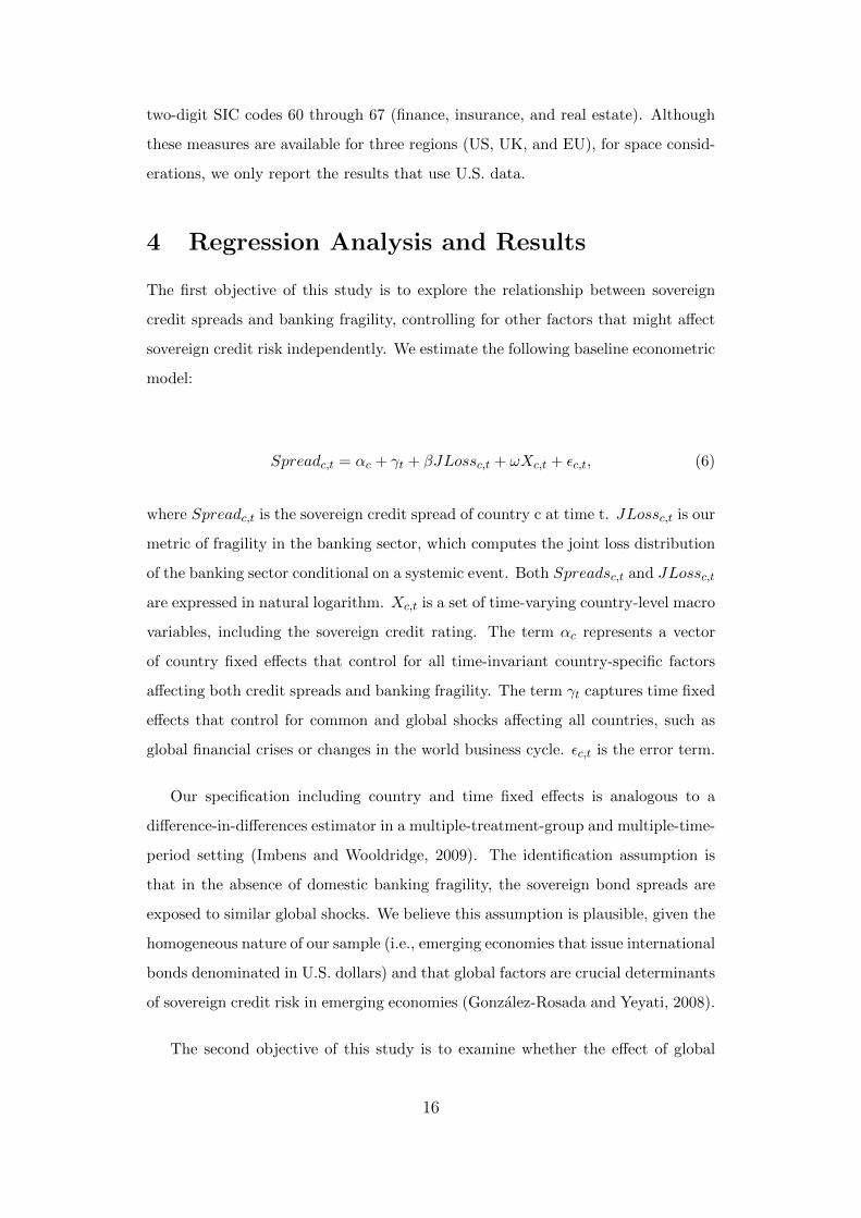
Table 3 provides summary information for the sovereign credit spreads by coun-

try. The average values of the spreads range widely across countries. The lowest

average is 135 basis points for China; the highest average is 1,405 basis points for

Argentina. Both the standard deviations and the minimum/maximum values indi-

cate significant variations also exist over time within countries. For example, the

credit spread for Argentina ranges from 204 to 7,078 basis points during the sample

period.

3.2 Banking Fragility

Our key explanatory variable of interest is our metric of banking fragility (JLoss).

JLoss is calculated using stock market and balance-sheet data of commercial banks

that are listed in the stock market of the 19 emerging economies in our sample.

Table A.2 in the appendix reports the number of banks by each country. Figure 1

displays the JLoss metric for each of the 19 emerging countries in the sample.

6Standard and Poor’s (2001) defines a foreign-currency credit rating as “A current opinion of anobligor’s overall capacity to meet its foreign-currency-denominated financial obligations. It may takethe form of either an issuer or an issue credit rating. As in the case of local currency credit ratings, aforeign currency credit opinion on Standard and Poor’s global scale is based on the obligor’s individualcredit characteristics, including the influence of country or economic risk factors. However, unlike localcurrency ratings, a foreign currency credit rating includes transfer and other risks related to sovereignactions that may directly affect access to the foreign exchange needed for timely servicing of the ratedobligation. Transfer and other direct sovereign risks addressed in such ratings include the likelihood offoreign exchange control and the imposition of other restrictions on the repayment of foreign debt.”

13

As shown in Figure 1, in most countries our JLoss metric captures both periods

of global financial distress and periods of country-specific idiosyncratic banking

fragility. In many countries, idiosyncratic factors seems to have stronger effects

on banking fragility than global factors. For example, for the case of Argentina

our metric shows that the fragility generated by the sub-prime crisis was smaller

than the fragility generated by the 2001 Argentinean sovereign default. In Brazil,

idiosyncratic factors such as the ”Impeachment” of Dilma Rousseff also seem to

have a much stronger effect on banking fragility than global banking fragility.

3.3 Country-Specific Factors

To capture the domestic macro environment, we also control for a set of time-varying

country-level macro variables that may directly affect sovereign credit risk: debt to

GDP, exchange-rate volatility, profit margin in the banking sector, and GDP per

capita. As previously mentioned, we also control for the long-term foreign-currency

sovereign credit rating. The debt-to-GDP ratio captures the degree of the economy

indebtedness. Exchange-rate volatility is the volatility of the country’s exchange

rate against the U.S. dollar. We added this variable because it is considered a

major determinant of firms’ revenues from abroad and their ability to repay debts

denominated in dollars. Profit margin in the banking sector captures the degree

of competitiveness in the domestic financial sector. Sovereign credit ratings are

credit-rating agencies’ opinion of a government’s overall capacity to meet its foreign-

currency-denominated financial obligations.

3.4 Global Factors

Far from being autarkies, the emerging economies included in this paper have in-

creasingly become more financially integrated with the rest of the world. Therefore,

their ability and willingness to serve their debt may depend not only on macroeco-

nomic domestic conditions, but also on the state of the global economy. To capture

broad changes in the state of the global (exogenous) financial markets, we consider

a set of global financial factors that reflect financial market volatility, risk-free in-

terest rates, risk premiums, and market liquidity. Specifically, the global financial

factors used in this study are the CBOE Volatility Index, the 10-year U.S. Trea-

14

sury rate, the 10-year U.S. High Yield spread, and the On/off-the-run U.S. Treasury

spread. For robustness, as we explain in the next section, we also control for a large

number of measures of systemic risk proposed in the literature.

The CBOE Volatility Index, known commonly as the VIX, measures the mar-

ket’s expectation for 30-day volatility in the S&P 500. Usually, a higher VIX

indicates a general increase in the risk premium and, consequently, an increase in

the cost of financing for emerging economies. The 10-year U.S. Treasury rate ad-

dresses the interest rate effect. It reflects the risk-free rate against which investors

in advanced economies evaluate the payoffs of all other assets of similar maturities.

The high-yield spread proxies for the price of risk in the global financial market. We

employ J. P. Morgan’s High Yield Spread Index, which measures the spread over

the U.S. Treasuries yield curve. Lastly, the On/off-the-run U.S. Treasury spread

is the spread between the yield of on-the-run and off-the-run U.S. Treasury bonds.

Although the issuer of both types of bonds is the same, on-the-run bonds generally

trade at a higher price than similar off-the-run bonds, because of the greater liq-

uidity and specialness of on-the-run bonds in the repo markets.7 We compute the

On/off-the-run U.S. Treasury spread using 10-year bonds, given that the spread

tends to be small and noisy at smaller maturities. The data sources used in the

construction of this spread are from Gurkaynak et al. (2007) and the Board of

Governors of the Federal Reserve System.

3.5 Systemic Risk Measures

Finally, for robustness purpose, in some regressions we augment our baseline spec-

ification with 19 systemic risk measures: Absorption, AIM, CoVaR, CoVaR, MES,

MES-BE, Book leverage, CatFin, DCI, Def. spr, Absorption, Intl. spillover, GZ,

Size conc., Mkt lvg., Volatility, TED spr., Term spr., and Turbulence. We also em-

ploy the systemic risk index (PQR) of the mentioned systemic risk measures. We

obtain this data from Giglio, Kellya and Pruitt (2016). Given that these measures

are constructed to capture systemic risk stemming from the core of the financial

system, these measures are based on data for financial institutions identified by

7This specialness arises from the fact that on-the-run Treasury bond holders are frequently able topledge these bonds as collateral and borrow in the repo market at considerably lower interest rates thanthose of similar loans collateralized by off-the-run Treasury bonds (Sundaresan and Wang, 2009).

15

two-digit SIC codes 60 through 67 (finance, insurance, and real estate). Although

these measures are available for three regions (US, UK, and EU), for space consid-

erations, we only report the results that use U.S. data.

4 Regression Analysis and Results

The first objective of this study is to explore the relationship between sovereign

credit spreads and banking fragility, controlling for other factors that might affect

sovereign credit risk independently. We estimate the following baseline econometric

model:

Spreadc,t = αc + γt + βJLossc,t + ωXc,t + εc,t, (6)

where Spreadc,t is the sovereign credit spread of country c at time t. JLossc,t is our

metric of fragility in the banking sector, which computes the joint loss distribution

of the banking sector conditional on a systemic event. Both Spreadsc,t and JLossc,t

are expressed in natural logarithm. Xc,t is a set of time-varying country-level macro

variables, including the sovereign credit rating. The term αc represents a vector

of country fixed effects that control for all time-invariant country-specific factors

affecting both credit spreads and banking fragility. The term γt captures time fixed

effects that control for common and global shocks affecting all countries, such as

global financial crises or changes in the world business cycle. εc,t is the error term.

Our specification including country and time fixed effects is analogous to a

difference-in-differences estimator in a multiple-treatment-group and multiple-time-

period setting (Imbens and Wooldridge, 2009). The identification assumption is

that in the absence of domestic banking fragility, the sovereign bond spreads are

exposed to similar global shocks. We believe this assumption is plausible, given the

homogeneous nature of our sample (i.e., emerging economies that issue international

bonds denominated in U.S. dollars) and that global factors are crucial determinants

of sovereign credit risk in emerging economies (Gonzalez-Rosada and Yeyati, 2008).

The second objective of this study is to examine whether the effect of global

16

(exogenous) financial factors on sovereign credit spreads is stronger in countries

with more vulnerable banking sectors. To explore this hypothesis, we estimate the

following model:

Spreadc,t = αc + βJLossc,t + γGlobalt + θJLossc,t x Globalt + ωXc,t + εc,t, (7)

where Globalt is a global (exogenous) financial factor at time t. The coefficient

associated with the interaction term, JLossc,t x Globalt, captures whether the

impact of global financial factors on sovereign credit spreads differs in countries with

different degrees of banking fragility in their banking sectors. We hypothesize that

in a financially integrated world where domestic banks and international capital

markets work as substitute sources of capital, a stronger banking sector should

attenuate a country’s exposure to global financial factors.

4.1 Sovereign Bond Spreads and Banking Fragility

Table 4 presents the results from the estimation of equation (6) with different sets

of control variables. The model is estimated by ordinary least squares (OLS) with

robust standard errors. The table also reports the estimates of our econometric

model by directly including global financial factors instead of time fixed effects.

The results suggest sovereign credit spreads are positively related to our metric of

banking fragility (JLoss). This positive correlation between JLoss and sovereign

credit spreads is statistically significant and economically meaningful, even after

controlling for country and time fixed effects (column 1), for sovereign credit ratings

(column 2), and for the standard determinants of sovereign credit risk (column

3). We also find similar results when we control for our set of global financial

factors instead of time fixed effects (column 4). Given that both the spread and the

JLoss metric are expressed in natural logarithm, each of our estimated coefficients

represent an elasticity. In terms of the economic magnitude of our findings, the

coefficient reported in column 1 suggests that, on average, a 100-percent increase in

our JLoss measure raises the sovereign credit spread by 22 percent. The coefficient

reported in column 3 suggests that a comparable increase in JLoss raises the average

spread by 13 percent. Our regressions appear to support the view that banking

17

fragility exerts a strong influence on the pricing of emerging-market sovereign bonds.

Despite the high correlation in our country-level control variables, most of the

estimated coefficients of our control variables are statistically significant in the

expected direction. On the one hand, the results show that sovereign credit ratings

and bank profits are negatively related to credit spreads. On the other hand,

the results show indebtedness, global financial instability, exchange rate volatility,

global premiums, and aggregate market illiquidity are positively related to spreads.

4.2 Are Countries with Fragile Banking Sectors More

Exposed to Global Financial Shocks?

Although the literature has explored the relevance of external factors as significant

determinants of sovereign credit risk in emerging economies (see, e.g., Gonzalez-

Rosada and Yeyati, 2008), little research has explored the aspects that make a

country more or less resilient to sudden changes in the external context. We ex-

plore whether global financial factors affect sovereigns differently depending on the

fragility of their banking sectors. Given that the emerging economies included in

this paper have increasingly become more financially integrated with the rest of the

world and that domestic and international capital markets can provide an alterna-

tive source of funding that can complement bank financing, we hypothesize that

global financial conditions should typically have a smaller effect on countries with

more resilient banking sectors.

Table 5 report the results from the estimation of two specification of equation

(7). The table reports the estimates of our econometric model including time fixed

effects (columns 1 to 4) and global financial factors instead of time fixed effects

(columns 5 to 8). As before, the model is estimated by ordinary least squares (OLS)

with robust standard errors. The positive and statistically significant coefficients

associated with the interaction terms in columns 1 to 4 in Table 5 indicate that a

deterioration in global market volatility, risk-free interest rates, high-yield spreads,

and aggregate liquidity produce a higher increase in sovereign credit spreads of

countries with more fragile banking sectors. These effects are highly statistically

significant and economically meaningful. Columns 5 to 8 in the table 5, which

18

consider the direct effects of global financial factors instead of time fixed effects,

show almost qualitatively identical results.

To analyze the magnitude of the impact of global factors on sovereign credit

spreads across different levels of banking fragility, we show in Figure 3 the partial

effect of each of our global factors at different levels of banking fragility.8 The mag-

nitudes and confidence intervals reported in the figures suggest that the effect of the

VIX index and the U.S. high yield on sovereign spreads are either zero or positive,

and they become positive and larger in economies with more fragile banking sectors.

The marginal effects of the U.S. treasury rate and aggregate illiquidity on sovereign

spreads are negative for low levels of banking fragility, zero for moderate levels

of banking fragility, and positive for high levels of banking fragility. Given that

sovereign spreads measures the average spread on U.S. dollar-denominated bonds

issued by sovereign entities over U.S. Treasuries, it is expected the marginal effect

of US Treasury rate is negative for low values of banking fragility. Overall, these

magnitudes suggest that countries with more fragile banking sectors are more ex-

posed to global (exogenous) financial factors than those with more resilient banking

sectors.Thus, our results suggest that stability of the banking sector is a precondi-

tion to become more resilient to global shocks and underscore that regulators must

ensure the stability of the banking sector to improve governments’ borrowing costs

in international debt markets.

5 Robustness Checks

We conduct a number of exercises to check the robustness of our main results. First,

we split our sample between periods of financial stability and periods of banking

crises. Next, we explore whether our interaction terms may be capturing other

non-linear effect of global factors on sovereign credit spreads. Finally, we control

for a large set of measures of systemic risk proposed in the literature to capture

systemic risk stemming from the core of the financial system.

Given that our metric of banking fragility in the banking sector spikes during

8It is important to note that if the relationship between global factors and sovereign credit spreads isjust a simple correlation caused by common macroeconomic factors rather than by a causal effect, globalfactors should always affect spreads in a similar way.

19

periods of systemic banking crises, our results are likely driven by a few observa-

tions that capture a very high correlation between sovereign risk and banking risk

during periods of financial turmoil. Columns 1 of Table 6 reports the results from

estimating our baseline regressions for the periods of financial stability. Column 2

reports the results for periods of systemic banking crises. The systemic-banking-

crises dummy variable used to divide our sample was constructed using the dataset

introduced by Laeven and Valencia (2018). The results are qualitatively identical

to our baseline regressions reported in Tables 4. As expected, the magnitude of our

coefficients decrease for the periods of financial stability and increase for the periods

of banking crises. However, in both specifications, they remain highly statistically

significant and economically meaningful in the expected directions.

Because our primary term of interest in Table 5 is the interaction between

JLoss and our four global factors, it is likely that JLoss may captures the effect

of another country-specific factor. Table 7 presents the results of a more explicit

test of this possibility by including a number of additional interaction terms. The

added terms correspond to the interaction of the sovereign credit rating and a

banking-crisis dummy variable with our four different measures associated with

global factors, respectively. Columns 1 to 4 augment our previous model with the

interaction between global financial factors and sovereign credit ratings. Columns

5 to 8 augment our previous model with the interaction between global factors and

banking crises. Overall, our main findings remain unchanged. That is, the effects of

the VIX index, the High Yield spread and the On/off-the-run spread on sovereign

spreads is larger in countries with more fragile banking sectors.

Finally, we control for a large collection of systemic risk measures proposed

in the literature: Absorption, AIM, CoVaR, CoVaR, MES, MES-BE, Book lever-

age, CatFin, DCI, Def. spr, Absorption, Intl. spillover, GZ, Size conc., Mkt lvg.,

Volatility, TED spr., Term spr., and Turbulence. We also employ the systemic risk

index (PQR) of the mentioned systemic risk measures. We take these measures

from Giglio, Kellya and Pruitt (2016). For space considerations, we only use the

measures for the US. The results reported in Table 8 show that the coefficients

associated with our JLoss measure remains positive and highly significant in all the

20 models. Our main finding proved to be robust to controlling for a large set of

20

systemic risk measures. Thus, our JLoss metric seems to capture not only systemic

risk factors but also idiosyncratic factors that are not capture on global financial

measures.

6 Conclusion

The global financial crisis of 2008-09 and the European debt crisis generated large

losses in the banking sector, triggering a significant deterioration of sovereign credit

risk with the greater expectation of public support for distressed banks. These

events spurred a renewed interest in generating new measures of banking fragility

as well as in understanding the consequences of such vulnerabilities. Despite a new

large body of research on the relationship between sovereign risk and bank risk in

the eurozone, rigorous research on the nexus between sovereign risk and bank risk

in emerging markets is scant. A better understanding of the factors influencing

sovereign risk and of how these factors can be properly measured in both advanced

and emerging economies is of key importance.

The goal of this paper is to shed light on the relationship between sovereign

credit risk and banking fragility in the banking sector. To achieve this goal, we

develop a novel model-based semi-parametric metric (JLoss) that computes the

joint-loss distribution of a country’s banking sector conditional on a systemic event.

We find that, controlling for country-level macro variables as well as for country and

time fixed effects, our metric of banking fragility (JLoss) is positively associated

with sovereign credit spreads and negatively associated with higher sovereign credit

ratings in our sample of emerging economies.

We also explore whether bank stability reduce a country’s exposure to global

financial factors. A better understanding of the mechanisms through which global

factors influence sovereign credit risk is crucial. As highlighted by Gonzalez-Rosada

and Yeyati (2008), emerging economies need to formulate mechanisms to reduce

their exposure to global financial factors, as the process of financial integration

exhibited over the past four decades brings contagion from other advanced and

emerging economies. Our results indicate that countries with more fragile banking

sectors are more exposed to the influence of global financial factors.

21

Our results have important policy implications because they underscore that

the stability of a country’s domestic banking sector plays a crucial role in reduc-

ing sovereign risk and its sensitivity to global factors. Therefore, countries must

implement policies oriented to improve the stability of their banking sectors to im-

prove their access to international capital and reduce potentially undesired effects

of integration.

This study on the relationship between our metric of banking fragility (JLoss)

and sovereign credit spread is a first approach to explore the validity and power

of our metric. Future research should focus on the effect of our JLoss metric on

corporate credit risk and firm level performance. More granular data at the firm

and bond levels should also allow us to have a more clean identification strategy to

examine causal effects of interest.

22

References

[1] Acharya, V., and Naqvi, H. The seeds of a crisis: A theory of bank liquidity

and risk taking over the business cycle. Journal of Financial Economics 106,

2 (2012), 349–366.

[2] Ang, A., and Longstaff, F. A. Systemic sovereign credit risk: Lessons

from the us and europe. Comision Presidencial de Isapres 60, 5 (2013), 493–

510.

[3] Barndorff-Nielsen, O., N. E., and Shepard, N. Some recent develop-

ments in stochastic volatility modelling. Journal Quantitative Finance 2, 1

(2002), 11–23.

[4] Black, L., C. R. H. X., and Zhou, H. The systemic risk of european banks

during the financial and sovereign debt crises. Journal of Banking Finance

(2016).

[5] Boehmer, E., and Megginson, W. L. Determinants of secondary market

prices for developing country syndicated loans. The Journal of Finance 45, 5

(1990), 1517–1540.

[6] Borensztein, E., Cowan. K., and Valenzuela, P. Sovereign ceilings

“lite”?: The impact of sovereign ratings on corporate ratings. Journal of

Banking and Finance 37, 11 (2013), 4014–4024.

[7] Brownlees, C., and Engle, R. F. Srisk: A conditional capital shortfall

measure of systemic risk. The Review of Financial Studies 30, 1 (2016), 48–79.

[8] Cavallo, E., and Valenzuela, P. The determinants of corporate risk in

emerging markets: an option-adjusted spread analysis. International Journal

of Finance and Economics 15, 1 (2010), 59–74.

[9] Dieckmann, S., and Plank, T. Default risk of advanced economies: An

empirical analysis of credit default swaps during the financial crisis. Review of

Finance 16, 4 (2012), 903–934.

[10] Edwards, S. The pricing of bonds and bank loans in international markets:

An empirical analysis of developing countries’ foreign borrowing. European

Economic Review 30, 3 (1986), 565–589.

23

[11] Farhi, E., and Tirole, J. Collective moral hazard, maturity mismatch, and

systemic bailouts. American Economic Review 102, 1 (2012), 60–93.

[12] Fratzscher, M., and Rieth, M. H. Monetary policy, bank bailouts and

the sovereign-bank risk nexus in the euro area. Review of Finance, 23 (2019),

745–775.

[13] Georgoustsos, D., and Migiakis, P. Heterogeneity of the determinants of

euro-area sovereign bond spreads; what does it tell us about financial stability?

Journal of Banking Finance (2013).

[14] Giglioa, S., K. B., and Pruitt, S. Systemic risk and the macroeconomy:

An empirical evaluation. Journal of Banking Finance (2016).

[15] Gonzalez-Rozada, M., and Yeyati, E. L. Global factors and emerging

market spreads. The Economic Journal 118, 533 (2008), 1917–1936.

[16] Gurkaynak, R. S., Sack. B., and Wright, J. H. The us treasury yield

curve: 1961 to the present. Journal of Monetary Economics 54, 8 (2007),

2291–2304.

[17] Hilscher, J., and Nosbusch, Y. Determinants of sovereign risk: Macroe-

conomic fundamentals and the pricing of sovereign debt. Review of Finance

14, 2 (2010), 235–262.

[18] Hu, G. X., Pan. J., and Wang, J. Noise as information for illiquidity. The

Journal of Finance 68, 6 (2013), 2341–2382.

[19] Imbens, G. W., and Wooldridge, J. M. Recent developments in the

econometrics of program evaluation. Journal of Economic Literature 47, 1

(2009), 5–86.

[20] Kallestrup, R., Lando. D., and Murgoci, A. Financial sector linkages

and the dynamics of bank and sovereign credit spreads. Journal of Empirical

Finance 38 (2016), 374–393.

[21] Kealhofer, S., and Kurbat, M. Benchmarking quantitative default risk

models: A validation methodology. Research Paper, Moody’s KMV (2000).

[22] Koylouglu, H., and Hickman, A. Reconcilable differences. Risk 11, 10

(1998), 56–62.

24

[23] Laeven, L., and Valencia, F. Systemic banking crises revisited. Working

Paper No. 18/206 (2018).

[24] Longstaff, F. A., Pan. J. Pedersen. L. H., and Singleton, K. J. How

sovereign is sovereign credit risk? American Economic Journal: Macroeco-

nomics 3, 2 (2011), 75–103.

[25] Martin, R., Thompson. K., and Browne, C. Taking to the saddle: An

analytical technique to construct the loss distribution of correlated events.

Risk-London-Risk Magazine Limited 14, 6 (2001), 91–94.

[26] Merton, R. C. On the pricing of corporate debt: The risk structure of

interest rates. The Journal of Finance 29, 2 (1974), 449–470.

[27] Mody, A., and Sandri, D. The eurozone crisis: How banks and sovereigns

came to be joined at the hip. Economic Policy 27, 70 (2012), 199–230.

[28] Press, W. H., Teukolsky. S. A. Vetterling. W. T., and Flannery,

B. P. Numerical Recipes 3rd Edition: The Art of Scientific Computing. Cam-

bridge University Press, 2007.

[29] Standard, and Poor’s. Rating methodology: Evaluating the issuer, 2001.

http://www.standardandpoors.com/.

[30] Sundaresan, S., and Wang, Z. Y2k and liquidity premium in treasury

bond markets. Review of Financial Studies 22, 3 (2009), 1021–1056.

[31] Valerie, O., G. M. S. G., and Vennet, R. Bank/sovereign risk spillovers

in the european debt crisis. Journal of Banking Finance (2013).

[32] Vasicek, O. The loan loss distribution. KMV Corporation (1997).

25

Table 1: Parameters Saddle-Point Estimation

Parameters Value

Time horizon 1 quarter

Loss given default (LGD) 45%

Approximation nodes 7

Number of systemic factors 1

Loses lower bound 0.010

Loses upper bound 0.048

Number of steps 500

Percentile 0.99

Systemic driver N(0, 0.16%)

Note: This table reports the parameterization used in the Jloss calculation once the individual expected default

frequencies are calculated.

26

Table 2: Descriptive Statistics

Variables N Mean Standard Minimum Maximum

Deviation

Sovereign Credit Risk

EMBI spread 1,406 3.913 6.336 -0.0300 70.78

S&P rating 1,406 11.44 3.545 1 18

Banking fragility

JLoss 1,406 6.804 9.057 0 47.16

Control Variables

Profit margin 1,348 20.19 36.34 -789.5 138.6

Exchange rate volatility 1,329 14.38 61.01 0 932.8

Debt to GDP 1,391 45.66 22.21 3.879 147.2

GDP per capita 1,406 7,021 4,278 534 16,056

VIX 1,406 20.07 8.509 9.510 53.54

U.S. treasury rate 1,406 3.211 1.301 0.657 6.442

High yield spread 1,406 5.201 2.583 2.380 17.22

On/off-the-run spread 1,406 0.114 0.112 -0.0182 0.518

Note: This table reports basic descriptive statistics (mean, standard deviation, minimum and maximum values) of the

outcome and control variables used in the regression analysis for the overall sample.

27

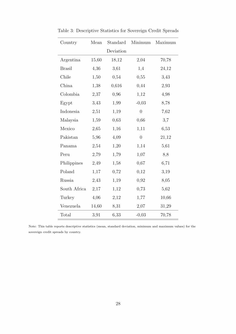
Table 3: Descriptive Statistics for Sovereign Credit Spreads

Country Mean Standard Minimum Maximum

Deviation

Argentina 15,60 18,12 2,04 70,78

Brasil 4,36 3,61 1,4 24,12

Chile 1,50 0,54 0,55 3,43

China 1,38 0,616 0,44 2,93

Colombia 2,37 0,96 1,12 4,98

Egypt 3,43 1,99 -0,03 8,78

Indonesia 2,51 1,19 0 7,62

Malaysia 1,59 0,63 0,66 3,7

Mexico 2,65 1,16 1,11 6,53

Pakistan 5,96 4,09 0 21,12

Panama 2,54 1,20 1,14 5,61

Peru 2,79 1,79 1,07 8,8

Philippines 2,49 1,58 0,67 6,71

Poland 1,17 0,72 0,12 3,19

Russia 2,43 1,19 0,92 8,05

South Africa 2,17 1,12 0,73 5,62

Turkey 4,06 2,12 1,77 10,66

Venezuela 14,60 8,31 2,07 31,29

Total 3,91 6,33 -0,03 70,78

Note: This table reports descriptive statistics (mean, standard deviation, minimum and maximum values) for the

sovereign credit spreads by country.

28

Table 4: Sovereign Credit Spreads and Banking fragility

EMBI spread (1) (2) (3) (4)

Jloss 0.217*** 0.152*** 0.134*** 0.144***

(0.0221) (0.0186) (0.0204) (0.0188)

Rating S&P -0.121*** -0.112*** -0.117***

(0.00884) (0.00915) (0.00942)

Exchange rate volatility 0.0681** 0.0536**

(0.0275) (0.0268)

Profit Margin -0.0240 -0.0492***

(0.0183) (0.0181)

Debt to GDP 0.199*** 0.236***

(0.0444) (0.0419)

GDP per capita 0.145*** 0.194***

(0.0545) (0.0405)

VIX 0.0658

(0.0447)

US treasury -0.125**

(0.0508)

US high yield 0.358***

(0.0671)

On/Off-the-run spread 0.238

(0.155)

Observations 1,406 1,406 1,223 1,223

R-squared 0.726 0.798 0.789 0.773

Adjusted R-squared 0.708 0.785 0.773 0.768

Country FE YES YES YES YES

Time FE YES YES YES NO

Note: This table reports estimates from panel regressions of sovereign credit spreads against banking fragility (JLoss) and

a comprehensive set of determinants of sovereign credit risk. Models 1 to 3 control for country and time fixed effects.

Model 4 controls for global factors instead of time fixed effects. Robust standard errors are in parentheses below each

coefficient estimate. ***, **, and * indicate significance at the 1, 5, and 10 percent levels, respectively.

29

Table 5: Sovereign Credit Spreads, Banking Fragility, and Global Financial Factors

EMBI spread (1) (2) (3) (4) (5) (6) (7) (8)

Jloss -0.442*** 0.0819 -0.274*** 0.0485** -0.231** -0.114** -0.0943 0.0724***

(0.0823) (0.0531) (0.0544) (0.0218) (0.106) (0.0549) (0.0645) (0.0219)

Rating S&P -0.112*** -0.112*** -0.112*** -0.111*** -0.118*** -0.116*** -0.117*** -0.116***

(0.00912) (0.00918) (0.00907) (0.00910) (0.00939) (0.00950) (0.00938) (0.00940)

Exchange rate volatility 0.0655** 0.0694** 0.0612** 0.0771*** 0.0586** 0.0655** 0.0576** 0.0688***

(0.0264) (0.0276) (0.0261) (0.0267) (0.0266) (0.0267) (0.0266) (0.0266)

Profit Margin -0.0249 -0.0243 -0.0222 -0.0228 -0.0527*** -0.0453** -0.0516*** -0.0495***

(0.0175) (0.0183) (0.0172) (0.0175) (0.0181) (0.0183) (0.0181) (0.0182)

Debt to GDP 0.193*** 0.193*** 0.201*** 0.176*** 0.228*** 0.206*** 0.236*** 0.220***

(0.0447) (0.0455) (0.0434) (0.0443) (0.0421) (0.0433) (0.0415) (0.0422)

GDP per capita 0.130** 0.139** 0.122** 0.0979* 0.197*** 0.168*** 0.188*** 0.166***

(0.0548) (0.0546) (0.0544) (0.0543) (0.0402) (0.0408) (0.0403) (0.0404)

VIX -0.151** 0.0836* 0.0721 0.0910**

(0.0716) (0.0446) (0.0450) (0.0445)

US treasury -0.106** -0.490*** -0.109** -0.113**

(0.0513) (0.0832) (0.0509) (0.0507)

US high yield 0.362*** 0.325*** 0.137 0.350***

(0.0668) (0.0665) (0.0865) (0.0662)

On/Off-the-run spread 0.165 0.266* 0.115 -1.010***

(0.158) (0.151) (0.158) (0.256)

VIX X Jloss 0.191*** 0.125***

(0.0270) (0.0352)

U.S Treasury rate X Jloss 0.0383 0.189***

(0.0363) (0.0382)

High Yield spread x Jloss 0.223*** 0.131***

(0.0278) (0.0339)

On/Off-the-run spread x Jloss 0.744*** 0.596***

(0.103) (0.103)

Observations 1,223 1,223 1,223 1,223 1,223 1,223 1,223 1,223

R-squared 0.801 0.789 0.802 0.799 0.776 0.778 0.776 0.780

Adjusted R-squared 0.785 0.773 0.787 0.784 0.771 0.773 0.771 0.774

Country FE YES YES YES YES YES YES YES YES

Time FE YES YES YES YES NO NO NO NO

Note: This table reports estimates from panel regressions of sovereign credit spreads against banking fragility (JLoss) and

a comprehensive set of determinants of sovereign credit risk. Models 1 to 4 control for country and time fixed effects.

Models 5 to 8 control for global factors instead of time fixed effects. Robust standard errors are in parentheses below each

coefficient estimate. ***, **, and * indicate significance at the 1, 5, and 10 percent levels, respectively.

30

Table 6: Periods of Financial Stability versus Periods of Crises

EMBI spread Periods of financial stability Periods of banking crises

Jloss 0.103*** 0.183***

(0.0226) (0.0497)

Rating S&P -0.106*** -0.111***

(0.00953) (0.0261)

Exchange rate volatility 0.0715** 0.0869*

(0.0304) (0.0485)

Profit Margin 0.00215 -0.0482**

(0.0201) (0.0230)

Debt to GDP 0.235*** -0.356

(0.0525) (0.236)

GDP per capita 0.132** -0.0286

(0.0592) (0.254)

Observations 1,010 213

R-squared 0.784 0.920

Adjusted R-squared 0.766 0.902

Country FE YES YES

Time FE YES YES

Note: This table reports estimates from panel regressions of sovereign credit spreads against banking fragility (JLoss) and

a comprehensive set of determinants of sovereign credit risk. The models control for country and time fixed effects.

Robust standard errors are in parentheses below each coefficient estimate. ***, **, and * indicate significance at the 1, 5,

and 10 percent levels, respectively.

31

Table 7: Robustness: Alternative Non-linear Effects

EMBI spread (1) (2) (3) (4) (5) (6) (7) (8)

Jloss -0.408*** 0.0885 -0.246*** 0.0480** -0.375*** 0.0687 -0.253*** 0.0536**

(0.0882) (0.0538) (0.0560) (0.0217) (0.0917) (0.0538) (0.0675) (0.0222)

Rating S&P -0.129*** -0.0710*** -0.134*** -0.111*** -0.112*** -0.111*** -0.112*** -0.111***

(0.0162) (0.0136) (0.0131) (0.00913) (0.00909) (0.00904) (0.00903) (0.00908)

Exchange rate volatility 0.0623** 0.0755*** 0.0547** 0.0767*** 0.0620** 0.0677** 0.0607** 0.0755***

(0.0267) (0.0272) (0.0270) (0.0267) (0.0262) (0.0270) (0.0260) (0.0267)

Profit Margin -0.0238 -0.0239 -0.0213 -0.0228 -0.0229 -0.0205 -0.0221 -0.0228

(0.0176) (0.0181) (0.0173) (0.0175) (0.0170) (0.0174) (0.0167) (0.0170)

Debt to GDP 0.197*** 0.131*** 0.205*** 0.178*** 0.185*** 0.175*** 0.193*** 0.169***

(0.0450) (0.0444) (0.0437) (0.0442) (0.0437) (0.0444) (0.0425) (0.0435)

GDP per capita 0.130** 0.133** 0.126** 0.0982* 0.139** 0.143*** 0.131** 0.110**

(0.0549) (0.0554) (0.0543) (0.0546) (0.0541) (0.0541) (0.0540) (0.0540)

Banking crisis -0.611 4.082*** 0.123 0.125

(0.523) (1.069) (0.506) (0.356)

VIX x Jloss 0.180*** 0.168***

(0.0294) (0.0306)

VIX x Rating S&P 0.00598

(0.00441)

VIX x Banking crisis 0.266*

(0.137)

U.S. Treasury rate x Jloss 0.0346 0.0453

(0.0366) (0.0370)

U.S. Treasury rate x Rating S&P -0.0355***

(0.00953)

U.S. Treasury rate x Banking crisis -2.072***

(0.540)

High yield spread x Jloss 0.207*** 0.211***

(0.0295) (0.0367)

High yield spread x Rating S&P 0.0130**

(0.00537)

High yield spread x Banking crisis 0.0429

(0.193)

On/off-the-run spread x Jloss 0.748*** 0.695***

(0.103) (0.122)

On/off-the-run spread x Rating S&P 0.00356

(0.0205)

On/off-the-run spread x Banking crisis 0.328

(0.894)

Observations 1,223 1,223 1,223 1,223 1,223 1,223 1,223 1,223

R-squared 0.801 0.794 0.803 0.799 0.803 0.795 0.803 0.800

Adjusted R-squared 0.786 0.778 0.788 0.784 0.787 0.779 0.788 0.785

Country FE YES YES YES YES YES YES YES YES

Time FE YES YES YES YES YES YES YES YES

Note: This table reports estimates from panel regressions of sovereign credit spreads against banking fragility (JLoss), a

comprehensive set of determinants of sovereign credit risk, and interaction terms. All regressions control for country and

time fixed effects. Robust standard errors are in parentheses below each coefficient estimate. ***, **, and * indicate

significance at the 1, 5, and 10 percent levels, respectively.

32

Table 8: Robustness: Systemic Risk Measures

EMBI spread (1) (2) (3) (4) (5) (6) (7) (8) (9) (10)

Jloss 0.144*** 0.231*** 0.216*** 0.223*** 0.220*** 0.219*** 0.224*** 0.224*** 0.220*** 0.216***

(0.0188) (0.0264) (0.0265) (0.0263) (0.0258) (0.0266) (0.0263) (0.0261) (0.0266) (0.0267)

CATFIN 0.0463

(0.141)

PQR 5.343***

(1.780)

Absorption -0.829***

(0.260)

AIM 5.987

(4.216)

Book - LVG -5.248***

(1.529)

Covar -2.323*

(1.336)

DCI -0.660**

(0.264)

Def - SPR -0.209***

(0.0472)

Delta Absorption 0.582**

(0.252)

Delta Covar -6.791***

(2.614)

Observations 1,223 695 695 695 695 695 695 695 695 695

R-squared 0.773 0.782 0.784 0.780 0.783 0.780 0.781 0.786 0.782 0.781

Adjusted R-squared 0.768 0.773 0.775 0.771 0.775 0.771 0.772 0.777 0.773 0.773

Control variables YES YES YES YES YES YES YES YES YES YES

Country FE YES YES YES YES YES YES YES YES YES YES

Time FE NO NO NO NO NO NO NO NO NO NO

Note: This table reports estimates from panel regressions of sovereign credit spreads against banking fragility (JLoss) and

a comprehensive set of determinants of sovereign credit risk, including 20 alternative measures of systemic risk. Robust

standard errors are in parentheses below each coefficient estimate. ***, **, and * indicate significance at the 1, 5, and 10

percent levels, respectively.

33

EMBI spread (11) (12) (13) (14) (15) (16) (17) (18) (19) (20)

Jloss 0.213*** 0.206*** 0.217*** 0.227*** 0.219*** 0.227*** 0.221*** 0.228*** 0.228*** 0.228***

(0.0286) (0.0293) (0.0265) (0.0264) (0.0262) (0.0275) (0.0263) (0.0268) (0.0261) (0.0269)

GZ -0.0783**

(0.0346)

Intl. Spillover -2.46e-06

(0.00156)

MES -2.318***

(0.819)

MES - be -7.964***

(2.376)

Market Leverage -0.0172***

(0.00572)

Real vol. -1.441

(2.058)

Size Conc. 0.200***

(0.0569)

Ted-SPR -0.000571**

(0.000278)

Term-SPR 0.0258***

(0.00991)

Turbulence -0.000640*

(0.000379)

Observations 612 595 695 695 695 695 695 695 695 695

R-squared 0.792 0.790 0.782 0.783 0.782 0.780 0.783 0.781 0.781 0.781

Adjusted R-squared 0.782 0.781 0.773 0.774 0.773 0.771 0.774 0.772 0.773 0.772

Control variables YES YES YES YES YES YES YES YES YES YES

YES YES

Country FE YES YES YES YES YES YES YES YES YES YES

Time FE NO NO NO NO NO NO NO NO NO NO

Note: This table reports estimates from panel regressions of sovereign credit spreads against banking fragility (JLoss) and

a comprehensive set of determinants of sovereign credit risk, including 20 alternative measures of systemic risk. Robust

standard errors are in parentheses below each coefficient estimate. ***, **, and * indicate significance at the 1, 5, and 10

percent levels, respectively.

34

Inputs:• Probability of

default• Exposure• Correlations

Output:• Implied

probability density of joint losses

Saddle point method

Step 1:• Random Variable

Laplace transformation

Step 2:• Moment

generating functions (MGM)

Bromwich integral

Step 3:• Probability density

of losses

Martin (2001) calculations:• Marginal

contribution to risk• Expected and

unexpected losses

𝑃 =

𝑖=1

𝑁

𝑒𝑖 ∙ 1Ι𝐷𝑖

Jloss computation:𝐽𝑙𝑜𝑠𝑠𝑖,𝑡

=σ𝐽=1𝑁 𝑇𝑜𝑡𝑎𝑙 𝑙𝑜𝑠𝑠𝑒𝑠𝑗,𝑡

σ𝐽=1𝑁 𝐸𝑥𝑝𝑜𝑠𝑢𝑟𝑒𝑗,𝑡

Figure 1: JLoss Methology

35

Figure 2: JLoss by Country

36

Figure 2: JLoss by Country (continued)

37

Figure 2: JLoss by Country (continued)

38

Figure 3: Marginal effects of global factors on sovereign credit spreads conditional onvalues of banking fragility (Jloss). Dotted lines are 95 percent confidence bands.

39

Appendix

Table A.1 Description of Variables

Nam

eL

evel

Des

crip

tion

Fre

quen

cySou

rce

Regre

ssio

nA

naly

sis

EM

BI

spre

adC

ountr

yJ.P

.M

orga

nE

MB

IG

lobal

spre

ad(i

nlo

g)Q

uar

terl

yB

loom

ber

g

S&

Pra

ting

Cou

ntr

yS&

Pso

vere

ign

cred

itra

ting,

long-

term

deb

t,Q

uar

terl

yB

loom

ber

g

fore

ign

curr

ency

,21

=A

AA

-1=

SD

(in

log)

GD

Pp

erca

pit

aC

ountr

yU

SD

GD

Pp

erca

pit

a(i

nlo

g)Q

uar

terl

yIF

S

Deb

tto

GD

PC

ountr

yD

ebt

div

ided

by

GD

P(i

nlo

g)Q

uar

terl

yIF

S

Pro

fit

mar

gin

Cou

ntr

yP

rofit

mar

gin

(in

log)

Quar

terl

yB

loom

ber

g

Exch

ange

rate

vola

tility

Cou

ntr

yE

xch

ange

rate

vola

tility

(per

centa

gep

oints

)Q

uar

terl

yB

loom

ber

g

VIX

Glo

bal

CB

OE

Vol

atilit

yIn

dex

(in

log)

Quar

terl

yB

loom

ber

g

U.S

.T

reas

ury

rate

Glo

bal

U.S

Tre

asury

yie

ld10

year

s(i

nlo

g)Q

uar

terl

yB

loom

ber

g

Hig

hyie

ldsp

read

Glo

bal

J.P

.M

orga

nhig

hyie

ldsp

read

(in

log)

Quar

terl

yB

loom

ber

g

On/o

ff-t

he-

run

spre

adG

lobal

Diff

eren

ceb

etw

een

the

yie

ldto

mat

uri

tyof

10ye

ars

off-t

he-

run

Quar

terl

yB

oard

ofG

over

nor

sof

the

and

on-t

he-

run

Tre

asury

bon

ds

(in

log)

Fed

eral

Res

erve

Syst

em

the

yie

lds

from

asm

oot

hze

ro-c

oup

onyie

ldcu

rve

(in

log)

JL

oss

Com

puta

tion

Sto

ckm

arke

tin

dex

Cou

ntr

ySto

ckm

arke

tin

dex

Dai

lyB

loom

ber

g

Sto

ckpri

cere

turn

sB

ank

Sto

ckpri

cere

turn

sD

aily

Blo

omb

erg

Lon

gte

rmliab

ilit

ies

Ban

kL

ong

term

liab

ilit

ies

Quar

terl

yB

loom

ber

g

Shor

tte

rmliab

ilit

ies

Ban

kShor

tte

rmliab

ilit

ies

Quar

terl

yB

loom

ber

g

Ave

rage

ban

kin

tere

stra

tes

Ban

kA

vera

geban

kin

tere

stra

tes

Quar

terl

yB

loom

ber

g

Mar

ket

capit

aliz

atio

nB

ank

Mar

ket

capit

aliz

atio

nQ

uar

terl

yB

loom

ber

g

Vol

atilit

yof

stock

pri

ceB

ank

Vol

atilit

yof

stock

pri

ceQ

uar

terl

yB

loom

ber

g

Cor

rela

tion

tosy

stem

icfa

ctor

Ban

kC

orre

lati

onst

ock

retu

rnQ

uar

terl

yB

loom

ber

g

40

Table A.2 Banks per Country

Country Number of banks

Argentina 5

Brazil 11

Bulgaria 3

Chile 6

China 13

Colombia 6

Egypt 9

Indonesia 23

Malaysia 7

Mexico 4

Pakistan 20

Panama 2

Peru 5

Philippines 10

Poland 10

Russia 5

South Africa 3

Turkey 8

Venezuela 3

41

Documentos de Trabajo

Banco Central de Chile

NÚMEROS ANTERIORES

La serie de Documentos de Trabajo en versión PDF

puede obtenerse gratis en la dirección electrónica:

www.bcentral.cl/esp/estpub/estudios/dtbc.

Existe la posibilidad de solicitar una copia impresa

con un costo de Ch$500 si es dentro de Chile y

US$12 si es fuera de Chile. Las solicitudes se

pueden hacer por fax: +56 2 26702231 o a través del

correo electrónico: bcch@bcentral.cl.

Working Papers

Central Bank of Chile

PAST ISSUES

Working Papers in PDF format can be downloaded

free of charge from:

www.bcentral.cl/eng/stdpub/studies/workingpaper.

Printed versions can be ordered individually for

US$12 per copy (for order inside Chile the charge

is Ch$500.) Orders can be placed by fax: +56 2

26702231 or by email: bcch@bcentral.cl.

DTBC – 957Sovereign Credit Spreads, Banking Fragility, and Global FactorsAnusha Chari, Felipe Garcés, Juan Francisco Martínez, Patricio Valenzuela

DTBC – 956Four facts about relationship lending: The case of Chile 2012-2019Miguel Acosta-Henao, Sangeeta Pratap, Manuel Taboada

DTBC – 955Modeling S&P500 returns with GARCH modelsRodrigo Alfaro, Alejandra Inzunza

DTBC – 954Unconventional credit policies during crises: A structural analysis of the Chilean experience during the COVID-19 pandemicBenjamín García, Mario González, Sebastián Guarda, Manuel Paillacar

DTBC – 953A Macro Financial Model for the Chilean EconomyMauricio Calani, Benjamín García, Tomás Gómez, Mario González, Sebastián Guarda, Manuel Paillacar

DTBC – 952The double impact of deep social unrest and a pandemic: Evidence from ChileGent Bajraj, Jorge Lorca and Juan M. Wlasiuk

DTBC – 951On Foreign Drivers of EMEs FluctuationsGent Bajraj, Jorge Lorca and Juan M. Wlasiuk

DTBC – 950Market Incompleteness, Consumption Heterogeneity and Commodity Price ShocksDamian Romero

DTBC – 949The effects of the job retention program during the Covid pandemic on the Chilean firms and householdsJosé Cristi, Carlos Madeira

DTBC – 948The role of financial surveys for economic research and policy making in emerging marketsSofía Gallardo, Carlos Madeira

DTBC – 947Relatos de inflación: percepción y expectativas de los hogares chilenos durante la pandemia de Covid-19Ignacio Zapata, Daniel Pérez, Karlla Muñoz, Valentina Cortés

DTBC – 946Median Labor Income in Chile Revised: Insights from Distributional National AccountsJosé De Gregorio, Manuel Taboada

DTBC – 945Ownership Networks and Earnings InequalityFederico Huneeus, Borja Larrain, Mauricio Larrain, Mounu Prem

DTBC – 944Pass-through from monetary policy to bank interest rates: A-symmetry analysis Juan Francisco Martínez, Daniel Oda, Gonzalo Marivil

DOCUMENTOS DE TRABAJO Mayo 2022