Do foreign portfolio flows increase risk in emerging stock markets? Evidence from six Latin American...

DO FOREIGN PORTFOLIO FLOWS INCREASE RISK IN EMERGING STOCK MARKETS?

EVIDENCE FROM SIX LATIN AMERICAN COUNTRIES 1999-2008

Diego Alonso Agudelo Milena Castaño

No. 11‐19

2011

Do foreign portfolio flows increase risk in emerging stock markets?

Evidence from six Latin American countries 1999 -2008.

Abstract

Foreign portfolio flows have been blamed for causing instability in emerging markets,

especially during financial crises. This study measured the effect of foreign capital flows on

volatility and exposure to world market risk in the six largest Latin American stock markets:

Argentina, Brazil, Colombia, Chile, Mexico and Peru, for around 10 years including the

2008’s World financial crisis. This will test whether these flows cause instability for those

markets and increase their exposure to international stock market returns. A proprietary

database, from Emerging Portoflio.com and time series models, both univariate (ARCH -

GARCH) and multivariate (VAR), are used to estimate the effect foreign portfolio flows on

the risk variables and the causality of these effects. We found no strong evidence to support

the hypothesis that foreign flows cause instability in the Latin American stock markets, in

spite of some evidence of causing price pressure. Instead, the evidence points to a strong

dependence of market returns on international stock and foreign exchange markets, both in

means and in volatility, instrumental to transmit crisis to those markets.

Key Words: Foreign portfolio flows, Emerging Markets, market risk, ARCH-GARCH, VAR

JEL Classification: F32, G01, G15,

Introduction.

Increasing financial integration between financial markets around the world in the lasts 30 years

has brought new investment opportunities. International Investors have looked to take advantage

of important capital gains, increased diversification, foreign exchange appreciation and

differentials in interest rates. (Ferrer, 1999; Di tella, 2004). As part of an increasing interest on

financial integration, academics have been studying the effect of portfolio funds on emerging

financial markets. Whether foreign portfolio funds have been overall helpful or harmful for

emerging markets is a complex, and still not completely solved question, that reappears from

time to time, especially during times as the 2008 World financial crisis.

On the positive side, some authors have associated foreign portfolio funds to the decreasing cost

of capital for listed companies (Miller, 1999; Errunza y Miller, 2000; Bekaert y Harvey, 2000),

increasing market efficiency (Kim y Singal, 2000) and more diversification choices for investors

(Villariño, 2001).

On the other hand, Krugman (1998, 1999) and Stiglitz (2000) expressed fears of excessive

volatilities and inflation, increased boom and bust cycles and appreciation of exchange rates

caused by the instability of foreign investor’s flows and holdings. Unlike foreign direct

investment, which is widely regarded as beneficial, foreign portfolio flows are considered

potentially damaging for emerging economies. Foreign portfolio investments, sometimes dubbed

‘hot money’, might flee from a developing country at the first sign of trouble during times of

financial stress, further disrupting its capital markets. Empirical studies as Brennan and Cao

(1997), Warther (1995) and Griffin, Nardari y Stulz (2004) have supported this point of view.

Moreover, this behavior has been criticized in the context of the worldwide financial crises

during the 90's, especially the Mexican crisis (Villarino, 2001) and the Asian crisis. (Flood y de

Paterson, 2008). A more recent example is provided by the 2008 World financial crisis, when

most emerging markets experienced important withdrawals of foreign capital along with large

negative returns. As a consequence some economists have called for increasing regulation on

foreign flows to emerging markets (Rubin and Weisberg; 2003; Ffrench-Davis and Griffith-

Jones, 2002; Ito and Portes,1998; and Eichengreen 1999).

In contrast, Edwards (1999) argues against capital controls in emerging countries due to being

costly and ineffective in avoiding crises, and fostering corruption. Although most of the

emerging markets identified by Standard and Poors (2004) currently have few or no direct

barriers to the entry of foreign investors, still countries such as India, China, Colombia, India,

Indonesia, the Philippines, Saudi Arabia, Taiwan and Thailand have either formal restrictions for

foreign outflows or ceilings to foreign ownership. In Latin America, from 2007 to 2009,

Colombia and Brazil restricted the mobility of foreign flows in and out the security markets in

order to stabilize and mitigate appreciations of their currencies against the dollar. Still, the

question of whether foreign flow causes increasing risk in emerging markets is to be solved

empirically.

Excessive volatility is widely regarded as harmful in stock markets. From a theoretical

standpoint there are at least three reasons for this. First, classical Asset pricing models require

higher expected returns ( i.e. "Equitiy Risk premium") in more volatile markets (Cochrane,

2001), implying a higher cost of capital for projects and companies, and lower market value.

Second, in the efficient market literature (Fama, 1979) price is an unbiased estimator or the

intrinsic value of an asset, but higher volatilities reduce the value of market price as an indicator

for economic decisions, thus impairing the market efficiency (Shiller, 1981). Finally, in the

market microstructure models, higher volatility leads to lower liquidity, by increasing the

adverse selection and inventory costs for a market marker. (Ho y Stoll, 1981; Kyle, 1985;

Glosten and Milgrom, 1985).

Empirical evidence of increasing volatility in emerging markets due to foreign flows has been

provided by Bekaert, Harvey and Lumsdaine (2002), Frenkel y Menkhoff (2003), both studies

analyzing the period around the liberalization of the markets. Moreover, Bae, Chan y Ng (2004)

provide evidence at firm level that links higher volatility with share ownership by foreign

investors. Besides Richards (2005), provide evidence of increasing volatility due to foreign

trading in six emerging markets of Asia during a period just after the Asian crisis. However, the

issue is far from being settled: Rea (1996), Froot, O’Connell y Seasholes (2001) and Alemmanni

and Haas (2006) don’t find larger volatility related to foreign flows, whereas Choe, Kho, and

Stultz (1999), Bekaert and Harvey (1998), Henry (2000), y Kim and Singal (2000) can't find

evidence of increasing volatility on the liberalization of the markets.

Excessive comovement of emerging stock markets with international markets, as measured by

the beta or correlation, is also generally perceived as negative, at least for two reasons. First, it

clearly reduces the benefit of international diversification for both local and foreign investors in

emerging markets. Second, higher comovements are especially harmful during financial crises,

those times where risk reduction is likely to be needed the most (Bekaert y Harvey, 2003)..

Transmission of negative returns across stock markets has been shown being too large to be

justified by fundamental factors during crises, which has been dubbed ‘Contagion’ (Bekaert y

Harvey, 2003). Contagion has been attributed to portfolio recomposition or behavioural effects

by international traders (Bikhchandani, Hirshleifer and Welch, 1992; Calvo 1998; Calvo and

Mendoza, 2000). Whereas increasing correlation upon liberalization has been evidenced in

different studies (Bekaert y Harvey, 2000), the eventual link between foreign flows and

increasing correlation in a post-liberalization period hasn't been tested to our knowledge.

In this context, we study the effects of foreign portfolio flows on six Latin American emerging

stock markets: Argentina, Brazil, Chile, Colombia, México and Perú. We estimate the effects of

those short-term flows on two risk measures: First, the volatility of the local stock market returns

and, second, the local market systemic risk, measured as the market sensitivity (beta) to

international stock market returns. This is achieved modeling the relationship between risk

measures, and measures of foreign flows, in two type of econometric models of the return:

univariate ARCH_GARCH models at daily frequency, return, and multivariate 4-VAR models

at monthly frequency. In both types of models, it is critical to control for variables that might

well explain increasing risk, as international equity market returns and foreign exchange rate

returns.

This paper contributes to the literature by testing directly a relationship between foreign flows

and increasing betas, which hasn't been done before. Besides, it uses a proprietary database of

foreign flows that hasn't been used in this branch of study, and more updated data that reflects

the effects of foreign flows in Latin-America during the 2008 World financial crisis.

This paper is organized as follows: The first section describes the data set used and examines the

evolution and possible relationships between the variables in the studied period, the second

section explains the econometric models used to test them and defines the hypothesis to be

tested, the third section presents and discusses the results, and finally, fourth section concludes

and presents suggestions for future research.

Data.

This study comprises the six largest stock exchanges of Latin America: Argentina, Brazil, Chile,

Colombia, México and Perú. Summary statistics for the markets are presented in Table 1.

Portfolio flows are taken from the proprietary database of Emerging Portfolio. Starting in 1993,

this database compiles the buys and sales of more than 1.500 funds that invest in 65 emerging

markets, with more than US$ 160 billion in capital, comprising about 90% of the foreign

portfolio investments in those markets. For each country, holdings and net flows (buys minus

sales) are reported in dollars on a monthly basis. Figure 1 presents the total monthly net flows for

the six countries of the study from April 1995 to December 2008. It’s apparent the increasing

size and volatility of those flows, the inflow peaks during 2005 and 2007, corresponding to the

boom in emerging stock markets, and the huge outflows during 2008, related to the World

financial crisis.

On the other hand, daily values for the main index of the local stock market, the S&P500 and the

dollar exchange rate were taken from Bloomberg, whereas total trading values and market

capitalizations of the six markets, at a monthly frequency, come from the database of the World

Federation of Exchanges (WFE).

Econometric modeling of returns, foreign flows and control variables require transformations

that guarantee stationarity. Specifically, local market returns, S&P500 returns, and foreign

exchange returns are calculated as the logarithmic difference of the market indexes in local

currency (RETURN), the S&P500 index in dollars (SP500_RET), and the dollar exchange rate

(FEX_RET) respectively, both at daily and monthly frequencies. Net portfolio fund flows are

normalized by the monthly market capitalization, obtaining the share of market capitalization

due to foreign portfolio investment (FOR_CAP) 1. Dickey-Fuller and Philipps-Perron tests were

applied to each series to assure stationarity.

Volatility of the returns is one of the two risk measures of the study. The daily univariate model

requires a proper specification of the conditional volatility in models of the ARCH_GARCH

type, as usual in the literature (Campbell, Lo and MacKinlay, 1997). For the multivariable

monthly models, monthly volatility (VOLAT)2 is defined as the average absolute value of the

daily returns within the month, as follows:

∑ , [1]

Where

, : Daily return of the local stock index, in month t, day k.

: number of trading days in month t

For the monthly multivariable model we calculate the BETA variable, as the sensitivity of the

local stock market to world stock market returns. BETA is estimated for each month “t” in the

following OLS regression

, , , [2]

Where

, : Daily return of the local stock index, in month t, day k.

, : Daily return ( in US$) of the S&P500 index, in month t, day k.

The study period for each country, listed in Table 2, is defined not only by the availability of

data, but also, in three cases by structural changes in the series of returns, induced by times of

1 Alternative measures were considered, as the share of holdings by foreign investors or its first difference, base on the total value of foreign portfolio holdings, also available from Emerging Portfolio. Total value traded in dollars, as taken from the WFE, was also tried as an alternative normalizing variable. Those were discarded either for excessive volatility, not stationarity or both. 2 The following two alternative measures of volatility were also considered, but performed poorly in the multivariate model: the standard deviation of daily returns, and the average conditional volatility measured with a GARCH(1,1) . Results can be obtained from the authors on request.

excessive volatility or institutional changes3, that demanded the partition of the series,.

Specifically, for the daily univariate model Argentina’s series are divided around November

2001, due to the excessive instability in markets brought on by the ‘Corralito crisis”. Colombia

sample period starts in July 2001, with the starting of the Colombian Stock Exchange, formed

from the merger of the three previous regional exchanges. Colombian series had to be divided in

two, excluding the months of May and June of 2006, when the Colombian securities market

experienced a deep drop and excessive volatility. For similar reasons the Peru series were

partitioned on early July 2006.

To motivate the analysis of this paper, the time series plot of the main variables of the study are

presented for each country in figures 2 to 7 : The main stock market index, the volatility, beta,

FOR_CAP and the share of foreign investors on market capitalization. Volatility and beta are

calculated on daily returns during a six-month window.

Overall the series of the six Latin-American markets present a general pattern that can be

described as follows: Prices tend to increase in the sample period, reaching a peak between 2007

and 2008. Increases were particularly dramatic for Colombia and Peru. The indexes for those

markets grew about 10-fold between July 2001 and January 2008. Argentina prices dropped by

47% between July and November 2001 corresponding to the Corralito crisis. Colombia

experienced a quick crash in prices and a similarly swift rebound in prices between May and July

in 2006. None of those two events appear to be associated to a dramatic change of foreign flows

in either market. On the contrary, the drop in prices in the last part of 2008, corresponding to the

World financial crisis, is associated with a reduction in the foreign share in all the countries, with

the sole exception of Chile.

Volatility for each country tends to move stably within a range, but increases dramatically to a

peak around October 2008, corresponding to the World financial crisis. Other than that, there are

peaks in volatility in Argentina in 2001 associated with the Corralito crisis, and in Colombia in

the middle of 2006 to the aforementioned crash and rebound. The volatility series don’t seem to

move along with either foreign flows or foreign share for any of the six countries. Foreign flows

are actually very volatile, but their clusters don’t match the ones of the return volatility.

3 Chow Breakpoint tests were performed to check for structural changes, as required. Results can be obtained from the authors on request.

The beta series present a more varied behavior across countries. In Argentina, Chile and

Colombia, beta moves in a range between 0 and 1.0, with some peaks and valleys associated

with high volatility times. In Brazil, it oscillates between 0 and 1.0 until a period beginning in

2004 when it rises, going as high as 2.5. Indeed Brazil has been known in recent years to have

become a market very sensitive to the US market movements. In Mexico, beta moves between

0.5 and 1.5, until 2006, where it reaches a peak of 2, and then progressively decreases until 0.7.

Perú’s Beta exhibits a different behavior: very low and relative stable values, mostly between 0

and 0.5, until 2006, and then a lot of variation in a wider range between -1 and 2.0. In all

countries peaks in beta are found between 2006 to 2007, corresponding to the boom in emerging

markets but tapers off from 2008 onwards. This suggests a relationship with foreign share that

also experienced a local or global peak in each country between 2006 and 2007 and decreased in

the last part of the sample. On the other hand, the cases of Chile, México and Peru don’t support

that relationship, taking the whole 10 year sample period, since foreign shares have decreased

but betas have risen.

All in all, the time series plots don’t show any apparent relationship between volatility and

foreign flows, but do suggest some relationship between foreign holdings and betas. This has to

be tested formally in an econometric model that properly controls for other factors. Indeed it

might be that the beta –foreign holdings relationship is spurious. For example, at the peak of the

boom cycle, emerging markets tend to be more volatile and attract more foreign portfolio

investment. Now, higher volatility also increases the beta with respect to international markets4.

Thus, an anecdotic observation might lead to inferring that foreign investors make emerging

markets more volatile and more sensitive to international markets. At the same time, real

economic relationships may exist but may be too entangled to appear at first glance. Econometric

models are called for to perform a proper test of these relationships.

4 Holding constant the correlation between the two markets and the US market risk, higher local volatility leads to higher beta, since beta = correlation × stand. Dev Local market / stand. Dev. US market

Econometric Models

Daily univariate models

As mentioned before, this paper uses two types of models to test for the effects of foreign flows

on the risk of six Latin American stock exchanges. First, at daily frequency, a univariate model

from the ARCH-GARCH family is used to model daily returns and conditional volatility, since

they provide for conditional heteroskedasticity of the variance, and allowing to include

exogenous factors. These models account for volatility clusters, whereas allowing to control

effects on the mean or the conditional volatility from exogenous variables. When required

EGARCH models were also used, since they account for the leverage effect, namely that

negative returns have a larger effect on conditional volatility than positive returns (Nelson,

1991). The general model is as follows:

∑ ∑ ∑ [3.a]

~ 0,1

, , , _ 500 , _ _ , _ [3.b]

Where Rt is the daily return of the local stock market, whereas are the exogenous

factors, previously defined: FEX_RET, SP500_RET, FOR_CAP. The coefficient for the S&P500

can be clearly identified with the beta, a measure of the sensitivity of the local market to the US

market. The model also includes a trend variable T , and two interactive variables SP500×T y

FOR_CAP×SP500, that account for changes on beta over time and changes on beta due to

foreign flows. Terms γ and a account for AR y MA effects, respectively, required for

assuring white noise in the residuals.

Besides, the conditional variance equation [3.b] includes past conditional variance and

past disturbance effects, as usual in a GARCH model. It also includes the absolute value of the

S&P500 and the Foreign Exchange returns, ABS_SP500 and ABS_FEX_RET,

respectively, to account for volatility transmission from those markets on the local stock

market. FOR_CAP is included in the variance equation to test for the assumed effects of foreign

investors on the volatility of the local market. The exact functional form will depend on whether

a GARCH or EGARCH model are required.

Dummy variables were included to filter out day of the week, month and holiday effects, both in

the equations of the mean and the variance of model [3]. Some dummies were used to filter our

extreme returns as required. The level of the ARMA model in the mean and the GARCH model

are determined based on the residual and square-of-residual correlograms This procedure assures

that the residuals of equation [3.a] are white noise in levels and squares.

Expected signs of the coefficients for the different regressors in model [3] as given by the extant

empirical and theoretical literature. Regarding the foreign exchange returns, two basic arguments

are usually presented. First, the ‘Portfolio Balancing” premise of Frankel (1983) argues that a

bullish trend in the equity markets usually attracts foreign investors, driving down the foreign

exchange rate. This has been empirically supported by Ferrari and Amalfi (2007) in Colombia

and Muller and Vershoor (2004) for Taiwan. In contrast, the “ market of goods” argument of

Dornbusch and Fischer (1980) states that, providing that most of the local listed companies are

net exporters, higher foreign exchange rates lead to higher earnings and returns on the local stock

market. Evidence on this has been provided on developed and emerging countries by Beer y F.

Hebein (2008) in 10 developed markets and Harmantzis y Miao (2009). Actually, both effects

might be working at the same time in a given country, depending on the degree of globalization

of the companies, and the relevance of foreign flows in its security markets. Based on anecdotal

evidence that supports the ‘Portfolio Rebalancing” theory, it is expected that for the Latin

American case there is a negative relationship between foreign exchange and local market

returns.

It’s very much expected that the S&P500 return be positively related to local stock market

returns. Both fundamental and trading-related reasons have been provided to explain this.

Economic globalization in the last 30 years has strengthened the economic ties between

countries, whereas financial liberalization has meant that foreign speculators are increasingly

more important players in the emerging stock markets (Edison and Warnock, 2009). In this

context, the existent of a worldwide systematic risk seems indisputable (Bodie, Kane y Marcus,

2005). This strong relationship of Latin American markets with international ones, especially the

US, has been documented by Benelli and Gangully (2007), Lucey and Zhang(2007), Miralles y

Miralles (2005), among others. Therefore we do expect a positive relationship between the

S&P500 return (measured in US dollars) and the local stock market return (measured in local

currency) 5 and a positive coefficient of the interactive SP500T term.

On the effect of foreign flows ( FOR_CAP) on returns, a positive relationship is hypothesized, as

given by two empirical observations on the extant literature. The first, called “price pressure”

(Froot, O’Connell y Seasholes, 2001), assumes that foreign buys (sell), due to their larger

liquidity demand and size of trade rises (lower) emerging market prices. The “price pressure”

might also come from informational reasons, since there is some evidence that foreign buys

(sells) are positive (negative) signal for an emerging market (Richards, 2005). Alternatively,

positive (negative) returns on emerging markets should lead to buys (sells) from foreigners, as

they might extrapolate that this trend continues, in what is called “ return chasing” (Choe, Kho

and Stulz, 2005).

Regarding to the increasing effect of foreign flows in both volatility and betas, there are studies

that do find such effects ( Frenken and Menkhoff, 2003; Bae, Chan and Ng, 2004), while other

don’t ( Rea, 1996, Dvorak, 2001; Alemmani and Hass, 2006). We assume, as the null hypothesis,

that in the variance equation [3.b] the coefficient of FOR_CAP is not different from zero, and so

the coefficient of the interactive variable FOR_CAP×SP500 in the mean equation [3.a]. The term

SP500×T is included in the mean equation to control for any economic factor, different to

foreign flows, that increases over time the systemic risk of the local market. Such an effect might

5 Whether US return should be measured in US dollars or in the local currency in the model is, in principle, an open question. We tried both and found the first a more meaningful measure, since entering the US return in local currency exaggerates the corresponding effect of the Foreign exchange return. Moreover, local traders in Colombia track closely the SP 500 expressed in US dollars.

be due, among others, to increasing financial or commercial integration with developed markets,

or an increasing role of ADRs, implying that the term SP500×T has a positive coefficient on the

mean equation.

Monthly multivariate model

Whereas univariate models are fit to describe high frequency financial series, they are not

appropriate to model in lower frequencies (De Arce Borda, 2004). Since we are interested in the

effects of foreign flows not only during a time span of a few days, but also during several

months; modeling returns and flows in a monthly basis are needed. Additionally, univariate

models don’t describe multiple interactive effects between critical variables in a stock market.

Thus, following the literature on Foreign flow effects (Bekaert, Harvey and Lumsdaine, 2002;

Richards, 2005; Griffin, Nardari and Stulz, 2006) we propose a non-structural monthly vector

autoregressive model (VAR). Non-structural VAR models are defined as a system of linear

simultaneous equations in which each variable is modeled as dependent of its own lags and of

those of the other variables, thus treating, in principle, all variables as endogenous. For this

study, we take as endogenous variables, the monthly returns, monthly volatility (VOLAT ), the

sensitivity to international markets (BETA), and the measure of foreign flows (FOR_CAP). The

proposed model is expressed as follows:

∝ , , , , _ ,

∝ , , , , _ ,

∝ , , , , _ ,

_ ∝ ∑ , ∑ , ∑ , ∑ , _ , [4]

Where

: Monthly return for the Exchange, as given by the market index

: Monthly volatility for the Exchange, as defined in eq. [1]

: Sensitivity to international markets, defined as the beta of eq. [2]

_ : Measure of foreign flows , defined before.

, , , : disturbance terms in each equation

: Number of lags required by the model, specific for each country.

A VAR model has two main technical requirements. First, it requires to find the number of

optimal number of lags to obtain a parsimonious model, which is accomplished by minimizing

the Akaike (AIC) and Schwartz ( SBC) statistics6. Second, white noise has to be achieved in

residuals of the model, as measured by the the LM autocorrelation and the VAR

heterokesdaticity tests. Whenever required, lags were increased or dummy variables were

included for specific dates to filter out extreme values, assuring white noise.

VAR models allow to test whether a given variable might cause changes in other variables. To

do so, we performed the Block Exogeneity Wald test, which excludes the lags of the assumed

exogenous variable in a given equation (corresponding to an assumed endogenous variable), and

measures whether the model changes significantly. If that’s the case, it is said that the exogenous

variable is said to Granger-cause the endogenous one (Enders, 1995, pg. 316). Now, the Granger

causality test doesn’t indicate either the sign or the dynamics of the effect between the variables.

Instead, this can be seen in the Impulse-Response function, which traces the response of the

endogenous variables to a standardized shock on the exogenous variable7.

The Expected signs on the VAR model are also taken from the above mentioned references for

the univariate model. It is expected that positive shocks on the foreign flows (FOR_CAP) induce

positive shocks on the volatility of the market (VOLAT), and the beta with the US market

(BETA). In turn, the ‘price pressure’ hypothesis implies that positive shocks on FOR_CAP cause

6 Whenever the two indicators gave contradictory results, SBC was upheld, since it has show better asymptotical behavior ( Enders, 2005. Pg 88) 7 A Cholesky decomposition is required in Unstructured VAR models to orthogonalize the disturbances, allowing to resolve a system of matricial equations. This requires to define an order on the variables. Usual practice requires to invert the variables orders and verify that the IRF results doesn’t depend critically on it.

positive shock on RETURN, whereas the ‘return chasing’ story implies the same positive

relationship but that the causal relationship runs the other way around.

Results

Univariate model.

Table (x) presents the results of the univariate model [3] with effects ARMA and conditional

volatility Coefficients and corresponding p-values are listed. There are nine versions of the

model corresponding to six countries, since, as explained before, the series of three countries had

to be divided in two because of structural breaks.

First, we discuss the resulting coefficients of the control variables. The foreign exchange variable

(FEX_RET) has a negative coefficient, significant at 5% level, in five out of nine cases.

Exceptions are Colombia in both periods, and Argentina II. In general, the evidence of Latin

American Markets support the ‘Portfolio balance’ point of view of Frankel (1983). Only in one

case, Argentina after Corralito, there is a positive and significant coefficient for this variable,

supporting the ‘market of goods” rationale of Dornsbuch and Fischer (1980)

As expected, the SP500_RET coefficient is significant and positive in seven cases, with the

exceptions of Colombia I and Perú II. This is clear evidence of the integration of Latin American

stock markets to that of the U.S. In contrast, Betas are lower or not significant for Colombia and

Peru, which might be explained by being historically less developed and internationally

integrated stock markets.

The coefficient of the SP500×T term is significant and positive, at least at the 10% level, for five

out of nine cases, detecting an increasing beta over time, as expected. This effect is particularly

high for Brazil and both periods of Argentina, with betas rising on 0.3, 0.43 and 0.48,

respectively8. Exceptions are Colombia I and II, México and Peru II.

Now, we turn to the effect of Foreign flows on the mean equation [3.a]. This is given by two

coefficients, the corresponding to FOR_CAP and FOR_CAP×SP500. FOR_CAP is significant,

8 Calculated as the estimated coefficient multiplied by the number of estimated trading days of the period.

at least at the 10% level, for Colombia I, Argentina I and Perú I. As explained before, these

results are consistent with both the ‘price pressure” and “return chasing” stories, but don’t

distinguish between the two. FOR_CAP×SP500 variable, which measures how foreign investors

increase the sensitivity to international markets, is only significant for Colombia I and Peru II, at

5% and 10% levels respectively. It’s is notable that this result only shows up in the historically

less developed stock markets of the region (at least until 2005, see Table 1), during their periods

of lower foreign holding shares ( see fig 5 and 7 )

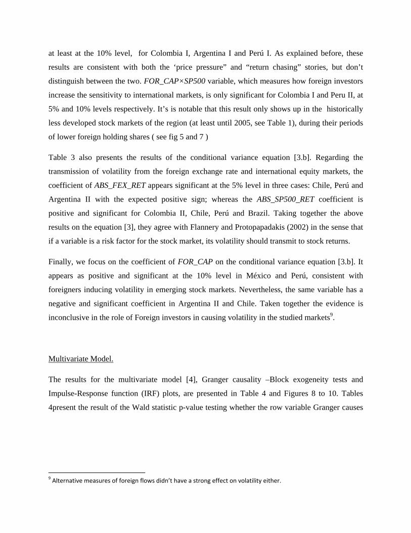
Table 3 also presents the results of the conditional variance equation [3.b]. Regarding the

transmission of volatility from the foreign exchange rate and international equity markets, the

coefficient of ABS_FEX_RET appears significant at the 5% level in three cases: Chile, Perú and

Argentina II with the expected positive sign; whereas the ABS_SP500_RET coefficient is

positive and significant for Colombia II, Chile, Perú and Brazil. Taking together the above

results on the equation [3], they agree with Flannery and Protopapadakis (2002) in the sense that

if a variable is a risk factor for the stock market, its volatility should transmit to stock returns.

Finally, we focus on the coefficient of FOR_CAP on the conditional variance equation [3.b]. It

appears as positive and significant at the 10% level in México and Perú, consistent with

foreigners inducing volatility in emerging stock markets. Nevertheless, the same variable has a

negative and significant coefficient in Argentina II and Chile. Taken together the evidence is

inconclusive in the role of Foreign investors in causing volatility in the studied markets9.

Multivariate Model.

The results for the multivariate model [4], Granger causality –Block exogeneity tests and

Impulse-Response function (IRF) plots, are presented in Table 4 and Figures 8 to 10. Tables

4present the result of the Wald statistic p-value testing whether the row variable Granger causes

9 Alternative measures of foreign flows didn’t have a strong effect on volatility either.

the column variable. Significant statistics at the 5% level are in bold, at the 10% level are

underlined. The sign and dynamics of the causality can be inferred from the IRF plots10.

First, we check the causality between foreign flows and return. Argentina and Mexico show

evidence of Granger causality from returns to foreign flows, and the short-term response in the

corresponding IRF plot is consistent with the ‘return chasing’ explanation. Conversely, Brazil

and México exhibit the reverse causality: foreign flows Granger cause returns, and the IRF plot

show a positive response, which is consistent with the ‘price pressure’ story.

The Granger causality tests along with the IRF plots show returns causing volatility in Brazil and

Argentina, in an inverse relation: positive (negative) returns induce an increase (reduction) of

volatility, consistent with the Leverage effect ( Nelson, 1991).

Similarly, the multivariate model results present volatility causing betas for Colombia, México

and Perú, in a direct direction: positive shocks to volatility cause higher betas. This relationship

seems to reflect the persistence on volatility and the fact that, holding correlation and the

S&P500 volatility constant, beta increase with an increase of volatility11.

The proposed VAR model also provides an answer to the central question of this study. First, the

results of the Granger causality test support in no case that foreign flows induce higher volatility

and neither the IRF plots. Second, with the only exception of México, there is no evidence of

Foreign flows causing Beta. Even in the case of México, the IRF plot doesn’t show a clear effect,

but if anything it appears to be inverse, contradicting the assumed hypothesis. All things

considered, the multivariate model indicates that foreign flows don’t have a discernible effect on

the volatility and systemic risk of the six Latin American markets of the study.

Conclusions

Several authors using different methodologies, theories and data have studied the influence of

Foreign Portfolio flows in emerging markets. Considering the results together, the results are

10 To obtain the IRFs, the Cholesky decomposition requires to rank the variables. The order chosen was, initially: RETURN, VOLAT, BETA and FOR_CAP. Robustness of IRF relations were checked by inverting the order of the Cholesky decomposition. Results are qualitatively the same, and available from the authors upon request. 11 BETA = correlation × stand. Dev Local market / stand. Dev. US market

ambiguous. This study contributes to the literature, testing not only effects on volatility but also

in systematic risk, and using a not yet used data, more recent sample periods that includes the

2008 World financial crisis, two different econometric models, and focusing on six emerging

markets of the same region.

The results of this study, taken together, indicate that there is no significant evidence that foreign

portfolio flows increase the risk of the six Latin American markets. In particular, we observe the

following:

Only in two out of nine cases, is there a positive and significant effect from foreign flows

on the betas to S&P500 returns: Colombia, before the 2006 crisis, and Perú, after July

2006. We suspect that this result might be due to the relative low development and

integration of both markets, which might make them more sensitive to Foreign flows.

Moreover, the fact that those effects don’t show up in the VAR monthly model suggest

that, if anything, those effects are either spurious or very short-lived.

According to the VAR monthly model, there is no evidence of Foreign flows having

lasting effects on the volatility of the markets. In turn, the univariate model shows only a

positive effect in two out of nine samples, but a negative and significant effect in two

others.

The evidence presented here does support empirical regularities reported in other studies on the

behavior of returns on emerging markets. It reports an important dependence of the local stock

returns on the returns of the foreign exchange rate and international equity markets, both in mean

and in volatility. We leave to future research to prove that the causality runs from those markets

to the stock one, and if those economic variables are priced risk factors of the equity market. We

find also evidence of returns causing higher foreign flows in some countries (‘return chasing’)

but also of foreign flows causing higher returns (‘price pressure’), that has also been found in

other emerging markets.

We conclude that foreign exchange and international returns do have a more important role on

increasing risk and dependence on international markets than foreign flows, providing no support

to the policy of restricting foreign portfolio flows due to alleged increasing risks or causing

instability in Latin American stock markets. We have left for future studies whether they have

disrupting effects on the foreign exchange rate markets.

References

Alemmani, B. and Haas, J.R., (2006). Behavior and effects of equity foreign investors on

emerging markets. Published paper.

Bae, K., Chan, K. and Ng, A. (2004). Investibility and return volatility. Journal of Financial

Economics. N° 71. pp. 239 – 263.

Beer F. and Hebein F. (2008). An Assessment Of The Stock Market And Exchange Rate

Dynamics In Industrialized And Emerging Markets. International Business & Economics

Research Journal. Vol 7 No 8. Pág 59-70.

Bekaert, G and Harvey, C., (2003). Emerging markets Finance. Journal of Empirical Finance

10, 3-57

Bekaert, G. and Harvey, C.R., (2000). Foreign speculators and emerging equity markets.

Journal of Finance. N° 55. pp. 565 – 614.

Bekaert, G., Harvey, C.R. and Lumsdaine, R.L., (2002). The Dynamics of emerging market

equity flows. Journal of International Money and Finance. N° 21. pp. 295 – 350.

Bekaert, G., Harvey, C.R., (1998). Capital flows and emerging market equity returns. NBER

working paper 6669.

Benelli, R. y Ganguly, S., ( 2007). Financial Linkages Between the United States and Latin

America – Evidence from Daily Data, International Monetary Fund, Working Paper.

Bikhchandani, S., Hirshleifer D. and Welch, I. 1998. Learning from the Behavior of Others:

Conformity, Fads, and Informational Cascades. Journal of Economic Perspectives. 12, pp.

151-70.

Bodie, Zvi, Kane, A. y Marcus, A., (2005). Investments. Sexta edición. Mc Graw Hill Irwin.

New York. pp. 1041.

Brennan, M. and Cao., (1997). International portfolio investment flows. Journal of Finance.

N° 52. pp. 1851 – 1880.

Calvo, G. (1998). Capital Market Contagion and Recession: An Explanation of the Russian

Virus. Working Paper.

Calvo, G. and Mendoza, E. (2000). Rational Contagion and the Globalization of Securities

Markets. Journal of International Economics. 51, pp. 79-113.

Campbell,J. Lo, A and MacKinlay, A. 1997. The Econometrics of Financial Markets.

Princeton University Press: Princeton. NJ.

Choe, H., Kho, B-C and Stultz, R., (1999). Do foreign investors destabilize stocks markets?

The Korean experience in 1997. Journal of Financial Economics. N° 54. pp. 227 – 264.

Choe H., Kho, B-C, and Stulz, R. (2005).“Do domestic investors have an edge? The trading

experience of foreign investors in Korea,” Review of Financial Studies, 18 pp. 795-829.

Cochrane, J. H., (2001). Asset pricing. Princeton University Press. Princeton, New Jersey.

pp. 495.

De Arce Borda, R., 2004. 20 años de modelos ARCH: una visión de conjunto de las distintas

variantes de la familia. Estudios de Economía Aplicada, Estudios de Economía Aplicada, vol.

22, p.22

Di Tella, T., (2004). Diccionario de ciencias sociales y políticas. Edición 2004. Editorial

Ariel. 776 p.

Dornbusch, R. and Fischer S., (1980). Exchange Rates and the Current Account. American

Economic Review, v70(5), 960-971.

Dvórak, T. (2001). Does Foreign trading destabilize local stock markets?. Published paper.

Department of Economics. Williams College.

Edison, H. Warnock E. (2009), Cross-Border Listings, Capital Controls, and Equity Flows to

Emerging Markets. NBER Working Paper No. W12589

Edwards, S. 1999 “International Capital Flows and the Emerging Markets: Amending the

Rules of the Game?” Federal Reserve Bank of Boston Conference Series 43, June 1999, pp.

137-57.

Eichengreen, B. 1999. Toward a New International Financial Architecture. Institute of

International Economics, Washington, DC.

Enders, W. (1995). Applied Econometric Time Series. Iowa State University, John Wiley &

Sons, Inc.

Errunza, V.R. and Miller, D.P., (2000). Market segmentation and the cost of capital in

international equity markets. Journal of Financial and Quantitative Analysis N° 35. pp. 577 –

600.

Fama, E.F., (1979). Efficient Capital Markets: A review of theory and empirical work.

Journal of finance.

Ferrari, C. y Amalfi A. (2007), Business and economic foundation in valuation of shares: the

Colombian stock exchange. Cuadernos de Administración, Vol. 20, N° 33, Junio 2007, pp. 11

– 48.

Ferrer, A., (1999). La Globalización, la crisis financiera y Latinoamérica. Revista Comercio

Exterior, México, Vol. 49, N° 6. pp. 527 – 536.

Ffrench-Davis, R. and Griffith-Jones S. 2002. Capital Flows to Developing Countries

since the Asian Crises: How to Manage their Volatility. Working paper UNU/WIDER

Research Project.

Flannery, M.J. and Protopapadakis, A. A., (2002). Macroeconomic Factor Do Influence

Aggregate Stock Return. Review of Financial Studies. Vol 15, Pág.751-782.

Flood, D. y De Paterson, M.. Efectos de las Crisis Asiática y de Rusia en la Economía y

Agricultura del Ecuador. Ministerio de Agricultura, ganadería, acuacultura y pesca del

Ecuador. 2008. http://www.sica.gov.ec/agro/docs/crisis_mundial.html

Frankel, J. A., (1983). Monetary and Portfolio-balance Models of Exchange Rate

Determination, in Economic Interdependence and Flexible Exchange Rates, J. S. Bhandari

and B. H. Putnam ed., MIT Press, Cambridge, MA.

Frenkel, M. and Menkhoff, L., (2003). Are foreign institutional investors good for emerging

markets?. Published paper.

Froot, K.A., O’ Connell, P.G. and Seasholes, M.S., (2001). The portfolio flows of

international investors. Journal of Financial Economics. N° 59. pp. 151 – 193.

Glosten, L. R. and Milgrom, P. R., (1985). Bid, Ask, and Transaction Prices in a Specialist

Market With Heterogeneously Informed Traders. Journal of Financial Economics 14. pp. 71-

100.

Griffin, J.M., Nardari, F. and Stulz, R., (2004). Daily cross border flows: pushed or pulled?.

The review of Economics and Statistics. N° 86. pp. 641 – 657.

Griffin, J. M., Nardari, F., and Stulz, R. (2006). Do investors trade more when stocks have

performed well? Evidence from 46 countries, Forthcoming Review of Financial Studies.

Harmantzis, F. and Miao, L. (2009). Dynamic Asymmetric Dependencies between Equities

and Exchange Rate Markets. Stevens Institute of Technology. Working Paper.

Henry, P.B., (2000). Stock market liberalization, economic reform and emerging market

equity prices. Journal of Finance. N° 55. pp. 529 – 564.

Ho, T. and Stoll, H.R., (1981). Optimal Dealer Pricing under Transactions and Return

Uncertainty. Journal of Financial Economics. N° 9. pp. 47-73.

Ito, T. and Portes, R.1998. “Dealing with the Asian Financial Crises.” European Economic

Perspectives, CERP.

Kim, E.H. and Singal, V., (2000). Stock market openings: experience of emerging

economies. Journal of Business. N° 73. pp. 25 -66.

Krugman, P., (1998). What happened to Asia?. Unpublished paper. MIT.

Krugman, P., (1999). Balance sheets, the transformers the problem and the financial crises.

Department of Economics. Cambridge.

Kyle, A.S., (1985). Continuous Auctions and Insider Trading, Econometrica 53, 1315-1335.

Lucey, B y Zhang, Q, Integration Analysis of Latin American Stock Markets 1993 – 2007.

Diciembre de 2007. SSRN: http://ssrn.com/abstract=1047421.

Nelson D. B. (1991). Conditional Heteroskedasticity in Asset Returns: A New Approach.

Econometrica. 59, pp. 347-370.

Miller, D.P., (1999). The impact of international market segmentation on securities prices:

evidence from depositary receipts. Journal of Financial Economics. N° 51. pp. 103 – 123.

Miralles M., J.L. y Miralles Q., J.L., (2005). Análisis de los efectos de las correlaciones

bursátiles en la composición de las carteras óptimas. Revista Española de Financiación y

Contabilidad, Vol. 34, N° 126, Julio – Septiembre 2005, pp 689 – 708.

Muller, A. and Verschoor, W. F.C. (2007). Asian Foreign Exchange Risk Exposure. Journal

of the Japanese and International Economies. Vol 21 Issue 1. Pag 16-37.

Rea, J., (1996). U.S. emerging market funds: hot money or stable source of investment

capital. Investment company institute perspective. Vol 2. N° 6. December.

Richards, A., (2005). Big fish in small ponds: the trading behavior and price impact of

foreign investors in Asian emerging equity markets. Journal of Financial and Quantitative

Analysis. Vol. 40. N° 1. 27 p.

Rubin, Robert and Jacob Weisberg (2003). In an Uncertain World: Tough Choices from Wall

Street to Washington. New York: Random House.

Shiller R. J. (1981). Do Stock Prices Move Too Much to be Justified by Subsequent Changes

in Dividends? The American Economic Review, 71, pp. 421-436

Standard and Poors 2004. Global Stock Markets Factbook. New York: Mac-Graw Hill.

Stiglitz, J., (2000). Capital Market liberalization, economic growth and instability. World

Development 25. pp. 1075 – 1086.

Villariño, A. (2001). Turbulencias financieras y riesgos de mercado. Primera edición.

Prentice Hall. España. pp. 300.

Warther, V.A., (1995). Aggregate mutual fund and security returns. Journal of Financial

Economics. N° 39. pp. 205 – 235.

Figure 1. Total Foreign Portfolio Net flows in Six Latin American Countries. Source: Emerging Portfolio

‐4,000

‐3,000

‐2,000

‐1,000

0

1,000

2,000

abr‐95

ene‐96

oct‐96

jul‐97

abr‐98

ene‐99

oct‐99

jul‐00

abr‐01

ene‐02

oct‐02

jul‐03

abr‐04

ene‐05

oct‐05

jul‐06

abr‐07

ene‐08

oct‐08

Stock Exchange Index (MERVAL)

Volatility Beta

Share of Foreign Portfolio Holdings FOR_CAP : Net Foreign Flows / Market value

Fig 2. Summary statistics for Argentina.

0

500

1000

1500

2000

2500

abr‐99 abr‐00 abr‐01 abr‐02 abr‐03 abr‐04 abr‐05 abr‐06 abr‐07 abr‐08

0

0,01

0,02

0,03

0,04

0,05

0,06

‐3

‐2

‐1

0

1

2

3

4

0,00000

0,01000

0,02000

0,03000

0,04000

0,05000

0,06000

0,07000

‐0,03000

‐0,02500

‐0,02000

‐0,01500

‐0,01000

‐0,00500

0,00000

0,00500

Stock Market Index (BOVESPA)

Volatility Beta


Fig 3 Summary statistics for Brazil

0

20000

40000

60000

80000

oct‐98 oct‐99 oct‐00 oct‐01 oct‐02 oct‐03 oct‐04 oct‐05 oct‐06 oct‐07 oct‐08

0

0,01

0,02

0,03

0,04

0,05

0,06

‐0,5

0

0,5

1

1,5

2

2,5

3

3,5

4

4,5

0,00000

0,00500

0,01000

0,01500

0,02000

0,02500

0,03000

‐0,00150

‐0,00100

‐0,00050

0,00000

0,00050

0,00100

0,00150

Stock Market Index (IPSA)

Volatility Beta


Fig 4. Summary statistics for Chile

0

1000

2000

3000

4000

nov‐98 nov‐99 nov‐00 nov‐01 nov‐02 nov‐03 nov‐04 nov‐05 nov‐06 nov‐07 nov‐08

0

0,005

0,01

0,015

0,02

0,025

0,03

0,035

‐1

‐0,5

0

0,5

1

1,5

2

0,000000,005000,010000,015000,020000,025000,030000,035000,04000

‐0,00400

‐0,00300

‐0,00200

‐0,00100

0,00000

0,00100

0,00200

0,00300

Stock Market Index (IGBC)

Volatility Beta


Fig 5. Summary statistics for Colombia

0

2000

4000

6000

8000

10000

12000

14000

06‐dic‐99 19‐abr‐01 01‐sep‐02 14‐ene‐04 28‐may‐05 10‐oct‐06 22‐feb‐08 06‐jul‐09

0,0%

0,5%

1,0%

1,5%

2,0%

2,5%

3,0%

3,5%

4,0%

4,5%

‐1,0000

‐0,5000

0,0000

0,5000

1,0000

1,5000

2,0000

2,5000

3,0000

3,5000

4,0000

0,00000

0,00100

0,00200

0,00300

0,00400

0,00500

0,00600

0,00700

0,00800

‐0,00150

‐0,00100

‐0,00050

0,00000

0,00050

0,00100

0,00150

0,00200

Stock Market Index (IPC)

Volatility Beta


Fig 6. Summary statistics for Mexico

0

5000

10000

15000

20000

25000

30000

35000


0

0,005

0,01

0,015

0,02

0,025

0,03

0,035

0,04

0

0,5

1

1,5

2

2,5

0,00000

0,01000

0,02000

0,03000

0,04000

0,05000

0,06000

0,07000

0,08000

0,09000

‐0,006

‐0,005

‐0,004

‐0,003

‐0,002

‐0,001

0

0,001

0,002

0,003

0,004

Stock Market Index (IGBVL)

Volatility Beta


Fig 7. Summary statistics for Perú

0

5000

10000

15000

20000

25000


0

0,01

0,02

0,03

0,04

0,05

0,06

‐1

‐0,5

0

0,5

1

1,5

2

2,5

0,00000

0,01000

0,02000

0,03000

0,04000

0,05000

0,06000

0,07000

‐0,01

‐0,008

‐0,006

‐0,004

‐0,002

0

0,002

0,004

0,006

0,008

Argentina Brasil

Fig. 8. Impulse response function plots for the monthly 4-VAR model.

Response of the row variable to a 1 normalized standard-deviation impulse of the column variable.

RETURN VOLAT BETA FOR_CAP RETURN VOLAT BETA FOR_CAP

RETURN

VOLAT

BETA

FOR_CAP

Chile Colombia




RETURN

VOLAT

BETA

FOR_CAP

México Perú




RETURN

VOLAT

BETA

FOR_CAP

Table 1. Market capitalization and Total Trading Value of the six Latin American stock

exchanges.

Univariate Model Multivariate Model

Starts Ends Starts Ends

Argentina 7‐Apr‐1999 20‐Nov‐2001

31‐May‐1999 30‐Dec‐2008 21‐Nov‐2001 30‐Dec‐2008

Brazil 4‐Nov‐1998 30‐Dec‐2008 31‐Jan‐1999 30‐Dec‐2008

Chile 4‐Nov‐1998 30‐Dec‐2008 30‐Nov‐1998 30‐Dec‐2008

Colombia 4‐Jul‐2001 28‐Apr‐2006

31‐Jul‐2001 30‐Dec‐2008 4‐Jul‐2006 30‐Dec‐2008

Mexico 4‐Nov‐1998 30‐Dec‐2008 30‐Nov‐1998 30‐Dec‐2008

Perú 3‐Nov‐1998 4‐Jul‐2006

31‐Jan‐1999 30‐Dec‐2008 5‐Jul‐2006 30‐Dec‐2008

Table 2. Study Period for each country for the Univariate and Multivariate Models.

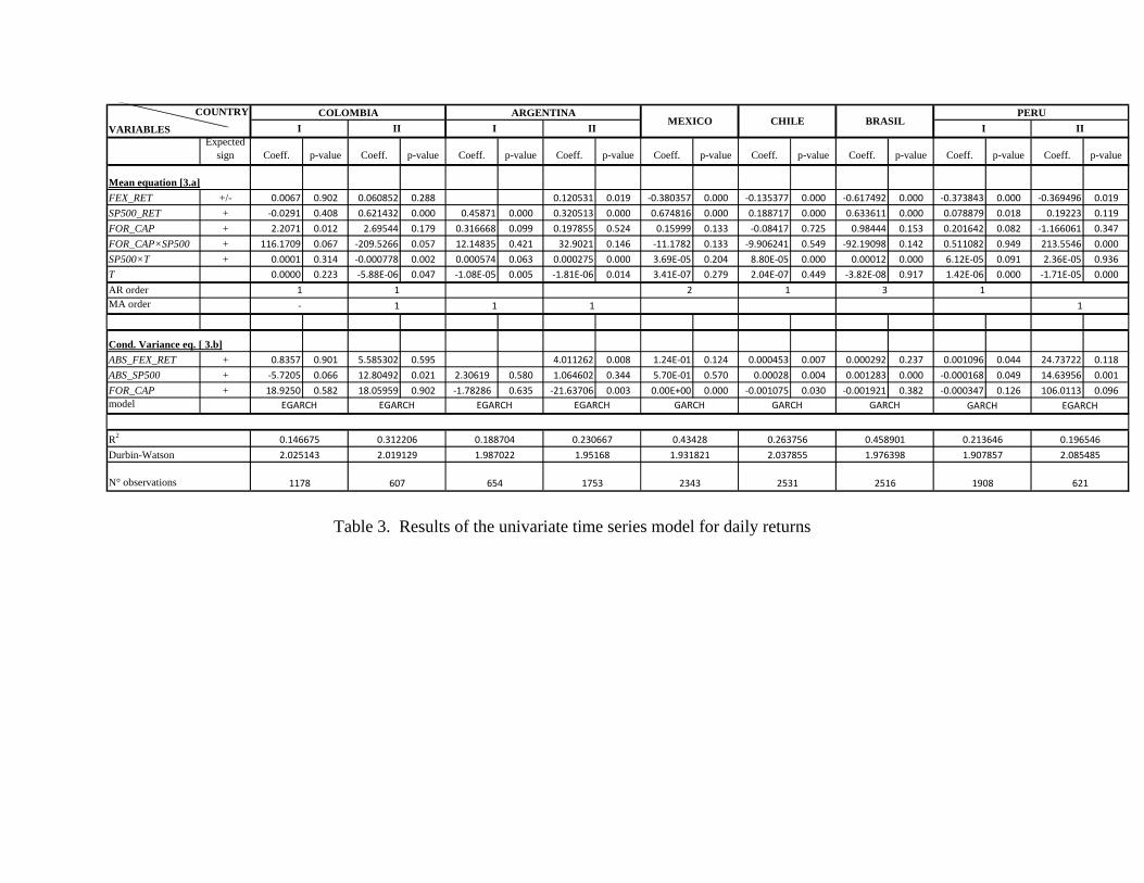
Table 3. Results of the univariate time series model for daily returns

Expected sign Coeff. p-value Coeff. p-value Coeff. p-value Coeff. p-value Coeff. p-value Coeff. p-value Coeff. p-value Coeff. p-value Coeff. p-value

FEX_RET +/- 0.0067 0.902 0.060852 0.288 0.120531 0.019 ‐0.380357 0.000 ‐0.135377 0.000 ‐0.617492 0.000 ‐0.373843 0.000 ‐0.369496 0.019

SP500_RET + ‐0.0291 0.408 0.621432 0.000 0.45871 0.000 0.320513 0.000 0.674816 0.000 0.188717 0.000 0.633611 0.000 0.078879 0.018 0.19223 0.119

FOR_CAP + 2.2071 0.012 2.69544 0.179 0.316668 0.099 0.197855 0.524 0.15999 0.133 ‐0.08417 0.725 0.98444 0.153 0.201642 0.082 ‐1.166061 0.347

FOR_CAP×SP500 + 116.1709 0.067 ‐209.5266 0.057 12.14835 0.421 32.9021 0.146 ‐11.1782 0.133 ‐9.906241 0.549 ‐92.19098 0.142 0.511082 0.949 213.5546 0.000

SP500×T + 0.0001 0.314 ‐0.000778 0.002 0.000574 0.063 0.000275 0.000 3.69E‐05 0.204 8.80E‐05 0.000 0.00012 0.000 6.12E‐05 0.091 2.36E‐05 0.936

T 0.0000 0.223 ‐5.88E‐06 0.047 ‐1.08E‐05 0.005 ‐1.81E‐06 0.014 3.41E‐07 0.279 2.04E‐07 0.449 ‐3.82E‐08 0.917 1.42E‐06 0.000 ‐1.71E‐05 0.000

AR orderMA order

ABS_FEX_RET + 0.8357 0.901 5.585302 0.595 4.011262 0.008 1.24E‐01 0.124 0.000453 0.007 0.000292 0.237 0.001096 0.044 24.73722 0.118

ABS_SP500 + ‐5.7205 0.066 12.80492 0.021 2.30619 0.580 1.064602 0.344 5.70E‐01 0.570 0.00028 0.004 0.001283 0.000 ‐0.000168 0.049 14.63956 0.001

FOR_CAP + 18.9250 0.582 18.05959 0.902 ‐1.78286 0.635 ‐21.63706 0.003 0.00E+00 0.000 ‐0.001075 0.030 ‐0.001921 0.382 ‐0.000347 0.126 106.0113 0.096

model

Mean equation [3.a]

Cond. Variance eq. [ 3.b]

PERU

I II

1753

1.931821

2343

1.987022

654

R2 0.146675 0.312206 0.188704 0.230667

1.95168

ARGENTINA

0.43428

Durbin-Watson

N° observations

2.025143

1178

2.019129

607

3

GARCH GARCH

1

‐

1

1 1

BRASILMEXICO CHILEVARIABLES I II I II

COUNTRY COLOMBIA

1

11

2 1

0.263756

2.037855

2531

0.458901 0.196546

EGARCH EGARCH EGARCH EGARCH GARCH GARCH EGARCH

2.085485

621

1.976398

2516

0.213646

1.907857

1908

Table 4. Results of the Granger causality test, in a monthly 4-VAR model.

p-values of the Wald test of excluding the row variable in the equation of the column variable.

Country RETURN VOLAT BETA FOR_CAP

RETURN 0.0129 0.5328 0.0018

VOLAT 0.5206 0.2756 0.5174

BETA 0.7232 0.2332 0.6192

FOR_CAP 0.1933 0.7795 0.9941

RETURN 0.0057 0.9861 0.9701

VOLAT 0.534 0.4516 0.4516

BETA 0.8558 0.053 0.4612

FOR_CAP 0.0598 0.8037 0.9484

RETURN 0.1525 0.5927 0.7824

VOLAT 0.6486 0.378 0.5391

BETA 0.1992 0.798 0.5044

FOR_CAP 0.8554 0.467 0.4098

RETURN 0.498 0.1312 0.3848

VOLAT 0.2847 0.0159 0.0065

BETA 0.0353 0.0004 0.0014

FOR_CAP 0.3101 0.2693 0.4595

RETURN 0.2032 0.7519 0.0063

VOLAT 0.8228 0.0446 0.0294

BETA 0.7586 0.4779 0.0932

FOR_CAP 0.0651 0.2541 0.0814

RETURN 0.1236 0.1706 0.5045

VOLAT 0.0742 0.0642 0.6146

BETA 0.3347 0.0146 0.8493FOR_CAP 0.9565 0.9034 0.7295

ARGENTINA

BRAZIL

CHILE

COLOMBIA

MEXICO

PERU

Do foreign portfolio flows increase risk in emerging stock markets? Evidence from six Latin American...

Documents

Transcript of Do foreign portfolio flows increase risk in emerging stock markets? Evidence from six Latin American...