DISCHARGE DISTRIBUTION IN MEANDERING COMPOUND CHANNELS

A PROJECT SUBMITTED IN PARTIAL FULFILMENT

OF THE REQUIREMENTS FOR THE DEGREE OF

Bachelor of Technology In

Civil Engineering By

Santosh Dash Roll No: 10401024

N.Swetha Roll No: 10401030

Under the guidance of Prof .DR. K. C. Patra

& DR. K. K. Khatua

Department of Civil Engineering


Rourkela

May, 2008


Rourkela

CERTIFICATE

This is to certify that the project entitled, “discharge distribution in meandering

compound channels” submitted by Santosh dash and N.Swetha in partial fulfillment of

the requirements for the award of Bachelor of Technology Degree in Civil Engineering

at the National Institute of Technology, Rourkela (Deemed University) is an authentic

work carried out by him under my supervision and guidance.

To the best of my knowledge, the matter embodied in the thesis has not been submitted to

any other university / institute for the award of any Degree or Diploma.

Prof. Dr.K.C.Patra Dr. K.K. Khatua Head of Department Dept. of Civil Engineering Dept. of Civil Engineering National Institute of Technology National Institute of Technology Rourkela-769008 Rourkela- 769008

ACKNOWLEDGEMENT

I am thankful to Dr. K.C.Patra and Dr. K.K.Khatua, Head of department and professor

in the Department of Civil Engineering, NIT Rourkela for giving me the opportunity to

work under them and lending every support at every stage of this project work.

I would also like to convey my sincerest gratitude and indebt ness to all other faculty

members and staff of Department of Civil Engineering, NIT Rourkela, who bestowed

their great effort and guidance at appropriate times without which it would have been

very difficult on my part to finish the project work.

Date: May 12, 2008

N.SWETHA

SANTOSH DASH

CONTENTS

A. ABSTRACT IV B. LIST OF FIGURES VI

C. LIST OF TABLES VII

D. CHAPTERS

1. Introduction 1

2. Literature review 3-9 2.1 Simple Meandering channels 2.2 Compound channels in straight reaches 2.3 Meander compound channels

3. Experimental Setup 10-16 3.1 Model Setup 3.2 Experiment procedure 3.2.1 Determination of channel slope 3.2.2 Measure of discharge and water surface elevation 3.2.3 Measure of velocity and its distribution 4. Observations 17-29 4.1 Calculation of 3-dimensional velocities 4.1.1 Compound meandering channels 4.2 Plotting of Contours 4.2.1 3DField 4.2.2 Compound meandering channels 4.2.3 FCF data

5. Analysis of Existing Datas 30-35 5.1 Development of the Model 5.2 Validation of the Model

E. CONCLUSION VII

F. REFERENCES VIII

G. PHOTO GALLERY X-XI

ABSTRACT Magnitude of flood prediction is the fundamental for flood warning,

determining the development for the present flood-risk areas and the long-term

management of rivers. Discharge estimation methods currently employed in river

modeling software are based on historic hand calculation formulae such as Chezy’s,

Darcy-Weisbatch or Manning’s equation. More recent work has provided significant

improvements in understanding and calculation of channel discharge. This ranges from

the gaining knowledge to interpretation of the complex flow mechanisms to the advent of

computing tools that enable more sophisticated solution techniques.

When the flows in natural or man-made channel sections exceed the main

channel depth, the adjoining floodplains become inundated and carry part of the river

discharge. Due to different hydraulic conditions prevailing in the river and floodplain, the

mean velocity in the main channel and in the floodplain are different. Just above the

bank-full stage, the velocity in main channel is much higher than the floodplain.

Therefore the flow in the main channel exerts a pulling or accelerating force on the flow

over floodplains, which naturally generates a dragging or retarding force on the flow

through the main channel. This leads to the transfer of momentum between the main

channel water and that of the floodplain. The interaction effect is very strong at just

above bank full stage and decreases with increase in depth of flow over floodplain. The

relative “pull” and “drag” of the flow between faster and slower moving sections of a

compound section complicates the momentum transfer between them. Failure to

understand this process leads to either overestimate or underestimate the discharge

leading to the faulty design of channel section. This causes frequent flooding at its lower

reaches.

Due to transfer of momentum between the subsections of the meandering

compound channel, the shear distribution is largely affected. For such compound

channels, the apparent shear force at the assumed interface plane gives an insight into the

magnitude of flow interaction. The results of some experiments concerning the velocity

distribution and the flow distribution in a smooth and rough compound meandering

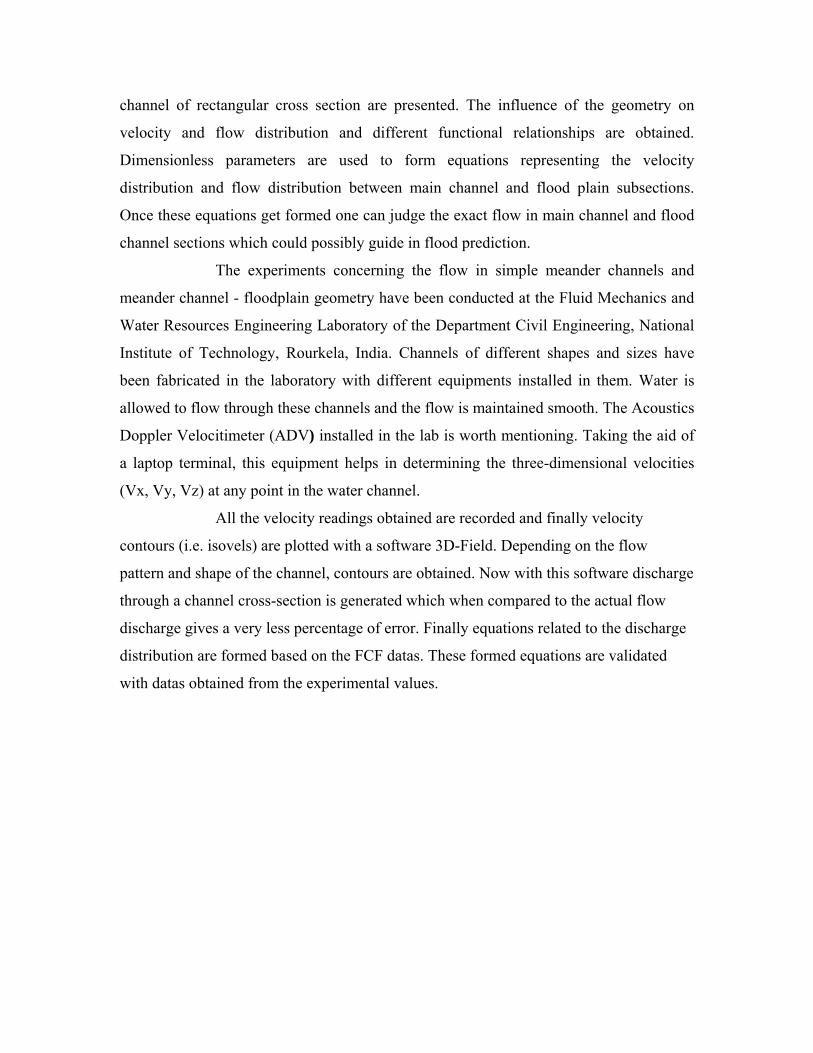
channel of rectangular cross section are presented. The influence of the geometry on

velocity and flow distribution and different functional relationships are obtained.

Dimensionless parameters are used to form equations representing the velocity

distribution and flow distribution between main channel and flood plain subsections.

Once these equations get formed one can judge the exact flow in main channel and flood

channel sections which could possibly guide in flood prediction.

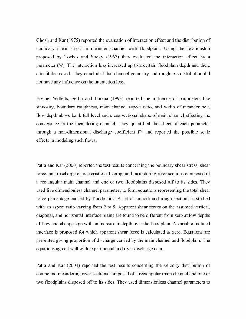
The experiments concerning the flow in simple meander channels and

meander channel - floodplain geometry have been conducted at the Fluid Mechanics and

Water Resources Engineering Laboratory of the Department Civil Engineering, National

Institute of Technology, Rourkela, India. Channels of different shapes and sizes have

been fabricated in the laboratory with different equipments installed in them. Water is

allowed to flow through these channels and the flow is maintained smooth. The Acoustics

Doppler Velocitimeter (ADV) installed in the lab is worth mentioning. Taking the aid of

a laptop terminal, this equipment helps in determining the three-dimensional velocities

(Vx, Vy, Vz) at any point in the water channel.

All the velocity readings obtained are recorded and finally velocity

contours (i.e. isovels) are plotted with a software 3D-Field. Depending on the flow

pattern and shape of the channel, contours are obtained. Now with this software discharge

through a channel cross-section is generated which when compared to the actual flow

discharge gives a very less percentage of error. Finally equations related to the discharge

distribution are formed based on the FCF datas. These formed equations are validated

with datas obtained from the experimental values.

List of Figures

1. Fig 3.1 Experimental set up with plan form of the meandering channel with

floodplain

2. Fig 3.2 One wave length of meandering compound channel

3. Fig 4.1 A 3DField software layout.

4. Fig 4.2 Velocity contours for FCF channels (A,B,C,D,E,F,G,H,I,J,L,M)

5. Fig 5.1. Finalized graph showing the fitted curve for variation of diff factor with

β.

6. Fig 5.2 the difference factor was plotted Keeping the value of ‘β’constant, and α

varying.

7. Fig 5.3 % Qmc predicted by the model developed against the % Qmc actually for

meandering channels.

8. Fig 5.4 % Qmc predicted by the model developed against the % Qmc actually for

data by FCF data and the data predicted by the proposed model.

List of Tables

1. Table 3.1 Compound channel plain with floodplain.

2. Table 3.2 All the three velocities at different water level.

3. Table 4 Experimental data. Photos

4. Plate 1: Front View of ADV

5. Plate 2: side looking probe

6. Plate 3: Measuring the velocities

7. Plate 4: A close look at the channel

Chapter 1

INTRODUCTION

INTRODUCTION Investigators have studied meanders and straight compound channels flows for a fairly long

time. The name meander, which probably originated from the river Meanders in Turkey is

so frequent in river that it has attracted the interest of investigators from many disciplines.

Thomson (1876) was probably the first to point out the existence of spiral motion in curved

open channel. Since then, a lot of laboratory and theoretical studies have been reported,

more so, in the last decade or two. It may be worthwhile to know the developments in the

field of constant curvature bends, simple meander channel flows and straight compound

channels before knowing about the meander channel-floodplain geometry as limited studies

concerning the meander plan form of the compound sections are available till date.

Information regarding the nature of flow distribution in a flowing simple and compound

channel is needed to solve a variety of river hydraulics and engineering problems such as

to give a basic understanding of resistance relationship, to understand the mechanism of

sediment transport, to design stable channels, revetments.

The flow distribution, velocity distribution and flow resistance in compound cross section

channels have been investigated by many authors.

Most of the flow distribution formulae assume that the roughness coefficient and the

other geometrical parameters of natural river channel do not change when the flow starts

overtopping the main channel.

For meandering channels the flood plain geometry, the wide variation in local shear stress

distribution from point to point in the wetted perimeter varies.

Therefore there is need for taking into account these parameters and developing one rock

solid model which would predict the discharge accurately during flood forecasting.

Chapter 2

REVIEW OF LITERATURE

2.1 SIMPLE MEANDER CHANNELS

The Meandering channel flow is considerably more complex than constant curvature

bend flow. The flow geometry in meander channel due to continuous stream wise

variation of radius of curvature is in the state of either development or decay or both. The

following important studies are reported concerning the flow in meandering channels.

Hook (1974) measured the bed elevation contours in a meandering laboratory flume with

movable sand bed for various discharges. For each discharge he measured the bed shear

stress, distribution of sediment in transport and the secondary flow and found that with

increasing discharge, the secondary current increased in strength.

Chang (1984 a) analyzed the meander curvature and other geometric features of the

channel using energy approach. It established the maximum curvature for which the river

did the last work in turning, using the relations for flow continuity, sediment load,

resistance to flow, bank stability and transverse circulation in channel bends. The analysis

demonstrated how uniform utilization of energy and continuity of sediment load was

maintained through meanders.

2.2 COMPOUND CHANNELS IN STRAIGHT REACHES

While simple channel sections have been studied extensively, compound channels

consisting of a deep main channel and one or more floodplains have received relatively

little attention. Analysis of these channels is more complicated due to flow interaction

taking place between the deep main channel and shallow floodplains. Laboratory

channels provide the most effective alternative to investigate the flow processes in

compound channels as it is difficult to obtain field data during over bank flow situations

in natural channels. Therefore, most of the works reported are experimental in nature.

Sellin (1964) confirmed the presence of the "kinematics effect" reported by

Zheleznyakov(1965) after series of laboratory studies and presented photographic

evidence of the presence of a series of vortices at the interface of main channel and flood

plain. He studied the channel velocities and discharge under both interacting and isolated

conditions by introducing a thin impermeable film at the junction. Under isolated

condition, velocity in the main channel was observed to be more and under interacting

condition the velocity in floodplain was less.

Rajaratnam and Ahmadi (1979) studied the flow interaction between straight main

channel and symmetrical floodplain with smooth boundaries. The results demonstrated

the transport of longitudinal momentum from main channel to flood plain. Due to flow

interaction, the bed shear in floodplain near the junction with main channel increased

considerably and that in the main channel decreased. The effect of interaction reduced as

the flow depth in the floodplain increased.

Knight and Demetriou (1983) conducted experiments in straight symmetrical compound

channels to understand the discharge characteristics, boundary shear stress and boundary

shear force distributions in the section. They presented equations for calculating the

percentage of shear force carried by floodplain and also the proportions of total flow in

various sub-areas of compound section in terms of two dimensionless channel

parameters. For vertical interface between main channel and floodplain the apparent

shear force was found to be more for low depths of flow and for high floodplain widths.

On account of interaction of flow between floodplain and main channel it was found that

the division of flow between the subsections of the compound channel did not follow a

simple linear proportion to their respective areas.

Knight and Hamed (1984) extended the work of Knight and Demetriou (1983) to rough

floodplains. The floodplains were roughened progressively in six steps to study the

influence of different roughness between floodplain and main channel to the process of

lateral momentum transfer. Using four dimensionless channel parameters, they presented

equations for the shear force percentages carried by floodplains and the apparent shear

force in vertical, horizontal diagonal and bisector interface plains. The apparent shear

force results and discharge data provided the weakness of these four commonly adopted

design methods used to predict the discharge capacity of the compound channel.

2.3 MEANDERING COMPOUND CHANNELS

There are limited reports concerning the characteristics of flow in meandering compound

sections.

A study by United States water ways experimental station (1956) related the channel and

floodplain conveyance to geometry and flow depth, concerning, in particular, the

significance of the ratios of channel width to floodplain width and meander belt width to

floodplain width in the meandering two stage channel.

Toebes and Sooky (1967) were probably the first to investigate under laboratory

conditions the hydraulics of meandering rivers with floodplains. They attempted to relate

the energy loss of the observed internal flow structure associated with interaction

between channel and floodplain flows. The significance of helicoidal channel flow and

shear at the horizontal interface between main channel and floodplain flows were

investigated. The energy loss per unit length for meandering channel was up to 2.5 times

as large as those for a uniform channel of same width and for the same hydraulic radius

and discharge. It was also found that energy loss in the compound meandering channel

was more than the sum of simple meandering channel and uniform channel carrying the

same total discharge and same wetted perimeter. The interaction loss increased with

decreasing mean velocities and exhibited a maximum when the depth of flow over the

floodplain was less. For the purpose of analysis, a horizontal fluid boundary located at the

level of main channel bank full stage was proposed as the best alternative to divide the

compound channel into hydraulic homogeneous sections. Hellicoidal currents in meander

floodplain geometry were observed to be different and more pronounced than those

occurring in a meander channel carrying in bank flow. Reynold's number (R) and Froude

number (F) had significant influence on the meandering channel flow.

Ghosh and Kar (1975) reported the evaluation of interaction effect and the distribution of

boundary shear stress in meander channel with floodplain. Using the relationship

proposed by Toebes and Sooky (1967) they evaluated the interaction effect by a

parameter (W). The interaction loss increased up to a certain floodplain depth and there

after it decreased. They concluded that channel geometry and roughness distribution did

not have any influence on the interaction loss.

Ervine, Willetts, Sellin and Lorena (1993) reported the influence of parameters like

sinuosity, boundary roughness, main channel aspect ratio, and width of meander belt,

flow depth above bank full level and cross sectional shape of main channel affecting the

conveyance in the meandering channel. They quantified the effect of each parameter

through a non-dimensional discharge coefficient F* and reported the possible scale

effects in modeling such flows.

Patra and Kar (2000) reported the test results concerning the boundary shear stress, shear

force, and discharge characteristics of compound meandering river sections composed of

a rectangular main channel and one or two floodplains disposed off to its sides. They

used five dimensionless channel parameters to form equations representing the total shear

force percentage carried by floodplains. A set of smooth and rough sections is studied

with an aspect ratio varying from 2 to 5. Apparent shear forces on the assumed vertical,

diagonal, and horizontal interface plains are found to be different from zero at low depths

of flow and change sign with an increase in depth over the floodplain. A variable-inclined

interface is proposed for which apparent shear force is calculated as zero. Equations are

presented giving proportion of discharge carried by the main channel and floodplain. The

equations agreed well with experimental and river discharge data.

Patra and Kar (2004) reported the test results concerning the velocity distribution of

compound meandering river sections composed of a rectangular main channel and one or

two floodplains disposed off to its sides. They used dimensionless channel parameters to

form equations representing the percentage of flow carried by floodplains and main

channel sub sections.

Shiono, Romaih &Knight (2004) carried out discharge measurements for over bank flow

in a two-stage meandering channel with various bed slopes, sinuosities, and water depths.

The effect of bed slope and sinuosity on discharge was found to be significant. A simple

design equation for the conveyance capacity based on dimensional analysis is proposed.

This equation may be used to estimate the stage-discharge curve in a meandering channel

with over bank flow. Predictions of discharge using existing methods and the proposed

method are compared and tested against the new measured discharge data and other

available over bank data. The strengths and weaknesses of the various methods are

discussed.

FLOOD CHANNEL FACILITY (FCF)

For the rigid boundary work 19 series of experiments were undertaken, 11 with

floodplains, 2 with isolated floodplains, and 6 with skewed floodplains, as shown in

Table below. For a given series, 8 experiments were undertaken at 8 different overbank

flow depths, ranging from (H-h)/H = 0.05 (0.05) to 0.5, where (H-h) = floodplain depth

and h = bankfull depth. By setting the same flow depths in each series, it was possible to

compare overbank flow results at a given depth for various types of geometry or

floodplain roughness. Some inbank flow experiments were also undertaken. For all tests,

the bed slope was moulded to 1.0270 x 10-3, and the semi-base width of the main

channel, b, was kept constant at 0.75 m, with h = 0.150 m, thus giving an aspect ratio of

10 (= 2b/h) for the main channel at the bankfull stage.

Fig 3.4 cross section of FCF straight channel

Series No. Type of experiment

Width parameters

Main channel side slope, s

Floodplain type Roughness

01 Straight B/b = 6.67 1.0 Symmetric Smooth 02 Straight B/b = 4.20 1.0 Symmetric Smooth 03 Straight B/b = 2.20 1.0 Symmetric Smooth 04 Straight B/b =1.20 1.0 Trapezoidal Smooth 05 Straight B/b = 2.50 1.0 (R Main) Smooth 06 Straight B/b = 4.20 1.0 Asymmetric Smooth 07 Straight B/b = 4.20 1.0 Symmetric Rough 08 Straight b fp/b = 3.0 0 Symmetric Smooth 09 Straight b fp/b = 3.0 0 Symmetric Rough 10 Straight b fp/b = 3.0 2.0 Symmetric Smooth 11 Straight b fp/b = 3.0 2.0 Symmetric Rough 12 Straight Isolated fp 1.0 - - 13 Straight Isolated fp 1.0 - - 14 Skew B/b = 3.7 1.0 θ = 5° Smooth 15 Skew B/b = 3.7 1.0 θ = 9° Smooth 16 Skew B/b = 3.7 0 θ = 5° Smooth 17 Skew B/b = 3.7 0 θ = 2° Smooth 18 Skew B/b = 3.7 2.0 θ = 5° Smooth 19 Skew B/b = 3.7 1.0 θ = 5° Rough

Chapter 3 ` EXPERIMENTAL SET-UP

3.1 EXPERIMENTAL SETUP

The experiments concerning the flow in meander channel- floodplain and were conducted

at the Fluid Mechanics and Hydraulics Engineering Laboratory of the Civil Engineering

Department, National Institute of Technology, Rourkela, India. The compound meandering

consisting of a meandering main channel with equal flood plains on both sides is fabricated

(Figs. 3.1). A photo graphs of the experimental channel with measuring equipments taken

from the upstream side end is shown in (photo 3.1).A photo graphs of the same channel

with measuring equipments taken from the downstream side end is shown in photo (3.2).

The channel surfaces formed out of Perspex sheets represents smooth boundary (Figs. 3.2).

The channels are placed inside a rectangular masonry flume. The masonry flume has the

overall dimension of 13 m long and 0.90 m wide. To facilitate fabrication, the whole

channel length has been made in blocks of 1.20 m length. Meandering compound channel

configurations were molded out of 50-mm-thick Perspex, which were cut to the dimensions

of the appropriate configuration. These were then glued and sealed to the base of the flume.

The model thus fabricated has a wavelength L = 85cm, double amplitude 2A’= 32.3cm,the

trapezoidal main channel has10cm as the base width and 28cm as the top width and flood

plain width B =46cm.The centerline of the meandering channel is taken as sinusoidal

having sinuosity = 1.1

.

All measurements were carried out under uniform flow conditions by setting the water

surface slope, using the downstream tailgate, parallel to the valley slope for straight

channel and parallel to the valley bed slope at each meander wavelength. Points 2 m from

both the inlet and outlet of the flume were eliminated from this slope estimation. The flume

is adequately supported on suitable masonry at its bottom. The geometrical parameters of

the experimental channels are given in Table-1.

A schematic diagram of the experimental setup for the channels is shown in Fig. 3.3. A re

circulating water supply was present. A pumps pumped water from underground sump to

an overhead tank. Water is supplied to the experimental channel from that overhead tank.

A glass tube indicator with a scale arrangement in the overhead tank enables to draw

water with constant flow head. The stilling tank located at the upstream of the channel

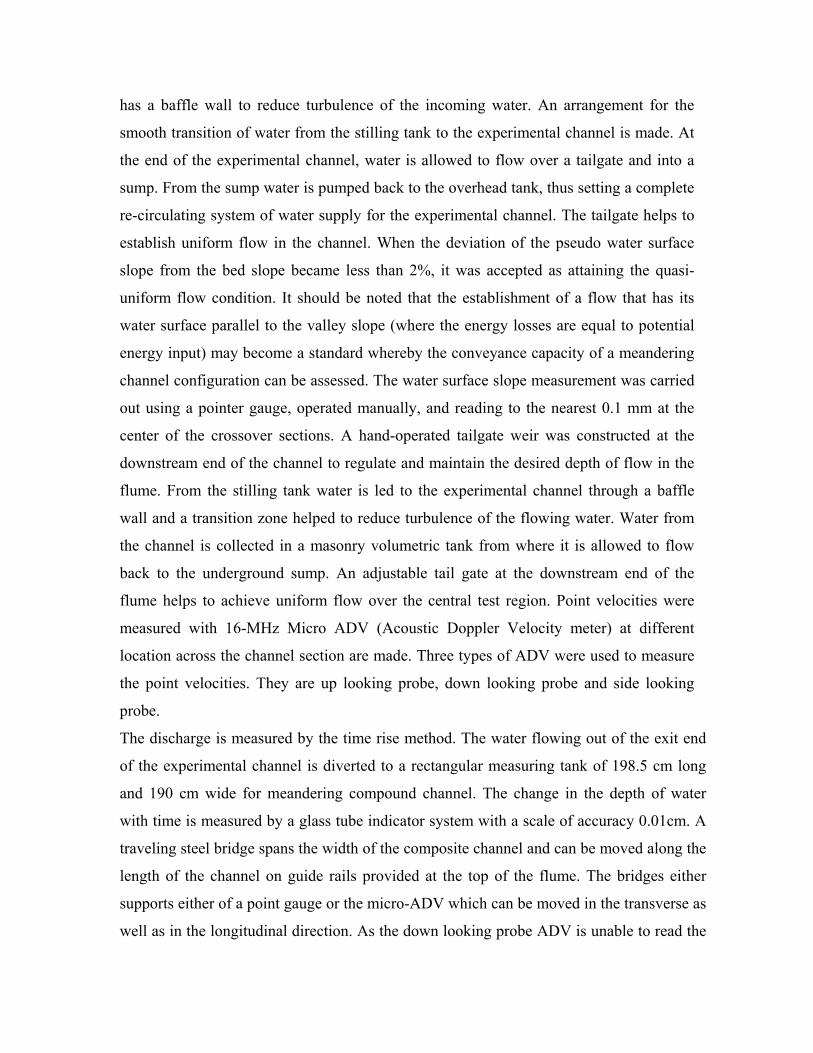
has a baffle wall to reduce turbulence of the incoming water. An arrangement for the

smooth transition of water from the stilling tank to the experimental channel is made. At

the end of the experimental channel, water is allowed to flow over a tailgate and into a

sump. From the sump water is pumped back to the overhead tank, thus setting a complete

re-circulating system of water supply for the experimental channel. The tailgate helps to

establish uniform flow in the channel. When the deviation of the pseudo water surface

slope from the bed slope became less than 2%, it was accepted as attaining the quasi-

uniform flow condition. It should be noted that the establishment of a flow that has its

water surface parallel to the valley slope (where the energy losses are equal to potential

energy input) may become a standard whereby the conveyance capacity of a meandering

channel configuration can be assessed. The water surface slope measurement was carried

out using a pointer gauge, operated manually, and reading to the nearest 0.1 mm at the

center of the crossover sections. A hand-operated tailgate weir was constructed at the

downstream end of the channel to regulate and maintain the desired depth of flow in the

flume. From the stilling tank water is led to the experimental channel through a baffle

wall and a transition zone helped to reduce turbulence of the flowing water. Water from

the channel is collected in a masonry volumetric tank from where it is allowed to flow

back to the underground sump. An adjustable tail gate at the downstream end of the

flume helps to achieve uniform flow over the central test region. Point velocities were

measured with 16-MHz Micro ADV (Acoustic Doppler Velocity meter) at different

location across the channel section are made. Three types of ADV were used to measure

the point velocities. They are up looking probe, down looking probe and side looking

probe.

The discharge is measured by the time rise method. The water flowing out of the exit end

of the experimental channel is diverted to a rectangular measuring tank of 198.5 cm long

and 190 cm wide for meandering compound channel. The change in the depth of water

with time is measured by a glass tube indicator system with a scale of accuracy 0.01cm. A

traveling steel bridge spans the width of the composite channel and can be moved along the

length of the channel on guide rails provided at the top of the flume. The bridges either

supports either of a point gauge or the micro-ADV which can be moved in the transverse as

well as in the longitudinal direction. As the down looking probe ADV is unable to read the

upper layer(up to 5cm from free surface),the up looking probe is unable to read the down

layer(up to 5cm from the base) and the side looking probe is unable to read the side

surface(up to 5cm from the side of the channel) so a micro -pitot tube of (4mm external

diameter) with a flow direction finder arrangements are used to measure some point

velocity and its direction with in that locations of the flow-grid points.

Fig 3.1 Channel section shown along with ADV positioning operation

Fig3.2 Experimental set up with plan form of the meandering channel with floodplain

Fig.3.3 One wave length of meandering compound channel

3.3 EXPERIMENTAL PROCEDURE

3.3.1 Determination of Channel Slope

By blocking the tail end, the impounded water in the channel is allowed to remain

standstill. The levels of channel bed and water surface are recorded at a distance of one

wavelength along its centerline. The mean slope for each type of channel is obtained by

dividing the level difference between these two points by the length of meander wave along

the centerline. The valley slope for meandering compound channels is equal to 0.0054.

3.3.2 Measurement of Discharge and water surface elevation

A point gauge with a least count of 0.01cm was used to measure the water surface elevation

above the bed of main channel or flood plain. As mentioned before, a measuring tank

located at the end of test channel receives water flowing through the channels Depending

on the flow rate the time of collection of water in the measuring tank varies between 50 to

240 seconds, lower one for higher discharge. The change in the mean water level in the

tank for the time interval is recorded. From the knowledge of the volume of water collected

in the measuring tank and the corresponding time of collection, the discharge flowing in the

experimental channel is obtained.

3.3.3 Measurement of Velocity and its Direction

16-MHz Micro ADV (Acoustic Doppler Velocity meter) from the original Son-Tek, San

Diego, Canada, is the most significant breakthrough in 3-axis (3D) Velocity meter

technology. The higher acoustical frequency of 16 MHz makes the Micro-ADV the optimal

instrument for laboratory study. After setup of the Micro ADV with the software package it

is used for taking high-quality three dimensional Velocity data at different points of the

flow area are received to the ADV-processor. Computer shows the raw data after compiling

the software package of the processor. At every point the instrument is recording a number

of velocity data for a minute. With the statistical analysis using the installed software, the

mean value of the point velocities (three dimensional) were recorded for each flow depths.

The Micro -ADV uses the Doppler shift principle to measure the velocity of small particles,

assuming to be moving at velocities similar to the fluid. Velocity is resolved into three

orthogonal components(Tangential, radial and vertical), and measured in a volume 5 cm

below the sensor head, minimizing interference of the flow field, and allowing

measurements to be made close to the bed.

The Micro ADV has the Features like

• Three-axis velocity measurement

• High sampling rates -- up to 50 Hz

• Small sampling volume -- less than 0.1 cm3

• Small optimal scatterer -- excellent for low flows

• High accuracy: 1% of measured range

• Large velocity range: 1 mm/s to 2.5 m/s

• Excellent low-flow performance

• No recalibration needed

• Comprehensive software

As the down looking ADV is unable to read the upper layer velocity i.e. up to 5cm from

free surface, the side looking probe is unable read 5cm from the side surface and the up

looking probe is unable to read 5cm from the base of the flume, so A standard Prandtl type

micro-pitot tube in conjunction with a water manometer of accuracy of 0.012 cm is also used

for the measurement of point velocity readings at some specified location for the upper 5cm

region from free surface across the channel. The results have been discussed in the next

chapter.

Chapter 4

OBSERVATIONS

4.1 Calculation of the three dimensional velocities As stated above, the three dimensional velocities at different heights of water level are

calculated and are pre recorded in the tables below:

4.1.1 Compound meandering channels

At flow depth H= 18.5 cm

X Y Vx Vy Vz

0.98 10 44.03 -1.72 -0.7713.49 10 46.506 0.797 -1.07417.5 1.83 50.048 3.908 0.08217.5 0.88 50.109 6.539 0.88617.5 0.48 51.965 -0.114 8.32720.3 4.64 56.208 -0.606 12.43320.3 3.54 53.019 -5.82 7.15320.3 2.81 55.786 -6.16 5.19320.3 1.67 46.163 -8.985 3.75320.3 0.8 44.643 -8.827 1.53323.5 6.84 33.123 -7.58 5.36523.5 4.64 34.809 -6.495 3.48423.5 2.61 45.749 0.548 4.97123.5 0.66 45.749 0.304 4.644

25 3.89 34.154 -33.186 -0.33125 3 36.288 -35.956 -1.84925 1.93 40.1 -38.179 -1.84925 1.55 35.962 -10.592 5.328

26.5 6.77 27.415 -31.833 -1.27126.5 4.67 31.584 -35.614 -5.88826.5 2.7 28.986 -25.605 3.6826.5 0.67 37.854 -24.146 5.4526.5 0.48 40.128 -19.497 6.51

28 4.28 35.892 -17.581 0.25328 3.68 19.546 2.546 4.99428 2.72 23.561 0.786 8.78328 1.65 22.01 -0.084 8.889

29.5 6.93 19.976 -0.366 8.10329.5 4.76 18.413 -0.929 6.20929.5 2.85 21.214 -2.904 5.96129.5 0.85 26.301 1.354 6.51429.5 0.73 25.646 3.874 3.654

31 4.09 26.282 3.964 3.28431 3.81 22.986 3.115 4.07431 3.72 20.755 3.19 3.54

31 2.99 20.276 1.864 3.19431 1.81 21.115 2.214 3.262

33.5 7.91 28.382 2.38 2.30433.5 4.96 28.744 6.748 1.78133.5 2.67 26.651 7.067 1.86933.5 0.79 24.048 6.505 2.01733.5 0.57 22.206 6.986 1.46133.5 0.38 22.207 6.78 1.263

34 3.09 21.506 6.877 0.56134 2.92 20.928 7.342 0.60634 2.06 27.892 7.651 -0.26834 1.56 28.45 10.167 0.81

36.5 4.89 26.965 9.326 0.52436.5 2.91 25.282 8.968 0.55436.5 0.94 21.647 8.644 -0.11241.5 0.74 22.274 7.863 -0.368

44 8.8 22.976 9.202 -0.70344 9.3 25.46 8.879 -1.05650 9.3 25.445 8.653 -0.78750 8.8 26.845 13.987 -0.35580 8.8 26.035 13.202 -0.57180 9.5 24.916 11.692 -1.47275 8.9 24.783 11.658 -2.37568 8.9 23.009 11.407 -2.329

At flow depth H= 17.5 cm

X Y Vx Vy Vz

0.98 10 50.11 9.674 -2.8933.49 10 59.804 8.894 -0.62117.5 1.83 54.317 12.276 -0.67117.5 0.88 48.305 6.775 3.33717.5 0.48 53.717 15.828 0.3420.3 4.64 48.403 9.936 1.07620.3 3.54 46.088 0.859 1.00120.3 2.81 45.933 3.108 0.25820.3 1.67 45.65 5.399 -0.18620.3 0.8 46.909 0.656 0.5523.5 6.84 43.623 0.15 -3.45923.5 4.64 43.579 7.654 -1.05923.5 2.61 63.949 -16.947 6.01923.5 0.66 70.709 -17.933 7.564

25 3.89 62.076 -13.956 7.956

25 3 63.204 -9.039 7.37625 1.93 43.582 -6.213 4.63325 1.55 54.136 -5.971 4.866

26.5 6.77 45.556 -5.259 4.17526.5 4.67 43.307 -2.921 -2.17426.5 2.7 51.318 -4.09 -6.8826.5 0.67 19.049 42.313 -4.6526.5 0.48 21.473 38.942 -14.499

28 4.28 30.355 28.298 -11.85128 3.68 30.873 24.875 4.35228 2.72 8.325 -43.279 12.35528 1.65 30.873 24.785 4.352

29.5 6.93 8.325 -43.279 12.329.5 4.76 40.58 5.955 3.1429.5 2.85 25.369 -0.166 3.36129.5 0.85 -8.079 -0.889 2.45629.5 0.73 32.552 3.852 5.556

31 4.09 14.776 5.064 10.15131 3.81 21.147 9.046 17.73231 3.72 26.538 -18.32 -2.35731 2.99 28.561 -10.4 0.69931 1.81 23.107 2.981 -9.104

33.5 7.91 22.519 6.038 -3.57833.5 4.96 13.553 19.446 3.40133.5 2.67 26.301 21.396 5.22733.5 0.79 17.894 24.48 5.69633.5 0.57 31.207 -8.154 -3.34933.5 0.38 28.786 -1.715 -9.007

34 3.09 24.501 5.244 -12.06434 2.92 23.135 7.526 -8.8734 2.06 28.303 18.268 -4.88534 1.56 35.263 1.587 4.514

36.5 4.89 2.685 0.127 0.34836.5 2.91 1.782 0.012 0.21136.5 0.94 36.603 5.388 -7.67441.5 0.74 35.771 -1.294 -8.22

44 8.8 33.677 -4.762 -6.49244 9.3 32.768 -9.511 -3.56450 9.3 36.143 -5.591 -2.1850 8.8 38.042 -2.194 -3.7480 8.8 39.684 1.469 -5.48580 9.5 43.162 8.543 -3.36675 8.9 44.547 11.423 -0.55468 8.9 43.296 -3.753 -0.996

At flow depth H=13.5cm

X Y Vx Vy Vz

0.31 9.1 -1.23 -4.578 4.7050.31 8.5 -1.594 -5.9 -0.883

6 2.74 44.567 -1.601 3.626 1.64 42.047 -1.601 2.7786 0.63 41.18 -1.257 2.426 0.38 36.632 -2.026 2.754

12.5 3.01 37.285 -1.265 5.10212.5 2 34.055 -0.303 4.43712.5 1 31.102 0.78 3.72712.5 0.57 0.051 -5.776 5.912.5 0.38 29.842 1.877 2.468

13 0.87 3.992 5.716 -2.60514.6 0.31 -1.23 6.0571 0.861

15 0.31 -1.594 6.055 0.79416.5 2.8 21.217 -2.161 0.10916.5 1.98 21.141 2.517 22.24316.5 0.98 21.26 6.234 23.35516.5 0.52 20.778 17.244 21.42220.5 6.12 18.998 -1.188 5.94720.5 3.08 14.771 12.784 8.18420.5 2.13 19.8 24.363 11.80920.5 0.39 26.131 24.624 15.3223.5 10.58 30.962 17.894 -9.10423.5 8.53 27.893 31.207 -3.57823.5 6.48 23.232 28.786 3.40123.5 4.58 21.861 24.501 5.22723.5 2.48 27.942 23.135 5.69623.5 0.54 32.056 22.55 -3.34933.5 8.83 42.236 63.949 -9.00733.5 6.56 45.591 70.709 -12.06433.5 4.43 47.312 62.076 -1.05933.5 2.43 50.415 63.204 6.01933.5 0.37 30.544 43.582 7.56439.5 2.72 48.709 54.136 7.95639.5 1.2 53.559 45.556 7.37639.5 0.5 55.596 43.307 4.63341.5 1 56.214 51.318 4.86645.5 2.43 55.314 19.049 4.17545.5 1.39 54.881 21.473 -2.17445.5 0.77 52.606 30.355 -6.8855.5 0.98 43.91 30.873 -4.6555.5 0.62 43.775 8.325 4.35255.5 0.54 44.514 30.873 12.35555.5 0.38 42.617 8.325 4.35265.5 2.4 37.265 40.58 12.365.5 1.4 36.899 25.369 3.1465.5 0.57 35.526 -8.079 3.361

65.5 0.44 35.418 32.552 2.45665.5 0.35 32.313 28.561 5.55675.5 1.65 47.751 23.107 10.15175.5 0.75 45.552 22.519 17.73275.5 0.6 44.217 13.553 -2.35775.5 0.49 44.661 26.301 0.699

At flow depth H = 12 cm X Y VX Vy Vz

0.98 10 29.024 23.753 9.3013.49 10 24.476 26.703 6.54917.5 1.83 22.573 23.74 4.3717.5 0.88 28.283 3.463 4.53617.5 0.48 28.206 26.301 3.66420.3 4.64 23.468 33.896 3.63820.3 3.54 19.999 32.693 1.75920.3 2.81 14.197 42.685 -0.44520.3 1.67 21.61 38.45 0.67320.3 0.8 27.782 26.78 0.08223.5 6.84 21.442 16.602 1.47723.5 4.64 29.087 24.94 -0.57123.5 2.61 28.509 30.947 -0.29223.5 0.66 20.281 39.573 -1.486

25 3.89 13.452 45.131 -2.47225 3 14.229 44.126 -2.97725 1.93 21.059 37.463 -4.08825 1.55 30.117 28.454 -4.501

26.5 6.77 34.161 21.8 -8.1326.5 4.67 30.916 28.368 -7.79226.5 2.7 22.243 39.94 -8.65226.5 0.67 23.19 -9.142 3.53826.5 0.48 16.294 5.784 1.647

4.2 Contours 4.2.1 3D Field

Using very popular software called 3DField all the velocity contours are plotted in it.

It is very user-friendly and has a wide application in engineering areas.

3DField reads:

- scattered data points (X, Y, Z) and matrix data sets.

3DField creates maps, color and BW contours, color cells, color points, Direchlet

tessellations, Delauney triangles, color and monotone relief, slices and circle values.

Features of this software are:

• 5 gridding methods.

• Automatic or user-defined contour intervals and ranges.

• Control over contour label format, font, frequency and spacing.

• Automatic or user-defined color for contour lines.

• Color fill between contours, either user-specified or as an automatic spectrum of

your choice.

• Base map

• Regression 2D data.

• View and zoom BMP, GIF, PNG and JPG images

• Automatically and manually digitize image

• Import and export lines.

• OpenGL view with full screen rotating.

• Convert a simple contour bitmap to a 3D view

• Output maps as EMF, WMF, BMP, JPG, PNG file formats

• Insert maps (as EMF or bitmap) in any document Microsoft Office

• Multipage scale print

• Multilingual interface

Fig 4.1 A 3DField software layout.

4.2.2 EXPERIMENTAL DATA

Fig. 4.2. Flow depth H=17.5cm

Fig.4.3. Flow depth H=15.5cm

Fig 4.4. Flow depth H=12 cm

Fig 4.5 Flow depth H= 18.5cm

4.3. FLOOD CHANNEL FACILITY DATA SERIES 01 At flow depth H=21.4cm

(A)


(B) At flow depth H=19.8 cm

(C)

SERIES 02 At flow depth H=24.9 cm

(D) At flow depth H=18.5 cm

(E)

At flow depth H=28.8 cm

(F)

SERIES 08 At flow depth H=25.02cm

(G) At flow depth H=21.48cm

(I)


(J)

SERIES-10 At flow depth H=27.97cm

(K)


(L)


(M)

FIG 4.2 cross sections of straight compound channel with velocity contours(A,B,C,D,E,f,G,H,I,,J,K,L,M) for various heights of flow.

Chapter 5

ANALYSIS OF THE EXISTING DATA

5.1 Development of model Plots of the isovels for the longitudinal velocities for the channel are used to find out the

area-velocity distributions that are subsequently integrated to obtain the discharge of the

main channel and floodplains separated by various assumed interface planes. At low

depths of flow over floodplain, there is wide disparity between main channel and

floodplain velocities confirming the process of momentum transfer between the main

channel and floodplain. As the depth of flow over the floodplain increases, the velocities

at the inner side of the floodplain are more rapid than the outer side, but the mean

velocities in the floodplain and main channel becomes equal, indicating a marked

reduction in momentum transfer.

the model %Qmc proposed by knight and Demetriou (1984) for straight channel is given

as

( )( )[ ] ( ) βαβ

αα

βα9.9

441

3.3110811

100% −⎟⎠⎞

⎜⎝⎛ −

+−−

= eQmc

In order to account for meandering effects to the meandering compound channels, Patra

and Kar (2000) proposed an improvement to the equation given by Knight and Demetriou

(1984).and for meandering compound channel the equation obtained were,

( )[ ] [ ]δββαβα

/)(361),(11

100%Q mc rSLnF +++−

=

( )( ) ( ) ⎥⎦⎤

⎢⎣⎡ +⎟

⎠⎞

⎜⎝⎛ −

+−−

= −

δββα

αβα

βα r

mcSLneQ 3613.31108

11100% 9.9

441

Where Sr is the parameter representing the sinuosity of the meander channel (str. Valley

length/ length along channel center). The std. error of estimate between the observed and

computed percentages of discharge is 5.39 with correlation coefficient of 0.967.

For lower main channel separated from the compound section by a horizontal interface

plain at the level of floodplain the following equations for the percentage of discharges

and the section mean velocity in lower main channel have been obtained by best fit as

( )[ ] ( ) ββα

αβαβ 9.152

25.1

lmc 3.5130011)1(100%Q −⎟

⎠⎞

⎜⎝⎛ −

++−

−= e

( )[ ] ( ) ( )[ ]δββα

αβαβ β /3613.51300

11)1(100%Q 9.152

25.1

lmc rSLne +⎟⎠⎞

⎜⎝⎛ −

++−

−= −

In which %Qlmc is the percentage of flow in the lower main channel. For straight

channels (i.e. for Sr =1) the equation attains the form of the equation proposed by Knight

and Demetriuo(1984).

Our intension here is to identify an accurate, simple and yet a practicable applicable

rational formula that holds the key to unwinding a powerful method of determining the

discharge for the main channel and the flood plain. The equation should be equally

capable to predict the upper main channel and lower main channel discharges with an

accuracy greater than any of the earlier proposed methods. From the present experimental investigation of both straight and meandering compound

channel it has been found that %Qlmc and %Almc follows a linear equation which can be

expressed as

⎥⎦⎤

⎢⎣⎡=

AAmc100

Q100Q mc + Constant (difference factor)

This constant varies from flow depth to depth and is function of the geometrical

parameters α and β, for straight compound channel which can be written as

( ) ⎥⎦

⎤⎢⎣

⎡−=A

Amc100Q

100Q,F mcβα , the values of Qmc and Amc being estimated experimentally

from the experimental setup discussed above. The values of (DF) difference factor were

then plotted against α and β, of the channel cross section. The variation of difference

factor was then captured in equations. The variation was first observed by keeping α

constant and varying β. The best fitted equation from the plot has been obtained

Difference factor=A (β)B

Fig 5.1 difference factor being plotted for α constant and varying β.

DF=-8.236Ln(x)-4.374------------ (A) the regression coefficient being 0.9085.

Fig 5.2 The difference factor was plotted Keeping the value of ‘β’constant, and α varying

Thus, the equation DF=32.71α² -349.3α+962.1----------- (B) was considered to be the

best fit curve which gave R² as 0.985

The final equation for

DF= A[(βe)B *C Log α) ],for

For meandering compound channel the meandering effect has been incorporated and a

final general form has been obtained and given as

5.2Validation of the data The results obtained from the equation in this model were validated with other previously

conducted experimental data and the plots for Qmc actually observed at the time of

experimentation and Qmc predicted through the equation developed in this model were

plotted

Fig 5.3 % Qmc predicted by the model developed against the % Qmc actually for

meandering channels by experiment done at NIT Rourkela.

The above graph is a plot for % Qmc predicted by the model developed against the % Qmc

actually calculated by counting the number of squares in the fig(4.3F,G,H,I,J,K). The

above data is for meandering channels.

Fig 5.4 % Qmc predicted by the model developed against the % Qmc actually for FCF

channels.

Conclusion

• The distribution of flow discharge along the perimeter meandering compound

channels are examined and a rational relationship to predict the percentage

discharge is obtained.

• The % Qmc so found out happened to be in greater accuracy as compared with the

FLOOD CHANNEL FACILITY DATA(FCF).

• The results obtained from the equation in this paper were validated with other

previously conducted experimental data and the plots for Qmc actually observed at

the time of experimentation and Qmc obtained through the equation developed in

this paper.

• The equation being dimensionless, it is more practically realizable. The equation

developed is not empirical. It is purely rational and known to satisfy the river

plain components discharges well.

• The discharge values predicted are more accurate. The equation involves only the

geometrical parameters of any natural channel.

• The equations presented in the paper are considered to be a reasonable attempt on

defining the interaction between main channel and flood plain flow. They will be

of particular benefit to those engaged in the numerical modeling of hydraulic

flows.

• For the meandering compound channels the important parameters effecting the

flow distribution are sinuosity(Sr) ,the amplitude (ε) ,relative depth (β) and the

width ratio (α) and the aspect ratio(δ). These five dimensionless parameters are

used to form general equations representing the total flow contribution in main

channels. The proposed equations give good result with the observed data.

• It is suggested that further investigation be focused on extending the present

analysis to the compound channel of different roughness.

Reference: 1. Bhattacharya, A. K. (1995). ‘‘Mathematical model of flow in meandering

channel.’’ PhD thesis, IIT, Kharagpur, India.

2. Ghosh, S.N., and Kar, S.K., (1975), "River Flood Plain Interaction and

Distribution of Boundary Shear in a Meander Channel with Flood Plain",

Proceedings of the Institution of Civil Engineers, London, England,

Vol.59,Part 2, December, pp.805-811.

3. Greenhill, R.K. and Sellin, R.H.J., (1993), "Development of a Simple

Method to Predict Discharge in Compound Meandering Channels", Proc.

of Instn. Civil Engrs Wat., Merit and Energy, 101, paper 10012, March,

pp. 37-44.

4. Knight, D.W., and Demetriou, J.D., (1983), "Flood Plain and Main

Channel Flow Interaction". Journal of Hyd. Engg., ASCE Vo.109, No.8,

pp-1073-1092.

5. Knight, D.W., and Shino, K. (1996). ‘‘River Channel and Floodplain

Hydraulics.Floodplain Processes.,Edited by M.G.Anderson,Des E.Walling

and Paul D.

6. Myers, W.R.C., (1987), "Velocity and Discharge in Compound Channels",

Jr. of Hydr. Engg., ASCE, Vol.113, No.6, pp.753-766.

7. Myer, W.R.C., and Lyness, J.F., (1997), "Discharge Ratios in Smooth and

Rough Compound Channels", Jr. of Hydr. Eng., ASCE, Vol., 123, No.3,

pp.182-188.

8. Odgaard, A.J., (1986), "Meander Flow Model I: Development", Jr. of

Hyd.Engg., ASCE, Vol 112, No.12, pp.1117-1135.

9. Odgaard, A.J., (1989), "River Meander Model-I: Development", Journal

of Hydr. Engineering, ASCE, Vol., 115, No.11, pp.1433-1450.

10. Patra,K.C.,Kar,S.K.,(2000) Flow interaction of Meandering River with

Flood plains Journal of Hydr. Engineering, ASCE, Vol., 126, No.8,

pp.593-603.

11. Shiono, K., , Al-Romaih, J. S. and Knight D. W. “stage-discharge

assessment in compound meandering channels” journal of hydraulic

engineering ASCE / april 2004 / 305

12. Shiono K. & Knight, D.W., (1990), “Mathematical Models of Flow in two

or Multistage Straight Channels”, Proc. Int. Conf. on River Flood Hyd., (Ed.

W.R.White), J. Wiley & Sons, Wallingford, September, Paper G1, pp 229-

238.

13. Shiono K., and Knight, D. W. (1989), ‘‘Two dimensional analytical solution

of compound channel’’ Proc., 3rd Int. Symp. on refined flow modeling and

turbulence measurements, Universal Academy Press, pp.591–599.

14. Shiono, K., and Knight, D. W. (1991). ‘‘Turbulent Open Channel Flows

with Variable Depth Across the Channel.’’ J. of Fluid Mech., Cambridge,

U.K., 222, pp.617–646

Photo Gallery:

Plate 1: Front View of ADV

Plate 2: side looking probe

Plate 3: Measuring the velocities

Plate 4: A close look at the channel

DISCHARGE DISTRIBUTION IN MEANDERING COMPOUND CHANNELS

Documents

Transcript of DISCHARGE DISTRIBUTION IN MEANDERING COMPOUND CHANNELS