Dirichlet mixtures: a method for improved detection of weak but significant protein sequence...

CABIOS Vol. 12 no. 4 1996Pages 327-345

Dirichlet mixtures: a method for improveddetection of weak but significant proteinsequence homology

Kimmen Sjolander3, Kevin Karplus, Michael Brown,Richard Hughey, Anders Krogh1,1.Saira Mian2 and David Haussler

Abstract

We present a method for condensing the information inmultiple alignments of proteins into a mixture of Dirichletdensities over amino acid distributions. Dirichlet mixturedensities are designed to be combined with observed aminoacid frequencies to form estimates of expected amino acidprobabilities at each position in a profile, hidden Markovmodel or other statistical model. These estimates give astatistical model greater generalization capacity, so thatremotely related family members can be more reliablyrecognized by the model. This paper corrects the previouslypublished formula for estimating these expected probabil-ities, and contains complete derivations of the Dirichletmixture formulas, methods for optimizing the mixtures tomatch particular databases, and suggestions for efficientimplementation.

Introduction

One of the main techniques used in protein sequenceanalysis is the identification of homologous proteins—proteins which share a common evolutionary historyand almost invariably have similar overall structureand function (Doolittle, 1986). Homology is straight-forward to infer when two sequences share 25% residueidentity over a stretch of 80 or more residues (Sanderand Schneider, 1991). Recognizing remote homologs, withlower primary sequence identity, is more difficult. Findingthese remote homologs is one of the primary motivatingforces behind the development of statistical models forprotein families and domains, such as profiles and theirmany offshoots (Waterman and Perlwitz, 1986; Gribskovel al. 1987, 1990; Altschul et al., 1990; Barton andSteinberg, 1990; Bowie et al., 1991; Luthy et al., 1991;

Baskin Center for Computer Engineering and Information Sciences,Applied Sciences Building, University of California at Santa Cruz, SantaCruz, CA 95064, USA, 'The Sanger Centre, Hinxton Hall, Hinxton,Cambs CB10 IRQ, UK and 2Life Sciences Division (Mail Stop 29-100),Lawrence Berkeley Laboratory, University of California, Berkeley, CA94720, USA

To whom correspondence should be addressed. E-mail: [email protected]

Thompson et al., 1994a,b; Bucher et al., 1996), Position-Specific Scoring Matrices (Henikoff et al., 1990), andhidden Markov models (HMMs) (Churchill, 1989; Baldiet al., 1992; Asai et al., 1993; Stultz et al., 1993; Baldiand Chauvin, 1994; Krogh et al., 1994; White et al., 1994;Eddy, 1995, 1996; Eddy et al., 1995; Hughey and Krogh,1996).

We address this problem by incorporating priorinformation about amino acid distributions that typi-cally occur in columns of multiple alignments into theprocess of building a statistical model. We present amethod to condense the information in databases ofmultiple alignments into a mixture of Dirichlet densities(Berger, 1985; Santner and Duffy, 1989; Bernardo andSmith, 1994) over amino acid distributions, and tocombine this prior information with the observedamino acids to form more effective estimates of theexpected distributions. Multiple alignments used in theseexperiments were taken from the Blocks database(Henikoff and Henikoff, 1991). We use MaximumLikelihood (Duda and Hart, 1973; Dempster et al.,1977; Nowlan, 1990), to estimate these mixtures, i.e. weseek to find a mixture that maximizes the probability ofthe observed data. Often, these densities capture someprototypical distributions. Taken as an ensemble, theyexplain the observed distributions in columns of multiplealignments.

With accurate prior information about which kindsof amino acid distributions are reasonable in columnsof alignments, it is possible with only a few sequences toidentify which prototypical distribution may have gener-ated the amino acids observed in a particular column.Using this informed guess, we adjust the expected aminoacid probabilities to include the possibility of amino acidsthat may not have been seen but are consistent withobserved amino acid distributions. The statistical modelsproduced are more effective at generalizing to previouslyunseen data, and are often superior at database searchand discrimination experiments (Brown et al., 1993;Tatusov et al., 1994; Bailey and Elkan, 1995; Karplus,1995a; Hughey and Krogh, 1996; Henikoff and Henikoff,1996; Wang et al., 1996).

© Oxford University Press 327

by guest on August 9, 2015

http://bioinformatics.oxfordjournals.org/

Dow

nloaded from


K-SJfllander tt al.

Database search using statistical models

Statistical models for proteins capture the statisticsdefining a protein family or domain. These models havetwo essential aspects: (i) parameters for every position inthe molecule or domain that express the probabilities ofthe amino acids, gap initiation and extension, and soon; and (ii) a scoring function for sequences with respectto the model.

Statistical models do not use percentage residueidentity to determine homology. Instead, these modelsassign a probability score [some methods report a costrather than a probability score; these are closely related(Altschul, 1991)] to sequences, and then compare thescore to a cutoff. Most models (including HMMs andprofiles) make the simplifying assumption that eachposition in the protein is generated independently. Underthis assumption, the score for a sequence aligning to amodel is equal to the product of the probabilities ofaligning each residue in the protein to the correspondingposition in the model. In homolog identification bypercentage residue identity, if a protein aligns a previouslyunseen residue at a position it is not penalized; it losesthat position, but can still be recognized as homologousif it matches at a sufficient number of other positions inthe search protein. However, in statistical models, if aprotein aligns a zero-probability residue at a position, theprobability of the sequence with respect to the modelis zero, regardless of how well it may match the rest of themodel. Because of this, most statistical models rigorouslyavoid assigning residues probability zero, and accurateestimates for the amino acids at each position areparticularly important.

Using prior information about amino acid distributions

The parameters of a statistical model for a protein familyor domain are derived directly from sequences in thefamily or containing the domain. When we have fewsequences, or a skewed sample, the raw frequencies area poor estimate of the distributions which we expectto characterize the homologs in the database. Skewedsamples can arise in two ways. In the first, the sample isskewed simply from the luck of the draw. This kind ofskew is common in small samples, and is akin to tossinga fair coin three times and observing three heads in a row.The second type of skew is more insidious, and can occureven when large samples are drawn. In this kind of skew,one subfamily is over-represented, such that a largefraction of the sequences used to train the statisticalmodel are minor variants of each other. In this kind ofskew, sequence weighting schemes are necessary tocompensate for the bias in the data. Models that usethese raw frequencies may recognize the sequences used

to train the model, but will not generalize well torecognizing remoter homologs.

It is illuminating to consider the analogous problemof assessing the fairness of a coin. A coin is said to be fairif Prob (heads) = Prob (tails) — 1/2. If we toss a cointhree times, and it comes up heads each time, what shouldour estimate be of the probability of heads for this coin?If we use the observed raw frequencies, we would set theprobability of heads to one, but, if we assume that mostcoins are fair, then we are unlikely to change this a prioriassumption based on only a few tosses. Given little data,we will believe our prior assumptions remain valid. Onthe other hand, if we toss the coin an additional thousandtimes and it comes up heads each time, few will insist thatthe coin is indeed fair. Given an abundance of data, we willdiscount any previous assumptions, and believe the data.

When we estimate the expected amino acids in eachposition of a statistical model for a protein family, weencounter virtually identical situations. Fix a numberingof the amino acids from 1 to 20. Then, each column ina multiple alignment can be represented by a vector ofcounts of amino acids of the form n = (n\,... ,n2o), wherent is the number of times amino acid i occurs in the columnrepresented by this count vector, and |w| = 52, n,. Theestimated probability of amino acid i is denoted p,. If theraw frequencies are used to set the probabilities, thenp, := n,-/|n|. Note that we use the symbol ' :=' to denoteassignment, to distinguish it from equality, since wecompute fa differently in different parts of the paper.

Consider the following two scenarios. In the first, wehave only three sequences from which to estimate theparameters of the model. In the alignment of these threesequences, we have a column containing only isoleucine,and no other amino acids. With such a small sample, wecannot rule out the possibility that homologous proteinsmay have different amino acids at this position. Inparticular, we know that isoleucine is commonly foundin buried /?-strand environments, and leucine and valineoften substitute for it in these environments. Thus, ourestimate of the expected distribution at this positionwould sensibly include these amino acids, and perhapsthe other amino acids as well, albeit with smallerprobabilities.

In a second scenario, we have an alignment of 100varied sequences and again find a column containing onlyisoleucine, and no other amino acids. In this case, we havemuch more evidence that isoleucine is indeed conserved atthis position, and thus generalizing the distribution at thisposition to include similar residues is probably not a goodidea. In this situation, it makes more sense to give lessimportance to prior beliefs about similarities amongamino acids, and more importance to the actual countsobserved.

328



Dow

nloaded from


Improved detection of weak protein sequence bomology

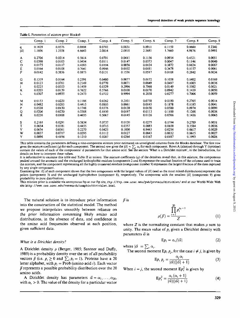
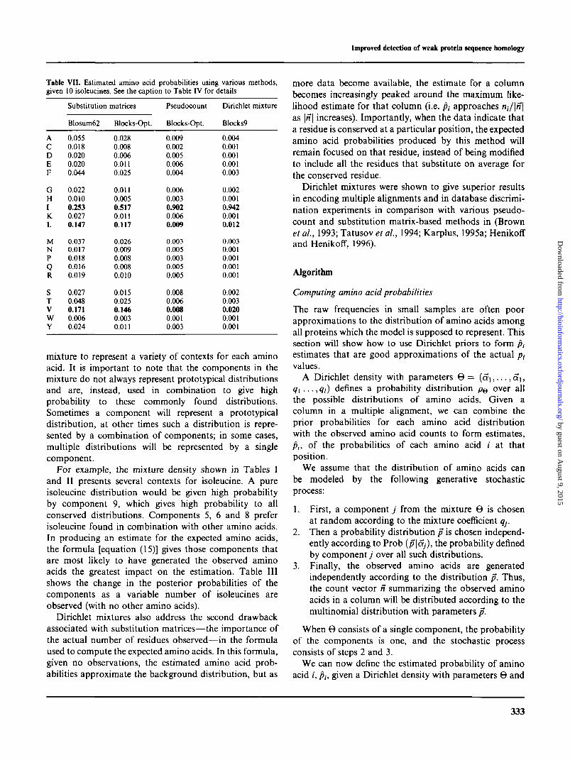
Table I.

q

A

cDEF

GHIKL

MNPQR

STVWY

Parameters

Comp. 1

0.18291.1806

0.27060.03980.01750.01640.0142

0.13190.01230.02250.02030.0307

0.01530.04820.05380.02060.0236

0.21610.06540.06540.00370.0096

of mixture prior

Comp. 2

0.05761.3558

0.02140.01030.01170.01080.3856

0.01640.07610.03530.01390.0935

0.02200.02850.01300.02300.0188

0.02910.01810.03610.07170.4196

Blocks9

Comp. 3

0.08986.6643

0.56140.04540.43830.76410.0873

0.25910.21490.14590.76220.2473

0.11860.44150.17480.53080.4655

0.58340.44550.22700.02950.1210

Comp. 4

0.07922.0814

0.07010.01110.01940.09460.0131

0.04800.07700.03290.57660.0722

0.02820.08030.03760.18500.5067

0.07370.07150.04250.01120.0287

Comp. 5

0.08312.0810

0.04110.01470.00560.01020.1536

0.00770.00710.29960.01080.9994

0.21010.00610.01300.01970.0145

0.01200.03570.18000.01270.0264

Comp. 6

0.09112.5681

0.11560.03730.01240.01810.0517

0.01720.00490.79680.01700.2858

0.07580.01450.01500.01130.0126

0.02750.08830.94430.00430.0167

Comp. 7

0.11591.7660

0.09340.00470.38720.34780.0108

0.10580.04970.01490.09420.0277

0.01000.18780.05000.11000.0386

0.11940.06580.02540.00320.0187

Comp. 8

0.06604.9876

0.45210.11460.06240.11570.2842

0.14020.10030.55020.14390.7006

0.27650.11850.09740.12660.1436

0.27890.35840.66170.06150.1993

Comp. 9

0.23400.0995

0.00510.00400.00670.00610.0034

0.01690.00360.00210.00500.0059

0.00140.00410.00900.00360.0065

0.00310.00360.00290.00270.0026

This table contains the parameters defining a nine-component mixture prior estimated on unweighted columns from the Blocks database. The first rowgives the mixture coefficient (q) for each component. The second row gives the \a\ = J2i ai f°r ^ch component. Rows A (alanine) through Y (tyrosine)contain the values of each of the components' a parameters for that amino acid. See the section 'What is a Dirichlet mixture', in the Introduction, fordetails on how to interpret these values.It is informative to examine this table and Table II in unison. The mixture coefficients (q) of the densities reveal that, in this mixture, the componentspeaked around the aromatic and the uncharged hydrophobic residues (components 2 and 8) represent the smallest fraction of the columns used to trainthe mixture, and the component representing all the highly conserved residues (component number 9) represents the largest fraction of the data capturedby any single component.Examining the |<3| of each component shows that the two components with the largest values of \a\ (and so the most mixed distributions) represent thepolars (component 3) and the uncharged hydrophobics (component 8), respectively. The component with the smallest |5 | (component 9) givesprobability to pure distributions.This mixture prior is available via anonymous ftp at our ftp site, ftp://ftp.cse.ucsc.edu/pub/protoin/diriclilet/ and at our World-Wide Website http: //www. cso.ucsc.edu/reseaxch/compbio/dirichlet.html.

The natural solution is to introduce prior informationinto the construction of the statistical model. The methodwe propose interpolates smoothly between reliance onthe prior information concerning likely amino aciddistributions, in the absence of data, and confidence inthe amino acid frequencies observed at each position,given sufficient data.

What is a Dirichlet density?

A Dirichlet density p (Berger, 1985; Santner and Duffy,1989) is a probability density over the set of all probabilityvectors p (i.e. p, > 0 and £^ pt — 1). Proteins have a 20letter alphabet, with/?, = Prob (amino acid /). Each vectorp represents a possible probability distribution over the 20amino acids.

A Dirichlet density has parameters a = a , , . . . ,a-^,with a, > 0. The value of the density for a particular vector

p is20

P(P) =1 = 1

(1)

where Z is the normalizing constant that makes p sum tounity. The mean value of /?, given a Dirichlet density withparameters a is

EPi = a,/\S\ (2)

where | 5 | = £], Q rThe second moment Ep, pp for the case / ^ j , is given by

When / = j , the second moment Ep) is given by

329



Dow

nloaded from


K.SJolander el at.

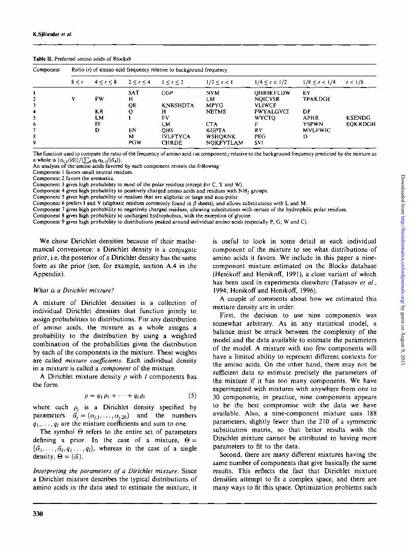
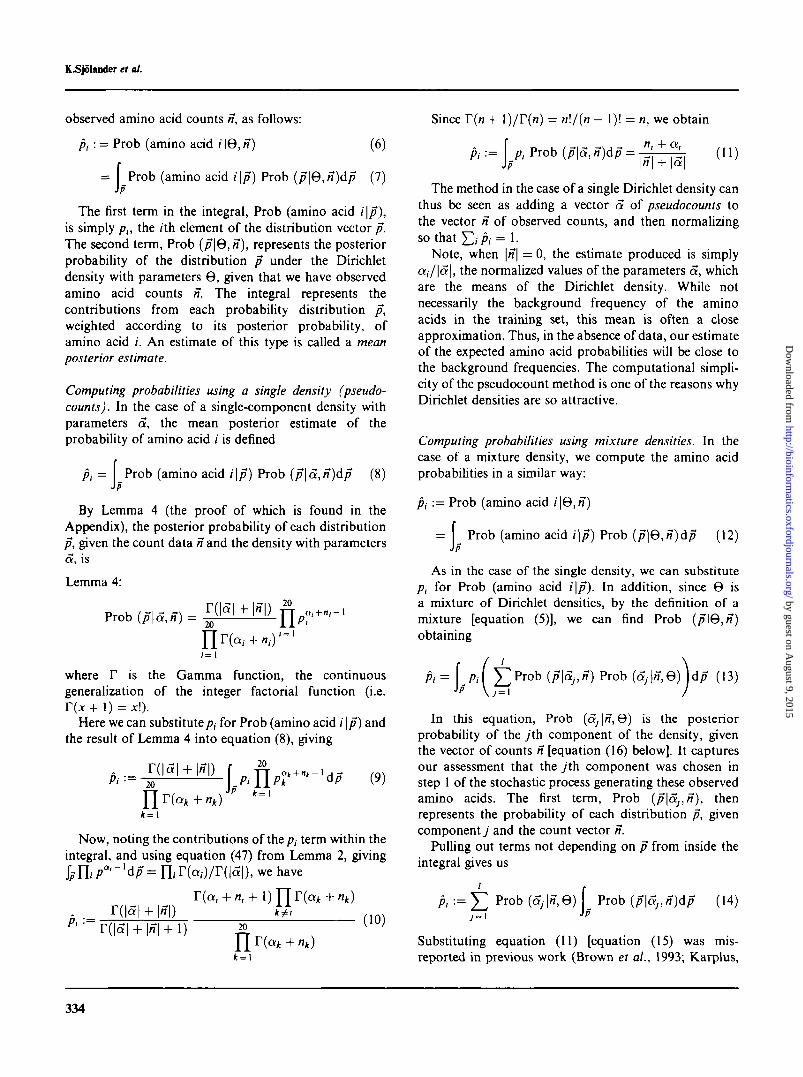
TaWe U. Preferred amino acids of Blocks9

Component Ratio (r) of amino acid frequency relative to background frequency

123456789

8 < r

Y

4 < r < 8

FW

KRLMIVD

2 < r < 4

SATHQEQ1

ENMPGW

1 <r< 2

CGP

K.NRSHDTAHFVLMQHSIVLFTYCACHRDE

1/2 < r < 1

NVMLMMPYGNETMS

CTAKGPTAWSHQRNKNQKFYTLAM

l / 4 < r < 1/2

QHRIKFLDWNQICVSRVLIWCFPWYALGVCIWYCTQFRYPEGSVI

1/8 <r< 1/4

EYTPAKDGE

DFAPHRYSPWNMVLFWICD

r < 1/8

K.SENDGEQKRDGH

The function used to compute the ratio of the frequency of amino acid i in component^ relative to the background frequency predicted by the mixture asa whole is (a/,(/|a|)/(£*<7*Q*,//l"*l)-An analysis of the amino acids favored by each component reveals the following-Component I favors small neutral residues.Component 2 favors the aromatics.Component 3 gives high probability to most of the polar residues (except for C, Y and W).Component 4 gives high probability to positively charged amino acids and residues with NH2 groups.Component 5 gives high probability to residues that are aliphatic or large and non-polar.Component 6 prefers I and V (aliphatic residues commonly found in /? sheets), and allows substitutions with L and M.Component 7 gives high probability to negatively charged residues, allowing substitutions with certain of the hydrophilic polar residues.Component 8 gives high probability to uncharged hydrophobics, with the exception of glycine.Component 9 gives high probability to distributions peaked around individual amino acids (especially P, G, W and C).

We chose Dirichlet densities because of their mathe-matical convenience: a Dirichlet density is a conjugateprior, i.e. the posterior of a Dirichlet density has the sameform as the prior (see, for example, section A.4 in theAppendix).

What is a Dirichlet mixture?

A mixture of Dirichlet densities is a collection ofindividual Dirichlet densities that function jointly toassign probabilities to distributions. For any distributionof amino acids, the mixture as a whole assigns aprobability to the distribution by using a weightedcombination of the probabilities given the distributionby each of the components in the mixture. These weightsare called mixture coefficients. Each individual densityin a mixture is called a component of the mixture.

A Dirichlet mixture density p with / components hasthe form

i i / c

where each p} is a Dirichlet density specified byparameters 5, = ( a y i , . . . ,0,20) and the numbers<7i,..., ql are the mixture coefficients and sum to one.

The symbol 0 refers to the entire set of parametersdefining a prior. In the case of a mixture, 0 =(5 [ , . . . ,<3/,<7i . . . ,<?/), whereas in the case of a singledensity, 0 = (a).

Interpreting the parameters of a Dirichlet mixture. Sincea Dirichlet mixture describes the typical distributions ofamino acids in the data used to estimate the mixture, it

is useful to look in some detail at each individualcomponent of the mixture to see what distributions ofamino acids it favors. We include in this paper a nine-component mixture estimated on the Blocks database(Henikoffand Henikoff, 1991), a close variant of whichhas been used in experiments elsewhere (Tatusov et ah,1994; Henikoffand Henikoff, 1996).

A couple of comments about how we estimated thismixture density are in order.

First, the decision to use nine components wassomewhat arbitrary. As in any statistical model, abalance must be struck between the complexity of themodel and the data available to estimate the parametersof the model. A mixture with too few components willhave a limited ability to represent different contexts forthe amino acids. On the other hand, there may not besufficient data to estimate precisely the parameters ofthe mixture if it has too many components. We haveexperimented with mixtures with anywhere from one to30 components; in practice, nine components appearsto be the best compromise with the data we haveavailable. Also, a nine-component mixture uses 188parameters, slightly fewer than the 210 of a symmetricsubstitution matrix, so that better results with theDirichlet mixture cannot be attributed to having moreparameters to fit to the data.

Second, there are many different mixtures having thesame number of components that give basically the sameresults. This reflects the fact that Dirichlet mixturedensities attempt to fit a complex space, and there aremany ways to fit this space. Optimization problems such

330



Dow

nloaded from


Improved detection of weak protein sequence homology

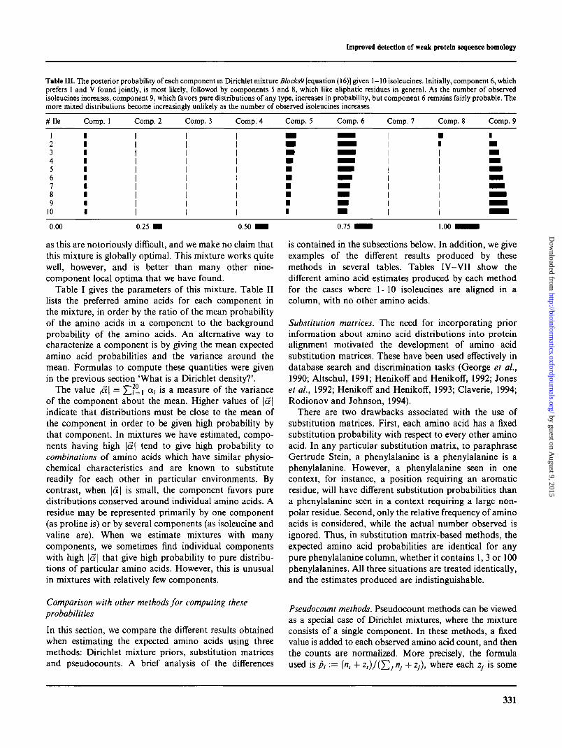
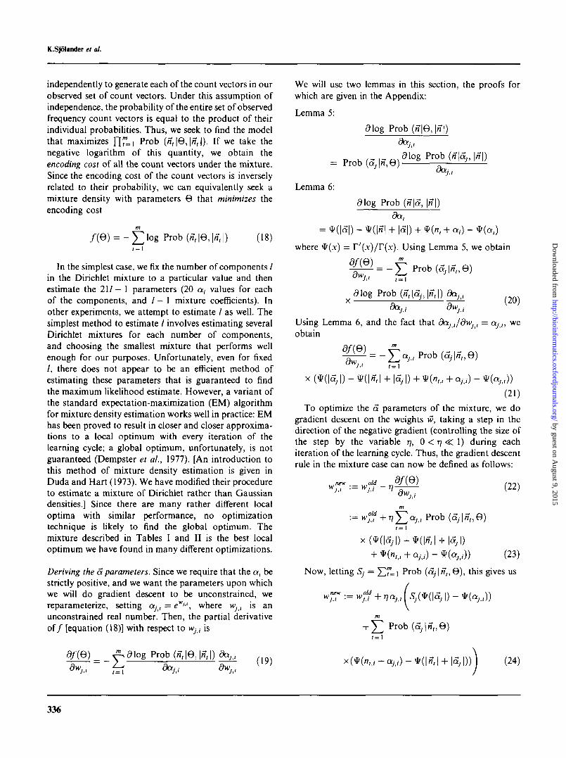
TaMe III. The posterior probability of each component in Dirichlet mixture Blocks9 [equation (16)] given 1-10 isoleucines. Initially, component 6, whichprefers I and V found jointly, is most likely, followed by components 5 and 8, which like aliphatic residues in general. As the number of observedisoleucines increases, component 9, which favors pure distributions of any type, increases in probability, but component 6 remains fairly probable. Themore mixed distributions become increasingly unlikely as the number of observed isoleucines increases

# He Comp. 1 Comp. 2 Comp. 3 Comp. 4 Comp. 5 Comp. 6 Comp. 7 Comp. 8 Comp. 9

12345678910

I I

0.00 0.25 0.50

as this are notoriously difficult, and we make no claim thatthis mixture is globally optimal. This mixture works quitewell, however, and is better than many other nine-component local optima that we have found.

Table I gives the parameters of this mixture. Table IIlists the preferred amino acids for each component inthe mixture, in order by the ratio of the mean probabilityof the amino acids in a component to the backgroundprobability of the amino acids. An alternative way tocharacterize a component is by giving the mean expectedamino acid probabilities and the variance around themean. Formulas to compute these quantities were givenin the previous section 'What is a Dirichlet density?'.

The value \a\ = Ylf^=\ at ls a measure of the varianceof the component about the mean. Higher values of |<3indicate that distributions must be close to the mean ofthe component in order to be given high probability bythat component. In mixtures we have estimated, compo-nents having high | 5 | tend to give high probability tocombinations of amino acids which have similar physio-chemical characteristics and are known to substitutereadily for each other in particular environments. Bycontrast, when \a\ is small, the component favors puredistributions conserved around individual amino acids. Aresidue may be represented primarily by one component(as proline is) or by several components (as isoleucine andvaline are). When we estimate mixtures with manycomponents, we sometimes find individual componentswith high \a\ that give high probability to pure distribu-tions of particular amino acids. However, this is unusualin mixtures with relatively few components.

Comparison with other methods for computing theseprobabilities

In this section, we compare the different results obtainedwhen estimating the expected amino acids using threemethods: Dirichlet mixture priors, substitution matricesand pseudocounts. A brief analysis of the differences

0.75 1.00

is contained in the subsections below. In addition, we giveexamples of the different results produced by thesemethods in several tables. Tables IV-VII show thedifferent amino acid estimates produced by each methodfor the cases where 1-10 isoleucines are aligned in acolumn, with no other amino acids.

Substitution matrices. The need for incorporating priorinformation about amino acid distributions into proteinalignment motivated the development of amino acidsubstitution matrices. These have been used effectively indatabase search and discrimination tasks (George et al.,1990; Altschul, 1991; Henikoff and Henikoff, 1992; Joneset al., 1992; Henikoff and Henikoff, 1993; Claverie, 1994;Rodionov and Johnson, 1994).

There are two drawbacks associated with the use ofsubstitution matrices. First, each amino acid has a fixedsubstitution probability with respect to every other aminoacid. In any particular substitution matrix, to paraphraseGertrude Stein, a phenylalanine is a phenylalanine is aphenylalanine. However, a phenylalanine seen in onecontext, for instance, a position requiring an aromaticresidue, will have different substitution probabilities thana phenylalanine seen in a context requiring a large non-polar residue. Second, only the relative frequency of aminoacids is considered, while the actual number observed isignored. Thus, in substitution matrix-based methods, theexpected amino acid probabilities are identical for anypure phenylalanine column, whether it contains 1, 3 or 100phenylalanines. All three situations are treated identically,and the estimates produced are indistinguishable.

Pseudocount methods. Pseudocount methods can be viewedas a special case of Dirichlet mixtures, where the mixtureconsists of a single component. In these methods, a fixedvalue is added to each observed amino acid count, and thenthe counts are normalized. More precisely, the formulaused is Pi := (n, + z,)/(J2j n} + ij), where each Zj is some

331



Dow

nloaded from


K^jolander el al.

TaMe IV. Estimated amino acid probabilities using various methods,given one isoleucine

Table V. Estimated amino acid probabilities using various methods,given three isoleucines. See the caption to Table IV for details

ACDEF

GHIKL

MNPQR

STV

wY

Substitution

Blosum62

0.0550.0180.0200.0200.044

0.0220.0100.2530.0270.147

0.0370.0170.0180.0160.019

0.0270.0480.1710.0060.024

matrices

SM-Opt.

0.0280.0080.0060.0110.025

0.0110.0050.5170.0110.117

0.0260.0090.0080.0080.010

0.0150.0250.1460.0030.011

Pseudocount

PC-Opt.

0.0460.0100.0260.0310.021

0.0330.0140.4950.0310.046

0.0170.0250.0180.0230.027

0.0390.0330.0420.0060.017

Dirichlet mixture

Blocks?

0.0370.0100.0080.0120.027

0.0120.0060.4720.0140.117

0.0300.0100.0080.0100.012

0.0200.0280.1490.0040.013

ACDEF

GHIKL

MNPQR

STV

wY

Substitution

Blosum62

0.0550.0180.0200.0200.044

0.0220.0100.2530.0270.147

0.0370.0170.0180.0160.019

0.0270.0480.1710.0060.024

matrices

SM-Opt.

0.02800080.0060.0110.025

0.0110.0050.5170 0110.117

0.0260.0090.0080.0080.010

0.0150.0250.1460.0030.011

Pseudocount

PC-Opt.

0.0240.0050.0140.0160.011

0.0170.0070.7370.0160.024

0.0090.0130.0090.0120.014

0.0200.0170.0220.0030.009

Dirichlet mixture

Blocks9

0.0180.0050.0030.0040.013

0.0060.0020.7370.0050.059

0.0150.0040.0040.0040.004

0.0080.0130.0890.0020.006

Tables IV—VII give amino acid probability estimates produced bydifferent methods, given a varying number of isoleucines observed (andno other amino acids). Methods used to estimate these probabilitiesinclude two substitution matrices: Blosum62, which does Gribskovaverage score (Gribskov et al., 1987) using the Blosum-62 matrix(Henikoffand Henikoff, 1992), and SM-Opt, which does matrix multiplywith matrix optimized for the Blocks database (Karplus, 1995a); onepseudocount method, PC-Opt, which is a single-component Dirichletdensity optimized for the Blocks database (Karplus, 1995a); and theDinchlet mixture Blocks9, the nine-component Dirichlet mixture givenin Tables I and II.

In order to interpret the changing amino acid probabilities produced bythe Dirichlet mixture, Blocks9, we recommend examining this table inconjunction with Table III which shows the changing contnbution ofthe components in the mixture as the number of isoleucines increases.In the estimate produced by the Dirichlet mixture, isoleucine has aprobability just under 0.5 when a single isoleucine is observed, andthe other aliphatic residues have significant probability. This reveals theinfluence of components 5 and 6, with their preference for allowingsubstitutions with valine, leucine and methionine. By 10 observations,the number of isoleucines observed dominates the pseudocounts addedfor other amino acids, and the amino acid estimate is peaked aroundisoleucine.The pseudocount method PC-Opt also converges to the observedfrequencies in the data, as the number of isoleucines increases, but doesnot give any significant probability to the other aliphatic residues whenthe number of isoleucines is small.By contrast, the substitution matrices give increased probability tothe aliphatic residues, but the estimated probabilities remain fixed as thenumber of isoleucines increases.

constant. Pseudocount methods have many of thedesirable properties of Dirichlet mixtures—in particular,that the estimated amino acids converge to the observedfrequencies as the number of observations increases—butbecause they have only a single component, they areunable to represent as complex a set of prototypicaldistributions.

Dirichlet mixtures. Dirichlet mixtures address the problemsencountered in substitution matrices and in pseudocounts.

The inability of both substitution matrices andpseudocount methods to represent more than one contextfor the amino acids is addressed by the multiple compo-nents of Dirichlet mixtures. These components enable a

Table VI. Estimated amino acid probabilities using various methods,given five isoleucines. See the caption to Table IV for details

ACDEF

GHIK.L

MNPQR

STV

wY

Substitution

Blosum62

0.0550.0180.0200.0200.044

0.0220.0100.2530.0270.147

0.0370.0170.0180.0160.019

0.0270.0480.1710.0060.024

matrices

SM-Opt.

0.0280.0080.0060.0110.025

0.0110.0050.5170.0110.117

0.0260.0090.0080.0080.010

0.0150.0250.1460.0030.011

Pseudocount

PC-Opt.

0.0160.0040.0090.0110.008

0.0120.0050.8220.0110.016

0.0060.0090.0060.0080.009

0.0140.0120.0150.0020.006

Dirichlet mixture

Blocks9

0.0100.0030.0020.0020.007

0.0040.0010.8460.0030.034

0.0080.0020.0020.0020.002

0.0040.0070.0540.0010.003

332



Dow

nloaded from



Table VII. Estimated amino acid probabilities using various methods,given 10 isoleucines. See the caption to Table IV for details

ACDEF

GHIKL

MNPQR

STV

wY

Substitution

Blosum62

0.0550.0180.0200.0200.044

0.0220.0100.2530.0270.147

0.0370.0170.0180.0160.019

0.0270.0480.1710.0060.024

matrices

Blocks-Opt.

0.0280.0080.0060.0110.025

0.0110.0050.5170.0110.117

0.0260.0090.0080.0080.010

0.0150.0250.1460.0030.011

Pseudocount

Blocks-Opt.

0.0090.0020.0050.0060.004

0.0060.0030.9020.0060.009

0.0030.0050.0030.0050.005

0.0080.0060.0080.0010.003

Dirichlet mixture

Blocks9

0.0040.0010.0010.0010.003

0.0020.0010.9420.0010.012

0.0030.0010.0010.0010.001

0.0020.0030.0200.0010.001

mixture to represent a variety of contexts for each aminoacid. It is important to note that the components in themixture do not always represent prototypical distributionsand are, instead, used in combination to give highprobability to these commonly found distributions.Sometimes a component will represent a prototypicaldistribution, at other times such a distribution is repre-sented by a combination of components; in some cases,multiple distributions will be represented by a singlecomponent.

For example, the mixture density shown in Tables Iand II presents several contexts for isoleucine. A pureisoleucine distribution would be given high probabilityby component 9, which gives high probability to allconserved distributions. Components 5, 6 and 8 preferisoleucine found in combination with other amino acids.In producing an estimate for the expected amino acids,the formula [equation (15)] gives those components thatare most likely to have generated the observed aminoacids the greatest impact on the estimation. Table IIIshows the change in the posterior probabilities of thecomponents as a variable number of isoleucines areobserved (with no other amino acids).

DirichJet mixtures also address the second drawbackassociated with substitution matrices—the importance ofthe actual number of residues observed—in the formulaused to compute the expected amino acids. In this formula,given no observations, the estimated amino acid prob-abilities approximate the background distribution, but as

more data become available, the estimate for a columnbecomes increasingly peaked around the maximum like-lihood estimate for that column (i.e. pt approaches ni/\n\as \n\ increases). Importantly, when the data indicate thata residue is conserved at a particular position, the expectedamino acid probabilities produced by this method willremain focused on that residue, instead of being modifiedto include all the residues that substitute on average forthe conserved residue.

Dirichlet mixtures were shown to give superior resultsin encoding multiple alignments and in database discrimi-nation experiments in comparison with various pseudo-count and substitution matrix-based methods in (Brownet ah, 1993; Tatusov et al., 1994; Karplus, 1995a; Henikoffand Henikoff, 1996).

Algorithm

Computing amino acid probabilities

The raw frequencies in small samples are often poorapproximations to the distribution of amino acids amongall proteins which the model is supposed to represent. Thissection will show how to use Dirichlet priors to form pt

estimates that are good approximations of the actual p,values.

A Dirichlet density with parameters 6 = (au...,au

q\...,qt) defines a probability distribution p e over allthe possible distributions of amino acids. Given acolumn in a multiple alignment, we can combine theprior probabilities for each amino acid distributionwith the observed amino acid counts to form estimates,p,, of the probabilities of each amino acid i at thatposition.

We assume that the distribution of amino acids canbe modeled by the following generative stochasticprocess:

1. First, a component j from the mixture 6 is chosenat random according to the mixture coefficient <jy.

2. Then a probability distribution p is chosen independ-ently according to Prob (p\aj), the probability definedby component j over all such distributions.

3. Finally, the observed amino acids are generatedindependently according to the distribution p. Thus,the count vector n summarizing the observed aminoacids in a column will be distributed according to themultinomial distribution with parameters p.

When 8 consists of a single component, the probabilityof the components is one, and the stochastic processconsists of steps 2 and 3.

We can now define the estimated probability of aminoacid i, ph given a Dirichlet density with parameters 6 and

333



Dow

nloaded from


K.Sj6tander el al.

observed amino acid counts n, as follows:

Pi : = Prob (amino acid i |0 ,n) (6)

= Prob (amino acid i\p) Prob (p\Q,n)dp (7)ip

The first term in the integral, Prob (amino acid i\p),is simply /?,, the /th element of the distribution vector p.The second term, Prob (p\Q,n), represents the posteriorprobability of the distribution p under the Dirichletdensity with parameters 0 , given that we have observedamino acid counts n. The integral represents thecontributions from each probability distribution p,weighted according to its posterior probability, ofamino acid /. An estimate of this type is called a meanposterior estimate.

Computing probabilities using a single density (pseudo-counts). In the case of a single-component density withparameters a, the mean posterior estimate of theprobability of amino acid / is defined

pi = Prob (amino acid i\p) Prob (p\a,n)dp (8)

By Lemma 4 (the proof of which is found in theAppendix), the posterior probability of each distributionp, given the count data n and the density with parametersa, is

Lemma 4:

where T is the Gamma function, the continuousgeneralization of the integer factorial function (i.e.T ( J C + ! ) = * ! ) .

Here we can substitute/?, for Prob (amino acid i\p) andthe result of Lemma 4 into equation (8), giving

Pi '•= 20

Y[T(ak+nk)(9)

Now, noting the contributions of the pt term within theintegral, and using equation (47) from Lemma 2, givingbill P°'~^P = Uir(a,)/r(|a|), we have

Pi •=• 20

IT* = i

(10)

+

Since T(n + \)/T(n) = n\/(n - 1)! = n, we obtain

Pi := f p , Prob (p\a,n)dp = p±^- (11)

The method in the case of a single Dirichlet density canthus be seen as adding a vector a of pseudocounts tothe vector n of observed counts, and then normalizingso that J2i Pi = 1 •

Note, when \n\ = 0, the estimate produced is simplya,-/|a|, the normalized values of the parameters a, whichare the means of the Dirichlet density. While notnecessarily the background frequency of the aminoacids in the training set, this mean is often a closeapproximation. Thus, in the absence of data, our estimateof the expected amino acid probabilities will be close tothe background frequencies. The computational simpli-city of the pseudocount method is one of the reasons whyDirichlet densities are so attractive.

Computing probabilities using mixture densities. In thecase of a mixture density, we compute the amino acidprobabilities in a similar way:

Pi := Prob (amino acid i\Q,n)

- Prob (amino acid i\p) Prob (p\Q,n)dp (12)Jp

As in the case of the single density, we can substitutep, for Prob (amino acid i\p). In addition, since 0 isa mixture of Dirichlet densities, by the definition of amixture [equation (5)], we can find Prob (p\Q,n)obtaining

P'= \-p'( J2 (P\SJ>") P r o b W (13)

In this equation, Prob (a, \n, 0 ) is the posteriorprobability of the yth component of the density, giventhe vector of counts n [equation (16) below]. It capturesour assessment that the y'th component was chosen instep 1 of the stochastic process generating these observedamino acids. The first term, Prob (p\Sj,n), thenrepresents the probability of each distribution p, givencomponent j and the count vector n.

Pulling out terms not depending on p from inside theintegral gives us

p, := Prob (Sj\n,0) [ Prob {p\Sj,n)dp (14)Jp

Substituting equation (11) [equation (15) was mis-reported in previous work (Brown et al., 1993; Karplus,

334



Dow

nloaded from



1995a,b)]:

A := (15)j=\

Thus, instead of identifying one single component of themixture that accounts for the observed data, we determinehow likely each individual component is to have producedthe data. Then, each component contributes pseudocountsproportional to the posterior probability that it producedthe observed counts. This probability is calculated usingBayes' Rule:

prob^'"'e)-CSf (16)

Prob {n\3j, \n\) is the probability of the count vector ngiven the y'th component of the mixture, and is derivedin section A.3 in the Appendix. The denominator,Prob (n | 6 , \n |), is defined

Prob (n\e, | ( " !<**> I" I (17)

Equation (15) reveals a smooth transition betweenreliance on the prior information, in the absence ofsufficient data, and confidence in the observed frequenciesas the number of observations increases. When \n\ = 0, />,is simply ^2j qjaj,i/\aj\, the weighted sum of the meanof each Dirichlet density in the mixture. As the numberof observations increases, the n, values dominate the a,values, and this estimate approaches the maximumlikelihood estimate, pt := nt/\n\.

When a component has a very small \a\, it adds a verysmall bias to the observed amino acid frequencies. Suchcomponents give high probability to all distributionspeaked around individual amino acids. The addition ofsuch a small bias allows these components to not shift theestimated amino acids away from conserved distributions,even given relatively small numbers of observed counts.

By contrast, components having a larger |<3| tend tofavor mixed distributions, i.e. combinations of aminoacids. In these cases, the individual a,, values tend to berelatively large for those amino acids / preferred by thecomponent. When such a component has high probabilitygiven a vector of counts, these a} ,• have a correspondinginfluence on the expected amino acids predicted for thatposition. The estimates produced may include significantprobability for amino acids not seen at all in the countvector under consideration.

Estimation of Dirichlet densities

In this section, we give the derivation of the procedure toestimate the parameters of a mixture prior. Much

statistical analysis has been done on amino acid distribu-tions found in particular secondary structural environ-ments in proteins. However, our primary focus indeveloping these techniques for protein modeling hasbeen to rely as little as possible on previous knowledgeand assumptions, and instead to use statistical techniquesthat uncover the underlying key information in the data.Consequently, instead of beginning with secondarystructure or other column labeling, our approach takesunlabeled training data (i.e. columns from multiplealignments with no information attached) and attemptsto discover those classes of distributions of amino acidsthat are intrinsic to the data. The statistical methoddirectly estimates the most likely Dirichlet mixture densitythrough clustering observed counts of amino acids. Inmost cases, the common amino acid distributions we findare easily identified (e.g. aromatic residues), but we do notset out a priori to find distributions representing knownenvironments.

As we will show, the case where the prior consists ofa single density follows directly from the general caseof a mixture. In the case of a mixture, we have two setsof parameters to estimate: the a parameters for eachcomponent and the q, or mixture coefficient, foreach component. In the case of a single density, we needonly estimate the a parameters. In our practice, weestimate these parameters in a two-stage process: first weestimate the a, keeping the mixture coefficients q fixed,then we estimate the q, keeping the a parameters fixed.This two-stage process is iterated until all estimatesstabilize. (This two-stage process is not necessary; wehave also implemented an algorithm for mixture esti-mation that optimizes all parameters simultaneously.However, the performance of these mixtures is no better,and the math is more complex.)

As the derivations that follow can become some-what complex, we provide two tables in the Appendix tohelp the reader: Table VIII summarizes our notation,and Table IX contains an index to key derivations anddefinitions.

Given a set of m columns from a variety of multiplealignments, we tally the frequency of each amino acid ineach column, with the end result being a vector of countsof each amino acid for each column in the data set. Thus,our primary data is a set of m count vectors. Manymultiple alignments of different protein families areincluded, so m is typically in the thousands.

We have used Maximum Likelihood to estimate theparameters 6 from the set of count vectors, i.e. we seekthose parameters that maximize the probability ofoccurrence of the observed count vectors. We assumethat the three-stage stochastic model described in thesection on computing amino acid probabilities was used

335



Dow

nloaded from


K.SJStander tt al.

independently to generate each of the count vectors in ourobserved set of count vectors. Under this assumption ofindependence, the probability of the entire set of observedfrequency count vectors is equal to the product of theirindividual probabilities. Thus, we seek to find the modelthat maximizes Y[7=\ P r o b («rl©> I«»D- If w e t a k e t n e

negative logarithm of this quantity, we obtain theencoding cost of all the count vectors under the mixture.Since the encoding cost of the count vectors is inverselyrelated to their probability, we can equivalently seek amixture density with parameters 6 that minimizes theencoding cost

Prob(n,|e,|n,|) (18)1 = 1

In the simplest case, we fix the number of components /in the Dirichlet mixture to a particular value and thenestimate the 2 1 / - 1 parameters (20 a, values for eachof the components, and / - 1 mixture coefficients). Inother experiments, we attempt to estimate / as well. Thesimplest method to estimate / involves estimating severalDirichlet mixtures for each number of components,and choosing the smallest mixture that performs wellenough for our purposes. Unfortunately, even for fixed/, there does not appear to be an efficient method ofestimating these parameters that is guaranteed to findthe maximum likelihood estimate. However, a variant ofthe standard expectation-maximization (EM) algorithmfor mixture density estimation works well in practice: EMhas been proved to result in closer and closer approxima-tions to a local optimum with every iteration of thelearning cycle; a global optimum, unfortunately, is notguaranteed (Dempster et al., 1977). [An introduction tothis method of mixture density estimation is given inDuda and Hart (1973). We have modified their procedureto estimate a mixture of DirichJet rather than Gaussiandensities.] Since there are many rather different localoptima with similar performance, no optimizationtechnique is likely to find the global optimum. Themixture described in Tables I and II is the best localoptimum we have found in many different optimizations.

Deriving the a parameters. Since we require that the a, bestrictly positive, and we want the parameters upon whichwe will do gradient descent to be unconstrained, wereparameterize, setting ay, = eKyi, where wJt, is anunconstrained real number. Then, the partial derivativeof/ [equation (18)] with respect to wy ,• is

>fllog Prob(«,|0,|/rt|) &*,,,(19)

We will use two lemmas in this section, the proofs forwhich are given in the Appendix:

Lemma 5:

9 log Prob (n|0,

9log Prob (n\5j, \n\)= Prob (5, \n, 6)

Lemma 6:

dlog Prob (n\a, \n\)

fa,

where 9(x) = T'(x)/T(x). Using Lemma 5, we obtain

df(S)_ y>

~d»J7~~h Prob aj""e

fllogProbfalSy.KI) fajy, (20)

Using Lemma 6, and the fact that fajj/dwJtl = a,,, weobtain

= ~Ylaj<> Prob ("yl""

(21)

To optimize the a parameters of the mixture, we dogradient descent on the weights iv, taking a step in thedirection of the negative gradient (controlling the size ofthe step by the variable 7], 0 < r\ <s^ 1) during eachiteration of the learning cycle. Thus, the gradient descentrule in the mixture case can now be defined as follows:

(22)

a , v ) - ,,)) (23)

Now, letting Sj = Y1T=\ P ro r j (<2/|«,,0), this gives us

Prob(5,|«,,0)r=l

x(*K, + ay.,.) - * ( | » , | + |5,|)) (24)

336



Dow

nloaded from


Improved detection of weak protein sequence homology

In the case of a single density, Prob (a | n, 9 ) = 1 for allvectors n; thus, Sj = J2T= 1 P r°b ("I"/!©) = m> ar>d thegradient descent rule for a single density can be written as

a , - ) - (25)

After each update of the weights, the a parameters arereset, and the process continued until the change in theencoding cost [equation (18)] falls below some pre-definedcutoff.

Mixture coefficient estimation. In the case of a mixtureof Dirichlet densities, the mixture coefficient, q, of thecomponent is also estimated. However, since we requirethat the mixture coefficients must be non-negative andsum to one, we first reparameterize, setting qj — Qj/\Q\,where the Q, are constrained to be strictly positive, and\Q\ = J2j= i Qj- As in the first stage, we want to maximizethe probability of the data given the model, which isequivalent to minimizing the encoding cost [equation (18)].In this stage, we take the derivative of / with respect toQj. However, instead of having to take iterative steps inthe direction of the negative gradient, as we did in thefirst stage, we can set the derivative to zero, and solve forthose qj = Qj/\Q\ that maximize the probability of thedata. As we will see, however, the new qj are a functionof the previous qf, thus, this estimation process must alsobe iterated.

Taking the gradient of/ with respect to Qj, we obtain

dQj = -£a log Prob(f?,|e,|B,|)(26)

We introduce Lemma 8 (the proof for which is foundin section A.8 in the Appendix).

Lemma 8:

d log Prob (n |0, | n |) _ Prob (a, | n, 6) 1

Qj \Q\

Using Lemma 8, we obtain

0/(6) ^ / P r o b ( a > - , , 8 ) 1

M Qj \Q\) ( '

m\Q\

Prob (a, | «„ 6)

(28)

Since the gradient must vanish for those mixturecoefficients giving the maximum likelihood, we set thegradient to zero, and solve. Thus, the maximum likelihoodsetting for qj is

• Ifil1 v^-v

:= — Yj Prob (5j \n,, 0)

(29)

(30)

Here, the re-estimated mixture coefficients are func-tions of the old mixture coefficients, so we iterate thisprocess until the change in the encoding cost falls belowthe predefined cutoff. (It is easy to confirm that thesecoefficients sum to one, as required, since ^ / = l 2~ J">= I Prob(aj\n,,e) = £7Li Ej=. Prob («,!«„6) = E"-! 1 = m.)

In summary, when estimating the parameters of amixture prior, we alternate between re-estimating the aparameters of each density in the mixture, by gradientdescent on the w, resetting a, , = eWjJ, after eachiteration, followed by re-estimating and resetting themixture coefficients as described above, until the processconverges.

Implementation

Implementing Dirichlet mixture priors for use in HMMsor other stochastic models of biological sequences is notdifficult, but there are many details that can causeproblems if not handled carefully.

This section splits the implementation details into twogroups: those that are essential for getting workingDirichlet mixture code (next section), and those thatincrease efficiency, but are not essential (section on'Efficiency improvements').

Essential details

In the section 'Computing amino acid probabilities', wegave the formulas for computing the amino acid prob-abilities in the cases of a single density [equation (11)] andof a mixture density [equation (15)].

For a single Dirichlet component, the estimationformula is trivial:

(31)

and no special care is needed in the implementation.For the case of a multi-component mixture, the implemen-tation is not quite so straightforward.

As we showed in the derivation of equation (15),

(32)

337



Dow

nloaded from


K^jdlander et at.

The interesting part for computation comes incomputing Prob (a,|n, 8) [see equation (16)]. We canexpand Prob (n\Q, \n\) using equation (17) to obtain

Prob (a , | n , e ) = —Prob (n\Sj, \n\)

(n\ak,\n\)

(33)

k=\

Note that this is a simple normalization of qj Prob(n\dj, \n\) to sum to one. Rather than carry the normali-zation through all the equations, we can work directlywith Prob (n\aj, \n\), and put everything back together atthe end.

First, we can expand Prob (n\dj, \n\) using Lemma 3(the proof of which is found in section A.3 in theAppendix):

(34)

If we rearrrange some terms, we obtain

20

Prob(«|5/,|«|) =

T(\n\20 (35)

The first two terms are most easily expressed using theBeta function: B(x) = n ^ i r(jc/)/r(|jc|), where, asusual, .v| = i xi- This simplifies the expression to

'

( 3 6 )

The remaining Gamma functions are not easilyexpressed with a Beta function, but they do not need tobe. Since they depend only on n and not on j , when we dothe normalization to make the Prob (a, | n, 6 ) sum to one,this term will cancel out, giving us

Prob (5j\n,e) =B(a,)

(37)

k=\

Plugging this formula into equation (32) gives us

Pi '•= ——i T^

n + a(38)

k=\

Since the dominator of equation (38) is independent of/, we can compute p, by normalizing

7 = 1

to sum to one. That is

Pi = 20

(39)

(40)

The biggest problem that implementers run into is thatthese Beta functions can get very large or very small—outside the range of the floating-point representationof most computers. The obvious solution is to work withthe logarithm of the Beta function:

Most libraries of mathematical routines include thelgamma function which implements logr(.x), and sousing the logarithm of the Beta function is not difficult.

We could compute each X, using only the logarithmicnotation, but it turns out to be slightly more convenientto use the logarithms just for the Beta functions:

a, + n

Some care is needed in the conversion from thelogarithmic representation back to floating point, sincethe ratio of the Beta functions may be so large or so smallthat it cannot be represented as floating-point numbers.Luckily, we do not really need to compute X,, onlyPi = XJ £ j tL | Xk. This means that we can divide X, byany constant and the normalization will eliminate theconstant. Equivalently, we can freely subtract a constant(independent of j and /') from logB(ay + n) — logB(5,)

338



Dow

nloaded from



before converting back to floating point. If we choosethe constant to be max, ( l o g B ^ + n) — logB(5,)), thenthe largest logarithmic term will be zero, and all the termswill be reasonable. (We could still get floating-pointunderflow to zero for some terms, but the p computationwill still be about as good as can be done within floating-point representation.)

Efficiency improvements

The previous section gave simple computation formulasfor pi [equations (39) and (40)]. When computations ofpt are done infrequently (e.g. for profiles, where pt onlyneeds to be computed once for each column of the profile),those equations are perfectly adequate.

When recomputing pt frequently, as may be done in aGibbs sampling program or training a hidden Markovmodel, it is better to have a slightly more efficientcomputation. Since most of the computation time isspent in the lgamma function used for computing the logBeta functions, the biggest efficiency gains come fromavoiding the lgamma computations.

If we assume that the ajti and qj values change lessoften than the values for n (which is true of almost everyapplication), then it is worthwhile to pre-computelogB(oy), cutting the computation time almost in half.

If the rij values are mainly small integers (zero iscommon in all the applications we've looked at), thenit is worth pre-computing logr(o / J ) , logr(ay , •+1),logr(ay ( + 2), and so on, out to some reasonable value.Pre-computation should also be done for logr(|ay|),logrfla/l + 1), logrf la j + 2), and so forth. If all the nvalues are small integers, this pre-computation almosteliminates the lgamma function calls.

In some cases, it may be worthwhile to build a special-purpose implementation of log F(x) that caches all callsin a hash table, and does not call lgamma for values of xthat it has seen before. Even larger savings are possiblewhen x is close to previously computed values, by usinginterpolation rather than calling lgamma.

Discussion

The methods employed to estimate and use Dirichletmixture priors are shown to be firmly based on Bayesianstatistics. While biological knowledge has been intro-duced only indirectly from the multiple alignments usedto estimate the mixture parameters, the mixture priorsproduced agree with accepted biological understanding.The effectiveness of Dirichlet mixtures for increasing theability of statistical models to recognize homologoussequences has been demonstrated experimentally (Brownet al., 1993; Tatusov et al., 1994; Bailey and Elkan, 1995;

Karplus, 1995a; Henikoff and Henikoff, 1996; Hughey andKrogh, 1996; Wang et al., 1996).

The mixture priors we have estimated thus far have beenon unlabeled multiple alignment columns—columns withno secondary structure or other information attached.Previous work deriving structurally informed distri-butions, such as that by Luthy et al. (1991), has beenshown to increase the accuracy of profiles in both databasesearch and multiple alignment by enabling them to takeadvantage of prior knowledge of secondary structure(Bowie et al., 1991). However, these distributions cannotbe used in a Bayesian framework, since there is no measureof the variance associated with each distribution, andBayes' rule requires that the observed frequency counts bemodified inversely proportional to the variance in thedistribution. Thus, to use these structural distributionsone must assign a variance arbitrarily. We plan to estimateDirichlet mixtures for particular environments, and tomake these mixtures available on the World-Wide Web.

Dirichlet mixture priors address two primary weak-nesses of substitution matrices: considering only therelative frequency of the amino acids while ignoringthe actual number of amino acids observed, and havingfixed substitution probabilities for each amino acid. Oneof the potentially most problematic consequences of thesedrawbacks is that substitution matrices do not produceestimates that are conserved, or mostly conserved, wherethe evidence is clear that an amino acid is conserved. Themethod presented here corrects these problems. Whenlittle data are available, the amino acids predicted arethose that are known to be associated in different contextswith the amino acids observed. As the available dataincrease, the amino acid probabilities produced by thismethod converge to the observed frequencies in the data.In particular, when evidence exists that a particularamino acid is conserved at a given position, the expectedamino acid estimates reflect this preference.

Because of the sensitivity of Dirichlet mixtures to thenumber of observations, any significant correlationamong the sequences must be handled carefully. Oneway to compensate for sequence correlation is by the useof a sequence weighting scheme (Sibbald and Argos, 1990;Thompson et al., 1994a,b; Henikoff and Henikoff, 1996).Dirichlet mixtures interact with sequence weighting in twoways. First, sequence weighting changes the expecteddistributions somewhat, making mixed distributions moreuniform. Second, the total weight allotted the sequencesplays a critical role when Dirichlet densities are used. Ifthe data are highly correlated, and this is not compensatedfor in the weighting scheme (by reducing the total counts),the estimated amino acid distributions will be too closeto the raw frequencies in the data, and not generalized toinclude similar residues. Since most sequence weighting

339



Dow

nloaded from


K.Sj6Under et al.

methods are concerned only with relative weights, andpay little attention to the total weight allotted thesequences, we are developing sequence weightingschemes that coordinate the interaction of Dirichletmixtures and sequence weights.

Since the mixture presented in this paper was estimatedand tested on alignments of fairly close homologs [theBLOCKS (Henikoff and Henikoff, 1991) and HSSP(Sander and Schneider, 1991) alignment databases], itmay not accurately reflect the distributions we wouldexpect from more remote homologs. We are planning totrain a Dirichlet mixture specifically to recognize trueremote homologies, by a somewhat different trainingtechnique on a database of structurally aligned sequences.

Finally, as the detailed analysis of Karplus (1995a,b)shows, the Dirichlet mixtures already available areclose to optimal as far as their capacity for assisting incomputing estimates of amino acid distributions, given asingle-column context, and assuming independencebetween columns and between sequences for a givencolumn. Thus, further work in this area will perhapsprofit by focusing on obtaining information fromrelationships among the sequences (for instance, asrevealed in a phylogenetic tree) or in inter-columnarinteractions.

The Dirichlet mixture prior from Table I is availableelectronically at our World-Wide Web site h t t p : / /www.c8e.uc8c.edu/research/compbio/. In addition tothe extensions described above, we plan to makeprograms for using and estimating Dirichlet mixturedensities available on our World-Wide Web and ftpsites later this year. See our World-Wide Web site forannouncements.

Acknowledgements

We gratefully acknowledge the input and suggestions of StephenAltschul, Tony Fink, Lydia Gregoret, Steven and Jorja Henikoff,Graeme Mitchison and Chris Sander. Richard Lathrop made numeroussuggestions that improved the quality of the manuscript greatly, as didthe anonymous referees. Special thanks to friends at Lafona, Universitede Pierre et Marie Curie, in Paris, and the Biocomputing Group atthe European Molecular Biology Laboratory at Heidelberg, whoprovided workstations, support and scientific inspiration during theearly stages of writing this paper. This work was supported in part byNSF grants CDA-9115268, IRI-9123692 and BIR-94O8579; DOE grant94-12-048216, ONR grant NOOO14-91-J-1162, NIH grant GM17129, aNational Science Foundation Graduate Research Fellowship and fundsgranted by the UCSC Division of Natural Sciences. The Sanger Centreis supported by the Wellcome Trust. This paper is dedicated to thememory of Tal Grossman, a dear friend and a true mensch.

References

Altschul,S.F. (1991) Amino acid substitution matrices from aninformation theoretic perspective. JMB, 219, 555-565.

Altschul.S.F., Gish.W., Miller.W., Meyers.E.W. and Lippman.D.J.(1990) Basic local alignment search tool. JMB, 215, 403-410.

Asai,K., Hayamizu.S. and Oruzuka.K. (1993) HMM with proteinstructure grammar. In Proceedings of the Hawaii InternationalConference on System Sciences, Los Alamitos, CA. IEEE ComputerSociety Press, pp. 783-791.

Bailey,T.L. and Elkan.C. (1995) The value of prior knowledge indiscovering motifs with MEME. In 1SMB-95, Menlo Park, CA.AAAI/MIT Press, pp. 21-29.

Baldi,P. and Chauvin.Y. (1994) Smooth on-line learning algorithms forhidden Markov models. Neural Computation, 6, 305-316.

Baldi,P., Chauvin.Y., Hunkapiller,T. and McClure,M.A. (1992)Adaptive algorithms for modeling and analysis of biological primarysequence information. Technical Report, Net-ID, Inc., 8 Cathy Place,Menlo Park, CA 94305.

Barton,G.J. and Sternberg,M.J. (1990) Flexible protein sequencepatterns. A sensitive method to detect weak structural similarities.JMB, 212, 389-402.

BergerJ. (1985) Statistical Decision Theory and Bayesian Analysis.Springer-Verlag, New York.

BernardoJ.M. and Smith.A.F.M. (1994) Bayesian Theory, 1st edn. JohnWiley and Sons.

Bowie,J.U., LQthy.R. and Eisenberg.D. (1991) A method to identifyprotein sequences that fold into a known three-dimensional structure.Science, 253, 164-170.

Brown.M.P., Hughey,R., Krogh.A., Mian,I.S., Sj61ander,K.. andHaussler.D. (1993) Using Dirichlet mixture priors to derive hiddenMarkov models for protein families. In Hunter,L., Searls.D. andShavlikJ. (eds), ISMB-93, Menlo Park, CA. AAAI/MIT Press,pp. 47-55.

Bucher.P., Karplus,K., Moeri.N. and Hoffman.K. (1996) A flexiblemotif search technique based on generalized profiles. ComputersChem., 20, 3-24.

Churchill.G.A. (1989) Stochastic models for heterogeneous DNAsequences. Bull. Math. Biol, 51, 79-94.

Claverie,J.-M. (1994) Some useful statistical properties of position-weight matrices. Computers Chem., 18, 287-294.

Dempster.A.P., Laird.N.M. and Rubin,D.B. (1977) Maximum likeli-hood from incomplete data via the EM algorithm, J. R. Statist. Soc.B, 39, 1-38.

Doolittle,R.F. (1986) Of URFs and ORFs: A Primer on How to AnalyzeDerived Amino Acid Sequences. University Science Books, Mill Valley,CA.

Duda,R.O. and Hart.P.E. (1973) Pattern Classification and SceneAnalysis. Wiley, New York.

Eddy.S.R. (1995) Multiple alignment using hidden Markov models. InISMB-95, Menlo Park, CA. AAAI/MIT Press, pp. 114-120

Eddy.S.R. (1996) Hidden Markov models. Curr. Opin. Struct. Biol. 6,361-365.

Eddy.S.R., Mitchison,G. and Durbin,R. (1995) Maximum discrimina-tion hidden Markov models of sequence consensus. J. Comput. Biol.,2,9-23

George.D.G., Barker.W.C. and Hunt.L.T. (1990) Mutation data matrixand its uses. Methods Enzymol., 183, 333-351.

Gradshteyn,I.S. and RyzhikJ.M. (1965) Table of Integrals. Series, andProducts, 4th edn. Academic Press.

Gribskov.M., McLachlanAD. and Eisenberg.D. (1987) Profile analy-sis: Detection of distantly related proteins. Proc. Nail Acad. Sci. USA,84, 4355^358.

Gribskov,M., Lflthy.R. and Eisenberg.D. (1990) Profile analysis.Methods Enzymol., 183, 146-159.

Henikoff.S. and Henikoff.J.G. (1991) Automated assembly of proteinblocks for database searching. Nucleic Acids Res., 19, 6565-6572.

Henikoff.S. and HenikoffJ.G. (1992) Amino acid substitution matricesfrom protein blocks. Proc. Natl Acad. Sci. USA, 89, 10915-10919.

Henikoff.S. and Herukoff,J.G. (1993) Performance evaluation of aminoacid substitution matrices. Proteins- Structure. Function Genet., 17,49-61.

Henikoff.J.G. and Henikoff.S. (1996) Using substitution probabilities toimprove position-specific scoring matrices. Comput. Applic. Biosci. 12,135-143.

Henikoff.S., Wallace.J.C. and Brown.J.P. (1990) Finding protein

340



Dow

nloaded from


Improved detection of weak protein sequence botnology

similarities with nucleotide sequence databases. Methods Enzymol.,183, 111-132.

Hughey.R. and Krogh,A. (1996) Hidden Markov models for sequenceanalysis: Extension and analysis of the basic method. Comput. Applic.Biosci., 12, 95-107.

Jones,D.T., Taylor,W.R. and Thornton.J.M. (1992) The rapid generationof mutation data matrices from protein sequences. Comput. Applic.Biosci., 8, 275-282.

Karplus.K.. (1995a) Regularizes for estimating distributions of aminoacids from small samples. In ISMB-95, Menlo Park, CA. AAAI/MITPress.

Karplus.K.. (1995b) Regularizes for estimating distributions of aminoacids from small samples. Technical Report UCSC-CRL-95-11,University of California, Santa Cruz. URL ftp://ftp.cse.ucsc.edu/pub/tr/ucsc-crl-95-ll.ps.Z.

Krogh.A., Brown.M., Mian.I.S., Sj61ander,K. and Haussler.D. (1994)Hidden Markov models in computational biology: Applications toprotein modeling. JMB, 235, 1501-1531.

Luthy.R., McLachlan.A.D. and Eisenberg,D. (1991) Secondary structure-based profiles: Use of structure-conserving scoring table in searchingprotein sequence databases for structural similarities. Proteins:Structure, Function. Gent., 10, 229-239.

Nowlan.S. (1990) Maximum likelihood competitive learning. InTouretsky.D. (ed.), Advances in Neural Information ProcessingSystems, Volume 2. Morgan Kaufmann, pp. 574-582.

Rodionov.M.A. and Johnson.M.S. (1994) Residue-residue contactsubstitution probabilities derived from aligned three-dimensionalstructures and the identification of common folds. Protein Sci., 3,2366-2377.

Sander.C. and Schneider.R. (1991) Database of homology-derived

protein structures and the structural meaning of sequence alignment.Proteins, 9, 56-68.

Santner.T.J. and Duffy,D.E. (1989) The Statistical Analysis of DiscreteData. Springer Verlag, New York.

Sibbald,P. and Argos,P. (1990) Weighting aligned protein or nucleicacid sequences to correct for unequal representation. JMB, 216, 813-818.

Stultz,C.M., White,J.V. and Smith.T.F. (1993) Structural analysis basedon state-space modeling. Protein Sci., 2, 305-315.

Tatusov.R.L., Altschul.S.F. and Koonin.E.V. (1994) Detection ofconserved segments in proteins: Iterative scanning of sequencedatabases with alignment blocks. Proc. Natl Acad. Sci. USA, 91,12091-12095.

ThompsonJ.D., Higgins,D.G. and Gibson.T.J. (1994a) Improvedsensitivity of profile searches through the use of sequence weightsand gap excision. Comput. Applic. Biosci., 10, 19-29.

Thompson^.D., Higgins.D.G. and Gibson.T.J. (1994b) CLUSTAL W.Improving the sensitivity of progressive multiple sequence alignmentthrough sequence weighting, position-specific gap penalties, and weightmatrix choice. Nucleic Acids Res., 22, 4673-4680.

WangJ.T.L., Marr.T.G., Shasha.D., Shapiro.B., Chirn,G.-W. andLee.T.Y. (1996) Complementary classification approaches for proteinsequences. Protein Eng. 9, 381-386

Waterman,M.S. and Perlwitz,M.D. (1986) Line geometries for sequencecomparisons. Bull. Math. Biol., 46, 567-577.

Whitej.V., Stultz,M. and Smith,T.F. (1994) Protein classification bystochastic modeling and optimal filtering of aminc-acid sequences.Math. Biosci., 119, 35-75.

Received on April 15, 1996; revised and accepted on June 4, 1996

Appendix

Table VIII. Summary of notation

|J?| = 52/ xit where J? is any vector.n = « ) , . . . ,ri2o is a vector of counts from a column in a multiple alignment. The symbol n, refers to the number of amino acids /in the column. The lib

such observation in the data is denoted n,.P= (P\ i • • • i Pw)» JlPt = 1, /»/ > 0, are the parameters of the multinomial distributions from which the n are drawn.9 is the set of all such p.a = (et\,... ,Q2o) s t - ai > 0, are the parameters of a Dirichlet density. The parameters of thejth component of a Dinchlet mixture are denoted 3j. The

symbol otjj refers to the /'th parameter of theyth component of a mixture.q, = Prob (aj) is the mixture coefficient of (hejth component of a mixture.8 = ( ? i , . . . , q/, Si,..., 3;) = all the parameters of the Dirichlet mixture.if — (H>| , . . . , H'20), are weight vectors, used during gradient descent to train the Dinchlet density parameters a. After each training cycle, <*y, is set to e"1-'.

The symbol Wjt is the value of the /th parameter of theyth weight vector. The nomenclature weights comes from artificial neural networks.m = the number of columns from multiple alignments used in training./ = the number of components in a mixture.7) = eta, the learning rate used to control the size of the step taken during each iteration of gradient descent.

341



Dow

nloaded from


K.SJdUoder et at.

Table IX. Index to key derivations and definitions

T(\n

*(.v)

Prob

Prob

Prob

Prob

(A.

+ 1)

(n\p,

(«|5,

(a\e

(5j\n

1*1)

1*1)

1*1)

• 8 )

') Lemma 1

= - £ log (Prob (n,|9,K,|))i - i

(the encoding cost of all the count vectors given the mixture—the function minimized)= n\ (for integer n > 0)(Gamma function)

a log r(.r) r'(.v)

dx r(x)(Psi function)

20 _ i

(the probability of n under the multinomial distribution with parametersp)

r(H + |S|) fJi I>, + 1)I>()(the probability of ff under the Dirichlet density with parameters 5)

Prob (»fo, |t - i

(the probability of n given the entire mixture prior)

= <?y Prob (n|o,, |n|)

Prob(/?|e, |n|)

(shorthand for the posterior probabiuty of theyth component of the mixture given the vector of counts n)

20

Prob («! Pi

equivalent form

Piob(n\p,\n\)=r(\n\ + l)f[

Proof:For a given vector of counts n, with pt being theprobability of seeing the /th amino acid, and |n| =5^/«/, there are |n|!/(/i,!«2! • • -"MO distinct permutationsof the amino acids which result in the count vector n.If we allow for the simplifying assumption that eachamino acid is generated independently (i.e. the sequencesin the alignment are uncorrelated), then each suchpermutation has probability \\ fL\p"'- Thus, the prob-ability of a given count vector n given the multinomialparameters p is

(A.2) Lemma 2

Prob (p\a)= ^aU T[P?20n

, i=i

1 = 1

(18)

(43)

(64)

(44)

(51)

(17)

(16)

(44)

Proof:Under the Dirichlet density with parameters a, theprobability of the distribution p (where p, > 0 andJ2i Pi = 1) is defined as follows:

n <20

n x \ n 2 \ .

20

HP?'20 m

?rob{p\a)=T±(42)

To enable us to handle real-valued data (such asthose obtained from using a weighting scheme on thesequences in the training set), we introduce the Gammafunction, the continuous generalization of the integerfactorial function,

r ( / i+ l ) = n! (43)

Substituting the Gamma function, we obtain the

Jpesr

(45)

We introduce two formulas concerning the Betafunction—its definition (Gradshteyn and Ryzhik, 1965,p. 948)

Jo

342



Dow

nloaded from



and its combining formula (Gradshteyn and Ryzhik, 1965,p. 285)

f = bx+y-l B(x,y).

This allows us to write the integral over all p vectorsas a multiple integral, rearrange some terms, and obtain

...B(al9,a20) (46)

( 4 7 )

We can now given an explicit definition of theprobability of the amino acid distribution p giventhe Dirichlet density with parameters a:

(48)1=1

(A3) Lemma 3

Prnh (S\rt\S\\

Prob(n|a,M) =I + 1) A (n, + a,

Proof:We can substitute equations (44) and (48) into the identity

Prob (n\S, \n\) = [ Prob {n\p, \n\) Prob (p\a)dp,Jpes>

(49)

rearranging terms, we obtain

r(|g|) TT _J>/ + «/)\Z\\ 1 1 Pin, .

(51)

(A.4) Lemma 4

Prob (p\3,n) = ^ 1 + 1" YlP'+n'20

Proof:By repeated application of the rule for conditionalprobability, the probability of the distribution p, giventhe Dirichlet density with parameters a, and the observedamino acid count vector n is defined

Prob (p\a,n) —Prob {p,a,n\\n\)

Prob (a,n\ \n\)

Prob (n\p,a,\n\) Prob (p,a)

Prob (n\a,\n\) Prob (a)

Prob (n\p,a, \n\) Prob (p\a)

Prob (n\3, \n\)

(52)

(53)

(54)

However, once the point p is fixed, the probability of nno longer depends on a. Hence,

Prob (p\a,n) =Prob (n\p, \n\) Prob (p\a)

Prob(n|a,|i?|)(55)

At this point, we apply the results from previousderivations for quantities Prob (n\p, \n\) [equation (44)],Prob (p\S) [equation (48)] and Prob («|a, \n\) [equation(51)]. This gives us

Prob (p\3,n) = (56)

giving

20

20n, 1 = 1

— IN ZU

-\>-Y[p^+a'-idp. (50)

Most of the terms cancel, and we have

Prob (p\a,n) =20

/ = i

Note that this is the expression for a Dirichlet densityPulling out terms not depending on p from inside the with parameters a + n. This property, that the posterior

integral, using the result from equation (47), and density of p is from the same family as the prior,

343



Dow

nloaded from


K.Sjolander el al.

characterizes all conjugate priors, and is one of theproperties that make Dirichlet densities so attractive.

(A.5) Lemma 5

Prob («|e,|/?|)

= Prob (Sj\n,Q)Slog Prob (n |a , , \n\)

Proof:The derivative with respect to a}, of the log likelihoodof each count vector n given the mixture is

d log Prob (n\Q,\n\)

1 d Prob (n|e, |n |)Prob («|0, |«|) dajj

Applying equation (17), this gives us

dlog Prob (»|e,|w|)

(58)

1P r o b

Prob(«|0, |« |) ft*/,l(59)

Since the derivative of Prob (n\ak, \n\) with respect tootjj is zero for all k ^j, and the mixture coefficients (theqk) are independent parameters, this yields

d log Prob(w|9,|w|)

q} Prob (/T|q,-, \n\)

Prob(«|0, |n |)(60)

We rearrange equation (16) somewhat, and replace(n|0, |«|) by its equivalent, obtaining

dlog Prob(n |e , |n | )

_ Prob (a,, |n,0) 9 Prob (w|(a,, |n|

Prob {n\ap \n\) daJt,(61)

Here, again using the fact that dlog(f(x))/dx =df{x)/f{x)dx, we obtain the final form

Slog Prob (#?|e,|n|)

Prob (a, n, 8 ) — '- . 62)

ft*/,.

Lemma 6

d log Prob («|a,

a,) -

/'TOO/-

In this proof, we use Lemma 3, giving

Prob (n\a, \n\) =

Since the derivative of terms not depending on a, arezero, we obtain that for a single vector of counts n

dlog Prob {n\a,\n\) 51ogr(|a|)da, da,

01ogr(|n|• +

da, ' da,

Now, if we substitute the shorthand

r'(x)

we have

eta/- • (63)

w " dx ~ T(x) '

dlog Prob (n\a, \n\)

(64)

= *(|5|) - *(|>i| + |5|) + *(«, + «,) - *(a,-). (65)

(A.7) Lemma 7

d Prob ( « | 0 , |« | ) Prob (n\at, \n\) - Prob ( M | 0 , |W|)

dQ, \Q\

Proof-Substituting equation (17), giving Prob («|0, |n|) =^ ' = i q} Prob (n\Sj, \n\) and replacing q} by Qj/\Q\, weobtain

d Prob (n|0,

dQi dQ,(66)

As the derivative of a sum is the sum of the derivatives,we can use the standard product rule for differentiation,and obtain

9 Prob («|8,|n|) ^

(67)

344



Dow

nloaded from



Since <9Prob (n\Sj, \n\)/dQt = 0 for ally, this gives us

./=>(68)

Taking the derivative of the fraction {Qj/\Q\) withrespect to Q,, we obtain

(A.8) Lemma 8

dlog Prob (n |9 , \n\) _ Prob {5j\n, 9 ) 1

dQj ~ Qj Ifii

Proof:Using Lemma 7, we can derive

a log Prob (n |e , |n | )

d(Qj/\Q\) i(69)

Prob (n |0 , |n | )

The first term, | g | xdQj/dQt, is zero when y ^ ;', andis l / | g | when ./ = /. The second term, Qjd\Q\~l/dQh issimply —Qj/\Q\2- Thus, this gives us

d Prob (n\S,\n\) Prob (n|a,-, |n |)

Prob (/r|e,|«|) dQj

I

Prob(/?|e,|n|)Prob (n|a,-, |«|) - Prob (/T|e, |n|

x iel

lei

(n\ah\n\)-Q^. (70)

Here, q} = Qj/\Q\ allows us to replace Qj/\Q\2 with

(71)

(73)

(74)

(75)

If we rearrange equation (16), we obtainProb(«|a, , |n |) /Prob(/f |8, |n|) = Prob{a]\n,Q)lq]. Thisallows us to write

Prob(w|9,H)

Prob (n\a,, \n\) -^qj Prob (n\5j,j=\

\Q\

At this point, we use equation (17) and obtain

d Prob (« |0, |«|) Prob (n\an \n\) - Prob (» |6, |« |

\Q\

(76)

Now we can use the identity qj = Qj/\Q\, obtainingthe equivalent

dlog Prob (f?|e,|»|) Prob (q,|w,0) 1

3 2 , G, IGI* l '(72)

345



Dow

nloaded from


Dirichlet mixtures: a method for improved detection of weak but significant protein sequence...

Documents

Transcript of Dirichlet mixtures: a method for improved detection of weak but significant protein sequence...