Dilatometry Study on a High- Chromium Cast Iron - Kth Diva ...
74
IN THE FIELD OF TECHNOLOGY DEGREE PROJECT MATERIALS DESIGN AND ENGINEERING AND THE MAIN FIELD OF STUDY MECHANICAL ENGINEERING, SECOND CYCLE, 30 CREDITS , STOCKHOLM SWEDEN 2018 Dilatometry Study on a High- Chromium Cast Iron BENJAMIN SOLEM KTH ROYAL INSTITUTE OF TECHNOLOGY SCHOOL OF ENGINEERING SCIENCES
-
Upload
khangminh22 -
Category
Documents
-
view
3 -
download
0
Transcript of Dilatometry Study on a High- Chromium Cast Iron - Kth Diva ...

IN THE FIELD OF TECHNOLOGYDEGREE PROJECT MATERIALS DESIGN AND ENGINEERINGAND THE MAIN FIELD OF STUDYMECHANICAL ENGINEERING,SECOND CYCLE, 30 CREDITS
, STOCKHOLM SWEDEN 2018
Dilatometry Study on a High-Chromium Cast Iron
BENJAMIN SOLEM
KTH ROYAL INSTITUTE OF TECHNOLOGYSCHOOL OF ENGINEERING SCIENCES

i
Acknowledgement
This report is the result of a Master Thesis in Mechanical Engineering at KTH Royal Insti-
tute of Technology, Stockholm, Sweden, performed between January and June 2018. The
work has been conducted for Xylem Water Solutions, Sundbyberg, Sweden, based on a thesis
proposal from the company.
I would like to acknowledge my gratitude towards all personnel in contact with this thesis at
Xylem Sundbyberg and Emmaboda. Special thanks to Måns Bergsten, Stefan Ramström, and
Keith Lothian for their support and guidance during this spring term, as well as for introduc-
ing this complex and intriguing material to me.
Furthermore, I want to thank my supervisor at KTH, Prof. Bo Alfredsson, as well as lab
technician Wenli Long at the Department of Materials Science and Engineering, for their
help throughout the course of this project.
Sundbyberg, 2018-06-05
Benjamin Solem
ii
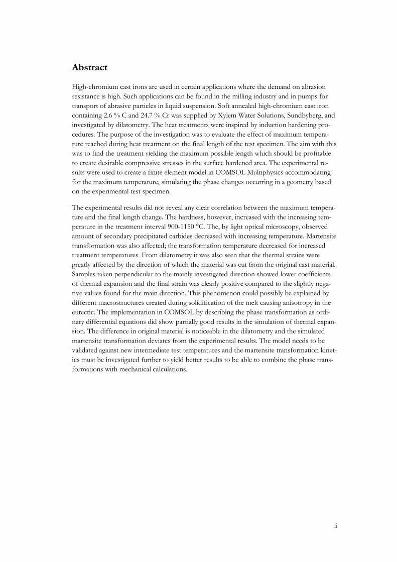
Abstract
High-chromium cast irons are used in certain applications where the demand on abrasion
resistance is high. Such applications can be found in the milling industry and in pumps for
transport of abrasive particles in liquid suspension. Soft annealed high-chromium cast iron
containing 2.6 % C and 24.7 % Cr was supplied by Xylem Water Solutions, Sundbyberg, and
investigated by dilatometry. The heat treatments were inspired by induction hardening pro-
cedures. The purpose of the investigation was to evaluate the effect of maximum tempera-
ture reached during heat treatment on the final length of the test specimen. The aim with this
was to find the treatment yielding the maximum possible length which should be profitable
to create desirable compressive stresses in the surface hardened area. The experimental re-
sults were used to create a finite element model in COMSOL Multiphysics accommodating
for the maximum temperature, simulating the phase changes occurring in a geometry based
on the experimental test specimen.
The experimental results did not reveal any clear correlation between the maximum tempera-
ture and the final length change. The hardness, however, increased with the increasing tem-
perature in the treatment interval 900-1150 °C. The, by light optical microscopy, observed
amount of secondary precipitated carbides decreased with increasing temperature. Martensite
transformation was also affected; the transformation temperature decreased for increased
treatment temperatures. From dilatometry it was also seen that the thermal strains were
greatly affected by the direction of which the material was cut from the original cast material.
Samples taken perpendicular to the mainly investigated direction showed lower coefficients
of thermal expansion and the final strain was clearly positive compared to the slightly nega-
tive values found for the main direction. This phenomenon could possibly be explained by
different macrostructures created during solidification of the melt causing anisotropy in the
eutectic. The implementation in COMSOL by describing the phase transformation as ordi-
nary differential equations did show partially good results in the simulation of thermal expan-
sion. The difference in original material is noticeable in the dilatometry and the simulated
martensite transformation deviates from the experimental results. The model needs to be
validated against new intermediate test temperatures and the martensite transformation kinet-
ics must be investigated further to yield better results to be able to combine the phase trans-
formations with mechanical calculations.

iii
Sammanfattning
Högkromhaltiga vita gjutjärn används i vissa tillämpningar med höga krav på slitstyrka och
nötningsmotstånd såsom stenkrossar och i pumputrustning lämpat för att förflytta partiklar i
suspension. Mjukglödgat högkromhaltigt vitt gjutjärn med 2,6 % C och 24,7 % Cr tillhanda-
hållet av Xylem Water Solutions, Sundbyberg, undersöktes med hjälp av dilatometri med
värmebehandlingar motsvarande induktionshärdning. Detta utfördes med syftet att under-
söka effekten av maximala temperaturen på slutgiltiga längdsförändringen av provet. Målet
var att hitta den temperatur som gav maximal längdutvidgning då det bör resultera i mest
gynnsamma spänningsförhållanden i ytskiktet följande en härdningscykel. Resultaten imple-
menterades i en finit elementmodell i COMSOL Multiphysics för att simulera fasomvand-
lingarna i en geometri matchande den experimentella med hänseende till den maximalt upp-
nådda temperaturen.
Resultaten visade inte något tydligt samband mellan maximal temperatur och slutgiltig längd.
Dock ökade hårdheten påtagligt med ökad maximal temperatur samtidigt som den kvalitativt
uppmätta mängden sekundärt utskilda karbider synliga i ljusoptiskt mikroskop minskade.
Martensitomvandlingstemperaturen sänktes vid ökad maximal temperatur. Tydligast resultat
var att ett riktningsberoende fanns i det undersökta materialet då prover tagna vinkelrätt mot
den huvudsakliga undersökningens riktning visade klart lägre termiska utvidgningskoefficien-
ter och en markant ökning i längd jämfört med de andra provernas minimala krympning.
Detta kan möjligen förklaras av en delvis annorlunda riktning i eutektiket på grund av en
anisotropisk stelningsriktning. Implementeringen i COMSOL med hjälp av beräkning av
fasandelar uttryckta som ordinära differentialekvationer lyckades på ett rimligt vis återskapa
den termiska utvidgningen. Skillnaden mellan olika ursprungsmaterial är dock märkbar i dila-
tometriresultaten och den simulerade omvandlingen till martensit avviker markant från det
experimentellt uppmätta beteendet. Modellen behöver valideras mot nya prover och marten-
sitomvandlingen utvärderas noggrannare mot andra möjliga modeller för att ge bättre resultat
i framtida simuleringar för att kunna implementeras i hållfasthetstekniska beräkningar.

iv
List of Figures
Figure 1 - Phase volume fraction of the alloy between 100 °C and liquidus. ............................. 7
Figure 2 - Phase volume fraction upon cooling of the melt. ....................................................... 8
Figure 3 - Mass fraction of all components, except Cr, in γ in the temperature range
850-1200 °C...................................................................................................................................... 9
Figure 4 - Mass fraction of Cr in FCC in the temperature range 850-1200 °C. ......................... 9
Figure 5 - A Bähr dilatometer DIL 805A chamber with details marked with arrows. ............ 10
Figure 6 - Schematic temperature history of the dilatometer samples A1-B3 .......................... 14
Figure 7 - Schematic idealization of the part where the specimens are cut from. .................... 14
Figure 8 - Illustration of the cast macro structure of the thicker material with the
notation of the directionality. ....................................................................................................... 14
Figure 9 - The test cylinder as seen in the COMSOL mesh interface, corresponding to
an eight part of the real specimen. The symmetry planes’ normal are shown by arrows. ....... 20
Figure 10 - Time-Temperature curve for the samples heated to 1150°C. Curves with
the same heating and cooling rates overlap. ................................................................................ 21
Figure 11 - Temperature-Strain curve for the samples heated to 900 °C. ................................ 22
Figure 12 - Temperature-Strain curve for the samples heated to 925 °C. ................................ 22
Figure 13 - Temperature-Strain curve for the slowly heated samples to 1000 °C. ................... 23
Figure 14 - Temperature-Strain curve for the samples heated to 1000 °C. .............................. 23
Figure 15 - Temperature-Strain curve for the samples heated to 1050 °C. .............................. 24
Figure 16 - Temperature-Strain curve for the samples heated to 1150 °C. .............................. 24
Figure 17 - Time-Elongation curve for the samples heated to 925 °C. .................................... 25
Figure 18 - Time-Elongation curve for the samples heated to 1050 °C. .................................. 25
Figure 19 - Time-Elongation curve for the samples heated to 1150 °C. .................................. 26
Figure 20 - Mean final strain values for all heating schemes. Suffix L denotes the
slower cooling rate and U the faster. B is the mean value for B1-B3........................................ 27
Figure 21 - Temperature-Power curve (left axis) plotted on top of the Temperature-
Strain curve (right axis) for A3 heated to 1150 °C. ..................................................................... 28
Figure 22 - Temperature-Power curve (left axis) plotted on top of the Temperature-
Strain curve (right axis) for P1 slowly heated to 1000 °C. .......................................................... 28
Figure 23 - Elongation of A2 plotted on the left axis with smoothed and original
derivative plotted on the right axis. Heating sequence is seen to the left and cooling on
the right hand side. Arrows indicate direction of temperature change (black) and
direction of differentiation (red). The dashed arrows connect the denotation of each
transformation to the point seen marked on the derivative curve. ........................................... 29
Figure 24 - Critical temperatures. ................................................................................................. 30
Figure 25 - 100x magnification untreated samples marked with direction and sample
denotation. ...................................................................................................................................... 31
Figure 26 - 1000x magnification Untreated samples .................................................................. 32
Figure 27 - 100x magnification P-samples. .................................................................................. 33

v
Figure 28 - 100x magnification A1-A6......................................................................................... 34
Figure 29 - 100x magnification A7-A12 ...................................................................................... 35
Figure 30 - 100x magnification B1-B3 ......................................................................................... 36
Figure 31 - 1000x magnification P-samples. ................................................................................ 37
Figure 32 - 1000x magnification A1-A6 ...................................................................................... 38
Figure 33 - 1000x magnification A7-A12 .................................................................................... 39
Figure 34 - 1000x magnification B1-B3 ....................................................................................... 40
Figure 35 - 1000x magnification for samples etched for shorter time. ..................................... 41
Figure 36 - 1000x magnification of A10 and A12. The image is taken by cropping the
original frame taken at 1000x magnification. .............................................................................. 42
Figure 37 - Hardness Rockwell C measured for each specimen. ............................................... 43
Figure 38 - Hardness Rockwell C averaged for each heat treatment separated by the
cooling rate. .................................................................................................................................... 43
Figure 39 - Results from simulations of the Temperature-Strain behavior for the A and
B samples. ....................................................................................................................................... 44
Figure 40 - The average effective plastic strain in the cylinder during the simulated
heat treatment. ............................................................................................................................... 44
Figure 41 - Temperature difference between the symmetry line at the surface and the
core line, a) 925 °C, b) 1050 °C, c) 1150 °C. ............................................................................... 45
Figure 42 - Results from simulations of the phase fractions apparent in the material
during each temperature cycle. a) 925 °C, b) 1050 °C, c) 1150 °C. ........................................... 46
Figure 43 - Final strain at 30 °C including the COMSOL model. ............................................. 46
Figure 44 - Two indentations in the material subjected to hardness test. The distance
from center to center is marked by arrows corresponding to the diameter of the top
indentation. ..................................................................................................................................... 50
Figure 45 - Schematic and exaggerated representation of carbide orientation in the
different samples. ........................................................................................................................... 52

vi
List of Tables
Table 1 - Previously initiated samples in dilatometry. ................................................................ 13
Table 2 - List of the specimens tested in dilatometry with respective heat treatment,
direction. ......................................................................................................................................... 15
Table 3 - The heat cycles tested in this dilatometry study. ......................................................... 15
Table 4 - Composition of the alloy (wt%) based on the smelt analysis of the batch
where A1-B3 are cut from. ........................................................................................................... 15
Table 5 - Material data used in simulations. Data dependent on temperature and/or
phase fractions, is given a value for the initial microstructure at 20 °C. Direction
dependent values are marked with A or B. .................................................................................. 18
Table 6 - Final strain for each specimen. ..................................................................................... 26
Table 7 - Critical temperatures observed by each heat treatment. Mean values for P-
samples, A- and B-samples, and all samples are presented in the bottom rows.
Subscript s indicates the start temperature of transformation and f the end (finish)
temperature. K is the martensite transformation temperatures determined by the
conductor of the dilatometry. N/A indicates no available data. ................................................ 29
Table 8 - Table of CTE found be the secant method. All B-samples are excluded in
rows starting with H, corresponding to the treatments described in Table 3. Instead,
they are presented below starting with B. The ratio A/B is the ratio between the A-
samples and B-samples. For heating, all A-samples are used and for the sections
occurring upon cooling, only the slowly cooled A-samples are accounted for. ....................... 30
vii
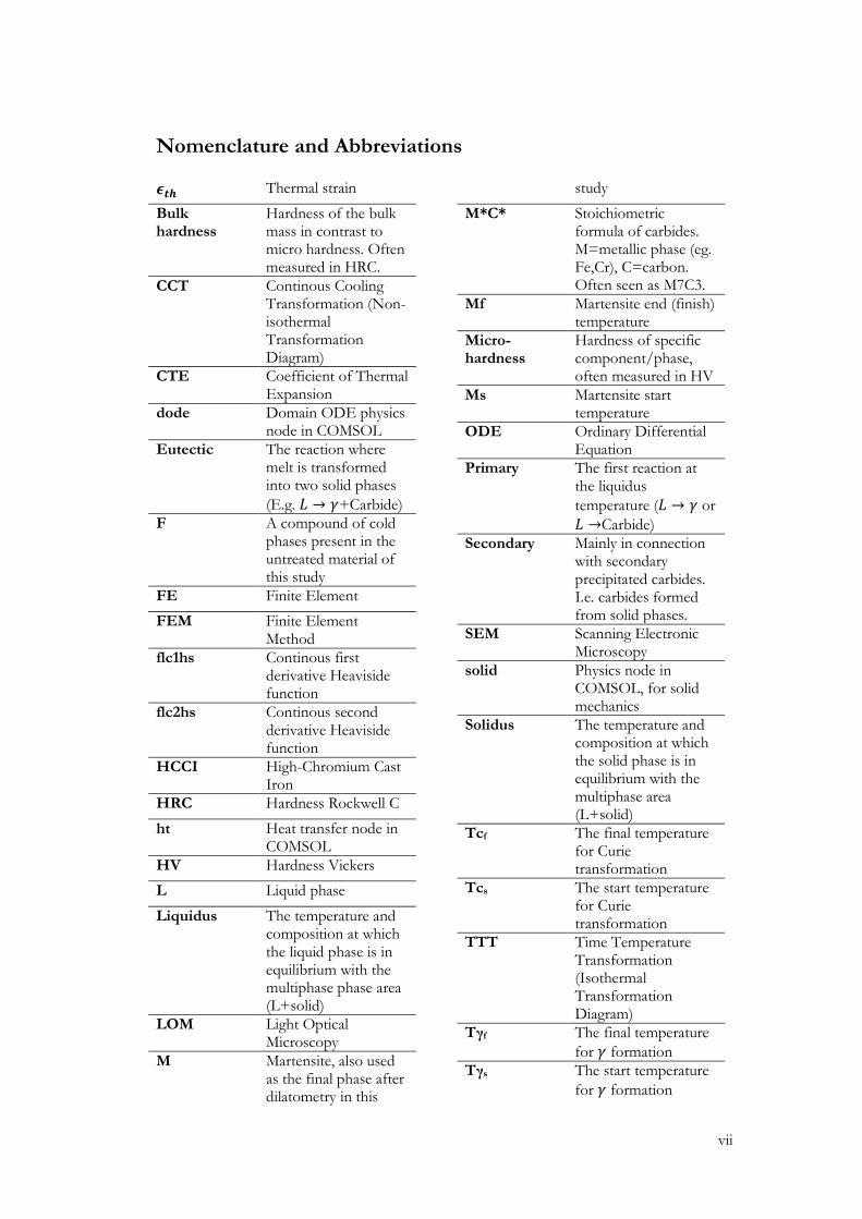
Nomenclature and Abbreviations
𝝐𝒕𝒉 Thermal strain
Bulk hardness
Hardness of the bulk mass in contrast to micro hardness. Often measured in HRC.
CCT Continous Cooling Transformation (Non-isothermal Transformation Diagram)
CTE Coefficient of Thermal Expansion
dode Domain ODE physics node in COMSOL
Eutectic The reaction where melt is transformed into two solid phases
(E.g. 𝐿 → 𝛾+Carbide)
F A compound of cold phases present in the untreated material of this study
FE Finite Element
FEM Finite Element Method
flc1hs Continous first derivative Heaviside function
flc2hs Continous second derivative Heaviside function
HCCI High-Chromium Cast Iron
HRC Hardness Rockwell C
ht Heat transfer node in COMSOL
HV Hardness Vickers
L Liquid phase
Liquidus The temperature and composition at which the liquid phase is in equilibrium with the multiphase phase area (L+solid)
LOM Light Optical Microscopy
M Martensite, also used as the final phase after dilatometry in this
study
M*C* Stoichiometric formula of carbides. M=metallic phase (eg. Fe,Cr), C=carbon. Often seen as M7C3.
Mf Martensite end (finish) temperature
Micro-hardness
Hardness of specific component/phase, often measured in HV
Ms Martensite start temperature
ODE Ordinary Differential Equation
Primary The first reaction at the liquidus
temperature (𝐿 → 𝛾 or
𝐿 →Carbide)
Secondary Mainly in connection with secondary precipitated carbides. I.e. carbides formed from solid phases.
SEM Scanning Electronic Microscopy
solid Physics node in COMSOL, for solid mechanics
Solidus The temperature and composition at which the solid phase is in equilibrium with the multiphase area (L+solid)
Tcf The final temperature for Curie transformation
Tcs The start temperature for Curie transformation
TTT Time Temperature Transformation (Isothermal Transformation Diagram)
Tγf The final temperature
for 𝛾 formation
Tγs The start temperature
for 𝛾 formation

viii
XRD X-Ray Diffraction
Xt Time derivative of variable X
𝜶 Ferrite
𝜸 Austenite, also used as the possible combination of austenite and other phases present in this study
𝚫𝝐𝒊𝒋 Difference in thermal strain for phase i to j.
Table of Content
1 Introduction .......................................................................................... 1
1.1 Xylem Water Solutions ................................................................................... 1
1.2 Background ....................................................................................................... 1
1.3 Project Outline ................................................................................................. 2
1.4 Needs and Limitations .................................................................................... 2
2 Literature Survey ................................................................................... 3
2.1 Heat Treatments .............................................................................................. 3
2.2 Carbides ............................................................................................................. 5
2.3 Metallographic Evaluation ............................................................................. 6
3 Theory ................................................................................................... 7
3.1 Metallurgical ...................................................................................................... 7
3.2 Dilatometry ....................................................................................................... 9
3.3 Hardness ......................................................................................................... 11
3.4 Implementation of Data in FE-models .................................................... 11
3.4.1 Heat Transfer and Phase Transformations ................................. 11
3.4.2 Thermal Strains ................................................................................ 12
4 Method ................................................................................................ 13
4.1 Experimental ................................................................................................. 13
4.1.1 Specimen Description and Preparation ....................................... 13
4.1.2 Dilatometry ....................................................................................... 15
4.1.3 Metallographic Evaluation ............................................................. 16
4.1.4 Hardness............................................................................................ 17
4.2 Simulations and Modelling .......................................................................... 17
4.2.1 Material Data and Parameters ....................................................... 18
4.2.2 Heat Transfer and Phase transformations .................................. 19
4.2.3 Solid Mechanics ............................................................................... 19
4.2.4 Geometry and Boundary and Initial Conditions ........................ 20
4.2.5 Study Configurations ...................................................................... 20
5 Results................................................................................................. 21
5.1 Dilatometry .................................................................................................... 21
5.2 Material Characterization ............................................................................ 31
5.3 Simulations and Modelling .......................................................................... 43
6 Discussion ........................................................................................... 47
6.1 Dilatometry .................................................................................................... 47
6.2 Material Characterization ............................................................................ 49
6.3 Simulations and Modelling .......................................................................... 51
6.4 Future Research ............................................................................................ 52
7 Conclusions ......................................................................................... 54
8 Cited Works ........................................................................................ 55

1
1 Introduction This report is the result of a Master Thesis in Mechanical Engineering performed 2018 at
KTH Royal Institute of Technology, Stockholm, Sweden. The work has been conducted for
Xylem Water Solutions, Sundbyberg, Sweden, based on a thesis proposal from the company.
1.1 Xylem Water Solutions
Xylem Water Solutions (Xylem) is a multinational company with 12 500 coworkers in 150
counties, working with water solutions. The company works to help people using water more
efficiently and have been part of the founders of Stockholm Water Prize which is one of the
ways the company works to increase people’s consciousness about the importance of the
available water resources. [1] All brands in the Xylem group work within a wide area con-
nected to water solutions. The products and services are used within dewatering, water and
wastewater treatment, water and wastewater transport, applied water systems and analytics.
[2]. Flygt is a Xylem brand with a large part of its production in Emmaboda, Sweden, where
they have been producing pumps since the 1930’s [3].
1.2 Background
Some submersible wastewater pumps, drainage pumps and slurry pumps are used to
transport abrasive particles suspended in liquid. To handle this abrasive environment the
products are sometimes made of abrasion resistant cast irons [4, 5]. One group of these irons
is the High-Chromium Cast Iron (HCCI) consisting of a high fraction of chromium carbides
in an austenitic or martensitic matrix. HCCI is a wide spectrum of cast irons with high alloy-
ing content of Chromium and sometimes Molybdenum, that can be sufficiently hard while
withstanding a certain degree of corrosive environments [4, 5, 6]. However, they are also
intimately connected with a somewhat difficult choice of composition, conditions in the cast-
ing, and casting geometry that may discourage foundries from using this material [6].
Not only is it difficult to cast a product free from cracks, another possible reason for the
material being seldom used outside of the milling and pump industry is the brittleness. If the
product needs increased hardness to reach a higher level of abrasion resistance it is possible
to harden the goods, e.g. by fully harden or by induction hardening of a specific surface
which is standard practice for many applications such as for gears and shafts. To get com-
pressive stresses in the surface region that reduces the risk of crack initiation and propagation
it is preferable with a volume expansion after a temperature cycle corresponding to harden-
ing [7]. As for this class of materials though, it has been shown in dilatometry studies that
shrinkage may occur when subjected to certain temperature cycles [8, 9].
To obtain data regarding the thermal strain behavior, dilatometry can be utilized where the
linear expansion of the material is determined. This method is also relevant today when the
trend in materials science and mechanical engineering points towards calculation-based re-
search and engineering. This can be seen in the calculation-based material science software
such as ThermoCalc, and the many finite element method (FEM) software available. Howev-
er, it is always necessary to possess mechanical and material data for the problem to perform
simulations and dilatometry makes it is possible to get data regarding the expansion of mate-
rials and revealing critical temperatures for transformations [7, 10, 11, 12, 13, 14].
2
1.3 Project Outline
The purpose of this study was to investigate how HCCI may behave during temperature
cycling in terms of elongation change after a temperature cycle corresponding to typical in-
duction hardening procedures. The sensitivity to temperatures and cooling rates on the final
dilatometric change were evaluated to find out if it is possible to maximize the volumetric
change by the choice of holding temperature. This should be advantageous in terms of resid-
ual stresses in the surface of the hardened part after cycling.
Many works aim at the destabilization and/or the destabilization followed by subcritical heat
treatment of as-cast material. Some of the destabilization processes are usually applied for the
hardening of the material and the combination for annealing for machining. It is, however,
not easy to find the destabilization-subcritical treatment followed by another destabilization
treatment/hardening step in the literature, especially for shorter time sequences as in induc-
tion hardening. This study contributes with material data for this sequence of treatments and
a proposal of implementation of this data in a simplified FE-model in the commercial soft-
ware, COMSOL Multiphysics (COMSOL), simulating the temperature change in a sample
geometry. The result from the simulation will show the phase distribution during a heat cycle
corresponding to those used in the experiments and be a first step in making it possible to
simulate hardening of products made of HCCI.
A hypothesis regarding the final length contraction is presented. An increased amount of
precipitated carbides in the hardening step could be favorable in the aspect of giving the
maximum volume expansion after the thermal cycle. A higher fraction of carbides leads to
lower C and Cr content in the austenite (𝛾) phase. This might lead to lower hardness but
higher martensite start temperature (Ms) and lower combined coefficient of thermal expan-
sion (CTE). The earlier transformation upon cooling should yield a higher fraction of mar-
tensite, and the CTE for previously for martensite is lowest of all phases [8]. Due to its be-
havior as the strengthening phase in the composite, more carbide should lead to less elastic
and plastic deformation of the bulk material martensite transformation. Hence, the final ex-
pansion should be maximized. The exact opposite was considered as well, since higher C
content will lead to harder martensite and a more expanding lattice, causing the actual expan-
sion of the martensite phase to be maximized.
In this report, fractions in percentage are shown by the symbol % regardless of the meaning
of the fraction. Furthermore, if not explicitly stated differently, volume fractions are used for
describing phases and mass fractions are used for describing alloying contents.
1.4 Needs and Limitations
The following limitations and needs were considered upon choosing the material and method
used. The experiments needed to yield information such as the thermal strain behavior, tem-
perature dependence of critical temperatures for phase changes, heat capacity, thermal con-
ductivity, modulus of elasticity, yield stress and flow/hardening function, and fracture stress.
Limiting factors were mainly the time frame of 20 weeks, financial aspects, and available
equipment and material. Therefore, only critical temperatures and thermal expansion were
evaluated, and only light optical microscopy (LOM) and hardness measurements were used
for the material characterization. Also, it was necessary to use material supplied by Xylem
and work specifically with this previously heat treated material which makes it more difficult
to apply results to a broader class of materials but might give indications of aspects needed to
evaluate further in a more experimental manner.

3
2 Literature Survey This chapter will highlight the existing knowledge regarding the investigated material and its
production. HCCI is a relatively wide group of metals with a narrow field of use and are of-
ten found in abrasion resistant applications [15, 16]. Zhou et al. [17] and Bedolla-Jacuinde et
al. [18] describe HCCI as a material with 11-30 % Cr and 1.8-3.6 % C. The material investi-
gated in this study falls within the Swedish standard SS-EN 12513:2011 [19], in literature
often referred to the previous SIS 140466:1971 [20]. Nearest American standard, ASTM
A532, is Class III Type A [20]. This is a material with 23%-30% Cr and 2.0%-3.3% C [20].
HCCI have been reported both as hypoeutectic, eutectic and hypereutectic alloys where the
primary crystals are austenite dendrites for hypoeutectic alloys and large M7C3 carbides for
most hypereutectic materials [18, 21, 22, 23]. The following equation (1) has been proposed
to determine the content of alloying elements in the Fe-Cr-C binary eutectic structure
(𝛾+M7C3) [24]
(% C) + 0.0474 × (% Cr) = 4.3 (1)
If the left-hand side equals less than 4.3 the composition is hypoeutectic [24].
The HCCI materials are known to be brittle and show little or no yield in tension at low
temperatures. Even in compression tests, some of the materials of this class have shown little
or no plasticity prior to fracture, especially for the eutectic and hypereutectic alloys [25]. The
metals may also show anisotropic behavior, especially following cold working such as rolling
and extrusion [26].
2.1 Heat Treatments
There are several reasons for subjecting a metal to heat treatments after casting. In this sec-
tion the heat treatments of HCCI found in literature are presented. Commonly, the proce-
dures reported regarding HCCI are called destabilization and subcritical heat treatment, often
performed in that order. While evaluating several materials in the HCCI class, Sare and Ar-
nold [27] found that “each of the four commercial grades of material studied must be treated
as separate entities, and that there are no generic trends that apply to all alloys”, especially in
connection with abrasion resistance. In addition, Tabrett and Sare [28] reports that there are
significant differences in microstructural changes and properties for the Cr15Mo3 and Cr27
white iron subjected to equal heat treatments. Since the material investigated falls within the
higher range of chromium content, the otherwise common Cr17 are not described in detail.
For hypoeutectic HCCI the solidification results in primary solidified 𝛾-dendrites followed by
a eutectic formed by 𝛾 and M7C3 carbides (𝐿 → 𝛾+M7C3) [16, 29, 30]. The eutectic can take
different forms based on the interaction with the dendrites and is either formed as a “flower-
like structure” [24] starting from a point in-between the dendrites, or as lamellar form [24,
30]. M7C3 carbides have been found to grow as rods or sometimes as plates in the eutectic,
oriented in the columnar direction of solidification [31]. Fredrikson and Remeaus [16] inves-
tigated a Cr26 alloy with 2.54 %C and 2.77 %C respectively. The as-cast structure consisted
of primary 𝛾-dendrites and eutectic (𝛾+M7C3) with a thin liner of martensite around the
carbides [16].
4
The solidified austenite contains an excessive amount of C and Cr and is therefore in indus-
try destabilized at temperatures around 930-1060 °C to precipitate carbides and deplete the
matrix on allowing elements allowing for transformation products to form upon cooling or
treatment at lower, subcritical temperatures [15, 32]. The carbides formed upon the eutectic
reaction have shown to be left unaffected by most heat treatments [15]. Depending on alloy-
ing content and temperature of isothermal heat treatments either or both M7C3 and M23C6
may form as secondary carbides [16, 30]. Different theories are presented for the temperature
ranges. For the Cr26 alloy investigated in [16] the M23C6 carbides are assumed to form upon
the eutectoid reaction forming a ferrite (𝛼)+carbide cluster (𝛾 → 𝛼+carbide) at lower tem-
peratures (<775 °C) while the M7C3 carbides are precipitated at higher temperatures (~975
°C). In [33] several different HCCI were investigated and the common conclusion was that
the isothermal treatment resulted in c-shaped curves with the fastest decomposition at 950-
1000 °C and 650-700 °C. For the higher temperature range, M7C3 was formed above the
temperature where 𝛼 is no longer stable (often denoted A3) and between the eutectoid tem-
perature, below which 𝛾 is no longer stable (often denoted A1), and A3 a combination of
M23C6, 𝛼, and 𝛾 were formed [33]. For the lower temperature range, subcritical treatment
below A1, 𝛾 formed 𝛼 and M3C carbides. This precipitation and depletion of alloying ele-
ments of the austenite matrix causes the Ms temperature to rise close to the carbides, hence
forming allowing martensite to form subsequent quenching [15, 16, 33]. The martensite is
often formed as a liner around the carbides while austenite is retained further away from the
carbides due to higher carbon content away from the carbides as reported in [16, 21]. The
“magnitude of martensitic transformation” defined as the expansion due to martensite for-
mation is discussed in [30]. It was found that higher temperatures and greater precipitation
lead to a greater magnitude.
The maximum hardness of different heat treatments is often seen as a c-curve of the destabi-
lization temperature with a maximum found at around between approximately 980-1050 °C
depending on the investigated alloy [17, 30, 33, 34]. Reference [16] report that the hardness
of the material is determined by the hardness of the martensite and the content of martensite
in the matrix. They write that the hardness of the martensite is strongly dependent on the
carbon content in the martensite and the solubility of carbon in austenite is increasing with
increasing temperature; however, the Ms temperature is decreased and the formation of mar-
tensite might be suppressed. Similar reasoning regarding the maximum hardness of the ma-
trix is pointed out in the extensive study performed by Maratray and Usseglio-Nanot [30] as
well. The authors found that the decrease in hardness at low temperatures is explained by the
lower hardness of the martensite due to the carbon content and at very high temperatures by
the increased amount of retained austenite. Maratray and Poulalion [29] connected this be-
havior with the retained austenite content and found that around 20 % retained austenite was
found at the maximum hardness. Sare and Arnold [27] showed that the higher austenitization
temperature will lead to increased fracture toughness and in the case of Cr27 the higher aus-
tenitization temperature (1100-1150 °C) resulted in the lowest abrasive wear as well, even
though the latter relation was subtler. The abrasion resistance did, however, depend strongly
of the tempering temperature; even though the microstructure was reportedly similar. The
relation with retained austenite showed that the optimal value is about 30% for the wear re-
sistance.
Destabilization at 1100 °C is reported to redissolve secondary carbides precipitated at lower
temperatures while they remained stable at 1000 °C [28, 35]. Lai et al. [36] presents a con-

5
stantly decreasing amount of carbides with temperature (950-1100 °C) and Bedolla et al. [18]
also shows that previously precipitated carbides may dissolve at higher temperatures while
further precipitation is detected for lower destabilization temperatures (900-1000 °C).
There are several proposed procedures described in the literature to decrease hardness and
retained austenite and thus increase the machining properties. Even though austenite is rela-
tively soft; it is sometimes unstable and therefore possible to transform to martensite upon
certain isothermal conditions, such as increased strain upon deformation [37, 38]. In [32]
either subcritical (between 690 °C and 705 °C) or full annealing are recommended for HCCI;
the latter, performed in the range 955-1010°C followed by a longer holding time at 760 °C is
recommended for alloys with particularly good hardenability. The same treatment is also
recommended in [15] where the austenite is described to be destabilized at the higher tem-
perature range followed by a formation of a ferrite-carbide structure at the lower range.
Maratray [33] writes that this annealing can be performed either by isothermal holding be-
tween A1 and A3 or by destabilization above A1 followed by slow cooling to about 650 °C
and that the most easily machined structure is the ferrite-carbide structure consisting of sphe-
rodized carbides of possibly M23C6. A heat treatment of a Cr27 alloy at 1000 °C followed by
a subcritical heat treatment at 550 °C or 600 °C showed a great decrease in retained austenite
and hardness and exhibited much higher wear losses than the as-cast alloy [28].
No experimental studies investigating the hardening treatment following soft annealing of
the higher range of chromium rich HCCI have been found in this literature survey.
2.2 Carbides
In the case of the high-alloyed cast irons, the carbide content may be very high. Equation (2)
proposed by Maratray [33] is used in the literature to estimate the amount of carbides in
HCCI and has shown good correspondence to both calculations performed in ThermoCalc
as well as experimental results [39, 40].
% carbides = 12.33 × (% C) + 0.55 × (% Cr) − 15.2 (2)
Liu et al. [25] also showed that the macrostructure caused by the casting of these materials
has impact on the strength and yield stress. They saw that the materials’ stress-strain relation-
ship was affected by the directionality of the material, especially for the slightly hypereutectic
alloys and at elevated temperatures. They also found that the eutectic structures grew in the
direction of solidification using a setup to control the solidification direction. The same di-
rectionality in the morphology of the carbides was found in a study performed by Lu et al.
[24]. In that study the unidirectional solidification was investigated and showed a clear fi-
brous network of eutectic carbides growing in the direction of solidification and the HCCI
was treated as a fiber composite. It was seen that the strength was drastically increased in the
direction of the carbide network. Tabrett and Sare [31] investigated the columnar macro-
structure formed during solidification in a regularly cast material. They found that the mainly
columnar structure of eutectic carbides in a Cr27 alloy had a clear impact on the fracture
toughness and that fractures often occurred along the carbide-matrix interface. The growth
as plates or bars of the eutectic hexagonal M7C3 is reported in [18] as well. By aligning the
columnar structure, and the longitudinal axis of the carbides, perpendicular to the crack plane
the fracture toughness increased [31].
Among other features, the extent of secondary carbide precipitation was investigated in an
extensive study by Maratray and Usseglio-Nanot [30]. Their results for destabilization at 800-

6
1000 °C showed that for samples with a high amount of carbides the extent of the isothermal
carbide formation at destabilization does not alter Ms; however, the temperature at which the
precipitation is performed does, as described in the previous section.
2.3 Metallographic Evaluation
The structures of the investigated materials in literature are often evaluated by LOM and
scanning electron microscopy (SEM). These methods yield a mostly qualitative understand-
ing of the material structures. For the metallography it is necessary to prepare samples ac-
cording to a regular metallographic procedure by polishing and often etching. A chemical
etchant attacks different compositions or different crystalline directions of grains at different
rates, causing irregularities in the surface that is detectable in the LOM and not only depend-
ing on the relative reflectivity of the phases in the polished state. [41, 42] The choice of etch-
ant, however, has been done differently throughout different studies. 4% Nital used in [17],
Viella’s etchant used in [18, 35, 43], and aqua regia with inhibitor [44] are some choices for
etching similar materials, mostly with a chromium content of 14-30 %.
SEM is used in addition to LOM to resolve fine structures and can be used in combination
with deep etching to evaluate the network of carbides formed. Since SEM in general gives
higher resolution and magnification it is possible to distinguish certain structures from each
other which otherwise can be difficult by the magnifications used in LOM [30]. Another
commonly used experiment in addition to LOM is X-Ray diffraction (XRD). This method is
used to detect phases present in the investigated material. The amount of austenite has been
found difficult or impossible to quantitatively determine by metallographic evaluation [29].
However, both these methods are time consuming and costly compared to LOM that is of-
ten easily obtainable and user friendly.
7
3 Theory In this chapter theory behind the metallurgical processes are described, as well as the dila-
tometry, hardness measurements, and FEM regarding this research area.
3.1 Metallurgical
A primary study performed by the author reveals some thermodynamic relations based on
computational thermodynamics. The software ThermoCalc was utilized to create diagrams of
relevant aspects in the material handling based on equilibrium equations in the database
TCFE7 for the material composition corresponding to that of the samples in dilatometry.
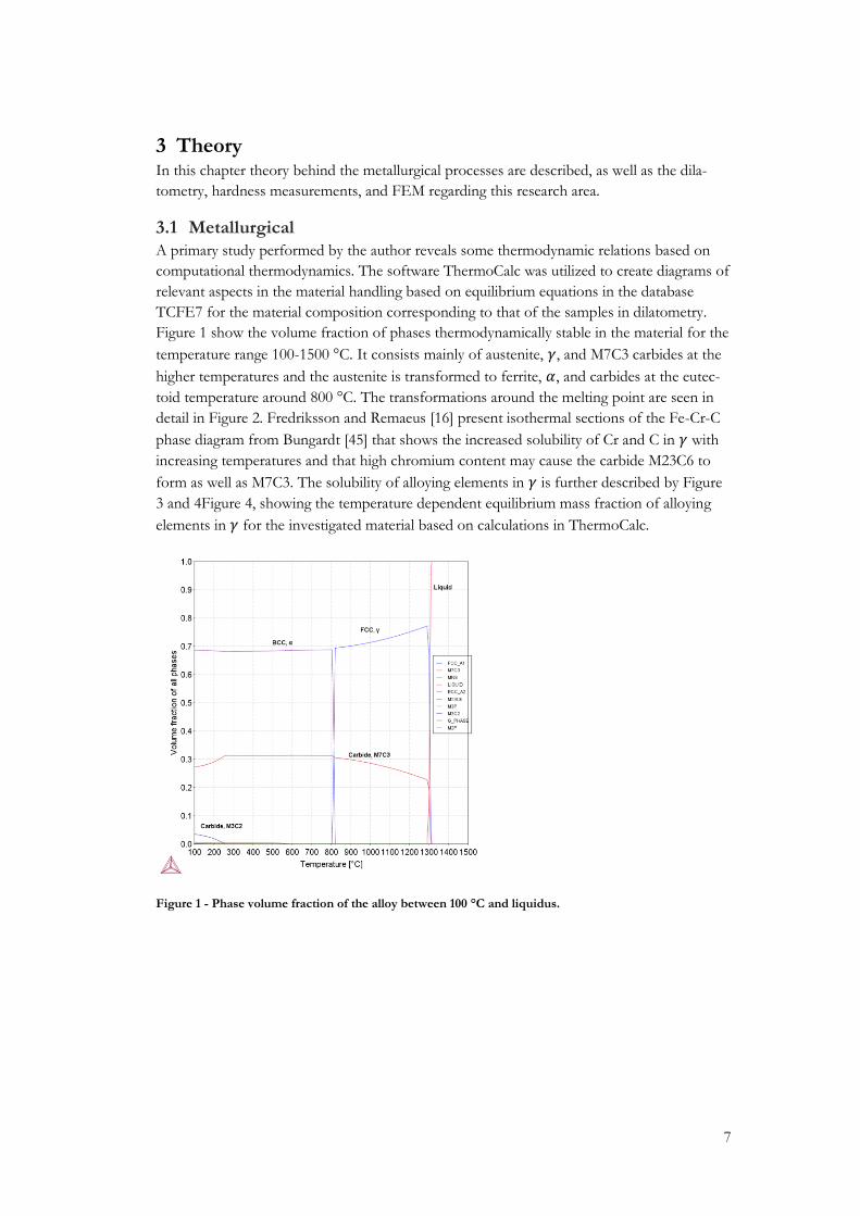
Figure 1 show the volume fraction of phases thermodynamically stable in the material for the
temperature range 100-1500 °C. It consists mainly of austenite, 𝛾, and M7C3 carbides at the
higher temperatures and the austenite is transformed to ferrite, 𝛼, and carbides at the eutec-
toid temperature around 800 °C. The transformations around the melting point are seen in
detail in Figure 2. Fredriksson and Remaeus [16] present isothermal sections of the Fe-Cr-C
phase diagram from Bungardt [45] that shows the increased solubility of Cr and C in 𝛾 with
increasing temperatures and that high chromium content may cause the carbide M23C6 to
form as well as M7C3. The solubility of alloying elements in 𝛾 is further described by Figure
3 and 4Figure 4, showing the temperature dependent equilibrium mass fraction of alloying
elements in 𝛾 for the investigated material based on calculations in ThermoCalc.
Figure 1 - Phase volume fraction of the alloy between 100 °C and liquidus.

8
Figure 2 - Phase volume fraction upon cooling of the melt.
An estimation of the phase fraction found in treated samples can be done by several meth-
ods. Point counting of the revealed microstructures after preparation by applying a grid to
the microstructure either in the ocular, or in post processing after taking a photograph of the
cross section, is one of the most commonly used methods. The lowest possible magnification
giving sufficient level of detail is to be used and the grid size is adjusted for the microstruc-
ture to be evaluated. The points are counted at the grid intersections where half a point is
counted when the intersection coincides with a phase boundary. The volumetric phase
amount is then calculated by dividing the points with the total amount of grid intersections.
[46]
Not visible in the Figure 1 and 2 is the Curie temperature (Tc), below which the 𝛼-ferrite is
ferromagnetic [47]. For unalloyed iron, this temperature is around 770 °C [47] (1043 K) and a
proposed relationship (3) seen in [48] is insensitive to carbon, but atomic fraction of manga-
nese (𝑥Mn) is considered
𝑇𝑐 = 1042 K − 𝑥Mn × 1500 K (3)
Belyakova et al. [49], however, report that the same author in a previously published article
found the Curie temperature depending on chromium by drastically lowering Tc with in-
creasing Cr content. They present a decrease in transformation temperature from 750 °C to
538 °C when increasing the Cr content from 13.6 % to 33.5 %. The effect of the magnetic
transformation on the dilatometry is pronounced when looking at the power needed to keep
a constant heating rate over the temperature interval as seen in reports regarding hypoeutec-
tiod steels [48, 50].

9
Figure 3 - Mass fraction of all components, except Cr, in γ in the temperature range 850-1200 °C.
‘
Figure 4 - Mass fraction of Cr in FCC in the temperature range 850-1200 °C.
3.2 Dilatometry
There are reportedly several possible methods to determine phase transformation tempera-
tures and some yield additional information such as phase volume fractions. Dilatometry is
one of these methods [51]. It is used to detect length changes of a material during heating
and cooling and through the operationalization of connecting phases with different densities
makes it possible to observe critical points of phase transformations and the phase fractions
[48, 50, 52]. The Curie transformation is also detectable due to the change in power of the
inductor and an additional observed strain [53, 54, 55].
10
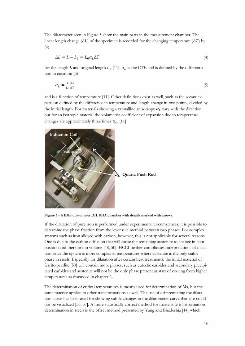
The dilatometer seen in Figure 5 show the main parts in the measurement chamber. The
linear length change (𝛥𝐿) of the specimen is recorded for the changing temperature (𝛥𝑇) by
(4)
Δ𝐿 = 𝐿 − 𝐿0 = 𝐿0𝛼𝐿Δ𝑇 (4)
for the length 𝐿 and original length 𝐿0 [11]. 𝛼𝐿 is the CTE and is defined by the differentia-
tion in equation (5)
𝛼𝐿 =1
𝐿0
𝑑𝐿
𝑑𝑇 (5)
and is a function of temperature [11]. Other definitions exist as well, such as the secant ex-
pansion defined by the difference in temperature and length change in two points, divided by
the initial length. For materials showing a crystalline anisotropy 𝛼𝐿 vary with the direction
but for an isotropic material the volumetric coefficient of expansion due to temperature
changes are approximately three times 𝛼𝐿. [11]
Figure 5 - A Bähr dilatometer DIL 805A chamber with details marked with arrows.
If the dilatation of pure iron is performed under experimental circumstances, it is possible to
determine the phase fraction from the lever rule method between two phases. For complex
systems such as iron alloyed with carbon, however, this is not applicable for several reasons.
One is due to the carbon diffusion that will cause the remaining austenite to change in com-
position and therefore in volume [48, 50]. HCCI further complicates interpretations of dilata-
tion since the system is more complex at temperatures where austenite is the only stable
phase in steels. Especially for dilatation after certain heat treatments, the initial material of
ferrite-pearlite [50] will contain more phases, such as eutectic carbides and secondary precipi-
tated carbides and austenite will not be the only phase present at start of cooling from higher
temperatures as discussed in chapter 2.
The determination of critical temperatures is mostly used for determination of Ms, but the
same practice applies to other transformations as well. The use of differentiating the dilata-
tion curve has been used for showing subtle changes in the dilatometer curve that else could
not be visualized [56, 57]. A more statistically correct method for martensite transformation
determination in steels is the offset method presented by Yang and Bhadeshia [14] which
Induction Coil
Quartz Push Rod
Sample

11
utilizes the lattice expansion of the phases and a fixed limit of offset from the expected dila-
tation.
3.3 Hardness
There are several hardness measurement methods available. In common is that the indenta-
tion depth/width is connected to the hardness value through specific formulas when tests
can be systematically performed. In the Rockwell test the hardness is determined by the dif-
ference in indentation depth of two different loads and in many testing machines the value is
given on a display after indentation [46]. Different critical distances are given in the literature
[46, 58]. However, the most conservative guideline states that the distance from the edge of
the sample should be no less than 1 mm and the center-to-center distance of two indenta-
tions should exceed 2 mm [58]. Rockwell C (HRC) is measured by a Brale penetrator first
indented by 10-kgf and then by 150-kgf load [46, 58].
3.4 Implementation of Data in FE-models
This chapter will only briefly explain some theoretical foundations for describing the heat
transfer, phase transformations, and stress and strain relationships in a FEM-simulations
related to the studied phenomena of dilatation and induction hardening. A thorough explana-
tion of the theory and equations used for describing the latent heat and the phase transfor-
mation can be found in [59] and, among others, [60] and [61] are works using FEM software
to model phase changes in steel containing various information of the theory behind the
modelling.
3.4.1 Heat Transfer and Phase Transformations
Austenite transformation is often described by the formula proposed by Leblond and De-
veaux [62] that consider the influence of time and temperature. Martensite fraction (M) is,
however, described frequently by the exponential K-M equation (6) [60, 61, 62, 63] based on
austenite fraction at Ms, 𝛾0, positive kinetics parameter 𝛽, and temperature 𝑇, formed by
Koistinen and Marburger [64].
𝑀 = 𝛾0(1 − exp(−𝛽(𝑀𝑠 − 𝑇))) (6)
The equations can be implemented into FEM software as (6) and the following ordinary dif-
ferential equation (7) [59, 63]. Here the time derivative (subscript t) of austenite (𝛾) and mar-
tensite are considered. 𝜏(𝑇) is a kinetics parameter, 𝑇(𝑡) is the temperature as a function of
time, 𝛾𝑒𝑞 is a linear function from 0 to 1 describing the maximum fraction of austenite, 𝑇𝛾𝑠
and Ms are the start temperature of respective transformation found in practice, and 𝐻 is the
Heaviside step function.
𝛾𝑡(𝑡) =1
𝜏(𝑇)max{[𝛾𝑒𝑞(𝑇(𝑡)) − 𝛾(𝑡)], 0} 𝐻[𝑇(𝑡) − 𝑇𝛾𝑠] − 𝑀𝑡 (7)
Neglecting radiation and mechanical effects on the thermal properties the energy equation is
described as (8) [59, 65]
𝜌(𝑇)𝐶𝑝(𝑇)𝜕𝑇
𝜕𝑡− ∇ ∙ (−𝑘(𝑇)∇𝑇) = 𝐹1 (8)
where 𝜌, 𝐶𝑝, and 𝑘, denotes the temperature dependent variables density, heat capacity at
constant pressure and conductivity respectively. The heat consumed or released during phase
transformations is described as a heat source, 𝐹1, by (9)-(11) [59]

12
𝐹1 = 𝐹11(𝐻(−𝑇𝑡)) + 𝐹12 (9)
𝐹11 = 𝜌(𝑇)𝐿𝑚𝑀𝑡 (10)
𝐹12 = −𝜌(𝑇)𝐿𝛾1
𝜏(𝑇)max{[𝛾𝑒𝑞(𝑇(𝑡)) − 𝛾(𝑡)], 0} 𝐻[𝑇(𝑡) − 𝑇𝛾𝑠] (11)
𝐿𝛾 and 𝐿𝑚 are positive values for the latent heat, hence heat is released upon martensite
transformation and consumed for austenite transformation from the original cold phases.
3.4.2 Thermal Strains
Instead of the usual heat expansion 𝜖𝑡ℎ(𝑇) = 𝛼𝐿(𝑇 − 𝑇𝑟𝑒𝑓) equation (12) can be imple-
mented in COMSOL [66]
𝜖𝑡ℎ = ∑ 𝜖𝑖(𝑇) 𝑓𝑖 (12)
where 𝑓𝑖 is the volume fraction, and 𝜖𝑖 are temperature dependent functions describing the
strain of the phases 𝑖. The CTE for each phase is accurately described by the lattice parame-
ters and carbon content as well as temperature dependence [60, 61]. A secant thermal expan-
sion has been used as well to describe the expansion and contraction due to temperature
changes [65].

13
4 Method This chapter will highlight the choice of method and describe the setup for the experimental
part of this study. Lastly, the procedure of implementing experimental data in the FEM-
simulations in COMSOL is presented.
4.1 Experimental
The main section of this study was based on experimental results. Dilatometry was the
choice of method to evaluate the volumetric change after temperature cycling. There are
other methods available to determine critical temperatures during cycling for implementation
in simulations such as cooling curve analysis [51]. However, since the volumetric change was
the focus of this study the dilatometry could yield more relevant data. A metallographic eval-
uation and hardness measurements is usually evaluated in connection to dilatometry [10, 67].
By evaluating the specimens by several methods, it is easier to rule out alternative explana-
tions to the behavior found in dilatometry.
4.1.1 Specimen Description and Preparation
The specimens in this report refer to previously initiated samples in dilatometry described in
Table 1, as well as the specimens subjected to dilatometry experiments designed by the au-
thor, see Table 2. The heating rate, holding time, cooling rate as well as the destabilization
temperature are reported as different heat treatments further described in Table 3.
Table 1 - Previously initiated samples in dilatometry.
Sample Heat treatment Direction
P1 H1000LL Iso P2 H1000LL Iso P3 H1000U Iso P4 H1000U Iso P5 H1000L Iso P6 H900U Iso P7 H900U Iso P8 H900L Iso
Pobh Untreated Iso
Pobh is untreated material from the same section as P1-P8. All specimens in Table 2 were
cut from material with the composition in Table 4, based on the analysis taken on the melt
before casting. The samples in Table 1 are of the same material standard, falling in the limits
of ASTM Class III cast irons; however, no charge analysis is available. The temperature his-
tory was available for A1-B3 and is schematically presented in Figure 6. Samples cut from the
other main material have followed a similar standardized scheme.
14
Figure 6 - Schematic temperature history of the dilatometer samples A1-B3
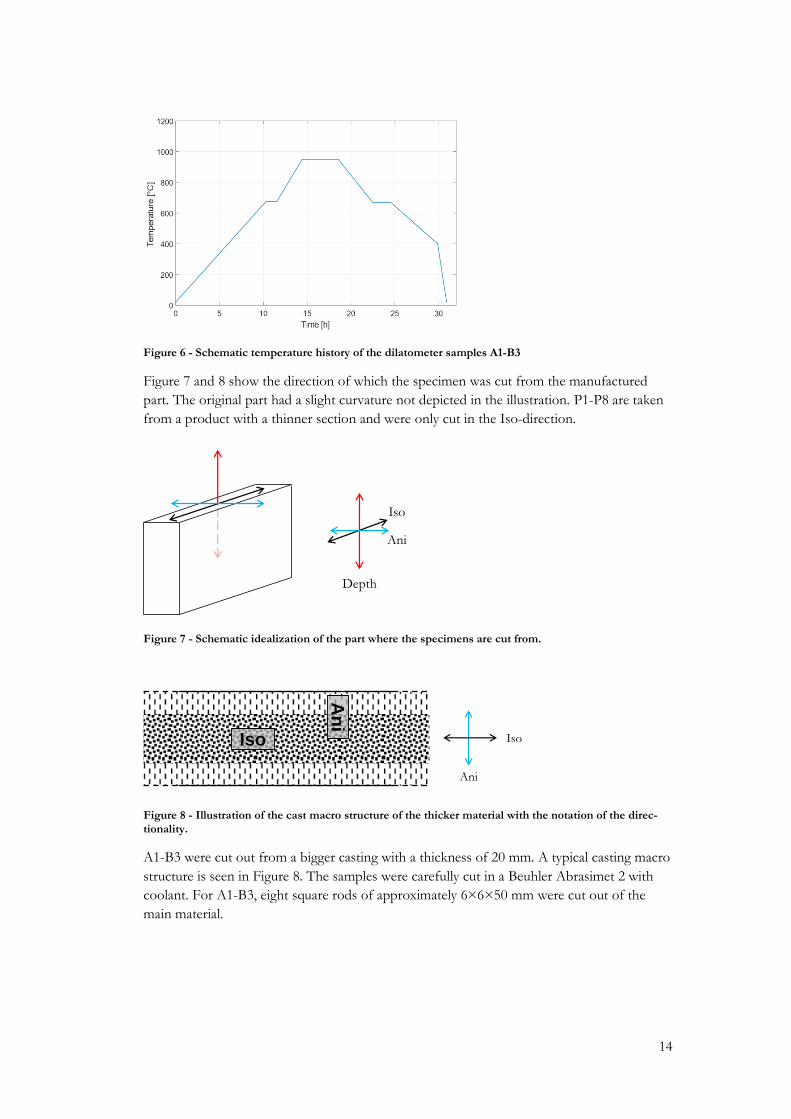
Figure 7 and 8 show the direction of which the specimen was cut from the manufactured
part. The original part had a slight curvature not depicted in the illustration. P1-P8 are taken
from a product with a thinner section and were only cut in the Iso-direction.
Figure 7 - Schematic idealization of the part where the specimens are cut from.
Figure 8 - Illustration of the cast macro structure of the thicker material with the notation of the direc-
tionality.
A1-B3 were cut out from a bigger casting with a thickness of 20 mm. A typical casting macro
structure is seen in Figure 8. The samples were carefully cut in a Beuhler Abrasimet 2 with
coolant. For A1-B3, eight square rods of approximately 6×6×50 mm were cut out of the
main material.
Iso
Ani
Depth
An
i
Iso
Ani
Iso

15
Table 2 - List of the specimens tested in dilatometry with respective heat treatment, direction.
Specimen ID Heat treatment Direction
A1 H925L Iso A7 H925L Iso B1 H925L Ani A10 H925U Iso A4 H925U Iso A2 H1050L Iso A8 H1050L Iso B2 H1050L Ani A11 H1050U Iso A5 H1050U Iso A3 H1150L Iso A9 H1150L Iso B3 H1150L Ani A12 H1150U Iso A6 H1150U Iso
H2 Untreated Depth Hi1 Untreated Iso Tö Untreated Ani (mid-section) Tu Untreated Ani (close to surface) Vy1 Untreated Iso
The choice of original rod for each sample and trial order were made randomly by using a
Matlab random generator. The square rods were then machined into cylindrical pieces of 10
mm length and 4 mm diameter at the Swedish research institute Swerea KIMAB, Stockholm.
Table 3 - The heat cycles tested in this dilatometry study.
Denotation Heating rate
[°𝐂/𝐬] End temperature
[°𝐂] Holding
Time [𝐬] Cooling rate
[°𝐂/𝐬] H900L 100 900 1 20 H900U 100 900 1 100 H1000LL 0.5 1000 1 10 H1000L 100 1000 1 20 H1000U 100 1000 1 100
H925L 50 925 3 10 H925U 50 925 3 50 H1050L 50 1050 3 10 H1050U 50 1050 3 50 H1150L 50 1150 3 10 H1150U 50 1150 3 50
Table 4 - Composition of the alloy (wt%) based on the smelt analysis of the batch where A1-B3 are cut from.
Alloy C Si Mn P S Cr Ni Mo Cu Fe
HCCI 2.60 0.72 0.41 0.016 0.018 24.70 0.19 0.10 0.01 71.2
4.1.2 Dilatometry
The dilatometry was used for different reasons. One was to evaluate the thermal expansion
and compression of the material during an arbitrary temperature cycle. It can also be used to

16
detect phase changes in the material. This is otherwise not directly observable, but the feature
is linked to a sudden volumetric change that is detectable by the dilatometer. This is to say
that the feature of phase changes is operationalized by observing the length change of the
material during heating and/or cooling. Hence, the method was used in this study.
The dilatometer used was a “Bähr dilatometer DIL 805A” at the research institute Swerea
KIMAB, Stockholm, Sweden. The instrument is shown previously in Figure 5. The sample
was held in the inductor by quartz push rods. The apparent length change (including the
possible expansion of the quartz rods) of the specimen was measured simultaneously as the
temperature is measured and controlled by a spot-welded thermocouple of type S, Pt and
Pt+10 % Rh. The dilatometry was performed in two sessions. The first tests were, as men-
tioned above, planned and initiated outside of this study. Therefore, the following descrip-
tion of the experimental randomization setup is valid for A1-B3 only. The results, however,
are reported together but with the distinct difference in denotation of the samples.
During the experiment, all samples were given two different numbers; one for the identifica-
tion for the position at the original material (works as specimen marker) and one randomized
for the experiment order. Hence, the experimental setup was randomized twice. The ran-
domization was done to allot the sample to a specific procedure and the second to determine
the sample order of the trials. This was to reduce the risk of influence of systematical errors
on the results. See Table 3 for the different heat treatment schemes and Table 2 for each
specimen denotation.
The recorded data in dilatometry was time, temperature, length change, and nominal temper-
ature. Additionally, it was possible to get the power used for the inductor. The strain was
found by dividing the recorded length change by the initial length of each specimen, given in
mm with two decimals. To more easily determine the phase transformations the derivative of
the experimental Temperature-Elongation data was calculated. Since fitted to experimental
data, the derivative values and the power values were then smoothed by “local regression
using weighted linear least squares and a 2nd degree polynomial model” [68] called “loess” in
Matlab before plotting in figures. In the case of noisy in-data the dilatation data were
smoothed as well. The raw data on cooling for the A and B-samples were smoothed by the
span 0.025 for slowly cooled (suffix L) and 0.05 for the higher cooling rates (suffix U). The
derivatives were evaluated both as unsmoothed and smoothed using a span of 0.05 at heating
and five times the span of the raw data smoothing during cooling.
Using the Temperature-Strain data the (secant) CTE is determined for all samples. This pro-
cedure was divided into two sections. Regression points for all sections of the dilatometer
curve were graphically chosen. Following this, a simplified curve was considered to evaluate
data for simulations for fewer sections. In the latter evaluation, only A- and B-samples were
considered.
4.1.3 Metallographic Evaluation
The metallographic evaluation included material previously tested in dilatometry (P3-P8) as
well as the samples prepared and designed by the author (A1-B3) and the samples without
heat treatment. The material from dilatometry was received as cylindrical pieces of 10 mm
length and 4 mm diameter. Common praxis for sample preparation was used, including cast-
ing in thermosetting Bakelite (Struer’s PolyFast), wet grinding (240P, 320P, 600P, 1200P),
and finally polishing using 3 µm diamond paste. Etching was performed in V2A etchant (100
ml H2O + 100 ml HCl + 10 ml HNO3 + 0.3 ml Nonidet P-40) at around 50-55 °C for 4-12

17
seconds. The same procedure was repeated for the samples A1-B3 after dilatometry and for
the specimens without heat treatment. All samples are inspected in an optical microscopy
(Nikon Optiphot 150S) with resulting magnification ranging from 50x-1000x. A Nikon D500
DSLR + Nikkor 50mm f/1.8 D was mounted to enable photographs to be taken. The
amount of primary phase was estimated at some samples by point counting photographs of
the structures with a 7×11 grid.
4.1.4 Hardness
Following the microscopy evaluation, the samples were polished as described in the previous
section and then tested in a hardness tester Otto Wolpert Werke of type Dia testor 2Rc with
test load 150 kpf as is practice for Rockwell C measurements. The measurements were di-
rectly read of the scale on the machine with a precision of 1 HRC. A calibration sequence
where the stability of obtained hardness values for calibration plates of HRC 59.2 and HRC
30.2 was performed. The hardness of the samples was then estimated with one decimal and
then rounded to the closest integer before averaging over the specimens and heat treatments.
First, a measurement was taken in the center of the cylinders to accompany to the standard
distances; however, at least one additional indentation was made between the center and
edge. For the untreated samples that had a much larger cross section, several measurements
were taken in rows from edge to edge.
4.2 Simulations and Modelling
Data from the dilatometry study were combined with data found in the literature to create a
model of a material exhibiting the similar heat treatment response as the investigated HCCI.
The simulations were conducted in COMSOL Multiphysics 5.3a which is a commercially
available FEM-software. The model was constructed using three different nodes, Heat
Transfer in Solids (ht), Domain ODEs and DAEs (dode), Solid Mechanics (solid) as well as
the Multiphysics node. This node connects the temperature between ht and solid and enables
calculations of thermal strains. As a rule, most functions given by data in tables were interpo-
lated with piecewise cubic functions to avoid discontinuities in the derivative otherwise
found in the data points.
The analysis was a transient study in three dimensions. A demonstration model of a different
problem involving induction heating and phase transformations provided by COMSOL Mul-
tiphysics, based on the works of [59, 69, 70, 71, 72], was used for some material data as well
as a reference for the implementation of the ordinary differential equations used to describe
the martensite phase evolution. The data were in some cases modified to better match data
found for HCCI and adjusted to better fit the dilatometry results. In this case, the dilatome-
try curves were assumed to show the correct behavior of the material as a bulk mass, even
though it might deviate from the demonstration model and/or findings regarding other
simulations of low alloyed steels. This is due to the difficulty of estimating the material be-
havior and constituents and therefor makes it diverge from normal calculation models that
are often based on calculations of each individual phase.
When discussing both the experimental and simulated dilatometer curve, the different sec-
tions of the curve will be denoted as in regular steels, i.e. cold phases (𝐹), austenite (𝛾), and
martensite (𝑀), even though the material may consist of different amount of carbides and
phases as well at all steps. The original material is assumed to be stress free and consist of
one single phase, 𝐹, which in practice is the composite of materials existing in the dilatome-
try samples before heat cycling. The CTE were assumed to be constant until the phase trans-

18
formation at around 880-960 °C, denoted 𝐹 → 𝛾. The CTE was then determined by a linear
combination of the present phases until the transformed material is going through the 𝛾 →
𝑀 transformation upon cooling below 400-200 °C where the CTE of 𝑀 was added.
4.2.1 Material Data and Parameters
Data used in this simulation were found for different materials and were accepted in absence
of more precise data for the HCCI in question. Material parameters are presented in Table 5.
Temperature dependent values for the thermal conductivity, 𝑘, Young’s modulus, 𝐸, and
heat capacity at constant pressure, 𝐶𝑝, were obtained from [49] while the temperature de-
pendent tangent modulus, 𝐸tan, and the nonlinear combination of phase and temperature
dependent initial yield stress (𝜎0) accepted as found and combined in [63]. Values for the
initial temperature and microstructure are presented in Table 5, and graphs of the material
data are available in Appendix 1. The latent heat of fusion for both the modelled phase
changes was set according to reference [59]. Density, 𝜌, and Poisson’s ratio, 𝜈, are set as con-
stants shown in Table 5.
Table 5 - Material data used in simulations. Data dependent on temperature and/or phase fractions, is given a value for the initial microstructure at 20 °C. Direction dependent values are marked with A or B.
Parameter Value Comment
𝒌 13.9 [W/(m∙K)] Non-linear, temperature de-pendent
𝑬 213 [GPa] Non-linear, temperature de-pendent
𝑪𝒑 0.45 [kJ/(kg∙K)] Non-linear, temperature de-pendent
𝑬𝐭𝐚𝐧 6.579 [GPa] Non-linear, temperature de-pendent
𝑳𝜸 82 [J/g]
𝑳𝑴 82 [J/g]
𝝈𝟎 320 [MPa] Non-linear, phase and tempera-ture dependent.
𝝆 7600 [kg/m3]
𝝂 0.28 [1]
𝜶𝑳,𝑴 A: (-13×Tmax/280+369/7)e-6 [1/K] B: (-5.27×Tmax/14010+301.71/7)e-6 [1/K]
Secant coefficient for A and B, function of maximum tempera-ture in °C.
𝜶𝑳,𝑭 A: 14.66 [1/K] B: 12.32 [1/K] Secant coefficient, constant
𝜶𝑳,𝜸 A: 20.53 [1/K] B: 17.48 [1/K] Secant coefficient, constant
𝚫𝝐𝑭𝜸 A: 1.06e-2 [1] B: 0.87e-2 [1] Different for A and B samples
𝚫𝝐𝑭𝑴 A: 6.81e-4 [1] B: -1.47e-2 [1] Different for A and B samples
𝜷 A: 0.035 [1/s], 0.035 [1/s], 0.015 [1/s]
B: 0.050 [1/s], -- --
Linear interpolation of maxi-mum temperature (Tmax) in °C. Values given for Tmax: 925, 1050, 1150 °C.
𝑴𝒔 A: 400 [°C], 320 [°C], 220 [°C]
B: 410 [°C] -- --
Linear interpolation of maxi-mum temperature (Tmax) in °C. Values given for Tmax: 925, 1050, 1150 °C.
𝑻𝜸𝒔 887 [°C]
𝒁𝑹 0.31 [1]

19
4.2.2 Heat Transfer and Phase transformations
The heat transfer was purely based on conduction; no convection or radiation was accounted
for. The phase transformations were described by equation (6)-(7) found in chapter 3.4.1 and
implemented in the dode node as equation (13), (14), and (15). Equation (16) was imple-
mented as a regular variable.
𝛾𝑡(𝑡) =1
𝜏(𝑇)max{[𝛾𝑒𝑞(𝑇(𝑡)) − 𝛾(𝑡)], 0} 𝑓𝑙𝑐2ℎ𝑠(𝑇 − 𝑇𝛾𝑠 − 10,10) − 𝑀𝑡 (13)
𝑇max = 𝑇𝑡 × (𝑇𝑡 > 0) × (𝑇 > 𝑇max) (14)
𝛾0 = 𝛾0𝑡× (𝛾0𝑡
> 0) × (𝛾 > 𝛾0𝑡) (15)
𝑀(𝑡) = 𝛾0(1 − exp(−𝛽 max( 𝑀𝑠 − 𝑇, 0))) (16)
𝛾𝑒𝑞 is a linear function from 0 to 1 defining the equilibrium content of austenite defined
from the dilatometer curve. 𝜏 is rapidly decreasing with temperature and the values found in
reference [62, 63] were adjusted to better fit the material used in this study. The Heaviside
function was described by the COMSOL-function, 𝑓𝑙𝑐2ℎ𝑠(𝑥, 𝑏), which has a continuous
second derivative and is equal to 1 when 𝑥 ≥ 𝑏 and 0 when 𝑥 ≤ −𝑏. Hence, 2𝑏 is the span
over which the step occurs. Wide spans are used for the temperature range to avoid numeri-
cal errors. 𝛽 and Ms were linearly interpolated between approximated values based on dila-
tometry, shown in Table 5. The final 𝜏 varied nonlinearly with the temperature (𝑇) and the
maximum reached temperature (𝑇max), respectively. Graphs of these variables are available
in Appendix 1.
The heat consumed or released during phase transformations were defined as in 3.4.1 except
for an additional factor (1 − 𝑍𝑅 ) where 𝑍𝑅 was set to 0.31 to accommodate for the car-
bides estimated by the equation (2) and Figure 1.
4.2.3 Solid Mechanics
The solid mechanics node was utilized to enable the Multiphysics node “Thermal expansion”
to define the isotropic thermal expansion (17) by modifying a proposed equation in [63].
𝜖𝑡ℎ = 𝐹(𝑡)[𝛼𝐹(𝑇 − 𝑇ref)] + 𝛾(𝑡)[𝛼𝛾(𝑇 − 𝑇ref) − (1 − 𝑍𝑅 )𝛥𝜖𝐹𝛾] + 𝑀(𝑡)[𝛼𝑀(𝑇 −
𝑇ref) − (1 − 𝑍𝑅 )𝛥𝜖𝐹𝑀] (17)
where the factors 𝛥𝜖𝑖𝑗 were determined as the difference in compaction between the cold
phase, 𝐹(𝑡), and the current phase, 𝑀(𝑡) and 𝛾(𝑡), for A-samples set to 1.06e-2 as found in
[63] and 6.81e-4 based on the dilatometry results. Values for B-samples, also found in Table
5, were adjusted to fit the dilatometry results. The reference temperature, 𝑇ref, was set to
room temperature (20 °C). The expansion coefficients were based on the dilatometry results
and are described in Table 5.
The influence of plasticity on the dilatation was evaluated by applying a large plastic strain
model based on von Mises yield function and a linear isotropic hardening model in the Plas-
ticity sub node in solid. The yield level, 𝜎𝑌, is based on the isotropic tangent modulus, 𝐸iso,
and plastic strains 𝜖pl, and described by equation (18) [73].
20
𝜎𝑌 = 𝜎0 + 𝐸iso𝜖pl,1
𝐸iso=
1
𝐸tan−
1
𝐸 (18)
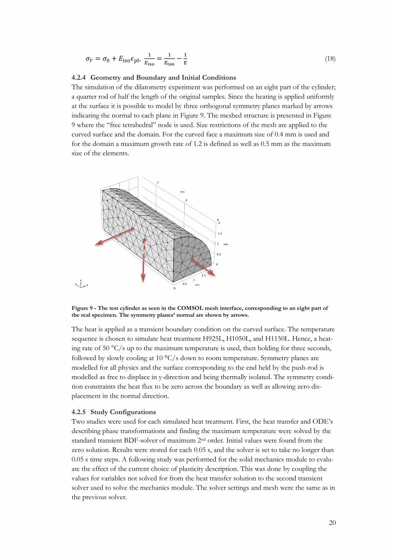
4.2.4 Geometry and Boundary and Initial Conditions
The simulation of the dilatometry experiment was performed on an eight part of the cylinder;
a quarter rod of half the length of the original samples. Since the heating is applied uniformly
at the surface it is possible to model by three orthogonal symmetry planes marked by arrows
indicating the normal to each plane in Figure 9. The meshed structure is presented in Figure
9 where the “free tetrahedral” node is used. Size restrictions of the mesh are applied to the
curved surface and the domain. For the curved face a maximum size of 0.4 mm is used and
for the domain a maximum growth rate of 1.2 is defined as well as 0.5 mm as the maximum
size of the elements.
Figure 9 - The test cylinder as seen in the COMSOL mesh interface, corresponding to an eight part of
the real specimen. The symmetry planes’ normal are shown by arrows.
The heat is applied as a transient boundary condition on the curved surface. The temperature
sequence is chosen to simulate heat treatment H925L, H1050L, and H1150L. Hence, a heat-
ing rate of 50 °C/s up to the maximum temperature is used, then holding for three seconds,
followed by slowly cooling at 10 °C/s down to room temperature. Symmetry planes are
modelled for all physics and the surface corresponding to the end held by the push-rod is
modelled as free to displace in y-direction and being thermally isolated. The symmetry condi-
tion constraints the heat flux to be zero across the boundary as well as allowing zero dis-
placement in the normal direction.
4.2.5 Study Configurations
Two studies were used for each simulated heat treatment. First, the heat transfer and ODE’s
describing phase transformations and finding the maximum temperature were solved by the
standard transient BDF-solver of maximum 2nd order. Initial values were found from the
zero solution. Results were stored for each 0.05 s, and the solver is set to take no longer than
0.05 s time steps. A following study was performed for the solid mechanics module to evalu-
ate the effect of the current choice of plasticity description. This was done by coupling the
values for variables not solved for from the heat transfer solution to the second transient
solver used to solve the mechanics module. The solver settings and mesh were the same as in
the previous solver.

21
5 Results The results are presented in three sections. First, the strain-temperature diagrams from the
dilatometry will be presented. To supplement the dilatometry results, the hardness values and
corresponding microstructures are shown in the following section. The information gathered
from the first sections used for the simulations and the results from FE-model made in
COMSOL Multiphysics can be seen in the final section of this chapter.
5.1 Dilatometry
The samples P3-P8, A1-A12, and B1-B3, are presented in groups of the maximum tempera-
ture for the specimens. Additionally, graphs of the slowly heated samples P1 and P2 are
shown separately. The typical heating scheme is seen in Figure 10 showing the Temperature-
Time curve for the samples heated to 1150 °C. Difficulties in adjusting for the latent heat
released during the transformation at low temperatures were explained by KIMAB as the
reason for the non-linear behavior below 200 °C. The Temperature-Strain raw data is shown
in the following graphs, Figure 11-16. The arrows indicate the direction of the temperature
change.
Figure 10 - Time-Temperature curve for the samples heated to 1150°C. Curves with the same heating and cooling rates overlap.

22
Figure 11 - Temperature-Strain curve for the samples heated to 900 °C.
Figure 12 - Temperature-Strain curve for the samples heated to 925 °C.

23
Figure 13 - Temperature-Strain curve for the slowly heated samples to 1000 °C.
Figure 14 - Temperature-Strain curve for the samples heated to 1000 °C.
24
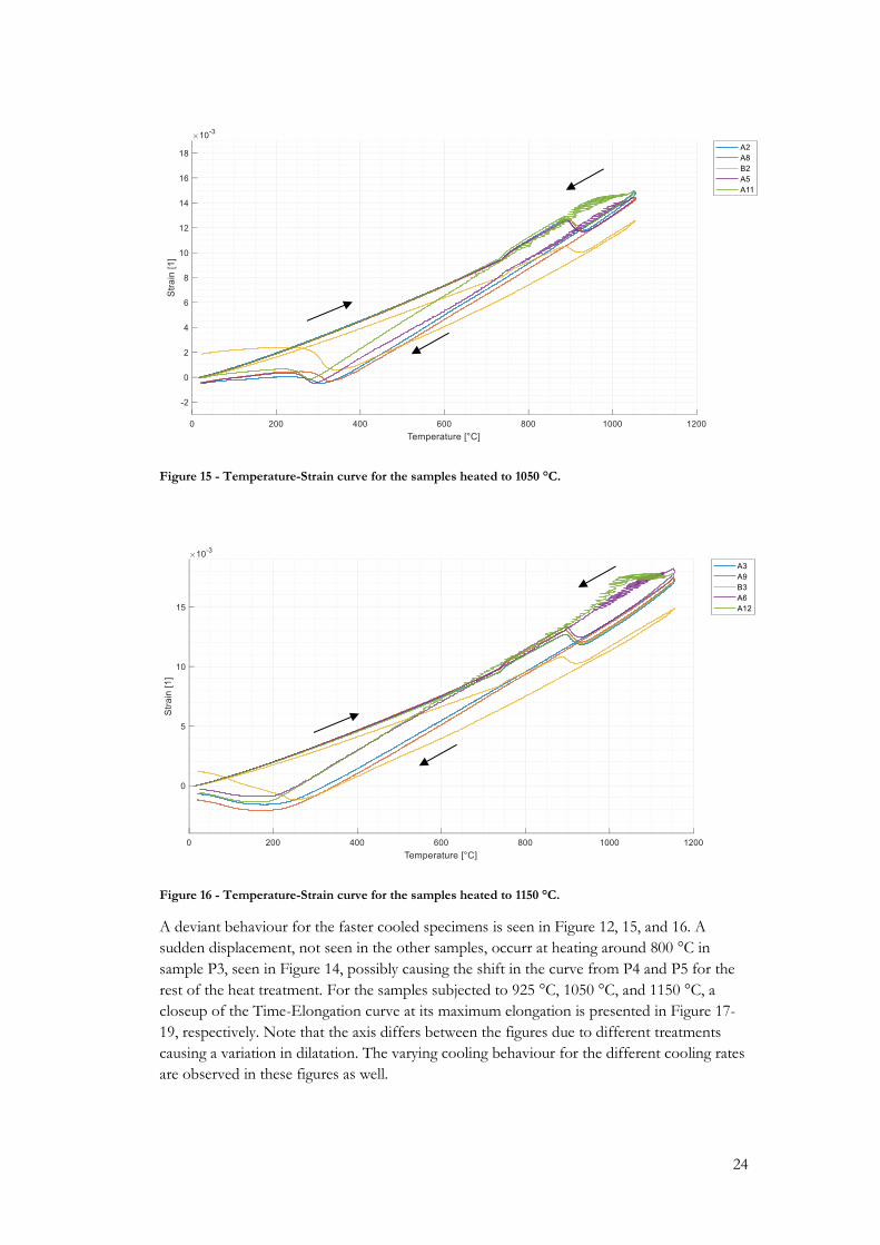
Figure 15 - Temperature-Strain curve for the samples heated to 1050 °C.
Figure 16 - Temperature-Strain curve for the samples heated to 1150 °C.
A deviant behaviour for the faster cooled specimens is seen in Figure 12, 15, and 16. A
sudden displacement, not seen in the other samples, occurr at heating around 800 °C in
sample P3, seen in Figure 14, possibly causing the shift in the curve from P4 and P5 for the
rest of the heat treatment. For the samples subjected to 925 °C, 1050 °C, and 1150 °C, a
closeup of the Time-Elongation curve at its maximum elongation is presented in Figure 17-
19, respectively. Note that the axis differs between the figures due to different treatments
causing a variation in dilatation. The varying cooling behaviour for the different cooling rates
are observed in these figures as well.

25
Figure 17 - Time-Elongation curve for the samples heated to 925 °C.
Figure 18 - Time-Elongation curve for the samples heated to 1050 °C.
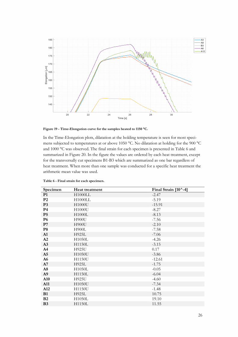
26
Figure 19 - Time-Elongation curve for the samples heated to 1150 °C.
In the Time-Elongation plots, dilatation at the holding temperature is seen for most speci-
mens subjected to temperatures at or above 1050 °C. No dilatation at holding for the 900 °C
and 1000 °C was observed. The final strain for each specimen is presented in Table 6 and
summarized in Figure 20. In the figure the values are ordered by each heat treatment, except
for the transversally cut specimens B1-B3 which are summarized as one bar regardless of
heat treatment. When more than one sample was conducted for a specific heat treatment the
arithmetic mean value was used.
Table 6 - Final strain for each specimen.
Specimen Heat treatment Final Strain [10^-4]
P1 H1000LL -2.47 P2 H1000LL -5.19 P3 H1000U -15.91 P4 H1000U -8.27 P5 H1000L -8.13 P6 H900U -7.56 P7 H900U -2.10 P8 H900L -7.58 A1 H925L -7.06 A2 H1050L -4.26 A3 H1150L -3.15 A4 H925U 0.17 A5 H1050U -3.86 A6 H1150U -12.61 A7 H925L -1.75 A8 H1050L -0.05 A9 H1150L -6.04 A10 H925U -4.60 A11 H1050U -7.34 A12 H1150U -1.48 B1 H925L 10.75 B2 H1050L 19.10 B3 H1150L 11.55

27
Figure 20 - Mean final strain values for all heating schemes. Suffix L denotes the slower cooling rate and U the faster. B is the mean value for B1-B3.
Other phenomena observable by dilatometry is phase transformations. The HCCI goes
through several transformations during thermal cycling through the temperatures chosen in
this study. This is seen in the Temperature-Strain plots above; however, it is sometimes more
clearly seen by the derivative of the Temperature-Strain curve or by the Temperature-Power
plot corresponding to the power needed to hold the specimen at constant heating and cool-
ing. Two typical Temperature-Power plots are seen in Figure 21 and 22, where the arrows
indicate the direction of temperature change. For A3, which shows representative results for
all A- and B-specimens, a change in the curve at around 740 °C and 900 °C upon heating and
200 °C during cooling is clearly visible in both dilatation and power as plotted in Figure 21.
For the slowly heated sample, P1, another change around 550 °C that is not detectable in the
strain curve is visible. The Temperature-Strain derivative looks different for each specimen;
however, the overall behaviour is similar. An example of these curves is seen in Figure 23
where the critical temperature evaluation points are included. No difference between the
plotted elongation data is seen, however some differences can be noted at the different
methods used for the differentiation. Though, if the data was not smoothed there was a ma-
jor increase of noise in the derivative curve, hence not depicted.
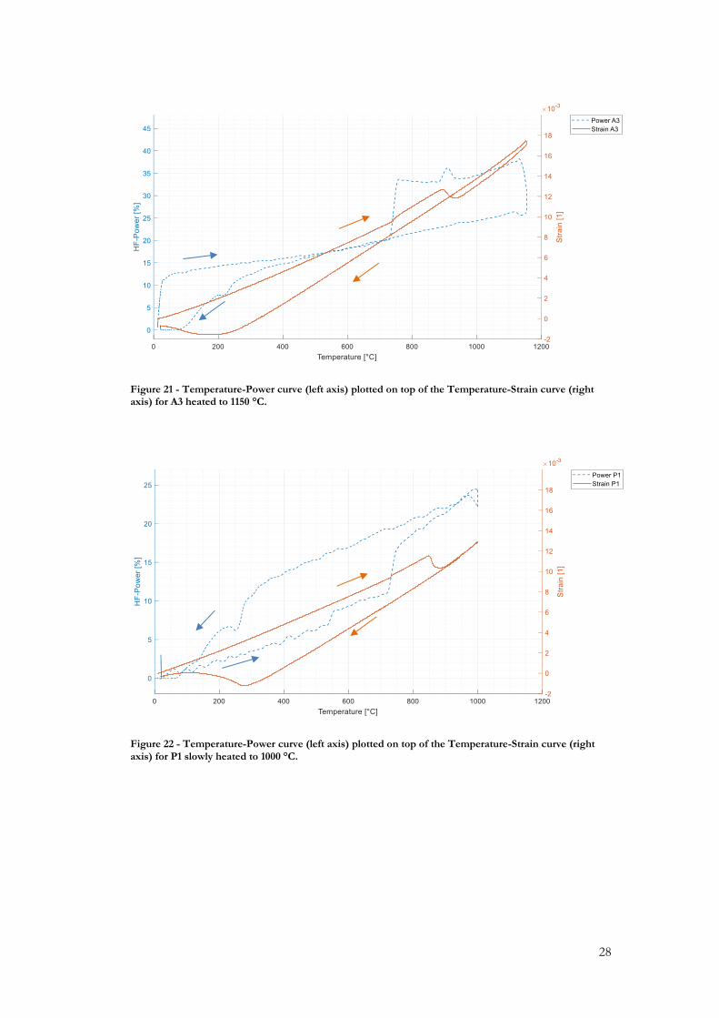
28
Figure 21 - Temperature-Power curve (left axis) plotted on top of the Temperature-Strain curve (right axis) for A3 heated to 1150 °C.
Figure 22 - Temperature-Power curve (left axis) plotted on top of the Temperature-Strain curve (right
axis) for P1 slowly heated to 1000 °C.

29
Figure 23 - Elongation of A2 plotted on the left axis with smoothed and original derivative plotted on the right axis. Heating sequence is seen to the left and cooling on the right hand side. Arrows indicate direction of temperature change (black) and direction of differentiation (red). The dashed arrows connect the denotation of each transformation to the point seen marked on the derivative curve.
Generally, two Ms (Ms1 and Ms2) temperatures were detected by this method and it was seen
that the Ms temperature roughly estimated by the conductor of the dilatometry was almost
consistently in between of these two values. All averaged critical temperatures for the differ-
ent heat treatment schemes are presented in Table 7.
Table 7 - Critical temperatures observed by each heat treatment. Mean values for P-samples, A- and B-samples, and all samples are presented in the bottom rows. Subscript s indicates the start temperature of transformation and f the end (finish) temperature. K is the martensite transformation temperatures de-
termined by the conductor of the dilatometry. N/A indicates no available data.
Heat treatment Tcs Tcf Tγs Tγf Ms1 Ms2 MsK Mf MfK
0900L 718 781 881 -- 395 388 386 247 266
0900U 719 771 837 -- 401 373 385 195 262
0925L 734 780 879 -- 459 428 444 269 276
0925U 723 777 871 -- 395 376 376 216 240
1000L 721 779 883 992 386 358 351 169 222
1000LL 722 745 842 910 331 304 N/A 40 N/A
1000U 724 780 887 992 363 345 349 217 227
1050L 733 777 879 965 390 352 355 178 189
1050U 725 778 875 965 325 302 300 164 187
1150L 731 780 880 963 290 251 272 N/A N/A
1150U 724 779 880 979 252 214 212 N/A N/A
Mean P 721 777 869 992
Mean A+B 729 778 878 967
Mean Total 726 778 875 973
Stddev. Total 6 7 20 12
Tcf
Tcs
Tγs
Tγf
Mf
Ms2
Ms1
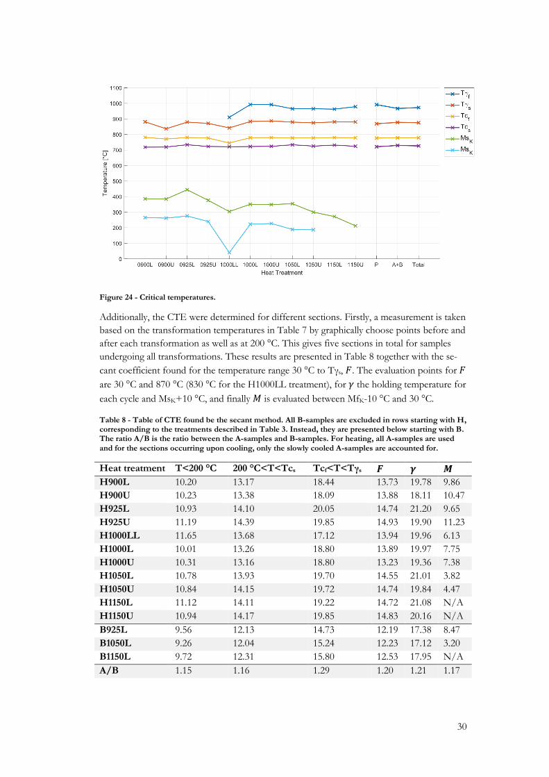
30
Figure 24 - Critical temperatures.
Additionally, the CTE were determined for different sections. Firstly, a measurement is taken
based on the transformation temperatures in Table 7 by graphically choose points before and
after each transformation as well as at 200 °C. This gives five sections in total for samples
undergoing all transformations. These results are presented in Table 8 together with the se-
cant coefficient found for the temperature range 30 °C to Tγs, 𝐹. The evaluation points for 𝐹
are 30 °C and 870 °C (830 °C for the H1000LL treatment), for 𝛾 the holding temperature for
each cycle and MsK+10 °C, and finally 𝑀 is evaluated between MfK-10 °C and 30 °C.
Table 8 - Table of CTE found be the secant method. All B-samples are excluded in rows starting with H, corresponding to the treatments described in Table 3. Instead, they are presented below starting with B. The ratio A/B is the ratio between the A-samples and B-samples. For heating, all A-samples are used
and for the sections occurring upon cooling, only the slowly cooled A-samples are accounted for.
Heat treatment T<200 °C 200 °C<T<Tcs Tcf<T<Tγs 𝑭 𝜸 𝑴
H900L 10.20 13.17 18.44 13.73 19.78 9.86
H900U 10.23 13.38 18.09 13.88 18.11 10.47
H925L 10.93 14.10 20.05 14.74 21.20 9.65
H925U 11.19 14.39 19.85 14.93 19.90 11.23
H1000LL 11.65 13.68 17.12 13.94 19.96 6.13
H1000L 10.01 13.26 18.80 13.89 19.97 7.75
H1000U 10.31 13.16 18.80 13.23 19.36 7.38
H1050L 10.78 13.93 19.70 14.55 21.01 3.82
H1050U 10.84 14.15 19.72 14.74 19.84 4.47
H1150L 11.12 14.11 19.22 14.72 21.08 N/A
H1150U 10.94 14.17 19.85 14.83 20.16 N/A
B925L 9.56 12.13 14.73 12.19 17.38 8.47
B1050L 9.26 12.04 15.24 12.23 17.12 3.20
B1150L 9.72 12.31 15.80 12.53 17.95 N/A
A/B 1.15 1.16 1.29 1.20 1.21 1.17

31
5.2 Material Characterization
Through the use of LOM the morphology of the dendritic structure is revealed. Images of
the material before dilatometry are seen in Figure 25 and 26 while Figure 27-34 shows sec-
tions of the specimens after dilatometry at 100x and 1000x magnification, respectively. Some
of the samples in those figures are also shown in Figure 35-36 where the etching time is
shorter. The P-samples showed about 33-48 % primary crystals (𝛾-dendrites) when estimated
by point counting while the A-samples show roughly 33-40 %. In Figure 25 and Figure 27-
30, a difference in the eutectic structure is seen between the samples taken in different direc-
tions. For some figures the structures are marked with numbers. ○1 indicates the (former) 𝛾-
dendrites, ○2 and ○3 different eutectics, ○4 and ○5 the eutectic carbides and 𝛾 respectively,
○6 the secondary carbides, and ○7 structures within the previous 𝛾 after heat treatment. Fur-
ther analysis and discussion regarding the structures are found in chapter 6.2.
Figure 25 - 100x magnification untreated samples marked with direction and sample denotation.
1
2
2
1
2
z
3

32
Figure 26 - 1000x magnification Untreated samples
4
1
4
5

33
Figure 27 - 100x magnification P-samples.

34
Figure 28 - 100x magnification A1-A6.
2
z
3
z
1
z
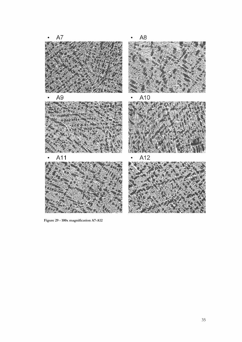
35
Figure 29 - 100x magnification A7-A12

36
Figure 30 - 100x magnification B1-B3
3
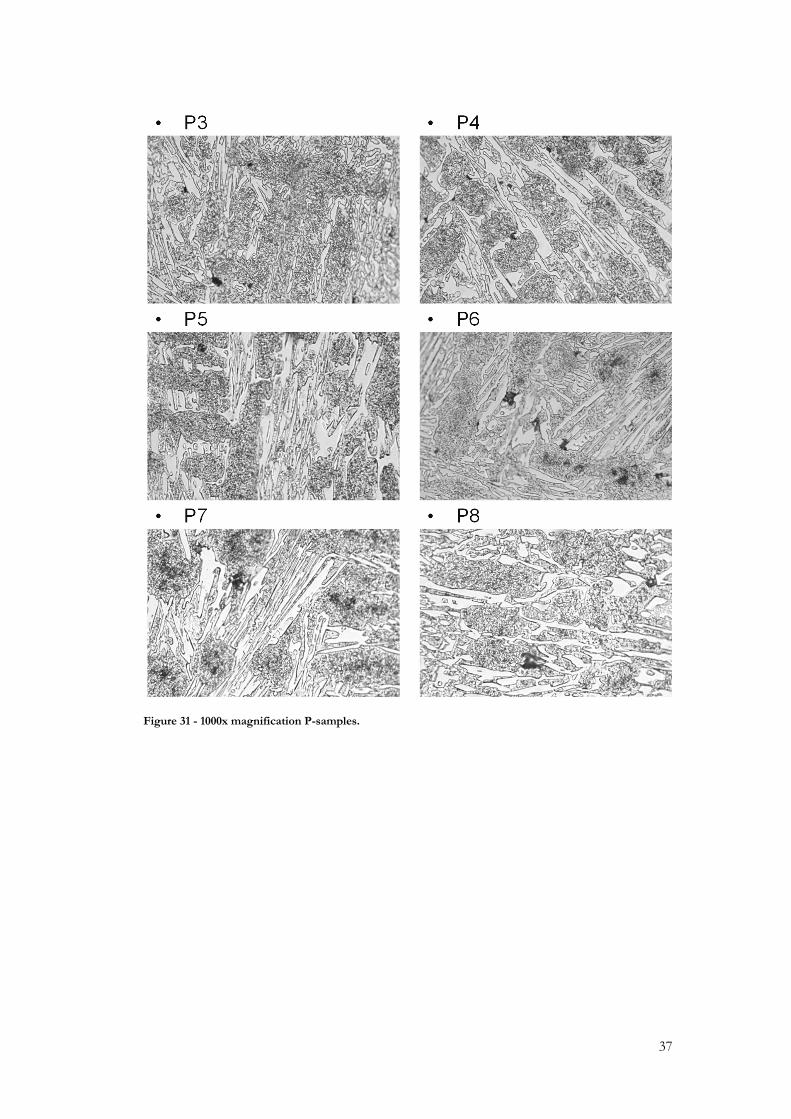
37
Figure 31 - 1000x magnification P-samples.

38
Figure 32 - 1000x magnification A1-A6

39
Figure 33 - 1000x magnification A7-A12

40
Figure 34 - 1000x magnification B1-B3

41
Figure 35 - 1000x magnification for samples etched for shorter time.
1 4
5

42
Figure 36 - 1000x magnification of A10 and A12. The image is taken by cropping the original frame taken
at 1000x magnification.
Hardness measurements are presented in Figure 37 and 38. Figure 37 shows mean HRC val-
ues for each specimen whereas in Figure 38 the values were also averaged for each heat
treatment. It should be noted that for sample P3-P8 the values varied from the measure-
ments taken in the center of the cylinder and those taken closer to the edge where the values
away from the center were higher. Two measurements were taken away from the center,
causing a shift in the mean hardness towards higher values. The difference for P3-P5 was
1 6
7

43
between 14-27 HRC within a sample and between 2-6 HRC in P6-P8 while 0-3 HRC in all
other samples.
Figure 37 - Hardness Rockwell C measured for each specimen.
Figure 38 - Hardness Rockwell C averaged for each heat treatment separated by the cooling rate.
5.3 Simulations and Modelling
For the COMSOL simulations average values of CTEs for 𝐹, 𝛾, and 𝑀 were used, based on
values found in Table 8. The strain behavior appeared nearly identical for the average thermal
strain in the volume and for the strain calculated by the displacement in y-direction divided
by the original length. When the plasticity mode was turned off, these two methods showed
the exact same pattern. This indicates that some plastic deformation occurred. This is detect-
ed in the 𝐹 → 𝛾 transition and can be seen in Figure 40. The temperature in the core and on
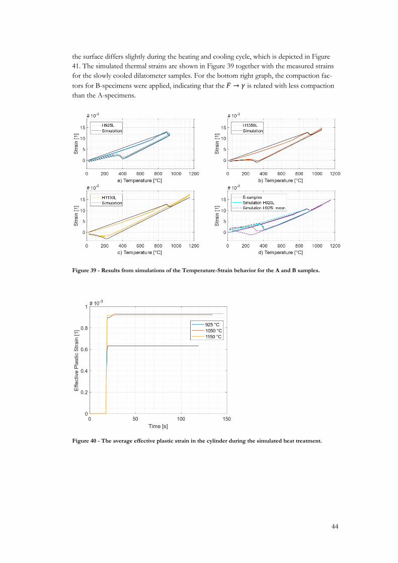
44
the surface differs slightly during the heating and cooling cycle, which is depicted in Figure
41. The simulated thermal strains are shown in Figure 39 together with the measured strains
for the slowly cooled dilatometer samples. For the bottom right graph, the compaction fac-
tors for B-specimens were applied, indicating that the 𝐹 → 𝛾 is related with less compaction
than the A-specimens.
Figure 39 - Results from simulations of the Temperature-Strain behavior for the A and B samples.
Figure 40 - The average effective plastic strain in the cylinder during the simulated heat treatment.
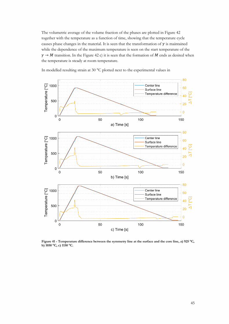
45
The volumetric average of the volume fraction of the phases are plotted in Figure 42
together with the temperature as a function of time, showing that the temperature cycle
causes phase changes in the material. It is seen that the transformation of 𝛾 is maintained
while the dependence of the maximum temperature is seen on the start temperature of the
𝛾 → 𝑀 transition. In the Figure 42 c) it is seen that the formation of 𝑀 ends as desired when
the temperature is steady at room temperature.
In modelled resulting strain at 30 °C plotted next to the experimental values in
Figure 41 - Temperature difference between the symmetry line at the surface and the core line, a) 925 °C, b) 1050 °C, c) 1150 °C.
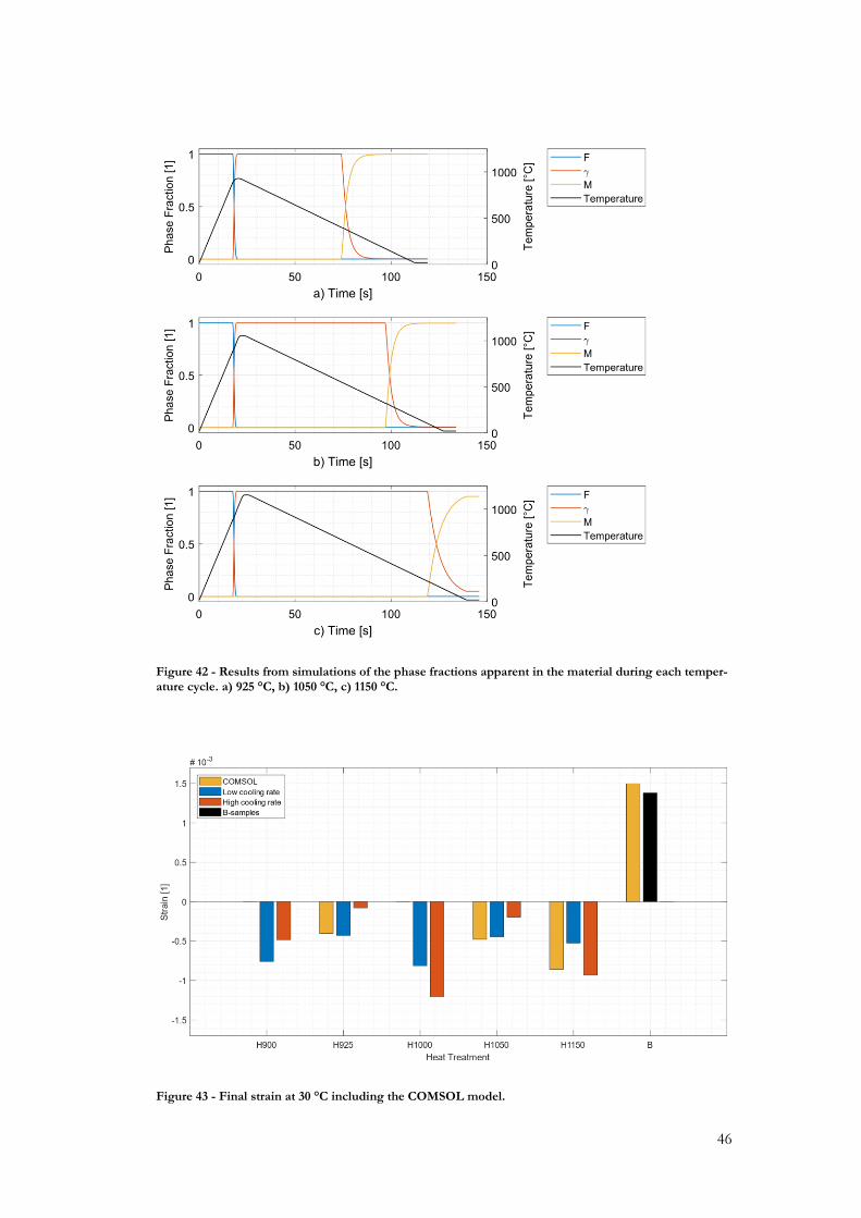
46
Figure 42 - Results from simulations of the phase fractions apparent in the material during each temper-
ature cycle. a) 925 °C, b) 1050 °C, c) 1150 °C.
Figure 43 - Final strain at 30 °C including the COMSOL model.

47
6 Discussion In this chapter the two main experimental parts are discussed in the light of the respective
results and what can be found in literature followed by a brief discussion regarding the results
and methods used for the FEM-implementation. A setup using ingots cast in a laboratory
furnace as is commonly seen in literature would be aimed at, but limitations did not allow for
such setup. Instead, the cutout material had to be used. This means less control of factors
such as composition, casting defects and structure, previous heat treatments, and the homo-
geneity of the material among the different samples. This, in turn, makes it more difficult to
replicate the results but might increase the external validity of the experiments for this mate-
rial, i.e. it is easier to connect the results from this study to the actual performance of the
material in application. However, the experiments performed are conducted in such a way
that given the same original material it should be possible to reproduce the results. The use
of two specimens undergoing the same heat treatment does not act as reproduction but may
indicate the minimum level of uncertainty within the material or experimental setup. Consid-
ering all results presented earlier it should once again be noted that the evaluated material is
treated in two different dilatometry studies. This might cause some differences between the
heat treatments that could be confused with differences in the material or heat treatments
between P and A/B denoted samples.
6.1 Dilatometry
As mentioned previously, the dilatometer curve denotation will be described as for regular
steels. The curves show several interesting features. For all specimens the start material, F, is
expanding almost linearly up until Tc, although not fully linear as seen in the different CTE
found for the section below and above 200 °C in Table 8. The following change in power
needed to maintain the steady heating (Figure 21) indicates the change of magnetic proper-
ties. This is expected for ferrite which should be one major phase apparent in the cold phase
state since the thermal history shown in Figure 6 is applied to soft anneal the material by
transforming any martensite and retained austenite found in the as-cast material to soft ferrite
and ferrite+carbide structures as described in chapter 2.1 [15, 74]. Using the proposed equa-
tion (3) in section 3.1 gives a value of Tc at 763 °C which is higher than the found values in
Table 7 where the mean value is found to be 726 °C. As Belyakova et al. [49] reports, the
Chromium is likely to decrease Tc. This transformation does not seem to be affected by the
heating rate. The maintained and clearly detected volume expansion did, however, surprise
the experimenter at Swerea KIMAB and Xylem’s contact at EFD Induction who had per-
formed several dilatometry experiments on other materials to get data for simulations before.
Swerea states that it normally shows as a small “bump” and then goes back to the original
path; this behavior is seen in [55]. A similar behavior in a material containing 24% Cr and
0.79% C has been found in literature; however, at a lower temperature [9]. In reference [13]
and [54] the authors point out that this additional strain detected at the Curie transformation
could be avoided by using conductive heating instead of induction [13, 54]. The Curie tem-
perature is interesting from a production perspective where the power is controlled by the
operator and it might be valuable to be aware of and account for the magnetic permeability
change at this temperature range.
Upon further heating after the Curie transformation the characteristic compaction is likely
related to the austenite transformation which has a denser structure compared to the cold
phases [56, 66, 75]. It is seen that for heat treatments below 925 °C the transformation is not
48
complete. It is important to recall that the austenite transformation is a diffusion-based trans-
formation and therefore both time and temperature dependent [16]. Hence, some cold phase
will probably still be present during the subsequent cooling for some samples since the hold-
ing time is short. The time dependence is detected in the drastically lower transformation
temperature seen in the slowly heated samples that should be closer to the equilibrium state.
Another diffusion-based transformation is seen for the higher temperature range for the
samples hold for 3 seconds where some elongation changes are detected during the holding
at constant temperature, see Figure 18 and 19. This is likely to be an effect of diffusion pro-
cesses in the material causing the material to expand. The process causing this is not possible
to determine based on these figures alone since both precipitation and dissolution of carbides
and changed carbon content in the matrix will lead to volumetric change. The effect of this
expansion is seen in Figure 16 as well were the cooling curve is displaced in positive direction
from the heating of 𝛾 following the end of 𝐹 → 𝛾 transformation.
The final transformation detected follows the cooling below approximately 400-200 °C, de-
pending on the maximum temperature in each cycle. In literature this is treated as the mar-
tensite transformation which is closely connected to the expansion seen in all dilatometer
curves in section 5.1 [29, 56, 60, 61]. There is a change in slope of the cooling curve before
the expansion is clearly visible, causing problems in determining the actual start temperature
of the transformation, Ms, as described in connection to Figure 23. Even though the trans-
formation seems to be fulfilled it should be remembered that it is the strain that is detected
through dilatometry and phase transformations are interpretations of the strain behavior.
This is important since uneven distribution of alloys, especially C, following segregations
during casting and precipitation and dissolution of carbides can cause different martensite
start and finish temperatures [29].
Upon further cooling room temperature is reached. No connection between maximum tem-
perature and final strain were found, therefore it could be possible that the two different
hypotheses are valid and no differences between the many heat treatments arise. For further
material characterization not focusing on the expansion of the material it is possible that
cooling curve analysis is more suitable due to its much simpler setup. Cooling curve analysis
has been used to characterize the transformation temperatures and describe the kinetics of
phase transformation successfully in reference [51] as an alternative to dilatometry. Differen-
tial scanning calorimetry has been used as another option to detect transformation tempera-
tures for the martensite phase [38]. This method could also be used to detect further trans-
formation below room temperature as well as the enthalpy of transformations [38].
The final property found in the dilatometry study was the apparent directionality in the mate-
rial. The final elongations seen in the dilatometry curves for the B-samples, and in the sum-
mation in Figure 20, depict that the material shrink slightly for all A- and P-specimen but
expands for the samples taken in the orthogonal direction. The reason for this were not fully
determined in this study; however, the microstructural differences are discussed in the fol-
lowing section and as mentioned earlier the anisotropy of the material and the carbides have
great impact on other mechanical properties. For the samples taken in the Iso direction, the
CTE of 𝐹, 𝛾, and 𝑀 presented in Table 8 are showing similarities with those found in litera-
ture [61] and only subtle differences were detected between the different heating and cooling
rates. The martensite expansion was, however, drastically lowered with increasing maximum
temperature. The same relation was seen for both A- and B-samples. Furthermore, it was
49
seen that the ratio of secant expansion coefficient for the slowly cooled A-samples and B-
specimens were constant at 1.15-1.29 for all sections.
Other phenomena that need to be addressed are the difference seen between the curves and
the fluctuations found in the cooling stage, especially evident for the 50 °C/s cooling rates in
Figure 12, 15 and 16. This is explained by KIMAB as an effect of the cooling rate and possi-
bly uneven temperature distribution within the sample. At this rate (50 °C/s) a larger valve
had to be used for the coolant which decreased the control of the temperature and the cyclic
behavior is seen in the time-temperature curves in section 5.1. This was not as severe in the
samples cooled at higher cooling rates (100 °C/s) where the risk of unevenly distributed
temperature in the sample should be higher. This could mean that cooling rates of approxi-
mately 50 °C/s are recommended to avoid in future dilatometry analysis with this dilatometer
and material.
6.2 Material Characterization
It is important to point out that results from the material characterization are dependent on
the instruments utilized and to some extent the knowledge and experience of the person
conducting and evaluating the experiments. Further information could certainly have been
produced from the tested material if it were tested in more advanced instruments, such as
SEM, XRD-analysis and micro-hardness. As Maratray and Usseglio-Nanot [30] show, the
structures can easily be confused, and the interpretation is strongly dependent on the prepa-
ration of the samples, especially the etching. Here the characterization was limited to LOM
and interpretation of results from previous research.
Though, the overall structure was possible to determine by LOM. The amount of primary
crystals, 𝛾-dendrites, found is in good correspondence to previously presented results for a
similar alloy, with a carbon content of 2.26% [25]. Since the measurement taken on this alloy
was taken prior to casting it is possible that some slight decarburization occurred before the
melt was cast, leading to a more hypoeutectic material. The difference in amount of primary
crystals indicates a slight variance in composition that could be a factor to the different CTE
and transformation temperatures found.
With the dilatometry study some additional knowledge is gained that could be used in deter-
mining the phases. The temperature history of the material (Figure 6) corresponds to soft
annealing procedures discussed in section 2.1. The structures seen in the untreated samples
in Figure 25 and 26Figure 26 possibly show secondary carbides ○6 precipitated during the
annealing in a mostly ferritic matrix in the dendrites ○1 and eutectic structures. The precipi-
tated carbides could have been spherodized and coalescence might have occurred due to the
long holding time; however, this is not possible to determine based on this LOM evaluation.
In the untreated samples some eutectoid ferrite+carbide structures might be present. In [21,
76] the authors interpreted similar structures as marked as ○3 as the eutectoid structure. They
did raise some doubts regarding this and stated that it could be the different eutectic struc-
ture as described by other authors (see section 2.1) instead of the plate/bar like structure that
is seen in the rest of the material ○2 . Overall, the plate/od eutectic is not seen in B-samples,
instead the cross section reveals what looks like isolated carbides particles and structure ○3 ,
possibly explained as the cross section of the carbide rods. The presence of ferrite is sup-
ported by the compaction at around 890 °C indicating the formation of a denser structure,
austenite.

50
During soaking at the higher temperature some elongation was detected as discussed in the
previous section. From Figure 35 and 36, showing areas of primary and eutectic structures in
high magnification of the rapidly cooled A-samples it is qualitatively seen that some dissolu-
tion of carbides must have occurred. This would lead to the austenite near the carbides get-
ting higher content of possibly both Cr and C, the latter leading to lower Ms. The isothermal
section by Bungardt [45] seen in [16] and Figure 3 and 4Figure 4 show the increased solubili-
ty of Cr and C in 𝛾 at 1150 °C compared to 850 °C and 1000 °C. The higher C content is
supported by the lower Ms found in dilatometry, as seen in Table 7 and Figure 24.
The variation in hardness of the samples could be caused by several reasons. Regarding the
difference within a single specimen, this could be derived to inhomogeneous temperature
distribution within the cylinder. The variation was only detected for the previously initiated
samples, P3-P8, where the heating rate was twice the heating rate for the other samples and
the holding time was one instead of two seconds. The high rates and short soaking time
could cause an unevenly distributed heat throughout the cylinder. The distance between two
indentations for one tested specimen is seen Figure 44 and is measured to approximately 2.5
times the diameter of indentation. According to the least conservative of the two sources
cited in the literature section, the minimum distance should at least be three impression di-
ameters between the indentations which indeed make this a risk of errors for measuring the
hardness outside of the center of the specimen [46]. Since the variation in hardness was that
seen especially for most of P3-P8, it is not likely that it was caused by the buildup of strains
from the previous indentations. If that would have been the main reason it could be expected
to show on all samples, regardless of heat treatment. The reason for the exceptionally high
hardness in P6 could not be explained.
Figure 44 - Two indentations in the material subjected to hardness test. The distance from center to center is marked by arrows corresponding to the diameter of the top indentation.
Another noticeable result from the hardness measurements is the correlation with tempera-
ture. A distinct difference was detected between the untreated and heat treated A and B sam-
ples. The discussed maximum of hardness at around 1050 °C [29] is not seen in this study.
Holding times found in literature are considerably longer and the effect of the thermal histo-
ry must be regarded when comparing the results to other findings. Results from the dilatom-
etry points toward readily lower martensite content in the samples treated at 1150 °C which
likely would cause the bulk hardness of the material to be lower than if the martensitic trans-
formation had been fully carried through. It was not possible to confirm the lower martensite
content and possibly retained austenite by metallography and it has been stated as a difficulty

51
in literature as well [32]. As mentioned in chapter 2.1 though, Maratray et al. [29] found that
the maximum hardness is related to austenite content about 20%. The martensite expands
more when the material have been destabilized at higher temperatures and the hardness of
carbon rich martensite, i.e. formed from austenite destabilized at high temperatures, is harder
than martensite of lower carbon content even though some austenite might be retained at
room temperature [30].
A contributing factor causing the sample to be harder than expected is that the austenite can
work harden [15]. This could be advantageous from an abrasion perspective as well, since the
highest resistance have been reported for a certain amount of retained austenite as discussed
in chapter 2.1. Strain induced, and stress assisted martensite formation from retained austen-
ite is not likely to happen during preparation, but the effect could still be of interest since it is
possible to increase the fracture toughness and hardness of the material [15, 38].
6.3 Simulations and Modelling
As previously mentioned, it has been the subject of whole theses to work with the implemen-
tation of dilatometry data in FE-models. Limitations made it necessary to consider simple
methods in this study and the equation used for describing the martensite transformation is
limited in its applications. Also, the material data such as high temperature data is limited and
is either assumed to match low alloyed steel as in previous simulations [77] and in this case;
by utilizing data mostly found in figures in papers regarding similar materials, combined with
data for steel. Secondly, HCCI consists of a more complex morphology and composition and
is therefore more demanding to evaluate than a pure Fe-C steel.
It is difficult to accommodate for all varying behaviors at different soaking temperatures,
especially in a way that is consistent with physical and well established mathematical models
that are already shown to accurately represent the actual process. It is also necessary to ad-
dress the differences found within the replicates of each sample. The deviations represent the
variation within the used material, such as compositional segregation and directionality. The
latter was seen in this study to have great impact on the dilatometry results. An attempt on
making the model fit parameters in the slowly cooled A-samples was made. For simulated
H925L and H1050L the strain response is decent, except for the beginning of martensite
transformation in H1050L. The simulated H1150L suffers from the inability to accommo-
date the additional strain at the holding temperature and the difficulties in describing the
martensite transformation. Difficulties in adjusting for the martensite transformation are seen
in literature as well [12, 29]; however, not as extreme as for the samples heated to 1150 °C in
this study. In these dilatometry curves there is a plateau that could not be modelled by the
applied equation, possibly due to the uneven distribution of alloying elements following the
assumed dissolution of carbides at the high temperatures [29].
It was seen that the calculation of strain response instead of direct calculation of thermal
strain did not result in any major differences. The deviation is minor, yet detectable at the
𝐹 → 𝛾 transformation, but still small compared to the variation between the two slowly
cooled dilatometry samples. If thermal or mechanical properties are changed, or temperature
conditions are applied differently this could naturally change this behavior. If the whole do-
main temperature were prescribed, only thermal strain would be present. For slow heating
and cooling rates the maximum temperature difference in a dilatometry sample was estimated
to less than 1 °C by Gibbs et al. [51] and in the literature [61, 66, 78] the simulation of dila-
tometry trials are performed by evaluating the thermal strain only. This assumption would

52
lead to significantly shorter computation times when simulating the response of dilatometer
trials.
Further evaluations of the same material for intermediate temperatures would indicate the
reliability in the use of the applied equations. To use the FE-model for stress analysis, kinet-
ics parameters must be more thoroughly investigated, especially for the martensite transfor-
mation. Also, there are several thermophysical properties that must be investigated to give an
accurate model of the HCCI. The difference in compaction for the 𝐹 → 𝛾 transformation
was accepted as 1.06e-2 as found in the demonstration model [63]. It is seen that the value
corresponds well to the difference in compaction between 𝛼 and 𝛾, mentioned in literature
to be around 1% [79]. Defining the reference state of 𝑍𝑅 in equation (17), as 0.31 results in a
very good fit for the A-samples. Whether this is a coincident is difficult to say, but doubts are
raised since the compaction varies with the direction, as seen in Figure 39 where the dotted
line (H1050L) for the B-samples have the same setting for Δ𝜖𝐹𝛾 and Δ𝜖𝐹𝑀 as for the A-
samples. Nevertheless, the value was found to fit the dilatometry curve for A-samples. The
cyan line (H925L) in the same figure is adjusted and the fit is good for all sections of the
curve.
Difference in composition and phase distribution could explain this. Another possibility,
however, is the carbide directionality leading to a stiffer composite. Figure 45 show the sim-
plified and greatly exaggerated uniform orientation in the test cylinders’ cross sections as
given by the structures from metallography. The brittle and stiff carbide phase can, as de-
scribed in chapter 2.2, act as reinforcement to the matrix of 𝐹 and 𝛾, and given the same
conditions, the B-samples in this case will generally behave stiffer and obtain higher strength
when loaded in the axial direction due to the orientation of the fiber reinforcement [24, 25,
80].
Figure 45 - Schematic and exaggerated representation of carbide orientation in the different samples.
6.4 Future Research
Some areas investigated in this study could be further evaluated. Even though no clear corre-
lation between the maximum temperature and final strain were found, other factors such as
compositional differences and directionality were shown to influence the results. Hence, ma-
terial from experimental casting conditions tested at slower heating and cooling rates than
A and P
Ani
Iso
Ani
Iso
B

53
50 °C/s to avoid unevenly distributed heat, could better show any possible relationship exist-
ing for this alloy. Using the proposed setup, the directionality of the eutectic could be further
evaluated to include three directions and be able to conclude the reason for the different
properties found.
A more comprehensive metallographic evaluation with SEM and/or XRD could more accu-
rately describe the material’s constituents following certain treatments. This would yield bet-
ter knowledge regarding the reason for steadily increased hardness with temperature that
slightly contradicts what has been found in literature [17, 30, 33, 34], and the amount of re-
tained austenite after heat treatments. The presence and effect of strain induced martensite
could be included in such experiments.
The implementation in FE-models was only introduced in this study. The kinetics parameters
must be further evaluated. Another equation describing, or implementation of, the martensite
transformation should be assessed to better describe the kinetics. The model can then be
validated by using several heating and cooling rates in dilatometer experiments of which the
implementation is not yet based on. It is possible that a better fitting could be done with the
already available data by more carefully evaluating different methods of implementation. Fur-
thermore, mechanical and thermophysical data, especially for the high-temperature range, as
well as the effect and parameters describing the transformation induced plasticity must be
evaluated to be able to apply the phase transformation and thermal expansion model to me-
chanical problems.

54
7 Conclusions Dilatometry experiments with different maximum temperatures, heating rates, and cooling
rates were performed on a high chromium cast iron and implementation of the data were
made in COMSOL Multiphysics.
The final strain shows no clear relationship with temperature in this study. The directionality
of this cast material has great impact on the thermal expansion. Specimens from this material
taken in the defined ani-direction expand following heat treatment with a resulting strain
around 1e-3 to 2e-3, while specimens from an orthogonal direction show a final strain
around -0.5e-3 to -1e-3.
The martensite start temperature is decreasing with increasing treatment temperature; from
around 430 °C for maximum 925 °C, to 250 °C for maximum 1150 °C. Some retained aus-
tenite is likely to exist in material treated at 1150 °C. Although, a heat treatment at 1150 °C
for three seconds results in the greatest hardness of 61 HRC. The difference between cooling
rates is generally less than 2 HRC. Therefore, relatively slow cooling rates at 10 °C/s could
be accepted for hardening procedures in practice.
For further evaluations following the experimental setup used in this study, a cooling rate of
50 °C/s should be avoided due to the disturbances in the recorded elongation present at this
cooling rate.
A simplified dilatometry curve can be successfully implemented into a FE-model simulating
the thermal expansion. Problems during the martensite transformation arises, likely partially
due to the absence of a clear martensite start temperature and the difference in thermal ex-
pansion coefficient depending on the maximum temperature.

55
8 Cited Works
[1] Xylem, "Water Solutions > Sweden > Om oss," [Online]. Available:
http://www.xylemwatersolutions.com/scs/sweden/sv-
se/om%20oss/Sidor/default.aspx. [Accessed 11 April 2018].
[2] Xylem, "Water Solutions > Sweden > Produkter/tjänster," [Online]. Available:
http://www.xylemwatersolutions.com/scs/sweden/sv-
se/produkter/Sidor/default.aspx. [Accessed 16 April 2018].
[3] Xylem, "Water Solutions > Sweden > Om oss > Historia," [Online]. Available:
http://www.xylemwatersolutions.com/scs/sweden/sv-
se/om%20oss/historia/Sidor/default.aspx. [Accessed 11 April 2018].
[4] KSB Materials Technology, ”Cast Materials From KSB,” KSB Aktiengesellschaft,
Pegnitz, 2006.
[5] Xylem, "White Paper - Material selection for wastewater pumps," Xylem Inc., 2013.
[6] G. Laird, R. Gundlach and K. Röhrig, Abrasion-Resistant Cast Iron Handbook, K. E.
Frink, Ed., Des Plaines: American Foundry Society, 2000, pp. 6-7.
[7] L. Markegård and H. Kristoffersen, "Optimized Properties of Car Components - an
Explanation of How Residual Stress is created during Surface Hardening," in Swedish
Suppliers of Heat Treatment Equipment Conference, Eskilstuna, 13-14 September, 2007.
[8] Swerea KIMAB, ”Dilatometry on high C and Cr steel [Internal report],” Stockholm,
2018.
[9] K. Wiczerzak, P. Bala, R. Dziurka, T. Tokarski, G. Cios, T. Koziel and L. Gondek, "The
effect of temperature on the evolution of eutectic carbides and M7C3 -> M23C6
carbides reaction in the rapidly solidified Fe-Cr-C alloy," Journal of Alloyes and Compounds,
vol. 698, pp. 673-684, 2017.
[10] T. G. Oakwood, ”Nomenclature, Definitions and Terms For Use in Reporting Steel
Transformation Data - A Literature Review and Recommendations,” U.S. Department
of Energy Office of Scientific and Technical Information, 2001.
[11] W. Buck and S. Rudtsch, "8.3 Thermal Expansion and Thermomechanical Analysis," in
Springer Handbook of Materials Measurement Methods, H. Czichos, T. Saito and L. Smith,
Eds., 2006, pp. 415-417.
[12] B. Ferguson, Z. Li and A. Freborg, "Modeling heat treatment of steel parts,"
Computational Materials Science, vol. 34, no. 3, pp. 274-281, 2005.
[13] M. Schwenk, J. Hoffmeister and V. Schulze, "Experimental Determination of Process
Parameters and Material Data for Numerical Modeling of Induction Hardening," Journal
56
of Materials Engineering and Performance, vol. 22, no. 7, pp. 1861-1870, 2013.
[14] H.-S. Yang and H. Bhadeshia, “Uncertainties in dilatometric determination of marteniste
start temperature,” Materials Science and Technology, vol. 23, no. 5, pp. 556-560, 2007.
[15] C. Walton, Ed., “White and High Alloy Irons,” in Iron Castings Handbook, Iron Castings
Society, Inc., 1981, pp. 441-461.
[16] H. Fredriksson and B. Remaeus, “Stelnings- och omvandlingsförlopp i vita gjutjärn med
hög kromhalt [Swedish],” Gjuteriet, Vols. 7-8, pp. 7-19, 1976.
[17] S. Zhou, Y. Shen, H. Zhang and D. Chen, "Heat Treatment Effect on Microstructure,
Hardness and Wear Reistance of Cr26 White Cast Iron," Chinese Journal of Mechanical
Engineering, vol. 28, no. 1, pp. 140-147, 2015.
[18] A. Bedolla-Jacuinde, L. Arias and B. Hernández, "Kinetics of Secondary Carbides
Precipitation in a High-Chromium White Iron," Journal of Materials Engineering and
Performance, vol. 12, no. 4, pp. 371-382, 2003.
[19] SIS, Swedish Standards Institute, "Standard - Swedish Standard - SIS 140466," [Online].
Available: https://www.sis.se/en/produkter/metallurgy/ferrous-
metals/irons/sis140466/. [Accessed 16 March 2018].
[20] G. Laird, R. Gundlach and K. Röhrig, Abrasion-Resistant Cast Iron Handbook, K. E.
Frink, Ed., Des Plaines: American Foundry Society, 2000, pp. 198,201.
[21] A. Karantzalis, A. Lekatou and H. Mavros, "Microstructure and properties of high
chromium cast irons: effect of heat treatments and alloying additions," International
Journal of Cast Metals Research, vol. 22, no. 6, pp. 448-456, 2009.
[22] A. Wiengmoon, T. Chairuangsri and J. T. Pearce, "Effects of Destabilisation Heat
Treatment on Microstructure, Hardness and Corrosion Behaviour of 18wt.%Cr Cast
Irons," Key Engineering Materials, vol. 658, pp. 76-80, 2015.
[23] V. Efremenko, K. Shimizu and Y. Chabak, "Effect of Destabilizing Heat Treatment on
Solid-State Phase Transformation in High-Chromium Cast Irons," Metallurgical and
Materials Transactions A: Physical Metallurgy and Materials Science, vol. 44, no. 12, pp. 5434-
5446, 2013.
[24] L. Lu, H. Soda and A. McLean, "Microstructure and mechanical properties of Fe-Cr-C
eutectic composites," Materials Science and Engineering A, vol. 347, pp. 214-222, 2003.
[25] C. Liu, S. Goto, S. Aso and Y. Komatsu, "Mechanical Properties of Chromium White
Cast Irons at High Temperatures," Int. J. of The Soc. of Mat. Eng. for Resources, vol. 7, no. 2,
pp. 350-358, 1999.

57
[26] P. Gudmundson, "7.4 Yield Critearia for Anisotropic Materials," in Material Mechanics,
Stockholm, Department of Solid Mechanics, KTH Engineering Sciences, 2006, pp. 95-
100.
[27] I. Sare and R. Arnold, "The influence of heat treatment on the high-stress abrasion
resistance and fracture toughness of alloy white cast irons," Metallurgical and Materials
Transactions A, vol. 26, no. 7, pp. 1785-1793, 1995.
[28] C. Tabrett and I. Sare, "The effect of heat treatment on the abrasion resistance of alloy
white irons," Wear, Vols. 203-204, pp. 206-219, 1997.
[29] F. Maratray and A. Poulalion, "Austenite Retention in High-Chromium White Irons,"
Transactions of the American Foundrymen's Society (AFS Trans.), vol. 90, pp. 795-804, 1982.
[30] F. Maratray and R. Usseglio-Nanot, Factors Affecting the Structure of Chromium and
Chromium-Molybdenum White Irons, Paris: Climax Molybdenum S.A., 1971.
[31] C. P. Tabrett and I. R. Sare, "Fracture toughness of high-chromium white irons:
Influence of cast structure," Journal of Materials Science, vol. 35, pp. 2069-2077, 2000.
[32] G. Laird, R. Gundlach and K. Röhrig, "Chapter 3. Heat Treatment of AR Cast Irons," in
Abrasion-Resistant Cast Iron Handbook, K. E. Frink, Ed., Des Plaines, American Foundry
Society, 2000, pp. 39-53.
[33] Maratray, F.; Climax Molybdenum S.A., "Choice of Appropriate Compositions for
Chromium-Molybdenum White Irons," Transactions of the American Foundrymen's Society
(AFS Trans.), vol. 79, pp. 121-124, 1971.
[34] N. Poolthong, H. Nomura and M. Takita, "Effect of heat treatment on microstructure,
wear properties and corrosion characteristics of semi-solid processed high chromium
cast iron," International Journal of Cast Metals Research, vol. 16, no. 6, pp. 573-578, 2003.
[35] C. Tabrett and I. Sare, "Effect of high temperature and sub-ambient treatments on the
matrix structure and abrasion resistance of a high-chromium white iron," Scripta
Materialia, vol. 38, pp. 1747-1753, 1998.
[36] J. Lai, Q. Pan, Z. Wang, H. Cui, X. Wang och Z. Gao, ”Effects of Destabilization
Temperature on the Microstructure and Mechanical Properties of High Chromium Cast
Iron,” Journal of Materials Engineering and Performance, vol. 26, nr 10, pp. 4667-4675, 2017.
[37] M. Hillert, J. Ågren and A. Borgenstam, Mikro och nanostrukturer i materialdesign,
[Swedish], Stockholm: Institutionen för Materialvetenskap, KTH, 2005, p. 261.
[38] S. K. Hann and J. D. Gates, "A transformation toughening white cast iron," Journal of
Materials Science, vol. 32, no. 5, pp. 1249-1259, 1997.
[39] H. Gasan and F. Erturk, "Effects of a Destabilization Heat Treatment on the
Microstructure and Abrasive Wear Behabior of High-Chromium White Cast Iron
Investigated Using Different Characterization Techniques," Metallurgical and Materials
58
Transactions A: Physical Metallurgy and Materials Science, vol. 44, no. 11, pp. 4993-5005, 2013.
[40] A. Bedolla-Jacuinde, M. Rainforth and I. Mejía, “The Role of Silicon in the Solidification
of High-Cr Cast Irons,” I. Metall and Mat Trans A, vol. 44A, pp. 856-872, 2013.
[41] G. F. Vander Voort, "Chapter 4 - Light Microscopy," in Metallography - Principles and
Practice, ASM International, 1999, pp. 267-308.
[42] M. Louthan Jr., ”Optical Metallography,” i ASM Handbook, vol. 10: Materials
Characterizations, R. Whan, Red., ASM International, 1986, pp. 299-308.
[43] G. L. F. Powell and G. Laird II, "Structure, nucleation, growth and morphology of
secondary carbides in high chromium and Cr-Ni white cast irons," Journal of Materials
Science, vol. 27, pp. 29-35, 1992.
[44] Institutet för metallforskning, ”Uppdrag nr 17.104 [Internal report, Swedish],”
Stockholm, 177.
[45] K. Bungardt, E. Kunge and E. Horn, "Untersuchungen über den Aufbau des Systems
Fe-Cr-C," Archiv für das Eisenhüttenwesen, vol. 29, pp. 193-203, 1958.
[46] G. F. Vander Voort, "5.3 Static Hardness Tests," in Metallography - Principles and Practice,
ASM International, 1999, pp. 339-369.
[47] Swerea IVF, "3 Basic concepts of physical metallurgy," in Steel and its Heat Treatment - A
Handbook, T. Holm, P. Olsson and E. Troell, Eds., Mölndal, Swerea IVF 12801, 2012,
pp. 46-104.
[48] T. Kop, J. Sietsma and S. Van Der Zwaag, "Dilatometric analysis of phase
transformations in hypo-eutectoid steels," Journal of Materials Science, vol. 36, no. 2, pp.
519-526, 2001.
[49] P. Belyakova, M. Garber och E. Rozhkova, ”Physical properties of white chromium cast
irons,” Metal Science and Heat Treatment, vol. 17, nr 12, pp. 1041-1044, 1975.
[50] S.-J. Lee, K. D. Clarke and C. J. van Tyne, "An On-Heating Dilation Conversional
Model for Austenite Formation in Hypoeutectiod Steels," Metallurgical and Materials
Transactions A, vol. 41A, pp. 2224-2235, 2010.
[51] J. W. Gibbs, C. Schlacher, A. Kamyabi-Gol, P. Mayr and P. F. Mendez, "Cooling Curve
Analysis as an Alternative to Dilatometry in Continuous Cooling Transformations,"
Metallurgical and Materials Transactions A, vol. 46, no. 1, pp. 148-156, 2015.
[52] Swerea IVF, "5.7 Dilatometer testing," in Steel and its Heat Treatment - A Handbook, T.
Holm, P. Olsson and E. Troell, Eds., Mölndal, Swerea IVF 12801, 2012, pp. 151-153.
[53] H. K. D. H. Bhadeshia, "Dilatometry," University of Cambridge Materials Science &
Metallurgy, 2002.
59
[54] M. Hunkel, H. Surm and M. Steinbacher, "Dilatometry," in Handbook of Thermal Analysis
and Calorimetry, vol. 6, S. Vyazovkin and N. S. Koga, Eds., Elsevier B.V., 2018, pp. 103-
129.
[55] A. Verma, M. Sundararaman, J. B. Singh and S. A. Nalawade, "A new method for
determining the Curie temperature using a dilatometer," Meas. Sci. Technol., vol. 21, no.
105106, 2010.
[56] B. Pawlowski, "Determination of Critical Points of Hypoeutectiod Steels," Archives of
Metallurgy and Materials, vol. 57, no. 4, pp. 957-962, 2012.
[57] A. Grajcar, W. Zalecki, P. Skrzypczyk, A. Kilarski, A. Kowalski and S. Kołodziej,
"Dilatometric study of phase transformations in advanced high-strength bainitic steel,"
Journal of Thermal Analysis and Calorimetry, vol. 118, no. 2, pp. 739-748, 2014.
[58] K. Herrmann, "2.1 Rockwell ISO 6508 and ASTM E 18 Procedures," in Hardness Testing
- Principles and Applications, ASM International, 2011, pp. 26-43.
[59] J. Fuhrmann and D. Hömberg, "Numerical simulation of the surface hardening of steel,"
International Journal of Numerical Methods for Heat & Fluid Flow, vol. 9, no. 6, pp. 705-724,
1999.
[60] M. Tehler, "Modeling Phase Transformations and Volume Changes during Cooling of
Case Hardening Steels [Lic. Thesis]," Royal Institute of Technology, KTH, Stockholm,
2009.
[61] J. Gyhlesten Back, "Modelling and Characterisation of the Martensite Formation in Low
Alloyed Carbon Steels [Lic. Thesis]," Luleå University of Technology, Luleå, 2017.
[62] J. Leblond och J. Devaux, ”A new kinetic model for anisothermal metallurgical
transformations in steels including effect of austenite grain size,” Acta metall., vol. 32, nr
1, pp. 137-146, 1984.
[63] COMSOL, Induction Hardening Simulation [Presentation Material + Comsol MPH file], 2017.
[64] D. Koistinen and R. Marburger, “A general equation prescribing the extent of the
austenite-martensite transformation in pure iron-carbon alloys and plain carbon steels,”
Acta Metallurgica, vol. 7, no. 1, pp. 59-60, 1959.
[65] J. Risso, A. Cardona and A. Anca, "A Simplified Model for Heat Treatment Simulation,"
Mecánica Computacional, vol. XXIII, pp. 2443-2458, November 2004.
[66] M. Tehler and S. Jonsson, “A Material Model for Simulating Volume Changes during
Phase Transformations,” in Proceedings of the COMSOL Users Conference 2007 Grenoble,
2007.
[67] Swerea KIMAB, “Dilatometry on Pump Material [Internal Report],” Swerea KIMAB,
Stockholm, 2018.
60
[68] The MathWorks, Inc., “smooth,” [Online]. Available:
https://se.mathworks.com/help/curvefit/smooth.html. [Accessed 6 May 2018].
[69] A. Bokota, A. Kulawik, R. Szymzcyk and J. Wróbel, "The Numerical Analysis of the
Phenomena of Superficial Hardening of the Hot-Work Tool Steel Elements," Archives of
Metallurgy and Materials, vol. 60, no. 4, pp. 2763-2772, 2015.
[70] S. Petit-Grostabussiat, "Consequences méqaniques des transformations structurales dans
les alliages ferreux," INSA de Lyon, 2000.
[71] N. Trinh, "Sur la Modélisation du Comportement Thérmomecanique et Métallurgique
des Aciers," École Polytecnique, 2008.
[72] D. Passarella, R. L-Cancelos, I. Vietez, F. Varas and E. Martin, "Thermo-Fluid-
Dynamics Quenching Model: Effect on Material Properties," in 10th World Congress on
Computational Mechanics, 2014.
[73] COMSOL, “COMSOL Documentation - Structural Mechanics Module User’s Guide -
Solid Mechanics - Solid Mechanics Interface - Plasticity,” COMSOL.
[74] Xylem, Interview, Stockholm, 2018.
[75] B. Bergman and M. Selleby, Materiallära för materialdesign - Metaller och keramer,
[Swedish], Stockholm: KTH, Printed 2015, pp. FAS7-FAS11.
[76] A. Karantzalis, A. Lekatou, A. Kapoglou, H. Mavros and V. Dracopoulus, “Phase
Transformations and Microstructructural Observations During Subcritical Heat
Treatments of a High-Chromium Cast Iron,” Journal of Materials Engineering and
Performance, vol. 21, no. 6, pp. 1030-1039, 2012.
[77] EFD Induction, "Simulation of hardening [Internal report]," 2018.
[78] J. Wróbel, A. Kulawik and A. Bokota, "The numerical analysis of the hardening of the
hot-work tool steel," Procedia Engineering, vol. 177, pp. 33-40, 2017.
[79] M. Hillert, J. Ågren and A. Borgenstam, Mikro och nanostrukturer i materialdesign,
[Swedish], Stockholm: Institutionen för Materialvetenskap, KTH, 2005, pp. 154-155.
[80] W. Callister Jr. and D. Rethwisch, “16.5 Influence of Fiber Orientation and
Concentration,” in Materials Science and Engineering, 8:th ed., John Wile & Sons, 2011, pp.
636-645.

I
Appendix 1
Figure I - Equilibrium of γ (a_eq_smooth) as a function of temperature (x) to the left and martensite kinetics parameter (beta) as a function of maximum temperature (t) to the right.
Figure II – Kinetics parameter of γ-formation (tau) as a function of temperature (t) to the left and Ms
(Ms_int) as a function of maximum temperature (t).
Figure III - Conductivity (fK) as a function of temperature (t) to the left and heat capacity at constant pressure Cp parameter (fCp) as a function of temperature (t) to the right.

II
Figure IV - Initial yield stress, 𝝈𝟎, for the cold phase 𝑭 seen in the top right figure, for 𝜸 in the top right figure, and for martensite, M, in the bottom figure.
Figure V - Young's modulus (fE) as a function of temperature (t) to the left and the tangent modulus
(E_tang) as a function of temperature (t) in the right figure.

TRITA SCI GRU 2018:266
www.kth.se