Digital Compensation of Frequency-Dependent Joint Tx/Rx I/Q Imbalance in OFDM Systems Under High...

1

Digital Compensation of Frequency-Dependent

Joint Tx/Rx I/Q Imbalance in OFDM Systems

Under High MobilityBalachander Narasimhan∗, Student Member, IEEE, Dandan Wang, Student Member, IEEE,

Sudharsan Narayanan, Student Member, IEEE, Hlaing Minn, Senior Member, IEEE,

and Naofal Al-Dhahir, Fellow, IEEE

Abstract

Direct-conversion Orthogonal Frequency Division Multiplexing (OFDM) systems suffer from transmit

and receive analog processing impairments such as In-phase/Quadrature (I/Q) imbalance causing Inter-

Carrier Interference (ICI) among sub-carriers. Another source of performance-limiting ICI in OFDM

systems is Doppler spread due to mobility. However, the nature of ICI due to each of them is quite

different. Unlike previous work which considered these two impairments separately, we develop a unified

mathematical framework to characterize, estimate, and jointly mitigate ICI due to I/Q imbalance and high

mobility. Based on our general model, we exploit the special ICI structure to design efficient OFDM

channel estimation and digital baseband compensation schemes for joint transmit/receive frequency-

independent and frequency-dependent I/Q imbalances under high-mobility conditions.

EDICS: SPC-APPL, SPC-CEST, SPC-MULT

The authors are with the Department of Electrical Engineering, University of Texas at Dallas, MSEC33, Richardson, TX,75080.E-mail: {bxn062000,dxw053000,sxn062100,Hlaing.Minn,aldhahir}@utdallas.edu

This work was supported by gifts from Texas Instruments Inc. and Research in Motion Inc.

March 31, 2009 DRAFT

2

I. INTRODUCTION

Next-generation broadband wireless systems are required to provide higher rates, better reliability,

and higher user mobility while targeting lower cost, lower power consumption, and higher levels of

integration (smaller form factor). OFDM has been adopted as the transmission technology for most

broadband wireless standards (such as IEEE 802.16 and IEEE 802.11). To support higher information

rates, the future trend is to operate at higher carrier frequencies and use higher-order signal constellations

(e.g., 64 QAM) which are more sensitive to mobility and to implementation imperfections such as I/Q

imbalance.

I/Q Imbalance refers to amplitude and phase mismatches between the in-phase (I) and quadrature (Q)

branches of a transceiver. Ideally, the I and Q branches of the mixers should have equal amplitude and 90◦

phase shift but this is rarely the case in practice. Amplitude and phase mismatches in the mixers result

in frequency-independent I/Q imbalance. However, those occurring in other analog components such as

transmit/receive analog filters, amplifiers, and D/A or A/D converters, could be frequency-dependent.

I/Q imbalance is especially pronounced in direct-conversion receivers and like other impairments in the

analog components, it is exacerbated due to fabrication process variations which are difficult to predict or

control, increase with the down-scaling of fabrication technologies, and cannot be efficiently or completely

canceled in the analog domain due to power-area-cost tradeoffs.

Besides I/Q imbalance, mobility (Doppler effect) also destroys sub-carrier orthogonality within each

OFDM symbol by introducing ICI which becomes more severe at higher speeds, higher carrier frequen-

cies, and for larger OFDM block durations (necessary to combat severe channel frequency selectivity). All

of the above-mentioned considerations coupled with the fact that embedded digital processors and custom

ASICs in mobile devices are becoming more powerful, motivate this research which aims at developing

high-performance low-complexity digital baseband compensation techniques for I/Q imbalance in mobile

OFDM systems.

Digital compensation of I/Q imbalance in OFDM systems has been investigated in several recent papers.

A representative (but not comprehensive) list is [1]–[8]. This paper is distinct from previous research in this

area (such as [1]–[8]) in the following major contribution. Previous work in this area considers either I/Q

imbalance or mobility. However, in broadband outdoor wireless systems (such as WiMAX, 3GPP LTE or

DVB-H), it is likely that both impairments will be present. We develop a generalized mathematical model

to quantify and compensate for the joint ICI effects of both impairments. This will allow us to evaluate the

individual as well as the combined effects of these impairments on system performance, better understand

their interactions, and identify the dominant impairment(s) under a specific operating scenario. Based on


3

this general model, a closed-form signal to interference plus noise ratio (SINR) expression is derived to

quantify the effects of both I/Q imbalance and mobility. Furthermore, we exploit the channel and ICI

structure to reduce the complexity of digital baseband compensation algorithms. In addition, we consider

the general case of joint transmit/receive (Tx/Rx) frequency-dependent I/Q imbalances in the presence of

high mobility which has not been addressed before in the literature. Moreover, effective compensation of

I/Q imbalance and mobility and reliable coherent signal detection require accurate channel estimates at

the receiver in the presence of these impairments. This is a very challenging task especially for broadband

channels under high mobility (due to the increased number of channel parameters to be estimated and

due to fast channel time variations). Based on our derived model, we first propose a general channel

estimation scheme for both frequency-flat and frequency-dependent I/Q imbalances. Then, a new channel

estimation scheme based on I/Q imbalance parameter ratios is proposed for frequency-independent I/Q

imbalance to reduce the pilot overhead.

This paper is organized as follows. In Section II, we develop a general input-output model in the

presence of joint transmit/receive frequency-dependent and frequency-independent I/Q imbalances and

extend it to OFDM systems under high mobility. In Section III, we analyze the SINR performance

degradation in the presence of I/Q imbalance and mobility. A reduced-complexity digital baseband joint

compensation scheme is presented in Section IV. In Section V, two channel estimation schemes are

proposed. Simulation results are given in Section VI and the paper is concluded in Section VII.

Notation: Functions x(·) are denoted by lower-case letters. All time-domain quantities {x(t), x, X}have a bar whereas frequency-domain quantities {x(f),x,X} do not. Vectors {x,x} are represented

by lower-case boldface. Matrices {X,X} are represented by upper-case boldface letters. ak represents

the k-th element of a and ak,l represents the (k, l)-element of matrix A. (·)H denotes the Hermitian,

i.e. conjugate transpose of a matrix or a vector. The conjugate of a matrix, a vector, or a scalar is

denoted by (·)∗ and the transpose of a matrix or a vector is denoted by (·)T . N is the size of the

Discrete Fourier Transform (DFT). F is the unitary DFT matrix whose (n, k) element is given by Fn,k =1√N

e−j 2π

Nkn with 0 ≤ n, k ≤ N − 1. Linear convolution is denoted by ⊗ while circular convolution

modulo-N is denoted by ~N . Ik is the identity matrix of size k. 0m×n represents the all-zero matrix of

size m × n. The operator Diag(·), when applied to a matrix results in a vector containing the diagonal

elements of the matrix and when it acts on a vector results in a diagonal matrix whose diagonal elements

are the elements of the vector. All signals are indexed modulo-N , i.e., x(k) = x((N − k))N . <{.} and

={.} denote the real and imaginary parts of a complex number, respectively. E{·} is the expectation

operator and δ(·) is the dirac-delta function.


4

II. SYSTEM MODEL AND ASSUMPTIONS

A. General I/Q Imbalance Model

In this section, we present a general mathematical model for frequency-dependent joint Tx/Rx I/Q

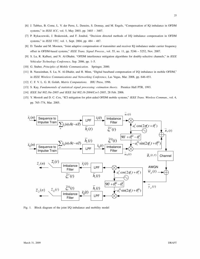
imbalance. The system block diagram under consideration is shown in Fig. 1. Let s(n) = sI(n)+jsQ(n)

denote the discrete-time complex baseband signal at the transmitter which passes through the Digital-to-

Analog Converter (DAC) and a pulse-shaping or Low Pass Filter (LPF). We model the combined DAC and

filters in the I and Q branches as a cascade of the desired LPF denoted as ht(t) and a filter representing

the mismatch between the I and Q branches, denoted as ξIt (t) and ξQ

t (t), respectively. Note that the

Fourier transforms of ξIt (t) and ξQ

t (t) could be frequency-dependent in practical systems and different

from each other, which makes the I/Q imbalance frequency-dependent. Then, the signal components are

up-converted using the quadrature tones of the mixer which (ideally) should have an equal amplitude and

a phase difference of 90◦. However, in most practical systems, there are amplitude and phase imbalances

between them which result in frequency-independent I/Q imbalance. The amplitude and phase imbalances

of the transmit-side mixers are denoted by aIt , a

Qt and θI

t , θQt , respectively.

The corresponding continuous-time ideal signal generated at the LPF output is s(t) = sI(t) + jsQ(t),

where sI(t) =∑∞

n=−∞ sI(n)ht(t−nT ), sQ(t) =∑∞

n=−∞ sQ(n)ht(t−nT ) and T is the OFDM sample

period. Let u(t) = uI(t) + juQ(t) denote the signal distorted by frequency-dependent I/Q imbalance

before the mixer given by

u(t) = sI(t)⊗ ξIt (t) + jsQ(t)⊗ ξQ

t (t). (1)

Also, let xp(t) = <{x(t)ej2πfct} and x(t) = xI(t)+jxQ(t) denote, respectively, the passband signal and

the baseband equivalent signal after the mixer. When there is no imbalance between the mixer branches,

x(t) = u(t). However, when there is imbalance (which is frequency-independent), we have

xp(t) = uI(t)aIt cos

(2πfct + θI

t

)− uQ(t)aQt sin

(2πfct + θQ

t

)

= xI(t) cos(2πfct)− xQ(t) sin(2πfct) = <{

x(t)ej2πfct} (2)

where xI(t) =(uI(t)aI

t cos θIt − uQ(t)aQ

t sin θQt

), xQ(t) =

(uQ(t)aQ

t cos θQt + uI(t)aI

t sin θIt

)(3)

represent the corresponding baseband signal components. Substituting uI(t) = u(t)+u∗(t)2 and uQ(t) =

u(t)−u∗(t)2j in (3) and grouping the terms carefully, we get

x(t) = µtu(t) + νtu∗(t) (4)


5

where µt = 12(aI

t ejθI

t + aQt ejθQ

t ) and νt = 12(aI

t ejθI

t − aQt ejθQ

t ). Substituting (1) in (3) and using the

relations sI(t) = s(t)+s∗(t)2 and sQ(t) = s(t)−s∗(t)

2j , we obtain

x(t) =12

((µt + νt)ξI

t (t) + (µt − νt)ξQt (t)

)

︸︷︷︸λt(t)

⊗s(t) +12

((µt + νt)ξI

t (t)− (µt − νt)ξQt (t)

)

︸︷︷︸φt(t)

⊗s∗(t). (5)

Then, xp(t) is transmitted through the channel and the received passband signal is

yp(t) = gp(t, τ)⊗ xp(t) + wp(t) (6)

which has the baseband equivalent signal

y(t) = g(t, τ)⊗ x(t) + w(t), (7)

where gp(t, τ) = 2<{g(t, τ)ej2πfct} is the channel impulse response (CIR) and wp(t) = <{w(t)ej2πfct}is Additive White Gaussian Noise (AWGN) with two-sided power spectral density of σ2. The received

signal is down-converted and input to the receive LPF in each branch. The impulse response of the receive

LPF hr(t) is matched to ht(t) and the frequency-dependent I/Q imbalances are modeled by the cascaded

filters ξIr (t) and ξQ

r (t). Denote the amplitudes and the phase imbalances of the receiver quadrature mixer

tones by aIr , a

Qr and θI

r , θQr , respectively. With yp(t) = <{y(t)ej2πfct} = 1

2(y(t)ej2πfct + y∗(t)e−j2πfct),

the output of the ideal receive LPF is

r(t) =12hr(t)⊗ (µry(t) + νry

∗(t)) (8)

where µr = 12(aI

re−jθI

r + aQr e−jθQ

r ) and νr = 12(aI

rejθI

r − aQr ejθQ

r ). After experiencing receive-side

frequency-dependent I/Q imbalance, the I and Q components are given by

zI(t) = ξIr (t)⊗ rI(t) =

(µry(t) + νry

∗(t) + µ∗r y∗(t) + ν∗r y(t)2

)⊗ ξI

r (t)⊗ hr(t)

zQ(t) = ξQr (t)⊗ rQ(t) =

(µry(t) + νry

∗(t)− µ∗r y∗(t)− ν∗r y(t)2j

)⊗ ξQ

r (t)⊗ hr(t) (9)

and the final output signal z(t) = zI(t) + jzQ(t) is given by

z(t) =12

((µr + ν∗r )ξI

r (t) + (µr − ν∗r )ξQr (t)

)

︸︷︷︸λr(t)

⊗hr(t)⊗ y(t)

+12

((νr + µ∗r)ξ

Ir (t) + (νr − µ∗r)ξ

Qr (t)

)

︸︷︷︸φr(t)

⊗hr(t)⊗ y∗(t). (10)


6

Substituting (5) and (7) into (10), we obtain the following relation between z(t) and the input signal s(t)

z(t) =[λr(t)⊗ g(t, τ)⊗ λt(t) + φr(t)⊗ g∗(t, τ)⊗ φ∗t (t)

]︸︷︷︸

ψ(1)(t,τ)

⊗hr(t)⊗ s(t)

+[λr(t)⊗ g(t, τ)⊗ φt(t) + φr(t)⊗ g∗(t, τ)⊗ λ∗t (t)

]︸︷︷︸

ψ(2)(t,τ)

⊗hr(t)⊗ s∗(t)

+ λr(t)⊗ hr(t)⊗ w(t) + φr(t)⊗ hr(t)⊗ w∗(t). (11)

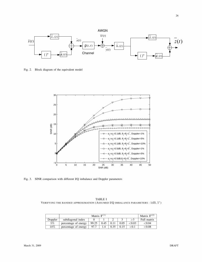
Equation (11) represents an equivalent model that is illustrated in Fig. 2. It is a generalization of the

frequency-independent I/Q imbalance model in [4], in that µt, νt, µr and νr are replaced by λt(t), φt(t),

λr(t) and φr(t), respectively.

Note on Symmetric Imbalances: Symmetric imbalance is the case when the amplitude and phase

imbalances are distributed equally among the I and Q branches. On the transmit-side, this special case

implies that aIt = 1 + αt, aQ

t = 1− αt , θIt = − θt

2 and θQt = θt

2 . In this case, the expressions for µt and

νt in (4) simplify to

µt = (cosθt

2− jαt sin

θt

2), νt = (αt cos

θt

2− j sin

θt

2), (12)

Similarly, symmetric imbalance on the receive-side implies aIr = 1 + αr, aQ

r = 1 − αr , θIr = − θr

2 and

θQr = θr

2 . Then, the expressions for µr and νr become

µr = (cosθr

2+ jαr sin

θr

2), νr = (αr cos

θr

2− j sin

θr

2). (13)

Therefore, in the symmetric imbalance case, the system performance depends on the amplitude differences

αt, αr and the phase differences θt, θr between the I and Q branches, rather than on the actual imbalance

parameters. The α’s are defined in log-scale as αt = 10 log10(1+ αt) dB and αr = 10 log10(1+ αr) dB,

so that 0 dB corresponds to no amplitude imbalance.

B. Mobile OFDM with Frequency-Dependent Joint Tx/Rx I/Q Imbalance

In this section, we apply the I/Q imbalance model we developed in Section II-A to mobile OFDM

systems. After sampling the receive filter output, each of the analog quantities of the previous section, over

one OFDM symbol duration, can be represented as a vector. The transmitted OFDM symbol, excluding

cyclic prefix (CP), has N samples of s(t), which constitute the vector s = [s(0), s(1), · · · , s(N − 1)]T .

Likewise, the sampled version of λt(t) is given by λt = [λt(0), λt(1), · · · , λt(Lλt− 1),0T

1×(N−Lλt )]T .

Similarly, we define the vectors λr, φt and φr associated with λr(t), φt(t) and φr(t), respectively. Also,


7

we sample the time-varying CIR at time n and form the vector g(n) = [g(n, 0), g(n, 1), · · · , g(n,L −1),0T

1×(N−L)]T for n = 0, · · · , N − 1, where L is the length of the channel. Assume that the combined

response of the ideal transmit and receive filters (hr(t) and ht(t)) satisfies the Nyquist criterion. Also,

assume that the CP is longer than the memory lengths of ψ(1)(t, τ) and ψ(2)(t, τ) defined in (11).

After removing CP, the linear convolutions corresponding to the signal terms in (11) become circular

convolutions and the discrete-time received signal is given by

z(n) =[λr(n) ~N g(n, l) ~N λt(n) + φr(n) ~N g∗(n, l) ~N φ∗t (n)

]~N s(n) (14)

+[λr(n) ~N g(n, l) ~N φt(n) + φr(n) ~N g∗(n, l) ~N λ∗t (n)

]~N s∗(n)

+ λr(n)⊗ w(n) + φr(n)⊗ w∗(n).

Collecting the N samples of z(n) in the vector z = [z(0), · · · , z(N − 1)], we can write

z = (ΛrGΛt + ΦrG∗Φ∗t )s + (ΛrGΦt + ΦrG∗Λ∗

t )s∗ + Λ′

rw + Φ′rw∗

︸︷︷︸v

(15)

where Λt is an N ×N circulant matrix with its first column equal to λt. Similarly, Λr, Φt and Φr are

circulant matrices with first columns equal to λr, φt and φr, respectively. Under high mobility where

the CIR varies within each OFDM symbol, G is not a circulant matrix but is given by

G =

g(0, 0) g(0, N − 1) g(0, N − 2) · · · g(0, 1)

g(1, 1) g(1, 0) g(1, N − 1) · · · g(1, 2)

g(2, 2) g(2, 1) g(2, 0) · · · g(2, 3)...

. . . . . . . . ....

g(N − 1, N − 1) · · · · · · g(N − 1, 1) g(N − 1, 0)

. (16)

Here g(n,m) = 0 for m ≥ L and w is the noise vector of length (N + NCP) where NCP is the number

of CP samples. Moreover, Λ′r and Φ′

r are matrices of size N × (N + NCP) whose n-th rows are given

by [01×n, λr(0), λr(1), · · · , λr(Lλr− 1),01×(N+NCP−n−Lλr )]T and [01×n, φr(0), φr(1), · · · , φr(Lφr

−1),01×(N+NCP−n−Lφr )]T respectively. The matrices Λ′

r and Φ′r represent linear convolutions for the

noise components which have no cyclic prefix.

After applying the DFT to (15), we obtain the frequency-domain relation

z = (ΛrGΛt + ΦrG#Φ#t )︸︷︷︸

Ψ(1)

s + (ΛrGΦt + ΦrG#Λ#t )︸︷︷︸

Ψ(2)

s# + v (17)

where Λt = FΛtFH , Λr = FΛrFH , Φt = FΦtFH , Φr = FΦrFH , G = FGFH , z = Fz, s = Fs and


8

v = Fv. The k-th element of vector b# is related to the (N − k) element of vector b by b#k = b∗N−k.

Similarly, the (n, k) element of matrix B# is related to the (N − n, N − k) element of matrix B by

b#n,k = b∗N−n,N−k. The following remarks are in order

• Since Λr, Λt,Φr and Φt are circulant matrices, Λr,Λt,Φr and Φt are diagonal matrices and so are

Φ#t and Λ#

t . Therefore, λt = [λt(0), λt(1), · · · , λt(N − 1)]T = Diag(Λt) represents the N -point

DFT of λt. The quantities λr, φt, φr, λ#t and φ#

t are defined in a similar manner.

• Under high mobility, the CIR can no longer be modeled as a time-invariant finite impulse response

(FIR) filter and the matrix G is no longer circulant. In the frequency domain, the channel matrix G

is no longer diagonal resulting in dispersion of symbol energy to adjacent sub-carriers and causing

ICI. However, G can be well-approximated by a banded matrix as discussed in Section IV-B (see

e.g., [9] and references therein) since most of the ICI energy is due to neighboring sub-carriers.

• g(n, n −m) is the (n,m) element of G where the first index represents the time-domain and the

second index represents the delay-domain. g(k, l) is the (k, l) element of G, and it represents the

interference due to the l sub-carrier at the k sub-carrier. From (16) and the fact that G = FGFH ,

it can be easily shown that the quantities g(n, n−m) and g(k, l) are related as follows

g(k, l) =1N

N−1∑

n=0

e−j 2π

Nkn

N−1∑

m=0

g(n, n−m)ej 2π

Nml. (18)

An useful form of (18) is obtained by rearranging the terms in the second summation as follows

g(k, l) =1N

N−1∑

n=0

e−j 2π

Nkn

N−1∑

m=0

g(n,m)ej 2π

N(n−m)l =

N−1∑

m=0

N−1∑

n=0

g(n,m)e−j 2π

N(kn−(n−m)l). (19)

• The noise vector v = Λ′rw + Φ′

rw∗, after being subject to the receiver frequency-dependent I/Q

imbalance, is no longer white and its covariance matrix is given by (67).

C. Equivalent Channel Matrix

This section develops an alternative and more compact matrix representation for (17) which sheds

more light on the distinctive features of ICI due to I/Q imbalance and mobility. First, the k and N − k

elements of z in (17) are given by

z(k) =N−1∑

l=0

(λr(k)λt(l)g(k, l) + φr(k)φ∗t (l

′)g∗(k′, l′))s(l)

+N−1∑

m=0

(λr(k)φt(m)g(k,m) + φr(k)λ∗t (m

′)g∗(k′, m′))s∗(m′) + v(k) (20)


9

z∗(k′) =N−1∑

l=0

(λ∗r(k

′)λ∗t (l)g∗(k′, l) + φ∗r(k

′)φt(l′)g(k, l′))s∗(l)

+N−1∑

m=0

(λ∗r(k

′)φ∗t (m)g∗(k′,m) + φ∗r(k′)λt(m′)g(k, m′)

)s(m′) + v∗(k′) (21)

where k′ = N − k, l′ = N − l,m′ = N − m and k = 0, · · · , N2 − 1. Though they take the same set

of values, two different indices l and m have been used in (20) for clarity in further development. For

m = N2 , N

2 + 1, . . . , N − 1 and l = N2 , N

2 − 1, . . . , 1 (in the decreasing order), we have m′ = l and

l′ = m. Therefore, we can rearrange the terms in the summations to write

z(k) =

N

2−1∑

l=0

{(λr(k)λt(l)g(k, l) + φr(k)φ∗t (l

′)g∗(k′, l′))s(l)

+(λr(k)φt(l′)g(k, l′) + φr(k)λ∗t (l)g

∗(k′, l))s∗(l)

}

+

N

2−1∑

m=0

{(λr(k)φt(m)g(k,m) + φr(k)λ∗t (m

′)g∗(k′,m′))s∗(m′)

+(λr(k)λt(m′)g(k, m′) + φr(k)φ∗t (m)g∗(k′,m)

)s(m′)

}+ v(k). (22)

In (22), each sum contains terms involving s(l) and s∗(l). This is because, due to mobility, each signal

term s(l) on sub-carrier l leaks to other sub-carriers including l′ = N − l. I/Q imbalance, on the other

hand, results in the addition of the image version of the leaked component of s(l) at the sub-carrier

l′ = N − l. In this image version, the component of the signal s(l) at sub-carrier l′ = N − l interferes

with itself in the conjugated form s∗(l). Such a self-interference scenario occurs only in the presence of

both I/Q imbalance and mobility. In a similar manner, we rewrite z∗(k′) in (21) as follows

z∗(k′) =

N

2−1∑

l=0

{(λ∗r(k

′)λ∗t (l)g∗(k′, l) + φ∗r(k

′)φt(l′)g(k, l′))s∗(l)

+(λ∗r(k

′)φ∗t (l′)g∗(k′, l′) + φ∗r(k

′)λt(l)g(k, l))s(l)

}

+

N

2−1∑

m=0

{(λ∗r(k

′)φ∗t (m)g∗(k′, m) + φ∗r(k′)λt(m′)g∗(k, m′)

)s(m′)

+(λ∗r(k

′)λ∗t (m′)g∗(k′,m′) + φ∗r(k

′)φt(m)g(k,m))s∗(m′)

}+ v∗(k′). (23)

For each sub-carrier pair (k, k′), (22) and (23) could be combined and written in matrix form as

zk =

N

2−1∑

l=0

(γ

(1)k,l sl + γ

(2)k,l s

∗l

)+ vk (24)


10

where zk = [z(k), z∗(k′)]T , sl = [s(l), s∗(l′)]T , vk = [v(k), v∗(k′)]T and

γ(1)k,l =

λr(k)λt(l)g(k, l) + φr(k)φ∗t (l′)g∗(k′, l′), λr(k)φt(l)g(k, l) + φr(k)λ∗t (l′)g∗(k′, l′)

λ∗r(k′)φ∗t (l′)g∗(k′, l′) + φ∗r(k′)λt(l)g(k, l), λ∗r(k′)λ∗t (l′)g∗(k′, l′) + φ∗r(k′)φt(l)g(k, l)

γ(2)k,l =

λr(k)φt(l′)g(k, l′) + φr(k)λ∗t (l)g∗(k′, l), λr(k)λt(l′)g(k, l′) + φr(k)φ∗t (l)g∗(k′, l)

λ∗r(k)λ∗t (l)g∗(k′, l) + φ∗r(k′)φt(l′)g(k, l′), λ∗r(k′)φ∗t (l)g∗(k′, l) + φ∗r(k′)λt(l′)g(k, l′)

.

The self-interference coefficient matrix γ(2)k,l represents the effect of a sub-carrier interfering with

itself due to the combined effects of mobility and I/Q imbalance. The terms in (24) could be collected

for all k as in (25) below. In the special case of no mobility, only g(k, l)’s for k = l are non-zero.

This implies that only those γ(1)k,l ’s for which k = l are non-zero, i.e., γ

(1)k,l becomes a block-diagonal

matrix. Furthermore, all γ(2)k,l ’s become zero and Γ(2) vanishes. Therefore, (25) decouples into N

2 sub-

systems of size 2 × 2. If we further specialize to the frequency-independent I/Q imbalance case, i.e.,

φr(k) = µr, φt(k) = µt, λr(k) = νr, λt(k) = νt ∀k, then (25) reduces to the model studied in [4].

z0

...

zN

2−1

︸︷︷︸z

=

γ(1)0,0 · · · γ

(1)

0, N

2−1

.... . .

...

γ(1)N

2−1,0

· · · γ(1)N

2−1, N

2−1

︸︷︷︸Γ(1)

s0

...

sN

2−1

︸︷︷︸s

+

γ(2)0,0 · · · γ

(2)

0, N

2−1

.... . .

...

γ(2)N

2−1,0

· · · γ(2)N

2−1, N

2−1

︸︷︷︸Γ(2)

s∗0...

s∗N2−1

︸︷︷︸s∗

+

v0

...

vN

2−1

︸︷︷︸v

(25)

III. SINR ANALYSIS FOR MOBILE OFDM SYSTEMS WITH I/Q IMBALANCE

In this section, we present new insights on the combined ICI effects of mobility and I/Q imbalance

by analyzing the resulting degradation in the received signal to interference plus noise ratio (SINR). We

make the following assumptions

1) Channel g(n,m) is uncorrelated for different taps m. For each m, {g(n,m) : n = 0, · · · , N − 1}is a circularly-symmetric complex Gaussian vector.

2) {s(k) : k = 0, · · · , N − 1} is a circularly symmetric complex random vector with average energy

Es = E{|s(k)|2}.

3)∑L−1

m=0 σ2gm

= 1 where σ2gm

is the power of tap-m, i.e. the channel results in no net gain.


11

Along with these assumptions, we split the terms in (20) into two parts, one being the signal term with

l = k and the other involving the ICI terms with l 6= k, and rewrite (20) as follows

z(k) = S(k) + I(k) + v(k) (26)

where S(k) =(λr(k)λt(k)g(k, k) + φr(k)φ∗t (k

′)g∗(k′, k′))s(k)

+(λr(k)φt(k′)g(k, k′) + φr(k)λ∗t (k)g∗(k′, k)

)s∗(k), (27)

I(k) =N−1∑

l=0l 6=k

(λr(k)λt(l)g(k, l) + φr(k)φ∗t (l

′)g∗(k′, l′))s(l)

+N−1∑

m=0m6=k′

(λr(k)φt(m)g(k, m) + φr(k)λ∗t (m

′)g∗(k′,m′))s∗(m′).(28)

In the Appendix, we derive the expressions for E{|S(k)|2} and E{|I(k)|2} for the generalized case and

also the variance of the colored noise. For the special case of frequency-independent I/Q imbalance, they

can be simplified as

E{|S(k)|2} =

1N2

Es

[(µ2

r|µt|2 + |νr|2|νt|2) N−1∑

n1=0

N−1∑

n2=0

R(n1, n2)

+ µ2r|νt|2

N−1∑

n1=0

N−1∑

n2=0

R(n1, n2)e−j 2π

N(2k)(n1−n2)

+ |νr|2|µt|2N−1∑

n1=0

N−1∑

n2=0

R(n1, n2)e−j 2π

N(−2k)(n1−n2)

], (29)

E{|I(k)|2} =

Es

N2

[(|µr|2|µt|2 + |νr|2|νt|2

)(

N2 −∑n1,n2

R(n1, n2)

)

+ |µr|2|νt|2(

N2 −∑n1,n2

R(n1, n2)e−j 2π

N(2k)(n1−n2)

)

+ |νr|2|µt|2(

N2 −∑n1,n2

R(n1, n2)e−j 2π

N(−2k)(n1−n2)

)](30)

E{|v(k)|2} = (|µr|2 + |νr|2)σ2, (31)

where R(n1, n2) = E {g(n1,m)g∗(n2,m)} is the normalized time-correlation of any CIR tap m. Finally,

the SINR and SIR (signal to interference ratio) are defined as

SINR =E

{|S(k)|2}

E {|I(k)|2}+ E {|v(k)|2} and SIR =E

{|S(k)|2}

E {|I(k)|2} . (32)


12

Case study: Assume that the time-varying CIR obeys the Jake’s model [10], i.e.,

R(n1, n2) = J0(2πfD(n2 − n1)T ), (33)

where J0(.) is the zero-order Bessel function and fD is the maximum Doppler frequency. Then, using

the symmetry properties of the Bessel function, we obtain

N−1∑

n1=0

N−1∑

n2=0

R(n1, n2) =N−1∑

n1=0

N−1∑

n2=0

J0(2πfD(n2 − n1)T ) = N + 2N−1∑

n=1

(N − n)J0(2πfDnT ) , R1, (34)

N−1∑

n1=0

N−1∑

n2=0

R(n1, n2)e−j 2π

N(2k)(n1−n2) = N + 2

N−1∑

n=1

(N − n)J0(2πfDnT ) cos(

4πkn

N

), R2. (35)

Substituting (34) and (35) into (29) and (30), we obtain the corresponding SINR and SIR expressions.

From (34) and (35), we see that R1 is not a function of the sub-carrier index k whereas R2 is. But

we found that the value of R2 is negligibly small in comparison to R1. Therefore, we ignore R2 in the

following results.

Let us consider the case of frequency-independent I/Q imbalance, i.e. , φr(k) = νr, φt(k) = νt, λr(k) =

µr, λt(k) = µt. Fig. 3 compares the SINR under mild and severe I/Q imbalance and mobility scenarios.

The channel model and the simulation parameters are described in detail in Section VI. It can be seen

that when the I/Q imbalance parameters change from αt = αr = 0.1 dB, θr = θt = 1◦ to αt = αr = 0.5

dB, θr = θt = 5◦, the performance degrades dramatically. For example, at high SNR levels, the SINR is

reduced from 28.5 dB to 14.7 dB at Doppler=1% (of sub-carrier spacing), from 22.7 dB to 14.2 dB at

Doppler=5% and from 17.5 dB to 12.9 dB at Doppler=10%. Another interesting observation from Fig.

3 is that at low I/Q imbalance (i.e., αt = αr = 0.1dB, θr = θt = 1◦), as Doppler increases (from 1%

to 5% to 10%), the SINR degrades significantly (from 28.5 dB to 22.7 dB to 14.2dB) while at high I/Q

imbalance (αt = αr = 0.5 dB, θr = θt = 5◦), the SINR performance only degrades slightly (from 14.7

dB to 14.2 dB to 12.9 dB) at 10% Doppler. Thus, when I/Q imbalance is mild, Doppler spread has larger

impact on the SINR performance. However, when I/Q imbalance is severe, the SINR performance is not

very sensitive to Doppler.

To gain more insight into the impact of different I/Q imbalance parameters, we define ηr = µr

νrand

ηt = µt

νt. Larger values of ηr and ηt indicate less severe I/Q imbalance effects. Ignoring noise effects,


13

SIR can be written as a function of ηr and ηt as follows

SIR =(|ηr|2|ηt|2 + 1)R1 + (|ηr|2 + |ηt|2)R2

(|ηr|2|ηt|2 + 1) (N2 −R1) + (|ηr|2 + |ηt|2) (N2 −R2). (36)

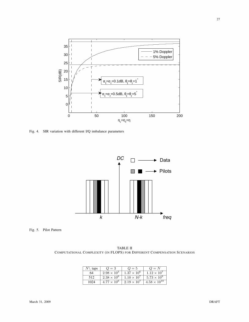
Fig. 4 shows how SIR varies as a function of ηr = ηt = η for mild and severe Doppler spreads. The

two vertical dashed lines in the figure correspond to mild and severe I/Q imbalance conditions. It can

be clearly seen that SIR increases with η (less severe I/Q imbalance) until it reaches its Doppler-limited

level. When ηr = ηt = ∞, there is no I/Q imbalance and SIR= R1N2−R1

, in agreement with the result in

[10]. Fig. 3 clearly illustrates the importance of compensating for the ICI due to both I/Q imbalance and

mobility. Compensating for only one of them can still result in significant performance degradation. This

motivates the design of effective joint ICI compensation schemes for both I/Q imbalance and mobility

which is the subject of the next section.

IV. DIGITAL BASEBAND COMPENSATION

In Section III, we have shown that both severe I/Q imbalance and high mobility degrade the SINR

performance dramatically. In this section, based on the model derived in Section II, we propose a

reduced-complexity digital baseband compensation scheme to jointly compensate for the effects of I/Q

imbalance and mobility. First, we investigate the linear block minimum mean square error frequency-

domain equalizer (MMSE-FEQ) which is high in complexity. Then, we revisit the structure of the channel

matrix and exploit some of its properties to derive a reduced-complexity symbol-by-symbol finite-impulse-

response (FIR) MMSE-FEQ.

A. Block MMSE-FEQ

The signal model in (25) has both s(k) and s∗(k) terms in addition to colored noise due to frequency-

dependent I/Q imbalance. We split the real and imaginary terms of the complex system in (25) as

<{z}={z}

︸︷︷︸zIQ

=

<{Γ(1)} −={Γ(1)}={Γ(1)} <{Γ(1)}

+

<{Γ(2)} ={Γ(2)}={Γ(2)} −<{Γ(2)}

︸︷︷︸ΓIQ

<{s}={s}

︸︷︷︸sIQ

+

<{v}={v}

︸︷︷︸vIQ

.

(37)

For the real-valued model of (37), the Block MMSE-FEQ is given by1

sIQ = ΓHIQ

(ΓIQΓH

IQ +1

SNRI2N

)−1

zIQ. (38)

1For simplicity, we approximate the noise to be white


14

However, the calculation of (38) involves the inversion of a real matrix of size 2N and is of high

complexity. In the following, we will present a reduced-complexity FIR-MMSE FEQ which exploits the

banded structure of the G matrix (see (16) and (17)).

B. Reduced-Complexity FIR MMSE-FEQ

As previously discussed in Section II, Λr, Λt,Φr, Φt, Λ#t and Φ#

t in (17) are diagonal matrices. G is

not diagonal in general and this results in a computationally-complex equalizer as in (38). But, as shown

in [9] and references therein, G can be well approximated by a banded matrix as most of the ICI energy

is from neighboring sub-carriers. Since the product of two diagonal matrices is also a diagonal matrix and

the product of a diagonal matrix with a banded matrix is a banded matrix, it is easy to see that ΛrΛtG,

ΦrΦ#t G#, ΛrΦtG and ΦrΛ

#t G# are all banded matrices and so are Ψ(1) and Ψ(2). The number of

significant diagonals of G depends on the Doppler spread. Assume that we only consider Q diagonals

in the banded matrix G (hence also in G#) and set Q = 2D + 1. With this banded G, we follow the

same steps described in Section II-C to arrive at the following 2× 2 sub-systems for 0 ≤ k ≤ N2

zk = γ(1)k,ksk +

D∑

i=−Di6=0

γ(1)k,k−isk−i +

D∑

i=−D

γ(2)k,k−is

∗k−i + vk, (39)

where the γk,l’s were defined in Section II-C. Equation (39) can also be derived from (25) by setting

all the sub-blocks γ(1)k,l = 02×2 when |k − l| > D. The same condition also annuls most blocks of

γ(2)k,l . Very few blocks of Γ(2) would still remain (near 0 and N

2 ), but can be safely ignored. Shown

in Table I are the energies of the diagonals of Γ(1) in a 512 sub-carrier 5-MHz OFDM system using

the Stanford University Interim-3 (SUI-3) Channel model. It can be seen that most of the energy of the

equivalent channel matrix is concentrated in its main diagonal. Less than 1% of the energy spills into the

sub-diagonals at 5% Doppler and less than 2.5% at 10% Doppler. Also, the energy of the whole matrix

Γ(2) is negligible as shown in the table.

Due to mobility and I/Q imbalance, the conventional single-tap FEQ in OFDM systems is no longer

optimum because of the interference from the adjacent sub-carriers and image sub-carriers. However,

the equivalent channel matrix has an approximately banded structure. As a performance complexity

tradeoff, we consider an FIR MMSE-FEQ structure [11] with 2Q taps per sub-carrier2, where the factor

2 accounts for inclusion of image sub-carriers and Q = 2D + 1, i.e., taking into account the Doppler-

induced ICI only from the 2D adjacent sub-carriers (D sub-carriers from each side). To compute the

2This holds for k = D to N2−D − 1. For sub-carriers outside this range which fall closer to the edges, the number of taps

decreases progressively.


15

optimum FEQ tap settings, based on (39), we define the quantities zk

, [zTk−D, · · · , zT

k , · · · , zTk+D]T ,

sk , [sTk−2D, · · · , sT

k , · · · , sTk−2D]T , vk , [vT

k−D, · · · ,vTk , · · · ,vT

k+D]T , and

Gk =

γ(1)k−D,k−2D · · · · · · · · · γ

(1)k−D,k 0 · · · · · · · · ·

0. . . . . . . . . . . . . . . 0 · · · · · ·

· · · 0 γ(1)k,k−D · · · γ

(1)k,k · · · γ

(1)k,k+D 0 · · ·

· · · · · · 0. . . . . . . . . . . . . . . 0

· · · · · · · · · 0 γ(1)k+D,k · · · · · · · · · γ

(1)k+D,k+2D

2Q×(8D+2)(40)

Then, we have zk

= Gks

k+ v

kand the linear MMSE estimator for sk = [s(k), s∗(N − k)]T is

sk

= wHkz

kwhere

wHk

= gHk

(GkGH

k+ σ2I2Q)−1 (41)

and gk

is the middle block column of Gk. Note that we detect the k-th sub-carrier s(k) and its image

s∗(N −k) jointly by mitigating the ICI from their Q neighboring sub-carriers (due to Doppler) and their

images (due to I/Q imbalance) using the 2Q-tap FEQ per subcarrier computed in (41). Since Q ¿ N ,

significant complexity reductions are achieved in comparison with the N -tap FEQ in Section IV-A at

negligible performance loss.

C. Complexity Analysis

First, we determine the number of computations required for the N -tap FEQ in (38). For this, we use

the following results from [12]

• Multiplying two real matrices of sizes m× n and n× r requires 2mnr flops.

• Gaussian elimination of a real square matrix of size n requires 2n3

3 flops.

• Matrix inversion of a real square matrix involves two Gaussian elimination steps and hence requires4n3

3 flops.

Here, a flop is defined as either an addition or multiplication operation. Therefore, an N -tap FEQ requires

8N2 + 128N3

3 flops. Also, we evaluate the complexity involved in computing the (Q = 2D + 1)-tap FEQ

in (41). This turns out to be 16N3 (1 + 2D)(35 + 128D(1 + D)) flops and is evaluated in Table II for

different values of N and D. Clearly, our proposed compensation schemes results in significant complexity

reductions.


16

V. CHANNEL ESTIMATION SCHEMES

To implement the FIR MMSE-FEQ proposed in Section IV, effective channel estimation schemes

are essential. In this section, we first propose a quadruple pilot pattern which can be used for channel

estimation in mobile OFDM systems with both frequency-dependent and frequency-independent I/Q

imbalances. Next, for the frequency-independent I/Q imbalance case, we propose a low-overhead pilot

pattern by computing I/Q imbalance parameter ratios ηr and ηt.

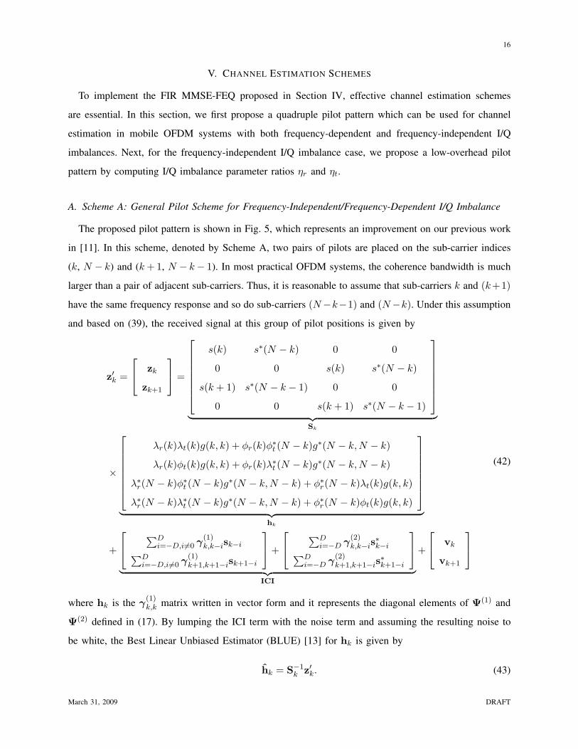
A. Scheme A: General Pilot Scheme for Frequency-Independent/Frequency-Dependent I/Q Imbalance

The proposed pilot pattern is shown in Fig. 5, which represents an improvement on our previous work

in [11]. In this scheme, denoted by Scheme A, two pairs of pilots are placed on the sub-carrier indices

(k, N − k) and (k + 1, N − k− 1). In most practical OFDM systems, the coherence bandwidth is much

larger than a pair of adjacent sub-carriers. Thus, it is reasonable to assume that sub-carriers k and (k+1)

have the same frequency response and so do sub-carriers (N−k−1) and (N−k). Under this assumption

and based on (39), the received signal at this group of pilot positions is given by

z′k =

zk

zk+1

=

s(k) s∗(N − k) 0 0

0 0 s(k) s∗(N − k)

s(k + 1) s∗(N − k − 1) 0 0

0 0 s(k + 1) s∗(N − k − 1)

︸︷︷︸Sk

×

λr(k)λt(k)g(k, k) + φr(k)φ∗t (N − k)g∗(N − k,N − k)

λr(k)φt(k)g(k, k) + φr(k)λ∗t (N − k)g∗(N − k,N − k)

λ∗r(N − k)φ∗t (N − k)g∗(N − k,N − k) + φ∗r(N − k)λt(k)g(k, k)

λ∗r(N − k)λ∗t (N − k)g∗(N − k, N − k) + φ∗r(N − k)φt(k)g(k, k)

︸︷︷︸hk

+

∑Di=−D,i6=0 γ

(1)k,k−isk−i

∑Di=−D,i 6=0 γ

(1)k+1,k+1−isk+1−i

+

∑Di=−D γ

(2)k,k−is

∗k−i∑D

i=−D γ(2)k+1,k+1−is

∗k+1−i

︸︷︷︸ICI

+

vk

vk+1

(42)

where hk is the γ(1)k,k matrix written in vector form and it represents the diagonal elements of Ψ(1) and

Ψ(2) defined in (17). By lumping the ICI term with the noise term and assuming the resulting noise to

be white, the Best Linear Unbiased Estimator (BLUE) [13] for hk is given by

hk = S−1k z′k. (43)


17

Moreover, we chose Sk to be an orthogonal matrix to achieve minimum variance for the estimator. If we

further restrict the pilots to be BPSK symbols, we can set Sk as follows

Sk =

1 1 0 0

0 0 1 1

1 −1 0 0

0 0 1 −1

. (44)

We assume that the ICI caused by the adjacent data sub-carriers could be ignored since the energy of

the pilots is typically boosted compared to the data as in the WiMAX standard [14]. Specifically, if

we define hk = [hk(1), hk(2), hk(3), hk(4)]T , then the (k, k) elements of Ψ(1) and Ψ(2) are hk(1) and

hk(2), respectively, while their (N − k, N − k) elements are h∗k(4) and h∗k(3), respectively. In [15],

the authors proposed a time-domain linear interpolation scheme to estimate the off-diagonal elements

of the equivalent frequency-domain channel matrix in mobile OFDM systems. Since Ψ(1) and Ψ(2) are

approximately banded matrices (as shown in Section IV-B), the approach in [15] can be used to estimate

their off-diagonal elements (see [15] for more details).

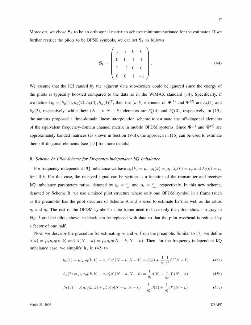
B. Scheme B: Pilot Scheme for Frequency-Independent I/Q Imbalance

For frequency-independent I/Q imbalance we have φr(k) = µr, φt(k) = µt, λr(k) = νr and λt(k) = νt

for all k. For this case, the received signal can be written as a function of the transmitter and receiver

I/Q imbalance parameters ratios, denoted by ηt = µt

νtand ηr = µr

νr, respectively. In this new scheme,

denoted by Scheme B, we use a mixed pilot structure where only one OFDM symbol in a frame (such

as the preamble) has the pilot structure of Scheme A and is used to estimate hk’s as well as the ratios

ηr and ηt. The rest of the OFDM symbols in the frame need to have only the pilots shown in gray in

Fig. 5 and the pilots shown in black can be replaced with data so that the pilot overhead is reduced by

a factor of one half.

Now, we describe the procedure for estimating ηt and ηr from the preamble. Similar to [4], we define

β(k) = µrµtg(k, k) and β(N − k) = µrµtg(N − k, N − k). Then, for the frequency-independent I/Q

imbalance case, we simplify hk in (42) to

hk(1) = µrµtg(k, k) + νrν∗t g∗(N − k,N − k) = β(k) +

1ηr

1η∗t

β∗(N − k) (45a)

hk(2) = µrνtg(k, k) + νrµ∗t g∗(N − k, N − k) =

1ηt

β(k) +1ηr

β∗(N − k) (45b)

hk(3) = ν∗r µtg(k, k) + µ∗rν∗t g(N − k, N − k) =

1η∗r

β(k) +1η∗t

β∗(N − k) (45c)


18

hk(4) = ν∗r νtg(k, k) + µ∗rµ∗t g∗(N − k,N − k) =

1η∗r

1ηt

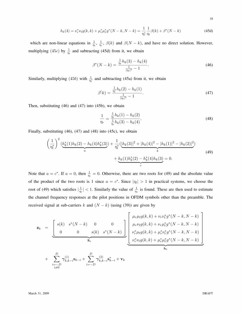
β(k) + β∗(N − k) (45d)

which are non-linear equations in 1ηt

, 1ηr

, β(k) and β(N − k), and have no direct solution. However,

multiplying (45c) by 1ηt

and subtracting (45d) from it, we obtain

β∗(N − k) =1ηt

hk(3)− hk(4)1

|ηt|2 − 1. (46)

Similarly, multiplying (45b) with 1η∗t

and subtracting (45a) from it, we obtain

β(k) =1η∗t

hk(2)− hk(1)1

|ηt|2 − 1. (47)

Then, substituting (46) and (47) into (45b), we obtain

1ηr

=1ηt

hk(1)− hk(2)1ηt

hk(3)− hk(4). (48)

Finally, substituting (46), (47) and (48) into (45c), we obtain(

1η∗t

)2

(h∗k(1)hk(2)− hk(4)h∗k(3)︸︷︷︸a

) +1η∗t

(|hk(3)|2 + |hk(4)|2 − |hk(1)|2 − |hk(2)|2︸︷︷︸b

)

+ hk(1)h∗k(2)− h∗k(4)hk(3)︸︷︷︸c

= 0.

(49)

Note that a = c∗. If a = 0, then 1ηt

= 0. Otherwise, there are two roots for (49) and the absolute value

of the product of the two roots is 1 since a = c∗. Since |ηt| > 1 in practical systems, we choose the

root of (49) which satisfies | 1ηt| < 1. Similarly the value of 1

ηris found. These are then used to estimate

the channel frequency responses at the pilot positions in OFDM symbols other than the preamble. The

received signal at sub-carriers k and (N − k) (using (39)) are given by

zk =

s(k) s∗(N − k) 0 0

0 0 s(k) s∗(N − k)

︸︷︷︸Sk

µrµtg(k, k) + νrν∗t g∗(N − k, N − k)

µrνtg(k, k) + νrµ∗t g∗(N − k,N − k)

ν∗r µtg(k, k) + µ∗rν∗t g∗(N − k, N − k)

ν∗r νtg(k, k) + µ∗rµ∗t g∗(N − k, N − k)

︸︷︷︸hk

+D∑

i=−Di6=0


D∑

i=−D

γ(2)k,k−is

∗k−i + vk


19

=

s(k) s∗(N − k) 0 0

0 0 s(k) s∗(N − k)

1 1ηr

1η∗t

1ηt

1ηr

1η∗r

1η∗t

1η∗r

1ηt

1

β(k)

β∗(N − k)

+D∑

i=−Di 6=0


D∑

i=−D

γ(2)k,k−is

∗k−i + vk

=

s(k) + 1

ηts∗(N − k) 1

ηr

1η∗t

s(k) + 1ηr

s∗(N − k)1η∗r

s(k) + 1η∗r

1ηt

s∗(N − k) 1η∗t

s(k) + s∗(N − k)

︸︷︷︸A

β(k)

β∗(N − k)

︸︷︷︸βk

+D∑

i=−Di 6=0


D∑

i=−D

γ(2)k,k−is

∗k−i + vk. (50)

It is clear that, unlike (42), there are now only two unknown parameters and thus one pair of pilots is

enough to jointly estimate β(k) and β(N − k). We choose s(k) and s∗(N − k) randomly from the set

{1,−1}3. Then, under the white noise assumption, the BLUE solution to (50) is given by

βk = A−1zk. (51)

Having obtained ηt, ηr and βk, we could obtain hk using Equations (45a)-(45d). We conclude this section

by summarizing our proposed compensation scheme

• Frequency-dependent I/Q Imbalance (Scheme A)

1) Using the pilot pattern in Fig. 5, obtain z′ as in (42).

2) Estimate hk of (42) using (43)

• Frequency-Independent I/Q Imbalance (Scheme B)

1) Estimate the ratios ηt and ηr from the preamble using (48) and (49).

2) For the other OFDM symbols loaded with less pilots, use (51) to estimate the β(k)’s.

3) Use the ηt, ηr and βk’s to obtain hk from (45a)-(45d)

It should be noted that hk’s provide only the diagonal elements of Ψ(1) and Ψ(2) in (17). To obtain the

off-diagonal elements, we applied the method in [15] to either scheme.

3Note that, in this paper, we assume that the transmitter does not know the estimated I/Q imbalance parameters ratios. Thus,the transmitter cannot design s(k) and s(N − k) to make A orthogonal.


20

VI. SIMULATION RESULTS

In this section, we present the simulation results for our proposed compensation and channel estimation

schemes under different operating scenarios.

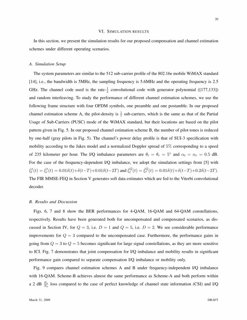
A. Simulation Setup

The system parameters are similar to the 512 sub-carrier profile of the 802.16e mobile WiMAX standard

[14], i.e., the bandwidth is 5MHz, the sampling frequency is 5.6MHz and the operating frequency is 2.5

GHz. The channel code used is the rate-12 convolutional code with generator polynomial ([177,133])

and random interleaving. To study the performance of different channel estimation schemes, we use the

following frame structure with four OFDM symbols, one preamble and one postamble. In our proposed

channel estimation scheme A, the pilot-density is 17 sub-carriers, which is the same as that of the Partial

Usage of Sub-Carriers (PUSC) mode of the WiMAX standard, but their locations are based on the pilot

pattern given in Fig. 5. In our proposed channel estimation scheme B, the number of pilot tones is reduced

by one-half (gray pilots in Fig. 5). The channel’s power delay profile is that of SUI-3 specification with

mobility according to the Jakes model and a normalized Doppler spread of 5% corresponding to a speed

of 235 kilometer per hour. The I/Q imbalance parameters are θt = θr = 5◦ and αt = αr = 0.5 dB.

For the case of the frequency-dependent I/Q imbalance, we adopt the simulation settings from [5] with

ξIt (t) = ξI

r (t) = 0.01δ(t)+δ(t−T )+0.01δ(t−2T ) and ξQt (t) = ξQ

r (t) = 0.01δ(t)+δ(t−T )+0.2δ(t−2T ).

The FIR MMSE-FEQ in Section V generates soft data estimates which are fed to the Viterbi convolutional

decoder.

B. Results and Discussion

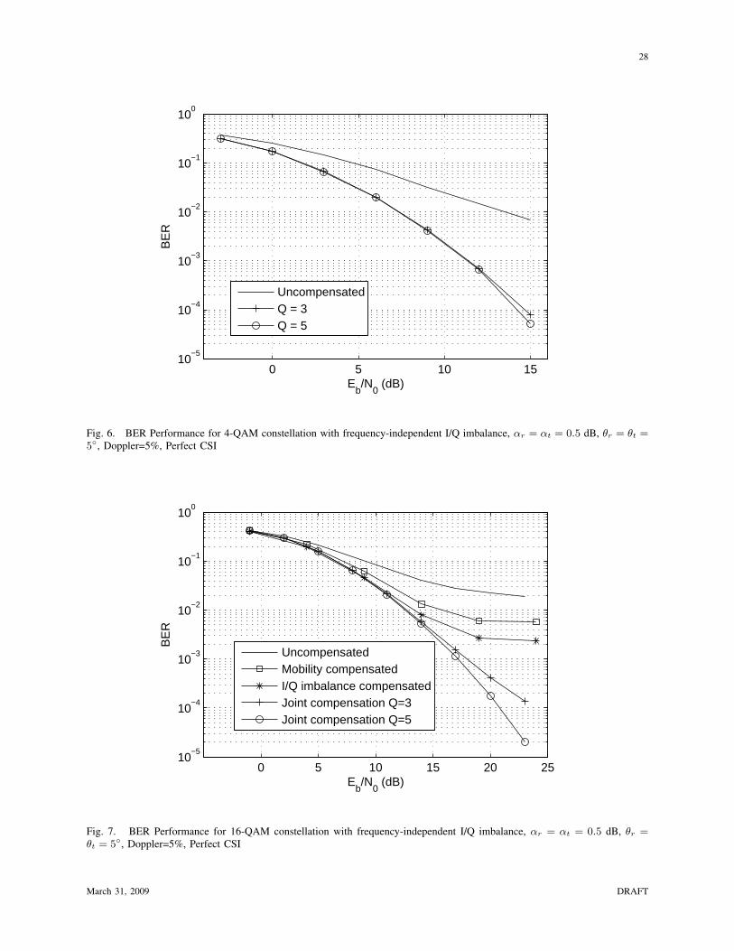
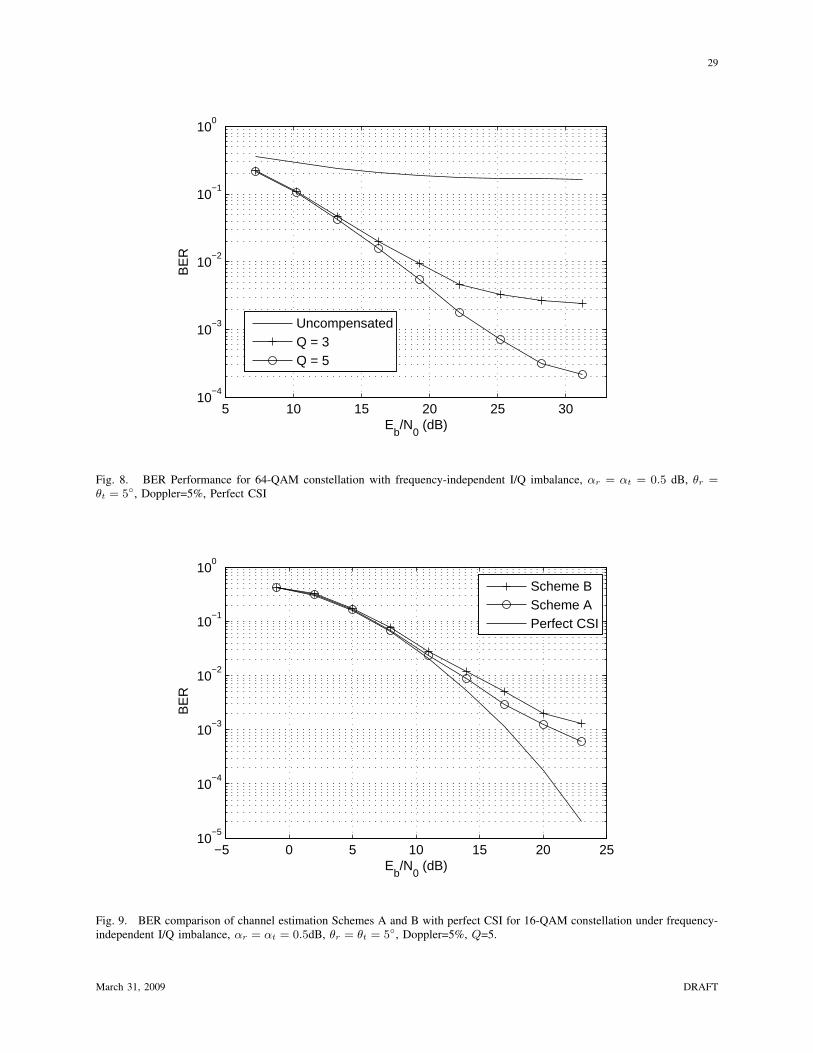
Figs. 6, 7 and 8 show the BER performances for 4-QAM, 16-QAM and 64-QAM constellations,

respectively. Results have been generated both for uncompensated and compensated scenarios, as dis-

cussed in Section IV, for Q = 3, i.e. D = 1 and Q = 5, i.e. D = 2. We see considerable performance

improvements for Q = 3 compared to the uncompensated case. Furthermore, the performance gains in

going from Q = 3 to Q = 5 becomes significant for large signal constellations, as they are more sensitive

to ICI. Fig. 7 demonstrates that joint compensation for I/Q imbalance and mobility results in significant

performance gain compared to separate compensation I/Q imbalance or mobility only.

Fig. 9 compares channel estimation schemes A and B under frequency-independent I/Q imbalance

with 16-QAM. Scheme-B achieves almost the same performance as Scheme-A and both perform within

a 2 dB Eb

N0loss compared to the case of perfect knowledge of channel state information (CSI) and I/Q


21

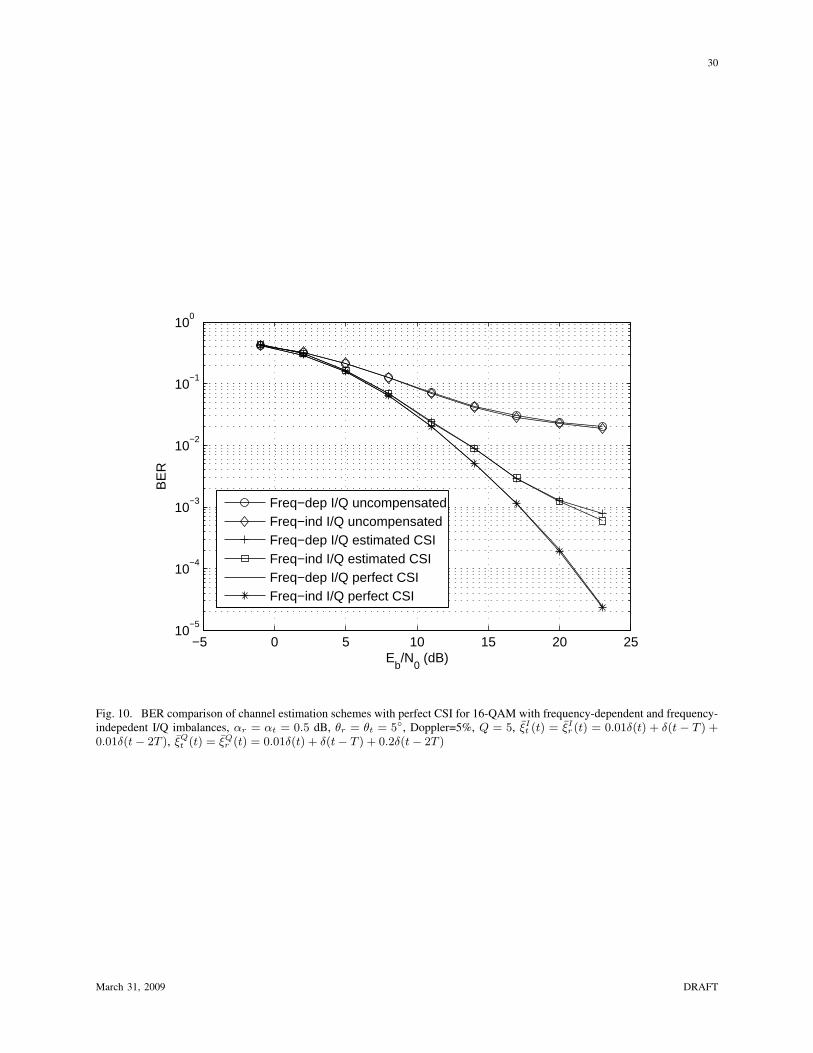
imbalance parameters. Fig. 10 compares the performance for 16-QAM with frequency-independent and

frequency-dependent I/Q imbalances. It is clear that our proposed channel estimation and compensation

schemes are quite effective in mitigating frequency-dependent I/Q imbalance even at high mobility.

VII. CONCLUSIONS

In this paper, we developed a generalized input-output model for mobile OFDM systems under both

frequency-independent and frequency-dependent joint transmit/receive I/Q imbalances. Based on this

generalized model, we derived a closed-form SINR expression as a function of the I/Q imbalance

parameters and Doppler spread. In addition, we presented a reduced-complexity FIR MMSE-FEQ digital

baseband compensation scheme and proposed an efficient channel estimation scheme which can be used

for both frequency-independent and frequency-dependent I/Q imbalances. To reduce the pilot overhead, we

proposed a second channel estimation scheme for frequency-independent I/Q imbalance. Our simulation

results show that our proposed joint compensation scheme using 6 taps per sub-carrier achieves significant

performance gains compared to the uncompensated case and also to schemes that compensate for I/Q

imbalance only or mobility only. The BER results of our proposed schemes are only within 2dB Eb

N0loss

from an ideal system with perfect knowledge of CSI and I/Q imbalance parameters.

APPENDIX A

SINR DEGRADATION ANALYSIS

In the section, all indices are from 0 to N − 1 and will be suppressed for brevity. Moreover, multiple

summations have also been combined together for brevity. For SINR analysis, we start by proving the

following proposition

Proposition: Given the Assumption-1 in Section-III, we have

E {g(k1, l1)g(k2, l2)} = 0 (52)

E{|g(k, l)|2} =

1N2

∑n1,n2

R(n1, n2)e−j 2π

N(k−l)(n1−n2) (53)

where R(n1, n2) is the normalized time-correlation function which is the same for each tap and the

relation between g(l, k) and g(n,m) is given by (19).

Proof: From the assumption that g(n,m) is circularly symmetric, we have the mean E{g(n,m)} = 0.

Combined with the fact that taps are uncorrelated for different m, this would imply that

E{g(n1,m1)g(n2,m2)} =

E{g(n1,m)g(n2,m)} m1 = m2 = m

0 m1 6= m2


22

Moreover, E{g(n1, m)g(n2,m)} is the pseudo-covariance function for tap m. Because of the circular-

symmetry assumption, this is equal to zero. Again, from the assumption of uncorrelated taps, we have

E{g(n1,m1)g∗(n2,m2)} =

E{g(n1,m)g∗(n2,m))} m1 = m2 = m

0 m1 6= m2

Now, E{g(n1,m)g∗(n2,m))} = Rm(n1, n2) is the time-correlation function of tap m. But each tap has

the same statistical behavior differing only in their average powers. Therefore, we can write Rm(n1, n2) =

σ2gm

R(n1, n2) where σ2gm

is the average power of tap m and R(n1, n2) is the normalized covariance

function common to all taps as defined in Section-III. So, we have the following

E{g(n1,m1)g(n2, m2)} = 0 (54)

E{g(n1,m1)g∗(n2, m2)} = σ2gm1

R(n1, n2)δ(m1 −m2) (55)

Using (19) and (54), we can obtain

E {g(k1, l1)g(k2, l2)} =1

N2

∑m1,n1,m2,n2

E {g(n1,m1)g(n2,m2)} e−j 2π

N(Q1+Q2) = 0

where Q1 = k1n1 − (n1 −m1)l1 and Q2 = k2n2 − (n2 −m2)l2. Moreover, using (19) and (55)

E{g(k1, l1)g∗(k2, l2)} =1

N2

∑m1,n1,m2,n2

E{g(n1,m1)g∗(n2,m2)}e−j 2π

N(Q1−Q2)

=1

N2

∑m

σ2gm

e−j 2π

Nm(l1−l2)

∑n1,n2

R(n1, n2)e−j 2π

N((k1n1−k2n2)−(l1n1−l2n2))

where m1 = m2 = m. For the special case of k1 = k2 and l1 = l2 and utilizing Assumption-III of

Section-III, the above equation simplifies to (53). This completes the proof of the proposition. Equation

(53) suggests that the average power of the (k, l) element in the frequency-domain channel matrix is

dependent only on the difference (k − l), i.e. elements in the same diagonal have same average power.

Next, we calculate the energy of S(k) and I(k) using the proposition. From (26), we know that

S(k) =[λr(k)λt(k)g(k, k) + φr(k)φ∗t (k

′)g∗(k′, k′)]

︸︷︷︸a

s(k)

+[λr(k)φt(k′)g(k, k′) + φr(k)λ∗t (k)g∗(k′, k)

]︸︷︷︸

b

s∗(k). (56)


23

We compute E{|S(k)|2} = E

{|s(k)|2(|a|2 + |b|2) + 2<{ab∗s2(k)}} ,

where E{|a|2} = |λr(k)|2|λt(k)|2E {|g(k, k)|2} + |φr(k)|2|φt(k′)|2E

{|g(k′, k′)|2} ,

E{|b|2} = |λr(k)|2|φt(k′)|2E

{|g(k, k′)|2} + |φr(k)|2|λt(k)|2E {|g(k′, k)|2} .

Let ab∗ = CR + jCI and s(k) = sR + jsI . Then,

E{<{

ab∗s2(k)}}

= E{CR(s2

R − s2I)− 2CIsRsI

}= E {CR}E

{s2R − s2

I

}−2E {CI}E {sR}E {sI} .

As a result of Assumption-2 of Section-III, we have E{s2R

}= E

{s2I

}and E {sR} = E {sI} = 0, and

hence E{<(ab∗s2(k))

}= 0. Then,

E{|S(k)|2} =

1N2

Es

[|λr(k)|2|λt(k)|2

∑n1,n2

R(n1, n2) + |φr(k)|2|φt(k′)|2∑n1,n2

R(n1, n2)

+|λr(k)|2|φt(k′)|2∑n1,n2

R(n1, n2)e−j 2π

N(2k(n1−n2)) + |φr(k)|2|λt(k)|2

∑n1,n2

R(n1, n2)ej 2π

N(2k(n1−n2))

],

where we have used the proposition to compute E{|g(., .)|2}.

Now, we need to compute the energy of the interference term I(k). The interference term in (30) can

be rewritten as

I(k) =∑

l 6=k

(λr(k)λt(l)g(k, l)s(l)︸︷︷︸

I1(l)

+φr(k)φ∗t (l′)g∗(k′, l′)s(l)︸︷︷︸I2(l)

+λr(k)φt(l′)g(k, l′)s∗(l)︸︷︷︸I3(l)

+φr(k)λ∗t (l)g∗(k′, l)s∗(l)︸︷︷︸

I4(l)

). (57)

We have introduced the new symbols I1(l), I2(l), I3(l) and I4(l), so we can write

E{|I(k)|2} =

∑

l1,l2 6=k

E {[I1(l1) + I2(l1) + I3(l1) + I4(l1)] [I∗1 (l2) + I∗2 (l2) + I∗3 (l2) + I∗4 (l2)]} . (58)

All terms of the type E{Ip(l1)I∗q (l2)} with p 6= q and of the type E{Ip(l1)I∗p (l2)} with l1 6= l2 are

zero, either because of (52) or because E{s(l1)s(l2)} = 0 which is a consequence of Assumption-2 of

Section-III. The non-zero terms (terms with p = q and l1 = l2 = l) are as follows

E{|I1(l)|2} = Es|λr(k)|2|λt(l)|2E{|g(k, l)|2} (59)

E{|I2(l)|2} = Es|φr(k)|2|φt(l′)|2E{|g(k′, l′)|2} (60)

E{|I3(l)|2} = Es|λr(k)|2|φt(l′)|2E{|g(k, l′)|2} (61)

E{|I4(l)|2} = Es|φr(k)|2|λt(l)|2E{|g(k′, l)|2}. (62)


24

Using (53) and noting that R(n1, n2) is the normalized time-correlation function, we have

EI1 =∑

l

E{|I1(l)|2} − E{|I1(k)|2}

=Es

N2|λr(k)|2

∑

n1,n2,l

R(n1, n2)|λt(l)|2e−j 2πN (k−l)(n1−n2) − |λt(k)|2

∑n1,n2

R(n1, n2)

(63)

In a similar manner, we can obtain

EI2 =Es

N2|φr(k)|2

∑

n1,n2,l

R(n1, n2)|φt(l′)|2e−j 2πN (k′−l′)(n1−n2) − |φt(k′)|2

∑n1,n2

R(n1, n2)

(64)

EI3 =Es

N2|λr(k)|2

∑

n1,n2,l

R(n1, n2)|φt(l′)|2e−j 2πN (k−l′)(n1−n2) − |φt(k′)|2

∑n1,n2

R(n1, n2)

(65)

EI4 =Es

N2|φr(k)|2

∑

n1,n2,l

R(n1, n2)|λt(l)|2e−j 2πN (k′−l)(n1−n2) − |λt(k)|2

∑n1,n2

R(n1, n2)

(66)

Finally, using (59) to (66), we can write E{|I(k)|2} = EI1 + EI2 + EI3 + EI4.

Colored noise variance: Consider the noise term in (15), namely v = Fv = FΛ′rw + FΦ′

rw∗. The

vector v is Gaussian distributed with zero-mean and its covariance matrix is given by

E{vvH

}= σ2(FΛ′

rΛ′Hr FH + FΦ′

rΦ′Hr FH), (67)

where E{w} = 0, E{wwT } = 0(N+NCP)×(N+NCP), E{wwH} = σ2I(N+NCP). To get an expression for

the noise power on the k-th sub-carrier, define ζ = Diag(FΛ′rΛ

′Hr FH + FΦ′

rΦ′Hr FH). If ζ(k) is the

k-th element of ζ, then

E{|v(k)|2} = σ2ζ(k). (68)

REFERENCES

[1] C. L. Liu, “Impacts of I/Q imbalance on QPSK-OFDM-QAM detection,” IEEE Trans. Consum. Electron., vol. 44, no. 3,

pp. 984–989, Aug. 1998.

[2] A. Schuchert, R. Hasholzne, and P. Anotine, “A novel I/Q imbalance compensation scheme for the reception of OFDM

signals,” IEEE Trans. Consum. Electron., vol. 47, no. 3, pp. 313–318, 2001.

[3] A. Tarighat, R. Bagheri, and A. H. Sayed, “Compensation schemes and peformance analysis of IQ imbalances in OFDM

receivers,” IEEE Trans. Signal Process., vol. 53, no. 8, pp. 3257–3268, Aug. 2005.

[4] A. Tarighat and A. H. Sayed, “Joint compensation of transmitter and receiver impairments in OFDM systems,” IEEE Trans.

Wireless Commun., vol. 6, no. 1, pp. 240–247, Jan. 2007.

[5] M. Valkama, M. Renfors, and V. Koivunen, “Compensation of frequency-selective I/Q imbalances in wideband receivers:

models and algorithms,” in IEEE Third Workshop on Signal Processing Advances in Wireless Communications (SPAWC

’01), Mar. 2001, pp. 42–45.


25

[6] J. Tubbax, B. Come, L. V. der Perre, L. Deneire, S. Donnay, and M. Engels, “Compensation of IQ imbalance in OFDM

systems,” in IEEE ICC, vol. 5, May 2003, pp. 3403 – 3407.

[7] P. Rykaczewski, J. Brakensiek, and F. Jondral, “Decision directed methods of I/Q imbalance compensation in OFDM

systems,” in IEEE VTC, vol. 1, Sept. 2004, pp. 484 – 487.

[8] D. Tandur and M. Moonen, “Joint adaptive compensation of transmitter and receiver IQ imbalance under carrier frequency

offset in OFDM-based systems,” IEEE Trans. Signal Process., vol. 55, no. 11, pp. 5246 – 5252, Nov. 2007.

[9] S. Lu, R. Kalbasi, and N. Al-Dhahir, “OFDM interference mitigation algorithms for doubly-selective channels,” in IEEE

Vehicular Technology Conference, Sep. 2006, pp. 1–5.

[10] G. Stuber, Principles of Mobile Communication. Springer, 2000.

[11] B. Narasimhan, S. Lu, N. Al-Dhahir, and H. Minn, “Digital baseband compensation of I/Q imbalance in mobile OFDM,”

in IEEE Wireless Communications and Networking Conference, Las Vegas, Mar. 2008, pp. 646–651.

[12] C. F. V. L. G. H. Golub, Matrix Computations. JHU Press, 1996.

[13] S. Kay, Fundamentals of statistical signal processing: estimation theory. Prentice Hall PTR, 1993.

[14] IEEE Std 802.16e-2005 and IEEE Std 802.16-2004/Cor1-2005, 28 Feb. 2006.

[15] Y. Mostofi and D. C. Cox, “ICI mitigation for pilot-aided OFDM mobile systems,” IEEE Trans. Wireless Commun., vol. 4,

pp. 765–774, Mar. 2005.

n

I nTtns )()(

I

tt

Q90

Sequence to

Impulse Train

)(tht )(tI

t

LPFImbalance

Filter)2cos(

I

tc

I

t tfa

)2sin(QQ

tct tfaSequence to Impulse Train

)(Q

tt

n

nTtns )()(Q

)(tsI

)(Q

ts

)(nsI

)(Q nsLPF

ImbalanceFilter

),(tpg Channel

)(twp

AWGN

I

rr

Q90

)2cos(I

rc

I

r tfa

)2sin(QQ

rcr tfa

LPFImbalance

Filter

LPFImbalance

Filter

)(tI

r

)(Q

tr

)(thr

)(Q tr

)(trI

)(tht

)(thr

)(Q tu

)(I tu

)(typ

)(tpx

Fig. 1. Block diagram of the joint I/Q imbalance and mobility model


26

( )*

),(tg

)(tw

AWGN

)(ty

)(tx)(ts

)(tt )(tr

)(tr)(tt

Channel( )*

)(th r

Fig. 2. Block diagram of the equivalent model

0 5 10 15 20 25 30 35 40 45 50−5

0

5

10

15

20

25

30

SNR (dB)

SIN

R (

dB)

αr=α

t=0.1dB, θ

r=θ

t=1°, Doppler=1%

αr=α

t=0.1dB, θ

r=θ

t=1°, Doppler=5%

αr=α

t=0.1dB, θ

r=θ

t=1°, Doppler=10%

αr=α

t=0.5dB, θ

r=θ

t=5°, Doppler=1%

αr=α

t=0.5dB, θ

r=θ

t=5°, Doppler=5%

αr=α

t=0.5dB,θ

r=θ

t=5°, Doppler=10%

Fig. 3. SINR comparison with different I/Q imbalance and Doppler parameters

TABLE IVERIFYING THE BANDED APPROXIMATION (ASSUMED I/Q IMBALANCE PARAMETERS : 1dB, 5◦)

Matrix Γ(1) Matrix Γ(2)

Doppler subdiagonal index 0 1 2 3 >3 Full matrix5% percentage of energy 99.25 0.45 0.11 0.05 <0.03 <0.0410% percentage of energy 97.7 1.4 0.35 0.15 <0.1 <0.08


27

0 50 100 150 200

0

5

10

15

20

25

30

35

ηr=η

t=η

SIR

(dB

)

1% Doppler5% Doppler

αt=α

r=0.1dB, θ

t=θ

r=1°

αt=α

r=0.5dB, θ

t=θ

r=5°

Fig. 4. SIR variation with different I/Q imbalance parameters

k N-k freq

DC

Fig. 5. Pilot Pattern

TABLE IICOMPUTATIONAL COMPLEXITY (IN FLOPS) FOR DIFFERENT COMPENSATION SCENARIOS

N\ taps Q = 3 Q = 5 Q = N

64 2.98× 105 1.37× 106 1.12× 107

512 2.38× 106 1.10× 107 5.73× 109

1024 4.77× 106 2.19× 107 4.58× 1010


28

0 5 10 1510

−5

10−4

10−3

10−2

10−1

100

Eb/N

0 (dB)

BE

R

UncompensatedQ = 3Q = 5

Fig. 6. BER Performance for 4-QAM constellation with frequency-independent I/Q imbalance, αr = αt = 0.5 dB, θr = θt =5◦, Doppler=5%, Perfect CSI

0 5 10 15 20 2510

−5

10−4

10−3

10−2

10−1

100

BE

R

Eb/N

0 (dB)

UncompensatedMobility compensatedI/Q imbalance compensatedJoint compensation Q=3Joint compensation Q=5

Fig. 7. BER Performance for 16-QAM constellation with frequency-independent I/Q imbalance, αr = αt = 0.5 dB, θr =θt = 5◦, Doppler=5%, Perfect CSI


29

5 10 15 20 25 3010

−4

10−3

10−2

10−1

100

Eb/N

0 (dB)

BE

R

UncompensatedQ = 3Q = 5

Fig. 8. BER Performance for 64-QAM constellation with frequency-independent I/Q imbalance, αr = αt = 0.5 dB, θr =θt = 5◦, Doppler=5%, Perfect CSI

−5 0 5 10 15 20 2510

−5

10−4

10−3

10−2

10−1

100

Eb/N

0 (dB)

BE

R

Scheme BScheme APerfect CSI

Fig. 9. BER comparison of channel estimation Schemes A and B with perfect CSI for 16-QAM constellation under frequency-independent I/Q imbalance, αr = αt = 0.5dB, θr = θt = 5◦, Doppler=5%, Q=5.


30

−5 0 5 10 15 20 2510

−5

10−4

10−3

10−2

10−1

100

Eb/N

0 (dB)

BE

R

Freq−dep I/Q uncompensatedFreq−ind I/Q uncompensatedFreq−dep I/Q estimated CSIFreq−ind I/Q estimated CSIFreq−dep I/Q perfect CSIFreq−ind I/Q perfect CSI

Fig. 10. BER comparison of channel estimation schemes with perfect CSI for 16-QAM with frequency-dependent and frequency-indepedent I/Q imbalances, αr = αt = 0.5 dB, θr = θt = 5◦, Doppler=5%, Q = 5, ξI

t (t) = ξIr (t) = 0.01δ(t) + δ(t − T ) +

0.01δ(t− 2T ), ξQt (t) = ξQ

r (t) = 0.01δ(t) + δ(t− T ) + 0.2δ(t− 2T )


Digital Compensation of Frequency-Dependent Joint Tx/Rx I/Q Imbalance in OFDM Systems Under High...

Documents

Transcript of Digital Compensation of Frequency-Dependent Joint Tx/Rx I/Q Imbalance in OFDM Systems Under High...