Diffusive and ebullitive transport of methane and nitrous oxidefrom streams: Are bubble-mediated fluxes important?

Helen M. Baulch,1,2 Peter J. Dillon,3 Roxane Maranger,4 and Sherry L. Schiff5

Received 14 January 2011; revised 12 July 2011; accepted 28 September 2011; published 15 December 2011.

[1] Using measured rates of bubble release and diffusive gas transport (also termed surfaceaeration), we address the role of these transport mechanisms in emissions of nitrous oxideand methane from four streams. While ebullition in streams and rivers has received littlestudy, we found that ebullition was an important mode of methane emissions, contributing20%–67% of methane emissions (among streams). Nitrous oxide emissions via ebullitionwere negligible (<0.1% of diffusive emissions). Total methane emissions (ebullition +diffusive transport) were over ten times greater than N2O emissions in terms of CO2

equivalents. Rates of bubble release were highly variable, ranging from 20 mL m�2 d�1 to170 mL m�2 d�1 (seasonal average among streams, with volumes reflecting ambienttemperature and pressure). Methane was the most abundant of the bubble gases thatwere measured (26% by volume on average among streams), followed by carbon dioxide(1% on average) then nitrous oxide. Average bubble nitrous oxide concentrations werebelow atmospheric mixing ratios for the majority of streams; however, one stream showedconcentrations as high as 3600 ppbv. Sediment characteristics were strong predictors ofbubble composition. Concentrations of methane and nitrous oxide were positively related tothe proportion of fine sediments. High methane concentrations in bubbles were related tohigh sediment organic carbon.

Citation: Baulch, H. M., P. J. Dillon, R. Maranger, and S. L. Schiff (2011), Diffusive and ebullitive transport of methane andnitrous oxide from streams: Are bubble-mediated fluxes important?, J. Geophys. Res., 116, G04028, doi:10.1029/2011JG001656.

1. Introduction

1.1. Aquatic Ecosystems as Sources of GreenhouseGases

[2] On a global basis, lakes, reservoirs and wetlands have asignificant role in global greenhouse gas balances. Lakeemissions have been estimated at 70–150 Tg y�1 of carbon inthe form of carbon dioxide (CO2-C) [Cole et al., 2007]although a recent reassessment places this number as high as530 Tg CO2-C y�1 [Tranvik et al., 2009]. Methane (CH4)emissions from lakes are on the order of 8–48 Tg y�1

[Bastviken et al., 2004], but this number may also be anunderestimate [Walter et al., 2006]. Wetland CH4 emissionsare globally more significant than lakes at between 145 and231 Tg of CH4 per year [Denman et al., 2007]; however,many wetlands appear to be net sinks of CO2 [Bridgham

et al., 2006]. Reservoirs are important not only for theirlarge emissions, but also because they are considered a formof land-use change, and are factored into anthropogenicgreenhouse gas budgets. Emissions from reservoirs are esti-mated at 280 Tg of CO2-C [Cole et al., 2007], and 70 Tg ofCH4 per year globally [St. Louis et al., 2000].[3] Fluvial systems have received less study in terms of

their role in CH4 emissions [Bastviken et al., 2011]; however,existing data suggest that they function as CH4 sources to theatmosphere [Jones and Mulholland, 1998]. The greenhousegas receiving significant study in fluvial ecosystems isnitrous oxide (N2O), due to an early model suggesting thatagricultural and sewage N inputs into streams, rivers andestuaries could lead to 20% of the world’s anthropogenicN2O emissions [Seitzinger and Kroeze, 1998]. Based onaccumulating evidence that river and stream emissionsare overestimated, the IPCC has recently downscaled N2Oemissions estimates from fluvial ecosystems [Egglestonet al., 2006]. However, new data suggests IPCC methodsmay now significantly underestimate riverine N2O fluxes[Beaulieu et al., 2011]. Carbon dioxide emissions from riversare estimated as 230 Tg CO2-C per year [Cole et al., 2007].Estimates of stream fluxes (based on stream heterotrophy,which likely represent a lower bound for emissions) suggestthat stream emissions are greater than river emissions at320 Tg CO2-C y�1 [Battin et al., 2008]. These high fluxesare supported by measurements from boreal streams wherestreams function as strong CO2 sources in the landscape

1Environmental and Life Sciences Graduate Program, Trent University,Peterborough Ontario, Canada.

2Now at the School of Environment and Sustainability and the GlobalInstitute for Water Security, National Hydrology Research Centre,University of Saskatchewan, Saskatoon, Saskatchewan, Canada.

3Department of Environmental and Resource Studies, Trent University,Peterborough, Ontario, Canada.

4Department of Biological Sciences, University of Montreal, Montreal,Quebec, Canada.

5Department of Earth and Environmental Sciences, University ofWaterloo, Waterloo, Ontario, Canada.

Copyright 2011 by the American Geophysical Union.0148-0227/11/2011JG001656

JOURNAL OF GEOPHYSICAL RESEARCH, VOL. 116, G04028, doi:10.1029/2011JG001656, 2011

G04028 1 of 15

[Teodoru et al., 2009]. In sum, inland waters may emit asmuch as 1400 Tg CO2-C per year [Tranvik et al., 2009].

1.2. Production and Emission of Greenhouse Gases

[4] Numerous pathways contribute to greenhouse gasproduction. Classical denitrification can lead to N2O pro-duction, as do the pathways nitrification and nitrifier-denitrification. The two dominant CH4 production pathwaysare acetate fermentation (aceticlastic methanogenesis) andH2-dependent (hydrogenotrophic) methanogenesis. Aerobicrespiration, denitrification, aceticlastic methanogenesis andother pathways contribute to CO2 production.[5] Gases are emitted from aquatic ecosystems by three

major mechanisms. The first and most frequently studied isdiffusive transport (also referred to as air-water gas exchangeor surface aeration). However, plant and bubble-mediated(ebullitive) transport can be important, particularly for CH4

[Dacey and Klug, 1979;Walter et al., 2006]. Gas bubbles canbe formed in sediments when the partial pressure of the gasesexceeds the sum of the pressure on the sediment and thesurface tension of water. Hence, bubble production dependson rates of gas production as well as water temperature, waterdepth, and barometric pressure. Bubble emissions tend to beepisodic, triggered by shear stress [Joyce and Jewell, 2003],lowering of the water table [Chanton et al., 1989], or periodsof low atmospheric pressure [Mattson and Likens, 1990].[6] A major limitation of our understanding of the impor-

tance of streams and rivers in greenhouse gas emissions isin our focus on diffusive gas transport across the air-waterinterface. The importance of bubble-mediated emissions,especially of N2O, has largely been overlooked with theassumption that diffusive transport is the dominant emissionmechanism. We assess this assumption in a series of streamsin southern Ontario, Canada by contrasting rates of gastransport via these two mechanisms. We also assess rates ofCH4 emissions and the role of ebullition in CH4 transport – atopic that has received relatively little study in small streams.Finally, we identify predictors of gas concentrations andfluxes among streams.

2. Site Description

[7] We studied four 2nd–5th order (Strahler) streams insouthern Ontario, Canada. These are north temperate, hardwater streams, with significant agricultural land use in theircatchments. Monoculture (continuous cultivation of annual

crops) constitutes 13%–22% of land area, mixed cropping(rotations of annual and forage crops) constitutes 10%–31%of land area, rural land uses (forage crops, idle lands, hay,pasture and marginal lands) include 12%–44% of catchmentareas, and wetlands constitute 9%–25% of land area. Urbanareas are <3% of catchment areas in all streams [OntarioMinistry of Natural Resources, 2006]. The highest propor-tion of wetland area is observed in Layton Creek (25%of catchment) and Jackson Creek (21% of catchment), whilethe greatest proportion of wooded area is in the Black River(24%) and lowest proportion in Mariposa Brook (9%).Mariposa Brook has the greatest proportion of land in agri-cultural land use (monoculture, mixed or rural). We sampledtwo sites (separated by 3.9–8.2 km; Table 1) in each stream.Land use data reflect the most downstream site sampled[Baulch, 2009]. Study streams and sampling sites wereselected to represent small streams of this region, whileensuring easy access, and minimizing the number of inflowsbetween sites. All streams were shallow (<50 cm meandepth), with relatively low slope (0.25 to 1.43°; Table 1).A map of study sites, and additional site characterization dataare available elsewhere [Baulch et al., 2011a].

3. Materials and Methods

[8] At each site, we measured stream discharge and waterchemistry, the rate of bubble release, bubble gas concentra-tions, and the rate of gas emissions driven by diffusivetransport (determined using measurement of piston velocityand dissolved gas concentrations). Sediment analyses werealso performed at each site.

3.1. Water Chemistry, Stream Discharge,Temperature, Pressure

[9] Water samples were obtained in �500 mL PET bottlesfrom midstream. A total organic carbon analyzer (ShimadzuTOC-V analyzer) was used to analyze concentrations ofdissolved organic carbon (GFF filtered). pH was measuredusing electrodes (Mantech PC titrator; Mantech Inc, GuelphCanada). Nitrogen species were GFF filtered then analyzedcolorimetrically. Nitrate was analyzed using the red azodye method, following reduction to nitrite, then correctedfor measured nitrite [Ministry of the Environment, 2001].Ammonium was analyzed using the phenate-hypochloritemethod [Ministry of the Environment, 2001]. Samples fortotal phosphorus analysis were obtained directly in glass

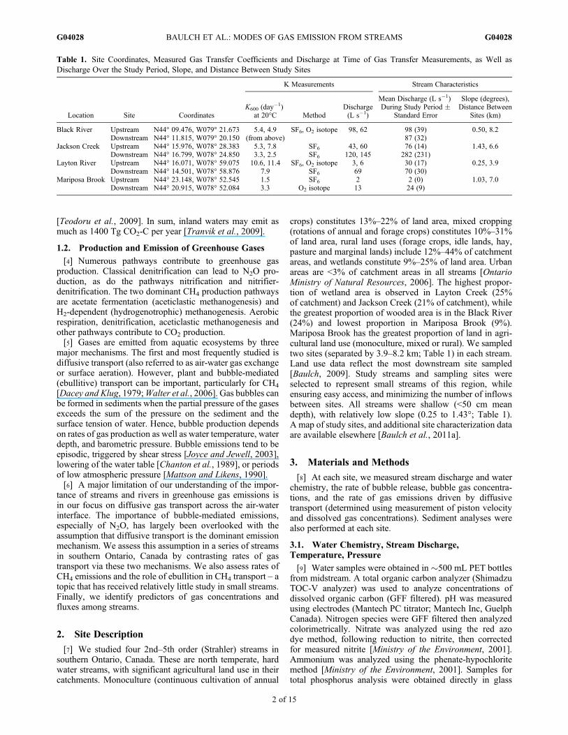
Table 1. Site Coordinates, Measured Gas Transfer Coefficients and Discharge at Time of Gas Transfer Measurements, as Well asDischarge Over the Study Period, Slope, and Distance Between Study Sites

Location Site Coordinates

K Measurements Stream Characteristics

K600 (day�1)

at 20°C MethodDischarge(L s�1)

Mean Discharge (L s�1)During Study Period �

Standard Error

Slope (degrees),Distance Between

Sites (km)

Black River Upstream N44° 09.476, W079° 21.673 5.4, 4.9 SF6, O2 isotope 98, 62 98 (39) 0.50, 8.2Downstream N44° 11.815, W079° 20.150 (from above) 87 (32)

Jackson Creek Upstream N44° 15.976, W078° 28.383 5.3, 7.8 SF6 43, 60 76 (14) 1.43, 6.6Downstream N44° 16.799, W078° 24.850 3.3, 2.5 SF6 120, 145 282 (231)

Layton River Upstream N44° 16.071, W078° 59.075 10.6, 11.4 SF6, O2 isotope 3, 6 30 (17) 0.25, 3.9Downstream N44° 14.501, W078° 58.876 7.9 SF6 69 70 (30)

Mariposa Brook Upstream N44° 23.148, W078° 52.545 1.5 SF6 2 2 (0) 1.03, 7.0Downstream N44° 20.915, W078° 52.084 3.3 O2 isotope 13 24 (9)

BAULCH ET AL.: MODES OF GAS EMISSION FROM STREAMS G04028G04028

2 of 15

vials, then analyzed using the ammonium-molybdate-stannous chloride method [Ministry of the Environment,1994].[10] Depth, velocity, and discharge were measured at

each site using a Swoffer 2100 velocity meter and apply-ing the velocity-area method. Air and water temperatureswere measured using a Fisherbrand Traceable Thermometer.Barometric pressure was measured using a handheldbarometer (Kestrel).

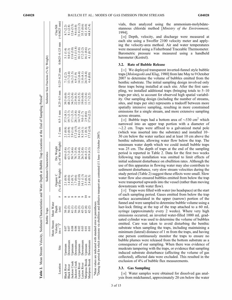
3.2. Rate of Bubble Release

[11] We deployed transparent inverted-funnel style bubbletraps [Molongoski and Klug, 1980] from lateMay to 9 October2007 to determine the volume of bubbles emitted from thebenthic substrate. The initial sampling design involved onlythree traps being installed at each site. After the first sam-pling, we installed additional traps (bringing totals to 5–10traps per site), to account for observed high spatial variabil-ity. Our sampling design (including the number of streams,sites, and traps per site) represents a tradeoff between morespatially intensive sampling, resulting in more constrainedemissions for a single stream, and more extensive samplingacross streams.[12] Bubble traps had a bottom area of �530 cm2 which

narrowed into an upper trap portion with a diameter of�2.2 cm. Traps were affixed to a galvanized metal pole(which was inserted into the substrate) and installed 10–30 cm below the water surface and at least 10 cm above thebenthic substrate, allowing water flow below the trap. Theminimum water depth which we could install bubble trapswas 25 cm. The depth of traps at the end of the samplingperiod is reported in Table 2. Data for the first two weeksfollowing trap installation was omitted to limit effects ofinitial sediment disturbance on ebullition rates. Although theuse of this apparatus in flowing water may also contribute tosediment disturbance, very slow stream velocities during thestudy period (Table 2) suggest these effects were small. Slowwater flow also ensured bubbles emitted from below the trapwere transported upwards into the vessel (rather than movingdownstream with water flow).[13] Traps were filled with water (no headspace) at the start

of each sampling period. Gases emitted from below the trapsurface accumulated in the upper (narrow) portion of thefunnel and were sampled to determine bubble volume using aluer-lock fitting at the top of the trap attached to a 60 mLsyringe (approximately every 2 weeks). Where very highemissions occurred, an inverted water-filled 1000 mL grad-uated cylinder was used to determine the volume of bubblesemitted. Care was taken to avoid disturbing the benthicsubstrate when sampling the traps, including maintaining aminimum (lateral) distance of 1 m from the traps, and havingone person continuously monitor the traps to ensure nobubble plumes were released from the bottom substrate as aconsequence of our sampling. When there was evidence ofmuskrats tampering with the traps, or evidence that samplinginduced substrate disturbance (affecting the volume of gascollected), affected data were excluded. This resulted in theexclusion of 4% of bubble flux measurements.

3.3. Gas Sampling

[14] Water samples were obtained for dissolved gas anal-ysis from midchannel, approximately 20 cm below the waterT

able

2.MeanStream

Velocity

,Sedim

entCharacteristicsandWater

Depth

atBub

bleTrapLocations

attheEnd

ofSam

plingPerioda

Location

Site

Bub

bleTraps

Sedim

entCharacteristics

Sedim

entSizeFractions

(%by

Weigh

t)

MeanStream

Velocity

(ms�

1)b

MeanWater

Depth

(cm)

#Organic

C(%

ofDry

Weigh

t)Dry

Weigh

t(%

ofWet

Weigh

t)1–2mm

0.5–1mm

0.25–0.5

mm

0.12

5–0.25

mm

0.06

25–0

.125

mm

Clay/Silt

(<0.06

25mm)

Black

River

Upstream

0.07

38(5)

82.1(0.9)

69.6

(3.6)

2.1(0.8)

37.5

(8.1)

39.5

(6.0)

7.1(2.2)

5.1(1.4)

8.7(2.2)

Black

River

Dow

nstream

0.07

56(3)

61.4(0.6)

63.7

(3.7)

2.3(0.9)

19.7

(3.7)

48.2

(3.3)

13.7

(2.4)

8.0(1.3)

8.1(2.8)

JacksonCreek

Upstream

0.08

41(1)

82.5(0.7)

50.7

(4.6)

5.9(1.6)

17.1

(3.3)

34.5

(5.6)

16.2

(1.5)

13.8

(3.0)

12.6

(5.5)

JacksonCreek

Dow

nstream

0.06

59(3)

91.7(0.6)

78.7

(3.9)

17.2

(4.5)

28.1

(5.6)

22.9

(6.5)

6.9(1.9)

15.3

(11.8)

9.6(4.0)

LaytonRiver

Upstream

0.02

56(3)

818

.6(2.0)

24.3

(4.4)

8.4(3.3)

14.7

(5.4)

12.8

(5.5)

14.2

(6.4)

18.1

(3.8)

31.8

(11.2)

LaytonRiver

Dow

nstream

0.03

45(2)

914

.1(1.3)

26.5

(2.8)

8.3(4.1)

9.0(1.7)

19.0

(4.0)

11.0

(4.1)

17.2

(3.2)

35.5

(8.6)

MariposaBrook

Upstream

0.01

65(4)

102.5(0.2)

46.4

(3.1)

1.1(0.3)

2.9(0.6)

13.5

(3.6)

24.3

(4.4)

16.1

(0.6)

42.1

(6.0)

MariposaBrook

Dow

nstream

0.01

42(2)

62.4(0.3)

69.9

(4.3)

17.3

(2.4)

17.6

(2.2)

11.7

(2.2)

4.4(0.8)

4.1(0.7)

44.8

(7.4)

a Meanvalues

areindicatedwith

standard

errorin

parentheses.

bDuringtheperiod

forwhich

emission

sviaebullitionanddiffusivetransportare

contrasted

(11June–11Octob

er20

07).

BAULCH ET AL.: MODES OF GAS EMISSION FROM STREAMS G04028G04028

3 of 15

surface. Sampling was performed at each study site on 9–10 occasions (between 15May to 30 October 2007). Sampleswere taken in 125 mL borosilicate glass serum bottleswith no headspace, capped with pre-baked butyl rubberstoppers and field preserved with saturated mercuric chloride(0.4% final v/v).[15] Following sampling for dissolved gases, trapped

bubble volume and water chemistry, we obtained bubblesamples from the benthic substrate for analysis of bubble gasconcentrations. Samples were obtained by walking transectsof the stream channel (perpendicular to streamflow at eachsite) and periodically disturbing the benthic substrate with afunnel attached to the body of a 60 mL syringe and luer-transfer port. Multiple transects were walked until at least30 mL of gas was obtained, which was then transferred intoa pre-evacuated vial. This process was then repeated 3 timesto obtain triplicate samples which were analyzed using gaschromatography (GC). Bubble gas sampling was performedon 9 or 10 dates at each study site (see results for exacttiming).[16] We opted to analyze fresh bubbles from the sediments

rather than those trapped within the headspace of bubbletraps because bubbles within the traps will undergo equili-bration with stream water. However, fresh bubbles may haveundergone further equilibration with surrounding pore watersprior to natural emission. In addition, bubbles undergoequilibration as they travel through the water column to thesurface. Because the length of the apparatus used in freshbubble sampling (�40 cm) was sometimes less than thestream depth (Table 2), the extent of equilibration may havediffered between naturally emitted samples and the values wereport. This effect is most important for highly soluble orreactive gases such as H2S and CO2. In contrast, effects onN2O and CH4 are expected to be minimal [Chanton andWhiting, 1995]. However, our CO2 measurements couldrepresent a slight overestimate of the CO2 concentration thesame bubbles would attain at the water-air interface.

3.4. Gas Analyses

[17] Dissolved gas samples were analyzed using a VarianCP-3800 gas chromatograph following headspace equilibra-tion. CH4 was analyzed by FID following separation using aHayesep D column (80/100 mesh, 0.5 m, 1/8” stainless steel).N2O was analyzed by ECD using the same column. Equi-librium concentrations for dissolved gases were calculatedusing measured temperature and barometric pressure[Yamamoto et al., 1976; Weiss and Price, 1980], assumingatmospheric concentrations of 320 ppbv N2O and 1.85 ppmvCH4. Given the long atmospheric residence time of N2O, it isexpected to be well mixed in the atmosphere [Stein and Yung,2003], which supports our assumption of atmospheric mix-ing ratios. However, regional variation in CH4 concentrationsis likely, and our assumption of constant atmospheric con-centrations may bias our flux estimates. Where dissolvedCH4 is highly supersaturated, this will have only small effectson CH4 flux estimates (i.e., see equation (1)).[18] All samples were obtained during the daytime. This

may result in a slight underestimate of diffusive CH4 fluxes.Diel sampling of these streams indicated that sampling nearsolar noon underestimated diffusive CH4 fluxes by 9% inthese streams, when compared to time-weighted samples

over a 24-h sampling period [Baulch, 2009]. Daytime sam-pling underestimates diffusive N2O flux from these streamsby �5% [Baulch, 2009]. Lateral variation in dissolved gasconcentrations across the stream channel was observed(average of 6% for N2O, 11% for CH4), but systematic dif-ferences between samples obtained from the middle of thestream channel and samples obtained near stream banks werenot observed.[19] Bubble samples were analyzed on two instruments.

Approximately 60% of samples were analyzed on the Variangas chromatograph as described previously. The remainderof samples were analyzed using a Shimadzu GC-2014 with aTekmar 7050 autosampler and 9 mL vials with thick butylrubber septa. Gases were separated on a Poropaq Q column(80/100 mesh size). Samples for CH4 analyses were dilutedwith UHP N2 or helium. Duplicate bubble samples run onboth gas chromatographs showed agreement within 3%(CH4), 2% (CO2), and 7% (N2O) between instruments.

3.5. Gas Emissions via Ebullition

[20] The masses of N2O, CO2 and CH4 released by ebul-lition were calculated by determining the number of moles oftotal bubble gas released (using measured volume, air tem-perature and atmospheric pressure), and multiplying thisvalue by measured gas concentrations in the fresh bubbles(at the start and end of the sampling period) for each site.Average, time-weighted emissions were then calculated,accounting for the duration of each sampling interval. Errorin ebullitive flux estimates was estimated using Monte Carlouncertainty analysis [Beck, 1987]. This method allows us toconstrain uncertainty associated with both the volume ofbubbles, and bubble gas concentrations. The volume of gasesemitted and the concentration of gases were represented as anormal distribution using measured means and standarddeviations, and truncating distributions to omit negativevalues [Decisioneering, Inc., 2001]. Ebullitive emissions ofboth N2O and CH4 were estimated by subsampling thesedistributions 1000 times using stratified random (LatinHypercube) sampling in the software package Crystal Ball2000.2 (Decisioneering, Inc., Denver, Colo.), resulting in aprobability distribution for ebullitive gas fluxes.

3.6. Gas Emissions via Diffusive Transport

[21] Gas fluxes due to diffusive transport were estimatedusing the two-layer model of diffusive gas exchange [Lissand Slater, 1974]:

Flux ¼ k CS � CLð Þ; ð1Þ

where k is the piston velocity (m h�1). The piston velocity issometimes termed the gas transfer velocity, and is equal tothe gas transfer coefficient K times the mean depth; CS issaturation concentration (mmol m�3); CL is the measuredconcentration (mmol m�3).[22] In this model, there are two interfacial layers, one in

the water at the water surface, and one in air, immediatelyoverlying the water surface. For CH4 and N2O, air-phaseresistance is negligible [Liss and Slater, 1974], and the mainresistance to gas transfer across the air-water interface ismolecular diffusion through the surface layer of the water.The depth of this surface layer, which dictates the length of

BAULCH ET AL.: MODES OF GAS EMISSION FROM STREAMS G04028G04028

4 of 15

the diffusion pathway, is related to turbulence. Within shal-low fluvial ecosystems, benthic turbulence is the primaryprocess affecting rates of gas exchange [Raymond and Cole,2001].[23] Our measurements of rates of air-water gas transfer

(Table 1) are described in detail elsewhere [Baulch et al.,2011a]. Briefly, we measured rates of air-water gas transfervia addition of a gas tracer (sulphur hexafluoride; analysis byGC-ECD as for N2O) and a conservative tracer at six of oureight study sites [Kilpatrick et al., 1987; Baulch, 2009]. Wealso used diel O2 dynamics to constrain the piston velocity[Venkiteswaran et al., 2007]. This method uses an O2-massbalance model, iteratively fit using constrained range ofpossible rates for respiration (0–5000 mg O2 m�2 h�1),photosynthesis (0–5000 mg O2 m

�2 h�1) and piston velocity(0.01 to 0.50 m h�1) [Venkiteswaran et al., 2007]. The modelwas run with different parameter combinations (i.e., ratesof respiration, photosynthesis and piston velocity) to obtainthe lowest sums of squares between measured and modeleddata. All model runs where an r2 of >0.8 were averaged toobtain a mean estimated piston velocity.[24] In one stream (Black River) where substrate, depth,

and flow varied little between sites (mean differences: pro-portion substrate >0.25 mm, 11%; mean depth 16%; meandischarge 9%), we used upstream gas transfer measurementsto estimate gas transfer at our downstream site. At all othersites, one or two direct measurements of gas transfer weremade at each study site (Table 1). Measured rates of gastransfer were converted to the stream temperature [Thomannand Mueller, 1987] and gas of interest (from SF6 or O2 toCH4 or N2O) using Schmidt number scaling [Wanninkhof,1992]. We assumed a Schmidt number exponent of 2/3which reflects smooth surfaces (in contrast to rough sur-faces, where a Schmidt number exponent of 1/2 is typicallyassumed [Jähne et al., 1987]). We report rates of air-watergas transfer in customary units, as the gas transfer coefficientfor CO2 at 20°C (K600; Table 1).[25] Depth, velocity, slope and substrate type are important

factors affecting benthic turbulence, and depth and velocitycan vary over time (Table 1). To account for this temporalvariation which is likely to affect rates of gas transfer, we usetwo approaches. First, in 5 of 8 study sites we use two mea-surements of gas transfer coefficient (Table 1) and reportthe range of estimates resulting from these measured values(in the remaining 3 sites, only a single measurement wasmade). This assumes that gas transfer coefficient was con-stant through the study period. Second, we applied a model-based approach to extrapolate measured values to differentflow conditions (varying depth and velocity) [Moog and Jirka,1998]. We calibrated three empirical models [O’Connor andDobbins, 1958; Bennett and Rathburn, 1972; Owens et al.,1964] to individual sites, using the ratio of measured K tomodeled K under the flow conditions when K was deter-mined [see equation (2);Moog and Jirka, 1998], then appliedthese calibrated empirical models to predict gas transfercoefficient, using measurements of stream depth and velocityfor each sampling occasion. The use of three models isintended to reflect error associated with model assumptions.

KPC ¼ ∑ Km=KPð Þn

� �KP; ð2Þ

where KPC is the calibrated gas transfer coefficient, Km isthe measured gas transfer coefficient, KP is the predicted gastransfer coefficient under measurement conditions, and nreflects the number of measurements. This equation ispresented in its original form, which uses the gas transfercoefficient, a value equal to the piston velocity (k) dividedby depth.[26] We used KPC values to determine whether dissolved

gases at upstream sampling sites were likely to affect gascomposition at the downstream location. In all cases, thedistance between sampling sites was great enough that dis-solved gases at upstream sites had minimal effects (<5%) onconcentrations at downstream sites based on first-order lossequations [Chapra and Di Toro, 1991]:

Dist5% ¼ 3v

KPC; ð3Þ

whereDist5% is the distance at which 5% of a gas will remainin solution, v is stream velocity and KPC is the calibrated gastransfer coefficient.[27] Dissolved gas concentrations and bubble gas concen-

trations are reported for the period 15 May to 30 October2007. Emissions via diffusive transport and ebullition arecalculated from 11 June to 11 October 2007 for the BlackRiver, Jackson Creek and Layton Creek. However, in Mar-iposa Brook, where changes in discharge led to changes inpiston velocity and added considerable uncertainly to ourdiffusive transport estimates, we restrict the time series to3 July to 12 September 2007 (upstream site) and 11 June to12 September 2007 (downstream site). Mean (time-weighted)diffusive flux estimates for the study period were determinedusing mean fluxes for each sampling interval (mean of startand end of each period), then multiplying by the duration ofthat interval, and dividing by the length of the study period.

3.7. Sediment Analyses

[28] Duplicate sediment cores were obtained from undereach bubble trap at the end of the study (October 2007). APVC core tube (10 cm diameter, 7 cm depth) was pressed intothe stream substrate. The base was sealed from below using aplastic sheet or hand, then the core tube was removed, and itscontents were transferred to pre-labeled bags. At two sites(Mariposa Brook, downstream site, Jackson Creek, down-stream site), we could not obtain cores from under all traps,because the rocky substrate prevented use of our core tube.Samples were split to allow analysis of dry weight percentage(comparing wet weight to weight following drying at 60°C)and sediment size fractions. Samples for size fractiona-tion were wet sieved following treatment with a dispersantto prevent clumping (sodium hexametaphosphate) [Poppeet al., 2000]. Sample retained on the largest sieve (2 mm)was discarded. Material passing through the smallest sieve(0.0625 mm) was poured into evaporating vessels, dried,weighed, and corrected for the addition of sodium hexa-metaphosphate. Material collected on intermediate sieves(1, 0.5, 0.25, 0.125, 0.0625 mm) was dried and weighed.[29] Samples for carbon analysis were sieved through the

1 mm sieve, dried at 40°C, and ground using a mortar andpestle. Duplicate subsamples were acidified (excess of 6%sulphurous acid at 70°C) prior to carbon analysis. Each

BAULCH ET AL.: MODES OF GAS EMISSION FROM STREAMS G04028G04028

5 of 15

subsample was dried, ground again, and split into two addi-tional subsamples prior to analysis using an Elementar CNSanalyzer [Skkjemstad and Baldock, 2008].

3.8. Statistics

[30] Correlation analyses were used to assess relationshipsbetween sediment characteristics and rates of bubble emis-sions, bubble gas concentrations and gas flux driven bydiffusive transport (mean of all estimates), and water chem-istry variables and total fluxes of CH4 and N2O [JMP, 2007].In addition, we assessed correlations between bubble N2Oand CH4 concentrations and dissolved N2O and CH4 con-centrations [JMP, 2007]. To meet the assumptions of theanalyses, some variables were log-transformed. The non-parametric Spearmans r was used for assessing relationshipswith sediment carbon (variables were not log-transformedfor this analysis) [JMP, 2007].

4. Results

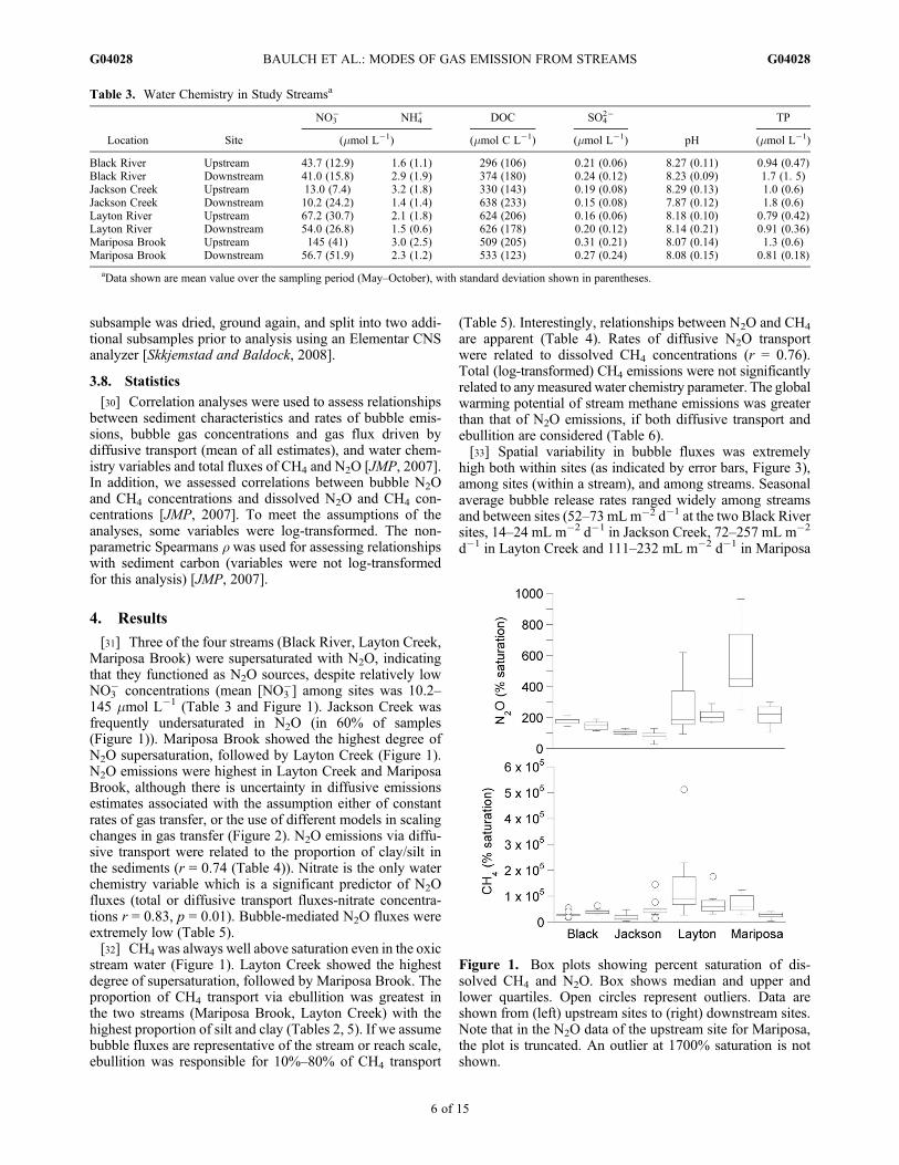
[31] Three of the four streams (Black River, Layton Creek,Mariposa Brook) were supersaturated with N2O, indicatingthat they functioned as N2O sources, despite relatively lowNO3

� concentrations (mean [NO3�] among sites was 10.2–

145 mmol L�1 (Table 3 and Figure 1). Jackson Creek wasfrequently undersaturated in N2O (in 60% of samples(Figure 1)). Mariposa Brook showed the highest degree ofN2O supersaturation, followed by Layton Creek (Figure 1).N2O emissions were highest in Layton Creek and MariposaBrook, although there is uncertainty in diffusive emissionsestimates associated with the assumption either of constantrates of gas transfer, or the use of different models in scalingchanges in gas transfer (Figure 2). N2O emissions via diffu-sive transport were related to the proportion of clay/silt inthe sediments (r = 0.74 (Table 4)). Nitrate is the only waterchemistry variable which is a significant predictor of N2Ofluxes (total or diffusive transport fluxes-nitrate concentra-tions r = 0.83, p = 0.01). Bubble-mediated N2O fluxes wereextremely low (Table 5).[32] CH4 was always well above saturation even in the oxic

stream water (Figure 1). Layton Creek showed the highestdegree of supersaturation, followed by Mariposa Brook. Theproportion of CH4 transport via ebullition was greatest inthe two streams (Mariposa Brook, Layton Creek) with thehighest proportion of silt and clay (Tables 2, 5). If we assumebubble fluxes are representative of the stream or reach scale,ebullition was responsible for 10%–80% of CH4 transport

(Table 5). Interestingly, relationships between N2O and CH4

are apparent (Table 4). Rates of diffusive N2O transportwere related to dissolved CH4 concentrations (r = 0.76).Total (log-transformed) CH4 emissions were not significantlyrelated to anymeasured water chemistry parameter. The globalwarming potential of stream methane emissions was greaterthan that of N2O emissions, if both diffusive transport andebullition are considered (Table 6).[33] Spatial variability in bubble fluxes was extremely

high both within sites (as indicated by error bars, Figure 3),among sites (within a stream), and among streams. Seasonalaverage bubble release rates ranged widely among streamsand between sites (52–73 mLm�2 d�1 at the two Black Riversites, 14–24 mL m�2 d�1 in Jackson Creek, 72–257 mL m�2

d�1 in Layton Creek and 111–232 mL m�2 d�1 in Mariposa

Figure 1. Box plots showing percent saturation of dis-solved CH4 and N2O. Box shows median and upper andlower quartiles. Open circles represent outliers. Data areshown from (left) upstream sites to (right) downstream sites.Note that in the N2O data of the upstream site for Mariposa,the plot is truncated. An outlier at 1700% saturation is notshown.

Table 3. Water Chemistry in Study Streamsa

Location Site

NO3� NH4

+ DOC SO42�

pH

TP

(mmol L�1) (mmol C L�1) (mmol L�1) (mmol L�1)

Black River Upstream 43.7 (12.9) 1.6 (1.1) 296 (106) 0.21 (0.06) 8.27 (0.11) 0.94 (0.47)Black River Downstream 41.0 (15.8) 2.9 (1.9) 374 (180) 0.24 (0.12) 8.23 (0.09) 1.7 (1. 5)Jackson Creek Upstream 13.0 (7.4) 3.2 (1.8) 330 (143) 0.19 (0.08) 8.29 (0.13) 1.0 (0.6)Jackson Creek Downstream 10.2 (24.2) 1.4 (1.4) 638 (233) 0.15 (0.08) 7.87 (0.12) 1.8 (0.6)Layton River Upstream 67.2 (30.7) 2.1 (1.8) 624 (206) 0.16 (0.06) 8.18 (0.10) 0.79 (0.42)Layton River Downstream 54.0 (26.8) 1.5 (0.6) 626 (178) 0.20 (0.12) 8.14 (0.21) 0.91 (0.36)Mariposa Brook Upstream 145 (41) 3.0 (2.5) 509 (205) 0.31 (0.21) 8.07 (0.14) 1.3 (0.6)Mariposa Brook Downstream 56.7 (51.9) 2.3 (1.2) 533 (123) 0.27 (0.24) 8.08 (0.15) 0.81 (0.18)

aData shown are mean value over the sampling period (May–October), with standard deviation shown in parentheses.

BAULCH ET AL.: MODES OF GAS EMISSION FROM STREAMS G04028G04028

6 of 15

Figure 2. Ebullitive gas fluxes and fluxes via surface aeration (diffusive transport) from study sites. Graysymbols represent bounds of error based on our assumption of constant rates of gas transfer, estimated usingcalibrated equations of Owens et al. [1964] (triangles), O’Connor and Dobbins [1958] (circles), andBennett and Rathburn [1972] (squares). See text for details. Error bars on ebullition plots represent standarddeviations based on uncertainty analysis. Note log-scale for ebullitive CH4 flux plot.

BAULCH ET AL.: MODES OF GAS EMISSION FROM STREAMS G04028G04028

7 of 15

Table 4. Correlations (r) Between Flux via Diffusive Transport, Ebullitive Flux, Bubble Gas Content and Dissolved GasConcentrations or Properties of Sedimenta

DiffusiveN2O flux

Ebullitive Flux Bubble Concentration

N2Ob CH4

b Volume Emittedb CO2 N2O CH4b

Sediment variablesSediment carbonc 0.971 mm–2 mm 0.850.5 mm–1 mm �0.740.0625 mm–0.125 mm 0.76Clay/silt (<0.0625 mm) 0.74 0.78 0.80 0.75 0.73Dry weight �0.92

Dissolved gasesDissolved N2O NMa 0.74Dissolved CH4 0.76 0.74

aSignificant correlations (p < 0.05) are shown. NM indicates that relationship was not assessed. No significant relationships werefound with (log-transformed) diffusive CH4 flux. Sediment size fractions of 0.25–0.5 mm and 0.125–0.25 mm were not correlated withreported variables.

bVariable is log-transformed.cNote that reported correlations for sediment carbon are related by Spearman r, and variables are not log-transformed for this analysis.

Table 5. Proportion of Gas Flux via Ebullition in Freshwaters in This Study and Published Dataa

Location

CH4 N2O CO2

(% Emitted Via Ebullition)

Streams and riversBlack River (this studyb) 22–33 0.01Jackson Creek (this studyb) 10–31 NA–0.02Layton Creek (this studyb) 29–35 0.01Mariposa Brook (this studyb) 55–80 0.01–0.02

Other regionsOrinoco River floodplain [Smith et al., 2000] 65Whakapipi and Toenepi streams [Wilcock and Sorrell, 2008] 20–60South Platte River [Higgins et al., 2008]c 0.1–0.6

Lakes and pondsBeaver Pond [Dove et al., 1999] 52 (open water sites)

20 (vegetated sites)Beaver Pond [Weyhenmeyer, 1999] 65Amazon floodplain lake [Bartlett et al., 1988, 1990] 32–53 (among open water, grass mat

and flooded forest habitats)Priest Pot (hypereutrophic lake) [Casper et al., 2000] 96 1Wintergreen Lake [Strayer and Tiedje, 1978] ≤50Floodplain lake [Crill et al., 1988] 70Searsville Lake [Miller and Oremland, 1988] �70Lake Erie [Ward and Frea, 1979] 1.1–88 5–15.6Onondaga Lake [Addess and Effler, 1996] �33

ReservoirsBalbina [Guérin et al., 2006] 25 0Samuel [Guérin et al., 2006] 11 0Petit Saut [Guérin et al., 2006] 5–17 0Experimentally flooded wetland [Kelly et al., 1997] <20 <2Experimentally flooded upland reservoirs [Matthews et al., 2005] 0–82 <1

WetlandsCoastal wetland [Chanton et al., 1989] 55Coastal wetland [Martens and Klump, 1980a; Kipphut and Martens, 1982] 90 (summer)

0 (winter)Temperate swamp [Wilson et al., 1989] 34Peatland [Tokida et al., 2007] 50–64

Laboratory systemsSediments incubated from a eutrophic lake [Liikanen et al., 2002] 26–33 at 1, 9 m depth

negligible at 4 m depthMixed sediments overlain by gravel and sand [Amos and Mayer, 2006] 36 19

aNA indicates the value was not calculated because the site was under-saturated therefore diffusive transport would lead to N2O uptake. Blank cellsindicate values were not reported.

bRange represents mean value from each of two sites on the stream. (Diffusive transport is mean of all modeled and measured values in Figure 2.)cOne estimate of N2 flux via ebullition exists globally for streams and rivers. The amount of N2 emitted from the South Platte River via ebullition is

6%–16%.

BAULCH ET AL.: MODES OF GAS EMISSION FROM STREAMS G04028G04028

8 of 15

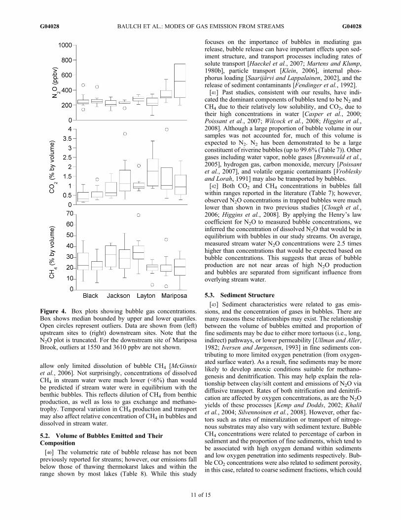
Brook). No clear seasonal trend in release rates was apparentacross sites (Figure 3).[34] In our study streams, CH4 concentrations in bubbles

ranged from <5% by volume to approximately 70% (Figure 4),but average values were relatively similar among sites andstreams, near 20%–30% (Table 7). CH4 concentrations inbubbles were related to dissolved CH4 (r = 0.74). CO2 con-centrations were much lower than CH4 concentrations,averaging 0.4%–1.8% (Table 7). N2O concentrations wereconsistently the smallest measured proportion of bubblecontent, often below atmospheric mixing ratios (Figure 4).Concentrations of N2O were greatest in bubble samplesobtained from the downstream site in Mariposa Brook(Figure 4). On average, 70% of bubble volume was notaccounted for in CH4, CO2 or N2O analyses.[35] Sediment characteristics were correlated with bubble

gas concentrations. A significant positive relationship wasshown between the volume of bubbles emitted, and the pro-portion of clay and silt (r = 0.75, Table 4). Bubble N2Oconcentrations were also significantly related to the propor-tion of clay/silt (r = 0.73, Table 4). Percentage of carbonin sediment was significantly related to bubble CH4 content(r = 0.97; Table 4). Bubble CH4 concentrations were alsopositively related to the proportion of fine (0.0625 mm–0.25 mm) sediments (r = 0.76, Table 4) and negativelyrelated to the dry weight (r = �0.92, Table 4). Bubble CO2

concentrations were positively correlated to the proportionof coarse sediment fractions (r = 0.85, Table 4).

5. Discussion

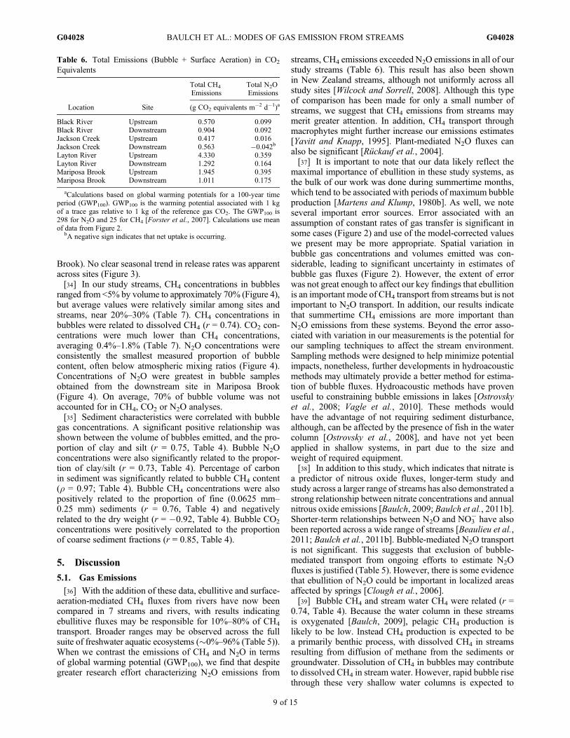
5.1. Gas Emissions

[36] With the addition of these data, ebullitive and surface-aeration-mediated CH4 fluxes from rivers have now beencompared in 7 streams and rivers, with results indicatingebullitive fluxes may be responsible for 10%–80% of CH4

transport. Broader ranges may be observed across the fullsuite of freshwater aquatic ecosystems (�0%–96% (Table 5)).When we contrast the emissions of CH4 and N2O in termsof global warming potential (GWP100), we find that despitegreater research effort characterizing N2O emissions from

streams, CH4 emissions exceeded N2O emissions in all of ourstudy streams (Table 6). This result has also been shownin New Zealand streams, although not uniformly across allstudy sites [Wilcock and Sorrell, 2008]. Although this typeof comparison has been made for only a small number ofstreams, we suggest that CH4 emissions from streams maymerit greater attention. In addition, CH4 transport throughmacrophytes might further increase our emissions estimates[Yavitt and Knapp, 1995]. Plant-mediated N2O fluxes canalso be significant [Rückauf et al., 2004].[37] It is important to note that our data likely reflect the

maximal importance of ebullition in these study systems, asthe bulk of our work was done during summertime months,which tend to be associated with periods of maximum bubbleproduction [Martens and Klump, 1980b]. As well, we noteseveral important error sources. Error associated with anassumption of constant rates of gas transfer is significant insome cases (Figure 2) and use of the model-corrected valueswe present may be more appropriate. Spatial variation inbubble gas concentrations and volumes emitted was con-siderable, leading to significant uncertainty in estimates ofbubble gas fluxes (Figure 2). However, the extent of errorwas not great enough to affect our key findings that ebullitionis an important mode of CH4 transport from streams but is notimportant to N2O transport. In addition, our results indicatethat summertime CH4 emissions are more important thanN2O emissions from these systems. Beyond the error asso-ciated with variation in our measurements is the potential forour sampling techniques to affect the stream environment.Sampling methods were designed to help minimize potentialimpacts, nonetheless, further developments in hydroacousticmethods may ultimately provide a better method for estima-tion of bubble fluxes. Hydroacoustic methods have provenuseful to constraining bubble emissions in lakes [Ostrovskyet al., 2008; Vagle et al., 2010]. These methods wouldhave the advantage of not requiring sediment disturbance,although, can be affected by the presence of fish in the watercolumn [Ostrovsky et al., 2008], and have not yet beenapplied in shallow systems, in part due to the size andweight of required equipment.[38] In addition to this study, which indicates that nitrate is

a predictor of nitrous oxide fluxes, longer-term study andstudy across a larger range of streams has also demonstrated astrong relationship between nitrate concentrations and annualnitrous oxide emissions [Baulch, 2009; Baulch et al., 2011b].Shorter-term relationships between N2O and NO3

� have alsobeen reported across a wide range of streams [Beaulieu et al.,2011; Baulch et al., 2011b]. Bubble-mediated N2O transportis not significant. This suggests that exclusion of bubble-mediated transport from ongoing efforts to estimate N2Ofluxes is justified (Table 5). However, there is some evidencethat ebullition of N2O could be important in localized areasaffected by springs [Clough et al., 2006].[39] Bubble CH4 and stream water CH4 were related (r =

0.74, Table 4). Because the water column in these streamsis oxygenated [Baulch, 2009], pelagic CH4 production islikely to be low. Instead CH4 production is expected to bea primarily benthic process, with dissolved CH4 in streamsresulting from diffusion of methane from the sediments orgroundwater. Dissolution of CH4 in bubbles may contributeto dissolved CH4 in stream water. However, rapid bubble risethrough these very shallow water columns is expected to

Table 6. Total Emissions (Bubble + Surface Aeration) in CO2

Equivalents

Location Site

Total CH4

EmissionsTotal N2OEmissions

(g CO2 equivalents m�2 d�1)a

Black River Upstream 0.570 0.099Black River Downstream 0.904 0.092Jackson Creek Upstream 0.417 0.016Jackson Creek Downstream 0.563 �0.042b

Layton River Upstream 4.330 0.359Layton River Downstream 1.292 0.164Mariposa Brook Upstream 1.945 0.395Mariposa Brook Downstream 1.011 0.175

aCalculations based on global warming potentials for a 100-year timeperiod (GWP100). GWP100 is the warming potential associated with 1 kgof a trace gas relative to 1 kg of the reference gas CO2. The GWP100 is298 for N2O and 25 for CH4 [Forster et al., 2007]. Calculations use meanof data from Figure 2.

bA negative sign indicates that net uptake is occurring.

BAULCH ET AL.: MODES OF GAS EMISSION FROM STREAMS G04028G04028

9 of 15

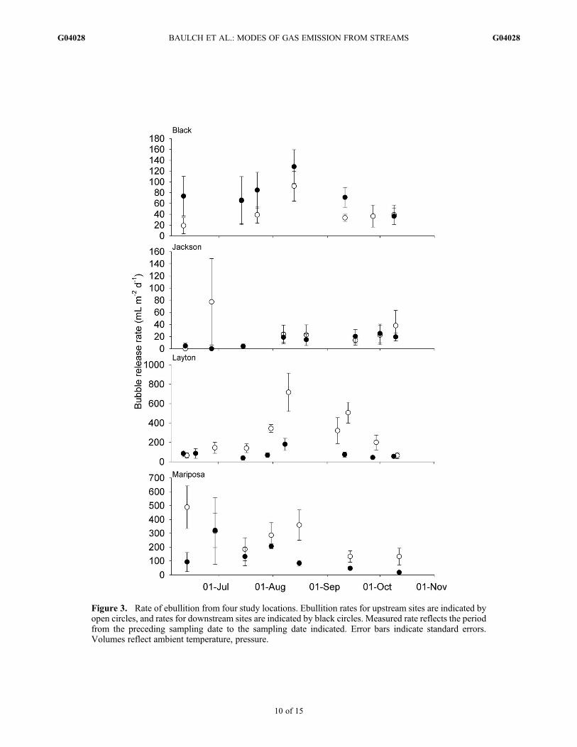
Figure 3. Rate of ebullition from four study locations. Ebullition rates for upstream sites are indicated byopen circles, and rates for downstream sites are indicated by black circles. Measured rate reflects the periodfrom the preceding sampling date to the sampling date indicated. Error bars indicate standard errors.Volumes reflect ambient temperature, pressure.

BAULCH ET AL.: MODES OF GAS EMISSION FROM STREAMS G04028G04028

10 of 15

allow only limited dissolution of bubble CH4 [McGinniset al., 2006]. Not surprisingly, concentrations of dissolvedCH4 in stream water were much lower (<6%) than wouldbe predicted if stream water were in equilibrium with thebenthic bubbles. This reflects dilution of CH4 from benthicproduction, as well as loss to gas exchange and methano-trophy. Temporal variation in CH4 production and transportmay also affect relative concentration of CH4 in bubbles anddissolved in stream water.

5.2. Volume of Bubbles Emitted and TheirComposition

[40] The volumetric rate of bubble release has not beenpreviously reported for streams; however, our emissions fallbelow those of thawing thermokarst lakes and within therange shown by most lakes (Table 8). While this study

focuses on the importance of bubbles in mediating gasrelease, bubble release can have important effects upon sed-iment structure, and transport processes including rates ofsolute transport [Haeckel et al., 2007; Martens and Klump,1980b], particle transport [Klein, 2006], internal phos-phorus loading [Saarijärvi and Lappalainen, 2002], and therelease of sediment contaminants [Fendinger et al., 1992].[41] Past studies, consistent with our results, have indi-

cated the dominant components of bubbles tend to be N2 andCH4 due to their relatively low solubility, and CO2, due totheir high concentrations in water [Casper et al., 2000;Poissant et al., 2007; Wilcock et al., 2008; Higgins et al.,2008]. Although a large proportion of bubble volume in oursamples was not accounted for, much of this volume isexpected to N2. N2 has been demonstrated to be a largeconstituent of riverine bubbles (up to 99.6% (Table 7)). Othergases including water vapor, noble gases [Brennwald et al.,2005], hydrogen gas, carbon monoxide, mercury [Poissantet al., 2007], and volatile organic contaminants [Vrobleskyand Lorah, 1991] may also be transported by bubbles.[42] Both CO2 and CH4 concentrations in bubbles fall

within ranges reported in the literature (Table 7); however,observed N2O concentrations in trapped bubbles were muchlower than shown in two previous studies [Clough et al.,2006; Higgins et al., 2008]. By applying the Henry’s lawcoefficient for N2O to measured bubble concentrations, weinferred the concentration of dissolved N2O that would be inequilibrium with bubbles in our study streams. On average,measured stream water N2O concentrations were 2.5 timeshigher than concentrations that would be expected based onbubble concentrations. This suggests that areas of bubbleproduction are not near areas of high N2O productionand bubbles are separated from significant influence fromoverlying stream water.

5.3. Sediment Structure

[43] Sediment characteristics were related to gas emis-sions, and the concentration of gases in bubbles. There aremany reasons these relationships may exist. The relationshipbetween the volume of bubbles emitted and proportion offine sediments may be due to either more tortuous (i.e., long,indirect) pathways, or lower permeability [Ullman and Aller,1982; Iversen and Jørgensen, 1993] in fine sediments con-tributing to more limited oxygen penetration (from oxygen-ated surface water). As a result, fine sediments may be morelikely to develop anoxic conditions suitable for methano-genesis and denitrification. This may help explain the rela-tionship between clay/silt content and emissions of N2O viadiffusive transport. Rates of both nitrification and denitrifi-cation are affected by oxygen concentrations, as are the N2Oyields of these processes [Kemp and Dodds, 2002; Khalilet al., 2004; Silvennoinen et al., 2008]. However, other fac-tors such as rates of mineralization or transport of nitroge-nous substrates may also vary with sediment texture. BubbleCH4 concentrations were related to percentage of carbon insediment and the proportion of fine sediments, which tend tobe associated with high oxygen demand within sedimentsand low oxygen penetration into sediments respectively. Bub-ble CO2 concentrations were also related to sediment porosity,in this case, related to coarse sediment fractions, which could

Figure 4. Box plots showing bubble gas concentrations.Box shows median bounded by upper and lower quartiles.Open circles represent outliers. Data are shown from (left)upstream sites to (right) downstream sites. Note that theN2O plot is truncated. For the downstream site of MariposaBrook, outliers at 1550 and 3610 ppbv are not shown.

BAULCH ET AL.: MODES OF GAS EMISSION FROM STREAMS G04028G04028

11 of 15

reflect respiratory production of CO2 or oxidation of CH4 toCO2 under oxic conditions.[44] Beyond effects on oxygen penetration, sediment

characteristics may also limit transport of gases (e.g., CH4

and N2) from areas with high rates of production, contribut-ing to bubble nucleation and growth. Physical characteristicsof fine sediments such as yield strength can affect rates ofbubble growth and the ability of bubbles to fracture sedi-ments [Algar and Boudreau, 2009]. Although prior to thisstudy, a relationship between fine sediments and bubbleproduction has not been reported in streams, fine sedimentshave been associated with a high degree of CH4 entrapmentin soils and rice paddies [Wang et al., 1993]. Future study ofa wider suite of streams and rivers would help assess the

generality of these relationships between gas fluxes andsediment character, and aid in identification of sedimenttypes associated with hot spots of ebullition.

6. Conclusions and Implications

[45] The importance of inland waters in continental meth-ane fluxes is a topic only beginning to receive attention, butexisting evidence suggests that freshwater CH4 emissionsmay offset a large proportion of the terrestrial carbon sink[Bastviken et al., 2011]. Our results support this assertion,showing high CH4 fluxes from small streams. In fact, despitethe much greater effort expended constraining nitrous oxideemissions from streams, results from this study suggest that if

Table 7. Gas Concentrations in Bubbles in Freshwater Ecosystems (This Study and Published Data)

LocationCH4

(% by volume)CO2

(% by volume)N2O(ppbv) Other

This study: Streams (seasonal means)Black River 19–22 0.4–0.6 259–262Jackson Creek 21–25 0.8–1.5 220–232Layton Creek 29–32 1.1–1.8 233–257Mariposa Brook (includes additional data from 3rd site) 21–35 0.4–1.5 345–816

Past studies: Streams, rivers and estuariesStouffville Creek (seasonal mean, 2 sites,

H. Baulch, unpublished data)27–27 0.3–0.9 271–287

Roenepi Stream [Wilcock and Sorrell, 2008] 20.7–69.9(among 3 sites)

2–6 <2% Ar + O2, balance N2.

Whakapipi [Wilcock and Sorrell, 2008] 8.6LII river [Clough et al., 2006] 7900St. Lawrence River Cornwall area of concern

[Poissant et al., 2007]23–31 0.5–1.4 CO (58–81 ppmv,

H2 (591–779 ppbv)South Platte River [Higgins et al., 2008] 1.1–38 3600–11500 61%–99.6% N2

White Oak River estuary (tidal freshwater estuary)[Chanton et al., 1989]

46–79.7 2–3.9 0.6%–1.4% O2 + Ar,12%–49.8% N2

White Oak River estuary (unvegetated site)[Chanton et al., 1989]

40.9 2–3.9 1.2% O2 + Ar, 52.1% N2

LakesMirror Lake [Mattson and Likens, 1990] 70Temperate swamp [Wilson et al., 1989] 30–80Deep Creek in Newport News Swamp [Chanton et al., 1989] 83.1 6.4 0.5% O2 + Ar, 7.5% N2

North Siberian Lakes [Walter et al., 2006] 80Lake Postilampi [Huttunen et al., 2001] 52–64 0.02–0.56Wintergreen Lake [Strayer and Tiedje, 1978] 73–100Great Fresh Creek (eutrophic lake) [Conger et al., 1943] 58–82 1.5–2.4 14%–40% N2, 0% CO,

0%–0.5% H2,Priest Pot [Casper et al., 2000] 66 3 36% N2

Onondaga Lake [Addess and Effler, 1996] �67–86Lake Wingra [Barber and Ensign, 1979] 0.4–33

ReservoirsPetit Saut dam [Galy-Lacaux et al., 1997] 80

WetlandsVegetated site in Newport News Swamp [Chanton et al., 1989] 26.8 7 2.1% O2 + Ar, 64.4% N2

Rice paddies [Holzapfel-Pschorn et al., 1985] 16–54

Table 8. Rates of Bubble Release Reported From Lakes and Estuaries

Location Release Rate (mL m�2 d�1) Reference

North Siberian Lakes Permafrost thaw lakes >2880 nearshores [Zimov et al., 1997]Lake Postilampi Hypereutrophic lake 3–151; 106 (summer average)

345 (maximum)[Huttunen et al., 2001; Saarijärvi

and Lappalainen, 2002]Lake Erie Eutrophic lake 0–2640 [Howard et al., 1971, in Fendinger et al., 1992;

Ward and Frea, 1979]Priest Pot Hypereutrophic lake 162 (<3 m depth)

236–380 (>3 m)[Casper et al., 2000]

Great Fresh Creek Eutrophic lake 630 [Conger et al., 1943]White Oak River estuary Tidal freshwater estuary 210–596 [Chanton et al., 1989]Lake Wingra Eutrophic lake 166–959 [Barber and Ensign, 1979]

BAULCH ET AL.: MODES OF GAS EMISSION FROM STREAMS G04028G04028

12 of 15

ebullition is considered, methane emissions far exceed N2Oemissions (in terms of GWP) from streams in summermonths. Ebullition was consistently an important means ofCH4 transport, as was diffusive transport. N2O emissions viadiffusive transport were far in excess of bubble-mediatedN2O emissions. More work is required to constrain annualCH4 emissions from all emissions pathways (bubbles, dif-fusive transport, and plant-mediated transport), understandcontrols on emissions across streams, and assess whetherhuman alteration of streams (e.g., changes in temperatures,nutrients, oxygen concentrations, flow dynamics or substratecomposition), particularly in urban and agricultural land-scapes, may have affected not only the emissions of N2O, butalso of CH4. Beyond the role of ebullition in CH4 transport,high rates of bubble release suggest the role of ebullitionin transport of nutrients and contaminants from sedimentsmerits further consideration.

[46] Acknowledgments. Funding was provided by an NSERC Dis-covery grant to P.J.D. and scholarship funding to H.M.B. We are gratefulto Jason Venkiteswaran, who assisted with oxygen modeling; to numerousothers who assisted in the lab and the field; and to anonymous reviewersfor helpful comments on the manuscript.

ReferencesAddess, J. M., and S. W. Effler (1996), Summer methane fluxes and falloxygen resources of Onondaga Lake, Lake Reservoir Manage., 12(1),91–101, doi:10.1080/07438149609354000.

Algar, C. K., and B. P. Boudreau (2009), Transient growth of an isolatedbubble in muddy, fine-grained sediments, Geochim. Cosmochim. Acta,73(9), 2581–2591, doi:10.1016/j.gca.2009.02.008.

Amos, R. T., and K. U. Mayer (2006), Investigating ebullition in a sandcolumn using dissolved gas analysis and reactive transport modeling,Environ. Sci. Technol., 40(17), 5361–5367, doi:10.1021/es0602501.

Barber, L. E., and J. C. Ensign (1979), Methane formation and releasein a small Wisconsin Lake, Geomicrobiol. J., 1, 341–353, doi:10.1080/01490457909377740.

Bartlett, K. B., P. M. Crill, D. I. Sebacher, R. C. Harriss, J. O. Wilson, andJ. M. Melack (1988), Methane flux from the Central Amazonian floodplain,J. Geophys. Res., 93(D2), 1571–1582, doi:10.1029/JD093iD02p01571.

Bartlett, K. B., P. M. Crill, J. A. Bonassi, J. E. Richey, and R. C. Harriss(1990), Methane flux from the Amazon River floodplain: Emissions dur-ing rising water, J. Geophys. Res., 95(D10), 16,773–16,788, doi:10.1029/JD095iD10p16773.

Bastviken, D., J. Cole, M. Pace, and L. Tranvik (2004), Methane emissionsfrom lakes: Dependence of lake characteristics, two regional assess-ments, and a global estimate, Global Biogeochem. Cycles, 18, GB4009,doi:10.1029/2004GB002238.

Bastviken, D., L. J. Tranvik, J. A. Downing, P. M. Crill, and A. Enrich-Prast (2011), Freshwater methane emissions offset the continental carbonsink, Science, 331, 50, doi:10.1126/science.1196808.

Battin, T. J., L. A. Kaplan, S. Findlay, C. S. Hopkinson, E. Marti, A. I.Packman, J. D. Newbold, and F. Sabater (2008), Biophysical controls onorganic carbon fluxes in fluvial networks, Nat. Geosci., 1(2), 95–100,doi:10.1038/ngeo101.

Baulch, H. M. (2009), Nitrous oxide emissions from streams, Ph.D. thesis,293 pp, Trent Univ., Peterborough, Ontario, Canada.

Baulch, H. M., S. L. Schiff, S. J. Thuss, and P. J. Dillon (2011a), Isotopiccharacter of nitrous oxide emitted from streams, Environ. Sci. Technol.,45(11), 4682–4688, doi:10.1021/es104116a.

Baulch, H. M., S. L. Schiff, R. Maranger, and P. J. Dillon (2011b), Nitrogenenrichment and the emission of nitrous oxide from streams, Global Bio-geochem. Cycles, doi:10.1029/2011GB004047, in press.

Beaulieu, J. J., et al. (2011), Nitrous oxide emission from denitrification instream and river networks, Proc. Natl. Acad. Sci. U. S. A., 108, 214–219,doi:10.1073/pnas.1011464108.

Beck, M. B. (1987), Water-quality modeling - a review of the analysisof uncertainty, Water Resour. Res., 23(8), 1393–1442, doi:10.1029/WR023i008p01393.

Bennett, J. P., and R. E. Rathburn (1972), Reaeration in open-channel flow,U. S. Geol. Surv. Prof. Pap. 737, U. S. Gov. Print. Off., Washington D. C.

Brennwald, M. S., R. Kipfer, and D. M. Imboden (2005), Release of gasbubbles from lake sediment traced by noble gas isotopes in the sediment

pore water, Earth Planet. Sci. Lett., 235(1–2), 31–44, doi:10.1016/j.epsl.2005.03.004.

Bridgham, S. D., J. P. Megonigal, J. K. Keller, N. B. Bliss, and C. Trettin(2006), The carbon balance of North American wetlands, Wetlands, 26(4),889–916, doi:10.1672/0277-5212(2006)26[889:TCBONA]2.0.CO;2.

Casper, P., S. C. Maberly, G. H. Hall, and B. J. Finlay (2000), Fluxes ofmethane and carbon dioxide from a small productive lake to the atmo-sphere, Biogeochemistry, 49(1), 1–19, doi:10.1023/A:1006269900174.

Chanton, J. P., and G. J. Whiting (1995), Trace gas exchange in freshwaterand coastal marine environments: Ebullition and transport by plants,in Biogenic Trace Gases: Measuring Emissions From Soil and Water,edited by P. A. Matson and R. C. Harriss, pp. 98–125, Blackwell Sci,Oxford, U. K.

Chanton, J. P., C. S. Martens, and C. A. Kelley (1989), Gas-transport frommethane-saturated, tidal fresh-water and wetland sediments, Limnol.Oceanogr., 34(5), 807–819, doi:10.4319/lo.1989.34.5.0807.

Chapra, S. C., and D. M. Di Toro (1991), Delta method for estimating pri-mary production respiration and reaeration in streams, J. Environ. Eng.Sci., 117, 640–655, doi:10.1061/(ASCE)0733-9372(1991)117:5(640).

Clough, T. J., J. E. Bertram, R. R. Sherlock, R. L. Leonard, andB. L. Nowicki (2006), Comparison of measured and EF5-r-derived N2Ofluxes from a spring-fed river, Global Change Biol., 12(2), 352–363,doi:10.1111/j.1365-2486.2005.01089.x.

Cole, J. J., et al. (2007), Plumbing the global carbon cycle: Integratinginland waters into the terrestrial carbon budget, Ecosystems (N. Y.),10(1), 172–185, doi:10.1007/s10021-006-9013-8.

Conger, P. S., et al. (1943), Ebullition of Gases From Marsh and LakeWaters, Chesapeake Biol. Lab., Solomons Island, Md.

Crill, P. M., K. B. Bartlett, J. O. Wilson, D. I. Sebacher, R. C. Harriss, J. M.Melack, S. MacIntyre, L. Lesack, and L. Smith-Morrill (1988), Tropo-spheric methane from an Amazonian floodplain lake, J. Geophys. Res.,93(D2), 1564–1570, doi:10.1029/JD093iD02p01564.

Dacey, J. W. H., and M. J. Klug (1979), Methane efflux from lake sedi-ments through water lilies, Science, 203, 1253–1255, doi:10.1126/science.203.4386.1253.

Decisioneering, Inc. (2001), Crystal Ball User Manual, Denver, Colo.Denman, K. L., et al. (2007), Couplings between changes in the climate sys-tem and biogeochemistry, in Climate Change 2007: The Physical ScienceBasis. Contribution of Working Group I to the Fourth AssessmentReport of the Intergovernmental Panel on Climate Change, edited byS. Solomon, et al., pp. 499–587, Cambridge Univ. Press, Cambridge,U. K.

Dove, A., N. Roulet, P. Crill, J. Chanton, and R. Bourbonniere (1999),Methane dynamics of a northern boreal beaver pond, Ecoscience, 6(4),577–586.

Eggleston, H. S., L. Buendia, K. Miwa, T. Ngara, and K. Tanabe (Eds.)(2006), N2O emissions from managed soils, and CO2 emissions fromlime and urea application, in 2006 IPCC Guidelines for National Green-house Gas Inventories: Vol. 4, Agriculture, Forestry and Other LandUse, pp. 11.1–11.53, Inst. for Global Environ. Strategies, Hayama, Japan.

Fendinger, N. J., D. D. Adams, and D. E. Glotfelty (1992), The role of gasebullition in the transport of organic contaminants from sediments, Sci.Total Environ., 112(2–3), 189–201, doi:10.1016/0048-9697(92)90187-W.

Forster, P., et al. (2007), Changes in atmospheric constituents and in radia-tive forcing, in Climate Change 2007: The Physical Science Basis. Con-tribution of Working Group I to the Fourth Assessment Report of theIntergovernmental Panel on Climate Change, edited by S. Soloman,et al., pp. 129–234, Cambridge Univ. Press, Cambridge, U. K.

Galy-Lacaux, C., R. Delmas, C. Jambert, J.-F. Dumestre, L. Labroue,S. Richard, and P. Gosse (1997), Gaseous emissions and oxygen con-sumption in hydroelectric dams: A case study in French Guyana, GlobalBiogeochem. Cycles, 11(4), 471–483, doi:10.1029/97GB01625.

Guérin, F., G. Abril, S. Richard, B. Burban, C. Reynouard, P. Seyler, andR. Delmas (2006), Methane and carbon dioxide emissions from tropicalreservoirs: Significance of downstream rivers, Geophys. Res. Lett., 33,L21407, doi:10.1029/2006GL027929.

Haeckel, M., B. P. Boudreau, and K. Wallmann (2007), Bubble-inducedporewater mixing: A 3-D model for deep porewater irrigation, Geochim.Cosmochim. Acta, 71(21), 5135–5154, doi:10.1016/j.gca.2007.08.011.

Higgins, T. M., J. H. McCutchan, and W. M. Lewis (2008), Nitrogenebullition in a Colorado plains river, Biogeochemistry, 89(3), 367–377,doi:10.1007/s10533-008-9225-4.

Holzapfel-Pschorn, A., R. Conrad, and W. Seiler (1985), Production, oxida-tion and emission of methane in rice paddies, FEMS Microbiol. Ecol.,31(6), 343–351, doi:10.1111/j.1574-6968.1985.tb01170.x.

Huttunen, J. T., K. M. Lappalainen, E. Saarijärvi, T. Vaisanen, and P. J.Martikainen (2001), A novel sediment gas sampler and a subsurface gascollector used for measurement of the ebullition of methane and carbon

BAULCH ET AL.: MODES OF GAS EMISSION FROM STREAMS G04028G04028

13 of 15

dioxide from a eutrophied lake, Sci. Total Environ., 266(1–3), 153–158,doi:10.1016/S0048-9697(00)00749-X.

Iversen, N., and B. B. Jørgensen (1993), Diffusion coeffucients of sulfateand methane in marine sediments: Influence of porosity, Geochim. Cos-mochim. Acta, 57(3), 571–578, doi:10.1016/0016-7037(93)90368-7.

Jähne, B., K. O. Münnich, R. B. A. Dutzi, W. Huber, and P. Libner (1987),On the parameters influencing air-water gas exchange, J. Geophys. Res.,92(C2), 1937–1949, doi:10.1029/JC092iC02p01937.

JMP (2007), JMP®, Version 7.0.2, edited, SAS Institute Inc., Cary, N. C.Jones, J. B., and P. J. Mulholland (1998), Influence of drainage basintopography and elevation on carbon dioxide and methane supersatu-ration of stream water, Biogeochemistry, 40, 57–72, doi:10.1023/A:1005914121280.

Joyce, J., and P. W. Jewell (2003), Physical controls on methane ebullitionfrom reservoirs and lakes, Environ. Eng. Geosci., 9(2), 167–178,doi:10.2113/9.2.167.

Kelly, C. A., et al. (1997), Increases in fluxes of greenhouse gasesand methyl mercury following flooding of an experimental reservoir,Environ. Sci. Technol., 31(5), 1334–1344, doi:10.1021/es9604931.

Kemp, M. J., and W. K. Dodds (2002), The influence of ammonium,nitrate, and dissolved oxygen concentrations on uptake, nitrification,and denitrification rates associated with prairie stream substrata, Limnol.Oceanogr., 47(5), 1380–1393, doi:10.4319/lo.2002.47.5.1380.

Khalil, K., B. Mary, and P. Renault (2004), Nitrous oxide production bynitrification and denitrification in soil aggregates as affected by O2 con-centration, Soil Biol. Biochem., 36(4), 687–699, doi:10.1016/j.soilbio.2004.01.004.

Kilpatrick, F. A., R. E. Rathbun, N. Yotsukura, G. W. Parker, and L. L.Delong (1987), Determination of stream reaeration coefficients by use of tra-cers, in Applications of Hydraulics, Bk. 3 of Techniques of Water-ResourcesInvestigations, USGS TWRI–3–A18, U. S. Geol. Surv., Washington, D. C.[Available at http://pubs.usgs.gov/twri/twri3-a18/#pdf.]

Kipphut, G. W., and C. S. Martens (1982), Biogeochemical cyclingin an organic-rich coastal marine basin. 3. Dissolved-gas transport inmethane-saturated sediments, Geochim. Cosmochim. Acta, 46(11),2049–2060, doi:10.1016/0016-7037(82)90184-3.

Klein, S. (2006), Sediment porewater exchange and solute release duringebullition, Mar. Chem., 102(1–2), 60–71, doi:10.1016/j.marchem.2005.09.014.

Liikanen, A., H. Tanskanen, T. Murtoniemi, and P. J. Martikainen (2002),A laboratory microcosm for simultaneous gas and nutrient flux measure-ments in sediments, Boreal Environ. Res., 7(2), 151–160.

Liss, P. S., and P. G. Slater (1974), Flux of gases across the air-sea interface,Nature, 247, 181–184, doi:10.1038/247181a0.

Martens, C. S., and J. V. Klump (1980a), Biogeochemical cycling in anorganic-rich coastal marine basin—I. Methane sediment-water exchangeprocesses, Geochim. Cosmochim. Acta, 44, 471–490, doi:10.1016/0016-7037(80)90045-9.

Martens, C. S., and J. V. Klump (1980b), Biogeochemical cycling in anorganic-rich coastal marine basin: I. Methane sediment-water exchangeprocesses, Geochim. Cosmochim. Acta, 44, 471–490, doi:10.1016/0016-7037(80)90045-9.

Matthews, C. J. D., E. M. Joyce, V. L. St Louise, S. L. Schiff, J. J.Venkiteswaran, B. D. Hall, R. A. Bodaly, and K. G. Beaty (2005),Carbon dioxide and methane production in small reservoirs floodingupland Boreal Forest, Ecosystems (N. Y.), 8(3), 267–285, doi:10.1007/s10021-005-0005-x.

Mattson, M. D., and G. E. Likens (1990), Air-pressure and methane fluxes,Nature, 347(6295), 718–719, doi:10.1038/347718b0.

McGinnis, D. F., J. Greinert, Y. Artemov, S. E. Beaubien, and A. Wüest(2006), Fate of rising methane bubbles in stratified waters: How muchmethane reaches the atmosphere?, J. Geophys. Res., 111, C09007,doi:10.1029/2005JC003183.

Miller, L. G., and R. S. Oremland (1988), Methane efflux from the pelagicregions of four lakes, Global Biogeochem. Cycles, 2(3), 269–277,doi:10.1029/GB002i003p00269.

Ministry of the Environment (1994), The Determination of Total Phospho-rus in Water by Colourimetry, Environ. Ont. Lab. Serv. Branch Qual.Manage. Off., Toronto, Ontario, Canada.

Ministry of the Environment (2001), The Determination of AmmoniumNitrogen and Nitrate Plus Nitrite Nitrogen in Water and Precipitationby Colourimetry, 27 pp., Environ. Ont. Lab. Serv. Branch Qual. Manage.Off., Dorset, Ontario, Canada.

Molongoski, J. J., and M. J. Klug (1980), Anaerobic metabolism of partic-ulate organic matter in the sediments of a hypereutrophic lake, Fresh-water Biol., 10, 507–518, doi:10.1111/j.1365-2427.1980.tb01225.x.

Moog, D. B., and G. H. Jirka (1998), Analysis of reaeration equationsusing mean multiplicative error, J. Environ. Eng., 124(2), 104–110,doi:10.1061/(ASCE)0733-9372(1998)124:2(104).

O’Connor, D. J., and W. E. Dobbins (1958), Mechanism of reaeration innatural streams, Am. Soc. Civil Eng. Trans., 123, 641–684.

Ontario Ministry of Natural Resources (2006), Southern Ontario InterimLand Cover Dataset, Ont. Minist. of Nat. Resour., Peterborough, Ontario,Canada.

Ostrovsky, I., D. F. McGinnis, L. Lapidus, and W. Eckert (2008), Quantify-ing gas ebullition with echosounder: The role of methane transportby bubbles in a medium-sized lake, Limnol. Oceanogr. Methods, 6,105–118, doi:10.4319/lom.2008.6.105.

Owens, M., R. W. Edwards, and J. W. Gibbs (1964), Some reaeration stud-ies in streams, Int. J. Air Water Pollut., 8, 469–486.

Poissant, L., P. Constant, M. Pilote, J. Canario, N. O’Driscoll, J. Ridal,and D. Lean (2007), The ebullition of hydrogen, carbon monoxide,methane, carbon dioxide and total gaseous mercury from the CornwallArea of Concern, Sci. Total Environ., 381(1–3), 256–262, doi:10.1016/j.scitotenv.2007.03.029.

Poppe, L. J., A. H. Eliason, J. J. Fredericks, R. R. Rendigs, D. Blackwood,and C. F. Polloni (2000), Grain-size analysis of marine sediments: Meth-odology and data processing, in USGS East-Coast Sediment Analysis:Procedures, Database, and Georeferenced Displays, U. S. Geol. Surv.Open-File Rep. 00–358, edited by L. J. Poppe and C. F. Polloni, U.S.Dep. of the Int., Woods Hole, Mass. [Available at http://pubs.usgs.gov/of/2000/of00-358/text/chapter1.htm.]

Raymond, P. A., and J. J. Cole (2001), Gas exchange in rivers and estuaries:Choosing a gas transfer velocity, Estuaries, 24(2), 312–317, doi:10.2307/1352954.

Rückauf, U., J. Augustin, R. Russow, and W. Merbach (2004), Nitrateremoval from drained and reflooded fen soils affected by soil N transfor-mation processes and plant uptake, Soil Biol. Biochem., 36(1), 77–90,doi:10.1016/j.soilbio.2003.08.021.

Saarijärvi, E., and K. M. Lappalainen (2002), Flotation-like gas ebullitionas a mechanism for sediment resuspension, Verh. Int. Ver. Limnol.,27(7), 4093–4096.

Seitzinger, S. P., and C. Kroeze (1998), Global distribution of nitrous oxideproduction and N inputs in freshwater and coastal marine ecosystems,Global Biogeochem. Cycles, 12(1), 93–113, doi:10.1029/97GB03657.

Silvennoinen, H., A. Liikanen, J. Torssonen, C. F. Stange, and P. J.Martikainen (2008), Denitrification and N2O effluxes in the BothnianBay (northern Baltic Sea) river sediments as affected by temperatureunder different oxygen concentrations, Biogeochemistry, 88(1), 63–72,doi:10.1007/s10533-008-9194-7.

Skkjemstad, J. O., and J. A. Baldock (2008), Total and organic carbon, inSoil Sampling and Methods of Analysis, 2nd ed., edited by M. R. Carterand E. G. Gregorich, Can. Soc. of Soil Sci., pp. 225–237, CRC Press,Boca Raton, Fla.

Smith, L. K., W. M. Lewis, J. P. Chanton, G. Cronin, and S. K. Hamilton(2000), Methane emissions from the Orinoco River floodplain, Venezuela,Biogeochemistry, 51(2), 113–140, doi:10.1023/A:1006443429909.

St. Louis, V. L., C. A. Kelly, E. Duchemin, J. W. M. Rudd, and D. M.Rosenberg (2000), Reservoir surfaces as sources of greenhouse gasesto the atmosphere: A global estimate, BioScience, 50(9), 766–775,doi:10.1641/0006-3568(2000)050[0766:RSASOG]2.0.CO;2.

Stein, L. Y., and Y. L. Yung (2003), Production, isotopic composition, andatmospheric fate of biologically produced nitrous oxide, Annu. Rev. EarthPlanet. Sci., 31, 329–356, doi:10.1146/annurev.earth.31.110502.080901.

Strayer, R. F., and J. M. Tiedje (1978), In situ methane production ina small, hypereutrophic, hard-water lake: Loss of methane from sedi-ments by vertical diffusion and ebullition, Limnol. Oceanogr., 23(6),1201–1206, doi:10.4319/lo.1978.23.6.1201.

Teodoru, C. R., P. A. del Giorgio, Y. T. Prairie, and M. Camire (2009), Pat-terns in pCO2 in boreal streams and rivers of northern Quebec, Canada,Global Biogeochem. Cycles, 23, GB2012, doi:10.1029/2008GB003404.

Thomann, R. V., and J. A. Mueller (1987), Principles of surface waterquality modeling and control, 282 pp., Harper and Row, New York.

Tokida, T., T. Miyazaki, M. Mizoguchi, O. Nagata, F. Takakai,A. Kagemoto, and R. Hatano (2007), Falling atmospheric pressure as atrigger for methane ebullition from peatland, Global Biogeochem. Cycles,21, GB2003, doi:10.1029/2006GB002790.

Tranvik, L. J., et al. (2009), Lakes and reservoirs as regulators of carboncycling and climate, Limnol. Oceanogr., 54(6), 2298–2314, doi:10.4319/lo.2009.54.6_part_2.2298.

Ullman, W. J., and R. C. Aller (1982), Diffusion-coefficients in nearshoremarine-sediments, Limnol. Oceanogr., 27(3), 552–556, doi:10.4319/lo.1982.27.3.0552.

Vagle, S., J. Hume, F. McLaughlin, E. MacIsaac, and K. Shortreed (2010),A methane bubble curtain in meromictic Sakinaw Lake, British Colum-bia, Limnol. Oceanogr., 55(3), 1313–1326, doi:10.4319/lo.2010.55.3.1313.

BAULCH ET AL.: MODES OF GAS EMISSION FROM STREAMS G04028G04028

14 of 15

Venkiteswaran, J. J., L. I. Wassenaar, and S. L. Schiff (2007), Dynamics ofdissolved oxygen isotopic ratios: A transient model to quantify primaryproduction, community respiration, and air-water exchange in aquaticecosystems, Oecologia, 153(2), 385–398, doi:10.1007/s00442-007-0744-9.

Vroblesky, D. A., and M. M. Lorah (1991), Prospecting for zones ofcontaminated groundwater discharge to streams using bottom-sedimentgas-bubbles, Ground Water, 29(3), 333–340, doi:10.1111/j.1745-6584.1991.tb00523.x.

Walter, K. M., S. A. Zimov, J. P. Chanton, D. Verbyla, and F. S. Chapin(2006), Methane bubbling from Siberian thaw lakes as a positive feed-back to climate warming, Nature, 443(7107), 71–75, doi:10.1038/nature05040.

Wang, Z. P., C. W. Lindau, R. D. Delaune, and W. H. Patrick (1993),Methane emission and entrapment in flooded rice soils as affected by soilproperties, Biol. Fertil. Soils, 16(3), 163–168, doi:10.1007/BF00361401.

Wanninkhof, R. (1992), Relationship between wind-speed and gas-exchangeover the ocean, J. Geophys. Res., 97(C5), 7373–7382, doi:10.1029/92JC00188.

Ward, T. E., and J. I. Frea (1979), Estimation of microbial activities in lakesediments by measurement of sediment gas evolution, in Methodologyfor Biomass Determinations and Microbial Activities in Sediments,ASTM Spec. Tech. Publ. 673, edited by C. D. Litchfield and P. L.Seyfried, pp. 156–166, Am. Soc. for Test. and Mater., Philadelphia,Pa., doi:10.1520/STP38148S.

Weiss, R. F., and B. A. Price (1980), Nitrous oxide solubility in water andseawater, Mar. Chem., 8, 347–359, doi:10.1016/0304-4203(80)90024-9.

Weyhenmeyer, C. E. (1999), Methane emissions from beaver ponds: Rates,patterns, and transport mechanisms, Global Biogeochem. Cycles, 13(4),1079–1090, doi:10.1029/1999GB900047.

Wilcock, R. J., and B. K. Sorrell (2008), Emissions of greenhouse gasesCH4 and N2O from low-gradient streams in agriculturally developed

catchments, Water Air Soil Pollut., 188(1–4), 155–170, doi:10.1007/s11270-007-9532-8.

Wilcock, R., S. Elliott, N. Hudson, S. Parkyn, and J. Quinn (2008), Climatechange mitigation for agriculture: Water quality benefits and costs, WaterSci. Technol., 58(11), 2093–2099, doi:10.2166/wst.2008.906.

Wilson, J. O., P. M. Crill, K. B. Bartlett, D. I. Sebacher, R. C. Harriss, andR. L. Sass (1989), Seasonal-variation of methane emissions from a tem-perate swamp, Biogeochemistry, 8(1), 55–71, doi:10.1007/BF02180167.

Yamamoto, S., J. B. Alcauskas, and T. E. Crozier (1976), Solubilityof methane in distilled water and seawater, J. Chem. Eng. Data, 21,78–80, doi:10.1021/je60068a029.

Yavitt, J. B., and A. K. Knapp (1995), Methane emission to the atmospherethrough emergent cattail (Typha-latifolia L) plants, Tellus, Ser. B, 47(5),521–534, doi:10.1034/j.1600-0889.47.issue5.1.x.

Zimov, S. A., Y. V. Voropaev, I. P. Semiletov, S. P. Davidov, S. F.Prosiannikov, F. S. Chapin, M. C. Chapin, S. Trumbore, and S. Tyler(1997), North Siberian lakes: A methane source fueled by Pleistocenecarbon, Science, 277(5327), 800–802, doi:10.1126/science.277.5327.800.

H. M. Baulch, School of Environment and Sustainability and theGlobal Institute for Water Security, National Hydrology Research Centre,University of Saskatchewan, 11 Innovation Blvd., Saskatoon, SK S7N3H5 Canada. (helen.baulch@usask.ca)P. J. Dillon, Department of Environmental and Resource Studies, Trent

University, 1600 West Bank Dr., Peterborough, ON K9J 7B8 Canada.R. Maranger, Department of Biological Sciences, University of Montreal,

P. O. Box 6128, Station Centre-ville, Montreal, QC H3C 3J7 Canada.S. L. Schiff, Department of Earth and Environmental Sciences,

University of Waterloo, 200 University Avenue West, Waterloo, ON N2L3G1 Canada.

BAULCH ET AL.: MODES OF GAS EMISSION FROM STREAMS G04028G04028

15 of 15