Dielectric properties of aged polymers and nanocomposites

Graduate Theses and Dissertations Iowa State University Capstones, Theses andDissertations

2011

Dielectric properties of aged polymers andnanocompositesLi LiIowa State University

Follow this and additional works at: https://lib.dr.iastate.edu/etd

Part of the Materials Science and Engineering Commons

This Dissertation is brought to you for free and open access by the Iowa State University Capstones, Theses and Dissertations at Iowa State UniversityDigital Repository. It has been accepted for inclusion in Graduate Theses and Dissertations by an authorized administrator of Iowa State UniversityDigital Repository. For more information, please contact [email protected].

Recommended CitationLi, Li, "Dielectric properties of aged polymers and nanocomposites" (2011). Graduate Theses and Dissertations. 12128.https://lib.dr.iastate.edu/etd/12128

http://lib.dr.iastate.edu/?utm_source=lib.dr.iastate.edu%2Fetd%2F12128&utm_medium=PDF&utm_campaign=PDFCoverPages

http://lib.dr.iastate.edu/?utm_source=lib.dr.iastate.edu%2Fetd%2F12128&utm_medium=PDF&utm_campaign=PDFCoverPages

https://lib.dr.iastate.edu/etd?utm_source=lib.dr.iastate.edu%2Fetd%2F12128&utm_medium=PDF&utm_campaign=PDFCoverPages

https://lib.dr.iastate.edu/theses?utm_source=lib.dr.iastate.edu%2Fetd%2F12128&utm_medium=PDF&utm_campaign=PDFCoverPages

https://lib.dr.iastate.edu/theses?utm_source=lib.dr.iastate.edu%2Fetd%2F12128&utm_medium=PDF&utm_campaign=PDFCoverPages

https://lib.dr.iastate.edu/etd?utm_source=lib.dr.iastate.edu%2Fetd%2F12128&utm_medium=PDF&utm_campaign=PDFCoverPages

http://network.bepress.com/hgg/discipline/285?utm_source=lib.dr.iastate.edu%2Fetd%2F12128&utm_medium=PDF&utm_campaign=PDFCoverPages

https://lib.dr.iastate.edu/etd/12128?utm_source=lib.dr.iastate.edu%2Fetd%2F12128&utm_medium=PDF&utm_campaign=PDFCoverPages

mailto:[email protected]

Dielectric properties of aged polymers and nanocomposites

by

Li Li

A thesis submitted to the graduate faculty

in partial fulfillment of the requirements for the degree of

DOCTOR OF PHILOSOPHY

Major: Materials Science and Engineering

Program of Study Committee: Nicola Bowler, Major Professor

Michael R. Kessler Steve W. Martin

Xiaoli Tan Robert J. Weber

Iowa State University Ames, Iowa

2011

Copyright © Li Li, 2011. All rights reserved.

ii

Table of Contents

LIST OF FIGURES .................................................................................................................. v

LIST OF TABLES ................................................................................................................... ix

Chapter I. Introduction ......................................................................................................... 1 1. Study on aged polymers .............................................................................................................................1

1.1 Motivation ..............................................................................................................................................1

1.2 History of wiring insulation ...................................................................................................................2

1.3 Technical approach ................................................................................................................................3

2. Study on PMMA-MMT nanocomposites ...................................................................................................5

2.1 Motivation ..............................................................................................................................................5

2.2 Sample material ......................................................................................................................................6

2.3 Effect of MMT loading on dielectric permittivity .................................................................................7

2.4 Technical approach ................................................................................................................................7

Chapter II. Literature Review ................................................................................................ 9 1. Dielectric polarization and permittivity ......................................................................................................9

1.1 Polarization and static permittivity ........................................................................................................9

1.2 Complex permittivity ...........................................................................................................................12

2. Electrical breakdown ................................................................................................................................14

2.1 Breakdown and dielectric strength .......................................................................................................14

2.2 Electrical breakdown mechanism of polymer insulations ...................................................................15

3. Electrical insulation materials ..................................................................................................................23

3.1 PTFE ....................................................................................................................................................23

3.2 ETFE ....................................................................................................................................................25

3.3 Polyimide .............................................................................................................................................25

4. Polymer nanocomposites ..........................................................................................................................27

4.1 Introduction ..........................................................................................................................................27

4.2 Structure ...............................................................................................................................................28

4.3 Dielectric permittivity ..........................................................................................................................31

4.4 Conclusion ...........................................................................................................................................34

Chapter III. Dielectric spectroscopy ................................................................................. 35 1. Novocontrol Dielectric Spectrometers .....................................................................................................35

2. Agilent E4980A LCR (inductance-capacitance-resistance) meter ...........................................................37

3. Experimental permittivity measurement ..................................................................................................42

iii

Chapter IV. Polyimide ...................................................................................................... 43 1. Sample material ........................................................................................................................................43

2. Effect of thermal exposure on permittivity ..............................................................................................45

3. Effect of water/saline exposure on permittivity .......................................................................................51

4. Effect of thermal and water exposure on electrical breakdown behavior ................................................56

4.1 Introduction ..........................................................................................................................................56

4.2 Weibull distribution .............................................................................................................................57

4.3 Experiment ...........................................................................................................................................59

4.4 Results and discussion .........................................................................................................................60

5. Summary ...................................................................................................................................................68

Chapter V. Polytetrafluoroethylene) (PTFE) ...................................................................... 69 1. Sample material ........................................................................................................................................69


2.1 Experiment ...........................................................................................................................................71

2.2 Result and discussion ...........................................................................................................................72

3. Effect of tensile strain on permittivity ......................................................................................................74

3.1 Experiment ...........................................................................................................................................74

3.2 Results and discussion .........................................................................................................................76

4. Summary ...................................................................................................................................................77

Chapter VI. Ethylene-tetrafluoroethylene (ETFE) ............................................................ 79 1. Sample material ........................................................................................................................................79


2.1 Experiment ...........................................................................................................................................82

2.2 Result and discussion ...........................................................................................................................83

3. Summary ...................................................................................................................................................86

Chapter VII. Polymethylmethacrylate- montmorillonite nanocomposites ......................... 87 1. Material Synthesis & Permittivity Measurement .....................................................................................87

2. Modeling ...................................................................................................................................................89

3. Results ......................................................................................................................................................90

4. Discussion .................................................................................................................................................95

4.1 Dielectric relaxations ...........................................................................................................................95

4.2 Conduction .........................................................................................................................................102

5. Conclusions ............................................................................................................................................104

Chapter VIII. Conclusion ................................................................................................... 105

iv

1. Aged polymers ........................................................................................................................................105

2. PMMA-MMT nanocomposites ..............................................................................................................106

Acknowledgements ............................................................................................................... 108

Bibliography ......................................................................................................................... 109

v

LIST OF FIGURES

Figure 1 Various polarization processes [11] ....................................................................................... 12

Figure 2 Schematic demonstration (not to scale) of the frequency dependence of the real and

imaginary permittivity in the presence of interfacial, orientational, ionic and electronic

polarization mechanisms [11] ............................................................................................................... 14

Figure 3 Temperature-pressure phase diagram of crystalline PTFE with the inter- and intra-

polymer chain crystalline structures [48] [49] ...................................................................................... 24

Figure 4 Chemical Structure of Kapton® Polyimide ........................................................................... 26

Figure 5 Crystal structure of layered silicates [73] .............................................................................. 29

Figure 6 Schematic illustration of three different types of polymer-MMT nanocomposites [73]

.............................................................................................................................................................. 30

Figure 7 Schematic demonstration of various morphology of MMT dispersed in polymer

matrices. (a) fully exfoliated; (b) partially exfoliated and partially intercalated; (c) severely

intercalated; (d) partially intercalated and partially aggregated; (e) severely aggregated. The

dark grey zones are interphases; (f) shows the change of the dispersions as the clay content

increases (from 0 to 15 vol%). Solid, dash and dot lines represent the volume fractions of

exfoliated, intercalated and phased-separated silicates, respectively [7]. ............................................ 30

Figure 8 Frequency-dependence of dielectric loss factor of PP-MMT nanocomposites

measured at 125 ºC [81] ....................................................................................................................... 32

Figure 9 Dielectric constant of neat polyimide (PI) and PI-MMT nanocomposites as a

function of frequency at -130 ºC (a) and 130 ºC (b) [82] ..................................................................... 32

Figure 10 Dielectric constants of PI-MMT and PI-mica nanocomposites as a function of

MMT or mico volume fraction, measured at 1 kHz and 150 °C [7]. ................................................... 33

Figure 11 Comparison of effective dielectric constants of three idealized types of PI-MMT

nanocomposites [7] ............................................................................................................................... 33

Figure 12 Novocontrol Dielectric Spectrometer .................................................................................. 36

Figure 13 Configuration of sandwich capacitor ................................................................................... 37

Figure 14 Agilent E4980A LCR meter ................................................................................................ 39

Figure 15 Agilent 16451 test fixture assembly ..................................................................................... 39

Figure 16 Capacitance measurement using (a) unguarded (b) guarded electrode system [86] ............ 40

Figure 17 Percentage weight loss of PI as a function of temperature measured at 30 °C/min

heating rate ........................................................................................................................................... 44

vi

Figure 18 The real permittivity (a) and loss factor (b) of dry PI over frequency range 1 Hz to

1 MHz and temperature range −140 to 180 °C ..................................................................................... 45

Figure 19 The loss factor of PI degraded at 475 °C for 3 hr, measured over frequency from 1

Hz to 1 MHz and temperature from −140 to 180 °C ............................................................................ 47

Figure 20 The loss factor of dry PI and PI degraded at 475 °C for 3 hr as a function of

frequency at room temperature ............................................................................................................. 47

Figure 21 Effect of thermal degradation time and temperature on ε' of PI at 1 kHz. Error bars

indicate the standard deviation in measurements on three nominally-identical samples ..................... 48

Figure 22 Arrhenius plot for β- and γ- relaxations of dry PI and PI degraded at 475 °C for 3 hr ........ 50

Figure 23 Pyrolysis process of imide groups of PI during heating [93] ............................................... 50

Figure 24 FTIR spectra of Katpon polyimide at 30, 400, 450 and 480 °C .......................................... 51

Figure 25 The real permittivity (a) and loss factor (b) of PI immersed in water and saline

solutions, measured at 1 kHz. Error bars indicate the standard deviation in measurements on

three nominally-identical samples ........................................................................................................ 52

Figure 26 The real permittivity (a) and loss factor (b) of PI following immersion in distilled

water ..................................................................................................................................................... 53

Figure 27 The real permittivity (a) and loss factor (b) of PI following immersion in 80 g/l

saline ..................................................................................................................................................... 54

Figure 28 Effect of dissolved sodium chloride on the real permittivity (a) and loss factor (b)

of PI, measured at 1 kHz ...................................................................................................................... 55

Figure 29 Chain scission mechanism of PI hydrolysis through interaction of H2O with the

carbonyl groups [99] ............................................................................................................................. 56

Figure 30 The cumulative distribution function of the measured dielectric strength of PI

samples heated at 475 °C for up to 4 hours. Symbols represent experimental data and lines

are obtained by least-squares fitting to the data ................................................................................... 62

Figure 31 As for Figure 41 but for PI samples heated for 4 hours at various temperatures from

450 to 480 °C ........................................................................................................................................ 63

Figure 32 The Weibull-statistical scale parameter (α) and the shape parameter (β) as functions

of heating time ...................................................................................................................................... 63


of heating temperature for 4 hr heating time ........................................................................................ 64


samples immersed in water for 0, 4, 8, 16 and 24 hours ...................................................................... 66

vii


of time of PI immersion in distilled water ............................................................................................ 66


samples immersed in water for 24, 48, 72 and 96 hours ...................................................................... 67

Figure 37 Real permittivity of as-received PTFE as function of frequency at room

temperature ........................................................................................................................................... 70

Figure 38 Real permittivity of as-received PTFE as a function of frequency and temperature ........... 71

Figure 39 Real permittivity of as-received PTFE as a function of temperature at 1.15 kHz.

(a): -150 to 300 °C; (b): -10 to 50 °C ................................................................................................... 72

Figure 40 Real permittivity of PTFE as a function of thermal exposure time at 340 °C in air ............ 74

Figure 41 Experimental arrangement for permittivity measurement while the sample is under

tensile strain .......................................................................................................................................... 75

Figure 42 Stress-strain curve of PTFE ................................................................................................. 76

Figure 43 The changes in the real permittivity of PTFE as a function of tensile strain ....................... 78

Figure 44 Open square: the difference between the real permittivity of released PTFE and that

of untreated PTFE; solid square: the difference between the real permittivity of PTFE with

strain and that of untreated PTFE ......................................................................................................... 78

Figure 45 Homogeneity of extruded ETFE by (a) DSC; (b) DMA ...................................................... 80

Figure 46 Real permittivity (a) and loss factor (b) of extruded ETFE as a function of

frequency and temperature ................................................................................................................... 81

Figure 47 Real permittivity and dissipation factor of extruded ETFE as a function of

temperature at 1.15 kHz ....................................................................................................................... 82

Figure 48 Real permittivity and dissipation factor of extruded and annealed ETFE as a

function of frequency at room temperature .......................................................................................... 84

Figure 49 Real permittivity of ETFE as a function of thermal exposure time at 160 °C ..................... 84

Figure 50 Dissipation factor of ETFE as a function of thermal exposure time at 160 °C .................... 85

Figure 51 Mid-IR spectra of annealed ETFE and ETFE thermally exposed at 160 °C for 96 hr ........ 85

Figure 52 TEM images of 5 MMT ....................................................................................................... 88

Figure 53 TEM images of 10 MMT ..................................................................................................... 88

Figure 54 Imaginary permittivity of PMMA at 50 ºC .......................................................................... 91

Figure 55 Imaginary permittivity of PMMA at 100 ºC ........................................................................ 92

Figure 56 Imaginary permittivity of PMMA at 150 ºC ........................................................................ 92

Figure 57 Imaginary permittivity of 5MMT at 50 ºC ........................................................................... 92

viii

Figure 58 Imaginary permittivity of 5MMT at 100 ºC ........................................................................ 93

Figure 59 Imaginary permittivity of 5MMT at 150 ºC ......................................................................... 93

Figure 60 Imaginary permittivity of 10MMT at 50 ºC ......................................................................... 94

Figure 61 Imaginary permittivity of 10MMT at 100 ºC ....................................................................... 94

Figure 62 Model fitting of the imaginary permittivity of 10MMT at 150 ºC ...................................... 95

Figure 63 Arrhenius plot of the characteristic α-, β- and MWS relaxation frequencies of

PMMA, 5MMT and 10MMT ............................................................................................................... 98

Figure 64 The linear dependence of log f of α- relaxation of 5MMT and 10MMT on 1/(T-283)

.............................................................................................................................................................. 98

Figure 65 ∆ε of the α-relaxation of PMMA, 5MMT and 10MMT ...................................................... 99

Figure 66 As for Figure 74 but for the β-relaxation ............................................................................. 99

Figure 67 ∆ε of the MWS relaxation of 5MMT and 10MMT ............................................................ 100

Figure 68 HN parameters, a and b of the α-relaxation of 5MMT and 10MMT ................................. 100

Figure 69 As for Figure 77 but for the β-relaxation ........................................................................... 101

Figure 70 HN parameters, a and b of the MWS relaxation of 5MMT and 10MMT .......................... 101

Figure 71 Conductivity parameter, A, of PMMA, 5MMT and 10MMT ........................................... 103

Figure 72 Conductivity parameter, σ, of PMMA, 5MMT and 10MMT ............................................ 103

ix

LIST OF TABLES

Table 1 History of wiring insulation used in commercial aircrafts .......................................... 4

Table 2 Properties of PTFE and PE. ....................................................................................... 24

Table 3 Properties of ETFE. ................................................................................................... 25

Table 4 Selected properties of 125 µm thick Kapton®HN film. ............................................ 26

Table 5 Four guarded/guard electrodes available for 16451 test fixture ................................ 41

Table 6 Correlated coefficient of two-parameter and three-parameter Weibull

distribution of dielectric strength of PI heated at 475 °C ....................................................... 62

Table 7 Weight loss of PI samples heated at 475 °C for up to 4 hours .................................. 64

Table 8 Weight loss of PI samples heated for 4 hours at various temperatures from

450 to 480 °C .......................................................................................................................... 64

Table 9 Weight gain of PI samples immersed in distilled water for up to 96 hours ............... 67

Table 10 The Weibull-statistical scale parameter (α) and the shape parameter (β) of

dry PI ....................................................................................................................................... 67

Table 11 Sample composition of PMMA-MMT nanocomposites ......................................... 88

1

Chapter I. Introduction

Polymers have been widely used as electrical insulation materials since the early 20th century. The

dielectric properties of insulation polymers can change over time, however, due to various aging

processes such as exposure to heat, humidity and mechanical stress. In part of the research presented

in this thesis, the dielectric properties of three electrical insulation polymers following various

environmental aging processes have been investigated.

Polymer-clay nanocomposites display improved dielectric, thermal and mechanical characteristics

compared with pure polymers, without requiring any significant change of polymer processing. Thus,

nanocomposite materials are considered promising for electrical insulation in the near future. The

second aspect of research presented in this thesis investigates the dielectric properties of Poly(methyl

methacrylate) (PMMA)-Montmorillonite (MMT) nanocomposites and analyzes the effect of MMT

loading.

1. Study on aged polymers

The theme of this research is focused on studying the ways in which dielectric properties of

polymers used in electrical wiring insulation change as the material is subject to various aging

processes, such as thermal exposure, hydrolytic aging and mechanical stress. Specifically, the

following questions are addressed:

a. What is the effect on permittivity, of thermal and hydrolytic exposure, and

mechanical stress?

b. What is the effect on dielectric breakdown strength of the same three processes?

c. Why the dielectric properties are changed by those aging processes?

1.1 Motivation

Dielectric wiring insulation is used to separate electrical conductors by preventing the flow of

charge between wires. Insulation materials function to maintain a continuous and specified value of

permittivity over a specified range of electromagnetic field frequency and strength. Another essential

property of wiring insulation is the dielectric strength, a field at which the material fails to resist the

flow of current and arcing occurs. The dielectric properties of potential wiring insulation materials are

always carefully considered to guarantee that the selected materials satisfy requirements of the

operating environment.

2

Both the dielectric permittivity and dielectric strength of wire insulation may change over time,

however, due to various degradation processes such as thermal aging, moisture exposure and

mechanical degradation. For example, wiring may be improperly installed and maintained, increasing

the risk of damage due to heat, moisture and chafing [1]. Such damage mechanisms may act acutely,

or act to ‘age’ the insulation material over many cycles of aircraft operation. These mechanisms by

which wire systems insulation may be degraded produce what are known as a ‘soft’ faults, which act

to modify the impedance of the affected region of the coated wire structure, when viewed as a

transmission line, rather than a ‘hard’ fault such as an open or short in the conductor itself. It has been

reported [2] that aircraft suffer from undiagnosed wiring degradation which may cause short-

circuiting, fire and loss of control function. According to Captain Jim Shaw, manager of the in-flight

fire project for the United States Air Line Pilots Association (ALPA), there are on average three fire

and smoke events in jet transport aircraft each day in USA and Canada alone, and the vast majority

are electrical. It was presented in Air Safety Week, in 2001, that aircraft were making emergency

landings, suffering fire damage to the point of being written off etc, at the rate of more than one a

month based on the experience of the previous few months. These issues remain a concern for new

aircraft.

Motivated by these concerns, the contribution of this work is to explore and record change in

dielectric properties of wire insulation due to various degradation processes.

1.2 History of wiring insulation

Table 1 shows wiring insulation materials applied in commercial aircraft since the 1960s [1]. PVC

(polyvinyl chloride) and Nylon were the main insulation materials from the 1960s to the 1980s.

However, in the next decades, PI (polyimide) was almost the only wiring insulation polymer used in

the listed airplanes. After the 1900s, another two materials, TKT 1 (Teflon -Kapton -Teflon) and

Tefzel® ETFE (ethylene-tetrafluoroethylene), have been widely used. This work focuses on three

polymers: PI, PTFE and ETFE. More detailed information about these polymers will be introduced in

Chapters II, section 3.

1 Teflon is a trade name for PTFE (polytetrafluoroethylene) and Kapton is a trade name for polyimide.

3

1.3 Technical approach

(1) Permittivity measurement

The permittivity is a parameter that indicates the relative charge storage capability of dielectrics in

the presence of an electric field. The dielectric polarization and permittivity are introduced in detail in

Chapter II, section 1. Complex permittivity measurements have been made on the sample materials

before and after degradation, to explore the changes in permittivity and dielectric relaxations. Two

instruments were employed to measure complex permittivity of the polymers. The first one is a

Novocontrol Spectrometer, which is capable of measurement over frequency range from 1 µHz to 3

GHz. A temperature-controlled sample cell also permits measurements at temperatures from -200 °C

to 500 °C. The other one is an Agilent E4980A LCR meter coupled with a 16451 dielectric test

fixture, which is available from 20 Hz to 2 MHz at room temperature. Dielectric spectroscopy using

the two instruments will be introduced in detail in Chapter III.

(2) Breakdown measurement

Another essential property of dielectric insulators is the dielectric breakdown voltage, the point at

which the applied voltage causes current flow in a device (transistor, capacitor etc) to increase

uncontrollably. Breakdown in a capacitor results in the replacement of a reactive insulating

component by either a low-resistance short circuit or open circuit, usually with disastrous

consequences as far as the overall circuit function is concerned. The probability of its occurrence

must therefore be kept to an absolute minimum. Dielectric breakdown of insulation polymers before

and after degradation processes have been measured by a DIELECTRIC RIGIDITY 6135 which can

supply voltage up to 60 kV. A literature review on mechanisms of electrical breakdown of polymers

has been conducted and is summarized in Chapter II, section 2.

(3) Thermal exposure

Thermal exposure can significantly influence properties of polymers by changing microstructure,

phase morphology, chemical composition, etc. The effect of thermal exposure in air on the

permittivity of PI, PTFE and PI has been explored, which will be discussed in Chapters IV, V, and VI,

respectively.

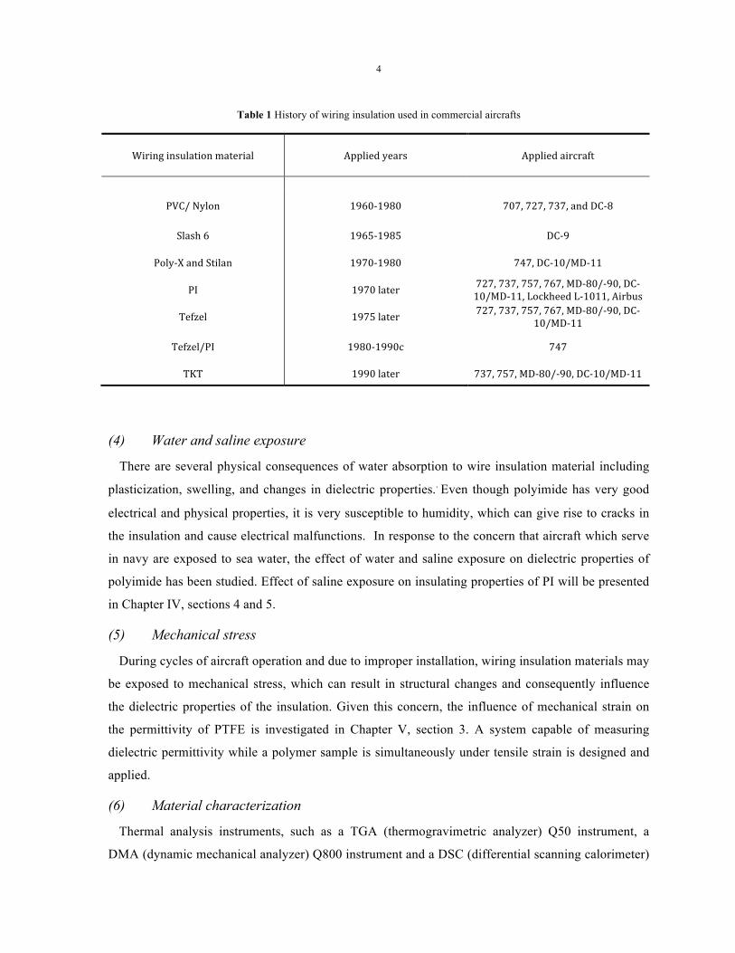
4

Table 1 History of wiring insulation used in commercial aircrafts

Wiring insulation material Applied years Applied aircraft

PVC/ Nylon 1960-‐1980 707, 727, 737, and DC-‐8

Slash 6 1965-‐1985 DC-‐9

Poly-‐X and Stilan 1970-‐1980 747, DC-‐10/MD-‐11

PI 1970 later 727, 737, 757, 767, MD-‐80/-‐90, DC-‐10/MD-‐11, Lockheed L-‐1011, Airbus

Tefzel 1975 later 727, 737, 757, 767, MD-‐80/-‐90, DC-‐10/MD-‐11

Tefzel/PI 1980-‐1990c 747

TKT 1990 later 737, 757, MD-‐80/-‐90, DC-‐10/MD-‐11

(4) Water and saline exposure

There are several physical consequences of water absorption to wire insulation material including

plasticization, swelling, and changes in dielectric properties.. Even though polyimide has very good

electrical and physical properties, it is very susceptible to humidity, which can give rise to cracks in

the insulation and cause electrical malfunctions. In response to the concern that aircraft which serve

in navy are exposed to sea water, the effect of water and saline exposure on dielectric properties of

polyimide has been studied. Effect of saline exposure on insulating properties of PI will be presented

in Chapter IV, sections 4 and 5.

(5) Mechanical stress

During cycles of aircraft operation and due to improper installation, wiring insulation materials may

be exposed to mechanical stress, which can result in structural changes and consequently influence

the dielectric properties of the insulation. Given this concern, the influence of mechanical strain on

the permittivity of PTFE is investigated in Chapter V, section 3. A system capable of measuring

dielectric permittivity while a polymer sample is simultaneously under tensile strain is designed and

applied.

(6) Material characterization

Thermal analysis instruments, such as a TGA (thermogravimetric analyzer) Q50 instrument, a

DMA (dynamic mechanical analyzer) Q800 instrument and a DSC (differential scanning calorimeter)

5

Q20 instrument, are used to investigate thermal properties of the polymers. TGA uses heat to induce

chemical and physical changes in materials and performs a corresponding measurement of mass

change as a function of temperature or time. In some advanced instruments, residual gases released

from materials can be analyzed using TGA-tandem instruments, such as TGA-FTIR or TGA-Mass

Spectrometry, to determine the identity of the released gas and give insight into the weight loss

mechanism. DMA measures the mechanical properties of polymer material as function of temperature

and frequency, which reveals molecular relaxations in polymers. DSC is used to measure

temperatures and heat flow during thermal transitions (glass transition, crystallization and melting) in

polymeric materials. The degree of crystallinity of semi-crystalline polymers can also be obtained

from the crystallization exotherm. Those methods have been applied to investigate thermal properties

of the three polymers, which will be presented in Chapters IV, V and VI.

X-ray diffraction (XRD) and Infrared (IR) spectroscopy are also utilized. Both of these analysis

methods are widely used to determine properties of polymers. XRD turns out to be a convenient and

reliable method to investigate crystalline structure. The degree of crystallinity of polymers, which

plays an important part in determining their dielectric properties, has been measured by XRD. IR

spectroscopy is one of the most common spectroscopic methods applied to analyze organic

compositions. It utilizes a Michelson interferometer and is based on IR absorption by dipolar

molecules as they undergo vibrational and rotational transitions. Each peak in an IR spectrum

indicates characteristic absorption regions for some commonly observed bond strength and bending

deformations. It has been used to detect signs of oxidation due to thermal exposure of PI and ETFE.

2. Study on PMMA-MMT nanocomposites

The subject of this research is focused on investigating dielectric properties of polymer-clay

nancomposite material, and analyzing effect of nanofiller on dielectric relaxation dynamics and

conduction mechanism and. Specifically, the following questions are addressed:

a. What is the effect on interfacial polarization?

b. What is the effect on molecular relaxations of the polymer matrix?

c. What is the effect on glass transition of the polymer matrix?

d. What is the effect on conductivity?

2.1 Motivation

Polymer nanocomposites can be defined as multiphase materials with nanometer-sized (1-100 nm)

fillers dispersed in a continuous polymer matrix. Even a small loading of nanofillers, which have

6

remarkably larger surface as compared to micrometer-sized fillers of the same volume, can give rise

to strong interaction with the polymer matrix. [3] Consequently, the nanocomposite material reveals

upgraded characteristics without any change of polymer processing, such as excellent flame

retardancy, decreased thermal expansion, and enhanced mechanical and dielectric properties. In the

1980s, the Toyota Central Research and Development Laboratories developed the first polymer-clay

nanocomposite, Nylon 6- Montmorillonite (MMT) nanocomposites, which has been used by Toyota

for tough, heat resistant, nylon timing belt covers [4] [5].

In the field of dielectrics and electrical insulation, polymer nanocomposites are known for their

excellent dielectric properties and are the subject of intensive research. For example, polymer-clay

nanocomposites are considered promising as electrical insulation for power apparatus, cables and

wires in the near future due to their good insulating capabilities, flame retardance and mechanical

properties [6]. Thermoplastic and thermoset resins reinforced by nanoparticles of clay, silica, rutile

and alumina have been developed and studied [4]. Changes in dielectric properties of composite

materials due to nanofiller loading have been widely observed by experimental measurement.

However, the way in which nanofillers influence permittivity of composite materials is considered

complicated and not conclusive yet. The contribution of this work is to investigate the conduction

mechanism and dielectric relaxations dynamics of a polymer-clay nanocomposite material, by

modeling frequency dependence of permittivity of the material based on parametric functions.

2.2 Sample material

In this study, polymethylmethacrylate (PMMA)-Montmorillonite (MMT) nanocomposite, produced

by in-situ polymerization of PMMA, is investigated. Among those inorganic additives mentioned in

section 2.1, MMT, a clay mineral, is the most commonly used due to its sandwich-structure silicate

layers with a fundamental unit of a 1-nm-thick planar structure [7] [8]. Stacking of the layers leads to

a regular van der Waals gap between the layers called the interlayer or gallery. The layer silicate

aggregates of MMT can be dispersed on a nanometer level in an engineering polymer and can be

more easily intercalated or exfoliated by various polymers [3] [7]. The structure of MMT and its

effect on dielectric properties of nanocomposite materials are introduced in Chapter II, section 4.

PMMA is an amorphous thermoplastic polymer possessing high strength, superior dimensional

stability and excellent outdoor wearing properties. PMMA reveals α-relaxation from 85 to 165 ºC,

which is associated with main chain motions in the form of glass transition, and β-relaxation below Tg

due to the hindered rotation of the methacrylate side group [9] [10]. The synthesis of the

nanocomposite material is discussed in Chapter VII, section 1.

7

2.3 Effect of MMT loading on dielectric permittivity

The effect of MMT nanofillers on dielectric permittivity is partly associated with changes in

dielectric relaxations due to the inherent heterogeneity of a nancomposite material. As a small volume

fraction of nanofillers can contain billions of nanoparticles, most of the polymer chains in a typical

nanocomposite are located in the vicinity of one or more MMT particles. The dynamics and

segmental motion of polymer chains can change in the confined MMT galleries. Hence, the addition

of MMT nanoparticles also is expected to influence the α- (in the form of glass transition) and β-

relaxations of the PMMA matrix. Further, the accumulation of charge carriers at the polymer-

nanoparticle interfaces gives rise to interfacial polarization, which is absent in pure PMMA. The

interfacial polarization, also known as Maxwell-Wagner-Sillars (MWS) relaxation, has been widely

observed experimentally. Another effect of MMT loading on permittivity of the nanocomposite is

enhancement of conduction at low frequency. The conductivity term of the nanocomposites is much

stronger than for pure PMMA, due to electrical conduction introduced by ions in MMT nanofillers.

The effect of MMT loading on conductivity, interfacial polarization/MWS relaxation and molecular

relaxation dynamics of the nanocomposites is investigated in Chapter VII.

2.4 Technical approach

(1) Permittivity measurement

The dielectric spectroscopy of the nanocomposite material is conducted by using the Novocontrol

Dielectric Spectrometer, as described in section 1.3 and Chapter III.

(2) Modeling of frequency dependence of permittivity

Since the MWS, α- and β-relaxations of the nanocomposite material are merged together [9], a

theoretical function is necessary for separate analysis of the frequency dependence of the three

relaxations. Four classical dielectric relaxation functions have been developed and widely applied:

Debye, Cole-Cole, Davidson-Cole, and Havriliak-Negami (HN) functions. Out of the four, the HN

function, which describes asymmetric distributions of relaxation times, has become preferred in the

analysis of dielectric relaxation of polymeric materials. Thus, in this work, the HN function was used

to model the frequency dependent MWS, α- and β-relaxations of PMMA-MMT nanocomposites.

Considering the contribution of free charge carriers to the low frequency tail of the loss maximum, an

exponential function was used to model the low-frequency conduction of the nanocomposite. The

criterion for a good model fitting is that the least square difference between the experimental data and

model superposition of the dielectric relaxations plus conduction is the smallest. Adopting this

8

approach, changes to the molecular dynamics and conductivity mechanisms of PMMA-MMT

nanocomposites as a function of MMT content have been inferred.

9

Chapter II. Literature Review

1. Dielectric polarization and permittivity

The primary role of electrical insulation is to maintain a continuous and specified value of dielectric

permittivity over a specified electromagnetic field, in order to resist current flow between

wires/cables. Due to presence of insulating medium, the capacitance is increased by a factor of the

dielectric permittivity. The increase in capacitance is attributed with polarization of the dielectrics

where charge distribution is distorted by applied electrical field.

1.1 Polarization and static permittivity

In the presence of an electric field, positive and negative charges in dielectrics are displaced from

their equilibrium positions to form local electric dipoles and the dielectric is said to be polarized. In

the polarized state, the charge distribution is distorted by the applied electric field E. By the principle

of superposition, this distorted charge distribution is equivalent to the original distribution plus a

dipole whose moment is

! = !! (1)

where d is the distance vector from –Q to +Q of the dipole. To measure intensity of the polarization,

we define that the polarization of a material at a point, P measured in Coulombs per meter (C/m), is

the electric dipole moment per unit volume in the material:

! = !! !! (2)

where τ represents volume, or

! = !!!" (3)

where pav is the average electric dipole moment per polarized entity (eg. molecule, ion, etc.), with N

of those per unit volume. [11] [12]

10

Even though the applied electric field E maintains its value, the electric flux density inside the

dielectric material varies from what would exist were the dielectric material replaced by free space. In

the free space part of the parallel capacitive electrodes where the electric field is applied, the electric

flux density D0 is given by

!! = !!! (4)

Where ε0 = 8.854 × 10−12 F/m is the permittivity of free space. In the dielectric portion, the electric

flux density D is related to that in free space D0 by

! = !!! + ! (5)

D can also be related to the applied electric field E by a parameter εs, which is static permittivity of

the dielectric.

! = !! ∙ ! (6)

Above, !! is a second order tensor, which describes anisotropy in the permittivity of material. In this

thesis, however, εs is considered as a scalar. So that,

! = !!! (7)

P can be related to E by another parameter, χe, which is called electric susceptibility.

! = !!!!! (8)

Finally, we can write that

! = !!! + !!!!! = !! 1 + !! ! = !!! (9)

The relative value of εs, εr is given by

!! =!!!!= 1 + !! (10)

11

which is usually referred to as the relative permittivity, or dielectric constant. The relative permittivity

is a parameter that indicates the relative charge storage capability of dielectrics compared with free

space. [12] [13]

Four types of polarization mechanisms are demonstrated in Figure 1.

a. Atomic (electronic) polarization results from shift of the electron clouds within each atom due

to application of an electric field. This type of polarization is quite small compared with the

polarization due to the valence electrons in the covalent bonds within the solid.

b. Ionic polarization occurs in ionic crystals which have distinctly identified ions located at well-

defined lattice sites. Each pair of oppositely charged neighboring ions has a dipole moment in

the presence of an electrical field.

c. Dipolar (orientational) polarization is present in molecules possessing permanent dipole

moments. Take NaCl solution as an example, the Na+ and Cl- ions move around randomly and

collide with each other and the container wall, which destroy the dipole alignments. But with

application of an electrical field, a net average dipole moment per molecule, pav, is directed

along the field, and thus the solution exhibits net polarization.

d. Interfacial (space charge or diffusional) polarization occurs whenever there is an accumulation

of charge at an interface between two materials or between regions within a material. A typical

interfacial polarization is the trapping of electrons or holes at defects at a crystal surface, at the

interface of crystal and the electrode. Dipoles between the trapped charges can increase the

polarization vector. Interfaces also arise in heterogeneous dielectric materials, such as

semicrystalline polymers.

In general a dielectric medium exhibits more than one polarization mechanism. Thus, the average

induced dipole moment per molecule will be the sum of all polarization contributions, depending on

which to determine dielectric permittivity of the material. For example, interfacial polarization plays

an important part in permittivity of semicrystalline polymers, such as PTFE and ETFE.

12

Figure 1 Various polarization processes [11]

1.2 Complex permittivity

The static permittivity is an effect of polarization under dc conditions. However, if a sinusoidal

electrical field is applied, the polarization of the medium under these ac conditions differs from that

of the static case. Polarization of a dielectric always fails to respond instantaneously to variations of

an applied field due to thermal agitations which randomizes the dipole orientations and rotation of

molecules in a viscous medium by virtue of their interactions with neighbors. Thus, the response of

normal material to external fields generally is always causal (arising after the applied field) and

dependent on the frequency of the field, which can be represented by a phase difference.

Consequently, dielectric permittivity is often treated as a complex function of the frequency of the

applied field:

!!!!!"# = ! ! !! !!!"# (11)

13

where ω is frequency of the electromagnetic field, t is time, and j is the imaginary unit.

By convention, we always write the complex dielectric permittivity as

!! = !!! − !!!!! (12)

For linear and causal dielectric response, the relation between the real and imaginary parts of the

complex permittivity is expressed by the Kramers-Kronig relations [13],

!!! ! = 1 + !!

!!!! !!!!

!! !!!!!! !!! (13)

!!!! ! = !!!

!!!! !!!

!! !!!!!! !!!!! (14)

The general features of the frequency dependence of the real and imaginary permittivity for the four

polarization mechanisms is revealed in Figure 2. Although it shows distinctive peaks in εr'' and

transition features in εr', in real materials these peaks and various features are often broader [11]. Fig

3 cannot represent any one particular material, very few materials exhibit all the polarization

mechanisms. [12]

The energy loss is determined by εr''. In engineering applications of dielectrics in capacitors,

smaller εr'' is always preferred for a given εr'. The relative magnitude of εr'' with respect to εr' is

defined as tan δ, called the loss factor or dissipation factor, D. [11]

! = tan ! = !!!!

!!! (15)

14

Figure 2 Schematic demonstration (not to scale) of the frequency dependence of the real and imaginary permittivity in the presence of interfacial, orientational, ionic and electronic polarization mechanisms [11]

2. Electrical breakdown

2.1 Breakdown and dielectric strength

Dielectric materials are widely used as electrical insulation between conductors at different voltage

levels to prevent the ionization of air and current flashovers between conductors. A dielectric medium

is not only defined by its ability to increase capacitance but also, equally importantly, by its insulating

behavior or low conductivity so that the charges are not simply conducted from one conductor to the

other through the dielectric. However, the voltage across a dielectric material and hence the field

within it cannot be increased without limit. Eventually a voltage is reached at which the applied

voltage causes current flow in a device (transistor, capacitor etc) to increase uncontrollably, which

appears as a short between the electrodes. The failure of dielectrics under electrical stress is called

dielectric breakdown, a complex phenomenon of very considerable practical importance.

In gaseous and many liquid dielectrics, the dielectric breakdown does not damage the material

permanently. When the high voltage is removed, the material can sustain electrical field again till its

voltage is sufficiently high to cause breakdown once more. However, in solid dielectrics the

breakdown always gives rise to permanent damage. [11] The maximum filed that can be applied to an

insulating medium without causing dielectric breakdown is called the dielectric strength, which is

15

dependent on the thickness of the medium. Usually, the dielectric strength is measured under standard

ASTM D 149 [14] and given by the ratio between breakdown voltage in test conditions and distance

between electrodes, which is the thickness of specimen.

2.2 Electrical breakdown mechanism of polymer insulations

Mechanisms of electrical breakdown in polymers can be helpful to explain how degradation

processes influence dielectric strength of in polymeric insulation materials can be represented by the

following models [15]:

(i) Low-level degradation models, in which the insulating system's characteristics are deleteriously

affected by the electric field, possibly in conjunction with other agents.

(ii) Deterministic models, in which the ultimate breakdown event is the direct effect of some earlier

causal event or condition produced by the exceeding of a critical electric field.

(iii) Stochastic models in which either local physical conditions are considered to be constantly

changing or there are local electric field variations caused by inhomogeneities such that there is a

finite probability at any time that breakdown may occur.

Here, low-level degrading models, electrical treeing and deterministic breakdown models are

discussed. To conclude the discussion, two ways in which electrical and mechanical aging are related

are discussed.

2.2.1 Low level degradation in polymers

Mechanisms of low-level degradation in polymers are categorized as either physical aging,

chemical aging or electrical aging by Dissado and Fothergill [15], due to different degradation causes.

Physical and chemical aging are considered to be important as they can influence the probability of

breakdown and they also may be accompanied with electrical degradation when driven by an

electrical field during service.

Although introduced separately, all three models may be responsible for polymer degradation in practice.

(1) Physical aging

Physical aging is due to decrease of polymer chain segmental motions in amorphous regions. A

physical description of the aging is usually given in terms of reduction of free volume [15]. All

polymers contain amorphous structure [16], and free volume is the unoccupied part of volume of the

amorphous phase [17] [18].The length of the free path depends on the size of the unoccupied part in

the amorphous phase.

16

Arbauer [19] [20] has developed a free volume breakdown model in which electrons (either

intrinsic or injected) gain kinetic energy by field acceleration in long free volume regions where the

distance between scattering events is large. In a given applied electric field the electrons surmount the

barriers to their motion in the polymer when the free volume is large enough, giving a rapid increase

in current density, and an increase in temperature sufficient to damage the polymer and cause instant

failure.

According to the breakdown criterion [19], the probability that all electrons will be accelerated

sufficiently on the free path to gain the energy necessary enough to overcome the barrier and start the

breakdown will be attained when the voltage drop Fx attains the value

!" = !! =!!!

(16)

where Uµ is an intrinsic property of the polymer dielectric, which is dependent only on its structure;

Eµ is the barrier energy; F is the breakdown electric field; and x is the longest free path which depends

on the sample size, temperature and crystallinity. Generally x is not a constant.

Distribution of the characteristic largest value xn in a sample of size n is:

! ! = !"#{−!!!!!!! !!"#} (17)

where N is a factor by which the sample size increases; and a is a scale parameter.

Both the longest free path and the breakdown field are considered to depend on temperature. When

the frequency f of thermal movements of molecules equals zero (only at zero absolute temperature), x

has its lowest value x0 and consequently the breakdown field has the highest value F0, which only

depends on the structure of the dielectric. At temperatures satisfying f = f(T) > 0, x increases [21] but

the breakdown strength decreases with temperature and time, during which the polymer has been

stressed by the applied field.

(2) Chemical aging

Chemical aging [22] usually proceeds via the formation of polymer free radicals R• following an

initiation step X, i.e.:

! + !(!!!) → ! ∙!+ ! ∙!

Free radicals are very active chemically and lead to propagating chain scission or cross-linking

network formation via chain reactions [15]. Two types of chain scission may occur. Either the bond

17

breaking is random in space with free radical transfer between chains or it unzips a chain by the

ejection of volatile monomers or side group products. The former case produces degradation products

containing large molecular weight fragments and is favored by polyethylene, whereas the latter case

is typical of poly (α-methylstyrene) where it results in a large monomer fraction and poly (vinyl

chloride) which dehydrochlorinates producing hydrogen chloride. The initiating step may be thermal,

oxidative, caused by UV absorption or ionizing radiation, or mechanical.

(3) Electrical aging

Electric field, especially DC, can apparently lead to dissociation and transport of ionized and

ionizable by-products, causing a deterioration of insulation performance through increased losses and

local stress enhancements [15].

According to Kao's theoretical model [23] of electrical discharge and breakdown in condensed

insulating materials, charge carrier injection and recombination play a decisive role in breaking of

polymer chains and the creation of free radicals, low-weight molecules, and traps. Liufu and his

coworkers [24], who believe that electrical aging is due to this gradual degradation process,

conducted a series of experiments which indicated that electrical aging phenomena in polypropylene

can be well interpreted on the basis of Kao's model. They also discovered that the degree of electrical

aging can be determined by the rate of increase in the concentration of stress-created traps.

It has been proved [20] that polyolefin degradation in the electric field under discharge conditions is

due to the formation of free radicals, especially initiated by accelerated electrons with energy higher

than 3.8 eV.

2.2.2. Electrical treeing Electrical treeing is usually considered as a principal form of electrical degradation distinct from

the low-level degradation mechanisms discussed in the former section [25]. It is well established that

electrical tree shapes can be roughly characterized as branch and/or bush-shaped structures [15].

Electrical trees found in polymeric insulation grow in regions of high electrical stress, such as

metallic asperities, conducting contaminant and structural irregularities [15]. Electrical treeing occurs

in all high voltage polymeric insulation and is the principal aging process that leads directly to

breakdown failure [26].

Growth of electrical trees can be divided into two steps: tree initiation and tree propagation.

According to the model for electrical tree initiation developed by Wu and Dissado [27], the

generation of new charge traps by the recombination of injected charges of opposite polarity from a

divergent field stress point, is sufficient to continuously drive the system to the initiation of an

18

electrical tree. They also showed that this is achieved by the increase of trap density to the point

where shallow traps can connect together in the form of a percolation cluster under the application of

an electric field. Bamji et al [28] discovered that certain type or polarity of charge is required in order

to initiate electrical treeing in LDPE (low density polyethylene). For example, it is impossible for the

unipolar injected charge to gain sufficient energy to cause impact ionization or break bonds of the

polymer chain.

Propagation of electrical trees was described as two stages of a tree growth model which was based

on partial discharge measurements [29]. Stage 1 is considered to be the growth of the first small

branches to the opposite electrode. And stage 2 is considered to be the stage where the small branches

will be widened to a pipe-shaped structure. Two alternative theoretical approaches to electrical tree

propagation exist. Stochastic models [30] [31] [32] attribute tree structures to random probabilistic

factors. On the other hand, in the discharge-valance model [33] [34], field fluctuation due to non-

uniformly distributed regions of trapped space charge is responsible.

A kinetic [35] electrical tree growth rate formula is developed. This formula is based on a

quantitative physical model [28] in which the propagation is considered to arise from the formation of

electrodamage that precedes and surrounds the tree tip during the tree propagation process.

! = (!/!!)!! (18)

!"!"=

!"!!!!

!!! !(!!!!) exp (!"#!

!!!!!!!"

) (19)

where X is the number of submicroscopic trees that have formed the electrical tree; L is electrical

tree length; Lb is unit increment in electrical tree length due to the jointing of a secondary tree and is

approximately equal to the average length of the secondary tree; df is the fractal dimension of the

electrical tree; k and h are the Boltzmann and Planck constant, respectively; T is the absolute

temperature; C0 is the size of the submicroscopic void; U0 is the activation energy of the breakdown

process in physics; ε is the dielectric permittivity. E is electric field strength and α is a property of the

material, which represents the activation area in the direction of applied electric field.

2.2.3. Deterministic models of breakdown

Breakdown in polymeric insulators is always ‘catastrophic’ in the sense that it is irreversible and

destructive resulting in a narrow breakdown channel between the electrodes [15]. All catastrophic

breakdown in solids is electrically power driven and ultimately thermal in the sense that the discharge

19

track involves at least the melting and probably carbonization or vaporization of the dielectric [36].

Deterministic models of breakdown can therefore be categorized according to the processes leading

up to this final breakdown stage, which are subdivided into: electric, thermal, electromechanical

(introduced in section 2.2.4) and partial discharge breakdown.

(1) Electric aging

The main classical models of electron driven breakdown include [15] [37]:

a. Avalanche breakdown due to field-induced impact ionization. A high energy electron

collides with a bound electron thereby producing a pair of free electrons which can acquire

sufficient energy in the presence of high field to produce two more pairs of free electrons.

Density of free electrons is thereby rapidly increased in this process and the avalanche can

lead to a very high local energy dissipation causing local lattice disruption after a sufficient

number of generations. Description of avalanche breakdown is in two parts: firstly the

number of generations of ionizing collisions required to cause damage must be estimated,

and secondly the corresponding field must be evaluated.

b. Intrinsic breakdown due to the transfer of the energy of free electrons to the lattice so as to

increase the lattice temperature to a critical value [15]. A recent paper [38] presents a

percolation model for intrinsic breakdown in insulating polymers. The model starts with the

premise that charges are present in the polymers in traps with a variable range of trap depth.

It is shown that the trap barrier can decrease to zero for a set of sites forming a 3-D

percolation cluster when the field becomes high enough. This will result in an abrupt

increase in charge mobility and electron mean free path and an irreversible breakdown via

current multiplication and impact ionization becomes possible.

c. Zener breakdown associating with the direct excitation from valence to conduction band. It

is nondestructive breakdown in semiconductor, occurring when the electric field across the

barrier region becomes high enough to produce a form of field emission that suddenly

increases the number of carriers in this region.

(2) Thermal breakdown

In thermal breakdown models [15], electrical power dissipation causes heating of at least part of the

insulation to above a critical temperature, which results directly or indirectly in catastrophic failure.

The general power balance equation governing thermal breakdown is:

!"!"= !

!!!(!!! + !∇!!) (20)

20

where Cp is the specific heat; D is the density; σ is the electrical conductivity; E is the electric field;

and κ is the thermal conductivity. Provided there is a solution such that !" = !" = 0 below the

critical temperature, thermal breakdown will not take place.

This general equation can be transferred to different forms for different thermal conditions.

If thermal equilibrium is assumed, !" = !" = 0, the general equation simplifies to

! !,! !! + !∇!! = 0 (21)

This is called steady-state breakdown which is a limiting case of general power balance in which

the temperature rise is so slow that the thermal capacity term can be ignored.

The opposite extreme is impulse breakdown in which the temperature rise can be considered so fast

that thermal conductivity may be ignored. This simplifies the analysis as the temperature of the whole

slab can always be considered uniform. In this case the insulator is considered to break down at the

end of the impulse, i.e. the time to breakdown is the length of the impulse. The general equation

therefore becomes:

!!!!"!"= !(!,!)!! (22)

where Cv is the specific heat at constant volume.

Breakdown does not usually occur on a broad front across the insulation area but at weak points.

The temperature of a weak spot reaches the critical temperature before the rest of the insulation. Such

behavior is difficult to analyze in a general manner as different assumptions give rise to a wide

variety of boundary conditions. Filamentary thermal breakdown can be applied in this case which is

illustrated with reference to specific experimental results. Two experimental methods have been used

to investigate filamentary breakdown: prebreakdown current measurement and direct observation of

the spatial and temporal evolution of specimen temperature. Based on result for the prebreakdown

current on several small-area specimens from Mizutani et al, the general equation above is rearranged

to

!!!

exp ∅!!!

= !!

!!!!"!!

!!! (23)

where σ0 and Ø are experimentally determined values which are found to be constant over a given

range of temperature; tb is the time of breakdown; and kB is the Boltzmann constant.

21

Various attempts have been made to monitor the spatial and temporal evolution of the temperature

of thin polymer films after the application of an electric field. Although existence of hot pots has been

proved [15], it has not yet conclusively demonstrated that the initiating breakdown mechanism is

thermal.

(3) Partial discharge breakdown

In partial discharge breakdown [15], sparks occur within voids in the insulation causing degradation

of the void walls and progressive deterioration of the dielectric. Voids are difficult to completely

eliminate in polymeric materials [39]. They may result simply from non-uniform contraction

produced in the slow chemical reactions of thermosetting occurring after the main manufacturing

process.

The influencing parameters in the initiation and the propagation of partial discharge are numerous.

For example, the temperature gradient changes the volume conductivity of the insulating material and

affects the discharge location. It is stated in [40] that inception discharge voltage decreases with gas

pressure within the cavity, depth of which is larger than 6 µm.

2.2.4 Relationship between electrical and mechanical breakdown

Electrical and mechanical aging can be related to each other in two ways.

a. Mechanical aging may be responsible for driving or increasing the possibility of electrical

aging, or even breakdown. In both thermosetting polymers and semicrystalline polymers, the effect of

mechanical stress of a sufficiently high level is to increase the micro-void density and size. The

mechanical stress occurs internally as a result of a slow crystallization in the amorphous regions.

Because the polymer is a solid whose volume is essentially constant, local density increase due to

secondary crystallization is compensated by generation of micro-voids and discontinuities. An

increase in the number of interfaces between amorphous and chain-fold regions may also occur,

giving a greater density of traps and defects and consequently an increase in local space-charge

concentrations. Based on the degradation and aging models presented above (like the free volume

theory, space charge and partial discharge models, etc.), the effect of mechanical aging can increase

the propensity of the polymeric insulation to a range of electrical degradation processes. [15] [39] [41]

[42]

Shu et al [43] measured dielectric strength of 120 µm thick Kapton thin-film after mechanical

fatigue. The sample presents poor partial discharge resistance and breakdown occurred at voltage 800

V. The breakdown point is just on the fatigue point which had undergone mechanical fatigue caused

22

by 300 flexing cycles. It was concluded that flexural stress has a great effect on insulation properties

of this film and the degree of electrical deterioration varies according to extent of mechanical fatigue.

One category of deterministic breakdown – electromechanical breakdown [15] – occurs when the

mechanical compressive stress on the dielectric caused by the electrostatic attraction of the electrodes

exceeds a critical value which cannot be balanced by the dielectric's elasticity. The electromechanical

breakdown voltage can be evaluated by equating these two stresses for the equilibrium situation

before breakdown in a parallel- plate dielectric slab:

!!!!!

!!

!= ! ln !!

! (24)

where Y is the Young's modulus of elasticity; d0 is the initial dielectric thickness; and d is the reduced

thickness after the application of voltage, V.

b. Based on similar features of mechanical and electrical aging, a similar model can be applied

to explain the two processes. Crine [44] detected submicrocavities by SAXS (small-angle X-ray

scattering) in mechanically aged polymers and in electrically aged XLPE (cross-linked polyethylene).

His experiment results showed that electrical and mechanical aging of polymers have similar features,

especially a critical stress above which aging is irreversible.

Harson et al [45] derived the reaction rate constants for material mechanical damage and

reformation given by,

!!!"#$%& = (!/2!)exp [−(! + !")/!"] (25)

!!"#$%&'( = (!/2!)exp [−(! − !")/!"] (26)

where ω is the angular frequency; U is the activation energy of the fracture process; γ is a material

coefficient; σ is the applied stress; k is the Boltzmann constant; and T is the absolute temperature.

They are very similar to formulas of the reaction rate constants for polymer breakdown (aging) and

reformation involved in a kinetic dielectric breakdown model [35], which are described as

!!"#$!%&'($) = (!/2!)exp [−(!! + !!!)/!"] (27)

!!"#$%&'() = (!/2!)exp [−(!! − !!!)/!"] (28)

23

where U0 is the initial well depth; Ge is the conducting microcrack extension force by analogy with

linear elastic fracture mechanisms; and α is a material property which strongly depends on molecular

orientation of the polymer chains.

3. Electrical insulation materials

In recent year, commercial aircrafts are mainly using three kinds of polymer as wire insulation:

Teflon®PTFE (polytetrafluoroethylene), Tefzel® ETFE (ethylene-tetrafluoroethylene), and Kapton®

Polyimide. In this section, basic properties of those polymers are introduced separately.

3.1 PTFE

PTFE, ( CF2 )n, is a fluorocarbon polymer, typically with a very high molecular weight. The

substitution of fluorine for hydrogen causes the material to exhibit extreme properties. Due to the C-F

bonds, it exhibits special properties surpassing those of most polymers due to the substitution of

fluorine for hydrogen, such as very high melting temperature and good chemical resistance. The main

physical and chemical properties of PTFE are compared with those of polyethylene (PE) in Table 2

[46].

In PTFE, closed connected amorphous and crystalline phases coexist due to its extremely high

molecular weight (~ 1×106) [47]. The temperature-pressure phase behavior of crystalline PTFE is

shown in Figure 3 [48] [49]. At atmospheric pressure, the room temperature crystalline structure of

PTFE (phase IV) transfers to phase II below 19 °C [50] and to phase I above 31 °C [51]. The first-

order transition at 19 °C from phase II triclinic to phase IV hexagonal reflects an untwisting in the

helical conformation from 13 atom/180 degree turn [51] [52] to 15 atoms/turn [51] [53] [54] and an

increase in the hexagonal lattice spacing. Above 31 °C the individual polymer chains lose their well

defined helical repeat unit [51] [55]. Further rotational disordering and untwisting of the helices

produces a pseudo-hexagonal structure. At room temperature, phase II transfers to phase III

orthorhombic above ~0.65 GPa [56]. Amorphous PTFE has the same repeat atomic structure as the

crystalline domains but without significant order [57].

PTFE has excellent electrical insulating properties due to its low relative permittivity (2.0-2.2 [58]),

low dielectric loss (<0.0002-0.0005 [59]), good frequency stability in a wide spectral range (up to

10 GHz), and high breakdown strength (19.2 kV/mm [59]). Reference [60] shows the complex

permittivity of PTFE as a function of temperature at microwave frequencies f ≈ 11.5 GHz. The real

permittivity of PTFE decreases from 2.12 to 2.01 as temperature increases from -151 to 102 °C and

24

the dissipation factor is less than 10-3 even at high temperatures. As presented in reference [61], the

real permittivity of PTFE decreases from 2.35 to 2.09 as temperature increases from -150 to 250 °C at

10 kHz. Additionally, because of its good mechanical and thermal stability over temperatures up to

260 °C [62], PTFE has been extensively applied as wire insulation material in air- and spacecraft.

Table 2 Properties of PTFE and PE.

Property PTFE Polyethelyne

Density (g/cm3) 2.2-2.3 0.92-1

Melting Temperature (°C) 342±10 (1st) 327±10 (2nd) 105-140

Tg (α-PTFE) (°C) Tg (β-PTFE) (°C) Tg (γ-PTFE) (°C)

126 30 80

- - -

Surface Energy (dynes/g) 18 33

Resistance to Solvents and Chemicals

Excellent, no known solvent.

Susceptible to hot hydrocarbons.

Figure 3 Temperature-pressure phase diagram of crystalline PTFE with the inter- and intra-polymer chain crystalline structures [48] [49]

25

3.2 ETFE

Ethylene-tetrafluoroethylene (1:1 ratio) alternating copolymer ( CH2CH2CF2CF2 )n is a

fluoroplastic material. At room temperature, it has a molecular conformation in which extended

zigzag chains are packed in orthorhombic cells with cell dimensions a = 0.96 nm, b = 0 nm, c = 0.50

nm and γ = 96° [46]. Each molecule is adjacent to four other molecules in which the –CH2− groups of

a chain are positioned next to the –CF2− groups of the next chain [63]. Essentially, the bulky –CF2−

groups nestle into the space above the smaller –CH2− groups of an adjacent chain [64], interlocking

the chains as a result. Due to this special chain conformation, ETFE has desirable properties such as a

stable dielectric constant, low dissipation factor, high melting temperature and high elastic modulus.

Selected physical and electrical properties of ETFE taken from the literature are listed in Table 3.

Reference [46] has presented the dielectric constant of ETFE over the frequency range from 1 kHz

to 10 GHz at 22 °C and 150 °C. At room temperature, the dielectric constant of ETFE is between 2.5

and 2.6 below 10 MHz and decreases to approximately 2.3 at 10 GHz. Change in dielectric constant

due to temperature can also be observed, especially at high frequencies. The dissipation factor of

ETFE is less than 0.001 below 10 kHz, increasing to 0.023 at 100 MHz and decreasing at higher

frequencies [46].

Table 3 Properties of ETFE.

Property Value Property Value

Density (g/cm3) 1.75-1.79 Dielectric constant 2.5-2.6 below 10 MHz

Melting Temperature (°C) 255-280 Dissipation factor Less than 0.007 below 1 MHz

Molecular relaxation temperatures (°C)

~ 110 (α) 0-100 (α') ~ -87 (γ)

Dielectric strength (kV/mm) 64 (254 µm film)

3.3 Polyimide

Kapton HN is a polyimide film developed by DuPont which has been successfully used as electrical

insulation in a wide range of temperatures, from -269 °C to +400 °C (4 K - 673 K) [65]. The chemical

name for Kapton HN is poly (4,4'-oxydiphenylene-pyromellitimide), and its chemical structure is

26

shown in Figure 4. Kapton® Polyimide is produced from the condensation of pyromellitic

dianhydride and 4,4'-oxydiphenylamine. In addition to its very light weight and advanced mechanical

properties compared to other insulator types, Kapton HN polyimide has good dielectric properties,

such as high breakdown field, low dielectric constant and low loss factor. Selected properties of

125 µm thick Kapton HN film are listed in Table 4 [65]. However, polyimide is very susceptible to

hydrolytic degradation, which can give rise to cracks in the insulation and cause electrical

malfunctions [66].

Figure 4 Chemical Structure of Kapton® Polyimide

Table 4 Selected properties of 125 µm thick Kapton®HN film.

Property Value

Dielectric strength 154 kV/mm at 60 Hz, 23 °C and 50% RH Dielectric constant 3.5 at 1kHz, 23 °C and 50% RH Dissipation factor 0.0026 at 1kHz, 23 °C and 50% RH

Melting point none Glass transition 360 to 410 ºC β-transition 60 to 127 °C

γ-transition -118 to -28 °C Ultimate tensile

strength 231 MPa at 23 °C

Impact strength 78 N cm at 23 °C Yield point at 3% 69 MPa at 23 °C

Melcher et al [67] explored the effect of moisture on the complex permittivity of polyimide film in

a temperature range from 80 to 325 K. It is presented that the imaginary part ε'' measured for a film

which was dried for two days shows only one maximum in the temperature range (the lowest curve).

Absorption of water alters this behavior for different water contents at fixed frequency 10 kHz. The

peak height increases with water content and an additional smaller loss peak appears at its lower

temperature shoulder.

ON N

O

O

O

On

27

The shape of the larger peak, which is notified as the high-temperature peak, is the same for all film.

The influence of the high-temperature peak can be subtracted because its shape is essentially

independent of the water content. But the height of the peak increases with higher water content. The

second peak, the low-temperature peak, is considered to be strongly overlapped by the high-

temperature peak. According to a statement in [68], since the high-temperature peak is present even at

low humidity levels, it is proposed to be associated with water absorbed at the carbonyl groups. And

the low-temperature peak is only visible at higher humidity, it is likely caused by water absorbed at

the ether linkage. As the two loss peaks can be removed by drying the film, it is concluded that the

water dipole causes this relaxation process and not an intrinsic dipole of the polyimide chain.

It is also presented in reference [67] that the increase of the real part ε' near room temperature

correlates to the peaks in ε''.

Thermal exposure of polyimide has also been explored [69] [70] [71] [72]. No significant changes

in the dielectric properties of polyimide were observed after thermal exposure in air or N2 from 200 to

350 °C for up to 5000 hours.

4. Polymer nanocomposites

4.1 Introduction

Polymer nanocomposite can be defined as multiphase materials with nanometer-sized fillers

dispersed in a continuous polymer matrix. Even a small loading of nanofillers, which have

remarkably larger surface as compared to micrometer-sized fillers of the same volume, can give rise

to strong interaction with the polymer matrix. [3] Consequently, the nanocomposite material reveals

upgraded characteristics without any change of polymer processing or composing, such as excellent

flame retardancy, decreased thermal expansion, and enhanced mechanical and dielectric properties. In

1980s, the Toyota Central Research and Development Laboratories developed the first polymer-clay

nanocomposite, Nylon 6- Montmorillonite (MMT) nanocomposites, which has been used by Toyota

for tough, heat resistant, nylon timing belt covers [4] [5].

In the field of dielectrics and electrical insulation, polymer nanocomposites are known for their

excellent dielectric properties and are targeted for investigation in labs. Thermoplastic and thermoset

resins reinforced by nanoparticles of clay, silica, rutile and alumina have been developed and studied

[4]. Among those inorganic additives, MMT (montmorillonite), a clay mineral, is the most commonly

used due to its sandwich-structure silicate layers with a fundamental unit of a 1-nm-thick planar

structure [7] [8]. The layer silicate aggregates of MMT can be dispersed on a nanometer level in an

28

engineering polymer and can be more easily intercalated or exfoliated by various polymers [3] [7],

such as vinyl polymers, condensation (step) polymers, polyolefins and biodegradable polymers [6]

[73].

4.2 Structure

Layered silicates of MMT belong to the family of 2:1 layered or phyllosilicates. As shown in Figure

5 [73], the crystal structure consists of layers made up of two tetrahedrally coordinated silicon atoms

fused to an edge-shared octahedral sheet of either aluminum or magnesium hydroxide. The layer

thickness is around 1 nm, and the lateral dimensions of these layers may vary from 3 nm to several

micrometers or larger, which depend on the particular layered silicate. Stacking of the layers leads to

a regular van der Waals gap between the layers called the interlayer or gallery. Isomorphic

substitution within the layers (for example, Al3+ replaced by Mg2+ or Fe2+, or Mg2+ replaced by Li1+)

generates negative charges that are counterbalanced by alkali and alkaline earth cations situated inside

the galleries. This type of layered silicate is characterized by a moderate surface charge known as the

cation exchange capacity. This charge in not locally constant, but varies from layer to layer, and

should be considered as an average value over the whole crystal. [6] MMT nanoparticles can

intercalate with various polymers, which causes an increase in the distance between the silicate layers

that depend on size of polymer molecules [8].

In order to obtain good mechanical and thermal properties, it is necessary to have strong interaction

between polymer and MMT phases so that the both can be dispersed at the nanometer level. However,

in the pristine state, layered silicates are only miscible with hydrophilic polymers, such as

poly(ethylene oxide) (PEO), or poly(vinyl alcohol) (PVA). To render layered silicates miscible with

other polymers, one must convert the normally hydrophilic silicate surface to an organophilic one,

making the intercalation of many engineering polymers possible. Generally, this modification process

can be done by ion-exchange reactions with cationic surfactants including primary, secondary,

tertiary, and quaternary alkylammonium or alkylphosphonium cations. Alkylammonium or

alkylphosphonium cations in the organosilicates lower the surface energy of the inorganic host and

improve the wetting characteristics of the polymer matrix, and result in a larger interlayer spacing. In

addition, the alkylammonium or alkylphosphonium cations can provide functional groups that can

react with the polymer matrix, or in some cases initiate the polymerization of monomers to improve

the strength of the interface between the inorganic and the polymer matrix. [74] [75] [76] [77]

29

Figure 5 Crystal structure of layered silicates [73]

In general, layered silicates have layer thickness on the order of 1 nm and a very high aspect ratio

(e.g. 10–1000). A few weight percent of layered silicates that are properly dispersed throughout the

polymer matrix thus create much higher surface area for polymer/filler interaction as compared to

conventional composites. Depending on the strength of interfacial interactions between the polymer

matrix and layered silicates, three different types of polymer-MMT nanocomposites are

thermodynamically achievable (see Figure 6):

a. Intercalated nanocomposites: in intercalated nanocomposites, the insertion of a polymer

matrix into the layered silicate structure occurs in a crystallographically regular fashion,

regardless of the clay to polymer ratio. The interlayer in intercalated nanocomposites is

normally a few molecular layers of polymer. Properties of the composites typically

resemble those of ceramic materials.

b. Flocculated nanocomposites: conceptually this is same as intercalated nanocomposites.

However, silicate layers are sometimes flocculated due to hydroxylated edge–edge

interaction of the silicate layers.

c. Exfoliated nanocomposites: in an exfoliated nanocomposite, the individual clay layers are

separated in a continuous polymer matrix by an average distance that depends on clay

loading. Usually, the clay content of an exfoliated nanocomposite is much lower than that

of an intercalated nanocomposite.

30

Figures 6 [73] and 7 [7] schematically show the three types of polymer-MMT nanocomposites.

Figure 6 Schematic illustration of three different types of polymer-MMT nanocomposites [73]

Figure 7 Schematic demonstration of various morphology of MMT dispersed in polymer matrices. (a) fully exfoliated; (b) partially exfoliated and partially intercalated; (c) severely intercalated; (d) partially intercalated and partially aggregated; (e)

severely aggregated. The dark grey zones are interphases; (f) shows the change of the dispersions as the clay content increases (from 0 to 15 vol%). Solid, dash and dot lines represent the volume fractions of exfoliated, intercalated and

phased-separated silicates, respectively [7].

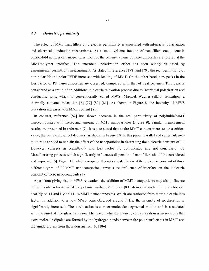
31

4.3 Dielectric permittivity

The effect of MMT nanofillers on dielectric permittivity is associated with interfacial polarization

and electrical conduction mechanisms. As a small volume fraction of nanofillers could contain

billion-fold number of nanoparticles, most of the polymer chains of nanocomposites are located at the

MMT/polymer interface. The interfacial polarization effect has been widely validated by

experimental permittivity measurement. As stated in references [78] and [79], the real permittivity of

non-polar PP and polar PVDF increases with loading of MMT. On the other hand, new peaks in the

loss factor of PP nanocomposites are observed, compared with that of neat polymer. This peak is

considered as a result of an additional dielectric relaxation process due to interfacial polarization and

conducting ions, which is conventionally called MWS (Maxwell-Wagner-Sillars) relaxation, a

thermally activated relaxation [6] [79] [80] [81]. As shown in Figure 8, the intensity of MWS

relaxation increases with MMT content [81].

In contrast, reference [82] has shown decrease in the real permittivity of polyimide/MMT

nanocomposites with increasing amount of MMT nanoparticles (Figure 9). Similar measurement

results are presented in reference [7]. It is also stated that as the MMT content increases to a critical

value, the decreasing effect declines, as shown in Figure 10. In this paper, parallel and series rules-of-

mixture is applied to explain the effect of the nanoparticles in decreasing the dielectric constant of PI.

However, changes in permittivity and loss factor are complicated and not conclusive yet.

Manufacturing process which significantly influences dispersion of nanofillers should be considered

and improved [6]. Figure 11, which compares theoretical calculation of the dielectric constant of three

different types of PI-MMT nanocomposites, reveals the influence of interface on the dielectric

constant of these nanocomposites [7].

Apart from giving rise to MWS relaxation, the addition of MMT nanoparticles may also influence

the molecular relaxations of the polymer matrix. Reference [83] shows the dielectric relaxations of

neat Nylon 11 and Nylon 11-4%MMT nanocomposites, which are retrieved from their dielectric loss

factor. In addition to a new MWS peak observed around 1 Hz, the intensity of α-relaxation is

significantly increased. The α-relaxation is a macromolecular segmental motion and is associated

with the onset off the glass transition. The reason why the intensity of α-relaxation is increased is that

extra molecule dipoles are formed by the hydrogen bonds between the polar surfactants in MMT and

the amide groups from the nylon matrix. [83] [84]

32

Figure 8 Frequency-dependence of dielectric loss factor of PP-MMT nanocomposites measured at 125 ºC [81]

Figure 9 Dielectric constant of neat polyimide (PI) and PI-MMT nanocomposites as a function of frequency at -130 ºC (a) and 130 ºC (b) [82]

33

Figure 10 Dielectric constants of PI-MMT and PI-mica nanocomposites as a function of MMT or mico volume fraction, measured at 1 kHz and 150 °C [7].

Figure 11 Comparison of effective dielectric constants of three idealized types of PI-MMT nanocomposites [7]

34

4.4 Conclusion

Polymer-MMT nanocomposites has been widely developed and investigated in labs. However, the

way how the addition of MMT influences dielectric properties is not conclusive yet. The mechanism

is believed to be complicated, and highly depends on MMT configuration, synthesis process and

polymer/MMT interaction. In this case, well-controlled synthesis process as well as accurate

experimental measurement is significant to successfully investigate properties of polymer-MMT

nanocomposites.

35

Chapter III. Dielectric spectroscopy

In this work, the dielectric permittivity of sample materials before and after degradation is

measured either by using a Novocontrol dielectric spectrometer or by a Agilent LCR meter coupled

with a 16451 LCR meter.

1. Novocontrol Dielectric Spectrometers

Dielectric spectroscopy measures the impedance spectrum Z*(ω) of a sample material arranged

between two or more electrodes. The sample material may be liquid or solid. The main interest here is

in material properties, and contributions due to electrode effects should typically be avoided.

Permittivity, ε*(ω), is a fundamental material parameter and can be easily evaluated from Z*(ω) with

the knowledge of sample dimensions. With modern equipment, impedance can be accurately and

automatically determined from a few mHz up to several GHz (15 decades of frequency) for nearly all

kind of materials. Beyond frequency, electrical materials properties depend on additional parameters,

the most important one being temperature. Time, DC bias (superimposed static electrical field), AC

field strength and pressure dependence are frequently determined as well.

Novocontrol dielectric spectrometer for material analysis is capable of measuring the electric

properties of materials over a wide frequency range, from 1 µHz to 3 GHz, and temperature range

from -160 °C to 400°C. This is done by measuring the impedance Z*(ω) of a capacitor made up by

two or more electrodes with the sample material in between at a controlled temperature. From Z*(ω),

the complex permittivity ε*(ω) spectrum is evaluated.

As shown in Figure 12, a dielectric spectrometer consists of four components: a system to measure

the complex impedance Z*(ω) of the sample capacitor over a sufficient frequency and impedance

range, a sample cell which connects the sample capacitor to the impedance analyzer and mounts it

into a cryostat for temperature control, a temperature control system which adjusts the sample

capacitor to fixed temperatures or continuously changes temperature, and a computer with a software

package for system control and evaluation.

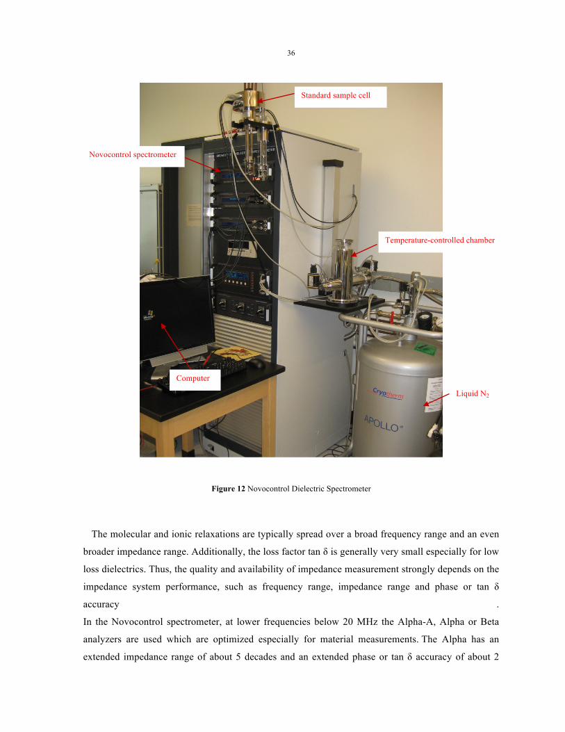
36

Figure 12 Novocontrol Dielectric Spectrometer

The molecular and ionic relaxations are typically spread over a broad frequency range and an even

broader impedance range. Additionally, the loss factor tan δ is generally very small especially for low

loss dielectrics. Thus, the quality and availability of impedance measurement strongly depends on the

impedance system performance, such as frequency range, impedance range and phase or tan δ

accuracy .

In the Novocontrol spectrometer, at lower frequencies below 20 MHz the Alpha-A, Alpha or Beta

analyzers are used which are optimized especially for material measurements. The Alpha has an

extended impedance range of about 5 decades and an extended phase or tan δ accuracy of about 2

Standard sample cell

Temperature-controlled chamber

Liquid N2

Novocontrol spectrometer

Computer

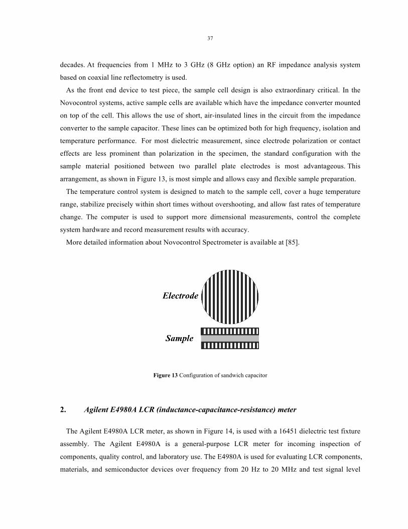
37

decades. At frequencies from 1 MHz to 3 GHz (8 GHz option) an RF impedance analysis system

based on coaxial line reflectometry is used.

As the front end device to test piece, the sample cell design is also extraordinary critical. In the

Novocontrol systems, active sample cells are available which have the impedance converter mounted

on top of the cell. This allows the use of short, air-insulated lines in the circuit from the impedance

converter to the sample capacitor. These lines can be optimized both for high frequency, isolation and

temperature performance. For most dielectric measurement, since electrode polarization or contact

effects are less prominent than polarization in the specimen, the standard configuration with the

sample material positioned between two parallel plate electrodes is most advantageous. This

arrangement, as shown in Figure 13, is most simple and allows easy and flexible sample preparation.

The temperature control system is designed to match to the sample cell, cover a huge temperature

range, stabilize precisely within short times without overshooting, and allow fast rates of temperature

change. The computer is used to support more dimensional measurements, control the complete

system hardware and record measurement results with accuracy.

More detailed information about Novocontrol Spectrometer is available at [85].

Figure 13 Configuration of sandwich capacitor

2. Agilent E4980A LCR (inductance-capacitance-resistance) meter

The Agilent E4980A LCR meter, as shown in Figure 14, is used with a 16451 dielectric test fixture

assembly. The Agilent E4980A is a general-purpose LCR meter for incoming inspection of

components, quality control, and laboratory use. The E4980A is used for evaluating LCR components,

materials, and semiconductor devices over frequency from 20 Hz to 20 MHz and test signal level

38

from 0.1 mV (rms) to 2 V (rms) or from 50 µA to 20 mA (rms). With Option 001, the E4980A’s test

signal level range spans 0.1 mV (rms) to 20 V (rms), and 50 µA (rms) to 200 mA (rms). Also, the

E4980A with Option 001 enables up to ± 40 V (rms) DC bias measurements (without Option 001, up

to ± 2 V (rms)), DCR measurements, and DC source measurements using the internal voltage source.

The E4980A offers C (capacitance)-D (dissipation factor) measurement with a basic accuracy of ±

0.05% (C), ± 0.0005 (D) at all frequencies with seven-digit resolution (the dissipation factor

resolution is 1 ppm) in every range. Its list sweep function permits entry of up to 201 frequencies, test

signal levels, or bias level points to be automatically measured. The E4980A allows one to obtain the

average value of up to 256 measurements.

The 16451 assembly is a test fixture for measuring disc and film dielectric materials when

connected to Agilent's LCR meters or impedance analyzers, and is usable up to 15 MHz. Figure 15

shows the configuration of the test fixture assembly. Its capacitive electrode pair contains one

unguarded electrode and a guarded/guard electrode which is the combination of a guarded electrode

and a guard electrode. The unguarded electrode is connected to the Hc (High current) and Hp (High

potential) terminal of the instrument, while the guarded electrode is connected to the Lc (Low current)

and Lp (Low potential) terminals of the instrument and the guard electrode is connected to the guard

terminal. The 16451B provides four guarded/guard electrodes and accessories, which are

interchangeable and movable using the knobs on the micrometer.

The main advantage of using the guarded electrode system is to inhibit measurement error due to

fringing field effects at the edges of the sample under test. The dielectric constant of the media

material is calculated from the measured capacitance value, as above-mentioned. While using the

unguarded electrode system shown in Figure 16a, there is measurement error caused by stray

capacitance at the edge of the test material. The guarded electrode system used in 16451 test fixture,

as shown in Figure 16b, can avoid the stray capacitance at the edge of the electrode and measure

capacitance accurately. Table 5 lists description, dimension and sample requirements of the four

guarded/guard electrodes.

39

Figure 14 Agilent E4980A LCR meter

Figure 15 Agilent 16451 test fixture assembly

40

Figure 16 Capacitance measurement using (a) unguarded (b) guarded electrode system [86]

For parallel capacitive electrodes, the permittivity of media material can be obtained from

capacitance:

! = ! !! (29)

where C and d are capacitance and distance between the electrodes, respectively; ε is dielectric

permittivity of media material and A is the area of the electrodes.

The relative permittivity εr of the media material is the ratio of permittivity over that of free space ε0:

0r

εε

ε= (30)

Thus, the relative permittivity of a sample under test is given by

(a)

(b)

41

0

pr

tCA

εε

= (31)

where, t is thickness of sample under test for contact measurement, which is equivalent to the distance

between the electrodes and Cp is the equivalent parallel capacitance.

More detailed information about the E4980A LCR meter and the 16451 test fixture is available at

[86] and [87].

Table 5 Four guarded/guard electrodes available for 16451 test fixture

Guarded electrode Description Electrode

diameter

Requirement of sample

dimension (mm)

Electrode A used to measure a

material without thin film 38 mm

40 ≤ d(diameter) ≤ 50;

t(thickness) ≤ 10

Electrode B used to measure a

material without thin film 5 mm

10 ≤ d ≤ 56;

t ≤ 10

Electrode C used to measure a

material with thin film NA

d of sample = 56;

5 ≤ d of guarded film

electrode ≤ 50;

Inner d of guarded

electrode ≤ 52;

t ≤ 10

Electrode D used to measure a

material with thin film NA

20 ≤ d of sample ≤ 56;

5 ≤ d of guarded film

electrode ≤ 14;

t ≤ 10

42

3. Experimental permittivity measurement

For permittivity measurement using either the Novocontrol dielectric spectrometer or the Agilent

E4980A LCR meter with option 001, all PTFE and ETFE samples were cut to approximately 30 × 30

× 1 mm3 with smooth and parallel surfaces. The thickness of the samples was measured using a

Fowler Ultra Digit Mark IV micrometer with systematic uncertainty of 1 µm. Ten measurements were

taken on both sides of each sample, the small value of relative uncertainty (less than 0.2%) shows that

the samples are quite uniform in thickness. Even though relative uncertainty increases with length of

thermal exposure, the smoothness of all the samples was considered sufficiently good that a

conductive coating was not applied before permittivity measurement. In this case, guarded electrode

B (Table 5) is suitable to permittivity measurement of PTFE and ETFE by the Agilent LCR meter.

All the PTFE and ETFE samples were cleaned with ethanol before permittivity measurement to

remove surface contaminants.

However, it was found that conductive coating is necessary for permittivity measurement of PI film

samples. A silver paint, which can dry quickly at room temperature but requires 20 hr for curing to

obtain excellent electrical properties, was used to coat samples measured at room temperature by the

LCR meter, which is attached with dielectric test fixture applying guarded electrode D. Samples

measured by the Novocontrol spectrometer are coated by gold sputtering. The thickness of PI samples

was measured with a micrometer with uncertainty of 1 µm, its accuracy had been verified with films

with standard thickness. Before silver painting, all the PI samples were cleaned by wiping with a little

ethanol.

43

Chapter IV. Polyimide

Polyimide (PI) is widely used as an insulation material for machines and wiring, and is effective at

temperatures up to 400 °C. Given the fact that polyimide may be exposed to extreme temperatures

during unusual events in service, and is commonly immersed in salt water while serving in navy

aircraft, the effect of thermal exposure above 400 °C and water/saline exposure on its permittivity is

investigated in this chapter. Statistical analysis of electrical breakdown behavior of PI following

thermal and water exposure is also conducted.

1. Sample material

All the PI samples under investigation in this chapter were cut from large sheets of 125-µm-thick

Kapton® HN PI film obtained from Dupont. Since the permittivity and electrical breakdown strength

of Kapton PI film changes significantly with moisture content [13], dry samples are needed in order

to obtain baseline (control) values of dielectric strength for comparing with those obtained following

thermal exposure and immersion in water. In order to determine a heating temperature to effectively

remove water from PI, weight loss of a PI sample was monitored by thermogravimetric analysis

(TGA) while it was heated from 30 to 900 °C in air at 30 °C/min. As shown in Figure 17, an initial

weight loss of 1% was observed at approximately 200 °C, which is attributed to loss of water from

the sample during the heating process. Therefore, PI samples for baseline breakdown measurement

were dried by heating at 200 °C for 1 hr, which, moreover, cannot give rise to degradation of PI.

One dry PI control sample was coated with gold paint immediately upon removal from the

isothermal furnace. Its complex permittivity was measured at frequencies from 1 Hz to 1 MHz

over temperatures increasing from −140 °C to 180 °C in increments of 10 °C, by using a

Novocontrol Dielectric Spectrometer with temperature-controlled standard sample cell. The real

permittivity, ε′, and loss factor, tan δ, of the dry PI control sample over the whole temperature and

frequency ranges are plotted as surface plots in Figures 18a and 18b, respectively. Below

approximately 0 °C, ε′increases with temperature; while it decreases with increasing temperature at

higher temperatures. Given that polyimide is a polar polymer, the dependence of its real permittivity

on temperature is determined by how much its intra- and intermolecular interactions change with

temperature [88]. If intra- and intermolecular interactions is independent of temperature, the

permittivity would decrease with temperature. However, if intra- and intermolecular interactions

change significantly with temperature, the dependence of permittivity on temperature would be

governed by the change in intra- and intermolecular interactions and ε′would increases with

44

temperature. Therefore, it is speculated here that the intra- and intermolecular interactions of

polyimide changes significantly with temperature below 0 °C, while at higher temperatures their

change with temperature is reduced. It can also be seen that ε′decreases with frequency at each

temperature; while tan δ as a function of temperature reveals two peaks. The higher-temperature peak

corresponds to the β-relaxation of PI, which is a sub-Tg relaxation that takes place at temperatures

between 60 and 127 °C [89]. It is considered to be a result of torsional oscillations of the phenylene

ring, involving imide groups of PI [90]. On the other hand, the lower-temperature peak can be

ascribed to the γ-relaxation of PI, which is usually observed at temperatures between -118 and -28 °C

[89] and occurs due to increase in the vibration of aromatic groups as intra- and intermolecular

interactions decrease in the presence of absorbed moisture [90]. The highest values of tan δ observed

at low frequencies and high temperatures are considered as a result of electrode polarization [91].

0 200 400 600 800 1000

0

20

40

60

80

100

80 100 120 140 160 180 200 220 240

96

98

100

102

104

Wei

ght (

%)

Temperature (oC)

Figure 17 Percentage weight loss of PI as a function of temperature measured at 30 °C/min heating rate

45

Figure 18 The real permittivity (a) and loss factor (b) of dry PI over frequency range 1 Hz to 1 MHz and temperature range −140 to 180 °C

2. Effect of thermal exposure on permittivity

It has been presented previously in the literature that dielectric properties of PI are not changed

significantly by heating at temperatures up to 350 °C for as long as 5000 hours either in air or N2 [69]

[70] [71] [72]. However, given the fact that electrical wiring insulation still has to work under

extreme temperatures, such as may occur in the vicinity of extreme events during service, it is also

valuable to explore the effect of thermal degradation at higher temperatures in air on the dielectric

permittivity of PI.

The Kapton PI film was sectioned into 3 cm by 10 cm rectangular samples, which were heated at

400, 425, 450 and 475 °C for 1, 2, 3, 4 and 5 hours in an isothermal muffle furnace. In order to

eliminate possible distortion of the samples during the heating process, the two shorter edges of each

PI sample were stabilized by a pair of mirror-finish stainless steel plates. Consequently, the majority

of each sample was exposed to oxygen and eligible for permittivity measurement. After heating, the

PI samples were removed from the furnace and cooled in air. With higher temperatures or longer

heating times, the samples became more brittle, darker and thicker, which can be associated

with the formation of oxidized layers on the sample surfaces during the initial degradation of PI [92]

[93]. Thermal degradation at temperatures higher than 475 °C or for exposure times longer than 5 hr

(a) (b)

β

γ

46

was not conducted because the PI became so badly deformed that its permittivity could not be

measured successfully.

The thickness of all treated samples was measured by using a micrometer with uncertainty of 1 µm

after cooling. Directly following thickness measurement, the samples were coated with silver paint,

serving both as film electrodes for permittivity measurement and to prevent significant moisture

exchange between the samples and air. The silver paint dries quickly at room temperature, but

requires curing for 16 hr at room temperature to achieve a volume resistivity as low as 5×10-6 to

1.25×10-5 Ω m. When the silver paint was totally cured, each sample was cut into three smaller

samples for permittivity measurement. The permittivity of all treated samples was measured from

1 kHz to 2 MHz at room temperature, using the Agilent E4980A LCR meter coupled with a 16451

test fixture. The three identically degraded samples under all degrading conditions revealed highly

similar values of ε' and tan δ, the standard deviation measured for both is less than 1%.

Figure 19 shows the loss factor of PI degraded at 475 °C for 3 hr as a function of temperature and

frequency. Compared with Figure 18b, the height of the β-relaxation peak is substantially increased,

indicating tremendous increase in the intensity of the β-relaxation [94]. The β-relaxation cannot be

observed at frequencies higher than 500 Hz after thermal degradation. To explore the effect of

thermal degradation on the γ-relaxation, the frequency dependence of tan δ at room temperature for

the degraded PI is plotted and compared with that of the dry PI in Figure 20. Even though the

intensity of the γ-relaxation is not obviously changed, the peak for γ-relaxation moves to higher

frequencies after the thermal degradation.

As shown in Figure 21, the real permittivity of PI measured at 1 kHz increases with time and

temperature of thermal degradation in air. The real permittivity of the PI sample heated at 475 °C for

3 hours is 4.15, versus 3.77 for the sample heated at 450 °C for 5 hours and 3.24 for the control

sample. PI samples degraded at 475 °C for 4 and 5 hours were highly brittle and wrinkled, which

meant that it was not possible to measure their permittivity successfully. On the other hand, tan δ of

PI reveals little change after thermal degradation at 400, 425 or 450 °C and is not shown here. After

thermal degradation at 475 °C for 3 hr, however, tan δ of PI as function of frequency is changed

significantly, as shown in Figure 20.

47

Figure 19 The loss factor of PI degraded at 475 °C for 3 hr, measured over frequency from 1 Hz to 1 MHz and temperature from −140 to 180 °C

100 101 102 103 104 105 1060

5

10

15

20

25

30

35

dry PI degraded PI

Loss

fact

or, t

an δ

10-3

Frequency (Hz)

γ-relaxation

Figure 20 The loss factor of dry PI and PI degraded at 475 °C for 3 hr as a function of frequency at room temperature

β γ

48

0 1 2 3 4 53.2

3.4

3.6

3.8

4.0

4.2

ε' a

t 1 k

Hz

Thermal exposure time (hr)

400 OC 425 OC 450 OC 475 OC

Figure 21 Effect of thermal degradation time and temperature on ε' of PI at 1 kHz. Error bars indicate the standard deviation in measurements on three nominally-identical samples

The activation energy for the β- and γ-relaxations can be calculated from the Arrhenius equation:

! = ! ln !!!!

!!!− !

!!

!! (32)

where E is the activation energy of molecular relaxation; k is the Boltzmann constant; T1 and T2 are

the absolute temperatures of transition at frequencies f1 and f2, respectively. The equation can be

rewritten as a linear function relating 1/T and ln ω:

!" ! = − !!!!+ ! (33)

where C is a constant. By plotting the dependence of ln f on 1/T, the activation energy can be

obtained from slope of the line. Based on the measured complex dielectric spectra as shown in

Figures 18b and 19, the Arrhenius plots of both β- and γ-relaxations of the dry and degraded PI (at

475 °C for 3 hr) are given in Figure 22. For the dry PI, the activation energy is determined to be 0.48

± 0.02 eV for the γ-relaxation and 0.85 ± 0.05 eV for the β-relaxation. The uncertainties arise from

estimated uncertainty in the slopes obtained via linear regression. Those values of activation energy

49

determined here agree, to within experimental uncertainty, with values presented in the literature:

0.47 eV for the γ-relaxation [95], and 0.87 eV for the β-relaxation [96] [89]. However, β-relaxation of

the degraded PI is only observed below 500 Hz and reveals no variation as function of temperature.

Therefore, the Arrhenius plot for β-relaxation is a vertical line as shown in Figure 22, and its

activation energy could not be determined. On the other hand, the activation energy of the γ-

relaxation is determined to be 0.46 ± 0.02 eV for degraded PI, which is not influenced by thermal

degradation at 475 °C for 3 hr, despite the shift of the γ-relaxation to higher frequency.

Dine-Hart et al have studied the process of oxidative thermal degradation of PI for a short period in

air by thermal analysis methods, saponification testing and infrared spectroscopy [92] [93]. It was

observed that the chemical structure of PI film was significantly changed by thermal degradation [92].

Figure 23 demonstrates pyrolysis process of imide groups during oxidative thermal degradation of PI,

which gives rise to CO2 and CO, breaks chemical bonding in imide groups and forms free radicals

[93]. Thus, we hypothesize that the significant increases in ε' of PI following oxidative thermal

degradation at 400 to 475 °C could arise from the formation of free radicals, which enhance electrical

polarization in PI. Moreover, due to scission in chemical bonding in imide groups, the torsional

oscillations of the phenylene ring become much easier, increasing the intensity of the β-relaxation. In

order to further investigate this hypothesis, a Mass Spectrometer (MS) coupled with a Fourier-

Transform Infrared (FTIR) Spectrometer was applied to detect release of gas while a Kapton PI

sample was heated from 30 °C to 900 °C with heating rate 30 °C/min. As shown in Figure 24,

compared with the spectrum at 30 °C, the FTIR spectra at 400, 450 and 480 °C reveal new

absorbance peaks at 2170, 2320 and 2370 cm-1, corresponding to chemical bonds of CO and CO2 [24].

The mass also confirmed the release of CO2 and CO at temperatures above 400 °C; and consequently

endorse the degradation path of PI shown in Figure 23. Thus, we can conclude that the significant

increase in the real permittivity and intensity of the β-relaxation are results of pyrolysis of imide

groups of PI during oxidative thermal degradation.

50

2.0 2.5 3.0 3.5 4.0 4.5 5.0 5.5 6.0 6.5 7.0

0

2

4

6

8

10

12

γ, 0 hr

ln ω

1000/T

β, 0 hr

γ, 3 hr

β, 3 hr

Figure 22 Arrhenius plot for β- and γ- relaxations of dry PI and PI degraded at 475 °C for 3 hr

Figure 23 Pyrolysis process of imide groups of PI during heating [93]

51

2000 2100 2200 2300 2400 2500

30 oC

400 oC

450 oC

480 oC

Abso

rban

ce (A

.U.)

CO 2170

CO2 2370

Wave number (cm-1)

CO2 2320

Figure 24 FTIR spectra of Katpon polyimide at 30, 400, 450 and 480 °C

3. Effect of water/saline exposure on permittivity

All PI samples for saline exposure experiments were cut into strips 3 cm wide by 9 cm long and

immersed in distilled water or saline solutions for various times, including 0.5, 1, 2, 4, 6, 12 and 24

days. Saline solutions with three different concentrations were made by mixing distilled water with

sodium chloride: 0.45 g/l, 6 g/l and 80 g/l, with conductivities 1 mS/cm, 10 mS/cm and 100 mS/cm

[97], respectively. Immediately after removal from water or saline solutions, the samples were wiped

to remove water on their surfaces, their thickness was measured by using the micrometer, and the

samples were coated with silver paint introduced in section 2. When the silver paint was totally cured,

each sample was cut into three smaller samples for permittivity measurement. The permittivity of all

treated samples was measured from 1 kHz to 2 MHz at room temperature, using the Agilent E4980A

LCR meter coupled with a 16451 test fixture. The three identically degraded samples under all

degrading conditions revealed highly similar values of ε' and tan δ, the standard deviation measured

for both is less than 1%.

Figure 25 shows the real permittivity and loss factor measured at 1 kHz as a function of sample

immersion time in water and saline solutions. In the case of both water and saline, the real

52

permittivity and loss factor of PI exhibit rapid increases in the first 4 days, but neither of them

changes obviously after 6 days. Figures 26 and 27 show how ε' and tan δ of PI behave as a function of

frequency from 1 kHz to 2 MHz and immersion time, in water and 80 g/l saline, over 4 days. ε' and

tan δ of PI immersed in water are increased by approximately 11% and 40%, respectively; and by

12% and 40% for the sample immersed in 80 g/l saline. As shown in Figures 26b and 27b, the

intensity of the γ-relaxation increases with time of immersion, because the PI samples absorb more

moisture with longer time of immersion. This observation agrees well with the findings by

mechanical testing methods [95]. The frequency of the γ-relaxation, however, is not changed as a

function of immersion time.

0 5 10 15 20 253.15

3.20

3.25

3.30

3.35

3.40

3.45

3.50

3.55

3.60

Rea

l per

mitt

ivity

, ε'

Immersion time (day)

0 g/l 0.45 g/l 6 g/l 80 g/l

0 2 4 6 8 10 12 14 16 18 20 22 240.0016

0.0017

0.0018

0.0019

0.0020

0.0021

0.0022

0.0023

0.0024

Loss

fact

or, t

an δ


Figure 25 The real permittivity (a) and loss factor (b) of PI immersed in water and saline solutions, measured at 1 kHz. Error bars indicate the standard deviation in measurements on three nominally-identical samples

(a)

(b)

53

103 104 105 1063.10

3.15

3.20

3.25

3.30

3.35

3.40

3.45

3.50

3.55

Rea

l per

mitt

ivity

, ε'

Frequency (Hz)

103 104 105 106

0.002

0.004

0.006

0.008

0.010

0.012

γ-relaxation

0 day 0.5 day 1 day 2 day 4 day

Loss

fact

or, t

an δ

Frequency (Hz)

Figure 26 The real permittivity (a) and loss factor (b) of PI following immersion in distilled water

(b)

(a)

54

103 104 105 1063.10

3.15

3.20

3.25

3.30

3.35

3.40

3.45

3.50

3.55

3.60

Rea

l per

mitt

ivity

, ε'

Frequency (Hz)

103 104 105 106

0.002

0.004

0.006

0.008

0.010

0.012 0 day 0.5 day 1 day 2 day 4 day

Loss

fact

or, t

an δ

Frequency (Hz)

γ-relaxation

Figure 27 The real permittivity (a) and loss factor (b) of PI following immersion in 80 g/l saline

In order to further explore the effect of dissolved sodium chloride on the complex permittivity of PI,

the differences in ε' and tan δ between the samples immersed in water and those immersed in saline

are plotted as function of immersion time in Figure 28. It can be concluded that the variation in

salinity does not change complex permittivity of PI significantly and that the increases in ε' and tan δ

are as a result of moisture absorption.

The reason for the increase in real permittivity and loss factor of PI by moisture absorption can be

attributed to the formation of polar groups and chain scission during hydrolytic degradation. Deiasi

(a)

(b)

55

and Russell [98] observed a decrease in number-average molecular weight of PI caused by chain

scission due to a chemical reaction between water and imperfections in the polymer chain. The chain

scission mechanism is shown schematically in Figure 29 [99], which agrees with the statement in

reference [100] that water molecules can bond to the carbonyl groups of PI. It has also been stated

that the chemical reaction is rapid in the early stages of aging, and then slows as the number of

susceptible sites in the polymer chain decrease [101]. This explains why the real permittivity and loss

factor of PI are increased significantly during the first 4 days of immersion, after which there is little

further change.

0 5 10 15 20 25-0.04

-0.03

-0.02

-0.01

0.00

0.01

0.02

0.03

0.04

0.05

0.06

ε'(in

sal

ine)

-ε'(i

n di

stille

d w

ater

)


0.45 g/l 6 g/l 80 g/l

0 5 10 15 20 25

-15

-10

-5

0

5

10

15

tan δ

(in s

alin

e)-ta

n δ(

in d

istil

led

wat

er)

10-5


0.45 g/l 6 g/l 80 g/l

Figure 28 Effect of dissolved sodium chloride on the real permittivity (a) and loss factor (b) of PI, measured at 1 kHz

(a)

(b)

56

Figure 29 Chain scission mechanism of PI hydrolysis through interaction of H2O with the carbonyl groups [99]

4. Effect of thermal and water exposure on electrical breakdown behavior

4.1 Introduction

The effect of heating at temperatures up to 400 °C on electrical breakdown behavior of PI has been

studied previously. In reference [102], decreases in both AC and DC dielectric strength of Kapton PI

as the testing temperature increased from 20 to 250 °C were presented. Diaham et al [103], who

tested at temperatures up to 400 °C, also observed a decrease in DC dielectric strength of PI film with

increasing temperature. In contrast, it has been stated in references [69] and [71] that the dielectric

strength of PI was enhanced after heat treatment below 350 °C for up to 300 hours.

However, considering that PI as electrical insulation often has to function at even higher

temperatures, such as in spacecraft [104] or in the vicinity of extreme events during service [105], it is

also valuable to study changes in its breakdown behavior due to thermal exposure at higher

temperatures. In this paper, the influence of short-period thermal exposure at 450 to 480 °C in air on

AC dielectric strength of PI is presented. Since none of the papers mentioned above have explored the

reason why dielectric strength was changed by the heating processes, the relationship between

thermal exposure mechanisms and electrical breakdown of PI is explored here.

57

PI is susceptible to moisture absorption. It has been reported that, while a MIL-W-81381 wire was

undergoing accelerated aging in a humidity chamber, cracks propagated from the PI insulation tape to

the conductor, acting as a current leakage path, and finally caused destructive failure in the circuit

[66]. Increases in both the dielectric constant and the loss factor of PI with increasing water uptake

have been observed [67]. However, even though Dupont has reported linear decrease in AC dielectric

strength of PI as a function of humidity [65], few have statistically studied the effect of moisture

absorption on breakdown behavior of PI. This paper statistically analyzes how AC dielectric strength

of PI changes as the material is immersed in water for up to 96 hours by using Weibull distribution

analysis.

As concluded in section 3 that the effect of dissolved sodium chloride on permittivity of PI

immersed in salt water is minor, it is speculated that electrical breakdown behavior could not be

influenced by variation in salinity significantly either. Thus, study of electrical breakdown behavior

of PI after saline exposure is not investigated here.

4.2 Weibull distribution

Given the random distribution of electrical weak points in insulation material, a different dielectric

strength can be measured on nominally identical samples [106]. As a result of this behavior, statistical

distribution analysis has been adopted to analyze the breakdown behavior of PI. Several statistical

distribution methods are available for the description of electrical breakdown behavior, including

Weibull, Gumbel, log-normal and recently proposed empirical failure probability methods [107],

among which the Weibull method is the most commonly used for solid insulation materials [106].

The cumulative distribution function (CDF) [108] for two-parameter Weibull distribution is shown in

the following equation [106]:

(34)

where F is the probability of failure at an electrical field up to E, E is the measured breakdown

strength of insulation, α is the scale parameter, and β is the shape parameter, which is a measure of

the dispersion of E and decreases with increasing scatter. Both α and β are always positive and

obtained through least-squares regression in this work. In the least-squares regression method [106],

Yi and Xi values are assigned by the following equations:

( ; , ) 1 exp EF Eβ

α βα

⎡ ⎤⎛ ⎞= − −⎢ ⎥⎜ ⎟⎝ ⎠⎢ ⎥⎣ ⎦

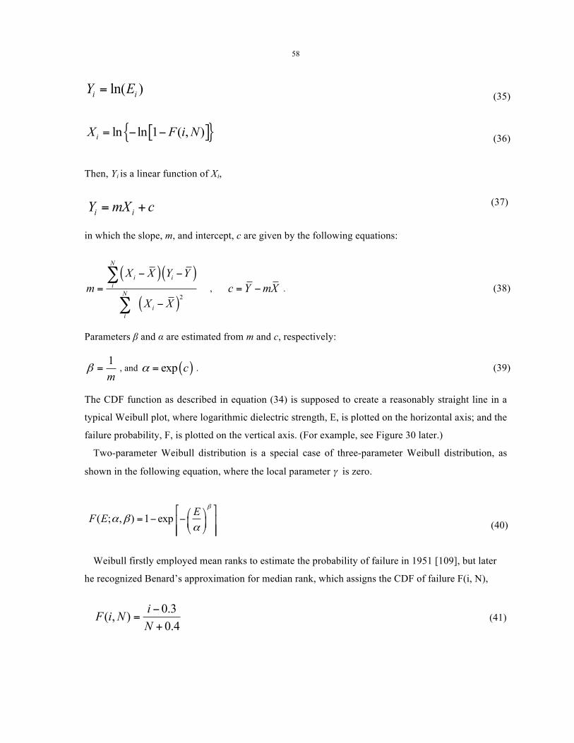
58

ln( )i iY E= (35)

[ ]{ }ln ln 1 ( , )iX F i N= − − (36)

Then, Yi is a linear function of Xi,

(37)

in which the slope, m, and intercept, c are given by the following equations:

( )( )

( )2

N

i ii

N

ii

X X Y Ym

X X

− −=

−

∑

∑

, c Y mX= − . (38)

Parameters β and α are estimated from m and c, respectively:

1m

β = , and ( )exp cα = . (39)

The CDF function as described in equation (34) is supposed to create a reasonably straight line in a

typical Weibull plot, where logarithmic dielectric strength, E, is plotted on the horizontal axis; and the

failure probability, F, is plotted on the vertical axis. (For example, see Figure 30 later.)

Two-parameter Weibull distribution is a special case of three-parameter Weibull distribution, as

shown in the following equation, where the local parameter γ is zero.

(40)

Weibull firstly employed mean ranks to estimate the probability of failure in 1951 [109], but later

he recognized Benard’s approximation for median rank, which assigns the CDF of failure F(i, N),

(41)

0.3( , )0.4

iF i NN−

=+

i iY mX c= +

( ; , ) 1 exp EF Eβ

α βα

⎡ ⎤⎛ ⎞= − −⎢ ⎥⎜ ⎟⎝ ⎠⎢ ⎥⎣ ⎦

59

where N is the total number of measured dielectric strength values and i is the assigned rank when the

dielectric strengths are listed in order from smallest to largest. Benard’s approximation is considered

to be of good accuracy for plotting the Weibull distribution and estimating α and β; its uncertainty is

only 0.1% for N = 50 and 1% for N = 5 [106]. The goodness of fit can be represented by a simple

correlation coefficient, P, which is a number between -1 and 1. As dielectric strength always gives a

linear fit with positive slope, the P in this study locates between 0 and 1. The closer the P to 1, the

better the fit is.

! = !!!! !"!!!!!!!

!!!! !!!!! !!!! !!

!!!

(42)

In this paper, the two-parameter Weibull distribution is applied to statistically analyze the influence

of thermal exposure and immersion in water on the electrical breakdown behavior of PI. As stated in

reference [106], 20 measured values of breakdown strength for each sample under test is considered

sufficient to provide meaningful results. Here, breakdown tests were conducted at 20 different points

on each sample.

4.3 Experiment

The samples for both thermal exposure and immersion in water were cut into 6 cm by 10 cm sheets,

large enough to measure dielectric strength 20 times at different points. The mass of each sample was

measured using a balance with uncertainty 0.01 mg. The thickness of the samples was measured using

a micrometer with uncertainty 1 µm. The PI samples for thermal exposure were heated at 475 °C for 1,

2, 3 and 4 hours in an isothermal muffle furnace to investigate the effect of thermal exposure time;

and at 450, 460, 465 and 480 °C for 4 hours to study the effect of temperature. Thermal exposure for

longer times or at higher temperatures was not conducted as the PI was so brittle and wrinkled that its

dielectric strength could not be measured successfully. Directly after thermal exposure, the samples

were removed from the furnace and cooled to room temperature. It was observed that the PI samples

became more brittle, darker and thicker with increasing thermal exposure times or temperatures. To

study the effect of moisture, the PI samples were immersed in distilled water at room temperature for

4, 8, 16, 24, 48, 72 and 96 hours. The surfaces of the samples were wiped dry after they were

removed from the water. Directly after either cooling or wiping, the mass of the samples was

measured again and compared with the value obtained before thermal exposure or immersion in water.

60

Breakdown voltage was measured using a Dielectric Rigidity 6135.054 instrument designed

according to standards ASTM D-149 [14] and D-876. The Dielectric Rigidity instrument consists of

an oil-insulated transformer, capable of supplying AC voltage up to 60 kV, and a shut-proof resistant

test chamber, which houses a bath for insulating liquid and a mobile support for electrodes with

diameter of 6.34 mm. In this work, Envirotemp® FR3® fluid, a vegetable oil with antioxidant

additive, cold flow additive and colorant, was applied as an insulating and cooling medium. During

the measurement process, the voltage across the PI samples was increased from zero at a rate of 0.5

kV/s and stopped at a value where the sample failed, which was recorded as its breakdown voltage,

VBD. Twenty measurements of dielectric strength were made on each sample.

4.4 Results and discussion

(1) Effect of thermal exposure

The two-parameter Weibull cumulative distribution function of dry PI and the samples heated at

475 °C for 1 to 4 hours is plotted in Figure 30. The symbols represent experimentally measured

dielectric strengths and the solid lines represent a linear fit to the 20 data points, for each exposure

condition. Since the symbols in Figure 30 reveal “S” shape curves around their linear fit, it is

hypothesized that three-parameter Weibull distribution could give a better fit [108]. The correlated

coefficients of two-parameter and three-parameter Weibull distributions for the experimentally

measured dielectric strengths have been calculated and are compared in Table 6. It is observed that

for each thermal exposure condition, the highest correlation coefficients of the three-parameter

Weibull distribution are very similar or even lower than those of two-parameter Weibull distribution.

For 0 hr and 3 hr, the local parameters are negative, which is physically unreasonable as dielectric

strength is always a positive number. As stated in reference [16], the correlated coefficient of the

three-parameter Weibull distribution should be much higher than that of the two-parameter Weibull

distribution to be an equally good fit. Therefore, it is concluded that three-parameter Weibull

distribution cannot give a better fit than two-parameter Weibull distribution, and statistical analysis of

electrical breakdown behavior of all PI samples investigated in this study will be conducted by using

two-parameter Weibull distribution.

The CDF of two-parameter Weibull distribution of the samples heated at 450 to 480 °C for 4 hours

is compared with that of dried PI in Figure 31. The dielectric strength values measured for dry PI (0

hr) are in the range from 130 to 160 kV/mm, agreeing well with values for PI films with equivalent

thickness presented in references [103] [110] [111]: 100 to 200 kV/mm.

61

With longer heating time or higher temperature, the linear fits to the measured data shift towards

lower dielectric strength and reveal decreasing slope, indicating greater dispersity in the measured

dielectric strength values. The scale parameter (α) and the shape parameter (β), obtained through

least-squares regression, are applied here to quantitatively analyze the effect of thermal exposure on

breakdown behavior of PI. The dependence of α and β on heating time and temperature is plotted in

Figures 32 and 33, respectively. Both α and β decrease with increasing heating time or temperature.

Statistically, the short-period thermal exposure at 450 to 480 °C significantly decreases the dielectric

strength of the PI samples and gives rise to much more randomly dispersed weak points in PI film.

It has been stated previously [15] [22] that low-level degradation in polymers due to thermal

exposure, such as chemical aging and physical aging, increases probability of electrical breakdown of

the material. The chemical aging of PI during thermal exposure, which gives rise to pyrolysis process

of imide groups and release of CO2 and CO gases, has been discussed in section 2. On the other hand,

as listed in Tables 7 and 8, weight loss in PI increases with heating time or temperature. It is 2.90%

for the sample heated at 450 °C for 4 hr, and 21.78% for the one heated at 480 °C for 4 hr. The large

weight loss following thermal exposure of PI further supports the occurance of chemical aging of PI

during thermal exposure. To explore the possibility of physical aging during thermal exposure,

enthalpic relaxation measurement on a PI sample heated at 480 °C for 4 hr was conducted by using

DSC. However, no endothermic peak was observed on the DSC curve, revealing no sign of physical

degradation in the degraded PI. Therefore, the increased susceptibility of PI film to electrical

breakdown following the heat treatment is considered to be a result of consequential chemical aging

of PI, which gives rise to free radicals, as shown in Figure 23.

62

0.01

0.1

0.5

1

80 100 120 140 160E (kV/mm)

0 hr

2 hr

Occ

uren

ce C

DF

4 hr

3 hr

1 hr

Figure 30 The cumulative distribution function of the measured dielectric strength of PI samples heated at 475 °C for up to 4 hours. Symbols represent experimental data and lines are obtained by least-squares fitting to the data

Table 6 Correlated coefficient of two-parameter and three-parameter Weibull distribution of dielectric strength of PI heated at 475 °C

Time of heating at 475 °C

Correlation coefficient, P Two-parameter

Weibull Three-parameter

Weibull

0 hr 0.9876 0.9876, γ is negative

1 hr 0.9903 0.9902

2 hr 0.9938 0.9933

3 hr 0.9451 0.9602, but γ is negative

4 hr 0.9770 0.9862

63

60 80 100 120 140 1600.01

0.1

0.5

1 dry PI

Occ

uren

ce C

DF

E (kV/mm)

450 OC

470 OC 480 OC

460 OC

Figure 31 As for Figure 41 but for PI samples heated for 4 hours at various temperatures from 450 to 480 °C

0 1 2 3 45

10

15

20

25

30

35

β α

Heating time (hr)

β

90

100

110

120

130

140

150

160

170

α (kV/m

m)

Figure 32 The Weibull-statistical scale parameter (α) and the shape parameter (β) as functions of heating time

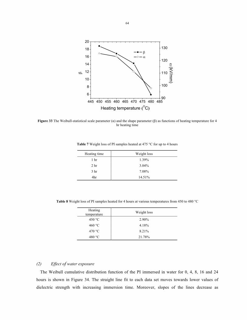
64

445 450 455 460 465 470 475 480 485

6

8

10

12

14

16

18

20

β α

Heating temperature (OC)

β

90

100

110

120

130

α (kV

/mm

)

Figure 33 The Weibull-statistical scale parameter (α) and the shape parameter (β) as functions of heating temperature for 4 hr heating time

Table 7 Weight loss of PI samples heated at 475 °C for up to 4 hours

Heating time Weight loss

1 hr 1.39% 2 hr 3.04% 3 hr 7.08% 4hr 14.51%

Table 8 Weight loss of PI samples heated for 4 hours at various temperatures from 450 to 480 °C

Heating temperature Weight loss

450 °C 2.90% 460 °C 4.18% 470 °C 8.21% 480 °C 21.78%

(2) Effect of water exposure

The Weibull cumulative distribution function of the PI immersed in water for 0, 4, 8, 16 and 24

hours is shown in Figure 34. The straight line fit to each data set moves towards lower values of

dielectric strength with increasing immersion time. Moreover, slopes of the lines decrease as

65

immersion time increases. As described in section 4.2, α and β parameters are obtained via least-

squares regression. Figure 35 shows how α and β decrease with longer PI immersion in water.

As shown in Table 9 and Figure 36, no significant further change in either weight gain or dielectric

strength of PI was observed after immersion in water for more than 24 hours. This observation is in

line with the statement in reference [67] that PI is saturated with moisture after immersion in water

for 25 hours.

Formation of side ionic groups due to dissociation of polymer chains is considered to be the reason

why the insulation capability of PI film is deteriorated due to water uptake. Figure 29 shows the

hydrolysis scheme for PI, in which polymer chains are broken and chemical composition is changed.

OH- from water molecules bonds to either of the four carbonyl groups and H+ bonds to the amine

groups, generating ionic groups at sides of the new polymer chain [66] [112] [98]. The side ionic

groups can greatly promote charge transport in PI insulation, which is termed as “intrinsic ionic

conduction” in reference [15]. Consequently, electrical failure of the PI film is significantly

accelerated.

It has been stated that chemical changes in PI due to moisture absorption are fully reversible by

annealing for 1 hour [113]. Thus, in order to investigate whether physical degradation occurred in PI

during immersion in water as well as chemical degradation, a sample immersed in distilled water for

24 hours was dried again by heating at 200 °C for 1 hour in order to eliminate the influence of ionic

side group formation on dielectric strength of PI. The Weibull plot of breakdown for the annealed

sample (not shown here) revealed no obvious change when compared with that of the control sample.

As listed in Table 10, the scale parameter, α, of the sample is not significantly changed. Therefore, it

is concluded that immersion in water did not give rise to significant physical degradation of the PI

film. The change in the shape parameter, β, could be a result of variation in dispersity of electrical

weak points in the two samples.

66

100 120 140 1600.01

0.1

0.5

1 0 hr

8 hr

24 hr

16 hr

Occ

urre

nce

CD

F

E (kV/mm)

4 hr

Figure 34 The cumulative distribution function of the measured dielectric strength of PI samples immersed in water for 0, 4,

8, 16 and 24 hours

0 5 10 15 20 25

15

20

25

30 β α

Immersion time (hr)

β

130

135

140

145

150

155

160

α (kV

/mm

)

Figure 35 The Weibull-statistical scale parameter (α) and the shape parameter (β) as functions of time of PI immersion in distilled water

\

67

Table 9 Weight gain of PI samples immersed in distilled water for up to 96 hours

Immersion time Weight gain

4 hr 0.87%

8 hr 1.32%

16 hr 1.75%

24 hr 1.80%

48 hr 1.80%

72 hr 1.81%

96 hr 1.80%

100 120 140 1600.01

0.1

0.5

1

96 hr

48 hr

Occ

urre

nce

CD

F

E (kV/mm)

24 hr

72 hr

Figure 36 The cumulative distribution function of the measured dielectric strength of PI samples immersed in water for 24, 48, 72 and 96 hours

Table 10 The Weibull-statistical scale parameter (α) and the shape parameter (β) of dry PI

sample α (kV/mm) β

The original dry PI 152.2 ± 0.3 32 ± 2

2nd dry PI 154.4 ± 0.2 40 ± 2

68

5. Summary

This chapter investigates the influence of thermal exposure above 400 °C in air and immersion in

water on permittivity and electrical breakdown behavior of Kapton PI film. After either the heating

process or immersion in water, the real permittivity and loss factor of PI are increased substantially.

Intensity of the β-relaxation is substantially increased due to scission of chemical bonding in imide

groups during thermal degradation at 475 °C for 3 hr. As PI samples absorbed more moisture with

longer time of immersion in water or saline, the intensity of γ-relaxation following saline exposure is

increased. On the other hand, using statistical analysis by two-parameter Weibull distribution, we

observed that the dielectric strength of PI is greatly decreased and individual measurements of

breakdown voltage are much more randomly distributed, with increasing time or temperature of

thermal exposure and increasing time of immersion in water. The deterioration of insulating

properties of PI after the degrading processes is explained in terms of chemical degradation due to

pyrolysis of imide groups during thermal exposure and formation of ionic side groups during the

hydrolysis process of PI while immersed in water. However, dissolved sodium chloride shows minor

influence on dielectric properties of PI immersed in saline solutions.

69

Chapter V. Polytetrafluoroethylene) (PTFE)

Due to its excellent dielectric properties and hydrophobicity, PTFE (polytetrafluoroethylene) is

widely used as an outer coating material for wiring insulation [1]. Therefore, it is always exposed to

heat and mechanical stress during service. In this chapter, the effect of thermal exposure and tensile

strain on permittivity of PTFE is investigated.

1. Sample material

In this work, all PTFE samples were cut from the same large sheet supplied by Fluoro-Plastics,

which is nominally 610 × 610 × 1 mm3. The melting point of as-received PTFE was determined to be

327 °C by a DSC (differential scanning calorimetry) test. The real permittivity of as-received PTFE was measured over frequency range from 1 Hz to 1 MHz

at room temperature by Novocontrol spectrometer, as shown in Figure 37. The error bar was given by

the Novocontrol spectrometer, which includes the accuracy of the used impedance analyzer and the

influences of cables and sample holders. The error bar also strongly depends on frequency of

measurement and the actual sample impedance. As expected, the permittivity of PTFE is extremely

stable over the whole frequency range. The mean value and standard deviation of the data points in

Figure 37 are 2.214 ± 0.001. Since the dissipation factor of PTFE is so small that it is beyond the

measurement accuracy of this spectrometer over most of the frequency range, the measured values of

loss factor are not shown here.

To explore dielectric performance of PTFE at extreme temperatures, the permittivity was also

measured over temperature range -150 to 300 °C at frequency from 1 Hz to 1 MHz. During

measurements, the whole sample cell was housed in a temperature-controlled container, in which the

temperature was gradually increased in 10 °C increments. Figure 38 shows the real permittivity of as-

received PTFE as functions of both frequency and temperature. Drawn with data points from

Figure 38, Figure 39a shows the real permittivity as a function of temperature at 1.15 kHz. At this

frequency, ε′ decreases from 2.287 to 1.968 as temperature increases from -150 °C to 300 °C. A

probable explanation of this behavior is that, as a nonpolar polymer, the polarization of PTFE is

mainly electronic. In that case, the Clausius-Mossotti equation can be applied, as stated in [114].

!!!!!!

= !!! !!!! !

(43)

70

where N is the number of polarizable entities per unit volume, αe is electronic polarizability, ε0 is the

permittivity of free space, ε is the relative permittivity of PTFE, M is molar weight and ρ is mass

density. Rearranging the above equation gives

! = !!!!!!!!!!!!

(44)

Since density decreases as the temperature increases, it can be postulated from the above equation

that ε′ should decrease slightly with temperature, as the measurements show in Figure 39a.

Focusing on the temperature range -10 °C to 50 °C in Figure 39b, two step-like decreases in ε′ are

observed near 19 °C and 31 °C, which can be associated with structural first-order phase transitions at

these two temperatures [61]. The room-temperature crystalline structure of PTFE (phase IV

hexagonal) transfers to phase II triclinic below 19 °C by angular displacement [50] and to phase I

pseudo-hexagonal above 31 °C by crystal disorder [51], which are both accompanied by step-like

changes of the specific volume. Due to the thermal expansion of the sample capacitor, ε′ of PTFE

shows two step-like decreases in the vicinity of the phase transition temperatures.

Figure 37 Real permittivity of as-received PTFE as function of frequency at room temperature

10-1 100 101 102 103 104 105 106 107

Frequency [Hz]

2.18

2.19

2.20

2.21

2.22

2.23

2.24

Per

mitt

ivity

'

Test SampleCurve 1

Rea

l per

mitt

ivity

, ε′

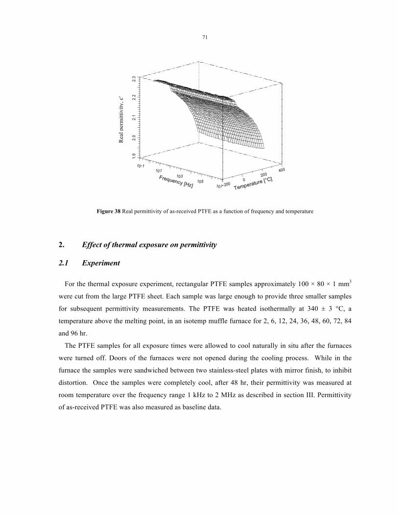
71

Figure 38 Real permittivity of as-received PTFE as a function of frequency and temperature


2.1 Experiment

For the thermal exposure experiment, rectangular PTFE samples approximately 100 × 80 × 1 mm3

were cut from the large PTFE sheet. Each sample was large enough to provide three smaller samples

for subsequent permittivity measurements. The PTFE was heated isothermally at 340 ± 3 °C, a

temperature above the melting point, in an isotemp muffle furnace for 2, 6, 12, 24, 36, 48, 60, 72, 84

and 96 hr.

The PTFE samples for all exposure times were allowed to cool naturally in situ after the furnaces

were turned off. Doors of the furnaces were not opened during the cooling process. While in the

furnace the samples were sandwiched between two stainless-steel plates with mirror finish, to inhibit

distortion. Once the samples were completely cool, after 48 hr, their permittivity was measured at

room temperature over the frequency range 1 kHz to 2 MHz as described in section III. Permittivity

of as-received PTFE was also measured as baseline data.

10-1101

103105

107

Frequency [Hz]

1.9

2.0

2.1

2.2

2.3

Per

mitt

ivity

'

-2000

200400

Temperature [°C]

Test Sample AC Volt [Vrms]=1.000

Rea

l per

mitt

ivity

, ε′

72

-100 0 100 200 300

1.95

2.00

2.05

2.10

2.15

2.20

2.25

2.30

Rea

l per

mitt

ivity

, ε'

Temperature (oC)

-10 0 10 20 30 40 50 602.20

2.21

2.22

2.23

2.24

2.25

Rea

l per

mitt

ivity

, ε '

Temperature (oC)

I Pseudo-hexagonal

II Triclinic IV Hexagonal

Figure 39 Real permittivity of as-received PTFE as a function of temperature at 1.15 kHz. (a): -150 to 300 °C; (b): -10 to

50 °C

2.2 Result and discussion

Figure 40 shows the way in which ε′ of PTFE increases as thermal exposure time increases, at four

frequencies. Thermal exposure at 340 °C for 96 hr increases ε' of PTFE by approximately 2%, which

is significantly larger than the standard deviation between measurements on three nominally identical

samples, which is less than 0.1%.

The increase in real permittivity of PTFE after thermal exposure at 340 °C is attributed to

enhancement of crystallinity following the heating and cooling processes. In semicrystalline

polymers, motion of charge carriers, such as degenerated monomer molecules, can be blocked at the

(a)

(b)

73

crystalline/amorphous phase boundaries and generate interfacial (Maxwell-Wagner-Sillars)

polarization [11]. If the crystalline phase grows, the interfacial polarization may be enhanced,

causing an increase in ε′. To investigate this hypothesis, X-ray diffraction (XRD) measurements were

conducted on as-received PTFE and PTFE thermally exposed at 340 °C for 48 hr and 96 hr. After

thermal exposure, three samples were allowed to cool slowly in situ as described in before. Three

other samples were quenched in liquid N2 to inhibit crystallization. While the XRD patterns of the

PTFE samples all suggest a hexagonal crystal structure is present regardless of thermal history, the

degree of crystallinity (as measured by peak area) in quickly-quenched PTFE was found to be 0.24 ±

0.01, versus 0.29 ± 0.01 in as-received PTFE, 0.32 ± 0.01 in PTFE slowly cooled after isothermal

heating at 340 °C for 48 hr and 0.35 ± 0.01 in PTFE slowly cooled after isothermal heating at 340 °C

for 96 hr. Hence the increase in ε′ as a function of thermal exposure time, shown in Figure 40, can be

attributed to increasing crystallinity. The uncertainties derive from the standard deviation of

measurements on three nominally identical samples.

The increase in crystallinity observed in slow-cooled thermally-exposed PTFE compared with as-

received samples supports the observation that ε′ increases following thermal exposure at 340 °C

(which is higher than the melting point 327 °C) with slow cooling (Figure 40). On the other hand, the

reduction in crystallinity of quickly-quenched, thermally-exposed PTFE compared with as-received

samples accompanied a reduction in ε′ of approximately 2%, much larger than the standard deviation

between measurements of three nominally identical samples (0.2%). This observation further

supports the hypothesis that increase in crystallinity is accompanied by an increase in ε′ for the range

of conditions studied here.

An alternative explanation for the increase in ε′ with increasing crystallinity of PTFE can be

framed in terms of a charge carrier diffusion model. In reference [115] it is suggested that

development of a heterogeneous structure such as exists in a semicrystalline polymer leads to an

increase in permittivity of the polymer approaching the formation of a percolating network of the

conducting amorphous phase.

The two proposed models offer similar features since the time to explore the percolation structure

by the charge carriers is equivalent to the time to transfer charges to the micro-capacitors formed by

semicrystalline structure in the interfacial polarization model.

74

0 20 40 60 80 100

2.22

2.23

2.24

2.25

2.26

2.27

Rea

l per

mitt

ivity

, ε'


f = 1.00 kHz f = 10.6 kHz f = 112 kHz f = 1.18 MHz

Figure 40 Real permittivity of PTFE as a function of thermal exposure time at 340 °C in air

3. Effect of tensile strain on permittivity

3.1 Experiment

As shown in Figure 41, the real permittivity of PTFE is extremely constant over this frequency

range, which agrees with the statement in section 1. Therefore, subsequent permittivity measurement

of all samples in this study was conducted only at 100 kHz.

In order to effectively study the influence of tensile strain on permittivity of PTFE, we designed a

unique system capable of simultaneous permittivity measurement while a polymer sample is under

tensile strain. In this way, the influence of mechanical strain on dielectric permittivity of PTFE is

studied directly. This avoids the difficulty that once the polymer sample is removed from a tensile

loading frame, the polymer chains may recover to some extent, changing the permittivity and making

it impossible to successfully study the influence of mechanical strain on dielectric permittivity by

using any normal dielectric spectrometer. As shown in Figure 41, the test fixture of an Agilent

E4980A LCR meter fits in between the two clamps of a tensile loading frame (TestResources Inc.,

Model 150Q250) in order to measure the capacitance of the sample while it is stretched. The

thickness of the samples was measured by using a micrometer with accuracy of 1 µm, which has a

pair of small rods tipped with flat, parallel discs that contact the sample and measure its thickness.

75

The diameter of the discs was selected to be similar as that of the capacitor electrodes, so that both the

capacitance and the thickness were measured over a similar region of the sample.

Figure 41 Experimental arrangement for permittivity measurement while the sample is under tensile strain

All the PTFE samples investigated in this study were cut into approximately 90 mm long, 40 mm

wide and 0.39 mm thick. The dielectric permittivity of each sample at 100 kHz was measured by

using the LCR meter before being stretched. The stress-strain curve of a sample was measured using

the tensile loading frame. Figure 42 shows the true stress of the PTFE sample as function of its strain.

The sample reveals elastic mechanical behavior below 18 MPa, and fails at approximately 114 MPa

(true stress) with strain of 190%. In order to ensure successful measurement without failure of PTFE,

mechanical strains of 25, 50, 75, 100, 125 and 150% are conducted here. To explore the potential

effect of strain rate, strains of 50, 100, and 150% were achieved by strain rates of 12.7 and 25.4

mm/min, respectively. Other strains studied were achieved by strain rate 25.4 mm/min. Once the

assigned strains are obtained, dielectric permittivity and thickness of all stretched samples were

measured at their centers, at which they were most reliably stretched to the desired strain with

assigned strain rate.

Additionally, to study the effect of stress relief, samples with strains of 50, 100, and 150% were

held in the tensile loading frame for 24 hours, and their permittivity was measured after the strain was

Sample

Tensile loading clamps

Stand

Capacitor electrodes

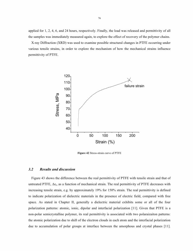
76

applied for 1, 2, 4, 6, and 24 hours, respectively. Finally, the load was released and permittivity of all

the samples was immediately measured again, to explore the effect of recovery of the polymer chains.

X-ray Diffraction (XRD) was used to examine possible structural changes in PTFE occurring under

various tensile strains, in order to explore the mechanism of how the mechanical strains influence

permittivity of PTFE.

0 50 100 150 200

40

50

60

70

80

90

100

110

120

failure strain

Stre

ss, M

Pa

Strain (%)

Figure 42 Stress-strain curve of PTFE

3.2 Results and discussion

Figure 43 shows the difference between the real permittivity of PTFE with tensile strain and that of

untreated PTFE, Δεr, as a function of mechanical strain. The real permittivity of PTFE decreases with

increasing tensile strain, e.g. by approximately 19% for 150% strain. The real permittivity is defined

to indicate polarization of dielectric materials in the presence of electric field, compared with free

space. As stated in Chapter II, generally a dielectric material exhibits some or all of the four

polarization patterns: atomic, ionic, dipolar and interfacial polarization [11]. Given that PTFE is a

non-polar semicrystalline polymer, its real permittivity is associated with two polaraizaiton patterns:

the atomic polarization due to shift of the electron clouds in each atom and the interfacial polarization

due to accumulation of polar groups at interface between the amorphous and crystal phases [11].

77

Therefore, the decreases in the real permittivity of PTFE could be a result of decrease in either atomic

polarization or interfacial polarization, or both. However, considering the mechanism of atomic

polarization as explained above, it is not considered changeable with mechanical strain. On the other

hand, according to the Fringed Micelle Model [116], the chains of a polymer under mechanical

loading increase their alignment along the direction in which the loading is applied, hence increasing

the degree of alignment in the amorphous phase and producing a greater degree of crystallinity. Thus,

it is hypothesized here that the interfacial polarization of PTFE is declined due to decreased amount

of polar groups accumulating at the interface, as motion of polar groups is limited as a result of

increased order in polymer chains.

In order to test this hypothesis, the degree of crystallinity of samples with tensile strain of 50, 100

and 150% was determined by XRD tests, immediately upon removal from the loading frame. It is

observed that the degree of crystallinity increases with mechanical strain. The degree of crystallinity

of untreated PTFE is 36%, versus 42% for the samples with 50% and 100% strains, and 47% for the

sample with 150% strain. The XRD spectra reveal that the crystal structure of strained PTFE at room

temperature is hexagonal, the same as that of un-strained PTFE [52].

It was also observed that after the samples were released from the tensile loading frame and

polymer chains recovered, their permittivity increases. As shown in Figure 44, the real permittivity

was increased by up to 8% after removal of loading, which, however, is still smaller than that of

untreated PTFE. Therefore, it is reasonable to conclude that the decrease in the real permittivity of

PTFE is associated with increased order in polymer chains in the presence of mechanical strain.

However, minor change in the real permittivity of PTFE was observed during the 24 hours when

the samples were held with 50%, 100%, and 150% strains. Additionally, the permittivity of PTFE

stretched with strain rate of 25.4 mm/min shows quantitatively similar permittivity as that stretched to

the same amount of strain with strain rate of 12.7 mm/min. Thus, it could be conclude that there is no

obvious influence of stress relief and strain rate on dielectric permittivity of PTFE.

4. Summary

Thermal exposure studies on PTFE show increase in real permittivity by approximately 2%

following isothermal heating at 340 °C for 96 hr. This observation is associated with increase in

crystallinity that enhances the interfacial polarization between the amorphous phase and crystal phase

of the polymer. On the other hand, with the presence of mechanical loading, polymer chains of PTFE

are oriented along the direction of loading, which, however, limits motion of polar groups and

weakens the interfacial polarization. It is observed that the real permittivity of PTFE was decreased

78

by approximately 19% with mechanical strain of 150%. Increase in degree of crystallinity with

increasing tensile strain is observed. Upon removal from the loading frame, the oriented polymer

chains of PTFE recovered to some extent, which increased the permittivity by up to 8%. The strain

rate by which the PTFE samples were stretched to various strains and the stress relief process while

the PTFE samples had been stretched for up to 24 hr hardly influences the real permittivity of PTFE.

Figure 43 The changes in the real permittivity of PTFE as a function of tensile strain

50 60 70 80 90 100110120130140150

-0.40

-0.35

-0.30

-0.25

-0.20

-0.15

-0.10

Δεr

Strain (%)

strained PTFE released PTFE

Figure 44 Open square: the difference between the real permittivity of released PTFE and that of untreated PTFE; solid

square: the difference between the real permittivity of PTFE with strain and that of untreated PTFE

-20 0 20 40 60 80 100 120 140 160

-0.40-0.35-0.30-0.25-0.20-0.15-0.10-0.050.000.05

Δεr

Strain (%)

79

Chapter VI. Ethylene-tetrafluoroethylene (ETFE)

ETFE (ethylene-tetrafluoroethylene) has been applied as the only wiring insulation material in

Boeing 747, 767 and 777 aircraft after the 1990s. This chapter describes an investigation of the way

in which the real permittivity and loss factor of ETFE change after thermal exposure in air for up to

96 hours.

1. Sample material

The ETFE samples studied here were discs nominally 1 mm thick and 63 mm in diameter, which

were extruded from Tefzel 750® ETFE pellets supplied by Dupont. The heat flow and storage

modulus as a function of temperature on samples cut from different spots of the extruded discs were

measured by DSC (Differential Scanning Calorimeter) and DMA (Dynamic Mechanical Analysis),

respectively. Good homogeneity in thermal and mechanical properties of the extruded samples was

verified, as shown in Figures 45a and 45b.

The real permittivity and loss factor of extruded ETFE was measured over the frequency range

1 Hz to 1 MHz and the temperature range -150 °C to 210 °C by the Novocontrol Dielectric

Spectrometer. Three dimensional dependences of ε′ and tan δ are shown in Figures 57a and 57b,

respectively. The highest values of ε′ and tan δ, observed at low frequency (below ~10 Hz) and high

temperature (above ~200 °C) may be due to one or more extrinsic or intrinsic electrical phenomena,

such as electrode polarization, interfacial polarization and conductivity effects [117].

Extracting data from Figure 46, the dependence of ε′ and tan δ on temperature at 1.15 kHz are

shown in Figure 47. Two peaks in the loss factor of ETFE at -80 °C and 92 °C are observed. These

are associated with γ- and α-transitions respectively [118]. The two peak temperatures are close to the

transition temperatures listed in Table 3, -87 °C and 110 °C. The differences in these values are likely

due to measurement of different material properties by different equipment on slightly different

samples.

80

Figure 45 Homogeneity of extruded ETFE by (a) DSC; (b) DMA

(a)

(b)

81

Figure 46 Real permittivity (a) and loss factor (b) of extruded ETFE as a function of frequency and temperature

10-1102

105108

Frequency [Hz]

23

4Pe

rmitt

ivity

'

-200 0200 400

Temperature [°C]


10-1102

105108

Frequency [Hz]

02

46

Tan(

Del

ta)

-2000

200 400

Temperature [°C]


(a)

(b)

82

-150 -100 -50 0 50 100 150 2002.30

2.35

2.40

2.45

2.50

2.55

2.60

Temperature (oC)

Rea

l per

mitt

ivity

, ε'

0.000

0.005

0.010

0.015

0.020

0.025

Loss Factor, tan δ

Figure 47 Real permittivity and dissipation factor of extruded ETFE as a function of temperature at 1.15 kHz


2.1 Experiment

Prior to thermal exposure, extruded ETFE discs were annealed isothermally at 60 °C in another

isotemp muffle furnace for 2 hr prior to thermal exposure. The annealing was done in order to relieve

residual stress that resulted from the extrusion process and flatten the samples for permittivity

measurement. When cooled completely, annealed discs were subjected to thermal exposure at 160 ± 2

°C for 2, 6, 12, 24, 36, 48, 60, 72, 84 and 96 hr. The temperature 160 °C, much lower than the melting

temperature of 245 °C, was chosen due to significant sample deformation after thermal exposure at

higher temperatures that prevented successful permittivity measurement. Three discs were exposed

for each exposure time.

During the exposure process, all the samples were sandwiched between two stainless-steel plates

with mirror finish, to inhibit distortion. After the furnace was turned off, doors of the furnaces were

not opened until all exposed ETFE samples were naturally cooled down in situ. Once the samples

were completely cool, after 48 hr, their permittivity was measured at room temperature over the

frequency range 1 kHz to 2 MHz. Permittivity of as-extruded ETFE and annealed ETFE samples

were also measured to provide comparative data.

83

2.2 Result and discussion

Values for ε′ and tan δ of both extruded and annealed ETFE samples are compared in Figure 48.

The ε′ of extruded ETFE decreases from 2.599 to 2.539 as frequency increases from 1 kHz to 2 MHz.

Loss factor, tan δ, increases over this frequency range but is small (below 0.007) even at 2 MHz.

These results agree with the values listed in Table 3 in Chapter II. It can be observed that ε′ of

extruded ETFE and annealed ETFE are similar over the frequency range measured and tan δ overlaps

closely until above 1 MHz. (The separation below 20 kHz is due to large uncertainty in the

measurements for low frequencies.) It can be concluded that the annealing process at 60 °C for 2 hr

does not influence the dielectric properties of ETFE significantly and it is reasonable to anneal the

samples prior to thermal exposure at 160 °C for up to 96 hr, for the purpose of relieving residual

stress.

Figures 49 and 50 show how thermal exposure duration influences ε′ and tan δ, respectively, of

ETFE at four frequencies. Since the measurement uncertainty in tan δ is quite large below 20 kHz,

tan δ at 1.00 and 10.6 kHz are not shown in Figure 50. Figure 49 shows how thermal exposure time

influences ε' of ETFE at four frequencies. As exposure time increases up to 96 hr, ε' increases by

0.05 (approximately 2%, which is significantly larger than the standard deviation between

measurements on three nominally identical samples, 0.5%). From Figure 50, tan δ is not changed

significantly by thermal exposure at 112 kHz. At 1.18 MHz, however, tan δ decreases by 11% after

thermal exposure for 96 hr.

XRD tests conducted on annealed ETFE and ETFE thermally exposed at 160 °C for both 48 hr and

96 hr indicated that the degree of crystallinity, 0.65 ± 0.01, was not changed by thermal exposure.

This is in accordance with results presented in reference [119].

On the other hand, mid-infrared (IR) analysis on annealed ETFE and ETFE thermally exposed at

160 °C for 96 hr has revealed chemical changes in ETFE following thermal exposure. The absorbance

spectra are shown in Figure 51. Similar peaks corresponding to the presence of CF2 at 1460 cm-1, and

C–H at 2850 cm-1 and 2890 cm-1 are observed in both spectra. However, the spectrum of thermally-

exposed ETFE contains an extra peak at 1680 cm-1, corresponding to the C=O group, and a much

higher and broader –OH peak at 3450 cm-1. These indicate that chemical changes occurred during

thermal exposure of ETFE, including oxidation and dehydrofluorination [120]. Oxidant thermal

exposure accompanied by chain breakage and polar group formation can increase dielectric

permittivity of polymers by enhancing their charge carrier mobility. It has been reported [121] that

chain breakage can decrease polymer viscosity by reducing average molecular weight, which

84

increases the charge carrier mobility. The formation of polar groups can also promote the charge

carrier mobility in ETFE. The decrease in tan δ at 1.18 MHz, shown in Figure 50, is also attributed to

the additional polar groups formed during thermal exposure [122].

103 104 105 1062.52

2.54

2.56

2.58

2.60

2.62

ETFE Annealed

Frequency (Hz)

Rea

l per

mitt

ivity

, ε'

0.000

0.001

0.002

0.003

0.004

0.005

0.006

0.007

Loss factor, tan δ

Figure 48 Real permittivity and dissipation factor of extruded and annealed ETFE as a function of frequency at room

temperature

Figure 49 Real permittivity of ETFE as a function of thermal exposure time at 160 °C

0 20 40 60 80 1002.55

2.56

2.57

2.58

2.59

2.60

2.61

2.62

2.63

2.64

2.65

Rea

l per

mitt

ivity

, ε'


f = 1.00 kHz f = 10.6 kHz f = 112 kHz f = 1.18 MHz

85

0 20 40 60 80 100

2.0

2.5

3.0

3.5

4.0

4.5

5.0

5.5

6.0

6.5

Loss

fact

or, t

an δ

(10-3)


f = 112 kHz f = 1.18 MHz

Figure 50 Dissipation factor of ETFE as a function of thermal exposure time at 160 °C

1500 1800 2100 2400 2700 3000 3300 3600

annealed ETFE

Wave number (cm-1)

Abs

orba

nce

(A.U

.)

thermally exposed ETFE

1680C=O

Figure 51 Mid-IR spectra of annealed ETFE and ETFE thermally exposed at 160 °C for 96 hr

86

3. Summary

Approximately 2% increase in the real permittivity and 11% decrease in the loss factor of ETFE are

observed after thermal exposure at 160 °C for 96 hr in air. These observations are considered as a

result of oxidation and dehydrofluorination during the heating process, which give rise to formation

of polar groups.

87

Chapter VII. Polymethylmethacrylate- montmorillonite nanocomposites

In this work, polymethylmethacrylate (PMMA) composites with a mixture of exfoliated and

intercalated montmorillonite (MMT) nanoparticles were prepared with PMMA/MMT ratios of 100/5

and 100/10. Havriliak-Negami (HN) function extended with an exponential function was used to

model dielectric relaxations and conductivity effect of the nanocomposites and a pure PMMA sample.

The effect of MMT content on dielectric properties of the nanocomposites was investigated.

1. Material Synthesis & Permittivity Measurement

The methylmethacrylate, MMA, monomer (99%, stabilized) employed in all experiments was

purchased from Acros Organics. The radical initiator, benzoyl peroxide, BPO, (97% dry weight) was

obtained from Alfa Aesar. The MMT clay (Cloisite 20A) was provided by Southern Clay Products

(Gonzales, TX, USA). Cloisite 20A is a Na-MMT modified with dimethyl dehydrogenated tallow

ammonium. The clay particles have a thickness of 1nm, and equivalent diameter from 100 nm to

approximately 10 microns.

The stabilizing inhibitor was removed from MMA by washing the monomer three times with a

10% NaOH aqueous solution, followed by three washes with distilled water. The purified monomer

was dried using molecular sieves. The first step in the composite preparation was the dissolution of

initiator in the monomer, followed by the addition of the filler, MMT. The molar ratio MMA / BPO

was maintained at 1 / (2 x 10-3) in all systems. The ratio MMA/MMT was 100/5 and 100/10;

compositions of the samples are listed in Table 11. The systems were sonicated and mixed at 1-2

minute intervals employing a horn sonicator. Following sonication the systems were centrifuged for

approximately one minute to remove possible air bubbles. The sequence sonication, followed by

mixing and centrifugation, was repeated five times for each sample. The in-situ polymerization of the

two systems was carried out in an oven at 80 °C overnight. Following this procedure, the binary

nanocomposites were prepared. The composition of each sample is described in Table 11.

As shown in Figures 52 and 53, the nanoclay particles in 5MMT and 10 MMT are homogenously

dispersed on nano-size level. In both the two samples, silicate layers of MMT are intercalated and

exfoliated by the PMMA matrix. Compared with 5MMT, silicate layers in 10MMT appear to be more

severely intercalated.

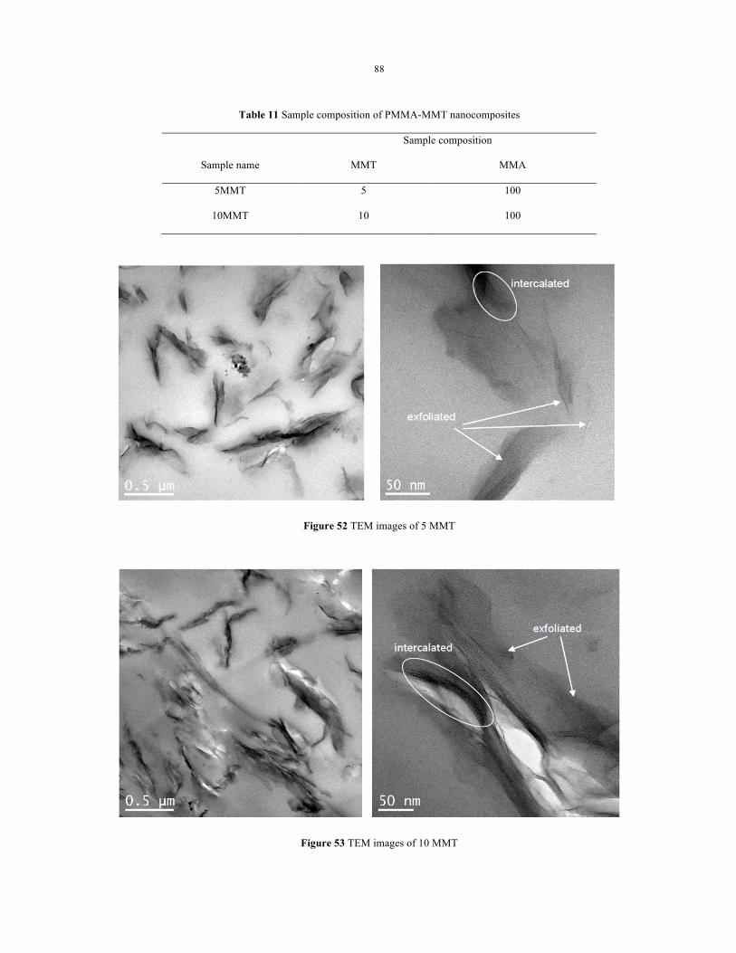
88

Table 11 Sample composition of PMMA-MMT nanocomposites

Sample composition

Sample name MMT MMA

5MMT 5 100

10MMT 10 100

Figure 52 TEM images of 5 MMT

Figure 53 TEM images of 10 MMT

89

The complex permittivity of the two nanocomposites and a pure PMMA sample was measured by

using the Novocontrol Dielectric Spectrometer, attached with the standard sample cell housed in a

temperature-controlled chamber. The measurement was carried out with applied voltage of 1 V, over

frequencies from 0.01 Hz to 1 MHz and temperatures from 30 to 150 °C with increment 10 °C. No

test at higher temperature was carried out as PMMA can decompose at approximately 160 °C. The

measured permittivity data were used to model frequency dependence of dielectric relaxations and

low-frequency conduction based on theoretic functions, as described in section 2.

2. Modeling

Three dielectric relaxations are observed in PMMA-MMT nanocomposites: α-, β- and MWS

relaxations. Apart from these, there is conduction at low frequency. Given the contribution of free

charge carriers at low frequency, there is always a tail of the loss maximum because of conduction.

The conductivity term of the nanocomposites is expected to be much stronger compared with pure

PMMA, due to electrical conduction introduced by ions in the MMT nanofillers. Since the four

dielectric phenomena are usually merged together [9], theoretical functions are necessary to separate

the dielectric phenomena for analyzing the frequency dependence of dielectric relaxations and low-

frequency conduction of the nanocomposites.

Four classical dielectric relaxation functions have been developed and widely applied: Debye,

Cole-Cole, Davidson-Cole, and Havriliak-Negami (HN) functions. Out of these four, the HN function,

equation (45), introducing asymmetric distributions of relaxation times, has been considered

advantageous to analyze dielectric relaxation of polymeric materials. [123]

(45)

where, ε* is the complex permittivity; ε∞ is the permittivity at a frequency higher than those of any

mechanisms of interest; ∆ε defines the strength of the relaxation process over the frequency range, ∆ε

= ε0 – ε∞; τ0 is the characteristic relaxation time, which depends on temperature; a and b are two shape

parameters that can be determined from the experimental data of dielectric complex permittivity. a is

a measure of the peak height of dielectric relaxation: as the a increases, the peak height decreases. b is

a measure of the width of the distribution of relaxation times. Conventionally, b>0.9 corresponds to a

single relaxation time process, the relaxation is considered as symmetric and a pure Debye type

relaxation. [4]

( ) ( )( )

( ){ }10

,1

baT Ti T

Tε ω ε

ωτε

∗ −−∞−⎡ ⎤= − ⎣ ⎦Δ

90

Considering the contribution of free charge carriers to the low frequency tail of the loss maximum,

a conductivity term, represented by an exponential function, was added to the HN function to model

frequency dependence of the imaginary permittivity [124].

(46)

where σ is a fractional exponent that represents charge transport process of solids, it always

lies between 0 and 1. In this work, the two theoretic functions are applied to model the dielectric

relaxations in PMMA-MMT nancomposites,

One criterion for the best fit between experimental and modeled data is that the least square

difference between them is the smallest. Here, the sequence of modeling the four dielectric

phenomena is considered important for obtaining the best fit to experimentally measured imaginary

permittivity. Below the glass transition temperature, the β-relaxation is separated from other

relaxation processes. Therefore, the β-relaxation was selected as the first one to model. By removing

the effect of the β-relaxation over frequency from 0.01 to approximately 50 Hz, the MWS relaxation

is then modeled. Third, the conductivity term is modeled by using the exponential function, after

removing the effect of both β- and MWS relaxations from the data. HN parameters, including a, b and

∆ε, for each of the three dielectric relaxations were refined by eliminating effect of the other two over

the frequency range that it dominates. On the other hand, above the glass transition temperature, the

α-relaxation can be observed. However, as the strength of α-relaxation is not as strong as that of the

MWS relaxation or the conductivity effect, the α-relaxation was lastly modeled. Again, the HN

parameters and conductivity parameters for each of the four dielectric phenomena were refined by

eliminating effect of the other three. Moreover, all those parameters were further refined by using

increment of 0.001 in their value. Using the recursive sequence of modeling described above, the

frequency dependence of dielectric relaxations and low-frequency conduction of both 5MMT and

10MMT nanocomposites are modeled and compared with experimental data. Similarly, the α-

relaxation, β-relaxation and conduction of the pure PMMA were also modeled.

3. Results

The frequency dependences of the experimental data were modeled at each measuring temperature.

In this paper, the plots for 50, 100 and 150 °C of PMMA, 5MMT and 10MMT are shown in Figures

54-62 to demonstrate the model fit below Tg, above Tg and at high temperatures where the

( ) ( )'' ''HN

A σε ω ω ε ω− ⎡ ⎤= + ⎣ ⎦

91

conductivity term is very strong. It is observed that the peaks of the MWS relaxation are always

between 0.01 to 1 Hz, whereas the peaks of the β-relaxation of the two nanocomposites are located at

higher frequencies. Above Tg, the α-relaxation appears between 0.01 Hz and 100 Hz. It is also

observed that the strength of conduction increases with temperature and MMT content. The HN

function parameters, ∆ε, a and b, as well as effect of increasing content of MMT nanofiller on

dielectric properties of the composites will be compared with those of the pure PMMA and discussed

in detail in section 4.

Figure 54 Imaginary permittivity of PMMA at 50 ºC

10-2 100 102 104 1060

0.05

0.1

0.15

0.2

0.25

0.3

0.35

Frequency (Hz)

εʹ′ʹ′ (ω

)

PMMA, T=50 0C

Experimental Dataβ-Relaxation

10-2 100 102 104 1060

0.2

0.4

0.6

0.8

1

Frequency (Hz)

εʹ′ʹ′ (ω

)

PMMA, T=100 0C

Experimental Dataβ-Relaxationα-RelaxationConductivity TermModel Superposition

92



Figure 57 Imaginary permittivity of 5MMT at 50 ºC

10-2 100 102 104 1060

100

200

300

400

500

600

700

Frequency (Hz)

εʹ′ʹ′ (ω

)

PMMA, T=150 0C

Experimental Dataβ-Relaxationα-RelaxationConductivity TermModel Superposition

10-2 100 102 104 1060

0.2

0.4

0.6

0.8

1

1.2

1.4

Frequency (Hz)

εʹ′ʹ′ (ω

)

5MMT, T=50 0C

Experimental Dataβ-RelaxationMWS-RelaxationConductivity TermModel Superposition

93



10-2 100 102 104 1060

5

10

15

Frequency (Hz)

εʹ′ʹ′ (ω

)

5MMT, T=100 0C

Experimental Dataβ-RelaxationMWS-Relaxationα-RelaxationConductivity TermModel Superposition

10-2 100 102 104 1060

2000

4000

6000

8000

Frequency (Hz)

εʹ′ʹ′ (ω

)

5MMT, T=150 0C


94



10-2 100 102 104 1060

0.5

1

1.5

2

2.5

Frequency (Hz)

εʹ′ʹ′ (ω

)

10MMT, T=50 0C

Experimental Dataβ-RelaxationMWS-RelaxationConductivity TermModel Superposition

10-2 100 102 104 1060

5

10

15

20

25

30

35

Frequency (Hz)

εʹ′ʹ′ (ω

)

10MMT, T=100 0C


95

Figure 62 Model fitting of the imaginary permittivity of 10MMT at 150 ºC

4. Discussion

4.1 Dielectric relaxations

The characteristic frequency of α-, β- and MWS relaxations are plotted as functions of

reciprocal temperature are plotted in Figure 63.

The glass transition temperature of both 5MMT and 10MMT are determined to be

approximately 80 °C, versus 100 °C for PMMA. As the content of MMT increases, the

characteristic frequency of the β- and MWS relaxations decrease, while that of the α-

relaxation increases. It is also observed in Figure 63 that the characterization frequency of the

α-relaxation increases with content of MMT. As silicate layer in MMT segregate the PMMA

polymer chains into small domains, the α-relaxation, which is due to motion of main polymer

chain, can take place at lower temperature and within shorter time [83]. The frequency of the

α-relaxation of PMMA is independent of temperature above Tg. On the other hand, the α-

relaxation both 5MMT and 10MMT follows the Vogel-Fulcher law:

10-2 100 102 104 1060

2000

4000

6000

8000

10000

12000

14000

16000

Frequency (Hz)

εʹ′ʹ′ (ω

)

10MMT, T=150 0C


96

( )00

exp Bf fT T

⎡ ⎤= ⎢ ⎥

−⎣ ⎦ (47)

Therefore, log f is a linear function of 1/(T-T0). It is stated in reference [125] that T0 is usually

30 to 70 degrees lower than Tg. Here, when T0 is equal to 10 °C (283 K), which is 70 degrees

lower than Tg, a nice linear curve can be obtained, as shown in Figure 64. Constant B of the

α-relaxation of 5MMT is determined to be 1001.39, versus 810.19for 10 MMT.

The β-relaxation of both 5MMT and 10MMT reveal a linear relationship between log

frequency and reciprocal of temperature, indicating that the β-relaxation of the

nanocomposites follows the Arrhenius law:

(48)

where f is the characteristic frequency; T is the measurement temperature; f0 is a

phenomenological parameter; Ea is the activation energy of dielectric relaxation; R is the gas

constant. By plotting the dependence of log f on 1/T, the activation energy can be obtained

from slope of the line. The Arrhenius plot of the β-relaxation of PMMA in Figure 63 shows a

change in slope at its Tg, which is a result of coupling between α- and β-relaxations. On the

other hand, the straight lines for 5MMT and 10MMT indicate that the coupling is suppressed

in the PMMA-MMT nanocomposites. The activation energy of the β-relaxation of PMMA is

determined to be 78.98 kJ/mole below Tg and 119.46 kJ/mole above Tg, while that of 5MMT

is 76.65 kJ/mole and that of 10MMT is 69.51 kJ/mole. Thus, the activation energy of the β-

relaxation decreases with MMT quality.

The characteristic frequency of the MWS relaxation of 5MMT is independent of

temperature, but at Tg, the characteristic frequency increases significantly, from 0.06 to 1.13

Hz. On the other hand, the MWS relaxation of 10MMT obeys an Arrhenius law above the

glass transition temperature, and its activation energy is determined to be 77.0 kJ/mole. This

observation agrees with the statement in references [126] [127]. However, below the glass

transition temperature, the characteristic frequency of MWS relaxation is independent of

temperature. It is speculated here that the number of free charges blocked at the interfaces is

not increased by increasing temperature of the glassy state, below Tg. In the glassy state the

0 exp aEf fRT−⎛ ⎞= ⎜ ⎟

⎝ ⎠

97

molecules are frozen in place, and do not display any segmental motion. Over the whole

measurement temperature range, peaks of the MWS relaxation of 10MMT are located at

higher frequencies than that of 5MMT. The shift of the relaxation peak to higher frequencies

in 10MMT indicates that the aptitude of the ions to be polarized at interfaces increase as the

concentration of MMT nanofillers in the composites increases. [126]

The HN function parameter of the dielectric relaxations, ∆ε, is plotted against reciprocal of

temperature in Figures 65-67. ∆ε is a measure of relaxation strength. As shown in Figures 65

and 64, the strength of the α- and β-relaxations increases with weight fraction of MMT

nanoparticles, which is considered as a result of loosened molecular packing of the polymer

chains [128]. The strength of the MWS relaxation is not influenced by weight fraction of

MMT nanofillers below Tg, as shown in Figure 67. However, above Tg, ∆ε of 10MMT is

much higher than that of 5MMT, in association with the greater number of free charges that

come to be blocked at the interfaces, thus increasing the MWS/interfacial polarization [126].

The other HN parameters, a and b, of the dielectric relaxations are plotted in Figures 68-

70. It is observed that a of the α-relaxation of PMMA, 5MMT or 10MMT changes with

temperature. For PMMA and 5MMT, it decreases with temperature at lower temperatures but

increases with temperature above 130 and 110 °C, respectively, which are 30 °C higher than

their Tg. Opposite conditions are observed for a of the α-relaxation of 10MMT. On the other

hand, as shown in Figures 69 and 70, a of the β- and MWS relaxations of PMMA, 5MMT

and 10 MMT are considered similar over the whole temperature range: within 0.05 of each

other for the β –relaxation and 0.1 for the MWS relaxation. This indicates that peak height of

the β –relaxation of the two samples is much higher than that of the MWS relaxation. From

Figures 68-70, it is concluded here that the α-relaxation of PMMA and 5MMT is asymmetric,

while that of 10MMT is symmetric. On the other hand, the β -relaxation of PMMA, 5MMT

and 10MMT is all symmetric. However, the MWS relaxations of 5MMT and 10MMT are

both asymmetric.

98

2.2 2.4 2.6 2.8 3.0 3.2 3.4-2

-1

0

1

2

3

4

5

log

[freq

uenc

y (H

z)]

1000/T (K-1)

PMMA, β PMMA, α 5MMT, β 5MMT, α 5MMT, MWS 10MMT, β 10MMT, α 10MMT, MWS

Tg

Figure 63 Arrhenius plot of the characteristic α-, β- and MWS relaxation frequencies of PMMA, 5MMT and 10MMT

0.008 0.010 0.012 0.014-2.0

-1.5

-1.0

-0.5

0.0

0.5

1.0

1.5

2.0

log

f, α

-rel

axat

ion

1/(T-283) (K-1)

5MMT 10MMT

Figure 64 The linear dependence of log f of α- relaxation of 5MMT and 10MMT on 1/(T-283)

99

2.4 2.5 2.6 2.7 2.80

5

10

15

20

25

1000/T (K-1)

Δε,

α-re

laxa

tion

PMMA 5MMT 10MMT

Figure 65 ∆ε of the α-relaxation of PMMA, 5MMT and 10MMT

2.2 2.4 2.6 2.8 3.0 3.2 3.4

2.0

2.5

3.0

3.5

4.0

4.5

5.0

Δε, β

-rel

axat

ion

1000/T (K-1)

PMMA 5MMT 10MMT

Figure 66 As for Figure 74 but for the β-relaxation

100

2.2 2.4 2.6 2.8 3.0 3.2 3.4

0

5

10

15

20

25

30

35

5MMT 10MMT

Δε,

MW

S re

laxa

tion

1000/T (K-1)

Figure 67 ∆ε of the MWS relaxation of 5MMT and 10MMT

2.4 2.6 2.8 3.0

0.0

0.2

0.4

0.6

0.8

1.0

a &

b, α

-rel

axat

ion

1000/T (K-1)

PMMA a PMMA b 5MMT a 5MMT b 10MMT a 10MMT b

Figure 68 HN parameters, a and b of the α-relaxation of 5MMT and 10MMT

101

2.4 2.6 2.8 3.0 3.2 3.4 3.60.2

0.3

0.4

0.5

0.6

0.7

0.8

0.9

1.0

a an

d b,

β-re

laxa

tion

1000/T (K-1)

PMMA a PMMA b 5MMT a 5MMT b 10MMT a 10MMT b

Figure 69 As for Figure 77 but for the β-relaxation

2.2 2.4 2.6 2.8 3.0 3.2 3.4

0.0

0.2

0.4

0.6

0.8

1.0

HN

par

amet

ers,

MW

S re

laxa

tion

1000/T (K-1)

5MMT, a 5MMT, b 10MMT, a 10MMT, b

Figure 70 HN parameters, a and b of the MWS relaxation of 5MMT and 10MMT

102

4.2 Conduction

Figures 71 and 72 show the parameters of the conductivity term, A and σ (Equation (46)),

of PMMA, 5MMT and 10MMT as functions of reciprocal temperature. At the two lowest

measuring temperatures, 30 to 70 ºC for PMMA and 30 to 40 ºC for the nanocomposites,

there are not enough experiment data at low frequency to model the conductivity term

accurately. Thus, A and σ at those temperatures are not included in the two figures.

As shown in Figure 71, the strength of conduction increase significantly with increasing

temperature and weight fraction of MMT nanofiller. This observation can be explained by

the fact that the motion of ions in the nanocomposites is increased at high temperatures and

that the quantity of available ions increases with increasing MMT.

Figure 72 shows σ of PMMA, 5MMT and 10MMT as a function of reciprocal temperature.

Our data agree with the statement in reference [123] that σ always lies between 0 and 1 over

the whole frequency range. Even though the σ curve of the nanocomposites shifts to lower

temperature, the shape of the curves for PMMA, 5MMT and 10MMT is similar, indicating

that content of MMT does not influence the way in which charges transport in these

nanocomposites. The dependence of σ on temperature does change, however, at Tg and 100

°C, implying that the mechanism of charge transport in PMMA and the nanocomposites also

changes at these temperature. The way in which charge transports in disordered solids under

AC electrical field is usually described by one of four classical models [129]: the polaron

tunneling model [130] [131] where the exponent σ increases with increasing temperature; the

correlated barrier hopping model [132] which predicts σ decreases with increasing

temperature, the quantum mechanical tunneling [130] and the symmetric hopping model

(random free energy barrier) [133] in both of which σ is considered temperature independent.

Above 100 °C, σ is close to 1, corresponding to pure conduction process (or ohmic contacts)

due to the highly enhanced motion of charges at high temperatures [124]. Below 100 °C, σ

shows different dependence on temperature below and above Tg, implying that the

conduction mechanism changes at the glass transition temperature. Below Tg, σ decrease

slightly with temperature, which can be explained by the correlated barrier hopping model:

thermally activated charge carrier jumps over energy barrier [130]. Above Tg, σ increase

slightly with temperature, and could be represented by the polaron tunnelling model, in

103

which the polaron energy is derived from polarization changes in the deformed structure [130]

[134].

2.3 2.4 2.5 2.6 2.7 2.8 2.9 3.0 3.1 3.2

0

200

400

600

800

1000

1200A

, con

duct

ivity

1000/T (K-1)

PMMA 5MMT 10MMT

Figure 71 Conductivity parameter, A, of PMMA, 5MMT and 10MMT

2.3 2.4 2.5 2.6 2.7 2.8 2.9 3.0 3.1 3.2

0.5

0.6

0.7

0.8

0.9

1.0

1000/T (K-1)

σ

PMMA 5MMT 10 MMT

Figure 72 Conductivity parameter, σ, of PMMA, 5MMT and 10MMT

104

5. Conclusions

Nanocomposites with a mixture of exfoliated and intercalated MMT were prepared by in-situ

polymerization of PMMA with PMMA/MMT weight ratios of 100/5 and 100/10. It is observed that

the real permittivity of the nanocomposites increases with temperature and quality of MMT

nanoparticles, especially below 0.2 Hz, which is considered as a result of the MWS relaxation and

electrical conduction introduced by adding MMT nanofillers.

Dielectric relaxation and conduction processes of the nanocomposites and a PMMA sample were

analyzed by using HN function and an exponential function, respectively. The model superposition

shows good fitting to experimental data at all the measuring temperatures. It is observed that with

increasing content of MMT nanofillers, the characteristic frequency of the α-relaxation of PMMA is

increased; while the characteristic frequency of its β-relaxation decreases with weight fraction of

MMT, which results in decreasing of activation energy. The characteristic frequency of the MWS

relaxation is highly depend on the glass transition temperature, but increases with content of MMT as

the aptitude of the ions to be polarized at the interface is more significant. The strength of the three

dielectric relaxations and low-frequency conduction is significantly increased with increasing amount

of MMT nanoparticles. The mechanism of low-frequency conduction changes from the correlated

barrier hopping model to the polaron tunnelling model at the glass temperatures, and becomes near

pure conduction above 100 °C.

The HN and exponential functions are considered as competent to model dielectric relaxations and

low frequency conduction of polymer nanocomposites. It could be interesting to develop other

polymer-MMT nanocomposites and analyze the effect of MMT nanofiller on dielectric properties of

the composite materials by using the functions.

105

Chapter VIII. Conclusion

The research presented in this thesis is motivated by two current concerns for electrical wiring

insulation materials: i) the aging of polymeric insulations that have been widely used for decades and

ii) the development of new dielectric materials with advanced insulating properties.

Chapters IV, V and VI of the thesis report the investigation of the deterioration of insulating

function of three insulation polymers in association with changes in their material characteristics

during various environmental aging processes. The findings of these investigations have successfully

answered questions related to how electrical signatures of insulation material change over time with

respect to environmental aging, and can be used to develop a library containing relationships between

material characteristics and insulation performances.

By modeling permittivity of a polymer-clay nanocomposite using a parametric approach, Chapter

VII presents analysis of the influence of content and dispersion of nanoclay particles on molecular

relaxation dynamics, polarization processes and conduction mechanisms of PMMA-MMT

nanocomposites. The results presented in Chapter VII partially fill the gap in understanding of how

dielectric properties of nanocomposite materials depend on the loading of nanofillers. The results can

also guide the processing of polymer-clay nanocomposites on the purpose of applying the material in

electrical insulation in the near future.

1. Aged polymers

Thermal exposure in air and immersion in water/saline of PI has been found to lead to significant

deterioration of insulating performance of PI, Chapter IV. After either the heating process or

immersion in water/saline, the real permittivity and loss factor of PI are increased substantially, there

is a significant decrease in dielectric breakdown strength and a more dense dispersion of electrical

weak points are observed. These observations are explained in terms of chemical degradation due to

pyrolysis of imide groups during thermal exposure and formation of ionic side groups during the

hydrolysis process of PI while immersed in water. However, dissolved sodium chloride shows no

significant influence on dielectric properties of PI immersed in saline solutions. Results of a study on

the influence of thermal exposure and tensile strain on permittivity of PTFE are presented in Chapter

V. An increase of approximately 2% in the real permittivity of PTFE is observed following

isothermal heating at 340 °C for 96 hr, due to associated increase in crystallinity that enhances the

interfacial polarization between the amorphous and crystal phases of the polymer. On the other hand,

the real permittivity of PTFE was observed to decrease by approximately 19% as a consequence of

106

150% mechanical strain, due to increase in the degree of crystallinity as a consequence of enhanced

alignment of polymer chains along the direction of loading. The observation is attributed to the more

ordered structure which limits motion of polar groups and weakens the interfacial polarization.

Results of a study on the effect of thermal exposure at 160 °C for 96 hr in air on permittivity of ETFE

are presented in Chapter VI. The 2% increase in the real permittivity and 11% decrease in the loss

factor of ETFE are considered in association with oxidation and dehydrofluorination of ETFE during

heating, which give rise to formation of polar groups and enhance polarization in the polymer with

presence of electrical field.

2. PMMA-MMT nanocomposites

Results of a study on the dielectric properties of PMMA-MMT nanocomposites are presented in

Chapter VII. Nanocomposites with a mixture of exfoliated and intercalated MMT (montmorillonite)

were prepared by in-situ polymerization of PMMA with PMMA/MMT ratios of 100/5 and 100/10.

Dielectric spectroscopy of the samples was conducted from 0.01 Hz to 1 MHz over a temperature

range of 30 to 150 ºC to investigate the effect of MMT loading on conductivity, interfacial

polarization/Maxwell-Wagner-Sillars (MWS) relaxation and the relaxation dynamics of the

nanocomposites. It is observed that the real permittivity of the nanocomposites increases with

temperature and amount of MMT nanoparticles, especially below 0.2 Hz, which is considered as a

result of the MWS relaxation and electrical conduction introduced by adding MMT nanofillers.

The Havriliak-Negami function was applied to model frequency dependence of the MWS, α- and β-

relaxations. The conduction observed at low frequencies was modeled by using an exponential

function. As MMT content increases it is observed that the strength of the dielectric relaxations and

conduction increases marginally. However, the characteristic frequencies of the relaxations change in

different ways. The characteristic frequency of the α-relaxation of PMMA is increased, while the

characteristic frequency of its β-relaxation decreases with increasing weight fraction of MMT, which

results in an observed decrease of the activation energy for the β-relaxation. The character of the

MWS relaxation changes at the glass transition temperature, due to associated increase in the

number of ions available to be polarized at the interfaces. It is also observed that the mechanism of

low-frequency conduction is independent of MMT content but changes from the correlated barrier

hopping model to the polaron tunnelling model at the glass temperature, and becomes near pure

conduction above 100 °C.

107

One contribution of this thesis has been to explore the influence of environmental aging processes

on dielectric parameters and insulating performance of three polymers that have been widely used as

electrical insulation materials for several decades. Secondly, the dielectric properties, molecular

relaxations and conductivity of one of a class of nanocomposite materials, that are considered

promising as next-generation electrical insulation materials, has also been studied as a function of

nano-filler content.

108

Acknowledgements

I would like to express my special thanks to Prof. Nicola Bowler for her guidance and support

throughout my work as well as her help of writing this report. Her insights, thoughtfulness and

encouragement have always inspired me with confidence to complete my graduate education. I

would also like to thank Prof. Michael R. Kessler, Prof. James McCalley, Prof. Steve W. Martin, Prof.

Xiaoli Tan, Prof. R. Bruce Thompson and Prof. Robert J. Weber for their support and serving on my

POS committee. In addition, I want to thank Dr. Sungho Yoon and Mr. Peter Hondred for their help

on thermal kinetics of polymer materials, and Dr. Eduard Stefanescu for his preparation of the

nanocomposite samples. I also want to thank Jennifer Klavon and Genna Tesdall, who worked with

me to conduct study effect of tensile strain on permittivity of insulation polymers. Finally, I will give

my thanks to NASA which supplies the funding for the research presented in this thesis under

cooperative agreements NNX07AU54A and NNX09AP70A.

109

Bibliography

[1] J. H. Collins, "The challenges facing U.S. navy aircraft electrical wiring systems," , 2006, 9th Joint FAA/DoD/NASA Aging Aircraft Conference.

[2] A. Hammoud, M. Staven, J. Suthar, and J. Laghari, "Effects of thermal and electric stressing on the breakdown behavior of space wiring," in IEEE Conf. Electr. Insul. Dielectr. Phenomena (CEIDP), 1995, pp. 266-269.

[3] T. Tanaka, "Dielectric nanocomposites with insulating properties," IEEE Transactions on Dielectrics and Electrical Insulation, vol. 12, pp. 914-928, 2005.

[4] J. W. Gilman, T. Kashiwagi, and J. Lichtenhan, "Nanocomposites: a revolutionary new flame retardant approach," SMMPE Journal, vol. 33, no. 4, pp. 40-46, 1997.

[5] Nylon-clay Nanocomposites. [Online]. http://www.pslc.ws/macrog/mpm/composit/nano/nylon_clay.htm

[6] T. Tanaka, G. C. Montanari, and R. Mulhaupt, "Polymer nanocomposites as dielectrics and electrical insulation-perspecitve for processing technologies, material characterization and future applications," IEEE Transactions on Dielectrics and Electrical Insulation, vol. 11, pp. 763-784, 2004.

[7] X. Yi, H. L. Duan, Y. Chen, and J. Wang, "Prediction of complex dielectric constants of polymer-clay nanocomposites," Physics Letters A, vol. 372, pp. 68-71, 2007.

[8] M. Kato and A. Usuki, Polymer-clay Nanocomposites, T. J. Pinnavaia and G. W. Beall, Eds. West Sussex, England: Wiley, 2000.

[9] R. Bergman, F. Alvarez, A. Alegria, and J. Colmenero, "The merging of the dielectric α- and β-relaxations in poly-(methyl methacrylate)," Journal o Chemical Physics, vol. 109, no. 17, pp. 7546-7555, 1998.

[10] P. S. Gill, C. L. Marcozzi, and I. F. Groves, "The characterization of poly(methyl methacrylate) (PMMA) by dielectric analysis and the study of the effect of beta-alkyl substitution on the dielectric properties," in Dielectric Materials, Measurements&Applications, Manchester , UK , 1992, pp. 429-432.

[11] S. O. Kasap, Principles of electrical engineering materials and devices. US: McGraw-Hill, 1997.

[12] M. N.O. Sadiku, Elements of electromagnetics, 4th ed. New York, US: Oxford, 2007.

110

[13] C. A. Balanis, Advanced engineering electromagnetics. Hoboken, NJ: John Wiley & Sons, 1989.

[14] "Standard Test Method for Dielectric Breakdown Voltage and Dielectric Strength of Solid Electrical Insulating Materials at Commercial Power Frequencies," ASTM International, West Conshohocken, PA, standard ASTM D 149, Oct 1, 2009.

[15] L. A. Dissado and J. C. Fothergill, Electrical degradation and breakdown in polymers. England: The Redwood Press, 1988.

[16] A. V. Robolsky, Properties and structure of polymers. New York: Wiley, 1960.

[17] F. Bueche, Physical properties of polymers. New York: Interscience, 1960.

[18] J. D. Ferry, Viscoelastic properties of polymer. New York: Wiley, 1960.

[19] J. Artbauer, "Electrical strength of polymers," J. Phys. D: Appl. Phys, vol. 29, pp. 446-456, 1996.

[20] G. Mazzanti and G. C. Montanari, "Electrical aging and life models: the role of space charge," IEEE Transactions on Dielectrics and Electrical Insulation, vol. 12, pp. 876-890, 2005.

[21] N. G. McCrum, B. E. Read, and G. Willams, Anelastic and dielectric effects in polymeric solids. London: Wiley, 1967.

[22] L. Reich and S. A. Stivala, Elements of polymer degradation. New York: McGraw-Hill, 1971.

[23] K. C. Kao, "New theory of electric discharge and breakdown in low-mobility condensed insulator," J. Appl. Phys, vol. 55, p. 752, 1984.

[24] D. Liufu, X. S. Wang, D. M. Tu, and K. C. Kao, "High-field induced electrical aging in polypropylene film," J. Appl. Phys, vol. 83, pp. 2209-2214, 1998.

[25] L. A. Dissado and J. C. Fothergill, Electrical degradation and breakdown in polymer. London: IEE Materials and Devices Series, 1992.

[26] H. Z. Ding and B. R. Varlow, "A new model for propagation of electrical tree structures in polymeric insulation," in Conference on Electrical Insulation and Dielectric Phenomena, 2002, pp. 934-937.

[27] K. Wu and L. A. Dissado, "Model for electrical tree initiation in epoxy resin," IEEE Transactions on Dielectrics and Electrical Insulation, vol. 12, pp. 655-668, 2005.

[28] S. S. Bamji, A. T. Bulinski, and R. J. Densley, "Degradation of polymeric insulation due to

111

photoemission caused by high electric field," IEEE Transactions on Electrical Insulation, vol. 24, pp. 91-98, 1989.

[29] R. Vofelsang, B. Fruth, T. Farr, and K. Frohlich, "Detection of electrical tree propagation by partial discharge measurements," European Transactions on Electrical Power, vol. 15, pp. 271-284, 2005.

[30] L. Niemeyer, L. Pietronero, and H. J. Wiesmann, "Fractal dimension of dielectric breakdown," Phys. Rev. Lett, vol. 52, pp. 1033-1036, 1984.

[31] H. J. Wiesmann and H. R. Zeller, "A fractal model of dielectric breakdown and prebreakdown in solid dielectrics," J. Appl. Phys, vol. 60, pp. 1770-1773, 1983.

[32] M. D. Noskov, V. R. Kukhta, and V. V. Lopatin, "Simulation of the electrical discharge development in inhomogeneous insulators," J. Phys. D, vol. 28, pp. 1187-1194, 1995.

[33] L. A. Dissado and P. J. J. Sweeney, "Physical model for breakdown structures in solid dielectrics," Phys. Rev, vol. 48, pp. 16261-16268, 1993.

[34] L. A. Dissado, "Fractal processes and Weibull statistics," Proc 3rd ICSD, pp. 528-532, 1989.

[35] H. Z. Ding and X. S. Xing, "A kinetic model of time-dependent dielectric breakdown for polymers," J. Phys. D: Appl. Phys., vol. 27, pp. 591-595, 1994.

[36] J. J. O'Dwyer, "The theory of electrical conduction and breakdown in solid dielectrics," in Conference on Electric Insulation and Dielectic Phenomena, 2004, pp. 514-518.

[37] I. O'Dwyer, The theory of electrical conductin and breakdown in solid dielectrics. Clarenton: Oxford, 1973.

[38] K. Wu and L. A. Dissado, "Percolation model for electrical breakdown in insulating polymers," in Conference on Electrical Insulating and Dielectric Phenomena, 2004, pp. 514-518.

[39] G. C. Stevens, E Perkins, and J. V. Champion, "Microvoid formation and growth in epoxy resins under mechanical and electrical stress by laser light scattering," in IEEE Conference on Dielectric Mateirals, 1988, pp. 234-237.

[40] C. Mayoux and C. Laurent, "Contribution of partial discharge to electrical breakdown of solid insulating materials," IEEE Transactions on Dielectrics and Electrical Insulation, vol. 2, pp. 641-652, 1995.

[41] C. Laurent and C. Mayoux, "Analysis of the propagation of electrical treeing using optical and electrical methods," IEEE Transactions on Electrical Insulation, vol. 15, pp. 33-42, 1980.

112

[42] A. Barlow, L A Hill, and M. F. Maringer, "Possible mechanism of microvoid formation in polyethylene insulated voltage cables," IEEE Transactions on Power Apparatus and Systems, vol. 7, pp. 1921-1926, 1983.

[43] W. Shu et al., "Study on mechanism and characteristics of dielectric breakdown in polyimide film," in International Conference on Solid Dielectrics, 2004.

[44] J. Crine, "A model of solid dielectrics aging," in IEEE International Symposium on Electrical Insulation, 1990.

[45] C. H. Andrew and J. Barker-Javis, "A rate dependent kinetic theory of fracture for polymers," International Journal of Fracture, vol. 4, pp. 221-231, 1990.

[46] S. Ebnesajjad, Fluoroplastics, melt processible fluoro-polymers, volume 2: melt processible fluoropolymers. New York: Norwich, 2003.

[47] R. Hosemann, "Crystallinity in high polymers, especially fibers," Polymer, vol. 3, pp. 349-392, 1966.

[48] E. N. Brown, C. P. Trujillo, G. T. Gray III, and P. J. Rae, "Soft recovery of polytetrafluoroethylene shocked through the crystallinephase II-III transition," Journal of Applied Physics, vol. 101, pp. 024916-1-10, 2007.

[49] E. N. Brown, P. J. Rae, D. M. Dattelbaum, B. Clausen, and D. W. Brown, "In-situ measurement of crystalline lattice strains in polytetrafluoroethylene," Experimental Mechanics, vol. 48, pp. 119-131, 2008.

[50] C. W. Bunn and E. R. Howells, "Structure of molecules and crystals of fluoro-carbons," Nature, vol. 174, pp. 549-551, 1954.

[51] C. A. Sperati and H. W. Starkweather, "Fluorine-containing polymers II: polytetrafluoroethylene," Fortschritte Der Hochpolymeren-Forschung, pp. 465-495, 1961.

[52] C. W. Bunn, A. J. Cobbold, and R. P. Palmer, "The fine structure of polytetrafluoroethylene," J. Polym. Sci, vol. 28, pp. 365-370, 1958.

[53] E. S. Clark, "Molecular conformations of polytetrafluoroethylene: form II and IV," Polymer, vol. 40, pp. 4659-4665, 1999.

[54] J. J. Weeks, I. C. Sanchez, and R. K. Eby, "Order-disorder transitions in polytetrafluoroethylene," Polymer, vol. 21, pp. 325-331, 1980.

[55] J. M. Cox and B. A. Wright, "Thermal degradation of fluorine-containing polymers-1,2," J.

113

Appl. PolymSci, vol. 82935-2961, 1964.

[56] H. D. Flack, "High-pressure phase of polytetrafluoroethylene," J. Polym. Sci, vol. 10, pp. 1799-1809, 1972.

[57] E. N. Brown, P. J. Rae, D. M. Dattelbaum, and B. Clausen, "In-situ measurement of crystalline lattice strains in polytetrafluoroethylene," Experimental mechanics, vol. 48, pp. 119-131, 2008.

[58] M. Bauccio, ASM Engineering Mateiral Reference. Materials Park, Ohio: ASM International, 1994.

[59] C. T. Lynch, Handbook of Materials Science, Vol III: Nonmetallic Materials and Applications. Cleveland, Ohio: CRC Press, 1975.

[60] B. Riddle and J. Baker-Jarvis, "Complex permittivity measurements of common plastic over variable temperatures," IEEE Transactions on Microwave Theory and Techniques, vol. 51, pp. 727-733, 2003.

[61] R. Schwodiauer et al., "Pulsed-laser-deposited and plasma-polymerized polytetrafluoroethylene (PTFE)-like thin film: a comparative study on PTFE-specific properties," J. Polym. Sci. B: Polym. Phys, vol. 37, pp. 2115-2125, 1999.

[62] H. J. Cho, D. J. Byun, and K. Y. Choi, "Investigation into the thermal stability of fluoropolymer coating for heat-resistant application," Polymer-Korea, vol. 29, pp. 96-101, 2005.

[63] S. V. Gangal, "Tetrafluoroethylene-ethylene copolymer ," in Kirk-Othmer Encyclopedia of Chemical Technoloty. New York: John Wiley & Sons, 1994, pp. 657-671.

[64] D. L. Kerbow, "Ethylene/tetrafluoroethylene copolymer resins," in Modern fluoropolymers science. New York: John Wiley & Sons, 1994, pp. 480-491.

[65] (2010) Technical data, Dupont Kapton HN Polyimide Film. [Online]. http://www2.dupont.com/Kapton/en_US/assets/downloads/pdf/HN_datasheet.pdf

[66] A. K. Brewer, R. J. Orr, and T. A. Janicke, "Hydrolytic deterioration of polyimide insulation on naval aircraft wiring," in Conference on Electrical Insulation and Dielectric Phenomena, 1988, pp. 180-188.

[67] J. Melcher, Y. Daben, and G. Arlt, "Dielectric effects of moisture in polyimide," IEEE Transactions on Electrical Insulation, vol. 24, pp. 31-38, 1989.

[68] D. W. van Krevelen, Properties of polymers. New York: Plenum Press.

114

[69] M. Tsukiji and W. Bitoh, "Thermal degradation and endurance of polyimide films," in IEEE International Sumposium on Electric Insulation, 1990, pp. 88-91.

[70] J. P. Bellomo, T. Lebey, J. M. Oraison, and F. Peltier, "Study of the aging of the different dielectrics materials under specific electrical constaints," in Proceeding of the 4th international conference on properties and applications of dielectric material, 1994, pp. 796-799.

[71] S. Diaham, M. L. Locattelli, and T. Lebey, "Improvement of polyimide electrical properties during short-term of thermal aging," in Conference on Electrical Insulation and Dielectric Phenomena, 2008, pp. 79-82.

[72] H. M. Banford, W. Yufen, D. J. Tedford, and M. J. Given, "The dielectric response of polyimide to combined radiation, vacuum and thermal aging," in Conference on Electrical Insulation and Dielectric Phenomena, 1995, pp. 239-242.

[73] S. S. Ray and M. Okamoto, "Polymerrlayered silicate nanocomposites: a review from preparation to processing," Progress in Polymer Science, vol. 28, pp. 1539-1641, 2003.

[74] S. W. Brindly and G. Brown, Crystal structure of clay minerals and their X-ray diffraction. London, UK: Mineralogical Society, 1980.

[75] P. Aranda and E. Ruiz-Hitzky, "Poly(ethylene oxide)-silicate intercalation materials," Chemical Mater, vol. 4, pp. 1395-1403, 1992.

[76] D. J. Greenland, "Adsorption of poly(vinyl alcohols) by montmorillonite," J. Colloid. Sci., vol. 18, pp. 647-664, 1963.

[77] Krishnamoorti, R. A. Vaia, and E. P. Giannelis, "Structure and dynamics of polymer-layered silicated nanocomposites," Chemical Mater, vol. 8, pp. 1728-1734, 1996.

[78] N. Furse, T. Tanaka, and Y. Ohki, "Evaluation of Dielectric Properties in Polypropylene/clay Nanocomposites," in Conference on Electrical Insulation and Dielectric Phenomena, 2009, p. 4.

[79] C. V. Chanmal and J. P. Jog, "Study of dielectric behavior in PVDF/clay nanocomposites," e-Polymers, vol. 112, pp. 1-8, 2009.

[80] N. Noda et al., "Dielectric properties of nylon 6/clay nanocomposites from on-line process monitoring and off-line measurements," Polymer, vol. 46, pp. 7201-7217, 2005.

[81] A. Motori, G. C. Montanari, A. Saccani, and F. Patuelli, "Electrical conductivity and polarization processes in nanocomposites based on isotactic polypropylene and modified synthetic clay," Journal of Polymer Science: Part B: Polymer Physics, vol. 45, pp. 705-713,

115

2007.

[82] Y. Zhang et al., "Dielectric and dynamic mechanical properties of polyimide–clay nanocomposite films," Chemical Physics Letters, vol. 401, pp. 553-557, 2005.

[83] Y. Lee, A. J. Bur, S. C. Roth, and P. R. Start, "Accelerated relaxation dynamics in the exfoliated Nylon-11/clay nanocomposites observed in the melt and semicrystalline state by dielectric spectroscopy," Macromolecules, vol. 38, pp. 3828-3837, 2005.

[84] Y. Lee, A. J. Bur, S. C. Roth, P. R. Start, and R. H. Harris, "Monitoring of the relaxation behavior of nylon/clay nanocomposites in the melt with an online dielectric sensor," Polymers for Advanced Technologies, vol. 16, pp. 249-256, 2005.

[85] (Novocontrol) [Online]. http://www.novocontrol.com/

[86] (2008, June) Agilent. [Online]. http://cp.literature.agilent.com/litweb/pdf/E4980-90120.pdf

[87] (2008, June) Agilent. [Online]. http://cp.literature.agilent.com/litweb/pdf/16451-90020.pdf

[88] C. C. Ku and R. Liepins, Electrical Properties of Polymers. New York: Hanser, 1987.

[89] J. E. Mark, Physical Properties of Polymers. Washington, DC: American Chemical Society, 1993.

[90] H. Ohya, V. V. Kudryavsev, and S. I. Semenova, Polymer Membranes: Applications, Fbrications and Poperties. Japan: Kodansha, 1996.

[91] V. Adamec, "Electrode polarizaiton in electrode dielectrics," IEEE Transactions on Electrical Insulation, vol. 24, pp. 205-214, 1989.

[92] R. A. Dine-Hart, D. B. V. Parker, and W. W. Wright, "Oxidative degradation of a polyimide film I initial studies," Br. Polym. J., vol. 3, pp. 222-225, 1971.

[93] R. A. Dine-Hart, D. B. V. Parker, and W. W. Wright, "Oxidative degradation of a polyimid film II studies using hydrazine hydrate," Br. Polym. J., vol. 3, pp. 226-236, 1971.

[94] M. Gupta, Sangita, M. Mathur, and J. Shukla, "Relaxation intensity in some polyacrylates," Pramana-Journal of Physics, vol. 36, pp. 179-183, 1991.

[95] E. Butta, S. D. Petris, and M. Pasquini, "Youngs modulus and secondary mechanical dispersions in polypyromellitimide," Journal of applied polymer science, vol. 13, p. 1073, 1969.

[96] T. Lim, V. Frosini, and V. Zaleckas, "Mechanical relaxation phenomena in polyimide and

116

poly(2,6-dimethyl-p-phenylene oxide)," Polymer Engineering and Science, vol. 13, pp. 51-58, 1973.

[97] IEEE Standard Techniques for High Voltage Testing., 1978.

[98] R. Deiasi and J. Russell, "Aqueous degradation of polyimides," J. Appl. Polym. Sci, vol. 15, pp. 2965-2974, 1971.

[99] F. J. Campbell, A. K. Brewer, R. J. Orr, and T. A. Janicke, "Hydrolytic deterioration of polyimide insulation on naval," in Conference on Electrical Insulation and Dielectric Phenomena, 1988, pp. 180-188.

[100] D. W. van Krevelen, Properties of Polymers. Oxford, UK: Elsevier, 1976.

[101] M.M. Koton, V.V. Kudryavtsev, L.A. Laius M.I. Bessonov, Polymides: Thermally Stable Polymers. New York: Plenum Press, 1987.

[102] A. N. Hammound, E. D. Baumann, and E. Overton, "High temperature dielectric properties of Apical, Kapton, PEEK, Teflon and Upilex polymers," in IEEE Conference on Electrical Insulation and Dielectric Phenomena (CEIDP), 1992, pp. 549-554.

[103] S. Diaham et al., "Dielectric breakdown of polyimide films: area, thickness and temperature dependence," IEEE Trans. Dieletr. Electr. Insul., vol. 17, pp. 18-27, 2010.

[104] M. Nagao, G. Sawa, M. Fukui, and M. Ieda, "Dielectric breakdown of polyimide film in high temperature region," Japanese Journal of Applyed Physics, vol. 15, pp. 1813-1814, 1976.

[105] S. Zelmat, S. Diaham, M. Decup, M. Locatelli, and T. Lebey, "Weibull statistical dielectric breakdown in polyimide up to 400 ºC," in IEEE Conference on Electrical Insulation and Dielectric Phenomena (CEIDP), 2008, pp. 180-188.

[106] "IEEE guide for the statistical analysis of electrical insulation breakdown data," IEEE, New York, Standard 930, 2005.

[107] E. Tuncer, D. R. James, I. Sauers, and A. R. Ellis, "On dielectric breakdown statistics," J. Phys. D: Appl. Phys., vol. 39, pp. 4257-4268, 2006.

[108] R. B. Abernethy, The New Weibull Handbook, 5th ed. North Palm Beach , Florida: Abernethy, R. B.;, 2006.

[109] W. Weibull, "A statistical distribution of wide applicability," Journal of Applied Mechnics, vol. 18, pp. 293-297, 1951.

117

[110] Y. Muramoto, M. Nagao, F. Mizuno, and M. Kosaki, "Self-healing breakdown and electrical conduction of polyimide thin films," in Proceeding of 30th International Symposium on Electrical Insulating Materials, 1998, pp. 173-176.

[111] K. Iida, S. Nakamura, and G. Sawa, "Dielectric breakdown and molecular orientation of Poly(4,4'-Oxydiphenylene Pyromellitimide)," Japanese Journal of Applied Physics, vol. 33, pp. 6235-6239, 1994.

[112] D. W. van Krevelen, Properties of Polymers. New York: Elsevier, 1976.

[113] S. Wu and D. Denton, "Dielectric modeling of polyimide exposed to enviromental stress," IEEE Transactions on Electrical Insulation, vol. 26, pp. 362-373, 1992.

[114] C. C. Ku and R. Liepins, Electrical properties of polymers. New York: Hanser, 1987.

[115] I. Alig, S. M. Dudkin, W. Jenninger, and M. Marzantowicz, "AC conductivity and dielectric permittivity of poly (ethylene glycol) during crystallization: Percolation picture," Polymer, vol. 47, pp. 1722-1731, 2006.

[116] S. L. Rosen, Foundamental Principles of Polymeric Materials, 2nd ed. New York: Wiley, 1993.

[117] Z. Dang, D. Xie, Y. Yu, H. Xu, and Y. Hou, "Enhancement of dielectric permittivity in the ZnO/PZT ceramic matrix nanocomposites," Materials Chemistry and Physics, vol. 109, pp. 1-4, 2008.

[118] P. Avakian and H. W. Starkweather, "Dielectric properties of fluoropolymers," in Modern Fluoropolymer Science. New York: John Wiley & Sons, 1997, pp. 91-102.

[119] G. Guerra, C. Rosa, M. Iuliano, V. Petraccone, and P. Corradini, "Structual variations as a function of temperature and dynamic mechanical relaxations for ethylene-tetrafluoroethylene and ethylene-chlorotrifluoroethylene alternating copolymers," Makromol. Chem, vol. 194, pp. 389-396, 1993.

[120] J. J. Morelli, C. G. Fry, M. A. Grayson, A. C. Lind, and C. J. Wolf, "The thermal oxidative degradation of an ethylene-tetrafluoroethylene-copolymer-based electrical wiring insulation," J. Appl. Polym. Sci, vol. 43, pp. 601-611, 1991.

[121] Y. Mecheri, L. Boukezzi, A. Boubakeur, and M. Lallouani, "Dielectric and mechanical behavior of cross-linked polyethylen under thermal aging," in IEEE Conference on Electrical Insulation and Dielectric Phenomena, 2000, pp. 560-563.

[122] M. Ehsani et al., "Effect of aging on dielectric behavior of outdoor polymeric insulators," in

118

Conference on Solid Dielectrics, 2004, pp. 312-315.

[123] A. K. Jonscher, Dielectric Relaxation in Solids. London, UK: Chelsea Dielectrics Press Limited, 1983.

[124] E. Schlosser and A. Schonhals, "Recent development in dielectric relaxation spectroscopy of polymers," Colloid & Polymer Science, vol. 267, pp. 963-969, 1989.

[125] G. R. Strobl, Physics of Polymers, 2nd ed. New York: Springer, 1996.

[126] H. Hammami, M. Arous, M. Lagache, and A. Kallel, "Study of the interfacial MWS relaxation by dielectric spectroscopy in unidirectional PZT fibers/epoxy resin composites," Journal of Alloys and Compounds, vol. 430, pp. 1-8, 2007.

[127] C. V. Chanmal and J. P. Jog, "Dielectric relaxation in PVDF/BaTiO3 nanocomposites," Polymer Letters, vol. 2, no. 4, pp. 294-301, 2008.

[128] D. Fragiadakis et al., "Polyimide/silica nanocomposites with low values of dielectric permittivity," in Second Conference on Microelectronics, Microsystems and Nanotechnology, 2005, pp. 139-142.

[129] A. Ghosh, S. Bhattacharya, and A. Ghosh, "Tunneling of large polarons in semiconducting zinc vanadate glasses," Journal of Physics Condensed Matter, vol. 21, p. 145802, 2009.

[130] N. F. Mott and E. A. Davis, Electronic Process in Non-crystalline Materials, 2nd ed. Clarendon: Oxford, 1979.

[131] A. R. Long, "Frequency-dependent loss in amorphous semiconductors," Advances in Physics, vol. 31, pp. 553-637, 1982.

[132] S. R. Elliott, "A.c. conduction in amorphous chalcogenide and pnictide semiconductors," Advances in Physics, vol. 36, pp. 135 – 217, 1987.

[133] J. C. Dyre, "The random free~energy barrier model for ac conduction in disordered solids," Journal of Applied Physics, vol. 64, no. 5, pp. 2456-2468, 1988.

[134] N. Bohli, A. Belhadj Mohamed, V. Vigneras-Lefebvre, and J. L. Miane, "Dielectric and rheological properties of polyaniline organic dispersions," The European Physical Journal Applied Physics, vol. 46, p. 20405, 2009.

Dielectric properties of aged polymers and nanocomposites

Documents

Transcript of Dielectric properties of aged polymers and nanocomposites