
Development of piping stress analysis guideline for Neste ...
140
LAPPEENRANTA UNIVERSITY OF TECHNOLOGY LUT School of Energy Systems LUT Mechanical Engineering Teemu Vähä-Impola DEVELOPMENT OF PIPING STRESS ANALYSIS GUIDELINE FOR NESTE JACOBS’ PROJECTS Examiners: Professor Timo Björk M.Sc. Irina Filatova
-
Upload
khangminh22 -
Category
Documents
-
view
0 -
download
0
Transcript of Development of piping stress analysis guideline for Neste ...

LAPPEENRANTA UNIVERSITY OF TECHNOLOGY
LUT School of Energy Systems
LUT Mechanical Engineering
Teemu Vähä-Impola
DEVELOPMENT OF PIPING STRESS ANALYSIS GUIDELINE FOR NESTEJACOBS’ PROJECTS
Examiners: Professor Timo BjörkM.Sc. Irina Filatova

ABSTRACT
Lappeenranta University of TechnologyLUT School of Energy SystemsLUT Mechanical Engineering
Teemu Vähä-Impola
Development of piping stress analysis guideline for Neste Jacobs’ projects
Master’s Thesis
2015
90 pages, 26 figures, 7 tables ja 6 appendices
Examiners: Professor Timo BjörkM.Sc. Irina Filatova
Keywords: piping, stress analysis, process technology, industry, case
The aim of this research was to develop a piping stress analysis guideline to be widely usedin Neste Jacobs Oy’s domestic and foreign projects. The company’s former guideline toperforming stress analysis was partial and lacked important features, which were to befixed through this research. The development of the guideline was based on literatureresearch and gathering of existing knowledge from the experts in piping engineering. Casestudy method was utilized by performing stress analysis on an existing project with help ofthe new guideline.
Piping components, piping engineering in process industry, and piping stress analysis werestudied in the theory section of this research. Also, the existing piping standards werestudied and compared with one another. By utilizing the theory found in literature and thevast experience and know-how collected from the company’s employees, a new guidelinefor stress analysis was developed. The guideline would be widely used in various projects.The purpose of the guideline was to clarify certain issues such as which of the pipingwould have to be analyzed, how are different material values determined and how will theresults be reported.
As a result, an extensive and comprehensive guideline for stress analysis was created. Thenew guideline more clearly defines formerly unclear points and creates clear parameters toperforming calculations. The guideline is meant to be used by both new and experiencedanalysts and with its aid, the calculation process was unified throughout the wholecompany’s organization. Case study was used to exhibit how the guideline is utilized inpractice, and how it benefits the calculation process.

TIIVISTELMÄ
Lappeenrannan teknillinen yliopistoLUT School of Energy SystemsLUT Kone
Teemu Vähä-Impola
Putkistojen jännitysanalyysiohjeen kehittäminen Neste Jacobs Oy:n projekteihin
Diplomityö
2015
90 sivua, 26 kuvaa, 7 taulukkoa ja 6 liitettä
Tarkastajat: Professori Timo BjörkDI Irina Filatova
Hakusanat: putkistosuunnittelu, jännitysanalyysi, prosessiteollisuus,Keywords: piping, stress analysis, process technology, industry, case
Tämän tutkimuksen tavoitteena oli luoda putkistojen jännitysanalyysiohje, jota käytetäänlaajasti Neste Jacobs Oy:n kotimaisissa ja ulkomaisissa projekteissa. Yrityksen aikaisempiohjeistus jännitysanalyyseihin oli vajaa ja sisälsi puutoksia, joihin haettiin ratkaisua tämäntutkimuksen kautta. Jännitysanalyysiohjeen kehitystyö pohjautui kirjallisuustutkimukseenja jo olemassa olevan tiedon keräämisen putkistosuunnittelun ammattilaisilta. Case -tutkimusmenetelmää hyödynnettiin suorittamalla jännitysanalyysi erääseen yrityksenolemassa olevaan projektiin uutta jännitysanalyysiohjetta käyttäen.
Tutkimuksen teoriaosassa tutkittiin laajasti putkiston osia, prosessiteollisuudenputkistosuunnittelua ja putkistoille suoritettavia jännitysanalyysejä, sekä tutustuttiinolemassa oleviin standardeihin ja niiden eroavuuksiin. Käyttäen kirjallisuudesta löydettyäteoriaa ja yrityksen työntekijöiden laajaa kokemusta ja tietotaitoa, kehitettiin uusiputkistojen jännitysanalyysiohje, jota tultaisiin käyttämään laajasti eri projekteissa.Laskentaohjeen tarkoituksena oli tuoda selvyyttä esimerkiksi siihen, mille putkistoillejännitysanalyysi on ehdottomasti suoritettava, miten eri materiaaliarvot laskennassamäärittyvät ja kuinka tulokset raportoidaan.
Tuloksena saatiin laaja ja kattava ohjeistus jännitysanalyysien suorittamiseksi. Uusi ohjemäärittää tarkasti aiemmin epäselväksi jääneitä asioita ja luo selvät parametrit laskennansuorittamiselle. Ohje on kohdistettu sekä uusien, että kokeneiden lujuuslaskijoidenkäytettäväksi ja sen avulla laskentaprosessi saatiin yhdenmukaistettua koko yrityksenorganisaatiossa. Case-tutkimuksen avulla osoitettiin miten laskentaohjetta käytännössäkäytetään ja mitkä sen hyödyt ovat.

PREFACE
This master’s thesis was done for Neste Jacobs Oy’s organization during the spring and
summer of 2015. The thesis was written in Kilpilahti and Kotka offices.
I would like to thank Neste Jacobs Oy for giving me such an opportunity to work on an
interesting master’s thesis topic that is simultaneously theoretical and practical. The
outcome of this research will hopefully prove to be of great practical use to the company.
I would also like to thank my instructor M.Sc. Irina Filatova, whose assistance and support
proved to be invaluable during this project. Without your knowledge and know-how the
outcome of this thesis could have been very different.
I would also like to show my appreciation to Professor Timo Björk, whose methods of
teaching and motivating are the reason why I specialized in steel structures in the first
place. Your teachings have already helped me on my career and shall never be forgotten.
Lastly, I would like to thank my parents for continuous support on my path to become a
Master of Science. I could not have done it without your help during my years of studying
in Lappeenranta.

5
TABLE OF CONTENT
PREFACE
TABLE OF CONTENT
SYMBOLS AND ABBREVIATIONS
1 INTRODUCTION ................................................................................................. 11
1.1 Background of the study .................................................................................. 11
1.2 State of the art .................................................................................................. 12
1.3 Objectives and limitations ................................................................................ 14
1.4 Research methodology ..................................................................................... 14
2 PIPING ENGINEERING AND DESIGN ............................................................. 15
2.1 Project work..................................................................................................... 15
2.2 Important documents........................................................................................ 17
2.3 Materials .......................................................................................................... 21
2.4 Main components ............................................................................................. 24
2.4.1 Pipes ............................................................................................................ 25
2.4.2 Valves .......................................................................................................... 28
2.4.3 Flanges ........................................................................................................ 30
2.4.4 Branches ...................................................................................................... 33
2.4.5 Reducers ...................................................................................................... 35
2.4.6 Elbows and bends ........................................................................................ 36
2.5 Mechanical equipment ..................................................................................... 37
2.5.1 Pumps .......................................................................................................... 38
2.5.2 Compressors ................................................................................................ 38
2.5.3 Exchangers................................................................................................... 39
2.5.4 Tanks ........................................................................................................... 39
2.5.5 Columns....................................................................................................... 39
2.5.6 Cooling towers ............................................................................................. 39
3 STRESS ANALYSIS IN PIPING ENGINEERING ............................................. 40

6
3.1 The fundamentals of stress analysis .................................................................. 40
3.2 Load cases ....................................................................................................... 43
3.2.1 Sustained loads ............................................................................................ 44
3.2.2 Expansion loads ........................................................................................... 48
3.2.3 Seismic loads ............................................................................................... 51
3.2.4 Wind loads ................................................................................................... 54
3.2.5 Snow loads ................................................................................................... 55
3.2.6 Other occasional loads ................................................................................. 56
3.2.7 Transient thermal loads ................................................................................ 58
3.3 Supports and restraints ..................................................................................... 59
3.3.1 Slides, weight supports, pipe rolls and rod hangers ....................................... 59
3.3.2 Guides.......................................................................................................... 60
3.3.3 Spring hangers ............................................................................................. 60
3.3.4 Guide anchors .............................................................................................. 61
3.3.5 Anchors ....................................................................................................... 61
3.4 Nozzle loads .................................................................................................... 61
3.5 Underground piping ......................................................................................... 62
3.6 Stress intensification factor (SIF) ..................................................................... 63
3.7 Loading case combinations .............................................................................. 64
3.8 Piping stress analysis software ......................................................................... 64
4 PIPING STANDARDS .......................................................................................... 66
4.1 ASME standards .............................................................................................. 66
4.2 SFS-EN standards ............................................................................................ 67
4.3 PSK standards .................................................................................................. 67
4.4 Comparison of important features .................................................................... 68
4.4.1 Wall thickness of a straight pipe under internal pressure ............................... 68
4.4.2 Stress due to sustained loads ........................................................................ 69
4.4.3 Stress due to thermal expansion and alternating loads ................................... 70
4.4.4 Stress intensification factors ......................................................................... 71

7
5 DEVELOPMENT OF THE NEW PIPING STRESS ANALYSIS GUIDELINE 72
5.1 Quality management ........................................................................................ 72
5.2 The development process ................................................................................. 74
6 EXEMPLAR CASE ............................................................................................... 77
6.1 Construction and analysis of the calculation model .......................................... 78
6.2 Results of the calculation ................................................................................. 82
6.3 Changes in the model and new results .............................................................. 85
7 CONCLUSIONS .................................................................................................... 88
8 DISCUSSION ........................................................................................................ 89
REFERENCES .............................................................................................................. 91
APPENDICES
Appendix I: Pipe and fitting materials
Appendix II: Different types of weight supports
Appendix III: List of flexibility factors and stress intensification factors
given by ASME B31.3 (2012)
Appendix IV: List of flexibility factors and stress intensification factors
given by EN 13480 (2012)
Appendix V: The new stress analysis guideline
Appendix VI: The isometric drawings used in the case study
8
SYMBOLS AND ABBREVIATIONS
ASCE American Society of Civil Engineers
ASME American Society of Mechanical Engineers
DLF Dynamic Load Factor
DN Diamètre Nominal (Nominal diameter)
DOF Degree of Freedom
NPS Nominal Pipe Size
OBE Operational-Basis Earthquake
PED Pressure Equipment Directive
PN Pression nominal (Nominal pressure)
SCH Schedule (Nominal pipe wall thickness)
SSE Safe-Shutdown Earthquake
A Discharge flow area [in2 or mm2]
Am Metal area of pipe [in2 or mm2]
Ap Internal area of pipe [in2 or mm2]
c Sum of mechanical allowances plus corrosion and erosion allowances
C Damping matrix
Cd Drag coefficient
Ce Exposure factor (determined by exposure to wind)
Cs Slope factor (determined by surface material and slope type)
Ct Thermal factor (determined by ambient temperature)
d Inside diameter of pipe (ASME) [inch or mm]
D Outside diameter of pipe (ASME) [inch or mm]
Di Inside diameter of the pipe (EN) [mm]
Do Outside diameter of the pipe (EN) [mm]
do Attachment outside diameter for circular hollow attachment [mm]
e Wall thickness (Without Allowances, According to EN 13480) [mm]
en Nominal run pipe wall thickness [mm]
E Modulus of elasticity [N/mm2, MPa]
Ec Modulus of elasticity at minimum metal temperature [MPa]
Eh Modulus of elasticity at maximum metal temperature [MPa]
Eq Quality factor for welded pipe

9
F Force on support [lb or N]
Fd Discharge force [N]
Fw Applied linear dynamic pressure load on projected length [N/m]
f Design stress [MPa]
f(t) External loading vector as a function of time
fsrf Stress range factor (ASME)
fa Allowable stress range
fc Allowable stress at minimum metal temperature [MPa]
ff Design stress for flexibility analysis (ff = min(f;fcr)) [MPa]
fh Allowable stress at maximum metal temperature [MPa]
I Moment of inertia [Nm]
If Importance factor (for piping snow loads)
i Stress intensification factor
K Stiffness matrix
L Length of pipe [inch or mm]
Ls Length of leg (support) perpendicular to the growth direction [mm]
M Developed moment on support [Nm]
MA Resultant moment from sustained loads [Nm, Nmm]
Mc Resultant moment from thermal expansion and alternating loads [Nm]
Mf Mass flow rate from valve times 1.11 [kg/s]
Mm Mass matrix of the system
P Internal design pressure [psi or MPa]
Ps Static gauge pressure at discharge [psi or MPa]
pc Calculation pressure [MPa]
Pg Ground snow load [kg/m2]
Ps Snow load on pipe [kg/m2]
q Dynamic pressure, calculated as q = (1/2) V2 [N/m2]
S Stress value for material [psi or MPa]
SA Allowable displacement stress range [MPa]
Sa Stress due to sustained longitudinal force [N]
Sb Stress due to sustained bending moment [Nm]
Sc Allowable stress at minimum metal temperature [MPa]
SL Sustained stress [MPa]

10
Sh Allowable stress at maximum metal temperature [MPa]
St Stress due to sustained torsional moment [Nm]
Sy The difference between the largest and the smallest principal stresses [MPa]
T Pipe temperature [ºC]
t Pipe wall thickness [inch or mm]
U Stress range reduction factor (calculated as 6.0N-0.2 1.0)
V Velocity of air [m/s]
Vf Fluid exit velocity [m/s2]
W Weight per linear unit of pipe [lb/in or N/mm]
Wr Weld joint strength reduction factor (ASME)
Acceleration vector
Velocity vector
x Displacement vector
Y Coefficient for calculating wall thickness (ASME B31.3)
z Joint coefficient
Z Section modulus of pipe [in3 or mm3]
Coefficient of thermal expansion [1/°C]
Thermal expansion in direction specified by length [mm]
i Imposed displacement [mm]
Dynamic viscosity of air [kg*s/m2]
Density [kg/m3]
b Bending stress [psi or MPa]
h Hoop stress (tangential/circumferential) [psi or MPa]
l Longitudinal stress (axial) [psi or MPa]
max The largest principal stress [MPa]
min The smallest principal stress [MPa]
r Radial stress [psi or MPa]
3 Maximum shear stress [MPa]
max Maximum shear stress [MPa]

11
1 INTRODUCTION
The purpose of this master’s thesis was to create a guideline for piping stress analysis for
Neste Jacobs Oy’s use. Prior to this work there had been no accurate guideline to
performing stress analysis on piping systems. Therefore the procedures and methods of
stress analysis have varied depending on the analyst. As a result of this thesis, a clear
guideline was meant to be created to assist and guide piping designers and stress analysts.
The guideline was meant to minimize divergence between analyses done by separate
analysts and to unify the information generated.
This thesis covers the basics of piping engineering and stress analyses and then moves on
to create a comprehensive guideline to performing stress analyses. The theory used in this
thesis is gathered from the vast amount of literature available in this certain industry and
the information is thereafter applied and used to create develop a step-by-step guideline for
Neste Jacobs’ use.
1.1 Background of the study
Stress analyses are a mandatory part of any project in process technology and process
industry. Stress analyses are meant to confirm that the designed pipes and piping systems
can endure sustained stresses that include deadweight and internal pressure, as well as
thermal loads that are caused by temperature changes, which induces thermal expansion. In
addition, piping is may be subjected to occasional loads such as earthquakes, snow and
wind.
A variety of different things need to be taken in to account, depending on the project at
hand. In Finland and Europe, rules and specifications for stress calculations are determined
by standard EN-13480. In addition, there are certain companies and projects that have their
own specifications. In the United States of America, standard ASME (American Society
of Mechanical Engineers) B31 is used for defining specifications for stress calculations.
Most obvious differences between the EN and the ASME standards are pipe sizes, pipe
classes and how different load cases are defined. The use of ASME B31 standards is
common in process industry and offshore projects.

12
Currently Neste Jacobs’ methods of stress analyses are highly incoherent. Depending on
the analyst, the methods of analysis vary. Thus it is of utmost importance to correct and
unify the different aspects of stress analyses within the company. Neste Jacobs has two
pieces of software that are used to analyze stresses: Caepipe and CAESAR II. Caepipe is
highly revered in the piping industry due to its simple user interface and fast analysis
speed. CAESAR II is also widely used because it is Intergraph’s original software and it
seamlessly functions with other Intergraph’s software such as piping design software PDS.
This study was conducted to create a unified guideline on how to perform stress analyses
within the company. This includes the creation of calculation model, analysis of the model,
extracting desired information from the model and finally correctly reporting and archiving
the achieved results.
1.2 State of the art
Piping engineering is an old industry that has existed for decades. Thus there is a lot of
literature on this matter. Also the amount of research that has been conducted on piping
systems is vast. Both European and American standards have been polished throughout the
years and contain the most basic requirements for all the elements in piping design and
engineering. Comparison between different standards was conducted and can be read in
chapter four.
A questionable point is the age of the literature that has been used in this thesis. Many of
the references are at least a decade old and might come across outdated. Like mentioned
before, the whole process piping industry is almost a century old, but the main theories and
facts still apply. With further familiarization with the literature used, it has become clear
that the information provided by them is still applicable and can be used in the piping
industry.
One of the groundbreaking books in the field of piping is the ‘Design of Piping Systems’
by M.W. Kellogg Company written in 1955. This publication is considered to be the very
basis of all modern piping stress analysis. It introduces methods of stress calculations in
fine detail, including failure modes, stress evaluation, local components, general analytical
methods of flexibility analysis, and supporting of the piping system. It also covers

13
vibration analysis, which is not included in this thesis. Even though FEM supported
analysis software are mainly used today, the information in this book is still valid and
could be used in certain cases.
Another comprehensive book about piping design is the ‘Piping and Pipeline Engineering:
Design, Construction, Maintenance, Integrity and Repair’ written by George A. Antaki in
2003. It comprises of all the necessary information needed in piping design, excluding
stress analysis. This book is highly revered among piping engineers all around the world
and the information is peer-reviewed and valid.
Some publications have been made regarding the piping stress analysis using FEM
software. One of these is a research written by Bhattacharya (2012) for Chicago Bridge &
Iron Company, and it addresses how simple analytical calculation methods and FEM
analysis yield different results in evaluating local stresses at pipe support attachments. The
author states that stress analysis is usually done using beam elements in finite element
analysis while local stresses at pipe support attachments are calculated using elementary
shell theory. In the paper, different methods are used to calculate supports stresses and the
results are critically reviewed. As a result, it is found that most analytical calculation
methods yield conservative results compared to FEM calculations. This seems to be in line
with the common understanding that less complicated analyzing methods always yield
conservative results in order to ensure safety in the designs.
A publication called ‘Stress Intensification & Flexibility in Pipe Stress Analysis’ by
Bhende and Tembhare (2013) discusses how the stress intensification factors (SIFs) in
ASME B31 standards are defined and how the results differ when using SIFs compared to
actual finite element analysis. The results based on B31 were obtained with CAESAR II
while FEA results were obtained using ANSYS. It was concluded that while branch
thickness increases the actual SIFs also increase, while in B31 the SIFs remain constant.
Furthermore, by variating header and branch thicknesses, some alterations in actual SIFs
are found compared to B31 SIF values. It can be said that pipe stress analysis software,
which utilize beam element theory, often yield accurate but conservative results compared
to fine-detailed FEM analysis with software such as ANSYS.

14
1.3 Objectives and limitations
The objective for this study is to create a clear guideline for performing stress analyses on
piping systems in Neste Jacobs’ projects. Fatigue analyses are not included in the new
stress analysis guideline. Only static analysis of the piping system is performed in the case
study shown later in this thesis. The study mainly focuses on linear elastic behavior.
Plasticity is not included. Stability of the pipes is not studied, but shall be covered in the
guideline due to strict standards.
1.4 Research methodology
The research methodology used in this thesis is empirical and more qualitative than
quantitative. The guideline will be created by depending on two main sources of
information. The first source is the theories and information that is collected from literature
and articles in the field of piping, process and petrol engineering. The second source of
information is the experienced stress analysts and piping engineers working for Neste
Jacobs. Through years of high quality engineering, the employees have been able to create
working methods that provide accurate results on piping stress calculations. Information
from experienced piping engineers and stress analysts will be gathered through interviews
and meetings concerning this very stress analysis guideline. The professionals of this
industry are interviewed and their knowledge, experience and know-how will all affect the
form of the final guideline.
One of the two research methods is literature review. The available literature is extensively
and comprehensively reviewed and studied, and afterwards the information and knowledge
is applied to the development process of the guideline.
The second research method is case study. The new stress analysis guideline that will be
developed as a result of this thesis shall be used to analyse a piping system in an ongoing
project for a customer. The case study is meant to exhibit how the guideline works in
practice. Lastly, the new working methods will be reviewed and discussed at length.

15
2 PIPING ENGINEERING AND DESIGN
In this thesis piping engineering implies the designing of pipes and piping system and such
work done in a variety of industries. Piping engineering is closely affiliated with designing
of plants, factories and processes, because in the end, pipes are the components that
connect and enable components and systems to work together in unison. The bases of
piping engineering, design and projects are examined more closely in this chapter.
According to Escoe (2006, p. 8) “The prime function of piping is to transport fluids from
one location to another. Pressure vessels, on the other hand, basically store and process
fluids.”
Escoe (2006, p. 8) states that “The word piping generally refers to in-plant piping, process
piping, utility piping etc. inside a plant facility. The word ‘pipeline’ refers to a long pipe
running over distances transporting liquids or gases.” The author further explains “Do not
confuse piping with pipelines; they have different design codes and different functions.
Each one has unique problems that do not exist in the other.”
2.1 Project work
In mechanical engineering and piping engineering, the success of a project is dependent on
over-all competence. According to Antaki (2003, p. 34) “The seven fundamental areas of
competence in the mechanical engineering disciplines are (1) materials, (2) design, (3)
construction, (4) inspection, (5) testing, (6) maintenance, and (7) operations.”
The success of projects is dependent on tight and continuous communication between
entities that are mentioned above. Each of the entities can be examined closer and split into
key tasks that determine success and failure. If one of the areas fail, it affects the all the
other areas and hinders the desired outcome. (Antaki, 2003, pp. 34-35.)
A usual project team consists of a project manager, a project engineer, a certain amount of
lead engineers depending on the number of engineering disciplines working on the project
and multiple engineers. The project manager is usually in charge of project control and

16
quality matters, whereas the project engineer assigns a lead engineer for every engineering
discipline and handles administration and construction management. The lead engineers
together with engineers are responsible for planning, designing and producing viable
technical solutions for the project and the client. A commonly used project organization is
shown in figure 1. (Smith & Van Laan, 1987, p. 40.)
Figure 1. Commonly used project team organization (Smith et al., 1987, p. 41).
In such organization piping engineer is given by the engineering organization the
responsibility and authority to manage and coordinate piping designing in a way that will
result in meeting the project objectives. These responsibilities include the following tasks
(Smith et al., 1987, pp. 40-41):
piping engineering, design and layout
pipe stress analysis
pipe support design
coordination of piping fabrication contract.

17
Smith et al. (1987, pp. 41-42) states that piping engineer discipline has to communicate
with other project disciplines to ensure the delivery of the piping and associated
components to the site and erected according to codes, standards, technical specifications
and schedule. The authors further explain that the piping engineer also helps by developing
and providing methods and tool that are needed to control the design, analysis,
procurement, fabrication and installation of the piping and supports. The authors define
that depending on the project at hand, the piping engineer reviews the project requirements
and decides which documents are to be submitted to the client and other project
participants for review and approval. Some of the most important documents to be
delivered are as listed (Smith et al., 1987, s. 42):
flow diagrams
piping and instrumentation drawing
piping drawings (outdated)
fabrication isometrics
stress analysis reports
stress isometrics (outdated)
design specifications
technical specifications.
2.2 Important documents
Flow diagram is the logical basis for all the piping system designs and drawings. It is also
known as piping and instrumentation drawing (P&ID). Systems engineer is the one to
provide such documentation for each plant system. A flow diagram clearly indicates which
types of process equipment, instrumentation and interconnecting piping is required to
perform the function that the system is supposed to. It contains all the necessary
information that is needed for further design and development of a plant. It is not drawn in
scale, because the emphasis is on the schematic relationships between equipment and
piping. A typical flow diagram is shown in figure 2. (Smith et al., 1987, pp. 41-43.)

18
Figure 2. Typical flow diagram (P&ID) (Smith et al., 1987, p. 43).
Each line that is indicated on the flow diagram has a unique line number. These lines can
also be found in a line list which has further information on the lines used in the project.
The pipe line number contains certain minimum information (Smith et al., 1987, p. 43):
pipe nominal diameter
system to which the pipe belongs
unique identifying number for the line
pipe safety class (if applicable).
A piping design specification is usually issued for each job and project separately. It
describes the criteria for design and construction of the piping systems that are required in
the project. The specification sets requirements concerning applicable codes, piping
materials, fabrication techniques, components and supports. Piping materials need to be
considered closely, not only because of allowable stresses vary with materials, but also

19
because corrosion is a problem. (Smith et al., 1987, p. 44.) Corrosion is introduced more
closely later in this chapter under materials.
According to Smith et al. (1987, pp. 46-47) “Flow diagrams, line lists and design
specifications are all used by the piping designer to lay out the piping and generate design
drawings. Piping of the size and schedule must be routed between the appropriate pieces of
equipment as shown on the flow diagrams. Routing will be affected by system operating
temperature, pipe weight, installation and material costs, applicable code requirements,
pressure drop requirements and equipment and building structure locations.”
Piping routing may also vary because of certain design criteria, such as loading cases of the
pipes and safety-related issues. Routing takes into account the expansion of the pipes while
operating at high temperatures, equipment locations, safety aspects, elevation and
maximum height, piping congestion and in-service inspection requirements. Accessibility
for maintenance is always an important aspect of piping design. (Smith et al., 1987, pp. 46-
47.)
After the piping layout is determined, piping design drawings can be prepared to show the
routing. The piping drawing is a plain two-dimensional drawing that usually shows both a
plan view from above and an elevation view from one side. Major vessels, piping routing ,
building penetrations and elevations are shown in this drawing. Pipes are shown as a single
solid line and the in-line components, such as reducers, valves and flanges, are shown with
symbols. (Smith et al., 1987, pp. 49-51.) Due to computer assisted design and engineering,
the piping design drawing is not in wide use anymore. Many of the design programs
translate the designs straight into piping isometrics, thus skipping the piping drawings
altogether.
Today, one of the most important documents for piping engineers and stress analysts is the
piping isometric drawing. Some project groups still use piping drawings as a source of
information, but it is very common to work from piping isometric drawings. Piping
isometrics are a three-dimensional representation of the designed piping, whereas piping
drawings show only two dimensions. The isometrics are used when scale is not as
important as conceptual layout. Even though the scale might not be correct, the isometrics

20
contain all the right information that is needed to further advance the project. Isometric
drawings are most commonly used for erection of the piping and as stress analysis models.
A typical handmade piping isometric drawing is shown in figure 3. (Smith et al., 1987, p.
53.)
The three-dimensional effect in piping isometrics is created by representing the two
horizontal axes (x and z) of the piping system 30° clockwise and 30° counterclockwise.
The vertical (y) axis conforms to the vertical axis of the paper. If the piping does not run
parallel to one of the major axes, it can be represented by showing its components along
the main axes. It can be seen from figure 3 that piping isometrics do not have to be drawn
to scale, as long as the necessary clarity remains. (Smith et al., 1987, p. 53.)
Figure 3. Typical handmade piping isometric drawing (Smith et al., 1987, p. 54).
The dimensions in the drawing are given to the center of the pipe. The pipe elevation is
given at some point of the pipe and each time the elevation changes a vertical reference
dimension is needed. Usually an isometric shows a complete pipeline from one piece of
equipment to another. In most cases, it is also prepared to facilitate pipe fabrication and
assembly. A complete isometrics may contain information concerning pipe support data,
pipe fabrication and pipe erection and thus is used by stress analysts and construction
workers. The pipe supports are designed in a way that the piping system can withstand the

21
design loading conditions and does not break under the stresses. (Smith et al., 1987, pp. 53-
55.) More about the stress analysis and loading cases are discussed in chapter 3.
2.3 Materials
There are many ways to classify and categorize engineering materials. One way is to take a
closer look at the base element that affects the chemical properties of a material. Another
way is to look at the material properties, but not the actual element. At times it is more
important to know how a material will behave under a load than what chemical
composition and properties the material has. Both aspects are examined in this section of
the thesis.
Process engineers, with guidance from existing standards, are usually the ones to decide
which piping materials are used in a project. However, the material information is very
important also for the piping engineers who are in charge of stress analyses. The piping
materials that are used in process industry are mostly different steel alloys. Nevertheless,
sometimes other materials are used to ensure optimal operation of plants. The most used
materials are reviewed in this chapter.
According to Antaki (2003, p. 43) “materials used in piping systems can be classified in
two large categories: metallic and non-metallic. Metallic pipe and fitting materials can in
turn be classified as ferrous (iron based) or non-ferrous (such as copper, nickel or
aluminium based). Finally, within the category of ferrous materials, we can differentiate
between two large groupings: wrought or cast irons, and steels.” In this thesis, the material
used and discussed most often will be steel. The full division of piping materials can be
found in Appendix I.
Another way to classify engineering materials is by closer focusing on the physical aspects
of the materials. Megson (2005, pp. 188-189) suggests that “Engineering materials may be
grouped into two distinct categories, ductile materials and brittle materials, which exhibit
very different properties under load. The materials in these two categories exhibit very
different properties when put under a load.”

22
According to Megson (2005, pp. 188-189) “A material is said to be ductile if it is capable
of withstanding large strains under load before fracture occurs. Materials in this category
include mild steel, aluminium and some of its alloys, copper and polymers.” He also states
that “A brittle materials exhibits little deformation before fracture, the strain normally
being below 5%. Brittle materials therefore may fail suddenly without visible warning.
Included in this group are concrete, cast iron, high-strength steel, timber and ceramics.”
All the materials used in engineering work have four essential characteristics that are
closely related to each other. These characteristics are chemistry, physical properties,
microstructure and mechanical properties. Chemistry contains the primary elements,
alloying elements and possible impurities. Physical properties include things such as
density , modulus of elasticity E, thermal expansion factor , and electrical and thermal
conductivity. Microstructure consists of atomic structure, metallurgical phase, type and
size of grains. Finally, mechanical properties take into account strength (yield, ultimate,
etc.) and toughness (fracture, charpy, etc.). (Antaki, 2003, pp. 44-45.)
Cast iron as a term implies a material that consists of iron (Fe) and carbon (C) alloys with a
carbon in excess of 1.7% (weight percent). Cast iron works well as a piping material,
because it is easily manufactured and it can be alloyed with silicon, nickel or chromium to
improve its resistance to corrosion and abrasion. (Antaki, 2003, p. 43.) Today, cast iron is
seldom used in process industry, because various steel alloys are more suitable as
materials.
Antaki (2003, p. 45) states that “Steel pipe and fittings are alloys of iron (Fe) and carbon,
containing less than 1.7% carbon. They can be classified in three groups: carbon steels,
low alloy steels and high alloy steels.”
Carbon steels consist of iron, carbon and less than 1.65% manganese and incidental
amounts of silicon and aluminium. Impurities such as sulphur, oxygen and nitrogen are
limited, but there is no specified minimum for elements such as aluminium, chromium,
cobalt, nickel or molybdenum. Carbon steel is most commonly used as a material in power,
chemical, process, pipeline and hydrocarbon industries. (Antaki, 2003, p. 45.)

23
According to Antaki (2003, p. 45) “Carbon steels can in turn be classified as “mild”,
“medium” and “high” carbon. Mild steel is a carbon steel with less than 0.30% carbon.
Medium carbon steel has 0.30% to 0.60% carbon. High carbon steel has over 0.6%
carbon.”
Antaki (2003, p. 45) states that “Alloy steels are steels containing deliberate amounts of
alloying elements, such as 0.3% chromium (Cr), 0.3% nickel (Ni) and 0.08% molybdenum
(Mo).” The accurate limits for the alloying elements can be found in ASTM standard. The
author further explains that “Alloy steels are common in high temperature service, such as
high-pressure steam lines in power plants, heat exchanger and furnace tubes, and chemical
reactor vessels.“ Each alloying element improves material’s properties in a unique way.
Some of the elements are considered impurities when mixed with steel. For example,
sulfur and phosphorous are such elements. According to Antaki (2003, p. 46) “Phosphorus
(P) increases the ultimate strength of steel; otherwise it is mostly considered an impurity
that forms brittle, crack prone iron-phosphide, particularly during heat treatment or high
temperature service.” The author also explains that “Sulfur (S) is an impurity that forms
brittle, crack-prone iron-sulfide.”
When used correctly, phosphorus and sulfur have some positive effects on steel.
Phosphorus can improve machinability in low alloy steels and increase corrosion
resistance. Sulfur in small amounts improves machinability as well, but does not cause hot
shortness. (Chase Alloys Ltd.) Hot shortness is a phenomenon where some alloys begin to
separate along grain boundaries when stressed or deformed at high temperatures. In
metallurgy it is called brittleness of steel.
For steel to be considered a high alloy steel it needs to contain over 10% chromium.
Commonly, high alloy steel is stainless steel with chromium content of 18-19%. Stainless
steels can be fabricated as martensitic steels, ferritic steels or austenitic stainless steels.
Stainless steel is usually used because it is highly resistant to certain forms of corrosion
and oxidation, it has excellent strength properties, it is ductile, and is easily welded and
machined. (Antaki, 2003, p. 49.)

24
Corrosion allowance is an additional thickness of metal that is added to pipes in order to
allow the unavoidable material losses caused by corrosion and erosion. Corrosion is a
complex phenomenon, and the corrosion allowances that are used are mostly only general
estimations that do not fit all circumstances. There are equations that help calculating
estimations, but the allowance should be based on empirical experience with the material
of construction under conditions that are similar to those of the proposed design. (Sinnott,
2005, p. 813.)
While there is no severe corrosion expected for carbon and low alloy steels, a minimum
allowance is usually set to 2.0 millimeters. If conditions are more severe for corrosion to
happen, the allowance should be increased to 4.0 millimeters. Most standards specify a
minimum of 1.0 millimeters for the allowance. (Sinnott, 2005, p. 813.) Comparison
between standards is carried out more closely in chapter 4.
In special cases corrosion is tackled with exotic materials, such as lesser-used nickel
alloys. They are only used for very special services that have highly corrosive
characteristics at both ambient and elevated temperatures. (Smith, 2007, p. 66.)
2.4 Main components
To connect the various equipment that make the process plant work, it is necessary to use a
range of piping components that form a piping system when used collectively. All of these
components have design function as well as different characteristics as to how they are
specified, manufactured and installed. It is essential to be aware of their weaknesses and
strengths when designing a complex system with valves and special piping items. (Smith,
2007, p. 50.)
The individual components that are necessary to complete a piping system are (Smith,
2007, p. 50):
pipe
pipe fittings, such as elbows, branches, flanges and reducers
valves
bolts and gaskets
piping special items, such as pipe supports, valve interlocking and steam traps.

25
The main components are introduced and explained separately in this chapter. This work
does not cover all of the instrumentation that belongs to plant engineering, but focuses
more closely on the essential equipment used in piping design and engineering. Different
components are investigated in detail because all of them have certain characteristics that
need to be taken into account when calculating stresses in piping systems. Thus it is
important to know how separate components behave and how their attributes affect the
process and piping system as a whole. An exemplary use of various important pipe fittings
in piping systems is shown in figure 4.
Figure 4. An example of different fittings in use (Parisher & Rhea, 2012, p. 13).
2.4.1 Pipes
Pipe is the main component that connects various pieces of process and equipment within a
process plant. It is considered to be the least complex component in a piping system. Pipes
used in a process plant are usually of a metallic construction such as carbon steel or
stainless steel, or one of the more exotic metals such as titanium. Non-metallic pipes, such
as plastic pipes, are not prohibited, but they are seldom used in process technology. (Smith,
2007, p. 51.)

26
Pipe, being circular in shape, is identified differently depending on codes and standards
used. The U.S. standards use nominal pipe size (NPS) with U.S. customary units (e.g.
inches), while European standards usually use “diamètre nominal” (DN) in metric units.
(Smith, 2007, p. 52.) The standard sizes and wall thicknesses are listed later in this thesis.
Steel pipe can be made by several ways, but the most usual methods are seamless,
longitudinally welded or spirally welded. The first two are most common since seamless
pipe is available up to 24 inches and longitudinally welded pipe is used for pipes above 16
inches in diameter. Even though longitudinally welded pipe has lower integrity than
seamless, if it is manufactured well, it is considered to be equal to seamless pipe with
quality factor Eq of 0.95 in ASME B31.3. Basic quality factors for longitudinal weld joints
are listed in ASME B31.3 for several materials and welding processes. (Smith, 2007, p.
52.)
Equation 1 from ASME B31.3 (2012) utilizes quality factor and weld joint strength
reduction factor for calculation of wall thickness. This means that a higher quality factor
results in thinner wall and thus lighter pipe. The wall thickness is (Smith, 2007, pp. 60-61):
= 2( + ) (1)
where P is the internal design gauge pressure
D is the outside diameter of pipe
S is the stress value for material
Eq is the quality factor
Wr is the weld joint strength reduction factor
Y is the coefficient, which is valid for t < D/6 and only certain materials.
If t D/6 is true, the value of Y can be interpolated for intermediate temperatures with
equation 2 (Smith, 2007, p. 61):
=+ 2
+ + 2(2)

27
where d is the inside diameter of pipe
c is the sum of mechanical allowances plus corrosion and erosion allowances.
Comparison of how wall thickness is determined in EN standards is carried out in chapter
4. The equations provide a clear example of how the dimensions are chosen, thus the
ASME equations work well as an example. Depending on the manufacturer, standard pipes
are manufactured according to either of the standards.
Generally, pipe sizes are standardized. Two reigning standards are nominal pipe size and
diamètre nominal. Essentially, NPS is a dimensionless designator that indicates pipe size
without an inch symbol. For example, NPS 2 indicates a pipe with outside diameter of
2.375 inches. The NPS smaller than 12 inches have diameters that are greater than the size
designator, but NPS 14 and larger have the same outside diameter as the designator. With
this analogy, NPS 14 has an outer diameter of 14 inches. The inside diameter always
depends on the schedule (SCH) number, which specifies the nominal wall thickness of
pipe. DN is the equivalent of NPS, but in metric unit system, made by International
Standards Organization (ISO). Cross reference between NPS (inches) and DN
(millimeters) is shown in table 1. (Smith, 2007, pp. 62-63.)
Table 1. Cross reference between NPS and DN with the actual outer pipe diameters in
metric units (Smith, 2007, p. 64).
NPS
[inches]
DN [mm] D [mm] NPS [inches] DN [mm] D [mm]
¼ 8 13.7 4 100 114.3
½ 15 21.3 6 150 139.7
1 25 33.7 8 200 168.3
1 ½ 40 48.3 10 250 273.0
2 50 60.3 12 300 323.9
2 ½ 65 76.1 14 350 355.6
3 80 88.9 16 400 406.4

28
Nayyar (1999, p. A.5) states that “The schedule of a pipe is a number that approximates the
value of the expression 1000P/S, where P is the service pressure and S is the allowable
stress.” In this matter, both values are U.S customary units, thus both are pounds per
square inch (psi). A higher schedule number means higher wall thickness. As said before,
the outside diameter is always standardized, so it is the inside diameter that changes
depending upon the schedule number.
In ASME B16.5 pipes are given a classification based on their pressure-temperature rating
the same way as flanges. The piping rating is decided by the weakest pressure-containing
item in the piping. The international equivalent for pipe class ratings is Pression nominal
(PN) and it is widely used around the world. PN is the rating designator that is followed by
a designator number that indicates the approximate pressure rating in bars. One bar equals
100 kilopascals or 14.5 psi. Table 2 shows a cross-reference between PN and ASME class
ratings. PN ratings do not have proportionality between them whereas class numbers do.
(Nayyar, 1999, pp. A.5-A.6.)
Table 2. Cross-reference between ASME B16.5 piping class ratings and PN designators
(Nayyar, 1999, p. A.6).
Class 150 300 400 600 900 1500 2500
PN 20 50 68 110 150 260 420
2.4.2 Valves
Valves are complex components that control process flow within a piping system. A valve
is a multicomponent item that has a variety of construction materials, as well as static and
dynamic parts. They are a vital part of piping systems in terms of transporting desired
substances such as liquids, gases and vapors. Valves start, stop, regulate and check the
process flow. Commonly used valves in petrochemical and power plant projects are
(Smith, 2007, pp. 80-81):
gate valves
globe valves
check valves
ball valves
plug valves

29
butterfly valves
diaphragm valves
control valves
pressure relief valves.
Each of these can be divided into subgroupings based on their design and construction
material. Valves are operated either manually or automatically, using either operating
personnel or independent power source. Process industry usually prefers metallic to non-
metallic valves. (Smith, 2007, pp. 81-82.)
A valve is used for performing one or more of the following functions (Smith, 2007, p.
82):
start/stop the flow (butterfly valve) – isolating valve, e.g. gate, ball or plug valve
regulate flow (butterfly valve) – throttle or globe valve
prevent backflow – nonreturn or check valve
control the flow – control valve.
A valve performs its function by obstructing the fluid path through the valve. The way in
which the valve obstructs fluid flow determines the valve type. Also, the valve’s form of
control decides for which the valve is suited. Variations in valve design are plenty and
have been developed to satisfy many different applications. (Stojkov, 1997, pp. 1-2.)
A valve must satisfy two conditions. Firstly, it cannot be allowed to leak into the
environment. Secondly, internal leakage must not happen. There can only be fluid flow
through the intended path of flow, any flow between parts is unintended. Valve testing
standards allow a minimal leakage at the seating surfaces for certain types of valves, but it
not recommended. (Stojkov, 1997, p. 2.)
Valves are manufactured to fit together with the most common piping connection methods.
These methods are threaded, flanged, butt-weld, socket-weld, solder and grooved. The
method is decided by the piping designer, and the decision is based on factors such as line
size, fluid pressure, construction materials and ease of assembly. However, standardization
30
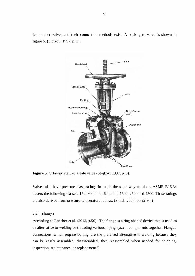
for smaller valves and their connection methods exist. A basic gate valve is shown in
figure 5. (Stojkov, 1997, p. 3.)
Figure 5. Cutaway view of a gate valve (Stojkov, 1997, p. 6).
Valves also have pressure class ratings in much the same way as pipes. ASME B16.34
covers the following classes: 150, 300, 400, 600, 900, 1500, 2500 and 4500. These ratings
are also derived from pressure-temperature ratings. (Smith, 2007, pp 92-94.)
2.4.3 Flanges
According to Parisher et al. (2012, p.56) “The flange is a ring-shaped device that is used as
an alternative to welding or threading various piping system components together. Flanged
connections, which require bolting, are the preferred alternative to welding because they
can be easily assembled, disassembled, then reassembled when needed for shipping,
inspection, maintenance, or replacement.”

31
Parisher et al. (2012, p. 56) also outline that “Flanged connections are favored over
threaded connections because threading large-bore pipe is not an economical or reliable
operation, as leakage on large-bore threaded pipe is difficult to prevent.”
Parisher et al. (2012, p. 58) mention “Flanges have been designed and to be used in a
myriad of applications. Each one has its own special characteristics and should be carefully
selected to meet specific function requirements.” The different flange types are weld neck,
threaded, socket weld, slip-on, lap-joint, reducing, blind, and orifice as listed by Parisher et
al. (2012, p. 58)
According to Parisher et al. (2012 p. 56) “Flanges are primarily used where a connecting or
dismantling joint is needed. These joints may include attaching pipe to fittings, valves,
mechanical equipment, or any other integral component within a piping configuration. In
the typical pipe facility, every piece of mechanical equipment is manufactured with at least
one inlet and outlet connection point. The point where the piping configuration is
connected to the equipment is called a nozzle. From this nozzle-to-flange connection point,
the piping routing is begun.” Figure 6 exhibits how piping may connect to vessel nozzles.
Figure 6. An example of vessel nozzles and flange connections (Parisher et al., 2012, p.
56).
32
Flanges follow the same analogy in pressure class ratings as pipes and valves. Parisher et
al. (2012, .p. 56) describe that “These pressure ratings, often called pound ratings, are
divided into seven categories for forged steel flanges. They are 150#, 300#, 400#, 600#,
900#, 1500# and 2500#. Cast iron flanges have pound ratings of 25#, 125#, 250# and
800#.”
Parisher et al. (2012, p. 56-57) describe “The surface of a flange, nozzle, or valve is called
the face. The face is usually machined to create a smooth surface. This smooth surface will
assure a leak-proof seal when two flanges are bolted together with a gasket sandwiched
between.” According to Parisher et al. (2012, p. 56-57), the most common types of flange
faces are:
flat face
raised face
ring-type joint.
Flat face flanges have flat mating surfaces, as the name implies. They are commonly used
in 150 and 300 pressure ratings when material of construction is forged steel. Their
primary use is to make connections with 125 and 250 rating cast iron flanges that are found
in some valves and mechanical equipment. (Parisher et al., 2012, p. 57.)
Raised face flanges are the most common type in use in all the seven of the aforementioned
pressure ratings. These flanges have a prominent raised surface, as the name implies. This
ensures a positive grip with a gasket in between. The height of the raised surface depends
on the pressure rating. (Parisher et al., 2012, p. 57.)
According to Parisher et al. (2012, p. 58) “The ring-type joint does not use a gasket to form
a seal between connecting flanges. Instead a round metallic ring is used that rests in a deep
groove cut into the flange face.”
Parisher et al. (2012, p. 59) state “The weld neck flange, occasionally referred to as the
high-hub flange, is designed to reduce high stress concentrations at the base of the flange
by transferring stress to the adjoining pipe. Although expensive, the weld neck flange is the
33
best-designer butt-weld flange available because of its inherent structural value and ease of
assembly.”
Weld neck flange is the most common type of flange used in process piping systems today.
It can be used in a variety of applications and it is the standard choice for any piping
system. Other types of flanges have their applications as well, but are not covered in detail
in this thesis.
2.4.4 Branches
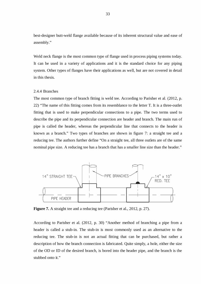
The most common type of branch fitting is weld tee. According to Parisher et al. (2012, p.
22) “The name of this fitting comes from its resemblance to the letter T. It is a three-outlet
fitting that is used to make perpendicular connections to a pipe. The two terms used to
describe the pipe and its perpendicular connection are header and branch. The main run of
pipe is called the header, whereas the perpendicular line that connects to the header is
known as a branch.” Two types of branches are shown in figure 7: a straight tee and a
reducing tee. The authors further define “On a straight tee, all three outlets are of the same
nominal pipe size. A reducing tee has a branch that has a smaller line size than the header.”
Figure 7. A straight tee and a reducing tee (Parisher et al., 2012, p. 27).
According to Parisher et al. (2012, p. 30) “Another method of branching a pipe from a
header is called a stub-in. The stub-in is most commonly used as an alternative to the
reducing tee. The stub-in is not an actual fitting that can be purchased, but rather a
description of how the branch connection is fabricated. Quite simply, a hole, either the size
of the OD or ID of the desired branch, is bored into the header pipe, and the branch is the
stubbed onto it.”

34
The branch line can be smaller than the header line, but never larger. The use of the stub-in
is becoming increasingly popular because of its cost effectiveness, even though it has
limitations in regards of operating pressure and temperature. Figure 8 exhibits the
attachment of a stub-in. (Parisher et al., 2012, p. 30.)
When internal pressure, temperature or external forces are placed on a stub-in, it may
require reinforcements to prevent failure of the branching. There are three reinforcement
possibilities that are listed below (Parisher et al., 2012, p.31):
reinforcing pad
welding saddle
O-lets.
Figure 8. Stub-in attachements (Parisher et al., 2012, p. 30).
According to Parisher et al. (2012, pp. 31) “The primary intent of the reinforcing pad is to
provide strength to the pipe header in the area where the branch hole has been cut.
Resembling a round, metal washer that has been bent to conform to the curvature of the
pipe, the reinforcing pad is a ring cut from steel plate that has a hole in the center equal to
the outside diameter of the branch connection.”
Third type of branch connection is the coupling. It is commonly used in instrument
connections. Figure 9 shows the two different types of coupling connections. (Parisher et
al., 2012, p. 32.)

35
Figure 9. The coupling branch connection methods (Parisher et al., 2012, p. 33).
2.4.5 Reducers
According to Silowash (2010, p. 173) “Reducers are used to change diameters between
two adjoining pipe sections.” The author further explains that there are two available
configurations for reducers: concentric and eccentric. Eccentric reducers have an offset in
centerline compared to the preceding pipeline, whereas concentric reducers and both
preceding and adjoining pipelines have a common centerline.
Silowash (2010, p. 173) states “Eccentric reducers are handy for establishing a constant
BOP (bottom of pipe) on headers that must reduce.” The author continues to state that they
also prevent complications with pump intakes. When eccentric type of reducer is used,
direction of the flat side must always be mentioned with “flat on top” (FOT) or “flat on
bottom” (FOB). Both types of reducers are shown in figure 10.
Figure 10. Eccentric and concentric reducers in a pipe rack (Parisher et al., 2012, p. 34).

36
2.4.6 Elbows and bends
The terms elbow and bend are sometimes used interchangeably, but they are not the same
thing. A bend is simply used when implying an offset – a change of direction. An elbow is
a standardized engineering bend that has been pre-fabricated to be either screwed, flanged
or welded to the piping it is associated with. Essentially, all elbows are bends but all bends
are not elbows. (Piping Elbows and Bends, 2014.)
Elbows are the most used fittings in piping systems. They are used to change the direction
in piping. The change of direction can be any made with any angle desired, but it is most
commonly done with either 90° or 45° elbows. The 90° elbow can be classified as long-
radius, short-radius, reducing, or mitered elbows. (Parisher et al., 2012, p. 14.)
Long-radius elbows are by far the most common types of elbows. In comparison with the
short-radius elbows, longer radius ensures better flow characteristics and lesser pressure
drop inside the pipeline. Comparison between long and short-radius elbows is shown in
figure 11. (Parisher et al., 2012, pp. 13-16.)
Figure 11. Comparison between a short and a long-radius elbow (Parisher et al., 2012, pp.
14-19).
Mitered elbow is a field-fabricated bend that is generally used on 24” or larger pipes,
because it is more cost effective and can be fabricated at the project site, rather than have it
manufactured and shipped. The mitered elbow is made using straight pipe and cutting it to
angular piece and lastly welding the pieces together, thus creating a 90° bend. Figure 12
shows two, three and four piece mitered elbows. (Parisher et al., 2012, p. 18.)

37
Figure 12. Mitered elbows (Parisher et al., 2012, p. 20).
A fitting also used to change directions is the 45° elbow, with the obvious difference of
angle compared to the 90° elbow. The 45° elbow being shorter than the 90° elbow yields
cost related savings and reserves space for the actual piping to be routed. (Parisher et al.,
2012, pp. 21-22.)
2.5 Mechanical equipment
No two plants or factories are exactly the same. However, they share many similar types of
process equipment, which perform necessary functions. Such items of equipment are
(Botermans et al., 2008, p. 1):
pumps to transport the liquids
compressors to transport compressible fluids
exchangers to transfer heat from a heating medium to a fluid
columns
tank to store compressible and non-compressible fluids
An optimum layout must be pursued in order to guarantee safety and efficiency of the
facility at hand. This means that the interrelationships between the various types of process
equipment need to be carefully considered. As projects advance and develop, the layout is
changed constantly and compromises are made in order to ensure safer placements of
equipment. (Botermans et al., 2008, p. 1.)
Even though piping components are important and mandatory in piping and processes,
according to Parisher et al. (2012, p. 112) “they play a minor role in the actual

38
manufacturing of a salable product. Other components of a piping facility actually perform
the tasks for which the facility is being built. Collectively, they are known as mechanical
equipment. Mechanical equipment can be used to start, stop, heat, cool, liquefy, purify,
distill, refine, store, mix or separate the commodity flowing through the piping system.”
2.5.1 Pumps
Pumps are used to generate a pressure to propel a liquid through a piping system and move
it from one location to another. It is essential for a process plant to function that liquids are
transported between equipment efficiently. There are three basic types of pumps that are
used in process facilities; centrifugal, reciprocating and rotary, each having their own
specific attributes and usage. (Botermans et al., 2008, p. 23.)
Centrifugal pumps rely on the centrifugal force that is generated by rotating impellers
inside a casing. A type of commodity, e.g. water, hits the vanes at high velocity and finally
seeks its path to the discharge outlet. The contained energy in the moving commodity is
converted to pressure energy before it is discharged. (Mackay, 2004, p. 1.)
Reciprocating pumps are positive-displacement pumps with a piston or plunger moving up
and down. During the suction stroke, the cylinder fills with liquid, which is displaced
during the discharge stroke through a check valve into the discharge line. Reciprocating
pumps can create very high pressures. (Jones, 2008, p. 11.3.)
Rotary pumps are also positive-displacement pumps and have rotating parts in them. These
rotating parts trap the liquid at the inlet port and force it through the discharge port into the
system. Gears, lobes, screws and vanes are common in this type of pumps. (Mobley, 2000,
pp. 28-29.)
2.5.2 Compressors
According to Parisher et al. (2012, pp. 116-117) “The compressor is similar to the pump,
but it is designed to move air, gases or vapors rather than liquids. The compressor is used
to increase the rate at which a gaseous commodity flows from one location to another.
Gases, unlike liquids, are elastic and must be compressed to increase flow rate. Similarly to
pumps, compressors are made in centrifugal, reciprocating and rotary configurations.”

39
2.5.3 Exchangers
Exchangers transfer heat between commodities. This can mean heating up a liquid or
cooling a product before final storage, both are possible. This is always done in a way that
commodities are not mixed during the heating or cooling process. They are simply meant
for heat transfer. A good example of exchanger is a household water heater. Exchanger can
be found in several different types, e.g. shell, double pipe, air fan and reboiler. (Parisher et
al., 2012, p. 117.) All of these have their own special attributes but are not covered in detail
in this thesis.
2.5.4 Tanks
Tanks are used for storage of liquids, gases and vapors for the operation of the process
plant. They are usually gathered outside the process area in tank farms. The stored
materials can be raw materials used in a process unit, intermediate products, end products,
waste products or even rainwater. Tanks are divided into two categories: atmospheric tanks
and pressurized tanks. A right type of tank is to be chosen depending on the stored
material. (Botermans et al., 2008, pp. 135-136.)
2.5.5 Columns
Columns are vertical vessels with associated internals. Their main function is usually to
distill fractions of raw product. The internals of the vessel are usually trays or a packing.
The column forms a process system with a number of other equipment such as reboilers
and condensers and should not be handled as an isolated piece of equipment. (Botermans et
al., 2008, p. 165.)
2.5.6 Cooling towers
Cooling towers are used to cool down the circulating cooling water that has been used in
exchangers and condenser and has gained a fair amount of heat during the process.
According to Parisher et al. (2012, p. 119) “Cooling towers are uniquely designed to
dissipate the heat gain by evaporating large amounts of aerated water that is circulated
through an air-induced tower.” The authors further explain that the fans used in the cooling
towers create draft and extract heat from falling water. A substantial amount of water is
lost during this process, but even so, cooling towers are widely used and highly efficient.
40
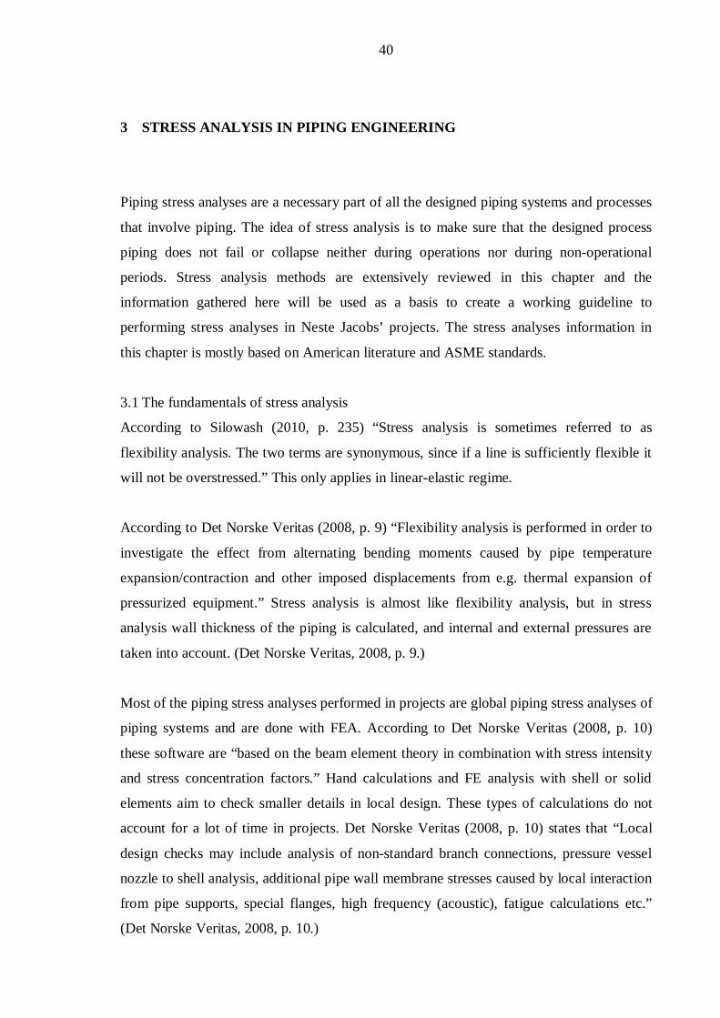
3 STRESS ANALYSIS IN PIPING ENGINEERING
Piping stress analyses are a necessary part of all the designed piping systems and processes
that involve piping. The idea of stress analysis is to make sure that the designed process
piping does not fail or collapse neither during operations nor during non-operational
periods. Stress analysis methods are extensively reviewed in this chapter and the
information gathered here will be used as a basis to create a working guideline to
performing stress analyses in Neste Jacobs’ projects. The stress analyses information in
this chapter is mostly based on American literature and ASME standards.
3.1 The fundamentals of stress analysis
According to Silowash (2010, p. 235) “Stress analysis is sometimes referred to as
flexibility analysis. The two terms are synonymous, since if a line is sufficiently flexible it
will not be overstressed.” This only applies in linear-elastic regime.
According to Det Norske Veritas (2008, p. 9) “Flexibility analysis is performed in order to
investigate the effect from alternating bending moments caused by pipe temperature
expansion/contraction and other imposed displacements from e.g. thermal expansion of
pressurized equipment.” Stress analysis is almost like flexibility analysis, but in stress
analysis wall thickness of the piping is calculated, and internal and external pressures are
taken into account. (Det Norske Veritas, 2008, p. 9.)
Most of the piping stress analyses performed in projects are global piping stress analyses of
piping systems and are done with FEA. According to Det Norske Veritas (2008, p. 10)
these software are “based on the beam element theory in combination with stress intensity
and stress concentration factors.” Hand calculations and FE analysis with shell or solid
elements aim to check smaller details in local design. These types of calculations do not
account for a lot of time in projects. Det Norske Veritas (2008, p. 10) states that “Local
design checks may include analysis of non-standard branch connections, pressure vessel
nozzle to shell analysis, additional pipe wall membrane stresses caused by local interaction
from pipe supports, special flanges, high frequency (acoustic), fatigue calculations etc.”
(Det Norske Veritas, 2008, p. 10.)

41
The U.S. piping codes utilize two separate failure theories; maximum principal stress
theory and maximum shear stress theory. Out of these two, the former is more often used.
Maximum principle stress theory states that yielding occurs when principal stresses exceed
the yield strength of material in any of the three perpendicular axes (x,y,z). Its biggest
advantage is the ease of use. In addition, when used with a sufficient factor of safety, it
yields acceptably safe results. (Smith et al., 1987, p. 62.)
Maximum shear stress theory states that failure occurs when maximum shear stress in a
material exceeds the shear occurring in a uniaxial test sample at yield. This means that the
maximum shear stress is equal to the difference between the largest and the smallest
principal stress divided by two. This is shown in Mohr’s circle, which is illustrated in
figure 13. Maximum shear stress is calculated with equation 3, which indicates that
yielding occurs when (Smith et al., 1987, p. 62):
= = 2 = 2(3)
Where 3 and max are the maximum shear stress
max is the largest principal stress
min is the smallest principal stress
Sy is the difference between the largest and the smallest principal stresses
Maximum shear stress theory is a more accurate evaluation of the state of stresses and thus
permits the use of higher allowable without decreasing safety. It also requires more
mathematical operations, which makes it more difficult to use. Even though both theories
give adequate results, maximum shear stress theory is thought to be more conservative.
(Smith et al., 1987, pp. 62-63.)

42
Figure 13. Mohr's circle exhibiting maximum shear stress (Smith et al., 1987, p. 62).
Nayyar (1999, pp. B.108-109) explains that piping codes have a certain set of failure
modes they address, but some are left unaddressed. Failure modes such as brittle fracture,
buckling and stress corrosion are not mentioned in the piping codes. According to Nayyar
(1999, p.B.108) “The piping codes address the following failure modes: excessive plastic
deformation, plastic instability or incremental collapse, and high-strain low-cycle fatigue.
Each of these modes of failure is caused by a different kind of stress and loading.”
Therefore the types of stresses have been placed into separate stress categories. These
categories are (Nayyar, 1999, pp. B.108-B.109):
primary stress – causes plastic deformation and bursting
secondary stress – causes plastic instability that leads to incremental collapse
peak stress – causes fatigue failure collapse that originates from cyclic loadings.
Primary stress develops due to mechanical loadings (forces). It is not self-limiting, which
means that when the yield strength is exceeded throughout the whole cross-sectional area
of the pipe, failure happens. In this case the only way to prevent failure is to remove or
reduce loadings. (Smith et al., 1987, p. 63.)
According to Smith (1987, p. 63) “Primary stresses are further divided into general
primary membrane stress, local primary membrane stress and primary bending stress.” The
piping under loading can only break after the whole cross-section of the pipe reaches the
limit of yield strength. Local primary stresses might exceed yielding strength but will not

43
cause failure by itself. The pipes cross-section needs to be in plastic behavior until failure
happens. Thus, the allowed primary bending moment may sometimes be increased over the
yielding moment by the shape factor. (Smith et al., 1987, p. 63.)
Secondary stress develops due to constraints that work against displacements such as
thermal expansions, imposed anchors and restraint movements. The piping system must
conform to imposed strains, rather than imposed forces, under secondary loading. This
means that the loading can be satisfied by system distortions. Local yielding and
distortions often alleviate these stresses due to imposed displacements. For this reason the
secondary stresses are sometimes known as self-limiting. (Smith et al., 1987, p. 64.)
Secondary stresses also develop due to discontinuity in the structure and primary stresses.
Discontinuity is caused by certain structural shaping and joint design, as well as distortion
of the structure due to welding.
Peak stresses are considered to cause virtually no distortion, which leads to high stress
levels. They are caused by thermal gradients across a pipe wall or stress concentrations at a
discontinuity such as a weld or a pipe fitting. Peak stresses are the highest stress in a local
region and are the cause for fatigue failure in non-static loading. (Smith et al., 1987, p. 64.)
Fluctuation of those stresses is also a major reason for fatigue failure in structures.
3.2 Load cases
Generally there are three different types of loads that need to be considered in stress
analyses. These load cases are (Smith et al., 1987, p. 87):
sustained loads – including weight and pressure
occasional loads – including wind, snow, vibrations, relief valve discharge and
seismic
expansion loads – including thermal expansion and contraction.
In stress analyses, a variety of these load cases are combined and used together to model a
realistic presentation of the actual real-world situation. The use of occasional loads
depends on the project at hand and the project’s geolocation. Different load cases are
covered more closely in this chapter.

44
3.2.1 Sustained loads
As previously mentioned, sustained loads are the loadings that are present throughout the
normal operation of the piping system such as weight and pressure. All piping systems
must be designed for weight loading, because they are usually not self-supporting.
Therefore they must be provided with supports to prevent the possible collapse. The
supports must carry the weight of pipes, insulation, fluid, components and the supports
themselves. (Smith et al., 1987, p. 87.)
The easiest way to estimate pipe stresses and support loads is to model the pipe as a beam
that is loaded uniformly throughout its length. This method works especially well when
calculating stresses on continuous horizontal pipe runs that have minimal geometrical
changes and only few in-line components. The length of the beam is thought to be the
distance between supports. (Smith et al., 1987, p. 87.)
The pipe can be modeled in two ways: the simply supported beam or the fixed-end beam.
The maximum stress and support loads for simply supported beam are calculated as shown
in equations 4 and 5 (Smith et al., 1987, p. 87):
= 8(4)
and
= 2(5)
where b is bending stress
W is weight per linear unit (length) of pipe
L is length of pipe
F is force on support
Z is section modulus of pipe.
If the pipe is considered to be a fixed-end beam, the maximum stress and support loads are
calculated with equations 6 and 7 (Smith et al., 1987, p. 87):

45
= 12(6)
and
= 2 . (7)
For both models, the force load on each support is the same, half of the weight imposed by
the pipe that is suspended between the two supports. However, the calculated stresses
between models vary. If the two models have same initial values, the bending stress with
fixed-end beam is less than with simply supported beam, meaning that fixed-end beams are
capable of having extended permissible support spacing in long pipelines. In practice,
support forces are only upward forces, meaning that pipes are usually modeled as simply
supported beams. (Smith et al., 1987, p. 88.)
In reality, the point of support does not allow a free rotation, which means that equal length
and equally loaded pipe runs may behave like a fixed-end beams. Thus, the true case lies
somewhere between the two models and stresses are often calculated with equation 8
(Smith et al., 1987, p. 88):
= 10 . (8)
There are standardized guidelines for support spacing for different pipe sizes, wall
thicknesses, insulation thicknesses, commodities and piping materials. Support spacing
tables are best used when most of the pipe runs are long and horizontal. However, the
following guidelines should be considered when designing supports (Smith et al., 1987, pp.
88-90):
pipe support should be located as near as possible to concentrated weights such as
flanges, valves and other instrumentation
when change of direction occur horizontally, the spacing between supports should
be less than what is given in tables
support spacing does not apply to vertical runs of pipe, pipe weight is divided
differently, thus supports need to be thought individually (usually placed in the
upper half of the rise to prevent buckling)
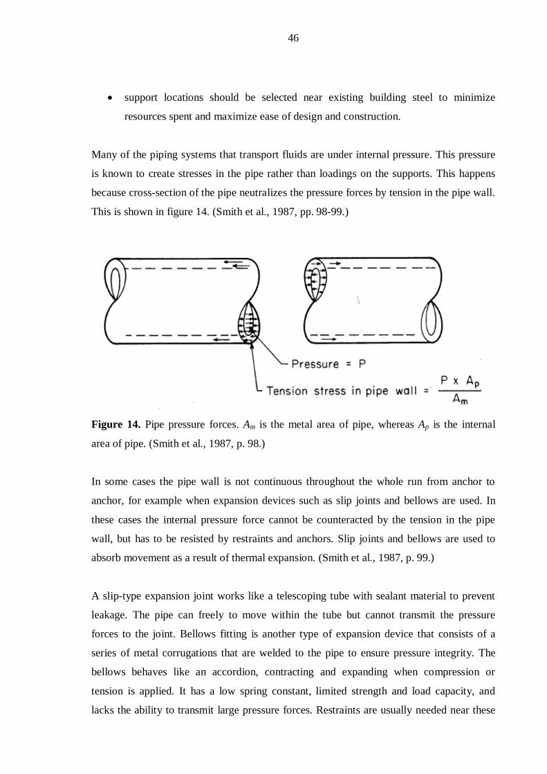
46
support locations should be selected near existing building steel to minimize
resources spent and maximize ease of design and construction.
Many of the piping systems that transport fluids are under internal pressure. This pressure
is known to create stresses in the pipe rather than loadings on the supports. This happens
because cross-section of the pipe neutralizes the pressure forces by tension in the pipe wall.
This is shown in figure 14. (Smith et al., 1987, pp. 98-99.)
Figure 14. Pipe pressure forces. Am is the metal area of pipe, whereas Ap is the internal
area of pipe. (Smith et al., 1987, p. 98.)
In some cases the pipe wall is not continuous throughout the whole run from anchor to
anchor, for example when expansion devices such as slip joints and bellows are used. In
these cases the internal pressure force cannot be counteracted by the tension in the pipe
wall, but has to be resisted by restraints and anchors. Slip joints and bellows are used to
absorb movement as a result of thermal expansion. (Smith et al., 1987, p. 99.)
A slip-type expansion joint works like a telescoping tube with sealant material to prevent
leakage. The pipe can freely to move within the tube but cannot transmit the pressure
forces to the joint. Bellows fitting is another type of expansion device that consists of a
series of metal corrugations that are welded to the pipe to ensure pressure integrity. The
bellows behaves like an accordion, contracting and expanding when compression or
tension is applied. It has a low spring constant, limited strength and load capacity, and
lacks the ability to transmit large pressure forces. Restraints are usually needed near these

47
types of expansion joints. A slip joint and bellows are shown in figure 15. (Smith et al.,
1987, p. 99.)
Figure 15. A slip joint and a bellows fitting (Smith et al., 1987, pp. 99-100).
If the pipe run is considered straight and continuous and filled with pressurized fluid, three
principal stresses are generated in the pipe wall due to internal pressure. These stresses are
h hoop stress (also referred to as circumferential or tangential stress), longitudinal stress l
(also known as axial stress), and radial stress r. When the ratio between the pipe diameter
and wall thickness D/t is greater than 20, the pipe can be considered to be thin wall. This
thin wall approximation allows the hoop stress to be thought as constant throughout the
wall thickness and can be calculated with equation 9 (Antaki, 2003, p. 81):
= 2(9)
where P is the design pressure
D is the outside pipe diameter
t is the pipe wall thickness.

48
The longitudinal stress caused by the internal pressure is also considered constant through
the wall and equal to half of the hoop stress. It can be calculated with equation 10 (Antaki,
2003, p. 81):
= 4 . (10)
The thin wall approximation is also used for cylindrical vessels. This means that the
stresses caused by the internal pressure in a cylindrical vessel are identical to those of
pipes. Radial stress is usually the smallest of the three principal stresses. The average radial
stress is calculated with equation 11 (Samuel et al., 2005, pp. 170-171):
= 2. (11)
Figure 16 illustrates the three different principal stresses and their orientation. Internal
pressure is always a part of sustained case calculations, but seldom proves to be a problem.
Figure 16. Illustration of the three principal stresses due to internal pressure (Antaki, 2003,
p. 82).
3.2.2 Expansion loads
Often when piping systems are operating, their temperature rises, and the pipes expand
accordingly. If the piping is too well restrained against deadweight, it will not be able to
expand properly and thus large forces will develop at the lockup points that cause large
stresses to develop in the pipe. The ideally restrained piping has no restraints at all, in
terms of preventing stresses caused by thermal expansion. However, this is not a feasible

49
solutions and even the most optimally supported piping system will develop some forces
and loads on restraints. (Smith et al., 1987, p. 128.)
Thermal expansion mostly affects the piping in axial (longitudinal) direction. Thermal
expansion can be calculated using the integral exhibited in equation 12 (Smith et al., 1987,
p. 128):
= (12)
where is the thermal expansion in direction specified by the length
L is the pipe length in direction of interest
is the coefficient of thermal expansion
T is the pipe temperature.
In most cases, the coefficient of thermal expansion varies with the temperature, which
means that equation 12 is not straightforwardly applied. The coefficients for common
piping materials at different temperatures have been studied and are usually found in
standards. (Smith et al., 1987, p. 129.)
ASME and EN standards have different standardized materials and their coefficients of
thermal expansion slightly vary. The equation for thermal expansion can be used linearly
for moderately accurate estimations and as a rule of thumb. Along with the coefficient of
thermal expansion, Young’s modulus also changes due to thermal changes. This also has
as impact on how loads caused by thermal expansion affect the piping system. However,
these values are always calculated based on linear analysis.
The simplest way to calculate thermal loads on supports is the guided-cantilever method.
This assumes that the longitudinal growth of the pipe run is absorbed by the bending of the
support beam that is perpendicular to the axial expansion. For a guided cantilever, the
imposed displacement induces a force and a moment at each end that are calculated with
equations 13 and 14 (Smith et al., 1987, p. 129):

50
=12 (13)
and
=6
(14)
where F is the developed force on support
M is the developed moment on support
E is the modulus of elasticity at installed temperature
I is the moment of inertia
i is the imposed displacement
Ls is the length of leg (support) perpendicular to the growth direction.
The guided-cantilever method does not provide fully accurate methods, because the
support legs are free to rotate to some extent at the intersection points. This means that the
developed moment is redistributed in the system. However, this method usually provides
conservative results, but in many cases a better accuracy is needed. (Smith et al., 1987, p.
134.) Today, greater accuracy is acquired with stress analysis software that complete these
calculations with utmost accuracy.
Occasionally, piping thermal movements are needed to accomplish tasks such as selection
of spring hangers. The movement can be estimated at intermediate points by assuming a
linear variation between two points of known displacements. (Smith et al., 1987, p. 134.)
Thermal expansions are often controlled with expansion loops. By adding a loop into a
piping system and placing supports properly, excessive thermal stresses can be reduced.
Properly placed supports direct the expansion to areas of greater flexibility, where thermal
stresses are better controlled. An appropriate use of expansion loop is shown in figure 17.
(Smith et al., 1987, p. 134.)

51
Figure 17. An exhibition of how an expansion loop with proper supports manages stresses
and nozzle forces in piping systems. (Smith et al., 1987, p. 135.)
3.2.3 Seismic loads
Seismic loads are categorized as occasional loads and are the first ones to be discussed in
this chapter. Regulations have been created for nuclear power plants demanding that
safety-related piping must be designed to withstand loads that yield from occasional
seismic activity and without losing the capability to function properly. It is recommended
that also non-nuclear piping should be designed according to the same regulations in
regions of high seismic activity. (Nayyar, 1999, p. B.161.)
According to Nayyar (1999, p. B.161) “Nuclear piping systems and components classified
as Seismic Category 1 are designed to withstand two levels of site-dependent hypothetical

52
earthquakes: the safe-shutdown earthquake (SSE) and the operational-basis earthquake
(OBE). For conservatism, the OBE must usually be equal to at least one-half of the SSE.
Their magnitudes are expressed in terms of the gravitational acceleration g. Their motions
are assumed to occur in three orthogonal directions: one vertical and two horizontal.”
Nayyar (1999, p. B.161) states “Seismic Category 1 systems are defined as those necessary
to assure:
1. the integrity of the reactor coolant pressure boundary
2. the capability to shut down the reactor and maintain it in a safe shutdown condition
3. the capability to prevent or mitigate potential off-site radiation exposure.”
According to Nayyar (1999, p. B.161) “Generally, piping seismic analysis is performed
through one of three methods: time-history analysis, modal response spectrum analysis or
static analysis.” Time-history analysis is used to solve the equation of motion. It describes
the piping system that is subjected to externally applied loadings, which are in this case
seismic excitations. The equation of motion is expressed in equation 15 (Nayyar, 1999, pp.
B.162):
+ + = ( ) (15)
where Mm is the mass matrix of the system
C is the damping matrix
K is the stiffness matrix
is the acceleration vector
is the velocity vector
x is the displacement vector
f(t) is the external loading vector as a function of time.
According to Nayyar (1999, p. B.162) “Time-history analysis is based on hypothetical
earthquake data in the form of ground displacement, velocity, or acceleration versus time.
The piping system is represented by lumped masses connected by massless elastic
members. The analysis is performed on this mathematical model by the direct numerical
integration method. At each time step, the piping stresses, displacements and restraint

53
loads are calculated. Time history simulates the behavior of the piping system during the
seismic excitation.”
The lumped-mass method is used to analyze and model elasticity in different structures.
The structures to be analyzed are divided into several separate mass lumps that all have
their own equation of motion. Springs are modeled in between the masses to simulate
elasticity. The lumped-mass method has several advantages: ease of use, simple theory and
moderate accuracy. However, it requires considerable amount of computational power
compared to other methods that model elasticity. Also, it may only be used for beams and
beam-like structures. In addition, the dampening of vibration in the structure is modelled in
a simplified way compared to other methods and yields less accurate results. (Mikkola,
2014.)
In regard of modal response spectrum analysis, Nayyar (1999, p. B.162) states that “The
seismic response spectrum is a plot of the maximum acceleration response of a number of
idealized single-degree-of-freedom oscillators attached to the floor (structure) with certain
damping. These response spectra are based on design response spectra and specified
maximum ground accelerations of the plant site.” The author continues to explain that the
spectra are used to study the pattern of the vibrations and generate a series of curves that
model the behavior of the structure during an earthquake. The single-DOF oscillators use
the same equation of motion that was given earlier in equation 15.
According to Nayyar (1999, p. B.164) “Static analysis may be used to evaluate power
piping or some piping systems in nuclear power plants. It is performed by analyzing a
piping system for the statically applied uniform load equivalent to the site-dependent
earthquake accelerations in each of the three orthogonal directions.” The author continues
to explain that it is less expensive than the two aforementioned methods and may be done
by hand calculation. At the end the results from all three directions are combined to acquire
the actual seismic loading. ANSI A58.1 recommends a simplified calculation method for
earthquake loads but shall not be covered in this thesis.

54
3.2.4 Wind loads
Wind loading is a periodic force that stems from aerodynamic iterations of the wind. Any
outdoor piping might be exposed to wind and thus must withstand great wind velocities
that might occur at any time. The wind velocity is dependent on geographic location and
local conditions of the facility. These conditions are usually observed over time to create a
realistic estimation of the conditions. The wind velocity can vary with aboveground
elevations. (Smith et al., 1987, p. 103.)
The wind loading is largely caused by the loss of momentum when the wind strikes the
piping system. The force is generally modelled as uniform load affecting the whole length
of the pipe and in the direction of the wind. The formula for wind force can be derived
from Bernoulli’s equation that describes the flow of fluid. The wind force per length is
calculated as (Smith et al., 1987, p. 105):
= 1000(16)
where Fw is the applied linear dynamic pressure load on projected length
Cd is the drag coefficient
q is the dynamic pressure, calculated as q = (1/2) V2
D is the pipe outside diameter, including insulation thickness
is the density of air
V is the velocity of air.
It is noteworthy that the pipe outside diameter is in millimeters, whereas all the other
values are meter-based. Thus equation 16 can also be expressed as (Shaughnessy et al.,
2005, p. 133):
=12 . (17)
Drag coefficient is a function of the shape of the structure and a dimensionless factor
called Reynolds number Re. Figure 18 illustrates the drag coefficient of a cylinder (pipe)
versus the Reynolds number. Wind loading on supports is generally not considered. The

55
Reynolds number gives an indication of the degree of turbulence in a fluid flow. Low
values indicate steady or laminar flow, whereas high values indicate transient or turbulent
flow. The Reynolds number is calculated as (Smith et al., 1987, p. 106):
= 1000(18)
where is the density of air
V is the wind velocity
D is the pipe diameter or structural outside length (note: in millimeters)
is the dynamic viscosity of air.
Figure 18. Drag coefficient for a cylinder as a function of Reynolds number (Shaughnessy
et al., 2005, p. 135).
For determination of wind loadings, the drag coefficient can be estimated from figure 18.
For certain conditions, a safety factor called the gust factor, may be used, when calculating
wind loads on piping. This factor usually ranges between 1.0 and 1.3, and addresses the
dynamic effects of non-steady-state air flow. (Smith et al., 1987, p. 106.)
3.2.5 Snow loads
Loadings that are caused by snow are seldom taken into account when analyzing stresses in
piping systems. This is due to the fact that many pipes are operating at higher temperatures

56
and are not affected by snow or ice. However, when exposed to cold weather, snow and ice
might accumulate on supports and possibly on pipes. (Ellenberger, 2014, pp. 228-229.)
It has been noticed that on curved surfaces, such as pipes and cylinders, with slope greater
than 70°, the snow will not stay in place. Thus, the horizontal projection of the surface is
used as the width of the area, meaning that the width is the pipe diameter (including
insulation thickness) times 0.93. (Ellenberger, 2014, pp. 230-231.)
The formula given by American Society of Civil Engineers (ASCE) for calculating the
snow load is (O’Rourke, Mazikins & Showalter, 2006):
= 0.7 (19)
where Ps is the snow load on pipe [kg/m2]
Ce is the exposure factor, determined by exposure to wind
Ct is the thermal factor, determined by ambient temperature
Cs is the slope factor, determined by surface material and slope type
If is the importance factor, 1.1 for most piping, 1.2 if hazardous substances
Pg is the ground snow load.
Snow loads can be included in the static analysis by calculating the maximum evenly
distributed load imposed by the snow and adding it on top of the piping’s own weight.
Thus it will be analyzed as a sustained load, even though it is an occasional load that can
only occur in winter.
3.2.6 Other occasional loads
Relief valves are installed to protect the piping system from overpressure by discharging
fluids to lower the pressure. When pressure rises too high, the valve opens and allows fluid
to escape in order to lower the pressure in the piping. This is a controlled way to prevent
pressure vessel ruptures. However, when a relief valve discharges, the fluid causes a jet
force that is transferred throughout the system. The force needs to be resisted by supports
or internally by the piping itself. The magnitude of the jet force is usually provided by the
valve manufacturer, but in some cases it is unknown and has to be calculated. The

57
calculations are fairly easy, if the valve vents straight to the atmosphere. In this case, the
situation is called open discharge. On the contrary, if the discharge flows through a closed
system to a vessel, it is called a closed discharge. (Smith et al., 1987, p. 108.)
For an open discharge relief valve, ASME B31.1 recommends that the discharge force
should be calculated as follows (Smith et al., 1987, p. 110):
= + 1 10(20)
where Fd is the discharge force
DLF is the dynamic load factor (varies between 1.1 and 2.0, depending on
rigidity of valve installation and opening time of the valve)
Mf is the mass flow rate from valve times 1.11
Vf is the fluid exit velocity
Ps is the static gauge pressure at discharge
A is the discharge flow area.
Pipe rupture works much the same way as relief valve discharge. According to Nayyar
(1999, pp. B.456-457) “if a pipe break occurs, thrust and jet forces generated by fluid
discharge can cause further damage to piping and other plant components unless adequate
mechanical restrains are employed. Discharging fluid creates a reaction thrust on the
ruptured pipe itself and impingement loads on objects struck by the jet of fluid. Moreover,
fluid acceleration inside the pipe generates forces on all segments that are bounded at
either end by an elbows or turn.”
According to Nayyar (1999, p. B.457) “Although pipe thrust may basically be considered
as a steady-state phenomenon, its initiation is accompanied by a violent transient following
the sudden sonic decompression wave starting at the break location. The mechanics of the
steady pipe thrust problem are similar to those involved in rocket propulsion.” In this
thesis, rupture mechanics won’t be considered, because the piping systems are designed to
withstand such events.

58
Generally, every piping system is connected to some type of rotating equipment, such as
compressors, pumps, turbine drives and motors. These are considered to be a large source
of mechanical vibration. The rotation generates a harmonic sinusoidal unbalance that
provides a force large enough to excite the piping system. The rotating machinery needs to
be supported on an elastic foundation to prevent vibration and forces caused by it. If the
rotational frequency is close to the natural frequency of the piping system, additional
resonant vibrations may occur and lead to possible piping failure. (Smith et al., 1987, p.
127.)
The best way to prevent vibration is to eliminate or isolate the source. Usually that is not
completely possible, and thus some vibration effects should be considered in the piping
system design. (Smith et al., 1987, p. 128.) In many cases, a separate vibration analysis is
performed after stress analysis to ensure maximum operating life for the piping system and
processes. Vibration analysis will not be more closely studied in this thesis.
One type of occasional load is the fluid or water hammer. According to Nayyar (1999, p.
B.458) “Water hammer is a pressure wave, usually resulting from rapid changes in the
flow rate in a pipe, which is characterized by the transformation of kinetic energy of
moving fluid into pressure.” The author further explains that water hammer is usually
caused by several different events, such as rapid valve closure and pump startup. The water
hammer phenomena can also occur due to formation of vapor pockets in the piping system.
The possibility of water hammer is erased by correct pipeline design and thus need not to
be discussed more closely.
3.2.7 Transient thermal loads
According to Escoe (2006, p. 229) “Failures resulting from thermal transients are more
common in in-plant piping than in pressure vessels, heat exchangers, and other process
equipment. The reason for this is the relatively smaller metal area to dissipate the thermal
energy and the larger number of structural discontinuities with valves and piping
intersections (e.g., tees and elbows). Transient heat transfer solutions are often difficult to
obtain with closed-form solutions.” The author further explains that there are several
simplistic algorithms that yield adequate results in one-dimensional cases. Transient heat
59
transfers can be studied by finite element method, which requires a more detailed analysis
of a certain structure.
3.3 Supports and restraints
Piping systems need to be designed to withstand the multiple loadings that have been
discussed earlier. A large amount of the design is based on supporting: what type of
supports to use, where should they be located, and how to minimize cost and maximize
efficiency.
Each type of pipe support has its own characteristics and they are meant to operate
differently from each other. Depending on the type, the boundary conditions vary.
Different support types are discussed in this chapter.
The term pipe support is used when referring to a device that supports the pipe weight,
whereas the term restraint is used when referring to a device that restrains the pipe against
lateral or axial movement. The standard supports are prefabricated, whereas custom
supports are handmade to support a special loading case. (Antaki, 2003, p.133.)
According to Antaki (2003, p. 133) “The term pipe support should be used to refer to a
device or assembly that supports the pipe weight. Pipe restraint should be used to refer to a
device or assembly that restrains the pipe against lateral or axial movement.” The author
further explains that the standard supports are prefabricated, whereas custom supports are
handmade to support a special loading case.
The supports can be divided into two categories: the standard catalogue supports and
custom support. In everyday practice (and this thesis), the term pipe support is used to refer
to all supports and restraints. (Antaki, 2003, p.133.)
3.3.1 Slides, weight supports, pipe rolls and rod hangers
Weight supports are used, when vertical downward pipe loads, such as deadweight, need to
be resisted. They are the very basic components of piping system supports. Different types
of weight supports are shown in Appendix II. (Smith et al., 1987, p. 153.)

60
Basically, slides and weight supports are used to block movement in vertical (usually
downward) direction, but allow axial and lateral movements. The standard catalog supports
are recommended to be used, but every support should be chosen to best fit the situation.
Pipe rolls are used in long pipelines and pipe runs, where longitudinal movement occurs
due to expansion. The rolls provide low friction, thus being more optimized than a rigid
weight support. (Antaki, 2003, p. 138.)
The most economical method to counter weight loads is to use rod hanger assemblies.
Steel rods are strong in tension, but inadequate for compression loading. Thus, rod hangers
are located above the pipe, so that it can carry the weight of the pipe. (Smith et al., 1987, p.
156.)
3.3.2 Guides
According to Parisher et al. (2012, p. 247) “When total restriction of pipe movement is not
required, pipe guides are used. Pipe guides confine movement along the pipe’s lineal axis.
Used primarily to maintain proper line spacing in a pipe rack, pipe guides prevent lateral or
sideways movement.”
Guides can be made with U-bolts or formed with structural steel, depending on special
requirements. Both guide types need to have a clearance of at least 1.5 millimeters between
the pipe and the support steel. If the guide is excessively tight, it becomes an anchor.
(Smith et al., 1987, pp.177-179.)
3.3.3 Spring hangers
Lines that have significant thermal expansion can be supported with spring hangers. They
allow the pipe to expand and move without placing unnecessary stress on the support itself.
(Parisher et al., 2012, p. 251.)
In some cases, if the pipe is supported with rigid supports, it may become unsupported due
to thermal movement, thus losing the weight load support. The rigid supports might also
cause thermal lockup that is accompanied with overstress in the pipe. (Smith et al., 1987, p.
161.)

61
Spring hangers can be divided into two main categories: constant load hangers and variable
load hangers. Constant load hanger provides an unchanged upward load on the pipe as it
moves up and down, whereas variable load hangers will provide more load as the spring is
moved from its balanced state by the vertical movement. Constant load hangers are used
where vertical movement is large, and variable load hangers when it is small. (Antaki,
2003, pp. 133-135.)
3.3.4 Guide anchors
Guide anchors can be considered as two-axis double-acting stops: their main task is to
prevent translation movement in the plane of two axes, while allowing movement normal
to the plane (The M.W. Kellogg Company, 1955, p. 232.)
Guide anchors are rarely used, but in some cases, they prove to be useful. In general, they
are used to prevent axial movement as well as vertical movement, but to allow movement
in lateral direction. This type of support can be created with structural steel, for example to
make rails for the pipe support, therefore forcing the movement in only one direction.
3.3.5 Anchors
According to Antaki (2003, p. 140) “Pipe anchors are restraints that constrain the pipe in
all degrees of freedom: three translations and three rotations. They are custom made, often
times by welding the pipe to a rigid support structure through sleeves, rectangular lugs or
round trunions.” The author further explains that the anchor point is heavily loaded due to
the concurrent forces and moments from both sides of the anchor points.
In long pipe runs, anchors are periodically to reset translations and rotations. In high
temperature piping, a sufficient flexibility is needed between the two anchor points to
ensure that the thermal stresses do not grow excessively due to thermal expansion. This
can be done with turns and elbows as well as expansion loops.
3.4 Nozzle loads
Whenever piping connects to mechanical equipment, e.g. pumps, tanks, or vessels, nozzle
forces and moments are studied. This is done in order to ensure that loadings caused by

62
weight or thermal movements of the adjoining pipes do not break the equipment or the
connection between equipment and piping.
For an equipment engineer there are two major reasons to calculate allowable nozzle loads.
The first reason is to provide vessel manufacturer with loading information that guides the
design process of the vessel shell. The second is to provide piping designer with
information on how to design and route the piping. The piping must not exceed the
allowable nozzle loads at vessel nozzle and with such information the piping designer can
minimize loads on nozzle by routing and supporting. (Moss et al., 2013, p. 462.)
If it is not possible to design the piping so that loadings do not exceed the limits, the work
process must go back to further calculating and analyzing the individual nozzle. This may
lead to a situation where the piping designer and vessel designer need to iteratively find a
solution to the problem. (Moss et al., 2013, p. 462.)
Manufacturing drawings contain the allowable nozzle loads in direction of every main axes
(X,Y,Z) and around the axes (moments), but the most important loads to mention are radial
force, longitudinal moment, circumferential moment and resultant moment. (Moss et al.,
2013, p. 463.)
3.5 Underground piping
There are advantages and disadvantages in buried piping. Biggest advantages are: reduced
plant congestion, shorter routes, protection from ambient temperature changes and wind
loads, and protected from surface traffic and activities. On the other hand, disadvantages of
an underground pipe are: unique corrosion from the soil, increased need for repairs,
accidental damage from digging and difficulty of detecting leaks. In addition, it has to be
designed for soil and surface loads. (Antaki, 2003, p. 302.)
Underground pipes may be under a wide range of loadings. According to Antaki (2003, p.
302) “Normal service loads include internal pressure, constrained expansion or contraction
due to changes in fluid temperature, soil weight, surface traffic and normal soil settlement.
Abnormal (accidential) loads include large pressure transients (such as water hammer),
large soil settlement (soil failure), and seismic forces.”

63
3.6 Stress intensification factor (SIF)
A piping system usually composes of many different components, such as bends, branches,
valves and flanges. In stress analysis, these various piping components are idealized into
two types of elements: the straight pipe beam element and the curved pipe beam element.
When a straight pipe is under bending stress, its cross-section remains circular and the
maximum stress occurs at the extreme outer fiber. However, a curved pipe element
behaves differently under bending, because the cross-section of the bend becomes oval.
The total effects of ovalization vary between in-plane and out-of-plane bending, but at least
the following phenomena occur due to the ovalization (Peng et al., 2009, pp. 67-68):
increase in flexibility due to relaxation of the extreme outer fiber of the bend
increase in longitudinal bending stress
creation of circumferential shell bending stress.
Every component is given a SIF in ASME and EN codes. The values of the SIFs have been
validated through testing the theories, for example, by performing fatigue tests. For process
piping, the applicable SIFs have been reduced to one-half of the theoretical SIFs, but they
still yield fairly conservative results. The SIFs are mainly used for thermal analysis and
support displacement analysis, but are also widely used for sustained loads. This has been
found to yield viable results in stress analyses and in piping system durability and lifetime.
For components such as branches and tees, equivalent bends, which are shown in figure
19, have been used to arrive at SIFs that are comparable with the test results. The SIFs
given for different components by ASME are shown in Appendix III. (Peng & Peng, 2009,
pp. 68-70.)
Figure 19. Equivalent elbows that have been used to achieve SIFs for different
components (Peng et al., 2009, p. 70).

64
SIFs are usually implemented into stress analysis software beforehand and do not need to
be applied separately. Stress intensification factors clarify the fact that the weakest point of
the piping system usually resides with the connected components, and almost never with
the pipe itself.
3.7 Loading case combinations
Pipe supports must be designed to endure any combination of loadings that may occur
simultaneously during operation of the process. Normal operating loads are deadweight
and thermal loadings. These can be combined with a variety of occasional loads,
depending on the project at hand. These loads can be added algebraically or absolutely to
achieve realistic or conservative results. A typical specification for different design load
combinations is (Smith et al., 1987, p. 150):
normal: deadweight
deadweight + thermal
upset: normal + relief valve discharge
normal + earthquake (OBE) + relief valve discharge
normal + waterhammer
emergency: normal + earthquake (SSE) + relief valve discharge
faulted: normal + earthquake (SSE) + pipe rupture.
In most cases, it is sufficient to check the loadings caused by deadweight and thermal
expansions. A more detailed analysis should always be separately requested, if it is not
instructed in the standards that are used. A more extensive loading case example is given in
the actual piping stress analysis guideline that is found in Appnedix V.
3.8 Piping stress analysis software
Piping stress analysis software utilize the finite element method. FEM has revolutionized
many aspects of structural engineering, as well as the piping engineering industry. Today
the various piping stress analysis software are plentiful, but only few are widely used and
recognized amongst piping designers. The most common software are:
CAEPipe by SST Systems Inc.
Caesar II by Intergraph
AutoPIPE by Bentley Systems.
65
These stress analysis software are based on beam element theory and utilized in
combination with stress intensification factors and stress concentration factors. The main
differences between the different software are usually related to user interface, and not the
fundamental operations.
The software are capable of performing static and dynamic analyses of piping systems.
Static analysis is the most common case of analysis used in the process industry and thus is
the type of analysis studied in this thesis. Static analysis takes into account the basic factors
such as temperature, weight, pressure, external forces, anchor movement, and also non-
linearity such as gaps and friction.
In certain cases, dynamic analysis is obligatory. The software can perform dynamic
analysis that takes into account a wide variety of occasional loads. These loads include
wind loads, time history loads, harmonic loads, seismic loads, and user specific natural
frequencies.
The software usually have built-in libraries for materials, valves, springs, flanges, pipe
cross-sections, codes (standard), which help the user to fasten the analysis process.
However, the values can be erroneous and always need to be checked from the actual
standards.
More precise analysis on nozzles and branches can be done by other FEM software, such
as Femap and ANSYS. They utilize other element theories to get more accurate results.
Two-dimensional elements that can be used include membrane and shell elements. Three-
dimensional elements, also known as 3D solid elements, include tetrahedral and
hexahedral elements. Other types of elements that might be generally used are
axisymmetric elements.

66
4 PIPING STANDARDS
This chapter is an overview of the most used and recognized standards in the field of
process piping and design. The standards reviewed are ASME B31.1, ASME B31.1, SFS-
EN 13480, and PSK standards that are widely used within Finnish companies. A
comparison between standards is also done in this chapter. The comparison includes things
such as calculation of wall thicknesses and how different allowable loadings are calculated.
4.1 ASME standards
According to Antaki (2003, pp. 13) “In the United States, the family of documents that
govern the design and construction of pressure piping is the ASME B31 pressure piping
code. The term “pressure piping” refers to piping systems or pipelines operating at or
above 15 psig, one atmosphere above the atmospheric pressure.” The author further
explains that B31 standard is divided into several separate books that are usually called
codes. These codes have been written ever since the 1927, and there are 11 different codes
altogether. In this thesis, the most used one will be code B31.3 that governs process piping.
In the code, process piping implicates pipes that are used for hydrocarbons and
petrochemicals.
ASME B31.1 is the code used for designing power piping. Silowash (2010, p. 21) states
“This code relates particularly to piping that would be found in electrical power plants,
commercial and institutional plants, geothermal plants, and central heating and cooling
plants. This code is primarily concerned with the effects of temperature and pressure on the
piping components.” This code can be applied to certain piping used in Neste Jacobs’
projects, but rarely is. The more commonly used code is B31.3 for process piping.
According to Det Norske Veritas (2008) “ASME B31.3 piping code has some basic
requirements regarding the integrity of the piping but leaves other aspects of the functional
design of the system to the designed.” The author further explains that B31.3 does not
address how stress calculations should be performed, which has led to the fact that working
practices for stress analyses vary between companies due to different interpretations of the
code.

67
ASME B31.3 (2012) has requirements for the qualifications of the designer (in this case,
the stress analyst). A completion of a degree in engineering, science or technology that
requires at least four years of full-time studies, and a minimum of five years of working
experience are required. If the designer has no education on this field, fifteen years of
working experience in the design of pressure piping is required.
4.2 SFS-EN standards
According to Det Norske Veritas (2008) “The intention of the EN 13480 piping code was
to harmonise a large number of European national piping codes in order to satisfy the
essential safety requirements of the new European Pressure Equipment Directive, PED.
European countries have now made the EN-13480 design code to a National piping
standard by adding national standards letter codes in front of it.” For example, SFS-EN
13480 is the Finnish national piping code.
EN 13480 is a more extensive piping design code than ASME B31.3 in regards with piping
stress analysis. Requirements for the calculations of all the loads are specified in this
standard with sufficient guidance. One of the biggest difference between EN 13480 and
B31.3 concerns pipe supports that are welded to the pipe. The EN standard has strict
instructions in that matter. Another big difference concerns a third-party analysis of piping
systems and pipe supports before the actual assembly. In fast moving off-shore projects
there is seldom time to analyse the flexibility before assembly and commissioning. (Det
Norske Veritas, 2008.)
EN 13480 (2012) does not pose requirements for the analyst’s education or working
experience. However, it is mentioned in Annex Q that only experienced personnel should
use the simplified pipe stress analysis, which consists of rules of thumb, supports spacing
tables and certain simplified loading calculations.
4.3 PSK standards
The PSK Standards Association serves process industry by compiling standards that are
utilized in industrial mills and plants. PSK works closely with the Finnish Standards
Association SFS to ensure quality in its works. (PSK Standards Association, 2014.)

68
PSK has published the PSK Handbook 7, which combines the various PSK pipe classes
that have been standardized beforehand. The PSK Handbook (2011) defines that a pipe
class denotes the selection of pipes and fittings that may be used for the same pipeline, and
in which the dimensions and materials have been predefined. This means that the various
components need not be separately designed and given dimensions, but have already been
defined. The pipe classes include materials, measurements and dimensions for components
such as straight pipes, elbows, reducers, tees, branches, collars, flanges, caps, screws, nut
and gaskets. The selection of a pipe class depends on the fluid, its corrosive attributes,
operating pressure and temperature of the pipeline.
The PSK handbook utilizes a variety of international and European standards that are used
in process industry. The materials are based on EN materials but, for example, a straight
pipe made of identical materials may have different dimensions. This logic applies to all of
the components.
4.4 Comparison of important features
Comparison between ASME B31.3 and EN 13480 is carried out to establish a clear
understanding of who these two major standards differ from each other. One of the biggest
differences is the units: B31.3 utilizes US customary units (formerly known as Imperial
units) while EN 13480 uses SI units. The differences in calculations and other various
matters are also covered in this part of the thesis.
4.4.1 Wall thickness of a straight pipe under internal pressure
Wall thicknesses are calculated to withstand internal pressure, as explained in chapter 3,
and the calculations are usually based on Tresca’s yield criterion. According to ASME
B31.3, wall thickness for a straight pipe is calculated as shown in chapter 2 and equation 1.
On the other hand, EN 13480 uses equations 21 and 22 to calculate wall thickness. If Do/Di
1.7:
= 2 + (21)
or
= 2 (22)

69
where e is the wall thickness without allowances
pc is the calculation pressure
Do is the outside diameter of the pipe
Di is the inside diameter of the pipe
f is the design stress
z is the joint coefficient.
The joint coefficient is used to calculate the thicknesses of components that have one or
more butt welds. Both ASME and EN use similar equations to calculate the wall thickness,
with the exception of different coefficients. These coefficients have an effect on the final
wall thickness, but both yield similar wall thicknesses. Due to the multiple coefficients that
ASME introduces, the wall thicknesses can be more conservative compared to EN wall
thicknesses. However, in many cases, the results are identical.
4.4.2 Stress due to sustained loads
The sum of primary stresses according to EN 13480 (2012) is calculated as shown in
equation 23:
= 4 +0.75
(23)
where pc is the calculation pressure
do is the attachment outside diameter for circular hollow attachment
en is the nominal run pipe wall thickness
i is the stress intensification factor
MA is the resultant moment
Z is the section modulus of run pipe
ff is the design stress for flexibility analysis (ff = min(f;fcr)).
In ASME B31.3 (2012) sustained loads are defined using Tresca’s model as follows:
= (| | + ) + (2 ) (24)

70
where Sa is the stress due to sustained longitudinal force
Sb is the stress due to sustained bending moment
St is the stress due to sustained torsional moment.
Sustained loads shall not exceed allowable stress at maximum metal temperature Sh, which
is provided in the standard.
4.4.3 Stress due to thermal expansion and alternating loads
SFS-EN 13480-3 (2012) gives the following equation to calculate thermal expansion
stresses for piping elements:
= (25)
where Mc is the resultant moment from thermal expansion and alternating loads
fa is the allowable stress range.
When conditions of equation 25 are not met, the sum of mechanical and thermal stresses,
4, can be calculated by using equation 26. Equation 25 gives more conservative results,
whereas equation 26 will give more accurate results. The loadings must satisfy the
following equation:
= 4 +0.75
+ + . (26)
Allowable stress range fa is calculated as follows:
= (1.25 + 0.25 ) (27)
where U is the stress range reduction factor calculated as 6.0N-0.2 1.0
fc is the allowable stress at minimum metal temperature
fh is the allowable stress at maximum metal temperature
Eh is the modulus of elasticity at maximum metal temperature

71
Ec is the modulus of elasticity at minimum metal temperature.
ASME B31.3 (2012) states that the displacement stress range should be based on the
temperature range from installation to maximum metal temperature during the thermal
cycles. The stress range for each element is calculated in accordance with equation 28:
= (1.25 + 0.25 ) (28)
where SA is the allowable displacement stress range
fsrf is the stress range factor calculated as 6.0N-0.2 fm (fm usually 1.0, for
ferrous materials 1.2)
Sc is the allowable stress at minimum metal temperature
Sh is the allowable stress at maximum metal temperature.
Equation 29 can also be used in appropriate situations. It allows the displacement stress to
exceed the calculated value for each piping element, based on each element’s sustained
stress SL.
= [1.25( + ) ]. (29)
The computed displacement stress SE shall never exceed the allowable displacement stress
range. Equation 34 is commonly not used in ASME based stress analysis.
It can be seen that both standards calculate things similarly and yield similar results. A big
difference between the standards is the materials that are used. Variance is found in
material strengths and compositions.
4.4.4 Stress intensification factors
Stress intensification factors given by ASME B31.3 are shown in Appendix III, and the
SIFs given by SFS-EN 13480-3 are shown in Appendix IV. The use of SIFs is explained
more closely in chapter 3.

72
5 DEVELOPMENT OF THE NEW PIPING STRESS ANALYSIS GUIDELINE
The new stress analysis guideline was created in order to unify calculation methods among
analysts and to clarify certain points that were left unclear in the older guideline. The new
guideline can be found in Appendix V.
The development of the new stress analysis guideline was set in motion due to the fact that
current guideline lacked clear parameters that control matters such as which piping systems
need to be calculated, how the calculation should be done and what type of documentation
is required.
5.1 Quality management
During the development, it was kept in mind that the guideline should meet the
requirements of ISO 9001 (2008) quality management systems standard. Figure 20 shows a
model of a process-based quality management system that can be used to improve a
company’s service’s quality. It puts emphasis on the customers by being the source of the
actual requirements of the said service. The processes are not shown in detail, but they are
more closely explained in the standard. Generally, the requirements are flexible and can be
met in many different ways.
The basic requirements for the designated organization in ISO 9001 quality management
system are as follows (SFS-EN ISO 9001, 2008, p. 15):
to determine the required processes and their application
to determine the interaction of these processes
to ensure functional control and operation of these processes
to monitor, measure and analyze the processes
to take action in order to achieve continual improvement of these processes.
The new stress analysis guideline controls only a part of a larger product, which in this
case is the actual service of plant design and engineering. Even though stress analysis is a
small part of the service provided for the customer, it is still considered a part of the quality
management system and must fulfill the requirements mentioned earlier.

73
Figure 20. A model of a process-based quality management system (SFS-EN ISO 9001,
2008, p. 11).
More detailed review of SFS-EN ISO 9001 (2008) reveals that the quality management
system requirements include the following points:
documentation (control of documents and records)
management responsibility
resource management (e.g. human resources)
product realization (in this case, the product is a service)
measurement, analysis and improvement.
The guideline was created to fulfill all the requirements and can be embedded as a part of
this quality management system.

74
5.2 The development process
The development process began by compiling all the necessary information needed to
create a complete and clear stress analysis guideline to be used by all the analysts in Neste
Jacobs. The previous guideline was not fully definitive in certain points and these points
were particularly addressed in the development process.
The following requirements for the new guideline were set: It must have a clear structure,
be a general instruction to performing stress analysis with any piping stress software, and
must clearly cover all relevant information regarding stress analysis. The guideline was
aimed to be usable by both beginners and experts in the field of stress analysis.
The first points presented in the guideline are the essential documentation, information and
values. The essential documentation addresses the standards that are viable in Neste
Jacobs’ projects. It was decided that without separate request or certain requirements, EN
13480 shall be used. Generally, the used standard is based upon which materials are used
in the project. ASME materials are always analyzed using ASME B31 standards.
Two new documents are to be filled out when performing stress analysis: “required
documentation and initial values checklist” and “analysis checklist”. The former will
ensure that all the necessary values are acquired before the analysis begins while the latter
is filled out after the first round of calculations in order to make sure that all the necessary
steps were taken correctly and the analysis is valid.
One of the most important points of the guideline was that which pipelines should be
calculated and which need not be analyzed. It was decided that piping marked as PED 1
class (Pressure Equipment Directive) will undergo a simplified analysis that does not
require a comprehensive report. On the other hand, PED classes 2 & 3 will undergo a
detailed analysis that requires a report to be filled out. PED class is given to piping by a
process engineer. A report template was created during the development that will be filled
out with all the important data from the calculations, such as important documents,
calculation and result files as attachments, calculation data, load cases, conclusions, stress
analysis results and comparison of nozzle loads.

75
Another important matter to be decided was how calculation packages are created and
which pipelines should be included in the same package. A rule of thumb for this was to
create a package that includes pipelines that form a sensible assembly. Rules for packages
are more accurately described in the actual guideline.
The guideline thereafter goes on to describe how a calculation is constructed. A general
practice for constructing a calculation model is given: First create geometry according to
isometric drawings, and then set material data, after that set pipe cross-sectional data. After
that insert all the different load cases that need to be studied. Thereafter, the support data
will be set, and after that the equipment data such as valve masses, flange masses and
equipment displacements. When all the necessary data is inserted, the calculation model
can be analyzed. This is a generalized instruction and does not affiliate with any particular
piping stress software. All the work stages mentioned before are extensively covered and
explained in the guideline found in Appendix V.
The guideline then goes on to explain how the analysis of the calculation model is done.
The different load cases are covered including occasional loads. The differences of
standard and their specific requirements for an acceptable result in the analysis are also
presented. Furthermore, allowable nozzle loads are explained and instructions on that
matter are given.
A few steps are given on how to inspect the calculation model in order to minimize errors
and save time. After inspections, instructions on how to analyze the results of the analysis
are given. This part includes instructions on how to act if the calculation results turn out to
be inadmissible. Instructions are specifically created to help taking the right steps
depending on which of the load cases fails to complete.
The guideline describes how most of the calculation processes are divided into two rounds.
The first round analysis is done according to AFD (approved for design) isometric
drawings whereas the second round analysis is performed using AFC (approved for
construction) isometric drawings. All the necessary documentation for both rounds are
explained in detail.
76
After that the guideline instructs what to do in case changes are made. If results are
inadmissible and changes are made, they must be properly logged and expressed. Major
changes must be marked into the isometric drawings of the stress isometrics and informed
to the designated piping designer. Instructions are also given concerning backup copies.
Lastly, the guideline guides how to save the files and report the results. Reporting is done
via a report template that includes every piece of necessary information concerning the
calculation. Afterwards the report shall be archived properly.
The development process of the guideline proved to be straightforward, because it
ultimately followed a logical structure in order to be as beginner-friendly and
comprehensive as possible. The guideline itself consists of all the necessary information
needed in stress analysis process and the electronic version of it includes three major
attachments: the report template, the analyst checklist and the initial values checklist.
The development of this guideline was the main objective of this thesis, however it was
utilized in a case study following this chapter. After that, the results of the case shall be
analyzed in conclusions and thereafter critically reviewed in discussion.

77
6 EXEMPLAR CASE
The objective of this case study was to use the newly created guideline in practice and
explain how it controls and guides the user through the calculation process. This case study
is meant to describe how the developmental work has enhanced the working process of
stress analysis.
Accroding to Runeson & Höst (2008, p. 5) “Different research methodologies serve
different purposes; One type of research methodology does not fit all purposes.” The
authors further define that the research purposes can be divided into four general types:
Exploratory: discovering what is happening, finding new insights and ideas,
generating hypotheses for new research
Descriptive: representing the current situation or phenomenon
Explanatory: seeking an explanation to a problem through causal relationships
Improving: trying to improve an aspect of the studied phenomenon.
According to Runeson et al. (2008) the case study method was originally used for
exploratory purposes, but it can also be used for descriptive purposes, if the situation or
phenomenon is of secondary importance. In this thesis, the case study has a descriptive
purpose to present how the stress analysis guideline works in practice, and concurrently the
designated project’s stress analysis process will be undergone and finished properly.
The piping system under study is a small part of a petrochemical plant under revision.
Some aspects of the process were revised and thus the piping materials had to be changed
from carbon steel to austenitic steel. Due to this change, the whole piping system needed to
be reanalyzed. Geometry was to remain unchanged. The up-to-date isometric drawings for
this analysis are found in Appendix VI.
There are 10 pages of isometric drawings that are fitted into one calculation package,
because they create a sensible assembly and are connected to the same pump pairing. This
project and its analyses are performed with Caepipe Version 7.0.
78
6.1 Construction and analysis of the calculation model
The construction and reanalyzing of the case follow the logical order suggested in the
guideline. The first part of constructing the calculation model begins with checking that all
the necessary initial values and required documentation are received in order to begin the
analysis. This is done by filling out the form “required documentation and initial values
checklist” found in Appendix V, page 27. After all the information is gathered, the
construction of the actual calculation model can begin.
The analysis is done according to ASME B31.3 standard because the piping system is a
part of process piping and the materials are ASTM standardized materials. Thus, the
formulae for allowable stress limits are also done according to ASME B31.3.
The pipelines under study were given PED 2 class, and thus shall be analyzed with detail,
meaning that the results will be reported in detail. Reporting shall be done using the report
template designed specifically for this type of use.
The model includes two standardized pumps and two filters. The equipment drawings were
given beforehand, but are not included in the appendices due to legal reasons. The
allowable nozzle loads on the pumps can be checked within Caepipe, because the pumps
manufactured according to API 610. The filters will be simplified and modeled as big
pipes, because the actual filter is a cylinder-like piece of equipment and is not under
scrutiny in this calculation.
Poisson’s ratio for all materials is 0.3 and the basic friction coefficients used with limit
stops is 0.35 and with guides is 0.4. The friction coefficients may change individually.
Geometry of the piping system was modelled as uniform with the isometric drawings.
Even though the materials of the piping system were changed, the geometry was meant to
remain unchanged. The dimensions are modelled according to the isometric drawings and
the nodes for supports and restraints are also correctly placed. Geometry of the assembled
calculation model is exhibited later in Figure 21 with correct cross-sectional data of the
pipes. It is taken in the correct isometric viewpoint like suggested in the guideline. In this

79
piping system, bends are always long radius bends, meaning that the bend radius is 1.5
times nominal diameter.
After the geometry is correctly modelled, material data can be set. Material data is given in
the isometric drawings and every separate material must be input correctly. The materials
used in the old version of the piping system and this case study are shown in table 3. The
table shows material name, type, density, yield strength, Young’s modulus and thermal
expansion coefficient.
Table 3. The material data of the materials used in the old revision and the new.
Material Type [kg/m3]y
[Mpa]E
[GPa] [mm/mm/C]
Old version:A335 Grade P5 (5Cr-1/2Mo) Carbon steel 7833 206.8 213 1.03E-05New version(currently used):A312 TP321 seamless 3/8"
& weldedAustenitic
steel 8027 206.8 195 1.62E-05Used in the filter supports:
A335 Grade P11 Carbon steel 7833 206.8 204 1.08E-05Used in the filters:
EN 1.4541 (X6CrNiTi18-10)Austenitic
steel 7900 520 200 1.60E-05
All the material data is checked with the correct standards even though they can be found
from Caepipe’s material library. The material library has some erroneous material values
and thus it has been decided that all the material information needs to be double-checked
from standards.
After material data is in place, every element is assigned with its designated material. After
this, all the different cross-sections of the pipes are input in the system. All of the used
cross-sections are found in table 4. For every cross-section, corrosion allowance is set to
1.5 millimeters according to the pipe class and mill tolerance is set to the normal value of
12.5%. Insulation thickness varies between 100 and 240 millimeters and every pipe’s value
is clearly indicated in the isometric drawings. The material for insulation is Mineral wool
with density of 136.16 kg/m3.
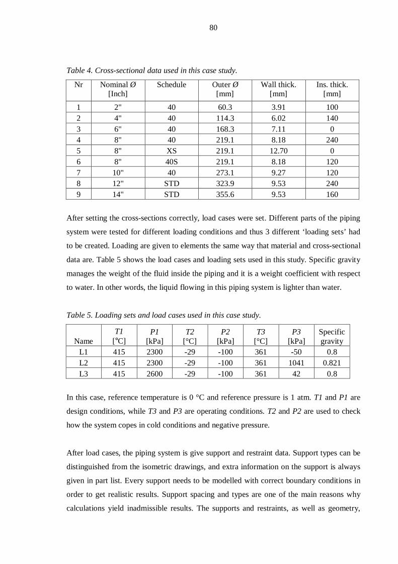
80
Table 4. Cross-sectional data used in this case study.
Nr Nominal Ø[Inch]
Schedule Outer Ø[mm]
Wall thick.[mm]
Ins. thick.[mm]
1 2" 40 60.3 3.91 1002 4" 40 114.3 6.02 1403 6" 40 168.3 7.11 04 8" 40 219.1 8.18 2405 8" XS 219.1 12.70 06 8" 40S 219.1 8.18 1207 10" 40 273.1 9.27 1208 12" STD 323.9 9.53 2409 14" STD 355.6 9.53 160
After setting the cross-sections correctly, load cases were set. Different parts of the piping
system were tested for different loading conditions and thus 3 different ‘loading sets’ had
to be created. Loading are given to elements the same way that material and cross-sectional
data are. Table 5 shows the load cases and loading sets used in this study. Specific gravity
manages the weight of the fluid inside the piping and it is a weight coefficient with respect
to water. In other words, the liquid flowing in this piping system is lighter than water.
Table 5. Loading sets and load cases used in this case study.
NameT1
[°C]P1
[kPa]T2
[°C]P2
[kPa]T3
[°C]P3
[kPa]Specificgravity
L1 415 2300 -29 -100 361 -50 0.8L2 415 2300 -29 -100 361 1041 0.821L3 415 2600 -29 -100 361 42 0.8
In this case, reference temperature is 0 °C and reference pressure is 1 atm. T1 and P1 are
design conditions, while T3 and P3 are operating conditions. T2 and P2 are used to check
how the system copes in cold conditions and negative pressure.
After load cases, the piping system is give support and restraint data. Support types can be
distinguished from the isometric drawings, and extra information on the support is always
given in part list. Every support needs to be modelled with correct boundary conditions in
order to get realistic results. Support spacing and types are one of the main reasons why
calculations yield inadmissible results. The supports and restraints, as well as geometry,

81
remains unchanged. The only thing under revision at first is the material of the piping and
the fluid flowing inside the system. If problems arise with the stresses, nozzle loads or
supports, they will be addressed.
Lastly, the piping system is given equipment data. This includes valve and flange masses
that have an effect on sustained loads of the system. Valves also increase the stiffness of
the system due to its lowered ability to flex and bend. The flanges used in this case study
are standardized and need not especially be mentioned. Instead, valves are always
particularly ordered and can have a variety of types and masses. Thus, every valve needs to
have its data delivered by the designer or manufacturer.
After every detail has been correctly set, the model is ready to be analyzed. A rendered
view of the complete piping system under study is shown in figure 21. Rendered view
clearly portrays the geometry, different sizes of cross-sections, all the supports, constraints
and hangers, as well as valves, flanges and anchors. The pump is not shown in the figure,
but instead the pump nozzles are modelled as anchors and will be checked for nozzle loads.
The nozzle loads of the pumps and the filters must stay below the allowable limits. Only
the closer one of the pumps is visible in the figure but both pumps have identical suction
and discharge sides and the modelling method is the same for both.
Figure 21. A rendered view of the piping system under study.

82
6.2 Results of the calculation
The calculation model was analyzed after the material was changed. Most important points
under study were pipe stresses due to sustained and expansion loads, and nozzle loads with
the pumps and filters. The stresses for sustained loads were well below the allowable
limits, as shown in figure 22. Maximum stress caused by sustained loads was found in
node 10 that is the suction nozzle for one of the two pumps. Node 10 is marked in figure
22 with a red mark. The stress ratio at node 10 was 0.50.
Figure 22. Stress ratios of sustained loads in the piping system under study.
The highest stress due to thermal expansion was found in node 260 that is a welding tee
with a higher SIF than the basic pipe element. The stress ratio in node 260 was 0.35. The
stress ratios are shown in figure 23.

83
Figure 23. Stress ratios due to thermal expansion in the piping system under study.
After checking the pipe stresses, nozzle loads for pumps and filters were checked. Both
pumps and filters have allowable nozzle loads given in the manufacturing drawings and the
loadings at correct nodes were compared to them. The comparison between allowable
nozzle loads and the results of the analysis are shown in table 6.
Table 6. Filter nozzle load comparison in load case 1 (T1 = 415 C, P1 = 2300 kPa).
Loading type inLoad case 1
Allowable[kN] [kNm]
Result[kN] [kNm]
Filter 1 Filter 2
Mainout
Feedinlet
Mainoutnode30
Feedinletnode110
Mainoutnode1030
Feedinletnode1110
Radial load FR 11.44 11.44 -2.93 4.13 2.60 10.07Longitudinal (axial) FL 11.44 11.44 -4.13 -17.80 -10.07 -30.66Circumferential load FC 11.44 11.44 0.73 -11.58 -12.51 8.83Torsional moment MT - 7.04 -0.66 6.07 3.49 -9.30Longitudinal moment FL 7.04 - -0.53 -1.16 -2.47 0.26Circumferential mom. MC 7.04 - 2.31 4.06 1.26 -13.59

84
Filter nozzle loads were above the allowable limit and thus certain steps were taken in
order to improve the situation. The pumps were also checked for nozzle loads and it was
done by using Caepipe’s built-in pump application. The pumps’ nozzle load comparison is
shown in figure 24.
Figure 24. Nozzle load comparison of the pumps used in the piping system under study.
The axial (longitudinal) load in node 1000 exceeded the allowable limits and needed to be
lowered in order to make the results admissible. Certain steps were taken to amend the
situation and fix the nozzle loads under study.

85
6.3 Changes in the model and new results
The stress analysis guideline suggests certain steps to be taken in case nozzle loads exceed
the allowable limits. The first step is to increase flexibility in the nozzle region in order to
lower the loads. The second step is to modify supports to receive admissible results. The
third option would be to approach the equipment manufacturer and get an approval on the
current nozzle loads.
In this case the loads were excessive and had to be fixed. The geometry had to stay
unchanged and thus the supports had to be changed. After some reiteration, two major
changes were made in order to fix the nozzle loads. One of the supports was changed to
Teflon coating that reduces the friction coefficient between the support and the pipe to
0.05. This change resulted in admissible results in the pump nozzle forces. By lowering the
friction force caused by the support, the forces at the nozzle were also lowered. This is
because the support and the nozzle create a force pair that counteracts the forces and
moments that are created by each other. The support configuration is shown in figure 25.
Figure 25. The two major modifications in the supports that were meant to lower the
nozzle loads in filters and pumps.

86
Another change is with the supports legs that hold the filter fixed. The limit stop that
constrained the translation along x-axis was removed, thus allowing the axial movement
due to thermal expansion from the pumps and pipes that lead to the filters. This change is
also showed in figure 26.
As a result of these changes, the highest sustained and expansion stresses were still found
in the same nodes as before, although minor changes in the overall stresses could be seen.
However, stresses were never the problem, therefore they are not further explained in this
study.
After the changes, the pump nozzle loads were lowered below the allowable limits and the
results for them were admissible. The results are shown in figure 26.
Figure 26. The nozzle load results of the pumps after the support changes.

87
The changes on supports did not drastically change the nozzle loads of the filters. One
reason for this is the fact that while freeing the translation in the directions of x-axis, the
feed inlet nozzle will affected by torque around the z-axis and force along the x-axis. The
nozzle loads for the filters are shown in table 7. Force directions are chosen according to
chapter 3 and figure 16.
Table 7. Filter nozzle loads after the support modifications.
Loading type inLoad case 1
Allowable[kN] [kNm]
Result[kN] [kNm]
Filter 1 Filter 2
Mainout
Feedinlet
Mainout
node30
Feedinletnode110
Mainout
node1030
Feedinletnode1110
Radial load FR 11.44 11.44 -1.14 1.84 1.48 8.52Longitudinal (axial) FL 11.44 11.44 -1.84 -16.51 -8.52 -30.69Circumferential load FC 11.44 11.44 3.06 -10.07 -7.56 9.92Torsional moment MT - 7.04 -0.38 4.94 -2.14 -8.63
Longitudinal moment FL 7.04 - 0.73 3.21 -1.41 -14.34Circumferential mom. MC 7.04 - 2.80 -2.96 0.08 -1.45
After the changes, the filter nozzle loads are still above allowable limits. Filter number 2
has an axial force of 30.69 kN in the feed inlet, but cannot be lowered without changing
the geometry. However, geometry must remain untouched and therefore the manufacturer
of the filters was contacted and asked if the nozzle loads are acceptable in this case. The
manufacturer examined the connection in detail and concluded that the both filters can be
used under these loads.
By releasing the restraints in the direction of y-axis the pipe between the pumps and the
filters were allowed to expand freely due to thermal expansion. Therefore the nozzle loads
of the pumps stayed below allowable limits. Due to thermal expansion, the axial force in
the feed inlet in node 1110 increases twofold in comparison with only sustained loads. This
could not be managed by merely changing supports but would have needed a geometrical
change instead. However, the piping system was completed once a confirmation was
received from the manufacturer of the filters on the durability of the nozzles.

88
7 CONCLUSIONS
The newly developed stress analysis guideline is an extensive and comprehensive
specification on how to correctly perform stress analyses in Neste Jacobs’ organization. It
covers all the essential information needed in stress analysis, beginning from initial values
to actually creating a calculation model. It also guides the user how to manage changes in
case the results are inadmissible. The guideline is an overall view of the entire calculation
process and functions as intended.
The exemplar case was calculated in order to show how the guideline should be used and
serves as a good example. The calculation case was not an easy one because the geometry
had to remain intact. This was due to a lack of space in the process area. Although
conditions were unfavorable, the piping system was successfully analyzed. The most
difficult part of the calculation was getting the filter nozzle loads below allowable limits,
and with the current geometry it proved to be impossible. However, with an approval for
use from the filter manufacturer, the calculation was successfully completed.
The guideline is very applicable in its designated use and serves its purpose well.
Compared to the previous stress analysis guideline, the one developed due to this thesis
gives a more comprehensive view of the actual calculation process and guides the user
through the whole calculation. In cases where problems are encountered, the guideline
gives proper and clear guidance on how to tackle these issues.

89
8 DISCUSSION
The development process of the stress analysis guideline was consistent but time
consuming. The whole process began by studying the literature found in libraries and
databases throughout the web. The amount of information on this industry is vast and
general in nature. Thus finding any valid information on actual stress analysis was quite
hard. On top of that, all the articles are very specific and study subjects that have particular
practical use for certain parties. Some articles have been written concerning piping stress
analyses, but usually one particular thing or aspect of it is studied, and thus most of the
articles were of no or little value to this thesis.
Getting familiarized with the most common piping standards was very eye-opening.
Mostly the standards provide similar requirements to piping stress analysis, but they do
have some differences, for example how allowable stresses are calculated and how stress
intensification factors are determined. Getting to know the legislation is an important part
of understanding the actual requisites of stress analysis.
The creation of the new guideline took some time to form in its final shape. Two team
meeting were held in a time span of two months and during those meetings all the
important points were finalized and the content of the guideline was agreed upon. At the
same time it was supposed to be a clear guide for users with little experience in stress
analyses, but also a specification that gives exact instructions on how stress analyses are to
be performed from the beginning.
For experienced analysts the new guideline introduces some new working methods that
they might have been unfamiliar with beforehand. The biggest changes are the introduction
of “Required documentation and initial values checklist” and “Analysis checklist” that are
to be filled out before and after the analysis. The former form allows the analyst to be sure
that all the necessary information has been received from responsible parties, whereas the
latter form is filled out after the analysis is done. The analysis checklist and the actual
analysis is also checked by a 3rd party to make sure that calculations are done correctly and
to decrease the amount of errors.

90
On top of these two forms, a report template was created and introduced. Report templates
have always been project specific and have had a lot of variance between each other. Thus,
it was decided that a unified report template should be developed and put into use. It is
meant to contain all essential points that should be filled out to clearly present achieved
results and at the same time enhance the reporting and archiving of the results. When a
uniform template is used in all projects, there will be no confusion on where to find certain
essential information.
The exemplar case was created and calculated in order to tie the theoretical guideline into
practice. It clearly shows how the guideline will be used by analysts and how the
calculation process moves forward. The case proved to be difficult because the main
problems were found with the nozzle loads of the filters and pumps. However, not every
calculation package is a straightforward job, and this case shows exactly that.
Nevertheless, the stress analysis process was carried out successfully.
Value of this thesis is more practical than theoretical. It is an extensive literature review
that aimed to create a stress analysis guideline to unify working methods. This thesis was
successful with that objective. Nothing ground breaking was discovered during this study,
but nevertheless, it turned out well and the guideline will henceforth be used throughout
the whole organization.
Possible future work concerning the guideline is plentiful. Whenever standards are
updated, the guideline needs to be revisited and updated as well. At this point, the
guideline does not yet clearly instruct how to calculate piping systems with bellows,
because they are seldom used. A third point of future work would be to add instructions on
how the analyst could make more detailed nozzle calculations using FEM software such as
NozzlePro in case that the nozzle loads given by the piping stress software turn out to be
inadmissible.

91
REFERENCES
Antaki, G.A. 2003. Piping and Pipeline Engineering: Design, Construction, Maintenance,
Integrity and Repair. New York: Marcel Dekker, Inc. 539 p.
ASME B31.3. 2012. ASME Code for Pressure Piping B31 Process Piping B31.3-2012
(Revision of ASME B31.3-2010). The American Society of Mechanical Engineers. 480 p.
Bhende, G. & Tembhare, G. 2013. Stress Intensification & Flexibility in Pipe Stress
Analysis. International Journal of Modern Engineering Research, 3:3. pp. 1324-1329.
Bhattacharya, A. 2012. A comparison of simple analytical methods for evaluating local
stresses at pipe support attachments with Finite Element Analysis results. Chicago Bridge
& Iron Company. [Referenced 21.07.2015.] Available at:
http://www.cbi.com/images/uploads/technical_articles/NAFEMS_UK_2012_final_paper.p
df.
Botermans, R. & Smith, P. 2008. Process Piping Design Handbook, Volume 2 - Advanced
Piping Design. Houston: Gulf Publishing Company. 217 p.
Chase Alloys Ltd. Effects of Alloying Elements in Steel. [Webpage]. [Referenced
12.03.2015.] Available at: http://www.chasealloys.co.uk/steel/alloying-elements-in-
steel/index.html.
Det Norske Veritas. 2008. Structural Analysis of Piping Systems – Recommended Practice
DNV-RP-D101. Available at:
http://www.jadelltd.com/wa_files/Recommended_20Practice_20DNV-RP-D101_20-
_20Structural_20Analysis_20of_20Piping_20Systems.pdf. [Referenced 25.03.2015]
Ellenberger, J.P. 2014. Piping and Pipeline Calculations Manual - Construction, Design
Fabrication and Examination (2nd Edition). Elsevier. 389 p.

92
Escoe, A.K. 2006. Piping and Pipeline Assessment Guide. Elsevier. 515 p.
Jones, G.M.. 2008. Pumping Station Design (Revised 3rd Edition). Elsevier. 1104 p.
Mackay, R. 2004. Practical Pumping Handbook. Elsevier. 273 p.
Megson, T.H.G. 2005. Structural and Stress Analysis (2nd Edition). Elsevier. 714 p.
Mikkola, A. 2014. Lecture 3. Lecture notes distributed in “Koneen simuloinnin työkurssi”
course’s Moodle page in Lappeenranta University of Technology on 21 January 2014.
Mobley, R.K. 2000. Fluid Power Dynamics. Elsevier. 284 p.
Moss, D.R. & Basic, M.M. 2013. Pressure Vessel Design Manual (4th Edition). Elsevier.
744p.
Nayyar, M. L. 1999. Piping Handbook (7th Edition). McGraw-Hill, Inc. Available
at:http://ptecgroup.ir/Books%20and%20Thecnical%20Documents/Handbooks/Piping%20
Handbook-Nayar.pdf
O’Rourke, M., Mazikins, P.J. & Showalter, J. 2006. Snow Provisions in ASCE 7-05.
[Referenced 26.05.2015.] Available at:
http://www.awc.org/pdf/PaperSnowProvisionsASCE7-05web.pdf
Parisher, R.A. & Rhea, R.A. 2012. Pipe Drafting and Design (3rd Edition). Elsevier. 460 p.
Peng, L.C. & Peng, T.L. 2009. Pipe Stress Engineering. Houston, Texas, USA. ASME
Press. 473 p.
Piping Elbows and Bends: A useful detailed literature for piping engineers. 2014.
[Webpage]. [Referenced 23.02.2015.] Available at: http://www.whatispiping.com/piping-
elbows-and-bends.

93
PSK Standards Association. 2011. PSK Handbook 7 – Pipe Classes. 2nd Edition. Copy-Set
Oy, Helsinki. ISBN 978-952-5930-01-6. 539 p.
Runeson, P. & Höst, M. 2008. Guidelines for conducting and reporting case study research
in software engineering. Springer. [Referenced 27.07.2015.] Available at:
http://lup.lub.lu.se/luur/download?func=downloadFile&recordOId=1276781&fileOId=127
6782
Samuel, A. & Weir, J. 2005. Introduction to Engineering Design - Modelling, Synthesis
and Problem Solving Strategies. Elsevier. 383 p.
Shaughnessy, E.J., Katz, I.M. & Schaffer, J.P. 2005. Introduction to Fluid Mechanics
(OUP Edition). Oxford University Press. 1018 p.
SFS-EN ISO 9001. 2008. Quality management systems: Requirements. Finnish Standards
Association SFS. 69 p.
SFS-EN 13480-3. 2012. Metallic Industrial Piping Part 3: Design and Calculation. Finnish
Standards Association SFS. 409 p.
Sinnott, R.K. 2005. Coulson and Richardson's Chemical Engineering Volume 6 - Chemical
Engineering Design (4th Edition). Elsevier. 916 p.
Smith, P.R. & Van Laan, T.J. 1987. Piping and Pipe Support Systems: Design and
Engineering. McGraw-Hill, Inc. 334 p.
Silowash, Brian. 2010. Piping Systems Manual. McGraw-Hill, Inc. 416 p.
Smith, P. 2007. Process Piping Design Handbook, Volume 1 - The Fundamentals of Piping
Design. Gulf Publishing Company. 217 p.
Stojkov, B. T., 1997. Valve Primer. Industrial Press. 204 p.

94
The M.W. Kellogg Company. 1955. Design of Piping Systems. New York: John Wiley &
Sons, Inc. 380p.

Appendix I

Appendix II, 1

Appendix II, 2

Appendix III, 1

Appendix III, 2
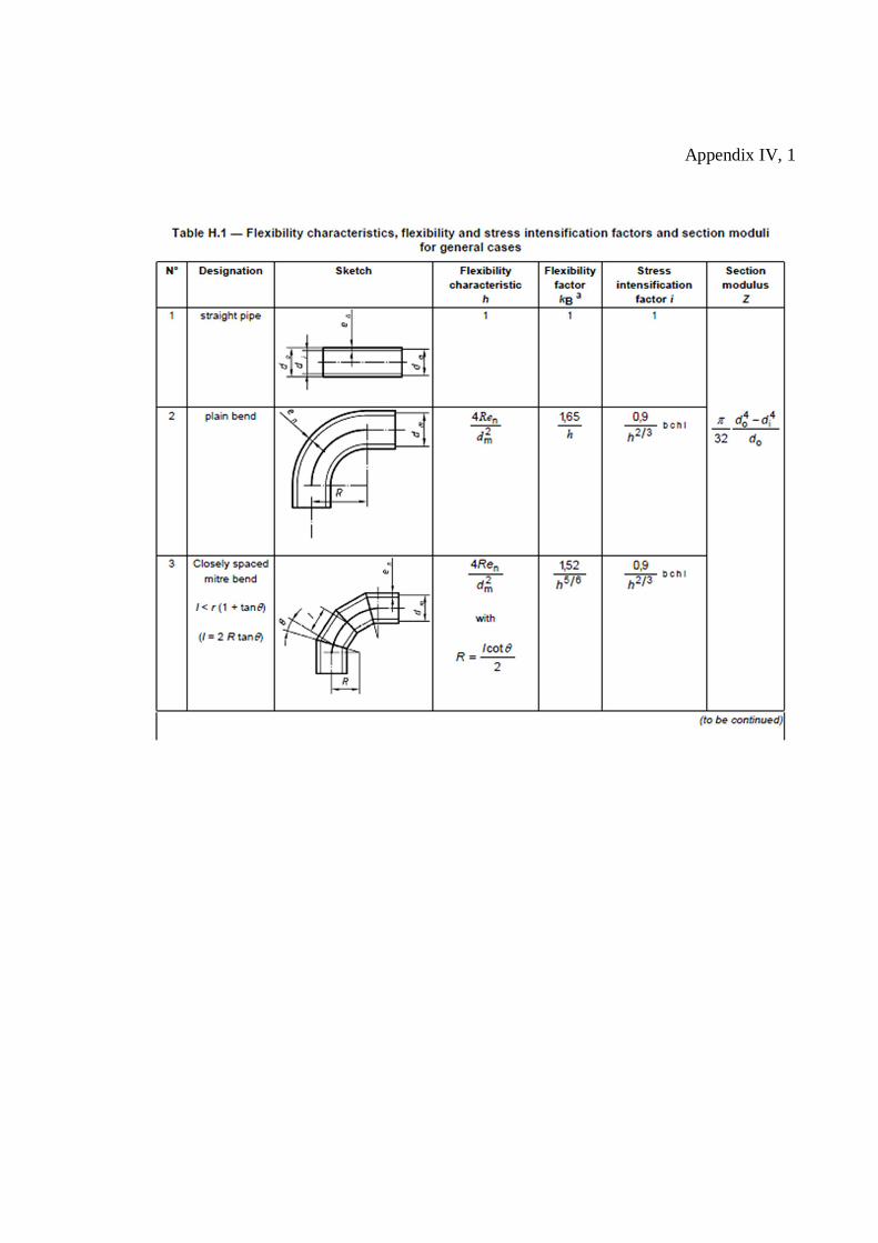
Appendix IV, 1

Appendix IV, 2

Appendix IV, 3

Appendix V, 1
STRESS ANALYSIS GUIDELINE
REV DATE STATUS WRITTEN BY CHECKED BY APPROV./AUTHO
1 15.7.2015 FIRST REVISION

Appendix V, 2
PIPING STRESS ANALYSIS GUIDELINE
The new guideline to performing stress analysis in Neste Jacobs Oy’s projects is presented
in this text. It will contain the required technical information on how to perform stress
analysis. Stress analyses are performed in order to make sure that the piping systems that
have been designed can handle the different loadings and will not break down and cause
process or system to seize function.
The guideline will begin by covering the required source data that is essential for stress
analysis in every project. It will continue by addressing issues that may arise with the
construction of the calculation model. After that, analysis and inspection of the calculation
model are discussed. Thereafter, how results and the changes in calculation models are
managed shall be covered. Lastly, the guideline will state how the results are reported and
archived.
ESSENTIAL DOCUMENTATION, INFORMATION AND VALUES
Stress analysis without certain requirements for the use of specific standards shall be
carried out according to newest revision of EN 13480. The use of other standards is
possible and shall be requested by the customer or the party commissioning the analyses.
Other applicable standards are ASME B31.3 (process piping) and ASME B31.1 (power
piping). In special cases, country specific standards may be used.
Used materials and pipe classes may specify which standard is used in stress analysis. If
ASME standardized materials are used, stress analysis ought to be performed according to
ASME standards and vice versa.
Neste Jacobs has approved the use of two separate third-party piping stress analysis
software: CAESAR II (Intergraph) and CAEPIPE (by SST Systems, Inc.).

Appendix V, 3
Important documentation and values for stress analysis are found in the “Required
documentation and initial values checklist” that is found in appendices. This checklist shall
be filled out by the analyst before the beginning of analysis. The checklist shall be used to
ensure all the necessary data and documentation is received prior to the analysis.
Another checklist is the “Analysis checklist” made for global analysis. It shall be filled out
to ensure that all the necessary data is correctly used and to assure that all necessary steps
are taken and required tasks are completed. The purpose of the checklist is to gather all
tasks in one place for the analyst and a 3rd party checker and thus decrease the amount of
possible errors and the overall time of the calculation process. The analysis checklist for
global analysis is presented in appendices.
Stress analysisWithout separate instructions, a formal piping stress analysis with third-party FEM
software shall be carried out, if one or more of the following criteria are met:
Sound Engineering Practice SEP – visual analysis (charts, cantilever method)
PED 1- simplified analysis (no reports needed)
PED 2 and 3 – detailed analysis (with report)
Pipes of any size that are connected to any equipment with limited allowable nozzle
loads and where nozzle loads must be verified
Customer’s request
In addition, any pipeline with possible concerns in terms of flexibility may be assessed by
a professional and assigned to be calculated. Every pipeline should be inspected by an
experienced engineer with years of experience in field of piping engineering and stress
analysis.
Visual analysis (approximate visual inspection) should be carried out in every case in
accordance with sound engineering practice. It can be done with help of charts and the
cantilever method to acquire sufficiently accurate estimations.
Simplified analysis is carried out with computer software using conservative (and
simplified) configurations. It is done in order to verify the piping system’s flexibility but
Appendix V, 4
needs not be reported separately. However, the results need to be given to the piping
designer in order to confirm the piping’s structural integrity.
Detailed analysis will be carried out with computer software using accurate and realistic
configurations. The piping code requirements shall be met. An extensive and detailed
report template (appendices) shall be filled out to report the results of the analysis.
The analyst shall define the different calculation packages that will be used in the project.
The packages shall be clearly marked into P&I drawings and pipeline list. One calculation
package should consist of several pipelines rather than only one. Some of the reasons to
combine several pipelines into one calculation are:
Pipelines are originating from the same vessel or tank (not column)
Pipelines that originate from the same pump (suction and pressure couplings)
Pipelines that originate from adjacent pumps (A/B)
Pipelines are connected in the process
Pipelines are part of the same task and near each other
Pipelines that create a sensible assembly.
Calculation packages shall always be created on case-by-case basis using sound
engineering practice and professional expertise.
Basic initial valuesEvery initial value needs to be checked and defined as required in the standard that is used
in calculations. This includes Young’s modulus E, thermal expansion coefficient , and
other material values such as yield strength and other allowable stresses. Some stress
analysis software contain material libraries that can help speed the calculation process, but
often enough the values are incorrectly entered. Especially the EN standard materials are
often erroneous. Thus, double-checking is necessary.
Modulus of elasticity E for different materials might be included in the stress analysis
software, but the values must always be checked and matched with the standard’s values.
The modulus of elasticity is temperature dependent and in high temperatures its value
tends to decrease. The value of modulus decreases nearly linearly as temperature rises.

Appendix V, 5
In a similar manner, the coefficients of thermal expansion need to be checked and
calculated separately in order to ensure that the values are according to standards. The
value of thermal expansion coefficient increases nearly linearly as temperature rises.
In EN 13480, the values for Young’s modulus and coefficient of thermal expansion for
different materials can be found in Annex G. In ASME B31.3, E and can be found in
Appendix C.
Allowable stresses need to be checked on a case-by-case basis. These values are found
from separate material standards unique for each standard type (ASME, EN).
Value for Poisson’s ratio shall be v = 0.3 for all metals at all temperatures. This value is
given in most standards and requires no further study.
Standard value for friction coefficient at all supports is = 0.4. Different values may be
agreed upon in the beginning of projects and those values must be coherently used. A value
of 0.35 for limit stops may be used in special cases. This does not include low-friction
supports. In some cases, the piping system needs to be calculated as a frictionless system.
This means that all the frictions between pipes and supports are assumed 0. This is
sometimes used in nuclear plant design.
The materials used in piping are ultimately chosen by process engineers or by a party
responsible for the design of the plant or process. Materials are always found in isometric
drawings. Only standardized materials and pipe classes shall be used (ASME, EN, PSK).
CONSTRUCTION OF A CALCULATION MODEL
In the beginning of a new calculation, important settings must be set. First one is the
correct standard that will be used in the calculation (usually ASME B31.3 or EN 13480).
The second one is the reference temperature, which influences how delta temperature is
calculated (the difference in operating temperature and reference temperature).

Appendix V, 6
The third one is a correct coordinate system. In Neste Jacobs’ projects vertical direction
shall always be Z-axis. Z-axis is also known as Elevation.
Construction of the calculation model may begin when isometric drawings are received
from designers. Isometric drawings contain most of the necessary data needed for
calculation, excluding certain project specific information. Figure 1 shows the steps of
constructing a valid calculation model.
Figure 1. The process of creating a stress analysis calculation model.
GeometryThe naming of the calculation model should be logical and informative. Thus it is logical
to say that the name of the calculation package should go by the head pipeline
In both Neste Jacobs’ approved software (CAESAR II and Caepipe), the modeling begins
by drawing the piping and pipelines as presented in the isometric drawings. The lines that
are drawn in the piping stress analysis software represent the pipe centerlines and thus
contain only geometrical data at first. The analyst must make sure that coordinates at the
beginning and at the end of the pipelines match in the isometrics as well as in the software.

Appendix V, 7
By matching the coordinates the analyst can minimize errors that could possibly result in
erroneous results in stress analysis.
The coordinate system that will be used in Neste Jacobs’ projects is shown in figure 2. The
coordinates in isometric drawings are always E, N, EL (East, North, Elevation). It has been
assigned that Eastern coordinate is +X (positive x-coordinate), Northern coordinate is +Y
(positive y-coordinate) and Elevation value is +Z (positive z-coordinate).
Figure 2. The coordinate system in accordance with isometric drawings.
All of the dimensions need to be modeled as given in the isometric drawings. An example
of this is shown in figure 3, which illustrates a long pipe run that is divided into separate
dimensions due to support spacing. The analyst needs to create lines with length of the
spacing between the supports, thus creating nodes at both ends of the line. These nodes
will be given data that will make the node location have, for example, supports, hangers,
guides, flanges, external forces and user SIFs (stress intensification factors).

Appendix V, 8
Figure 27. A long pipe run with dimensions showing support spacing.
Basically this means that the lines created shall be: 5500, 4000, 4000, 4000 and 271 in +X
direction. The nodes will have support data implemented into them. In figure 2, S3’s are
guides and S4’s are slide supports.
Isometric drawings show dimensions for every component separately. This means that a
long straight pipe run is expressed with one length and a connecting component (e.g. valve,
bend, support or branch) has its own length shown. An example of this is shown in figure
4.
The length of flanges and gaskets are not shown in the dimensions, but they must always
be included in the calculation model. The thickness of gaskets and dimensions of the
flanges are usually standardized and given in the beginning of a project. The thickness of a
gasket is usually from 2 to 4.5 millimeters.
In figure 4, there are gaskets at both ends of the valve (item number 12). They are not
shown in any dimensions, but need to be accounted for in the final calculation model. By
leaving the thicknesses of gaskets out of the model, the final coordinates can be erroneous

Appendix V, 9
by hundreds of millimeters. The gaskets share the same cross-section as the pipe it is
connected to.
Figure 4. Dimensions when flanges and valves are involved.
There are two ways to start and end a calculation to prevent singularity with stiffness
matrices and incorrect results:
From an anchor
From mechanical equipment (e.g. pump, vessel).
In the calculation model, mechanical equipment nozzles are modeled as anchors. When
calculation begins or ends at a nozzle, thermal movement of the equipment must be
factored in. This is done by inducing a forced displacement by thermal movement, which is
derived from hand calculations. Also, the extra flexibility provided by the nozzle needs to
be taken into account. This can be done with help of certain software’s nozzle tool that
factors in the connected equipment’s flexibility and yields conservative flexibility increase.
If the calculation cannot be ended at an anchor, the pipeline calculation must be continued
until it can be made sure that leaving the pipe unanchored does not affect the stresses and
strain under investigation. Usually an anchor can be substituted by consecutive guides and
supports that jointly counter the excessive movements and mimic the actions of an anchor.
This practice should only be used when no other means are possible.

Appendix V, 10
When a new pipeline connects to an old one, the old isometrics need to be used to continue
the calculation until the next anchor. If isometrics are unavailable, piping drawings need to
be used. Piping drawings include plan view drawings and elevation view drawings. If
piping drawings are unavailable, a sketch of the old piping needs to be acquired from
reliable sources.
When the piping system has branches, all of the piping connected to it needs to be modeled
and combined into the calculation. This sometimes makes the calculation model grow too
vast and thus there is a practice to cut the ‘inconsequential’ (unimportant) piping from the
calculations:
While Ø 6, if the branch pipe diameter is half of the size of the header diameter
(or smaller), it may be cut from the final calculation due to its insignificance to
final results
While header Ø > 6”, branch lines shall be cut from the calculation when the
branch line’s diameter is one third (1/3) of the header diameter.
Branch lines that need not be calculated but cannot be excluded from the calculation (due
to big diameter) should always be modeled until it is restrained by an anchor. This way the
calculation package will not overgrow but the effect of the branch line will be taken into
account.
Material dataMaterial data is always included in the isometric drawings. It can be found by either
looking up the pipe class and its materials or by looking up the part list and finding the
material used from the part’s description. Figure 5 exhibits how materials are marked in
the isometric drawings.

Appendix V, 11
Figure 5. How to find the material information from the isometric drawings.
In figure 5, the material used with the 6” straight pipe is a standardized carbon steel API5L
Grade B with schedule 40. In third-party software the material can be found from the
material library, which quickens the calculation process. Also, schedule numbers and
standardized cross-sections can be used when creating a cross-section for the pipe, which
also makes the modeling easier.
If material library is not a viable option, all the necessary values for the material can be
found from different standards and manually entered into the stress analysis software. It
will yield the same results both ways.
Pipe cross-sectional dataPipe cross-section depends on the outside diameter of the pipe and the wall thickness. In
addition, wall thickness is affected by mechanical allowances, corrosion allowance and
mill tolerance. On top of that, most of the pipes have insulation on them, which increases
the outside diameter of the pipe run and adds more weight per length. All of these factors
need to be taken into account when performing stress analyses.
Pipe sizes are according to EN standards or ASME standards. EN standards use Diametre
Nominal (DN) scale that makes use of millimeters and quite logically expresses pipe sizes
in comparison with the actual outside diameter. For example DN50 pipe has an outside
diameter of 60.3 mm. This is comparable with the North American Nominal Pipe Size of 2
inches.

Appendix V, 12
Figure 5 shows how the material information is received from the isometric drawings. The
cross-sectional data is can also be found from the same part list. N.S shows that the
nominal size is 6” and schedule 40. In this case, the outside diameter is 168.3 mm and wall
thickness 7.11 mm. The cross-sectional is often easily input into the stress analysis
software, but some non-common and non-standardized section might need to be set by
hand.
Insulation thickness around the pipe depends on the pipe classes that are used. This
information can be found either in the isometric drawings or in the pipe class form. The
materials for insulation are diverse, but one commonly used is mineral wool with density
of 136.36 kg/m3. This adds more weight to the piping and affects the sustained load case,
where deadweight is the main type of loading.
Corrosion allowance usually varies between 1 and 3 millimeters, depending on the fluid’s
corrosiveness. This information can be found in the pipe class form. The calculation
software does not factor in corrosion allowance when calculating flexibility. Only the
nominal thickness of the pipe is taken into account.
Mill tolerance is a factor used for seamless pipes due to its manufacturing process, which
leads to uneven or divergent wall thickness in the pipe. It is commonly set to 12.5% and is
thought to yield realistic or conservative results. Mill tolerance is not factored in by the
software when performing flexibility analysis.
Load casesDepending on the situation and the project parameters, different types of load cases may be
used. The basic case is to use reference temperature of 20ºC or 0ºC. Temperatures T1 and
T2 need to be set as design temperature and operating temperature. Accordingly, pressures
P1 and P2 will be set as design pressure and operating pressure. All of these values can be
found in the isometric drawings.
Load cases are always project specific and are designed to sufficiently explain and model
the actual loads imposed to the piping system. In some projects, there are a variety of load
cases that need to be studied. An example of this is shown in table 1.

Appendix V, 13
Table 1. An example of load cases under study.LOAD
CASE
No.
LOAD CASE
DESCRIPTION
STRESS
TYPEDEFINITION
L1 WW+HP HYD HYDRAULIC TEST
L2 W+T1+P1 OPE OPERATING CONDITION
L3 W+T2+P2 OPE DESIGN CONDITION
L4 W+T3+P1 OPE OPERATING CONDITION MINIMUM METAL TEMP
L5 W+T1+P1+WIN1 OPE DESIGN CONDITION+WIND FORCE
L6 W+T1+P1+WIN2 OPE DESIGN CONDITION+WIND FORCE
L7 W+T1+P1+WIN3 OPE DESIGN CONDITION+WIND FORCE
L8 W+T1+P1+WIN4 OPE DESIGN CONDITION+WIND FORCE
L9 W+P1 SUS SUSTAINED CASE DESIGN
L10 W+P2 SUS SUSTAINED CASE OPERATING
L11 WNC SUS WEIGHT NO CONTENT
L12 L5-L2 OCC PURE WIND FORCE
L13 L6-L2 OCC PURE WIND FORCE
L14 L7-L2 OCC PURE WIND FORCE
L15 L8-L2 OCC PURE WIND FORCE
L16 L9+L12 OCC SUSTAINED CASE DESIGN+WIND FORCE
L17 L9+L13 OCC SUSTAINED CASE DESIGN+WIND FORCE
L18 L9+L14 OCC SUSTAINED CASE DESIGN+WIND FORCE
L19 L9+L15 OCC SUSTAINED CASE DESIGN+WIND FORCE
L20 L2-L9 EXP THERMAL EXPANSION CASE
L21 L2-L3 EXP THERMAL EXPANSION CASE
L22 L2-L4 EXP THERMAL EXPANSION CASE
L23 L3-L10 EXP THERMAL EXPANSION CASE
L24 L3-L4 EXP THERMAL EXPANSION CASE
L25 L4-L9 EXP THERMAL EXPANSION CASE
Notes for load case description:W: Weight HP: Hydro-test pressureT1: Thermal case 1 WW: Weight when filled with waterT2: Thermal case 2 L1: Load case 1T3: Thermal case 3 OPE: OperatingP1: Pressure case 1 EXP: ExpansionP2: Pressure case 2 OCC: OccasionalWin: wind case

Appendix V, 14
Sometimes occasional loads are needed to be included in the analysis. Such loads include
snow load, wind load, earthquake load, fluid hammer and pressure safety valve relief force.
In static analysis, these loads can be simplified to act as uniform loads along the whole
piping. In third party software, these occasional loads can usually be set separately and the
software automatically includes the loads in the calculations.
The directions of occasional loads vary and must be realistically selected. Snow load can
be added as extra mass to the piping system (in the vertical Z direction), whereas wind and
earthquake loads are horizontal and require further analysis of the actual real life situation.
Fluid hammer and pressure safety valve relief are seldom used in analysis and require
precise study to be applied into the stress analysis.
For an open discharge relief valve, ASME B31.1 recommends that the discharge force
should be calculated as follows (Smith et al., 1987, p. 110):
= + 1 10(1)
where F is the discharge force
DLF is the dynamic load factor (varies between 1.1 and 2.0, depending on
rigidity of valve installation and opening time of the valve)
M is the mass flow rate from valve times 1.11
V is the fluid exit velocity
P is the static gauge pressure at discharge
A is the discharge flow area.
Supports dataSupports need to be modeled exactly the same way they appear in isometric drawings. The
basic markings used in the isometric drawings give an idea of how the supports work and
how the pipe will be restrained. However, the supports are not always as simple as they
seem. Thus, extra information on the support is sometimes needed and that information can
be found from the part list. The basic support markings are shown in table 2.

Appendix V, 15
Table 2. Different types of markings used for supports and restraints in isometricdrawings. In this table, the pipes are directed along the X axis. Boundary conditionschange accordingly when the pipes are headed along other axes. 1 means that certainmovement is restrained, whereas 0 means that the specific movement is free.
No Marking style in planand isometric drawings Description
Boundary conditionsTX TY TZ RX RY RZ
1Support thatallows freesliding of the pipe
0 0 1(-Z)
0 0 0
2 Slide
0 0 1 0 0 0
3Guide (axialmovementallowed)
0 1 1 0 0 0
4 Anchor(Fixed point)
1 1 1 0(1)
0(1)
0(1)
5Guide anchor(lateral movementallowed)
1 0 1 0 0 0
6
HangerSpring hangerFloor standSpecial support
0 0 1(kx)
0 0 0
More support information can be found in the part list. For example, figure 5 shows parts
number 3 and 4 to be a guide and a slide support. Their types are NOS2042 and NOS2041
and their drawings can be found in project specific specifications.
Support number 1 is a slide support that allows the pipe move in X and Y –directions, but
restrains movement along negative Z –axis. Basically this means that it supports the weight
of the pipe but allows it move in axial and lateral directions and it can also rise from the

Appendix V, 16
support and be left unsupported. In CAEPIPE this support is modeled with ‘Limit stop’ by
setting boundary conditions correctly.
Support type number 2 is a slide that allows movement in axial and lateral directions, but
restrains vertical movement. Usually there is an upper limit to how much the pipe can rise
from the support. In any case, it will not be left to hanging freely. This slide type can also
be modeled with ‘Limit stop’ with correct boundary conditions.
Support type number 3 is a guide that guides the pipe in axial direction. This means that
the pipe can move in axial direction, but is restrained from moving laterally or vertically.
Guides can be modeled with a pair of limit stops or a guide. In both cases, a gap between
the pipe and the guide may be used to ensure realistic calculations. In most cases, the gap
is thought to be 2 millimeters. A gap of 0 mm can be used in order to achieve conservative
results. The analyst can define the gap to best suit the calculation’s purposes.
Support number 4 is an anchor. It restrains all the translations (axial, lateral and vertical
movements) and sometimes rotations. All six degrees of freedom are restrained when
calculation is stopped and the pipeline is cut. When anchors are used in the middle of a
calculation, they are modeled in a way that allows rotations. Anchor is used to begin or end
calculations, thus making sure the calculation is theoretically valid. Anchors need to be
used with appropriate frequency to ‘reset’ stresses along the piping. Anchors can be
modeled with anchor tool.
Support type number 5 is a guide anchor that restrains movement in axial and vertical
directions, but allows movement in lateral direction. This type of support is not too
common, but used in some cases. Guide anchor should be modeled using limit stops.
In isometric drawings, a rod hanger and a spring hanger look similar to normal slides, but
in the part list they have different information that indicates the support to be a hanger.
Rod hanger restrains vertical downward movement but allows all the others. Spring hanger
does not restrain any movements, but applies force whenever the spring is displaced from
its neutral position, thus managing or limiting pipe movements. Spring hangers should be
chosen by hand, because in some cases the software makes spring choices that do not serve
Appendix V, 17
the situation well. The aim of a spring hanger is to hold the pipe statically in place in every
load case condition. The choice of spring hangers should always be done using extreme
care and they need always be marked clearly into stress isometrics/ isometric drawings.
Special supports’ design drawings should always be delivered to the analyst who is in
charge of calculating a piping system where such support is used. In case of special
support, good engineering practice should be utilized to conclude what type of support it
really is.
Equipment dataPiping equipment comprise mainly of valves and flanges. Valves are almost always
attached to piping with flanges, mainly because it is easily attached and detached in case of
maintenance. In stress analysis, equipment data means mostly the masses of these parts.
Valves have high concentrated mass compared to straight pipe and have high influence on
the piping system by inducing bending moments and sometimes even torsion.
Main data for valves that should be input in to the stress analysis is mass, center of the
mass (if there is an offset and the center of the mass is not along the pipe centerline), and
thickness coefficient (has an impact on stiffness). Valve type can be found from part list
and further information (such as mass) from the design/manufacturing drawings.
The most important data for flanges is mass. Flanges are usually standardized and their
masses can be found by looking up the type in the part list and finding the right
standard/specification.
If the calculation starts or stops from a vessel or a tank, it is usually connected to a nozzle.
Connecting equipment, such as vessels, pumps, tanks, columns and heat exchangers, are
marked in the piping isometric drawings. Connecting equipment must be modeled as an
anchor to study the nozzle forces at connecting point.
In these cases, nozzle tool can be used, or the nozzle can be modeled with straight pipe and
an anchor where the nozzle and vessel shell connect. Both practices give the piping system
more flexibility, which makes the calculation more realistic.
Appendix V, 18
In case bellows are used, they are modeled with spring coefficient given by the
manufacturer. More detailed instructions coming in upcoming revision.
ANALYSIS OF THE CALCULATION MODEL
The person performing a piping stress analysis must be adequately acquainted with the
calculation software, piping standards and design criteria. Static stress analysis comprises
of:
1. Sustained loads
2. Expansion loads
3. Operating loads
4. Occasional loads.
Load case 1, also called ‘cold state’, studies the sustained loads, such as deadweight,
pressure, external mechanical loads.
Load case 2, also called ‘hot state’, studies loads caused by thermal expansion, including
thermal movement, pressure, friction forces and thermal movement of the supports.
Load case 3 is called the ‘operating state’ and it combines the results of hot and cold states,
thus revealing how the piping system is functioning when it is operating.
Occasional loads, such as earthquake, snow, wind and pressure safety valve relief force,
are combined to the former load cases in ways that best describe the actual situation (and
worst-case scenario)
Load cases 1 and 2 need to be independently satisfactory in terms of stresses (stress ratio
1.0). Load case 3 can be studied to further understand how the piping system operates.
Also, support loads may be checked in the operating state. Support loads can be an
important piece of information for steel structure designers.

Appendix V, 19
If analysis is done according to EN 13480, the reserve strength in load case 1 can be
utilized to help load case 2 reach allowable limits. If stress ratio in cold state is only minor
and thermal loads are slightly over the allowed limits, according to the standards equations
the reserve strength can be utilized in order to pass the calculations. This is usually done
automatically by the software.
Nozzle loads are an important part of stress analysis. Whenever piping is connected to
equipment with limited nozzle forces and moments, it needs to be analyzed. Allowable
nozzle loads are usually provided by the manufacturer of the equipment. If allowable loads
are not provided, consult a pressure equipment designer/engineer.
An example of nozzle forces and moments are exhibited in figure 6.
Figure 6. An example of allowable nozzle loads in a pump.
Most common type of analysis is a static analysis that takes into account sustained loads
and thermal loads (plus operating loads). This is done according to the specific standards
used in the projects. Standards are usually embedded into the stress analysis software and
the stress limits and equations are predetermined and need not be further studied.
Occasional loads, such as wind and earthquake loads, can be studied as sustained loads.
They will have their own load cases that will be combined with load case 1 to calculate the
sum of stresses. The stresses produced by occasional loads and sustained loads may be as
Appendix V, 20
much as 1.33 times the basic allowable stress when the loading remains for less than 100
hours per year. (ASME B31.3, 2014).
Earthquake loads may need to be calculated depending on the region of the project at hand.
The decision needs to be based on the geological location of the project and national
legislation and norms. In Finland earthquake does not need to be taken into account.
Deflections must always be in reasonable limits. In this matter, reasonable means that the
deflected pipe does not collide with other pipes or obstruct any functions in the piping
system (e.g. space for maintenance must be reserved).
A rule of thumb is that maximum deflection in a straight pipe run is 12 millimeters. There
is no actual numerical limit to deflection, but it should always be kept in mind.
Dynamic analysis can be performed when the piping system is under a loading of dynamic
nature. This is done by special request only.
Fatigue analysis can be done when the piping is under fatiguing loading from either
external forces or thermal loads (thermal transients).
INSPECTION OF THE CALCULATION MODEL
To double check the calculation model, a few steps should be taken:
Render the piping system and see if there are any problems with diameters (pipe,
bend, weld tee, branches, reducers)
Fill out the analysis check list “Output data” part and see that the data is correct and
valid
Check that supports are placed logically and with adequate frequency, and the
boundary conditions are correctly applied
Check that every pipeline starts and ends at an anchor
Check mechanical equipment are modeled with anchors and possibly imposed
displacement.
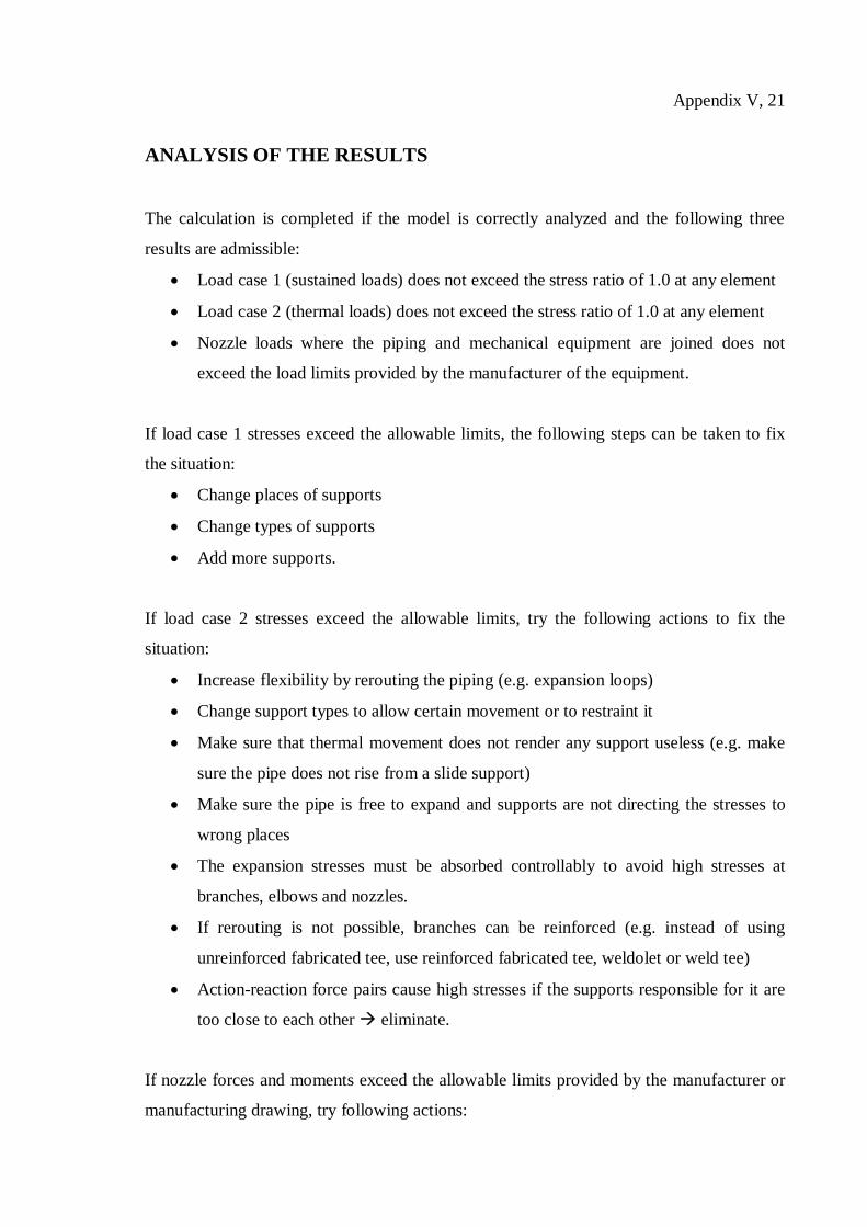
Appendix V, 21
ANALYSIS OF THE RESULTS
The calculation is completed if the model is correctly analyzed and the following three
results are admissible:
Load case 1 (sustained loads) does not exceed the stress ratio of 1.0 at any element
Load case 2 (thermal loads) does not exceed the stress ratio of 1.0 at any element
Nozzle loads where the piping and mechanical equipment are joined does not
exceed the load limits provided by the manufacturer of the equipment.
If load case 1 stresses exceed the allowable limits, the following steps can be taken to fix
the situation:
Change places of supports
Change types of supports
Add more supports.
If load case 2 stresses exceed the allowable limits, try the following actions to fix the
situation:
Increase flexibility by rerouting the piping (e.g. expansion loops)
Change support types to allow certain movement or to restraint it
Make sure that thermal movement does not render any support useless (e.g. make
sure the pipe does not rise from a slide support)
Make sure the pipe is free to expand and supports are not directing the stresses to
wrong places
The expansion stresses must be absorbed controllably to avoid high stresses at
branches, elbows and nozzles.
If rerouting is not possible, branches can be reinforced (e.g. instead of using
unreinforced fabricated tee, use reinforced fabricated tee, weldolet or weld tee)
Action-reaction force pairs cause high stresses if the supports responsible for it are
too close to each other eliminate.
If nozzle forces and moments exceed the allowable limits provided by the manufacturer or
manufacturing drawing, try following actions:

Appendix V, 22
Increase flexibility in the nozzle region by rerouting the piping (e.g. longer the
pipe, better the flexibility)
Try changing the supports to direct the loads somewhere else
MANAGING CHANGES IN CALCULATIONS TO ACHIEVE
NECESSARY RESULTS
Stress analysis processes always include “two rounds”: First round based on raw AFD
(Approved for design) isometric drawings and second round based on AFC (Approved for
construction) isometric drawings.
The first round of analysis requires the following documents in order to be completed:
AFD isometrics
Equipment drawings with allowable nozzle loads (+ thermal expansion
displacement)
Layout
Pipe classes and support specs
Pipe line list
Process values (design temperature and pressure)
Special support drawings
Weight of the valves
3D model (e.g. NavisWorks model).
The first round of analysis includes several tasks:
Creating the calculation model
Checking that the requirements of the used standard are met
Checking that nozzle loads are below allowable limits
Determining springs and constant supports.
If nozzle loads are above the allowable limits, or stress ratios are too high in the piping
system, the analyst will try to change supports spacing/types/amount to fix the problem. If

Appendix V, 23
support changes cannot fix the system, the analyst must report these exact problems to the
piping designer. The piping designer can change the geometry by rerouting the piping
system in order to manage the stresses and nozzle loads. The analyst can propose certain
geometrical changes that could fix the system, but the piping designer will always make
the last changes and adjustments in the piping. Any changes in the first rounds need to be
well documented in the isometrics and sent forward to the designated piping designer.
The second round of analysis requires the following documentation:
AFC isometric drawings
The latest revisions of equipment drawings (including nozzle loads)
Layout (latest revision)
Pipe line list (latest revision)
Special support drawings (latest revision)
Weight of the valves (if they have changed)
3D model (latest revision).
The second round of analysis includes the following tasks:
Checking that calculation model is according to AFC isometrics (update calculation
model if needed)
Checking that standard requirements are met
Checking that nozzle loads are below allowable limits
Checking that springs and supports are functional
If nozzle loads or standard requirements are not met, the same steps are to be taken
as in the first round (support changes and rerouting by the piping designer)
Reporting.
If results are inadmissible and changes are made in order to achieve acceptable results, the
changes must be properly logged and the designated piping engineer must be informed of
the changes. The piping engineer who originally designed the piping system must be
informed of all changes at all times. He/she is ultimately responsible for the piping and
makes the last calls on every modification that may be done. 3D models and calculation
models need to be in accordance with one another at all times.

Appendix V, 24
Major changes in the piping need to be marked in the isometric drawings or stress
isometric drawings. These markings need to be done clearly and simply so that there can
be no confusion with what they stand for. An example of this is shown in figure 7.
Figure 7. Expressing changes in isometric drawings.
Whenever a big change is made, a back-up copy of the old calculation model should be
saved in the project’s calculation directory. In a same manner, old isometric drawings
should always be saved in case certain changes need to be traced back.
SAVING AND REPORTING THE RESULTS
All the files related to a project shall be stored and saved in the same location. The
following files need to found under the same directory:
All of the isometric drawings
All manufacturing drawings of mechanical equipment (with allowable nozzle
loads)
Calculation models (.mod) (old calculation models in a folder called ‘OLD’)
Calculation result file (.res)

Appendix V, 25
Calculation tracking list (.xlsx)
Cover page
Information of the liaison/person in charge of the project (e.g. a manager in layout
and piping)
If possible, the project folder is on a server where only the relevant parties have access to.
Another possibility is a cloud-based service and shared directory.
The results will be reported using ‘Report template’. This word file shall sum up the results
of the calculations and consist of the following parts:
Cover page (with predetermined content)
Isometric drawings as attachment
Document reference list
Calculation input file and result file as attachments
All of the result printed out or attached as PDF from the software, for example:
o List of nodes
o List of stress ratios
o List of displacements
o List of hangers
The results shall be reported to the person in charge and all the necessary designers and
clients. In some cases, the person in charge will handle the clientele and the analyst reports
only to the manager and designers. The stress analysis report PDF will be shared among all
the relevant parties.
ARCHIVING THE RESULTS
The results shall be archived in a predesigned T:\ file path and shall hold all the files and
drawings (new and old) used during stress analysis process.
The report template file shall be uploaded to Kronodoc (containing all the native files).
Appendix V, 26
Both of the checklists and the word template for the report are found as original files here:
Analysis checklist Documentation and initial
values checklist
Final report template
analyst checklist.xlsx
Initial valueschecklist.xlsx
Reporttemplate.docx

Appendix V, 27
REQUIRED DOCUMENTATION AND INITIAL VALUES CHECKLIST
CALCULATIONNAME/NBR:
SYSTEM INFORMATION:
REQ
UIR
EDD
OC
UM
ENTA
TIO
NA
ND
INIT
IAL
VA
LUES
CH
ECK
LIST
REFERENCE DESCRIPTION RECEIVED STATUS
Standards E.g. ASME B31.1, B31.3, EN 13480
Design specs Project specific design specifications
P&I Drawings Piping and instrumentation drawings (flowdiagram)
Line list List of all pipelines in the system
Layout E.g. NavisWorks model
Isometric drawings All of the isometric drawings
Pipe classes Pipe classes and related information
Valve informationValve design drawings (incl. dimensions)
Valve masses
Equipment information
Equipment design drawings
Equipment nozzle information (incl. allowablenozzle loads)
Conditions (operating, design)
Methods of fixation
Loading information
Operating conditions (temperature, pressure)
Design conditions
Reference conditions
Support specs Support specifications used in the project
Special supports Drawings of special supports
Instruments Masses for flow meters, thermometers, connectingflanges
ADDITIONAL NOTES:
Different entries forreceived: Y = Yes, N = No
Different entries for status: PREL = Preliminary, PROG = In progress, FIN = Final revisionChecklist filled out by: Date:Checklist checked by: Date:

Appendix V, 28
ANALYSIS CHECK LIST(Idea and format from Det Norske Veritas, found in references)
CALCULATION NAME/NUMBER:
SYSTEM INFORMATION:
INPU
TD
ATA
REFERENCE DESCRIPTION Analyst 3rd Party
Piping code Is the correct code used? (B31.3, EN 13480)
Number Is the numbering of the calculation model correct?
Units Are the correct units used? (SI vs. Imperial)
Pipe Specification Is the correct pipe specification used?
Geometry Are coordinates and pipe routes according to isometricdrawings?
Commodity Is commodity density accurate or conservative?
Insulation Are insulation thicknesses correct or conservative?
Pressure Are pressures correct? (Design and operating)
Temperature Are temperatures correct? (Design, operating, reference)
Weights Correct weights of flanges, valves and other equipment?
Equipment Are all the equipment in right places? (flanges, valves)
Supports
Are all the supports in right places with right boundaryconditions? Correct friction coefficient?Are correct types of supports used? (Limit stop, guide,anchor, spring)
Nozzles Is nozzle tool correctly used or is the nozzle modeledcorrectly into the calculation?
Earthquake Are earthquake loads correctly modeled or accelerationscorrectly applied?
Wind Correct wind speed, direction, Cd coefficient?
Reaction forces Pressure safety valve relief, fluid hammer, etc?
Dynamic Analysis Is dynamic analysis done correctly?
Fatigue Are fatigue cycles modeled correctly?
OU
TPU
TD
ATA
Calculation Output
Are relevant load cases analyzed? Are load casecombinations viable?
Are deflections within reasonable limits?
Are stresses within the limits? (ratio 1.0)
Are fatigue/dynamic analysis results realistic?Are nozzle loads within the limits that are provided by theequipment manufacturer?
DRAWINGS INCLUDED IN THE CALCULATION:
Different entries to be used: OK = Checked and working, NO = Not working, NC = Not CheckedAnalysis by: Date:Checked by: Date:
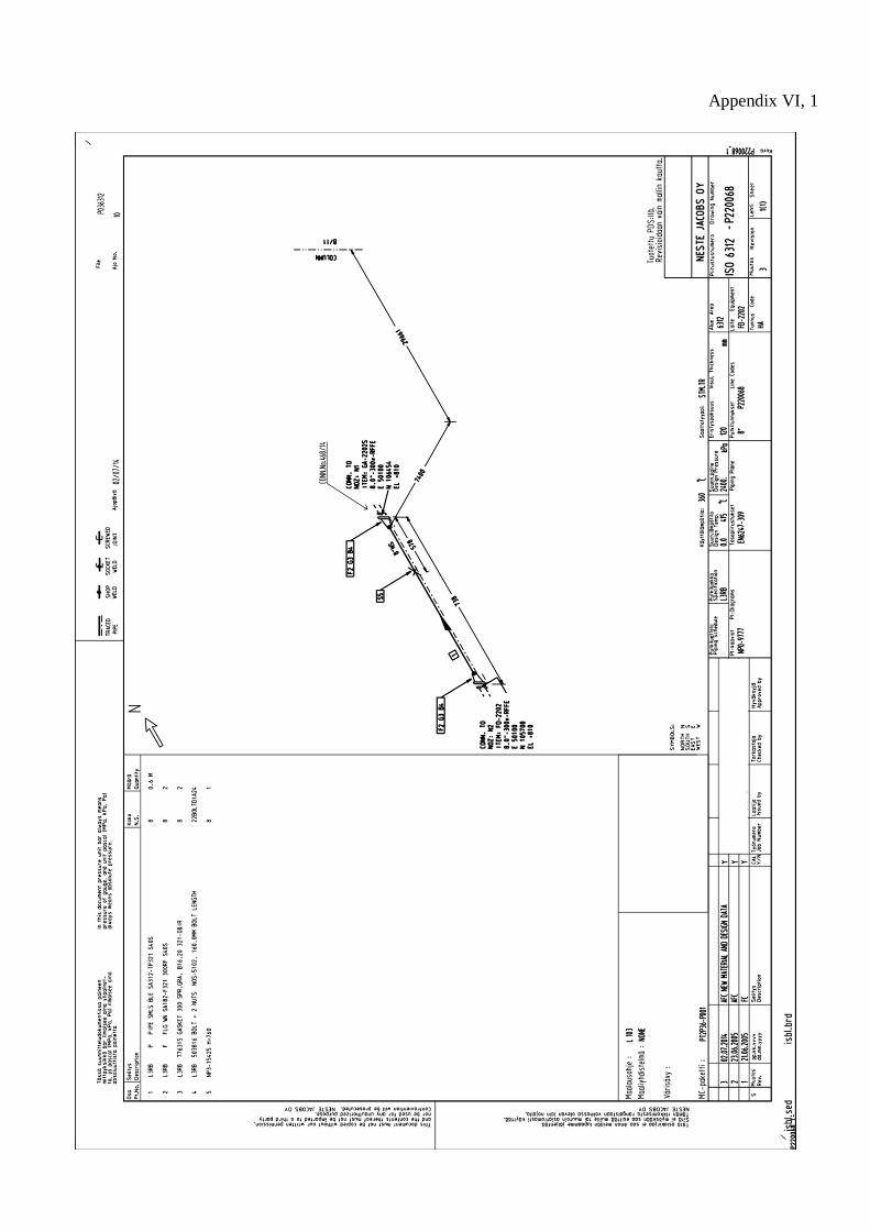
Appendix VI, 1

Appendix VI, 2

Appendix VI, 3

Appendix VI, 4

Appendix VI, 5

Appendix VI, 6

Appendix VI, 7

Appendix VI, 8

Appendix VI, 9

Appendix VI, 10