Development of a watershed modling selection program and ...

DISSERTATION

DEVELOPMENT OF A WATERSHED MODELING SELECTION PROGRAM AND SIMPLE

EQUATIONS AS AN ALTERNATIVE TO COMPLEX WATERSHED MODELING

Submitted by

Yongdeok Cho

Department of Civil and Environmental Engineering

In partial fulfillment of the requirements

For the Degree of Doctor of Philosophy

Colorado State University

Fort Collins, Colorado

Fall 2013

Doctoral Committee:

Advisor: Larry A. Roesner

Neil S Grigg

Mazdak Arabi

John Stednick

ii

ABSTRACT

DEVELOPMENT OF A WATERSEHD MODELING SELECTION PROGRAM AND SIMPLE

EQUATIONS AS AN ALTERNATIVE TO COMPLEX WATERSHED MODELING

Population pressures, land-use conversion and its resulting pollution consequences appear

to be the major diffuse pollution problems of today. Research also indicates that the increase in

imperviousness of land due to urbanization increases the volume, rate of stormwater runoff

causing increased channel erosion and flooding downstream, water quality contamination,

aquatic biota, and drinking water supplies. In the past, negative impacts were never seriously

considered as urbanization increased, but the attitude of citizens and governments are changing

and people now want to retain, restore or rehabilitate existing waterways, and manage future

urban and rural development in order to improve environmental conditions.

Water quality management in the contributing watersheds is vital to the management of

water quality in the main stem rivers. Hence, policy makers should decide which places should

be considered for restoration projects based on priority analyses. To carry out these evaluations

in Korea, mathematical models are needed to forecast the environmental results after applying

watershed restoration measures. However, the scope of sophisticated watershed modeling is very

complicated, expensive and time consuming, and not really required for planning level decision

making. Therefore, simpler evaluation methods should be applied, that can adequately discern

for planning purposes the changes in aquatic environmental quality that can be expected in

different watersheds after adapting restoration or protective measures.

iii

Thus, this research proposed to create a simple equation specifically for watershed

planning. To create such a simple equation, three main tasks were undertaken. The tasks are as

follows: (1) the creation of a selection program for available watershed models, (2) establish

simple equations to be used instead of watershed models, and (3) verify the simple equations by

comparing them with a physically based model (HSPF).

In regards to the first task mentioned above, this dissertation presents a review of thirty

three watershed models available for watershed planning and shows that these watershed models

can not easily be applied to large-scale planning projects that are being undertaken by South

Korea like the Four River Restoration Project. One of the main reasons for their inapplicability is

that they require vast amounts of data and significant application effort to be used in a

prioritization project involving many watersheds (Roesner, personal commucation). In addition,

it is vital to select an appropriate watershed model that are realistically models a watershed’s

conditions and more specifically, to match users’ needs. However a selection program has not

yet developed, as well. Therefore, eight factors were selected for task 1 to examine the specific

characteristics of each of the 33 watershed models in great detail. Based on the results of the 8

factors proposed, the selection program was developed to screen which will be most useful to a

project.

Based on these literature reviews of the 33 available watershed models but unrealistically

complex models, it was determined that a simpler model utilizing accessible base data, such as

land use type, is needed to evaluate and prioritize watersheds in the feasibility stage of a spatially

large projectstudies for national based projects (i.e. National level). A correlation study between

land use types and water quality parameters has been published (Tu, 2011, Mehaffey et al., 2005,

Schoonover et al., 2005, etc.), however, the research examined the correlation between land

iv

usage and water quality in great detail, but did not address any correlations to implement real-

based watersheds.

Therefore, Task 2 is the development of simple equstions, for this task, two important

sub-tasks were undertaken 1) Hydrology (rainfall), geology (slope), and land usage data were

analyzed to verify their relationships with the water quality (BOD, COD, T-N, T-P) in the

watershed, and 2) Simple Equations were constructed based on Statistical Methods (Excel Solver,

Statistical Analysis Systems) and Data Mining (Model Tree, Artificial Neural Network, and

Radial Based Function) in order to prove their accuracy. Thus, if the equations are accurate, they

can be used to prioritize basins within a watershed with respect to their impact on water quality

in the mainstem river.

For the final task, task 3, Simple Equations were verified by comparing them with a

physically based model, HSPF, based upon the real-based watersheds which are located in South

Korea in order to prove the Simple Equations are capable of being a reliable alternative to

physically based models. These simple equations could be used to allow management to identify

and prioritize restoration and rehabilitation areas in a watershed even though sufficient data had

yet been collected to satisfy the requirements of a physically based model.

v

ACKNOWLEDGEMENTS

What is a Ph.D.? It is the process one undertakes to complete a goal by one’s self but

would be impossible without the support of others. So many people helped me along the journey

to complete my research. With this in mind, I would like to thank my advisor, Dr. Larry Roesner,

for his unwavering support over the years. I could not have asked for a better advisor, both

academically and on a personal level. I also appreciate the support of the committee members,

Dr. Neil S Grigg, Dr. Mazdak Arabi, and Dr. John Stednick for providing me with invaluable

insight and direction for my dissertation.

Especially, I was fortunate to get a lot of data from K-water, so I would like to express

my gratitude to K-water. As well, there were many people who helped me to overcome the many

obstacles and challenges I faced. I would like to say a special thank you to Dr. Sanggee Jung, Dr.

Sungwoo Lee, Dr. Kyungtak Yum, Dr. Illhyun Jung, Dr. Yongsu Yoon, Dr. Inkwon Hong. Mr.

Yangjin Ban, Dr. Songhee Lee, Mr. Yongyeon Kim, Dr. Sangjin Song, and Dr. Jinwon Kim.

What is the purpose of devoting some much time to studying and researching? To

become experts and to provide help and give advice to those who need it. Dr. Hyunsuk Shin, Dr.

Bumhan Bae, Dr. Youngil Song, and Dr. Taeho No have enlightened me and welcomed me to

anytime whenever I need, in order to discuss research that will help to improve our country,

Korea. I admire your devotion and passion and I will endeavor to follow in your footsteps.

During the course work and when I took the preliminary exam via video conferencing,

my colleague helped me a lot and gave me the good advice, Thus, I would like to say thank you

to Dr. Jaeyun Kim, Mr. Namyoung Lee, Mr. Inbok Kim, Mr. Daeik Shon, Dr. Changhyun Cho,

Dr. Gangdo Seo, Mr. Hongyul Choi, Mr. Janghwan In, Dr. Sangwook Lee, Mrs. Heysuk Lee,

and Dr. Sangjin Lee.

vi

In addition, I had a great experience from 2009 to 2011 while working as a K-water staff

member during the 8th

Labor Union with Mr. Byunhoon Jang, Mr. Hansik Choi, Mr. Dongjin

Kim, Mr. Daejoon Won, Mrs. Jeeeun Lee, Mr. Jaechang Cho, Mr. Donghyuk Sim, Mr.

Seungwoo Choi, and Mr. Namjae Lee. I will never ever forget your names because you are my

brothers and sister, thanks for the memories.

Also, I would like to thank the many CSU alumni for always giving me the passion to

succeed: Dr. Giuk Cha, Dr. Hangoo Lee, Mr. Bongjae Kim, Dr. Youngdae Cho, Dr. Youngho

Shin, Mr. Junpyo Gil, Mr. Yongbae Jung, Dr. Jeonggon Kim, Dr. Sangdo An, and Dr. Giyoung

Park.

Especially, I would like to express my gratitude to Andy Guitard and Ms. Jennifer Moor

for editing my dissertation and for their great ideas.

I would like to thank my family for their unwavering love and assistance throughout my

life, and I would like to devote my dissertation to my mother, Mrs. Jeongsup Shim, and father,

Mr. Mankyu Cho and to my parents-in-law, Mrs. Chulbun Kim and Mr. Kijung Lee and my

family, Yongsun, Mora, Anan, late Mira, and Yongjae. As well, I would like to thank my lovely

American family Harry, Becky, Pepe, Carlota, Mitchell, Joy, and Genesis.

Finally, I owe everything to my lovely wife, Eunsuk, daughter, Jacqueline Seoyon, son,

Woohyun. You are the reason why I live and why I wrote this dissertation. And I and mom

always pray and desire you are to be the most valuable persons in the world.

Thanks to all who know me and God bless you.

vii

TABLE OF CONTENTS

ABSTRACT .................................................................................................................................... II

ACKNOWLEDGEMENTS ............................................................................................................ V

TABLE OF CONTENTS ............................................................................................................. VII

LIST OF TABLES ........................................................................................................................ XI

LIST OF FIGURES ................................................................................................................... XVI

CHAPTER 1. INTRODUCTION .............................................................................................. 1

1.1. BACKGROUND INFORMATION ................................................................................... 1

1.2. PROBLEM STATEMENT ................................................................................................. 2

1.3. HYPOTHESIS OF THIS RESEARCH .............................................................................. 3

CHAPTER 2. SELECTION PROGRAM FOR AVAILABLE WATERSHED MODELING 5

2.1. WATERSHED MODEL’S PRESENT CONDITION ........................................................ 5

2.2. MODEL FUNCTION AND PROCESS ............................................................................. 6

2.3. REVIEW OF WATERSHED MODELING ....................................................................... 9

2.4. COMPARING WATERSHED MODELS BASED ON THEIR CHARACTERISTICS 12

2.4.1 GENERAL CHARACTERISTICS OF WATERSHED MODELS ............................. 13

2.4.2 SPECIFIC CHARACTERISTICS OF WATERSHED MODELS ............................... 15

2.5. CRITERIA FOR SELECTING APPROPRIATE APPLICATIONS ............................... 27

2.5.1 EXPLANATION OF THE FACTORS USED FOR DEVELOPEING A SELECTION

PROGRAM ............................................................................................................................... 28

viii

2.6. SELECTION PROGRAM FOR AVAILABLE WATERSHED MODELS .................... 30

2.6.1 SELECTION ITEMS OF 8 VARIABLES ................................................................... 30

2.6.2 MODEL DESCRIPTIONS OF SELECTED WATERSHED MODELS ..................... 32

2.7. SUMMARY AND CONCLUSION ................................................................................. 33

CHAPTER 3. DEVELOPING SIMPLE EQUATIONS FOR WATER QUALITY IN SOUTH

KOREA 35

3.1. INTRODUCTION ............................................................................................................ 35

3.2. DATA COLLECTION FOR SIMPLE EQUATIONS ..................................................... 38

3.3. ALLOCATION TO EACH SCENARIO.......................................................................... 43

3.3.1 FIRST STEP: AREA ALLOCATION OF SUB-WATERSHEDS .............................. 44

3.3.2 SECOND STEP: DIVIDE THE BASINS INTO SEVERAL GROUPS BASED UPON

THE PERCENTAGE OF IMPERVIOUSNESS ...................................................................... 45

3.3.3 THIRD STEP: COMBINE STEPS ONE (AREAS) AND TWO (IMPERVIOUS

COVER) .................................................................................................................................... 49

3.4. DATA SOURCES FOR ANALYSIS ............................................................................... 49

3.4.1 FIRST STEP ................................................................................................................. 50

3.4.2 SECOND STEP ............................................................................................................ 51

3.4.3 THIRD STEP ................................................................................................................ 52

3.4.4 ESTABLISH SIMPLE EQUATIONS .......................................................................... 52

3.5. BUILDING SIMPLE EQUATIONS ................................................................................ 53

3.5.1 MODEL SELECTION PROCESS ............................................................................... 53

3.5.2 EVALUATION MODEL WITH PARAMETER ESTIMATION ............................... 59

3.5.3 MODEL SELECTION PROCESS FOR EACH DATA ANALYSIS METHODS ..... 61

3.6. TOOLS FOR DATA ANALYSIS .................................................................................... 62

3.6.1 EXCEL SOLVER ......................................................................................................... 62

ix

3.6.2 DATA MINING............................................................................................................ 63

3.6.3 M5P MODEL TREE..................................................................................................... 65

3.6.4 ARTIFICIAL NEURAL NETWORK (ANN) .............................................................. 70

3.6.5 RADIAL BASIS FUNCTION (RBF) ........................................................................... 74

3.6.6 STATISTICAL ANALYSIS SYSTEMS ..................................................................... 76

3.7. THE PROCESS AND RESULTS OF DATA ANALYSIS ............................................. 77

3.7.1 THE PROCESS OF DATA ANALYSIS ..................................................................... 77

3.7.2 EXCEL SOLVER ......................................................................................................... 78

3.7.3 STATISTICAL ANALYSIS SYSTEM (SAS) ............................................................. 89

3.7.4 MODEL TREE 5, ANN (ARTIFICIAL NEURAL NETWORK), RBF ...................... 96

3.8. SUMMARY AND CONCLUSIONS ............................................................................. 110

CHAPTER 4. VERIFICATION SIMPLE EQUATIONS COMPARING PHYSICALLY

BASED MODEL, HSPF ............................................................................................................. 114

4.1. INTRODUCTION .......................................................................................................... 114

4.2. MODEL DESCRIPTIONS ............................................................................................. 115

4.2.1 HSPF MODEL ............................................................................................................ 115

4.2.2 SIMPLE EQUATIONS .............................................................................................. 119

4.3. APPLY HSPF AND SIMPLE EQUATIONS................................................................. 122

4.3.1 YONGDAM DAM’S WATERSHED ........................................................................ 122

4.3.2 NAKDONG RIVER’S WATERSHED ...................................................................... 128

4.3.3 HSPF APPLICATION FOR NAKDONG RIVER WATERSHED AND YOUNGDAM

DAM’S WATERSHED .......................................................................................................... 131

4.3.4 CALIBRATION AND VALIDATION ...................................................................... 143

4.3.5 SIMPLE EQUATION APPLICATION FOR NAKDONG RIVER WATERSHED

AND YOUNGDAM DAM WATERSHED ........................................................................... 170

x

4.3.6 COMPARING HSPF AND SIMPLE EQUATIONS APPLICABILITY FOR

NAKDONG RIVER WATERSHED AND YOUNGDAM DAM WATERSHED ............... 177

4.3.7 SUMMARY AND CONCLUSION ........................................................................... 182

CHAPTER 5. CONCLUSION AND RECOMMENDATION .............................................. 185

REFERENCES ........................................................................................................................... 192

APPENDIX A –DESCRIPTION OF MATHEMATICAL MODELS CONSIDERED FOR

SIMULATION WATERSHED HYDROLOGY AND WATER QUALITY. ........................... 220

APPENDIX B - THE OBSERVATION DATA OF EACH SUB-WATERSHED .................... 273

APPENDIX C – WATERSHED CHARACTERISTICS OF YONGDAM DAM’S

WATERSHED ............................................................................................................................ 290

APPENDIX D – WATERSHED CHARACTERISTICS OF NAKDONG RIVER WATERSHED

..................................................................................................................................................... 300

xi

LIST OF TABLES

TABLE 2-1: DESCRIPTION OF WATERSHED MODELS REVIEWED. .................................................. 10

TABLE 2-2: GENERAL CHARACTERISTICS OF WATERSHED MODELS. .............................................. 14

TABLE 2-3: SPECIFIC CHARACTERISTICS OF WATERSHED MODELS. ................................................ 19

TABLE 2-4: THE FIVE SEPARATE FACTORS FOR WATERSHED MODEL EVALUATIONS. ..................... 27

TABLE 3-1: THE COLLECTION DATA TO MAKE SIMPLE METHODS. .................................................. 39

TABLE 3-2: THE PRESENT SITUATION FOR SURVEY OF THE LARGE, MIDDLE, AND SMALL-SCALE

CLASSIFICATION (HTTP://EGIS.ME.GO.KR/EGIS/HOME/INFO/M02_DB_A3.ASP). ..................... 40

TABLE 3-3: THE ITEMS OF LARGE-SCALE AND MIDDLE-SCALE CLASSIFICATION. ........................... 41

TABLE 3-4: THE PRESENT SITUATION OF FIVE RIVERS’ WATERSHEDS (MOCT, 2006, MOE)......... 43

TABLE 3-5: THE NUMBER OF APPLIED SUB-WATERSHEDS IN SOUTH KOREA.................................. 45

TABLE 3-6: THE NUMBER OF APPLIED SUB-WATERSHED OF EACH RIVER WATERSHED. .................. 45

TABLE 3-7: CONVERTED RUNOFF COEFFICIENTS FROM RUNOFF C-COEFFICIENT OF RATIONAL

METHOD. ................................................................................................................................ 46

TABLE 3-8: THE NUMBER OF SUB-WATERSHEDS USED TO ANALYZE THE IMPACT OF

IMPERVIOUSNESS. .................................................................................................................. 48

TABLE 3-9: THE NUMBER OF STANDARD BASINS FOR BOTH AREA ALLOCATION AND THE

PERCENTAGE OF IMPERVIOUSNESS OF STANDARD BASINS. ..................................................... 49

TABLE 3-10: THE DATA SOURCE AND PERIOD IN ORDER TO COMPARE LAND USAGE AND WATER

QUALITY. ............................................................................................................................... 50

TABLE 3-11: THE NUMBER OF APPLIED SUB-WATERSHEDS FOR EACH RIVER WATERSHED (STEP ONE).

............................................................................................................................................... 51

TABLE 3-12: THE NUMBER OF APPLIED SUB-WATERSHEDS FOR EACH RIVER WATERSHED (STEP

TWO). ..................................................................................................................................... 51

TABLE 3-13: ANOVA TABLE FOR SIMPLE LINEAR EQUATION FOR CALCULATION F-TEST ............ 56

TABLE 3-14: MODEL SELECTION PROCESS AND EVALUATION METHODS FOR EACH DATA ANALYSIS

METHOD. ................................................................................................................................ 61

TABLE 3-15: GENERAL CLASSIFICATION OF DATA MINING ALGORITHMS. ...................................... 64

TABLE 3-16: TEN SCENARIOS FOR MAKING A SIMPLE EQUATION BASED UPON THE PARAMETERS. . 78

TABLE 3-17: THE BEST SIMPLE EQUATIONS FOR COD (MG/L) BASED ON PARAMETERS AND THE

AREA OF THREE WATERSHEDS FOR THE FIRST STEP. ............................................................... 79

TABLE 3-18: THE BEST SIMPLE EQUATIONS FOR BOD (MG/L) BASED ON PARAMETERS AND THE

AREA OF THREE WATERSHEDS FOR THE FIRST STEP. ............................................................... 80

TABLE 3-19: THE BEST SIMPLE EQUATIONS FOR TN (MG/L) BASED ON PARAMETERS AND THE AREA

OF THREE WATERSHEDS FOR THE FIRST STEP. ......................................................................... 81

TABLE 3-20: THE BEST SIMPLE EQUATIONS FOR TP (MG/L) BASED ON PARAMETERS AND THE AREA

OF THREE WATERSHEDS FOR THE FIRST STEP. ......................................................................... 82

TABLE 3-21: THE NUMBER OF BEST SIMPLE EQUATIONS OF EACH SCENARIO FOR THE FIRST STEP. 84


AREA OF THREE WATERSHEDS FOR THE SECOND STEP. ........................................................... 84



TABLE 3-24: THE BEST SIMPLE EQUATIONS FOR T-N (MG/L) BASED ON PARAMETERS AND THE


xii

TABLE 3-25: THE BEST SIMPLE EQUATIONS FOR T-P (MG/L) BASED ON PARAMETERS AND THE AREA

OF THREE WATERSHEDS FOR THE SECOND STEP. .................................................................... 86

TABLE 3-26: THE NUMBER OF BEST SIMPLE EQUATIONS OF EACH SCENARIO FOR THE SECOND STEP.

............................................................................................................................................... 87


AREA OF THREE WATERSHEDS FOR THE THIRD STEP. .............................................................. 88



TABLE 3-29: THE BEST SIMPLE EQUATIONS FOR T-N (MG/L) BASED ON PARAMETERS AND THE


TABLE 3-30: THE BEST SIMPLE EQUATIONS FOR T-P (MG/L) BASED ON PARAMETERS AND THE AREA

OF THREE WATERSHEDS FOR THE THIRD STEP. ....................................................................... 89

TABLE 3-31: THE SIMPLE EQUATIONS (BOD) BASED UPON REGRESSION ANALYSIS USING SAS. .. 93

TABLE 3-32: THE SIMPLE EQUATIONS (COD) BASED UPON REGRESSION ANALYSIS USING SAS. .. 94

TABLE 3-33: THE SIMPLE EQUATIONS (TN) BASED UPON REGRESSION ANALYSIS USING SAS. ...... 94

TABLE 3-34: THE SIMPLE EQUATIONS (TP) BASED UPON REGRESSION ANALYSIS USING SAS. ...... 95

TABLE 3-35: DATA CLASSIFICATION AND SCENARIOS FOR MODEL TREE, ANN, RBF. ................. 97

TABLE 3-36: THE BOD RESULT OF VERIFICATION USING MODEL TREE . .................................... 100

TABLE 3-37: THE BOD RESULT OF VERIFICATION USING ANN. .................................................. 102

TABLE 3-38: THE BOD RESULT OF VERIFICATION USING RBF. ................................................... 103

TABLE 3-39: THE EVALUATION RESULTS OF FIRST STEP’S M5P, ANN, RBF (BOD, MG/L). ....... 104

TABLE 3-40: THE EVALUATION RESULTS OF SECOND STEP’S M5P, ANN, RBF (BOD, MG/L). ... 104

TABLE 3-41: THE EVALUATION RESULTS OF THIRD STEP’S M5P, ANN, RBF (BOD, MG/L). ...... 105

TABLE 3-42: THE EVALUATION RESULTS OF FIRST STEP’S M5P, ANN, RBF (COD, MG/L). ....... 106

TABLE 3-43: THE EVALUATION RESULTS OF SECOND STEP’S M5P, ANN, RBF (COD, MG/L). ... 106

TABLE 3-44: THE EVALUATION RESULTS OF THIRD STEP’S M5P, ANN, RBF (COD, MG/L). ...... 106

TABLE 3-45: THE EVALUATION RESULTS OF FIRST STEP’S M5P, ANN, RBF (TN, MG/L). .......... 108

TABLE 3-46: THE EVALUATION RESULTS OF SECOND STEP’S M5P, ANN, RBF (TN, MG/L). ...... 108

TABLE 3-47: THE EVALUATION RESULTS OF THIRD STEP’S M5P, ANN, RBF (TN, MG/L). ......... 108

TABLE 3-48: THE EVALUATION RESULTS OF FIRST STEP’S M5P, ANN, RBF (TP, MG/L). .......... 109

TABLE 3-49: THE EVALUATION RESULTS OF SECOND STEP’S M5P, ANN, RBF (TP, MG/L). ...... 109

TABLE 3-50: THE EVALUATION RESULTS OF THIRD STEP’S M5P, ANN, RBF (TP, MG/L). ......... 109

TABLE 3-51: THE SIMPLE EQUATIONS FOR WATER QUALITY SIMULATION BASED UPON EXCEL

SOLVER ................................................................................................................................ 113

TABLE 4-1: THE CHARACTERISTICS OF THE HSPF MODELS. ........................................................ 116 TABLE 4-2: TEN SCENARIOS USED FOR FINDING OUT THE PARAMETERS WHICH HAVE THE BEST

RELATIONSHIP WITH WATER QUALITY. ................................................................................. 120 TABLE 4-3: EXAMPLES OF AREA ALLOCATION OF SUB-WATERSHED (THE FIRST CASE). .............. 120 TABLE 4-4: EXAMPLES OF THE DIVISION OF BASINS INTO SEVERAL GROUPS BASED UPON THE

PERCENTAGE OF IMPERVIOUSNESS (THE SECOND CASE). ..................................................... 121 TABLE 4-5: THE NUMBER OF STANDARD BASINS BASED ON BOTH AREA ALLOCATION AND THE

PERCENTAGE OF IMPERVIOUSNESS OF STANDARD BASINS (THE THIRD CASE). ..................... 121 TABLE 4-6: THE INTERVAL AND NUMBER OF SAMPLES AT YONGDAM WATERSHED. .................... 126 TABLE 4-7: THE STATUS OF LAND COVER AND LAND USE IN RESEARCHED SITE. ......................... 130 TABLE 4-8: WEATHER INPUT DATA IN WDMUTIL. ..................................................................... 139 TABLE 4-9: THE LOCATION OF WEATHER STATIONS FOR HSPF MODEL. ...................................... 139

xiii

TABLE 4-10: THE STATUS OF SEWAGE AND WASTE WATER TREATMENT PLANT FOR HSPF. ........ 140 TABLE 4-11: THE PRESENT SITUATION OF DAM’S HYDROLOGY IN NAKDONG RIVER WATERSHED.

............................................................................................................................................. 141 TABLE 4-12: THE MONITORING SITUATIONS OF HOURLY FLOW IN YONGDAM DAM WATERSHED. 141 TABLE 4-13: CONFIDENCE RANGE AND EFFECTIVE RANGE OF HSPF CALIBRATION AND

VALIDATION (DONIGAN, 2000). ........................................................................................... 145 TABLE 4-14: THE PARAMETER VALUES OF PRECEDING RESEARCH FOR HSPF MODEL. ................ 145 TABLE 4-15: SIMULATED AND OBSERVED DISCHARGE FROM 2009 TO 2010 FOR STREAMS IN THE

NAKDONG RIVER WATERSHED (THE RESULTS OF HSPF MODEL). ........................................ 147 TABLE 4-16: SIMULATED AND OBSERVED DISCHARGE FROM 2005 TO 2006 IN THE YONGDAM DAM

WATERSHED (THE RESULTS OF HSPF MODEL). ................................................................... 150 TABLE 4-17: THE CONFIDENCE RANGE OF THE PERCENT DIFFERENCE FOR EACH PARAMETER. .... 153 TABLE 4-18: THE PARAMETERS IN RELATION WITH WATER TEMPERATURE SIMULATION. ........... 154 TABLE 4-19: THE PARAMETERS IN RELATION WITH DO AND BOD. ............................................ 155 TABLE 4-20: THE PARAMETERS IN RELATION WITH TN AND TP. ................................................. 155 TABLE 4-21: THE RESULTS OF WATER QUALITY CALIBRATION AND VALIDATION OF NAKDONG

RIVER WATERSHED. ............................................................................................................. 156 TABLE 4-22: THE RESULTS OF WATER QUALITY CALIBRATION OF NAKDONG RIVER WATERSHED.

............................................................................................................................................. 159 TABLE 4-23: THE RESULTS OF WATER QUALITY CALIBRATION AND VALIDATION OF YONGDAM

DAM WATERSHED. ............................................................................................................... 163 TABLE 4-24: THE RESULTS OF WATER QUALITY CALIBRATION AND VALIDATION FOR THE

YONGDAM DAM WATERSHED. ............................................................................................. 165 TABLE 4-25: SIMPLE EQUATIONS FOR NAKDONG AND GEUM-SUM-YOUNGSAN RIVER WATERSHED

USED BY EXCEL SOLVER. ...................................................................................................... 170 TABLE 4-26: SIMPLE EQUATIONS FOR NAKDONG AND GEUM-SUM-YOUNGSAN RIVER WATERSHED

USED BY SAS (STATISTICAL ANALYSIS SYSTEMS). ............................................................. 171 TABLE 4-27: SIMPLE EQUATIONS FOR NAKDONG AND GEUM-SUM-YOUNGSAN RIVER WATERSHED

USED BY DATA MINING (M5P, ANN, AND RBF). ................................................................ 171 TABLE 4-28: DATA SETS FOR WATER QUALITY SIMULATION USING SIMPLE EQUATIONS (GEUM-

SUM-YOUNGSAN RIVER WATERSHED). ................................................................................. 172 TABLE 4-29: DATA SETS FOR WATER QUALITY SIMULATION USING SIMPLE EQUATIONS (NAKDONG

RIVER WATERSHED). ............................................................................................................ 172 TABLE 4-30: THE RESULTS OF WATER QUALITY SIMULATION FOR YONGDAM DAM WATERSHED

USING SIMPLE EQUATIONS. ................................................................................................... 173 TABLE 4-31: THE RESULTS OF WATER QUALITY SIMULATION FOR NAKDONG RIVER WATERSHED

USING SIMPLE EQUATIONS. ................................................................................................... 175 TABLE 4-32: APPROPRIATE DEVELOPMENT METHOD TO CREATE SIMPLE EQUATIONS FOR EACH

WATERSHED. ........................................................................................................................ 177 TABLE 4-33: THE RESULTS OF WATER QUALITY SIMULATION FOR YONGDAM DAM WATERSHED

BASED UPON HSPF AND SIMPLE EQUATIONS. ....................................................................... 178 TABLE 4-34: THE RESULTS OF WATER QUALITY SIMULATION FOR NAKDONG RIVER WATERSHED

BASED UPON HSPF AND SIMPLE EQUATIONS. ....................................................................... 180 TABLE 4-35: THE % DIFFERENCE OF WATER QUALITY SIMULATION FOR YONGDAM DAM AND

NAKDONG RIVER WATERSHED BASED UPON SIMPLE EQUATIONS AND HSPF MODEL. ........... 181

TABLE A-1: THE MECHANISM FOR GWLF MODEL’S PARAMETERS (HAITH, 1992). ..................... 233

xiv

TABLE A-2: THE CAPABILITIES AND APPLIED METHOD OF HEC-HMS WATERSHED MODEL

(SOURCE: HEC-HMS USER’S MANUAL, 2009)..................................................................... 237

TABLE B-1: THE OBSERVATION DATA (PERVIOUS/IMPERVIOUS, RAINFALL, SLOPE, LAND USE,

WATER QUALITY) OF HAN RIVER WATERSHED (0 ~ 200KM2) FOR FIRST STEP ....................... 273


WATER QUALITY) OF HAN RIVER WATERSHED (200 ~ 500 KM2) FOR FIRST STEP .................. 274


WATER QUALITY) OF HAN RIVER WATERSHED (500 KM2 ~) FOR FIRST STEP ......................... 274


WATER QUALITY) OF NAKDONG RIVER WATERSHED (0 ~ 500 KM2) FOR FIRST STEP ............. 275


WATER QUALITY) OF NAKDONG RIVER WATERSHED (500 KM2 ~) FOR FIRST STEP ............... 276


WATER QUALITY) OF GEUM-SUM-YOUNGSAN RIVER WATERSHED (0 ~ 150 KM2) FOR FIRST

STEP ..................................................................................................................................... 278


WATER QUALITY) OF GEUM-SUM-YOUNGSAN RIVER WATERSHED (150 KM2 ~ ) FOR FIRST STEP

............................................................................................................................................. 279


WATER QUALITY) OF HANGANG RIVER WATERSHED (0 ~ 20%) FOR SECOND STEP .............. 280


WATER QUALITY) OF HANGANG RIVER WATERSHED (20 % ~ ) FOR SECOND STEP ............... 281


WATER QUALITY) OF NAKDONG RIVER WATERSHED (0 ~ 20 %) FOR SECOND STEP .............. 282


WATER QUALITY) OF NAKDONG RIVER WATERSHED (20 % ~ ) FOR SECOND STEP ................ 283


WATER QUALITY) OF GEUM-SUM-YOUNGSAN RIVER WATERSHED (0% ~ 25 %) FOR SECOND

STEP ..................................................................................................................................... 284


WATER QUALITY) OF GEUM-SUM-YOUNGSAN RIVER WATERSHED (20% ~ ) FOR SECOND STEP

............................................................................................................................................. 285

TABLE B-14: THE OBSERVATION DATA OF HANGANG, NAKDONG, AND GEUM-SUM-YOUNGSAN

RIVER FOR THIRD STEP (AREA: 0 ~ 250 KM2, IMPERVIOUSNESS: 0 ~ 25 %) ........................... 286


RIVER FOR THIRD STEP (AREA: 0 ~ 250 KM2, IMPERVIOUSNESS: 20 % ~ ) ............................. 287


RIVER FOR THIRD STEP (AREA: 250 KM2 ~, IMPERVIOUSNESS: 0 ~ 25 % ) ............................. 288


RIVER FOR THIRD STEP (AREA: 250 KM2 ~, IMPERVIOUSNESS: 20 % ~ ) ................................ 289

TABLE C-1 THE INFLOW TRIBUTARIES OF YONGDAM’S RESERVOIR ............................................. 291 TABLE C-2: HYDROLOGY OF YONGDAM’S RESERVOIR IN 2005 (AVERAGE ± STANDARD DEVIATION

AND MAXIMUM/MINIMUM) ................................................................................................... 293 TABLE C-3: HYDROLOGY OF YONGDAM’S RESERVOIR IN 2006 (AVERAGE ± STANDARD DEVIATION

AND MAXIMUM/MINIMUM) ................................................................................................... 294

xv

TABLE C-4: HYDROLOGY OF YONGDAM’S RESERVOIR IN 2007 (AVERAGE ± STANDARD DEVIATION

AND MAXIMUM/MINIMUM) ................................................................................................... 294 TABLE C-5: THE RIVER CHARACTERISTICS OF YONGDAM WATERSHED ....................................... 296 TABLE C-6: THE STREAM ORDERS OF YONGDAM WATERSHED .................................................... 297

TABLE D-1: THE RIVER STATUS OF NAKDONG WATERSHED ......................................................... 300 TABLE D-2: MONTHLY HYDROLOGY DATA FOR NAKDONG RIVER WATERSHED (AS OF 2010) ...... 302 TABLE D-3: THE WEATHER STATION OF NAKDONG RIVER WATERSHED ....................................... 303 TABLE D-4: THE WEATHER DATA OF NAKDONG RIVER WATERSHED............................................ 303

xvi

LIST OF FIGURES

FIGURE 2-1 THE PROCESS OF APPLICATION FOR WATERSHED MODEL. .............................................. 7

FIGURE 2-2 NEW FACTORS TO DEVELOP THE SELECTION PROGRAM. ............................................. 29

FIGURE 2-3 THE SCHEMATIC FOR RESEARCHING EXISTING WATERSHED MODELS .......................... 29

FIGURE 2-4 THE COVER PAGE OF THE SELECTION PROGRAM FOR AVAILABLE WATERSHED MODELS.

............................................................................................................................................... 30

FIGURE 2-5 DETAILED EXPRESSION WINDOW FOR SELECTING ITEMS OF THE 8 VARIABLES. ........... 31

FIGURE 2-6 SELECTED MODEL DESCRIPTION IN RESULT WINDOW. ................................................ 32

FIGURE 3-1: COMPARISON OF PRE AND POST DEVELOPMENT (SOURCE: SCHUELER, 1987)............. 35

FIGURE 3-2: WATER QUALITY MODELING PROCESS. .................................................................... 37

FIGURE 3-3: RESEARCH SCHEMATIC FOR DEVELOPING SIMPLE METHODS. ..................................... 38

FIGURE 3-4: SEPERATED CLASSIFIED STANDARD BASIN THROUGH THE CLIP FUNCTION OF GEO

PROCESSING. .......................................................................................................................... 42

FIGURE 3-5: MERGED CLIPPED LAND-COVER MAP AND THE STANDARD BASIN. .............................. 42

FIGURE 3-6: CLASSIFIED STANDARD BASIN IN SOUTH KOREA. ...................................................... 42

FIGURE 3-7: WATERSHED MAP OF SOUTH KOREA. ........................................................................ 44

FIGURE 3-8: THE IMPERVIOUSNESS OF THE STANDARD BASINS IN SOUTH KOREA. ........................ 47

FIGURE 3-9: REPRESENTATION OF THE IMPERVIOUS COVER (IC) (CWP, 2005). ............................ 48

FIGURE 3-10: THE SCHEMATIC DIAGRAM TO ESTABLISH SIMPLE EQUATIONS ................................ 52

FIGURE 3-11 EIGENVALUES OF THE CORRELATION MATRIX ........................................................... 58

FIGURE 3-12 SCREE PLOT OF EIGENVALUES ................................................................................... 58

FIGURE 3-13: SIMPLE LINEAR REGRESSION ................................................................................... 72

FIGURE 3-14: COMMONLY USED ACTIVATION FUNCTIONS ............................................................ 73

FIGURE 3-15: MULTILAYER PERCEPTRON ANN. ........................................................................... 73

FIGURE 3-16: RADIAL BASIS FUNCTION ANN. ............................................................................. 74

FIGURE 3-17: PROCEDURE TO SELECT THE BEST SIMPLE EQUATIONS BASED ON EXCEL SOLVER. . 79

FIGURE 3-18: FACTOR ANALYSIS EXAMPLES FOR FIRST STEP, BELOW 200KM2 IN THE HAN-RIVER

WATERSHED. .......................................................................................................................... 90

FIGURE 3-19: MEAN AND STANDARD DEVIATION FOR FIRST STEP, BELOW 200KM2 IN THE HAN-

RIVER WATERSHED. ................................................................................................................ 90

FIGURE 3-20: CORRELATIONS BETWEEN PARAMETERS AND WATER QUALITY FOR FIRST STEP,

BELOW 200KM2 IN THE HAN-RIVER WATERSHED. ................................................................... 91

FIGURE 3-21: REGRESSION ANALYSIS CODE FOR FIRST STEP, BELOW 200KM2 IN THE HAN-RIVER

WATERSHED. .......................................................................................................................... 91

FIGURE 3-22: REGRESSION ANALYSIS CODE FOR FIRST STEP, BELOW 200KM2 IN THE HAN-RIVER

WATERSHED. .......................................................................................................................... 92

FIGURE 3-23: WEKA SOFTWARE (VERSON 3.4.4). ......................................................................... 96

FIGURE 3-24: THE PREPROCESS TO OPEN THE INPUT FILE FOR MODEL TREE 5, ANN, RBF. .......... 98

FIGURE 3-25: THE CLASSIFICATION SCENE TO CHOOSE MODEL TREE 5, ANN, AND RBF MODEL. 98

FIGURE 3-26: STRUCTURE AND LINEAR MODELS OF MODEL TREE FOR HAN RIVER WATERSHED. 99

FIGURE 3-27: STRUCTURE OF ANN WITH FOUR HIDDEN LAYERS. ................................................ 101

FIGURE 3-28: CLASSIFIER MODEL USING MULTILAYERPERCEPTRON (ANN). ............................. 102

FIGURE 3-29: CLASSIFIER MODEL USING RBFNETWORK. ........................................................... 103

FIGURE 3-30: R VALUE (BOD) OF FIRST, SECOND, THIRD SCENARIOS USING M5P, ANN, RBF. . 105

xvii

FIGURE 3-31: R VALUE (COD) OF FIRST, SECOND, THIRD SCENARIOS USING M5P, ANN, RBF. . 107

FIGURE 3-32: R VALUE (TN) OF FIRST, SECOND, THIRD SCENARIOS USING M5P, ANN, RBF. .... 107

FIGURE 3-33: R VALUE (TP) OF FIRST, SECOND, THIRD SCENARIOS USING M5P, ANN, RBF. ..... 110

FIGURE 4-1: THE SCHEMATIC DIAGRAM TO ESTABLISH SIMPLE EQUATIONS BASED ON SEVERAL

DATA ANALYSIS METHODS. .................................................................................................. 121

FIGURE 4-2: YONGDAM DAM’S WATERSHED. ............................................................................. 123

FIGURE 4-3: SCHEMATIC OF THE WATERSHED STREAMS.............................................................. 124

FIGURE 4-4: THE LAND COVER MAP OF YONGDAM WATERSHED. ................................................ 125

FIGURE 4-5: THE SAMPLING STATION FOR WATER QUALITY, QUANTITY, AND METEOROLOGICAL

DATA OF YONGDAM WATERSHED. ........................................................................................ 127

FIGURE 4-6: RIVER MAP OF SOUTH KOREA. ................................................................................ 128

FIGURE 4-7: NAKDONG RIVER WATERSHED’S WATER QUALITY MONITORING MAP....................... 129

FIGURE 4-8: THE MAP OF NAKDONG RIVER (LEFT) AND YONGDAM DAM’S (RIGHT) WATERSHED. 131

FIGURE 4-9: OUTLET LOCATION, WATERSHED DELINEATION, AND GENERATED STREAM NETWORK

............................................................................................................................................. 132


............................................................................................................................................. 132


............................................................................................................................................. 133


AT HAPCHUN DAM WATERSHED. ......................................................................................... 133


AT NAMGANG DAM WATERSHED. ....................................................................................... 133


AT MILYANG DAM WATERSHED. ......................................................................................... 134


AT YONGDAM DAM WATERSHED. ....................................................................................... 134

FIGURE 4-16: DEM FOR ANDONG DAM. ..................................................................................... 135

FIGURE 4-17: DEM FOR IMHA DAM. ........................................................................................... 135

FIGURE 4-18: DEM FOR YOUNGCHUN DAM. ............................................................................... 135

FIGURE 4-19: DEM FOR HAPCHUN DAM. .................................................................................... 135

FIGURE 4-20: DEM FOR NAMGANG DAM. ................................................................................... 135

FIGURE 4-21: DEM FOR MILYANG DAM. .................................................................................... 135

FIGURE 4-22: DEM FOR YONGDAM DAM. ................................................................................... 135

FIGURE 4-23: LAND USE OF ANDONG DAM. ................................................................................. 136

FIGURE 4-24: LAND USE OF IMHA DAM. ...................................................................................... 136

FIGURE 4-25: LAND USE OF YOUNGCHUN DAM. .......................................................................... 137

FIGURE 4-26: LAND USE OF HAPCHUN DAM ................................................................................ 137

FIGURE 4-27: LAND USE OF NAMGANG DAM. .............................................................................. 137

FIGURE 4-28: LAND USE OF MILYANG DAM. ............................................................................... 137

FIGURE 4-29: LAND USE OF YONGDAM DAM. ............................................................................. 138

FIGURE 4-30: THE NEW PROJECT GENERATING PICTURE FOR HSPF MODEL. ................................ 142

FIGURE 4-31: THE PICTURE OF HSPF RUNNING. .......................................................................... 142

FIGURE 4-32: THE CALIBRATION AND VALIDATION POINT FOR NAKDONG RIVER WATERSHED. ... 143

FIGURE 4-33: THE CALIBRATION AND VALIDATION POINT FOR NAKDONG RIVER WATERHED. .... 144

xviii

FIGURE 4-34: MODEL CALIBRATION RESULTS OF NAKDONG RIVER WATERSHED, HSPF (2009 –

2010) (1). ............................................................................................................................. 148

FIGURE 4-35: MODEL CALIBRATION RESULTS OF YONGDAM DAM’S WATERSHED, HSPF (2005 –

2006) (1). ............................................................................................................................. 151

FIGURE 4-36: CALIBRATION & VALIDATION POINT OF EACH DAM’S WATERSHED. ....................... 153

FIGURE 4-37: BOD SIMULATION RESULTS BASED ON SIMPLE EQUATIONS (YONGDAM WATERSHED).

............................................................................................................................................. 173

FIGURE 4-38: T-N SIMULATION RESULTS BASED UPON SIMPLE EQUATIONS (YONGDAM

WATERSHED). ....................................................................................................................... 174

FIGURE 4-39: T-P SIMULATION RESULTS BASED UPON SIMPLE EQUATIONS (YONGDAM WATERSHED).

............................................................................................................................................. 174

FIGURE 4-40: BOD SIMULATION RESULTS BASED ON SIMPLE EQUATIONS (NAKDONG WATERSHED).

............................................................................................................................................. 175

FIGURE 4-41: T-N SIMULATION RESULTS BASED ON SIMPLE EQUATIONS (NAKDONG WATERSHED).

............................................................................................................................................. 176

FIGURE 4-42: T-P SIMULATION RESULTS BASED ON SIMPLE EQUATIONS (NAKDONG WATERSHED).

............................................................................................................................................. 176

FIGURE 4-43: THE RESULTS OF BOD SIMULATION FOR YONGDAM DAM WATERSHED ................ 178

FIGURE 4-44: THE RESULTS OF T-N SIMULATION FOR YONGDAM DAM WATERSHED .................. 179

FIGURE 4-45: THE RESULTS OF T-P SIMULATION FOR YONGDAM DAM WATERSHED .................. 179

FIGURE 4-46: THE RESULTS OF BOD SIMULATION FOR NAKDONG RIVER WATERSHED ................ 180

FIGURE 4-47: THE RESULTS OF T-N SIMULATION FOR NAKDONG RIVER WATERSHED ................. 180

FIGURE 4-48: THE RESULTS OF T-P SIMULATION FOR NAKDONG RIVER WATERSHED ................. 181

FIGURE 5-1: FUTURE RESEARCH SCHEMATIC FOR SUB-WATERSHED MANAGEMENT BASED UPON

SIMPLE EQUATIONS. ............................................................................................................ 190

FIGURE 5-2: THE PROCESS TO ESTABLISH SIMPLE EQUATION TO THE NEW WATERSHEDS ............ 191

FIGURE A-1: BASINS SYSTEM OVERVIEW (HTTP://WWW.BASINSLIVE.ORG/). .......................... 222

FIGURE A-2: PHOSPHORUS EXPORT VS. URBAN LAND USE FOR TWIN CITIES WATERSHEDS .......... 227

FIGURE A-3: THE PHYSICAL SYSTEM AND PROCESSES REPRESENTED IN GLEAMS. .................... 229

FIGURE A-4: LSPC (LOADING SIMULATION PROGRAM IN C++) DATA FLOW SCHEMATIC .......... 240

FIGURE A-5: MERCURY’S MOVEMENT AND AVAILABLE MODELS FROM THE WATERSHED TO

TRIBUTARIES (SOURCE AMBROSE, 2005). ............................................................................ 241

FIGURE A-6: SCHEMATIC REPRESENTATION OF MIKE SHE MODEL (REFSGAARD AND STORM,

1995). .................................................................................................................................. 243

FIGURE A-7: FRAMEWORK OF THE MUSIC MODEL (SOURCE: WONG ET AL., 2002) .................. 245

FIGURE A-8: SIMPLE P8-UCM SET UP (SOURCE: TETRA TECH, INC., 2005). ............................... 247

FIGURE A-9: BMP TYPES OF BMP TOOLBOX MODEL (CHENG ET AL., 2004, 2009). ................... 250

FIGURE A-10: FLOW SCHEMATIC DIAGRAM OF SHETRAN MODEL (SOURCE: DUNN ET AL., 1996).

............................................................................................................................................. 251

FIGURE A-11: THE MECHANISM OF POLLUTANT DEPOSITION AND REMOVAL AT SOURCES AREAS

FOR SLAMM (SOURCE: PITT ET AL., 2000). ........................................................................ 253

FIGURE A-12: SCHEMATICS OF THE MAJOR SPARROW MODEL COMPONENTS (SOURCE:

SCHWARZ ET AL., 2006). ...................................................................................................... 255

FIGURE A-13: THE SCHEMATICS OF STORM MODEL’S FLOW MECHANISM (U.S. ACE, 1997). ... 258

FIGURE A-14: THE SCHEMATIC OF SWAT’S DEVELOPMENT (SOURCE: GASSMAN ET AL, 2007). 259

xix

FIGURE A-15: THE SCHEMATIC OF A POTENTIAL WATER PATHWAY OF THE SWAT MODEL

(NEITSCH ET AL., 2005). ...................................................................................................... 260

FIGURE A-16: THE SWMM MODEL’S SCHEMATIC (SOURCE: ROSSMAN, 2010). ......................... 262

FIGURE A-17: HYDROLOGICAL BEHAVIOR OF THE CATCHMENT IN TOPMODEL (SOURCE: HOLKO

ET AL, 1997)......................................................................................................................... 265

FIGURE A-18: THE DISTANCE GRID CREATION OF FLOW AND LOAD GENERATION. ..................... 267

FIGURE A-19: COMPONENTS OF LAND CATCHMENTS (CHEN ET AL., 2000). ............................... 269

FIGURE A-20: THE ZERONET DECISION SUPPORT SYSTEM (SOURCE: RICH ET AL., 2005). ........ 270

FIGURE A-21: THE PROCESS SCHEMATIC OF THE WEPP MODEL (SOURCE: FLANAGAN ET AL.,

1995). .................................................................................................................................. 271

FIGURE C- 1: THE ALTITUDE ANALYSIS MAP AND THE ACCUMULATIVE AREA RATIO FOR THE

ALTITUDE ANALYSIS ............................................................................................................ 290

FIGURE C-2: A WATERSHED DIVISIONAL MAP OF YONGDAM WATERSHED ................................. 291

FIGURE C-3: HYDROLOGY GRAPH OF YONGDAM RESERVOIR (2005 ~2007) ................................ 293

FIGURE C-4: THE STREAM ORDER MAP OF YONGDAM WATERSHED ............................................. 295

FIGURE C-5: THE STREAM NUMBER OF EACH STREAM ORDER ...................................................... 297

FIGURE C-6: THE AREA RATIO BASED ON THE SLOPE DISTRIBUTION (%) ..................................... 298

FIGURE C-7: THE SLOPE MAP OF YONGDAM WATERSHED ........................................................... 299

FIGURE C-8: THE AREA RATIO OF SLOPE DIRECTION DISTRIBUTION ............................................. 299

FIGURE D-1: NAKDONG RIVER WATERSHED .............................................................................. 301

1

CHAPTER 1. INTRODUCTION

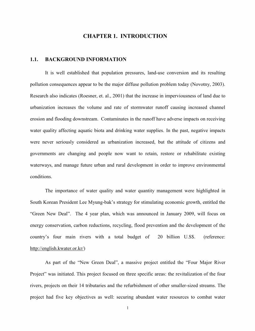
1.1. BACKGROUND INFORMATION

It is well established that population pressures, land-use conversion and its resulting

pollution consequences appear to be the major diffuse pollution problem today (Novotny, 2003).

Research also indicates (Roesner, et. al., 2001) that the increase in imperviousness of land due to

urbanization increases the volume and rate of stormwater runoff causing increased channel

erosion and flooding downstream. Contaminates in the runoff have adverse impacts on receiving

water quality affecting aquatic biota and drinking water supplies. In the past, negative impacts

were never seriously considered as urbanization increased, but the attitude of citizens and

governments are changing and people now want to retain, restore or rehabilitate existing

waterways, and manage future urban and rural development in order to improve environmental

conditions.

The importance of water quality and water quantity management were highlighted in

South Korean President Lee Myung-bak’s strategy for stimulating economic growth, entitled the

“Green New Deal”. The 4 year plan, which was announced in January 2009, will focus on

energy conservation, carbon reductions, recycling, flood prevention and the development of the

country’s four main rivers with a total budget of 20 billion U.S$. (reference:

http://english.kwater.or.kr/)

As part of the “New Green Deal”, a massive project entitled the “Four Major River

Project” was initiated. This project focused on three specific areas: the revitalization of the four

rivers, projects on their 14 tributaries and the refurbishment of other smaller-sized streams. The

project had five key objectives as well: securing abundant water resources to combat water

http://english.kwater.or.kr/

2

scarcity, implementing comprehensive flood control measures, improving water quality and

restoring river ecosystems, creating multipurpose spaces for local residents, and regional

development centered on the rivers. More than 929 km of streams in Korea will be restored as

part of the project, with a follow-up operation planned to restore more than 10,000 km of local

streams. More than 35 riparian wetlands will also be reconstructed.

While this project will improve water resources and quality situation of the major rivers,

much work remains to be done to insure that the numerous tributaries to the main rivers are

protected and that mainstem river improvements are not reduced in the future as the South

Korean population continues to migrate to urban areas. In order for this project to succeed, water

quality management in the contributing watersheds is vital to the management of water quality in

the mainstem rivers. Therefore, there is a great demand for schematic watershed water quality

management skills.

1.2. PROBLEM STATEMENT

For the Four River Restoration project to be successful, many urban areas contributing to

the deteriorated condition of receiving water need to be compared with respect to their individual

impacts on receiving water quality and then prioritized for remediation because the amount of

funds needed to conduct a nationwide restoration project would be insurmountable for the

government to bear. Hence, policy makers should decide which places should be considered for

restoration projects based on priority analyses. This prioritization has to include the evaluation of

economic, social, technological, and environmental factors. To carry out these evaluations in

Korea, mathematical models are needed to forecast the environmental results after applying

watershed restoration measures. However, the scope of sophisticated watershed modeling is very

complicated, expensive, time consuming, and not definitively required for planning-level

3

decision making. Given time, resource, and data constraints, simpler evaluation methods capable

of adequately discerning the impacts of restoration and protective measures on the aquatic

environmental quality of different watersheds at the planning level should be applied.

A major problem that needs to be addressed is how simple can the watershed model be

and still produce sufficiently accurate results and sufficient detail to enable planners to prioritize

watersheds and projects for implementation in a planning area that covers about 17 km2 to about

1,574 km2.

1.3. HYPOTHESIS OF THIS RESEARCH

This dissertation presents a review of thirty three watershed models available for

watershed planning and shows that these watershed models can not easily be applied to large-

scale planning projects like the Four Rivers Restoration Project in order to be used to prioritize

watershed, because these watershed models require too much data and significant application

effort (Roesner, personal commucation). In addition, it is so crucial to select appropriate

watershed models that are applicable to unique watershed conditions and more specifically, to

match users’ needs and a selection program has not yet developed, as well. Therefore, a selection

program was developed based on thirty three watershed models reviews to screen which will be

most useful to a project in Chapter II.

The conclusion is that a simpler model is required to implement evaluate and prioritize

watershed in the feasibility phase of spatially large national projects. A correlation study between

land use types and water quality parameters has been published (Tu, 2011, Mehaffey et al., 2005,

Schoonover et al., 2005, etc.). However, this study’s objective was to determine a correlation

between land usage and water quality, not apply the correlation to a real-world watershed to

obtain unknown data, as is the objective of the study in this dissertation.

4

My hypotheses in this research are the following:

1. Hydrology, geology, and land usage have great relationships with water quality (BOD,

COD, T-N, T-P) in the watershed.

2. Simple equations constructed based on Statistical Methods (i.e. Excel Solver and

Statistical Analysis Systems) and Data Mining (i.e. Model Tree, Artificial Neural

Network, and Radial Based Function) are sufficiently accurate to allow user to

prioritize basins within a watershed with respect to their impact on water quality in a

mainstem river which is covered in Chapter III.

3. Results from these simple equations can be verified by comparing their results with

those of a physically-based HSPF model of real watershed in South Korea in order to

prove that the Simple Equations are capable of being a reliable alternative the

physically based model analyzed in Chpater IV.

5

CHAPTER 2. SELECTION PROGRAM FOR AVAILABLE

WATERSHED MODELING

2.1. WATERSHED MODEL’S PRESENT CONDITION

Watershed modeling is a combination of hydrogeographical and biochemical

mathematical models that simulate the movement of water and the relevant biogeochemical

process in order to reflect the change of water quality and quantity as affected by watershed

management plans (Novotny, 2008, Singh, 2004). These components include: areal precipitation,

watershed representation, surface runoff, infiltration, subsurface flow and interflow, groundwater

flow and base flow, evaporation and evapotranspiration, interception, depression storage,

detention storage, rainfall-excess/soil moisture accounting, snowmelt runoff, stream-aquifer

interaction, reservoir flow routing, channel flow routing, and water quality (Singh, 2004).

Watershed models provide the methods of approach for estimating loads, source loads, and

evaluating various management alternatives, including sets of equations which take into

consideration natural or man-made processes such as runoff or stream transport in a watershed

system, and forecasting or estimating future condition based on various conditions in order to

comparing pre- and post-development (EPA, 2008).

The development of watershed models began in the 1970s to estimate non-point sources

of pollution in the United States and their impacts on receiving water quality (Leon et al., 2000).

From the middle of the 1980s, a variety of models were developed due to advancements in

computers and science. Many watershed models have been developed for specific pollutants

based on each watershed conditions (EPA, 2008).

6

2.2. MODEL FUNCTION AND PROCESS

Models are a description of an environmental system based on a set of equations or

algorithms that are used to simulate a physical system and offers a reliable method for estimating

loads, provide source load estimates, and evaluate various management alternatives. In addition,

models are used to forecast natural or man-made process in an environmental system such as

runoff or stream transport (Leslie et al., 2005, EPA 2008).

Flooding, upland soil, stream erosion, sedimentation, and contamination of water from

agricultural chemicals are serious environmental, social, and economical problems all over the

world (Borah, 2003). Hence, various kinds of models have been developed that present specific

characteristics depending on the applicant’s needs. If a user needs to find a resolution very

quickly, simplified techniques such as USLE (Universal Soil Loss Equations) could be used but

is limited in applicability to the various pollutants and water bodies by TMDLs. On the other

hand, physical based models, known as the state of art models, include various mechanisms

associated with water, sediment, pollutant, movement, transport, transformation, and delivery.

Both simplified models and physical based models have advantages and disadvantages, and if

there is enough data to represent the watersheds, such as areal precipitation, watershed

representation (geometry characteristics), surface runoff, infiltration, subsurface flow and

interflow, groundwater flow and baseflow, evapotranspiration, interception, depression storage,

detention storage, snowmelt runoff, stream-aquifer interaction, reservoir flow routing, channel

flow routing, water quality, etc., it is easy to access a physical based model. However, if there is

not enough data for a physical based model, a simplified model could be applied to start with and

then the database can accumulate data continuously to achieve the next steps.

7

A watershed model is a tool for analyzing watershed characteristics based on the

pollutant loads. In order to enhance a watershed model’s ability, users have to understand the

processes of the watershed model. The process applied for watershed is shown below in Figure

2-1.

Figure 2- 1: The process of application for watershed model.

(Sources: http://www.watershedactivities.com/projects/fall/h2omodel.html)

A. Data Collection

Data collection is the first process required for watershed modeling application.

Required data could vary depend on each watershed’s characteristics. Basically weather

data, point source data, land coverage, and geological characteristic data would be

required. In addition, weather data should be determined based on certain times or daily

data according to the watershed model.

B. Model input Preparations

After the input data has been collected for the watershed model, the data should be

reorganized by using an input form for each watershed model because various watershed

models have used respective computer programming languages. At this point, input data

has to be built accurately, if not, the model will not perform well because of language

1. Data Collection

2. Model Input Preparation

3. Parameter evaluation

4. Calibration/Validation

5. Analysis of alternatives

Watershed delineation

Land coverage,

Weather data

Point source. etc.

http://www.watershedactivities.com/projects/fall/h2omodel.html

8

problems. In addition, sub-watershed (separate) and land coverage classifications should

be implemented by using the available data and their applied purposes appropriately

when making the input data.

C. Parameter Evaluation

The third step of a watershed model is the process of deciding parameters. In order to

reflect the watershed characteristics, the process to decide parameters needs to predict the

current situation, such as soil maps, land coverage, and the buildup and wash off of

polluted matter. During this process, each predicted item and parameter should be

analyzed and evaluated carefully to determine how much the differenes were from before

and after as well as any kinds of interaction among the reactions.

D. Calibration & Validation

After evaluating the predicted items and parameters, calibrations need to be

implemented to decide the parameters when comparing the estimated and observed data.

The next step, validation, is to confirm whether the parameters satisfy the other

conditions which could represent watershed characteristics. At this time, the best method

for deciding the appropriate parameters is to conduct field experiments of watersheds,

however, experiments do take up a significant amount of time, they are costly and require

labor force, etc. Hence, a trial and error method was used to compare the measured field

and estimated data based on the suggestion value through watershed model.

E. Analysis Alternatives

In the last step, users can analyze pollution characteristics and loading from a

targeted watershed through the use of the constructed watershed model which was

9

calibrated and validated. Loading could be analyzed by numerous conditions. The effects

of sub-watershed management alternatives could be evaluated by the contributing factors

of pollutants from the sub-watershed to the reservoir through the process of calibration

and validation.

2.3. REVIEW OF WATERSHED MODELING

As part of the background research for this thesis proposal, thirty three currently most

popular watershed models were reviewed. From the models reviewed, the U.S. Environmental

Protection Agency (U.S. EPA.) developed twelve of the watershed models; The United States

Department of Agriculture – Agricultural Research Service (USDA-ARS) developed five of the

watershed models which are AGNPS, AnnAGNPS, KINEROS2, SWAT, and WEPP. The United

States Army Corps of Engineers (USACE) developed three of the watershed models (GSSHA,

HEC-HMS, STORM). As well, the U.S. Geological Survey developed one of the watershed

models; SPARROW. In addition, various universities and research agencies developed several of

the models such as Colorado State University (CASC2D), Argonne National Laboratory

(DIAS/IDLAMS), North Carolina State University (DRAINMOD), Illinois State Water Survey

(DWSM), Texas A & M (EPIC), College of Charleston (GISPLM), DHI Water and Environment

(MIKE SHE), Prince George’s County, MD (PGC-BMP), University of Newcastle upon Tyne

(SHETRAN), Lancaster University (TOPMODEL), Systech Engineering, Inc. (WARMF), and

Scientific Software Group (WMS). These models are listed below in Table 2-1 with abbreviated

descriptions of their capabilities.

10

Table 2-1: Description of Watershed Models Reviewed.

MODEL Full-name Description Literature

AGNPS Agricultural Nonpoint Source

Pollution An event-based model simulating water

runoff, sediment, COD, N, P, and pesticides Borah, 2003b; Deva, 2002.

AnnAGNPS

Annualized Agricultural

Nonpoint Source Pollution

Model

Annualized of AGNPS; continuous

simulation watershed scale program

developed based on the AGNPS

A. Shamshad et al., 2008; Polyakov, 2007; Shrestha, 2005.

ANSWERS

Area Nonpoint Source

Watershed Environment

Response Simulation

Developed for agricultural watersheds and

construction sites for surface water

hydrology and erosion/sediment transport

Huggins et al., 1966; Beasley et al., 1980; Ramadhar et al., 2005.

BASINS

Better Assessment Science

Integrating point and

Nonpoint Sources

A decision support system for multipurpose environmental

analysis by regional, state, and local

agencies performing watershed and water-quality based studies

EPA, 2000; Imhoff, et al., 2007.

CASC2D -

The runoff and soil erosion modeling and a

state-of-art hydrologic model based on GIS

(Geographic Information Systems) and

remote sensing

Julien, 1998

DIAS/IDLAMS

Dynamic Information

Architecture System/

Integrated Dynamic Landscape Modeling and

Analysis System

An object-based software framework for

modeling and simulation application and allows many disparate simulation models

and other applications to interpolate to

address a complex problem based on the context of the specific problem

Leslie et al, 2005; Hummel et al,

2002 ; Sydelko et al., 2000

DRAINMOD A Hydrological Model for

Poorly Drained Soils

Used to simulate the performance of

drainage and related water management system on a field scale.

Sinai, 2006; Leslie et al., 2005;

Helwig et al., 2002; Wang et al., 2006; Gupta et al, 1993

DWSM Dynamic Watershed

Simulation Model

Simulates surface and subsurface storm

water runoff, flood waves, soil erosion, entrainment and transport of sediment, and

agricultural chemicals in agricultural

watersheds.

Borah, et al, 2001A; Borah et al., 2001B; Kim et al.,2003; Ashraf, et

al., 1992

EPIC Erosion Productivity Impact

Calculator

A tool used for determining the effects of soil erosion on crop production including

erosion, plant growth, related processes, and

economic components for assessing the cost of erosion and components for determining

optimal management strategies.

Williams, 1990; Williams et al.,

1983; Martin et al., 1993; Gassman et al, 2004, Leslie et al., 2005; Warner

et al., 1997; Chung et al., 2002;

Guerra et al., 2002

GISPLM GIS-Based Phosphorus

Loading Model

A tool used for developing cost-effective strategies to reduce phosphorus loads from

watersheds

GeoEngineers 2010; Leslie et al. 2005; William W. W. 1997; Walker,

W. W. 1987.

GLEAMS Groundwater Loading Effects of Agricultural Management

Systems

A mathematical model for field-size areas

to evaluate the effects of agricultural management system and could predict the

movement of agricultural chemicals within

and through the plant root zone.

Leonard et al., 1987, 1989 ; Foster et

al., 1981, 1985; Knisel et al, 1980, 1993, 1999; Jensen et al., 1990;

Monteith, 1965; Onstad et al., 1975;

Leone et al, 2007

GSSHA Gridded Surface Subsurface

Hydrologic Analysis

A reformulation and enhancement of the

two-dimensional physically based model

CASC2D, sediment and water quality transport and coupled to one-dimensional

stream flow

Ogden et al., 2008; Sharif et al.,

2010; Niedzialek et al., 2003; Downer et al., 2004.

GWLF Generalized Watershed

Loading Functions

A middle ground between the empiricism of

export coefficients and the complexity of

chemical simulation models

Medina, 2005; Haith, 1992;

Chikondi, 2010; Limbrunner, 2005;

Ning, 2005.

HSPF Hydrologic Simulation

Program FORTRAN

A comprehensive model for simulating the

quantity and quality of streamflow,

reservoir system operations, ground water development and protection

Said et al., 2007; Ryu, 2009; Lohani

et al., 2000; Bicknell et al., 2001; Bai, 2010; Yanqing, 2007; Jeon,

2007; Mishra, 2009; Ribarova, 2008;

Hayashi ,2004; Albek, 2003.

HEC-HMS Hydraulic Engineering Center

Hydrologic Modeling System

Simulating the rainfall-runoff processes of

networked watershed systems as a

successor to HEC-1 and includes large river basin water supply and flood hydrology,

and small urban or natural watershed runoff

Scharffenberg et al., 2008; HEC-HMS user’s manual, 2009; Chu,

2009; Anderson et al.,2002; Goodell,

2005.

11

Table 2-1: Description of Watershed Models Reviewed (Continued).

MODEL Full-name Description Literature

KINEROS2 Kinematic Runoff and

Erosion Model v2

A physically based, distributed, rainfall-runoff model describing the processes of

interception, infiltration, surface runoff and

erosion from small agricultural and urban watersheds in arid and semi-arid zone

catchment

Aisha et al., 2008; Woolhiser et al., 1990,2000; Duru, 1993; Canfield et

al., 2005; Smith et al., 1999; Martinez-

Carreras et al., 2006.

LSPC Loading Simulation Program

in C++

A comprehensive data management and

watershed modeling system which includes

HSPF algorithms for simulating hydrology, sediment, and general water quality on land

as well as a simplified stream transport

model

LSPC Users’ Manual; Lu et al., 2005;

Shen et al., 2004, 2005; Henry et al., 2002; Wang, T. et al., 2005; Zou et al.,

2007; Steg et al., 2008.

Mercury

Loading

Model

Watershed Characterization

System─Mercury Loading

Model

A distributed grid-based watershed mercury

loading model which represents the spatial

and temporal dynamics of mercury from both

point and nonpoint sources with long-term

average hydrology and sediment yield and

mercury transport.

Dai et al., 2005; Ambrose, 2005; U.S.

EPA, 2001, 2004.

MIKE SHE -

A physically based, spatially distributed hydrological model and combining four

components such as overland flow (two-

dimensional saint-venant equation), river flow (one-dimensional saint-venant

equation), soil profile (one-dimensional

Richards’ equation), and ground water flow (three-dimensional Boussinesq equation)

Christiaens et al., 2001, 2002; Copp,

2004, 2007; CUI, 2005; DHI, 2007; Im et al., 2008; Cui, 2005; Demetriou

et al.,1998; Gupta, 2008

MUSIC Model for Urban Stormwater

Improvement Conceptualization

A decision support system to improve and

integrate the urban stormwater management measures

Wong et al., 2002; MUSIC brochure

version 4; Persson et al., 1999; Chiew et al.,1997;

P8-UCM

Program for Predicting

Polluting Particle Passage

through Pits, Puddles, and

Ponds─Urban Catchment

Model

A hydrologic and BMP model for predicting

the generation and transport of stormwater runoff pollutants in urban watersheds

Tetra Tech, Inc., 2005, 2005b, 2007;

William, 1990;

PCSWMM Storm Water Management

Model

Simulate runoff and hydraulics in pipe networks having the capacity to create a

storm sewer network and massive database

management with relative ease

Sands et al., 2004; nhc, 2010;

PCSWMM Brochure; James, 2002, 2003; Heier et al., 2003; Hong, 2008.

PGC-BMP

Program for Predicting Polluting Particle Passage

through Pits, Puddles, and

Ponds─Urban Catchment

Model

BMP ToolBox model, in order to evaluate

BMP applications before and after the development and effectiveness of structural

BMP

Tetra Tech, 2003; Cheng et al., 2004,

2009; Riverson, 2004; Chen et al.,

2010; Zhen et al., 2010.

SHETRAN Système Hydrologique

Europeén

TRANsport

A 3D coupled surface/subsurface Physically

Based Spatially Distributed finite-difference model for coupled water flow, multi fraction

sediment transport, and multiple, reactive

solute transport in river basins.

Ewen et al., 2000; Lukey et al., 2000;

Dunn et al., 1995, 1996; Adams et al., 2002, Bathurst et al ., 2004;

Birkinshaw et al., 2000, 2010; Burton

et al., 1998.

SLAMM Source Loading and

Management Model

Developed to enhance the understanding of the relationship between sources of urban

runoff pollutants and runoff quality in an

urban area.

Pitt et al., 2000, 2002, 2007; Kabbes et

al, 2008; Neilson et al., 2010;

SPARROW SPAtially Referenced

Regression on Watershed

Attributes

SPARROW is a statistically calibrated

regression model composed of both

mechanistic components and mass-balance constraints used to set up mathematical

relationships between water quality

measurements and the attributes of watersheds.

Schwarz et al., 2006; Alexander et al.,

2000, 2002a,2004, 2006, 2008; Goodall et al., 2010; Robert et al.,

2010; Smith et al., 1997, 2003;

Brakebill et al., 2003

STORM Storage, Treatment, Overflow,

Runoff Model

Provides predictions of wet-weather

pollutographs (Mass Loading curves for use in a receiving water assessment model) and

preliminary sizing of storage and treatment

facilities to satisfy the desired criteria for control of stormwater runoff.

Deliman, 1999; Abbott, 1997; U.S. ACE, 1997; Heineman, 2005;

Baerenklaus et al., 2008; Najjar et al.,

1995; Warwick et al., 1990;

12

Table 2-1: Description of Watershed Models Reviewed (Continued). MODEL Full-name Description Literature

SWAT Soil and Water Assessment

Tool

A multidiscipline model and includes following models: GLEAMS for pesticide

components, GREAMS for daily rainfall

hydrology components, EPIC for crop growth components, SWRRB for multiple

subbasins and other components, Qual2E for

instream kinetics, and ROTO for routing structures.

Gassman et al., 2007; Neitsch et al.,

2005; Heathman et al., 2008; Fitz

Hugh et al., 2001; Gong et al., 2010; Ghebremichael et al., 2008; Ullrich et

al., 2009;

SWMM Storm Water Management

Model

A dynamic rainfall-runoff simulation model

for water quality and quantity and is used primarily for urban areas. The purposes of

this model are for planning, analysis and

design of urban watersheds, including rainfall-runoff, flow routing, water quality,

storage/treatment, and sewer-systems

Rossman, 2010; Huber, 2003, 2010; Jawdy et al., 2010; Alfredo et al.,

2010; Roehr et al., 2010; Lucas, 2010;

McCutcheon et al., 2010; Magill et al., 2010

TOPMODEL -

A semi-distributed variable contributing area

hydrological model (rainfall-runoff model)

which provides distributed predictions of

catchment response to rainfall based on the a simple theory of hydrological similarities of

points in a catchment

Wu et al., 2007; Gallart et al., 2007;

Candela et al., 2005; Xiong et al.,

2004; Holko et al., 1997; Brasington

et al., 1998; Cameron et al. 1999; Xiong et al., 2004; Candela et al.,

2005; Engman, 1986; Beven, 1997

WAMVIEW Watershed Assessment Model

with an Arc View Interface

A process-based model with GIS

(Geographic Information System) interface to simulate watershed hydrologic and

pollutant transport.

Bottcher and Hiscock, Bottcher, 2003; Zhang et al., 2005, 2006;

WARMF Watershed Analysis Risk

Management Framework

A watershed model and analysis tool with short and long term predictions capabilities

and has a variety of functions such as the

ability to calculate TMDL, evaluate water quality management for a river basin,

simulating flow, water quality constituents

Keller, 2007; Chen et al., 2005, 2004,

2000 A, B; Geza et al., 2009, 2010;

Rich et al., 2005; Weintraub et al., 2004;

WEPP Water Erosion Prediction

Project

A process-based distributed parameter model

and a continuous simulation computer program used to predict soil loss (erosion)

and sediment deposition (delivery) based on

the overland flow on hillslopes, the concentrated flow in small channels, and the

sediment deposition in compounds.

Flanagan et al., 1995; Abaci et al.,

2007, 2008; Baigorria et al., 2006.

2.4. COMPARING WATERSHED MODELS BASED ON THEIR

CHARACTERISTICS

Each of the watershed models were developed based on the needs of unique

environmental situations. Therefore watershed models could be classified into several groups

such as field scales1, physically based models

2, lumped models

3, mechanistic models

4, numerical

1 Field scale: some applications are focused on small areas at the subbasin or smaller level.

Field-scale modeling usually refers to geographic areas composed of one land use (e.g., a

cornfield) (Leslie et al, 2005)

13

models5, steady state models

6, dynamic models

7. Selection of a watershed model is so important

to accomplish the most accurate and efficient solution because watershed models have various

complexities, strengths, and weakness. To begin with, general characteristics of a watershed such

as the developer, programming language, temporal scale etc. are going to explain and then

specify characteristics of a watershed like runoff, subsurface, sediment, etc.

2.4.1 GENERAL CHARACTERISTICS OF WATERSHED MODELS

The general characteristics of a watershed model are the developer, programming

language, temporal scale, level of complexity, lumped or distributed model, and spatial scale

which are shown in Table 2-2.

2 Physically based models: A physically based model includes a more detailed representation of

fundamental processes such as filtration. Applying physically based models requires extensive

data and experience to set up and test model (U.S. EPA, 2005). 3

Lumped model: A model in which the physical characteristics for land units within a

subwatershed unit are assumed to be homogeneous is referred to as a “lumped” model.

Discrete land use areas within a subwatershed area are lumped into one group (Leslie et al,

2005). 4 Mechanical model: A mechanistic model attempts to quantitatively describe a phenomenon by

its underlying casual mechanisms 5 Numerical model: A numerical model approximates a solution of governing partial equations

that describe a natural process. The approximation uses a numerical discretization of the space

and time components of the system or process(Leslie et al, 2005) 6 Steady state model: A steady state model is a mathematical model of fate and transport that

uses constant values of input variables to protect constant values of receiving water quality

concentrations. Steady state models are typically used to evaluate low-flow conditions(Leslie et

al, 2005). 7 Dynamic model: A dynamic model is a mathematical formulation describing the physical

behavior of a system or a process and its temporal variability(Leslie et al, 2005).

14

Table 2-2: General characteristics of watershed models.

MODEL Developer Program Language Lumped or

distributed Level of complexity

AGNPS USDA -ARS Borland C distributed Physically based8

AnnAGNPS USDA-ARS /National

Sediment Laboratory ANSI FORTRAN 95 distributed Physically based

ANSWERS USEPA distributed Physically based

BASINS USEPA

•BASINS system & PLOAD :

ArcView 3.X.

•Models(HSPF, SWAT and

KINEROS) : FORTRAN

lumped export coefficients9, loading

functions10, physically based

CASC2D

Prof. Pierre Y. Julien at

Colorado State University -> USEPA

Fortran version was reformulated,

-> C programming language distributed physically based

DIAS/IDLAMS Argonne National

Laboratory

SmallTalk, C, Java, and

FORTRAN distributed -

DRAINMOD North Carolina

State University Visual Basic and FORTRAN lumped physically based

DWSM Illinois State Water Survey FORTRAN distributed physically based

EPIC

Texas A&M University–

Texas Agricultural Experiment Station

FORTRAN version 5125 lumped -

GISPLM

College of Charleston, Stone

Environmental, and Dr. William Walker

Quattro Pro Macros and

FORTRAN

-

Loading functions

GLEAMS U.S EPA FORTRAN lumped -

GSSHA U.S. ACE C Language distributed Physically based

GWLF U.S. EPA BASIC, Visual BASIC distributed Loading functions

HSPF U.S. EPA FORTRAN (model) Semi-distributed physically based

HEC-HMS HEC US Army Corps of

Engineers C, C++, and FORTRAN lumped physically based

KINEROS2 USDA-ARS FORTRAN 77/90 distributed physically based

LSPC EPA and

Tetra Tech, Inc. C++ lumped physically based

Mercury

Loading Model U.S. EPA ArcView 3.x and Avenue script distributed physically based

MIKE SHE DHI Water and Environment.

(MIKE SHE 2003)

- distributed physically based

MUSIC

Monash University,Cooperative

Research Center for

Catchment Hydrology

Unknown distributed physically based

P8-UCM U.S. EPA FORTRAN lumped export coefficients,

physically based

PCSWMM U.S. EPA FORTRAN (model)

Visual Basic (interface) lumped

loading functions, physically

based

PGC-BMP Prince George’s County, MD Module interface: C++, Analysis Tool: Visual Basic Applications

in Microsoft Excel

distributed loading functions

8 Physically based models include more physically based representations of runoff, pollutant

accumulation and washoff, and sediment detachment and transport. Most detailed models use a

mixture of empirical and physically based algorithms (Leslie et al., 2005) 9 Export functions are simplified rates that estimate loading based on a very limited set of factors

(e.g., Land use) 10

Loading Functions are empirically based estimates of load based on generalized

meteorological factors (e.g. precipitation, temperature)

15

Table 2-2: General characteristics of watershed models (Continued).

MODEL Developer Program Language Lumped or

distributed Level of complexity

SHETRAN

Origins SHE : A consortium of the Danish Hydraulic

Institute, the British Institute

of Hydrology and SOGREAH, France

SHETRAN (SHE-

TRANsport) : the Water Resource Systems Research

Laboratory, School of Civil

Engineering and Geosciences, University of

Newcastle upon Tyne

No information distributed physically based

SLAMM U.S EPA Visual Basic distributed -

SPARROW USGS,

NAWQA Hydrologic

Systems Team

SAS Macro Language, SAS IML Stochastic/

probabilistic

Between empirically and

physically based

STORM

USACE (mainframe

version), Dodson & Associates, Inc. (PC version)

FORTRAN lumped export coefficients,

physically based

SWAT USDA Agricultural

Research Service

FORTRAN (model) and ArcView

Avenue (interface) distributed physically based

SWMM U.S. EPA FORTRAN (v4.4 and previous

ver.)

C (v5)

Semi-distributed physically based

TOPMODEL Lancaster University(UK), Institute of Environmental

and Natural Sciences

FORTRAN, Visual Basic Semi-distributed physically based

WAMVIEW Soil and Water Engineering

Technology (SWET) and

U.S. EPA

•FORTRAN for BUCSHELL and

BLASROUTE

•AVENUE for pre- and post-

processor in a customized

ArcView

- physically based

WARMF Systech Engineering,Inc Computational code: FORTRAN lumped physically based

WEPP USDA ARS FORTRAN 77 distributed physically based

Various program languages have been used to build these watershed models, for example,

FORTRAN, C programming language, Arcview series, Visual Basic, SAS, etc. FORTRAN has

been used the most, followed by C programming language, Visual Basic, Arcview series, and

SAS (Statistical Analysis Software).

2.4.2 SPECIFIC CHARACTERISTICS OF WATERSHED MODELS

Each watershed model has different characteristics based on various fields such as land

usage (urban, rural, agricultural, etc.), temporal scale (event or continuous), type of model (grid-

16

based, stream routing included, dynamic), watershed representation, rainfall on overland,

subsurface flow, overland sediment, BMP evaluation, and so on. Major specific characteristics

are shown in Table 2-3. There are several land usages of watershed models such as urban, rural,

agriculture, forest, river, lake, and reservoir/impoundment. BASINS, GWLF, HSPF, HEC-HMS,

LSPC, MIKE SHE, MUSIC, P8-UCM, PCSWMM, PGC-BMP, SHETRAN, SPARROW,

STORM, SWAT, and SWMM models are typically applied to simulate urban areas. AGNPS,

AnnAGNPS, BASINS, CASC2D, DIAS/IDLAMS, DIAMOND, DWSM, EPIC, GISPLM,

GSSHA, GWLF, HSPF, HEC-HMS, KINEROS2, LSPC, Mercury Loading Model, MIKE SHE,

PCSWMM, PGC-BMP, SHETRAN, SPARROW, SWAT, SWMM, TOPMODEL, WAMVIEW,

WARMF, and WEPP models are applied to rural areas. AGNPS, AnnACNPS, ANSWERS,

BASINS, CASC2D, DIAS/IDLAMS, DIAMOND, DWSM, EPIC, GISPLM, GLEAMS,


PGC-BMP, SPARROW, SWAT, TOPMODEL, WAMview, WARMF, and WEPP models are

used for predicting agriculture areas. BASINS, CASC2D, DIAS/IDLAMS, DIAMOND, DWSM,

EPIC, GISPLM, GSSHA, GWLF, HSPF, HEC-HMS, KINEROS2, LSPC, Mercury Loading

Model, MIKE SHE, PGC-BMP, SPARROW, SWAT, TOPMODEL, WARview, WARMF,

WEPP models are usually applied to forested areas.

The temporal scale could be classified into two cases, events and continuous. As well,

continuous also classifies several time steps: seconds, minutes, hours, days, months, and years.

Event based models are as follows; AGNPS, ANSWERS, CASC2D, and DWSM (interval

ranging from a few minutes to a few hours). GSSHA is capable of using time steps in seconds.

KINEROS2, SWMM, and MUSIC are capable of using time steps in minutes. Watershed models

that use hourly time steps are as follows: DRAINMOD, HSPF, LSPC, P8-UCM, PGC-BMP,

17

SLAMM, STORM, SWAT, PCSWMM, and TOPMODEL. AnnAGNPS, EPIC, GISPLM,

GLEAMS, GWLF (input data), HEC-HMS, MISE SHE, SHETRAN, WAMview, WARMF, and

WEPP models use daily time steps. Only GWLF (output) uses monthly time steps.

DIAS/IDLAMS, Mercury Loading Model, and SPARROW models use annual time steps.

In order to represent a watershed, each watershed model has different characteristics; one

dimensional-grid-channel network and overland elements, two dimensional square overland

grids, three dimensional finite-difference mesh, and so on.

Rainfall excess on overland could be estimated using a variety of methods depending on

each watershed model. Generally, runoff curve number and water balance methods (surface

detention, interception and ET loss, and infiltration) were used. Some watershed models use

WDM file, USLE and MUSLE, which can profile soils, in order to estimate effective rooting

depths for water, precipitation distribution, generic balance, and empirical regression approach

based on the mass balance.

In order to simulate runoff, various methods were used such as the runoff curve number

method, coefficient method, flow peak, SCS (TR-55 method), Manning’s equation, continuity

equations, explicit finite-difference, explicit or implicit numerical scheme, flow routing equation,

unidirectional flow, dynamic wave routing, kinematic wave, steady-state routing, diffusive wave

equation, overland flow routing, unit hydrograph, GIUH method, empirical equations, time delay

histogram, grid-based runoff, approximate method, etc. Among these methods, runoff curve

number (AGNPS, AnnAGNPS, GISPLM, GLEAMS, GWLF, Mercury Loading Model,

STORM) was used at first and then SCS (TR-55) was used (AGNPS, AnnAGNPS, EPIC, P8-

UCM, SWAT, SWMM), followed by flow peak (AGNPS, AnnAGNPS, EPIC, SWAT, SWMM),

18

then Manning’s equation (ANSWERS, HSPF, WAMVIEW, WARMF) and finally overland

flow routing (CASC2D, GLEAMS, GSSHA, LSPC).

There are several methods that are suitable for simulating overland sediments such as

USLE, RUSLE, MUSLE, HUSLE, steady-state continuity, Bagnold stream power equation,

Manning’s equation, Horton’s equation, runoff curve number, SCS TR-55, Yalin’s equation,

explicit numerical solution, sediment module equations (accumulation/attachment, detachment,

transport, and scour of soil matrix), Kilinc-Richardson equation, conservation of mass, water

balance, sediment transport capacity, the order kinetics model, empirical equation, advection

equation advection-dispersion equation, etc. USLE had the highest number when used for

predicting overland sediment and sediment transport capacity and MUSL was used for several

watershed models. The remaining methods have only been used on one or two watershed models.

In addition, watershed models have various Best Management Practices (BMP) based on

their field scales. The types of BMPs vary and listed are as follows: agricultural practices, forest,

wetlands, ponds, grass water ways, tile drainage, vegetative field strips, vegetated swales,

riparian buffer, irrigation, filter strips, bioretention system, infiltration practices, land use

planning, sediment and pollutant load reductions, nutrient and pesticide management, subsurface

drainage system, detention basins, septic systems, CSOs, SSOs, LIDs and so on. Watershed

models have different BMPs based on a model’s characteristics therefore when we choose a

watershed model, BMP has to be considered.

19

Table 2-3: Specific characteristics of watershed models.

MODEL Model Usage Temporal

scale

Type of

model

Watershed

representation Rainfall excess

on overland Runoff & subsurface Overland sediment BMP evaluation

AGNPS Rural,

Agricultural Event

Grid-based,

stream

routing included

Uniform square

areas (cells),

some containing channels

(1-D overland

and channel network)

Runoff curve

number method.

Runoff volume using

runoff curve number, and

flow peak using an empirical relation similar

to Rational formula or SCS

TR-55 method./ Subsurface not simulated

Soil erosion using USLE

and routing of clay, silt, sand,

and small and large aggregates through cells based on steady-

state continuity, effective

transport capacity from a modification of the Bagnold

stream power equation, fall

velocity, and Manning’s equation.

Agricultural practices, ponds, grassed

waterways, tile

drainage, vegetative filter strips, riparian

buffers

AnnAGNPS Rural,

Agricultural Daily

Stream

routing

included

Homogeneous

land areas

(cells), reaches,

and impoundments.

GEM and

Complete-Climate

used for

generating climate

data and simple water balance

approach

Runoff curve number

generating daily runoff

following SWRRB and EPIC procedures and SCS

TR-55 method for peak

flow/ Lateral subsurface flow

using Darcy’s equation or

tile drain flow using Hooghoudt’s

equation and parallel drain approximation

Runoff curve number generating

daily runoff following SWRRB and EPIC procedures and SCS

TR-55 method for peak flow

Agricultural practices,

ponds, grassed

waterways, tile drainage, vegetative

filter strips, riparian

buffers

ANSWERS Agricultural

Storm

event;

variable constant

step

depending numerical

stability.

Grid-based

Square grids with uniform

hydrologic

characteristics, channel

elements (1-D

simulations)

Surface detention

(empirical relations),

Infiltration

(modified Holton-Overton relation)

Manning and continuity

equations (temporarily variable and spatially

uniform) solved using an

explicit numerical scheme/ Water moving from a

control zone to tile

drainage and groundwater release or interflow

depending on infiltration

rate, total porosity, and field capacity.

Raindrop detachment using USLE factors and flow erosion

and transport of four sizes (0.01

to 0.30 mm) using modified Yalin’s equation and an explicit

numerical solution of the steady-

state continuity equation

Agricultural management, ponds,

grassed waterways,

tile drainage

20

Table 2-3: Specific characteristics of watershed models (Continued).


scale

Type of

model

Watershed

representation

Rainfall

excess on

overland

Runoff/subsurface Overland sediment BMP evaluation

BASINS

Urban, Rural, Agriculture,

Forest, River,

Lake, Reservoir

BASINS

consists of four models

having

different temporal

scales11

Dynamic,

stream routing

included

Automatic

watershed

delineation tools based on DEM

GRID

(1-D waterbody)

Using WDM file

(Watershed

Data Management)

Flow routing equation (continuity) based on

completely mixed reach (single layer), unidirectional flow, kinematic wave or storage-

routing method (conservation of momentum is not

considered)/ Simulates watershed processes using SWM and 1-D transport in stream channels. Includes agricultural components for

nutrient and pesticide processes. (HSPF)

Sediment module equations for accumulation/ attachment,

detachment, transport, and scour

of soil matrix depending on the pervious (applied all cases) and

impervious land (applied

accumulation and transport cases).

Changes in land use acreage’s due to

land use planning/ management, wet

detention pond, dry detention pond, vegetated swale, stream buffers, sediment and pollutant load

reductions

CASC2D

Rural, Agriculture,

Forest, River,

Lake, Reservoir/

impoundment

Long term

& storm event;

variable

steps depending

numerical

stability.

two-dimensional

overland

flow routing

algorithm

2-D square

overland grids

and 1-D channels.

Interception

and ET loss,

infiltration using Green-

Ampt method,

and overland

flow retention.

2-D diffusive wave equations solved by explicit finite-

difference scheme

The two-dimensional overland flow routing/

Not simulated

Soil erosion and sediment

deposition are computed using modified Kilinc-Richardson

equation with USLE factors and

conservation of mass.

No information

DIAS/IDLAMS

Rural,

Agriculture, forest

Annual step

Depends on models

integrated in the

system

Dynamic

1-D grid and

subwatershed overland

- -

The Revised Universal Soil Loss Equation

(RUSLE) to generate an erosion

status map for each current condition or simulated

vegetation/land cover map input by the user.

-

DRAINMOD

Rural Agriculture

Forest

Reservoir/ Impoundment

Sub-daily

step :

Hourly and

daily

one-

dimensional

water

balance

1-D water

balance

DRAINMOD

is based on

water balances

in the soil and

at the soil

surface

-/

Subsurface drainage is

computed using the

Hooghoudt’s equation

P = F + ΔS + RO

Where P is the precipitation (cm), F is infiltration (cm),

ΔS is the change in volume of

water stored on the surface(cm), and RO is runoff during time

interval Δt. (water balance)

Design subsurface

drainage system

11

HSPF (user-defined time step, typically hourly, continuous simulation from days to years), SWAT (daily time step, continuous

simulation for months to years), PLOAD (Export coefficient model, annual), and KINEROS (single-storm event, part of AGWA,

variable time step typically in minutes)

21



scale

Type of

model

Watershed


on overland Runoff/subsurface Overland sediment

BMP

evaluation

DWSM

Rural, Agriculture,

Forest, River (Reservoir/ impoundment)

Several days of

storm

events

divided

into

constant time

intervals

ranging from few

minutes to

few hours

Dynamic, stream

routing

included

1-D overland

elements,

channel segments, and

reservoir units.

Distributed, single event

model

Curve number method.

Smith-Parlange

infiltration model.

Kinematic Wave equations

The overland elements are the

primary sources of runoff in which rainfall turns into surface runoff

after losing first to interception at

canopies and ground covers. /

A portion of the infiltrated water

flows laterally towards downstream as subsurface flow

sometimes in accelerated mode in

the presence of tile drains using an effective lateral saturated hydraulic

conductivity concept

Raindrop detachment and sediment transport, scour,

and deposition of user

specified particle size groups based on sediment

transport capacity and

approximate analytical solution of temporarily

and spatially varying

continuity equation.

Detention

basins,

alternative ground covers,

tile drains

EPIC Rural, Agriculture,

Forest

Daily time step, long-

term

simulations (1–4,000

years)

-

One-

dimensional,

agricultural field/farm

scale, Field-

scale, erosion based

equations—the USLE, the Onstad-

Foster modification

of the USLE, the MUSLE, variations

of MUSLE

the SCS curve number method and

the peak runoff rate/

Lateral subsurface flow is computed for each soil layer using

a kinematic storage model starting

at the top layer and progressing downward

The variation between these models is the energy

factor used to drive

erosion, where USLE uses rainfall only, MUSLE

uses runoff only, and

Onstad-Foster uses a combination of rainfall

and runoff.

Agricultural

practices

GISPLM

Rural, Forest Agriculture, (Urban,

Lake,

Reservoir/impoundment)

Daily time

step

Dynamic, stream

routing

included

A number of subwatersheds

or segments

linked in a branched

network: One-

dimensional

Summarizes downstream flow

and loads simply

by adding the outputs from the

upstream

subwatersheds

HYDRO generates a table relating

unit area surface runoff from pervious areas to SCS Runoff

Curve Number./

Highly simplifies groundwater inflow

Does not simulate

sediment and sediment phosphorus

-

GLEAMS Agriculture Daily Continuous

simulation

One-

dimensional field-scale

Soil profile and

crop data were used

to estimate the effective rooting

depth for water.

Priestley-Taylor (PM) equation and

Modified Penman-

Monteith equations for

evaportranspiration.

Physically based, daily simulation

interface

Flow is determined by SCS curve number method

One and two-dimensional diffusive

wave flow routing at channels and overland planes/

water losses below root zone

Erosion in overland flow

areas is estimated using modified USLE

Agricultural practices,

ponds,

irrigation

22



scale

Type of

model

Watershed

representation Rainfall excess on

overland Runoff/subsurface Overland sediment

BMP

evaluation

GSSHA

Rural, Agriculture,

Forest, River, Lake,

(Urban,


Sub-daily

step

Variable time step

(seconds

to minutes)

Dynamic, Grid-

based,

stream

routing

included

square-grid-

based Two-

dimensional

grid overland

the equations of conservation of mass

and energy to

determine the timing

for precipitation

distribution

an explicit finite-

difference, two-dimensional, diffusive-

wave method for overland

flow routing/

Darcy’s Law for

stream/groundwater

interaction and exfiltration

The empirical Kilinc and

Richardson soil erosion model,

as modified by Julien (1995), is applied in GSSHA to determine

the sediment transport from one

overland flow grid cell to the next.

Agricultural

practices

GWLF

Urban, Rural,

Agriculture, Forest, (River)

Input: daily

Output:

monthly

stream

routing included

One-dimensional,

subwatershed

overland

Generic / Water

balance is performed daily using supplied

or computed

precipitation, snowmelt, initial

unsaturated zone

storage, maximum

available zone

storage, and

evapotranspiration values

Surface runoff using the

SCS-CN approach with daily weather (temperature

and precipitation) inputs/

Implicit – recharge

movement of water

Erosion and sediment yield are

estimated using monthly erosion calculations based on the USLE

algorithm (with monthly

rainfall-runoff coefficients) and a monthly composite of KLSCP

values for each source area (i.e.,

land cover/soil type combination).

Agricultural practices, septic

systems, manured

areas

HSPF

Urban, Rural,

Agriculture, Forest,

River, Lake, Reservoir/impoundment

User-

defined time step,

typically

hourly

Dynamic,

stream

routing included

Plane / Channel Pervious and

impervious

land areas, stream

channels,

and mixed reservoirs; 1-D

simulation

Water budget considering,

interception, ET, and

infiltration with empirically based

areal distribution.

Non-linear reservoir Empirical outflow depth

to detention storage

relation and flow using Chezy-Manning equation/

Interflow outflow,

percolation, and groundwater outflow

using empirical relations.

Rainfall splash detachment and

wash off of the detached

sediment based on transport capacity as function of water

storage and outflow plus scour

from flow using power relation with water storage and flow.

Nutrient and

pesticide management,

ponds,

urbanization

HEC-

HMS

Urban, Rural, Agriculture, Forest,

River,

Reservoir/impoundment

Sub-daily step

User-

defined

stream

routing included

Plane / Channel

The GUI has

the capability to create

schematic

representations of a network of

hydrologic

elements (1-D

simulation)

The SCS curve

number method, and the Green-Ampt

method. Runoff

transform methods include the Clark,

Snyder, and SCS unit

hydrograph techniques.

Unit hydrograph, GIUH

Method/ The constant monthly

method, linear reservoir

method, and non-linear Boussinesq methods

No information No information

23



scale Type of model

Watershed representation

Rainfall excess on overland


KINEROS

2

Rural, Agriculture, Forest, (Urban,

River, Reservoir/impound

ment)

Sub-daily step

Variable time step (normally

in minutes)

stream routing

included

Plane / Channel Runoff surfaces or planes, channels or conduits, and

ponds or detention storage; 1-D simulations

Interception loss and extensive infiltration procedure by Smith and Parlange.

Non-linear reservoir Kinematic wave equations

solved by an implicit numerical scheme/

Not simulated.

Raindrop detachment and sediment transport, scour, and deposition of one particle size based on sediment transport

capacity and explicit numerical solution of

temporarily and spatially varying continuity

equation

Agricultural practices, detention

basins, culverts

LSPC


River, Lake, Reservoir/impound

ment

Sub-daily step

User-defined

time step, typically hourly

Dynamic, stream routing

included

One-dimensional in-stream fate and

transport

Water balance of soil (or storage) in different layers as described by the

Stanford Watershed Model (SWM) methodology.

For overland flow, model assumes one-directional kinematic-wave flow/

considering infiltration, interflow, subsurface

storage, groundwater flow and loss (a grid-based watershed simulation

model)

Using PQUAL and IQUAL modules in HSPF model. -Land process: wash off of loose sediment, scouring soil matrix -Stream channel process: transport, deposition, and scouring of sediments

Support TMDL study and loads

allocation

Mercury

Loading Model

Rural, Agriculture, Forest, (Urban River, Lake,


Annual and long-term average

spatial and

temporal dynamic

ArcView 3.x based, calculates

soil mercury concentrations

and loading potential grid-by-

grid (1-D sub-

watershed, grid)

Rainfall/event is used to calculate the

runoff using the curve number

method developed by USDA-NRCS

Water balances including evaportranspiration and

infiltration is used to calculate the mercury load

from surface runoff through curve numbers and monthly

rainfall/ -

Using WCS Mercury Loading Model through USLE,

hydrologic algorithm, mercury chemistry algorithm

Mercury simulation and reduction for

watershed

MIKE

SHE


River, Reservoir/impound

ment

Sub-daily step

User-defined, variable

time step.

stream routing

included

2-D rectangular /square overland

grids,1-D channels, 1-D

unsaturated and 3-D saturated flow

layers.

Interception and ET loss and vertical

flow solving Richard’s equation

using implicit numerical method.

Interception and ET loss and vertical flow solving

Richards equation using implicit numerical method/

3-D groundwater flow equations solved using a

numerical finite-difference scheme and simulated river-

groundwater exchange.

No information

Agricultural and forest practices,

wetlands, nutrient and pesticide management,

irrigation, drainage

MUSIC Urban

Sub-daily step

6 minutes to 24 hours

-

A catchment (the entire catchment being simulated) is made up of a

number of nodes, joined together by

drainage links. (the 1st order

kinetic model)

Involves potential ET, impervious

storage, soil moisture storage,

and a groundwater component.

generally represented by empirical equations/

generally represented by empirical equations

Physical process (sedimentation) is the

predominant pollutant removal mechanism during the event and is described by the order

kinetics (k-C*) model

Retarding basin, wetlands,

bioretention systems, and

vegetated swales etc.

24


MODEL Model

Usage

Temporal

scale

Type of

model

Watershed


on overland Runoff/subsurface Overland sediment BMP evaluation

P8-UCM

Urban,

Reservoir/impoundme

nt, (Rural,


River)

Hourly

Continuous

water & mass

balance

- Generic, Storm - mass balance

Runoff from pervious areas is computed

using the Soil Conservation Service’s

(SCS) curve number technique/ Linear reservoir ground water model,

shallow saturated zone (simple linear

reservoir)

Empirical equation for

pervious land and differential equation

for impervious land.

Detention basin, infiltration practices,

swale/buffer strip,

Manhole/splitter, street sweeping

PCSWM

M

Urban,

Rural, River,

Reservoir/i

mpoundment,

(Agricultur

e, Forest, Lake)

User-defined time step,

typically

hourly

Dynamic

Subwatershed.

Flexible size One-

dimensional

channel/pipe system

One-dimensional mass balance flow

and pollutant

routing

Three routing runoff methods: dynamic

wave routing, kinematic wave routing,

steady-state routing./ Unsaturated soil layers (Horton, Green-

Ampt, and SCS curve number),

percolation of infiltrated water into groundwater layers, interflow between

groundwater and the drainage system

Subcatchments were

divided based on soil

type, slope, and land use through GIS.

Manning's N, Horton's

equation, and USLE used to simulate

sediment.

Design and sizing of

drainage system,

detention facilities, CSOs, and SSOs,

BMP, LIDs.

PGC-

BMP

Urban,

Rural,


(Reservoir/

impoundment)

Hourly input and output

time series

-

Site-level or

small

watershed-scale analysis

One-dimensional

mass balance flow

and pollutant

routing (land-to-BMP or BMP-to-

BMP)

Class A: the storage/Infiltration BMPs and includes physical storage

volume exists, storage routing techniques need to be applied, and

outflow can be controlled by weir, orifice, pump, etc.

Class B: the channelized BMP included no physical storage volume exists, friction flow routing technique needs to be applied and

outflow can be estimated by a frictional flow formula

detention basins,

infiltration trenches,

dry wells, porous

pavement, wetlands, swale filter strips,

bioretention, etc.

SHETRAN

Urban, Rural,

Agriculture

, Forest,

River

Daily, Sub-daily step

User-defined,

variable time

step.

Dynamic,

stream routing

included

Three-

dimensional finite-difference

mesh.(Physicall

y based,

spatially

distributed)

Actual evaporation Ea

(Penman-

Monteith) Canopy interception

storage (Rutter)

and snowmelt model

Overland & channel flow model

including water depth, surface area, lateral influxes, and vertical influxes

(Saint-Venant equations, diffusion

approximation(2D))/ The subsurface is treated as a variably-

saturated heterogeneous porous medium

and fully three-dimensional flow including unsaturated and saturated flow

(Variably saturated flow equation (3D))

Advection-dispersion equation (2D) with

terms for deposition

and erosion by raindrop and leaf drip

impact and overland

flow (Ewen et al., 2000)

Land erosion,

pollution, and the effects of changes in

land use and climate.

A decision-support

system for env.

impact management

SLAMM Urban, Rural,

(Forest)

Sub-daily step

Variable time

step (hourly or sub-hourly)

-

Physically

based, spatially distributed,

Statistical

approach

Generic - mass

balance for particulate and

dissolved pollutant

and runoff volume

computes runoff volume for each source

area using empirical non-linear equations

Runoff is based on rainfall minus initial abstraction. Triangular runoff

hydrograph/

Implicit – recharge Does not simulate base flow

Not simulated

Infiltration practices, wet detention ponds,

porous pavement,

street & catchment cleaning, grass

swales, etc.

25


MODEL Model

Usage

Temporal

scale

Type of

model

Watershed


on overland Runoff/subsurface Overland sediment

BMP

evaluation

SPARROW

Urban, Rural,

Agriculture, Forest, River

Annual step User-defined

modeling period

spatially calibrated regression

model

Empirical, regression-based Uses national datasets, wide applicability

The model is based on an empirical regression approach using mass balance calculations

First step is pre-processing steps for obtaining reach-level information: diffuse source, industrial/municipal point source, landscape transport, and aquatic transport. Second step is the monitoring of station flux estimations for estimating the long-term flux: water-quality & flow data, rating curve model of pollutant flux, mean-annual pollutant flux estimation Calibration minimize differences between predicted (by first step) and calculated mean-annual loads (by second step)/ no simulation of subsurface

The probability of exceeding Water-quality criteria. Total nitrogen and phosphorus estimation

STORM Urban Sub-daily step

Hourly Quasi-

dynamic,

Urban watershed model Watershed scale

Pollutants accumulated over the land between the consecutive

rainfall events will be washed off

during a rainfall event

methods—coefficient method, the SCS Curve Number technique, or a

combination of the two/ Not simulated

Erosion is simulated using USLE, and water quality is simulated by linear buildup and wash off coefficients.

pollutants accumulation and

wash off, land surface erosion, treatment rates, and detention

reservoir storage

SWAT

Urban, Rural,


(River, Lake Reservoir/i

mpoundment)

Long term / a daily time

step/an hourly time step

Quasi-dynamic,

stream routing

included

Sub-basins group based on climate Hydrologic response units Ponds, Groundwater, Main channel (1-D simulation)

Daily water budget;

precipitation, runoff, ET,

percolation, and return flow from subsurface and

groundwater flow.

Runoff volume using curve number and flow peak using modified Rational

formula or SCS TR-55 method. / Lateral subsurface flow using

kinematic storage model (Sloan et al., 1983), and groundwater flow using

empirical relations.

Sediment yield based on Modified Universal Soil Loss Equation (MUSLE) expressed in terms of runoff volume, peak flow, and USLE factors.

Agricultural management:

irrigation, fertilization,

pesticide applications, and

grazing

SWMM

Urban, Rural,

Reservoir/impoundmen

t, (Agriculture

, Forest, River, Lake)

User-defined time step, typically

minutes to hourly


included

Homogeneous land areas

(cells), reaches, and

impoundments. (1-D simulation, subwatershed of

flexible size)

Water balance for constant sub-daily time steps and two soil layers (8-in. tillage depth and

user supplied second layer).

a non-linear reservoir model to compute overland flow,

Runoff curve number generating daily runoff following SWRRB and EPIC

procedures and SCS TR-55 method for peak flow/

Lateral subsurface flow using Darcy’s equation or tile drain flow using Hooghoudt’s equation and

parallel drain approximation.

Uses RUSLE to generate sheet and rill erosion daily or user-defined runoff event, HUSLE for delivery ratio and sediment deposition based on size distribution and particle fall velocity.

Agricultural management,

Detention basins, street cleaning

TOPMODE

L

Rural, Agriculture,

Forest, (River)

Variable, from 1 to 24

hours Dynamic

A regular raster grid of

elevations for any watershed

or subwatershed

Grid, catchment response to rainfall

based on the topographic index

ln (α/tanβ)

Overland flow is routed using a time delay histogram computed

from pixel slope, distance from the stream, and a velocity parameter/

Subwatershed discharges are routed to the watershed outlet using a linear

routing algorithm with constant velocity both in the main channel and

in the internal subwatershed. Soil hydraulic conductivity

Only simulates watershed hydrology

-

26



scale

Type of

model

Watershed

representation

Rainfall

excess on

overland


WAMview


River, Lake, Reservoir/impoundment

User-defined

time step: typically,

a day

Dynamic, Grid-based, stream routing

included

One-dimensional stream routing. Grid-based watershed; typical grid size 100m x 100m. Typical reach/stream length 1000m to 10000m.

climate data input to the unique cells

for load estimation by BUCSHELL

BUCSHELL generate grid-based runoff and BLASROUTE simulate the routing and attenuation of loads and flow generated on each source cell. BLASROUTE is developed based on Manning's equation without a momentum component./ Simulate groundwater based on land use, soil and weather empirically without fully integrated into the system

Including Total Suspended Solids, Soluble (nitrate, ammonia, organic nitrogen, phosphorous), Sediment (Ammonia, Organic Nitrogen, Phosphorous)

Overland, wetland, and stream load

attenuation. TMDL and stormwater treatment.

WARMF


Lake, Reservoir/impoundment,

(River)

Daily step


included

Watershed One-dimensional stream Lake layers

Precipitation based on

temp., canopy by the leaf area

index (LAI), ET by a

function of latitude

according to Hargreave12

The total surface runoff from catchment is the sum of water on impervious surfaces plus runoff from pervious surfaces calculated using Manning’s equation/ Each of the five soil layers has their own characteristics. Infiltration used modified-Raphson method. Lateral flow used Darcy’s law

The transport of clay, silt, and sand simulate separately. Along with the results are combined for total suspended solids. Algorithms for sediment erosion and pollutant transport from farm lands and other land uses were adapted from ANSWERS and the Universal Soil Loss Equation (USLE).

Management Alternative,

TMDL, Cost and benefit

WEPP Rural, Agriculture,

Forest

Daily, monthly or annual

continuous simulation

Single watershed

composed of a network of

hillslopes and channels

The two-state Markov chain

model was used.

Precipitation occurs based

on the previous day's wet and dry

conditions; A random

number (0-1) is generated

and compared with the

appropriate wet-dry

probability.

Surface runoff is relevant to infiltration, rainfall excess, depression storage and peak discharge; infiltration

is computed using the Green-Ampt Mein-Larson model and rainfall excess and peak discharge are calculated by

the kinematic wave model or approximate method/

No simulation

A steady-state sediment continuity equation, hydrologic inputs, flow shear stress, sediment transport capacity

terraces, farm ponds, and check

dams

12

Hargreaves, 1974.

27

2.5. CRITERIA FOR SELECTING APPROPRIATE APPLICATIONS

The models reviewed and shown in Table 2-3 vary greatly in terms of their complexity;

some are very simple, whereas others are extremely complex; and the complex models can only

be run by modeling experts. Some of the models target urban runoff and others target

agricultural runoff, but none of the models do a good job at both. Furthermore, the focus of the

models is different, some are watershed based focusing on watershed loading to receiving waters

while others focus on receiving water impacts. Finally, most of the models are not well

documented and some models are no longer available, and the others are used as non-

commercial or commercial models (Borah et al., 2009). The selection process for determining

which models are appropriate can be an extremely difficult exercise because there is no guidance

available for model selection. Leslie et al. (2005) suggests that five factors be taken into account

in reviewing a model: type, complexity, time-step, hydrology and water quality. The factors are

shown below in Table 2-4.

Table 2-4: The five separate factors for watershed model evaluations.

Separate factor Detail explain

Type Land-based Simulate only land-based process

Comprehensive Including land and rivers, pipes (conveyance systems)

Complexity

Export coefficient Loading based on limited factors such as land use etc.

Loading functions Empirically load based on generalized meteorological factors such as

temperature, precipitation etc.

Physically based Physically based representations of runoff, pollutant accumulate and

wash off, and sediment detachment and transport.

Time steps Single-event Limited to simulation of individual events

Continuous Second, minute, Hour, day, month, year

Hydrology Includes surface runoff only

Includes surface and groundwater inputs

Water quality Based on the pollutants or parameters simulated by the model complexity

28

2.5.1 EXPLANATION OF THE FACTORS USED FOR DEVELOPEING A

SELECTION PROGRAM

Thirty three available watershed models were selected and reviewed for this research (see

Table 2-3). When taking into consideration the five factors from Leslie et al. (2005) (see Table 2-

4) and the reviewed literature, it was assumed that eight factors would provide more vital

descriptions and represent the watershed models more accurately. The eight factors are land

usage, lumped/distributed, event/continuous, time steps, overland sediment transport, subsurface,

water quality, and BMP. Each of the factors will be used as follows and can be compared like in

Figure 2-2 between five factors and eight factors. In addition, a selection program will be

developed based on the process of Figure 2-3.

Land use (1) can be segregated into urban, rural, agriculture, forest, river, and

lake/reservoir

Complexity will be changed to lumped and distributed (2).

Temporal scale will be divided into single-event model and continuous

simulation model (3). The period of steps include seconds,

minutes, hours, days, months, and years (Time steps (4) ).

Hydrology will be divided into overland sediment transport (5) and subsurface

flow (6) For overland sediment transport, there are many equations that

have been put into practice such as USLE, RUSLE, MUSLE, manning’s

equations, etc. In the case of subsurface flow, some watershed models

were applicable while others were not.

Water quality (7) Will be used based upon available water quality parameters

BMPs (8) were carried out based upon land type/use characteristics like agricultural,

forest, wetlands, etc.

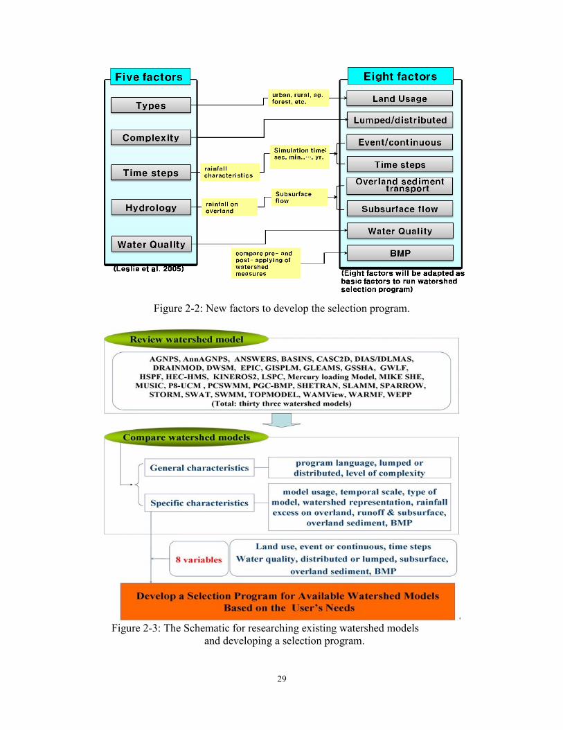
29

Figure 2-2: New factors to develop the selection program.

Figure 2-3: The Schematic for researching existing watershed models

and developing a selection program.

30

2.6. SELECTION PROGRAM FOR AVAILABLE WATERSHED MODELS

As was mentioned above, each watershed model has its own unique characteristics which

are shown in Tables 2-2 and 2-3. When approaching the models for predicting of watersheds, in

order to save time and effort, a program and methods for choosing available watershed models

needed to be developed. In this chapter, a Selection Program for Available Watershed Models

(Version 1) was developed using Excel Visual Basic, as shown in Figure 2-4.

Figure 2-4: The cover page of the Selection Program for Available Watershed models.

2.6.1 SELECTION ITEMS OF 8 VARIABLES

If you were to click the start button like in Figure 2-4, you can see a more detailed

expression window (Figure 2-5). In order to simplify the selection process of watershed models

for each watershed area, eight variables were chosen, which are as follows; (1) Land Use, (2)

Event or Continuous, (3) Time Steps, (4) Water Quality, (5) Distributed or Lumped, (6)

Subsurface, (7) Overland Sediment, and (8) BMP. Variables can be chosen separately or they

31

can overlap. Then the items of 8 variables could be selected based on the user’s need, as shown

in Figure 2-5. When you select the desirable items of each variable, the selected watershed

models change to a yellow color in the model window.

Figure 2-5: Detailed expression Window for selecting items of the 8 variables.

Land use includes urban, rural, agriculture, forests, rivers, and lakes or reservoirs. Event

or Continuous could be selected separately or they can overlap. Time steps can be chosen

separately and can overlap as well among seconds, minutes, hours, days, months, and years.

Distributed or lumped, Subsurface, Overland Sediment, and BMP could be selected depending

on the user’s needs.

32

2.6.2 MODEL DESCRIPTIONS OF SELECTED WATERSHED MODELS

After choosing the desirable items of the 8 variables, push the ok button. You will see the

model description in the results window which includes input data, the developer, programming

language, level of complexity, rainfall excess on overland/water balance, runoff on overland,

subsurface flow, overland sediment, water quality simulation, BMP evaluation, Model limitation,

and References which are connected to an excel file sheet.

Figure 2-6: Selected Model Description in result window.

If you select a desirable watershed model, you can see the detailed model description.

Furthermore, results could be shown as a text file by pushing the model export button. To go

back to the previous page, click the previous button.

33

2.7. SUMMARY AND CONCLUSION

In this chapter, numerous watersheds models, which have their own unique

characteristics, were reviewed to determine each model’s mechanisms and functions.

Furthermore, about 217 references examples, which have been applied to the watershed models,

were reviewed and analyzed with a focus on their applicability. Hence, in this paper, thirty three

different watershed models were reviewed to show how they can be applied to different

situations and watershed characteristics. These models included AGNPS, AnnAGNPS,

ANSWERS, BASINS, CASC2D, IAS/IDLMAS, DRAINMOD, DWSM, GISPLM, GLEAMS,


MUSIC, P8-UCM, PGC-BMP, SHETRAN, SLAMM, SPARROW, STORM, SWAT, SWMM,

TOPMODEL, WAMView, WARMF, and WEPP.

In addition, the watershed models were classified based on several characteristics which

were program language, lumped or distributed, level of complexity, model usage (Land use),

temporal scale, type of model, watershed representation, rainfall excess on overland, runoff and

subsurface, overland sediment, and BMP evaluation. According to these classifications, the

characteristics of watershed models could be explained in detail and the key points of each

model are highlighted.

Based on this study’s literature review, currently available watershed models designed for

the purpose of developing flow and water quality management plans at a watershed scale—such

as Nakdong River watershed (23,860 km2) in South Korea—require too much data and

application effort to be used to prioritize watersheds with respect to their relative contribution to

environmental degradation within a multiwatershed basin. Therefore, as was hypothesized in

Chapter 1, simple equations relating easily obtained data to watershed water quality impacts need

34

to be developed to sufficiently prioritize target restoration areas in the feasibility phase of

spatially large projects (i.e. national scale).

In addition, a model selection program is needed to aid the engineer in the selection of

the best watershed model to use in future complex modeling following the feasibility phase.

Eight variables were chosen considering five factors from Leslie et al. (2005) and the reviewed

literature such as land use, event or continuous, time steps, water quality, distributed or lumped,

subsurface, overland sediment, and BMP. Using these eight variables as input, the selection

program developed in this dissertation screens available watershed models for the best model for

the user’s needs.

After the selection program uses the modeler’s needs to screen available watershed

models and makes a selection, information related to the data of the selected model—such as

input data, the developer, programming language, level of complexity, rainfall excess on

overland / water balance, runoff on overland, subsurface flow, overland sediment, water quality

simulation, BMP evaluation, model limitation, and references—are shown and can be printed out

if ‘sheet export’ is selected.

The watershed selection program described in this dissertation could be highly useful to

many watershed modelers. In addition, this program could be upgraded by anyone who knows

how to apply state-of-art data that has been collected from a watershed model. This program is

still not perfect because we could not obtain the entire data for each watershed model. Finally

this program is going to be upgraded continuously to fulfill the needs of users of watershed

models.

35

CHAPTER 3. DEVELOPING SIMPLE EQUATIONS FOR WATER

QUALITY IN SOUTH KOREA

3.1. INTRODUCTION

Population pressures and mitigation, land-use conversion and its pollution consequences

appear to be the major diffuse pollution problem today (Novotny, 2003). Many people have

moved to the countryside and have transformed rural areas into suburban areas. Due to the recent

trends of land use, imperviousness has abruptly increased. This increase in impervious land has

resulted in the increase in the ease of pollutant conveyance from the watershed to river channels

downstream. Watershed changes to impervious cover have resulted in the shifting of stream and

watershed environmental conditions that are entirely different from their historic forms. In

addition, such changes have affected urban stream hydrographic conditions and have resulted in

significantly higher and earlier peak discharge rate than is seen in rural or undeveloped streams

(CWP, 2005).

Figure 3-1: Comparison of pre and post development (Source: Schueler, 1987).

Urbanization has spread widely all over the world. However, people want to restore or

rehabilitate urban and rural areas for better environmental conditions. In order to do this, we

36

need to compare urban areas and then try to find the best areas through priority comparison,

because the amount of funds needed to conduct a nationwide project would be insurmountable

for the government to bear. Hence, policy makers should decide which places have the highest

priority for restoration. This has to include the evaluation of economic, social, technological, and

environmental factors. To carry out these evaluations, we need to adapt nationwide watershed

modeling for forecasting after applying watershed restoration measures. However, sophisticated

watershed modeling is extremely broad, complicated, and time-consuming work. Therefore,

simplified evaluation methods of watershed environmental conditions should be applied, such as

pre- and post-water quality measures, to quantify the effects of restoration methods.

Watershed modeling is a hydrological and geographical model that simulates the

movement of water and relevant processes in order to reflect the change of water quality and

quantity (Novotny, 2008, Singh, 2004). A plethora of watershed models exist, all of which

combining and integrating together physically and empirically relationships and parameters to

approximate the behavior of the natural systems. A few of these watershed modeling parameters,

characteristics and processes include: areal precipitation, watershed representation, surface

runoff, infiltration, subsurface flow and interflow, groundwater flow and base flow, evaporation

and evapotranspiration, interception, depression storage, detention storage, rainfall-excess/soil

moisture accounting, snowmelt runoff, stream-aquifer interaction, reservoir flow routing,

channel flow routing, water quality, model calibration and model testing (Singh, 2004). However,

these methods are difficult to follow and only modeling experts deal with them. In addition, it

takes a lot of time to collect data from an area.

In order to perform water quality modeling for one watershed and carry out data

collection, a significant amount of time and money must be devoted. This process will require a

37

period of more than two years just to collect data and at least two to three additional years to

analyze it (Roesner, personal communication). Along with the time needed, a large amount of

money will be required for data gathering, and model application. The Water Quality Modeling

Process is shown in Figure 3-2 (by Chapra, 2003). In the case of the Four River Restoration

project in South Korea, this is neither a practical or affordable approach due to the scale of work

being done.

Figure 3-2: Water Quality Modeling Process.

The objective of this research is to streamline the process outlined in Figure 3-3 and

develop a sophisticated yet simple decision-making system that utilizes existing data such as

land coverage and watershed area. Water quality could change due to the watershed conditions,

especially land coverage. Therefore, if a relationship is found between land coverage and water

quality, it can be used to prioritize watersheds for restoration. Therefore, a simple method is to

be developed to prove the relationship between land coverage and water quality and this

methodology will then be verified using an existing watershed model in this research.

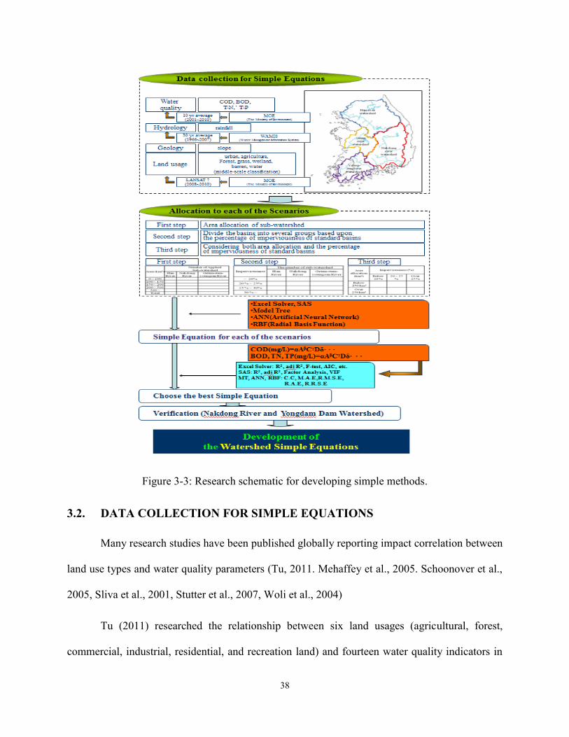
38

Figure 3-3: Research schematic for developing simple methods.

3.2. DATA COLLECTION FOR SIMPLE EQUATIONS

Many research studies have been published globally reporting impact correlation between

land use types and water quality parameters (Tu, 2011. Mehaffey et al., 2005. Schoonover et al.,

2005, Sliva et al., 2001, Stutter et al., 2007, Woli et al., 2004)

Tu (2011) researched the relationship between six land usages (agricultural, forest,

commercial, industrial, residential, and recreation land) and fourteen water quality indicators in

39

Eastern Massachusetts. Most of the water quality indicators have been significantly associated

with most of the land use indicators. Randhir (2001) studied a watershed-based land

prioritization model for water supply protection based on the integration of three types of

information: geographic information, relationships between land criteria and effects, and travel-

time of runoff. In the case of land use modeling studies, geographic information systems (GIS)

have been used for assembling data and defining decision zones (Wang, 2004).

Lately, there has been a dramatic increase in watershed surveys. Therefore, data on water

quality and land coverage could be obtainable for all over the world, including South Korea. In

order to determine a relationship among water quality, hydrology, geology, and land usage, the

data shown in Table 3-1 were collected.

Table 3-1: The collection data to make simple methods.

Division Parameter

Water Quality COD, BOD, T-N, and T-P

Hydrology Rainfall

Geology Slope

Land Usage

Pervious and impervious,

Middle-

scale

(23 items)

residential areas, industry areas, business areas, recreational facilities areas,

traffic areas, public facilities areas, rice paddies, fields, greenhouse areas,

orchards, cultivation areas, broad-leaved forests, coniferous forests, mixed

stand forests, natural grasslands, golf courses, grasslands, inland wetlands,

coastal wetlands, mining areas, bare land, inland water, and sea water

Large-scale

(7 items) urban, agriculture, forest, grass, wetland, barren, and water

Water quality data were obtained from the Ministry of Environment (MOE) from 2001 to

2010. For rainfall, the 30 years average rainfall was used per standard basin from 1966 to 2007,

which was obtained from the WAMIS (Water Management Information System). Land Usage is

gained from land cover maps (scale of 1:50,000) which was photographed by LANSAT 7 from

40

2008 to 2010. It was published by MOE, Republic of Korea, in 2010. The characteristics of the

present land usage survey are displayed in Table 3-2.

Table 3-2: The present situation for survey of the large, middle, and small-scale classification

(http://egis.me.go.kr/egis/home/Info/m02_DB_a3.asp).

Classification

Large-scale Middle-scale Small-scale

Production

years

(photographs

years)

1998(1987~1989)

2000(1997~1999)

2010(2008~2010)

2000~2004

(1999,

2000, 2002)

2007

(2006)

2009

~04

(2002)

2010

Demonstration

Area The whole nation

Seoul, Gyunggi,

Inchun, Hangang

Geumgang

Nakdong

Youngsangang

The whole

nation

Seoul, Inchun,

Daegeon,

Gyunggi,

Chungnam, and

Chungbuk

A few areas

Primitive

images Lansat TM (30m)

IRS-1C(5m),

Lansat ETM+(30m),

IKONOS(1m), IRS-

1D(5m),

SPOT5(5.2m)

SPOT5(5.2m) KOMPSAT-

2(1m)

KOMPSAT-

2(1m)

Scale 1:50,000 1:50,000 1:25,000 1:25,000 1:5,000

Format GeoTiff GeoTiff shp shp shp

Land use classification at both large and middle scales are listed in Table 3-3. Large-scale

land use classifications include seven categories and middle-scale land use classifications include

23 categories.

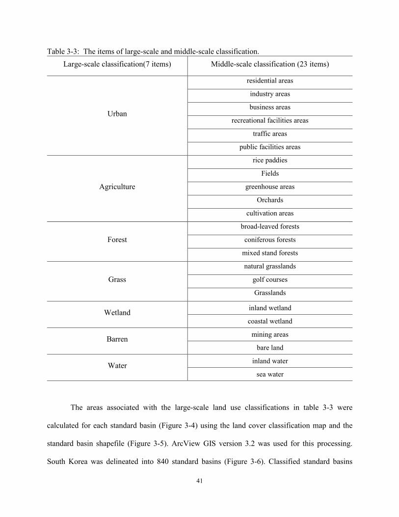
http://egis.me.go.kr/egis/home/Info/m02_DB_a3.asp

41

Table 3-3: The items of large-scale and middle-scale classification.

Large-scale classification(7 items) Middle-scale classification (23 items)

Urban

residential areas

industry areas

business areas

recreational facilities areas

traffic areas

public facilities areas

Agriculture

rice paddies

Fields

greenhouse areas

Orchards

cultivation areas

Forest

broad-leaved forests

coniferous forests

mixed stand forests

Grass

natural grasslands

golf courses

Grasslands

Wetland inland wetland

coastal wetland

Barren mining areas

bare land

Water inland water

sea water

The areas associated with the large-scale land use classifications in table 3-3 were

calculated for each standard basin (Figure 3-4) using the land cover classification map and the

standard basin shapefile (Figure 3-5). ArcView GIS version 3.2 was used for this processing.

South Korea was delineated into 840 standard basins (Figure 3-6). Classified standard basins

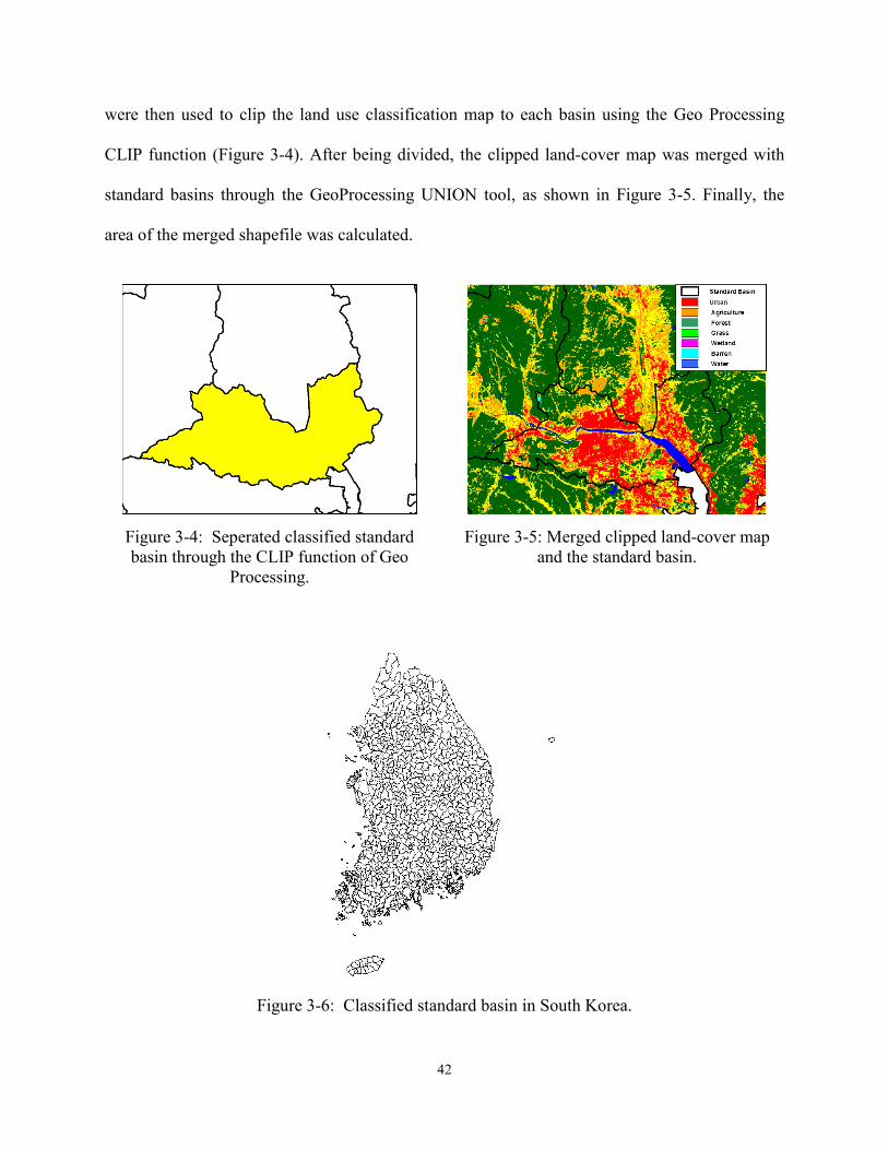
42

were then used to clip the land use classification map to each basin using the Geo Processing

CLIP function (Figure 3-4). After being divided, the clipped land-cover map was merged with

standard basins through the GeoProcessing UNION tool, as shown in Figure 3-5. Finally, the

area of the merged shapefile was calculated.

Figure 3-4: Seperated classified standard

basin through the CLIP function of Geo

Processing.

Figure 3-5: Merged clipped land-cover map

and the standard basin.

Figure 3-6: Classified standard basin in South Korea.

43

3.3. ALLOCATION TO EACH SCENARIO

The sub-watersheds of South Korea consist of about 840 sub-watersheds which are called

standard basins. The five rivers considered in this research flow through 522 of these standard

basins. Table 3-4 shows the present situation of the five rivers’ watersheds and the number of

standard basins.

Table 3-4: The present situation of five rivers’ watersheds (MOCT, 2006, MOE).

Watershed watershed

area (km2)

Annual

rainfall

(mm/year)

river

length

(km)

Number

of

standard

basins

Number of

water quality

monitoring

points

Adaptable water

quality monitoring

point and sub-

watersheds

Han River 25,954 1,208 494 195 236 64

Nakdong

River 23,384 1,178 506 191 191 69

Geum River 9,912 1,227 398 79 78 56

Sumjin River 3,468 1,433 224 46 46 17

Youngsan

River 3,468 1,336 32 11 32 11

Total - - - 522 583 217

Water quality points were chosen based on the available sites for representation of

watersheds’ land use. Therefore, at first, standard basins and water quality points were compared

and then water quality, which stand for standard basins, were chosen. If there were no water

quality points for standard basins, upstream and downstream standard basins were combined.

Through this process, adaptable water quality monitoring points and sub-watersheds were chosen

at 217 points and are shown in Table 3-4.

In addition, in order to build simple methods for watershed water quality forecasting, the

interrelationship between water quality and land usage, including pervious or impervious, has to

be considered. Therefore the allocation of land usage should be divided into 3 steps. The first

44

step takes into consideration the area of sub-watersheds, while the second step is imperviousness,

and last step is the combination of the area and imperviousness.

3.3.1 FIRST STEP: AREA ALLOCATION OF SUB-WATERSHEDS

Sub-watersheds were divided into 5 cases, as shown in Table 3-5. However, areas were

separated based upon the area distribution of each watershed which is shown in Table 3-6. The

reason for this is because the co-relationships between land use and water quality are not

constant in different regions because the characteristics and pollution sources of watersheds are

not the same in different places (Tu, 2011). Hence, five rivers’ watersheds were divided into

three groups of watersheds, the Han River, Nakdong River, and Geun-Sum-Youngsan River,

which are located on the upper side, east side, and west side of South Korea, respectively as

shown in Figure 3-7. The difference in the total numbers between Table 3-5 and Table 3-6 is due

to the lack of data like water quality, land use, etc.

Figure 3-7: Watershed map of South Korea.

45

Table 3-5: The number of applied sub-watersheds in South Korea.

Area (km2) Number of Applied Sub-watershed

0 ~ 100 30

100 ~ 150 36

150 ~ 200 25

200 ~ 500 82

500 ~ 44

Total 217

Table 3-6: The number of applied sub-watershed of each river watershed.

Area (km2)

Number of Applied Sub-watershed

Han River Nakdong River Geum-sum-youngsan River

0 ~ 100 8 4 14

100 ~ 150 7 9 17

150 ~ 200 7 4 13

200 ~ 500 23 28 38

500 ~ 16 19 -

Total (207) 61 64 82

3.3.2 SECOND STEP: DIVIDE THE BASINS INTO SEVERAL GROUPS BASED

UPON THE PERCENTAGE OF IMPERVIOUSNESS

In order to find the imperviousness of each standard basin, land-cover maps were used to

characterize the pervious and impervious surface in each basin. Land-cover maps have several

scales—large-scale, middle-scale, and small scale—which vary in their amount of detail. Large-

scale and middle-scale, but not small-scale could be used right now in South Korea. In this

research, large-scale and middle-scale maps were considered to find the percentage of

imperviousness for seven land-cover and twenty three land-cover items using the runoff C-

coefficients (Michael, 2003) of the rational method, which is shown in Table 3-7.

The runoff C-coefficients of the rational method for seven & twenty three land-covers do

not exactly correspond. Hence, to match the coefficient value, the average value of the runoff C-

coefficient of the rational method was used. In addition, it was assumed that runoff coefficients

46

are the same as imperviousness; for example, if the runoff coefficient for a watershed is 0.7, it is

the same as saying the watershed has an imperviousness of 70%, because the C value is the

amount of rainfall that transforms into runoff. Additionally, there is no exact standard to allocate

between pervious and impervious at present in South Korea.

Table 3-7: Converted runoff coefficients from runoff C-coefficient of rational method. Large and middle scale classification

Land usage runoff coefficient Land usage runoff coefficient

Urban 0.530

residential areas 0.500

industry areas 0.700

business areas 0.713

recreational facilities areas 0.275

traffic areas 0.819

public facilities areas 0.175

Agriculture 0.319

rice paddies 0.319

Fields 0.319

greenhouse areas 0.319

orchards 0.319

cultivation areas 0.319

Forest 0.150

broad-leaved forests 0.150

coniferous forests 0.150

mixed stand forests 0.150

Grass 0.207

natural grasslands 0.225

golf courses 0.171

grasslands 0.225

Wetland 0.000 inland wetland 0.000

coastal wetland 0.000

Barren 0.450 mining areas 0.500

bare land 0.400

Water 0.000 inland water 0.000

sea water 0.000

47

In conclusion, the imperviousness of the standard basins ranges from 9.8 % to 42 %,

while the average imperviousness is 22.27 %, as shown in Figure 3-8.

Figure 3-8: The imperviousness of the standard basins in South Korea.

Based upon the imperviousness of the standard basins, several previously grouped

watersheds had to be divided in order to match the watershed land-usage characteristics. The

Center for Watershed Protection shows recent research on the impact of urbanization on stream

quality for subwatersheds with more than 10% impervious cover. Impervious cover (IC) of

watersheds could impact the following: stream hydrology, physical alteration of the stream

corridor, stream habitat degradation, declining water quality, and loss of aquatic diversity.

Therefore IC is divided into 4 cases according to Figure 3-9. Below 10% is sensitive, 10 to 25%

is impacted, 25 to 60% is non-supporting and over 60% is urban drainage.

48

Figure 3-9: Representation of the impervious cover (IC) (CWP, 2005).

However, it was not possible to find a standard basin with an impervious cover over 60 %

because the maximum basin imperviousness is 42 % for South Korea. Therefore in order to

divide the standard basin effectively and considering CWP reporting, 25 % imperviousness was

set as the mid-point. This point was chosen because it borders both impacted and non-supporting

streams which are shown in Figure 3-9. Twenty percent and 30 %, which have a ±5 % different

from 25%, were then set as additional dividing points. When IC is used to divide sub-watersheds

into categories, 84 sub-watersheds fall below 20% imperviousness, 94 sub-watersheds fall

between 20 % ~ 25 %, 29 sub-watersheds fall between 25 % ~ 30 %, and 10 sub-watersheds fall

over 30 %. The breakdown of sub-watersheds is shown in Table 3-8.

Table 3-8: The number of sub-watersheds used to analyze the impact of imperviousness.

Imperviousness

The number of sub-watersheds

Total Han River Nakdong

River

Geum-Sum-

Youngsan River

~ 20% 84 34 25 25

20 % ~ 25% 91 19 36 39

25 % ~ 30% 29 5 7 17

30 % ~ 10 6 1 3

49

3.3.3 THIRD STEP: COMBINE STEPS ONE (AREAS) AND TWO

(IMPERVIOUS COVER)

In order to achieve optimized results, the first and second steps should be merged, the

area allocation and the percentage of imperviousness of standard basin. Actually, the first step

was modified from 50 km2 intervals for each step to below and over 250 km

2 in regards to

considering the balance of the number of allocated sub-watersheds which are shown in Table 3-9.

Table 3-9: The number of standard basins for both area allocation and the percentage of

imperviousness of standard basins.

Area allocation

(km2)

Imperviousness (%)

Below 20 % 20 ~ 25 % Over 25 %

Below 250 km2 23 53 24

Over 250 km2 53 41 13

3.4. DATA SOURCES FOR ANALYSIS

This study was based on four types of data — water quality, hydrology, geology, and

land usage — which are shown in Table 3-10. Large and middle scale land use maps were

considered to help correlate land use to other watershed parameters like perviousness,

imperviousness, slope, etc. When the middle-scale land use classifications were used, it was

found that land usage was too detailed. Hence, it is hard to get the multi-lateral relationship

among parameters. On the other hand, out of the seven items of large scale classifications, almost

all includes data, except for a few cases. Therefore, in order to maintain the clarity of the study,

obtain data readily, and determine correlations clearly, large-class land use classification (i.e.

urban, agriculture, forest, grass, wetland, barren, and water) and perviousness/ imperviousness

were used.

50

Table 3-10: The data source and period in order to compare land usage and water quality.

Division Parameter Source Period

Water Quality COD, BOD, T-N, T-P Ministry of Environment 10 years

(2001-2010)

Hydrology Rainfall Water Management Information System

(WAMIS)

30 years

(1966~2007)

Geology Slope

Land Usage

Pervious & impervious,

urban, agriculture, forest,

grass, wetland, barren,

water

Remote sensing. Landsat TM data was

collected between 2008 and 2010 at a

30*30m spatial resolution, and were

processed in order to reveal the LUCC

features. The data geometrical corrections,

classification and accuracy assessment were

carried out with the support of the digital

image processing software PCI.

Topographical maps (1:50, 000) were used

as the reference for the geometric

corrections. According to the geographical

names, the maps were re-drawn on the

digitized topographical map base using

ArcView GIS 3.2 ver. software to complete

editing, labeling, projection,

transformation, edge matching and

overlaying processes.

2008~2010

3.4.1 FIRST STEP

The first step in correlating water quality, hydrology, geology, and land usage was to sort

the sub-watersheds into bins according to area—0 ~ 100 km2, 100 ~ 150 km

2, 150 ~ 200 km

2,

200 ~ 500 km2, and over 500 km

2 like in Table 3-11. However the number of data collected was

slightly small to represent the characteristics of sub-watersheds. According to Hyudman (2007),

it is always necessary to have more observations than parameters in terms of a purely statistical

point of view. Due to this observation, the number of intervals used to divide the sub-watersheds

into bins was increased as shown in Table 3-11. The observation data (pervious/impervious,

rainfall, slope, land use, water quality) of each sub-watershed like the Han, Nakdong, and Geum-

Sum-Youngsan River are attached in Appendix B.

51

Table 3-11: The number of applied sub-watersheds for each river watershed (step one).

Area (km2)

Number of Applied Sub-watershed

Han River Nakdong River Geum-sum-youngsan River

0 ~ 100 - - 14

100 ~ 150 - - 17

150 ~ 200 - - 13

200 ~ - - 38

0 ~ 200 22 17 -

200 ~ 500 23 28 -

500 ~ 16 19 -

Total (207) 61 64 82

3.4.2 SECOND STEP

Imperviousness has a strong relationship with water-quality impacts (Conway, 2006).

Therefore, in the second step, imperviousness is the standard to allocate watershed data. In this

step, imperviousness is divided into four intervals—below 20 %, 20 % ~ 25 %, 25 % ~ 30 %,

and over 30%. However, when applied to each watershed, over 30 % is included in the 25 % ~

30 % interval because the number of watersheds over 30 % is so small. The number of sub-

watersheds falling within each range of impervious cover for each watershed is shown in Table

3-12. The observation data (pervious/impervious, rainfall, slope, land use, water quality) of each

sub-watershed for step two are attached in Appendix B.

Table 3-12: The number of applied sub-watersheds for each river watershed (step two).

Imperviousness

The number of sub-watersheds

Total Han River Nakdong

River

Geum-Sum-Youngsan

River

~ 20% 75 33 21 21

20 % ~ 25% 88 19 35 34

25 % ~ 36 9 8 19

52

3.4.3 THIRD STEP

In order to consider both sub-watershed areas and the percentage of imperviousness

among sub-watershed characteristics, sub-watershed areas were divided below and above 250

km2 and their imperviousness cover was broken up into categories of 0 ~ 20 %, 20 ~ 25 %, and

over 25 % which is same as the guideline already displayed in Table 3-9. The total observation

data of each sub-watershed for step three is shown in Appendix B.

3.4.4 ESTABLISH SIMPLE EQUATIONS

Figure 3-10 shows the process that is used to determine simple equations for the final

analysis. After completing the three cases and ten scenarios, Excel solver, Model Tree, ANN

(Artificial Neural Network), RBF (Radial Basis Function), and SAS (Statistical Analysis

System) were used based on these same scenarios to conduct the data analysis.

Figure 3-10: The schematic diagram to establish simple equations

based on several data analysis methods.

53

3.5. BUILDING SIMPLE EQUATIONS

In order to build the best implemented simple equations, two processes were reviewed

such as; model selection process and evaluation/validation model with parameter estimation

(Kutner et al., 2004). Which are calculated and evaluated using following methods (chapter 3.5.1

through 3.5.2).

3.5.1 MODEL SELECTION PROCESS

There are many criteria for model selection. In this research, five “good” subsets

according to the criteria specified were used to select the best applicability model to represent

watershed characteristics in relevant with water quality (Kutner et al., 2004, Pruden et al., 2012).

Which are including such as; coefficient of multiple determination (R2), adjusted coefficient of

multiple determination (Adj R2), F-test, Akaike Information Criteria (AIC), and factor analysis.

① Coefficient of multiple determination (R2)

R2 is the coefficient of determination which could apply to finding a quantitative relation

between the predicted and observed values. The range of this coefficient is zero to 1, where zero

means no correlation and 1 means a perfect correlation.

Equation 1

Where, SSE = the sum of squares of residuals

=

SSTO = the total sum of squares

=

fi = the modeled (predicted) values

yi = the observed values

the mean of the observed values

54

② Adjusted R2

Since R2 does not take account of the number of parameters in the regression model and

since max can never decrease as p increases, the adjust coefficient of multiple determination R2

has been suggested as an alternative criterion (Kutner et al., 2004)

Equation 2

Where, n = the total number of data sample size

p = the total number of regressors in the linear model

③ EF

EF is the Nash-Sutcliffe efficiency or coefficient of efficiency which compares the

predicted values to the mean of the observed values. The range of this measure is -∞ to 1, where

1 represents the best model performance. A value near one indicates a close match between

observations and model predictions. A value of zero indicates that the model predicts individual

observations no better than the mean of the observations. Values less than zero indicate that the

observation mean would be a better predictor than the model results (Stow et al, 2002). The

equations of three statistical methods are as follow;

Equation 3

④ CC, MAE, RAE, RMSE, and RRSE

Correlation coefficient (CC) measures the statistical correlation between observed (a) and

predicted (p) values. The correlation coefficient ranges from 1 for perfectly correlated results,

through to o when there is no correlation, to -1 when the results are perfectly negative, which

could be calculated by equation 5 (Witten et al., 2011).

55

Ap

PA

SS

SCC

Equation 4

Where, 1

))((

n

aaPPS i ii

PA,

1

)( 2

n

PPS i i

P,

1

)( 2

n

aaS i i

A

p = predicted value, a = actual value, n = the number of data

P = the mean value of predicted data, a = the mean value of the test data.

Mean absolute error (MAE) is the average magnitude of the individual errors without

taking account of their signs. Mean-squared error tends to exaggerate the effect of outliers-

instances when the prediction errors are larger than the others-but an absolute error does not have

this effect. Therefore all sizes of errors are treated evenly according to their magnitude based

upon MAE and could be calculated by equation 6 (Witten et al., 2011)..

n

apapMAE

nn

...11 Equation 5

In some cases, the Relative absolute error (RAE) is more important than MAE, for

example, when we consider the errors in both cases 50 to 500 and 0.2 to 2, the absolute error will

be meaningless. Therefore, relative errors are appropriate in this case. It could be calculated

using Equation 7 (Witten et al., 2011).

aaaa

apapRAE

n

nn

...

...

1

11 Equation 6

RMSE is the root mean squared error and measures the size of the discrepancies between

predicted and observed values. The range of this measure is zero to ∞ and the smaller a value is,

the better the model’s performance will be (i.e. zero indicates a close match). It could be

calculated by Equation 7.

n

apapRMSE nn

2211 )(...)(

Equation 7

56

Root relative squared error (RRSE) is calculated from relative square error which takes

the total squared error and normalizes it by dividing it by the total squared error of the default

preditor. And the root relative squred error could be obtained by Equation 8.

22

1

2211

)(...)(

)(...)(

aaaa

apapRRSE

n

nn

Equation 7

⑤ F-test

An F-test is the analysis of variance approach to provide us useful tests for regression

models. For the simple linear regression case considered here, the analysis of variance provides

us with a test for:

, Equation 8

The test statistic for the analysis of variance approach is denoted by F, it compared MSR

and MSE in the following equation:

Equation 9

In addition, MSR and MSE could be calculated following.

Table 3-13: ANOVA table for Simple Linear Equation for calculation F-test

Source of

variance

SS

(sum of square)

df

(degree of freedom)

MS

(mean square) F

regression

(Between

groups)

SSR

=

(regression sum

of square)

1

error

(within groups)

SSE

=

(sum of squares

of residuals)

n-2

(n=the number of

data)

total

SSTO

=

the total sum of

squares

57

According F-test (upper-tail), the results could be decided following procedures:

F* is distributed as F (1, n-2) when Ho holds, the decision rule is as follows when the risk

of error is to be controlled at α:

If F* ≤ F (1- α: 1, n-2), conclude Ho

If F* ≥ F (1- α: 1, n-2), conclude Ha Equation 10

Therefore, F* is larger than F (1- α: 1, n-2), there is some difference between their

different groups and if p-value is less than 0.05, we would conclude Ha , as well.

⑥ Akaike Information Criterion(AIC)

The Akaike information criterion (AIC) is a measure of the relative quality of a statistical

model, for a given set of data. And also AIC could provide a means for model selection which

could be calculated by following equation:

Equation 11

Where, n= a number of sample size, p=the number of parameters

On the other hand, AIC does not provide a test of a model in the sense of testing a null

hypothesis.

Therefore, in order to select the best applicable simple equations, using coefficient of

multiple determination (R2), adjusted coefficient of multiple determination (Adj R

2), and F-test,

each simple equations could be qualified whether it is applicable or not. And the best simple

equation could be selected by using Akaike Information Criteria (AIC).

⑦ Factor Analysis

Factor analysis is a statistical method for investigating whether response variable, Y, is

linearly related to exploratory variables, X1, X2,∙∙∙,Xn which is shown as follows;

58

- determining the factor extraction model

Equation 12

- extracting and determining the number of factors

① eigenvalue

The “eigenvalues greater than

one” rule has been most

commonly used due to its simple

nature and availability in various

computer packages. It states that

the number of factors to be

extracted should be equal to the

number factors having an

eigenvalue greater than 1.0

(Source: SAS library)

② scree test

Plotting the eigenvalues against the

corresponding factor numbers gives

insight into the maximum number of

factors to extract. The Scree plot

illustrates the rate of change in the

magnitude of the eigenvalues for the

factors. The rate of decline tends to be

Figure 3-11 Eigenvalues of the correlation

matrix

Figure 3-12 Scree plot of

eigenvalues

59

fast for the first few factors but then level off. The “elbow”, or the point at which

the curve bends, is considered to indicate the number of factors to extract. The

figure 3-12 illustrates an example of scree plot, where a elbow occurred at the

fourth factor, which has an eigenvalue right around 1 (Source: SAS library).

- Calculate factor loading using correlation between response variable, Y, and

exploratory variable, X1, X2,∙∙∙,Xn.

Below 0.3 low significance level

Below 0.4 medium of significance level

Over 0.5 high significance level

- Selecting final simple equations using variables having high significance level.

Equation 13

3.5.2 EVALUATION MODEL WITH PARAMETER ESTIMATION

To examine the normality of the error terms of simple equation, the Shapiro-Wilk test

could be used. In addition, to identify multicollinearity in the matrix of predictor variables for

each general linear regression model, the variance inflation factor (VIF) could be used (Amy

Pruden et al., 2012).

① Shapiro-Wilk test

The Shapiro-Wilk test, proposed in 1965 (Shapiro and Wilk, 1965), calculates a W

statistic that tests whether a random sample comes from normal distribution. Pearson and Hartley

(1972) reproduced the way of obtaining the W statistic using Monte Carlo simulations. This test

60

could be used for normality among elements which has a limitation of samples between 3 and 50

elements. And this test could be calculated as follows (NIST/SEMATECH e-Handbook of

Statistical Methods) :

- Rearrange the data in ascending order so that x1 ≤ … ≤ xn.

- Calculate SS as follows

Equation 14

Where, SS = the sum of squares of deviations of data points from

their sample mean

= the average of data

n = the number of data

- If n is even, let m = n/2, while if n is odd let m = (n–1)/2

- Calculate b as follows, taking the ai weights from the Shapiro-Wilk Table (based on

the value of n). Note that if n is odd, the median data value is not used in the

calculation of b.

Equation 15

- Calculate the test statistics W = b2 ⁄ SS

- p-value could be calculated using the Shapiro-Wilk Table (probability) based upon

the n and W, and it could be proved whether the data are normally distributed or not.

② Variance Inflation Factor

Variance Inflation Factor (VIF) is widely accepted a formal method of detecting the

presence of multicollinearity (Kutner, 2004, O’Brien, 2007, Amy Pruden et al., 2012).

Collinearity can increase estimates of parameter variance; even though R2 is large, if there is no

statistically significant variable, the results of parameter estimations could be the “incorrect sign”.

Therefore VIF value in excess of 10 is frequently taken as an indication that multicollinearity

may be unduly influencing the least squares estimates. VIF is able to be calculated as follows:

Equation 16

http://www.real-statistics.com/statistics-tables/shapiro-wilk-table/

61

Where, = the square of standard deviation of the variable

n = the number of data (observation)

= the square of standard error of the parameter

= the mean square of residual

3.5.3 MODEL SELECTION PROCESS FOR EACH DATA ANALYSIS

METHODS

As abovementioned in Chapter 3.4.4, five data analysis methods were used to establish

Simple Equations, such as Excel Solver, SAS, Model Tree, ANN, and RBF. In addition, model

selection process and model evaluation with parameter analysis were implemented for each data

analysis methods based on table 3-14.

Table 3-14: Model selection process and evaluation methods for each data analysis method.

Methods Type of

Simple Equation Model Selection Process Evaluation Model

Excel

Solver Non-linear Eq. R

2, Adj R

2, F-test, and AIC Shapiro-Wilk test

SAS Linear Eq. R2, Adj R

2, Factor Analysis

Variance Inflation

Factor (VIF)

Model Tree Linear Eq. for each

divided section C.C (correlation coefficient), M.A.E.(mean

absolute error), R.M.S.E (root mean squred error),

R.A.E (relative absolute error), R.R.S.E (root

relative squred error)

ANN Neural Network using

sigmoid funtion

RBF Neural Network using

Gaussian function

For Excel Solver, R2, Adj R

2, F-test, and AIC to select the best Simple Equation among

the bunch of Simple Equations and Shapiro-Wilk test were implemented for model evaluation

with parameter analysis. The Simple Equations using Model Tree, ANN, and RBF were

evaluated and selected by computing C.C (correlation coefficient), M.A.E.(mean absolute error),

R.M.S.E (root mean squred error), R.A.E (relative absolute error), and R.R.S.E (root relative

62

squred error). In case of SAS, R2, Adj R

2, Factor Analysis were applied to select the best Simple

Equation, and Variance Inflation Factor were used for model evaluation with parameter analysis.

3.6. TOOLS FOR DATA ANALYSIS

3.6.1 EXCEL SOLVER

The Excel Solver (Microsoft Excel 2007 for Windows) is a tool for solving linear and

nonlinear optimization problems, as well as integer programs. The Solver is easy to use,

powerful, fast, can handle constraints, and can maximize and minimize. Solver performs three

main functions: 1) optimization through maximum or minimum with constraints on values, 2)

nonlinear regression which is an optimization problem that seeks to minimize the sum of the

squared error, SSE, between dependent values predicted by a regression model (yp) and those

from the data set (y) (equations 1), and 3) linear programming (Larsen, 2005).

Equation 17

Where, yp = the value predicted by the regression model

y = the data set.

Solver has been evaluated and tested in its abilities to solve both linear and non-linear

equations by Walsh et al. (1994) and found to be successful in modeling data obtained in many

analytical situations. Manoj et al. (2010) used Solver to determine critical and normal depths

based on geometric parameters for complex compound sections and suggested that Solver is an

easy and efficient method to calculate critical and normal depths. Nilsson et al. (2010) used

Solver to minimize the root-mean-squared error (RMSE) between the actual pool volumes and

the V-h (Volume/depth) model generated volumes by adjusting the respective wetland shape

parameter. Solver was used to optimize linear programs in order to maximize the net benefit of

63

watershed management including the specified constraints such as human demand, management

limits on human demand reduction, in-stream flow standards, land-use restrictions, the capacity

or volume of facilities, and surface water and groundwater flow out of a watershed (Zoltay et al.,

2010). In Helbling et al., (2009) Solver was used to minimize the sum of the squares of the

residuals between the observed and predicted chlorine concentrations for modeling residual

chlorine response to a microbial contamination event in drinking water distribution systems

using nonlinear regression.

In this research, whose purpose is to determine relationships and derive a simple equation

between water quality and other watershed parameters—hydrology, geology, and land usage, the

multi-lateral connection should be discovered using various methods. Solver is one of the best

and easiest tools available to determine these final results.

3.6.2 DATA MINING

While the availability of data has increased due to the technical development and

globalization of information networks, the reliable data is, contradictorily, still difficult to find.

In order to overcome this limitation, many researches have been implemented in finding and

organizing data and data mining is one of these efforts. Data mining is applicable to many

applications such as decision supporting, predicting and forecasting. Data mining began to make

its mark in the early 2000s with the development of Data Warehouses (Hadzilacos et al., 2000,

Saegrove et al., 1999).

Data mining can be classified according to various criteria, as shown in Table 3-15. Data-

driven data mining is used to discover the relationships between attributes in unknown data, with

or without known data with which to compare the outcome. There may or may not be a specific

scenario. Clustering and association, for example, are primarily data-driven data mining

64

techniques. In data-driven data mining, the data itself drives the data mining process. This

approach is best employed in situations in which true data discovery is needed to uncover rules

and patterns in unknown data. This tends to be the "I don't know what I don't know" approach:

you can discover significant attributes and patterns in a diverse set of data without using training

data or a predefined scenario. Data-driven data mining is treated as a "white box" operation, in

which the user is concerned about both the process used by the data mining algorithm to create

the model and the results generated by viewing data through the model.

Table 3-15: General classification of data mining algorithms.

Types Rules Algorithms

Data mining-oriented

(Data-driven data mining)

Association: any association between features is

sought, not just ones y\that predict a particular

class value

Apriori/AprioriTid, DHP etc.

Clustering: groups of examples that belong

together are sought PAM, CLARA etc.

Machine learning-oriented

(Model-driven data mining)

Clustering/Classification: examining the features

of a newly presented object and assigning it to

one of a predefined set of classes

(Unsupervised learning: detects & categorizes

persistent features without any feedback from the

environment)

Bayesian Network, GA,

ANN(SOM, ART)

Classification

(Supervised learning: operates under supervision

by being provided with the actual outcome for

each of the training examples.)

ANN (MLP, RBF),

Decision Tree

Machine learning known as model-driven data mining provides the technical basis of data

mining. Classifications and estimations are typically categorized as model-driven data mining

techniques. This approach is best employed when a clear scenario can be employed against a

large body of known historical data to construct a predictive data mining model. This tends to be

the "I know what I don't know" approach: you have a good idea of the specific scenarios to be

modeled, and have solid data illustrating such scenarios, but are not sure about the outcome itself

65

or the relationships that lead to this outcome. Model-driven data mining is treated as a "black

box" operation, in which the user cares less about the model and more about the predictive

results that can be obtained by viewing data through the model.

Data mining depends on both data-driven and model-driven data mining techniques to be

truly effective, depending on what questions are asked and what data is analyzed. Data-driven

and model-driven data mining can be employed separately or together, in varying amounts,

depending on specific business requirements. There is no set formula for mining data; each data

set has its own patterns and rules. Generally speaking, the data mining model drives the process

in model-driven data mining in environmental research fields because of its predictive results.

The basic ideas underlying data mining in recent studies are linked between many

artificial intelligence algorithms, for examples, neural network (NN), fuzzy logic (FL), genetic

algorithm (GA), probabilistic reasoning (PR) and model tree (MT). The combination of these

algorithms is generally called soft computing (SC). The inclusion of neural network theory in

soft computing came at a later point. At this juncture, the principal constituents of soft

computing (SC) are fuzzy logic (FL), neural network theory (NN) and probabilistic reasoning

(PR), with the latter subsuming belief networks, genetic algorithms, chaos theory and parts of

learning theory. What is important to note is that SC is not a melange of FL, NN and PR. Rather,

it is a partnership in which each of the partners contributes a distinct methodology for addressing

problems in its domain. In this perspective, the principal contributions of FL, NN and PR are

complementary rather than competitive.

3.6.3 M5P MODEL TREE

Many problems have been encountered during the process of predicting a “class” that

takes on a continuous numeric value rather than a discrete category into which an example falls.

66

However, decision-tree and decision-rule learners are not commonly extended to situations

where the class value itself is numeric.

There are, of course, several learning techniques that do predict numeric values. These

techniques include standard regression, neural nets, regression trees, and prediction by pre

discretization. But all of these have weaknesses. Standard regression is not a very potent way of

representing and inducing functions because it imposes a linear relationship on the data having

special and temporal variations rather non-linear. Neural nets are more powerful but suffer from

opacity: the model does not reveal anything about the structure of the function that it represents.

MTs are not yet as popular as ANNs. For example, their use started only recently

(Kompare, 1997; Solomatine and Dulal, 2003) in the water sector, and they are unknown to

water quality related research. Solomatine (2002) demonstrated the use of MTs in hydrological

and other problems, along with other data-driven models. The predictive accuracy of the simplest

MT model was observed to be very high and on par with that of an ANNs model built with the

same data. The advantages of model trees (M5) (Solomatine & Dulal, 2003) are that they are

more accurate than regression trees, more understandable than ANNs, easy to train, and robust

when dealing with missing data.

Model trees are tree-structured regression models that associate leaves with multiple

linear regression functions calculating numeric values. A regression tree is a machine learning

concept, which takes input data, and tries to learn the characteristics of the data. It looks like a

decision tree with each of the intermediate nodes as routing nodes with a ‘split’ value to decide

the destination data and the terminal nodes which have the function to compute the estimates.

Internal nodes are typically splitting tests that partition the space spanned by m

independent (or predictor) random variables xi (both numerical and categorical). Regression

67

models at the leaves capture the linear dependency between one or more independent variables

and the continuous dependent (or response) variable y, locally to a partition of the sample space.

Therefore, MTs differ from the better-known classification or decision trees only in that they

have a numeric value rather than a class label associated with the leaves. Statistics and machine

learning have settled the problem of inducing MTs from a training set. Several methods have

been proposed for the construction of the tree and for the estimation of the linear dependence at

the leaves on the basis of a training sample. They have been implemented in some well-known

model tree induction systems such as SMOTI (Stepwise Model Tree Induction, Orkin, Drogin,

1990), MARS (Multiple Adaptive Regression Splines, Friedman,1991), M5 (machine learning

method, Quinlan, 1992), RETIS (Karalic, 1992), TSIR (Lubinsky, 1996), M5’ (Wang, Witten,

1997), RegTree (Lanubile, Malerba, 1997), and HTL (Torgo, 1997). All these systems perform a

top-down induction of model trees (TDIMT). However, the SMOTI and TSIR are characterized

by two types of internal nodes: regression nodes, which perform only straight line regressions,

and splitting nodes, which partition the sample space. The regression model at a leaf is obtained

by combining the straight-line regression functions associated to the regression nodes along the

path from the root to the leaf.

The new technique for machine learning algorithms is called “M5 model tree” for dealing

with continuous-class learning problems and was developed by Quinlan (1992). An

implementation called M5P was described by Wang and Witten (1997) as performing somewhat

better than the original algorithm M5P. M5P allows the tree size to be reduced dramatically with

only a small penalty in prediction performance leading to much more comprehensible models.

Finally, the results which test the method used for dealing with missing values are presented.

68

[Building the Tree]

The basic tree has been formed by splitting criteria. The splitting criterion is based on

treating the standard deviation of the class values that reach a node as a measure of the error at

that node and calculating the expected reduction in error as a result of testing each attribute at

that node. The attribute which maximizes the expected error reduction is chosen. The standard

deviation reduction (SDR) for M5 is calculated by the Equation 18.

Equation 18

Where, SDR = the standard deviation reduction

T = the set of examples that reach the node

T1, T2, · are the sets that result from splitting the node according to the chosen

attribute. The splitting process ceases when the class values of all the instances that reach a node

vary very slightly, that is, just less than 5% of the standard deviation of the original instance set or

only a few instances remain.

[Pruning the Tree]

The pruning procedure makes use of an estimate of the expected error that will be

experienced at each node for test data. First, the absolute difference between the predicted value

and the actual class value is averaged for each of the training examples that reach that node. This

average will underestimate the expected error for unseen cases, of course, and to compensate, it

is multiplied by factor (n+ν)/ (n-ν), where n is the number of training examples that reach the

node and ν is the number of parameters in the model that represents the class value at that node.

M5 computes a linear model for each interior node of the unpruned tree. The model is

calculated using standard regression, using only the attributes that are tested in the subtree below

69

this node. The resulting linear model is simplified by dropping terms to minimize the estimated

error calculated using the above multiplication. By factor-dropping a term, it decreases the

multiplication factor, which may be enough to offset the inevitable increase in average error over

the training examples as terms are dropped one by one, greedily, so long as the error estimate

decreases. Finally, once a linear model is in place for each interior node, the tree is pruned back

from the leaves, so long as the expected estimated error decreases.

[Smoothing]

The final stage is to use a smoothing process to compensate for sharp discontinuities that

will inevitably occur between adjacent linear models at the leaves of the pruned tree, particularly

for some models constructed from a small number of training instances. The smoothing

procedure described by Quinlan (1992) first uses the leaf model to compute the predicted value,

and then filters that value along the path back to the root, smoothing it at each node by

combining it with the value predicted by the linear model for that node. The calculation is

Equation 19

Where, p’ = the prediction passed up to the next higher node,

p = the prediction passed to this node from below, q = the value predicted by the model at this

node, n = the number of training instances that reach the node below, and k = a constant. In

general, smoothing substantially increases the accuracy of predictions.

[Modification of SDR]

M5P does not clearly know how enumerated attributes and missing values should be

handled. These features are of vital importance for real-world data sets that have been

encountered in our practical working cases. To take account for the enumerated attributes and the

missing values the SDR is further modified to

Equation 20

70

Where, m = the number of examples without missing values for that attribute, T = is the

set of examples that reach this node, β(i) = the correction factor calculated for the original

attribute to which this synthetic attribute corresponds, TL, and TR = sets that result from splitting

on this attribute for all attributes are now binary.

3.6.4 ARTIFICIAL NEURAL NETWORK (ANN)

An artificial neural network (ANN) is an information processing system that replicates

the rudimentary behaviors of a human brain by emulating the operations and connectivity of

biological neurons. It consists of an often large number of neurons, i.e. simple linear on

nonlinear computing elements, interconnected in often complex ways and often organized into

layers. ANN is used in three main ways:

as models of biological nervous systems and intelligence

as real-time adaptive signal processors or controllers implemented in hardware for

applications such as robots

as data analytic methods

In this study, ANN was used in data analysis. ANN, like many statistical methods, is

capable of processing vast amounts of data and making predictions that are sometimes

surprisingly accurate. This, however, does not make it “intelligent” in the useful sense of the

word. ANN learns in much the same way statistical algorithms arrive at optimization estimations,

but usually much more slowly than statistical algorithms.

ANNs and statistics are not competing methodologies for data analysis. There is

considerable overlap between the two fields. ANNs include several models, such as Multi-Layer

Perception (MLPs), that are useful for statistical applications. Statistical methodology is directly

applicable to neural networks in a variety of ways, including the estimation of criteria,

71

optimization algorithms, confidence intervals, diagnostics, and graphical methods. Better

communication between the fields of statistics and neural networks would benefit both.

From a mathematical point of view, an ANN is a complex non-linear function with many

parameters that are adjusted (calibrated, or trained) in such a way that the ANN output becomes

similar to the measured output of a known data set.

The true power and advantage of neural networks lie in their ability to represent both

linear and non-linear relationships and in their ability to learn these relationships directly from

the data being modeled. Traditional linear models are simply inadequate when it comes to

modeling data that contains non-linear characteristics.

MLP ANN (Multi-Layer Perceptron Artificial Neural Network)

The most common neural network model is the multi-layer perceptron (MLP). This type

of neural network is known as a supervised network because it requires a desired output in order

to learn. The goal of this type of network is to create a model that correctly maps the input to the

output using historical data so that the model can then be used to produce the output when the

desired output is unknown.

[Network Diagrams]

Various models can be displayed as network diagrams such as the one shown in Figure 3-

13, which illustrates ANN and the statistical terminology for a simple linear regression model.

Neurons are represented by circles and boxes, while the connections between neurons are shown

as arrows:

Circles represent observed variables, with the name shown inside the circle.

72

Boxes represent values computed as a function of one or more arguments. The symbol

inside the box indicates the type of function. Most boxes also have a corresponding

parameter called a bias.

Arrows indicate that the source of the arrow is an argument of the function computed at

the destination of the arrow. Each arrow usually has a corresponding weight or

parameter to be estimated.

Two long parallel lines indicate that the values at each end are to be fitted by the least

squares, maximum likelihood, or some other estimation criterion.

Figure 3-13: Simple linear regression

[Perceptrons]

A perceptron computes a small linear combination of the inputs called the net input. A

possible nonlinear activation function is then applied to the net input to produce the output. An

activation function maps any real input into a usually bounded range, often 0 to 1 or -1 to 1.

Some common activation functions are:

linear or identity: act(x) = x

hyperbolic tangent: act(x) = tanh(x)

logistic: act(x): = (1 + e-x

)-1

= (tanh(x/2) + 1)/2

threshold: act(x) = 0 if x < 0, 1 otherwise

Gaussian: act(x) = /2-x 2

e

73

The symbols used in the network diagrams for various types of neurons and activation

functions are shown in Figure 3-14. A perceptron can have one or more outputs. Each output has

a separate bias and set of weights. Usually the same activation function is used for each output,

although it is possible to use different activation functions.

Figure 3-14: Commonly used activation functions

[Multilayer Perceptrons (MLPs)]

A Functional link network introduces an extra hidden layer of neurons, but there is still

only one layer of weights to be estimated. If the model includes estimated weights between the

inputs and the hidden layer, and the hidden layer uses nonlinear activation functions such as a

logistic function, the model becomes genuinely nonlinear, i.e., nonlinear in the parameters. The

resulting model is called a multilayer perceptron or MLP. An MLP can have multiple inputs and

outputs, as shown in Figure 3-15, and this is what makes the methodology non-linear.

Figure 3-15: Multilayer perceptron ANN.

74

3.6.5 RADIAL BASIS FUNCTION (RBF)

A Radial Basis Function (RBF) is another type of feed-forward ANN. Typically in an

RBF network, there are three layers: one input, one hidden layer and one output layer which are

shown in Figure 3-16. The number of hidden layers cannot be more than one. The hidden layer

uses a radial basis (Gaussian) function instead of the sigmoid or other function used in the MLP

ANN. A sigmoid function is a mathematical function having an “S” shape (sigmoid curve). In

RBF networks, one major advantage is that if the number of input variables is not too high, then

learning is much faster than other types of networks. However, the required number of hidden

units increases geometrically with the number of the input variables. It becomes practically

impossible to use this network for a large number of input variables.

Figure 3-16: Radial Basis Function ANN.

The net input to the hidden layer is the distance from the input vector to the weight vector

called a ‘radial centre’ vector (Schalkoff, 1997). There is usually a bandwidth sj associated with

each hidden node, often called sigma. The activation function can be any of a variety of

75

functions on the non-negative real numbers with a maximum at zero, approaching zero at infinity,

such as 2/2xe . The outputs are computed as linear combinations of the hidden values with an

identity activation function.

For comparison, typical formulas for an MLP hidden neuron and an RBF neuron are as

follows:

MLP:

xn

i

iijjj xbag

1 ,

1)1( jg

j eh Equation 21

RBF:

2/1

1

2

2

)(

xn

i j

iijj

s

xbg

,

2/2jg

j eh

Equation 22

Where, gj = net input to hidden layer, aj = bias for hidden layer, nx = number of

independent variables (inputs), bij = weight from input to hidden layer.

Since an RBF network can be viewed as a nonlinear regression model, the weights can be

estimated by any of the usual methods for nonlinear least squares or maximum likelihood,

although this would yield a vastly overparameterized model if every observation were used as an

RBF centre. Usually, however, RBF networks are treated as hybrid networks. The inputs are

clustered, and the RBF centres are set equal to the cluster means. The bandwidths are often set to

the nearest-neighbor distance from the centre (Moody and Darken 1988), although this is not a

good idea because nearest-neighbor distances are excessively variable; it works better to

determine the bandwidths from the cluster variances. Once the centres and bandwidths are

determined, the weights from the hidden layer to the outputs reduce to an estimate derived from

linear least squares.

76

3.6.6 STATISTICAL ANALYSIS SYSTEMS

SAS (Statistical Analysis Systems) – The SAS@

system is an integrated system of software

for data management, analysis, and presentation (Littell, 2006). Using the SAS@

system, the

linear simple equation is established as shown in the following procedures:

UNIVARIATE: The univariate procedure compliments the central tendency of the

input data and involves the study of the data’s statistical dispersion. The SAS code

use in this analysis is shown below.

PROC UNIVARIATE <OPTION>;

VAR variables ;

FREQ variable ;

ID variables ;

RUN;

Factor Analysis: Factor analysis involves trying to describe the variability of the

observed data and determining the parameter priorities impacted by water quality.

The SAS code used in this procedure is shown in the box below.

PROC FACTOR DATA= OUT;

NFACTORS= ROTATE=VARIMAX SCORE;

RUN;

Linear regression or non-linear regression: Linear or non-linear regression uses the

results of the factor analysis to determing simple equations characterizing the

pattern of the data. The SAS code used in this portion of the analysis is shown in

the box below.

PROC REG DATA= OUT ;

MODEL ;

RUN;

77

3.7. THE PROCESS AND RESULTS OF DATA ANALYSIS

The full data analysis used to link pervious/impervious, slope, rainfall, land use, and

water quality was implemented using Excel Solver, MT, ANN, RBF, and SAS.

3.7.1 THE PROCESS OF DATA ANALYSIS

Through the Data Analysis method illustrated in chapters 3.6.1 to 3.6.6 (Excel Solver,

Model tree, ANN, RBF, SAS), several simple equations were determined using the ten scenarios

developed in chapters 3.7.2 to 3.7.4 which linked each watershed parameter−hydrology, geology,

land usage−, and water quality. Five parameters−impervious, pervious, rainfall, slope, and land

usage−were combined with impervious and land usage as shown in Table 3-16. The equations

representing the basin water-quality measures COD, BOD, T-N, and T-P (mg/L) of the ten

scenarios were determined through an analysis of observed (10 year average) and predicted

water quality values. The overall relationship determined from this analysis is shown in Equation

23. Coefficients were used as variables in order to minimize the difference between observed and

predicted water quality. Once the difference between observed and model-predicted value was

minimized, the most representative simple equation relating to the watershed parameters was

selected based upon the model selection process which was shown in chapter 3.5.

In order to select the best Simple Equation, R2, Adjusted R

2, F-test, and Akaike’s

information criterion (AIC), Factor Analysis, Variance Inflation Factor (VIF), Shapiro-wilk test

were implemented depending upon the analysis method as shown in Table 3-16.

78

Table 3-16: Ten scenarios for making a simple equation based upon the parameters.

Scenarios Parameters Equation Statistical Methods

for selection model

1 Impervious

COD,

BOD,

T-N,

T-P

R2, Adj. R

2, F-test,

AIC, Shapiro-wilk

test, , Factor

Analysis, VIF

(Variance Inflation

Factor)

2 Impervious Pervious

3 Impervious Rainfall

4 Impervious Slope

5 Impervious Rainfall Slope

6 Slope

7 Land Usage

8 Land Usage Rainfall

9 Land Usage Slope

10 Land Usage Rainfall Slope

Equation 23

Where, COD, BOD, TN, TP are predicted water quality concentrations (mg/L) based on

the coefficients and parameters, α, β, γ, δ, ε, ···. α, β, γ, δ, ε, ··· are the optimizing coefficients

for developing a simple equation based upon minimizing the difference between observed and

predicted water quality values, P1, P2, P3, P4, ···. P1, P2, P3, P4, ··· are the standard watershed

parameters (p= pervious, ip= impervious, Ra= rainfall, Sl= slope, Ur= urban, Ag=agriculture,

Fo=forest, Gr=grass, Wet=wetland, Ba= barren, and Wa= water)

3.7.2 EXCEL SOLVER

The best appropriate Simple Equations were selected like in Figure 3-17 based upon

Excel Solver. There are five steps including developing simple equation (1st step), trying to

minimize observed water quality data and predicted water quality data using solver (2nd

step),

calculating R2, adj. R

2, F-test, Shapiro-wilk test, and AIC (3

rd step). Then the simple equations

for each of the 10 scenarios (table 3-16) were established and the best appropriate Simple

Equation was selected based on the model which has the small value of AIC (4th

and 5th

step).

79

Figure 3-17: Procedure to select the best Simple Equations based on Excel Solver.

[The results of the first step simple equations]

Tables 3-17 to 3-20 show the best simple equations derived from the first step of the

analysis described in chapter 3.4.1. These equations relate the standard watershed parameter (i.e.

watershed land use, imperviousness, rainfall, slope, etc.) to the watershed’s water quality as

represented through COD, BOD, TN, and TP

Table 3-17: The best simple equations for COD (mg/L) based on parameters and the area of

three watersheds for the first step. Selection

(Akaike)

R2

Adj R2 F p-value n d.f. w p-value parameter SSE AIC

landusage/rainfall 0-200 COD(mg/L)= 3.45 Ur 0.69 Ag 0.29 Fo -0.18 Gr -0.35 Wet -0.01 Ba 0.01 Wa -0.11 Ra -0.28 0.937 0.934 299 0.000 22 20 0.72 0.00 8 9.85 -1.68 km2

land usage/rainfall/slope 200-500 COD(mg/L)= 4.81 Ur -0.07 Ag -0.45 Fo -0.29 Gr 0.00 Wet 0.06 Ba 0.40 Wa -0.18 Ra 1.43 Sl -1.08 0.963 0.961 549 < 2.2e-16 23 21 0.71 0.00 9 8.75 -4.23 km2

land usage/rainfall/slope 500- COD(mg/L)= 3.59 Ur 0.09 Ag 0.00 Fo 1.25 Gr 0.23 Wet -0.32 Ba 0.35 Wa 0.00 Ra -0.25 Sl -1.39 0.990 0.989 1242 0.000 15 13 0.73 0.73 9 0.25 -43.24 %

impervious 0-200 COD(mg/L)= 5.50 IP 0.02 0.471 0.442 16 0.001 20 18 0.96 0.63 1 34.09 12.67 %

land usage/rainfall 200-500 COD(mg/L)= 5.08 Ur 0.46 Ag 0.02 Fo 0.31 Gr 0.08 Wet 0.17 Ba -0.17 Wa 0.15 Ra -0.48 0.621 0.609 51 0.000 33 31 0.86 0.00 8 35.81 18.70 %

landusage/rainfall 500- COD(mg/L)= 4.06 Ur 0.47 Ag -0.09 Fo -0.11 Gr 0.57 Wet -0.48 Ba -0.53 Wa 0.29 Ra -0.06 0.995 0.994 1682 0.000 11 9 0.83 0.02 8 0.13 -32.90 km2

land usage/slope 0-100 COD(mg/L)= 5.54 Ur 0.32 Ag -0.51 Fo 0.97 Gr -0.47 Wet 0.16 Ba -0.12 Wa 0.33 Sl -0.93 0.919 0.913 137 0.000 14 12 0.92 0.19 8 2.61 -7.53 km2

slope 100-150 COD(mg/L)= 155.40 Sl -1.09 0.780 0.763 46 0.000 15 13 0.78 0.00 1 18.62 5.24 km2

landusage/rainfall/slope 150-200 COD(mg/L)= 5.93 Ur 0.44 Ag -0.19 Fo 0.48 Gr -0.15 Wet -0.21 Ba -0.15 Wa 0.88 Ra -0.77 Sl 0.13 0.962 0.958 228 0.000 11 9 0.89 0.14 9 0.78 -11.11 km2

land usage 200 - COD(mg/L)= 5.21 Ur -0.02 Ag 0.33 Fo -0.33 Gr -0.01 Wet 0.00 Ba 0.17 Wa 0.13 0.771 0.764 114 0.000 36 34 0.90 0.00 7 20.21 -6.78 %

Hanriver

Nakdong

river

Geun

-Sum

-Youngsan

river

ArttributeRiver parametersArea

(km2)

EquationSimple Equation

Normality

(Shapiro)

*km

2: Impervious, pervious, and land usage were calculated by area (km

2)

*%: Impervious, pervious, and land usage were calculated by percentage (%) of area

80

For COD simulation, the Han River and Geum-sum-youngsan River watersheds have a

strong and significant relationship between water quality and watershed parameters compared

with the Nakdong River watershed. The statistical values of Han River are as follows: 0 ~ 200

km2

(F = 299, P < 0.001, df =20, R2 = 0.937), 200 ~ 500 km

2 (F = 549, P < 0.001, df =21, R

2 =

0.963), over 500km2

(F = 1242, P < 0.001, df =13, R2 = 0.990). Geum-sum-youngsan River’s

statistical values are as follows: 0 ~ 100 km2

(F = 137, P < 0.001, df =12, R2 = 0.919), 100 ~ 150

km2

(F = 46, P < 0.001, df =13, R2 = 0.780), 150 ~ 200 km

2 (F = 228, P < 0.001, df =9, R

2 =

0.962), over 200km2

( F = 114, P < 0.001, df =34, R2 = 0.771). The Nakdong River watershed

has a weak relationship between water quality and watershed parameters as follows: 0 ~ 200 km2

(F = 16, P < 0.001, df =18, R2 = 0.471), 200 ~ 500 km

2 (F = 51, P < 0.001, df =31, R

2 = 0.621),

over 500km2

(F = 1682, P < 0.001, df =9, R2 = 0.995). Otherwise, based upon the F-test results,

all of the p-values are less than 0.05, hence, these Simple Equations were fitted to a data set well.

According to the Shapiro-wilk test, the null hypothesis that the predicted data are normally

distributed is rejected (p value < 0.05) such as; 0 ~ 200 km2 and 200 ~ 500 km

2 of the Han River

watersheds, 200 ~ 500 km2 and over 500 km

2 of Nakdong River watershed, and 100 ~ 150 km

2

and over 200 km2 of the Geum-sum-youngsan River watershed. As for the rest of the watersheds,

the null hypothesis is not rejected (p-value > 0.05).

Table 3-18: The best simple equations for BOD (mg/L) based on parameters and the area of

three watersheds for the first step. Selection

(Akaike)

R2


landusage/rainfall/slope 0-200 BOD(mg/L)= 2.66 Ur 1.30 Ag 0.29 Fo 0.42 Gr -0.54 Wet 0.03 Ba -0.41 Wa -0.22 Ra -0.68 Sl -0.61 0.974 0.973 762 < 2.2e-16 22 20 0.671 0.000 9 3.42 -22.95 km2

land usage/rainfall 200-500 BOD(mg/L)= 2.33 Ur 0.47 Ag -0.51 Fo -0.64 Gr 0.20 Wet 0.26 Ba 0.35 Wa -0.64 Ra 0.90 0.988 0.988 1788 < 2.2e-16 23 21 0.604 0.000 8 5.10 -18.64 AREA

land usage/slope 500- BOD(mg/L)= 1.53 Ur 0.12 Ag -0.13 Fo 1.83 Gr 0.27 Wet -0.47 Ba 0.54 Wa -0.04 Sl -2.40 0.962 0.959 324 0.000 15 13 0.676 0.000 8 0.44 -37.04 %

impervious 0-200 BOD(mg/L)= 0.01 IP 1.97 0.319 0.284 9 0.008 21 19 0.888 0.021 1 13.03 -8.03 %

impervious 200-500 BOD(mg/L)= 0.00 IP 2.16 0.335 0.313 15 0.001 32 30 0.893 0.004 1 13.98 -24.50 %

landusage/rainfall 500- BOD(mg/L)= 1.91 Ur 0.39 Ag -0.06 Fo -0.65 Gr 0.45 Wet -0.07 Ba -0.61 Wa 0.28 Ra 0.47 0.985 0.983 573 0.000 11 9 0.775 0.004 8 0.09 -36.50 %

land usage/rainfall/slope 0-100 BOD(mg/L)= 3.32 Ur 0.48 Ag -0.98 Fo 2.04 Gr -0.69 Wet 0.22 Ba -0.40 Wa 0.09 Ra 0.27 Sl -2.24 0.863 0.851 75 0.000 14 12 0.856 0.027 9 1.26 -15.70 km2

land usage/slope 100-150 BOD(mg/L)= 1.95 Ur 0.00 Ag 0.33 Fo 2.62 Gr 0.21 Wet -0.51 Ba 0.00 Wa -0.28 Sl -3.63 0.919 0.912 136 0.000 14 12 0.886 0.071 8 2.61 -7.51 %

landusage/rainfall 150-200 BOD(mg/L)= 2.85 Ur 1.16 Ag -0.40 Fo 1.54 Gr 0.10 Wet -0.55 Ba -0.71 Wa 1.63 Ra -1.99 0.998 0.998 4296 0.000 11 9 0.882 0.111 8 0.02 -52.36 km2

pervious/impervious 200 - BOD(mg/L)= 3.45 P -1.98 IP 2.38 0.643 0.632 61 0.000 36 34 0.832 0.000 2 21.16 -15.13 km2

Hanriver

Nakdong

river

Geun

-Sum

-Youngsan

river

Simple EquationNormality

(Shapiro) ArttributeRiver parametersArea

(km2)

Equation

81

For BOD simulation, the Han River and Geum-sum-youngsan River watersheds have a


with the Nakdong River watershed like the results of COD simulation. The statistical values of

Han River are as follows: 0 ~ 200 km2

(F = 762, P < 0.001, df =20, R2 = 0.974), 200 ~ 500 km

2

(F = 1788, P < 0.001, df =21, R2 = 0.988), over 500km

2 (F = 324, P < 0.001, df =15, R

2 = 0.962).

Geum-sum-youngsan River’s statistical values are as follows: 0 ~ 100 km2

(F = 75, P < 0.001, df

=12, R2 = 0.863), 100 ~ 150 km

2 (F = 136, P < 0.001, df =12, R

2 = 0.919), 150 ~ 200 km

2 (F =

4296, P < 0.001, df =9, R2 = 0.998), over 200km

2 (F = 61, P < 0.001, df =34, R

2 = 0.643). The

Nakdong Rver watershed has a weak relationship between water quality and watershed

parameters as follows: 0 ~ 200 km2

(F = 9, P = 0.008, df =19, R2 = 0.319), 200 ~ 500 km

2 (F = 15,

P = 0.001, df =30, R2 = 0.335), over 500km

2 (F = 573, P < 0.001, df =9, R

2 = 0.985). Otherwise,

based upon the F-test results, all of the p-values are less than 0.05, hence, these Simple Equations

were fitted to a data set well. According to the Shapiro-wilk test, the null hypothesis that the

predicted data are normally distributed is rejected such as; the total Han River watersheds, 200 ~

500 km2 and over 500 km

2 of Nakdong River watershed, and 0 ~ 100 km

2 and over 200 km

2 of

the Geum-sum-youngsan River watershed. And for the rest of the watersheds, the null hypothesis

that the predicted data are normally distributed is not rejected.

Table 3-19: The best simple equations for TN (mg/L) based on parameters and the area of three

watersheds for the first step. Selection

(Akaike)

R2


landusage/rainfall 0-200 TN(mg/L)= 4.59 Ur 0.44 Ag 0.15 Fo -0.30 Gr -0.04 Wet 0.00 Ba 0.34 Wa -0.01 Ra -0.14 0.937 0.934 298.900 0.000 22 20 0.720 0.000 8 9.850 -1.68 km2

land usage/rainfall/slope 200-500 TN(mg/L)= 4.97 Ur -0.01 Ag -0.68 Fo 0.62 Gr -0.21 Wet 0.03 Ba 0.41 Wa -0.48 Ra 1.66 0.963 0.961 548.800 < 2.2e-16 23 21 0.707 0.000 9 8.750 -4.23 km2

land usage/slope 500- TN(mg/L)= 2.84 Ur -0.08 Ag -0.27 Fo 1.83 Gr 0.03 Wet -0.27 Ba 0.70 Wa -0.10 Sl -2.11 0.912 0.905 134.300 0.000 15 13 0.885 0.056 8 1.161 -22.38 %

impervious 0-200 TN(mg/L)= 0.52 IP 0.56 0.251 0.210 6.039 0.024 20 18 0.953 0.421 1 12.490 -7.42 %

land usage/rainfall 200-500 TN(mg/L)= 3.35 Ur 0.65 Ag 0.23 Fo 0.61 Gr -0.05 Wet 0.11 Ba -0.04 Wa -0.13 Ra -0.91 0.602 0.589 46.860 0.000 33 31 0.856 0.000 8 23.830 5.26 %

landusage/rainfall/slope 500- TN(mg/L)= 4.14 Ur -0.75 Ag -0.07 Fo -1.00 Gr -0.31 Wet -1.91 Ba 0.08 Wa 1.65 Ra 1.52 Sl -1.05 0.979 0.977 421.100 0.000 11 9 0.961 0.784 9 0.327 -20.67 %

impervious/slope 0-100 TN(mg/L)= 2.23 IP 0.32 Sl -0.23 0.362 0.309 6.814 0.023 14 12 0.944 0.477 2 12.652 2.58 km2

land usage/rainfall/slope 100-150 TN(mg/L)= 4.79 Ur -0.02 Ag -0.14 Fo 2.48 Gr 0.03 Wet -0.04 Ba 0.82 Wa -0.17 Ra -0.46 Sl -2.67 0.983 0.982 744.000 0.000 15 13 0.800 0.004 9 1.890 -13.07 km2

slope 150-200 TN(mg/L)= 10.45 Sl -0.40 0.276 0.196 3.435 0.097 11 9 0.935 0.464 1 5.026 -6.62 %

pervious/impervious 200 - TN(mg/L)= 8.87 P -1.97 IP 2.26 0.677 0.668 71.360 0.000 36 34 0.832 0.000 2 27.800 -5.31 km2

ArttributeRiver parametersArea

(km2)


Normality

(Shapiro)

Hanriver

Nakdong

river

Geun

-Sum

-Youngsan

river

82

For TN simulation, the Han River watershed has a strong and significant relationship

between water quality and watershed parameters compared with the Nakdong River and Geum-

sum-youngsan River watersheds. The statistical values of Han River are as follows: 0 ~ 200 km2

(F = 299, P < 0.001, df =20, R2 = 0.937), 200 ~ 500 km

2 (F = 549, P < 0.001, df =21, R

2 = 0.963),

over 500km2

(F = 134, P < 0.001, df =13, R2 = 0.912). The Nakdong River and Geum-sum-

youngsan River watersheds have a weak relationship between water quality and watershed

parameters. The statistical values of Nakdong River are as follows: 0 ~ 200 km2

(F = 6, P = 0.02,

df =18, R2 = 0.251), 200 ~ 500 km

2 (F = 47, P < 0.001, df =31, R

2 = 0.602), over 500km

2 (F =

421, P < 0.001, df =9, R2 = 0.979). Geum-sum-youngsan River’s statistical values are as follows:

0 ~ 100 km2

(F = 7, P = 0.02, df =12, R2 = 0.362), 100 ~ 150 km

2 (F = 744, P < 0.001, df =13, R

2

= 0.983), 150 ~ 200 km2

(F = 3, P = 0.09, df =9, R2 = 0.276), over 200km

2 (F = 71, P < 0.001, df

=34, R2 = 0.677). Otherwise, based upon the F-test results, all of the p-values are less than 0.05,

hence, these Simple Equations were fitted to a data set well except 150 ~ 200 km2

of the Geum-

sum-youngsan River watershed. According to the Shapiro-wilk test, the null hypothesis that the

predicted data are normally distributed is rejected such as; 0 ~ 200 km2

and 200 ~ 500 km2 of the

Han River watersheds, 200 ~ 500 km2 of Nakdong River watershed, and 100 ~ 150 km

2 and over

200 km2 of the Geum-sum-youngsan River watershed. As for the rest of the watersheds, the null

hypothesis that the predicted data are normally distributed is not rejected.

Table 3-20: The best simple equations for TP (mg/L) based on parameters and the area of three

watersheds for the first step. Selection

(Akaike)

R2


landusage/rainfall/slope 0-200 TP(mg/L)= 0.13 Ur 1.58 Ag 0.75 Fo -0.72 Gr -1.07 Wet #### Ba 0.39 Wa -0.20 Ra -0.97 Sl 0.58 0.998 0.998 10410 < 2.2e-16 22 20 0.475 0.000 9 0.006 -162.55 km2

landusage/slope 200-500 TP(mg/L)= 0.12 Ur 1.13 Ag 0.60 Fo -0.05 Gr -1.04 Wet 0.31 Ba 0.91 Wa -0.47 Sl -1.11 0.990 0.990 2137 < 2.2e-16 23 21 0.551 0.000 8 0.032 -135.28 %

land usage/rainfall 500- TP(mg/L)= 0.05 Ur -0.05 Ag 0.85 Fo 1.78 Gr 0.95 Wet #### Ba 0.96 Wa -0.09 Ra -2.34 0.962 0.960 332 0.000 15 13 0.760 0.001 8 0.001 -129.99 %

impervious 0-200 TP(mg/L)= 0.12 IP 0.02 0.192 0.148 4 0.053 20 18 0.964 0.633 1 0.098 -104.37 %

land usage 200-500 TP(mg/L)= 0.10 Ur 1.08 Ag -0.27 Fo -0.23 Gr 0.26 Wet #### Ba -0.30 Wa -0.25 0.654 0.642 58 0.000 33 31 0.648 0.000 7 0.127 -169.51 %

landusage/rainfall 500- TP(mg/L)= 0.11 Ur 0.19 Ag 1.81 Fo -0.54 Gr -0.15 Wet #### Ba -0.52 Wa 0.87 Ra -1.64 0.989 0.987 779 0.000 11 9 0.851 0.044 8 0.001 -91.10 km2

land usage/slope 0-100 TP(mg/L)= 0.15 Ur 0.71 Ag -0.92 Fo 2.62 Gr -0.70 Wet 0.34 Ba -0.51 Wa 0.25 Sl -2.68 0.964 0.961 317 0.000 14 12 0.917 0.198 8 0.002 -108.74 km2

land usage/rainfall/slope 100-150 TP(mg/L)= 0.08 Ur -0.13 Ag -0.33 Fo 9.73 Gr 0.35 Wet #### Ba 0.47 Wa -0.71 Ra -1.82 Sl #### 0.996 0.995 2851 < 2.2e-16 15 13 0.747 0.001 9 0.002 -120.16 %

land usage/rainfall/slope 150-200 TP(mg/L)= 0.14 Ur 0.08 Ag 0.51 Fo 8.61 Gr -0.53 Wet #### Ba 0.46 Wa 0.27 Ra -5.56 Sl #### 0.999 0.999 7368 0.000 11 9 0.677 0.000 9 0.000 -102.07 %

pervious/impervious 200 - TP(mg/L)= 0.68 P -3.25 IP 3.63 0.659 0.649 66 0.000 36 34 0.744 0.000 2 0.126 -199.69 km2

Hanriver

Nakdong

river

Geun

-Sum

-Youngsan

river


(Shapiro) ArttributeRiver parametersArea

(km2)

Equation

83

For TP simulation, the Han River and Geum-sum-youngsan River watershed have a


with Nakdong River watershed like the results of COD and BOD simulation. The statistical

values of Han River are as follows: 0 ~ 200 km2

(F = 10410, P < 0.001, df =20, R2 = 0.998), 200

~ 500 km2

(F = 2137, P < 0.001, df =21, R2 = 0.990), over 500km

2 (F = 332, P < 0.001, df =13,

R2 = 0.962). Geum-sum-youngsan River’s statistical values are as follows: 0 ~ 100 km

2 (F = 317,

P < 0.001, df =12, R2 = 0.964), 100 ~ 150 km

2 (F = 2851, P < 0.001, df =13, R

2 = 0.996), 150 ~

200 km2

(F = 7368, P < 0.001, df =9, R2 = 0.999), over 200km

2 (F = 66, P < 0.001, df = 34, R

2 =

0.659). The Nakdong River watershed has a weak relationship between water quality and

watershed parameters as follows: 0 ~ 200 km2

(F = 4, P = 0.05, df =18, R2 = 0.192), 200 ~ 500

km2

(F = 58, P = 0.001, df =31, R2 = 0.654), over 500km

2 (F = 779, P < 0.001, df = 9, R

2 =

0.989). Otherwise, based upon the F-test results, all of the p-values are less than 0.05, hence,

these Simple Equations were fitted to a data set well except 0 ~ 200 km2

of the Nakdong River

watershed. According to the Shapiro-wilk test, the null hypothesis that the predicted data are

normally distributed is rejected such as; the total Han River watersheds, 200 ~ 500 km2 and over

500 km2 of Nakdong River watershed, and 100 ~ 150 km

2, 100 ~ 150 km

2, and over 200 km

2 of

the Geum-sum-youngsan River watershed. As for the rest of the watersheds, the null hypothesis

that the predicted data are normally distributed is not rejected.

The number of equations relating land usage and watershed characteristics (i.e. rainfall,

slope, imperviousness, etc.) determined in the first step of the analysis process are shown in

Table 3-21. Land usage is the best important factors to display the watershed characteristics

compared to imperviousness. The combination of land usage/rainfall/slope is the best resuts in

84

the first step. The relationships between land usage and rainfall and land usage and slope have

the same number of best simple equations.

Table 3-21: The number of best simple equations of each scenario for the first step.

Scenarios Parameters COD BOD T-N T-P

1 Impervious 1 2 1 1

2 Impervious Pervious 1 1 1


4 Impervious Slope 1


6 Slope 1 1

7 Land Usage 1 1

8 Land Usage Rainfall 3 3 2 2

9 Land Usage Slope 1 2 1 2

10 Land Usage Rainfall Slope 3 2 3 3

[The results of the second step simple equations]

Tables 3-22 to 3-25 show the best simple equations derived from the second step of the

anlaysis decribed in chapter 3.4.2. These equations relate the standard watershed parameters (i.e.


represented through COD, BOD, TN, and TP.


three watersheds for the Second step. Selection

(Akaike)

R2

Adj R2 F p-value n d.f. w p-value AIC

landusage/rainfall/slope 0~20% COD(mg/L)= 2.72 Ur 0.08 Ag 0.18 Fo 0.67 Gr 0.13 Wet 0.03 Ba -0.02 Wa 0.10 Ra -0.60 Sl -0.190.565 0.551 40 0.000 33 31 0.973 0.575 9 3.87 -52.72 %

land usage/slope 20~25% COD(mg/L)= 5.01 Ur 0.52 Ag -0.04 Fo 0.10 Gr 0.09 Wet 0.13 Ba -0.01 Wa -0.58 Sl -0.380.895 0.889 145 0.000 19 17 0.907 0.064 8 4.58 -11.03 km2

landusage/rainfall/slope 25%~ COD(mg/L)= 12.87 Ur 0.45 Ag -0.64 Fo 0.64 Gr 1.23 Wet -0.15 Ba -0.07 Wa 0.13 Ra -0.35 Sl -1.241.000 1.000 1005000 < 2.2e-16 9 7 0.880 0.156 9 0.00 - %

land usage/rainfall/slope 0~20% COD(mg/L)= 4.77 Ur 0.23 Ag -0.22 Fo 0.66 Gr 0.03 Wet 0.15 Ba 0.13 Wa 0.01 Ra -0.12 Sl -0.560.601 0.580 29 0.000 21 19 0.941 0.231 9 7.64 -3.23 %

land usage/slope 20~25% COD(mg/L)= 5.54 Ur 0.11 Ag 0.34 Fo 0.24 Gr -0.03 Wet 0.03 Ba 0.24 Wa -0.12 Sl -0.77 0.445 0.428 26 0.000 35 33 0.958 0.199 8 48.15 27.16 %

landusage 25%~ COD(mg/L)= 7.41 Ur -0.21 Ag 0.34 Fo -0.41 Gr 0.47 Wet 0.01 Ba 0.12 Wa 0.16 1.000 1.000 33250 0.000 8 6 0.955 0.763 7 0.00 -49.11 %

land usage/rainfall/slope 0~25% COD(mg/L)= 4.77 Ur 0.23 Ag -0.22 Fo 0.66 Gr 0.03 Wet 0.15 Ba 0.13 Wa 0.01 Ra -0.12 Sl -0.56 0.638 0.620 35 0.000 22 20 0.897 0.026 9 4.77 -15.63 km2

land usage/slope 20~25% COD(mg/L)= 5.54 Ur 0.11 Ag 0.34 Fo 0.24 Gr -0.03 Wet 0.03 Ba 0.24 Wa -0.12 Sl -0.77 0.483 0.467 31 0.000 35 33 0.906 0.006 8 50.29 28.69 km2

landusage 25%~ COD(mg/L)= 7.41 Ur -0.21 Ag 0.34 Fo -0.41 Gr 0.47 Wet 0.01 Ba 0.12 Wa 0.160.648 0.627 31 0.000 19 17 0.944 0.310 7 24.32 18.69 km2

ArttributeRiver parameters Area Equationpara-

meterSSE

Hanriver

Nakdong

river

Geun

-Sum

-Youngsan

river


(Shapiro)

For COD simulation, the results of the second step have weak relationships between

water quality and watershed parameters. And the reasons for having high R2 valules of over 25%

85

in the Han River watershed and over 25% in the Nakdong River watershed are because they have

a very small degree of freedom compared to the number of parameters. Based upon the F-test

results, all of the p-value are less than 0.05, hence, these Simple Equations were fitted to a data

set well. However the R2 of this step’s results are lower than first step’s results. According to the

Shapiro-wilk test, the null hypothesis that the predicted data are normally distributed is rejected

such as; 0 ~ 20 % and 20 ~ 25 % of the Geum-sum-youngsan River watershed. As for the rest of

the watersheds, the null hypothesis that the predicted data are normally distributed is not rejected.


three watersheds for the Second step. Selection

(Akaike)

R2


landusage/rainfall 0~20% BOD(mg/L)= 1.09 Ur 0.10 Ag -0.09 Fo -0.36 Gr 0.03 Wet 0.07 Ba 0.08 Wa 0.02 Ra 0.430.429 0.410 23 0.000 33 31 0.934 0.045 8 0.98 -99.991 km2

landusage/rainfall 20~25% BOD(mg/L)= 2.38 Ur 0.41 Ag -0.90 Fo -3.01 Gr 0.51 Wet 0.06 Ba 0.65 Wa -1.47 Ra 3.150.954 0.951 349 0.000 19 17 0.741 0.000 8 1.90 -27.749 %

land usage/rainfall/slope 25%~ BOD(mg/L)= 12.53 Ur 1.59 Ag -1.05 Fo 0.28 Gr 2.75 Wet 0.08 Ba -1.18 Wa 0.16 Ra -1.47 Sl -0.091.000 1.000 813800000 < 2.2e-16 9 7 0.877 0.147 9 0.00 - km2

land usage/rainfall/slope 0~20% BOD(mg/L)= 1.47 Ur 0.51 Ag 0.69 Fo -1.45 Gr -0.05 Wet -0.03 Ba 0.03 Wa 0.18 Ra -0.80 Sl 2.110.674 0.657 39 0.000 21 19 0.943 0.248 9 1.60 -36.131 km2

land usage/rainfall 20~25% BOD(mg/L)= 2.00 Ur 0.66 Ag 0.27 Fo -1.03 Gr 0.22 Wet 0.21 Ba -0.24 Wa -0.13 Ra 0.55 0.543 0.529 39 0.000 35 33 0.960 0.231 8 12.05 -21.320 km2

land usage/rainfall/slope 25%~ BOD(mg/L)= 3.92 Ur -0.35 Ag -0.28 Fo -0.03 Gr 0.64 Wet 0.09 Ba -0.49 Wa 0.01 Ra 0.10 Sl 0.39 1.000 1.000 2506000 < 2.2e-16 8 6 0.943 0.637 9 0.00 - %

land usage/slope 0~25% BOD(mg/L)= 1.15 Ur 0.28 Ag -0.23 Fo 1.79 Gr 0.09 Wet 0.02 Ba 0.03 Wa -0.09 Sl -2.03 0.541 0.518 24 0.000 22 20 0.938 0.177 8 0.81 -56.525 %

land usage/rainfall/slope 20~25% BOD(mg/L)= 3.71 Ur 0.77 Ag -0.38 Fo 0.00 Gr -0.28 Wet 0.13 Ba 0.11 Wa -0.07 Ra 0.35 Sl -0.66 0.477 0.461 30 0.000 35 33 0.928 0.024 9 17.82 -5.626 km2

landusage/rainfall 25%~ BOD(mg/L)= 3.31 Ur 0.06 Ag 0.35 Fo -0.84 Gr 0.49 Wet -0.07 Ba -0.01 Wa 0.04 Ra 0.26 0.535 0.508 20 0.000 19 17 0.924 0.137 8 18.99 15.990 km2

Hanriver

Nakdong

river

Geun

-Sum

-Youngsan

river

ArttributeRiver parameters Area EquationSimple Equation

Normality

(Shapiro)para-

meterSSE

For BOD simulation, the results of the second step have weak relationships between

water quality and watershed parameters. And the reasons for having high R2 valules over 25% in

the Han River watershed and over 25% in the Nakdong River watershed are because they have a

very small degree of freedom compared to the number of parameters. Based upon the F-test

results, all of the p-values are less than 0.05, hence, these Simple Equations were fitted to a data

set well. However the R2 of this step’s results are lower than first step’s results. According to the


such as; 20 ~ 25 % of the Han River watershed and the Geum-sum-youngsan River watershed.

As for the rest of the watersheds, the null hypothesis that the predicted data are normally

distributed is not rejected.

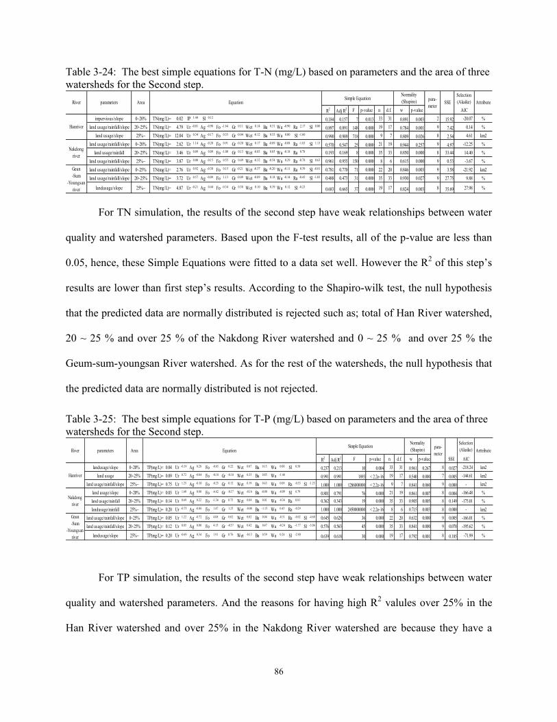
86

Table 3-24: The best simple equations for T-N (mg/L) based on parameters and the area of three

watersheds for the Second step. Selection

(Akaike)

R2


impervious/slope 0~20% TN(mg/L)= 0.02 IP 1.44 Sl 0.120.184 0.157 7 0.013 33 31 0.891 0.003 2 15.92 -20.07 %

land usage/rainfall/slope 20~25% TN(mg/L)= 4.79 Ur -0.01 Ag -0.98 Fo -1.64 Gr 0.11 Wet 0.14 Ba 0.31 Wa -0.90 Ra 2.17 Sl 0.000.897 0.891 148 0.000 19 17 0.784 0.001 9 7.42 0.14 %

land usage/slope 25%~ TN(mg/L)= 12.04 Ur 0.34 Ag -0.17 Fo 0.55 Gr -0.04 Wet -0.12 Ba 0.53 Wa 0.00 Sl -1.600.990 0.989 718 0.000 9 7 0.809 0.026 8 2.54 4.61 km2

land usage/rainfall/slope 0~20% TN(mg/L)= 2.62 Ur 1.14 Ag -0.20 Fo 0.91 Gr -0.20 Wet 0.17 Ba -0.09 Wa -0.08 Ra -1.83 Sl 1.130.570 0.547 25 0.000 21 19 0.944 0.257 9 4.97 -12.25 %

land usage/rainfall 20~25% TN(mg/L)= 3.46 Ur 0.09 Ag 0.09 Fo -1.00 Gr 0.13 Wet -0.03 Ba 0.05 Wa -0.18 Ra 0.78 0.193 0.169 8 0.008 35 33 0.850 0.000 8 33.44 14.40 %

land usage/rainfall/slope 25%~ TN(mg/L)= 3.87 Ur 0.00 Ag -0.15 Fo 0.55 Gr 0.49 Wet -0.32 Ba -0.54 Wa 0.29 Ra -0.78 Sl 0.63 0.961 0.955 150 0.000 8 6 0.615 0.000 9 0.53 -3.67 %

land usage/rainfall/slope 0~25% TN(mg/L)= 2.76 Ur 0.92 Ag -0.30 Fo 0.15 Gr -0.21 Wet -0.37 Ba -0.20 Wa -0.11 Ra 0.39 Sl -0.81 0.781 0.770 71 0.000 22 20 0.846 0.003 9 3.58 -21.92 km2

land usage/rainfall/slope 20~25% TN(mg/L)= 3.72 Ur 0.57 Ag -0.09 Fo 1.13 Gr -0.09 Wet -0.09 Ba 0.18 Wa -0.14 Ra -0.45 Sl -1.03 0.488 0.473 31 0.000 35 33 0.930 0.027 9 27.75 9.88 %

landusage/slope 25%~ TN(mg/L)= 4.87 Ur -0.21 Ag 0.44 Fo -0.34 Gr 0.58 Wet 0.10 Ba 0.39 Wa 0.12 Sl -0.230.683 0.665 37 0.000 19 17 0.824 0.003 8 35.69 27.98 %

Hanriver

Nakdong

river

Geun

-Sum

-Youngsan

river

AttributeRiver parameters Area EquationSimple Equation

Normality

(Shapiro)para-

meterSSE

For TN simulation, the results of the second step have weak relationships between water

quality and watershed parameters. Based upon the F-test results, all of the p-value are less than

0.05, hence, these Simple Equations were fitted to a data set well. However the R2 of this step’s

results are lower than first step’s results. According to the Shapiro-wilk test, the null hypothesis

that the predicted data are normally distributed is rejected such as; total of Han River watershed,

20 ~ 25 % and over 25 % of the Nakdong River watershed and 0 ~ 25 % and over 25 % the

Geum-sum-youngsan River watershed. As for the rest of the watersheds, the null hypothesis that

the predicted data are normally distributed is not rejected.

Table 3-25: The best simple equations for T-P (mg/L) based on parameters and the area of three

watersheds for the Second step. Selection

(Akaike)

R2

Adj R2 F p-value n d.f. w p-value SSE AIC

landusage/slope 0~20% TP(mg/L)= 0.04 Ur -0.19 Ag 0.28 Fo -0.65 Gr 0.22 Wet 0.07 Ba 0.15 Wa 0.00 Sl 0.500.237 0.213 10 0.004 33 31 0.961 0.267 8 0.027 -218.24 km2

land usage 20~25% TP(mg/L)= 0.09 Ur 0.72 Ag -0.04 Fo -0.10 Gr -0.10 Wet 0.33 Ba 0.85 Wa -1.480.991 0.991 1893 < 2.2e-16 19 17 0.540 0.000 7 0.005 -144.61 km2

land usage/rainfall/slope 25%~ TP(mg/L)= 0.75 Ur 1.25 Ag -0.10 Fo -0.25 Gr 0.12 Wet 0.19 Ba 0.43 Wa 0.09 Ra -0.35 Sl -1.251.000 1.000 1286000000 < 2.2e-16 9 7 0.841 0.060 9 0.000 - km2

land usage/slope 0~20% TP(mg/L)= 0.03 Ur 1.60 Ag 0.80 Fo -6.42 Gr -0.17 Wet -0.16 Ba -0.08 Wa -0.09 Sl 6.790.801 0.791 76 0.000 21 19 0.861 0.007 8 0.004 -166.48 %

land usage/rainfall 20~25% TP(mg/L)= 0.14 Ur 0.69 Ag 0.22 Fo -1.36 Gr 0.75 Wet 0.04 Ba 0.01 Wa -0.36 Ra 0.81 0.362 0.343 19 0.000 35 33 0.905 0.005 8 0.149 -175.01 %

landusage/rainfall 25%~ TP(mg/L)= 0.20 Ur -0.75 Ag -0.86 Fo 1.47 Gr 1.25 Wet -0.08 Ba -1.15 Wa 0.45 Ra -0.29 1.000 1.000 2450000000 < 2.2e-16 8 6 0.715 0.003 8 0.000 - km2

land usage/rainfall/slope 0~25% TP(mg/L)= 0.05 Ur 1.22 Ag -0.72 Fo 4.08 Gr 0.02 Wet 0.02 Ba 0.04 Wa -0.31 Ra -0.02 Sl -4.68 0.645 0.628 36 0.000 22 20 0.632 0.000 9 0.005 -166.01 %

land usage/rainfall/slope 20~25% TP(mg/L)= 0.12 Ur 0.85 Ag 0.00 Fo 4.15 Gr -0.37 Wet 0.42 Ba 0.47 Wa -0.24 Ra -1.77 Sl -3.06 0.576 0.563 45 0.000 35 33 0.841 0.000 9 0.078 -195.62 %

landusage/slope 25%~ TP(mg/L)= 0.20 Ur -0.69 Ag 0.34 Fo 1.91 Gr 0.76 Wet -0.13 Ba 0.59 Wa 0.24 Sl -2.900.639 0.618 30 0.000 19 17 0.792 0.001 8 0.185 -71.99 %

ArttributeRiver parameters Area Equationpara-

meter

Hanriver

Nakdong

river

Geun

-Sum

-Youngsan

river


(Shapiro)

For TP simulation, the results of the second step have weak relationships between water

quality and watershed parameters. And the reasons for having high R2 valules over 25% in the

Han River watershed and over 25% in the Nakdong River watershed are because they have a

87

very small degree of freedom compared to the number of parameters. Based upon the F-test

results, all of the p-values are less than 0.05, hence, these Simple Equations were fitted to a data

set well. However, the R2 of this step’s results are lower than first step’s results. According to the


such as; 20 ~ 25 % for the Han River watershed and total of Nakdong River and Geum-sum-

youngsan River watershed. As for the rest of watersheds, the null hypothesis that the predicted

data are normally distributed is not rejected.

As in the results of the second step, land usage and not imperviousness resulted in the

large number of simple equations generated. The combination of land usage/rainfall/slope

resulted in the largest number of equations relating water quality and watershed parameters, land

usage and slope resulted in the second largest number of equations, and land usage alone resulted

in the third largest number of eqautions. The correlations between imperviousness and water

quality were the poorest and, in most cased did not result in any equations relating the

parameters. These results are shown in Table 3-26.

Table 3-26: The number of best simple equations of each scenario for the second step.

Scenarios Parameters COD BOD T-N T-P

1 Impervious



4 Impervious Slope 1


6 Slope

7 Land Usage 2 2 2

8 Land Usage Rainfall 1 1

9 Land Usage Slope 3 4 2 3

10 Land Usage Rainfall Slope 4 3 5 3

88

[The results of the third step simple equations]

Tables 3-27 through 3-30 show the best simple equations derived from the third step of

the analysis in chapter 3.4.3. These equations relate the standard watershed parameters (i.e.


represented through COD, BOD, TN, and TP.


three watersheds for the Third step. Selection

(Akaike)

R2


land usage/slope 0~20% COD(mg/L)= 3.76 Ur 0.06 Ag 0.25 Fo -0.40 Gr 0.05 Wet 0.07 Ba 0.06 Wa 0.06 Sl 0.230.4192 0.4134 72.2 0.000 102 100 0.9742 0.0428 8 39.77 -80.07 %

land usage/slope 20~25% COD(mg/L)= 8.17 Ur 0.30 Ag 0.05 Fo 0.00 Gr -0.24 Wet 0.08 Ba -0.01 Wa -0.01 Sl -0.370.2524 0.2385 18.2 0.000 56 54 0.9765 0.3428 8 128.83 62.66 km2

land usage/rainfall/slope 25%~ COD(mg/L)= 7.43 Ur -0.23 Ag 0.05 Fo -1.00 Gr 0.38 Wet 0.04 Ba 0.11 Wa -0.04 Ra 0.65 Sl 0.170.7719 0.7599 64.3 0.000 21 19 0.7954 0.0006 9 28.73 24.58 %

land usage 0~20% COD(mg/L)= 3.51 Ur 0.05 Ag 0.19 Fo -0.16 Gr 0.08 Wet 0.05 Ba 0.06 Wa 0.070.481 0.4697 42.6 0.000 48 46 0.9788 0.5291 7 15.05 -41.67 %

land usage/rainfall 20~25% COD(mg/L)= 6.86 Ur 0.40 Ag 0.25 Fo -0.49 Gr -0.13 Wet 0.09 Ba -0.08 Wa 0.01 Ra 0.01 0.3641 0.3442 18.3 0.000 35 33 0.9667 0.3767 8 42.15 22.51 %

landusage/slope 25%~ COD(mg/L)= 7.53 Ur 0.05 Ag -0.14 Fo 0.36 Gr 0.09 Wet -0.04 Ba 0.20 Wa -0.18 Sl -0.52 0.0287 -0.06 0.3 0.580 8 6 0.9319 0.3606 8 76.93 34.11 %

Below

250km

Above

250km

AttributeArea parameters impervious EquationSimple Equation

Normality

(Shapiro)para-

meterSSE


three watersheds for the Third step. Selection

(Akaike)

R2

Adj R2 F p-value n d.f. w p-value SSE AIC

land usage/rainfall/slope 0~20% BOD(mg/L)= 3.60 Ur 0.17 Ag 0.16 Fo 0.26 Gr -0.03 Wet 0.07 Ba 0.02 Wa 0.01 Ra -0.30 Sl -0.380.284 0.277 39.64 0.000 102 100 0.968 0.013 9 9.48 -224.35 %

land usage/slope 20~25% BOD(mg/L)= 8.99 Ur 0.60 Ag 0.01 Fo 0.14 Gr -0.27 Wet 0.07 Ba -0.01 Wa -0.32 Sl -0.860.379 0.368 32.98 0.000 56 54 0.938 0.007 8 43.83 2.28 km2

land usage/rainfall 25%~ BOD(mg/L)= 6.78 Ur -0.07 Ag 0.08 Fo -0.83 Gr 0.40 Wet -0.06 Ba 0.06 Wa -0.11 Ra 0.410.846 0.838 104.20 0.000 21 19 0.675 0.000 8 14.09 7.62 %

land usage/rainfall/slope 0~20% BOD(mg/L)= 4.21 Ur 0.17 Ag 0.12 Fo -0.70 Gr -0.03 Wet 0.06 Ba 0.07 Wa 0.03 Ra 0.01 Sl 0.470.465 0.453 39.96 0.000 48 46 0.979 0.525 9 3.29 -110.73 km2

land usage/rainfall/slope 20~25% BOD(mg/L)= 5.10 Ur 0.82 Ag -0.12 Fo -0.26 Gr -0.01 Wet 0.05 Ba -0.01 Wa -0.21 Ra 0.39 Sl -0.88 0.606 0.594 49.29 0.000 35 33 0.873 0.001 9 11.91 -19.73 km2

landusage/rainfall/slope 25%~ BOD(mg/L)= 7.73 Ur -2.41 Ag -3.16 Fo 0.29 Gr -0.39 Wet -0.01 Ba 0.66 Wa -0.73 Ra 4.94 Sl -2.58 0.973 0.970 393.30 0.000 8 6 0.835 0.018 9 7.65 17.64 %

Below

250km2

Above

250km2


Normality

(Shapiro)para-

meter

Table 3-29: The best simple equations for T-N (mg/L) based on parameters and the area of three

watersheds for the Third step. Selection

(Akaike)

R2


land usage/rainfall 0~20% TN(mg/L)= 6.87 Ur 0.40 Ag -0.08 Fo -0.03 Gr -0.16 Wet -0.01 Ba -0.02 Wa -0.13 Ra -0.230.255 0.247 34.1 0.000 102 100 0.931 0.000 8 50.23 -56.25 km2

land usage/rainfall 20~25% TN(mg/L)= 5.45 Ur 0.56 Ag -0.17 Fo 0.12 Gr -0.15 Wet 0.01 Ba 0.14 Wa -0.19 Ra -0.290.265 0.251 19.4 0.000 56 54 0.846 0.000 8 87.34 40.89 %

land usage/rainfall 25%~ TN(mg/L)= 6.97 Ur -0.22 Ag -0.01 Fo -1.16 Gr 0.53 Wet 0.04 Ba 0.31 Wa -0.05 Ra 0.800.802 0.792 77.1 0.000 21 19 0.766 0.000 8 57.83 37.27 %

land usage/rainfall/slope 0~20% TN(mg/L)= 2.62 Ur 0.09 Ag 0.26 Fo -0.04 Gr -0.09 Wet -0.17 Ba 0.17 Wa -0.20 Ra -0.41 Sl 0.280.227 0.210 13.5 0.001 48 46 0.986 0.812 9 22.427 -18.52 km2

land usage/slope 20~25% TN(mg/L)= 5.41 Ur 0.35 Ag 0.51 Fo -0.44 Gr -0.37 Wet 0.03 Ba 0.40 Wa -0.37 Sl -0.29 0.480 0.464 29.5 0.000 34 32 0.946 0.093 8 28.37 9.85 km2

landusage/rainfall/slope 25%~ TN(mg/L)= 7.62 Ur 0.70 Ag -0.34 Fo 0.25 Gr 0.53 Wet 0.01 Ba -0.02 Wa -0.19 Ra 0.26 Sl -1.51 0.939 0.934 170.2 0.000 13 11 0.803 0.007 9 22.4 25.07 km2

Below

250km

Above

250km


Normality

(Shapiro)para-

meterSSE

89

Table 3-30: The best simple equations for T-P (mg/L) based on parameters and the area of three

watersheds for the Third step.

Selection

(Akaike)

R2


impervious/rainfall/slope 0~20% TP(mg/L)= 19.54 IP -0.14 Ra -0.19 Sl -1.380.077 0.068 8.4 0.005 102 100 0.974 0.038 8 0.09 -703.45 km2

slope 20~25% TP(mg/L)= 11.81 Sl -1.650.000 -0.019 0.0 0.984 56 54 0.690 0.000 8 0.73 -226.75 km2

pervious/impervious 25%~ TP(mg/L)= 6.30 P -1.86 IP 1.250.322 0.286 9.0 0.007 21 19 0.780 0.000 9 1.85 -33.03 %

pervious/impervious 0~20% TP(mg/L)= 76.42 P -4.06 IP 3.680.122 0.103 6.4 0.015 48 46 0.964 0.146 7 0.04 -328.53 km2

land usage/rainfall/slope 20~25% TP(mg/L)= 5.55 Ur 0.78 Ag 0.47 Fo -2.26 Gr -0.51 Wet 0.08 Ba 0.50 Wa -0.96 Ra 0.73 Sl -0.19 0.698 0.689 74.0 0.000 35 33 0.835 0.000 8 0.06 -209.64 %

landusage/slope 25%~ TP(mg/L)= 8.88 Ur 1.33 Ag -0.55 Fo 0.23 Gr -0.86 Wet 0.59 Ba -0.21 Wa -0.18 Sl -1.68 0.937 0.932 164.4 0.000 8 6 0.743 0.002 8 0.14 -16.13 %

Below

250km

Above

250km


Normality

(Shapiro)para-

meterSSE

The results of the third step resulted in poor values of R2, thus the simple equations

derived from the third step’s methodology should not be used to relate watershed characteristics

to water quality parameters because the correlations between the parameters are poor and the

relationships are not suitable.

An overall comparison of the statistical results of the equations generated through the

methodologies in analysis steps first, second, and third, show that the strongest equations are

those derived in step first. Therefore, the first step’s simple equations are the best of the simple

equations and should be used for predicting the future water quality in South Korea for each

standard sub-watershed according to analyses undertaken using the Excel Solver tool.

3.7.3 STATISTICAL ANALYSIS SYSTEM (SAS)

An additional analysis was undertaken using SAS to correlate water quality parameters to

watershed parameters. The “SAS 8.02” software was used to perform regression analysis

between watershed parameters and water quality. Factor analysis was implemented to describe

the variability among observed data and determinded the parameter priorities as they relate to

impacts on water quality. The code shown in Figure 3-18 below was used.

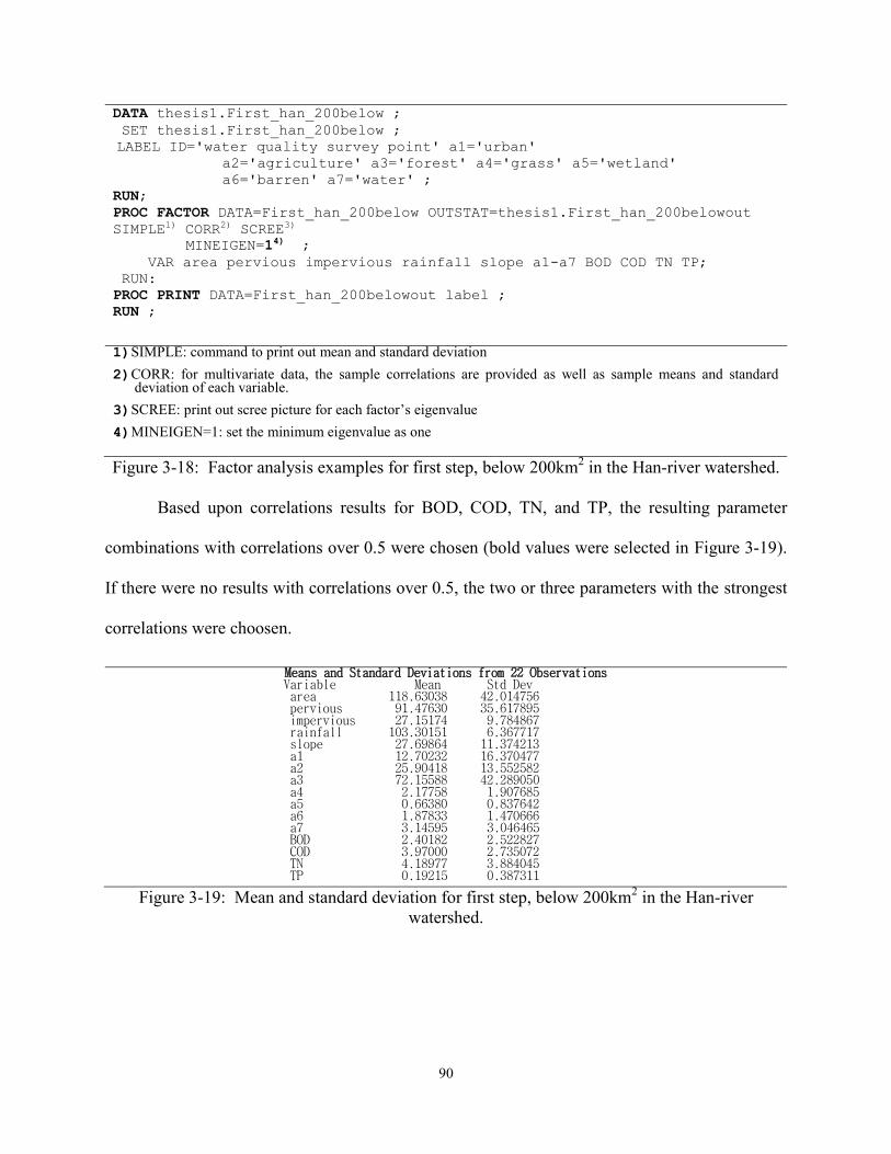
90

DATA thesis1.First_han_200below ;

SET thesis1.First_han_200below ;

LABEL ID='water quality survey point' a1='urban'

a2='agriculture' a3='forest' a4='grass' a5='wetland'

a6='barren' a7='water' ;

RUN;

PROC FACTOR DATA=First_han_200below OUTSTAT=thesis1.First_han_200belowout

SIMPLE1) CORR2) SCREE3)

MINEIGEN=14) ;

VAR area pervious impervious rainfall slope a1-a7 BOD COD TN TP;

RUN:

PROC PRINT DATA=First_han_200belowout label ;

RUN ;

1) SIMPLE: command to print out mean and standard deviation

2) CORR: for multivariate data, the sample correlations are provided as well as sample means and standard deviation of each variable.

3) SCREE: print out scree picture for each factor’s eigenvalue

4) MINEIGEN=1: set the minimum eigenvalue as one

Figure 3-18: Factor analysis examples for first step, below 200km2 in the Han-river watershed.

Based upon correlations results for BOD, COD, TN, and TP, the resulting parameter

combinations with correlations over 0.5 were chosen (bold values were selected in Figure 3-19).

If there were no results with correlations over 0.5, the two or three parameters with the strongest

correlations were choosen.

Means and Standard Deviations from 22 Observations Variable Mean Std Dev area 118.63038 42.014756 pervious 91.47630 35.617895 impervious 27.15174 9.784867 rainfall 103.30151 6.367717 slope 27.69864 11.374213 a1 12.70232 16.370477 a2 25.90418 13.552582 a3 72.15588 42.289050 a4 2.17758 1.907685 a5 0.66380 0.837642 a6 1.87833 1.470666 a7 3.14595 3.046465 BOD 2.40182 2.522827 COD 3.97000 2.735072 TN 4.18977 3.884045 TP 0.19215 0.387311

Figure 3-19: Mean and standard deviation for first step, below 200km2 in the Han-river

watershed.

91

Correlations

BOD COD TN TP

area area 0.05467 0.04801 -0.03589 0.07954

pervious pervious -0.11685 -0.12572 -0.20416 -0.09007

impervious impervious 0.65959 0.66323 0.58850 0.66884

rainfall rainfall 0.23548 0.22133 0.19241 0.09040

slope slope -0.54583 -0.59897 -0.50919 -0.47123

a1 urban 0.88137 0.90186 0.89691 0.84966

a2 agriculture 0.05197 0.05239 -0.05055 0.06670

a3 forest -0.34486 -0.37039 -0.40169 -0.30967

a4 grass 0.43312 0.47729 0.38747 0.45946

a5 wetland -0.12422 -0.04831 -0.17653 -0.14145

a6 barren 0.78164 0.80128 0.77551 0.73040

a7 water -0.04219 0.05017 -0.08394 -0.07012

BOD BOD 1.00000 0.98573 0.97697 0.97065

COD COD 0.98573 1.00000 0.96866 0.96471

TN TN 0.97697 0.96866 1.00000 0.97406

TP TP 0.97065 0.96471 0.97406 1.00000

Figure 3-20: Correlations between parameters and water quality for first step, below 200km2 in

the Han-river watershed.

Using the selected parameters, statistical multiple regression was performed using the

following SAS code.

PROC REG DATA=thesis1.First_200below ;

model BOD = impervious a1 a6 /collin vif tol ;

RUN;

PROC REG DATA=thesis1.First_200below ;

model COD = impervious a1 a6 /collin vif tol ;

RUN;

PROC REG DATA=thesis1.third_per_250o_25over ;

model TN = impervious a1 a6 /collin vif tol ;

RUN;

PROC REG DATA=thesis1.third_per_250o_25over ;

model TP = impervious a1 a6 /collin vif tol ;

RUN;

PROC REG: Estimates the coefficients of a multiple regression and their standard errors are provided

Collin: prints multicollinearity

vif: prints the variance inflation factor for each parameter

estimate

tol: prints the tolerance

Figure 3-21: Regression analysis code for first step, below 200km2 in the Han-river watershed.

After implementing the regression analysis procedure, the results shown in Figure 3-22

were obtained.

92

The REG Procedure Model: MODEL1 Dependent Variable: BOD BOD Analysis of Variance

Sum of Mean Source DF Squares Square F Value Pr > F Model 3 109.90871 36.63624 27.77 <.0001 Error 18 23.74902 1.31939 Corrected Total 21 133.65773 Root MSE 1.14865 R-Square 0.8223 Dependent Mean 2.40182 Adj R-Sq 0.7927 Coeff Var 47.82406 Parameter Estimates Parameter Standard Variance Label DF Estimate Error t Value Pr > |t| Tolerance Inflation Intercept 1 -0.82862 0.77558 -1.07 0.2995 . 0 impervious 1 0.07385 0.03572 2.07 0.0534 0.51432 1.94430 urban 1 0.12744 0.02947 4.33 0.0004 0.27002 3.70346 barren 1 -0.20956 0.37897 -0.55 0.5871 0.20226 4.94402

Figure 3-22: Regression analysis code for first step, below 200km2 in the Han-river watershed.

The models for BOD, COD, TN, and TP in relation with available parameters could be

calculated by following the procedures mentioned above. For instance, the following function

shown in equation 11 gave the BOD model in the Han-river of 200km2 below watershed. Based

on Figure 3-22, p-value (Pr) is less than 0.05, and multicollinearity doesn’t need to be considered

because the tolerance is over 0.1 and Variance Inflation is less than 10 based upon the Kim

(2011).

Equation 24

Based upon the abovementioned procedures, a variety of regression functions were

examined and evaluated. Among them, the best simple equations (regression analysis) are shown

in Tables 3-31 to 3-34. These tables include the statistical coefficients of each statistical model

used. The first case of the analysis in chapter 3.4.1, which is the area allocation of a sub-

watershed, could acquire the best coefficient when compared with the second and third step,

which were the percentage of imperviousness in chapter 3.4.2, both area allocations and the

93

percentage of imperviousness in chapter 3.4.3, respectively. These results show the same

tendencies in the results as were determined using EXCEL SOLVER. Thus, these equations

could also be used to predict the concentrations (mg/L) of BOD, COD, TN, and TP depending on

the areas of standard sub-watersheds. For instance, the equations can be used for standard sub-

watershed within the Geum-Sum-Youngsan River watershed with the following areas: below

100 km2, 100 to 150 km

2, 150 to 200 km

2, and over 200 km

2. They can also be used for the Han

River and Nakdong River watersheds for the following areas: below 200 km2, 200 to 500 km

2,

and over 500 km2.

According to the statistical analysis of the simple equations for BOD (mg/L), the range of

RMSE was 0.392 to 1.908, R2 was 0.427 to 0.854, adjusted R

2 was 0.267 to 0.801, and the p-

value is almost lower than 0.05 except in the case of the Geum-Sum-Youngsan River’s sub-

watershed below 100 km2. Most of the simple equations were within the criteria in which

multicollinearity did not occur, except the Geum-Sum-Youngsan River, which was over the

200km2 scenario based on the criteria of the tolerance (tol) and variance inflation factor (vif),

which were below 0.1 and over 10, respectively.

Table 3-31: The simple equations (BOD) based upon regression analysis using SAS. Watershed Cases Scenarios RMSE R

2Adj R

2 coeff var p-value tol vif

first(km) 100 below BOD= 0.218 + 0.080 imp + 0.017 ag + 0.215 we 0.720 0.436 0.267 32.318 0.1121

0.75598

0.65237

0.54489

1.32278

1.53287

1.83523

100-150 BOD= -7.682 + 0.458 imp - 0.054 ur + 0.006 gr + 0.099 ba 0.905 0.770 0.667 41.572 0.006

0.13947

0.06820

0.34954

0.15016

7.17009

14.66381

2.86088

6.65934

150-200 BOD= 0.116 + 0.026 imp + 0.036 ag + 0.415 wa 0.744 0.651 0.476 31.397 0.08

0.16515

0.14073

0.62690

6.05514

7.10573

1.59514

200 over BOD= 1.041 - 0.090 imp + 0.164 ur + 0.058 ag + 0.469 ba 0.700 0.744 0.711 34.177 <.0001

0.00927

0.03920

0.02271

0.43282

107.88533

25.50841

44.03676

2.31044

first(km) 200 below BOD= -0.829 + 0.074 imp + 0.127 ur - 0.210 ba 1.149 0.822 0.793 47.824 <.0001

0.51432

0.27002

0.20226

1.94430

3.70346

4.94402

200~500 BOD= 4.322 - 0.296 imp + 0.298 ur + 1.867 ba 1.908 0.842 0.818 61.424 <.0002

0.10321

0.12300

0.39578

9.68944

8.13036

2.52663

500 over BOD= 0.030 + 0.003 imp + 0.187 ur + 0.262 gr + 0.242 ba 0.392 0.854 0.801 30.596 0.0001

0.34282

0.30225

0.43529

0.52463

2.91701

3.30850

2.29732

1.90612

200 below BOD= -2.742 + 0.217 imp 0.760 0.427 0.397 34.475 0.0013 1.000 1.000

200~500 BOD= 1.799 - 0.056 imp + 0.061 ur + 0.664 gr 0.700 0.471 0.414 42.663 0.0004

0.31338

0.23590

0.26163

3.19099

4.23917

3.82220

first(km) 500 over BOD= -0.020 - 0.004 ur - 0.026 gr + 0.108 we + 0.115 wa 0.534 0.777 0.628 38.427 0.0372

0.18933

0.13205

0.08443

0.08840

5.28167

7.57290

11.84382

11.31225

Han-river

first(%)

Nak-river

first(per)

Equations

Geum-Sum-

Youngsan-

riverfirst(%)

94

Table 3-32: The simple equations (COD) based upon regression analysis using SAS.

watershed Cases Scenarios RMSE R2

Adj R2 coeff var p-value tol vif

first(km) 100 below COD= 2.231 + 0.023 ag + 0.945 we + 0.562 wa 0.985 0.700 0.609 21.527 0.0057

0.55441

0.64430

0.83002

1.80373

1.55206

1.20479

first(%) 100-150 COD= -14.540 + 0.924 imp - 0.363 ur + 0.078 ga + 0.664 ba 1.363 0.800 0.711 28.941 0.0033

0.13947

0.06820

0.34954

0.15016

7.17009

14.66381

2.86088

6.65934

first(km) 150-200 COD= 1.870 + 0.017 ag + 0.850 wa 0.774 0.770 0.705 15.676 0.08

0.47767

0.41484

0.79793

2.09351

2.41056

1.25325

first(%) 200 over COD= 13.917 - 0.880 imp + 0.376 ur + 0.221 ag + 1.443 ba 0.701 0.827 0.805 15.950 <.0001

0.00927

0.03920

0.02271

0.43282

107.88533

25.50841

44.03676

2.31044

first(km) 200 below COD= 0.504 + 0.075 imp + 0.140 ur - 0.185 ba 1.128 0.854 0.830 28.423 <.0001

0.51432

0.27002

0.20226

1.94430

3.70346

4.94402

200~500 COD= -0.160 + 0.089 imp + 0.123 ur + 1.164 ba 1.007 0.919 0.906 23.674 <.0001

0.10321

0.12300

0.39578

9.68944

8.13036

2.52663

500 over COD= -1.649 + 0.205 imp + 0.169 ag - 0.039 ag + 0.638 gr 0.466 0.904 0.869 16.241 0.0001

0.34282

0.30225

0.43529

0.52463

2.91701

3.30850

2.29732

1.90612

200 below COD= -4.009 + 0.404 imp 1.396 0.433 0.403 26.886 0.0013 1.000 1.000

200~500 COD= 3.042 - 0.062 imp + 0.130 ur + 1.373 gr 1.406 0.538 0.489 36.242 0.0004

0.31338

0.23590

0.26163

3.19099

4.23917

3.82220

500 over COD= -1.758 + 0.003 ar + 0.658 gr + 0.916 we + 1.266 wa 1.071 0.799 0.664 29.701 0.0441

0.46770

0.21932

0.19118

0.21798

2.13811

4.55945

5.23075

4.58750

Han-river

first(%)

Nak-river first(per)

Equations

Geum-Sum-

Youngsan-

river

According to the statistical analysis of the simple equations for COD (mg/L), the range of

RMSE was 0.466 to 1.406, R2 was 0.433 to 0.854, adjusted R

2 was 0.403 to 0.906, p-value was

almost lower than 0.05, except in the case of the Geum-Sum-Youngsan River’s 150 to 200 km2

area and Nakdong River’s over 500 km2 scenarios. The multicollinary value is almost satisfied

within the criteria except Geum-Sum-Youngsan River’s over 200km2 scenarios as was found

with the BOD simple equations.

Table 3-33: The simple equations (TN) based upon regression analysis using SAS. watershed Cases Scenarios RMSE R

2Adj R


100 below TN= 0.690 + 0.098 imp + 0.922 we 1.000 0.445 0.345 32.203 0.0390.75639

0.75639

1.32206

1.32206

100-150 TN= -6.839 + 0.299 imp + 0.038 ur + 1.129 ba 0.839 0.933 0.913 21.325 <.0001

0.28627

0.08394

0.14761

3.49317

11.91298

6.77456

150-200 TN= 2.063 + 0.011 ag + 0.250 wa 0.762 0.335 0.145 23.468 0.2400.86407

0.86407

1.15731

1.15731

first(%) 200 over TN= 5.393 - 0.363 imp + 0.285 ur + 0.110 ag + 0.760 ba 0.913 0.700 0.662 32.903 <.0001

0.00927

0.03920

0.02271

0.43282

107.88533

25.50841

44.03676

2.31044

200 below TN= 0.232 + 0.064 imp + 0.210 ur + -0.244 ba 1.788 0.818 0.788 42.673 <.0001

0.51432

0.27002

0.20226

1.94430

3.70346

4.94402

200~500 TN= 2.563 - 0.018 imp + 0.136 ur + 0.049 ba 1.783 0.895 0.879 36.164 <.0001

0.36232

0.34358

0.38673

2.76002

2.91049

2.58581

first(%) 500 over TN= -0.082 + 0.103 imp + 0.124 ur - 0.039 gr + 0.308 ba 0.676 0.618 0.480 26.326 0.022

0.34282

0.30225

0.43529

0.52463

2.91701

3.30850

2.29732

1.90612

first(%) 200 below TN= -0.221 + 0.142 imp 0.841 0.206 0.164 27.952 0.039 1.000 1.000

first(km) 200~500 TN= 2.352 - 0.009 imp + 0.079 ur - 0.079 gr 1.183 0.445 0.385 43.977 0.001

0.77809

0.43720

0.38797

1.28520

2.28729

2.57754

first(%) 500 over TN= -1.310 + 0.002 ar + 0.107 ag 0.945 0.638 0.548 32.565 0.0170.99925

0.99925

1.00075

1.00075

Han-river

first(km)

Nak-river

Equations

Geum-

Sum-

Youngsan-

river

first(km)

95

The statistical analysis of the simple equations for TN (mg/L) acquired the following

results: RMSE ranged from 0.676 to 1.788, R2 ranged from 0.206 to 0.933, adjust R

2 ranged

from 0.164 ~ 0.933, the p-value of Geum-Sum-Youngsan river’s 150 to 200 km2 was over 0.05

and the others were less than 0.05. The multicollinary value is almost satisfied within the criteria

except Geum-Sum-Youngsan river’s over 200km2 scenarios as was found for the BOD simple

equations.

The statistical analysis of the simple equations for TP (mg/L) acquired the following

results, RMSE ranged from 0.025 to 0.189, R2 ranged from 0.151 to 0.960, adjust R

2 ranged

from 0.106 ~ 0.899, and the p-value was over 0.05 with Geum-Sum-Youngsan River’s over 200

km2 and Nakdong river’s below 200 km

2 scenarios. Multicollinary value is almost satisfied

within the criteria except in the case of the Geum-Sum-Youngsan River’s over 200km2 and

Nakdonf river’s over 500 km2 scenarios.

Table 3-34: The simple equations (TP) based upon regression analysis using SAS. watershed Cases Scenarios RMSE R

2Adj R


100 below TP= 0.018 + 0.000 ag + 0.067 we + 0.01468 wa 0.041 0.666 0.565 40.012 0.010

0.55441

0.64430

0.83002

1.80373

1.55206

1.20479

100-150 TP= -0.230 + 0.008 imp + 0.015 ur + 0.000734 gr + 0.027 ba 0.057 0.908 0.868 40.677 0.000

0.28302

0.08389

0.53288

0.13644

3.53336

11.92074

1.87659

7.32915

150-200 TP= 0.184 - 0.011 imp + 0.007 ag 0.119 0.383 0.207 82.968 0.080

0.16515

0.14073

0.62690

6.05514

7.10573

1.59514

200 over TP= 0.105 - 0.012 imp + 0.018 ur + 0.00405 ag + 0.038 ba 0.058 0.719 0.682 62.076 <.0001

0.00927

0.03920

0.02271

0.43282

107.88533

25.50841

44.03676

2.31044

200 below TP= -0.338 + 0.015 imp + 0.021 ur + -0.0748 ba 0.189 0.795 0.761 98.568 <.0001

0.51432

0.27002

0.20226

1.94430

3.70346

4.94402

200~500 TP= 0.072 - 0.002 imp + 0.010 ur + 0.01011 ba 0.152 0.868 0.847 71.221 <.0001

0.36232

0.34358

0.38673

2.76002

2.91049

2.58581

first(%) 500 over TP= -0.007 + 0.00004 imp + 0.007 ur + 0.01583 gr + 0.007 ba 0.021 0.800 0.727 46.578 0.001

0.34282

0.30225

0.43529

0.52463

2.91701

3.30850

2.29732

1.90612

200 below TP= -0.111 + 0.010 imp 0.074 0.151 0.106 59.354 0.4510.82642

0.82642

1.21004

1.21004

200~500 TP= 0.090 - 0.001 imp + 0.006 ur + 0.003 gr 0.074 0.587 0.543 74.154 0.001

0.77809

0.43720

0.38797

1.28520

2.28729

2.57754

500 over TP= -0.052 + 0.001 imp - 0.001 ur - 0.00010 ag - 0.002 gr - 0.020 we + 0.015 wa 0.025 0.960 0.899 28.410 0.009

0.04364

0.15002

0.10024

0.04770

0.07979

0.06523

22.91369

6.66583

9.97600

20.96563

12.53244

15.32989

Han-river

first(km)

Nak-river first(km)

Equations

Geum-Sum-

Youngsan-

river

first(km)

first(%)

96

In conclusion, it is determined using the methodology carried out by the SAS program as

the R2 values obtained for the data correlations were smaller than those obtained through other

methods like the Excel Solver method.

3.7.4 MODEL TREE 5, ANN (ARTIFICIAL NEURAL NETWORK), RBF

Three methods used to generate equations relating watershed parameters to water quality

parameters utilized the Weka Software. The Weka Software was used for building the Model

Tree, the ANN, and the RBF. Version 3.4.4 (Figure 3-23) was used in the analysis. In this

research, the input files were constructed based upon three steps which were already mentioned

in chapter 3.3 (Table 3-35).

Figure 3-23: Weka Software (Verson 3.4.4).

97

Table 3-35: Data classification and scenarios for Model Tree, ANN, RBF.

step Watershed range km, percent

of land use scenarios total Scenarios

First

(area)

Han river

watershed

Below 200 km2

(01) Km

(land use),

(02)Percent

(land use)

(01) imp

(02) imp, per

(03) imp, ra

(04) imp, ra, sl

(05) imp, sl

(06) sl

(07) land

(08) land, ra

(09) land, sl

(10) land, ra, sl

60 (han)

60(Nak)

80(GSY)

Total:200

200 ~ 500 km2

Over 500 km2

Nakdong river

watershed

Below 200 km2

200 ~ 500 km2

Over 500 km2

Geum-sum-

youngsum river

watershed

Below 100 km2

100 ~ 150 km2

150 ~ 200 km2

Over 200 km2

Second

(impervious)

Han river

watershed

Below 20 %

(01) Km

(land use),

(02)Percent

(land use)

(01) imp

(02) imp, per

(03) imp, ra

(04) imp, ra, sl

(05) imp, sl

(06) sl

(07) land

(08) land, ra

(09) land, sl

(10) land, ra, sl

60 (han)

60(Nak)

60(GSY)

Total:180

20 ~ 25 %

Over 25%

Nakdong river

watershed

Below 20 %

20 ~ 25 %

Over 25%

Geum-sum-youngsum river

watershed

Below 20 %

20 ~ 25 %

Over 25%

Third

(area+impervious)

Below 250Km2

Below 20 %

(01) Km

(land use),

(02)Percent

(land use)

(01) imp

(02) imp, per

(03) imp, ra

(04) imp, ra, sl

(05) imp, sl

(06) sl

(07) land

(08) land, ra

(09) land, sl

(10) land, ra, sl

60 (be250)

60(ov250)

Total:120

20 ~ 25 %

Over 25%

Over

250Km2

Below 20 %

20 ~ 25 %

Over 25%

*imp: impervious, per: pervious, ra: rain, sl: slope, land: land usage,

Land usage: urban, agriculture, forest, grass, wetland, barren, water (7 items)

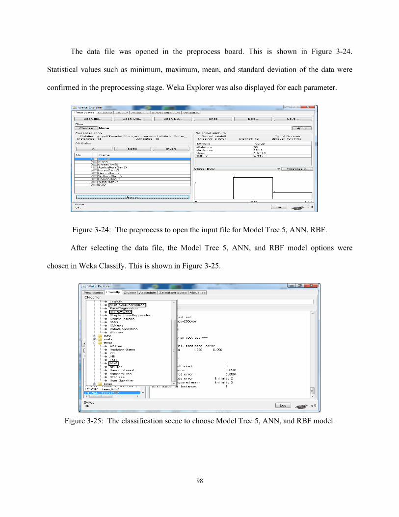
98

The data file was opened in the preprocess board. This is shown in Figure 3-24.

Statistical values such as minimum, maximum, mean, and standard deviation of the data were

confirmed in the preprocessing stage. Weka Explorer was also displayed for each parameter.

Figure 3-24: The preprocess to open the input file for Model Tree 5, ANN, RBF.

After selecting the data file, the Model Tree 5, ANN, and RBF model options were

chosen in Weka Classify. This is shown in Figure 3-25.

Figure 3-25: The classification scene to choose Model Tree 5, ANN, and RBF model.

99

There are four kinds of test options; use training set, used supplied test set, cross-

validation, and percentage split. In this research, percentage split was chosen. Two thirds of the

data (66%) were selected for calibration and the rest (34%) were used for verification. In order to

compare the three models, Model Tree 5, ANN, and RBF model, for example, first step (area) –

Han River watershed – km of land usage – 10 scenarios (see the Table 3-36) was applied.

In the case of Model Tree 5, the regression trees were tried not pruned and pruned to find

optimization results. The minimum number of instances was set to 4 instances. The results of

Model Tree 5 are shown at Figure 3-26. Verification could then be assured using the correlation

coefficient, mean absolute error, root mean squared error, etc. as illustrated in Table 3-36.

According to the statistical evaluation value, the correlation coefficient was 0.9872 and the mean

absolute error was 0.3897. These measures indicate the equation is a reasonably applicable

equation.

LM1 BOD(mg/L) = 0.0228ⅹurban(km2) - 0.0011ⅹ Forest(km2) + 0.0532ⅹ Grass(km2) + 1.0866

LM2 BOD(mg/L) = 0.0228ⅹurban(km2) - 0.0011ⅹForest(km2) + 0.0549ⅹGrass(km2) + 1.1347

LM3 BOD(mg/L) = 0.0176ⅹurban(km2)- 0.0009ⅹForest(km2)+ 0.0199ⅹGrass(km2)+ 1.0422

LM4 BOD(mg/L) = 0.0006ⅹrainfall+ 0.0176ⅹurban(km2) - 0.0009ⅹForest(km2)

+ 0.0199ⅹGrass(km2)- 0.0003ⅹWater(km2)+ 0.9968

LM5 BOD(mg/L) = 0.001ⅹrainfall+ 0.0176ⅹurban(km2)- 0.0009ⅹForest(km2)


LM6 BOD(mg/L) = 0.001ⅹ rainfall+ 0.0176ⅹurban(km2) - 0.0009ⅹForest(km2)


Figure 3-26: Structure and linear models of Model Tree for Han River Watershed.

100

Table 3-36: The BOD result of verification using Model Tree . Han River Watershed (over 500km

2)

Number of Model 6

Time taken to build model 0.02 seconds

Predictions on test split

Instance

number actual predicted Error

1 0.8 0.574 -0.226

2 1.4 1.843 0.443

3 1 0.902 -0.098

4 1.6 2.642 1.042

5 0.9 0.578 -0.322

6 0.8 0.592 -0.208

Correlation coefficient 0.9872

Mean absolute error 0.3897

Root mean squared error 0.4982

Relative absolute error 101.6737 %

Root relative squared error 112.8298 %

The ANN model was built with MultilayerPerceptron. In order to make a condition for

MultilayerPerceptron, training time, validation threshold were set to 700 iterations and 20,

respectively. Learning rate and momentum were installed at 0.3 and 0.2. In order to optimize the

results, several hidden layer values were input into the model. This neural network uses back-

propagation to train the model. Figure 3-27 shows the model training process to try to determine

the best value of each sigmoid Node.

101

Figure 3-27: Structure of ANN with four hidden layers.

As in the case of the ANN scenario, two thirds of the data were used for training and

calibration in the ANN training and the remaining data were used for calculated for verification

same as Model Tree 5. The results of ANN processing are shown at Figure 3-28. These resulting

data could be saved and applied to another supplied data set using “the Re-evaluate model on

current test set” menu. In addition, verification could be assured using correlation coefficient,

mean absolute error, root-mean squared error, etc. as shown in Table 3-37. According to the

statistical evaluation, correlation coefficient was 0.7528 and the mean absolute error was 1.0297.

These correlations indicate the resulting equation could be used to correlate watershed

parameters and water quality. However, the equations determined using the Model Tree 5

methodology are stronger than those determined by ANN, and are therefore preferred.

102

=== Classifier model (full training set) ===

Linear Node 0

Inputs Weights

Threshold 1.8622749989837082 Node 1 -0.21940230009537384

Node 2 -2.23255189052738

Node 3 -0.6202904016938504 Node 4 -0.34135450095104486

Sigmoid Node 1

Inputs Weights Threshold -0.7360270615068755

Attrib rainfall -0.1139465968588408

Attrib urban(km2) 0.33303280195517315 Attrib Agriculture(km2) -0.019795138003605314

Attrib Forest(km2) 0.367797710083048

Attrib Grass(km2) 0.15898404232619276 Attrib Wetland(km2) -0.36669851485770805

Attrib Barren(km2) -0.585618850560819

Attrib Water(km2) 0.49681931588765066 Sigmoid Node 2

Inputs Weights

Threshold 2.02543079184067 Attrib rainfall 0.5705568302691448

Attrib urban(km2) -2.0320851218826936

Attrib Agriculture(km2) -0.5917153760451686 Attrib Forest(km2) 1.0859168414123292

Attrib Grass(km2) -2.003568605239934

Attrib Wetland(km2) 0.3636330381036232 Attrib Barren(km2) -0.9768696531212865

Attrib Water(km2) -0.6129437639777807

Sigmoid Node 3

Inputs Weights Threshold 0.07364216566072915

Attrib rainfall 0.1694010483610415

Attrib urban(km2) 0.10275601786731599 Attrib Agriculture(km2) 0.4954698730996255

Attrib Forest(km2) 0.257984550987477

Attrib Grass(km2) -0.1504141015367104 Attrib Wetland(km2) -0.780562333070119

Attrib Barren(km2) -0.06056344738700687

Attrib Water(km2) 0.013978311691206292 Sigmoid Node 4

Inputs Weights

Threshold -0.9198120364007478 Attrib rainfall -0.09708242430119039

Attrib urban(km2) 0.2771978368085623

Attrib Agriculture(km2) -0.10026262070524744 Attrib Forest(km2) 0.4377005493812114

Attrib Grass(km2) 0.35058832662335515

Attrib Wetland(km2) -0.38816459718986707 Attrib Barren(km2) -0.6408645248822346

Attrib Water(km2) 0.42204597926064963

Class Input

Node 0

Time taken to build model: 0.03 seconds

Figure 3-28: Classifier model using MultilayerPerceptron (ANN).

Table 3-37: The BOD result of verification using ANN. Han River Watershed (over 500km

2)

Number of Model 6



Instance


1 0.8 2.443 1.633

2 1.4 3.288 1.888

3 1 1.600 0.600

4 1.6 3.104 1.504

5 0.9 0.392 -0.508

6 0.8 0.754 -0.046






The RBF model was built with the RBFNetwork which implements a normalized

Gaussian radial basics function network. It uses the k-means clustering algorithm to provide the

basics functions and learns either a logistic regression or linear regression. Clustering Seed,

103

minimum standard deviation, and number of clusters were set to 1, 0.1 and 4, respectively. In

order to optimize the results, the number of cluster values was input from 2 to 5 or 6.

For RBF training, two third of the data were used for calibration and the remaining data

were used for verification as with Model Tree 5 and ANN processing. The results of RBF are

shown in Figure 3-29 which could be saved and applied to another supplied data set using “the

Re-evaluate model on current test set” menu. In addition, verification could be assured using the

correlation coefficient, mean absolute error, roots mean squared error, etc. as shown in Table 3-

38. According to the statistical evaluation, the correlation coefficient was 0.4521 and mean

absolute error was 0.5387. The correlation coefficient for the RBF process is less than both those

for the Model Tree 5 and ANN.

=== Classifier model (full training set) === Radial basis function network (Linear regression applied to K-means clusters as basis functions): Linear Regression Model BOD = -0.0459 * pCluster_0_0 + 0.0459 * pCluster_0_1 + 1.2872 Time taken to build model: 0.02 seconds

Figure 3-29: Classifier model using RBFNetwork.

Table 3-38: The BOD result of verification using RBF.

Han River Watershed (over 500km2)

Number of Model 6



Instance


1 0.8 1.952 1.152

2 1.4 1.960 0.560

3 1 0.840 -0.16

4 1.6 1.960 0.360

5 0.9 1.860 0.960

6 0.8 0.840 0.04






104

A comparison of the three models used in the Weka software package (Model Tree 5,

ANN, and RBF) shows that Model Tree 5 is the best model to relate BOD to watershed

parameters of standard subwatershed areas 500km2 in the Han River watershed.

Following the above-mentioned procedure, the best applicable simple equations of each

watershed are shown in Tables 3-39 to 3-41.

Table 3-39: The evaluation results of First step’s M5P, ANN, RBF (BOD, mg/L).

C.C M.A.E R.M.S.E R.A.E R.R.S.ETotal No.

Of instances

gsy(M5P)_100 9 14 2 0.9943 0.2044 0.2401 40.52% 42.45% 5 km

gsy(ANN)_150 2 14 6 0.959 1.1982 1.4216 67.07% 63.91% 5 km

gsy(ANN)_200 5 10 6 0.9374 0.3663 0.4321 38.89% 34.00% 4 km

gsy(RBF)_200over 7 36 6 0.9192 0.2501 0.3272 28.52% 35.09% 13 %

han(M5P)_200 2 22 1 0.9408 0.7205 1.0108 61.13% 79.48% 8 %

han(ANN)_500 5 23 7 0.9949 2.5715 4.3443 101.91% 146.32% 8 km

han(RBF)_500over 5 16 3 0.9682 0.2217 0.2957 57.84% 66.96% 6 km

nakdong(M5P)_200 3 21 2 0.7428 0.6569 0.6923 79.62% 77.21% 8 %

nakdong(ANN)_500 8 32 6 0.7651 0.5259 0.5861 68.98% 66.82% 11 km

nakdong(RBF)_500over 9 11 3 0.8828 0.3331 0.404 49.88% 49.07% 4 %

Model ScenarioNo.of

Instances

No.of

Rules/hidden

/cluster

Evaluation on test split

km2/%

*C.C: Correlation coefficient, M.A.E: Mean absolute error, R.M.S.E: Root mean squared error,

R.A.E: Relative absolute error, R.R.S.E: Root relative squared error,

Total NO. of Instances: Total number of instances.

* Scenario 1: impervious, Scenario 2: Impervious + pervious

Scenario 3: Impervious + rainfall, Scenario 4: Impervious + rainfall + slope

Scenario 5: Impervious + slope Scenario 6: slope

Scenario 7: Land use Scenario 8: Land use + rainfall

Scenario 9: Land use + slope Scenario 10: Land use + rainfall + slope

Table 3-40: The evaluation results of Second step’s M5P, ANN, RBF (BOD, mg/L).

* Scenario 1 : impervious


Of instances

gsy(RBF)_20 8 22 3 0.8006 0.0769 0.0952 60.68% 64.86% 8 km

gsy(M5P)_25 4 35 16 0.7918 0.5101 0.5812 63.76% 63.57% 12 km

gsy(M5P)_25over 8 17 7 0.8349 1.368 1.7094 104.99% 122.68% 6 %

han(RBF)_20 8 22 3 0.7967 0.1335 0.1619 65.58% 70.65% 8 %

han(ANN)_25 9 19 7 0.8791 0.8319 1.0882 105.40% 123.76% 7 km

han(ANN)_25over 6 9 4 0.9734 2.1819 2.9446 35.28% 46.20% 4 %

nakdong(ANN)_20 3 21 2 0.7842 0.3947 0.5347 107.73% 118.51% 6 %

nakdong(ANN)_25 5 35 6 0.6889 0.7105 0.8348 101.13% 108.22% 12 %

nakdong(M5P)_25over 5 8 1 0.9991 0.2502 0.2997 43.63% 45.40% 3 %

km2/%Model ScenarioNo.of

Instances

No.of

Rules/hidden/

cluster


105

Table 3-41: The evaluation results of Third step’s M5P, ANN, RBF (BOD, mg/L).


Of instances

250km(RBF)_20per 5 23 5 0.7115 0.1341 0.1916 69.67% 65.40% 8 %

250km(RBF)_25per 6 53 4 0.7731 1.0049 1.1041 77.52% 70.24% 19 km

250km(ANN)_25over 3 13 4 0.8315 2.7585 3.5475 55.67% 54.34% 5 %

250over(ANN)_20per 8 53 4 0.5242 0.4451 0.5893 177.03% 189.75% 19 %

250over(RBF)_25per 3 41 4 0.8375 0.5184 0.6751 65.39% 70.55% 14 %

250over(ANN)_25over 9 13 6 0.941 2.5878 3.4387 52.23% 52.68% 5 km

Model ScenarioNo.of

Instances

No.of

Rules


km2/%

When it comes to the BOD simple equations, the R value obtained using the first method

was much higher than those obtained using the second and third methods except in the case of

the second method’s Nakdong River watershed for sub-watershed with over 25 %

imperviousness. Therefore, as was the case with the Excel Solver results, the first method results

can be applied to the Han River, Nakdong River, and Geum-Sum-Youngsan River watersheds.

Additionally, the second methodology can be applied to the abovementiond specific condition

which is shown in Figure 3-30.

Figure 3-30: R value (BOD) of first, second, third scenarios using M5P, ANN, RBF.

106

Table 3-42: The evaluation results of First step’s M5P, ANN, RBF (COD, mg/L).


Of instances

gsy(ANN)_100 7 14 7 0.9797 0.3207 0.437 20.30% 26.83% 5 km

gsy(ANN)_150 5 14 6 0.9486 0.8815 1.1354 26.62% 30.10% 5 km

gsy(ANN)_200 5 10 6 0.9787 0.4142 0.4792 33.14% 36.43% 4 km

gsy(ANN)_200over 6 36 6 0.9612 0.5482 0.6887 44.50% 50.16% 13 %

han(M5P)_200 4 22 1 0.9116 0.8383 0.9723 64.75% 65.25% 8 %

han(RBF)_500 1 23 3 0.983 1.5737 2.2918 76.80% 83.10% 8 km

han(M5P)_500over 3 16 2 0.9591 0.3172 0.3503 55.98% 55.46% 6 km

nakdong(M5P)_200 3 21 2 0.9591 0.3172 0.3503 55.98% 55.46% 6 km

nakdong(M5P)_500 6 23 2 0.7361 2.046 2.6269 99.84% 95.25% 8 km

nakdong(ANN)_500over 2 11 5 0.9471 0.5433 0.7336 41.91% 44.44% 4 %

Model ScenarioNo.of

Instances

No.of

Rules/hidden

/cluster


km2/%

Table 3-43: The evaluation results of Second step’s M5P, ANN, RBF (COD, mg/L).


Of instances

gsy(ANN)_20 9 22 5 0.7519 0.4453 0.5087 78.4% 74.4% 8 %

gsy(ANN)_25 4 35 2 0.7943 0.7779 1.014 54.3% 63.8% 12 %

gsy(RBF)_25over 5 17 4 0.6196 1.4373 1.7643 65.56% 73.23% 6 km

han(RBF)_20 8 33 5 0.8208 0.4132 0.453 85.48% 78.66% 12 %

han(RBF)_25 7 23 2 0.7997 0.956 1.198 91.88% 93.27% 7 %

han(ANN)_25over 9 9 6 0.995 2.1461 3.0918 55.7% 72.9% 4 km

nakdong(ANN)_20 4 21 6 0.7272 0.9333 1.2449 141.1% 156.1% 8 %

nakdong(RBF)_25 9 35 3 0.5036 1.2243 1.3252 90.44% 87.06% 12 km

nakdong(ANN)_25over 5 8 6 0.9826 1.0467 1.3161 71.7% 73.1% 3 km


Instances

No.of

Rules/hidden/

cluster


Table 3-44: The evaluation results of Third step’s M5P, ANN, RBF (COD, mg/L).


Of instances

250km(RBF)_20per 8 23 2 0.8049 0.8907 1.0529 97.70% 98.17% 8 %

250km(ANN)_25per 4 53 2 0.9123 2.3575 2.7006 88.96% 86.05% 19 %

250km(RBF)_25over 7 13 2 0.976 0.7985 0.9599 30.13% 30.58% 5 %

250over(M5P)_20per 1 53 23 0.3957 0.481 0.6694 100.67% 104.31% 19 %

250over(RBF)_25per 1 41 2 0.7511 2.2422 2.5397 84.61% 80.92% 14 %

250over(RBF)_25over 7 13 2 0.976 0.7985 0.9599 30.13% 30.58% 5 %


Instances

No.of

Rules


In case of the developed COD simple equations, the R value trend is similar to the trend

of the BOD simple equations. The first methodology produces much higher correlations than the

second and third methods except in the case of the second methodology’s Nakdong River

watershed for sub-watershed with imperviousness over 25 %. The first methodology for COD

simulation can be applied to the Han River, Nakdong River, and Geum-Sum-Youngsan River

107

watersheds. Additionally, the results from the second scenarios can be applied to the

abovementioned specific condition which is shown in Figure 3-31.

Figure 3-31: R value (COD) of first, second, third scenarios using M5P, ANN, RBF.

The average R values were 0.820, 0.819, and 0.818 with the first, second, and third

methodologies as shown in Figure 3-32. Based on these strong correlations, the equations

derived using these three methods can be applied to simulate TN concentration of the watershed

and depend on the watershed’s case.

Figure 3-32: R value (TN) of first, second, third scenarios using M5P, ANN, RBF.

108

Table 3-45: The evaluation results of First step’s M5P, ANN, RBF (TN, mg/L).


Of instances

gsy(ANN)_100 9 14 7 0.9138 0.754 0.9051 53.44% 58.59% 5 km

gsy(ANN)_150 1 14 7 0.9955 1.5211 1.9738 45.81% 43.62% 5 %

gsy(RBF)_200 8 10 2 0.5868 0.3753 0.4215 94.12% 87.23% 4 km

gsy(M5P)_200over 10 36 15 0.9092 0.5854 0.6454 50.50% 52.78% 13 km

han(RBF)_200 2 22 2 0.9099 1.2393 1.9347 64.26% 95.81% 8 %

han(M5P)_500 10 23 2 0.9598 1.3066 1.7262 35.71% 32.92% 8 km

han(RBF)_500over 7 16 6 0.8338 0.4062 0.6188 85.64% 84.98% 6 km

nakdong(RBF)_200 5 21 5 0.6812 0.6489 0.7179 90.58% 90.35% 8 km

nakdong(RBF)_500 7 32 2 0.4579 1.0166 1.1383 92.86% 88.67% 11 %

nakdong(ANN)_500over 9 11 6 0.8285 0.7515 0.8961 48.21% 47.84% 4 %


Instances

No.of

Rules/hidden

/cluster


Table 3-46: The evaluation results of Second step’s M5P, ANN, RBF (TN, mg/L).


Of instances

gsy(ANN)_20 7 22 4 0.8942 0.5527 0.7501 126.43% 119.92% 8 %

gsy(RBF)_25 8 35 4 0.7486 0.7202 0.8525 61.10% 61.56% 12 %

gsy(RBF)_25over 4 17 4 0.664 1.6691 2.9519 78.55% 91.11% 4 %

han(RBF)_20 3 33 2 0.7221 0.4084 0.5836 72.21% 83.97% 12 %

han(RBF)_25 9 23 4 0.8748 0.432 0.492 40.13% 40.79% 8 km

han(ANN)_25over 9 9 6 0.8916 8.437 8.7956 99.34% 102.88% 4 km

nakdong(RBF)_20 7 21 4 0.7955 0.3386 0.4633 59.88% 72.03% 8 km

nakdong(RBF)_25 2 35 4 0.7777 0.6232 0.7031 77.23% 78.96% 12 %

nakdong(ANN)_25over 4 8 3 1 0.8764 1.2363 58.59% 58.30% 4 %

Model ScenarioNo.of

Instances

No.of

Rules/hidden/

cluster


km2/%

Table 3-47: The evaluation results of Third step’s M5P, ANN, RBF (TN, mg/L).


Of instances

250km(RBF)_20per 3 23 4 0.5258 0.4649 0.6059 75.18% 78.15% 8 km

250km(RBF)_25per 6 53 4 0.8968 1.3994 1.4847 62.48% 58.47% 19 km

250km(M5P)_25over 10 13 6 0.9569 1.5245 2.1475 25.50% 31.22% 5 %

250over(RBF)_20per 10 53 2 0.6396 0.6283 0.7472 93.94% 91.54% 12 %

250over(ANN)_25per 9 41 7 0.9108 2.2629 2.9337 37.85% 42.65% 14 km

250over(ANN)_25over 7 13 7 0.9786 1.3111 1.5207 21.93% 22.11% 5 km

Model ScenarioNo.of

Instances

No.of

Rules


km2/%

TP simple equations displayed different results for BOD, COD, and TN as shown in

Figure 3-33. First step’s R value was higher for the Han River and Geum-Sum-Youngsum River

watersheds and lower for the Nakdong river watershed than the second step’s R. Therefore for

TP simulation, the first and second methods results can be applied to Han River, Geum-Sum-

Youngsan River, and Nakdong river watershed, respectively. Third step’s results are not

applicable as they lack consistency.

109

Table 3-48: The evaluation results of First step’s M5P, ANN, RBF (TP, mg/L).


Of instances

gsy(RBF)_100 8 14 2 0.9245 0.0377 0.0439 72.48% 70.32% 5 km

gsy(M5P)_150 9 14 5 0.9922 0.0318 0.0393 17.79% 16.61% 5 %

gsy(RBF)_200 8 10 2 0.9382 0.1176 0.1901 92.75% 93.70% 4 km

gsy(M5P)_200over 10 36 13 0.9697 0.0315 0.0521 48.55% 75.31% 13 km

han(RBF)_200 2 22 3 0.913 0.1151 0.1907 70.82% 108.95% 8 %

han(RBF)_500 9 23 4 0.9605 0.0639 0.0943 29.10% 30.85% 8 %

han(RBF)_500over 10 16 3 0.8286 0.0121 0.0136 72.86% 79.26% 6 %

nakdong(ANN)_200 3 21 5 0.7478 0.0718 0.0836 124.69% 136.00% 8 km

nakdong(RBF)_500 7 32 2 0.6127 0.0507 0.0606 88.35% 90.07% 11 %

nakdong(RBF)_500over 3 11 3 0.7268 0.0485 0.0578 64.12% 73.60% 4 %

Model ScenarioNo.of

Instances

No.of

Rules/hidden

/cluster


km2/%

Table 3-49: The evaluation results of Second step’s M5P, ANN, RBF (TP, mg/L).


Of instances

gsy(M5P)_20 6 22 9 0.7404 0.009 0.0127 66.64% 78.59% 8 km

gsy(RBF)_25 4 14 2 0.7235 0.0599 0.0675 76.28% 76.32% 5 km

gsy(RBF)_25over 10 10 4 0.6014 0.085 0.1434 52.15% 78.34% 4 km

han(ANN)_20 7 19 5 0.6784 0.0394 0.0529 54.71% 64.01% 7 km

han(RBF)_25 3 19 4 0.7345 0.0262 0.0298 36.35% 36.10% 7 km

han(RBF)_25over 10 9 4 0.8738 1.1019 1.1118 137.13% 138.09% 6 %

nakdong(RBF)_20 6 21 4 0.9116 0.0132 0.0152 63.54% 49.30% 8 km

nakdong(RBF)_25 1 35 5 0.7619 0.0442 0.0536 82.95% 88.60% 12 %

nakdong(RBF)_25over 7 8 3 0.9994 0.1304 0.2016 88.98% 92.33% 4 %

km2/%


Model ScenarioNo.of

Instances

No.of

Rules/hidden/

cluster

Table 3-50: The evaluation results of Third step’s M5P, ANN, RBF (TP, mg/L).


Of instances

250km(M5P)_20per 7 23 10 0.472 0.0402 0.0473 171.87% 190.63% 8 %

250km(RBF)_25per 6 53 4 0.8657 0.1217 0.1569 69.54% 79.39% 19 km

250km(RBF)_25over 9 13 3 0.9977 0.045 0.0499 11.41% 11.50% 5 %

250over(RBF)_20per 8 53 6 0.513 0.0121 0.0147 88.18% 91.24% 12 km

250over(ANN)_25per 9 41 6 0.8809 0.2941 0.3835 74.54% 88.41% 14 km

250over(RBF)_25over 9 13 3 0.9977 0.045 0.0499 11.41% 11.50% 5 %


Instances

No.of

Rules


110

Figure 3-33: R value (TP) of first, second, third scenarios using M5P, ANN, RBF.

3.8. SUMMARY AND CONCLUSIONS

Data collection, the development of a simple equation for each scenario, and the selection

of the best simple equations were implemented in this chapter to establish simple equations most

applicable to water quality forecasting.

Water quality (BOD, COD, T-N, and T-P, 10 year average from 2001 to 2010),

Hydrology (rainfall, 30 year average from 1966 to 2007), Geology (slope of sub-watershed), and

Land Usage (Large-scale classification: urban, agriculture, forest, grass, wetland, barren, and

water) were accumulated from MOE (The Ministry of Environment) and WAMIS (Water

Management Information Systems).

217 standard basins of the 522 within the five watersheds were selected because they

contain available water quality monitoring points. The five rivers’ watersheds were divided into

three groups of watersheds and then the allocation of land usage was divided into three cases: 1)

the area allocation of sub-watersheds (Han River and Nakdong River are 0 km2 ~ 200 km

2, 200

km2 ~ 500 km

2, and 500 km

2 ~ and Geum-Sum-Young River is 0 km

2 ~ 100 km

2, 100 km

2 ~ 150

km2, and 150 km

2 ~). 2) the watershed imperviousness (below 20 %, 20 % ~ 25 %, and over

111

25 %), and 3) the combination of the area (below and above 250 km2) and imperviousness

(below 20 %, 20 % ~ 25 %, and over 25 %).

To find out the co-relationship between water quality and watershed parameters,

parameters were separated into ten scenarios: 1) impervious, 2) impervious+pervious, 3)

impervious+rainfall, 4) impervious+slope, 5) impervious+rainfall+slope, 6) slope, 7) land usage,

8) lang usage+rainfall, 9) land usage+slope, 10) land usage+rainfall+slope.

The Simple equations were established through the application of the three cases and ten

scenarios in Excel Solver, SAS (Statistical Analysis System), Model Tree, ANN (Artificial

Neural Network), and RBF (Radial Basis Function). The best simple equations were then

identified from the generated equations using statistical methods (Excel Solver: R2, Adj. R

2, F-

test AIC and Shpari-Wilk test, SAS: R2, Adj. R

2, Factor Analysis, and VIF, and Model Tree,

ANN, RBF: CC, MAE, RMSE, and RRSE).

When Excel Solver was used, the first step’s R2 for COD was 0.96 (Han River), 0.70

(Nakdong River), and 0.86 (GSY River), the second step’s R2 for COD was 0.78 (Han River),

0.61 (Nakdong River), and 0.54 (GSY River), and the last step’s R2 for COD was 0.48 (below

250 km2) and 0.52 (over 250 km

2). The results for BOD, T-N, and T-P have a similar trend to

those for COD. The simple equations determined using Eexcel Solver can be used for water

quality simulation of three watersheds as shown in Table 3-51. Based upon the F-test results of

first step, most of the p-values are is less than 0.05, hence, these Simple Equations were fitted to

a data set well.

When the SAS was used, R2 ranged from 0.43 to 0.85 for BOD, 0.43 to 0.85 for COD,

0.21 to 0.93 for T-N, and 0.15 to 0.96 for T-P, A comparison of these results with those

generated from Excel Solver, show that the SAS results have smaller R2

values.

112

When Data Mining (Model Tree, ANN, and RBF) is used, the first step’s R (correlation

coefficient) for COD ranged from 0.91 to 0.98 (Han River), 0.73 to 0.96 (Nakdong River), and

0.95 to 0.98 (GSY River), the second step’s R for COD ranged from 0.79 to 0.99 (Han River),

0.50 to 0.98 (Nakdong River), and 0.61 to 0.79 (GSY river), and the last step’s R for COD

ranged from 0.80 to 0.98 (below 250 km2) and 0.40 to 0.98 (over 250 km

2). The results for BOD,

T-N, and T-P have the same trend as the results presented for COD.

Based on the collected results from Excel Solver, the SAS, and Data Mining, the first

steps’ results are much better than the second and third step’s results. Therefore, these simple

equations generated from the first step are the best to apply to real-based watersheds. This

chapter proved the hypothesis that simple equations can be determined correlating water quality

and phycial watershed parameters.

113

Table 3-51: The Simple Equations for water quality simulation based upon Excel Solver Selection

(Akaike)

R2


landusage/rainfall/slope 0-200 BOD(mg/L)= 2.66 Ur1.30

Ag0.29

Fo0.42

Gr-0.54

Wet0.03

Ba-0.41

Wa-0.22

Ra-0.68

Sl-0.61

0.974 0.973 762 < 2.2e-16 22 20 0.671 0.000 9 3.42 -22.95 km2

land usage/rainfall 200-500 BOD(mg/L)= 2.33 Ur0.47

Ag-0.51

Fo-0.64

Gr0.20

Wet0.26

Ba0.35

Wa-0.64

Ra0.90

0.988 0.988 1788 < 2.2e-16 23 21 0.604 0.000 8 5.10 -18.64 km2

land usage/slope 500- BOD(mg/L)= 1.53 Ur0.12

Ag-0.13

Fo1.83

Gr0.27

Wet-0.47

Ba0.54

Wa-0.04

Sl-2.40

0.962 0.959 324 0.000 15 13 0.676 0.000 8 0.44 -37.04 %

impervious 0-200 BOD(mg/L)= 0.01 IP1.97

0.319 0.284 9 0.008 21 19 0.888 0.021 1 13.03 -8.03 %


0.335 0.313 15 0.001 32 30 0.893 0.004 1 13.98 -24.50 %

landusage/rainfall 500- BOD(mg/L)= 1.91 Ur0.39

Ag-0.06

Fo-0.65

Gr0.45

Wet-0.07

Ba-0.61

Wa0.28

Ra0.47

0.985 0.983 573 0.000 11 9 0.775 0.004 8 0.09 -36.50 %

land usage/rainfall/slope 0-100 BOD(mg/L)= 3.32 Ur0.48

Ag-0.98

Fo2.04

Gr-0.69

Wet0.22

Ba-0.40

Wa0.09

Ra0.27

Sl-2.24

0.863 0.851 75 0.000 14 12 0.856 0.027 9 1.26 -15.70 km2

land usage/slope 100-150 BOD(mg/L)= 1.95 Ur0.00

Ag0.33

Fo2.62

Gr0.21

Wet-0.51

Ba0.00

Wa-0.28

Sl-3.63

0.919 0.912 136 0.000 14 12 0.886 0.071 8 2.61 -7.51 %

landusage/rainfall 150-200 BOD(mg/L)= 2.85 Ur1.16

Ag-0.40

Fo1.54

Gr0.10

Wet-0.55

Ba-0.71

Wa1.63

Ra-1.99

0.998 0.998 4296 0.000 11 9 0.882 0.111 8 0.02 -52.36 km2

pervious/impervious 200 - BOD(mg/L)= 3.45 P-1.98

IP2.38

0.643 0.632 61 0.000 36 34 0.832 0.000 2 21.16 -15.13 km2

landusage/rainfall 0-200 COD(mg/L)= 3.45 Ur 0.69 Ag 0.29 Fo -0.18 Gr -0.35 Wet -0.01 Ba 0.01 Wa -0.11 Ra -0.28 0.937 0.934 299 0.000 22 20 0.72 0.00 8 9.85 -1.68 km2

land usage/rainfall/slope 200-500 COD(mg/L)= 4.81 Ur -0.07 Ag -0.45 Fo -0.29 Gr 0.00 Wet 0.06 Ba 0.40 Wa -0.18 Ra 1.43 Sl -1.08 0.963 0.961 549 < 2.2e-16 23 21 0.71 0.00 9 8.75 -4.23 km2

land usage/rainfall/slope 500- COD(mg/L)= 3.59 Ur 0.09 Ag 0.00 Fo 1.25 Gr 0.23 Wet -0.32 Ba 0.35 Wa 0.00 Ra -0.25 Sl -1.39 0.990 0.989 1242 0.000 15 13 0.73 0.73 9 0.25 -43.24 %








landusage/rainfall 0-200 TN(mg/L)= 4.59 Ur 0.44 Ag 0.15 Fo -0.30 Gr -0.04 Wet 0.00 Ba 0.34 Wa -0.01 Ra -0.14 0.937 0.934 298.900 0.000 22 20 0.720 0.000 8 9.850 -1.68 km2

land usage/rainfall/slope 200-500 TN(mg/L)= 4.97 Ur -0.01 Ag -0.68 Fo 0.62 Gr -0.21 Wet 0.03 Ba 0.41 Wa -0.48 Ra 1.66 0.963 0.961 548.800 < 2.2e-16 23 21 0.707 0.000 9 8.750 -4.23 km2

land usage/slope 500- TN(mg/L)= 2.84 Ur -0.08 Ag -0.27 Fo 1.83 Gr 0.03 Wet -0.27 Ba 0.70 Wa -0.10 Sl -2.11 0.912 0.905 134.300 0.000 15 13 0.885 0.056 8 1.161 -22.38 %






slope 150-200 TN(mg/L)= 10.45 Sl -0.40 0.276 0.196 3.435 0.097 11 9 0.935 0.464 1 5.026 -6.62 %


landusage/rainfall/slope 0-200 TP(mg/L)= 0.13 Ur 1.58 Ag 0.75 Fo -0.72 Gr -1.07 Wet -0.12 Ba 0.39 Wa -0.20 Ra -0.97 Sl 0.58 0.998 0.998 10410 < 2.2e-16 22 20 0.475 0.000 9 0.006 -162.55 km2

landusage/slope 200-500 TP(mg/L)= 0.12 Ur 1.13 Ag 0.60 Fo -0.05 Gr -1.04 Wet 0.31 Ba 0.91 Wa -0.47 Sl -1.11 0.990 0.990 2137 < 2.2e-16 23 21 0.551 0.000 8 0.032 -135.28 %

land usage/rainfall 500- TP(mg/L)= 0.05 Ur -0.05 Ag 0.85 Fo 1.78 Gr 0.95 Wet -0.62 Ba 0.96 Wa -0.09 Ra -2.34 0.962 0.960 332 0.000 15 13 0.760 0.001 8 0.001 -129.99 %


land usage 200-500 TP(mg/L)= 0.10 Ur 1.08 Ag -0.27 Fo -0.23 Gr 0.26 Wet -0.23 Ba -0.30 Wa -0.25 0.654 0.642 58 0.000 33 31 0.648 0.000 7 0.127 -169.51 %

landusage/rainfall 500- TP(mg/L)= 0.11 Ur 0.19 Ag 1.81 Fo -0.54 Gr -0.15 Wet -0.19 Ba -0.52 Wa 0.87 Ra -1.64 0.989 0.987 779 0.000 11 9 0.851 0.044 8 0.001 -91.10 km2


land usage/rainfall/slope 100-150 TP(mg/L)= 0.08 Ur -0.13 Ag -0.33 Fo 9.73 Gr 0.35 Wet -0.25 Ba 0.47 Wa -0.71 Ra -1.82 Sl -9.11 0.996 0.995 2851 < 2.2e-16 15 13 0.747 0.001 9 0.002 -120.16 %

land usage/rainfall/slope 150-200 TP(mg/L)= 0.14 Ur 0.08 Ag 0.51 Fo 8.61 Gr -0.53 Wet -0.85 Ba 0.46 Wa 0.27 Ra -5.56 Sl -3.56 0.999 0.999 7368 0.000 11 9 0.677 0.000 9 0.000 -102.07 %


Water

Quality

BOD

COD

TN

TP

Hanriver

Nakdong

river

Geun

-Sum

-Youngsan

river

para-

meterSSE

Hanriver

Nakdong

river

Geun

-Sum

-Youngsan

river

Hanriver

Nakdong

river

Geun

-Sum

-Youngsan

river

Normality

(Shapiro)Attri-

bute

Hanriver

Nakdong

river

Geun

-Sum

-Youngsan

river

River parametersArea

(km2)


114

CHAPTER 4. VERIFICATION SIMPLE EQUATIONS COMPARING

PHYSICALLY BASED MODEL, HSPF

4.1. INTRODUCTION

Urbanization has accelerated land cover and usage changes. The increase in impervious

surface has lead to the following water quality problems: sedimentation, turbidity, eutrophication,

hypoxia, reducing submerged aquatic vegetation (SAV), and affecting many other aquatic

ecosystems (Brietbure, 1992, Hasset et al., 2005, Roberts et al., 2009). Non-Point Source

pollution is the main pollutant of the watersheds and is transported either in a solution with

runoff water, suspended in water, or absorbed by eroded soil particles. A variety of watershed

models could be used to evaluate the relationship between land use/cover and water quality

processing within a watershed (Im et al., 2003).

Watershed models can be classified into comprehensive models (physical based models)

and empirical based models. The established simple equations determined in this study were

generated from empirical based models in chapter 3. In order to verify these simple equations

applicability to real-world conditions, a comparative study was implemented with the physical

based model and is presented in this chapter.

There are many physically based models, however, starting in the 2000s, South Korea has

started to use models such as HSPF and SWAT for watershed management. HSPF needs an

enormous amount of data including hourly temperature, rainfall, evaporation, etc. which are

possible to access in the United States of America because of institutions like USEPA, USGS,

and others that collect and provide the data for research and analysis purposes. On the other hand,

South Korea has not yet collected enough data base to simulate conditions using HSPF and

115

SWAT, hence the data base has to be updated continuously (K-water, 2005). K-water (Korea

Water Resources Corporation) researched the applicability of HSPF using data from 2005 to

2006 at the Yongdam Dam’s watershed. These data included field survey estimates of the

watershed’s water quality changes at pre- and post- watershed management and restoration.

There are also several additional available watersheds that can be used in the HSPF model within

the Nakdong River area. In this research, the HSPF was used to compare physically based model

results with those determined from the simple equations. HSPF is a physical based model and

relies on criteria to provide predictions at fine spatial and temporal resolution, however the cost

of parameterizing and calibrating the model are excessive.

4.2. MODEL DESCRIPTIONS

4.2.1 HSPF MODEL

HSPF (Hydrologic Simulation Program Fortran) is a comprehensive model for simulating

the quantity and quality of streamflow, reservoir system operations, ground water development

and protection, surface water and ground water conjunctive use management, water distribution

systems, water use, and a range of water resources management activities on pervious and

impervious land segments and river channels (Leslie et al., 2005, Said et al., 2007, Ryu, 2009).

Table 4-1 shows the characteristics of the HSPF model.

116

Table 4-1: The characteristics of the HSPF models.

Reference HSPF

Hydrologic Simulation Program-FORTRAN

Developer USEPA

Program

Language FORTRAN (model)

Model usage Urban, Rural, Agriculture, Forest, River, Lake, Reservoir/impoundment

Temporal

scale User-defined time step, typically hourly

Type of model Dynamic, stream routing included

Watershed

representation

Plane / Channel

Pervious and impervious land areas, stream channels,

and mixed reservoirs; 1-D simulation

Rainfall

excess on

overland

Water budget considering, interception, ET, and infiltration with empirically based areal

distribution.

Runoff

Non-linear reservoir

Empirical outflow depth to detention storage relation and flow using Chezy-Manning

equation

Overland

sediment

Rainfall splash detachment and wash off of the detached sediment based on transport

capacity as a function of water storage and outflow plus scour from flow using power

relation with water storage and flow.

Subsurface Interflow outflow, percolation, and groundwater outflow using empirical relations.

BMP Nutrient and pesticide management, ponds,

urbanization

The HSPF model was composed of the following models: Stanford Watershed Model

(SWM), advanced process conceptual models, and several water quality models (Lohani et al.,

2000). Especially SWM is used to determine the water balance of soil or storage from different

layers of hydrology. The advantages of the HSPF model are its cell-based representation of land

segments and drainage channels, subdivided storage columns to denote the water available for

infiltration, runoff, and groundwater recharge, and automatic calibration tools to optimize model

performance by adjusting hydrologic parameters (Ryu, 2009). Subwatersheds were classified

into various groups depending on their land uses (forest, agricultural and urban built-up),

impervious land segment (urban built-up), and stream or mixed reservoir segment which are all

117

routed to a representative stream segment (Leslie et al., 2005, Ryu, 2009). Interception,

infiltration, evapotranspiration, interflow, groundwater loss, and overland flow processes are

calculated based on the empirical equations. The primary parameter modules are composed of

three representative modules called PERLND, IMPLND, and RCHRES (Bicknell et al., 2001).

The main functions of PERLND are the simulation of snow accumulation and melt (SNOW), the

water budget (PWATER), sediment produced by land surface erosion (SEDMNT), and water

quality constituents by various methods (PQUAL). IMPLND has the following functions:

simulating retention, routing, and evaporation of water from impervious land water without

infiltration and subsurface processes (IWATER), simulating the accumulation and removal of

solids by runoff and other means from the impervious land segment (SOLIDS), estimating the

water temperature and concentrations of dissolved oxygen and carbon dioxide in the outflow

from the impervious land segment (IWYGAS), and simulating water quality constituents or

pollutants in the outflows from an impervious land segment using simple relationships with

water yield and/or solids (IQUAL). The RCHRES module simulates the flow of water in a single

reach of open or closed channel or a completely mixed lake which is a one-dimensional fluid

dynamic model (Ryu, 2009, Bicknell et al., 2001).

The HSPF model has been used frequently for research and engineering practice,

therefore there is an abundance of literature available on simulated data and resolution: sediment

transport modeling in the watershed, sediment yield simulation by typhoon events, stream water

temperature modeling, herbicide transport simulation, and nutrient simulation (Bai, 2010). The

North Creek watershed is located in Knox County, Illinois and has experienced problems like

flooding, excessive stream bank erosion, and agricultural pollution. In this watershed, the HSPF

and SWAT models were applied based on the same topographic, hydrographic, land use, soil

118

type data, and hydrologic data. The HSPF model outperformed the SWAT model for daily and

monthly flow (the r2 of HSPF was 0.83, 0.87, 0.93 and the r

2 of SWAT was 0.67, 0.76, 0.95, for

daily, monthly, and annual temporal resolutions, respectively). In the case of the suspended

sediment load, the HSPF model also performed better than the SWAT model as well (Yanqing,

2007). The HSPF-Paddy model, a modified version of HSPF (Jeon, 2007), simulates rice paddy

fields and the watershed reasonably well. Mishra (2009) successfully applied the HSPF model to

decide the most appropriate management option for protecting the water resources from NPS

pollution and minimizing nutrient losses from the agricultural fields. Furthermore, nitrogen and

phosphorus were simulated in the Iskar River case study, Bulgaria. The simulation provided a

better understanding and was able to forecast nutrient concentrations during first flood events.

Percent differences between observed and simulated values for nitrogen and phosphorus were

13.1% (hourly) and 18% (daily simulations), 16.6% (hourly) and 34.4 (daily simulations),

respectively (Ribarova, 2008).

Hayashi (2004) used HSPF in order to simulate runoff and sediment loads in the upper

region of the Changjiang (Yangtze River) basin, China. For water runoff, the Nash-Sutcliffe

coefficient (R2) was 0.94 for calibration and 0.95 for verification when the simulated and

observed 5-day average streamflows were compared. Peak flows in the case of this model were

underestimated. For sediment runoff, R2 was 0.31 to 0.65 which performed fairly well in the

headwaters, but it is underestimated during the flood season. In conclusion, HSPF is suitable for

simulating runoff and sediment load over short time intervals in this research area, but the model

did not perform well in all regions at all times especially during flooding situations

(underestimated) because ISLSCP (International Satellite Land Surface Climatology Project)

precipitation was more frequent and less intense than observed.(Hayashi, 2004).

119

The HSPF model was applied to find out how watershed outflow is impacted by climate

change (air temperature increases) in the Seydi suyu stream in Turkey. There are three kinds of

scenarios: first is just increasing annual mean temperature by 3℃ with no other meteorological

time series being changed, second is the existence of deep root vegetation covering the whole of

the watershed, and third is no deep root vegetation. The result of the first scenarios was that

watershed outflow decreased by 21%, which means that there will be a serious water shortage

problem in the future. The second scenario showed a 37% decrease due to the increase of

evapotranspiration, and the third scenario experienced a 40% increase due to the decrease of

evapotranspiration. Therefore, in order to cope with the climate change, we need to consider the

relationship among vegetation, evapotranspiration, stream flow et al. through the HSPF and other

models (Albek, 2003).

4.2.2 SIMPLE EQUATIONS

Simple equations relating water quality to watershed parameters were established using

Excel SOLVER, the Statistical Analysis Systems (SAS), M5P, ANN, and RBF. An assumption

was made that adjacent watershed do not have similar physical characteristics. This assumption

is based on the fact that the co-relationships between land use and water quality are not constant

in different regions because the characteristics and pollution sources of watersheds are not the

same in different places (Tu, 2011). For this research, South Korea was delineated into four large

watersheds: 1) the Han River watershed, 2) the Nakdong River watershed, 3) the Geum River

watershed, and 4) the Sumjin/Youngsan River watershed shown in Figure 3-7. To reflect

watershed characteristics and determine the best parameters requires two steps. The first step is

to subdivide each watershed based on the watershed’s area and imperviousness. The second step,

120

as shown in Table 4-2, is to create scenarios which use various parameters and equations in order

to determine which parameters have the strongest relationships with water quality.

In order to access the data in detail, the first step will be divided into three cases. The first

case is the area allocation of sub-watersheds. The second case is the division of basins into

several groups based upon the percentage of imperviousness of standard basins, and the third

case takes into consideration both area allocation and the percentage of imperviousness of

standard basins, which is shown in Tables 4-3, 4-4, and 4-5.

Table 4-2: Ten scenarios used for finding out the parameters which have the best relationship

with water quality.

Scenarios Parameters Equation

1 Impervious

COD,

BOD,

T-N,

T-P



4 Impervious Slope


6 Slope

7 Land Usage

8 Land Usage Rainfall

9 Land Usage Slope

10 Land Usage Rainfall Slope

Land usage will be divided into urban, agriculture, forest, grass, wetland, barren, and water (7 items)

Table 4-3: Examples of area allocation of sub-watershed (The First case).

Area (km2)

The number of Applied Sub-watersheds

Han River Nakdong River Geum River

Sum-youngsan River

0 ~ 100

100 ~ 150

150 ~ 200

200 ~ 500

500 ~

Total

121

Table 4-4: Examples of the division of basins into several groups based upon the percentage of

imperviousness (The Second case).

Imperviousness The number of sub-watersheds

Han River Nakdong River Geum River Sum-youngsan River

~ 20%

20 % ~ 25%

25 % ~ 30%

30 % ~

Table 4-5: The number of standard basins based on both area allocation and the percentage of

imperviousness of standard basins (The Third case).

Area allocation (km

2)

Imperviousness (%)

Below 20 % 20 ~ 25 % Over 25 %

Below 250 km2

Over 250 km2

Using the process shown in Figure 4-1, the simple equations were established using Excel

SOLVER, Model Tree, ANN (Artificial Neural Network), RBF (Radial Basis Function), and

SAS (Statistical Analysis System) based on the same three methodologies/steps used to conduct

data analysis.

Figure 4-1: The Schematic diagram to establish simple equations based on several data analysis

methods.

122

4.3. APPLY HSPF AND SIMPLE EQUATIONS

4.3.1 YONGDAM DAM’S WATERSHED

The Present Situation

Yongdam Dam’s watershed is located at 127˚18′49″ ~ 127˚44′47″ east longitude and

35˚34′50″ ~ 36˚1′37″ north latitude. Jinan Gun, Muju Gun, and Jangsu Gun, Jeunbuk provinces are

included in Yongdam Dam watershed. The area of the Yongdam Dam watershed is 930.43 km2.

The circumference, average width, average elevation, and average slope of the watershed are

188.69 km, 14.87 km, EL. 510.22 m and 37.52%, respectively. The river length is about 60km.

Total population is 42,360 and the density is 46 persons/km2. There is a forested area which is

743.57 km2 and covers 79.92 % of the total watershed area. The agricultural area is 130.13 km

2

(13.99 %), the urban area is 29.44 km2 (3.16 %), and grassland/water makes up 27.29 km

2

(2.93 %) of the watershed.

The Yongdam Dam’s watershed is surrounded by several mountains; Deokyou Mt. (EL.

1,614 m) is at the eastern end of the watershed and Jangan Mt (EL. 1,236.9 m), Sinmu Mt. (EL.

896.8 m), Palgong Mt. (EL. 1,151 m), Sungsu Mt. (EL. 1,059.2 m), and Mai Mt. (EL. 678 m) are

at the southern end of the watershed. Jangsu Mt. (EL. 1,125.9 m) is at the eastern end of the

watershed. The watershed of Juja-Cheon, the first tributary to the Yongdam Dam’s watershed, is

mainly composed of granite and porphyry and has a steep slope. On the other hand, the

watershed of Jeongja-Cheon consists of Granite Gneiss and has a slow gradient. Relatively broad

farmland exists in the upper zone of the watershed, with stone and gravel the main composition

of the river bed. The Yongdam Multi-purpose Dam is located at the outlet of the watershed. The

usable capacity and flood control storage of Yongdam Dam is 672 million m3 and 137 million m

3.

There are two kinds of water supply systems, agricultural water (492.7 million m3/year) and river

123

maintenance water (157.7 million m3/year). The yearly electric generation capacity is

198,553,000GWh. Figure 4-2 shows a map of the Yongdam watershed and Figure 4-3 shows the

schematic of the watershed streams.

Figure 4-2: Yongdam Dam’s watershed.

124

Figure 4-3: Schematic of the watershed streams.

Land Coverage and Land Usage (LC/LU)

As of 2000, the urban area of the Yongdam watershed is 3.2% of the total area, while

agricultural land, forest, grass land, marshy land, bare land, and waters are 14.0 %, 79.9%, 2.4%,

0.0%, 0.3%, and 0.3%, respectively. This watershed is mainly composed of forests. The trend in

watershed urbanization has experienced a 4.5 times increase from 4.5 km2

(0.5 %) as of 1975 to

above 29.44 km2

(3.2 %) by 2000. Urban areas have been developed at the junction of the Gu

ryang and Tong ahn streams. Agricultural land has increased by 8.26 km2, 0.9% (121.87 km

2,

13.1% → 130.13 km2, 14.0%) from 1975 to 2000, and is adjacent to the Gumgang river. There

was almost no exchanged agricultural land in the upstream of the Gumgang River as it is mostly

composed of forests. According to the image of Landsat MultiSpectral Scanner (MSS) image

shown in Figure 4-4, agricultural land rapidly reduced from 1980. Forestry was continuously

reduced from 778.84 km2 (83.7%) in 1975 to 743.57 km

2 (79.9%) in 2000. It has been estimated

that the reduced forestry was changed to urban and dry land. Five years of land cover change in

the Yongdam watershed is shown in Figure 4-4.

125

Figure 4-4: The land cover map of Yongdam watershed.

126

Water Quality

The water quality and quantity data were obtained from the Yongdam Dam Management

office of Korea Water Resources Corporation for a period of two years from 2005 to 2006. They

measured two sites at inflow tributaries and four sites in the reservoir once a month. In order to

analyze more specifically the water quality, the sampling station and times were added. The data

is shown in Table 4-6 and Figure 4-5. There were ten sites at three differnet layers in the

reservoir, five sites at inflow tributaries and an Automatic Weather Station (AWS) installed in

the reservoir.

Table 4-6: The interval and number of samples at Yongdam watershed.

Month Interval

(times/month) Number of samples Remarks

Jan. ~ Mar. One 159

Sampling site (35 sites)

= inflow tributary (5 sites)

+ reservoir (10sites, 3 layer)

April Two 106

May ~ Oct. Four 1,272

Nov. ~ Dec. Two 212

Total 33 1,749

The sampling interval was set at about 30 times per year in order to obtain reliable data.

In detail, the interval of spring/fall, summer, and winter were decided twice a month, once a

week, and once a month, respectively. In brief, the detailed parameters of the water quality,

meteorological data, hydraulic and hydrologic data are as follows

Water quality: Dissolved Oxygen, pH, Electrical conductivity, Transparency, Turbidity,

BOD, SS, Chlorophyll-a, Phosphorous (Total Phosphorous, Inorganic Phosphorous),

Nitrogen (Ammoniac Nitrogen, Nitrate/Nitrite Nitrogen), Dissolved Oxygen Carbon

(DOC), Particle Oxygen Carbon (POC), CODMn, CODCr, etc.

Meteorological data: Water temperature, Wind direction and speed, etc.

127

Hydraulic and hydrologic data: Precipitation, Evaporation, water quantity (inflow and

outflow), and water level.

Interval of measure: week to month in general, increasing the interval during the

initial steps of when rainfall occurred depending on the situation.

Figure 4-5: The sampling station for water quality, quantity, and meteorological data of

Yongdam watershed.

More information pertaining to Yongdam Dam’s Watershed characteristics, topography

characteristics, hydrology, river characteristics, and geographic characteristics are shown in

Appendix C.

128

4.3.2 NAKDONG RIVER’S WATERSHED

General Condition of Watershed

Nakdong river’s watershed is located at 127°29′~129°18′ east longitude and

35°03′~37°13′ north latitude. The watershed area is 23,702 ㎢ which is one fourth the size of

South Korea. The average watershed elevation and slope are EL. 291.2 m and 32.3%,

respectively. Nakdong River begins in Taebaek which is located in the Gangwon-do sub-

watershed. The northern side of the river is adjacent to the Han-river watershed, the western side

is close to the Geum and Sumjin river watersheds, the eastern side is close to the coastal area,

and the southern side is the main stream of the Nakdong River which is 521.5 km length. The

Nakdong river watershed includes the Busan, Daegu, Woolsan, Gyeongsangnam-do,

Gyeongsanbuk-do, and Gangwon-do administrative districts.

Figure 4-6: River Map of South Korea.

129

The Status of Water Quality Monitoring

The Nakdong River watershed has a total of 424 water quality monitoring sites. 198 of

these sites are in the river, 23 sites are at the reservoir and 174 sites are on agriculture land. The

six watersheds for this research are circled in Figure 4-7.

Figure 4-7: Nakdong river watershed’s water quality monitoring map.

Andong Dam

Inha Dam

Youngchun

Dam

Milyang Dam

Hapchun Dam

Namgang Dam

130

The Status of Land Cover & Land Use

Land-usage analysis indicates that 16,107.43 km

2 of the Nakdong River watershed, about

68.0% of total area is forest. Agriculture is 24.4%, 5,772.78 km2 and urban area is 5.6%,

1,324.39 km2. The land cover and land usage of the six dam’s watersheds are displayed in Table

4-7. Forest is the largest land use area among the six watersheds and ranges from 70.9 % ~

89.4 % of the watershed area. The second most abundant land use type is agriculture which

ranges from 4.5 % to 22.3 % of the total watershed areas. Other land cover types are distributed

equally within the watersheds.

Table 4-7: The status of land cover and land use in researched site.

Watershed Divide Area Urban Agriculture Forest Grass Wetland Barren Water

Andong Dam

Area(km2) 1,590.7 22.5 189.1 138.5 6.4 9.8 15.7 38.6

Percent(%) 100 1.4 11.9 82.3 0.4 0.6 1.0 2.4

Imha Dam

Area(km2) 1367.7 18.8 204.6 1,091.6 5.5 6.2 8.1 32.9

Percent(%) 100 1.4 15.0 79.8 0.4 0.5 0.6 2.4

Younchun Dam

Area(km2) 234.5 2.3 22.1 201.6 0.3 1.5 1.3 5.4

Percent(%) 100 1.0 9.4 86.0 0.1 0.7 0.6 2.3

Hapchun Dam

Area(km2) 928.9 23.8 207.3 658.9 4.4 3.8 12.0 18.9

Percent(%) 100 2.56 22.31 70.93 0.47 0.41 1.29 2.03

Milyang Dam

Area(km2) 103.5 1.0 4.6 92.5 2.0 0.2 1.3 1.9

Percent(%) 100 1.0 4.5 89.4 1.9 0.1 1.3 1.9

Namgang Dam

Area(km2) 2,293.1 54.4 452.8 4,685.5 23.6 20.0 23.0 33.7

Percent(%) 100 2.4 19.7 73.5 1.0 0.9 1.0 1.5

General conditions of rivers, the status of main dams, and the status of weather conditions

for the Nakdong River watershed are shown in Appendix D. Nakdong River watershed survey

data was based upon quotes from “K-water Report (2013)”.

131

4.3.3 HSPF APPLICATION FOR NAKDONG RIVER WATERSHED AND

YOUNGDAM DAM’S WATERSHED

Delineate Watershed & Stream Network

Six sub-watersheds within the Nakdong River watershed−andong dam, imha dam,

youngchun dam, hapchun dam, namgang dam, and milyangdam−and Yongdam Dam’s

watershed were used and modeled in this research These sub-watershed are shown in Figure 4-8.

Figure 4-8: The map of Nakdong river (left) and Yongdam dam’s (right) watershed.

BASINS was used to delineate the study watershed by calculating the flow direction and

flow accumulation using an automatic procedure operating on the watershed’s DEM (Digital

Elevation Model). In addition, a national standard watershed map was used to delineate

watersheds as well. The initial stream networks of the watersheds and their outlets were defined

using a threshod area for which to define a stream. The threshold area used was determined by

comparing stream networks generated through BASINS to the existing stream networks shown

on maps. This ensured the generated stream networks being reliable.

132

The determined threshold area for stream delineation differed for each watershed, on the

other hand, when this number was close to minimum values, it has a tendency to be similar

between generated stream network and existing stream network.

The threshold areas for the Nakdong River watershed were 158, 136, 23, 92, 226, and 10

km for the Andong-dam, Imha-dam, Youngchun-dam, Hapchun-dam, Namgang-dam, and

Milyang-dam. The threshold area used for the Yongdam dam stream delineation was 1,800km.

Figure 4-9 ~ 4-15 show the outlet locations, watershed delineations, and stream networks

determined through threshold processing for the sites of this study.

Figure 4-9: Outlet location, watershed delineation, and generated stream network

at Andong Dam Watershed.


at Imha Dam Watershed.

133


at Youngchun Dam Watershed.

Figure 4-12: Outlet location, watershed delineation, and generated stream network at Hapchun

Dam Watershed.

Figure 4-13: Outlet location, watershed delineation, and generated stream network at Namgang

Dam Watershed.

134

Figure 4-14: Outlet location, watershed delineation, and generated stream network at Milyang

Dam Watershed.

Figure 4-15: Outlet location, watershed delineation, and generated stream network at Yongdam

Dam Watershed.

DEM (Digital Elevation Model)

A DEM (Digital elevation model) is a digital model representing elevation as a constant

grid of earth’s surface. DEM files are provided as 30 m grids by US Geological Survey (USGS).

In order to implement the HSPF model, a DEM was downloaded and processed for six

sites−Andong dam, Imha dam, Youngchun dam, Hapchun dam, Namgang dam, and Milyang

dam watersheds which are shown in Figures 4-16 to 4-22.

Su

bb

asi

n

St

re

a

m

s

Monitori

ng

stations

O

u

tl

et

s

135

Figure 4-16: DEM for

Andong Dam.

Figure 4-17: DEM for Imha

Dam.


Youngchun Dam.


Hapchun Dam.


Namgang Dam.


Milyang Dam.

Figure 4-22: DEM for Yongdam Dam.

136

Land use

Land use was used for extracting land usage information of the delineated sub basins

using “Land use and Soil Definition Utility” based on over layer land use map. In this research,

land use was downloaded from the Environmental Geographic Information System (EGIS) at the

Ministry of Environmental in South Korea. Large scale classification land use among three scale

classification (large, medium, and small scale classification) were used. Data for the HSPF

model were constructed by overlapping both land use data and a database input file. Each dam’s

land use map is shown in Figures 4-23 through ~ 4-29.

Figure 4-23: Land use of Andong Dam. Figure 4-24: Land use of Imha Dam.

137

Figure 4-25: Land use of Youngchun Dam. Figure 4-26: Land use of Hapchun Dam

Figure 4-27: Land use of Namgang Dam. Figure 4-28: Land use of Milyang Dam.

138

Figure 4-29: Land use of Yongdam Dam.

Weather Data

Seven types of weather input data are required for watershed modeling: hourly rainfall,

temperature, dew point temperature, clouds, solar radiation, wind, and evapotranspiration data

which are shown in Table 4-8. Six of the seven variables’ hourly data were saved in the

WDMUtil file and used to generate a *.wdm file. Hourly evapotranspiration is generated first

using, daily evapotranspiration calculated using the Jensen equation and the Penman Pan

equation in WDMUtil based upon daily maximum and minimum temperature, dew point

temperature, the amount of clouds, and solar radiation data from WDMUtil. Secondly, hourly

evapotranspiration is developed by using “Evapotranspiration” among Disaggregate Functions in

WDMUtil.

139

Table 4-8: Weather input data in WDMUtil.

Parameter Name Parameter Time step Unit Name in UCI file

ATEM Air Temperature Hourly ℃ GATMP

PREC Precipitation Hourly Mm/hr PREC

DEWP Dewpoint Temperature Hourly ℃ DEWTMP

WIND Wind movement Hourly km/hr WIND

SOLR Solar radiation Hourly Ly/hr SOLRAD

CLOU Cloud cover Hourly 1/10 CLOUD

PEVT Potential Evapotranspiration Hourly mm/hr PETINP

For this research, each watershed’s weather data was acquired from six weather stations

for the Nakdong River watershed and two weather stations for Yongdam Dam’s watershed.

These are shown in Table 4-9.

Table 4-9: The location of weather stations for HSPF model.

Watershed Weather station Longitude

(TM)

Latitude

(TM) Height (EL. m)

Andong Dam Andong 128.70732 36.572930 140.700

Imha Dam Youngdeok 129.40936 36.533310 41.200

Youngchun Dam Youngchun 128.95141 35.977430 93.300

Hapchun Dam Gyuchang 127.91102 35.671210 221.400

Namgang Dam Sanchung 127.87910 35.412990 138.700

Milyang Dam Milyang 128.74410 35.491480 10.700

Yongdam Dam

Jangsu 127.52029 35.656950 407.000

Jeonju 127.09 35.49 54.200

Pollution Loads

Pollution loads were computed from pollution sources data collected from 2004 to 2010

from the National Institute of Environmental Research (NIER) for Nakdong River watershed and

Yongdam Dam watershed pollution sources were collected from the Annual Report of Dam

Reservoir Water Quality (K-water) generated from 2005 to 2006. Point source loads included

140

sewage effluent. Land usage and stock loads were excluded from the considered discharge loads.

In case of sewage and wastewater treatment plants with flow over 500 m3, daily effluent flow

and water quality were collected and input into the model as a point source load. The status of

sewage and waste water treatment plants are shown in Table 4-10.

Table 4-10: The status of sewage and waste water treatment plant for HSPF.

Watershed Treatment

plant Location Capacity

(ton/d)

Effluent

River Sort of facility

Nakdong

river

watershed

Andong Dam Taebaek Dongjeom-dong, Taebaek-si,

Gangwon-do 30,000

Hwangji

stream

Sewage water treatment

plant

Imha Dam

Cheongsong Pacheon-myeon, Cheongsong-

gun, Gyeongsangbuk-do 20 -

Human waste treatment

plant

yeongyang Yeongyang-eup, yeongyang-

gun, Gyeongsangbuk-do 30 -

Human waste treatment

plant

Youngchun

Dam - - -- - -

Hapchun Dam

Geochang

Yangpyeong-ri, Geochang-eup,

Geochang-gun,

Gyeongsangnam-do

10,500 Nakdong

river


plant

Gajo

Daecho-ri, Gajo-myeon,

Geochang-gun,

Gyeongsangnam-do

5,500 Nakdong

river


plant

Namgang

Dam

Hamyang

Yongpyeong-ri, Hamyang-eup,

Hamyang-gun, Gyeongsangnam-

do

7,000 Nam river Sewage water treatment

plant

Sancheong

Oksan-ri, Sancheong-eup,

Sancheong-gun,

Gyeongsangnam-do

2,800 Nam river Sewage water treatment

plant

Milyang Dam -

Yongdam

river

watershed

Yongdam

Dam

Jinan Gunsnag-ri, Jian-eup, Jian-gun, Jeollabuk-do 3,000 Jinan

Stream


plant

Jangsu Seonchang-ri, Jangsu-eup, jangsu-gun,

Jeollabuk-do 2,000 Geum river


plant

Janggye Munong-ri, Janggye-myeon, jangsu-gun,

Jeollabuk-do 2,000 Geum river


plant

141

Hydrology Data

Hourly effluent flow data from 2006 to 2010 were accumulated and input into WDMutil

in order to run HSPF model for Andong dam, Imha dam, Youngchun dam, Hapchun dam,

Namgang dam, and Milyang dam. The Dam status is displayed in Table 4-11.

Table 4-11: The present situation of Dam’s hydrology in Nakdong river watershed.

Division Dam Watershed Area

(km2)

Total Capacity

(million m3)

Effective capacity

(million m3)

river

Multipurpose

Dam

Andong Dam 1,584 1,248 1,000 Nakdong river

Imha Dam 1,361 595 424 Banbyun stream

Hapchun Dam 925 790 560 Hwang river

Namgang Dam 2,285 309.2 299.7 Nam river

Milyang Dam 95.4 73.6 69.8 Danjang stream

Domestic &

industry

purpose

Dam

Youngchun Dam 235 96.4 81.4 Jaho stream

For acquiring Yongdam dam watershed’s hydrology data, hourly effluent flow data from

2005 to 2006 was calculated from a rating curve of water elevation and flow for 5 monitoring

stations. This is shown in Table 4-12.

Table 4-12: The monitoring situations of hourly flow in Yongdam dam watershed.

Watershed Station name Stream Area (km2)

Yongdam dam

Jucheon Juja 57

Seokjeong Jeongja 97

Dochi Jinan 34

Donghyang Guryang 163

Cheoncheon Geum river 282

142

PERFORM HSPF

HSPF pre-process includes generating the river network, watershed delineation, and land

use overlay, after the pre-processing is finished, a BASINS *wsd file is produced through the

following: BASINS > DATA folder.

First of all, create a new project in the initial image and then input *.wsd file to BASINS

Watershed File, second of all, select *.wdm file including weather data, point pollution loads, the

amount of dam effluent to the Met WDM Files, lastly, in Project WDM File, select the new

*.wdm file for accumulating HSPF results (Figure 4-30).

Figure 4-30: The new project generating picture for HSPF model.

Following Figure 4-30 processes and if there is no error, Figure 4-31 will be generated.

Figure 4-31: The picture of HSPF running.

143

4.3.4 CALIBRATION AND VALIDATION

Discharge Calibration & Validation

Model calibration and validation are important steps in ensuring the realism of a model.

Calibration is an iterative procedure of parameter evaluation and refinement to compare

simulated and observed values of interest based upon changing the model parameters. Validation

is an extension of the calibration process. The purpose of validation is to assure that the

calibrated models evaluated the variables and condition which can affect results (Donigian,

2002).

In order to calibrate and validate for Nakdong river watershed, observed data from the

Dosan water level station was adopted for Andong dam watershed, and inflow data of Dam’s

upstream is chosen for the other dams’ watersheds which are shown at Figure 4-32.

Figure 4-32: The calibration and validation point for Nakdong river watershed.

For Yongdam Dam’s Discharge calibration and validation, the end points of

subwatersheds; Juja, Jeongja, Jinan, Guryang, and Geum river subwatersheds were used which

are shown in Figure 4-33.

144

Figure 4-33: The calibration and validation point for Nakdong river waterhed.

Three goodness-of-fit statistical measures were used to evaluate the model results in

calibration and validation results: the Coefficient of Determination (R2), EF (NSE), and %

difference. R2 ranges from 0.0 to 1.0 and a value of 1.0 indicates a perfect correlation between

observed and simulated data. However R2 only evaluates the random error, therefore, in order to

consider fluctuation between simulation and observation, NSE and percent difference (Equation

25 and 26) were used as additional measures of fit. If the simulation value is perfect, the value is

close to one, if not, the value is close to zero. percent difference used to confirm the credibility of

repeated survey values which are predicting same results comparing between observed and

simulated data. Donigan (2000) suggested the confidence range of R2, NSE, and percent

difference for HSPF calibration and validation which are shown in Table 4-13.

Equation 25

Equation 26

145

Where, : simulation value, : observation value, : the number of data,

: average of observation value

Table 4-13: Confidence range and effective range of HSPF calibration and validation (Donigan,

2000).

Criteria Very good Good Fair Poor

R2 > 0.80 0.80 ~ 0.70 0.70 ~ 0.60 < 0.60

NSE 0.90 ~ 0.8 0.80 ~ 0.70 0.70 ~ 0.60 0.60 ~ 0.50

% difference < 10 10 ~ 15 15 ~ 25 -

The largest impact parameters of HSPF discharging calibration and validation were

LZSN, INFILT, AGWRC, UZSN, DEEPER, INTEW, IRC, and so on. Table 4-14 shows the

parameter values of preceding research.

Table 4-14: The parameter values of preceding research for HSPF model.

Para-

meter Definition unit Typicalrange

Laroche et al.

(1996)

Engelmann et

al.

(2002)

Minealbdk et

al.

(2003)

Jaswinder at

al.

(2005)

Ribarovaatal.

(2008)

A-Hyun,

Shin

(2008)

Jae-Ho Jang

(2010)

LZSN Lower zone nominal soil

moisture storage in 3.0~8.0 14.2 5 3.1 5.00 15 4~6.5

6.0

~6.5

UZSN Upper zone nominal soil

moisture storage

in 0.05

~2.0 0.76 0.7 0.6 0.2~1.4 2 0.128~1.128 0.55

mm 1.27

~50.8

INFILT The infiltration capacity of

the soil

in/hr 0.01

~0.25 0.23 0.04 0.0 0.20

0.05

~0.16

0.16

~0.96

mm/hr 0.25

~25.0

0.46

~9.96

AGWRC The basic groundwater

recession rate 1/day

0.92

~0.99 0.99 0.99 0.99 0.98 0.994

0.90

~0.98 0.95

DEEPER

Fraction of groundwater

inflow which will enter deep

groundwater

- 0.0~2.0 - 0.18 0.35 0.05 0.15 0.55

~0.90 0.5

LZETP Lower zone ET parameter - 0.1~0.9

0.1

0.2~0.7

0.1

INTFW Interflow inflow parameter - 1.0

~10.0 9.83 0.5 2.0 1.2~1.8 1.25

8.0

~30.0 6.2

IRC The interflow recession parameter

1/day 0.30 ~0.85

0 0.5 0.65 0.6~0.8 0.3 0.50 ~0.79

0.45

KVARY Parameter which affects the behavior of groundwater

recessionflow 1/in 0.0~3.0

3.00 0 0~0.9 0.0~0.2

146

The Results of Discharge Calibration & Validation

The calibration was performed for the observed streamflow of the watershed outlet.

Figures 4-34 shows the observed versus simulated daily streamflow for the calibration period

(2009 ~ 2010). In this study, calibration was carried out and parameters determinded by the

calibration process were used for validation of the model (Table 4-15). The values for R2 of

discharge during the calibration period were 0.63~0.95 for Nakdong River watershed. Also,

performance of the HSPF model was tested by calculating the NSE and percent difference. The

observed and the simulated annual discharge volumes are compared and the results are shown in

Table 4-15. The percent differences between the observed and simulated volumes for each

annual discharge, as well as summer, and spring discharge over a 2-year time period were

calculated for each of the 6 streams in the Nakdong River Watershed.

Of the 6 streams used in this calibration and validation test, the results for Andong were

very good. The percent difference was below 7.18 during the summer, and 25 % in the spring,

NSE was less than 0.5 in the summer with spring values of over 0.6. The resulting R2 valus were

over 0.7 for all the modeled annual and seasonal discharges. Thus, the HSPF values for the

Andong River watershed are acceptable. In case of Imha, the percent difference was slightly

higher compared to Andong. This is due to the fact that the simulated data was overestimated

during the rainfall seasons. NSE was over 0.61 and R2 was over 0.74 for all modeled annual and

seasonal discharges. Thus, the HSPF values are acceptable for Imha. Youngchun’s percent

difference ranged from 6.45 % ~ 22.28 %, NSE ranged from 0.60 ~ 0.83, and the R2 0.71 ~ 0.89.

Hapchun’s percent difference ranged from 15.22 % ~ 101.99 %, the NSE ranged from -0.1 ~

0.61, and R2 from 0.63 ~ 0.95. Namgang’s percent difference ranged from 24.50 % ~ 34.31 %,

the NSE ranged from 0.66 ~ 0.78, and R2 from 0.54 ~ 0.89. Finally, the Milyang’s percent

difference ranged from 20.02 % ~ 32.85 %, NSE ranging from 0.68 ~ 0.87, and R2 from 0.75 ~

0.86. Even though Hapchun’s percent difference in 2009 was very high at 101.99 %, the R2 was

also remarkably high at 0.95 which means that the simulated data was changing in a similar trend

147

as the measured data while the difference was staying relatively constant. Overall, eventhough

the percent differences for each stream had significantly large ranges, R2 was over 0.7 in 2009

and 2010 for all of the streams and modeled results are therefore considered acceptable as a good

criterion (Donigan, 2000, Ouyang et al., 2012) .

Table 4-15: Simulated and observed discharge from 2009 to 2010 for streams in the Nakdong

River watershed (The results of HSPF model).

Stream Parameter Observed

(m3)

Simulated

(m3)

Difference

(%) NSE R

2

Andong

2009 4,955 4,969 0.28 0.80 0.89

2010 5,867 5,678 3.22 0.67 0.71

Summer (Jun-Aug) 5,014 5,374 7.18 0.49 0.82

Spring(Mar-May) 2,669 2,001 25.03 0.67 0.81

Imha

2009 2,988 4,425 48.06 0.79 0.82

2010 5,125 6,299 22.90 0.63 0.74

Summer (Jun-Aug) 4,248 5,790 36.30 0.74 0.81

Spring(Mar-May) 2,047 1,908 6.78 0.61 0.76

Youngchun

2009 558 682 22.28 0.83 0.89

2010 1,168 994 19.15 0.61 0.71

Summer (Jun-Aug) 1,000 936 6.45 0.72 0.84

Spring(Mar-May) 355 234 34.17 0.60 0.75

Hapchun

2009 3,561 7,192 101.99 0.42 0.95

2010 8,207 9,456 15.22 0.61 0.63

Summer (Jun-Aug) 6,497 9,507 46.34 0.48 0.74

Spring(Mar-May) 1,400 3,438 145.64 -0.1 0.91

Namgang

2009 16,815 12,695 24.50 0.78 0.82

2010 39,271 28,529 27.35 0.77 0.89

Summer (Jun-Aug) 34,641 22,755 34.31 0.78 0.84

Spring(Mar-May) 7,668 5,175 32.51 0.66 0.54

Milyang

2009 698 927 32.85 0.85 0.86

2010 947 1,213 28.06 0.84 0.85

Summer (Jun-Aug) 1,015 1,242 22.43 0.87 0.87

Spring(Mar-May) 372 446 20.02 0.68 0.75

148

Andong Dam

Imha Dam

Youngchun Dam

Hapchun Dam

Figure 4-34: Model calibration results of Nakdong river watershed, HSPF (2009 – 2010) (1).

149

Namgang Dam

Milyang Dam

Figure 4-34: Model calibration results of Nakdong river watershed, HSPF (2009 – 2010) (2).

In the case of the Yongdam Dam’s watershed, calibration was performed for the observed

streamflow of the watershed outlet. Figure 4-35 shows the observed versus simulated daily

streamflow for calibration and validation (2005–2006). The values for R2 of streamflow during

the calibration period were 0.68~0.96. Also, performance of the HSPF model was tested by

calculating % difference and NSE.

The observed and the simulated annual discharge volumes were compared and the results

are shown in Table 4-16. The percent differences between the observed and the simulated annual,

summer, and spring discharge volumes over a 2-year time period from 2005 through 2006 were

calculated for each of the 5 streams in the Yongdam Dam’s watershed. Juja’s percent difference

ranged from 24.39 % to 48.69 % which is below fair, whereas the NSE ranged was from 0.61 ~

0.77 which is more than fair with an R2 of 0.68 ~ 0.91 tells us this model works well for this

watershed and is good criterion for calibration except for during dry season. The reasons for

having a high percent difference are due to the fact that the simulated data were underestimated

compared to the observed data. Jeongja’s percent difference was from 62.64 % to 90.07 % where,

150

NSE ranged from -0.58 to 0.47, and the R2 was 0.70 to 0.88. The reason for having such a high

percent difference and a negative value for NSE is due to the overestimation of simulated data

compared to observed data. Jinan’s percent difference was 23.06 % ~ 44.14 % which is due to

the underestimation of simulated data, while the NSE range was 0.60 ~ 0.78, and R2 ranged from

0.67 ~ 0.86. Guryang’s percent difference ranged from 2.44 % ~ 20.45 %, the NSE range 0.40 ~

0.84 with an R2 from 0.67 ~ 0.90. Geum’s percent difference was 9.47 % ~ 36.41 %, where the

NSE ranged from 0.4 ~ 0.84 with an R2 from 0.67 ~ 0.90. Guryang and Geum’s percent

differences can be considered fair criteria for the model except for Guryang’s and Geum’s dry

season values. Even though several percent differences in the comparison can be considered

below fair criterion, the R2 was over 0.7 in 2005 and 2006 for all of the streams compared.

Therefore, using these streams is a good and acceptable as criterion for calibration (Donigan,

2000, Ouyang et al., 2012) .

Table 4-16: Simulated and observed discharge from 2005 to 2006 in the Yongdam Dam

Watershed (The results of HSPF model).

Stream Parameter Observed (m3) Simulated (m

3) Difference(%) NSE R

2

Juja

2005 955 511 48.69 0.61 0.91

2006 848 641 24.39 0.70 0.71

Summer (Jun-Aug) 1,544 922 40.27 0.65 0.79

Spring(Mar-May) 174 110 36.72 0.77 0.68

Jungja

2005 586 954 62.64 0.47 0.88

2006 499 949 90.07 -0.58 0.68

Summer (Jun-Aug) 910 1,534 68.63 -0.09 0.75

Spring(Mar-May) 103 186 81.00 0.24 0.70

Guryang

2005 1,672 1,977 18.25 0.71 0.96

2006 1,423 1,183 16.88 0.87 0.95

Summer (Jun-Aug) 2,593 2,656 2.44 0.79 0.95

Spring(Mar-May) 293 233 20.45 0.82 0.74

Jinan

2005 355 273 23.06 0.78 0.80

2006 302 169 44.14 0.60 0.81

Summer (Jun-Aug) 550 358 34.88 0.68 0.81

Spring(Mar-May) 62 40 35.39 0.76 0.67

Geum

2005 2,906 3,621 24.61 0.84 0.90

2006 2,474 2,708 9.47 0.75 0.75

Summer (Jun-Aug) 4,508 5,051 12.06 0.80 0.80

Spring(Mar-May) 509 695 36.41 0.40 0.67

151

Juja watershed

Jungja

watershed

Guryang watershed

Jinan watershed

Figure 4-35: Model calibration results of Yongdam Dam’s watershed, HSPF (2005 – 2006) (1).

152

Geum watershed

Figure 4-35: Model calibration results of Yongdam Dam’s watershed, HSPF (2005 – 2006) (2).

Water Quality Calibration & Validation

Water quality simulation of HSPF is classified both pervious and impervious allowing the

integrated simulation of land and soil contaminant runoff processes with in-stream hydraulic and

sediment-chemical interaction. Especially pre-implemented water quantity (flow) simulation has

a great relationship with water quality simulation because the water quality mechanism is

impacted runoff.

In order to calibrate and validate the Nakdong River watershed model, water quality data

from the Nakdong River Environment Research Center were used which surveyed at an eight

day interval over thirty times per year. Water quality surveys are carried out mostly during non

rainfall conditions. Therefore the simulation results during rainfall conditions were assumed to

be equivalent to the surveyed data even though their conditions are much differnet. Calibration

and validation points are shown in Figure 4-36.

In relation to Yongdam’s calibration and validation results, water quality data from the

Yongdam Dam Management office of K-water were used. This data includes surveys which

were conducted approximately 30 times per year from 2005 to 2006. The same holds true for the

Nakdong river survey. Water quality surveys were implemented mostly during non-precipitation

conditions. The calibration and validation points are shown in Figure 4-33.

153

Figure 4-36: Calibration & validation point of each Dam’s watershed.

The periods used for calibration and validation were 2009 to 2010 for the Nakdong River

watershed model and 2005 to 2006 for the Yongdam Dam watershed model. In addition, to

evaluate the applicability of calibration and validation results, the confidence range of the

percent difference for each water quality parameter that was applied are shown in Table 4-17.

Table 4-17: The confidence range of the percent difference for each parameter.

Constituent Very Good Good Fair

Hydrology/Flow < 10 10 ~ 15 15 ~ 25

Sediment < 20 20 ~ 30 30 ~ 45

Water Temperature < 7 8 ~ 12 13 ~ 18

Water Quality/Nutrients < 15 15 ~ 25 25 ~ 35

Pesticides/Toxics < 20 20 ~ 30 30 ~ 40

Source: “Watershed Model Calibration and Validation: Issues and Procedures” from

BASINS/HSPF Training Lecture No. 15.

When calibrating the HSPF model, firstly, Dissolved Oxygen were calibrated and then

BOD, T-N, T-P were calibrated, respectively. The main parameters were water quality, water

154

temperature, Dissolved Oxygen, Biochemical Oxygen Demand, Total Nitrogen, and Total

Phosphorous are shown in Table 4-18 ~ 4-20.

The major parameters for water temperature simulation was PSTEMP module and

IWATGAS module of PERLND and IMPLND section, KATRAD, KCOND, KEVAP, CFSAEX

of HTRCH module of REACHES Section. Among these parameters, CFSAEX was a relatively

high sensitivity parameter among these parameters because this parameter has the function of

determining the amount of solar radiation to the river.

Table 4-18: The parameters in relation with water temperature simulation.

Parameter Definition unit Typical

Range Possible range

ASLT The surface layer temperature when the air temperature

is 32 degrees F in Pervious land deg F 0 ~ 100 40

BSLT The slope of the surface layer temperature regression

equation in Pervious land deg F 0.001 ~ 0.2 0.3

ULTP1 The smoothing factor in upper layer temperature

calculation - 40

AWTF The surface water temperature, when the air temperature

is 32 degrees F in impervious land deg F 0 ~ 100 40

BWTF The slope of the surface water temperature regression

equation in Impervious land deg F 0.001 ~ 2 0.1

KATRAD The longwave radiation coefficient - 1~20 9.5

KCOND The conduction-convection heat transfer coefficient - 1~20 6.12

KEVAP The evaporation coefficient 1~10 2.24

CFSAEX The correction factor for solar radiation 0.001~2 0.95

Parameters in OXRX module were used for DO and BOD simulation and a few

parameters for examples, CVBO, CVBPC, CVBPN in NUTRIX module were applied for

calibration, as well which are shown in Table 4-19.

155

Table 4-19: The parameters in relation with DO and BOD.

Parameter Definition unit Typical range

Hyesook Lee

at al.

(2007)

Wonmo Yang

(2007)

Jyungwoon

Han(2007)

Jae-Ho Jang

(2010)

Ahyun Shin

(2008)

Najung Jun

(2011)

KBOD20 BOD decay rate at 20 ℃ 1/hr 0.001

~0.14 0.04~ 0.09 0.001~0.01 0.002~0.004 0.011~ 0.015 0.001~0.014 0.004~ 0.067

KODSET Rate of BOD settling ft/hr > 0 0.004~ 0.02 0.0001~0.027 0.018~ 0.033 0.017~0.028 0.011~ 0.027

REAK Reaeration coefficient 1/hr - 0.5 0.2

~0.726 0.48

0.2

~0.7 0.05~ 0.2

TCBOD Temperature correction coefficient

for BOD decay - - 1.075 1.047

BRBOD Base release rate of BOD materials ㎎/㎡ >0.0001 0.001~5.001 0.001~ 150

BODOX Dissolved oxygen ㎎/L 19.8

BOD Biochemical oxygen demand 1.5

CVBO Conversion from milligrams

biomass to milligrams oxygen ㎎/㎎ 1.0~5.0 1.63-2.00

1.00

~3.00 1.63

CVBPC Conversion from biomass

expressed as phosphorus to carbon moles/mol 50~200 80-180

56

~196 106

CVBPN Conversion from biomass

expressed as phosphorus to nitrogen moles/mol 16-35 16-46

For T-N and T-P calibration, the initial water quality value and accumulation rate of

PQUAL module in PERLND Section and the parameters of NUTRX module in RCHRES

Section were controlled to minimize the difference between observed data and simulated data.

The parameters for T-N and T-P are shown in Table 4-20.

Table 4-20: The parameters in relation with TN and TP.

Parameter Definition unit Typical range Ribarova at al.

(2008)

Hyesook Lee at

al.

(2007)

Najung Jung

(2011)

Jae-Ho Jang

(2010)

Wonmo Yang

(2007)

Jungwoon

Han(2007)

Ahyun

Shin(2008)

KNO320 Denitrification rate of nitrate 1/hr 0.0001~ 0.05 0.002 0.008 0.001 0.001~0.5 0.001~0.045 0.001~0.045

KTAM20 Oxidation rate of total ammonia 1/hr 0.0001~ 0.05 0.055 0.045 0.025 0.001~10.05 0.015~0.05 0.001~0.055

KNO220 Oxidation rate of nitrites 1/hr 0.0001~ 0.05 0.001 0.008 0.012 0.002~0.05 0.002~0.052

TCNIT Temperature coefficient for the

nitrogen oxidation rate - 1.07 1.07~2

1.00~

1.07

TCDEN Temperature coefficient for the

denitrification rate - 1.07 1.04

DENOXT Oxygen concentration threshold

above which denitrification ceases mg/L 2 1.00~

5.00

KDSAM Ammonium desorption factor 1/day 0~none

KIMNI Nitrate immobilization factor 1/day 0~none

TAM Initial concentrations of total

ammonia mg/L - 0.1

PO4 Initial concentrations of total

ortho-phosphorus mg/L -

BROPO41

the benthal release rate of ortho-

phosphate under aerobic

conditions ㎎/㎡/hr

BROPO42

the benthal release rate of ortho-

phosphate under anaerobic

conditions ㎎/㎡/hr

156

The Results of Water Quality Calibration & Validation

The calibration (2009) and validation (2010) for six dams located in the Nakdong River

watershed was performed with four water quality parameters: DO, BOD, T-N, and T-P which are

shown in Table 4-21. On the whole, patterns within the observed and simulated data have similar

tendencies. Data however, was not colleted during rainfall events; hence percent differences

could not be compared during rainfall events but were analyzed for during non rainfall

conditions. That is a possible reason why percent differences were so low for this particular

calibration. Percent differences for all of the water quality parameters were below fair (25 % ~

35 %) except for Andong Dam’s BOD during the spring season (37.91%), for Hapchun Dam’s

TP in 2009 (63.33%), summer (55.54%), and spring (40.06%), for Imha Dam’s TP spring

(45.85%), and for Milyang Dam’s TP in 2009 (139.33%), summer (58.27%), and spring

(289.20%). Most of percent differences for DO, BOD, and TN were below fair. On the other

hand, T-P percent differences of several spring seasons exceeded the fair criterion. The ratio

between simulated and observed mean concentration for DO, BOD, and TN during 2009 and

2010 are mostly between 0.81 and 1.25 except for the spring and summer season simuation

results which ranged from 0.31 to 1.14. The biggest differences were for TP. The ratio for TP

was between 1.07 and 1.41 except for Milyang Dams in 2009 yr T-P ratio of 2.39 and spring and

summer simulation results which ranged from 0.44 to 1.95 ( Donigian, 2002).

Table 4-21: The results of water quality calibration and validation of Nakdong River watershed.

Dam Water quality Observed

(average)

Simulated

(average) % Difference Criteria Ratio*

Andong

Dam

DO

(mg/L)

2009 12.1 11.7 2.92 very good 0.97

2010 11.7 11.6 1.29 very good 1.00

Summer 10.0 9.9 0.77 very good 0.99

Spring 12.7 12.2 3.49 very good 0.96

BOD

(mg/L)

2009 0.66 0.62 7.11 very good 0.93

2010 0.79 0.73 18.9 good 0.92

Summer 1.02 1.11 8.69 very good 1.09

Spring 1.75 0.54 37.91 below fair 0.31

T-N

(mg/L)

2009 2.08 2.09 0.72 very good 1.01

2010 2.11 2.16 1.14 very good 1.02


Spring 3.8 2.0 1.71 very good 0.51

157

Table 4-21: The results of water quality calibration and validation of Nakdong River watershed

(Continued).


(average)

Simulated

(average) % Difference Criteria Ratio*

Andong

Dam

T-P

(mg/L)

2009 0.014 0.017 21.09 good 1.21

2010 0.019 0.020 1.33 very good 1.08

Summer 0.026 0.030 17.52 good 1.17

Spring 0.035 0.015 12.02 very good 0.44

Imha

Dam

DO

(mg/L)

2009 12.2 10.7 12.81 very good 0.87

2010 11.8 10.7 10.65 very good 0.91

Summer 10.0 8.3 16.84 good 0.83

Spring 12.8 10.5 17.92 good 0.82

BOD

(mg/L)

2009 1.01 0.88 13.22 very good 0.87

2010 0.79 0.81 4.07 very good 1.02

Summer 1.04 0.82 21.50 good 0.79

Spring 2.02 0.99 1.10 very good 0.49

T-N

(mg/L)

2009 1.82 1.97 8.43 very good 1.08

2010 2.35 1.89 24.96 good 0.81

Summer 2.1 1.6 22.77 good 0.77

Spring 4.8 1.8 30.79 Fair 0.38

Imha

Dam

T-P

(mg/L)

2009 1.155 1.479 28.10 fair 1.28

2010 0.874 1.086 24.28 good 1.41

Summer 0.031 0.033 7.00 very good 1.06


Young-

Chun

Dam

DO

(mg/L)

2009 10.7 9.6 10.79 very good 0.89

2010 10.5 10.7 4.39 very good 1.03


Spring 11.2 9.9 10.91 very good 0.89

BOD

(mg/L)

2009 0.61 0.60 1.88 very good 0.98

2010 0.58 0.54 16 good 0.93

Summer 0.48 0.43 10.10 very good 0.90

Spring 1.40 0.74 5.31 very good 0.53

T-N

(mg/L)

2009 1.66 1.63 1.79 very good 0.98

2010 1.65 1.59 4.29 very good 0.96

Summer 2.3 1.8 18.52 good 0.81


T-P

(mg/L)

2009 0.013 0.014 15.4 good 1.15

2010 0.013 0.014 9.42 very good 1.07

Summer 0.065 0.060 7.08 very good 0.91

Spring 0.063 0.071 12.70 very good 0.49

Hap-

Chun

Dam

DO

(mg/L)

2009 12.2 10.2 16.92 good 0.89

2010 11.3 10.6 8.05 very good 1.03

Summer 11.1 8.5 23.88 good 0.95

Spring 11.6 10.1 12.81 very good 0.89

BOD

(mg/L)

2009 1.56 1.61 3.07 very good 0.98

2010 1.33 1.60 33.99 fair 0.93

Summer 1.40 1.71 21.98 good 0.90

Spring 3.59 2.28 26.82 fair 0.53

T-N

(mg/L)

2009 2.70 2.06 23.69 good 0.98

2010 2.70 2.30 17.17 good 0.96

Summer 2.3 1.8 20.66 good 0.81

Spring 4.7 1.9 18.87 good 0.53

*Ratios calculated from Simulated and Observed concentrations prior to rounding (Love et al., 2002)

158

Table 4-21: The results of water quality calibration and validation of Nakdong River watershed

(Continued). Dam

Water quality Observed

(average)

Simulated

(average)

%

Difference

Criteria Ratio*

T-P

(mg/L)

2009 0.179 0.066 63.33 below fair 1.15

2010 0.097 0.079 15.49 good 1.07

Summer 0.172 0.076 55.54 below fair 0.91


Nam-

Gang

Dam

DO

(mg/L)

2009 11.4 9.5 16.45 good 0.84

2010 11.0 9.9 12.56 very good 0.89

Summer 9.7 7.8 19.90 good 0.80

Spring 11.3 9.4 17.11 good 0.83

BOD

(mg/L)

2009 1.19 1.18 9.27 very good 0.91

2010 1.10 1.28 21.78 good 1.17

Summer 1.33 1.39 4.45 very good 1.04

Spring 2.86 1.41 1.47 very good 0.49

T-N

(mg/L)

2009 1.29 1.54 19.36 good 1.19

2010 1.56 1.54 6.31 very good 1.07


Spring 2.7 1.6 16.42 good 0.58

T-P

(mg/L)

2009 0.029 0.036 25.04 fair 1.25

2010 0.030 0.036 24.26 good 1.21

Summer 0.050 0.041 17.99 good 0.81

Spring 0.072 0.040 10.33 very good 0.55

Milyang

Dam

DO

(mg/L)

2009 9.5 11.0 15.37 good 1.15

2010 11.2 11.0 1.56 very good 0.98


Spring 10.8 11.9 9.54 very good 1.10

BOD

(mg/L)

2009 0.80 0.78 2.14 very good 0.98

2010 0.82 1.02 24.19 good 1.25

Summer 0.78 0.88 14.03 very good 1.14

Spring 1.43 0.84 17.70 good 0.59

T-N

(mg/L)

2009 0.88 0.83 4.79 very good 0.95

2010 0.97 0.86 15.98 good 0.89

Summer 0.9 0.8 18.84 good 0.85


T-P

(mg/L)

2009 0.005 0.012 139.33 below fair 2.39

2010 0.015 0.017 12.86 very good 1.14

Summer 0.009 0.014 58.27 below fair 1.58


The graphs for calibration (2009) and validation (2010) of the six dams located in the

Nakdong River watershed were shown in Table 4-22. This table presents the graphical

comparison between simulated and observed water quality parameters including the coefficient

of determination (R2) between simulated and observed data in 2009 and 2010.

159

Table 4-22: The results of water quality calibration of Nakdong River watershed.

Dam Water

quality Simulation/observation 2009 year 2010 year

An-

Dong

Dam

DO

(mg/L)

BOD

(mg/L)

An-

Dong

Dam

T-N

(mg/L)

T-P

(mg/L)

Im-

Ha

Dam

DO

(mg/L)

BOD

(mg/L)

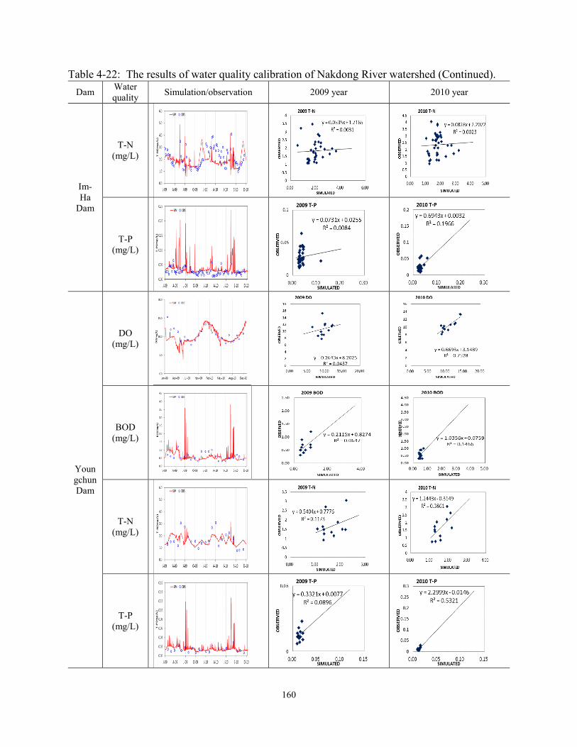
160

Table 4-22: The results of water quality calibration of Nakdong River watershed (Continued).

Dam Water


Im-

Ha

Dam

T-N

(mg/L)

T-P

(mg/L)

Youn

gchun

Dam

DO

(mg/L)

BOD

(mg/L)

T-N

(mg/L)

T-P

(mg/L)

161


Dam Water


Hap-

chun

Dam

DO

(mg/L)

BOD

(mg/L)

T-N

(mg/L)

T-P

(mg/L)

Nam-

gang

Dam

DO

(mg/L)

BOD

(mg/L)

162


Dam Water


Nam-

gang

Dam

T-N

(mg/L)

T-P

(mg/L)

Mil-

yang

Dam

DO

(mg/L)

BOD

(mg/L)

T-N

(mg/L)

T-P

(mg/L)

163

The calibration for five sub-watersheds located at Yongdam Dam’s watershed was

performed on four water quality parameters: DO, BOD, T-N, and T-P shown in Table 4-23. On

the whole, patterns of both observed and simulated data have similar tendencies as those found in

the Nakdong watershed simulation results. Data was not collected during rainfall events, hence

the percent differences could not be compared during rainfall events but analyzed for only during

non rainfall conditions. That is a possible reason why percent differences were so low for this

particular calibration. Percent differences for most of the water quality parameters were very

good, good and fair except for T-P. Parameters that fell outside of very good, good, and fair

include Juja’s T-P during 2005, 2006, summer, and spring, the Jungja’s BOD in 2006, TN during

2006, summer, and spring, TP during 2005, and spring, the Jinan’s BOD and TP in the summer,

the Guryang’s BOD and TP during 2005, 2006, summer, and spring, the Geum’s TP during 2005,

2006, and spring.

76.2 % of the percent differences for BOD, TN, and TP were below fair. The ratio

between simulated and observed mean concentration during 2005, 2006, summer, and spring for

BOD were between 0.28 and 1.07, while T-N were between 0.28 and 1.12, and T-P were

between 0.18 and 2.47. The biggest differences and thus the least confidence for this calibration

were for TP (Donigian, 2002).

Table 4-23: The results of water quality calibration and validation of Yongdam Dam watershed.


(average)

Simulated

(average) % Difference Criteria Ratio

Juja

DO

(mg/L)

2005 10.1 9.7 3.53 Very good 0.96

2006 9.3 10.6 0.47 Very good 1.13

Summer 9.2 8.8 3.87 Very good 0.96

Spring 10.1 10.8 7.21 Very good 1.07

BOD

(mg/L)

2005 0.86 0.83 2.85 Very good 0.97

2006 1.17 0.98 29.35 Fair 0.84

Summer 1.20 0.83 31.09 Fair 0.69

Spring 1.41 0.96 31.37 Fair 0.68

T-N

(mg/L)

2005 1.32 1.39 5.51 Very good 1.06

2006 1.62 1.36 29.84 Fair 0.84

Summer 1.60 1.20 26.56 Fair 0.75

Spring 3.49 1.36 23.89 Good 0.39

164

Table 4-23: The results of water quality calibration and validation of Yongdam Dam watershed

(Continued).


(average)

Simulated


Juja T-P

(mg/L)

2005 0.012 0.029 147.26 - 2.47

2006 0.015 0.026 73.29 - 1.69

Summer 0.018 0.034 87.14 - 1.87

Spring 0.018 0.025 161.66 - 1.38

JungJa

DO

(mg/L)

2005 10.3 9.8 5.01 Very good 0.95

2006 9.0 10.4 1.94 Very good 1.15


Spring 10.1 10.1 0.25 Very good 1.01

BOD

(mg/L)

2005 0.72 0.77 7.18 Very good 1.07

2006 1.04 0.84 40.53 - 0.81

Summer 0.89 0.71 21.40 Good 0.79

Spring 1.81 0.66 31.66 Fair 0.36

T-N

(mg/L)

2005 2.04 1.44 29.45 Fair 0.71

2006 2.58 1.49 52.80 - 0.58

Summer 2.7 1.2 54.63 - 0.46

Spring 5.2 1.4 46.41 - 0.28

T-P

(mg/L)

2005 0.014 0.033 128.93 - 2.29

2006 0.026 0.034 8.79 Very good 1.32

Summer 0.026 0.030 16.00 Good 1.16

Spring 0.023 0.026 109.11 - 1.13

Jinan

DO

(mg/L)

2005 10.1 10.0 1.75 Very good 0.98

2006 8.9 10.6 3.49 Very good 1.19


Spring 10.0 10.2 1.26 Very good 1.02

BOD

(mg/L)

2005 1.63 1.38 15.31 Good 0.85

2006 1.26 1.81 30.54 Fair 0.64

Summer 2.11 0.91 56.79 - 0.43

Spring 3.07 1.43 5.06 Very good 0.47

T-N

(mg/L)

2005 2.35 2.64 12.47 Very good 1.12

2006 2.17 2.33 7.41 Very good 1.07

Summer 2.03 2.26 10.59 Very good 1.11

Spring 5.66 3.33 18.02 Good 0.59

T-P

(mg/L)

2005 0.065 0.076 15.60 Good 1.16

2006 0.076 0.096 13.61 Very good 1.25

Summer 0.099 0.053 46.04 - 0.54

Spring 0.117 0.080 27.88 Fair 0.68

Gu-

ryang

DO

(mg/L)

2005 10.8 8.8 18.71 Good 0.81

2006 9.3 9.6 11.91 Very good 1.04

Summer 9.4 7.7 17.42 Good 0.83

Spring 10.5 9.1 14.05 Very good 0.87

BOD

(mg/L)

2005 2.24 1.25 44.17 - 0.56

2006 2.45 0.94 61.68 - 0.38

Summer 2.49 0.80 68.23 - 0.32

Spring 5.20 1.46 47.13 - 0.28

T-N

(mg/L)

2005 2.77 2.73 1.56 Very good 0.98

2006 2.70 2.41 10.71 Very good 0.89

Summer 2.63 2.39 9.46 Very good 0.91

Spring 6.63 3.22 4.10 Very good 0.49

165

Table 4-23: The results of water quality calibration and validation of Yongdam Dam watershed

(Continued).


(average)

Simulated


Gu-

ryang

T-P

(mg/L)

2005 0.119 0.071 40.14 - 0.60

2006 0.129 0.063 69.92 - 0.49

Summer 0.136 0.064 53.59 - 0.47

Spring 0.267 0.047 67.28 - 0.18

Geum

DO

(mg/L)

2005 10.1 8.7 14.00 Very good 0.86

2006 9.1 9.3 10.14 Very good 1.03


Spring 10.1 8.6 15.02 Good 0.86

BOD

(mg/L)

2005 2.05 1.81 11.66 Very good 0.88

2006 2.06 1.72 28.95 Fair 0.83

Summer 2.36 1.67 29.19 Fair 0.71

Spring 4.77 1.57 37.58 Fair 0.33

T-N

(mg/L)

2005 2.79 3.02 8.21 Very good 1.08

2006 2.67 2.83 0.85 Very good 1.06

Summer 2.57 2.65 2.68 Very good 1.03

Spring 6.55 3.75 12.61 Very good 0.57

T-P

(mg/L)

2005 0.052 0.074 43.16 - 1.43

2006 0.086 0.060 36.77 - 0.63

Summer 0.096 0.076 22.66 Good 0.79

Spring 0.156 0.045 43.40 - 0.29

The calibration (2005) and validation (2006) graphs for five streams located in the

Yongdam Dam watershed are shown in Table 4-24. This table presents graphical comparisons

between simulated and observed water quality parameters including the coefficient of

determination (R2) between simulated and observed data in 2005 and 2006.

Table 4-24: The results of water quality calibration and validation for the Yongdam Dam

watershed.

Dam Water


Juja DO

(mg/L)

166


watershed (Continued).

Dam Water


BOD

(mg/L)

T-N

(mg/L)

T-P

(mg/L)

Jung

Ja

DO

(mg/L)

BOD

(mg/L)

167



Dam Water


T-N

(mg/L)

T-P

(mg/L)

Jinan

DO

(mg/L)

BOD

(mg/L)

T-N

(mg/L)

168



Dam Water


Jinan T-P

(mg/L)

Gu-

ryang

DO

(mg/L)

BOD

(mg/L)

T-N

(mg/L)

T-P

(mg/L)

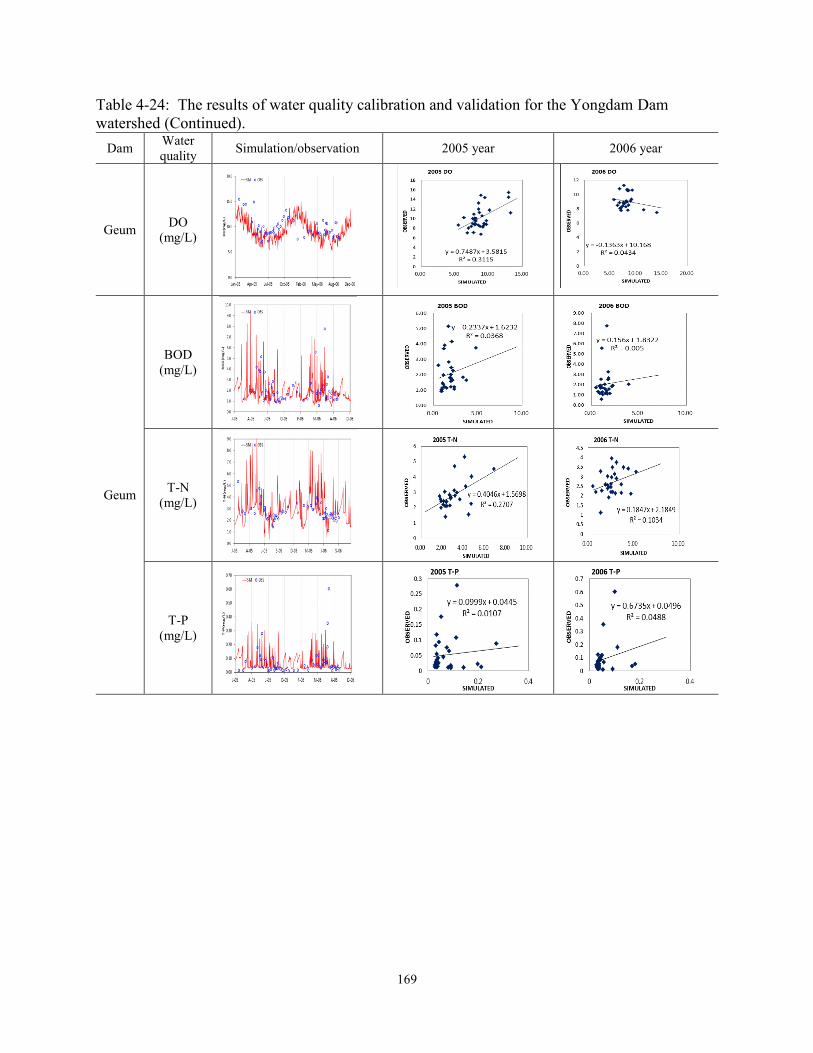
169



Dam Water


Geum DO

(mg/L)

Geum

BOD

(mg/L)

T-N

(mg/L)

T-P

(mg/L)

170

4.3.5 SIMPLE EQUATION APPLICATION FOR NAKDONG RIVER

WATERSHED AND YOUNGDAM DAM WATERSHED

The simple equations to apply to the Nakdong River watershed and Yongdam watershed

were established using by Excel SOLVER, SAS (Statistical Analysis Systems), and Data Mining

(M5P, ANN, and RBF). The results are displayed in Tables 4-25 ~ 4-27.

Excel SOLVER and SAS determined simple equations can use input data such as land

usage, rainfall, slope, etc. based upon the watershed area.

Table 4-25: Simple equations for Nakdong and Geum-Sum-Youngsan river watershed used by

excel solver. Selection

(Akaike)

R2



0.319 0.284 9 0.008 21 19 0.888 0.021 1 13.03 -8.03 %


0.335 0.313 15 0.001 32 30 0.893 0.004 1 13.98 -24.50 %

landusage/rainfall 500- BOD(mg/L)= 1.91 Ur0.39

Ag-0.06

Fo-0.65

Gr0.45

Wet-0.07

Ba-0.61

Wa0.28

Ra0.47

0.985 0.983 573 0.000 11 9 0.775 0.004 8 0.09 -36.50 %








land usage 200-500 TP(mg/L)= 0.10 Ur 1.08 Ag -0.27 Fo -0.23 Gr 0.26 Wet -0.23 Ba -0.30 Wa -0.25 0.654 0.642 58 0.000 33 31 0.648 0.000 7 0.127 -169.51 %

landusage/rainfall 500- TP(mg/L)= 0.11 Ur 0.19 Ag 1.81 Fo -0.54 Gr -0.15 Wet -0.19 Ba -0.52 Wa 0.87 Ra -1.64 0.989 0.987 779 0.000 11 9 0.851 0.044 8 0.001 -91.10 km2

land usage/rainfall/slope 0-100 BOD(mg/L)= 3.32 Ur0.48

Ag-0.98

Fo2.04

Gr-0.69

Wet0.22

Ba-0.40

Wa0.09

Ra0.27

Sl-2.24

0.863 0.851 75 0.000 14 12 0.856 0.027 9 1.26 -15.70 km2

land usage/slope 100-150 BOD(mg/L)= 1.95 Ur0.00

Ag0.33

Fo2.62

Gr0.21

Wet-0.51

Ba0.00

Wa-0.28

Sl-3.63

0.919 0.912 136 0.000 14 12 0.886 0.071 8 2.61 -7.51 %

landusage/rainfall 150-200 BOD(mg/L)= 2.85 Ur1.16

Ag-0.40

Fo1.54

Gr0.10

Wet-0.55

Ba-0.71

Wa1.63

Ra-1.99

0.998 0.998 4296 0.000 11 9 0.882 0.111 8 0.02 -52.36 km2

pervious/impervious 200 - BOD(mg/L)= 3.45 P-1.98

IP2.38

0.643 0.632 61 0.000 36 34 0.832 0.000 2 21.16 -15.13 km2







slope 150-200 TN(mg/L)= 10.45 Sl -0.40 0.276 0.196 3.435 0.097 11 9 0.935 0.464 1 5.026 -6.62 %



land usage/rainfall/slope 100-150 TP(mg/L)= 0.08 Ur -0.13 Ag -0.33 Fo 9.73 Gr 0.35 Wet -0.25 Ba 0.47 Wa -0.71 Ra -1.82 Sl -9.11 0.996 0.995 2851 < 2.2e-16 15 13 0.747 0.001 9 0.002 -120.16 %

land usage/rainfall/slope 150-200 TP(mg/L)= 0.14 Ur 0.08 Ag 0.51 Fo 8.61 Gr -0.53 Wet -0.85 Ba 0.46 Wa 0.27 Ra -5.56 Sl -3.56 0.999 0.999 7368 0.000 11 9 0.677 0.000 9 0.000 -102.07 %


Normality

(Shapiro)para-

meterSSE

Attri-

bute

Nakdong

river

watershed

Geum

-Sum

-Youngsan

river

watershed

Watershed parametersArea

(km2)


* COD, BOD, TN, TP= predicted water quality concentration (mg/L)

* P= pervious, IP= impervious, Ra= rainfall, Sl= slope, Ur= urban, Ag=agriculture, Fo=forest, Gr=grass,

Wet=wetland, Ba= barren, and Wa= water

171


SAS (Statistical Analysis Systems). Watershed Scenarios RMSE R

2Adj R

2 coeff var p-value km2/%

200 below BOD(mg/L)= -2.742 + 0.217 imp 0.760 0.427 0.397 34.475 0.0013 %

200~500 BOD(mg/L)= 1.799 - 0.056 imp + 0.061 ur + 0.664 gr 0.700 0.471 0.414 42.663 0.0004 %

500 over BOD(mg/L)= -0.020 - 0.004 ur - 0.026 gr + 0.108 we + 0.115 wa 0.534 0.777 0.628 38.427 0.0372 km2

200 below COD(mg/L)= -4.009 + 0.404 imp 1.396 0.433 0.403 26.886 0.0013 %

200~500 COD(mg/L)= 3.042 - 0.062 imp + 0.130 ur + 1.373 gr 1.406 0.538 0.489 36.242 0.0004 %

500 over COD(mg/L)= -1.758 + 0.003 ar + 0.658 gr + 0.916 we + 1.266 wa 1.071 0.799 0.664 29.701 0.0441 %

200 below TN(mg/L)= -0.221 + 0.142 imp 0.841 0.206 0.164 27.952 0.039 %

200~500 TN(mg/L)= 2.352 - 0.009 imp + 0.079 ur - 0.079 gr 1.183 0.445 0.385 43.977 0.001 km2

500 over TN(mg/L)= -1.310 + 0.002 ar + 0.107 ag 0.945 0.638 0.548 32.565 0.017 %

200 below TP(mg/L)= -0.111 + 0.010 imp 0.074 0.151 0.106 59.354 0.451 km2

200~500 TP(mg/L)= 0.090 - 0.001 imp + 0.006 ur + 0.003 gr 0.074 0.587 0.543 74.154 0.001 km2

500 over TP(mg/L)= -0.052 + 0.001 imp - 0.001 ur - 0.00010 ag - 0.002 gr - 0.020 we + 0.015 wa 0.025 0.960 0.899 28.410 0.009 km2

100 below BOD(mg/L)= 0.218 + 0.080 imp + 0.017 ag + 0.215 we 0.720 0.436 0.267 32.318 0.1121 km2

100-150 BOD(mg/L)= -7.682 + 0.458 imp - 0.054 ur + 0.006 gr + 0.099 ba 0.905 0.770 0.667 41.572 0.006 %

150-200 BOD(mg/L)= 0.116 + 0.026 imp + 0.036 ag + 0.415 wa 0.744 0.651 0.476 31.397 0.08 %

200 over BOD(mg/L)= 1.041 - 0.090 imp + 0.164 ur + 0.058 ag + 0.469 ba 0.700 0.744 0.711 34.177 <.0001 %

100 below COD(mg/L)= 2.231 + 0.023 ag + 0.945 we + 0.562 wa 0.985 0.700 0.609 21.527 0.0057 km2

100-150 COD(mg/L)= -14.540 + 0.924 imp - 0.363 ur + 0.078 ga + 0.664 ba 1.363 0.800 0.711 28.941 0.0033 %

150-200 COD(mg/L)= 1.870 + 0.017 ag + 0.850 wa 0.774 0.770 0.705 15.676 0.08 km2

200 over COD(mg/L)= 13.917 - 0.880 imp + 0.376 ur + 0.221 ag + 1.443 ba 0.701 0.827 0.805 15.950 <.0001 %

100 below TN(mg/L)= 0.690 + 0.098 imp + 0.922 we 1.000 0.445 0.345 32.203 0.039 km2

100-150 TN(mg/L)= -6.839 + 0.299 imp + 0.038 ur + 1.129 ba 0.839 0.933 0.913 21.325 <.0001 km2

150-200 TN(mg/L)= 2.063 + 0.011 ag + 0.250 wa 0.762 0.335 0.145 23.468 0.240 km2

200 over TN(mg/L)= 5.393 - 0.363 imp + 0.285 ur + 0.110 ag + 0.760 ba 0.913 0.700 0.662 32.903 <.0001 %

100 below TP(mg/L)= 0.018 + 0.000 ag + 0.067 we + 0.01468 wa 0.041 0.666 0.565 40.012 0.010 km2

100-150 TP(mg/L)= -0.230 + 0.008 imp + 0.015 ur + 0.000734 gr + 0.027 ba 0.057 0.908 0.868 40.677 0.000 km2

150-200 TP(mg/L)= 0.184 - 0.011 imp + 0.007 ag 0.119 0.383 0.207 82.968 0.080 %

200 over TP(mg/L)= 0.105 - 0.012 imp + 0.018 ur + 0.00405 ag + 0.038 ba 0.058 0.719 0.682 62.076 <.0001 %

Simple Equations

Nakdong

river

watershed

Geum-Sum-

Youngsan

river

watershe


Data Mining (M5P, ANN, and RBF).


Of instances

nakdong(M5P)_200 3 21 2 0.7428 0.6569 0.6923 79.62% 77.21% 8 %

nakdong(ANN)_500 8 32 6 0.7651 0.5259 0.5861 68.98% 66.82% 11 km

nakdong(RBF)_500over 9 11 3 0.8828 0.3331 0.404 49.88% 49.07% 4 %

gsy(M5P)_100 9 14 2 0.9943 0.2044 0.2401 40.52% 42.45% 5 km

gsy(ANN)_150 2 14 6 0.959 1.1982 1.4216 67.07% 63.91% 5 km

gsy(ANN)_200 5 10 6 0.9374 0.3663 0.4321 38.89% 34.00% 4 km

gsy(RBF)_200over 7 36 6 0.9192 0.2501 0.3272 28.52% 35.09% 13 %

nakdong(M5P)_200 3 21 2 0.9591 0.3172 0.3503 55.98% 55.46% 6 km

nakdong(M5P)_500 6 23 2 0.7361 2.046 2.6269 99.84% 95.25% 8 km

nakdong(ANN)_500over 2 11 5 0.9471 0.5433 0.7336 41.91% 44.44% 4 %

gsy(ANN)_100 7 14 7 0.9797 0.3207 0.437 20.30% 26.83% 5 km

gsy(ANN)_150 5 14 6 0.9486 0.8815 1.1354 26.62% 30.10% 5 km

gsy(ANN)_200 5 10 6 0.9787 0.4142 0.4792 33.14% 36.43% 4 km

gsy(ANN)_200over 6 36 6 0.9612 0.5482 0.6887 44.50% 50.16% 13 %

nakdong(RBF)_200 5 21 5 0.6812 0.6489 0.7179 90.58% 90.35% 8 km

nakdong(RBF)_500 7 32 2 0.4579 1.0166 1.1383 92.86% 88.67% 11 %

nakdong(ANN)_500over 9 11 6 0.8285 0.7515 0.8961 48.21% 47.84% 4 %

gsy(ANN)_100 9 14 7 0.9138 0.754 0.9051 53.44% 58.59% 5 km

gsy(ANN)_150 1 14 7 0.9955 1.5211 1.9738 45.81% 43.62% 5 %

gsy(RBF)_200 8 10 2 0.5868 0.3753 0.4215 94.12% 87.23% 4 km

gsy(M5P)_200over 10 36 15 0.9092 0.5854 0.6454 50.50% 52.78% 13 km

nakdong(ANN)_200 3 21 5 0.7478 0.0718 0.0836 124.69% 136.00% 8 km

nakdong(RBF)_500 7 32 2 0.6127 0.0507 0.0606 88.35% 90.07% 11 %

nakdong(RBF)_500over 3 11 3 0.7268 0.0485 0.0578 64.12% 73.60% 4 %

gsy(RBF)_100 8 14 2 0.9245 0.0377 0.0439 72.48% 70.32% 5 km

gsy(M5P)_150 9 14 5 0.9922 0.0318 0.0393 17.79% 16.61% 5 %

gsy(RBF)_200 8 10 2 0.9382 0.1176 0.1901 92.75% 93.70% 4 km

gsy(M5P)_200over 10 36 13 0.9697 0.0315 0.0521 48.55% 75.31% 13 km

Water

quality

BOD

COD

T-N

T-P

Model ScenarioNo.of

Instances

No.of

Rules/hidden/c

luster


km2/%

172

The simple equations based on Data Mining (M5P, ANN, and RBF) were created by the

Weka program. In order to simulate water quality, the “Re-evaluate model on current test set”

option of the Weka program could be used based on Table 4-27’s simple equations.

Data sets for simulation of Geum-Sum-Youngsan River watershed and Nakdong River

watershed are shown in Tables 4-28 ~ 4-29 which include pervious, impervious, rainfall, slope,

and land usage.

Table 4-28: Data sets for water quality simulation using simple equations (Geum-Sum-

Youngsan river watershed).

Geum River (km2) 224 57.70 112.4 32.87 8.43 74.52 178.14 16.61 1.03 3.42 2.24 282.157

Geum River (%) 80 20 112.4 32.87 2.99 26.41 63.13 5.89 0.37 1.21 0.79 100

Guryang Stream(km2) 129 33.23 146.9 29.75 4.59 44.67 109.23 2.59 0.21 1.33 0.98 162.629

Guryang Stream (%) 80 20 146.9 29.75 2.82 27.47 67.17 1.59 0.13 0.82 0.60 100

Jinan Stream (km2) 27 7.63 113.7 26.98 1.99 10.74 20.39 1.12 0.16 0.13 0.20 34.517

Jinan Stream (%) 78 22 113.7 26.98 5.77 31.11 59.07 3.24 0.46 0.36 0.57 100

Jeongja Stream (km2) 80 16.68 134.4 40.46 1.34 11.71 81.95 1.64 0.15 0.17 0.48 96.954

Jeongja Stream (%) 83 17 134.4 40.46 1.38 12.08 84.52 1.69 0.15 0.18 0.49 100

Juja stream (km2) 48 9.40 137.8 40.23 0.62 5.21 50.22 0.74 0.10 0.16 0.35 57.038

Juja stream (%) 84 16 137.8 40.23 1.08 9.14 88.04 1.29 0.17 0.28 0.61 100

Geum-Sum-

Youngsan

river

Watershed

watershed

urban agriculture forest grass wetland barren water

sub-watershed pervious imperviousrainfall

(mm/month)

slope

(%)

Land use

total

Table 4-29: Data sets for water quality simulation using simple equations (Nakdong river

watershed).

Milyang Dam(km2) 87 17 122.5 22.43 0.99 4.62 92.50 1.97 0.16 1.31 1.93 103

Milyang Dam(%) 84 16 122.5 22.43 0.95 4.46 89.40 1.91 0.15 1.26 1.87 100

Namgang Dam(km2) 1,852 441 163.3 23.97 54.44 452.82 1685.48 23.58 20.05 22.96 33.73 2,293

Namgang Dam(%) 81 19 163.3 23.97 2.37 19.75 73.50 1.03 0.87 1.00 1.47 100

Andong Dam(km2) 1,314 277 120.8 22.43 22.54 189.10 1308.53 6.38 9.82 15.72 38.62 1,591

Andong Dam(%) 83 17 120.8 22.43 1.42 11.89 82.26 0.40 0.62 0.99 2.43 100

Youngchun Dam(km2) 195 39 94.2 22.43 2.29 22.05 201.61 0.26 1.53 1.35 5.44 235

Youngchun Dam(%) 83 17 94.2 22.43 0.97 9.40 85.96 0.11 0.65 0.57 2.32 100

Imha Dam(km2) 1,124 244 104.2 22.43 18.82 204.64 1091.63 5.45 6.18 8.10 32.87 1,368

Imha Dam(%) 82 18 104.2 22.43 1.38 14.96 79.82 0.40 0.45 0.59 2.40 100

Hapchu Dam(km2) 745 184 152.5 22.43 23.77 207.25 658.90 4.35 3.81 11.99 18.85 929

Hapchun Dam(%) 80 20 152.5 22.43 2.56 22.31 70.93 0.47 0.41 1.29 2.03 100

water totalurban agriculture forest grass wetland barren

Land use

Nakdong

River

Watershed

watershed sub-watershed pervious imperviousrainfall

(mm/month)

slope

(%)

The result of water quality simulation based on simple equation were displayed Table 4-

30 ~ 4-31.

173

Table 4-30: The results of water quality simulation for Yongdam Dam watershed using simple

equations.

M5P ANN RBF M5P ANN RBF M5P ANN RBF

Geum River 0.80 1.80 - - 1.46 2.12 1.44 2.63 1.89 - - 2.72 0.039 0.076 0.030 - - 0.151

Guryang Stream 0.47 1.88 - 1.90 - 2.45 2.71 2.78 - - 3.12 2.68 0.077 0.154 - - 0.148 0.158

Jinan Stream 0.57 1.04 1.03 - - 1.93 2.02 1.58 - 1.23 - 1.86 0.010 0.036 - - 0.110 0.096

Jeongja Stream 2.25 1.78 1.04 - - 1.29 2.38 2.46 - 1.49 - 2.58 0.068 0.040 - - 0.085 0.026

Juja stream 2.03 1.08 0.80 - - 1.17 1.98 1.70 - 1.03 - 1.62 0.034 0.032 - - 0.085 0.015

sum 6.13 7.58 8.97 10.53 11.15 11.45 0.227 0.339 0.446

% difference 31.66 15.55 - 8.08 2.66 - 48.948 24.009 -

6.23

30.62

8.77

23.44

0.458

2.786

Data MiningObserved Excel Solver SAS

Data MiningObserved

sub-

watershed

BOD (mg/L) T-N (mg/L) T-P (mg/L)

Excel Solver SASData Mining

Observed Excel Solver SAS

Comparing simple equations to observed data for the case of the BOD simulation, the

results of data mining almost have the same trend as the observed data. Otherwise, the other

simple equations: Excel Solver and SAS displayed different trends.

Figure 4-37: BOD simulation results based on simple equations (Yongdam watershed).

In case of the T-N simulation, the result of SAS and Data Mining resulted in similar

trends with the observed data except in the case of the Excel SOLVER equation. The results

generated by the SAS derived equations especially had a strong correlation with the observed

data.

174

Figure 4-38: T-N simulation results based upon simple equations (Yongdam watershed).

The T-P simulation results determined using the equations developed using Data Mining

and SAS have the same trend as the observed data. On the other hand, the results of Excel

SOLVER did not match well with the observed data.

Figure 4-39: T-P simulation results based upon simple equations (Yongdam watershed).

175

Table 4-31: The results of water quality simulation for Nakdong river watershed using simple

equations.

M5P ANN RBF M5P ANN RBF M5P ANN RBF

Milyang Dam 1.23 6.28 0.90 - - 0.93 2.49 2.09 - - 3.14 0.90 0.000 0.064 - 0.019 - 0.010

Namgang Dam 1.68 1.96 - - 2.20 1.23 4.73 6.07 - 1.37 - 1.77 0.001 0.256 - - 0.150 0.033

Andong Dam 0.89 4.33 - - 1.64 0.72 26.17 3.62 - 3.11 - 2.23 0.001 0.501 - - 0.150 0.024

Youngchun Dam 5.75 0.99 - - 1.42 0.68 1.28 2.16 - - 2.35 1.85 0.000 0.053 - - 0.065 0.007

Imha Dam 1.14 3.45 - - 1.64 0.90 37.22 3.43 - 3.80 - 2.78 0.003 0.463 - - 0.105 0.025

Hapchu Dam 1.18 1.74 - - 1.64 1.45 42.02 3.20 - 5.22 - 2.66 0.002 0.248 - - 0.150 0.048

Sum 11.88 18.75 5.91 113.91 20.57 12.20 0.01 1.59 0.15

% difference 101.09 217.36 - 833.71 68.64 - 95.557 979.384 -

sub-

watershedData Mining Data Mining Data Mining

Excel solver SAS Observed Excel solver SAS Observed


Excel solver SAS Observed

9.44

59.80 55.62 335.083

18.99 0.639

Figure 4-40: BOD simulation results based on simple equations (Nakdong watershed).

According to the BOD simulation for Nakdong River watershed, the results of Data

Mining and Excel SOLVER produced a strong match with the observed data. However, results

determined using the equations developed in SAS did not match the observed data.

The results of the T-N simulation using equations determined with Excel SOLVER

produced results that were extremely different than the observed data. Results produced by the

equations developed using data mining techniques had more similarities to the observed data but

still resulted in a poor fit to the data.

176

Figure 4-41: T-N simulation results based on simple equations (Nakdong watershed).

The T-P simulation based on equations determined through SAS had a totally different

trend in comparison with the observed data, but the results of Data Mining and Excel SOLVER

had similar trends as the observed data.

Figure 4-42: T-P simulation results based on simple equations (Nakdong watershed).

In brief, water quality simulations based upon the simple equation using Excel SOLVER,

SAS, and Data Mining (M5P, ANN, and RBF) produced fairly good results with correlations to

observed data. Results showed that different simple equations can be applied to different

watersheds and water quality simulations. Therefore, in order to determine the priority of simple

equations, the percent differences were considered. The percent differences of Yongdam Dam

watershed’s BOD were 25.55 %, 15.55 %, and 30.62% from excel solver, SAS, and Data Mining,

177

respectively. SAS and excel solver are ranked first and second in terms of percent difference,

however the trend of excel sover is reversed. Therefore SAS and Data Mining were

recommended for BOD simulation of Yongdam watershed. For the T-N simulation of the

Yongdam Dam watershed, SAS is recommended because it was ranked first in terms of percent

difference. For the T-P simulation, Data Mining and SAS were recommended because percent

difference is 2.79 % (very good) and 24.01 % (good), respectively. For the Nakdong River

watershed water quality simuation, Data Mining is recommended for BOD and T-N simuation

based upon the percent differences. For the T-P simulation, excel solver and Data Mining are

recommended based upon the first and second rank of percent difference. The recommended

simple equations for each watershed are shown in Table 4-32.

Table 4-32: Appropriate development method to create simple equations for each watershed.

Watershed BOD simulation T-N simulation T-P simulation

Yongdam Dam

watershed SAS, Data Mining SAS SAS, Data Mining

Nakdong river

watershed Data Mining Data Mining

Data Mining &

Excel Solver

4.3.6 COMPARING HSPF AND SIMPLE EQUATIONS APPLICABILITY FOR

NAKDONG RIVER WATERSHED AND YOUNGDAM DAM

WATERSHED

In order to achieve the credibility of simple equations, the HSPF and simple equations

were applied to Nakdong River watershed and Yongdam Dam watershed. The HSPF models for

Nakdong River watershed and Yongdam Dam watershed were implemented based on data

collectd from 2009 to 2010 and from 2005 to 2006, respectively. Simple equations were

developed using several tools: Excel SOLVER, SAS, and Data Mining (M5P, ANN, and RBF)

were adapted. The most appropriate methods are shown Table 4-32.

178

The water quality simulation results for Yongdam Dam watershed are shown in Table 4-

33 and Figures 4-43, 44, and 45. According to the BOD simulation results, % difference of Data

mining was smaller than the HSPF results. T-N and T-P results of Data Mining also had small %

differences compared with the results from the HSPF models. In addition, the Data Mining fit of

BOD was systematically biased, therefore, a best fit was determined by adding a constant of 0.5

(DM+0.5) through which a 2.76 % difference was achieved based on the Data Mining

Simulation.

Table 4-33: The results of water quality simulation for Yongdam Dam watershed based upon

HSPF and simple equations.

SAS Data Mining DM+0.5 HSPF observed SAS HSPF observed SAS Data Mining HSPF observed

Geum 1.80 1.46 1.96 1.46 2.12 2.63 2.65 2.72 0.076 0.030 0.055 0.151

Guryang 1.88 1.90 2.40 0.90 2.45 2.78 2.40 2.68 0.154 0.148 0.038 0.158

Jinan 1.04 1.03 1.53 1.20 1.93 1.58 2.60 1.86 0.036 0.110 0.069 0.096

Jeongja 1.78 1.04 1.54 0.62 1.29 2.46 1.22 2.58 0.040 0.085 0.028 0.026

Juja 1.08 0.80 1.30 0.83 1.17 1.70 1.13 1.62 0.032 0.085 0.027 0.015

Sum 7.58 6.23 8.73 5.02 8.97 11.15 10.00 11.45 0.339 0.458 0.217 0.446

% difference 15.52 30.62 2.76 44.10 - 2.66 12.69 - 24.03 2.79 51.36 -

T-P (mg/L)T-N (mg/L)

watershed

BOD (mg/L)

Figure 4-43: The results of BOD simulation for Yongdam Dam watershed

based upon HSPF and simple equation.

179

Figure 4-44: The results of T-N simulation for Yongdam Dam watershed


Figure 4-45: The results of T-P simulation for Yongdam Dam watershed


The simulation results of Nakdong river watershed are shown in Table 4-34 and Figures

4-46, 4-47, and 4-48. The percent differences of HSPF were smaller than those found with the

simple equations. However, the Data Mining and Excel SOLVER fits were systemically biased

like the Yongdam simple equation was. Therefore, by subtracting a constant of 0.5 (DM-0.5)

from the Data Mining Simulation for BOD, a 9.01 % difference was achieved. This is a very

good result according to Table 4-27. For the T-N simulation, by subtracting a constant of 1.0

(DM-1.0) from the Data Mining Simulation, the percent difference was smaller than the HSPF

180

model. For the T-P simulation, by adding a constant of 0.02 (ES+0.02) from the Data Mining

Simulation, the percent difference was almost same as with the HSPF model.

Table 4-34: The results of water quality simulation for Nakdong river watershed based upon

HSPF and simple equations.

Data Mining DM-0.5 HSPF Observed Data Mining DM-1 HSPF Observed Excel Solver ES+0.02 Data Mining DM-0.1 HSPF Observed

Milyang 0.90 0.40 0.97 0.93 3.14 2.14 0.86 0.90 0.000 0.020 0.019 -0.041 0.019 0.010

Namgang 2.20 1.70 1.17 1.23 1.37 0.37 1.60 1.77 0.001 0.021 0.150 0.090 0.033 0.033

Andong 1.64 1.14 0.91 0.72 3.11 2.11 2.12 2.23 0.001 0.021 0.150 0.090 0.024 0.024

Youngchun 1.42 0.92 0.64 0.68 2.35 1.35 1.61 1.85 0.000 0.020 0.065 0.005 0.006 0.007

Imha 1.64 1.14 0.72 0.90 3.80 2.80 1.72 2.78 0.003 0.023 0.105 0.045 0.028 0.025

Hapchun 1.64 1.14 1.55 1.45 5.22 4.22 2.13 2.66 0.002 0.022 0.150 0.090 0.107 0.048

Sum 9.44 6.44 5.96 5.91 18.99 12.99 10.04 12.20 0.007 0.127 0.639 0.279 0.216 0.147

% difference 59.80 9.01 0.88 - 55.62 6.44 17.68 - 95.557 13.851 335.083 89.966 46.823 -


watershed

Figure 4-46: The results of BOD simulation for Nakdong river watershed


Figure 4-47: The results of T-N simulation for Nakdong river watershed


181

Figure 4-48: The results of T-P simulation for Nakdong river watershed


The simulation results of the developed simple equations were better when applied to the

Yongdam Dam watershed in comparison to those of the Nakdong River watershed. Otherwise,

the results of simple equations for water quality simulation were found to be “systematically

biased”. Therefore, when adding and subtracting the appropriate constants, shown in Table 4-35,

the results of the simple equation improved. Using this adjustment, the results are much more

accurate than with the HSPF model in Yongdam Dam watershed and were very similar in terms

of accuracy with the HSPF model in Nakdong River watershed.

Table 4-35: The % difference of water quality simulation for Yongdam Dam and Nakdong river

watershed based upon simple equations and HSPF model. Water-

shed Yongdam Dam Nakdong River

Water

quality BOD T-N T-P BOD T-N T-P

Models DM* DM

- 0.5 HSPF SAS HSPF DM HSPF DM

DM

-

0.5

HSPF DM DM

- 1 HSPF ES* ES+0.01 HSPF

%

differ. 30.6 2.8 44.1 2.7 12.7 2.8 51.4 59.8 9.0 0.9 55.6 6.4 17.7 95.6 13.9 46.8

*DM: Data Mining, ES: Excel Solver

182

4.3.7 SUMMARY AND CONCLUSION

The purpose of this chapter was to verify the simple equations determined in Chapter 3

by modeling two watersheds—the Yongdam Dam’s watershed and the Nakdong River

watershed—in the HSPF watershed model and comparing their results with those from the

simple equations.

The Yongdam Dam’s watershed was divided into five sub-watersheds and the Nakdong

River watershed was divided into six sub-watersheds. Watershed parameters were generated

through HSPF pre-processing which included the generation of the river network, waterhed

delineation and land use overlay. At the end of pre-processing, a BASINS *.wsd file was

produced. A new project was created and the *.wsd file was input into BASINS. The *.wdm

file containing weather data, point pollution loads, and dam effluent was then input into the Met

WDM files. Finally, a new *.wdm file for accumulating HSPF results was created.

Using the HSPF results, calibration and validation of discharge for both Nakdong River’s

watershed and Yongdam Dam’s watershed were performed between observed and simuate flow.

In Nakdong River’s watershed, the value of R2 of discharge during 2009 to 2010 were 0.63 ~

0.95, the percent differences during 2009 to 2010 were 0.28 ~ 101.99. In Yongdam Dam’s

watershed, the value of R2 of discharge during 2005 to 2006 were 0.68 to 0.96, the percent

differences during 2005 to 2006 were 9.47 ~ 90.07. Overall, even though the percent differences

for each stream had significantly large ranges, R2 was over around 0.7 for all of the streams and

modeled results are therefore considered acceptable as a good criterion.

According to the results of water quality calibration and validation, most of the percent

differences for DO, BOD, and T-N during 2009 to 2010 were below fair criterion (25 ~ 35

percent difference) except T-P simulation and the ratio between simulated and observed mean

concentration for DO, BOD, T-N during 2009 to 2010. The ratio between simulated and

observed mean concentration for the parameters in the previous sentence were mostly between

0.81 and 1.25 and T-P was 1.07 to 1.41 in the Nakdong River watershed. In the case of the

183

Yongdam Dam’s watershed, 76.2 % of the percent differences for BOD, T-N, and T-P were

below fair. The ratio between simulated and observed mean concentration for BOD was 0.28 ~

1.07, whie T-N was 0.28 to 1.12 and T-P was 0.18 to 2.47.

Simple equations generated using Excel Solver, SAS, and Data Mining processes were

applied to the Nakdong and Yongdam Dam watersheds. The data sets used as inputs to the

equations included pervious area, impervious area, rainfall, slope, and land usage which was

harvested from the HSPF input data.

Water quality results simulated through the simple equations produced fairly good

correlation to observed data. The percent difference of Yongdam Dam watershed’s BOD were

25.55% (Excel Solver), 15.55% (SAS), and 30.62 % (Data Mining). In the case of T-N, the

percent differences were 8.42 % (Excel Solver), 2.66 % (SAS), and 23.44 % (Data Mining). In

the case of T-P, the percent differences were 61.84 % (Excel Solver), 24.0 % (SAS), and 2.79 %

(Data Mining).

The percent difference of Nakdong River watershed’s BOD were 85.20 % (Excel Solver),

217.36% (SAS), and 59.80 % (Data Mining). In the case of T-N, the percent differences were

832.08 % (Excel Solver), 68.64 % (SAS), and 55.62 % (Data Minging). In the case of T-P, the

percent differences were 80.70 % (Excel Solver), 979.3 % (SAS), and 335.08 % (Data Mining).

Based on these results, SAS and Data Mining are recommended for the simulation of

BOD, SAS is recommended for T-N simulation, and SAS and Data Mining are recommended for

T-P simulation in the Yongdam Dam’s watershed. In the case of the Nakdong River watershed,

Data Mining is recommend for the simulation of BOD and T-N, and Data Mining and Excel

Solver are recommended for the simulation of T-P.

Results generated from the simple equations and HSPF modeling were compared. It was

determined that the fits generated by the equations developed through Data Mining were

systematically biased for BOD and T-P for the Yongdam Dam watershed and for BOD, T-N, and

184

T-P for the Nakdong River watershed. Therefore, a best fit was determined by adding and

subtracting a constant of 0.01, 0.1, 0.5, and 1.0.

The best percent difference for BOD simulation in the case of Yongdam Dam’s

watershed was 2.79 % when 0.5 was added to the Data Mining result. The percent different for

the same parameter using HSPF was 44.10 %. The percent difference for T-N was 2.66 % using

the SAS results and 12.69 % using the HSPF results. The percent difference for T-P was 2.79 %

for the SAS results and 51.36 % for the HSPF results for the Yongdam Dam’s watershed.

For Nakdong River Watershed, the percent difference of BOD simulation became 9.01%

when 0.5 was subtracted from the Data Mining results. The HSPF results had a 0.88 % percent

different in the case of BOD for this watershed. The percent difference for T-N was 6.44 %

when 1.0 was subtracted from the Data Mining result. This compares favorily to the 17.68 %

different obtained by the HSPF results. The percent different for T-P was 49.43 % using the

Excel Solver results pluse 0.01. This was similar to the 46.82 % difference obtained for T-P for

the HSPF results.

In conclusion, the developed simple equations produced better or similar water quality

results compared with those produced by the HSPF model. This illustrates that these equations

can be used instead of a physically-based model like HSPF to forecast water quality conditions

in a watershed using watershed parameters as input data. This was illustrated in the case of the

Geum-Sum-Youngsan River watershed and Nakdong River watershed.

This chapter proved the final hypothesis of this dissertation, that water-quality results

generated by the simple equations could be verified against the results from a physically-based

watershed model and be comparable. This proves that the simple equations relating watershed

parameters to watershed water quality can be used as a screening device to aid in the

determination of the best restoration locations.

185

CHAPTER 5. CONCLUSION AND RECOMMENDATION

Philosophically speaking, watersheds and the quality of water they provide delineate the

boundaries of life for people who life in them. These boundaries are different for different people

as water quality needs and conditions are different between watersheds. In order to evaluate and

estimate water quality in a watershed, generally, a mechanical watershed model is used even

though we don’t have enough data to properly calibrate prior to use. That’s the main reason why

the estimations and evaluations for watersheds are often incorrect. Based on literature review of

thirty three watershed models that are currently available models that are designed for the

purpose of developing flow and water quality management plans, they require too much data and

application effort to be used to prioritize watersheds with respect to their relative contribution to

environmental degradation within a multiwatershed basin.

In Chapter 2, numerous watersheds models, which have their own unique characteristics,

were reviewed to determine each model’s mechanisms and functions. Furthermore, about 217

references examples, which have been applied to the watershed models, were reviewed and

analyzed with a focus on their applicability.

Based on this study’s literature review, currently available watershed models designed for

the purpose of developing flow and water quality management plans at a watershed scale require

too much data and application effort to be used to prioritize watersheds with respect to their

relative contribution to environmental degradation within a multiwatershed basin. Therefore, as

was hypothesized in Chapter 1, simple equations relating easily obtained data to watershed water

quality impacts need to be developed to sufficiently prioritize target restoration areas in the

feasibility phase of spatially large projects (i.e. national scale).

186

In addition, a model selection program is needed to aid the engineer in the selection of

the best watershed model to use in future complex modeling following the feasibility phase.

Eight variables were chosen considering five factors from Leslie et al. (2005) and the reviewed

literature such as land use, event or continuous, time steps, water quality, distributed or lumped,

subsurface, overland sediment, and BMP. Using these eight variables as input, the selection

program developed in this dissertation screens available watershed models for the best model for

the user’s needs.

The watershed selection program described in this dissertation could be highly useful to

many watershed modelers. In addition, this program could be upgraded by anyone who knows

how to apply state-of-art data that has been collected from a watershed model. This program is

still not perfect because we could not obtain the entire data for each watershed model. Finally

this program is going to be upgraded continuously to fulfill the needs of users of watershed

models.

In Chapter 3, to find out the co-relationship between water quality and watershed

parameters, parameters were separated into ten scenarios: 1) impervious, 2) impervious+pervious,

3) impervious+rainfall, 4) impervious+slope, 5) impervious+rainfall+slope, 6) slope, 7) land

usage, 8) lang usage+rainfall, 9) land usage+slope, 10) land usage+rainfall+slope.

The Simple equations were established through the application of the three cases and ten

scenarios in Excel Solver, SAS (Statistical Analysis System), Model Tree, ANN (Artificial

Neural Network), and RBF (Radial Basis Function). The best simple equations were then

identified from the generated equations using statistical methods (R2, adj. R2, F-AIC, VIF,

Shapiro-wilk test, etc.).

187

Based on the collected results from Excel Solver, the SAS, and Data Mining, the first

steps’ results are much better than the second and third step’s results. Therefore, these simple

equations generated from the first step are the best to apply to real-based watersheds. This

chapter proved the hypothesis that simple equations can be determined correlating water quality

and phycial watershed parameters.

In Chpater 4, to verify the simple equations determined in Chapter 3 by modeling two

watersheds—the Yongdam Dam’s watershed and the Nakdong River watershed—in the HSPF

watershed model and comparing their results with those from the simple equations.

Results generated from the simple equations and HSPF modeling were compared. It was

determined that the fits generated by the equations developed through Data Mining were

systematically biased for BOD and T-P for the Yongdam Dam watershed and for BOD, T-N, and

T-P for the Nakdong River watershed. Therefore, a best fit was determined by adding and

subtracting a constant of 0.02, 0.1, 0.5, and 1.0.

The best percent difference for BOD simulation in the case of Yongdam Dam’s

watershed was 2.79 % when 0.5 was added to the Data Mining result. The percent different for

the same parameter using HSPF was 44.10 %. The percent difference for T-N was 2.66 % using

the SAS results and 12.69 % using the HSPF results. The percent difference for T-P was 2.79 %

for the SAS results and 51.36 % for the HSPF results for the Yongdam Dam’s watershed.

For Nakdong River Watershed, the percent difference of BOD simulation became 9.01%

when 0.5 was subtracted from the Data Mining results. The HSPF results had a 0.88 % percent

different in the case of BOD for this watershed. The percent difference for T-N was 6.44 %

when 1.0 was subtracted from the Data Mining result. This compares favorily to the 17.68 %

different obtained by the HSPF results. The percent different for T-P was 13.85 % using the

Excel Solver results pluse 0.02. This was similar to the 46.82 % difference obtained for T-P for

the HSPF results.

188

In conclusion, the developed simple equations produced better or similar water quality

results compared with those produced by the HSPF model. This illustrates that these equations

can be used instead of a physically-based model like HSPF to forecast water quality conditions

in a watershed using watershed parameters as input data. This was illustrated in the case of the

Geum-Sum-Youngsan River watershed and Nakdong River watershed.

This research proved the final hypothesis of this dissertation, that water-quality results

generated by the simple equations could be verified against the results from a physically-based

watershed model and be comparable. This proves that the simple equations relating watershed

parameters to watershed water quality can be used as a screening device to aid in the

determination of the best restoration locations.

Recommendation for Future Research

Recently, in order to ensure and improve water quality, river restoration projects were

implemented in Korea. A total of 16 weirs and other facilities were installed in four of the largest

rivers in Korea for the purpose of implementing advanced water quality management for the

watersheds and dams which are located in the upstream, and the weirs. Algal blooms have

become a major issue because of increasing retention times due to the installation of weirs in the

main river.

As a result of needs to collect and monitor the water quality and the issues that can arise

due to the methods of collecting that data, a variety of measures have been implemented as

follows;

i. Establishment of standards for water quality monitoring.

ii. Enforcement of water quality surveys.

iii. Establishment of real time water quality surveys based upon weir operations.

iv. Establishment and implementation of integrated national rivers management.

189

v. Introduced physical and chemical treatment measures for decreasing the algal

blooms.

vi. Water quality improvement based upon the integration of operations from weir to

weir and from dam to weir.

vii. Secure discharges to maintain and improve environmental quality of the four river

environment.

viii. Mapped distribution of algae species found within each river and conducting

research to determine optimal weir operations to resolve algal blooms.

A significant amount of research has been devoted to gathering information and

predicting future water quality. Thus three dimensional water quality models can and have been

implemented. However, application of these models limited by the requirement for massive

amounts of data. As a result, they have reached a limit in terms of existing data. Hence,

according to this research, a simple equation could be used with confidence to predict water

quality based upon watershed land usage. Furthermore, the simple equations method could be

used to analyze, evaluate, and prioritize sub-watersheds of the four major rivers that could

benefit from land usage improvement using Best Management Practices and Low Impact

Development. The schematic in Figure 5-1 represents the flow or process of analysis and

prioritization for determing priority subwatersheds and identification of specific needs for water

quality improvements.

190

Figure 5-1: Future research schematic for sub-watershed management based upon Simple

Equations.

191

Recommendation for developing the “Simple Equation”

As has been mentioned in this research, the Simple Equation can be easily assessed for

priority analysis in order to restore and rehabilitate a specific watershed among whole nations.

And the Simple Equation could be developed using the relationships between water quality and

watershed characteristics such as land usage, rainfall, and slope which have been mentioned in

this dissertation. Therefore, I would like to recommend that countries which have insufficient

data bases to run physically based and mechanica models to follow the process (Figure 5-2) to

develope “Simple Equations” using existing data and then evaluate and analyze the whole nation

for considering water quality aspects.

Figure 5-2: The process to establish Simple Equation to the new watersheds

192

REFERENCES

Abaci, O., A. N. Papanicolaou, 2007, Identifying the equilibrium conditions for an agricultural

Iowa catchment using the Water Erosion Prediction Project (WEPP) model, World

Environmental and Water Resources Congress 2007: Restoring Our Natural Habitat.

Abaci, O., A. N. Papanicolaou, 2008, Evaluating the Performance of the Water Erosion

Prediction Project (WEPP) Model for Larger Watersheds, World Environmental and Water

Resources Congress 2008 Ahupua’a.

Abbott, J. 1977. Guidelines for Calibration and Application of STORM. Training Document No.

8. Hydrologic Engineering Center, Corps of Engineers, Davis, CA.

Adams, F., G. Parkin, 2002, Development of a coupled surface-groundwatr-pipe network model

for the sustainable management of karstic groundwater, Environmental Geology (2002) 42: 513-

517.

Ambrose, Robert B. Jr. P.E., 2005, Modeling Mercury Fata and Transport in Watersheds and

streams.

Aisha Al-Qurashi, Neil Mclntyre, Howard Wheater, Carl Unkrich, 2008, Application of the

Kineros2 rainfall-runoff model to an arid tacthment in Oman, Journal of Hydrology (2008), 355,

91-105.

Albek, Mine, Ulker Bakir Ogutveren, Erdem Albek, 2003, Hydrological modeling of Seydi Suyu

Watershed (Turkey) with HSPF, Journal of Hydrology 285 (2004) 260-271.

Alexander, R. B., Penny J. Johnes, Elizabeth W. Boyer & Richard A. Smith, 2002, A comparison

of models for estimating the riverine export of nitrogen from large watersheds, Biogeochemistry

57/58: 295-339, 2002.

193

Alexander, R. B, Elliot, A. H., Shankar, U., McBridge, G. B., 2002a. Estimating the sources and

transport of nutrients in the Waikato River Basin, New Zealand, Water Resources Research 38

(12), 1-23.

Alexander, R. B, and R. A. Smith, 2006, Trends in the nutrient enrichment of the U.S. rivers

during the late 20th

century and their relation to changes in probable stream trophic conditions,

Limnol. Oceanogr., 51 (1, part 2).

Alexander, R. B., R. A. Smith and G.E. Schwarz, 2004, Estimates of diffuse phosphorus sources

in surface waters of the United States using a spatially referenced watershed model, Water

Science and Technology Vol 49 No 3pp 1-10.

Alexander, R. B., R. A. Smith, Gregory E. Schwarz, Elizabeth W. Boyer, Jacqueline V. Nolan,

and John W. Brakebill, 2008, Differences in Phosphorus and Nitrogen Delivery to the Gulf of

Mexico from the Mississippi River Basin, Environmental Science and Technology/Vol. 42, No.

3, 2008.

Alfredo, Katherine, Franco Montalto, Alisha Goldstein, 2010, Observed and Modeled

Performances of Prototype Green Roof Test Plots Subjected to Simulated Low- and High-

Intensity Precipitations in a Laboratory Experiment, Journal of Hydrologic Engineering, Vol. 15,

No 6, June 1. 2010.

Anderson, M. L, Z.-Q. Chen, M. L. Kavvas, and Arlen Feldman, 2002, Coupling HEC-HMS

with Atmospheric Models for prediction of Watershed Runoff, Journal of Hydrologic

Engineering, Vol. 7, No. 4, July 1, 2002.

Ashraf, M.S., Borah, D.K., 1992, Modeling Pollutant Transport in Runoff and Sediment,

Transactions of the ASAE 35(6): 1789-1797.

Baerenklau, Kenneth A., W. Bowman Cutter, Autumn DeWoody, Ritu Sharama, and Joong

Gwnag Lee, 2008, Capturing Urban Stormwater Runoff: A Decentralized Market-Based

Alternative, Policy Matters A Quarterly Publication of the University of California, Riverside,

Volume 2, issue 3.

194

Bai, Sen, 2010, Evaluation of the Advection Scheme in the HSPF Model, Journal of Hydrologic

Engineering @ ASCE/March 2010/191-1999.

Baigorria, Guillermo A., Consuelo C. Romero, 2006, Assessment of erosion hotspots in a

watershed: Integrating the WEPP model and GIS in a case study in the Peruvian Andes,

Environmental Modelling & Software 22 (2007) 1175-1183.

Bathurst, J.C., J. Ewen, G. Parkin, P.E. O’Connell, J.D. Cooper, 2004, Validation of catchment

models for predicting land-use and climate change impacts. 3. Blind validation for internal and

outlet responses, Journal of Hydrology 287 (2004) 74-94.

Beasley, D.B., Huggins,L.F., 1980. ANSWERS User’s Manual, Department of Agricultural

Engineering, Purdue University, West Lafayette, In.

Bevel, Keith, 1997, TOPMODEL: A CRITIQUE, Hydrological Processes, Vol. 11, 1069-1085.

Bicknell, Brian P., John C. imhoff, John L. Kittle, Jr., Thomas H. Jobes, Anthony S. Donigian, Jr,

2001, Hydrological Simulation Program- Fortran HSPF version 12.

Birkinshaw, Stephen J., J. Ewen, 2000, Modelling nitrate transport in the Slapton Wood

catchment using SHETRAN, Journal of Hydrology 230 (2000) 18-33.

Birkinshaw, Stephen J., Bruce Webb, 2010, Flow pathways in the Slapton Wood catchment

using temperature as a tracer, Journal of Hydrology 383 (2010) 269-279.

Borah, Deva K., Xia, Renjie., Bera, Maitreyee., 2001A, DWSM – A Dynamic Watershed

Simulation Model for Studying Agricultural Nonpoint Source Pollution, Paper Number: 01-2028,

An ASAE meeting Presentation.

Borah, Deva K., Bera, M., Xia, R., 2001B, Hydrologic and Sediment Transport Modeling of the

Big Ditch in Illinois Pp. 291-294 in Soil Erosion Research for the 21st Century, Proc. Int. Symp.

(3-5 January 2001, Honolulu, HI, USA). Eds. J.C. Ascough II and D.C. Flanagan. St. Joseph,

MI: ASAE.701P0007.

195

Borah, Deva K., Misganaw Demissie, Laura L. Keefer, 2002, AGNPS-based Assessment of the

Impact of BMPs on Nitrate-Nitrogen Discharging into an Illinois Water Supply Lake,

International Water Resources Association, Water International, Volume 27, Number 2, Page

255-265.

Borah, D. K., M. Bera, 2003a, Watershed-Scale Hydrologic and Nonpoint-Source Pollution

Models: Review of Applications.

Borah, D. K., M. Bera, 2003b, Watershed-Scale Hydrologic and Nonpoint-Source Pollution

Models: Review of Mathematical Bases.

Borah, D. K., Jamie H. Weist, Jack D. Wall, and David N. Powell, 2009, Watershed Models for

Storm Water Management: Comparing Hydrologic and Hydraulic Procedures, World

Environmental and Water Resoures Congress 2009.

Bottcher, Del, Hiscock, Jeffrey G., WAMview – A GIS/Land Source Based Approach to

Watershed Assessment Model.

Bottcher, A. B., B. M. Jacobson, and J. G. Hiscock, 2003, Characterizing flow and nutrient loads

for TMDL Development in Florida using WAM, ASAE Publication Number 701P1503.

Boyer, Elizabeth W., Richard B. Alexander, William J. Parton, Changsheng Li, Klaus Butter

bach-bahl, Simon D. Donner, R. Wayne Skaggs, and Stephen J. Del Grosso, 2006, Modeling

Denitrification in Terrestrial and Aquatic Ecosystems at Regional Scales, Ecological Application,

16(6), 2006, pp. 2123-2142.

Brakebill, John W., Stephen D. Preston, 2003, A Hydrologic Network Supporting Spatially

Referenced Regression Modeling in the Chesapeake Bay Watershed, Environmental Monitoring

and Assessment 81: 73-84.

Brasington, James, Keith Richards, 2008, Interactions between Model Predictions, Parameters

and DTM Scales for TOPMODEL, Computers and Geosciences Vol. 24, No. 4, pp 299-314.

196

Breiman, L., Friedman, J.H., Olshen, R.A. and Stone, C.J., 1984, Classification and regression

tree. Belmont CA:Wadsworth.

Breitburg, D.L., 1992. Episodic hypoxia in Chesapeake Bay: interacting of recruitment, behavior,

and physical disturbance. Ecological Monographs 62 (4), 525–546.

Burton, A., J. C. Bathurst, 1998, Physically based modeling of shallow landslide sediment yield

at a catchment scale, Environmental Geology 35 (2-3) August 1998.

Cameron, D. S., K, J. Beven, J. Tawn, S. Blazkova, P. Naden, 1999, Flood frequency estimation

by continuous simulation for a gauged upland catchment (with uncertainty), Journal of

Hydrology 219, 169-187.

Candela, A., L. V. Noto., G. Aronica, 2005, Influence of surface roughness in hydrological

response of semiarid catchments, Journal of Hydrology 313, 119-131.

Canfield, H. Evan, David C. Goodrich, I Shea Burns, 2000, Selection of Parameters Values Post-

fire Runoff and Sediment Transport at the Watershed Scale in Southwestern Forests, Watershed

2005.

Chang, In Soo, Jin Kyeng Jung, Ki Bum Park, 2010, Analysis of Correlation Relationship for

Flow and Water Quality at Up and Down Streams, Journal of the Environmental Sciences, No19,

771~778.

Center for Watershed Protection, 2005, Urban Subwatershed Restoration Manual No. 1, An

Integrated Framework to Restore Small Urban Watershed.

Chen, Carl W., Joel Herr, Laura.H.Z. Weintraub, Robert A. Goldstein, Rick Herd, and

J.M.Brown, 2000A, Framework to calculated TMDL of Acid Drainage for Cheat River Basin in

West Virginia, Watershed Management 2000.

Chen, Carl W., Laura H. Z. Weintraub, Joel Herr, Robert A. Goldstein, 2000B, Impacts of a

thermal power pland on the phosphorus TMDL of a reservoir, Environmental Science & Policy 3

(2000) S217-223.

197

Chen, Carl W., J. W. Herr, R. A. Goldstein, G. Ice, T. Cundy, 2005, Retrospective Comparison

of Watershed Analysis Risk Management Framework and Hydrologic Simulation Program

Fortran Applications to Mica Creek Watershed, Journal of Environmental Engineering, Vol. 131,

No. 9.

Chen, Chi-Feng, Jen-Yang Lin, Shyh-Fang Kang, Yan-Jen Lee, and Chung-Hsun Yang, 2010,

Predicting the Long-Term Performance of a Structural Best Management Practice with the BMP

ToolBox Model, Environmental Engineering Science, Vol. 27, Number 1.

Cheng, Mow-Soung, Larry S. Coffman, Yanping Zhang, John Riverson, and Jenny Zhen, 2004,

BMP model for Low-Impact Development, World Water Congress, 2004.

Cheng, Mow-Soung, Jenny X. Zhen, Leslie Showmaker, 2009,BMP decision support system for

evaluating stormwater management alternatives, Front. Environ. Sci. Engin. China 2009,

3(4):453-463.

Cheon, Se-Uk, Jea-An Lee, Jay J. Lee, Yung-Bok Yoo, Kyu-Chul Bang, Yeoul-Jae Lee, 2006,

Relationship among Inflow Volume, Water Quality and Algal Growth in the Daecheong Lake,

Journal of Korean Society on Water Quality, Vol. 22, No.2 pp 342-348.

Chiew, F.H.S., Mudgway, L.B., Duncan, H.P. and McMahon, T.A. (1997), Urban Stormwater

Pollution, Industry Report 97/5, Cooperative Research Centre for Catchment Hydrology, July

1997.

Chikondi, Gomani McDonald, Valeta Joshua and Samson J. K. S. Phiri, 2010, Modeling the

fluxes of nitrogen, phosphate and sediments in Linthipe catchment, Southern Lake Malawi

Basin: Implications for catchment management, African Journal of Agricultural Research Vol. 5

(6), pp. 424-430, 18 March, 2010.

Choi, Han kyu, Baek, Kyung Won, Choi, Yong Mook, Oh, Ki Ho, 2002, A Stochastic Analysis

of the Water Quality on the Basin of Soyang River with Discharge Variation.

198

Christiaens, K., J. Feyen, 2001, Analysis of uncertainties associated with different methods to

determine soil hydraulic properties and their propagation in the distributed hydrological MIKE

SHE model, Journal of Hydrology 246 (2001) 63-81.

Christiaens, K., J. Feyen, 2002, Use of sensitivity and uncertainty measures in distributed

hydrological modeling with an application to the MIKE SHE model, Water Resources Research,

VOL. 38, NO.9, 1169.

Chu, Xuefeng and Alan Steinman, 2009, Event and Continuous Hydrologic Modeling with HEC-

HMS, Journal of Irrigation and Drainage Engineering, Vol. 135, No. 1.

Chung, S. W., Gassman, P. W., GU, R., Kanwar, R. S., 2002, Evaluation of EPIC for Assessing

Tile Flow and Nitrogen Losses for Alternative Agricultural Management System. American

Society of Agricultural Engineers ISSN 0001–2351. Vlo. 45(4):1135-1146.

Conway, Tenley M., Impervious surface as an indicator of pH and specific conductance in the

urbanizing coastal zone of New Jersey, USA, Journal of Environmental Management 85 (2007)

308-316.

Copp, Roger S., and Annata K. Nath, 2004, Verification of Wetland Restoration Using

Mathematical Models, World Water Congress.

Copp, Roger S., Charles Rowney, and Ananta Nath, 2007, Development of an Integrated Surface

Water-Groundwater Model for wetland restoration and habitat evaluation in a Southwest Florida

Basin using MIKE SHE Part Ⅲ- Application of the Regional Scale Model, World Environmental

and Water Resources Congress 2007.

Cui, Jianbo, Changsheng Li, Ge Sun, and Carl Trettin, 2005, Linkage of MIKE SHE to Wetland-

DNDC for carbon budgeting and anaerobic biogeochemistry simulation, Biogeochemistry (2005)

72: 147-167.

Dai,Ting, Robert B. Ambrose, Khalid Alvi, Tim Wool, Henry Manguerra, Mira Chokshi,

Haihong Yang, and Stephen Kraemer, 2005, Characterizing Spatial and Temporal Dynamics:

Development of a Grid-Based Watershe Mercury Loading Model, Watershed 2005.

199

Deliman, Patrick N., Roger H. Glick, Carlos E. Ruiz, 1999, Water Quality Research Progem,

Review of Watershed Water Quality Models, Technical Report W-99-1, US Army Corps of

Engineers.

DHI water and environment, 2007, MIKE SHE USER MANUAL.

Dillaha T.A.Dillaha, Ⅲ, D. B. Beasley, and L. F. Huggins, Using the ANSWERS model to

estimate sediment yields on construction sites.

Donigian, A. S., 2002, Watershed Model Calibration and Validation: The HSPF Experience,

Nation al TMDL Science and Policy 2002, pp. 44-73(30).

Downer, Charles W., Fred L. Ogden, 2004, GSSHA: Model To Simulate Diverse Stream Flow

Producing Processes. Journal of Hydrologic Engineering, Vol. 9, No. 3, May 1, 2004.

Dunn, S. M., R. Mackay, 1995, Spatial variation in evapotranspiration and the influence of land

use on catchment hydrology, Journal of Hydrology 171 (1995) 49-73.

Dunn, S. M., R. Mackay, 1996, Modelling the hydrological impacts of open ditch drainage,

Journal of Hydrology 179 (1996) 37-66.

Duru, J. Obiukwu, Allen T. Hjelmfelt, 1993, Investigating prediction capability of HEC-1 and

KINEROS kinematic wave runoff models, Journal of Hydrology 157 (1994).

Dunn, S. M, R. Mackay, R.Adams, D.R.Oglethorpe, 1996, The hydrological component of the

NELUP decision-support system: an appraisal, Journal of Hydrology 1777 (1996) 213-235.

Engman, Edwin T., 1986, Roughness Coefficients for Routing Surface Runoff, Journal of

Irrigation and Drainage Engineering, Vol. 112, No. 1.

EPA, 2000, BASINS Case Study 1; Cottonwood Creek Watershed Idaho Country, Idaho/EPA-

823-R-00-024, Office of Water 4305.

EPA, 2008, Handbook for Developing Watershed Plans to Restore and Protect Out Waters,

Chapter 8.3 Watershed Modeling.

200

Ewen, John, Geoff Parkin, Patrick Enda O’Connell, 2000, SHETRAN: Distributed River Basin

Flow and Transport Modeling System, Journal of Hydrologic Engineering, Vol. 5, No.3

Fipps, G., Skaggs, R.W., 1986. Effect of canal seepage on drainage to parallel drains. Trans.

ASAE 29, 1278–1283.

Fitzpatrick, J.J., J.C. Imhoff, E.H. Burgess and R.W. Brashear. 2001. Assessment and Use of

Hydrodynamic, Land-based Runoff, and Fate and Transport Models. Project 99-WSM-5 Final

Report. Published by the Water Environment Federation, Alexandria.

Flanagan, D. C., M. A. Nearing, 1995, USDA-Water Erosion Prediction Project Hillslope Profile

and Watershed Model Documentation, NSERL Report No.10 USDA-ARS National Soil Erosion

Research Laboratory, West Lafayette, Indiana.

Fletcher, T. D., Wong, T. H. F., Duncan, H. P., Coleman, J. R. and Jenkins, G. A., 2001,

Managing Impacts of Urbanisation on Receiving Waters: A Decision-making Framework,

preceedings of the 3rd

Australian Stream Management Conference, Brisbane. pp 217-223.

Foster, G. R., and V. A. Ferreira, 1981, Deposition in uniform grade terraces. Proceedings of the

American Society of Agricultural Engineers Conference on Crop Production with Conservation

in the 80’s ASAE, St. Joseph, MI. pp. 185-197.

Foster, G. R., R. A. Young, and W. H. Neibling, 1985, Sediment composition for nonpoint

source pollution analyses, Transactions of the ASAE 28(1): 133-139, 146.

Gallart, Francesc, Jerome Latron, Pilar Llorens, Keith Bevel, 2007, Using internal catchment

information to reduce the uncertainty of discharge and baseflow predictions, Advances in Water

Resources 30 (2007) 808-823.

Gassman, P. W., M. R. Reyes, C.H. Green, and J. G. Arnold, 2007, The Soil and Water

Assessment Tool: Historical Development, Applications, And Future Research Directions,

American Society of Agricultural and Biological Engineers ISSN 0001-2351.

201

Gassman, P. W., Williams,J. R., Benson, V.W., R.Cesar Lzaurralde, Hauck, L.M., C.Allan Jones,

Atwood, Jay D., Kiniry, James R., Flowers, Joan D., 2004, Historical Development and

Applications of EPIC and APEX models, Written for presentation at the 2004 ASAE/CSAE

Annual International Meeting Sponsored by ASAE/CSAE Fairmont Chateau Laurier, The

Westin, Government Centre Ottawa, Ontario, Canada 1 - 4 August 2004.

GeoEngineers, Inc. 2010, Bi-State Nonpoint Source Phosphorus Study Spokane County,

Washington, File No. 0188-135-01 (April 27, 2010).

Georgia Department of Natural Resources, Environmental Protection Division, 2005, Lake

Lanier Nutrient Study Plan Outline.

Geza, Mengistu, Eileen P. Poeter, John E. McCray, 2009, Quantifying predictive uncertainty for

a mountain-watershed model, Journal of Hydrology 376 (2009) 170-181.

Geza, Mengistue, Kyle E. Murray, John E. McCray, 2010, Watershed-Scale Impacts of Nitrogen

from On-site wastewater systems: Parameter Sensitivity and Model Calibration, Journal of

Environmental Engineering, Vol. 136, No.9. 926-938.

Ghebremichael, L. T., T.L.Veith, J.M.Hamlett, and W.J.Gburek, 2008, Precision feeding and

forage management effects on phosphorus loss modeled at a watershed scale, Journal of Soil and

Water Conservation 63(5):280-291.

Gong, Yongwei, Zhenyao Shen, Ruimin Liu, Xiujuan Wang, and Tao Chen, 2010, Effect of

watershed subdivision on SWAT modeling with consideration of parameter uncertainty, Journal

of Hydrologic Engineering.

Goodall, J. L., John P. Fay, David L. Bollinger Jr., 2010, A Software library for quantifying

regional-scale nitrogen transport within river basin systems, Environmental Modeling &

Software.

Goodell, Christopher R., 2005, Dam Break Modeling for Tandem Reservoirs-a Case Study using

HEC-RAS and HEC-HMS, EWRI 2005.

202

Guerra, Larry C., Gerrit Hoogenboom, Boken, Vijendra K., Hook, James E., Thomas, Daniel L.,

Harrison, Kerry A., 2002, Estimating Water Demand For Irrigation Using A crop Simulation

Model. Paper Number: 022030, An ASAE Meeting Presentation.

Gupta, G.P., Prasher, S.O., Chieng, S.T., Mathur, I.N., 1993, Application of DRIANMOD under

semi-arid conditions, Agricultural Water Management, Volume 24, Issue 1, September 1993,

Pages 63-80.

Gupta, P. K, R. Singh, N. S. Raghuwanshi, S. Dutta, and S. Panigrahy, 2008, Effect of Remotely

Sensed Data on the Performance of a Distributed Hydrological Model: Case Study, Journal of

Hydrologic Engineering, Vol. 13, No. 10.

Hadzilacos, T., Kalles, D., Preston, N., Melbourne, P., Camarinopoulous, L., Eimermacher, M.,

Kallidromitis, V., F, 2000, UTILNETS: A Water Mains Rehabilitation Decision Support System.

Haith, Douglas A., Ross Mandel & Ray Shyan Wu, 1992, GWLF Generalized Watershed

Loading Functions Version 2.0 User’s Manual.

Hargreaves, G. H., 1974, “Estimation of Potential and Crop Evapotranspiration”, Transactions

ASAE, Vol. 17: 701-704.

Hargreaves, G. H., and Samani, Z. A. (1985). “Reference crop evapotranspiration from

temperature.” Appl. Eng. Agric., 1, 96-99.

Hassett, B., Palmer, M., Bernhardt, E., Smith, S., Carr, J., Hart, D., 2005, Restoring watersheds

project by project: trends in Chesapeake Bay tributary restoration, Frontiers in Ecology and the

Environment 3 (5), 259–267.

Hayashi, Seiji, Shogo Murakami, Masataka Watanabe, and Xu Bao-Hua, 2004, HSPF Simulation

of Runoff and Sediment Loads in the upper Changjiang River Basin, China, Journal of

Environmental Engineering @ ASCE/July 2004/801-814.

203

Heathman, G. C., D.C. Flanagan, M. Larose, and B.W. Zuercher, 2008, Application of the Soil

and Water Assessment Tool and Annualized Agricultural Non-Point Source Models in the St.

Joseph River Watershed.

Heier, Travis, and Dr. Steve Starrett, 2003, Using SWMM to Model Sediment Runoff from A

Golf Course, World Water Congress.

Heineman, Mitchell, Xin Huang, Ajay Prasad, Scott Craig, Shawn Dent, Constantic Banciulescu,

2010, Integrated Collection Systems Model for Hartford, Connecticut, World Environmental and

Water Resources Congress 2010.

Helbling, Damian E., Jeanne M. VanBriesen, 2009, Modeling Residual Chlorine Response to a

Microbial Contamination Event in Drinking Water Distribution Systems, Journal of

Environmental Engineering, Vol. 135, No. 10, October 1, 2009.

Helwig, Trevor G., Madramootoo, Chandra A., Dodds, Georges T., 2002, Modelling nitrate

losses in drainage water using DRAINMOD 5.0, Agricultural Water Management, Volume 56,

Issue 2, 30 July 2002, Pages 153-168.

Henry, T., Beck, M., Campbell, P., Montali, D., Ludwig, J., Shen, Parker, A., 2002, Metals and

pH TMDL development for the Tygart Valley. Watershed 2002, WEF Specialty Conference.

Hong, Won Pyo, 2008, Establishment of Integrated Watershed Management Plan for the

Mokgamcheon Watershed Using PCSWMM.

Holko, L., and A. Lepisto, 1997, Modelling the hydrological behavior of a mountain catchment

using TOPMODEL, Journal of Hydrology 196(1997) 361-377.

Huggins, L.F., Monke, E.J., 1966. The mathematical simulation of the hydrology of small

watersheds. Technical Report No. 1. Water Resour. Res. Center Purdue University. (130 p).

Hummel, John R., Christiansen, John H., 2002, The Dynamic Information Architecture System:

A Simulation Framework to Provide Interoperability for Process Models; Presented to Spring

2002 Simulation Interoperbility Standards Organization, Orlando, FL.

204

Huber, Wayne C., 2001, New Options for Overland Flow Routing in SWMM.

Huber, Wayne C., 2003, Hydrologic Modeling Processes of the EPA Storm Water Management

Model (SWMM), World Water Congress 2003.

Hyudman, Rob J., Andrey V. Kostenko, 2007, Minimum sample size requirements for seasonal

forecasting models, FORESIGHT Issue 6 Spring 2007.

Imhoff, J.C, J.L. Kittle, M.R. Gray and T.E. Johnson. 2007. Using the Climate Assessment Tool

(CAT) in U.S. EPA BASINS integrated modeling system to assess watershed vulnerability to

climate change. Water Science and Technology Vol 56 No 8. IWA Publishing, London. pp 49-56.

Im, S., K. Brannan, S. Mostaghimi, J. Cho, 2003, A Comparison of SWAT and HSPF Models for

Simulating Hydrologic and Water Quality Responses from an Urbanizing Watershed, The

Society for engineering in agricultural, food, and biological systems.

Im, Sangjun, Hyeonjun Kim, Chulgyum Kim, Cheolhee Jang, 2008, Assessing the impacts of

land use changes on watershed hydrology using MIKE SHE, Environ Geol (2009) 57: 231-239.

James, W.Robert C., Benny Wan, and William James, 2002, Implementation in PCSWMM using

Genetic Algorithms for auto calibration and design-optimization, Urban drainage 2002.

James, William, and Steve Auger, 2003, Least-Cost Design of Urban Drainage Systems for

Various Levels of Quantity and Quality Management, World Water Congress 2003.

Jawdy, C., Andrew Reese, Joseph Parker, 2010, The Potential for Green Infrastructure Practices

to Reduce Combined Sewer Overflows as Examined in Nashville, Tennessee, World

Environmental and Water Resources Congress 2010.

Jeon, Ji-Hong, Chun G. Yoon, Anthony S. Donigian Jr., Kwang-wook Jung, 2007, Development

of the HSPF-Paddy model to estimate watershed pollutant loads in paddy farming regions,

Agricultural Water Management 90 (2007) 75 – 86.

205

Jinliang Huang, Huasheng Hong, 2009, Comparative study of two models to simulate diffuse

nitrogen and phosphorus pollution in a medium-sized watershed, southeast China.

John Riverson Tetra Tech inc., Loading Simulation Program in C++, TMDL Modeling Toolbox.

Julien VA., P.Y, 1998, Runoff and Sediment Modeling with CASC2D, GIS and Radar Data,

Parallel Session (parallel15), 31.08.1998, 16:00 - 18:15 Simulation for Urban, Watershed and

River Systems.

Kabbes, Karen C., Stephen McCracken, Jonn W. Hood, 2008, Determining Cost Effective

Pollution Reduction BMP Scenarios for Low Impact Redevelopment and a Watershed Plan using

WinSLAMM, Low Impact Development 2008.

Kass, 1980, Chi-squard Automatic Interaction Detection. Magidson and SPSS inc..

Keller, Arturo A., 2007, User’s Guide for Developing a WARMF 6.2 Watershed Model using

BASINS 4.0.

Kim, Chung-Ryun, 2011, Satatistical Analysis System for Data Analysis.

Kim, Jin-Kwan, Yang, Dong-Yoon, Kim, Ju-Yong, and Park, Jong-kwan, 2004, Suspended

Sediment Yields related to Discharge-Turbidity in Small Mountainous Catchment, Journal of the

Geomorphological Association of Korea Vol. 11, No. 3, 25-36.

Kim, Kyunghyun., Kalita, Prasanta K., Borah, D. K., 2003, Performance of Two Watershed

Models for Hydrologic Simulations in an Illinois Watershed, Paper Number: 032300, An ASAE

Meeting Presentation.

Kim, Sanghyun, Jacques W. Delleur, 1997, Sensitivity Analysis of Extended TOPMODEL for

Agricultural Watershed Equipped with Tile Drains, Hydrological Processes, Vol. 11, 1243-1261.

Kim, Tae Geun, 2006, Variational Characteristics of Nutrient Loading in Inflow Streams of the

Yongdam Reservoir Using Flow-Loading Equation.

206

Knightes, Christopher D., Elsie M. Sunderland, M. Craig Barber, John M. Johnson, and Robert B.

Amborse, Jr, Application of Ecosystem Scale and Bioaccumulation Models to Predict Fish

Mercury Response Times to Changes in Atmospheric Deposition.

Knisel, W. G., 1980, GREAMS: A field-scale model for Chemical, Runoff, and Erosion from

Agricultural Management Systems. U. S. Department of Agriculture, Science and Education

Administration, Conservation Research Report No. 26, 643 pp.

Knisel, W. G., 1991, Water balance components in the Georgia Coastal Plain: A GLEAMS

model validation and simulation, Journal of soil and water conservation 46(6): 450-456,

www.swcs.org.

Knisel, W. G., 1993, GLEAMS: Groundwater Loading Effects of Agricultural Management

Systems, Version 2.10. Biological, Version 2.10. Biological and Agricultural Engineering

Department, University of Georgia, Coastal Plain Experiment Station, Tifton. BAED Publ. No. 5,

260pp.

K-water, 2005, Decision Support System for Total Maximum Daily Loads of Reservoir Water

Quality, page 69~72.

Kutner, Michael H., Christoper J. Nachtsheim, John Neter, William Li, 2004, Applied Linear

Statistical Models, ISBN 0-07-238688-6

Larsen, Ronald W., 2005, Engineering with Excel Second Edition.

Lindeburg, Michael R., 2003, Civil Engineering Reference Manual for the PE Exam.

Lohani, Vinod K., Jeff Chanat, David Kibler, 2000, Use of HSPF Model in Land Use

Management in Urbanizing Watersheds, Water Resource 2000, ASCE.

Leon, L. F. and Lam, D. C., 2000, Preliminary Models, Lake Malawi/Nysa, Section 6. The

AGNPS Watershed Model.

207

Leslie shoemaker, Ting Dai, and Jessica Koenig Tetra Tech, Inc., 2005, TMDL Model

Evaluation and Research Needs (EPA/600/R-05/149).

Leonard, R. A., Knisel, W. G., Still, D. A., 1987, GLEAMS: Groundwater Loading Effects of

Agricultural Management System, ASAE (Vol. 30, NO.5, pp. 1403-1418, 1987).

Leonard, R. A., Knisel, W. G., Davis, F. M., Johnson, A. W., 1989, Validating GLEAMS with

Field Data for Fenamiphos and Its Metabolites, Journal of Irrigation and Drainage Engineering,

Vol. 116, No. 1, February, 1990.

Leone, A., M. N. Ripa, V. Uricchio, J. Deak, Z. Vargay, 2007, Vulnerability and risk evaluation

of agricultural nitrogen pollution for Hungry’s. Journal of Environmental Management 90 (2009)

2969-2978.

Lorgulescu, I., J.-P. Jordan, 1994, Validation of TOPMODEL on a small Swiss catchment,

Journal of Hydrology 159 (1994) 255-273.

Love, J. T. and A. S. Donigian, Jr., 2002 The Connecticut Watershed Model – Model

Development, Calibration, and Validation, Water Environment Federation.

Limbrunner, J. F., S. C. Chapra, R. M. Vogel, and P. H. Kirshen, 2005, Tufts Watershed Loading

Function: Best Management Practice Model for Decision Support, ASCE.

Lu, Silong and Steven R. Davie, 2005, Charleston Harbor System 3-Dimensional Modeling,

Charleston, SC, Estuarine and Coastal Modeling.

Lucas, William C., 2010, Design of Integrated Bioinfiltration-Detention Urban Retrofits with

Design Storm and Continuous Simulation Methods.

Lukey, B.T., J. Sheffield, J.C. Bathurst, R.A. Hiley, N. Mathys, 2000, Test of the SHETRAN

technology for modeling the impact of reforestation on badlands runoff and sediment yield at

Draix, France, Journal of Hydrology 235 (2000) 44-62.

208

Magill, Natalie and John Sansalone, 2010, Distribution of Particulate-Bound Metals for Source

Area Snow in the Lake Tahoe Watershed, Journal of Environmental Engineering, ASCE.

Manoj KC., Janesh Devkota, Xing Fang, 2010, Comprehensive Evaluation and New

Development of Determination of Critical and Normal Depths for Different Types of Open-

Channel Cross-Section, World Environmental and Water Resources Congress 2010.

Martinez-Carreras, N., M. Soler, E. Hernandez, F. Gallart, 2006, Simulating badland erosion

with KINEROS2 in a small Mediterranean mountain basin (Vallcebre, Eastern Pyrenees), Catena

71(2007) 145-154.

McCutcheon, Matthew D., Steven G. Buchberger, and Y. Jeffery Yang, 2010, Incorporating

Storm Sewer Exfiltration into SWMM: Proof of Concept, World Environmental and Water

Resources Congress 2010.

McMahon, Gerard. Richard B. Alexander, and Song Qian, 2003, Support of Total Maximum

Daily Load Programs Using Spatially Referenced Regression Models, Journal of Water

Resources Planning and Management, Vol. 129, No. 4, July 1, 2003.

Medina, William, William Frost, David Yao, Christopher Heyn, 2005, GIS Interface for GWLF

Watershed Model, ASCE.

Mehaffey, M. H., Nash, M. S., Wade, T. G., Ebert, D. W., Jones, K. B., and Rager, A. 2005,

Linking land cover and water quality in New York City’s water supply watershed,

Environmental Monitoring and Assessment, 107, 29-44.

Ministry of Construction and Transportation, 2006, The Long-term Master Plan for Korea Water

Resources.

Mishra, Ashok, S. Kar and N. S. Raghuwanshi, 2009, Modeling Nonpoint Source Pollutant

Losses from a Small Watershed Using HSPF model, Journal of Environmental Engineering

@ASCE/92-100.

209

Monteith, J. L. (1965). “Climate and the efficiency of crop production in Britain.” Philos. Trans.

R. Sco. London, Ser. B. 281, 277-329.

Mukundan, R., D. E. Radcliffe, and L. M. Risse, 2010, Spatial resolution of soil data and channel

erosion effects on SWAT model predictions of flow and sediment, Journal of Soil and Water

Conservation, Vol. 65, No. 2.

Najjar, Kenneth F., Seok S. Park, and Christopher G. Uchrin, 1995, A Water Quality

Management Model for the Lakes Bay Estuarine Embayment 1: Receiving Water Quality Model,

J. Environ. Sci. Health, A30(5), 1001-1023.

Nash, J.E., Sutcliffe, J.V., 1970. River flow forecasting through conceptual models. Part Ⅰ. A

discussion of principles. J. Hydrol. 10 (3), 282-290.

Neilson, I. B., D. Turney, 2010, Green Infrastructure Optimization Analyses for Combined

Sewer Overfow (CSO) Control, Low Impact Development 2010: Redefining Water in the City.

Neitsch, S. L., J. G. Arnold, J. R., Kiniry, J. R. Williams, 2005, Soil and Water Assessment Tool

Theoretical Documentation (Version 2005).

NHC (Northwest hydraulic consultants), 2010, Overlake Drainage Basin PCSWMM Model

Documentation prepared for City of Redmond.

Niedzialek, Justin M., Fred L. Ogden, 2003, Physics-Based Distributed Rainfall-Runoff

Modeling of Urbanized Watersheds Revised with GSSHA, ASCE 2004.

Nilsson, Kenneth A., Kenneth E. Trout, Mark A. Ross, 2010, General Model to Represent

Multiple Wetland and Lake Stage-Storage Behavior, Journal of Hydrologic Engineering, Vol. 15,

No. 10, October 1, 2000.

Ning, Shu-Kuang, Ni-Bin Chang, Kai-Yu Jeng, Yi-Hsing Tseng, 2005, Soil erosion and non-

point source pollution impacts assessment with the aid of multi-temporal remote sensing images,

Journal of Environmental Management 79 (2006)88-101.

210

Novotny, V., 2003, Water Quality Diffuse Pollution and Watershed Management.

Novotny, V., 2008, Watershed Models, Encyclopedia of Ecology, pages 3748-3759.

Nutter, W. L., P. B. Bush, D. G. Neary, R. McKenna, and J. Taylor, 1986, Pesticide runoff risk

assessment for a Gerogia Piedmont seed orchard. Forest Science (In press).

Ogden, Fred L., Aaron R. Byrd, Charles W. Downer, Billy E. Johnson, 2008, TMDL Watershed

Analysis with the Physics-Based Hydrologic, Sediment, Transport, and Contaminant Transport

Model GSSHA, World Environmental and Water Resources Congress 2008.

Ouyang, Ying, John Higman, Jeff Hatten, 2012, Estimation of dynamic load of mercury in a

river with BASIN-HSPF model, J Soils Sedeiments (2012) 12:207-216.

Pak, Jang, Matt Fleming, William Scharffenberg, and Paul Ely, 2008, Soil Erosion and Sediment

Yield Modeling with the Hydrologic Modeling System(HEC-HMS), World Environmental and

Water Resources Congress 2008 Ahupua’a.

Persson, J., Somes, N.L.G. and Wong, T.H.F., (1999), Hydraulics Efficiency of Constructed

Wetlands and Ponds, Wat. Sci. Tech.,Vol 40, No.3, 1999, pp. 291-300.

Pitt, Robert, John Voorhees,(a) The Use of WinSLAMM to Evaluate Combinations of Source

Area and Outfall Controls Using Continuous, Long-term Rainfall Records.

Pitt, Robert, John Voorhees, 2000, the Source Loading and Management Model (SLAMM), A

Water Quality Management Planning Model for Urban Stormwater Runoff.

Pitt, Robert, John Voorhees, 2002, SLAMM, the Source Loading and Management Model, Wet-

Weather Flow in the Urban Watershed: Technology and Management.

Pitt, Robert E., John Voorhees, 2007, Using Decision Analyses to Select an Urban Runoff

Control Program, Stormwater and Urban Water Systems Modeling Proceedings, Monograph 15.

Polyakov, V., Fares, A., D.Kubo, J.Jacobi, C. Smith, 2007, Evaluation of a non-point source

pollution model, AnnAGNPS in a tropical watershed.

211

Priestly, C.H.B., Taylor, R., 1972, On the assessment of surface heat flux and evaporation using

large-scale parameters. Mon. Weather Rev. 100, 81-92

Pruden, Amy, Mazdak Arabi, and Heather N. Storeboom, 2012, Correlation Between Upstream

Human Activities and Riverine Antibiotic Resistance Genes, Environmental Science and

Technology. 2012, 46, 11541-11549.

Ramadhar Singh, K.N.Tiwari, B.C.Mal, 2005, Hydrological studies for small watershed in India

using the ANSWERS model, Journal of Hydrology 318 (2006) 184-199.

Quilan, J.R., 1993, C4.5: Programs for machine learning. Morgan Kaufmann.

Randhir, Timothy O., Robert O’Connor, Paul R. Penner, David W. Goodwin, 2001, A

watershed-based land prioritization model for water supply protection, Forest Ecology and

Management 143 (2001) 47-56.

Refsgaard, J.C., Storm, B., 1995. MIKE SHE. In: Singh, V.P.(Ed.). Computer Models of

Watershed Hydrology. Water Resources Publications, Colorado, USA, pp. 809-846.

Ribarova, Irina, Plamen Ninov, David Cooper, 2008, Modeling nutrient pollution during a first

flood event using HSPF software: Iskar River case study, Bulgaria, Ecological Modelling 211

(2008) 241-246.

Rich, P.M., L.H.Z. Weintraub, M.E. Ewers, T.L. Riggs, and C.J. Wilson, 2005, Decision support

for water planning: the ZeroNet water-energy initiative. Proceedings of the American Society of

Civil Engineers - Environmental & Water Resources Institute (ASCE-EWRI) "World Water and

Environmental Resources Congress 2005: Impacts of Global Climate Change", May 15-19,

Anchorage, AK. LA-UR-05-1068.

Richard O. Duda, Peter E. Hart, David G. Stork, 2000, Pattern Classification. Willy Interscience.

Riverson, John, Jenny Zhen, Leslie Shoemaker, and Fu-hsiung Lai, 2004, Design of a Decision

Support System for Selection and Placement of BMPs in Urban Watersheds. World Water

Congress, 2004.

212

Robert, Allen D., Stephen D. Prince, 2010, Effects of urban and non-urban land cover on

nitrogen and phosphorus runoff to Chesapeake Bay, Ecological Indicators 10 (2010) 459-474.

Robert, J. Reimold, 1998, Watershed Management, page 1 ~ 9.

Roehr, Daniel, and Yuewei Kong, 2010, Stromwater Runoff Reduction Achieved by Green

Roofs Comparing SWMM Method to TR-55 Method, Low Impact Development 2010.

Rossman, Lewis A., 2010, Storm Water Management Model User’s Manual Version 5.0,

USEPA/600/R-05/040 Revised July 2010.

Ryu, Jae H., 2009, Application of HSPF to the Distributed Model Intercomparison Project: Case

Study, Journal of Hydrologic Engineering @ ASCE / AUGUST 2009.

Said, Ahmed, Mark Ross, and Ken Trout, 2007, Calibration of HSPF Using Active Ground

Water Storage, World Environmental and Water Resource Congress 2007: Restoring Our

Natural Habitat.

Sands, R. J., C.C. Chang, J. M. McDonald, 2004, Storm Water Management Study After

Flooding of the South Bronx, NYC, New York, Urban Drainage.

Scharffenberg, William A. and Matthew J. Fleming, 2009, Hydrologic Modeling System HEC-

HMS User’s Manual version 3.4 August 2009.

Scharffenberg, William, and Jeff Harris, 2008, Hydrologic Engineering Center Hydrologic

Modeling System, HEC-HMS: Interior Flood Modeling, World Environmental and Water

Resources Congress 2008 Ahupua’a.

Schoonover, J. E., Lockaby, B. G., Pan, S., 2005, Changes in chemical and physical properties of

stream water across an urban-rural gradient in western Georgia, Urban Ecosystems, 8, 107-124.

Schueler, T. 1987, Controlling Urban Runoff: A Practical Manual for Planning and Designing

Urban Best Management Practices. Metropolitan Washington Council of Governments.

Washington, D.C.

213

Schwarz, G. E., A.B. Hoos, R.B. Alexander, R.A. Smith, 2006, The SPARROW Surface Water-

Quality Model: Theory, Application and User Documentation, U.S. Geological Survey

Techniques and Methods Book 6, Section B, Chapter 3.

Shamshad, A., C.S.Leow, A, Ramlah, W.M.A.Wan Hussin, S.A. Mohd. Sanusi, 2008,

Applications of AnnAGNPS model for soil loss estimation and nutrient loading for Malaysian

conditions, International Journal of Applied Earth Observation and Geoinformation 10 (2008)

239-252.

Sharif, Hatim O., LeonSparks, Almoutaz A. Hassan, Jon Zeitler, and Hongjie Xie, 2010,

Application of a Distributed Hydrologic Model to the November 17, 2004 Flood of Bull Creek

Watershed, Austin, Texas, Journal of Hydrologic Engineering.

Shen, Jian, Andrew Parker, John Riverson, 2004, A new approach for a Windows-based

watershed modeling system based on a database-supporting architecture, Environmental

Modelling & Software 20 (2005) 1127-1138.

Shen, Jian, Shucun Sun, and Taiping Wang, 2005, Development of the Fecal Coliform Total

Maximum Daily Load Using Loading Simulation Program C++ and Tidal Prism Model in

Estuarine Shellfish Growing Areas: A Case Study in the Nassawadox Coastal Embayment,

Virginia, Journal of Environmental Science and Health, 40:1791-1807, 2005.

Shrestha S., Mukand S. Babel, A. Das Gupta, F. Kazama, 2005, Evaluation of annualized

agricultural nonpoint source model for a watershed in the Siwalik Hills of Nepal.

Sinai, G., Jain, P.K., 2006, Evaluation of DRAINMOD for predicting water table heights in

irrigated fields at the Jordan Valley, Agricultural Water Management, Volume 79, Issue 2, 18

January 2006, Pages 137-159.

Singh, Vijay P. and Frevert, Donald K., 2002, Watershed Models, Environmental and Water

Resources History 2002.

Singh, Vijay P. and Donald K. Frevert, 2004, Watershed Modeling, World Water Congress 2003.

214

Sliva, L., Williams, D. D., 2001, Buffer zone versus whole catchment approaches to studying

land use impact on river water quality, Water Research, 35, 3462-3472.

Smith, R.A., Schwarz, G.E., Alexander, R.B., 1997, Regional Interpretation of Water-quality

Monitoring data, Water Resources Research 33 (12), 2781-2798.

Smith, R.A., Alexander, R.A., Schwarz, G.E., 2003, Natural Background Concentrations of

Nutrients in Streams and Rivers in the Conterminous United States. Environmental Science and

Technology 37 (14), 3039-3047.

Smith, R.E., D.C.Goodrich, C.L. Unkrich, 1999, Simulation of Selected events on the Catsop

catchment by KINEROS2 A report for GCTE conference on catchment scale erosion models,

Catena 37 (1999) 457-475.

Snedecor, George W. and Cochran, William G., 1989, Statistical Methods, Eighth Edition, Iowa

State University Press.

http://www.ars.usda.gov/Research/docs.htm?docid=5222.

Steg, Ron, Jason Gildea, John Riverson, Joe Butcher, and Kelvin Kratt, 2008, Modeing the

impact of complex irrigation, agricultural impoundments, and mining activities on salinity and

SAR in the Tongue River Watershed, Montana, World Environmental and Water Resources

Congress 2008 Ahupua’a.

Stow, Craig A., Chris Roessier, Mark E. Borsuk, James D. Bowen, and Kenneth H. Reckhow,

2002, Comparison of Estuarine Water Quality Models for Total Maximum Daily Load

Development in Neuse River Estuary, Journal of Water Resources Planning and Management,

Vol. 129, No. 4, July 1, 2003.

Strahler, A. N. (1952), Dynamic basis of geomorphology, Geological Society of America

Bulletin, 63, 923-938.

http://www.ars.usda.gov/Research/docs.htm?docid=5222

215

Stutter, M. I., Langan, S. J., Demars, B. O.L., 2007, River Sediments provide a link between

catchment pressures and ecological status in a mixed land use Scottish River System, Water

Research, 41, 2803-2815.

SWET, 1999, EAAMOD Technical and User Manuals, Final Reports to the Everglades Research

and Education Center, University of Florida, Belle Glade, FL.

SWET, 2000, Development of Gride GIS Based Simulation Models for Lower St. Johns River

Basin (LSJRB) hydrologic/Water Quality Assessment, Phase 2 Final Report to the St. Johns

River Water Management District. Patlaka, FL.

Sydelko, Pamela J., Ihor Hlohowskyj, Kimbery Majerus, John Christiansen, Hayne Dolph, 2000,

An object-oriented framework for dynamic ecosystem modeling: application for integrated risk

assessment.

Tetra Tech, Inc., The LSPC Watershed Modeling System Users’ Manual.

Tetra Tech, Inc. 2003, Low-impact Development Design Strategies: An Integrated Design

Approach. Department of Environmental Resources Programs and Planning Division, Largo,

MD.

Tetra Tech, Inc. 2005a, Stormwater Modeling for Selected Vermont Watersheds, Presented at

Department of Environmental Conservation Agency of Natural Resources Waterbury, VT.

Tetra Tech, Inc. 2005b, Stormwater Modeling for Flow Duration Curve Development in

Vermont, Final Report November 11, 2005.

Tetra Tech, Inc. 2007, Final Total Maximum Daily Load for Nutrients in the Lower Charles

River Basin, Massachusetts CN 301.0, prepared by the Massachusetts Department of

Environmental Protection and U.S. EPA.

Tu, Jun, 2011, Spatially varying relationships between land use and water quality across an

urbanization gradient explored by geographically weighted regression, Applied Geography 31

(2011) 376-392.

216

Uhm, Mi-Jeong, Young-Hun Moon, Byung-Koo Ahn, and Yong-Kyu Shin, 2008, Assessment of

Water Quality and Pollutant Loads on Agricultural Watershed in Jeonbuk Province, Korean

Journal of Environmental Agriculture, Vol. 27, No. 2, pp. 111-119.

Ullrich, Antje, Martin Volk, 2009, Application of the Soil and Water Assessment Tool (SWAT)

to predict the impact of alternative practices on water quality and quantity.

U.S. Army Corps of Engineers, Institute for Water Resources Hydrologic Engineering Center

(HEC), 1997, STORM Storage, Treatment, Overflow Runoff Model User’s Manual, CPD-7.

U.S. Department of Agriculture, Soil Conservation Service, 1964, National Engineering

Handbook, Section 4. Hydrology.

U.S. EPA, 2001, Total Maximum Daily Load (TMDL) for Total Mercury in Fish Tissue Residue

in the Middle and Lower Savannah River Watershed, U.S. Environmental Protection Agency,

Athens, GA.

U.S. EPA, 2004, Total Maximum Daily Load (TMDL) Development for Total Mercury in Fish

Tissue Residue in the Canoochee River (Canoochee Watershed), U.S. EPA Region 4, Athens,

GA.

U.S. EPA, 2005, Handbook for Developing Watershed Plans to Restore and Protect Our Waters,

EPA 841-B-05-005.

Walling, D.E., Whelan, Q. He, P.A., 2003 Using 137 Cs measurements validate the

application of the AGNPS and ANSWERS erosion and sediment yield models in two small

Devon catchments, Soil & Tillage Research 69 (2003) 27-43.

Walsh, S., D. Diamond, 1994, Non-Linear Curve Fitting Using Microsoft Excel Solver, Talanta,

Vol. 42, No. 4. Pp. 561-572. 1995.

WAMIS, Water Management Information System, http://www.wamis.go.kr/

http://www.wamis.go.kr/

217

Wang, T., J. Shen, S. Sun, and H. V. Wang, 2005, Fecal Coliform Modeling in Small Coastal

Waters Using a linked watershed and tidal prism water quality model: A Preliminary study in

Jarrett Bay, North Carolina, ASAE Publication Number 701P0105, ed. P. W. Gassman.

Wang, Xinhao, Sheng Yu, G.H. Huang, 2004, Land allocation based on integrated GIS-

optimization modeling at a watershed level, Landscape and Urban Planning 66 (2004) 61-74.

Wang, X., Mosley,C.T., Frankenberger, J.R., Kladivko, E.J., 2006, Subsurface drain flow and

crop yield predictions for different drain spacings using DRAINMOD, Agricultural Water

Management, Volume 79, Issue 2, 18 January 2006, Pages 113-136.

Warner, G. S., Stake, J. D., Guillard, K., Neafsey, J., 1997, Evaluation of EPIC for a Shallow

New England Soil: Ⅰ. Maize Yield and Nitrogen Uptake. American Society of Agricultural

Engineers 0001-2351 / 97 / 4003-575. VOL. 40(3):575-583.

Warwick, J. J., and J. S. Wilson, 1990, Estimating Uncertainty of Stormwater Runoff

Computations, Journal of Water Resources Planning and Management, Vol. 116, No. 2.

Weintraub, L.H.Z., C.W.Chen, R.A.Goldstein, R.L.Siegrist, 2004, WARMF: A Watershed

Modeling Tool for Onsite Wastewater Systems, pp.636-646 in the On-site Wastewater Treatment

X, Conference Proceedings, 21-24 March 2004.

Williams, J.R., 1990, The Erosion-Productivity Impact Calculator (EPIC) Model: A case history,

Biological Sciences, Vol. 329, No. 1255, Quantitative Theory is Soil Productivity and

Environmental Pollution (Sep. 29, 1990), pp. 421-428.

Williams, J. R., K. G. Renard and P. T. Dyke. 1983. EPIC: A new method for assessing erosions

effect on soil productivity. J. of Soil and Water Conserv. 38(5):381-383.

William, W. Walker, Jr., 1985, Urban Nonpoint Source Impacts on a Surface Water Supply, U.S.

Environmental Protection Agency.

William, W. Walker, Jr., 1987, Phosphorus Removal by Urban Runoff Detention Basins, Lake

and Reservoir Management, 3: 1, 314-326.

218

William, W. Walker, Jr., 1997, GISPLM User’s Guide, LaPlatte River Phosphorus Modeling

Project Vermont Department of Environmental Conservation, February 1997.

William, W. Walker, Jr., 1990, P8 Urban Catchment Model Program Documentation version 1.1.

Witten, Ian H., Eibe Frank, Mark A. Hall, 2011, Data Mining Practical Machine Learning Tools

and Techniques.

Woli, K. P., Nagumo, T., Kuramochi, K., andHatano, R., 2004, Evaluating river water quality

through land use analysis and N budget approaches in liverstock farming areas, Science of the

Total Environment, 329, 61-74.

Wong, T.H.F., Duncan, H. P., Fletcher, T. D., Jenkins, G. A., and Coleman, J. R., 2001, A

unified approach to modeling urban stormwater treatment. Second South Pacific Stormwater

Conference, Auckland, New Zealand Water and Wastewater Association, pp 319-327.

Wong, Tony H. F., Tim D. Fletcher, Huge P. Duncan, John R. Coleman & Graham A. Jenkins,

2002, A Model for Urban Stromwater Improvement Conceptualisation, Urban Drainage 2002.

Woolhiser, D. A., Stuart A. Stothoff, Gordon W. Wittmeyer, 2002, Channel Infitration in

Solitario Canyon, Yucca Moutain, Nevada, Journal of Hydrologic Engineering Vol. 5 No.3

Woolhiser, D. A., R.E. Smith, and D.C. Goodrich, 1990, KINEROS, A Kinematic Runoff and

Erosion Model: Documentation and User Manual, U.S. Department of Agriculture, Agricultural

Research Service, ARS-77, 130 pp.

Wu, Simon, Jonathan Li, G.H. Huang, 2007, Modeling the effects of elevation data resolution on

the performance of topography-based watershed runoff simulation. Environmental Modelling &

software 22, 1250-1260.

Xiong, Lihua, and Shenglian Guo, 2004, Effects of the catchment runoff coefficient on the

performance of TOPMODEL in rainfall-runoff modeling, Hydrological processes 18, 1823-1836

(2004).

219

Yanqing Lian, Ph.D., Misganaw Demissie, Ph.D., P.E., Hua Xie, Jaswinder Singh, and H.

Vernon Knapp, 2007, Comparison of Flow and Sediment Modeling Using SWAT and HSPF for

Watersheds in the Illinois River Basin, World Environmental and Water Resources Congress

2007.

Zhang Joyce, and Benita Whalen, 2005, Estimated Phosphorus Load Reductions under Various

Water Management Alternatives, The Society for engineering in agricultural, food, and

biological systems.

Zhang J., J. G. Hiscock, A. B. Bottcher, B. M. Jacobson, P. J. Bohlen, 2006, Modeling

Phosphorus Load Reductions of Agricultural Water Management Practices on a Beef Cattle

Ranch, American Society of Agricultural and Biological Engineers.

Zhen Jenny, Leslie Shoemaker, John Riverson,Khalid Alvi, Mow-soung Cheng, 2010, BMP

Analysis System for Watershed-Based Stormwater Management, Journal of Environmental

Science and Health,Part A, 41: 1391-1403.

Zou, Rui, Sen Bai, and Andrew Parker, 2007, Hydrodynamic and Eutrophication Modeling for a

Tidal Marsh Impacted Estuarine System using EFDC, Estuarine and Coastal Modeling Congress.

Zoltay, Viktoria I., Richard M. Vogel, Paul H. Kirshen, Kirk S. Westphal, 2010, Integrated

Watershed Management Modeling: Generic Optimization Model Applied to the Ipswich River

Basin, Journal of Water Resources Planning and Management, Vol. 136, No. 5, September 1,

2010.

220

APPENDIX A –DESCRIPTION OF MATHEMATICAL

MODELS CONSIDERED FOR SIMULATION WATERSHED

HYDROLOGY AND WATER QUALITY.

AGNPS

AGNPS (Agricultural Nonpoint Source Pollution) is an event-based model simulating

water runoff, sediments, chemical oxygen demand (COD), pesticides, and transport of nitrogen

(N), phosphorous (P) (Borah et al., 2003b). Technically, erosion modeling is based on USLE

(Universal Soil Loss Equation) and hydrology is based on SCS (Soil Conservation Service curve

number technique). In the Lake Decatur watershed, AGNPS was used to evaluate the effects of

different BMP scenarios for reducing nitrate-N discharge (periodically exceeding the 10 mg/L

drinking water) into the lake from 2,400-square-kilometer Lake Decatur agricultural watershed

(Deva, 2002).

AnnAGNPS

AnnAGNPS (Annualized Agricultural Nonpoint Source Pollution Model) is a continuous

simulation watershed-scale program developed based on the AGNPS. The model simulates the

quantities of surface water, sediment, nutrients and pesticides leaving the land areas and their

subsequent travel through the watershed

(www.epa.gov/nrmrl/pubs/600r05149/600r05149annagnps.pdf,

www.ars.usda.gov/Research/docs.htm?docid=5222). AnnAGNPS was used to evaluate the

performance and suitability regarding the runoff, sediment loading and nutrient loading (A.

Shamshad et al., 2008). AnnAGNPS has advantages in detailed emission assessment and

scenario development for BMP, etc. when compared with GIS-based empirical models which

http://www.epa.gov/nrmrl/pubs/600r05149/600r05149annagnps.pdf

http://www.ars.usda.gov/Research/docs.htm?docid=5222

221

doesn’t conclude the process of sediment and pollutant, transport, and retention (Polyakov, 2007).

This model performs well in simulating runoff volumes but the estimations for peak flow and

sediment yields have some problems (Shrestha, 2005).

ANSWERS

ANSWERS (Areal Nonpoint Source Watershed Environment Response Simulation) was

developed for agricultural watersheds and covers construction sites that have not had any major

modifications as well. The original ANSWERS model included only surface water hydrology

(Huggins et al., 1966) and was developed to include erosion and sediment transport (Beasley et

al., 1980). ANSWERS is a distributed parameter model integrated with spatial variability of the

controlling parameters such as topography, soil type, land use, etc. There are two advantages,

first is that it has the potential to provide a more accurate simulation of natural catchment

behaviors and it can simulate simultaneously conditions at all points within the watershed. The

overall model’s structure consists of a hydrologic model, a sediment detachment, a transport

model, and several routing components for describing the movement of overland water,

subsurface, and channel flow phase. Soil moisture of a watershed is simulated by using the soil

water balance equation and soil detachment, transport, and deposition are implemented by the

precipitation and runoff processes (Beasley et al., 1980). ANSWERS is available to simulate

runoff, peak flow and sediment yield from a watershed with the acceptable level of deviation

(Ramadhar et al., 2005).

BASINS

BASINS (Better Assessment Science Integration point and Nonpoint Sources) is a

decision support system for multipurpose environmental analysis by regional, state, and local

agencies performing watershed and water-quality based studies. It is mainly used to meet the

222

TMDL (Total Maximum Daily Load) process, which was developed by EPA researchers

(www.epa.gov/waterscience/basins). In addition, BASINS supports cost-effective watershed

management and environmental protection and is configured to support environmental and

ecological studies. The main interface of BASIN is a Geographic Information System (GIS)

which provides tools to display and analyze spatial information and includes the national

database, watershed delineation tools, classification utilities, characterization reports, two

watershed loading & transport model (HSPF and SWAT), a simplified GIS model, PLOAD, used

to estimate annual average nonpoint loads, the automated Geospatial Watershed Assessment

(AGWA) tool, a GIS-based hydrologic modeling tool, and model calibration tool, parameter

estimation (PEST) tool.

Figure A-1: BASINS system overview (http://www.basinslive.org/).

BASINS was used to help develop a bacteria TMDL for Cottonwood Creek watershed,

Idaho Country, Idaho (EPA, 2000). Lately, climate change has been a primary consideration of

environmental variables, hence watershed models should take into consideration that climate

variables are much more important. BASIN CAT (Climate Assessment tool) model uses

modified historical climate data and conducts a systematic sensitivity analysis of specific

http://www.basinslive.org/

223

hydrologic and water quality endpoints to change in climate using the BASINS model (HSPF)

(Imhoff, et al., 2007).

CASC2D

CASC2D is the runoff and soil erosion modeling and a state-of-art hydrologic model

based on GIS (Geographic Information Systems) and remote sensing. The model’s

characteristics are a fully-unsteady, physically-based which consists of the equations of

conservation of mass and energy to determine the timing and path of runoff in watersheds,

distributed-parameter, raster (square-grid), two-dimensional, infiltration-excess (Hortonian),

hydrologic model. The major components are continuous soil-moisture accounting, rainfall

interception, infiltration, surface and channel runoff routing, soil erosion and sediment transport.

CASC2D is capable of describing a variety of subwatershed characteristics compared to HEC-1

which assumes subcatchments are hierologically uniform

(http://gcmd.nasa.gov/records/CASC2D.html).

CASC2D was applied to the Goodwin Creek Watershed, covering 21.4km2 in Mississippi.

In this research, overland and channel flow were simulated simultaneously. (Julien, 1998)

DIAS/IDLMAS

DIAS/IDLMAS (Dynamic Information Architecture System/Integrated Dynamic

Landscape Modeling and Analysis System) is one-dimensional grid of subwatershed overland.

DIAS is an object-based software framework for modeling and simulation application and allows

many disparate simulation models and other applications to interpolate to address a complex

problem based on the context of the specific problem (Leslie et al, 2005). DIAS embraces and

extends the object paradigm with its own attributes and dynamic behaviors from parent object

http://gcmd.nasa.gov/records/CASC2D.html

224

classes, thereby promoting code reuse and extensibility. In addition, DIAS has been applied to so

many fields such as dynamic weather and terrain influence unit mobility, route planning and IPB

analysis, Integrated land management and land use planning at military training bases,

agricultural and social sustainability of ancient urban centers, Integrated oceanic systems

simulation, Health care (integrated physiological, clinical and logistical simulations) and

understanding the chemical “language” of cellular division (Hummel et al, 2002). IDLAMS

could be classified by two features; GIS-IDLAMS and OO-IDLAMS (Object-Oriented) (Sydelko

et al., 2000).

DRAINMOD

DRAINMOD (A Hydrological Model for Poorly Drained Soils) originally was used to

simulate the performance of drainage and related water management system on a field scale. The

input data for DRAINMOD are soil properties, crop parameters, drainage systems parameters,

weather and irrigation data, and so on. This model could be operated based on day-by-day and

hour-by-hour data and calculate infiltration, ET(evapotranspiration), drainage, surface runoff,

subirrigation, deep seepage, water table depth, and soil water status at each time interval (Sinai,

2006). The water balance for a time increment Δt is expressed as,

ΔV = D + ET + DS +LS - F Equation A-1

Where ΔV= the change in the water free pore space or air volume (cm) D = the drainage

from (or subirrigation into) the section (cm) ET= the evapotranspiration (cm) DS= the deep

seepage (cm) LS= the lateral seepage (cm) F = the infiltration (cm) entering the section

The infiltration of water into a soil’s profile is computed by the Green and Ampt equation

in this model and the subsurface drainage rate is calculated by the Hoogoudt equation (Leslie et

225

al., 2005, Sinai et al., 2006). This model is an excellent tool that was used for the simulation of

field-scale hydrological parameters in the southwestern Quebec regions (Helwig et al., 2002) and

achieved excellent results in regards to the drain flow especially long-term DRAINMOD runs

gave better average yield predictions to reasonably guide spacing design than short-term

DRAINMOD (Wang et al., 2006). Otherwise, DRAINMOD can be used to design and evaluate

subsurface drainage system in semi-arid conditions with some future evaluation (Gupta et al,

1993).

DWSM

DWSM (Dynamic Watershed Simulation Model) uses physically based governing

equations and simulates surface and subsurface storm water runoff, flood waves, soil erosion,

entrainment and transport of sediment, and agricultural chemicals in agricultural watersheds.

This model has three compounds; first is DWSM-Hydrology (Hydro) simulating watershed

hydrology, second is DWSM-Sediment (Sed) simulating soil erosion and sediment transport,

third is DWSM-Agricultural chemical (Agchem) simulating agricultural chemical (nutrients and

pesticides) transport.

The DWSM predicted the water and sediment discharges reasonably well with only a few

minor discrepancies at the Upper Sangamon River basin (Borah, et al, 2001A). This model

computes soil erosion due to the raindrop impact by using the sediment continuity equation

which keeps track of erosion, deposition, and sediment discharge along the flow segments

(Borah et al., 2001B). DWSM was applied to the Big Ditch Watershed (100 km2) in Illinois

which is a tributary subwatershed of the 2,400 km2 Upper Sangamon River watershed. The

interception-infiltration method was employed to compute the rainfall excess (Kim et al.,2003).

DWSM-Agchem simulates the mixing of nutrients and pesticides and transportation of chemicals

226

with surface runoff in a dissolved form, and with sediment in transport components. (Ashraf, et

al., 1992).

EPIC

EPIC (Erosion Productivity Impact Calculator) is a tool used for determining the effects

of soil erosion on crop production. EPIC has several components for simulating; erosion, plant

growth, related processes, and economic components for assessing the cost of erosion and

components for determining optimal management strategies and also has nine divisions as well;

hydrology, weather, erosion, nutrients (nitrogen and phosphorus losses from fertilizer and

manure applications), plant growth, plant environmental control), soil temperature, tillage, and

economic budgets (Williams, 1990). In addition, the temporal scale used is a daily time step and

a long-term simulation (1 to 4000 years), but the drainage area is so small (about 1hectare) like

agricultural field/farm scale (Williams et al., 1983, Martin et al., 1993, Gassman et al, 2004,

Leslie et al., 2005).

EPIC should be supplemented due to the lack of both an upward capillary transport

mechanism and a preferential flow component in EPIC influence (Warner et al., 1997). In

addition, EPIC has the following errors as well; using a daily-time step rather than a more

refined time-step such as hourly, nitrogen transformation routines that may not adequately reflect

all of the processes that occur in the field (Chung et al., 2002). When this model was evaluated

under two different conditions; rain-fed conditions and irrigated conditions, under rain-fed

conditions, EPIC simulated fairly well when compared with the irrigation conditions (Guerra et

al., 2002).

227

GISPLM

GISPLM (GIS-based Phosphorus Loading Model) is a tool used for developing cost-

effective strategies to reduce phosphorus loads from watersheds. Flow and phosphorus loads

could be calculated by watershed features from GIS, climatological data, and other local data.

The main sources of phosphorus are from runoff, farm animal populations, and point discharges.

This model is composed of HYDRO and LOADS; HYDRO (a compiled Fortran Program)

predicts surface runoff from pervious areas on a daily base, LOADS (a compiled Fortran

Program) calculates flows and phosphorus loads based on watershed features such as segment

numbers (index), model land use codes, existing BMP codes, soil groups, soil origins, slopes,

stream proximities, and so on. Flow and loads from each source category (runoff, animal units,

and point source) are summed by model segment, adjusted by existing phosphorus and then

summed by segment until the mouth of the watershed (GeoEngineers 2010, Leslie et al. 2005,

William W. W., 1997). An empirical model (Walker, W. W. 1987) was used for the retention of

phosphorus in impoundments and lakes which is shown Figure A-2.

Figure A-2: Phosphorus export vs. urban land use for twin cities watersheds

(Sources: Walker, W. W, 1985).

228

Point and non-point sources for the GISPLM model are controlled by up to 3 treatment

levels based on effluent phosphorus concentration and flow-dependent cost and up to 12 land use

categories, respectively (William W. W., 1997)

GLEAMS

GLEAMS (Groundwater Loading Effects of Agricultural Management Systems) is a

mathematical model for field-size areas to evaluate the effects of agricultural management

system and could predict the movement of agricultural chemicals within and through the plant

root zone (Leonard et al., 1987). The GLEAMS model was modified by hydrology, plant nutrient,

and pesticide components of CREAMS (Leonard et al., 1987). Actually, the CREAM model

(Chemical, Runoff and Erosion from Agricultural Management System) could reflect differences

in water, sediment, and chemical responses from different management practices (Foster et al.,

1981; Knisel, 1980; Leonard et al., 1987). Knisel (1993) added to the model to simulate nitrogen

and phosphorus cycles in the soil.(Knisel et al., 1999)

The GLEAMS model consists of four components; hydrology, erosion/sediment yield,

pesticides, and plant nutrients. For the hydrology components, soil profile and crop data were

used to estimate the effective rooting depth (the upper portion of the root zone where plant get

most of their water. Effective root zones are estimated as one-half the maximum rooting zone)

such as maximum 12 computational layers with input maximum 5 soil horizons ( Leonard et al.,

1987; Knisel et al., 1999). ET was calculated by the Priestley-Taylor (PT) model (Priestley and

Taylor, 1972) or by a modification of the Penman-Monteith (PM) equations (Jensen et al., 1990;

Monteith, 1965). Soil Conservation Service (SCS) curve number method was used for

calculating runoff. A storage-routing technique was used for percolation out of the below root

229

zone and redistribution of infiltrated water within seven computational layers in the root zone

(Leonard et al., 1989).

Figure A-3: The physical system and processes represented in GLEAMS.

For the erosion/sediment components, in order to define aggregate sizes and their

respective fractions in the detached soil, additional data was used based on the fraction of clay in

the matrix soil, the fraction of primary clay, silt, and sand particle, the fraction of small and large

aggregates, and the primary particle composition of five sediment class (Foster et al., 1985,

Leonard et al., 1987). The erosion component is the Onstad-Foster (Onstad et al., 1975, Knisel,

1999) which was modified by USLE (Universal Soil Loss Equation) for storm-by-storm

simulation. Non-uniform slope was used for rill and inter-rill erosion (Leonard et al., 1989).

230

For the pesticide component, the primary purpose of this model is to simulate the effects

of management practices on pesticide movement within and through the root zone. The

mechanisms of pesticide in nature is adsorption/desorption onto soil and organic carbon,

adsorption and wash-off from living and dead plant tissue, and degradative characteristics from

foliage, surface soil, and root zone. And these mechanism’s impacts are different depending on

the kind of pesticides and the surround environment. The impacted surface layer’s thickness

could be diverse based on soil characteristics such as crusted surface layer in a no-till system,

compacted surface due to continuous animal gazing of a pasture or rangeland (effective surface

layer; a few millimeters), and cloddy surface (effective surface layer; 2~3cm), however there is

no good relationship, therefore the surface layer in GLEAMS assumed a constant 1 cm thickness

(Leonard et al., 1987, 1989).

The GLEAMS and CREAMS model were simulated to compare simulation results and

observed surface pesticide (atrazine and paraquat) losses at Watkinsville, GA. from 1973 to 1975.

GLEAMS model could get the closer result than CREAMS model (Leonard et al., 1987). In

southern Finland, the GREAMS model could be used for depicting clay soils, crops, climate, and

management (Knisel et al., 1999). Slightly changing water balance components (rooting depth,

curve number, porosity, and field capacity) could improve simulated runoff, percolation, and

evaporation so the calibration of the GLEAMS hydrology component does not require alternative

management practices to be assessed (Knisel et al., 1991). The GLEAMS model was applied at

agricultural areas in Hungary (Leone et al, 2007). The results were satisfactory at least in terms

of management purposes because three of the area (orchard, arable, forest) simulations were

quite similar to the real situation. In addition, the leaching rate of the orchard and arable areas

were relatively high, but the forest was so slow, as well.

231

GSSHA

GSSHA (Gridded Surface/Subsurface Hydrologic Analysis) model is a reformulation and

enhancement of the two-dimensional physically based model CASC2D, sediment and water

quality transport and coupled to one-dimensional stream flow (Ogden et al., 2008). This model is

better at representing spatially-varied land surface parameters compared to the lumped-parameter

modeling approach (Sharif et al., 2010). The model has been successfully applied to a number of

watersheds from 0.016 to 2,300km2 (Niedzialek et al., 2003). This model is generated using four

components; infiltration-excess, saturation-excess, exfiltration, and groundwater discharge to

streams. The additional processes of the GSSHA model are snow accumulation and melting

(Energy Balance), lateral groundwater flow (2D vertically averaged), stream/groundwater

interaction (Darcy’s law), and exfiltration (Darcy’s law) when compared with CASC2D. Vadose

zone’s (unsaturated zone is located on the upper groundwater surface) analysis is very important

for surface water hydrology, infiltration, ET, and groundwater recharge. Therefore, Rechard’s

Equations (RE) were used in this model. In addition, this model is extending the capability of the

model to all seasons by including precipitation freezing and melting and seasonality change of

ET parameters (Downer et al., 2004).

The GSSHA has a capability of predicting discharge, stream depths, soil moistures, and

the location of saturated areas in watersheds and accurately reproduces event peaks, runoff

volumes, and hourly flows (Downer et al., 2004).

In the Bull Creek Watershed which is 55 km2 partially urbanized watershed, both rain

gauges and spatial & temporal distribution of rainfall (30-m square grid) were compared. The

model simulation, which is driven by rain gauges, overestimated the peak flow and volume of

runoff, while on the other hand spatial & temporal distribution (GSSHA model) was more

232

accurate than the rain gauges. However, the GSSHA model needs more detailed data about

spatial & temporal information of watershed (Sharif et al., 2010, Niedzialek et al., 2003).

Furthermore, when the GSSHA model was compared with HEC-1 at Storrs Campus (0.98km2,

0.4mi2) in University of Connecticut, GSSHA could achieve better quality results than the

lumped model HEC-1 regarding runoff model and flood predictions in a small, urbanized

watershed (Niedzialek et al., 2003). Ogden et al., (2008) applied advanced methods for a more

detailed simulation of sediment runoff; detachment by raindrops, detachment by surface runoff,

sediment transport capacity of surface runoff, and sediment transport in channels with breakpoint

cross-sections. The advanced GSSHA model achieved good results for predicting sediment

runoff volumes.

GWLF

GWLF (Generalized Watershed Loading Functions) was a middle ground between the

empiricism of export coefficients and the complexity of chemical simulation models (Medina,

2005). The structure of the model is composed of dissolved and solid-phase nitrogen, phosphorus

in stream flow and primary parameters such as runoff, erosion, nutrient loads etc. are shown in

Table A-1.

233

Table A-1: The mechanism for GWLF model’s parameters (Haith, 1992).

Division Composing for calculating Equations

Rural

Runoff

Loads

Dissolved multiplying runoff by dissolved

concentrations

Where LDm: dissolved nutrient loads, Cdk: nutrient

concentration, Qkt: runoff, ARk: area, dm: number of

day

Solid-Phase The product of monthly

watershed sediment yields and

average sediment nutrient

concentrations

Where SRm = Solid-phase rural nutrient loads, Cs:

average sediment nutrient concentrations, Ym: the

product of monthly watershed sediment yields

Urban

Runoff

General

accumulation

The exponential accumulation

function was subsequently used

in SWMM

Where Nk: the accumulated nutrient load, nk: a

constant accumulation rate, β: a depletion rate

constant,

Wash-off

relationships

The wash-off function is used

in both SWMM and STORM

Where Wkt: runoff nutrient load from land use k on day t,

Ground-

water

sources

Groundwater discharge is described by the lumped

parameter. The groundwater discharge from shallow

saturated zone is added to the total watershed runoff. Where DGm: monthly groundwater nutrient load, Cg: nutrient concentration in groundwater, AT: watershed

area, Gt:groundwater discharge to the stream on day t

Septic Normal On-site wastewater disposal

system (USEPA)

Where DS1m=the dissolved nutrient load to stream-flow from normal systems, DRm = total groundwater

discharge to streamflow in month,SL1m = the nitrogen

load to ground water from normal system in month

Short-circuited Located close enough to surface

water (about 15m)

Where DS2m= the dissolved nutrient load to stream-

flow from short-circuited systems, a2m=per capita

effluent loads and monthly populations served ajm for each systems, e=per capita daily nutrient load in

septic tank effluent, Um=per capita daily nutrient

uptake by plants in month

Ponded These systems exhibit hydraulic

failure of the tank’s absorption

field and resulting surfacing of

the effluent

Where DS3m: the dissolved nutrient load to stream-

flow from ponded systems, PNt: watershed nutrient

load in runoff from ponded systems on day

Direct discharge Illegal discharge from septic

tank effluent directly into

surface waters

Where DS3m: the dissolved nutrient load to stream-

flow from direct discharge

Land use Runoff source areas are identified from land use maps, soil surveys and aerial or satellite

photography

Weather Daily precipitation and temperature data are obtained from meteorological records and assembled

in the data file WEATHER.DAT.

This model was used in the Linthipe River catchment of Lake Malawi basin. According

to the results, anthropogenic activities (agriculture and deforestation) create/cause much more

234

sediments and nutrients from the catchment, especially during the rainy season (Chikondi, 2010).

Limbrunner (2005) tried to upgrade this model to include daily simulations of BMPs as well as a

structure to allow for convenient interface with an optimization algorithm to optimally select

BMPs for each land use class, using the so called Tufts Watershed Loading Function (TWLF). In

order to assess soil erosion and non-point source pollution impact, the GWLF model was used in

the Kao-Ping River Basin in Southern part of Taiwan (Ning, 2005).

HSPF

HSPF (Hydrologic Simulation Program Fortran) is a comprehensive model for simulating

the quantity and quality of streamflow, reservoir system operations, ground water development

and protection, surface water and ground water conjunctive use management, water distribution

systems, water use, and a range of water resources management activities on pervious and

impervious land segments and river channels (Leslie et al., 2005, Said et al., 2007, Ryu, 2009).

The model was composed of the following models: Stanford Watershed Model (SWM),

advanced process conceptual models, and several water quality models (Lohani et al., 2000).

Especially SWM was used to determine the water balance of soil or storage from different layers

of hydrology. The advantages of the HSPF model are cell-based representation of land segments

and drainage channels, subdivided storage columns to denote the water that is available for

infiltration, runoff, and groundwater recharge, and automatic calibration tools to optimize model

performance by adjusting hydrologic parameters (Ryu, 2009). Therefore a subwatershed is

classified by a group of various land uses such as pervious land segments, forests, agricultural

and urban built-up, impervious land segment (urban built-up), and stream or mixed reservoir

segments which are all routed to a representative stream segments (Leslie et al., 2005, Ryu,

2009). Specifically, interception, infiltration, evapotranspiration, interflow, groundwater loss,

235

and overland flow processes are calculated based on the empirical equations. The primary

parameter modules are composed of three representative modules such as PERLND, IMPLND,

and RCHRES (Bicknell et al., 2001). The main functions of PERLND are the simulation of snow

accumulation and melt (SNOW), the water budget (PWATER), sediment produced by land

surface erosion (SEDMNT), and water quality constituents by various methods (PQUAL).

IMPLND also has the following functions: simulating the retention, routing, and evaporation of

water from impervious land water without infiltration and subsurface processes (IWATER),

simulating the accumulation and removal of solids by runoff and other means from the

impervious land segment (SOLIDS), estimating the water temperature and concentrations of

dissolved oxygen and carbon dioxide in the outflow from the impervious land segment

(IWYGAS), and simulating water quality constituents or pollutants in the outflows from an

impervious land segment using simple relationships with water yield and/or solids (IQUAL).

RCHRES module simulates the flow of water in a single reach of an open or closed channel or a

completely mixed lake which is a one-dimensional fluid dynamic model (Ryu, 2009, Bicknell et

al., 2001).

The HSPF model was used a lot for research and engineering practice fields, therefore

there are so many simulated data and resolutions we can find in the literature: sediment transport

modeling in the watershed, sediment yield simulation by typhoon events, stream water

temperature modeling, herbicide transport simulation, and nutrient simulation (Bai, 2010). When

the HSPF and SWAT models were applied based on the same topographic, hydrographic, land

use, soil type data, and hydrologic data. The HSPF model outperformed the SWAT model for

daily and monthly flow (Yanqing, 2007). The HSPF-Paddy model, a modified version of HSPF

(Jeon, 2007), simulates rice paddy fields and the watershed reasonably well (Mishra, 2009). The

236

HSPF model was used to decide most appropriate management options for protecting the water

resources from NPS pollution and minimizing nutrient losses from the agricultural fields

(Ribarova, 2008). Hayashi (2004) used HSPF in order to simulate runoff and sediment load in

the upper region of the Changjiang (Yangtze River) basin, HSPF is suitable for simulating runoff

and sediment load over a short time interval in this research area. The HSPF model was applied

to find out how watershed outflow has been affected due to the climate change (air temperature

increases) at the Seydi suyu stream, Turkey. The result is that we need to consider the

relationship among vegetation, evapotranspiration, stream flow et al. through HSPF model in

order to cope with climate change (Albek, 2003).

HEC-HMS

HEC-HMS (Hydrologic Engineering Center Hydrologic modeling system) is capable of

simulating the rainfall-runoff processes of networked watershed systems as a successor to HEC-1

and includes large river basin water supply and flood hydrology, and small urban or natural

watershed runoff. There are so many kinds of functions in this model such as reservoir

simulation, lateral weirs, pump stations, channel loss methods, snowmelt and improved

computational speed among many others (Scharffenberg et al., 2008, Leslie et al., 2005). The

capabilities and applied method of HEC-HMS watershed model are shown in Table A-2.

237

Table A-2: The capabilities and applied method of HEC-HMS watershed model (Source: HEC-

HMS user’s manual, 2009).

Division The applied methods for simulate each mechanism

Watershed

Physical

Description

elements for

simulate runoff

Subbasin, reach, junction, reservoir, diversion, source and sink

Infiltration losses Event model include initial constant: SCS curve number, grided SCS

curve number, exponential, Green Ampt, Smith Parlange

Simple continuous model(Gridded methods): the one-layer deficit

constant method, the five-layer soil moisture accounting

method(infiltration and evaportranspiration),

Runoff into

surface runoff

Unit hydrograph methods: the Clark, Snyder, and SCS techniques

User-specified unit hydrograph or s-graph ordinates

The modified Clark method and Kinematic Wave method

Baseflow to

subbasin outflow

The recession method of single event or multiple sequential events, the

constant monthly method, the linear reservoir method, and the non linear

Boussinesq method

Open channels Lag methods: routing with no attenuation

The traditional Muskingum method: with attenuation

The modified plus method: cascade, pool with a user-specified storage-

discharge relationship

Kinematic wave or Muskingum-Cunge methods: trapezoidal,

rectangular, triangular, circular cross sections, and overbank areas

Modified Plus: routing method while percolation method

Water

impoundments

Lake: a user-entered storage-discharge relationship

Reservoir: simulated by describing the physical spillway and outlet

structures.

Pumps: interior flood area, collection pond etc.

Meteorology

description

Precipitation Historical precipitation methods: The user-specified hyetograph

method, the gage weights method, the Thiessen technique, the inverse

distance method (dynamic data problems), the gridded precipitation

method

Synthetic precipitation methods: The standard project storm method, the

SCS hypothetical storm method,

Potential

evaportranspiration

The constant monthly method, the new Priestly Taylor method, and the

gridded Priestly Taylor method.

*computed using monthly average values

Snowmelt A temperature index method and a gridded snowmelt method

Hydrologic

simulation

Control

specification

A starting data and time, ending date and time, and a time interval

Simulation run Combining a basin model, meteorologic model, and control specifications.

Simulation results Global and element summary tables include information on peak flow and

total flow.

Parameter

estimation

Objective function Estimating the goodness-of-fit between the computed results and observed

discharge

- The peak-weighted RMS error function, the sum of squared residuals

function, the sum of absolute residuals function, the percent error in peak

flow function, the percent error in volume function etc.

Search methods Minimizing objective function

-The univariate gradient method, and the Nelder and Mead method

Analyzing

simulation

Working with simulation runs to provide additional information or processing.

GIS

connection

Hundreds of hydrologic elements could be represented easily using a geographic information

system (GIS).

238

Chu (2009) suggested that the HEC-HMS model could improve the results through both

events and continuous hydrologic modeling, especially for the small subbasins. Anderson et al.

(2002) applied the MM513

model to link the Eta model precipitation forecast results to the

watershed model HEC-HMS. Using this procedure, runoff predictions were also improved and

result in an improved lead-time for better reservoir operations and emergency management

results.

Goodell (2005) compared both the HEC-RAS and HEC-HMS models for dam break

simulation of Tandem Reservoirs. Both models produced similar results of dam break

simulations. However the HEC-RAS model needs more time to construct and run for simulations

than the HEC-HMS model.

KINEROS2

KINEROS2 (Kinematic Runoff and Erosion Model v2) is a physically based, distributed,

rainfall-runoff model describing the processes of interception, infiltration, surface runoff and

erosion from small agricultural and urban watersheds in arid and semi-arid zone catchment

(Aisha et al., 2008, http://www.tucson.ars.ag.gov/kineros). The model’s basic structures are

composed of runoff surface, rainfall excess calibration, Hortonian overland flow when rainfall

rates exceed the infilterability, surface erosion and sediment transport, channel erosion and

sediment transport (Woolhiser et al., 1990). The watershed for KINEROS 2 model was divided

into many rectangular planes and straight-line channels which each having a specific a set of

13

MM5 model is that The Fifth-Generation NCAR / Penn State Mesoscale Model (MM5) is the latest in a series that

developed from a mesoscale model used by Anthes at Penn State in the early 70's

(http://www.mmm.ucar.edu/mm5/overview.html).

http://www.tucson.ars.ag.gov/kineros

239

parameters. Surface flow was simulated for all planes and the channel 1 D kinematic wave

equation solved by finite-difference techniques and wave movement and depth are controlled by

slope, channel geometry, Manning’s coefficient (n), and two relief parameters. Interception was

specified with the percentage of a plane area. The infiltration rate is the same as the rainfall rate

until an infiltration limit is reached and is governed by the following parameters: Saturated

hydraulic conductivity (ks), capillary length scale (g), soil porosity (θ), and a scaling parameters

(Woolhiser et al., 2000, Aisha et al., 2008, Duru, 1993).

The KINEROS2 model provides useful estimates of relative change in peak-runoff when

physically-realistic values of roughness are used (Canfield et al., 2005). The dynamic and

spatially distributed simulation performed well (Smith et al., 1999). KINEROS2 was used to

simulate badland erosion at the Cal’lsard catchment in the Mediterranean. Generally, this model

simulates with reasonable accuracy using realistic parameter values. However, in order to more

accurately perform a simulation, more representation data for calibrating the watershed and

relevant role of sediment sources are needed (Martinez-Carreras et al., 2006).

LSPC

LSPC (Loading Simulation Program in C++) is a comprehensive data management and

watershed modeling system which includes HSPF algorithms for simulating hydrology, sediment,

and general water quality on land as well as a simplified stream transport model (LSPC Users’

Manual, Lu et al., 2005). LSPC is a modified version of Mining Data Analysis System developed

by the U.S. EPA to deal with Total Maximum Daily Load especially for mining-related metals

and pH impairments (Shen et al., 2004, Henry et al., 2002). The key design considerations are

the potential for very large-scale modeling like statewide, increase efficiency of model setup and

execution, simplified model output by eliminating unnecessary and repetitive user input,

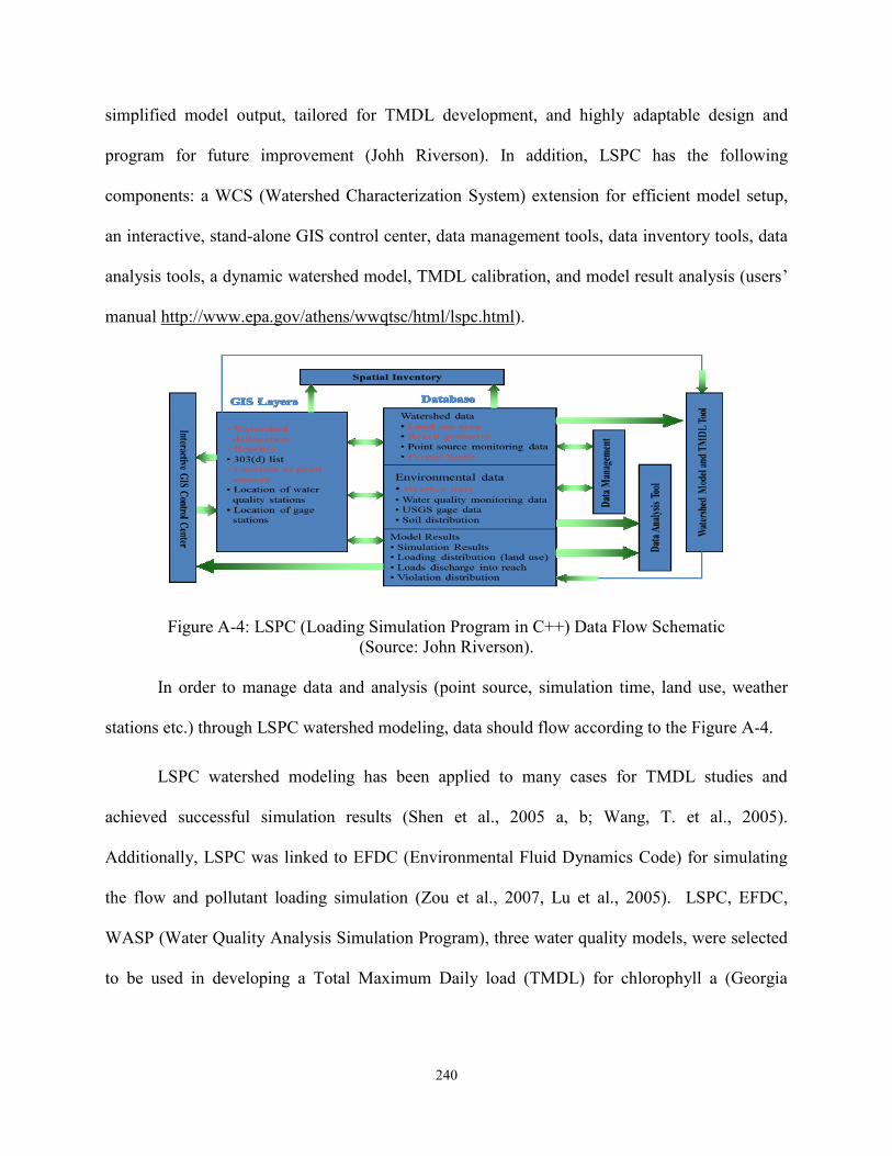
240

simplified model output, tailored for TMDL development, and highly adaptable design and

program for future improvement (Johh Riverson). In addition, LSPC has the following

components: a WCS (Watershed Characterization System) extension for efficient model setup,

an interactive, stand-alone GIS control center, data management tools, data inventory tools, data

analysis tools, a dynamic watershed model, TMDL calibration, and model result analysis (users’

manual http://www.epa.gov/athens/wwqtsc/html/lspc.html).

Figure A-4: LSPC (Loading Simulation Program in C++) Data Flow Schematic

(Source: John Riverson).

In order to manage data and analysis (point source, simulation time, land use, weather

stations etc.) through LSPC watershed modeling, data should flow according to the Figure A-4.

LSPC watershed modeling has been applied to many cases for TMDL studies and

achieved successful simulation results (Shen et al., 2005 a, b; Wang, T. et al., 2005).

Additionally, LSPC was linked to EFDC (Environmental Fluid Dynamics Code) for simulating

the flow and pollutant loading simulation (Zou et al., 2007, Lu et al., 2005). LSPC, EFDC,

WASP (Water Quality Analysis Simulation Program), three water quality models, were selected

to be used in developing a Total Maximum Daily load (TMDL) for chlorophyll a (Georgia

http://www.epa.gov/athens/wwqtsc/html/lspc.html

241

Department of Natural Resources, 2005). Steg et al. (2008) used LSPC to simulate hydrology,

salinity, and the sodium adsorption ratio (SAR) of the Tongue River.

Mercury Loading Model

Mercury Loading Model (Watershed Characterization System-Mercury Loading Model)

is a distributed grid-based watershed mercury loading model which represents the spatial and

temporal dynamics of mercury from both point and nonpoint sources with long-term average

hydrology and sediment yield and mercury transport. This model has six major components: an

ArcGIS interface for processing spatial input data, a basic hydrologic module, a sediment

transport module, a mercury transport and transformation module, a spread sheet-based model

post-processor, and links to other models such as WASP and WHAEM 2000 (Dai et al., 2005,

Knightes). Mercury comes from atmospheric wet and dry depositions, followed by the flow of

surface watr, impervious surfaces, and HgⅡ in the soil, respectively. And then the mercury in

the water surface exports to the tributaries, impervious surface runoffs to the tributaries, and

HgⅡ in soil runoffs and erosion to tributaries or leaching to subsurface. The schematics of the

mercury mechanism are shown in Figure A-5 (Ambrose, 2005).

Figure A-5: Mercury’s movement and available models from the watershed to tributaries

(source Ambrose, 2005).

242

Knightes et al. used the WCS Mercury Loading model to simulate watershed loading of

mercury in systems with large watershed to water surface area ratios (a farm pond, a seepage

lake, a stratified lake, a drainage lake, and a coastal plain lake) for application of ecosystem scale

fate and bioaccumulation to predict fish mercury response time to changes in atmospheric

deposition. In addition, the WCS model was used in the middle and lower parts of the Savannah

River Watershed (U.S. EPA, 2001) and in the Canoochee River Watershed (U.S. EPA, 2004) to

simulate total mercury in fish tissue residue.

WCS MLM has generally been used for mercury simulations from watersheds and it is a

non-dynamic annual mass-balance GIS model and provides yearly-average concentration. To

supplement these deficiencies, GBMM (Gride-Based Watershed Mercury Loading Model) was

developed with a daily time step concentration, user-specified grid, a simple forest and wetland

transport and transformation algorithms for mercury, a bedrock weathering algorithm, a mercury

reduction algorithm and a stream network pre-processor for WASP, and a link to WhAEM2000.

It is a developmental model (Ambrose, 2005; Dai et al, 2005).

MIKE SHE

MIKE SHE, developed by DHI Water and Environment, is a physically based, spatially

distributed hydrological model and combining four components such as overland flow (two-

dimensional saint-venant equation), river flow (one-dimensional saint-venant equation), soil

profile (one-dimensional Richards’ equation), and ground water flow (three-dimensional

Boussinesq equation) (Christiaens et al., 2001, 2002). It has the ability to model both surface and

ground water dynamics in an area with large wetlands, urban areas, irrigated agricultural lands,

and complex hydraulic structures (Copp, 2004). Especially, for simulating forest wetland, the

243

unsaturated zone process which acts like a conduit for water flow is the vital role in order to

couple the surface flow system to the saturated zone (CUI, 2005).

Figure A-6: Schematic Representation of MIKE SHE model (Refsgaard and Storm, 1995).

This model could link MIKE 11 to simulate channel flow which includes complex

channel networks, lakes, reservoirs, and river structures (gates, sluices, and weirs) and MOUSE

sewer model to simulate the interaction between urban storm water and sanitary sewer networks

and groundwater (DHI, 2007).

MIKE SHE has been a widely used model for analyzing, planning, and management

against water resources, environmental and ecological problems related to surface water and

ground water (DHI, 2007; Leslie, 2005). MIKE SHE/MIKE 11 was used as integrated surface

and ground water models for the Picayune Strand Restoration Project (PSRP) in Collier Country,

Florida. This area is experiencing over-drainage due to land development projects in the 1950s

and is affected by several ecological and hydrologic factors (Copp et al., 2007). Copp et al

(2004) applied MIKE SHE/MIKE 11 to evaluate the effectiveness of structural measures for

244

restoration of the wetlands in Southern Golden Gate Estates, which is a part of the Big Cypress

Basin. Im et al., (2008) also applied MIKE SHE/MIKE 11 to analyze the impact of forest-to-

urban land use conversion on watershed hydrology and water availability at the watershed outlet.

MIKE SHE was also linked with Wetland-DNDC for carbon dynamics and greenhouse gases

(GHGs) in the forest wetlands, the change in the water table was a very important point for

GHGs fluxes which were based on the MIKE SHE and Wetland-DNDC linkage model (Cui,

2005). Wakool Irrigation District (74,000 ha of agricultural Land) in New South Wales, Austria

had problems such as rising water table levels and land salinisation, So Demetriou et al. (1998)

applied MIKE SHE for analysis of the complex hydrogeological regime in the region, the

prediction of the environmental impacts of various management options, and the selection of the

best options for restoration were chosen. In addition, MIKE SHE was linked to Remote Sensing

derived data and GIS managed data for applying to a major irrigation project (Gupta, 2008).

MUSIC

MUSIC (Model for Urban Stormwater Improvement Conceptualization) is a decision

support system which was developed by Monash University and Cooperative Research Center

for Catchment Hydrology and is not a detailed design. This model could be operated based on

temporal and spatial scales from 0.01km2 to 100km

2 watershed areas and 6 minutes to 24 hours

for time steps and has a user-friendly interface to provide quick and efficient simulation for

complex stormwater management scenarios and the results were based on a graphical and tabular

format. MUSIC was developed in order to improve and integrate the urban stormwater

management measures because only models based on ad-hoc or single-focus approaches existed.

Hence MUSIC has the following capabilities to manage urban catchment; (1) Conceptual Design

to generate the most efficient and cost effective urban stormwater systems and integrated

245

stormwater management plan for each catchment against a range of water quality standards, (2)

Evaluation and Assessment if urban subdivision proposals and development applications are

available to meet water quality objectives and urban drainage regulations, (3) System planning

and Management for treatment strategies and measurement and monitoring of new and existing

drainage schemes, (4) Regulation for development guidelines for the urban water management

industry (Wong et al., 2002; MUSIC brochure version 4; Leslie et al., 2005).

The framework of MUSIC is shown in Figure A-7 and includes contaminant load

characteristics, structural and non-structural stormwater BMP models, Stormwater management

criteria, and so on.

Figure A-7: Framework of the MUSIC model (Source: Wong et al., 2002)

The engine of MUSIC is the Universal Stormwater Treatment Model (USTM).

In addition, the hydraulic efficiency of stormwater treatment systems is calculated by

two-dimensional hydrodynamic modeling based on λvalues which is different with a number of

pond or wetland shapes and depends on the inlet/outlet and length to width configuration

(Persson et al., 1999; Wong et al., 2002)

246

MUSIC hydrology algorithm was developed by Chiew et al.(1997). It is largely two

flows; one is runoff contributed from an impervious surface and the other is baseflow which is

influenced by sub-surface soil moisture and groundwater level.

MUSIC was applied in an Australian city for comparing a number of options of

retrofitting stormwater quality improvement measures (Wong et al., 2002).

P8-UCM

P8-UCM (Program for Predicting Polluting Particle Passage through Pits, Puddles, and

Ponds-Urban Catchment Model) is a hydrologic and BMP model for predicting the generation

and transport of stormwater runoff pollutants in urban watersheds (Leslie et al., 2005, Tetra Tech,

Inc., 2007) and is simulated by continuous water-balance and mass-balance through a user-

defined system. There are four components of P8; watersheds, devices (runoff storage, treatment

areas, BMP’s), particle classes, and water quality components which are simulated by hourly

rainfall and daily air temperature time series data (William, 1990, Tetra Tech, Inc., 2005).

In order to simulate the P8-UCM model, site-specific input data which are familiar to

local engineers and planners and initial calibration of certain water-quality parameters such as

particle settling velocities, particle build up/wash off, and particle contaminant contents are

needed and it simulates a variety of treatment device including swales, buffer strips, detention

ponds (dry, wet, extended), flow splitters, infiltration basins (offline, online) (William, 1990).

The following figure (Figure A-8) shows the simple P8-UCM set up.

247

Figure A-8: Simple P8-UCM set up (Source: Tetra Tech, Inc., 2005).

Numerous Vermont watersheds did not meet Vermont’s aquatic life standards because of

the urban drainage and suburban storm runoff, so Four models (GWLF, SLAMM, P8-UCM,

SWMM) were used to investigate the project needs, data availability, and the level of effort

required for model implementation. SWMM and P8-UCM achieved the highest ranks but when

comparing calibrations, developing flow duration curves, and many urban pollutants as well as

urban BMP, P8-UCM was chosen as the best model for Vermont’s watersheds and is suitable to

simulate both event based and long-term hydrological simulations for relative variability among

watersheds and drainage areas (Tetra Tech inc., 2005b).

P8-UCM was used for evaluating the amount of groundwater recharging when diverting

to an infiltration-type BMP from completely impervious drainage (100% impervious) (Tetra

Tech. Inc., 2007).

248

PCSWMM

PCSWMM (Storm Water Management Model) is a commercial software package with

the computational engine of the U.S. EPA’s Software Water Management Model version 5 (EPA

SWMM 5) and a graphical interface of SWMM to simulate runoff and hydraulics in pipe

networks having the capacity to create a storm sewer network and massive database management

with relative ease (Sands et al., 2004, nhc, 2010)

A spatially-distributed rainfall method was applied to simulate rainfall and non-linear

reservoir routing, subcatchment to subcatchment routing, triangular unit hydrograph,

groundwater interflow, and inflow from other hydrologic models were used for runoff simulation.

Especially, time-varying rainfall, for the non-linear reservoir routing of overland flow, rainfall

interception from depression storage, evaporation of standing surface water, snow accumulation

and melting, infiltration of rainfall into unsaturated soil layers (Horton, Green-Ampt, and SCS

curve number), percolation of infiltrated water into groundwater layers, interflow between

groundwater and the drainage system, and overland sheet flow (Manning’s formula) were

included in this model. There were three routing runoff methods used (dynamic wave routing,

kinematic wave routing, steady-state routing), RDⅡ, DWF, and external inflows through the

pipes, channels, storage/treatment units and diversion structures which is includes the following

abilities: handle networks of unlimited size, use a wide variety of standardized closed and open

conduit shapes as well as natural channels, model special elements such as storage/treatment

units, flow dividers, pumps, weirs, and orifices, apply external flows and water quality inputs

from surface runoff, groundwater interflow, compute rainfall dependent infiltration/inflow

(RDⅡ), dry weather sanitary flow (DWF), and user-defined inflow, utilize either kinematic

water or full dynamic water flow routing methods, model various flow regimes, such as

249

backwater, surcharging, reverse flow, and surface ponding, and apply priority-based, dynamic

control rules to simulate the operation of pumps, orifice openings, and weir crest levels

(PCSWMM Brochure, www.chiwater.com/software/PCSWMM.NET).

PCSWMM contains a genetic algorithm (GA)-based software tool for the calibration of

the Storm Water Management Model (SWMM). Through this GA calibration tool, the effort for

general calibration and design optimization was significantly reduced (James, 2002). In addition,

PCSWMM’s genetic algorithm routine could examine the best management practices such as

infiltration, detention, and retention systems and select the best combination of urban stormwater

infrastructure and their sizes. James (2003) compared several different BMPs (Best Management

Practices) with PCSWMM’s genetic algorithm against several constraints, for instance, local

quantity and quality regulations, sewer capacities, not exceeding predevelopment flow rates and

could systematically decrease the total drainage cost.

Heier et al. (2003) used PCSWMM for predicting the sediment yield changes between the

pre-construction and construction period of an 18-hole champion golf course which is located

near Manhattan, Kansas, on the Little Kitten Creek watershed. PCSWMM was used for the

establishment of an integrated watershed management plan for the Mokgamcheon watershed in

South Korea (Hong, 2008).

PGC-BMP

PGC-BMP (Prince George’s County Best Management Practice Module), BMP ToolBox

model, was developed by Tetra Tech and Prince George’s County in Maryland, USA, in order to

evaluate BMP applications before and after the development and effectiveness of structural BMP

(Tetra Tech, 2003). BMP could be classified based on the structural mechanisms which are

http://www.chiwater.com/software/PCSWMM.NET

250

divided into classes A and B: class A (retention, interception, and vegetation), class B (open

channel units, infiltration, and filtration) which is shown at Figure A-9.

Figure A-9: BMP types of BMP Toolbox model (Cheng et al., 2004, 2009).

The PGC-BMP module could evaluate detention basins, infiltration trenches, dry wells,

porous pavement, wetlands, swale, filter strips, bioretention, etc., and the treatment processes are

composed of several mechanisms like storage, infiltration, overflow/outlet flow, decay process,

and soil media pollutant removal as well. The algorithms of this module used the following

methods: Storage routing, Holtan’s equation, weir/orifice, and first-order decay and the water

quality were applied by user-defined pollutants (Riverson, 2004).

Chen et al. (2010) applied the BMP ToolBox model to the study site of Feitsui reservoir

watershed (total treatment area is 2,953 m2, and the total hydraulic retention time was 5.24 days),

the Feitsui reservoir was in a mesotrophic status due to nonpoint source pollution. Lately,

BMPDSS (BMP Decision Support System) has been used. It is a state of art decision supporting

system for placing BMPs at strategic locations in urban watersheds on the basis of integrated

data collection and hydrologic, hydraulic, and water quality modeling. And this system could

251

compare the trade-off relationship between BMP costs and excavation volume (Cheng et al.,

2009, Zhen et al., 2010).

SHETRAN

SHETRAN (Système Hydrologique Europeén TRANsport) is a 3D coupled

surface/subsurface PBSD (Physically Based Spatially Distributed) finite-difference model for

coupled water flow, multi fraction sediment transport, and multiple, reactive solute transport in

river basins. There are three major components in this model: water flow, sediment transport,

and solute transport. They are not affected by each other, as the three components depend on the

natural situation. SHETRAN is capable of integrating flow and transport of both surface and

subsurface with major hydrological cycle factors such as interception, evapotranspiration,

snowmelt, overland and channel flow, unsaturated and saturated zone flow (Ewen et al., 2000,

Lukey et al., 2000)

Figure A-10: Flow schematic diagram of SHETRAN model (Source: Dunn et al., 1996).

252

SHETRAN could be suitable to simulate the flow processes in Karst aquifers allowing

both surface and subsurface processes to be modeled. Adams et al. (2002) applied the VSS (A

Variably Saturated Subsurface) – NET to the SHETRAN model for the Karst aquifers’

simulation. Dunn et al. (1996) implemented the SHETRAN model to simulate the hydrological

impact of open ditch drainage and the most import processes according to the results of the

simulation are the sub-surface and under near saturated conditions, interaction between sub-

surface and stream network, and the speed of the surface runoff. In addition, Dunn et al., (1995)

assessed how variations such as climate and land use in evaportranspiration affect the hydrology

of a region in the Tyne Basin in North East England through the SHETRAN model as well.

The SHETRAN model is like physically based, spatially distributed models which have

been criticized and the model parameterizations have to be validated and incorporated with

internal response data and demonstration of a model’s fitness, so Bathurst et al (2004) tested

several scenarios to validate the SHETRAN model for predicting land-use and climate change

impacts at the Slapton Wood catchment (there have been many researches implemented to

simulate water flow and water quality because it is a complicated catchment with a combination

of various land cover) in Southwest England. SHETRAN was also used to find the depth of

subsurface flow at the Slapton Wood catchment (Birkinshaw et al., 2010). Birkinshaw et al.

(2000) used the SHETRAN model to simulate nitrate transport at the Slapton Wood catchment

and this model can also simulate the landslide erosion and sediment transport, Burton et al.

(1998) applied SHETRAN at the Kirton research catchment in Balquhidder, Scotland to simulate

shallow landslide erosion and sediment yield components.

253

SLAMM

SLAMM (Source Loading and Management Model) was developed to enhance the

understanding of the relationship between sources of urban runoff pollutants and runoff quality

and is an urban rainfall runoff water quality model which does not deal with agricultural areas,

etc. It is a multi-scale model controlled from individual lots to whole communities. This model

includes many source areas and outfall control practices such as infiltration practices, wet

detention ponds, porous pavement, street cleaning, catchment cleaning, grass swales (Pitt et al.,

2002). Land use could be classified for up to 6 different land uses, 14 source area types and it is

permitted to simulate additional sub-areas or different management scenarios. Runoff volumes

and urban pollutant loadings could be calculated annually as well as seasonal pollutant loads and

event pollutant probability distributions using long-term rainfall records (Source: SLAMM)

SLAMM considers many kind sources of pollutions and simulate the urban area’s flow

routing like in Figure A-11. From unconnected sources to directly connected impervious areas,

gutters, sewerage systems, and receiving water each have their own characteristics and removal

system which can be applied to compose SLAMM (Pitt et al., 2000).

Figure A-11: The mechanism of pollutant deposition and removal at sources areas for SLAMM

(Source: Pitt et al., 2000).

254

Another unique characteristic of the SLAMM model is the wash-off model which can

predict the losses of suspended solids from different surfaces based on an individual first-flush

(exponential) relationship (Pitt et al., 2002).

WinSLAMM could use as a decision analysis program for finding out the best

alternatives before starting urbanization plans. Pitt et al.(a) and Pitt et al. (2007) applied

WinSLAMM as a systematic procedure for trade-offs among multiple and usually conflicting

program objectives by comparing both the costs and effectiveness.

SLAMM was used as a planning tool for BMP implementation. Furthermore, this model

includes a cost analysis tool in order to compare the costs for different BMP as well (Kabbes et

al, 2008). And Neilson et al. (2010) used SCS based WinSLAMM modeling for green

infrastructure sizing, water quality treatment, and to input the following various parameters in

order to achieve the best predictions.

SPARROW

SPARROW (SPAtially Referenced Regression On Watershed attributes) is a watershed

modeled used to set up mathematical relationships between water quality measurements and the

attributes of watersheds. SPARROW is a statistically calibrated regression model composed of

both mechanistic components and mass-balance constraints and there are two main functions;

one is the empirical rate of nutrient delivery from point and diffused sources to streams, lakes,

and watershed outlets. The other is the spatial referencing of stream monitoring stations, nutrient

sources, and the climatic and hydrogeologic properties of catchments based on the landscape and

surface-water features (Schwarz et al., 2006, Alexander et al., 2004). The model structure,

including the two main functions that were just mentioned, are shown in Figure A-12 and

demonstrates the functional linkage between the major spatial components of the SPARROW

255

model. Sparrow is mainly composed of two steps, like two main functions. First is the pre-

processing step for getting reach-level information and the second is the monitoring of station

flux estimations for estimating the long-term flux.

Figure A-12: Schematics of the major SPARROW model components (Source: Schwarz et al.,

2006).

The following two components could display the contaminant load or flux leaving a

reach: load generated within upstream reaches and transported to the reach via the stream

network and load originating within the reach’s incremental watershed and delivered to the reach

segment. Based on the two components, the formula is shown in the below in Equation 14

(Goodall et al., 2010)

Equation A-2

Where, Li = the mass loading of reach i, measured in metric tons; n, N= source index

where N is the total number of individual n sources; J(i)= set of all reaches upstream and

includes reach I, except reaches at or above the monitoring stations upstream from reach i; Sn,j=

transported to downstream reach i according to the two nonlinear processes; D(Zj)= first process;

256

transported load from the land surface to the stream which is a function of the watershed

properties for reach j; K(Tij)= second process; instream transport from reach j to reach i which is

a function of the flow path properties between i and j.

The SPARROW model has a hybrid-statistical-process structure and deals with pure

statistical and regression-based models by combining nutrient transport components like flow

paths, first-order loss functions, and mass-balance constraints and reduces problems related to

the data interpretation caused by sparse stream sampling measurement networks, network

sampling biases and basin heterogeneity (Alexander et al., 2002a, 2004, Robert et al., 2010,

Smith et al., 1997, 2003).

Goodall et al. (2010) used the SPARROW model for the Upper Neuse River Basin to

answer the following questions: First, how much load is provided by a unit area? Second, what

portion of the incremental load from each watershed is transported to the river basin outlet?

Third, how would a 10% increase in fertilizer application impact loading at the watershed outlet?

Through solving these problems with the SPARROW model, it proves detains about which

subwatersheds are potential pollution areas. Brakebill et al. (2003) improved the hydrologic

network system according to the application of the 30 m DEM (Digital Elevation Models) from

the 1 km DEM. Alexander (2002) compared the six nitrogen export models (SPARROW, LS1-

GLOBAL, LS2-GLOBAL, GLOBAL, PEIERLS, HOWARTH) to find out the accuracy (bias

and precision) of each model. The resolution showed that 5 models, except the SPARROW

model, had significantly negative correlations between prediction errors and runoff and

suggested the improvement of the ability by combining both the mechanistic description of

process in the deterministic model and the statistical model. The SPARROW model is good at

257

applying the TMDL (Total Maximum Daily Load) program. McMahon et al. (2002) applied the

SPARROW model to TMDL for Eastern North Carolina- Cape Fear, Neuse, and Tar-Pamlico.

Alexander et al. (2008) also applied the SPARROW model to find out the differences

both phosphorus and nitrogen delivery to the Gulf of Mexico from the Mississippi River Basin.

In addition, Alexander et al. (2006) estimated TN and TP’s trends from 1975 to 1994 in the

United States through the SPARROW model

STORM

STORM (Storage, Treatment, Overflow, Runoff Model) was developed by the

Hydrologic Engineering Center (HEC) in the early 1970’s (Deliman, 1999, Abbott, 1997). This

model provides predictions of wet-weather pollutographs (Mass Loading curves for use in a

receiving water assessment model) and preliminary sizing of storage and treatment facilities to

satisfy the desired criteria for control of stormwater runoff. STORM considers seven storm water

elements which are shown in Figure A-13: rainfall/snowmelt, runoff, dry weather flow, pollutant

accumulation and wash off, land surface erosion, treatment rates, and detention reservoir storage.

The following are the four major steps: the first is the computation of runoff quantity, the second

is the computation of runoff quality, the third is the computation of treatment, storage, and

overflow, and the last is the computation of land surface erosion. For the computation of the

quantity of runoff, the coefficient method, the U.S. Soil Conservation Service Curve Number

technique or combination method (the coefficient method for impervious land and SCS for

pervious land) were used. For the quality of runoff, the dust and dirt method (assumes that all

pollutants are associated with the dust and dirt accumulation in the street) and the daily pollutant

accumulation (mainly non-urban areas) were used.

258

Figure A-13: The schematics of STORM model’s flow mechanism (U.S. ACE, 1997).

Heineman (2005) used NetSTORM and STORM DLL (dynamic-link library file) to show

the capabilities of cost optimization and detention pond sizing’s determination. Baerenklaus et al

(2008) also used STORM for estimating the costs for land, construction, maintenance expenses,

and rehabilitation costs. When compared between decentralized and centralized BMPs (Best

Management Practices), decentralized BMP’s costs were much less than centralized BMPs

because the latter needs additional fees to obtain BMP’s land.

Najjar et al. (1995) researched the water quality model at the Lakes Bay Estuarine

Embayment (Lake: surface area, 8.90Χ106 m2, average depth, 1.5 m, volume, 13.2 and

Drainage area: 16.2Χ106 m2) to develop a mathematical model for estimating the expected

pollutant loading, to simulate water quality of tidal embayment systems, to perform field studies

for the collection of data to calibrate and refine, and to calibrate and verify the model for creating

a useful management tool for limited land use situations. Warwick et al. (1990) used Monte

Carlo simulation techniques to ascertain in probable ranges of STORM water quality predictions

in regards to both water quantity and quality input parameter uncertainties (BOD5, TSS,

Orthophosphate, T-N) because there was not enough water quality data in the research areas.

259

SWAT

SWAT (Soil and Water Assessment Tool) was developed by USDA Agricultural

Research Service (ARS) and is mainly adapted as parts of the U.S. EPA BASINS (Better

Assessment Science Integrating Point and Non-point Sources). SWAT has grown as a

multidiscipline model and includes following models: GLEAMS for pesticide components,

GREAMS for daily rainfall hydrology components, EPIC for crop growth components, SWRRB

for multiple subbasins and other components, Qual2E for instream kinetics, and ROTO for

routing structures. The schematic of SWAT’s development is shown in Figure A-14 (Gassman et

al., 2007).

Figure A-14: The Schematic of SWAT’s development (Source: Gassman et al, 2007).

Rainfall may be intercepted and held in a vegetation canopy or fall to the soil surface and

then infiltrated, interflowed and runoff through aquifer and surface. The potential pathway of

water from precipitation to stream flow including irrigation, surface runoff, aquifer, etc., is

shown in Figure A-15 (Neitsch et al., 2005).

260

Figure A-15: The Schematic of a potential water pathway of the SWAT model (Neitsch et al.,

2005).

In this model, the watershed could be divided into a number of subwatersheds or

subbasins which are grouped depending on climate, HRU, ponds, groundwater and main

channels.

SWAT and AnnAGNPS were compared by Heathman et al. (2008) to apply uncalibrated

(for eliminating bias due to parameter optimization) to the Cedar Creek watershed within the St.

Joseph River watershed in northeastern Indiana to predict streamflow and atrazine losses. As a

result, the SWAT model’s performance was remarkably superior to AnnAGNPS in estimating

streamflow.

261

Fitz Hugh et al. (2001) used the SWAT model to compare the impaction of subwatershed

partitioning on modeled sources and transport-limited14

sediment yield with other factors such as

slope gradient, slope length, and HRU (Hydrologic response units) area. In addition, in order to

delineate subwatershed moderately, Gong et al. (2010) analyzed the parameter uncertainty of

subwatersheds with the newly developed sequential uncertainty fitting version-2 (SUFI-2)

procedure to supplement any shortcomings in existing parameter uncertainty analysis method

(sensitivity analysis, first-order error analysis, and the Monte Carlo method).

SWAT was also used for estimating the comprehensive and economically viable

solutions of the P reduction from dairy agriculture near the Cannonsville Reservoir by

Ghebremichael et al. (2008). Ullrich et al. (2009) applied the SWAT model to predict the impact

of alternative management practices on water quality and quantity in the state of Saxony in

Central Germany has a drainage are of about 315km2. This was the first time research for a

sensitivity analysis for conservation management parameters such as tillage depth, mechanical

soil mixing efficiency, biological soil mixing efficiency, curve numbers, Manning’s roughness

coefficient for overland flow,

SWMM

SWMM (Storm Water Management Model) is a dynamic rainfall-runoff simulation

model for water quality and quantity and is used primarily for urban areas. This model could be

used for single events or long-term (continuous) simulations. SWMM was developed by the U.S.

Environmental Protection Agency from 1969-71 and Camp Dresser & McKee Inc. are

14

Source-limited watershed: more material can be transported away than can be detached

Transport-limited watershed: more material can be detached than can be carried away by way

of transport processes.

262

researching and controlling the SWMM model presently. The purposes of this model are for

planning, analysis and design of urban watersheds, including rainfall-runoff, flow routing, water

quality, storage/treatment, and sewer-systems, especially flow routing of an urban watershed as it

transports through a system of pipes, channels, storage/treatment devices, pumps and regulators

(Rossman, 2010, Huber, 2003).

SWMM has a variety of capabilities for urban areas, including various hydrologic

processes as follows: time-varying rainfall, evaporation of standing surface water, snow

accumulation and melting, rainfall interception from depression storage, infiltration of rainfall

into unsaturated soil layers, percolation of infiltrated water into groundwater layers, interflow

between groundwater and the drainage system, nonlinear reservoir routing of overland flow, and

capture and retention of rainfall/runoff with various types of low impact development (LID)

practices (Rossman, 2010).

The SWMM model simulates the hydrology, hydraulics, and water quality transport

behavior of a drainage system as shown in Figure A-16.

Figure A-16: The SWMM model’s Schematic (Source: Rossman, 2010).

263

The SWMM model simulates LID (Low Impact Development) units such as bio-retention

cells, porous pavement, infiltration trenches, rain barrels, and vegetation swale. In detail, each

layer (surface, pavement, soil, storage, underdrain) could be used separately based on the

different types of LID.

The SWMM model was used for integrating the collection systems for Hartford,

Connecticut (Heineman et al., 2010). Originally, the Hartford Water Pollution Control Facility

controlled individual collection systems such as combined sewers, sanitary sewers, storm drains,

and open channel drainage. After integrating the collection systems, it is easy to access, modify

and upgrade the drainage system in regards to items such as CSO estimations and long term

control plans, sanitary sewer overflow, etc. Jawdy et al. (2010) used the SWMM model to

analyze the effects of Green Infrastructure (GI) practices for reducing combined sewer overflows

in Nashville, Tennessee. 103 prototype models including bio-retention cells, pervious pavements,

green roofs and tree planters having a various media depths, ratio of run-on areas to facility areas,

deep percolation rates, media and plantings were run and evaluated for the volume of runoff.

Alfredo et al. (2010) also researched the hydrologic performance of green roofs under variable

precipitation conditions: steady, low-intensity rainfall and short duration, and high-intensity

rainfall. Green roofs were installed with both control membrane roofs and prototype green roofs

(2.5, 6.3, 10.1 cm depth). Roehr et al. (2010) also used the SWMM model to simulate runoff

generated by impervious roofs and green roofs by integrating the Green-Ampt method and

evapotranspiration of green roofs because the Green-Ampt method cannot accurately simulate

green roof runoff. Lucas (2010) designed integrated bioinfiltration-detention urban retrofits (a

bioretention planter/trench infiltration-detention system) with the SWMM model. McCutcheon et

al. (2010) tried to make an exfiltration modified SWMM source code to allow the simulation of

264

the storm hydrograph for controlled partial exfiltration from the sewers. Moreover, the SWMM

model was used to estimate the distribution of particulate-bound metals for source area snow in

the Lake Tahoe watershed (Magill et al., 2010).

TOPMODEL

TOPMODEL is a semi-distributed variable contributing area hydrological model

(rainfall-runoff model) which provides distributed predictions of catchment response to rainfall

based on the a simple theory of hydrological similarities of points in a catchment with the

topographic index ln (α/tan β), where α is the area of the hillslope per unit contour length that

drains through the given point, used as the index for hydrological similarities. This model used

simple parameters because it has a simple structure, so there are several basin model assumptions

which are as followings; 1. Dynamics of the saturated zone can be approximated by successive

steady-state representations, 2. Hydraulic gradient of the saturated zone can be approximated by

the local surface topographic slope, tan β; groundwater table and saturated flow are parallel to

the local surface slope, 3. Distribution of downslope transmissivity with depth is an exponential

function of storage deficit or depth to the water table. Based on these assumptions, a correlation

could be found between the catchment mean water table (storage deficit) and local water table

level (storage deficit) (Wu et al., 2007, Gallart et al., 2007, Candela et al., 2005, Xiong et al.,

2004, Holko et al., 1997).

Major hydrologic behaviors of the TOPMODEL are precipitation (snow and rain),

infiltration, snowmelt, and evaporation which were shown in Figure A-17. And the parameter’s

mechanism is simply divided into topography, saturated store, root zone and unsaturated store,

and flow routing.

265

Figure A-17: Hydrological behavior of the catchment in TOPMODEL (Source: Holko et al,

1997).

TOPMODEL is significantly sensitive to the scale of topography including the terrain

attributes. Especially, grid sizes could be compared to determine the impaction using

TOPMODEL. According to the Brasington et al., (1998) research, 100 ~ 200m grid size is the

range in which rapid deterioration occurs in the information content of the DEM. The scale of

topography should be investigated based on the watershed’s characteristics. Cameron et al.

(1999) researched the possibility of deriving frequency distributions of extreme discharge by

continuous simulation through the rainfall-runoff model TOPMODEL is implemented by GLUE

(Generalized Likelihood Uncertainty Estimation). Xiong et al. (2004) used TOPMODEL to

simulate the relationship between rainfall and runoff based on a variety runoff coefficients from

0.333 to 0.733 during flood seasons in the semi-arid Yihe catchment (2,623km2) in the Yellow

River basin of China.

TOPMODEL had limitations when applied to semi-arid catchments, because the way in

which semi-arid catchment’s land is used is totally different with general catchments. So Candela

266

et al. (2005) applied to modify the TOPMODEL routing algorithms to consider different patterns

of routing between hillslope & channel even though TOPMODEL is applied to a semi-arid area.

In order to adapt the semiarid characteristics, surface roughness was applied based on the routing

velocity for each pixel of the watershed linked to the watershed land use which is through the

different roughness derived on the basis of Engman’s table (Engman, 1986).

TOPMODEL has generally been considered a simplified model of the saturated zone so

far. However in order to complete a continuous simulation model, it needs more component

mechanisms such as interception, snow accumulation and melt, infiltration, evapotranspiration,

the unsaturated zone and flow routing (Beven, 1997).

WAMView

WAMView (Watershed Assessment Model with an ArcView Interface) is a process-based

model with GIS (Geographic Information System) interface to simulate watershed hydrologic

and pollutant transport. This model includes the following features: ① Source cell mapping of

TSS and nutrient surface and groundwater loads, ② Flow/constituent transport modeling of land

source areas on a spatial scale/grid of 1ha or less, ③ Unique cell recognition for faster run times,

④ Tabular ranking of land uses by constituent contributions, ⑤ Overland, wetland, and stream

load attenuation mapped back to source cells, ⑥ Optional Index Model for Toxins, BOD, and

bacteria for source mapping, ⑦ Hydrodynamic stream routing of flow and constituents (N, P,

BOD, Dissolved Oxygen, Chlorophyll-A if WASP Linkage is used) with annual, daily, or

hourly outputs, ⑧ Optional Index Model for Toxins, BOD, and bacteria for source mapping, ⑨

Ground water flow modeling with well withdrawals and surface/groundwater interactions, ⑩

Allows time series of point source inflows and wastewater treatment plant service area coverage

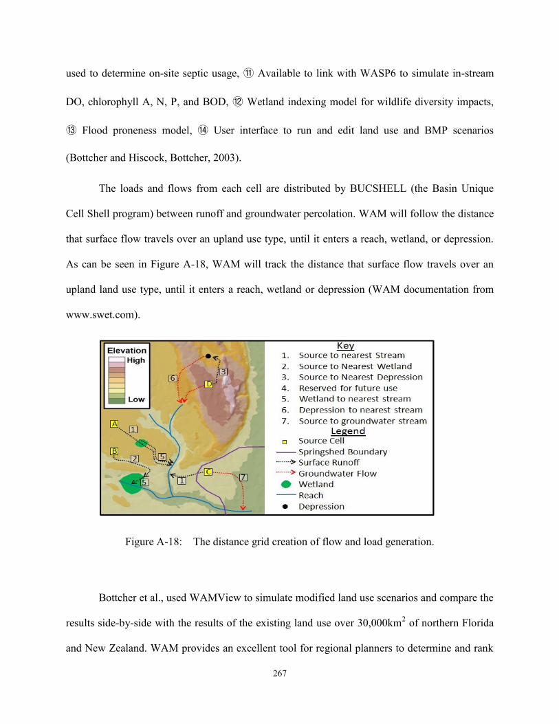
267

used to determine on-site septic usage, ⑪ Available to link with WASP6 to simulate in-stream

DO, chlorophyll A, N, P, and BOD, ⑫ Wetland indexing model for wildlife diversity impacts,

⑬ Flood proneness model, ⑭ User interface to run and edit land use and BMP scenarios

(Bottcher and Hiscock, Bottcher, 2003).

The loads and flows from each cell are distributed by BUCSHELL (the Basin Unique

Cell Shell program) between runoff and groundwater percolation. WAM will follow the distance

that surface flow travels over an upland use type, until it enters a reach, wetland, or depression.

As can be seen in Figure A-18, WAM will track the distance that surface flow travels over an

upland land use type, until it enters a reach, wetland or depression (WAM documentation from

www.swet.com).

Figure A-18: The distance grid creation of flow and load generation.

Bottcher et al., used WAMView to simulate modified land use scenarios and compare the

results side-by-side with the results of the existing land use over 30,000km2 of northern Florida

and New Zealand. WAM provides an excellent tool for regional planners to determine and rank

268

current areas under environmental stress, estimate future impacts of land use management

decisions, determine achievable pollution load reduction goals and establish Total Maximum

Daily Loads (TMDLs). Bottcher et al. (2003) also simulated flow and water quality constituents

for several Florida watersheds in terms of Florida’s TMDL program and other watershed

restoration projects. The WAM model has been successfully applied to multiple basins within

Florida for the development of TMDLs and for alternative assessments to meet the flow and

water quality goals of impaired water bodies.

Lake Okeechobee is a large, shallow freshwater lake located in southern Florida. In an

effort to reduce phosphorus loads, phosphorus loading to Lake Okeechobee was set to be

reduced by 40% through the 1987 Surface Water Improvement and Management (SWIM) Act.

So WAM was applied to determine the detention volume (water detention depth) depending

upon typical land uses such as abandoned dairies, citrus groves, daily pastures, field crops,

improved/unimproved/woodland pastures, row crops, and other land uses (Zhang et al., 2005).

Zhang et al. (2006) also studied about the detention depth of Buck Island Ranch which is located

at the MacArthur Agro-ecology Research Center, near Lake Placid, Florida.

WARMF

WARMF (Watershed Analysis Risk Management Framework) is a watershed model and

analysis tool with short and long term predictions capabilities. WARMF has a variety of

functions such as the ability to calculate TMDL, evaluate water quality management for a river

basin, simulating flow, water quality constituents (Temp, TSS, Coliform, Bacteria), BOD, DO,

nutrients (phosphorus & nitrogen species), and Chlorophyll. In addition, decision support

capabilities, sensitivities and uncertainties, and analyses of WARMF projects have been studied

continuously by EPRI (the Electric Power Research Institute). This model has five integrated

269

modules such as Engineering, Consensus, TMDL, Data, and Knowledge: the Engineering

module performs hydrologic and water quality simulations using data files from the DATA

module and contains a dynamic watershed simulation model. It calculates daily surface runoff,

groundwater flow, non-point source loads, hydrology, water quality of river segments, and

stratified reservoirs. Watersheds are divided into a network of land catchments, river segments,

and reservoir layers. In order to promote the water routing from land, land catchments are

classified by land surface (land use and cover) and soil layer (air, water, and solid fractions)

which are shown in Figure A-19. The TMDL module is a decision module based on a step-by-

step procedure and can decide multiple possible solutions for a TMDL. The consensus module

guides stakeholders to select a preferable TMDL which takes into consideration the following

factors: costs, pollution trading, social and political factors (Keller, 2007, Chen et al., 2004, 2000

A, B).

Figure A-19: Components of land catchments (Chen et al., 2000).

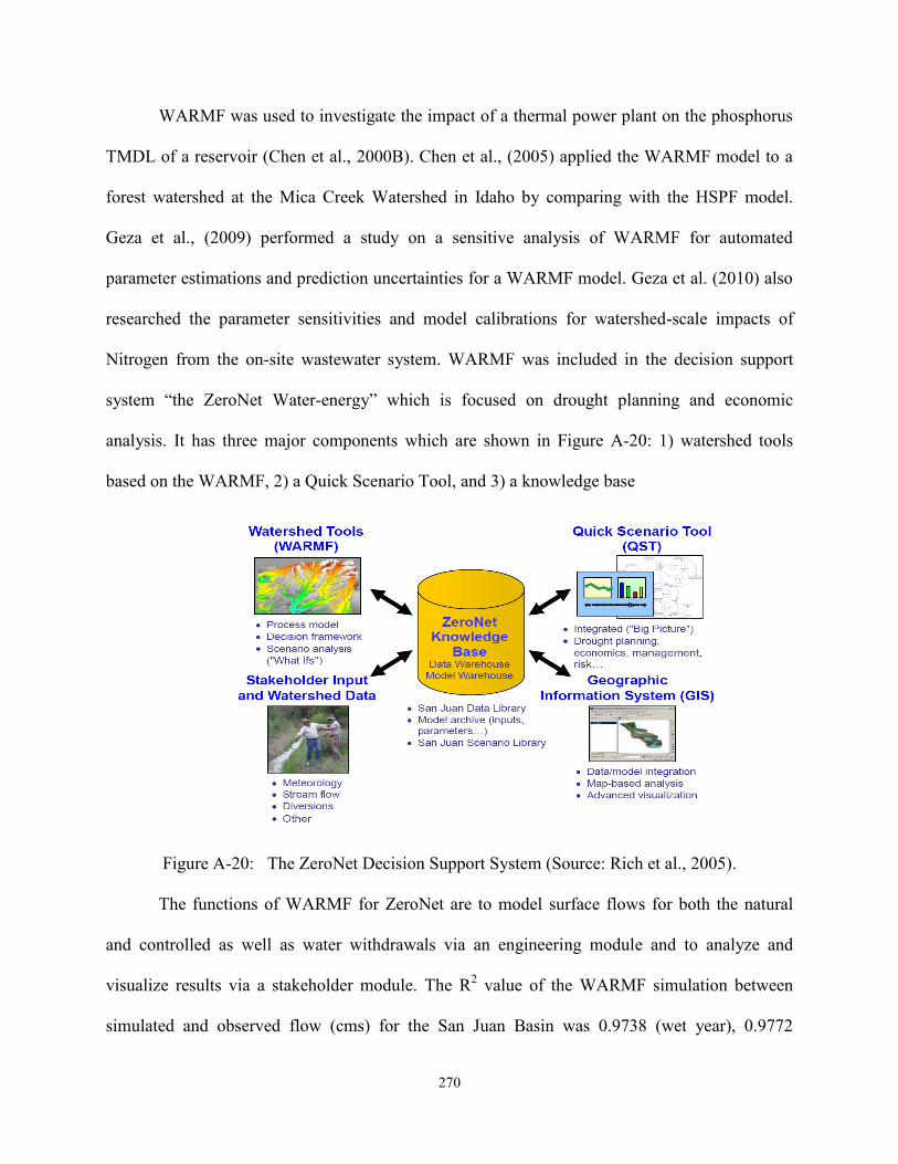
270

WARMF was used to investigate the impact of a thermal power plant on the phosphorus

TMDL of a reservoir (Chen et al., 2000B). Chen et al., (2005) applied the WARMF model to a

forest watershed at the Mica Creek Watershed in Idaho by comparing with the HSPF model.

Geza et al., (2009) performed a study on a sensitive analysis of WARMF for automated

parameter estimations and prediction uncertainties for a WARMF model. Geza et al. (2010) also

researched the parameter sensitivities and model calibrations for watershed-scale impacts of

Nitrogen from the on-site wastewater system. WARMF was included in the decision support

system “the ZeroNet Water-energy” which is focused on drought planning and economic

analysis. It has three major components which are shown in Figure A-20: 1) watershed tools

based on the WARMF, 2) a Quick Scenario Tool, and 3) a knowledge base

Figure A-20: The ZeroNet Decision Support System (Source: Rich et al., 2005).

The functions of WARMF for ZeroNet are to model surface flows for both the natural

and controlled as well as water withdrawals via an engineering module and to analyze and

visualize results via a stakeholder module. The R2 value of the WARMF simulation between

simulated and observed flow (cms) for the San Juan Basin was 0.9738 (wet year), 0.9772

271

(Normal year), and 0.8853 (dry year) (Rich et al., 2005). Weintraub et al., (2004) used WARMF

for TN/TP loading and transport of nutrients from OWS in the 840 km2 Dillon River Watershed

in Colorado. The R2 value of the comparison of simulated and observed stream flow was

0.816~0.835

WEPP

WEPP (Water Erosion Prediction Project) is a process-based distributed parameter model.

It is a continuous simulation computer program used to predict soil loss (erosion) and sediment

deposition (delivery) based on the overland flow on hillslopes, the concentrated flow in small

channels, and the sediment deposition in compounds. This model is composed of several

components: a climate component, a hydrology component, a daily water balance component, a

plant growth and residue decomposition component, and an irrigation component. These

components are computed by spatial and temporal distributions of soil loss and decomposition

by single events and longer time periods, respectively (Flanagan et al., 1995, Abaci et al., 2007).

Figure A-21: The process schematic of the WEPP model (Source: Flanagan et al., 1995).

272

Like in Figure A-21, the WEPP model processes the following components: infiltration

(Green-Ampt model), different land management practices (e.g. tillage, contouring), plant

growth, residue decomposition, freezing and thawing, percolation, evaporation and transpiration.

For a stochastic weather data generator, WEPP utilizes CLIGEN version 4.3 to generate daily

input data (Flanagan et al., 1995, Abaci et al., 2007, 2008).

SDR (Sediment Delivery Ratio) is vital for predicting the sediment runoff from

watersheds. Abaci et al. (2008) applied the WEPP model to a 26 km2 watershed even though it is

10 times larger than the maximum size 2.6 km2 documented in the literature. According the

results, WEPP is suitable for and can be applied to larger sized watersheds than documented in

the literature.

Nutrients (N, P) carried by runoff and sediments have impacted the proliferation of algae

and aquatic plants in the Iowa catchment, so Abaci et al., (2007) researched to identify and

understand critical nonpoint source pollution under equilibrium conditions in order to enhance

best management practices (BMP). Baigorria et al. (2006) upgraded the availability of the WEPP

model by adding GEMSE (Geospatial Modelling of Soil Erosion) in order to analyze the spatial

variations of runoff and soil loss.

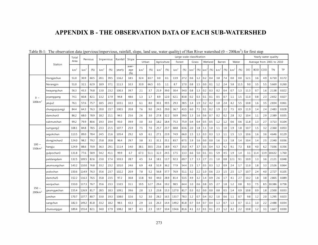
273

APPENDIX B - THE OBSERVATION DATA OF EACH SUB-WATERSHED

Table B-1: The observation data (pervious/impervious, rainfall, slope, land use, water quality) of Han River watershed (0 ~ 200km2) for first step

km2 km2 (%) km2 (%) yearly

aver-

age

(%)

km2 (%) km2 (%) km2 (%) km2 (%) km2 (%) km2 (%) km2 (%) DO BOD COD TN TP

Hongjechun 51.0 30.9 60.5 20.1 39.5 116.2 18.5 32.4 63.7 0.0 0.1 13.9 27.2 0.6 1.2 0.2 0.4 3.8 7.4 0.0 0.0 12.1 3.6 4.9 6.710 0.172

Norangjin 51.0 32.1 62.9 18.9 37.1 111.3 10.3 33.9 66.5 0.5 1.1 8.7 17.0 0.8 1.5 0.0 0.1 1.2 2.4 5.8 11.5 9.0 3.5 5.5 5.669 0.260

hwayangchun 56.3 43.3 76.8 13.0 23.2 100.3 39.7 2.1 3.7 21.9 39.0 30.4 54.0 0.8 1.3 0.2 0.3 0.2 0.4 0.7 1.3 11.3 0.7 1.6 2.138 0.022

joyanggang 74.1 60.8 82.1 13.2 17.9 94.8 48.6 1.3 1.7 8.9 12.0 62.1 83.8 0.2 0.3 0.1 0.1 0.5 0.7 1.1 1.5 11.0 0.8 2.3 2.652 0.027

yeuju2 76.1 57.6 75.7 18.5 24.3 103.1 10.3 6.1 8.0 30.1 39.5 29.3 38.5 1.4 1.9 3.2 4.2 1.8 2.4 4.2 5.5 10.8 1.6 3.5 2.834 0.061

chungjujojungji 84.4 64.3 76.3 20.0 23.7 100.5 20.8 7.6 9.0 24.5 29.0 36.7 43.5 6.0 7.1 0.1 0.2 1.9 2.2 7.5 8.9 11.9 1.4 2.4 2.483 0.028

damchun3 86.2 68.0 78.9 18.2 21.1 94.5 25.6 2.6 3.0 27.8 32.2 50.9 59.0 1.3 1.6 0.6 0.7 0.2 0.2 2.8 3.2 10.4 1.1 2.9 2.389 0.035

sukmunchun 99.2 79.9 80.6 19.3 19.4 93.0 39.9 3.0 3.0 18.2 18.4 75.3 75.9 0.4 0.4 0.5 0.5 1.2 1.2 0.6 0.6 11.8 1.3 2.7 3.713 0.104

sumgang2 108.1 84.8 78.5 23.3 21.5 107.7 25.9 7.5 7.0 25.7 23.7 68.8 63.6 2.0 1.8 1.1 1.0 1.1 1.0 1.9 1.8 10.7 1.5 3.2 2.360 0.053

segokchun 113.5 89.0 78.4 24.5 21.6 105.4 29.2 6.9 6.1 27.1 23.9 74.9 66.0 1.5 1.3 0.3 0.3 1.3 1.1 1.5 1.3 10.6 1.6 3.6 4.646 0.129

dongjinchun2 124.0 98.2 79.2 25.8 20.8 96.4 29.7 3.8 3.1 31.1 25.1 83.7 67.5 1.9 1.6 0.0 0.0 1.6 1.3 1.8 1.4 10.4 1.4 2.5 2.340 0.036

hangju 124.9 88.6 70.9 36.3 29.1 111.4 14.0 38.1 30.5 23.6 18.9 43.7 35.0 4.7 3.7 0.5 0.4 5.3 4.2 9.1 7.3 8.8 4.0 6.2 7.036 0.356

gulpochun3 131.8 77.6 58.9 54.2 41.1 99.9 6.7 67.3 51.1 32.3 24.5 17.5 13.3 6.6 5.0 0.1 0.1 5.9 4.5 1.9 1.4 3.1 11.4 13.9 18.632 1.760

paldangdam 132.5 109.5 82.6 23.0 17.4 103.3 28.7 4.5 3.4 18.1 13.7 92.3 69.7 1.7 1.3 2.7 2.1 1.0 0.8 12.1 9.1 10.9 1.3 3.6 2.121 0.048

yeumsungchun 143.2 110.0 76.8 33.2 23.2 101.0 24.6 6.9 4.8 51.9 36.2 77.9 54.4 2.5 1.7 0.5 0.3 1.2 0.9 2.4 1.7 11.0 1.8 3.3 2.526 0.064

yodochun 150.6 114.9 76.3 35.6 23.7 102.2 20.9 7.8 5.2 56.8 37.7 76.9 51.1 3.2 2.2 1.0 0.6 2.3 1.5 2.5 1.7 10.7 2.4 4.0 2.727 0.105

damchul5 152.2 116.3 76.5 35.8 23.5 97.2 30.8 13.8 9.0 44.0 28.9 81.4 53.5 4.9 3.2 1.4 0.9 2.6 1.7 4.1 2.7 10.2 1.8 3.8 2.865 0.089

wonjuchun 153.0 117.3 76.7 35.6 23.3 110.5 31.1 19.5 12.7 29.4 19.2 98.5 64.4 1.0 0.6 0.8 0.5 2.7 1.8 1.2 0.8 9.3 7.5 8.5 10.386 0.758

geumgyechun 155.4 126.9 81.7 28.5 18.3 109.1 39.6 2.0 1.3 23.8 15.3 127.0 81.7 0.3 0.2 0.0 0.0 0.8 0.5 1.4 0.9 10.8 0.9 1.8 2.500 0.033

junchun 170.7 137.7 80.7 33.0 19.3 108.0 32.6 5.2 3.0 28.2 16.5 133.7 78.3 1.2 0.7 0.4 0.2 1.0 0.6 1.1 0.7 9.8 1.2 2.0 1.295 0.023

sangchun 182.3 149.2 81.8 33.2 18.2 98.5 43.3 2.9 1.6 26.3 14.4 149.2 81.8 0.7 0.4 0.7 0.4 1.3 0.7 1.3 0.7 11.1 1.0 2.2 2.488 0.034

chunsunggyo 189.4 155.4 82.1 34.0 17.9 108.2 38.7 4.3 2.3 19.7 10.4 154.6 81.6 4.1 2.2 0.1 0.1 2.3 1.2 4.2 2.2 10.8 1.2 3.1 1.667 0.030

Forest Grass Wetland Barren WaterStation

Total

AreaPervious Impervious

0 ~

100km2

Large scale classification Yearly water quality

Average from 2001 to 2010

100 ~

150km2

150 ~

200km2

Rainfall SlopeUrban Agriculture

274

Table B-2: The observation data (pervious/impervious, rainfall, slope, land use, water quality) of Han River watershed (200 ~ 500 km2) for first step


aver-

age

(%)


yeamdam 228.0 176.5 77.4 51.5 22.6 105.2 24.8 26.1 11.4 48.1 21.1 131.6 57.7 4.0 1.8 0.4 0.2 3.6 1.6 14.2 6.2 10.5 1.1 2.8 1.657 0.030

damchun1 256.8 203.4 79.2 49.1 19.1 96.5 33.1 6.4 2.5 51.2 19.9 189.7 73.9 1.4 0.5 0.8 0.3 0.6 0.2 2.4 1.0 10.6 0.9 2.7 1.841 0.028

jojongchun3 260.6 214.6 82.4 46.0 17.6 115.9 38.1 5.6 2.2 29.9 11.5 213.9 82.1 4.5 1.7 0.0 0.0 1.2 0.5 5.3 2.0 11.0 1.1 2.6 3.298 0.057

gokneungchun3 261.5 193.5 74.0 67.9 26.0 106.2 17.0 31.0 11.8 84.4 32.3 116.2 44.5 13.5 5.1 1.3 0.5 11.4 4.3 3.7 1.4 9.4 7.4 9.8 8.298 0.268

jechuchun2 268.4 212.1 79.1 56.2 20.9 109.6 32.0 14.9 5.5 54.1 20.2 193.4 72.1 0.6 0.2 0.2 0.1 3.5 1.3 1.6 0.6 11.5 1.8 3.8 5.667 0.272

soyangdam5 278.2 233.5 83.9 44.7 16.1 98.8 45.2 3.9 1.4 14.3 5.1 245.0 88.1 1.3 0.5 6.8 2.5 0.9 0.3 6.1 2.2 9.9 1.2 2.4 1.705 0.022

ananyangchun5 281.2 182.6 65.0 98.6 35.0 103.0 15.5 130.4 46.4 32.1 11.4 104.2 37.1 3.9 1.4 0.2 0.1 6.9 2.5 3.5 1.2 6.1 9.8 11.1 18.217 0.972

gyechun2 283.7 234.6 82.7 49.1 17.3 114.0 43.7 1.4 0.5 36.0 12.7 243.0 85.7 0.4 0.1 0.1 0.0 0.8 0.3 2.0 0.7 10.2 0.8 2.1 1.798 0.013

tanchun5 302.8 215.6 71.2 87.1 28.8 105.3 18.9 92.8 30.6 36.9 12.2 146.6 48.4 7.3 2.4 2.4 0.8 13.1 4.3 3.7 1.2 6.9 17.9 11.9 15.417 1.047

gapyungchun5 305.4 254.1 83.2 51.3 16.8 111.0 48.3 5.3 1.7 18.5 6.1 274.1 89.7 2.2 0.7 0.2 0.1 2.1 0.7 3.1 1.0 11.0 0.9 2.0 2.507 0.035

bokhachun3 309.5 227.4 73.5 82.2 26.5 110.3 12.9 31.4 10.2 135.5 43.8 124.5 40.2 7.3 2.4 1.8 0.6 3.2 1.0 5.6 1.8 9.7 4.2 5.5 6.322 0.214

heukchun3 314.1 252.2 80.3 61.8 19.7 113.5 33.3 13.0 4.1 57.2 18.2 232.8 74.1 3.7 1.2 1.3 0.4 2.8 0.9 3.2 1.0 10.3 1.1 2.8 2.858 0.035

gyesandam3 315.3 257.3 81.6 58.0 18.4 97.0 38.5 5.3 1.7 50.4 16.0 252.2 80.0 1.1 0.3 1.2 0.4 1.0 0.3 4.2 1.3 9.7 1.2 3.0 1.834 0.025

deokyeunlee 317.1 250.0 78.8 67.1 21.2 101.0 27.6 10.6 3.3 83.0 26.2 200.0 63.1 10.0 3.2 0.8 0.3 5.2 1.6 7.5 2.4 10.8 1.2 2.9 2.445 0.038

sumgang3 319.9 261.1 81.6 58.9 18.4 107.8 33.9 5.1 1.6 48.8 15.2 254.3 79.5 3.3 1.0 1.2 0.4 2.9 0.9 4.3 1.3 10.2 1.8 4.0 4.454 0.195

jungryangchun4 350.4 246.7 70.4 103.7 29.6 111.3 16.2 111.3 31.8 55.3 15.8 157.8 45.0 6.4 1.8 2.3 0.7 12.1 3.4 5.1 1.5 7.9 12.1 11.2 17.647 1.439

deokchun 371.5 305.9 82.4 65.5 17.6 93.1 48.8 5.8 1.6 39.5 10.6 316.3 85.1 1.1 0.3 0.9 0.2 3.4 0.9 4.4 1.2 10.7 1.0 2.7 2.965 0.034

paldamdam4 380.3 309.7 81.4 70.6 18.6 107.9 33.4 15.0 4.0 42.1 11.1 295.1 77.6 7.4 1.9 0.4 0.1 5.9 1.6 14.3 3.8 11.0 1.2 3.2 1.800 0.032

soyangdam1 400.5 342.6 85.5 57.9 14.5 103.7 46.9 2.5 0.6 12.0 3.0 339.4 84.7 0.9 0.2 0.5 0.1 2.4 0.6 42.8 10.7 9.1 0.9 2.2 1.459 0.018

pyungchanggang1 402.5 332.2 82.5 70.3 17.5 111.4 39.2 4.3 1.1 40.5 10.1 350.6 87.1 2.6 0.7 0.1 0.0 2.3 0.6 2.0 0.5 11.1 0.8 1.8 3.598 0.027

guri 413.6 319.3 77.2 94.3 22.8 105.2 23.4 39.8 9.6 89.1 21.5 249.0 60.2 11.5 2.8 0.4 0.1 10.1 2.4 13.7 3.3 10.7 1.5 3.7 2.478 0.052

odaechun2 451.7 375.9 83.2 75.8 16.8 105.7 46.3 4.7 1.0 33.2 7.4 407.2 90.1 2.0 0.5 1.9 0.4 1.1 0.2 1.6 0.4 11.2 0.8 2.3 3.478 0.037

okdongchun2 495.3 414.0 83.6 81.2 16.4 97.0 50.9 3.5 0.7 25.6 5.2 459.7 92.8 1.5 0.3 0.3 0.1 3.4 0.7 1.3 0.3 11.3 0.7 1.5 1.671 0.013

Water Average from 2001 to 2010rainfall slope

large scale classification yearly water quality

Urban Agriculture Forest Grass Wetland Barrenstation

Total

Areapervious impervious

200 ~

500km2

275

Table B-3: The observation data (pervious/impervious, rainfall, slope, land use, water quality) of Han River watershed (500 km2 ~) for first step


aver-

age

(%)km2 (%) km2 (%) km2 (%) km2 (%) km2 (%) km2 (%) km2 (%) DO BOD COD TN TP

chungjudam4 502.1 403.1 80.3 92.2 18.4 103.6 43.7 13.0 2.6 57.5 11.4 401.1 79.9 2.1 0.4 3.5 0.7 12.1 2.4 6.0 1.2 11.1 1.3 2.2 2.479 0.022

paldangdam1 505.1 382.4 75.7 122.7 24.3 110.7 20.8 35.5 7.0 197.7 39.1 230.2 45.6 10.9 2.2 3.4 0.7 8.6 1.7 18.9 3.7 11.3 1.6 3.7 2.502 0.058

yeju1 536.0 427.3 79.7 108.7 20.3 101.7 25.8 17.6 3.3 123.9 23.1 354.4 66.1 14.4 2.7 5.4 1.0 5.9 1.1 14.5 2.7 10.0 1.4 3.3 2.822 0.060

gyunganchun6 561.1 433.2 77.2 128.0 22.8 105.6 26.5 63.3 11.3 92.9 16.6 364.1 64.9 17.2 3.1 1.6 0.3 11.1 2.0 10.9 1.9 9.9 3.9 6.6 5.066 0.166

chungmichun3 596.6 447.9 75.1 148.7 24.9 104.0 17.3 34.3 5.7 257.8 43.2 262.3 44.0 15.4 2.6 3.3 0.5 10.6 1.8 13.0 2.2 10.9 2.9 5.1 3.767 0.101

juchungang2 607.4 496.5 81.7 110.9 18.3 113.1 36.7 7.8 1.3 87.1 14.3 499.0 82.2 2.1 0.3 1.4 0.2 5.4 0.9 4.6 0.8 11.0 0.9 2.1 2.988 0.016

inbukchun2 660.1 414.9 62.9 89.3 13.5 93.1 40.4 13.4 2.0 39.5 6.0 432.6 65.5 8.9 1.4 0.8 0.1 4.5 0.7 4.6 0.7 11.1 0.9 2.4 1.739 0.026

chunchendam2 774.9 645.5 83.3 129.4 16.7 104.2 44.1 18.7 2.4 56.6 7.3 672.1 86.7 4.8 0.6 1.4 0.2 4.1 0.5 17.2 2.2 9.7 0.9 2.4 1.315 0.020

youngwol2 809.2 654.4 80.9 154.9 19.1 102.2 41.0 19.0 2.3 128.7 15.9 631.1 78.0 5.0 0.6 3.0 0.4 14.6 1.8 7.9 1.0 11.0 0.9 2.3 2.976 0.034

chungpyungdam1 818.4 670.2 81.9 148.2 18.1 109.8 37.0 17.0 2.1 106.8 13.1 660.5 80.7 7.9 1.0 2.3 0.3 7.9 1.0 15.9 1.9 10.4 1.0 3.0 1.969 0.033

chungjudam 833.6 686.6 82.4 147.1 17.6 101.4 41.6 15.9 1.9 117.1 14.0 627.0 75.2 2.5 0.3 1.4 0.2 11.3 1.4 58.5 7.0 9.0 0.8 2.2 2.236 0.021

choyanggang 918.7 753.6 82.0 165.0 18.0 109.4 43.0 11.9 1.3 126.2 13.7 760.0 82.7 4.4 0.5 3.0 0.3 5.3 0.6 7.7 0.8 11.0 0.8 2.3 2.652 0.027

hongchungang1 1006.1 819.0 81.4 187.0 18.6 109.0 37.4 47.5 4.7 105.8 10.5 826.4 82.1 3.3 0.3 2.3 0.2 7.6 0.8 13.1 1.3 10.6 0.9 2.3 2.423 0.023

youngwol1 1022.9 840.4 82.2 182.3 17.8 97.6 49.8 17.9 1.8 106.8 10.4 867.7 84.8 6.6 0.6 1.8 0.2 12.3 1.2 9.5 0.9 10.8 0.9 2.3 2.834 0.069

naelinchun1 1084.4 908.7 83.8 175.7 16.2 105.7 45.9 5.8 0.5 57.4 5.3 1004.4 92.6 5.7 0.5 1.4 0.1 4.0 0.4 5.8 0.5 11.1 0.6 1.7 2.180 0.014

hawchundam1 1265.7 863.6 68.2 181.6 14.4 95.0 43.0 23.0 1.8 111.7 8.8 949.5 75.0 21.0 1.7 2.3 0.2 5.1 0.4 36.9 2.9 9.8 0.8 2.0 1.121 0.027

yearly water quality

Urban Agriculture Forest Grass Wetland Barren Water Average from 2001 to 2010station

Total

Areapervious impervious rainfall slope

large scale classification

500km2 ~

276

Table B-4: The observation data (pervious/impervious, rainfall, slope, land use, water quality) of Nakdong River watershed (0 ~ 500 km2) for first step

km2 km2 (%) km2 (%) yearlyaver-

age(%)km2 (%) km2 (%) km2 (%) km2 (%) km2 (%) km2 (%) km2 (%)

DO BOD COD TN TP

youngsun 17.0 13.2 77.9 3.8 22.1 90.3 22.4 0.5 3.2 5.5 32.2 8.8 51.8 0.1 0.5 0.2 1.0 0.7 4.1 1.2 7.2 9.6 0.9 3.3 2.320 0.052

andong3 38.0 29.3 77.2 8.6 22.8 87.4 20.3 1.7 4.6 13.4 35.3 21.3 56.1 0.3 0.9 0.0 0.1 0.2 0.6 1.0 2.5 7.5 0.8 2.9 1.484 0.028

nakdonghagu2 54.7 37.7 69.0 17.0 31.0 120.9 14.4 19.5 35.7 7.3 13.4 15.5 28.4 1.1 2.0 1.1 2.1 1.2 2.2 8.8 16.1 10.5 2.6 6.3 3.318 0.129

gupo 72.1 54.8 76.0 17.3 24.0 114.9 22.3 11.5 16.0 14.3 19.9 38.8 53.8 0.5 0.7 0.1 0.2 1.3 1.7 5.6 7.8 10.2 2.6 6.0 3.109 0.132

deokchungang1 106.3 87.8 82.7 18.4 17.3 158.5 47.1 1.8 1.6 7.3 6.9 93.8 88.3 0.7 0.7 0.3 0.3 1.7 1.6 0.6 0.6 10.1 0.6 1.4 1.198 0.037

gyesungchun 107.1 81.8 76.3 25.3 23.7 94.9 23.9 5.4 5.1 42.9 40.0 53.2 49.7 1.2 1.1 0.9 0.9 0.6 0.5 2.9 2.7 8.6 3.4 8.0 5.392 0.365

imheajin 107.2 82.0 76.5 25.2 23.5 94.5 27.0 5.1 4.7 42.4 39.5 48.4 45.1 1.3 1.2 2.0 1.8 2.6 2.4 5.6 5.3 10.6 2.7 6.1 3.144 0.148

yangsanchun3 107.3 79.0 74.0 27.8 26.0 114.1 28.6 15.3 14.2 14.5 13.5 64.3 60.0 3.9 3.6 0.9 0.8 6.2 5.8 1.6 1.5 10.1 3.8 7.1 4.278 0.246

hyunpung 109.2 84.6 77.5 24.5 22.5 98.4 30.4 8.6 7.9 22.2 20.3 70.8 64.9 1.5 1.4 0.4 0.4 2.1 2.0 3.5 3.2 10.9 2.9 6.7 4.217 0.207

yeryungchun 114.4 91.0 79.5 23.4 20.5 106.9 36.1 4.6 4.0 26.8 23.4 79.6 69.6 1.0 0.8 0.6 0.5 0.4 0.3 1.4 1.3 9.2 2.1 7.1 2.542 0.104

sungju 120.1 91.9 76.5 28.3 23.5 84.5 20.6 9.6 8.0 32.1 26.8 63.0 52.4 2.0 1.7 1.9 1.5 5.4 4.5 6.1 5.1 11.0 2.1 5.0 2.996 0.095

hwapochun 138.1 101.2 73.3 36.9 26.7 106.6 23.4 13.8 10.0 51.3 37.2 61.5 44.5 3.5 2.5 1.8 1.3 3.8 2.8 2.4 1.8 8.6 3.5 7.2 3.313 0.150

yangsanchun1 138.9 112.0 80.7 26.8 19.3 118.4 36.7 6.1 4.4 17.3 12.4 108.4 78.0 4.5 3.2 0.3 0.2 1.2 0.9 1.2 0.9 9.8 1.1 2.7 2.542 0.074

dalsung 155.5 122.0 78.5 33.5 21.5 92.5 24.3 5.8 3.7 45.9 29.5 93.7 60.3 1.5 1.0 1.6 1.0 2.5 1.6 4.5 2.9 11.2 2.1 5.2 2.927 0.096

gwangryuchun3 158.0 121.3 76.8 36.7 23.2 102.5 31.7 11.3 7.1 40.7 25.7 96.9 61.3 1.4 0.9 1.9 1.2 4.0 2.5 1.9 1.2 9.8 3.0 5.9 2.553 0.150

daeam 189.6 145.6 76.8 44.0 23.2 96.4 25.4 8.0 4.2 68.6 36.2 96.3 50.8 1.8 1.0 1.8 1.0 5.0 2.6 8.1 4.3 11.2 3.1 6.9 4.116 0.193

milyanggang3 193.4 200.2 80.5 48.6 19.5 94.6 38.8 5.8 3.0 51.9 26.8 181.3 93.7 2.2 1.1 1.8 0.9 2.4 1.2 3.5 1.8 10.6 2.3 4.4 3.013 0.120

goryung 210.6 149.7 71.1 60.9 28.9 93.7 20.1 47.9 22.8 43.2 20.5 96.6 45.9 5.8 2.8 3.1 1.5 6.7 3.2 7.2 3.4 10.7 2.9 6.8 4.178 0.215

hamanchun2 216.2 167.0 77.2 49.3 22.8 103.8 26.4 10.5 4.9 75.2 34.8 117.3 54.3 2.5 1.2 2.9 1.4 1.7 0.8 6.0 2.8 10.1 3.0 6.5 4.780 0.194

ianchun 242.3 193.3 79.8 49.0 20.2 99.0 31.5 7.0 2.9 53.9 22.2 173.3 71.5 1.7 0.7 0.9 0.4 2.9 1.2 2.7 1.1 6.2 0.7 1.6 1.018 0.015

mulgeum 254.8 204.8 80.4 50.0 19.6 107.6 37.4 9.4 3.7 44.6 17.5 179.0 70.3 3.3 1.3 1.6 0.6 4.9 1.9 12.0 4.7 10.3 2.6 6.0 3.022 0.130

hanchun 256.5 200.0 78.0 56.4 22.0 99.3 27.0 9.5 3.7 82.7 32.3 157.7 61.5 2.4 0.9 1.0 0.4 0.9 0.4 2.2 0.9 10.3 1.4 3.6 3.114 0.110

ramchun2 264.1 211.6 80.1 52.5 19.9 124.0 34.4 6.5 2.5 60.9 23.1 189.3 71.7 3.7 1.4 1.1 0.4 0.5 0.2 2.2 0.8 9.4 1.2 2.8 1.594 0.056

nakdonghagu1 288.6 206.8 71.7 81.8 28.3 115.3 17.5 38.8 13.4 109.1 37.8 104.0 36.0 7.7 2.7 1.5 0.5 13.3 4.6 14.2 4.9 10.5 2.2 5.4 3.293 0.110

beakchun 289.1 223.2 77.2 65.9 22.8 89.9 25.0 11.2 3.9 99.2 34.3 168.8 58.4 2.3 0.8 0.6 0.2 4.1 1.4 3.0 1.0 7.9 1.2 2.8 1.746 0.057

woonmumdam1 302.0 249.8 82.7 52.2 17.3 101.7 44.3 3.7 1.2 32.5 10.8 252.8 83.7 1.7 0.6 1.9 0.6 2.9 1.0 6.4 2.1 8.8 1.4 2.6 1.271 0.018

imhaho1 303.0 249.1 82.2 53.9 17.8 79.5 35.2 5.2 1.7 53.9 17.8 215.8 71.2 2.9 0.9 1.4 0.4 1.6 0.5 22.3 7.3 8.2 2.0 3.4 1.501 0.028

geumchun 313.1 245.9 78.5 67.2 21.5 99.4 34.1 10.2 3.3 97.6 31.2 194.2 62.0 2.2 0.7 1.2 0.4 1.3 0.4 6.4 2.0 3.5 0.4 3.2 0.534 0.018

sinbanchun 327.9 158.0 48.2 36.7 11.2 105.6 39.0 4.3 1.3 36.2 11.0 147.8 45.1 1.0 0.3 2.3 0.7 0.9 0.3 2.3 0.7 10.3 1.6 3.2 2.446 0.066

byungsungchun 341.0 258.1 75.7 82.8 24.3 97.5 31.3 19.2 5.6 137.4 40.3 167.6 49.2 4.3 1.3 2.5 0.7 4.0 1.2 5.9 1.7 10.2 1.7 4.5 3.883 0.211

geumhogang4 344.8 166.0 48.2 47.4 13.7 94.3 22.3 22.4 6.5 31.1 9.0 146.9 42.6 5.0 1.4 1.0 0.3 3.5 1.0 3.5 1.0 12.0 3.7 8.2 5.062 0.293

milyanggang1 349.3 271.8 77.8 76.5 21.9 103.4 41.9 40.1 11.5 40.9 11.7 247.4 70.8 5.2 1.5 2.7 0.8 6.8 1.9 5.4 1.5 10.1 1.0 2.4 2.358 0.046

andong5 363.2 284.6 78.3 78.7 21.7 89.0 26.6 11.2 3.1 115.2 31.7 221.7 61.0 3.4 0.9 2.8 0.8 3.0 0.8 6.0 1.7 3.3 0.3 1.3 0.690 0.012

youngjuseochun2 364.6 282.2 77.4 82.4 22.6 101.9 28.1 19.2 5.3 110.0 30.2 224.6 61.6 1.5 0.4 1.8 0.5 4.1 1.1 3.4 0.9 8.2 1.8 3.4 5.118 0.216

michun 374.5 302.2 80.7 72.3 19.3 86.3 34.1 8.7 2.3 71.8 19.2 283.0 75.6 2.3 0.6 2.4 0.6 2.3 0.6 4.0 1.1 11.1 1.2 3.6 3.585 0.048

weechun1 392.8 312.7 79.6 80.1 20.4 92.8 31.6 12.9 3.3 93.6 23.8 273.1 69.5 3.6 0.9 2.4 0.6 2.6 0.7 4.6 1.2 11.8 1.4 3.8 4.035 0.069

youngjunchun1 397.8 325.8 81.9 72.0 18.1 85.0 40.4 5.7 1.4 56.5 14.2 324.1 81.5 1.5 0.4 1.7 0.4 3.4 0.9 4.9 1.2 9.7 1.5 2.0 1.751 0.025

weechun6 408.4 338.4 82.9 97.8 23.9 83.5 19.1 13.8 3.4 160.5 39.3 238.3 58.3 4.4 1.1 4.1 1.0 4.0 1.0 11.2 2.7 4.2 0.6 1.9 1.016 0.020

andong1 425.7 349.6 82.1 76.1 17.9 84.1 36.8 5.0 1.2 76.3 17.9 297.9 70.0 1.1 0.2 5.6 1.3 7.9 1.9 31.8 7.5 9.6 0.9 3.6 1.669 0.043

samrangjin 435.8 322.1 73.9 113.7 26.1 100.5 20.4 32.0 7.3 211.3 48.5 149.0 34.2 6.1 1.4 6.3 1.5 8.9 2.0 22.3 5.1 10.4 2.8 5.9 3.089 0.163

namji 467.2 361.3 77.3 106.0 22.7 99.4 25.4 18.7 4.0 171.3 36.7 236.8 50.7 9.0 1.9 5.4 1.2 6.1 1.3 19.9 4.3 10.3 2.7 6.0 3.239 0.159

geumhogang6 468.8 209.0 44.6 77.9 16.6 97.9 26.1 67.1 14.3 34.2 7.3 163.2 34.8 7.4 1.6 2.3 0.5 6.8 1.5 5.8 1.2 10.2 3.8 9.3 7.244 0.543

ssanggyechun 480.3 385.0 80.2 95.1 19.8 91.0 31.4 13.6 2.8 104.0 21.7 348.8 72.6 2.2 0.5 3.0 0.6 2.6 0.5 6.1 1.3 11.7 1.6 4.5 3.226 0.052

namgangdam1 484.8 394.0 81.3 90.8 18.7 136.8 34.5 11.4 2.4 87.9 18.1 346.3 71.4 4.1 0.8 9.8 2.0 6.8 1.4 18.4 3.8 8.9 1.2 2.7 1.247 0.027

hapchundam1 491.6 395.2 80.4 96.4 19.6 107.7 30.2 11.7 2.4 106.2 21.6 345.3 70.2 2.0 0.4 2.9 0.6 6.9 1.4 16.6 3.4 8.6 1.5 2.5 1.723 0.017

Yearly water quality

Water Average(2001~2010)

0~

200km2

200 ~

500km2

pervious impervious rainfallWetland Barren

station

Total

Area

large scale classificationslope

Urban Agriculture Forest Grass

277

Table B-5: The observation data (pervious/impervious, rainfall, slope, land use, water quality) of Nakdong River watershed (500 km2 ~) for first step


age(%)km2 (%) km2 (%) km2 (%) km2 (%) km2 (%) km2 (%) km2 (%)

DO BOD COD TN TP

wegwan 500.7 369.4 73.8 131.3 26.2 86.7 20.4 54.7 10.9 164.6 32.9 239.8 47.9 5.9 1.2 4.3 0.9 17.1 3.4 14.2 2.8 10.2 1.8 4.5 3.041 0.108

dosan 617.9 507.7 82.2 110.2 17.8 92.3 46.4 7.0 1.1 85.8 13.9 514.0 83.2 2.0 0.3 2.7 0.4 1.9 0.3 4.4 0.7 11.5 0.8 2.5 2.360 0.044

gilanchun1 652.4 424.5 65.1 94.9 14.6 85.7 41.0 7.9 1.2 75.6 11.6 421.1 64.6 3.0 0.5 2.1 0.3 4.3 0.7 5.3 0.8 6.8 0.5 1.6 2.109 0.010

younggang2 672.1 542.5 80.7 129.6 19.3 104.7 36.4 19.1 2.8 113.3 16.9 518.5 77.1 4.5 0.7 3.6 0.5 7.6 1.1 5.5 0.8 11.1 1.2 2.8 2.010 0.035

gyechangdongchun2 679.3 155.4 22.9 42.6 6.3 98.1 32.9 5.6 0.8 57.0 8.4 129.7 19.1 0.8 0.1 0.3 0.0 3.3 0.5 1.3 0.2 10.2 1.1 2.9 2.906 0.079

namgang3 711.9 552.6 77.6 159.3 22.4 120.4 28.2 43.3 6.1 210.7 29.6 420.0 59.0 6.5 0.9 6.9 1.0 6.7 0.9 17.7 2.5 10.1 2.7 5.5 3.018 0.124

banbyunchun1A 747.0 465.4 62.3 116.8 15.6 80.8 42.6 40.3 5.4 74.5 10.0 452.7 60.6 2.1 0.3 2.1 0.3 5.6 0.7 4.9 0.7 3.3 0.3 1.2 0.338 0.005

naesungchun1 794.2 623.8 78.5 170.4 21.5 94.7 27.6 21.1 2.7 237.6 29.9 509.8 64.2 4.3 0.5 3.8 0.5 9.1 1.2 8.4 1.1 10.6 1.0 2.6 4.232 0.095

bonghwa 1114.7 299.4 26.9 57.8 5.2 95.4 49.1 2.4 0.2 16.1 1.4 332.6 29.8 1.1 0.1 1.0 0.1 1.9 0.2 2.1 0.2 11.5 0.8 2.4 1.968 0.037

gamchun2 1162.4 910.4 78.3 252.0 21.7 89.7 29.1 41.7 3.6 327.0 28.1 743.4 64.0 8.2 0.7 5.6 0.5 21.1 1.8 15.5 1.3 10.1 1.1 3.6 4.348 0.159

gyunghogang2 1257.4 835.3 66.4 206.9 16.5 113.3 34.0 25.8 2.1 221.4 17.6 755.8 60.1 10.9 0.9 6.7 0.5 11.5 0.9 9.9 0.8 10.4 1.2 3.4 1.596 0.042

imchun 1558.8 178.3 81.7 39.9 18.3 129.3 41.5 3.2 0.2 33.9 2.2 175.1 11.2 1.7 0.1 1.3 0.1 1.6 0.1 1.5 0.1 10.4 0.9 2.7 1.390 0.052

geumhogang3 1573.4 1230.5 78.2 342.9 21.8 90.6 29.0 80.6 5.1 306.1 19.5 508.1 32.3 18.1 1.2 8.8 0.6 16.1 1.0 24.0 1.5 10.8 3.2 7.7 5.192 0.268

gyechangweechun2 1719.1 192.9 11.2 46.5 2.7 108.1 35.3 6.5 0.4 44.1 2.6 184.0 10.7 1.6 0.1 0.6 0.0 1.7 0.1 0.9 0.1 10.5 1.1 2.8 1.787 0.054

andong2 1858.3 145.8 7.8 42.0 2.3 80.3 28.1 15.1 0.8 40.0 2.2 112.6 6.1 2.1 0.1 4.2 0.2 6.9 0.4 6.9 0.4 10.8 1.0 4.0 1.889 0.046

yechun1 2053.5 199.7 9.7 55.9 2.7 88.9 22.9 6.8 0.3 88.0 4.3 141.9 6.9 3.3 0.2 3.8 0.2 3.8 0.2 8.0 0.4 4.3 0.4 1.5 0.970 0.012

sangju2 2450.7 158.8 6.5 48.3 2.0 91.2 19.1 7.0 0.3 79.4 3.2 105.7 4.3 1.6 0.1 1.7 0.1 5.4 0.2 6.3 0.3 10.1 0.9 3.4 2.491 0.059

chungdochun 2917.1 408.1 14.0 109.9 3.8 98.1 34.2 18.0 0.6 145.1 5.0 337.0 11.6 3.5 0.1 2.7 0.1 4.3 0.1 7.4 0.3 11.4 1.6 4.2 3.686 0.063

hamyangweechun2 6227.7 141.8 79.7 36.1 20.3 115.7 34.8 5.8 0.1 41.4 0.7 125.4 2.0 2.4 0.0 0.8 0.0 0.8 0.0 1.2 0.0 10.9 1.5 3.7 3.123 0.121

Average(2001~2010)slope

large scale classification Yearly water quality

Urban Agriculture Forest Grass Wetland Barren Waterstation

Total

Areapervious impervious rainfall

500 km2~

278

Table B-6: The observation data (pervious/impervious, rainfall, slope, land use, water quality) of Geum-Sum-Youngsan River watershed (0 ~ 150 km2) for first

step

km2

km2 (%) km

2 (%) yearlyaver-

age(%)km

2 (%) km2 (%) km

2 (%) km2 (%) km

2 (%) km2 (%) km

2 (%) DO BOD COD TN TP

bakgokchun2 39.8 29.4 73.9 10.4 26.1 105.0 15.2 5.8 14.5 32.3 81.1 74.0 186.1 1.3 3.3 1.0 2.5 1.8 4.4 4.3 10.8 11.4 1.8 3.3 2.553 0.074

hyundo 43.3 31.5 72.7 11.8 27.3 102.7 20.2 6.5 15.0 24.6 56.8 111.1 256.3 0.5 1.1 0.6 1.4 1.3 3.0 0.9 2.0 10.1 0.8 3.7 1.814 0.026

youdengchun5 59.2 37.2 62.8 22.1 37.2 110.7 14.7 8.5 14.4 24.1 40.8 115.9 195.7 5.1 8.6 0.6 1.0 1.6 2.6 1.2 2.0 11.3 2.9 4.2 3.061 0.092

sungdong 65.1 49.2 75.7 15.8 24.3 106.6 12.0 2.5 3.8 23.9 36.8 36.7 56.4 1.1 1.7 0.2 0.3 0.6 0.9 0.9 1.4 9.3 3.2 6.8 3.835 0.162

daegyochun 65.9 51.0 77.3 15.0 22.7 106.6 21.6 14.7 22.2 86.3 130.8 101.8 154.3 6.9 10.5 2.0 3.1 4.5 6.8 4.5 6.8 10.6 2.0 3.5 2.119 0.050

jusukchun4 82.9 59.1 71.3 23.8 28.7 111.0 11.1 7.6 9.2 49.7 59.9 20.5 24.7 0.4 0.5 1.4 1.7 1.3 1.6 2.0 2.4 11.0 2.7 5.6 3.400 0.146

bakgokchun1 85.7 70.6 82.5 15.0 17.5 102.2 34.1 2.2 2.6 18.7 21.8 62.4 72.8 1.0 1.2 0.3 0.3 2.1 2.5 3.3 3.8 11.5 1.3 2.5 2.389 0.042

yungi 86.1 65.1 75.5 21.1 24.5 104.2 15.2 5.0 5.8 19.1 22.2 66.7 77.4 1.5 1.8 1.2 1.4 1.6 1.9 3.6 4.2 10.0 3.2 6.8 5.315 0.218

daejeonchun3 89.4 63.7 71.3 25.7 28.7 107.2 29.4 11.6 13.0 77.9 87.2 117.6 131.5 4.9 5.5 2.2 2.4 2.4 2.7 3.7 4.2 12.0 2.6 3.9 4.745 0.117

jewon 89.9 72.0 80.0 18.0 20.0 99.0 33.1 4.4 4.9 28.0 31.1 105.3 117.1 1.5 1.7 0.3 0.4 1.5 1.7 0.8 0.9 10.3 1.0 3.7 1.765 0.029

gapchun2 93.9 71.6 76.2 22.3 23.8 110.7 23.7 16.6 17.7 146.7 156.2 377.2 401.7 23.0 24.5 1.8 1.9 5.7 6.0 4.2 4.4 10.6 2.2 3.7 2.907 0.091

yongsuchun 95.1 75.6 79.4 19.6 20.6 118.1 32.7 30.9 32.4 57.5 60.4 97.1 102.0 3.9 4.1 1.8 1.9 4.7 4.9 1.6 1.7 8.1 1.7 2.8 1.376 0.054

buyeu1 96.9 74.8 77.1 22.2 22.9 109.0 19.8 5.3 5.5 18.4 19.0 66.7 68.8 2.4 2.5 0.7 0.7 0.9 0.9 0.7 0.8 10.4 3.1 6.8 4.146 0.162

gongju1 98.7 79.0 80.0 19.7 20.0 113.3 28.9 11.8 12.0 73.9 74.8 155.1 157.2 2.1 2.2 0.4 0.4 2.1 2.2 1.9 1.9 10.2 2.9 6.6 4.323 0.182

gapchun5-1 107.6 75.2 69.9 32.4 30.1 111.5 15.1 5.5 5.1 51.8 48.2 279.1 259.4 7.6 7.1 0.9 0.8 6.9 6.4 3.3 3.1 9.4 5.5 9.9 11.938 0.570

naju 111.3 79.3 71.3 31.9 28.7 110.7 8.2 7.8 7.0 73.4 66.0 22.7 20.4 0.9 0.8 1.4 1.3 1.5 1.4 3.5 3.1 10.3 5.3 6.5 6.961 0.454

hwasunchun 127.7 100.1 78.3 27.7 21.7 120.2 31.3 7.3 5.7 30.7 24.0 83.5 65.3 3.0 2.3 0.8 0.6 1.4 1.1 1.2 0.9 10.5 2.1 4.2 2.477 0.064

gilsanchun 113.0 84.0 74.3 29.0 25.7 101.8 14.1 19.5 17.2 106.9 94.6 429.0 379.6 5.2 4.6 3.6 3.2 4.2 3.8 55.6 49.2 9.1 3.5 7.3 1.889 0.109

bochungchun4 113.6 90.4 79.6 23.2 20.4 94.2 32.4 4.5 4.0 28.8 25.3 23.2 20.4 0.5 0.4 0.4 0.4 1.3 1.1 6.5 5.7 10.5 1.1 2.7 2.029 0.035

woosan 120.4 94.4 78.4 26.0 21.6 101.3 30.6 3.4 2.8 17.8 14.8 16.6 13.8 0.3 0.2 0.3 0.3 0.7 0.5 0.7 0.6 10.1 1.0 3.7 2.339 0.044

mokmyun 120.6 94.6 78.4 26.1 21.6 107.9 26.1 7.1 5.9 64.9 53.8 164.9 136.7 4.0 3.3 1.4 1.2 0.8 0.7 3.3 2.7 11.6 3.6 7.4 4.949 0.188

ganggyungchun 123.5 88.5 71.7 35.0 28.3 96.5 10.8 5.9 4.8 41.7 33.8 270.9 219.4 3.1 2.5 0.5 0.4 1.8 1.4 1.7 1.4 9.8 5.9 10.4 9.033 0.453

mihochun6-1 125.6 92.7 73.8 32.9 26.2 101.2 13.3 2.2 1.8 16.7 13.3 104.5 83.2 0.4 0.3 0.7 0.5 1.5 1.2 1.7 1.4 9.8 4.8 9.2 6.424 0.264

younpo 127.7 104.4 81.8 23.3 18.2 96.6 43.1 1.1 0.8 11.0 8.6 68.5 53.6 2.5 2.0 0.1 0.1 0.3 0.2 2.3 1.8 9.9 0.9 3.5 1.662 0.020

chungwon1 129.8 97.5 75.1 32.3 24.9 97.4 19.6 25.0 19.3 19.6 15.1 41.6 32.0 10.5 8.1 0.8 0.6 7.4 5.7 2.7 2.1 10.9 2.4 6.0 5.690 0.216

chopyungchun 132.6 108.2 81.6 24.4 18.4 100.5 32.1 5.8 4.4 32.3 24.3 74.0 55.9 1.3 1.0 1.0 0.8 1.8 1.3 4.3 3.2 10.7 1.1 2.3 1.580 0.034

jochun 136.3 105.2 77.2 31.1 22.8 102.7 23.1 22.9 16.8 11.9 8.8 49.3 36.2 2.0 1.4 0.6 0.4 2.2 1.6 0.5 0.3 9.9 3.6 5.1 4.421 0.284

bochungchun2 140.6 111.5 79.3 29.1 20.7 188.1 29.9 8.3 5.9 75.8 54.0 74.8 53.2 1.1 0.8 1.0 0.7 1.0 0.7 3.2 2.2 10.2 1.1 2.1 2.115 0.031

youdengchun-a 141.9 113.6 80.0 28.3 20.0 108.3 40.0 8.1 5.7 24.9 17.5 53.3 37.6 2.2 1.5 1.0 0.7 2.8 1.9 1.7 1.2 11.9 0.9 2.2 2.924 0.031

donggye 144.4 116.6 80.8 27.7 19.2 116.1 35.4 2.2 1.6 28.8 19.9 101.5 70.3 7.9 5.5 1.7 1.2 0.6 0.4 1.6 1.1 9.7 1.1 3.6 1.445 0.043

youngdongchun2 145.4 116.6 80.2 28.8 19.8 92.2 35.7 8.8 6.1 67.6 46.5 197.4 135.7 3.0 2.1 2.2 1.5 1.2 0.8 2.5 1.7 10.5 1.4 4.1 5.061 0.123


Average(2001-2010)Agriculture


Forest Grass Wetland Barren Water

Total


Urban

0~

100 km2

100 ~

150km2

Station

279

Table B-7: The observation data (pervious/impervious, rainfall, slope, land use, water quality) of Geum-Sum-Youngsan River watershed (150 km2 ~ ) for first

step

km2

km2 (%) km

2 (%) yearlyaver-

age(%)km

2 (%) km2 (%) km

2 (%) km2 (%) km

2 (%) km2 (%) km

2 (%) DO BOD COD TN TP

suksungchun 152.2 111.3 73.2 40.8 26.8 103.5 12.4 5.3 3.5 36.8 24.2 36.5 24.0 1.1 0.7 2.0 1.3 1.1 0.7 3.3 2.2 8.7 4.2 7.0 4.574 0.345

naju 152.8 100.7 65.9 52.1 34.1 113.1 7.7 62.1 40.6 23.1 15.1 52.1 34.1 7.7 5.0 1.9 1.2 4.2 2.8 1.8 1.2 11.4 5.3 6.5 6.961 0.454

bonggok 2 gyo 156.9 125.3 79.9 31.6 20.1 107.7 32.8 11.3 7.2 39.2 25.0 79.6 50.7 2.1 1.3 1.2 0.8 1.3 0.9 1.5 0.9 11.2 1.9 3.3 3.396 0.193

bogangchun 157.6 118.0 74.9 39.6 25.1 99.3 19.2 4.6 2.9 32.9 20.9 53.3 33.8 0.5 0.3 0.2 0.1 2.2 1.4 3.3 2.1 10.5 1.8 3.6 3.621 0.087

hadong 156.3 126.5 80.9 29.8 19.1 143.1 39.8 5.4 3.4 21.9 14.0 120.3 77.0 1.7 1.1 1.0 0.6 3.1 2.0 2.9 1.8 9.0 1.2 4.8 2.275 0.047

goksung 183.4 147.4 241.2 36.0 58.8 113.7 32.4 4.7 2.5 38.7 21.1 130.2 71.0 3.1 1.7 2.3 1.2 1.7 0.9 2.8 1.5 10.0 1.4 4.0 2.521 0.066

deokyeun 184.2 154.9 84.1 29.3 15.9 143.0 45.3 1.8 1.0 5.4 2.9 173.2 94.0 1.5 0.8 0.6 0.3 0.5 0.3 1.3 0.7 9.6 1.3 3.4 2.298 0.046

yochuun A 191.7 158.5 82.7 33.2 17.3 112.9 46.5 3.2 1.7 17.5 9.1 163.5 85.3 3.4 1.8 1.3 0.7 0.8 0.4 2.1 1.1 3.4 0.3 0.7 0.676 0.005

geumchun 165.2 124.3 75.3 40.9 24.7 96.3 18.6 6.6 4.0 79.9 48.4 201.8 122.2 2.1 1.3 0.8 0.5 4.1 2.5 4.2 2.6 9.9 3.3 6.1 2.511 0.088

gongju2 171.4 135.0 78.7 36.5 21.3 109.2 24.2 5.3 3.1 37.7 22.0 169.9 99.1 1.0 0.6 1.6 0.9 3.0 1.7 4.4 2.5 10.3 3.3 7.1 4.476 0.174

geumganggapmun 194.8 151.3 77.6 43.6 22.4 100.6 13.8 13.1 6.7 142.1 72.9 493.5 253.3 5.2 2.7 1.6 0.8 2.7 1.4 6.5 3.3 3.2 0.9 2.2 1.312 0.039

musimchun3 197.3 144.5 73.2 52.9 26.8 98.4 20.1 5.2 2.7 43.3 21.9 160.2 81.2 2.0 1.0 0.7 0.3 0.6 0.3 7.4 3.8 11.0 2.2 4.2 3.173 0.081

gomnaru 197.7 153.7 77.8 44.0 22.2 104.9 26.6 8.9 4.5 58.0 29.3 385.2 194.9 3.8 1.9 1.6 0.8 3.7 1.8 2.9 1.5 10.1 3.1 6.5 4.321 0.171

nosungchun 202.5 150.5 74.4 51.9 25.6 105.3 17.7 11.1 5.5 44.7 22.1 64.9 32.1 2.6 1.3 1.2 0.6 2.1 1.0 3.2 1.6 10.6 2.6 4.6 2.125 0.068

nonsanchun1 219.4 177.9 81.1 41.6 18.9 110.3 34.0 22.4 10.2 157.7 71.9 91.8 41.9 6.2 2.8 2.9 1.3 4.4 2.0 3.4 1.5 10.4 1.2 3.1 3.576 0.034

byungchunchun 220.3 169.1 76.8 51.2 23.2 102.9 19.4 12.0 5.5 98.9 44.9 84.0 38.1 2.6 1.2 0.8 0.4 1.1 0.5 3.0 1.4 10.5 2.2 3.8 2.709 0.060

mihochun4 220.7 165.8 75.1 54.9 24.9 101.6 18.7 10.6 4.8 78.8 35.7 75.7 34.3 2.3 1.0 2.1 0.9 1.0 0.4 24.5 11.1 10.2 2.7 5.8 4.031 0.191

youngdong 222.8 180.9 81.2 41.9 18.8 173.9 36.4 11.4 5.1 55.4 24.9 119.6 53.7 2.3 1.0 1.6 0.7 4.0 1.8 3.4 1.5 10.2 1.1 3.7 2.132 0.036

nonsanchun4 244.2 171.5 70.2 72.7 29.8 97.0 9.1 2.8 1.1 24.3 9.9 97.1 39.8 1.5 0.6 0.8 0.3 0.3 0.1 5.8 2.4 4.1 1.6 3.0 2.377 0.085

jichun 246.4 195.8 79.5 50.6 20.5 104.8 26.7 26.1 10.6 4.1 1.7 19.9 8.1 2.9 1.2 0.4 0.2 5.3 2.1 0.6 0.2 10.6 1.9 3.6 2.212 0.048

bonghwangchun 247.4 192.1 77.6 55.3 22.4 143.4 30.7 10.3 4.2 59.0 23.8 45.7 18.5 2.8 1.1 2.2 0.9 2.2 0.9 3.3 1.3 10.3 1.5 3.7 3.337 0.118

youguchun 282.6 225.5 79.8 57.1 20.2 105.1 31.4 7.4 2.6 10.3 3.6 21.2 7.5 1.6 0.5 0.2 0.1 1.0 0.3 1.7 0.6 10.2 1.7 2.8 1.785 0.037

mihochun3 288.8 207.8 71.9 81.0 28.1 98.2 14.3 6.8 2.3 56.9 19.7 43.4 15.0 1.5 0.5 0.5 0.2 0.3 0.1 3.7 1.3 10.2 3.1 6.3 4.479 0.173

bochungchun3 299.5 237.8 79.4 61.7 20.6 99.6 31.3 8.3 2.8 85.7 28.6 50.2 16.8 2.1 0.7 0.0 0.0 3.0 1.0 2.8 0.9 10.7 1.2 2.6 2.457 0.036

gamak 313.5 247.2 78.9 66.2 21.1 109.1 34.6 8.8 2.8 78.6 25.1 201.1 64.2 17.4 5.5 1.1 0.4 3.9 1.3 2.6 0.8 7.8 0.8 2.2 2.085 0.025

mujunamdaechun 325.5 266.2 81.8 59.3 18.2 187.4 43.4 12.2 3.8 69.8 21.5 34.8 10.7 2.9 0.9 0.0 0.0 1.9 0.6 1.7 0.5 9.9 0.8 2.7 2.333 0.024

daegang 204.3 157.2 77.0 47.1 23.0 112.2 22.3 7.9 3.8 77.3 37.8 107.9 52.8 5.3 2.6 2.0 1.0 1.3 0.7 2.6 1.2 3.3 0.5 1.4 0.569 0.016

namwon 227.0 178.9 78.8 48.2 21.2 113.7 26.6 6.7 3.0 69.4 30.6 134.0 59.0 6.6 2.9 3.9 1.7 1.6 0.7 4.9 2.1 10.4 1.4 3.8 1.664 0.052

bosungchun-1 283.8 228.2 80.4 55.5 19.6 122.3 35.3 6.1 2.1 61.9 21.8 201.2 70.9 8.1 2.8 2.6 0.9 0.9 0.3 3.0 1.1 4.2 0.4 1.3 0.496 0.011

yochun 294.8 227.1 77.0 67.7 23.0 113.3 22.8 15.7 5.3 97.4 33.0 163.4 55.4 5.4 1.8 4.4 1.5 3.9 1.3 4.7 1.6 10.2 1.6 4.0 2.707 0.161

jinwol 298.9 238.3 319.4 60.5 80.6 139.3 32.4 11.0 3.7 67.9 22.7 202.6 67.8 4.4 1.5 2.0 0.7 2.3 0.8 8.6 2.9 3.6 0.5 1.4 0.457 0.016

bosunggang 1 327.0 257.8 78.9 69.1 21.1 123.7 26.9 10.5 3.2 92.6 28.3 205.3 62.8 8.6 2.6 2.1 0.6 2.1 0.6 5.8 1.8 4.1 0.5 1.3 0.342 0.013

churyungchun 355.9 284.3 79.9 71.6 20.1 111.9 31.8 10.3 2.9 79.5 22.3 249.9 70.2 8.9 2.5 1.8 0.5 1.6 0.4 3.9 1.1 3.7 0.3 0.8 0.845 0.005

osuchun 371.3 289.6 78.0 81.3 21.9 112.9 24.6 11.6 3.1 124.3 33.5 220.6 59.4 5.0 1.4 3.5 0.9 1.6 0.4 4.3 1.1 10.9 1.5 3.8 2.010 0.060

imsil 429.3 351.1 81.8 78.2 18.2 114.2 34.0 9.3 2.2 77.3 18.0 310.4 72.3 4.9 1.2 2.1 0.5 1.0 0.2 24.3 5.7 10.8 1.1 3.3 1.608 0.038

gurye 489.0 391.8 80.1 97.2 19.9 120.0 36.6 13.9 2.8 108.7 22.2 343.0 70.1 9.6 2.0 5.0 1.0 2.2 0.5 6.5 1.3 10.0 1.3 3.7 2.382 0.053

juamdam 702.4 578.8 82.4 123.7 17.6 119.8 34.6 9.7 1.4 104.6 14.9 527.1 75.0 23.2 3.3 4.0 0.6 1.6 0.2 32.1 4.6 3.7 0.4 1.4 0.443 0.006

jisukchun2 215.8 174.2 80.7 41.6 19.3 111.9 29.7 5.6 2.6 44.7 20.7 147.5 68.4 3.7 1.7 2.1 1.0 2.7 1.3 9.6 4.4 10.8 2.2 4.4 2.674 0.109

gomakwonchun2 219.0 164.4 75.1 54.5 24.9 110.7 18.4 12.3 5.6 105.2 48.0 91.6 41.8 2.0 0.9 1.9 0.9 1.8 0.8 4.3 2.0 10.2 2.9 5.9 2.653 0.070

jisukpo 237.7 191.6 80.6 45.9 19.3 116.0 32.9 5.8 2.5 45.4 19.1 170.8 71.9 7.8 3.3 2.1 0.9 1.6 0.7 4.0 1.7 10.2 1.4 3.1 1.367 0.038

youngsanpo 309.9 227.9 73.5 82.1 26.5 110.4 14.7 19.2 6.2 166.1 53.6 108.1 34.9 3.4 1.1 2.3 0.8 3.1 1.0 7.7 2.5 9.6 5.6 6.5 6.624 0.435

gwangju1 562.0 422.5 75.2 139.5 24.8 112.8 25.5 46.0 8.2 206.2 36.7 268.9 47.8 13.5 2.4 5.7 1.0 8.2 1.5 13.5 2.4 10.6 3.7 5.8 2.793 0.103

hwangryong3 565.0 443.7 78.5 121.4 21.5 114.9 27.7 28.4 5.0 152.4 27.0 350.9 62.1 6.8 1.2 4.5 0.8 4.8 0.8 17.3 3.1 10.1 3.0 4.6 1.733 0.063

mooan2 885.4 661.7 74.7 223.7 25.3 101.8 15.1 42.2 4.8 470.0 53.1 291.8 33.0 8.7 1.0 8.9 1.0 10.3 1.2 53.5 6.0 9.9 2.0 5.7 4.194 0.133

youngdam2 355.1 288.0 81.1 67.1 18.9 112.1 40.3 4.4 1.2 33.8 9.5 74.7 21.0 1.8 0.5 0.3 0.1 2.7 0.8 2.8 0.8 3.3 0.2 1.0 0.507 0.006

mujunamdaechun1 464.1 379.6 81.8 84.5 18.2 200.0 43.6 26.2 5.6 149.2 32.2 55.3 11.9 4.9 1.1 0.8 0.2 3.9 0.9 3.8 0.8 4.3 0.4 1.2 0.871 0.016

mihochun5 471.5 355.8 75.5 115.7 24.5 102.5 18.5 33.4 7.1 271.8 57.6 180.9 38.4 5.4 1.1 4.4 0.9 2.5 0.5 38.1 8.1 9.7 4.4 8.2 5.526 0.288

geumganggapmun 536.6 400.9 74.7 135.7 25.3 100.3 12.4 5.0 0.9 35.8 6.7 96.3 17.9 0.6 0.1 0.5 0.1 0.9 0.2 1.5 0.3 3.2 0.9 2.2 1.312 0.039

yongdam4 575.2 453.9 78.9 121.3 21.1 106.1 35.2 5.1 0.9 51.4 8.9 103.9 18.1 2.1 0.4 1.4 0.2 2.2 0.4 5.3 0.9 8.0 1.1 2.6 1.539 0.022

daechung 624.1 511.2 81.9 112.9 18.1 104.1 34.2 37.4 6.0 157.2 25.2 243.4 39.0 10.3 1.7 3.5 0.6 12.2 1.9 7.6 1.2 2.9 0.2 1.1 0.575 0.006

chogang2 664.6 535.0 80.5 129.6 19.5 96.2 34.0 2.9 0.4 28.2 4.2 77.2 11.6 1.1 0.2 0.7 0.1 1.5 0.2 2.1 0.3 10.4 1.1 3.4 2.251 0.029


Urban Agriculture Forest Grass Wetland Barren Water Average(2001-2010)Station

Total



150

~ 200km2

200km2~

280

Table B-8: The observation data (pervious/impervious, rainfall, slope, land use, water quality) of Hangang River watershed (0 ~ 20%) for second step


aver-

age

(%)


inbukchun2 660.1 414.9 62.9 89.3 13.5 93.1 40.4 13.4 2.0 39.5 6.0 432.6 65.5 8.9 1.4 0.8 0.1 4.5 0.7 4.6 0.7 11.1 0.9 2.4 1.739 0.026

hawchundam1 1265.7 863.6 68.2 181.6 14.4 95.0 43.0 23.0 1.8 111.7 8.8 949.5 75.0 21.0 1.7 2.3 0.2 5.1 0.4 36.9 2.9 9.8 0.8 2.0 1.121 0.027

soyangdam1 400.5 342.6 85.5 57.9 14.5 103.7 46.9 2.5 0.6 12.0 3.0 339.4 84.7 0.9 0.2 0.5 0.1 2.4 0.6 42.8 10.7 9.1 0.9 2.2 1.459 0.018

soyangdam5 278.2 233.5 83.9 44.7 16.1 98.8 45.2 3.9 1.4 14.3 5.1 245.0 88.1 1.3 0.5 6.8 2.5 0.9 0.3 6.1 2.2 9.9 1.2 2.4 1.705 0.022

naelinchun1 1084.4 908.7 83.8 175.7 16.2 105.7 45.9 5.8 0.5 57.4 5.3 1004.4 92.6 5.7 0.5 1.4 0.1 4.0 0.4 5.8 0.5 11.1 0.6 1.7 2.180 0.014

okdongchun2 495.3 414.0 83.6 81.2 16.4 97.0 50.9 3.5 0.7 25.6 5.2 459.7 92.8 1.5 0.3 0.3 0.1 3.4 0.7 1.3 0.3 11.3 0.7 1.5 1.671 0.013

chunchendam2 774.9 645.5 83.3 129.4 16.7 104.2 44.1 18.7 2.4 56.6 7.3 672.1 86.7 4.8 0.6 1.4 0.2 4.1 0.5 17.2 2.2 9.7 0.9 2.4 1.315 0.020

odaechun2 451.7 375.9 83.2 75.8 16.8 105.7 46.3 4.7 1.0 33.2 7.4 407.2 90.1 2.0 0.5 1.9 0.4 1.1 0.2 1.6 0.4 11.2 0.8 2.3 3.478 0.037

gapyungchun5 305.4 254.1 83.2 51.3 16.8 111.0 48.3 5.3 1.7 18.5 6.1 274.1 89.7 2.2 0.7 0.2 0.1 2.1 0.7 3.1 1.0 11.0 0.9 2.0 2.507 0.035

gyechun2 283.7 234.6 82.7 49.1 17.3 114.0 43.7 1.4 0.5 36.0 12.7 243.0 85.7 0.4 0.1 0.1 0.0 0.8 0.3 2.0 0.7 10.2 0.8 2.1 1.798 0.013

paldangdam 132.5 109.5 82.6 23.0 17.4 103.3 28.7 4.5 3.4 18.1 13.7 92.3 69.7 1.7 1.3 2.7 2.1 1.0 0.8 12.1 9.1 10.9 1.3 3.6 2.121 0.048

pyungchanggang1 402.5 332.2 82.5 70.3 17.5 111.4 39.2 4.3 1.1 40.5 10.1 350.6 87.1 2.6 0.7 0.1 0.0 2.3 0.6 2.0 0.5 11.1 0.8 1.8 3.598 0.027

deokchun 371.5 305.9 82.4 65.5 17.6 93.1 48.8 5.8 1.6 39.5 10.6 316.3 85.1 1.1 0.3 0.9 0.2 3.4 0.9 4.4 1.2 10.7 1.0 2.7 2.965 0.034

jojongchun3 260.6 214.6 82.4 46.0 17.6 115.9 38.1 5.6 2.2 29.9 11.5 213.9 82.1 4.5 1.7 0.0 0.0 1.2 0.5 5.3 2.0 11.0 1.1 2.6 3.298 0.057

chungjudam 833.6 686.6 82.4 147.1 17.6 101.4 41.6 15.9 1.9 117.1 14.0 627.0 75.2 2.5 0.3 1.4 0.2 11.3 1.4 58.5 7.0 9.0 0.8 2.2 2.236 0.021

youngwol1 1022.9 840.4 82.2 182.3 17.8 97.6 49.8 17.9 1.8 106.8 10.4 867.7 84.8 6.6 0.6 1.8 0.2 12.3 1.2 9.5 0.9 10.8 0.9 2.3 2.834 0.069

joyanggang 74.1 60.8 82.1 13.2 17.9 94.8 48.6 1.3 1.7 8.9 12.0 62.1 83.8 0.2 0.3 0.1 0.1 0.5 0.7 1.1 1.5 11.0 0.8 2.3 2.652 0.027

chunsunggyo 189.4 155.4 82.1 34.0 17.9 108.2 38.7 4.3 2.3 19.7 10.4 154.6 81.6 4.1 2.2 0.1 0.1 2.3 1.2 4.2 2.2 10.8 1.2 3.1 1.667 0.030

choyanggang 918.7 753.6 82.0 165.0 18.0 109.4 43.0 11.9 1.3 126.2 13.7 760.0 82.7 4.4 0.5 3.0 0.3 5.3 0.6 7.7 0.8 11.0 0.8 2.3 2.652 0.027

chungpyungdam1 818.4 670.2 81.9 148.2 18.1 109.8 37.0 17.0 2.1 106.8 13.1 660.5 80.7 7.9 1.0 2.3 0.3 7.9 1.0 15.9 1.9 10.4 1.0 3.0 1.969 0.033

sangchun 182.3 149.2 81.8 33.2 18.2 98.5 43.3 2.9 1.6 26.3 14.4 149.2 81.8 0.7 0.4 0.7 0.4 1.3 0.7 1.3 0.7 11.1 1.0 2.2 2.488 0.034

juchungang2 607.4 496.5 81.7 110.9 18.3 113.1 36.7 7.8 1.3 87.1 14.3 499.0 82.2 2.1 0.3 1.4 0.2 5.4 0.9 4.6 0.8 11.0 0.9 2.1 2.988 0.016

geumgyechun 155.4 126.9 81.7 28.5 18.3 109.1 39.6 2.0 1.3 23.8 15.3 127.0 81.7 0.3 0.2 0.0 0.0 0.8 0.5 1.4 0.9 10.8 0.9 1.8 2.500 0.033

chungjudam4 502.1 403.1 80.3 92.2 18.4 103.6 43.7 13.0 2.6 57.5 11.4 401.1 79.9 2.1 0.4 3.5 0.7 12.1 2.4 6.0 1.2 11.1 1.3 2.2 2.479 0.022

gyesandam3 315.3 257.3 81.6 58.0 18.4 97.0 38.5 5.3 1.7 50.4 16.0 252.2 80.0 1.1 0.3 1.2 0.4 1.0 0.3 4.2 1.3 9.7 1.2 3.0 1.834 0.025

sumgang3 319.9 261.1 81.6 58.9 18.4 107.8 33.9 5.1 1.6 48.8 15.2 254.3 79.5 3.3 1.0 1.2 0.4 2.9 0.9 4.3 1.3 10.2 1.8 4.0 4.454 0.195

paldamdam4 380.3 309.7 81.4 70.6 18.6 107.9 33.4 15.0 4.0 42.1 11.1 295.1 77.6 7.4 1.9 0.4 0.1 5.9 1.6 14.3 3.8 11.0 1.2 3.2 1.800 0.032

hongchungang1 1006.1 819.0 81.4 187.0 18.6 109.0 37.4 47.5 4.7 105.8 10.5 826.4 82.1 3.3 0.3 2.3 0.2 7.6 0.8 13.1 1.3 10.6 0.9 2.3 2.423 0.023

damchun1 256.8 203.4 79.2 49.1 19.1 96.5 33.1 6.4 2.5 51.2 19.9 189.7 73.9 1.4 0.5 0.8 0.3 0.6 0.2 2.4 1.0 10.6 0.9 2.7 1.841 0.028

youngwol2 809.2 654.4 80.9 154.9 19.1 102.2 41.0 19.0 2.3 128.7 15.9 631.1 78.0 5.0 0.6 3.0 0.4 14.6 1.8 7.9 1.0 11.0 0.9 2.3 2.976 0.034

junchun 170.7 137.7 80.7 33.0 19.3 108.0 32.6 5.2 3.0 28.2 16.5 133.7 78.3 1.2 0.7 0.4 0.2 1.0 0.6 1.1 0.7 9.8 1.2 2.0 1.295 0.023

sukmunchun 99.2 79.9 80.6 19.3 19.4 93.0 39.9 3.0 3.0 18.2 18.4 75.3 75.9 0.4 0.4 0.5 0.5 1.2 1.2 0.6 0.6 11.8 1.3 2.7 3.713 0.104

heukchun3 314.1 252.2 80.3 61.8 19.7 113.5 33.3 13.0 4.1 57.2 18.2 232.8 74.1 3.7 1.2 1.3 0.4 2.8 0.9 3.2 1.0 10.3 1.1 2.8 2.858 0.035

0 ~

20 %


Urban Agriculture Forest Grass Wetland Barren Water Average from 2001 to 2010Station

Pervious Impervious Rainfall SlopeLarge scale classificationTotal

Area

281

Table B-9: The observation data (pervious/impervious, rainfall, slope, land use, water quality) of Hangang River watershed (20 % ~ ) for second step

km2 km2 (%) km2 (%) yearly aver-

agekm2 (%) km2 (%) km2 (%) km2 (%) km2 (%) km2 (%) km2 (%) DO BOD COD TN TP

yeju1 536.0 427.3 79.7 108.7 20.3 101.7 25.8 17.6 3.3 123.9 23.1 354.4 66.1 14.4 2.7 5.4 1.0 5.9 1.1 14.5 2.7 10.0 1.4 3.3 2.822 0.060

dongjinchun2 124.0 98.2 79.2 25.8 20.8 96.4 29.7 3.8 3.1 31.1 25.1 83.7 67.5 1.9 1.6 0.0 0.0 1.6 1.3 1.8 1.4 10.4 1.4 2.5 2.340 0.036

jechuchun2 268.4 212.1 79.1 56.2 20.9 109.6 32.0 14.9 5.5 54.1 20.2 193.4 72.1 0.6 0.2 0.2 0.1 3.5 1.3 1.6 0.6 11.5 1.8 3.8 5.667 0.272

damchun3 86.2 68.0 78.9 18.2 21.1 94.5 25.6 2.6 3.0 27.8 32.2 50.9 59.0 1.3 1.6 0.6 0.7 0.2 0.2 2.8 3.2 10.4 1.1 2.9 2.389 0.035

deokyeunlee 317.1 250.0 78.8 67.1 21.2 101.0 27.6 10.6 3.3 83.0 26.2 200.0 63.1 10.0 3.2 0.8 0.3 5.2 1.6 7.5 2.4 10.8 1.2 2.9 2.445 0.038

sumgang2 108.1 84.8 78.5 23.3 21.5 107.7 25.9 7.5 7.0 25.7 23.7 68.8 63.6 2.0 1.8 1.1 1.0 1.1 1.0 1.9 1.8 10.7 1.5 3.2 2.360 0.053

segokchun 113.5 89.0 78.4 24.5 21.6 105.4 29.2 6.9 6.1 27.1 23.9 74.9 66.0 1.5 1.3 0.3 0.3 1.3 1.1 1.5 1.3 10.6 1.6 3.6 4.646 0.129

yeamdam 228.0 176.5 77.4 51.5 22.6 105.2 24.8 26.1 11.4 48.1 21.1 131.6 57.7 4.0 1.8 0.4 0.2 3.6 1.6 14.2 6.2 10.5 1.1 2.8 1.657 0.030

guri 413.6 319.3 77.2 94.3 22.8 105.2 23.4 39.8 9.6 89.1 21.5 249.0 60.2 11.5 2.8 0.4 0.1 10.1 2.4 13.7 3.3 10.7 1.5 3.7 2.478 0.052

gyunganchun6 561.1 433.2 77.2 128.0 22.8 105.6 26.5 63.3 11.3 92.9 16.6 364.1 64.9 17.2 3.1 1.6 0.3 11.1 2.0 10.9 1.9 9.9 3.9 6.6 5.066 0.166

hwayangchun 56.3 43.3 76.8 13.0 23.2 100.3 39.7 2.1 3.7 21.9 39.0 30.4 54.0 0.8 1.3 0.2 0.3 0.2 0.4 0.7 1.3 11.3 0.7 1.6 2.138 0.022

yeumsungchun 143.2 110.0 76.8 33.2 23.2 101.0 24.6 6.9 4.8 51.9 36.2 77.9 54.4 2.5 1.7 0.5 0.3 1.2 0.9 2.4 1.7 11.0 1.8 3.3 2.526 0.064

wonjuchun 153.0 117.3 76.7 35.6 23.3 110.5 31.1 19.5 12.7 29.4 19.2 98.5 64.4 1.0 0.6 0.8 0.5 2.7 1.8 1.2 0.8 9.3 7.5 8.5 10.386 0.758

damchul5 152.2 116.3 76.5 35.8 23.5 97.2 30.8 13.8 9.0 44.0 28.9 81.4 53.5 4.9 3.2 1.4 0.9 2.6 1.7 4.1 2.7 10.2 1.8 3.8 2.865 0.089

yodochun 150.6 114.9 76.3 35.6 23.7 102.2 20.9 7.8 5.2 56.8 37.7 76.9 51.1 3.2 2.2 1.0 0.6 2.3 1.5 2.5 1.7 10.7 2.4 4.0 2.727 0.105


paldangdam1 505.1 382.4 75.7 122.7 24.3 110.7 20.8 35.5 7.0 197.7 39.1 230.2 45.6 10.9 2.2 3.4 0.7 8.6 1.7 18.9 3.7 11.3 1.6 3.7 2.502 0.058

yeuju2 76.1 57.6 75.7 18.5 24.3 103.1 10.3 6.1 8.0 30.1 39.5 29.3 38.5 1.4 1.9 3.2 4.2 1.8 2.4 4.2 5.5 10.8 1.6 3.5 2.834 0.061

chungmichun3 596.6 447.9 75.1 148.7 24.9 104.0 17.3 34.3 5.7 257.8 43.2 262.3 44.0 15.4 2.6 3.3 0.5 10.6 1.8 13.0 2.2 10.9 2.9 5.1 3.767 0.101

gokneungchun3 261.5 193.5 74.0 67.9 26.0 106.2 17.0 31.0 11.8 84.4 32.3 116.2 44.5 13.5 5.1 1.3 0.5 11.4 4.3 3.7 1.4 9.4 7.4 9.8 8.298 0.268

bokhachun3 309.5 227.4 73.5 82.2 26.5 110.3 12.9 31.4 10.2 135.5 43.8 124.5 40.2 7.3 2.4 1.8 0.6 3.2 1.0 5.6 1.8 9.7 4.2 5.5 6.322 0.214

tanchun5 302.8 215.6 71.2 87.1 28.8 105.3 18.9 92.8 30.6 36.9 12.2 146.6 48.4 7.3 2.4 2.4 0.8 13.1 4.3 3.7 1.2 6.9 17.9 11.9 15.417 1.047

hangju 124.9 88.6 70.9 36.3 29.1 111.4 14.0 38.1 30.5 23.6 18.9 43.7 35.0 4.7 3.7 0.5 0.4 5.3 4.2 9.1 7.3 8.8 4.0 6.2 7.036 0.356

jungryangchun4 350.4 246.7 70.4 103.7 29.6 111.3 16.2 111.3 31.8 55.3 15.8 157.8 45.0 6.4 1.8 2.3 0.7 12.1 3.4 5.1 1.5 7.9 12.1 11.2 17.647 1.439

ananyangchun5 281.2 182.6 65.0 98.6 35.0 103.0 15.5 130.4 46.4 32.1 11.4 104.2 37.1 3.9 1.4 0.2 0.1 6.9 2.5 3.5 1.2 6.1 9.8 11.1 18.217 0.972

Norangjin 51.0 32.1 62.9 18.9 37.1 111.3 10.3 33.9 66.5 0.5 1.1 8.7 17.0 0.8 1.5 0.0 0.1 1.2 2.4 5.8 11.5 9.0 3.5 5.5 5.669 0.260

Hongjechun 51.0 30.9 60.5 20.1 39.5 116.2 18.5 32.4 63.7 0.0 0.1 13.9 27.2 0.6 1.2 0.2 0.4 3.8 7.4 0.0 0.0 12.1 3.6 4.9 6.710 0.172

gulpochun3 131.8 77.6 58.9 54.2 41.1 99.9 6.7 67.3 51.1 32.3 24.5 17.5 13.3 6.6 5.0 0.1 0.1 5.9 4.5 1.9 1.4 3.1 11.4 13.9 18.632 1.760


Urban Agriculture Forest Grass Wetland Barren Water Average from 2001 to 2010

Total

AreaPervious Impervious Rainfall Slope

Large scale classification

20 % ~

25 %

25 %

~

Station

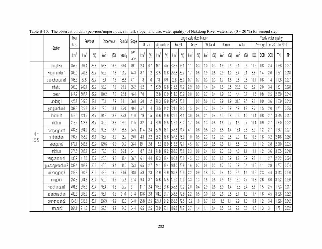
282

Table B-10: The observation data (pervious/impervious, rainfall, slope, land use, water quality) of Nakdong River watershed (0 ~ 20 %) for second step



bonghwa 357.2 299.4 83.8 57.8 16.2 98.0 49.1 2.4 0.7 16.1 4.5 332.6 93.1 1.1 0.3 1.0 0.3 1.9 0.5 2.1 0.6 11.5 0.8 2.4 1.968 0.037

woonmundam1 302.0 249.8 82.7 52.2 17.3 101.7 44.3 3.7 1.2 32.5 10.8 252.8 83.7 1.7 0.6 1.9 0.6 2.9 1.0 6.4 2.1 8.8 1.4 2.6 1.271 0.018

deokchungang1 106.3 87.8 82.7 18.4 17.3 158.5 47.1 1.8 1.6 7.3 6.9 93.8 88.3 0.7 0.7 0.3 0.3 1.7 1.6 0.6 0.6 10.1 0.6 1.4 1.198 0.037

imhaho1 303.0 249.1 82.2 53.9 17.8 79.5 35.2 5.2 1.7 53.9 17.8 215.8 71.2 2.9 0.9 1.4 0.4 1.6 0.5 22.3 7.3 8.2 2.0 3.4 1.501 0.028

dosan 617.9 507.7 82.2 110.2 17.8 92.3 46.4 7.0 1.1 85.8 13.9 514.0 83.2 2.0 0.3 2.7 0.4 1.9 0.3 4.4 0.7 11.5 0.8 2.5 2.360 0.044

andong1 425.7 349.6 82.1 76.1 17.9 84.1 36.8 5.0 1.2 76.3 17.9 297.9 70.0 1.1 0.2 5.6 1.3 7.9 1.9 31.8 7.5 9.6 0.9 3.6 1.669 0.043

yongjunchun1 397.8 325.8 81.9 72.0 18.1 85.0 40.4 5.7 1.4 56.5 14.2 324.1 81.5 1.5 0.4 1.7 0.4 3.4 0.9 4.9 1.2 9.7 1.5 2.0 1.751 0.025

ilanchun1 519.5 424.5 81.7 94.9 18.3 85.3 41.0 7.9 1.5 75.6 14.6 421.1 81.1 3.0 0.6 2.1 0.4 4.3 0.8 5.3 1.0 11.4 0.8 2.7 3.515 0.017

imchun 218.2 178.3 81.7 39.9 18.3 129.3 41.5 3.2 1.4 33.9 15.5 175.1 80.2 1.7 0.8 1.3 0.6 1.6 0.7 1.5 0.7 10.4 0.9 2.7 1.390 0.052

namgangdam1 484.8 394.0 81.3 90.8 18.7 136.8 34.5 11.4 2.4 87.9 18.1 346.3 71.4 4.1 0.8 9.8 2.0 6.8 1.4 18.4 3.8 8.9 1.2 2.7 1.247 0.027

sinbanchun 194.7 158.0 81.1 36.7 18.9 105.7 39.0 4.3 2.2 36.2 18.6 147.8 75.9 1.0 0.5 2.3 1.2 0.9 0.5 2.3 1.2 10.3 1.6 3.2 2.446 0.066

youngang2 672.1 542.5 80.7 129.6 19.3 104.7 36.4 19.1 2.8 113.3 16.9 518.5 77.1 4.5 0.7 3.6 0.5 7.6 1.1 5.5 0.8 11.1 1.2 2.8 2.010 0.035

michun 374.5 302.2 80.7 72.3 19.3 86.3 34.1 8.7 2.3 71.8 19.2 283.0 75.6 2.3 0.6 2.4 0.6 2.3 0.6 4.0 1.1 11.1 1.2 3.6 3.585 0.048

yangsanchun1 138.9 112.0 80.7 26.8 19.3 118.4 36.7 6.1 4.4 17.3 12.4 108.4 78.0 4.5 3.2 0.3 0.2 1.2 0.9 1.2 0.9 9.8 1.1 2.7 2.542 0.074

guchangweechun2 239.4 192.9 80.6 46.5 19.4 111.3 35.3 6.5 2.7 44.1 18.4 184.0 76.9 1.6 0.7 0.6 0.2 1.7 0.7 0.9 0.4 10.5 1.1 2.8 1.787 0.054

milyanggang3 248.8 200.2 80.5 48.6 19.5 94.6 38.8 5.8 2.3 51.9 20.9 181.3 72.9 2.2 0.9 1.8 0.7 2.4 1.0 3.5 1.4 10.6 2.3 4.4 3.013 0.120

mulgeum 254.8 204.8 80.4 50.0 19.6 107.6 37.4 9.4 3.7 44.6 17.5 179.0 70.3 3.3 1.3 1.6 0.6 4.9 1.9 12.0 4.7 10.3 2.6 6.0 3.022 0.130

hapchundam1 491.6 395.2 80.4 96.4 19.6 107.7 31.1 11.7 2.4 106.2 21.6 345.3 70.2 2.0 0.4 2.9 0.6 6.9 1.4 16.6 3.4 8.6 1.5 2.5 1.723 0.017

ssanggyechun 480.3 385.0 80.2 95.1 19.8 91.0 31.4 13.6 2.8 104.0 21.7 348.8 72.6 2.2 0.5 3.0 0.6 2.6 0.5 6.1 1.3 11.7 1.6 4.5 3.226 0.052

gyunghogang2 1042.1 835.3 80.1 206.9 19.9 113.3 34.0 25.8 2.5 221.4 21.2 755.8 72.5 10.9 1.0 6.7 0.6 11.5 1.1 9.9 1.0 10.4 1.2 3.4 1.596 0.042

ramchun2 264.1 211.6 80.1 52.5 19.9 124.0 34.4 6.5 2.5 60.9 23.1 189.3 71.7 3.7 1.4 1.1 0.4 0.5 0.2 2.2 0.8 10.5 1.3 3.1 1.771 0.062

0 ~20 %

Pervious Impervious Rainfall SlopeLarge scale classification

Station

Total

Area


Average from 2001 to 2010Urban Agriculture Forest Grass Wetland Barren Water

283

Table B-11: The observation data (pervious/impervious, rainfall, slope, land use, water quality) of Nakdong River watershed (20 % ~ ) for second step



banbyunchun1a 583.2 465.4 79.8 116.8 20.0 81.3 42.6 40.3 6.9 74.5 12.8 452.7 77.6 2.1 0.4 2.1 0.4 5.6 1.0 4.9 0.8 11.1 1.1 4.1 1.128 0.018

ianchun 242.3 193.3 79.8 49.0 20.2 99.0 31.5 7.0 2.9 53.9 22.2 173.3 71.5 1.7 0.7 0.9 0.4 2.9 1.2 2.7 1.1 10.3 1.1 2.7 1.697 0.025

hamyangweechun2 177.9 141.8 79.7 36.1 20.3 115.7 34.8 5.8 3.3 41.4 23.3 125.4 70.5 2.4 1.4 0.8 0.5 0.8 0.5 1.2 0.7 10.9 1.5 3.7 3.123 0.121

weechun1 392.8 312.7 79.6 80.1 20.4 92.8 31.6 12.9 3.3 93.6 23.8 273.1 69.5 3.6 0.9 2.4 0.6 2.6 0.7 4.6 1.2 11.8 1.4 3.8 4.035 0.069

yeryungchun 114.4 91.0 79.5 23.4 20.5 106.9 36.1 4.6 4.0 26.8 23.4 79.6 69.6 1.0 0.8 0.6 0.5 0.4 0.3 1.4 1.3 9.2 2.1 7.1 2.542 0.104

chungdochun 518.0 408.1 78.8 109.9 21.2 99.1 34.2 18.0 3.5 145.1 28.0 337.0 65.1 3.5 0.7 2.7 0.5 4.3 0.8 7.4 1.4 11.4 1.6 4.2 3.686 0.063

naesungchun1 794.2 623.8 78.5 170.4 21.5 94.7 27.6 21.1 2.7 237.6 29.9 509.8 64.2 4.3 0.5 3.8 0.5 9.1 1.2 8.4 1.1 10.6 1.0 2.6 4.232 0.095

gyuchangdongchun2 197.9 155.4 78.5 42.6 21.5 100.2 32.9 5.6 2.8 57.0 28.8 129.7 65.5 0.8 0.4 0.3 0.1 3.3 1.7 1.3 0.7 10.2 1.1 2.9 2.906 0.079

dalsung 155.5 122.0 78.5 33.5 21.5 92.5 24.3 5.8 3.7 45.9 29.5 93.7 60.3 1.5 1.0 1.6 1.0 2.5 1.6 4.5 2.9 11.2 2.1 5.2 2.927 0.096

andong5 363.2 284.6 78.3 78.7 21.7 89.0 26.6 11.2 3.1 115.2 31.7 221.7 61.0 3.4 0.9 2.8 0.8 3.0 0.8 6.0 1.7 11.0 1.0 4.2 2.300 0.040

gamchun2 1162.4 910.4 78.3 252.0 21.7 89.7 29.1 41.7 3.6 327.0 28.1 743.4 64.0 8.2 0.7 5.6 0.5 21.1 1.8 15.5 1.3 10.1 1.1 3.6 4.348 0.159

geumhogang3 1573.4 1230.5 78.2 342.9 21.8 90.6 27.5 80.6 5.1 306.1 19.5 508.1 32.3 18.1 1.2 8.8 0.6 16.1 1.0 24.0 1.5 10.8 3.2 7.7 5.192 0.268

yechun1 255.6 199.7 78.1 55.9 21.9 88.0 22.9 6.8 2.7 88.0 34.4 141.9 55.5 3.3 1.3 3.8 1.5 3.8 1.5 8.0 3.1 10.8 1.0 3.8 2.425 0.029

milyanggang1 349.3 271.8 77.8 76.5 21.9 103.4 41.9 40.1 11.5 40.9 11.7 247.4 70.8 5.2 1.5 2.7 0.8 6.8 1.9 5.4 1.5 10.1 1.0 2.4 2.358 0.046

hanchun 256.5 200.0 78.0 56.4 22.0 99.3 27.0 9.5 3.7 82.7 32.3 157.7 61.5 2.4 0.9 1.0 0.4 0.9 0.4 2.2 0.9 10.3 1.4 3.6 3.114 0.110

youngsun 17.0 13.2 77.9 3.8 22.1 90.3 22.4 0.5 3.2 5.5 32.2 8.8 51.8 0.1 0.5 0.2 1.0 0.7 4.1 1.2 7.2 10.7 1.0 3.6 2.578 0.058

geumhogang4 213.4 166.0 77.8 47.4 22.2 98.6 22.3 22.4 10.5 31.1 14.6 146.9 68.8 5.0 2.3 1.0 0.5 3.5 1.6 3.5 1.6 12.0 3.7 8.2 5.062 0.293

andong 187.8 145.8 77.7 42.0 22.3 83.8 28.1 15.1 8.1 40.0 21.3 112.6 59.9 2.1 1.1 4.2 2.2 6.9 3.7 6.9 3.7 10.8 1.0 4.0 1.889 0.046

namgang3 711.9 552.6 77.6 159.3 22.4 120.4 28.2 43.3 6.1 210.7 29.6 420.0 59.0 6.5 0.9 6.9 1.0 6.7 0.9 17.7 2.5 10.1 2.7 5.5 3.018 0.124

weechun6 436.2 338.4 77.6 97.8 22.4 83.6 19.1 13.8 3.2 160.5 36.8 238.3 54.6 4.4 1.0 4.1 0.9 4.0 0.9 11.2 2.6 10.4 1.4 4.7 2.539 0.049

hyunpung 109.2 84.6 77.5 24.5 22.5 98.4 30.4 8.6 7.9 22.2 20.3 70.8 64.9 1.5 1.4 0.4 0.4 2.1 2.0 3.5 3.2 10.9 2.9 6.7 4.217 0.207

youngjusuchun2 364.6 282.2 77.4 82.4 22.6 101.9 28.1 19.2 5.3 110.0 30.2 224.6 61.6 1.5 0.4 1.8 0.5 4.1 1.1 3.4 0.9 9.1 2.0 3.8 5.687 0.240

namji 467.2 361.3 77.3 106.0 22.7 99.4 25.4 18.7 4.0 171.3 36.7 236.8 50.7 9.0 1.9 5.4 1.2 6.1 1.3 19.9 4.3 10.3 2.7 6.0 3.239 0.159

andong3 38.0 29.3 77.2 8.6 22.8 87.4 20.3 1.7 4.6 13.4 35.3 21.3 56.1 0.3 0.9 0.0 0.1 0.2 0.6 1.0 2.5 10.7 1.1 4.1 2.120 0.040

hamanchun2 216.2 167.0 77.2 49.3 22.8 103.8 26.4 10.5 4.9 75.2 34.8 117.3 54.3 2.5 1.2 2.9 1.4 1.7 0.8 6.0 2.8 10.1 3.0 6.5 4.780 0.194

bakchun 289.1 223.2 77.2 65.9 22.8 89.9 25.0 11.2 3.9 99.2 34.3 168.8 58.4 2.3 0.8 0.6 0.2 4.1 1.4 3.0 1.0 11.2 1.7 4.0 2.494 0.082

gwangryuchun3 158.0 121.3 76.8 36.7 23.2 102.5 31.7 11.3 7.1 40.7 25.7 96.9 61.3 1.4 0.9 1.9 1.2 4.0 2.5 1.9 1.2 9.8 3.0 5.9 2.553 0.150

daeam 189.6 145.6 76.8 44.0 23.2 96.4 25.4 8.0 4.2 68.6 36.2 96.3 50.8 1.8 1.0 1.8 1.0 5.0 2.6 8.1 4.3 11.2 3.1 6.9 4.116 0.193

sangju2 207.2 158.8 76.7 48.3 23.3 92.2 19.1 7.0 3.4 79.4 38.3 105.7 51.0 1.6 0.8 1.7 0.8 5.4 2.6 6.3 3.0 10.1 0.9 3.4 2.491 0.059

imhaejin 107.2 82.0 76.5 25.2 23.5 94.5 27.0 5.1 4.7 42.4 39.5 48.4 45.1 1.3 1.2 2.0 1.8 2.6 2.4 5.6 5.3 10.6 2.7 6.1 3.144 0.148

sungju 120.1 91.9 76.5 28.3 23.5 84.5 20.6 9.6 8.0 32.1 26.8 63.0 52.4 2.0 1.7 1.9 1.5 5.4 4.5 6.1 5.1 11.0 2.1 5.0 2.996 0.095

gyesungchun 107.1 81.8 76.3 25.3 23.7 94.9 23.9 5.4 5.1 42.9 40.0 53.2 49.7 1.2 1.1 0.9 0.9 0.6 0.5 2.9 2.7 8.6 3.4 8.0 5.392 0.365

gupo 72.1 54.8 76.0 17.3 24.0 114.9 22.3 11.5 16.0 14.3 19.9 38.8 53.8 0.5 0.7 0.1 0.2 1.3 1.7 5.6 7.8 10.2 2.6 6.0 3.109 0.132

byungsungchun 341.0 258.1 75.7 82.8 24.3 97.5 31.3 19.2 5.6 137.4 40.3 167.6 49.2 4.3 1.3 2.5 0.7 4.0 1.2 5.9 1.7 10.2 1.7 4.5 3.883 0.211

geumchun 165.2 124.3 75.3 40.9 24.7 96.3 18.6 8.3 5.0 75.8 45.9 74.8 45.3 1.1 0.7 1.0 0.6 1.0 0.6 3.2 1.9 9.9 3.3 6.1 2.511 0.088

yangsanchun3 107.3 79.0 74.0 27.8 26.0 114.1 28.6 15.3 14.2 14.5 13.5 64.3 60.0 3.9 3.6 0.9 0.8 6.2 5.8 1.6 1.5 10.1 3.8 7.1 4.278 0.246

samrangjin 435.8 322.1 73.9 113.7 26.1 100.5 20.4 32.0 7.3 211.3 48.5 149.0 34.2 6.1 1.4 6.3 1.5 8.9 2.0 22.3 5.1 10.4 2.8 5.9 3.089 0.163

wegwan 500.7 369.4 73.8 131.3 26.2 86.7 20.4 54.7 10.9 164.6 32.9 239.8 47.9 5.9 1.2 4.3 0.9 17.1 3.4 14.2 2.8 10.2 1.8 4.5 3.041 0.108

hwapochun 138.1 101.2 73.3 36.9 26.7 106.6 23.4 13.8 10.0 51.3 37.2 61.5 44.5 3.5 2.5 1.8 1.3 3.8 2.8 2.4 1.8 8.6 3.5 7.2 3.313 0.150

geumhogang6 287.2 209.0 72.8 77.9 27.1 91.1 26.1 67.1 23.4 34.2 11.9 163.2 56.8 7.4 2.6 2.3 0.8 6.8 2.4 5.8 2.0 10.2 3.8 9.3 7.244 0.543

nakdongganghagu1 288.6 206.8 71.7 81.8 28.3 115.3 17.5 38.8 13.4 109.1 37.8 104.0 36.0 7.7 2.7 1.5 0.5 13.3 4.6 14.2 4.9 10.5 2.2 5.4 3.293 0.110

goryung 210.6 149.7 71.1 60.9 28.9 93.7 20.1 47.9 22.8 43.2 20.5 96.6 45.9 5.8 2.8 3.1 1.5 6.7 3.2 7.2 3.4 10.7 2.9 6.8 4.178 0.215

nakdongganghagu2 54.7 37.7 69.0 17.0 31.0 120.9 14.4 19.5 35.7 7.3 13.4 15.5 28.4 1.1 2.0 1.1 2.1 1.2 2.2 8.8 16.1 10.5 2.6 6.3 3.318 0.129

20 ~ 25%

25 % ~

Station

Total

AreaPervious Impervious Rainfall Slope


Urban Agriculture Forest Grass Wetland Barren Water Average from 2001 to 2010

284

Table B-12: The observation data (pervious/impervious, rainfall, slope, land use, water quality) of Geum-sum-youngsan River watershed (0% ~ 25 %) for

second step

km2

km2 (%) km

2 (%) yearlyaver-

age

(%)

km2 (%) km

2 (%) km2 (%) km

2 (%) km2 (%) km

2 (%) km2 (%)

DO

(mg/L)

BOD

(mg/L)

COD

(mg/L)

TN

(mg/L)

TP

(mg/L)

deokeun 184.2 154.9 84.1 29.3 15.9 143.0 45.3 1.8 1.0 5.4 2.9 173.2 94.0 1.5 0.8 0.6 0.3 0.5 0.3 1.3 0.7 9.6 1.3 3.4 2.298 0.046

bakgokchun1 85.7 70.6 82.5 15.0 17.5 102.2 34.1 1.1 1.3 11.0 12.8 68.5 80.0 2.5 2.9 0.1 0.1 0.3 0.3 2.3 2.6 11.5 1.3 2.5 2.389 0.042

juamdam 702.4 578.8 82.4 123.7 17.6 119.8 34.6 9.7 1.4 104.6 14.9 527.1 75.0 23.2 3.3 4.0 0.6 1.6 0.2 32.1 4.6 7.5 0.9 2.8 0.886 0.013

daechung 624.1 511.2 81.9 112.9 18.1 104.1 34.2 19.5 3.1 106.9 17.1 429.0 68.7 5.2 0.8 3.6 0.6 4.2 0.7 55.6 8.9 9.8 0.8 3.5 1.915 0.018

mujunamdaechun-1 464.1 379.6 81.8 84.5 18.2 200.0 43.6 8.9 1.9 58.0 12.5 385.2 83.0 3.8 0.8 1.6 0.3 3.7 0.8 2.9 0.6 10.7 1.1 3.0 2.177 0.039

imsil 429.3 351.1 81.8 78.2 18.2 114.2 34.0 9.3 2.2 77.3 18.0 310.4 72.3 4.9 1.2 2.1 0.5 1.0 0.2 24.3 5.7 10.8 1.1 3.3 1.608 0.038

yongpo 127.7 104.4 81.8 23.3 18.2 96.6 43.1 2.2 1.7 16.7 13.1 104.5 81.8 0.4 0.3 0.7 0.5 1.5 1.1 1.7 1.4 9.9 0.9 3.5 1.662 0.020

chopyungchun 132.6 108.2 81.6 24.4 18.4 100.5 32.1 2.8 2.1 24.3 18.3 97.1 73.3 1.5 1.1 0.8 0.6 0.3 0.2 5.8 4.4 10.7 1.1 2.3 1.580 0.034

youngdong 222.8 180.9 81.2 41.9 18.8 173.9 36.4 5.3 2.4 37.7 16.9 169.9 76.3 1.0 0.4 1.6 0.7 3.0 1.3 4.4 2.0 10.2 1.1 3.7 2.132 0.036

yongdam 355.1 288.0 81.1 67.1 18.9 112.1 40.3 5.5 1.5 51.8 14.6 279.1 78.6 7.6 2.1 0.9 0.2 6.9 1.9 3.3 0.9 10.9 0.8 3.3 1.691 0.018

nonsanchun1 219.4 177.9 81.1 41.6 18.9 110.3 34.0 5.2 2.4 43.3 19.7 160.2 73.0 2.0 0.9 0.7 0.3 0.6 0.3 7.4 3.4 10.4 1.2 3.1 3.576 0.034

hadong 156.3 126.5 80.9 29.8 19.1 143.1 39.8 5.4 3.4 21.9 14.0 120.3 77.0 1.7 1.1 1.0 0.6 3.1 2.0 2.9 1.8 9.0 1.2 4.8 2.275 0.047

donggye 144.4 116.6 80.8 27.7 19.2 116.1 35.4 2.2 1.6 28.8 19.9 101.5 70.3 7.9 5.5 1.7 1.2 0.6 0.4 1.6 1.1 9.7 1.1 3.6 1.445 0.043

jisukchun2 215.8 174.2 80.7 41.6 19.3 111.9 29.7 5.6 2.6 44.7 20.7 147.5 68.4 3.7 1.7 2.1 1.0 2.7 1.3 9.6 4.4 10.8 2.2 4.4 2.674 0.109

jisukchun1 237.7 191.6 80.6 45.9 19.3 116.0 32.9 5.8 2.5 45.4 19.1 170.8 71.9 7.8 3.3 2.1 0.9 1.6 0.7 4.0 1.7 10.2 1.4 3.1 1.367 0.038

chogang2 664.6 535.0 80.5 129.6 19.5 96.2 34.0 13.1 2.0 142.1 21.4 493.5 74.3 5.2 0.8 1.6 0.2 2.7 0.4 6.5 1.0 10.4 1.1 3.4 2.251 0.029

bosungchun-1 283.8 228.2 80.4 55.5 19.6 122.3 35.3 6.1 2.1 61.9 21.8 201.2 70.9 8.1 2.8 2.6 0.9 0.9 0.3 3.0 1.1 10.4 1.0 3.1 1.240 0.028

youngdongchun2 145.4 116.6 80.2 28.8 19.8 92.2 35.7 6.5 4.5 24.6 16.9 111.1 76.4 0.5 0.3 0.6 0.4 1.3 0.9 0.9 0.6 10.5 1.4 4.1 5.061 0.123

guryu 489.0 391.8 80.1 97.2 19.9 120.0 36.6 13.9 2.8 108.7 22.2 343.0 70.1 9.6 2.0 5.0 1.0 2.2 0.5 6.5 1.3 10.0 1.3 3.7 2.382 0.053

youdeungchun A 141.9 113.6 80.0 28.3 20.0 108.3 40.0 4.4 3.1 28.0 19.7 105.3 74.2 1.5 1.1 0.3 0.2 1.5 1.1 0.8 0.6 11.9 0.9 2.2 2.924 0.031

jewon 89.9 72.0 80.0 18.0 20.0 99.0 33.1 2.2 2.4 18.7 20.8 62.4 69.4 1.0 1.2 0.3 0.3 2.1 2.3 3.3 3.6 10.3 1.0 3.7 1.765 0.029

gongju1 98.7 79.0 80.0 19.7 20.0 113.3 28.9 5.0 5.1 19.1 19.4 66.7 67.6 1.5 1.5 1.2 1.2 1.6 1.6 3.6 3.7 10.2 2.9 6.6 4.323 0.182

churyungchun 355.9 284.3 79.9 71.6 20.1 111.9 31.8 10.3 2.9 79.5 22.3 249.9 70.2 8.9 2.5 1.8 0.5 1.6 0.4 3.9 1.1 11.1 0.9 2.6 2.818 0.017

bonggok2gyo 156.9 125.3 79.9 31.6 20.1 107.7 32.8 8.5 5.4 24.1 15.4 115.9 73.9 5.1 3.2 0.6 0.4 1.6 1.0 1.2 0.7 11.2 1.9 3.3 3.439 0.182

youguchun 282.6 225.5 79.8 57.1 20.2 105.1 31.4 8.8 3.1 67.6 23.9 197.4 69.8 3.0 1.1 2.2 0.8 1.2 0.4 2.5 0.9 10.2 1.7 2.8 1.785 0.037

bochungchun4 113.6 90.4 79.6 23.2 20.4 94.2 32.4 2.9 2.5 28.2 24.8 77.2 68.0 1.1 0.9 0.7 0.6 1.5 1.3 2.1 1.9 10.5 1.1 2.7 2.029 0.035

jichun 246.4 195.8 79.5 50.6 20.5 104.8 26.7 7.1 2.9 64.9 26.3 164.9 66.9 4.0 1.6 1.4 0.6 0.8 0.3 3.3 1.3 10.6 1.9 3.6 2.212 0.048

yongsuchun 95.1 75.6 79.4 19.6 20.6 118.1 32.7 5.3 5.6 18.4 19.3 66.7 70.1 2.4 2.5 0.7 0.7 0.9 1.0 0.7 0.8 8.1 1.7 2.8 1.376 0.054

bochungchun3 299.5 237.8 79.4 61.7 20.6 99.6 31.3 6.6 2.2 79.9 26.7 201.8 67.4 2.1 0.7 0.8 0.3 4.1 1.4 4.2 1.4 11.4 1.2 3.6 2.470 0.047

bochungchun2 140.6 111.5 79.3 29.1 20.7 188.1 29.9 5.0 3.5 35.8 25.5 96.3 68.5 0.6 0.4 0.5 0.4 0.9 0.6 1.5 1.1 10.2 1.1 2.1 2.115 0.031

yongdamdam4 575.2 453.9 78.9 121.3 21.1 106.1 35.2 16.6 2.9 146.7 25.5 377.2 65.6 23.0 4.0 1.8 0.3 5.7 1.0 4.2 0.7 8.7 1.2 2.8 1.658 0.022

bosunggang-1 327.0 257.8 78.9 69.1 21.1 123.7 26.9 10.5 3.2 92.6 28.3 205.3 62.8 8.6 2.6 2.1 0.6 2.1 0.6 5.8 1.8 10.2 1.2 3.4 0.854 0.031

namwon 227.0 178.9 78.8 48.2 21.2 113.7 26.6 6.7 3.0 69.4 30.6 134.0 59.0 6.6 2.9 3.9 1.7 1.6 0.7 4.9 2.1 10.4 1.4 3.8 1.664 0.052

gongju2 171.4 135.0 78.7 36.5 21.3 109.2 24.2 5.1 3.0 51.4 30.0 103.9 60.6 2.1 1.2 1.4 0.8 2.2 1.3 5.3 3.1 10.3 3.3 7.1 4.476 0.174

hwangryonggang3 565.0 443.7 78.5 121.4 21.5 114.9 27.7 28.4 5.0 152.4 27.0 350.9 62.1 6.8 1.2 4.5 0.8 4.8 0.8 17.3 3.1 10.1 3.0 4.6 1.733 0.063

woosan 120.4 94.4 78.4 26.0 21.6 101.3 30.6 5.8 4.8 32.3 26.8 74.0 61.5 1.3 1.1 1.0 0.8 1.8 1.5 4.3 3.6 10.5 0.9 3.6 1.999 0.039

mokmyun 120.6 94.6 78.4 26.1 21.6 107.9 26.1 4.4 3.6 33.8 28.1 74.7 61.9 1.8 1.5 0.3 0.3 2.7 2.3 2.8 2.4 11.6 3.6 7.4 4.949 0.188

Average from 2001 to 2010


Station

Total

Area

20 % ~

25%

SlopeLarge scale classification

Urban Agriculture Forest Grass Wetland Barren Water

0 ~

20 %

Pervious Impervious Rainfall

285

Table B-13: The observation data (pervious/impervious, rainfall, slope, land use, water quality) of Geum-sum-youngsan River watershed (20% ~ ) for second

step

km2

km2 (%) km

2 (%) yearlyaver-

age

(%)

km2 (%) km

2 (%) km2 (%) km

2 (%) km2 (%) km

2 (%) km2 (%)

DO

(mg/L)

BOD

(mg/L)

COD

(mg/L)

TN

(mg/L)

TP

(mg/L)

hwasunchun 127.7 100.1 78.3 27.7 21.7 120.2 31.3 7.3 5.7 30.7 24.0 83.5 65.3 3.0 2.3 0.8 0.6 1.4 1.1 1.2 0.9 10.5 2.1 4.2 2.477 0.064

osuchun 371.3 289.6 78.0 81.3 21.9 112.9 24.6 11.6 3.1 124.3 33.5 220.6 59.4 5.0 1.4 3.5 0.9 1.6 0.4 4.3 1.1 10.9 1.5 3.8 2.010 0.060

gomnaru 197.7 153.7 77.8 44.0 22.2 104.9 26.6 11.4 5.8 55.4 28.0 119.6 60.5 2.3 1.2 1.6 0.8 4.0 2.0 3.4 1.7 10.1 3.1 6.5 4.321 0.171

bonghwangchun 247.4 192.1 77.6 55.3 22.4 143.4 30.7 11.8 4.8 73.9 29.9 155.1 62.7 2.1 0.9 0.4 0.2 2.1 0.9 1.9 0.8 10.3 1.5 3.7 3.337 0.118

daegyochun 65.9 51.0 77.3 15.0 22.7 106.6 21.6 2.5 3.8 23.9 36.3 36.7 55.7 1.1 1.7 0.2 0.3 0.6 0.9 0.9 1.3 10.6 2.0 3.5 2.119 0.050

jochun 136.3 105.2 77.2 31.1 22.8 102.7 23.1 11.3 8.3 39.2 28.8 79.6 58.4 2.1 1.6 1.2 0.9 1.3 1.0 1.5 1.1 9.9 3.6 5.1 4.421 0.284

buyoe1 96.9 74.8 77.1 22.2 22.9 109.0 19.8 4.6 4.7 32.9 33.9 53.3 55.0 0.5 0.5 0.2 0.2 2.2 2.2 3.3 3.4 10.4 3.1 6.8 4.146 0.162

yochun 294.8 227.1 77.0 67.7 23.0 113.3 22.8 15.7 5.3 97.4 33.0 163.4 55.4 5.4 1.8 4.4 1.5 3.9 1.3 4.7 1.6 10.2 1.6 4.0 2.707 0.161

daegang 204.3 157.2 77.0 47.1 23.0 112.2 22.3 7.9 3.8 77.3 37.8 107.9 52.8 5.3 2.6 2.0 1.0 1.3 0.7 2.6 1.2 10.9 1.8 4.5 1.895 0.052

gapchun2 93.9 71.6 76.2 22.3 23.8 110.7 23.7 8.1 8.6 24.9 26.5 53.3 56.8 2.2 2.3 1.0 1.0 2.8 2.9 1.7 1.9 10.8 2.2 3.8 2.933 0.088

sungdong 65.1 49.2 75.7 15.8 24.3 106.6 12.0 4.5 6.9 28.8 44.2 23.2 35.6 0.5 0.7 0.4 0.6 1.3 1.9 6.5 9.9 9.3 3.2 6.8 3.835 0.162

yongi 86.1 65.1 75.5 21.1 24.5 104.2 15.2 5.3 6.2 36.8 42.8 36.5 42.4 1.1 1.3 2.0 2.3 1.1 1.2 3.3 3.9 10.0 3.2 6.8 5.315 0.218

mihochun5 471.5 355.8 75.5 115.7 24.5 102.5 18.5 37.4 7.9 157.2 33.3 243.4 51.6 10.3 2.2 3.5 0.7 12.2 2.6 7.6 1.6 10.1 4.8 8.8 5.112 0.220

geumchun 165.2 124.3 75.3 40.9 24.7 96.3 18.6 8.3 5.0 75.8 45.9 74.8 45.3 1.1 0.7 1.0 0.6 1.0 0.6 3.2 1.9 9.9 3.3 6.1 2.511 0.088

gwangju1 562.0 422.5 75.2 139.5 24.8 112.8 25.5 46.0 8.2 206.2 36.7 268.9 47.8 13.5 2.4 5.7 1.0 8.2 1.5 13.5 2.4 10.6 3.7 5.8 2.793 0.103

mihochun4 220.7 165.8 75.1 54.9 24.9 101.6 18.7 14.7 6.6 86.3 39.1 101.8 46.1 6.9 3.1 2.0 0.9 4.5 2.0 4.5 2.0 10.2 2.7 5.8 4.031 0.191

chungwon-1 129.8 97.5 75.1 32.3 24.9 97.4 19.6 11.1 8.5 44.7 34.4 64.9 50.0 2.6 2.0 1.2 1.0 2.1 1.6 3.2 2.4 10.9 2.4 6.0 5.690 0.216

gomakwonchun2 219.0 164.4 75.1 54.5 24.9 110.7 18.4 12.3 5.6 105.2 48.0 91.6 41.8 2.0 0.9 1.9 0.9 1.8 0.8 4.3 2.0 10.2 2.9 5.9 2.653 0.070

bogangchun 157.6 118.0 74.9 39.6 25.1 99.3 19.2 10.1 6.4 69.0 43.8 72.0 45.7 1.8 1.2 0.8 0.5 1.6 1.0 2.3 1.5 10.5 1.8 3.6 3.621 0.087

muan2 885.4 661.7 74.7 223.7 25.3 101.8 15.1 42.2 4.8 470.0 53.1 291.8 33.0 8.7 1.0 8.9 1.0 10.3 1.2 53.5 6.0 9.9 2.0 5.7 4.194 0.133

geumganggapmun 536.6 400.9 74.7 135.7 25.3 100.3 12.4 33.4 6.2 271.8 50.6 180.9 33.7 5.4 1.0 4.4 0.8 2.5 0.5 38.1 7.1 10.6 2.9 7.3 4.374 0.131

nosungchun 202.5 150.5 74.4 51.9 25.6 105.3 17.7 12.0 5.9 98.9 48.8 84.0 41.5 2.6 1.3 0.8 0.4 1.1 0.6 3.0 1.5 10.6 2.6 4.6 2.125 0.068

bakgokchun2 39.8 29.4 73.9 10.4 26.1 105.0 15.2 3.4 8.6 17.8 44.7 16.6 41.8 0.3 0.7 0.3 0.8 0.7 1.6 0.7 1.8 11.4 1.8 3.3 2.553 0.074

mihochun6-1 125.6 92.7 73.8 32.9 26.2 101.2 13.3 10.3 8.2 59.0 47.0 45.7 36.4 2.8 2.2 2.2 1.8 2.2 1.7 3.3 2.6 9.8 4.8 9.2 6.424 0.264

youngsanpo 309.9 227.9 73.5 82.1 26.5 110.4 24.4 19.2 6.2 166.1 53.6 108.1 34.9 3.4 1.1 2.3 0.8 3.1 1.0 7.7 2.5 9.6 5.6 6.5 6.624 0.435

musimchun3 197.3 144.5 73.2 52.9 26.8 98.4 20.1 30.9 15.6 57.5 29.1 97.1 49.2 3.9 2.0 1.8 0.9 4.7 2.4 1.6 0.8 11.1 2.2 4.3 3.171 0.082

suksungchun 152.2 111.3 73.2 40.8 26.8 103.5 12.4 8.3 5.5 85.7 56.3 50.2 33.0 2.1 1.4 0.0 0.0 3.0 2.0 2.8 1.8 8.3 4.2 6.5 3.838 0.495

hyundo 43.3 31.5 72.7 11.8 27.3 102.7 20.2 7.4 17.0 10.3 23.8 21.2 48.9 1.6 3.6 0.2 0.5 1.0 2.3 1.7 4.0 10.5 0.7 3.8 1.530 0.023

mihochun2 288.8 207.8 71.9 81.0 28.1 98.2 14.3 22.4 7.8 157.7 54.6 91.8 31.8 6.2 2.1 2.9 1.0 4.4 1.5 3.4 1.2 10.2 3.1 6.3 4.479 0.173

jisukchun4 82.9 59.1 71.3 23.8 28.7 111.0 11.1 7.6 9.2 49.7 59.9 20.5 24.7 0.4 0.5 1.4 1.7 1.3 1.6 2.0 2.4 11.0 2.7 5.6 3.400 0.146

daejeonchun3 89.4 63.7 71.3 25.7 28.7 107.2 29.4 22.9 25.6 11.9 13.4 49.3 55.2 2.0 2.2 0.6 0.7 2.2 2.5 0.5 0.5 12.0 2.6 3.9 4.745 0.117

nonsanchun4 244.2 171.5 70.2 72.7 29.8 97.0 9.1 26.2 10.7 149.2 61.1 55.3 22.6 4.9 2.0 0.8 0.3 3.9 1.6 3.8 1.6 10.2 4.3 7.9 6.374 0.215

gapchun5-1 107.6 75.2 69.9 32.4 30.1 111.5 15.1 25.0 23.2 19.6 18.2 41.6 38.6 10.5 9.7 0.8 0.7 7.4 6.9 2.7 2.5 9.4 5.5 9.9 11.938 0.570

naju 264.1 180.0 68.2 84.1 31.8 112.1 8.0 69.9 26.5 96.5 36.6 74.8 28.3 8.5 3.2 3.3 1.3 5.8 2.2 5.3 2.0 10.3 5.3 6.5 6.961 0.454

youdeungchun5 59.2 37.2 62.8 22.1 37.2 110.7 14.7 26.1 44.0 4.1 7.0 19.9 33.6 2.9 4.9 0.4 0.7 5.3 8.9 0.6 1.0 11.3 2.9 4.2 3.061 0.092

goksung 183.4 147.4 241.2 36.0 58.8 113.7 32.4 4.7 2.5 38.7 21.1 130.2 71.0 3.1 1.7 2.3 1.2 1.7 0.9 2.8 1.5 10.0 1.4 4.0 2.521 0.066

jinwol 298.9 238.3 319.4 60.5 80.6 139.3 32.4 11.0 3.7 67.9 22.7 202.6 67.8 4.4 1.5 2.0 0.7 2.3 0.8 8.6 2.9 9.0 1.2 3.6 1.144 0.040

Average from 2001 to 2010Slope



20 % ~

25%

Station

Total

AreaPervious

25 % ~

Impervious Rainfall

286

Table B-14: The observation data of Hangang, Nakdong, and Geum-sum-youngsan river for third step (Area: 0 ~ 250 km2, Imperviousness: 0 ~ 25 %)

km2

km2 (%) km

2 (%) yearlyaver-

age(%)km

2 (%) km2 (%) km

2 (%) km2 (%) km

2 (%) km2 (%) km

2 (%)DO BOD COD TN TP

deokyeun 184.2 154.9 84.1 29.3 15.9 143.0 45.3 1.8 1.0 5.4 2.9 173.2 94.0 1.5 0.8 0.6 0.3 0.5 0.3 1.3 0.7 9.6 1.3 3.4 2.298 0.046

deokchungang1 106.3 87.8 82.7 18.4 17.3 158.5 47.1 1.8 1.6 7.3 6.9 93.8 88.3 0.7 0.7 0.3 0.3 1.7 1.6 0.6 0.6 10.1 0.6 1.4 1.198 0.037

yochuun A 191.7 158.5 82.7 33.2 17.3 112.9 46.5 3.2 1.7 17.5 9.1 163.5 85.3 3.4 1.8 1.3 0.7 0.8 0.4 2.1 1.1 3.4 0.3 0.7 0.676 0.005

paldangdam 132.5 109.5 82.6 23.0 17.4 103.3 28.7 4.5 3.4 18.1 13.7 92.3 69.7 1.7 1.3 2.7 2.1 1.0 0.8 12.1 9.1 10.9 1.3 3.6 2.121 0.048

bakgokchun1 85.7 70.6 82.5 15.0 17.5 102.2 34.1 2.2 2.6 18.7 21.8 62.4 72.8 1.0 1.2 0.3 0.3 2.1 2.5 3.3 3.8 11.5 1.3 2.5 2.389 0.042

joyanggang 74.1 60.8 82.1 13.2 17.9 94.8 48.6 1.3 1.7 8.9 12.0 62.1 83.8 0.2 0.3 0.1 0.1 0.5 0.7 1.1 1.5 11.0 0.8 2.3 2.652 0.027

chunsunggyo 189.4 155.4 82.1 34.0 17.9 108.2 38.7 4.3 2.3 19.7 10.4 154.6 81.6 4.1 2.2 0.1 0.1 2.3 1.2 4.2 2.2 10.8 1.2 3.1 1.667 0.030

sangchun 182.3 149.2 81.8 33.2 18.2 98.5 43.3 2.9 1.6 26.3 14.4 149.2 81.8 0.7 0.4 0.7 0.4 1.3 0.7 1.3 0.7 11.1 1.0 2.2 2.488 0.034

younpo 127.7 104.4 81.8 23.3 18.2 96.6 43.1 1.1 0.8 11.0 8.6 68.5 53.6 2.5 2.0 0.1 0.1 0.3 0.2 2.3 1.8 9.9 0.9 3.5 1.662 0.020

geumgyechun 155.4 126.9 81.7 28.5 18.3 109.1 39.6 2.0 1.3 23.8 15.3 127.0 81.7 0.3 0.2 0.0 0.0 0.8 0.5 1.4 0.9 10.8 0.9 1.8 2.500 0.033

chopyungchun 132.6 108.2 81.6 24.4 18.4 100.5 32.1 5.8 4.4 32.3 24.3 74.0 55.9 1.3 1.0 1.0 0.8 1.8 1.3 4.3 3.2 10.7 1.1 2.3 1.580 0.034

youngdong 222.8 180.9 81.2 41.9 18.8 173.9 36.4 11.4 5.1 55.4 24.9 119.6 53.7 2.3 1.0 1.6 0.7 4.0 1.8 3.4 1.5 10.2 1.1 3.7 2.132 0.036

nonsanchun1 219.4 177.9 81.1 41.6 18.9 110.3 34.0 22.4 10.2 157.7 71.9 91.8 41.9 6.2 2.8 2.9 1.3 4.4 2.0 3.4 1.5 10.4 1.2 3.1 3.576 0.034

hadong 156.3 126.5 80.9 29.8 19.1 143.1 39.8 5.4 3.4 21.9 14.0 120.3 77.0 1.7 1.1 1.0 0.6 3.1 2.0 2.9 1.8 9.0 1.2 4.8 2.275 0.047

donggye 144.4 116.6 80.8 27.7 19.2 116.1 35.4 2.2 1.6 28.8 19.9 101.5 70.3 7.9 5.5 1.7 1.2 0.6 0.4 1.6 1.1 9.7 1.1 3.6 1.445 0.043

jisukchun2 215.8 174.2 80.7 41.6 19.3 111.9 29.7 5.6 2.6 44.7 20.7 147.5 68.4 3.7 1.7 2.1 1.0 2.7 1.3 9.6 4.4 10.8 2.2 4.4 2.674 0.109

junchun 170.7 137.7 80.7 33.0 19.3 108.0 32.6 5.2 3.0 28.2 16.5 133.7 78.3 1.2 0.7 0.4 0.2 1.0 0.6 1.1 0.7 9.8 1.2 2.0 1.295 0.023

yangsanchun1 138.9 112.0 80.7 26.8 19.3 118.4 36.7 6.1 4.4 17.3 12.4 108.4 78.0 4.5 3.2 0.3 0.2 1.2 0.9 1.2 0.9 9.8 1.1 2.7 2.542 0.074

jisukpo 237.6 191.6 80.7 45.9 19.3 116.0 32.9 5.8 2.5 45.4 19.1 170.8 71.9 7.8 3.3 2.1 0.9 1.6 0.7 4.0 1.7 10.2 1.4 3.1 1.367 0.038

sukmunchun 99.2 79.9 80.6 19.3 19.4 93.0 39.9 3.0 3.0 18.2 18.4 75.3 75.9 0.4 0.4 0.5 0.5 1.2 1.2 0.6 0.6 11.8 1.3 2.7 3.713 0.104

milyanggang3 248.8 200.2 80.5 48.6 19.5 94.6 38.8 5.8 3.0 51.9 26.8 181.3 93.7 2.2 1.1 1.8 0.9 2.4 1.2 3.5 1.8 10.6 2.3 4.4 3.013 0.120

goksung 183.4 147.4 80.4 36.0 19.6 113.7 32.4 4.7 2.5 38.7 21.1 130.2 71.0 3.1 1.7 2.3 1.2 1.7 0.9 2.8 1.5 10.0 1.4 4.0 2.521 0.066

youngdongchun2 145.4 116.6 80.2 28.8 19.8 92.2 35.7 8.8 6.1 67.6 46.5 197.4 135.7 3.0 2.1 2.2 1.5 1.2 0.8 2.5 1.7 10.5 1.4 4.1 5.061 0.123

youdengchun-a 141.9 113.6 80.0 28.3 20.0 108.3 40.0 8.1 5.7 24.9 17.5 53.3 37.6 2.2 1.5 1.0 0.7 2.8 1.9 1.7 1.2 11.9 0.9 2.2 2.924 0.031

jewon 89.9 72.0 80.0 18.0 20.0 99.0 33.1 4.4 4.9 28.0 31.1 105.3 117.1 1.5 1.7 0.3 0.4 1.5 1.7 0.8 0.9 10.3 1.0 3.7 1.765 0.029

gongju1 98.7 79.0 80.0 19.7 20.0 113.3 28.9 11.8 12.0 73.9 74.8 155.1 157.2 2.1 2.2 0.4 0.4 2.1 2.2 1.9 1.9 10.2 2.9 6.6 4.323 0.182

bonggok 2 gyo 156.9 125.3 79.9 31.6 20.1 107.7 32.8 11.3 7.2 39.2 25.0 79.6 50.7 2.1 1.3 1.2 0.8 1.3 0.9 1.5 0.9 11.2 1.9 3.3 3.396 0.193

ianchun 242.3 193.3 79.8 49.0 20.2 99.0 31.5 7.0 2.9 53.9 22.2 173.3 71.5 1.7 0.7 0.9 0.4 2.9 1.2 2.7 1.1 6.2 0.7 1.6 1.018 0.015

bochungchun4 113.6 90.4 79.6 23.2 20.4 94.2 32.4 4.5 4.0 28.8 25.3 23.2 20.4 0.5 0.4 0.4 0.4 1.3 1.1 6.5 5.7 10.5 1.1 2.7 2.029 0.035

yeryungchun 114.4 91.0 79.5 23.4 20.5 106.9 36.1 4.6 4.0 26.8 23.4 79.6 69.6 1.0 0.8 0.6 0.5 0.4 0.3 1.4 1.3 9.2 2.1 7.1 2.542 0.104

jichun 246.4 195.8 79.5 50.6 20.5 104.8 26.7 26.1 10.6 4.1 1.7 19.9 8.1 2.9 1.2 0.4 0.2 5.3 2.1 0.6 0.2 10.6 1.9 3.6 2.212 0.048

yongsuchun 95.1 75.6 79.4 19.6 20.6 118.1 32.7 30.9 32.4 57.5 60.4 97.1 102.0 3.9 4.1 1.8 1.9 4.7 4.9 1.6 1.7 8.1 1.7 2.8 1.376 0.054

bochungchun2 140.6 111.5 79.3 29.1 20.7 188.1 29.9 8.3 5.9 75.8 54.0 74.8 53.2 1.1 0.8 1.0 0.7 1.0 0.7 3.2 2.2 10.2 1.1 2.1 2.115 0.031

dongjinchun2 124.0 98.2 79.2 25.8 20.8 96.4 29.7 3.8 3.1 31.1 25.1 83.7 67.5 1.9 1.6 0.0 0.0 1.6 1.3 1.8 1.4 10.4 1.4 2.5 2.340 0.036

damchun3 86.2 68.0 78.9 18.2 21.1 94.5 25.6 2.6 3.0 27.8 32.2 50.9 59.0 1.3 1.6 0.6 0.7 0.2 0.2 2.8 3.2 10.4 1.1 2.9 2.389 0.035

namwon 227.0 178.9 78.8 48.2 21.2 113.7 26.6 6.7 3.0 69.4 30.6 134.0 59.0 6.6 2.9 3.9 1.7 1.6 0.7 4.9 2.1 10.4 1.4 3.8 1.664 0.052

gongju2 171.4 135.0 78.7 36.5 21.3 109.2 24.2 5.3 3.1 37.7 22.0 169.9 99.1 1.0 0.6 1.6 0.9 3.0 1.7 4.4 2.5 10.3 3.3 7.1 4.476 0.174

dalsung 155.5 122.0 78.5 33.5 21.5 92.5 24.3 5.8 3.7 45.9 29.5 93.7 60.3 1.5 1.0 1.6 1.0 2.5 1.6 4.5 2.9 11.2 2.1 5.2 2.927 0.096

sumgang2 108.1 84.8 78.5 23.3 21.5 107.7 25.9 7.5 7.0 25.7 23.7 68.8 63.6 2.0 1.8 1.1 1.0 1.1 1.0 1.9 1.8 10.7 1.5 3.2 2.360 0.053

segokchun 113.5 89.0 78.4 24.5 21.6 105.4 29.2 6.9 6.1 27.1 23.9 74.9 66.0 1.5 1.3 0.3 0.3 1.3 1.1 1.5 1.3 10.6 1.6 3.6 4.646 0.129

woosan 120.4 94.4 78.4 26.0 21.6 101.3 30.6 3.4 2.8 17.8 14.8 16.6 13.8 0.3 0.2 0.3 0.3 0.7 0.5 0.7 0.6 10.1 1.0 3.7 2.339 0.044

mokmyun 120.6 94.6 78.4 26.1 21.6 107.9 26.1 7.1 5.9 64.9 53.8 164.9 136.7 4.0 3.3 1.4 1.2 0.8 0.7 3.3 2.7 11.6 3.6 7.4 4.949 0.188

hwasunchun 127.7 100.1 78.3 27.7 21.7 120.2 31.3 7.3 5.7 30.7 24.0 83.5 65.3 3.0 2.3 0.8 0.6 1.4 1.1 1.2 0.9 10.5 2.1 4.2 2.477 0.064

youngsun 17.0 13.2 77.9 3.8 22.1 90.3 22.4 0.5 3.2 5.5 32.2 8.8 51.8 0.1 0.5 0.2 1.0 0.7 4.1 1.2 7.2 9.6 0.9 3.3 2.320 0.052

gomnaru 197.7 153.7 77.8 44.0 22.2 104.9 26.6 8.9 4.5 58.0 29.3 385.2 194.9 3.8 1.9 1.6 0.8 3.7 1.8 2.9 1.5 10.1 3.1 6.5 4.321 0.171

bonghwangchun 247.4 192.1 77.6 55.3 22.4 143.4 30.7 10.3 4.2 59.0 23.8 45.7 18.5 2.8 1.1 2.2 0.9 2.2 0.9 3.3 1.3 10.3 1.5 3.7 3.337 0.118

20 ~ 25%

Impervious

0 ~ 20 %

station

Total


Average(2001~2010)slope

large scale classification Yearly water quality


287

Table B-15: The observation data of Hangang, Nakdong, and Geum-sum-youngsan river for third step (Area: 0 ~ 250 km2, Imperviousness: 20 % ~ )

km2

km2 (%) km

2 (%) yearlyaver-

age(%)km

2 (%) km2 (%) km

2 (%) km2 (%) km

2 (%) km2 (%) km


geumganggapmun 194.8 151.3 77.6 43.6 22.4 100.6 13.8 13.1 6.7 142.1 72.9 493.5 253.3 5.2 2.7 1.6 0.8 2.7 1.4 6.5 3.3 3.2 0.9 2.2 1.312 0.039

hyunpung 109.2 84.6 77.5 24.5 22.5 98.4 30.4 8.6 7.9 22.2 20.3 70.8 64.9 1.5 1.4 0.4 0.4 2.1 2.0 3.5 3.2 10.9 2.9 6.7 4.217 0.207

yeamdam 228.0 176.5 77.4 51.5 22.6 105.2 24.8 26.1 11.4 48.1 21.1 131.6 57.7 4.0 1.8 0.4 0.2 3.6 1.6 14.2 6.2 10.5 1.1 2.8 1.657 0.030

daegyochun 65.9 51.0 77.3 15.0 22.7 106.6 21.6 14.7 22.2 86.3 130.8 101.8 154.3 6.9 10.5 2.0 3.1 4.5 6.8 4.5 6.8 10.6 2.0 3.5 2.119 0.050

andong3 38.0 29.3 77.2 8.6 22.8 87.4 20.3 1.7 4.6 13.4 35.3 21.3 56.1 0.3 0.9 0.0 0.1 0.2 0.6 1.0 2.5 7.5 0.8 2.9 1.484 0.028

hamanchun2 216.2 167.0 77.2 49.3 22.8 103.8 26.4 10.5 4.9 75.2 34.8 117.3 54.3 2.5 1.2 2.9 1.4 1.7 0.8 6.0 2.8 10.1 3.0 6.5 4.780 0.194

jochun 136.3 105.2 77.2 31.1 22.8 102.7 23.1 22.9 16.8 11.9 8.8 49.3 36.2 2.0 1.4 0.6 0.4 2.2 1.6 0.5 0.3 9.9 3.6 5.1 4.421 0.284

buyeu1 96.9 74.8 77.1 22.2 22.9 109.0 19.8 5.3 5.5 18.4 19.0 66.7 68.8 2.4 2.5 0.7 0.7 0.9 0.9 0.7 0.8 10.4 3.1 6.8 4.146 0.162

daegang 204.3 157.2 77.0 47.1 23.0 112.2 22.3 7.9 3.8 77.3 37.8 107.9 52.8 5.3 2.6 2.0 1.0 1.3 0.7 2.6 1.2 3.3 0.5 1.4 0.569 0.016

hwayangchun 56.3 43.3 76.8 13.0 23.2 100.3 39.7 2.1 3.7 21.9 39.0 30.4 54.0 0.8 1.3 0.2 0.3 0.2 0.4 0.7 1.3 11.3 0.7 1.6 2.138 0.022

gwangryuchun3 158.0 121.3 76.8 36.7 23.2 102.5 31.7 11.3 7.1 40.7 25.7 96.9 61.3 1.4 0.9 1.9 1.2 4.0 2.5 1.9 1.2 9.8 3.0 5.9 2.553 0.150

yeumsungchun 143.2 110.0 76.8 33.2 23.2 101.0 24.6 6.9 4.8 51.9 36.2 77.9 54.4 2.5 1.7 0.5 0.3 1.2 0.9 2.4 1.7 11.0 1.8 3.3 2.526 0.064

byungchunchun 220.3 169.1 76.8 51.2 23.2 102.9 19.4 12.0 5.5 98.9 44.9 84.0 38.1 2.6 1.2 0.8 0.4 1.1 0.5 3.0 1.4 10.5 2.2 3.8 2.709 0.060

daeam 189.6 145.6 76.8 44.0 23.2 96.4 25.4 8.0 4.2 68.6 36.2 96.3 50.8 1.8 1.0 1.8 1.0 5.0 2.6 8.1 4.3 11.2 3.1 6.9 4.116 0.193

wonjuchun 153.0 117.3 76.7 35.6 23.3 110.5 31.1 19.5 12.7 29.4 19.2 98.5 64.4 1.0 0.6 0.8 0.5 2.7 1.8 1.2 0.8 9.3 7.5 8.5 10.386 0.758

imheajin 107.2 82.0 76.5 25.2 23.5 94.5 27.0 5.1 4.7 42.4 39.5 48.4 45.1 1.3 1.2 2.0 1.8 2.6 2.4 5.6 5.3 10.6 2.7 6.1 3.144 0.148

sungju 120.1 91.9 76.5 28.3 23.5 84.5 20.6 9.6 8.0 32.1 26.8 63.0 52.4 2.0 1.7 1.9 1.5 5.4 4.5 6.1 5.1 11.0 2.1 5.0 2.996 0.095

damchul5 152.2 116.3 76.5 35.8 23.5 97.2 30.8 13.8 9.0 44.0 28.9 81.4 53.5 4.9 3.2 1.4 0.9 2.6 1.7 4.1 2.7 10.2 1.8 3.8 2.865 0.089

gyesungchun 107.1 81.8 76.3 25.3 23.7 94.9 23.9 5.4 5.1 42.9 40.0 53.2 49.7 1.2 1.1 0.9 0.9 0.6 0.5 2.9 2.7 8.6 3.4 8.0 5.392 0.365

yodochun 150.6 114.9 76.3 35.6 23.7 102.2 20.9 7.8 5.2 56.8 37.7 76.9 51.1 3.2 2.2 1.0 0.6 2.3 1.5 2.5 1.7 10.7 2.4 4.0 2.727 0.105


gapchun2 93.9 71.6 76.2 22.3 23.8 110.7 23.7 16.6 17.7 146.7 156.2 377.2 401.7 23.0 24.5 1.8 1.9 5.7 6.0 4.2 4.4 10.6 2.2 3.7 2.907 0.091

gupo 72.1 54.8 76.0 17.3 24.0 114.9 22.3 11.5 16.0 14.3 19.9 38.8 53.8 0.5 0.7 0.1 0.2 1.3 1.7 5.6 7.8 10.2 2.6 6.0 3.109 0.132

yeuju2 76.1 57.6 75.7 18.5 24.3 103.1 10.3 6.1 8.0 30.1 39.5 29.3 38.5 1.4 1.9 3.2 4.2 1.8 2.4 4.2 5.5 10.8 1.6 3.5 2.834 0.061

sungdong 65.0 49.2 75.7 15.8 24.3 106.6 12.0 2.5 3.8 23.9 36.8 36.7 56.4 1.1 1.7 0.2 0.3 0.6 0.9 0.9 1.4 9.3 3.2 6.8 3.835 0.162

yungi 86.1 65.1 75.5 21.1 24.5 104.2 15.2 5.0 5.8 19.1 22.2 66.7 77.4 1.5 1.8 1.2 1.4 1.6 1.9 3.6 4.2 10.0 3.2 6.8 5.315 0.218

geumchun 165.2 124.3 75.3 40.9 24.7 96.3 18.6 6.6 4.0 79.9 48.4 201.8 122.2 2.1 1.3 0.8 0.5 4.1 2.5 4.2 2.6 9.9 3.3 6.1 2.511 0.088

mihochun4 220.7 165.8 75.1 54.9 24.9 101.6 18.7 10.6 4.8 78.8 35.7 75.7 34.3 2.3 1.0 2.1 0.9 1.0 0.4 24.5 11.1 10.2 2.7 5.8 4.031 0.191

chungwon1 129.8 97.5 75.1 32.3 24.9 97.4 19.6 25.0 19.3 19.6 15.1 41.6 32.0 10.5 8.1 0.8 0.6 7.4 5.7 2.7 2.1 10.9 2.4 6.0 5.690 0.216

gomakwonchun2 219.0 164.4 75.1 54.5 24.9 110.7 18.4 12.3 5.6 105.2 48.0 91.6 41.8 2.0 0.9 1.9 0.9 1.8 0.8 4.3 2.0 10.2 2.9 5.9 2.653 0.070

bogangchun 157.6 118.0 74.9 39.6 25.1 99.3 19.2 4.6 2.9 32.9 20.9 53.3 33.8 0.5 0.3 0.2 0.1 2.2 1.4 3.3 2.1 10.5 1.8 3.6 3.621 0.087

nosungchun 202.5 150.5 74.4 51.9 25.6 105.3 17.7 11.1 5.5 44.7 22.1 64.9 32.1 2.6 1.3 1.2 0.6 2.1 1.0 3.2 1.6 10.6 2.6 4.6 2.125 0.068

gilsanchun 113.0 84.0 74.3 29.0 25.7 101.8 14.1 19.5 17.2 106.9 94.6 429.0 379.6 5.2 4.6 3.6 3.2 4.2 3.8 55.6 49.2 9.1 3.5 7.3 1.889 0.109

yangsanchun3 106.7 79.0 74.0 27.8 26.0 114.1 28.6 15.3 14.2 14.5 13.5 64.3 60.0 3.9 3.6 0.9 0.8 6.2 5.8 1.6 1.5 10.1 3.8 7.1 4.278 0.246

bakgokchun2 39.8 29.4 73.9 10.4 26.1 105.0 15.2 5.8 14.5 32.3 81.1 74.0 186.1 1.3 3.3 1.0 2.5 1.8 4.4 4.3 10.8 11.4 1.8 3.3 2.553 0.074

mihochun6-1 125.6 92.7 73.8 32.9 26.2 101.2 13.3 2.2 1.8 16.7 13.3 104.5 83.2 0.4 0.3 0.7 0.5 1.5 1.2 1.7 1.4 9.8 4.8 9.2 6.424 0.264

hwapochun 138.1 101.2 73.3 36.9 26.7 106.6 23.4 13.8 10.0 51.3 37.2 61.5 44.5 3.5 2.5 1.8 1.3 3.8 2.8 2.4 1.8 8.6 3.5 7.2 3.313 0.150

musimchun3 197.3 144.5 73.2 52.9 26.8 98.4 20.1 5.2 2.7 43.3 21.9 160.2 81.2 2.0 1.0 0.7 0.3 0.6 0.3 7.4 3.8 11.0 2.2 4.2 3.173 0.081

suksungchun 152.2 111.3 73.2 40.8 26.8 103.5 12.4 5.3 3.5 36.8 24.2 36.5 24.0 1.1 0.7 2.0 1.3 1.1 0.7 3.3 2.2 8.7 4.2 7.0 4.574 0.345

hyundo 43.3 31.5 72.7 11.8 27.3 102.7 20.2 6.5 15.0 24.6 56.8 111.1 256.3 0.5 1.1 0.6 1.4 1.3 3.0 0.9 2.0 10.1 0.8 3.7 1.814 0.026

ganggyungchun 123.5 88.5 71.7 35.0 28.3 96.5 10.8 5.9 4.8 41.7 33.8 270.9 219.4 3.1 2.5 0.5 0.4 1.8 1.4 1.7 1.4 9.8 5.9 10.4 9.033 0.453

naju 111.3 79.3 71.3 31.9 28.7 110.7 8.2 7.8 7.0 73.4 66.0 22.7 20.4 0.9 0.8 1.4 1.3 1.5 1.4 3.5 3.1 10.3 5.3 6.5 6.961 0.454

jusukchun4 82.9 59.1 71.3 23.8 28.7 111.0 11.1 7.6 9.2 49.7 59.9 20.5 24.7 0.4 0.5 1.4 1.7 1.3 1.6 2.0 2.4 11.0 2.7 5.6 3.400 0.146

daejeonchun3 89.4 63.7 71.3 25.7 28.7 107.2 29.4 11.6 13.0 77.9 87.2 117.6 131.5 4.9 5.5 2.2 2.4 2.4 2.7 3.7 4.2 12.0 2.6 3.9 4.745 0.117

goryung 210.6 149.7 71.1 60.9 28.9 93.7 20.1 47.9 22.8 43.2 20.5 96.6 45.9 5.8 2.8 3.1 1.5 6.7 3.2 7.2 3.4 10.7 2.9 6.8 4.178 0.215

hangju 124.9 88.6 70.9 36.3 29.1 111.4 14.0 38.1 30.5 23.6 18.9 43.7 35.0 4.7 3.7 0.5 0.4 5.3 4.2 9.1 7.3 8.8 4.0 6.2 7.036 0.356

nonsanchun4 244.2 171.5 70.2 72.7 29.8 97.0 9.1 2.8 1.1 24.3 9.9 97.1 39.8 1.5 0.6 0.8 0.3 0.3 0.1 5.8 2.4 4.1 1.6 3.0 2.377 0.085

gapchun5-1 107.6 75.2 69.9 32.4 30.1 111.5 15.1 5.5 5.1 51.8 48.2 279.1 259.4 7.6 7.1 0.9 0.8 6.9 6.4 3.3 3.1 9.4 5.5 9.9 11.938 0.570

nakdonghagu2 54.7 37.7 69.0 17.0 31.0 120.9 14.4 19.5 35.7 7.3 13.4 15.5 28.4 1.1 2.0 1.1 2.1 1.2 2.2 8.8 16.1 10.5 2.6 6.3 3.318 0.129

naju 152.8 100.7 65.9 52.1 34.1 113.1 7.7 62.1 40.6 23.1 15.1 52.1 34.1 7.7 5.0 1.9 1.2 4.2 2.8 1.8 1.2 11.4 5.3 6.5 6.961 0.454

Norangjin 51.0 32.1 62.9 18.9 37.1 111.3 10.3 33.9 66.5 0.5 1.1 8.7 17.0 0.8 1.5 0.0 0.1 1.2 2.4 5.8 11.5 9.0 3.5 5.5 5.669 0.260

youdengchun5 59.2 37.2 62.8 22.1 37.2 110.7 14.7 8.5 14.4 24.1 40.8 115.9 195.7 5.1 8.6 0.6 1.0 1.6 2.6 1.2 2.0 11.3 2.9 4.2 3.061 0.092

Hongjechun 51.0 30.9 60.5 20.1 39.5 116.2 18.5 32.4 63.7 0.0 0.1 13.9 27.2 0.6 1.2 0.2 0.4 3.8 7.4 0.0 0.0 12.1 3.6 4.9 6.710 0.172

gulpochun3 131.8 77.6 58.9 54.2 41.1 99.9 6.7 67.3 51.1 32.3 24.5 17.5 13.3 6.6 5.0 0.1 0.1 5.9 4.5 1.9 1.4 3.1 11.4 13.9 18.632 1.760

20 ~ 25%


Urban Agriculture Forest Grass Wetland Barren Water Average(2001~2010)pervious impervious rainfall slope


25 % ~

Impervious station

Total

Area

288

Table B-16: The observation data of Hangang, Nakdong, and Geum-sum-youngsan river for third step (Area: 250 km2 ~, Imperviousness: 0 ~ 25 % )

km2

km2 (%) km

2 (%) yearlyaver-

age(%)km

2 (%) km2 (%) km

2 (%) km2 (%) km

2 (%) km2 (%) km


soyangdam1 400.5 342.6 85.5 57.9 14.5 103.7 46.9 2.5 0.6 12.0 3.0 339.4 84.7 0.9 0.2 0.5 0.1 2.4 0.6 42.8 10.7 9.1 0.9 2.2 1.459 0.018

soyangdam5 278.2 233.5 83.9 44.7 16.1 98.8 45.2 3.9 1.4 14.3 5.1 245.0 88.1 1.3 0.5 6.8 2.5 0.9 0.3 6.1 2.2 9.9 1.2 2.4 1.705 0.022

bonghwa 357.2 299.4 83.8 57.8 16.2 95.4 49.1 2.4 0.2 16.1 1.4 332.6 29.8 1.1 0.1 1.0 0.1 1.9 0.2 2.1 0.2 11.5 0.8 2.4 1.968 0.037

naelinchun1 1084.4 908.7 83.8 175.7 16.2 105.7 45.9 5.8 0.5 57.4 5.3 1004.4 92.6 5.7 0.5 1.4 0.1 4.0 0.4 5.8 0.5 11.1 0.6 1.7 2.180 0.014

okdongchun2 495.3 414.0 83.6 81.2 16.4 97.0 50.9 3.5 0.7 25.6 5.2 459.7 92.8 1.5 0.3 0.3 0.1 3.4 0.7 1.3 0.3 11.3 0.7 1.5 1.671 0.013

chunchendam2 774.9 645.5 83.3 129.4 16.7 104.2 44.1 18.7 2.4 56.6 7.3 672.1 86.7 4.8 0.6 1.4 0.2 4.1 0.5 17.2 2.2 9.7 0.9 2.4 1.315 0.020

odaechun2 451.7 375.9 83.2 75.8 16.8 105.7 46.3 4.7 1.0 33.2 7.4 407.2 90.1 2.0 0.5 1.9 0.4 1.1 0.2 1.6 0.4 11.2 0.8 2.3 3.478 0.037

gapyungchun5 305.4 254.1 83.2 51.3 16.8 111.0 48.3 5.3 1.7 18.5 6.1 274.1 89.7 2.2 0.7 0.2 0.1 2.1 0.7 3.1 1.0 11.0 0.9 2.0 2.507 0.035

woonmumdam1 302.0 249.8 82.7 52.2 17.3 101.7 44.3 3.7 1.2 32.5 10.8 252.8 83.7 1.7 0.6 1.9 0.6 2.9 1.0 6.4 2.1 8.8 1.4 2.6 1.271 0.018

gyechun2 283.7 234.6 82.7 49.1 17.3 114.0 43.7 1.4 0.5 36.0 12.7 243.0 85.7 0.4 0.1 0.1 0.0 0.8 0.3 2.0 0.7 10.2 0.8 2.1 1.798 0.013

hawchundam1 1045.2 863.6 82.6 181.6 17.4 95.0 43.0 23.0 1.8 111.7 8.8 949.5 75.0 21.0 1.7 2.3 0.2 5.1 0.4 36.9 2.9 9.8 0.8 2.0 1.121 0.027

pyungchanggang1 402.5 332.2 82.5 70.3 17.5 111.4 39.2 4.3 1.1 40.5 10.1 350.6 87.1 2.6 0.7 0.1 0.0 2.3 0.6 2.0 0.5 11.1 0.8 1.8 3.598 0.027

juamdam 702.4 578.8 82.4 123.7 17.6 119.8 34.6 9.7 1.4 104.6 14.9 527.1 75.0 23.2 3.3 4.0 0.6 1.6 0.2 32.1 4.6 3.7 0.4 1.4 0.443 0.006

deokchun 371.5 305.9 82.4 65.5 17.6 93.1 48.8 5.8 1.6 39.5 10.6 316.3 85.1 1.1 0.3 0.9 0.2 3.4 0.9 4.4 1.2 10.7 1.0 2.7 2.965 0.034

jojongchun3 260.6 214.6 82.4 46.0 17.6 115.9 38.1 5.6 2.2 29.9 11.5 213.9 82.1 4.5 1.7 0.0 0.0 1.2 0.5 5.3 2.0 11.0 1.1 2.6 3.298 0.057

chungjudam 833.6 686.6 82.4 147.1 17.6 101.4 41.6 15.9 1.9 117.1 14.0 627.0 75.2 2.5 0.3 1.4 0.2 11.3 1.4 58.5 7.0 9.0 0.8 2.2 2.236 0.021

inbukchun2 504.3 414.9 82.3 89.3 17.7 93.1 40.4 13.4 2.0 39.5 6.0 432.6 65.5 8.9 1.4 0.8 0.1 4.5 0.7 4.6 0.7 11.1 0.9 2.4 1.739 0.026

imhaho1 303.0 249.1 82.2 53.9 17.8 79.5 35.2 5.2 1.7 53.9 17.8 215.8 71.2 2.9 0.9 1.4 0.4 1.6 0.5 22.3 7.3 8.2 2.0 3.4 1.501 0.028

youngwol1 1022.7 840.4 82.2 182.3 17.8 97.6 49.8 17.9 1.8 106.8 10.4 867.7 84.8 6.6 0.6 1.8 0.2 12.3 1.2 9.5 0.9 10.8 0.9 2.3 2.834 0.069

dosan 617.9 507.7 82.2 110.2 17.8 92.3 46.4 7.0 1.1 85.8 13.9 514.0 83.2 2.0 0.3 2.7 0.4 1.9 0.3 4.4 0.7 11.5 0.8 2.5 2.360 0.044

andong1 425.7 349.6 82.1 76.1 17.9 84.1 36.8 5.0 1.2 76.3 17.9 297.9 70.0 1.1 0.2 5.6 1.3 7.9 1.9 31.8 7.5 9.6 0.9 3.6 1.669 0.043

choyanggang 918.5 753.6 82.0 165.0 18.0 109.4 43.0 11.9 1.3 126.2 13.7 760.0 82.7 4.4 0.5 3.0 0.3 5.3 0.6 7.7 0.8 11.0 0.8 2.3 2.652 0.027

daechung 624.1 511.2 81.9 112.9 18.1 104.1 34.2 37.4 6.0 157.2 25.2 243.4 39.0 10.3 1.7 3.5 0.6 12.2 1.9 7.6 1.2 2.9 0.2 1.1 0.575 0.006

youngjunchun1 397.8 325.8 81.9 72.0 18.1 85.0 40.4 5.7 1.4 56.5 14.2 324.1 81.5 1.5 0.4 1.7 0.4 3.4 0.9 4.9 1.2 9.7 1.5 2.0 1.751 0.025

chungpyungdam1 818.4 670.2 81.9 148.2 18.1 109.8 37.0 17.0 2.1 106.8 13.1 660.5 80.7 7.9 1.0 2.3 0.3 7.9 1.0 15.9 1.9 10.4 1.0 3.0 1.969 0.033

mujunamdaechun1 464.1 379.6 81.8 84.5 18.2 200.0 43.6 26.2 5.6 149.2 32.2 55.3 11.9 4.9 1.1 0.8 0.2 3.9 0.9 3.8 0.8 4.3 0.4 1.2 0.871 0.016

mujunamdaechun 325.5 266.2 81.8 59.3 18.2 187.4 43.4 12.2 3.8 69.8 21.5 34.8 10.7 2.9 0.9 0.0 0.0 1.9 0.6 1.7 0.5 9.9 0.8 2.7 2.333 0.024

imsil 429.3 351.1 81.8 78.2 18.2 114.2 34.0 9.3 2.2 77.3 18.0 310.4 72.3 4.9 1.2 2.1 0.5 1.0 0.2 24.3 5.7 10.8 1.1 3.3 1.608 0.038

juchungang2 607.4 496.5 81.7 110.9 18.3 113.1 36.7 7.8 1.3 87.1 14.3 499.0 82.2 2.1 0.3 1.4 0.2 5.4 0.9 4.6 0.8 11.0 0.9 2.1 2.988 0.016

gilanchun1 519.4 424.5 81.7 94.9 18.3 85.7 41.0 7.9 1.2 75.6 11.6 421.1 64.6 3.0 0.5 2.1 0.3 4.3 0.7 5.3 0.8 6.8 0.5 1.6 2.109 0.010

imchun 218.2 178.3 81.7 39.9 18.3 129.3 41.5 3.2 0.2 33.9 2.2 175.1 11.2 1.7 0.1 1.3 0.1 1.6 0.1 1.5 0.1 10.4 0.9 2.7 1.390 0.052

gyesandam3 315.3 257.3 81.6 58.0 18.4 97.0 38.5 5.3 1.7 50.4 16.0 252.2 80.0 1.1 0.3 1.2 0.4 1.0 0.3 4.2 1.3 9.7 1.2 3.0 1.834 0.025

sumgang3 319.9 261.1 81.6 58.9 18.4 107.8 33.9 5.1 1.6 48.8 15.2 254.3 79.5 3.3 1.0 1.2 0.4 2.9 0.9 4.3 1.3 10.2 1.8 4.0 4.454 0.195

paldamdam4 380.3 309.7 81.4 70.6 18.6 107.9 33.4 15.0 4.0 42.1 11.1 295.1 77.6 7.4 1.9 0.4 0.1 5.9 1.6 14.3 3.8 11.0 1.2 3.2 1.800 0.032

hongchungang1 1006.1 819.0 81.4 187.0 18.6 109.0 37.4 47.5 4.7 105.8 10.5 826.4 82.1 3.3 0.3 2.3 0.2 7.6 0.8 13.1 1.3 10.6 0.9 2.3 2.423 0.023

chungjudam4 495.3 403.1 81.4 92.2 18.6 103.6 43.7 13.0 2.6 57.5 11.4 401.1 79.9 2.1 0.4 3.5 0.7 12.1 2.4 6.0 1.2 11.1 1.3 2.2 2.479 0.022

namgangdam1 484.8 394.0 81.3 90.8 18.7 136.8 34.5 11.4 2.4 87.9 18.1 346.3 71.4 4.1 0.8 9.8 2.0 6.8 1.4 18.4 3.8 8.9 1.2 2.7 1.247 0.027

sinbanchun 194.7 158.0 81.1 36.7 18.9 105.6 39.0 4.3 1.3 36.2 11.0 147.8 45.1 1.0 0.3 2.3 0.7 0.9 0.3 2.3 0.7 10.3 1.6 3.2 2.446 0.066

youngdam2 355.1 288.0 81.1 67.1 18.9 112.1 40.3 4.4 1.2 33.8 9.5 74.7 21.0 1.8 0.5 0.3 0.1 2.7 0.8 2.8 0.8 3.3 0.2 1.0 0.507 0.006

youngwol2 809.2 654.4 80.9 154.9 19.1 102.2 41.0 19.0 2.3 128.7 15.9 631.1 78.0 5.0 0.6 3.0 0.4 14.6 1.8 7.9 1.0 11.0 0.9 2.3 2.976 0.034

younggang2 672.1 542.5 80.7 129.6 19.3 104.7 36.4 19.1 2.8 113.3 16.9 518.5 77.1 4.5 0.7 3.6 0.5 7.6 1.1 5.5 0.8 11.1 1.2 2.8 2.010 0.035

michun 374.5 302.2 80.7 72.3 19.3 86.3 34.1 8.7 2.3 71.8 19.2 283.0 75.6 2.3 0.6 2.4 0.6 2.3 0.6 4.0 1.1 11.1 1.2 3.6 3.585 0.048

gyechangweechun2 239.4 192.9 80.6 46.5 19.4 108.1 35.3 6.5 0.4 44.1 2.6 184.0 10.7 1.6 0.1 0.6 0.0 1.7 0.1 0.9 0.1 10.5 1.1 2.8 1.787 0.054

damchun1 252.4 203.4 80.6 49.1 19.4 96.5 33.1 6.4 2.5 51.2 19.9 189.7 73.9 1.4 0.5 0.8 0.3 0.6 0.2 2.4 1.0 10.6 0.9 2.7 1.841 0.028

chogang2 664.6 535.0 80.5 129.6 19.5 96.2 34.0 2.9 0.4 28.2 4.2 77.2 11.6 1.1 0.2 0.7 0.1 1.5 0.2 2.1 0.3 10.4 1.1 3.4 2.251 0.029

bosungchun-1 283.8 228.2 80.4 55.5 19.6 122.3 35.3 6.1 2.1 61.9 21.8 201.2 70.9 8.1 2.8 2.6 0.9 0.9 0.3 3.0 1.1 4.2 0.4 1.3 0.496 0.011

mulgeum 254.8 204.8 80.4 50.0 19.6 107.6 37.4 9.4 3.7 44.6 17.5 179.0 70.3 3.3 1.3 1.6 0.6 4.9 1.9 12.0 4.7 10.3 2.6 6.0 3.022 0.130

hapchundam1 491.6 395.2 80.4 96.4 19.6 107.7 30.2 11.7 2.4 106.2 21.6 345.3 70.2 2.0 0.4 2.9 0.6 6.9 1.4 16.6 3.4 8.6 1.5 2.5 1.723 0.017

heukchun3 314.1 252.2 80.3 61.8 19.7 113.5 33.3 13.0 4.1 57.2 18.2 232.8 74.1 3.7 1.2 1.3 0.4 2.8 0.9 3.2 1.0 10.3 1.1 2.8 2.858 0.035

ssanggyechun 480.2 385.0 80.2 95.1 19.8 91.0 31.4 13.6 2.8 104.0 21.7 348.8 72.6 2.2 0.5 3.0 0.6 2.6 0.5 6.1 1.3 11.7 1.6 4.5 3.226 0.052

gyunghogang2 1042.1 835.3 80.1 206.9 19.9 113.3 34.0 25.8 2.1 221.4 17.6 755.8 60.1 10.9 0.9 6.7 0.5 11.5 0.9 9.9 0.8 10.4 1.2 3.4 1.596 0.042

ramchun2 264.1 211.6 80.1 52.5 19.9 124.0 34.4 6.5 2.5 60.9 23.1 189.3 71.7 3.7 1.4 1.1 0.4 0.5 0.2 2.2 0.8 9.4 1.2 2.8 1.594 0.056

gurye 489.0 391.8 80.1 97.2 19.9 120.0 36.6 13.9 2.8 108.7 22.2 343.0 70.1 9.6 2.0 5.0 1.0 2.2 0.5 6.5 1.3 10.0 1.3 3.7 2.382 0.053

slopelarge scale classification Yearly water quality

Urban Agriculture Forest Grass Wetland Barren Water Average(2001~2010)station

Total


0 ~ 20 %

Impervious

289

Table B-17: The observation data of Hangang, Nakdong, and Geum-sum-youngsan river for third step (Area: 250 km2 ~, Imperviousness: 20 % ~ )

km2

km2 (%) km

2 (%) yearlyaver-

age(%)km

2 (%) km2 (%) km

2 (%) km2 (%) km

2 (%) km2 (%) km


banbyunchun1A 582.3 465.4 79.9 116.8 20.1 80.8 42.6 40.3 5.4 74.5 10.0 452.7 60.6 2.1 0.3 2.1 0.3 5.6 0.7 4.9 0.7 3.3 0.3 1.2 0.338 0.005

churyungchun 355.9 284.3 79.9 71.6 20.1 111.9 31.8 10.3 2.9 79.5 22.3 249.9 70.2 8.9 2.5 1.8 0.5 1.6 0.4 3.9 1.1 3.7 0.3 0.8 0.845 0.005

youguchun 282.6 225.5 79.8 57.1 20.2 105.1 31.4 7.4 2.6 10.3 3.6 21.2 7.5 1.6 0.5 0.2 0.1 1.0 0.3 1.7 0.6 10.2 1.7 2.8 1.785 0.037

jinwol 298.9 238.3 79.8 60.5 20.2 139.3 32.4 11.0 3.7 67.9 22.7 202.6 67.8 4.4 1.5 2.0 0.7 2.3 0.8 8.6 2.9 3.6 0.5 1.4 0.457 0.016

yeju1 536.0 427.3 79.7 108.7 20.3 101.7 25.8 17.6 3.3 123.9 23.1 354.4 66.1 14.4 2.7 5.4 1.0 5.9 1.1 14.5 2.7 10.0 1.4 3.3 2.822 0.060

hamyangweechun2 177.9 141.8 79.7 36.1 20.3 115.7 34.8 5.8 0.1 41.4 0.7 125.4 2.0 2.4 0.0 0.8 0.0 0.8 0.0 1.2 0.0 10.9 1.5 3.7 3.123 0.121

weechun1 392.8 312.7 79.6 80.1 20.4 92.8 31.6 12.9 3.3 93.6 23.8 273.1 69.5 3.6 0.9 2.4 0.6 2.6 0.7 4.6 1.2 11.8 1.4 3.8 4.035 0.069

bochungchun3 299.5 237.8 79.4 61.7 20.6 99.6 31.3 8.3 2.8 85.7 28.6 50.2 16.8 2.1 0.7 0.0 0.0 3.0 1.0 2.8 0.9 10.7 1.2 2.6 2.457 0.036

jechuchun2 268.4 212.1 79.1 56.2 20.9 109.6 32.0 14.9 5.5 54.1 20.2 193.4 72.1 0.6 0.2 0.2 0.1 3.5 1.3 1.6 0.6 11.5 1.8 3.8 5.667 0.272

yongdam4 575.2 453.9 78.9 121.3 21.1 106.1 35.2 5.1 0.9 51.4 8.9 103.9 18.1 2.1 0.4 1.4 0.2 2.2 0.4 5.3 0.9 8.0 1.1 2.6 1.539 0.022

gamak 313.5 247.2 78.9 66.2 21.1 109.1 34.6 8.8 2.8 78.6 25.1 201.1 64.2 17.4 5.5 1.1 0.4 3.9 1.3 2.6 0.8 7.8 0.8 2.2 2.085 0.025

bosunggang 1 327.0 257.8 78.9 69.1 21.1 123.7 26.9 10.5 3.2 92.6 28.3 205.3 62.8 8.6 2.6 2.1 0.6 2.1 0.6 5.8 1.8 4.1 0.5 1.3 0.342 0.013

deokyeunlee 317.1 250.0 78.8 67.1 21.2 101.0 27.6 10.6 3.3 83.0 26.2 200.0 63.1 10.0 3.2 0.8 0.3 5.2 1.6 7.5 2.4 10.8 1.2 2.9 2.445 0.038

chungdochun 518.0 408.1 78.8 109.9 21.2 98.1 34.2 18.0 0.6 145.1 5.0 337.0 11.6 3.5 0.1 2.7 0.1 4.3 0.1 7.4 0.3 11.4 1.6 4.2 3.686 0.063

naesungchun1 794.2 623.8 78.5 170.4 21.5 94.7 27.6 21.1 2.7 237.6 29.9 509.8 64.2 4.3 0.5 3.8 0.5 9.1 1.2 8.4 1.1 10.6 1.0 2.6 4.232 0.095

geumchun 313.1 245.9 78.5 67.2 21.5 99.4 34.1 10.2 3.3 97.6 31.2 194.2 62.0 2.2 0.7 1.2 0.4 1.3 0.4 6.4 2.0 3.5 0.4 3.2 0.534 0.018

hwangryong3 565.0 443.7 78.5 121.4 21.5 114.9 27.7 28.4 5.0 152.4 27.0 350.9 62.1 6.8 1.2 4.5 0.8 4.8 0.8 17.3 3.1 10.1 3.0 4.6 1.733 0.063

gyechangdongchun2 197.9 155.4 78.5 42.6 21.5 98.1 32.9 5.6 0.8 57.0 8.4 129.7 19.1 0.8 0.1 0.3 0.0 3.3 0.5 1.3 0.2 10.2 1.1 2.9 2.906 0.079

andong5 363.2 284.6 78.3 78.7 21.7 89.0 26.6 11.2 3.1 115.2 31.7 221.7 61.0 3.4 0.9 2.8 0.8 3.0 0.8 6.0 1.7 3.3 0.3 1.3 0.690 0.012

gamchun2 1162.4 910.4 78.3 252.0 21.7 89.7 29.1 41.7 3.6 327.0 28.1 743.4 64.0 8.2 0.7 5.6 0.5 21.1 1.8 15.5 1.3 10.1 1.1 3.6 4.348 0.159

geumhogang3 1573.3 1230.5 78.2 342.9 21.8 90.6 29.0 80.6 5.1 306.1 19.5 508.1 32.3 18.1 1.2 8.8 0.6 16.1 1.0 24.0 1.5 10.8 3.2 7.7 5.192 0.268

yechun1 255.6 199.7 78.1 55.9 21.9 88.9 22.9 6.8 0.3 88.0 4.3 141.9 6.9 3.3 0.2 3.8 0.2 3.8 0.2 8.0 0.4 4.3 0.4 1.5 0.970 0.012

osuchun 370.9 289.6 78.1 81.3 21.9 112.9 24.6 11.6 3.1 124.3 33.5 220.6 59.4 5.0 1.4 3.5 0.9 1.6 0.4 4.3 1.1 10.9 1.5 3.8 2.010 0.060

hanchun 256.5 200.0 78.0 56.4 22.0 99.3 27.0 9.5 3.7 82.7 32.3 157.7 61.5 2.4 0.9 1.0 0.4 0.9 0.4 2.2 0.9 10.3 1.4 3.6 3.114 0.110

milyanggang1 348.4 271.8 78.0 76.5 22.0 103.4 41.9 40.1 11.5 40.9 11.7 247.4 70.8 5.2 1.5 2.7 0.8 6.8 1.9 5.4 1.5 10.1 1.0 2.4 2.358 0.046

geumhogang4 213.4 166.0 77.8 47.4 22.2 94.3 22.3 22.4 6.5 31.1 9.0 146.9 42.6 5.0 1.4 1.0 0.3 3.5 1.0 3.5 1.0 12.0 3.7 8.2 5.062 0.293

andong2 187.8 145.8 77.7 42.0 22.3 80.3 28.1 15.1 0.8 40.0 2.2 112.6 6.1 2.1 0.1 4.2 0.2 6.9 0.4 6.9 0.4 10.8 1.0 4.0 1.889 0.046

namgang3 711.9 552.6 77.6 159.3 22.4 120.4 28.2 43.3 6.1 210.7 29.6 420.0 59.0 6.5 0.9 6.9 1.0 6.7 0.9 17.7 2.5 10.1 2.7 5.5 3.018 0.124

weechun6 436.2 338.4 77.6 97.8 22.4 83.5 19.1 13.8 3.4 160.5 39.3 238.3 58.3 4.4 1.1 4.1 1.0 4.0 1.0 11.2 2.7 4.2 0.6 1.9 1.016 0.020

youngjuseochun2 364.6 282.2 77.4 82.4 22.6 101.9 28.1 19.2 5.3 110.0 30.2 224.6 61.6 1.5 0.4 1.8 0.5 4.1 1.1 3.4 0.9 8.2 1.8 3.4 5.118 0.216

namji 467.2 361.3 77.3 106.0 22.7 99.4 25.4 18.7 4.0 171.3 36.7 236.8 50.7 9.0 1.9 5.4 1.2 6.1 1.3 19.9 4.3 10.3 2.7 6.0 3.239 0.159

beakchun 289.1 223.2 77.2 65.9 22.8 89.9 25.0 11.2 3.9 99.2 34.3 168.8 58.4 2.3 0.8 0.6 0.2 4.1 1.4 3.0 1.0 7.9 1.2 2.8 1.746 0.057

guri 413.6 319.3 77.2 94.3 22.8 105.2 23.4 39.8 9.6 89.1 21.5 249.0 60.2 11.5 2.8 0.4 0.1 10.1 2.4 13.7 3.3 10.7 1.5 3.7 2.478 0.052

gyunganchun6 561.1 433.2 77.2 128.0 22.8 105.6 26.5 63.3 11.3 92.9 16.6 364.1 64.9 17.2 3.1 1.6 0.3 11.1 2.0 10.9 1.9 9.9 3.9 6.6 5.066 0.166

yochun 294.8 227.1 77.0 67.7 23.0 113.3 22.8 15.7 5.3 97.4 33.0 163.4 55.4 5.4 1.8 4.4 1.5 3.9 1.3 4.7 1.6 10.2 1.6 4.0 2.707 0.161

sangju2 207.1 158.8 76.7 48.3 23.3 91.2 19.1 7.0 0.3 79.4 3.2 105.7 4.3 1.6 0.1 1.7 0.1 5.4 0.2 6.3 0.3 10.1 0.9 3.4 2.491 0.059

paldangdam1 505.1 382.4 75.7 122.7 24.3 110.7 20.8 35.5 7.0 197.7 39.1 230.2 45.6 10.9 2.2 3.4 0.7 8.6 1.7 18.9 3.7 11.3 1.6 3.7 2.502 0.058

byungsungchun 341.0 258.1 75.7 82.8 24.3 97.5 31.3 19.2 5.6 137.4 40.3 167.6 49.2 4.3 1.3 2.5 0.7 4.0 1.2 5.9 1.7 10.2 1.7 4.5 3.883 0.211

mihochun5 471.5 355.8 75.5 115.7 24.5 102.5 18.5 33.4 7.1 271.8 57.6 180.9 38.4 5.4 1.1 4.4 0.9 2.5 0.5 38.1 8.1 9.7 4.4 8.2 5.526 0.288

gwangju1 562.0 422.5 75.2 139.5 24.8 112.8 25.5 46.0 8.2 206.2 36.7 268.9 47.8 13.5 2.4 5.7 1.0 8.2 1.5 13.5 2.4 10.6 3.7 5.8 2.793 0.103

chungmichun3 596.6 447.9 75.1 148.7 24.9 104.0 17.3 34.3 5.7 257.8 43.2 262.3 44.0 15.4 2.6 3.3 0.5 10.6 1.8 13.0 2.2 10.9 2.9 5.1 3.767 0.101

mooan2 885.4 661.7 74.7 223.7 25.3 101.8 15.1 42.2 4.8 470.0 53.1 291.8 33.0 8.7 1.0 8.9 1.0 10.3 1.2 53.5 6.0 9.9 2.0 5.7 4.194 0.133

geumganggapmun 536.6 400.9 74.7 135.7 25.3 100.3 12.4 5.0 0.9 35.8 6.7 96.3 17.9 0.6 0.1 0.5 0.1 0.9 0.2 1.5 0.3 3.2 0.9 2.2 1.312 0.039

gokneungchun3 261.5 193.5 74.0 67.9 26.0 106.2 17.0 31.0 11.8 84.4 32.3 116.2 44.5 13.5 5.1 1.3 0.5 11.4 4.3 3.7 1.4 9.4 7.4 9.8 8.298 0.268

samrangjin 435.8 322.1 73.9 113.7 26.1 100.5 20.4 32.0 7.3 211.3 48.5 149.0 34.2 6.1 1.4 6.3 1.5 8.9 2.0 22.3 5.1 10.4 2.8 5.9 3.089 0.163

wegwan 500.7 369.4 73.8 131.3 26.2 86.7 20.4 54.7 10.9 164.6 32.9 239.8 47.9 5.9 1.2 4.3 0.9 17.1 3.4 14.2 2.8 10.2 1.8 4.5 3.041 0.108

youngsanpo 309.9 227.9 73.5 82.1 26.5 110.4 14.7 19.2 6.2 166.1 53.6 108.1 34.9 3.4 1.1 2.3 0.8 3.1 1.0 7.7 2.5 9.6 5.6 6.5 6.624 0.435

bokhachun3 309.5 227.4 73.5 82.2 26.5 110.3 12.9 31.4 10.2 135.5 43.8 124.5 40.2 7.3 2.4 1.8 0.6 3.2 1.0 5.6 1.8 9.7 4.2 5.5 6.322 0.214

geumhogang6 286.8 209.0 72.9 77.9 27.1 97.9 26.1 67.1 14.3 34.2 7.3 163.2 34.8 7.4 1.6 2.3 0.5 6.8 1.5 5.8 1.2 10.2 3.8 9.3 7.244 0.543

mihochun3 288.8 207.8 71.9 81.0 28.1 98.2 14.3 6.8 2.3 56.9 19.7 43.4 15.0 1.5 0.5 0.5 0.2 0.3 0.1 3.7 1.3 10.2 3.1 6.3 4.479 0.173

nakdonghagu1 288.6 206.8 71.7 81.8 28.3 115.3 17.5 38.8 13.4 109.1 37.8 104.0 36.0 7.7 2.7 1.5 0.5 13.3 4.6 14.2 4.9 10.5 2.2 5.4 3.293 0.110

tanchun5 302.8 215.6 71.2 87.1 28.8 105.3 18.9 92.8 30.6 36.9 12.2 146.6 48.4 7.3 2.4 2.4 0.8 13.1 4.3 3.7 1.2 6.9 17.9 11.9 15.417 1.047

jungryangchun4 350.4 246.7 70.4 103.7 29.6 111.3 16.2 111.3 31.8 55.3 15.8 157.8 45.0 6.4 1.8 2.3 0.7 12.1 3.4 5.1 1.5 7.9 12.1 11.2 17.647 1.439

ananyangchun5 281.2 182.6 65.0 98.6 35.0 103.0 15.5 130.4 46.4 32.1 11.4 104.2 37.1 3.9 1.4 0.2 0.1 6.9 2.5 3.5 1.2 6.1 9.8 11.1 18.217 0.972


Urban Agriculture Forest Grass Wetland Barren Water Average(2001~2010)pervious impervious rainfall slope


Impervious station

Total

Area

20 ~ 25 %

25 % ~

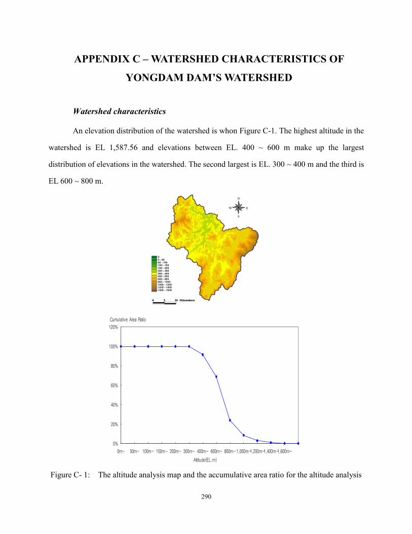
290

APPENDIX C – WATERSHED CHARACTERISTICS OF

YONGDAM DAM’S WATERSHED

Watershed characteristics

An elevation distribution of the watershed is whon Figure C-1. The highest altitude in the

watershed is EL 1,587.56 and elevations between EL. 400 ~ 600 m make up the largest

distribution of elevations in the watershed. The second largest is EL. 300 ~ 400 m and the third is

EL 600 ~ 800 m.

0%

20%

40%

60%

80%

100%

120%

0m~ 50m~ 100m~ 150m~ 200m~ 300m~ 400m~ 600m~ 800m~1,000m~1,200m~1,400m~1,600m~

Cumulative Area Ratio

Altitude(EL.m)

Figure C- 1: The altitude analysis map and the accumulative area ratio for the altitude analysis

291

Topography Characteristics

Yongdam Dam has changed the ecosystem of the Geum River because the water

ecosystem is impacted by the changes in flow. Dam construction has affected geological

characteristics, river length, water depth, surface water, and hydraulic retention time. In

particular, due to its deep depth, the reservoir is stratified and does not mix smoothly. The

Yongdam reservoir is 38.5 km in length, 1.2 km in the width, and 70 m at its deepest point.

Stratification in the reservoir is a serious problem in the summer season and the average

hydraulic retention time (t=V/Q) is 318 days. Five tributaries impact flow velocity of the

reservoir, and it has complex geology.

Figure C-2: A Watershed divisional map of Yongdam watershed

Table C-1 The inflow tributaries of Yongdam’s reservoir

River Watershed area (km2) River length (km) Slope (%)

Keumgang 1 116.3 12.5 1.416

Keumgang 2 82.53 16.1 1.773

Keumgang 3 84.3 10.0 0.153

Juja-Cheon 126.4 16.4 1.714

Jeongja-Cheon 142.8 14.9 0.584

Jinan-Cheon 89.0 7.9 1.506

Guyang-Cheon 172.1 26.6 2.360

Jang-gyae-Cheon 114.2 8.5 2.270

292

Hydrology

The data describing Yongdam watershed’s hydrology were collected from January 2005

to October 2007 as shown in Figure C-3 and Tables C-2 ~ C-4. In 2005, yearly rainfall was

1,474.8 mm. Annual average rainfall, excluding days without rainfall, was 9.0 mm and

precipitation ranged from 0.1 to 186.0 mm. The maximum daily runoff was 180 mm in July. In

addition, July was the largest rainfall month (519.9 mm) in 2005. There is a close relationship

between inflow/outflow and rainfall patterns. The inflow range and average value were 0.1 ~

1,979.8 m3/s and 28.4 m

3/s, respectively and the outflow was 11.9 ~ 705.6 m

3/s and 29.9 m

3/s.

The average water level of the reservoir was 250.9 m and the range was 241.2 ~ 261.7 m. The

largest month of water level difference was in July.

In 2006, the total annual rainfall was 1,378.2 mm. Annual average rainfall, excluding

days without rainfall, was 9.6 mm and the range was 0.1 ~ 85.0 mm. The 2006 results of

inflow/outflow and rainfall patterns had a close relationship as well. The inflow range and

average value were 0.1 ~ 671.3 m3/s and 24.1 m

3/s, respectively and the outflow was 9.1 ~ 509.5

m3/s and 19.8 m

3/s. The average water level of the reservoir was 250.0m and the range was 241.2

~ 261.7 m. The largest month of water level difference was in July, which was the same as in

2005.

In 2007, the data was collected until October. It was an abundant year for water quantity

because it rained continuously for a long period from June to August. The total rainfall was

1485.8 mm. Annual average rainfall and rainfall range, excluding days without rainfall, were

11.3 mm and 0.1~126.5mm, respectively.

293

Figure C-3: Hydrology graph of Yongdam reservoir (2005 ~2007)

Table C-2: Hydrology of Yongdam’s reservoir in 2005 (average ± standard deviation and

maximum/minimum)

Factors\Season Total Pre-Monsoon

(January-June)

Post-Monsoon

(July-December)

Total rainfall (mm) 1,474.8 418.1 1,056.7

Average rainfall (mm) 9.0±22.9

(186.0/0.1)

6.2±10.6

(46.9/0.1)

10.9±28.4

(186.0/0.1)

Total inflow (m3/s) 9,412.2 1,267.0 8,145.2

Average influent water (m3/s)

28.4±134.4

(1979.8/0.1)

7.1±10.4

(62.7/0.1)

53.6±195.3

(1,979.8/0.3)

Total outflow (m3/s) 10,903.3 4,313.6 6,589.7

Average effluent water (m3/s)

29.9±60.5

(705.6/11.9)

23.8±4.5

(27.8/11.9)

35.8±84.8

(705.6/12.6)

Water level (EL. m) 250.9±4.6

(261.7/241.2)

247.8±3.7

(254.6/241.2)

253.9±3.2

(261.7/242.2)

294


maximum/minimum)


(January-June)

Post-Monsoon

(July-December)

Total rainfall (mm) 1,378.2 417.5 960.7


(85.0/0.1)

6.7±10.2

(49.4/0.1)

11.7±18.4

(85.0/0.1)

Total inflow (m3/s) 8,013.4 1,451.9 6,561.5


24.1±75.0

(671.3/0.1)

8.4±10.3

(67.0/0.1)

41.0±15.2

(671.3/0.1)

Total outflow (m3/s) 7,237.9 2,985.6 4,252.4


19.8±30.6

(509.5/9.1)

16.5±4.9

(25.3/10.4)

23.1±42.7

(509.5/9.1)


(260.0/241.4)

245.5±1.9

(248.9/241.5)

254.3±3.7

(260.0/241.4)


maximum/minimum)


(January-June)

Post-Monsoon

(July-December)

Total rainfall (mm) 1,485.5 479.8 1,005.7


(126.5/0.1)

8.1±10.1

(38.4/0.1)

14.0±22.5

(126.5/0.1)

Total inflow (m3/s) 8,779.1 1,655.3 7,123.8


29.8±69.9

(640.6/0.2)

9.6±15.1

(120.7/0.2)

57.9±100.4

(640.6/2.9)

Total outflow (m3/s) 6,087.6 3,453.8 2,633.8


20.0±7.1

(89.6/10.7)

19.1±4.9

(26.0/14.1)

21.4±9.2

(89.6/10.7)


(261.7/243.7)

248.7±2.2

(251.8/243.7)

253.6±6.6

(261.7/244.4)

295

River Characteristics

Stream order has been used to measure the relative size of streams. Strahler’s (1952)

stream order system is a simple method of classifying stream segments based on the number of

tributaries upstream. A stream with no headwater stream is a first order stream. A second order

stream is the segment downstream of the confluence of two first order streams. Therefore a nth

order stream is located downstream of the confluence of two (n-1)th

order stream. Based on

Strahler’s stream order system, Yongdam watershed’s stream order was drawn in Figure C-4.

Figure C-4: The stream order map of Yongdam watershed

296

The basin length of the river channel and the length of river channel are 63.00 km and

62.58 km, respectively. The total length of river channel is 2,130.50 km. The characteristics of

river are shown in Table C-5.

Table C-5: The river characteristics of Yongdam watershed

River Characteristics The basin length (㎞) The length of river channel

(km) Total river channel(㎞)

Yong dam 63.00 62.58 2,130.50

Jang gye junction 21.28 20.86 390.22

Jang gye 16.06 15.62 445.96

Gu ryang 35.07 34.53 289.13

Jin ahn junction - - 138.36

Jin ahn 20.44 20.14 291.99

Jeong ja 30.92 30.07 227.24

Ju ja 20.84 20.52 195.61

Yong dam - - 151.99

According to the stream order analysis of Yongdam watershed, the maximum stream

order is 7th

which has shown in Table C-6 and Figure C-5. In general, first to third order streams

are usually called headwater streams. Medium streams range from fourth to sixth order. Streams

over the seventh order are termed rivers (http://www.cotf.edu/ete/modules/

waterq3/WQassess4b.html.). Therefore, Yongdam watershed is composed of headwater streams,

medium streams, and a river.

http://www.cotf.edu/ete/modules/%20waterq3/WQassess4b.html

http://www.cotf.edu/ete/modules/%20waterq3/WQassess4b.html

297

Table C-6: The stream orders of Yongdam watershed

Watershed division Stream order

Total 1

st 2

nd 3

rd 4

th 5

th 6

th 7

th 8

th 9

th

Yong dam 2,746 742 183 41 10 3 1 - - 3,726

Jang gye junction 649 176 43 11 2 2 1 - - 884

Jang gye 688 194 53 8 3 1 - - - 947

Gu ryang 198 50 11 4 1 - - - - 264

Jin ahn junction 90 25 6 1 1 1 1 - - 125

Jin ahn 545 143 36 9 2 1 - - - 736

Jeong ja 237 60 14 3 1 - - - - 315

Ju ja 181 48 11 3 1 - - - - 244

Yong dam 158 46 9 2 2 - 1 - - 218

Figure C-5: The stream number of each stream order

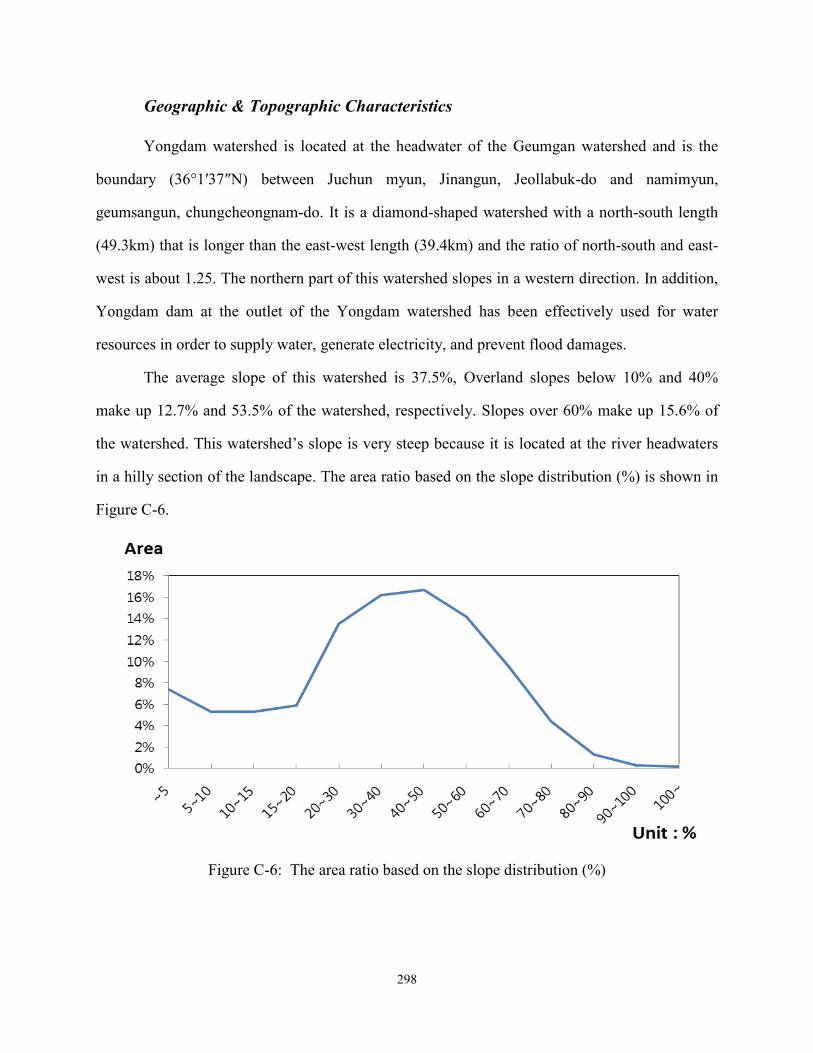
298

Geographic & Topographic Characteristics

Yongdam watershed is located at the headwater of the Geumgan watershed and is the

boundary (36°1′37″N) between Juchun myun, Jinangun, Jeollabuk-do and namimyun,

geumsangun, chungcheongnam-do. It is a diamond-shaped watershed with a north-south length

(49.3km) that is longer than the east-west length (39.4km) and the ratio of north-south and east-

west is about 1.25. The northern part of this watershed slopes in a western direction. In addition,

Yongdam dam at the outlet of the Yongdam watershed has been effectively used for water

resources in order to supply water, generate electricity, and prevent flood damages.

The average slope of this watershed is 37.5%, Overland slopes below 10% and 40%

make up 12.7% and 53.5% of the watershed, respectively. Slopes over 60% make up 15.6% of

the watershed. This watershed’s slope is very steep because it is located at the river headwaters

in a hilly section of the landscape. The area ratio based on the slope distribution (%) is shown in

Figure C-6.

Figure C-6: The area ratio based on the slope distribution (%)

299

The slope map of Yongdam watershed is shown in Figure C-7.

Figure C-7: The slope map of Yongdam watershed

The area ratio of slope direction distribution is shown in Figure C-8.

Figure C-8: The area ratio of slope direction distribution

300

APPENDIX D – WATERSHED CHARACTERISTICS OF

NAKDONG RIVER WATERSHED

General Condition of River

There are a total of 803 rivers located in the Nakdong River watershed. The main River is

shown in Table D-1. National River and Local River are thirteen and ten, respectively.

Table D-1: The river status of Nakdong watershed

Number Name of river/stream

River Systems

River grade Watershed area

(㎢)

Length of

River (㎞) Mainstream First tributary Second

tributary

1 Nakdong river Nakdong river

Nation 23,384.21 510.36

2 Nakdong river Nakdong river

Local 1,159.90 109.66

3 Banbyun stream Nakdong river Banbyun stream

Local 1,973.11 109.40

4 Naesung stream Nakdong river Naesung stream

Nation 1,814.71 108.20

5 Naesung stream Nakdong river Naesung stream

Local 1,159.01 80.29

6 Byungsung stream Nakdong river Byungsung stream

Local 434.06 32.30

7 Wee stream Nakdong river Wee stream

Local 1,403.06 113.50

8 Gam stream Nakdong river Gam stream

Nation 1,004.06 69.00

9 Geumho river Nakdong river Geumho river

Nation 2,107.87 116.00

10 Shin stream Nakdong river Geumho river Shin stream Local 179.97 28.30

11 Hwe stream Nakdong river Hwe stream

Local 781.42 78.00

12 Hwang river Nakdong river Hwang river

Nation 1,329.80 111.00

13 Guechangwee stream Nakdong river Hwang river Guechangwee

stream Local 239.41 32.89

14 Nam river Nakdong river Nam river

Nation 3,467.52 185.60

15 Nam river Nakdong river Nam river

Local 500.47 40.20

16 Hamyangwee stream Nakdong river Nam river Hamyangwee

stream Local 178.88 26.93

17 Deokchun river Nakdong river Nam river Deokchun river Nation 445.14 46.72

18 Haman stream Nakdong river Nam river Haman stream Nation 155.53 22.00

19 Milyang river Nakdong river Milyang river

Nation 1,421.26 101.50

20 Yangsna stream Nakdong river Yangsna stream

Nation 243.22 32.30

21 West Nakdong river West Nakdong river

Nation 285.08 26.40

22 Pyunggang stream West Nakdong river Pyunggang stream

Nation 34.61 15.40

23 Maekdo river West Nakdong river Pyunggang stream Maekdo river Nation 6.21 11.60

301

Figure D-1: Nakdong River Watershed

The Status of Main Dam

Tha Nakdong watershed contains five Multipurpose dams−Andong Dam, Imha Dam,

Hapchun Dam, Milyang Dam−ten domestic & industry Dams, one hydroelectric Dam, and five

302

thousands seven hundreds seventy one agriculture dams. The Monthly hydrology data of the

main dams is shown at Table D-2.

Table D-2: Monthly hydrology data for Nakdong river watershed (as of 2010)

Division Jan Feb Mar Apr May Jun Jul Aug Sep Oct Nov Dec Tot/

Avg

An

Dong

Dam

Avg. rainfall (㎜)1) 32.1 70.8 80.3 60.7 128.2 33.8 89.9 254.9 254.5 31.1 6.2 17.3 1,059.

8

Storage rate (%)2) 37.1 34.8 37.3 36.5 33.9 31.8 25.3 26.9 43.4 52.1 50.3 48.0 38.1

Inflow (㎥/s)2) 3.1 17.4 34.2 24.4 42.2 9.3 9.6 47.5 110.9 10.9 3.6 2.9 26.3

Outflow (㎥/s)2) 16.9 18.0 22.8 41.3 37.4 46.2 28.2 12.1 12.5 13.9 13.9 15.2 23.2

Im

Ha

Dam

Avg. rainfall (㎜) 19.4 59.9 50.7 43.6 108.0 26.4 120.1 257.3 153.6 27.4 8.1 17.9 892.4

Storage rate (%) 41.7 39.2 42.2 36.7 31.2 28.0 25.1 35.9 52.1 54.3 49.8 45.5 40.1

Inflow (㎥/s) 1.5 12.6 19.0 14.2 24.1 3.3 8.9 50.5 34.6 3.7 1.2 1.3 14.6

Outflow (㎥/s)2) 8.5 9.9 21.4 31.7 22.4 23.7 5.7 5.3 12.0 12.4 11.4 10.3 14.6

Hap

Chun

Dam

Avg. rainfall (㎜) 21.9 90.5 68.0 90.0 113.1 22.8 294.7 544.4 246.7 57.0 9.1 30.8 1,589.

0

Storage rate (%) 34.0 31.9 31.6 29.4 28.2 24.3 27.3 53.8 83.6 84.0 79.7 74.4 48.5

Inflow (㎥/s) 2.1 7.9 10.0 10.0 15.5 3.2 40.3 125.7 83.3 10.0 4.8 4.0 26.4

Outflow (㎥/s)2) 8.8 11.2 14.5 15.6 17.0 22.3 7.3 10.8 42.6 20.0 19.6 21.5 17.6

Nam

Gang

Dam

Avg. rainfall (㎜) 27.7 129.1 96.0 141.6 141.5 36.6 427.4 545.3 316.2 65.5 9.4 25.0 1,961.

3

Storage rate (%) 31.8 37.6 57.7 48.7 51.5 36.7 40.7 45.4 55.5 57.1 52.6 48.9 47.0

Inflow (㎥/s) 7.5 42.1 46.0 77.9 72.7 12.6 242.1 423.5 310.0 26.0 12.6 11.3 107.0

Outflow (㎥/s)2) 8.0 11.8 55.8 55.5 76.7 45.7 220.9 433.2 282.3 33.7 16.7 16.2 104.7

Mil

Yang

Dam

Avg. rainfall (㎜) 41.7 105.0 72.9 102.9 159.3 40.2 289.4 321.3 190.5 42.6 14.4 22.3 1,402.

5

Storage rate (%) 52.5 50.4 56.0 53.2 54.0 47.7 50.3 70.0 81.7 78.8 73.3 68.3 61.4

Inflow (㎥/s) 0.2 2.2 2.6 2.8 4.1 0.5 5.5 7.9 4.5 0.4 0.2 0.2 2.6

Outflow (㎥/s)2) 1.3 1.2 2.5 3.0 3.4 4.3 1.7 2.5 2.9 1.9 1.7 1.5 2.3

Young

Chun

Dam

Avg. rainfall (㎜) 15.7 78.3 71.6 63.8 131.0 30.8 198.4 290.6 175.2 34.6 4.5 22.9 1,117.

4

Storage rate (%) 26.8 26.9 32.7 36.2 37.1 36.8 32.0 44.0 56.3 50.6 42.3 37.9 38.3

Inflow (㎥/s) 4.8 6.0 7.3 7.3 9.7 3.6 5.2 14.9 7.3 3.3 5.2 5.2 6.7

Outflow (㎥/s)2) 5.0 4.6 5.5 6.5 7.5 7.6 5.0 7.1 6.0 7.7 7.2 6.9 6.4

1) Average rainfall: the sum of the Month rainfall based on daily rainfall within Dam watershed.

2) Storage, Inflow, Outflow: daily average data.

303

The Status of Weather

Six weather stations were used in this study. Characteristics of these weather stations are

shown in Table D-3. The weather data, average temperature, rainfall, evaporation, rainfall

duration, average wind, average humidity, dew point temperature, vapor pressure, amount of

clouds, and insolation were displayed in Table D-4.

Table D-3: The weather station of Nakdong river watershed Weather

station watershed Agency Location TM_X TM_Y

Andong Andong &

Imha Dam

Korea

Metrorological

Administrative

Gyeongsangbuk-do

Guchang Hapchun Dam Gyeongsangnam-do Jeongjang-ri, Geochang-eup, Geochang-gun 341975.4556 282184.6521

Hapchun Hapchun

Dam Gyeongsangnam-do Hapcheon-ri, Hapcheon-eup 330449.3885 305802.4144

Milyang Milyang

Dam Gyeongsangnam-do Naei-dong, Miryang-si 323055.5046 357987.8181

Youngchun Youngchun

Dam Gyeongsangbuk-do Mangjeong-dong, Yeongcheon-si 377317.0166 375725.2739

Jinju Namgang

Dam Gyeongsangnam-do Pyeonggeo-dong, Jinju-si 285822.7331 294501.2589

Table D-4: The weather data of Nakdong river watershed

Weather

Station Yr.

Avg. Temp

(℃)

Rainfall*

(0.1㎜)

Evapo-

ration

(0.1㎜)

Rainfall

duration

(0.01 hr)

Avg. wind

(0.1m/s)

Max Wind

direction

Avg. humidity

(0.1%)

Dew point temp.

℃)

Vapor pressure

(0.1hpa)

Local pressure

(0.1hpa)

Amount of cloud

(%)

insolation

(0.01MJ/m²)

Duriation of sunshine

(0.1hr)

Gu

chang

2010 11.8 1,549.0 - - 15 - 699 - - - 520 - 19,601

2009 12.0 975.3 - 65,960 15 N 660 46 109 9,893 500 - 21,035

2008 12.1 615.7 - 4,402 15 NW 660 49 113 9,899 - - 21,023

2007 13.1 1,729.0 - - 13 S 680 66 123 9,895 - - 19,559

2006 12.6 1,411.4 - - 13 S 690 61 121 9,897 - - 20,963

2005 12.2 1,244.9 - - 14 W 660 51 119 9,895 - - 22,832

2004 12.3 1,547.8 - - 13 W 680 56 118 9,899 - - 23,082

Avg./Sum1) 12.3 9,073.1 - 35,181 14 - 676 55 117 9,896 510 - 21,156

304

Table D-4: The weather data of Nakdong river watershed (Continued)

Weather

Station Yr.

Avg.

Temp

(℃)

Rainfall*

(0.1㎜)

Evapo- ration

(0.1㎜)

Rainfall duration

(0.01

hr)

Avg.

wind (0.1m/s)

Max

Wind direction

Avg.

humidity (0.1%)

Dew point

temp.

℃)

Vapor

pressure (0.1hpa)

Local

pressure (0.1hpa)

Amount of

cloud (%)

insolation

(0.01MJ/m²)

Duriation of

sunshine (0.1hr)

Mil

yang

2010 13.7 1,252.0 - - 17 - 641 - - - - - 20,748

2009 14.5 1,130.8 - - 16 S 620 60 120 10,141 - - 21,639

2008 13.6 807.5 - - 14 SSW 640 57 117 10,147 - - 21,756

2007 13.7 1,061.0 - - 14 N 630 59 118 10,143 - - 18,873

2006 13.1 1,324.5 - - 13 S 630 54 114 10,145 - - 19,563

2005 13.2 971.5 - - 13 WNW 610 47 115 10,144 - - 22,165

2004 14.4 1,377.4 - - 14 WNW 630 64 124 10,148 - - 23,495

Avg./Sum 13.7 7,924.7 - - 14 - 629 57 118 10,145 - - 21,177

Young

chun

2010 12.5 1,030.0 - - 19 - 645 - - - - - 20,307

2009 12.7 866.6 - 980 20 WNW 620 45 107 10,042 - - 21,179

2008 12.7 774.3 - - 20 WNW 650 54 115 10,048 - - 21,683

2007 13.1 1,142.1 - - 16 WNW 690 67 125 10,056 - - 21,684

2006 12.7 1,363.0 - - 17 NNE 680 63 121 10,058 - - 22,436

2005 12.5 772.8 - - 18 WNW 600 44 111 10,056 - - 24,553

2004 13.2 1,116.9 - - 17 N 620 53 112 10,059 - - 24,018

Avg./Sum 12.8 7,065.7 - 980 18 - 644 54 115 10,053 - - 22,266

Jinju

2010 13.2 1,896.0 - - 12 - 675 - - - 490 - 21,095

2009 13.8 1,608.9 11,091 66,158 13 WSW 650 62 118 10,120 470 540,589 21,860

2008 14.0 885.6 11,685 60,938 12 WSW 660 68 125 10,126 480 472,019 22,318

2007 14.0 1,701.0 11,040 87,985 12 W 700 79 134 10,122 490 546,936 21,617

2006 13.6 1,674.0 11,013 92,342 13 WSW 680 72 130 10,124 490 518,964 21,607

2005 13.3 1,113.7 10,649 62,256 16 NNE 650 60 128 10,132 450 523,641 23,628

2004 14.0 1,575.0 10,884 70,563 16 NNW 660 69 129 10,136 430 519,542 23,699

Avg./Sum 13.7 10,454.2 11,060 73,374 13 - 668 68 127 10,127 471 520,282 22,261

Hap

chun

2010 13.3 1,547.0 - - 14 - 672 - - - - - 20,325

2009 13.6 1,066.0 - - 14 S 640 58 116 10,117 - - 21,416

2008 13.2 767.0 - - 14 N 670 62 121 10,123 - - 21,876

2007 14.3 1,232.6 - - 12 NE 700 79 133 10,119 - - 20,073

2006 13.8 1,306.6 - - 12 NNE 680 73 127 10,122 - - 20,043

2005 13.5 1,119.6 - - 12 NNE 650 62 124 10,120 - - 22,582

2004 14.0 1,477.4 - - 11 NNE 680 73 127 10,127 - - 22,845

Avg./Sum 13.7 8,516.2 - - 13 - 670 68 125 10,121 - - 21,309

1) Sum is the rainfall data

Development of a watershed modling selection program and ...

Documents

Transcript of Development of a watershed modling selection program and ...