Purdue UniversityPurdue e-PubsDepartment of Earth, Atmospheric, and PlanetarySciences Faculty Publications

Department of Earth, Atmospheric, and PlanetarySciences

2011

Selection and placement of best managementpractices used to reduce water quality degradationin Lincoln Lake watershedHector German RodriguezUniversity of Arkansas

Jennie PoppUniversity of Arkansas

Chetan MaringantiPurdue University

Indrajeet ChaubeyPurdue University

Follow this and additional works at: http://docs.lib.purdue.edu/easpubs

This document has been made available through Purdue e-Pubs, a service of the Purdue University Libraries. Please contact epubs@purdue.edu foradditional information.

Repository CitationRodriguez, Hector German; Popp, Jennie; Maringanti, Chetan; and Chaubey, Indrajeet, "Selection and placement of best managementpractices used to reduce water quality degradation in Lincoln Lake watershed" (2011). Department of Earth, Atmospheric, and PlanetarySciences Faculty Publications. Paper 141.http://dx.doi.org/10.1029/2009WR008549

Selection and placement of best management practices used to reducewater quality degradation in Lincoln Lake watershed

Hector German Rodriguez,1 Jennie Popp,1 Chetan Maringanti,2 and Indrajeet Chaubey2

Received 21 August 2009; revised 27 September 2010; accepted 3 November 2010; published 20 January 2011.

[1] An increased loss of agricultural nutrients is a growing concern for water quality inArkansas. Several studies have shown that best management practices (BMPs) are effectivein controlling water pollution. However, those affected with water quality issues needwater management plans that take into consideration BMPs selection, placement, andaffordability. This study used a nondominated sorting genetic algorithm (NSGA-II). Thismultiobjective algorithm selects and locates BMPs that minimize nutrients pollution cost-effectively by providing trade-off curves (optimal fronts) between pollutant reduction andtotal net cost increase. The usefulness of this optimization framework was evaluated in theLincoln Lake watershed. The final NSGA-II optimization model generated a number ofnear-optimal solutions by selecting from 35 BMPs (combinations of pasture management,buffer zones, and poultry litter application practices). Selection and placement of BMPswere analyzed under various cost solutions. The NSGA-II provides multiple solutions thatcould fit the water management plan for the watershed. For instance, by implementing allthe BMP combinations recommended in the lowest-cost solution, total phosphorous (TP)could be reduced by at least 76% while increasing cost by less than 2% in the entirewatershed. This value represents an increase in cost of $5.49 ha�1 when compared to thebaseline. Implementing all the BMP combinations proposed with the medium- and thehighest-cost solutions could decrease TP drastically but will increase cost by $24,282 (7%)and $82,306 (25%), respectively.

Citation: Rodriguez, H. G., J. Popp, C. Maringanti, and I. Chaubey (2011), Selection and placement of best management practices

used to reduce water quality degradation in Lincoln Lake watershed, Water Resour. Res., 47, W01507, doi:10.1029/2009WR008549.

1. Introduction[2] Arkansas is a state rich in water resources. These

water resources have been fundamental for the develop-ment of the manufacturing, recreation, navigation, con-struction, and agriculture sectors. Among these waters isthe Illinois River, which flows from northwest Arkansasinto northeast Oklahoma and back to Arkansas again. TheArkansas side of the Illinois River watershed covers areasof both Washington and Benton counties. These countieshave experienced a 27% population growth between 2000and 2008 (Benton and Washington counties data are avail-able at http://www.census.gov/), as well as road, industrial,commercial, and residential infrastructure development tosupport this growth. Agriculture, and in particular cattleand poultry activities, maintains a strong presence in thesecounties. Benton and Washington counties produced almost200 thousand head of cattle and calves and almost 41 mil-lion broilers and other meat-type chickens a year (Bentonand Washington counties data are available at http://

www.agcensus.usda.gov/Publications/2007/index.asp). Thepoultry industry alone generated over 40,000 jobs, $1.29billion in income, and $1.69 billion in value added to theregion in 2008 [Popp et al., 2010].

[3] The Illinois River watershed is currently on the303(d) Impaired Water List because of excessive in-streamphosphorous (P) concentrations [Arkansas Department ofEnvironmental Quality, 2008] sourced on the Arkansas sideof the watershed, which eventually flows into Oklahoma(section 303(d) of the U.S. Clean Water Act (CWA) estab-lishes that states are to list (the 303(d) list) waters for whichtechnology-based limits alone do not ensure attainment ofapplicable water quality standards). This has triggered aninterstate water quality dispute between Oklahoma andArkansas regarding the role that animal agriculture, particu-larly poultry, contributes to the existence of excess P con-centrations. Animal waste is linked to some environmentalproblems, especially high P concentrations in the watershedwater [Sharpley et al., 2007]. Other nutrient sources, suchas from wastewater treatment plants, industry, and construc-tion, are acknowledged [Haggard and Soerens, 2006; Poppet al., 2007] as contributors as well, but most attentionremains focused on animal agriculture. More informationregarding the lawsuit is given by Haggard and Soerens[2006] and Sharpley et al. [2007].

[4] While there is a need to reduce excess P from allpotential sources, this paper focuses on addressing P runoff

1Department of Agricultural Economics and Agribusiness, University ofArkansas, Arkansas, USA.

2Department of Agricultural and Biological Engineering, Purdue Uni-versity, West Lafayette, Indiana, USA.

Copyright 2011 by the American Geophysical Union.0043-1397/11/2009WR008549

W01507 1 of 13

WATER RESOURCES RESEARCH, VOL. 47, W01507, doi:10.1029/2009WR008549, 2011

from cattle and poultry operations in the watershed.Although several studies have analyzed P concentration inthe watershed [e.g., Haggard et al., 2003; Haggard andSoerens, 2006; Massey et al., 2009], none have analyzedthe combined effect that pastureland, buffer zone, and poul-try litter management could have as a P or nitrogen (N) con-centration reduction strategy. Therefore, the purpose of thisstudy is to estimate the water quality benefit and cost trade-offs associated with different watershed management strat-egies to optimize best management practice (BMP) imple-mentation and water quality improvement at the watershedlevel. Specifically, the objective of this study is to apply agenetic algorithm (GA) to find near-optimal sets of BMPsthat minimize total P (TP) or total N (TN) concentrationand total cost (TC) increases simultaneously in the LincolnLake watershed (described in section 1.1) on the Arkansasside of the Illinois River watershed. A watershed manage-ment expert can use the results of this analysis to make hisleast cost decision by determining which set of BMP com-binations could reduce nutrients to a specific target level.

[5] It is hypothesized that TP (or TN) concentration atthe watershed outlet could be reduced without considerableincrease in TC, as compared with current concentrationsand costs, by optimizing selection and placement of sets ofBMP combinations across the watershed. This study used anondominated sorting GA (NSGA-II) to evaluate the opti-mal fitness of each BMP combination on the basis of sub-field pollutant loads estimated with the Soil and WaterAssessment Tool (SWAT) [Arnold and Fohrer, 2005;Gassman et al., 2007], percent reductions of BMPs esti-mated by comparing to those concentrations generatedunder current management practices, and BMP costs.

1.1. Lincoln Lake Watershed

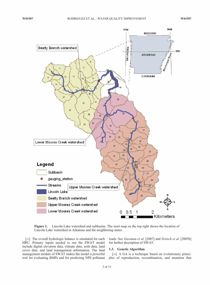
[6] This study was conducted in the Lincoln Lake water-shed (35�5802900N, 94�250500W), a subbasin within the Illi-nois River watershed. The Lincoln Lake watershed is asmall agricultural watershed with a total contributing areaof 32 km2. Moores Creek and Beatty Branch are two majortributaries that flow into Lincoln Lake (Figure 1). MooresCreek and Beatty Branch drain 21 and 11 km2, respectively[Gitau et al., 2010].

[7] The Lincoln Lake watershed has an average 6% ofslope, with the elevation approximately ranging from 365to 487 m. The major soil series in the watershed are Endersgravelly loam, Hector-Mountainburg gravelly fine sandyloam, and Captina silt loam and Linker loam. These soilseries account for 23%, 21%, and 13% of the entire area,respectively. An average annual precipitation (1230.5 mm)was observed during 1990 – 2002, with the lowest averageprecipitation (74 mm) in January and the highest averageprecipitation (158.3 mm) in April. The average minimumand maximum temperatures during 1990 –2002 were 8.7�Cand 20.1�C, respectively.

[8] The watershed has mixed land use, with agricultural,forest, urban residential, urban commercial, and water rep-resenting 36%, 48%, 12%, 2%, and 2% of the watershedarea, respectively. Pasturelands (Bermuda grass fields)used for haying and/or grazing are the primary agriculturalland use in the watershed. Urbanization in the watershedhas been increasing during the last 2 decades, where urbanareas have increased from 3% in 1992 to almost 12% in

2004. Concurrently, pastureland in the watershed hasdecreased from 43% to 36% during the same time period[Gitau et al., 2010]. Animal manure, including land appli-cation of poultry litter, is the primary means of fertilizingpasture areas in the watershed.

[9] Flow and water quality data have been collected atthree different sites in the watershed since 1991. Chaubeyet al. [2010] and Gitau et al. [2010] provide a detaileddescription of the water quality data monitored in thiswatershed. Continuous streamflow was monitored using apressure transducer to measure stream depth, which wassubsequently converted to streamflow using site-specificdepth-discharge rating curves. Concentrations of sedimentand various forms of P (orthophosphate and TP) and N(nitrate, ammonia, and TN) were measured separately dur-ing base flow and stormflow conditions. An autosamplerwas used to collect flow-weighted storm samples. Simi-larly, grab samples at biweekly intervals were collected toquantify water quality during base flow conditions. Detailsof laboratory analyses are provided by Vendrell et al.[1997] and M. A. Nelson, et al., Water quality monitoringof Moores Creek above Lincoln Lake 2006 and 2007(unpublished manuscript, 2008).

[10] In 2005, the U.S. Department of Agriculture(USDA) funded a conservation effectiveness assessmentproject (CEAP) to quantify how different BMPs in thewatershed impacted water quality [Duriancik et al., 2008].This watershed was selected because the agricultural pro-duction, BMPs, and water quality issues are representativeof the political, economic, and ecological challenges facingresource managers across the region.

1.2. Description of the Soil and Water AssessmentTool Model

[11] Hydrological models are powerful tools for assess-ing nonpoint sources (NPS) of pollution and evaluatingeffectiveness of BMPs on large watersheds [Srivastavaet al., 2007; Borah et al., 2006]. In this study, the SWATmodel was used to quantify the impacts of BMP options onP and N transport. SWAT is a watershed-scale modelwidely used for quantifying the impact of land managementpractices. It helps to identify sources and causes of waterimpairment as well as to plan management strategies tocontrol NPS of pollution in complex watersheds [Arnoldand Fohrer, 2005; Neitsch et al., 2005a]. The SWATmodel was selected because it is one of the most commonlyused models to evaluate the implementation impacts of var-ious BMPs on watershed response in the USDA CEAPstudies [Duriancik et al., 2008]. In addition, more than 650peer-reviewed journal articles have been published demon-strating the utility of the SWAT model in evaluatingimpacts of land use, land cover, watershed management,and climate change on watershed hydrology and pollutanttransport [Gassman et al., 2007].

[12] SWAT has eight main components: hydrology,weather, sedimentation, soil temperature, crop growth,nutrients, pesticides, and agricultural management. It simu-lates these processes by dividing watersheds into subbasins(see Figure 1). Subbasins are also divided into hydrologicresponse units (HRUs), which are areas of land that haveunique characteristics such as land use, soil, or land man-agement practices.

W01507 RODRIGUEZ ET AL.: WATER QUALITY IMPROVEMENT W01507

2 of 13

[13] The overall hydrologic balance is simulated for eachHRU. Primary inputs needed to run the SWAT modelinclude digital elevation data, climate data, soils data, landcover data, and land management information. The landmanagement module of SWAT makes the model a powerfultool for evaluating BMPs and for predicting NPS pollutant

loads. See Gassman et al. [2007] and Neitsch et al. [2005b]for further description of SWAT.

1.3. Genetic Algorithm

[14] A GA is a technique based on evolutionary princi-ples of reproduction, recombination, and mutation that

Figure 1. Lincoln Lake watershed and subbasins. The inset map on the top right shows the location ofLincoln Lake watershed in Arkansas and the neighboring states.

W01507 RODRIGUEZ ET AL.: WATER QUALITY IMPROVEMENT W01507

3 of 13

seeks optimal solutions to solve a search problem [Gold-berg, 1989; Holland, 1975]. It models individuals of a pop-ulation as chromosomes (solutions) with genes on thechromosome encoding a specific trait of an individual. Al-leles are the possible settings for a trait. Fitness of eachchromosome is evaluated with objective functions that usethe genetic information as the variables. More fit chromo-somes are the most likely ones to survive into the next gen-eration (iteration).

[15] This process occurs in generations starting with arandom set of solutions. The fitness (i.e., the value of theobjective function) of each individual in the population isevaluated; multiple individuals are randomly reproducedon the basis of their fitness and then randomly recombinedand randomly mutated to form a new population [Koza,1992]. This occurs in each generation (iteration). The newpopulation is then used in the next iteration of the algo-rithm. The algorithm stops either when an adequate fitnesslevel has been achieved for the population or when a maxi-mum number of generations have been produced [Koza,1992].

[16] Genetic algorithms have been applied to compli-cated optimization problems because of their capacity tohandle complex and irregular solution spaces when search-ing for a global optimum [Chambers, 2001]. The searchspace includes all feasible solutions and their associated fit-ness, which is based on the objective function value. Theliterature is rich in examples of the use of GAs to find com-binations of BMPs to reduce sediment runoff, nutrient run-off, or both at the watershed level. Several studies [Arabiet al., 2006; Gitau et al., 2006; Veith et al., 2004] linked atleast three components (a NPS pollution reduction model,an economic component, and an optimization model (GA))in a single objective function to find optimal solutions towater quality problems for several watersheds across theUnited States. This kind of optimization is functional.However, some of the studies concluded that a singleobjective function is not always the best alternative andthat a more sophisticated and robust objective functionshould maximize pollutant reduction and minimize costssimultaneously.

[17] In contrast, other studies [Bekele and Nicklow,2005; Maringanti et al., 2009; Muleta and Nicklow, 2005]used multiobjective functions with conflicting objectives.As a result, these studies did not find a single optimal solu-tion; rather, they provided trade-off curves between differ-ent objectives and alternative solutions. Agricultural waterquality degradation is a multiobjective problem; therefore,this second approach seems to be more accurate becausetrade-offs between benefits and costs provide decision mak-ers with more flexibility when selecting solutions.

1.4. Multiobjective Optimization

[18] In this study NSGA-II was employed. This GA is afast and efficient multiobjective evolutionary algorithm thatfinds multiple near-optimal solutions (Pareto-optimal solu-tions) in a single model execution [Deb et al., 2002]. FindingPareto-optimal solutions assure that none of the solutionsdominate the other solutions. Consequently, every Pareto-optimal solution is better than the rest in at least one objec-tive function. According to Zitzler and Thiele [1999], in amultiobjective optimization problem, if gi, fi ¼ 1, . . . ,Mg,

are the objective functions that need to be minimized, a solu-tion x(1) is said to dominate x(2) if both of the following con-ditions are true:

8i 2 f1; . . . ;Mg : giðxð1ÞÞ � giðxð2ÞÞ ;

9j 2 f1; . . . ;Mg : gjðxð1ÞÞ < gjðxð2ÞÞ : ð1Þ

[19] That is, x(2) is dominated by x(1), or in other words,x(1) is nondominated by x(2). Nondominance assures thatthe solutions are spread along a smooth curve when pro-jected on a two-dimensional space. Maringanti et al.[2009] describe in more detail the nondominance propertyof a NSGA-II algorithm, and Deb [2001], Deb et al.[2002], and Maringanti et al. [2009] provide a detailedmathematical description of this algorithm.

2. Materials and Methods[20] The approach proposed in this study linked three

components as inputs into the NSGA-II multiobjective opti-mization model to evaluate the objective functions of agiven chromosome (i.e., solution). The three componentswere (1) nutrient loading (i.e., TP or TN) at the HRU levelgenerated in SWAT, (2) an allele set that provides all allow-able BMP combinations to be implemented, and (3) nutrientreduction efficiency and implementation cost for each BMPcombination. A Cþþ programming language implementa-tion of NSGA-II was used to link these various componentsto evaluate the objective functions (equations (3) and (4)).As mentioned, this process occurs in generations startingfrom a random population. Individuals in the populationreproduce, recombine, and mutate to create a new popula-tion for the next generation. The algorithm stops eitherwhen an adequate fitness level has been achieved or a maxi-mum number of generations has been reached.

2.1. Best Management Practices Characterization

[21] Agricultural BMPs suggested by a collaborative dia-logue among northwest Arkansas stakeholders [Penningtonet al., 2008; Popp et al., 2007], practices used in the devel-opment of the Arkansas P index [DeLaune et al., 2004],and previous BMP studies in the region [Chaubey et al.,1995; Srivastava et al., 1996; Moore and Edwards, 2007]served as the basis for the initial choice of BMP factors forinclusion in this analysis. The factors were grouped intothree general categories: pastureland, buffer zone, andpoultry litter management.

[22] Pastureland management contained one factor atthree levels (no grazing, optimum grazing, and overgraz-ing). Grazing operations started on 30 September of eachyear. The number of days animals grazed in any given fieldvaried for both overgrazing and optimum grazing. Theovergrazing lasted for 213 days until 30 April of each year.The animals were rotated through various HRUs for opti-mum grazing such that a minimum biomass of 200 kg ha�1

was maintained in the field.[23] Buffer zones contained one factor: buffer zone

width at three levels (0, 15, and 30 m). Buffer zones weresimulated to be placed at the edge of the pasture fields. Thebuffer widths (15 and 30 m) were based on previous studiesevaluated in the pasture areas [Chaubey et al., 1995] and

W01507 RODRIGUEZ ET AL.: WATER QUALITY IMPROVEMENT W01507

4 of 13

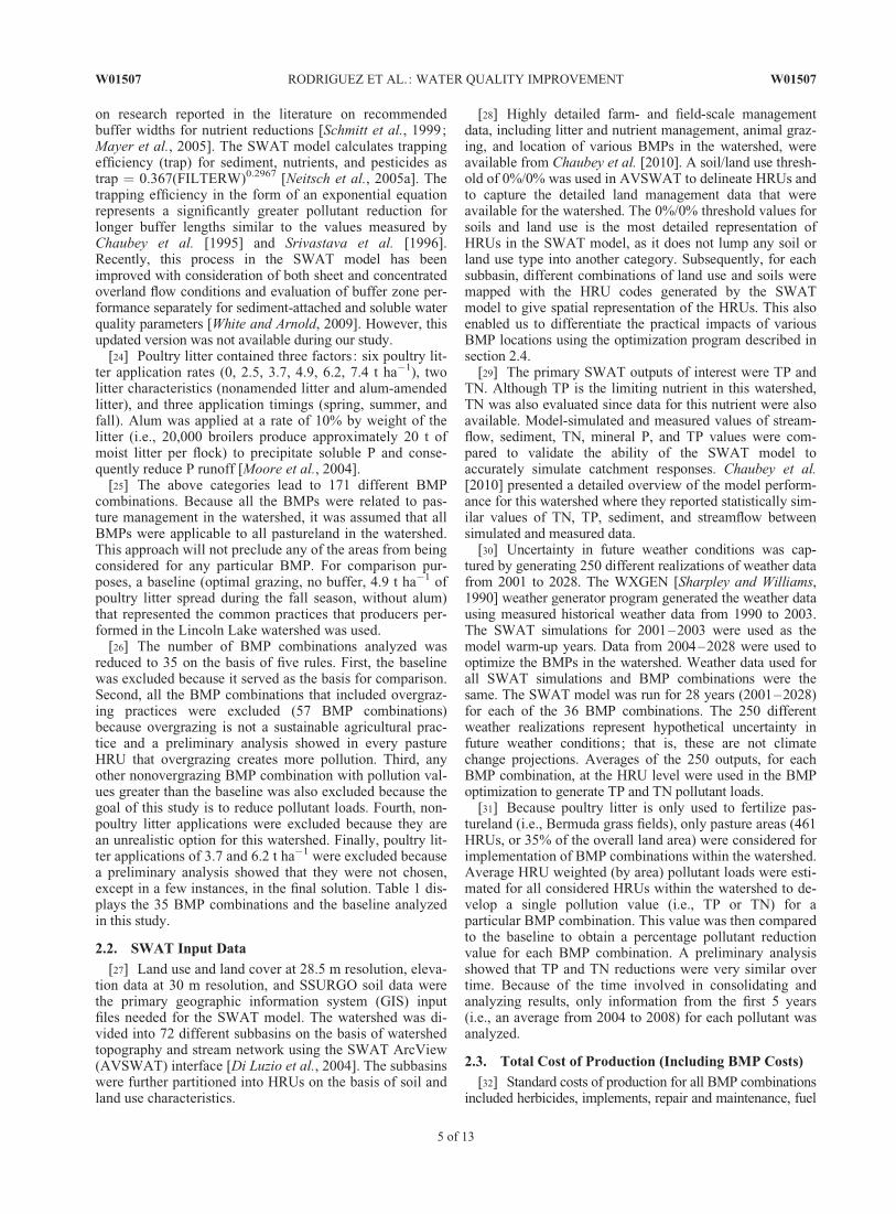
on research reported in the literature on recommendedbuffer widths for nutrient reductions [Schmitt et al., 1999;Mayer et al., 2005]. The SWAT model calculates trappingefficiency (trap) for sediment, nutrients, and pesticides astrap ¼ 0.367(FILTERW)0.2967 [Neitsch et al., 2005a]. Thetrapping efficiency in the form of an exponential equationrepresents a significantly greater pollutant reduction forlonger buffer lengths similar to the values measured byChaubey et al. [1995] and Srivastava et al. [1996].Recently, this process in the SWAT model has beenimproved with consideration of both sheet and concentratedoverland flow conditions and evaluation of buffer zone per-formance separately for sediment-attached and soluble waterquality parameters [White and Arnold, 2009]. However, thisupdated version was not available during our study.

[24] Poultry litter contained three factors: six poultry lit-ter application rates (0, 2.5, 3.7, 4.9, 6.2, 7.4 t ha�1), twolitter characteristics (nonamended litter and alum-amendedlitter), and three application timings (spring, summer, andfall). Alum was applied at a rate of 10% by weight of thelitter (i.e., 20,000 broilers produce approximately 20 t ofmoist litter per flock) to precipitate soluble P and conse-quently reduce P runoff [Moore et al., 2004].

[25] The above categories lead to 171 different BMPcombinations. Because all the BMPs were related to pas-ture management in the watershed, it was assumed that allBMPs were applicable to all pastureland in the watershed.This approach will not preclude any of the areas from beingconsidered for any particular BMP. For comparison pur-poses, a baseline (optimal grazing, no buffer, 4.9 t ha�1 ofpoultry litter spread during the fall season, without alum)that represented the common practices that producers per-formed in the Lincoln Lake watershed was used.

[26] The number of BMP combinations analyzed wasreduced to 35 on the basis of five rules. First, the baselinewas excluded because it served as the basis for comparison.Second, all the BMP combinations that included overgraz-ing practices were excluded (57 BMP combinations)because overgrazing is not a sustainable agricultural prac-tice and a preliminary analysis showed in every pastureHRU that overgrazing creates more pollution. Third, anyother nonovergrazing BMP combination with pollution val-ues greater than the baseline was also excluded because thegoal of this study is to reduce pollutant loads. Fourth, non-poultry litter applications were excluded because they arean unrealistic option for this watershed. Finally, poultry lit-ter applications of 3.7 and 6.2 t ha�1 were excluded becausea preliminary analysis showed that they were not chosen,except in a few instances, in the final solution. Table 1 dis-plays the 35 BMP combinations and the baseline analyzedin this study.

2.2. SWAT Input Data

[27] Land use and land cover at 28.5 m resolution, eleva-tion data at 30 m resolution, and SSURGO soil data werethe primary geographic information system (GIS) inputfiles needed for the SWAT model. The watershed was di-vided into 72 different subbasins on the basis of watershedtopography and stream network using the SWAT ArcView(AVSWAT) interface [Di Luzio et al., 2004]. The subbasinswere further partitioned into HRUs on the basis of soil andland use characteristics.

[28] Highly detailed farm- and field-scale managementdata, including litter and nutrient management, animal graz-ing, and location of various BMPs in the watershed, wereavailable from Chaubey et al. [2010]. A soil/land use thresh-old of 0%/0% was used in AVSWAT to delineate HRUs andto capture the detailed land management data that wereavailable for the watershed. The 0%/0% threshold values forsoils and land use is the most detailed representation ofHRUs in the SWAT model, as it does not lump any soil orland use type into another category. Subsequently, for eachsubbasin, different combinations of land use and soils weremapped with the HRU codes generated by the SWATmodel to give spatial representation of the HRUs. This alsoenabled us to differentiate the practical impacts of variousBMP locations using the optimization program described insection 2.4.

[29] The primary SWAT outputs of interest were TP andTN. Although TP is the limiting nutrient in this watershed,TN was also evaluated since data for this nutrient were alsoavailable. Model-simulated and measured values of stream-flow, sediment, TN, mineral P, and TP values were com-pared to validate the ability of the SWAT model toaccurately simulate catchment responses. Chaubey et al.[2010] presented a detailed overview of the model perform-ance for this watershed where they reported statistically sim-ilar values of TN, TP, sediment, and streamflow betweensimulated and measured data.

[30] Uncertainty in future weather conditions was cap-tured by generating 250 different realizations of weather datafrom 2001 to 2028. The WXGEN [Sharpley and Williams,1990] weather generator program generated the weather datausing measured historical weather data from 1990 to 2003.The SWAT simulations for 2001–2003 were used as themodel warm-up years. Data from 2004–2028 were used tooptimize the BMPs in the watershed. Weather data used forall SWAT simulations and BMP combinations were thesame. The SWAT model was run for 28 years (2001–2028)for each of the 36 BMP combinations. The 250 differentweather realizations represent hypothetical uncertainty infuture weather conditions; that is, these are not climatechange projections. Averages of the 250 outputs, for eachBMP combination, at the HRU level were used in the BMPoptimization to generate TP and TN pollutant loads.

[31] Because poultry litter is only used to fertilize pas-tureland (i.e., Bermuda grass fields), only pasture areas (461HRUs, or 35% of the overall land area) were considered forimplementation of BMP combinations within the watershed.Average HRU weighted (by area) pollutant loads were esti-mated for all considered HRUs within the watershed to de-velop a single pollution value (i.e., TP or TN) for aparticular BMP combination. This value was then comparedto the baseline to obtain a percentage pollutant reductionvalue for each BMP combination. A preliminary analysisshowed that TP and TN reductions were very similar overtime. Because of the time involved in consolidating andanalyzing results, only information from the first 5 years(i.e., an average from 2004 to 2008) for each pollutant wasanalyzed.

2.3. Total Cost of Production (Including BMP Costs)

[32] Standard costs of production for all BMP combinationsincluded herbicides, implements, repair and maintenance, fuel

W01507 RODRIGUEZ ET AL.: WATER QUALITY IMPROVEMENT W01507

5 of 13

diesel, interest on capital, and labor. Predetermined standardcosts of production and costs of BMPs were estimated usinginformation obtained for 2007. These were the most recentdata available at the time of the calculation. A fixed rate ofinflation was used to account for inflation effects each year.Total costs for each BMP combination were calculated withinflation from 2005 to 2028 and then annualized to 2004 (i.e.,deflated to 2004 dollars).

[33] The costs for each BMP combination were calculatedon the basis of the different practices used. Buffer zone costswere estimated following the Natural Resources Conserva-tion Service (Riparian forest buffer (Ac.) code 391, Conser-vation practice standard, in Field Office Technical GuideSection IV, available at http://efotg.sc.egov.usda.gov/references/public/AR/391.pdf). Buffer zone costs were calculatedassuming a predetermined buffer area. The area was esti-mated by multiplying the width (15 and 30 m) with a con-stant length of 30 m provided by Natural ResourcesConservation Service (Filter strip (acre) code 393, Conserva-tion practice specifications, in Field Office Technical GuideSection IV, available at http://efotg.sc.egov.usda.gov/referen-ces/public/AR/393spec.pdf). This length was chosen on thebasis of the most predominant slope (>6%) in the watershed.Costs included establishment of the buffer every 10 years

and maintaining the buffer for a period of 25 years. Practicesincluded fertilizer, warm season grass seeding, and herbicidecosts. Additionally, loss in yield due to pasture area reductionwas also added as an extra (opportunity) cost. The cost of lit-ter, including field application, was assumed to be $12 t�1.This cost was provided by H. L. Goodwin (personal commu-nication, 2008). Total costs for each BMP combination werecalculated by adding the standard costs of production and therespective costs for each BMP combination. These costs canbe expressed as follows:

TCj;k;l ¼ CPþ CBMPj;k;l; ð2Þ

where TC represents total cost of production, CP repre-sents cost of production, CBMP represents BMP cost, jis buffer, k is poultry litter, and l is alum. BMP combi-nation cost-effectiveness was estimated by calculatingthe percentage change in cost when compared to the costof the baseline. Table 1 displays TC per hectare includ-ing BMP cost associated with each BMP combination.

2.4. NSGA-II Multiobjective Optimization ModelDevelopment

[34] Pollution loading output data from SWAT and costdata were the inputs used in the NSGA-II optimization

Table 1. BMP Combinations and Associated Total Cost

BMP Set Grazing Buffer Width (m)

Poultry Litter Management

Total Costa ($ ha�1)Quantity (t ha�1) Application Time Alum

24 Optimal 0 2.47 Spring No 288.3336b Optimal 0 4.94 Fall No 314.0178 Optimal 30 2.47 Spring Yes 437.4280 Optimal 30 4.94 Spring Yes 577.2581 Optimal 30 2.47 Spring No 334.6883 Optimal 30 4.94 Spring No 371.7684 Optimal 30 2.47 Summer Yes 437.4286 Optimal 30 4.94 Summer Yes 577.2587 Optimal 30 2.47 Summer No 334.6889 Optimal 30 4.94 Summer No 371.7690 Optimal 30 4.94 Fall Yes 577.2592 Optimal 30 7.41 Fall Yes 717.0793 Optimal 30 4.94 Fall No 371.76116 No 15 2.47 Spring Yes 414.25118 No 15 4.94 Spring Yes 548.38119 No 15 2.47 Spring No 311.50121 No 15 4.94 Spring No 342.88122 No 15 2.47 Summer Yes 414.25124 No 15 4.94 Summer Yes 548.38125 No 15 2.47 Summer No 311.50127 No 15 4.94 Summer No 342.88128 No 15 4.94 Fall Yes 548.38130 No 15 7.41 Fall Yes 682.50131 No 15 4.94 Fall No 342.88133 No 15 7.41 Fall No 374.27135 Optimal 15 2.47 Spring Yes 414.25137 Optimal 15 4.94 Spring Yes 548.38138 Optimal 15 2.47 Spring No 311.50140 Optimal 15 4.94 Spring No 342.88141 Optimal 15 2.47 Summer Yes 414.25143 Optimal 15 4.94 Summer Yes 548.38144 Optimal 15 2.47 Summer No 311.50146 Optimal 15 4.94 Summer No 342.88147 Optimal 15 4.94 Fall Yes 548.38149 Optimal 15 7.41 Fall Yes 682.50150 Optimal 15 4.94 Fall No 342.88

aFive year average (2004–2008); total costs were estimated in 2004 dollars.bBaseline.

W01507 RODRIGUEZ ET AL.: WATER QUALITY IMPROVEMENT W01507

6 of 13

model. Output from SWAT provided pollutant (i.e., TP andTN) loads at the HRU level for each of the 35 BMP combi-nations analyzed in this study. Cost data for each BMPcombination were used to calculate the percentage costchange from the baseline. This information was used to esti-mate each BMP combination effectiveness (percentagechange from the baseline) to reduce TP or TN. Pollutantloadings (kg ha�1) were averaged with area as a weight toestimate a load at the watershed level. Similarly, the unit costfor implementation of BMP ($ ha�1) was averaged to obtaina single cost estimate for BMP implementation at the water-shed level. A weighted average of the pollutant loading perhectare (i.e., TP or TN) and the TC for each BMP combina-tion at the HRU level was estimated at the watershed level.

[35] The objective was to minimize two objective func-tions: (1) percentage change in total pollutant runoff and(2) total cost increases at the watershed level. The follow-ing were the two objective functions that needed to beminimized during the optimization process:

f ðX Þ ¼

PnHRU

hru¼1Ppol;hruð1� Rpol;bmpÞAhru

� �

PnHRU

hru¼1ðPpol;hruAhruÞ

0BBB@

1CCCA ð3Þ

gðX Þ ¼

PnHRU

hru¼1ðChruAhruÞ

PnHRU

hru¼1Ahru

0BBB@

1CCCA; ð4Þ

where HRU represents the hydrologic response unit in thewatershed, P is the unit pollutant load from a HRU (i.e., TPor TN), R is the pollutant reduction efficiency of BMP, A isthe area of each HRU, and C is the unit cost of each BMPcombination.

[36] Placement of BMP combinations was planned forthe HRU level. Thus, the searching space consisted of35461 possible combinations (i.e., any BMP combination ofthe 35 available can be placed in any of the 461 pastureHRUs). NSGA-II simulates individuals of a population aschromosomes (solutions), which in turn contain genes(HRUs) as the building blocks (in this case each chromo-some consists of 461 genes), and each of these genes repre-sents a particular set of BMPs (BMP combination) on thechromosome encoding a specific trait.

[37] The NSGA-II results are very sensitive to the opera-tional parameters that define the search algorithm. In orderto search effectively for near-optimal solutions, the optimalNSGA-II operational parameters, such as population size,number of generations, crossover, and mutation rates, needto be estimated. This task was performed by using a nonlin-ear sensitivity analysis in which different values of theNSGA-II operational parameters were incremented one at atime at the end of the final generation using differentpopulation sizes, numbers of generations, mutations, andcrossover probabilities. Maringanti et al. [2009] providemore details of how to conduct sensitivity analyses to esti-mate GA parameters.

[38] Table 2 describes the parameters that were used dur-ing the sensitivity analyses. The final optimization model

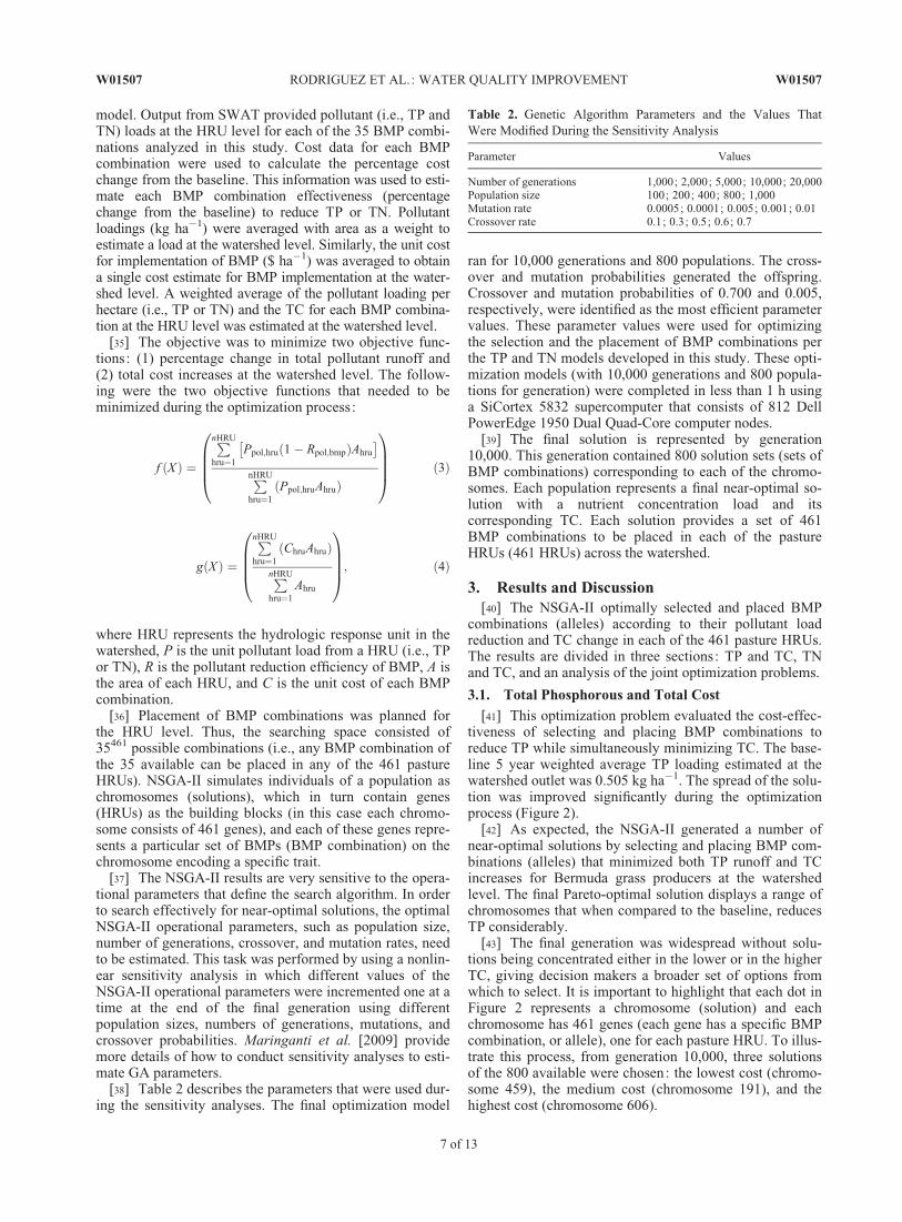
ran for 10,000 generations and 800 populations. The cross-over and mutation probabilities generated the offspring.Crossover and mutation probabilities of 0.700 and 0.005,respectively, were identified as the most efficient parametervalues. These parameter values were used for optimizingthe selection and the placement of BMP combinations perthe TP and TN models developed in this study. These opti-mization models (with 10,000 generations and 800 popula-tions for generation) were completed in less than 1 h usinga SiCortex 5832 supercomputer that consists of 812 DellPowerEdge 1950 Dual Quad-Core computer nodes.

[39] The final solution is represented by generation10,000. This generation contained 800 solution sets (sets ofBMP combinations) corresponding to each of the chromo-somes. Each population represents a final near-optimal so-lution with a nutrient concentration load and itscorresponding TC. Each solution provides a set of 461BMP combinations to be placed in each of the pastureHRUs (461 HRUs) across the watershed.

3. Results and Discussion[40] The NSGA-II optimally selected and placed BMP

combinations (alleles) according to their pollutant loadreduction and TC change in each of the 461 pasture HRUs.The results are divided in three sections: TP and TC, TNand TC, and an analysis of the joint optimization problems.

3.1. Total Phosphorous and Total Cost

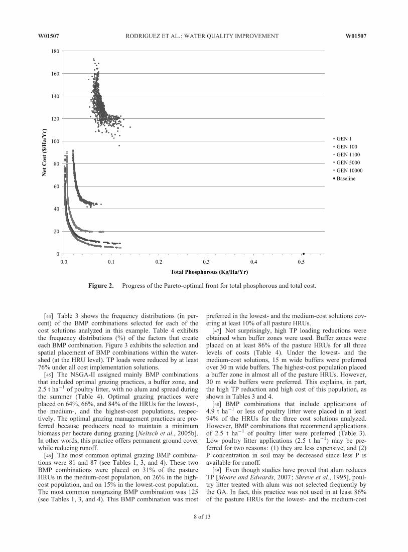
[41] This optimization problem evaluated the cost-effec-tiveness of selecting and placing BMP combinations toreduce TP while simultaneously minimizing TC. The base-line 5 year weighted average TP loading estimated at thewatershed outlet was 0.505 kg ha�1. The spread of the solu-tion was improved significantly during the optimizationprocess (Figure 2).

[42] As expected, the NSGA-II generated a number ofnear-optimal solutions by selecting and placing BMP com-binations (alleles) that minimized both TP runoff and TCincreases for Bermuda grass producers at the watershedlevel. The final Pareto-optimal solution displays a range ofchromosomes that when compared to the baseline, reducesTP considerably.

[43] The final generation was widespread without solu-tions being concentrated either in the lower or in the higherTC, giving decision makers a broader set of options fromwhich to select. It is important to highlight that each dot inFigure 2 represents a chromosome (solution) and eachchromosome has 461 genes (each gene has a specific BMPcombination, or allele), one for each pasture HRU. To illus-trate this process, from generation 10,000, three solutionsof the 800 available were chosen: the lowest cost (chromo-some 459), the medium cost (chromosome 191), and thehighest cost (chromosome 606).

Table 2. Genetic Algorithm Parameters and the Values ThatWere Modified During the Sensitivity Analysis

Parameter Values

Number of generations 1,000; 2,000; 5,000; 10,000; 20,000Population size 100; 200; 400; 800; 1,000Mutation rate 0.0005; 0.0001; 0.005; 0.001; 0.01Crossover rate 0.1; 0.3; 0.5; 0.6; 0.7

W01507 RODRIGUEZ ET AL.: WATER QUALITY IMPROVEMENT W01507

7 of 13

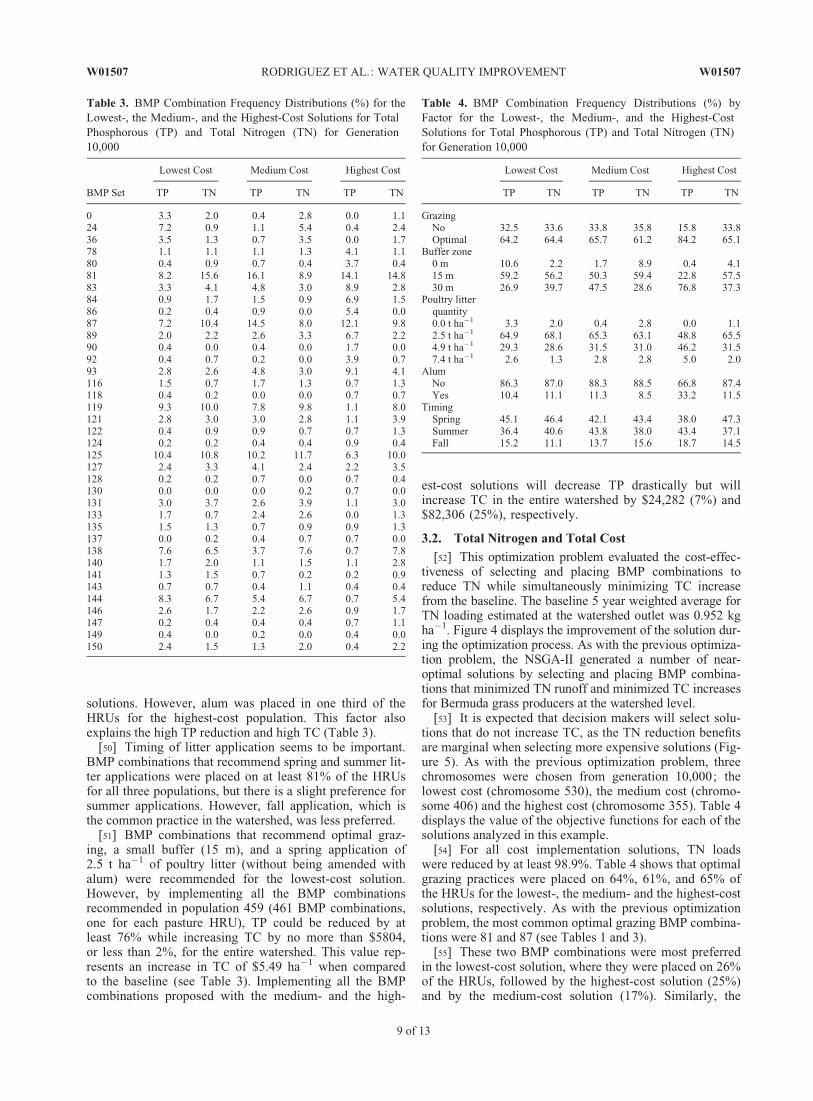
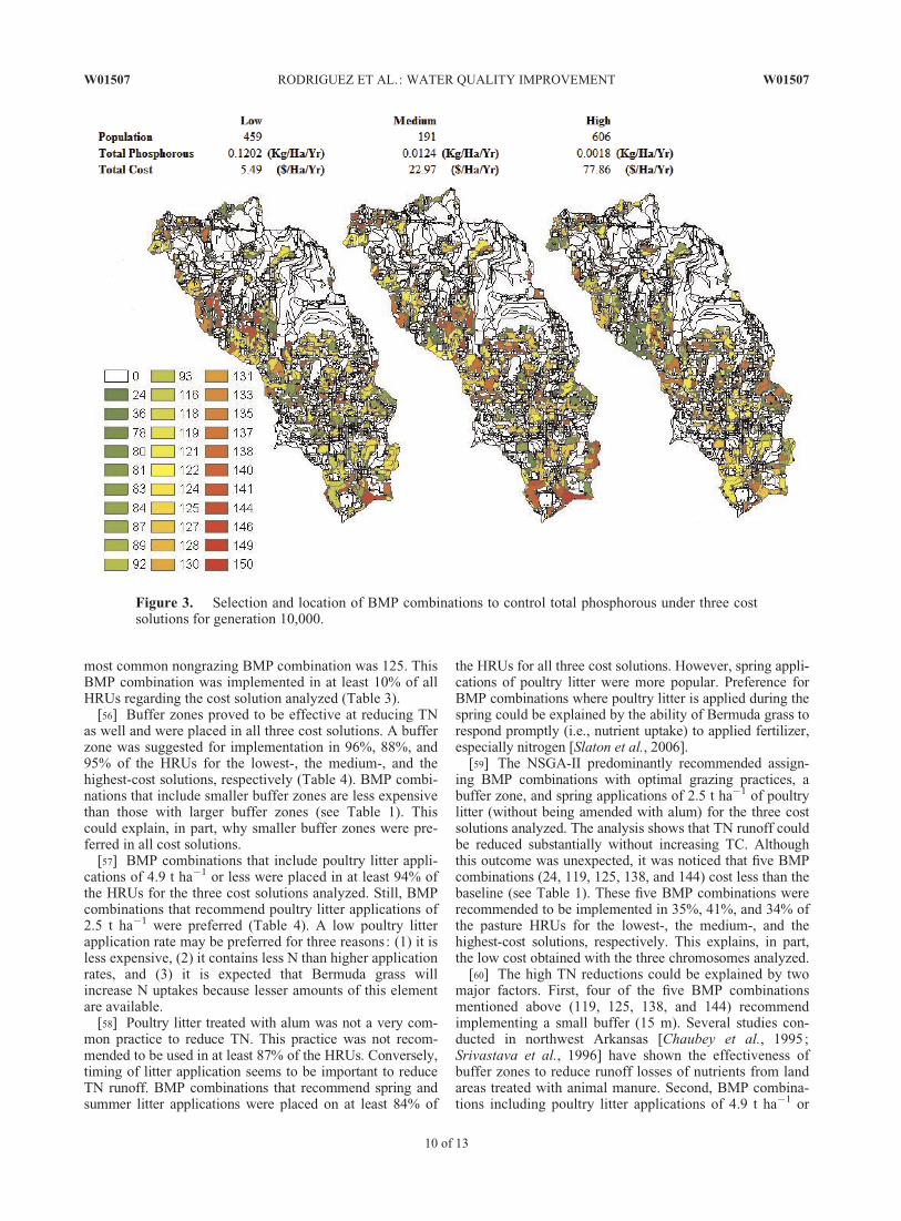
[44] Table 3 shows the frequency distributions (in per-cent) of the BMP combinations selected for each of thecost solutions analyzed in this example. Table 4 exhibitsthe frequency distributions (%) of the factors that createeach BMP combination. Figure 3 exhibits the selection andspatial placement of BMP combinations within the water-shed (at the HRU level). TP loads were reduced by at least76% under all cost implementation solutions.

[45] The NSGA-II assigned mainly BMP combinationsthat included optimal grazing practices, a buffer zone, and2.5 t ha�1 of poultry litter, with no alum and spread duringthe summer (Table 4). Optimal grazing practices wereplaced on 64%, 66%, and 84% of the HRUs for the lowest-,the medium-, and the highest-cost populations, respec-tively. The optimal grazing management practices are pre-ferred because producers need to maintain a minimumbiomass per hectare during grazing [Neitsch et al., 2005b].In other words, this practice offers permanent ground coverwhile reducing runoff.

[46] The most common optimal grazing BMP combina-tions were 81 and 87 (see Tables 1, 3, and 4). These twoBMP combinations were placed on 31% of the pastureHRUs in the medium-cost population, on 26% in the high-cost population, and on 15% in the lowest-cost population.The most common nongrazing BMP combination was 125(see Tables 1, 3, and 4). This BMP combination was most

preferred in the lowest- and the medium-cost solutions cov-ering at least 10% of all pasture HRUs.

[47] Not surprisingly, high TP loading reductions wereobtained when buffer zones were used. Buffer zones wereplaced on at least 86% of the pasture HRUs for all threelevels of costs (Table 4). Under the lowest- and themedium-cost solutions, 15 m wide buffers were preferredover 30 m wide buffers. The highest-cost population placeda buffer zone in almost all of the pasture HRUs. However,30 m wide buffers were preferred. This explains, in part,the high TP reduction and high cost of this population, asshown in Tables 3 and 4.

[48] BMP combinations that include applications of4.9 t ha�1 or less of poultry litter were placed in at least94% of the HRUs for the three cost solutions analyzed.However, BMP combinations that recommend applicationsof 2.5 t ha�1 of poultry litter were preferred (Table 3).Low poultry litter applications (2.5 t ha�1) may be pre-ferred for two reasons: (1) they are less expensive, and (2)P concentration in soil may be decreased since less P isavailable for runoff.

[49] Even though studies have proved that alum reducesTP [Moore and Edwards, 2007; Shreve et al., 1995], poul-try litter treated with alum was not selected frequently bythe GA. In fact, this practice was not used in at least 86%of the pasture HRUs for the lowest- and the medium-cost

Figure 2. Progress of the Pareto-optimal front for total phosphorous and total cost.

W01507 RODRIGUEZ ET AL.: WATER QUALITY IMPROVEMENT W01507

8 of 13

solutions. However, alum was placed in one third of theHRUs for the highest-cost population. This factor alsoexplains the high TP reduction and high TC (Table 3).

[50] Timing of litter application seems to be important.BMP combinations that recommend spring and summer lit-ter applications were placed on at least 81% of the HRUsfor all three populations, but there is a slight preference forsummer applications. However, fall application, which isthe common practice in the watershed, was less preferred.

[51] BMP combinations that recommend optimal graz-ing, a small buffer (15 m), and a spring application of2.5 t ha�1 of poultry litter (without being amended withalum) were recommended for the lowest-cost solution.However, by implementing all the BMP combinationsrecommended in population 459 (461 BMP combinations,one for each pasture HRU), TP could be reduced by atleast 76% while increasing TC by no more than $5804,or less than 2%, for the entire watershed. This value rep-resents an increase in TC of $5.49 ha�1 when comparedto the baseline (see Table 3). Implementing all the BMPcombinations proposed with the medium- and the high-

est-cost solutions will decrease TP drastically but willincrease TC in the entire watershed by $24,282 (7%) and$82,306 (25%), respectively.

3.2. Total Nitrogen and Total Cost

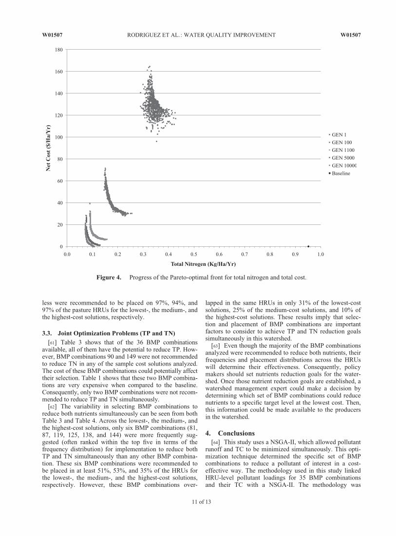
[52] This optimization problem evaluated the cost-effec-tiveness of selecting and placing BMP combinations toreduce TN while simultaneously minimizing TC increasefrom the baseline. The baseline 5 year weighted average forTN loading estimated at the watershed outlet was 0.952 kgha�1. Figure 4 displays the improvement of the solution dur-ing the optimization process. As with the previous optimiza-tion problem, the NSGA-II generated a number of near-optimal solutions by selecting and placing BMP combina-tions that minimized TN runoff and minimized TC increasesfor Bermuda grass producers at the watershed level.

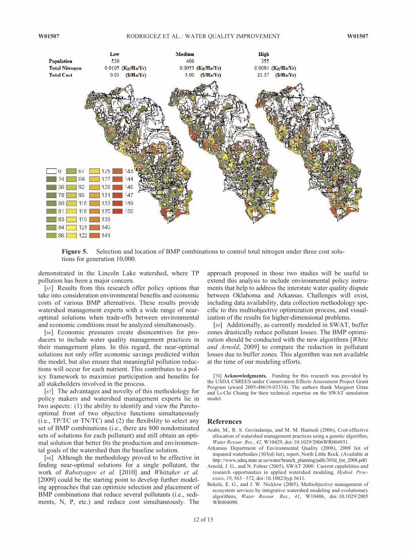
[53] It is expected that decision makers will select solu-tions that do not increase TC, as the TN reduction benefitsare marginal when selecting more expensive solutions (Fig-ure 5). As with the previous optimization problem, threechromosomes were chosen from generation 10,000; thelowest cost (chromosome 530), the medium cost (chromo-some 406) and the highest cost (chromosome 355). Table 4displays the value of the objective functions for each of thesolutions analyzed in this example.

[54] For all cost implementation solutions, TN loadswere reduced by at least 98.9%. Table 4 shows that optimalgrazing practices were placed on 64%, 61%, and 65% ofthe HRUs for the lowest-, the medium- and the highest-costsolutions, respectively. As with the previous optimizationproblem, the most common optimal grazing BMP combina-tions were 81 and 87 (see Tables 1 and 3).

[55] These two BMP combinations were most preferredin the lowest-cost solution, where they were placed on 26%of the HRUs, followed by the highest-cost solution (25%)and by the medium-cost solution (17%). Similarly, the

Table 3. BMP Combination Frequency Distributions (%) for theLowest-, the Medium-, and the Highest-Cost Solutions for TotalPhosphorous (TP) and Total Nitrogen (TN) for Generation10,000

Lowest Cost Medium Cost Highest Cost

BMP Set TP TN TP TN TP TN

0 3.3 2.0 0.4 2.8 0.0 1.124 7.2 0.9 1.1 5.4 0.4 2.436 3.5 1.3 0.7 3.5 0.0 1.778 1.1 1.1 1.1 1.3 4.1 1.180 0.4 0.9 0.7 0.4 3.7 0.481 8.2 15.6 16.1 8.9 14.1 14.883 3.3 4.1 4.8 3.0 8.9 2.884 0.9 1.7 1.5 0.9 6.9 1.586 0.2 0.4 0.9 0.0 5.4 0.087 7.2 10.4 14.5 8.0 12.1 9.889 2.0 2.2 2.6 3.3 6.7 2.290 0.4 0.0 0.4 0.0 1.7 0.092 0.4 0.7 0.2 0.0 3.9 0.793 2.8 2.6 4.8 3.0 9.1 4.1116 1.5 0.7 1.7 1.3 0.7 1.3118 0.4 0.2 0.0 0.0 0.7 0.7119 9.3 10.0 7.8 9.8 1.1 8.0121 2.8 3.0 3.0 2.8 1.1 3.9122 0.4 0.9 0.9 0.7 0.7 1.3124 0.2 0.2 0.4 0.4 0.9 0.4125 10.4 10.8 10.2 11.7 6.3 10.0127 2.4 3.3 4.1 2.4 2.2 3.5128 0.2 0.2 0.7 0.0 0.7 0.4130 0.0 0.0 0.0 0.2 0.7 0.0131 3.0 3.7 2.6 3.9 1.1 3.0133 1.7 0.7 2.4 2.6 0.0 1.3135 1.5 1.3 0.7 0.9 0.9 1.3137 0.0 0.2 0.4 0.7 0.7 0.0138 7.6 6.5 3.7 7.6 0.7 7.8140 1.7 2.0 1.1 1.5 1.1 2.8141 1.3 1.5 0.7 0.2 0.2 0.9143 0.7 0.7 0.4 1.1 0.4 0.4144 8.3 6.7 5.4 6.7 0.7 5.4146 2.6 1.7 2.2 2.6 0.9 1.7147 0.2 0.4 0.4 0.4 0.7 1.1149 0.4 0.0 0.2 0.0 0.4 0.0150 2.4 1.5 1.3 2.0 0.4 2.2

Table 4. BMP Combination Frequency Distributions (%) byFactor for the Lowest-, the Medium-, and the Highest-CostSolutions for Total Phosphorous (TP) and Total Nitrogen (TN)for Generation 10,000

Lowest Cost Medium Cost Highest Cost

TP TN TP TN TP TN

GrazingNo 32.5 33.6 33.8 35.8 15.8 33.8Optimal 64.2 64.4 65.7 61.2 84.2 65.1

Buffer zone0 m 10.6 2.2 1.7 8.9 0.4 4.115 m 59.2 56.2 50.3 59.4 22.8 57.530 m 26.9 39.7 47.5 28.6 76.8 37.3

Poultry litterquantity0.0 t ha�1 3.3 2.0 0.4 2.8 0.0 1.12.5 t ha�1 64.9 68.1 65.3 63.1 48.8 65.54.9 t ha�1 29.3 28.6 31.5 31.0 46.2 31.57.4 t ha�1 2.6 1.3 2.8 2.8 5.0 2.0

AlumNo 86.3 87.0 88.3 88.5 66.8 87.4Yes 10.4 11.1 11.3 8.5 33.2 11.5

TimingSpring 45.1 46.4 42.1 43.4 38.0 47.3Summer 36.4 40.6 43.8 38.0 43.4 37.1Fall 15.2 11.1 13.7 15.6 18.7 14.5

W01507 RODRIGUEZ ET AL.: WATER QUALITY IMPROVEMENT W01507

9 of 13

most common nongrazing BMP combination was 125. ThisBMP combination was implemented in at least 10% of allHRUs regarding the cost solution analyzed (Table 3).

[56] Buffer zones proved to be effective at reducing TNas well and were placed in all three cost solutions. A bufferzone was suggested for implementation in 96%, 88%, and95% of the HRUs for the lowest-, the medium-, and thehighest-cost solutions, respectively (Table 4). BMP combi-nations that include smaller buffer zones are less expensivethan those with larger buffer zones (see Table 1). Thiscould explain, in part, why smaller buffer zones were pre-ferred in all cost solutions.

[57] BMP combinations that include poultry litter appli-cations of 4.9 t ha�1 or less were placed in at least 94% ofthe HRUs for the three cost solutions analyzed. Still, BMPcombinations that recommend poultry litter applications of2.5 t ha�1 were preferred (Table 4). A low poultry litterapplication rate may be preferred for three reasons: (1) it isless expensive, (2) it contains less N than higher applicationrates, and (3) it is expected that Bermuda grass willincrease N uptakes because lesser amounts of this elementare available.

[58] Poultry litter treated with alum was not a very com-mon practice to reduce TN. This practice was not recom-mended to be used in at least 87% of the HRUs. Conversely,timing of litter application seems to be important to reduceTN runoff. BMP combinations that recommend spring andsummer litter applications were placed on at least 84% of

the HRUs for all three cost solutions. However, spring appli-cations of poultry litter were more popular. Preference forBMP combinations where poultry litter is applied during thespring could be explained by the ability of Bermuda grass torespond promptly (i.e., nutrient uptake) to applied fertilizer,especially nitrogen [Slaton et al., 2006].

[59] The NSGA-II predominantly recommended assign-ing BMP combinations with optimal grazing practices, abuffer zone, and spring applications of 2.5 t ha�1 of poultrylitter (without being amended with alum) for the three costsolutions analyzed. The analysis shows that TN runoff couldbe reduced substantially without increasing TC. Althoughthis outcome was unexpected, it was noticed that five BMPcombinations (24, 119, 125, 138, and 144) cost less than thebaseline (see Table 1). These five BMP combinations wererecommended to be implemented in 35%, 41%, and 34% ofthe pasture HRUs for the lowest-, the medium-, and thehighest-cost solutions, respectively. This explains, in part,the low cost obtained with the three chromosomes analyzed.

[60] The high TN reductions could be explained by twomajor factors. First, four of the five BMP combinationsmentioned above (119, 125, 138, and 144) recommendimplementing a small buffer (15 m). Several studies con-ducted in northwest Arkansas [Chaubey et al., 1995;Srivastava et al., 1996] have shown the effectiveness ofbuffer zones to reduce runoff losses of nutrients from landareas treated with animal manure. Second, BMP combina-tions including poultry litter applications of 4.9 t ha�1 or

Figure 3. Selection and location of BMP combinations to control total phosphorous under three costsolutions for generation 10,000.

W01507 RODRIGUEZ ET AL.: WATER QUALITY IMPROVEMENT W01507

10 of 13

less were recommended to be placed on 97%, 94%, and97% of the pasture HRUs for the lowest-, the medium-, andthe highest-cost solutions, respectively.

3.3. Joint Optimization Problems (TP and TN)

[61] Table 3 shows that of the 36 BMP combinationsavailable, all of them have the potential to reduce TP. How-ever, BMP combinations 90 and 149 were not recommendedto reduce TN in any of the sample cost solutions analyzed.The cost of these BMP combinations could potentially affecttheir selection. Table 1 shows that these two BMP combina-tions are very expensive when compared to the baseline.Consequently, only two BMP combinations were not recom-mended to reduce TP and TN simultaneously.

[62] The variability in selecting BMP combinations toreduce both nutrients simultaneously can be seen from bothTable 3 and Table 4. Across the lowest-, the medium-, andthe highest-cost solutions, only six BMP combinations (81,87, 119, 125, 138, and 144) were more frequently sug-gested (often ranked within the top five in terms of thefrequency distribution) for implementation to reduce bothTP and TN simultaneously than any other BMP combina-tion. These six BMP combinations were recommended tobe placed in at least 51%, 53%, and 35% of the HRUs forthe lowest-, the medium-, and the highest-cost solutions,respectively. However, these BMP combinations over-

lapped in the same HRUs in only 31% of the lowest-costsolutions, 25% of the medium-cost solutions, and 10% ofthe highest-cost solutions. These results imply that selec-tion and placement of BMP combinations are importantfactors to consider to achieve TP and TN reduction goalssimultaneously in this watershed.

[63] Even though the majority of the BMP combinationsanalyzed were recommended to reduce both nutrients, theirfrequencies and placement distributions across the HRUswill determine their effectiveness. Consequently, policymakers should set nutrients reduction goals for the water-shed. Once those nutrient reduction goals are established, awatershed management expert could make a decision bydetermining which set of BMP combinations could reducenutrients to a specific target level at the lowest cost. Then,this information could be made available to the producersin the watershed.

4. Conclusions[64] This study uses a NSGA-II, which allowed pollutant

runoff and TC to be minimized simultaneously. This opti-mization technique determined the specific set of BMPcombinations to reduce a pollutant of interest in a cost-effective way. The methodology used in this study linkedHRU-level pollutant loadings for 35 BMP combinationsand their TC with a NSGA-II. The methodology was

Figure 4. Progress of the Pareto-optimal front for total nitrogen and total cost.

W01507 RODRIGUEZ ET AL.: WATER QUALITY IMPROVEMENT W01507

11 of 13

demonstrated in the Lincoln Lake watershed, where TPpollution has been a major concern.

[65] Results from this research offer policy options thattake into consideration environmental benefits and economiccosts of various BMP alternatives. These results providewatershed management experts with a wide range of near-optimal solutions when trade-offs between environmentaland economic conditions must be analyzed simultaneously.

[66] Economic pressures create disincentives for pro-ducers to include water quality management practices intheir management plans. In this regard, the near-optimalsolutions not only offer economic savings predicted withinthe model, but also ensure that meaningful pollution reduc-tions will occur for each nutrient. This contributes to a pol-icy framework to maximize participation and benefits forall stakeholders involved in the process.

[67] The advantages and novelty of this methodology forpolicy makers and watershed management experts lie intwo aspects : (1) the ability to identify and view the Pareto-optimal front of two objective functions simultaneously(i.e., TP/TC or TN/TC) and (2) the flexibility to select anyset of BMP combinations (i.e., there are 800 nondominatedsets of solutions for each pollutant) and still obtain an opti-mal solution that better fits the production and environmen-tal goals of the watershed than the baseline solution.

[68] Although the methodology proved to be effective infinding near-optimal solutions for a single pollutant, thework of Rabotyagov et al. [2010] and Whittaker et al.[2009] could be the starting point to develop further model-ing approaches that can optimize selection and placement ofBMP combinations that reduce several pollutants (i.e., sedi-ments, N, P, etc.) and reduce cost simultaneously. The

approach proposed in those two studies will be useful toextend this analysis to include environmental policy instru-ments that help to address the interstate water quality disputebetween Oklahoma and Arkansas. Challenges will exist,including data availability, data collection methodology spe-cific to this multiobjective optimization process, and visual-ization of the results for higher-dimensional problems.

[69] Additionally, as currently modeled in SWAT, bufferzones drastically reduce pollutant losses. The BMP optimi-zation should be conducted with the new algorithms [Whiteand Arnold, 2009] to compare the reduction in pollutantlosses due to buffer zones. This algorithm was not availableat the time of our modeling efforts.

[70] Acknowledgments. Funding for this research was provided bythe USDA CSREES under Conservation Effects Assessment Project GrantProgram (award 2005-48619-03334). The authors thank Margaret Gitauand Li-Chi Chiang for their technical expertise on the SWAT simulationmodel.

ReferencesArabi, M., R. S. Govindaraju, and M. M. Hantush (2006), Cost-effective

allocation of watershed management practices using a genetic algorithm,Water Resour. Res., 42, W10429, doi:10.1029/2006WR004931.

Arkansas Department of Environmental Quality (2008), 2008 list ofimpaired waterbodies (303(d) list), report, North Little Rock. (Available athttp://www.adeq.state.ar.us/water/branch_planning/pdfs/303d_list_2008.pdf)

Arnold, J. G., and N. Fohrer (2005), SWAT 2000: Current capabilities andresearch opportunities in applied watershed modeling, Hydrol. Proc-esses, 19, 563– 572, doi:10.1002/hyp.5611.

Bekele, E. G., and J. W. Nicklow (2005), Multiobjective management ofecosystem services by integrative watershed modeling and evolutionaryalgorithms, Water Resour. Res., 41, W10406, doi:10.1029/2005WR004090.

Figure 5. Selection and location of BMP combinations to control total nitrogen under three cost solu-tions for generation 10,000.

W01507 RODRIGUEZ ET AL.: WATER QUALITY IMPROVEMENT W01507

12 of 13

Borah, D. K., G. Yagow, A. Saleh, P. L. Barnes, W. Rosenthal, E. C. Krug,and L. M. Hauck (2006), Sediment and nutrient modeling for TMDL de-velopment and implementation, Trans. ASABE, 49, 967–986.

Chambers, L. (2001), The Practical Handbook of Genetic Algorithms:Applications, 2nd ed., 501 pp., Chapman and Hall, Boca Raton, Fla.

Chaubey, I., D. R. Edwards, T. C. Daniel, P. A. Moore, and D. J. Nichols(1995), Effectiveness of vegetative filter strips in controlling losses ofsurface-applied poultry litter constituents, Trans. ASAE, 38, 1687–1692.

Chaubey, I., L. Chiang, M. Gitau, and S. Mohamed (2010), Effectiveness ofBMPs in improving water quality in a pasture dominated watershed,J. Soil Water Conserv., 65(6), 424– 437, doi:10.2489/jswc.65.6.424.

Deb, K. (2001), Multi-objective Optimization Using Evolutionary Algo-rithms, John Wiley, New York.

Deb, K., A. Pratap, S. Agarwal, and T. Meyarivan (2002), A fast and elitistmultiobjective genetic algorithm: NSGA-II, IEEE Trans. Evol. Comput.,6, 182– 197.

DeLaune, P. B., P. A. Moore, D. K. C. Carman, A. N. Sharpley, B. E. Hag-gard, and T. C. Daniel (2004), Development of a phosphorus index forpastures fertilized with poultry litter—Factors affecting phosphorus run-off, J Environ. Qual., 33, 2183– 2191, doi:10.2134/jeq2004.2183.

Di Luzio, M., R. Srinivasan, and J. G. Arnold (2004), A GIS-coupledhydrological model system for the watershed assessment of agriculturalnonpoint and point sources of pollution, Trans. GIS, 8, 113– 136.

Duriancik, L. F., et al. (2008), The first five years of the ConservationEffects Assessment Project, J. Soil Water Conserv., 63, 185A– 197A,doi:10.2489/jswc.63.6.185A.

Gassman, P. W., M. R. Reyes, C. H. Green, and J. G. Arnold (2007), TheSoil Water Assessment Tool: Historical development, applications, andfuture research directions, Trans. ASABE, 50, 1211– 1250.

Gitau, M. W., T. L. Veith, W. J. Gburek, and A. R. Jarrett (2006), Watershedlevel best management practice selection and placement in the town Brookwatershed, New York, J. Am. Water Resour. Assoc., 42, 1565–1581.

Gitau, M., I. Chaubey, E. Gbur, J. Pennington, and B. Gorham (2010),Impact of land use change and BMP implementation on water quality ina pastured northwest Arkansas watershed, J. Soil Water Conserv., 65(6),353– 368, doi:10.2489/jswc.65.6.353.

Goldberg, D. E. (1989), Genetic Algorithms in Search, Optimization andMachine Learning, Addison-Wesley, Boston, Mass.

Haggard, B. E., and T. S. Soerens (2006), Sediment phosphorous release ata small impoundment on the Illinois River, Arkansas and Oklahoma,USA, Biol. Eng., 28, 280–287, doi:10.1016/j.ecoleng.2006.07.013.

Haggard, B. E., T. Soerens, W. R. Green, and R. P. Richards (2003), Usingregression methods to estimate stream phosphorous loads at the IllinoisRiver, Arkansas, Appl. Eng. Agric., 19, 187–194.

Holland, J. H. (1975), Adaptation in Natural and Artificial Systems: An In-troductory Analysis With Applications to Biology, Control, and ArtificialIntelligence, 1st MIT Press ed., 211 pp., MIT Press, Cambridge, Mass.

Koza, J. R. (1992), Genetic Programming: On the Programming of Com-puters by Means of Natural Selection, 819 pp., MIT Press, Cambridge,Mass.

Maringanti, C., I. Chaubey, and J. Popp (2009), Development of a multiob-jective optimization tool for the selection and placement of best manage-ment practices for nonpoint source pollution control, Water Resour. Res.,45, W06406, doi:10.1029/2008WR007094.

Massey, L. B., L. W. Cash, and B. E. Haggard (2009), Water quality sam-pling, analysis and annual load determinations for the Illinois River atArkansas Highway 59 bridge, 2008, Arkansas Soil Fertil. Stud., MSC 352,1–11.

Mayer, P. M., S. K. Reynolds, T. J. Canfield, and M. D. McCutchen (2005),Riparian buffer width, vegetative cover, and nitrogen removal effective-ness: A review of current science and regulations, Rep. EPA/600/R-05/118, U.S. Environ. Prot. Agency, Washington, D. C.

Moore, P. A., and D. R. Edwards (2007), Long-term effects of poultry litter,alum-treated litter, and ammonium nitrate on phosphorus availability insoils, J. Environ. Qual., 36, 163– 174, doi:10.2134/jeq2004.0472.

Moore, P. A., S. Watkins, D. Carmen, and P. B. DeLaune (2004), Treatingpoultry litter with alum, Rep. FSA8003-PD-1-04N, Coop. ExtensionServ., Div. of Agr., Univ. of Arkansas, Little Rock.

Muleta, M. K., and J. W. Nicklow (2005), Decision support for watershedmanagement using evolutionary algorithms, J. Water Resour. Plann.Manage., 131, 35–44, doi:10.1061/(ASCE)0733-9496(2005)131:1(35).

Natural Resources Conservation Service Arkansas (2002), Buffer strip code391, Conserv. Pract. Stand. 1, 1 – 5.

Neitsch, S. L., J. G. Arnold, J. R. Kiniry, and J. R. Williams (2005a), Soiland Water Assessment Tool theoretical documentation, version 2005,494 pp., Grassland, Soil and Water Res. Lab., Agric. Res. Serv.,Temple, Tex. (Available at http://swatmodel.tamu.edu/media/1292/SWAT2005theory.pdf)

Neitsch, S. L., J. G. Arnold, J. R. Kiniry, R. Srinivasan, and J. R. Williams(2005b), Soil and Water Assessment Tool: Input/output file documenta-tion, version 2005, 541 pp., Grassland, Soil and Water Res. Lab., Agric.Res. Serv., Temple, Tex. (Available at http://swatmodel.tamu.edu/media/1291/SWAT2005io.pdf)

Pennington, J., M. A. Steele, K. A. Teague, B. Kurz, E. Gbur, J. Popp, G.Rodr�ıguez, I. Chaubey, M. Gitau, and M. A. Nelson (2008), Breakingground: A cooperative approach to data collection from an initially unco-operative population, J. Soil Water Conserv., 63, 208–211, doi:10.2489/jswc.63.6.208A.

Popp, J., H. G. Rodr�ıguez, E. Gbur, and J. Pennington (2007), The role ofstakeholders’ perceptions in addressing water quality disputes in anembattled watershed, J. Environ. Monit. Restor., 3, 255–263,doi:10.4029/2007jemrest3no125.

Popp, J., N. Kemper, W. Miller, K. McGraw, and K. Karr (2010), Contribu-tion of the agricultural sector to the Arkansas economy in 2007, Res.Rep. 989, Arkansas Agric. Exp. Stn., Div. of Agric., Univ. of Arkansas,Fayetteville.

Rabotyagov, S., T. Campbell, M. Jha, P.W. Gassman, J. Arnold, L. Kurka-lova, S. Secchi, H. Feng and C. L. Kling (2010), Least cost control of ag-ricultural nutrient contributions to the Gulf of Mexico hypoxic zone,Ecol. Appl., 20, 1542–1555, doi:10.1890/08-0680.1.

Schmitt, T. J., M. G. Dosskey, and K. D. Hoagland (1999), Filter strip per-formance and processes for different vegetation, widths, and contami-nants, J. Environ. Qual., 28, 1479–1489, doi:10.2134/jeq1999.00472425002800050013x.

Sharpley, A. N., and J. R. Williams (1990), EPIC-erosion productivityimpact calculator, 1. Model documentation, Tech. Bull. 1768, Agric. Res.Serv., U.S. Dep. of Agric., Washington, D. C.

Sharpley, A. N., S. Herron, and T. Daniel (2007), Overcoming the chal-lenges of phosphorus-based management in poultry farming, J. SoilWater Conserv., 62, 375– 389.

Shreve, B. R., P. A. Moore, T. C. Daniel, D. R. Edwards, and D. M. Miller(1995), Reduction of phosphorus in runoff from field-applied poultry lit-ter using chemical amendments, J. Environ. Qual., 24, 106–111,doi:10.2134/jeq1995.00472425002400010015x.

Slaton, N. A., R. E. Delong, B. R. Golden, C. G. Massey, and T. L. Roberts(2006), Bermuda grass forage response to nitrogen, phosphorous and po-tassium fertilization rate, Arkansas Soil Fertil. Stud., 548, 52– 57.

Srivastava, P., D. R. Edwards, T. C. Daniel, P. A. Moore, and T. A. Costello(1996), Performance of vegetative filter strips with varying pollutantsource and filter strip lengths, Trans. ASAE, 39, 2231– 2239.

Srivastava, P., K. W. Migliaccio, and J. Simune (2007), Landscape modelsfor simulating water quality at point, field, and watershed scales, Trans.ASABE, 50, 1683– 1693.

Veith, T. L., M. L. Wolfe, and C. D. Heatwole (2004), Cost-effectiveBMP placement: Optimization versus targeting, Trans. ASAE, 47,1585–1594.

Vendrell, P. F., M. A. Nelson, W. L. Cash, K. F. Steele, K. A. Teague, andD. R. Edwards (1997), Nutrient transport by streams in the Lincoln Lakebasin, Publ. MSC-210, pp. 45– 51, Arkansas Water Resour. Cent.,Fayetteville.

White, K. L., and J. G. Arnold (2009), Development of a simplistic vegeta-tive filter strip model for sediment and nutrient retention at the field scale,Hydrol. Processes, 23, 1602–1616, doi:10.1002/hyp.7291.

Whittaker, G., R. Confesor, S. M. Griffith, R. Fare, S. Grosskopf, J. Steiner,G. Muller-Warrant, and G. M. Banowetz (2009), A hybrid genetic algo-rithm for multiobjective problems with activity analysis-based localsearch, Eur. J. Oper. Res., 193, 195–203, doi:10.1016/j.ejor.2007.10.050.

Zitzler, E., and L. Thiele (1999), Multiobjective evolutionary algorithms:A comparative case study and the strength Pareto approach, IEEE Trans.Evol. Comput., 3, 257–271, doi:10.1162/106365600568202.

I. Chaubey and C. Maringanti, Department of Agricultural and Biologi-cal Engineering, Purdue University, West Lafayette, IN 47907, USA.

J. Popp and H. G. Rodriguez, Department of Agricultural Economicsand Agribusiness, University of Arkansas, Fayetteville, AR 72701, USA.(hrodrig@uark.edu)

W01507 RODRIGUEZ ET AL.: WATER QUALITY IMPROVEMENT W01507

13 of 13