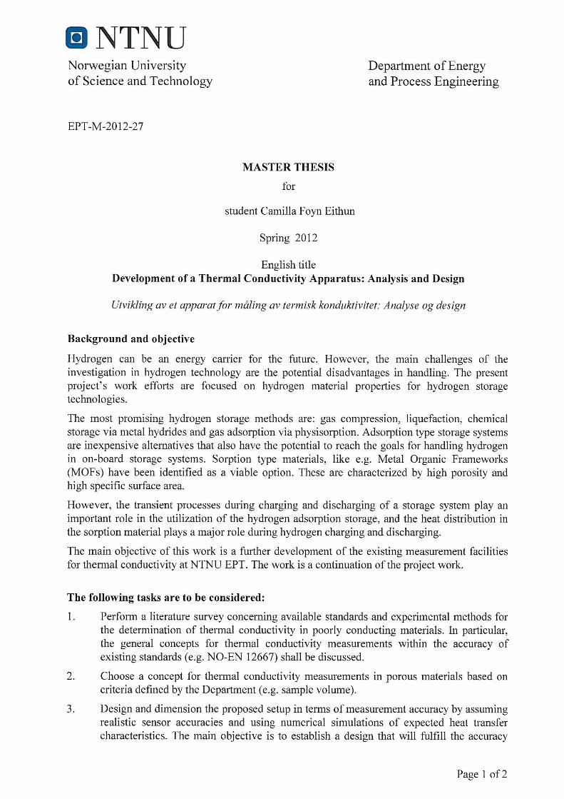
Development of a thermal conductivity apparatus: Analysis and design

Camilla Foyn Eithun

Master of Science in Product Design and Manufacturing

Supervisor: Erling Næss, EPTCo-supervisor: Christian Schlemminger, EPT

Department of Energy and Process Engineering

Submission date: June 2012

Norwegian University of Science and Technology

i

Acknowledgements This report is a result of my Master Thesis at The Norwegian University of Science and Technology, Department of Energy and Process Engineering. It has been written in the period from January to June 2012.

I would like to thank my supervisor, Erling Næss, for our regular meetings throughout this spring. His great knowledge and patience has been very valuable for my learning and the progression of my work. I would also like to give a special thanks to my co-supervisor, Christian Schlemminger, for always taking time to answer questions and providing me with relevant and important information. As well, his positive attitude and enthusiasm has been a great motivation during the progress of the research.

I would also like to thank Geir Hansen for the guided tour in the laboratory, which gave me a realistic view of what my theoretical work and simulations would look like in real life.

Finally, I would like to thank Julie Foyn Eithun, Jørgen Nilsen and Inger-Anne Rasmussen for all their help and support during this semester.

Camilla Foyn Eithun,

Trondheim, June 9th, 2012

ii

iii

Abstract This objective of this thesis has been to development and analysis a measurement apparatus designed to determine thermal conductivity of porous materials. A literature survey concerning available experimental techniques for thermal conductivity measurements was conducted. A steady state radial heat transfer method with cylindrical geometry and a centered heating element was found to be most suited technique for achieving accurate and reliable results. A side wall cooling arrangement was used to achieve desired cooling temperatures.

To restrict the extent of the work, it was decided to only investigate heat transfer behavior at cryogenic temperatures. Test specimen with a thermal conductivity of 0.05 W/(m*K), (assumed to be the thermal conductivity of the materials to be tested in the apparatus) and a thermal conductivity of 0.01 W/(m*K) for the insulation components, were the ones chosen for investigations.

The design process of the new apparatus, using the software COMSOL Multiphysics 4.2, was initiated by evaluating heat transfer behavior in a simple cylinder, containing a hollow heating element and the test specimen. Radial heat transfer was verified, hence, the design process proceeded. Extensive, step-wise analyses were conducted to evaluate heat transfer behavior as the complexity of the apparatus increased. Implemented elements such as insulation blocks, a heater support and three thermocouples proved to cause heat losses in the test section, which resulted in errors in the calculated thermal conductivities. Furthermore, an electric wire, supplying the heating element with current, was included in the model. In addition, the hollow heater was replaced by an aluminum oxide heater since such an element is to be used when building the apparatus. Unexpected results revealed critical heat transfer into the test section from the wire. This led to an investigation of the wire length to reduce such effects. Lastly, as a result of the analyses carried out, the overall error of the thermal conductivity measurements due to heat losses was determined. Dimensional drawings of the characteristic dimensions, as well as practical solutions for the final compilation of the apparatus, were suggested as the last step of the design process.

It was of interest to estimate the overall uncertainty of the apparatus when all parameters effecting the measurements, were included. For this, a comprehensive uncertainty analysis was conducted and compared to previous work. Results showed that temperature recordings from the thermocouples placed in the mid-section of the test cylinder would provide the most reliable results for the determination of thermal conductivity in the test apparatus.

iv

Sammendrag Formålet med denne masteravhandlingen har vært å utvikle og analysere et målingsapparat designet for å kunne måle termisk konduktivitet i porøse materialer. For å kartlegge tilgjengelige eksperimentelle teknikker for måling av termisk konduktivitet, ble en litteraturstudie gjennomført. En stasjonær metode med radiell varmeoverføring i en konsentrisk sylinder med et sentrert varmeelement viste seg å være den best egnede metoden for å oppnå gode, pålitelige resultater. Kjøling av ytterveggen til sylinderen ble benyttet for å oppnå ønskelig kjøletemperaturer for systemet.

For å begrense omfanget av oppgaven ble det besluttet å kun etterforske termisk konduktivitet ved kryogene temperaturer. Det ble valgt en termisk konduktivitet på 0,05 W/(m*K) for testmaterialet i apparatet. Dette er antatt å tilsvare den termiske konduktiviteten på materialene som skal testes i apparatet i fremtidige tester. Den lavest oppnåelige termiske konduktiviteten på isolasjonen i apparatet ble bestemt til å være 0,01 W/(m*K).

Testapparatet ble modellert og evaluert med analyseverktøyet COMSOL Multiphysics 4.2. Designprosessen ble startet ved å observere varmeoverføring i en enkel sylinder, bestående av et hult varmeelement og testmateriale. Ettersom radiell varmeoverføring ble påvist fortsatte designprosessen. For å evaluere forandringer i varmetransporten etter hvert som kompleksiteten av apparatet økte ble en omfattende og trinnvis analyse utført. Ved å implementere elementer som isolasjonsklosser, støtte til varmeelementet og termoelementer, ble det påvist varmetap i bunnen av testseksjonen. Dette resulterte i avvik da den termiske konduktiviteten ble regnet ut. For at varme skal kunne genereres i systemet måtte det tilføres strøm til varmeelementet via en elektrisk ledning. I tillegg ble det hule varmeelementet erstattet av et aluminiumsoksidelement, ettersom et slikt element vil bli tatt i bruk når apparatet senere skal bygges. Uventede resultater avslørte en kritisk varmeoverføring inn i testseksjonen etter å ha implementerte den elektriske ledningen. En omfattende analyse for å redusere denne varmeoverføringen ble derfor utført. Problemet viste seg å kunne løses dersom ledningen ble betydelig forlenget i forhold til den opprinnelige lengden.

Etter de utførte analysene, ble det totale avviket for de termiske konduktivitetsmålingene anslått. Dimensjonstegninger for de karakteristiske elementene, samt praktiske løsninger for den endelige sammenstillingen av apparatet, ble foreslått som siste steg i designprosessen.

Som en avsluttende del av oppgaven ble det utført en omfattende usikkerhetsanalyse, hvor alle parametere som kan påvirke målingene, ble estimert og tatt hensyn til. Resultatene ble sammenlignet med usikkerhetsanalyser utført i forbindelse med tidligere arbeid. Det viste seg at de mest pålitelige målingene vil oppnås dersom temperaturmålinger i midtseksjonen av apparatet benyttes.

v

Table of Contents 1. Introduction ........................................................................................................................ 1

1.1. Background and Objective ........................................................................................... 1

1.2. Motivation ................................................................................................................... 2

1.3. Organization of the report ........................................................................................... 2

2. Thermal conductivity measurement technologies and standards ..................................... 3

2.1. Introduction to thermal conductivity measurements ................................................. 3

2.2. Steady- State methods ................................................................................................ 4

2.2.1. Guarded hot plate ................................................................................................ 4

2.2.2. Axial Flow Method................................................................................................ 5

2.2.3. Cylinder method ................................................................................................... 6

2.2.4. Heat flow meter method ...................................................................................... 7

2.3. Transient methods ....................................................................................................... 8

2.3.1. Hot wire method .................................................................................................. 9

2.3.2. Needle probe ...................................................................................................... 10

2.3.3. Transient plane source method ......................................................................... 10

2.4. Summary thermal conductivity measurement techniques ....................................... 11

3. Apparatus concept ............................................................................................................ 13

3.1. Choice of Concept: Goal and limitations ................................................................... 13

3.2. Theoretical Basis ........................................................................................................ 14

3.3. Previous work ............................................................................................................ 15

3.4. Delimitations for the new apparatus design ............................................................. 17

4. Thermal design: development and analysis ..................................................................... 19

4.1. Introduction ............................................................................................................... 19

4.2. Design and analysis tool: Comsol Multiphysics 4.2 ................................................... 19

4.3. Investigation and design of the new test apparatus ................................................. 21

4.3.1. Basic idea of the new concept ........................................................................... 21

4.3.2. Validating radial heat transfer ........................................................................... 23

4.3.3. Influence of insulation in top and bottom of the sample cylinder .................... 26

4.3.4. Isolating the sample cylinder from base plate of sealed container ................... 29

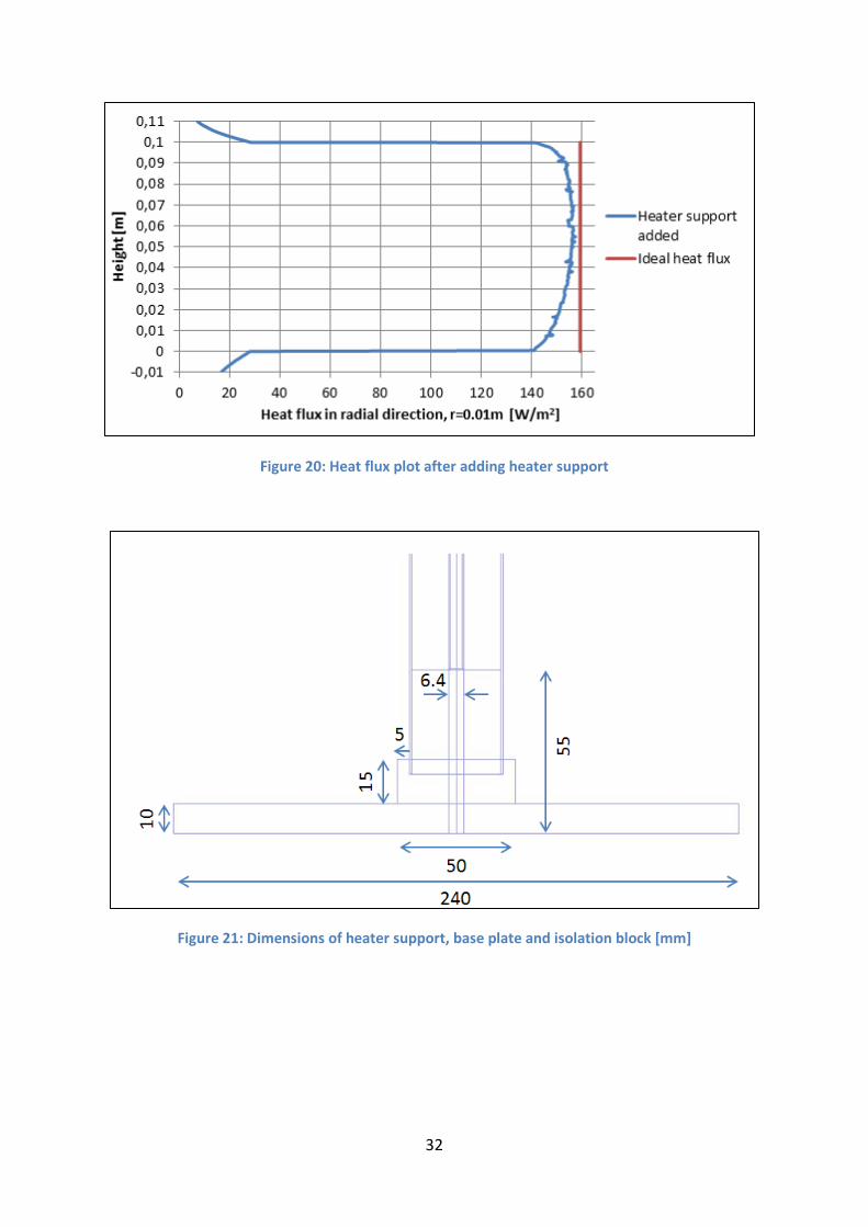
4.3.5. Influence of implementing a heater support ..................................................... 31

4.3.6. Influence of thermocouples and thermocouple protectors .............................. 33

vi

4.3.7. Effect of implementing the electric wire ........................................................... 36

4.4. Heater analysis........................................................................................................... 39

4.5. Investigation of the electric wire length.................................................................... 42

4.6. Concluding remarks for the thermal design process ................................................ 46

5. Proposed Design ............................................................................................................... 49

5.1. Dimensions of characteristic components ................................................................ 49

5.2. Alignment of electric wire ......................................................................................... 51

5.3. Suggested insulation materials .................................................................................. 52

5.4. Evacuation of the apparatus ...................................................................................... 53

5.5. Cooling pipe arrangement ......................................................................................... 54

5.6. Assembly of sealed container .................................................................................... 54

6. Uncertainty Analysis ......................................................................................................... 57

6.1. Estimation of 𝛿𝑄 ........................................................................................................ 58

6.1.1. Heat loss estimation ........................................................................................... 58

6.1.2. Estimation of δQloss: ......................................................................................... 60

6.1.3. Estimation of δU and δI ...................................................................................... 60

6.1.4. Estimation of total 𝛿𝑄 ........................................................................................ 61

6.2. Estimation of δr1, δr2 and δh .................................................................................... 62

6.3. Estimation of δΔT ...................................................................................................... 62

6.4. Overall uncertainty for the thermal conductivity measurements ............................ 64

6.5. Discussion .................................................................................................................. 69

7. Conclusion ......................................................................................................................... 71

8. Suggestions for further work ............................................................................................ 73

Bibliography .............................................................................................................................. 75

APPENDIX ................................................................................................................................... A

Appendix A .............................................................................................................................. C

Relevant standards for thermal conductivity measurement techniques ........................... C

Appendix B .............................................................................................................................. E

Material references ............................................................................................................. E

Appendix C .............................................................................................................................. G

Heat transfer calculations for wire outside sealed container ............................................ G

vii

List of figures Figure 1: Principle sketch of guarded hot plate methods, a) two-specimen apparatus. b) single-specimen apparatus [4] ................................................................................................... 5 Figure 2: Basic elements for the cylinder method and the temperature profile of a cross section ........................................................................................................................................ 7 Figure 3: Typical heat flux transducer heat flow meter apparatus ............................................ 8 Figure 4: Principle sketch of the hot-wire method[4] ................................................................ 9 Figure 5: Heating/sensor element used for TSP [11] ............................................................... 11 Figure 6: Abrahamsen's rig design and dimensions [12] ......................................................... 15 Figure 7: Gauthier's experimental test setup [13] ................................................................... 16 Figure 8: Sealed container concept with cooling pipe ............................................................. 22 Figure 9: Sealed container illustrating the main components of the test cylinder ................. 22 Figure 11: Sample cylinder ....................................................................................................... 23 Figure 10: Dimensions of test section [mm] ............................................................................ 23 Figure 12: Radial heat flux validation ....................................................................................... 24 Figure 13: Temperature distribution in radial direction for the validation of radial heat transfer ..................................................................................................................................... 25 Figure 14: 1 cm insulation blocks and 3 cm insulation blocks ................................................. 26 Figure 15: Heat flux plot for insulation blocks ......................................................................... 27 Figure 16: Dimensions of insulation blocks and top and bottom plates [mm] ........................ 28 Figure 17: Isolation block and base plate ................................................................................. 29 Figure 18: Temperature distribution when base plate is added .............................................. 30 Figure 19: Heater support added ............................................................................................. 31 Figure 20: Heat flux plot after adding heater support ............................................................. 32 Figure 21: Dimensions of heater support, base plate and isolation block [mm] ..................... 32 Figure 22: Thermocouples with protectors .............................................................................. 33 Figure 23: Thermocouples with protectors added .................................................................. 34 Figure 24: Heat flux plot after adding thermocouples w/protectors ...................................... 35 Figure 25: Temperature plot in radial direction, thermocouples added ................................. 35 Figure 26: Illustration of electric wire alignment ..................................................................... 36 Figure 27: 2D Temperature distribution after electric wire is added ...................................... 37 Figure 28: Heat flux plot in r-direction, r=0.01m, electric wire added .................................... 37 Figure 29: Temperature plot in radial direction, electric wire added ...................................... 38 Figure 30: Dimensions of Al2O3 heating element [mm] ........................................................... 39 Figure 31: Heat flux distribution with the two heaters, without and with electric wire ......... 40 Figure 32: Heat flux plot, 2 different heaters ........................................................................... 41 Figure 33: Heat into the test section as a function of wire length (Al2O3 heater) ................... 43 Figure 34: Heat flux in radial direction (z=0.06m, r=0.01m) as a function of the wire length 43 Figure 35: Calculated thermal conductivities as a function of the wire length, Al2O3 heater 44 Figure 36: Calculated thermal conductivities as a function of the wire length, hollow heater .................................................................................................................................................. 45

viii

Figure 37: Summarized results from the design process ......................................................... 47 Figure 38: Characteristic dimensions, 1-7 ................................................................................ 49 Figure 39: Characteristic dimensions, 8-19 .............................................................................. 50 Figure 40: Heat transfer through wire as a function of wire length (outside test rig) ............ 51 Figure 41: Thermal insulation performance of various materials [18] .................................... 52 Figure 42: Principal sketch for evacuation of container .......................................................... 53 Figure 43: Cooling pipe illustration .......................................................................................... 54 Figure 44: Tightening of bolts [19] ........................................................................................... 55 Figure 45: Selected vacuum feed-throughs [20] ...................................................................... 55 Figure 46: Fluke 45 Dual Display Multimeter [23] ................................................................... 61 Figure 47: Estimated uncertainties between the different thermocouples ............................ 64 Figure 48: Uncertainty analysis from Abrahamsen's thesis ..................................................... 65 Figure 49: Uncertainty analysis for the new rid design, 2-3 .................................................... 65 Figure 50: Uncertainty analysis from Gauthier's thesis ........................................................... 66 Figure 51: Uncertainty analysis for the new rid design, 1-2 .................................................... 66 Figure 52: Uncertainty analysis for the new rid design, 2-4 .................................................... 67 Figure 53: Coupling of bounding surface conductivity ksb and the effective conductivity of the porous media and the near bounding surface [13] ................................................................. 68 Figure 54: Conductivity error for various D/dp ratios [13] ....................................................... 68

ix

List of Tables Table 1: Summary of the thermal conductivity measurement techniques ............................. 12 Table 2: The basic components: materials, thermal conductivity and color code .................. 22 Table 3: Specifications for the test section .............................................................................. 23 Table 4: Specifications for the sample cylinder: plates and insulation .................................... 26 Table 5: Heat loss and conductivity error after adding insulation blocks ................................ 28 Table 6: Specifications for isolation block and base plate ....................................................... 29 Table 7: Specifications for the heater support ......................................................................... 31 Table 8: Specifications for the thermocouples and protectors ............................................... 34 Table 9: Specifications for the electric wire ............................................................................. 36 Table 10: Specifications for heating elements ......................................................................... 39 Table 11: Dimensions of numbered components in dimensional drawings ............................ 50

x

xi

Nomenclature

Symbol Name Unit

A Area m2

Cp Specific heat capacity J/(kg*K)

d Diameter m

dp Particle diameter m

h Height m

I Current A

k Thermal conductivity W/(m*K)

ke Effective thermal conductivity W/(m*K)

ksb Bounding surface conductivity W/(m*K)

L Length m

Q Heat W

�̇� Heat flux W/m2

Q* Heat source/ Volumetric heat flux W/m3

r Radius m

T Temperature K

U Voltage V

u Velocity vector m/s

x Separation distance m

ρ Density kg/m3

Ω Resistance V/A

xii

1

1. Introduction

1.1. Background and Objective The use of fuel cell and hydrogen to power vehicles offers a promising solution for the desire to reduce greenhouse gas emissions and petroleum usage. For hydrogen to be successful as an energy carrier, the hydrogen storage technology must be improved. The key factor for the use of hydrogen is to be able to create a lightweight storage media with good storage capacity, particularly for onboard hydrogen storage applications.

In 2003, The U.S. Department of Energy (DOE) established a comprehensive set of performance metrics for onboard hydrogen storage systems based on comparisons with gasoline fueled vehicles [1]. The metrics included ultimate targets for specific energy and energy density of 2.5 kWh/kg (7.5 wt.%) and 2.3 kWh/L (70 g H2/L), respectively, on system basis. This should allow for a driving range of greater than 500 km, as well as meeting requirements for safety, packaging, costs and performance to compete with comparable vehicles in the market. Neither normal compressed hydrogen nor liquid hydrogen, which are the most well-known storage technologies, are theoretically able to meet these metrics. Therefore, advanced hydrogen storage technologies would need to be developed to reach the targets [1].

A promising solution to this challenge is to utilize the technologies related to hydrogen storage in materials. When hydrogen interacts with materials, one can achieve hydrogen densities as of compressed hydrogen gas or liquid hydrogen. The hydrogen molecules can be adsorbed in porous, high-surface materials and even at low pressures of a few MPa, the density of the adsorbed hydrogen can reach the density of liquid hydrogen. It has therefore been recognized that material-based hydrogen storage has the potential to meet the DOE performance targets to high storage density, even at low pressure.

However, the thermo-physical properties of such sorption materials are key elements for the determination of the hydrogen uptake in the materials. This has led to the desire to develop a test apparatus where determination of the thermal conductivity of such materials can be performed.

The objective for this thesis is to further develop and analyze a thermal conductivity apparatus existing in the laboratory at NTNU EPT, where the purpose is to determine the thermal conductivity of porous materials with poor heat transfer properties. The main focus will be to conduct a descriptive study where effects of heat losses to the accuracy of the thermal conductivity measurements are thoroughly determined. In addition, an uncertainty analysis, estimating the thermal conductivity measurement uncertainty, is to be carried out.

2

1.2. Motivation In 2008, a cooperation between NTNU, Max Planck Institute for Intelligent Systems and Technical University Dresden on the research project “Advanced MOFs for hydrogen Storage in Cryo-adsorption Tanks” was launched. The main objective of this project is to carry out the development of advanced hydrogen storage systems by adsorption in materials. In NTNU’s part of the project, three tasks have been defined, whereas the following task is relevant for this thesis:

• “Measurement and development of models for predicting the basic material quantities: of particular interest are the thermo physical and flow related properties (e.g. effective thermal conductivity….) ” [2]

It is also defined that for measurements of effective thermal conductivity, a new test rig for static measurements will be developed. The materials to be tested in this apparatus are mainly poorly conducting materials which have the potential of storing hydrogen by the process of adsorption. A so-called Metal-Organic Framework material (MOF) has been newly developed at the university in Dresden and the unknown thermal properties needs to be determined to better being able to evaluate its behavior and adsorption potential.

1.3. Organization of the report This report consists of five main parts. In Chapter 2, an overview of selected thermal conductivity measurement techniques are presented. Chapter 3 addresses the choice of apparatus concept, as well as previously conducted work and delimitations. In Chapter 0, the development thermal design of the test apparatus is systematically described and analyzed. Chapter 0 suggests relevant solutions for completion and assembly of the apparatus. Dimensional drawings of the new design are presented here. An uncertainty analysis for the apparatus is carried out in Chapter 0, and in addition, the results are compared to previous analysis.

3

2. Thermal conductivity measurement technologies and standards

The continuous desire for increasing heat transfer for various applications is one of the most difficult challenges faced by thermal engineers. With the advancement of technologies, heat transfer at higher rates and efficiency from small cross section areas or over low temperature difference are causing a rise in demands. As a consequence of the wide range of thermal properties there is no single measure method which can be used for all thermal conductivity measurements. Desired temperature range, sample size, required accuracy and thermal conductivity range all need to be considered when designing a measurement apparatus (insulation materials and foams require different methods than for materials like metals). Consequently, over the past decades a wide variety of techniques for the enhancement of heat transfer has been suggested, where the most well-known and promising methods are briefly described in this chapter. The emphasis will be on techniques for thermal conductivity measurements of poorly conduction materials. This chapter is summarized with a table presenting the different methods together with relevant, published standards. A reference list of all relevant standards can be found in Appendix A (referred to as [A#] in the text).

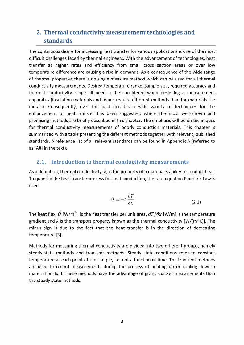
2.1. Introduction to thermal conductivity measurements As a definition, thermal conductivity, k, is the property of a material’s ability to conduct heat. To quantify the heat transfer process for heat conduction, the rate equation Fourier’s Law is used.

�̇� = −𝑘𝜕𝑇𝜕𝑥

(2.1)

The heat flux, �̇� [W/m2], is the heat transfer per unit area, 𝜕𝑇/𝜕𝑥 [W/m] is the temperature gradient and k is the transport property known as the thermal conductivity [W/(m*K)]. The minus sign is due to the fact that the heat transfer is in the direction of decreasing temperature [3].

Methods for measuring thermal conductivity are divided into two different groups, namely steady-state methods and transient methods. Steady state conditions refer to constant temperature at each point of the sample, i.e. not a function of time. The transient methods are used to record measurements during the process of heating up or cooling down a material or fluid. These methods have the advantage of giving quicker measurements than the steady state methods.

4

2.2. Steady- State methods In practice, the temperature in a steady state system is maintained by an internal heat source, typically an electrical heater. The temperature difference is determined between two points with a separation distance, x, inside the test specimen. Methods are classified by the cell geometry in which heat transfer is achieved, where axial and radial systems are most commonly used. Axial flow methods have been long established and have provided some of the most consistent results with the highest accuracy found in literature. The most commonly used method for axial system is the parallel plate apparatus (also called guarded hot plate apparatus), whereas the concentric cylinder is often used for radial systems. Steady state measuring methods can provide accurate and reliable results; however, they have the disadvantage of being time consuming.

2.2.1. Guarded hot plate

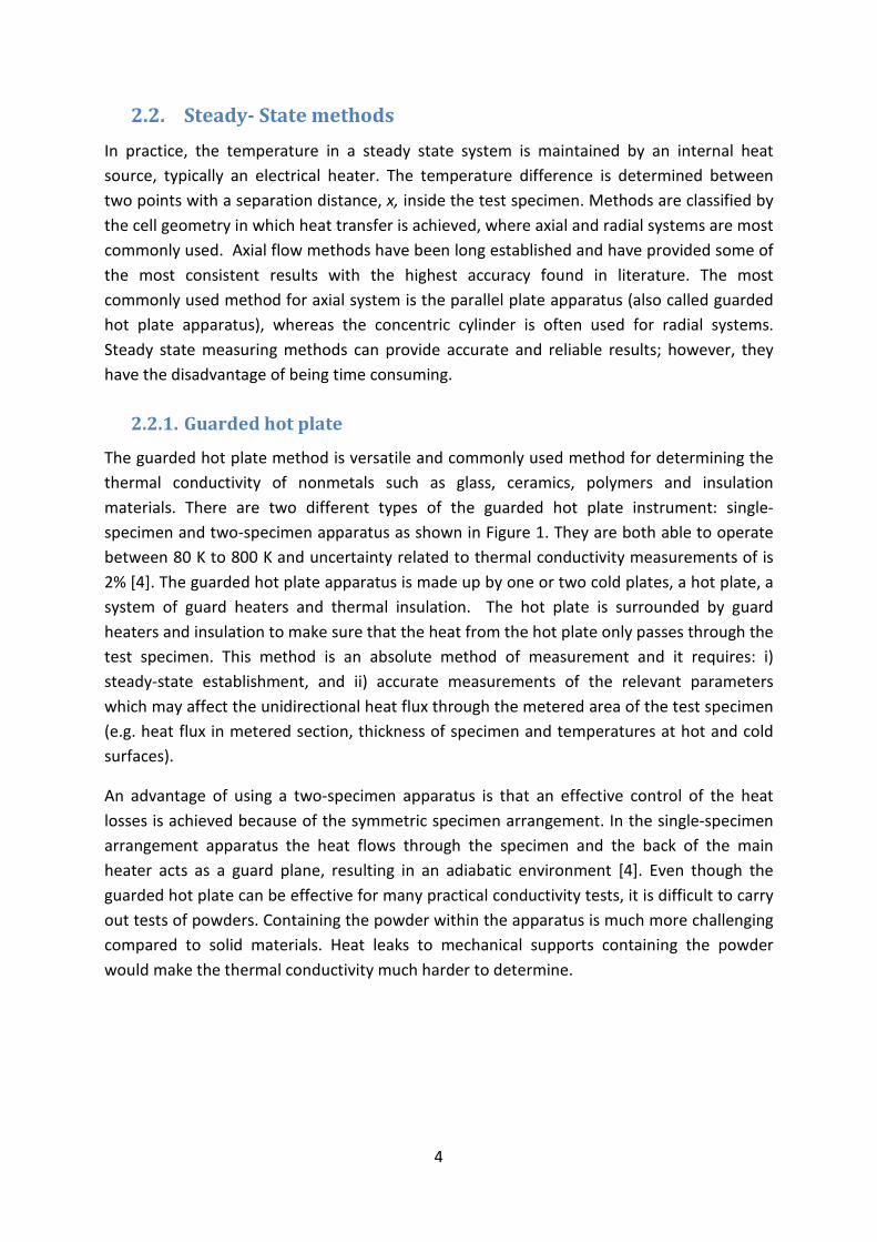
The guarded hot plate method is versatile and commonly used method for determining the thermal conductivity of nonmetals such as glass, ceramics, polymers and insulation materials. There are two different types of the guarded hot plate instrument: single- specimen and two-specimen apparatus as shown in Figure 1. They are both able to operate between 80 K to 800 K and uncertainty related to thermal conductivity measurements of is 2% [4]. The guarded hot plate apparatus is made up by one or two cold plates, a hot plate, a system of guard heaters and thermal insulation. The hot plate is surrounded by guard heaters and insulation to make sure that the heat from the hot plate only passes through the test specimen. This method is an absolute method of measurement and it requires: i) steady-state establishment, and ii) accurate measurements of the relevant parameters which may affect the unidirectional heat flux through the metered area of the test specimen (e.g. heat flux in metered section, thickness of specimen and temperatures at hot and cold surfaces).

An advantage of using a two-specimen apparatus is that an effective control of the heat losses is achieved because of the symmetric specimen arrangement. In the single-specimen arrangement apparatus the heat flows through the specimen and the back of the main heater acts as a guard plane, resulting in an adiabatic environment [4]. Even though the guarded hot plate can be effective for many practical conductivity tests, it is difficult to carry out tests of powders. Containing the powder within the apparatus is much more challenging compared to solid materials. Heat leaks to mechanical supports containing the powder would make the thermal conductivity much harder to determine.

5

Figure 1: Principle sketch of guarded hot plate methods, a) two-specimen apparatus. b) single-specimen apparatus [4]

Details for this test method and be found in the following published standards: European Standard EN 12667 [A1], International Standard ISO 8302 [A2] and ASTM C177 [A3].

2.2.2. Axial Flow Method

Axial flow methods have been long established and have provided some of the most consistent and high accuracy results reported in literature. The method is the most widely used method for thermal conductivity measurements for temperatures below 100 K due to minimal heat losses at low temperatures for this method. The axial flow method is most suitable for small specimens with thermal conductivities greater than 1 W/(m*K) and for investigations where simultaneous measurements of other transport properties are required. The key measurement issue for this method is to reduce the radial heat losses in the axial heat flow developed [5].

For this technique, a test specimen of unknown thermal conductivity is sandwiched between two reference specimens of known thermal conductivity, forming the sample column. A heater at one end of the sample column and a heat sink in the other end, creates a temperature gradient measured through the test specimen [5].

For an idealized case of perfect axial heat flow (no heat losses), the cross section of the specimen and the effective separation of temperature sensors, Δx, is of importance. The cross section can easily be found, however the determination of Δx is more complicated due to the geometrical location of the sensor position. In most cases the heat flow will not purely axial, and corrections for peripheral losses have to be made. The temperature range for the axial heat flow method is 90-1300 K where the accuracy has been determined to be between 0.5-2% [5]

Details regarding the axial flow method are found in the published standards: ASTM E 1225 [A4] and ASTM C335 [A5].

6

2.2.3. Cylinder method

The cylinder method, also referred to as the radial heat flow method, has proven to be very successful in measurements of thermal conductivity. The concept of the technique is to have heat flowing radially away from a central heater towards a heat sink, and from this measure the temperature gradient inside the system.

In most cases the apparatus consists of an electrically heated wire or cylinder placed at the central axis inside a hollow cylinder. The cylinder is typically liquid cooled. Between the cylinder wall and the heater the specimen can be filled and, if desirable, evacuated to a preferred pressure. Thermocouples are mounted in the specimen at least two radii near the mid-section of the specimen. Determining the specimen’s thermal conductivity is done by first passing a stable electric current through the core heater to generate a radial heat flow outwards. This establishes a temperature difference between the thermocouples placed in the specimen. When steady state is reached, the temperature measurements at the thermocouples are recorded.

Ideally, a uniform heat flux in the radial direction should be generated in the concentric cylinder apparatus. However, heat losses to the top and bottom will affect temperature gradients in the specimen. These heat losses are challenging to avoid, especially if the conductivity of the specimen is low. Therefore, a key element for a concentric cylinder apparatus design is to make the cylinder long with respect to the cylinder radius. This allows for a fairly uniform temperature profile to be established in the mid-section of the cylinder, where measurements are done. However, heat losses to the top and bottom of the cylinder should still be minimized or one should at least be able to determine the magnitude of the losses. The main advantages of the cylinder method are that the system can be operated with relatively simple instrumentation as well as the wide range of applicability on specimens with both high and low thermal conductivities. The greatest disadvantage however, is that to be able to get as accurate measurements as possible, large specimen sizes should be used. This can be costly and also requires longer running time to reach steady state conditions. [5]

The cylinder method can be used for temperatures in the range of 4 K to 1000 K, and achievable uncertainty for the thermal conductivity measurements of 2% [4].

7

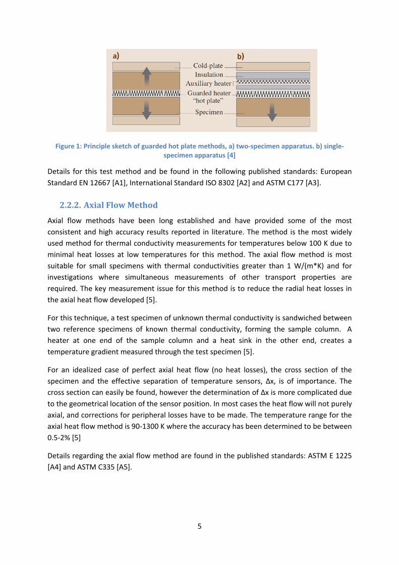
Figure 2 illustrates the basic components used for the cylinder method. It also shows what the temperature profile would look like for a cross-section of the apparatus.

Figure 2: Basic elements for the cylinder method and the temperature profile of a cross section

No standard for the cylinder method has been found. However, the International Standard ISO 8497 [A6] covers relevant performance requirements and test procedure which can be used for the cylinder method.

2.2.4. Heat flow meter method

The basic idea for the heat flow meter method is to determine the heat flux by measuring the temperature difference across a thermal resistor during steady-state conditions. The design of the heat flow meter method is quite similar to the single-specimen guarded hot plate apparatus, with the difference that the main heater is exchanged with a heat flux sensor. Heat flux sensors are thermal resistors with a series of thermocouples. In some cases a heat flux sensor is placed at the cold plate to determine radial losses and reduce the time duration of measurements. The method is mostly used for polymers and insulation materials where the thermal conductivity is less than 0.3 W/(m*K) and an uncertainty of 3% can be accomplished [4]. However, if losses in radial direction are present the uncertainty increases rapidly.

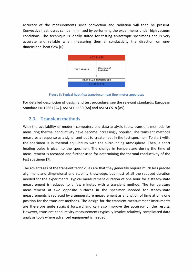
The conventional heat flow meter method assumes one-dimensional conduction for heat transfer, i.e. no convection or radiation present. This assumption is reasonable if the test specimen is thin in the direction of heat flow and has a large cross-section area. The surface area for convection and radiation becomes negligible compared to the conductive heat transfer through the specimen and the method is suited for materials with low thermal conductivity. However, for materials with high thermal conductivity, a thicker test specimen is required to be able to measure the temperature difference. This results in doubt of the

8

accuracy of the measurements since convection and radiation will then be present. Convective heat losses can be minimized by performing the experiments under high vacuum conditions. The technique is ideally suited for testing anisotropic specimens and is very accurate and reliable when measuring thermal conductivity the direction on one-dimensional heat flow [6].

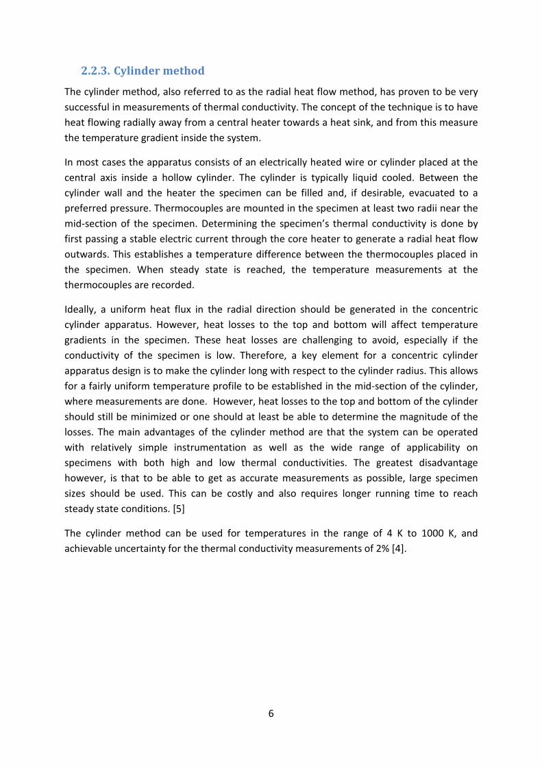
Figure 3: Typical heat flux transducer heat flow meter apparatus

For detailed description of design and test procedure, see the relevant standards: European Standard EN 12667 [A7], ASTM E 1530 [A8] and ASTM C518 [A9].

2.3. Transient methods With the availability of modern computers and data analysis tools, transient methods for measuring thermal conductivity have become increasingly popular. The transient methods measures a response as a signal sent out to create heat in the test specimen. To start with, the specimen is in thermal equilibrium with the surrounding atmosphere. Then, a short heating pulse is given to the specimen. The change in temperature during the time of measurement is recorded and further used for determining the thermal conductivity of the test specimen [7].

The advantages of the transient techniques are that they generally require much less precise alignment and dimensional and stability knowledge, but most of all the reduced duration needed for the experiments. Typical measurement duration of one hour for a steady-state measurement is reduced to a few minutes with a transient method. The temperature measurement at two opposite surfaces in the specimen needed for steady-state measurements is replaced by a temperature measurement as a function of time at only one position for the transient methods. The design for the transient measurement instruments are therefore quite straight forward and can also improve the accuracy of the results. However, transient conductivity measurements typically involve relatively complicated data analysis tools where advanced equipment is needed.

9

2.3.1. Hot wire method

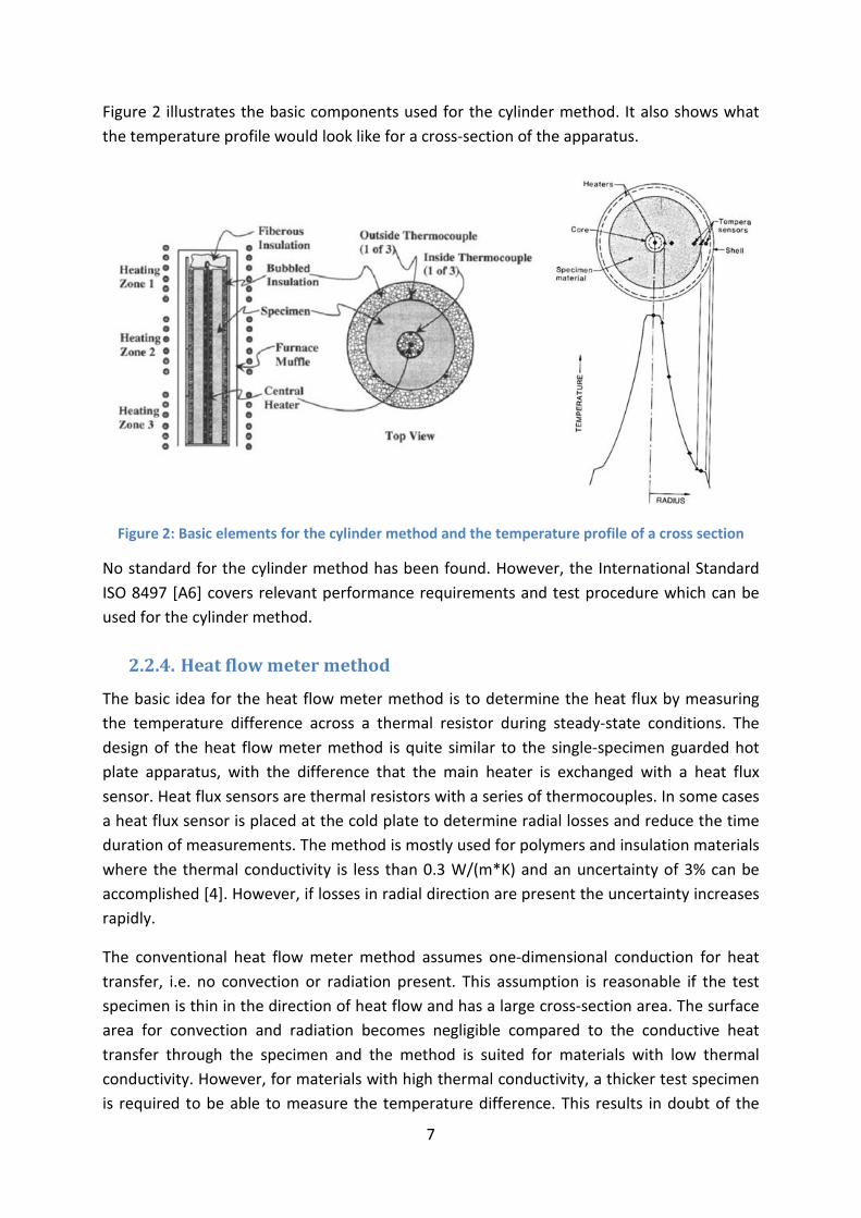
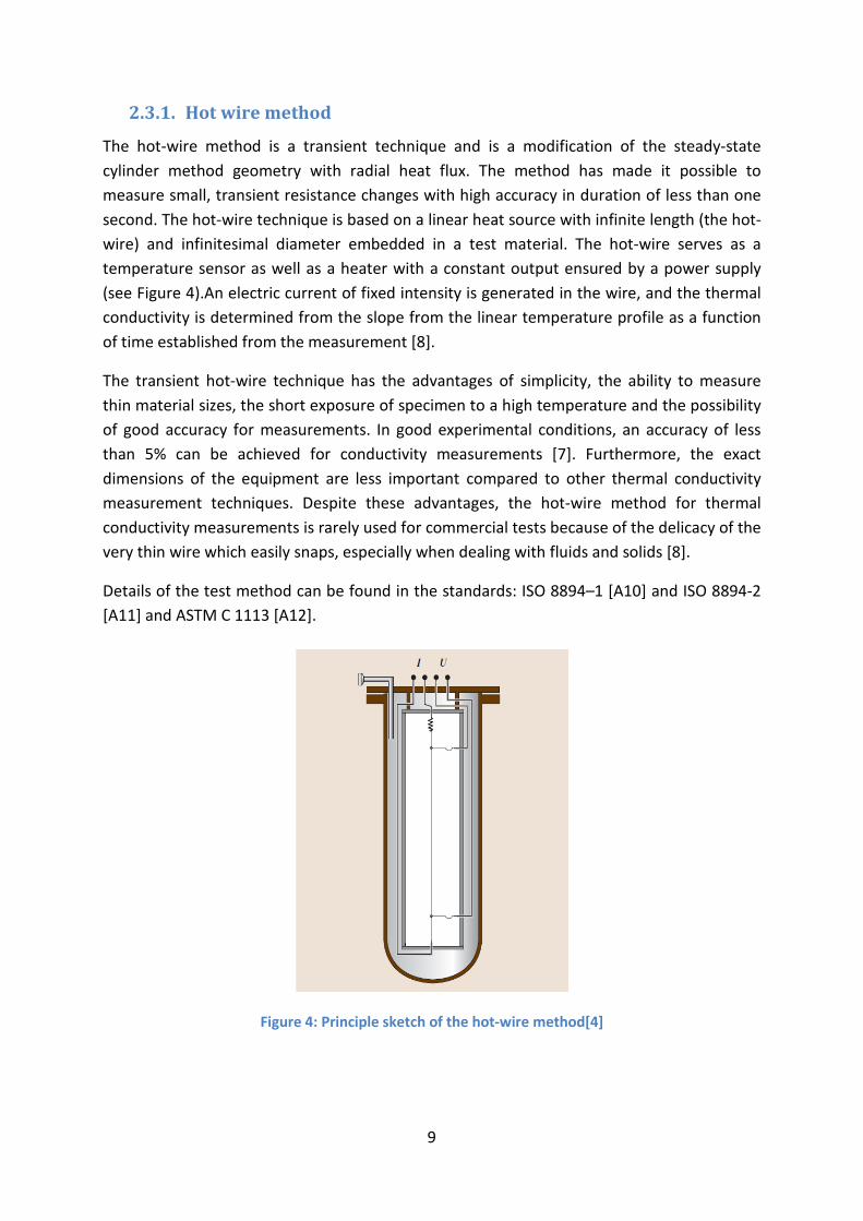
The hot-wire method is a transient technique and is a modification of the steady-state cylinder method geometry with radial heat flux. The method has made it possible to measure small, transient resistance changes with high accuracy in duration of less than one second. The hot-wire technique is based on a linear heat source with infinite length (the hot-wire) and infinitesimal diameter embedded in a test material. The hot-wire serves as a temperature sensor as well as a heater with a constant output ensured by a power supply (see Figure 4).An electric current of fixed intensity is generated in the wire, and the thermal conductivity is determined from the slope from the linear temperature profile as a function of time established from the measurement [8].

The transient hot-wire technique has the advantages of simplicity, the ability to measure thin material sizes, the short exposure of specimen to a high temperature and the possibility of good accuracy for measurements. In good experimental conditions, an accuracy of less than 5% can be achieved for conductivity measurements [7]. Furthermore, the exact dimensions of the equipment are less important compared to other thermal conductivity measurement techniques. Despite these advantages, the hot-wire method for thermal conductivity measurements is rarely used for commercial tests because of the delicacy of the very thin wire which easily snaps, especially when dealing with fluids and solids [8].

Details of the test method can be found in the standards: ISO 8894–1 [A10] and ISO 8894-2 [A11] and ASTM C 1113 [A12].

Figure 4: Principle sketch of the hot-wire method[4]

10

2.3.2. Needle probe

The needle probe method, also referred to as the Line-Source Method, is a variant of the hot wire method and is capable of very fast measurements. It is suitable for both melt and solid-state thermal conductivity measurements; however, it is not suited for directional solid-state property measurements in anisotropic materials [9].

A needle probe is located at the center of the test specimen, both kept at constant initial temperature. When running experiments, a known amount of heat is produced in the needle, creating a heat wave which propagates radially in the specimen. The temperature rise in the probe varies linearly with the logarithm of time, and this relationship can be used directly to calculate the thermal conductivity of the test specimen. Small test samples makes it possible to subject the samples to a wide variety of test conditions; the method can cover a temperature range from 233 K to 673 K on materials with thermal conductivity between 0.08 to 2 W/(m*K). However, the standard for this test method, ASTM D 5930 [A13], does not contain numerical precision and bias statement and therefore it should not be used as a reference test method in case of dispute [10].

2.3.3. Transient plane source method

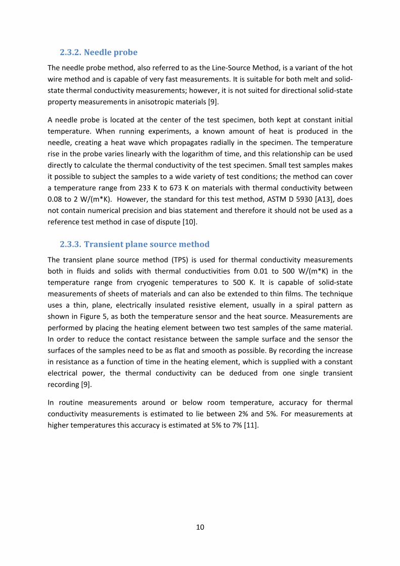
The transient plane source method (TPS) is used for thermal conductivity measurements both in fluids and solids with thermal conductivities from 0.01 to 500 W/(m*K) in the temperature range from cryogenic temperatures to 500 K. It is capable of solid-state measurements of sheets of materials and can also be extended to thin films. The technique uses a thin, plane, electrically insulated resistive element, usually in a spiral pattern as shown in Figure 5, as both the temperature sensor and the heat source. Measurements are performed by placing the heating element between two test samples of the same material. In order to reduce the contact resistance between the sample surface and the sensor the surfaces of the samples need to be as flat and smooth as possible. By recording the increase in resistance as a function of time in the heating element, which is supplied with a constant electrical power, the thermal conductivity can be deduced from one single transient recording [9].

In routine measurements around or below room temperature, accuracy for thermal conductivity measurements is estimated to lie between 2% and 5%. For measurements at higher temperatures this accuracy is estimated at 5% to 7% [11].

11

Figure 5: Heating/sensor element used for TSP [11] Details regarding the design and test procedure for the TSP method can be found in the International Standard ISO 22007-2 [A14].

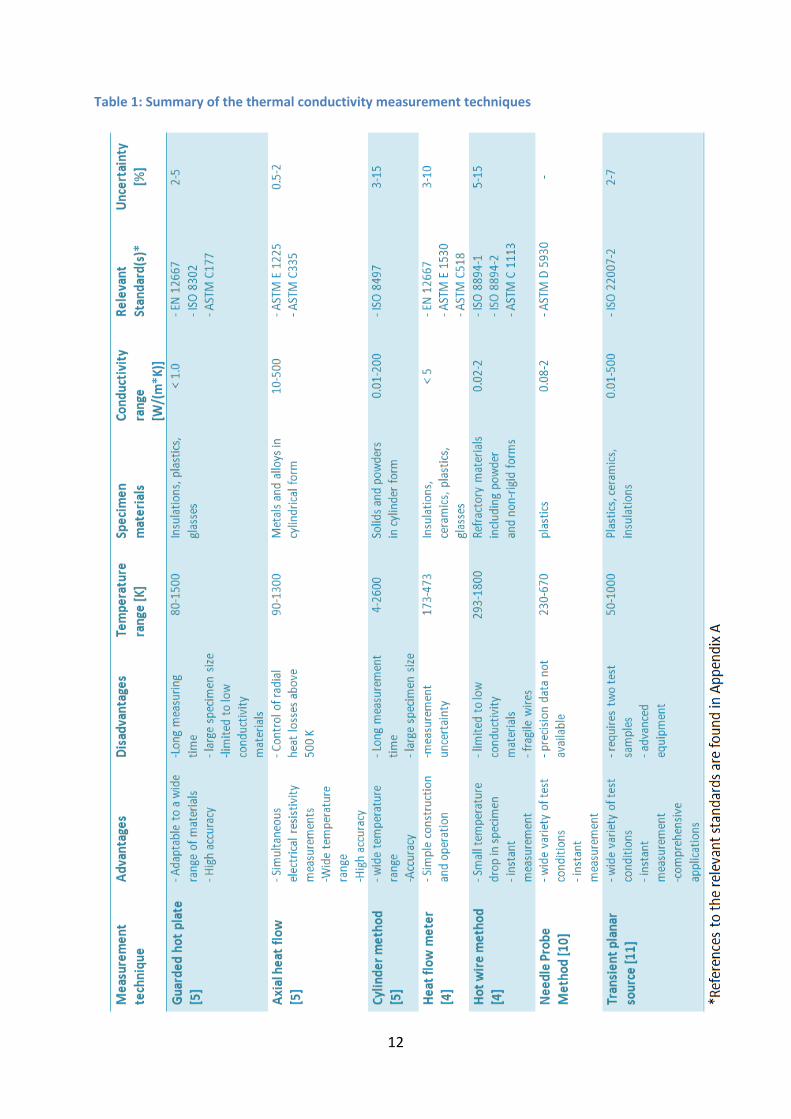
2.4. Summary thermal conductivity measurement techniques The general concepts of the relevant thermal conductivity measurement techniques have been described in the precious sections. A comparison of the techniques in terms of advantages, disadvantages, uncertainties and other relevant parameters is included in Table 1. The table also includes relevant standards related to each of the methods.

The steady state methods presented have long been establish and has provided some of the most consistent and accurate results reported in literature. Heat flow in the axial direction dominates these techniques, where the guarded hot plate method is the most versatile and commonly used method. However, when dealing with porous materials such as powders, the axial methods causes limitations. Radial heat transfer methods, such as the cylinder method, could solve this challenge. To minimize axial heat losses for such methods, infinite long test section is required. All the steady state methods have the disadvantage of being quite time consuming. Uncertainties in the range of 2-10% are most likely to be achieved when using any of these methods.

Transient measurement methods are results of the computers and data analysis tools for thermal conductivity measurements. These methods’ greatest advantage is the reduced duration required for experiments. Also much less precise alignment and stability knowledge is needed. Porous materials with very low thermal conductivities can be examined over a wide temperature range and an uncertainty range of 2-15% is expected for these methods. Despite these advantages, some of the transient methods often require complicated analysis tools and also very delicate measurement instruments, which could make the methods undesirable, especially when dealing with fluids and solids.

12

Table 1: Summary of the thermal conductivity measurement techniques

13

3. Apparatus concept

3.1. Choice of Concept: Goal and limitations The overall goal of the development of a new and improved test facility is to better be able to determine the thermal conductivity of porous materials. Since materials to be tested are typically low-conductivity materials, quantitative determination of areas of concern is of great interest.

When deciding on the concept for the new conductivity apparatus several limitations restricted the possibilities. As mentioned in Section 1.1, it was desirable to further develop the existing measurement facility already in use in the laboratory at NTNU to reduce costs of new equipment as well as having results to compare with. Steady state tests were desirable, which precluded any of the transient methods introduced in Chapter 2. Other general limitations also had to be taken into account when choosing on the concept:

• Test specimen available • Specimens to be tested are powders • Liquid nitrogen available for cooling • Gas tight container to be able to carry out tests with different gases and vacuum

conditions • Improved accuracy

The main limitation was the availability of the test specimen. The amount of the material developed at the University in Dresden (mentioned in Section 1.2) is only available in 0.1 L. Since the materials to be investigated are mainly powders, an apparatus which easily could handle this challenge was important. Also, cryogenic temperature tests are to be carried out, which restricted the choice of concept even further. Even though the cylinder method in Section 2.2.3 emphasized the disadvantage of the need for large specimen sizes, it was decided to go forward with such a method since this method can deal with most of the requirements specified. However, to compensate for the specimen size, good insulation solutions need to be implemented to minimize axial heat losses in the apparatus.

14

3.2. Theoretical Basis Cylindrical systems often experience temperature gradients in the radial direction and can therefore be treated as one dimensional. Under steady state conditions such systems can be analyzed by the standard method, which starts out with the right form of Fourier’s Law (Equation 2.1). For cylindrical coordinates, this equation becomes [3]:

𝑄 = −𝑘𝐴𝑑𝑇𝑑𝑟

= −𝑘(2𝜋𝑟ℎ)𝑑𝑇𝑑𝑟

(3.1)

here Q is the heat flow, A=2πrh is the area normal to the direction of heat transfer where r and h are the radius and height, dT is the temperature difference and dr is the difference in radial positions related to the temperature positions. k is the thermal conductivity. An integration of this equation results in the following expression for the heat transfer rate:

𝑄 =

2𝜋ℎ𝑘(𝑇1 − 𝑇2)

𝑙𝑛(𝑟2𝑟1)

(3.2)

By rearranging, the thermal conductivity is expressed as:

𝑘 =𝑄𝑙𝑛(𝑟2𝑟1

)

2𝜋ℎ(𝑇1 − 𝑇2)

(3.3)

These equations will be used for determination of the deviations in thermal conductivity calculations during the design analysis in Chapter 4.

It is worth mentioning that when dealing with materials such as powders, the term “Effective thermal conductivity”, ke, is of importance. The effective thermal conductivity is a combined property of a powder and an interstitial gas. Several models and correlations have been proposed for the prediction of the effective thermal conductivity and a selection of these correlations can be found in the project thesis completed in advance on this thesis (see description of the thesis in the following section). The thermal conductivity of the specimen chosen for the analysis in the following chapters is assumed to be the effective thermal conductivity.

15

3.3. Previous work Since the startup of the development project introduced in Section 1.2, several attempts to develop a test apparatus and executing experiments have been completed at NTNU. The background for this thesis is based on the work performed by Ole Kristoffer Abrahamsen [12] and Jeremy Gauthier [13] in the master thesis and project thesis, respectively. As well, a project thesis was completed in the advance of this thesis [14].

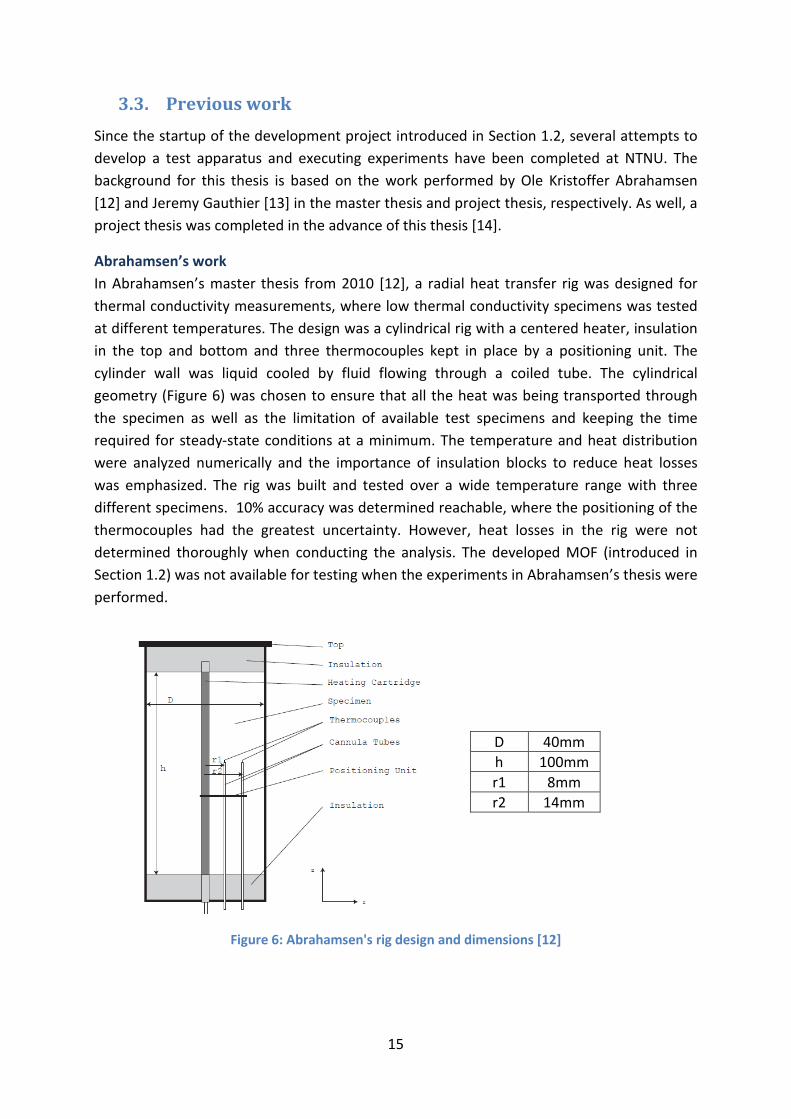
Abrahamsen’s work In Abrahamsen’s master thesis from 2010 [12], a radial heat transfer rig was designed for thermal conductivity measurements, where low thermal conductivity specimens was tested at different temperatures. The design was a cylindrical rig with a centered heater, insulation in the top and bottom and three thermocouples kept in place by a positioning unit. The cylinder wall was liquid cooled by fluid flowing through a coiled tube. The cylindrical geometry (Figure 6) was chosen to ensure that all the heat was being transported through the specimen as well as the limitation of available test specimens and keeping the time required for steady-state conditions at a minimum. The temperature and heat distribution were analyzed numerically and the importance of insulation blocks to reduce heat losses was emphasized. The rig was built and tested over a wide temperature range with three different specimens. 10% accuracy was determined reachable, where the positioning of the thermocouples had the greatest uncertainty. However, heat losses in the rig were not determined thoroughly when conducting the analysis. The developed MOF (introduced in Section 1.2) was not available for testing when the experiments in Abrahamsen’s thesis were performed.

Figure 6: Abrahamsen's rig design and dimensions [12]

D 40mm h 100mm r1 8mm r2 14mm

16

Gauthier’s work Gauthier [13] followed up on Abrahamsen’s work with the thermal conductivity rig and by adding a few adjustments he wanted to achieve more accurate results. He implemented two additional thermocouples: one at the entrance of the cooling tube, and in addition, he moved the other cooling tube thermocouple to the outlet. The second one was used for measuring the ambient temperature, as shown in Figure 7. Gauthier’s experiments were carried out in the same manner as Abrahamsen did, but Gauthier had improved cooling facilities and also the MOF. Gauthier completed a more detailed uncertainty analysis, especially with concern to the heat losses in the test rig. His uncertainty analysis showed uncertainties of roughly 20%.

Figure 7: Gauthier's experimental test setup [13]

Project thesis In advance of this thesis a project work [14] was completed as well. Both tests with the existing rig and an analysis of an improved apparatus design were commenced. The laboratory tests were carried out with a metal foam structure in the cylinder to increase heat transfer in the system. By implementing such structures the readings had great deviations due to the uncertain positioning of the thermocouples. The possibility of thermocouples being in direct contact with the metal structure lead to doubts in the credibility of the tests as well. Therefore, a model of an improved test setup was started. However, analyzes did not provide enough information for the determination of the areas of concern. Thus, the desire to continue develop and analyze an improved apparatus was a basis for this thesis.

17

3.4. Delimitations for the new apparatus design A number of delimitations have been set for the development process. First, only cryogenic temperatures will be investigated. The temperature differences in apparatus and the ambient will have the greatest value at such temperatures, which will result in the largest heat losses. These heat losses were important identify. The system developed could be used for higher temperatures as well, but this not investigated in this thesis. Secondly, a test specimen of only one set thermal conductivity has been investigated, 0.05 W/(m*K). The apparatus will be capable of completing tests with materials with other thermal conductivities, however, the conductivity of the investigated specimen is assumed to be of the lowest value tested. Finally, only one insulation material in the test section has been investigated. This insulation has been assumed to have the lowest thermal conductivity achievable for the required conditions during testing.

18

19

4. Thermal design: development and analysis In the following sections, the development process for the thermal design of the test apparatus will step-wise be described and analyzed. As a starting point, a simple design of a test cylinder will be presented. As the process proceeds, all elements required to achieve the assigned requirements will be implemented and analyzed. Lastly, concluding remarks from the development process will be presented to summarize the overall results from the analyses. All material references are found in Appendix B (referred to as [B#] in the text).

4.1. Introduction As mentioned in Section 1.1, one of the main objectives of this thesis is to further develop a measurement facility for thermal conductivity already existing at NTNU EPT. In the project work completed in advance of this master thesis [14], the suggested design showed great errors and challenges, which lead to doubts on whether or not this design could be used. However, as the modeled apparatus was further investigated as a starting point for this thesis, the cause of errors was discovered. The errors were corrected and by running new simulations, promising behavior was revealed after all. Even though the design from the project work was quite simplified and essential components were not included in the model, the model has still been chosen as a starting point for the further development of the proposed apparatus in this thesis.

4.2. Design and analysis tool: Comsol Multiphysics 4.2 Due to the complexity of the apparatus design the use of only theoretical considerations is unlikely to provide a complete and realistic behavior of the heat transfer in the system. Thus, numerical investigations are expected to provide a more realistic representation of the heat transfer, and additionally, the results will be presented graphically. The software Comsol Multiphysics 4.2 has been used for designing the test rig as well as for doing simulations to generate data for numerical calculations. Comsol Multiphysics can model and analyze a wide variety of scientific and engineering problems such as fluid dynamics, electromagnetics, and heat transfer, where the latter has been implemented for the simulations in this thesis. When solving models, Comsol uses the Finite Element Method (FEM) [15] and it runs the finite element analysis together with adaptive meshing and error control using a variety of numerical solvers [16].

The problem to be solved is the determination of the effects to change in heat transfer caused by implemented components required for thermal conductivity measurement. Quantifying heat losses, determining heat flux propagations as well as assurance of accurate temperature recordings will be emphasized throughout the development process.

The Heat Transfer Module in Comsol Multiphysics 4.2 has been implemented to all the models to be able to evaluate how the temperature distribution in the system develops, how heat fluxes propagate and where the areas of concern are located. The heat transfer module

20

supports all fundamental mechanisms of heat transfer, including radiative, conductive and convective heat transfer. A wide variety of physics interfaces can be applied to the heat transfer module, and the “Heat transfer in Solids” interface has consistently been applied to models in the following sections. For the heat transfer modules, the fundamental law governing is the first law of thermodynamics, written in terms of temperature, T, from equation 2.1:

𝜌𝐶𝑝𝜕𝑇𝜕𝑡

+ 𝜌𝐶𝑝𝐮 ∙ ∇T = ∇ ∙ (𝑘∇T) + 𝑄∗

(4.1)

where

• ρ is the density [kg/m3] • Cp is the specific heat capacity at constant pressure [J/(kg·K)] • T is absolute temperature [K] • u is the velocity vector [m/s] • k is the thermal conductivity [W/(m·K)] • Q* is a heat source (or sink) [W/m3]

If the velocity vector is set to zero, the governing equation for pure conductive heat transfer becomes:

𝜌𝐶𝑝𝜕𝑇𝜕𝑡

+ ∇ ∙ (−𝑘∇𝑇) = 𝑄∗

(4.2)

which is the equation Comsol uses when running simulations. The simulations carried out are used to gather useful information for the analyses of the developing design in the next chapter. Temperature profiles will provide an overall picture of dispersion of heat generation whereas heat flux graphs give more detailed information of undesirable changes as the system becomes more complex. Gathered temperatures from specified locations in the test section are used to determine the thermal conductivity measurement error for the proposed design as well as estimating the uncertainty related to heat losses for the conducted uncertainty analysis in Chapter 6.

21

4.3. Investigation and design of the new test apparatus First, a brief introduction of the new concept will describe the features of the apparatus. Following, investigations of heat transfer as the complexity of the apparatus increases will be presented graphically and carefully analyzed.

4.3.1. Basic idea of the new concept

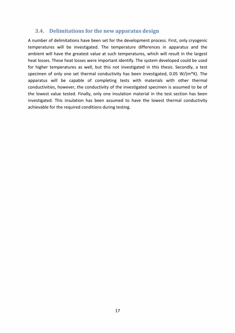
The concept of the new test apparatus is based on the cylinder method as stated in Section 3.1. The major difference to the previous designs is the implementation of a sealed container surrounding the test cylinder, this to be able to establish different pressure conditions in the system. The choice of a sealed container is mainly due to simplicity and practical reasons. This way, preparations for tests can be completed before placing a container lid around the test cylinder, creating a gas tight environment inside the sealed container. Placing the test cylinder on top of the base plate of the container, which will be at ambient temperatures, requires the cylinder to be isolated from the base plate. If not, heat will flow from the base plate and into the test section which will lead to an undesirable temperature increase in the test section. To solve this challenge, the test cylinder will be placed on top of an insulation block, establishing isolation from the base plate.

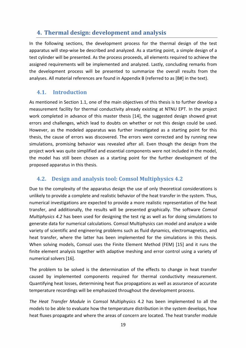
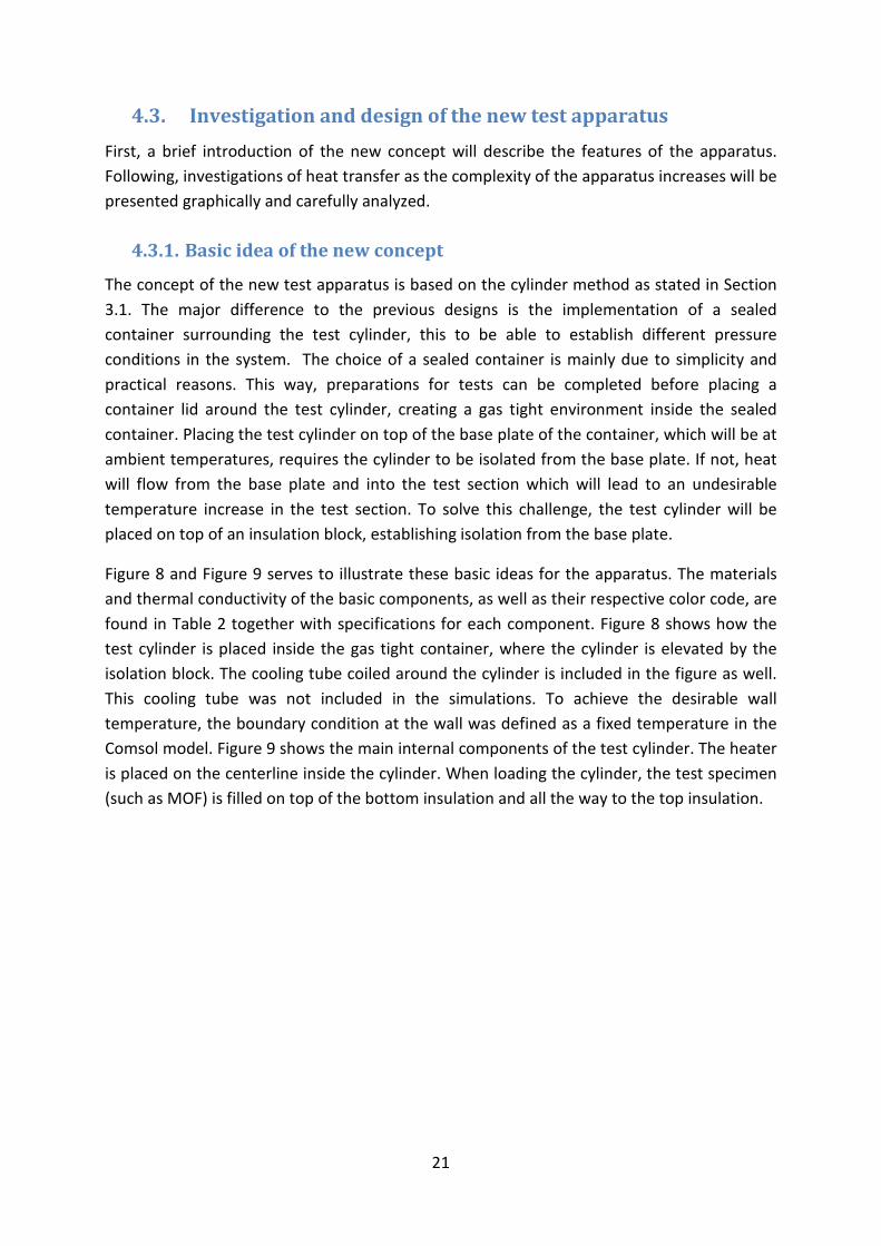
Figure 8 and Figure 9 serves to illustrate these basic ideas for the apparatus. The materials and thermal conductivity of the basic components, as well as their respective color code, are found in Table 2 together with specifications for each component. Figure 8 shows how the test cylinder is placed inside the gas tight container, where the cylinder is elevated by the isolation block. The cooling tube coiled around the cylinder is included in the figure as well. This cooling tube was not included in the simulations. To achieve the desirable wall temperature, the boundary condition at the wall was defined as a fixed temperature in the Comsol model. Figure 9 shows the main internal components of the test cylinder. The heater is placed on the centerline inside the cylinder. When loading the cylinder, the test specimen (such as MOF) is filled on top of the bottom insulation and all the way to the top insulation.

22

Table 2: The basic components: materials, thermal conductivity and color code

Component Material Thermal Conductivity [W/(m*K)]

Color code

Cylinder wall Stainless Steel 15 [B1] Dark grey Top and bottom plate of cylinder

Stainless Steel 15 Light grey

Heating element Stainless Steel 15 Red Insulation top, bottom Insulation 0.01 Green Isolation block Teflon 0.24 [B2] Yellow Cooling tube Stainless Steel 15 Light blue

As the design and analysis process progressed, certain parameters were kept constant:

• All components made of stainless steel were assigned with a thermal conductivity of 15 W/(m*K). Thermal conductivity of steel changes with temperature, but the value of 15 W/(m*K) was chosen since most literature showed that the conductivity at the desirable temperatures was in the range of +- 5 of this value.

• The temperature at the cooling wall was kept at 77.3 K (evaporation temperature of liquid Nitrogen at 0.1 MPa [17]).

• The heat generated from the heating elements was set to 1 W. • The temperature at the bottom of the base plate was kept at 293 K.

Figure 9: Sealed container illustrating the main components of the test cylinder

Figure 8: Sealed container concept with cooling pipe

23

4.3.2. Validating radial heat transfer

As a starting point for the design development, verifying radial heat transfer through the test specimen was of interest. A simple system containing the heater, the cylinder wall and the specimen was constructed in Comsol, as shown in Figure 11. Here, the top and bottom part of the model was thermally insulated to prevent heat leakages. The blue part of this figure illustrates the test specimen filled in the sample cylinder. The thermal conductivity of the test specimen was set to 0.05 W/(m*K). This value is assumed to be the lowest conductivity of materials to be tested in the apparatus in future work. The heating element was constructed as a hollow cylinder with a wall thickness of 0.5 mm, where a heat flux on the inner wall was selected to enforced radial heat flow and also to minimize heat generation at ends of the heater.

This sample cylinder is the main part of the rig developed in this thesis. The heater and specimen dimensions, as shown in Figure 10, was kept constant through all further steps of implementing additional components unless something else is specified.

Table 3: Specifications for the test section

Component Material Thermal conductivity [W/(m*K)]

Color code

Heating element Stainless Steel 15 Red Cylinder wall Stainless Steel 15 Dark grey

Test specimen Powder 0.05 Blue

Figure 10: Sample cylinder Figure 11: Dimensions of test section [mm]

24

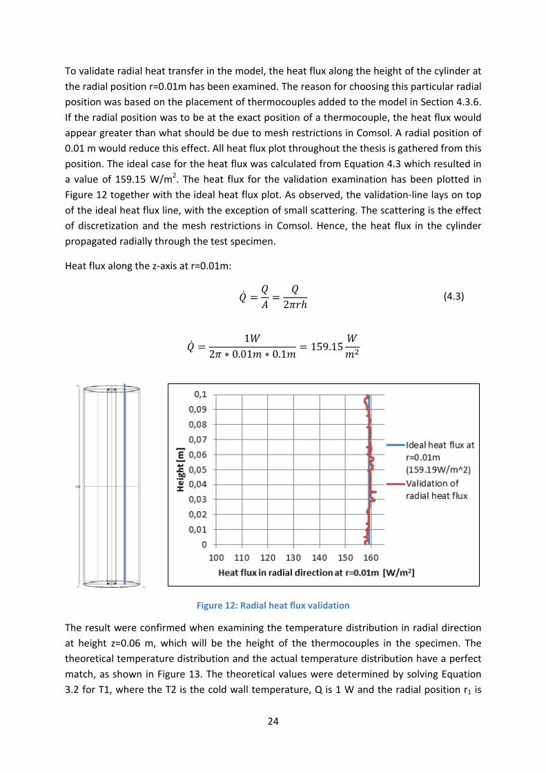
To validate radial heat transfer in the model, the heat flux along the height of the cylinder at the radial position r=0.01m has been examined. The reason for choosing this particular radial position was based on the placement of thermocouples added to the model in Section 4.3.6. If the radial position was to be at the exact position of a thermocouple, the heat flux would appear greater than what should be due to mesh restrictions in Comsol. A radial position of 0.01 m would reduce this effect. All heat flux plot throughout the thesis is gathered from this position. The ideal case for the heat flux was calculated from Equation 4.3 which resulted in a value of 159.15 W/m2. The heat flux for the validation examination has been plotted in Figure 12 together with the ideal heat flux plot. As observed, the validation-line lays on top of the ideal heat flux line, with the exception of small scattering. The scattering is the effect of discretization and the mesh restrictions in Comsol. Hence, the heat flux in the cylinder propagated radially through the test specimen.

Heat flux along the z-axis at r=0.01m:

�̇� =𝑄𝐴

=𝑄

2𝜋𝑟ℎ (4.3)

�̇� =1𝑊

2𝜋 ∗ 0.01𝑚 ∗ 0.1𝑚= 159.15

𝑊𝑚2

Figure 12: Radial heat flux validation

The result were confirmed when examining the temperature distribution in radial direction at height z=0.06 m, which will be the height of the thermocouples in the specimen. The theoretical temperature distribution and the actual temperature distribution have a perfect match, as shown in Figure 13. The theoretical values were determined by solving Equation 3.2 for T1, where the T2 is the cold wall temperature, Q is 1 W and the radial position r1 is

25

varied. The two black points of the graph illustrates the radial position of the thermocouples to be implemented. From these examinations it was safe to conclude that the 1 W generated from the heater propagates radially in the test specimen when no heat losses were taken into account.

Figure 13: Temperature distribution in radial direction for the validation of radial heat transfer

26

4.3.3. Influence of insulation in top and bottom of the sample cylinder

Results from the previous section confirmed that the heat propagates radially in the cylinder and key elements needed for the setup could then be added. Since low thermal conductivity specimens are to be examined in the apparatus, insulation in both the top and bottom of the sample cylinder will be of great importance to minimize heat losses. The ideal case would be to implement insulation blocks having extremely low thermal conductivity (>0.001W/(m*K)), such as Multi-Layer Insulations. However, such insulations can be difficult to customize and manufacture for the purpose in this setup. As well, there is a great uncertainty related to the behavior of such insulations when evacuating the system to vacuum conditions. In agreement with the supervisor, it was decided that the lowest thermal conductivity possible to achieve for the insulation for use in the top and bottom of the sample cylinder would be 0.01 W/(m*K).

The insulation blocks were placed at the top and bottom of the heater and test specimen. When deciding on dimensions, it was of importance to achieve minimal heat losses. Additionally, the required amount of cooling liquid for the walls was taken into account. Insulation blocks with thickness of 1 cm and 3 cm where investigated. Top and bottom plates of stainless steel with thickness of 0.5 cm, were added to the model as well, c.f. Figure 14.

Figure 14: 1 cm insulation blocks and 3 cm insulation blocks

Table 4: Specifications for the sample cylinder: plates and insulation

Component Material Thermal conductivity [W/(m*K)] Color code Top and bottom

insulation Insulation 0.01 Green

Top and bottom plate of cylinder Stainless Steel 15 Light grey

27

When evaluating the heat flux plot in Figure 15, it is observed that there is not a great difference for the two cases. The heat flux plot for the case where the insulation thickness is 3 cm shows slightly better values compared to the 1 cm case. Extracting the exact heat flux value at height z=0.06 m showed a value of 156.36 W/m2 for the 1 cm case and 157.77 W/m2 for the 3 cm case. The latter case only deviates 0.9% from the ideal heat flux of 159.15 W/m2.

Figure 15: Heat flux plot for insulation blocks

Analyses of the heat losses to the top and bottom of the cylinder, as well as checking the error of thermal conductivity measurement of the specimen by doing a backward calculation, were conducted. A surface integration of the top and the bottom of the test section in the Comsol model was performed to evaluate the heat losses. The thermal conductivity calculation was conducted by using Equation 3.3, where T1 and T2 were retrieved from the model. Radial positions of r1= 3.2 mm and r2= 20 mm (heater wall and cylinder wall) and the height of z=0.06 m are used for all such calculations throughout this chapter unless specified otherwise. The result showed that the thermal conductivity of the specimen was calculated to be 0.0507 W/(m*K) and 0.0506 W/(m*K) for the 1 cm and 3 cm case, respectively. The percentage deviation from the specified conductivity of 0.05W/(m*K) is presented in Table 5, together with the percentage heat loss.

28

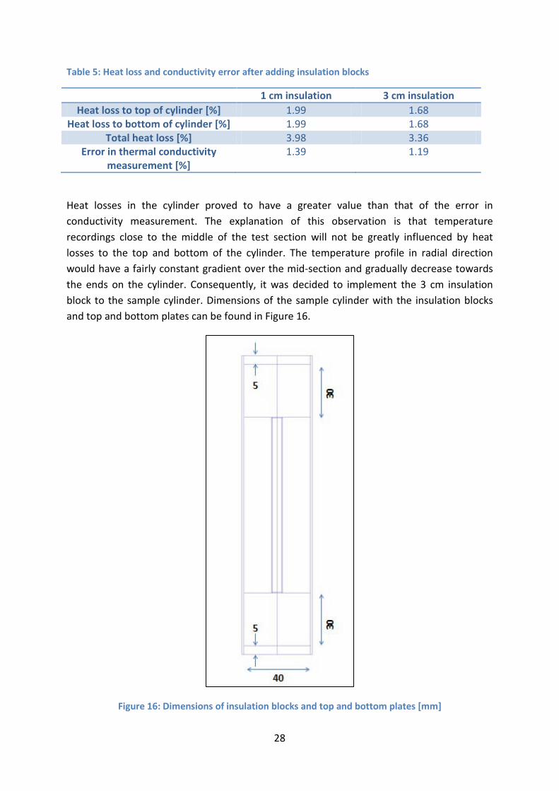
Table 5: Heat loss and conductivity error after adding insulation blocks

1 cm insulation 3 cm insulation Heat loss to top of cylinder [%] 1.99 1.68

Heat loss to bottom of cylinder [%] 1.99 1.68 Total heat loss [%] 3.98 3.36

Error in thermal conductivity measurement [%]

1.39 1.19

Heat losses in the cylinder proved to have a greater value than that of the error in conductivity measurement. The explanation of this observation is that temperature recordings close to the middle of the test section will not be greatly influenced by heat losses to the top and bottom of the cylinder. The temperature profile in radial direction would have a fairly constant gradient over the mid-section and gradually decrease towards the ends on the cylinder. Consequently, it was decided to implement the 3 cm insulation block to the sample cylinder. Dimensions of the sample cylinder with the insulation blocks and top and bottom plates can be found in Figure 16.

Figure 16: Dimensions of insulation blocks and top and bottom plates [mm]

29

4.3.4. Isolating the sample cylinder from base plate of sealed container

As mentioned in Section 4.3.1, the sample cylinder is to be placed on top of a base plate made out of steel, which also serves as the bottom of the gas tight container. This base plate will have ambient temperatures. Since the diameter of the base plate is much greater than the diameter of the cylinder, heat would be transferred from the base plate and into the test section of the sample cylinder. To prevent this from happening, a Teflon (insulation material) block was placed between the base plate and the sample cylinder, isolating the cylinder from the base plate, illustrated in Figure 17. Specifications for the two components are found in Table 6. Due to the fact that Teflon has a much lower thermal conductivity compared to stainless steel, the purpose of the Teflon block is to minimize impact of heat transfer from the base plate.

Figure 17: Isolation block and base plate

Table 6: Specifications for isolation block and base plate

Component Material Thermal conductivity [W/(m*K)] Color code Elevation insulation Teflon 0.24 Yellow

Base plate Stainless Steel 15 Purple

When analyzing the results from the simulations it was discovered that there is no influence of additional heat transfer from the base plate and into the test section after implementing the base plate and isolation block. The heat flux plot in radial direction appeared identical to the plot in Figure 15 and thermal conductivity calculations showed no changes. Figure 18 shows the temperature distribution of a cross section of the rig. Results from the analysis were verified from this figure, where it is seen that even though the base plate has a much higher temperature compared to the sample cylinder, the bottom plate of the cylinder is kept cold by the cylinder wall, preventing a heat leakage into the test section. Another important issue related to the isolation block is the cooling capacity of liquid nitrogen. If the isolation block is too small, greater amounts of liquid nitrogen is required to prevent heat

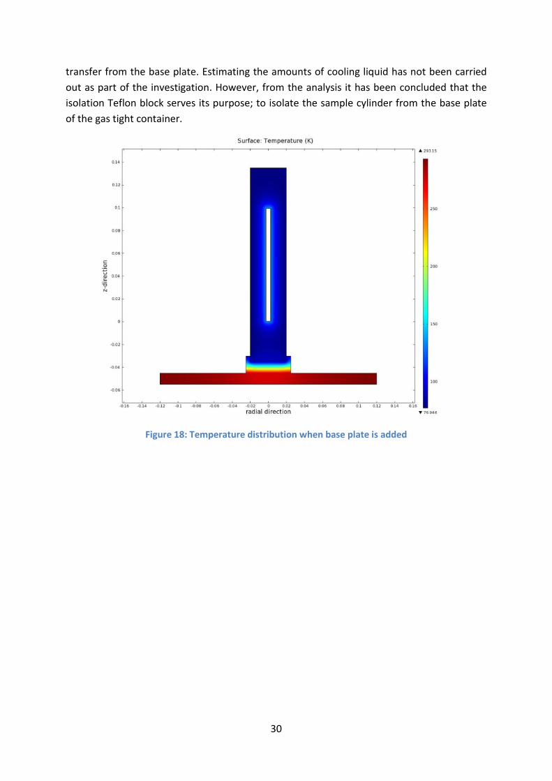
30

transfer from the base plate. Estimating the amounts of cooling liquid has not been carried out as part of the investigation. However, from the analysis it has been concluded that the isolation Teflon block serves its purpose; to isolate the sample cylinder from the base plate of the gas tight container.

Figure 18: Temperature distribution when base plate is added

31

4.3.5. Influence of implementing a heater support

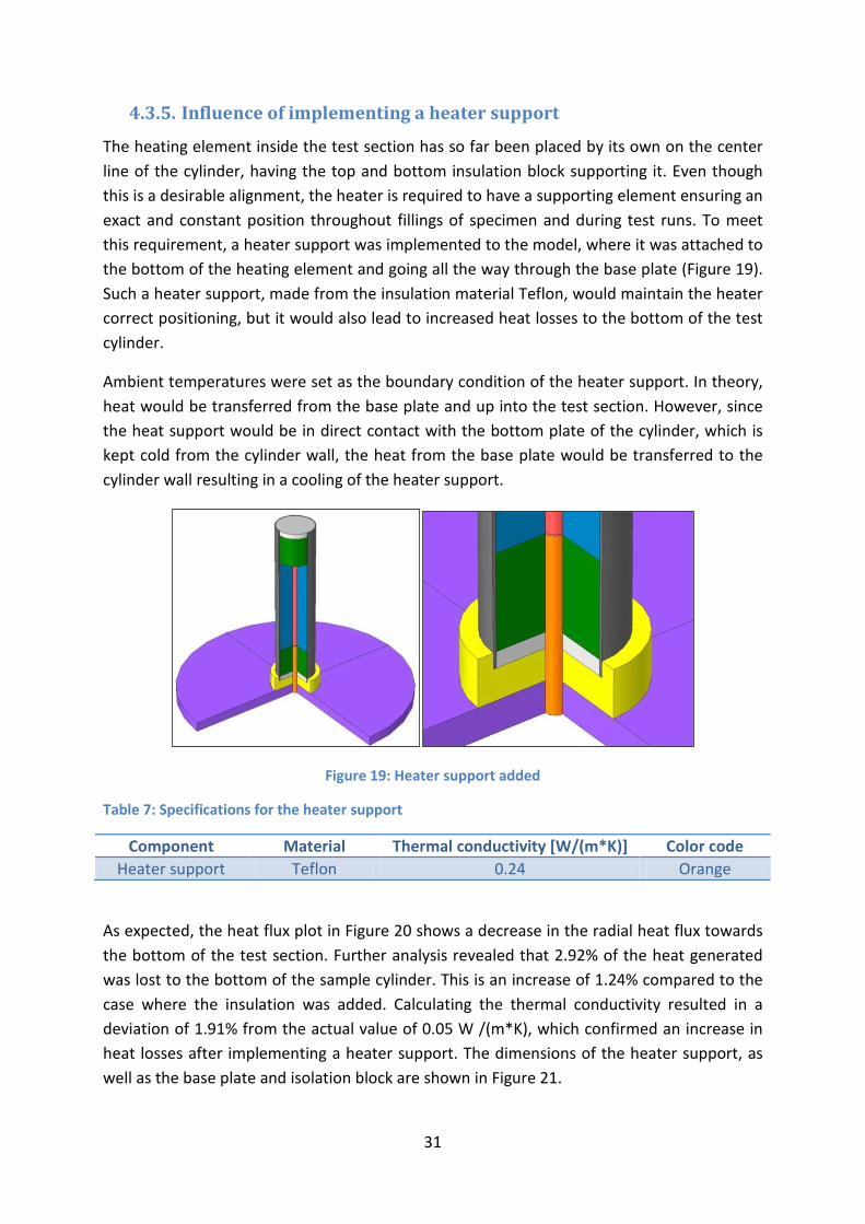
The heating element inside the test section has so far been placed by its own on the center line of the cylinder, having the top and bottom insulation block supporting it. Even though this is a desirable alignment, the heater is required to have a supporting element ensuring an exact and constant position throughout fillings of specimen and during test runs. To meet this requirement, a heater support was implemented to the model, where it was attached to the bottom of the heating element and going all the way through the base plate (Figure 19). Such a heater support, made from the insulation material Teflon, would maintain the heater correct positioning, but it would also lead to increased heat losses to the bottom of the test cylinder.

Ambient temperatures were set as the boundary condition of the heater support. In theory, heat would be transferred from the base plate and up into the test section. However, since the heat support would be in direct contact with the bottom plate of the cylinder, which is kept cold from the cylinder wall, the heat from the base plate would be transferred to the cylinder wall resulting in a cooling of the heater support.

Figure 19: Heater support added

Table 7: Specifications for the heater support

Component Material Thermal conductivity [W/(m*K)] Color code Heater support Teflon 0.24 Orange

As expected, the heat flux plot in Figure 20 shows a decrease in the radial heat flux towards the bottom of the test section. Further analysis revealed that 2.92% of the heat generated was lost to the bottom of the sample cylinder. This is an increase of 1.24% compared to the case where the insulation was added. Calculating the thermal conductivity resulted in a deviation of 1.91% from the actual value of 0.05 W /(m*K), which confirmed an increase in heat losses after implementing a heater support. The dimensions of the heater support, as well as the base plate and isolation block are shown in Figure 21.

32

Figure 20: Heat flux plot after adding heater support

Figure 21: Dimensions of heater support, base plate and isolation block [mm]

33

4.3.6. Influence of thermocouples and thermocouple protectors

In order to predict the thermal conductivity of the test specimen filled in the sample cylinder, temperature recordings at several positions inside the test section are essential. The temperature profile from the heater wall to the cylinder wall can be established by logging temperature recordings from thermocouples placed inside the test specimen, all at the same height. For the proposed apparatus it was decided, as for the previous test rigs (Abrahamsen and Gauthier, Section 3.3), that it was desirable to take temperature recordings at four different radial positions: at the heater wall (TC 1), at r=0.075 m (TC 2), at r=0.014 m (TC 3) and at the cylinder wall (r=0.02m) (TC 4), all at the height of 0.06m inside the test specimen. The diameter and length of the thermocouples were 0.5 mm and 10.5 cm, respectively. Boundary conditions such as for the heater support were assumed. Consequently, heat from the base plate was transported through the bottom plate of the cylinder and further on to the cold wall.

The thermocouples were designed as thin capillary tubes covering metal wires which can easily bend or move when filling the specimen. To protect and assure constant positioning, the two thermocouples in the mid-section of the specimen were supported by thermocouple protectors in stainless steel, shaped as hollow canola tubes, c.f. Figure 22. The canola tubes were designed with an outer diameter of 1mm and a wall thickness of 0.2 mm. The heights of the protectors were purposely constructed 1 cm shorter than the thermocouples. This way, temperature readings from the thermocouples would not be hugely influenced by the improved heat transfer in the stainless steel of the protectors. Figure 23 illustrates the placement of the three thermocouples with their protectors placed inside the test cylinder. The fourth thermocouple would to be placed at the cooling wall, but is not included in model.

In the existing apparatus used by Abrahamsen [12] and Gauthier [13], a positioning device was also used for position assurance. It is likely that such a component is to be used in a new build-up as well; however, it was not included in the apparatus in this thesis due to modeling restrictions in Comsol.

Figure 22: Thermocouples with protectors

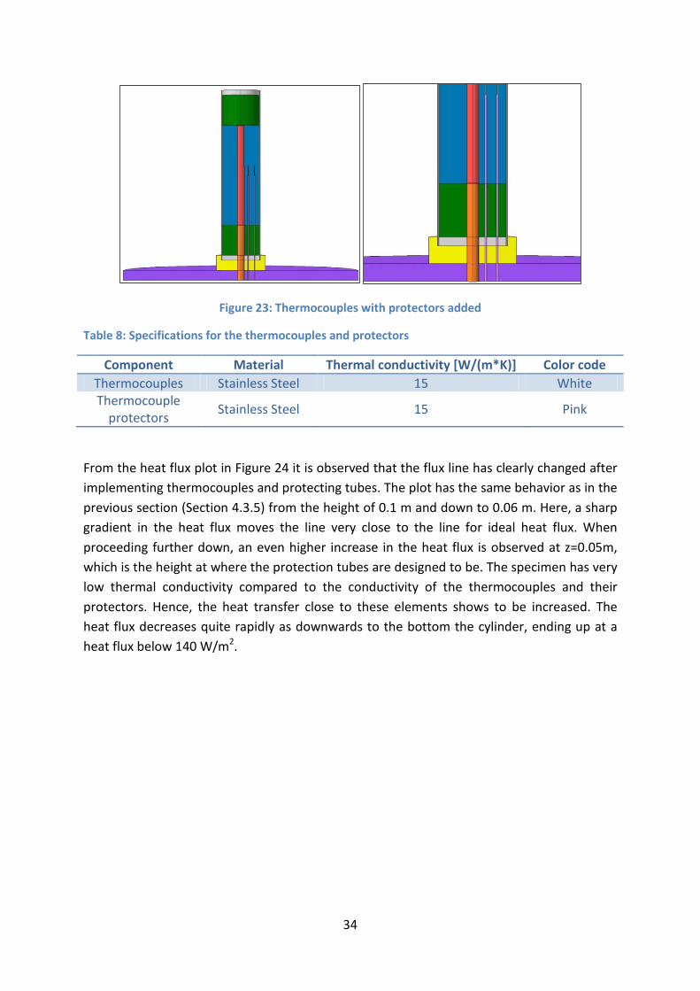
34

Figure 23: Thermocouples with protectors added

Table 8: Specifications for the thermocouples and protectors

Component Material Thermal conductivity [W/(m*K)] Color code Thermocouples Stainless Steel 15 White Thermocouple

protectors Stainless Steel 15 Pink

From the heat flux plot in Figure 24 it is observed that the flux line has clearly changed after implementing thermocouples and protecting tubes. The plot has the same behavior as in the previous section (Section 4.3.5) from the height of 0.1 m and down to 0.06 m. Here, a sharp gradient in the heat flux moves the line very close to the line for ideal heat flux. When proceeding further down, an even higher increase in the heat flux is observed at z=0.05m, which is the height at where the protection tubes are designed to be. The specimen has very low thermal conductivity compared to the conductivity of the thermocouples and their protectors. Hence, the heat transfer close to these elements shows to be increased. The heat flux decreases quite rapidly as downwards to the bottom the cylinder, ending up at a heat flux below 140 W/m2.

35

Figure 24: Heat flux plot after adding thermocouples w/protectors

Heat loss to the bottom of the test section, after including thermocouples with protectors, was found to be 3.6%. However, when plotting the temperature distribution in radial direction at z=0.06m, promising results were observed. Figure 25 shows how the temperature changed in the radial direction at the height z=0.06 m. For comparison, the theoretical values (same as in Section 4.3.1) have been included as well. The numerical values show almost identical behavior as the theoretical values, except for three positions; where the thermocouples are located (black dots of the graph). At these positions, the heat flux is short-circuited over the diameter of the thermocouples, leading to an increased heat transfer. This means that even though the heat loss to the bottom increased as the thermocouples with protectors were added, temperature recordings proved to be promising. It also indicates that by placing the thermocouples at a location high into the specimen, heat losses are not that great of a concern. Calculating of the thermal conductivity resulted in 0.0514 W/(m*K), 2.7% higher that the exact value of 0.05 W/(m*K).

Figure 25: Temperature plot in radial direction, thermocouples added

36

4.3.7. Effect of implementing the electric wire

The final component to be added to the test apparatus in this thesis was an electric wire, providing current to the heater. The electric wire has not been included in any of the models analyzed in the previously conducted work and was therefore one of the most important elements to investigate.

Figure 26: Illustration of electric wire alignment

Figure 26 illustrates the concept of the electric wire alignment; a copper wire was drawn thought the heater support all the way from the bottom of the base plate and up to the heating element. A more realistic alignment would have been to have two wires going through the support (this is how the heater and wire elements are built up in the existing equipment in the laboratory at NTNU), but for simplicity reason one wire with the same cross section area as two wires added together has been designed. The diameter of the wire was set to 1.4 mm (the wires in the existing rig has a diameter of 1 mm), the height was set to 6 cm and the material chosen was copper, having a thermal conductivity of 400 W/(m*K). The boundary condition for the end of the electric wire was set to ambient, 293 K.

Table 9: Specifications for the electric wire

Component Material Thermal conductivity [W/(m*K)] Color code Electric wire Copper 400 [B3] Gold

So far, only heat losses had proven to be of concern. Despite these losses, the thermal conductivity measurements inside the test section were calculated to have an uncertainty of less than 3 %. As the electric wire needed to be implemented, there was a suspicion that heat would be transferred from the base plate, thought the electric wire and into the test section, affecting the measurements in the opposite direction. In other word: increasing the temperature in the test section.

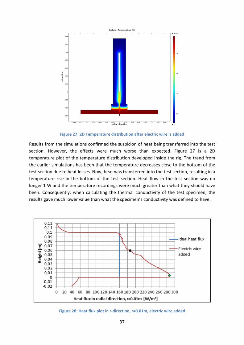
37

Figure 27: 2D Temperature distribution after electric wire is added Results from the simulations confirmed the suspicion of heat being transferred into the test section. However, the effects were much worse than expected. Figure 27 is a 2D temperature plot of the temperature distribution developed inside the rig. The trend from the earlier simulations has been that the temperature decreases close to the bottom of the test section due to heat losses. Now, heat was transferred into the test section, resulting in a temperature rise in the bottom of the test section. Heat flow in the test section was no longer 1 W and the temperature recordings were much greater than what they should have been. Consequently, when calculating the thermal conductivity of the test specimen, the results gave much lower value than what the specimen’s conductivity was defined to have.

Figure 28: Heat flux plot in r-direction, r=0.01m, electric wire added

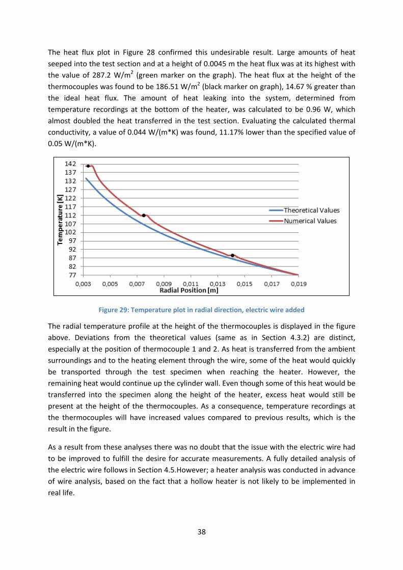
38

The heat flux plot in Figure 28 confirmed this undesirable result. Large amounts of heat seeped into the test section and at a height of 0.0045 m the heat flux was at its highest with the value of 287.2 W/m2 (green marker on the graph). The heat flux at the height of the thermocouples was found to be 186.51 W/m2 (black marker on graph), 14.67 % greater than the ideal heat flux. The amount of heat leaking into the system, determined from temperature recordings at the bottom of the heater, was calculated to be 0.96 W, which almost doubled the heat transferred in the test section. Evaluating the calculated thermal conductivity, a value of 0.044 W/(m*K) was found, 11.17% lower than the specified value of 0.05 W/(m*K).

Figure 29: Temperature plot in radial direction, electric wire added

The radial temperature profile at the height of the thermocouples is displayed in the figure above. Deviations from the theoretical values (same as in Section 4.3.2) are distinct, especially at the position of thermocouple 1 and 2. As heat is transferred from the ambient surroundings and to the heating element through the wire, some of the heat would quickly be transported through the test specimen when reaching the heater. However, the remaining heat would continue up the cylinder wall. Even though some of this heat would be transferred into the specimen along the height of the heater, excess heat would still be present at the height of the thermocouples. As a consequence, temperature recordings at the thermocouples will have increased values compared to previous results, which is the result in the figure.

As a result from these analyses there was no doubt that the issue with the electric wire had to be improved to fulfill the desire for accurate measurements. A fully detailed analysis of the electric wire follows in Section 4.5.However; a heater analysis was conducted in advance of wire analysis, based on the fact that a hollow heater is not likely to be implemented in real life.

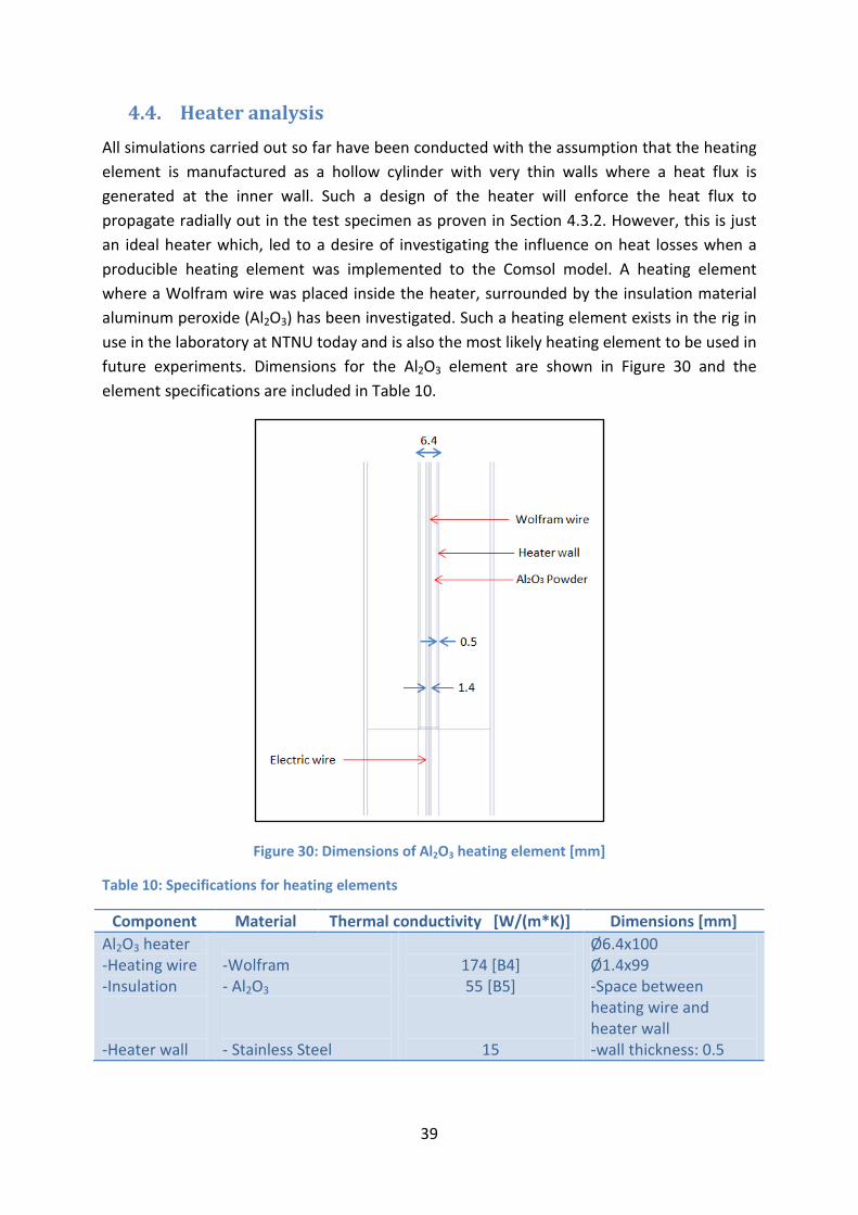
39

4.4. Heater analysis All simulations carried out so far have been conducted with the assumption that the heating element is manufactured as a hollow cylinder with very thin walls where a heat flux is generated at the inner wall. Such a design of the heater will enforce the heat flux to propagate radially out in the test specimen as proven in Section 4.3.2. However, this is just an ideal heater which, led to a desire of investigating the influence on heat losses when a producible heating element was implemented to the Comsol model. A heating element where a Wolfram wire was placed inside the heater, surrounded by the insulation material aluminum peroxide (Al2O3) has been investigated. Such a heating element exists in the rig in use in the laboratory at NTNU today and is also the most likely heating element to be used in future experiments. Dimensions for the Al2O3 element are shown in Figure 30 and the element specifications are included in Table 10.

Figure 30: Dimensions of Al2O3 heating element [mm]

Table 10: Specifications for heating elements

Component Material Thermal conductivity [W/(m*K)] Dimensions [mm] Al2O3 heater -Heating wire -Insulation -Heater wall

-Wolfram - Al2O3

- Stainless Steel

174 [B4] 55 [B5]

15

Ø6.4x100 Ø1.4x99 -Space between heating wire and heater wall -wall thickness: 0.5

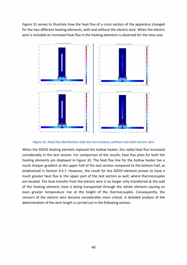
40

Figure 31 serves to illustrate how the heat flux of a cross section of the apparatus changed for the two different heating elements, with and without the electric wire. When the electric wire is included an increased heat flux in the heating elements is observed for the new case.

Figure 31: Heat flux distribution with the two heaters, without and with electric wire

When the Al2O3 heating element replaced the hollow heater, the radial heat flux increased considerably in the test section. For comparison of the results, heat flux plots for both the heating elements are displayed in Figure 32. The heat flux line for the hollow heater has a much sharper gradient at the upper half of the test section compared to the bottom half, as emphasized in Section 4.3.7. However, the result for the Al2O3 element proves to have a much greater heat flux in the upper part of the test section as well, where thermocouples are located. The heat transfer from the electric wire is no longer only transferred at the wall of the heating element; heat is being transported through the whole element causing an even greater temperature rise at the height of the thermocouples. Consequently, the concern of the electric wire became considerably more critical. A detailed analysis of the determination of the wire length is carried out in the following section.

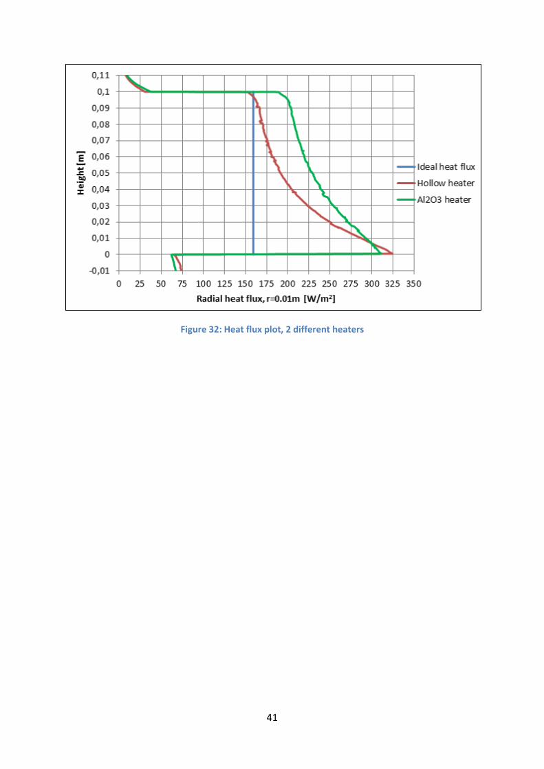
41

Figure 32: Heat flux plot, 2 different heaters

42

4.5. Investigation of the electric wire length The electric wire supplying current to the heater has been proven to have a much greater influence on the temperature in the test section than expected. When the hollow heater was analyzed, heat going into the system from the electric wire was found to be 0.96 W. Completing the same analysis as the Al2O3 heater was implemented, resulted in a heat flux of 1.15 W into the test section through the wire. Such an amount of heat transferred through the wire would not be acceptable. One way of dealing with this challenge could be to reduce the cross section area of the wire by decreasing the diameter. However, this would result in an increased voltage drop along the wire. A second option would be to cool the wire so that the temperature at the end of the wire would no longer have ambient temperature. Nevertheless, it has been decided, in agreement with the supervisors, that the best way to solve the challenge related to the wire was to increase the wire length.

To evaluate the required length of the wire needed to meet a satisfactory value of the heat transferred to the test section, the following equations have been adopted:

𝑄𝑤𝑖𝑟𝑒 = 𝑘𝑤𝐴𝑤𝐿𝑤

(𝑇2 − 𝑇1) (4.4)

𝐿𝑤 = 𝑘𝑤𝐴𝑤𝑄𝑤𝑖𝑟𝑒

(𝑇2 − 𝑇1) (4.5)

where 𝑄𝑤𝑖𝑟𝑒 is the amount of heat transferred from the base plate and up to the heating element, Lw is the length of the wire, kw is the thermal conductivity of the wire, Aw is the cross sectional area of the wire and T1 and T2 are the temperatures where the wire meets the heater and the temperature at the start of the wire (ambient), respectively.

Figure 33 depicts the heat flow into the test section as a function of the wire length from the starting length of 0.06 m. In order to reduce the heat flow into the system down to a value of 0.01 W, the wire length was estimated to be 6.9 m, which is extremely long compared to the dimensions of the rig. However, if 0.1 W was an accepted amount of heat, the length of the wire would reduce significantly (L=0.69 m).

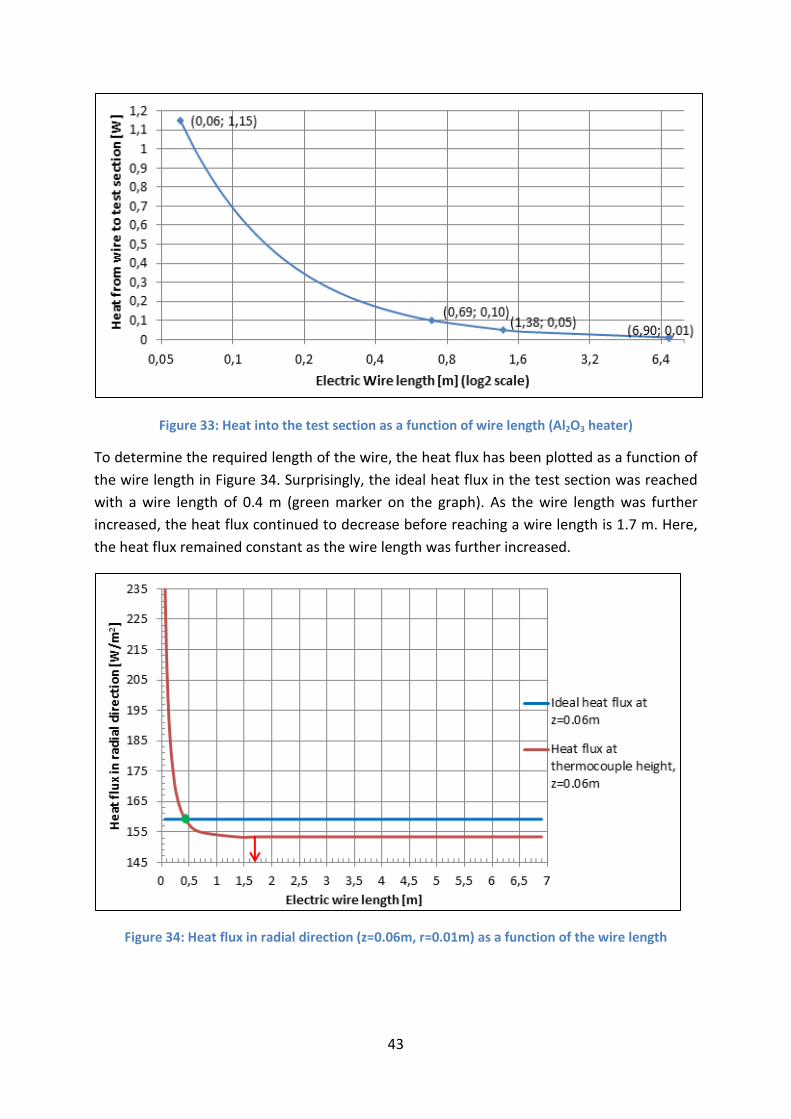
43

Figure 33: Heat into the test section as a function of wire length (Al2O3 heater)

To determine the required length of the wire, the heat flux has been plotted as a function of the wire length in Figure 34. Surprisingly, the ideal heat flux in the test section was reached with a wire length of 0.4 m (green marker on the graph). As the wire length was further increased, the heat flux continued to decrease before reaching a wire length is 1.7 m. Here, the heat flux remained constant as the wire length was further increased.

Figure 34: Heat flux in radial direction (z=0.06m, r=0.01m) as a function of the wire length

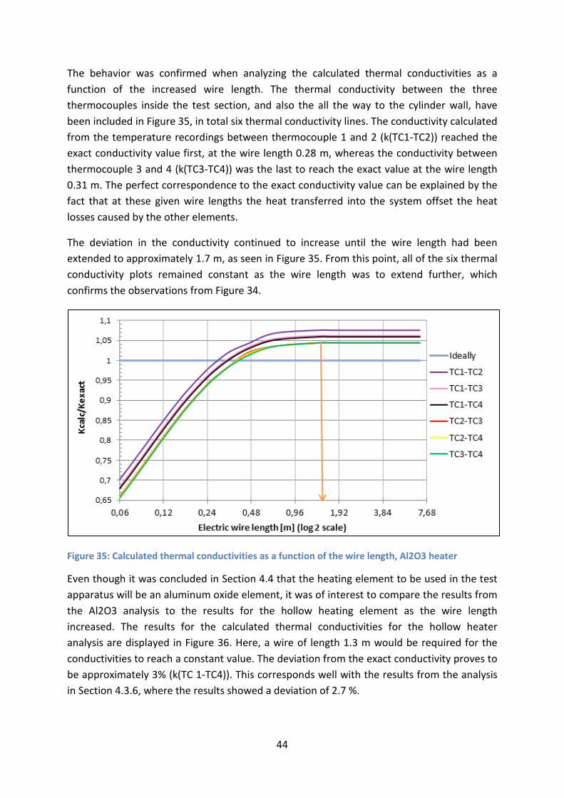
44

The behavior was confirmed when analyzing the calculated thermal conductivities as a function of the increased wire length. The thermal conductivity between the three thermocouples inside the test section, and also the all the way to the cylinder wall, have been included in Figure 35, in total six thermal conductivity lines. The conductivity calculated from the temperature recordings between thermocouple 1 and 2 (k(TC1-TC2)) reached the exact conductivity value first, at the wire length 0.28 m, whereas the conductivity between thermocouple 3 and 4 (k(TC3-TC4)) was the last to reach the exact value at the wire length 0.31 m. The perfect correspondence to the exact conductivity value can be explained by the fact that at these given wire lengths the heat transferred into the system offset the heat losses caused by the other elements.

The deviation in the conductivity continued to increase until the wire length had been extended to approximately 1.7 m, as seen in Figure 35. From this point, all of the six thermal conductivity plots remained constant as the wire length was to extend further, which confirms the observations from Figure 34.

Figure 35: Calculated thermal conductivities as a function of the wire length, Al2O3 heater

Even though it was concluded in Section 4.4 that the heating element to be used in the test apparatus will be an aluminum oxide element, it was of interest to compare the results from the Al2O3 analysis to the results for the hollow heating element as the wire length increased. The results for the calculated thermal conductivities for the hollow heater analysis are displayed in Figure 36. Here, a wire of length 1.3 m would be required for the conductivities to reach a constant value. The deviation from the exact conductivity proves to be approximately 3% (k(TC 1-TC4)). This corresponds well with the results from the analysis in Section 4.3.6, where the results showed a deviation of 2.7 %.

45

Figure 36: Calculated thermal conductivities as a function of the wire length, hollow heater

From these observations it seemed reasonable to choose a wire length of 1.7 m, extending it further would not improve the accuracy of the thermal conductivity measurements. With this length, the deviations from the exact conductivity value are caused by heat losses through the other elements in the setup. The thermal conductivity calculated for thermocouple 1 and 2 had the greatest deviation from the exact value after reaching the desired wire length, approximately 7%. The best results were found to be between thermocouple 2 and 3, 2 and 4 and 3 and 4, with an error of 4%. The overall thermal conductivity from the heater wall and to the cylinder wall (k(TC1-TC4)) measured a value 6% above the exact thermal conductivity of the test specimen, which is 3% greater than for the case with the hollow heater

46

4.6. Concluding remarks for the thermal design process During stepwise increase of the model complexity the sample cylinder heat losses continued to increase and deviations from the ideal heat flux plots were discovered, as expected. The major concern arose when the electric wires was included in the model.

The calculated thermal conductivity deviated by 2.7% (from thermocouple 1 to 4) from the exact value after all components were added, excluding the wire. The electric wire took the results in the opposite direction; the increased temperature in the test section caused conductivity calculations to be below the exact value. An aluminum oxide heating element replaced the hollow heater due to a more realistic heat generation, which resulted in even greater deviations in the results. However, by increasing the length of the wire to 1.7 m, the impact of heat transferred into the test section was reduced so that only heat losses to other components were present. The most accurate results for the calculated thermal conductivity were seen for the measurement where thermocouple 1 was not included, where a deviation is 4 % due to heat losses. The measurement from the heater wall to the cylinder wall (TC1-TC4) showed a deviation of 6% from the exact value.

Figure 37 summarizes all the steps of the development process. All the heat flux plots from the previous sections have been included, as well as the heat fluxes when the Al2O3 heater was implemented. The large discrepancy after the wire was included in the model can clearly be seen here, both for the hollow and Al2O3 heating elements. The graph of most relevance is the final result after the aluminum oxide heater was included and the wire length had been adjusted to 1.7 m (green line). The heat flux is overall somewhat lower than for the case with the hollow heater, but at the height of 0.06 m into the test section, the heat flux displays a value of 155 W/m2, 2.6% off from the ideal flux of 159.19 W/m2. The overall uncertainty, including not only the heat losses but also positioning errors and other parameters, is carried out in Chapter 6.

The design process has provided a greater knowledge of thermal behavior of the test apparatus than what was available from the previous work. The effects of heat losses in the apparatus have been thoroughly identified. The effect of the heat gains due to the wire was discovered for the first time and required adjustments were made. The overall analysis has proved to be quite promising. However, finalizing the proposed design, where all other aspects of the apparatus build-up are included, is still to be suggested. Proposed solutions for the remaining considerations of the whole apparatus is included in Chapter 0.

Unfortunately there was no time to vary the ratio of the thermal conductivities for insulation and test specimen from a 1/5 ratio to for example 1/1 or 2/1 ratios. Such results would have provided a greater knowledge of how the heat transfer depends on the specimens tested.

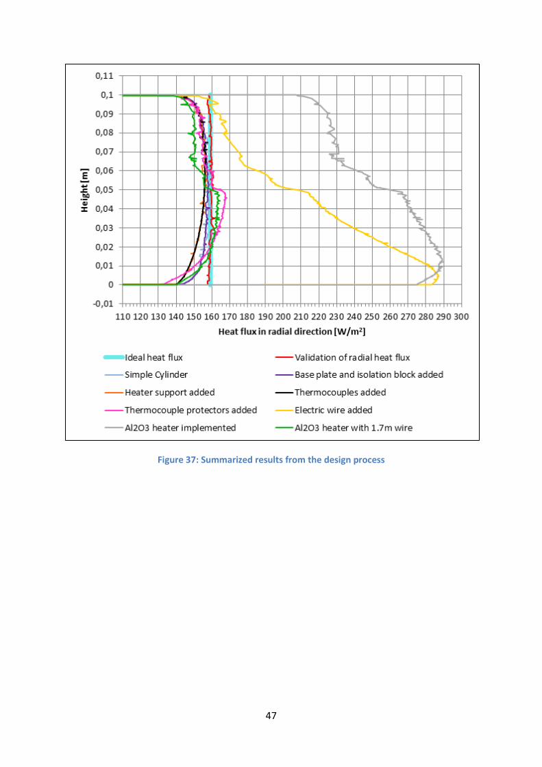
47

Figure 37: Summarized results from the design process

48

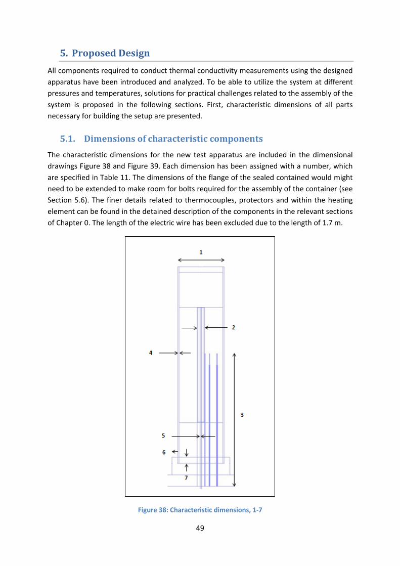
49

5. Proposed Design All components required to conduct thermal conductivity measurements using the designed apparatus have been introduced and analyzed. To be able to utilize the system at different pressures and temperatures, solutions for practical challenges related to the assembly of the system is proposed in the following sections. First, characteristic dimensions of all parts necessary for building the setup are presented.

5.1. Dimensions of characteristic components The characteristic dimensions for the new test apparatus are included in the dimensional drawings Figure 38 and Figure 39. Each dimension has been assigned with a number, which are specified in Table 11. The dimensions of the flange of the sealed contained would might need to be extended to make room for bolts required for the assembly of the container (see Section 5.6). The finer details related to thermocouples, protectors and within the heating element can be found in the detained description of the components in the relevant sections of Chapter 0. The length of the electric wire has been excluded due to the length of 1.7 m.

Figure 38: Characteristic dimensions, 1-7

50

Figure 39: Characteristic dimensions, 8-19

Table 11: Dimensions of numbered components in dimensional drawings

Number Dimension [mm] Number Dimension [mm] 1 40 11 100 2 6.4 12 30 3 11.5 13 50 4 1 14 195 5 1.4 15 20 6 5 16 10 7 5 17 10 8 10 18 15 9 5 19 240

10 30 (electric wire) (1700)

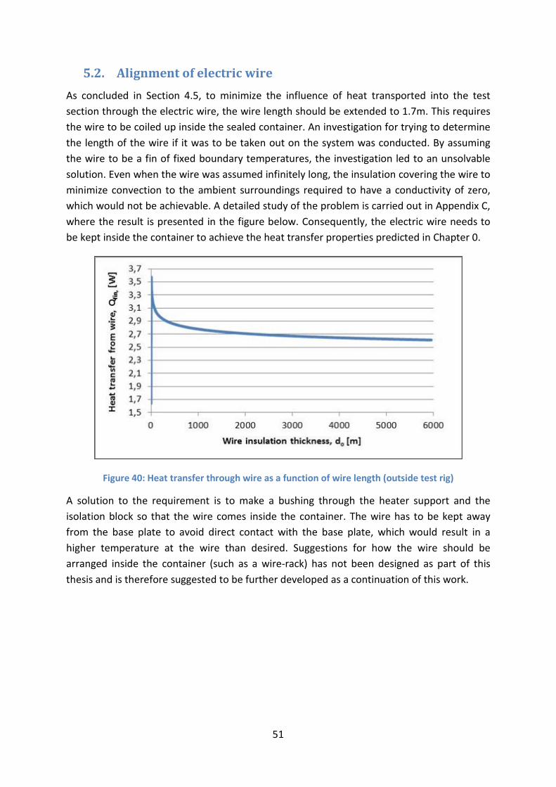
51

5.2. Alignment of electric wire As concluded in Section 4.5, to minimize the influence of heat transported into the test section through the electric wire, the wire length should be extended to 1.7m. This requires the wire to be coiled up inside the sealed container. An investigation for trying to determine the length of the wire if it was to be taken out on the system was conducted. By assuming the wire to be a fin of fixed boundary temperatures, the investigation led to an unsolvable solution. Even when the wire was assumed infinitely long, the insulation covering the wire to minimize convection to the ambient surroundings required to have a conductivity of zero, which would not be achievable. A detailed study of the problem is carried out in Appendix C, where the result is presented in the figure below. Consequently, the electric wire needs to be kept inside the container to achieve the heat transfer properties predicted in Chapter 0.

Figure 40: Heat transfer through wire as a function of wire length (outside test rig)

A solution to the requirement is to make a bushing through the heater support and the isolation block so that the wire comes inside the container. The wire has to be kept away from the base plate to avoid direct contact with the base plate, which would result in a higher temperature at the wire than desired. Suggestions for how the wire should be arranged inside the container (such as a wire-rack) has not been designed as part of this thesis and is therefore suggested to be further developed as a continuation of this work.

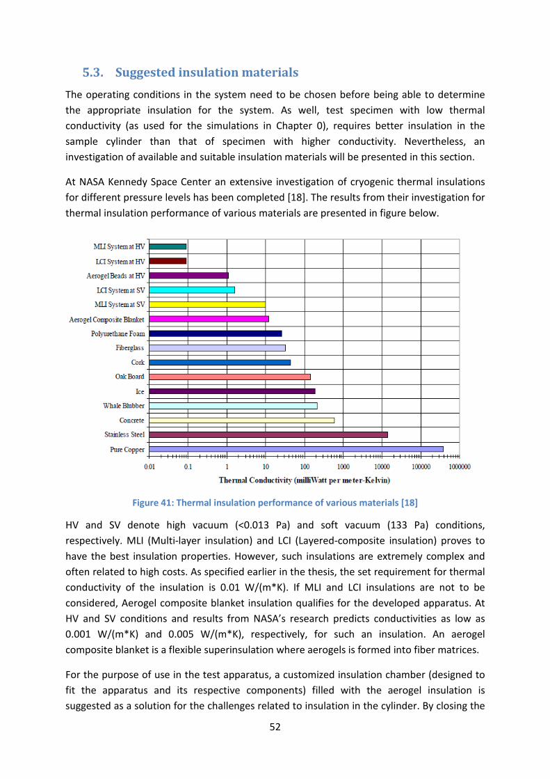
52

5.3. Suggested insulation materials The operating conditions in the system need to be chosen before being able to determine the appropriate insulation for the system. As well, test specimen with low thermal conductivity (as used for the simulations in Chapter 0), requires better insulation in the sample cylinder than that of specimen with higher conductivity. Nevertheless, an investigation of available and suitable insulation materials will be presented in this section.

At NASA Kennedy Space Center an extensive investigation of cryogenic thermal insulations for different pressure levels has been completed [18]. The results from their investigation for thermal insulation performance of various materials are presented in figure below.

Figure 41: Thermal insulation performance of various materials [18]

HV and SV denote high vacuum (<0.013 Pa) and soft vacuum (133 Pa) conditions, respectively. MLI (Multi-layer insulation) and LCI (Layered-composite insulation) proves to have the best insulation properties. However, such insulations are extremely complex and often related to high costs. As specified earlier in the thesis, the set requirement for thermal conductivity of the insulation is 0.01 W/(m*K). If MLI and LCI insulations are not to be considered, Aerogel composite blanket insulation qualifies for the developed apparatus. At HV and SV conditions and results from NASA’s research predicts conductivities as low as 0.001 W/(m*K) and 0.005 W/(m*K), respectively, for such an insulation. An aerogel composite blanket is a flexible superinsulation where aerogels is formed into fiber matrices.

For the purpose of use in the test apparatus, a customized insulation chamber (designed to fit the apparatus and its respective components) filled with the aerogel insulation is suggested as a solution for the challenges related to insulation in the cylinder. By closing the

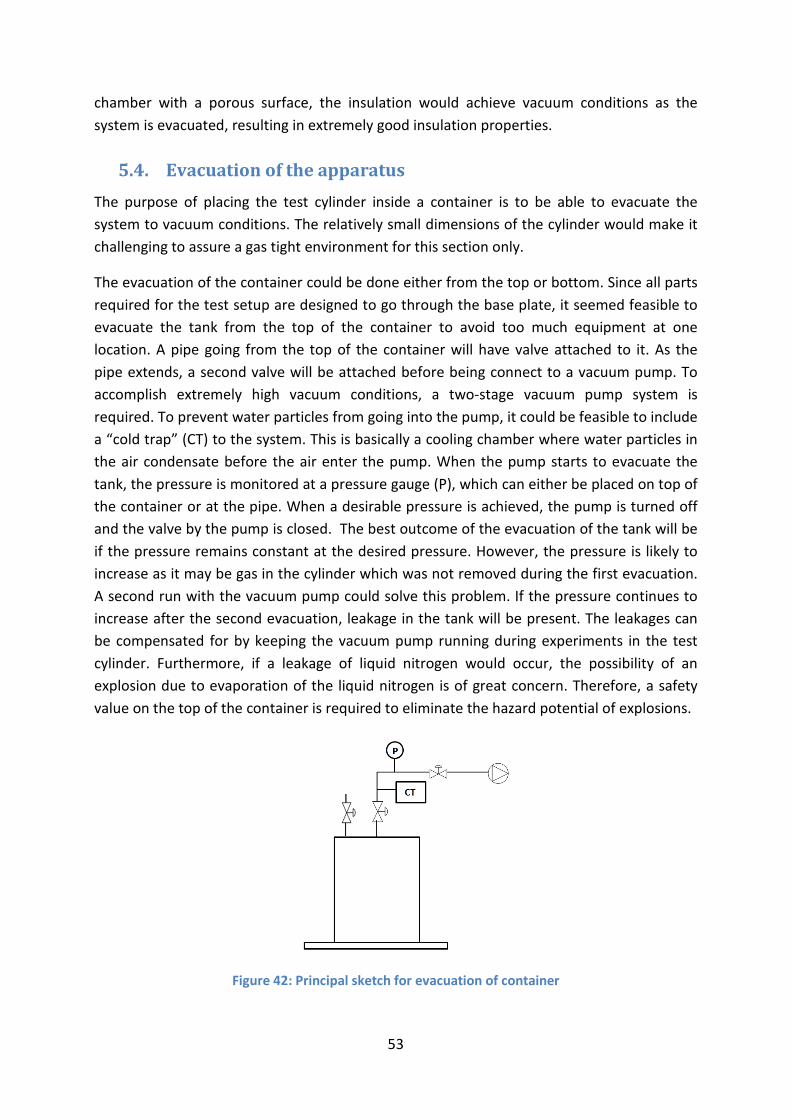
53

chamber with a porous surface, the insulation would achieve vacuum conditions as the system is evacuated, resulting in extremely good insulation properties.

5.4. Evacuation of the apparatus The purpose of placing the test cylinder inside a container is to be able to evacuate the system to vacuum conditions. The relatively small dimensions of the cylinder would make it challenging to assure a gas tight environment for this section only.

The evacuation of the container could be done either from the top or bottom. Since all parts required for the test setup are designed to go through the base plate, it seemed feasible to evacuate the tank from the top of the container to avoid too much equipment at one location. A pipe going from the top of the container will have valve attached to it. As the pipe extends, a second valve will be attached before being connect to a vacuum pump. To accomplish extremely high vacuum conditions, a two-stage vacuum pump system is required. To prevent water particles from going into the pump, it could be feasible to include a “cold trap” (CT) to the system. This is basically a cooling chamber where water particles in the air condensate before the air enter the pump. When the pump starts to evacuate the tank, the pressure is monitored at a pressure gauge (P), which can either be placed on top of the container or at the pipe. When a desirable pressure is achieved, the pump is turned off and the valve by the pump is closed. The best outcome of the evacuation of the tank will be if the pressure remains constant at the desired pressure. However, the pressure is likely to increase as it may be gas in the cylinder which was not removed during the first evacuation. A second run with the vacuum pump could solve this problem. If the pressure continues to increase after the second evacuation, leakage in the tank will be present. The leakages can be compensated for by keeping the vacuum pump running during experiments in the test cylinder. Furthermore, if a leakage of liquid nitrogen would occur, the possibility of an explosion due to evaporation of the liquid nitrogen is of great concern. Therefore, a safety value on the top of the container is required to eliminate the hazard potential of explosions.

Figure 42: Principal sketch for evacuation of container

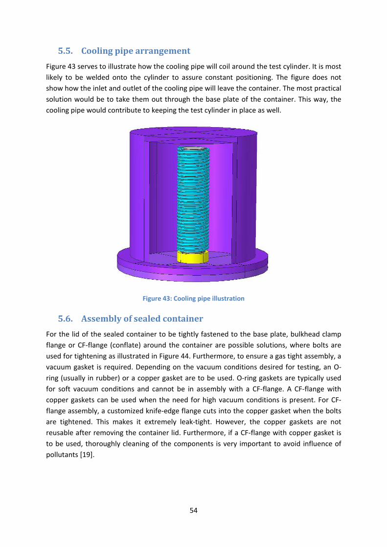
54

5.5. Cooling pipe arrangement Figure 43 serves to illustrate how the cooling pipe will coil around the test cylinder. It is most likely to be welded onto the cylinder to assure constant positioning. The figure does not show how the inlet and outlet of the cooling pipe will leave the container. The most practical solution would be to take them out through the base plate of the container. This way, the cooling pipe would contribute to keeping the test cylinder in place as well.

Figure 43: Cooling pipe illustration

5.6. Assembly of sealed container For the lid of the sealed container to be tightly fastened to the base plate, bulkhead clamp flange or CF-flange (conflate) around the container are possible solutions, where bolts are used for tightening as illustrated in Figure 44. Furthermore, to ensure a gas tight assembly, a vacuum gasket is required. Depending on the vacuum conditions desired for testing, an O-ring (usually in rubber) or a copper gasket are to be used. O-ring gaskets are typically used for soft vacuum conditions and cannot be in assembly with a CF-flange. A CF-flange with copper gaskets can be used when the need for high vacuum conditions is present. For CF-flange assembly, a customized knife-edge flange cuts into the copper gasket when the bolts are tightened. This makes it extremely leak-tight. However, the copper gaskets are not reusable after removing the container lid. Furthermore, if a CF-flange with copper gasket is to be used, thoroughly cleaning of the components is very important to avoid influence of pollutants [19].

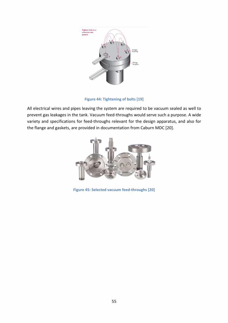
55

Figure 44: Tightening of bolts [19]

All electrical wires and pipes leaving the system are required to be vacuum sealed as well to prevent gas leakages in the tank. Vacuum feed-throughs would serve such a purpose. A wide variety and specifications for feed-throughs relevant for the design apparatus, and also for the flange and gaskets, are provided in documentation from Caburn MDC [20].

Figure 45: Selected vacuum feed-throughs [20]

56

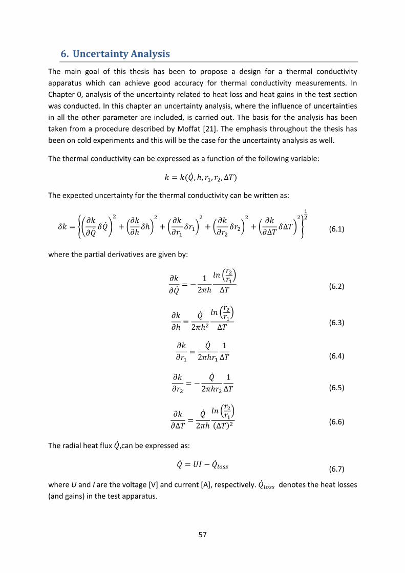
57

6. Uncertainty Analysis The main goal of this thesis has been to propose a design for a thermal conductivity apparatus which can achieve good accuracy for thermal conductivity measurements. In Chapter 0, analysis of the uncertainty related to heat loss and heat gains in the test section was conducted. In this chapter an uncertainty analysis, where the influence of uncertainties in all the other parameter are included, is carried out. The basis for the analysis has been taken from a procedure described by Moffat [21]. The emphasis throughout the thesis has been on cold experiments and this will be the case for the uncertainty analysis as well.

The thermal conductivity can be expressed as a function of the following variable:

𝑘 = 𝑘(�̇�,ℎ, 𝑟1, 𝑟2,∆𝑇)

The expected uncertainty for the thermal conductivity can be written as:

𝛿𝑘 = ��𝜕𝑘𝜕�̇�

𝛿�̇��2

+ �𝜕𝑘𝜕ℎ

𝛿ℎ�2

+ �𝜕𝑘𝜕𝑟1

𝛿𝑟1�2

+ �𝜕𝑘𝜕𝑟2

𝛿𝑟2�2

+ �𝜕𝑘𝜕∆𝑇

𝛿∆𝑇�2

�

12

(6.1)

where the partial derivatives are given by:

𝜕𝑘𝜕�̇�

= −1

2𝜋ℎ

𝑙𝑛 �𝑟2𝑟1�

∆𝑇

(6.2)

𝜕𝑘𝜕ℎ

=�̇�

2𝜋ℎ2𝑙𝑛 �𝑟2𝑟1

�

∆𝑇

(6.3)

𝜕𝑘𝜕𝑟1

=�̇�

2𝜋ℎ𝑟11∆𝑇

(6.4)

𝜕𝑘𝜕𝑟2

= −�̇�

2𝜋ℎ𝑟21∆𝑇

(6.5)

𝜕𝑘𝜕∆𝑇

=�̇�

2𝜋ℎ

𝑙𝑛 �𝑟2𝑟1�

(∆𝑇)2

(6.6)

The radial heat flux 𝑄,̇ can be expressed as:

�̇� = 𝑈𝐼 − �̇�𝑙𝑜𝑠𝑠 (6.7)

where U and I are the voltage [V] and current [A], respectively. �̇�𝑙𝑜𝑠𝑠 denotes the heat losses (and gains) in the test apparatus.

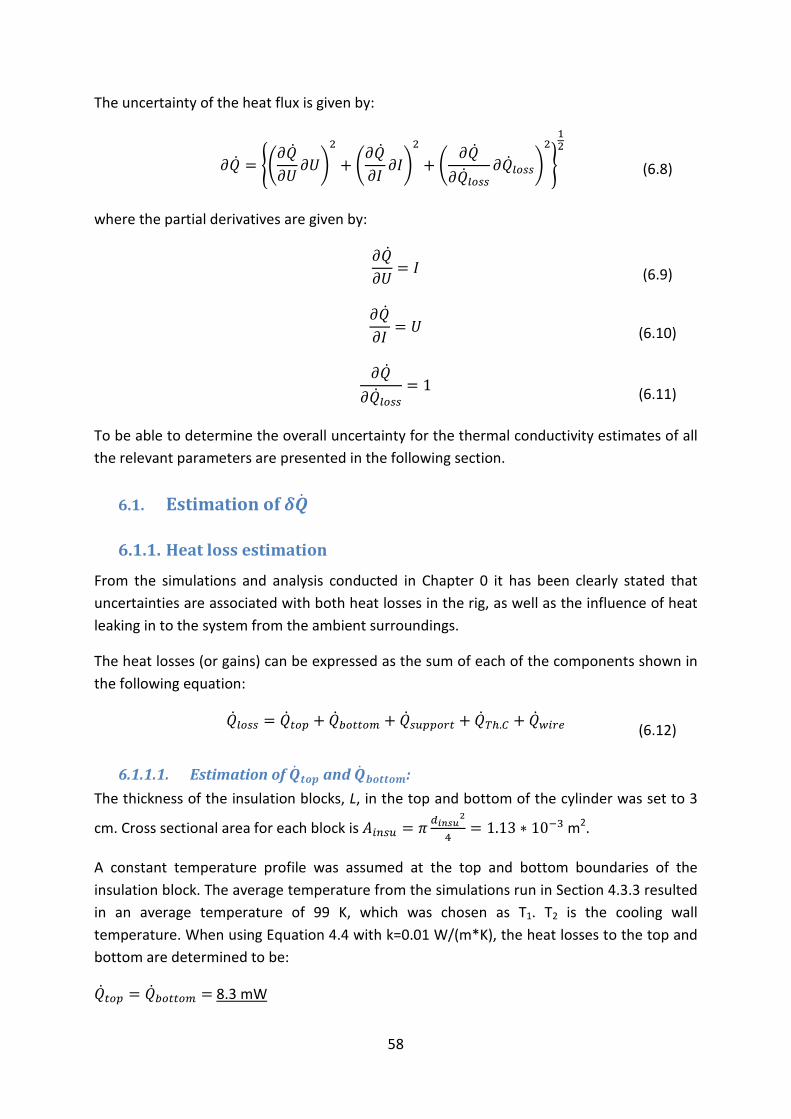
58

The uncertainty of the heat flux is given by:

𝜕�̇� = ��𝜕�̇�𝜕𝑈

𝜕𝑈�2

+ �𝜕�̇�𝜕𝐼

𝜕𝐼�2

+ �𝜕�̇�

𝜕�̇�𝑙𝑜𝑠𝑠𝜕�̇�𝑙𝑜𝑠𝑠�

2

�

12

(6.8)

where the partial derivatives are given by:

𝜕�̇�𝜕𝑈

= 𝐼

(6.9)

𝜕�̇�𝜕𝐼

= 𝑈

(6.10)

𝜕�̇�

𝜕�̇�𝑙𝑜𝑠𝑠= 1

(6.11)

To be able to determine the overall uncertainty for the thermal conductivity estimates of all the relevant parameters are presented in the following section.

6.1. Estimation of 𝜹�̇�

6.1.1. Heat loss estimation

From the simulations and analysis conducted in Chapter 0 it has been clearly stated that uncertainties are associated with both heat losses in the rig, as well as the influence of heat leaking in to the system from the ambient surroundings.

The heat losses (or gains) can be expressed as the sum of each of the components shown in the following equation:

�̇�𝑙𝑜𝑠𝑠 = �̇�𝑡𝑜𝑝 + �̇�𝑏𝑜𝑡𝑡𝑜𝑚 + �̇�𝑠𝑢𝑝𝑝𝑜𝑟𝑡 + �̇�𝑇ℎ.𝐶 + �̇�𝑤𝑖𝑟𝑒

(6.12)

6.1.1.1. Estimation of �̇�𝒕𝒐𝒑 and �̇�𝒃𝒐𝒕𝒕𝒐𝒎: The thickness of the insulation blocks, L, in the top and bottom of the cylinder was set to 3

cm. Cross sectional area for each block is 𝐴𝑖𝑛𝑠𝑢 = 𝜋 𝑑𝑖𝑛𝑠𝑢2

4= 1.13 ∗ 10−3 m2.

A constant temperature profile was assumed at the top and bottom boundaries of the insulation block. The average temperature from the simulations run in Section 4.3.3 resulted in an average temperature of 99 K, which was chosen as T1. T2 is the cooling wall temperature. When using Equation 4.4 with k=0.01 W/(m*K), the heat losses to the top and bottom are determined to be:

�̇�𝑡𝑜𝑝 = �̇�𝑏𝑜𝑡𝑡𝑜𝑚 = 8.3 mW

59

6.1.1.2. Estimation of �̇�𝒔𝒖𝒑𝒑𝒐𝒓𝒕: The heater support was proven to have an effect of the heat losses to the bottom of the cylinder. The material suggested for the heater support was Teflon (k=0.24 W/(m*K)) and the diameter and length of 0.0064 m and 0.055 m, respectively. The average temperature at the top of the heater support was evaluated to be 127.7 K, whereas the bottom temperature, T2, was 293 K. Inserting the values into Equation 4.4 gives:

�̇�𝑠𝑢𝑝𝑝𝑜𝑟𝑡 = 23.2mW

6.1.1.3. Estimation of �̇�𝑻𝒉.𝑪𝒔: The estimation of the heat losses due to the thermocouples and their canola tubes is much more complex. For simplicity reasons the thermocouple 2 and 3 has been merged together with their protectors, assuming massive steel rods with a diameter of 0.9 mm (diameter of the thermocouple is 0.5 mm and the protector wall thickness is 0.2 mm). This assumption will lead to a greater heat loss caused by thermocouple 2 and 3 than what the real value would have been. The length was 0.105 m, but since the thermocouple protectors are cooled by the bottom plate of the cylinder, the length used for the calculations has been 0.05 m. For thermocouple 1 there is no protection tube, hence; the diameter and length are 0.001 m and 0.05 m, respectively. Using Equation 4.4, where T1 on top of each thermocouple was collected from the numerical analysis and T2 is 77 K, give the following estimates:

�̇�𝑇ℎ.𝐶 1 = 13 mW (T1=132.21 K)

�̇�𝑇ℎ.𝐶 2 = 22.3 mW (T1=106.09 K)

�̇�𝑇ℎ.𝐶 2 = 7.3 mW (T1=86.55 K)

The summation of the estimated contributions to the heat loss is:

�̇�𝑇ℎ.𝐶𝑠 = 42.6 mW

6.1.1.4. Estimation of �̇�𝒘𝒊𝒓𝒆: The influence of the temperature recordings in the system when the electric wire was added to the apparatus proved to have a large impact. From the electric wire analysis in Section 4.5, it was concluded that the length of the electric wire should be extended to 1.7 m. With this length, a diameter of 0.0014 m and a thermal conductivity of 400 W/(m*K), the gain to the system would be:

�̇�𝑤𝑖𝑟𝑒 =-59.5 mW (T1=128.86 K)

Even though this estimation shows that the contribution of 𝑄𝑤𝚤𝑟𝑒̇ is rather large compared to the other �̇�-estimates, the results from the analysis of the wire length (Section 4.5) showed that the influence of this gain did not play an important role for the temperature measurements at the thermocouples in the test section. However, it has been included in this uncertainly analysis.

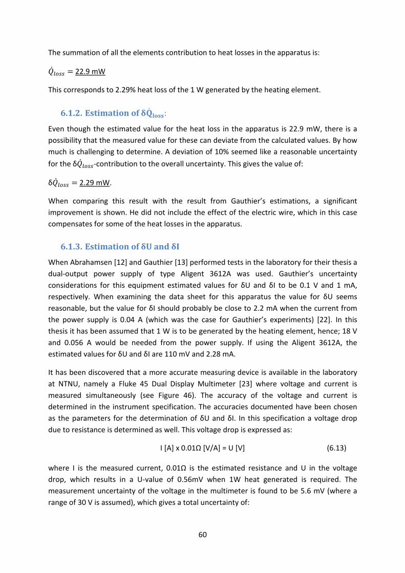
60

The summation of all the elements contribution to heat losses in the apparatus is:

�̇�𝑙𝑜𝑠𝑠 = 22.9 mW

This corresponds to 2.29% heat loss of the 1 W generated by the heating element.

6.1.2. Estimation of δ�̇�𝐥𝐨𝐬𝐬:

Even though the estimated value for the heat loss in the apparatus is 22.9 mW, there is a possibility that the measured value for these can deviate from the calculated values. By how much is challenging to determine. A deviation of 10% seemed like a reasonable uncertainty for the δ�̇�𝑙𝑜𝑠𝑠-contribution to the overall uncertainty. This gives the value of:

δ�̇�𝑙𝑜𝑠𝑠 = 2.29 mW.

When comparing this result with the result from Gauthier’s estimations, a significant improvement is shown. He did not include the effect of the electric wire, which in this case compensates for some of the heat losses in the apparatus.

6.1.3. Estimation of δU and δI

When Abrahamsen [12] and Gauthier [13] performed tests in the laboratory for their thesis a dual-output power supply of type Aligent 3612A was used. Gauthier’s uncertainty considerations for this equipment estimated values for δU and δI to be 0.1 V and 1 mA, respectively. When examining the data sheet for this apparatus the value for δU seems reasonable, but the value for δI should probably be close to 2.2 mA when the current from the power supply is 0.04 A (which was the case for Gauthier’s experiments) [22]. In this thesis it has been assumed that 1 W is to be generated by the heating element, hence; 18 V and 0.056 A would be needed from the power supply. If using the Aligent 3612A, the estimated values for δU and δI are 110 mV and 2.28 mA.

It has been discovered that a more accurate measuring device is available in the laboratory at NTNU, namely a Fluke 45 Dual Display Multimeter [23] where voltage and current is measured simultaneously (see Figure 46). The accuracy of the voltage and current is determined in the instrument specification. The accuracies documented have been chosen as the parameters for the determination of δU and δI. In this specification a voltage drop due to resistance is determined as well. This voltage drop is expressed as:

I [A] x 0.01Ω [V/A] = U [V]

(6.13)

where I is the measured current, 0.01Ω is the estimated resistance and U in the voltage drop, which results in a U-value of 0.56mV when 1W heat generated is required. The measurement uncertainty of the voltage in the multimeter is found to be 5.6 mV (where a range of 30 V is assumed), which gives a total uncertainty of:

61

δU = 6.16 mV

The uncertainty for the measurement of the current is determined to be (a range of 100mA is assumed):

δI = 0.033 mA

As these results show, the uncertainty related to the measurement of the voltage and current can be significantly reduced by using the Fluke 45 Dual Display Multimeter. The connection, as shown in Figure 46, is called 3-wire measurement and allows measurements of voltage drop over the heater and the current of the circuit at the same time. The error of current measurement due to the parallel installation of the load and voltmeter will be neglected. This is valid due to much higher resistance in the voltmeter compared to the load.

Figure 46: Fluke 45 Dual Display Multimeter [23]

6.1.4. Estimation of total 𝜹�̇�

All the parameters contributing to the uncertainty related to �̇� have been determined. When implementing them into Equation 6.8, the value becomes:

𝛿�̇� = 2.6 mW

62

6.2. Estimation of δr1, δr2 and δh The uncertainty related to the positioning of the thermocouples depends on the accuracy of measuring their position, as well as implementing a well-designed positioning device. The radial positions of the thermocouples, as well as the height of the test section, are possible to measure accurately. The following uncertainties for these parameters have been assumed:

δr1 = 0.05 mm

δr2 = 0.05 mm

δh = 0.05 mm

6.3. Estimation of δΔT In the earlier thesis (Abrahamsen and Gauthier, Section 3.3), the only uncertainty estimations related to δΔT were the calibration errors and accuracy of the thermocouple itself. However, there are a few more parameters which should be determined when it comes to estimating the temperature error δΔT. Equation 6.14 is a more complete expression for the determination. The methodology has been gathered from a document published by National Instruments [24], whereas the defined parameters related to the equipment available at NTNU was provided by the co-supervisor.

𝛿∆𝑇 = ��𝜕𝑇𝑟𝑒𝑎𝑑𝑖𝑛𝑔�2

+ �𝜕𝑇𝐴𝐽𝐵�2

+ �𝜕𝑇𝑐𝑓𝑐�2

+ (𝜕𝑇𝑐𝑎𝑙𝑖𝑏)2 + (𝜕𝑇𝑇ℎ.𝐶𝑠)2�12

(6.14)

- δTreading is the uncertainty related to the voltage difference in the thermocouples and is estimated to have a value of 0.2K.

- δTAJB is related to the voltage drop when the thermocouple wire is attached to the junction box (AJB). The value is estimated to be 0.2 K.

- δTcfc is the uncertainty due to a temperature difference in the junction box which the thermocouples are attached to. The value is found to be 0.6K.

- There is an uncertainty related to the calibration of the thermocouples. Especially when calibrating the thermocouples is ice water. Here, the thermocouple could be in direct contact with ice in the water which would result in inaccurate calibration values. This uncertainty, δTcalib is assumed to be 0.2K.

- δTTh.Cs is the uncertainty of the temperature measurement in the thermocouples and could be due to manufacturing tolerances. The value has been determined by the manufacturer of the elements to be 0.3K.

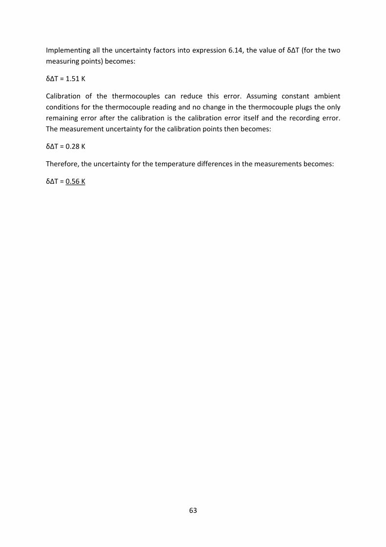
63

Implementing all the uncertainty factors into expression 6.14, the value of δΔT (for the two measuring points) becomes:

δΔT = 1.51 K

Calibration of the thermocouples can reduce this error. Assuming constant ambient conditions for the thermocouple reading and no change in the thermocouple plugs the only remaining error after the calibration is the calibration error itself and the recording error. The measurement uncertainty for the calibration points then becomes:

δΔT = 0.28 K

Therefore, the uncertainty for the temperature differences in the measurements becomes:

δΔT = 0.56 K

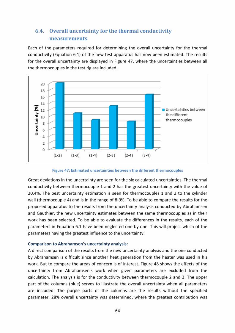
64

6.4. Overall uncertainty for the thermal conductivity measurements

Each of the parameters required for determining the overall uncertainty for the thermal conductivity (Equation 6.1) of the new test apparatus has now been estimated. The results for the overall uncertainty are displayed in Figure 47, where the uncertainties between all the thermocouples in the test rig are included.

Figure 47: Estimated uncertainties between the different thermocouples

Great deviations in the uncertainty are seen for the six calculated uncertainties. The thermal conductivity between thermocouple 1 and 2 has the greatest uncertainty with the value of 20.4%. The best uncertainty estimation is seen for thermocouples 1 and 2 to the cylinder wall (thermocouple 4) and is in the range of 8-9%. To be able to compare the results for the proposed apparatus to the results from the uncertainty analysis conducted by Abrahamsen and Gauthier, the new uncertainty estimates between the same thermocouples as in their work has been selected. To be able to evaluate the differences in the results, each of the parameters in Equation 6.1 have been neglected one by one. This will project which of the parameters having the greatest influence to the uncertainty.

Comparison to Abrahamsen’s uncertainty analysis: A direct comparison of the results from the new uncertainty analysis and the one conducted by Abrahamsen is difficult since another heat generation from the heater was used in his work. But to compare the areas of concern is of interest. Figure 48 shows the effects of the uncertainty from Abrahamsen’s work when given parameters are excluded from the calculation. The analysis is for the conductivity between thermocouple 2 and 3. The upper part of the columns (blue) serves to illustrate the overall uncertainty when all parameters are included. The purple parts of the columns are the results without the specified parameter. 28% overall uncertainty was determined, where the greatest contribution was

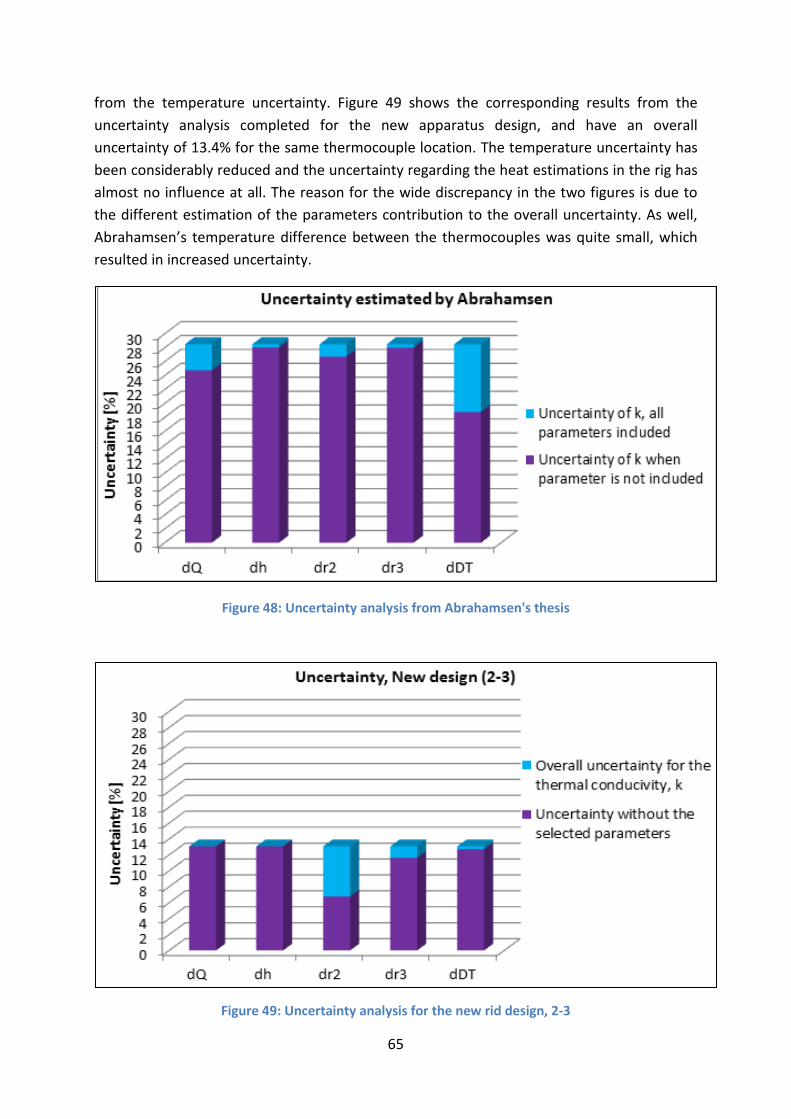
65

from the temperature uncertainty. Figure 49 shows the corresponding results from the uncertainty analysis completed for the new apparatus design, and have an overall uncertainty of 13.4% for the same thermocouple location. The temperature uncertainty has been considerably reduced and the uncertainty regarding the heat estimations in the rig has almost no influence at all. The reason for the wide discrepancy in the two figures is due to the different estimation of the parameters contribution to the overall uncertainty. As well, Abrahamsen’s temperature difference between the thermocouples was quite small, which resulted in increased uncertainty.

Figure 48: Uncertainty analysis from Abrahamsen's thesis

Figure 49: Uncertainty analysis for the new rid design, 2-3

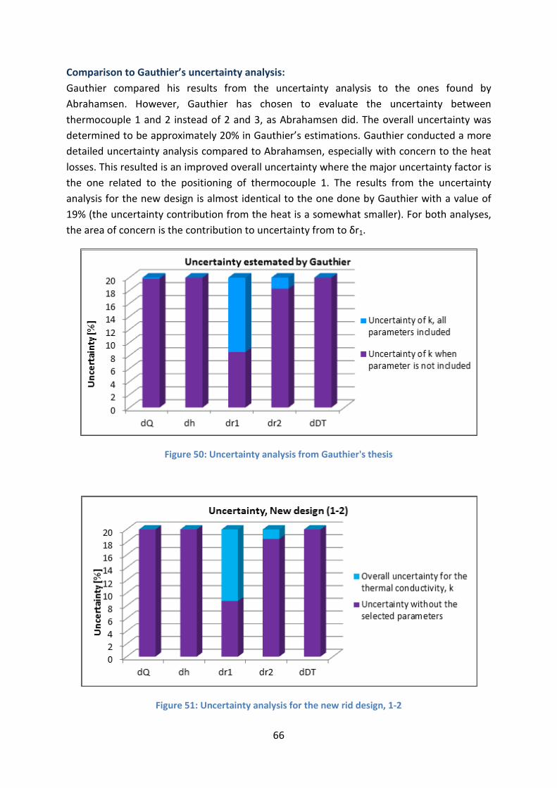
66

Comparison to Gauthier’s uncertainty analysis: Gauthier compared his results from the uncertainty analysis to the ones found by Abrahamsen. However, Gauthier has chosen to evaluate the uncertainty between thermocouple 1 and 2 instead of 2 and 3, as Abrahamsen did. The overall uncertainty was determined to be approximately 20% in Gauthier’s estimations. Gauthier conducted a more detailed uncertainty analysis compared to Abrahamsen, especially with concern to the heat losses. This resulted is an improved overall uncertainty where the major uncertainty factor is the one related to the positioning of thermocouple 1. The results from the uncertainty analysis for the new design is almost identical to the one done by Gauthier with a value of 19% (the uncertainty contribution from the heat is a somewhat smaller). For both analyses, the area of concern is the contribution to uncertainty from to δr1.

Figure 50: Uncertainty analysis from Gauthier's thesis

Figure 51: Uncertainty analysis for the new rid design, 1-2

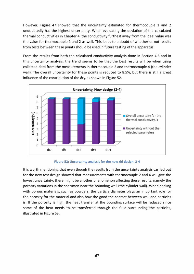
67

However, Figure 47 showed that the uncertainty estimated for thermocouple 1 and 2 undoubtedly has the highest uncertainty. When evaluating the deviation of the calculated thermal conductivities in Chapter 4, the conductivity furthest away from the ideal value was the value for thermocouple 1 and 2 as well. This leads to a doubt of whether or not results from tests between these points should be used in future testing of the apparatus.

From the results from both the calculated conductivity analysis done in Section 4.5 and in this uncertainty analysis, the trend seems to be that the best results will be when using collected data from the measurements in thermocouple 2 and thermocouple 4 (the cylinder wall). The overall uncertainty for these points is reduced to 8.5%, but there is still a great influence of the contribution of the δr2, as shown in Figure 52.

Figure 52: Uncertainty analysis for the new rid design, 2-4

It is worth mentioning that even though the results from the uncertainty analysis carried out for the new test design showed that measurements with thermocouple 2 and 4 will give the lowest uncertainty, there might be another phenomenon affecting these results, namely the porosity variations in the specimen near the bounding wall (the cylinder wall). When dealing with porous materials, such as powders, the particle diameter plays an important role for the porosity for the material and also how the good the contact between wall and particles is. If the porosity is high, the heat transfer at the bounding surface will be reduced since some of the heat needs to be transferred through the fluid surrounding the particles, illustrated in Figure 53.

68

Figure 53: Coupling of bounding surface conductivity ksb and the effective conductivity of the porous media and the near bounding surface [13]

Gauthier [13] took a closer look at this phenomenon and established a correlation for the error when neglecting the bounding effect. Figure 54 shows the conductivity error when the ratio between the outer diameter of the test section, D, and the particle diameter, dp, increases. The overall conductivity, ke,tot, is assumed to be:

𝑘𝑒,𝑡𝑜𝑡 =1𝐴𝑡𝑜𝑡

�𝑘𝑒,𝑏𝑢𝑙𝑘𝐴𝑏𝑢𝑙𝑘 + 𝑘𝑒,𝑖𝑛𝑡𝑒𝑟𝑓𝑎𝑐𝑒(𝐴𝑡𝑜𝑡 − 𝐴𝑏𝑢𝑙𝑘)�

(6.15)

And the error when neglecting the bounding effect will be:

∆𝑘𝑒,𝑡𝑜𝑡 = 2𝑑𝑝𝐷− �

𝑑𝑝𝐷�2

(6.16)

Figure 54: Conductivity error for various D/dp ratios [13]

69

The figure proves that the error is significant for low D/dp ratios. However, even at high ratios the error cannot be neglected. From these observations, it has been concluded that the most reliable results for thermal conductivity calculations with the proposed design will most likely be when temperatures are recorded at thermocouple 2 and 3. Consequently, the uncertainty will be in the range of 13% (see Figure 47). However, the uncertainty related to the positioning of thermocouple 2 should still be improved to reduce the overall uncertainty. Measuring temperatures at different positions at r2 would minimize the influence of the error.

6.5. Discussion A detailed analysis estimating the uncertainty for thermal conductivity measurements for the proposed apparatus has been carried out. For the prediction of the parameter related to heat losses, the heat transfer effect from the electric wire was included in the analysis, even though the results from Section 4.5 proved that if the wire is extended to a certain length, heat gain in the system would no longer effects the measurements. The estimations of the current and voltage parameters showed to be improved if utilizing of a more accurate multimeter. Together, these estimations resulted in a reduced heat loss uncertainty compared to previously conducted estimations. Estimations of the uncertainty parameter related to temperature recordings were thoroughly evaluated and by calibrating the thermocouples, the only parameters contributing to the temperature uncertainty were the recording error and the calibration error itself.

The overall uncertainty for the thermal conductivity showed a wide discrepancy depending on which temperature recordings are being used for the measurements. A great improvement of the uncertainty was observed when comparing the results with Abrahamsen’s uncertainty estimations. Comparing the results with Gauthier’s analysis showed almost identical results. However, the uncertainty compared to Gauthier’s work proved to be the uncertainty with the largest value. The best uncertainty was observed for measurements between thermocouple 2 and 4. The concern of this uncertainty estimation was the bounding wall effects at the cylinder wall. Consequently, the most credible measurements are assumed to be done for measurements between thermocouple 2 and 3, where the overall uncertainty is estimated to lie around 13%. Here, uncertainty in the position r2 is the most critical parameter for the conductivity determinations. This uncertainty can be minimized by measuring several temperatures at different positions at radius r2, which will reduce the error influenced by the radial position.

70

71

7. Conclusion The objective of this thesis was to select and analyze a method for measuring thermal conductivity of porous materials with low thermal conductivity, such as MOFs. Based on an initial literature survey of measurement techniques, a steady state method base on radial heat transfer in a concentric cylinder, equipped with a central heater, was selected as the most suited method for the present applications.

A numerical analysis was performed on the proposed test apparatus. A step-wise analysis was conducted in order to evaluate the isolated influence of each additional component on the system behavior. The analysis revealed the following:

• Expected heat loss behavior was confirmed as the insulation blocks and heater support was added to the simple, initial cylinder. Despite the losses, temperature recordings at the position of the thermocouples proved to be only slight affected by the heat losses. The calculated thermal conductivity showed a value of 1.19 % greater than the exact value.

• Implementing thermocouples and their respective protection tubes led to greater heat losses. However, fairly accurate temperature recordings were obtained due to increased heat transfer in the steel of the thermocouples. The deviation in thermal conductivity measurement increased to 2.7%.

• Unexpected impact to the heat transfer in the test section when implementing the electric wire (providing current to the heating element) has been proven to be a major concern. Heat transfer into the test section from ambient surroundings increased the heat flow in the test section with 1.15 W when the aluminum oxide heating element substituted the hollow heater.

• An extensive investigation of the effects of increasing the wire length to reduce heat flow from the wire showed that by increasing the wire length to 1.7 m, heat flow into the system did not affect the temperature recordings. Consequently, the results predicted an overall deviation in thermal conductivity measurement of 6 % above the exact value. However, it was shown that the 1.7 m wire needs to be coiled up inside the sealed container to achieve such results.

An uncertainty analysis was performed on the complete setup. The estimated parameter related to heat loss was considerably reduced from previously conducted analyses. Another important finding was that thermal conductivity measurements between thermocouple 2 and 3 are predicted to provide the most reliable results, close to 13 %. The worst uncertainty was observed for measurements between thermocouple 1 and 2. Here, small radial and temperature differences had great influence on the uncertainty, which increased the uncertainty to 20.4%.

72

73

8. Suggestions for further work

• To predict the time required to reach steady state for the proposed apparatus, performing a transient simulation in the Comsol model should be done. From this, one should be able to get a feeling of the amounts of liquid Nitrogen required for cooling the system as well.

• Only one specified thermal conductivity of the test specimen and insulation has been investigated. The heat transfer behavior when implementing test specimen with other thermal conductivities, as well as different thermal conductivities for the insulation, should be investigated and compared to the results from this research. Evaluating the impact of other wall temperatures would also be of great value.

• The electric wire has proven to be the most critical parameter. If the proposed apparatus is to be built, practical solution for how the wire will be arranged inside the container should be further developed. As well, the possibility of improving the accuracy of measurements by implementing alternative heating elements without electric wires (such as induction elements), should be investigated.

• To be able to achieve measurement accuracies as determined in the thesis, development of suitable insulation blocks in the test section needs to be completed in advance of building the apparatus.

• The uncertainty analysis carried out is only valid for cryogenic temperatures. Hence, an uncertainty analysis estimating the uncertainty for higher temperatures should be conducted to determine the effects of temperature to the uncertainty.

• To further reduce the uncertainty estimated in the uncertainty analysis, suitable options for the positioning of the thermocouples to reduce the impact of dr2 should be investigated. This could lead to implementation of additional thermocouples inside the test section, which would further result in greater heat losses.

• In the project thesis completed in advance of this thesis, tests where metal foam structures was included to enhance heat transfer, were carried out. If such a heat distribution element is to be included in future tests, improved solutions for assuring accurate positioning of the thermocouples should be clarified.

74

75

Bibliography 1. Ott, K., L. Simpson, and L. Klebanoff, Executive Summaries for the Hydrogen Storage

Materials Centers of Excellence: Chemical Hydrogen Storage CoE, Hydrogen Sorption CoE and Metal Hydride CoE, O.o.E.E.a.R.E. Fuel Cell Technologies Program, U.S. Department of Energy, Editor 2012.

2. U. Büenger, E.N., M.Schlichtenmayer, M. Hirscher, I. Senkovska, S.Kaskel, Analysis of Hydrogen Storage in Porous Adsorption Materials, in 18th World Hydrogen Energy Conference 2010 - WHEC 20102010: Essen, Germany.

3. Incropera, F.P., et al., Fundamentals of heat and mass transfer2011: Wiley. 4. Buck, W. and S. Rudtsch, "8.Thermal Properties" Springer Handbook of Materials

Measurement Methods, H. Czichos, T. Saito, and L. Smith, Editors. 2006, Springer Berlin Heidelberg. p. 399-429.

5. K.D Maglic, A.C., V.E. Peletsky, Compendium of Thermophysical Property Measurement Methods, Vol.1: Survey of Measurement Techniques Vol. 1. 1984, New York: Plenum Press. 789pp.

6. Mahanta, N.K. and A.R. Abramson, The dual-mode heat flow meter technique: A versatile method for characterizing thermal conductivity. International Journal of Heat and Mass Transfer, 2010. 53(23–24): p. 5581-5586.

7. Alessandro, F., An apparatus for the routine measurement of thermal conductivity of materials for building application based on a transient hot-wire method. Applied Thermal Engineering, 2007. 27(14–15): p. 2495-2504.

8. William, W. and A. Marc, Thermal Conductivity Measurement, in The Measurement, Instrumentation and Sensors Handbook on CD-ROM1999, CRC Press.

9. International_Standard, ISO 22007-1 Plastics - Determination of thermal conductivity and thermal diffusivity - Part 1: General Prinsiples, 2009.

10. American-Society-for-Testing-and-Materials, ASTM D 5930-01: Standard Test Method for Thermal Conductivity of Plastics my Means of a Transient Line-Source Technique, 2009.

11. International_Standard, ISO 22007-2: Plastics - Determination of thermal conductivity and thermal diffusivity - Part 2: Transient plane heat source (hot disk) method, 2008.

12. Abrahamsen, O.K., Hydrogen Storage: Thermophysical data and flow properties for some porous media, in Department of Energy and Process Engineering2010, Norwegian University of Science and Technology,: Trondheim.

13. Gauthier, J., Thermal Conductivity in Porous Media: Theory, experiments and model fitting, in Department of Energy, Process and Engineering2011, NTNU: Trondheim.

14. Eithun, C.F. and I.-A. Rasmussen, Hydrogen storage: Development of a setup for thermal conductivity measurements for porous materials in Department of Energy and Process Engineering 2011, NTNU: Trondheim.

15. Dixit, U.S., FINITE ELEMENT METHOD: AN INTRODUCTION, 2008, Department of Mechanical Engineering, Indian Institue of Technology: Guwahati, India

16. Comsol Multiphysics. 1998-2012 [cited 2012 Febuary 5th]; Available from: http://www.comsol.com/products/heat-transfer/.

17. (NIST), N.I.o.S.a.T., Nitrogen 2011. 18. Fesmire, J.E. and S.D. Augustynowicz, Cryogenic Thermal Insulation Systems, in 16th

Thermal and Fluids Analysis Workshop2005, NASA Kennedy Space Center: Orlando, Florida.

76

19. Ltd, C.M.E. Flanges and Fittings. 2003-2012 [cited 2012 June 5th]; Available from: http://www.caburn.co.uk/resources/downloads/pdfs/sec1.pdf.

20. Ltd, C.M.E. The feedthrough product line 2003-2012 [cited 2012 June 5th]; Available from: http://www.caburn.co.uk/resources/downloads/pdfs/sec6.pdf.

21. Moffat, R.J., Describing the Uncertainty in Experimental Results, in Mechanical Engineering 1988, Stanford University: Stanford.

22. Aglient_Technologies. E36XXA Series, Non-Programmable DC Power Supplies. 2009 [cited 2012 May 7th]; Available from: http://cp.literature.agilent.com/litweb/pdf/5968-9727EN.pdf.

23. FLUKE_Corporations. Fluke 45: Dual Display Multimeter. [cited 2012 May 11th]; Available from: http://www.fluke.com/fluke/usen/Bench-Instruments/Bench-Multimeters/Fluke-45.htm?PID=56082.

24. National_Instruments Performing High-Accuracy Temperature Measurements Using a NI Digital Multimeter and Switch, Tutorial. 2011.

A

APPENDIX

B

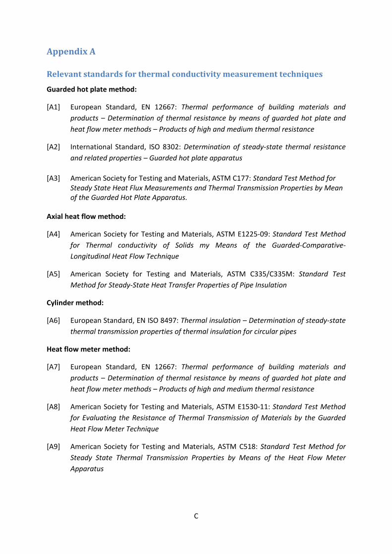
C

Appendix A

Relevant standards for thermal conductivity measurement techniques Guarded hot plate method:

[A1] European Standard, EN 12667: Thermal performance of building materials and products – Determination of thermal resistance by means of guarded hot plate and heat flow meter methods – Products of high and medium thermal resistance

[A2] International Standard, ISO 8302: Determination of steady-state thermal resistance and related properties – Guarded hot plate apparatus

[A3] American Society for Testing and Materials, ASTM C177: Standard Test Method for Steady State Heat Flux Measurements and Thermal Transmission Properties by Mean of the Guarded Hot Plate Apparatus.

Axial heat flow method:

[A4] American Society for Testing and Materials, ASTM E1225-09: Standard Test Method for Thermal conductivity of Solids my Means of the Guarded-Comparative-Longitudinal Heat Flow Technique

[A5] American Society for Testing and Materials, ASTM C335/C335M: Standard Test Method for Steady-State Heat Transfer Properties of Pipe Insulation

Cylinder method:

[A6] European Standard, EN ISO 8497: Thermal insulation – Determination of steady-state thermal transmission properties of thermal insulation for circular pipes

Heat flow meter method:

[A7] European Standard, EN 12667: Thermal performance of building materials and products – Determination of thermal resistance by means of guarded hot plate and heat flow meter methods – Products of high and medium thermal resistance

[A8] American Society for Testing and Materials, ASTM E1530-11: Standard Test Method for Evaluating the Resistance of Thermal Transmission of Materials by the Guarded Heat Flow Meter Technique

[A9] American Society for Testing and Materials, ASTM C518: Standard Test Method for Steady State Thermal Transmission Properties by Means of the Heat Flow Meter Apparatus

D

Hot wire method:

[A10] International Standard, ISO 8894-1: Refractory materials – Determination of thermal conductivity – Part 1: Hot-wire methods (cross-array and resistance thermometer)

[A11] International Standard, ISO 8894-2: Refractory materials – Determination for thermal conductivity – Part 2: Hot-wire method (parallel)

[A12] American Society for Testing and Materials, ASTM C1113/C1113M – 09: Standard Test Method for Thermal Conductivity of Refractories by Hot Wire (Platinum Resistance Thermometer Technique)

Needle probe method:

[A13] American Society for Testing and Materials, ASTM D 5930-01: Standard Test Method for Thermal Conductivity of Plastics my Means of a Transient Line-Source Technique

Transient planar source method:

[A14] International Standard, ISO 22007-2: Plastics – Determination of thermal conductivity and thermal diffusivity – Part 2: Transient plane heat source (hot disk) method

E

Appendix B

Material references [B1] Stainless steel: http://cryogenics.nist.gov/Papers/Cryo_Materials.pdf, March 2012 [B2] Teflon: http://cryogenics.nist.gov/MPropsMAY/Teflon/Teflon_rev.htm, March 2012 [B3] Copper: http://www.nist.gov/data/nsrds/NSRDS-NBS-8.pdf, April 2012 [B4] Wolfram: http://www.nist.gov/data/nsrds/NSRDS-NBS-8.pdf, April 2012 [B5] Aluminum oxide: http://www.nist.gov/data/nsrds/NSRDS-NBS-8.pdf, April 2012

F

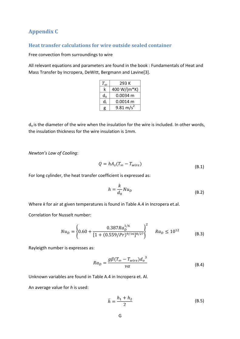
G

Appendix C

Heat transfer calculations for wire outside sealed container

Free convection from surroundings to wire

All relevant equations and parameters are found in the book : Fundamentals of Heat and Mass Transfer by Incropera, DeWitt, Bergmann and Lavine[3].

𝑇∞ 293 K k 400 W/(m*K) do 0.0034 m di 0.0014 m g 9.81 m/s2

do is the diameter of the wire when the insulation for the wire is included. In other words, the insulation thickness for the wire insulation is 1mm.

Newton’s Law of Cooling:

𝑄 = ℎ𝐴𝑠(𝑇∞ − 𝑇𝑤𝑖𝑟𝑒) (B.1)

For long cylinder, the heat transfer coefficient is expressed as:

ℎ =𝑘𝑑0𝑁𝑢𝐷

(B.2)

Where k for air at given temperatures is found in Table A.4 in Incropera et.al.

Correlation for Nusselt number:

𝑁𝑢𝐷 = �0.60 +0.387𝑅𝑎𝐷

1/6

[1 + (0.559/𝑃𝑟)9/16]8/27�2

𝑅𝑎𝐷 ≤ 1012

(B.3)

Rayleigth number is expresses as:

𝑅𝑎𝐷 =𝑔𝛽(𝑇∞ − 𝑇𝑤𝑖𝑟𝑒)𝑑𝑜

3

𝜈𝛼

(B.4)

Unknown variables are found in Table A.4 in Incropera et. Al.

An average value for h is used:

ℎ� =ℎ1 + ℎ2

2 (B.5)

H

Overall resistance for wire with insulation:

𝑈 = �𝑑𝑜2𝑘

𝑙𝑛 �𝑑𝑜𝑑𝑖� +

1ℎ��−1

(B.6)

Twire, 1 Twire, 2 h1 h2 �̅� U 129 K 273 K 19.69

W/(m2K) 12.30

W/(m2K) 15.5

W/(m2K) 15.15

W/(m2K)

The wire is can be considered as a fin of uniform cross-sectional area. For prescribed temperature, Case C in table 3.4 in Incropera et.al is chosen:

𝑄𝑓𝑖𝑛 = �ℎ𝑃𝑘𝐴𝑐𝜃𝑏cosh�� ℎ𝑃

𝑘𝐴𝑐𝐿� − 𝜃𝐿

𝜃𝑏

𝑠𝑖𝑛ℎ �� ℎ𝑃𝑘𝐴𝑐

𝐿�

(B.7)

Where,

𝜃(𝑥) = 𝑇∞ − 𝑇𝑥, 𝑃 = 𝜋𝑑𝑜 , 𝐴𝑐 =𝜋4𝑑𝑖2

An interation was conducted to determine the length of the wire if an accepted heat transfer of 0.04W is transported into the system. Due to the fact that Equation B.7 is asymptotic, a solution was not reachable as proven in figure C1. The asymptote stabilizes at 1.63 W, an unexpected result.

Figure C1: Heat transfer through wire as a function of wire length (outside test rig)

1,5

1,6

1,7

1,8

1,9

2

2,1

2,2

0 0,5 1 1,5 2 2,5 3 3,5 4 4,5 5Heat

Tra

nsfe

r fro

m w

ire,Q

fin, [

W]

Wire length [m]

I

Investigation of the thickness of the insulation covering the wire, assuming infinitely long wire, did not lead to promising either. The results are displayed in figure C2. Even at extreme thicknesses, the results do not improve. Observations actually show a sudden rise in heat transfer when increasing the insulation thickness, before is slowly decreases, never reaching the desirable value. Achieving the accepted heat transfer when keeping the wire outside the sealed container would only be reachable if zero-conductivity insulation could be used for the wire. This is practically impossible, hence; it is safe to conclude that the extended length of 1.7 m for the electric wire needs to be placed inside the sealed container (or in a cooling chamber outside the rig, which could be challenging).

Figure C2: Heat transfer through wire as a function of wire insulation thickness (outside test rig)