Development of a Predictive Optimal Controller for Thermal EnergyStorage SystemsGregor P. Henze� Robert H. Dodiery Moncef KrartizJoint Center for Energy ManagementCEAE Department, Campus Box 428University of Colorado at BoulderBoulder, Colorado 80309{0428January 15, 1997AbstractThis paper describes the development and simulation of a predictive optimal controller for thermalenergy storage systems. The `optimal' strategy minimizes the cost of operating the cooling plant overthe simulation horizon. The particular case of a popular ice storage system (ice-on-coil with internalmelt) has been investigated in a simulation environment. Various predictor models have been analyzedwith respect to their performance in forecasting cooling load data and information on ambient conditions(dry-bulb and wet-bulb temperatures). The predictor model provides load and weather information to theoptimal controller in discrete time steps. An optimal storage charging and discharging strategy is plannedat every time step over a �xed look-ahead time window utilizing newly available information. The �rstaction of the optimal sequence of actions is executed over the next time step and the planning process isrepeated at every following time step. The e�ect of the length of the planning horizon was investigatedand it was found that short horizons on the order of one day are only marginally suboptimal relative toa strategy that is optimal over the entire simulation horizon of one week. Various utility rate structureswere analyzed to cover a range of potential real-time pricing scenarios. The predictive optimal controllerwas then compared to conventional control heuristics. In summary, it was found that in the presence ofcomplex rate structures the proposed controller has a signi�cant performance bene�t over the conventionalcontrols while requiring only a simple predictor.1 IntroductionThermal energy storage provides the opportunity to reduce the operating cost of the cooling plant in com-mercial buildings. Though ice storage technology as a popular implementation of thermal energy storage isthe focus of this work, the methodology can easily be extended to other types of thermal energy storage.1.1 Previous WorkExperience with operating ice storage systems shows that a signi�cant shortfall of the current technology isthe poor performance of the control strategies (Akbari and Sezgen (1992), Guven and Flynn (1992), Tran etal. (1989)). The best-known control mechanism for these systems is chiller-priority. This simple heuristicconsists of using direct cooling (no storage usage) anytime during o�-peak hours, and during on-peak hours�E-Mail: Gregor.Henze@jci.comyE-Mail: dodier@colorado.eduzE-Mail: krarti@colorado.edu 1

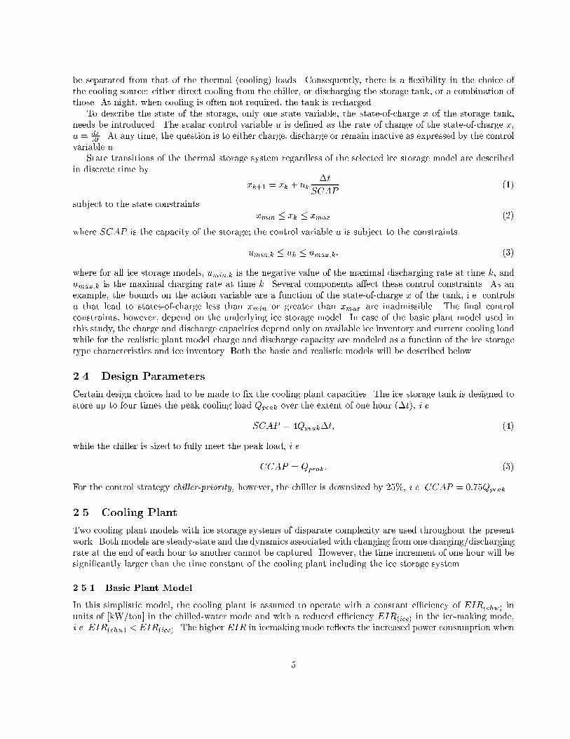
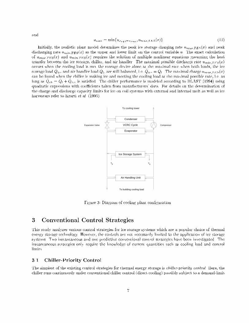
(a) as long as the current cooling load can be met by a chiller that is downsized in capacity, or (b) while animposed electrical demand limit is not yet exceeded by the cooling plant; otherwise the storage provides theremaining cooling capacity. In this study, the cooling plant consists of one chiller for both chilled-water andicemaking modes, pumps, fans, cooling tower, and all other equipment needed to provide cooling as sketchedin Figure 3. Though chiller-priority can be an appropriate strategy under peak cooling load conditions, itgenerally makes poor use of the available storage during swing seasons. With chiller-priority being the mostwidely used control, the potential of ice storage systems is only partially harnessed.Recognizing the need for research in the area of optimal control for thermal storage systems, variousapproaches have been proposed. However, the term \optimal control" has been used rather loosely whenreferring to the control of ice storage systems. Spethmann (1989) states the optimization problem as a list ofdesirable features that includes the proper consideration of utility rates, cost of ice-making as a function ofevaporator temperature, shape of cooling load pro�le, and many more. Rather than �nding the solution to astrictly variational problem, optimal control is treated as the problem of developing a knowledge base for areal-time expert system. Similarly, Knebel (1990) interprets optimal control for an ice harvesting system asthe correct variation of build and defrost time as a function of compressor capacity and saturated dischargepressure of the refrigerant. Braun (1992) and Drees (1994), on the other hand, carried out simulations thatare in accordance with the strict mathematical de�nition of optimal control. Assuming known load pro�les,Braun carried out daily simulations comparing chiller-priority, storage-priority, and optimal control, where thelatter was based on the minimization of either energy charges or peak demand charges. Drees, in addition tominimizing either daily energy or demand charges, investigated an objective function that minimizes energycost while preventing the demand cost from exceeding a prede�ned target. He also developed a heuristiccontrol strategy that is simple to implement yet approaches optimal performance.Kintner-Meyer and Emery (1995) investigated the bene�ts of an optimal control that minimizes daily (i.e.,24 h) operating cost for a large o�ce building by adjusting indoor air temperature and humidity setpointsas well as cooling plant operating parameters. Two sources of thermal energy storage were considered: anice storage tank (ice-on-coil with internal melt) and the thermal capacitance of the building mass (heavy,light, and ultra-light construction). The investigation therefore links the problem of dynamic building control(building pre-cooling or pre-heating) with the problem of cool storage control. Thermal building response andloads are part of the problem of HVAC control with TES rather than external constraints on the optimization.The study therefore e�ectively compares the individual and combined e�ects of building internal mass andcool storage on load shifting and peak power reduction. They found that signi�cant operating cost savingsand electrical demand reduction can be achieved, compared to the basecase of using direct cooling only,through early-morning ventilation utilizing free cooling and by shifting cooling loads to o�-peak periods.The investigators concluded that optimal building control is most e�ective in dry climates with large diurnaltemperature swings, in the presence of utility rates strongly encouraging load-shifting, and when cool storagesystems allow more e�ective load-shifting than building pre-cooling alone.Driven by the need for a better understanding of the behavior of ice storage systems in general, a simulationenvironment had been developed by Krarti et al. (1995) that allows the investigation of a wide range of keyparameters in uencing the system's operating cost.Within this environment, the optimal control strategy that minimizes the total electricity cost combiningenergy and demand charges was developed and validated. Based on building cooling loads and weather data,the optimal control strategy properly accounted for the e�ects of all environmental variables including utilityrate structure and cooling plant characteristics. This optimal strategy was used as a reference against whichconventional control strategies were compared. Three conventional control strategies were modeled: Chiller-priority, constant-proportion, and storage-priority control. Chiller-priority and constant-proportion controlare both instantaneous. Like optimal control, storage-priority control requires short-term load forecasting. Asa fundamental assumption, perfect predictions of weather and load variables were assumed for both storage-priority and optimal control in the study of Krarti et al. (1995).In particular, Krarti et al. (1995) found that under favorable conditions such as high cost incentives toshift loads to o�-peak hours or a small energy penalty for operating the chiller in icemaking mode, an ice2

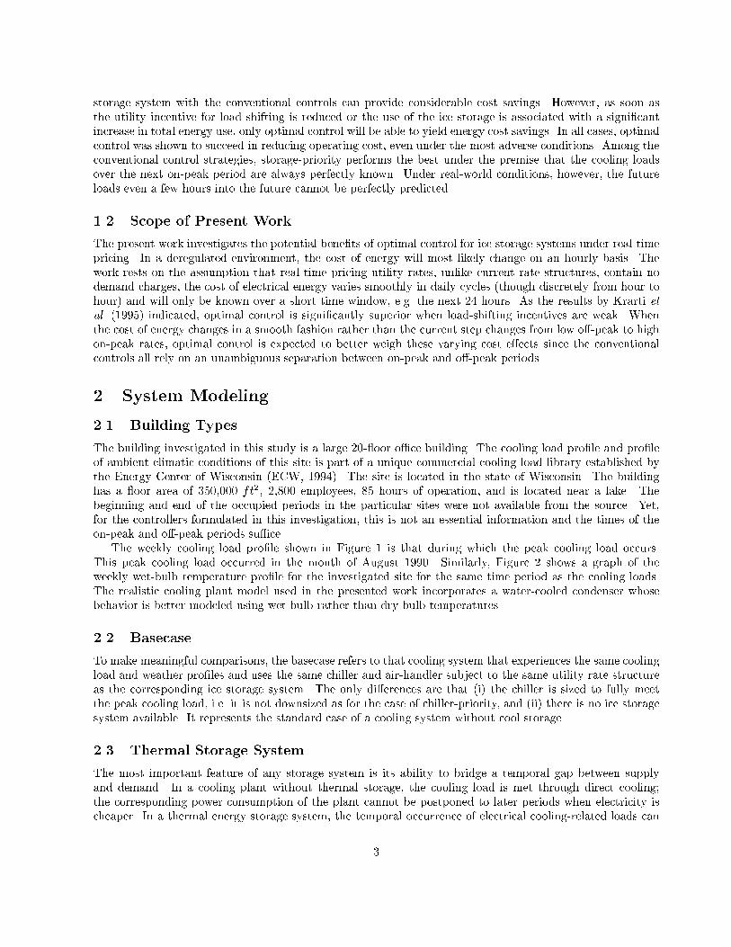
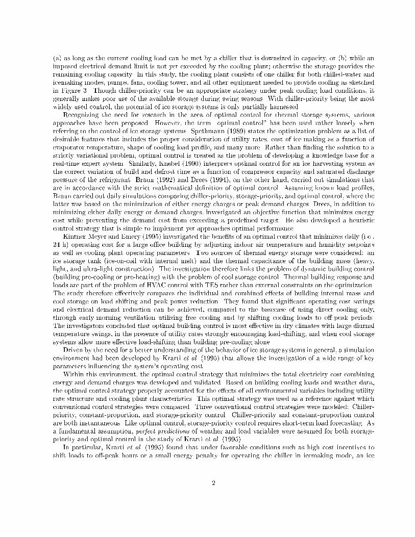
storage system with the conventional controls can provide considerable cost savings. However, as soon asthe utility incentive for load shifting is reduced or the use of the ice storage is associated with a signi�cantincrease in total energy use, only optimal control will be able to yield energy cost savings. In all cases, optimalcontrol was shown to succeed in reducing operating cost, even under the most adverse conditions. Among theconventional control strategies, storage-priority performs the best under the premise that the cooling loadsover the next on-peak period are always perfectly known. Under real-world conditions, however, the futureloads even a few hours into the future cannot be perfectly predicted.1.2 Scope of Present WorkThe present work investigates the potential bene�ts of optimal control for ice storage systems under real-timepricing. In a deregulated environment, the cost of energy will most likely change on an hourly basis. Thework rests on the assumption that real-time pricing utility rates, unlike current rate structures, contain nodemand charges, the cost of electrical energy varies smoothly in daily cycles (though discretely from hour tohour) and will only be known over a short time window, e.g. the next 24 hours. As the results by Krarti etal. (1995) indicated, optimal control is signi�cantly superior when load-shifting incentives are weak. Whenthe cost of energy changes in a smooth fashion rather than the current step changes from low o�-peak to highon-peak rates, optimal control is expected to better weigh these varying cost e�ects since the conventionalcontrols all rely on an unambiguous separation between on-peak and o�-peak periods.2 System Modeling2.1 Building TypesThe building investigated in this study is a large 20- oor o�ce building. The cooling load pro�le and pro�leof ambient climatic conditions of this site is part of a unique commercial cooling load library established bythe Energy Center of Wisconsin (ECW, 1994). The site is located in the state of Wisconsin. The buildinghas a oor area of 350,000 ft2, 2,800 employees, 85 hours of operation, and is located near a lake. Thebeginning and end of the occupied periods in the particular sites were not available from the source. Yet,for the controllers formulated in this investigation, this is not an essential information and the times of theon-peak and o�-peak periods su�ce.The weekly cooling load pro�le shown in Figure 1 is that during which the peak cooling load occurs.This peak cooling load occurred in the month of August 1990. Similarly, Figure 2 shows a graph of theweekly wet-bulb temperature pro�le for the investigated site for the same time period as the cooling loads.The realistic cooling plant model used in the presented work incorporates a water-cooled condenser whosebehavior is better modeled using wet-bulb rather than dry-bulb temperatures.2.2 BasecaseTo make meaningful comparisons, the basecase refers to that cooling system that experiences the same coolingload and weather pro�les and uses the same chiller and air-handler subject to the same utility rate structureas the corresponding ice storage system. The only di�erences are that (i) the chiller is sized to fully meetthe peak cooling load, i.e. it is not downsized as for the case of chiller-priority, and (ii) there is no ice storagesystem available. It represents the standard case of a cooling system without cool storage.2.3 Thermal Storage SystemThe most important feature of any storage system is its ability to bridge a temporal gap between supplyand demand. In a cooling plant without thermal storage, the cooling load is met through direct cooling;the corresponding power consumption of the plant cannot be postponed to later periods when electricity ischeaper. In a thermal energy storage system, the temporal occurrence of electrical cooling-related loads can3

0 24 48 72 96 120 144 168Time [hrs] starting at Monday 00:00

0

100

200

300

400

500

600

700

Coo

ling

Load

[ton

s]

Figure 1: Cooling load pro�le of investigated large 20- oor o�ce building.

0 24 48 72 96 120 144 168Time [hrs] beginning Monday 00:00

40

45

50

55

60

65

70

75

80

Wet

-Bul

b T

empe

ratu

re [d

eg F

]

Figure 2: Wet-bulb temperature pro�le of investigated large 20- oor o�ce building.4

be separated from that of the thermal (cooling) loads. Consequently, there is a exibility in the choice ofthe cooling source: either direct cooling from the chiller, or discharging the storage tank, or a combination ofthose. At night, when cooling is often not required, the tank is recharged.To describe the state of the storage, only one state variable, the state-of-charge x of the storage tank,needs be introduced. The scalar control variable u is de�ned as the rate of change of the state-of-charge x,u = dxdt . At any time, the question is to either charge, discharge or remain inactive as expressed by the controlvariable u.State transitions of the thermal storage system regardless of the selected ice storage model are describedin discrete time by xk+1 = xk + uk �tSCAP (1)subject to the state constraints xmin � xk � xmax (2)where SCAP is the capacity of the storage; the control variable u is subject to the constraintsumin;k � uk � umax;k: (3)where for all ice storage models, umin;k is the negative value of the maximal discharging rate at time k, andumax;k is the maximal charging rate at time k. Several components a�ect these control constraints. As anexample, the bounds on the action variable are a function of the state-of-charge x of the tank, i.e. controlsu that lead to states-of-charge less than xmin or greater than xmax are inadmissible. The �nal controlconstraints, however, depend on the underlying ice storage model. In case of the basic plant model used inthis study, the charge and discharge capacities depend only on available ice inventory and current cooling loadwhile for the realistic plant model charge and discharge capacity are modeled as a function of the ice storagetype characteristics and ice inventory. Both the basic and realistic models will be described below.2.4 Design ParametersCertain design choices had to be made to �x the cooling plant capacities. The ice storage tank is designed tostore up to four times the peak cooling load Qpeak over the extent of one hour (�t), i.e.SCAP = 4Qpeak�t; (4)while the chiller is sized to fully meet the peak load, i.e.CCAP = Qpeak: (5)For the control strategy chiller-priority, however, the chiller is downsized by 25%, i.e. CCAP = 0:75Qpeak.2.5 Cooling PlantTwo cooling plant models with ice storage systems of disparate complexity are used throughout the presentwork. Both models are steady-state and the dynamics associated with changing from one charging/dischargingrate at the end of each hour to another cannot be captured. However, the time increment of one hour will besigni�cantly larger than the time constant of the cooling plant including the ice storage system.2.5.1 Basic Plant ModelIn this simplistic model, the cooling plant is assumed to operate with a constant e�ciency of EIR(chw) inunits of [kW/ton] in the chilled-water mode and with a reduced e�ciency EIR(ice) in the ice-making mode,i.e. EIR(chw) < EIR(ice). The higher EIR in icemaking mode re ects the increased power consumption when5

providing cooling at subfreezing temperatures. These values lump together the e�ciencies of all componentsof the cooling plant. The total power consumption Pk of the basic plant model isPk = � Qch;kEIR(ice) if u > 0, i.e. chargingQch;kEIR(chw) if u � 0, i.e. discharging (6)where the chiller load Qch;k is de�ned as the sum of the cooling load Qk and the discharging/charging rateuk, Qch;k = Qk + uk: (7)For the basic plant model, the charge and discharge capacities depend only on available ice inventory andcurrent cooling load. The constraints on the control variable for the basic plant model are formulated asumin = maxf�Qk; uxk+1=xming (8)and umax = minfCCAP �Qk; uxk+1=xmaxg (9)where uxk+1=x0 denotes the control action u that leads to a state-of-charge x0 when operating the coolingsystem over the next hour (k ! k + 1) at exactly that control u. Thus, no actions can be taken that wouldlead to states-of-charge outside the limits. Furthermore, the (�xed) capacity of the chiller CCAP minus thecurrent load Qk de�nes the maximal charging rate umax;k, i.e. how much can be charged after meeting theload.2.5.2 Realistic Plant ModelThe realistic cooling plant model used in this study is a modular steady-state model that computes the powerconsumption of each plant component (Krarti et al. (1995)). The correlations used in the plant model arebased on the building simulation program BLAST (1994). The components include an air-handling unit, anice storage system, a chiller, a cooling tower, and all required pumps and fans as illustrated in Figure 3.The modularity allows one to easily switch between one of three ice storage system types (ice-on-coil withinternal melt, ice-on-coil with external melt, and a dynamic ice harvester) as well as between one of threechiller compressor types (centrifugal, reciprocating, and screw compressors).The plant model determines the component power consumptions in response to a set of external parametersand a set of plant parameters. The external parameters are the cooling load Qk at hour k, the ambient wet-bulb temperature at that hour TWB;k, the state-of-charge xk, and the charging/discharging rate uk. Inaddition, a set of plant parameters governs the operation of the cooling plant. For the realistic plant modelused in this analysis, the plant parameters include either one or two temperature setpoints of the cooling plantdepending on the mode of operation. These cooling plant temperature setpoints are the chilled water supplytemperature leaving the evaporator, the chilled water supply temperature entering the air handling unit,and the supply air temperature and they are adjusted in a separate optimization step (plant optimization)so that the total power consumption for the current set of external parameters is minimized. Only thesimultaneous cost and plant optimization allows the determination of an optimal control trajectory in whicheach charging/discharging control is associated with the minimal attainable cooling plant power consumption.When evaluating conventional control strategies, the plant power consumptions will also be the smallestattainable for the chosen control action u under the given conditions. The plant optimization is described indetail by Krarti et al. (1995).In case of a realistic cooling plant model, constraints on the heat transfer capabilities of the thermal storagesystem further restrict the admissible values of u. These additional constraints include the ability to absorb orreject heat as expressed by umin;TES(x) and umax;TES(x), respectively. These limits depend on the selectedthermal storage system type and the state-of-charge x.The constraints on the control variable for the realistic plant model are formulated asumin = maxf�Qk; uxk+1=xmin ; umin;TES(x)g (10)6

and umax = minfuxk+1=xmax ; umax;TES(x)g (11)Initially, the realistic plant model determines the peak ice storage charging rate umax;TES(x) and peakdischarging rate umin;TES(x) as the upper and lower limit on the control variable u. The exact calculationof umax;TES(x) and umin;TES(x) requires the solution of multiple nonlinear equations governing the heattransfer between the ice storage, chiller, and air handler. The maximal possible discharge rate umin;TES(x)occurs when the cooling load is met the storage device alone at the maximal rate when both loads, the icestorage load _Qice and air handler load _Ql, are still balanced, i.e. _Qice = _Ql. The maximal charge umax;TES(x)can be found when the chiller is making ice and meeting the cooling load at the maximal possible rate, i.e. aslong as _Qch = _Ql + _Qice is satis�ed. The chiller performance is modeled according to BLAST (1994) usingquadratic expressions with coe�cients taken from manufacturers' data. For details on the determination ofthe charge and discharge capacity limits for ice-on-coil systems with external and internal melt as well as iceharvesters refer to Krarti et al. (1995).

Tfr Tfr

Condenser

Evaporator

Air Handling Unit

Ice Storage System

VCRC CycleExpansion Valve Compressor

To cooling tower

To building cooling loadFigure 3: Diagram of cooling plant con�guration.3 Conventional Control StrategiesThis study analyzes various control strategies for ice storage systems which are a popular choice of thermalenergy storage technology. However, the controls are not necessarily limited to the application of ice storagesystems. Two instantaneous and one predictive conventional control strategies have been investigated. Theinstantaneous strategies only require the knowledge of current quantities such as cooling load and controllimits.3.1 Chiller-Priority ControlThe simplest of the existing control strategies for thermal energy storage is chiller-priority control. Here, thechiller runs continuously under conventional chiller control (direct cooling) possibly subject to a demand-limit7

while the storage provides the remaining cooling capacity if required.uk = 8<: umax;k if k is o�-peak0 if k is on-peak and CCAPk � Qkumax;k if k is on-peak and CCAPk < Qk (Note: umax < 0 in this case) (12)where uk is the charging/discharging rate, CCAPk is the reduced (75%) chiller capacity, and Qk is the coolingload each taken at hour k.The simplicity lies in the fact that the conventional chiller control is not altered yielding high chillere�ciencies and a smooth demand curve, however, with the disadvantage that the meltdown of the ice isnot controlled to allow for maximal demand reduction. In addition, the time-of-day dependent energy ratestructure in [$/kWh] is not accounted for, i.e. load-shifting performance is inadequate.3.2 Constant-Proportion ControlThis control strategy implies that the storage meets a constant fraction fQ of the cooling load under allconditions. Thus, neither the chiller nor the storage have priority in providing cooling. This simple controlstrategy provides a greater demand reduction than chiller-priority control since the chiller capacity fractionused for a particular month will track the fraction of the annual cooling design load the building experiencesduring that month. For example, in a month in which 50% of the annual design load occurs, only 50% of thechiller capacity will be requested.uk = � umax;k if k is o�-peakmaxf�fQQk; umin;kg if k is on-peak (13)Constant-proportion control is rather easy to implement by assigning a �xed fraction of the total temper-ature di�erence between brine supply and return ow to be realized by the storage and the remainder by thechiller. Finding the best load fraction fQ for each application is a matter of trial and error. Caution shouldbe exercised that the chiller can always meet the remaining load fraction, i.e.(1� fQ)Qmax � CCAPnomor in other terms fQ � 1� CCAPnomQpeak ;where CCAPnom is the nominal chiller capacity.3.3 Storage-Priority ControlAs the name re ects, storage-priority control requires melting as much ice as possible during the on-peakperiod. It is generally de�ned as that control strategy that aims at fully discharging the available storagecapacity over the next on-peak period. Thus, the simultaneous operation of the chiller and the storage andthe terminal state-of-charge is speci�ed, yet not how this is accomplished in detail; see Tamblyn (1985).In the present work the following implementation is suggested. The chiller is base loaded during o�-peakhours to recharge the ice storage for the next on-peak period. The chiller operates in one of two modes duringthe on-peak period. The chiller operates either in Mode 0 at a reduced capacity A0 in parallel with thestorage during on-peak hours so that at the end of the on-peak period the storage inventory is just depleted.If this is not possible without prematurely depleting storage, the control switches to Mode 1 and the storageprovides a constant proportion A1 of the load in each on-peak hour similar to constant-proportion control.Both parameters, A0 and A1 are determined from predicted cooling loads over the next on-peak period. Theon-peak period used throughout the analysis regardless of whether time-of-use or real-time pricing rates areused, is from 10 a.m. until 6 p.m. during weekdays. All other hours are o�-peak.8

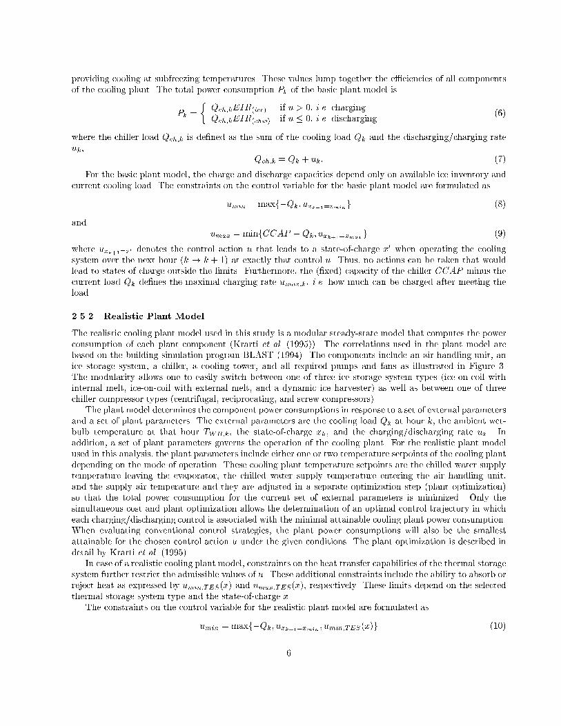
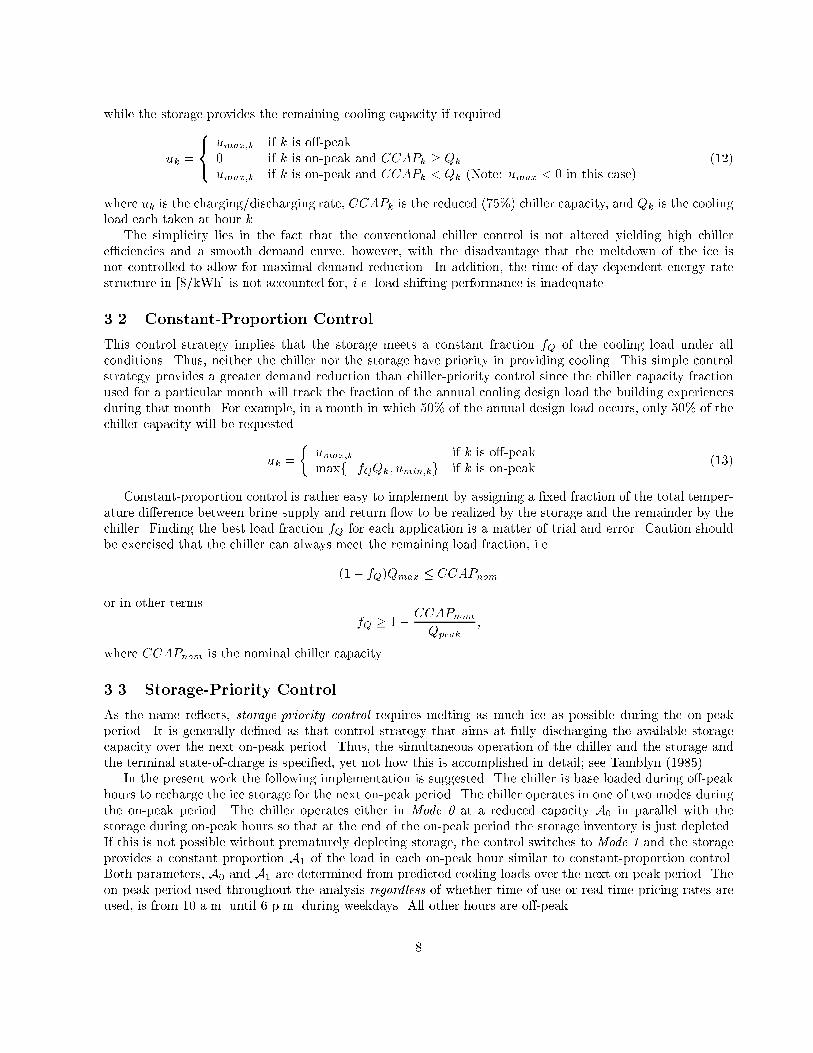
The tank discharge/charge rates are determined byuk = 8<: umax;k if k is o�-peakA0 �Qk if k is on-peak and discharge mode is 0maxf�A1Qk; umin;kg if k is on-peak and discharge mode is 1 (14)The chiller capacity A0 is computed fromA0 = 1N (N�1Xi=0 Qk0+i � xk0 SCAP�t ) (15)where N is the number of hours in the on-peak period and k0 is the �rst hour therein. The constant proportionA1 in turn is determined from A1 = xk0 SCAP�tPN�1i=0 Qk0+i (16)Refer to Krarti et al. (1995) for a more detailed description of storage-priority control and graphs of theperformance and behavior of chiller-priority, constant-proportion, and storage-priority controls.4 Optimal ControlOptimal control in the current context is that sequence of controls that minimizes the operating cost of thecooling plant over the simulation periodJ = J(u1; u2; : : : ; uK) = KXk=0 rkPk�t (17)where K is the total number of hours in the simulation period, rk is the cost of electrical energy at hour k,and Pk is the cooling plant electrical power consumption. The sequence frkgKk=0 is the cost of electrical energyas driven by real-time pricing in a deregulated utility environment. Several periodic utility rate structureswith varying amplitude were investigated as shown in Figure 4. Note that rk is only an energy charge; inthe real-time pricing scenario we have investigated, there are no demand charges. For all rate structures andfor all control strategies, on-peak period is de�ned as the time between 10 a.m. and 6 p.m. Monday throughFriday with o�-peak period being the remaining hours and weekend. All three conventional controls requireinformation on the beginning and end of on-peak periods to function properly as indicated by Equations 12,13, and 14. Times of actual occupancy are not required, since the discharge rates are adjusted as a functionof the current cooling load.The real-time pricing scenarios in this work are chosen for illustrative purposes and no claim is madethat these rate structures will be typical once utilities are deregulated. Rather, the examined rate structuresrepresent idealized pro�les of what the authors consider probable realizations.4.1 Dynamic ProgrammingThe task of minimizing operating cost J is framed as a sequential decision-making process of decision variableu: The optimization technique called dynamic programming, commonly used for this type of problems, was�rst formally introduced by the mathematician Richard Bellman in 1957. Bellman's Principle of Optimalitystates that the optimal solution to a K-step process must come from the optimal solution of an K � 1-stepprocess that is based on the optimal outcome of the �rst step. The solution of one K-step process will thusbe found recursively by optimizing K single-step processes.9

0 6 12 18 24 30 36 42 48Time [hrs] starting midnight

0.00

0.02

0.04

0.06

0.08

0.10

0.12

0.14

0.16

0.18

Cos

t of E

lect

ricity

[$/k

Wh]

Rate Structure 1Rate Structure 2Rate Structure 3

Figure 4: Rate Structures used in the study.The basic optimization model has two fundamental features: (i) an underlying discrete-time dynamicsystem, and (ii) an incrementally additive cost function. The dynamic system has the general formxk+1 = f(xk; uk; wk) (18)where x is the state of the system, u is the control, and w is a random disturbance. Consider a process inwhich the transition from one state xj at time j through the control uj is associated with the instantaneouscost l(xj ; uj ; wj): (19)Then the total expected cost of starting at time k and ending at time K can be expressed byJ = KXj=kE [l(xj ; uj ; wj)] (20)where the expectation in this and other equations is taken with respect to the disturbance wj . It is assumedthere exists a sequence of controls u that minimizes J , thus there exists for each state x and time k an optimalcost-to-go function, I(x; k) = minuj2U;j=k;:::;K J = minuj2U;j=k;:::;K8<: KXj=kE [l(xj ; uj ; wj)]9=; : (21)Here U is the constrained set of admissible controls. In deriving the desired iterative functional equation, theoptimal cost-to-go may be rewritten asI(x; k) = minuj2U;j=k;:::;K8<:E [l(xk; uk; wk)] + KXj=k+1E [l(xj ; uj ; wj)]9=; (22)where x = xk. This expression is equivalent toI(x; k) = minuk2U minuj2U;j=k+1;:::;K8<:E [l(xk; uk; wk)] + KXj=k+1E [l(xj ; uj ; wj)]9=; (23)10

Consider, for the moment, only the inner minimization over uj 2 U; j = k + 1; : : : ;K. Since E [l(xk; uk; wk)]does not depend on uk+1; uk+2; uk+3; : : :, the inner minimization becomesE [l(xk; uk; wk)] + minuj2U;j=k+1;:::;K KXj=k+1E [l(xj ; uj ; wj)] : (24)Now employing the general state transition equation f , the second argument in Equation 24 can be expressedas minuj2U;j=k+1;:::;K 8<: KXj=k+1E [l(xj ; uj ; wj)]9=;= I(xk+1; k + 1)= I(f(xk ; uk; wk); k + 1) (25)Summarizing Eqs. 23, 24, and 25,I(x; k) = minuk2U fE [l(xk; uk; wk)] + I(f(xk ; uk; wk); k + 1)g : (26)This is an iterative equation that can be used to determine I(x; k) for all admissible x, entirely from theknowledge of I(x; k+1). The starting point of the iteration is the terminal cost I(x;K), which expresses thepreference for a particular �nal state x. For example, a full storage may be preferred and thus all I(x 6= 1;K)will be given a very high value. In the present work, I(x;K) = 0 for all states of charge x, thus the �nal stateat the end of the planning horizon is free; no �nal state is preferred.In summary, it is found that the minimal cost at state x and stage k, I(x; k), is determined by minimizingthe sum of the cost at the present stage k, and the minimal cost in going to the end of the process from theresulting state at the next stage k + 1, as expressed by Equation 26.4.2 Application of the Certainty Equivalence PrincipleIn this study, the discrete-time dynamic system as represented by Equation 1 is only a function of the state-of-charge and the control variable (both scalar) and not of the external disturbance wk,xk+1 = xk + uk �tSCAP = f(xk; uk); (27)and is therefore deterministic. The instantaneous cost l of Equation 19 is the cost of electrical energy consumedby the cooling plant over the next time step,l(xk; uk; wk) = rkPk�t: (28)As supported by the �ndings in Section 6, the optimization is only carried out over short horizons, overwhich|even in the case of real-time pricing|the cost of energy r will be known. Thus, r is a deterministicvariable.The cooling plant power consumption Pk is (in the most general case) a function of the control u, i.e.charging/discharging rate, and the state-of-charge x (the state variable). Both of these variables are assumedto be known through noise-free observation. Furthermore, the performance of the cooling plant is a�ected byambient conditions (as they a�ect the thermodynamic process e�ciency) as well as chiller part-load perfor-mance. The condenser temperature (the upper process temperature) is the sum of either the ambient dry-bulbtemperature TDB for an air-cooled condenser or the ambient wet-bulb temperature TWB for a water-cooledcondenser, plus the corresponding condenser approach. It is assumed that the part-load performance can becomputed from the chiller cooling capacity CCAP and the chiller cooling load Qch. The chiller load is a11

function of the cooling load Qk and the charging/discharging rate uk. Ambient temperature and cooling loadare modeled as a deterministic signal plus an uncorrelated Gaussian noise term. (However, previous work byDodier (1995) suggests that this noise model is not as accurate as a correlated noise model; for simplicity,the uncorrelated noise model was used.) The disturbance wk comprises the ambient temperature and coolingload, wk = � TkQk � ; (29)where Tk is either dry-bulb or wet-bulb temperature depending on the condenser type employed. The powerconsumption function Pk = P (xk ; uk; wk) is a mapping established by the cooling plant model described inSection 2.5. As mentioned there, the basic plant model does not account for weather in uences and thuswk = Qk for the basic model.To apply Equation 26, the expected value of the instantaneous cost l has to be determined. For the basicplant model and the realistic cooling plant model, the expectation has to be taken over the cooling plantpower consumption given the distribution of cooling load at hour k or the joint distribution of temperatureand cooling load at hour k, respectivelyE [l(xk; uk; wk)] = E [rkP (xk ; uk; wk)�t] = rkE [P (xk ; uk; wk)]�t: (30)As minimizing over this expected value could be di�cult and time-consuming, an investigation was carriedout to �nd a convenient approximation of E[P (x; u; w)]. For smooth functions, the expected value of a functionof a random variable is the function evaluated at the mean of the variable plus higher order terms.E[g(w)] = g( �w) + 12Trace (rrg( �w)�w) + � � � (31)where rrg is the Hessian matrix and �w is the covariance of w. In this investigation, a �rst-order approxi-mation is considered, E[P (x; u; w)] � P (x; u; �w): (32)The left-hand side is estimated by Monte-Carlo integration,E[P (x; u; w)] = Z 1�1 P (x; u; w)p(w)dw � 1R RXi=1 P (x; u; ~wi) � ~E[P (x; u; w)] (33)where ~wi is a simulated disturbance, ~w = �w + �; � � N(0; �2); (34)and R is some large number of realizations. The assumption underlying this simulation is that weather andload processes are composed of a deterministic signal plus uncorrelated, additive, Gaussian noise. The noisemagnitude � was chosen di�erently for temperature than for load.To determine whether the approximation in Equation 32 is valid, large noise levels in the temperature andcooling load processes were assumed. For temperature, the standard deviation of the temperature noise �Twas taken as the standard deviation of the available historical data. This assumption is conservative sinceeven a simple predictor model will predict better than the average. For cooling loads, the RMS error of atwo-component harmonic model (168-hour fundamental and 1-hour �rst harmonic) �tted to the cooling loaddata of a 20- oor o�ce building by least-squares was used as an approximation of the standard deviation ofthe load noise �Q.With R = 200 realizations, �T = 7, and �Q = 78 the analysis showed that for a large number of cases,the power consumption P evaluated at the mean disturbance �w is on average 3.5% below the Monte-Carloapproximated expected power consumption ~E[P ] of Equation 33 with a standard deviation of 2.6%. \Onaverage" in this context refers to a representative range of x and u values. As expected, for lower levels of12

noise in both stochastic variables, the approximation of Equation 32 becomes even better and is consequentlyapplied to the present optimization problem.The modi�ed cost function that will be minimized is therefore~J = KXj=k l(xj ; uj ; �wj) (35)and the new iterative function for the approximated optimal cost-to-go becomes~I(x; k) = minuk2U nl(xk; uk; �wk) + ~I(f(xk; uk); k + 1)o : (36)If the optimal policy is una�ected whether the disturbances or their means are used, the certainty equiva-lence principle is said to hold (Bertsekas, 1995). The suboptimal control that applies at each stage the controlthat would be optimal if some or all of the stochastic variables are �xed at their expected value, is thereforecalled a certainty equivalence controller.In this analysis, closed-loop optimization is employed, i.e. the certainty equivalence controller carries outan optimization over a prede�ned planning horizon L and of the generated optimal strategy only the �rstaction is executed. At the next time step the process is repeated. The �nal control strategy of this near-optimal controller over a total simulation horizon of K steps is thus composed of K initial control actions ofK optimal strategies of horizon L; where L < K. This ensures that newly available, improved forecasts offuture variables are always utilized. As an example, if the simulation lasts from t0 until t0 + 100�t, then thecertainty of variables at t0 + 50�t is most probably better at t0 + 45�t than at t0 + 20�t and incorporatingupdated forecasts \along the way" is useful.Thus, the investigated implementation of optimal control for the thermal energy storage problem is acertainty-equivalence, closed-loop control. Throughout thermal energy storage literature, the term optimalcontrol is used with di�erent degrees of rigor. Even though the need for discretization in dynamic program-ming and optimization over shorter horizons than the simulation period are sources of suboptimality in theoptimization algorithm, the solutions are optimal in the mathematical sense and the term optimal control isretained. This is to avoid confusion with control heuristics that have been termed \near-optimal" but thatare not based on mathematical optimization.5 Prediction of Future DisturbancesThe \disturbances" which a�ect the cooling system are the ambient conditions and cooling loads, which inturn are determined for the most part by the number of people in the building. If one knew the exact coolingloads that will occur during the planning horizon, one could use dynamic programming to �nd the best courseof action (ignoring discretization problems). In reality one can only guess at future loads, and the costsincurred will increase with decreasing accuracy of predictions. In this section, the load forecasting modelswhich were studied are presented. In each case, a year of hourly data was available for model building (ECW,1994). About one week of data were withheld from each month, and models �tted on the remaining data.Some of the withheld data were used to compare prediction schemes.As this is not meant to be a comprehensive survey of prediction methods, only a representative few arepresented here. The prediction models used in this research range from the very simple (unbiased randomwalk model) through the less simple (bin predictor and harmonic models) to the complex (autoregressiveneural network). Due to its greater complexity and additional input variables, one might expect the neuralnetwork to outperform the simpler models, as indeed it does.5.1 Unbiased Random Walk ModelThis predictor is very simple. If the present load isQt, then one predicts that the future loadsQt+1; Qt+2; Qt+3; : : :are all equal to Qt. It turns out that this prediction is best in the least-squares sense if the process generating13

the sequence of loads is an unbiased random walk|that is, if the load at the next hour is with equal proba-bility either somewhat greater or somewhat less than the present load. This forecasting model is perhaps thesimplest interesting model and provides a base case against which one can test more sophisticated predictors.Despite the simplicity of this model, substantial cost reduction can be gained by using this model.5.2 Bin Predictor ModelA \bin model" is a simple piecewise constant (and thus nonlinear) model. To set the model parameters, theinput space is divided up into a number of disjoint regions, and the average value of the output variable overeach region is computed. The average of the output variable is taken over the data used for training; theinput regions are �xed and are not modi�ed according to the training data. If an input falls into a certainregion, then the average of that region is the prediction of the output for the input. The regions are alwaysrectangular sets of the form [a1; b1]� [a2; b2]� : : :� [an; bn], where n is the number of input variables. Thusit is convenient to represent the bin model as a table or an array which is indexed by the input variables. Forthis study, the bin model for cooling load includes as inputs month, hour of the day, and temperature. Monthand hour of the day were naturally divided into 1, 2, . . . , 12, and 1, 2, . . . , 24, respectively. Temperature wasdivided into 15 equal intervals from 33 to 97 �F , and a temperature index � = 1; 2; : : : ; 15 was calculated as�(T ) = d15(T � 33)=(97� 33)e (37)(The notation dxe means the least integer greater than or equal to x. No temperatures were outside the range33 to 97 �F .) Future temperatures were predicted using a separate bin model which used only month andhour of the day as inputs. So future loads were predicted in a two-step process as follows.T (m;h) = �Tm;h (38)Q(m;h) = Q(m;h; T (m;h)) = �Qm;h;�(T (m;h)): (39)Here �T and �Q are the tables constructed from average values of T and Q, respectively, in the training data.Subscripts indicate indices into the tables.More complicated bin models can be considered. Additional input variables such as wet-bulb temperatureare possible. One might use unequal intervals, or allow the input regions to have arbitrary shapes, or allowthe prediction function over a region to be a more general function rather than just a constant. Such modelsare related to so-called spline or multi-phase regressions (Seber and Wild, 1989), mixtures of experts models(Haykin, 1994). Another related model, the cerebellar model articulatory controller (CMAC), has been appliedto building energy use forecasting (Seem and Braun, 1991).5.3 Harmonic Predictor ModelThe harmonic predictor models the target time-series as a sum of sine and cosine functions. For this analysis,one harmonic model for each month of the year was considered; it was found that this model gave a somewhatbetter �t than a single model based on the same frequency components. The harmonic model for dry-bulbtemperature T can be expressed asT (m; t) = m + 4Xk=1(Am;k sin(!kt) +Bm;k cos(!kt)): (40)Where, m is the month, t is the number of hours after midnight of January 1, and !k are the frequencycomponents of the model with !1 = 2�=8760; !2 = 2�=24; !3 = 2�=12; and !4 = 2�=6: A similar model forthe cooling load Q(m;h) was constructed.The harmonic model of temperature was �tted by solving the least-squares equations for Eq. 40, and theanalogous least-squares equations were solved for the cooling load model. Least-squares is a `slow' way to �ta harmonic model; however, since some data were withheld for testing purposes, the data do not not form anunbroken temporal sequence and so the fast Fourier transform (FFT) is not applicable.14

5.4 Autoregressive Network Predictor ModelThe autoregressive neural network model is a nonlinear autoregressive model. That is, the model takes theform y(t) = f(x(t); y(t � 1); y(t� 2); y(t� 3); : : :) (41)where y denotes the output and x denotes the inputs, and the mapping f is given by a neural network. Such amodel is a form of recurrent neural network; see Kreider et al. (1995) for an application of such networks to anenergy prediction task. Past values of the output used as inputs need not be separated by one time unit (onehour in the work at hand); networks with time lags outputs separated by 1, 3, and 6 hours were constructed.All networks considered had 6 time lag inputs altogether. For example, the 3-hour, 6-lag network used asinputs the outputs at times t � 3; t � 6; : : : ; t � 18: Networks were trained by setting the time-lag inputs totheir target values, instead of using actual network outputs. This training method is called teacher forcingin neural network parlance. Network outputs were fed back as inputs only when generating predictions froma trained network. Networks were trained by the backpropagation (gradient descent) algorithm to a localminimum of the training error.Each network had 11 inputs altogether, including the 6 time-lag outputs. Other inputs included day of theyear and hour of the day, with two input units each. The day of the year k was given a \clock" representationwith a sine and cosine pair: sin(2�k=365); cos(2�k=365) (42)Likewise, hour of the day was given a clock representation. Such a representation makes December 31and January 1 very similar, likewise 11 p.m. and midnight are very similar. The other input unit was aweekday/weekend ag (zero or one). There were 15 hidden units with tanh activation. The single output unithad a linear activation. Each input variable and the sole output variable were normalized by subtracting itstraining-set average and dividing by its training-set standard deviation. This gives variables that are mostlyin the range from �1 to +1, which makes the backpropagation algorithm better behaved.Comparing the various autoregressive networks that were constructed, it was found that a network withtime-lag outputs 1 hour apart had small errors for short-term (short look-ahead) predictions, but errors grewquickly for long-term predictions. With time-lag outputs 6 hours apart, errors did not grow much as look-ahead time increased, but for all look-ahead times, errors were fairly large. Using time-lag outputs 3 hoursapart gave the best overall performance over the range of look-ahead times from zero to 24 hours, and thisscheme was therefore chosen to make the predictions that were used in planning the optimal control.5.5 Comparison of Prediction ModelsThe prediction errors of the random walk, harmonic, bin, and network prediction models are compared inFigure 5. In this �gure, root mean square error (RMSE) was computed over the third quarter of the Julydata, which was withheld from training. It is clear that the autoregressive neural network (6 outputs, 3 hoursapart, as inputs) had a substantially lower RMSE than the other predictors. The RMSE for the networkmodel increases somewhat as the look-ahead time increases, and seems to saturate after about 18 hours.The harmonic and bin models each took only time and date as input variables, but the bin model was moreaccurate, perhaps because the bin model allows greater exibility; the data is not quite periodic, hence theharmonic model is not a good �t. The harmonic and bin models' RMSE are shown as horizontal lines becausethe predictions for these models do not change as the look-ahead time changes; these models do not take newinformation into account as time progresses. Not surprisingly, the random walk prediction is quite accuratefor short look-ahead times. For longer times, the RMSE grows rapidly, although it decreases again as thelook-ahead time approaches 24 hours. This is due to the 24-hour periodic component in the load, which causesa strong correlation in the load at times t and t+ 24.15

0 3 6 9 12 15 18 21 24Horizon L [hrs]

0

25

50

75

100

125

150

175

200

225

250

275

300

RM

S E

rror

of P

redi

ctio

n [to

ns]

Bin Predictor ModelUnbiased Random WalkHarmonic Predictor ModelAR Network

Figure 5: Root mean square errors of prediction for planning horizons L of zero to 24 hours. The RMSE wascomputed on data from the third quarter of July, which was withheld from model training.6 Results6.1 LimitationsThe results in this section and the conclusions drawn on their basis are subject to limitations that are explicitlynoted below:� The results are the outcome of numerical simulations and not of lab or �eld experiments.� In these simulations, the cooling plant is assumed to behave like the quasi-steady-state models describedin Section 2.5. Like any other model, these models have limited validity and will not, by their very nature,properly re ect the dynamic behavior of an actual cooling plant.� Since the performance curves for the ice storage systems are based on manufacturer's and otherwisepublished data, they cannot perfectly model all thermal energy storage systems of this type, e.g. iceharvester, available in the market. Di�erent ice storage types might exhibit di�erent penalties forovercharging, as in the case of ice-on-coil systems with external melt, which in turn may a�ect thesensitivity to the forecasting performance.� Design choices on storage and chiller capacities SCAP and CCAP as described in Section 2.4 have beenmade that may be di�erent from design choices encountered in actual applications.� Utility rate structures under real-time pricing will vary signi�cantly among utilities. Scenarios of real-time pricing were chosen in which the cost of electricity is high during early afternoon hours of highdemand and low during night hours as well as hours of early morning while varying smoothly (sinu-soidally) between the low and peak values. Actual scenarios may di�er signi�cantly.� The results generated are speci�c to the building and the weather data described in Section 2.1. Natu-rally, these results depend on the underlying models whether it is the basic or the realistic cooling plantmodel. Other modeling approaches, ice storage types, and cooling plant con�gurations, e.g. multiplechillers either in series or parallel, may lead to di�erent results.16

6.2 Perfect Plant KnowledgeThe results of this section are generated based on the assumption that the basic plant model is used forplanning the optimal control actions and for simulation of the actual plant behavior.Perfect plant knowledge means that the cooling plant in reality behaves exactly as modeled by the coolingplant model. Thus, the four variables (state-of-charge x, control variable u, temperature T , and cooling loadQ) in conjunction with the cooling plant model of choice|either basic or realistic|are su�cient to describethe behavior of the actual cooling plant. This validity of the assumption, of course, is dictated by the qualityor �t of the model. Though perfect plant knowledge will never be exactly achieved, the results presented inthis section indicate the theoretical cost savings potential of a predictive optimal controller when the onlysource of uncertainty lies in the prediction of cooling loads.Figures 6 and 7 are provided to illustrate the charging and discharging behavior as a result of either one ofthe conventional controls or optimal control for rate structure 2. For the example of perfect plant knowledgethese graphs describe to which extent the ice storage tank is utilized under the various control strategies.Figure 6 shows that storage-priority does not fully deplete the ice storage tank on Thursday because theautoregressive neural network model underestimates the cumulative on-peak cooling load of Thursday's on-peak period. Again, in all simulations, on-peak period is set to be from 10 a.m. until 6 p.m. Monday throughFriday. Constant-proportion utilizes the storage to no more than 45%. The degree of utilization could havebeen increased by selecting a load fraction in excess of the assumed 25% (fQ = 0:25). For the three daysdepicted, chiller-priority with a chiller downsized by 25% from the peak cooling load utilizes the storage onlyweakly on Tuesday and Wednesday and not all on Thursday. Using a smaller chiller or enforcing a load-limiton the chiller would have increased the bene�t of thermal energy storage under chiller-priority control.

24 36 48 60 72 84 96Time [hrs] starting at Monday 00:00

0.0

0.1

0.2

0.3

0.4

0.5

0.6

0.7

0.8

0.9

1.0

Sta

te-o

f-C

harg

e x

[-]

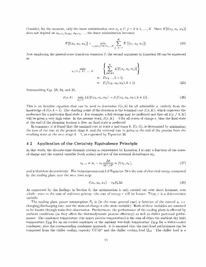
Chiller-Priority ControlConstant-Proportion ControlStorage-Priority ControlFigure 6: State-of-charge versus time under chiller-priority, constant-proportion, and storage-priority controlusing an autoregressive neural network model for cooling load prediction using rate structure 2 for Tuesdaythrough Thursday.Figure 7 illustrates the e�ect of prediction performance on the control trajectory selected by optimalcontrol. The look-ahead (planning) horizon is L = 15 hours. It can be stated that all �ve trajectoriesare roughly similar and exhibit the expected daily charging and discharging cycles. During the night fromWednesday to Thursday, the unbiased random walk model appears to overestimate the nighttime cooling loadand/or underestimate the loads during the Thursday on-peak period since it decides not fully recharge theice storage tank. Furthermore, perfect prediction leads to an optimal control trajectory that is always fullcharged at the onset and fully discharged at the end of the on-peak period. The remaining models pursuesimilar trajectories which, however, over the simulation period lead to smaller cost savings than for the case17

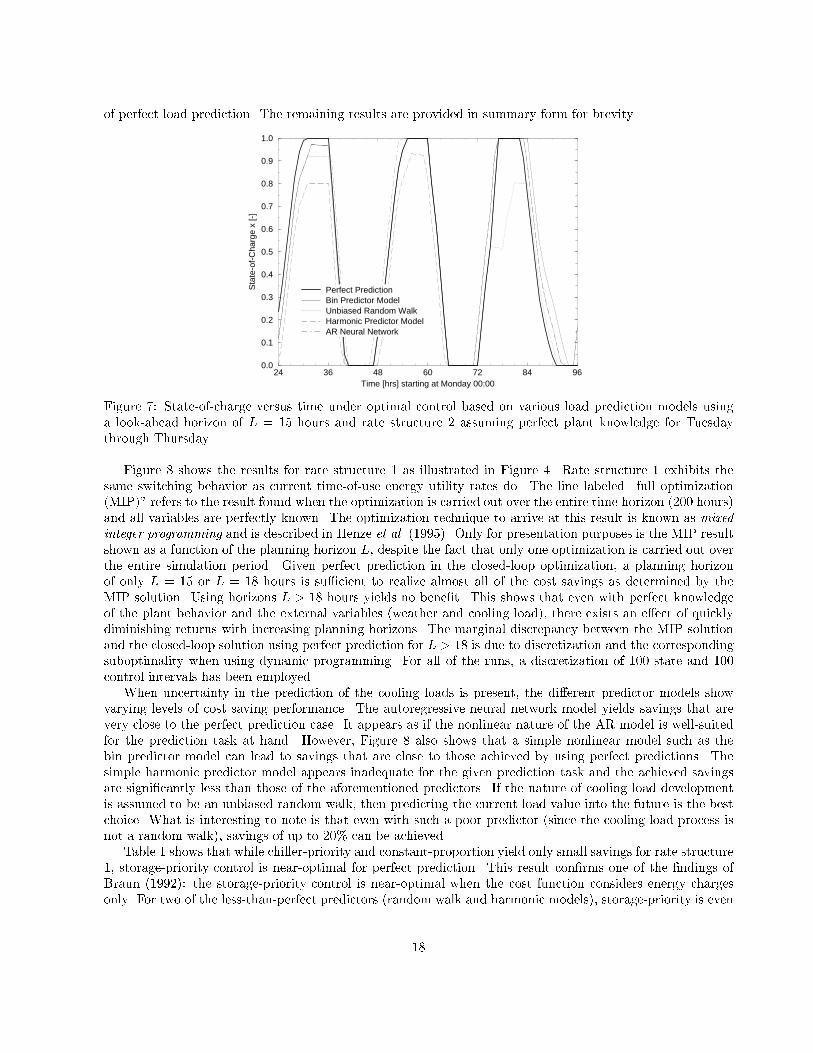
of perfect load prediction. The remaining results are provided in summary form for brevity.

24 36 48 60 72 84 96Time [hrs] starting at Monday 00:00

0.0

0.1

0.2

0.3

0.4

0.5

0.6

0.7

0.8

0.9

1.0

Sta

te-o

f-C

harg

e x

[-]

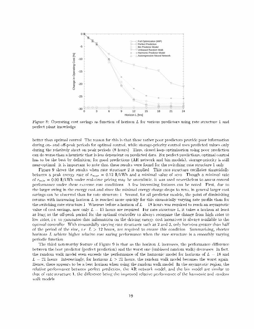
Perfect PredictionBin Predictor ModelUnbiased Random WalkHarmonic Predictor ModelAR Neural NetworkFigure 7: State-of-charge versus time under optimal control based on various load prediction models usinga look-ahead horizon of L = 15 hours and rate structure 2 assuming perfect plant knowledge for Tuesdaythrough Thursday.Figure 8 shows the results for rate structure 1 as illustrated in Figure 4. Rate structure 1 exhibits thesame switching behavior as current time-of-use energy utility rates do. The line labeled \full optimization(MIP)" refers to the result found when the optimization is carried out over the entire time horizon (200 hours)and all variables are perfectly known. The optimization technique to arrive at this result is known as mixedinteger programming and is described in Henze et al. (1995). Only for presentation purposes is the MIP resultshown as a function of the planning horizon L, despite the fact that only one optimization is carried out overthe entire simulation period. Given perfect prediction in the closed-loop optimization, a planning horizonof only L = 15 or L = 18 hours is su�cient to realize almost all of the cost savings as determined by theMIP solution. Using horizons L > 18 hours yields no bene�t. This shows that even with perfect knowledgeof the plant behavior and the external variables (weather and cooling load), there exists an e�ect of quicklydiminishing returns with increasing planning horizons. The marginal discrepancy between the MIP solutionand the closed-loop solution using perfect prediction for L > 18 is due to discretization and the correspondingsuboptimality when using dynamic programming. For all of the runs, a discretization of 100 state and 100control intervals has been employed.When uncertainty in the prediction of the cooling loads is present, the di�erent predictor models showvarying levels of cost saving performance. The autoregressive neural network model yields savings that arevery close to the perfect prediction case. It appears as if the nonlinear nature of the AR model is well-suitedfor the prediction task at hand. However, Figure 8 also shows that a simple nonlinear model such as thebin predictor model can lead to savings that are close to those achieved by using perfect predictions. Thesimple harmonic predictor model appears inadequate for the given prediction task and the achieved savingsare signi�cantly less than those of the aforementioned predictors. If the nature of cooling load developmentis assumed to be an unbiased random walk, then predicting the current load value into the future is the bestchoice. What is interesting to note is that even with such a poor predictor (since the cooling load process isnot a random walk), savings of up to 20% can be achieved.Table 1 shows that while chiller-priority and constant-proportion yield only small savings for rate structure1, storage-priority control is near-optimal for perfect prediction. This result con�rms one of the �ndings ofBraun (1992): the storage-priority control is near-optimal when the cost function considers energy chargesonly. For two of the less-than-perfect predictors (random walk and harmonic models), storage-priority is even18

0 3 6 9 12 15 18 21 24Horizon L [hrs]

-30

-25

-20

-15

-10

-5

0

Cha

nge

in O

pera

ting

Cos

t [%

]

Full Optimization (MIP)Perfect PredictionBin Predictor ModelUnbiased Random WalkHarmonic Predictor ModelAutoregressive Neural Network

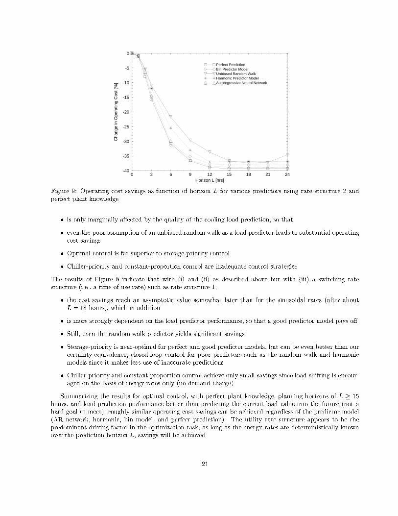
Figure 8: Operating cost savings as function of horizon L for various predictors using rate structure 1 andperfect plant knowledge.better than optimal control. The reason for this is that these rather poor predictors provide poor informationduring on- and o�-peak periods for optimal control, while storage-priority control uses predicted values onlyduring the relatively short on-peak periods (8 hours). Thus, closed-loop optimization using poor predictioncan do worse than a heuristic that is less dependent on predicted data. For perfect predictions, optimal controlhas to be the best by de�nition; for good predictions (AR network and bin models), storage-priority is stillnear-optimal. It is important to note that these results were found for the switching rate structure 1 only.Figure 9 shows the results when rate structure 2 is applied. This rate structure oscillates sinusoidallybetween a peak energy rate of rmax = 0:12 $/kWh and a minimal value of zero. Though a minimal rateof rmin = 0:00 $/kWh under real-time pricing may be unrealistic, it was used nevertheless to assess controlperformance under these extreme cost conditions. A few interesting features can be noted. First, due tothe larger swing in the energy cost and since the minimal energy charge drops to zero, in general larger costsavings can be observed than for rate structure 1. Second, for all predictor models, the point of diminishingreturns with increasing horizon L is reached more quickly for this sinusoidally varying rate pro�le than forthe switching rate structure 1. Whereas before a horizon of L = 18 hours was required to reach an asymptoticvalue of cost savings, now only L = 15 hours are required. For rate structure 1, it takes a horizon at leastas long as the o�-peak period for the optimal controller to always recognize the change from high rates tolow rates, i.e. to guarantee that information on the driving energy cost incentives is always available to theoptimal controller. With sinusoidally varying rate structures such as 2 and 3, only horizons greater than halfof the period of the sine, i.e. L > 12 hours, are required to ensure this condition. Summarizing, shorterhorizons L achieve higher relative cost saving performance when the rate structure is a smoothly varyingperiodic function.The third noteworthy feature of Figure 9 is that as the horizon L increases, the performance di�erencebetween the best predictor (perfect prediction) and the worst one (unbiased random walk) decreases. In fact,the random walk model even exceeds the performance of the harmonic model for horizons of L = 18 andL = 21 hours. Interestingly, for horizons L > 21 hours, the random walk model becomes the worst again.Hence, there appears to be a best horizon when using the random walk model. In the asymptotic region, therelative performance between perfect prediction, the AR network model, and the bin model are similar tothat of rate structure 1, the di�erence being the improved relative performance of the harmonic and randomwalk models. 19

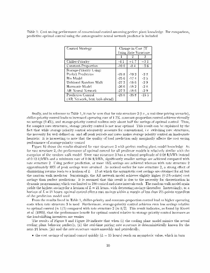
Table 1: Cost saving performance of conventional control assuming perfect plant knowledge. For comparison,predictive optimal control using the autoregressive neural network predictor is included.Control Strategy Change in Cost [%]Using Rate Structure1 2 3Chiller-Priority -4.1 +1.7 +3.1Constant-Proportion -10.0 -0.4 +3.6Storage-Priority Using:Perfect Prediction -28.8 -19.3 -3.2Bin Model -25.6 -17.4 -2.5Unbiased Random Walk -27.3 -18.6 -2.9Harmonic Model -26.6 -18.2 -2.8AR Neural Network -27.3 -18.6 -2.9Predictive Control -28.0 -38.8 -15.5(AR Network, best look-ahead)�nally, and in reference to Table 1, it can be seen that for rate structure 2 (i.e., a real-time pricing scenario),chiller-priority control leads to increased operating cost of 1.7%, constant-proportion control achieves virtuallyno savings (0.4%), and storage-priority control realizes only about half the savings of optimal control. Thus,for complex rate structures, storage-priority control is not near-optimal. This result can be explained by thefact that while storage-priority control adequately accounts for conventional, i.e. switching rate structures,the necessity for well de�ned on- and o�-peak periods and rates makes storage-priority control an inadequateheuristic. It is interesting to note that the quality of load prediction only marginally a�ects the cost savingperformance of storage-priority control.Figure 10 shows the results obtained for rate structure 3 with perfect cooling plant model knowledge. Asfor rate structure 2, the performance of optimal control for all predictor models is relatively similar with theexception of the random walk model. Since rate structure 3 has a reduced amplitude of 0.08 $/kWh insteadof 0.12 $/kWh and a minimum rate of 0.04 $/kWh, signi�cantly smaller savings are achieved compared withrate structure 2. Using perfect prediction, at most 15% savings are achieved whereas with rate structure 2approximately 39% of peak savings were attained. As noticed earlier for rate structure 2, a strong e�ect ofdiminishing returns leads to a horizon of L = 15 at which the asymptotic cost savings are obtained for all butthe random walk predictor. Surprisingly, the AR network model achieves slightly higher (0.2%-points) costsavings than perfect predictions. It is assumed that this result is due to the necessity for discretization indynamic programming which was limited to 100 control and state intervals each. The randomwalk model againyields the highest savings for a horizon of L = 21 hours, with decreasing savings thereafter. Interestingly, at ahorizon of L = 21 hours, optimal control e�ects cost savings within a margin of less than 2%-points regardlessof the prediction model used.From the results listed in Table 1, chiller-priority and constant-proportion control lead to higher operatingcosts when rate structure 3 is used. Furthermore, storage-priority control achieves even less savings relativeto optimal control (� 1=5) compared with rate structure 2 (� 1=2). This result indicates, as found by Krartiet al. (1995), that the performance bene�t for optimal control relative to storage-priority control increases asthe load-shifting incentives are weaker.The results of Figure 9 and Figure 10 indicate that when (i) the cooling plant model mimics the actualcooling plant behavior perfectly, (ii) the real-time pricing rate structure is deterministically known for thenext 24 hours, (iii) and the rate structure varies smoothly and periodically,� the cost savings of optimal control quickly (L = 15 hours) reach an asymptotic value, which in turn20

0 3 6 9 12 15 18 21 24Horizon L [hrs]

-40

-35

-30

-25

-20

-15

-10

-5

0

Cha

nge

in O

pera

ting

Cos

t [%

]

Perfect PredictionBin Predictor ModelUnbiased Random WalkHarmonic Predictor ModelAutoregressive Neural Network

Figure 9: Operating cost savings as function of horizon L for various predictors using rate structure 2 andperfect plant knowledge.� is only marginally a�ected by the quality of the cooling load prediction, so that� even the poor assumption of an unbiased random walk as a load predictor leads to substantial operatingcost savings.� Optimal control is far superior to storage-priority control.� Chiller-priority and constant-proportion control are inadequate control strategies.The results of Figure 8 indicate that with (i) and (ii) as described above but with (iii) a switching ratestructure (i.e., a time-of-use rate) such as rate structure 1,� the cost savings reach an asymptotic value somewhat later than for the sinusoidal rates (after aboutL = 18 hours), which in addition� is more strongly dependent on the load predictor performance, so that a good predictor model pays o�.� Still, even the random walk predictor yields signi�cant savings.� Storage-priority is near-optimal for perfect and good predictor models, but can be even better than ourcertainty-equivalence, closed-loop control for poor predictors such as the random walk and harmonicmodels since it makes less use of inaccurate predictions.� Chiller-priority and constant-proportion control achieve only small savings since load-shifting is encour-aged on the basis of energy rates only (no demand charge).Summarizing the results for optimal control, with perfect plant knowledge, planning horizons of L � 15hours, and load prediction performance better than predicting the current load value into the future (not ahard goal to meet), roughly similar operating cost savings can be achieved regardless of the predictor model(AR network, harmonic, bin model, and perfect prediction). The utility rate structure appears to be thepredominant driving factor in the optimization task; as long as the energy rates are deterministically knownover the prediction horizon L, savings will be achieved.21

0 3 6 9 12 15 18 21 24Horizon L [hrs]

-20

-15

-10

-5

0

Cha

nge

in O

pera

ting

Cos

t [%

]

Perfect PredictionBin Predictor ModelUnbiased Random WalkHarmonic Predictor ModelAutoregressive Neural Network

Figure 10: Operating cost savings as function of horizon L for various predictors using rate structure 3 andperfect plant knowledge.6.3 Imperfect Plant KnowledgeIf the cooling plant model used in the closed-loop optimization, i.e. for planning optimal strategies, di�ers fromthe behavior of the actual cooling plant, the plant knowledge is said to be imperfect. Consequently, there aretwo sources of uncertainty, (i) in the prediction of those variables required for the optimization and (ii) in thecomputation of the cooling plant power consumption P given the predicted variables. To simulate this case,the basic plant model was used for planning in the dynamic programming algorithm and the realistic plantmodel was used in the simulation stage to determine the power consumptions that are actually incurred. Inthe case of perfect plant knowledge described in Section 6.2, the basic plant model was assumed to mirror theactual plant behavior. Therefore, the changes of operating cost for a particular rate structure, e.g. Figure 8and Figure 12, for the cases of perfect and imperfect plant knowledge cannot be compared as they are basedon di�erent simulation cooling plant models.The basic and realistic plant models predict substantially di�erent values of plant energy use for the samevalues of the charge/discharge control variable u, cooling load Q, and ambient dry-bulb temperature Tdb. Thedi�erence between the models was quanti�ed as the average absolute di�erence of energy use computed bythe basic and realistic plant models. The average was estimated over a one month simulation period; at eachhour in the month, the di�erence in energy use computed by the basic and realistic models was recorded. Theaverage energy use predicted by the realistic plant model was 430 kW, while the average absolute di�erencewas 100 kW. At almost every hour in the month, the basic plant model predicted less energy use than therealistic model. It appears, then, that the basic plant model is not an accurate approximation of the realisticplant model.The results for all of the three rate structures investigated in this study, as shown in Figures 12, 13, and 14,exhibit one prevailing feature: The cost savings performance of optimal control as a function of the planninghorizon L and the prediction quality is very similar to the behavior found for perfect plant knowledge asdepicted by the corresponding �gures Figures 8, 9, and 10. In particular, using rate structure 1, Figure 12depicts the same feature of diminishing returns for perfect prediction, the autoregressive neural network, andthe bin predictor models for L > 18 hours as for Figures 8. Furthermore, the unbiased random walk modelyields the smallest savings and the harmonic model the second smallest, however only for L < 18 hours.Again, for L � 18 hours, all predictors but the random walk model e�ect similar savings. Though the savings�gures for the cases of perfect and imperfect plant knowledge are not comparable since di�erent simulation22

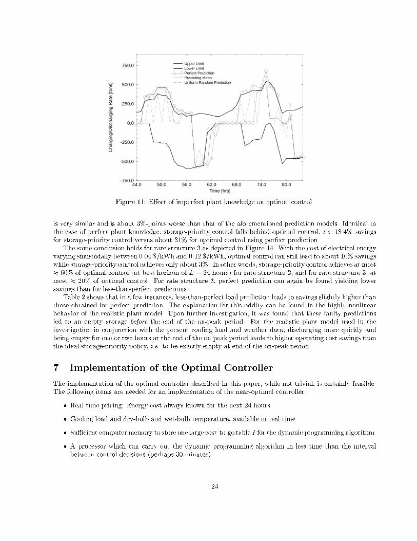
models have been used, the overall behavior appears similar. This supports the conclusion made for the caseof perfect plant knowledge that utility rate structure is the driving parameter.But there is one signi�cant di�erence. Perfect prediction no longer necessarily yields the highest costsavings in the presence of model uncertainty. In fact, for L > 12 hours, both the bin predictor and the neuralnetwork models fare better than perfect prediction. This apparent paradox may be explained by the followingargument. Regardless of the predictor model, the planning phase devises an optimal strategy that may notbe executable with the simulation plant model, i.e. the one that is taken to mirror the actual plant behavior.Both plant models are subject to di�erent control constraints umin and umax. In particular, the constraintsof the realistic plant model are more restrictive than those of the basic plant model. Investigating the controltrajectories for the various predictors, it can be seen that most of the time the controls considered optimal bythe planning model (basic) lie outside the permissible range of the realistic plant model as shown in Figure 11.In those cases, the recommended control is curtailed to the corresponding control limit of the actual plant.For example, if the planning model determines up = 100 to be the optimal charging rate, but due to heattransfer limitations and chiller capacity only ua = 70 can be realized in the actual cooling plant (realisticmodel), consequently only u = 70 will be executed. Since the optimal strategies determined by the planningplant model exhibit a strong switching behavior, i.e. the controls are either at the upper or lower limit, andsince these controls are either too high or too low for the actual plant, the corresponding upper or lowercontrol limit of the actual plant becomes the new, overridden control action. Hence, if the constraints ofthe planning model and the actual cooling plant di�er strongly, perfect knowledge of future variables (inthis case cooling loads) used within the context of an imperfect model for planning may not necessarily leadto the best performance. Essentially, imperfect load information used by an imperfect planning model mayserendipitously outperform perfect load information used by an imperfect planning model when evaluated inthe simulation stage. (Note: This argument is valid for the case of the mismatch between the planning andsimulation models and the speci�c conditions considered in this study.)Figure 11 shows how the optimal control action at each point in time, regardless of the cooling loadprediction performance (perfect, predicting the mean value, and uniform random prediction) used in theplanning stage, tends be at or beyond the control limits umin and umax of the realistic simulation model. Aheuristic could be derived from this observation that recommends to discharge the storage at the maximal rateduring periods when the utility rates are highest and to charge at the maximum rate when the utility ratesare lowest. Therefore, the control becomes virtually independent of the forecast algorithm under particularrate structures and cooling load pro�les. However, future work is needed to validate this heuristic.Referring to the results summarized in Table 2 storage-priority control is again near-optimal for theswitching rate structure 1. But storage-priority control is found to be even slightly better than optimal (forperfect prediction and the harmonic model). The reason for this particular result for rate structure 1 canbe found in the fact that optimal control relies on both imperfect plant knowledge and imperfect predictionswhile storage-priority relies only on imperfect load predictions available at the beginning of the on-peakperiod. Storage-priority predicts the cumulative on-peak cooling load and determines the correspondingcontrol parameters A0 and A1 thereafter. Because the on-peak period for the investigated case is only eighthours long, the impact of the uncertainty on the cooling load prediction is relatively small for both the basicand the realistic plant models. Again, it can be observed that the quality of load prediction only marginallya�ects the cost saving performance of storage-priority control.In summary, with traditional time-of-use rate structures (rate structure 1) and model uncertainty, storage-priority control outperforms optimal control while being the simpler strategy. Since the prediction is onlycarried out over the short on-peak period of, the e�ect of load prediction uncertainty is marginal. As shown inTable 2, storage-priority control retains its performance bene�t over constant-proportion and chiller-prioritycontrol.Figure 13 illustrates the cost savings performance in the presence of plant model uncertainty under ratestructure 2. As found in Figure 9, the performance of all predictors can be found within a narrow envelope.The perfect prediction yields the highest savings, followed by the autoregressive neural network. For horizonsL � 9 hours, the performance for the bin predictor, the harmonic predictor and the unbiased random walk23

44.0 50.0 56.0 62.0 68.0 74.0 80.0Time [hrs]

-750.0

-500.0

-250.0

0.0

250.0

500.0

750.0

Cha

rgin

g/D

isch

argi

ng R

ate

[tons

]

Upper LimitLower LimitPerfect PredictionPredicting MeanUniform Random Prediction

Figure 11: E�ect of imperfect plant knowledge on optimal control.is very similar and is about 3%-points worse than that of the aforementioned prediction models. Identical tothe case of perfect plant knowledge, storage-priority control falls behind optimal control, i.e. 18.4% savingsfor storage-priority control versus about 31% for optimal control using perfect prediction.The same conclusion holds for rate structure 3 as depicted in Figure 14. With the cost of electrical energyvarying sinusoidally between 0.04 $/kWh and 0.12 $/kWh, optimal control can still lead to about 10% savingswhile storage-priority control achieves only about 3%. In other words, storage-priority control achieves at most� 60% of optimal control (at best horizon of L = 24 hours) for rate structure 2, and for rate structure 3, atmost � 20% of optimal control. For rate structure 3, perfect prediction can again be found yielding lowersavings than for less-than-perfect predictions.Table 2 shows that in a few instances, less-than-perfect load prediction leads to savings slightly higher thanthose obtained for perfect prediction. The explanation for this oddity can be found in the highly nonlinearbehavior of the realistic plant model. Upon further investigation, it was found that these faulty predictionsled to an empty storage before the end of the on-peak period. For the realistic plant model used in theinvestigation in conjunction with the present cooling load and weather data, discharging more quickly andbeing empty for one or two hours at the end of the on-peak period leads to higher operating cost savings thanthe ideal storage-priority policy, i.e. to be exactly empty at end of the on-peak period.7 Implementation of the Optimal ControllerThe implementation of the optimal controller described in this paper, while not trivial, is certainly feasible.The following items are needed for an implementation of the near-optimal controller.� Real-time pricing: Energy cost always known for the next 24 hours.� Cooling load and dry-bulb and wet-bulb temperature, available in real time.� Su�cient computer memory to store one large cost-to-go table I for the dynamic programming algorithm.� A processor which can carry out the dynamic programming algorithm in less time than the intervalbetween control decisions (perhaps 30 minutes).24

0 3 6 9 12 15 18 21 24Horizon L [hrs]

-25

-20

-15

-10

-5

0

Cha

nge

in O

pera

ting

Cos

t [%

]

Perfect PredictionBin Predictor ModelUnbiased Random WalkHarmonic Predictor ModelAutoregressive Neural Network

Figure 12: Operating cost savings as function of horizon L for various predictors using rate structure 1 andimperfect plant knowledge.� Processor time is also needed to make the cooling load predictions which are used in the dynamicprogramming algorithm.Assuming that temperature and load data are available in real time, computing power appears to be thelimiting factor. The memory needed for dynamic programming is proportional to the product of the number ofintervals in the state and control variables and length of the planning horizon. Using a L = 18 hour planninghorizon, and 50 intervals in both the state and control variables, a memory allocation of 7800 bytes usingdouble-precision arithmetic is required. Reducing the discretization to 20 intervals each, only 3200 bytes willhave to be available. Additional memory will be required for the executable program. The size of the dynamicprogramming code, as compiled, is about 15 kilobytes. A complete program based on this code may be from25 to 50 kilobytes. Thus, the total memory required for both the data and the program code is somethingless than 60 kilobytes. Finally, a small operating system is needed to execute the program and handle variousfunctions, bringing the total memory required for an implementation to about 100 kilobytes.The number of ops ( oating point operations) to compute the dynamic programming solution for aplanning horizon of L time-steps withM control values and N state values is approximately LMN2+20LMN ,as determined by counting oating point operations in the innermost loop of the dynamic programming code.If L = 18, M = 50, and N = 50 as described above, the total ops needed for each planning interval areapproximately 3.2 million ops. Additional operations are needed outside the innermost loop, but as theinnermost loop dominates the dynamic programming algorithm, this gives us a rough estimate of the totalprocessing needed. A 16-MHz 80386 processor without oating point hardware (a slow processor by currentstandards) can execute about 50,000 ops per second. Thus to execute the dynamic programming algorithmwould require about one minute of processor time. This is much less than the typical 30 to 60 minute planningand control interval.Making predictions requires few ops and little memory at run time, but assumes that a large historicaldata base is available for model building. For example, the autoregressive network which made the predictionsused in this study required about 1600 bytes to store the weights and biases, and about 400 ops to makeeach prediction. Thus the memory and ops required by the dynamic programming algorithm far outweighthe requirements of the predictor.It appears, then, that a slow computer with limited memory, for example an 80386 processor without oating point hardware and only 100 kilobytes of memory, could implement the certainty-equivalence, closed-25

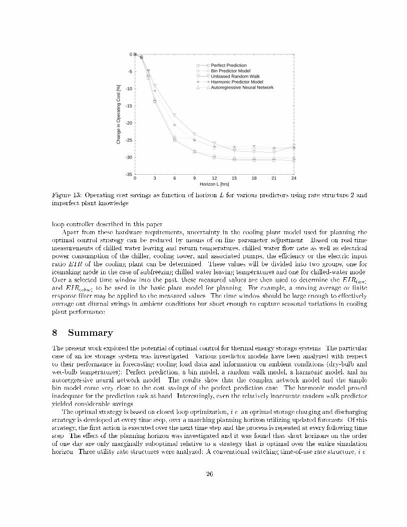
0 3 6 9 12 15 18 21 24Horizon L [hrs]

-35

-30

-25

-20

-15

-10

-5

0

Cha

nge

in O

pera

ting

Cos

t [%

]

Perfect PredictionBin Predictor ModelUnbiased Random WalkHarmonic Predictor ModelAutoregressive Neural Network

Figure 13: Operating cost savings as function of horizon L for various predictors using rate structure 2 andimperfect plant knowledge.loop controller described in this paper.Apart from these hardware requirements, uncertainty in the cooling plant model used for planning theoptimal control strategy can be reduced by means of on-line parameter adjustment. Based on real-timemeasurements of chilled water leaving and return temperatures, chilled water ow rate as well as electricalpower consumption of the chiller, cooling tower, and associated pumps, the e�ciency or the electric inputratio EIR of the cooling plant can be determined. These values will be divided into two groups, one foricemaking mode in the case of subfreezing chilled water leaving temperatures and one for chilled-water mode.Over a selected time window into the past, these measured values are then used to determine the EIR(ice)and EIR(chw) to be used in the basic plant model for planning. For example, a moving average or �niteresponse �lter may be applied to the measured values. The time window should be large enough to e�ectivelyaverage out diurnal swings in ambient conditions but short enough to capture seasonal variations in coolingplant performance.8 SummaryThe present work explored the potential of optimal control for thermal energy storage systems. The particularcase of an ice storage system was investigated. Various predictor models have been analyzed with respectto their performance in forecasting cooling load data and information on ambient conditions (dry-bulb andwet-bulb temperatures): Perfect prediction, a bin model, a random walk model, a harmonic model, and anautoregressive neural network model. The results show that the complex network model and the simplebin model come very close to the cost savings of the perfect prediction case. The harmonic model provedinadequate for the prediction task at hand. Interestingly, even the relatively inaccurate random walk predictoryielded considerable savings.The optimal strategy is based on closed-loop optimization, i.e. an optimal storage charging and dischargingstrategy is developed at every time step, over a marching planning horizon utilizing updated forecasts. Of thisstrategy, the �rst action is executed over the next time step and the process is repeated at every following timestep. The e�ect of the planning horizon was investigated and it was found that short horizons on the orderof one day are only marginally suboptimal relative to a strategy that is optimal over the entire simulationhorizon. Three utility rate structures were analyzed: A conventional switching time-of-use rate structure, i.e.26

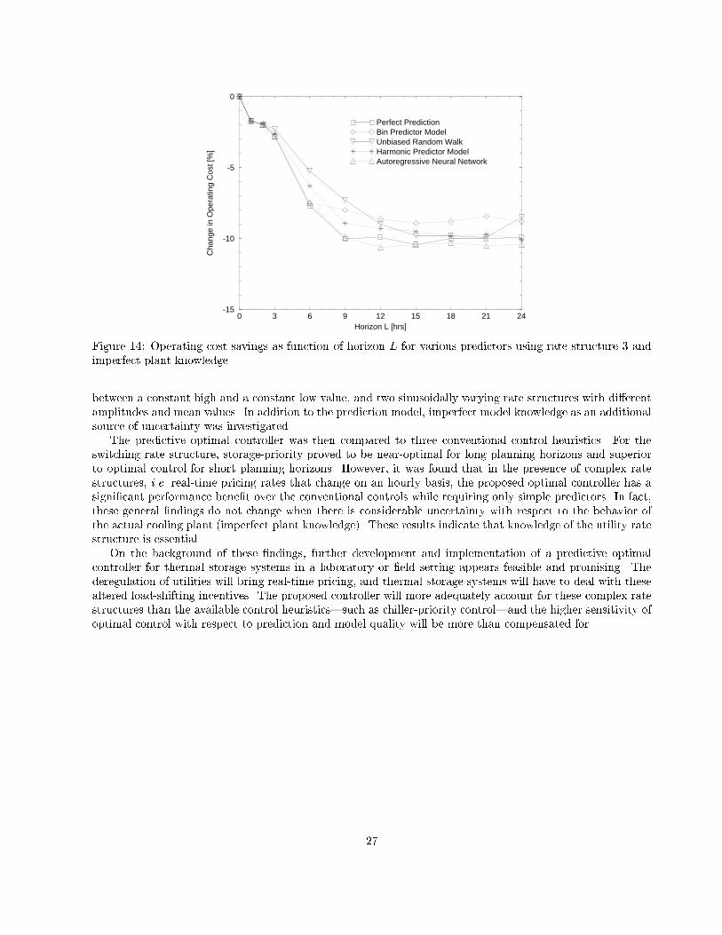
0 3 6 9 12 15 18 21 24Horizon L [hrs]

-15

-10

-5

0

Cha

nge

in O

pera

ting

Cos

t [%

]

Perfect PredictionBin Predictor ModelUnbiased Random WalkHarmonic Predictor ModelAutoregressive Neural Network

Figure 14: Operating cost savings as function of horizon L for various predictors using rate structure 3 andimperfect plant knowledge.between a constant high and a constant low value, and two sinusoidally varying rate structures with di�erentamplitudes and mean values. In addition to the prediction model, imperfect model knowledge as an additionalsource of uncertainty was investigated.The predictive optimal controller was then compared to three conventional control heuristics. For theswitching rate structure, storage-priority proved to be near-optimal for long planning horizons and superiorto optimal control for short planning horizons. However, it was found that in the presence of complex ratestructures, i.e. real-time pricing rates that change on an hourly basis, the proposed optimal controller has asigni�cant performance bene�t over the conventional controls while requiring only simple predictors. In fact,these general �ndings do not change when there is considerable uncertainty with respect to the behavior ofthe actual cooling plant (imperfect plant knowledge). These results indicate that knowledge of the utility ratestructure is essential.On the background of these �ndings, further development and implementation of a predictive optimalcontroller for thermal storage systems in a laboratory or �eld setting appears feasible and promising. Thederegulation of utilities will bring real-time pricing, and thermal storage systems will have to deal with thesealtered load-shifting incentives. The proposed controller will more adequately account for these complex ratestructures than the available control heuristics|such as chiller-priority control|and the higher sensitivity ofoptimal control with respect to prediction and model quality will be more than compensated for.

27

Table 2: Cost saving performance of conventional control assuming imperfect plant knowledge. For compari-son, predictive optimal control using the autoregressive neural network predictor is included.Control Strategy Change in Cost [%]Using Rate Structure1 2 3Chiller-Priority -3.8 +0.3 +2.4Constant-Proportion -9.2 -2.4 +2.8Storage-Priority Using:Perfect Prediction -23.5 -18.4 -1.5Bin Model -22.7 -17.5 -1.9Unbiased Random Walk -22.8 -17.7 -1.3Harmonic Model -23.6 -18.3 -2.1AR Neural Network -23.0 -17.9 -1.3Predictive Control -23.4 -30.0 -10.5(AR Network, best look-ahead)NomenclatureA0 capacity for storage-priority control [tons]A1 load fraction from storage for storage-priority control [-]I(x; k) optimal cost-to-go used in DP algorithm [$]J cost function used in optimal control strategy [$]CCAP nominal chiller capacity [tons]EIRi electric input ratio in operating mode i [kW/ton]fQ load fraction from storage for constant-proportion control [-]k time index [-]K total number of time intervals in simulation [hrs]l instantaneous cost used in DP algorithm [$]Pk total power consumption of cooling plant in hour k ! k + 1 [kW]Qk cooling load in hour k ! k + 1 [tons]Qch;k chiller load in hour k ! k + 1 [tons]Qpeak peak cooling load in simulation [tons]rk energy charge in hour k [$/kWh]SCAP storage capacity [ton-hrs]TDB;k dry-bulb temperature in hour k ! k + 1 [�F ]TWB;k wet-bulb temperature in hour k ! k + 1 [�F ]uk rate of charge or discharge in hour k ! k + 1 [tons]umin maximal storage discharging rate [tons]umax maximal storage charging rate [tons]umin;TES(x) maximal heat transfer discharging limit [tons]umax;TES(x) maximal heat transfer charging limit [tons]xk state-of-charge of the ice storage tank in hour k ! k + 1 [-]xmin lower limit on state-of-charge [-]xmax upper limit on state-of-charge [-]�t time interval used in simulation [hrs]28

ReferencesAkbari, H. and Sezgen, O. (1992) Case Studies of Thermal Energy Storage (TES) Systems: Evaluation andVeri�cation of System Performance. LBL-30852. Lawrence Berkeley Laboratory, University of California,Energy and Environment Division.Bertsekas, D.P. (1995) Dynamic Programming and Optimal Control. Volume 1. Belmont, MA: AthenaScienti�c.BLAST: Building Load Analysis and System Thermodynamics (1994) User Manual. U.S. Army ConstructionEngineering Research Laboratory and University of Illinois at Urbana-Champaign.Braun, J.E. (1992) \A Comparison of Chiller-Priority, Storage-Priority, and Optimal Control of an Ice-StorageSystem." ASHRAE Transactions, 98/1 893{902.Dodier, R.H. (1995) Statistical Properties of Neural Networks, with Application to Building Energy Prediction.Master's Thesis, University of Colorado at Boulder.Drees, K.H. (1994) Modeling and Control of Area Constrained Ice Storage Systems. Master's Thesis, PurdueUniversity, West Lafayette, IN.ECW: The Commercial Cooling Load Library. (1994) Energy Center of Wisconsin. Madison, WI.Guven, H. and Flynn J. (1992) \Commissioning TES Systems." Heating/Piping/Air Conditioning, 64/1.Haykin, S. (1994) Neural Networks. New York: Macmillan College Publishing Co.Henze, G.P. Laguna, M., and Krarti, M. (1995) \Heuristics for the Optimal Control of Thermal Energy Stor-age," Proceedings of the Metaheuristics International Conference, Norwell, MA: Kluwer Academic Publishers.Kintner-Meyer, M. and Emery, E.F. (1995) \Optimal control of an HVAC system using cold storage andbuilding thermal capacitance" Energy and Buildings 23 19{31. New York: Elsevier Science Inc.Knebel, D.E. (1990) \Optimal Control of Ice Harvesting Thermal Energy Storage Systems." Proceedings ofthe 25th Intersociety Energy Conversion Engineering Conference, 6 209{214. New York: IECE.Krarti, M., Brandemuehl, M.J., and Henze, G.P. (1995) \Final Project Report for ASHRAE 809-RP: Evalu-ation of Optimal Control for Ice Storage Systems." ASHRAE ReportKreider, J., Claridge, D., Curtiss, P., Dodier, R., Haberl, J., and Krarti, M. (1995) Building Energy UsePrediction and System Identi�cation using Recurrent Neural Networks. J. Solar Energy Engineering 117/3161{166.Seber, G.A.F., and Wild, C.J. (1989) Nonlinear Regression. New York: John Wiley and Sons.Seem, J.E., and Braun, J.E. (1991) \Adaptive methods for real-time forecasting of building electrical demand."ASHRAE Transactions, 97/1: 710{721.Spethmann, D.H. (1989) \Optimal Control for Cool Storage." ASHRAE Transactions, 95/1 1189{1193.Tamblyn, R.T. (1985) \Control Concepts for Thermal Storage." ASHRAE Transactions, 91/1b 5{10.Tran, N., Kreider, J.F., and Brothers, P. (1989) \Field Measurement of Chilled Water Storage ThermalPerformance." ASHRAE Transactions, 95/1.29