L-02/70

Development of a New MeteorologicalVentilation Index for Urban Air Quality

Studies

0

5

10

15

20

25

30

35

Alingsås Borås Trollhättan Vänersborg Kungälv Göteborg

NO

2 (µg

/m3 )

Calculated NO2 new URBAN-modelCalculated NO2 old URBAN-modelMeassured NO2

Marie Haeger-Eugensson1, Katarina Borne2,

Deliang Chen1,2, Karin Persson1

1IVL Swedish Environmental Research Ltd2Earth Sciences Center, Gothenburg University

Table of content

Abstract ............................................................................................................................. 2

1. Introduction................................................................................................................... 11.1 Background ............................................................................................................. 11.2 The URBAN-model ................................................................................................ 11.3 Purpose.................................................................................................................... 3

2 Methods ......................................................................................................................... 32.1 New Mixing Height calculation .............................................................................. 4

2.1.1 Short description of TAPM .............................................................................. 62.1.2 Validation of the TAPM-model........................................................................ 6

2.2 Calculation of H with Holzworth algorithm ........................................................... 72.3 Calculation of the new mixing parameters.............................................................. 8

3. Results........................................................................................................................... 83.1 Mixing height .......................................................................................................... 8

3.1.1 Mixing height in the investigated area ............................................................. 83.2 The new ventilation index, V ................................................................................ 123.3 The dispersion-adjusting constant Cd.................................................................... 133.4 The NO2 concentrations calculated by the new URBAN model .......................... 143.5 Comparison between old and new calculations and measurements...................... 16

4. Discussion and conclusions ........................................................................................ 17

Reference ........................................................................................................................ 19

Appendix 1 Description of the model -TAPM ................................................................. 1

Appendix 2 Validation of the model system..................................................................... 7

Appendix 3 Calculation of mixing height using Holzworth algorithm .......................... 16

AbstractExperience from many years of measurements in urban areas in Sweden shows that highconcentrations of various air pollutant components occur not only in large cities but alsoin small towns. One possible reason is variation in the local meteorological conditionscausing poor ventilation facilities. For some years IVL has used an empirical statisticalcalculation method (the so called "URBAN-model") developed by IVL. The model hasprimarily been used for estimating the risk of exceeding different national standardvalues of air pollution concentrations in small and medium sized towns in Sweden.

The purpose of this investigation was to develop a method in a test area to improve thecalculations of air pollution concentrations used in the former URBAN-model. This wasachieved by reproducing the local meteorological variations better in a new ventilationindex and a dispersion-adjusting constant and also with better temporal and spatialresolution of the parameters. By using an advanced numerical model, TAPM (The AirPollution Model), the old ventilation factor was improved by using the outputparameters mixing height and wind-speed respectively, for calculating new ventilationparameters with high time and spatial resolution (1 month and 1x1 km). The resultswere then included in an improved calculation routine/model implemented into theURBAN model. Since the TAPM model previously has only been validated in Asia andas the circumstances are rather different in northern Europe (rain, soil moisture daylength etc) it was necessary to verify the model�s performance on meteorologymodelling, before using the output of the model to develop new ventilation parameters.The validation showed that the model performs well in simulating air temperature andwind, which are the two most important fields to drive air pollution modelling. Also,TAPM was confirmed to have strong ability in simulating thermally driven mesoscalesystems, such as sea-land breeze and urban heat island effects. It is thus concluded thatTAPM is a very useful tool for local meteorological air pollution applications.

A comparison between monthly averages of measured and calculated NO2

concentrations (with the new model) shows a fair accordance. When comparing NO2

calculated with the old and the new URBAN-model and NO2 measurements, the newmodel shows a much better agreement with measured data. Consequently, the need ofevaluation of the air quality in communities and small cities can be better met by usingthis improved URBAN model. Since the time consuming and complicatedmeteorological modelling is only used to generate the new ventilation parameters, theactual NO2 calculations with the new URBAN model can still remain rather simplecompare to other dispersion models.

The method developed for the test area can be developed for whole Sweden and thusmeets the extended demands of accurate air pollution calculations in small communities.

1

1. Introduction

1.1 Background

Experience from many years of measurements in urban areas in Sweden shows that highconcentration of various air pollution components occur not only in large cities but alsoin small towns. One possible reason is variations of the local meteorological conditionscausing poor ventilation. According to the investigation performed by The ParliamentCommittee on Environmental Objectives (Miljömålskommittén) about 10% of thecommunities in the country are going to exceed the threshold values of NO2 even ifproposed reductions of emissions are being carried through. In areas where there are noinformation about the air quality or meteorology, it is a very expensive and time-consuming procedure to obtain reliable data from either long-term measurements oradvanced modelling. Thus, there will be a continuous need of reliable, cost effective andrapid calculations of the air quality in the future, in order to meet the EU air qualitydirectives in both small and medium sized towns. Until recently IVL has used anempirical statistical calculation method, i.e. the "URBAN-model" developed by IVL,for estimating the risk of exceeding different national standard values of theconcentration of air pollutant in these locations. The dispersion possibility in the modelis based on a ventilation index calculated from the mixing height and wind speed(Holzwoth, 1972 and Krieg and Olsson, 1977). Similar methods have recently beenused in the United States, especially in determining the ventilation potential for smokefrom wildland fires (Hardy et al 2002), with a further development by adding a locallydeveloped inversion potential (Fergeson, 2002 and Fergeson et al., 2003).

1.2 The URBAN-model

The URBAN-model has primarily been used for estimating the risk of exceedingdifferent national standard values of the concentration of air pollutant in small andmedium sized towns in Sweden. The scale of the calculation area is about a Swedishmedium sized community. Percentile calculation and street level concentrations areestimated from the urban background concentration with a statistical relationship basedon measurements (Persson et al. 2002).

The URBAN model (equation 1) is thus based on measured air pollution concentrationin urban background, Ct, collected at the national URBAN measuring network (Persson2002), minus rural background concentration, Cb, and a ventilation factor, FV.

Ct-Cb=log(population)*FV (1)

The logarithmic function in the model is based on the assumption that the emission of

2

air pollutants in a region is proportional to the population in the area. Even though thismethod of calculating the emissions are rather rough there is a clear connection betweenthe two parameters. This can be explained as the activity of each person produces acertain amount of air pollution (traffic, heating etc.) which is distributed over the area.The relation between NOx emission and population from 35 different communities inSweden from 1995 has been tested and is shown in Figure 1. The logarithmiccorrelation is valid for small to medium sized communities (straight line in a log-arithmetic scale) but for larger communities that relation is less accurate (exponentialline in a logarithmic scale).

0

5000

10000

15000

20000

25000

1000 10000 100000 1000000Population

NO

x (to

n)

Figure 1. Relation between population (logarithmic scale) and emission of NOx (linearscale).

The determination of ventilation index in Sweden was developed by SMHI (Krieg andOlsson. 1977) and is derived from calculations of the mixing height1 (H) and the groundlevel wind speed (U) (2).

V=U*H (2)1 The mixing height is defined as that level where the temperature of the adiabatically lifted parcelbecomes less than the measured ambient temperature. This means that the mixing height is the heightfrom ground to the top of the mixing layer. In the mixing layer the turbulence is rather uniform resultingin fairly good dispersion of air pollutants. However, at the mixing height the turbulence is suppressedcausing difficulties for pollutants to penetrate. The vertical limitation can be caused by for example aninversion layer.

For the calculation of H the vertical temperature from balloon soundings is used. Thewind profile is thus not taken into consideration. Since there are very few radiosoundings in the country, both in time (at 00 and 12 GMT) and place, these calculationsonly show a mixing height that is assumed to represent large areas. The partition of

3

Sweden into zones with different ventilation indexes is therefore very approximate(Figure 2) without consideration of local variations (SOU, 1979). This is also true forthe calculated ventilation factor, Fv.

From the calculated Fv (Equation 1) it is possible to derive air pollution concentrationsof towns without measurements (of air quality and/or meteorology), by first determinein which zone of ventilation index the town is located (Figure 2) and then use thecalculated Fv for that region. The background concentrations for all regions are alreadyspecified in the model.

Figure 2. The former ventilation index (V)(SOU 1979) based on calculations of mixingheight and wind speed (Krieg and Olsson. 1977).

1.3 Purpose

In order to improve the calculations of concentration of air pollution in towns with theformer URBAN model, the local meteorological variations needs to be representedbetter in a new improved calculation routine. The aim of this study is to develop themethod and to demonstrate its usefulness in southwestern Sweden. The long-term goalis to apply the method for whole Sweden, which will help meeting extended demands ofcalculations in small communities.

2 Methods

Improved mixing parameters has been developed and tested in the southwestern part of

Ventilation

Very good

Good

Rather good

Poor

Bad

Very bad

4

Sweden, in order to improve the calculations of the concentration of air pollutants insmall cities without meteorological and/or air quality measurements. The mixingparameters are a new ventilation index (V) combined with a dispersion-adjustingconstant (Cd). Vi is based on similar method as SMHI have used (Krieg and Olsson,1977) but with higher time and spatial resolution, since the circumstances for ventilationdiffers rather much during different seasons, especially in northern Sweden. The mixingparameters are then used to improve the calculations of the air pollution concentrationsin the URBAN-model.

2.1 New Mixing Height calculation

In order to improve the old ventilation factor used in the URBAN-model, a higher timeand spatial resolution in the calculation of mixing height was essential. This wascompleted by using an advanced numerical model, TAPM, (The Air Pollution Model)developed by Australian CSIRO Atmospheric Research Division (see further Appendix1). This model system integrates meteorology and air dispersion and air chemistry(Hurley, 1999b), but in this case only the meteorology was used. Here the spatialresolution of 1x1 km and the time resolution 1-month are used to represent theventilation conditions for two years (1999 and 2000). The investigated area issouthwestern Sweden including 6 urban areas, Alingsås, Borås, Göteborg, Kungälv,Vänersborg and Trollhättan (Figure 3).

Figure 3. Map over the investigated area with the 6 cities marked with circles.

A very important feature of TAPM is its ability to explicitly deal with surface energybudget and temperature, which allows simulation of thermally driven wind systems andalso a properly modelled mixing height. The development presented in shows the

distinct diurnal variation of mixing height, which is strong at the day time due to theunstable atmosphere and weak at the nigh time due to the stable stratification of theatmosphere. More information about the validation is found in appendix 2 and in Chenet al. (2002).

)

a

)

b

5

Figure 4. The modelled mixing height (m) during night and day on the 12th of June

6

1999 a) at 03:00 local time; b) at 15:00 local time.

The output parameter from TAPM used here is mixing height (H) with a resolution of1x1 km. This is calculated for each hour using boundary layer variables includingtemperature and wind profile, also calculated by TAPM. The monthly mean H is thencalculated for each town by integrating the hourly values.

2.1.1 Short description of TAPM

Air pollution models typically use either observed data from a surface basedmeteorological station or a diagnostic wind field model based on available observations.TAPM is different from these approaches in that it solves the fundamental fluiddynamics and scalar transport equations to predict meteorology and pollutantconcentration for a range of pollutants important for air pollution applications. Iteliminates the need of site-specific meteorological observations. Instead, the modelpredicts the flows important to local-scale air pollution transport, such as sea breezesand terrain induced flows, against a background of larger-scale meteorology providedby synoptic analyses. It predicts meteorological and pollution parameters directly onlocal, city or inter-regional scales.

The model was designed to be run in a nestable way so that the spatial resolution can beas fine as ~100 m. In addition, it can be run for one year or longer, which provides ameans to deal with statistics of meteorological and pollutant variables (furtherinformation on TAPM in appendix 1).

2.1.2 Validation of the TAPM-model

The model has previously been validated in different parts of Asia (appendix 2).However, since the circumstances are rather different in northern Europe (rain, soilmoisture day length etc.) it was necessary to verify the model�s performance onmeteorology modelling before using the output of the model in calculating a newventilation index. For this purpose, TAPM was run with three nestings that have spatialresolution of 9 km, 3 km and 1 km. There are 90*90 grid points in horizontaldimensions (see Figure 1) and 20 levels in vertical (from 10 to 8000 meters).

Based on the comparisons between the TAPM output from the two years run and thesurface/profile measurements on air temperature and wind, it has been found thatTAPM performs well in simulating air temperature and wind for Swedish conditions.These parameters are the two most important fields to drive the air pollution modelling.In addition, TAPM has strong ability in modelling sea-land breeze and urban heat islandeffect (see Appendix 2). As such, it is concluded that in the future TAPM can be appliedin meteorological modelling and environmental impact assessment in Sweden withconfidence. (Further results from the validation in Appendix 2).

7

2.2 Calculation of H with Holzworth algorithm

The Holzworth algorithm is the method which have been used for many years and wasalso used by SMHI 1977 to calculate H for developing the ventilation index V. Here anattempt is made to validate the mixing height (H) from TAPM at Landvetter airport bycomparing it with H calculated using Holzworth algorithm (1972) based on balloonsounding data (Figure 9).

The calculation of H was made twice a day based on synoptic observations as well asdata from a radiosonde sounding. To compute the morning mixing height, the minimumtemperature from 0200 to 0600 (LST) is determined. To this value 5°C is added.Holzworth developed his algorithm for an urban environment in order to estimate urbanair pollution. He established this adjustment to account for temperature differencesbetween rural and urban environments and for some initial surface heating just aftersunrise. To estimate the morning H, the adjusted minimum surface temperature followsthe dry adiabatic lapse rate up to the intersection with the observed 1200 (GMT)temperature radio sounding.

A similar computation is made using the maximum temperature from 1200 to 1600(LST) and the 1200 (GMT) radio sounding, except that the surface temperature is notadjusted. The assumption made by Holzworth was that afternoon H in urban and nearbyrural areas does not differ significantly, whereas the nocturnal H is often very different.

0

200

400

600

800

1000

1200

0 200 400 600 800 1000 1200 1400HTAPM

HH

olzw

orth

Figure 9. Comparison between calculation of mixing height by TAPM and by Holzworthalgorithm.

However, the agreement, visualised in Figure 9, is rather poor, possibly due to thedifference in the calculation techniques and the quality of the substitute input data to the

8

Holzworth method (Hozworth 1972).

2.3 Calculation of the new mixing parameters

The new mixing parameters are a new ventilation index (V) and a dispersion-adjustingconstant (Cd) which are substituting Fv from the old URBAN-model (Cd*V=Fv). Thecalculation of V are based on the calculation in equation 2 but includes calculation ofwind speed (U) and a new types of calculations of mixing height (H) both performedwith TAPM in a grid resolution of 1x1 km.

To determine Cd, measurements of monthly average of NO2 minus the backgroundconcentration and the monthly average of V (or H*U). Cd is thus calculated according toequation 3, which are based on equation (1).

Ct-Cb=log(population)* V*Cd (3)

At all sites and times where measurements of NO2-concentrations (Ct) existed, Cd wascalculated separately at each site and months for the two years. Those calculations werethen used to determine the NO2 concentration in towns where there were nomeasurements, by assuming that Cd is similar for towns with similar V's.

3. Results

3.1 Mixing height

3.1.1 Mixing height in the investigated area

The mixing height calculation in TAPM is performed in each grid (1x1 km) over theinvestigated area. An example from January 1999 is presented in Figure 10.

9

Figure 10. The distribution of mixing height (H) in the investigated area during January1999 calculated by the TAPM-model.

The distribution of mixing height is closely linked to surface characteristics andtopography. This is visualised in Figure 11 where the mixing height increase rapidlyalong the coast line and further inland continue to increase due to topography but in thevalleys H is still low. However, in the highest eastern part of the area, the mixing heightbecomes less again despite the high terrain. The reason for low mixing heights here ispossibly caused by the more inland and thus more stable mixing conditions duringnight.

Colour altitude (m)Dark blue 0

Light blue 10-40

Turquoise 40-70

Green 70-100

Green-yellow 100-170

Yellow 170-190

Orange 190-220

Red 220-280

Pink >280

N

H (m)

10

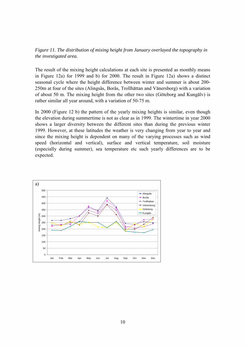
Figure 11. The distribution of mixing height from January overlayed the topography inthe investigated area.

The result of the mixing height calculations at each site is presented as monthly meansin Figure 12a) for 1999 and b) for 2000. The result in Figure 12a) shows a distinctseasonal cycle where the height difference between winter and summer is about 200-250m at four of the sites (Alingsås, Borås, Trollhättan and Vänersborg) with a variationof about 50 m. The mixing height from the other two sites (Göteborg and Kungälv) israther similar all year around, with a variation of 50-75 m.

In 2000 (Figure 12 b) the pattern of the yearly mixing heights is similar, even thoughthe elevation during summertime is not as clear as in 1999. The wintertime in year 2000shows a larger diversity between the different sites than during the previous winter1999. However, at these latitudes the weather is very changing from year to year andsince the mixing height is dependent on many of the varying processes such as windspeed (horizontal and vertical), surface and vertical temperature, soil moisture(especially during summer), sea temperature etc such yearly differences are to beexpected.

a)

0

50

100

150

200

250

300

350

400

450

500

Jan Feb Mar Apr May Jun Jul Aug Sep Oct Nov Dec

mix

ing

heig

ht (m

)

AlingsåsBoråsTrollhättanVänersborgGöteborgKungälv

11

b)

0

50

100

150

200

250

300

350

400

450

500

Jan Feb Mar Apr May Jun Jul Aug Sep Oct Nov Dec

mix

ing

heig

ht (m

)

AlingsåsBoråsTrollhättanVänersborgGöteborgKungälv

Figure 12 a) The monthly mean mixing height from 1999 and b) from 2000, separatedfor each site.

From the results of the mixing height calculations, presented in Figure 12 a) and b), itbecomes clear that there are two different developments of the mixing heights. One atthe two sites (Göteborg, Kungälv) located close to the coast, and one at the other foursites, (Alingsås, Borås, Trollhättan and Vänersborg) located inland. In order togeneralise and simplify the further calculations in the new URBAN-model, aclassification of the values of mixing height was made into a coastal and an inlandgroup. This is assumed to be relevant since the variability between the inland andcoastal sites respectively, as well as between the years, is rather moderate. The monthlymeans of the two years and groups have been calculated and are presented in Figure 13.

The mean mixing height during the six winter months (Oct-Mar) from the inland sitesvaries between 225-260 m, and from the coastal sites between 200-250 m. Duringsummer (May-Sep) the mixing height at the inland sites is stable located at around 325m but it descend in September to 250 m.

0

50

100

150

200

250

300

350

400

Jan Feb Mar Apr May Jun Jul Aug Sep Oct Nov Dec

mix

ing

heig

ht (m

)

12

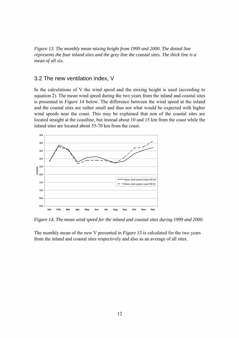
Figure 13. The monthly mean mixing height from 1999 and 2000. The dotted linerepresents the four inland sites and the grey line the coastal sites. The thick line is amean of all six.

3.2 The new ventilation index, V

In the calculations of V the wind speed and the mixing height is used (according toequation 2). The mean wind speed during the two years from the inland and coastal sitesis presented in Figure 14 below. The difference between the wind speed at the inlandand the coastal sites are rather small and thus not what would be expected with higherwind speeds near the coast. This may be explained that non of the coastal sites arelocated straight at the coastline, but instead about 10 and 15 km from the coast while theinland sites are located about 55-70 km from the coast.

0.0

0.5

1.0

1.5

2.0

2.5

3.0

3.5

4.0

4.5

Jan Feb Mar Apr May Jun Jul Aug Sep Oct Nov Dec

U (m

/s)

Mean wind speed inland 99-00

Mean wind speed coast 99-00

Figure 14. The mean wind speed for the inland and coastal sites during 1999 and 2000.

The monthly mean of the new V presented in Figure 15 is calculated for the two yearsfrom the inland and coastal sites respectively and also as an average of all sites.

13

0.0

0.5

1.0

1.5

2.0

2.5

3.0

3.5

4.0

4.5

5.0

Jan Feb Mar Apr May Jun Jul Aug Sep Oct Nov Dec

V i

Mean inlandMean CoastMean tot

Figure 15. Mean calculations of the new the ventilation index, V, for the inland, coastaland all sites.

High values of V indicate poor dispersion facilities and varies both between the seasonsand locations with the lowest values during summer and highest during winter, exceptfor April at the coastal sites, which performs a very high V.

When comparing the results in Figure 13 and Figure 14 it becomes clear that themixing height is the parameter that has the greatest influence on V resulting in thedifference between the locations. However, the high value of V in April is possiblyderived from the low wind speed in April. Further, the difference of V, between theinland and coastal sites is derived from the mixing height, since there is not muchdifference between the wind speed at the different locations.

3.3 The dispersion-adjusting constant Cd

The monthly means of Cd was calculated according to equation 3 for each month at eachsite for the two years. Since there was a rather large difference between the inland andthe coastal sites both in terms of V and H, the calculation of Cd was also separated intoinland and coastal, (Figure 16). Similar to V high Cd indicates poor dispersionconditions. (Figure 16).

14

0.000

0.001

0.002

0.003

0.004

0.005

0.006

0.007

0.008

0.009

0.010

Jan Feb Mar Apr May Jun Jul Aug Sep Oct Nov Dec

Cd

Mean inland 99-00Mean coast 99-00Mean all sites

Figure 16. Monthly mean calculation for 1999 and 2000 of Cd separated into inlandand coastal sites compared with the mean Cb of all sites.

The shapes of the curves in Figure 16 are similar to the shapes of curves of V but with amodification, mainly during the winter season. These adjustments are depending on theurban background concentrations of NO2, which are also included in the equation. Thevalues of Cd's are thus adjusted by the air pollution concentration in the various citieswhich will improved the reflection of local conditions resulting in further tuning of themodel.

3.4 The NO2 concentrations calculated by the new URBAN model

For calculating the concentration of NO2 in cities without measurements, the new model(equation 3) can be used. Here either Cb-inland or Cb-coastal is used, depending on thelocation of the city. However, the mixing height and wind speed used in the calculationwas not taken as an average of an inland or coastal location. They were instead derivedfrom the monthly means for the specific grid in TAPM where the city is located.

Following this procedure, a comparison is done between monthly mean measured andcalculated concentration of NO2 (Figure 17) which shows a good agreement (with a R2

of 0.6 and N=68).

15

0

5

10

15

20

25

30

35

40

0 5 10 15 20 25 30 35 40

Calculated NO2 (µg/m3)

Mea

ssur

ed N

O2 (

µg/m

3 )

Figure 17. Comparison between monthly mean of measured and calculatedconcentration of NO2 for the two years (99-00). Cb-inland and Cb-coastal is used dependingon the location of the town.

According to Figure 17 the calculated concentrations are in general slightlyoverestimated when the concentrations are below 20 µg/m3 and somewhat under-estimated when the concentrations are higher than 20 µg/m3. The measuredconcentration of NO2 and the ratio between measured and calculated concentrations arepresented in Figure 18.

0.0

0.2

0.4

0.6

0.8

1.0

1.2

1.4

1.6

1.8

2.0

0 5 10 15 20 25 30 35 40measured NO2

mea

ssur

ed/c

alcu

late

d N

O2

Figure 18. Comparison between measured NO2 and the ratio of measured/ calculatedNO2.

16

The above comparison shows that between 17-27 µg/m3 the calculated NO2 values areapproximately in a ratio of 1 and with an accuracy of ±0.2 µg/m3. The calculatedconcentrations are therefore well modelled in this interval. For concentrations higherthan about 27µg/m3 the ratio is about 0.8, indicating a slight underestimation of theconcentration. However, in this range there are to few observations and thus why theresult becomes more uncertain. For lower concentrations than 17µg/m3 the ratio is 1.3,resulting in somewhat overestimating of the modelled concentrations. The accuracyhere is about ±0.3 µg/m3. Consequently, the results presented in Figure 17 and Figure18 show that the agreements between measured and calculated monthly means of NO2

are generally good.

3.5 Comparison between old and new calculations andmeasurements.

The old URBAN-model only calculates mean concentration over six months during thewintertime. The monthly mean concentration calculated by the new URBAN-model isthus converted into six month means and then compared with the calculations by the oldURBAN model for the same period. The result of that comparison is presented inFigure 19.

0

5

10

15

20

25

30

35

Alingsås Borås Trollhättan Vänersborg Kungälv Göteborg

NO

2 (µg

/m3 )

Calculated NO2 new URBAN-modelCalculated NO2 old URBAN-modelMeassured NO2

Figure 19. Comparison between measurements (red squares) of the six month mean ofthe NO2 concentration and calculated six month means by the old (dotted line) and thenew URBAN-model (black line) at each site.

The comparison between NO2 calculations by the old and the new URBAN-modelshows that the new model calculates NO2 concentrations with a much better accuracy inall cases but one (Kungälv), according to the measured concentration. The monitoring

17

point in Kungälv is suspected not to be located in a representative urban backgroundspot. Thus, this might be one reason why the calculated NO2 concentration in Kungälvis not performing a fit as good as for the others sites.

4. Discussion and conclusions

The problem with dispersion modelling of today is that if all the important processesshould be included into the calculation, the model becomes difficult to run (a decentknowledge in meteorology is required to run the models properly) and they oftenrequire long computation time. By calculating some of the main parameters fordispersion (H and U) with the advanced model TAPM and using this result in a simplemodel, some of these problems are solved. Consequently, the high demands of thesimple model being able to reproduce a site specific climatology is thus being fulfilled,by the calculation of V (H*U) in the high resolution and in combination with thedispersion-adjusting constant, Cb. This is thus resulting in improved calculationscompared to the performance of the URBAN-model. The reason why the urbanbackground concentration is appropriate to use when calculating the Cb, is that the resultof all dispersion processes in an area (in combination with the regional backgroundconcentration) are representing the �correct� answers, provided that the measurementsare located at comparable urban background sites.

Is it relevant to use the population as an estimation of the emissions? The test presentedin Figure 1 shows that the connection is rather apparent for NO2. The idea is that eachperson is generating about the same amount of air pollutants from vehicles, heatinga.s.o. resulting in a rather good valuation of the emission in a community, as long as thepopulation remains in the community most of the time. One can therefore assume this isa relevant approach at least for air pollutants mainly generated from local sources. Oneother possible improvement of the emission calculations in the new URBAN-modelcould be a separate calculation for each town and city, instead of the whole community.As the new URBAN-model calculates in a much higher geographical resolution than theold version, this change would be relevant to perform. It has not yet been tested if theconnection is as good between population and other pollutants as it is for NO2. Thisrequires further investigations.

Another possibility is to use other types of emission inputs such as the new Swedishnational emission inventory, which have been updated during the last year. When theresolution of this emission data is better it might be used to improve the calculationsfurther and also for adding other pollutants.

The relevance of using a simple model

This type of rather simple empirical, statistical calculation of the concentrations of airpollutants, the old URBAN-model, has been used for some years by IVL and the

18

Swedish road administration as a screening method to indicate if the concentration of airpollution is exceeding the threshold values in small communities. However, since therequirements of more accurate estimations are rising even for small towns animprovement of the calculations has been done. This improvement results in:

• a dispersion-related constant, Cb, is calculated from measurements of monthlymeans of concentration of air pollution at different geographical locations.

• a better description of the meteorological site-specific dispersion processes,described in the new ventilation index, V, including mixing height, wind speed incombination with Cb. All parameters are calculated with better time andgeographical resolution than for the old Fv.

• the emissions are, like in the old model, still derived from the amount of thepopulation in the communities (Figure 1), but its accordance has been verified here.

• the background concentration is upgraded, when needed, from the databases at IVL

• the new empirical calculation method implemented into the new URBAN-model,which meet the increasing demands of air pollution modelling, especially in smallcities.

The need of a valuation of the air quality in small cities is thus assumed to be fulfilledby using this rather simple but appropriate model rather than using a more advancedmodel. The reason is that the result does not become better with an advanced modelthan with a simple, if the input emissions are not performed with good resolution bothaccording to time and geographical resolution. So far the model has been tested in thesouthwestern part of Sweden with promising result why the next step is to continuesimilar development for the whole Sweden. However, in accordance to the Swedishstandards, the percentiles are to be calculated for some parameters. Thus, in the oldURBAN-model the urban background concentration is transferred into differentpercentiles and also street level concentration. For applying these relations into the newURBAN-model they may have to be recalculated into monthly means.

Since the result from this investigation is very promising the method should be possibleto apply for the whole Sweden in the future. This will not necessarily result in moregroups of V than the old V's, but instead a more detailed gridded information of V andCb like a mosaic for the whole of Sweden.

19

Reference

Chen D, Wang T, Haeger-Eugensson M, Ashberger C and Borne K. (2002).'Application of TAPM (v.1) in Swedish West Coast: validation during 1999 and 2000'.IVL rapport L02/51.

Fergeson, S. (2002). 'Ventilation Climate Information System' USDA Forest Serviceand FERA- Fire and Environmental Research Applications' (http://www.fs.fed.us/pnw/fera/vent.html/.

Fergeson, S. (2003). 'The potential for smoke to ventilate from windland fires in theUnited States'. Pre-prints for the Fourth Symposium on Fire and Forest Meteorologyorganised by American Meteorological Society in February 2003.

Hardy, C., Ottmar, R. D., Petersen, J. and Core, J. (2003). 'Smoke managementguide for prescribed and wildland fire' 2000 edition. Bois, ID: National WildfireCoordinating Group.

Holzworth, G. C (1972). 'Mixing heights, wind speeds, and potentials for urban airpollution throughout the contiguous United States. Office of Air Publication No. AP-101. Research Triangular Park, NC US Environmental Protection Agency, Office of AirPrograms.

Hurley, P.J. (1999a). �The Air Pollution Model (TAPM) Version 1: TechnicalDescription and Examples�, CAR Technical Paper No. 43. 42 p.

Hurley, P.J. (1999b). �The air pollution model (TAPM) version 1: User manual�.Internal paper 12 of CSIRO Atmospheric Research Division 22 p.

Krieg R and Olsson L (1977). 'Undersökning av ventilationsklimatet i Sverige'. SMHI

Persson, K., Haeger-Eugensson, M., Ferm, M. and Sjöberg, K (2002). 'Luft-kvaliteten i Sverige sommaren 2001 och vintern 2001/2002. IVL rapport B-1478.

Persson K, Sjöberg K, Svanberg P-A, and Blomgren H (1999). 'Dokumentation avURBAN-modellen'. IVL rapport L99/7.

SOU (1979): SOU rapport 1979:55, "Hushållning mark och vatten" del 2. Statensoffentliga utredningar.

1

Appendix 1 Description of the model -TAPM

The TAPM model

Recently, TAPM (The Air Pollution Model) developed by Australian CSIROAtmospheric Research Division, appeared as an attractive model system since itintegrates meteorology and air chemistry (Hurley, 1999b). This model was designed tobe run in a nestable way so that the spatial resolution can be as fine as ~100 m. Inaddition, it can be run for one year or longer, which provides a means to deal withstatistics of meteorological and pollutant variables.

Essentials of the Model

Air pollution models that can be used to predict pollution concentrations for periods ofup to a year, are generally semi-empirical/analytic approaches based on Gaussianplumes or puffs. Typically, these models use either observed data from a surface basedmeteorological station or a diagnostic wind field model based on available observations.TAPM is different from these approaches in that it solves the fundamental fluiddynamics and scalar transport equations to predict meteorology and pollutantconcentration for a range of pollutants important for air pollution applications. Itconsists of coupled prognostic meteorological and air pollution concentrationcomponents, eliminating the need to have site-specific meteorological observations.Instead, the model predicts the flows important to local-scale air pollution transport,such as sea breezes and terrain induced flows, against a background of larger-scalemeteorology provided by synoptic analyses. It predicts meteorological and pollutionparameters directly (including some photochemistry) on local, city or inter-regionalscales.

Meteorology model

The meteorological component of TAPM is an incompressible, non-hydrostatic,primitive equation model with a terrain-following vertical co-ordinate for three-dimensional simulations. The model solves the momentum equations for horizontalwind components, the incompressible continuity equation for vertical velocity, andscalar equations for potential virtual temperature and specific humidity of water vapour,cloud water and rainwater. Explicit cloud microphysical processes are included.Turbulence kinetic energy and eddy dissipation rates are calculated for determining theturbulence terms and the vertical fluxes. Further, surface energy budget is considered tocomputer the surface temperature. A vegetative canopy and soil scheme is used at thesurface. Radiative fluxes at the surface and at upper levels are also calculated.

2

Air pollution model

The air pollution component of TAPM, which uses predicted meteorology andturbulence from the meteorological component, includes three modules. The EulerianGrid Module (EGM) solves prognostic equations for concentration and for cross-correlation of concentration and virtual potential temperature. The Lagrangian ParticleModule (LPM) can be used to represent near-source dispersion more accurately, whilethe Plume Rise Module is used to account for plume momentum and buoyancy effectsfor point sources. The model also has gas-phase photochemical reactions based on theGeneric Reaction Set, and gas- and aqueous-phase chemical reactions for sulphurdioxide and particles. In addition, wet and dry deposition effects are also included.

Graphical user interface

The model is driven by a graphical user interface, which is used to:

(1) select all model input and configuration options, including access to supplieddatabases of terrain height, vegetation and soil type (USGS), synoptic-scalemeteorology (CSIRO), and sea-surface temperature (NOAA)

(2) run the model

(3) choose and process model output, including options for visualisation, extraction oftime-series, production of static 1-D and 2-D plots and summary statistics usingcommon packages such as EXCEL.

Comments on use of TAPM

Model limitations

Although TAPM performs well in many aspects, it has some major limitations as thefollowing:

(1) TAPM should not be used for larger domains than 1000 km by 1000 km, due tocurvature of the earth.

(2) The GRS photochemistry option in the model may not be suitable for examiningsmall perturbations in emissions inventories, particularly in VOC emissions, due to thehighly lumped approach taken for VOC's in this mechanism. VOC reactivates shouldalso be chosen carefully for each region of application.

Soil moisture setting

3

The soil moisture is an import parameter in determining the surface energy balance.Based on our experience, a seasonal variable should be used. The following soilmoisture (Table 1:1) is recommended for the model running for the Swedish WestCoast. This table is based on NCEP reanalysis of 1999 over the area. Further study maybe needed to specify it in a better way.

Table 1:1 Deep soil volumetric moisture in content m3 m-3 (i.e. the volume of water pervolume of soil) used in model run

Mon Jan Feb Mar Apr May Jun Jul Aug Sep Oct Nov Dec

Value 0.29 0.30 0.28 0.24 0.21 0.19 0.18 0.19 0.21 0.23 0.26 0.28

Model outputs

The output of TAPM is rich, covering both 2D and 3D fields. The 2D fields are:

• total solar radiation, net radiation, sensible heat flux, evaporative heat flux, frictionvelocity, potential virtual temperature, potential temperature, convective velocity,mixing height, screen-level temperature, screen-level relative humidity, surfacetemperature and rainfall,

The 3D fields are:

• horizontal wind speed, horizontal wind direction, vertical velocity, temperature,relative humidity, and potential temperature and turbulence kinetic energy.

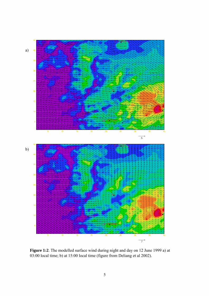
A very important feature of TAPM is its ability to explicitly deal with surface energybudget and temperature, which allows simulation of thermally driven wind systems. Asexamples, Figures 1:1-1:2 give snapshots of modelled surface temperature wind duringone day and one night. The figures show distinct diurnal variations both in temperatureand wind patterns.

The figure 1:1 show that during the daytime, solar radiation heats the ground faster thanthe sea, which results in higher air temperature over land compared to the sea.Therefore, air with lower density ascends over land and air with higher density descendsover sea. Near the surface, air flow (figure 1:2) from the sea to the land, leading todevelopment of sea breeze. During clear nights, the cooling of land is faster than thesea, hence air blow from land to sea over the surface, leading to formation of landbreeze.

Figure 1:3 is a snap shot of the vertical wind during day and night. The return flow ofthe sea breeze can be seen at the model level 9 (750 m).

a)

)

b

4

Figure 1:1. The modelled surface air temperature (oC) during night and day on 12 June1999 (a) at 03:00 local time; (b) at 15:00 local time.

)

a

)

b

5

Figure 1:2. The modelled surface wind during night and day on 12 June 1999 a) at03:00 local time; b) at 15:00 local time (figure from Deliang et al 2002).

)

a

6

Figure 1:3. The modelled cross section (X-Z or u-10w) of wind during night and day on12 June 1999 a) at 03:00 local time; b) at 15:00 local time. Unit of u and w m/s (figurefrom Deliang et al 2002).

b)

7

Appendix 2 Validation of the model system

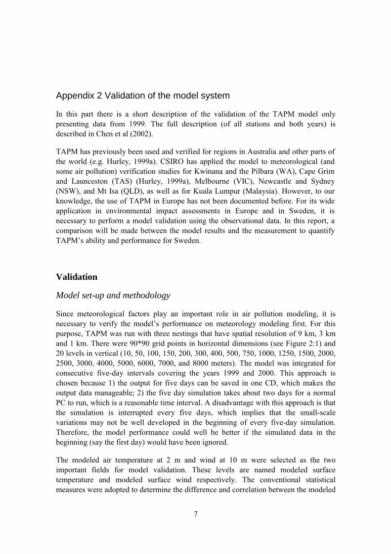
In this part there is a short description of the validation of the TAPM model onlypresenting data from 1999. The full description (of all stations and both years) isdescribed in Chen et al (2002).

TAPM has previously been used and verified for regions in Australia and other parts ofthe world (e.g. Hurley, 1999a). CSIRO has applied the model to meteorological (andsome air pollution) verification studies for Kwinana and the Pilbara (WA), Cape Grimand Launceston (TAS) (Hurley, 1999a), Melbourne (VIC), Newcastle and Sydney(NSW), and Mt Isa (QLD), as well as for Kuala Lumpur (Malaysia). However, to ourknowledge, the use of TAPM in Europe has not been documented before. For its wideapplication in environmental impact assessments in Europe and in Sweden, it isnecessary to perform a model validation using the observational data. In this report, acomparison will be made between the model results and the measurement to quantifyTAPM�s ability and performance for Sweden.

Validation

Model set-up and methodology

Since meteorological factors play an important role in air pollution modeling, it isnecessary to verify the model�s performance on meteorology modeling first. For thispurpose, TAPM was run with three nestings that have spatial resolution of 9 km, 3 kmand 1 km. There were 90*90 grid points in horizontal dimensions (see Figure 2:1) and20 levels in vertical (10, 50, 100, 150, 200, 300, 400, 500, 750, 1000, 1250, 1500, 2000,2500, 3000, 4000, 5000, 6000, 7000, and 8000 meters). The model was integrated forconsecutive five-day intervals covering the years 1999 and 2000. This approach ischosen because 1) the output for five days can be saved in one CD, which makes theoutput data manageable; 2) the five day simulation takes about two days for a normalPC to run, which is a reasonable time interval. A disadvantage with this approach is thatthe simulation is interrupted every five days, which implies that the small-scalevariations may not be well developed in the beginning of every five-day simulation.Therefore, the model performance could well be better if the simulated data in thebeginning (say the first day) would have been ignored.

The modeled air temperature at 2 m and wind at 10 m were selected as the twoimportant fields for model validation. These levels are named modeled surfacetemperature and modeled surface wind respectively. The conventional statisticalmeasures were adopted to determine the difference and correlation between the modeled

8

results and the measurements. All comparisons were made for 1999 and 2000respectively, in order to determine eventual differences from year to year.

Figure 2:1. Model domains of the three nestings. The three surfaces stations (circles)and two Sodar stations (squares) used in the comparisons are shown in the lastnesting.

Observational DataThe observational data used for model validation are from NCDC/NOAA in theTD9956-Datsav III variable length ASCII format. The TD9956 data contain all hourlyrecords as well as any observations taken in-between hours.

9

The stations used in the validation are GOTEBORG (Göteborg), LANDVETTER andSAVE (Säve), as indicated by bold letters. The time period of the data is from 1 January1999 to 31 December 2000. The three stations provide meteorological data from variouslevels above the ground (Göteborg ≈ 50 m, Landvetter ≈ 10 m and Säve ≈ 10 m)characterising the urban and suburban surface in the area. These levels are all namedobserved surface temperature and observed surface wind respectively.

In addition, upper level wind data from two sound radar stations (Hunneberg, Borås, seefigure 2:1) were selected for profiles comparisons. Compared with the surface data, theSodar data is rather incomplete. The details about the measurements can be found inDeliang et al. (2002). The instruments provide wind profiles from 50 m height up tomaximum 475 m height. Generally, data is collected up to a level of approximately 175m, but very seldom above 400 m. The horizontal wind range is 35 m/s, the vertical windrange is ±10 m/s. The wind accuracy is 0.2 m/s or better for the horizontal and 0.05 m/sfor the vertical wind.

To make the direct comparison possible, sodar measurements at different levels areinterpolated to the model levels. Missing values appear in both the surface and upper airmeasurement occasionally. Simulated values are omitted if the correspondingobservations are missing. Thus, the numbers of data available for different comparisonsvary always and need to be indicated in the statistics.

Some of the results

Surface comparison

The scatter plots of the observed and modelled hourly near ground air temperature,horizontal wind (u, v component) at the Göteborg station are displayed in Figures 2:2-2:4 for 1999. Plotts from the other stations and for 2000 are found in Deliang (2002).The related statistics can be found in Table 2:1.

GÖTEBORG 1999

-20

-10

0

10

20

30

-10 0 10 20 30

Modeled surface temperature (°C)

Obs

erve

d su

rface

tem

pera

ture

(°C

)

a)

10

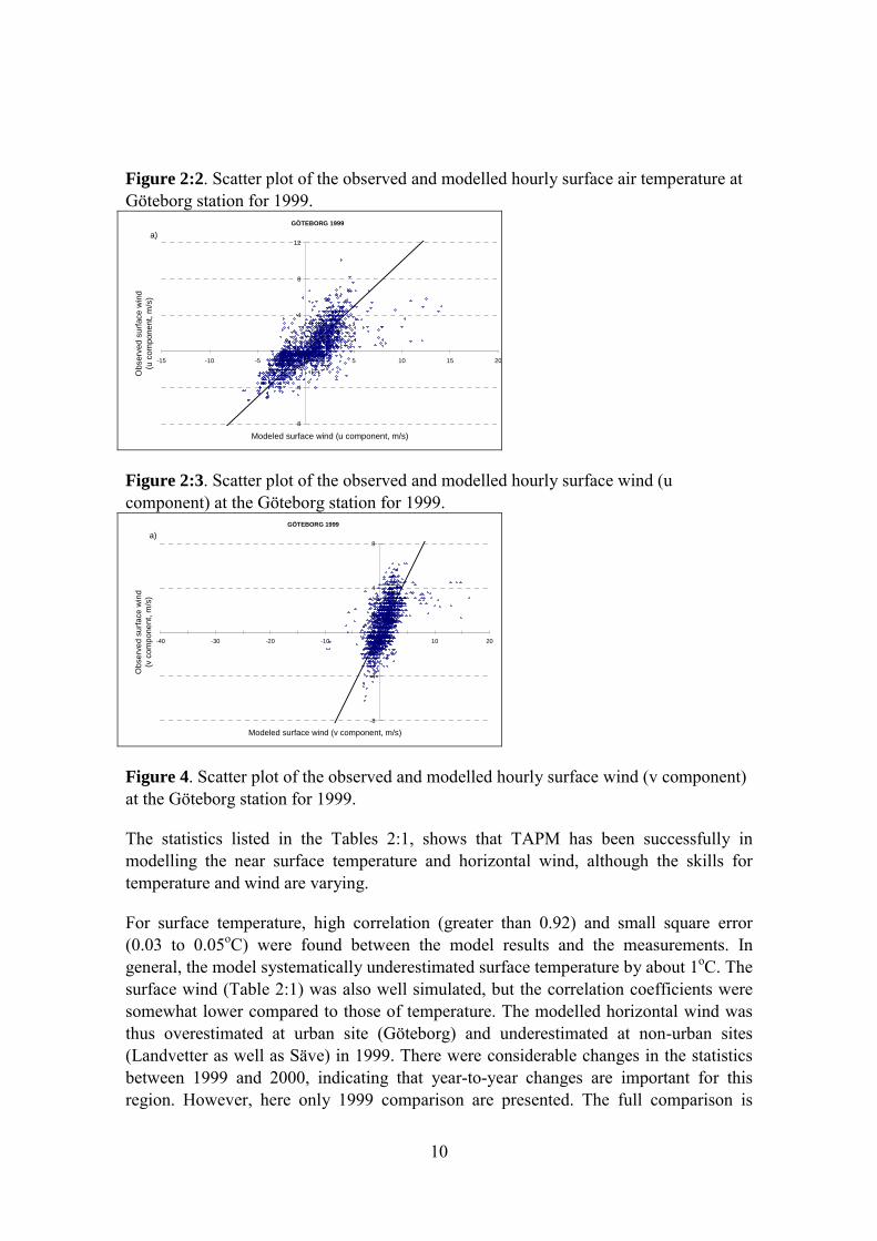
Figure 2:2. Scatter plot of the observed and modelled hourly surface air temperature atGöteborg station for 1999.

GÖTEBORG 1999

-8

-4

0

4

8

12

-15 -10 -5 0 5 10 15 20

Modeled surface wind (u component, m/s)

Obs

erve

d su

rface

win

d (u

com

pone

nt, m

/s)

a)

Figure 2:3. Scatter plot of the observed and modelled hourly surface wind (ucomponent) at the Göteborg station for 1999.

GÖTEBORG 1999

-8

-4

0

4

8

-40 -30 -20 -10 0 10 20

Modeled surface wind (v component, m/s)

Obs

erve

d su

rface

win

d (v

com

pone

nt, m

/s)

a)

Figure 4. Scatter plot of the observed and modelled hourly surface wind (v component)at the Göteborg station for 1999.

The statistics listed in the Tables 2:1, shows that TAPM has been successfully inmodelling the near surface temperature and horizontal wind, although the skills fortemperature and wind are varying.

For surface temperature, high correlation (greater than 0.92) and small square error(0.03 to 0.05oC) were found between the model results and the measurements. Ingeneral, the model systematically underestimated surface temperature by about 1oC. Thesurface wind (Table 2:1) was also well simulated, but the correlation coefficients weresomewhat lower compared to those of temperature. The modelled horizontal wind wasthus overestimated at urban site (Göteborg) and underestimated at non-urban sites(Landvetter as well as Säve) in 1999. There were considerable changes in the statisticsbetween 1999 and 2000, indicating that year-to-year changes are important for thisregion. However, here only 1999 comparison are presented. The full comparison is

11

presented in Chen et al. (2002).

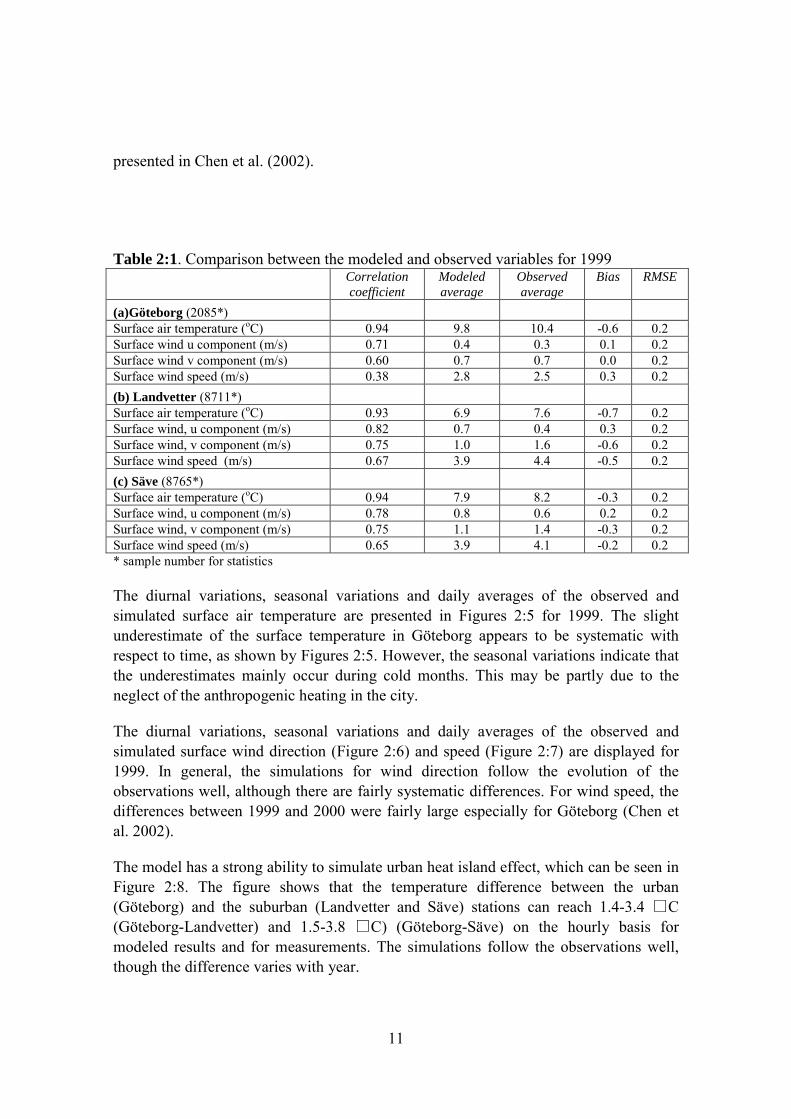
Table 2:1. Comparison between the modeled and observed variables for 1999Correlationcoefficient

Modeledaverage

Observedaverage

Bias RMSE

(a)Göteborg (2085*)Surface air temperature (oC) 0.94 9.8 10.4 -0.6 0.2Surface wind u component (m/s) 0.71 0.4 0.3 0.1 0.2Surface wind v component (m/s) 0.60 0.7 0.7 0.0 0.2Surface wind speed (m/s) 0.38 2.8 2.5 0.3 0.2(b) Landvetter (8711*)Surface air temperature (oC) 0.93 6.9 7.6 -0.7 0.2Surface wind, u component (m/s) 0.82 0.7 0.4 0.3 0.2Surface wind, v component (m/s) 0.75 1.0 1.6 -0.6 0.2Surface wind speed (m/s) 0.67 3.9 4.4 -0.5 0.2(c) Säve (8765*)Surface air temperature (oC) 0.94 7.9 8.2 -0.3 0.2Surface wind, u component (m/s) 0.78 0.8 0.6 0.2 0.2Surface wind, v component (m/s) 0.75 1.1 1.4 -0.3 0.2Surface wind speed (m/s) 0.65 3.9 4.1 -0.2 0.2* sample number for statistics

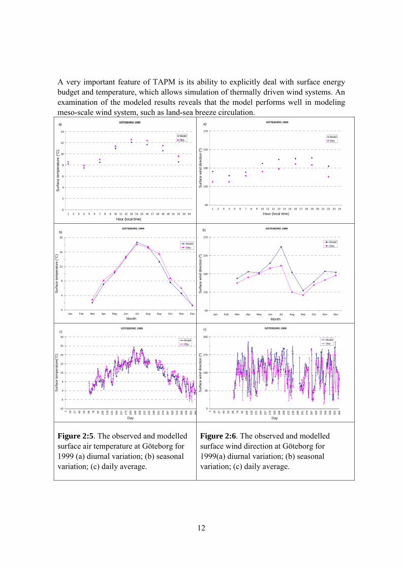
The diurnal variations, seasonal variations and daily averages of the observed andsimulated surface air temperature are presented in Figures 2:5 for 1999. The slightunderestimate of the surface temperature in Göteborg appears to be systematic withrespect to time, as shown by Figures 2:5. However, the seasonal variations indicate thatthe underestimates mainly occur during cold months. This may be partly due to theneglect of the anthropogenic heating in the city.

The diurnal variations, seasonal variations and daily averages of the observed andsimulated surface wind direction (Figure 2:6) and speed (Figure 2:7) are displayed for1999. In general, the simulations for wind direction follow the evolution of theobservations well, although there are fairly systematic differences. For wind speed, thedifferences between 1999 and 2000 were fairly large especially for Göteborg (Chen etal. 2002).

The model has a strong ability to simulate urban heat island effect, which can be seen inFigure 2:8. The figure shows that the temperature difference between the urban(Göteborg) and the suburban (Landvetter and Säve) stations can reach 1.4-3.4 ºC(Göteborg-Landvetter) and 1.5-3.8 ºC) (Göteborg-Säve) on the hourly basis formodeled results and for measurements. The simulations follow the observations well,though the difference varies with year.

12

A very important feature of TAPM is its ability to explicitly deal with surface energybudget and temperature, which allows simulation of thermally driven wind systems. Anexamination of the modeled results reveals that the model performs well in modelingmeso-scale wind system, such as land-sea breeze circulation.

GÖTEBORG 1999

0

2

4

6

8

10

12

14

1 2 3 4 5 6 7 8 9 10 11 12 13 14 15 16 17 18 19 20 21 22 23 24

Hour (local time)

Surfa

ce te

mpe

ratu

re (°

C)

ModelObs

a) GÖTEBORG 1999

90

135

180

225

270

1 2 3 4 5 6 7 8 9 10 11 12 13 14 15 16 17 18 19 20 21 22 23 24

Hour (local time)

Surfa

ce w

ind

dire

ctio

n (º

)

ModelObs

a)

GÖTEBORG 1999

0

4

8

12

16

20

Jan Feb Mar Apr May Jun Jul Aug Sep Oct Nov Dec

Month

Surfa

ce te

mpe

ratu

re (°

C)

ModelObs

b)GÖTEBORG 1999

90

135

180

225

270

Jan Feb Mar Apr May Jun Jul Aug Sep Oct Nov Dec

Month

Surfa

ce w

ind

dire

ctio

n (º

)

ModelObs

b)

GÖTEBORG 1999

-10

-5

0

5

10

15

20

25

30

1 14 27 40 53 66 79 92 105

118

131

144

157

170

183

196

209

222

235

248

261

274

287

300

313

326

339

352

365

Day

Surfa

ce te

mpe

ratu

re(°

C)

ModelObs

c)GÖTEBORG 1999

0

90

180

270

360

1 14 27 40 53 66 79 92 105

118

131

144

157

170

183

196

209

222

235

248

261

274

287

300

313

326

339

352

365

Day

Surfa

ce w

ind

dire

ctio

n (º

)

ModelObs

c)

Figure 2:5. The observed and modelledsurface air temperature at Göteborg for1999 (a) diurnal variation; (b) seasonalvariation; (c) daily average.

Figure 2:6. The observed and modelledsurface wind direction at Göteborg for1999(a) diurnal variation; (b) seasonalvariation; (c) daily average.

13

GÖTEBORG 1999

0

1

2

3

4

1 2 3 4 5 6 7 8 9 10 11 12 13 14 15 16 17 18 19 20 21 22 23 24

Hour (local time)

Surfa

ce w

ind

spee

d (m

/s)

ModelObs

a)

0

1

2

3

4

1 2 3 4 5 6 7 8 9 10 11 12 13 14 15 16 17 18 19 20 21 22 23 24

Hour (local time)

Surfa

ce te

mpe

ratu

re d

iffer

ence

(°C

)

G-L(Model)G-S(Model)G-L(Obs)G-S(Obs)

a)

GÖTEBORG 1999

0

1

2

3

4

5

Jan Feb Mar Apr May Jun Jul Aug Sep Oct Nov Dec

Month

Surfa

ce w

ind

spee

d (m

/s)

ModelObs

b)

-1

-0,5

0

0,5

1

1,5

2

Jan Feb Mar Apr May Jun Jul Aug Sep Oct Nov Dec

Month

Surfa

ce te

mpe

ratu

re d

iffer

ence

(°C

)G-L(Model)G-S(Model)G-L(Obs)G-S(Obs)

b)

GÖTEBORG 1999

0

5

10

15

20

25

1 14 27 40 53 66 79 92 105

118

131

144

157

170

183

196

209

222

235

248

261

274

287

300

313

326

339

352

365

Day

Surfa

ce w

ind

spee

d (m

/s)

ModelObs

c)

-3

-2

-1

0

1

2

3

4

5

1 14 27 40 53 66 79 92 105

118

131

144

157

170

183

196

209

222

235

248

261

274

287

300

313

326

339

352

365

Day

Surfa

ce te

mpe

ratu

re d

iffer

ence

(°C

)

G-L(Model)G-S(Model)G-L(Obs)G-S(Obs)

c)

Figure 2:7. The observed and modelledsurface wind speed at Göteborg for 1999(a) diurnal variation; (b) seasonalvariation; (c) daily average.

Figure 2:8. The observed and modelledsurface temperature difference betweenGöteborg and Landvetter (G-L), as well asbetween Göteborg and Säve (G-S) for1999(a) diurnal variation; (b) seasonalvariation; (c) daily average

14

Profile comparison

The statistics of observed and modelled wind profiles at selected levels at Hunnebergand Borås are listed in Table 2:2 and Table 2:3, respectively.

From the results following features are obvious:

1) The evolution of the simulated upper winds follows those of the observed fairly well,as reflected in the correlation coefficients that are comparable to those in the surfacecomparison.

2) The agreements at the two sites are comparable.

3) The Sodar measurements at the two sites have a persistent bias, pointing to asystematic error in the measurements or in simulations.

4) Difference between results in 1999 and 2000 are considerable, with results in 1999being better than those in 2000 are. One possible reason could be poorer quality ofsynoptic data in 2000.

Table 2:2. Comparison between the modeled and observed wind profiles at Hunnebergin 1999. Unit of wind speed: m/s.Component Height Correlation

coefficientModeledaverage

Observedaverage

Bias RMSE

wind-u 50m (7672*) 0.78 0.2 wind-v 0.66 0.2wind speed 0.54 6.0 3.5 2.5 0.2wind-u 100m

(7674*)0.81 0.2

wind-v 0.70 0.2wind speed 0.60 7.0 5.5 1.5 0.3 wind-u 150m

(7658*)0.82 0.2

wind-v 0.70 0.2wind speed 0.62 7.8 6.6 1.2 0.3 wind-u 200m

(7015*)0.81 0.2

wind-v 0.70 0.2wind speed 0.57 8.5 7.2 1.3 0.3 wind-u 300m

(3908*)0.76 0.3

wind-v 0.69 0.3wind speed 0.50 9.5 7.8 1.7 0.4

15

wind-u 400m(1253*)

0.73 0.4

wind-v 0.68 0.4wind speed 0.51 10.5 8.2 2.3 0.5* sample number for statistics

Table 2:3. Comparison between the modeled and observed wind profiles at Borås in1999. Unit of wind speed: m/s.Component Height Correlation

coefficientModeledaverage

Observedaverage

Bias RMSE

Wind-u 50m (7297*) 0.80 0.2 Wind-v 0.71 0.2Wind speed 0.60 5.3 3.8 1.5 0.2 Wind-u 100m (7851) 0.83 0.2 Wind-v 0.72 0.2Wind speed 0.64 6.6 5.0 1.6 0.2 wind-u 150m (7364*) 0.77 0.2 wind-v 0.71 0.2wind speed 0.49 7.5 5.5 2.0 0.3 wind-u 200m (5013*) 0.77 0.3 wind-v 0.71 0.2wind speed 0.51 8.0 6.1 1.9 0.3 wind-u 300m (1544*) 0.81 0.4 wind-v 0.67 0.4wind speed 0.45 9.8 8.0 1.8 0.4 wind-u 400m (298*) 0.87 0.5 wind-v 0.70 0.5wind speed 0.56 11.7 9.6 2.1 0.6* sample number for statistics

16

Appendix 3 Calculation of mixing height using Holzworth algorithm

A brief description of the theoretical background and calculation procedure ofcalculation of mixing height (H) at Landvetter uses Holzworth algorithm (1967).

The algorithm

The algorithm is used to calculate a twice-daily H based on synoptic observations aswell as data from a radio sonde sounding. To compute the morning mixing height, theminimum temperature from 0200 to 0600 (LST) is determined. To this value 5°C isadded. Holzworth developed his algorithm for an urban environment in order toestimate urban air pollution. He established this adjustment to account for temperaturedifferences between rural and urban environments and for some initial surface heatingjust after sunrise. To estimate the morning H, the adjusted minimum surfacetemperature follows the dry adiabatic lapse rate up to the intersection with the observed1200 (GMT) temperature radio sounding.

A similar computation is made using the maximum temperature from 1200 to 1600(LST) and the 1200 (GMT) radio sounding, except that the surface temperature is notadjusted. The assumption made by Holzworth was that afternoon H in urban and nearbyrural areas does not differ significantly, whereas the nocturnal H is often very different.

Calculation procedure

Before calculating the H the temperature at 925 hPa level are converted in to potentialtemperature θ=T[P0/P]0.286 where P0=air pressure at the surface level and P=air pressureat 925 hPa level.

The surface potential temperature should be computed from the minimum temperature(in the morning) and the pressure at the first level in the 1200 (GMT) radio sounding(Why use pressure data several hours later?). Unless the data are missing, the first levelin a sounding is representative of the surface (check the height of the field station toverify the true first level of sounding, at Landvetter 155 m.a.s.l and after moving theposition 164 m.a.s.l). In this calculation the surface potential temperature is equal to thesurface absolute temperature. Since potential temperature generally increases withheight in the atmosphere, the linearly interpolation that is assumed in the calculation isacceptable.

H is calculated by plotting two linear gradients (one based on surface temperature andthe dry adiabatic lapse rate and one based on radio sound measurements at 1200 (GMT).The gradients are described using the equation y1=k1x+m1 and y2=k2x+m2 wherey1=temperature gradient based on radio sound observations

17

y2=temperature gradient based on surface observations and the dry adiabatic lapse rate

m1=radiosound measured surface temperature (for Landvetter: at 155 m or 164 m level)

m2=surface minimum temperature (+5°C) during 0100-0500 (UTC, this is equal to0200-0600 LST) respectively surface maximum temperature during 1100-1500 (UTC).

k1=radiosound mesured temperature gradient (using temperature at 155 m.a.s.l (or 164m.a.s.l.) and temperature at 925 hPa level)

k2=dry adiabatic lapse rate (=0,0098 K/m)

The height x where the two linear equation cross each other is expressed:

k1x+m1=k2x+m2

(k1- k2)x=m1-m2

x=m1-m2/k1- k2

x=mixing height (m)

From this easy way of calculating the H, sensible values are only achieved if a.) Theradiosond gradient is smaller than the dry adiabatic lapse rate and the radiosond surfacetemperature is higher than the observed surface temperature during the morning, or b.)The radiosond gradient is larger than the dry adiabatic lapse rate and the radiosondsurface temperature is lower than the observed surface temperature during the morning.If these conditions do not occur there will be no crossing of the gradients or the crossingwill occur at a level less than the surface height above sea level. These situations arelabelled XXX in the file MIXING.TXT (which show date and the calculated H (m)) andoccur most frequently during the winter months. In the file TEMPGRAD.TXT datafrom the radiosoundings with date, time (UTC), temperature at ground level, heightabove ground at 925 hPa (m), and calculated temperature gradient (K/m) are shown.The file TMINMAX.TXT includes observations from the surface field station with date,minimum temperature at 2m during 0100-0500 (UTC), and maximum temperature at2m during 1100-1500 (UTC).

Detailed information of the field stations, instruments and data

Detailed information of the field stations, instruments and data used for calculation ofthe mixing height (MH) in the Swedish west coast area during 1999 � 2000, arepresented in this chapter.

Location• Radiosond data from Landvetter (lat. 57.67N lon. 12.30E height 155 m.a.s.l.)• Synoptic meteorological station Säve (lat. 57.47 N lon. 11.53E height 53

m.a.s.l.)• Synoptic meteorological station Göteborg (lat. 57.42 N lon. 12.00E height 5

m.a.s.l.)• Synoptic meteorological station Landvetter (lat. 57.40 N lon. 12.18E height 169

18

m.a.s.l.)

Sampling

Radiosond data are measured continuously at hour: 0, 6, 12, 18 during Jan 1999 � Jun2000; at hour: 0, 12 during Jul - 17 Sep 2000; and at approximate hour: 11, 23 (reallythe hour the radiosonde is launched) during 18 Sep � Dec 2000.

The radiosonde takes measurements at intervals of approximately 2 seconds. The high-resolution data files contain all such data. Though, Landvetter measures standardresolution and the data files contain measurements taken at particular levels of theatmosphere. Measurements are reported to the Met. Office at standard and significantpressures levels. The standard pressure levels are 1000, 925, 850, 700, 500, 400, 300,250, 200, 150, 100, 70, 50, 30, 20 and 10 mb.

The radiosonde parameters are pressure (hPa), height above sea level (m), dry-bulbtemperature (º K), dew-point temperature (º K), wind direction (º), wind speed (m/s).

The synoptic meteorological station Göteborg (WMO number 025130) is run by SMHIand measures data every third hour. Station Landvetter (WMO number 025260, ESGG)run by the Landvetter airport and station Säve (WMO number 025120, ESGP) run bythe Swedish Military Weather Service measures continuously every hour.

Instrumentation

The radiosonde at Landvetter (WMOnumber 02527) uses a radiosonde called VRS80N, groundequipment called DIGICORA, and the windfinding method: OMEGA/LORAN.

The RS80 radiosonde, manufactured by the Finnish Company Vaisala, has beenroutinely used in many countries. Powered by a water-activated battery, the instrumenttakes measurements at approximately 1.3 second intervals during the ascent. Pressure,temperature (and humidity) are measured using three capacitative sensors. A schematicdiagram of the layout of the RS80 is shown in the figure below.

General technical specifications of Vaisala RS80 are:

PTU sensors are individually factories calibrated.

Pressure: BAROCAP® Capacitive aneroidMeasuring range: 1060 hPa to 3hPa (mb)Resolution: 0.1 hPaAccuracy: Reproducibility (1): 0.5 hPa

Repeatability of calibration (2): 0.5 hPaTemperature: THERMOCAP® Capacitive beadMeasuring range: +60 °C to - 90 °C

19

Resolution: 0.1 °CAccuracy: Reproducibility (1): 0.2 °C up to 50 hPa, 0.3 °C for 50-15 hPa,

0.4°C above 15 hPa levelRepeatability of calibration (2): 0.2 °C

Lag: < 2.5 s (6 m/s flow at 1000 hPa)Humidity: HUMICAP® Thin film capacitorMeasuring range: 0 to 100 % RHResolution: 1 % RHLag: 1 s (6 m/s flow at 1000 hPa, +20 °C)Accuracy: Reproducibility (1): <3 %RH

Repeatability of calibration (2): 2 %RH

Wind speed and direction are not directly measured by the radiosonde. These parametersare calculated from the position of the sonde at successive time intervals.

The LORAN-C Radio Navigation System:

This system uses a network of LOng RAnge Navigation beacons, which transmit radiosignals at known frequencies. In addition to the sensors of the RS80 already described,the RS80L radiosonde carries a radio receiver to detect the LORAN signals.

The receiver measures the difference in time taken for the signals from two beacons ofknown position to reach the sonde. Such points of equal time difference form the loci ofa set of rectangular hyperbolae. Signals are received from three pairs of beacons. Thedifference in the time of signal reception from each pair identifies a hyperbola. Theradiosonde is thus located at the intersection of these hyperbolae, a known distance fromthe fixed LORAN beacons. The wind speed and direction can then be calculated from thedifference between successive positions of the sonde. The ground station equipmentperforms these calculations.

The LORAN-C method calculates the position of the radisonde with an accuracy ofapproximately +/- 300m. Wind speeds are calculated with an accuracy of +/- 1 to 2m/s.

The instrumentation on the three synoptic meteorological stations is standardequipments.

The station at Säve measures at the level of 2 m above the ground, wind speed anddirection using Vaisala cup anemometer WAA 15 (accuracy: +/- 0.1 m/s, thresholdvalue: 0.4 m/s) and wind vaneWAV 15 (accuracy: +/- 2.8 º, threshold value: 0.3 m/s,resolution: 5.6 º), temperature using a thermistor (accuracy +/- 0.2 ºC) and cloud coverusing visual observations.

The station at Landvetter measures temperature at the level of 1.5 m and wind at the levelof 10 m above the ground. Similar equipment (including measuring accuracy and units)

20

as at Säve are used here.

The station at Göteborg measures at the level of a 10 m height mast positioned on theroof of an approximately 40 m high building. On the mast the temperature sensor ispositioned at the 1.5 m level and wind anemometer and wind vane at the 10 m level.Similar equipment (including measuring accuracy and units) as at Säve are used here.

Miscellaneous

Further information on radiosond instrumentation may be find athttp://www.badc.rl.ac.uk/data/radiosonde/radhelp.html#wind