
Development and performance evaluation of a multistatic ...
213
Development and Performance Evaluation of a Multistatic Radar System Shaun Raymond Doughty A thesis submitted in partial fulfillment of the requirements for the degree of Doctor of Philosophy of the University of London. Department of Electronic and Electrical Engineering University College London 2008
-
Upload
khangminh22 -
Category
Documents
-
view
2 -
download
0
Transcript of Development and performance evaluation of a multistatic ...
Development and Performance Evaluation of aMultistatic Radar System
Shaun Raymond Doughty
A thesis submitted in partial fulfillment
of the requirements for the degree of
Doctor of Philosophy
of the
University of London.
Department of Electronic and Electrical Engineering
University College London
2008

2
I, Shaun Raymond Doughty, confirm that the work presented in this thesis is my own. Where
information has been derived from other sources, I confirm that this has been indicated in the thesis.
Abstract
Multistatic radar systems are of emerging interest as they can exploit spatial diversity, enabling improved
performance and new applications. Their development is being fuelled by advances in enabling technolo-
gies in such fields as communications and Digital Signal Processing (DSP). Such systems differ from
typical modern active radar systems through consisting of multiple spatially diverse transmitter and re-
ceiver sites. Due to this spatial diversity, these systems present challenges in managing their operation as
well as in usefully combining the multiple sources of information to give an output to the radar operator.
In this work, a novel digital Commercial Off-The-Shelf (COTS) based coherent multistatic radar
system designed at University College London, named ‘NetRad’, has been developed to produce some
of the first published experimental results, investigating the challenges of operating such a system, and
determining what level of performance might be achievable. Full detail of the various stages involved
in the combination of data from the component transmitter-receiver pairs within a multistatic system is
investigated, and many of the practical issues inherent are discussed.
Simulation and subsequent experimental verification of several centralised and decentralised detec-
tion algorithms in terms of localisation (resolution and parameter estimation) of targets was undertaken.
The computational cost of the DSP involved in multistatic data fusion is also considered. This gave a
clear demonstration of several of the benefits of multistatic radar. Resolution of multiple targets that
would have been unresolvable in a conventional monostatic system was shown. Targets were also shown
to be plotted as two-dimensional vector position and velocities from use of time delay and Doppler shift
information only. A range of targets were used including some such as walking people which were
particularly challenging due to the variability of Radar Cross Section (RCS).
Performance improvements were found to be dependant on the type of multistatic radar, method of
data fusion and target characteristics in question. It is likely that future work will look to further explore
the optimisation of multistatic radar for the various measures of performance identified and discussed in
this work.

Acknowledgements
I would like to thank my supervisors, Dr Karl Woodbridge and Professor Chris Baker, for the opportunity
to undertake this work. Their continuing support and guidance from my very first steps into radar as an
undergraduate has been invaluable. It has been a privilege to work under their supervision, and I am
deeply grateful.
I also would like to thank the UCL Sensors Systems and Circuits group, led first by Professor Hugh
Griffiths and later by Professor Baker, which has proved an excellent research environment and provided
numerous useful interactions with fellow researchers. I am particularly grateful to those members of
the group who assisted in the experimental trials of the NetRad. I would like to acknowledge Graeme
Smith for being an excellent sounding board for much of my research work (including putting up with
countless hours of me debating ideas with myself out loud!) and also for being incredibly helpful in
assisting with the organisation and running of the experimental trials. As well as Graeme, Kevin Chetty
and Waddah Al-Ashwal have taken charge of the future development of the NetRad, and it is pleasing
to see work continuing and the system in good hands. Daniel O’Hagan also deserves mention for many
useful, and often entertaining, discussions throughout my time at UCL. I wish to thank EPSRC for the
funding to undertake my research within the group.
I am thankful to the many visiting researchers who have taken the time to listen to my ideas and
volunteer their own valuable advice. In particular I would like to give mention to regular visitors includ-
ing Professor Ralph Benjamin, Dr Andrew Stove and Professor Simon Watts. Professor Mike Inggs of
the University of Cape Town has been of constant support to this work, and I am most grateful for his
expertise. Collaboration with Stephan Sanderbergh and Marc Brooker of UCT has proved fascinating,
and I wish them luck in their continued research efforts.
I am indebted to Dr Tom Derham for his concise explanation of both theory and implementation
of multistatic radar at the beginnings of my own research, and the opportunity to closely follow the
conclusion of his own work. The legacy of his hardware development was the foundations of this work,
and his achievements became all the more impressive to me as my understanding of the challenges
involved in designing and operating a multistatic system grew over the years.
The support and motivation from my friends and family has been immense over the course of my
studies, and I thank them all, particularly for keeping me sane whilst writing up, and at the times when
things didn’t go to plan! I am thankful for the constant encouragement of my mother and sisters, I am
truly lucky to have been brought up in such a close family, full of people that I love.

Acknowledgements 5
Finally, I would like to dedicate this thesis to my father, Raymond John Doughty, who unexpectedly
passed away during the course of this work. He will forever be a hero to me, and I am hugely proud to
be his son.
Contributions
Novel contributions of this work include:
• Hardware development of NetRad, a novel digital COTS-based coherent multistatic radar (Chapter
5). This unique system is capable of measuring the time delay and Doppler shift of target echoes
using nine spatially diverse transmitter-receiver pairs.
• Use of this system to obtain some of the first published experimental multistatic radar measure-
ments (Chapter 6), including investigation of data fusion methods to produce target plots.
• Assessment of many of the practical issues of the designing and deploying a multistatic radar -
both within hardware itself to ‘characterise’ the system (Section 5.3), as well as those concerning
the propagation of transmissions in the surveillance environment (Section 6.2).
• A side-by-side assessment of several centralised and decentralised detection algorithms in perfor-
mance measures not previously considered. The major focus was on the localisation (resolution
and parameter estimation) of targets. Also considered is the computational cost of the DSP in-
volved in multistatic data fusion. Applications of these detection algorithms were investigated
through simulation (Section 4.1 and 4.2) and subsequently through experimental measurements
from NetRad (Section 6.2).
• A clear demonstration of several of the benefits of multistatic radar, including:
– Resolution of multiple targets that would have been unresolvable in a conventional monos-
tatic system (Section 6.2.3, first published in [Doughty et al., 2007]).
– Plotting of targets with two-dimensional vector position and velocities from use of time delay
and Doppler shift information only. This is accomplished for a range of targets, some such as
walking people being particularly challenging due to the variability of RCS (Section 6.2.5).
• A unique simultaneous comparison of monostatic and bistatic radar outputs which make up the
component transmitter-receiver pairs of the multistatic system. In particular the simultaneous
measurement of the RCS over multiple monostatic and bistatic pairs was undertaken (Section
6.2.2). This was done firstly for purpose-built targets which could easily be simulated, before
more complex targets such as a vehicles and people were investigated.

Publications
Parts of this work have been previously published or presented:
• S. Doughty, K. Woodbridge, and C. Baker. Characterisation of a Multistatic Radar System. Radar
Conference, 2006. EuRAD 2006. 3rd European, pages 58, September 2006.
• T.E. Derham, S. Doughty, K. Woodbridge, C.J. Baker, Realisation and Evaluation of a Low Cost
Netted Radar System. Radar, 2006. CIE 06. International Conference on, pages 16-19, October
2006.
• Y. Teng, S. Doughty, K. Woodbridge, H. Griffiths, C. Baker, Netted Radar Theory and Experi-
ments. Information, Decision and Control, 2007. IDC ’07, pages 23-28, February 2007.
• T.E. Derham, S. Doughty, K. Woodbridge, and C.J. Baker. Design and evaluation of a low-cost
multistatic netted radar system. Radar, Sonar & Navigation, IET, Volume 1, Issue 5, pages 362-
368, October 2007.
• S.R. Doughty, K. Woodbridge, C.J. Baker, Improving Resolution Using Multistatic Radar. Pro-
ceedings of the IET International Conference on Radar Systems, October 2007

Acronyms
AC Alternating Current
ADC Analog to Digital Converter
CAN Controller Area Network
CFAR Constant False Alarm Rate
COTS Commercial Off-The-Shelf
CW Continuous Wave
DAC Digital to Analog Converter
DC Direct Current
DDS Direct Digital Synthesis
DFT Discrete Fourier Transform
DSP Digital Signal Processing
DMA Direct Memory Access
ECM Error Covariance Matrix
ERP Effective Radiated Power
FFT Fast Fourier Transform
FIM Fisher Information Matrix
FM Frequency Modulation
FMCW Frequency Modulated Continuous Wave
FPGA Field Programmable Gate Array
GDOP Geometric Dilution Of Precision
GPS Global Positioning System
GUI Graphical User Interface

Acronyms 9
HF High Frequency
IF Intermediate Frequency
IC Integrated Circuit
IEEE Institute of Electrical and Electronics Engineers
ISAR Inverse Synthetic Aperture Radar
ISM Industrial, Scientific and Medical
JTAG Joint Test Action Group
LAN Local Area Network
LED Light Emitting Diode
LNA Low Noise Amplifier
LO Local Oscillator
LOS Line Of Sight
LVDS Low Voltage Differential Signalling
MBET Monostatic-to-Bistatic Equivalence Theorem
MIMO Multiple-Input Multiple-Output
M-LVDS Multi-point Low Voltage Differential Signalling
MoM Method of Moments
MTI Moving Target Indicator
OCXO Oven Controlled Crystal Oscillator
PC Personal Computer
PCB Printed Circuit Board
PCI Peripheral Component Interconnect
PDF Probability Distribution Function
PLL Phase Locked Loop
PO Physical Optics
PRF Pulse Repetition Frequency
PRI Pulse Repetition Interval
Acronyms 10
PSD Power Spectral Density
RAM Random Access Memory
RCS Radar Cross Section
RF Radio Frequency
RMS Root Mean Squared
ROC Receiver Operator Characteristic
SAR Synthetic Aperture Radar
SCR Signal to Clutter Ratio
SDRAM Synchronous Dynamic Random Access Memory
SNR Signal to Noise Ratio
STAP Space Time Adaptive Processing
TCP/IP Transmission Control Protocol / Internet Protocol
TDOA Time Difference Of Arrival
TOA Time Of Arrival
UCL University College London
UHF Ultra High Frequency
USB Universal Serial Bus
UTP Unshielded Twisted Pair
VCO Voltage Controlled Oscillator
VHF Very High Frequency
WLAN Wireless Local Area Network

Contents
1 Introduction 19
1.1 Overview of the study . . . . . . . . . . . . . . . . . . . . . . . . . . . . . . . . . . . . 19
1.2 Aims of this work . . . . . . . . . . . . . . . . . . . . . . . . . . . . . . . . . . . . . . 20
1.3 Thesis outline . . . . . . . . . . . . . . . . . . . . . . . . . . . . . . . . . . . . . . . . 21
2 Background 22
2.1 Radar fundamentals . . . . . . . . . . . . . . . . . . . . . . . . . . . . . . . . . . . . . 22
2.1.1 Monostatic radar . . . . . . . . . . . . . . . . . . . . . . . . . . . . . . . . . . 24
2.1.2 Bistatic radar . . . . . . . . . . . . . . . . . . . . . . . . . . . . . . . . . . . . 40
2.2 Multistatic radar principles . . . . . . . . . . . . . . . . . . . . . . . . . . . . . . . . . 45
2.2.1 Degree of spatial coherence . . . . . . . . . . . . . . . . . . . . . . . . . . . . 45
2.2.2 Information integration level . . . . . . . . . . . . . . . . . . . . . . . . . . . . 47
2.2.3 Principal advantages and disadvantages . . . . . . . . . . . . . . . . . . . . . . 48
2.3 Multistatic radar literature review . . . . . . . . . . . . . . . . . . . . . . . . . . . . . . 50
3 Multistatic Radar Detection Theory 61
3.1 Optimal centralised target detection . . . . . . . . . . . . . . . . . . . . . . . . . . . . 61
3.1.1 An analogy to pulse integration . . . . . . . . . . . . . . . . . . . . . . . . . . 62
3.1.2 Construction of optimal detection algorithms . . . . . . . . . . . . . . . . . . . 62
3.1.3 Fully spatially coherent multistatic radar . . . . . . . . . . . . . . . . . . . . . . 64
3.1.4 Short-term spatially coherent and spatially incoherent multistatic radar . . . . . . 69
3.1.5 Summary and performance analysis of optimal detection algorithms . . . . . . . 70
3.2 Decentralised target detection . . . . . . . . . . . . . . . . . . . . . . . . . . . . . . . . 74
3.3 Summary of detection theory . . . . . . . . . . . . . . . . . . . . . . . . . . . . . . . . 78
4 Multistatic Localisation Performance 79
4.1 Localisation performance of centralised detection . . . . . . . . . . . . . . . . . . . . . 80
4.2 Localisation performance of decentralised detection . . . . . . . . . . . . . . . . . . . . 94
4.2.1 Application of likelihood ratio detectors over parameters . . . . . . . . . . . . . 94
4.2.2 Multilateration of decentralised measurements . . . . . . . . . . . . . . . . . . 98
4.2.3 Measurement association and optimisation of target parameter estimates . . . . . 101

Contents 12
4.3 Processing requirements of detection algorithms . . . . . . . . . . . . . . . . . . . . . . 103
4.4 Application example . . . . . . . . . . . . . . . . . . . . . . . . . . . . . . . . . . . . 107
4.5 Summary of localisation performance . . . . . . . . . . . . . . . . . . . . . . . . . . . 110
5 System Design and Development 112
5.1 Review of initial system design . . . . . . . . . . . . . . . . . . . . . . . . . . . . . . . 112
5.1.1 Time transfer . . . . . . . . . . . . . . . . . . . . . . . . . . . . . . . . . . . . 113
5.1.2 Transmitter . . . . . . . . . . . . . . . . . . . . . . . . . . . . . . . . . . . . . 116
5.1.3 Receiver . . . . . . . . . . . . . . . . . . . . . . . . . . . . . . . . . . . . . . 116
5.1.4 Data transfer . . . . . . . . . . . . . . . . . . . . . . . . . . . . . . . . . . . . 117
5.1.5 General operation . . . . . . . . . . . . . . . . . . . . . . . . . . . . . . . . . . 118
5.2 Areas of improvement for experimental testing . . . . . . . . . . . . . . . . . . . . . . 118
5.2.1 Radar hardware . . . . . . . . . . . . . . . . . . . . . . . . . . . . . . . . . . . 120
5.2.2 Software and data processing . . . . . . . . . . . . . . . . . . . . . . . . . . . . 123
5.2.3 System diagrams of current NetRad system . . . . . . . . . . . . . . . . . . . . 124
5.3 Acceptance tests / Calibration . . . . . . . . . . . . . . . . . . . . . . . . . . . . . . . 124
5.3.1 Time transfer . . . . . . . . . . . . . . . . . . . . . . . . . . . . . . . . . . . . 124
5.3.2 Transmitter . . . . . . . . . . . . . . . . . . . . . . . . . . . . . . . . . . . . . 128
5.3.3 Receiver . . . . . . . . . . . . . . . . . . . . . . . . . . . . . . . . . . . . . . 130
5.3.4 Antennas . . . . . . . . . . . . . . . . . . . . . . . . . . . . . . . . . . . . . . 135
6 Experimental Results 139
6.1 Urban environment measurements . . . . . . . . . . . . . . . . . . . . . . . . . . . . . 139
6.2 Low-clutter test range measurements . . . . . . . . . . . . . . . . . . . . . . . . . . . . 143
6.2.1 Noise and clutter measurements . . . . . . . . . . . . . . . . . . . . . . . . . . 144
6.2.2 Surveillance of single stationary targets . . . . . . . . . . . . . . . . . . . . . . 157
6.2.3 Surveillance of multiple stationary targets . . . . . . . . . . . . . . . . . . . . . 172
6.2.4 Surveillance of single moving targets . . . . . . . . . . . . . . . . . . . . . . . 178
6.2.5 Surveillance of multiple moving targets . . . . . . . . . . . . . . . . . . . . . . 185
7 Summary and Conclusions 195
7.1 Discussion of results . . . . . . . . . . . . . . . . . . . . . . . . . . . . . . . . . . . . 195
7.2 Main achievements and contributions . . . . . . . . . . . . . . . . . . . . . . . . . . . 197
7.3 Future work . . . . . . . . . . . . . . . . . . . . . . . . . . . . . . . . . . . . . . . . . 199
A Appendix A - Levenberg-Marquardt algorithm for multilateration 201
B Appendix B - Future hardware development 203
Bibliography 206

List of Figures
2.1 Monostatic radar geometry . . . . . . . . . . . . . . . . . . . . . . . . . . . . . . . . . 25
2.2 Detection in a monostatic radar . . . . . . . . . . . . . . . . . . . . . . . . . . . . . . . 27
2.3 A simple example of matched filtering . . . . . . . . . . . . . . . . . . . . . . . . . . . 28
2.4 Doppler shift in a pulsed radar system . . . . . . . . . . . . . . . . . . . . . . . . . . . 31
2.5 Monostatic resolution cell area . . . . . . . . . . . . . . . . . . . . . . . . . . . . . . . 33
2.6 PDFs for noise and signal + noise . . . . . . . . . . . . . . . . . . . . . . . . . . . . . 35
2.7 Bistatic radar geometry . . . . . . . . . . . . . . . . . . . . . . . . . . . . . . . . . . . 40
2.8 Comparison of bistatic to monostatic iso-range contours . . . . . . . . . . . . . . . . . . 41
2.9 Comparison of bistatic to monostatic iso-power contours (Ovals of Cassini) . . . . . . . 41
2.10 Bistatic resolution cell area . . . . . . . . . . . . . . . . . . . . . . . . . . . . . . . . . 43
2.11 Multistatic radar system capabilities . . . . . . . . . . . . . . . . . . . . . . . . . . . . 48
2.12 ‘Ghost target’ issue . . . . . . . . . . . . . . . . . . . . . . . . . . . . . . . . . . . . . 49
3.1 Correlation of signal returns . . . . . . . . . . . . . . . . . . . . . . . . . . . . . . . . 65
3.2 Block diagram of Lc detection algorithm . . . . . . . . . . . . . . . . . . . . . . . . . . 72
3.3 Probability of detection using Lc for a non-fluctuating target . . . . . . . . . . . . . . . 73
3.4 Probability of detection using Lic for a non-fluctuating target . . . . . . . . . . . . . . . 73
3.5 Block diagram of Lic and Lic2 detection algorithms . . . . . . . . . . . . . . . . . . . . 74
3.6 Probability of detection using Lic for a fluctuating (Swerling I) target . . . . . . . . . . 75
3.7 Block diagram of Ld and Ld2 detection algorithms . . . . . . . . . . . . . . . . . . . . 76
3.8 Probability of detection using Ld2 with AND gating for a fluctuating (Swerling I) target . 77
3.9 Probability of detection using Ld2 with OR gating for a fluctuating (Swerling I) target . . 78
4.1 Error bounds for position estimation with two monostatic pairs . . . . . . . . . . . . . . 81
4.2 Autocorrelation of a 0.6µs NetRad 40Mhz bandwidth chirp . . . . . . . . . . . . . . . . 83
4.3 Windowing-on-receive correlation for a 0.6µs 40Mhz bandwidth chirp . . . . . . . . . . 84
4.4 Multistatic radar geometry for simulations . . . . . . . . . . . . . . . . . . . . . . . . . 85
4.5 Response of Lic to a point target situated at (0,120) normalised to maximum response
(large coverage area) . . . . . . . . . . . . . . . . . . . . . . . . . . . . . . . . . . . . 86
4.6 Response of Lic to a point target situated at (0,120) normalised to maximum response . . 87
4.7 -3 dB bounds of Lic to a point target situated at (0,120) . . . . . . . . . . . . . . . . . . 87

List of Figures 14
4.8 Response of Lic to two point targets situated at (-21,120) and (21,120) normalised to
maximum response . . . . . . . . . . . . . . . . . . . . . . . . . . . . . . . . . . . . . 88
4.9 Top 3 dB of response of Lic to two point targets situated at (-21,120) and (21,120)
normalised to maximum response . . . . . . . . . . . . . . . . . . . . . . . . . . . . . 89
4.10 Response of Lic to two directional RCS targets situated at (-21,120) and (21,120) nor-
malised to maximum response . . . . . . . . . . . . . . . . . . . . . . . . . . . . . . . 89
4.11 Top 3 dB of response of Lic to two directional RCS targets situated at (-21,120) and
(21,120) normalised to maximum response . . . . . . . . . . . . . . . . . . . . . . . . . 90
4.12 Response of Lc to a point target situated at (0,500) normalised to maximum response . . 91
4.13 Interference patterns in the response of Lc to a selection of point targets at different ranges 92
4.14 Flowchart of application of centralised detection method over a two dimensional area . . 93
4.15 Response of Ld2 to a point target situated at (0,120) . . . . . . . . . . . . . . . . . . . . 95
4.16 Response of Ld2 to two directional RCS targets situated at (-21,120) and (21,120) . . . . 95
4.17 Response of Ld2 to two directional RCS targets situated at (-21,120) and (21,120) using
Hamming windowing . . . . . . . . . . . . . . . . . . . . . . . . . . . . . . . . . . . . 96
4.18 Response of Ld2 to two directional RCS targets situated at (-21,120) and (21,120) using
Hamming windowing and Peak Detection . . . . . . . . . . . . . . . . . . . . . . . . . 97
4.19 Difficulties in specifying resolution for a large dynamic range . . . . . . . . . . . . . . . 98
4.20 Flowchart of application of decentralised detection method over a two dimensional area . 99
4.21 Least mean squared error of hypothesised target position to 9 closest decentralised range
measurements . . . . . . . . . . . . . . . . . . . . . . . . . . . . . . . . . . . . . . . . 100
4.22 Least mean squared error of hypothesised target position to 9 closest decentralised range
measurements (with individual range errors introduced) . . . . . . . . . . . . . . . . . . 100
4.23 Flowchart of application of decentralised detection method using measurement association102
4.24 Flowchart of a method of obtaining reduced ‘initial guesses’ for measurement association 104
4.25 Effect of increasing nx and ny on computational requirements . . . . . . . . . . . . . . 106
4.26 Effect of increasing number of targets on computational requirements . . . . . . . . . . 107
4.27 Different target regions for a multistatic radar providing airport surveillance . . . . . . . 108
5.1 Radar node and system (antennas disconnected) . . . . . . . . . . . . . . . . . . . . . . 112
5.2 Sources of phase noise on an oscillator . . . . . . . . . . . . . . . . . . . . . . . . . . . 113
5.3 Limiting effect of phase noise on stationary clutter . . . . . . . . . . . . . . . . . . . . 114
5.4 Radar system timing . . . . . . . . . . . . . . . . . . . . . . . . . . . . . . . . . . . . 115
5.5 Data paths within initial radar system design . . . . . . . . . . . . . . . . . . . . . . . . 117
5.6 System Diagram of Initial state of Radar Node . . . . . . . . . . . . . . . . . . . . . . . 119
5.7 Ruggedised System (Node 1) . . . . . . . . . . . . . . . . . . . . . . . . . . . . . . . . 120
5.8 Radar hardware - Mini PC, Data Capture Board and Power Supply . . . . . . . . . . . . 121
5.9 Radar hardware - FPGA Control, Transmitter and Receiver Chain . . . . . . . . . . . . 122
5.10 System Diagram of a Radar Node . . . . . . . . . . . . . . . . . . . . . . . . . . . . . 125
List of Figures 15
5.11 System Diagram of a Radar Node . . . . . . . . . . . . . . . . . . . . . . . . . . . . . 126
5.12 Relative phase of received signal . . . . . . . . . . . . . . . . . . . . . . . . . . . . . . 128
5.13 Relative phase of received signal during warmup . . . . . . . . . . . . . . . . . . . . . 129
5.14 Phase noise of Local Oscillator . . . . . . . . . . . . . . . . . . . . . . . . . . . . . . . 129
5.15 Transmitter characteristics of Node 1 . . . . . . . . . . . . . . . . . . . . . . . . . . . . 131
5.16 Transmitter characteristics of Node 2 . . . . . . . . . . . . . . . . . . . . . . . . . . . . 132
5.17 Transmitter characteristics of Node 3 . . . . . . . . . . . . . . . . . . . . . . . . . . . . 133
5.18 Gain of receiver chain with compensation filters applied . . . . . . . . . . . . . . . . . . 134
5.19 Q-Q plots for received noise . . . . . . . . . . . . . . . . . . . . . . . . . . . . . . . . 136
5.20 Power Spectral Density (PSD) for received noise . . . . . . . . . . . . . . . . . . . . . 137
5.21 8 degree beamwidth antenna beam pattern . . . . . . . . . . . . . . . . . . . . . . . . . 137
5.22 30 degree beamwidth antenna beam pattern . . . . . . . . . . . . . . . . . . . . . . . . 138
5.23 Coupling between 30 beamwidth antennas . . . . . . . . . . . . . . . . . . . . . . . . 138
6.1 Urban environment test location . . . . . . . . . . . . . . . . . . . . . . . . . . . . . . 140
6.2 Interference in radar bandwidth . . . . . . . . . . . . . . . . . . . . . . . . . . . . . . . 140
6.3 Large response values used for assessing stability . . . . . . . . . . . . . . . . . . . . . 141
6.4 Birds eye view of surrounding area at radar test range . . . . . . . . . . . . . . . . . . . 143
6.5 Experimental setup (three nodes) . . . . . . . . . . . . . . . . . . . . . . . . . . . . . . 144
6.6 Birds eye view of radar test range and experimental geometry . . . . . . . . . . . . . . . 145
6.7 NetRad system in operation on the test range . . . . . . . . . . . . . . . . . . . . . . . 146
6.8 Q-Q plots for received noise . . . . . . . . . . . . . . . . . . . . . . . . . . . . . . . . 147
6.9 PSD for received noise . . . . . . . . . . . . . . . . . . . . . . . . . . . . . . . . . . . 148
6.10 Output of matched filter with no transmission (Coherent average of 10000 pulses) . . . . 149
6.11 Multipath of the Ground Plane . . . . . . . . . . . . . . . . . . . . . . . . . . . . . . . 151
6.12 Expected power returns for a 10 dBm transmission . . . . . . . . . . . . . . . . . . . . 152
6.13 Clutter - Node 1 Monostatic . . . . . . . . . . . . . . . . . . . . . . . . . . . . . . . . 154
6.14 Clutter - Node 2 Monostatic . . . . . . . . . . . . . . . . . . . . . . . . . . . . . . . . 154
6.15 Clutter - Node 3 Monostatic . . . . . . . . . . . . . . . . . . . . . . . . . . . . . . . . 154
6.16 Clutter - Node 1 and 2 Bistatic . . . . . . . . . . . . . . . . . . . . . . . . . . . . . . . 155
6.17 Clutter - Node 1 and 3 Bistatic . . . . . . . . . . . . . . . . . . . . . . . . . . . . . . . 155
6.18 Clutter - Node 2 and 3 Bistatic . . . . . . . . . . . . . . . . . . . . . . . . . . . . . . . 155
6.19 Cylinder target - Node 1 Monostatic . . . . . . . . . . . . . . . . . . . . . . . . . . . . 157
6.20 Cylinder target - Node 2 Monostatic . . . . . . . . . . . . . . . . . . . . . . . . . . . . 157
6.21 Cylinder target - Node 3 Monostatic . . . . . . . . . . . . . . . . . . . . . . . . . . . . 158
6.22 Cylinder target - Node 1 and 2 Bistatic . . . . . . . . . . . . . . . . . . . . . . . . . . . 158
6.23 Cylinder target - Node 1 and 3 Bistatic . . . . . . . . . . . . . . . . . . . . . . . . . . . 158
6.24 Cylinder target - Node 2 and 3 Bistatic . . . . . . . . . . . . . . . . . . . . . . . . . . . 159
6.25 NEC wireframe models . . . . . . . . . . . . . . . . . . . . . . . . . . . . . . . . . . . 160

List of Figures 16
6.26 Simulation of cylinder reflector RCS using NEC (in dBm2) . . . . . . . . . . . . . . . . 161
6.27 Simulation of flat plate reflector RCS using NEC (in dBm2) . . . . . . . . . . . . . . . . 161
6.28 Simulation of corner reflector RCS using NEC (in dBm2) . . . . . . . . . . . . . . . . . 162
6.29 RCS plots for a cylinder target (in dBm2) . . . . . . . . . . . . . . . . . . . . . . . . . 163
6.30 RCS plots for a flat plate target (in dBm2) . . . . . . . . . . . . . . . . . . . . . . . . . 164
6.31 RCS plots for a corner reflector target (in dBm2) . . . . . . . . . . . . . . . . . . . . . . 165
6.32 RCS plots for a person (in dBm2) . . . . . . . . . . . . . . . . . . . . . . . . . . . . . . 167
6.33 RCS plots for a van (in dBm2) . . . . . . . . . . . . . . . . . . . . . . . . . . . . . . . 168
6.34 Change of RCS for a full rotation of a person . . . . . . . . . . . . . . . . . . . . . . . 169
6.35 Comparison of Swerling cases to measured RCS for monostatic measurement . . . . . . 170
6.36 Comparison of Swerling cases to measured RCS for bistatic measurement . . . . . . . . 170
6.37 Change of phase for a full rotation of a person . . . . . . . . . . . . . . . . . . . . . . . 171
6.38 Response of Lic to a cylinder target situated at (0,120) . . . . . . . . . . . . . . . . . . 171
6.39 Response of Ld2 to a cylinder target situated at (0,120) . . . . . . . . . . . . . . . . . . 172
6.40 Multiple stationary target measurements . . . . . . . . . . . . . . . . . . . . . . . . . . 173
6.41 Response of Lic to two cylinder targets situated at (-21,120) and (21,120) . . . . . . . . 173
6.42 Peak response of Lic to two cylinder targets situated at (-21,120) and (21,120) . . . . . . 174
6.43 Response of Ld2 to two cylinder targets situated at (-21,120) and (21,120) . . . . . . . . 175
6.44 Response of Ld2 to two cylinder targets situated at (-21,120) and (21,120) using Peak
Detection . . . . . . . . . . . . . . . . . . . . . . . . . . . . . . . . . . . . . . . . . . 175
6.45 Least mean squared error ofLd2 to two cylinder targets situated at (-21,120) and (21,120)
for z′0 = 9 . . . . . . . . . . . . . . . . . . . . . . . . . . . . . . . . . . . . . . . . . . 176
6.46 Response of Lic to a cylinder target situated (21,120) and a flat plate target at (-21,120)
facing Node 3 . . . . . . . . . . . . . . . . . . . . . . . . . . . . . . . . . . . . . . . . 177
6.47 Peak responses of Lic to a cylinder target situated (21,120) and a flat plate target at
(-21,120) facing Node 3 . . . . . . . . . . . . . . . . . . . . . . . . . . . . . . . . . . . 177
6.48 Response of Ld2 to a cylinder target situated (21,120) and a flat plate target at (-21,120)
facing Node 3 . . . . . . . . . . . . . . . . . . . . . . . . . . . . . . . . . . . . . . . . 178
6.49 Response of Ld2 to a cylinder target situated (21,120) and a flat plate target at (-21,120)
facing Node 3 using Peak Detection . . . . . . . . . . . . . . . . . . . . . . . . . . . . 179
6.50 Least Mean Squared Error of Ld2 to a cylinder target situated (21,120) and a flat plate
target at (-21,120) facing Node 3 for z′0 = 9 . . . . . . . . . . . . . . . . . . . . . . . . 179
6.51 Single moving target measurements . . . . . . . . . . . . . . . . . . . . . . . . . . . . 180
6.52 Moving van target at (0,120) - Node 1 Monostatic . . . . . . . . . . . . . . . . . . . . . 181
6.53 Moving van target at (0,120) - Node 2 Monostatic . . . . . . . . . . . . . . . . . . . . . 181
6.54 Moving van target at (0,120) - Node 3 Monostatic . . . . . . . . . . . . . . . . . . . . . 181
6.55 Moving van target at (0,120) - Node 1 and 2 Bistatic . . . . . . . . . . . . . . . . . . . 182
6.56 Moving van target at (0,120) - Node 1 and 3 Bistatic . . . . . . . . . . . . . . . . . . . 182
List of Figures 17
6.57 Moving van target at (0,120) - Node 2 and 3 Bistatic . . . . . . . . . . . . . . . . . . . 182
6.58 Response of Lic to a moving van target at (0,120) . . . . . . . . . . . . . . . . . . . . . 184
6.59 Mean squared error of hypothesised target velocity to 9 closest decentralised Doppler shifts185
6.60 ‘Micro-Doppler’ effect for a walking person . . . . . . . . . . . . . . . . . . . . . . . . 186
6.61 Multiple moving target measurements . . . . . . . . . . . . . . . . . . . . . . . . . . . 187
6.62 Decentralised detection, z′0 = 9, least mean squared error of 0.5 (normalised to resolu-
tion), individual threshold levels 22 dB down on calibration cylinder . . . . . . . . . . . 188
6.63 Decentralised detection, z′0 = 7, least mean squared error of 0.5 (normalised to resolu-
tion), individual threshold levels 22 dB down on calibration cylinder . . . . . . . . . . . 189
6.64 Decentralised detection, z′0 = 5, least mean squared error (normalised to resolution) less
than 0.5, individual threshold levels 22 dB down on calibration cylinder . . . . . . . . . 189
6.65 Decentralised detection, z′0 = 9, least mean squared error (normalised to resolution) less
than 0.5, individual threshold levels 27 dB down on calibration cylinder . . . . . . . . . 190
6.66 Decentralised detection, z′0 = 7, least mean squared error (normalised to resolution) less
than 0.5, individual threshold levels 27 dB down on calibration cylinder . . . . . . . . . 191
6.67 Decentralised detection, z′0 = 7, least mean squared error (normalised to resolution) less
than 0.25, individual threshold levels 27 dB down on calibration cylinder . . . . . . . . . 191
6.68 Decentralised detection, z′0 = 7, least mean squared error (normalised to resolution) less
than 1, individual threshold levels 27 dB down on calibration cylinder . . . . . . . . . . 192
6.69 Decentralised detection, z′0 = 9, least mean squared error (normalised to resolution) less
than 0.5, individual threshold levels 27 dB down on calibration cylinder . . . . . . . . . 193
6.70 Previous decentralised detections prior to optimisation and thresholding . . . . . . . . . 194
B.1 Interfacing with UCT GPS-DO units . . . . . . . . . . . . . . . . . . . . . . . . . . . . 204
B.2 Relative phase of received signal using GPS oscillators (undisciplined) . . . . . . . . . . 205

List of Tables
3.1 Optimal centralised detection algorithms to be used by NetRad . . . . . . . . . . . . . . 71
4.1 Computational requirements for multistatic data fusion . . . . . . . . . . . . . . . . . . 105
5.1 Time delay in µs recorded for a direct connection (all predelays set to minimum) . . . . 127
5.2 ADC limits . . . . . . . . . . . . . . . . . . . . . . . . . . . . . . . . . . . . . . . . . 130
5.3 Receiver chain gain with compensation filters applied . . . . . . . . . . . . . . . . . . 134
5.4 Noise measured with receiver input terminated by a 50Ω load . . . . . . . . . . . . . . 135
6.1 Clutter stability - single node . . . . . . . . . . . . . . . . . . . . . . . . . . . . . . . . 142
6.2 Clutter stability - node to node . . . . . . . . . . . . . . . . . . . . . . . . . . . . . . . 142
6.3 Noise measured with antenna disconnected . . . . . . . . . . . . . . . . . . . . . . . . 146
6.4 Radar Land Reflectivity for σ0 S-Band radar . . . . . . . . . . . . . . . . . . . . . . . 149
6.5 Monostatic RCS of various test targets . . . . . . . . . . . . . . . . . . . . . . . . . . . 150
6.6 Predicted direct signal power between bistatic pairs . . . . . . . . . . . . . . . . . . . . 153
6.7 Measured signal between bistatic pairs (difference from prediction) . . . . . . . . . . . . 156
6.8 Measured signal from cylinder target (difference from prediction) . . . . . . . . . . . . 159
6.9 Observed Doppler shift caused by van motion (difference from prediction) . . . . . . . . 183
6.10 Summary of moving target detection performance . . . . . . . . . . . . . . . . . . . . . 193
Chapter 1
Introduction
1.1 Overview of the studyMultistatic radar systems differ from typical modern active radar systems through consisting of multiple
spatially diverse transmitter and receiver sites. This spatial diversity may provide several advantages
over conventional monostatic radar. Technologies in such fields as communications and DSP continue to
enable development of many aspects of multistatic operation, such as data transfer and fusion, and thus
interest continues to grow in the achievable performance of such systems. In this work, a low-cost COTS
coherent multistatic system designed at University College London [Derham, 2005], named ‘NetRad’,
has been developed to explore how these challenges might be dealt with, and what level of performance
might be achievable. The system consists of three spatially diverse ‘nodes’ capable of both transmit and
receive within the 2.4 GHz Industrial, Scientific and Medical (ISM) band. This work will contribute to
the emerging research into multistatic radar, which will as a result be increasingly well understood at
both a theoretical and practical level.
Radar systems utilise the reflection of electromagnetic waves from a target. The primary application
of radar is one of detecting and locating targets of interest - although modern systems are able to perform
further useful functions, such as target tracking, identification and imaging. Typically a system contains a
single transmitter and receiver pair - often arranged in a monostatic (transmitter and receiver co-located)
or a bistatic (transmitter and receiver spatially separated) arrangement.
The definition of ‘multistatic radar’ is not completely consistent within the literature on the sub-
ject. In general terms, it is assumed that a multistatic radar will deal with surveillance areas which are
covered by multiple transmitter-receiver pairs and that information from these pairs will be combined to
provide target detection and further functions. This differentiates what might be termed as a multistatic
radar system from a simple network of radars which have different spatial coverage areas and simply
share track or plot information to cover a larger area. The terms ‘multisite radar’ and ‘netted radar’ are
commonly interchanged to describe much the same form of system in the literature. Another recently
popular subset of multistatic radar is spatial Multiple-Input Multiple-Output (MIMO) radar, and again
there are no rigorous definitions of what constitutes a MIMO radar.
The ‘headline advantages’ of multistatic radar come from the increased information available due
to observation of targets from the multiple different transmitter-receiver pairs in the system. These pairs

1.2. Aims of this work 20
can view different aspects of a target, and may have differing coverage due to geometry. This allows
for detection of targets that might otherwise be missed by monostatic radars - either due to the ‘aver-
aging’ effect of utilising multiple returns, or due to gains from intelligently weighting the combination
of returns. Multistatic radar can be used to improve resolution and parameter estimation, which are
commonly poor in the cross-range dimension for monostatic radars. The larger amount of information
obtained on a target may also be used to improve target identification schemes.
The development of radar, originally an acronym for Radio Detection And Ranging, can be at-
tributed to many scientists and engineers - starting as far back as Hertz and his experiments to prove
the electromagnetic propagation theories proposed by Maxwell. Radar became a very prominent area
of research from the 1930’s onward. Several notable implementations took place during the Second
World War, indeed Skolnik [1980] suggests that these radars were invented in response to the maturing
of the modern airplane and it’s capability as a long range bomber to cause significant damage. Develop-
ment for military purposes similar to this continues today, although effort is also more diversified over a
wider range of radar uses - such as Synthetic Aperture Radar (SAR) for imaging of terrain, short range
automotive collision avoidance systems, weather radars and air traffic control.
Increasingly, developments in radar are facilitated by the availability of components and tech-
nology produced. Moore’s law and the exponential increase in processor complexity has meant huge
leaps in DSP and similar useful technologies, such as the availability of Field Programmable Gate
Arrays (FPGAs) since the 1980s, have taken place since the first radar systems were developed. The
modern radar designer can take advantage of this, and in this work the availability of COTS compo-
nents largely intended for use in communications at the unlicensed 2.4 GHz ISM band have been heavily
utilised. Current developments such as mobile phones and other portable devices are furthering future
radar development. As well as the hardware advantages, there is much to be gained from processing
methods developed in other fields with spatial MIMO radar [Fishler et al., 2004a] for example being
very much born of work in communications.
Multistatic radar is an emerging area, facilitated by the continuing developments in digital tech-
nology and hence there is still much to be clarified on how it might be best used. Experimental mea-
surements to demonstrate the feasibility and performance of such systems are of great interest. Such
measurements would be the first step to determining in which surveillance situations that multistatic
radar might best be implemented. It is also important to show the challenges of system deployment, and
thus how much potential such a system might eventually have as a commercial product.
1.2 Aims of this workThe aims of this work were:
• To explore data fusion methods of the detection process, with particular emphasis on the perfor-
mance measure of the accuracy of target position and velocity measurements and the resolution
capabilities where multiple targets are present. Throughout this work the combination of these
measures; accuracy and resolution, are referred to jointly as localisation performance. The re-
1.3. Thesis outline 21
quirements of these methods in terms of space-time synchronisation and amount of processing are
also to be investigated.
• To develop the UCL Multistatic Radar System, ‘NetRad’, to a stage where experimental mea-
surements could be made using this novel coherent multistatic radar. These novel experimental
measurements may be compared to simulation and used to demonstrate several of the advantages
of multistatic radar systems (including improvements in localisation).
• To assess the performance of the NetRad, outline future research and predict likely commercial
applications which may follow from the findings of this thesis.
1.3 Thesis outlineThis introductory chapter details the overview and motivation of the work, with reference to work that
has been undertaken. It sets out clear aims of this work.
Chapter 2 deals with the background to the work - looking in more detail at the basic principle
of monostatic, bistatic and multistatic radar. A literature review of previous research in the field is
presented.
Chapter 3 examines the theory behind multistatic radar detection in more depth. The optimal algo-
rithms in terms of detection from past literature are detailed. These algorithms are further developed for
implementation on the NetRad system. Detection performance of each algorithm is also discussed.
Chapter 4 takes the algorithms discussed in the previous chapter and investigates the performance
in terms of localisation of targets. This includes both the positional accuracy with which multistatic radar
can observe targets, as well as the resolution capabilities to distinguish multiple targets.
Chapter 5 is concerned with the design and development of the University College London (UCL)
Multistatic Radar System, ‘NetRad’, where such algorithms could be implemented. The capabilities
and limitations of the system at the start of this work are detailed, before areas of development that
took place during the work are described. The calibration and acceptance testing undertaken on the
NetRad to ensure that the system was suitable for experimental measurement purposes is described.
Issues such as the characterisation of each transmitter and receiver and setting the boundaries on the
time synchronisation errors and phase noise present in the system are considered in this section.
Chapter 6 moves on to document the results and analysis of tests using NetRad in different envi-
ronments to observe both specific targets and clutter. The aims of these experiments are to examine the
previous theory presented in Chapters 3 and 4. The various test sites used are detailed, with the inherent
advantages/disadvantages found at each. The method for setting up each experimental trial is explained,
before results obtained (and the processing steps to achieve them) are presented and analysed.
Chapter 7 concludes the thesis by summarising the findings and achievements of this study. The
opportunities that the progress made presents for use in any future work in multistatic radar are also
discussed.

Chapter 2
Background
2.1 Radar fundamentalsIn this chapter the basics of radar, and in particular multistatic radar are introduced. This provides a
foundation for greater detailing and development of multistatic theory in Chapter 3 and 4. Prior to
reviewing the very basics however, a brief overview of the main functions of radar are summarised and
the benefits realisable from the use of a multistatic geometry are highlighted.
• Detection
The fundamental operation of any radar system is to confirm that reflection of a signal from a
target is occurring. Once this confirmation is obtained then further parameters can be investigated.
The presence of the noise and clutter at the radar receiver means that this is often not a trivial task.
For example, received signals may be comparable in power to receiver noise, or clutter charac-
teristics similar to that of desired targets - thus making a decision on whether a signal has been
reflected from a target difficult. Another matter to consider is the parameter estimation inherent in
the detection process itself. Matched (pulse compression) filtering is often applied prior to making
a final decision as to whether a target is present. Intrinsically this process parametrises the radar
receiver data in terms of both target range and speed. Multistatic radar may provide several inter-
esting advantages in terms of detection [Baker and Hume, 2003] through intelligent combination
(or data fusion) of responses obtained using multiple transmitters and receivers.
• Resolution
Resolution in terms of radar operation is the minimum separation that two targets can have whilst
still being discernible from one another. For a pulsed radar, this separation may be in terms of time
delay of signal returns, in frequency (due to Doppler shift), or based on antenna beamwidth. Mul-
tiple targets and the interference of their signal returns being treated as a single target may produce
rather unpredictable effects on processes such as parameter estimation, tracking and identification.
Multistatic radar has the potential to resolve targets which would be unresolvable for a monostatic
system in the same scenario. A simple example of this would be to consider the well known case
of a target travelling tangentially to the monostatic radar antenna beam being unresolvable from
2.1. Radar fundamentals 23
the surrounding stationary clutter. Conversely, with a multistatic radar the spatial diversity inher-
ent will generally make it unlikely, if not impossible, for moving targets to be unresolvable from
stationary clutter in all transmitter-receiver pairs.
• Parameter estimation
Given a target detection has been made, it is desirable to measure parameters, such as a two or three
dimensional position and velocity, as accurately as possible. Information contained in the echoed
signals can be used to estimate the range of the target. Knowledge of orientation and beamwidth
of the antennas may also be used. The upper limits to the degree of accuracy will be linked to the
signal and noise powers present. The processing used, for example the degree of interpolation in
discrete time systems, will also be a factor in determining the accuracy of information presented to
the radar operation. It is an important point to consider how all relevant information is combined
to build up a useful output to a radar operator. For instance, an ignorance of the radar position in
the first place will in turn provide limits of target position estimation relative to other measures,
even if down-range measurements made by this radar are known to be very accurate. One often-
proposed advantage of multistatic radar, in that typically down-range information will be much
more accurate than cross-range obtained from estimations of antenna azimuth and beamwidth,
due to practical limitations on antenna size. Because of this, accuracy in a multistatic system
might be improved through making use of the down-range information from multiple spatially
separated radars to determine an increasingly precise target location.
• Tracking
Tracking continuously monitors the location and velocity of a moving target to determine both its
track history and heading. A target might be expected to behave in a fairly predictable manner
providing it can be fairly consistently detected - whereas false alarms might typically be expected
to occur randomly and thus not consistently enough so as appear as a recognisable target trajec-
tory and thus initiate a new track. The advantages listed for detection, resolution and parameter
estimation through the use of multistatic radar will also apply in improving tracking performance.
• Identification
Once detected, information obtained by the radar, such as the results of parameter estimation
over time, can be used to attempt to identify targets. This can vary quite widely in degrees of
sophistication - a simple example being the classification of land, air or sea targets based on the
position of their tracks, referenced to map data of the surrounding area. Target identification could
also be based at a radar signal level - perhaps through examination of high resolution range profile
[Tait, 2006], or looking at subtle differences in ‘micro-Doppler signature’ [Chen et al., 2003]. Such
methods can benefit from the extra information available from the multiple perspectives inherent
in a multistatic system [Vespe et al., 2005]. However the investigation into the exact higher level
processing involved in fully classifying a target and performance gains from a shift to the use of
multistatic radar was beyond the scope of this work.
2.1. Radar fundamentals 24
• Imaging
Post processing of radar returns can also be used to generate images of targets. Perhaps the most
well known of these imaging processes are SAR and Inverse Synthetic Aperture Radar (ISAR). In
SAR the movement of a radar over a stationary target (such as the ground) is used to synthesise an
aperture with a much larger dimension; through this post processing it is possible to produce im-
ages of very high cross-range resolution. Conversely ISAR uses a stationary radar and a moving
target to again produce high cross-range resolution images. There are parallels with these pro-
cesses and multistatic radar, since both consider the multiple spatially separated measurements.
The sort of target types, radar parameters, number of radars and the stationary nature of the radar
that are likely to be encountered with NetRad are unlikely to lend themselves to SAR processing,
aside from the concept of improving resolution as already mentioned. ISAR and RCS imaging
may be potential applications for multistatic radar.
• Guidance
A well known usage of radar guidance is in homing missiles. In this case the detection and track-
ing process is performed by a radar attached to the missile - allowing the missile knowledge of
surroundings and target position, and thus information to act with some degree of autonomy. With
reference to multistatic radar, applications such as semi-active homing systems could be envis-
aged, as used on the Patriot Air and Missile Defence System developed by Raytheon [Raytheon,
2008]. In this system targets can be tracked both by a separate radar system, as well as the missiles
themselves which have their own on-board transmitter-receiver and guidance computer. The use
of these multiple transmitter-receiver pairs, and the fact that the missiles will communicate with
the Patriot radar system whilst in flight, draws some clear similarities to the operation of a multi-
static radar system. However this sort of system is rather specialised for the primary objective of
delivering the missile payload, with the added complication of a control guidance system acting
on any multistatic measurements.
It is noticeable that many of these radar functions are interlinked. Having identified the main radar
uses that might be relevant to operation of NetRad, the specifics of some of these processes can be
explored in more detail; starting with the background theory behind common monostatic and bistatic
cases. It can then be investigated as to how this can be translated to a multistatic system.
2.1.1 Monostatic radar
The basic functions of a radar is to measure the time delay of a transmitted burst of electromagnetic
energy to reach a target, be reflected and return to the radar receiver. In a monostatic radar the transmitter
and receiver are nominally in the same place so, after removal of internal radar delays, the time delay is
simply due to propagation of a transmission to and from a target along the same path. It is of interest
to investigate monostatic radar; providing a useful foundation of radar theory, such as optimal detection
methods and further detailing concepts such as resolution. Throughout this work, a spatially separate
transmitter or receiver site will be referred to as a node. Nominally a single NetRad node is a monostatic
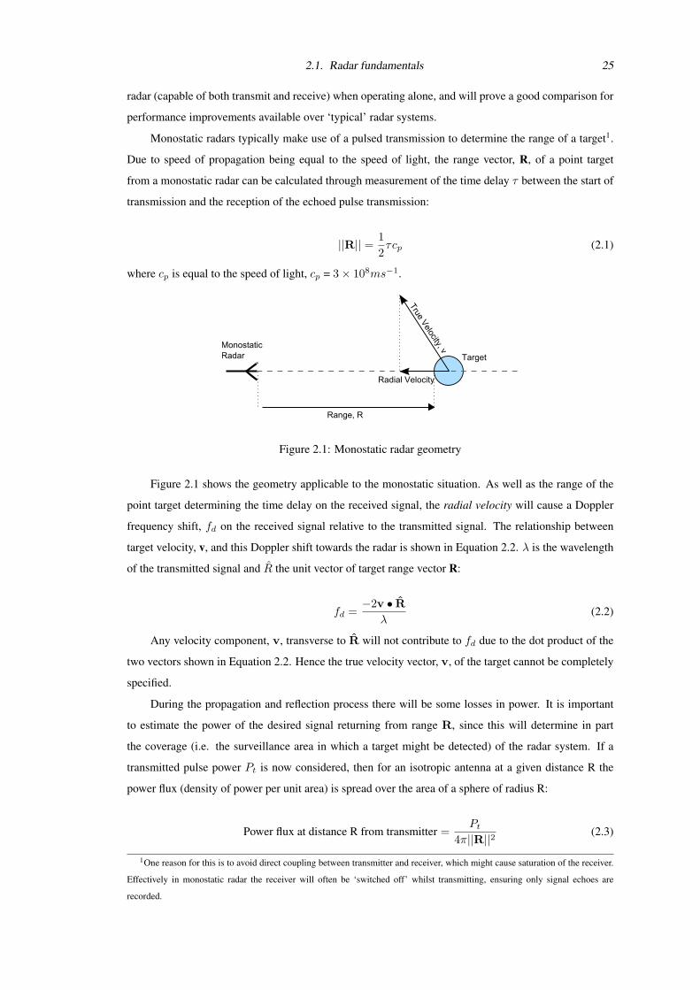
2.1. Radar fundamentals 25
radar (capable of both transmit and receive) when operating alone, and will prove a good comparison for
performance improvements available over ‘typical’ radar systems.
Monostatic radars typically make use of a pulsed transmission to determine the range of a target1.
Due to speed of propagation being equal to the speed of light, the range vector, R, of a point target
from a monostatic radar can be calculated through measurement of the time delay τ between the start of
transmission and the reception of the echoed pulse transmission:
||R|| = 12τcp (2.1)
where cp is equal to the speed of light, cp = 3× 10⁸ms−1.
Figure 2.1: Monostatic radar geometry
Figure 2.1 shows the geometry applicable to the monostatic situation. As well as the range of the
point target determining the time delay on the received signal, the radial velocity will cause a Doppler
frequency shift, fd on the received signal relative to the transmitted signal. The relationship between
target velocity, v, and this Doppler shift towards the radar is shown in Equation 2.2. λ is the wavelength
of the transmitted signal and R the unit vector of target range vector R:
fd =−2v • R
λ(2.2)
Any velocity component, v, transverse to R will not contribute to fd due to the dot product of the
two vectors shown in Equation 2.2. Hence the true velocity vector, v, of the target cannot be completely
specified.
During the propagation and reflection process there will be some losses in power. It is important
to estimate the power of the desired signal returning from range R, since this will determine in part
the coverage (i.e. the surveillance area in which a target might be detected) of the radar system. If a
transmitted pulse power Pt is now considered, then for an isotropic antenna at a given distance R the
power flux (density of power per unit area) is spread over the area of a sphere of radius R:
Power flux at distance R from transmitter =Pt
4π||R||2(2.3)
1One reason for this is to avoid direct coupling between transmitter and receiver, which might cause saturation of the receiver.
Effectively in monostatic radar the receiver will often be ‘switched off’ whilst transmitting, ensuring only signal echoes are
recorded.
2.1. Radar fundamentals 26
A real radar antenna will have some directionality, with energy being focussed towards a certain
direction, thus increasing the power flux within this ‘beamwidth’. The equation for power flux may be
modified to account for this concentration by inclusion of a transmitter gain term2 Gt. This amount of
power reaches the target and is reflected back towards the radar receiver. The effective area from which
power is re-radiated at the target location is known as the RCS of the target. This RCS will be dependant
on the reflectivity of the target at a given target orientation. The power re-radiated from a target towards
the radar receiver must travel the same distance, ||R||, in the monostatic case and thus the returning
power flux will be spread over a similar sphere of radius ||R||, this time centred on the target. The ‘gain
term’ associated with the directionality of this re-radiation is included in the RCS, ω, thus the power flux
at the radar receive antenna is:
Power flux at receive antenna =PtGtσ
(4π||R||2)2 (2.4)
The amount of power intercepted, which then enters the receiver chain is determined by the effective
antenna area Ae. This effective area can be calculated if the receiver gain Gr and the carrier wavelength
λ are known:
Ae =Grλ
2
4π(2.5)
Thus the power of the returning pulse, Pr, can be calculated through the product of Equations 2.4
and 2.5. The ratio of Pr to inherent noise power N (which will be present at any radar receiver) can
be quantified - the Signal to Noise Ratio (SNR). N is generally assumed to be white Gaussian thermal
noise. A system loss factor, Ls, is included to collectively account for losses which might typically cause
deviation from the theoretical SNR, such as receiver noise figure or cable losses.
SNR =PrN
=PtGtGrσλ
2Ls(4π)3||R||4N
(2.6)
This is a standard form of the Radar Equation which is central to radar detection theory. SNR plays
a large part in determining the reliability and ease of detection of target echoes, as well as influencing
further higher-level functions such as parameter estimation. An increase in noise relative to the received
signal power will decrease the probability of detection and accuracy of parameter estimation. As well as
receiver noise, there may be ‘clutter’ consisting of the unwanted echoes from the surroundings - typically
arising from the landscape, buildings, trees and other sources. Of course what might be considered clutter
in one surveillance situation may be a target of interest in another. Similarly to noise, the presence of
clutter may make detection and parameter estimation of targets rather more problematic - for this reason
occasionally a Signal to Clutter Ratio (SCR) may be more appropriate if there is no way to differentiate
a large clutter component from targets. A simplified overview of the detection process can be seen in
Figure 2.2.
2Technically this gain term will be dependant on the unit vectors relating to range and antenna orientation. However the gain is
represented here in the common convention of a scalar quantity equal to the maximum antenna main-lobe gain
2.1. Radar fundamentals 27
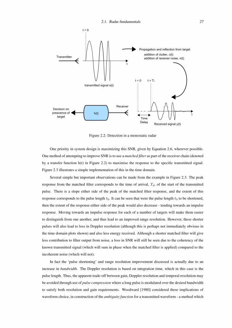
Figure 2.2: Detection in a monostatic radar
One priority in system design is maximizing this SNR, given by Equation 2.6, wherever possible.
One method of attempting to improve SNR is to use a matched filter as part of the receiver chain (denoted
by a transfer function h(t) in Figure 2.2) to maximise the response to the specific transmitted signal.
Figure 2.3 illustrates a simple implementation of this in the time domain.
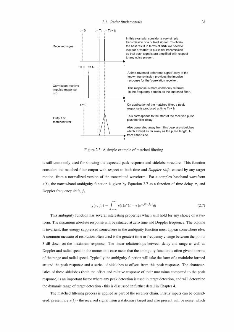
Several simple but important observations can be made from the example in Figure 2.3. The peak
response from the matched filter corresponds to the time of arrival, Td, of the start of the transmitted
pulse. There is a slope either side of the peak of the matched filter response, and the extent of this
response corresponds to the pulse length t0. It can be seen that were the pulse length t0 to be shortened,
then the extent of the response either side of the peak would also decrease - tending towards an impulse
response. Moving towards an impulse response for each of a number of targets will make them easier
to distinguish from one another, and thus lead to an improved range resolution. However, these shorter
pulses will also lead to loss in Doppler resolution (although this is perhaps not immediately obvious in
the time domain plots shown) and also less energy received. Although a shorter matched filter will give
less contribution to filter output from noise, a loss in SNR will still be seen due to the coherency of the
known transmitted signal (which will sum in phase when the matched filter is applied) compared to the
incoherent noise (which will not).
In fact the ‘pulse shortening’ and range resolution improvement discussed is actually due to an
increase in bandwidth. The Doppler resolution is based on integration time, which in this case is the
pulse length. Thus, the apparent trade-off between gain, Doppler resolution and temporal resolution may
be avoided through use of pulse compression where a long pulse is modulated over the desired bandwidth
to satisfy both resolution and gain requirements. Woodward [1980] considered these implications of
waveform choice, in construction of the ambiguity function for a transmitted waveform - a method which
2.1. Radar fundamentals 28
Figure 2.3: A simple example of matched filtering
is still commonly used for showing the expected peak response and sidelobe structure. This function
considers the matched filter output with respect to both time and Doppler shift, caused by any target
motion, from a normalized version of the transmitted waveform. For a complex baseband waveform
s(t), the narrowband ambiguity function is given by Equation 2.7 as a function of time delay, τ , and
Doppler frequency shift, fd.
χ(τ, fd) =∫ ∞−∞
s(t)s∗(t− τ)e−j2πfdtdt (2.7)
This ambiguity function has several interesting properties which will hold for any choice of wave-
form. The maximum absolute response will be situated at zero time and Doppler frequency. The volume
is invariant; thus energy suppressed somewhere in the ambiguity function must appear somewhere else.
A common measure of resolution often used is the greatest time or frequency change between the points
3 dB down on the maximum response. The linear relationships between delay and range as well as
Doppler and radial speed in the monostatic case mean that the ambiguity function is often given in terms
of the range and radial speed. Typically the ambiguity function will take the form of a mainlobe formed
around the peak response and a series of sidelobes at offsets from this peak response. The character-
istics of these sidelobes (both the offset and relative response of their maxmima compared to the peak
response) is an important factor where any peak detection is used in target detection, and will determine
the dynamic range of target detection - this is discussed in further detail in Chapter 4.
The matched filtering process is applied as part of the receiver chain. Firstly inputs can be consid-
ered; present are s(t) - the received signal from a stationary target and also present will be noise, which
2.1. Radar fundamentals 29
can be described in terms of N0/2 - the average two sided spectral noise density. The received signal
energy, E, can be calculated:
E =∫ ∞−∞|s(t)|2dt =
12π
∫ ∞−∞|S(ω)|2dω (2.8)
The maximum possible SNR at the output is equal to the ratio of the received signal energy and
received noise per unit bandwidth. Since this upper limit can be described in terms of E and N0, let us
now look at the output y(t) when the received signal passes through a filter with an impulse response
h(t) and a corresponding frequency response H(ω), thus:
y(t) =1
2π
∫ ∞−∞
S(ω)H(ω)ejωtdω (2.9)
The average noise power, N , at the output of the filter can also be shown:
N =N0
4π
∫ ∞−∞|H(ω)|2dω (2.10)
The peak SNR 3 obtained at the filter output at time t0 can be calculated, corresponding to the time
of maximum response to a signal input, as follows:
SNRpeak =|y(t0)|2
N=|∫∞−∞ S(ω)H(ω)ejωt0dω|2
πN0
∫∞−∞ |H(ω)|2dω
(2.11)
If the problem faced now is to maximise this value of SNR through the design of H(ω) then the
Cauchy-Schwartz inequality can be used [Skolnik, 1980]. This specifies that for any two complex func-
tions, X(ω) and Y (ω), of finite energy the following bound applies:
∫ ∞−∞
X∗(ω)X(ω)dω ≥
∣∣∣∫∞−∞X∗(ω)Y (ω)dω∣∣∣2∫∞
−∞ Y ∗(ω)Y (ω)dω(2.12)
Applying the substitutions X∗(ω) = S(ω)ejωt0 and Y (ω) = H(ω) to this inequality, produces a
new inequality which defines the maximum value of SNR in Equation 2.11:
∫∞−∞ |S(ω)|2dω
πN0≥|∫∞−∞ S(ω)H(ω)ejωt0dω|2
πN0
∫∞−∞ |H(ω)|2dω
(2.13)
Now substituting in Equation 2.8 and rearranging, it can be seen from Equation 2.14 that the maxi-
mum value of peak SNR depends only on the energy of the received signal and the noise power per unit
bandwidth, thus:
2EN0≥|∫∞−∞ S(ω)H(ω)ejωt0dω|2
πN0
∫∞−∞ |H(ω)|2dω
(2.14)
3Note that this now refers to the peak instantaneous power of a received signal divided by the average noise power, whereas in
earlier discussion of the radar equation the average power over the duration of a pulse is referred to.
2.1. Radar fundamentals 30
Since the equality of Equation 2.12 applies when X(ω) is some scalar multiple of Y (ω), it can be
seen that the frequency response which will produce the maximal SNR will be:
H(ω) = AS∗(ω)e−jωt0 (2.15)
where A is a constant and t0 is the time delay through the filter. This corresponds to the following
impulse response in the time domain:
h(t) = A2s∗(t0 − t) (2.16)
whereA2 is a further constant. These constant terms can in fact be removed, since they will provide
equal gain to both signal and noise entering the filter, and so will not in fact improve SNR. Hence, the
output of the matched filter which maximises can finally be given through the convolution of the input
signal, x(t), with the impulse response, h(t). This matched filter output, y(t), to a receiver input x(t)
can be shown:
y(t) =∫ ∞−∞
x(τ)s∗(τ + t0 − t)dτ (2.17)
The transmitted signal in the case of the NetRad as well as many other radar systems is narrowband,
with a carrier frequency ωc which is several orders of magnitude greater than the signal bandwidth. Thus
the signal s(t) and matched filter output will have a phase value dependant upon the difference in phase
between that the received signal and the demodulating carrier frequency. The returning baseband signal
(assuming only the upper sideband is transmitted, as is the case in the NetRad system) for a received
signal returning at a time delay td, as a receiver input x(t) is shown in Equation 2.18.
x(t) = s(t− td)e−jωctd (2.18)
Therefore it can be seen x(t) here and hence y(t) in Equation 2.17 will have an initial phase value
dependant on the time delay td. This is due to the the modulation/demodulation by carrier frequency ωc
within the radar. This phase shift may be matched to, effectively re-phasing the output to that ‘expected’
of td, although in the monostatic case this is generally unnecessary since the magnitude of the matched
filter response remains unchanged.
Of greater interest than this initial phase however is the effect of a moving target on this phase. If
the signal is received at time td in Equation 2.18 but this time experiencing a Doppler shift, given by
angular frequency Ω, due to a moving target. Effectively the value td of Equation 2.18 is varying with
time to produce this modulation due to the e−jωctd term. If it is assumed that the total change in td is
comparable to the wavelength, but much shorter than the inverse of the signal bandwidth, then this may
be represented this as a phase modulation as shown in Equation 2.19.
x(t) = s(t− td)e−jωctdejΩ(t−td) (2.19)
2.1. Radar fundamentals 31
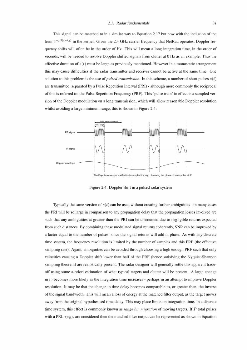
This signal can be matched to in a similar way to Equation 2.17 but now with the inclusion of the
term e−jΩ(t−td) in the kernel. Given the 2.4 GHz carrier frequency that NetRad operates, Doppler fre-
quency shifts will often be in the order of Hz. This will mean a long integration time, in the order of
seconds, will be needed to resolve Doppler shifted signals from clutter at 0 Hz as an example. Thus the
effective duration of s(t) must be large as previously mentioned. However in a monostatic arrangement
this may cause difficulties if the radar transmitter and receiver cannot be active at the same time. One
solution to this problem is the use of pulsed transmission. In this scheme, a number of short pulses s(t)
are transmitted, separated by a Pulse Repetition Interval (PRI) - although more commonly the reciprocal
of this is referred to; the Pulse Repetition Frequency (PRF). This ‘pulse train’ in effect is a sampled ver-
sion of the Doppler modulation on a long transmission, which will allow reasonable Doppler resolution
whilst avoiding a large minimum range, this is shown in Figure 2.4:
Figure 2.4: Doppler shift in a pulsed radar system
Typically the same version of s(t) can be used without creating further ambiguities - in many cases
the PRI will be so large in comparison to any propagation delay that the propagation losses involved are
such that any ambiguities at greater than the PRI can be discounted due to negligible returns expected
from such distances. By combining these modulated signal returns coherently, SNR can be improved by
a factor equal to the number of pulses, since the signal returns will add in phase. As with any discrete
time system, the frequency resolution is limited by the number of samples and this PRF (the effective
sampling rate). Again, ambiguities can be avoided through choosing a high enough PRF such that only
velocities causing a Doppler shift lower than half of the PRF (hence satisfying the Nyquist-Shannon
sampling theorem) are realistically present. The radar designer will generally settle this apparent trade-
off using some a-priori estimation of what typical targets and clutter will be present. A large change
in td becomes more likely as the integration time increases - perhaps in an attempt to improve Doppler
resolution. It may be that the change in time delay becomes comparable to, or greater than, the inverse
of the signal bandwidth. This will mean a loss of energy at the matched filter output, as the target moves
away from the original hypothesised time delay. This may place limits on integration time. In a discrete
time system, this effect is commonly known as range bin migration of moving targets. If P total pulses
with a PRI, τPRI , are considered then the matched filter output can be represented as shown in Equation
2.1. Radar fundamentals 32
2.20, where xp(t) is now the received signal for pulse p.
y(t,Ω) =P∑p=1
e−jΩ(p−1)τP RI
∫ T/2
−T/2xp(τ)s∗(τ + t0 − t)dτ (2.20)
Clearly the summing and phase shift for any fixed time delay, t, is a Discrete Fourier Transform
(DFT) across the array of pulses. This will give a maximum unambiguous Doppler shift of ±1/2τPRI ,
and a resolution equal to 1/PτPRI .
Woodward and Davies [1950] showed that for a large SNR, the Probability Distribution Function
(PDF) of the measured delay is approximately Gaussian around the true delay, with a standard deviation:
δτ =1
2πσω√SNR
(2.21)
where σω is the effective bandwidth of the received signal. Similarly, Manasse [1960] showed
that the minimum Root Mean Squared (RMS) error in angular frequency measurement, where T is the
effective integration time, is:
δω =1
2πT√SNR
(2.22)
The frequency resolution, as well as the accuracy, will be determined by the effective integration
time. In a real system recording of received signals may only take place for a fixed amount of time,
effectively multiplying in the time domain by a square window. This process, again with the narrowband
transmission assumptions, is equivalent to convolution in the frequency domain by sinc(1/T ), where T
is the length of the window. Effectively this convolution process will produce sidelobes at neighbouring
frequencies, and thus will determine the Doppler frequency resolution.
So far accuracy and resolution for down-range measurements only has been discussed. However it
is desirable for a radar operator to have information on a target in two or three dimensions. To this end,
in monostatic radars this extra information will come from the knowledge of the antenna orientation. If
a radar antenna sweeps over an area containing a target, then a peak response will be obtained when the
target is in the centre of the antenna main lobe. Around this peak response will be sidelobes correspond-
ing to the antenna beam pattern. Parallels can be drawn to the matched filter output varying with time
delay in this, and indeed Kingsley and Quegan [1992] detail the angular accuracy to be limited by an
RMS error, similarly related to the inverse of SNR:
δθ =θB√SNR
(2.23)
where θB is the effective beamwidth of the antenna in radians. The effective beamwidth is central
to the concept of ‘cross-range’ monostatic radar resolution in a similar way as effective bandwidth was
in the ‘down-range’ sense. Angular resolution can similarly be determined from antenna beam pattern.
In a monostatic radar the two-way beam pattern must be accounted for, since antenna gain will apply on
both transmit and receive, as seen in the earlier radar equation. Figure 2.5 depicts an example of how a
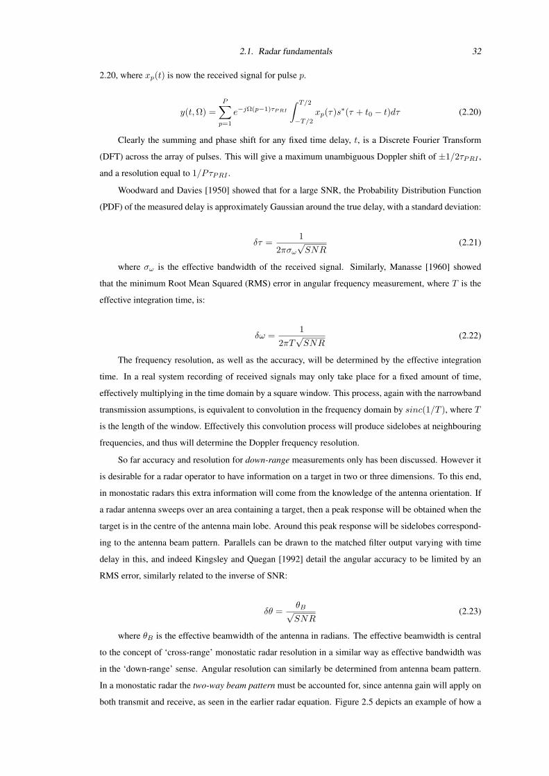
2.1. Radar fundamentals 33
‘resolution cell’ for a monostatic radar might be constructed over a two-dimensional area where targets
must have separation of a cell or greater (i.e. they cannot be in the same cell) to be resolvable.
Figure 2.5: Monostatic resolution cell area
The quantities4DR and4CR are determined by c/2σω and θBR. The definition of this resolution
cell in itself is a simplification, and the values σω and θB assumptions. Conventionally (and most simply)
these effective values are taken to be the those of either frequency or angle which are 3dB down on the
peak value. In a real situation, where targets can have highly variable returns, both angular, temporal and
Doppler resolution is less clear. Factors such as antenna and ambiguity function sidelobes will always
provide some ambiguity outside of assumed effective resolution cells. Such effects must be considered
carefully against the knowledge of the antenna and waveform characteristics by the radar designer. There
are a variety of ‘super resolution’ techniques such as use of CLEAN [Deng, 2004b] or MUSIC [Schmidt,
1986] algorithms which given certain assumptions can improve the ability to resolve targets, although
these will make some a-priori assumptions about targets to be resolved. However this cell area serves as
a useful benchmark for comparing monostatic radar to bistatic and multistatic cases. This area for the
shaded region in Figure 2.5 can be calculated using Equation 2.24.
Amonostatic =θBcR
2σω(2.24)
Evidently the methods discussed must be adapted so as to be usable as a discrete time system
- given that NetRad, in common with many others, digitises the received signal before any matched
filter is applied. So long as the discrete sampling frequency of the digitiser is at least twice that of
the maximum frequency component of the received signal the Nyquist-Shannon sampling theorem is
satisfied. Given this, the continuous time signal can be reconstructed exactly at any stage - similarly
filters can be applied digitally with no loss of information. Implicitly a sampled matched filter output
will mean that the true delay of any returns will generally fall somewhere between the discrete range
bins. The principle of band-limited interpolation allows re-sampling of the matched filter output and
thus improve the accuracy of the parameter estimation. This involves an increase in the amount of
processing, thus it is a case of balancing accuracy of parameter estimation against the processing budget
available for the task. If parameter estimation need not be particularly accurate for example, the nearest
(peak) range bin response might simply be picked to represent the target distance.
At the start of the receiver chain Johnson noise (often referred to as thermal noise) caused by the
2.1. Radar fundamentals 34
thermal agitation of electrons inside any electrical conductor will always be present. The mean noise
power at the input to a receiver with bandwidth B (in Hz) can be described:
N0 = kT0B (2.25)
where k is the Boltzmann constant 1.38 × 10⁻²³WsK−1 and T0 is the temperature of the system
in Kelvin. Of course the gain of the receiver must also be accounted for (this is often assumed to be
a flat value within the receiver bandwidth - where any deviation can be compensated for during post
processing using digital filter techniques) and the response of the matched filter. This is simply a case
of substituting in the mean noise power into Equation 2.10 and applying the receiver gain term GR will
provide the expected noise power output, σ2.
Nout = GRFnkT0B
4π
∫ ∞−∞|H(ω)|2dω (2.26)
Equation 2.26 can be seen to have a further term however, Fn. This noise figure is to account for
the fact that a real receiver chain will produce a noise output slightly greater than the ideal receiver.
This increase in noise will typically be from further thermal contributions within active components, and
obviously it is preferable that the noise figure be as low as possible.
The probability distributions of both noise alone and signal in the presence of noise can be con-
structed. A common assumption is that thermal noise can be well represented as a zero-mean Gaussian
distribution, through the application of the central limit theorem due to the noise being the composition
of many independent components. Since over bandwidth, B, the receiver chain is effectively a linear
filter, the well known result that both real and complex outputs will also have a zero mean Gaussian
distribution can be used. The output of the receiver in Equation 2.20 will be complex. In monostatic
detection, however, there is little point in using this phase information when applying a threshold, so
the absolute envelope detected value is taken, which alters the distribution. The specific distribution for
signal in the presence of noise is a Ricean distribution, shown in Equation 2.27 for absolute matched
filter output value y:
psn(y) =y
Noute−(y2+V 2)/2NoutI0(
yV
Nout) (2.27)
where V is the peak instantaneous absolute matched filter response to the received signal, and I0 is
the zero-order modified Bessel function of the first kind, given as:
I0(z) =1
2π
∫ 2π
0
ezcosθdθ (2.28)
Since for noise alone no V term is expected (since no signal is present), the PDF becomes a Rayleigh
distribution.
pn(y) =y
Noute−y
2/2Nout (2.29)
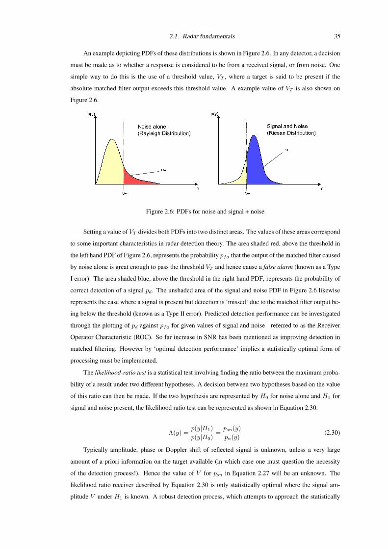
2.1. Radar fundamentals 35
An example depicting PDFs of these distributions is shown in Figure 2.6. In any detector, a decision
must be made as to whether a response is considered to be from a received signal, or from noise. One
simple way to do this is the use of a threshold value, VT , where a target is said to be present if the
absolute matched filter output exceeds this threshold value. A example value of VT is also shown on
Figure 2.6.
Figure 2.6: PDFs for noise and signal + noise
Setting a value of VT divides both PDFs into two distinct areas. The values of these areas correspond
to some important characteristics in radar detection theory. The area shaded red, above the threshold in
the left hand PDF of Figure 2.6, represents the probability pfa that the output of the matched filter caused
by noise alone is great enough to pass the threshold VT and hence cause a false alarm (known as a Type
I error). The area shaded blue, above the threshold in the right hand PDF, represents the probability of
correct detection of a signal pd. The unshaded area of the signal and noise PDF in Figure 2.6 likewise
represents the case where a signal is present but detection is ‘missed’ due to the matched filter output be-
ing below the threshold (known as a Type II error). Predicted detection performance can be investigated
through the plotting of pd against pfa for given values of signal and noise - referred to as the Receiver
Operator Characteristic (ROC). So far increase in SNR has been mentioned as improving detection in
matched filtering. However by ‘optimal detection performance’ implies a statistically optimal form of
processing must be implemented.
The likelihood-ratio test is a statistical test involving finding the ratio between the maximum proba-
bility of a result under two different hypotheses. A decision between two hypotheses based on the value
of this ratio can then be made. If the two hypothesis are represented by H0 for noise alone and H1 for
signal and noise present, the likelihood ratio test can be represented as shown in Equation 2.30.
Λ(y) =p(y|H1)p(y|H0)
=psn(y)pn(y)
(2.30)
Typically amplitude, phase or Doppler shift of reflected signal is unknown, unless a very large
amount of a-priori information on the target available (in which case one must question the necessity
of the detection process!). Hence the value of V for psn in Equation 2.27 will be an unknown. The
likelihood ratio receiver described by Equation 2.30 is only statistically optimal where the signal am-
plitude V under H1 is known. A robust detection process, which attempts to approach the statistically
2.1. Radar fundamentals 36
optimal receiver, is required. One such method employed is the use of the maximum likelihood principle
to construct the generalised likelihood ratio [McDonough and Whalen, 1995], shown in Equation 2.30.
Λ(y) =maxV psn(y|V )
pn(y)(2.31)
Simply stated, this generalised likelihood ratio uses the best available estimate of V from the mea-
surements made by the radar. To investigate how this value is obtained, the natural logarithm of both
sides of psn from Equation 2.27 can be taken, shown in Equation 2.32.
ln(psn(y)) = ln
(y
Nout
)− y2
2Nout− V 2
2Nout+ ln
(I0(
yV
Nout))
(2.32)
Large SNRs4 ( 1) leads to ln(I0(yV/Nout)) approximating to yV/Nout [Skolnik, 1980]. This,
coupled with setting the partial differentiation with respect to V to 0 will give the maximum likelihood
estimate V .
δ
δVln(psn(y)) =
y
Nout− V
Nout= 0 (2.33)
Thus the maximum likelihood estimate V in this case, is in fact simply the matched filter output, y.
Putting this into the generalised likelihood ratio, and comparing to some threshold λ0 produces Equation
2.34.
Λ(y) = e−y2/2NoutI0
(y2
Nout
)> λ0 (2.34)
Again taking the natural logarithms to simplify this ratio, and approximating ln(I0( y2
Nout)) to y2
Nout:
ln(Λ(y)) =y2
2Nout> ln(λ0) (2.35)
With the earlier assumption of a large SNR, that the minimum value that ln(λ0) must be some
constant real positive value. Thus rearranging this inequality for the absolute matched filter output
y alone against some new fixed threshold λ1 will still be statistically optimal in this case. Having
determined the required test that the detector must make, the problem of how the threshold λ1 (which is
effectively the same as VT in Figure 2.6) of the matched filter output is set must be solved. In radar this
is generally accomplished by use of the Neyman-Pearson criterion [Neyman and Pearson, 1933]. The
Neyman-Pearson criterion sets a threshold by considering the two types of errors that can be made in
choosing a hypothesis - in the case of radar detection these are namely the probabilities of false alarm
(Type I error) and missed detection (Type II error). It seeks to minimise one of these errors, given a fixed
value for the other - which is done optimally through use of use of the generalized likelihood ratio test.
Considering the mean noise power discussed previously, Nout, at the output of the matched filter with
known probability distribution given by Equation 2.29. The threshold λ1 is set by solving the integral
shown below for the desired value of pfa as shown in Equation 2.36.
4A common figure of SNR requirement for reliable detection is 13dB
2.1. Radar fundamentals 37
pfa =∫ ∞λ1
y
Noute−y
2/2Noutdy (2.36)
= e−λ21/2Nout (2.37)
Often a normalised threshold level, λn, will be quoted where λn = λ1
√Nout - in which case the
false alarm probability can be determined as e−λ2n/2. This is the simplest case, assuming thermal noise
alone with a fixed mean power and Rayleigh distribution to be present. Probability of detection can be
determined by taking this same threshold and applying it as the lower integral limit for the Ricean PDF
for signal in the presence of noise discussed previously - using the substitution u = y2/2Nout.
pd =∫ ∞λ2
n/2
exp
(−V 2
2Nout
)e−uI0
(√2
V√Nout
u
)du (2.38)
= e−SNR∫ ∞λ2
n/2
e−uI0
(2u√SNR
)du (2.39)
In a real situation further complications may arise:
• RCS Fluctuations
In a real situation the RCS of a target will be a stochastic variable. This accommodates any
fluctuations present as a target is viewed from various aspect angles, and is considered by Swerling
[1960]. Here a number of models of different target behaviour, and PDFs are constructed to
represent the fluctuations in each case. There is also the practical consideration in selecting these
models as to whether the resulting RCS values selected are correlated from pulse to pulse or scan
to scan. Obviously this introduction of this extra distribution will alter the structure of the signal
in the presence of noise PDF significantly, thus changing the detection characteristics.
Cases 1 and 2 refers to a complex target made up of multiple independent scatterers of approxi-
mately equal area. The distribution of RCS for such these cases are shown in Equation 2.40. The
difference between these two cases is the rate of variation of fluctuations; where in case 1 the target
RCS is effectively unchanged from pulse to pulse, but fluctuates from scan to scan and in case 2
the target fluctuates from both pulse to pulse and scan to scan.
pσ(σ) =1σav
exp
(− σ
σav
)σ ≥ 0 (2.40)
The ‘signal and noise’ PDF will thus alter so that the probability of detection can now be expressed
as shown in Equation 2.41.
pd = exp
(−λ2
n
2(1 + 2SNRmean)
)(2.41)
Cases 3 and 4 refers to a complex target made up of multiple independent scatterers, but now
containing a dominant reflective surface. The distribution for this case is represented as shown in
2.1. Radar fundamentals 38
Equation 2.42. Again the difference between these two cases is the rate of variation of fluctuations;
where in case 3 the target RCS is effectively unchanged from pulse to pulse, but fluctuates from
scan to scan and in case 4 the target fluctuates from both pulse to pulse and scan to scan.
pσ(σ) =4σσ2av
exp
(− 2σσav
)σ ≥ 0 (2.42)
The ‘signal and noise’ PDF will again alter, and the probability of detection for cases 3 and 4 are
shown in Equation 2.43.
pd =(
11 + 1/SNRmean
)(1 +
λ2n
2(1 + SNRmean)+
1SNRmean
)exp
(−λ2
n
2(1 + 2SNRmean)
)(2.43)
These expressions refer to the single pulse case. Swerling [1960] detailed further expressions for
the probability of detection for averages of multiple pulses - where the rate of variation would have
an effect. The case of a constant RCS is often referred to as Swerling case 0 or case 5.
• Coloured Noise
Detection may take place in the presence of coloured noise. Often the assumption of white noise
(independent of frequency) is used, as above, due to the simplicity which this presents in terms of
modelling the noise process. It is well known that in terms of maximisation of SNR, the matched
filter may be combined with a whitening filter.
• Clutter
In Equation 2.36 the probability of false alarm for a given threshold is calculated using a known
mean noise power and a known distribution. As mentioned previously, radar often operates in the
presence of clutter, a term used to describe the ‘undesired’ reflections. Clutter may be attenuated
through Doppler filtering, Moving Target Indicator (MTI) methods or more complex techniques
such as Space Time Adaptive Processing (STAP), although each of these methods may also have
implications on target detection if incapable of resolving targets from this clutter. Where the detec-
tion of clutter causes a false alarm, then this contribution must be accounted for when constructing
the probability distribution of Equation 2.36. Obviously this will have implications when choosing
a constant false alarm rate for thresholding. Clutter will not be quite as simple to represent - vary-
ing over the surveyed geometry (such as large discrete scatterers in urban clutter) or perhaps being
non-stationary (either movement of clutter itself, or movement of the radar). For certain types of
clutter attempts have been made to provide useful clutter models; for example [Ward et al., 1990]
uses a K-distribution to represent the returns of sea clutter. Due to the potential for change of this
clutter in each resolution cell, assessing the predicted returns may become an adaptive process
over time. The term adaptive in this sense refers to a process that self-adjusts, constantly looking
for an up-to-date estimate of clutter present in each cell based on data available. It follows that
estimating the false alarm distribution, and setting a threshold are also adaptive processes - which

2.1. Radar fundamentals 39
is commonly known as Constant False Alarm Rate (CFAR) detection. An important issue to con-
sider is how these up-to-date clutter estimates are obtained. Methods such as cell-averaging are
commonly used to avoid including target returns in clutter estimates.
As mentioned previously, coherent pulse integration of P pulses increases SNR. The NetRad sys-
tem is capable of both coherent and incoherent pulse integration for each monostatic node, due to use
of the same local oscillator for transmit and receive. This makes the assumption that the noise for each
pulse is zero-mean complex Gaussian distributed, independent from pulse to pulse. In Kingsley and
Quegan [1992] this process is considered in terms PDFs for noise alone and signal + noise (for a non-
fluctuating target). For both a single pulse and for a coherent average of P pulses, the mean values
of these distributions remain unchanged (as the signal amplitude adds coherently). However it is well
known that the average value of N zero-mean Gaussian random variables is also zero-mean Gaussian,
only with variance reduced by a factor of P . Thus the distributions of noise and signal + noise become
more ‘sharply peaked’. Since the mean noise power is given by the variance of the the noise PDF, and
the signal amplitude remains unchanged, the coherent pulse integration provide an SNR gain equal to the
number of pulses integrated. Levanon [1988] further explores the case of non-coherent pulse integration,
where the removal of phase information by envelope detection takes place prior to pulse integration. This
is done for a square-law detector, rather than the linear detector considered in Equation 2.27 earlier - due
to a simplification in the analysis, although it is stated that there is ‘very little difference in integration
performance’ between the two. The method of assessing the ‘effective’ SNR gains is a little more com-
plex following the move away from Gaussian distributions, and the resulting incoherent sum is given
in terms of a convolution of ‘individual pulse’ PDFs. This is simplified by working in the frequency
domain, leading to a PDF to represent the incoherent (square-law) summation of P pulses. Levanon
states a convenient approximation to improvement in detection performance; that for a large number of
summed square-law pulses P , the required single-pulse SNR, for the same detection performance, is
reduced by a factor of√P .
Unfortunately thermal noise is not the only unavoidable noise source in a radar system. In any
radar system there will generally be several oscillators, whether it is sampling purposes or for carrier-
wave generation for a narrowband system. Ideally this would be a perfect periodic signal, however due to
jitter caused by inevitable small imperfections in any electronic component, real oscillator outputs cannot
achieve this. The sources of this imperfection are grouped into the term ‘phase noise’ as these effectively
cause phase fluctuations away from that of a perfect oscillator. Obviously these deviations of phase in
the time domain will, in the frequency domain, appear as sidebands around any carrier frequency and are
often characterised through recording the power density relative to the carrier (in units of dBc/Hz), to
demonstrate short term stability for an oscillator. Long term frequency stability is typically given as an
Allan variance; the RMS differences between successive readings of frequency deviation, sampled over
a given period. Phase noise and frequency characteristics will be discussed further in Chapter 5.
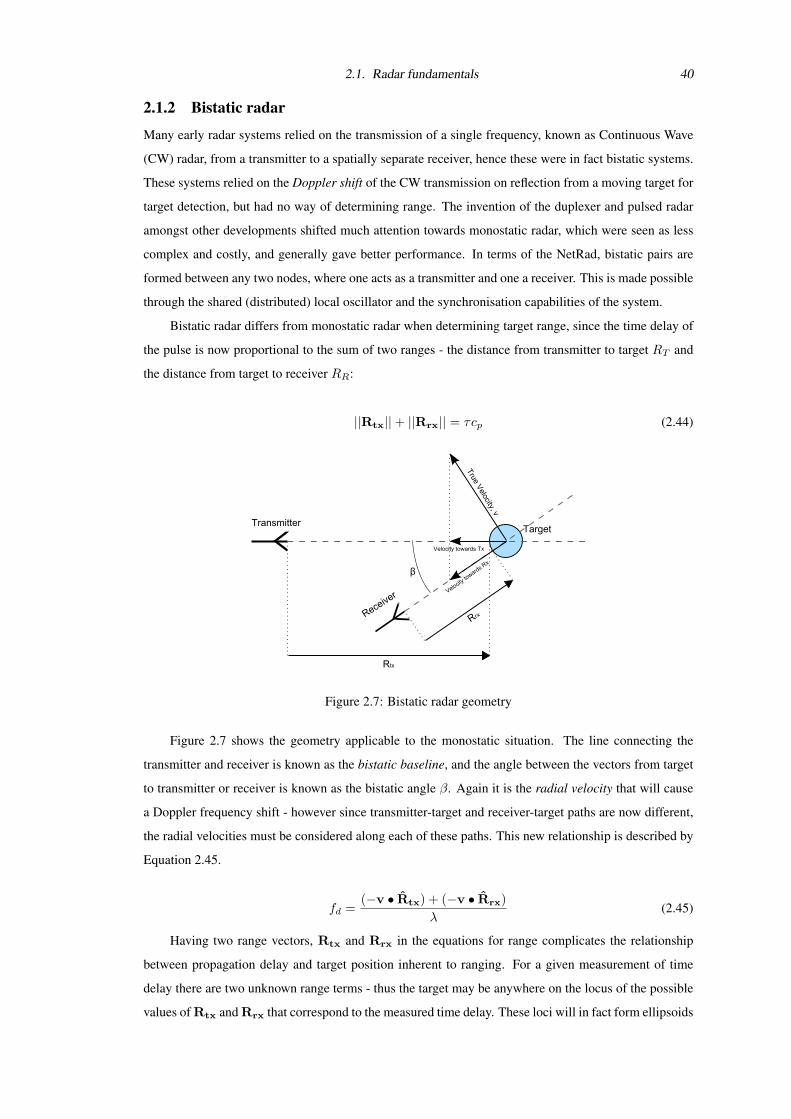
2.1. Radar fundamentals 40
2.1.2 Bistatic radar
Many early radar systems relied on the transmission of a single frequency, known as Continuous Wave
(CW) radar, from a transmitter to a spatially separate receiver, hence these were in fact bistatic systems.
These systems relied on the Doppler shift of the CW transmission on reflection from a moving target for
target detection, but had no way of determining range. The invention of the duplexer and pulsed radar
amongst other developments shifted much attention towards monostatic radar, which were seen as less
complex and costly, and generally gave better performance. In terms of the NetRad, bistatic pairs are
formed between any two nodes, where one acts as a transmitter and one a receiver. This is made possible
through the shared (distributed) local oscillator and the synchronisation capabilities of the system.
Bistatic radar differs from monostatic radar when determining target range, since the time delay of
the pulse is now proportional to the sum of two ranges - the distance from transmitter to target RT and
the distance from target to receiver RR:
||Rtx||+ ||Rrx|| = τcp (2.44)
Figure 2.7: Bistatic radar geometry
Figure 2.7 shows the geometry applicable to the monostatic situation. The line connecting the
transmitter and receiver is known as the bistatic baseline, and the angle between the vectors from target
to transmitter or receiver is known as the bistatic angle β. Again it is the radial velocity that will cause
a Doppler frequency shift - however since transmitter-target and receiver-target paths are now different,
the radial velocities must be considered along each of these paths. This new relationship is described by
Equation 2.45.
fd =(−v • Rtx) + (−v • Rrx)
λ(2.45)
Having two range vectors, Rtx and Rrx in the equations for range complicates the relationship
between propagation delay and target position inherent to ranging. For a given measurement of time
delay there are two unknown range terms - thus the target may be anywhere on the locus of the possible
values of Rtx and Rrx that correspond to the measured time delay. These loci will in fact form ellipsoids
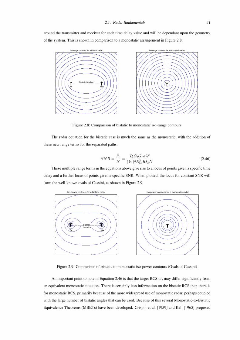
2.1. Radar fundamentals 41
around the transmitter and receiver for each time delay value and will be dependant upon the geometry
of the system. This is shown in comparison to a monostatic arrangement in Figure 2.8.
Figure 2.8: Comparison of bistatic to monostatic iso-range contours
The radar equation for the bistatic case is much the same as the monostatic, with the addition of
these new range terms for the separated paths:
SNR =PrN
=PtGtGrσλ
2
(4π)3R2txR
2rxN
(2.46)
These multiple range terms in the equations above give rise to a locus of points given a specific time
delay and a further locus of points given a specific SNR. When plotted, the locus for constant SNR will
form the well-known ovals of Cassini, as shown in Figure 2.9.
Figure 2.9: Comparison of bistatic to monostatic iso-power contours (Ovals of Cassini)
An important point to note in Equation 2.46 is that the target RCS, σ, may differ significantly from
an equivalent monostatic situation. There is certainly less information on the bistatic RCS than there is
for monostatic RCS, primarily because of the more widespread use of monostatic radar, perhaps coupled
with the large number of bistatic angles that can be used. Because of this several Monostatic-to-Bistatic
Equivalence Theorems (MBETs) have been developed. Crispin et al. [1959] and Kell [1965] proposed
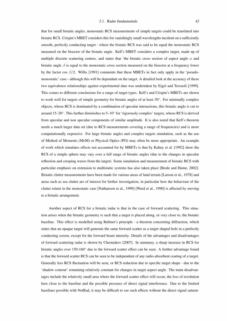
2.1. Radar fundamentals 42
that for small bistatic angles, monostatic RCS measurements of simple targets could be translated into
bistatic RCS. Crispin’s MBET considers this for vanishingly small wavelengths incident on a sufficiently
smooth, perfectly conducting target - where the bistatic RCS was said to be equal the monostatic RCS
measured on the bisector of the bistatic angle. Kell’s MBET considers a complex target, made up of
multiple discrete scattering centres, and states that ‘the bistatic cross section of aspect angle α and
bistatic angle β is equal to the monostatic cross section measured on the bisector at a frequency lower
by the factor cos β/2. Willis [1991] comments that these MBETs in fact only apply in the ‘pseudo-
monostatic’ case - although this will be dependant on the target. A detailed look at the accuracy of these
two equivalence relationships against experimental data was undertaken by Eigel and Terzuoli [1999].
This comes to different conclusions for a range of target types. Kell’s and Crispin’s MBETs are shown
to work well for targets of simple geometry for bistatic angles of at least 30. For minimally complex
objects, whose RCS is dominated by a combination of specular interactions, this bistatic angle is cut to
around 15–20. This further diminishes to 5–10 for ‘rigorously complex’ targets, whose RCS is derived
from specular and non specular components of similar amplitude. It is also noted that Kell’s theorem
needs a much larger data set (due to RCS measurements covering a range of frequencies) and is more
computationally expensive. For large bistatic angles and complex targets simulation, such as the use
of Method of Moments (MoM) or Physical Optics (PO) may often be more appropriate. An example
of work which simulates effects not accounted for by MBETs is that by Kahny et al. [1992] show the
RCS of a simple sphere may vary over a full range of bistatic angles (due to the changes in specular
reflection and creeping waves from the target). Some simulation and measurement of bistatic RCS with
particular emphasis on extension to multistatic systems has also taken place [Beale and Hume, 2002].
Bistatic clutter measurements have been made for various areas of land terrain [Larson et al., 1978] and
areas such as sea clutter are of interest for further investigation, in particular how the behaviour of the
clutter return in the monostatic case [Nathanson et al., 1999] [Ward et al., 1990] is affected by moving
to a bistatic arrangement.
Another aspect of RCS for a bistatic radar is that in the case of forward scattering. This situa-
tion arises when the bistatic geometry is such that a target is placed along, or very close to, the bistatic
baseline. This effect is modelled using Babinet’s principle - a theorem concerning diffraction, which
states that an opaque target will generate the same forward scatter as a target shaped hole in a perfectly
conducting screen, except for the forward beam intensity. Details of the advantages and disadvantages
of forward scattering radar is shown by Cherniakov [2007]. In summary, a sharp increase in RCS for
bistatic angles over 150-160 due to the forward scatter effect can be seen. A further advantage found
is that the forward scatter RCS can be seen to be independent of any radio-absorbent coating of a target.
Generally less RCS fluctuation will be seen, or RCS reduction due to specific target shape - due to the
‘shadow contour’ remaining relatively constant for changes in target aspect angle. The main disadvan-
tages include the relatively small area where the forward scatter effect will occur, the loss of resolution
here close to the baseline and the possible presence of direct signal interference. Due to the limited
baselines possible with NetRad, it may be difficult to see such effects without the direct signal saturat-
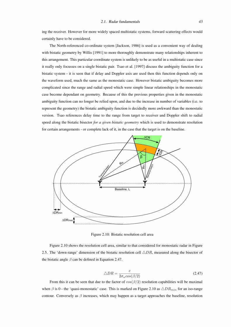
2.1. Radar fundamentals 43
ing the receiver. However for more widely spaced multistatic systems, forward scattering effects would
certainly have to be considered.
The North-referenced co-ordinate system [Jackson, 1986] is used as a convenient way of dealing
with bistatic geometry by Willis [1991] to more thoroughly demonstrate many relationships inherent to
this arrangement. This particular coordinate system is unlikely to be as useful in a multistatic case since
it really only focusses on a single bistatic pair. Tsao et al. [1997] discuss the ambiguity function for a
bistatic system - it is seen that if delay and Doppler axis are used then this function depends only on
the waveform used, much the same as the monostatic case. However bistatic ambiguity becomes more
complicated since the range and radial speed which were simple linear relationships in the monostatic
case become dependant on geometry. Because of this the previous properties given in the monostatic
ambiguity function can no longer be relied upon, and due to the increase in number of variables (i.e. to
represent the geometry) the bistatic ambiguity function is decidedly more awkward than the monostatic
version. Tsao references delay time to the range from target to receiver and Doppler shift to radial
speed along the bistatic bisector for a given bistatic geometry which is used to demonstrate resolution
for certain arrangements - or complete lack of it, in the case that the target is on the baseline.
Figure 2.10: Bistatic resolution cell area
Figure 2.10 shows the resolution cell area, similar to that considered for monostatic radar in Figure
2.5. The ‘down-range’ dimension of the bistatic resolution cell 4DR, measured along the bisector of
the bistatic angle β can be defined in Equation 2.47.
4DR =c
2σωcos(β/2)(2.47)
From this it can be seen that due to the factor of cos(β/2) resolution capabilities will be maximal
when β is 0 - the ‘quasi-monostatic’ case. This is marked on Figure 2.10 as 4DRmin for an iso-range
contour. Conversely as β increases, which may happen as a target approaches the baseline, resolution
2.1. Radar fundamentals 44
is lost to the point when targets on the baseline are unresolvable. In Skolnik [1990] the assumption
is made to reference the (one-way) beamwidth of a single antenna, for construction of a ‘clutter cell’
comparable to that of the monostatic case. It is stated ‘for a given geometry one or the other beam
will usually determine the clutter cell area’. In Figure 2.10 this situation is depicted where the receive
antenna bounds the resolution cell. Thus 4CR can be determined as being equal to the range from
the target to this ‘dominant’ antenna multiplied by the effective beamwidth of this antenna in radians.
Precise expressions for resolution cell area can be seen in Moyer et al. [1989], however a more simple
expression is to approximate area to that of a parallelogram, containing an area as defined by Equation
2.48.
Abistatic =cRrxθBrx
2σωcos2(β/2)(2.48)
Obviously this assumption that a single beam will enclose the cell will not always hold. Notable
cases will be close to the baseline (large β) where more complex hexagonal cells may be formed, or
where the target range becomes much greater than the baseline distance such that the cell approx-
imates to the monostatic case already discussed. Similarly range accuracy will be maximal for the
quasi-monostatic case - decreasing with β to the point where accuracy is completely lost on the bistatic
baseline. Conversely improvements in angular accuracy might be seen for a given Rtx + Rrx since a
target will be closer to a single antenna ‘dominant’ in terms of resolution. It might be noted from the
green-shaded area in Figure 2.10 that unlike the monostatic case, antenna beamwidths are no longer com-
pletely overlapping. This will mean a reduction in coverage area. One method reclaiming this coverage
area for a pulsed radar is known as ‘pulse chasing’. Here the receive beamwidth is selected or steered
such that coverage is maintained over the point on the transmitter beam from which target returns are
predicted to be arriving from, given the timing and geometry information inherent in the system.
The complexities of such a ‘coverage area’ can only be expected to increase in a multistatic system
such as the NetRad if multiple transmitter-receiver pairs are desired to have a common coverage area.
An important issue in bistatic radar is the synchronisation between nodes. The process of measuring
the delay τ in the monostatic case is generally simpler - the exact clock pulse on which transmission
began is known and any received signal can be referenced in time to it by utilizing the same reference
clock. However in the bistatic case this referencing of time is made more difficult due to the spatial
separation of transmitter and receiver - the ‘start of transmission’ is unknown at the receiver and needs
to be communicated for any useful measurements of delay of a reflected signal to be made. A good
summary of modern synchronization techniques is given by Weib [2004] who discusses a variety of
methods including coaxial links, optical fibre links (such as those used in BICOMS [Lane et al., 1999]),
Line Of Sight (LOS) transmission, Global Positioning System (GPS), satellite communications link and
the sort of accuracies typically involved. Since all the relationships between target location/velocity and
delay/Doppler are now also a function of the geometry of the radar system5, arguably just as important
5Of course, this is also strictly true in the monostatic case - only that from the start the specific monostatic geometry, where
transmitter and receiver are co-located, will simplify many relationships somewhat
2.2. Multistatic radar principles 45
as the time synchronisation is the accurate knowledge of the system geometry.
Inherently passive radar, which relies on illuminators of opportunity (such as Frequency
Modulation (FM) radio transmissions), is also a bistatic arrangement - albeit a special case where
there is generally limited control over the transmitter. This sort of system may see benefits from use of
multiple receivers to form a passive multistatic system, however in-depth discussion of the particular
issues involved is beyond the scope of this work.
2.2 Multistatic radar principlesMultistatic radar is often referred to as ‘multisite’ or ‘netted’ radar. Collectively, these operate on the
same principle of multiple, spatially diverse transmitters and/or receivers. These multiple transmitter-
receiver pairs may take the form of either of the two geometries covered in the previous sections, namely
monostatic and bistatic. The appropriate theory will still therefore be relevant for each of these pairs
within a multistatic system. The considerations of bistatic geometry discussed are closer in nature to
the multistatic, since both will always require spatio-temporal synchronisation of some sort between
nodes. Intrinsically the existence of a shared surveillance area between transmitter-receiver pairs in
a multistatic system implies some fusion of information from the transmitter-receiver pairs involved.
This fusion process may range from the simple case of selecting plots from the receiver closest to a
target (ignoring others), increasing in complexity to effectively beamforming through radio signal fusion.
The potential information gain obtained through the spatial diversity of transmitter-receiver pairs in a
multistatic system can give rise to a number of advantages over both the individual monostatic and
bistatic cases in typical radar functions, hence the motivation for the investigation of such systems.
During implementation of such a system, there will need to be consideration of the operation of the
individual monostatic and bistatic elements, the management of the system incorporating them and,
finally, the method by which information is combined to give a useful output to an operator. Multistatic
radar can take many forms, and here two key attributes are identified and used to classify several types
of multistatic system. These two key attributes are the degree of spatial coherence and the information
integration (data fusion) level.
2.2.1 Degree of spatial coherence
Spatial coherence refers to the correlation (fixed phase relationship) between the radiated electric fields
at points in a given spatial region. The nature of this correlation can be use to provide one way of
classifying a multistatic system. More precisely the degree of spatial coherence between transmitter-
receiver pairs within the system is referred to. It is of course possible for pairs to individually have
a high degree of spatial coherence, through use of the same local oscillator and known co-location of
transmitter and receiver, but to be less when compared/combined with other transmitter-receiver pairs in
the system. The degree of spatial coherence of the within the system can be described by the following
definitions:
• Fully-known spatial coherence - in which phases and frequency of transmitted Radio Frequency
(RF) signals, as well as the locations of the antenna phase centres, are fully known and maintained
2.2. Multistatic radar principles 46
so that any received signal can be fully referenced to any transmission across the entire system in
both time of arrival and phase. This sort of knowledge of time and space would be similar to that
needed for phased array beamforming in terms of absolute accuracy.
• Short-term spatial coherence - in which frequency of transmitted RF signals are fully known and
maintained, and relative phase offsets between locations are maintained throughout short term
intervals over which measurements are made across the system. To achieve this a high relative
frequency stability between transmitter-receiver pairs is required - generally achieved by some
sort of broadcast of a ‘reference oscillator’ to all pairs in the multistatic system. This level of
coherency would be a requirement for a bistatic pair to coherently sum and utilize pulsed Doppler
methods.
• Incoherence - where phase information and its changes over time cannot be utilised. This may
be the case where stations nominally operate on the same frequency, but separate oscillators are
used which may, for example, be subject to different frequency drift. Obviously this rules out any
coherent processing methods, and thus phase information is generally removed through envelope
detection.
Obviously to maintain greater spatial coherency nodes must be increasingly co-operative, hence
these systems tend to become more complex and expensive. How data in a multistatic system is fused
will depend on this degree of spatial coherency, but other factors such as the node topology, target lo-
cation, complexity of observed targets and fluctuation of returns will also play a part. Theoretically a
system with fully-known spatial coherence between all transmitter nodes can coherently sum multiple
transmissions at a single point in space, however this would be very difficult in practise due to manage-
ment of the timing. Such an arrangement on receive is inherently easier, since any compensation can be
done in post-processing. A system with fully-known spatial coherence will have full knowledge of the
phase and time of any transmission, as well as the relative antenna phase centre locations. Any error in
these measurements must be significantly lower than the carrier wavelength of any transmissions - so a
shift to higher frequencies will provide an increasing challenge in operating such a system. A phased
array antenna might be thought of as a type of multistatic system fully-known spatial coherence, albeit
one which will always observe the same aspect of a target. Increasing the spatial separation between
elements in this array effectively produces a sparse array, which eventually begin to see different angular
aspects of targets under surveillance. As separation increases, maintaining full coherency generally be-
comes more difficult. A short-term coherent system also has node phase and location knowledge which
is maintained over the period of radar operation. However the degree of uncertainty over the initial
state of the system is now comparable to the spatial or temporal attributes of the carrier wave used. An
incoherent system uses no phase knowledge between nodes.
The initial design of NetRad aimed to be achieving the ‘ultimate’ in spatial coherency - namely
the fully known spatial coherence. The challenges inherent in typical experimental situations will be
discussed in Chapter 5.
2.2. Multistatic radar principles 47
2.2.2 Information integration level
The information integration level of a multistatic radar describes the stage at which data between
transmitter-receiver pairs is combined. This is considered from a detection point of view - since this
either must precede or be performed simultaneously with parameter estimation.
• Radio signal fusion - Again this fits with the comparison to phase arrays, and will generally only be
useful6 where there is fully-known spatial coherence between the collection of transmitter-receiver
pairs involved. This is a centralised processing method including all phase information. The term
‘centralised’ refers to the fact that data fusion takes place prior to any thresholding or decision
making based on information from any individual transmitter-receiver pair. The data is combined
before or after linear filtering (such as application of matched filters) and channel weighting. The
intention of this method of fusion is to make gains in detection through coherent summation,
similar to those described for coherent pulse integration (in terms of signal processing) and hence
a gain in SNR over all individual pairs in the system. Re-phasing of returned signals given the
hypothesised time delay will be required, as will be explained in detail in Chapter 3. This method
of fusion will generally require the greatest amount of bandwidth between nodes for data transfer,
as well as being the most processor-intensive method.
• Video signal fusion - This is a slightly less demanding form of fusion, in that it can be used between
either spatially coherent or incoherent systems. Data is combined in much the same way as radio
signal fusion, but with phase information discarded before the final data fusion process. It is again
a centralised processing method. This method requires a similar bandwidth for data transfer - but
has potential for reduced processing requirements when compared to radio signal fusion as there
is no longer a need to consider the spatial interference patterns (and methods such as re-phasing)
inherent in radio signal fusion. This method of fusion looks to make gains in detection through
incoherent summation, in a similar way to that described for non-coherent pulse integration.
• Plot fusion - Plot fusion is a decentralised process - where individual detections, including
thresholding/decision-making takes place for each transmitter-receiver pair. These individual de-
cisions are then fused to lead to a final ‘system’ decision. Due to the ‘abandonment of information’
inherent in thresholding, fusing data in this way has a greatly reduced bandwidth requirement for
data transfer and multistatic processing.
The choice of information integration level will be influenced by the degree of spatial coherence of
the radar system itself and the desired application. However other factors will contribute to determining
the most appropriate level. Fully-known spatial coherence of the system itself is the ‘ultimate’ in spatio-
temporal synchronisation. This alone does not mean that it should be expected to achieve coherent
summation of signals received from a target. An example of this being if attempts are made to use
radio signal fusion when observing a complex, unknown target. Such a target will if observed from
6It is difficult to see the use of random interference caused by summing target returns which have no known correlation between
their phases.
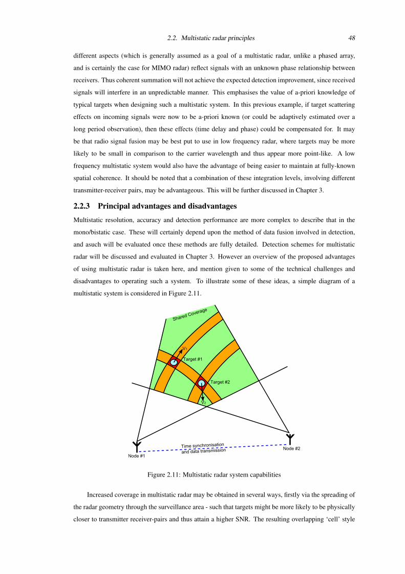
2.2. Multistatic radar principles 48
different aspects (which is generally assumed as a goal of a multistatic radar, unlike a phased array,
and is certainly the case for MIMO radar) reflect signals with an unknown phase relationship between
receivers. Thus coherent summation will not achieve the expected detection improvement, since received
signals will interfere in an unpredictable manner. This emphasises the value of a-priori knowledge of
typical targets when designing such a multistatic system. In this previous example, if target scattering
effects on incoming signals were now to be a-priori known (or could be adaptively estimated over a
long period observation), then these effects (time delay and phase) could be compensated for. It may
be that radio signal fusion may be best put to use in low frequency radar, where targets may be more
likely to be small in comparison to the carrier wavelength and thus appear more point-like. A low
frequency multistatic system would also have the advantage of being easier to maintain at fully-known
spatial coherence. It should be noted that a combination of these integration levels, involving different
transmitter-receiver pairs, may be advantageous. This will be further discussed in Chapter 3.
2.2.3 Principal advantages and disadvantages
Multistatic resolution, accuracy and detection performance are more complex to describe that in the
mono/bistatic case. These will certainly depend upon the method of data fusion involved in detection,
and asuch will be evaluated once these methods are fully detailed. Detection schemes for multistatic
radar will be discussed and evaluated in Chapter 3. However an overview of the proposed advantages
of using multistatic radar is taken here, and mention given to some of the technical challenges and
disadvantages to operating such a system. To illustrate some of these ideas, a simple diagram of a
multistatic system is considered in Figure 2.11.
Figure 2.11: Multistatic radar system capabilities
Increased coverage in multistatic radar may be obtained in several ways, firstly via the spreading of
the radar geometry through the surveillance area - such that targets might be more likely to be physically
closer to transmitter receiver-pairs and thus attain a higher SNR. The resulting overlapping ‘cell’ style
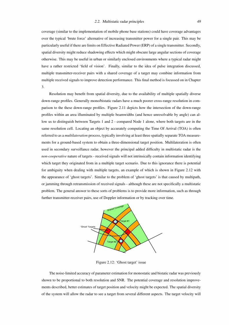
2.2. Multistatic radar principles 49
coverage (similar to the implementation of mobile phone base stations) could have coverage advantages
over the typical ‘brute force’ alternative of increasing transmitter power for a single pair. This may be
particularly useful if there are limits on Effective Radiated Power (ERP) of a single transmitter. Secondly,
spatial diversity might reduce shadowing effects which might obscure large angular sections of coverage
otherwise. This may be useful in urban or similarly enclosed environments where a typical radar might
have a rather restricted ‘field of vision’. Finally, similar to the idea of pulse integration discussed,
multiple transmitter-receiver pairs with a shared coverage of a target may combine information from
multiple received signals to improve detection performance. This final method is focussed on in Chapter
3.
Resolution may benefit from spatial diversity, due to the availability of multiple spatially diverse
down-range profiles. Generally mono/bistatic radars have a much poorer cross-range resolution in com-
parison to the these down-range profiles. Figure 2.11 depicts how the intersection of the down-range
profiles within an area illuminated by multiple beamwidths (and hence unresolvable by angle) can al-
low us to distinguish between Targets 1 and 2 - compared Node 1 alone, where both targets are in the
same resolution cell. Locating an object by accurately computing the Time Of Arrival (TOA) is often
referred to as a multilateration process, typically involving at least three spatially separate TOA measure-
ments for a ground-based system to obtain a three-dimensional target position. Multilateration is often
used in secondary surveillance radar, however the principal added difficulty in multistatic radar is the
non-cooperative nature of targets - received signals will not intrinsically contain information identifying
which target they originated from in a multiple target scenario. Due to this ignorance there is potential
for ambiguity when dealing with multiple targets, an example of which is shown in Figure 2.12 with
the appearance of ‘ghost targets’. Similar to the problem of ‘ghost targets’ is that caused by multipath,
or jamming through retransmission of received signals - although these are not specifically a multistatic
problem. The general answer to these sorts of problems is to provide more information, such as through
further transmitter-receiver pairs, use of Doppler information or by tracking over time.
Figure 2.12: ‘Ghost target’ issue
The noise-limited accuracy of parameter estimation for monostatic and bistatic radar was previously
shown to be proportional to both resolution and SNR. The potential coverage and resolution improve-
ments described, better estimates of target position and velocity might be expected. The spatial diversity
of the system will allow the radar to see a target from several different aspects. The target velocity will
2.3. Multistatic radar literature review 50
contribute to Doppler shift of returned signals along several different unit vectors. Thus the ignorance of
radial target velocity found in the monostatic or bistatic case might be avoided - and with enough spatially
diverse transmitter-receiver pairs the target velocity fully specified as a two or three dimensional vector.
Velocity is only one example of increased information that might be provided to the radar operator on a
target by viewing it from different aspects. Other examples include target RCS, or micro-Doppler effects
and how they change - both of which would be of interest for target identification methods or imaging,
in a similar fashion to ISAR.
The appearance of clutter will also be altered through the spatial diversity of multistatic radar.
An example might be sea clutter, where a larger reflectivity from non-zero Doppler clutter if using a
monostatic radar facing oncoming sea waves can typically be seen. Were the option of using a different
transmitter-receiver in a multistatic system available, then the returns of this clutter could be reduced.
The reduction of such clutter could enable improved target detection.
Increased survivability and ‘graceful degradation’ may result from the distributed nature of the
system. A fault in either transmitter or receiver for a monostatic or bistatic system will lead to a complete
loss of radar functionality. From a tactical point of view, a single large transmitter will be easier to locate
and destroy compared to several distributed transmitters. Likewise, it will be increasingly difficult to
successfully focus jamming on multiple receivers compared to a single site. This is particularly true if
receiver sites are not co-located with transmitter (i.e. bistatic pairs are utilised), since it will be impossible
for jammers to pinpoint receiver locations simply by looking to where transmission originated, as in the
monostatic case.
The use of multiple low cost radars, potentially with COTS components, may lead to cost savings
over construction of single high power, due to economies of scale. Obviously extra expenditure must go
into the communications and management of the system. However many of the components for these
function will not be particularly specific to radar, and may be in widespread use, and so likely to be
comparatively cheap. This is opposed to high power transmitters and antennas typically used in mod-
ern military radar - which may conversely have a fairly narrow market. Many difficulties involved in
operation of a bistatic radar will also apply in a multistatic system. In particular spatio-temporal syn-
chronisation between all nodes will determine the maximum degree of spatial correlation in the system,
as well as contributing to the accuracy of any parameter estimation. Other problems such as the reception
of a direct transmission will also still apply. An increase in information obtained at each receiver neces-
sitates a certain amount of data transmission between nodes (aside from that used to actually control the
system). Linked to this is the amount of signal processing power required, which will be increased also.
Where this processing takes place will depend upon the information integration level.
2.3 Multistatic radar literature review
Having discussed the theory behind multistatic radar, the literature surrounding the area can be explored
with rather less fear of unknown nomenclature. This section surveys the multistatic radar research area
and identifies a number of potential areas for future research.
2.3. Multistatic radar literature review 51
Chernyak [1998] is currently the most detailed source on multistatic radar theory. To give an
overview of the work, the general characteristics of multistatic radar are first defined, and some ad-
vantages/disadvantages of such systems are listed. A brief historical outline of the development of mul-
tistatic radar systems is given - mostly discussing the technical details of various military installations.
Coverage and RCS for monostatic, bistatic and multistatic radars is also mentioned. The second part of
the book is devoted to the problem of target detection - seeking to utilise the likelihood ratio detector to
provide optimal detection algorithms. These are considered in the context of varying available degree
of coherency within a system, for both coherent and incoherent data fusion between transmitter-receiver
pairs with a shared coverage area. Much of these algorithms, and how they might best be adapted and
implemented on a radar system such as the NetRad, will be considered in slightly more detail in Chapter
3. The third and final part of the book explores parameter estimation and tracking in multistatic systems.
This work is very comprehensive, and perhaps the main challenge for those following it would appear to
be in adapting and applying the vast number of optimal algorithms discussed.
Previous work by Derham [2005] was based on the initial construction of the NetRad system. The
aim of this work was the design and calibration of the low-cost fully spatially coherent multistatic radar
system, where a distributed clock was used to lock the phase of each nodes on-board reference oscil-
lators together, with further calibration by direct transmission from transmitter and receivers removing
the uncertainty of any phase offsets between transmitted RF signals at short node separations (no more
than about 12 m). In this work performance bounds for coverage (extrapolated from the radar equation)
for different detection algorithms was investigated. An ambiguity function using Cartesian co-ordinates
was constructed and again investigated for different detection algorithms. Several detection algorithms
are considered, in terms of ‘optimal detectors’ as first constructed by Chernyak, which might be imple-
mented in the NetRad system. Their performance under a variety of effects such as signal fluctuations
was considered. Signal processing techniques such as use of digital fractional delays filters to allow
temporal and phase alignment of signals as required by the detection algorithms were listed. A detailed
analysis of noise sources and oscillator generation in multistatic radar was undertaken. With these in
mind a specification is developed of an achievable phase coherent radar design using COTS compo-
nents. The three node NetRad system and user interface was constructed, for a nominal cost of under
$ 6000. The design was demonstrated to meet a planned specification. Individual monostatic measure-
ments demonstrated the capability of each individual radar node. A monostatic (transmit and receive
antennas were ∼1m apart) clutter survey was undertaken, where a 180 sweep of an area of urban clut-
ter surrounding UCL was taken (in steps of 11.25). The returns were cross-referenced with a map of
the area and many identifiable pieces of clutter with a particularly large RCS could be seen, along with
shadowing effects from these (typically large buildings) as might be expected. Very short range ‘quasi-
monostatic’ measurements were made with a multistatic setup consisting of one transmitter and three
receivers. Here a trihedral corner reflector 7 with a 150 m2 RCS at boresight was set up 18 m away from
three receivers and a single transmitter (which were set up adjacent to each other). The relative phases
7Constructed based on the cubic ‘optimum corner reflector’ discussed in Sarabandi and Chiu [1996]
2.3. Multistatic radar literature review 52
between each local oscillator were recorded (by simple closed loop from transmitter to receiver) for later
phase adjustment of the returned signal. A coherent signal gain of 9.2 dB was achieved from coherent
integration of the three nodes, which was only 0.34 dB less than the expected theoretical increase (so
effectively a complete coherent summation). No signal processing gain was obtained where square-law
(incoherent) detection was used. Sidelobes were noted as being fairly uneven and also fairly variable
between nodes. This could be due to several factors, including detection of other nearby clutter. All
three nodes were spaced by small distances (bistatic baselines range between 5.04 m and 11.64 m) and
attempted to detect the corner reflector, which was placed at a distance of approximately 210 m away
in heavy urban clutter. Again a simple closed loop from each transmitter to receiver was used to com-
pensate for the phase offsets between local oscillators - although due to the node separation this was
obviously a rather longer loop than in the short range tests. The Chernyak-derived detector Lc described
here in Chapter 3, was implemented for this arrangement. However, the results for this experiment are
fairly inconclusive. A coherent signal gain of 10 dB was quoted as being achieved from the coherent
integration of the three nodes, which was 4.3 dB less than expected (compared to a single ‘reference’
bistatic pair). There are no specific details of received signal levels when discussing coherent gains;
whether these had any amount of variation and how the ‘reference’ bistatic pair was determined. The
output of the detector was plotted over a two-dimensional plane. It had poor location resolution due to
low bandwidth utilised by the polyphase codes used. Some ‘eclipsing’ due to sidelobes from the direct
transmission of the 5.6 µs polyphase code and from surrounding clutter returns is blamed for dominat-
ing the target position (no ‘interleave’ of higher resolution chirp signals was available at the time). A
clear point response from the target could not be seen, and an interference pattern is seen across the
two-dimensional plot of detector output for location - although it is not made clear whether a sufficient
‘resolution’ of hypothesised locations is considered. A summary of the work is also presented in the first
half of Derham et al. [2007].
Glaser [1989] gives a review of the history of investigations into bistatic RCS; starting with some
of the earliest developments in the 1930s, moving on to World War 2 and finishing with some more
recent (post 1965) developments. Interestingly, ‘ghost target’ effects are mentioned in ‘Plato’ and ‘Ordir’
bistatic radar schemes arising from sidelobes of one antenna crossing the mainlobe of another, similar
to the effects which can be seen when using multilateration, which will be discussed later. The paper
also discusses the approximation of bistatic RCS of Kell [1965] before looking at alternative rather more
complex simulation methods such as MoM and PO which might be used to model bistatic RCS. The
differences between monostatic and bistatic RCS is of importance in multistatic radar - a simple example
being the often quoted potential ‘anti-stealth’ capabilities of such a system. This can be seen clearly in
a ‘bistatic coherent measurement system’ [Lane et al., 1999] set up by the US Department of Defence
in conjunction with Georgia Tech Research Institute due to concerns of bistatic signatures of military
vehicles. This project, which was scheduled for completion in 1999, was designed to measure monostatic
and bistatic signatures simultaneously using CW with a very large variable frequency range (1-36 GHz).
The system was based around a fixed radar site and a movable radar site, with a system set-up time
2.3. Multistatic radar literature review 53
of under 40 hours. A slightly different approach, concentrating on investigating bistatic clutter rather
than RCS of individual targets, is demonstrated in a DARPA-sponsored measurement program [Larson
et al., 1978] which ran from 1975-76. In these tests two test sites - smooth concrete and grassland
were observed using an airborne transmitter and a receiver on a control tower. These sorts of bistatic
measurements, as well as further environments likely to have different statistical behaviour, such as sea
clutter [Ward et al., 1990], will also be important in multistatic radar. This is because of their relative
sparsity compared to monostatic data, and given the fact that many multistatic systems will contain
bistatic pairs - often in greater number than monostatic pairs.
TechSat21 [Steyskal et al., 2003] is a space-based radar network operating at X band through a
2 m2 electronically steered antenna. It operates over a cluster of 19 satellites, which are solar powered
with on-board propulsion and orientation control systems. It has a relatively low data rate of 160 kbps
for exchange of tracking, telemetry and control data between satellites. Such an arrangement might be
considered to be closer to a ‘sparse array’ rather than a true multistatic radar - due to the relative close-
ness of the satellites (distributed over an 80 m by 40 m area) compared with the distance to any targets.
The system itself is ‘not designed to provide operational capability, but rather to demonstrate technical
feasibility of the concept’ [Winter and Anderson, 2003]. One of the particularly relevant areas of this
demonstration to any multistatic system is the spatio-temporal synchronisation of the satellites. This is
done in several stages, firstly GPS is used to provide position accurate to ±10 cm, timing to ± 20 ns
(absolute timing to Coordinated Universal Time (UTC) is accurate to ±100 ns) as well as disciplining
local oscillators to provide a time precision of ±5 ps over a maximum integration time of 5 s. Kalman
filters maintain the best estimates of this time and position information. Prior to radar transmission, syn-
chronisation pulses between satellites improve position and timing to ±1 cm and ±50 psec respectively.
Using this information, post-processing is capable of aligning phase information to within a wavelength
- thus signal processing techniques involving clutter co-registration can coherently align sensor data to
within 1/20th of a wavelength. The system can therefore be said to be fully spatially coherent. The Infer-
ometric Cartwheel system [Massonnet, 2001] is a further similar concept for a satellite implementation
of a multi-radar. In this case a wider separation between transmitter and receiver is considered. The
ORION system [Robey et al., 2000] is another - a high-risk, low-cost NASA funded project dedicated to
the research of distributed satellite sensing and formation flying. It might be noted for a ground based
system such as NetRad, the sorts of technique may be more difficult due to multipath, line-of-sight and
available bandwidth. However they serve as a good high-end benchmark, and aligning phase information
would obviously become increasingly achievable were transmission frequency to drop.
An experimental demonstration of a distributed array antenna [Attia and Abend, 1991] looks at
using recorded data from multiple spatially distributed elements to focus on one large corner reflector,
then electronically scanning in angle to successfully detect a smaller target, using three coherent X-band
radars separated by a few metres (where the targets were ∼50m away). No mention is specifically given
to the obtained coherent gains or location gains, so this may be difficult to compare with any of the
results of NetRad. Self calibration/cohering of large antenna arrays is further considered by Attia and
2.3. Multistatic radar literature review 54
Steinberg [1989]. Typically calibration is done through observation of a point source, such as a corner
reflector or a beacon - however here an alternative technique is used relying on multiple non-coherent
scatterers, such as sea clutter or moving leaves to phase synchronise the array. Certainly synchronisation
against clutter is a method which could be put into practise using the NetRad - however there is a clear
difference between doing this for arrays where the same set of scattering centres are seen and multistatic
radar where this will generally not be the case.
MIMO radar has recently received considerable attention. This concept stems from communica-
tions and the desire to transmit more information from a multitude of transmit antennas to a multitude of
receive antennas in the same frequency channel. If the signals from each transmitter arrive at the receiver
antenna array with sufficiently different spatial signatures these channels can be separated, thus increas-
ing the information throughput. Obviously such an information gain is desirable for radar (as succinctly
described by Woodward [1980]), and these ‘spatial signatures’ can be thought of as being analogous
to target fluctuations between different multistatic transmitter-receiver pairs. This is perhaps described
more precisely by Fishler et al. [2004a] where it is stated that ‘to achieve spatial diversity it is required
that different transmit antennas see different uncorrelated aspects of a target’. This paper demonstrates
this concept by considering a model containing M transmit elements of an array, N receive elements and
Q scatterers. Each scatterer is assumed to have isotropic reflectivity modelled by a zero-mean, indepen-
dent and identically distributed complex random variable. The aim of any processing is to estimate the
M × N channel matrix. Fishler et al. [2004b] compares closely spaced antennas (phased arrays) to inde-
pendent radars which fuse data incoherently, showing improvements in receiver operator curves above
a certain false alarm probability, and the later work of Fishler et al. [2006] expands on this to provide
optimal detectors for MIMO radars. Robey et al. [2004] shows theoretical and experimental results of
improvements of beam pattern when comparing MIMO to a receive only array for a moving target sim-
ulator. As far as more widely spaced multistatic radar is concerned, these comparisons between MIMO
and phased arrays are not particularly relevant. A slightly more useful comparison from the point of view
of this work is shown by Sammartino et al. [2006]. Here decision making for the ‘MIMO processing’
is clearly defined and compared to a re-phased centralised multistatic detector (termed in this paper as a
‘netted radar’8). The processing described is similar to that used by Chernyak [1998], which is extended
to look at the specific case of target detection in sea clutter. In this case the MIMO processing is shown
to be only a few decibels behind ‘netted radar’ in terms of ‘individual’ SNR required for a given detec-
tion performance - even for a relatively large number of transmitter-receiver pairs. Interestingly a lot of
assessment of detection performance for multistatic systems tend to deal with transmitter-receiver pairs
with equal mean ‘individual’ SNR values (whilst still accounting for target fluctuations about this mean).
This case may be unlikely in many multistatic geometries, but is the simplest way to demonstrate clear
improvements in detection performance from a system, compared to any individual single transmitter-
receiver pair. Ambiguity of a MIMO radar is considered by San Antonio et al. [2007], again comparing
MIMO to a phased array. Here the ambiguity function is inclusive of azimuth angle and range. It is
8More concise definitions for specific detection algorithms will be explored in the Chapter 3
2.3. Multistatic radar literature review 55
difficult to see how this is applicable for large spatial separations expected in operation of NetRad.
Netted radar is defined by Farina [1984] as two or more spatially separated radar, with overlap-
ping coverage. This is further subdivided into ‘synchronous’ data collection, where radars with this
shared coverage area are aimed towards the same cell of airspace in the same time instant, and ‘non-
synchronous’ where different cells are explored. ‘Netted monostatic configurations’ are explored in
detail, with a concise list of advantages/disadvantages, with the British ‘Chain Home’ system quoted as
an earliest example of an integrated radar system. Farina and Hanle [1983] compares the accuracy of
multilateration for target position estimation in this ‘monostatic netted radar’ to ‘bistatic netted radar’ for
a simple antenna arrangement. This comparison is presented as a contour plot of the ratio of the accuracy
of each arrangement for a given target position. In Godrich et al. [2008] target localisation capability
throughout the surveillance area for a MIMO radar is discussed. This is considered for a large spacing
between radars (i.e. spread over the surveillance area) and is expressed as a measure of Geometric Dilu-
tion Of Precision (GDOP); a single measure of accuracy based on the error of position in two-dimension
Cartesian coordinates. Such a measure is commonly used in GPS to express the accuracy of latitude and
longitude provided by the GPS receiver based on the satellite geometry.
The idea of using multistatic radar as an anti-stealth measure is explored by Jinlei et al. [1998].
Here a rather high level outline of a proposed system for using two separate missiles, each housing a
monostatic radar is given. These missiles are to be launched together and maintain a separation such that
both cannot be within the ‘blind zone’ of the minimised frontal RCS of the stealth vehicle. It is stated,
‘To raise the detecting accuracy, the target information detected by the two seekers is fused after they are
exchanged by using the data communication system’. This fusion appears to take place after individual
detection, where target co-ordinates are estimated, but prior to processing in any tracking filter. The
importance of a common coordinate system between the two radars is emphasised, as is the ability to
exchange data.
Waveform diversity is of interest in multistatic radar, as demonstrated by Deng [2004a] where
quasi-orthogonal codes are considered so that a multistatic radar might transmit simultaneously without
addition of any large ambiguities which would occur if identical waveforms were used by transmitters
operating in the same coverage area. An alternative to these specifically designed codes is the use of
multiple pseudo-random noise codes [Johnsen et al., 2004]. Also discussed is the interesting prospect
of having angular resolution such that separate coverage areas might be used. Strictly this veers away
from the earlier definition of a ‘multistatic radar’ with a shared coverage area, which is the main thrust
of this thesis. Some interesting questions are posed though, such as how methods such as bistatic ‘pulse
chasing’ might be applied in a multi-radar setting.
The construction of an ambiguity function for a multistatic radar is discussed by Papoutsis et al.
[2005]. This is extended by Teng et al. [2006], where sensitivity of various geometric distributions is
considered, based on the summations of individual SNRs. For this summation to be available in practise,
received signals must be coherently summed (as described by Baker and Hume [2003]), which would
require a fully known spatial coherence of the multistatic system and appropriate re-phasing for the
2.3. Multistatic radar literature review 56
target time delays. The paper goes on to demonstrate the ambiguity of a fixed point target for various
geometries, presenting the function as a range-velocity plot, similar to those of Tsao et al. [1997] for
bistatic radar. However it is difficult to see how these ambiguity functions account for the re-phasing
which would be required to provide such maximal coherent gains with any more than two transmitter-
receiver pairs. Bradaric et al. [2006] considers a multistatic ambiguity function for a weighted centralised
detector - this time there is no mention of coherent gains and it can be seen that phase information is
removed during matched filtering. Again the ambiguity function is considered in terms of a single range-
velocity plot. These plots do not show the entirety of what a radar engineer might need to consider in
terms of ambiguity over a two or three dimensional area. Arguably the plots in [Derham, 2005] using
Cartesian co-ordinates over a coverage area are better suited to this. Another concern would be that
within a multistatic system there may be a large dynamic range of target returns across each of the
receivers. This inherently will greatly change the ‘ambiguity’ in a centralised detector if returns are
weighted so as to provide this maximum system SNR. It would appear that for multistatic radar a lot
of the intuitive applicability of Woodward’s ambiguity function is lost in the translation to a multistatic
version. This is due to the increase in dimensionality and number of variables, and perhaps the variety
of data fusion methods. An ambiguity function is discussed in Bradaric et al. [2008] for the centralised
incoherent case, and this work also contains an investigation of the effect of receiver placement on this
ambiguity function. The situation considered is that where receivers (and transmitter) are equidistant
to the target under surveillance, i.e. a ‘circular’ geometry. This geometry is also seen in Paolini et al.
[2008], which rather than focussing on resolution through the ambiguity function looks at the Cramer-
Rao lower bounds and resulting multistatic ‘uncertainty area’ as a measure of accuracy. It is important
to note that measures of resolution and accuracy in the multistatic case will be multi-dimensional in both
position and velocity, and that the relationships between resolution, accuracy and SNR will be more
complex than that of the conventional monostatic case, as will be further discussed in Chapter 4.
Stove [2007] considers simulation of having detection in one sensor affect the false alarm rate in
another. The presence of a target in a local area of surveillance on one sensor allowed the false alarm rate
in others to be increased threefold or more. This led to an increased detection probability - from 35% to
73%, and track initiation from 23% to 87%. No mention is made of the equivalent system false alarm
and false track initiation probabilities however. This is certainly interesting insofar as any decentralised
multistatic system must set individual thresholds. With communication available between nodes there
may be rather more sophisticated methods, as hinted at here, than simply using CFAR individually
before thresholding to a number of decentralised detections. Similar methods using a slightly different
approach will be explored in Chapter 3. The management of netted surveillance systems is considered
by Lopez et al. [1997], which seperates tasks into ‘system tasks’ and ‘sensor tasks’. It advocates a
‘decentralised’ management system, where decentralised in this sense refers to an increase in the amount
of tasks performed at each individual sensor, to reduce the amount of decisions which need to be made
at the fusion centre. General data fusion methods for non-radar sensors can be further seen for the case
of sonar in Martinerie [1997], which consider decentralised data fusion to determine both target position
2.3. Multistatic radar literature review 57
and velocity, as well as target tracking.
The first discussion of the ‘ghost target’ problem in multistatic radar appears to be by Mrstik [1978],
depicted in terms of intersecting resolution cells for multiple transmitter-receiver pairs. Here it is rea-
soned that the effect can be reduced by either increasing range resolution (thus providing smaller inter-
secting areas) or increasing the number of (spatially separated) measurements. It is noted that making
‘multistatic cells’ smaller than the basic radar accuracy would be counter-productive since real targets as
well as ghosts would be lost. Uniquely, an attempt is made to account for these ghost targets when ac-
counting for system detection performance. The method by which this is done is to assign Pfa to include
an addition term of Pd multiplied by ρ, where Pd is the probability of a transmitter-receiver pair detect-
ing a target in a specific ‘multistatic cell’ (the intersection of all transmitter-receiver pair resolution cell
areas) and ρ is the probability of having one or more targets at the bistatic range of the cell in question,
but not actually being in the cell. ρ is stated as being closely related to target density (expected targets
per individual transmitter-receiver pair resolution cell) over a coverage area, and this target density is a
good approximation to ρ when lower than a few tenths9. Again the assumption of equal individual SNR
is used for each target. Simulation results show the Pfa plotted against individual SNR. It is shown that
Pfa is greatly reduced by decreasing target density, until a certain point where false alarm due to thermal
noise becomes the more dominant term. When number of transmitter-receiver pairs are increased for
a constant target density, false alarm rates are again seen to fall. Finally the case where density and
SNR are high, and all detections are required in a cell, such that Pfa is dominated by ghost targets, the
lower bound to Pfa is given as ρN , where N is the number of transmitter-receiver pairs (in fact the paper
considers only a single transmitter and multiple receivers). The issue of common ‘resolution cells’ is
also discussed in [Rago et al., 1999]. Here a system is considered without close time synchronisation
between individual radars - so an increase in error of actual target position during fusion results, and data
association is made more difficult. The fusion process is ‘resolution cell based’ - so the information sent
to the fusion centre is in fact the area of these cells.
A ‘netted radar demonstration’ at Fort Sill, Oklahoma, networked five monostatic radars between
September 1980 and January 1981 [Knittel, 1980]. The Target Integration Centre (TIC) focussed on
fusion of tracks from three ground based TPS-5X radars, an airborne radar and a further state-of-the-art
Advanced Ground Surveillance Radar. Individual radars operated at different frequency ranges nomi-
nally around 5 GHz or 16 GHz. Rather narrowband radio modem links of 2 kbps were used for the
exchange of data. The output of the TIC is then output, in ‘real time’ (within 5-10 s), to multiple users
on the battlefield. Of the track fusion process it is mentioned that ‘when the coverage areas of two radars
overlap, the TIC may receive reports for more than one radar. It combines such reports into a single tar-
get report on its display screens.’. A ‘Multistatic Measurement System’ developed at the Massachusetts
Institute of Technology was deployed at the Kiernan Reentry Measurements Site (KREMS), located in
the Marshall Islands [Salah and Morriello, 1980]. L-band and UHF radars were used monostatically on
one island; also two remote receivers were situated ∼40km away from these radars. Radio signals were
9This of course assumes that targets are randomly distributed, which obviously may not be the case in a real situation.

2.3. Multistatic radar literature review 58
digitally transmitted via radio links from these remote stations to a central location for data fusion. This
system claims to measure three-dimensional target position to within 4 m RMS accuracy, and Doppler
velocity to 0.1 ms−1. Interestingly, synchronisation is claimed with an error of around 0.5ns - timing is
aligned through processing noise-like signals received from quasars.
The Norwegian Defence Research Establishment have developed a prototype multistatic system
comprised of multiple transmitters and a single receiver, which has been used to look at the Doppler re-
turns from different aspects of a hovering helicopter [Johnsen et al., 2003]. Further specific installations
include the Jindalee Over-the-horizon Operational Radar Network, which is designed to detect aircraft
and marine traffic of Australia’s north coast. This comprises of two co-operative but spatially incoher-
ent bistatic High Frequency (HF) radars [Cameron, 1995]. The co-operation of sensors and sharing of
information in existing installations is a major focus which generally amounts to an spatially incoherent
multistatic system. Military interest in this area includes various initiatives to increase the capability
for this co-operation [John Hopkins APL, 1995] [Lockheed Martin, 2007] [Lambert, 1999]. Several ex-
amples of the potential use of multistatic radar for the purposes of homeland security are also given by
Giompapa et al. [2008] and Giuli et al. [2007].
Another type of installation similar in nature to multistatic radar is Very Long Baseline Interferom-
etry (VLBI), an array of radio telescopes which use distant sources for self-calibration (and have in fact
been used to detect millimetre level precision relative movement in tectonic plates), sites are operational
in Europe [Schilizzi, 1999] and in the US [National Radio Astronomy Observatory, 2007], and occa-
sionally are used together to form a global VLBI. The VSOP (VLBI Space Observatory Programme) led
by the Japanese Institute of Space and Astronautical Science, in collaboration with the National Astro-
nomical Observatory of Japan, utilized an 8 m radio telescope to provide VLBI baselines between space
and Earth until 2003.
Multistatic radar is used by Seliga and Coyne [2003] to provide an airport surveillance system with
particular emphasis on mitigation of detection of false multipath targets. Here the motivation was to
remove these ghost targets, which could compromise the performance of the radar system - potentially
leading to such undesirable effects as aborting take-off and landing of aircraft when multipath false
targets were located on runways. Since multipath will generally be different for spatially separated
bistatic pairs, fusion of the targets produced by these pairs was predicted to remove the effects plaguing
the monostatic system. To test this concept experimentally the existing Ku band monostatic Airport
Surface Detection Equipment (ASDE) radar was supplemented by two further receivers. This ‘Bistatic
Receiver and Recording System’ (BRRS) was built to enable synchronisation with transmissions from
the ASDE radar. It was found that aircraft targets were successfully detected, and transformation of
BRRS video data to ASDE co-ordinates yielded excellent spatial and temporal registration. The results
presented show a comparison of video output of each (although the ASDE data is said to be CFAR
thresholded), but no further details of any fusion process or any display of fused data. Multipath false
targets in the ASDE could clearly be seen to be missing in the BRRS, whilst a real aircraft target is
present in both. Polarisation and the effect on clutter returns is also briefly mentioned for the bistatic
2.3. Multistatic radar literature review 59
receivers. Airport surveillance is a fairly popular area, with networks of ‘mini-radars’ being proposed by
Galati et al. [1999], where video from each is centrally processed.
Another area where multistatic radar has been applied is in automotive applications [Folster and
Rohling, 2005]. Here four 24 GHz monostatic wide azimuth beamwidth radars are mounted on the
front of an automobile - assumed to provide range measurements alone (Doppler is not mentioned).
Decentralised detection is used, with target position estimates produced through finding the minimum
mean squared error of the multilateration of closest range measurement from each individual radar.
The ghost target problem is again discussed - where for three targets, 51 range intersections of all four
monostatic detections occur. To solve this, two possible methods are mentioned. Firstly the use of
previous tracks to provide an initial target position, although this still leaves the problem of how to
construct these initial tracks. Secondly is a proposed ‘bottom up’ data association, where discrete points
representing range-azimuth cells are considered. A minimum mean squared error method is again used
for each location against the four closest range measurements in multilateration - and the peak outputs
(lowest error) of this process are taken as the assumed target positions. This second process is shown to
give a reduction in ‘median ghost targets’ from 14 using multilateration alone, to 2 in an experiment with
observing four individual (person) targets, using this radar system over 100 consecutive measurements
separated by 20 ms. It is somewhat unclear as to the effects of this process on target resolution however,
or performance outside this particular automotive arrangement where the radars are fairly closely spaced.
Despite this, the methods employed to estimate target position are very relevant (and easily implemented)
when using NetRad with a decentralised detection scheme - which will be further discussed in Chapter
4.
A passive multistatic system developed using COTS components [Carson et al., 2007] was deployed
to take experimental measurements in Washington DC. This system made use of radio transmissions
around a nominal 677 MHz centre frequency. Four receive nodes, each with two channels (one for
recording a reference signal, one for surveillance). Upon matched filtering of the surveillance channel
by the reference signal, CFAR detection is applied. Detected targets are passed to a central node for
multilateration. There are few details of the fusion process, with the paper being more concerned with
some of the challenges of passive bistatic radar at each individual node. These challenges are namely the
removal of direct path interference from the surveillance channel, as well as clutter cancellation. Indi-
vidual node range-Doppler plots are presented to show the Doppler signature of several aircraft. Finally
the position of a Cessna test target is fairly successfully observed using multilateration, in comparison to
a GPS record of position.
From this literature review, several areas of interest can be identified for future multistatic radar
research. Many of these are only possible as a result of having a system such as NetRad available for ob-
taining extensive and novel multistatic data. The full spatial coherence10 capabilities of this pulsed radar
system, and the potential to provide an array of nine transmitter-receiver pairs, is unique. The above
survey has shown that much experimental data for radar functions of detection, resolution, parameter
10Potentially the system has a full spatial coherence, although this and the calibration issue inherent will be further discussed
further in Chapter 5

2.3. Multistatic radar literature review 60
estimation and other ‘higher level’ functions is either missing or rather sparsely detailed. Obtaining and
analysing this data and referencing to the appropriate theory was one of the major goals of this thesis. In
more general terms, this study has concentrated on using the NetRad system to experimentally demon-
strate the advantages and disadvantages of a multistatic system in comparison to typical monostatic and
bistatic arrangements.
Optimal multistatic detector performance is well covered by Chernyak and Derham. Additional
consideration of other radar parameters, such as resolution, can been seen elsewhere in the literature
(generally for decentralised detectors). Improved detection performance will of course be a priority in
any radar system. However in other work such as the airport and automotive surveillance, it can clearly
be seen the desired radar characteristic for improvement over the mono/bistatic case is in fact the reso-
lution/localisation of targets, rather than detection performance. It is clear that the choice of detection
algorithm to be ‘fit for purpose’ (i.e. is increased detection desired, or is resolution or some other pa-
rameter more important?) could be further investigated. This is something which could be accomplished
with the NetRad system, which could potentially be put to use in quite a variety of surveillance tasks. By
using robust detectors, implementations with certain pragmatic ‘all round’ improvements over the ‘op-
timal’ case can be constructed - assuming no detector can be found which is optimal for all parameters
- this will be discussed in detail in Chapter 3. A step-by-step application of such detection algorithms
to a real system seems to be slightly lacking from much of the literature; something that should again
be easily accomplished using data from the NetRad system. For example, it is noted that only two pa-
pers mentioned discuss the problem of ‘ghost targets’ in the detector output, both of which merely use
range information. With the short-time coherent multistatic system, the novel area of using frequency
information to reduce this number of ‘ghost targets’ may be investigated.
Multistatic radar can be used for the purposes of distinguishing between real targets and multipath
reflections. It might be asked if a similar procedure might be successful on delayed jamming in a military
setting. How data is shared, and at what level fusion must take place is another question - and certainly
the practicalities of this decision must be considered in terms of processing and time limitations.
Chapter 3
Multistatic Radar Detection Theory
Unlike operation of monostatic or bistatic radars, multistatic radar must include fusion of information
obtained from different transmitter-receiver pairs at some level. The theoretical implementation of some
of these fusion methods, so as to give optimal detection performance, has been considered in detail by
Chernyak [1998] and is also covered by Conte et al. [1983], producing much the same results. In this
chapter these methods are summarised and the implications of each detector choice discussed. Two
distinct classes of detection scheme will be investigated. These are namely centralised and decentralised
detection. Together these cover the information integration levels discussed in Chapter 2. Centralised
detectors combine either radio or video signals from each receiver at a central location - a ‘fusion centre’.
In decentralised detection thresholding takes place prior to data fusion - generally after application of
a matched filter and envelope detection for each transmitted signal, much the same as described for a
monostatic radar in Chapter 2. Centralised detectors will typically require the largest data bandwidth
between nodes and this fusion centre, although there are further factors apart from data bandwidth to
consider which can now be investigated in both this chapter and the next. These detection algorithms
can be later applied to the NetRad system to investigate their performance experimentally.
3.1 Optimal centralised target detection
In this section optimal centralised multistatic detectors, based around those derived by Chernyak [1998]
are summarised. The measure of detection improvement is often given in terms of effective SNR gains in
a similar method discussed for coherent (radio signal) and incoherent (video signal) pulse integration, as
discussed in Chapter 2. This is because differences between ROC curves and performance improvements
inherent are often more difficult to neatly summarise otherwise. For clarity, the mathematical derivations
of each individual detection algorithm will not be given here in full, rather the methods involved will
be summarised alongside the resulting algorithm. This will allow for greater focus on discussion of
implementation of these algorithms. Many of the methods used, such as construction of likelihood ratio,
maximum likelihood parameter estimation and application of the Neyman-Pearson criterion have already
been seen in full detail for the simpler monostatic case in Chapter 2.
3.1. Optimal centralised target detection 62
3.1.1 An analogy to pulse integration
A useful introduction to the idea of construction of algorithms used to combine data from multiple
transmitter-receiver pairs to provide optimal detection, is with an analogy to a subject which has rather
more coverage in radar literature. As discussed previously, in pulse integration gains are made by ei-
ther summing pulses coherently or incoherently (after envelope detection). In the coherent case this
summation process may also be matched to a given change in phase between pulses - pulsed Doppler
processing. In simple terms, exactly the same thing is being done for multistatic radar - only there is
a spatial separation between pulses rather than a temporal one. Swerling cases consider fluctuations of
target RCS values between temporal separations - be they from scan-to-scan or pulse to pulse. One of
the major causes of these fluctuations is the changing aspect angle at which a target is viewed. Such
fluctuations will also exist for the transmitter-receiver pairs which make up a multistatic system, where
the target is viewed from an array of different aspect angles. As discussed in Chapter 2, an increase in
detection performance can be obtained from integration of a series of pulses due to the effective ‘aver-
aging’ of these fluctuations. Interestingly the work of Conte et al. [1983], to derive a likelihood ratio
for a multistatic detector, begins similarly in referencing the work of Di Franco and Rubin [1968] on
‘weighted integrators’ where pulse trains are amplitude modulated over time (perhaps as a result of an
antenna scan, or range bin migration).
The geometry of the multistatic system will determine whether these RCS fluctuations are inde-
pendant, or whether they maintain some correlation. If several transmitter-receiver pairs are co-located,
then they will see exactly the same target aspect - so any fluctuations will be identical. Perhaps the
first major departure from typical pulse integration methods come from the fact that the average SNR,
about which fluctuations can occur, can be vastly different. This might be caused by propagation losses,
different transmitter power, different noise levels or RCS values which are particularly directional. The
distribution of these fluctuations may also be different depending on the bistatic angle for the transmitter-
receiver pair. To gain the optimal detection performance, a higher ‘weighting’ must be applied to the
stronger signals when received signals are summed, increasing the proportion of the output due to these
strong signals. An extreme example of why this is necessary would be if a receiver in the multistatic
system received noise alone and no signal information. In this case information could only be lost at
the multistatic detector output by including some contribution of this receiver. One complication is how
much a-priori knowledge of the average SNR for each transmitter-receiver pair is available at the time of
data fusion.
3.1.2 Construction of optimal detection algorithms
The starting point for all the detection algorithms constructed by Chernyak [1998] is the generalised
likelihood ratio for a signal arriving at all receive stations, in the presence of white Gaussian noise. This
likelihood ratio can be constructed using a similar process to that seen in the conventional monostatic
case in Chapter 2, however this time returns from multiple transmitter-receiver pairs must be combined
to give a single output. To construct the likelihood ratio, noise with spectral density Ni, is assumed to be
present at the ith receiver input of a total of m receivers. The hypothesis test investigated is whether this
3.1. Optimal centralised target detection 63
noise alone is present at each receiver, or whether the signal is also present. A single point in position
and velocity may be considered for the source of the signal (upon reflection from the target). At each
receiver site the matched filter output for the signal will have an amplitude ai and an initial phase value
φi. The resulting general likelihood ratio, Λ, to account for these parameters is shown in Equation 3.1.
Λ = expatN−1Re[E∗(φ)G]− t0atN−1adφda (3.1)
a is the m× 1 matrix of RMS amplitude values, ai
φ is a vector containing initial phase values, φi
E(φ) is the diagonal m×m matrix containing values exp(−jφi)
N−1 is the diagonal m×m matrix containing values 1/Ni
t0 is the time duration of the received signal
The transpose of a matrix such as a is denoted as at. The use of an asterisk, such as in the term
E∗(φ) refers to the complex conjugate of each matrix value and transpose of the resulting matrix -
known as the Hermitian conjugate. The term G is the m×m vector of matched filter outputs discussed
in Chapter 2, prior to any envelope detection to remove the phase information of the output. The variable
parameters inside G, namely time delay and Doppler frequency shift, will be dependant upon the discrete
point in space and velocity that the multistatic system is attempting to ‘probe’. This of course requires
knowledge of system geometry for each transmitter-receiver pair. The NetRad system operates using
a pulsed transmission, where the Doppler shift Ω is assumed to have a negligible effect over the short
pulse duration t0. Thus to filter for a Doppler shift the phase shift from pulse to pulse at the output of
the matched filter must be considered. This can be included in the matched filtering process as follows,
for P pulses separated by a known PRI τPRI :
Gi(t,Ω) = ejωctP∑p=1
e−jΩ(p−1)τP RI
∫ T/2
−T/2xp(τ)s∗0(τ + t0 − t)dτ (3.2)
This is the same as the matched filter described previously in Equation 2.20, with two notable
differences. The term ejωctd is now included to re-phase the received signal, matching to the phase of
the signal arriving from time delay t. Thus matching to the time delay of any point target should produce
a matched filter output with a phase value of zero. For any coherent summation between elements of
G, this is important if full coherent gains are to be realised. The vector φ contains the ‘initial phase’
values - the deviation from the zero phase that the matched filter will produce when correctly matched
to the target position. This ‘initial phase’ arises due to complex scattering from a target. Again, if
this re-phasing to compensate for these initial phase values does not take place, then when matched
filter outputs are summed they will interfere in arbitrary fashion, to give an output anywhere between the
desired coherent sum of signals and complete cancellation. Complex scattering will also cause variations
in RCS which will contribute to the elements of vector a. To keep in line with Chernyak’s notation for
3.1. Optimal centralised target detection 64
the likelihood ratio, s0 is normalised so that∫∞∞ |s0(t)|2dt = 2t0. This notation deals with purely
real values of the baseband signal, which explains the use of RMS values and why the normalisation
takes place to 2t0 rather than t0. Whether complex amplitude values, or RMS real values are used in
construction of the likelihood ratio is unimportant1. Any weightings between receivers will remain the
same, as will likelihood ratio values.
The likelihood ratio of Equation 3.1 may now be adapted based on knowledge of both a and φ for
the returned signal, as well as the degree of coherency within the multistatic radar system observing this
signal. If parameters are deterministic then the likelihood ratio of Equation 3.1 can be directly applied.
However in radar this is unlikely to be the case and the parameters a and φ will have some unknown or
random component. The optimum detection method will depend upon what information is available on
these parameters. If PDFs for random parameters is known then the unconditional likelihood ratio can
be constructed, and this is shown in Equation 3.3.
Λ =∫a
∫φ
w(a)w(φ)expatN−1Re[E∗(φ)G]− t0atN−1adφda (3.3)
where w(a) and w(φ) are the PDFs for amplitude and initial phase respectively. In the case where
these parameters have unknown PDFs or are non-random then maximum likelihood estimates of a and
φ can be used in Equation 3.1. The construction of likelihood ratio detectors for several of these cases
will now be considered in detail.
3.1.3 Fully spatially coherent multistatic radar
First the idea of a fully spatially coherent radar is considered, where the amplitude and phase of signal
returns between stations are closely correlated. Here the maximum gain could be made from coherent
summation, similar to that used in coherent pulse integration. Given a close correlation between values
in φ, the detection process can re-phase individual matched filter returns accordingly so that they add
in-phase. Given a close correlation between values of a, an optimal detection process can also weight
individual matched filter returns, based on expected received amplitude and known noise power at a
receiver. For coherent summation this weighting aims to achieve the maximal output SNR equal to the
sum of the individual receiver SNRs.
At this point it is important to clarify in which situations a strong correlation between amplitude
and phase values between receive sites are likely to actually exist. Two slightly different approaches
are presented in the work of Chernyak [1998] and Derham [2005]. Chernyak deals with the satisfaction
of the following conditions for strong spatial correlation, producing the following conditions based on
analysis of distinct flare spots, separated by some distance comparable to the transmission wavelength,
λ:
(L12eff/R1) ≤ αλ/l12 (for two receiving stations) (3.4)
(L12eff/R1) ≤ αλ/2l12 (for two monostatic radars) (3.5)
1NetRad samples using only a single channel, and thus produces a real baseband signal. However later use of the Hilbert
transform provides a decimated complex output without loss of information (providing the Nyquist sampling rate is satisfied for
the received baseband signal).
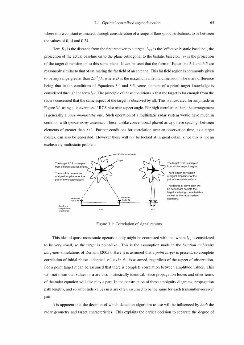
3.1. Optimal centralised target detection 65
where α is a constant estimated, through consideration of a range of flare spot distributions, to be between
the values of 0.14 and 0.24.
Here R1 is the distance from the first receiver to a target. L12 is the ‘effective bistatic baseline’, the
projection of the actual baseline on to the plane orthogonal to the bistatic bisector. l12 is the projection
of the target dimension on to this same plane. It can be seen that the form of Equations 3.4 and 3.5 are
reasonably similar to that of estimating the far field of an antenna. This far field region is commonly given
to be any range greater than 2D2/λ, where D is the maximum antenna dimension. The main difference
being that in the conditions of Equations 3.4 and 3.5, some element of a-priori target knowledge is
considered through the term l12. The principle of these conditions is that the target is far enough from the
radars concerned that the same aspect of the target is observed by all. This is illustrated for amplitude in
Figure 3.1 using a ‘conventional’ RCS plot over aspect angle. For high correlation then, the arrangement
is generally a quasi-monostatic one. Such operation of a multistatic radar system would have much in
common with sparse array antennas. These, unlike conventional phased arrays, have spacings between
elements of greater than λ/2. Further conditions for correlation over an observation time, as a target
rotates, can also be generated. However these will not be looked at in great detail, since this is not an
exclusively multistatic problem.
Figure 3.1: Correlation of signal returns
This idea of quasi-monostatic operation only might be contrasted with that where l12 is considered
to be very small, so the target is point-like. This is the assumption made in the location ambiguity
diagrams simulations of Derham [2005]. Here it is assumed that a point target is present, so complete
correlation of initial phase - identical values in φ - is assumed, regardless of the aspect of observation.
For a point target it can be assumed that there is complete correlation between amplitude values. This
will not mean that values in a are also intrinsically identical, since propagation losses and other terms
of the radar equation will also play a part. In the construction of these ambiguity diagrams, propagation
path lengths, and so amplitude values in a are often assumed to be the same for each transmitter-receiver
pair.
It is apparent that the decision of which detection algorithm to use will be influenced by both the
radar geometry and target characteristics. This explains the earlier decision to separate the degree of
3.1. Optimal centralised target detection 66
spatial coherency in the system from the information integration level. Just because a fully spatially
coherent system is available will not mean that radio signal fusion will automatically prove the optimal
choice of detection algorithm. The idea of ‘amplitude fluctuations’ of the received signals, and their
correlation between spatially separated receivers, can be investigated. First strongly spatially correlated
signals will be considered (nominally where conditions of Equations 3.4 and 3.5 are satisfied) where the
value A2i1 is taken as the known ratio of the second raw moments of the probability distributions for ai
and a1, where a1 is some given ‘reference’ receiver within the system.
ai = Ai1a1; w(ai) =∫ ∞
0
w(a1)δ(ai −Ai1a1)da1 (3.6)
Thus A2i1 is effectively the ratio of the expected signal power at each station.
∫ ∞0
a2iw(ai)dai = A2
i1
∫ ∞0
a21w(a1)das1 (3.7)
In terms of a real system, this situation could be envisaged in the case where knowledge of all terms
of the parameters in the radar equation apart from the RCS were to be available. The correlation between
RCS values for each receiver is also assumed to be known (but not the actual RCS values themselves).
This will mean that although the measurement-to-measurement fluctuations (such as those considered
by Swerling) of the target will be random, they will still have a known correlation between receivers.
Similarly, w(φi) is given as the convolution of w(φ1) with the phase offset given by Φi1. Simply put,
this will mean that the shape of the distribution will stay the same, but that the position of the distribution
will move by this known phase offset, as shown in Equation 3.8:
φi = φ1 − Φi1; w(φi) =∫ ∞∞
w(φ1)δ(φi − φ1 + Φi1)dφ1 (3.8)
Taking these assumptions, the likelihood ratio of Equation 3.3 can be simplified. Since the distribu-
tions of a and φ are now known with respect to φ1 and a1, the likelihood can be rewritten as shown in
Equation 3.9:
Λ =∫ ∞
0
∫ π
−πw(a1)w(φ1)expa1AtN−1Re[exp(jφ1)E∗(φ)G]− t0a2
1AtN−1Adφ1da1 (3.9)
Chernyak first considers the expected signal complex amplitude to be a Gaussian random value.
This leads to a uniform distribution between −π and π for φ1, and a Rayleigh distribution for a1. This
approach is the same as that considered by Conte. Substitution of the probability distribution and some
simplification similarly leads to the optimum processing algorithm, L2, as shown in Equation 3.10. It
can be seen that t0a21A
tN−1A has been removed; since this set of terms will have a constant value,
being independent of the output of G.
L2 =
∣∣∣∣∣m∑i=1
Ai1Ni
e−jΦi1Gi
∣∣∣∣∣ (3.10)
Since phase terms are present in summation between received signals, this detection algorithm
can be said to perform radio signal fusion. However, such probability distributions will in reality be
3.1. Optimal centralised target detection 67
dependant on unknown targets, and so will also be unknown or even non-random (as in the point target
case). Therefore an optimal adaptive processing algorithm is produced, where values φ1 and a1 are
maximum likelihood estimates. The principles behind the use of these estimates, which are produced
from the received data (hence an adaptive process) was first discussed in Chapter 2. These estimates are
now produced through partial differentiation of the exponent of Equation 3.9 (i.e. where φ1 and a1 are
fixed values). This again produces L2.
Repeating this reasoning for the case of n transmitted signals arriving at m receivers produces Lc,
shown in Equation 3.11. This assumes that different signals arriving at each receiver can be resolved
(i.e. it is clear which transmitter produced each signal). This might be done through the interleaving of
transmitter PRF, or through the use of different waveforms and orthogonal codes [Deng, 2004a].
Lc =
∣∣∣∣∣n∑k=1
m∑i=1
Aik1
Nie−jΦik1Gik
∣∣∣∣∣ (3.11)
where A2ik1 is the known averaged power ratio for the kth expected signal at the ith receiving signal
to that of the 1st ‘reference’ signal at the 1st receiving station. Φik1 is the known initial phase difference.
In the case where complex amplitude fluctuations are independent can also be considered. Here
the initial phases φik and amplitude values aik are uncorrelated. The distributions shown in Equations
3.12 and 3.13 may represent this situation if amplitudes are now considered as independent Rayleigh
distributed variables.
w(ai) = (2ai/σ21A
2i1)exp(−a2
1/σ21Ai1); ai ∈ (0,∞) (3.12)
w(φi) =1
2π; ai ∈ (0, 2π) (3.13)
The optimum processing algorithm for these conditions is given by L5, shown in Equation 3.14.
L5 =m∑i=1
A2i1
N2i
|Gi|2(
1 +σ2
1A2i1t0
Ni
)−1
(3.14)
It can be seen that the term Φi1 is no longer present and square-law envelope detection follows the
matched filter. Thus phase information is removed before any summation between receivers, hence this
algorithm is video signal fusion. This time, rather than directly relating received signal amplitude as
in Equation 3.6, the mean received power σ2i is considered. This immediately raises the question as to
how σ2i and hence Ai1 are determined, without the assumption of strong spatial correlation. Estimating
these values from past measurements may be possible. This would not seem to sit particularly well with
the previous simple detector considered for spatially coherent signals - having more in common with
the later process of tracking. In all cases where estimates or assumptions are required however, some
sub-optimality is unavoidable. It can be investigated as to whether any of the problematic terms in L5
are removed with assumptions about received signals.
First the presence of strong signals, where σ21A
2i1t0/Ni 1 can be investigated. Here (1 +
(σ21A
2i1t0/Ni)) can be approximated to σ2
1A2i1t0/Ni. Several terms will now cancel, and σ1t0 can be
3.1. Optimal centralised target detection 68
removed since it is constant for all i. This produces algorithm L6 which is also found to be the optimal
adaptive processing algorithm produced through utilising maximum likelihood estimates for φi and ai
(−arg(G) and |Gi|/2t0 respectively) for the case of independent amplitude fluctuations.
L6 =m∑i=1
|Gi|2
Ni(3.15)
This is very convenient, since it means simple summation of noise weighted matched filter outputs.
No longer is any measure of σ2i required. This reasoning can be repeated for the case for n transmitted
signals arriving at m receivers, to produce Lic:
Lic =n∑k=1
m∑i=1
|Gik|2
Ni(3.16)
However if weak signals are assumed to be present, so that σ21A
2i1t0/Ni 1, then it can be seen
that L5 simplifies to the following optimum processing algorithm:
L3 =m∑i=1
A2i1|Gi|2
N2i
(3.17)
In the weak signal case, the optimal processing algorithm differs from the optimal adaptive pro-
cessing algorithm. L3 contains the relationship Ai1 between mean received power, which are included
as weightings. This again asks the question as to how the values of Ai1 should be obtained. If an at-
tempt is made to simply use L6 and maximum likelihood estimates in the weak signal case, then as the
mean received power decreases it can be seen that the probability distribution of the signal + noise PDF
and hence ai will approach that of the Rayleigh distributed noise. This will lead to an estimator bias
that approaches√N/2t0. For weak signals, this bias becomes large in comparison to the actual signal
amplitude values. Hence using L6 for weak signals would potentially give equal weighting to receivers
with little or no received signal, resulting in potentially large losses in detection performance.
If a large variation of σ21A
2i1t0/Ni is expected in the weak signal case, where σ2
1A2i1t0/Ni 1,
a robust method of implementing detection algorithms L3 could prove useful. A simple adaptation of
L3 developed here is to substitute estimates Ai1 corresponding to the predicted returns using the bistatic
radar equation (Equation 2.46) whilst assuming a constant average RCS for any target. Thus the entirety
of any a-priori knowledge of the radar system might be made use of in an attempt to improve estimates
of Ai1. L3 can be rewritten as shown in Equation 3.18, as well as expanding to account for n transmitted
signals. This is sub-optimal in the sense that it assumes a constant average RCS value seen by each
transmitter-receiver pair, where this might not in reality be quite the case. This could be improved if
further information on the target RCS behaviour became available.
Lic2 =n∑k=1
m∑i=1
A2ik1|Gik|2
N2i
(3.18)
A2ik1 =
PkGkGiR2tx1R
2rx1
Ptx1Gtx1Grx1R2kR
2i
(3.19)
3.1. Optimal centralised target detection 69
where Rk is the hypothesised range from transmitter k to target, Ri is the hypothesised range from
target to receiver i. Pk is the output power of transmitter k. Gk is the effective antenna gain of transmitter
k, Gi the effective antenna gain of receiver i. tx1 and rx1 refer to the first ‘reference’ transmitter and
receiver respectively.
A further dilemma comes where both weak and strong signals must be considered, which may be
a common situation in a very widely spaced multistatic radar, due to the nature of propagation losses.
A pragmatic approach would be one similar to typical radar estimates of coverage; to determine which
receivers might expect strong signals (again based on the radar equation and typical target RCS), and
then to use Lic on these alone 2. In effect this method looks to ‘turn off’ receivers which will con-
tribute mainly noise to the detector output due to poor maximum likelihood estimates of their received
signal amplitudes. If no receivers are expected to contain strong signals then Lic2 should be used. Pre-
cisely where the threshold between weak and strong signals is placed is fairly arbitrary either side of
σ21A
2i1t0/Ni = 1, and could be fine tuned by the radar operator. This might also have implications in
target parameter estimation, which will be discussed in Chapter 4. It might be noted that where ex-
pected average values of σ2i /Ni are the same that Lic and Lic2 are equivalent anyway, since the common
weighting on Lic2 can be removed.
3.1.4 Short-term spatially coherent and spatially incoherent multistatic radar
For fully spatially coherent multistatic radars, the case was considered where complex amplitude fluctu-
ations at the receiver input caused by the target meant that useful information on the initial phase of such
signals was lost. Such loss of information may also be caused if the receivers themselves have unknown
or random initial phase offsets - perhaps due to difficulties in either oscillator synchronisation between
transmitter and receiver, or inaccuracy of determining phase centres of antennas themselves.
The case where strongly spatially correlated signals arriving at such a system can be considered in
the same way. The value A2i1 is taken to have the known relationships as detailed in Equations 3.6 and
3.7. However this time the distribution of φ is said to be constant between −π and π as in Equation
3.13 due to a random3 initial phase offset. Substituting these distributions into Equation 3.3, assuming a
Rayleigh distribution for a1 and integrating produces the detector L3 once again. The proviso here being
that again weak signals (the exact condition specified as a21A
2i1|Gi|/16Ni 1) are present, similar to
the previous use of L3.
The optimal adaptive processing algorithm may again be derived in the case where the distributions
of a1 and φi are not available - or are not random, but unknown. In this case a new detector L4 is
produced:
L4 =m∑i=1
Ai1|Gi|Ni
(3.20)
It is in fact found that for L4 it proves rather more difficult to express false alarm and detection
2Of course, this ignores any gains which might be made from the incoherent summation of many weaker signals, and so is
somewhat sub-optimal3That phase offsets are random is something of an assumption for simplicity of the derivation
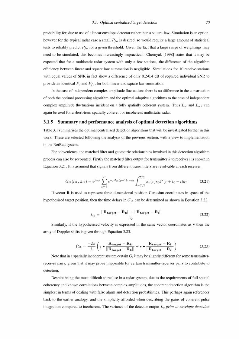
3.1. Optimal centralised target detection 70
probability for, due to use of a linear envelope detector rather than a square-law. Simulation is an option,
however for the typical radar case a small Pfa is desired, so would require a large amount of statistical
tests to reliably predict Pfa for a given threshold. Given the fact that a large range of weightings may
need to be simulated, this becomes increasingly impractical. Chernyak [1998] states that it may be
expected that for a multistatic radar system with only a few stations, the difference of the algorithm
efficiency between linear and square law summation is negligible. Simulations for 10 receive stations
with equal values of SNR in fact show a difference of only 0.2-0.4 dB of required individual SNR to
provide an identical Pd and Pfa, for both linear and square law summation.
In the case of independent complex amplitude fluctuations there is no difference in the construction
of both the optimal processing algorithm and the optimal adaptive algorithms to the case of independent
complex amplitude fluctuations incident on a fully spatially coherent system. Thus Lic and Lic2 can
again be used for a short-term spatially coherent or incoherent multistatic radar.
3.1.5 Summary and performance analysis of optimal detection algorithms
Table 3.1 summarises the optimal centralised detection algorithms that will be investigated further in this
work. These are selected following the analysis of the previous section, with a view to implementation
in the NetRad system.
For convenience, the matched filter and geometric relationships involved in this detection algorithm
process can also be recounted. Firstly the matched filter output for transmitter k to receiver i is shown in
Equation 3.21. It is assumed that signals from different transmitters are resolvable at each receiver.
Gik(tik,Ωik) = ejωctP∑p=1
e−jΩik(p−1)τP RI
∫ T/2
−T/2xp(τ)s0k
∗(τ + t0 − t)dτ (3.21)
If vector R is used to represent three dimensional position Cartesian coordinates in space of the
hypothesised target position, then the time delays in Gik can be determined as shown in Equation 3.22.
tik =||Rtarget −Rk||+ ||Rtarget −Ri||
cp(3.22)
Similarly, if the hypothesised velocity is expressed in the same vector coordinates as v then the
array of Doppler shifts is given through Equation 3.23.
Ωik =−2πλ
(v • Rtarget −Rk
||Rtarget −Rk||+ v • Rtarget −Ri
||Rtarget −Ri||
)(3.23)
Note that in a spatially incoherent system certainGik may be slightly different for some transmitter-
receiver pairs, given that it may prove impossible for certain transmitter-receiver pairs to contribute to
detection.
Despite being the most difficult to realise in a radar system, due to the requirements of full spatial
coherency and known correlations between complex amplitudes, the coherent detection algorithm is the
simplest in terms of dealing with false alarm and detection probabilities. This perhaps again references
back to the earlier analogy, and the simplicity afforded when describing the gains of coherent pulse
integration compared to incoherent. The variance of the detector output Lc prior to envelope detection
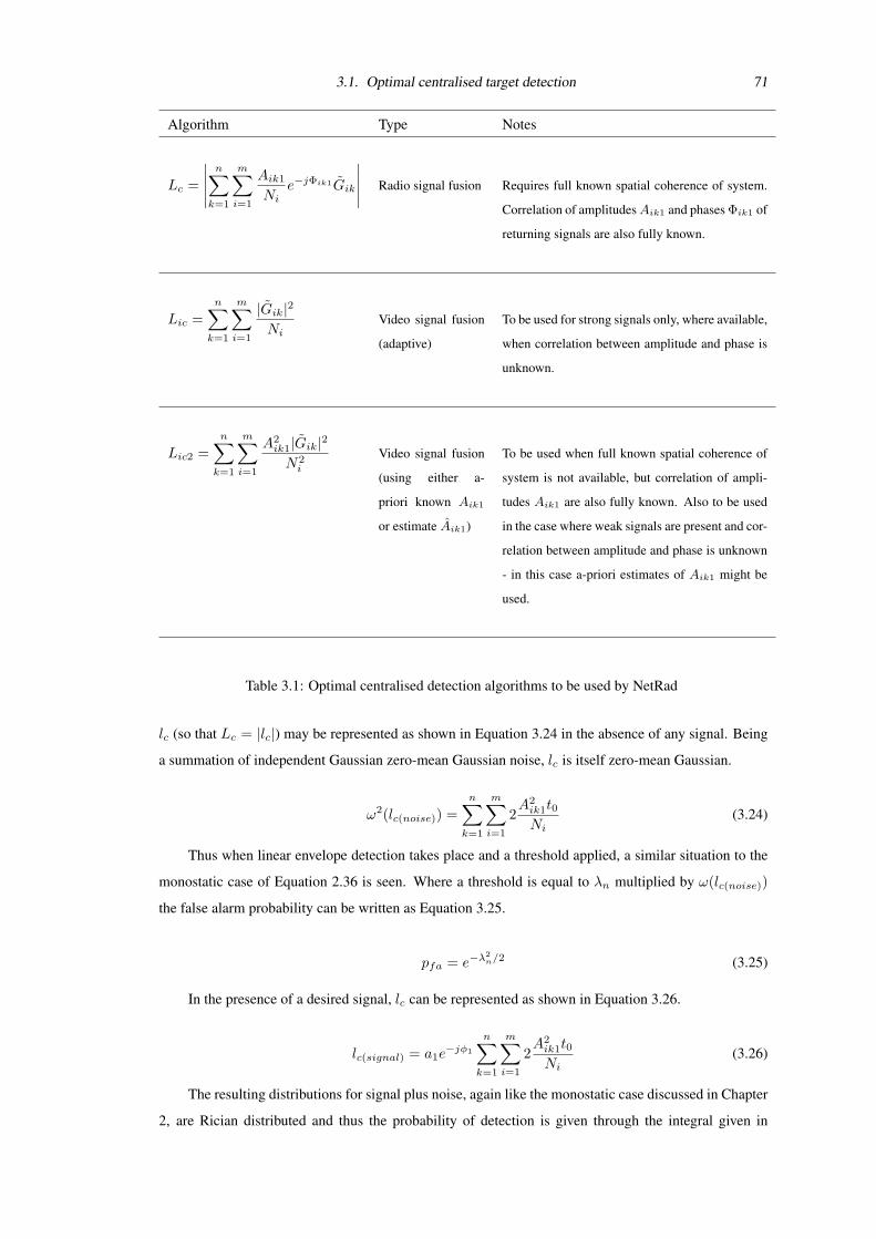
3.1. Optimal centralised target detection 71
Algorithm Type Notes
Lc =
∣∣∣∣∣n∑k=1
m∑i=1
Aik1
Nie−jΦik1Gik
∣∣∣∣∣ Radio signal fusion Requires full known spatial coherence of system.
Correlation of amplitudes Aik1 and phases Φik1 of
returning signals are also fully known.
Lic =n∑k=1
m∑i=1
|Gik|2
NiVideo signal fusion
(adaptive)
To be used for strong signals only, where available,
when correlation between amplitude and phase is
unknown.
Lic2 =n∑k=1
m∑i=1
A2ik1|Gik|2
N2i
Video signal fusion
(using either a-
priori known Aik1
or estimate Aik1)
To be used when full known spatial coherence of
system is not available, but correlation of ampli-
tudes Aik1 are also fully known. Also to be used
in the case where weak signals are present and cor-
relation between amplitude and phase is unknown
- in this case a-priori estimates of Aik1 might be
used.
Table 3.1: Optimal centralised detection algorithms to be used by NetRad
lc (so that Lc = |lc|) may be represented as shown in Equation 3.24 in the absence of any signal. Being
a summation of independent Gaussian zero-mean Gaussian noise, lc is itself zero-mean Gaussian.
ω2(lc(noise)) =n∑k=1
m∑i=1
2A2ik1t0Ni
(3.24)
Thus when linear envelope detection takes place and a threshold applied, a similar situation to the
monostatic case of Equation 2.36 is seen. Where a threshold is equal to λn multiplied by ω(lc(noise))
the false alarm probability can be written as Equation 3.25.
pfa = e−λ2n/2 (3.25)
In the presence of a desired signal, lc can be represented as shown in Equation 3.26.
lc(signal) = a1e−jφ1
n∑k=1
m∑i=1
2A2ik1t0Ni
(3.26)
The resulting distributions for signal plus noise, again like the monostatic case discussed in Chapter
2, are Rician distributed and thus the probability of detection is given through the integral given in
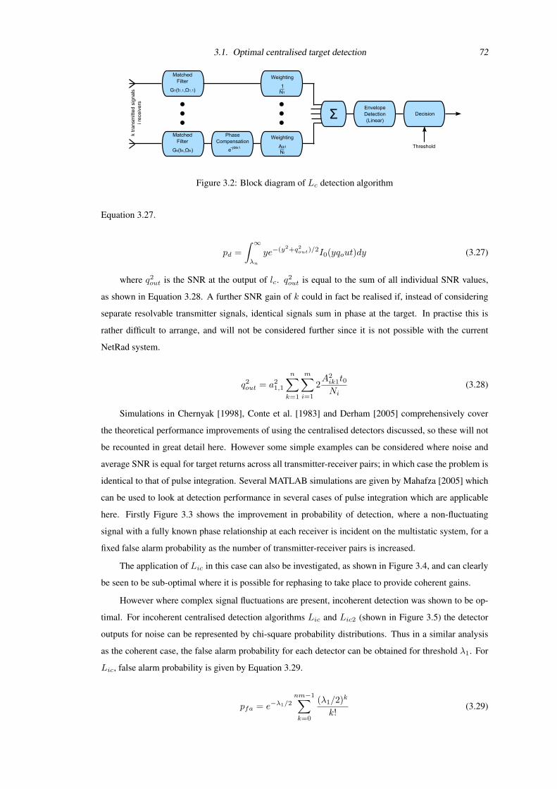
3.1. Optimal centralised target detection 72
Figure 3.2: Block diagram of Lc detection algorithm
Equation 3.27.
pd =∫ ∞λn
ye−(y2+q2out)/2I0(yqout)dy (3.27)
where q2out is the SNR at the output of lc. q2
out is equal to the sum of all individual SNR values,
as shown in Equation 3.28. A further SNR gain of k could in fact be realised if, instead of considering
separate resolvable transmitter signals, identical signals sum in phase at the target. In practise this is
rather difficult to arrange, and will not be considered further since it is not possible with the current
NetRad system.
q2out = a2
1,1
n∑k=1
m∑i=1
2A2ik1t0Ni
(3.28)
Simulations in Chernyak [1998], Conte et al. [1983] and Derham [2005] comprehensively cover
the theoretical performance improvements of using the centralised detectors discussed, so these will not
be recounted in great detail here. However some simple examples can be considered where noise and
average SNR is equal for target returns across all transmitter-receiver pairs; in which case the problem is
identical to that of pulse integration. Several MATLAB simulations are given by Mahafza [2005] which
can be used to look at detection performance in several cases of pulse integration which are applicable
here. Firstly Figure 3.3 shows the improvement in probability of detection, where a non-fluctuating
signal with a fully known phase relationship at each receiver is incident on the multistatic system, for a
fixed false alarm probability as the number of transmitter-receiver pairs is increased.
The application of Lic in this case can also be investigated, as shown in Figure 3.4, and can clearly
be seen to be sub-optimal where it is possible for rephasing to take place to provide coherent gains.
However where complex signal fluctuations are present, incoherent detection was shown to be op-
timal. For incoherent centralised detection algorithms Lic and Lic2 (shown in Figure 3.5) the detector
outputs for noise can be represented by chi-square probability distributions. Thus in a similar analysis
as the coherent case, the false alarm probability for each detector can be obtained for threshold λ1. For
Lic, false alarm probability is given by Equation 3.29.
pfa = e−λ1/2nm−1∑k=0
(λ1/2)k
k!(3.29)
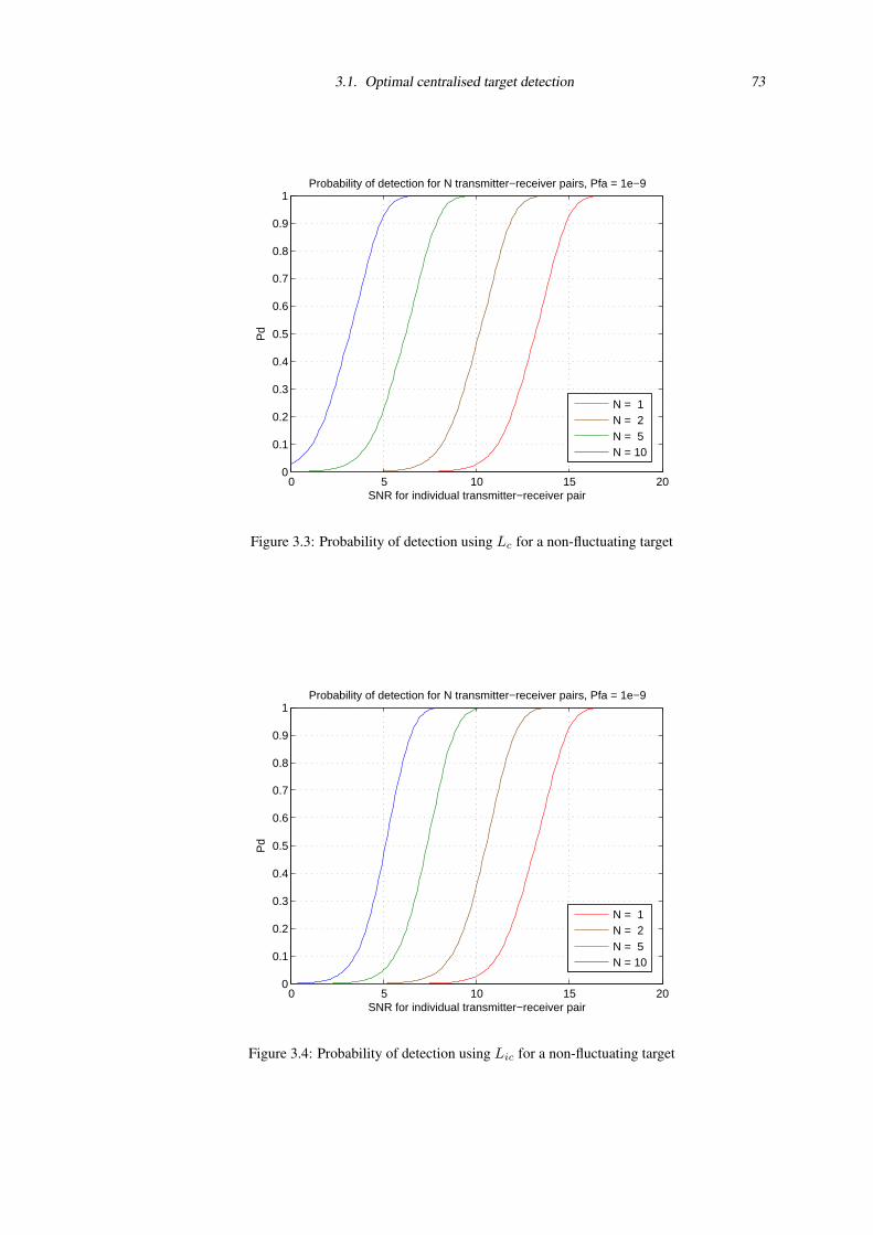
3.1. Optimal centralised target detection 73
0 5 10 15 200
0.1
0.2
0.3
0.4
0.5
0.6
0.7
0.8
0.9
1
SNR for individual transmitter−receiver pair
Probability of detection for N transmitter−receiver pairs, Pfa = 1e−9
Pd
N = 1N = 2N = 5N = 10
Figure 3.3: Probability of detection using Lc for a non-fluctuating target
0 5 10 15 200
0.1
0.2
0.3
0.4
0.5
0.6
0.7
0.8
0.9
1
SNR for individual transmitter−receiver pair
Probability of detection for N transmitter−receiver pairs, Pfa = 1e−9
Pd
N = 1N = 2N = 5N = 10
Figure 3.4: Probability of detection using Lic for a non-fluctuating target
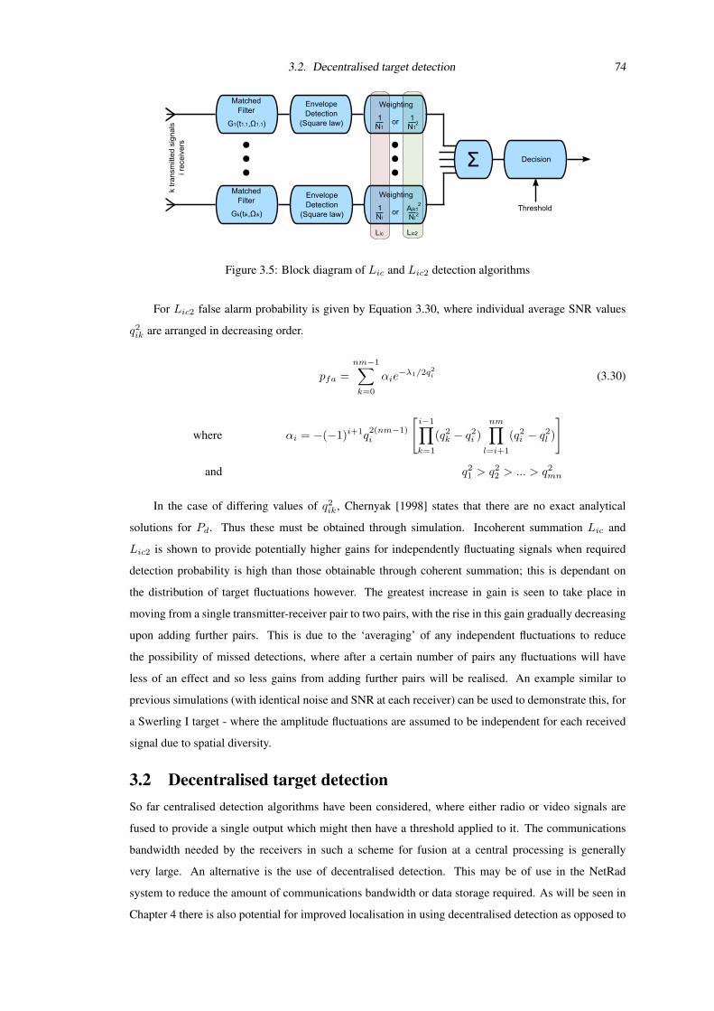
3.2. Decentralised target detection 74
Figure 3.5: Block diagram of Lic and Lic2 detection algorithms
For Lic2 false alarm probability is given by Equation 3.30, where individual average SNR values
q2ik are arranged in decreasing order.
pfa =nm−1∑k=0
αie−λ1/2q
2i (3.30)
where αi = −(−1)i+1q2(nm−1)i
[i−1∏k=1
(q2k − q2
i )nm∏l=i+1
(q2i − q2
l )
]
and q21 > q2
2 > ... > q2mn
In the case of differing values of q2ik, Chernyak [1998] states that there are no exact analytical
solutions for Pd. Thus these must be obtained through simulation. Incoherent summation Lic and
Lic2 is shown to provide potentially higher gains for independently fluctuating signals when required
detection probability is high than those obtainable through coherent summation; this is dependant on
the distribution of target fluctuations however. The greatest increase in gain is seen to take place in
moving from a single transmitter-receiver pair to two pairs, with the rise in this gain gradually decreasing
upon adding further pairs. This is due to the ‘averaging’ of any independent fluctuations to reduce
the possibility of missed detections, where after a certain number of pairs any fluctuations will have
less of an effect and so less gains from adding further pairs will be realised. An example similar to
previous simulations (with identical noise and SNR at each receiver) can be used to demonstrate this, for
a Swerling I target - where the amplitude fluctuations are assumed to be independent for each received
signal due to spatial diversity.
3.2 Decentralised target detectionSo far centralised detection algorithms have been considered, where either radio or video signals are
fused to provide a single output which might then have a threshold applied to it. The communications
bandwidth needed by the receivers in such a scheme for fusion at a central processing is generally
very large. An alternative is the use of decentralised detection. This may be of use in the NetRad
system to reduce the amount of communications bandwidth or data storage required. As will be seen in
Chapter 4 there is also potential for improved localisation in using decentralised detection as opposed to
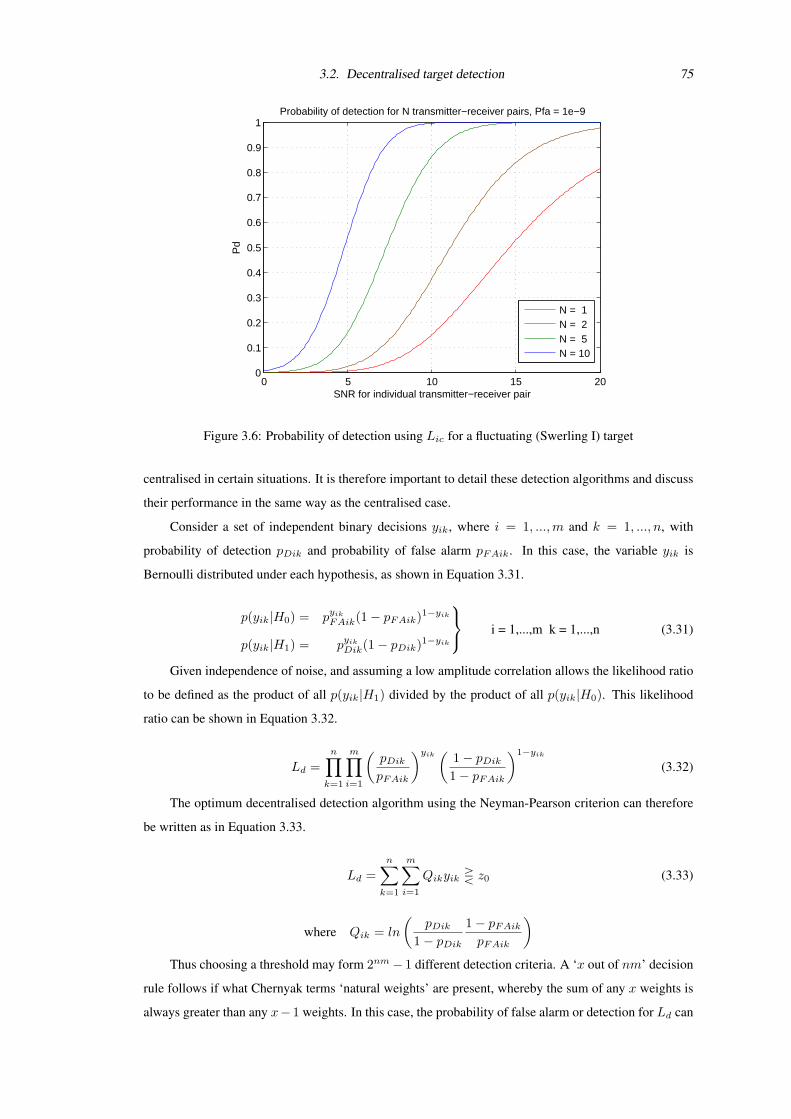
3.2. Decentralised target detection 75
0 5 10 15 200
0.1
0.2
0.3
0.4
0.5
0.6
0.7
0.8
0.9
1
SNR for individual transmitter−receiver pair
Probability of detection for N transmitter−receiver pairs, Pfa = 1e−9
Pd
N = 1N = 2N = 5N = 10
Figure 3.6: Probability of detection using Lic for a fluctuating (Swerling I) target
centralised in certain situations. It is therefore important to detail these detection algorithms and discuss
their performance in the same way as the centralised case.
Consider a set of independent binary decisions yik, where i = 1, ...,m and k = 1, ..., n, with
probability of detection pDik and probability of false alarm pFAik. In this case, the variable yik is
Bernoulli distributed under each hypothesis, as shown in Equation 3.31.
p(yik|H0) = pyik
FAik(1− pFAik)1−yik
p(yik|H1) = pyik
Dik(1− pDik)1−yik
i = 1,...,m k = 1,...,n (3.31)
Given independence of noise, and assuming a low amplitude correlation allows the likelihood ratio
to be defined as the product of all p(yik|H1) divided by the product of all p(yik|H0). This likelihood
ratio can be shown in Equation 3.32.
Ld =n∏k=1
m∏i=1
(pDikpFAik
)yik(
1− pDik1− pFAik
)1−yik
(3.32)
The optimum decentralised detection algorithm using the Neyman-Pearson criterion can therefore
be written as in Equation 3.33.
Ld =n∑k=1
m∑i=1
Qikyik R z0 (3.33)
where Qik = ln
(pDik
1− pDik1− pFAikpFAik
)Thus choosing a threshold may form 2nm− 1 different detection criteria. A ‘x out of nm’ decision
rule follows if what Chernyak terms ‘natural weights’ are present, whereby the sum of any x weights is
always greater than any x− 1 weights. In this case, the probability of false alarm or detection for Ld can
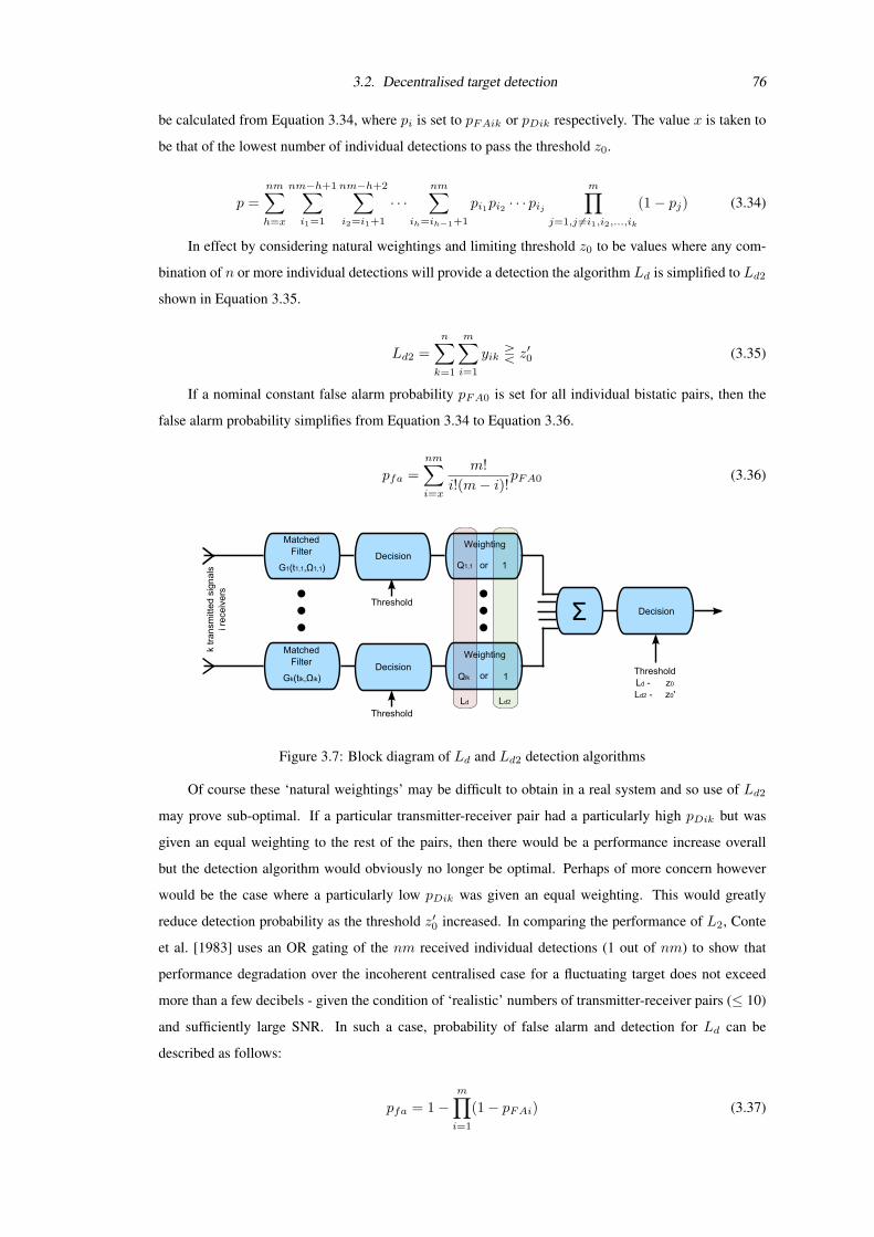
3.2. Decentralised target detection 76
be calculated from Equation 3.34, where pi is set to pFAik or pDik respectively. The value x is taken to
be that of the lowest number of individual detections to pass the threshold z0.
p =nm∑h=x
nm−h+1∑i1=1
nm−h+2∑i2=i1+1
· · ·nm∑
ih=ih−1+1
pi1pi2 · · · pijm∏
j=1,j 6=i1,i2,...,ik
(1− pj) (3.34)
In effect by considering natural weightings and limiting threshold z0 to be values where any com-
bination of n or more individual detections will provide a detection the algorithm Ld is simplified to Ld2
shown in Equation 3.35.
Ld2 =n∑k=1
m∑i=1
yik R z′0 (3.35)
If a nominal constant false alarm probability pFA0 is set for all individual bistatic pairs, then the
false alarm probability simplifies from Equation 3.34 to Equation 3.36.
pfa =nm∑i=x
m!i!(m− i)!
pFA0 (3.36)
Figure 3.7: Block diagram of Ld and Ld2 detection algorithms
Of course these ‘natural weightings’ may be difficult to obtain in a real system and so use of Ld2
may prove sub-optimal. If a particular transmitter-receiver pair had a particularly high pDik but was
given an equal weighting to the rest of the pairs, then there would be a performance increase overall
but the detection algorithm would obviously no longer be optimal. Perhaps of more concern however
would be the case where a particularly low pDik was given an equal weighting. This would greatly
reduce detection probability as the threshold z′0 increased. In comparing the performance of L2, Conte
et al. [1983] uses an OR gating of the nm received individual detections (1 out of nm) to show that
performance degradation over the incoherent centralised case for a fluctuating target does not exceed
more than a few decibels - given the condition of ‘realistic’ numbers of transmitter-receiver pairs (≤ 10)
and sufficiently large SNR. In such a case, probability of false alarm and detection for Ld can be
described as follows:
pfa = 1−m∏i=1
(1− pFAi) (3.37)
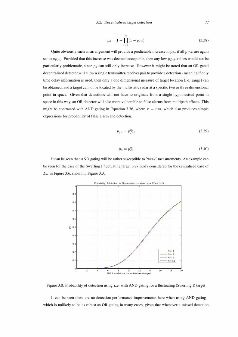
3.2. Decentralised target detection 77
pd = 1−m∏i=1
(1− pDi) (3.38)
Quite obviously such an arrangement will provide a predictable increase in pfa if all pFAi are again
set to pFA0. Provided that this increase was deemed acceptable, then any low pDik values would not be
particularly problematic, since pd can still only increase. However it might be noted that an OR gated
decentralised detector will allow a single transmitter-receiver pair to provide a detection - meaning if only
time delay information is used, then only a one dimensional measure of target location (i.e. range) can
be obtained, and a target cannot be located by the multistatic radar at a specific two or three dimensional
point in space. Given that detections will not have to originate from a single hypothesised point in
space in this way, an OR detector will also more vulnerable to false alarms from multipath effects. This
might be contrasted with AND gating in Equation 3.36, where x = nm, which also produces simple
expressions for probability of false alarm and detection.
pfa = pmfai (3.39)
pd = pmdi (3.40)
It can be seen that AND gating will be rather susceptible to ’weak’ measurements. An example can
be seen for the case of the Swerling I fluctuating target previously considered for the centralised case of
Lic in Figure 3.6, shown in Figure 3.3.
0 2 4 6 8 10 12 14 16 18 200
0.1
0.2
0.3
0.4
0.5
0.6
0.7
0.8
0.9
1
SNR for individual transmitter−receiver pair
Probability of detection for N transmitter−receiver pairs, Pfa = 1e−9
Pd
N = 1N = 2N = 5N = 10
Figure 3.8: Probability of detection using Ld2 with AND gating for a fluctuating (Swerling I) target
It can be seen there are no detection performance improvements here when using AND gating -
which is unlikely to be as robust as OR gating in many cases, given that whenever a missed detection
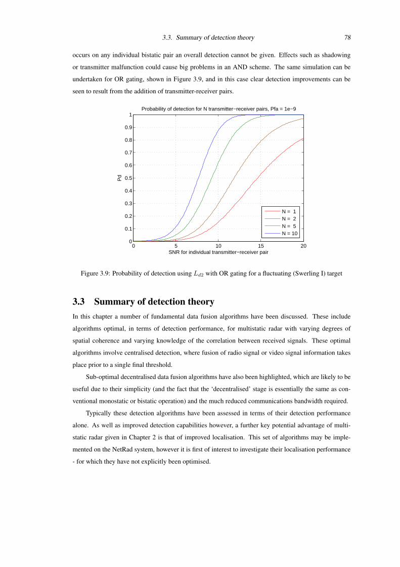
3.3. Summary of detection theory 78
occurs on any individual bistatic pair an overall detection cannot be given. Effects such as shadowing
or transmitter malfunction could cause big problems in an AND scheme. The same simulation can be
undertaken for OR gating, shown in Figure 3.9, and in this case clear detection improvements can be
seen to result from the addition of transmitter-receiver pairs.
0 5 10 15 200
0.1
0.2
0.3
0.4
0.5
0.6
0.7
0.8
0.9
1
SNR for individual transmitter−receiver pair
Probability of detection for N transmitter−receiver pairs, Pfa = 1e−9
Pd
N = 1N = 2N = 5N = 10
Figure 3.9: Probability of detection using Ld2 with OR gating for a fluctuating (Swerling I) target
3.3 Summary of detection theoryIn this chapter a number of fundamental data fusion algorithms have been discussed. These include
algorithms optimal, in terms of detection performance, for multistatic radar with varying degrees of
spatial coherence and varying knowledge of the correlation between received signals. These optimal
algorithms involve centralised detection, where fusion of radio signal or video signal information takes
place prior to a single final threshold.
Sub-optimal decentralised data fusion algorithms have also been highlighted, which are likely to be
useful due to their simplicity (and the fact that the ‘decentralised’ stage is essentially the same as con-
ventional monostatic or bistatic operation) and the much reduced communications bandwidth required.
Typically these detection algorithms have been assessed in terms of their detection performance
alone. As well as improved detection capabilities however, a further key potential advantage of multi-
static radar given in Chapter 2 is that of improved localisation. This set of algorithms may be imple-
mented on the NetRad system, however it is first of interest to investigate their localisation performance
- for which they have not explicitly been optimised.
Chapter 4
Multistatic Localisation Performance
The term ‘localisation’ is used in the context of this work to describe in broad terms the degree with
which targets can be located. This encompasses both the error inherent in position and velocity measured
by the radar system, as well as the concept of resolution of multiple targets. The reason for grouping
these under a single heading is that they are somewhat linked - for example if two targets are unresolvable
then the resultant (single) detection will have a degree of error relative to both actual target positions (as
well as obviously erroneously only detecting a single target). The localisation capabilities of a multistatic
radar will be an important measure of performance in many situations. Clear examples were found in
the literature search where improvements in localisation were desired/obtained over the monostatic case.
Conversely, the detection algorithms of Chernyak [1998] and Conte et al. [1983] explored in the previous
chapter assume a ‘resolution cell’ bounded by antenna beamwidths, and a single target contained within.
In this chapter the main focus is on comparing these algorithms (specified in Chapter 3) and mak-
ing the first attempt to give a side-by-side comparison of these in terms of localisation performance.
Throughout these comparisons, information of antenna bearing and beamwidth will not be used when
producing multistatic detector outputs; thus any localisation gains are the result of the data fusion of
multiple time delay and Doppler frequency shift information. Therefore this presents a ‘general case’
where a surveillance area has complete antenna coverage at all times, and avoids the complexities that
might otherwise be involved in positioning antenna and implementing techniques such as pulse chasing.
Attempting to look at ‘optimal’ localisation methods over every possible scenario and has been
avoided for two reasons. Firstly, the complexity involved in detecting and localising multiple targets
is significantly increased compared to the detection theory, nominally for a single target, presented in
Chapter 3. This is due to the geometry of the system and location of the targets, and interaction of target
returns now being a factor in ‘optimising’ localisation; whereas previous detection methods consider
only the amplitude of the received signals (and their correlation) and receiver noise levels. Secondly,
it is desired to later replicate the examples presented here with experimental measurements; to explore
some of the theoretical capabilities of multistatic radar that are often quoted but rarely demonstrated
experimentally (as discussed in Chapter 2). Further modification of these algorithms and further practical
details of processing methods that need to be applied to NetRad data are also discussed.
To begin by looking at localisation, the means by which the target parameter estimates are pro-
4.1. Localisation performance of centralised detection 80
duced must be considered. In the centralised detector case (Lc, Lic and Lic2) this is simple enough,
through searching for the peak (maximum likelihood) values in much the same way as might take place
for monostatic or bistatic radar. In decentralised detection, it is perhaps not immediately so obvious as
to what information is passed to the ‘fusion centre’. The algorithms discussed in Chapter 3 imply that
every time delay which crosses the threshold must be passed to the fusion centre. More likely however
(and certainly to reduce data bandwidth and be better in agreement with the term ‘plot level fusion’)
would again be some sort of peak detection process which would produce discrete individual detections
at a single time delay and Doppler shift for each target, rather than a range of values. A further con-
sideration for decentralised detection is how the output of the fusion centre is then itself interpreted to
produce discrete estimates of target parameters. This chapter will explore these issues with reference
to implementation in the NetRad system. At the end of the chapter a view on how operation in a more
purpose-orientated (rather than purely experimental) commercial system might take place is considered.
4.1 Localisation performance of centralised detectionTo determine the localisation performance of the centralised detection algorithms described in Chapter
3 it is important to start by defining how target parameters (such as position and velocity) are actually
determined following detection. The method of using multiple down-range information over a shared
‘coverage’ area will largely be focussed upon during this chapter. This implies use of the likelihood ratio
detection algorithms previously specified to actually improve localisation. This is not to say that use of
cross-range information will always be redundant (for example if a target is particularly close to a node),
and certainly the methods described could be developed to account for this. This further complication
is beyond the scope of this work, which concentrates on the down-range only case so as to provide a
simpler more general case which could be implemented for any choice of antenna beamwidth and is
easy to test experimentally using the NetRad.
Optimum estimates of all target parameters will maximise the centralised likelihood ratio detectors
of Table 3.1. Chernyak [1998] considers the construction of the Fisher Information Matrix (FIM) and the
inversion of this to evaluate the Error Covariance Matrix (ECM) of target parameters. This allows deter-
mination of improvements of target position (and velocity) estimation over those for a typical monostatic
radar, as defined in Chapter 2. This is done through derivation of a ‘special’ likelihood function, creating
a FIM for the desired parameters only. This takes into account the effect of the ‘unneeded’ parameters
through solving likelihood ratios for these parameters averaged over received signals, before substitu-
iting the results of these in terms of t1, t2 and t3, so as to obtain the following 3 × 3 FIM Jnp given
in Equation 4.1. Without this ‘special’ likelihood function, the FIM would be rather larger due to the
number of parameters, and even more difficult to invert.
Jnp(t1, t2, t3) = δnp2EnNn4 ω2
n +m∑i=4
2EiNi4 ω2
i
δhi(t1, t2, t3)δtn
δhi(t1, t2, t3)δtp
(4.1)
where hi(t1, t2, t3) is a function which determines the time delay of the point in space defined by
t1, t2, t3 at the ith bistatic pair. 4ω2 is the effective mean squared bandwidth of the receiver and E

4.1. Localisation performance of centralised detection 81
the energy of the received signals. N is again the noise spectral density (again assuming white noise
only at receiver inputs). By inverting this matrix the ECM can be generated, containing the Cramer-
Rao lower bounds of error. One can see that the addition of further time-of-arrival measurements, other
than t1, t2, t3, may certainly add to the Fisher information, and hence only improve estimates of target
position when using the optimal centralised detection algorithms described.
The time delays may be transformed into Cartesian co-ordinates to define a target position to the
radar operator. Figure 4.1 depicts a simple overview of how increasing the spatial separation can increase
the accuracy of target position in a two-dimensional case using down-range information only1.
Figure 4.1: Error bounds for position estimation with two monostatic pairs
It can be seen for the two-radar example of Figure 4.1 that the target position is much more accurate
along the x-axis where each radar is arranged to measure orthogonal range vectors, since the largest
dimension of the grey shaded ‘area of uncertainty’ along this axis decreases. As the separation angle,
θ, moves away from this arrangement, towards either 0 or 180 in Figure 4.1, it can be seen that this
x-axis measurement may span an increasingly large range of values. In fact, as θ approaches 0 or
180, the situation may also arise where it becomes impossible to find a solution to the trilateration
problem (where the sum of the separation and the lesser of the measured ranges is less than that of
the greater range measurement). Along the y-axis, a degradation of accuracy is seen in Figure 4.1,
bounded by√
2 multiplied by the individual down-range error. A similar situation can be seen to occur
in the idea of GDOP seen in both Godrich et al. [2008] and in GPS positional estimates - where there
is said to be a high GDOP where satellites are close together. Estimation of target velocity can be
similarly improved through use of multiple perspectives and Doppler processing. It might be noted
that for a monostatic radar, the only way of estimating target velocity tangential to the down-range
measurement would again be through generally rather less accurate azimuth and elevation prediction
over time (although as always this will be dependant on the specific radars and geometry involved). The
exact bounds of target parameter errors will not be discussed further in great detail as the intention here
is to examine simple examples that can also be analysed experimentally. Another consideration is that
targets will often be complex, and time delays may not relate exactly to a single point. There is little
to be gained therefore from estimating a target’s position to an accuracy of much larger degree than it’s
1Strictly speaking there will be two solutions for target position on the two-dimensional plane shown. It is assumed for
simplicity that in this example some degree of directionality on the monostatic radars is capable of determining the correct solution.
4.1. Localisation performance of centralised detection 82
dimension for example, unless a radar is attempting to image or identify component parts of the target
itself which requires a high resolution.
Resolution is an important issue when attempting to estimate target parameters without error. So far
it has been discussed how multistatic radar might effectively increase target position estimation where
it is assumed a single target is present and thus a single set of time of arrival measurements to be
present for each transmitter-receiver pair. In reality, radar systems will often have to deal with multiple
targets as well as multipath effects and so must deal with the determination of which time of arrival
measurements are from which target. With this in mind, it would seem that sufficient resolution is
often a requirement for the any improvements in accuracy discussed above to truly be realisable. The
resolution cell geometry, much like the error bounds, is complex in the multistatic case since the number
of variables relating to the geometry is large. The concept of resolution in a conventional monostatic
sense is, in itself, a subtle one so care must be taken in the increasingly complex multistatic case. Earlier
definitions in Chapter 2 stated resolution to be the measure of the minimum separation that two targets
can have whilst still being discernible from one another. The idea of using the -3 dB points of a given
waveform is a common one, but this is in itself an assumption. The implications of such an assumption
will later be seen as resolution gains are attempted to be made by multistatic radar detection in some
difficult, but fairly realistic, scenarios.
Before beginning to discuss the resolution capabilities of multistatic radar, it is first important to
re-cap on the specifics of down-range resolution for monostatic and bistatic radar. This is due to these
down-range returns effectively being the ‘component parts’ of the multistatic detection algorithms, as
well as being a useful comparison to the final multistatic detector output. The choice of transmitted
waveform will define the down-range resolution. For a large part of this work, a simple linear FM
‘chirp’ waveform will be considered. This allows for both increased bandwidth and gain through the
process of pulse compression using a matched filter - as described in Chapter 2. The ambiguity function
when considering a Doppler shift of zero can be given by Equation 4.2:
χ(τ, 0)chirp =∣∣∣∣sin[πfmτ(1− |τ |/τp)]
πfmτ
∣∣∣∣ (4.2)
where fm is the upper frequency limit and τp the time duration of the chirp signal. It is well known
that when τp is large in comparison to τ , the ambiguity function can be approximated to a sinc function.
The first (and maximal) sidelobe for such a function will be approximately 13 dB down on the peak value
at a time delay of |τ | = 1.43/fm. For short linear FM chirps, a single pulse will not provide sufficient
Doppler resolution to distinguish typical moving targets from stationary clutter. To this end, a series
of pulses is used as described in Chapter 2, to provide sufficient resolution. For a Doppler shift fd the
location of the peak response will be shifted from its true delay by fdτp/fm. This will mean some error
in localisation as well as potentially some losses when fusing detector outputs. To put this into context,
if typical NetRad values of τp = 0.6 µs, fm = 40 MHz are used for a Doppler shift of 20 Hz typical for
a walking person, it can be seen that the error in time delay is a mere 0.3 ps. Thus the waveform might
be said to be Doppler tolerant. Figure 4.2 shows a simulation of the autocorrelation of a typical 0.6 µs
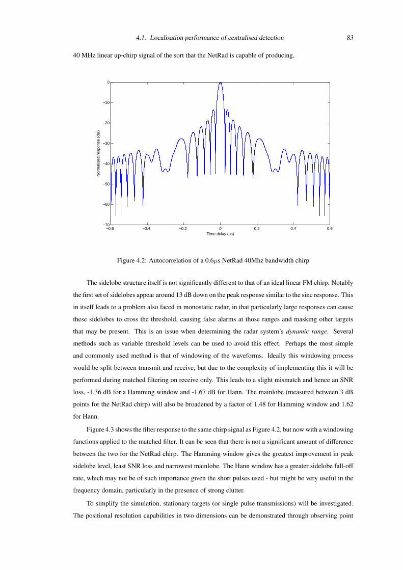
4.1. Localisation performance of centralised detection 83
40 MHz linear up-chirp signal of the sort that the NetRad is capable of producing.
−0.6 −0.4 −0.2 0 0.2 0.4 0.6−70
−60
−50
−40
−30
−20
−10
0
Time delay (us)
Nor
mal
ised
res
pons
e (d
B)
Figure 4.2: Autocorrelation of a 0.6µs NetRad 40Mhz bandwidth chirp
The sidelobe structure itself is not significantly different to that of an ideal linear FM chirp. Notably
the first set of sidelobes appear around 13 dB down on the peak response similar to the sinc response. This
in itself leads to a problem also faced in monostatic radar, in that particularly large responses can cause
these sidelobes to cross the threshold, causing false alarms at those ranges and masking other targets
that may be present. This is an issue when determining the radar system’s dynamic range. Several
methods such as variable threshold levels can be used to avoid this effect. Perhaps the most simple
and commonly used method is that of windowing of the waveforms. Ideally this windowing process
would be split between transmit and receive, but due to the complexity of implementing this it will be
performed during matched filtering on receive only. This leads to a slight mismatch and hence an SNR
loss, -1.36 dB for a Hamming window and -1.67 dB for Hann. The mainlobe (measured between 3 dB
points for the NetRad chirp) will also be broadened by a factor of 1.48 for Hamming window and 1.62
for Hann.
Figure 4.3 shows the filter response to the same chirp signal as Figure 4.2, but now with a windowing
functions applied to the matched filter. It can be seen that there is not a significant amount of difference
between the two for the NetRad chirp. The Hamming window gives the greatest improvement in peak
sidelobe level, least SNR loss and narrowest mainlobe. The Hann window has a greater sidelobe fall-off
rate, which may not be of such importance given the short pulses used - but might be very useful in the
frequency domain, particularly in the presence of strong clutter.
To simplify the simulation, stationary targets (or single pulse transmissions) will be investigated.
The positional resolution capabilities in two dimensions can be demonstrated through observing point
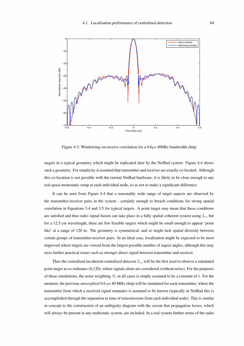
4.1. Localisation performance of centralised detection 84
−0.6 −0.4 −0.2 0 0.2 0.4 0.6−70
−60
−50
−40
−30
−20
−10
0
Time delay (us)
Nor
mal
ised
res
pons
e (d
B)
Hann windowHamming window
Figure 4.3: Windowing-on-receive correlation for a 0.6µs 40Mhz bandwidth chirp
targets in a typical geometry which might be replicated later by the NetRad system. Figure 4.4 shows
such a geometry. For simplicity it assumed that transmitter and receiver are exactly co-located. Although
this co-location is not possible with the current NetRad hardware, it is likely to be close enough to any
real quasi-monostatic setup at each individual node, so as not to make a significant difference.
It can be seen from Figure 4.4 that a reasonably wide range of target aspects are observed by
the transmitter-receiver pairs in the system - certainly enough to breach conditions for strong spatial
correlation in Equations 3.4 and 3.5 for typical targets. A point target may mean that these conditions
are satisfied and thus radio signal fusion can take place in a fully spatial coherent system using Lc, but
for a 12.5 cm wavelength, there are few feasible targets which might be small enough to appear ‘point
like’ at a range of 120 m. The geometry is symmetrical, and so might lack spatial diversity between
certain groups of transmitter-receiver pairs. In an ideal case, localisation might be expected to be most
improved where targets are viewed from the largest possible number of aspect angles, although this may
raise further practical issues such as stronger direct signal between transmitter and receiver.
Thus the centralised incoherent centralised detector Lic will be the first used to observe a simulated
point target at co-ordinates (0,120), where signals alone are considered (without noise). For the purposes
of these simulations, the noise weighting Ni in all cases is simply assumed to be a constant of 1. For the
moment, the previous unweighted 0.6 µs 40 MHz chirp will be simulated for each transmitter, where the
transmitter from which a received signal emanates is assumed to be known (typically in NetRad this is
accomplished through the separation in time of transmissions from each individual node). This is similar
in concept to the construction of an ambiguity diagram with the caveat that propagation losses, which
will always be present in any multistatic system, are included. In a real system further terms of the radar
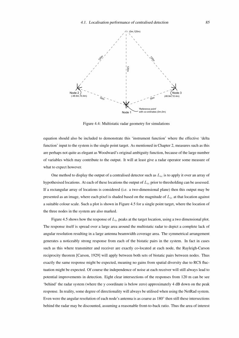
4.1. Localisation performance of centralised detection 85
Figure 4.4: Multistatic radar geometry for simulations
equation should also be included to demonstrate this ‘instrument function’ where the effective ‘delta
function’ input to the system is the single point target. As mentioned in Chapter 2, measures such as this
are perhaps not quite as elegant as Woodward’s original ambiguity function, because of the large number
of variables which may contribute to the output. It will at least give a radar operator some measure of
what to expect however.
One method to display the output of a centralised detector such as Lic is to apply it over an array of
hypothesised locations. At each of these locations the output of Lic prior to thresholding can be assessed.
If a rectangular array of locations is considered (i.e. a two-dimensional plane) then this output may be
presented as an image, where each pixel is shaded based on the magnitude of Lic at that location against
a suitable colour scale. Such a plot is shown in Figure 4.5 for a single point target, where the location of
the three nodes in the system are also marked.
Figure 4.5 shows how the response of Lic peaks at the target location, using a two dimensional plot.
The response itself is spread over a large area around the multistatic radar to depict a complete lack of
angular resolution resulting in a large antenna beamwidth coverage area. The symmetrical arrangement
generates a noticeably strong response from each of the bistatic pairs in the system. In fact in cases
such as this where transmitter and receiver are exactly co-located at each node, the Rayleigh-Carson
reciprocity theorem [Carson, 1929] will apply between both sets of bistatic pairs between nodes. Thus
exactly the same response might be expected, meaning no gains from spatial diversity due to RCS fluc-
tuation might be expected. Of course the independence of noise at each receiver will still always lead to
potential improvements in detection. Eight clear intersections of the responses from 120 m can be see
‘behind’ the radar system (where the y coordinate is below zero) approximately 4 dB down on the peak
response. In reality, some degree of directionality will always be utilised when using the NetRad system.
Even were the angular resolution of each node’s antenna is as coarse as 180 then still these intersections
behind the radar may be discounted, assuming a reasonable front-to-back ratio. Thus the area of interest
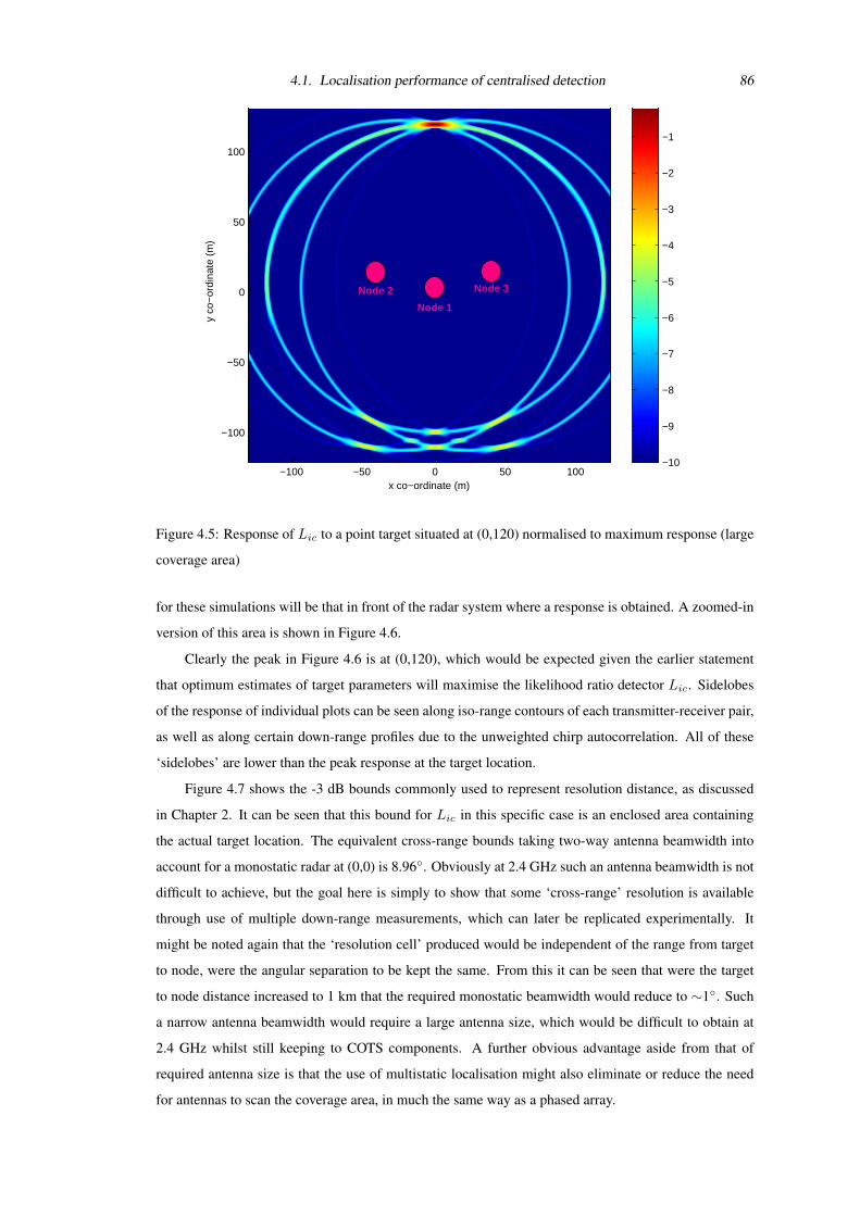
4.1. Localisation performance of centralised detection 86Normalised output of detector Lic /dB
x co−ordinate (m)
y co
−or
dina
te (
m)
−100 −50 0 50 100
−100
−50
0
50
100
−10
−9
−8
−7
−6
−5
−4
−3
−2
−1
0
Node 1
Node 2 Node 3
Figure 4.5: Response of Lic to a point target situated at (0,120) normalised to maximum response (large
coverage area)
for these simulations will be that in front of the radar system where a response is obtained. A zoomed-in
version of this area is shown in Figure 4.6.
Clearly the peak in Figure 4.6 is at (0,120), which would be expected given the earlier statement
that optimum estimates of target parameters will maximise the likelihood ratio detector Lic. Sidelobes
of the response of individual plots can be seen along iso-range contours of each transmitter-receiver pair,
as well as along certain down-range profiles due to the unweighted chirp autocorrelation. All of these
‘sidelobes’ are lower than the peak response at the target location.
Figure 4.7 shows the -3 dB bounds commonly used to represent resolution distance, as discussed
in Chapter 2. It can be seen that this bound for Lic in this specific case is an enclosed area containing
the actual target location. The equivalent cross-range bounds taking two-way antenna beamwidth into
account for a monostatic radar at (0,0) is 8.96. Obviously at 2.4 GHz such an antenna beamwidth is not
difficult to achieve, but the goal here is simply to show that some ‘cross-range’ resolution is available
through use of multiple down-range measurements, which can later be replicated experimentally. It
might be noted again that the ‘resolution cell’ produced would be independent of the range from target
to node, were the angular separation to be kept the same. From this it can be seen that were the target
to node distance increased to 1 km that the required monostatic beamwidth would reduce to ∼1. Such
a narrow antenna beamwidth would require a large antenna size, which would be difficult to obtain at
2.4 GHz whilst still keeping to COTS components. A further obvious advantage aside from that of
required antenna size is that the use of multistatic localisation might also eliminate or reduce the need
for antennas to scan the coverage area, in much the same way as a phased array.
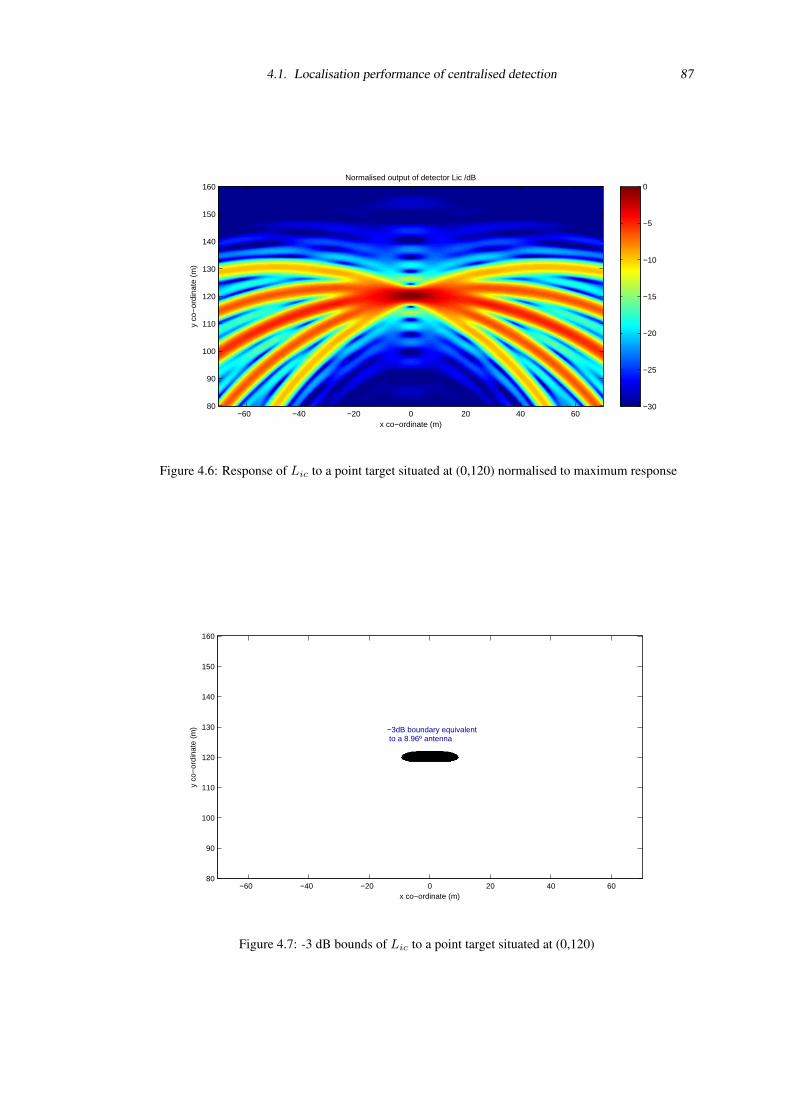
4.1. Localisation performance of centralised detection 87
Normalised output of detector Lic /dB
x co−ordinate (m)
y co
−or
dina
te (
m)
−60 −40 −20 0 20 40 6080
90
100
110
120
130
140
150
160
−30
−25
−20
−15
−10
−5
0
Figure 4.6: Response of Lic to a point target situated at (0,120) normalised to maximum response
x co−ordinate (m)
y co
−or
dina
te (
m)
−60 −40 −20 0 20 40 6080
90
100
110
120
130
140
150
160
−3dB boundary equivalent to a 8.96º antenna
Figure 4.7: -3 dB bounds of Lic to a point target situated at (0,120)

4.1. Localisation performance of centralised detection 88
Given this measure of resolution from a ‘point response’, it is of interest to analyse how detector Lic
now performs if multiple simulated targets are present. Thus the previous plots of ‘resolution’ which are
similar to the ‘multistatic ambiguity functions’ of the literature, can be slightly more rigorously assessed.
For the first simulation, two targets are situated either side of the previous target location of (0,120) - but
now separated by a distance greater than the -3 dB cross range, with targets at (-21,120) and (21,120).
Both targets are again considered point targets with identical RCS values for every aspect. The resulting
output of Lic can be seen in Figure 4.8.
Normalised output of detector Lic /dB
x co−ordinate (m)
y co
−or
dina
te (
m)
−60 −40 −20 0 20 40 6080
90
100
110
120
130
140
150
160
−30
−25
−20
−15
−10
−5
0
Figure 4.8: Response of Lic to two point targets situated at (-21,120) and (21,120) normalised to maxi-
mum response
Again the symmetry of the system gives a particularly large response, in particular for the mono-
static and outlying bistatic cases2. By increasing the lower threshold of Figure 4.8, so that the scale
showed only the top 3 dB of response, the peaks of the detector output can be investigated. This is
shown in Figure 4.9
Clearly two distinct peaks are visible in Figure 4.9, thus the targets might be said to be resolvable.
The specifics as to how target plots (as in discrete x and y values for detected targets) might be produced
from this detector output will be put to one side for a moment, whilst a further situation is considered.
As mentioned in the derivation of detector Lic, it is optimal for the situation where unknown amplitude
relationships exist between signals returned from targets. Independently fluctuating returned signals have
been stated to particularly benefit from use of Lic. Thus a situation where varying signal amplitudes
arrive at receivers can be considered for a very simple modification of the previous two-target example.
For the target at (-21,120) an increase in returned signal of 13 dB is now simulated for the Node 3
monostatic transmitter-receiver pair. Likewise for (21,120) an increase in returned signal of 13 dB is
now simulated for the Node 2 monostatic transmit-receive pair. This situation is quite reasonable, given2In this idealised case, delay and hence phase of signals from both targets are in fact identical for both of these. There are
obviously implications for resolution and interference between signals in such a situation, but these will not be considered in
detail.
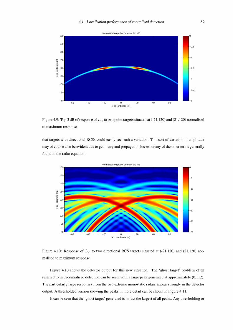
4.1. Localisation performance of centralised detection 89
Normalised output of detector Lic /dB
x co−ordinate (m)
y co
−or
dina
te (
m)
−60 −40 −20 0 20 40 6080
90
100
110
120
130
140
150
160
−3
−2.5
−2
−1.5
−1
−0.5
0
Figure 4.9: Top 3 dB of response of Lic to two point targets situated at (-21,120) and (21,120) normalised
to maximum response
that targets with directional RCSs could easily see such a variation. This sort of variation in amplitude
may of course also be evident due to geometry and propagation losses, or any of the other terms generally
found in the radar equation.
Normalised output of detector Lic /dB
x co−ordinate (m)
y co
−or
dina
te (
m)
−60 −40 −20 0 20 40 6080
90
100
110
120
130
140
150
160
−30
−25
−20
−15
−10
−5
0
Figure 4.10: Response of Lic to two directional RCS targets situated at (-21,120) and (21,120) nor-
malised to maximum response
Figure 4.10 shows the detector output for this new situation. The ‘ghost target’ problem often
referred to in decentralised detection can be seen, with a large peak generated at approximately (0,112).
The particularly large responses from the two extreme monostatic radars appear strongly in the detector
output. A thresholded version showing the peaks in more detail can be shown in Figure 4.11.
It can be seen that the ‘ghost target’ generated is in fact the largest of all peaks. Any thresholding or
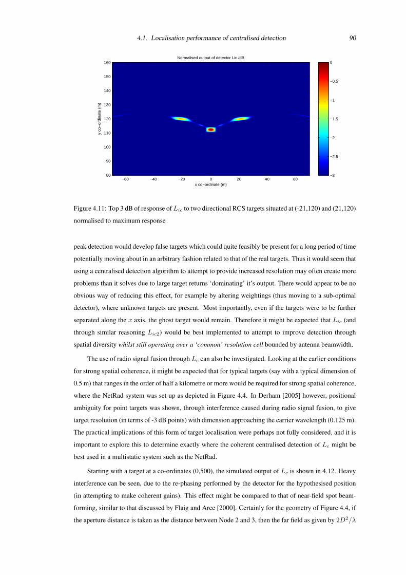
4.1. Localisation performance of centralised detection 90
Normalised output of detector Lic /dB
x co−ordinate (m)
y co
−or
dina
te (
m)
−60 −40 −20 0 20 40 6080
90
100
110
120
130
140
150
160
−3
−2.5
−2
−1.5
−1
−0.5
0
Figure 4.11: Top 3 dB of response ofLic to two directional RCS targets situated at (-21,120) and (21,120)
normalised to maximum response
peak detection would develop false targets which could quite feasibly be present for a long period of time
potentially moving about in an arbitrary fashion related to that of the real targets. Thus it would seem that
using a centralised detection algorithm to attempt to provide increased resolution may often create more
problems than it solves due to large target returns ‘dominating’ it’s output. There would appear to be no
obvious way of reducing this effect, for example by altering weightings (thus moving to a sub-optimal
detector), where unknown targets are present. Most importantly, even if the targets were to be further
separated along the x axis, the ghost target would remain. Therefore it might be expected that Lic (and
through similar reasoning Lic2) would be best implemented to attempt to improve detection through
spatial diversity whilst still operating over a ‘common’ resolution cell bounded by antenna beamwidth.
The use of radio signal fusion through Lc can also be investigated. Looking at the earlier conditions
for strong spatial coherence, it might be expected that for typical targets (say with a typical dimension of
0.5 m) that ranges in the order of half a kilometre or more would be required for strong spatial coherence,
where the NetRad system was set up as depicted in Figure 4.4. In Derham [2005] however, positional
ambiguity for point targets was shown, through interference caused during radio signal fusion, to give
target resolution (in terms of -3 dB points) with dimension approaching the carrier wavelength (0.125 m).
The practical implications of this form of target localisation were perhaps not fully considered, and it is
important to explore this to determine exactly where the coherent centralised detection of Lc might be
best used in a multistatic system such as the NetRad.
Starting with a target at a co-ordinates (0,500), the simulated output of Lc is shown in 4.12. Heavy
interference can be seen, due to the re-phasing performed by the detector for the hypothesised position
(in attempting to make coherent gains). This effect might be compared to that of near-field spot beam-
forming, similar to that discussed by Flaig and Arce [2000]. Certainly for the geometry of Figure 4.4, if
the aperture distance is taken as the distance between Node 2 and 3, then the far field as given by 2D2/λ
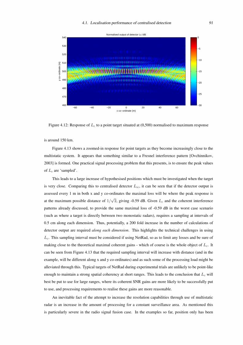
4.1. Localisation performance of centralised detection 91
Normalised output of detector Lc /dB
x co−ordinate (m)
y co
−or
dina
te (
m)
−60 −40 −20 0 20 40 60460
470
480
490
500
510
520
530
540
−30
−25
−20
−15
−10
−5
0
Figure 4.12: Response of Lc to a point target situated at (0,500) normalised to maximum response
is around 150 km.
Figure 4.13 shows a zoomed-in response for point targets as they become increasingly close to the
multistatic system. It appears that something similar to a Fresnel interference pattern [Ovchinnikov,
2003] is formed. One practical signal processing problem that this presents, is to ensure the peak values
of Lc are ‘sampled’.
This leads to a large increase of hypothesised positions which must be investigated when the target
is very close. Comparing this to centralised detector Lic, it can be seen that if the detector output is
assessed every 1 m in both x and y co-ordinates the maximal loss will be where the peak response is
at the maximum possible distance of 1/√
2, giving -0.59 dB. Given Lc and the coherent interference
patterns already discussed, to provide the same maximal loss of -0.59 dB in the worst case scenario
(such as where a target is directly between two monostatic radars), requires a sampling at intervals of
0.5 cm along each dimension. Thus, potentially, a 200 fold increase in the number of calculations of
detector output are required along each dimension. This highlights the technical challenges in using
Lc. This sampling interval must be considered if using NetRad, so as to limit any losses and be sure of
making close to the theoretical maximal coherent gains - which of course is the whole object of Lc. It
can be seen from Figure 4.13 that the required sampling interval will increase with distance (and in the
example, will be different along x and y co-ordinates) and as such some of the processing load might be
alleviated through this. Typical targets of NetRad during experimental trials are unlikely to be point-like
enough to maintain a strong spatial coherency at short ranges. This leads to the conclusion that Lc will
best be put to use for large ranges, where its coherent SNR gains are more likely to be successfully put
to use, and processing requirements to realise these gains are more reasonable.
An inevitable fact of the attempt to increase the resolution capabilities through use of multistatic
radar is an increase in the amount of processing for a constant surveillance area. As mentioned this
is particularly severe in the radio signal fusion case. In the examples so far, position only has been
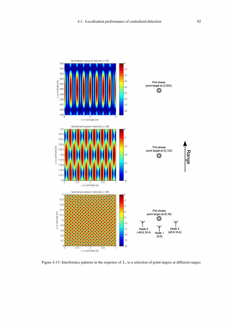
4.1. Localisation performance of centralised detection 92
Figure 4.13: Interference patterns in the response of Lc to a selection of point targets at different ranges
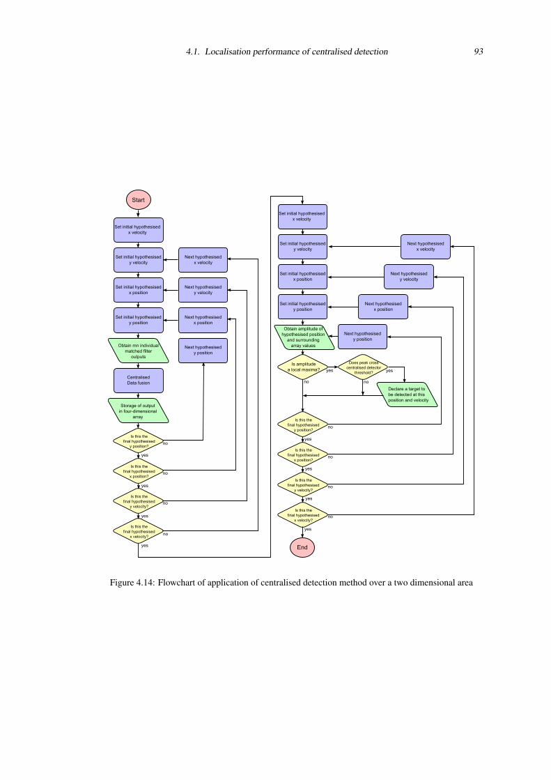
4.1. Localisation performance of centralised detection 93
Figure 4.14: Flowchart of application of centralised detection method over a two dimensional area
4.2. Localisation performance of decentralised detection 94
considered. To be able to increase resolution capabilities between moving targets Doppler information
can also be accounted for, as detailed for all centralised detectors in Chapter 3. In the two-dimensional
case this leads to four-dimensional output, to account for the velocity vector at each discrete location
considered. This increase in dimensionality leads to a large increase in processing. For example, if the
area of Figures 4.5 to 4.11 are sampled at 1 m intervals (a fraction of down-range resolution) along each
axis, then a 140×180 grid is formed - meaning 25200 different applications of the centralised detection
algorithms are required. For each of these applications the hypothesised time delay inputs to the matched
filter banks of Equation 3.21 must be determined by Equation 3.22. To avoid significant losses of the
matched filter output the ‘sampling rate’ of the parameters (location, velocity) to be investigated must
be a fraction of the down-range resolution for video signal fusion, or the carrier wavelength for radio
signal fusion. If velocity were to require a similar number of applications as position in this example,
then the total number is effectively squared again, leading to approximately 6.3 × 10⁸ applications of
the centralised detection algorithm. To reduce both the problems with ‘ghost targets’ and this large
processing overhead, alternative algorithmic methods such as decentralised detection might be explored.
4.2 Localisation performance of decentralised detectionDecentralised target detection offers potential solutions to some of the problems encountered in trying
to provide improved localisation using down-range measurements only. The thresholding of individual
transmitter-receiver pairs prior to data fusion may limit the ability of a single return to dominate the
detector output as shown in the centralised examples. Given that thresholding is a reduction in informa-
tion, reduced communications bandwidth between receivers will be required. Thus system design may
be simplified and it may be easier to network existing radar into a multistatic system. The reduction in
information may also lead to a decrease in the large amount of processing mentioned in the centralised
case.
4.2.1 Application of likelihood ratio detectors over parameters
A similar plot to Figure 4.7 can be generated, but this time using Ld2 to demonstrate decentralised detec-
tion. Of course, applying the likelihood ratio over location and velocity parameters as in the centralised
case will mean that the earlier problem of immense processing requirements remains. The threshold
of all receivers in this simulation are set 10 dB down on the response expected from the point target at
(0,120). In reality these thresholds might be set to give a certain false alarm probability, but setting a
nominal value for the moment is of use to demonstrate a similar ‘point response’ as in the centralised
case, shown in Figure 4.15.
Clearly there are regions around the target where different numbers of individual detections occur,
although it is noted that only towards larger possible values of threshold (z′0 ≥ 5) that a single enclosed
area is seen over the coverage area shown by the plot. The OR decision rule (z′0 = 1) will readily
detect a target given a crossing of individual threshold by a single down-range profile and thus might
be expected to utilise antenna information to produce a two or three dimensional position estimate. The
harsher AND decision rule (z′0 = 9) provides the smallest enclosed area, and perhaps demonstrates a
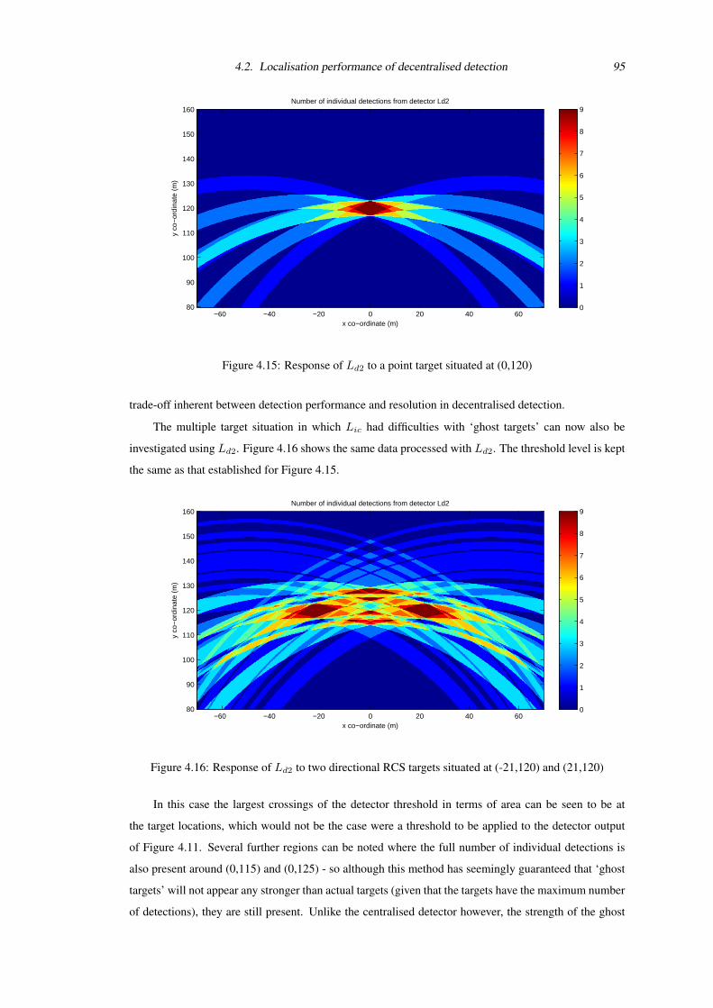
4.2. Localisation performance of decentralised detection 95
Number of individual detections from detector Ld2
x co−ordinate (m)
y co
−or
dina
te (
m)
−60 −40 −20 0 20 40 6080
90
100
110
120
130
140
150
160
0
1
2
3
4
5
6
7
8
9
Figure 4.15: Response of Ld2 to a point target situated at (0,120)
trade-off inherent between detection performance and resolution in decentralised detection.
The multiple target situation in which Lic had difficulties with ‘ghost targets’ can now also be
investigated using Ld2. Figure 4.16 shows the same data processed with Ld2. The threshold level is kept
the same as that established for Figure 4.15.
Number of individual detections from detector Ld2
x co−ordinate (m)
y co
−or
dina
te (
m)
−60 −40 −20 0 20 40 6080
90
100
110
120
130
140
150
160
0
1
2
3
4
5
6
7
8
9
Figure 4.16: Response of Ld2 to two directional RCS targets situated at (-21,120) and (21,120)
In this case the largest crossings of the detector threshold in terms of area can be seen to be at
the target locations, which would not be the case were a threshold to be applied to the detector output
of Figure 4.11. Several further regions can be noted where the full number of individual detections is
also present around (0,115) and (0,125) - so although this method has seemingly guaranteed that ‘ghost
targets’ will not appear any stronger than actual targets (given that the targets have the maximum number
of detections), they are still present. Unlike the centralised detector however, the strength of the ghost
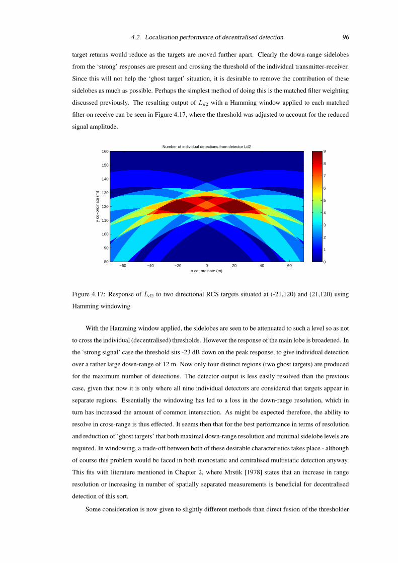
4.2. Localisation performance of decentralised detection 96
target returns would reduce as the targets are moved further apart. Clearly the down-range sidelobes
from the ‘strong’ responses are present and crossing the threshold of the individual transmitter-receiver.
Since this will not help the ‘ghost target’ situation, it is desirable to remove the contribution of these
sidelobes as much as possible. Perhaps the simplest method of doing this is the matched filter weighting
discussed previously. The resulting output of Ld2 with a Hamming window applied to each matched
filter on receive can be seen in Figure 4.17, where the threshold was adjusted to account for the reduced
signal amplitude.
Number of individual detections from detector Ld2
x co−ordinate (m)
y co
−or
dina
te (
m)
−60 −40 −20 0 20 40 6080
90
100
110
120
130
140
150
160
0
1
2
3
4
5
6
7
8
9
Figure 4.17: Response of Ld2 to two directional RCS targets situated at (-21,120) and (21,120) using
Hamming windowing
With the Hamming window applied, the sidelobes are seen to be attenuated to such a level so as not
to cross the individual (decentralised) thresholds. However the response of the main lobe is broadened. In
the ‘strong signal’ case the threshold sits -23 dB down on the peak response, to give individual detection
over a rather large down-range of 12 m. Now only four distinct regions (two ghost targets) are produced
for the maximum number of detections. The detector output is less easily resolved than the previous
case, given that now it is only where all nine individual detectors are considered that targets appear in
separate regions. Essentially the windowing has led to a loss in the down-range resolution, which in
turn has increased the amount of common intersection. As might be expected therefore, the ability to
resolve in cross-range is thus effected. It seems then that for the best performance in terms of resolution
and reduction of ‘ghost targets’ that both maximal down-range resolution and minimal sidelobe levels are
required. In windowing, a trade-off between both of these desirable characteristics takes place - although
of course this problem would be faced in both monostatic and centralised multistatic detection anyway.
This fits with literature mentioned in Chapter 2, where Mrstik [1978] states that an increase in range
resolution or increasing in number of spatially separated measurements is beneficial for decentralised
detection of this sort.
Some consideration is now given to slightly different methods than direct fusion of the thresholder
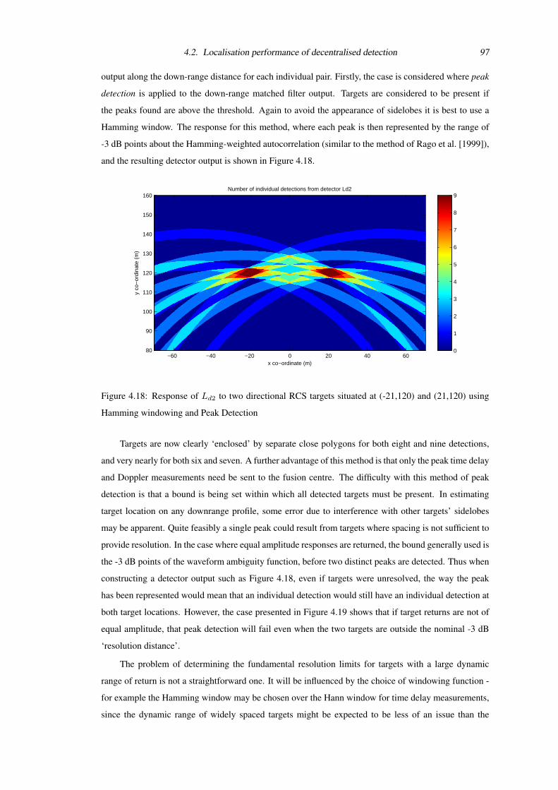
4.2. Localisation performance of decentralised detection 97
output along the down-range distance for each individual pair. Firstly, the case is considered where peak
detection is applied to the down-range matched filter output. Targets are considered to be present if
the peaks found are above the threshold. Again to avoid the appearance of sidelobes it is best to use a
Hamming window. The response for this method, where each peak is then represented by the range of
-3 dB points about the Hamming-weighted autocorrelation (similar to the method of Rago et al. [1999]),
and the resulting detector output is shown in Figure 4.18.
Number of individual detections from detector Ld2
x co−ordinate (m)
y co
−or
dina
te (
m)
−60 −40 −20 0 20 40 6080
90
100
110
120
130
140
150
160
0
1
2
3
4
5
6
7
8
9
Figure 4.18: Response of Ld2 to two directional RCS targets situated at (-21,120) and (21,120) using
Hamming windowing and Peak Detection
Targets are now clearly ‘enclosed’ by separate close polygons for both eight and nine detections,
and very nearly for both six and seven. A further advantage of this method is that only the peak time delay
and Doppler measurements need be sent to the fusion centre. The difficulty with this method of peak
detection is that a bound is being set within which all detected targets must be present. In estimating
target location on any downrange profile, some error due to interference with other targets’ sidelobes
may be apparent. Quite feasibly a single peak could result from targets where spacing is not sufficient to
provide resolution. In the case where equal amplitude responses are returned, the bound generally used is
the -3 dB points of the waveform ambiguity function, before two distinct peaks are detected. Thus when
constructing a detector output such as Figure 4.18, even if targets were unresolved, the way the peak
has been represented would mean that an individual detection would still have an individual detection at
both target locations. However, the case presented in Figure 4.19 shows that if target returns are not of
equal amplitude, that peak detection will fail even when the two targets are outside the nominal -3 dB
‘resolution distance’.
The problem of determining the fundamental resolution limits for targets with a large dynamic
range of return is not a straightforward one. It will be influenced by the choice of windowing function -
for example the Hamming window may be chosen over the Hann window for time delay measurements,
since the dynamic range of widely spaced targets might be expected to be less of an issue than the
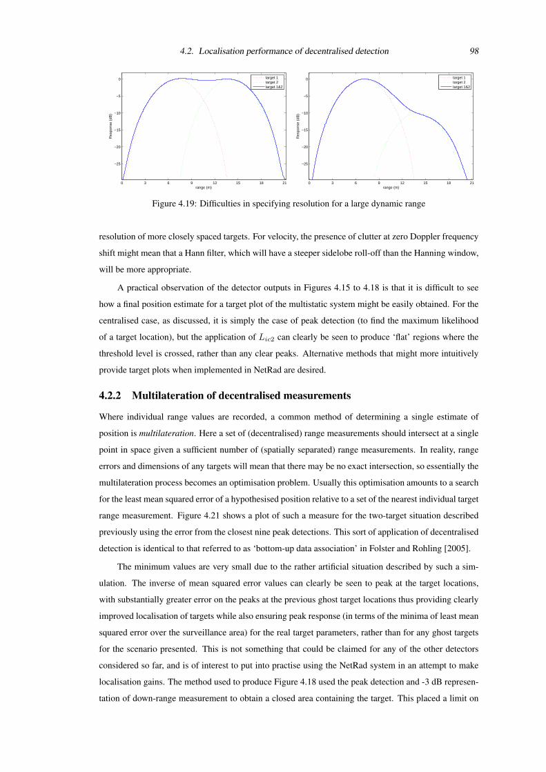
4.2. Localisation performance of decentralised detection 98
0 3 6 9 12 15 18 21
−25
−20
−15
−10
−5
0
range (m)
Res
pons
e (d
B)
target 1target 2target 1&2
0 3 6 9 12 15 18 21
−25
−20
−15
−10
−5
0
range (m)
Res
pons
e (d
B)
target 1target 2target 1&2
Figure 4.19: Difficulties in specifying resolution for a large dynamic range
resolution of more closely spaced targets. For velocity, the presence of clutter at zero Doppler frequency
shift might mean that a Hann filter, which will have a steeper sidelobe roll-off than the Hanning window,
will be more appropriate.
A practical observation of the detector outputs in Figures 4.15 to 4.18 is that it is difficult to see
how a final position estimate for a target plot of the multistatic system might be easily obtained. For the
centralised case, as discussed, it is simply the case of peak detection (to find the maximum likelihood
of a target location), but the application of Lic2 can clearly be seen to produce ‘flat’ regions where the
threshold level is crossed, rather than any clear peaks. Alternative methods that might more intuitively
provide target plots when implemented in NetRad are desired.
4.2.2 Multilateration of decentralised measurements
Where individual range values are recorded, a common method of determining a single estimate of
position is multilateration. Here a set of (decentralised) range measurements should intersect at a single
point in space given a sufficient number of (spatially separated) range measurements. In reality, range
errors and dimensions of any targets will mean that there may be no exact intersection, so essentially the
multilateration process becomes an optimisation problem. Usually this optimisation amounts to a search
for the least mean squared error of a hypothesised position relative to a set of the nearest individual target
range measurement. Figure 4.21 shows a plot of such a measure for the two-target situation described
previously using the error from the closest nine peak detections. This sort of application of decentralised
detection is identical to that referred to as ‘bottom-up data association’ in Folster and Rohling [2005].
The minimum values are very small due to the rather artificial situation described by such a sim-
ulation. The inverse of mean squared error values can clearly be seen to peak at the target locations,
with substantially greater error on the peaks at the previous ghost target locations thus providing clearly
improved localisation of targets while also ensuring peak response (in terms of the minima of least mean
squared error over the surveillance area) for the real target parameters, rather than for any ghost targets
for the scenario presented. This is not something that could be claimed for any of the other detectors
considered so far, and is of interest to put into practise using the NetRad system in an attempt to make
localisation gains. The method used to produce Figure 4.18 used the peak detection and -3 dB represen-
tation of down-range measurement to obtain a closed area containing the target. This placed a limit on
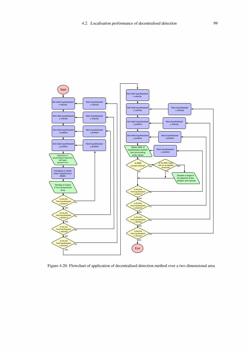
4.2. Localisation performance of decentralised detection 99
Figure 4.20: Flowchart of application of decentralised detection method over a two dimensional area
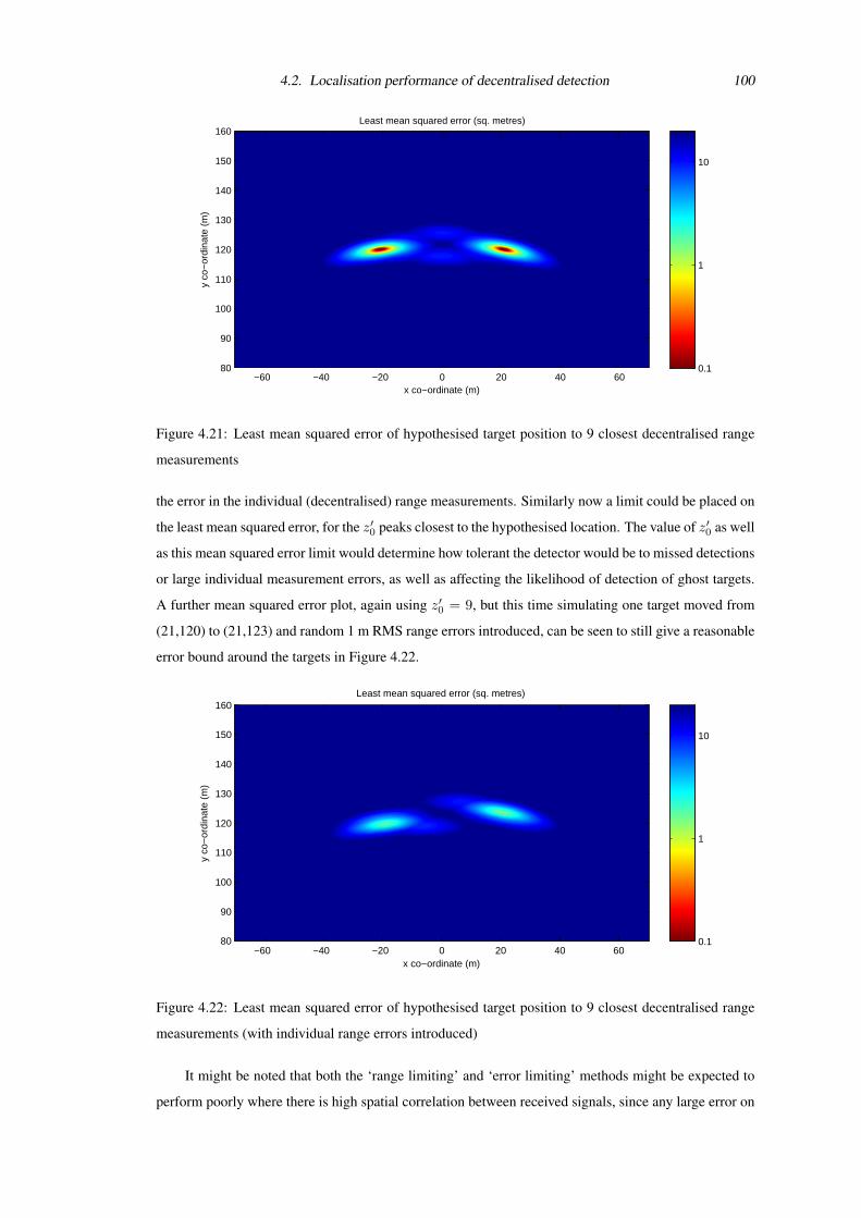
4.2. Localisation performance of decentralised detection 100
Least mean squared error (sq. metres)
x co−ordinate (m)
y co
−or
dina
te (
m)
−60 −40 −20 0 20 40 6080
90
100
110
120
130
140
150
160
0.1
1
10
Figure 4.21: Least mean squared error of hypothesised target position to 9 closest decentralised range
measurements
the error in the individual (decentralised) range measurements. Similarly now a limit could be placed on
the least mean squared error, for the z′0 peaks closest to the hypothesised location. The value of z′0 as well
as this mean squared error limit would determine how tolerant the detector would be to missed detections
or large individual measurement errors, as well as affecting the likelihood of detection of ghost targets.
A further mean squared error plot, again using z′0 = 9, but this time simulating one target moved from
(21,120) to (21,123) and random 1 m RMS range errors introduced, can be seen to still give a reasonable
error bound around the targets in Figure 4.22.
Least mean squared error (sq. metres)
x co−ordinate (m)
y co
−or
dina
te (
m)
−60 −40 −20 0 20 40 6080
90
100
110
120
130
140
150
160
0.1
1
10
Figure 4.22: Least mean squared error of hypothesised target position to 9 closest decentralised range
measurements (with individual range errors introduced)
It might be noted that both the ‘range limiting’ and ‘error limiting’ methods might be expected to
perform poorly where there is high spatial correlation between received signals, since any large error on
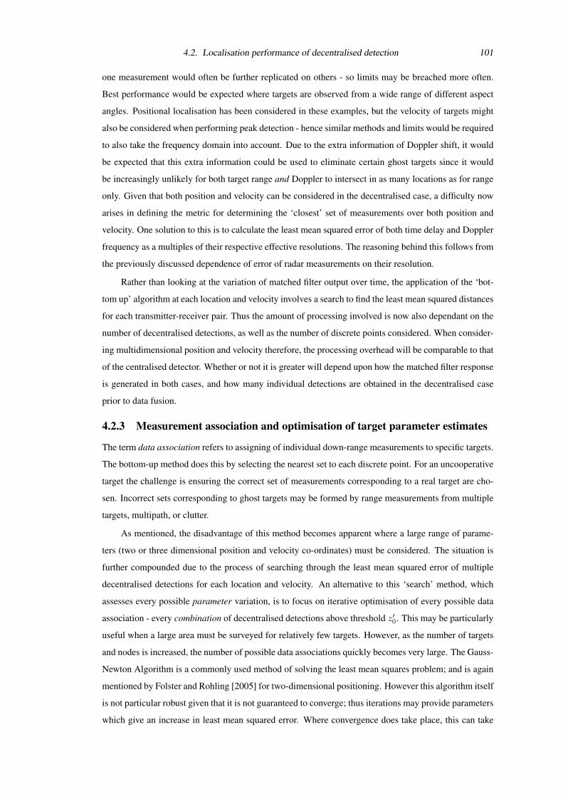
4.2. Localisation performance of decentralised detection 101
one measurement would often be further replicated on others - so limits may be breached more often.
Best performance would be expected where targets are observed from a wide range of different aspect
angles. Positional localisation has been considered in these examples, but the velocity of targets might
also be considered when performing peak detection - hence similar methods and limits would be required
to also take the frequency domain into account. Due to the extra information of Doppler shift, it would
be expected that this extra information could be used to eliminate certain ghost targets since it would
be increasingly unlikely for both target range and Doppler to intersect in as many locations as for range
only. Given that both position and velocity can be considered in the decentralised case, a difficulty now
arises in defining the metric for determining the ‘closest’ set of measurements over both position and
velocity. One solution to this is to calculate the least mean squared error of both time delay and Doppler
frequency as a multiples of their respective effective resolutions. The reasoning behind this follows from
the previously discussed dependence of error of radar measurements on their resolution.
Rather than looking at the variation of matched filter output over time, the application of the ‘bot-
tom up’ algorithm at each location and velocity involves a search to find the least mean squared distances
for each transmitter-receiver pair. Thus the amount of processing involved is now also dependant on the
number of decentralised detections, as well as the number of discrete points considered. When consider-
ing multidimensional position and velocity therefore, the processing overhead will be comparable to that
of the centralised detector. Whether or not it is greater will depend upon how the matched filter response
is generated in both cases, and how many individual detections are obtained in the decentralised case
prior to data fusion.
4.2.3 Measurement association and optimisation of target parameter estimates
The term data association refers to assigning of individual down-range measurements to specific targets.
The bottom-up method does this by selecting the nearest set to each discrete point. For an uncooperative
target the challenge is ensuring the correct set of measurements corresponding to a real target are cho-
sen. Incorrect sets corresponding to ghost targets may be formed by range measurements from multiple
targets, multipath, or clutter.
As mentioned, the disadvantage of this method becomes apparent where a large range of parame-
ters (two or three dimensional position and velocity co-ordinates) must be considered. The situation is
further compounded due to the process of searching through the least mean squared error of multiple
decentralised detections for each location and velocity. An alternative to this ‘search’ method, which
assesses every possible parameter variation, is to focus on iterative optimisation of every possible data
association - every combination of decentralised detections above threshold z′0. This may be particularly
useful when a large area must be surveyed for relatively few targets. However, as the number of targets
and nodes is increased, the number of possible data associations quickly becomes very large. The Gauss-
Newton Algorithm is a commonly used method of solving the least mean squares problem; and is again
mentioned by Folster and Rohling [2005] for two-dimensional positioning. However this algorithm itself
is not particular robust given that it is not guaranteed to converge; thus iterations may provide parameters
which give an increase in least mean squared error. Where convergence does take place, this can take
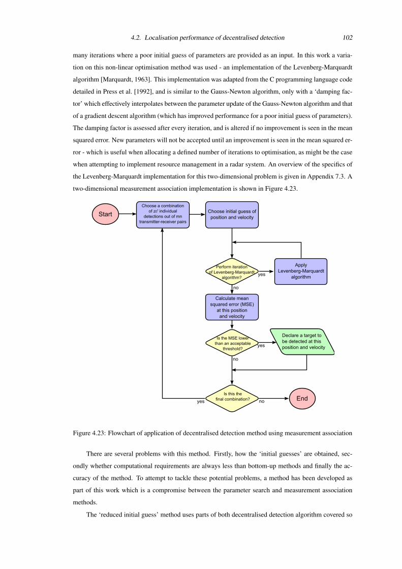
4.2. Localisation performance of decentralised detection 102
many iterations where a poor initial guess of parameters are provided as an input. In this work a varia-
tion on this non-linear optimisation method was used - an implementation of the Levenberg-Marquardt
algorithm [Marquardt, 1963]. This implementation was adapted from the C programming language code
detailed in Press et al. [1992], and is similar to the Gauss-Newton algorithm, only with a ‘damping fac-
tor’ which effectively interpolates between the parameter update of the Gauss-Newton algorithm and that
of a gradient descent algorithm (which has improved performance for a poor initial guess of parameters).
The damping factor is assessed after every iteration, and is altered if no improvement is seen in the mean
squared error. New parameters will not be accepted until an improvement is seen in the mean squared er-
ror - which is useful when allocating a defined number of iterations to optimisation, as might be the case
when attempting to implement resource management in a radar system. An overview of the specifics of
the Levenberg-Marquardt implementation for this two-dimensional problem is given in Appendix 7.3. A
two-dimensional measurement association implementation is shown in Figure 4.23.
Figure 4.23: Flowchart of application of decentralised detection method using measurement association
There are several problems with this method. Firstly, how the ‘initial guesses’ are obtained, sec-
ondly whether computational requirements are always less than bottom-up methods and finally the ac-
curacy of the method. To attempt to tackle these potential problems, a method has been developed as
part of this work which is a compromise between the parameter search and measurement association
methods.
The ‘reduced initial guess’ method uses parts of both decentralised detection algorithm covered so
4.3. Processing requirements of detection algorithms 103
far. Rather than apply the bottom-up method over both position and velocity to effectively produce a
four-dimensional output, the reduced initial guess method uses a single application of the bottom-up
method for position only. This will identify a number of potential targets, which may contain both false
targets and real targets. Obviously no resolution in velocity is available when searching position alone,
so the next stage is to search over a range of hypothesised velocities. However this velocity search
is now only applied at the potential target locations identified in the previous search - rather than at
every possible location. If the number of targets is many orders of magnitude less than the number
of possible target locations, then this will make large savings on processing required by effectively
‘ignoring’ locations where no targets might be positioned. The resulting output will be a series of discrete
positions and velocities. Since these parameters were dealt with separately, it is possible that the positions
and velocities will not in fact match to the same set of decentralised measurements. Thus, for each
position and velocity, a final check should be performed to ensure that a set of z′0 measurements can be
found that will have a mean squared error (this time in terms of both time delay and frequency shift)
that is deemed acceptable. Thus the resulting output will be a list of sets of z′0 measurements, linked
to a position and velocity. Any positional errors in the initial bottom-up (positional) application will
propagate to the velocity due to dependence of geometry on Doppler shift. Thus accuracy can be further
improved by passing these ‘initial guesses’ to the Levenberg-Marquardt optimisation algorithm. Figure
4.24 shows a flowchart of this ‘reduced initial guesses’ method.
One modification of this method to attempt to further reduce processing would be to discard the
decentralised measurements outside a given time delay (say twice the resolution) before performing the
‘velocity search’.
4.3 Processing requirements of detection algorithmsAs mentioned, much of the motivation in choice of algorithm may lie on the computational requirements.
It is difficult to quantify these requirements exactly, since some factors such as processing delays will be
rather platform dependant. In the case of NetRad, processing can be done without any time requirements
on any suitable available platform. Thus, to a point, the system has rather more flexibility than might be
expected of a commercial system built for a specific real-time purpose.
Some simple analysis of the likely processing involved is a useful tool to demonstrate the processing
overhead inherent in multistatic data fusion. This will be undertaken for the algorithms described by the
flowcharts given in Figures 4.14, 4.20, 4.23 and 4.24. The resulting estimates of required data storage,
processing operations and transmission of data to the fusion centre are tabulated in Table 4.1. Here
an ‘operation’ is considered to be either the summation of a matched filter value, comparison of an
amplitude to a surrounding array value, or the calculation of a mean squared error from a decentralised
detection. The application of an iteration of the Levenberg-Marquardt algorithm is estimated at around
150 such operations. For data storage, a single 32 bit float is assumed to represent any stored real value.
Initial processing of matched filtering will have near identical processing requirements to the typical
monostatic case so will not be considered in great detail. Some interpolation may be required if the
baseband sampling frequency is not deemed sufficient. This may be done through several methods such
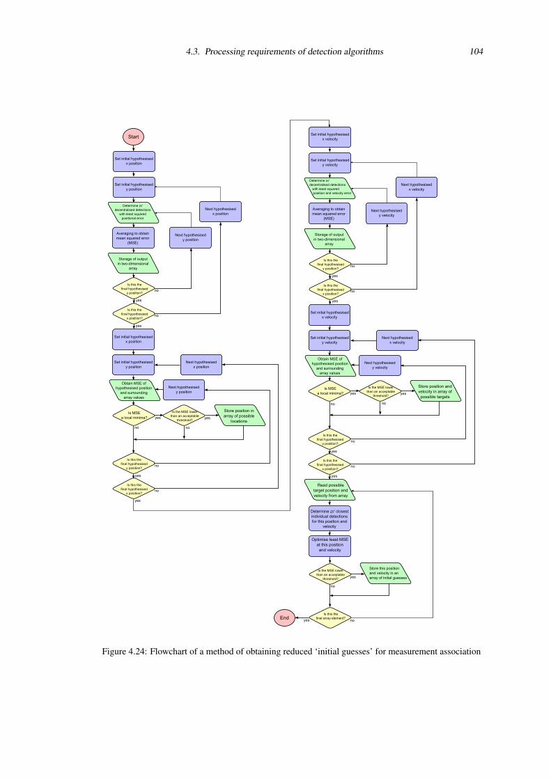
4.3. Processing requirements of detection algorithms 104
Figure 4.24: Flowchart of a method of obtaining reduced ‘initial guesses’ for measurement association

4.3. Processing requirements of detection algorithms 105
Algorithm Storage (bytes) Operations Data transmis-
sion (bytes per
node)
Centralised detection 8N2rd + 4nxnynvxnvy + 8t nxnynvxnvy(N2 + 1) 8Nrd
Bottom-up data asso-
ciation
8N2t + 4nxnynvxnvy + 8t nxnynvxnvy(N2t + 1) 8Nt
Measurement associ-
ation
8tN2!/(z′0!(N2 − z′0)!) 150tN2(i+1)N2!/(z′0!(N2−
z′0)!)
8Nt
Reduced initial guess
method
4nxny + 4nvxnvy + 8t N2tnxny + N2t2nvxnvy +
150t(i + 1)
8Nt
Table 4.1: Computational requirements for multistatic data fusion
where N is the number of nodes
r is the number of range bins recorded at each receiver
d is the number of Doppler bins recorded at each receiver
nx is the number of discrete x-coordinate locations considered
ny is the number of discrete y-coordinate locations considered
nvx is the number of discrete x-coordinate velocities considered
nvy is the number of discrete y-coordinate velocities considered
t is the number of targets present
z′0 is the secondary decentralised detector threshold
i is the number of iterations of the Levenberg-Marquardt algorithm
as zero padding in the frequency domain, linear interpolation or application of an array of fractional
delay filters. One difference to the mono/bistatic case is that if a system of N nodes have transmit
and receive capabilities to/from every other node (such as in the case of NetRad) then an N2 increase
in total processing during matched filtering might be expected to result (if other radar parameters are
kept constant). The actual recorded signal information may or may not be increased, dependant on how
different transmitters are to be resolved (for example, whether orthogonal codes or interleaving of the
same transmitted signal is used).
It may be convenient to apply the matched filter process in parallel at each receiver location. In the
decentralised case this might be the expected method, given that one objective of decentralised detection
is to reduce require communications bandwidth. However in the centralised case where a larger amount
of information, and therefore larger communications bandwidth, is required between nodes and the ‘fu-
sion centre’ it may be prudent to ensure the least amount of necessary data is transmitted. This will often
mean that the unprocessed signal data be sent; with processing leading to an increase in data storage,
such as interpolation or application of filters matched to orthogonal codes, to be performed at the fusion
centre.
Applying the formulas of Table 4.1, some idea of the requirements of each algorithm for likely
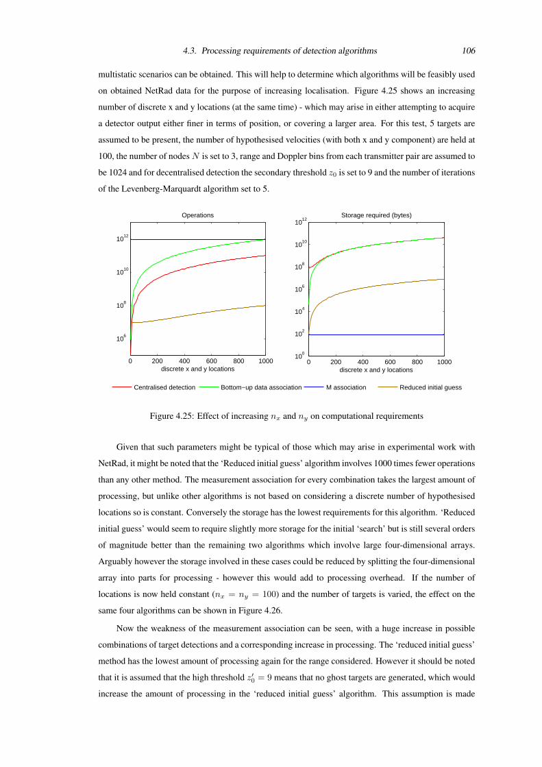
4.3. Processing requirements of detection algorithms 106
multistatic scenarios can be obtained. This will help to determine which algorithms will be feasibly used
on obtained NetRad data for the purpose of increasing localisation. Figure 4.25 shows an increasing
number of discrete x and y locations (at the same time) - which may arise in either attempting to acquire
a detector output either finer in terms of position, or covering a larger area. For this test, 5 targets are
assumed to be present, the number of hypothesised velocities (with both x and y component) are held at
100, the number of nodesN is set to 3, range and Doppler bins from each transmitter pair are assumed to
be 1024 and for decentralised detection the secondary threshold z0 is set to 9 and the number of iterations
of the Levenberg-Marquardt algorithm set to 5.
0 200 400 600 800 1000
106
108
1010
1012
discrete x and y locations
Operations
0 200 400 600 800 100010
0
102
104
106
108
1010
1012
discrete x and y locations
Storage required (bytes)
Centralised detection Bottom−up data association M association Reduced initial guess
Figure 4.25: Effect of increasing nx and ny on computational requirements
Given that such parameters might be typical of those which may arise in experimental work with
NetRad, it might be noted that the ‘Reduced initial guess’ algorithm involves 1000 times fewer operations
than any other method. The measurement association for every combination takes the largest amount of
processing, but unlike other algorithms is not based on considering a discrete number of hypothesised
locations so is constant. Conversely the storage has the lowest requirements for this algorithm. ‘Reduced
initial guess’ would seem to require slightly more storage for the initial ‘search’ but is still several orders
of magnitude better than the remaining two algorithms which involve large four-dimensional arrays.
Arguably however the storage involved in these cases could be reduced by splitting the four-dimensional
array into parts for processing - however this would add to processing overhead. If the number of
locations is now held constant (nx = ny = 100) and the number of targets is varied, the effect on the
same four algorithms can be shown in Figure 4.26.
Now the weakness of the measurement association can be seen, with a huge increase in possible
combinations of target detections and a corresponding increase in processing. The ‘reduced initial guess’
method has the lowest amount of processing again for the range considered. However it should be noted
that it is assumed that the high threshold z′0 = 9 means that no ghost targets are generated, which would
increase the amount of processing in the ‘reduced initial guess’ algorithm. This assumption is made
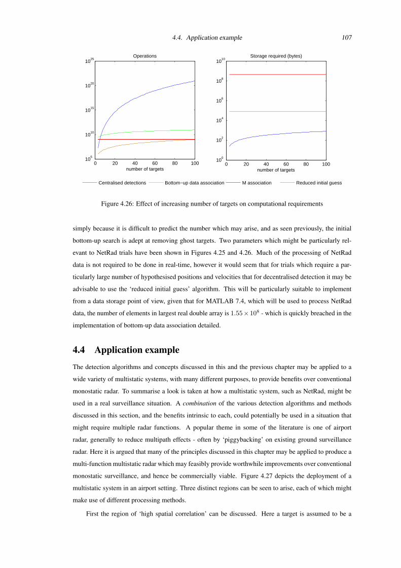
4.4. Application example 107
0 20 40 60 80 10010
5
1010
1015
1020
1025
number of targets
Operations
0 20 40 60 80 10010
0
102
104
106
108
1010
number of targets
Storage required (bytes)
Centralised detections Bottom−up data association M association Reduced initial guess
Figure 4.26: Effect of increasing number of targets on computational requirements
simply because it is difficult to predict the number which may arise, and as seen previously, the initial
bottom-up search is adept at removing ghost targets. Two parameters which might be particularly rel-
evant to NetRad trials have been shown in Figures 4.25 and 4.26. Much of the processing of NetRad
data is not required to be done in real-time, however it would seem that for trials which require a par-
ticularly large number of hypothesised positions and velocities that for decentralised detection it may be
advisable to use the ‘reduced initial guess’ algorithm. This will be particularly suitable to implement
from a data storage point of view, given that for MATLAB 7.4, which will be used to process NetRad
data, the number of elements in largest real double array is 1.55× 10⁸ - which is quickly breached in the
implementation of bottom-up data association detailed.
4.4 Application example
The detection algorithms and concepts discussed in this and the previous chapter may be applied to a
wide variety of multistatic systems, with many different purposes, to provide benefits over conventional
monostatic radar. To summarise a look is taken at how a multistatic system, such as NetRad, might be
used in a real surveillance situation. A combination of the various detection algorithms and methods
discussed in this section, and the benefits intrinsic to each, could potentially be used in a situation that
might require multiple radar functions. A popular theme in some of the literature is one of airport
radar, generally to reduce multipath effects - often by ‘piggybacking’ on existing ground surveillance
radar. Here it is argued that many of the principles discussed in this chapter may be applied to produce a
multi-function multistatic radar which may feasibly provide worthwhile improvements over conventional
monostatic surveillance, and hence be commercially viable. Figure 4.27 depicts the deployment of a
multistatic system in an airport setting. Three distinct regions can be seen to arise, each of which might
make use of different processing methods.
First the region of ‘high spatial correlation’ can be discussed. Here a target is assumed to be a
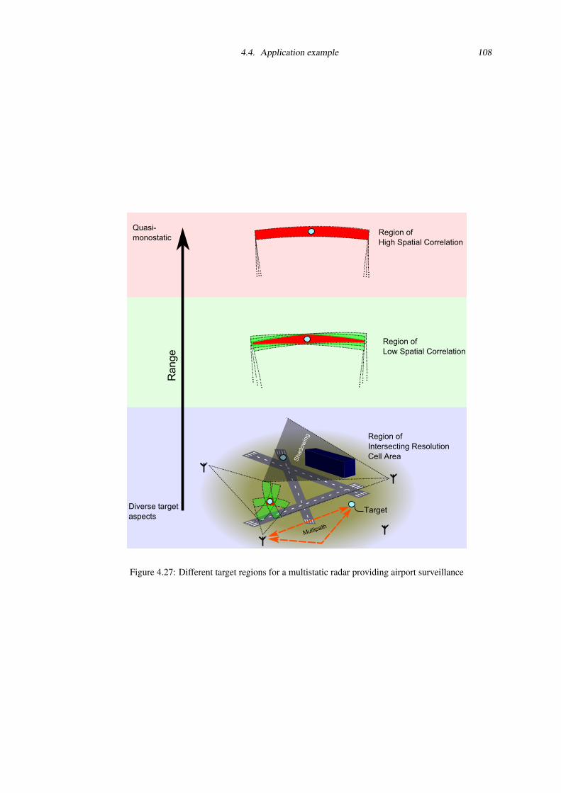
4.4. Application example 108
Figure 4.27: Different target regions for a multistatic radar providing airport surveillance
4.4. Application example 109
large distance from the nodes within the multistatic system. Thus the inequality of Equation 3.4 or 3.5
will be satisfied for targets of interest and returns to all stations will be correlated in amplitude and
phase. In terms of detection, this allows a fully spatially coherent system to make SNR gains equal
to N2 where N is the number of nodes (assuming equal individual transmitter-receiver pair SNRs).
Given that any fluctuations of signal are expected to be the same for each transmitter-receiver pair there
is no advantage to using Lic, Lic2 or Ld, unless full spatial coherence cannot be maintained. From a
localisation point of view, the transmitter-receiver pairs view near-identical target aspects, so localisation
gains from multistatic processing would be very small. With this in mind, it may often be the case,
particularly at higher frequencies, that better localisation is to be obtained through use of antenna-based
cross-range measurements. This is in keeping with assumptions originally made by Chernyak [1998]
in constructing optimal detection algorithms, that all transmitter-receiver pairs have the same individual
‘resolution cell area’. At long ranges, the interference pattern of a centralised detection algorithm Lc
will change very slowly over range, and thus will not require the large number of hypothesised positions
that would be evident were the target to be closer.
Next, the region of ‘low spatial correlation’ is entered as the target moves closer to the multistatic
system. Here the distance to the target is still large, and coverage of the individual resolution cell areas
largely co-incident. However, angular separation is now sufficient so that the inequality of Equation
3.4 or 3.5 no longer holds, and the phase and amplitude of returns are no longer correlated. In this
case coherent gains cannot be made, and Lic or Lic2 may be used for optimal detection performance
- dependant on expected signal strength. In both this and the previous region, the aim is to effectively
operate the multistatic radar similar to a sparse array - where the choice between coherent or incoherent
fusion is similar to the comparison of phased arrays and MIMO systems.
The final region is that of intersecting resolution cells. Here the targets of interest have a distance
comparable to that between nodes in the multistatic system, so that vastly different aspects of them are
visible by different transmitter-receiver pairs. As documented in the literature, in an airport setting there
are often difficulties in localising targets, due to multipath and shadowing effects in operating radar in
this region. At such short ranges it is typically easier to detect targets. Hence sub-optimal methods in
terms of detection, such as Ld, which are advantageous in terms of localisation as shown in this chapter.
A potential exploitation of the different ‘zones’ presented in Figure 4.27 can be based around the
fact that the long range radars looking for distant targets will also transmit and receive energy via antenna
sidelobes. Thus whilst focussing on distant targets and utilising centralised detection algorithms, power
transmitted at a lower level in other directions, which might typically be considered undesirable, may
be used to localise nearby targets using the the decentralised ‘time delay only’ implementation detailed
in this chapter. In this way, it can be seen how the methods described in Chapters 3 and 4 are brought
together to perform different functions in a single multistatic installation. This may have distinct com-
mercial advantages; where new nodes can ‘piggyback’ existing installations to both increase detection
at long ranges and provide improved localisation at close range without the need for two separate radar
installations.
4.5. Summary of localisation performance 110
4.5 Summary of localisation performance
It is clear that additional spatially separate transmitter and receiver pairs complicates previous relatively
simple measures of localisation performance in the monostatic case - namely the down-range resolution
determined by the bandwidth of the radar waveform, and the cross range resolution determined by the an-
tenna beamwidth. Measures of performance in the multistatic case must account for several phenomena
not seen in conventional radar. These mainly arise in the multiple target situation due to the interaction
of the target returns (which has been referred to as data association in the decentralised case).
Given the complexity of assessing localisation performance for every type of scenario, a specific
set-up was considered in this chapter, where different target types were then observed. This allowed for
investigation of the various issues inherent in attempting to localise targets. It could be seen that for
multiple targets, which presumably would be present for the example of airport radar, that the detection
scheme which successfully resolved targets and to produce correct plots of two-dimensional target po-
sition was the use of multilateration following the decentralised detection algorithm Ld2. In effect the
thresholding process in decentralised detection algorithm Ld2 increases the contribution of weaker re-
sponses (hence is sub-optimal in terms of detection) in an attempt to successfully resolve targets through
the use of multiple perspectives. In centralised detection the localisation was judged to be poor in multi-
ple target cases due to peaks of the detector output often occurring as ghost targets rather than at actual
target locations.
It should be noted that results here are dependant on the type of targets and the characteristics of
the multistatic radar. Thus although the expected performance for experimental trials with the same ar-
rangement may be well documented, a different system setup, such as one with a very large number of
nodes and point-like (constant) RCSs, might be expected to provide a very different localisation perfor-
mance. However the same multistatic-specific phenomena discussed in this work would be seen in both
systems. Despite the clear improvement of performance that multilateration algorithms were shown to
demonstrate in this chapter, it could not be claimed that this algorithm is ‘optimal’ at locating and re-
solving targets. Finding such an algorithm is difficult due to the number of variables involved - increased
compared to the ‘optimal detection algorithms’ discussed in Chapter 3 due to the dependence on the
geometry and targets themselves amongst other factors. Improvements over these algorithms could at-
tempt to decrease the ‘cost of resolution’ on detection whilst maintaining localisation performance - an
example being the centralised fusion between transmitter-receiver pairs viewing the same target aspect
(and so with no potential localisation gains) prior to decentralised detection.
This chapter has focussed upon trying to localise targets based on time delay only. There are
purely practical reasons behind this - it was rather simpler to explore localisation gains given the case
of shared antenna beamwidth coverage area. It was also convenient when attempting to later replicate
simulations experimentally - given that the NetRad antennas are positioned by hand! An example of
where time delay only might actually be used was given in the airport example, and further obvious
examples are where low frequencies are used, antenna size is limited, where ERP is limited or where
a wide coverage ‘broadcast’ antenna is made use of for transmission. This also allowed the ‘general
4.5. Summary of localisation performance 111
case’ scenario to be explored - since in assuming no azimuth or elevation information is available, it is
only possible to further improve the localisation obtained. It is possible that at increasingly short ranges
that for some nodes antenna beamwidth information might also be used (and cross-range resolution
becomes comparable to down-range). However, this would certainly increase complexity in terms of
including antenna orientation in the algorithms discussed or arranging antenna beamwidths; methods
such as ‘pulse-chasing’ seen in bistatic radar might be used, as for phased array antennas.
A discussion and approximation of the processing requirements of each algorithm was also pre-
sented - an important issue given the way in which renewed interest in multistatic radar is often quoted
as being due to advances in signal processing, amongst other factors. There is scope for future work
in this area, with further data fusion methods to investigate as well as different surveillance scenarios
to consider. These performance of these algorithms can now be investigated experimentally using the
NetRad system.

Chapter 5
System Design and Development
In this chapter, the hardware development of NetRad necessary to enable testing of the theory presented
in Chapters 3 and 4 is documented. This begins with an initial overview of the system at the start
of the project (and the limitations on experimental trials), followed by details of changes made during
the course of this work. The design of the system used COTS components to adhere to a nominal
system budget of $6000. A fairly open, modular architecture was used in an attempt to facilitate easy
development or changes - which might be required due to the large variety of potential experimental
measurements of interest. Operation was in the ISM band from 2.4-2.45 GHz, which offered advantages
in terms of both readily available component parts and the ease of obtaining permission for transmission1.
5.1 Review of initial system design
The NetRad initially consisted of three nodes where a single 100 MHz clock signal was distributed from
a board attached to the side of Node 1 via a set of three 50 m CAT-6 cables. A further two 50 m cable
links from Node 1 to Nodes 2 and 3 were used to carry both data along a Controller Area Network
(CAN) bus and also incorporated an Multi-point Low Voltage Differential Signalling (M-LVDS) bus for
synchronisation of the timers in each node to within a clock pulse. Figure 5.6 shows a system diagram
of the NetRad at the start of this work.
Figure 5.1: Radar node and system (antennas disconnected)
1The 23 dBm peak transmitted power of the radar falls within the license exempt conditions, however permission was also
obtained for higher power transmissions at various test sites
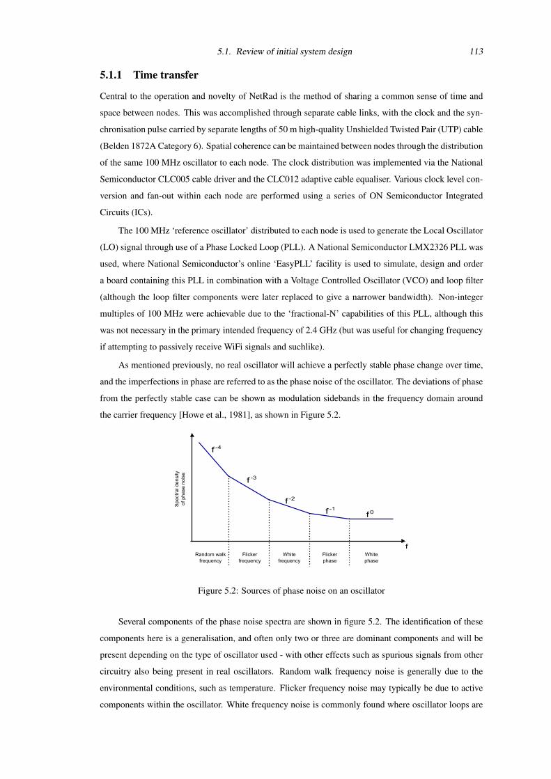
5.1. Review of initial system design 113
5.1.1 Time transfer
Central to the operation and novelty of NetRad is the method of sharing a common sense of time and
space between nodes. This was accomplished through separate cable links, with the clock and the syn-
chronisation pulse carried by separate lengths of 50 m high-quality Unshielded Twisted Pair (UTP) cable
(Belden 1872A Category 6). Spatial coherence can be maintained between nodes through the distribution
of the same 100 MHz oscillator to each node. The clock distribution was implemented via the National
Semiconductor CLC005 cable driver and the CLC012 adaptive cable equaliser. Various clock level con-
version and fan-out within each node are performed using a series of ON Semiconductor Integrated
Circuits (ICs).
The 100 MHz ‘reference oscillator’ distributed to each node is used to generate the Local Oscillator
(LO) signal through use of a Phase Locked Loop (PLL). A National Semiconductor LMX2326 PLL was
used, where National Semiconductor’s online ‘EasyPLL’ facility is used to simulate, design and order
a board containing this PLL in combination with a Voltage Controlled Oscillator (VCO) and loop filter
(although the loop filter components were later replaced to give a narrower bandwidth). Non-integer
multiples of 100 MHz were achievable due to the ‘fractional-N’ capabilities of this PLL, although this
was not necessary in the primary intended frequency of 2.4 GHz (but was useful for changing frequency
if attempting to passively receive WiFi signals and suchlike).
As mentioned previously, no real oscillator will achieve a perfectly stable phase change over time,
and the imperfections in phase are referred to as the phase noise of the oscillator. The deviations of phase
from the perfectly stable case can be shown as modulation sidebands in the frequency domain around
the carrier frequency [Howe et al., 1981], as shown in Figure 5.2.
Figure 5.2: Sources of phase noise on an oscillator
Several components of the phase noise spectra are shown in figure 5.2. The identification of these
components here is a generalisation, and often only two or three are dominant components and will be
present depending on the type of oscillator used - with other effects such as spurious signals from other
circuitry also being present in real oscillators. Random walk frequency noise is generally due to the
environmental conditions, such as temperature. Flicker frequency noise may typically be due to active
components within the oscillator. White frequency noise is commonly found where oscillator loops are
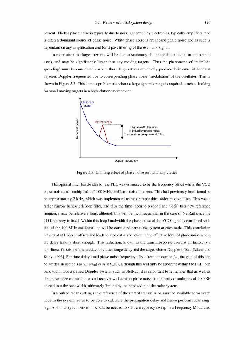
5.1. Review of initial system design 114
present. Flicker phase noise is typically due to noise generated by electronics, typically amplifiers, and
is often a dominant source of phase noise. White phase noise is broadband phase noise and as such is
dependant on any amplification and band-pass filtering of the oscillator signal.
In radar often the largest returns will be due to stationary clutter (or direct signal in the bistatic
case), and may be significantly larger than any moving targets. Thus the phenomena of ‘mainlobe
spreading’ must be considered - where these large returns effectively produce their own sidebands at
adjacent Doppler frequencies due to corresponding phase noise ‘modulation’ of the oscillator. This is
shown in Figure 5.3. This is most problematic where a large dynamic range is required - such as looking
for small moving targets in a high-clutter environment.
Figure 5.3: Limiting effect of phase noise on stationary clutter
The optimal filter bandwidth for the PLL was estimated to be the frequency offset where the VCO
phase noise and ‘multiplied-up’ 100 MHz oscillator noise intersect. This had previously been found to
be approximately 2 kHz, which was implemented using a simple third-order passive filter. This was a
rather narrow bandwidth loop filter, and thus the time taken to respond and ‘lock’ to a new reference
frequency may be relatively long, although this will be inconsequential in the case of NetRad since the
LO frequency is fixed. Within this loop bandwidth the phase noise of the VCO signal is correlated with
that of the 100 MHz oscillator - so will be correlated across the system at each node. This correlation
may exist at Doppler offsets and leads to a potential reduction in the effective level of phase noise where
the delay time is short enough. This reduction, known as the transmit-receive correlation factor, is a
non-linear function of the product of clutter range delay and the target-clutter Doppler offset [Scheer and
Kurtz, 1993]. For time delay t and phase noise frequency offset from the carrier fm, the gain of this can
be written in decibels as 20log10(2sin(πfmt)), although this will only be apparent within the PLL loop
bandwidth. For a pulsed Doppler system, such as NetRad, it is important to remember that as well as
the phase noise of transmitter and receiver will contain phase noise components at multiples of the PRF
aliased into the bandwidth, ultimately limited by the bandwidth of the radar system.
In a pulsed radar system, some reference of the start of transmission must be available across each
node in the system, so as to be able to calculate the propagation delay and hence perform radar rang-
ing. A similar synchronisation would be needed to start a frequency sweep in a Frequency Modulated
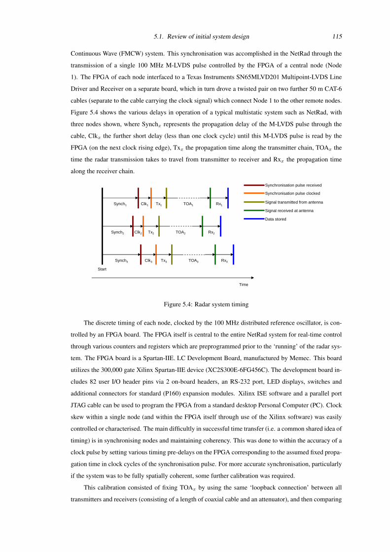
5.1. Review of initial system design 115
Continuous Wave (FMCW) system. This synchronisation was accomplished in the NetRad through the
transmission of a single 100 MHz M-LVDS pulse controlled by the FPGA of a central node (Node
1). The FPGA of each node interfaced to a Texas Instruments SN65MLVD201 Multipoint-LVDS Line
Driver and Receiver on a separate board, which in turn drove a twisted pair on two further 50 m CAT-6
cables (separate to the cable carrying the clock signal) which connect Node 1 to the other remote nodes.
Figure 5.4 shows the various delays in operation of a typical multistatic system such as NetRad, with
three nodes shown, where Synchx represents the propagation delay of the M-LVDS pulse through the
cable, Clkx the further short delay (less than one clock cycle) until this M-LVDS pulse is read by the
FPGA (on the next clock rising edge), Txx the propagation time along the transmitter chain, TOAx the
time the radar transmission takes to travel from transmitter to receiver and Rxx the propagation time
along the receiver chain.
Synch1 Clk1 Tx1 TOA1 Rx1
Synch2 Clk2 Tx2 TOA2 Rx2
Synch3 Clk3 Tx3 TOA3 Rx3
Time
Start
Synchronisation pulse received
Synchronisation pulse clocked
Signal transmitted from antenna
Signal received at antenna
Data stored
Figure 5.4: Radar system timing
The discrete timing of each node, clocked by the 100 MHz distributed reference oscillator, is con-
trolled by an FPGA board. The FPGA itself is central to the entire NetRad system for real-time control
through various counters and registers which are preprogrammed prior to the ‘running’ of the radar sys-
tem. The FPGA board is a Spartan-IIE. LC Development Board, manufactured by Memec. This board
utilizes the 300,000 gate Xilinx Spartan-IIE device (XC2S300E-6FG456C). The development board in-
cludes 82 user I/O header pins via 2 on-board headers, an RS-232 port, LED displays, switches and
additional connectors for standard (P160) expansion modules. Xilinx ISE software and a parallel port
JTAG cable can be used to program the FPGA from a standard desktop Personal Computer (PC). Clock
skew within a single node (and within the FPGA itself through use of the Xilinx software) was easily
controlled or characterised. The main difficultly in successful time transfer (i.e. a common shared idea of
timing) is in synchronising nodes and maintaining coherency. This was done to within the accuracy of a
clock pulse by setting various timing pre-delays on the FPGA corresponding to the assumed fixed propa-
gation time in clock cycles of the synchronisation pulse. For more accurate synchronisation, particularly
if the system was to be fully spatially coherent, some further calibration was required.
This calibration consisted of fixing TOAx by using the same ‘loopback connection’ between all
transmitters and receivers (consisting of a length of coaxial cable and an attenuator), and then comparing
5.1. Review of initial system design 116
the total delay times. Of course the pre-delays should ensure that these delay times were within a sample
of each other (by ensuring the maximum response after cross correlation appeared in the same range
bin for each measurement). Rather than try to correct for phase differences by attempting to estimate
the delay more accurately, the phases of the maximum responses were measured and this difference
was compensated for between nodes. This calibration method was used with node separations up to
12 m. It was noticed that movement of the 50 m clock cables could produce large changes in the
relative phase of LOs, invalidating previous phase compensation. For increasingly large separations this
effect would make it more difficult to calibrate for phase using the ‘loopback connection’, which would
likely suffer from the same effect and be no more accurate than simply characterising the delays of the
synchronisation and clock cables.
5.1.2 Transmitter
Transmission began with a series of commands being uploaded from this FPGA to memory in a Direct
Digital Synthesis (DDS) IC - namely the Analog Devices AD9854 DDS. In keeping with the modular
design the DDS IC was on a separate board to the FPGA, with the programmable ‘user I/O’ pins of
the FPGA evaluation board set appropriately to interconnect the two boards. After commands had been
uploaded the DDS, when enabled by the FPGA, outputted baseband I and Q channels which, following
low-pass image-reject filtering, passed to a Analog Devices AD8346 quadrature modulator. Both the
DDS, filter components and quadrature modulator were on the same Printed Circuit Board (PCB) -
where particular care was taken to ensure correct impedances were used for the microstrip transmission
lines formed on the PCB and that separate power supplies were used to supply both digital and analog
components - to avoid coupling of noise caused by digital switching. The quadrature modulator used the
2.4 GHz LO, to produce an upper sideband output between 2.4 and 2.45 GHz (if the maximum baseband
signal bandwidth of 50 MHz is used). This RF output is then amplified using a Minicircuits ZRL-2400
Low Noise Amplifier (LNA) to a nominal maximum transmit power of 23 dBm at the antenna output.
The DDS operation was complicated by various logic latencies within the chip itself, which had to be
accounted for within the FPGA. This inhibited some phase-coded waveforms to a lower bandwidth,
which could be quite a drawback in any multiple transmitter arrangement. For example, the polyphase
codes specified in Deng [2004a] were limited to 7.1 MHz.
5.1.3 Receiver
The receiver chain, whose input was fed by a separate receive antenna, began with a LNA before being
down-converted by mixing with the LO and then low-pass filtering. The signal was then sampled at
100 MHz using a single channel Analog to Digital Converter (ADC). The digital output of the ADC
was cached in block Random Access Memory (RAM) on the FPGA (which is limited in size to 2048
12 bit samples). These samples were then transferred to the Synchronous Dynamic Random Access
Memory (SDRAM) on a Texas Instruments C6711 DSP starter kit evaluation board. This had to be done
via an ‘Expansion Memory INterface’ (EMIF) bus in time for the block RAM to be free to accept the
next pulse. This process is the limiting factor on the radar PRF - a maximum of 3 kHz for a full set of
2048 samples.
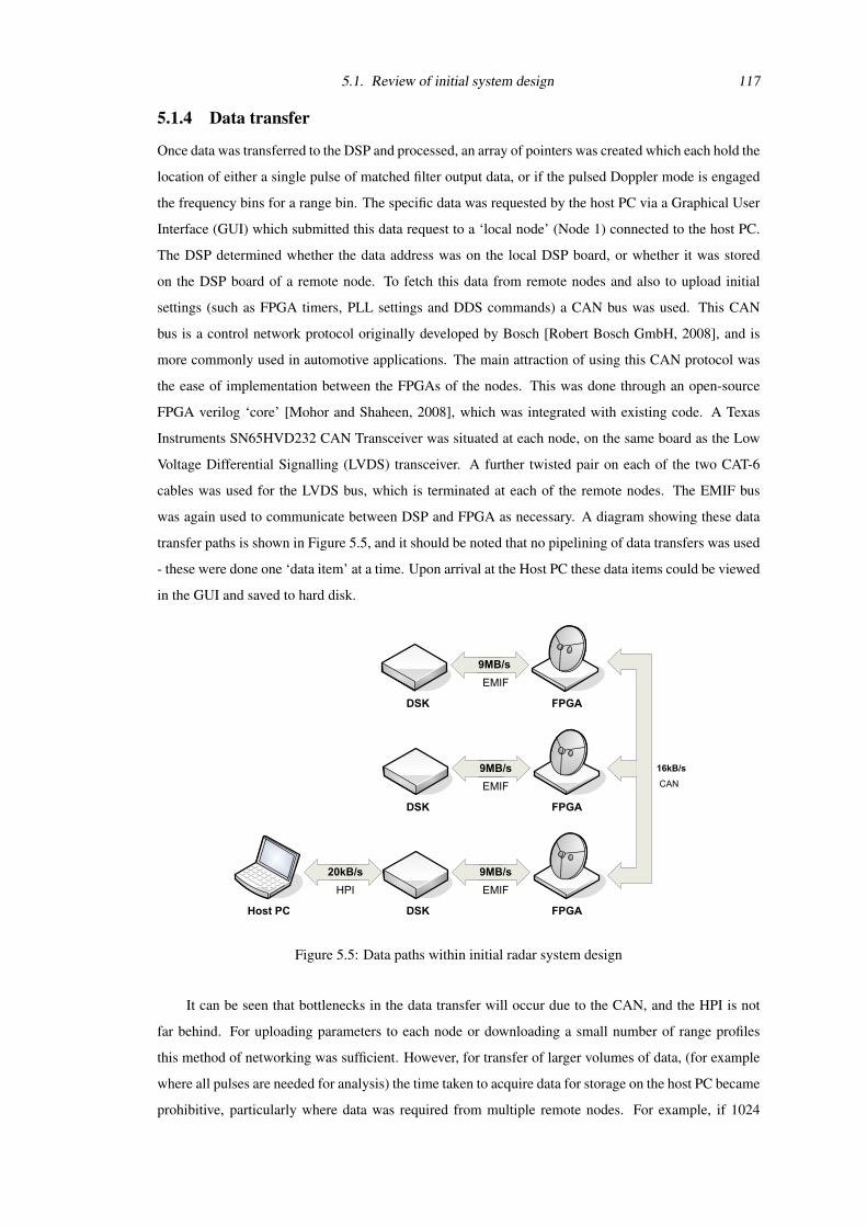
5.1. Review of initial system design 117
5.1.4 Data transfer
Once data was transferred to the DSP and processed, an array of pointers was created which each hold the
location of either a single pulse of matched filter output data, or if the pulsed Doppler mode is engaged
the frequency bins for a range bin. The specific data was requested by the host PC via a Graphical User
Interface (GUI) which submitted this data request to a ‘local node’ (Node 1) connected to the host PC.
The DSP determined whether the data address was on the local DSP board, or whether it was stored
on the DSP board of a remote node. To fetch this data from remote nodes and also to upload initial
settings (such as FPGA timers, PLL settings and DDS commands) a CAN bus was used. This CAN
bus is a control network protocol originally developed by Bosch [Robert Bosch GmbH, 2008], and is
more commonly used in automotive applications. The main attraction of using this CAN protocol was
the ease of implementation between the FPGAs of the nodes. This was done through an open-source
FPGA verilog ‘core’ [Mohor and Shaheen, 2008], which was integrated with existing code. A Texas
Instruments SN65HVD232 CAN Transceiver was situated at each node, on the same board as the Low
Voltage Differential Signalling (LVDS) transceiver. A further twisted pair on each of the two CAT-6
cables was used for the LVDS bus, which is terminated at each of the remote nodes. The EMIF bus
was again used to communicate between DSP and FPGA as necessary. A diagram showing these data
transfer paths is shown in Figure 5.5, and it should be noted that no pipelining of data transfers was used
- these were done one ‘data item’ at a time. Upon arrival at the Host PC these data items could be viewed
in the GUI and saved to hard disk.
16kB/s
CAN
20kB/s
9MB/s
9MB/s
9MB/s
DSK
DSK
DSK
Host PC
FPGA
FPGA
FPGA
EMIF
EMIF
EMIFHPI
Figure 5.5: Data paths within initial radar system design
It can be seen that bottlenecks in the data transfer will occur due to the CAN, and the HPI is not
far behind. For uploading parameters to each node or downloading a small number of range profiles
this method of networking was sufficient. However, for transfer of larger volumes of data, (for example
where all pulses are needed for analysis) the time taken to acquire data for storage on the host PC became
prohibitive, particularly where data was required from multiple remote nodes. For example, if 1024
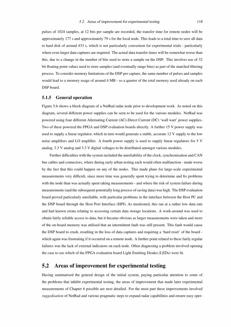
5.2. Areas of improvement for experimental testing 118
pulses of 1024 samples, at 12 bits per sample are recorded, the transfer time for remote nodes will be
approximately 177 s and approximately 79 s for the local node. This leads to a total time to save all data
to hard disk of around 433 s, which is not particularly convenient for experimental trials - particularly
where even larger data captures are required. The actual data transfer times will be somewhat worse than
this, due to a change in the number of bits used to store a sample on the DSP. This involves use of 32
bit floating point values used to store samples (and eventually range bins) as part of the matched filtering
process. To consider memory limitations of the DSP per capture, the same number of pulses and samples
would lead to a memory usage of around 4 MB - so a quarter of the total memory used already on each
DSP board.
5.1.5 General operation
Figure 5.6 shows a block diagram of a NetRad radar node prior to development work. As noted on this
diagram, several different power supplies can be seen to be used for the various modules. NetRad was
powered using four different Alternating Current (AC)-Direct Current (DC) ‘wall wart’ power supplies.
Two of these powered the FPGA and DSP evaluation boards directly. A further 15 V power supply was
used to supply a linear regulator, which in turn would generate a stable, accurate 12 V supply to the low
noise amplifiers and LO amplifier. A fourth power supply is used to supply linear regulators for 5 V
analog, 3.3 V analog and 3.3 V digital voltages to be distributed amongst various modules.
Further difficulties with the system included the unreliability of the clock, synchronisation and CAN
bus cables and connectors, where during early urban testing each would often malfunction - made worse
by the fact that this could happen on any of the nodes. This made plans for large-scale experimental
measurements very difficult, since more time was generally spent trying to determine and fix problems
with the node than was actually spent taking measurements - and where the risk of system failure during
measurements (and the subsequent potentially long process of saving data) was high. The DSP evaluation
board proved particularly unreliable, with particular problems in the interface between the Host PC and
the DSP board through the Host Port Interface (HPI). As mentioned, this ran at a rather low data rate
and had known errata relating to accessing certain data storage locations. A work-around was used to
obtain fairly reliable access to data, but it became obvious as larger measurements were taken and more
of the on-board memory was utilised that an intermittent fault was still present. This fault would cause
the DSP board to crash, resulting in the loss of data captures and requiring a ‘hard reset’ of the board -
which again was frustrating if it occurred on a remote node. A further point related to these fairly regular
failures was the lack of external indicators on each node. Often diagnosing a problem involved opening
the case to see which of the FPGA evaluation board Light Emitting Diodes (LEDs) were lit.
5.2 Areas of improvement for experimental testingHaving summarised the general design of the initial system, paying particular attention to some of
the problems that inhibit experimental testing, the areas of improvement that made later experimental
measurements of Chapter 6 possible are next detailed. For the most part these improvements involved
ruggedisation of NetRad and various pragmatic steps to expand radar capabilities and ensure easy oper-
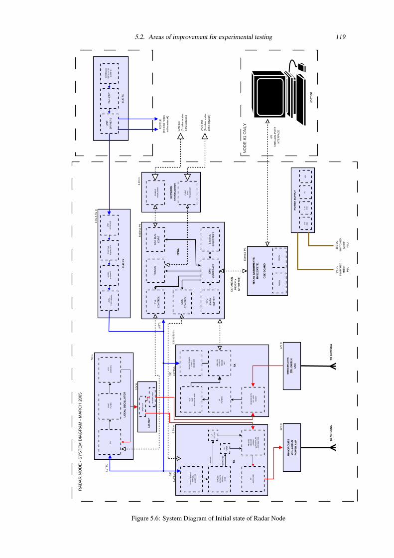
5.2. Areas of improvement for experimental testing 119
TE
XA
S IN
ST
RU
ME
NT
ST
MS
320C
6711
DS
K B
OA
RD
FP
GA
NE
TW
OR
KT
RA
NS
CE
IVE
R
MIN
ICIR
CU
ITS
ZR
L-2
400L
NP
OW
ER
AM
P
TX
RX
CL
K R
X
EX
PA
NS
ION
ME
MO
RY
INT
ER
FA
CE
HP
IP
AR
ALL
EL
PO
RT
INT
ER
FA
CE
HO
ST
PC
AN
ALO
GD
EV
ICE
SA
D98
54D
DS
LPF
ILT
ER
RF
AM
PLI
FIE
R
AN
ALO
GD
EV
ICE
SA
D83
46Q
UA
DR
AT
UR
EM
OD
ULA
TO
R
LPF
ILT
ER
S
AN
ALO
GD
EV
ICE
SA
D94
32A
DC
MIN
ICIR
CU
ITS
ZE
L-43
00M
IXE
R
MIN
ICIR
CU
ITS
ZR
L-2
400L
NL
NA
FLA
SH
SD
RA
M
LO
CA
L O
SC
ILL
AT
OR
PLL
LOO
PF
ILT
ER
LO
AM
P
VC
O24
00 M
Hz
CA
N b
us(T
o ot
her
node
sin
the
netw
ork)
RA
DA
R N
OD
E -
SY
ST
EM
DIA
GR
AM
- M
AR
CH
200
5
NO
DE
#1
ON
LY
TX
AN
TE
NN
AR
X A
NT
EN
NA
LPF
ILT
ER
I CH
AN
NE
L
Q C
HA
NN
EL
LEV
EL
CO
NV
ER
SIO
N
LVP
EC
LF
AN
-OU
T
LIN
ER
EC
EIV
ER
AD
AP
TIV
EE
QU
ALI
SE
R
CA
N B
US
CO
RE
TIM
ER
SP
LLC
ON
TR
OL
ST
AT
US
RE
GIS
TE
RS
EM
IFIN
TE
RF
AC
E
FIF
OD
AT
AB
UF
FE
R
DD
SC
ON
TR
OL
CLK
TX
LIN
ED
RIV
ER
SF
AN
-OU
TR
EF
ER
EN
CE
OS
CIL
LAT
OR
(100
MH
z)
RE
FC
LK(T
o ot
her
node
sin
the
netw
ork)
12V
in12
V in
12V
in
3.3V
& 5
V in
3.3V
& 5
V in
5V in
3.3V
in
3.3V
in
Ext
erna
l PS
Ext
erna
l PS
LVT
TL
LVT
TL
PO
WE
R S
UP
PL
Y
3.3V
DIG
3.3V
AN
A5V
12V
6V D
CS
WIT
CH
ED
MO
DE
PS
U
15V
DC
SW
ITC
HE
DM
OD
EP
SU
CA
NB
US
TR
AN
CE
IVE
R
EV
EN
TS
YN
CT
RA
NC
EIV
ER
LVD
S b
us(T
o ot
her
node
sin
the
netw
ork)
SIN
GLE
-EN
DE
DLV
PE
CL
RE
CE
IVE
R
SIN
GLE
-EN
DE
DLV
PE
CL
RE
CE
IVE
R
S/E
LVP
EC
LS
/ELV
PE
CL
SP
LIT
TE
R
RF
AM
PLI
FIE
R
VC
AA
ND
BU
FF
ER
IF A
MP
Figure 5.6: System Diagram of Initial state of Radar Node
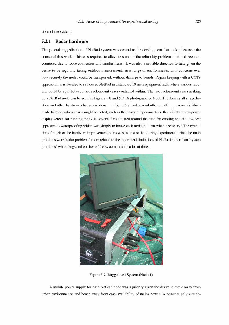
5.2. Areas of improvement for experimental testing 120
ation of the system.
5.2.1 Radar hardware
The general ruggedisation of NetRad system was central to the development that took place over the
course of this work. This was required to alleviate some of the reliability problems that had been en-
countered due to loose connectors and similar items. It was also a sensible direction to take given the
desire to be regularly taking outdoor measurements in a range of environments; with concerns over
how securely the nodes could be transported, without damage to boards. Again keeping with a COTS
approach it was decided to re-housed NetRad in a standard 19 inch equipment rack, where various mod-
ules could be split between two rack-mount cases contained within. The two rack-mount cases making
up a NetRad node can be seen in Figures 5.8 and 5.9. A photograph of Node 1 following all ruggedis-
ation and other hardware changes is shown in Figure 5.7, and several other small improvements which
made field operation easier might be noted, such as the heavy duty connectors, the miniature low-power
display screen for running the GUI, several fans situated around the case for cooling and the low-cost
approach to waterproofing which was simply to house each node in a tent when necessary! The overall
aim of much of the hardware improvement plans was to ensure that during experimental trials the main
problems were ‘radar problems’ more related to the theoretical limitations of NetRad rather than ‘system
problems’ where bugs and crashes of the system took up a lot of time.
Figure 5.7: Ruggedised System (Node 1)
A mobile power supply for each NetRad node was a priority given the desire to move away from
urban environments; and hence away from easy availability of mains power. A power supply was de-
5.2. Areas of improvement for experimental testing 121
veloped for each node to directly replace the ‘wall-wart’ AC-DC power supplies. This provided the
DC supplies through the use of DC-DC converters powered by a 12 V 65 Ah battery, which given the
measured power consumption of the electronics on-board the Node was predicted to give at least 10
hours of operation time. The decision to use battery power over generators was largely a pragmatic one,
the biggest deciding factor being that it removed the requirement for any fuel to be obtained and stored
during trials, and also allowed for safer operation (due to lack of exhaust fumes etc.) in laboratory con-
ditions using exactly the same equipment setup. Over an extended trial period, it was a relatively easy
routine to leave the batteries to charge overnight, using COTS ‘car battery’ chargers. The power supply
board can be seen in the top right of Figure 5.8. Additional indicators were added to the front of the
system to display battery charge level, and switches allowed for certain DC supplies to be powered down
between tests (notably the power amplifiers) if necessary - although as mentioned this was not generally
necessary due to the 10 hour battery life. It is certainly possible that the power supply method would
have to be re-thought however were future changes to the system to take place, thus the power supply is
perhaps not as ‘future-proof’ as many of the other NetRad modules. An example of this might be where
a higher power transmitter is required, or if measurements exceeding 10 hours of NetRad operation were
deemed necessary.
Figure 5.8: Radar hardware - Mini PC, Data Capture Board and Power Supply
For fast data transfer and storage of received data on the network between nodes, the easiest solution
was to include a PC as part of each node rather than having a single ‘Host PC’ connected to Node 1 only.
This was seen as a useful solution for more than just this reason however, since it also meant that the
networking function provided by the CAN bus could be replaced by standard Windows-based Local
Area Network (LAN) networking over Ethernet links (for which the same 50 m CAT-6 cables could be
used). This was found to be much faster to transfer data, and allowed for better ‘future proofing’ of the
system. Software could simply use Transmission Control Protocol / Internet Protocol (TCP/IP) and let
the operating system handle the networking function, so further conventional COTS networking methods
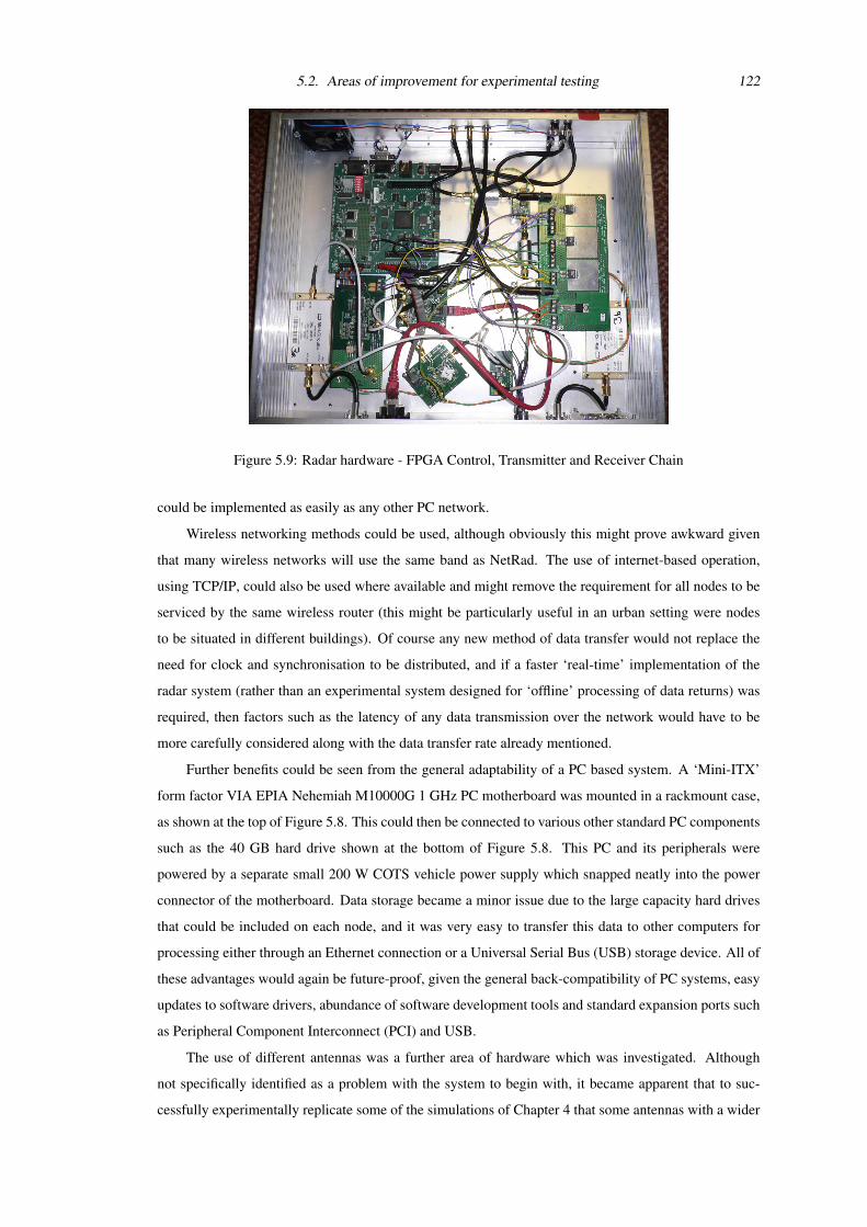
5.2. Areas of improvement for experimental testing 122
Figure 5.9: Radar hardware - FPGA Control, Transmitter and Receiver Chain
could be implemented as easily as any other PC network.
Wireless networking methods could be used, although obviously this might prove awkward given
that many wireless networks will use the same band as NetRad. The use of internet-based operation,
using TCP/IP, could also be used where available and might remove the requirement for all nodes to be
serviced by the same wireless router (this might be particularly useful in an urban setting were nodes
to be situated in different buildings). Of course any new method of data transfer would not replace the
need for clock and synchronisation to be distributed, and if a faster ‘real-time’ implementation of the
radar system (rather than an experimental system designed for ‘offline’ processing of data returns) was
required, then factors such as the latency of any data transmission over the network would have to be
more carefully considered along with the data transfer rate already mentioned.
Further benefits could be seen from the general adaptability of a PC based system. A ‘Mini-ITX’
form factor VIA EPIA Nehemiah M10000G 1 GHz PC motherboard was mounted in a rackmount case,
as shown at the top of Figure 5.8. This could then be connected to various other standard PC components
such as the 40 GB hard drive shown at the bottom of Figure 5.8. This PC and its peripherals were
powered by a separate small 200 W COTS vehicle power supply which snapped neatly into the power
connector of the motherboard. Data storage became a minor issue due to the large capacity hard drives
that could be included on each node, and it was very easy to transfer this data to other computers for
processing either through an Ethernet connection or a Universal Serial Bus (USB) storage device. All of
these advantages would again be future-proof, given the general back-compatibility of PC systems, easy
updates to software drivers, abundance of software development tools and standard expansion ports such
as Peripheral Component Interconnect (PCI) and USB.
The use of different antennas was a further area of hardware which was investigated. Although
not specifically identified as a problem with the system to begin with, it became apparent that to suc-
cessfully experimentally replicate some of the simulations of Chapter 4 that some antennas with a wider
5.2. Areas of improvement for experimental testing 123
beamwidth would be required. Fortunately it was very easy to procure antennas with the desired charac-
teristics, which in this case was determined to be a 30 beamwidth antenna, due to their high availability
for use in networking applications in the ISM band.
The clock distribution and synchronisation of NetRad were experiencing intermittent faults due to
wear and tear on the connectors. The addition of Ethernet-based networking between host PCs on-board
each node meant running two further CAT-6 cables between Node 1 and the ‘remote’ nodes - which
would mean seven cables in total used in the NetRad system. The most convenient solution for clock
and synchronisation transmissions to Nodes 2 and 3 was the use of twisted pairs on the same CAT-6
cables. To ensure that the same connector problems did not arise again, heavy duty connectors were
used at the front panel of the nodes (as seen in Figure 5.7), and a redesign of the receiving boards helped
facilitate easy distribution within the node through a single RJ-45 connector. The clock transmitter was
moved to be housed within Node 1, and the transmission of the synchronisation pulse incorporated on
the same board - thus all nodes effectively have a ‘wired timing’ board which handles all distribution
of timing and synchronisation. This was somewhat deliberate, given that future wireless solutions could
then easily directly replace this board. A secondary ‘clock receiver’ board, and hence the previous 50 m
clock cable to Node 1, is not used - where instead the clock signal is distributed straight to the various
clock inputs within the node. This will mean that the relative delays of the clock signal are no longer
roughly equal, but that Nodes 2 and 3 have an extra delay due to the 50 m cables that is not seen in Node
1. This will see a reduction in any attenuation of phase noise seen due to the range-correlation effect
for any bistatic pairs involving Node 1. However for the typical target ranges and NetRad geometries of
interest, the lower attenuation due to the range-correlation effect (of around 3 dB across the 2 kHz loop
filter bandwidth) was decided to be an acceptable cost for the increased ruggedness of the system, and
therefore the final ‘wired setup’ of the NetRad required only four cables.
5.2.2 Software and data processing
Initial work looked to make the DSP board processing more configurable, so as to reduce the amount
of data transfer to the minimum needed. For instance, where multiple matched filters are to be used
the radar could be programmed to capture raw data only, allowing the filters themselves to be applied
at a later date. This improved memory management allowed around three times more range profiles
to be recorded. It was also noted that the recording of ‘raw data’ in this way meant that during later
investigation it was far simpler to apply various different DSP methods ‘offline’ - such as a choice of
different windowing functions on the matched filter.
Some third-party replacement drivers, ‘DirectDSP’ from Signalogic, were first implemented for the
DSP board, which claimed to utilize the HPI more effectively to give consistent data transfer rates of 200
to 300 kB/s - a tenfold improvement on previously measured data rates. However due to the desire to
also capture larger numbers of pulses (including sets of pulses for potential ‘tracking’ measurements), a
decision was made to look at a more suitable COTS data capture method. The most suitable solution was
determined to be use of a Signatec PDA14 100 MHz Data Acquisition Signal Waveform Digitizer. This
PCI based digitiser card allowed capture of 512 Msamples, likely to be sufficient for all experimental
5.3. Acceptance tests / Calibration 124
measurements planned. Further to this large on-board RAM, the board also allows for Direct Memory
Access (DMA) transfer of captured data to the Hard Disk of a PC through a standard PCI interface - thus
also mitigating the problems caused by the slow data rate of the HPI of the DSP boards.
The use of the DSP board was increasingly questionable due to unreliability and slow data transfer
rates, as well as the increasing tendency of measurements to record data for later ‘offline’ DSP in MAT-
LAB. Thus the DSP board was therefore removed from the NetRad, which meant that a new method of
communication between Host PC and FPGA was required. A convenient method was to use the RS-232
serial port on the FPGA board. The GUI which operated NetRad was rewritten in C# (an object-oriented
programming language similar to C++ developed by Microsoft as part of the .NET framework initiative)
to handle both this serial port communication, as well as further new functions of interfacing with the
PDA14 data capture board and handling the TCP/IP networking between nodes.
Various improvements were added to the FPGA code, the GUI code and new MATLAB functions
were written to read in and process the collected data. An example is the ‘pulse interleave’ mode added
to NetRad - here the timers of the FPGA are arranged such that one node transmits at a time in sequence
from pulse to pulse. This provides an alternative to use of orthogonal codes in distinguishing which
node was transmitting for each set of received data. This will mean that effectively the ‘receive PRF’
of NetRad will be three times that of the ‘transmit PRF’ to utilise all nine transmitter-receiver pairs in
the system. The MATLAB functions will include the application of multistatic data fusion discussed in
Chapters 3 and 4. Other small improvements were also made in the GUI, such as a C# implementation of
the matched filtering previous undertaken by the DSP. This was implemented for zero Doppler shift for
the sum of received pulses, and was not intended as a replacement for previous DSP functionality or that
of the later ‘offline’ processing, but was useful as a quick confidence check during field experiments that
various reference targets were appearing as expected. Other functions such as automated file naming
conventions, were also added to the GUI to make use of NetRad for experimental trials even more
convenient.
5.2.3 System diagrams of current NetRad system
Figure 5.10 shows a block diagram for Node 1, which is used as a ‘central node’ for both housing the
distributed oscillator, transmitting the synchronisation pulse and operating the GUI. Nodes 2 and 3 are
shown in Figure 5.11.
5.3 Acceptance tests / CalibrationBefore any environment was observed with NetRad, it was important to characterise the system as thor-
oughly as possible. By doing this, uncertainty is removed in results that might otherwise be caused by
unknown system behaviour.
5.3.1 Time transfer
In order for the radar system to operate, it must have a shared idea of time and space between each
node. Estimation of the location and velocity characteristics of a target is accomplished in radar systems
through measurement of the time delay of a transmission to return upon reflection from the target. In
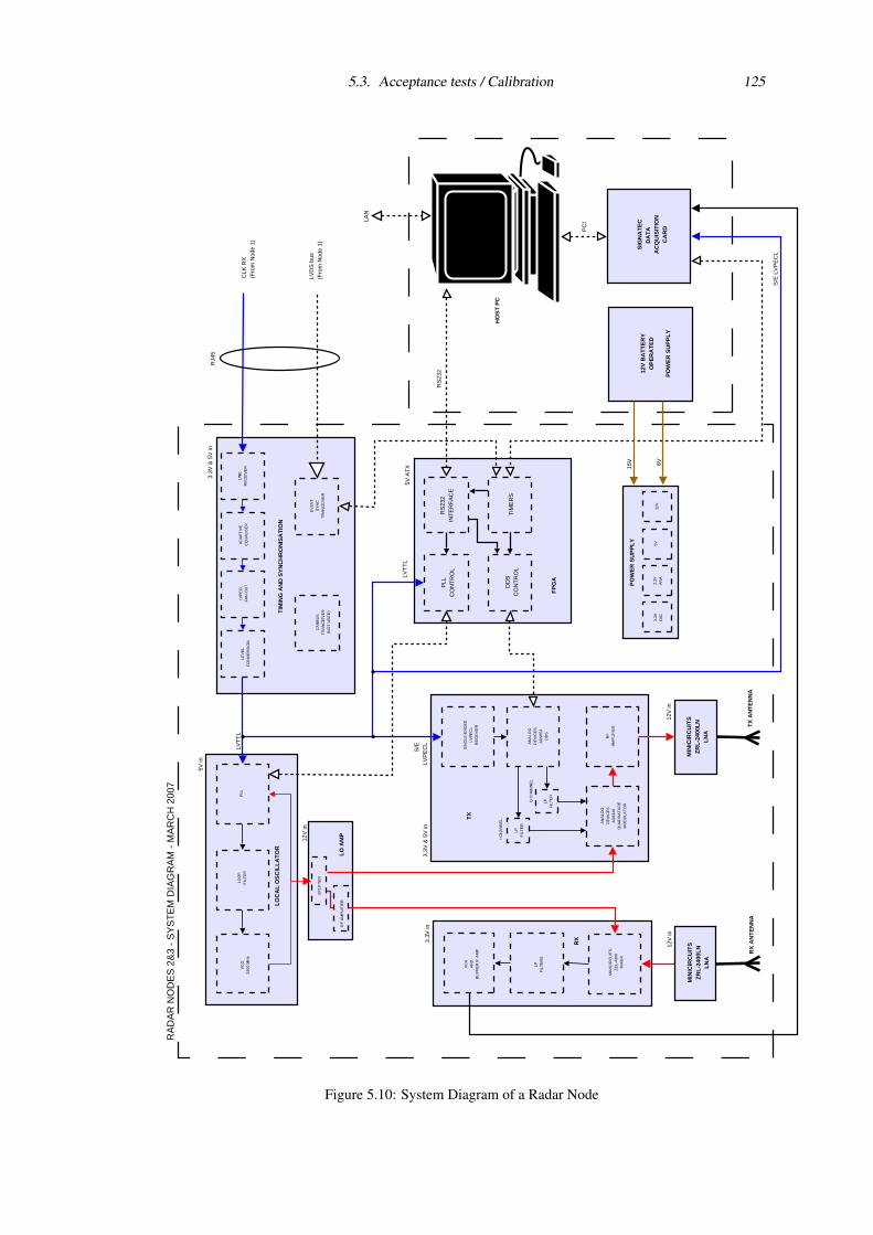
5.3. Acceptance tests / Calibration 125
FP
GA
TX
RX
TIM
ING
AN
D S
YN
CH
RO
NIS
AT
ION
HO
ST
PC
AN
ALO
GD
EV
ICE
SA
D98
54D
DS
LPF
ILT
ER
RF
AM
PLI
FIE
R
AN
ALO
GD
EV
ICE
SA
D83
46Q
UA
DR
AT
UR
EM
OD
ULA
TO
R
LPF
ILT
ER
S
MIN
ICIR
CU
ITS
ZE
L-43
00M
IXE
R
LO
CA
L O
SC
ILL
AT
OR
PLL
LOO
PF
ILT
ER
LO
AM
P
VC
O24
00 M
Hz
RA
DA
R N
OD
ES
2&
3 -
SY
ST
EM
DIA
GR
AM
- M
AR
CH
200
7
TX
AN
TE
NN
AR
X A
NT
EN
NA
LPF
ILT
ER
I CH
AN
NE
L
Q C
HA
NN
EL
LEV
EL
CO
NV
ER
SIO
N
LVP
EC
LF
AN
-OU
T
LIN
ER
EC
EIV
ER
AD
AP
TIV
EE
QU
ALI
SE
R
TIM
ER
S
PLL
CO
NT
RO
L
RS
232
INT
ER
FA
CE
DD
SC
ON
TR
OL
12V
in
12V
in
3.3V
& 5
V in
3.3V
& 5
V in
5V in
3.3V
in
5V A
TX
LVT
TL
LVT
TL
PO
WE
R S
UP
PL
Y
3.3V
DIG
3.3V
AN
A5V
12V
LVD
S b
us(F
rom
Nod
e 1)
SIN
GLE
-EN
DE
DLV
PE
CL
RE
CE
IVE
R
S/E
LV
PE
CL
S/E
LVP
EC
L
SP
LIT
TE
R
RF
AM
PLI
FIE
R
VC
AA
ND
BU
FF
ER
IF A
MP
RS
232
MIN
ICIR
CU
ITS
ZR
L-2
400L
NL
NA
MIN
ICIR
CU
ITS
ZR
L-2
400L
NL
NA
SIG
NA
TE
CD
AT
A
AC
QU
ISIT
ION
CA
RDPC
I
CA
NB
US
TR
AN
CE
IVE
R(N
OT
US
ED
)
EV
EN
TS
YN
CT
RA
NC
EIV
ER
12V
in
12V
BA
TT
ER
YO
PE
RA
TE
D
PO
WE
R S
UP
PL
Y
15V 6V
CLK
RX
(Fro
m N
ode
1)
RJ4
5
LAN
Figure 5.10: System Diagram of a Radar Node
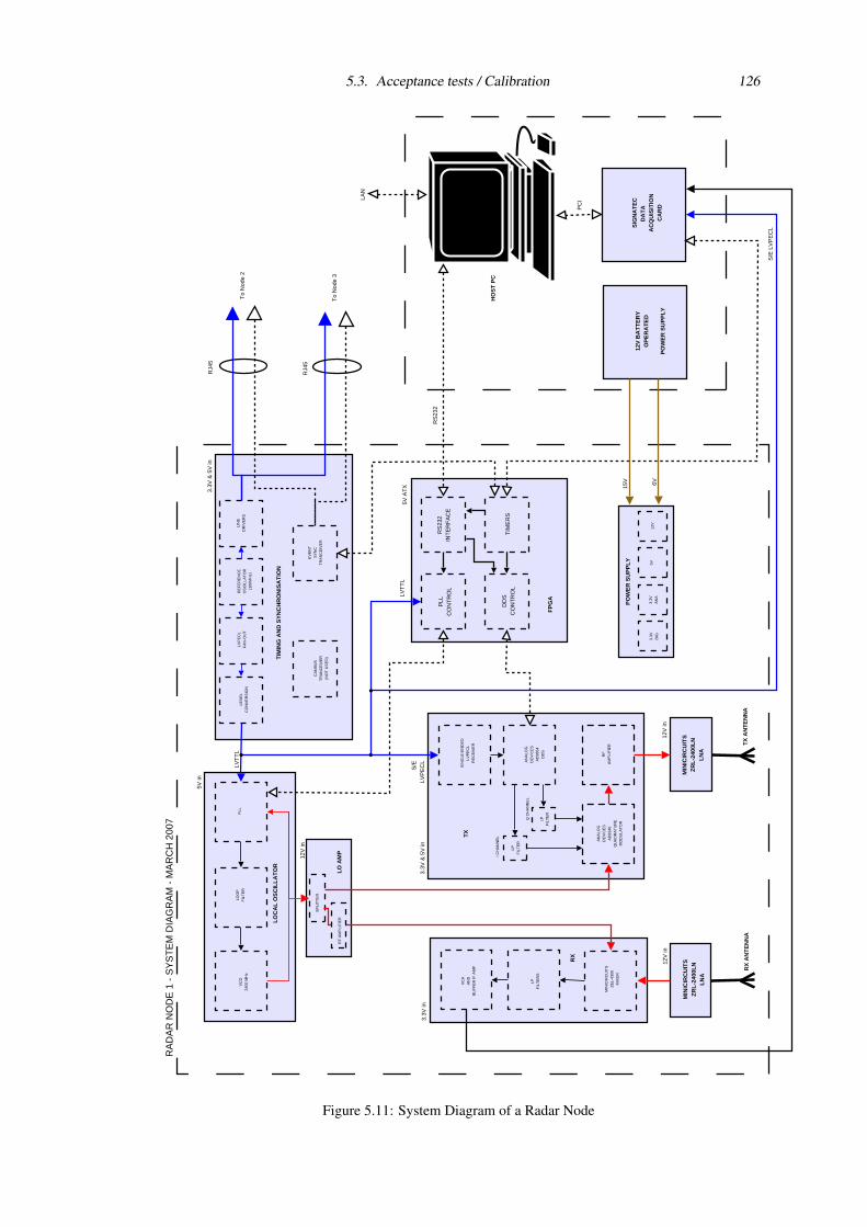
5.3. Acceptance tests / Calibration 126
FP
GA
TX
RX
TIM
ING
AN
D S
YN
CH
RO
NIS
AT
ION
HO
ST
PC
AN
ALO
GD
EV
ICE
SA
D98
54D
DS
LPF
ILT
ER
RF
AM
PLI
FIE
R
AN
ALO
GD
EV
ICE
SA
D83
46Q
UA
DR
AT
UR
EM
OD
ULA
TO
R
LPF
ILT
ER
S
MIN
ICIR
CU
ITS
ZE
L-43
00M
IXE
R
LO
CA
L O
SC
ILL
AT
OR
PLL
LOO
PF
ILT
ER
LO
AM
P
VC
O24
00 M
Hz
RA
DA
R N
OD
E 1
- S
YS
TE
M D
IAG
RA
M -
MA
RC
H 2
007
TX
AN
TE
NN
AR
X A
NT
EN
NA
LPF
ILT
ER
I CH
AN
NE
L
Q C
HA
NN
EL
LEV
EL
CO
NV
ER
SIO
N
LVP
EC
LF
AN
-OU
T
LIN
ED
RIV
ER
SR
EF
ER
EN
CE
OS
CIL
LAT
OR
(100
MH
z)
TIM
ER
S
PLL
CO
NT
RO
L
RS
232
INT
ER
FA
CE
DD
SC
ON
TR
OL
12V
in
12V
in
3.3V
& 5
V in
3.3V
& 5
V in
5V in
3.3V
in
5V A
TX
LVT
TL
LVT
TL
PO
WE
R S
UP
PL
Y
3.3V
DIG
3.3V
AN
A5V
12V
SIN
GLE
-EN
DE
DLV
PE
CL
RE
CE
IVE
R
S/E
LV
PE
CL
S/E
LVP
EC
L
SP
LIT
TE
R
RF
AM
PLI
FIE
R
VC
AA
ND
BU
FF
ER
IF A
MP
RS
232
MIN
ICIR
CU
ITS
ZR
L-2
400L
NL
NA
MIN
ICIR
CU
ITS
ZR
L-2
400L
NL
NA
SIG
NA
TE
CD
AT
A
AC
QU
ISIT
ION
CA
RDPC
I
CA
NB
US
TR
AN
CE
IVE
R(N
OT
US
ED
)
EV
EN
TS
YN
CT
RA
NC
EIV
ER
12V
in
12V
BA
TT
ER
YO
PE
RA
TE
D
PO
WE
R S
UP
PL
Y
15V 6V
To
Nod
e 2
RJ4
5
LAN
To
Nod
e 3
RJ4
5
Figure 5.11: System Diagram of a Radar Node
5.3. Acceptance tests / Calibration 127
both the monostatic and multistatic case, if there are any ‘unknowns’ in this time delay, then errors are
introduced. Without a large anechoic chamber it was difficult to characterise these delays accurately
whilst including transmission between both antennas in the far field (either directly or using a reference
target) - which in the case of the 8 antenna was 12.5 m. A rather easier and more repeatable approach
was to characterise the delays within the system without the antennas, using an attenuator in place of
the pair of antennas, with the delays due to the antennas estimated based on the length of the co-axial
feed line and the position of the phase centre. This made it rather questionable as to whether full spatial
coherency could be achieved with this level of calibration. The measured delays (through recording of a
chirp transmission and interpolation to find the maximum likelihood time-of-arrival) for each transmitter-
receiver pair are shown in Table 5.1.
Receiving Node
Tran
smitt
ing
Nod
e
1 2 3
1 1.238 0.960 0.967
2 1.513 1.240 1.236
3 1.509 1.244 1.242
Table 5.1: Time delay in µs recorded for a direct connection (all predelays set to minimum)
The distributed Crystek Crystals CCHD-950 Ultra-Low Phase Noise Clock Oscillator will be the
time reference used by NetRad, and the nominal frequency of this oscillator is 100 MHz. The stability
of this oscillator is quoted as ±20 ppm, and the measured frequency of the NetRad clock signal can be
seen to be within this bound at 99.999518 MHz. Given that the oscillator is more than a year old, further
ageing is quoted as being at a rate of less than 1 ppm per year. When multiplied up using the digital PLL
on each node, this can be seen to correspond to a frequency 2399.9884 MHz. The central aspect to the
clock distribution of NetRad is that the oscillators used as a measure of time at each node are consistent
with each other. An offset of LO between nodes of only a few Hz would see stationary clutter observed at
an apparent Doppler shift, for example. To investigate the longer term frequency stability between nodes,
a known reference source from a signal generator at an offset of a few kHz was distributed through a
splitter. The beat frequency caused by the mixing with this signal reference can be recorded as the radar
would normally operated - on a pulsed basis. Each recorded pulse (effectively a sample of the beat
frequency) will have an initial phase which can be measured. If the LO frequencies are stable, then the
phase offsets measured between nodes should remain relatively constant. If the frequencies are separate
then the differing beat frequencies will mean that the phase offsets might be expected to change at a rate
equal to the difference in LO frequencies between nodes. Using a low PRF 2 of 2 Hz, the relative stability
of the LOs over a long period of time can be measured. Figure 5.12 shows a typical plot of the phase
difference between nodes, where the flat response shows the relative frequency stability afforded through
the reference oscillator distribution. About a minute in to this plot, the clock cable connecting to Node 2
2It should be noted that were a particularly large frequency difference to be expected, that it would be better to use a larger
PRF, which would be required to satisfy the Nyquist-Shannon sampling rate for the maximum frequency difference between nodes
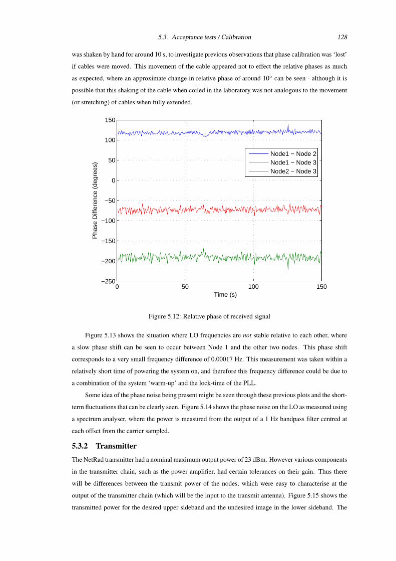
5.3. Acceptance tests / Calibration 128
was shaken by hand for around 10 s, to investigate previous observations that phase calibration was ‘lost’
if cables were moved. This movement of the cable appeared not to effect the relative phases as much
as expected, where an approximate change in relative phase of around 10 can be seen - although it is
possible that this shaking of the cable when coiled in the laboratory was not analogous to the movement
(or stretching) of cables when fully extended.
0 50 100 150−250
−200
−150
−100
−50
0
50
100
150
Time (s)
Pha
se D
iffer
ence
(de
gree
s)
Node1 − Node 2Node1 − Node 3Node2 − Node 3
Figure 5.12: Relative phase of received signal
Figure 5.13 shows the situation where LO frequencies are not stable relative to each other, where
a slow phase shift can be seen to occur between Node 1 and the other two nodes. This phase shift
corresponds to a very small frequency difference of 0.00017 Hz. This measurement was taken within a
relatively short time of powering the system on, and therefore this frequency difference could be due to
a combination of the system ‘warm-up’ and the lock-time of the PLL.
Some idea of the phase noise being present might be seen through these previous plots and the short-
term fluctuations that can be clearly seen. Figure 5.14 shows the phase noise on the LO as measured using
a spectrum analyser, where the power is measured from the output of a 1 Hz bandpass filter centred at
each offset from the carrier sampled.
5.3.2 Transmitter
The NetRad transmitter had a nominal maximum output power of 23 dBm. However various components
in the transmitter chain, such as the power amplifier, had certain tolerances on their gain. Thus there
will be differences between the transmit power of the nodes, which were easy to characterise at the
output of the transmitter chain (which will be the input to the transmit antenna). Figure 5.15 shows the
transmitted power for the desired upper sideband and the undesired image in the lower sideband. The
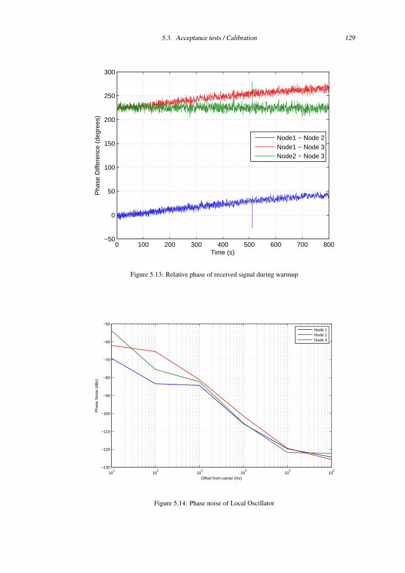
5.3. Acceptance tests / Calibration 129
0 100 200 300 400 500 600 700 800−50
0
50
100
150
200
250
300
Time (s)
Pha
se D
iffer
ence
(de
gree
s)
Node1 − Node 2Node1 − Node 3Node2 − Node 3
Figure 5.13: Relative phase of received signal during warmup
101
102
103
104
105
106
−130
−120
−110
−100
−90
−80
−70
−60
−50
Offset from carrier (Hz)
Pha
se N
oise
(dB
c)
Node 1Node 2Node 3
Figure 5.14: Phase noise of Local Oscillator
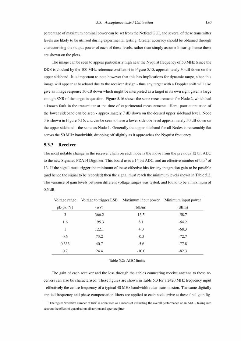
5.3. Acceptance tests / Calibration 130
percentage of maximum nominal power can be set from the NetRad GUI, and several of these transmitter
levels are likely to be utilised during experimental testing. Greater accuracy should be obtained through
characterising the output power of each of these levels, rather than simply assume linearity, hence these
are shown on the plots.
The image can be seen to appear particularly high near the Nyquist frequency of 50 MHz (since the
DDS is clocked by the 100 MHz reference oscillator) in Figure 5.15, approximately 30 dB down on the
upper sideband. It is important to note however that this has implications for dynamic range, since this
image will appear at baseband due to the receiver design - thus any target with a Doppler shift will also
give an image response 30 dB down which might be interpreted as a target in its own right given a large
enough SNR of the target in question. Figure 5.16 shows the same measurements for Node 2, which had
a known fault in the transmitter at the time of experimental measurements. Here, poor attenuation of
the lower sideband can be seen - approximately 7 dB down on the desired upper sideband level. Node
3 is shown in Figure 5.16, and can be seen to have a lower sidelobe level approximately 30 dB down on
the upper sideband - the same as Node 1. Generally the upper sideband for all Nodes is reasonably flat
across the 50 MHz bandwidth, dropping off slightly as it approaches the Nyquist frequency.
5.3.3 Receiver
The most notable change in the receiver chain on each node is the move from the previous 12 bit ADC
to the new Signatec PDA14 Digitizer. This board uses a 14 bit ADC, and an effective number of bits3 of
13. If the signal must trigger the minimum of these effective bits for any integration gain to be possible
(and hence the signal to be recorded) then the signal must reach the minimum levels shown in Table 5.2.
The variance of gain levels between different voltage ranges was tested, and found to be a maximum of
0.5 dB.
Voltage range Voltage to trigger LSB Maximum input power Minimum input power
pk-pk (V) (µV) (dBm) (dBm)
3 366.2 13.5 -58.7
1.6 195.3 8.1 -64.2
1 122.1 4.0 -68.3
0.6 73.2 -0.5 -72.7
0.333 40.7 -5.6 -77.8
0.2 24.4 -10.0 -82.3
Table 5.2: ADC limits
The gain of each receiver and the loss through the cables connecting receive antenna to these re-
ceivers can also be characterised. These figures are shown in Table 5.3 for a 2420 MHz frequency input
- effectively the centre frequency of a typical 40 MHz bandwidth radar transmission. The same digitally
applied frequency and phase compensation filters are applied to each node arrive at these final gain fig-
3The figure ‘effective number of bits’ is often used as a means of evaluating the overall performance of an ADC - taking into
account the effect of quantisation, distortion and aperture jitter
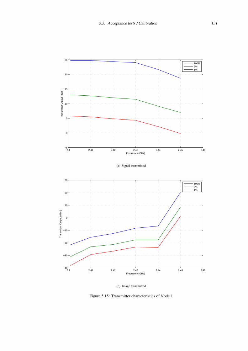
5.3. Acceptance tests / Calibration 131
2.4 2.41 2.42 2.43 2.44 2.45 2.46−5
0
5
10
15
20
25
Frequency (GHz)
Tra
nsm
itter
Out
put (
dBm
)
100%5%1%
(a) Signal transmitted
2.4 2.41 2.42 2.43 2.44 2.45 2.46−40
−30
−20
−10
0
10
20
30
Frequency (GHz)
Tra
nsm
itter
Out
put (
dBm
)
100%5%1%
(b) Image transmitted
Figure 5.15: Transmitter characteristics of Node 1
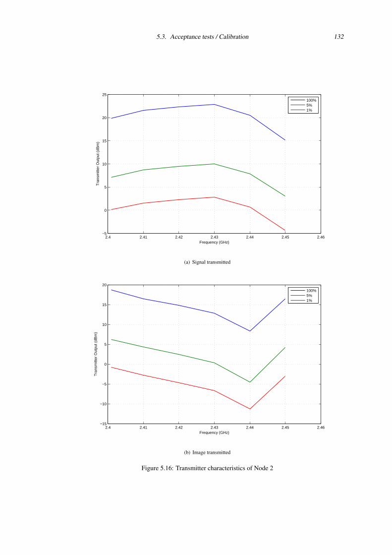
5.3. Acceptance tests / Calibration 132
2.4 2.41 2.42 2.43 2.44 2.45 2.46−5
0
5
10
15
20
25
Frequency (GHz)
Tra
nsm
itter
Out
put (
dBm
)
100%5%1%
(a) Signal transmitted
2.4 2.41 2.42 2.43 2.44 2.45 2.46−15
−10
−5
0
5
10
15
20
Frequency (GHz)
Tra
nsm
itter
Out
put (
dBm
)
100%5%1%
(b) Image transmitted
Figure 5.16: Transmitter characteristics of Node 2
5.3. Acceptance tests / Calibration 133
2.4 2.41 2.42 2.43 2.44 2.45 2.46−5
0
5
10
15
20
25
Frequency (GHz)
Tra
nsm
itter
Out
put (
dBm
)
100%5%1%
(a) Signal transmitted
2.4 2.41 2.42 2.43 2.44 2.45 2.46−30
−25
−20
−15
−10
−5
0
5
10
15
20
Frequency (GHz)
Tra
nsm
itter
Out
put (
dBm
)
100%5%1%
(b) Image transmitted
Figure 5.17: Transmitter characteristics of Node 3
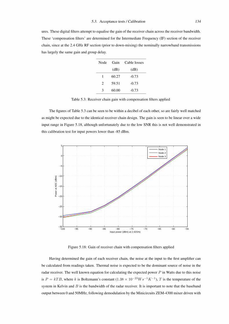
5.3. Acceptance tests / Calibration 134
ures. These digital filters attempt to equalise the gain of the receiver chain across the receiver bandwidth.
These ‘compensation filters’ are determined for the Intermediate Frequency (IF) section of the receiver
chain, since at the 2.4 GHz RF section (prior to down-mixing) the nominally narrowband transmissions
has largely the same gain and group delay.
Node Gain Cable losses
(dB) (dB)
1 60.27 -0.73
2 59.51 -0.73
3 60.00 -0.73
Table 5.3: Receiver chain gain with compensation filters applied
The figures of Table 5.3 can be seen to be within a decibel of each other, so are fairly well matched
as might be expected due to the identical receiver chain design. The gain is seen to be linear over a wide
input range in Figure 5.18, although unfortunately due to the low SNR this is not well demonstrated in
this calibration test for input powers lower than -85 dBm.
−100 −95 −90 −85 −80 −75 −70 −65 −60 −55−35
−30
−25
−20
−15
−10
−5
0
5
Input power (dBm) at 2.42GHz
Pow
er a
t AD
C (
dBm
)
Node 1
Node 2
Node 3
Figure 5.18: Gain of receiver chain with compensation filters applied
Having determined the gain of each receiver chain, the noise at the input to the first amplifier can
be calculated from readings taken. Thermal noise is expected to be the dominant source of noise in the
radar receiver. The well known equation for calculating the expected power P in Watts due to this noise
is P = kTB, where k is Boltzmann’s constant (1.38 × 10⁻²³Ws−1K−1), T is the temperature of the
system in Kelvin and B is the bandwidth of the radar receiver. It is important to note that the baseband
output between 0 and 50MHz, following demodulation by the Minicircuits ZEM-4300 mixer driven with
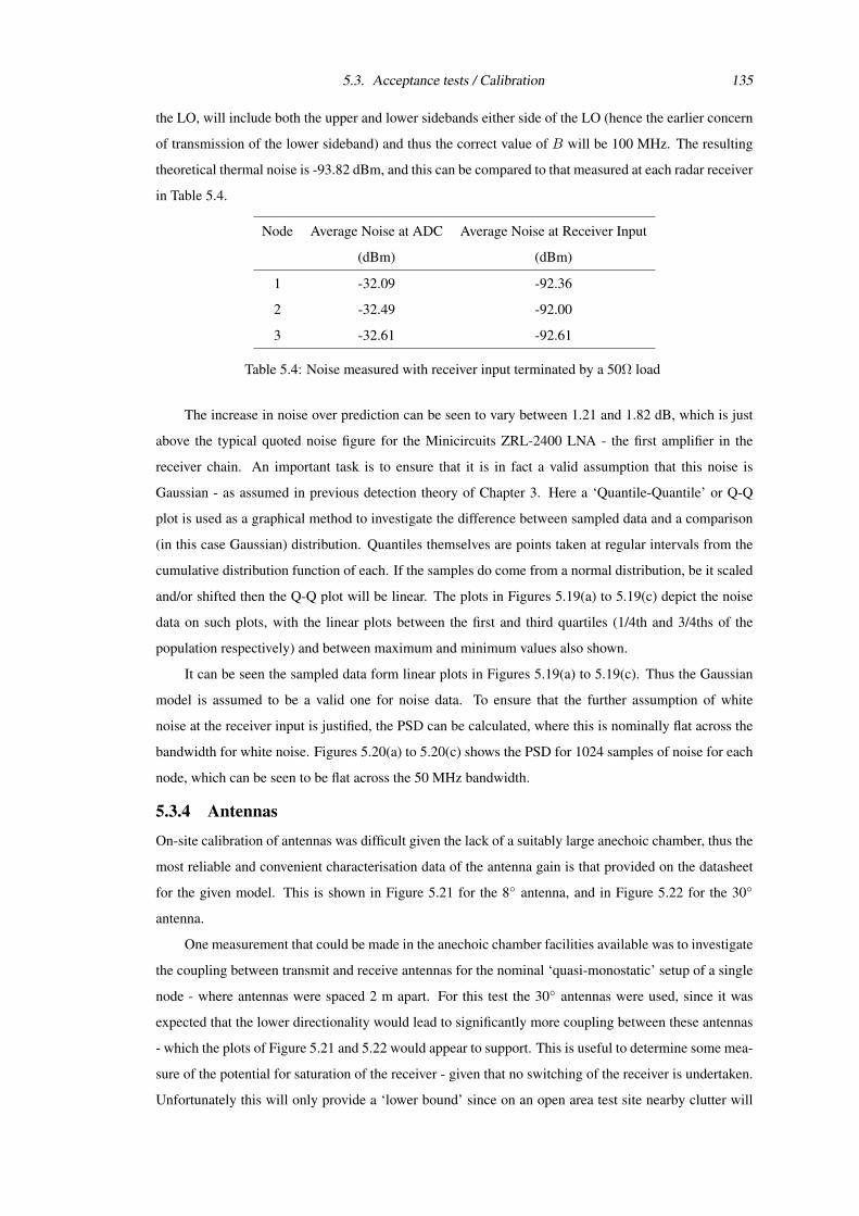
5.3. Acceptance tests / Calibration 135
the LO, will include both the upper and lower sidebands either side of the LO (hence the earlier concern
of transmission of the lower sideband) and thus the correct value of B will be 100 MHz. The resulting
theoretical thermal noise is -93.82 dBm, and this can be compared to that measured at each radar receiver
in Table 5.4.
Node Average Noise at ADC Average Noise at Receiver Input
(dBm) (dBm)
1 -32.09 -92.36
2 -32.49 -92.00
3 -32.61 -92.61
Table 5.4: Noise measured with receiver input terminated by a 50Ω load
The increase in noise over prediction can be seen to vary between 1.21 and 1.82 dB, which is just
above the typical quoted noise figure for the Minicircuits ZRL-2400 LNA - the first amplifier in the
receiver chain. An important task is to ensure that it is in fact a valid assumption that this noise is
Gaussian - as assumed in previous detection theory of Chapter 3. Here a ‘Quantile-Quantile’ or Q-Q
plot is used as a graphical method to investigate the difference between sampled data and a comparison
(in this case Gaussian) distribution. Quantiles themselves are points taken at regular intervals from the
cumulative distribution function of each. If the samples do come from a normal distribution, be it scaled
and/or shifted then the Q-Q plot will be linear. The plots in Figures 5.19(a) to 5.19(c) depict the noise
data on such plots, with the linear plots between the first and third quartiles (1/4th and 3/4ths of the
population respectively) and between maximum and minimum values also shown.
It can be seen the sampled data form linear plots in Figures 5.19(a) to 5.19(c). Thus the Gaussian
model is assumed to be a valid one for noise data. To ensure that the further assumption of white
noise at the receiver input is justified, the PSD can be calculated, where this is nominally flat across the
bandwidth for white noise. Figures 5.20(a) to 5.20(c) shows the PSD for 1024 samples of noise for each
node, which can be seen to be flat across the 50 MHz bandwidth.
5.3.4 Antennas
On-site calibration of antennas was difficult given the lack of a suitably large anechoic chamber, thus the
most reliable and convenient characterisation data of the antenna gain is that provided on the datasheet
for the given model. This is shown in Figure 5.21 for the 8 antenna, and in Figure 5.22 for the 30
antenna.
One measurement that could be made in the anechoic chamber facilities available was to investigate
the coupling between transmit and receive antennas for the nominal ‘quasi-monostatic’ setup of a single
node - where antennas were spaced 2 m apart. For this test the 30 antennas were used, since it was
expected that the lower directionality would lead to significantly more coupling between these antennas
- which the plots of Figure 5.21 and 5.22 would appear to support. This is useful to determine some mea-
sure of the potential for saturation of the receiver - given that no switching of the receiver is undertaken.
Unfortunately this will only provide a ‘lower bound’ since on an open area test site nearby clutter will
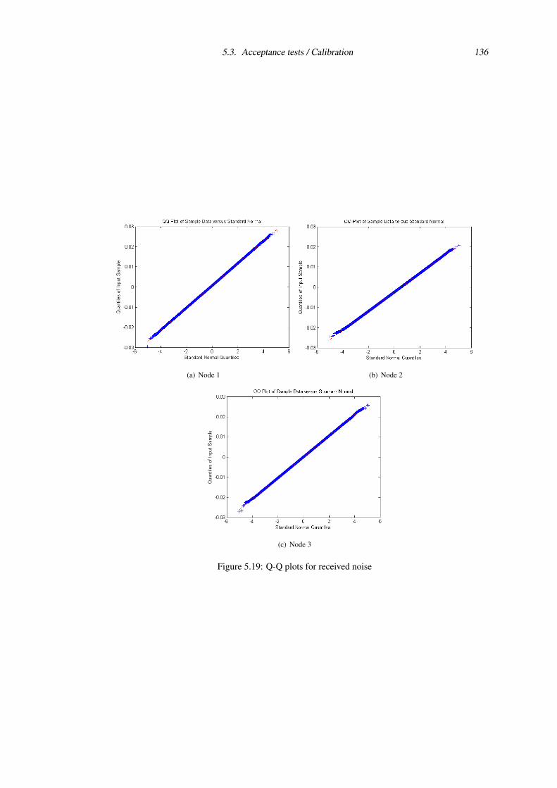
5.3. Acceptance tests / Calibration 136
(a) Node 1 (b) Node 2
(c) Node 3
Figure 5.19: Q-Q plots for received noise
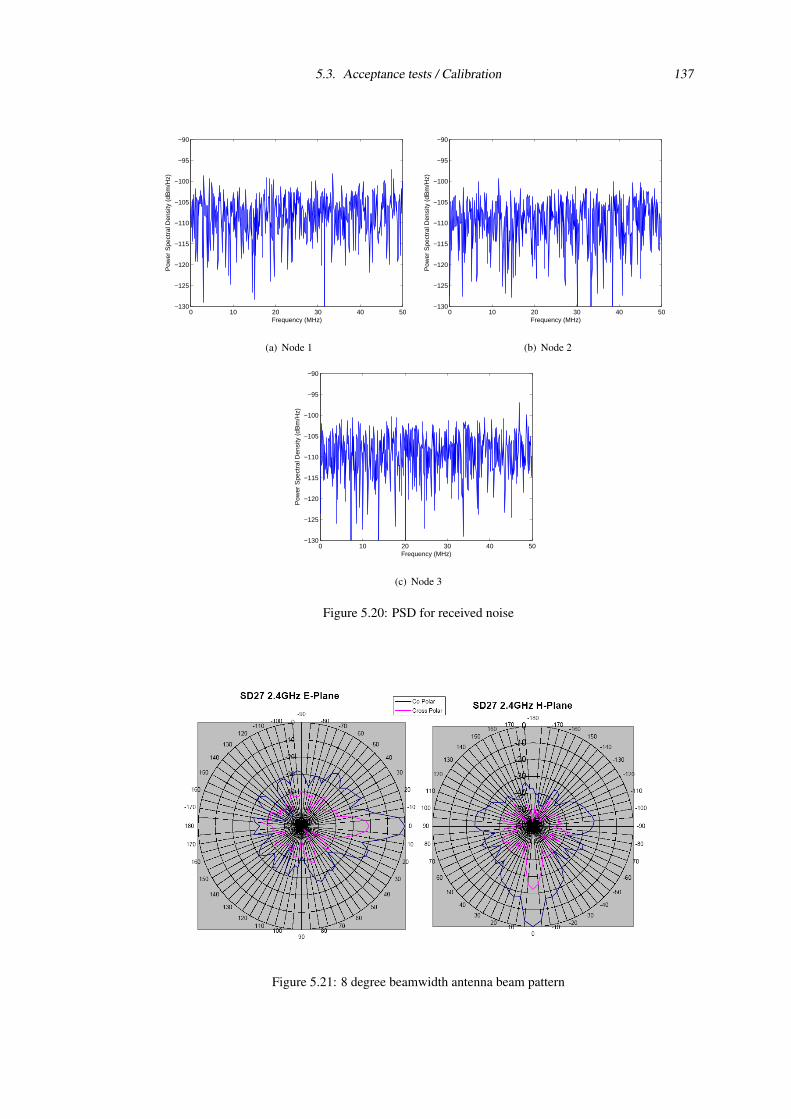
5.3. Acceptance tests / Calibration 137
0 10 20 30 40 50−130
−125
−120
−115
−110
−105
−100
−95
−90
Frequency (MHz)
Pow
er S
pect
ral D
ensi
ty (
dBm
/Hz)
(a) Node 1
0 10 20 30 40 50−130
−125
−120
−115
−110
−105
−100
−95
−90
Frequency (MHz)
Pow
er S
pect
ral D
ensi
ty (
dBm
/Hz)
(b) Node 2
0 10 20 30 40 50−130
−125
−120
−115
−110
−105
−100
−95
−90
Frequency (MHz)
Pow
er S
pect
ral D
ensi
ty (
dBm
/Hz)
(c) Node 3
Figure 5.20: PSD for received noise
Figure 5.21: 8 degree beamwidth antenna beam pattern
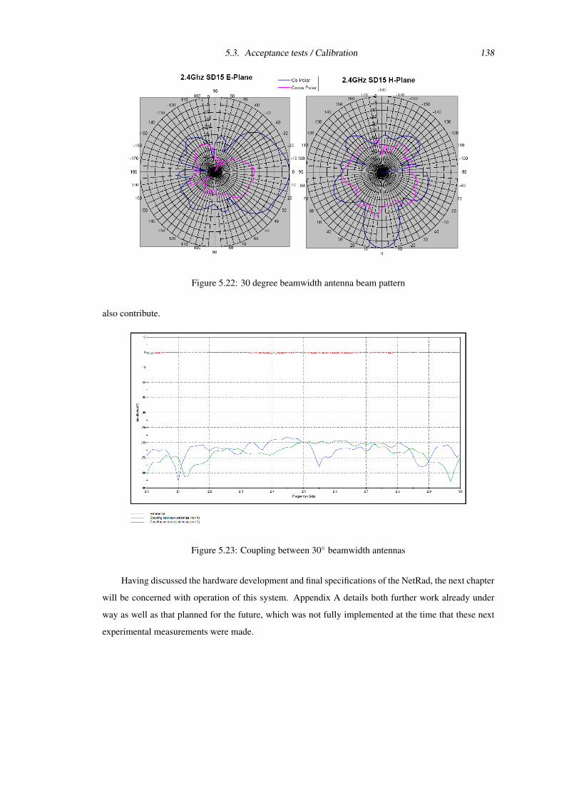
5.3. Acceptance tests / Calibration 138
Figure 5.22: 30 degree beamwidth antenna beam pattern
also contribute.
Figure 5.23: Coupling between 30 beamwidth antennas
Having discussed the hardware development and final specifications of the NetRad, the next chapter
will be concerned with operation of this system. Appendix A details both further work already under
way as well as that planned for the future, which was not fully implemented at the time that these next
experimental measurements were made.
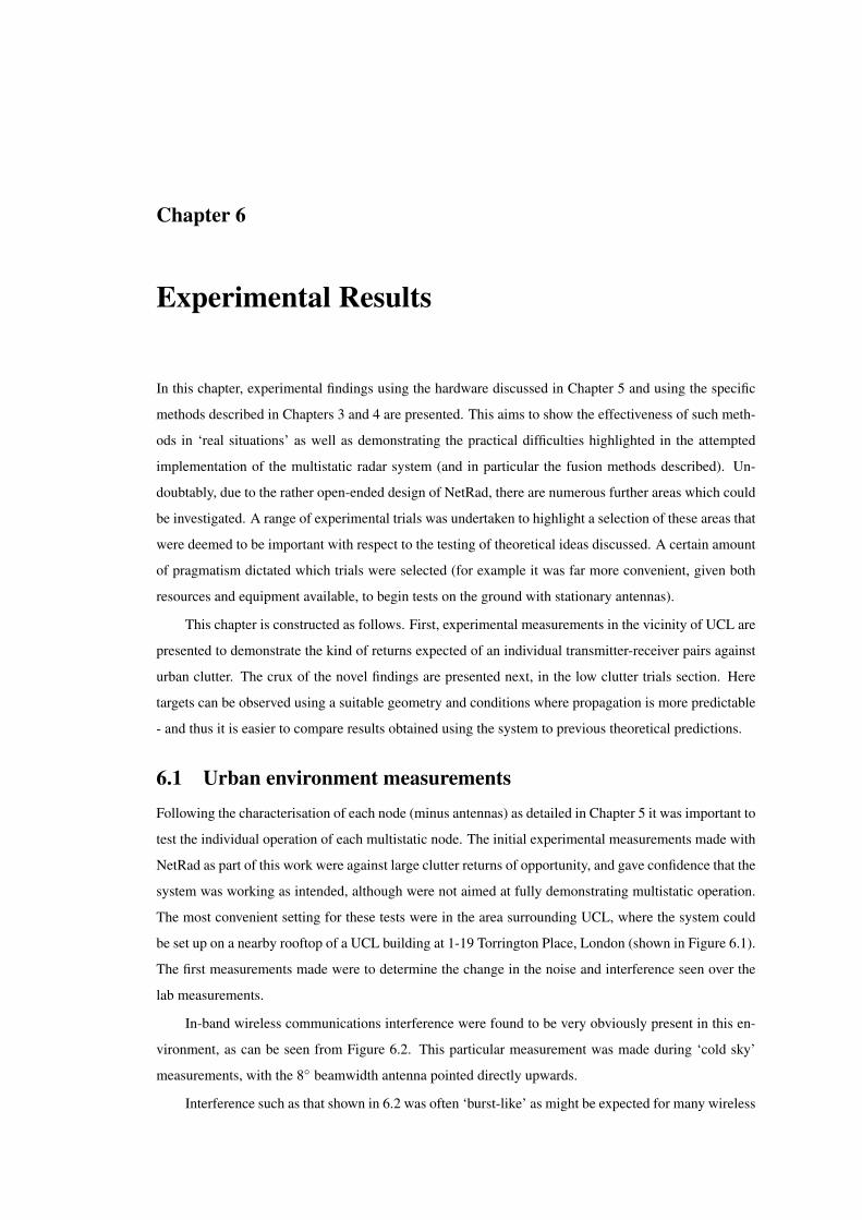
Chapter 6
Experimental Results
In this chapter, experimental findings using the hardware discussed in Chapter 5 and using the specific
methods described in Chapters 3 and 4 are presented. This aims to show the effectiveness of such meth-
ods in ‘real situations’ as well as demonstrating the practical difficulties highlighted in the attempted
implementation of the multistatic radar system (and in particular the fusion methods described). Un-
doubtably, due to the rather open-ended design of NetRad, there are numerous further areas which could
be investigated. A range of experimental trials was undertaken to highlight a selection of these areas that
were deemed to be important with respect to the testing of theoretical ideas discussed. A certain amount
of pragmatism dictated which trials were selected (for example it was far more convenient, given both
resources and equipment available, to begin tests on the ground with stationary antennas).
This chapter is constructed as follows. First, experimental measurements in the vicinity of UCL are
presented to demonstrate the kind of returns expected of an individual transmitter-receiver pairs against
urban clutter. The crux of the novel findings are presented next, in the low clutter trials section. Here
targets can be observed using a suitable geometry and conditions where propagation is more predictable
- and thus it is easier to compare results obtained using the system to previous theoretical predictions.
6.1 Urban environment measurementsFollowing the characterisation of each node (minus antennas) as detailed in Chapter 5 it was important to
test the individual operation of each multistatic node. The initial experimental measurements made with
NetRad as part of this work were against large clutter returns of opportunity, and gave confidence that the
system was working as intended, although were not aimed at fully demonstrating multistatic operation.
The most convenient setting for these tests were in the area surrounding UCL, where the system could
be set up on a nearby rooftop of a UCL building at 1-19 Torrington Place, London (shown in Figure 6.1).
The first measurements made were to determine the change in the noise and interference seen over the
lab measurements.
In-band wireless communications interference were found to be very obviously present in this en-
vironment, as can be seen from Figure 6.2. This particular measurement was made during ‘cold sky’
measurements, with the 8 beamwidth antenna pointed directly upwards.
Interference such as that shown in 6.2 was often ‘burst-like’ as might be expected for many wireless
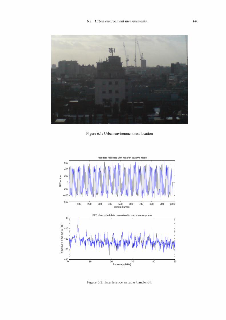
6.1. Urban environment measurements 140
Figure 6.1: Urban environment test location
100 200 300 400 500 600 700 800 900 1000−600
−400
−200
0
200
400
600
sample number
AD
C o
utpu
t
real data recorded with radar in passive mode
0 10 20 30 40 50−40
−30
−20
−10
0 FFT of recorded data normalised to maximum response
frequency (MHz)
mag
nitu
de o
f res
pons
e (d
B)
Figure 6.2: Interference in radar bandwidth
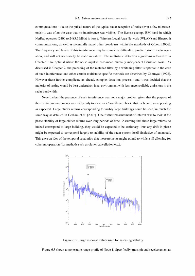
6.1. Urban environment measurements 141
communications - due to the pulsed nature of the typical radar reception of noise (over a few microsec-
onds) it was often the case that no interference was visible. The license-exempt ISM band in which
NetRad operates (2400 to 2483.5 MHz) is host to Wireless Local Area Network (WLAN) and Bluetooth
communications; as well as potentially many other broadcasts within the standards of Ofcom [2006].
The frequency and levels of this interference may be somewhat difficult to predict prior to radar oper-
ation, and will not necessarily be static in nature. The multistatic detection algorithms referred to in
Chapter 3 are optimal where the noise input is zero-mean mutually independent Gaussian noise. As
discussed in Chapter 2, the preceding of the matched filter by a whitening filter is optimal in the case
of such interference, and other certain multistatic-specific methods are described by Chernyak [1998].
However these further complicate an already complex detection process - and it was decided that the
majority of testing would be best undertaken in an environment with less uncontrollable emissions in the
radar bandwidth.
Nevertheless, the presence of such interference was not a major problem given that the purpose of
these initial measurements was really only to serve as a ‘confidence check’ that each node was operating
as expected. Large clutter returns corresponding to visibly large buildings could be seen, in much the
same way as detailed in Derham et al. [2007]. One further measurement of interest was to look at the
phase stability of large clutter returns over long periods of time. Assuming that these large returns do
indeed correspond to large building, they would be expected to be stationary; thus any drift in phase
might be expected to correspond largely to stability of the radar system itself (inclusive of antennas).
This gave an idea of the temporal separation that measurements might extend to whilst still allowing for
coherent operation (for methods such as clutter cancellation etc.).
0 100 200 300 400 500 600 700 800 900 100010
3
104
105
106
107
108
109
sample number
cros
s co
rrel
ator
out
put
Responseat ~830m
Responseat ~1560m
Figure 6.3: Large response values used for assessing stability
Figure 6.3 shows a monostatic range profile of Node 1. Specifically, transmit and receive antennas
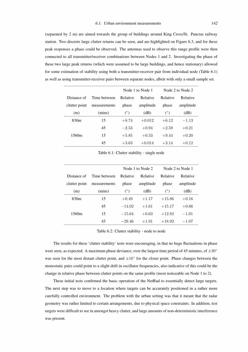
6.1. Urban environment measurements 142
(separated by 2 m) are aimed towards the group of buildings around King Cross/St. Pancras railway
station. Two discrete large clutter returns can be seen, and are highlighted on Figure 6.3, and for these
peak responses a phase could be observed. The antennas used to observe this range profile were then
connected to all transmitter/receiver combinations between Nodes 1 and 2. Investigating the phase of
these two large peak returns (which were assumed to be large buildings, and hence stationary) allowed
for some estimation of stability using both a transmitter-receiver pair from individual node (Table 6.1)
as well as using transmitter-receiver pairs between separate nodes, albeit with only a small sample set.
Node 1 to Node 1 Node 2 to Node 2
Distance of Time between Relative Relative Relative Relative
clutter point measurements phase amplitude phase amplitude
(m) (mins) () (dB) () (dB)
830m 15 +8.74 +0.012 +6.12 −1.13
45 −2.53 +0.94 +2.59 +0.21
1560m 15 +5.85 +0.53 +9.44 +0.20
45 +3.63 +0.014 +3.14 +0.12
Table 6.1: Clutter stability - single node
Node 1 to Node 2 Node 2 to Node 1
Distance of Time between Relative Relative Relative Relative
clutter point measurements phase amplitude phase amplitude
(m) (mins) () (dB) () (dB)
830m 15 +0.49 +1.17 +15.86 +0.16
45 −14.02 +1.61 +15.17 +0.66
1560m 15 −15.64 +0.63 +12.82 −1.01
45 −29.46 +1.91 +18.92 −1.07
Table 6.2: Clutter stability - node to node
The results for these ‘clutter stability’ tests were encouraging, in that no huge fluctuations in phase
were seen, as expected. A maximum phase deviance, over the largest time period of 45 minutes, of±30
was seen for the most distant clutter point, and ±16 for the closer point. Phase changes between the
monostatic pairs could point to a slight drift in oscillator frequencies, also indicative of this could be the
change in relative phase between clutter points on the same profile (most noticeable on Node 1 to 2).
These initial tests confirmed the basic operation of the NetRad to essentially detect large targets.
The next step was to move to a location where targets can be accurately positioned in a rather more
carefully controlled environment. The problem with the urban setting was that it meant that the radar
geometry was rather limited to certain arrangements, due to physical space constraints. In addition, test
targets were difficult to see in amongst heavy clutter, and large amounts of non-deterministic interference
was present.

6.2. Low-clutter test range measurements 143
6.2 Low-clutter test range measurementsThe UCL Shenley Sports Ground at London Colney in Hertfordshire was chosen as a suitable test range,
given the expected low clutter over the relatively flat grass fields - and the ability to position both radar
nodes and targets wherever desired in this surveillance area (in contrast to the previous urban environ-
ment measurements).
Figure 6.4: Birds eye view of surrounding area at radar test range
Figure 6.4 shows a birds eye view of the area surrounding the test range. Possible sources of
interference could include any wireless networking from both the houses close to the fields, or more
likely from the supermarket/restaurant complex north of the motorway. Given that the site was no longer
in an urban environment it was likely that interference would be less. A quick confidence check was
undertaken by using a laptop computer to check for available WiFi networks. Despite the rather more
rural setting, several networks were still found, but all were at much lower levels than those seen in the
earlier urban environment.
The maximum separation between nodes was dictated by the cabling between them. This was
50 m due to the length of the clock and synchronisation cables connected to Nodes 2 and 3 from Node
1. As discussed in Chapter 4 for maximal increase in localisation, it is desirable for the radar system
to observe diverse target aspects. However the minimum range to the target for the monostatic cases is
determined by the transmitted pulse length. Some compromise is needed when deciding upon a geometry
for NetRad due to each of these factors, and the geometry chosen is shown in Figure 6.5, with the target
under observation typically positioned at a ‘calibration point’ with a distance of 120 m from each node.
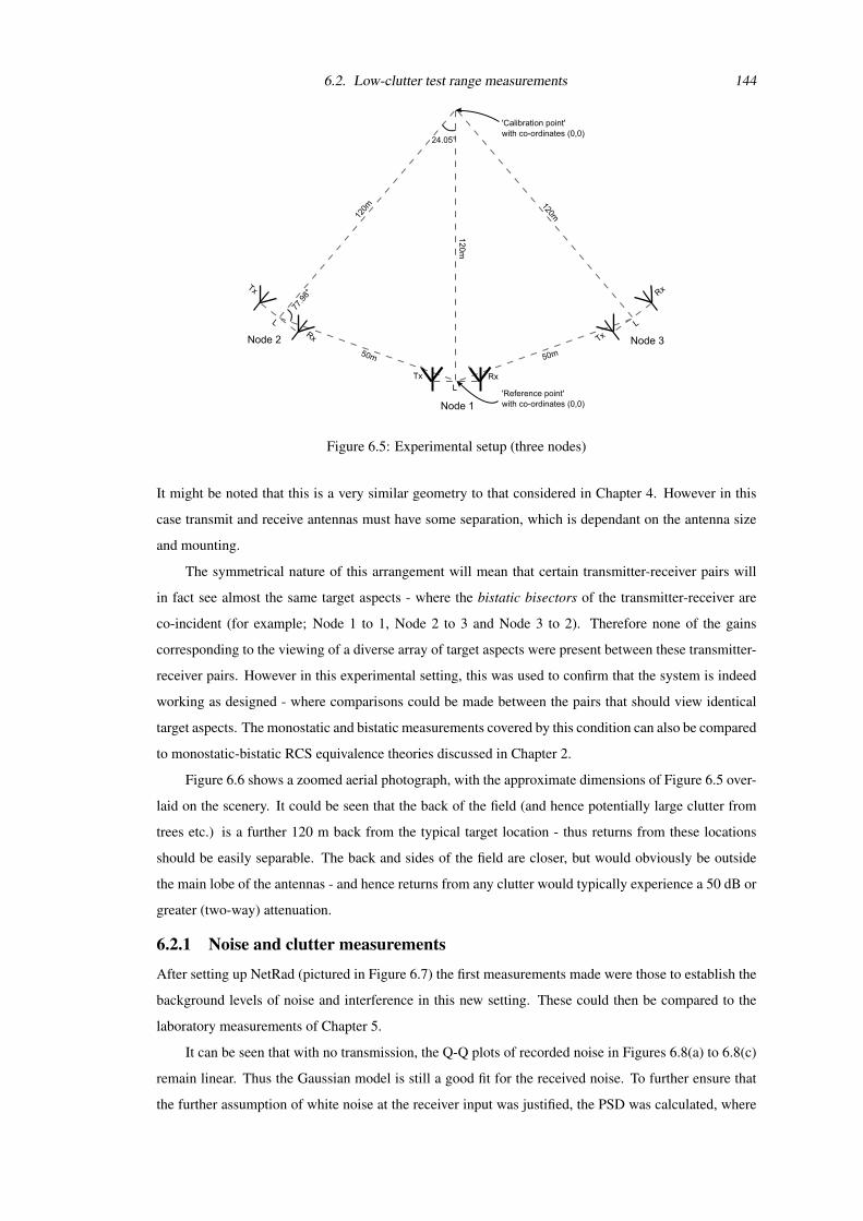
6.2. Low-clutter test range measurements 144
Figure 6.5: Experimental setup (three nodes)
It might be noted that this is a very similar geometry to that considered in Chapter 4. However in this
case transmit and receive antennas must have some separation, which is dependant on the antenna size
and mounting.
The symmetrical nature of this arrangement will mean that certain transmitter-receiver pairs will
in fact see almost the same target aspects - where the bistatic bisectors of the transmitter-receiver are
co-incident (for example; Node 1 to 1, Node 2 to 3 and Node 3 to 2). Therefore none of the gains
corresponding to the viewing of a diverse array of target aspects were present between these transmitter-
receiver pairs. However in this experimental setting, this was used to confirm that the system is indeed
working as designed - where comparisons could be made between the pairs that should view identical
target aspects. The monostatic and bistatic measurements covered by this condition can also be compared
to monostatic-bistatic RCS equivalence theories discussed in Chapter 2.
Figure 6.6 shows a zoomed aerial photograph, with the approximate dimensions of Figure 6.5 over-
laid on the scenery. It could be seen that the back of the field (and hence potentially large clutter from
trees etc.) is a further 120 m back from the typical target location - thus returns from these locations
should be easily separable. The back and sides of the field are closer, but would obviously be outside
the main lobe of the antennas - and hence returns from any clutter would typically experience a 50 dB or
greater (two-way) attenuation.
6.2.1 Noise and clutter measurements
After setting up NetRad (pictured in Figure 6.7) the first measurements made were those to establish the
background levels of noise and interference in this new setting. These could then be compared to the
laboratory measurements of Chapter 5.
It can be seen that with no transmission, the Q-Q plots of recorded noise in Figures 6.8(a) to 6.8(c)
remain linear. Thus the Gaussian model is still a good fit for the received noise. To further ensure that
the further assumption of white noise at the receiver input was justified, the PSD was calculated, where
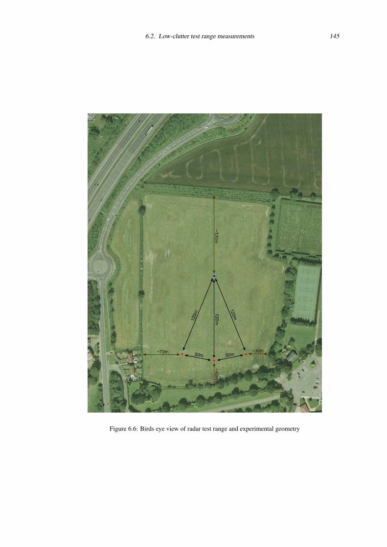
6.2. Low-clutter test range measurements 145
Figure 6.6: Birds eye view of radar test range and experimental geometry
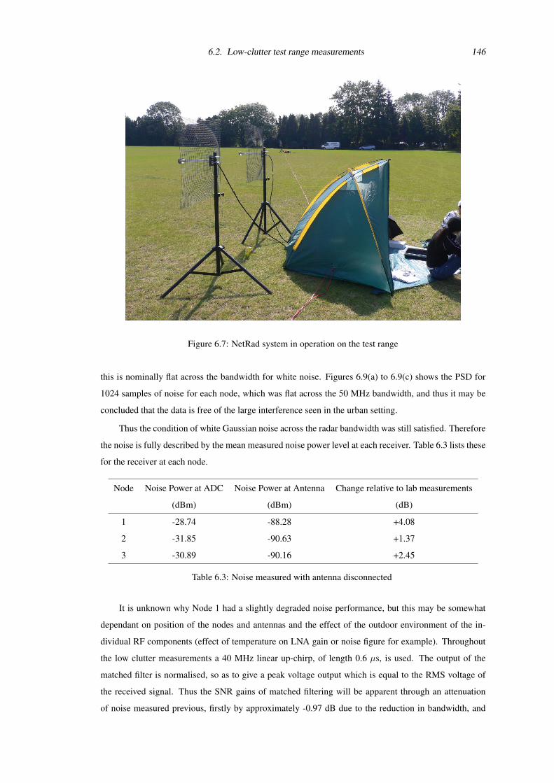
6.2. Low-clutter test range measurements 146
Figure 6.7: NetRad system in operation on the test range
this is nominally flat across the bandwidth for white noise. Figures 6.9(a) to 6.9(c) shows the PSD for
1024 samples of noise for each node, which was flat across the 50 MHz bandwidth, and thus it may be
concluded that the data is free of the large interference seen in the urban setting.
Thus the condition of white Gaussian noise across the radar bandwidth was still satisfied. Therefore
the noise is fully described by the mean measured noise power level at each receiver. Table 6.3 lists these
for the receiver at each node.
Node Noise Power at ADC Noise Power at Antenna Change relative to lab measurements
(dBm) (dBm) (dB)
1 -28.74 -88.28 +4.08
2 -31.85 -90.63 +1.37
3 -30.89 -90.16 +2.45
Table 6.3: Noise measured with antenna disconnected
It is unknown why Node 1 had a slightly degraded noise performance, but this may be somewhat
dependant on position of the nodes and antennas and the effect of the outdoor environment of the in-
dividual RF components (effect of temperature on LNA gain or noise figure for example). Throughout
the low clutter measurements a 40 MHz linear up-chirp, of length 0.6 µs, is used. The output of the
matched filter is normalised, so as to give a peak voltage output which is equal to the RMS voltage of
the received signal. Thus the SNR gains of matched filtering will be apparent through an attenuation
of noise measured previous, firstly by approximately -0.97 dB due to the reduction in bandwidth, and
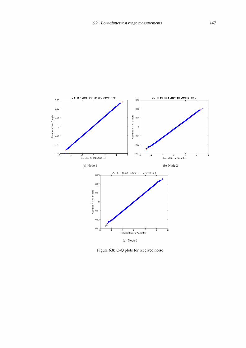
6.2. Low-clutter test range measurements 147
(a) Node 1 (b) Node 2
(c) Node 3
Figure 6.8: Q-Q plots for received noise
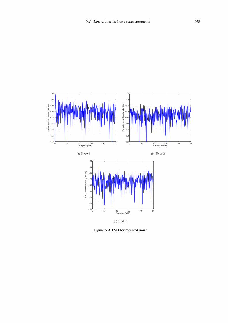
6.2. Low-clutter test range measurements 148
0 10 20 30 40 50−130
−125
−120
−115
−110
−105
−100
−95
−90
Freqency (MHz)
Pow
er S
pect
ral D
ensi
ty (
dBm
/Hz)
(a) Node 1
0 10 20 30 40 50−130
−125
−120
−115
−110
−105
−100
−95
−90
Frequency (MHz)
Pow
er S
pect
ral D
ensi
ty (
dBm
/Hz)
(b) Node 2
0 10 20 30 40 50−130
−125
−120
−115
−110
−105
−100
−95
−90
Frequency (MHz)
Pow
er S
pect
ral D
ensi
ty (
dBm
/Hz)
(c) Node 3
Figure 6.9: PSD for received noise
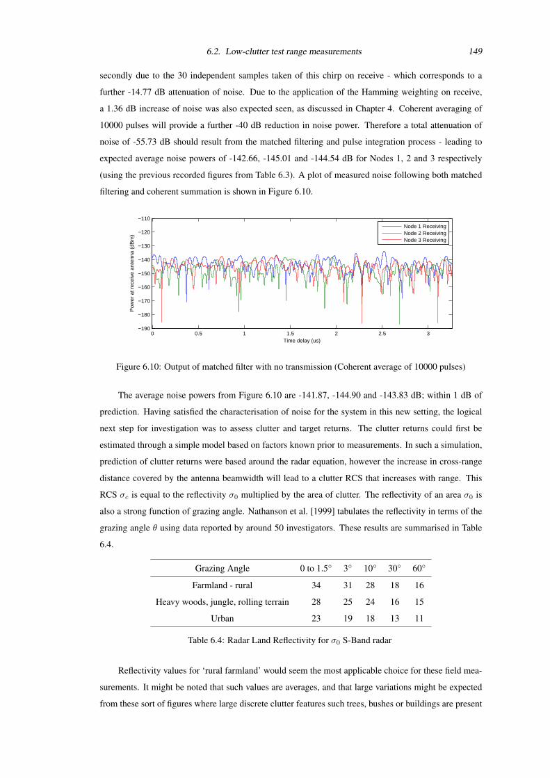
6.2. Low-clutter test range measurements 149
secondly due to the 30 independent samples taken of this chirp on receive - which corresponds to a
further -14.77 dB attenuation of noise. Due to the application of the Hamming weighting on receive,
a 1.36 dB increase of noise was also expected seen, as discussed in Chapter 4. Coherent averaging of
10000 pulses will provide a further -40 dB reduction in noise power. Therefore a total attenuation of
noise of -55.73 dB should result from the matched filtering and pulse integration process - leading to
expected average noise powers of -142.66, -145.01 and -144.54 dB for Nodes 1, 2 and 3 respectively
(using the previous recorded figures from Table 6.3). A plot of measured noise following both matched
filtering and coherent summation is shown in Figure 6.10.
0 0.5 1 1.5 2 2.5 3−190
−180
−170
−160
−150
−140
−130
−120
−110
Time delay (us)
Pow
er a
t rec
eive
ant
enna
(dB
m)
Node 1 ReceivingNode 2 ReceivingNode 3 Receiving
Figure 6.10: Output of matched filter with no transmission (Coherent average of 10000 pulses)
The average noise powers from Figure 6.10 are -141.87, -144.90 and -143.83 dB; within 1 dB of
prediction. Having satisfied the characterisation of noise for the system in this new setting, the logical
next step for investigation was to assess clutter and target returns. The clutter returns could first be
estimated through a simple model based on factors known prior to measurements. In such a simulation,
prediction of clutter returns were based around the radar equation, however the increase in cross-range
distance covered by the antenna beamwidth will lead to a clutter RCS that increases with range. This
RCS σc is equal to the reflectivity σ0 multiplied by the area of clutter. The reflectivity of an area σ0 is
also a strong function of grazing angle. Nathanson et al. [1999] tabulates the reflectivity in terms of the
grazing angle θ using data reported by around 50 investigators. These results are summarised in Table
6.4.
Grazing Angle 0 to 1.5 3 10 30 60
Farmland - rural 34 31 28 18 16
Heavy woods, jungle, rolling terrain 28 25 24 16 15
Urban 23 19 18 13 11
Table 6.4: Radar Land Reflectivity for σ0 S-Band radar
Reflectivity values for ‘rural farmland’ would seem the most applicable choice for these field mea-
surements. It might be noted that such values are averages, and that large variations might be expected
from these sort of figures where large discrete clutter features such trees, bushes or buildings are present
6.2. Low-clutter test range measurements 150
- as well as effects such as shadowing. Even without these sort of effects, Nathanson notes that 5 dB
variations of the means themselves are not uncommon, for grazing angles below 10.
σc = σ0Ac (6.1)
≈ σ0(4DR)Rθazi (6.2)
Here4DR, the down-range resolution, was that of a Hamming weighted-on-receive 40 MHz linear
FM up-chirp - with a -3 dB distance of 4.92 m. Given a fixed antenna elevation, the maximum gain of
antenna boresight may not be realised for all mainlobe clutter. An approximate model to represent the
loss of gain for the antenna mainlobe away from boresight was sinc2(θ/θele), where θele is the antenna
-3 dB elevation beamwidth. Given that that elevation of all antennas will be parallel to the ground plane,
the radar equation for this mainlobe clutter was then constructed in Equation 6.3.
Pclutter =PtGtGrsinc
4(θ/θele)σcλ2Ls(4π)3||R||4
(6.3)
The power returned for a typical target was also considered. Again the radar equation (Equation
6.4) is used, where targets are assumed to be at the antenna boresight.
Ptarget =PtGtGrσλ
2FLs(4π)3||R||4
(6.4)
Two variables in this equation deserve further explanation - RCS σ and pattern propagation factor
F . The specific properties of RCS, σ, will vary depending on both the target and the bistatic angle of the
transmitter-receiver pair. For purposes of producing simple quantitative predictions of returned signal
power from targets, well known formulas for the monostatic RCS based on simple target geometry
[Kingsley and Quegan, 1992] can be produced, and are shown in Table 6.5, alongside a commonly
quoted figure of 1m2 for a person. A reflector of each type was constructed for use in testing. The corner
reflector was a square trihedral flat plate target, constructed in accordance with the ‘optimum corner
reflector’ design discussed in Sarabandi and Chiu [1996] with an edge measurement of 0.5 m.
Target RCS (m2) RCS (dBm2) Notes
Corner reflector 12πl4
λ2 150 21.76 edge length l = 0.5 m
Flat plate 4πw2h2
λ2 141.87 21.52 width w = 0.75 m
height h = 0.56 m
Cylinder 2πrh2
λ 3.39 5.3 radius r = 0.15 m
height h = 0.65 m
Person (typical) 1 0
Table 6.5: Monostatic RCS of various test targets
For the purposes of experimental testing, the cylinder target was often the focus of investigation.
This target, unlike the flat plate or corner reflector, has the same geometry when viewed from any az-
imuth. Thus this target was ideal for effectively ‘calibrating’ a ground-based multistatic radar as it is the
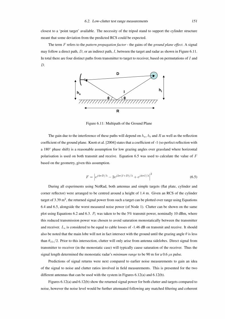
6.2. Low-clutter test range measurements 151
closest to a ‘point target’ available. The necessity of the tripod stand to support the cylinder structure
meant that some deviation from the predicted RCS could be expected.
The term F refers to the pattern propagation factor - the gains of the ground plane effect. A signal
may follow a direct path, D, or an indirect path, I , between the target and radar as shown in Figure 6.11.
In total there are four distinct paths from transmitter to target to receiver, based on permutations of I and
D.
R
D
I htha
Figure 6.11: Multipath of the Ground Plane
The gain due to the interference of these paths will depend on ha, ht and R as well as the reflection
coefficient of the ground plane. Knott et al. [2004] states that a coefficient of -1 (so perfect reflection with
a 180 phase shift) is a reasonable assumption for low grazing angles over grassland where horizontal
polarisation is used on both transmit and receive. Equation 6.5 was used to calculate the value of F
based on the geometry, given this assumption.
F =∣∣∣ej4πD/λ − 2ej2π(I+D)/λ + ej4πI/λ
∣∣∣2 (6.5)
During all experiments using NetRad, both antennas and simple targets (flat plate, cylinder and
corner reflector) were arranged to be centred around a height of 1.4 m. Given an RCS of the cylinder
target of 3.39 m2, the returned signal power from such a target can be plotted over range using Equations
6.4 and 6.5, alongside the worst measured noise power (of Node 1). Clutter can be shown on the same
plot using Equations 6.2 and 6.3. Pt was taken to be the 5% transmit power, nominally 10 dBm, where
this reduced transmission power was chosen to avoid saturation monostatically between the transmitter
and receiver. Ls is considered to be equal to cable losses of -1.46 dB on transmit and receive. It should
also be noted that the main lobe will not in fact intersect with the ground until the grazing angle θ is less
than θele/2. Prior to this intersection, clutter will only arise from antenna sidelobes. Direct signal from
transmitter to receiver (in the monostatic case) will typically cause saturation of the receiver. Thus the
signal length determined the monostatic radar’s minimum range to be 90 m for a 0.6 µs pulse.
Predictions of signal returns were next compared to earlier noise measurements to gain an idea
of the signal to noise and clutter ratios involved in field measurements. This is presented for the two
different antennas that can be used with the system in Figures 6.12(a) and 6.12(b).
Figures 6.12(a) and 6.12(b) show the returned signal power for both clutter and targets compared to
noise, however the noise level would be further attenuated following any matched filtering and coherent
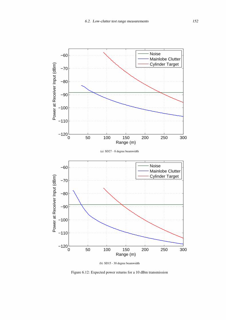
6.2. Low-clutter test range measurements 152
0 50 100 150 200 250 300−120
−110
−100
−90
−80
−70
−60
Range (m)
Pow
er a
t Rec
eive
r In
put (
dBm
)
NoiseMainlobe ClutterCylinder Target
(a) SD27 - 8 degree beamwidth
0 50 100 150 200 250 300−120
−110
−100
−90
−80
−70
−60
Range (m)
Pow
er a
t Rec
eive
r In
put (
dBm
)
NoiseMainlobe ClutterCylinder Target
(b) SD15 - 30 degree beamwidth
Figure 6.12: Expected power returns for a 10 dBm transmission
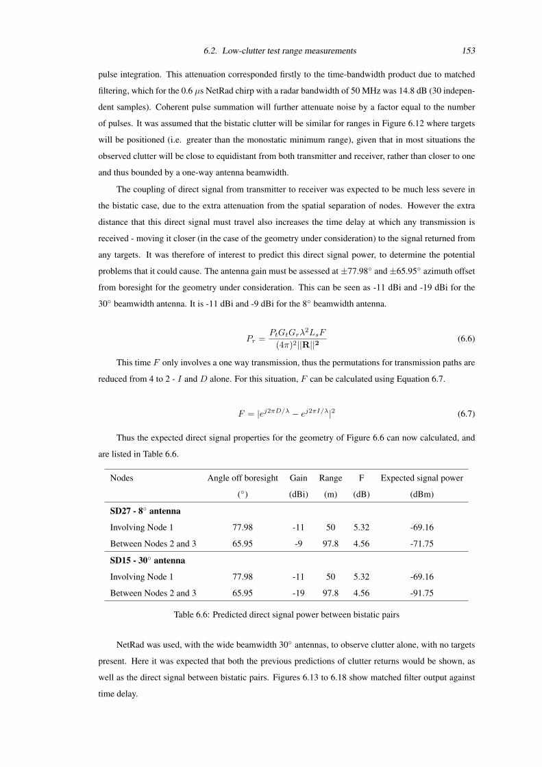
6.2. Low-clutter test range measurements 153
pulse integration. This attenuation corresponded firstly to the time-bandwidth product due to matched
filtering, which for the 0.6 µs NetRad chirp with a radar bandwidth of 50 MHz was 14.8 dB (30 indepen-
dent samples). Coherent pulse summation will further attenuate noise by a factor equal to the number
of pulses. It was assumed that the bistatic clutter will be similar for ranges in Figure 6.12 where targets
will be positioned (i.e. greater than the monostatic minimum range), given that in most situations the
observed clutter will be close to equidistant from both transmitter and receiver, rather than closer to one
and thus bounded by a one-way antenna beamwidth.
The coupling of direct signal from transmitter to receiver was expected to be much less severe in
the bistatic case, due to the extra attenuation from the spatial separation of nodes. However the extra
distance that this direct signal must travel also increases the time delay at which any transmission is
received - moving it closer (in the case of the geometry under consideration) to the signal returned from
any targets. It was therefore of interest to predict this direct signal power, to determine the potential
problems that it could cause. The antenna gain must be assessed at±77.98 and±65.95 azimuth offset
from boresight for the geometry under consideration. This can be seen as -11 dBi and -19 dBi for the
30 beamwidth antenna. It is -11 dBi and -9 dBi for the 8 beamwidth antenna.
Pr =PtGtGrλ
2LsF
(4π)2||R||2(6.6)
This time F only involves a one way transmission, thus the permutations for transmission paths are
reduced from 4 to 2 - I and D alone. For this situation, F can be calculated using Equation 6.7.
F = |ej2πD/λ − ej2πI/λ|2 (6.7)
Thus the expected direct signal properties for the geometry of Figure 6.6 can now calculated, and
are listed in Table 6.6.
Nodes Angle off boresight Gain Range F Expected signal power
() (dBi) (m) (dB) (dBm)
SD27 - 8 antenna
Involving Node 1 77.98 -11 50 5.32 -69.16
Between Nodes 2 and 3 65.95 -9 97.8 4.56 -71.75
SD15 - 30 antenna
Involving Node 1 77.98 -11 50 5.32 -69.16
Between Nodes 2 and 3 65.95 -19 97.8 4.56 -91.75
Table 6.6: Predicted direct signal power between bistatic pairs
NetRad was used, with the wide beamwidth 30 antennas, to observe clutter alone, with no targets
present. Here it was expected that both the previous predictions of clutter returns would be shown, as
well as the direct signal between bistatic pairs. Figures 6.13 to 6.18 show matched filter output against
time delay.
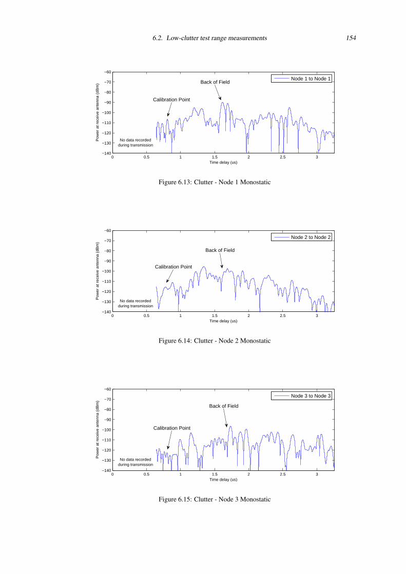
6.2. Low-clutter test range measurements 154
0 0.5 1 1.5 2 2.5 3−140
−130
−120
−110
−100
−90
−80
−70
−60
Time delay (us)
Pow
er a
t rec
eive
ant
enna
(dB
m)
Node 1 to Node 1Back of Field
Calibration Point
No data recordedduring transmission
Figure 6.13: Clutter - Node 1 Monostatic
0 0.5 1 1.5 2 2.5 3−140
−130
−120
−110
−100
−90
−80
−70
−60
Time delay (us)
Pow
er a
t rec
eive
ant
enna
(dB
m)
Node 2 to Node 2
Calibration Point
Back of Field
No data recordedduring transmission
Figure 6.14: Clutter - Node 2 Monostatic
0 0.5 1 1.5 2 2.5 3−140
−130
−120
−110
−100
−90
−80
−70
−60
Time delay (us)
Pow
er a
t rec
eive
ant
enna
(dB
m)
Node 3 to Node 3
Calibration Point
Back of Field
No data recordedduring transmission
Figure 6.15: Clutter - Node 3 Monostatic
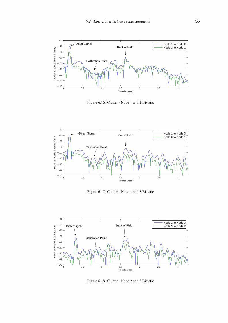
6.2. Low-clutter test range measurements 155
0 0.5 1 1.5 2 2.5 3−140
−130
−120
−110
−100
−90
−80
−70
−60
Time delay (us)
Pow
er a
t rec
eive
ant
enna
(dB
m)
Node 1 to Node 2Node 2 to Node 1
Direct Signal
Calibration Point
Back of Field
Figure 6.16: Clutter - Node 1 and 2 Bistatic
0 0.5 1 1.5 2 2.5 3−140
−130
−120
−110
−100
−90
−80
−70
−60
Time delay (us)
Pow
er a
t rec
eive
ant
enna
(dB
m)
Node 1 to Node 3Node 3 to Node 1
Direct Signal Back of Field
Calibration Point
Figure 6.17: Clutter - Node 1 and 3 Bistatic
0 0.5 1 1.5 2 2.5 3−140
−130
−120
−110
−100
−90
−80
−70
−60
Time delay (us)
Pow
er a
t rec
eive
ant
enna
(dB
m)
Node 2 to Node 3Node 3 to Node 2Direct Signal
Calibration Point
Back of Field
Figure 6.18: Clutter - Node 2 and 3 Bistatic
6.2. Low-clutter test range measurements 156
The smooth degradation of received power theorised in Figure 6.12 was not seen with the 30
beamwidth antennas. This is probably due to the resolution of the waveform coupled with the number
of clutter features surrounding the field. Between approximately 0.5 and 1 µs the expanse of the field
can be seen at a relatively low returned power (around -110 dBm), although this is interrupted in some
instances by sidelobes from direct transmission - particularly noticeable where the highest direct bistatic
transmission level (involving Node 1) are present. The characteristic sidelobe ‘floor’ due to the Hamming
window, -30 dB down on the peak response, can be seen for these signals. At 1.6 µs a large response
corresponding to the back of the field can be seen. Several other peaks can also be seen between 1 µs and
1.6 µs which vary more in time delay from profile to profile. These can be accounted to the sides of the
field - which, unlike the back of the field, will have a rather variable distance dependant on the specific
transmit and receive nodes. Profiles involving the same pair of nodes are plotted on the same figure, and
can be seen to be very close to one another. In theory if transmitter and receiver locations, orientations
and gains are exactly the same then the Rayleigh-Carson reciprocity theorem dictates that these pairs
should be exactly identical - however small differences in each of these explain the differences observed.
The large response corresponding to the direct signal can be seen more precisely at around either
0.17 µs or 0.33 µs. This delay corresponds to the range of transmitter to receiver of around 51 m and
99 m (slight differences will be apparent between pairs due to specific antenna positions). The measured
signal from Figures 6.16 to 6.18 is tabulated in Table 6.7 and compared to the a-priori predictions based
on knowledge of transmitter power and antenna pattern.
Receiving Node
Tran
smitt
ing
Nod
e
1 2 3
1 -69.40 dBm @ 52.08 m -68.09 dBm @ 49.68 m
(+10.76 dBm +1.11 m) (+12.07 dBm +0.53 m)
2 -79.08 dBm @ 47.46 m -91.42 dBm @ 99.18 m
(+3.58 dBm -1.69 m) (+13.84 dBm +2.11 m)
3 -73.68 dBm @ 51.42 m -97.38 dBm @ 96.18 m
(+9.48 dBm +0.45 m) (+8.37 dBm -2.59 m)
Table 6.7: Measured signal between bistatic pairs (difference from prediction)
It can be seen that measured direct signals are generally 10 dB higher than prediction. This could
be due to deviation of the antenna sidelobes from those quoted. Further, difficult to predict, propagation
effects could also be involved, such as interaction from the other antenna at each node or even reflections
from the physical form of the node itself. The same effects could also have an effect on the difference in
distances, also shown in Table 6.7. A more likely explanation is some inaccuracy in the measuring out
and setting up the test range. The accuracy of the distance measure of the test range was estimated to
be ∼1m due to some give in the set lengths of rope used. The antennas were positioned by eye; aiming
boresight at the ‘calibration point’ shown in Figure 6.5.
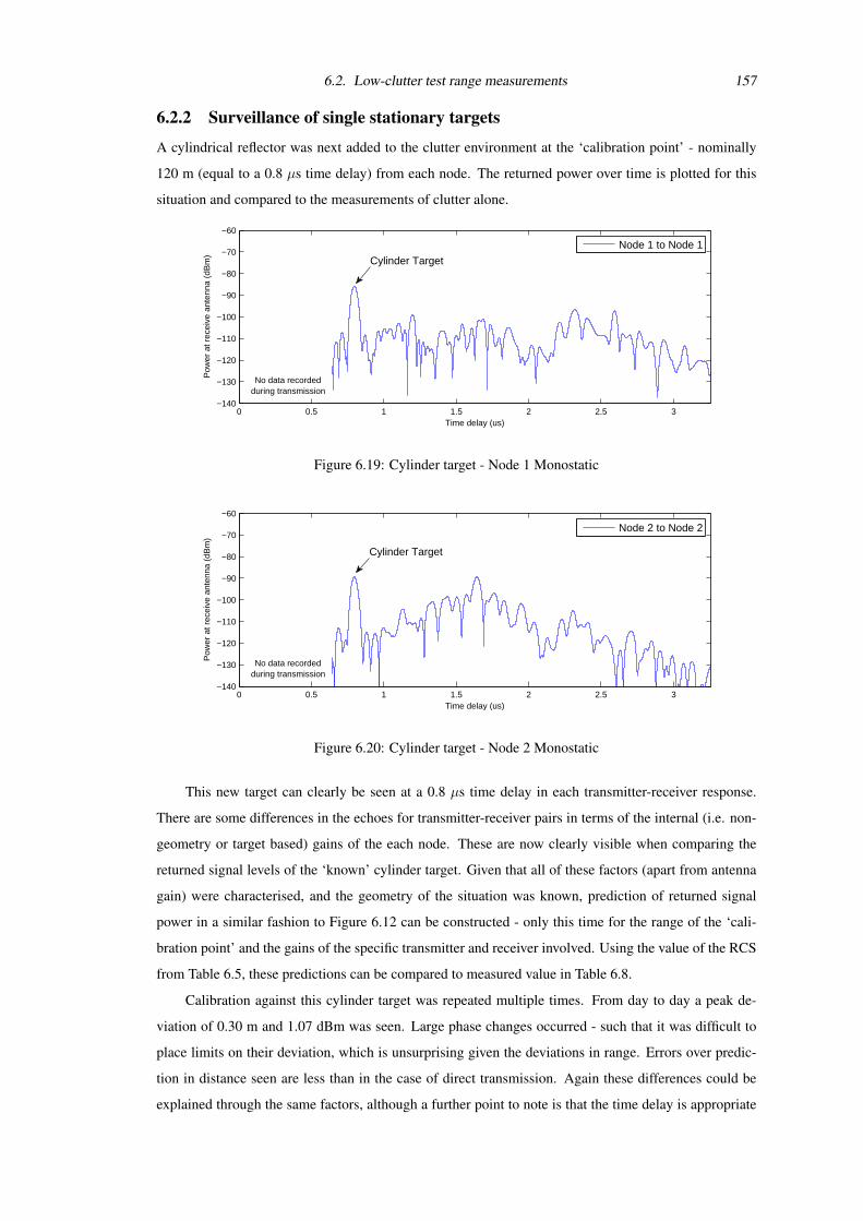
6.2. Low-clutter test range measurements 157
6.2.2 Surveillance of single stationary targets
A cylindrical reflector was next added to the clutter environment at the ‘calibration point’ - nominally
120 m (equal to a 0.8 µs time delay) from each node. The returned power over time is plotted for this
situation and compared to the measurements of clutter alone.
0 0.5 1 1.5 2 2.5 3−140
−130
−120
−110
−100
−90
−80
−70
−60
Time delay (us)
Pow
er a
t rec
eive
ant
enna
(dB
m)
Node 1 to Node 1
Cylinder Target
No data recordedduring transmission
Figure 6.19: Cylinder target - Node 1 Monostatic
0 0.5 1 1.5 2 2.5 3−140
−130
−120
−110
−100
−90
−80
−70
−60
Time delay (us)
Pow
er a
t rec
eive
ant
enna
(dB
m)
Node 2 to Node 2
Cylinder Target
No data recordedduring transmission
Figure 6.20: Cylinder target - Node 2 Monostatic
This new target can clearly be seen at a 0.8 µs time delay in each transmitter-receiver response.
There are some differences in the echoes for transmitter-receiver pairs in terms of the internal (i.e. non-
geometry or target based) gains of the each node. These are now clearly visible when comparing the
returned signal levels of the ‘known’ cylinder target. Given that all of these factors (apart from antenna
gain) were characterised, and the geometry of the situation was known, prediction of returned signal
power in a similar fashion to Figure 6.12 can be constructed - only this time for the range of the ‘cali-
bration point’ and the gains of the specific transmitter and receiver involved. Using the value of the RCS
from Table 6.5, these predictions can be compared to measured value in Table 6.8.
Calibration against this cylinder target was repeated multiple times. From day to day a peak de-
viation of 0.30 m and 1.07 dBm was seen. Large phase changes occurred - such that it was difficult to
place limits on their deviation, which is unsurprising given the deviations in range. Errors over predic-
tion in distance seen are less than in the case of direct transmission. Again these differences could be
explained through the same factors, although a further point to note is that the time delay is appropriate

6.2. Low-clutter test range measurements 158
0 0.5 1 1.5 2 2.5 3−140
−130
−120
−110
−100
−90
−80
−70
−60
Time delay (us)
Pow
er a
t rec
eive
ant
enna
(dB
m)
Node 3 to Node 3
Cylinder Target
No data recordedduring transmission
Figure 6.21: Cylinder target - Node 3 Monostatic
0 0.5 1 1.5 2 2.5 3−140
−130
−120
−110
−100
−90
−80
−70
−60
Time delay (us)
Pow
er a
t rec
eive
ant
enna
(dB
m)
Node 1 to Node 2Node 2 to Node 1Cylinder Target
Direct Signal
Figure 6.22: Cylinder target - Node 1 and 2 Bistatic
0 0.5 1 1.5 2 2.5 3−140
−130
−120
−110
−100
−90
−80
−70
−60
Time delay (us)
Pow
er a
t rec
eive
ant
enna
(dB
m)
Node 1 to Node 3Node 3 to Node 1Cylinder Target
Direct Signal
Figure 6.23: Cylinder target - Node 1 and 3 Bistatic
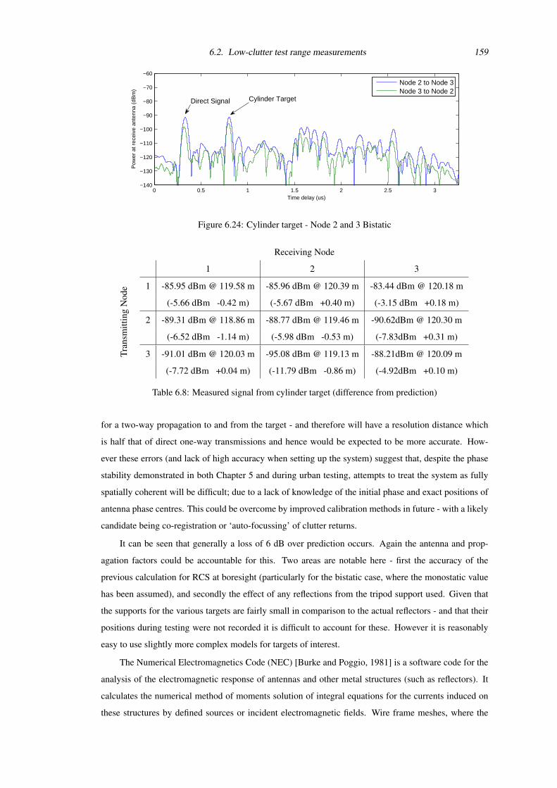
6.2. Low-clutter test range measurements 159
0 0.5 1 1.5 2 2.5 3−140
−130
−120
−110
−100
−90
−80
−70
−60
Time delay (us)
Pow
er a
t rec
eive
ant
enna
(dB
m)
Node 2 to Node 3Node 3 to Node 2
Cylinder TargetDirect Signal
Figure 6.24: Cylinder target - Node 2 and 3 Bistatic
Receiving Node
Tran
smitt
ing
Nod
e
1 2 3
1 -85.95 dBm @ 119.58 m -85.96 dBm @ 120.39 m -83.44 dBm @ 120.18 m
(-5.66 dBm -0.42 m) (-5.67 dBm +0.40 m) (-3.15 dBm +0.18 m)
2 -89.31 dBm @ 118.86 m -88.77 dBm @ 119.46 m -90.62dBm @ 120.30 m
(-6.52 dBm -1.14 m) (-5.98 dBm -0.53 m) (-7.83dBm +0.31 m)
3 -91.01 dBm @ 120.03 m -95.08 dBm @ 119.13 m -88.21dBm @ 120.09 m
(-7.72 dBm +0.04 m) (-11.79 dBm -0.86 m) (-4.92dBm +0.10 m)
Table 6.8: Measured signal from cylinder target (difference from prediction)
for a two-way propagation to and from the target - and therefore will have a resolution distance which
is half that of direct one-way transmissions and hence would be expected to be more accurate. How-
ever these errors (and lack of high accuracy when setting up the system) suggest that, despite the phase
stability demonstrated in both Chapter 5 and during urban testing, attempts to treat the system as fully
spatially coherent will be difficult; due to a lack of knowledge of the initial phase and exact positions of
antenna phase centres. This could be overcome by improved calibration methods in future - with a likely
candidate being co-registration or ‘auto-focussing’ of clutter returns.
It can be seen that generally a loss of 6 dB over prediction occurs. Again the antenna and prop-
agation factors could be accountable for this. Two areas are notable here - first the accuracy of the
previous calculation for RCS at boresight (particularly for the bistatic case, where the monostatic value
has been assumed), and secondly the effect of any reflections from the tripod support used. Given that
the supports for the various targets are fairly small in comparison to the actual reflectors - and that their
positions during testing were not recorded it is difficult to account for these. However it is reasonably
easy to use slightly more complex models for targets of interest.
The Numerical Electromagnetics Code (NEC) [Burke and Poggio, 1981] is a software code for the
analysis of the electromagnetic response of antennas and other metal structures (such as reflectors). It
calculates the numerical method of moments solution of integral equations for the currents induced on
these structures by defined sources or incident electromagnetic fields. Wire frame meshes, where the
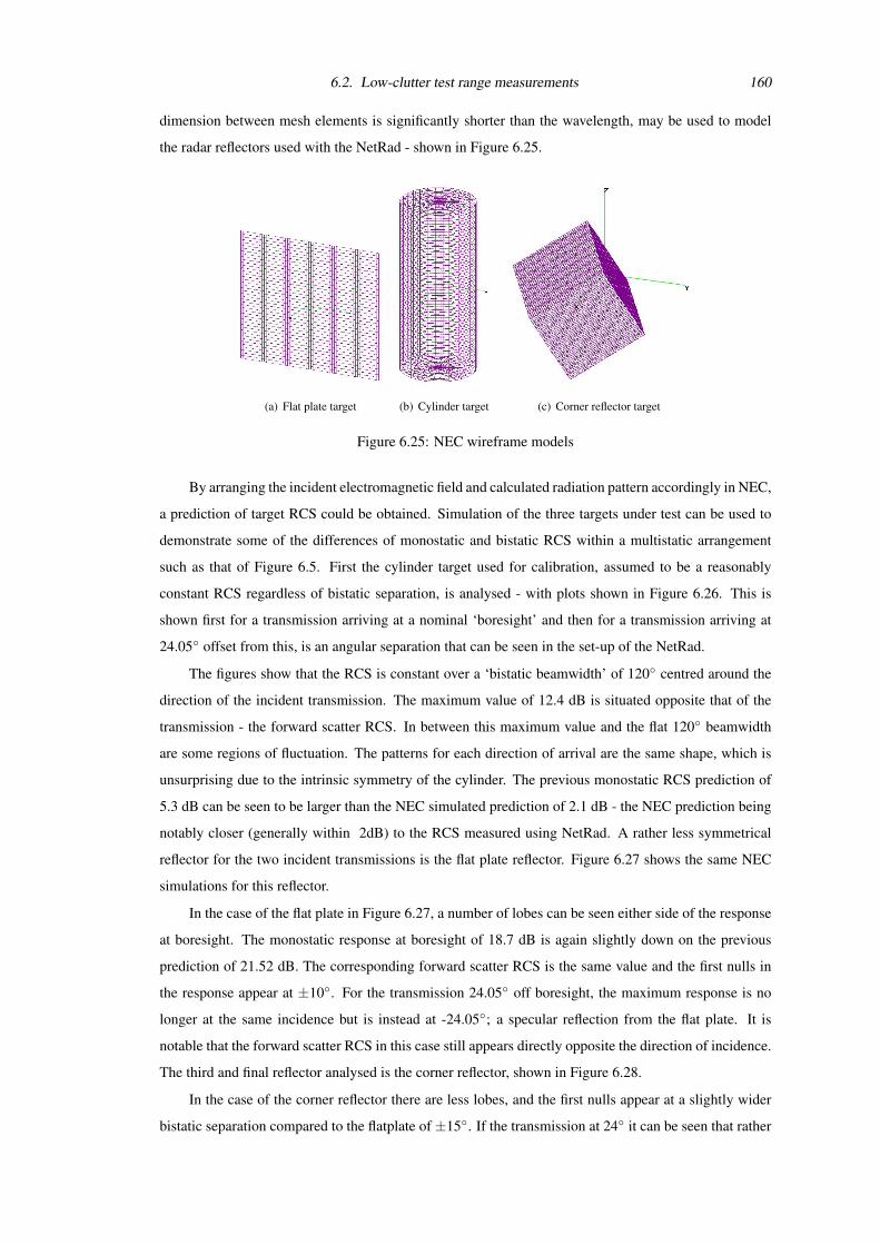
6.2. Low-clutter test range measurements 160
dimension between mesh elements is significantly shorter than the wavelength, may be used to model
the radar reflectors used with the NetRad - shown in Figure 6.25.
(a) Flat plate target (b) Cylinder target (c) Corner reflector target
Figure 6.25: NEC wireframe models
By arranging the incident electromagnetic field and calculated radiation pattern accordingly in NEC,
a prediction of target RCS could be obtained. Simulation of the three targets under test can be used to
demonstrate some of the differences of monostatic and bistatic RCS within a multistatic arrangement
such as that of Figure 6.5. First the cylinder target used for calibration, assumed to be a reasonably
constant RCS regardless of bistatic separation, is analysed - with plots shown in Figure 6.26. This is
shown first for a transmission arriving at a nominal ‘boresight’ and then for a transmission arriving at
24.05 offset from this, is an angular separation that can be seen in the set-up of the NetRad.
The figures show that the RCS is constant over a ‘bistatic beamwidth’ of 120 centred around the
direction of the incident transmission. The maximum value of 12.4 dB is situated opposite that of the
transmission - the forward scatter RCS. In between this maximum value and the flat 120 beamwidth
are some regions of fluctuation. The patterns for each direction of arrival are the same shape, which is
unsurprising due to the intrinsic symmetry of the cylinder. The previous monostatic RCS prediction of
5.3 dB can be seen to be larger than the NEC simulated prediction of 2.1 dB - the NEC prediction being
notably closer (generally within 2dB) to the RCS measured using NetRad. A rather less symmetrical
reflector for the two incident transmissions is the flat plate reflector. Figure 6.27 shows the same NEC
simulations for this reflector.
In the case of the flat plate in Figure 6.27, a number of lobes can be seen either side of the response
at boresight. The monostatic response at boresight of 18.7 dB is again slightly down on the previous
prediction of 21.52 dB. The corresponding forward scatter RCS is the same value and the first nulls in
the response appear at ±10. For the transmission 24.05 off boresight, the maximum response is no
longer at the same incidence but is instead at -24.05; a specular reflection from the flat plate. It is
notable that the forward scatter RCS in this case still appears directly opposite the direction of incidence.
The third and final reflector analysed is the corner reflector, shown in Figure 6.28.
In the case of the corner reflector there are less lobes, and the first nulls appear at a slightly wider
bistatic separation compared to the flatplate of ±15. If the transmission at 24 it can be seen that rather
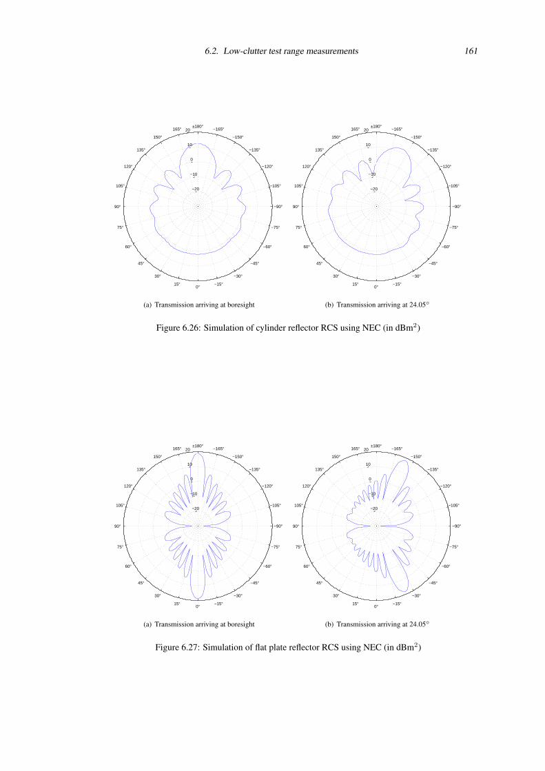
6.2. Low-clutter test range measurements 161
0°15°
30°
45°
60°
75°
90°
105°
120°
135°
150°
165° ±180°−165°
−150°
−135°
−120°
−105°
−90°
−75°
−60°
−45°
−30°
−15°
−20
−10
0
10
20
(a) Transmission arriving at boresight
0°15°
30°
45°
60°
75°
90°
105°
120°
135°
150°
165° ±180°−165°
−150°
−135°
−120°
−105°
−90°
−75°
−60°
−45°
−30°
−15°
−20
−10
0
10
20
(b) Transmission arriving at 24.05
Figure 6.26: Simulation of cylinder reflector RCS using NEC (in dBm2)
0°15°
30°
45°
60°
75°
90°
105°
120°
135°
150°
165° ±180°−165°
−150°
−135°
−120°
−105°
−90°
−75°
−60°
−45°
−30°
−15°
−20
−10
0
10
20
(a) Transmission arriving at boresight
0°15°
30°
45°
60°
75°
90°
105°
120°
135°
150°
165° ±180°−165°
−150°
−135°
−120°
−105°
−90°
−75°
−60°
−45°
−30°
−15°
−20
−10
0
10
20
(b) Transmission arriving at 24.05
Figure 6.27: Simulation of flat plate reflector RCS using NEC (in dBm2)
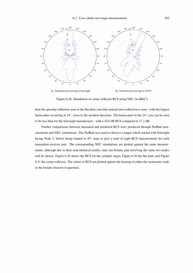
6.2. Low-clutter test range measurements 162
0°15°
30°
45°
60°
75°
90°
105°
120°
135°
150°
165° ±180°−165°
−150°
−135°
−120°
−105°
−90°
−75°
−60°
−45°
−30°
−15°
−20
−10
0
10
20
(a) Transmission arriving at boresight
0°15°
30°
45°
60°
75°
90°
105°
120°
135°
150°
165° ±180°−165°
−150°
−135°
−120°
−105°
−90°
−75°
−60°
−45°
−30°
−15°
−20
−10
0
10
20
(b) Transmission arriving at 24.05
Figure 6.28: Simulation of corner reflector RCS using NEC (in dBm2)
than the specular reflection seen in the flat plate case that instead retro-reflection is seen - with the largest
backscatter occurring at 19, close to the incident direction. The backscatter in the 24 case can be seen
to be less than for the boresight transmission - with a 10.8 dB RCS compared to 17.2 dB.
Further comparisons between measured and predicted RCS were produced through NetRad mea-
surements and NEC simulations. The NetRad was used to observe a target which started with boresight
facing Node 3, before being rotated in 45 steps to give a total of eight RCS measurements for each
transmitter-receiver pair. The corresponding NEC simulations are plotted against the same measure-
ments; although due to their near-identical results, only one bistatic pair involving the same two nodes
will be shown. Figure 6.29 shows the RCS for the cylinder target, Figure 6.30 the flat plate and Figure
6.31 the corner reflector. The values of RCS are plotted against the bearing of either the monostatic node
or the bistatic bisector in question.
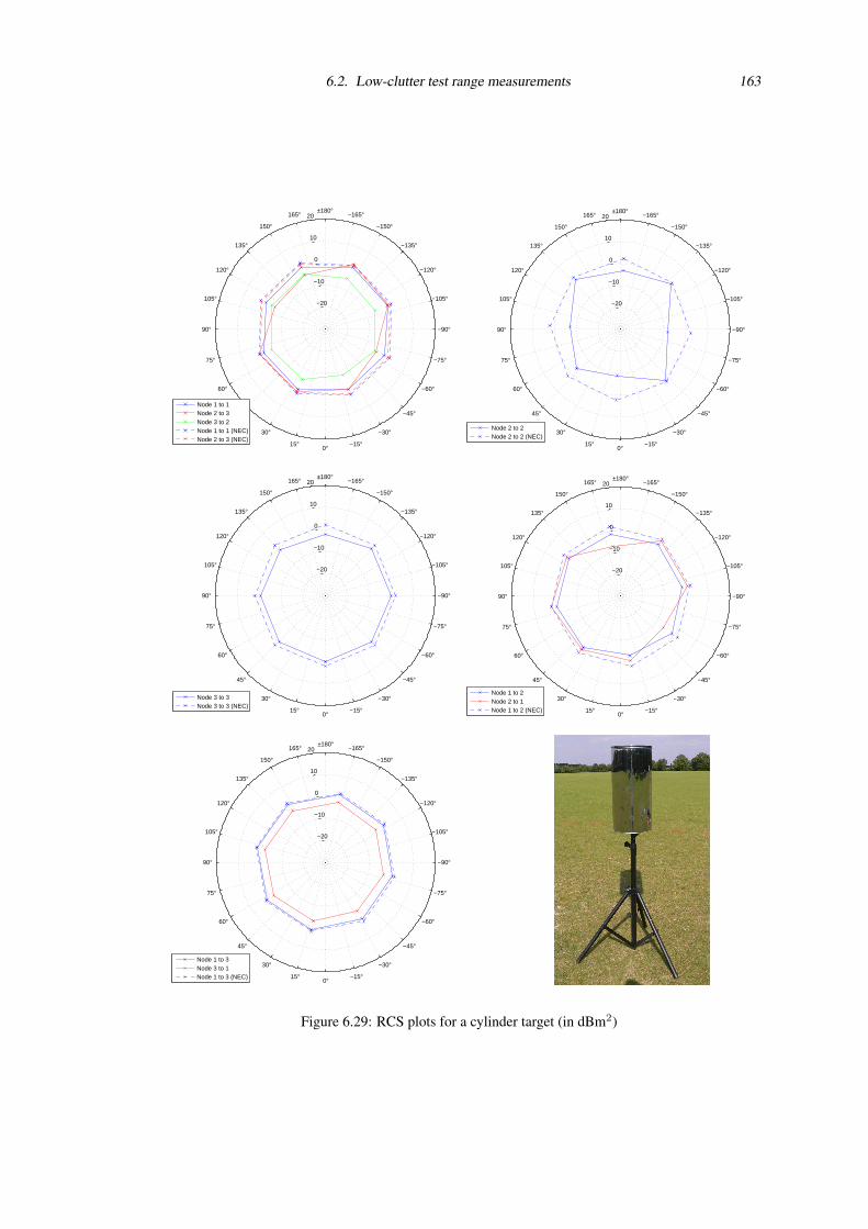
6.2. Low-clutter test range measurements 163
0°15°
30°
45°
60°
75°
90°
105°
120°
135°
150°
165° ±180°−165°
−150°
−135°
−120°
−105°
−90°
−75°
−60°
−45°
−30°
−15°
−20
−10
0
10
20
Node 1 to 1Node 2 to 3Node 3 to 2Node 1 to 1 (NEC)Node 2 to 3 (NEC)
0°15°
30°
45°
60°
75°
90°
105°
120°
135°
150°
165° ±180°−165°
−150°
−135°
−120°
−105°
−90°
−75°
−60°
−45°
−30°
−15°
−20
−10
0
10
20
Node 2 to 2Node 2 to 2 (NEC)
0°15°
30°
45°
60°
75°
90°
105°
120°
135°
150°
165° ±180°−165°
−150°
−135°
−120°
−105°
−90°
−75°
−60°
−45°
−30°
−15°
−20
−10
0
10
20
Node 3 to 3Node 3 to 3 (NEC)
0°15°
30°
45°
60°
75°
90°
105°
120°
135°
150°
165° ±180°−165°
−150°
−135°
−120°
−105°
−90°
−75°
−60°
−45°
−30°
−15°
−20
−10
0
10
20
Node 1 to 2Node 2 to 1Node 1 to 2 (NEC)
0°15°
30°
45°
60°
75°
90°
105°
120°
135°
150°
165° ±180°−165°
−150°
−135°
−120°
−105°
−90°
−75°
−60°
−45°
−30°
−15°
−20
−10
0
10
20
Node 1 to 3Node 3 to 1Node 1 to 3 (NEC)
Figure 6.29: RCS plots for a cylinder target (in dBm2)
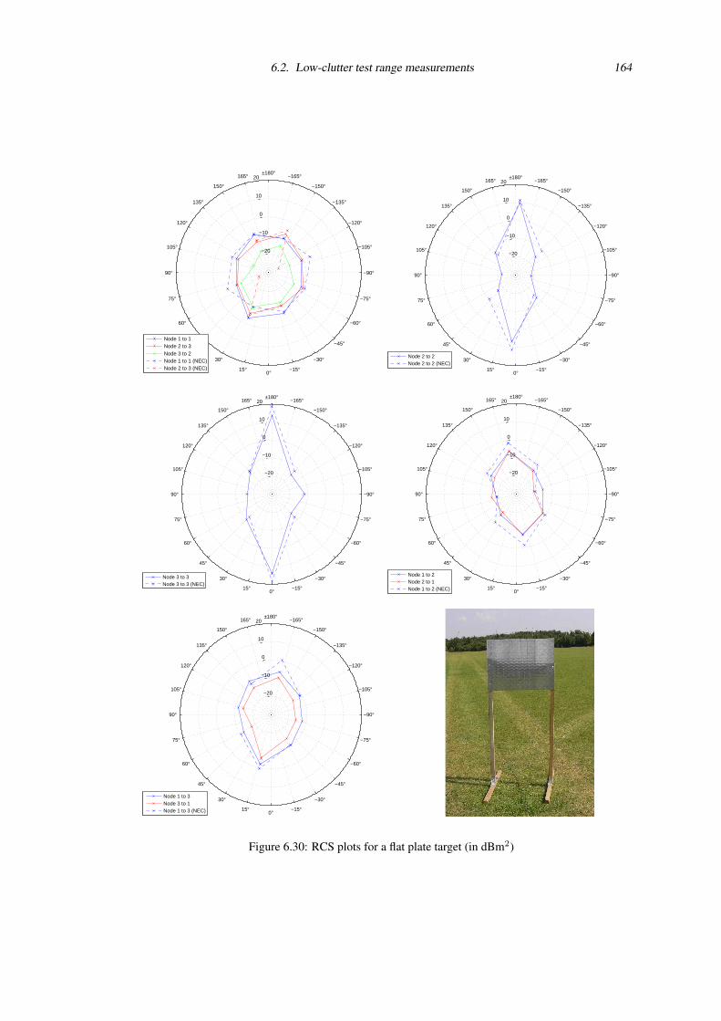
6.2. Low-clutter test range measurements 164
0°15°
30°
45°
60°
75°
90°
105°
120°
135°
150°
165° ±180°−165°
−150°
−135°
−120°
−105°
−90°
−75°
−60°
−45°
−30°
−15°
−20
−10
0
10
20
Node 1 to 1Node 2 to 3Node 3 to 2Node 1 to 1 (NEC)Node 2 to 3 (NEC)
0°15°
30°
45°
60°
75°
90°
105°
120°
135°
150°
165° ±180°−165°
−150°
−135°
−120°
−105°
−90°
−75°
−60°
−45°
−30°
−15°
−20
−10
0
10
20
Node 2 to 2Node 2 to 2 (NEC)
0°15°
30°
45°
60°
75°
90°
105°
120°
135°
150°
165° ±180°−165°
−150°
−135°
−120°
−105°
−90°
−75°
−60°
−45°
−30°
−15°
−20
−10
0
10
20
Node 3 to 3Node 3 to 3 (NEC)
0°15°
30°
45°
60°
75°
90°
105°
120°
135°
150°
165° ±180°−165°
−150°
−135°
−120°
−105°
−90°
−75°
−60°
−45°
−30°
−15°
−20
−10
0
10
20
Node 1 to 2Node 2 to 1Node 1 to 2 (NEC)
0°15°
30°
45°
60°
75°
90°
105°
120°
135°
150°
165° ±180°−165°
−150°
−135°
−120°
−105°
−90°
−75°
−60°
−45°
−30°
−15°
−20
−10
0
10
20
Node 1 to 3Node 3 to 1Node 1 to 3 (NEC)
Figure 6.30: RCS plots for a flat plate target (in dBm2)
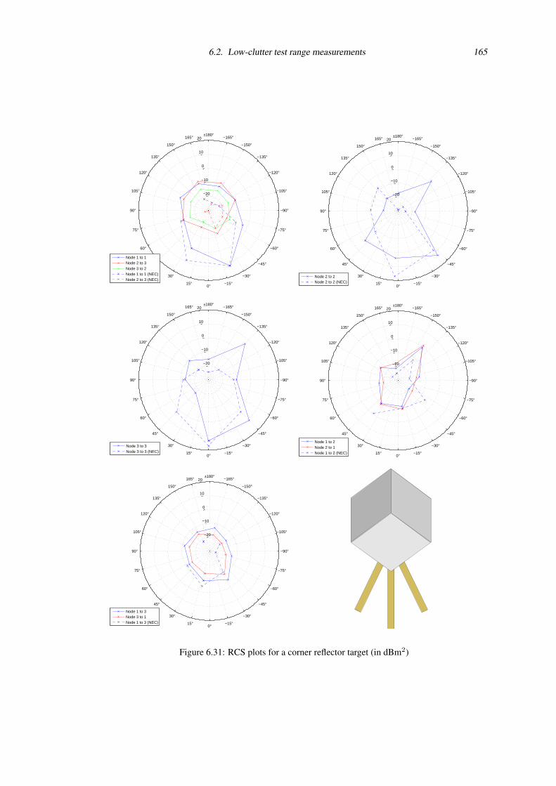
6.2. Low-clutter test range measurements 165
0°15°
30°
45°
60°
75°
90°
105°
120°
135°
150°
165° ±180°−165°
−150°
−135°
−120°
−105°
−90°
−75°
−60°
−45°
−30°
−15°
−20
−10
0
10
20
Node 1 to 1Node 2 to 3Node 3 to 2Node 1 to 1 (NEC)Node 2 to 3 (NEC)
0°15°
30°
45°
60°
75°
90°
105°
120°
135°
150°
165° ±180°−165°
−150°
−135°
−120°
−105°
−90°
−75°
−60°
−45°
−30°
−15°
−20
−10
0
10
20
Node 2 to 2Node 2 to 2 (NEC)
0°15°
30°
45°
60°
75°
90°
105°
120°
135°
150°
165° ±180°−165°
−150°
−135°
−120°
−105°
−90°
−75°
−60°
−45°
−30°
−15°
−20
−10
0
10
20
Node 3 to 3Node 3 to 3 (NEC)
0°15°
30°
45°
60°
75°
90°
105°
120°
135°
150°
165° ±180°−165°
−150°
−135°
−120°
−105°
−90°
−75°
−60°
−45°
−30°
−15°
−20
−10
0
10
20
Node 1 to 2Node 2 to 1Node 1 to 2 (NEC)
0°15°
30°
45°
60°
75°
90°
105°
120°
135°
150°
165° ±180°−165°
−150°
−135°
−120°
−105°
−90°
−75°
−60°
−45°
−30°
−15°
−20
−10
0
10
20
Node 1 to 3Node 3 to 1Node 1 to 3 (NEC)
Figure 6.31: RCS plots for a corner reflector target (in dBm2)
6.2. Low-clutter test range measurements 166
It should be noted that the plots of RCS consist of eight discrete points connected by lines. These
interconnections are intended to make the plots easier to read, rather than be any sort of accurate interpo-
lation between the points. It is clear from earlier NEC simulations that a rather finer resolution than the
45 steps used here would be needed to fully describe the RCS for any target orientation. The cylinder
target of Figure 6.29 can be seen to be reasonably constant regardless of orientation
Deviation from the ‘hexagonal’ shape seen in every other plot can be seen for all plots involving
a transmission of Node 2. It is difficult to think of a specific reason for this given that during target
rotation NetRad was not moved - therefore it is theorised that this effect is merely coincidental. Generally
deviation from the RCS ‘shape’ could be caused through non-ideal reflector construction (perhaps the
cylinder not being completely level, or slightly bent/misshapen) or interaction of the reflections from
the tripod support. It can be seen that levels in general are generally consistently less (over every target
orientation) than prediction. Certain transmitter-receiver pairs can be seen to experience this loss rather
more than others - notably Node 3 transmitting to Node 2, which is approximately 5 dB down on the
‘reciprocal pair’ of Node 2 transmitting to Node 3. An explanation for these losses is any deviation of
antenna gain from that quoted as well as mis-alignment of antennas. Any slight curvature or disturbance
of the nominally flat ground within the field may have some effect, resulting in a change in the pattern
propagation factor and hence further losses in RCS.
The shape of the flat plate response can be seen to be greatest at boresight as expected - which can
be seen in the monostatic case for Nodes 2 and 3. Unfortunately due to the rather coarse target rotation
angle these large responses are not seen in other plots. The loss of measured RCS over prediction seems
consistent with that obtained for the cylinder target and thus can be attributed to the same factors. One
particular peculiarity of the RCS simulation output in this flat plate case is the rather low RCS values
in certain cases - where the RCS is smaller than the lower -25 dB limit of the plot scale. In some
instances NEC gives an ‘infinitely small’ predicted RCS, notably at 90 away from boresight. In a
real measurements this would be difficult to see due to the response of the supporting structure of the
reflector as well as any surrounding ground clutter. Given the directionality of this target, it is easy to
see how multiple perspectives may improve detection of such a target - making it more difficult for the
‘mainlobe’ or the RCS to be ‘missed’. The corner reflector RCS seems to be the worse of the three target
plots in terms of discrepancy between prediction and measured values. Fitting with the idea of the corner
reflector being a retro-reflector, the monostatic RCS can be seen to have a much larger response about
the target boresight.
Further to the measurements of the three reflectors with NetRad, other less well-defined complex
targets can also be observed. In this case, no NEC simulations can so easily be undertaken. The targets
used include a person of height 1.82 m, shown in Figure 6.32 and a large van, shown in Figure 6.33.
In the case of the person measurements, because of the rather smaller RCS, measurements were taken
using the 8 beamwidth antennas.
Being a rather ‘unknown’ target given no prior simulation data, the first observation of the RCS
plots of the person is that the RCS is consistently less than the often-quoted figure of 0 dBm2 (1 m2) and
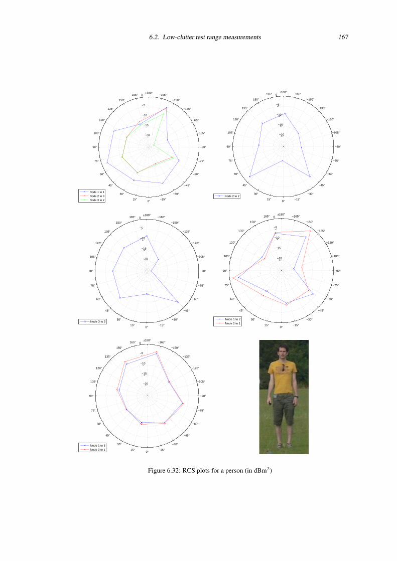
6.2. Low-clutter test range measurements 167
0°15°
30°
45°
60°
75°
90°
105°
120°
135°
150°
165° ±180°−165°
−150°
−135°
−120°
−105°
−90°
−75°
−60°
−45°
−30°
−15°
−20
−15
−10
−5
0
Node 1 to 1Node 2 to 3Node 3 to 2 0°15°
30°
45°
60°
75°
90°
105°
120°
135°
150°
165° ±180°−165°
−150°
−135°
−120°
−105°
−90°
−75°
−60°
−45°
−30°
−15°
−20
−15
−10
−5
0
Node 2 to 2
0°15°
30°
45°
60°
75°
90°
105°
120°
135°
150°
165° ±180°−165°
−150°
−135°
−120°
−105°
−90°
−75°
−60°
−45°
−30°
−15°
−20
−15
−10
−5
0
Node 3 to 3
0°15°
30°
45°
60°
75°
90°
105°
120°
135°
150°
165° ±180°−165°
−150°
−135°
−120°
−105°
−90°
−75°
−60°
−45°
−30°
−15°
−20
−15
−10
−5
0
Node 1 to 2Node 2 to 1
0°15°
30°
45°
60°
75°
90°
105°
120°
135°
150°
165° ±180°−165°
−150°
−135°
−120°
−105°
−90°
−75°
−60°
−45°
−30°
−15°
−20
−15
−10
−5
0
Node 1 to 3Node 3 to 1
Figure 6.32: RCS plots for a person (in dBm2)
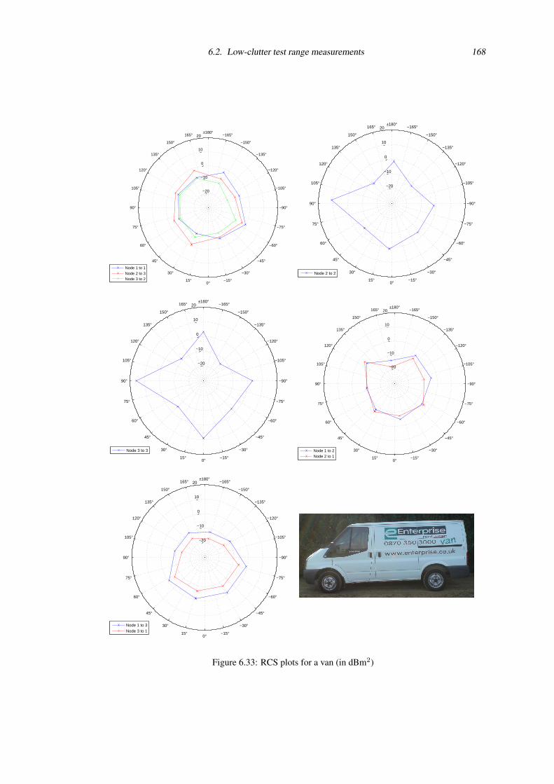
6.2. Low-clutter test range measurements 168
0°15°
30°
45°
60°
75°
90°
105°
120°
135°
150°
165° ±180°−165°
−150°
−135°
−120°
−105°
−90°
−75°
−60°
−45°
−30°
−15°
−20
−10
0
10
20
Node 1 to 1Node 2 to 3Node 3 to 2
0°15°
30°
45°
60°
75°
90°
105°
120°
135°
150°
165° ±180°−165°
−150°
−135°
−120°
−105°
−90°
−75°
−60°
−45°
−30°
−15°
−20
−10
0
10
20
Node 2 to 2
0°15°
30°
45°
60°
75°
90°
105°
120°
135°
150°
165° ±180°−165°
−150°
−135°
−120°
−105°
−90°
−75°
−60°
−45°
−30°
−15°
−20
−10
0
10
20
Node 3 to 3
0°15°
30°
45°
60°
75°
90°
105°
120°
135°
150°
165° ±180°−165°
−150°
−135°
−120°
−105°
−90°
−75°
−60°
−45°
−30°
−15°
−20
−10
0
10
20
Node 1 to 2Node 2 to 1
0°15°
30°
45°
60°
75°
90°
105°
120°
135°
150°
165° ±180°−165°
−150°
−135°
−120°
−105°
−90°
−75°
−60°
−45°
−30°
−15°
−20
−10
0
10
20
Node 1 to 3Node 3 to 1
Figure 6.33: RCS plots for a van (in dBm2)
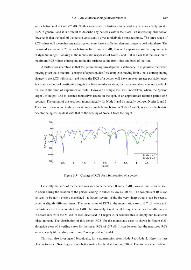
6.2. Low-clutter test range measurements 169
varies between -1 dB and -26 dB. Neither monostatic or bistatic can be said to give a noticeably greater
RCS in general, and it is difficult to describe any patterns within the plots - an interesting observation
however is that the back of the person consistently gives a relatively strong response. The large range of
RCS values will mean that any radar system must have a sufficient dynamic range to deal with these. The
measured van target RCS varies between 16 dB and -18 dB, thus will experience similar requirements
of dynamic range. Looking at the monostatic responses of Node 2 and 3, it is clear that the location of
maximum RCS values correspond to the flat surfaces at the front, side and back of the van.
A further consideration is that the person being investigated is stationary. It is possible that when
moving given the ‘structural’ changes of a person, due for example to moving limbs, that a corresponding
change to the RCS will occur; and hence the RCS of a person will have an even greater possible range.
Accurate methods of positioning targets at a finer angular rotation, such as a turntable, were not available
for use at the time of experimental trials. However a simple test was undertaken, where the ‘person
target’, of height 1.82 m, rotated themselves round on the spot, at an approximate rotation period of 5
seconds. The output of this test both monostatically for Node 1 and bistatically between Nodes 2 and 3.
These were chosen due to the greatest bistatic angle being between Nodes 2 and 3, as well as the bistatic
bisector being co-incident with that of the bearing of Node 1 from the target.
0 0.5 1 1.5 2 2.5 3 3.5 4 4.5 5−50
−40
−30
−20
−10
0
10
Time (s)
RC
S (
dBsm
)
Node 1 to 1Node 3 to 2
Figure 6.34: Change of RCS for a full rotation of a person
Generally the RCS of the person was seen to be between 0 and -15 dB, however nulls can be seen
to occur during the rotation of the person leading to values as low as -40 dB. The two plots of RCS can
be seen to be fairly closely correlated - although several of the the very sharp troughs can be seen to
occur at slightly different times. The mean value of RCS in the monostatic case is -3.7 dB whereas in
the bistatic case this amounts to -6.1 dB. Unfortunately it is difficult to say whether such a difference is
in accordance with the MBET of Kell discussed in Chapter 2, or whether this is simply due to antenna
misalignment. The distribution of this person RCS, for the monostatic case, is shown in Figure 6.35,
alongside plots of Swerling cases for the mean RCS of -3.7 dB. It can be seen that the measured RCS
values largely fit Swerling case 1 and 2 as opposed to 3 and 4.
This was also investigated bistatically, for a transmission from Node 3 to Node 2. Here it is less
clear as to which Swerling case is a better match for the distribution of RCS. Due to the rather ‘ad-hoc’
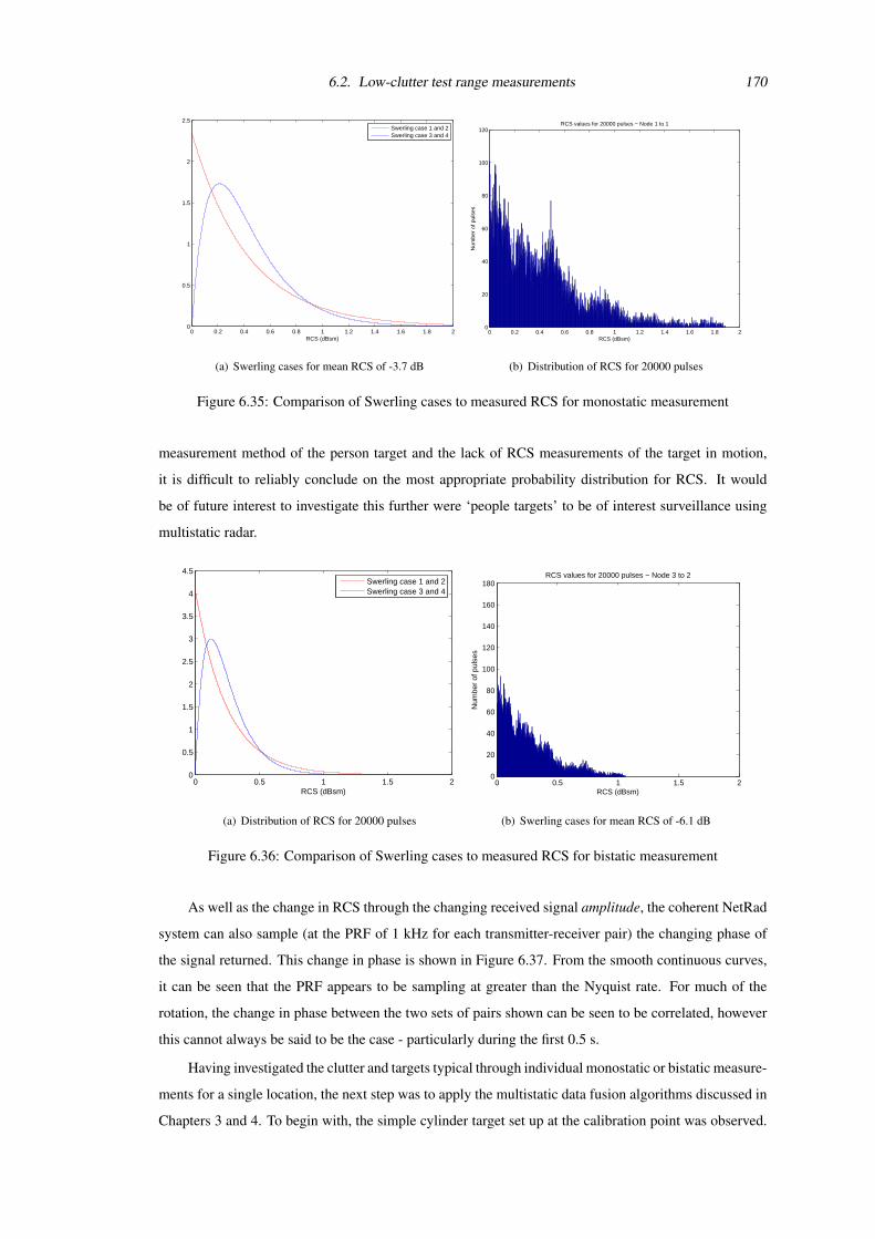
6.2. Low-clutter test range measurements 170
0 0.2 0.4 0.6 0.8 1 1.2 1.4 1.6 1.8 20
0.5
1
1.5
2
2.5
RCS (dBsm)
Swerling case 1 and 2Swerling case 3 and 4
(a) Swerling cases for mean RCS of -3.7 dB
0 0.2 0.4 0.6 0.8 1 1.2 1.4 1.6 1.8 20
20
40
60
80
100
120
RCS (dBsm)
Num
ber
of p
ulse
s
RCS values for 20000 pulses − Node 1 to 1
(b) Distribution of RCS for 20000 pulses
Figure 6.35: Comparison of Swerling cases to measured RCS for monostatic measurement
measurement method of the person target and the lack of RCS measurements of the target in motion,
it is difficult to reliably conclude on the most appropriate probability distribution for RCS. It would
be of future interest to investigate this further were ‘people targets’ to be of interest surveillance using
multistatic radar.
0 0.5 1 1.5 20
0.5
1
1.5
2
2.5
3
3.5
4
4.5
RCS (dBsm)
Swerling case 1 and 2Swerling case 3 and 4
(a) Distribution of RCS for 20000 pulses
0 0.5 1 1.5 20
20
40
60
80
100
120
140
160
180
RCS (dBsm)
Num
ber
of p
ulse
s
RCS values for 20000 pulses − Node 3 to 2
(b) Swerling cases for mean RCS of -6.1 dB
Figure 6.36: Comparison of Swerling cases to measured RCS for bistatic measurement
As well as the change in RCS through the changing received signal amplitude, the coherent NetRad
system can also sample (at the PRF of 1 kHz for each transmitter-receiver pair) the changing phase of
the signal returned. This change in phase is shown in Figure 6.37. From the smooth continuous curves,
it can be seen that the PRF appears to be sampling at greater than the Nyquist rate. For much of the
rotation, the change in phase between the two sets of pairs shown can be seen to be correlated, however
this cannot always be said to be the case - particularly during the first 0.5 s.
Having investigated the clutter and targets typical through individual monostatic or bistatic measure-
ments for a single location, the next step was to apply the multistatic data fusion algorithms discussed in
Chapters 3 and 4. To begin with, the simple cylinder target set up at the calibration point was observed.
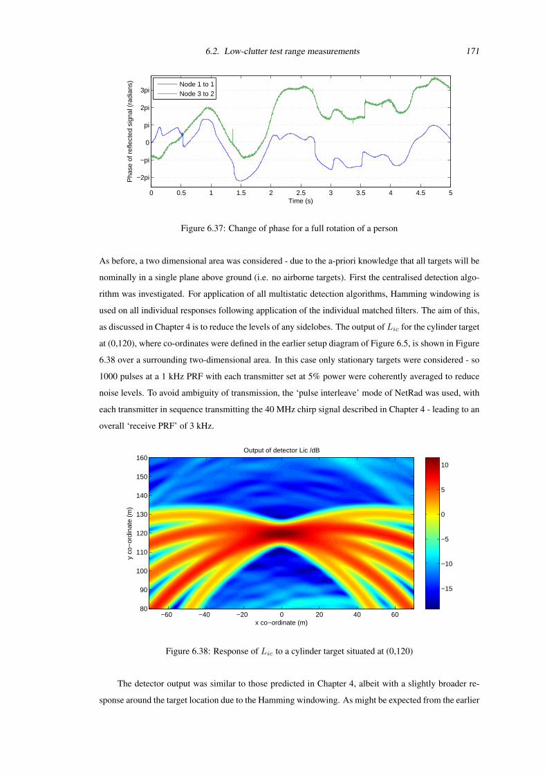
6.2. Low-clutter test range measurements 171
0 0.5 1 1.5 2 2.5 3 3.5 4 4.5 5
3pi
2pi
pi
0
−pi
−2pi
Time (s)
Pha
se o
f ref
lect
ed s
igna
l (ra
dian
s)
Node 1 to 1Node 3 to 2
Figure 6.37: Change of phase for a full rotation of a person
As before, a two dimensional area was considered - due to the a-priori knowledge that all targets will be
nominally in a single plane above ground (i.e. no airborne targets). First the centralised detection algo-
rithm was investigated. For application of all multistatic detection algorithms, Hamming windowing is
used on all individual responses following application of the individual matched filters. The aim of this,
as discussed in Chapter 4 is to reduce the levels of any sidelobes. The output of Lic for the cylinder target
at (0,120), where co-ordinates were defined in the earlier setup diagram of Figure 6.5, is shown in Figure
6.38 over a surrounding two-dimensional area. In this case only stationary targets were considered - so
1000 pulses at a 1 kHz PRF with each transmitter set at 5% power were coherently averaged to reduce
noise levels. To avoid ambiguity of transmission, the ‘pulse interleave’ mode of NetRad was used, with
each transmitter in sequence transmitting the 40 MHz chirp signal described in Chapter 4 - leading to an
overall ‘receive PRF’ of 3 kHz.
Output of detector Lic /dB
x co−ordinate (m)
y co
−or
dina
te (
m)
−60 −40 −20 0 20 40 6080
90
100
110
120
130
140
150
160
−15
−10
−5
0
5
10
Figure 6.38: Response of Lic to a cylinder target situated at (0,120)
The detector output was similar to those predicted in Chapter 4, albeit with a slightly broader re-
sponse around the target location due to the Hamming windowing. As might be expected from the earlier
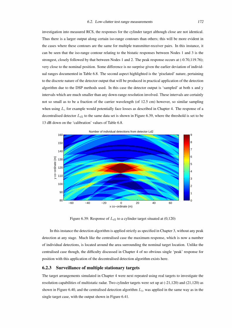
6.2. Low-clutter test range measurements 172
investigation into measured RCS, the responses for the cylinder target although close are not identical.
Thus there is a larger output along certain iso-range contours than others; this will be more evident in
the cases where these contours are the same for multiple transmitter-receiver pairs. In this instance, it
can be seen that the iso-range contour relating to the bistatic responses between Nodes 1 and 3 is the
strongest, closely followed by that between Nodes 1 and 2. The peak response occurs at (-0.70,119.76);
very close to the nominal position. Some difference is no surprise given the earlier deviation of individ-
ual ranges documented in Table 6.8. The second aspect highlighted is the ‘pixelated’ nature, pertaining
to the discrete nature of the detector output that will be produced in practical application of the detection
algorithm due to the DSP methods used. In this case the detector output is ‘sampled’ at both x and y
intervals which are much smaller than any down-range resolution involved. These intervals are certainly
not so small as to be a fraction of the carrier wavelength (of 12.5 cm) however, so similar sampling
when using Lc for example would potentially face losses as described in Chapter 4. The response of a
decentralised detector Ld2 to the same data set is shown in Figure 6.39, where the threshold is set to be
13 dB down on the ‘calibration’ values of Table 6.8.
Number of individual detections from detector Ld2
x co−ordinate (m)
y co
−or
dina
te (
m)
−60 −40 −20 0 20 40 6080
90
100
110
120
130
140
150
160
0
1
2
3
4
5
6
7
8
9
Figure 6.39: Response of Ld2 to a cylinder target situated at (0,120)
In this instance the detection algorithm is applied strictly as specified in Chapter 3, without any peak
detection at any stage. Much like the centralised case the maximum response, which is now a number
of individual detections, is located around the area surrounding the nominal target location. Unlike the
centralised case though, the difficulty discussed in Chapter 4 of no obvious single ‘peak’ response for
position with this application of the decentralised detection algorithm exists here.
6.2.3 Surveillance of multiple stationary targets
The target arrangements simulated in Chapter 4 were next repeated using real targets to investigate the
resolution capabilities of multistatic radar. Two cylinder targets were set up at (-21,120) and (21,120) as
shown in Figure 6.40, and the centralised detection algorithm Lic was applied in the same way as in the
single target case, with the output shown in Figure 6.41.
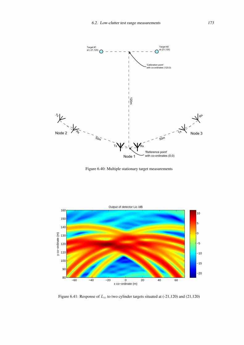
6.2. Low-clutter test range measurements 173
Figure 6.40: Multiple stationary target measurements
Output of detector Lic /dB
x co−ordinate (m)
y co
−or
dina
te (
m)
−60 −40 −20 0 20 40 6080
90
100
110
120
130
140
150
160
−20
−15
−10
−5
0
5
10
Figure 6.41: Response of Lic to two cylinder targets situated at (-21,120) and (21,120)
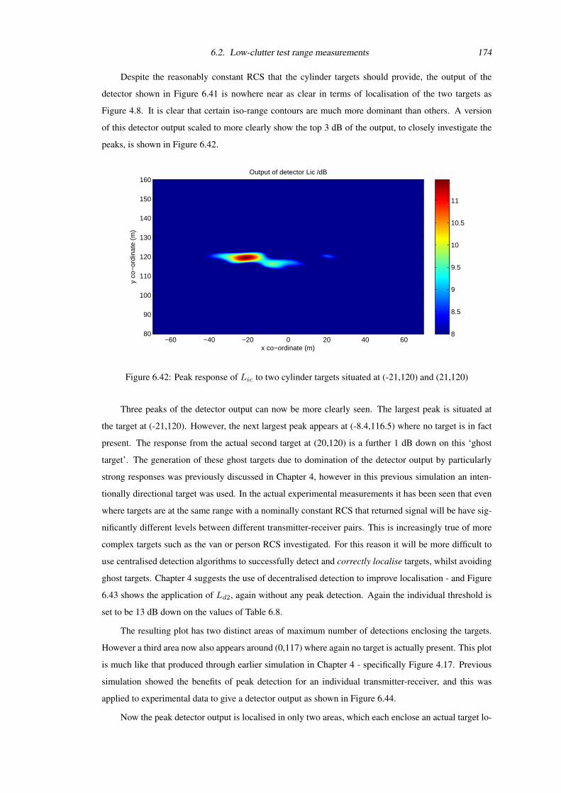
6.2. Low-clutter test range measurements 174
Despite the reasonably constant RCS that the cylinder targets should provide, the output of the
detector shown in Figure 6.41 is nowhere near as clear in terms of localisation of the two targets as
Figure 4.8. It is clear that certain iso-range contours are much more dominant than others. A version
of this detector output scaled to more clearly show the top 3 dB of the output, to closely investigate the
peaks, is shown in Figure 6.42.
Output of detector Lic /dB
x co−ordinate (m)
y co
−or
dina
te (
m)
−60 −40 −20 0 20 40 6080
90
100
110
120
130
140
150
160
8
8.5
9
9.5
10
10.5
11
Figure 6.42: Peak response of Lic to two cylinder targets situated at (-21,120) and (21,120)
Three peaks of the detector output can now be more clearly seen. The largest peak is situated at
the target at (-21,120). However, the next largest peak appears at (-8.4,116.5) where no target is in fact
present. The response from the actual second target at (20,120) is a further 1 dB down on this ‘ghost
target’. The generation of these ghost targets due to domination of the detector output by particularly
strong responses was previously discussed in Chapter 4, however in this previous simulation an inten-
tionally directional target was used. In the actual experimental measurements it has been seen that even
where targets are at the same range with a nominally constant RCS that returned signal will be have sig-
nificantly different levels between different transmitter-receiver pairs. This is increasingly true of more
complex targets such as the van or person RCS investigated. For this reason it will be more difficult to
use centralised detection algorithms to successfully detect and correctly localise targets, whilst avoiding
ghost targets. Chapter 4 suggests the use of decentralised detection to improve localisation - and Figure
6.43 shows the application of Ld2, again without any peak detection. Again the individual threshold is
set to be 13 dB down on the values of Table 6.8.
The resulting plot has two distinct areas of maximum number of detections enclosing the targets.
However a third area now also appears around (0,117) where again no target is actually present. This plot
is much like that produced through earlier simulation in Chapter 4 - specifically Figure 4.17. Previous
simulation showed the benefits of peak detection for an individual transmitter-receiver, and this was
applied to experimental data to give a detector output as shown in Figure 6.44.
Now the peak detector output is localised in only two areas, which each enclose an actual target lo-
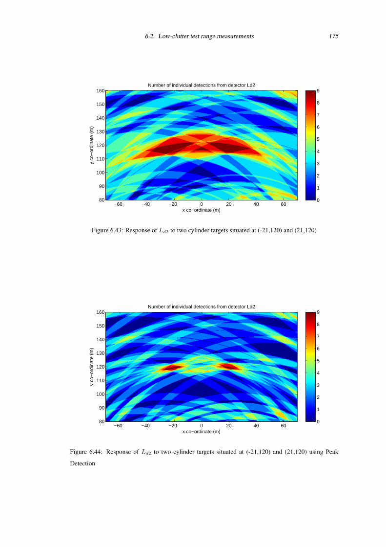
6.2. Low-clutter test range measurements 175
Number of individual detections from detector Ld2
x co−ordinate (m)
y co
−or
dina
te (
m)
−60 −40 −20 0 20 40 6080
90
100
110
120
130
140
150
160
0
1
2
3
4
5
6
7
8
9
Figure 6.43: Response of Ld2 to two cylinder targets situated at (-21,120) and (21,120)
Number of individual detections from detector Ld2
x co−ordinate (m)
y co
−or
dina
te (
m)
−60 −40 −20 0 20 40 6080
90
100
110
120
130
140
150
160
0
1
2
3
4
5
6
7
8
9
Figure 6.44: Response of Ld2 to two cylinder targets situated at (-21,120) and (21,120) using Peak
Detection
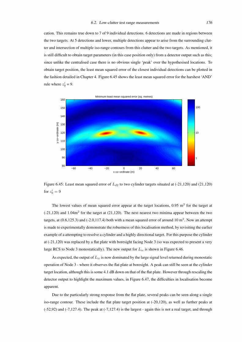
6.2. Low-clutter test range measurements 176
cation. This remains true down to 7 of 9 individual detections. 6 detections are made in regions between
the two targets. At 5 detections and lower, multiple detections appear to arise from the surrounding clut-
ter and intersection of multiple iso-range contours from this clutter and the two targets. As mentioned, it
is still difficult to obtain target parameters (in this case position only) from a detector output such as this;
since unlike the centralised case there is no obvious single ‘peak’ over the hypothesised locations. To
obtain target position, the least mean squared error of the closest individual detections can be plotted in
the fashion detailed in Chapter 4. Figure 6.45 shows the least mean squared error for the harshest ‘AND’
rule where z′0 = 9.
Minimum least mean squared error (sq. metres)
x co−ordinate (m)
y co
−or
dina
te (
m)
−60 −40 −20 0 20 40 6080
90
100
110
120
130
140
150
160
1
10
100
Figure 6.45: Least mean squared error of Ld2 to two cylinder targets situated at (-21,120) and (21,120)
for z′0 = 9
The lowest values of mean squared error appear at the target locations, 0.95 m2 for the target at
(-21,120) and 1.04m2 for the target at (21,120). The next nearest two minima appear between the two
targets, at (0.6,125.3) and (-2.0,117.4) both with a mean squared error of around 10 m2. Now an attempt
is made to experimentally demonstrate the robustness of this localisation method, by revisiting the earlier
example of a attempting to resolve a cylinder and a highly directional target. For this purpose the cylinder
at (-21,120) was replaced by a flat plate with boresight facing Node 3 (so was expected to present a very
large RCS to Node 3 monostatically). The new output for Lic is shown in Figure 6.46.
As expected, the output ofLic is now dominated by the large signal level returned during monostatic
operation of Node 3 - where it observes the flat plate at boresight. A peak can still be seen at the cylinder
target location, although this is some 4.1 dB down on that of the flat plate. However through rescaling the
detector output to highlight the maximum values, in Figure 6.47, the difficulties in localisation become
apparent.
Due to the particularly strong response from the flat plate, several peaks can be seen along a single
iso-range contour. These include the flat plate target position at (-20,120), as well as further peaks at
(-52,92) and (-7,127.4). The peak at (-7,127.4) is the largest - again this is not a real target, and through
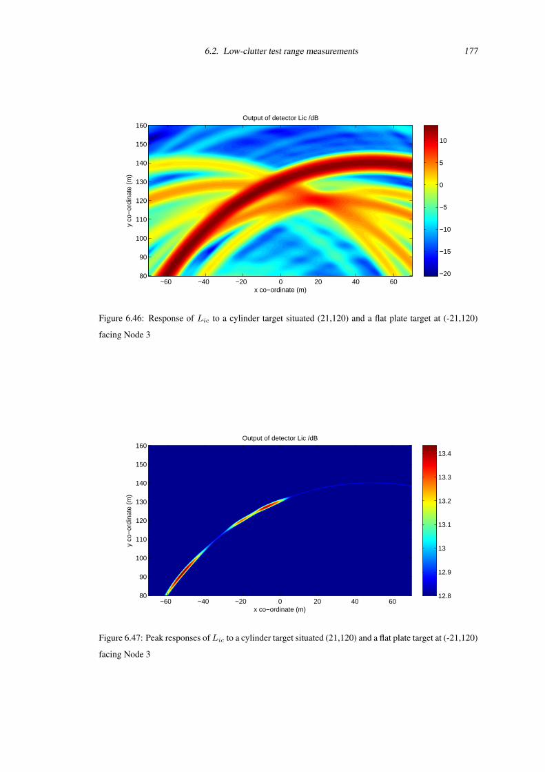
6.2. Low-clutter test range measurements 177
Output of detector Lic /dB
x co−ordinate (m)
y co
−or
dina
te (
m)
−60 −40 −20 0 20 40 6080
90
100
110
120
130
140
150
160
−20
−15
−10
−5
0
5
10
Figure 6.46: Response of Lic to a cylinder target situated (21,120) and a flat plate target at (-21,120)
facing Node 3
Output of detector Lic /dB
x co−ordinate (m)
y co
−or
dina
te (
m)
−60 −40 −20 0 20 40 6080
90
100
110
120
130
140
150
160
12.8
12.9
13
13.1
13.2
13.3
13.4
Figure 6.47: Peak responses ofLic to a cylinder target situated (21,120) and a flat plate target at (-21,120)
facing Node 3
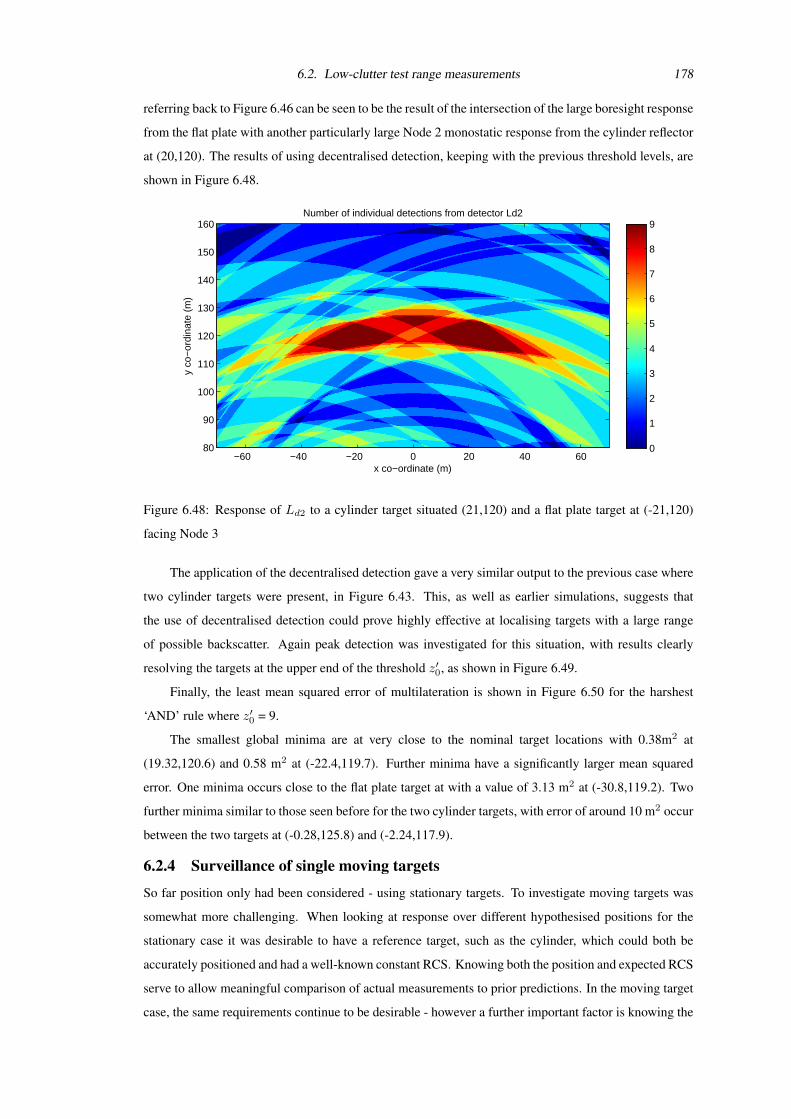
6.2. Low-clutter test range measurements 178
referring back to Figure 6.46 can be seen to be the result of the intersection of the large boresight response
from the flat plate with another particularly large Node 2 monostatic response from the cylinder reflector
at (20,120). The results of using decentralised detection, keeping with the previous threshold levels, are
shown in Figure 6.48.
Number of individual detections from detector Ld2
x co−ordinate (m)
y co
−or
dina
te (
m)
−60 −40 −20 0 20 40 6080
90
100
110
120
130
140
150
160
0
1
2
3
4
5
6
7
8
9
Figure 6.48: Response of Ld2 to a cylinder target situated (21,120) and a flat plate target at (-21,120)
facing Node 3
The application of the decentralised detection gave a very similar output to the previous case where
two cylinder targets were present, in Figure 6.43. This, as well as earlier simulations, suggests that
the use of decentralised detection could prove highly effective at localising targets with a large range
of possible backscatter. Again peak detection was investigated for this situation, with results clearly
resolving the targets at the upper end of the threshold z′0, as shown in Figure 6.49.
Finally, the least mean squared error of multilateration is shown in Figure 6.50 for the harshest
‘AND’ rule where z′0 = 9.
The smallest global minima are at very close to the nominal target locations with 0.38m2 at
(19.32,120.6) and 0.58 m2 at (-22.4,119.7). Further minima have a significantly larger mean squared
error. One minima occurs close to the flat plate target at with a value of 3.13 m2 at (-30.8,119.2). Two
further minima similar to those seen before for the two cylinder targets, with error of around 10 m2 occur
between the two targets at (-0.28,125.8) and (-2.24,117.9).
6.2.4 Surveillance of single moving targets
So far position only had been considered - using stationary targets. To investigate moving targets was
somewhat more challenging. When looking at response over different hypothesised positions for the
stationary case it was desirable to have a reference target, such as the cylinder, which could both be
accurately positioned and had a well-known constant RCS. Knowing both the position and expected RCS
serve to allow meaningful comparison of actual measurements to prior predictions. In the moving target
case, the same requirements continue to be desirable - however a further important factor is knowing the
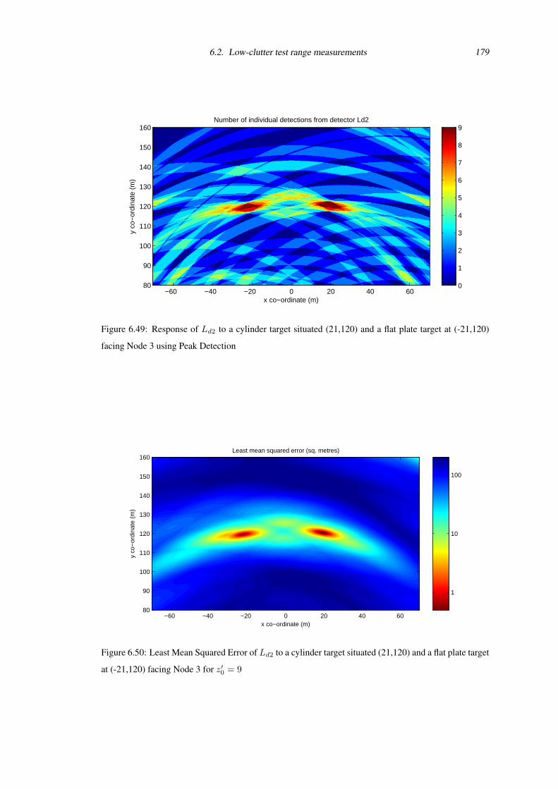
6.2. Low-clutter test range measurements 179
Number of individual detections from detector Ld2
x co−ordinate (m)
y co
−or
dina
te (
m)
−60 −40 −20 0 20 40 6080
90
100
110
120
130
140
150
160
0
1
2
3
4
5
6
7
8
9
Figure 6.49: Response of Ld2 to a cylinder target situated (21,120) and a flat plate target at (-21,120)
facing Node 3 using Peak Detection
Least mean squared error (sq. metres)
x co−ordinate (m)
y co
−or
dina
te (
m)
−60 −40 −20 0 20 40 6080
90
100
110
120
130
140
150
160
1
10
100
Figure 6.50: Least Mean Squared Error of Ld2 to a cylinder target situated (21,120) and a flat plate target
at (-21,120) facing Node 3 for z′0 = 9
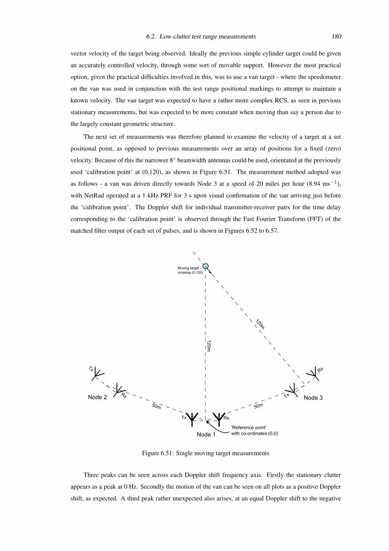
6.2. Low-clutter test range measurements 180
vector velocity of the target being observed. Ideally the previous simple cylinder target could be given
an accurately controlled velocity, through some sort of movable support. However the most practical
option, given the practical difficulties involved in this, was to use a van target - where the speedometer
on the van was used in conjunction with the test range positional markings to attempt to maintain a
known velocity. The van target was expected to have a rather more complex RCS, as seen in previous
stationary measurements, but was expected to be more constant when moving than say a person due to
the largely constant geometric structure.
The next set of measurements was therefore planned to examine the velocity of a target at a set
positional point, as opposed to previous measurements over an array of positions for a fixed (zero)
velocity. Because of this the narrower 8 beamwidth antennas could be used, orientated at the previously
used ‘calibration point’ at (0,120), as shown in Figure 6.51. The measurement method adopted was
as follows - a van was driven directly towards Node 3 at a speed of 20 miles per hour (8.94 ms−1),
with NetRad operated at a 1 kHz PRF for 3 s upon visual confirmation of the van arriving just before
the ‘calibration point’. The Doppler shift for individual transmitter-receiver pairs for the time delay
corresponding to the ‘calibration point’ is observed through the Fast Fourier Transform (FFT) of the
matched filter output of each set of pulses, and is shown in Figures 6.52 to 6.57.
Figure 6.51: Single moving target measurements
Three peaks can be seen across each Doppler shift frequency axis. Firstly the stationary clutter
appears as a peak at 0 Hz. Secondly the motion of the van can be seen on all plots as a positive Doppler
shift, as expected. A third peak rather unexpected also arises, at an equal Doppler shift to the negative
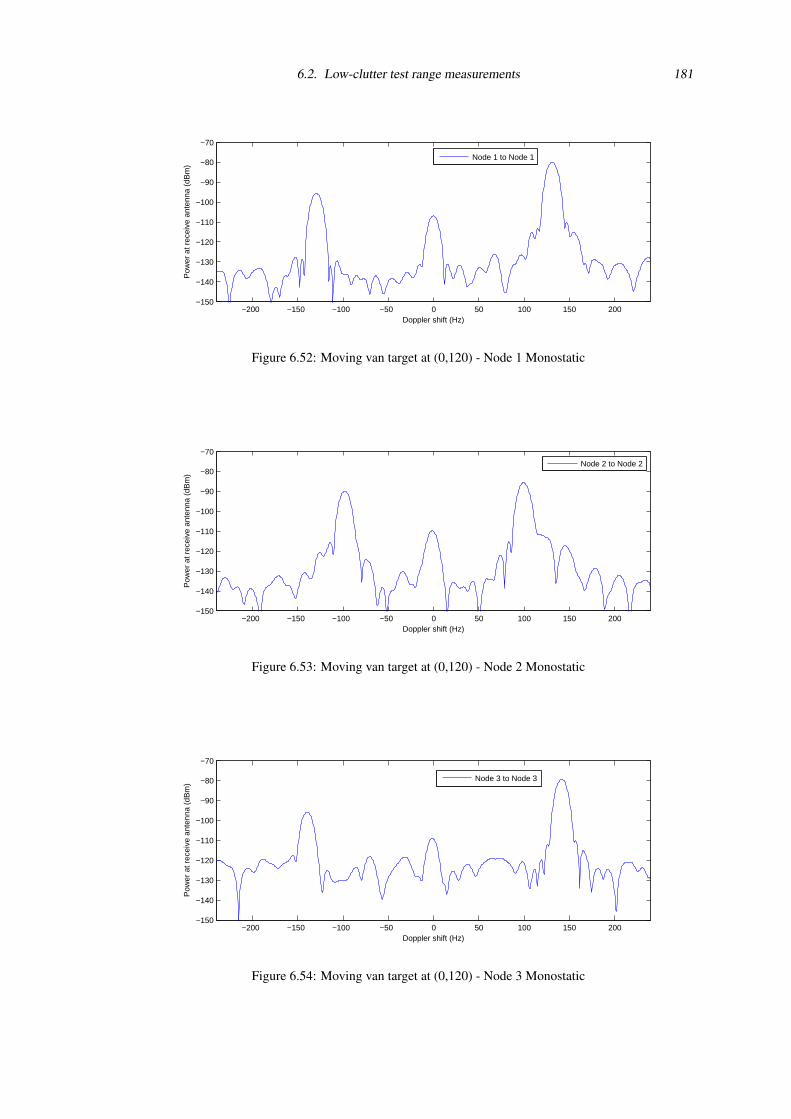
6.2. Low-clutter test range measurements 181
−200 −150 −100 −50 0 50 100 150 200−150
−140
−130
−120
−110
−100
−90
−80
−70
Doppler shift (Hz)
Pow
er a
t rec
eive
ant
enna
(dB
m)
Node 1 to Node 1
Figure 6.52: Moving van target at (0,120) - Node 1 Monostatic
−200 −150 −100 −50 0 50 100 150 200−150
−140
−130
−120
−110
−100
−90
−80
−70
Doppler shift (Hz)
Pow
er a
t rec
eive
ant
enna
(dB
m)
Node 2 to Node 2
Figure 6.53: Moving van target at (0,120) - Node 2 Monostatic
−200 −150 −100 −50 0 50 100 150 200−150
−140
−130
−120
−110
−100
−90
−80
−70
Doppler shift (Hz)
Pow
er a
t rec
eive
ant
enna
(dB
m)
Node 3 to Node 3
Figure 6.54: Moving van target at (0,120) - Node 3 Monostatic
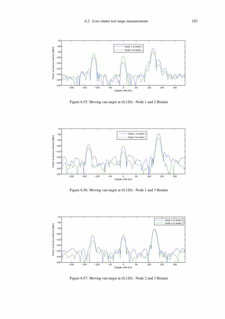
6.2. Low-clutter test range measurements 182
−200 −150 −100 −50 0 50 100 150 200−150
−140
−130
−120
−110
−100
−90
−80
−70
Doppler shift (Hz)
Pow
er a
t rec
eive
ant
enna
(dB
m)
Node 1 to Node 2
Node 2 to Node 1
Figure 6.55: Moving van target at (0,120) - Node 1 and 2 Bistatic
−200 −150 −100 −50 0 50 100 150 200−150
−140
−130
−120
−110
−100
−90
−80
−70
Doppler shift (Hz)
Pow
er a
t rec
eive
ant
enna
(dB
m)
Node 1 to Node 3
Node 3 to Node 1
Figure 6.56: Moving van target at (0,120) - Node 1 and 3 Bistatic
−200 −150 −100 −50 0 50 100 150 200−150
−140
−130
−120
−110
−100
−90
−80
−70
Doppler shift (Hz)
Pow
er a
t rec
eive
ant
enna
(dB
m)
Node 2 to Node 3Node 3 to Node 2
Figure 6.57: Moving van target at (0,120) - Node 2 and 3 Bistatic
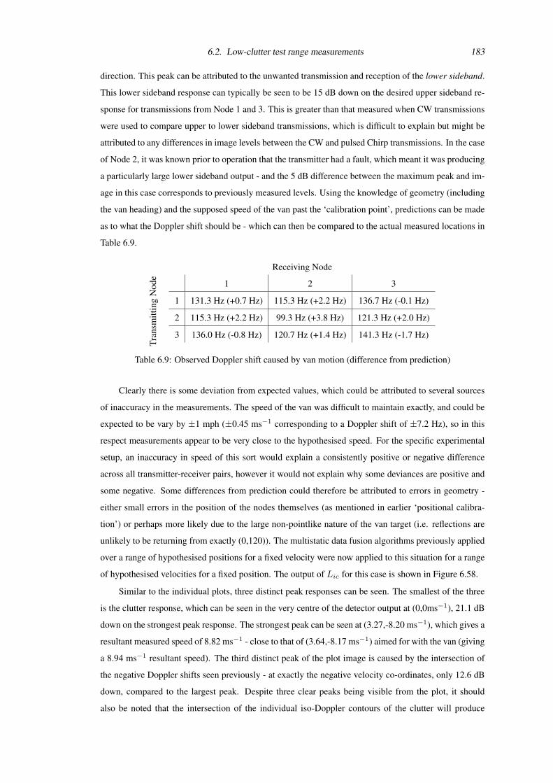
6.2. Low-clutter test range measurements 183
direction. This peak can be attributed to the unwanted transmission and reception of the lower sideband.
This lower sideband response can typically be seen to be 15 dB down on the desired upper sideband re-
sponse for transmissions from Node 1 and 3. This is greater than that measured when CW transmissions
were used to compare upper to lower sideband transmissions, which is difficult to explain but might be
attributed to any differences in image levels between the CW and pulsed Chirp transmissions. In the case
of Node 2, it was known prior to operation that the transmitter had a fault, which meant it was producing
a particularly large lower sideband output - and the 5 dB difference between the maximum peak and im-
age in this case corresponds to previously measured levels. Using the knowledge of geometry (including
the van heading) and the supposed speed of the van past the ‘calibration point’, predictions can be made
as to what the Doppler shift should be - which can then be compared to the actual measured locations in
Table 6.9.
Receiving Node
Tran
smitt
ing
Nod
e
1 2 3
1 131.3 Hz (+0.7 Hz) 115.3 Hz (+2.2 Hz) 136.7 Hz (-0.1 Hz)
2 115.3 Hz (+2.2 Hz) 99.3 Hz (+3.8 Hz) 121.3 Hz (+2.0 Hz)
3 136.0 Hz (-0.8 Hz) 120.7 Hz (+1.4 Hz) 141.3 Hz (-1.7 Hz)
Table 6.9: Observed Doppler shift caused by van motion (difference from prediction)
Clearly there is some deviation from expected values, which could be attributed to several sources
of inaccuracy in the measurements. The speed of the van was difficult to maintain exactly, and could be
expected to be vary by ±1 mph (±0.45 ms−1 corresponding to a Doppler shift of ±7.2 Hz), so in this
respect measurements appear to be very close to the hypothesised speed. For the specific experimental
setup, an inaccuracy in speed of this sort would explain a consistently positive or negative difference
across all transmitter-receiver pairs, however it would not explain why some deviances are positive and
some negative. Some differences from prediction could therefore be attributed to errors in geometry -
either small errors in the position of the nodes themselves (as mentioned in earlier ‘positional calibra-
tion’) or perhaps more likely due to the large non-pointlike nature of the van target (i.e. reflections are
unlikely to be returning from exactly (0,120)). The multistatic data fusion algorithms previously applied
over a range of hypothesised positions for a fixed velocity were now applied to this situation for a range
of hypothesised velocities for a fixed position. The output of Lic for this case is shown in Figure 6.58.
Similar to the individual plots, three distinct peak responses can be seen. The smallest of the three
is the clutter response, which can be seen in the very centre of the detector output at (0,0ms−1), 21.1 dB
down on the strongest peak response. The strongest peak can be seen at (3.27,-8.20 ms−1), which gives a
resultant measured speed of 8.82 ms−1 - close to that of (3.64,-8.17 ms−1) aimed for with the van (giving
a 8.94 ms−1 resultant speed). The third distinct peak of the plot image is caused by the intersection of
the negative Doppler shifts seen previously - at exactly the negative velocity co-ordinates, only 12.6 dB
down, compared to the largest peak. Despite three clear peaks being visible from the plot, it should
also be noted that the intersection of the individual iso-Doppler contours of the clutter will produce

6.2. Low-clutter test range measurements 184
Output of detector Lic /dB
x velocity (m/s)
y ve
loci
ty (
m/s
)
−10 −8 −6 −4 −2 0 2 4 6 8 10−10
−8
−6
−4
−2
0
2
4
6
8
10
−25
−20
−15
−10
−5
0
5
10
15
Figure 6.58: Response of Lic to a moving van target at (0,120)
several peaks - for example at (-10,-2.3 ms−1) 10.8 dB down on the largest peak, and at (-7.8,-3.3 ms−1)
10.9 dB down on the largest peak. The application of decentralised detection to determine velocity was
investigated, with results of least mean squared error for hypothesised velocity shown in Figure 6.59.
Here the decentralised threshold for all received signals is set to a rather low -105 dBm, which when
compared to the Figures 6.52 to 6.57 can be seen to include several of the lower sideband and zero
Doppler frequencies.
The thresholds appears to make little difference in the peak target positions in z′0 = 7 and z′0 = 9,
which now correspond to (3.19,-8.25 ms−1) and (3.25,-8.25 ms−1) respectively. Noticeably none of the
previous responses from clutter and lower sideband appear to feature on the detector output.
The other convenient moving target available was a walking person target. Again a ‘gross’ Doppler
component was expected due the overall motion of the target. However in the action of walking, multiple
moving parts of the body will reflect incident transmissions. Any oscillations of ‘swinging’ legs and arms
may show as modulations of the gross Doppler component - the ‘micro-Doppler’ effect. Such an effect
is demonstrated through use of a similar setup as the van target measurements, only now with a person
(again of height 1.82 m) crossing the calibration point at (0,120) whilst travelling at a walking speed
(approximately 1.4 ms−1) towards Node 3. A spectrogram was used to look at the change in Doppler
shift over time.
Oscillations in frequency over time can be seen in Figure 6.60, with a period of 0.5 s - which may
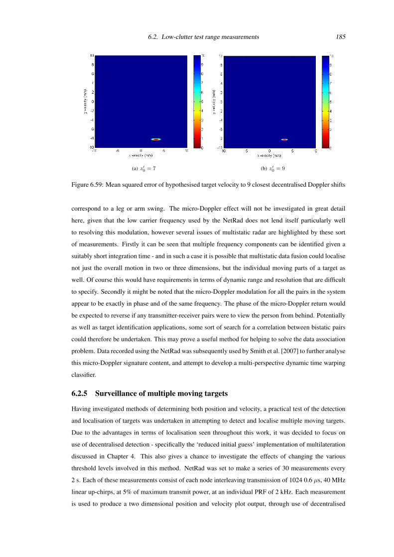
6.2. Low-clutter test range measurements 185
(a) z′0 = 7 (b) z′0 = 9
Figure 6.59: Mean squared error of hypothesised target velocity to 9 closest decentralised Doppler shifts
correspond to a leg or arm swing. The micro-Doppler effect will not be investigated in great detail
here, given that the low carrier frequency used by the NetRad does not lend itself particularly well
to resolving this modulation, however several issues of multistatic radar are highlighted by these sort
of measurements. Firstly it can be seen that multiple frequency components can be identified given a
suitably short integration time - and in such a case it is possible that multistatic data fusion could localise
not just the overall motion in two or three dimensions, but the individual moving parts of a target as
well. Of course this would have requirements in terms of dynamic range and resolution that are difficult
to specify. Secondly it might be noted that the micro-Doppler modulation for all the pairs in the system
appear to be exactly in phase and of the same frequency. The phase of the micro-Doppler return would
be expected to reverse if any transmitter-receiver pairs were to view the person from behind. Potentially
as well as target identification applications, some sort of search for a correlation between bistatic pairs
could therefore be undertaken. This may prove a useful method for helping to solve the data association
problem. Data recorded using the NetRad was subsequently used by Smith et al. [2007] to further analyse
this micro-Doppler signature content, and attempt to develop a multi-perspective dynamic time warping
classifier.
6.2.5 Surveillance of multiple moving targets
Having investigated methods of determining both position and velocity, a practical test of the detection
and localisation of targets was undertaken in attempting to detect and localise multiple moving targets.
Due to the advantages in terms of localisation seen throughout this work, it was decided to focus on
use of decentralised detection - specifically the ‘reduced initial guess’ implementation of multilateration
discussed in Chapter 4. This also gives a chance to investigate the effects of changing the various
threshold levels involved in this method. NetRad was set to make a series of 30 measurements every
2 s. Each of these measurements consist of each node interleaving transmission of 1024 0.6 µs, 40 MHz
linear up-chirps, at 5% of maximum transmit power, at an individual PRF of 2 kHz. Each measurement
is used to produce a two dimensional position and velocity plot output, through use of decentralised
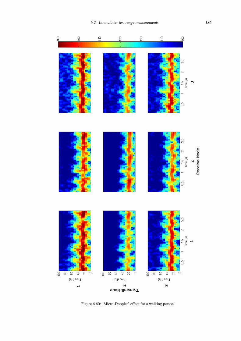
6.2. Low-clutter test range measurements 186
Figure 6.60: ‘Micro-Doppler’ effect for a walking person
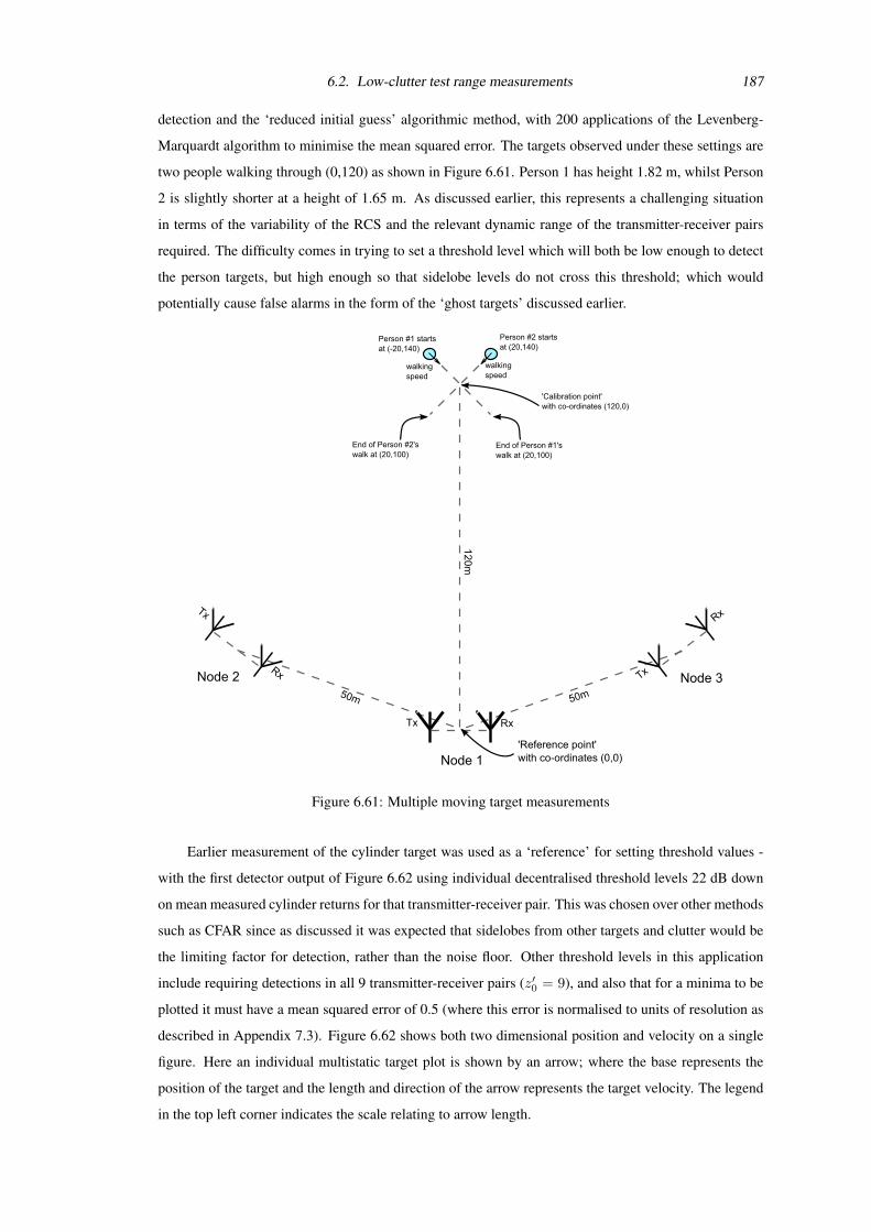
6.2. Low-clutter test range measurements 187
detection and the ‘reduced initial guess’ algorithmic method, with 200 applications of the Levenberg-
Marquardt algorithm to minimise the mean squared error. The targets observed under these settings are
two people walking through (0,120) as shown in Figure 6.61. Person 1 has height 1.82 m, whilst Person
2 is slightly shorter at a height of 1.65 m. As discussed earlier, this represents a challenging situation
in terms of the variability of the RCS and the relevant dynamic range of the transmitter-receiver pairs
required. The difficulty comes in trying to set a threshold level which will both be low enough to detect
the person targets, but high enough so that sidelobe levels do not cross this threshold; which would
potentially cause false alarms in the form of the ‘ghost targets’ discussed earlier.
Figure 6.61: Multiple moving target measurements
Earlier measurement of the cylinder target was used as a ‘reference’ for setting threshold values -
with the first detector output of Figure 6.62 using individual decentralised threshold levels 22 dB down
on mean measured cylinder returns for that transmitter-receiver pair. This was chosen over other methods
such as CFAR since as discussed it was expected that sidelobes from other targets and clutter would be
the limiting factor for detection, rather than the noise floor. Other threshold levels in this application
include requiring detections in all 9 transmitter-receiver pairs (z′0 = 9), and also that for a minima to be
plotted it must have a mean squared error of 0.5 (where this error is normalised to units of resolution as
described in Appendix 7.3). Figure 6.62 shows both two dimensional position and velocity on a single
figure. Here an individual multistatic target plot is shown by an arrow; where the base represents the
position of the target and the length and direction of the arrow represents the target velocity. The legend
in the top left corner indicates the scale relating to arrow length.
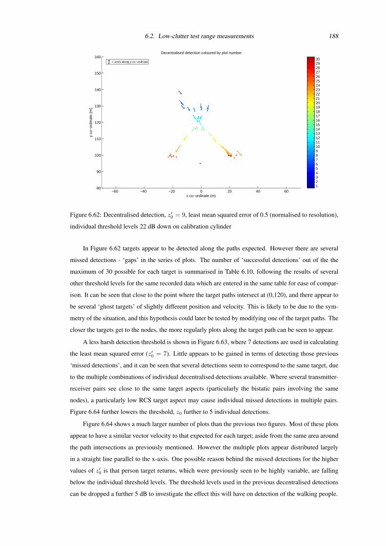
6.2. Low-clutter test range measurements 188
−60 −40 −20 0 20 40 6080
90
100
110
120
130
140
150
160= 1m/s along y co−ordinate
Decentralised detection coloured by plot number
x co−ordinate (m)
y co
−or
dina
te (
m)
1 2 3 4 5 6 7 8 9 101112131415161718192021222324252627282930
Figure 6.62: Decentralised detection, z′0 = 9, least mean squared error of 0.5 (normalised to resolution),
individual threshold levels 22 dB down on calibration cylinder
In Figure 6.62 targets appear to be detected along the paths expected. However there are several
missed detections - ‘gaps’ in the series of plots. The number of ‘successful detections’ out of the the
maximum of 30 possible for each target is summarised in Table 6.10, following the results of several
other threshold levels for the same recorded data which are entered in the same table for ease of compar-
ison. It can be seen that close to the point where the target paths intersect at (0,120), and there appear to
be several ‘ghost targets’ of slightly different position and velocity. This is likely to be due to the sym-
metry of the situation, and this hypothesis could later be tested by modifying one of the target paths. The
closer the targets get to the nodes, the more regularly plots along the target path can be seen to appear.
A less harsh detection threshold is shown in Figure 6.63, where 7 detections are used in calculating
the least mean squared error (z′0 = 7). Little appears to be gained in terms of detecting those previous
‘missed detections’, and it can be seen that several detections seem to correspond to the same target, due
to the multiple combinations of individual decentralised detections available. Where several transmitter-
receiver pairs see close to the same target aspects (particularly the bistatic pairs involving the same
nodes), a particularly low RCS target aspect may cause individual missed detections in multiple pairs.
Figure 6.64 further lowers the threshold, z0 further to 5 individual detections.
Figure 6.64 shows a much larger number of plots than the previous two figures. Most of these plots
appear to have a similar vector velocity to that expected for each target; aside from the same area around
the path intersections as previously mentioned. However the multiple plots appear distributed largely
in a straight line parallel to the x-axis. One possible reason behind the missed detections for the higher
values of z′0 is that person target returns, which were previously seen to be highly variable, are falling
below the individual threshold levels. The threshold levels used in the previous decentralised detections
can be dropped a further 5 dB to investigate the effect this will have on detection of the walking people.
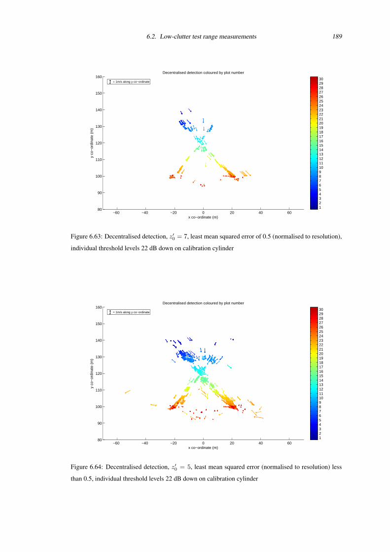
6.2. Low-clutter test range measurements 189
−60 −40 −20 0 20 40 6080
90
100
110
120
130
140
150
160= 1m/s along y co−ordinate
Decentralised detection coloured by plot number
x co−ordinate (m)
y co
−or
dina
te (
m)
1 2 3 4 5 6 7 8 9 101112131415161718192021222324252627282930
Figure 6.63: Decentralised detection, z′0 = 7, least mean squared error of 0.5 (normalised to resolution),
individual threshold levels 22 dB down on calibration cylinder
−60 −40 −20 0 20 40 6080
90
100
110
120
130
140
150
160= 1m/s along y co−ordinate
Decentralised detection coloured by plot number
x co−ordinate (m)
y co
−or
dina
te (
m)
1 2 3 4 5 6 7 8 9 101112131415161718192021222324252627282930
Figure 6.64: Decentralised detection, z′0 = 5, least mean squared error (normalised to resolution) less
than 0.5, individual threshold levels 22 dB down on calibration cylinder
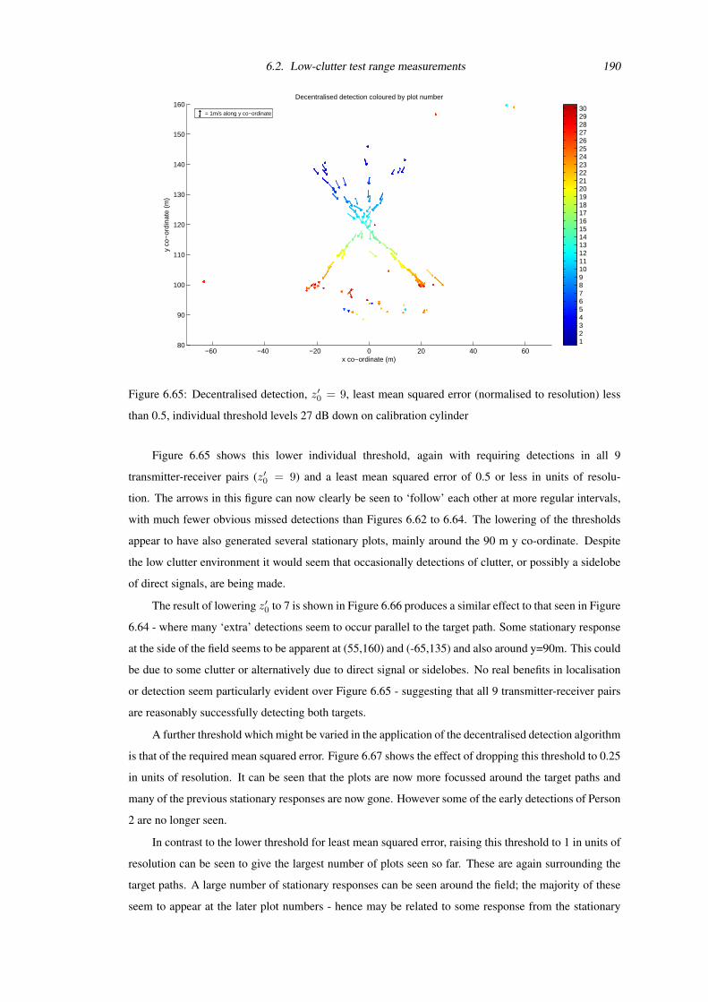
6.2. Low-clutter test range measurements 190
−60 −40 −20 0 20 40 6080
90
100
110
120
130
140
150
160= 1m/s along y co−ordinate
Decentralised detection coloured by plot number
x co−ordinate (m)
y co
−or
dina
te (
m)
1 2 3 4 5 6 7 8 9 101112131415161718192021222324252627282930
Figure 6.65: Decentralised detection, z′0 = 9, least mean squared error (normalised to resolution) less
than 0.5, individual threshold levels 27 dB down on calibration cylinder
Figure 6.65 shows this lower individual threshold, again with requiring detections in all 9
transmitter-receiver pairs (z′0 = 9) and a least mean squared error of 0.5 or less in units of resolu-
tion. The arrows in this figure can now clearly be seen to ‘follow’ each other at more regular intervals,
with much fewer obvious missed detections than Figures 6.62 to 6.64. The lowering of the thresholds
appear to have also generated several stationary plots, mainly around the 90 m y co-ordinate. Despite
the low clutter environment it would seem that occasionally detections of clutter, or possibly a sidelobe
of direct signals, are being made.
The result of lowering z′0 to 7 is shown in Figure 6.66 produces a similar effect to that seen in Figure
6.64 - where many ‘extra’ detections seem to occur parallel to the target path. Some stationary response
at the side of the field seems to be apparent at (55,160) and (-65,135) and also around y=90m. This could
be due to some clutter or alternatively due to direct signal or sidelobes. No real benefits in localisation
or detection seem particularly evident over Figure 6.65 - suggesting that all 9 transmitter-receiver pairs
are reasonably successfully detecting both targets.
A further threshold which might be varied in the application of the decentralised detection algorithm
is that of the required mean squared error. Figure 6.67 shows the effect of dropping this threshold to 0.25
in units of resolution. It can be seen that the plots are now more focussed around the target paths and
many of the previous stationary responses are now gone. However some of the early detections of Person
2 are no longer seen.
In contrast to the lower threshold for least mean squared error, raising this threshold to 1 in units of
resolution can be seen to give the largest number of plots seen so far. These are again surrounding the
target paths. A large number of stationary responses can be seen around the field; the majority of these
seem to appear at the later plot numbers - hence may be related to some response from the stationary
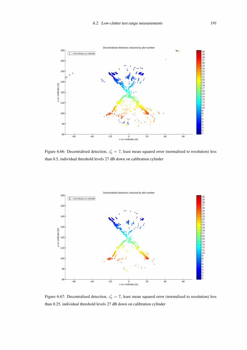
6.2. Low-clutter test range measurements 191
−60 −40 −20 0 20 40 6080
90
100
110
120
130
140
150
160= 1m/s along y co−ordinate
Decentralised detection coloured by plot number
x co−ordinate (m)
y co
−or
dina
te (
m)
1 2 3 4 5 6 7 8 9 101112131415161718192021222324252627282930
Figure 6.66: Decentralised detection, z′0 = 7, least mean squared error (normalised to resolution) less
than 0.5, individual threshold levels 27 dB down on calibration cylinder
−60 −40 −20 0 20 40 6080
90
100
110
120
130
140
150
160= 1m/s along y co−ordinate
Decentralised detection coloured by plot number
x co−ordinate (m)
y co
−or
dina
te (
m)
1 2 3 4 5 6 7 8 9 101112131415161718192021222324252627282930
Figure 6.67: Decentralised detection, z′0 = 7, least mean squared error (normalised to resolution) less
than 0.25, individual threshold levels 27 dB down on calibration cylinder
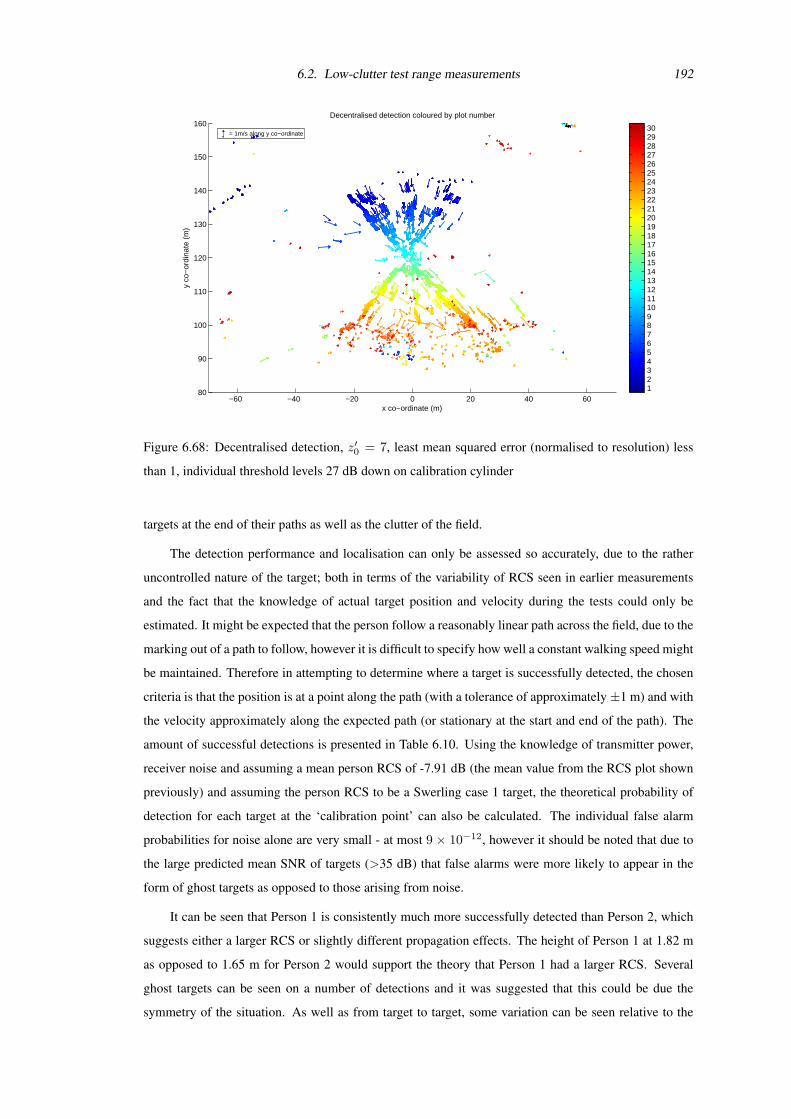
6.2. Low-clutter test range measurements 192
−60 −40 −20 0 20 40 6080
90
100
110
120
130
140
150
160= 1m/s along y co−ordinate
Decentralised detection coloured by plot number
x co−ordinate (m)
y co
−or
dina
te (
m)
1 2 3 4 5 6 7 8 9 101112131415161718192021222324252627282930
Figure 6.68: Decentralised detection, z′0 = 7, least mean squared error (normalised to resolution) less
than 1, individual threshold levels 27 dB down on calibration cylinder
targets at the end of their paths as well as the clutter of the field.
The detection performance and localisation can only be assessed so accurately, due to the rather
uncontrolled nature of the target; both in terms of the variability of RCS seen in earlier measurements
and the fact that the knowledge of actual target position and velocity during the tests could only be
estimated. It might be expected that the person follow a reasonably linear path across the field, due to the
marking out of a path to follow, however it is difficult to specify how well a constant walking speed might
be maintained. Therefore in attempting to determine where a target is successfully detected, the chosen
criteria is that the position is at a point along the path (with a tolerance of approximately±1 m) and with
the velocity approximately along the expected path (or stationary at the start and end of the path). The
amount of successful detections is presented in Table 6.10. Using the knowledge of transmitter power,
receiver noise and assuming a mean person RCS of -7.91 dB (the mean value from the RCS plot shown
previously) and assuming the person RCS to be a Swerling case 1 target, the theoretical probability of
detection for each target at the ‘calibration point’ can also be calculated. The individual false alarm
probabilities for noise alone are very small - at most 9 × 10⁻¹², however it should be noted that due to
the large predicted mean SNR of targets (>35 dB) that false alarms were more likely to appear in the
form of ghost targets as opposed to those arising from noise.
It can be seen that Person 1 is consistently much more successfully detected than Person 2, which
suggests either a larger RCS or slightly different propagation effects. The height of Person 1 at 1.82 m
as opposed to 1.65 m for Person 2 would support the theory that Person 1 had a larger RCS. Several
ghost targets can be seen on a number of detections and it was suggested that this could be due the
symmetry of the situation. As well as from target to target, some variation can be seen relative to the
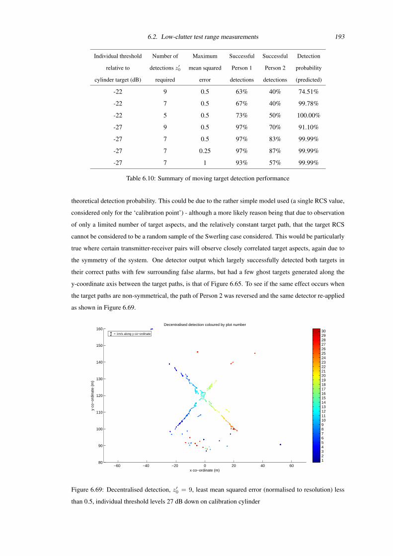
6.2. Low-clutter test range measurements 193
Individual threshold Number of Maximum Successful Successful Detection
relative to detections z′0 mean squared Person 1 Person 2 probability
cylinder target (dB) required error detections detections (predicted)
-22 9 0.5 63% 40% 74.51%
-22 7 0.5 67% 40% 99.78%
-22 5 0.5 73% 50% 100.00%
-27 9 0.5 97% 70% 91.10%
-27 7 0.5 97% 83% 99.99%
-27 7 0.25 97% 87% 99.99%
-27 7 1 93% 57% 99.99%
Table 6.10: Summary of moving target detection performance
theoretical detection probability. This could be due to the rather simple model used (a single RCS value,
considered only for the ‘calibration point’) - although a more likely reason being that due to observation
of only a limited number of target aspects, and the relatively constant target path, that the target RCS
cannot be considered to be a random sample of the Swerling case considered. This would be particularly
true where certain transmitter-receiver pairs will observe closely correlated target aspects, again due to
the symmetry of the system. One detector output which largely successfully detected both targets in
their correct paths with few surrounding false alarms, but had a few ghost targets generated along the
y-coordinate axis between the target paths, is that of Figure 6.65. To see if the same effect occurs when
the target paths are non-symmetrical, the path of Person 2 was reversed and the same detector re-applied
as shown in Figure 6.69.
−60 −40 −20 0 20 40 6080
90
100
110
120
130
140
150
160= 1m/s along y co−ordinate
Decentralised detection coloured by plot number
x co−ordinate (m)
y co
−or
dina
te (
m)
1 2 3 4 5 6 7 8 9 101112131415161718192021222324252627282930
Figure 6.69: Decentralised detection, z′0 = 9, least mean squared error (normalised to resolution) less
than 0.5, individual threshold levels 27 dB down on calibration cylinder
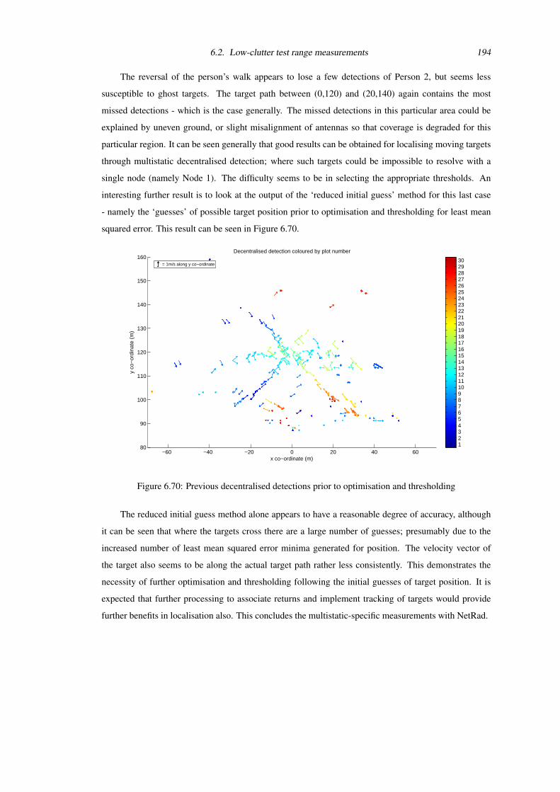
6.2. Low-clutter test range measurements 194
The reversal of the person’s walk appears to lose a few detections of Person 2, but seems less
susceptible to ghost targets. The target path between (0,120) and (20,140) again contains the most
missed detections - which is the case generally. The missed detections in this particular area could be
explained by uneven ground, or slight misalignment of antennas so that coverage is degraded for this
particular region. It can be seen generally that good results can be obtained for localising moving targets
through multistatic decentralised detection; where such targets could be impossible to resolve with a
single node (namely Node 1). The difficulty seems to be in selecting the appropriate thresholds. An
interesting further result is to look at the output of the ‘reduced initial guess’ method for this last case
- namely the ‘guesses’ of possible target position prior to optimisation and thresholding for least mean
squared error. This result can be seen in Figure 6.70.
−60 −40 −20 0 20 40 6080
90
100
110
120
130
140
150
160= 1m/s along y co−ordinate
Decentralised detection coloured by plot number
x co−ordinate (m)
y co
−or
dina
te (
m)
1 2 3 4 5 6 7 8 9 101112131415161718192021222324252627282930
Figure 6.70: Previous decentralised detections prior to optimisation and thresholding
The reduced initial guess method alone appears to have a reasonable degree of accuracy, although
it can be seen that where the targets cross there are a large number of guesses; presumably due to the
increased number of least mean squared error minima generated for position. The velocity vector of
the target also seems to be along the actual target path rather less consistently. This demonstrates the
necessity of further optimisation and thresholding following the initial guesses of target position. It is
expected that further processing to associate returns and implement tracking of targets would provide
further benefits in localisation also. This concludes the multistatic-specific measurements with NetRad.
Chapter 7
Summary and Conclusions
In this section the results of the research work are first discussed. The principle achievements and
contributions to the knowledge base in the area of multistatic radar are then highlighted. Finally the
potential for future work in light of the findings of this work is examined.
7.1 Discussion of resultsAmong the first results to be taken for both urban and low-clutter test ranges were measurements of noise
alone - effectively operating a receive-only multistatic system. Interference in the ISM band could clearly
be seen in an urban environment, making the common assumption of white Gaussian noise (as discussed
in Chapter 3) questionable. The use of whitening filters would be appropriate in such interference, which
would lead to some loss of detection performance and resolution. However in the low-clutter environ-
ment, where the vast majority of the measurements in this work were undertaken it can be seen that the
white Gaussian model fits well to the recorded noise data, albeit with some increase in power compared
to laboratory tests of Chapter 5. This was speculated to be due to the effect of the outdoor environment
of the individual RF components (effect of temperature on LNA gain or noise figure for example), which
could be somewhat compensated were the NetRad to be more comprehensively characterised over likely
operating temperature ranges.
The next step was to transmit, forming the multiple transmitter-receiver pairs which make up the
NetRad. Throughout all following measurements involving transmission, a 40 MHz linear up-chirp of
length 0.6 µs was used. In both test ranges this meant received signal both direct from transmitter to
receiver and reflected from the surrounding clutter. In the urban case responses could be seen corre-
sponding to large buildings, and it can be shown that the phase of these responses are stable even over
large time intervals. This was as far as testing in the urban environment was taken, mainly due to the
difficulties in distinguishing of test targets from the surroundings, as well as the inability to position
nodes and targets as desired.
The low-clutter environment allowed for much more flexibility in system geometry and target posi-
tion. Some error was present in the test range set-up; since methods used to position and align antennas
were only so accurate, and therefore full spatial coherence and gains of SNR through coherent sum-
mation were not expected to be achievable. This was also due to the complex, non-pointlike nature of
7.1. Discussion of results 196
targets used. Given the largely successful results later, this appears to suggest that similar sorts of inac-
curacies which may result from the future use of GPS positioning and synchronisation may be capable
of achieving similar performance. The clutter response of this test range can indeed be seen to be low
until the time delay relating to the surroundings of the field is reached, which are rather arbitrary, but
certainly allowed for an area over the field where targets were likely to be clearly distinguishable from
clutter.
Prior to investigating data fusion, the response of the individual transmitter-receiver pairs to targets
was considered. Simulations were used to show the target scattering behaviour that may be observed
within a multistatic system, such as specular reflection and retro-reflection. These simulations were
then compared to actual measurements taken with the NetRad system, with results largely as expected;
although the rather small number of target rotations observed led to a somewhat limited analysis of mul-
tistatic RCS. Future measurements might be better facilitated with some sort of better control of target
rotation, such as a turntable arrangement. Several rather more complex targets were also investigated,
including vehicles and people. People targets in particular were shown to have a highly variable RCS,
with a maximum measured value around the often quoted 1m2, but minima in this RCS as much as
30 dB down on this can also be seen - making detection difficult. It should be noted that these RCS
measurements were for stationary targets only; and differences to scattering characteristics would arise
in moving targets.
Having considered the noise, clutter and target returns individually over the nine transmitter-receiver
pairs in NetRad, the various multistatic data fusion algorithms discussed in Chapter 3 and 4 were inves-
tigated. Two dimensional positional plots for various targets and groups of targets which were set up
to closely resemble earlier simulations in Chapter 4. Again these include side-by-side comparisons of
centralised and decentralised detection algorithms - with the focus on determining the localisation of the
targets. In particular the appearance of any ghost targets compared to the real known targets that were
placed in the field was noted. As in the simulation, it can be seen that decentralised detection using
multilateration consistently produces the best estimates of target positions. This is due to a lack of ghost
targets, which are seen to have a much greater mean squared error than real targets and hence will be
removed with a suitable threshold.
As well as position, the coherence afforded between all nine transmitter-receiver pairs through the
distributed oscillator allowed Doppler frequency shifts from target motion to be measured. The movable
targets available were all complex targets. The application of centralised and decentralised algorithms
for a range of hypothesised two-dimensional velocity, similar to that undertaken for position of stationary
targets, was shown. The peak response appeared at a velocity very close to that expected in both cases,
the centralised case clearly had the potential for returns to ‘dominate’ the detector output as seen in
the positional case. Some inaccuracy might be expected due to the limits on either trying to match
a speedometer or attempting to maintain a constant ‘walking pace’. Further problems related to the
transmission of the lower sideband are highlighted due to the particularly high SNR, where the image of
the target Doppler frequency can clearly be seen and may place further restrictions on threshold levels
7.2. Main achievements and contributions 197
and hence dynamic range (especially for one transmitter where a fault meant a particularly large image
could be seen).
Finally, these individual areas of multistatic data fusion were brought together. Given the success of
localisation when using decentralised detection and multilateration, this method was chosen to attempt
to detect and localise targets in a situation where a single monostatic node would be unable to resolve
and position them. The targets in question were walking people, which had previously been shown to be
a complex scatterer with a fluctuating RCS. This was successfully accomplished, given that the correct
path of the people targets could indeed be seen from plot to plot with two-dimensional position and
velocity largely as expected. The measured detection probabilities are nearly all lower than predictions,
which may be due to the targets moving along set paths such that similar target RCS values may be seen
(i.e. some correlation) from plot to plot, or simply due to the rather small sample set of the 20 attempted
detections. Another explanation is of some unaccounted-for propagation effects, such as a non-flat area
of ground or misalignment of antennas. Clearly the symmetry of the radar system geometry does not
provide the greatest amount of spatial diversity possible, meaning despite the successful operation of the
system that there is potential for further improvement still. It could be seen that the multiple threshold
levels involved had an effect on both any missed detections and ghost targets. For any given implemen-
tation of a multistatic radar system, how these threshold values are set will be somewhat dependant on
both the target characteristics and the accuracy of the system. There would be little point, for example,
in setting mean squared error bounds to be particularly low if there are intrinsic errors in the radar an-
tenna positioning, or if the target itself has significantly large dimensions. The figures showing multiple
plots separated in time have no tracking algorithms applied; so no information on past plots is used to
affect the future detection of targets. This was intentional to keep already rather complex (in comparison
to conventional radar) detection algorithms simple, and present a series of ‘initial detections’. There is
certainly potential that tracking could further improve detection performance - effectively lowering the
threshold at the predicted position to avoid missed detections, whilst simultaneously keeping thresholds
at other positions high, so as to reduce the appearance of ghost targets and other false alarms. This again
will be somewhat dependant on the type of target; for example, tracking the people targets may prove
difficult due to their high manoverability (i.e. they may be able to completely change direction or speed)
in the 2 s interval between plots and unpredictable paths.
7.2 Main achievements and contributionsThe particular requirements of a multistatic system are explored through detailed explanation of the op-
eration of the NetRad system. Most development of the system highlighted practical consideration of
multistatic radar design - such as methods of power supply and requirement of reliable synchronisation
methods. The development of the system has enabled the experimental measurements detailed through-
out this work. Many of the practical issues of the designing and deploying a multistatic radar are detailed
- both within hardware itself to ‘characterise’ the system, as well as those concerning the propagation of
signals within the surveillance environment.
Much of the literature on multistatic radar is notable for the lack of attention to the localisation
7.2. Main achievements and contributions 198
inherent in the application of the detection algorithms. In specific cases this may be justified - for
example where the ‘resolution cell’ areas for each transmitter-receiver pair coincide. However often this
may not be the case - particularly where individual angular resolution is poor compared to down-range
and nodes are viewing diverse aspects of a target, so it is important to characterise the performance
of these detectors in terms of positioning and resolving targets. A comparison of these detectors in
terms of this localisation is presented in Chapter 4 for simulated returns, which was later investigated
experimentally in Chapter 6. The detector output in the centralised case is clearly dominated by any
particularly strong individual responses. In the multiple target case this can be seen to lead to peak
outputs at two dimensional positions where no targets are in fact present - ‘ghost targets’. The formation
of these ghost targets is due to the errors in data association where a detector output considers a response
from multiple targets to be a single target. The solution to the problem of this domination of the detector
response was shown to be effectively increasing the contribution from the weaker responses from the
target, and a simple way to accomplish this is through use of the decentralised detection algorithm Ld2
as shown in Chapter 4. Here at the cost of some sub-optimality of detection, reduction of ghost targets
(which themselves might be considered false alarms) and better localisation of real targets was shown to
be obtained.
To produce discrete parameter estimates using decentralised detection, a multilateration process was
detailed, and shown to produce the best localisation of all detection algorithms considered. During this
process, an implementation of the Levenberg-Marquardt algorithm was developed to minimise a joint
measure of time delay and Doppler shift (which were normalised to a measure of their own resolution)
for several decentralised detections to give a vector position and velocity output.
A discussion of the processing requirements of the detection algorithms used was presented. Some
simple predictions were used to demonstrate the factors which each detection algorithm discussed was
dependant upon. A robust (in processing terms) ‘reduced initial guess’ method of multilateration was
developed, and later used to process experimental measurements. Similarities here might be drawn to
other areas of radar such as resource allocation in phased array radar.
As well as the experimental measurements of Chapter 6 which investigated predictions of earlier
simulation in terms of localisation performance, further findings were made through the successful op-
eration of the multistatic system. These included observation of more complex targets, whose RCS were
difficult to simulate. The final set of measurements presented demonstrated a wide range of the ben-
efits of a multistatic system in a difficult target situation - where people targets were used, which had
been shown to have fluctuating RCS. These targets were clearly shown to be detected with correct two-
dimensional position and velocity, in a situation where a single monostatic node of the system would
otherwise be incapable of resolving and producing a vector position and velocity output for these targets.
From the results of this work, it can be seen that many of the quoted benefits of multistatic radar are
indeed realisable. The particular performance improvements afforded are very much dependant on the
characteristics of the multistatic radar in question, the method of data fusion and the target characteristics
in question. With so many variables to contend with, it would seem that it will be extremely difficult,
7.3. Future work 199
if not impossible, to optimise performance for any given situation - and it also comes down to a case of
which ‘performance measure’ is most important. This disadvantage of multistatic radar is highlighted in
this work, where it might previously be grouped into the heading of ‘increased complexity’. Seemingly
the easiest way to attempt to optimise the system is to narrow down the number of variables involved if
possible. For example, in attempting to localise the moving people targets with NetRad, the geometry of
the system was known, as was the approximate behaviour of the targets (from previous RCS measure-
ments) - thus some initial idea of threshold levels was easy to implement and further investigate through
actual measurements.
7.3 Future workAs a way of summarising Chapters 3 and 4, a practical implementation involving the algorithms dis-
cussed, in combination, was presented. This example was one of using multistatic radar for airport
surveillance - an application of multistatic radar which might provide real benefits over existing systems;
perhaps even ‘piggybacking’ current installations. Development of such a system might therefore be
commercially viable, particularly given the viability of COTS systems such as the radar.
Further development of some of the algorithms could further improve both detection and localisa-
tion performance - although further complications were considered outside the scope of this investiga-
tion. The use of all available a-priori knowledge in terms of system geometry and surroundings could
be used. An example in the related area of GPS multilateration being the discarding of all time of ar-
rival measurements after those first received from each satellite, since it is known that these will be the
line-of-sight transmissions whereas anything received later will be the result of multipath. Extending
this thinking to multistatic radar could see the discounting of ghost targets in impossible positions (such
as inside the surrounding terrain). In fact, this was somewhat demonstrated by applying detection algo-
rithms over a two-dimensional area (rather than three) during this work - given the knowledge that both
radars and targets were situated over a flat ground plane. In terms of detection improvement, the a-priori
knowledge of factors, such as high spatial correlation between pairs in the system (a good example being
the reciprocal pairs within the system geometry), could be used to further improve detection with no
localisation losses - perhaps combining a centralised detection stage for the highly spatially correlated
pairs within an otherwise decentralised data fusion process.
This work concentrated on the simplest detection schemes where possible, with the most complex
being the addition of multilateration to the decentralised detection. Several of these algorithms were
optimal in terms of detection performance. These were then applied to an example situation that could
later be tested experimentally - with the localisation being evaluated rather qualitatively. Further work
could attempt to better characterise some measure of ‘localisation performance’. It remains to be seen
whether useful solutions can be obtained for attempting to optimise both detection and localisation
performance.
Synchronisation in time and space is an important issue in multistatic radar. Although the direct
transmission itself is largely assumed to be an ‘unwanted’ signal in this work, it may be of interest
for future work to determine if these signals could be used as a either a method of synchronisation
7.3. Future work 200
(particularly in a wireless setting) or to determine the relative position of nodes. This method would
require on line of site propagation, and thus would only have applications in certain situations. Rather
than rely on direct transmission, further methods could be that of clutter co-registration, or use of a ‘third-
party’ transmitter/receiver with LOS to all nodes, such as GPS and a system described in Sandenbergh
and Inggs [2007] (as well as discussed in Appendix A) is planned to be integrated with the NetRad.
Further environments may be of interest to investigate, for example a direct comparison between
monostatic and bistatic sea clutter returns within a multistatic system would be of interest to investigate
any changes in clutter distribution, and hence determine possible benefits available from spatial diversity
in this situation.
Keeping with the low cost COTS approach used in the design of NetRad, a likely direction of
future work is the rapid construction of multistatic radar systems to ‘piggyback’ other radar systems, or
use other ‘illuminators of opportunity’. This would negate the need for systems to contain expensive
high-power transmitters, and make use of the ever increasing congestion within the electromagnetic
spectrum. This may be helped by interest in other enabling technologies such as wideband antennas and
software defined radio, and would have immediate applications to overcome conventional radar problems
in specific scenarios, such as multipath or lack of vector velocity. Such ‘receiver-only’ solutions would
be reasonably cheap to implement, particularly if other COTS technologies such as GPS and wireless
networking can also be successfully used to make deployment even simpler. However, it would seem
unlikely that any immediate action will be taken to replace conventional radar with multistatic systems,
due to the complexity mentioned and the rather small amount of trials undertaken using such systems.
It is hoped that the results of this work, from both simulation and subsequently NetRad measurements,
will play a substantial part in adding to the understanding of multistatic systems, and thus help to both
facilitate and direct efforts for future systems.
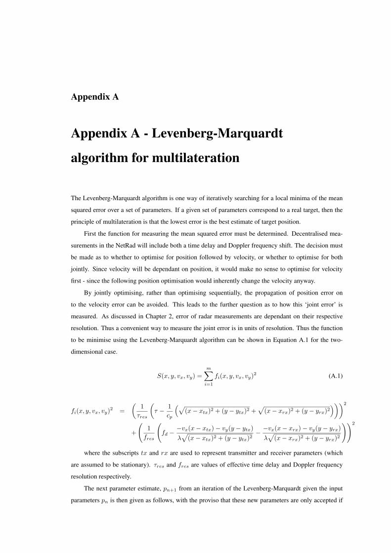
Appendix A
Appendix A - Levenberg-Marquardt
algorithm for multilateration
The Levenberg-Marquardt algorithm is one way of iteratively searching for a local minima of the mean
squared error over a set of parameters. If a given set of parameters correspond to a real target, then the
principle of multilateration is that the lowest error is the best estimate of target position.
First the function for measuring the mean squared error must be determined. Decentralised mea-
surements in the NetRad will include both a time delay and Doppler frequency shift. The decision must
be made as to whether to optimise for position followed by velocity, or whether to optimise for both
jointly. Since velocity will be dependant on position, it would make no sense to optimise for velocity
first - since the following position optimisation would inherently change the velocity anyway.
By jointly optimising, rather than optimising sequentially, the propagation of position error on
to the velocity error can be avoided. This leads to the further question as to how this ‘joint error’ is
measured. As discussed in Chapter 2, error of radar measurements are dependant on their respective
resolution. Thus a convenient way to measure the joint error is in units of resolution. Thus the function
to be minimise using the Levenberg-Marquardt algorithm can be shown in Equation A.1 for the two-
dimensional case.
S(x, y, vx, vy) =m∑i=1
fi(x, y, vx, vy)2 (A.1)
fi(x, y, vx, vy)2 =(
1τres
(τ − 1
cp
(√(x− xtx)2 + (y − ytx)2 +
√(x− xrx)2 + (y − yrx)2
)))2
+
(1fres
(fd −
−vx(x− xtx)− vy(y − ytx)λ√
(x− xtx)2 + (y − ytx)2− −vx(x− xrx)− vy(y − yrx)λ√
(x− xrx)2 + (y − yrx)2
))2
where the subscripts tx and rx are used to represent transmitter and receiver parameters (which
are assumed to be stationary). τres and fres are values of effective time delay and Doppler frequency
resolution respectively.
The next parameter estimate, pn+1 from an iteration of the Levenberg-Marquardt given the input
parameters pn is then given as follows, with the proviso that these new parameters are only accepted if

202
fi(x, y, vx, vy)2 is found to be further minimised.
pn+1 = pn − (Jf (pn)TJf (pn) + λdiag(Jf (pn)TJf (pn)))−1Jf (pn)T f(pn) (A.2)
where pn = (x, y, vx, vy)T is the matrix of the target parameters for guess n, f = (f1, ..., fi)T
and Jf (pn) is the Jacobian matrix of partial derivatives of f at pn. In processing the NetRad data, these
partial derivatives must be approximated by a finite difference method.
The conditions for setting λ were taken from the recommendations given in Press et al. [1992] ;
namely λ is initially set to 0.001. If an iteration is successful (fi(x, y, vx, vy)2 is found to be further
minimised) then new parameters are accepted and λ is divided by a factor of 10 for the next iteration. If
the iteration is unsuccessful, then λ is multiplied by a factor of 10 for the next iteration. This means that
as λ increases the algorithm becomes closer to the Gauss-Newton method, which although potentially
fast has a tendency to overshoot the minima, whereas an increase in λ moves the algorithm closer to a
gradient descent method with an increasingly small step size.
Appendix B
Appendix B - Future hardware development
A major effort in this work was the ruggedisation of the system in the effort to make experimental
trials simple to set up and more reliable (and consequently give more confidence in results produced).
The wired nature of the system has remained, with the tried-and-tested 50 m cables being a constant
throughout development. This presents little problem where the set-up of the nodes are such that these
cables can easily be run between them. However were it desired that distances between nodes be greater
than 50 m, or if obstacles (such as attempting to situate nodes on different buildings in an urban setting)
prevent easy ‘direct’ links then some alternative method must be considered. Direct RF transmission
between nodes can be seen to be used in other systems - notably in space-based applications such as
the TechSat 21 array of satellites [Steyskal et al., 2003]. The earlier timing delays of Figure 5.4 would
still apply, where the TOA values would now be determined by the propagation through free space,
rather than through the fixed cable lengths. Thus successful time transfer would rely on first determining
the locations of the nodes (which is also needed for multistatic data fusion). However if LOS cannot
be guaranteed, or if there are inherently unpredictable propagation paths such as unknown multipath
or ground plane effects present, then there are limitations on how accurate such methods might be for
synchronisation.
One possible COTS solution which could provide position, synchronisation and a distributed refer-
ence oscillator is that of GPS. Such methods have been used previously, for time synchronisation alone,
in Weedon and Stribley [2000] to determine aircraft height through multilateration of received secondary
surveillance radar transmissions from the aircraft. Here ‘short baseline’ trials, where GPS antennas are
arranged 1.25 m apart, demonstrated an RMS error of approximately 0.3 ns - thus comparable to the ca-
ble based synchronisation used by NetRad. A subsequent ‘medium baseline’ trial, where GPS antennas
are arranged 6.5 km apart, was inconclusive due to the difficulty at measuring the error, but was expected
to be approximately 1.5 ns. A more concise investigation into the synchronisation through GPS method
is explored in Hambly and Clark [2002], where the use of highly stable hydrogen maser frequency stan-
dards at each GPS receiver test site allows for measurment over a larger baselength. Here a specific GPS
timing receiver, the Motorola M12+, is shown to be capable of time stability of 4.2 ns RMS (and 30 ns
pk-pk) over a 21.5 km baseline.
GPS disciplined oscillators provide a stable frequency standard, effectively by receiving the atomic
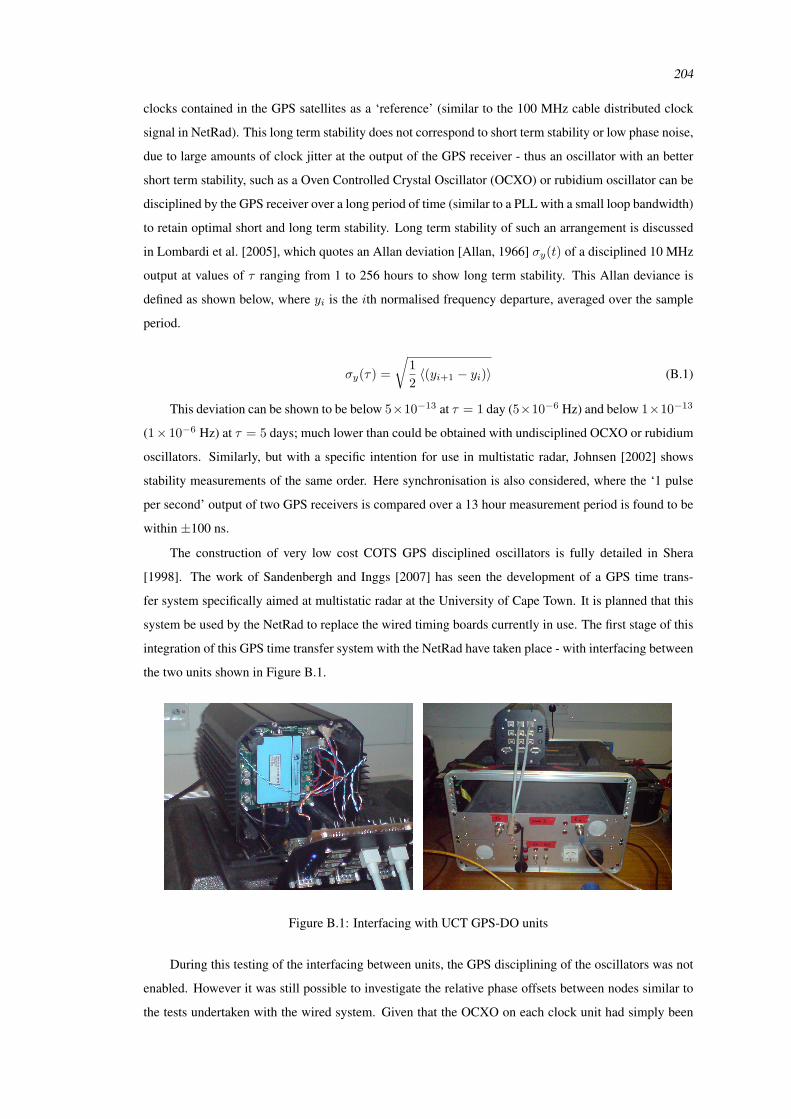
204
clocks contained in the GPS satellites as a ‘reference’ (similar to the 100 MHz cable distributed clock
signal in NetRad). This long term stability does not correspond to short term stability or low phase noise,
due to large amounts of clock jitter at the output of the GPS receiver - thus an oscillator with an better
short term stability, such as a Oven Controlled Crystal Oscillator (OCXO) or rubidium oscillator can be
disciplined by the GPS receiver over a long period of time (similar to a PLL with a small loop bandwidth)
to retain optimal short and long term stability. Long term stability of such an arrangement is discussed
in Lombardi et al. [2005], which quotes an Allan deviation [Allan, 1966] σy(t) of a disciplined 10 MHz
output at values of τ ranging from 1 to 256 hours to show long term stability. This Allan deviance is
defined as shown below, where yi is the ith normalised frequency departure, averaged over the sample
period.
σy(τ) =
√12〈(yi+1 − yi)〉 (B.1)
This deviation can be shown to be below 5×10⁻¹³ at τ = 1 day (5×10⁻⁶ Hz) and below 1×10⁻¹³
(1× 10⁻⁶ Hz) at τ = 5 days; much lower than could be obtained with undisciplined OCXO or rubidium
oscillators. Similarly, but with a specific intention for use in multistatic radar, Johnsen [2002] shows
stability measurements of the same order. Here synchronisation is also considered, where the ‘1 pulse
per second’ output of two GPS receivers is compared over a 13 hour measurement period is found to be
within ±100 ns.
The construction of very low cost COTS GPS disciplined oscillators is fully detailed in Shera
[1998]. The work of Sandenbergh and Inggs [2007] has seen the development of a GPS time trans-
fer system specifically aimed at multistatic radar at the University of Cape Town. It is planned that this
system be used by the NetRad to replace the wired timing boards currently in use. The first stage of this
integration of this GPS time transfer system with the NetRad have taken place - with interfacing between
the two units shown in Figure B.1.
Figure B.1: Interfacing with UCT GPS-DO units
During this testing of the interfacing between units, the GPS disciplining of the oscillators was not
enabled. However it was still possible to investigate the relative phase offsets between nodes similar to
the tests undertaken with the wired system. Given that the OCXO on each clock unit had simply been
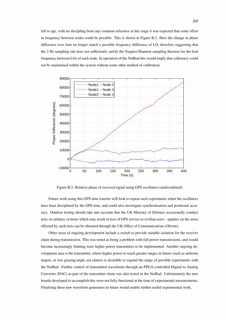
205
left to age, with no discipling from any common reference at this stage it was expected that some offset
in frequency between nodes could be possible. This is shown in Figure B.2. Here the change in phase
difference over time no longer match a possible frequency difference of LO, therefore suggesting that
the 2 Hz sampling rate does not sufficiently satisfy the Nyquist-Shannon sampling theorem for the beat
frequency between LOs of each node. In operation of the NetRad this would imply that coherency could
not be maintained within the system without some other method of calibration.
0 50 100 150 200 250 300 350 400−10000
0
10000
20000
30000
40000
50000
60000
70000
80000
90000
Time (s)
Pha
se D
iffer
ence
(de
gree
s)
Node1 − Node 2Node1 − Node 3Node2 − Node 3
Figure B.2: Relative phase of received signal using GPS oscillators (undisciplined)
Future work using this GPS time transfer will look to repeat such experiments when the oscillators
have been disciplined by the GPS time, and could also investigate synchronisation and positional accu-
racy. Outdoor testing should take into account that the UK Ministry of Defence occasionally conduct
tests on military systems which may result in loss of GPS service to civilian users - updates on the areas
effected by such tests can be obtained through the UK Office of Communications (Ofcom).
Other areas of ongoing development include a switch to provide suitable isolation for the receiver
chain during transmission. This was noted as being a problem with full power transmissions, and would
become increasingly limiting were higher power transmitters to be implemented. Another ongoing de-
velopment area is the transmitter, where higher power to reach greater ranges in future (such as airborne
targets, or low grazing-angle sea clutter) is desirable to expand the range of possible experiments with
the NetRad. Further control of transmitted waveforms through an FPGA-controlled Digital to Analog
Converter (DAC) as part of the transmitter chain was also tested in the NetRad. Unfortunately the new
boards developed to accomplish this were not fully functional at the time of experimental measurements.
Finalising these new waveform generators in future would enable further useful experimental work.

Bibliography
D.W. Allan. Statistics of atomic frequency standards. Proceedings of the IEEE, 54(2):221–230, February
1966. ISSN 0018-9219.
E.H. Attia and K. Abend. An experimental demonstration of a distributed array radar. Antennas and
Propagation Society International Symposium, 1991. AP-S. Digest, 3:1720–1723, June 1991. doi:
10.1109/APS.1991.175189.
E.H. Attia and B.D. Steinberg. Self-cohering large antenna arrays using the spatial correlation properties
of radar clutter. Antennas and Propagation, IEEE Transactions on, 37(1):30–38, January 1989. ISSN
0018-926X. doi: 10.1109/8.192160.
C.J. Baker and A.L. Hume. Netted radar sensing. Aerospace and Electronic Systems Magazine, IEEE,
18(2):3–6, February 2003. ISSN 0885-8985. doi: 10.1109/MAES.2003.1183861.
D.A.R. Beale and A.L. Hume. Bistatic RCS tools for the assessment of multi-static radar. RADAR 2002,
pages 31–35, October 2002.
I. Bradaric, G.T. Capraro, D.D. Weiner, and M.C. Wicks. Multistatic radar systems signal processing.
Radar, 2006 IEEE Conference on, pages 106–113, April 2006. doi: 10.1109/RADAR.2006.1631783.
I. Bradaric, G.T. Capraro, and M.C. Wicks. Sensor placement for improved target resolution in dis-
tributed radar systems. Radar Conference, 2008. Proceedings of the 2008 IEEE, pages 345–350, May
2008.
G.J. Burke and A.J. Poggio. Numerical electromagnetic code (NEC): Description theory. Lawrence
Livermore Laboratory, 1981.
A. Cameron. The Jindalee operational radar network: its architecture and surveillance capability. Radar
Conference, 1995., Record of the IEEE 1995 International, pages 692–697, May 1995. doi: 10.1109/
RADAR.1995.522633.
J.R. Carson. Reciprocal Theorems in Radio Communication. Proceedings of the IRE, 17(6):952–956,
June 1929. ISSN 0096-8390.
S. Carson, D. Kilfoyle, M. Potter, and J. Vance. A Passive, Multi-Static Radar System. Proceedings of
the IET International Conference on Radar Systems, October 2007.

BIBLIOGRAPHY 207
V.C. Chen, F. Li, S.-S. Ho, and H. Wechsler. Analysis of micro-Doppler signatures. Radar, Sonar and
Navigation, IEE Proceedings -, 150(4):271–276, August 2003. ISSN 1350-2395. doi: 10.1049/ip-rsn:
20030743.
M. Cherniakov. Bistatic Radars - Principle and Practice. John Wiley and Sons Ltd, 2007. ISBN
978-0-470-02630-4.
V. S. Chernyak. Fundamentals of Multisite Radar System. Gordon and Breach Science Publishers, 1998.
ISBN 90-5699-165-5.
E. Conte, E. D’Addio, A. Farina, and M. Longo. Multistatic radar detection: Synthesis and comparison
of optimum and suboptimum receivers. IEE Proceedings, Part F - Communications, Radar and Signal
Processing, 130(6):484–494, October 1983.
J. W. Crispin, R. F. Goodrich, and K. M. Siegel. A theoretical method for the calculation of the radar
cross sections of aircraft and missiles. Technical Report Rept. 2591-1-H, Radiation Lab. University of
Michigan, July 1959.
H. Deng. Polyphase code design for Orthogonal Netted Radar systems. Signal Processing, IEEE Trans-
actions on, 52(11):3126–3135, November 2004a. ISSN 1053-587X. doi: 10.1109/TSP.2004.836530.
H. Deng. Effective CLEAN algorithms for performance-enhanced detection of binary coding radar
signals. Signal Processing, IEEE Transactions on, 52(1):72–78, January 2004b. ISSN 1053-587X.
doi: 10.1109/TSP.2003.820075.
T. E. Derham. The Design and Calibration of a Coherent Multistatic Radar System. PhD thesis, Univer-
sity College London, April 2005.
T.E. Derham, S. Doughty, K. Woodbridge, and C.J. Baker. Design and evaluation of a low-cost mul-
tistatic netted radar system. Radar, Sonar & Navigation, IET, 1(5):362–368, October 2007. ISSN
1751-8784. doi: 10.1049/iet-rsn:20060100.
J. V. Di Franco and W. L. Rubin. Radar Detection. Prentice-Hall, 1968.
S. R. Doughty, K. Woodbridge, and C. J. Baker. Improving Resolution Using Multistatic Radar. Radar
Systems, 2007. RADAR 2007. The Institution of Engineering and Technology International Conference
on, October 2007.
Jr. Eigel, R.L. and Jr. Terzuoli, A.J. Bistatic scattering characterization of a complex object. Antennas
and Propagation Society International Symposium, 1999. IEEE, 3:1784–1787, August 1999. doi:
10.1109/APS.1999.788301.
A. Farina. Survey of Data Processing in Netted Radar. Electro-Technology, 28(2), June 1984.
A. Farina and E. Hanle. Position Accuracy in Netted Monostatic and Bistatic Radar. Aerospace and
Electronic Systems, IEEE Transactions on, AES-19(4):513–520, July 1983. ISSN 0018-9251. doi:
10.1109/TAES.1983.309339.
BIBLIOGRAPHY 208
E. Fishler, A. Haimovich, R. Blum, D. Chizhik, L. Cimini, and R. Valenzuela. MIMO radar: an idea
whose time has come. Radar Conference, 2004. Proceedings of the IEEE, pages 71–78, April 2004a.
ISSN 1097-5659.
E. Fishler, A. Haimovich, R. Blum, R. Cimini, D. Chizhik, and R. Valenzuela. Performance of MIMO
radar systems: advantages of angular diversity. Signals, Systems and Computers, 2004. Conference
Record of the Thirty-Eighth Asilomar Conference on, 1:305–309, November 2004b. doi: 10.1109/
ACSSC.2004.1399142.
E. Fishler, A. Haimovich, R.S. Blum, Jr. Cimini, L.J., D. Chizhik, and R.A. Valenzuela. Spatial diversity
in radars-models and detection performance. Signal Processing, IEEE Transactions on [see also
Acoustics, Speech, and Signal Processing, IEEE Transactions on], 54(3):823–838, March 2006. ISSN
1053-587X. doi: 10.1109/TSP.2005.862813.
A. Flaig and G.R. Arce. Nearfield spot-beamforming with distributed arrays. Sensor Array and Mul-
tichannel Signal Processing Workshop. 2000. Proceedings of the 2000 IEEE, pages 390–394, March
2000. doi: 10.1109/SAM.2000.878036.
F. Folster and H. Rohling. Data association and tracking for automotive radar networks. Intelligent
Transportation Systems, IEEE Transactions on, 6(4):370–377, December 2005. ISSN 1524-9050.
doi: 10.1109/TITS.2005.858784.
G. Galati, M. Naldi, and M. Ferri. Airport surface surveillance with a network of miniradars. Aerospace
and Electronic Systems, IEEE Transactions on, 35(1):331–338, January 1999. ISSN 0018-9251. doi:
10.1109/7.745702.
S. Giompapa, A. Farina, F. Gini, A. Graziano, R. Croci, and R. Di Stefano. Study of the classification
task into an integrated multisensor system for maritime border control. Radar Conference, 2008.
Proceedings of the 2008 IEEE, pages 482–487, May 2008.
D. Giuli, F. Cuccoli, G.B. Gentili, and D. Erricolo. Ad hoc receive sensors aimed at enhancing multistatic
radar operation for surveillance of limited critical areas. Electromagnetics in Advanced Applications,
2007. ICEAA 2007. International Conference on, pages 476–479, Sept. 2007. doi: 10.1109/ICEAA.
2007.4387340.
J.I. Glaser. Some results in the bistatic radar cross section (RCS) of complex objects. Proceedings of the
IEEE, 77(5):639–648, May 1989. ISSN 0018-9219. doi: 10.1109/5.32054.
H. Godrich, A.H. Haimovich, and R.S. Blum. Target Localization Techniques and Tools for MIMO
Radar. Radar Conference, 2008. Proceedings of the 2008 IEEE, pages 1056–1061, May 2008.
R. M. Hambly and T. A. Clark. Critical Evaluation of the Motorola M12+ GPS Timing Receiver vs. the
Master Clock at the United States Naval Observatory. Proceedings of the 34th Annual Precise Time
and Time Interval (PTTI) Meeting, pages 109–116, December 2002.

BIBLIOGRAPHY 209
D.A. Howe, D.U. Allan, and J.A. Barnes. Properties of Signal Sources and Measurement Methods.
Thirty Fifth Annual Frequency Control Symposium. 1981, pages 669–716, 1981.
M. C. Jackson. The geometry of bistatic radar systems. IEE Proceedings, Part F - Communications,
Radar and Signal Processing, 133:604–612, December 1986.
J. Jinlei, R. Hongbin, G. Fuli, and D. Huaisuo. A preliminary research into the netted radar seekers
for anti-stealth aircraft. Signal Processing Proceedings, 1998. ICSP ’98. 1998 Fourth International
Conference on, 2:1566–1569, 1998. doi: 10.1109/ICOSP.1998.770925.
John Hopkins APL. Cooperative Engagement Capability (CEC). John Hopkins APL Technical Digest,
16(4):377–396, 1995.
T. Johnsen. Time and frequency synchronization in multistatic radar. Consequences to usage of GPS
disciplined references with and without GPS signals. Radar Conference, 2002. Proceedings of the
IEEE, pages 141–147, April 2002. ISSN 1097-5659. doi: 10.1109/NRC.2002.999711.
T. Johnsen, K.E. Olsen, and R. Gundersen. Hovering helicopter measured by bi-/multistatic CW radar.
Radar Conference, 2003. Proceedings of the 2003 IEEE, pages 165–170, May 2003. ISSN 1097-5659.
doi: 10.1109/NRC.2003.1203397.
T. Johnsen, K.E. Olsen, S. Johnsrud, and R. Skjerpeng. Simultaneous use of multiple pseudo random
noise codes in multistatic CW radar. Radar Conference, 2004. Proceedings of the IEEE, pages 266–
270, April 2004. ISSN 1097-5659.
D. Kahny, K. Schmitt, and W. Wiesbeck. Calibration of bistatic polarimetric radar systems. Geoscience
and Remote Sensing, IEEE Transactions on, 30(5):847–852, September 1992. ISSN 0196-2892. doi:
10.1109/36.175318.
R.E. Kell. On the derivation of bistatic RCS from monostatic measurements. Proceedings of the IEEE,
53(8):983–988, August 1965. ISSN 0018-9219.
S. Kingsley and S. Quegan. Understanding Radar Systems. McGraw-Hill Book Company Europe, 1992.
ISBN 978-0077074265.
G. H. Knittel. Phase 2 Netted radar demonstration. NASA STI/Recon Technical Report N, 81, October
1980.
E. F. Knott, J. F. Shaeffer, and M. T. Tuley. Radar Cross Section. SciTech Publishing, 2nd edition, 2004.
ISBN 1-891121-25-1.
D.A. Lambert. Ubiquitous command and control. Information, Decision and Control, 1999. IDC 99.
Proceedings. 1999, pages 35–40, February 1999. doi: 10.1109/IDC.1999.754123.
T.L. Lane, N.T. Alexander, and C.A. Blevins. The bistatic coherent measurement system (BICOMS).
Radar Conference, 1999. The Record of the 1999 IEEE, pages 154–159, April 1999. doi: 10.1109/
NRC.1999.767300.

BIBLIOGRAPHY 210
R. Larson, A. Maffett, R. Heimiller, A. Fromm, E. Johansen, R. Rawson, and F. Smith. Bistatic clutter
measurements. Antennas and Propagation, IEEE Transactions on, 26(6):801–804, November 1978.
ISSN 0096-1973.
N. Levanon. Radar Principles. John Wiley and Sons, 1988. ISBN 978-0471858812.
Lockheed Martin. UK Co-operative Engagament Capability (UK CEC), 2007. URL http://www.
lockheedmartin.co.uk/products/ukcec.html.
M.A. Lombardi, A.N. Novick, and V.S. Zhang. Characterizing the performance of GPS disciplined oscil-
lators with respect to UTC(NIT). Frequency Control Symposium and Exposition, 2005. Proceedings
of the 2005 IEEE International, pages 677–684, August 2005. doi: 10.1109/FREQ.2005.1574017.
J.M.M. Lopez, F.J.J. Rodriguez, and J.R.C. Corredera. Cooperative management of netted surveillance
sensors. Systems, Man, and Cybernetics, 1997. ’Computational Cybernetics and Simulation’., 1997
IEEE International Conference on, 1:845–850, Oct 1997. doi: 10.1109/ICSMC.1997.626205.
B. R. Mahafza. Radar Systems Analysis and Design Using MATLAB (Second Edition). Chapman &
Hall/CRC, 2005. ISBN 1-58488-532-7.
R. Manasse. Summary of maximum theoretical accuracy of radar measurements. Technical report, Mitre
Corp, April 1960.
D. W. Marquardt. An Algorithm for Least-Squares Estimation of Nonlinear Parameters. Journal of the
Society for Industrial and Applied Mathematics, 11(2):431–441, June 1963.
F. Martinerie. Data fusion and tracking using HMMs in a distributed sensor network. Aerospace and
Electronic Systems, IEEE Transactions on, 33(1):11–28, January 1997. ISSN 0018-9251. doi: 10.
1109/7.570704.
D. Massonnet. Capabilities and limitations of the interferometric cartwheel. Geoscience and Remote
Sensing, IEEE Transactions on, 39(3):506–520, March 2001. ISSN 0196-2892. doi: 10.1109/36.
911109.
R. McDonough and A. Whalen. Detection of Signals in Noise (2nd Edition). Academic Press, 1995.
ISBN 978-0127448527.
I. Mohor and S. Shaheen. CAN Protocol Controller, 2008. URL http://www.opencores.org/
projects.cgi/web/can/overview.
L.R. Moyer, C.J. Morgan, and D.A. Rugger. An exact expression for resolution cell area in special case
of bistatic radar systems. Aerospace and Electronic Systems, IEEE Transactions on, 25(4):584–587,
July 1989. ISSN 0018-9251. doi: 10.1109/7.32092.
A.V. Mrstik. Multistatic-Radar Binomial Detection. Aerospace and Electronic Systems, IEEE Transac-
tions on, AES-14(1):103–108, January 1978. ISSN 0018-9251. doi: 10.1109/TAES.1978.308583.
BIBLIOGRAPHY 211
F. E. Nathanson, J. P. Reilly, and M. N. Cohen. Radar Design Principles - Signal Processing and the
Environment, chapter 7. SciTech Publishing, 2nd edition, 1999. ISBN 978-1891121098.
National Radio Astronomy Observatory. Very Long Baseline Array, 2007. URL http://www.vlba.
nrao.edu.
J. Neyman and E. Pearson. On the problem of the most efficient tests of statistical hypotheses. Philo-
sophical Transactions of the Royal Society of London, 231(9):289–337, 1933.
Ofcom. UK Interface Requirement 2005, November 2006. URL http://www.ofcom.org.uk/
radiocomms/ifi/tech/interface_req/uk2005.pdf.
Y. B. Ovchinnikov. Fresnel interference pattern of a triple-slit interferometer. Optics Communications,
216(1):33–40, February 2003.
E. Paolini, A. Giorgetti, M. Chiani, R. Minutolo, and M. Montanari. Localization Capability of Cooper-
ative Anti-Intruder Radar Systems. EURASIP Journal on Advances in Signal Processing, 2008, May
2008. doi: 10.1155/2008/726854.
I. Papoutsis, C. J. Baker, and H. D. Griffiths. Location accuracy of multistatic radars based on ranging
information. Proceedings of the IEEE International Conference on Radar, pages 883–888, May 2005.
W. H. Press, B. P. Flannery, S. A. Teukolsky, and W. T. Vetterling. Numerical Recipes in C: The Art of
Scientific Computing, chapter 15, pages 683–688. Cambridge University Press, 2nd edition, October
1992. ISBN 978-0521431088.
C. Rago, P. Willett, and M. Alford. Predetection fusion: resolution cell grid effects. Aerospace and
Electronic Systems, IEEE Transactions on, 35(3):778–789, July 1999. ISSN 0018-9251. doi: 10.
1109/7.784051.
Raytheon. Patriot: Combat-Proven Air and Missile Defense, 2008. URL http://www.raytheon.
com/products/patriot.
Robert Bosch GmbH. Controller Area Network (CAN), 2008. URL http://www.
semiconductors.bosch.de/en/20/can/index.asp.
F. C. Robey, S. Coutts, D. Weikle, J. C. McHarg, and K. Cuomo. Precise formation flying control of
multiple spacecraft using carrier-phase differential GPS. Proceedings of the AAS/AIAA Space Flight
Mechanics Meeting, January 2000.
F.C. Robey, S. Coutts, D. Weikle, J.C. McHarg, and K. Cuomo. MIMO radar theory and experimental
results. Signals, Systems and Computers, 2004. Conference Record of the Thirty-Eighth Asilomar
Conference on, 1:300–304, November 2004. doi: 10.1109/ACSSC.2004.1399141.
J. E. Salah and J. E. Morriello. Development of a Multistatic Measurement System. Proceedings of the
IEEE International Radar Conference, pages 88–93, April 1980.

BIBLIOGRAPHY 212
P.F. Sammartino, C.J. Baker, and H.D. Griffiths. MIMO radar performance in clutter environment.
Radar, 2006. CIE ’06. International Conference on, pages 32–35, October 2006. doi: 10.1109/ICR.
2006.343554.
G. San Antonio, D.R. Fuhrmann, and F.C. Robey. Mimo radar ambiguity functions. Selected Topics in
Signal Processing, IEEE Journal of, 1(1):167–177, June 2007. ISSN 1932-4553. doi: 10.1109/JSTSP.
2007.897058.
J. S. Sandenbergh and M. R. Inggs. A Common View GPSDO to Synchronise Netted Radar. Proceedings
of the IET International Conference on Radar Systems, October 2007.
K. Sarabandi and Tsen-Chieh Chiu. Optimum corner reflectors design. Radar Conference, 1996., Pro-
ceedings of the 1996 IEEE National, pages 148–153, May 1996. doi: 10.1109/NRC.1996.510672.
J. A. Scheer and J. L. Kurtz. Coherent Radar Performance Estimation, chapter 12, pages 298–301.
Artech House, 1993. ISBN 0-89006-628-0.
R.T. Schilizzi. The European VLBI Network, its new data processor at JIVE, and opportunities for
expansion. Radio Science Conference, 1999. NRSC ’99. Proceedings of the Sixteenth National, pages
INV1/1–INV1/6, Feb 1999. doi: 10.1109/NRSC.1999.760864.
R. Schmidt. Multiple emitter location and signal parameter estimation. Antennas and Propagation, IEEE
Transactions on, 34(3):276–280, March 1986. ISSN 0096-1973.
T.A. Seliga and F.J. Coyne. Multistatic radar as a means of dealing with the detection of multipath false
targets by airport surface detection equipment radars. Radar Conference, 2003. Proceedings of the
2003 IEEE, pages 329–336, May 2003. ISSN 1097-5659. doi: 10.1109/NRC.2003.1203422.
B. Shera. A GPS-based frequency standard. QST Magazine, pages 37–44, July 1998.
M. I. Skolnik. Introduction to Radar Systems (2nd Edition). McGraw-Hill, 1980. ISBN 978-
0070579095.
M. I. Skolnik. Radar Handbook (2nd Edition). McGraw-Hill, 1990. ISBN 978-0070579132.
G. E. Smith, K. Woodbridge, and C. J. Baker. Multiperspective Micro-Doppler Signature Classification.
Radar Systems, 2007. RADAR 2007. The Institution of Engineering and Technology International
Conference on, October 2007.
H. Steyskal, J.K. Schindler, P. Franchi, and R.J. Mailloux. Pattern synthesis for TechSat21 - a distributed
space-based radar system. Antennas and Propagation Magazine, IEEE, 45(4):19–25, August 2003.
ISSN 1045-9243. doi: 10.1109/MAP.2003.1241307.
A. G. Stove. Sharing False Alarm Rate Information Between Disparate Sensors. Proceedings of the IET
International Conference on Radar Systems, October 2007.
BIBLIOGRAPHY 213
P. Swerling. Probability of detection for fluctuating targets. Information Theory, IEEE Transactions on,
6(2):269–308, April 1960. ISSN 0018-9448.
P. Tait. Introduction to Radar Target Recognition. Institution of Engineering and Technology, January
2006. ISBN 978-0863415012.
Y. Teng, C. Baker, and K. Woodbridge. Netted Radar Sensitivity and the Ambiguity Function. Radar,
2006. CIE ’06. International Conference on, pages 65–68, October 2006. doi: 10.1109/ICR.2006.
343573.
T. Tsao, M. Slamani, P. Varshney, D. Weiner, H. Schwarzlander, and S. Borek. Ambiguity function for a
bistatic radar. Aerospace and Electronic Systems, IEEE Transactions on, 33(3):1041–1051, July 1997.
ISSN 0018-9251. doi: 10.1109/7.599331.
M. Vespe, C.J. Baker, and H.D. Griffiths. Multi-perspective target classification. Radar Conference,
2005 IEEE International, pages 877–882, May 2005. doi: 10.1109/RADAR.2005.1435951.
K.D. Ward, C.J. Baker, and S. Watts. Maritime surveillance radar. I. Radar scattering from the ocean
surface. Radar and Signal Processing, IEE Proceedings F, 137(2):51–62, April 1990. ISSN 0956-
375X.
R. Weedon and K. Stribley. The Development and implementation of a GPS Time Transfer System.
Proceedings of the 13th International Technical Meeting of the Satellite Division of the Institute of
Navigation ION GPS 2001, pages 19–22, September 2000.
M. Weib. Synchronisation of bistatic radar systems. Geoscience and Remote Sensing Symposium, 2004.
IGARSS ’04. Proceedings. 2004 IEEE International, 3:1750–1753, September 2004. doi: 10.1109/
IGARSS.2004.1370671.
N. J. Willis. Bistatic Radar. Artech House, 1991. ISBN 978-0890064276.
J.E. Winter and N.C. Anderson. Distributed aperture implementation on the techsat 21 satellites.
Aerospace Conference, 2003. Proceedings. 2003 IEEE, 2:815–823, March 2003. ISSN 1095-323X.
doi: 10.1109/AERO.2003.1235493.
P. M. Woodward. Probability and Information Theory, with Application to Radar. Artech House, 1980.
ISBN 978-0890061039.
P. M. Woodward and I. L. Davies. A theory of radar information. Phil. Mag., 41:1001–1017, 1950.