b i om a s s a n d b i o e n e r g y 3 5 ( 2 0 1 1 ) 2 9 6 1e2 9 7 4

Avai lab le a t www.sc iencedi rec t .com

ht tp : / /www.e lsev ier . com/ loca te /b iombioe

Development and application of BioFeed model foroptimization of herbaceous biomass feedstock production

Yogendra Shastri a,*, Alan Hansen b, Luis Rodrı́guez b, K.C. Ting b

aEnergy Biosciences Institute, University of Illinois at Urbana-Champaign, 1206W. Gregory Drive, 1119 IGB, Urbana, IL 61801, United StatesbDepartment of Agricultural and Biological Engineering, University of Illinois at Urbana-Champaign, 1304 W. Pennsylvania Avenue,

Urbana, IL 61801, United States

a r t i c l e i n f o

Article history:

Received 15 July 2009

Received in revised form

14 March 2011

Accepted 16 March 2011

Available online 12 April 2011

Keywords:

BioFeed

Biomass feedstock

Optimization

Switchgrass

Panicum virgatum

Illinois

* Corresponding author. Tel.: þ1 217 333 177E-mail addresses: yshast1@illinois.edu (Y

edu (K.C. Ting).0961-9534/$ e see front matter ª 2011 Elsevdoi:10.1016/j.biombioe.2011.03.035

a b s t r a c t

An efficient and sustainable biomass feedstock production system is critical for the success

of the biomass based energy sector. An integrated systems analysis framework to coor-

dinate various feedstock production related activities is, therefore, highly desirable. This

article presents research conducted towards the creation of such a framework. A breadth

level mixed integer linear programming model, named BioFeed, is proposed that simulates

different feedstock production operations such as harvesting, packing, storage, handling

and transportation, with the objective of determining the optimal system level configu-

ration on a regional basis. The decision variables include the design/planning as well as

management level decisions. The model was applied to a case study of switchgrass

production as an energy crop in southern Illinois. The results illustrated that the total cost

varied between 45 and 49 $ Mg�1 depending on the collection area and the sustainable

biorefinery capacity was about 1.4 Gg d�1. The transportation fleet consisted of 66 trucks

and the average utilization of the fleet was 86%. On-farm covered storage of biomass was

highly beneficial for the system. Lack of on-farm open storage and centralized storage

reduced the system profit by 17% and 5%, respectively. Increase in the fraction of larger

farms within the system reduced the cost and increased the biorefinery capacity, sug-

gesting that co-operative farming is beneficial. The optimization of the harvesting schedule

led to 30% increase in the total profit. Sensitivity analysis showed that the reduction in

truck idling time as well as increase in baling throughput and output density significantly

increased the profit.

ª 2011 Elsevier Ltd. All rights reserved.

1. Introduction important precursor for the success of this approach is an

The biomass based energy sector, especially the one based on

lignocellulosic sources such as switchgrass (Panicum virga-

tum), Miscanthus (Miscanthus � giganteus), forest residues,

short rotation coppice and mixed prairie grasses, will play an

important role in our drive towards renewable energy [1,2]. An

5; fax: þ1 217 244 3637.. Shastri), achasnen@illin

ier Ltd. All rights reserved

efficient, reliable and cost effective biomass feedstock

production (BFP) system that satisfies the expected high

demand rates. Preliminary studies have shown that feedstock

supply (farming and delivery) costs can be up to 35e50% of the

delivered cost of ethanol [3]. Hence, the biofuel supply reli-

ability and cost competitiveness will depend significantly on

ois.edu (A. Hansen), lfr@illinois.edu (L. Rodrı́guez), kcting@illinois.

.

b i om a s s an d b i o e n e r g y 3 5 ( 2 0 1 1 ) 2 9 6 1e2 9 7 42962

feedstock production and provision. Achieving that reliability

while simultaneously optimizing the economic, environ-

mental, technological and social goals will be critical.

Biomass feedstock production can be classified into the

following different tasks: pre-harvest crop management

(including precision agriculture), harvesting (including densi-

fication), transportation (in-field as well as long distance),

storage and pre-processing. Since large scale energy crop

farming is not yet established, there is a significant lack of

expert knowledge in accomplishing these tasks. The logistical

complexity of the systems is further characterized by a wide

distribution of sources, time and weather sensitive crop

maturity, short windows for biomass collection, and compe-

tition from concurrent harvest operations [4]. It is, therefore,

extremely valuable to create a framework that enables

a systematic and holistic analysis of the biomass feedstock

production system.

This work presents the first step towards the creation of

such a framework, and proposes a breadth levelmathematical

programming model called BioFeed for the optimization of

various feedstock production activities such as harvesting,

packing, storage, biomass handling and transportation. The

objective of the mixed integer linear programming (MILP)

model is to determine the optimal configuration of the feed-

stock production system at a regional scale subject to local

and regional constraints. The major strength and uniqueness

of the model is to incorporate not only the long term design

decisions such as farm equipment selection, but also the

management decisions such as farm harvest scheduling in

a single framework. The model has been applied to a case

study of switchgrass production as an energy crop in southern

Illinois.

The subsequent article is arranged as follows. The next

section reviews past work in this field and motivates the

formulation of the presented model. Section 3 describes the

BioFeed model in detail. Section 4 describes the scope of the

case study while Section 5 presents the results and discussion

of the case study. The final section draws the important

conclusions and points towards future model extensions.

2. Literature review and motivation

The interest in the analysis and efficiency improvement of

bioenergy feedstock production increased in the mid 1990s

with focus on switchgrass in the US [5] and Miscanthus in

Europe [6e8]. These and other similar recent studies [9e12]

compared a number of different scenarios based on avail-

able data to determine the best option and identify bottle-

necks. Although these studies are very insightful, their

applicability is rather limited due to the lack of a mathemat-

ical model. Mathematical programming approaches have

been used to develop optimization models that are applicable

to a variety of cases subject to the availability of data [13e16].

More recently, focus has shifted to simulation models using

object-oriented programming [3] or discrete event simulation

[17,18]. The object-oriented approach as used in developing

the IBSALmodel [3,4] simplifies scenario building, particularly

related to various equipment for the same operation, since

data pertaining to different options are stored in a standard

object-oriented format.While highlighting some of the critical

issues in biomass feedstock production, the literature review

also helps in identifying the following important issues that

have not been rigorously explored:

� Farm size and its impact on-farm management: It is most

likely that farm operational and management strategies for

energy crops will differ based on the farm size since the

expected returns for the same investment will differ. Yet,

this aspect has been ignored in the past.

� Seasonality mismatch: A strong supply and demand

mismatch exists since energy crops have definite growth

and harvesting seasons. Although this mismatch has been

acknowledged in the literature, its impact on the system

configuration and cost has not been rigorously quantified.

� Biomass storage: The seasonality of supply makes biomass

storage that minimizes quantity and quality losses critical.

Different storage options including drying and pre-pro-

cessing, therefore, must be evaluated and their impact on

the complete system must be studied.

The goal of this research, therefore, is to develop

a modeling and systems analysis framework that allows us to

explore such issues in addition to the ones that have been

previously analyzed.

The scope of biomass feedstockproduction iswide in terms

of the spatial and temporal scales, and can be classified into

three distinct levels: strategic level (long-term), management

level (mid-term) and operational level (short-term). The Bio-

Feedmodel presented in thiswork focuses on the strategic and

management level decision making. It therefore considers

long-term decisions such as biorefinery capacity that do not

change formanyyearsaswell asmid-termdecisionsuchas the

transportation fleet distribution. Furthermore, the complexity

and interconnectedness of various operations within the

feedstock production system motivates the development of

a rigorous optimization model instead of a simulation model.

In addition to determining a configuration that is optimal for

the whole system, the optimization approach often highlights

certain non-intuitive relationships that are difficult to model

using a simulation approach. The value of the optimization

model has been further enhanced by supporting the model

with an object-oriented database which enables the incorpo-

ration of exhaustive information through standardized repre-

sentation [19]. The next section describes the proposedmodel,

its assumptions, features and limitations.

3. Model description

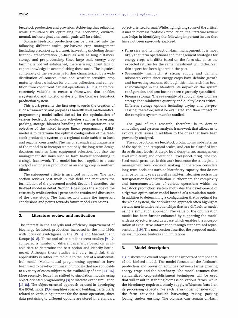
Fig. 1 shows the overall scope and the important components

of the BioFeed model. The model focuses on the feedstock

production and provision activities between farms growing

energy crops and the biorefinery. The model assumes that

standardized crop-establishment techniques will be used

that will result in standing biomass on various farms, while

the biorefinery requires a steady supply of biomass based on

its processing capacity. For each farm under consideration,

the farm activities include harvesting, raking, packing

(baling) and/or ensiling. The biomass can remain on-farm

Fig. 1 e Biomass feedstock production model: BioFeed.

b i om a s s a n d b i o e n e r g y 3 5 ( 2 0 1 1 ) 2 9 6 1e2 9 7 4 2963

post raking if a packingmachine is not immediately available.

The packed biomass can either be directly transported to the

biorefinery, or stored in one of the three storage options,

namely, on-farm open storage, on-farm covered storage, and

centralized storage which is shared by all the farms. The

transportation activities are carried out using a set of trucks

that are independently owned. It should be noted that the

model optimizes the farm level activities for each farm under

consideration.

The objective of the BioFeed model is to determine the

overall system optimum, and hence it integrates the impor-

tant operations in the biomass production value chain in

a single framework. It is possible that the optimal solution

recommended by BioFeed may not be implemented in a real

system, either due to unforeseen disturbances such as

weather or due to the actions of independent stakeholders

such as farmers. However, an integrated model such as Bio-

Feed is necessary to determine the optimal configuration,

system bottlenecks and potential improvements. Such

a model is also extremely valuable in quantifying the

systemic impacts of technology improvement [20]. Moreover,

a biorefinery can establish contracts with farmers and may

have complete control of the farm operations. In such cases,

BioFeed can be used by the biorefinery to optimize its

operations.

The following sections describe the model input require-

ment, simulation features and options, and the model

formulation details. A comprehensive description of the

model including the mathematical equations in provided as

part of the supplementary material.

3.1. Model inputs

The various inputs necessary for the BioFeed model simula-

tion are:

� Farm land allocation and farm size distribution: Since large scale

farming of lignocellulosic energy crops is not yet estab-

lished, the BioFeed model uses model based predictions

from literatures [10,21] to determine farm land allocation.

Since such data are often reported at the county level, Bio-

Feed uses either the typical county level farm size distri-

bution published by the National Agricultural Statistical

Services (NASS) of the USDA [22] or the typical national farm

size distribution published by the USDA [23] to determine

the number of farms in a county and their size distribution.

� Spatial distribution of the farms - Collection area: The model

assumes that farms in a given county are uniformly

distributed in the county area. For greater accuracy in

calculating transportation distances, it uses the land divi-

sion data published by the national or state geological

survey to determine the spatial distribution of farms in

a given county [24]. If such data are not available, a constant

land utilization factor is used to calculate the spatial

distribution and collection area [4].

� Biomass growth potential: The total harvestable yield of the

energy crop is calculated using crop growth models such as

ALMANAC for switchgrass [25] and MISCANMOD for Mis-

canthus [10,26].

3.2. Simulation horizon and simulation time step

The simulation horizon for the BioFeed model is one year,

which is divided into harvesting and non-harvesting horizons.

Since many farm activities such as harvesting, raking and

packing are performed only during the harvesting season,

those can be ignored during the non-harvesting horizon to

reduce the computational load. The smallest possible simu-

lation time step is one day and a higher simulation time step

can be selected by the user. In such cases, the model assumes

that the decisions taken for a particular time step apply to all

the days in that time step. It is possible to select different

time-steps for the harvesting and non-harvesting horizons.

The selection of the time step is a trade-off between accuracy

and computational requirement with smaller time step

increasing the computational demand. The simulation

horizon for themodel is independent of the calendar year and

b i om a s s an d b i o e n e r g y 3 5 ( 2 0 1 1 ) 2 9 6 1e2 9 7 42964

is instead correlated with the growth cycle of the energy crop

under consideration.

3.3. Model formulation details

The following sections describe the model formulation

details including the summary of the decision variables for

each task.

3.3.1. Harvesting, raking and packingThe BioFeed model simulates farming activities of harvesting,

raking and packing (baling) for each farm. The selection of the

necessaryequipmentand theiruse isoptimizedbyBioFeed.The

harvestingschedule isdefinedastheareaharvestedduringeach

time step, which is correlated to the total harvested biomass

using biomass growthmodels. The harvesting rate is limited by

the capacity of the selected equipment. Biomass harvesting is

followed by raking, and the raked biomass can either be packed

for storage and transportation or can be sent to a silage pit for

ensiling in loose form. The capacity of the selected equipment

limits the raking and packing rates. The packed biomass is sent

either to one of the various storage options or directly trans-

ported to the biorefinery. An important long term objective of

BioFeed model development is to provide decision support to

farmers for energy crop farming. Selection of the appropriate

equipment (technology) is an important decision for farmers

due to the availability of a number of existing and novel tech-

nologies. The BioFeedmodel is, therefore, designed to utilize an

extensive object-oriented farm equipment (commercial as well

as prototypes) database for its optimization decision making.

The equipment selection decisions are one-time decisions, and

the farmer incurs the capital and operating costs of the selected

equipment. The model limits each farm to select only one type

(model) of equipment. However, multiple equipment of the

same type can be selected to increase the capacity. Since farms

of similar size are expected to select the same farmmachinery,

the computational demands can be reduced by classifying the

farms into a limited number of classes based on the farm size

and assuming that the equipment selection decisions for

a particular class apply to all the farms within that class. The

model also provides the option for a user to pre-define the farm

equipment to build more specific scenarios. The optimization

model decisions for each farm are:

� Selection of harvesting, raking and packing equipment (type

and number)

� Harvesting schedule (area harvested per unit time step)

� Raking and packing schedule (biomass per unit time step)

� Post-harvest biomass distribution between ensiling and

packing for each time step

� Post-packing biomass distribution between direct trans-

portation to biorefinery and storage

3.3.2. StorageThere are four storage options available to each farm, namely:

on-farm covered storage, on-farm open air storage, on-farm

ensiling and centralized covered storage. The on-farm storage

facilities on a particular farm cannot be shared with other

farms, whereas the centralized storage facility is common to

all the farms.

The on-farm open air storage is a temporary storage option

available only during the harvesting horizon. It is associated

withminimum capital and operating cost but also leads to the

highest dry matter loss. On the contrary, the on-farm covered

storage, which can be of different types [27], entails higher

capital and operating expenses but is associated with lower

dry matter loss. The total area allocated to on-farm storage

(open as well as covered) is limited to a fraction of the total

farm area. The necessary volume of the on-farm storage

facility is a function of the output density of the selected

packing equipment. Each covered storage facility must

provide a buffer space for safety reasons. Ensiling is modeled

as an additional storage option for relatively long term storage

of biomass. The centralized storage facility is located at a fixed

distance from the biorefinery and the farms. The size of the

centralized storage facility is optimized by themodel. It is also

possible to include two or more potential storage locations

and optimize the location and size of the storage facilities.

The storage cost and biomass storage loss are calculated

using data and methods published in literatures [12,27e29].

The total storage cost includes the capital recovery (amortized

capital cost), land cost (either amortized or annual rent),

insurance and repairs (for the buildings), labor (for construc-

tion and/or tarpaulin installation), and materials (such as

fans). The biomass loss in storage is calculated by using the

yearly loss values published in the literature [27,28] and

assuming that the loss is linearly distributed over the whole

year. Biomass drying is currently not modeled since it is

expected to be cost-intensive and no data exists regarding

large scale biomass drying operations. The optimization

model decisions for the storage task are:

� Selection of the storage locations for the biomass

� Biomass distribution between different storage locations for

each farm at each time step

� Size of the on-farm storage facilities, silage pits and

centralized storage facilities

3.3.3. TransportationThe transportation task includes in-field transportation such

as roadsiding of bales as well as long distance transportation

between farms, centralized storage facilities and the bio-

refinery. The in-field transportation cost is based on the

values reported in literature [4]. For long distance trans-

portation, the model considers only road transportation using

trucks and assumes that a shared transportation fleet is used

for all the transportation activities. This enables BioFeed to

determine the optimal logistic chain by optimizing the fleet

size and its scheduling as a function of farm decisions. This is

one of the unique features of the BioFeed model. Since the

transportation distances are not expected to be very large, the

model assumes the complete transportation fleet is available

for deployment every day. Multiple trips by a single truck in

one day are possible. The transportation rate is limited by the

volumetric as well as weight capacity of the trucks. It is

assumed that trucks that are not used on a particular day are

idle and cannot be used for other activities. The transportation

cost comprises the amortized capital cost representing the

purchase of trucks, and the operating cost which includes

b i om a s s a n d b i o e n e r g y 3 5 ( 2 0 1 1 ) 2 9 6 1e2 9 7 4 2965

labor, fuel, maintenance, insurance and repairs. The fuel

consumption cost depends on the distance traveled between

different destinations which is known a-priori as well as the

fuel consumption rate of the trucks. Themodel also calculates

the total biomass handling costs (loading, unloading and

roadsiding) associated with the transportation operation

using data from literature [4]. The optimization model deci-

sions for the transportation task are:

� Transportation fleet configuration (the total number of

vehicles as well as the type)

� Total number of trucks required for each day between

different locations

3.3.4. Biorefinery

The capacity (in dry Mg d�1) is the primary biorefinery

constraint in the current version of the BioFeed model. Since

the sustainable capacity and the collection area are correlated,

the model incorporates multiple possibilities of deciding the

biorefinery capacity.

� The biorefinery capacity can be optimized by the model

based on the collection (farm) area of the case study.

� The desired/target biorefinery capacity can be specified by

the user. In this case, the necessary collection area is first

estimated by using typical farm characteristics (such as land

utilization factor), and the optimization problem is then

solved as usual.

The biorefinery can possibly have an additional buffer

storage facility on-site. However, the model does not consider

the flow of material into or out of such a storage facility.

3.3.5. Objective functionThe model currently uses a profit based objective function.

The biorefinery gate price for the delivered biomass can be

specified. The objective function is then formulated as the

maximization of the total profit for the production system

which is represented as:

Objective ¼ Biorefinery Capacity (Mg d�1) � Biorefinery Gate

Price ($ Mg�1) � Simulation Horizon (d) � [Harvesting Cost

($) þ Ranking Cost ($) þ Packing Cost ($) þ In-field Trans-

portation Cost ($) þ Biomass Handling Cost ($) þ Storage Cost

($) þ Transportation Cost ($)] (1)

where, the costs represent the total cost for all farms for the

whole year. It should be noted that the objective function and

the model do not consider the distribution of the total profit

among the various stakeholders such as farmers, trans-

portation company and storage elevators. This is currently

being explored in a separate study using the agent based

simulation approach.

3.3.6. Energy consumption and greenhouse gas emissionIn addition to the profit based objective function, the BioFeed

model also calculates two additional performance indicators,

namely, energy consumption and greenhouse gas emission.

For calculating both values, the total fuel consumption for

each activity is first estimated. For farm machinery, the fuel

consumption is calculated from the power requirement of the

machinery using the ASABE (American Society of Agricultural

and Biological Engineers) recommendations [30]. For the

transportation sector, the total transportation distance and

the fuel consumption of the truck (in dm3 per 100 km) give the

total fuel consumption. The total energy consumption is then

calculated using the calorific value of the fuel. The model

assumes that all machines use diesel fuel which has the

calorific value of about 43 MJ kg�1. The greenhouse gas emis-

sions are quantified by the model by calculating the total

direct CO2 emissions resulting from the consumption of liquid

fuel for operatingmachinery and transportation trucks. Diesel

fuel is associated with the emission of 2.67 kg of CO2 per dm3

of diesel [31]. Future versions of the model will also calculate

the emission of other greenhouse gases due to fuel

consumption. It should be noted that these indicators are

calculated post-optimization and are not included in the

optimization objective. The multi-objective optimization

framework where these three performance indicators (and

possibly more) are simultaneously optimized is a future

extension to the model.

3.4. Model simulation and solution

All the model equations (constraints) along with the objective

function in BioFeed are linear. The decision variables include

continuous positive variables such as harvest rate and storage

area as well as integer variables such as number of machines

and number of trucks. Consequently, this is an MILP model.

The model has been developed in GAMS� (GAMS Develop-

ment Corporation, Washington DC), and uses the CPLEX�

solver to optimize the model [32].

4. Model application: switchgrass insouthern Illinois

The BioFeed model can potentially be used to study the

production of any crop in any geographical region subject to

the availability of data. Since a commercial scale biorefinery

based on lignocellulosic feedstock currently does not exist, the

model could not be applied to a real case study. This work,

therefore, applied the model to a hypothetical case of switch-

grass production in southern Illinois. The selection of switch-

grass was motivated primarily by the availability of data

specific to the US, particularly the Midwestern states of the US

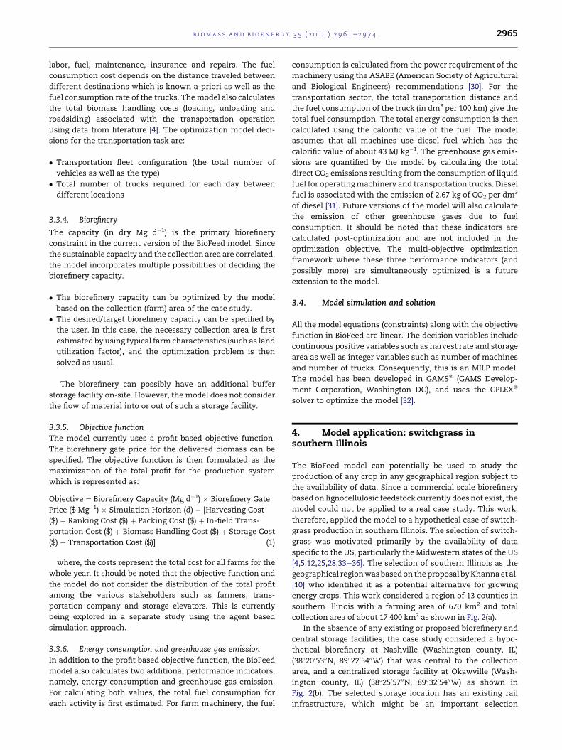
[4,5,12,25,28,33e36]. The selection of southern Illinois as the

geographical regionwasbasedon theproposal byKhannaet al.

[10] who identified it as a potential alternative for growing

energy crops. This work considered a region of 13 counties in

southern Illinois with a farming area of 670 km2 and total

collection area of about 17 400 km2 as shown in Fig. 2(a).

In the absence of any existing or proposed biorefinery and

central storage facilities, the case study considered a hypo-

thetical biorefinery at Nashville (Washington county, IL)

(38�2005300N, 89�2205400W) that was central to the collection

area, and a centralized storage facility at Okawville (Wash-

ington county, IL) (38�2505700N, 89�3205400W) as shown in

Fig. 2(b). The selected storage location has an existing rail

infrastructure, which might be an important selection

Fig. 2 e Biomass farming and collection area for switchgrass in southern Illinois.

b i om a s s an d b i o e n e r g y 3 5 ( 2 0 1 1 ) 2 9 6 1e2 9 7 42966

criterion in future to enable multi-modal transportation. The

farm size distribution was assumed to be similar to the

existing distribution for conventional crops, while the

geographical distribution of the farms was determined using

the county division published by the ISGS. Since the farm

locations were random and uniformly distributed within

a particular county, they did not have any specific geo-coor-

dinates. The transportation distances between the farms,

biorefinery and storage facilities were calculated using the

Google� maps facility (http://maps.google.com/).

The peak harvestable yield of switchgrass was 10 Mg ha�1

[37]. The switchgrass moisture content varied linearly

between 60% at peak yield and 15% which was the minimum

[38,4]. The short term variations in the moisture content due

to weather variability were ignored. The harvesting horizon

consisted of four months from September to December

Table 1 e Cost distribution, energy consumption andgreenhouse gas emission for switchgrass production insouthern Illinois.CollectionareaofWashingtoncounty (Illinois)(1440 km2), single central storage facility, transportation usingtrucks and pre-defined harvesting schedule.

Type Optimizedcost

($ Mg�1

(drybasis))(%)

Energyconsumption(MJ Mg�1 (drybasis))(%)

Greenhouse gas(CO2) emission(kg Mg�1 (drybasis))(%)

Total 45.07 (100) 200 (100) 14.51 (100)

Harvesting 8.64 (19.18) 49.00 (24.49) 3.554 (24.49)

Raking 3.13 (6.96) 22.05 (11.02) 1.6 (11.02)

Packing - total 5.04 (11.18) 79.99 (39.98) 5.80 (39.98)

Packing - fixed 1.17 (2.62) e e

Packing -

operating

3.862 (8.57) e e

Storage 6.07 (13.47) e e

Transportation -

total

9.96 (22.11) 49.034 (24.50) 3.56 (24.50)

Transportation -

fixed

2.80 (6.23) e e

Transportation -

operating

7.15 (15.88) e e

b i om a s s a n d b i o e n e r g y 3 5 ( 2 0 1 1 ) 2 9 6 1e2 9 7 4 2967

(approximated as 120 days), while the non-harvesting horizon

spanned January to August of the following year.

The farm equipment data for most of the equipment were

taken from published literature [4,30,39,40]. Data pertaining to

traditional haying machinery operations were used where

data for switchgrass operations were not available. Themodel

used several sources for data related to switchgrass storage

[12,27,28,34]. The biomass loss during ensiling depends on the

moisture content at the time of ensiling [41,42]. Data reported

in Shinners et al. [41] for corn stoverwas used for this purpose.

The case study considered transportation by class 7e8

trucks, which had a fuel consumption rate of about 37.7 dm3

per 100 km [43]. The fuel consumption while idling for such

trucks during biomass loading and unloading operations was

about 3.78 dm3 per hour [44]. The biomass handling costs

which include loading, unloading and roadsiding were based

on values reported in literature [4]. The truck loading and

unloading time at the farm and biorefinery was constant and

equal to 30 min based on Mukunda et al. [17]. The trans-

portation dry matter loss was 2.5% [4]. Appendix A summa-

rizes the data used for the case study. The next section reports

the important simulation results for the case study.

In-field

transportation

6.55 (14.55) e e

Biomass

handling

5.66 (12.56) e e

5. Results and discussion

5.1. Base case

Themodel was first solved to study switchgrass production in

Washington County, IL. The total collection area for the

county was about 1440 km2. The switchgrass farm area of

670 km2 was distributed among 284 farms. The average farm-

biorefinery distance was 24 km. The average, minimum and

maximum farm sizes were 2.36 km2, 0.2 km2 and 19.70 km2,

respectively. The farmswere classified into four size ranges as

follows: Class-1: fa < 0.728; Class-2: 0.728 � fa < 2.023; Class-3:

2.023 � fa < 4.046; Class-4: 4.046 � fa; where fa is the farm area

in km2. The model assumed that all farms used a mower-

conditioner. For the base case simulation, it was assumed that

the cumulative harvesting schedule was pre-defined and fol-

lowed an approximately normal distribution [40]. Since

smaller farms are less likely to construct on-farm covered

storage facilities, only Class-3 and Class-4 farms in the model

were allowed to have on-farm covered storage. Themodelwas

solved using a 15 day time step for the harvesting horizon and

a 60 day time step for the non-harvesting horizon.

Model simulation and optimization for the base case

showed that the biorefinery gate biomass (delivered) cost was

45.07 $ Mg�1 and the sustainable biorefinery capacity based on

the collection and farming area was 1.402 Gg d�1 (dry basis).

Table 1 shows the distribution of the total cost amongst the

various tasks along with the energy consumption and green-

house gas emissions associated with some of the activities.

Since the model calculated energy consumption for only

a subset of operations, the total energy consumption for feed-

stock production will be higher than the value reported here.

Transportationwas themost expensive operationwhile raking

was the least expensive operation.Moreover, storage costs that

have often been ignored in many analyses constituted about

14% of the total delivered cost. The delivered cost did not

include the establishment and pre-harvest crop management

cost, which is expected to be about 10 $ Mg�1 [10]. Hence, the

final biorefinery gate cost would be about 55 $ Mg�1. The

biomass packing operation was the most energy intensive and

hence led to thehighestCO2emissions.Theoptimal centralized

storage facility area for a height of 15 m was about 1550 m2.

The value of developing an optimization model becomes

evidentwhileanalyzing thepacking, storageand transportation

decisions.Theoptimization results indicated thatClass-1 farms

should store the harvested biomass in silage pits. This was

because the Class-1 farms did not produce large quantities of

biomass.Consequently, purchaseof apackingmachinewasnot

cost-efficient. In the pre-defined harvest schedule, most of the

small farms were harvesting biomass towards the end of the

harvesting horizon when the biomass moisture content was

low. This led to lower biomass loss in ensiling [41].

The throughput capacity and packing density of the square

baler were higher than those for the round baler by 80% and

12.5%, respectively [4,34,45].However, thesquarebalerwasmore

expensive than the round baler, which represented a trade-off

for the farmers. The optimization result recommended that

a square baler be used only on the Class-3 and Class-4 farms,

while a round baler be used on the Class-2 farms since the

advantages offered by the square baler did not compensate the

higher capital and operating costs for the Class-2 farms.

Fig. 3 shows the optimal transportation fleet utilization for

the complete simulation horizon (one year). Although the

total transportation fleet size was 66, the truck utilization

changed significantly during the year and the average truck

utilization was about 86%. During the second half of the har-

vesting horizon, biomass from a number of smaller farmswas

being harvested which led to higher requirement of trans-

portation trucks. During the end of the simulation horizon

Fig. 3 e Transportation fleet schedule for switchgrass production in Washington county (Illinois) during the simulation

horizon: Number of trucks required during each day of the simulation horizon to manage all transportation activities.

b i om a s s an d b i o e n e r g y 3 5 ( 2 0 1 1 ) 2 9 6 1e2 9 7 42968

(day 300 to day 360), biomass from silage pits on the Class-1

farms was removed. Since these farms were geographically

dispersed, the truck requirement went up accordingly.

When biomass distribution at individual farm level was

analyzed, it was observed that the majority of biomass from

Class-3 and Class-4 farms was stored in on-farm covered

storage facilities. Biomass from the Class-2 farms close to the

biorefinery was directly transported to the biorefinery as

much as possible without storage. If a storage option had to be

selected, then the optimal solution recommended that these

farms use either the on-farm open storage or the centralized

storage depending on the relative distance of the biorefinery

and central storage facility from the farm. These results

highlight the ability of the BioFeedmodel to establish the daily

operating plan for each farm that also satisfies the storage,

transportation and biorefinery infrastructure limitations.

5.2. Comparison with other studies

The BioFeed model results were compared with three recent

studies in literature that also quantified the switchgrass

production cost [4,10,12]. The scope of the BioFeed model was

similar to the combination of scenarios C1/C2 and T1 (without

grinding) fromKumar and Sokhansanj [4], where the delivered

cost was estimated to be about 35 $Mg�1 (dry basis) (excluding

biomass grinding). The major cost differences as compared to

BioFeed were for harvesting and storage. While Kumar and

Sokhansanj [4] ignored the storage costs, they also considered

a self-propelled forage harvester which had a higher

throughput capacity than the mower-conditioner considered

here, thereby reducing the cost. Khanna et al. [10] reported the

switchgrass delivered cost of 64.84 $ Mg�1 which was similar

to the BioFeed cost estimate. However, the baling cost esti-

mated in that study was higher than BioFeed model while the

harvesting estimate was lower. The study by Duffy [12] esti-

mated the delivered cost to be 124.3 $ Mg�1. However, the

major difference in the estimates was due to a much higher

establishment cost as compared to the BioFeed model

assumption. When the components common to the BioFeed

model were extracted from that study (harvesting, baling,

storage and transportation), the delivered cost for that study

was about 59 $ Mg�1. However, the storage cost estimates

were quite high in that study, primarily because it considered

on-farm covered storage as the only available option. Since

the scope of the analyses and the assumptions differed for

each study, it was not possible to make a very accurate

comparison. However, the comparison illustrated that the

overall BioFeed model predictions agree reasonably well with

other studies with similar scope, with the additional capa-

bility of providing the management and operational schedule.

5.3. Impact of distributed farming and collection

The model was used to determine the impact of larger collec-

tion area and more distributed farming on the total cost, cost

distribution and infrastructure requirements. To conduct this

analysis, the same farm area with 284 farms considered in the

base case was distributed over multiple counties, i.e., the land

utilization factor which represents the fraction of the total land

converted to energy crops progressively decreased. Starting

with the base case of a single county, the model solved seven

different cases where the collection area consisted of 3, 5, 7, 9,

11 and 13 counties. Fig. A-1 in Appendix A shows these cases. It

must be noted that since the counties were not systematically

structured around the central biorefinery location, the collec-

tion area increased non-linearly. The average farm-biorefinery

transportation distance increased fromabout 24 km for a single

county to about 70 km for thirteen counties.

Fig. 4 shows that the total cost increased by about 10% as

a result of the increased collection area. The transportation

operating cost constituted the major component of the cost

increase, while the transportation fleet size also increased

from 66 to 81. The overall storage configuration such as the

central storage facility area did not change significantly. The

sustainable biorefinery capacity also decreased with the

increasing collection distance due to higher transportation

losses. The base case results illustrated that small and inter-

mediate sized farms can be profitable when using round

balers. This could be used as a driver to encourage smaller

farmers closer to the biorefinery to grow switchgrass. If the

collection area could thus be reduced, the switchgrass

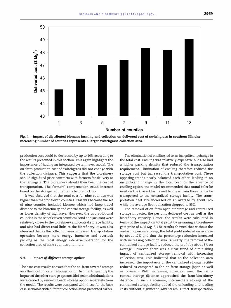
Fig. 4 e Impact of distributed biomass farming and collection on delivered cost of switchgrass in southern Illinois:

Increasing number of counties represents a larger switchgrass collection area.

b i om a s s a n d b i o e n e r g y 3 5 ( 2 0 1 1 ) 2 9 6 1e2 9 7 4 2969

production cost could be decreased by up to 10% according to

the results presented in this section. This again highlights the

importance of having an integrated system level model. The

on-farm production cost of switchgrass did not change with

the collection distance. This suggests that the biorefinery

should sign fixed price contracts with farmers for delivery at

the farm-gate. The biorefinery should then bear the cost of

transportation. The farmers’ compensation could increase

based on the storage requirements before pick up.

It was observed that the total cost for nine counties was

higher than that for eleven counties. This was because the set

of nine counties included Monroe which had large travel

distance to the biorefinery and central storage facility, as well

as lower density of highways. However, the two additional

counties in the set of eleven counties (Bond and Jackson) were

relatively closer to the biorefinery and central storage facility,

and also had direct road links to the biorefinery. It was also

observed that as the collection area increased, transportation

operation became more energy intensive and overtook

packing as the most energy intensive operation for the

collection area of nine counties and more.

5.4. Impact of different storage options

The base case results showed that the on-farm covered storage

was themost important storage option. In order to quantify the

impact of the other storage options, BioFeedmodel simulations

were carried by removing each storage option separately from

the model. The results were compared with those for the base

case scenarios with different collection areas presented earlier.

The elimination of ensiling led to an insignificant change in

the total cost. Ensiling was relatively expensive but also had

a higher packing density that reduced the transportation

requirement. Elimination of ensiling therefore reduced the

storage cost but increased the transportation cost. These

opposing trends nearly balanced each other, leading to an

insignificant change in the total cost. In the absence of

ensiling option, the model recommended that round baler be

used on the Class-1 farms and biomass from those farms be

transported to the centralized storage facility. The trans-

portation fleet size increased on an average by about 32%

while the average fleet utilization dropped to 55%.

The removal of on-farm open air storage and centralized

storage impacted the per unit delivered cost as well as the

biorefinery capacity. Hence, the results were calculated in

terms of the impact on total profit by assuming a biorefinery

gate price of 60 $ Mg�1. The results showed that without the

on-farm open air storage, the total profit reduced on average

by about 17% and that the percentage reduction increased

with increasing collection area. Similarly, the removal of the

centralized storage facility reduced the profit by about 5% on

average. However, there was a clear trend of diminishing

impact of centralized storage removal with increasing

collection area. This indicated that as the collection area

increased, the importance of the centralized storage facility

reduced as compared to the on-farm storage (open as well

as covered). With increasing collection area, the farm-

central storage distance approached the farm-biorefinery

distance. In such a scenario, intermediate storage at the

centralized storage facility added the unloading and loading

costs without significant advantages. Direct transportation

Fig. 6 e Impact of varying farm size distribution on

delivered cost of switchgrass production and sustainable

biorefinery capacity in southern Illinois: Collection area of

13 counties in Illinois (17 000 km2).

b i om a s s an d b i o e n e r g y 3 5 ( 2 0 1 1 ) 2 9 6 1e2 9 7 42970

of biomass from farms to the biorefinery therefore became

more profitable.

The base case limited on-farmcovered storageonly to Class-

3 and Class-4 farms. However, it is important to knowwhether

building such facilities on smaller farms leads to significant

changes in the system configuration to decide whether appro-

priate incentives should be put in place to encourage such

practice. To study this, BioFeedmodel simulationswere carried

out for different cases with varying collection area as before

(from Section 5.3), the only difference being that Class-2 farms

could also have an on-farm covered storage facility. The results

showed that the total delivered cost reduced on an average by

about 6.7% and the major contribution in terms of cost reduc-

tion came from transportation and biomass handling. It must,

however, be realized that the BioFeed optimization model

determines what the farmer should do and not what a farmer

would do. In practice, if the cost of installing a storage facility is

excessive, then a farmer will not build it even if it optimizes the

system level costs. This result can, therefore, be used as an

argument to develop policy based incentives such as higher

farm-gate price during the non-harvesting horizon to

encourage on-farm covered storage facilities.

5.5. Impact of farm-size distribution

The base case results showed that farm size had implications

on the farm management decisions and costs. In order to

systematically quantify these impacts, BioFeed model simula-

tions were carried out for different farm-size distributions.

Here, the fraction of farms in Class-1 and Class-2 was

decreased, while the fraction of farms in Class-3 and Class-4

was increased. Since the farms in Class-3 and Class-4 were

significantly larger than those inClass-1, ameaningful increase

in Class-3 and Class-4 farm area required a substantial reduc-

tion in the number of Class-1 farms. Hence, all farms in Class-1

were removedfromthenewdistributions. Fig. 5 showsthebasic

distribution as well as the two new distributions. This meant

that the minimum farm size for the two new cases was

0.728km2. The total farmareadidnot changewith the changing

distributions. Consequently, the total number of farms in the

analysis reduced from 284 to 169 and 149 for the second and

0

0.1

0.2

0.3

0.4

0.5

Basic Distribution-2 Distribution-3

Frac

tion

Class-1 Class-2 Class-3 Class-4

Fig. 5 e The distribution of switchgrass farms within

various size ranges for the same cumulative farm area: The

proportion of larger farms in Class-3 and Class-4 increases

while that of smaller farms in Class-1 and Class-2

decreases for distributions 2 and 3, respectively.

Distribution 2 and 3 do not include any farm from Class-1.

third distribution, respectively. The results, presented in Fig. 6,

showed a significant positive impact on the delivered cost and

the sustainable biorefinery capacity for the collection area of

thirteen counties. This was due to better return on investment

for farm equipment and better utilization of the transportation

fleet leading to a reduction in the required fleet size. The fleet

size requirement reduced from 81 to 58 and 49 for the two

distributions, respectively. Given these strong benefits, co-

operative farming where the farming equipment is shared or

leased instead of being owned should be encouraged.

5.6. Impact of optimized harvesting schedule

The results presented in the preceding sections considered

a fixed harvesting schedule with a pseudo-normal overall

distribution. To quantify the importance of optimizing the

harvesting schedule, the BioFeed model was solved by

declaring the harvest rate for each farm as a variable. When

the problemwas solved for a collection area of a single county,

the results showed that the optimization of the harvesting

schedule led to about 9% reduction in the delivered cost and

about 30% increase in the total profit (due to higher capacity).

Fig. 7 compares the optimal cumulative harvesting schedule

Fig. 7 e Comparison of the fixed switchgrass harvesting

schedule with the optimized harvesting schedule

determined by the BioFeed model: Collection area of

Washington County (Illinois) (1440 km2).

Fig. 8 e Sensitivity analysis: Impact of improvement in

production technology or management on switchgrass

production profit: Production in 13 counties of southern

Illinois (17 000 km2).

b i om a s s a n d b i o e n e r g y 3 5 ( 2 0 1 1 ) 2 9 6 1e2 9 7 4 2971

with the fixed schedule considered before. The optimized

schedule leads to significant harvesting of biomass in the

initial half of the harvesting season, which caused a reduction

in storage space requirement. It must though be noted that

the consideration of biomass quality related constraints that

are presently ignored will affect the schedule.

5.7. Sensitivity analysis

Sensitivity analysis was conducted to determine the impact of

improvement in technology or management practices on the

complete production system. Fig. 8 shows the various

parameters pertaining to different technologies or manage-

ment practices that were improved by 25%. A plus (þ) sign

indicates a 25% increase in the value while a minus (�) sign

indicates 25% decrease, both representing improvement in the

respective technologies. Each case was optimized for the new

value of the specific parameter and the figure plots the

increase in the overall profit for each case. It was observed that

25% reduction in truck idling time (waiting time for loading

and unloading) led to about 22% increase in profit. Similarly,

improving the density or throughput of the balers increased

the profit bymore than 10%. Itmust be noted that this analysis

assumed that the technological improvements were achieved

at the samecapital andoperating costs.However, if actual data

for new technologies are available, it is possible to use the

BioFeed model to quantify its systemic impact.

6. Conclusions

This work presented an optimization model named BioFeed

that has been developed to model and optimize the bioenergy

feedstock production system. The unique feature of the model

is the integration of the design as well asmanagement decision

making using an optimization platform. The MILP model was

applied to a case study of switchgrass production in southern

Illinois. The results illustrated that the total cost of switchgrass

production was between 45 and 49 $ Mg�1 depending on the

collection area. The sustainable biorefinery capacity for

a farming area of 670 km2 and peak harvestable yield of

10 Mg ha�1 was about 1.4 Gg d�1. Larger farms were recom-

mended square baling of switchgrass while smaller farms were

recommended either ensiling or round baling. The trans-

portation fleet size varied between 66 and 81 and the average

utilization of the fleet was about 86%. On-farm covered storage

of biomass was extremely beneficial for the system. Removal of

on-farm open storage and centralized storage reduced the

systemprofit by about 17% and 5%, respectively. Increase in the

fraction of larger farms within the system led to lower cost and

higher capacity, suggesting that co-operative farming was

beneficial. The optimization of the harvesting schedule led to

about 9% reduction in the delivered cost and about 30% increase

in the total profit. This emphasized the value of the optimiza-

tion model in determining the optimal farm management

schedules. Sensitivity analysis showed that 25% reduction in

truck idling time (waiting time for loading and unloading) led to

about 22% increase in profit. Similarly, improving the density or

throughput of the balers increased the profit bymore than 10%.

The model has been recently extended to incorporate addi-

tional biomass packing options and evaluate other energy crops

[20]. TheBioFeedmodelwill be further expanded in the future to

incorporate biomass quality preservation and degradation

modeling, pre-harvest crop-establishment modeling as well as

life cycle impact assessment modeling, and will be applied to

study the production of novel energy crops.

Acknowledgment

This work has been funded by the Energy Biosciences Institute

through the program titled ‘Engineering solutions for biomass

feedstock production’.

Appendix A. Case study input data

Fig. A-1. Switchgrass collection area in Illinois for different

cases for modeling distributed biomass collection: Number

indicates the number of counties considered in the analysis.

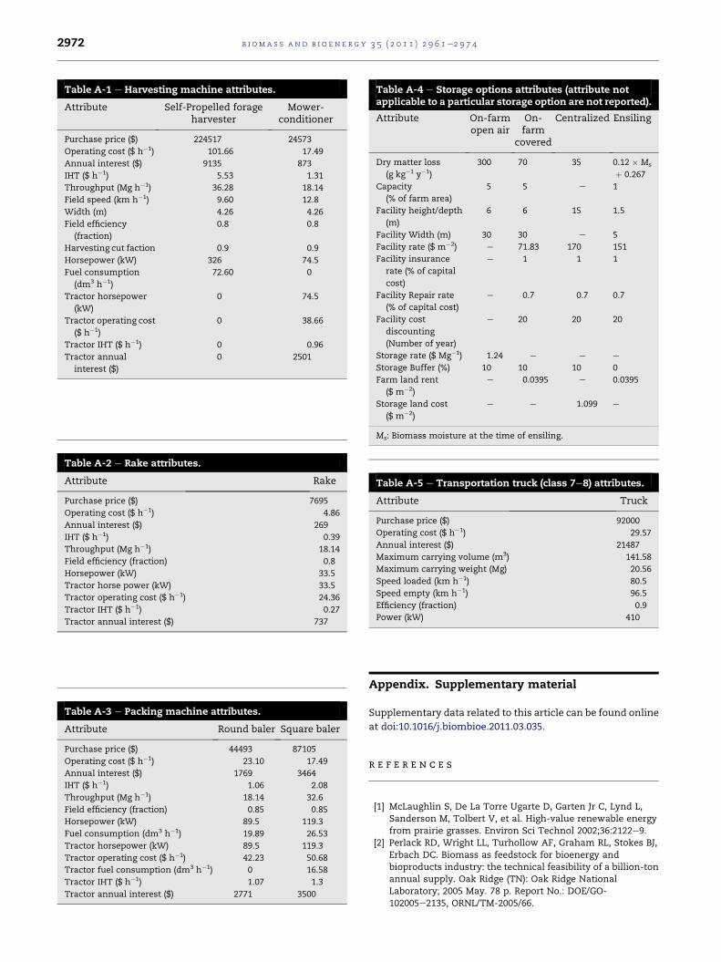
Table A-1 e Harvesting machine attributes.

Attribute Self-Propelled forageharvester

Mower-conditioner

Purchase price ($) 224517 24573

Operating cost ($ h�1) 101.66 17.49

Annual interest ($) 9135 873

IHT ($ h�1) 5.53 1.31

Throughput (Mg h�1) 36.28 18.14

Field speed (km h�1) 9.60 12.8

Width (m) 4.26 4.26

Field efficiency

(fraction)

0.8 0.8

Harvesting cut faction 0.9 0.9

Horsepower (kW) 326 74.5

Fuel consumption

(dm3 h�1)

72.60 0

Tractor horsepower

(kW)

0 74.5

Tractor operating cost

($ h�1)

0 38.66

Tractor IHT ($ h�1) 0 0.96

Tractor annual

interest ($)

0 2501

Table A-4 e Storage options attributes (attribute notapplicable to a particular storage option are not reported).

Attribute On-farmopen air

On-farm

covered

Centralized Ensiling

Dry matter loss

(g kg�1 y�1)

300 70 35 0.12 � Ms

þ 0.267

Capacity

(% of farm area)

5 5 e 1

Facility height/depth

(m)

6 6 15 1.5

Facility Width (m) 30 30 e 5

Facility rate ($ m�2) e 71.83 170 151

Facility insurance

rate (% of capital

cost)

e 1 1 1

Facility Repair rate

(% of capital cost)

e 0.7 0.7 0.7

Facility cost

discounting

(Number of year)

e 20 20 20

Storage rate ($ Mg�1) 1.24 e e e

Storage Buffer (%) 10 10 10 0

Farm land rent

($ m�2)

e 0.0395 e 0.0395

Storage land cost

($ m�2)

e e 1.099 e

b i om a s s an d b i o e n e r g y 3 5 ( 2 0 1 1 ) 2 9 6 1e2 9 7 42972

Table A-2 e Rake attributes.

Attribute Rake

Purchase price ($) 7695

Operating cost ($ h�1) 4.86

Annual interest ($) 269

IHT ($ h�1) 0.39

Throughput (Mg h�1) 18.14

Field efficiency (fraction) 0.8

Horsepower (kW) 33.5

Tractor horse power (kW) 33.5

Tractor operating cost ($ h�1) 24.36

Tractor IHT ($ h�1) 0.27

Tractor annual interest ($) 737

Table A-3 e Packing machine attributes.

Attribute Round baler Square baler

Purchase price ($) 44493 87105

Operating cost ($ h�1) 23.10 17.49

Annual interest ($) 1769 3464

IHT ($ h�1) 1.06 2.08

Throughput (Mg h�1) 18.14 32.6

Field efficiency (fraction) 0.85 0.85

Horsepower (kW) 89.5 119.3

Fuel consumption (dm3 h�1) 19.89 26.53

Tractor horsepower (kW) 89.5 119.3

Tractor operating cost ($ h�1) 42.23 50.68

Tractor fuel consumption (dm3 h�1) 0 16.58

Tractor IHT ($ h�1) 1.07 1.3

Tractor annual interest ($) 2771 3500

Ms: Biomass moisture at the time of ensiling.

Table A-5 e Transportation truck (class 7e8) attributes.

Attribute Truck

Purchase price ($) 92000

Operating cost ($ h�1) 29.57

Annual interest ($) 21487

Maximum carrying volume (m3) 141.58

Maximum carrying weight (Mg) 20.56

Speed loaded (km h�1) 80.5

Speed empty (km h�1) 96.5

Efficiency (fraction) 0.9

Power (kW) 410

Appendix. Supplementary material

Supplementary data related to this article can be found online

at doi:10.1016/j.biombioe.2011.03.035.

r e f e r e n c e s

[1] McLaughlin S, De La Torre Ugarte D, Garten Jr C, Lynd L,Sanderson M, Tolbert V, et al. High-value renewable energyfrom prairie grasses. Environ Sci Technol 2002;36:2122e9.

[2] Perlack RD, Wright LL, Turhollow AF, Graham RL, Stokes BJ,Erbach DC. Biomass as feedstock for bioenergy andbioproducts industry: the technical feasibility of a billion-tonannual supply. Oak Ridge (TN): Oak Ridge NationalLaboratory; 2005 May. 78 p. Report No.: DOE/GO-102005e2135, ORNL/TM-2005/66.

b i om a s s a n d b i o e n e r g y 3 5 ( 2 0 1 1 ) 2 9 6 1e2 9 7 4 2973

[3] Kumar A, Sokhansanj S, Flynn PC. Development ofa multicriteria assessment model for ranking biomassfeedstock collection and transportation systems. ApplBiochem Biotechnol 2006;129e132:71e87.

[4] Kumar A, Sokhansanj S. Switchgrass (Panicum vigratum, L.)delivery to a biorefinery using integrated biomass supplyanalysis and logistics (IBSAL) model. Bioresour Technol 2007;98(5):1033e44.

[5] Epplin F. Cost to produce and deliver switchgrass biomass toan ethanol-conversion facility in the southern plains of theUnited States. Biomass Bioenergy 1996;11(6):459e67.

[6] Huisman W, Venturi G, Molenaar J. Cost of supply chain forMiscanthus x Giganteus. Ind Crops Prod 1997;6:353e66.

[7] Venturi P, Huisman W, Molenaar J. Mechanization and costsof primary production chains for Miscanthus x Giganteus inThe Netherlands. J Agric Eng Res 1998;69:209e15.

[8] Venturi P, Gigler J, Huisman W. Economic and technicalcomparison between herbaceous (Miscanthus x Giganteus)and woody energy crops (Salix viminalis). Renew Energ 1999;16:1023e6.

[9] Styles D, Thorne F, Jones MB. Energy crops in Ireland: aneconomic comparison of willow and Miscanthus productionwith conventional farming systems. Biomass Bioenergy 2008;32(5):407e21.

[10] Khanna M, Dhungana B, Clifton-Brown J. Costs of producingMiscanthus and switchgrass for bioenergy in Illinois.Biomass Bioenergy 2008;32(6):482e93.

[11] Monti A, Fazio S, Lychnaras V, Soldatos P, Venturi G. A fulleconomic analysis of switchgrass under different scenariosin Italy estimated by BEE model. Biomass Bioenergy 2007;31(4):177e85.

[12] Duffy M. Estimated costs for production, storage andtransportation of switchgrass. Ames (IA): Iowa StateUniversity, University Extension; 2007 October. 8 p. ReportNo.: PM 2042.

[13] De Mol R, Jogems M, Van Beek P, Gigler J. Simulation andoptimization of the logistics of biomass fuel collection. Neth JAgric Sci 1997;45:219e28.

[14] Cundiff J, Dias N, Sherali HD. A linear programmingapproach for designing a herbaceous biomass deliverysystem. Bioresour Technol 1997;59:47e55.

[15] Zuo M, Kuo W, McRoberts KL. Application of mathematicalprogramming to a large-scale agricultural production anddistribution system. J Oper Res Soc 1991;42(8):639e48.

[16] Mapemba LD, Epplin FM, Huhnke RL, Taliaferro CM.Herbaceous plant biomass harvest and delivery cost withharvest segmented by month and number of harvestmachines endogenously determined. Biomass Bioenergy2008;32(11):1016e27.

[17] Mukunda A, Ileleji KE, Wan H. Simulation of corn stoverlogistics from on-farm storage to an ethanol plant. In:ASABE Annual International Meeting, Paper Number066177; 2006 July 9e12; Portland, OR. St. Joseph, MI:ASABE; 2006.

[18] Ravula P, Grisso R, Cundiff J. Comparison between two policystrategies for scheduling trucks in a biomass logistic system.Bioresour Technol 2008;99:5710e21.

[19] Domdouzis K, Rodriguez LF, Shastri Y, Hu MC, Hansen AC,Ting KC. Systems informatics for biomass feedstockproduction engineering. In: ASABE Annual InternationalMeeting, Paper Number 096702; 2009 June 21e24; Reno, NV.St. Joseph, MI: ASABE; 2009.

[20] Shastri Y, Hansen A, Rodriguez L, Ting KC. Optimization ofMiscanthus harvesting and handling as an energy crop:BioFeed model application. Biol Eng 2011;3(1):37e69.

[21] De La Torre Ugarte DG, Ray D. Biomass and bioenergyapplications of the POLYSYS modeling framework. BiomassBioenergy 2000;18(4):291e308.

[22] Vilsack T, Clark CZF. 2007 Census of agriculture: UnitedStates summary and state data. Washington (DC): UnitedStates Department of Agriculture, National AgriculturalStatistics Service; 2009 December. 739 p. Report No.: AC-07-A-51.

[23] Key N, Roberts MJ. Measures of trends in farm size telldiffering stories. Amber Waves 2007;5(5):36e7.

[24] Illinoi State Geological Survey [internet]. 7.5-minutequadrangles in Illinois, 2010. [updated 2010 November 19;cited 2011 March 7]. Available from: http://www.isgs.illinois.edu/maps-data-pub/quads/all-quads.shtml.

[25] Kiniry J, Cassida K, Hussey M, Muir J, Ocumpaugh W, Read J,et al. Switchgrass simulation by the ALMANAC model atdiverse sites in the southern US. Biomass Bioenergy 2005;29(6):419e25.

[26] Clifton-Brown J, Stampfel PF, Jones M. Miscanthus biomassproduction for energy in Europe and its potentialcontribution to decreasing fossil fuel carbon emissions. GlobChange Biol 2004;10:509e18.

[27] Turhollow A, Wilkerson E, Sokhansanj S. Cost methodologyfor biomass feedstocks: herbaceous crops and agriculturalresidues. Oak Ridge (TN): Oak Ridge National Laboratory;2009 December. 42 p. Report No.: ORNL/TM-2008/105.

[28] Sanderson M, Egg R, Wiselogel A. Biomass losses duringharvest and storage of switchgrass. Biomass Bioenergy 1997;12(2):107e14.

[29] Hess JR, Wright CT, Kenney KL. Cellulosic biomassfeedstocks and logistics for ethanol production. BiofuelBioprod Bioref 2007;1(3):181e90.

[30] ASABE. Agricultural machinery management. St. Joseph (MI):American Society of Agricultural and Biological Engineers;2006 February. 7 p. Report No.: ASAE EP496.3 FEB2006.

[31] USEPA. Emission facts: average carbon dioxide emissionsresulting from gasoline and diesel fuel. Washington (DC):Office of Transportation and Air Quality, United StatedEnvironmental Protection Agency; 2005 February. 3 p. ReportNo.: EPA420-F-05-001.

[32] Rosenthal RE. GAMS - A user’s guide. Washington (DC):GAMS Development Corporation; 2010. 273 p.

[33] Aiken G, Springer T. Seed size distribution, germination, andemergence of switchgrass cultivars. J Range Manage 1995;48(5):455e8.

[34] Cundiff J, Marsh L. Harvest and storage costs for bales ofswitchgrass in the southeastern United States. BioresourTechnol 1996;56(1):95e101.

[35] McLaughlin SB, Kszos LA. Development of switchgrass(panicum virgatum) as a bioenergy feedstock in the UnitedStates. Biomass Bioenergy 2005;28(6):515e35.

[36] McLaughlin S, Kiniry J, Taliaferro C, De La Torre Ugarte D.Projecting yield and utilization potential of switchgrass asenergy crop. Adv Agron 2006;90:267e96.

[37] Heaton E, Voigt T, Long S. A quantitative review ofcomparing the yields of two candidate C4 biomass crops.Biomass Bioenergy 2004;27(1):21e30.

[38] Yu M, Womac A, Igathinathane C, Ayers P, Buschermohle M.Switchgrass ultimate stresses at typical biomass conditionsavailable for processing. Biomass Bioenergy 2006;30(3):214e9.

[39] ASABE. Agricultural machinery management data. St. Joseph(MI): American Society of Agricultural and BiologicalEngineers; 2006 June. 8 p. Report No.: ASAE D497.6 JUN2009.

[40] Sokhansanj S, Turhollow A, Wilkerson E. Development of theintegrated biomass supply analysis and logistics model(IBSAL). Oak Ridge (TN): Oak Ridge National Laboratory; 2008March. 63 p. Report No.: ORNL/TM-2006/57.

[41] Shinners KJ, Binversie BN, Muck RE, Weimer PJ. Comparisonof wet and dry corn stover harvest and storage. BiomassBioenergy 2007;31(4):211e21.

b i om a s s an d b i o e n e r g y 3 5 ( 2 0 1 1 ) 2 9 6 1e2 9 7 42974

[42] Mani S, Patterson J, Bi X. Modeling of thewet storage of biomass.In: ASABE Annual International Meeting, Paper Number: 061014;2006 July 9e12; Portland, OR. St. Joseph, MI: ASABE; 2006.

[43] Engineering T. Vehicle technologies heavy vehicle program:FY 2008 benefits analysis, methodology and results - Finalreport. Argonne (IL): Argonne National Laboratory; 2007December. 76 p. Report No.: ANL-08/07.

[44] Stodolsky F, Gaines L, Vyas A. Analysis of technology optionsto reduce the fuel consumption of idling trucks. Argonne (IL):Center for Transportation Research, Argonne NationalLaboratory; 2000 June. 40 p. Report No.: ANL/ESD-43.

[45] Schmer M, Vogel K, Mitchell R, Perrin R. Net energy ofcellulosic ethanol from switchgrass. Proc Natl Acad Sci U S A2008;105(2):464e9.