Developing an Erosion Risk Map Using Soft Computing Methods (Case Study at Sifnos Island

Natural Hazards 31: 63–83, 2004.© 2004 Kluwer Academic Publishers. Printed in the Netherlands.

63

Developing an Erosion Risk Map Using SoftComputing Methods (Case Study at Sifnos Island)

TH. GOURNELLOS, N. EVELPIDOU� and A. VASSILOPOULOSUniversity of Athens, Geology Department, Geography and Climatology Sector PanepistimiopolisZografou 15784, Athens, Greece

(Received: 4 January 2000; accepted 11 September 2002)

Abstract. The erosional processes depend on various variables such as lithology, topography, drain-age system, rock structure and climatic conditions. The quantitative evaluation of some of the abovegeological and geomorphological parameters is of primary importance for the purpose of developingerosion risk maps. These maps can become useful tools for developing appropriate strategies onenvironmental protection, hazard assessment and regional planning.

The island of Sifnos, in Cyclades, was chosen as a case study, where in the final map of thesub-basins of this island, erosion risk distribution is presented.

Key words: erosion, G.I.S., fuzzy, cyclades, soft computing

1. Introduction

Erosion, the result of surface water flow, is a very complicated process. Prior tothe erosional stage, a physical or chemical rock alteration takes place. Products ofthis process are the soil and the weathered mantle. Since the beginning of erosionstudies, five variables have been recognized as of major importance for weathering:climate, biological activity, topography, parent material and time (Jenny, 1941).

The erosion process carries away the soil and weathered material. There aremany factors that control erosion. The first factor is the rainfall, the main erodingagent. Rainfall’s erosivity depends on its duration, spatial distribution and intensity.The second factor is the morphology as it is expressed by the slope forms and theinclination. The third factor is the rock’s and surface’s deposit’s properties. Theabove factors define the region’s flow regime, the Hortonian or not runoff, andfinally the critical time and the amount of erosion. The flow characteristics arecontrolled by microtopographic features, and produce either rills or sheet erosion(Emmett, 1978). The role of splash erosion, by raindrop impact, seems to be moreimportant for the detachment. The rate of the soil erosion can be calculated by thedistance of the divide, or the surface water flow discharge, multiplied by a powerof slope gradient (Kirkby, 1978). In order to calculate a region’s erosion risk, onemust study its geological, geomorphological and hydrological variables.

� Author for correspondence. E-mail: [email protected]

64 TH. GOURNELLOS ET AL.

Erosion risk maps are land resource evaluations, as they classify basins ofsimilar erosion risk degree. Various papers involve methods of evaluating erosionrisk, based on many parameters, such as morphometric variables (Morgan, 1974;Jozefaciuk and Jozefaciuk, 1993), sediment yield information (Diaconu, 1969;Rooseboom and Annandale, 1981) and rainfall erosion indexes (Fournier, 1960;Hundson, 1981; Stocking and Elwell, 1976; Wischmeier and Smith, 1978).

Simple erosion risk scoring systems were previously proposed by Stocking andElwell, 1973 and later by the European Union CORINE program (Briggs andGiordano, 1992), using morphometric variables and rainfall indexes but Morgan(1996) has criticized the results. Finally, different kinds of soil erosion rate modelshave been proposed (Wischmeier and Smith, 1978; Elwell, 1978; Morgan et al.,1984; Knisel, 1980; Nearing et al., 1989; Morgan et al., 1997; Morgan et al., 1994).Various soil erosion models have been developed (Giordano, 1986; Kirkby, 1995;Thornes et al., 1996; Baturst et al., 1996). All this activity indicates an expandinginterest on the study of erosion and related processes to environmental changes, inthe European Mediterranean (De Ploey, 1989; Poesen and Hooke, 1997).

2. Methodology

The development of erosion risk maps involves a series of different stages, as fieldwork, air-photo stereo-observation, digitization of geological, topographical anddrainage system maps, definition of the input and output variables, establishment oflogical rules between the input and the output variables, analysis and visualizationof the results. At some of the above stages, GIS technology and fuzzy sets theorywere used (Figure 1).

Similar erosional or related to natural hazards problems, have been examined,by the use of different approaches (Brundsen et al., 1975; Carrara et al., 1977;Malgot and Mahr, 1979; Ives and Messerli, 1981; Carrara, 1983; Carrara et al.,1991; Marinos et al., 1997) and the recently used uncertainty factors and fuzzysets (Binagli et al., 1998) or probability networks (Stassopoulou et al., 1998).

The principal variables used in this paper were:– erodibility of the rocks,– slope gradient of the morphology,– drainage density.

The erodibility variable is very complicated as it depends on the physical andchemical composition of the rock and the existence of major (folds, faults) andminor (bedding, foliation and joints) tectonical structures. The mineral compos-ition is critical as it has been proved that Olivine, Augite, Hornblende, Biotiteand in general, dark-colored minerals are more susceptible to weathering thanOrthoclase, Muscovite, Quartz, and other light-colored minerals (Sparks, 1965).Generally, the erodibility of the rock depends on the lithology, the process involvedand the protective mechanisms. Lithology is connected to the hardness of the rocksand the resistance to erosion. This variable is difficult to be directly measured.

DEVELOPING AN EROSION RISK MAP USING SOFT COMPUTING METHODS 65

Fig

ure

1.F

low

diag

ram

for

the

prod

ucti

onof

the

eros

ion

risk

map

.


Some observations on the resistance of rocks to abrasion have resulted in a rocklist with decreasing resistance to erosion (Kuenen, 1956). On the other hand, Selby(1987) has proposed a rock mass strength classification and rating, to express theresistance to erosion. In the above classification limestones are more resistant toerosion than schists. The first attempt to assign erodibility values on different rocktypes was made by Jensen and Painter, (1974). Erodibility is a function involvingrock’s hardness, permeability and infiltration capacity. Marbles and blueschistsare considered to be more resistant to erosion, while alluvials, soil and weatheredmantle more prone to erosion.

The grain’s form and size defines rock’s permeability. This variable controlsthe quantity of the runoff water, which is the dominant erosion factor. Three cat-egories of permeability values can be distinguished: very low (10−12 − 10−8 m/s),low to medium (10−8 − 10−5 m/s) and high (10−5 − 10−2 m/s) (Bolton, 1979).Metamorphic schists are considered to have a very low permeability while marblesand surface rocks are quite permeable formations. The amount of runoff and un-derground water depends on surface deposit’s infiltration properties. In general,deposits with coarse grain present high infiltration rates. The infiltration capacityof the surface deposit (Horton, 1945; Kirkby, 1969) strongly influences erosion.Concerning the above, one may say that erodibility is the factor of rock’s resistanceto erosion (hardness of the rock), permeability and infiltration capacity. Finally theexistence of vegetation acts as a protective mechanism to erosional processes.

The second variable that has been processed is the morphological slope gradientof each drainage basin. Apart from the slope gradient, form (convex, concaves),aspect and extent are also important factors. It is obvious that slope steepness is crit-ical to the erosional intensity. Schumm (1977) proved that there is an exponentialrelation between average slope and sediment-yield.

Finally the last input variable was drainage density (ratio of the total streamlengths to the drainage basin’s area) which is highly related to water’s runoff quant-ity and substratum’s permeability. In general, drainage density is high at basins ofweak impermeable rocks and low in basins of resistant and permeable rocks. It wasfound that drainage density increases according to basin’s average slope (Gregoryand Wallig, 1973). Furthermore, drainage density of rills is highly related to slopegradient (Schumm, 1977).

The development of the drainage system reflects the interrelations betweendifferent geological and hydrological variables. Drainage basin is the smallestautonomous hydrogeological unit. All the above-discussed variables have beencalculated for each Sifnos sub-basin. This means that there is one ordered valuetriad corresponding to each sub-basin. Using these variables, thematic maps tovisualise them were produced.

The next step was to formulate proper logical rules in order to produce the finalerosion risk values and map. Logical rules, mainly based on empirical knowledge,were applied on all input variables to deduce degrees of erosion risk.


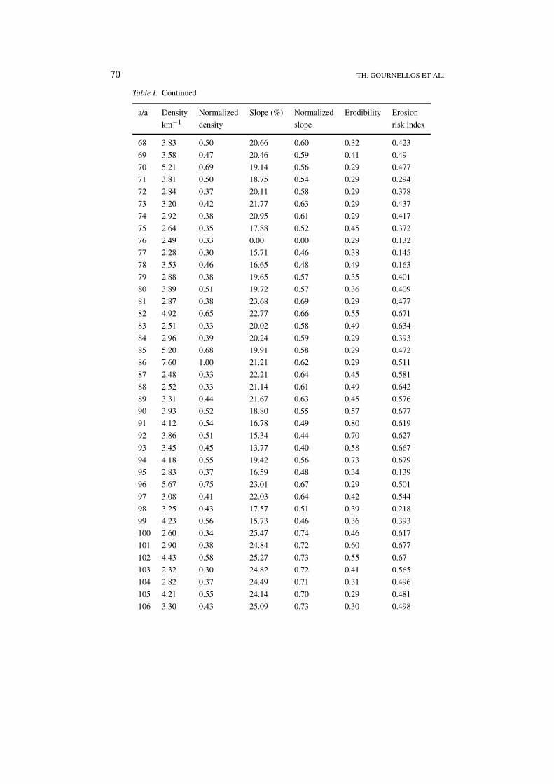
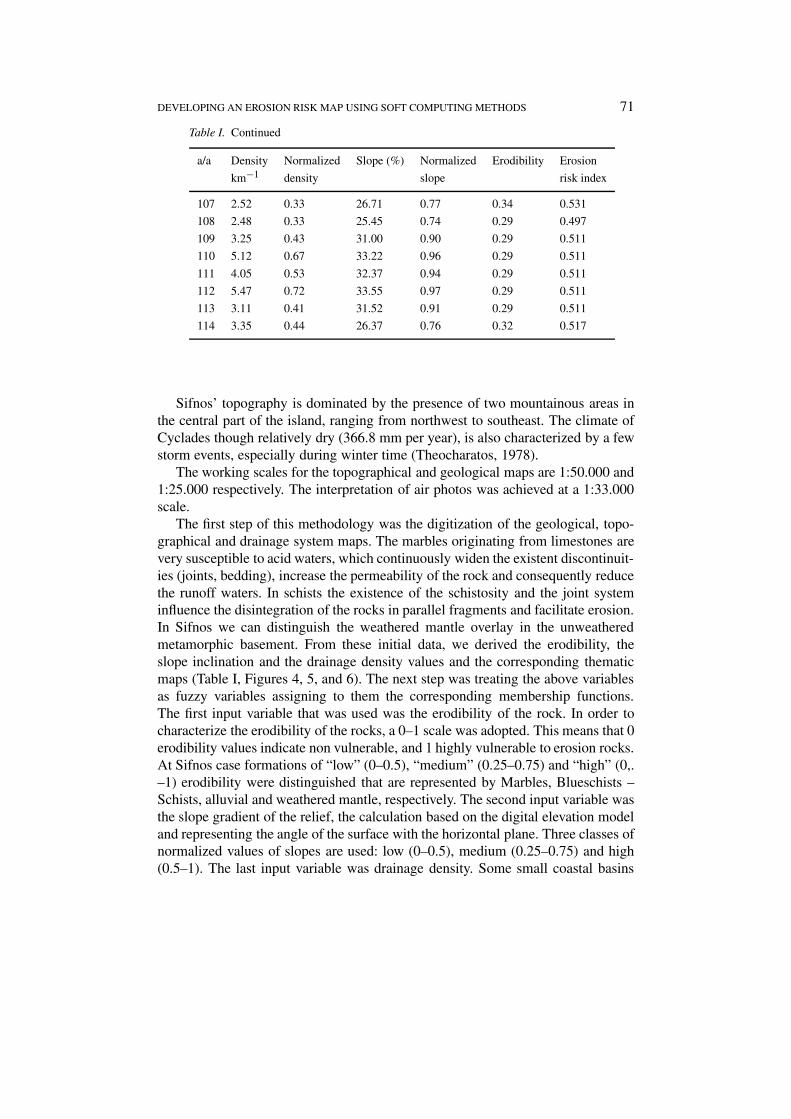
In such problems, two kinds of inexact knowledge are present: the boundaryvagueness and the relative spatial imprecision of most input variables. For thisreason the fuzzy set theory was applied (Zadeh, 1965; Zadeh, 1987; Yager et al.,1987; Dubois and Prade, 1980; Zimmermann, 1991; Klir and Yuan, 1995). Bur-rough (1989) and Burrough et al. (1992) have proposed a fuzzy methodology forland evaluation of soil profile observations. In our case, triangular functions havebeen adopted. All the above variables were characterized by fuzzy set values, andexpressed by a corresponding membership function. In the present study, “low”,“medium” and “high” define the different degrees of rock’s erodibility. The erodib-ility value of each formation was based on empirical and theoretical data (Kuenen,1956; Leopold et al., 1964; Spark, 1965; Bolton, 1979; Selby 1987). The samegradation was used for the relief’s slope, and the drainage density. Output variablewas characterized by “Very Low”, “Low”, “Medium” and “High” erosion risk de-grees. In order to combine data layers, all the original data have been normalizeddividing them by their maximum value. All normalized values are presented inTable I.

Based on the above variables, a fuzzy model was developed. The fuzzy infer-ence process that was used, is known as Mamdani method (Mamdani and Assilian,1975) and is characterized by its fuzzy outputs. The last step was the defuzzificationof fuzzy outputs, using the centroid technique.

3. Case Study

The island of Sifnos (Figure 2), located at the northwestern part of the CycladicArchipelagos, belongs to the Attic-Cycladic geological unit, which is mainly char-acterized by metamorphic rocks, crystalline limestones and schists. This islandhas been chosen as a case study, as different sources of geological and geo-morphological data were available. Moreover, it has a similar morphostructuralevolution with the entire surrounding Cycladic islands, presenting a typical andvery attractive Cycladic landscape, with a unique type of architecture.

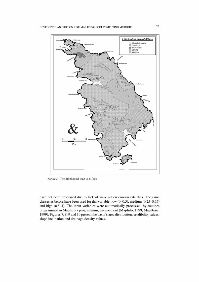
Davis (1966) and Gournellos (1980) have studied the geology of Sifnos (Figure3). The lithostratigraphy of Sifnos island, corresponds to a depositional environ-ment of a continental margin. The main sequence contains three carbonaceousand two clastic formations. Recent sediments are found in a few coastal areasand are mainly alluvial or dilluvial. The soil deposits and the weathered mantle,are overlaying alluvials and schist formations and appear in a discontinuous way.Vegetation cover is very limited.

The tectonometamorphic evolution of this island, is the result of many deform-ational phases. Both the first and the second folding phase were isoclinal, whilethe later ones had vertical axial planes (Gournellos, 1980). The final deformationphase is the discontinuous neotectonic one, which is responsible for the island’sfracturing.


Table I. The initial data of the three input variables (Drainage density, Slope, Erodibility)and the derived output variable (Erosion risk index)

a/a Density Normalized Slope (%) Normalized Erodibility Erosion

km−1 density slope risk index

1.1 1.91 0.25 2.48 0.07 0.33 0.138

1.2 1.31 0.17 3.11 0.09 0.77 0.667

1.3 2.79 0.37 1.16 0.03 0.55 0.666

1.4 4.07 0.54 0.28 0.01 0.41 0.293

1.5 3.53 0.46 0.55 0.02 0.46 0.158

1.6 4.64 0.61 0.00 0.00 0.59 0.481

2 3.32 0.44 29.28 0.85 0.39 0.573

3 4.76 0.63 26.11 0.76 0.47 0.63

4 3.84 0.51 29.79 0.86 0.38 0.568

5 3.42 0.45 31.67 0.92 0.37 0.563

6 2.31 0.30 34.49 1.00 0.41 0.591

7 3.76 0.49 32.65 0.95 0.35 0.225

8 1.93 0.25 30.96 0.90 0.33 0.537

9 1.27 0.17 23.74 0.69 0.29 0.477

10 2.84 0.37 34.02 0.99 0.29 0.511

11 3.00 0.39 30.62 0.89 0.29 0.511

12 3.53 0.46 25.22 0.73 0.31 0.503

13 3.51 0.46 21.94 0.64 0.78 0.692

14 3.06 0.40 21.46 0.62 0.88 0.688

15 2.87 0.38 17.64 0.51 0.88 0.67

16 3.37 0.44 17.34 0.50 0.87 0.5

17 2.46 0.32 16.58 0.48 0.66 0.666

18 3.91 0.51 19.14 0.55 0.62 0.677

19 2.81 0.37 18.12 0.53 0.68 0.674

20 2.79 0.37 17.69 0.51 0.79 0.67

21 2.56 0.34 14.41 0.42 0.67 0.667

22 2.70 0.36 18.36 0.53 0.69 0.674

23 3.50 0.46 19.04 0.55 0.88 0.677

24 4.16 0.55 16.50 0.48 0.88 0.592

25 3.40 0.45 19.01 0.55 0.87 0.677

26 2.54 0.33 23.18 0.67 0.78 0.696

27 2.71 0.36 27.75 0.80 0.75 0.709

28 2.91 0.38 24.21 0.70 0.60 0.678

29 3.13 0.41 26.88 0.78 0.29 0.509

30 1.77 0.23 25.08 0.73 0.29 0.494

31 2.47 0.33 28.23 0.82 0.29 0.511

32 1.03 0.13 18.47 0.54 0.29 0.294

33 3.45 0.45 22.19 0.64 0.29 0.445


Table I. Continued



34 3.21 0.42 27.26 0.79 0.29 0.511

35 3.31 0.44 26.52 0.77 0.29 0.506

36 3.55 0.47 25.73 0.75 0.29 0.5

37 3.68 0.48 26.76 0.78 0.29 0.509

38 3.80 0.50 27.73 0.80 0.29 0.511

39 3.76 0.49 28.24 0.82 0.30 0.518

40 2.26 0.30 22.22 0.64 0.30 0.45

41 3.22 0.42 18.89 0.55 0.42 0.435

42 3.04 0.40 17.01 0.49 0.51 0.665

43 2.72 0.36 17.74 0.51 0.44 0.47

44 2.52 0.33 18.68 0.54 0.33 0.316

45 1.69 0.22 21.51 0.62 0.54 0.67

46 4.54 0.60 27.52 0.80 0.78 0.72

47 3.81 0.50 22.25 0.65 0.56 0.672

48 1.89 0.25 13.80 0.40 0.42 0.151

49 1.80 0.24 16.93 0.49 0.62 0.665

50 2.82 0.37 17.56 0.51 0.88 0.67

51.1 3.13 0.41 0.97 0.03 0.82 0.667

51.2 0.00 0.00 7.24 0.21 0.87 0.667

51.3 1.68 0.22 0.29 0.01 0.56 0.667

51.4 2.09 0.27 0.41 0.01 0.85 0.667

52 2.19 0.29 15.02 0.44 0.88 0.667

53 2.59 0.34 12.96 0.38 0.88 0.667

54 2.87 0.38 9.91 0.29 0.88 0.667

55 3.14 0.41 15.71 0.46 0.88 0.666

56 1.99 0.26 14.15 0.41 0.85 0.667

57 1.64 0.22 13.42 0.39 0.88 0.667

58 2.17 0.29 14.79 0.43 0.85 0.666

59 2.41 0.32 12.27 0.36 0.80 0.667

60 2.13 0.28 13.92 0.40 0.77 0.666

61.1 2.60 0.34 1.26 0.04 0.86 0.667

61.2 2.38 0.31 0.00 0.00 0.82 0.667

62 2.75 0.36 14.21 0.41 0.71 0.667

63.1 2.09 0.27 1.27 0.04 0.66 0.667

63.2 3.12 0.41 3.13 0.09 0.73 0.667

64 3.98 0.52 13.24 0.38 1.00 0.668

65 2.91 0.38 20.81 0.60 0.47 0.594

66 3.80 0.50 16.71 0.48 0.44 0.154

67 4.03 0.53 13.28 0.39 0.42 0.376


Table I. Continued



68 3.83 0.50 20.66 0.60 0.32 0.423

69 3.58 0.47 20.46 0.59 0.41 0.49

70 5.21 0.69 19.14 0.56 0.29 0.477

71 3.81 0.50 18.75 0.54 0.29 0.294

72 2.84 0.37 20.11 0.58 0.29 0.378

73 3.20 0.42 21.77 0.63 0.29 0.437

74 2.92 0.38 20.95 0.61 0.29 0.417

75 2.64 0.35 17.88 0.52 0.45 0.372

76 2.49 0.33 0.00 0.00 0.29 0.132

77 2.28 0.30 15.71 0.46 0.38 0.145

78 3.53 0.46 16.65 0.48 0.49 0.163

79 2.88 0.38 19.65 0.57 0.35 0.401

80 3.89 0.51 19.72 0.57 0.36 0.409

81 2.87 0.38 23.68 0.69 0.29 0.477

82 4.92 0.65 22.77 0.66 0.55 0.671

83 2.51 0.33 20.02 0.58 0.49 0.634

84 2.96 0.39 20.24 0.59 0.29 0.393

85 5.20 0.68 19.91 0.58 0.29 0.472

86 7.60 1.00 21.21 0.62 0.29 0.511

87 2.48 0.33 22.21 0.64 0.45 0.581

88 2.52 0.33 21.14 0.61 0.49 0.642

89 3.31 0.44 21.67 0.63 0.45 0.576

90 3.93 0.52 18.80 0.55 0.57 0.677

91 4.12 0.54 16.78 0.49 0.80 0.619

92 3.86 0.51 15.34 0.44 0.70 0.627

93 3.45 0.45 13.77 0.40 0.58 0.667

94 4.18 0.55 19.42 0.56 0.73 0.679

95 2.83 0.37 16.59 0.48 0.34 0.139

96 5.67 0.75 23.01 0.67 0.29 0.501

97 3.08 0.41 22.03 0.64 0.42 0.544

98 3.25 0.43 17.57 0.51 0.39 0.218

99 4.23 0.56 15.73 0.46 0.36 0.393

100 2.60 0.34 25.47 0.74 0.46 0.617

101 2.90 0.38 24.84 0.72 0.60 0.677

102 4.43 0.58 25.27 0.73 0.55 0.67

103 2.32 0.30 24.82 0.72 0.41 0.565

104 2.82 0.37 24.49 0.71 0.31 0.496

105 4.21 0.55 24.14 0.70 0.29 0.481

106 3.30 0.43 25.09 0.73 0.30 0.498


Table I. Continued



107 2.52 0.33 26.71 0.77 0.34 0.531

108 2.48 0.33 25.45 0.74 0.29 0.497

109 3.25 0.43 31.00 0.90 0.29 0.511

110 5.12 0.67 33.22 0.96 0.29 0.511

111 4.05 0.53 32.37 0.94 0.29 0.511

112 5.47 0.72 33.55 0.97 0.29 0.511

113 3.11 0.41 31.52 0.91 0.29 0.511

114 3.35 0.44 26.37 0.76 0.32 0.517

Sifnos’ topography is dominated by the presence of two mountainous areas inthe central part of the island, ranging from northwest to southeast. The climate ofCyclades though relatively dry (366.8 mm per year), is also characterized by a fewstorm events, especially during winter time (Theocharatos, 1978).

The working scales for the topographical and geological maps are 1:50.000 and1:25.000 respectively. The interpretation of air photos was achieved at a 1:33.000scale.

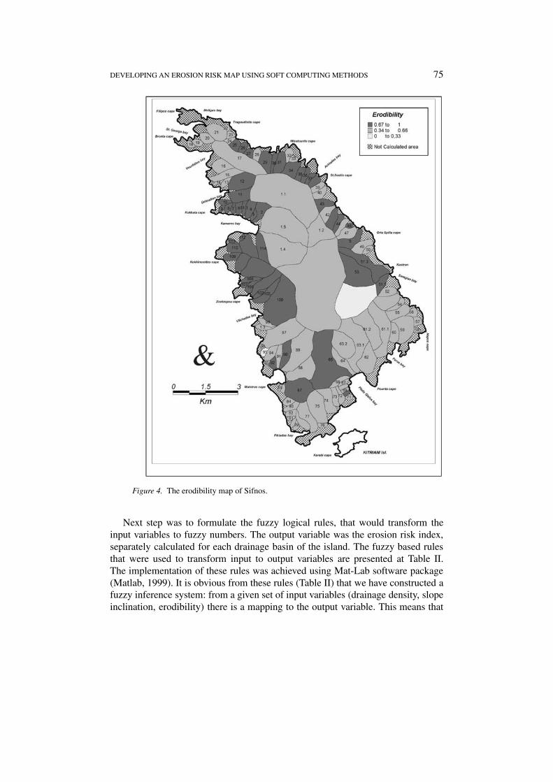
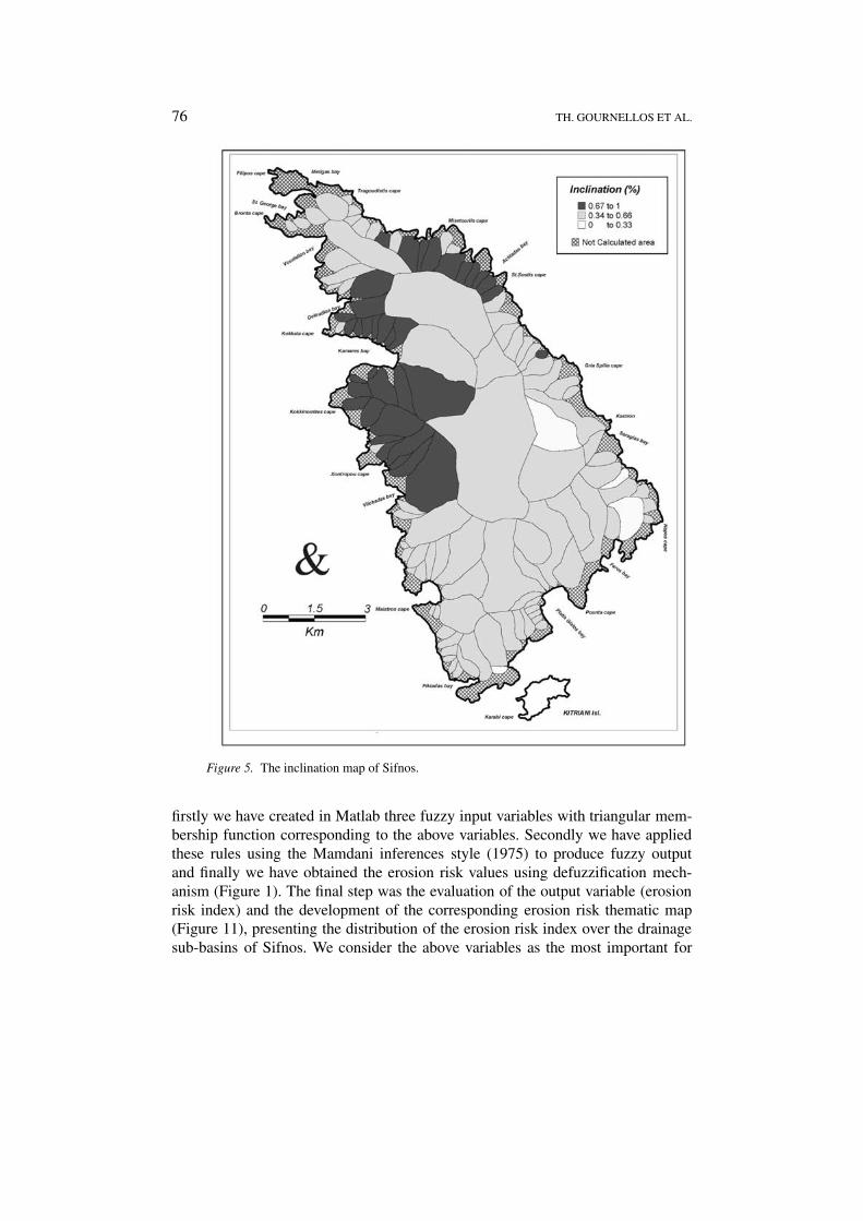
The first step of this methodology was the digitization of the geological, topo-graphical and drainage system maps. The marbles originating from limestones arevery susceptible to acid waters, which continuously widen the existent discontinuit-ies (joints, bedding), increase the permeability of the rock and consequently reducethe runoff waters. In schists the existence of the schistosity and the joint systeminfluence the disintegration of the rocks in parallel fragments and facilitate erosion.In Sifnos we can distinguish the weathered mantle overlay in the unweatheredmetamorphic basement. From these initial data, we derived the erodibility, theslope inclination and the drainage density values and the corresponding thematicmaps (Table I, Figures 4, 5, and 6). The next step was treating the above variablesas fuzzy variables assigning to them the corresponding membership functions.The first input variable that was used was the erodibility of the rock. In order tocharacterize the erodibility of the rocks, a 0–1 scale was adopted. This means that 0erodibility values indicate non vulnerable, and 1 highly vulnerable to erosion rocks.At Sifnos case formations of “low” (0–0.5), “medium” (0.25–0.75) and “high” (0,.–1) erodibility were distinguished that are represented by Marbles, Blueschists –Schists, alluvial and weathered mantle, respectively. The second input variable wasthe slope gradient of the relief, the calculation based on the digital elevation modeland representing the angle of the surface with the horizontal plane. Three classes ofnormalized values of slopes are used: low (0–0.5), medium (0.25–0.75) and high(0.5–1). The last input variable was drainage density. Some small coastal basins


Figure 2. General location of the studied area, Sifnos, Greece.


Figure 3. The lithological map of Sifnos.

have not been processed due to lack of wave action erosion rate data. The sameclasses as before have been used for this variable: low (0–0.5), medium (0.25–0.75)and high (0.5–1). The input variables were automatically processed, by routinesprogrammed in MapInfo’s programming environment (MapInfo, 1999; MapBasic,1999). Figures 7, 8, 9 and 10 present the basin’s area distribution, erodibility values,slope inclination and drainage density values.


Tabl

eII

.T

hefu

zzy

logi

calr

ules

used

tode

rive

the

eros

ion

risk

inde

x

IfE

RO

DIB

ILIT

YIS

Hig

h&

SL

OP

EIS

Hig

hT

hen

Ero

sion

Ris

kIn

dex

IsH

igh

IfE

RO

DIB

ILIT

YIS

Hig

h&

SL

OP

EIS

Med

ium

&D

rain

age

Den

sity

ISH

igh

The

nE

rosi

onR

isk

Inde

xIs

Hig

h

IfE

RO

DIB

ILIT

YIS

Hig

h&

SL

OP

EIS

Low

The

nE

rosi

onR

isk

Inde

xIs

Med

ium

IfE

RO

DIB

ILIT

YIS

Med

ium

&S

LO

PE

ISH

igh

The

nE

rosi

onR

isk

Inde

xIs

Med

ium

IfE

RO

DIB

ILIT

YIS

Med

ium

&S

LO

PE

ISM

ediu

m&

Dra

inag

eD

ensi

tyIS

Hig

hT

hen

Ero

sion

Ris

kIn

dex

IsM

ediu

m

IfE

RO

DIB

ILIT

YIS

Med

ium

&S

LO

PE

ISL

ow&

Dra

inag

eD

ensi

tyIS

Hig

hT

hen

Ero

sion

Ris

kIn

dex

IsL

ow

IfE

RO

DIB

ILIT

YIS

Low

&S

LO

PE

ISL

owT

hen

Ero

sion

Ris

kIn

dex

IsV

ery

Low


Figure 4. The erodibility map of Sifnos.

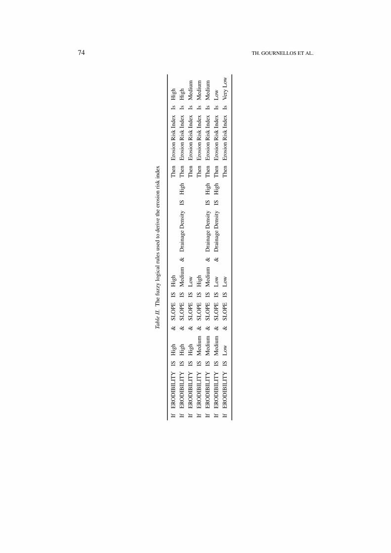
Next step was to formulate the fuzzy logical rules, that would transform theinput variables to fuzzy numbers. The output variable was the erosion risk index,separately calculated for each drainage basin of the island. The fuzzy based rulesthat were used to transform input to output variables are presented at Table II.The implementation of these rules was achieved using Mat-Lab software package(Matlab, 1999). It is obvious from these rules (Table II) that we have constructed afuzzy inference system: from a given set of input variables (drainage density, slopeinclination, erodibility) there is a mapping to the output variable. This means that


Figure 5. The inclination map of Sifnos.

firstly we have created in Matlab three fuzzy input variables with triangular mem-bership function corresponding to the above variables. Secondly we have appliedthese rules using the Mamdani inferences style (1975) to produce fuzzy outputand finally we have obtained the erosion risk values using defuzzification mech-anism (Figure 1). The final step was the evaluation of the output variable (erosionrisk index) and the development of the corresponding erosion risk thematic map(Figure 11), presenting the distribution of the erosion risk index over the drainagesub-basins of Sifnos. We consider the above variables as the most important for


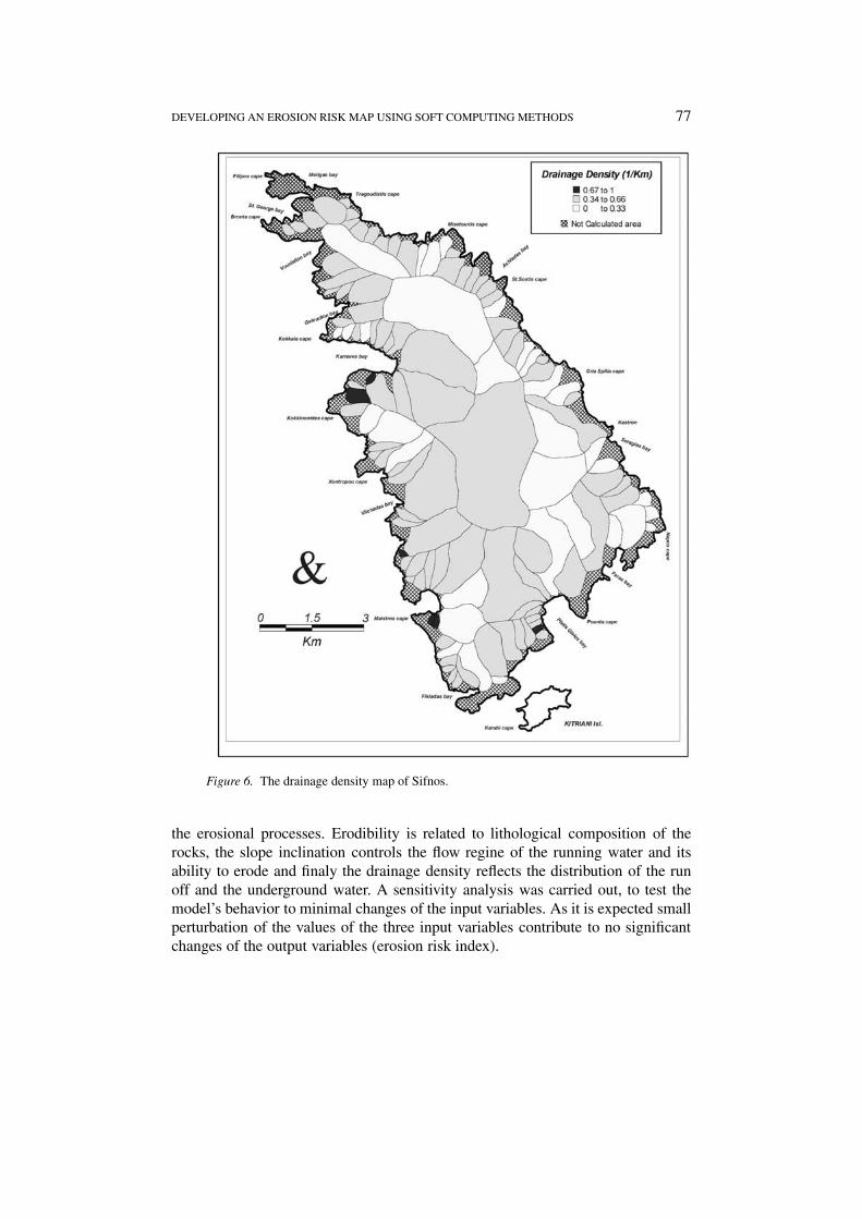
Figure 6. The drainage density map of Sifnos.

the erosional processes. Erodibility is related to lithological composition of therocks, the slope inclination controls the flow regine of the running water and itsability to erode and finaly the drainage density reflects the distribution of the runoff and the underground water. A sensitivity analysis was carried out, to test themodel’s behavior to minimal changes of the input variables. As it is expected smallperturbation of the values of the three input variables contribute to no significantchanges of the output variables (erosion risk index).


Figure 7. Histogram of the area of drainage basins of Sifnos.

Figure 8. Histogram of the erodibility values of drainage basins of Sifnos.

4. Conclusion

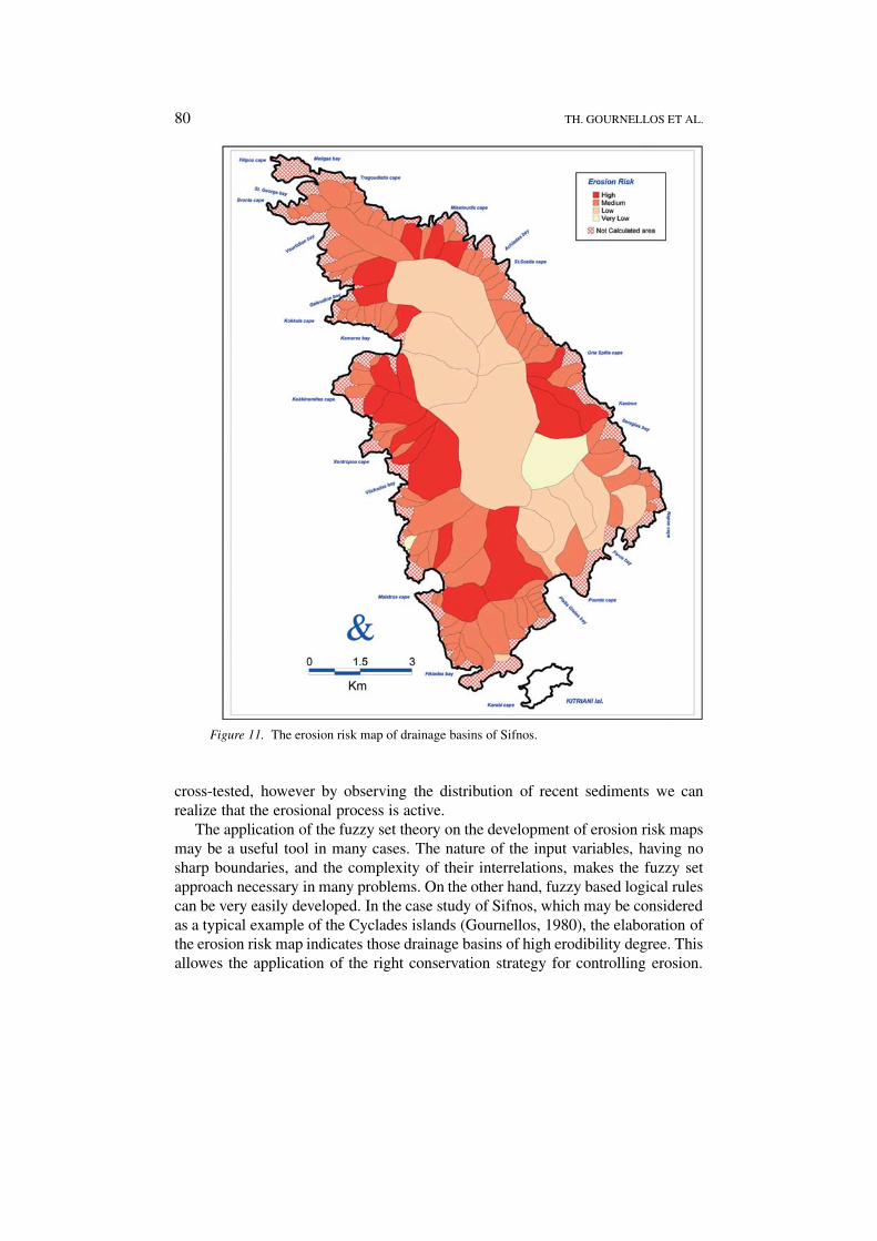
It is obvious (Figure 11) that some small coastal sub-basins of Sifnos at the northernand central parts present high erosion risk. Nevertheless, the largest part of Sifnosisland is classified as medium degree erosion risk. This is mainly explained bythe lithological and morphological characteristics of the island. We must note thatSifnos, like all the islands of Cyclades, presents high juxtaposition of resistantand permeable rocks (Marbles) against the moderate resistant and impermeableschists. In this substratum, soils and surface deposits are overlain with the ab-sence of significant vegetation. The high vulnerability to erosion at all semi-arid


Figure 9. Histogram of the slope inclination values of drainage basins of Sifnos.

Figure 10. Histogram of the drainage density values of drainage basins of Sifnos.

regions including the Mediterranean region (Walling and Webb, 1983) is alreadyknown. Small drainage basins receive uniform rainfalls. The climate conditions,the existence of a long summer dry period and the appearance of rainfalls in theautumn-winter period, contributed to erosion. It was already noted that the sedi-ment yield per unit area, increases as the drainage area is decreasing (Schumm,1977) and that in general the Mediterranean climates present high erosion rates(Jensen and Painter, 1974). The model proposed by this paper cannot be easily


Figure 11. The erosion risk map of drainage basins of Sifnos.

cross-tested, however by observing the distribution of recent sediments we canrealize that the erosional process is active.

The application of the fuzzy set theory on the development of erosion risk mapsmay be a useful tool in many cases. The nature of the input variables, having nosharp boundaries, and the complexity of their interrelations, makes the fuzzy setapproach necessary in many problems. On the other hand, fuzzy based logical rulescan be very easily developed. In the case study of Sifnos, which may be consideredas a typical example of the Cyclades islands (Gournellos, 1980), the elaboration ofthe erosion risk map indicates those drainage basins of high erodibility degree. Thisallowes the application of the right conservation strategy for controlling erosion.


This kind of data analysis should also be taken into consideration for both localand regional planning.

This GIS framework may be applied to all Cycladic islands to map erosionaldeterioration. This is a simple model, demanding only three variables and a fewlogical rules, making its use easy.

Modifications on the fuzzy rules and the membership functions should bemade, when more quantitative and qualitative data are available, concerning thegeodynamic process of the studied drainage basins.

Acknowledgements

We would like to thank the unknown referees for their constructive comments onan earlier manuscript.

References

Baturst, J. C., Kilsby, C., and White, S.: 1996, Modeling the impacts of climate and land-use changeon basin hydrology and soil erosion in Mediterranean Europe, In: J. Brandt and J. B. Thornes(eds), Mediterranean Desertification, Wiley, Chichester, pp. 354–387.

Binagli, E., Luzi, L., Madella, P., Pergalani, F., and Rampini, A.: 1998, Slope instability zonation: acomparison between certainty factor and fuzzy Dempster–Shafer approaches, Natural Hazards17, 77–97.

Bolton, M.: 1979, A Guide to Soil Mechanics, McMillan, London.Briggs, D. and Giordano, A.: 1992, CORINE soil erosion risk and important land resources in

the southern regions of the European Community. Commission of the European CommunitiesPublication EUR 13233 EN.

Brundsen, D., Doornkamp, J. C., Fookes, P. G., Jones, D. K. C., and Kelly, J. M. H.: 1975, Large scalegeomorphological mapping and highway engineering design, Quart. J. Eng. Geol. 8, 227–253.

Burrough, P. A., MacMillan, R. A., van Deursen, W.: 1992, Fuzzy classification methods for determ-ining land suitability from soil profile observations and topography, Journal of Soil Science 43,193–210.

Burrough, P. A.: 1989, Fuzzy mathematical methods for soil survey and land evaluation, Journal ofSoil Science 40, 477–492.

Carrara, A., Cardinali, M., Detti, R., Guzzetti, F., Pasqui, V., and Reichenbach, P.: 1991, Gistechniques and statistical models in evaluating landslide hazard, Earth Surface Processes andLandforms 16(5), 427–455.

Carrara, A., Pugliese Garratelli, E., and Merenda, L.: 1977, Computer based data bank and statisticalanalysis of slope stability phenomena, Zeitschrift für Geomorphologie, N.F., 21(2), 187–222.

Carrara, A.: 1983, Multivariate models for landslides hazard evaluation, Math. Geol. 15(3), 403–427.Davis, E.: 1966, Der geologische Bau der insel Siphnos, In ts. Geol. Subs, Res, Athenes, pp. 161–220.De Ploey, J.: 1989, A model for headcut retreat in rills and gullies, Catena Supplement 14, 81–86.Diaconu, C.: 1969, Resultats de l’etude de l’ecoulement des alluvions en suspension des rivieres de

la Roumanie. Bulletin of the International Association of Scientific Hydrology 14, 51–89.Dubois, D. and Prade, H.: 1980, Fuzzy Sets and Systems Theory and Applications, Academic Press,

New York.Elwell, H. A.: 1978, Modeling soil losses in Southern Africa. Journal of Agricultural Engineering

Research 23, 117–127.Emmett, W. W.: 1978, Overland flow, In Kirkby (ed.), Hillslope Hydrology, pp. 145–157,


Fournier, F.: 1960, Climat et Erosion: La Relation entre l’Erosion du Sol par l’Eau et les PrecipationsAtmospheriques, Presses Universitaires de France, Paris.

Giordano, A.: 1986: A first approximation of soil erosion risk assessment in the southern countriesof the European Community, In: R. P. C. Morgan and R. J. Rickson (eds), Erosion Assessmentand Modelling. Commission of the European Communities Report EUR 10860, pp. 3–24.

Gournellos, T.: 1980, Contribution l’etude geologique des Cyclades, L’ile de Siphnos, These de 3eme cycle, Universite de Paris VI, p. 182.

Gregory, K. J. and Walling, D. E.: 1973, Drainage Basin Form and Process, Wiley, New York, p.456.

Horton, R. E.: 1945, Erosional development of streams and their drainage basins: hydrophysicalapproach to quantitative morphology, Bull. Geolog. Soc. Am. 56, 275–370.

Hundson, N. W.: 1981, Soil Conservation, Batsford, London.Ives, J. D. and Mersserli, B.: 1981, Mountain hazard mapping in Nepal, Introduction to an applied

mountain research project, Mountain Research and Development 1(3–4), 223–230.Jenny, H.: 1941, Factors of Soil Formation, McGraw-Hill Book Company, New York, p. 281.Jensen, J. M. and Painter, R. B.: 1974, Predicting sediment yield from climate and topography, J.

Hydrol. 21, 371–380.Jozefaciuk, C. and Jozefaciuk, A.: 1993, Gullies net density as a factor of water system deforma-

tion in Vistula River basin, In: K. Banasik and A. Zbikowski (eds), Runoff and Sediment YieldModelling, Warsaw Agricultural University Press, Warsaw, pp. 169–174.

Kirkby, M. J.: 1969, Infiltration, throughflow and overland flow, In: R. J. Chorley (ed.), Water, Earthand Man, Methuen, London, Ch. 5.1, pp. 215–227.

Kirkby, M. J.: 1978, Implications for sediment transport, In: Kirkby (ed.), Hillslope Hydrology, pp.325–340.

Kirkby, M. J.: 1995, Modeling the links between vegetation and landforms, Geomorphology 13,319-335.

Klir, G. J. and Yuan, B.: 1995, Fuzzy Sets and Fuzzy Logic Theory and Applications, Prentice-Hall,New Jersey.

Knisel, W. G.: 1980, CREAMS: a field scale model for chemicals, runoff and erosion fromagricultural management systems. USDA Conservation Research Report 26.

Kuenen, P. H.: 1956, Rolling by current (Pt) 2 of Experimental abrasion of pebbles, J. Geol. 64,336–368.

Leopold, L. B., Wolman, M. G., and Millet, J. P.: 1964, Fluvial Processes in Geomorphology, W. H.Fraeman and Company, San Francisco.

Malgot, J. and Mahr, T.: 1979, Engineering geological mapping of the West Carpathian landslideareas, Bull. Int. Ass. Eng. Geol. 19, 116–121.

Mamdani, E. H. and Assilian, S.: 1975, An experiment in linguistic synthesis with a fuzzy logiccontroler, International Journal of Man-Machine Studies 7(1), 1–13.

MapInfo Professional, 1999, MapInfo Corporation, Troy, New York.MapBasic, 1999, MapInfo Corporation, Troy, New York.Marinos, P. G., Plessas, S. P., and Valadaki-Plessa, K.: 1997, Erosion risk maps for the greater

Athens region and a G.I.S. based processing of data, Engineering and the Environment, Balkema,Rotterdam, pp.1353–1386.

Matlab, 1999, The Math works Inc.Morgan, R. P. C., Morgan, D. D. V., and Finney, H. J.: 1984, A predictive model for the assessment

of soil erosion risk, Journal of Agricultural Engineering Research 30, 245–253.Morgan, R. P. C.: 1974, Estimating regional variations in Peninsular Malaysia, Malayan Nature

Journal 28, 94–106.Morgan, R. P. C., Quinton, J. N., and Rickson, R. J.: 1994, Modelling methodology for soil erosion

assessment and soil conservation design: the EUROSEM approach, Outlook in Agriculture 23,5–9.


Morgan, R. P. C., Quinton, J. N., Smith, R. E., Govers, G., Poesen, J., Auerswald, K., Chisci, G.,Torri, D., and Styczen, M. E.: 1997, The European soil erosion model (EUROSEM): a dynamicapproach for predicting sediment transport from fields and small catchments, In: J. Boardman andD. Favis-Mortlock (eds), Modeling Soil Erosion by Water, Springer-Verlag NATO-ASI GlobalChange Series, Springer-Verlag, Berlin, in press.

Morgan, R. P. C.: 1996, Soil Erosion and Conservation, Longman (ed.), 2nd edition.Nearing M. A., Foster, G. R., Lane, L. J., and Finker S. C.: 1989, A process-based soil erosion model

for USDA-Water Erosion Prediction Project technology, Transactions of the American Society ofAgricultural Engineers 32, 1587–1593.

Poesen, J. W. A. and Hooke, J. M.: 1997, Erosion, flooding and channel management in Mediter-ranean environments of southern Europe, Progress in Physical Geography 21(2), 157–199.

Rooseboom, A. and Annandale, G. W.: 1981, Techniques applied in determining sediment loads inSouth African rivers, International Association of Scientific Hydrology Publication 133, 219–224.

Schumm, S. A.: 1977, The Fluvial System, A Wiley-Interscience Publication, p. 338.Selby, M. J.: 1987, Rock slopes, In: M. G. Anderson and K. S. Richards (eds), Slope Stability, Wiley,

Chichester, pp. 475–504.Sparks, B. W., 1965, Geomorphology, Longmans (ed.), p. 371.Stassopoulou, A., Petrou, M., and Kittler, J.: 1998, Application of a Bayesian network in a GIS based

decision making system, Int. J. Geographical Information Science 12(1), 23–45.Stocking, M. A. and Elwell H. A.: 1973b, Soil erosion hazard in Rhodesia, Rhodesian Agricultural

Journal 70, 93–101.Stocking, M. A. and Elwell, H. A.: 1976, Rainfall erosivity over Rhodesia. Transactions of the

Institute of British Geographers New Series 1, 231–245.Theocharatos, G.: 1978, The Climate of Cyclades, Athens.Thornes, J. B., Shao, J. X., Diaz, E., Roldan, A., McMahon, M., and Hawkes, J. C.: 1996, Testing

the MEDALUS hillslope model, Catena 26, pp. 137–160.Walling, D. E. and Webb, B. W.: 1983, Patterns of sediment yield, In: K. J. Gregory (ed.), Background

to Palaeohydrology, Chichester, Wiley, pp. 69–100.Wischmeier, W. H. and Smith, D. D.: 1978, Predicting rainfall erosion losses. USDA Agricultural

Research Service Handbook 537.Yager, R. R., Ovchinnikov, S., Tong, R. M., and Nguyen, H. T.: 1987, Fuzzy Sets and Applications,

selected papers by L. A. Zadeh, Wiley, New York.Zadeh, L. A.: 1965, Fuzzy Sets, Information and Control, 8, pp. 338–353.Zadeh, L. A.: 1987, The concept of linguistic variable and its application to approximate reason-

ing, In: R. R. Yager, S. Ovchinnikov, R. M. Tong, and H. T. Nguyen (eds), Fuzzy Sets andApplications, Wiley, New York, pp. 293–329.

Zimmermann, H. J.: 1991, Fuzzy Set Theory and Its Application, 2nd ed., Kluwer Academic, MA.

Developing an Erosion Risk Map Using Soft Computing Methods (Case Study at Sifnos Island

Documents

Transcript of Developing an Erosion Risk Map Using Soft Computing Methods (Case Study at Sifnos Island