minerals

Article

Determination of Trace Metal (Mn, Fe, Ni, Cu, Zn, Co, Cd andPb) Concentrations in Seawater Using Single QuadrupoleICP-MS: A Comparison between Offline and OnlinePreconcentration Setups

Saumik Samanta 1,*,†, Ryan Cloete 1,*,†, Jean Loock 1,†, Riana Rossouw 2 and Alakendra N. Roychoudhury 1,*

Citation: Samanta, S.; Cloete, R.;

Loock, J.; Rossouw, R.;

Roychoudhury, A.N. Determination

of Trace Metal (Mn, Fe, Ni, Cu, Zn,

Co, Cd and Pb) Concentrations in

Seawater Using Single Quadrupole

ICP-MS: A Comparison between

Offline and Online Preconcentration

Setups. Minerals 2021, 11, 1289.

https://doi.org/10.3390/min11111289

Academic Editor: Cécile Grosbois

Received: 27 October 2021

Accepted: 17 November 2021

Published: 19 November 2021

Publisher’s Note: MDPI stays neutral

with regard to jurisdictional claims in

published maps and institutional affil-

iations.

Copyright: © 2021 by the authors.

Licensee MDPI, Basel, Switzerland.

This article is an open access article

distributed under the terms and

conditions of the Creative Commons

Attribution (CC BY) license (https://

creativecommons.org/licenses/by/

4.0/).

1 Centre for Trace Metal and Experimental Biogeochemistry (TracEx), Department of Earth Sciences,Stellenbosch University, Stellenbosch 7600, South Africa; 16041399@sun.ac.za

2 ICP-MS & XRF Unit, Central Analytical Facility, Department of Earth Sciences, University of Stellenbosch,Stellenbosch 7600, South Africa; rrossouw@sun.ac.za

* Correspondence: 22505709@sun.ac.za or saumiksamanta@gmail.com (S.S.); ryan.cloete76@gmail.com (R.C.);roy@sun.ac.za (A.N.R.)

† These authors contributed equally.

Abstract: The quantification of dissolved metals in seawater requires pre-treatment before the mea-surement can be done, posing a risk of contamination, and requiring a time-consuming procedure. De-spite the development of automated preconcentration units and sophisticated instruments, the entireprocess often introduces inaccuracies in quantification, especially for low-metal seawaters. This studypresents a robust method for measuring dissolved metals from seawater accurately and preciselyusing a seaFAST and quadrupole Inductively Coupled Plasma Mass Spectrometer (ICPMS), em-ployed in both offline (2016–2018) and online (2020–2021) setups. The proposed method shows dataprocessing, including the re-calculation of metals after eliminating the instrumental signals caused bypolyatomic interferences. Here, we report the blank concentration of Fe below 0.02 nmol kg−1, some-what lower values than that have been previously reported using high-resolution and triple-quadICPMS. The method allows for the accurate determination of Cd and Fe concentrations in low-metal seawaters, such as GEOTRACES GSP, using a cost-effective quadrupole ICPMS (Cdconsensus:2 ± 2 pmol kg−1, Cdmeasured: 0.99 ± 0.35 pmol kg−1; Feconsensus: 0.16 ± 0.05 nmol kg−1, Femeasured:0.21 ± 0.03 nmol kg−1). Between two setups, online yields marginally lower blank values for met-als based on short-term analysis. However, the limit of detection is comparable between the two,supporting optimal instrumental sensitivity of the ICPMS over 4+ years of analysis.

Keywords: geotraces; seaFAST; ICP-MS; trace metals; GSP; GSC

1. Introduction

The sources, cycling, and fluxes of trace elements in seawater have become a primeinterest in understanding ocean life and the interaction between ocean and atmosphere.The role of trace elements in the global ocean widely varies based on their involvementin oceanic processes, starting from the primary production of phytoplankton to assessinganthropogenic contributions. Using trace elements as tracers, e.g., Fe, Mn, Cu, Zn, Ni, Co,and Cd as bio-essential metals for productivity, Fe and Mn for hydrothermal/riverine input,Mo for redox processes, Pb for anthropogenic activities, Al for natural dust input, and Ndfor mixing of water masses, has provided new insights regarding our understanding of theocean [1]. Therefore, the GEOTRACES and its precursor programs (e.g., JGOFS, WOCE),enabled the construction of a spatiotemporal database of trace elements and their isotope(TEIs) within the global ocean. However, analytical processes for generating TEIs data,especially for particulate and dissolved metals, contain challenges. The extremely lowconcentration of metals, sea salt-derived interferences, and the risk of contamination could

Minerals 2021, 11, 1289. https://doi.org/10.3390/min11111289 https://www.mdpi.com/journal/minerals

Minerals 2021, 11, 1289 2 of 19

limit the analytical accuracies. Thus, scientists devised methods to purify (remove sea salts)and preconcentrate seawater before analysis. The pre-processing of the samples has beenimproved by applying different methodologies (e.g., solvent extraction, magnesium hydrox-ide co-precipitation, solid-phase extraction) [2–4]. In addition, technological advancementshave facilitated the quantification procedure accurately and precisely by utilizing sophis-ticated analytical techniques (e.g., flow injection, cathodic stripping, atomic absorption,mass spectrometry; [5–8]). In particular, a commercially available automated module,the seaFAST system, simplifies and streamlines the pre-processing treatment of seawatersamples. Several studies have shown the potential of using the seaFAST pre-treatmentsystem before quantifying trace metals [9–13], rare earth elements [14,15], and their isotopiccomposition [16]. Once preconcentrated, the advanced, high-resolution mass spectrome-ters, e.g., sector field (SF-ICPMS; [9]) and triple quadrupole (QQQ-ICPMS; [10]) have beencommonly used for quantification. In some studies, a single quadrupole ICPMS was alsoapplied for the determination of trace metals [12,17].

The seaFAST comprises a column packed with chelating resin that effectively removessea salts and then elutes preconcentrated trace elements. Although the preconcentrationfactor may reach up to 50 times and more, quantifying selective bio-essential metals(e.g., Fe, Zn, Cd), often requires high mass resolution in the ICPMS to distinguish theanalytes from instrumental backgrounds [10,11]. However, adding a collision reaction cell(CRC) to the ICP-MS instrument minimizes the instrumental background by dissociatingpolyatomic interferences [18]. To further optimise the analytical setup, the seaFAST modulemay be coupled directly to the ICPMS, i.e., online (e.g., [12]), which reduces preparationtime and intermediate steps between preconcentration and quantification involved inthe offline method.

The development of offline and online systems improved and simplified the method-ology by simultaneous quantification of multiple analytes for a large number of seawatersamples. However, measuring selective bio-essential and contamination-prone metals(e.g., Fe, Zn, Pb, Cd) often introduces inaccuracies that stem from potential contaminantcontributions from the various steps in the analytical process (e.g., reagents, tubing) usedin the seaFAST and/or higher background signals caused by polyatomic interferences onspecific metals. For example, it was estimated that argon oxide (ArO+), derived from theargon gas used to produce the plasma, contributed 60%–85% of the measured 56Feblankconcentration [10]. The contribution of masses from both contamination and polyatomicinterferences could increase the limit of detection for metals thereby preventing the mea-surement of selected analytes (e.g., Cd, Fe, Zn) which are characterised by extremely lowconcentrations in surface seawater. In addition, measurement can be erroneous becauseof the high proportional contribution of added mass. Therefore, the measured concentra-tion is generally subtracted by the instrumental counts of procedural blanks [9]. For Cd,Cd-free seawater or molybdenum (Mo)-standard is analysed to quantify the magnitudeof molybdenum oxide (MoO+) derived Cd, i.e., up to 9 pmol kg−1 [9]. However, we havelimited knowledge on the following: (1) the degree of proportional contribution of addedmass for a range of analyte concentration, (2) the requirement of blank subtraction to obtainthe actual concentration of metals in seawater, (3) polyatomic interference and its effecton different isotopes of an analyte, and (4) selection of isotopic mass that produces theleast interference.

Based on our experiments carried out in the previous five years, using both offlineand online, we present a robust methodology that allows accurate and precise measure-ment of dissolved metals (Mn, Fe, Co, Ni, Cu, Zn, Cd, and Pb) using a single Q-ICPMS.The proposed methodology includes both measurement and post-processing calculationof data. The results of selected metals measured using offline setup are already pub-lished [19–21]. In this manuscript, we focus mainly on the effect and magnitude of poly-atomic interferences, especially while measuring Fe and Cd, and present our findingsto assess the magnitude and degree of interference needing to be corrected. In addition,the results from this study offer a comparison between offline and online method setups

Minerals 2021, 11, 1289 3 of 19

and support using cost-effective single Q-ICPMS (compared to High Resolution-, SF-, andQQQ-ICPMS) for quantifying dissolved trace metals from seawater.

2. Analytical Methods2.1. Reagents and Materials

High-quality deionized water (DIW; 18.2 M-Ω resistivity) was produced using theMilli-Q® advantage A10® system (MilliporeSigma, Burlington, MA, USA), fitted with aQ-POD® Element dispenser as an added trace contaminant removal device, and usedthroughout the analytical procedures and preparations thereof. For use during the pre-concentration procedure (Section 2.2), an ammonium acetate buffer (pH: 6.0 ± 0.2) wasprepared by mixing 25% ammonium hydroxide (NH4OH; Merck Suprapur®, Darmstadt,Germany), 100% glacial acetic acid (CH3COOH; Merck Suprapur®), and DIW. The pHof the buffer solution was read using a pH electrode (Hach® sensIONTM PH1, resolu-tion of ±0.01). The elution acid comprised 5% M nitric acid (HNO3; Merck Ultrapur).All solutions were prepared inside a fume hood housed within a class 100 clean laboratory(TracEx lab, Stellenbosch University, Stellenbosch, South Africa). All plasticware, contain-ers, and sample bottles used for the storage of seawater and reagents were extensivelyacid cleaned according to strict protocols outlined by GEOTRACES [22]. The materialof the lab wares (e.g., reagent bottles, measuring cylinder, vials, and pipette tips) waseither polypropylene/ethylene (PP/PE) or Perfluoroalkoxy alkanes (PFA) and used afterthorough acid cleaning.

2.2. Automated Preconcentration Using seaFAST Module

Both offline (period of use: 2016–2018) and online (period of use: 2020–2021) variationsof the method utilised a solid phase extraction (SPE) technique to separate the trace metalions from the seawater matrix elements. A SC-4 DX seaFAST-pico module (ElementalScientific Inc; ESI, Omaha, NE, USA) was used for the offline preconcentration of samples,while the SC-4 DX seaFAST S3 (ESI) was used for the online variation of the method(Table 1). The SC-4 DX seaFAST S3 has a hood with a built-in high-efficiency particulate air(HEPA) filter, which encloses the autosampler allowing the module to be used outside theclean lab (Figure S1). The SC-4 DX seaFAST-pico does not come standard with a HEPA hood,and therefore, the module was kept in a class 100 clean lab. As an added precaution againstsample contamination from falling particulate, we manufactured a perspex hood to fit overthe autosampler and sample rack. Both modules are commercially available and consist ofan autosampler, a syringe module (S400V), a sample loop (10 mL for seaFAST pico and 3 mLfor the seaFAST S3), two 11-port valves (A11b and P11), one 5-port valve (A5e), one tracemetal clean-up column (CF-N-0200 for seaFAST S3 and CF-M-0600 for seaFAST pico;200 µL bed volume) and a preconcentration column (CF-N-0200; 200 µL bed volume). Bothmodules were pressurized using clean air (99.999% O2; Air Products). The autosampler,with an inner probe diameter of 1 mm, introduced samples from the sample rack into thepreconcentration manifold via a vacuum pump system. The S400V syringe pump controlledthe four syringes (S1, S2, S3, and S4), which were dedicated to reagent distribution whiletheir flow path was controlled by the FAST DX 3 valve module. Syringe S1 (DIW) consistsof a 12 mL barrel with a dispense rate of 500 µL min−1, while the other syringes (S2: Buffer;S3: Eluent/Carrier; S4: Eluent/Diluent/Internal Standard) comprised a 3 mL syringe witha dispense rate of 496 µL min−1. Once introduced, the sample was loaded through the5-port valve by vacuum pressure and then transferred to the sample loop connected tothe A11b valve. Since the A11b valve switches, the sample is pushed to the P11 valveand mixed with the buffer solution, before transferring to the seawater preconcentrationcolumn (See Supplementary Section Figure S1). The preconcentration resin comprised bothethylenediaminetriacetic acid (EDTriA) and iminodiacetic acid (IDA) functional groupsimmobilized on a hydrophilic methacrylate polymer (60 µm bead diameter). As thebuffered seawater passes through the column, the dissolved trace metals are chelatedby the resin, while the seawater matrix is washed out from the column. The eluent is

Minerals 2021, 11, 1289 4 of 19

then driven through the preconcentration column, thereby eluting the trace metal ions.For offline preconcentration, the chelated metal ions were eluted into acid cleaned PPFalcon™ tubes during 4 elution cycles for a final elution volume of 0.25 mL, achievinga preconcentration factor of 40 and a sample throughput of 20 min/sample. For onlinepreconcentration, the chelated metal ions were eluted directly into the nebuliser of the ICP-MS instrument after 1 elution cycle for a final volume of 0.1 mL, a preconcentration factorof 30, and a sample throughput of 11 min/sample. The elution is followed by cleaning andcondition by a mixture of buffer and DIW in preparation for the next sample. After eachsample, the probe was rinsed in a 2% HNO3 (Ultrapur, Merck) solution followed by DIW.

Table 1. Offline and online preconcentration setup.

Mode of Analysis Offline Online

Preconcentration module SC-4 DX seaFAST-pico SC-4 DX seaFAST S3Column resin Nobias (EDTriA and IDA) Nobias (EDTriA and IDA)

Sample pH 1.7 1.7

Buffer Ammonium acetate(pH: 6.0 ± 0.2)

Ammonium acetate(pH: 6.0 ± 0.2)

Eluent 5% HNO3 5% HNO3Internal Standard - 10 µg kg−1 InSample loop (mL) 10 3

Elution cycles 4 1Elution volume (mL) 0.25 0.1

Preconcentration factor 40 30Sample throughput (min sample−1) 20 11

2.3. ICP-MS

Sample analysis of preconcentrated samples was performed on an Agilent 7900quadrupole Inductively Coupled Plasma Mass Spectrometer (ICP-MS) (Agilent Technolo-gies, Santa Clara, CA, USA) with operating conditions outlined in Table 2. The offlinemethod requires the eluted samples to be taken to the ICP-MS laboratory, therefore, thereis a time interval between sample elution and ICP-MS analysis. The instrument was opti-mized for sensitivity and low oxide ratios (<0.3%). Trace metals (Mn, Fe, Ni, Cu, Zn, Co,Cd, and Pb) concentrations were measured using the Agilent Octopole Reaction System(ORS) in He collision mode. For samples preconcentrated offline, Fe was analysed in H2reaction mode in order to eliminate plasma-based interferences (e.g., 40Ar16O+). For onlinepreconcentrated samples, Fe was run in He collision mode like the other trace metals andthe argon oxide signal from the plasma was used to correct Fe values manually.

Table 2. ICP-MS operating parameters.

Mode of Analysis Offline Online

Instrument Agilent 7900 Agilent 7900Nebulizer 200 µL PFA PFA-ST microflow (400 µL min−1)

Cones Ni plated (sample and skimmer) Ni plated (sample and skimmer)Sensitivity >109 cps/ppm at <2% CeO >109 cps/ppm at <2% CeO

RF power (W) 1600 1450Spray chamber Double pass Cyclonic

Torch depth (mm) 10 8Make-up gas (L/min) 0.25 0He gas flow (mL/min) 4.8 4.8H2 gas flow (mL/min) 6 0Cool gas flow (L/min 15 15

Auxiliary gas flow (L/min) 0.9 0.9Sample gas flow (L/min) 0.95 1.07

Sample uptake (s) 18 100Sensitivity for 1 ppb Y (cps) 45,000 32,000

Oxide ratio <0.3% <0.3%

2.3.1. Calibration

The instrument was calibrated using two different methods. For samples precon-centrated offline, a custom blend ICP-MS multi-element standard (MES) from Inorganic

Minerals 2021, 11, 1289 5 of 19

Ventures was used as a calibration standard. The MES contained only metals and noalkali ions and was verified by simultaneous analysis of a certified MES (IV-28; InorganicVentures®). A 4-point calibration curve was constructed over a wide concentration rangeusing: 0, 1, 10, and 20 µg kg−1 concentrations. The linearity of the calibration was decidedensuring that 40 times preconcentrated trace elements fall within the range. The MES wasprepared in 2% HNO3 (Ultrapur, Merck).

For samples preconcentrated online, the instrument was calibrated using three di-lutions of the calibration standard (STD1, STD2, and STD3) and the diluent (surfaceseawater; STD0). Given that the concentration of dissolved metals (bio-reactive) is min-imum in surface seawater, we used it as a diluent to ensure the measured concentra-tions fall within the linearity of calibration. The calibration standards were made as perEquations (1)–(3). We particularly used the serial dilution technique, where STD3 (highconcentration) was used to prepare STD2 (mid-concentration), and STD2 was furtherdiluted to STD1 (low concentration).

CSTD3 = CM × mMmM + mSTD0(i)

(1)

CSTD2 = CSTD3 ×mSTD3

mSTD3 + mSTD0(i+1)(2)

CSTD1 = CSTD2 ×mSTD2

mSTD2 + mSTDo(i+2)(3)

where C is the concentration, m is the mass, M is the stock solution (Inorganic ventures®

SEP-445), and I is the dilution step.The linearity of calibration varies among analytes based on their concentration in

the surface seawater used as a diluent. For example, the linearity ranged from ca. 1.4 to242 ng kg−1 for Co and Cd, ca. 7 to 600 ng kg−1 for Fe, and ca.40 to 696 ng kg−1 for Ni.The lowest calibration point was always higher than the limit of detection (LOD).

2.3.2. Monitoring Instrument Drift

For samples preconcentrated offline, internal standard addition for drift correction wasnot possible using the self-aspirating nebulizer. When the internal standard was pumped inand mixed with the sample, the resulting change in the uptake speed of the self-aspirationwould induce signal instability. We used self-aspiration for the sample introduction inorder to analyse all the trace elements simultaneously from the very small sample volume(0.25 mL). Manual drift correction was applied using the continuous standards measuredduring each analysis session. Analysis was therefore carried out in a standard samplebracketing format by running the MES calibration standard every 6 samples. Where driftexceeded 5% relative to the starting concentration of the MES for a specific element, a driftcorrection was applied using Equation (4).

2 × ConcMES_start(ConcMES_a + ConcMES_b

) × Concsample (4)

where a and b are the MES before and after each set of 6 samples. The instrument wasre-calibrated if the drift exceeded 20% or after 3 h of instrument run time. To reducecontamination risk, preconcentrated samples were manually opened ±5 s prior to eachsample introduction.

For samples preconcentrated online, Indium (In) was monitored throughout theanalyses as an internal standard to track instrumental drift with time. A single internalstandard was used in order to minimise the risk of contamination, and In was chosen as itdoes not suffer from or produce any matrix interferences on the analytes of interest, whileits position on the periodic table places it within the mass range of the analytes (55Mn to208Pb) to be appropriate for drift correction.

Minerals 2021, 11, 1289 6 of 19

The In-normalized analytical signal was processed to calculate the calibration slopes (S)and final concentrations. A typical operational sequence begins with a calibration, which isthen followed by a set of unknown samples (reference standards, unknown seawater,procedural blank) and ends with another calibration. We performed several consecutivesequences in a single instrument run. The calibration slope of analyte j (nth calibration)can be estimated:

Snj =

(STD3j : STD0j)( signalSTD3−jsignalSTD3−IS

:signalSTD0−j

signalSTD0−IS

) (5)

The measured concentration of analyte j for an unknown sample (US) was calculatedbased on a standard bracketing method.

CUSj =

signalUS−j

signalUS−IS× Avg

(Sn

j : Sn+1j

)(6)

The blank corrected concentration of seawater (SW) was finally determined followingEquation (7).

corrected CSWj = CSW

j − Cprocedural blankj (7)

2.4. Procedural Blanks and Limit of Detection (LOD)

The procedural blank incorporates the potential contribution of the reagents, mate-rials, instrument manifolds, and arbitrary incidents, to the field sample. For the offlinemethod, the procedural blank was quantified during a single instrument run (short-term)by preconcentrating a solution of 2% HNO3 (n = 5) using the same analytical techniqueemployed for field samples. For the online method, the procedural blank was quantifiedby preconcentrating 1% HCl, where we monitored both short-term (n = 7, based on a singleinstrument run) and long-term (n = 77, combination of 13 separate instrument runs) blankvalues. In both cases, the LOD was calculated according to Equation (8).

LODj = 3σprocedural blank (8)

For the online preconcentrated samples, a second approach, based on the calibrationcurve of each element, was also used to calculate the LOD (Equation (9))

LODj =3σcal

S(9)

where σcal represents the standard deviation associated with the y-intercept and S is thecalibration slope.

2.5. Reference Materials—NASS-7 and GEOTRACES (GSP and GSC)

The NASS-7 (National Research Council, Ottawa, ON, Canada) certified referencematerial (CRM) as well as two GEOTRACES reference materials representing low (GSP-62)and high (GSC 1–19) trace metal concentration ocean water were analysed in order toassess method accuracy. The measured trace metal concentrations were compared torespective certified and consensus values and the accuracy of each metal was calculatedusing Equation (10)

Accuracy =

(dTMmeasured − dTMreported

dTMreported

)× 100 (10)

2.6. Recovery

For samples preconcentrated offline, a simple experiment was designed to test theseaFAST resin recovery. Bulk seawater representing Southern Ocean Surface Waters (SOSW;55 S; 28 E) was spiked with a 200 ng kg−1 multi-element standard (MES). The initial

Minerals 2021, 11, 1289 7 of 19

trace metal concentrations of the SOSW were determined by replicate analysis (n = 10) inconjunction with the NASS-7 and GEOTRACES reference seawater. For samples precon-centrated online, a similar experiment was carried out. Bulk seawater, also representingSouthern Ocean surface waters but from a different location (38 S; 11 E), was spiked witha MES. The MES contained 161 ng kg−1 for all trace metals except Co and Cd (65 ng kg−1).The initial trace metal concentrations of the SOSW were also determined by replicate anal-ysis (n = 10) in conjunction with the NASS-7 and GEOTRACES reference seawater. In bothexperiments, the initial trace metal concentrations were subtracted from the SOSW + spikeconcentrations in order to quantify the recovery as a percentage of the spike concentration.

2.7. Quantifying Polyatomic Interferences

During ICP-MS analysis, polyatomic interferences on trace metal signals, particularlyisotopes of Fe and Cd, can lead to inaccurate quantification. For 56Fe, argon oxide is themost pertinent interference (Table 3). For Cd, a host of interferences including argon andmolybdenum (Mo) oxides, other trace metals such as zirconium (Zr) and ruthenium (Ru)as well as palladium (Pd) and tin (Sn) isobaric interferences can influence the variousisotopic signals of Cd (Table 3). In order to understand the polyatomic interferences on theinstrument signals, we monitored multiple atomic masses for Fe and Cd and compared theresulting isotopic ratios to the natural isotopic abundance.

Table 3. Potential polyatomic interferences on Fe and Cd isotopes.

Isotope Interference56Fe 40Ar16O+

110Cd 94Mo16O+; 110Pd111Cd 95Mo16O+; 94Zr16O1H+

112Cd 96Mo16O+; 40Ar216O2

+; 96Ru16O+; 112Sn+

114Cd 98Mo16O+; 98Ru16O+; 114Sn+

Due to the ICP-MS plasma being produced by ionizing Ar gas (Ar+ + e−), the forma-tion of argon oxides is difficult to circumvent. The contribution of 40Ar16O+ and 40Ar2

16O2+

to the procedural blanks of 56Fe and 112Cd respectively were therefore determined bymonitoring the instrumental signal of 56Fe/57Fe and 111Cd/112Cd without introducingsamples into the ICP-MS (i.e., isotopic signals derived only from the plasma).

The Mo concentration in seawater is ubiquitously high (~100 nmol kg−1), comparedto the picomolar concentration range of Cd, and results in Mo oxide interferences onnumerous Cd isotopes. Therefore, Cd-free Mo solutions were analysed over a range of Moconcentrations in order to quantify any Cd production (from Mo oxides) and correct themeasured Cd concentrations, especially for low-Cd seawaters. The Pd, Zr, Ru, and Sn-basedinterferences on Cd are not dealt with further in this manuscript owing to (1) their lowpicomolar concentrations in seawater [23–26]; (2) their low natural isotopic abundances:110Pd (12%); 94Zr (17%); 96Ru (6%); 98Ru (2%); 112Sn (1%) and 114Sn (1%) and (3) robustinstrument conditions and the use of CRC within the ICP-MS to eliminate oxide-basedinterferences [27,28].

Lastly, seawater matrix elements (Na+, K+, Ca2+, Mg2+, and Cl−) can affect the quan-tification of other trace metals, e.g., 40Ar23Na+ on 63Cu [3] as well as compromise iontransmission (and therefore ICP-MS instrument sensitivity and recovery), by precipitatingon the instrument cones. Matrix-based interferences were however eliminated during thepreconcentration step whereby matrix ions were separated from the trace metal ions anddiscarded.

2.8. Data Verification

In addition to the analysis of various reference materials (Section 2.5), further stepswere taken to verify the trace metal data.

Minerals 2021, 11, 1289 8 of 19

2.8.1. Precision

Method precision was calculated based on sample replicates from analyses usingEquation (11).

% Coe f f icients o f variation (CV) =

[1

2n× ∑

(σ

µ

)2]0.5

× 100 (11)

where σ is the standard deviation between replicates, µ is the mean of replicates and n isthe number of samples.

2.8.2. Crossover Station

Seawater samples were collected between surface and depth from the Southern Ocean(54 S; 0) during the Southern Ocean Seasonal Cycle Experiment (SOSCEx) expeditionin July 2015. Samples were collected along a transect between Cape Town and Antarc-tica using twenty-four 12 L Teflon coated GO-FLO bottles (General Oceanics) mountedon a GEOTRACES compliant CTD rosette. A vertical depth profile sampling methodwas executed according to GEOTRACES compliant clean protocol [22]. Directly uponrecovery of the rosette, the GO-FLO bottles were transported into a class 100 clean lab forsub-sampling. Samples for dissolved trace metal determination were collected in 125 mLacid-cleaned, Nalgene™ (Thermo Scientific™) LDPE bottles after online filtration through0.2 µm Acropak™ Capsule (Supor® 500) filters under slight N2 gas (99.999% N2, BIP tech-nology) assistance. Samples were acidified (pH = 1.7) on-board under a class 10 laminarflowhood using hydrochloric acid (HCl, Ultrapur, Merck) and stored until analysis. Sam-ples were analysed for a suite of trace metals by both offline and online method variationsand compared in order to assess analytical consistency. Method comparisons were focusedon the upper water column, where trace metal concentrations are typically at their lowestand most dynamic.

2.8.3. External Intercalibration

Seawater samples, collected as described in Section 2.8.2, were also collected duringa 2017 cruise to the Southern Ocean. Samples collected from station 56 S; 30 E wereanalysed via the offline preconcentration method described here as well as by an externallaboratory using an offline preconcentration and SF-ICP-MS technique. The externalinter-calibration focused on Fe, the trace metal most prone to contamination.

3. Results3.1. Blanks and Limits of Detection

Procedural blank values and corresponding LOD’s for both offline and online methodvariations are shown in Table 4. Online procedural blank values based on short-term analysesranged between 0.083 ± 0.032 pmol kg−1 for Pb and 0.067 ± 0.051 nmol kg−1 for Zn, whereasthe values based on long-term analyses ranged between 0.670 ± 0.440 pmol kg−1 for Pb and0.260 ± 0.102 nmol kg−1 for Zn. Offline procedural blank values, only measured during short-term analyses, ranged between 0.218 ± 0.074 pmol kg−1 for Pb and 0.090 ± 0.008 nmol kg−1

for Zn. Generally, the short-term blanks produced lower values compared to the long-term, with the exception of Cu and Cd for offline. Between two short-term datasets,online blanks values were generally lower and, in some cases (e.g., Mn, Fe, and Co),marginally higher. The LOD’s for trace metals, estimated based on short-term analyses, var-ied from 0.096 pmol kg−1 for Pb to 0.151 nmol kg−1 for Zn during online preconcentration,and from 0.221 pmol kg−1 for Pb to 0.024 nmol kg−1 for Zn during offline preconcentration.The long-term LOD’s were generally higher compared to short-term values, as observedpreviously [11]. Here, we note that the long-term LOD’s represent the average of LOD’scalculated based on 13 separate instrument runs. Therefore, the reported values maydiffer from what is expected using the standard deviation of long-term blanks (Table 4).We additionally report the long-term LOD’s based on the calibration slope (Equation (9)).

Minerals 2021, 11, 1289 9 of 19

The first approach (3 × S.D. of the blank value; Equation (8) produced lower LOD’s for alltrace metals except Fe (where the LOD’s were similar for both approaches) compared tothe second approach (based on the calibration slope; Equation (9).

Table 4. Procedural blanks and Limit of Detection values for online and offline methods.

Procedural Blank Mn(nmol kg−1)

Fe(nmol kg−1)

Ni(nmol kg−1)

Cu(nmol kg−1)

Zn(nmol kg−1)

Co(pmol kg−1)

Cd(pmol kg−1)

Pb(pmol kg−1)

Online a (n = 5) 0.007 ± 0.001 0.025 ± 0.005 0.021 ± 0.006 0.021 ± 0.005 0.067 ± 0.051 0.791 ± 0.122 0.451 ± 0.085 0.083 ± 0.032Online b (n = 77) 0.018 ± 0.008 0.050 ± 0.020 0.052 ± 0.017 0.026 ± 0.017 0.260 ± 0.102 1.730 ± 0.910 0.671 ± 0.136 0.670 ± 0.440Offline a (n = 5) 0.001 ± 0.001 0.023 ± 0.006 0.033 ± 0.004 0.086 ± 0.007 0.090 ± 0.008 0.687 ± 0.162 1.218 ± 0.296 0.218 ± 0.074

Limit of detectionOnline a,c 0.003 0.015 0.018 0.015 0.151 0.366 0.255 0.096Online b,c 0.008 0.081 0.030 0.020 0.090 0.590 1.200 0.900Online b,d 0.015 0.072 0.050 0.050 0.150 1.210 5.660 1.410Offline a,c 0.001 0.019 0.011 0.020 0.024 0.485 0.888 0.221

a short-term (based on a single instrument run), b long-term (based on 13 instrument runs), c Calculated using Equation (8), d Calculatedusing Equation (9). Note: The long-term LOD show the average of LODs calculated based on 13 separate instrument runs carried out oversix months.

3.2. Method Accuracy and Precision

Results from the trace metal analysis of the NASS-7 CRM and GEOTRACES referencematerials are shown in Table 5. For the NASS-7, all trace metals concentrations were withinanalytical error of the certified values. Online method accuracy ranged from 92% (Cd)to 106% (Zn), while offline method accuracy ranged from 93% (Ni) to 126% (Pb). For theGEOTRACES reference materials, there was a good general agreement between bothoffline and online measurements and consensus values. For the GSP reference material,the offline derived concentrations for Fe and Zn were higher than consensus, while themean Cd was approximately double the consensus value. Owing to the large uncertaintyassociated with the reference value (2 ± 2 pmol kg−1); however, the measured Cd valuewas within the upper limits of analytical error. The online derived Fe and Cd displayedbetter accuracy and were within analytical error of the consensus values. For online derivedZn, however, the GSC reference seawater was below detection limits. Method accuracy forthe high concentration GSC reference seawater was generally higher compared to the lowconcentration GSP reference seawater. Furthermore, the online method was, on average,more accurate (100%–106% accuracy for GSC) compared to the offline method (92–117%accuracy for GSC). Both online and offline method variations showed excellent precision(<5%; n > 26) for all metals except Fe. For Fe, online precision was 11% and offline precisionwas 12%.

Table 5. Results of seawater reference materials compared to consensus values.

NASS-7 Mn(nmol kg−1)

Fe(nmol kg−1)

Ni(nmol kg−1)

Cu(nmol kg−1)

Zn(nmol kg−1) Co (pmol kg−1) Cd

(pmol kg−1)Pb

(pmol kg−1)

Certified 13.47 ± 1.09 6.16 ± 0.47 4.14 ± 0.31 3.07 ± 0.22 6.27 ± 1.22 243.00 ± 24.00 142.00 ± 14.00 12.07 ± 3.86Online (n = 6) 13.07 ± 0.07 5.98 ± 0.10 3.84 ± 0.13 2.90 ± 0.14 6.65 ± 0.44 228.00 ± 12.00 130.00 ± 2.10 11.35 ± 0.33Offline (n = 5) 13.43 ± 0.78 5.77 ± 0.28 3.85 ± 0.10 3.11 ± 0.08 6.59 ± 0.07 261.42 ± 5.43 132.69 ± 3.08 15.19 ± 1.86

GSP-62Consensus 0.78 ± 0.03 0.16 ± 0.05 2.60 ± 0.10 0.57 ± 0.05 0.03 ± 0.05 5.00 ± 0.70 2.00 ± 2.00 62.00 ± 5.00

Online (n = 5) 0.76 ± 0.04 0.21 ± 0.03 2.72 ± 0.15 0.63 ± 0.04 b.d.l. 6.00 ± 1.10 0.99 ± 0.35 a 62.00 ± 8.00Offline (n = 5) 0.73 ± 0.07 0.31 ± 0.08 2.44 ± 0.12 0.57 ± 0.02 0.10 ± 0.02 8.77 ± 4.75 4.07 ± 0.48 67.13 ± 3.91

GSC 1-19Consensus 2.18 ± 0.08 1.54 ± 0.12 4.39 ± 0.21 1.10 ± 0.15 1.43 ± 0.10 81.70 ± 4.06 364.00 ± 22.00 39.00 ± 4.00

Online (n = 5) 2.17 ± 0.11 1.63 ± 0.10 4.59 ± 0.41 1.16 ± 0.11 1.46 ± 0.07 87.00 ± 6.80 366.00 ± 27.00 40.00 ± 5.00Offline (n = 5) 2.01 ± 0.17 1.50 ± 0.07 3.93 ± 0.14 1.14 ± 0.04 1.41 ± 0.10 81.71 ± 4.06 345.00 ± 21.00 40.05 ± 1.79

b.d.l. below detection limit; a The reported value is Mo-oxide subtracted Cd concentration. Note that the measured concentrations prior tothe subtraction were larger compared to the LOD.

3.3. Recovery

The trace metal recoveries from both offline and online recovery experiments areshown in Table 6. Quantitative recovery was demonstrated for all trace metals and for bothspike solutions with recoveries ranging from 100% to 109% for offline preconcentrationand between 98 and 104% for online preconcentration. The offline preconcentration mode

Minerals 2021, 11, 1289 10 of 19

on average demonstrated slightly elevated recoveries, particularly for Ni (109%) and Cu(108%). However, considering the analytical error of the SOSW + spike, the recoveriesranged from 101% to 116% for Ni and 105% to 112% for Cu, respectively.

Table 6. Recoveries of trace elements on the seaFAST resin column.

Offline Mn (ng kg−1) Fe (ng kg−1) Ni (ng kg−1) Cu (ng kg−1) Zn (ng kg−1) Co (ng kg−1) Cd (ng kg−1) Pb (ng kg−1)

SOSW 23.21 ± 1.11 17.79 ± 0.07 379.59 ± 0.21 92.32 ± 0.21 543.66 ± 5.74 0.54 ± 0.03 98.39 ± 1.75 1.91 ± 0.01

SOSW + spike (n = 5) 232.70 ± 7.24 228.21 ± 5.15 598.46 ±15.47 309.47 ± 6.53 746.84 ± 11.54 206.64 ± 4.73 299.13 ± 4.99 207.20 ± 2.99

Spike recovery 209.49 210.41 218.88 217.15 203.18 206.1 200.75 205.28Spike recovery (%) 105 105 109 108 101 103 100 102

OnlineSOSW 11.50 ± 0.55 10.10 ± 0.97 258.90 ± 2.21 18.31 ± 1.02 10.28 ± 2.22 0.81 ± 0.02 34.90 ± 1.22 1.54 ± 0.01

SOSW + spike (n = 5) 174.50 ± 2.32 169.00 ± 3.52 424.10 ± 9.32 180.21 ± 8.55 178.12 ± 5.52 66.07 ± 2.21 99.10 ± 2.23 159.50 ± 3.22Spike recovery 163.00 158.90 165.20 161.90 167.84 65.27 64.21 157.96

Spike recovery (%) 101 98 102 100 104 101 100 98

3.4. Polyatomic Interferences

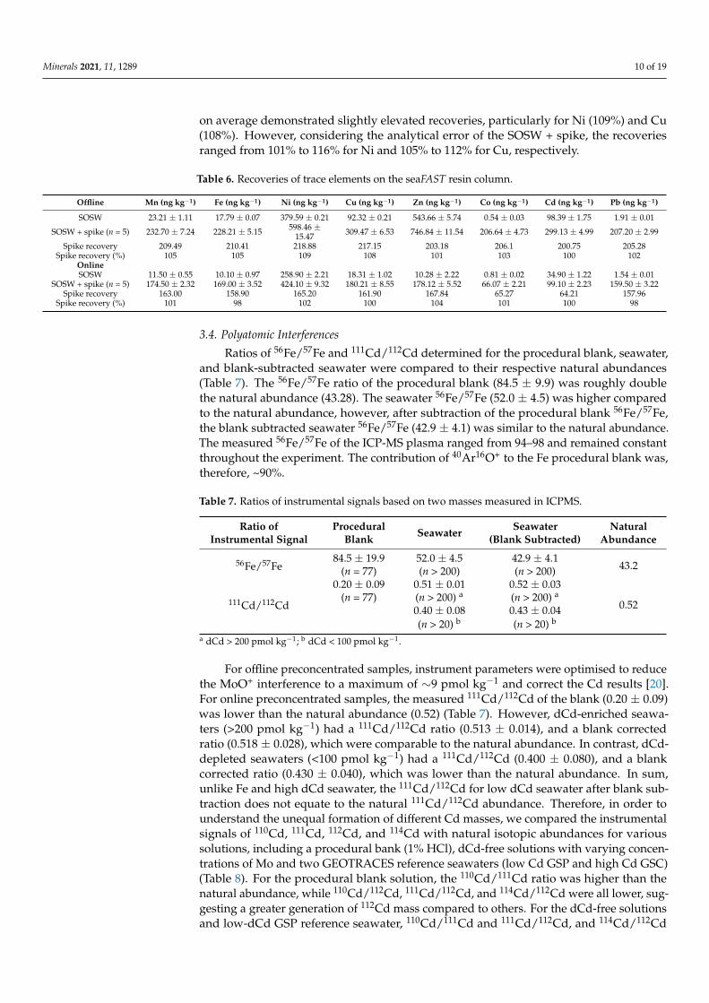
Ratios of 56Fe/57Fe and 111Cd/112Cd determined for the procedural blank, seawater,and blank-subtracted seawater were compared to their respective natural abundances(Table 7). The 56Fe/57Fe ratio of the procedural blank (84.5 ± 9.9) was roughly doublethe natural abundance (43.28). The seawater 56Fe/57Fe (52.0 ± 4.5) was higher comparedto the natural abundance, however, after subtraction of the procedural blank 56Fe/57Fe,the blank subtracted seawater 56Fe/57Fe (42.9 ± 4.1) was similar to the natural abundance.The measured 56Fe/57Fe of the ICP-MS plasma ranged from 94–98 and remained constantthroughout the experiment. The contribution of 40Ar16O+ to the Fe procedural blank was,therefore, ~90%.

Table 7. Ratios of instrumental signals based on two masses measured in ICPMS.

Ratio ofInstrumental Signal

ProceduralBlank Seawater Seawater

(Blank Subtracted)Natural

Abundance

56Fe/57Fe84.5 ± 19.9 52.0 ± 4.5 42.9 ± 4.1

43.2(n = 77) (n > 200) (n > 200)

111Cd/112Cd

0.20 ± 0.09 0.51 ± 0.01 0.52 ± 0.03

0.52(n = 77) (n > 200) a (n > 200) a

0.40 ± 0.08 0.43 ± 0.04(n > 20) b (n > 20) b

a dCd > 200 pmol kg−1; b dCd < 100 pmol kg−1.

For offline preconcentrated samples, instrument parameters were optimised to reducethe MoO+ interference to a maximum of ∼9 pmol kg−1 and correct the Cd results [20].For online preconcentrated samples, the measured 111Cd/112Cd of the blank (0.20 ± 0.09)was lower than the natural abundance (0.52) (Table 7). However, dCd-enriched seawa-ters (>200 pmol kg−1) had a 111Cd/112Cd ratio (0.513 ± 0.014), and a blank correctedratio (0.518 ± 0.028), which were comparable to the natural abundance. In contrast, dCd-depleted seawaters (<100 pmol kg−1) had a 111Cd/112Cd (0.400 ± 0.080), and a blankcorrected ratio (0.430 ± 0.040), which was lower than the natural abundance. In sum,unlike Fe and high dCd seawater, the 111Cd/112Cd for low dCd seawater after blank sub-traction does not equate to the natural 111Cd/112Cd abundance. Therefore, in order tounderstand the unequal formation of different Cd masses, we compared the instrumentalsignals of 110Cd, 111Cd, 112Cd, and 114Cd with natural isotopic abundances for varioussolutions, including a procedural bank (1% HCl), dCd-free solutions with varying concen-trations of Mo and two GEOTRACES reference seawaters (low Cd GSP and high Cd GSC)(Table 8). For the procedural blank solution, the 110Cd/111Cd ratio was higher than thenatural abundance, while 110Cd/112Cd, 111Cd/112Cd, and 114Cd/112Cd were all lower, sug-gesting a greater generation of 112Cd mass compared to others. For the dCd-free solutionsand low-dCd GSP reference seawater, 110Cd/111Cd and 111Cd/112Cd, and 114Cd/112Cd

Minerals 2021, 11, 1289 11 of 19

values strongly deviated from their respective natural abundance, whereas 110Cd/112Cdequated well with the natural abundance. For the high-Cd GSC reference seawater, all Cdisotopic ratios considered were comparable with their natural abundances.

Table 8. Ratios of instrumental signals based on multiple Cd masses.

Material 110Cd/111Cd 110Cd/112Cd 111Cd/112Cd 114Cd/112Cd

Natural abundance 0.97 0.52 0.53 1.19Solution1% HCl 1.66 ± 0.45 0.33 ± 0.06 0.23 ± 0.05 0.98 ± 0.08

dCd-free solutionMo (13.5 nmol kg−1) 0.63 ± 0.12 0.52 ± 0.10 0.83 ± 0.01 1.49 ± 0.11

Mo (53.3 nmol kg−1) a 0.53 0.49 0.83 1.56Mo (117.2 nmol kg−1) 0.56 ± 0.03 0.52 ± 0.10 0.83 ± 0.01 1.49 ± 0.11Mo (248.9 nmol kg−1) 0.56 ± 0.03 0.50 ± 0.01 0.88 ± 0.04 1.62 ± 0.03Mo (543.5 nmol kg−1) 0.56 ± 0.01 0.50 ± 0.01 0.90 ± 0.01 1.68 ± 0.01

Mo (1006.7 nmol kg−1) a 0.56 0.50 0.90 1.63Reference standard

GSP(dCd: 2 ± 2 pmol kg−1) 0.55 ± 0.01 0.48 ± 0.01 0.83 ± 0.03 1.57 ± 0.06

GSC(dCd: 364 ± 22 pmol kg−1) 0.90 0.47 ± 0.01 0.52 ± 0.01 1.30 ± 0.01

a n = 1.

3.5. Crossover and Intercalibration Stations

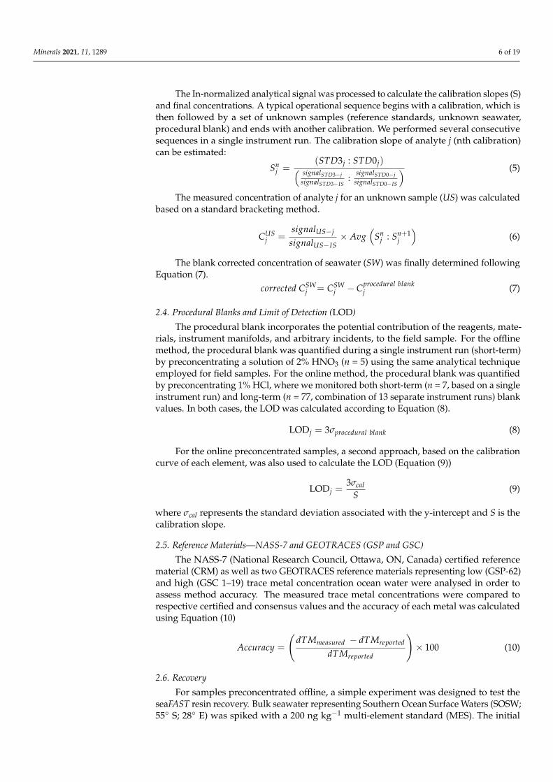
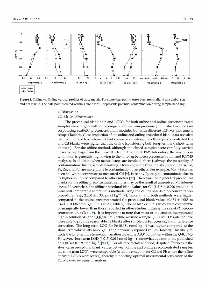
Trace metal concentrations, obtained from both offline and online method variations,at the crossover station are shown graphically in Figure 1. There was a good generalagreement between methods for all trace metals considered. For example, depth compar-isons for all trace metals were within 10% RSD of each other, with the exception of Cuat 125 m where %RSD was 19% (Figure 1). Based on the Cu concentrations above andbelow, it appears the value derived from the online method was an outlier. This outlier iseither related to contamination of the bottle during the second analysis or ICP-MS error.Metals which displayed particularly good vertical profile comparisons were Mn (onlinedMn = 0.96 [offline Mn] + 0.03; r2 = 0.97; p < 0.005), Cd (online Cd = 0.94 [offline Cd] + 44;r2 = 0.94; p < 0.005) and Pb (online Pb = 1.05 [offline Pb] + 0.01; r2 = 0.98; p < 0.005).For Cu, Ni, and Co, a slight offset between method variations was noticeable with theoffline concentrations consistently lower than the online. Offsets were typically around0.20 nmol kg−1 for Cu, 0.3 nmol kg−1 for Ni, and 2.0 pmol kg−1 for Co and small (3%–9%)relative to the respective surface concentrations of these trace metals in seawater. Ironprofiles were not reproduced in the two modes because as per the Fe measurement protocolof the TracEx lab, once opened, we do not reuse samples from the same bottle. The samplealiquots collected in 2015 were, therefore, not reused for Fe measurement in the onlinesetup approximately five years later. Instead of comparing Fe concentration based ononline and offline setups, Fe data was validated by external intercalibration, which showeda good correlation between concentrations measured using the offline method describedhere and by the external laboratory (Figure S2). The correlation equation was calculated asFe = 1.11 [Feexternal)] nmol kg−1 − 0.04; r2 = 0.98; n = 20.

Minerals 2021, 11, 1289 12 of 19

Minerals 2021, 11, 1289 12 of 20

3.5. Crossover and Intercalibration Stations Trace metal concentrations, obtained from both offline and online method variations,

at the crossover station are shown graphically in Figure 1. There was a good general agree-ment between methods for all trace metals considered. For example, depth comparisons for all trace metals were within 10% RSD of each other, with the exception of Cu at 125 m where %RSD was 19% (Figure 1). Based on the Cu concentrations above and below, it appears the value derived from the online method was an outlier. This outlier is either related to contamination of the bottle during the second analysis or ICP-MS error. Metals which displayed particularly good vertical profile comparisons were Mn (online dMn = 0.96 [offline Mn] + 0.03; r2 = 0.97; p < 0.005), Cd (online Cd = 0.94 [offline Cd] + 44; r2 = 0.94; p < 0.005) and Pb (online Pb = 1.05 [offline Pb] + 0.01; r2 = 0.98; p < 0.005). For Cu, Ni, and Co, a slight offset between method variations was noticeable with the offline concentra-tions consistently lower than the online. Offsets were typically around 0.20 nmol kg−1 for Cu, 0.3 nmol kg−1 for Ni, and 2.0 pmol kg−1 for Co and small (3%–9%) relative to the re-spective surface concentrations of these trace metals in seawater. Iron profiles were not reproduced in the two modes because as per the Fe measurement protocol of the TracEx lab, once opened, we do not reuse samples from the same bottle. The sample aliquots collected in 2015 were, therefore, not reused for Fe measurement in the online setup ap-proximately five years later. Instead of comparing Fe concentration based on online and offline setups, Fe data was validated by external intercalibration, which showed a good correlation between concentrations measured using the offline method described here and by the external laboratory (Figure S2). The correlation equation was calculated as Fe = 1.11 [Feexternal)] nmol kg−1 − 0.04; r2 = 0.98; n = 20.

Mn (nmol kg−1)

0.3 0.4 0.5 0.6

Dept

h (m

)

0

100

200

300

400

500

OfflineOnline

Cu (nmol kg−1)

1.8 2.4

Ni (nmol kg−1)

6.0 7.2

Zn (nmol kg− 1)

3 4 5 6 7

Co (pmol kg− 1)

25 30 35 40

Cd (pmol kg− 1)

600 800 1000

Pb (pmol kg− 1)

0 5 10 15 20

Figure 1. Offline vs. Online vertical profiles of trace metals. For some data points, error bars are smaller than symbol size and not visible. The data point isolated within a circle for Cu represents potential contamination during sample handling.

4. Discussion 4.1. Method Performance

The procedural blank data and LOD’s for both offline and online preconcentrated samples were largely within the range of values from previously published methods in-corporating seaFAST preconcentration modules but with different ICP-MS instrument setups (Table 9). Close inspection of the online and offline procedural blank data revealed that, while most trace elements had comparable values, the offline preconcentrated Cu and Cd blanks were higher than the online (considering both long-term and short-term datasets). For the offline method, although the eluted samples were carefully carried in

Figure 1. Offline vs. Online vertical profiles of trace metals. For some data points, error bars are smaller than symbol sizeand not visible. The data point isolated within a circle for Cu represents potential contamination during sample handling.

4. Discussion4.1. Method Performance

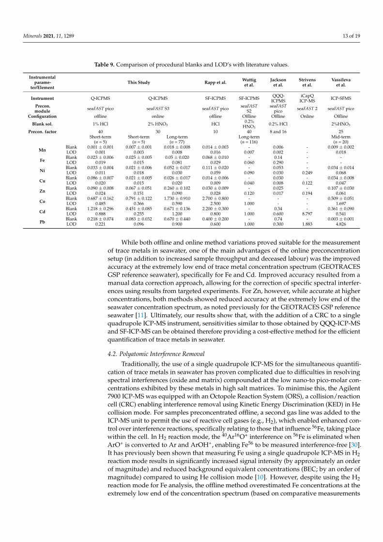
The procedural blank data and LOD’s for both offline and online preconcentratedsamples were largely within the range of values from previously published methods in-corporating seaFAST preconcentration modules but with different ICP-MS instrumentsetups (Table 9). Close inspection of the online and offline procedural blank data revealedthat, while most trace elements had comparable values, the offline preconcentrated Cuand Cd blanks were higher than the online (considering both long-term and short-termdatasets). For the offline method, although the eluted samples were carefully carriedin sealed zip bags from the class 100 clean lab to the ICPMS laboratory, the risk of con-tamination is generally high owing to the time-lag between preconcentration and ICPMSanalyses. In addition, when manual steps are involved, there is always the possibility ofcontamination during sample handling. However, some trace metals (including Cu, Cd,Fe, Zn, and Pb) are more prone to contamination than others. For example, Mo, which hasbeen shown to contribute to measured Cd [9], is relatively easy to contaminate due toits higher solubility compared to other metals [29]. Therefore, the higher Cd proceduralblanks for the offline preconcentrated samples may be the result of unresolved Mo interfer-ences. Nevertheless, the offline procedural blank values for Cd (1.218 ± 0.296 pmol kg−1)were still comparable to previous methods using the offline seaFAST preconcentrationprocedure, (e.g., 2.200 ± 0.300 pmol kg−1 [9]; Table 9), and both methods were highercompared to the online preconcentrated Cd procedural blank values (0.451 ± 0.085 to0.671 ± 0.136 pmol kg−1, this study, Table 9). The Fe blanks in this study were comparableor marginally lower than those reported in other studies utilising the seaFAST precon-centration unit (Table 9). It is important to note that most of the studies incorporatedhigh-resolution SF- and QQQ-ICPMS, while we used a single Q-ICPMS. Despite that, wewere able to provide reasonable Fe blanks after simple post-processing and interferencecorrection. The long-term LOD for Fe (0.081 nmol kg−1) was higher compared to theshort-term value (0.015 nmol kg−1) and previously reported values (Table 9). This likely re-flects the long-term instrumental variation regarding ArO+ formation within the Q-ICPMS.However, short-term LOD (0.015–0.019 nmol kg−1) somewhat equates to the publisheddata (0.060–0.029 nmol kg−1; [9,11]). For all trace metals analysed, despite differences in theshort-term procedural blank values between offline and online preconcentrated samples,the short-term LOD’s were comparable (with the exception for Cd and Pb where the onlinederived LOD’s were lower), thereby supporting optimal instrumental sensitivity of theICPMS over 4+ years of analysis.

Minerals 2021, 11, 1289 13 of 19

Table 9. Comparison of procedural blanks and LOD’s with literature values.

Instrumentalparame-

ter/ElementThis Study Rapp et al. Wuttig

et al.Jackson

et al.Strivens

et al.Vassileva

et al.

Instrument Q-ICPMS Q-ICPMS SF-ICPMS SF-ICPMS QQQ-ICPMS

iCapQICP-MS ICP-SFMS

Precon.module seaFAST pico seaFAST S3 seaFAST pico seaFAST

S2seaFAST

pico seaFAST 2 seaFAST pico

Configuration offline online offline Offline Offline Online Offline

Blank sol. 1% HCl 2% HNO3 HCl 0.2%HNO3

0.2% HCl 2%HNO3

Precon. factor 40 30 10 40 8 and 16 25Short-term

(n = 5)Short-term

(n = 5)Long-term

(n = 77)Long-term(n = 116)

Mid-term(n = 20)

MnBlank 0.001 ± 0.001 0.007 ± 0.001 0.018 ± 0.008 0.014 ± 0.003 - 0.006 - 0.009 ± 0.002LOD 0.001 0.003 0.008 0.016 0.007 0.002 - 0.018

FeBlank 0.023 ± 0.006 0.025 ± 0.005 0.05 ± 0.020 0.068 ± 0.010 - 0.14 - -LOD 0.019 0.015 0.081 0.029 0.060 0.290 - -

NiBlank 0.033 ± 0.004 0.021 ± 0.006 0.052 ± 0.017 0.111 ± 0.020 - 0.053 - 0.034 ± 0.014LOD 0.011 0.018 0.030 0.059 0.090 0.030 0.249 0.068

CuBlank 0.086 ± 0.007 0.021 ± 0.005 0.026 ± 0.017 0.014 ± 0.006 - 0.030 - 0.034 ± 0.008LOD 0.020 0.015 0.020 0.009 0.040 0.008 0.122 0.047

ZnBlank 0.090 ± 0.008 0.067 ± 0.051 0.260 ± 0.102 0.030 ± 0.009 - 0.025 - 0.107 ± 0.030LOD 0.024 0.151 0.090 0.028 0.120 0.017 0.194 0.061

CoBlank 0.687 ± 0.162 0.791 ± 0.122 1.730 ± 0.910 2.700 ± 0.800 - - - 0.509 ± 0.051LOD 0.485 0.366 0.590 2.500 1.000 - - 1.697

CdBlank 1.218 ± 0.296 0.451 ± 0.085 0.671 ± 0.136 2.200 ± 0.300 - 0.34 - 0.361 ± 0.090LOD 0.888 0.255 1.200 0.800 1.000 0.600 8.797 0.541

PbBlank 0.218 ± 0.074 0.083 ± 0.032 0.670 ± 0.440 0.400 ± 0.200 - 0.74 - 0.003 ± 0.001LOD 0.221 0.096 0.900 0.600 1.000 0.300 1.883 4.826

While both offline and online method variations proved suitable for the measurementof trace metals in seawater, one of the main advantages of the online preconcentrationsetup (in addition to increased sample throughput and deceased labour) was the improvedaccuracy at the extremely low end of trace metal concentration spectrum (GEOTRACESGSP reference seawater), specifically for Fe and Cd. Improved accuracy resulted from amanual data correction approach, allowing for the correction of specific spectral interfer-ences using results from targeted experiments. For Zn, however, while accurate at higherconcentrations, both methods showed reduced accuracy at the extremely low end of theseawater concentration spectrum, as noted previously for the GEOTRACES GSP referenceseawater [11]. Ultimately, our results show that, with the addition of a CRC to a singlequadrupole ICP-MS instrument, sensitivities similar to those obtained by QQQ-ICP-MSand SF-ICP-MS can be obtained therefore providing a cost-effective method for the efficientquantification of trace metals in seawater.

4.2. Polyatomic Interference Removal

Traditionally, the use of a single quadrupole ICP-MS for the simultaneous quantifi-cation of trace metals in seawater has proven complicated due to difficulties in resolvingspectral interferences (oxide and matrix) compounded at the low nano-to pico-molar con-centrations exhibited by these metals in high salt matrices. To minimise this, the Agilent7900 ICP-MS was equipped with an Octopole Reaction System (ORS), a collision/reactioncell (CRC) enabling interference removal using Kinetic Energy Discrimination (KED) in Hecollision mode. For samples preconcentrated offline, a second gas line was added to theICP-MS unit to permit the use of reactive cell gases (e.g., H2), which enabled enhanced con-trol over interference reactions, specifically relating to those that influence 56Fe, taking placewithin the cell. In H2 reaction mode, the 40Ar16O+ interference on 56Fe is eliminated whenArO+ is converted to Ar and ArOH+, enabling Fe56 to be measured interference-free [30].It has previously been shown that measuring Fe using a single quadrupole ICP-MS in H2reaction mode results in significantly increased signal intensity (by approximately an orderof magnitude) and reduced background equivalent concentrations (BEC; by an order ofmagnitude) compared to using He collision mode [10]. However, despite using the H2reaction mode for Fe analysis, the offline method overestimated Fe concentrations at theextremely low end of the concentration spectrum (based on comparative measurements

Minerals 2021, 11, 1289 14 of 19

of the GEOTRACES GSP low-Fe reference seawater; Table 5), suggesting Fe interferenceswere not fully removed. Similarly, the reduced accuracy of Cd measurements for the GSPreference seawater also suggested unresolved interferences compounded at extremely lowconcentrations. For Zn, there are no apparent interferences on 66Zn [31], therefore, thereduced accuracy in the GSP reference seawater indicates a loss of sensitivity. Furthermore,switching between He collision mode and H2 reaction mode for each sample resulted intime-consuming analyses.

In order to address these issues, the online method variation was developed, whichsignificantly increased sample throughput and reduced labour time. In addition, datawas processed manually (instead of using the MassHunter software), which allowed en-hanced control of necessary interference corrections (e.g., Fe and Cd) based on quantitativedata from various targeted experiments as discussed below. We show that accuratelymeasuring Fe in He collision mode is possible but only with the necessary interferencecorrections. Likewise, for Cd, correcting for specific interferences allowed for more accuratemeasurements over a wide concentration range.

4.2.1. Recalculation of Fe

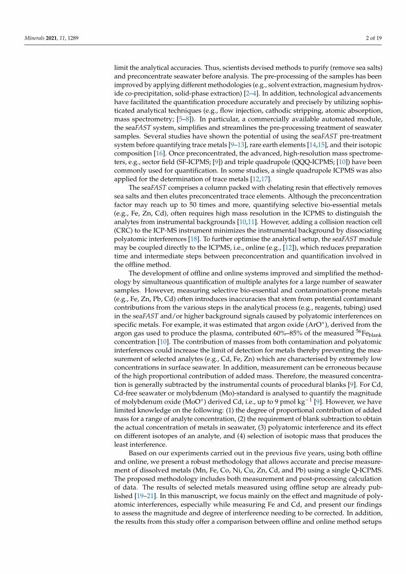
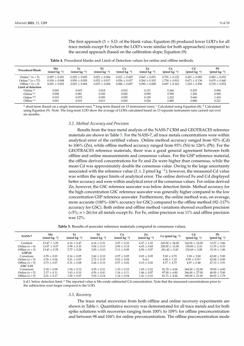
The high ratio of 56Fe/57Fe in the procedural blank, with respect to the natural isotopicabundance, suggests that the formation of 40Ar16O+ increases the instrumental signal of56Fe. This is consistent with measured 56Fe/57Fe in seawater also being above natural iso-topic abundance. Therefore, we validate Fe measurements by showing the blank subtractedFe concentrations (with 56Fe/57Fe similar to the natural isotopic abundance) calculatedbased on 56Fe and 57Fe masses, which follow the line of equity with an agreement of betterthan 20% (Figure 2a). We further subtract the proportional contribution of 40Ar16O+ and re-port the blank concentration of Fe (0.05 ± 0.02 nmol kg−1, n = 77, Table 4). The contributionof 40Ar16O+ is generally high for low Fe concentrations and noticeable up to 10 nmol kg−1

(Figure 2b). Hence, blank subtraction is essential to measure Fe concentrations accuratelyin seawater.

4.2.2. Recalculation of Cd

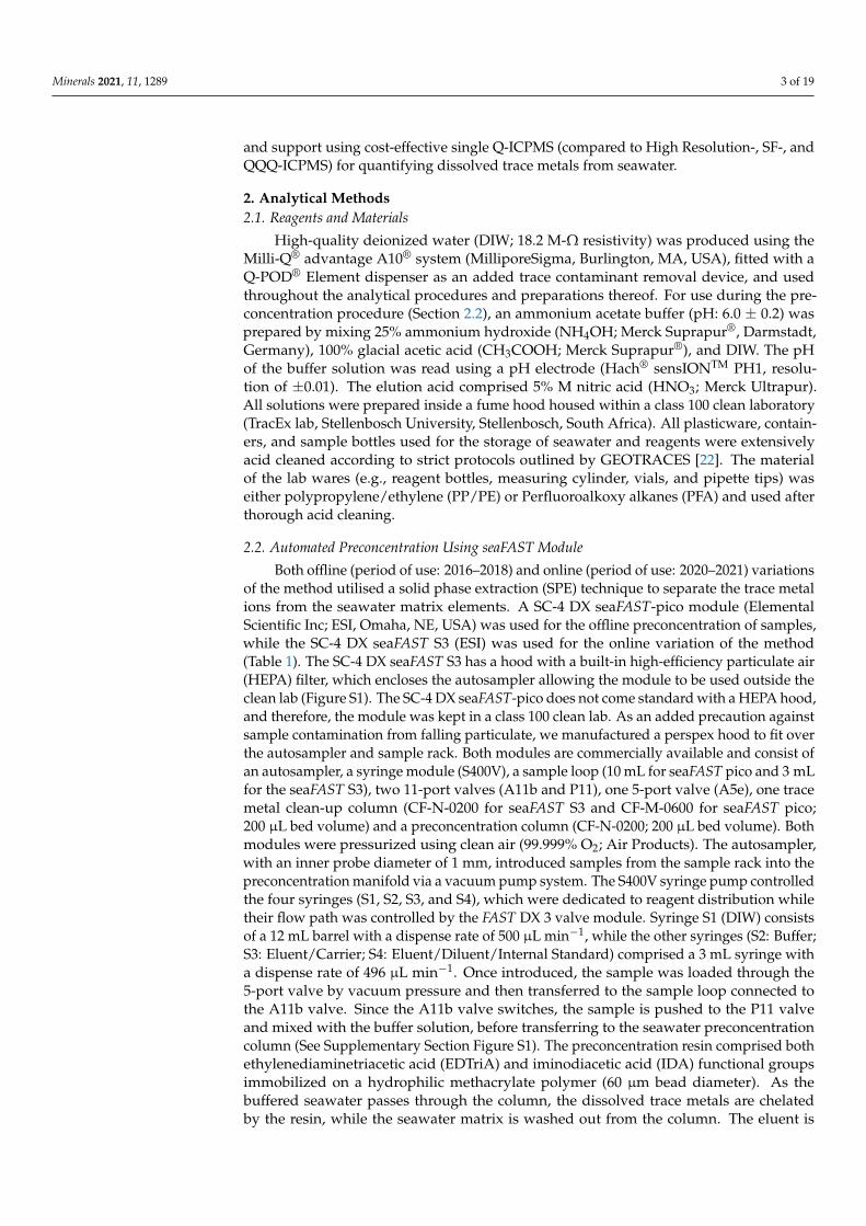
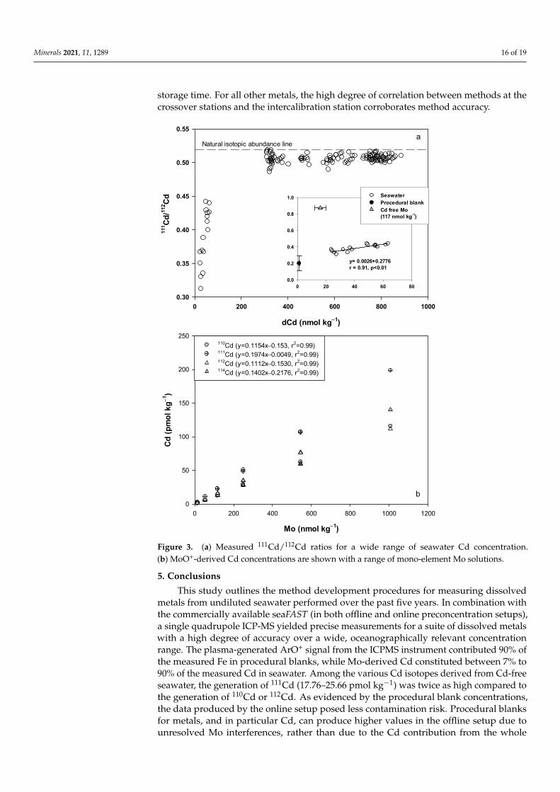
For Cd, the high 110Cd/111Cd and low 110Cd/112Cd, 111Cd/112Cd and 114Cd/112Cd ofthe blank as well as the low 111Cd/112Cd of Cd-depleted seawaters (Figure 3a), relative tothe respective natural isotopic abundances, indicates the preferential generation of 112Cdover 111Cd from the plasma. This likely reflects the contribution of plasma derived 40Ar16O+

on the instrumental signal of 112Cd. Cd-depleted seawater further results in a strongpositive correlation between dCd and 111Cd/112Cd, where the y-intercept characterizesthe 111Cd/112Cd-blank (Figure 3a), confirming a greater contribution of plasma-derived112Cd. The presence of Mo in seawater also appeared to contribute to measured Cddespite the buffer pH (6.00 ± 0.2) chosen to limit Mo recovery [32]. Unlike the blanks,the observed instrumental masses for Cd-free Mo solutions showed that the preferentialgeneration of 111Cd and, to a lesser degree, 114Cd masses compared to others (Table 8). Themeasured Cd concentration (based on four Cd masses) of Cd-free solutions increased withincreasing Mo concentrations and showed a strong positive correlation (Figure 3b). Giventhat the Mo concentration in seawater varies between 90–130 nmol kg−1 (e.g., [33–35]),the equations of the Cd/Mo slopes were used to calculate the magnitude of added Cdresulting from polyatomic interference of Mo oxides. The added Cd ranged between9.73–14.21 (based on 110Cd) and 10.23–14.85 pmol kg−1 (based on 112Cd) with varyingMo in seawater. Based on 111Cd and 114Cd signals, the added Cd was higher, between17.76–25.66 pmol kg−1 and 12.45–18.01 pmol kg−1 respectively, because of their preferentialgeneration over 110Cd and 112Cd. Therefore, we recommend monitoring 110Cd or 112Cdmasses while measuring dCd for seawater. We additionally suggest using measured Moconcentration to calculate the magnitude of added Cd, and then to recalculate the actualCd concentrations, particularly for low-dCd seawaters. We applied the above approach torecalculate the dCd concentration for the GEOTRACES GSP reference seawater (sampling

Minerals 2021, 11, 1289 15 of 19

location: 30 N, 140 W; consensus value: 2 ± 2 pmol L−1). Using the Mo concentrationof surface water of the North Pacific Ocean (107 ± 2.5 nM; [34]), dCd was recalculatedwith a range of 0.47–1.23 (0.99 ± 0.35) pmol kg−1. This suggests that the proportionalcontribution of Mo-derived Cd constituted up to 90% of the measured Cd. However,for high-Cd seawater, the proportional contribution of Mo-derived Cd was less than 7%,and therefore had minimal effects on high-Cd concentrations.

Minerals 2021, 11, 1289 15 of 20

from various targeted experiments as discussed below. We show that accurately measur-ing Fe in He collision mode is possible but only with the necessary interference correc-tions. Likewise, for Cd, correcting for specific interferences allowed for more accurate measurements over a wide concentration range.

4.2.1. Recalculation of Fe The high ratio of 56Fe/57Fe in the procedural blank, with respect to the natural isotopic

abundance, suggests that the formation of 40Ar16O+ increases the instrumental signal of 56Fe. This is consistent with measured 56Fe/57Fe in seawater also being above natural iso-topic abundance. Therefore, we validate Fe measurements by showing the blank sub-tracted Fe concentrations (with 56Fe/57Fe similar to the natural isotopic abundance) calcu-lated based on 56Fe and 57Fe masses, which follow the line of equity with an agreement of better than 20% (Figure 2a). We further subtract the proportional contribution of 40Ar16O+ and report the blank concentration of Fe (0.05 ± 0.02 nmol kg−1, n = 77, Table 4). The con-tribution of 40Ar16O+ is generally high for low Fe concentrations and noticeable up to 10 nmol kg−1 (Figure 2b). Hence, blank subtraction is essential to measure Fe concentrations accurately in seawater.

56Fe (nmol kg−1)

0 1 2 3

57Fe

(nm

ol k

g−1 )

0

1

2

3

0.0 0.2 0.4 0.6 0.8 1.00.0

0.2

0.4

0.6

0.8

1.0

Line of equity

10% of Line of equity

20% of Line of equity

Fe (nmol kg−1)

0 2 4 6 8 10 12

56Fe

/57Fe

30

40

50

60

70

80

90

Natural background line

a

b

Figure 2. (a) Measured Fe concentrations, calculated based on 57Fe and 56Fe masses, follow the line of equity. (b) measured 56Fe/57Fe ratios are presented for a range of Fe concentration. Figure 2. (a) Measured Fe concentrations, calculated based on 57Fe and 56Fe masses, follow the lineof equity. (b) measured 56Fe/57Fe ratios are presented for a range of Fe concentration.

4.3. Crossover Stations

For the crossover stations, the slight offset observed in the vertical profiles of Cu, Ni,and Co (Figure 1) potentially stem from differences in storage length times of the samplebottles. Offline preconcentrated samples were analysed approximately one year after sam-ple collection and online preconcentrated samples approximately five years after collection.Previously, it has been suggested that even two years of sample storage at low pH maynot be long enough to dissociate all organically complexed Cu [36]. Therefore, the offsetbetween the vertical profiles of Cu may be due to the incomplete dissociation of organi-cally complexed Cu in the offline preconcentrated samples. To our knowledge, the effectof sample storage time on Ni and Co concentrations has not been directly investigated.However, considering both metals are characterised by strong organic complexes [37,38],it is reasonable to suggest the offset in Ni and Co also stem from differences in sample

Minerals 2021, 11, 1289 16 of 19

storage time. For all other metals, the high degree of correlation between methods at thecrossover stations and the intercalibration station corroborates method accuracy.

Minerals 2021, 11, 1289 17 of 20

dCd (nmol kg−1)

0 200 400 600 800 1000

111 Cd

/112 Cd

0.30

0.35

0.40

0.45

0.50

0.55

Natural isotopic abundance line

0 20 40 60 800.0

0.2

0.4

0.6

0.8

1.0 SeawaterProcedural blankCd free Mo (117 nmol kg-1)

y= 0.0026+0.2776r = 0.91, p<0.01

Mo (nmol kg−1)

0 200 400 600 800 1000 1200

Cd (p

mol

kg−1

)

0

50

100

150

200

250110Cd (y=0.1154x−0.153, r2=0.99)111Cd (y=0.1974x−0.0049, r2=0.99)112Cd (y=0.1112x−0.1530, r2=0.99) 114Cd (y=0.1402x−0.2176, r2=0.99)

a

b

Figure 3. (a) Measured 111Cd/112Cd ratios for a wide range of seawater Cd concentration. (b) MoO+-derived Cd concentrations are shown with a range of mono-element Mo solutions.

4.3. Crossover Stations For the crossover stations, the slight offset observed in the vertical profiles of Cu, Ni,

and Co (Figure 1) potentially stem from differences in storage length times of the sample bottles. Offline preconcentrated samples were analysed approximately one year after sam-ple collection and online preconcentrated samples approximately five years after collec-tion. Previously, it has been suggested that even two years of sample storage at low pH may not be long enough to dissociate all organically complexed Cu [36]. Therefore, the offset between the vertical profiles of Cu may be due to the incomplete dissociation of organically complexed Cu in the offline preconcentrated samples. To our knowledge, the effect of sample storage time on Ni and Co concentrations has not been directly investi-gated. However, considering both metals are characterised by strong organic complexes [37,38], it is reasonable to suggest the offset in Ni and Co also stem from differences in sample storage time. For all other metals, the high degree of correlation between methods at the crossover stations and the intercalibration station corroborates method accuracy.

Figure 3. (a) Measured 111Cd/112Cd ratios for a wide range of seawater Cd concentration.(b) MoO+-derived Cd concentrations are shown with a range of mono-element Mo solutions.

5. Conclusions

This study outlines the method development procedures for measuring dissolvedmetals from undiluted seawater performed over the past five years. In combination withthe commercially available seaFAST (in both offline and online preconcentration setups),a single quadrupole ICP-MS yielded precise measurements for a suite of dissolved metalswith a high degree of accuracy over a wide, oceanographically relevant concentrationrange. The plasma-generated ArO+ signal from the ICPMS instrument contributed 90% ofthe measured Fe in procedural blanks, while Mo-derived Cd constituted between 7% to90% of the measured Cd in seawater. Among the various Cd isotopes derived from Cd-freeseawater, the generation of 111Cd (17.76–25.66 pmol kg−1) was twice as high compared tothe generation of 110Cd or 112Cd. As evidenced by the procedural blank concentrations,the data produced by the online setup posed less contamination risk. Procedural blanksfor metals, and in particular Cd, can produce higher values in the offline setup due tounresolved Mo interferences, rather than due to the Cd contribution from the whole

Minerals 2021, 11, 1289 17 of 19

procedure itself. From these outcomes, we were able to recommend necessary measuresusing a simple instrumental set up to generate the highest-quality data for dissolvedmetals: (1) Monitor multiple isotopes of an analyte to track interferences within the massspectrometer. (2) Blank subtraction is essential to measure Fe concentrations accurately inseawater. (3) Selecting 110Cd or 112Cd masses while analysing Cd from seawater. (4) For low-Cd seawater (<100 pmol kg−1), first quantify the Mo concentration, then recalculate the Cdconcentration based on the measured Mo concentration. Ultimately, this study shows thatwith careful post-processing, accurate analysis of trace metals over a wide range of seawaterconcentrations is achievable using a Q-ICP-MS, making it accessible to even financiallyconstrained laboratories, and suitable for the demands of the GEOTRACES program.

Supplementary Materials: The following are available online at https://www.mdpi.com/article/10.3390/min11111289/s1, Figure S1: Schematic setups of online and offline seaFAST systems, mod-ified from a previous study. Figure S2: Comparison of Fe measurements from this study and anexternal laboratory.

Author Contributions: A.N.R. conceived the study and provided funding. R.C. and J.L. contributedoffline preconcentrated trace metal data, S.S. contributed online preconcentrated trace metal data.R.R. calibrated and optimised the ICPMS instrument for all analyses as well as processing of data.R.C., J.L. and S.S. wrote the manuscript. All authors have read and agreed to the published versionof the manuscript.

Funding: This research was supported by NRF grants to AR (#UID 93069, 105826 and 110715). RyanCloete was supported through the National Research Foundation (NRF) Innovation PhD scholarship.Jean Loock was supported through the Harry Crossley PhD scholarship. Saumik Samanta wassupported by postdoctoral fellowships awarded by Subcommittee B and the Deputy Vice-Rector,Research, Stellenbosch University.

Data Availability Statement: Please contact the corresponding author.

Acknowledgments: The authors would like to thank the South African National Antarctic Program(SANAP) as well as the captain and crew of the SA Agulhas II for their determined support duringthe cruises. We thank the two anonymous reviewers for their constructive comments.

Conflicts of Interest: The authors declare no conflict of interest.

References1. Anderson, R.F.; Francois, R.H.G.M.; Frank, M.; Henderson, G.M.; Jeandel, C.; Sharma, M. GEOSECS to GEOTRACES: Lessons

Learned from Large Programs Studying Ocean Chemistry. In AGU Fall Meeting Abstracts; American Geophysical Union:Washington, DC, USA, 2019; p. OS41A-05.

2. Bruland, K.W.; Franks, R.P. Sampling and analytical methods for the determination of copper, cadmium, zinc and nickel at thenanogram per litre level in seawater. Anal. Chim. Acta 1979, 28, 367–376. [CrossRef]

3. Wu, J.; Boyle, E.A. Low Blank Preconcentration Technique for the Determination of Lead, Copper, and Cadmium in Small-VolumeSeawater Samples by Isotope Dilution ICPMS. Anal. Chem. 1997, 69, 2464–2470. [CrossRef] [PubMed]

4. Wells, M.L.; Bruland, K.W. An improved method for rapid preconcentration and determination of bioactive trace metals inseawater using solid phase extraction and high resolution inductively coupled plasma mass spectrometry. Mar. Chem. 1998, 63,145–153. [CrossRef]

5. Bowie, A.R.; Achterberg, E.P.; Mantoura, R.F.C.; Worsfold, P.J. Determination of sub-nanomolar levels of iron in seawater usingflow injection with chemiluminescence detection. Anal. Chim. Acta 1998, 361, 189–200. [CrossRef]

6. Colombo, C.; van den Berg, C.M.G. Simultaneous determination of several trace metals in seawater using cathodic strippingvoltammetry with mixed ligands. Anal. Chim. Acta 1997, 337, 29–40. [CrossRef]

7. Kingston, H.M.; Barnes, I.L.; Brady, T.J.; Rains, T.C.; Champ, M.A. Separation of eight transition elements from alkali and alkalineearth elements in estuarine and seawater with chelating resin and their determination by graphite furnace atomic absorptionspectrometry. Anal. Chem. 1978, 50, 2064–2070. [CrossRef]

8. King, D.W.; Lin, J.; Kester, D.R. Spectrophotometric determination of iron (II) in seawater at nanomolar concentrations. Anal. Chim. Acta1991, 247, 125–132. [CrossRef]

9. Rapp, I.; Schlosser, C.; Rusiecka, D.; Gledhill, M.; Achterberg, E.P. Automated preconcentration of Fe, Zn, Cu, Ni, Cd, Pb, Co, andMn in seawater with analysis using high-resolution sector field inductively-coupled plasma mass spectrometry. Anal. Chim. Acta2017, 976, 1–13. [CrossRef]

Minerals 2021, 11, 1289 18 of 19

10. Jackson, S.L.; Spence, J.; Janssen, D.J.; Ross, A.R.S.; Cullen, J.T. Determination of Mn, Fe, Ni, Cu, Zn, Cd and Pb in seawater usingoffline extraction and triple quadrupole ICP-MS/MS. J. Anal. At. Spectrom. 2018, 33, 304–313. [CrossRef]

11. Wuttig, K.; Townsend, A.T.; van der Merwe, P.; Gault-Ringold, M.; Holmes, T.; Schallenberg, C.; Latour, P.; Tonnard, M.;Rijkenberg, M.J.A.; Lannuzel, D.; et al. Critical evaluation of a SeaFAST system for the analysis of trace metals in a wide range ofmarine samples. Talanta 2019, in press. [CrossRef]

12. Strivens, J.E.; Brandenberger, J.M.; Johnston, R.K. Data trend shifts induced by method of concentration for trace metals inseawater: Automated online preconcentration vs. borohydride reductive coprecipitation of nearshore seawater samples foranalysis of Ni, Cu, Zn, Cd, and Pb via ICP-MS. Limnol. Oceanogr. Methods 2019, 17, 266–276. [CrossRef]

13. Vassileva, E.; Wysocka, I.; Orani, A.M.; Quétel, C. Off-line preconcentration and inductively coupled plasma sector field massspectrometry simultaneous determination of Cd, Co, Cu, Mn, Ni, Pb and Zn mass fractions in seawater: Procedure validation.Spectrochim. Acta Part B At. Spectrosc. 2019, 153, 19–27. [CrossRef]

14. Wysocka, I.; Vassileva, E. Method validation for high resolution sector field inductively coupled plasma mass spectrometry determi-nation of the emerging contaminants in the open ocean: Rare earth elements as a case study. Spectrochim. Acta Part B At. Spectrosc.2017, 128, 1–10. [CrossRef]

15. Behrens, M.K.; Muratli, J.; Pradoux, C.; Wu, Y.; Böning, P.; Brumsack, H.J.; Goldstein, S.L.; Haley, B.; Jeandel, C.; Paffrath, R.; et al.Rapid and precise analysis of rare earth elements in small volumes of seawater—Method and intercomparison. Mar. Chem. 2016,186, 110–120. [CrossRef]

16. Vassileva, E.; Wysocka, I. Development of procedure for measurement of Pb isotope ratios in seawater by application of seaFASTsample pre-treatment system and SF ICP-MS. Spectrochim. Acta Part B At. Spectrosc. 2016, 126, 93–100. [CrossRef]

17. Poehle, S.; Schmidt, K.; Koschinsky, A. Determination of Ti, Zr, Nb, V, W and Mo in seawater by a new online-preconcentrationmethod and subsequent ICP-MS analysis. Deep. Res. Part I Oceanogr. Res. Pap. 2015, 98, 83–93. [CrossRef]

18. Tanner, S.D.; Baranov, V.I. Theory, Design, and Operation of a Dynamic Reaction Cell for ICP-MS. At. Spectrosc. 1999, 20, 45–78.[CrossRef]

19. Cloete, R.; Loock, J.C.; Mtshali, T.; Fietz, S.; Roychoudhury, A.N. Winter and summer distributions of Copper, Zinc and Nickelalong the International GEOTRACES Section GIPY05: Insights into deep winter mixing. Chem. Geol. 2019, 511, 342–357. [CrossRef]

20. Cloete, R.; Loock, J.C.; van Horsten, N.R.; Fietz, S.; Mtshali, T.N.; Planquette, H.; Roychoudhury, A.N. Winter biogeo-chemical cycling of dissolved and particulate cadmium in the Indian sector of the Southern Ocean (GEOTRACES GIpr07transect). Front. Mar. Sci. 2021, 8, 1014. [CrossRef]

21. Cloete, R.; Loock, J.C.; van Horsten, N.R.; Menzel Barraqueta, J.-L.; Fietz, S.; Mtshali, T.N.; Planquette, H.; García-Ibáñez, M.I.;Roychoudhury, A.N. Winter dissolved and particulate zinc in the Indian Sector of the Southern Ocean: Distribution and relationto major nutrients (GEOTRACES GIpr07 transect). Mar. Chem. 2021, 236, 104031. [CrossRef]

22. Cutter, G.; Casciotti, K.; Croot, P.; Geibert, W.; Heimbürger, L.-E.; Lohan, M.; Planquette, H.; van de Flierdt, T. Sampling andSample-Handling Protocols for GEOTRACES Cruises; GEOTRACES International Project Office: Toulouse, France, 2017.

23. Byrd, J.T.; Andreae, M.O. Dissolved and particulate tin in North Atlantic seawater. Mar. Chem. 1986, 19, 193–200. [CrossRef]24. McKelvey, B.A.; Orians, K.J. Dissolved zirconium in the North Pacific Ocean. Geochim. Cosmochim. Acta 1993, 57, 3801–3805.

[CrossRef]25. Bekov, G.I.; Letokhov, V.S.; Radaev, V.N.; Baturin, G.N.; Egorov, A.S.; Kursky, A.N.; Narseyev, V.A. Ruthenium in the ocean.

Nature 1984, 312, 748–750. [CrossRef]26. Liu, K.; Gao, X.; Li, L.; Chen, C.T.A.; Xing, Q. Determination of ultra-trace Pt, Pd and Rh in seawater using an off-line pre-

concentration method and inductively coupled plasma mass spectrometry. Chemosphere 2018, 212, 429–437. [CrossRef]27. Feldmann, I.; Jakubowski, N.; Stuewer, D. Application of a hexapole collision and reaction cell in ICP-MS Part I: Instrumental

aspects and operational optimization. Fresenius J. Anal. Chem. 1999, 365, 415–421. [CrossRef]28. Yamada, N. Kinetic energy discrimination in collision/reaction cell ICP-MS: Theoretical review of principles and limitations.

Spectrochim. Acta Part B At. Spectrosc. 2015, 110, 31–44. [CrossRef]29. Smedley, P.L.; Kinniburgh, D.G. Molybdenum in natural waters: A review of occurrence, distributions and controls. Appl. Geochem.

2017, 84, 387–432. [CrossRef]30. Arnold, T.; Harvey, J.N.; Weiss, D.J. An experimental and theoretical investigation into the use of H2 for the simultaneous removal

of ArO+ and ArOH+ isobaric interferences during Fe isotope ratio analysis with collision cell based Multi-Collector InductivelyCoupled Plasma Mass Spectrometry. Spectrochim. Acta Part B 2008, 63, 666–672. [CrossRef]

31. Sadagopa Ramanujam, V.M.; Yokoi, K.; Egger, N.G.; Dayal, H.H.; Alcock, N.W.; Sandstead, H.H. Polyatomics in zinc isotope ratioanalysis of plasma samples by inductively coupled plasma-mass spectrometry and applicability of nonextracted samples for zinckinetics. Biol. Trace Elem. Res. 1999, 68, 143–158. [CrossRef]

32. Biller, D.V.; Bruland, K.W. Analysis of Mn, Fe, Co, Ni, Cu, Zn, Cd, and Pb in seawater using the Nobias-chelate PA1 resin andmagnetic sector inductively coupled plasma mass spectrometry (ICP-MS). Mar. Chem. 2012, 130–131, 12–20. [CrossRef]

33. Schlitzer, R.; Anderson, R.F.; Dodas, E.M.; Lohan, M.; Geibert, W.; Tagliabue, A.; Bowie, A.; Jeandel, C.; Maldonado, M.T.; Landing,W.M.; et al. The GEOTRACES Intermediate Data Product 2017. Chem. Geol. 2018, 493, 210–223. [CrossRef]

34. Collier, R.W. Molybdenum in the Northeast Pacific Ocean. Limnol. Oceanogr. 1985, 30, 1351–1354. [CrossRef]

Minerals 2021, 11, 1289 19 of 19

35. Ho, P.; Lee, J.-M.; Heller, M.I.; Lam, P.J.; Shiller, A.M. The distribution of dissolved and particulate Mo and V along the U.S.GEOTRACES East Pacific Zonal Transect (GP16): The roles of oxides and biogenic particles in their distributions in the oxygendeficient zone and the hydrothermal plume. Mar. Chem. 2018, 201, 242–255. [CrossRef]

36. Posacka, A.M.; Semeniuk, D.M.; Whitby, H.; Van Den Berg, C.M.; Cullen, J.T.; Orians, K.; Maldonado, M.T. Dissolved copper(dCu) biogeochemical cycling in the subarctic Northeast Pacific and a call for improving methodologies. Mar. Chem. 2017, 196,47–61. [CrossRef]

37. Saito, M.A.; Moffett, W. Cobalt and nickel in the Peru upwelling region: A major flux of labile cobalt utilized as a micronutrient.Glob. Biogeochem. Cycles 2004, 18, GB4030. [CrossRef]

38. Morel, F.M.M.; Milligan, A.J.; Saito, M.A. Marine Bioinorganic Chemistry: The Role of Trace Metals in the Oceanic Cycles ofMajor Nutrients. In Treatise on Geochemistry, 2nd ed.; Holland, H.D., Turekian, K.K., Eds.; Elsevier: Amsterdam, The Netherlands,2014; pp. 123–150. [CrossRef]