Determinants of foreign direct investment across China

Journal of International Money and Finance21 (2002) 79–113

www.elsevier.com/locate/econbase

Determinants of foreign direct investmentacross China

Qian Suna, Wilson Tongb,*, Qiao Yu c, d

aDivision of Banking and Finance, Nanyang Business School, Nanyang Technological University,Singapore, Singapore 639798

bDepartment of Accountancy, Faculty of Business and Information Systems, The Hong KongPolytechnic University, Hong Hum, Kowloon, Hong Kong, People’s Republic of China

cDepartment of Finance, Fudan University, Shanghai, People’s Republic of ChinadDepartment of Economics, National University of Singapore, Singapore, Singapore 119074

Abstract

We analyze the spatial and temporal variation in foreign direct investment (FDI) amongChina’s 30 provinces from 1986 to 1998. Motivated by Naughton (Brooklings Pap EconoActiv 2 (1996) 273), we distinguish our study from similar studies by examining changes inimportance of FDI determinants through time. We do find supporting evidence. This is dueto the shift in the nature of FDI in China. We also find that the cumulative FDI relative tocumulative domestic investment has a negative impact on the new FDI. Provincial officialshave to improve the investment environment. Otherwise, multinational corporations maychoose to invest in provinces with fewer FDI competitors. Our analysis is robust across differ-ent specifications. However, it explains the FDI distribution in the coastal provinces better thanit does for Central and Western provinces. 2002 Elsevier Science Ltd. All rights reserved.

JEL classification:F21; F30

Keywords:Foreign direct investment; Foreign portfolio investment; Location theory; Agglomeration;China

* Corresponding author. Tel.:+852-2766-4399; fax:+852-2356-9550.E-mail addresses:[email protected] (Q. Sun); [email protected] (W. Tong).

0261-5606/02/$ - see front matter 2002 Elsevier Science Ltd. All rights reserved.PII: S0261 -5606(01)00032-8

80 Q. Sun et al. / Journal of International Money and Finance 21 (2002) 79–113

1. Introduction

Interest in the study of foreign direct investment (FDI) has grown rapidly. Existingstudies of FDI in the US help us to understand factors that are important to attractingforeign investments across different states.1 In this paper, we examine if these factorsare also important for FDI distribution across different provinces in a developingcountry, China. For sure, there are many studies of FDI on developing countries butmost of them are cross-country analyses.2 As such, the interwoven relationshipsbetween social, cultural, economic, and political factors are difficult to delineate. Byfocusing on only one country, we can make a cleaner study on the economicdetermining factors that attract FDI.

Analysis of FDI in China is also timely. After China’s successful talks with theUS and the European Union on WTO and US granting China PNTR, China enteringinto the WTO is almost a sure thing. China’s entering of the WTO would likelysparkle another round of FDI projects. MNCs in Shanghai and Tianjin have alreadyplanned to expand their investment scale in China. Erickson plans to double itscurrent investment amount of US$3 billion by 2001. On the other hand, China haspromised to open more of its servicing industries to foreign investments, especiallyon areas like financial sector, insurance, telecommunication, trade, and tourism. Infact, China has already been the second largest host of FDI in the world since 1994,next only to the US. An American credit-rating agency projects that by 2005, annualFDI in China will reach U$100 billion.3

However, there are only a few empirical studies on the overall FDI situation inChina. Wang and Swain (1995) examine the host country determinants of FDI inChina. They find that the FDI in manufacturing sector is positively related to China’sGDP, GDP growth, wages, and trade barriers, but negatively related to interest rateand exchange rate for the period of 1978–1992. Chen et al. (1995) study the effectof FDI on China’s output and find that the FDI has a positive impact on the outputgrowth between 1978 and 1990. Using cross-country data, Wei (1995a,b) find thatdespite the large amount of FDI China has received in recent years, the country stillappears to host too little FDI compared to an ‘average’ host country.

The present analysis focuses upon the spatial and temporal variation in FDI amongChina’s all 30 provinces from 1986 to 1998. Such studies are minimal except a fewthat use data at the city level with a relatively short time span. Heid and Ries (1996)study 931 joint ventures in 54 cities from 1984 to 1991. They intentionally excludeinvestments by overseas Chinese (Hong Kong, Macau, Singapore) which probablyhave a different set of location determinants due to familial, linguistic, and culturalties. Their conditional logit regression shows that cities with good infrastructure,established industrial base and foreign investment presence are more attractive to

1 See Coughlin et al. (1991), Graham and Krugman (1991), Lipsey (1993), Klein and Rosengren(1994), Heid et al. (1995) and Hines (1996), among others.

2 See Kravis and Lipsey (1982), Edwards (1990) and Lipsey (1999) and the survey paper by DeMello (1997).

3 Shenzhen Commercial, November 17, 1999.

81Q. Sun et al. / Journal of International Money and Finance 21 (2002) 79–113

investors. Wei (1995a) also looks at individual cities. He finds clear evidence thatin the late 1980s, FDIs contribute to higher growth of the cities.

Kinoshita (1997) examines the data from a special survey conducted by the WorldBank in 1992 on 468 firms in eight cities in China (six located in coastal provincesand two in inland cities). She investigates the possible effects of FDI on improvinga firm’s total factor productivity during the 1990–1992 period. She finds no evidencethat foreign investment helps increase the productivity growth of local firms viaforeign joint ventures, foreign linkages, and the mere presence of foreign firms inthe industry. Hence, she concludes that opening up to foreign investments is notsufficient for a country to benefit from foreign technology spillovers.

Branstetter and Feenstra (1999) have an interesting working paper, which doeslook at FDI in China at the provincial level. However, their focus is different. Theyuse 29 provincial data over the years 1984–1995 to estimate the structural parametersof government’s welfare function. They want to examine the tradeoff between thebenefits of increased trade and FDI against the losses incurred by state-ownedenterprises as a result of such liberalization. Indeed, they find that the governmentplaces much heavier weights on the output of the state-owned enterprises than onconsumer welfare, although such preference has declined somewhat over time. Theyhence post skepticism on China’s entering into the WTO. Similar to our study is apaper by Cheng and Kwan (1999). They look at data from 29 provinces from 1986to 1995 and observe agglomeration effects of foreign capital stock.

However, there is an important fact that none of these studies has taken accountinto, and that is the big differences in the scale and nature of FDIs in the 1980s andthe 1990s. In his important paper, Naughton (1996) points out the critical role thatHong Kong and Taiwan has played on the FDI in Guangdong and Fujian provinces,especially in the 1980s and early 1990s. The total FDI never exceeded 1 percent ofGDP before 1991 with over 40 percent of all FDI in Guangdong and 10 percent inFujian. This is probably due to the linguistic and cultural ties of Guangdong withHong Kong and Fujian with Taiwan. In fact, between 1984 and 1990, Hong Kongaccounted over 50 percent of China’s total FDI all along (Wei, 1995a,b). Naughton(1996) also points out that until 1991 virtually all of the industrial output of FDIwas exported. Such lop-sided phenomenon began to fade away when China beganto offer significant domestic market access to foreign investors in 1992. The outputof these foreign-invested enterprises (FIEs) has increasingly been directed towardthe domestic market. Given this, it is conceivable that the factors drawing FDI intoChina in the early period may not be the same, or at least may not be as importantas those in the later period. Pooling everything together under one regression modelhence ignores the possible dynamic complexity of the issue.

As an attempt to address Naughton’s point, our paper makes contributions onthis line of research by examining FDI determinants over different periods of time.Furthermore, we contrast results based on the full sample of 30 provinces againstthose based on 28 provinces, excluding Guangdong and Fujian. By doing so, we areable to see if FDI determinants change through time and if Guangdong and Fujian,two of the earliest provinces opening to and drawing in most of the FDI, have differ-ent attributes attracting FDI.


Our results do show that the importance of the FDI determinants changes throughtime. However, there is no evidence that Guangdong and Fujian are very differentfrom other provinces in terms of attracting FDI. Surprisingly, we find that the cumu-lative foreign investment relative to the cumulative domestic investment has a nega-tive impact on the new FDI. It provides implications to both policy-makers in Chinaand foreign investors interested in the China market. Specifically, provincial officialshave to improve the investment environment. Otherwise, multinational corporations(MNCs) may choose to invest in provinces with fewer FDI competitors.

The analysis is organized as follows. Section 2 gives an overview of FDI develop-ment in China. Section 3 discusses the conceptual framework. Data and empiricalmethodology are described in Section 4. Section 5 presents the empirical results,and Section 6 concludes the paper.

2. FDI in China

FDI is conventionally defined as a form of international inter-firm cooperationthat involves a significant equity stake in or effective management control of hostcountry enterprises. However, in China, FDI is considered to encompass also other,non-equity co-operations such as contractual joint ventures, compensation trade, andjoint exploration.

2.1. Three stages of FDI development

China has attracted a spectacular amount of FDI since its opening to the outsideworld in 1979. FDI jumps from virtually zero in 1979 to an amount of US$45.46billion in 1998. Its development can be viewed as going through three stages. Firststage starts from 1979 when the “ law of the People’s Republic of China on JointVentures Using Chinese and Foreign Investment” , the first of its kind, was enacted.A state foreign investment commission was established to direct and oversee theinvestment process. Four special economic zones (SEZs) were quickly set up atShenzhen, Zhuhai, Xiamen, and Shantou in the early 1980s. In 1984, 14 more coastalcities and Hainan Island were opened to foreign investment. Furthermore, three zoneswere opened to FDI in early 1985: the Yangtze River delta, the Pearl River delta,and the Zhangzhou–Quanzhou–Xiamen region. FDI hence spread out from the SEZsbut the boom ended in late 1985 due to high inflation. During this stage, foreigninvestments were concentrated in small-sized assembling and processing for exports.

In response to a decline in FDI, the government promulgated the PRC Law onForeign Enterprises in April 1986, formally granting legal rights to wholly ownedforeign enterprises in China. This marks the beginning of the second stage of FDIdevelopment. In October 1986, the State Council further issued the “Provisions forthe Encouragement of Foreign Investment” to encourage foreign investment, permit-ting more freedom of independent operations for FIEs and granting more tax incen-tives for foreign investment. Local governments were also given more authority inreviewing the applications of foreign investment. In 1988, Hainan was incorporated


as another SEZ and the Chinese government further amended the joint venture laws,which included a legal ban on expropriation, relaxed restrictions regarding expatri-ation of profits and dividends, and allowed foreign nationals to be the chairman ofthe board of directors in FIEs. Starting from a very low base, China experienceddouble- or triple-digit annual growth of FDI from 1979 to 1988 and received a totalof US$12.05 billion actual FDI during this period. In contrast to the first stage, over70 percent of FDI projects were involved in manufacturing industries in this stage.

The Tianman Square Incident slowed down the FDI growth rate to a single digitin 1989 and 1990, which ends this second stage of FDI development. To reversethe worsening investment climate, the Chinese government issued the Amendmentsto the Joint Venture Law in April 1990. In 1991, the Income Tax Law for Enterpriseswith Foreign Capital and Foreign Enterprises was passed. FDI situation wasimproved and resumed double-digit growth in 1991. The third stage of FDI develop-ment begins. Following Deng Xiaoping’s South China tour, actual FDI surged by150 percent to US$11 billion in 1992. It surged another 150 percent in 1993 andmaintained the double-digit growth thereafter. In the 1980s, FDI mainly takes theform of contractual or equity joint ventures. However, the wholly owned foreignfirm is the fastest growing form of FDI in the 1990s. It accounts for 40% of theFDI value in 1996. The average capital size of FDI increases, with the main focusshifting to large infrastructure and manufacturing projects.

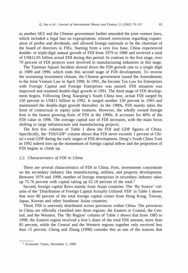
The first few columns of Table 1 show the FDI and GDP figures of China.Specifically, the ‘FDI/GDP’ column shows that FDI never exceeds 1 percent of Chi-na’s total GDP during the early stages of FDI development. Deng’s South China Tourin 1992 indeed stirs up the momentum of foreign capital inflow and the proportion ofFDI begins to climb up.

2.2. Characteristics of FDI in China

There are several characteristics of FDI in China. First, investments concentrateon the secondary industry like manufacturing, utilities, and property development.Between 1979 and 1998, number of foreign enterprises in secondary industry takesup 75.76 percent with capital taking up 62.18 percent of the total.4

Second, foreign capital flows mainly from Asian countries. The ‘By Source’ col-umn of the ‘Distribution of Foreign Capital Actually Utilized: FDI’ in Table 1 showsthat over 80 percent of the total foreign capital comes from Hong Kong, Taiwan,Japan, Korean and other Southeast Asian countries.

Third, FDI is unevenly distributed across provinces within China. The provincesin China are officially classified into three regions: the Eastern or Coastal, the Cen-tral, and the Western. The ‘By Region’ column of Table 1 shows that from 1985 to1998, the Eastern region received a lion’s share of the total FDI amount, more than85 percent, while the Central and the Western regions together only received lessthan 15 percent. Cheng and Zhang (1998) consider this as one of the reasons that

4 Economic Times, December 2, 1999.

84 Q. Sun et al. / Journal of International Money and Finance 21 (2002) 79–113T

able

1B

asic

feat

ures

ofFD

Iin

Chi

na(s

ourc

e:D

RI

CE

ICD

atab

ase

and

vari

ous

issu

esof

the

Stat

istic

alY

earb

ook

ofC

hina

)

Yea

rSt

age

ofG

DP

FDI

FDI/

GD

PD

istr

ibut

ion

offo

reig

nca

pita

lac

tual

lyut

ilize

d:FD

IFD

ID

ev.

(US$

m)

(US$

m)

(%)

By

sour

cea

(%)

By

regi

onB

ypr

ovin

ce(%

)

Asi

aW

este

rnO

ther

sE

aste

rnC

entr

alW

este

rnG

uang

dong

Fujia

nO

ther

prov

ince

1979

–1s

tSt

age

1083

337

1166

0.11

1982

1983

3075

5263

60.

2119

8430

7881

1258

0.41

1985

2993

8716

610.

5567

276

90.1

85.

564.

2646

1144

1986

2nd

Stag

e29

3466

1874

0.64

7423

387

.95

7.28

4.76

506

4419

8731

6614

2314

0.73

8414

388

.58

6.02

5.40

364

5919

8839

5046

3194

0.81

8212

687

.00

5.94

7.06

435

5219

8943

7239

3392

0.78

7714

992

.16

3.84

3.99

3811

5119

9038

2949

3487

0.91

8416

093

.87

3.87

2.26

469

4519

9139

9805

4366

1.09

8213

592

.46

4.48

3.06

4411

45

1992

3rd

Stag

e46

8977

1100

72.

3590

83

91.3

06.

821.

8934

1353

1993

5987

7127

515

4.60

8711

387

.38

8.88

3.74

2811

6219

9454

1737

3376

76.

2384

133

87.8

37.

854.

3128

1160

1995

7006

6637

521

5.36

8215

487

.71

9.21

3.08

2811

6219

9682

1852

4172

65.

0880

155

88.0

49.

522.

4528

10%

6219

9790

3451

4525

75.

0168

1616

86.9

010

.56

2.54

279%

6419

9896

4528

4546

34.

7169

1813

88.0

49.

862.

1030

10%

61

aT

heda

taar

eco

mpu

ted

base

don

DR

IC

EIC

Dat

abas

e,w

hich

grou

psFD

Ian

dot

her

inve

stm

ents

toge

ther

.H

ence

,th

eba

seof

the

perc

enta

gegi

ven

inth

isco

lum

nis

FDI

and

othe

rin

vest

men

ts,

not

the

‘pur

e’FD

Ifig

ures

show

nin

the

tabl

e.


have led to the fast development of the coastal provinces in the east and the wideningof the gap in economic development between coastal and inland provinces since1979. The increasing regional differences have created social and political problems.In order to narrow or slow down the widening of the gap, China’s central governmenthas adopted a series of measures which includes encouraging FDI in the Central andWestern regions. The provinces in these regions also try to jump onto the bandwagonto attract FDI. As a result, the share of FDI in the Central and Western regions havebeen slowly increasing since 1989.

The concentration of FDI in the coastal region can be explained by many factors(Cheng and Zhang, 1998). However, the fact that the coastal region has high popu-lation density but poor natural resources, while inland provinces have low populationdensity but rich natural resources seems to suggest that the purpose of FDI in Chinais mainly for the potential market and labor abundance but not natural resources.

2.3. Macroeconomic impacts of FDI

FDI is expected to help the development of the host countries in various aspects.In China, FDI has significant impact on its trade flows. Sun (1999) notices thatChina’s total trade volume (i.e. export plus import) relative to GDP rose from 15.4percent in 1981 to 26.6 percent in 1995. During the same period, exports by FIEsgrew at an annual rate of 63.3 percent. In the coastal region, the contribution ofFIEs is even more significant. He concludes that FDI is trade-creating in China.Chen (1999) runs cross-sectional regressions on 29 provinces in different years andconfirms that FDI has a positive impact both on promoting China’s host provincetotal trade flows with the rest of the world and on increasing the bilateral trade flowsbetween China and its trade partners.

Yet, about the FDI impact on technological development and economic growth,empirical studies are not conclusive.5 In the case of China, Naughton (1996) castsdoubt that FDI engines China’s economic growth. He highlights a few facts thatlimited the impact of foreign investment on the domestic economy. As stated above,FDI was geographically concentrated, especially in the Guangdong province. SinceGuangdong is relatively small and remote, its benefits from Hong Kong investmentscan hardly spillover to other provinces. Second, until 1991 virtually all of the indus-trial output of FIEs was exported; from which it follows that the domestic marketpresence of foreign firms was insignificant. Furthermore, foreign investment neverexceeded 1 percent of GDP before the 1990s. Hence, the external reforms are only

5 Early studies like those of Caves (1974) on Australia, Globerman (1979) on Canada, and Blomstromand Persson (1983) on Mexico have found a positive impact of FDI on the productivity of local firms.However, later studies like those of Cantwell (1989) on European countries, Haddad and Harrison (1991)on Morocco, Aitken and Harrison (1991) on Venezuela do not find that technological spillovers aresignificant. More recent studies tend to find supporting evidence. See the studies of De Gregorio (1991)on 12 Latin American countries, Blomstrom et al. (1992) on 78 developing countries and 23 developedcountries, Kokko (1994) on 216 Mexican manufacturing industries, Borensztein et al. (1998) on 69developing countries, Hejazi and Safarian (1999) on the OECD countries.


secondary to the main progress of domestic economic reforms in the early stage ofChina’s development. Foreign trade and investment only become important to Chi-na’s economic growth in the 1990s. Kinoshita (1998) focuses on FDI impact onfactor productivity of Chinese firms. Although she finds both ‘catch-up’ and trainingbeing important sources of productivity growth, the effects are more important forlocal-owned firms than foreign-owned firms. Local firms give more training to work-ers whereas foreign firms import intermediate inputs.

Yet, some other studies do find FDI impacts being important to China’s techno-logical development and economic growth. Sit (1985) points out that FDI has pro-vided a substantial impetus in modernizing China’s existing industries, including thetransfer of technological know-how, managerial expertise, and international market-ing skill. Wei (1995b) also finds that in the late 1980s, the contribution to growthcomes mainly from foreign investment. Furthermore, the contribution of foreigninvestment comes in the form of technological or managerial spillovers across firmsas opposed to an infusion of new capital. Based on time series data from 1960 to1991, Zhao (1995) finds that imported technology has significantly enhanced China’stechnological build-up. Chen et al. (1995) study the role of FDI in China’s post-1978 economic development. They find that FDI has positive association with econ-omic growth. The pooled regression results of Sun (1998) on ten coastal provincesfrom 1983 to 1995 confirm that FDI significantly promoted the economic growth ofChina. Shan et al. (1999) apply a six-variable VAR model on China’s quarterly datafrom 1985 to 1996 to examine the causality between FDI and economic growth.They conclude that there is a two-way causality running between the two.

As seen, the impacts of FDI are quite controversial. However, our focus lies onthe provincial characteristics that draw in foreign capital.

3. Determining factors on FDI

As pointed out by Braunerhjelm and Svensson (1996), the theoretical foundationof FDI is rather fragmented, comprising bits and pieces from different fields of eco-nomics to elucidate the locational pattern of firms. Several theories have been putforward to explain the FDI. Hymer (1960) views the MNC as an oligopolist. FDIis considered to be the outcome of broad corporate strategies and investmentdecisions of profit-maximizing firms facing worldwide competition. Dunning (1977)and Rugman (1981) invoke transaction costs to explain firms’ internationalization,putting emphasis on the intangible assets firms have acquired. Bhagwati and Srinava-san (1983) and Grossman and Helpman (1991) use the international trade theory toexplain the allocative aspects of FDI. However, more relevant to our study is thelocation theory, which is often used to explain why a MNC would choose to investin a particular host country. It can also be used to explain why foreign investorswould choose to invest in a specific location within a particular host country.

Previous researchers have identified quite a few determinants for the location ofFDI. In their study on state characteristics and the location of FDI within the US,Coughlin et al. (1991) assume that a foreign firm will choose to invest in a particular


state if and only if doing so will maximize profit. The FDI in a particular statedepends on the levels of its characteristics that affect profits relative to the levels ofthese characteristics in the other states. They identify state land area, per capitaincome, agglomeration, labor market conditions (wage rates, the degree of unioniz-ation, the unemployment rate), transportation network, taxes, and the state expendi-tures to attract FDI as the determinants of FDI across the states within the US. Percapita income and densities of manufacturing activities affect market demand that,in turn, affects the revenue. State land area, labor market conditions, transportationnetwork, taxes and expenditures to attract FDI affect the cost. Their results indicatethat states with higher per capita incomes and higher densities of manufacturingactivities attract relatively more FDI. In addition, higher wages deter FDI, whilehigher unemployment rates attract it. Overall, higher taxes deter FDI; more extensivetransportation infrastructures and larger promotional expenditures are associated withhigher FDI.

Similarly, Bagchi-Sen and Wheeler (1989) find that population size, populationgrowth, and per capita retail sales are important determinants of the spatial distri-bution of FDI among metropolitan areas in the US. Friedman et al. (1996) find thatmarket potential, wage, skilled labor measured by per capita number of scientistsand engineers, construction cost, major port, and funds spent on attracting FDI havesignificant impact on the location of foreign branch plants in the US. Braunerhjelmand Svensson (1996) further show that agglomeration, exports, and R&D areimportant factors affecting Swedish MNCs’ FDI location. Mody and Srinivasan(1998) find that during the 1980s, US and Japanese multinationals were attracted bysome similar country characteristics like low wage inflation, low country risk, goodinfrastructure, and an educated work force. Both groups of investors were alsostrongly attracted to locations with significant past investment.

Xin and Ni (1995) conducted a survey to rank provinces of China with the bestinvestment environment. They identified eight variables with following weightings:market scale 30%, wage level 20%, education level 10%, extent of industrialization10%, transport facilities 10%, communication facilities 10%, living environment 5%,and the level of scientific research 5%.

Built on the above findings, we identify eight potentially important determinantsof FDI distribution across provinces within China, as summarized in Table 2.

First of all, the market demand and market size has positive impact on the FDIbecause it directly affects the expected revenue of the investment. In fact, one majormotivation for FDI is to look for new markets.6 The larger the market size of aparticular province is, other things being constant, the more FDI the province shouldattract. Kravis and Lipsey (1982) and many other empirical studies find such positiverelationship. Blomstrom and Lipsey (1991) show a significant size threshold effectfor firms’ decision to invest abroad. We use GDP, GDP per capita, retail sales, andretail sales per capita to capture demand and size effect. By doing so, we implicitlyassume away the possibility of the demand on a province’s FDI output coming from

6 See Shapiro (1998) for a detailed discussion on FDI motivations.


Table 2The possible determinants of FDI distribution

Category Proxy

1. Market demand and market size GDPGDP per capitaRetail salesRetail sales per capita

2. AgglomerationInfrastructure GDP per km2

Highway per km2 (Highway)Railway per km2 (Railway)

Degree of industrialization Domestic investment (INV)Domestic investment per worker (PERWI)

Level of foreign investment Cumulative domestic investment (CINV)Cumulative FDI (CFDI)CFDI/CINV

3. Labor quality RSET — number of research engineers, scientists andtechnicians as a percent of the total employees

4. Labor Cost Average wage (Wage)5. The level of scientific research R&D expenditures

Number of patentsNumber of universities

6. Degree of Openness Total trade amountImport/GDP

7. Country risk Risk ranking by political risk services8. FDI substitutes Foreign portfolio investment

other provinces.7 According to Young (1997), the provinces in China have onlylimited trade with each other and hence multinationals can only serve the marketwhere they locate. In fact, based on the firm interviews done by Branstetter andFeenstra (1999), even local Chinese firms can hardly develop into truly ‘multi-prov-incial’ enterprises.

Agglomeration refers to the concentration and co-location of economic activitiesthat give rise to the economies of scale and positive externalities. The level ofagglomeration of a particular province should be positively related to the FDI. Fol-lowing Wheeler and Mody (1992), we use infrastructure quality, the degree of indus-trialization, and cumulative foreign investment to capture the agglomeration benefits.The GDP per square kilometer is proxied for the quality of infrastructure. Relatedto infrastructure is the transportation network. More highway and railway mileageper square kilometer are expected to relate positively with FDI. Domestic investmentper worker reflects the degree of industrialization. The cumulative FDI amount cap-tures the possible ‘herding effect’ among foreign investors. Other than the absolutemeasure, we construct also a relative measure, the ratio of the cumulative FDI rela-tive to the cumulative domestic investment, CFDI/CINV. Since both CFDI and CINV

7 We thank the referee for pointing out the assumption we have made.


increase over time, the larger the ratio, the faster the accumulation of FDI relativeto that of domestic investment.

Labor quality should be an important factor for FDI consideration. It is proxiedby the number of research scientists, engineers and technicians per 1000 of theemployees (RSET) which has been used by Braunerhjelm and Svensson (1996). Thisvariable measures the relative endowment of skilled labor in each province andshould have a positive impact on FDI.

Labor cost, as measured by WAGE, is a negative factor to FDI. However, sucha measure is not without problems. Workers in the SOEs are typically provided withhousing benefits and health care whereas workers in the private sector get ‘pure’salaries with cash bonuses (which may not be reported for tax purpose). That weak-ens the ability of the variable to capture the true labor cost.8 On the other hand, inrecent years of fast economic development, China attracts foreign investment notpurely through cheap labor. As reflected in the model of Branstetter and Feenstra(1999), multinational firms in China tend to pay a wage premium to their workers.This may be because multinational firms want to hire quality workers. Higher wagemay well reflect higher labor quality. Hence, it is conceivable that wages in thoseprovinces that can attract relatively more FDIs can be higher, too. Furthermore, aspointed out by Lipsey (1999), most studies show no evidence that low wages, asso-ciated with low per capital real income, were the main attraction for FDI. We willgo back to this variable later.

The level of scientific research indicates the level of human capital and the levelof general development. Measured by R&D expenditures and the number of patents,the higher level of scientific research should promote FDI in a province. Educationis another variable measuring human capital. It is commonly proxied by the percent-age of population (or employee) who have received the secondary or above edu-cation. Since such data are not available, we use the number of universities as arough proxy for the level of education. Of course, the level of education is expectedto have positive impact on the inflow of FDI.

The degree of openness has mixed blessings on FDI. On the one hand, a moreopen economy attracts FDI because it welcomes foreign capital and foreign investorsare more familiar with the host economy. Edwards (1990) finds supporting evidenceon that. But on the other hand, openness can have a negative impact on FDI due tokeen competition. Wheeler and Mody (1992) find that Brazil and Mexico attractedmajor US investment in their sample period despite these two countries have verylow ratings in openness. Hence, the exact relationship between the two is an empiri-cal question. We use the ratio of total import over GDP of a province to measureits degree of openness.9

Political risk is an important factor to consider, especially in developing countries.However, as we are dealing with a single country, the difference in political risk

8 We thank the referee for pointing out this.9 Using total trade value (summation of export and import value) divided by GDP may overstate the

openness of China. See footnote 4 of Naughton (1996) for some of the reasons. We use only the importfigure to hopefully reduce the noise of the proxy.


among different provinces should not be much. We use it only as a macro variableand see how it affects the FDI through time. The variable is constructed using therisk ranking provided by Political Risk Services.

The last factor to consider is the FDI substitutes. FDI brings in a lot of benefitsand one of those is the inflow of foreign capital. A province may not need muchFDI if it can tap the foreign capital market and use the money to invest in the localindustry. In this sense, other means of foreign capital inflow can partly substitutethe need for FDI. One major source we consider is foreign equity capital. We lookat the number of firms in each province that have B-share, H-share, and/or N-shareissues. These are means to raise foreign equity capital. The total number becomesour variable of foreign portfolio investment, FPI. We expect the variable to be nega-tively related to the amount of FDI within the province.

Certainly, there are other commonly used variables like number of tourists, numberof telephone sets, promotion expenditures for attracting FDI, tax structure, and thespecial treatment offered to foreign investors that may have impacts, too. However,such data are either not available or hard to measure. We use fixed effect panel dataanalysis to control for that.

4. Data and methodology

Panel data analysis is adopted because we examine the determinants of FDI distri-bution across provinces and over time. Most of the data used in this study areobtained from various issues of China’s Statistical Yearbook. The Yearbooks providetwo figures of FDI, ‘Signed Agreement’ and ‘Actually Utilized’ . We use the laterone, which is the actual amount of FDI invested in the province. The data on thenumber of firms that issue foreign equity shares are from Datastream. Political riskdata are from Political Risk Yearbook published by Political Risk Services. Theygive an 18-month forecast on the risk level of a country on several aspects. We lookat their forecasts on the risk level of Financial Transfer, Direct Investment, and theCurrency Market in China. During our sample period, their forecasts range from ‘A-’ (lower risk) to ‘B-’ (higher risk). Our risk variable is constructed by assigning ‘1’to ‘A-’ , ‘2’ to ‘B+’ , 3 to ‘B’ , so on and so forth. As such, when the risk level goesup, the variable becomes larger in value.

Due to the lacking of complete set of provincial variables in the early period, oursample begins in 1986 and covers up to 1998. Since GDP, retail sales, domesticinvestment, R&D expenditures, and wage are denominated in RMB (Chinesecurrency) and the FDI in US dollars, we convert the FDI into RMB using yearlyaverage dollar/RMB exchange rate. The swap market rate is used for the period from1986 to 1993 while China was still under the dual exchange rate system. Then allmonetary data are converted to 1990 constant RMB using the relevant deflater10.The Cumulative FDI (CFDI) is the total sum of the FDIs in the previous years. For

10 Retail sales and wage are adjusted by CPI and the others are deflated by the GDP deflator.


instance, the 1990 CFDI is the sum of FDIs up to 1989. Since we do not have thecomplete data history of China’s FDI figure, we take the FDI figure of 1985 as theCFDI figure of 1986. We do not think this would constitute a serious problem asthe amount of FDI relative to the GDP level is very small in the early period anyway,as mentioned before.11

A problem with this data set is the possible high correlation between the variousproxies. It is quite obvious that the proxies listed in Table 2 may overlap with oneanother. This may lead to serious multicollinearity. In order to ascertain the degreeof multicollinearity, we calculate the correlation matrix between all the potentialdeterminants. We will exclude those highly correlated pairs. Specifically, we trans-form all variables into the natural logarithm form and stack these transformed vari-ables up across the 30 provinces, then calculate the correlation coefficients betweenthem.12 The results are presented in Panel A of Table 3.

As expected, high degree of correlation (correlation coefficient of 0.7 or above,as highlighted) exists in many pairs of proxies. To avoid multicollinearity in thesubsequent analysis, we select only seven proxies in our panel regression model. ForMarket Demand factor, we use only the GDP series. For Agglomeration factor, weuse railway length per squared kilometer (RLWAY) to capture the infrastructurelevel. The annual domestic investment per worker (PERWI) is used to capture thedegree of industrialization. As CFDI is highly correlated with GDP, we use therelative measure CFDI/CINV, which is the relative accumulation of foreign invest-ment to domestic investment. For Labor Quality, we only use RSET.

Panel B of Table 3 gives the new correlation matrix for the seven selected proxiesand confirms that none of the variables are highly correlated now. Since we will addtwo more variables, the foreign portfolio investment FPI and the degree of opennessOPEN that have a shorter data span from 1992 to 1998 into our second set of tests,we also want to make sure they are not highly correlated with the seven chosenvariables. The correlation matrix of the nine variables shown in Panel C of Table 3confirms that it is the case.

A general pooled regression model is used on these variables and is specified as

ln(FDIit) � ai � b1 ln(GDPit�1) � b2 ln(PERWIit�1)� b3 ln(WAGEit�1) � b4 ln(RSETit�1) � b5 ln(RLWAYit�1) (1)� b6RISKt � b7 ln(CFDI /CINV)it � �it, (i � 1,2,...,30 and t� 1,2,...,12)

where subscript i refers to individual provinces, t refers to years from 1987 to 1998,and ai is the intercept. Notice that all explanatory variables except RISK and

11 We have tried another approach. We have aggregate FDI figures beginning 1979. Using the provincialproportion of FDI in 1985, we pro-rate the aggregate figures in these early years into different provinces.The sum of the pro-rated FDI figures of a province from 1980 to 1984 with the 1985 figure becomes theCFDI of that province in 1986. The results using this approach are qualitatively the same.

12 Since log 0 is undefined, 10�4 is used to replace the zero whenever it occurs in our data set.


Tab

le3

Cor

rela

tion

mat

rix

for

pote

ntia

lde

term

inan

ts

Pan

elA

:A

llpo

tent

ial

inde

pend

ent

vari

able

sG

DP

GD

P/P

INV

CIN

VPE

RPO

PR

TL

RT

L/P

PAT

UN

IVW

AG

ER

DR

DST

FH

IR

LR

ISK

CFD

IC

FDI/

WI

NT

WA

YW

AY

CIN

V

GD

P/P

0.45

INV

0.95

0.56

CIN

V0.

880.

650.

89PE

RW

I0.

240.

840.

470.

48PO

P0.

82�

0.14

0.69

0.55

�0.

28R

TL

0.97

0.40

0.92

0.80

0.20

0.82

RT

L/P

0.37

0.90

0.48

0.50

0.78

�0.

170.

43PA

TN

T0.

860.

530.

840.

840.

360.

610.

830.

46U

NIV

0.86

0.24

0.77

0.60

0.03

0.80

0.89

0.26

0.76

WA

GE

0.21

0.73

0.33

0.58

0.66

�0.

240.

130.

590.

31�

0.12

RD

0.82

0.60

0.81

0.77

0.41

0.52

0.80

0.55

0.82

0.80

0.32

RD

STF

0.73

0.36

0.68

0.52

0.18

0.57

0.76

0.40

0.71

0.87

�0.

060.

90H

IWA

Y0.

700.

360.

650.

530.

170.

540.

720.

380.

680.

730.

060.

710.

72R

LW

AY

0.55

0.36

0.51

0.41

0.22

0.38

0.56

0.37

0.62

0.63

�0.

110.

660.

750.

81R

ISK

�0.

28�

0.43

�0.

36�

0.52

�0.

42�

0.03

�0.

15�

0.20

�0.

300.

00�

0.58

�0.

32�

0.01

�0.

06�

0.01

CFD

I0.

830.

630.

840.

850.

470.

520.

800.

550.

790.

620.

380.

760.

630.

650.

61�

0.36

CFD

I/C

INV

0.64

0.49

0.65

0.58

0.38

0.40

0.65

0.48

0.62

0.52

0.17

0.62

0.59

0.62

0.64

�0.

180.

93R

SET

�0.

080.

470.

00�

0.04

0.50

�0.

39�

0.03

0.55

0.14

0.12

0.12

0.43

0.50

0.21

0.45

0.06

0.13

0.23

(con

tinu

edon

next

page

)


Tab

le3

(Con

tinu

ed)

Pan

elB

:In

depe

nden

tva

riab

les

incl

uded

inth

ew

hole

sam

ple

and

first

sub-

sam

ple

regr

essi

ons

GD

PPE

RW

IW

AG

ER

LW

AY

RIS

KC

FDI/

CIN

V

PER

WI

0.24

WA

GE

0.21

0.65

RL

WA

Y0.

550.

22�

0.11

RIS

K�

0.28

�0.

42�

0.58

�0.

01C

FDI/

CIN

V0.

640.

380.

170.

65�

0.18

RSE

T�

0.08

0.50

0.12

0.45

0.06

0.23

Pan

elC

:In

depe

nden

tva

riab

les

inth

ese

cond

sub-

sam

ple

regr

essi

ons

GD

PPE

RW

IW

AG

ER

SET

RL

WA

YR

ISK

FPI

OPE

N

PER

WI

0.32

WA

GE

0.32

0.68

RSE

T�

0.03

0.53

0.13

RL

WA

Y0.

520.

30�

0.08

0.52

RIS

K�

0.03

�0.

12�

0.04

�0.

020.

00FP

I0.

290.

520.

590.

250.

120.

09O

PEN

�0.

100.

640.

540.

480.

06�

0.24

0.42

CFD

I/C

INV

0.57

0.42

0.21

0.29

0.64

�0.

010.

300.

33


CFDI/CINV are in one-period lag.13 The amount of foreign investment and theexplanatory variables may very likely affect each other. For instance, larger marketdemand (captured by GDP) may attract FDI which, in turn, bring up the GDP of aprovince. To avoid such endogeneity problem, we follow Blomstrom et al. (1992)and use lag variables to ensure that we are looking at the impact of variables a yearearlier on the current FDI situation. The log linear specification allows us to interpretthe coefficient estimates as elasticities.

A major advantage of using the panel data method, as pointed out by Hsiao (1989),is to resolve or reduce the magnitude of a key econometric problem that often arisesin empirical studies, namely, the omitted (mis-measured, not observed) variables thatare correlated with explanatory variables. In the application here, Eq. (1) allows forfixed effects in the cross-section so that intercepts need not be identical across differ-ent provinces. As such, unique but missing or unobserved factors driving the FDIamount of individual provinces would be captured in the respective intercepts inthe equation.

Two major types of omitted variables are the individual time-invariant variablesand the period individual-invariant variables. The individual time-invariant variablesare variables that are the same for a given cross-sectional unit through time but varyacross cross-sectional units. Examples of omitted provincial specific variables in ourstudy are the geographical proximity and/or historical connection to the source coun-tries or regions, special economic policies granted by the central government, thedegree of openness to the outside world, good sea and air linkages. The periodindividual-invariant variables are variables that are the same for all cross-sectionalunits at a given point in time but vary through time. Examples of these are changesof political and macroeconomic policy, widespread optimism or pessimism. All theseomitted variables may correlate with the independent variables in Eq. (1). RISK inthe model is used to control for such omitted period individual-invariant variables.However, the provincial specific omitted variables are more of our concern becauseour main focus is FDI distribution across provinces.

The provincial specific characteristics may also give rise to cross-sectional het-eroskedasticity. To cater for this, we follow Bekaert and Harvey (1997). The initialestimation is done using OLS with the standard White (1980) correction for heterosk-edasticity, then followed by GLS estimation which allows for heteroskedasticityacross provinces (‘group-wise heteroskedasticity’ ). However, we do not adjust forautocorrelation. In view of the short time series and the long time interval, it doesnot make much sense to use Prais–Winsten correction (Greene, 1993). We also doregressions on the first difference data. Since our data are transformed into naturallogarithm, the first difference gives growth rate for the respective variables. Thisallows us to test whether FDI growth is determined by the growth rate of GDPand/or other factors. Note that the first difference also ‘sweeps out’ the provincialspecific intercept, ai.

13 Recall that we compute the accumulation of domestic and foreign investments of year t by summingthe past investment amount up to year t�1.


Other than estimating the full sample, we also split the sample into two periods,1986–1991 and 1992–1998. As discussed at the beginning, it is important to caterfor the fact that the composition of investors and the nature of FDIs change signifi-cantly before and after 1992, the year of the famous South China Tour of DengXiaoping. Splitting the sample enables us to examine the possibility that the factorsdrawing FDI into China before and after 1992 are different. Notice that for the lattersample, we add two more variables into Eq. (1), FPI and OPEN, which we do nothave earlier data.

Along this line, there is also a concern that Guangdong and Fujian, having closecultural and historical ties with Hong Kong and Taiwan, respectively, may havedistinct features in attracting foreign capital. In fact, from the last major column ofTable 1, it is seen that the two provinces draw in half of the total FDI of China,especially during the early stages. To cater for this possibility, we run a separate setof tests excluding them to see if the results with and without the two provinceswould be different.

5. Results

5.1. Full sample period: 1986–1998

Table 4 reports the estimation results of Eq. (1) for the entire sample period. PanelA gives the results for the full sample of 30 provinces and Panel B gives the resultsof 28 provinces excluding Guangdong and Fujian. Within the panel, Model (1) isthe fixed effect regression with a different intercept for each province. Model (2) isthe regression with common intercept and Model (3) is the pooled regression on thedifferencing data. Within each model, both OLS and GLS results are reported.

In Panel A, the OLS estimates for Model (1) are not quite significant in generalexcept for GDP and RISK. A 1% increase in GDP leads to a 2.89% increase in FDI.This supports the hypothesis that the market size and general development level ofa province have a positive impact on attracting FDI. This is also consistent withprevious findings in the US and other countries. RISK is a very important factor.One-level jump in the political risk ranking in China leads to 56% drop in FDI.RSET and RLWAY enter only marginally significant into the regression at the 10percent level.

However, as a proxy of the level of industrialization, PERWI shows no signifi-cance in the regression. Since this variable is used to capture the agglomerationeffect, the result is not supportive to the agglomeration argument. The second vari-able to capture the effect is the level of the relative cumulative FDI amount,CFDI/CINV. The result is surprising. A 1% increase in CFDI/CINV leads to a 0.30%decrease in FDI. Although a t-value of �1.23 indicates no statistical significance,this seems to suggest that FDI cannot create a ‘herding effect’ . The more FDIaccumulated relative to the domestic investment accumulated, the less FDI to come.We will come back to this point later.

OLS regression with White adjustment cannot adjust for group-wise heteroskedas-


Tab

le4

Pool

edre

gres

sion

resu

lts(1

987–

1998

).T

hepo

oled

regr

essi

onm

odel

is

ln(F

DI it

)�a

i�b 1

ln(G

DP i

t�1)

�b 2

ln(P

ER

WI it

�1)

�b 3

ln(R

SET

it�

1)

�b 4

ln(W

AG

Eit

�1)

�b 5

ln(R

LW

AY

it�

1)

�b 6

ln(C

FDI it

/CIN

Vit)

�b 7

RIS

Kt�

� it,

(i�

1,2,

...,3

0an

dt

�1,

2,...

,12)

whe

reFD

Ian

dG

DP

are

inm

illio

nsR

MB

,PE

RW

Iis

defin

edas

dom

estic

inve

stm

ent

divi

ded

byth

eem

ploy

men

tan

dis

inth

ousa

nds

ofR

MB

per

wor

ker,

RSE

Tis

the

tota

lnu

mbe

rof

rese

arch

engi

neer

s,sc

ient

ists

and

tech

nici

ans

divi

ded

byth

eem

ploy

men

t,W

isth

ew

age

rate

inth

ousa

nds

ofR

MB

,CFD

I/C

INV

isth

ecu

mul

ativ

efo

reig

ndi

rect

inve

stm

ent

inm

illio

nsof

RM

Bdi

vide

dby

the

cum

ulat

ive

dom

estic

inve

stm

ent

inm

illio

nsof

RM

B,a

ndR

isk

take

sth

eva

lue

of1–

4ac

cord

ing

toth

era

nkin

gin

the

Polit

ical

Ris

kY

earb

ook

and

Inte

rnat

iona

lC

ount

ryR

isk

Gui

defo

rth

epe

riod

of19

87–1

998.

All

RM

Bar

ein

1990

cons

tant

pric

e.i

refe

rsto

indi

vidu

alpr

ovin

ces

and

tre

fers

toea

chye

arin

the

sam

ple

peri

od.

Whi

teH

eter

oske

dast

icity

-con

sist

ent

t-st

atis

tics

inpa

rent

hese

s

Pane

lA

:30

prov

ince

s(f

ull

sam

ple)

Pane

lB

:28

prov

ince

s(e

xclu

ding

Gua

ngdo

ngan

dFu

jian)

Fixe

def

fect

s(M

odel

1)C

omm

onIn

t.(M

odel

2)D

iff.

data

(Mod

el3)

Fixe

def

fect

s(M

odel

1)C

omm

onIn

t.(M

odel

2)D

iff.

data

(Mod

el3)

OL

SG

LS

OL

SG

LS

OL

SG

LS

OL

SG

LS

OL

SG

LS

OL

SG

LS

Con

stan

t�

1.15

6236

�0.

0539

53�

1.42

95�

1.90

17(�

0.50

18)

(�0.

0497

)(�

0.56

2)(�

1.04

5)G

DP

2.89

421

3.19

4055

1.16

3835

1.20

3408

2.83

7098

2.36

3072

2.94

83.

5973

1.16

881.

263

3.18

522.

8972

(4.7

445)

***

(12.

9016

)***

(9.3

742)

***

(11.

7483

)***

(2.4

957)

**(7

.447

0)**

*(4

.660

)**

(9.2

02)*

*(1

1.02

)**

(13.

26)*

*(3

.446

)**

(5.3

14)*

*Pe

rW

orke

rIn

v.�

0.05

2999

�0.

1136

440.

3684

630.

3359

690.

1113

530.

1067

94�

0.00

64�

0.05

780.

3679

0.28

150.

0819

0.04

68(�

0.33

03)

(�1.

4742

)(2

.711

5)**

*(4

.677

5)**

*(0

.402

8)(1

.034

8)(�

0.02

7)(�

0.39

8)(2

.320

)**

(2.5

08)*

*(0

.31)

(0.2

9)W

age

�0.

6340

59�

0.75

1419

�0.

3857

17�

0.45

0698

0.44

454

0.14

4117

�0.

5996

�1.

0042

�0.

3847

�0.

3402

0.43

420.

1875

(�0.

9195

)(�

2.98

79)*

**(�

1.41

06)

(�3.

4343

)***

(0.3

889)

(0.3

256)

(�0.

685)

(�2.

070)

**(�

1.16

7)(�

1.53

1)(0

.33)

(0.2

4)R

SET

0.45

2918

0.77

7509

�0.

1978

8�

0.09

0281

�0.

3883

4�

0.11

819

0.35

630.

6438

�0.

1743

�0.

0406

�0.

375

�0.

0961

(1.6

450)

*(5

.893

5)**

*(�

2.38

06)*

*(�

1.94

30)*

(�1.

2884

)(�

0.83

64)

(0.8

1)(2

.582

)**

(�1.

492)

(�0.

524)

(�0.

803)

(�0.

346)

Rai

lway

1.69

318

1.82

4953

0.36

320.

1616

640.

3290

520.

8707

21.

4744

1.47

180.

4327

0.27

44�

0.02

410.

2299

(1.6

385)

*(3

.827

4)**

*(2

.919

9)**

*(2

.418

5)**

(0.3

763)

(1.7

223)

*(1

.28)

(1.8

13)*

(4.0

33)*

*(2

.933

)**

(�0.

012)

(0.2

0)(c

onti

nued

onne

xtpa

ge)


Tab

le4

(Con

tinu

ed)

Pane

lA

:30

prov

ince

s(f

ull

sam

ple)

Pane

lB

:28

prov

ince

s(e

xclu

ding

Gua

ngdo

ngan

dFu

jian)

Fixe

def

fect

s(M

odel

1)C

omm

onIn

t.(M

odel

2)D

iff.

data

(Mod

el3)

Fixe

def

fect

s(M

odel

1)C

omm

onIn

t.(M

odel

2)D

iff.

data

(Mod

el3)

OL

SG

LS

OL

SG

LS

OL

SG

LS

OL

SG

LS

OL

SG

LS

OL

SG

LS

Ris

k�

0.56

2067

�0.

5049

1�

0.48

8982

�0.

3764

31�

0.23

606

�0.

2585

�0.

5717

�0.

5166

�0.

5187

�0.

4125

�0.

2339

�0.

2603

(�8.

7383

)***

(�21

.192

5)**

*(�

7.14

33)*

**(�

13.7

451)

***

(�2.

6964

)***

(�9.

4681

)***

(�8.

645)

**(�

13.0

3)**

(�7.

629)

**(�

9.44

3)**

(�2.

611)

**(�

4.97

8)**

CFD

I/C

INV

�0.

3034

11�

0.36

7945

0.85

9729

0.88

5817

�1.

7274

7�

1.01

131

�0.

3499

�0.

5275

0.79

380.

7655

�1.

7691

�1.

1029

(�1.

2335

)(�

3.41

46)*

**(1

4.44

94)*

**(1

7.68

27)*

**(�

5.07

29)*

**(�

5.60

97)*

**(�

2.21

0)**

(�4.

106)

**(1

2.11

)**

(14.

05)*

*(�

7.96

7)**

(�6.

224)

**

Adj

uste

dR

20.

8824

760.

9734

920.

8089

630.

8928

360.

1661

640.

1421

610.

8732

0.97

290.

8485

0.94

970.

1712

0.15

9D

W1.

8439

171.

8543

351.

8559

991.

8734

952.

3699

32.

0802

21.

8474

1.88

731.

8519

1.86

122.

3749

2.07

52

Not

e:*,

**,

and

***

deno

tesi

gnifi

canc

eat

the

10,

5,an

d1

perc

ent

leve

l,re

spec

tivel

y.


ticity. In fact, a standard Lagrange multiplier test reveals that homoskedasticity acrossprovinces can be easily rejected at the 5 percent level. Using GLS approach is neces-sary and gives much stronger results. All estimates on the full sample become highlysignificant except for PERWI. For instance, a 1% increase in RSET leads to a 0.77%increase in FDI, which is statistically significant at any conventional level. Recallthat this variable is the number of engineers, scientists, and technicians relative tothe total number of employees within a province. Its significance suggests that laborquality is indeed important to FDI consideration. Wage variable enters significantlynegative into the regression. A 1% increase in WAGE leads to a 0.75% decrease inFDI. That is to say, high labor cost deters the inflow of FDI. This is consistent withCoughlin et al. (1991) and Friedman et al. (1996). RAILWAY that proxies for theinfrastructure level shows up to be a big attraction for FDI. A 1% increase in infra-structure buildup almost doubles the inflow of FDI.

The most interesting result is that CFDI/CINV is significantly negative with a t-value of �3.41. A 1% increase in CFDI/CINV leads to a 0.36% decrease in FDI.Such a result seems to suggest that the more the accumulated FDI, the less theamount of FDI that will come. It is surprising given the fact that studies typicallyfind agglomeration effect of FDI.14 However, the interpretation has to be careful.Recall that we use relative cumulative foreign investment and not absolute cumulat-ive foreign investment, CFDI because CFDI is highly correlated with GDP. That isto say, the major impact of CFDI is already captured in the positive impact of GDPon FDI found in the regression results. Another important point to look into is thelinkage between CFDI and CINV. From Table 3, their correlation coefficient is ashigh as 0.93. In fact, Borensztein et al. (1998) have found a strong ‘crowding-in’effect of foreign investment on domestic investment. In the paper, they investigatewhether the inflow of foreign capital ‘crowds out’ domestic investment. But theirresults show the opposite, a one-dollar increase in the net inflow of FDI is associatedwith 1.5- to 2.3-dollar increase in total investment in the host economy. Now, ifsuch an effect in China is stronger than the agglomeration effect, i.e. FDI leads tomore accumulation of domestic capital than more inflow of foreign capital, a negativerelationship between FDI and CFDI/CINV will be observed. Hence, the result needsnot be inconsistent with the agglomeration argument.

Yet, it does indicate that existing FDI does not attract further inflow of FDI fastenough. It may be that agglomeration has a limit. Beyond certain level, positiveexternalities of investing in the same location turn into negative externalities. Thishas several important implications. First, the FDI growth in China may not be sus-tainable without creating more special incentives for FDI. Second, foreign investorsin general are not satisfied with the results of their investment in China. This isconsistent with many anecdotal stories and the survey results of Chen (1993) inwhich 22 FDI firms in Tianjin and Shenzhen are asked to evaluate the investmentenvironment in China. The average score given for all evaluated items by these firms

14 For instance, Heid et al. (1995), Heid and Ries (1996) and Cheng and Kwan (1999) find supportevidence for the agglomeration effect of FDI in China.


are at the low end of the scale. Through firm interviews, Branstetter and Feenstra(1999) find that the foreign invested enterprises compete with state-owned firms andthe Chinese government tries to impede the ability of foreign firms to compete inthe Chinese market. No wonder Wei (1995b) find that China has received too littleFDI compared to ‘an average host country’ although it has attracted large amountin absolute terms.15 Finally, from the point of view of multinational enterprises, theremay be diminishing return for FDI in certain ‘hot’ provinces and it may be betterto invest in provinces that are not flooded with FDIs.

Although the fixed effect model seems to be a sensible model to use here andgives significant results, one may query if it is due to the missing factors capturedby the intercepts of individual provincial groups. To see how much independentvariation remains in the explanatory variables, we take away the provincial fixedeffects by running a common-intercept regression. The results presented in Model(2) show that the variables still give highly significant estimates and the model givesan adjusted R-squared of 80 percent for the OLS regression and 89 percent for theGLS regression. This clearly shows that the major explanatory power comes fromthe independent variables, not the fixed effect. Yet, fixed effects do provide additionalexplanatory power, as reflected in higher adjusted R-squared values. Anyway, weshould not pay too much attention on the common-intercept results as they are mis-specified with omitted variable problems. In fact, some coefficients have signs differ-ent from that of fixed effect regressions.

Model (3) examines whether FDI growth rate is affected by the growth rate ofthe various determinants. For the OLS results, GDP, RISK, and CFDI/CINV are thethree variables enter significantly into the regression. Specifically, the FDI growthof a province is positively related to its GDP growth, negatively related to theincrease inflow of FDI to the province and to the increase in political risk of China.The GLS results are qualitatively the same except that the estimate for RAILWAYis also marginally significant at the 10-percent level. This means that the FDI growthof a province is positively related to the improvement in the province’s infrastructure.Notice that the Durbin–Watson statistics do not show serious autocorrelation acrossvarious models.

Since Guangdong and Fujian provinces draw in most of the FDI, they may be themain driving forces for the results found so far. However, the results shown in PanelB, which come from regressions excluding the two provinces, do not support suchview. The results are qualitatively the same as before. Specifically, results in Model(1) show that large market (GDP), high labor quality (RSET), and good infrastructure(Railway) are still found to be the significant attractions for FDI. On the other hand,high labor cost (Wage), high risk (Risk) and too much FDI presence (CFDI/CINV)are still big negatives to attract new FDI.

Results in Model (2) indicate that the explanatory power of the chosen variablesremains strong even without Guangdong and Fujian provinces. All in all, results in

15 A new working paper by Wei (2000) suggests that corruption is an important deterring factor forFDI in China.


Panel (B) suggest that factors determining FDI in China are similar across provinces.Guangdong and Fujian are not that special, especially after controlling for the fixedeffect, as reflected in the high adjusted R-squared values.

5.2. Sub-sample period: 1986–1991

As discussed earlier, FDI development in China takes several stages and the natureand source of FDI are different in different stages. 1991 marks the end of the secondstage of FDI development. We hence split the sample into pre- and post-1991 periodsand examine individually to see if the relationship between FDI and the factorsbehaves differently. The results of the earlier period from 1987 to 1991 are shownin Table 5.

Both OLS and GLS results in Model (1) of Panel A again indicate that politicalrisk and the relative cumulative FDI have adverse effect in attracting FDI. However,there are two notable differences from the previous results, GDP and WAGE. GDPis no longer significant in this period whereas the labor cost factor, WAGE, nowenters significantly positive in the regressions. For the OLS regression, the WAGEestimate is 6.06 with a t-value of 2.74. For the GLS regression, the estimate is 4.66with a t-value of 6.72. Such a result is opposite from what is found in the full sample.Recall that during this early period, most of the FDI originates from Hong Kong.Other than the ethnic and historical linkage between the Mainland and the then Bri-tish colony, one important reason for the influx of Hong Kong capital into China isthe exceedingly high costs of production in Hong Kong like land cost and labor cost.During the 1980s, most of the Hong Kong manufacturers moved their factories intothe Guangdong province of China and maintained only the head offices in HongKong. Since the Hong Kong manufacturing industry was export-oriented, goods pro-duced by these Chinese factories were export out eventually. Quality control forthese export products was essential. In this period, factory managers with skilledworkers were sent to China to train up the local workers. Needless to say, it wasquite costly and hence Chinese skilled workers were in big demand. This situationmay explain why WAGE was positively related with the amount of FDI. The variablecaptures more on the skill level of the workers than the labor cost, as the labor costin China in the 1980s was quite low anyway. The Hong Kong manufacturers weretoo willing to give higher wages to quality workers than to station expatriates inChina to train the local workers.

Such interpretation is supported by other variables. RSET, the proxy for the laborquality, also enters significantly positive into the GLS regression. A 1% increase inRSET leads to 0.85% increase in FDI. On the other hand, the market demand proxy,GDP, does not enter significantly in either the OLS regression or the GLS regression.Since FDI from Hong Kong was essentially export-oriented, the size of the localmarket would not be of serious concern.

In Model (2) where we force the provincial intercepts to be common, the resultsagain indicate that the variables have explanatory power, especially for the GLSresults. In Model (3), we look at the impact of changes in the variables on thechanges in FDI. Both OLS and GLS results show only RISK and CFDI/CINV being


Tab

le5

Pool

edre

gres

sion

resu

lts(1

987–

1991

).T

hepo

oled

regr

essi

onm

odel

is

ln(F

DI it

)�a

i�b 1

ln(G

DP i

t�1)

�b 2

ln(P

ER

WI it

�1)

�b 3

ln(R

SET

it�

1)

�b 4

ln(W

AG

Eit

�1)

�b 5

ln(R

LW

AY

it�

1)

�b 6

ln(C

FDI it

/CIN

Vit)

�b 7

RIS

Kt�

� it,

(i�

1,2,

…,3

0an

dt

�1,

2,…

,5)

whe

reFD

Ian

dG

DP

are

inm

illio

nsR

MB

,PE

RW

Iis

defin

edas

dom

estic

inve

stm

ent

divi

ded

byth

eem

ploy

men

tan

dis

inth

ousa

nds

ofR

MB

per

wor

ker,

RSE

Tis

the

tota

lnu

mbe

rof

rese

arch

engi

neer

s,sc

ient

ists

and

tech

nici

ans

divi

ded

byth

eem

ploy

men

t,W

isth

ew

age

rate

inth

ousa

nds

ofR

MB

,CFD

I/C

INV

isth

ecu

mul

ativ

efo

reig

ndi

rect

inve

stm

ent

inm

illio

nsof

RM

Bdi

vide

dby

the

cum

ulat

ive

dom

estic

inve

stm

ent

inm

illio

nsof

RM

B,a

ndR

isk

take

sth

eva

lue

of1–

4ac

cord

ing

toth

era

nkin

gin

the

Polit

ical

Ris

kY

earb

ook

and

Inte

rnat

iona

lC

ount

ryR

isk

Gui

defo

rth

epe

riod

of19

87–1

991.

All

RM

Bar

ein

1990

cons

tant

pric

e.i

refe

rsto

indi

vidu

alpr

ovin

ces

and

tre

fers

toea

chye

arin

the

sam

ple

peri

od.

Whi

teH

eter

oske

dast

icity

-con

sist

ent

t-st

atis

tics

inpa

rent

hese

s

Pane

lA

:30

prov

ince

s(f

ull

sam

ple)

Pane

lB

:28

prov

ince

s(e

xclu

ding

Gua

ngdo

ngan

dFu

jian)

Fixe

def

fect

s(M

odel

1)C

omm

onIn

t.(M

odel

2)D

iff.

data

(Mod

el3)

Fixe

def

fect

s(M

odel

1)C

omm

onIn

t.(M

odel

2)D

iff.

data

(Mod

el3)

OL

SG

LS

OL

SG

LS

OL

SG

LS

OL

SG

LS

OL

SG

LS

OL

SG

LS

Con

stan

t�

8.68

2827

�8.

2050

07�

4.76

61�

5.67

71(�

1.14

82)

(�3.

1843

)***

(�0.

561)

(�1.

313)

GD

P�

0.08

0974

0.63

982

1.30

2713

1.22

4527

�1.

9438

�1.

9709

2�

0.39

55�

0.39

781.

3327

1.26

18�

2.09

97�

2.13

92(�

0.05

58)

(1.5

995)

(5.0

327)

***

(8.5

179)

***

(�1.

1010

)(�

0.91

69)

(�0.

225)

(�0.

437)

(6.4

80)*

*(8

.871

)**

(�0.

975)

(�1.

902)

*Pe

rW

orke

rIn

v.0.

0367

87�

0.05

5782

0.22

8532

0.18

9101

�0.

3541

80.

2388

820.

0985

�0.

115

0.12

660.

030.

3282

�0.

2109

(0.0

789)

(�0.

4897

)(0

.777

1)(1

.958

8)*

(�1.

9498

)*(0

.338

1)(0

.14)

(�0.

372)

(0.3

6)(0

.17)

(0.3

8)(�

0.46

8)W

age

6.06

2576

4.66

7018

0.67

1328

0.76

2889

�1.

1347

19�

1.44

4421

6.59

045.

7109

0.13

190.

3725

�1.

5919

�2.

1152

(2.7

479)

***

(6.7

241)

***

(0.6

619)

(2.3

193)

**(�

1.22

04)

(�0.

5059

)(2

.566

)**

(4.1

36)*

*(0

.11)

(0.7

0)(�

0.48

1)(�

1.13

3)R

SET

0.51

7995

0.85

4237

�0.

1598

88�

0.11

1335

�0.

1004

98�

0.69

6517

0.40

430.

8077

0.02

290.

0428

�0.

8033

�0.

3529

(0.9

475)

(5.4

296)

***

(�0.

8965

)(�

1.97

46)*

*(�

0.50

08)

(�0.

9192

)(0

.50)

(2.1

67)*

*(0

.08)

(0.3

5)(�

0.86

6)(�

0.75

2)R

ailw

ay1.

7840

753.

9467

820.

2952

650.

2012

771.

3529

06�

0.72

472

�0.

7883

2.30

160.

3184

0.28

24�

2.00

771.

0502

(0.7

867)

(5.9

206)

***

(1.5

951)

(2.6

272)

***

(1.6

159)

(�0.

1690

)(�

0.15

0)(1

.08)

(1.5

9)(2

.342

)**

(�0.

271)

(0.3

9)(c

onti

nued

onne

xtpa

ge)


Tab

le5

(Con

tinu

ed)

Pane

lA

:30

prov

ince

s(f

ull

sam

ple)

Pane

lB

:28

prov

ince

s(e

xclu

ding

Gua

ngdo

ngan

dFu

jian)

Fixe

def

fect

s(M

odel

1)C

omm

onIn

t.(M

odel

2)D

iff.

data

(Mod

el3)

Fixe

def

fect

s(M

odel

1)C

omm

onIn

t.(M

odel

2)D

iff.

data

(Mod

el3)

OL

SG

LS

OL

SG

LS

OL

SG

LS

OL

SG

LS

OL

SG

LS

OL

SG

LS

Ris

k�

1.16

7061

�1.

0704

34�

1.03

7411

�0.

9497

4�

1.29

6421

�1.

2352

11�

1.17

37�

1.01

88�

0.91

67�

0.89

021.

2713

�1.

4204

(�4.

6668

)***

(�18

.836

7)**

*(�

4.32

60)*

**(�

14.4

696)

***

(�3.

4435

)***

(2.7

803)

***

(�3.

460)

**(�

6.65

0)**

(�3.

504)

**(�

7.66

4)**

(2.7

66)*

*(�

6.13

2)**

CFD

I/C

INV

�0.

9834

32�

0.88

6592

0.86

030.

8445

02�

2.16

4398

�2.

4229

11�

0.99

79�

0.85

950.

7545

0.72

86�

2.42

4�

2.09

68(�

2.52

16)*

*(�

4.60

30)*

**(8

.683

2)**

*(1

6.28

74)*

**(�

9.08

89)*

**(�

5.53

31)*

**(�

4.13

8)**

(�4.

165)

**(6

.315

)**

(11.

82)*

*(�

7.16

1)**

(�6.

843)

**

Adj

uste

dR

20.

8703

250.

9844

430.

7792

060.

9038

810.

3651

180.

3107

920.

8551

0.98

060.

7568

0.97

320.

3082

0.35

68D

W2.

2548

172.

0745

32.

0266

411.

8649

592.

2222

572.

2971

332.

5601

2.08

312.

0119

1.91

113.

0097

2.28

22

Not

e:*,

**,

and

***

deno

tesi

gnifi

canc

eat

the

10,

5,an

d1

perc

ent

leve

l,re

spec

tivel

y.


statistically significant and are negatively related to changes in FDI. The proxy fordegree of industrialization, PERWI, enters marginally significant at the 5 percentlevel, which we do not think as of importance.

Panel B reports results on excluding Guangdong and Fujian provinces. Again, theresults are essentially the same. For instance, labor quality rather than potential mar-ket demand is an important consideration. Higher quality, as reflected in higher laborwages, attracts more FDI. Market size, as proxied by GDP, does not enter signifi-cantly into the fixed-effect regressions. On the other hand, risk and relative cumulat-ive FDI are strong deterring factors for new inflows of foreign capital.

5.3. Sub-sample period: 1992–1998

The current period from 1992 to 1998 allows us to consider two more interestingvariables, foreign portfolio investment in each province and the degree of opennessof China. As discussed before, we believe foreign portfolio investment would be asubstitute to FDI and the degree of openness will attract more FDI. The OLS andGLS regressions of Eq. (1) are run again under three different settings, the fixedeffects (Model 1), the common intercept (Model 2), and the differencing data (Model3). The results are given in Table 6.

In Panel A, Model (1) gives very interesting results. First, consistent with ourexpectation, the degree of openness of China to the outside world enters significantlypositive into the regression. For the OLS estimate, the coefficient is 0.50 and the t-value is 1.97. For the GLS estimate, the coefficient is 0.37 and the t-value is 7.68.That is, openness does attract foreign investment. On the other hand, foreign portfolioinvestment, FPI, has only marginal impact on FDI. The variable is significant in theGLS estimation but at a statistical level of 10 percent only. The economic signifi-cance is also minimal.

Another interesting result is that the market demand variable, GDP, now becomeshighly significant in both OLS and GLS regressions. In both estimates, a 1% increasein provincial GDP will give rise to around 4.7% increase in FDI. This is quite differ-ent from what is found in the early sample period. As discussed before, the continu-ous opening of China to the outside world attracts foreign capital other than HongKong and Taiwan. Direct investments from Japan, Europe and US play increasinglyimportant part. Furthermore, the nature of the investments is different. Instead ofexport-oriented, the investments target mainly at local market demand within China.Conceivably, provincial GDP becomes an important consideration for foreigninvesting capital.

More interestingly, labor cost WAGE enters significantly negative into theregressions. For the OLS result, 1% increase in labor cost reduces 3.23 percent ofFDI. For the GLS result, it sends FDI down by 2.75 percent. Recall that in theprevious sample period, the variable gives a significantly positive estimate. In recentyears, China has impressive, continuous economic growth. Since 1983, China hasmaintained a two-digit per capita GDP grow rate with exceptions only in 1990, 1997,and 1998. For the latter two years, the Chinese government intentionally sloweddown the growth to curb inflation. It is conceivable that the Chinese labor cost picks


Tab

le6

Pool

edre

gres

sion

resu

lts(1

992–

1998

).T

hepo

oled

regr

essi

onm

odel

is

ln(F

DI it

)�a

i�b 1

ln(G

DP i

t�1)

�b 2

ln(P

ER

WI it

�1)

�b 3

ln(R

SET

it�

1)

�b 4

ln(W

AG

Eit

�1)

�b 5

ln(R

LW

AY

it�

1)

�b 6

ln(C

FDI it

/CIN

Vit)

�b 7

RIS

Kt�b 8

ln(F

PIit

�1)

�b 9

ln(O

PEN

it�

1)

�� i

t,(i

�1,

2,...

,30

and

t�

1,2,

...,7

)

whe

reFD

Ian

dG

DP

are

inm

illio

nsR

MB

,PE

RW

Iis

defin

edas

dom

estic

inve

stm

ent

divi

ded

byth

eem

ploy

men

tan

dis

inth

ousa

nds

ofR

MB

per

wor

ker,

RSE

Tis

the

tota

lnu

mbe

rof

rese

arch

engi

neer

s,sc

ient

ists

and

tech

nici

ans

divi

ded

byth

eem

ploy

men

t,W

isth

ew

age

rate

inth

ousa

nds

ofR

MB

,CFD

I/C

INV

isth

ecu

mul

ativ

efo

reig

ndi

rect

inve

stm

ent

inm

illio

nsof

RM

Bdi

vide

dby

the

cum

ulat

ive

dom

estic

inve

stm

ent

inm

illio

nsof

RM

B,a

ndR

isk

take

sth

eva

lue

of1–

4ac

cord

ing

toth

era

nkin

gin

the

Polit

ical

Ris

kY

earb

ook

for

the

peri

odof

1992

–199

8,FP

Iis

the

num

ber

ofto

tal

B-,

H-

and

N-s

hare

sav

aila

ble

for

fore

ign

inve

stor

s,an

dO

penn

ess

isde

fined

asto

tal

impo

rtas

ape

rcen

tage

ofG

DP.

All

RM

Bar

ein

1990

cons

tant

pric

e.A

llR

MB

are

in19

90co

nsta

ntpr

ice.

ire

fers

toin

divi

dual

prov

ince

san

dt

refe

rsto

each

year

inth

esa

mpl

epe

riod

.W

hite

Het

eros

keda

stic

ity-c

onsi

sten

tt-

stat

istic

sin

pare

nthe

ses

Pane

lA

:30

prov

ince

s(f

ull

sam

ple)

Pane

lB

:28

prov

ince

s(e

xclu

ding

Gua

ngdo

ngan

dFu

jian)

Fixe

def

fect

s(M

odel

1)C

omm

onIn

t.(M

odel

2)D

iff.

data

(Mod

el3)

Fixe

def

fect

s(M

odel

1)C

omm

onIn

t.(M

odel

2)D

iff.

data

(Mod

el3)

OL

SG

LS

OL

SG

LS

OL

SG

LS

OL

SG

LS

OL

SG

LS

OL

SG

LS

Con

stan

t8.

6477

618.

4448

455.

7009

6.22

06(2

.038

5)**

(6.3

035)

***

(1.4

65)

(2.8

09)*

*G

DP

4.69

1472

4.73

7627

1.05

5985

1.09

3751

9.67

4571

9.24

7752

3.24

82.

844

1.02

591.

0394

4.78

923.

4136

(2.6

911)

***

(18.

1825

)***

(5.6

724)

***

(12.

3831

)***

(3.1

522)

***

(22.

8026

)***

(3.9

95)*

*(7

.144

)**

(10.

14)*

*(1

3.94

)**

(5.3

84)*

*(5

.935

)**

Per

Wor

ker

Inv.

0.24

3811

0.02

8064

0.24

6181

0.22

3671

�0.

2380

25�

0.26

9296

0.08

77�

0.07

570.

2419

0.13

4�

0.13

89�

0.10

14(1

.044

0)(0

.497

9)(1

.126

9)(2

.782

0)**

*(�

0.92

21)

(�1.

5238

)(0

.39)

(�0.

711)

(1.5

6)(1

.31)

(�0.

634)

(�0.

870)

Wag

e�

3.23

31�

2.75

3889

�1.

6191

64�

1.60

372

�0.

9141

14�

0.81

3439

�1.

0811

�1.

0126

�1.

1911

�1.

2281

0.98

290.

9739

(�2.

8886

)***

(�13

.288

1)**

*(�

2.38

30)*

**(�

10.1

573)

***

(�0.

7347

)(�

2.30

90)*

*(�

1.03

2)(�

1.82

6)*

(�2.

592)

**(�

4.70

9)**

(0.7

6)(1

.21)

RSE

T1.

1544

721.

3325

76�

0.35

5467

�0.

3192

581.

2156

541.

0080

520.

8085

1.11

2�

0.32

02�

0.31

660.

4444

0.33

88(1

.713

1)*

(7.7

773)

***

(�2.

5504

)**

(�7.

4665

)***

(2.2

357)

**(4

.983

6)**

*(0

.85)

(2.6

70)*

*(�

2.73

3)**

(�4.

675)

**(0

.47)

(0.7

9)R

ailw

ay1.

0569

261.

5451

660.

5575

040.

4378

040.

3077

080.

3778

661.

2724

1.89

250.

5557

0.45

240.

6888

1.09

98(2

.103

3)**

(4.2

248)

***

(2.1

932)

**(3

.634

8)**

*(0

.410

0)(1

.402

6)(1

.14)

(3.4

94)*

*(5

.085

)**

(5.4

13)*

*(0

.45)

(1.4

2)

(con

tinu

edon

next

page

)


Tab

le6

(Con

tinu

ed)

Pane

lA

:30

prov

ince

s(f

ull

sam

ple)

Pane

lB

:28

prov

ince

s(e

xclu

ding

Gua

ngdo

ngan

dFu

jian)

Fixe

def

fect

s(M

odel

1)C

omm

onIn

t.(M

odel

2)D

iff.

data

(Mod

el3)

Fixe

def

fect

s(M

odel

1)C

omm

onIn

t.(M

odel

2)D

iff.

data

(Mod

el3)

OL

SG

LS

OL

SG

LS

OL

SG

LS

OL

SG

LS

OL

SG

LS

OL

SG

LS

Ris

k�

0.36

683

�0.

2597

44�

0.25

9773

�0.

1375

16�

0.16

0854

�0.

0786

45�

0.32

82�

0.27

35�

0.23

18�

0.14

52�

0.19

91�

0.09

3(�

4.20

44)*

**(�

16.0

145)

***

(�1.

8356

)*(�

4.30

92)*

**(�

1.38

49)

(�3.

0766

)***

(�4.

396)

**(�

7.64

8)**

(�3.

342)

**(�

3.64

6)**

(�1.

789)

*(�

1.52

5)C

FDI/

CIN

V�

0.66

417

�0.

5308

60.

7807

590.

8144

22�

2.15

665

�1.

9962

46�

0.40

55�

0.21

20.

7948

0.82

96�

1.40

18�

0.80

28(�

1.56

08)

(�8.

4666

)***

(7.4

586)

***

(14.

2446

)***

(�3.

0199

)***

(�19

.089

2)**

*(�

1.67

6)*

(�1.

652)

*(1

1.00

)**

(18.

45)*

*(�

4.08

8)**

(�3.

565)

**FP

I�

0.00

705

�0.

0071

820.

0076

420.

0088

47�

0.02

1673

�0.

0177

17�

0.01

190.

0035

�0.

0003

0.00

580.

0163

0.02

2(�

0.44

376)

(�1.

7728

29)*

(1.4

5284

1)(3

.812

687)

***

(�0.

8731

41)

(�2.

1931

)**

(�0.

477)

(0.3

2)(�

0.03

0)(0

.98)

(0.3

6)(0

.86)

Ope

nnes

s0.

5088

330.

3737

80.

3910

540.

3957

180.

6527

320.

6932

810.

4595

0.32

690.

3206

0.39

953

0.37

580.

4574

(1.9

6971

9)**

(7.6

8122

7)**

*(2

.459

535)

**(8

.445

541)

***

(2.1

0379

3)**

(6.5

9836

7)**

*(2

.337

)**

(3.2

00)*

*(3

.425

)**

(6.4

82)*

*(2

.022

)**

(3.4

73)*

*

Adj

uste

dR

20.

9261

920.

9957

80.

8565

180.

9078

370.

4198

590.

7410

550.

9249

0.99

120.

9027

0.97

150.

1715

0.22

88D

W1.

7948

731.

7603

741.

6723

081.

6625

921.

8665

421.

8679

581.

7697

1.80

421.

5373

1.42

691.

7077

1.76

24

Not

e:*,

**,

and

***

deno

tesi

gnifi

canc

eat

the

10,

5,an

d1

perc

ent

leve

l,re

spec

tivel

y.


up significantly in recent years, especially in comparison to that in the SoutheastAsian countries. More importantly, the products of joint-venture companies andforeign enterprises are for the local China market. As a result, high labor cost meanshigh product cost which has direct adverse effect on the market demand. Labor costhence becomes negatively correlated with FDI in this sample period. Notice thatlabor quality, as captured by RSET, is still a significantly determining factor forFDI. So are other factors like infrastructure, political risk, and openness. It is worthmentioning that cumulative FDI relative to cumulative domestic investment is alwaysnegative to new FDI whereas PERWI is almost always insignificant to FDI. This isinconsistent with the findings of Edwards (1999) that domestic investment and FDIare complements, and does not support the agglomeration argument of FDI.

Model (3) on change in FDI posts the same picture. Both the OLS and GLS resultsshow that increase in market demand (GDP), labor quality (RSET), and countryopenness (OPEN) significantly attract more FDI whereas increase in relative cumu-lative foreign investment (CFDI/CINV) deters further inflow of FDI. Increase inlabor cost (WAGE) and political risk (RISK) are also found to be significant deterringfactors for FDI in the GLS results. Increase in foreign portfolio investment (FPI)seems to substitute away some of real FDI. However, improvement in infrastructure(RAILWAY) does not bear high enough t-values to indicate significant impact ondrawing in FDI.

Again, results excluding Guangdong and Fujian provinces, as shown in Panel B,do not change the overall picture except for the labor cost variable, Wage. Duringthis period, labor cost does not seem to be an important consideration for foreigninvestments although it tends to be an adverse factor. Such a result hence posts asimilar picture that in the earlier period (1987–1991), foreign investors concernedmore on labor quality than labor cost. Later, labor cost becomes more important.Yet, it is mostly a concern for FDI in Guangdong and Fujian, the two earliest prov-inces opening their doors to foreign investors. It is conceivable that intensive compe-titions for quality workers drive up the labor cost. This is less serious a problem forother provinces that open up later.

5.4. Model fitness

Before concluding this section, we would like to examine how well the predictedFDI that is based on our model fits the actual FDI of each province. Specifically,we look at the residuals generated by the GLS fixed-effect model applied to the fullsample period of 1987–1998. A standardized residual greater than 1.65 constitutesa significant outlier. A positive outlier indicates that, after accounting for the impactof the model, a province attracted more than its share of FDI in a particular year.A negative outlier indicates that a province attracted less than its predicted amountof FDI. Since the sum of time series residuals are forced to be zero by model con-struction, we cannot identify, ceteris paribus, which provinces received higher orlower than the average amount of FDI for the whole period. However, we calculatethe standard deviation of time series residuals for each province to identify the FDIof which provinces can be better explained by our fixed effect regression model.


Table 7 presents the standardized residuals of individual provinces across time. Thetime series standard deviation of residuals, denoted by s, for each province is shownin the last column.

There is no discernible pattern of positive or negative residuals across the 30provinces overtime. Among 360 standardized residuals, there are only 24 significantoutliers. This is consistent with the high goodness of fit of our model. However, theoutliers are almost exclusively concentrated in the Western region, while Easternprovinces only have one and Central provinces have two. The standard deviationsshown in the last column also indicate that s is generally smaller for eastern prov-inces than for central and western provinces. This means the model explains the FDIdistribution better for Eastern provinces than it does for the Central and Westernprovinces. This may suggest that the FDI in the Eastern provinces is more predictablebecause these provinces started earlier in receiving FDI and have a more maturedFDI receiving mechanism and more stable environment. By contrast, Central andWestern provinces did not start to get FDI until the mid-1980s. The less maturedmechanism and environment to attract FDI may make the FDI there less predictable.

6. Conclusion and further study

China’s economic reform has attracted worldwide attention. From the early stageof pulling in exported-oriented industries from Hong Kong and Taiwan that luredby cheap production cost in China to the later stage of drawing in real investmentsfrom the Western world that eager to tap the huge domestic market, China has gradu-ally opened up to the rest of the world. The most recent giant step is a series ofsuccessful talks with the US and the European Union on getting into the WTO.Our paper provides a timely study in this area. Motivated by Naughton (1996), wedifferentiate our study from other similar studies on China’s FDI by looking at poss-ible changes in importance of determining factors through time. As such, the studyadvances our understanding in the factors affecting the level of FDI across provincesin China.

Our study does provide evidence that the importance of the FDI determinantsmoves through time. Wage has positive relationship with FDI before 1991 but hasa negative relationship after then. Similarly, provincial GDP bears no significantrelationship with GDP before 1991 but becomes highly positive after 1991. Thisreflects the fact that the nature of FDI before and after 1991 is quite different.

Labor quality and infrastructure are also important determinants of the distributionof FDI. High labor quality and good infrastructure attract foreign investors. For thecountry as a whole, it political stability and its openness to the foreign world addanother important dimensions to drawing in foreign capital.

We have some mild evidence that foreign portfolio investments are substitutes ofFDI. A surprising but important finding is that cumulative FDI relative to cumulativedomestic investment has a negative impact on new FDI. We argue that it needs notimply non-existence of the agglomeration effect. However, it does carry an importantpolicy implication that provincial officials have a lot more to do to improve the


Tab

le7

Stan

dard

ized

diff

eren

cebe

twee

nac

tual

and

pred

icte

dFD

I(b

ased

onG

LS

Fixe

d-E

ffec

tM

odel

for

1987

–199

8)(*

(**)

deno

tes

sign

ifica

ntat

10(5

)pe

rcen

t)

Prov

ince

1987

1988

1989

1990

1991

1992

1993

1994

1995

1996

1997

1998

s

Eas

tern

Bei

jing

0.02

1.14

0.69

0.43

0.31

0.18

�0.

35�

0.02

�1.

01�

0.93

�0.

630.

180.

64T

ianj

in�

0.52

1.07

�0.

93�

0.61

0.32

�0.

210.

140.

24�

0.22

�0.

120.

280.

550.

55H

eBei

�1.

04�

0.34

�0.

42�

0.20

0.18

0.39

0.50

0.45

�0.

22�

0.05

0.32

0.43

0.46

Lia

oN

ing

�0.

350.

20�

0.53

0.31

0.64

0.63

0.32

0.09

�0.

66�

0.74

�0.

170.

240.

48Sh

ando

ng�

0.31

�0.

24�

0.18

�0.

20�

0.10

0.96

0.55

0.54

�0.

01�

0.24

�0.

11�

0.65

0.45

Jian

gsu

�0.

64�

0.49

�1.

05�

0.53

�0.

181.

110.

510.

740.

25�

0.11

0.29

0.10

0.62

Shan

ghai

0.21

0.17

0.08

�0.

43�

0.66

0.05

0.73

0.35

�0.

30�

0.28

0.07

0.02

0.37

Zhe

jiang

0.13

0.31

�0.

55�

0.33

0.01

0.26

0.50

0.42

�0.

20�

0.16

0.19

�0.

570.

36Fu

jian

�0.

180.

230.

07�

0.15

0.06

0.82

0.44

0.41

�0.

39�

0.26

0.02

�1.

060.

48G

uang

dong

0.50

0.82

0.29

0.26

0.23

0.50

0.09

�0.

01�

0.62

�0.

66�

0.47

�0.

940.

55G

uang

xi0.

140.

32�

0.02

�0.

59�

0.81

0.46

0.85

0.70

�0.

21�

0.51

0.06

�0.

390.

52H

aina

n�

1.83

*0.

230.

010.

080.

321.

050.

360.

57�

0.09

�0.

38�

0.06

�0.

250.

69

Cen

tral

Shan

xi�

0.69

0.12

0.17

�0.

89�

0.88

1.27

0.65

�0.

45�

0.61

�0.

290.

581.

020.

75In

ner

0.75

1.08

�2.

59**

0.86

�1.

11�

0.32

1.10

0.34

�0.

26�

0.27

�0.

120.

551.

06M

ongo

liaJi

Lin

0.35

�0.

69�

2.04

**�

0.14

�0.

020.

600.

660.

350.

020.

060.

150.

720.

75H

eilo

ngjia

ng�

0.21

0.49

�0.

39�

0.38

�0.

680.

260.

240.

40�

0.10

�0.

180.

310.

240.

37A

nhui

0.52

1.08

�1.

40�

0.71

�0.

550.

690.

420.

46�

0.09

�0.

060.

02�

0.38

0.69

Jian

gxi

�0.

15�

0.29

�0.

83�

1.05

�0.

190.

860.

630.

660.

16�

0.20

0.09

0.31

0.58

Hen

an�

0.51

0.39

0.21

�0.

960.

210.

070.

440.

42�

0.13

�0.

280.

14�

0.01

0.42

Hub

ei0.

18�

0.03

�0.

62�

0.48

�0.

070.

820.

640.

36�

0.20

�0.

35�

0.20

�0.

050.

43H

unan

�1.

60�

0.68

�1.

52�

0.95

�0.

310.

861.

040.

710.

320.

450.

840.

840.

97

(con

tinu

edon

next

page

)


Tab

le7

(Con

tinu

ed)

Prov

ince

1987

1988

1989

1990

1991

1992

1993

1994

1995

1996

1997

1998

s

Wes

tern

Sich

uan

0.30

1.24

�1.

51�

0.91

0.72

0.34

0.67

0.85

�0.

31�

0.74

�1.

050.

400.

88G

uizh

ou�

2.50

**0.

790.

31�

0.04

0.94

0.83

0.60

0.62

�0.

23�

1.00

�0.

410.

090.

98Y

unan

0.43

0.46

0.21

�1.

24�

1.14

0.54

0.75

0.36

�0.

20�

0.59

0.32

0.10

0.66

Tib

et0.

133.

16**

1.21

1.21

1.01

0.97

�0.

54�

0.96

�1.

66*

�2.

07**

�1.

64�

0.81

1.55

Shaa

nxi

0.82

1.32

0.86

0.20

0.19

�0.

360.

09�

0.33

�0.

79�

1.18

�0.

39�

0.44

0.73

Gan

su�

2.46

**1.

43�

0.39

�0.

850.

63�

2.04

**0.

011.

420.

640.

650.

150.

811.

24Q

ingh

ai�

3.66

**2.

94**

�3.

04**

�2.

83**

�3.

12**

2.00

**2.

34**

1.79

*0.

63�

0.07

0.98

2.03

**2.

47N

ingx

ia1.

332.

26**

�4.

62**

�0.

22�

0.66

�0.

241.

811.

08�

0.24

�0.

93�

0.57

1.01

1.79

Xin

gjia

ng2.

76**

2.56

**�

0.17

1.16

�2.

10**

�6.

78**

0.88

1.23

0.44

0.38

�0.

12�

0.22

2.50

Tot

al�

1.48

3.84

**�

3.41

**�

1.86

*�

1.25

1.20

3.12

**2.

52**

�1.

15�

2.03

**�

0.20

0.70


investment environment. On the other hand, MNCs may want to consider investingin provinces not yet flooded with FDI competitors. In fact, accompanied with theso-called ‘ tilted policy’ towards developing the Western Region, the Chinese govern-ment begins to encourage foreign capital to move investments into the inland andthe Western region by providing various incentive schemes like investment benefits,tax benefits, and financing benefits.16

Our model is robust whether Guangdong and Fujian, the two early and majorprovinces opening up for FDI, are excluded or not. Our model is also robust acrossdifferent fixed effect specifications and has a high goodness of fit. However, itexplains the FDI distribution in the coastal provinces better than it does for Centraland Western provinces.

Our study has several limitations that deserve further investigations. First, we havenot broken down the nature of the FDI. For instance, Wheeler and Mody (1992)find that factors important to FDI in the electronics industry may not be importantto the manufacturing industry as a whole. There may be a clientele effect in thesense that different provinces may attract different types of FDI industries. Lumpingthem together may well conceal some important factors. Second, due to data limi-tation, we are not able to consider the tax effect of FDI on China. Hines (1996)demonstrates that in the US, higher state tax rates have a significantly negative effecton investment. Third, Branstetter and Feenstra (1999) suggest that FDI in China arecompeting with state-owned enterprises. Hence, opening up the domestic market toforeign importers and investors means sacrificing the benefits gained by state-ownedenterprises. It would be quite interesting to examine empirically whether and to whatextent such a trade-off relationship exists. Fourth, Kinoshita and Mody (2000) sug-gest a new and interesting perspective that private information of investing firmsabout the host country is an important factor in making FDI decisions. On the otherhand, Wei (2000) suggests that the corruption and red tape problems are importantdeterring factors that make China under-achiever as a host of FDI. These are veryinteresting aspects that worth further investigations.

Acknowledgements

We would like to thank the anonymous referee for detailed comments and sugges-tions. The paper was presented at the 2000 meeting of the FMA European Conferencein Barcelona and the Seventh Annual Asia Pacific Finance Association Conferencein Shanghai.

References

Aitken, B., Harrison, A., 1991. Are there spillovers from foreign direct investment: evidence from paneldata for Venezuela, Mimeo. MIT, Cambridge, MA and World Bank, Washington, DC.

16 Beijing Economic Post, December 15, 1996.


Bagchi-Sen, S., Wheeler, J.O., 1989. A spatial and temporal model of foreign direct investment in theUnited States. Economic Geography 65 (2), 113–129.

Bekaert, G., Harvey, C., 1997. Emerging equity market volatility. Journal of Financial Economics 43,29–77.

Bhagwati, J.N., Srinavasan, T.N., 1983. Lectures in International Trade. MIT Press, Cambridge, MA.Blomstrom, M., Lipsey, R.E., 1991. Firm size and foreign operations of multinationals. Scandinavian

Journal of Economics 93 (1), 101–107.Blomstrom, M., Lipsey, R.E., Zejan, M., 1992. What explains developing country growth? NBER Work-

ing Paper No. 4132.Blomstrom, M., Persson, H., 1983. Foreign investment and spillover efficiency in an underdeveloped

economy: evidence form the Mexican manufacturing industry. World Development 11, 493–501.Borensztein, E., de Gregorio, J., Lee, J.-W., 1998. How does foreign direct investment affect economic

growth? Journal of International Economics 45, 115–135.Branstetter, L., Feenstra, R., 1999. Trade and foreign direct investment in China: a political economy

approach. NBER Working Paper No. 7100.Braunerhjelm, P., Svensson, R., 1996. Host country characteristics and agglomeration in foreign direct

investment. Applied Economics 28 (7), 833–840.Cantwell, J., 1989. Technological Innovation and Multinational Corporations. Oxford, Basel Blackwell.Caves, R., 1974. Multinational firms, competition, and productivity in host country markets. Economica

41, 176–193.Chen, C., 1999. The impact of FDI and trade. In: Yanrui Wu (Ed.), Foreign Direct Investment and

Economic Growth in China. Edward Elgar Publishing.Chen, J., 1993. The environment for foreign direct investment and the characteristics of joint ventures in

China. Development Policy Review 11 (2), 167–183.Chen, C., Chang, L., Zhang, Y., 1995. The role of foreign direct investment in China’s post-1978 econ-

omic development. World Development 23 (4), 691–703.Cheng, J.Y.S., Zhang, M., 1998. Analysis of regional differences in china and the delayed development

of the central and western regions. Issues and Studies 34 (2), 35–68.Cheng, L.K., Kwan, Y.K., 1999. Foreign capital stock and its determinants. In: Yanrui Wu (Ed.), Foreign

Direct Investment and Economic Growth in China. Edward Elgar Publishing.Coughlin, C.C., Terza, J.V., Arromdee, V., 1991. State characteristics and the location of foreign direct

investment within the United States. Review of Economics and Statistics 73 (4), 675–683.De Gregorio, J., 1991. Economic growth in Latin America. Journal of Development Economics 39, 59–84.De Mello, L.R. Jr, 1997. Foreign direct investment in developing countries and growth: a selective survey.

Journal of Development Studies 34, 1–34.Dunning, J.H., 1977. Trade, location of economic activity and the MNE: a search for an eclectic approach.

In: Ohlin, Bertil, Hesselborn, Per Ove, Wijkman, Per Magnus (Eds.), International Allocation of Econ-omic Activity. The Macmillan Press, London.

Edwards, S., 1990. Capital flows, foreign direct investment, and debt-equity swaps in developing countries.NBER Working Paper No. 3497.

Edwards, S., 1999. How effective are capital controls. Journal of Economic Perspectives 13 (4), 65–84.Friedman, J., Gerlowski, D.A., Silberman, J., 1996. Foreign direct investment: the factors affecting the

location of foreign branch plants in the United States. Global Finance Journal 7 (2), 209–222.Globerman, S., 1979. Foreign direct investment and ‘spillover’ efficiency benefits in Canadian manufactur-

ing industries. Canadian Journal of Economics 12, 42–56.Graham, E., Krugman, P., 1991. Foreign Direct Investment in the United States, 2nd ed. Institute for

International Economics, Washington, DC.Greene, W.H., 1993. Econometric Analysis. MacMillan, New York.Grossman, G.M., Helpman, E., 1991. Innovation and Growth in the Global Economy. MIT Press, Cam-

bridge, MA.Haddad, M., Harrison, A., 1991. Are there positive spillovers from direct foreign investment: evidence

from panel data for Morocco, Mimeo. Harvard University, Cambridge, MA and World Bank, Wash-ington, DC.


Hejazi, W., Safarian, E.A., 1999. Trade, foreign direct investment, and R&D spillovers. Journal of Inter-national Business Studies 30, 491–511.

Heid, K., Ries, J., Swenson, D., 1995. Agglomeration benefits and location choice: evidence from Japanesemanufacturing investment in the United States. Journal of International Economics 38, 223–247.

Heid, K., Ries, J., 1996. Inter-city competition for foreign investment: static and dynamic effects ofChina’s incentive areas. Journal of Urban Economics 40, 38–60.

Hines, J., 1996. Altered states: taxes and the location of foreign direct investment in America. AmericanEconomic Review 86, 1076–1094.

Hsiao, C., 1989. Analysis of Panel Data. Cambridge University Press, New York.Hymer, S., 1960. The International Operations of National Firms: A Study of Direct Foreign Investments.

MIT Press, Cambridge, MA.Kinoshita, Y., 1997. Technology spillovers through Foreign Direct Investment, Working paper. New York

University, Department of Economics.Kinoshita, Y., 1998. Technology spillovers through foreign direct investment. Working Paper.Kinoshita, Y., Mody, A., 2000. Private and public information for foreign investment decisions. Davidson

Institute Working Paper, University of Michigan.Klein, M.W., Rosengren, E., 1994. The real exchange rate and foreign direct investment in the United

States: relative wealth vs. relative wage effects. Journal of International Economics 36, 373–389.Kokko, A., 1994. Technology, market characteristics, and spillovers. Journal of Development Economics

43, 279–293.Kravis, I., Lipsey, R., 1982. The location of overseas production and production for export by U.S.

multinational firms. Journal of International Economics 12 (3/4), 201–223.Lipsey, R., 1993. Foreign direct investment in the United States: changes over three decades. In: Froot,

Kenneth (Ed.), Foreign Direct Investment. University of Chicago Press, Chicago, pp. 113–170.Lipsey, R., 1999. The location and characteristics of U.S. affliliates in Asia. NBER Working Paper

No. 6876.Mody, A., Srinivasan, K., 1998. Japanese and U.S. firms as foreign investors: do they march to the same

tune? The Canadian Journal of Economics 31, 778–799.Naughton, B., 1996. China’s emergence and prospects as a trading nation. Brooklings Papers in Economic

Activity 2, 273–343.Rugman, A., 1981. Inside the Multinationals: the Economics of Internal Markets. Columbia University

Press, New York.Shan, J., Tian, G., Sun, F., 1999. Causality between FDI and economic growth. In: Yanrui Wu (Ed.),

Foreign Direct Investment and Economic Growth in China. Edward Elgar Publishing.Shapiro, A.C., 1998. Foundations of Multinational Financial Management, 3rd ed. Prentice Hall, NJ, USA.Sit, V., 1985. The special economic zones of China: a new type of export processing zone? Development

Economics 23 (1), 69–86.Sun, H., 1998. Macroeconomic impact of direct foreign investment in China: 1979–96. The World Econ-

omy 21, 675–694.Sun, H., 1999. FDI, trade and transfer pricing. In: Yanrui Wu (Ed.), Foreign Direct Investment and

Economic Growth in China. Edward Elgar Publishing.Wang, Z.Q., Swain, N.J., 1995. The determinants of foreign direct investment in transforming economies:

evidence from Hungary and China. Weltwirtschaftsliches Archiv 131, 359–382.Wei, S.-J., 1995a. 1995a, The Open Door Policy and China’s Rapid Growth: Evidence from City-Level

Data. In: Ito, Takatoshi, Krueger, Anne (Eds.), Growth Theories in Light of the East Asian Experience.University of Chicago Press, Chicago.

Wei, S.-J., 1995b. Attracting foreign direct investment: has China reached its potential? China EconomicReview 6, 187–199.

Wei, S.-J., 2000. Can China and India double their inward foreign direct investment? NBER WorkingPaper.

Wheeler, D., Mody, A., 1992. International investment location decisions. Journal of International Eco-nomics 33, 57–76.

White, H., 1980. A heteroskedasticity-consistent covariance matrix and a direct test for heteroskedasticity.Econometria 48, 817–838.


Xin, X., Ni, J. (Eds.), 1995. Dongxi Lunheng: Tianping Shang de Zhongguo (A Discussion of the Eastand West: China on the Scale). China Social Press, Beijing.

Young, A., 1997. The Razor’s Edge: Distortions and Incremental Reforms in the People’s Republic ofChina. University of Chicago, mimeo.

Zhao, H., 1995. Technology imports and their impacts on the enhancement of China’s indigenous techno-logical capability. Journal of Development Studies 31, 585–602.

Determinants of foreign direct investment across China

Documents

Transcript of Determinants of foreign direct investment across China